theory and numerical applications of compositional multi
TRANSCRIPT
Heft 228 Andreas Lauser
Theory and Numerical Applications of
Compositional Multi-Phase Flow in
Porous Media


Theory and Numerical Applications ofCompositional Multi-Phase Flow in Porous Media
Von der Fakultät Bau- und Umweltingenieurwissenschaften der Universität Stuttgartzur Erlangung der Würde eines Doktors der
Ingenieurwissenschaften (Dr.-Ing.) genehmigte Abhandlung
Vorgelegt von
Andreas Lauser
aus Kirchheim unter Teck
Hauptberichter: Prof. Dr.-Ing. Rainer HelmigMitberichter: Prof. Dr. rer. nat. Barbara Wohlmuth,
apl. Prof. Dr.-Ing. Holger Class
Tag der mündlichen Prüfung: 28. Juni 2013
Institut für Wasser- und Umweltsystemmodellierung der Universität Stuttgart
2014


Heft 228 Theory and NumericalApplications of CompositionalMulti-Phase Flow in PorousMedia
vonDr.-Ing.Andreas Lauser
Eigenverlag des Instituts für Wasser- und Umweltsystemmodellierungder Universität Stuttgart

D93 Theory and Numerical Applications of CompositionalMulti-Phase Flow in Porous Media
Bibliografische Information der Deutschen NationalbibliothekDie Deutsche Nationalbibliothek verzeichnet diese Publikation in der Deutschen National-bibliografie; detaillierte bibliografische Daten sind im Internet über http://www.d-nb.deabrufbar
Lauser, Andreas:Theory and Numerical Applications of Compositional Multi-Phase Flow in Porous Media /Institut für Wasser- und Umweltsystemmodellierung, Universität Stuttgart, Stuttgart, 2014
(Mitteilungen / Institut für Wasser- und Umweltsystemmodellierung,Universität Stuttgart ; Heft 228)
Zugl.: Stuttgart, Univ., Diss., 2014ISBN 978-3-942036-32-0NE: Institut für Wasser- und Umweltsystemmodellierung, Stuttgart: Mitteilungen
Gegen Vervielfältigung und Übersetzung bestehen keine Einwände, es wird lediglich umQuellenangabe gebeten.
Herausgegeben 2014 vom Eigenverlag des Instituts für Wasser- und Umweltsystem-modellierung der Universität Stuttgart
Druck: DCC Kästl GmbH & Co. KG, Ostfildern

Thanks
That’s a giant leap for a man, one small step for mankind.—loosely based on a quote by NEIL ARMSTRONG
The thesis you are about to read would not have been possible without the support of manypeople who I whish to thank for: First of all, I obviously am in debt with my supervisorsRainer Helmig, Barbara Wohlmuth, and Holger Class who inspired many of the ideaspresented in this work—all stupidities which you will undoubtedly encounter are purelymy own work. I also want to thank Rainer and Holger for allowing me the luxury towork full-time on this thesis at their department whilst still getting a full salary most ofthe time. In addition, I profited tremendously from the nicely written overview articles ofWikipedia and the discussions I had, amongst others, with Corinna Hager, Ivar Aavatsmark,Atgeirr Rasmussen, Ove Sævareid, Alexandru Tatomir, and Onur Dogan. Further, this thesiswould be much worse if I would not have gotten the feedback from its rigorous but alwaysbenevolent proof readers Alexander Lauser, Heinz Isengard, and Rainer Helmig.
Also, I would like to thank Kristin Flornes, Ivar Aavatsmark, Ove Sævareid, Holger Class,and Bartek Vik for making my visit at the Center of Integrated Petroleum Engineering inBergen possible and as pleasant as it was. I would also like to express my gratitude to AlfBirger Rustad for the warm reception in the cool city of Trondheim and for his philosophicalinspirations. When I was not hanging around in Norway, my time in Stuttgart was muchmore enjoyable in the company of my apartment mates Markus Üffinger, Steffen Frey, myfellow sufferer Oliver Kopp, and the faithful friends of “Uncle K.” Alexandru Tatomir, JeffreyThutan, Onur Dogan, David Werner, Yufei Cao, and Vishal Jambhekar.
Finally, and most importantly, I am deeply grateful for the warm and unconditional supportof my girlfriend Meike and my family during all those interesting times.
You guys rock!
Stuttgart, March 2013


Contents
List of Figures IV
List of Tables VI
Notation VII
Abstract IX
Deutschsprachige Kurzfassung XI
1 Introduction 1
2 Continuum-Scale Fluid Flows 52.1 Representative Elementary Volumes . . . . . . . . . . . . . . . . . . . . . . . . 52.2 Continuum-Scale Conservation Equations . . . . . . . . . . . . . . . . . . . . . 82.3 Conserved Quantities . . . . . . . . . . . . . . . . . . . . . . . . . . . . . . . . . 11
2.3.1 Conservation of Mass . . . . . . . . . . . . . . . . . . . . . . . . . . . . 112.3.2 Conservation of Momentum . . . . . . . . . . . . . . . . . . . . . . . . 112.3.3 NEWTONIAN Fluids . . . . . . . . . . . . . . . . . . . . . . . . . . . . . 132.3.4 Creeping Flows . . . . . . . . . . . . . . . . . . . . . . . . . . . . . . . . 142.3.5 Conservation of Energy . . . . . . . . . . . . . . . . . . . . . . . . . . . 15
2.4 Porous Media . . . . . . . . . . . . . . . . . . . . . . . . . . . . . . . . . . . . . 172.4.1 Volume Averaging . . . . . . . . . . . . . . . . . . . . . . . . . . . . . . 172.4.2 Applicability . . . . . . . . . . . . . . . . . . . . . . . . . . . . . . . . . 232.4.3 Multi-Phase Flows . . . . . . . . . . . . . . . . . . . . . . . . . . . . . . 242.4.4 Multi-Phase, Multi-Component Flows . . . . . . . . . . . . . . . . . . . 252.4.5 Experimental Derivation of the Momentum Conservation Equation . . 252.4.6 Filter Velocity and Seepage Velocity . . . . . . . . . . . . . . . . . . . . 27
2.5 Chapter Synopsis . . . . . . . . . . . . . . . . . . . . . . . . . . . . . . . . . . . 28
3 Supplementary and Closure Relations 293.1 Saturation Closure Condition . . . . . . . . . . . . . . . . . . . . . . . . . . . . 293.2 Given Parameters and Empiric Relations . . . . . . . . . . . . . . . . . . . . . 303.3 Thermodynamic Relations . . . . . . . . . . . . . . . . . . . . . . . . . . . . . . 30
3.3.1 Equations of State . . . . . . . . . . . . . . . . . . . . . . . . . . . . . . . 303.3.2 Local Thermodynamic Equilibrium . . . . . . . . . . . . . . . . . . . . 33
3.4 Capillary Pressure and Relative Permeability . . . . . . . . . . . . . . . . . . . 363.4.1 Generic Two-Phase Relations for Relative Permeability . . . . . . . . . 37

II Contents
3.4.2 Relation of BROOKS and COREY . . . . . . . . . . . . . . . . . . . . . . 383.4.3 Curve of VAN GENUCHTEN . . . . . . . . . . . . . . . . . . . . . . . . . 383.4.4 Three-Phase Systems . . . . . . . . . . . . . . . . . . . . . . . . . . . . . 393.4.5 Advanced Concepts . . . . . . . . . . . . . . . . . . . . . . . . . . . . . 40
3.5 Model Constraints . . . . . . . . . . . . . . . . . . . . . . . . . . . . . . . . . . 403.5.1 Immiscibility . . . . . . . . . . . . . . . . . . . . . . . . . . . . . . . . . 413.5.2 Primary Variable Switching . . . . . . . . . . . . . . . . . . . . . . . . . 423.5.3 Non-Linear Complementarity Functions . . . . . . . . . . . . . . . . . 433.5.4 Black-Oil . . . . . . . . . . . . . . . . . . . . . . . . . . . . . . . . . . . . 43
3.6 Chapter Synopsis . . . . . . . . . . . . . . . . . . . . . . . . . . . . . . . . . . . 47
4 Numerics 494.1 Spatial Discretization . . . . . . . . . . . . . . . . . . . . . . . . . . . . . . . . . 494.2 Time Discretization . . . . . . . . . . . . . . . . . . . . . . . . . . . . . . . . . . 544.3 Method of NEWTON and RAPHSON . . . . . . . . . . . . . . . . . . . . . . . . 55
4.3.1 Calculation of the JACOBIAN Matrix . . . . . . . . . . . . . . . . . . . . 564.3.2 Discretized Partial Differential Equations . . . . . . . . . . . . . . . . . 57
4.4 Linear Solvers . . . . . . . . . . . . . . . . . . . . . . . . . . . . . . . . . . . . . 584.4.1 Direct Solution . . . . . . . . . . . . . . . . . . . . . . . . . . . . . . . . 584.4.2 Iterative Solvers . . . . . . . . . . . . . . . . . . . . . . . . . . . . . . . . 59
4.4.2.1 Steepest Descent . . . . . . . . . . . . . . . . . . . . . . . . . . 594.4.2.2 Conjugate Gradients . . . . . . . . . . . . . . . . . . . . . . . 604.4.2.3 Bi-Conjugate Gradients . . . . . . . . . . . . . . . . . . . . . . 614.4.2.4 GMRES . . . . . . . . . . . . . . . . . . . . . . . . . . . . . . . 62
4.4.3 Preconditioners . . . . . . . . . . . . . . . . . . . . . . . . . . . . . . . . 624.5 Parallelization . . . . . . . . . . . . . . . . . . . . . . . . . . . . . . . . . . . . . 63
4.5.1 Domain Decomposition Methods . . . . . . . . . . . . . . . . . . . . . . 634.5.2 Distributed Linearization . . . . . . . . . . . . . . . . . . . . . . . . . . 644.5.3 Parallel Iterative Linear Solvers . . . . . . . . . . . . . . . . . . . . . . . 65
4.6 Chapter Synopsis . . . . . . . . . . . . . . . . . . . . . . . . . . . . . . . . . . . 66
5 Implementation Aspects 695.1 DUNE . . . . . . . . . . . . . . . . . . . . . . . . . . . . . . . . . . . . . . . . . 695.2 eWoms . . . . . . . . . . . . . . . . . . . . . . . . . . . . . . . . . . . . . . . . . 70
5.2.1 General Structure . . . . . . . . . . . . . . . . . . . . . . . . . . . . . . . 705.2.2 Flow Models . . . . . . . . . . . . . . . . . . . . . . . . . . . . . . . . . 715.2.3 Implementational Complexity . . . . . . . . . . . . . . . . . . . . . . . 74
6 Numerical Applications 776.1 The Heat-Pipe Problem . . . . . . . . . . . . . . . . . . . . . . . . . . . . . . . . 77
6.1.1 Uniform Domain Extrusion . . . . . . . . . . . . . . . . . . . . . . . . . 786.1.2 Semi-Analytical Solution . . . . . . . . . . . . . . . . . . . . . . . . . . 786.1.3 Results . . . . . . . . . . . . . . . . . . . . . . . . . . . . . . . . . . . . . 80
6.2 A Radially Symmetric CO2 Injection Problem . . . . . . . . . . . . . . . . . . . 826.2.1 Radial Domain Extrusion . . . . . . . . . . . . . . . . . . . . . . . . . . 83

Contents III
6.2.2 Results . . . . . . . . . . . . . . . . . . . . . . . . . . . . . . . . . . . . . 856.3 The Ninth SPE Benchmark Problem . . . . . . . . . . . . . . . . . . . . . . . . 876.4 The Fifth SPE Benchmark Problem . . . . . . . . . . . . . . . . . . . . . . . . . 926.5 The Ketzin CO2 Storage Project . . . . . . . . . . . . . . . . . . . . . . . . . . . 94
7 Summary and Conclusion 99
A Reproducibility and Raw Data 105
Bibliography 107

List of Figures
1.1 Applications of Multi-Phase Flow in Porous Media . . . . . . . . . . . . . . . 2
2.1 Concept of Representative Elementary Volumes . . . . . . . . . . . . . . . . . 62.2 Upscaling from Molecular- to Continuum-Scale . . . . . . . . . . . . . . . . . 72.3 EULERIAN and LAGRANGIAN Points of View . . . . . . . . . . . . . . . . . . . 92.4 COUETTE Flow . . . . . . . . . . . . . . . . . . . . . . . . . . . . . . . . . . . . 132.5 Internal Energy and Enthalpy . . . . . . . . . . . . . . . . . . . . . . . . . . . . 162.6 Porous Medium . . . . . . . . . . . . . . . . . . . . . . . . . . . . . . . . . . . . 172.7 DARCY’s Experiment . . . . . . . . . . . . . . . . . . . . . . . . . . . . . . . . . 262.8 Tortuosity . . . . . . . . . . . . . . . . . . . . . . . . . . . . . . . . . . . . . . . 27
3.1 Shapes of Cubic Equations of State . . . . . . . . . . . . . . . . . . . . . . . . . 323.2 BROOKS-COREY and VAN GENUCHTEN Functions . . . . . . . . . . . . . . . . 373.3 Definition of the Black-Oil Parameters . . . . . . . . . . . . . . . . . . . . . . . 44
4.1 Conforming Grid . . . . . . . . . . . . . . . . . . . . . . . . . . . . . . . . . . . 494.2 Finite Volume Discretization . . . . . . . . . . . . . . . . . . . . . . . . . . . . . 514.3 Concept of Upstreaming . . . . . . . . . . . . . . . . . . . . . . . . . . . . . . . 524.4 Two-Point Gradient Approximation . . . . . . . . . . . . . . . . . . . . . . . . 534.5 Vertex-Centered Finite Volume Discretization . . . . . . . . . . . . . . . . . . . 534.6 NEWTON-RAPHSON Method . . . . . . . . . . . . . . . . . . . . . . . . . . . . 564.7 Steepest Descent Algorithm . . . . . . . . . . . . . . . . . . . . . . . . . . . . . 614.8 Domain Decomposition . . . . . . . . . . . . . . . . . . . . . . . . . . . . . . . 64
5.1 The DUNE Framework . . . . . . . . . . . . . . . . . . . . . . . . . . . . . . . . 70
6.1 Initial Configuration of the Heat-Pipe Experiment . . . . . . . . . . . . . . . . 786.2 Uniform Domain Extrusion . . . . . . . . . . . . . . . . . . . . . . . . . . . . . 786.3 Results of the Heat-Pipe Problem . . . . . . . . . . . . . . . . . . . . . . . . . . 816.4 Spatial Domain of the Synthetic CO2 Injection Problem . . . . . . . . . . . . . 826.5 Concept of Radial Domain Extrusion . . . . . . . . . . . . . . . . . . . . . . . . 836.6 Results of the Synthetic CO2 Injection Problem . . . . . . . . . . . . . . . . . . 846.7 Scalability of the Synthetic CO2 Injection Problem . . . . . . . . . . . . . . . . 866.8 The SPE-9 Problem . . . . . . . . . . . . . . . . . . . . . . . . . . . . . . . . . . 886.9 Production and Injection Rates of the SPE-9 Problem . . . . . . . . . . . . . . . 896.10 Typical Behavior of the PVS Model for the SPE-9 Problem . . . . . . . . . . . . 906.11 The SPE-5 Problem . . . . . . . . . . . . . . . . . . . . . . . . . . . . . . . . . . 916.12 Production and Injection Rates of the SPE-5 Problem . . . . . . . . . . . . . . . 93

List of Figures V
6.13 Grid and Intrinsic Permeability of the Ketzin Project . . . . . . . . . . . . . . . 956.14 Material Parameters of the Ketzin Simulations . . . . . . . . . . . . . . . . . . 966.15 Gas Phase Plume Shapes of the Ketzin Simulations . . . . . . . . . . . . . . . . 976.16 Predicted Share of Dissolved CO2 at the Ketzin Project . . . . . . . . . . . . . 98

List of Tables
3.1 Parameterizations of Cubic Equations of State for Pure Substances . . . . . . . 31
5.1 Implementational Complexity of Numerical Models in eWoms . . . . . . . . . 74
6.1 Computational Performance of the Heat-Pipe Problem . . . . . . . . . . . . . 826.2 Material Parameters of the Synthetic CO2 Injection Problem . . . . . . . . . . 836.3 Computational Performance of the Synthetic CO2 Injection Problem . . . . . . 876.4 Computational Performance of the SPE-9 Problem . . . . . . . . . . . . . . . . 906.5 PENG-ROBINSON Parameters of the SPE-5 Problem . . . . . . . . . . . . . . . 926.6 Computational Performance of the SPE-5 Problem . . . . . . . . . . . . . . . . 94
Notation
Symbol DescriptionN Set of natural numbersR Set of real numbersa Scalar quantityf Scalar functiona VectorF Vector-valued functionaT Transposed vectorA MatrixAT Transposed matrixI Identity matrixa · b Scalar product of a and ba⊗ b Tensor product of a and bV Arbitrary, small spatial domain‖a‖ Absolute value of a‖a‖ Two-norm of a‖V‖ Space occupied by V〈f〉 Spatial average of f
〈f〉α Intrinsic phase average of f for fluid phase αgrad f Spatial gradient of f
divF Divergence of Ff ∗ g Convolution of f with g
Subscripts and Superscripts
Subscript/Superscript Description〈·〉mass Mass-based quantity〈·〉mol Molar quantity〈·〉mom Momentum-related quantity〈·〉energy Energy-related quantity〈·〉α Fluid phase α〈·〉κ Component κ〈·〉[k] Value at iteration k

VIII Notation
Quantities
If not explicitly stated otherwise, all quantities should be assumed to be arbitrary, smoothfunctions which depend on the spatial position x and time t.
Symbol SI-Unit Descriptiont [s] Timex [m] Spatial positionΩ [m] Complete spatial domainV [m] Small, arbitrary spatial subdomain (averaging volume)n [m] Outer unit normal of a spatial domainv [m/s] Velocityb [〈·〉] Arbitrary conservation quantityq [〈·〉/m3 s] Source term of conservation quantityM [−] Number of phases (fluids)N [−] Number of components (chemical compounds)pα [Pa] Pressure of phase αpc,αβ [Pa] Pressure difference between phases α and βSα [−] Saturation of phase αT [K] TemperatureMκ [kg/mol] Molar mass of component κMα [kg/mol] Mean molar mass of phase αxκα [−] Mole fraction of component κ in phase αXκα [−] Mass fraction of component κ in phase αφ [−] Porosity of the mediumK [m2] Intrinsic permeabilitykr,α [−] Relative permeability of phase αµα [Pa s] Dynamic viscosity of phase αρα [kg/m3] Mass density of phase α
ρmol,α [mol/m3] Molar density of phase ατ [N/m2] Stress tensorT [N/m2] Shear stress tensorfκα [Pa] Fugacity of component κ in phase αΦκα [−] Fugacity coefficient of component κ in phase α
Dκα [mol/m s] Molecular diffusion coefficient of component κ in phase α
λα [W/K m] Thermal conductivity of phase αλpm [W/K m] Overall thermal conductivity of the porous medium
Abstract
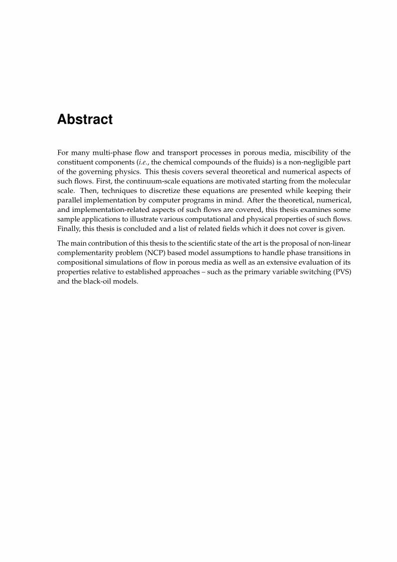
For many multi-phase flow and transport processes in porous media, miscibility of theconstituent components (i.e., the chemical compounds of the fluids) is a non-negligible partof the governing physics. This thesis covers several theoretical and numerical aspects ofsuch flows. First, the continuum-scale equations are motivated starting from the molecularscale. Then, techniques to discretize these equations are presented while keeping theirparallel implementation by computer programs in mind. After the theoretical, numerical,and implementation-related aspects of such flows are covered, this thesis examines somesample applications to illustrate various computational and physical properties of such flows.Finally, this thesis is concluded and a list of related fields which it does not cover is given.
The main contribution of this thesis to the scientific state of the art is the proposal of non-linearcomplementarity problem (NCP) based model assumptions to handle phase transitions incompositional simulations of flow in porous media as well as an extensive evaluation of itsproperties relative to established approaches – such as the primary variable switching (PVS)and the black-oil models.


Kurzfassung
Mischbarkeitseffekte sind für eine Reihe von technisch, wissenschaftlich und wirtschaftlichbedeutsamen Anwendungen von Fluidströmungen in porösen Medien von herausragenderBedeutung. Eine Auswahl dieser Anwendungsgebiete ist in Abbildung 1 wiedergegeben:Sie umfasst Techniken zur Erdöl- und Erdgasförderung, die Speicherung von klimaaktivenGasen wie CO2 in geologischen Formationen, Aufgabenstellungen zur Bodendekontamina-tion, sowie Anwendungen aus der chemischen Verfahrenstechnik, welche an dieser Stellebeispielhaft durch Polymer-Elektrolyt-Membran-Brennstoffzellen repräsentiert werden.
Bei derartigen Anwendungen ist die Erstellung geeigneter physischer Modelle zur Auslegungund Optimierung des Systems oft sehr teuer oder im Extremfall unmöglich. Um dieserTatsache zum Trotz ein Verständnis der relevanten physikalischen Prozesse zu gewinnen, istdie numerische Simulation häufig das Mittel der Wahl. Eine der Hauptschwierigkeiten dieserSimulationen ist die numerische Behandlung von Stoffgemischen und hierbei insbesonderedie Präsenz der Fluidphasen innerhalb des betrachteten Raumgebiets.
In der vorliegenden Arbeit werden wir uns in den Kapiteln 2 und 3 näher mit der theore-tischen Behandlung von Strömungen in porösen Medien beschäftigen. In diesem Kontextwerden wir einen besonderen Schwerpunkt auf die Einbeziehung von Mischbarkeitseffektenlegen. Im anschließenden Kapitel 4 werden wir kurz die numerische Behandlung der sichdaraus ergebenden Gleichung besprechen, während wir in Kapitel 5 die im Kontext dieserArbeit verwendete numerische Software näher betrachten und in Kapitel 6 Ergebnisse fürausgewählte numerische Experimente vorstellen und auswerten werden. Abschließend folgteine Zusammenfassung sowie ein Ausblick auf wichtige weiterführende Themenfelder, dieden Umfang dieser Arbeit übersteigen würden.
Erhaltungsgleichungen für Fluidströmungen in porösen Medien
Im ersten Teil von Kapitel 2 beschäftigen wir uns mit Kontinuumsmechanik im Allgemeinen.Hierzu werden wir zunächst die kontinuumsmechanische Betrachtungsweise basierend aufmolekularen Größen motivieren. In diesem Kontext werden wir feststellen, dass dies mitdem mathematischen Konzept der Faltung von molekularen Größen erreicht werden kann,wie Abbildung 2 illustriert: Zunächst definieren wir eine Dichtefunktion
ζb :=∑i
ψibi ,
die die mit den individuellen molekularen oder atomaren Partikeln assoziierte Größe biräumlich verteilt. Hierbei ist ψi : R3 → R eine glatte und an der Position des i-ten Moleküls

XII Kurzfassung
(a) (b)
(c) (d)
Abbildung 1: Anwendungsgebiete von Mehrphasenströmungen in porösen Medien beidenen Mischbarkeitseffekte berücksichtigt werden sollten: (a) Erdölproduktion.(b) Geologische Speicherung von CO2. (Bildquelle: [90]) (c) Bodendekontami-nation. (Bildquelle: [39]) (d) Polymer-Elektrolyt-Membran-Brennstoffzellen.
zentrierte Funktion, deren Integral über den Definitionsbereich 1 ergibt.
Nachdem wir eine passende Dichtefunktion definiert haben, können wir diese nach Anwe-nung der Faltungsoperation
b(x) = (ζb ∗ χ)(x) :=
∫R3ζb(x− y) · χ(y) dy
mit einem Glättungskern χ : R3 → R auf Kontinuumsebene behandeln. Der Glättungskern χkönnen wir dabei als eine um den Koordinatenursprung zentrierte, radial monoton fallendeFunktion mit der Eigenschaft annehmen, dass ihr Integral über den Defintionsbereich 1 ergibt.Um Oszillationen in b vernachlässigen zu können, muss der Träger der Glättungsfunktioneinerseits groß genug sein, dass die Eigenschaften einzelner Moleküle keinen wesentlichenEinfluss auf das Ergebnis der Faltungsoperation haben. Andererseits muss der Träger jedoch

Erhaltungsgleichungen für Fluidströmungen in porösen Medien XIII
(a) Partikel (b) Dichtefunktion ζb (c) Kontinuumsgröße b
Abbildung 2: Illustration des Übergangs von der Molekular- zur Kontinuumsskala.
klein genug sein, um makroskopische Änderungen der Eigenschaften der Größe b nicht zusehr zu mitteln. Zur Verdeutlichung dieses Konzepts bietet sich als einfaches Beispiel dieMassendichte ρ an: Hierzu verwenden wir die Dichtefunktion
ζρ =∑i
ψimi ,
wobei mi der Masse des i-ten Partikels entspricht. Nach der anschließenden Anwendung derFaltungsoperation erhalten wir als Kontinuumsgröße die Massendichte ρ.
Nach dieser kurzen Motivation der kontinuumsmechanischen Betrachtungsweise, werdenwir im selben Kapitel partielle Differenzialgleichungen herleiten, welche die Erhaltung belie-biger Größen auf Kontinuumsebene beschreiben. Diese Gleichungen wenden wir sodannauf verschiedene Erhaltungsgrößen der klassischen Physik an und betrachten hierbei insbe-sondere den Spezialfall der NEWTONSCHEN Fluide, bei denen die viskosen Kräfte linear zurSchergeschwindigkeit des Fluids angenommen werden. Wir beschränken unseren Diskurshierbei auf die Erhaltungsgrößen Masse, Impuls und Energie; andere physikalischen Erhal-tungsgrößen – etwa elektrische Ladung – werden wir also nicht berücksichtigen. Als Ergebnisunserer Bemühungen erhalten wir für NEWTONSCHE Fluide die Massenerhaltungsgleichung
∂xκρmol
∂t+ div(xκρmol v −Dκgrad xκ) = qκ ,
die Energieerhaltungsgleichung
∂ ρ(u+ 1/2‖v‖2 + z · g
)∂t
+ div(hρv − λgrad T ) = qenergy − ρv · g
und die NAVIER-STOKES-Gleichungen zur Impulserhaltung
ρ∂v
∂t+ ρv · grad v = −grad p+ µdiv grad v + ρg + qmom .

XIV Kurzfassung
Die Energieerhaltungsgleichung können wir weiter zu
∂ uρ
∂t+ div(hρv − λgrad T ) = qenergy
vereinfachen, falls wir annehmen, dass die kinetischen und potentiellen Anteile vernachläs-sigbar sind gegenüber der spezifischen inneren Energie u.
Bei schleichenden inkompressiblen Strömungen können wir weiterhin die Trägheitstermeder NAVIER-STOKES-Gleichungen als vernachlässigbar gegenüber den viskosen Termenannehmen. Dies führt uns zu den STOKES-Gleichungen
−grad p+ µ div grad v + ρ g + qmom = 0 .
Nach dieser Herleitung der für uns relevanten Erhaltungsgleichungen, erörtern wir in Ab-schnitt 2.4 die Verhältnisse in porösen Medien. Hierbei ist zu beachten, dass für die meistentechnischen und wissenschaftlichen Anwendungen die genaue Geometrie der Poren un-bekannt ist. Dieser Umstand ist analog zur initialen Partikelkonfiguration beim Übergangvon der molekularskaligen zur kontinuumsskaligen Betrachtungsweise, da auch diese nor-malerweise unbekannt ist. Üblicherweise wird bei dieser Herleitung, wie bei der Motivati-on der kontinuumsmechanischen Betrachtungsweise, ein Mittelungsansatz verwendet; esMedien werden jedoch die Erhaltungsgleichungen der Kontinuumsskala gemittelt. DieseMittelungsansätze können wir auch als Spezialfälle von Faltungsoperationen auffassen. Inder vorliegenden Arbeit verwenden wir die von WHITAKER [89] vorgestellte Vorgehens-weise, welche ausgehend von der Massenerhaltungs-, den vereinfachten Energieerhaltungs-und den STOKES-Gleichungen die bestimmenden Gleichungen für die makroskopische Ber-schreibung von Strömungen von NEWTONSCHEN Fluiden in porösen Medien ergibt. AlsMassenerhaltungsgleichung einer Komponente1 κ in einem porösen Medium erhalten wir
∑α
∂φSα〈xκα〉α〈ρmol,α〉α
∂t+∑α
div(〈xκα〉α〈ρmol,α〉α〈vα〉 − 〈Dκ
α〉grad 〈xκα〉) = qκmol ,
wobei wir die Quellterme der Komponente zu
qκmol :=∑α
⟨qκmol,α
⟩zuammenfassen und
〈b(x)〉 =1
‖V(x)‖
∫Vα(x)
b(y) dy
die Mittelungsoperation der Größe b(x) über das Raumgebiet V(x) repräsentiert. Ferner
1Eine Komponente bezeichnet hier eine chemische Verbindung die in Phasen enthalten sein kann, währendeine Phase als Materialgemisch definiert ist, das eine Grenzfläche zu allen anderen Phasen ausbildet. AlsBeispiel soll hier das Zweiphasen-, Zweikomponentensystem Wasser-Stickstoff dienen, bei dem die flüssigeund gasförmige Phase jeweils Gemische der Verbindungen Wasser (H2O) und Stickstoff (N2) sind.

Schlussbedingungen und ergänzende Gleichungen XV
definieren wir das auf die Fluidphase α bezogene Mittel an Position x als
〈b(x)〉α =1
Sαφ〈b(x)〉 .
Analog zur Massenerhaltungsgleichung erhalten wir die Impulserhaltungsgleichungen
〈vα〉 = −kr,αK
〈µα〉α(grad 〈pα〉α − 〈ρα〉αg)
und die Energieerhaltungsgleichung
∂
∂t
((1− φ)〈us〉s 〈ρs〉s +
∑α
φSα〈uα〉α 〈ρα〉α)
− div
(〈λs〉s grad 〈Ts〉+
∑α
(〈hα〉α〈ρα〉α〈vα〉 − 〈λα〉α grad 〈Tα〉)
)= 〈qenergy〉 .
Hierbei bezeichnet 〈·〉s eine für die Feststoffphase definierte Größe. Diese Gleichung könnenwir unter Annahme des lokalen thermischen Gleichgewichts zu
∂
∂t
((1− φ)〈us〉s 〈ρs〉s +
∑α
φSα〈uα〉α 〈ρα〉α)
− div
(∑α
〈hα〉α〈ρα〉α〈vα〉+ λpm grad 〈T 〉
)= 〈qenergy〉
vereinfachen.
Für die folgenden Betrachtungen werden wir die Mittelungsoperatoren nicht mehr explizitschreiben, so dass wir die Erhaltungsgleichungen wie folgt ausdrücken werden:
∑α
∂φSαxκαρmol,α
∂t+∑α
div(xκαρmol,αvα −Dκ
pm,αgrad xκα
)= qκmol
vα = −kr,α
µαK (grad pα − ραg)
∂
∂t
((1− φ)usρs +
∑α
φSαuα ρα
)− div
(∑α
hαραvα − λpm grad T
)= qenergy
Schlussbedingungen und ergänzende Gleichungen
Nach dieser Herleitung der Erhaltungsgleichungen beschäftigen wir uns anschließend inKapitel 3 damit, ein mathematisch geschlossenes Gleichungsystem für die Erhaltungsglei-
XVI Kurzfassung
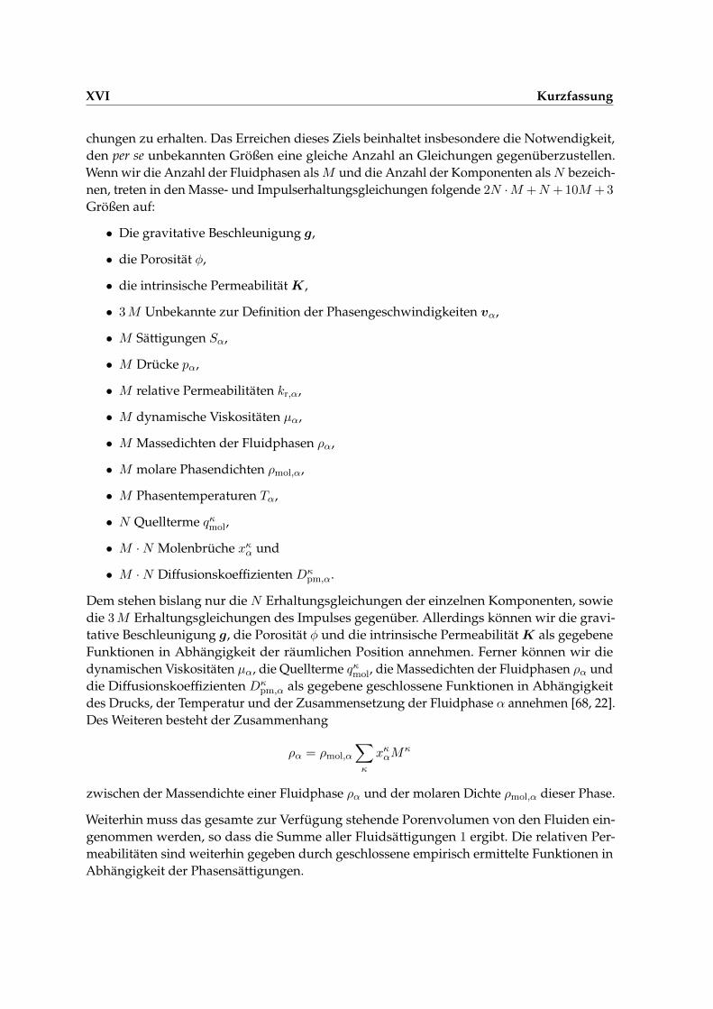
chungen zu erhalten. Das Erreichen dieses Ziels beinhaltet insbesondere die Notwendigkeit,den per se unbekannten Größen eine gleiche Anzahl an Gleichungen gegenüberzustellen.Wenn wir die Anzahl der Fluidphasen alsM und die Anzahl der Komponenten alsN bezeich-nen, treten in den Masse- und Impulserhaltungsgleichungen folgende 2N ·M +N + 10M + 3
Größen auf:
• Die gravitative Beschleunigung g,
• die Porosität φ,
• die intrinsische PermeabilitätK,
• 3M Unbekannte zur Definition der Phasengeschwindigkeiten vα,
• M Sättigungen Sα,
• M Drücke pα,
• M relative Permeabilitäten kr,α,
• M dynamische Viskositäten µα,
• M Massedichten der Fluidphasen ρα,
• M molare Phasendichten ρmol,α,
• M Phasentemperaturen Tα,
• N Quellterme qκmol,
• M ·N Molenbrüche xκα und
• M ·N Diffusionskoeffizienten Dκpm,α.
Dem stehen bislang nur die N Erhaltungsgleichungen der einzelnen Komponenten, sowiedie 3M Erhaltungsgleichungen des Impulses gegenüber. Allerdings können wir die gravi-tative Beschleunigung g, die Porosität φ und die intrinsische PermeabilitätK als gegebeneFunktionen in Abhängigkeit der räumlichen Position annehmen. Ferner können wir diedynamischen Viskositäten µα, die Quellterme qκmol, die Massedichten der Fluidphasen ρα unddie Diffusionskoeffizienten Dκ
pm,α als gegebene geschlossene Funktionen in Abhängigkeitdes Drucks, der Temperatur und der Zusammensetzung der Fluidphase α annehmen [68, 22].Des Weiteren besteht der Zusammenhang
ρα = ρmol,α
∑κ
xκαMκ
zwischen der Massendichte einer Fluidphase ρα und der molaren Dichte ρmol,α dieser Phase.
Weiterhin muss das gesamte zur Verfügung stehende Porenvolumen von den Fluiden ein-genommen werden, so dass die Summe aller Fluidsättigungen 1 ergibt. Die relativen Per-meabilitäten sind weiterhin gegeben durch geschlossene empirisch ermittelte Funktionen inAbhängigkeit der Phasensättigungen.

Schlussbedingungen und ergänzende Gleichungen XVII
Wenn wir nun annehmen, dass zu jedem Zeitpunkt lokal thermodynamisches Gleichge-wicht herrscht, erhalten wir weitere (M − 1) Relationen, die das mechanische, (M − 1)
Relationen, die das thermische und N · (M − 1) Relationen, die das chemische Gleichge-wicht beschreiben. Im Kontext von Fluidströmungen in porösen Medien müssen wir beider Definition des mechanischen Gleichgewichts das Konzept des Kapillardrucks einführen,welches die Differenz der absoluten Drücke der Fluidphasen im stationären Zustands imporösen Medium ausdrückt. Die Kapillardrücke werden für gewöhnlich gemeinsam mit denrelativen Permeabilitäten als geschlossene empirisch ermittelte Funktionen in Abhängigkeitder Phasensättigungen behandelt.
Bisher wurden erst die folgenden 2N ·M +N + 9M + 3 Relationen identifiziert:
• 3M Impulserhaltungsgleichungen,
• N Massenerhaltungsgleichungen,
• drei gegebene räumliche Funktionen für g,K und φ,
• eine Schlussbedingung für die Phasensättigungen,
• M Gleichungen für die Verknüpfung zwischen der molaren Dichte und der Massen-dichte der Fluidphasen,
• M geschlossene Funktionen, die für die dynamischen Viskositäten µα wiedergeben,
• M empirisch gegebene Funktionen für die relativen Permeabilitäten kr,α,
• N Quellterme qκ,
• M ·N geschlossene Funktionen Dκpm,α zur Berechnung der molekularen Diffusionsko-
effizienten,
• M Zustandsgleichungen,
• M − 1 Gleichungen für die aus dem lokale thermischen Gleichgewicht stammen,
• M − 1 Gleichungen, die das lokale mechanische Gleichgewicht beschreiben sowie
• (M − 1) ·N Gleichungen für das chemische Gleichgewicht und
• ein extern vorgegebenes, räumlich abhängiges Temperaturfeld T falls wir die Energie-erhaltungsgleichung ignorieren, ansonsten die Energieerhaltungsgleichung.
Um ein geschlossenes Gleichungssystem zu erhalten, fehlen also nochM Relationen. DieseMGleichungen bilden Modellannahmen ab, wobei wir die Annahmen folgender Modelle näherbetrachten:
Unmischbarkeit [39]: Bei diesem Modell wird die Anzahl der Fluidphasen mit der Anzahlder Komponenten gleichgesetzt, also M = N angenommen. Ferner wird angenommen,dass jede Fluidphase aus genau einer Komponente besteht. Diesen Umstand könnenwir mittels
xκα =
1 wenn α die Fluidphase der Komponente κ ist,0 sonst
ausdrücken.

XVIII Kurzfassung
Primärvariablentausch [33, 23]: Falls wir für alle Fluidphasen Mischbarkeit annehmen,können wir für den Fall, dass eine Fluidphase an einem Raumpunkt präsent ist, anneh-men, dass die Summe der Komponentenmolenbrüche für diese Fluidphase 1 ergibt,also dass ∑
κ
xκα = 1
gilt. Andererseits muss die Sättigung einer Fluidphase die nicht präsent ist Null sein;also muss in diesem Fall
Sα = 0
gelten. Diese beiden Gleichungen können zusammengefasst werden zu
0 =
1−
∑κ x
κα falls die Fluidphase α präsent ist,
Sα sonst.
Zur Bestimmung der Menge der zu einem gegebenen Zeitpunkt vorhandenen Fluid-phasen wird diese initial vorgegeben und bei physikalisch unmöglichen Zuständen –etwa bei negativen Sättigungen – während der Simulation angepasst.
Komplementaritätsprobleme [48, 41]: Die Bedingungen des Primärvariablentauschmo-dells können wir auch direkt in das Gleichungssystem einbeziehen: Zu diesem Zweckwerden wir uns zuerst der Tatsache bewusst, dass die Summe der „Molenbrüche“ fürdiese Phase nur kleiner 1 werden kann, wenn die Sättigung einer Fluidphase Null ist,wenn also
Sα = 0 =⇒∑κ
xκα ≤ 1
gilt. Umgekehrt kann die Sättigung einer Fluidphase nur dann größer als 0 werden,wenn diese Phase präsent sein kann, also die Summe der Molenbrüche 1 ist. Es gilt also∑
κ
xκα = 1 =⇒ Sα ≥ 0 .
Da jede Fluidphase immer entweder präsent oder abwesend ist, muss eine der bei-den Gleichungen auf der linken Seite erfüllt sein und wir erhalten das nichtlineareKomplementaritätsproblem
Sα
(1−
∑κ
xκα
)= 0 ∧ 1−
∑κ
xκα ≥ 0 ∧ Sα ≥ 0 .
Dieses können wir mittels einer nichtlinearen Komplementaritätsfunktion Ψ : R2 → R,welche die Eigenschaft
Ψ(a, b) = 0 ⇐⇒ a ≥ 0 ∧ b ≥ 0 ∧ a · b = 0
erfüllt, direkt in das zu lösende Gleichungssystem einbeziehen. In diesem Zusammen-hang ist es hilfreich zu erwähnen, dass die oben aufgeführte Eigenschaft die Funktion Ψ
nicht eindeutig definiert, also mehrere Funktionsklassen existieren, die diese Eigen-

Diskretisierung XIX
schaft aufweisen. Im Kontext dieser Arbeit verwenden wir aufgrund ihrer stückweisenLinearität als nichtlineare Komplementaritätsfunktion jedoch stets die Minimumfunkti-on
Ψ(a, b) := min(a, b) .
Black-Oil [19]: Die letzten Modellannahmen die im Kontext dieser Dissertation besprochenwerden, sind die des Black-Oil Modells. Diese Annahmen werden häufig im Bereich derFörderung von Erdöl angewandt und beschreiben die Eigenschafen der FluidphasenÖl, Gas und Wasser mittels der drei gleichnamigen Pseudokomponenten Öl, Gas undWasser. Sowohl die Wasser- als auch die Gasphase werden hierbei als unmischbar vor-ausgesetzt, während die Ölphase als Gemisch der Öl- und der Gaspseudokomponenteangenommen wird. Die Black-Oil-Parameter definieren nun die Massendichten allerPhasen sowie den maximal möglichen Gasanteil der Ölphase in Abhängigkeit desDrucks. Aus diesen Parametern können wir die benötigten Modellannahmen herleiten.
Diskretisierung
Nachdem wir nun die zu lösenden Gleichungssysteme bestimmt haben, widmen wir Kapitel 4Methoden zum Finden von Näherungslösungen für jene Gleichungen. Unsere abstrakteVorgehensweise ist dabei folgende:
• Die partiellen Differenzialgleichungen werden zunächst räumlich diskretisiert. Zudiesem Zweck wird das zu untersuchende räumliche Gebiet in ein konformes Gitterpartitioniert und die zu lösende Differenzialgleichung für jedes Element dieses Git-ters einzeln betrachtet und anschließend addiert. Als Ergebnis erhalten wir ein – imAllgemeinen sehr großes – nichtlineares, gekoppeltes System gewöhnlicher Differenzi-algleichungen.
• Auf dieses System gekoppelter gewöhnlicher Differenzialgleichungen wenden wirnun eine Zeitdiskretisierung an. Zur Herleitung dieser verwenden wir den Satz vonTAYLOR und erhalten für jeden Zeitschritt ein großes gekoppeltes System nichtlineareralgebraischer Gleichungen. Das Finden einer Näherungslösung des ursprünglichenGleichungssystems reduziert sich also auf das wiederholte Lösen solcher nichtlineareralgebraischer Gleichungsysteme.
• Jedes der sich ergebenden nichtlinearen algebraischen Gleichungssysteme lösen wiranschließend iterativ mit Hilfe des NEWTON-RAPHSON-Ansatzes. Hierzu müssen wirdas zu lösende nichtlineare Gleichungssystem wiederholt linearisieren.
• Die sich aus der NEWTON-RAPHSON-Methode ergebenden linearen Gleichungssystemewerden im finalen Schritt mittels einer direkten oder einer iterativen Methode exaktoder näherungsweise gelöst.
In Kapitel 4 werden wir uns mit jedem dieser Schritte näher beschäftigen.

XX Kurzfassung
(a) (b)
t/a
ml,CO2/mtot,CO2
0.00 0.46 0.92 1.38 1.83 2.29 2.75 3.21
0.00
0.09
0.18
0.27
0.36
0.45
0.54
0.63
(c)
Abbildung 3: Ergebnisse der Modellrechnungen für das Experiment zur Untersuchung dergeologischen CO2-Speicherung in Ketzin/Havel [55]. (a) Gassättigung nachdreijähriger CO2-Injektion bei Annahme von Unmischbarkeit von CO2 undSalzwasser. (b) Gassättigung nach dreijähriger CO2-Injektion unter Berücksich-tigung der Mischbarkeit von CO2 und Salzwasser. (c) Anteil des injizierten CO2das in der Salzwasserphase gelöst ist.
Numerische Anwendungen
Nachdem wir die theoretischen und numerischen Grundlagen zur numerischen Simulationvon Fluidströmungen in porösen Medien abgehandelt haben, werden wir uns in Kapitel 5kurz mit eWoms beschäftigen, des C++ Softwarepakets in dessen Rahmen die hier vorgestell-ten Konzepte implementiert wurden. Ein besonderes Augenmerk dieses Kapitels wird derbenötigte Aufwand zur Implementierung der oben genannten Modellkonzepte bilden.
Nach diesem kurzen Abstecher zur Softwareimplementierung, werden wir uns in Kapitel 6den physikalischen und numerischen Eigenschaften der obigen Modelle anhand ausgewähl-ter Beispiele zuwenden und sie untereinander vergleichen. Die numerischen Anwendungenwerden hierbei grob in der Reihenfolge ihrer Komplexität abgehandelt:
• Zunächst beschäftigen wir uns mit dem Heatpipeproblem von UDELL [84]. Dieses be-schreibt einen eindimensionalen nicht-isothermen Versuchsaufbau, für den die Lösungim stationären Fall semi-analytisch berechnet werden kann. Wir vergleichen dabei das

Numerische Anwendungen XXI
Konvergenzverhalten der Raumdiskretisierung unter Verwendung des Primärvaria-blentauschmodells und des Modells, das die nichtlinearen Komplementaritätsproblemedirekt in das zu lösende Gleichungssystem einbettet. Außerdem werden wir in diesemAbschnitt den benötigten Rechenaufwand der beiden betrachteten Modelle miteinandervergleichen.
• Nach dem Heatpipeproblem werden wir die vorgestellten Modelle mit Hilfe der vonDARCIS [25] vorgestellten synthetischen Problemstellung zur geologischen Speicherungvon CO2 untersuchen. Hierbei widmen wir uns zunächst dem Einfluss der Energieer-haltungsgleichung sowie den Einfluss von Mischbarkeitseffekten. Des Weiteren werdenwir anhand dieses Beispiels das Konzept der radialen Gebietsextrusion vorstellen,welches es erlaubt, radialsymmetrische dreidimensionale Raumgebiete mittels eineszweidimensionalen Raumgebiets abzubilden. Ergebnisse, die mit Hilfe dieser Methodeerzeugt wurden, werden dann mit denjenigen einer dreidimensionalen Simulation des-selben Problems verglichen. Ferner werden wir anhand dieses Beispiels das Verhaltender vorgestellten Methoden für parallele Berechnungen analysieren.
• Anschließend werden wir eine leicht vereinfachte Version des neunten Benchmarkpro-blems der Society of Petroleum Engineers (SPE-9) [45] näher untersuchen. In diesemKontext vergleichen wir die Ergebnisse der Modelle welche auf den Ansätzen desPrimärvariablentauschs (PVS) und den nicht-linearen Komplementaritätsproblemen(NCP) beruhen mit den Ergebnissen die mit Hilfe des Black-Oil-Modells berechnetwurden. Wir werden dabei feststellen, dass sich das PVS-Modell für dieses Problem sehrinstabil verhält und deshalb nicht anwendbar ist. Die Ergebnisse der beiden verblei-benden Modelle, zeigen eine gute Übereinstimmung hinsichtlich der prognostiziertenInjektions- und Produktionsraten, der benötigte Rechenaufwand ist jedoch für dasBlack-Oil-Modell bedeutend geringer.
• Nach dem neunten Benchmarkproblem der Society of Petroleum Engineers werden wiruns näher mit dem fünften Benchmarkproblem (SPE-5) [46] beschäftigen. Die Besonder-heit dieser Problemstellung liegt weniger in einer komplexen geologischen Abbildungdes Problems, als vielmehr in der außerordentlichen Komplexität der verwendetenthermodynamischen Relationen: Die Problemspezifikation umfasst drei Fluidphasensowie sieben Komponenten, welche mittels einer nicht-linearen kubischen Zustandsglei-chung definiert werden. Das Problem wurde mit Hilfe des NCP- und des PVS-Modellssimuliert. Die hierbei erhaltenen Ergebnisse sind sich sehr ähnlich. Der benötigte Be-rechnungsaufwand war auch in diesem Fall für das PVS-Modell höher als für dasNCP-Modell. Im Gegensatz zu den anderen hier beschriebenen Vergleichsproblemenbenötigt das PVS-Modell zur Lösung des SPE-5 Problems jedoch nicht nur eine grö-ßere Anzahl an Zeitschritten als das NCP-Modell, sondern weist auch einen höherenRechenaufwand pro NEWTON-RAPHSON-Iteration auf. Letzteres liegt wahrscheinlichdaran, dass die zu lösenden lokalen Gleichungssysteme für Dreiphasensysteme mitvielen Komponenten relativ groß werden, während die Anzahl der Fluidphasen beimNCP-Modell keine Rolle spielt.
• Zuletzt werden wir Ergebnisse für eine Anwendung besprechen, welche die Verhält-nisse des realen CO2-Speicherungsexperiments nahe der brandenburgischen Stadt
XXII Kurzfassung
Ketzin/Havel [55] abbilden. Ketzin/Havel wurde als deutscher Pilotstandort zur Un-tersuchung der Realisierbarkeit geologischer CO2-Speicherung ausgewählt. Hierbeiwerden wir zeigen, dass die vorgestellten Methoden auch großskalig einsetzbar sind –im Falle des vorgestellten Beispiels beträgt die planare Ausdehnung des Simulationsge-biets 5 km mal 5 km bei einer mittleren Dicke des Speichergesteins von ca. 130 m; diesesGebiet wurde mittels gut vier Millionen Tetraedern diskretisiert. Anhand dieser Auf-gabenstellung zeigen wir außerdem, dass Mischbarkeit von Stoffen bei geologischenAnwendungen eine nicht vernachlässigbare Rolle spielen kann.
Die wichtigsten Ergebnisse dieser Modellrechnungen sind in Abbildung 3 zusammen-gefasst. Bei der Interpretation dieser Ergebnisse sollten wir uns allerdings der Tatsachebewusst sein, dass die Menge des im Salzwasser gelösten CO2 aufgrund der hier ver-wendeten Finite-Volumen-Raumdiskretisierungen systematisch überschätzt wird. ImFalle des Ketziner CO2-Speicherprojekts wird diese Einschätzung durch seismischeDaten gestützt [55].
Abschließend findet sich eine Zusammenfassung dieser Arbeit mit Empfehlungen zur An-wendung der vorgestellten Modelle und ein Ausblick auf wichtige Themenfelder die imRahmen dieser Arbeit nicht besprochen werden konnten.

1 Introduction
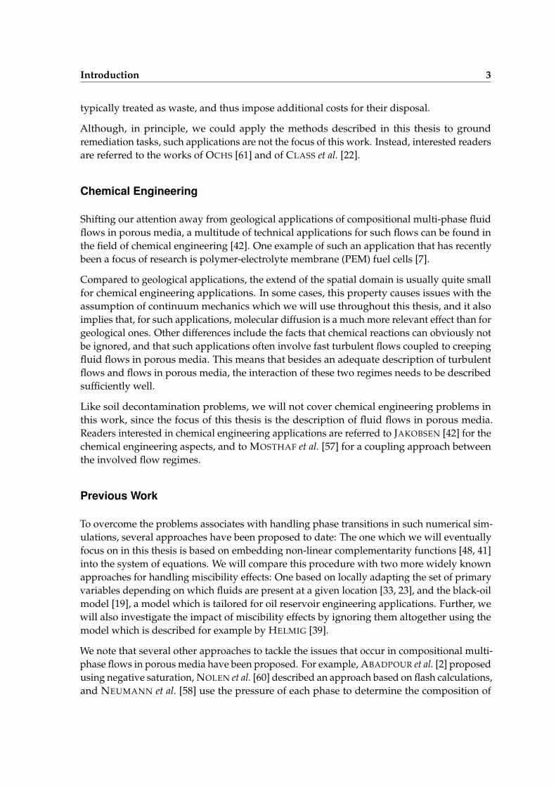
For many multi-phase flow and transport processes in porous media, miscibility of theconstituent components is a non-negligible part of the governing physics. Some of theseapplications are depicted in Figure 1.1, and include the fields of petroleum production [19], ge-ological storage of CO2 [69], substantial parts of chemical engineering [42] (exemplified hereby polymer-electrolyte-membrane (PEM) fuel cells [7]) and advanced in-situ ground remedia-tion procedures [64, 61, 22]. Most of these fields are of significant economic, environmental,and scientific interest.
Petroleum Production
Our focus when using numerical simulation of multi-phase flows in porous media forpetroleum reservoir engineering applications is to make predictions of the expected oil andgas production rates to maximize the amount of hydrocarbons which can be profitablyextracted from a given reservoir. Some of the particular issues which need to be overcomein this field are the enormous physical extends of hydrocarbon reservoirs [91]—commonly,their volume is in the range of cubic kilometers—, complex thermodynamics involving highpressures and temperatures [19] as well as high heterogeneity in the material of the reservoirwith a large uncertainty in its parameters [54].
Geological Storage of CO2
The purpose of geological CO2 storage applications [69] is to curb the greenhouse effect bypreventing the injected CO2 from entering the atmosphere of the earth. In this context, ourmain goal is thus to make long-term predictions about the risk of the injected CO2 escapingfrom the reservoir formation [69] and to make predictions on the amount of CO2 which canbe safely injected into a given formation [69]. Like for oil production applications, one of themajor challenges of numerical simulations for CO2 injection problems is the enormous size ofthe spatial domains involved [69, 55]. Moreover, the uncertainties in the parameters for thematerial of the geological formation are typically even larger than for petroleum productionapplications. The primary reasons for these issues is the lower economic incentive of the CO2storage application compared to petroleum production.
Another similarity of CO2 injection and reservoir engineering applications is the complexthermodynamics of the fluid systems involved: Due to the high pressures and relatively hightemperatures, both applications potentially require to deal with critical as well as subcriticalfluids. Having said that, the fact that these applications usually only involve two phases (gas

2 Introduction
(a) (b)
(c) (d)
Figure 1.1: Important applications for multi-phase flow in porous media for which misci-bility is relevant: (a) Petroleum production, (b) Geological storage of CO2 (im-age courtesy of [90]). (c) Ground decontamination (image courtesy of [39]), (d)Polymer-electrolyte membrane fuel cells.
and brine) instead of the three fluids gas, brine, and oil which are typically considered byreservoir engineering problems simplify matters considerably for CO2 injection scenarios.
Ground Decontamination
Another topic which exhibits some similarities to oil reservoir engineering are in-situ groundremediation methods [64, 61, 22]. Like in petroleum production scenarios, the aim of theseapplications is to remove hydrocarbons from the subsurface. In the case of ground decon-tamination methods, the depths at which the contaminants are to be removed are typicallymuch lower compared to the hydrocarbon production applications, which implies muchlower pressures and temperatures. Thus, we can often use much simpler thermodynamicrelations [61, 22] in the context of such problems. Another difference to reservoir engineeringis that the commercial value of the extracted hydrocarbons is usually significantly lower thanthe monetary costs of the methods to extract them. In fact, the extracted hydrocarbons are
Introduction 3
typically treated as waste, and thus impose additional costs for their disposal.
Although, in principle, we could apply the methods described in this thesis to groundremediation tasks, such applications are not the focus of this work. Instead, interested readersare referred to the works of OCHS [61] and of CLASS et al. [22].
Chemical Engineering
Shifting our attention away from geological applications of compositional multi-phase fluidflows in porous media, a multitude of technical applications for such flows can be found inthe field of chemical engineering [42]. One example of such an application that has recentlybeen a focus of research is polymer-electrolyte membrane (PEM) fuel cells [7].
Compared to geological applications, the extend of the spatial domain is usually quite smallfor chemical engineering applications. In some cases, this property causes issues with theassumption of continuum mechanics which we will use throughout this thesis, and it alsoimplies that, for such applications, molecular diffusion is a much more relevant effect than forgeological ones. Other differences include the facts that chemical reactions can obviously notbe ignored, and that such applications often involve fast turbulent flows coupled to creepingfluid flows in porous media. This means that besides an adequate description of turbulentflows and flows in porous media, the interaction of these two regimes needs to be describedsufficiently well.
Like soil decontamination problems, we will not cover chemical engineering problems inthis work, since the focus of this thesis is the description of fluid flows in porous media.Readers interested in chemical engineering applications are referred to JAKOBSEN [42] for thechemical engineering aspects, and to MOSTHAF et al. [57] for a coupling approach betweenthe involved flow regimes.
Previous Work
To overcome the problems associates with handling phase transitions in such numerical sim-ulations, several approaches have been proposed to date: The one which we will eventuallyfocus on in this thesis is based on embedding non-linear complementarity functions [48, 41]into the system of equations. We will compare this procedure with two more widely knownapproaches for handling miscibility effects: One based on locally adapting the set of primaryvariables depending on which fluids are present at a given location [33, 23], and the black-oilmodel [19], a model which is tailored for oil reservoir engineering applications. Further, wewill also investigate the impact of miscibility effects by ignoring them altogether using themodel which is described for example by HELMIG [39].
We note that several other approaches to tackle the issues that occur in compositional multi-phase flows in porous media have been proposed. For example, ABADPOUR et al. [2] proposedusing negative saturation, NOLEN et al. [60] described an approach based on flash calculations,and NEUMANN et al. [58] use the pressure of each phase to determine the composition of

4 Introduction
the fluids at phase equilibrium. Like the models which we will investigate here, all of thesemodels exhibit specific challenges, and some of them are restricted in their versatility. Forexample, a common restriction of many models is to assume only two fluid phases and afixed number of components.
Structure of this Thesis
Before we can describe compositional multi-phase fluid flows in porous media, we first needto introduce the concept of continuum mechanics. Based on this, we derive the fundamentalpartial differential equations that govern the physical conservation laws for mass, energy, andmomentum in the continuum mechanical context in Chapter 2. In the final part of this chapter,we will proceed to adapt these equations for macroscopic porous media flow problems bymeans of volume averaging.
In Chapter 3, we will look at how the equations derived for macroscopic flow in porous mediain Chapter 2 can be made mathematically well-defined in the sense that there exists a uniquesolution. Besides using thermodynamic constraints, we also have to use semi-empiricalclosure relations and auxiliary assumptions, so-called model constraints.
Proceeding to Chapter 4 we will discuss discretization schemes, i.e., how to transform theresulting system of non-linear partial differential equations into a set of non-linear algebraicequations. Generally, we divide this process into two conceptually independent parts: Firstwe apply a spatial discretization – which we will cover in Section 4.1 – which transforms thepartial differential equations into a set of coupled ordinary differential equations. Then a timediscretization – discussed in Section 4.2 – transforms this set of ordinary differential equationsinto a system of coupled non-linear algebraic equations. The solution for these non-linearsystems of equations is then calculated using the NEWTON-RAPHSON method. We will seethat this method repeatedly linearizes the non-linear systems of equations and solving theselinearized systems of equations. Finally, Chapter 4 concludes with a brief overview of linearsolvers.
After the discourse on numerics, we will briefly discuss the computer software implementa-tion of these concepts which was used in the context of this thesis in Chapter 5. Chapter 6,then follows with an investigation of the results obtained using this software. The resultspresented in this chapter are mainly intended to compare the numerical performance and thephysical quality of the discretized mathematical models. The discourse on the individual ap-plications is roughly ordered by their complexity: We will first investigate a one-dimensionalproblem for which a semi-analytical steady-state solution is known; then we will proceedto a synthetic, radially symmetric CO2 injection problem. Following that, we will comparethe NCP fully-compositional model with the black-oil model using the ninth benchmarkproblem of the society of petroleum engineers (SPE-9) followed by a comparison of the NCPand PVS models using the fifth SPE benchmark problem (SPE-5). Finally, we will concludethe chapter with a discussion of some results of simulations of the Ketzin project, a geologicalscale, real-world CO2 storage application.
After this, we will conclude this thesis with a brief summary and some suggestions forpossible future work in Chapter 7.

2 Continuum-Scale Fluid Flows
In this chapter, we will discuss the mathematical basis of this work. We first motivate therelevant equations on the continuum scale by introducing the concept of representativeelementary volumes (REVs) in Section 2.1, then we will briefly derive the general form ofconservation equations in Section 2.2, and finally we will look at the actual conservationequations for mass, momentum, and energy in Section 2.3.
2.1 Representative Elementary Volumes
On a very small scale, all conventional matter composed of atomic particles like molecules,atoms or ions. Thus, one approach we could take to describe the physical world is todirectly simulate the interactions between those individual particles. This approach is calledmolecular dynamics [18], and requires to solve an enormously large system of coupled ordinarydifferential equations—typically one equation per particle.
Using this approach, we are able to approximate the physical world quite well [8], but evenwhen using the largest available supercomputers we need to restrict ourselves to tiny systemsbecause of the enormous number of particles involved. For example, to describe a singledroplet of water using this approach, we need to account for approximately 1021 molecules(assuming a droplet exhibiting a weight of 0.03 grams). For engineering and geologicalapplications, we thus need to use an alternative approach. Typically, this approach is basedon continuum mechanics: Instead of defining the physical laws on a molecular scale, wedescribe the system in terms of average or bulk properties of the constituent molecules.
To illustrate this concept, let us look at Figure 2.1: In order to calculate, for example, themass density, i.e., the average mass contained in a given amount of space, one can sum up theweight of the individual molecules and divide it by the size of the considered spatial domain.If we subsequently apply this method to domains of increasing size, we will obtain a graphsimilar to the one outlined on the right of Figure 2.1. There, the value of the mass densityvaries considerably for small averaging domains, whilst it becomes nearly constant for largeones. The cause for this is that, for an averaging domain that contains a large number ofparticles, the addition of an individual molecule does not have a significant effect on thetotal amount of the mass inside the considered domain. On the large end of the scale, themass density would start to fluctuate again; this is due to macroscopic effects like variationsin pressure. We call spatial averaging domains which domains which are large enough notto change the value of the averaged quantity significantly by the addition or removal of asingle particle but small enough to capture macroscopic fluctuations representative elementaryvolumes (REVs).

6 Continuum-Scale Fluid Flows
V1V2V3V4V5
|V|
∫V b
|V|
〈b〉rev
Figure 2.1: Averaging a quantity for successively larger spatial volumes Vi first yields stronglyoscillating values. These oscillations become smaller as the size of the averagingvolume gets larger. For very large averaging volumes, oscillations originatingfrom macroscopic variations of the quantity appear (not depicted).
To get a mathematical rigorous definition of the above, we may use the procedure illustratedin Figure 2.2: First we distribute bi, i.e., the amount of a quantity associated with each particle iin space. This can be achieved using a radial function ψi : R3 ×R→ R which is centered atthe position of particle i and which has the property that the integral overR3 is one. We getthe following spatial distribution function for the particle i:
bi := ψibi .
Now, we calculate the sum of these distribution functions, and get
ζb :=∑i
bi =∑i
ψibi ,
which represents a density function for the quantity b. If we now apply a convolution usingthe kernel χ, we get
b(x) :=
∫R3ζb(x− y) · χ(y) dy = (χ ∗ ζb)(x) , (2.1)
which is a continuum-scale representation of the quantity b as depicted in Figure 2.2c. Notethat in order to obtain a smooth result, we need to use a convolution kernel with a sufficientlylarge spatial support.
Using this abstract framework, we can replicate the procedure depicted in Figure 2.1, bychoosing the convolution kernel
χ(x) =
1/‖V‖ if x ∈ V
0 else,
where V is a sphere with an arbitrary but fixed radius r centered around the origin of the

Representative Elementary Volumes 7
(a) Particles (b) Density Function ζb (c) Continuum-Scale Quantity b
Figure 2.2: Illustration of the conversion from molecular- to continuum-scale: First, theamount of a quantity associated with each particle is distributed around thelocation of a particle, and we get a density function ζb. Then this density functiongets averaged at each spatial point by a convolution kernel χ, and we get thecontinuum-scale quantity b.
coordinate system, i.e.,V :=
y ∈ R3 | ‖y‖ < r
.
Using Equation 2.1, we can define the following continuum-scale quantities:
Mass Density: We define the mass density ρ as the mass per volume unit:
ζρ :=∑i
ψimi
where mi is the mass of particle i.
Bulk velocity: The bulk velocity v is defined as the net velocity of the particles, so we use
ζv :=∑i
ψivi
as the velocity density function.
Pressure: The pressure of an averaging domain V is given by the linear momentum of theparticles inside V . One complication is that pressure is a quantity which is definedvia its effect on a surface, but the distribution function which we need is a volumetricquantity. Neglecting external force-fields, we can use the distribution function
ζp :=∑i
ψi‖vi‖2
mi
for pressure according to MARTYNAL, et al. [56].
Internal energy: The specific internal energy u is defined as the energy per unit of mass ofthe particles inside V . On a molecular scale, each particle exhibits kinetic, rotational,and oscillatory energy. For the specific internal energy, this means that we get the

8 Continuum-Scale Fluid Flows
density function
ζu :=1
ρ
∑i
ψi
(1
2mi‖vi‖2 + Er,i + Eo,i
)where Er,i and Eo,i are the energies of particle i due to its rotation and its oscillation.
The hypothesis which we now need to make for continuum mechanics is that the propertiesof interest of the physical system can be described in terms of quantities that result from aconvolution of the form given by Equation 2.1. In this context, we should remember that, ifthe filter kernel χ exhibits a too small or a too large spatial support, this assertion may not bevalid.
Scales
For gases, we can define the minimum size of the support of the convolution kernel χ usingthe KNUDSEN number Kn [20], which is defined as
Kn :=λ
L,
where λ is the mean free path between molecules, and L is the characteristic length of thespatial support of the convolution kernel. For air at standard conditions, the mean freepath is approximately λ ≈ 60 · 10−9 m. Assuming that the spatial support of a sphericalconvolution kernel is sufficiently large if it averages about 5000 molecules, we need to usean averaging volume with a diameter of L ≈ 1.3 · 10−6 m which corresponds to a KNUDSEN
number of Kn ≈ 0.05. The Knudsen number for the same averaging domain is typicallyconsiderably smaller for liquids, as the average distance of the molecules of the substance ismuch smaller in this case.
The largest valid size of the characteristic length depends on the properties of the consideredsetup more strongly than the smallest: If the system exhibits largely uniform conditions,the maximum diameter of the support can be in the magnitude of lightyears (for examplein galaxy-scale problems), or it might be at the submillimeter scale (for example in manytechnical applications).
2.2 Continuum-Scale Conservation Equations
Within the context of this work, we will consider the conservation of the three physicalquantities mass, momentum, and energy. Since the conservation equations for these are verysimilar, we will first derive a common form of them in this section. For this derivation, we willassume that the continuum hypothesis of the previous section holds, i.e., that conservation ofthese quantities can be described on the continuum-scale.
We start our endeavor by assuming an infinitely large spatial domain. Next, we let ω ⊂ R3
be an arbitrary, simply connected, bounded, and open subset of the spatial domain. Further,

Continuum-Scale Conservation Equations 9
(a) EULERIAN
(b) LAGRANGIAN
Figure 2.3: The EULERIAN and the LAGRANGIAN points of view: While in the EULERIAN
point of view, the observed volume stays constant in time, it is transported alongwith the conserved material in the LAGRANGIAN point of view.
let us now assume that ω “tracks” the quantity b which is to be conserved. In this case, at anygiven time t, the total amount of the quantity B contained within the volume is given by
B(t) =
∫ω(t)
b(x, t) dx .
Since b is conserved, its amount within the tracked volume ω(t) is constant. This leads us to
d
dtB(t) =
d
dt
∫ω(t)
b(x, t) dx = 0 .
In a slightly more general setting, we add or remove the conserved quantity at a given rate,which we can describe by a source term q:
d
dt
∫ω(t)
b(x, t) dx =
∫ω(t)
q(x, t) dx. (2.2)
We may interpret Equation 2.2—which was introduced by JOSEPH-LOUIS DE LAGRANGE—asthe continuum-scale conservation equation for an observer that moves with the conservedquantity b. A different point of view is the one taken by LEONHARD EULER: In contrastto LAGRANGE, EULER always observed the same part of space over time as illustratedin Figure 2.3. We can derive the EULERIAN form of any conservation equation from theLAGRANGIAN form (2.2) by taking advantage of the REYNOLDS transport theorem [72]
d
dt
∫ω(t)
bdx =
∫ω(t0)
(d
dtb+ bdiv v
)dx
which enables us to transpose the ordering of the time derivative and the spatial integration.

10 Continuum-Scale Fluid Flows
Here, t0 represents an arbitrary but fixed reference time, and v = ∂x/∂t is the velocity1 of thetransported quantity at a given location x at time t. Using this relation, we can transformEquation 2.2 into ∫
ω(t0)
(d
dtb+ bdiv v
)dx =
∫ω(t0)
(d
dtq + q div v
)dx .
In this equation, instead of specifying a source term q which tracks the volume occupied bythe conserved quantity, we can also use a source term q which is fixed in space, so that we get∫
ω(t0)
(d
dtb+ bdiv v
)dx =
∫ω(t0)
q dx . (2.3)
In order to keep the observed volume constant over time, we also have to transform thetotal time derivative of b in Equation 2.3. For this, we can take advantage of the convectivederivative
db
dt=∂b
∂t+ v · grad b
and transform Equation 2.3 to∫ω(t0)
(∂
∂tb+ v · grad b+ bdiv v
)dx =
∫ω(t0)
q dx . (2.4)
Finally, taking advantage of the vectorial product rule
div(bv) = v · grad b+ bdiv v ,
we get ∫ω(t0)
(∂
∂tb+ div(bv)
)dx =
∫ω(t0)
q dx , (2.5)
the integral EULERIAN form of the conservation equation of any quantity b which is to beconserved. To express this in differential form, we remember that ω(t0) is an arbitrary simplyconnected, bounded, and open subset of the domain. This means that Equation 2.5 is validpointwise, provided that b is a C1-continuous function. In other words, we can drop theintegrals on both sides of Equation 2.5, and get
∂b
∂t+ div(bv) = q . (2.6)
If not explicitly stated otherwise, we will use this form for conservation equations during therest of this thesis.
1In the molecular sense, v is the bulk velocity.
Conserved Quantities 11
2.3 Conserved Quantities
In this section, we will adapt the generic EULERIAN conservation equation (2.6) to specificallyexpress conservation of the three quantities mass, momentum, and energy. In this context, wewill not consider any other physical conservation quantity like, for example, electric charge.We will also strictly stay within the bounds of classical mechanics, so advanced concepts likethe equivalence of mass and energy will not be considered here.
2.3.1 Conservation of Mass
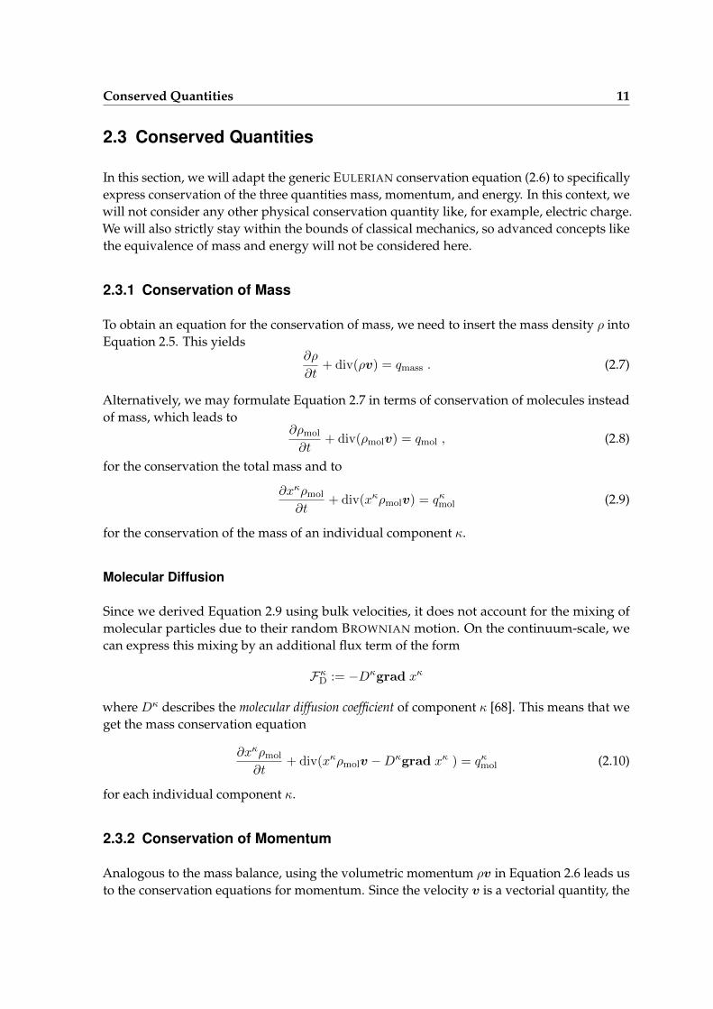
To obtain an equation for the conservation of mass, we need to insert the mass density ρ intoEquation 2.5. This yields
∂ρ
∂t+ div(ρv) = qmass . (2.7)
Alternatively, we may formulate Equation 2.7 in terms of conservation of molecules insteadof mass, which leads to
∂ρmol
∂t+ div(ρmolv) = qmol , (2.8)
for the conservation the total mass and to
∂xκρmol
∂t+ div(xκρmolv) = qκmol (2.9)
for the conservation of the mass of an individual component κ.
Molecular Diffusion
Since we derived Equation 2.9 using bulk velocities, it does not account for the mixing ofmolecular particles due to their random BROWNIAN motion. On the continuum-scale, wecan express this mixing by an additional flux term of the form
FκD := −Dκgrad xκ
where Dκ describes the molecular diffusion coefficient of component κ [68]. This means that weget the mass conservation equation
∂xκρmol
∂t+ div(xκρmolv −Dκgrad xκ ) = qκmol (2.10)
for each individual component κ.
2.3.2 Conservation of Momentum
Analogous to the mass balance, using the volumetric momentum ρv in Equation 2.6 leads usto the conservation equations for momentum. Since the velocity v is a vectorial quantity, the

12 Continuum-Scale Fluid Flows
result is a bit more complicated than Equation 2.7:
∂ρv
∂t+ div(ρv ⊗ v) = e+ qmom . (2.11)
For this equation, we also used a term e capturing forces and a term qmom for the remainingsources and sinks of momentum in the system.
We can reformulate Equation 2.11 by taking advantage of the product rule for the timederivative
∂ρv
∂t= v
∂ρ
∂t+ ρ
∂v
∂t
and for the divergence term
div(ρv ⊗ v) = ρv · grad v + v div(ρv) ,
and get
v∂ρ
∂t+ ρ
∂v
∂t+ ρv · grad v + v div(ρv) = e+ qmom .
Reordering the left-hand side yields
ρ∂v
∂t+ ρv · grad v + v
(∂ρ
∂t+ div(ρv)
)= e+ qmom . (2.12)
In Equation 2.12, we now notice that the third additive term corresponds to the left-hand sideof the mass conservation Equation 2.7, but multiplied with the velocity. Assuming that thesource term for mass qmass is zero leads us to
ρ∂v
∂t+ ρv · grad v = e+ qmom . (2.13)
Otherwise – i.e., if we do not assume the source term of the mass balance equation to be zero– the third term of Equation 2.12 can be brought to the right-hand side and integrated intothe momentum source term qmom. This means that the general form of the equation for theconservation of momentum is given by Equation 2.13.
Let us now have a closer look at the force term e of the right-hand side of Equation 2.13. Itshould be clear that we can split e into a term f capturing the forces which are exercisedupon the surface of a considered domain, and a term h, representing forces which attack inthe interior:
e = f + h
The former are called surface forces and are exerted on the material by its environment, thelatter are called body forces and are caused by force fields like gravity or electromagnetism.
It can be shown [72] that the surface forces f can be expressed as
f = div τ (2.14)

Conserved Quantities 13
Figure 2.4: The COUETTE thought experiment comprises two infinitely large parallel planarplates with the space between them occupied by a fluid; in the experiment, theupper plate moves with a velocity of vx relative to the lower one. At each plate, theobserved force per area Fx is proportional to the relative velocity of the plates vxand anti-proportional to the distance y between the plates. The proportionalitycoefficient µ is determined by the fluid between the two plates, and is called thedynamic viscosity.
where τ ∈ R3×3 is called stress tensor. Taking advantage of Equation 2.14 and neglecting allbody forces except gravity, we get
ρ∂v
∂t+ ρv · grad v = div τ + ρ g + qmom (2.15)
as the momentum balance equation where g is the gravitational acceleration.
2.3.3 NEWTONIAN Fluids
For NEWTONIAN fluids, we can substantiate the momentum conservation Equation 2.15 asfollows: First, we assume that the stress tensor τ can be split into
τ = −pI + T (2.16)
where the term pI represents pressure, and the term T represents the shear stresses [9]. Thereason why the term pI is negative is that the tensor τ represents the stresses which act uponthe material within the observed domain, and not the stresses which this material exercisesupon its environment.
Inserting Equation 2.16 into the momentum balance equation (2.15), we get
ρ∂v
∂t+ ρv · grad v = −grad p+ divT + ρg + qmom . (2.17)
We now consider the fact that the shear stress tensor T of NEWTONIAN fluids does notdepend on the absolute deformation of the material relative to its initial position, but onlyon the rate at which the fluid gets displaced relative to its environment as illustrated inFigure 2.4. Since T needs to be symmetric [9], we get a shear stress tensor T of the form
T ij = µ
(∂vj∂xi
+∂vi∂xj
)+ δijλ div v , (2.18)
using the proportionality coefficients µ ∈ R+ and λ ∈ R, with δij being the KRONECKER

14 Continuum-Scale Fluid Flows
delta. The factor λ captures the stress due to expansion or contraction of the volume of thefluid. Since there are many difficulties for determining λ, it is usually either assumed [9] tobe zero as in the following, or −3µ/2.
If we take advantage of Equation 2.18 in the momentum balance equation (2.17), we get
ρ∂v
∂t+ ρv · grad v = −grad p+ div
(µ(grad v + (grad v)T
))(2.19)
+ ρ g + qmom ,
the NAVIER-STOKES equations for compressible NEWTONIAN fluids.
For incompressible fluids with constant dynamic viscosity we can simplify Equation 2.19further: First, we use the relation
div (grad v)T = grad div v
and then consider the fact that div v is identical to zero if the density ρ is constant. We thusget
ρ∂v
∂t+ ρv · grad v = −grad p+ µdiv grad v + ρ g + qmom (2.20)
as the conservation equation for momentum.
2.3.4 Creeping Flows
For creeping incompressible flows, we can also neglect the inertia term of the NAVIER-STOKES
Equation 2.20, and get the STOKES equation
− grad p+ µ div grad v + ρ g + qmom = 0 . (2.21)
In order for this assumption to be applicable, we need to be able to define what “creeping”means. Usually, this property is defined using the REYNOLDS number
Re :=vc Lc
νc
where vc is the characteristic velocity of the considered physical system (for example, theabsolute value of the maximum velocity of the fluid), Lc represents the characteristic lengthof the system (for example, the diameter of the pipe for pipe-flow problems), and νc = µc/ρcis the characteristic kinematic viscosity of the fluid. We now define a flow as “creeping” if itexhibits a REYNOLDS number smaller than 1.
Since the characteristic length and the characteristic velocity can be chosen arbitrarily, wecannot assign too much meaning to the absolute value of the REYNOLDS number. Havingsaid that, for many important classes of flow problems there are standard conventions of howto determine Lc and vc. This means that we can compare the absolute value of the REYNOLDS
number only within a given class of flow problems. Such classes include, for example, pipe-flowsor flows around airfoils.

Conserved Quantities 15
2.3.5 Conservation of Energy
The last conservation quantity which we will consider in this work is energy. We may think ofenergy as a scalar quantity that has kinetic, potential, and thermal contributions. Assumingthat the gravitational acceleration is constant and that gravity is the only body force, we canexpress conservation of energy [9] as
∂
∂tρ
(u+
1
2‖v‖2 + z · g
)+ div(hρv + τv − λgrad T ) = qenergy − ρv · g (2.22)
where u is the specific internal energy of the substance as described in Section 2.1, z = x−xref
is the distance of a spatial position relative to an arbitrary but fixed reference point in space, λis the heat conduction coefficient, h = u+p/ρ is the specific enthalpy of the substance, and qenergy
is the source or sink term for energy.
If we neglect the kinetic energy and friction, we get
∂
∂tρ (u+ z · g) + div(hρv − λgrad T ) = qenergy − ρv · g
as the equation for the conservation of energy. Amongst others, these assumptions are validfor creeping fluid flows. If we also assume that the considered system only exhibits smallvariations of its height z, we get
∂ ρu
∂t+ div(hρv − λgrad T ) = qenergy . (2.23)
The fact that we need to consider the specific internal energy u in the accumulation term butthe specific enthalpy h in the flux term is due to the fact that transported material needs todisplace other material before it can occupy a given volume. As illustrated in Figure 2.5, theenergy required to displace the other material is equivalent to the volume occupied by thetransported material times the force with which the displaced material pushes back. In fluidsthis “push-back force” is the pressure that the displaced material exercises upon the surfaceof the transported material.
Dissipation
The third law of thermodynamics states that, in a closed system, all spontaneously occuringprocesses increase the entropy of the system as a whole2. In the context of the conservationof energy, this means that some energy is always converted into heat, i.e., internal energy. InEquation 2.23, we account for this effect by transporting enthalpy, while accumulating onlythe internal energy. To illustrate the point, let us consider Figure 2.5: There, some materialgets transported from the left to the right of a cylinder. The energy which is on the rightside at the end is the internal energy which the material originally possessed when it was on
2There might be parts of the system where entropy is reduced, but this is always compensated by additionalentropy elsewhere.

16 Continuum-Scale Fluid Flows
Figure 2.5: To move the substance with the specific internal energy u from the left to theright, one has to displace the material on the right of the cylinder. This can beimagined as a four-step process: First, the right piston creates a vacuum, then thevessel with the substance moves to the right. The work required by the pistonto create the vacuum is called the volume changing work Wv =
∫ s0+∆ss0
F ds.Assuming a constant cross-section A of the cylinder and constant pressure pright ofthe environment of the right side, this is equivalent to Wv,right = ∆sA pright. Afterthe substance has been transferred to the right, the left piston can occupy the voidspace and “recovers” the volume changing work Wv,left = ∆sA pleft.
the left side. But in addition, a piston had to displace the material originally occupying thespace on the right side, which requires a physical work of ∆sApright to be done. Assumingthe pressure to be constant at a fixed spatial location, i.e., the moved substance reduces itspressure from pleft to pright, requires work of (pleft − pright)A∆s. Since energy is conserved,this work gets converted into internal energy if the transport of material does not happen ina closed vessel that cannot expand.

Porous Media 17
Figure 2.6: An example of a porous medium where two fluid phases are co-located with asolid.
2.4 Porous Media
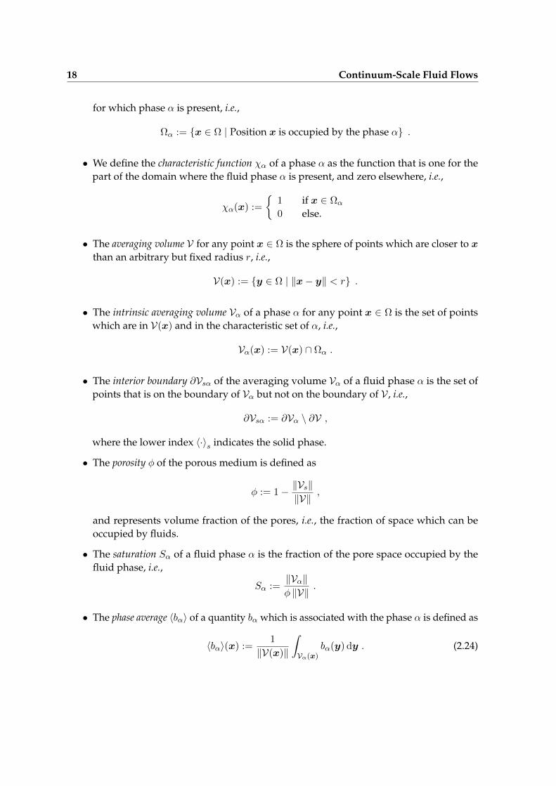
In this section, we will adapt the conservation equations for fluids, i.e., Equations 2.7, 2.20and 2.23 to multi-phase flows in porous media. The situation which we face is depicted inFigure 2.6: A solid shares the available space with multiple fluids. In the following, we aim atmaking macroscopic statements on the behavior of the fluids, assuming that the solid phaseis rigid.
To allow such quantitative statements, we will first look at volume averaging. Volume aver-aging is an upscaling technique which allows us to consider the flow and transport processeswithout having to know the geometry of the solid-fluid interface. Thus, the resulting equa-tions require much less information, and solving them is much less elaborate than solving themicro-scale equations. After introducing the volume averaging technique, we will sketch howto derive the volume averaged conservation equations for the three considered conservationquantities mass, momentum, and energy. After this, we will give a brief historical overviewand discuss how the resulting relation which governs the conservation of momentum wasdiscovered experimentally.
2.4.1 Volume Averaging
To directly solve Equations 2.7, 2.21, and 2.23 we need to provide the geometry of the solidphase of the porous medium. Generally, this is infeasible, but it turns out that in orderto get meaningful macroscopic statements about the fluid behavior in such a medium, weusually can avoid having to obtain this information. Equations which do not require thetopology of the solid are generally called to be on the laboratory-scale, the macro-scale, or onthe DARCY-scale.
Before we can derive these macro-scale equations, we first need to introduce a few conceptsbased on the definitions of WHITAKER [89]:
• The characteristic set Ωα ⊆ Ω of a phase α is the set of points of the spatial domain Ω ⊆ R3
18 Continuum-Scale Fluid Flows
for which phase α is present, i.e.,
Ωα := x ∈ Ω | Position x is occupied by the phase α .
• We define the characteristic function χα of a phase α as the function that is one for thepart of the domain where the fluid phase α is present, and zero elsewhere, i.e.,
χα(x) :=
1 if x ∈ Ωα
0 else.
• The averaging volume V for any point x ∈ Ω is the sphere of points which are closer to xthan an arbitrary but fixed radius r, i.e.,
V(x) := y ∈ Ω | ‖x− y‖ < r .
• The intrinsic averaging volume Vα of a phase α for any point x ∈ Ω is the set of pointswhich are in V(x) and in the characteristic set of α, i.e.,
Vα(x) := V(x) ∩ Ωα .
• The interior boundary ∂Vsα of the averaging volume Vα of a fluid phase α is the set ofpoints that is on the boundary of Vα but not on the boundary of V , i.e.,
∂Vsα := ∂Vα \ ∂V ,
where the lower index 〈·〉s indicates the solid phase.
• The porosity φ of the porous medium is defined as
φ := 1− ‖Vs‖‖V‖
,
and represents volume fraction of the pores, i.e., the fraction of space which can beoccupied by fluids.
• The saturation Sα of a fluid phase α is the fraction of the pore space occupied by thefluid phase, i.e.,
Sα :=‖Vα‖φ ‖V‖
.
• The phase average 〈bα〉 of a quantity bα which is associated with the phase α is defined as
〈bα〉(x) :=1
‖V(x)‖
∫Vα(x)
bα(y) dy . (2.24)

Porous Media 19
Note, that we can consider Equation 2.24 as a convolution of b · χα with the kernel
m(y) =
1‖V‖ if ‖y‖ < r
0 else.
This means that we can think of the procedures discussed in this section as analogousto the upscaling procedure from molecular to continuum-scale which we sketched inSection 2.1.
• The intrinsic phase average 〈bα〉α of the quantity bα is the average of bα considering onlythe points where the phase α is present, i.e.,
〈bα〉α(x) :=1
‖Vα(x)‖
∫Vα(x)
bα(y) dy . (2.25)
The phase average and the intrinsic phase average are thus connected by the relation
〈bα〉α =‖V‖‖Vα‖
〈bα〉 =〈bα〉φSα
.
The Spatial Averaging Theorem
Using these tools, we can now average the micro-scale conservation Equations 2.7, 2.21,and 2.23. One problem which occurs during this procedure is that we will get averages ofgradients in the results but that we would rather like to express the equations in terms ofgradients of averages.
We can overcome this issue using the Spatial Averaging Theorem [89, 67]
〈grad bα〉 = grad 〈bα〉+1
‖V‖
∫∂Vsα
bα n dy , (2.26)
where n is the outer unit normal vector of Vα at position y.
We will also get an average of the divergence instead of the divergence of averaged quantities.In this case, we can substitute the gradients in Equation 2.26 by divergences [89, 67], and get
〈div bα〉 = div 〈bα〉+1
‖V‖
∫∂Vsα
bα · n dy . (2.27)
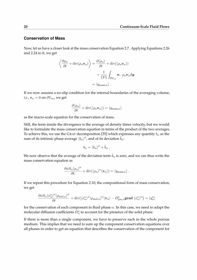
20 Continuum-Scale Fluid Flows
Conservation of Mass
Now, let us have a closer look at the mass conservation Equation 2.7. Applying Equations 2.26and 2.24 to it, we get ⟨
∂ρα∂t
+ div(ραvα)
⟩=∂〈ρα〉∂t
+ div(〈ραvα〉)
+1
‖V‖
∫∂Vsα
n · ραvαdy
= 〈qmass,α〉 .
If we now assume a no-slip condition for the internal boundaries of the averaging volume,i.e., vα = 0 on ∂Vsα, we get
∂〈ρα〉∂t
+ div(〈ραvα〉) = 〈qmass,α〉
as the macro-scale equation for the conservation of mass.
Still, the term inside the divergence is the average of density times velocity, but we wouldlike to formulate the mass conservation equation in terms of the product of the two averages.To achieve this, we use the GRAY decomposition [35] which expresses any quantity bα as thesum of its intrinsic phase average 〈bα〉α, and of its deviation bα:
bα = 〈bα〉α + bα .
We now observe that the average of the deviation term bα is zero, and we can thus write themass conservation equation as
∂φSα〈ρα〉α
∂t+ div(〈ρα〉α〈vα〉) = 〈qmass,α〉 .
If we repeat this procedure for Equation 2.10, the compositional form of mass conservation,we get
∂φSα〈xκα〉α〈ρmol,α〉α
∂t+ div
(〈xκα〉
α〈ρmol,α〉α〈vα〉 −Dκpm,αgrad 〈xκα〉
α) = 〈qκα〉
for the conservation of each component in fluid phase α. In this case, we need to adapt themolecular diffusion coefficients Dκ
α to account for the presence of the solid phase.
If there is more than a single component, we have to preserve each in the whole porousmedium. This implies that we need to sum up the component conservation equations overall phases in order to get an equation that describes the conservation of the component for

Porous Media 21
the whole multi-phase system. This leads to
∑α
∂φSα〈xκα〉α〈ρmol,α〉α
∂t+∑α
div(〈xκα〉
α〈ρmol,α〉α〈vα〉 −Dκpm,αgrad 〈xκα〉
α) =∑α
〈qκα〉 .
(2.28)
Conservation of Momentum
The procedure for conservation of momentum is much more elaborate than the one for theconservation of mass. Thus, we will only sketch it here and refer the interested reader toWHITAKER [89] for further details.
First, we neglect compressibility and the inertia terms of the NAVIER-STOKES equations, andstart with the STOKES Equations 2.21. Averaging those leads us to
0 = −〈grad pα〉+ 〈µα div grad vα〉+ 〈ραg〉+⟨qmom,α
⟩.
We now use the GRAY decomposition for the viscosity µα and the mass density ρα, andassume a sufficiently small averaging volume, so that we may neglect the deviation terms.Further assuming that the gravitational acceleration g is constant within the averagingvolume, and that the momentum source term qmom,α is zero, we get
0 = −〈grad pα〉+ 〈µα〉α〈div grad vα〉+ 〈ρα〉αg . (2.29)
Taking advantage of the Spatial Averaging Theorem 2.26, we may write the pressure term as
〈grad pα〉 = grad 〈pα〉+1
‖V‖
∫∂Vsα
pαndy .
Now, we apply the GRAY decomposition on pα, and rewrite pα as the sum of its intrinsicphase average and the deviation, and get
〈grad pα〉 = 〈pα〉α grad(φSα) + φSα grad 〈pα〉α
+1
‖V‖
∫∂Vsα
n 〈pα〉α dy +1
‖V‖
∫∂Vsα
n pα dy (2.30)
after applying the product rule to the first term. Since 〈pα〉α is constant within an averagingvolume,
1
‖V‖
∫∂Vsα
n 〈pα〉α dy =〈pα〉α
‖V‖
∫∂Vsα
ndy
holds. Now we use the spatial averaging theorem with bα ≡ 1 to obtain
1
‖V‖
∫∂Vsα
ndy = −grad(φSα) . (2.31)

22 Continuum-Scale Fluid Flows
Taking advantage of Equations 2.31 and 2.30 in Equation 2.29, and using the same procedureto the phase velocities, we get
0 = −φSαgrad 〈pα〉α −1
‖V‖
∫∂Vsα
n pα dy +〈µα〉α
‖V‖
∫∂Vsα
n · grad vα dy + 〈ρα〉αg . (2.32)
The problem we now face is that we need to define pα and vα. WHITAKER [89] argues that
vα = Bα〈vα〉α and (2.33)
pα = bα · 〈µα〉α〈vα〉α (2.34)
hold, whereBα and bα are the solutions of the following boundary value problem:
−grad bα + div grad Bα =1
‖Vα‖
∫Vα−grad bα + div grad Bα dV
Bα = −I on Vα
Bα = Gα on ∂Vα \ ∂Vs
〈Bα〉α = 〈bα〉α = 0 .
Inserting Equations 2.33 and 2.34 into Equation 2.32, we get
0 = −grad 〈pα〉α +
〈µα〉α
‖V‖
∫∂Vsα
n · grad Bα − n⊗ bα dy
〈vα〉α + 〈ρα〉αg . (2.35)
Using the abbreviation
Cα = − 1
‖V‖
∫∂Vsα
n · grad B − n⊗ bα dy
we get a relation for the intrinsic phase velocity of fluid phase α:
〈vα〉α = − C−1α
〈µα〉α(grad 〈pα〉α − 〈ρα〉αg) . (2.36)
We can convert Equation 2.36 from the intrinsic phase velocity to the more common phasevelocity by introducing
Kα = φSαC−1α
which yields
〈vα〉 = − Kα
〈µα〉α(grad 〈pα〉α − 〈ρα〉αg) . (2.37)
Conservation of Energy
To obtain an equation for the conservation of energy in a fluid phase, we neglect potentialand kinetic energy, and start with Equation 2.23. After applying the phase average (2.24) and

Porous Media 23
GRAY’s decomposition, we get
∂ φSα〈uα〉α 〈ρα〉α
∂t+ div(〈hα〉α〈ρα〉α 〈vα〉 − 〈λα〉α grad 〈Tα〉) = 〈qenergy〉 .
Unlike mass and momentum, energy can be transported by the solid. Since we assumed arigid solid phase, the advective part of the divergence term is zero for the solid, and we get
∂ (1− φ)〈us〉s 〈ρs〉s
∂t− div(〈λs〉s grad 〈Ts〉) = 〈qenergy〉 .
In this context we usually assume the internal energy us of the solid to be proportional totemperature, i.e.,
us = cp,sTs
holds with a constant heat capacity cp,s.
2.4.2 Applicability
To derive the macro-scale conservation equations, and especially the momentum conservationequation (2.37), we had to make several assumptions:
• These equations are only valid for creeping flows, and we required an incompressiblefluid with constant dynamic viscosity when simplifying the NAVIER-STOKES equa-tions (2.20) to the STOKES equations (2.21). At this point, we note that we do not needto consider these simplifications in practice, since in order to derive Equation 2.37, weonly used the STOKES equations within the averaging volumes where compressibilityand variations in viscosity can usually be neglected.
• The averaging volume must be large enough for the continuum assumption to be appli-cable for the macro-scale system. This means that slightly increasing or decreasing thesize of the averaging volume only leads to small changes of the averaged quantities [89].
• The averaging volume must be small enough so that we may neglect the deviation of allphysical quantities from their average within an averaging volume. This assumptionis potentially problematic for systems featuring low absolute pressures in conjunctionwith highly compressible fluids.
Of these assumptions, we usually have to pay most attention to the constraint of the flowvelocity. To get a feeling about this, we first need to specify a REYNOLDS number, i.e., wedefine a characteristic length Lc and a characteristic kinematic viscosity νc = µc/ρc. In this case,we choose the diameter of a typical pore of the porous medium as the characteristic length;for the characteristic kinematic viscosity νc we choose the value of the fluid at a representativetemperature and pressure. Allowing REYNOLDS numbers smaller than 1, Equation 2.37 isvalid up to relatively high velocities3: For example, if the typical pore diameter of a porousmedium is the one of a typical sand with 100 · 10−6 m, and the characteristic kinematic
3At least “high” velocities in the context of fluid flows in porous media.

24 Continuum-Scale Fluid Flows
viscosity is 20 · 10−5 m2/s (roughly the value of air at 20 C), the velocity constraints impliedby Equation 2.37 are met for intrinsic phase velocities smaller than about 2 m/s.
Simplification of Notation
In order to simplify notation, we will not write the averaging operator henceforth, so we willuse the conservation equations
∂ραφSα∂t
+ div(ραvα) = qmass,α for mass, (2.38)
vα = −Kα
µα(grad pα − ραg) for momentum, (2.39)
∂uαραφSα∂t
+ div(hαραvα − λα grad Tα) = qenergy,α for energy within a fluid, and (2.40)
∂(1− φ)ρs cp,sTs∂t
− div(λs grad Ts) = qenergy,s for energy within the solid. (2.41)
Also, since the momentum conservation equation (2.39) determines the phase velocitiesexplicitly, we can also insert it into the mass and energy conservation equations. In this casemomentum is conserved implicitly, and we get
∂ραφSα∂t
− div
(ραKα
µα(grad pα − ραg)
)= qmass,α (2.42)
for mass conservation as well as
∂ραuαφSα∂t
− div
(hαρα
Kα
µα(grad pα − ραg) + λα grad Tα
)= qenergy,α (2.43)
for energy conservation within a fluid.
2.4.3 Multi-Phase Flows
When considering flow of more than a single fluid in a porous medium, it is convenient todecompose the permeability matrix of the fluidsKα into a part which only depends on theproperties of the porous medium, a part which only depends on the fluid characteristics, anda part which describes the interactions between the fluids. We call the first of these factorsthe intrinsic permeability tensor K. It describes the permeability tensor of a medium if thepore space were completely filled with a fluid that exhibits a dynamic viscosity of 1 Pa s.The fluid-dependent part is 1/µα, the inverse of the dynamic viscosity of the fluid; and theinteractions between the fluids are usually expressed by relative permeabilities 0 ≤ kr,α ≤ 1.This leads to [14]
Kα =kr,α
µαK . (2.44)
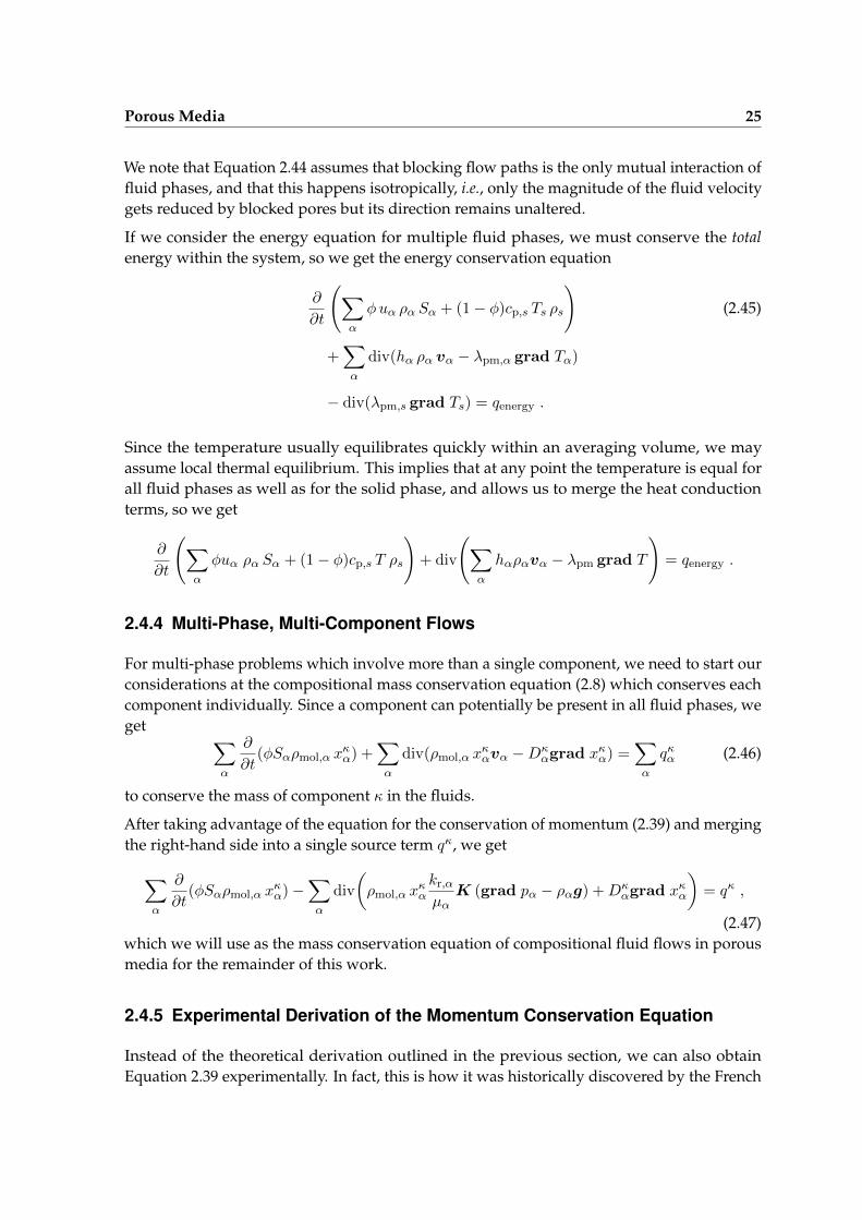
Porous Media 25
We note that Equation 2.44 assumes that blocking flow paths is the only mutual interaction offluid phases, and that this happens isotropically, i.e., only the magnitude of the fluid velocitygets reduced by blocked pores but its direction remains unaltered.
If we consider the energy equation for multiple fluid phases, we must conserve the totalenergy within the system, so we get the energy conservation equation
∂
∂t
(∑α
φuα ρα Sα + (1− φ)cp,s Ts ρs
)(2.45)
+∑α
div(hα ρα vα − λpm,α grad Tα)
− div(λpm,s grad Ts) = qenergy .
Since the temperature usually equilibrates quickly within an averaging volume, we mayassume local thermal equilibrium. This implies that at any point the temperature is equal forall fluid phases as well as for the solid phase, and allows us to merge the heat conductionterms, so we get
∂
∂t
(∑α
φuα ρα Sα + (1− φ)cp,s T ρs
)+ div
(∑α
hαραvα − λpm grad T
)= qenergy .
2.4.4 Multi-Phase, Multi-Component Flows
For multi-phase problems which involve more than a single component, we need to start ourconsiderations at the compositional mass conservation equation (2.8) which conserves eachcomponent individually. Since a component can potentially be present in all fluid phases, weget ∑
α
∂
∂t(φSαρmol,α x
κα) +
∑α
div(ρmol,α xκαvα −Dκ
αgrad xκα) =
∑α
qκα (2.46)
to conserve the mass of component κ in the fluids.
After taking advantage of the equation for the conservation of momentum (2.39) and mergingthe right-hand side into a single source term qκ, we get
∑α
∂
∂t(φSαρmol,α x
κα)−
∑α
div
(ρmol,α x
κα
kr,α
µαK (grad pα − ραg) +Dκ
αgrad xκα
)= qκ ,
(2.47)which we will use as the mass conservation equation of compositional fluid flows in porousmedia for the remainder of this work.
2.4.5 Experimental Derivation of the Momentum Conservation Equation
Instead of the theoretical derivation outlined in the previous section, we can also obtainEquation 2.39 experimentally. In fact, this is how it was historically discovered by the French
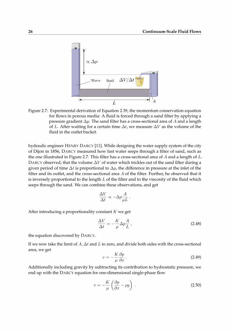
26 Continuum-Scale Fluid Flows
Figure 2.7: Experimental derivation of Equation 2.39, the momentum conservation equationfor flows in porous media: A fluid is forced through a sand filter by applying apressure gradient ∆p. The sand filter has a cross-sectional area of A and a lengthof L. After waiting for a certain time ∆t, we measure ∆V as the volume of thefluid in the outlet bucket.
hydraulic engineer HENRY DARCY [11]. While designing the water supply system of the cityof Dijon in 1856, DARCY measured how fast water seeps through a filter of sand, such asthe one illustrated in Figure 2.7. This filter has a cross-sectional area of A and a length of L.DARCY observed, that the volume ∆V of water which trickles out of the sand filter during agiven period of time ∆t is proportional to ∆p, the difference in pressure at the inlet of thefilter and its outlet, and the cross-sectional area A of the filter. Further, he observed that itis inversely proportional to the length L of the filter and to the viscosity of the fluid whichseeps through the sand. We can combine these observations, and get
∆V
∆t∝ −∆p
A
µL.
After introducing a proportionality constant K we get
∆V
∆t= −K
µ∆p
A
L, (2.48)
the equation discovered by DARCY.
If we now take the limit of A,∆t and L to zero, and divide both sides with the cross-sectionalarea, we get
v = −Kµ
∂p
∂x. (2.49)
Additionally including gravity by subtracting its contribution to hydrostatic pressure, weend up with the DARCY equation for one-dimensional single-phase flow
v = −Kµ
(∂p
∂x− ρg
). (2.50)
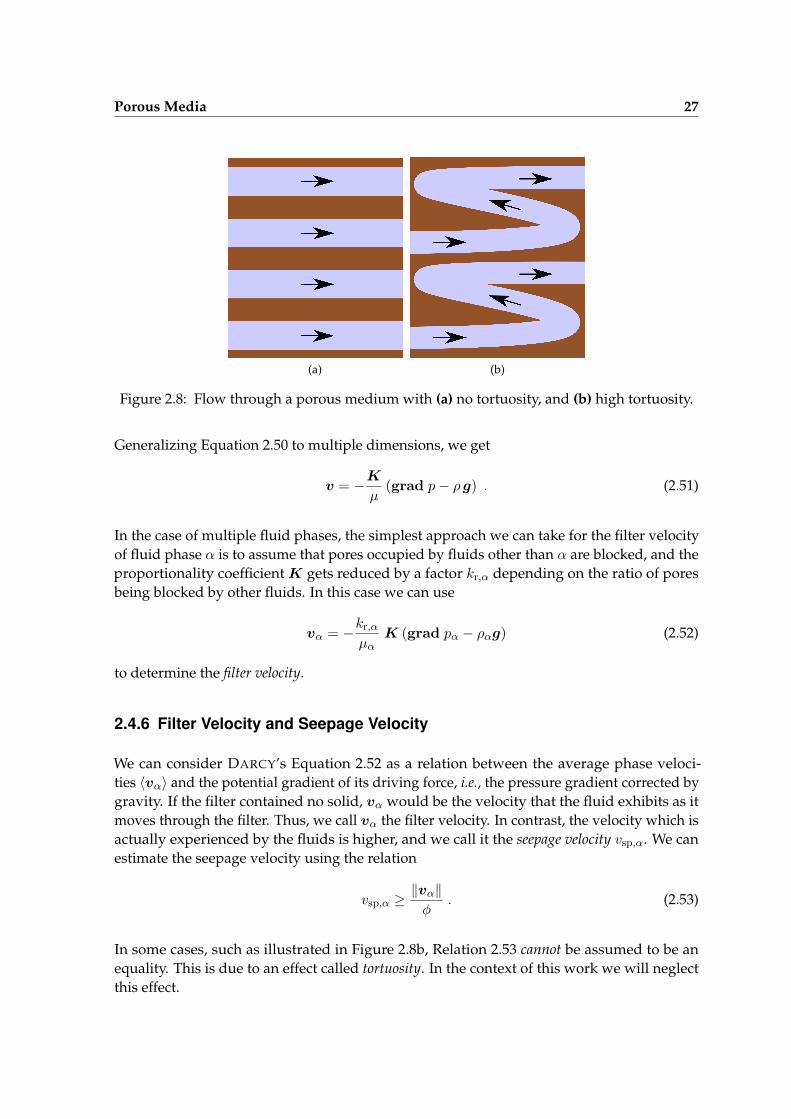
Porous Media 27
(a) (b)
Figure 2.8: Flow through a porous medium with (a) no tortuosity, and (b) high tortuosity.
Generalizing Equation 2.50 to multiple dimensions, we get
v = −Kµ
(grad p− ρ g) . (2.51)
In the case of multiple fluid phases, the simplest approach we can take for the filter velocityof fluid phase α is to assume that pores occupied by fluids other than α are blocked, and theproportionality coefficientK gets reduced by a factor kr,α depending on the ratio of poresbeing blocked by other fluids. In this case we can use
vα = −kr,α
µαK (grad pα − ραg) (2.52)
to determine the filter velocity.
2.4.6 Filter Velocity and Seepage Velocity
We can consider DARCY’s Equation 2.52 as a relation between the average phase veloci-ties 〈vα〉 and the potential gradient of its driving force, i.e., the pressure gradient corrected bygravity. If the filter contained no solid, vα would be the velocity that the fluid exhibits as itmoves through the filter. Thus, we call vα the filter velocity. In contrast, the velocity which isactually experienced by the fluids is higher, and we call it the seepage velocity vsp,α. We canestimate the seepage velocity using the relation
vsp,α ≥‖vα‖φ
. (2.53)
In some cases, such as illustrated in Figure 2.8b, Relation 2.53 cannot be assumed to be anequality. This is due to an effect called tortuosity. In the context of this work we will neglectthis effect.

28 Continuum-Scale Fluid Flows
2.5 Chapter Synopsis
In this chapter we have sketched a procedure to transform a molecular-scale descriptionof a physical system to a continuum-scale description in Section 2.1. Mathematically, thisprocedure can be considered to be a convolution with an adequate kernel. Then, starting atthe continuum-scale, we derived the equations for the conservation of mass, momentum,and energy in Section 2.3 and adapted them to the special case of NEWTONIAN fluids inSection 2.3.3. This lead us to the conservation equations
∂xκρmol
∂t+ div(xκρmolv −Dκgrad xκ ) = qκmol ,
ρ∂v
∂t+ ρv · grad v = −grad p+ µdiv grad v + ρ g + qmom and
∂ u ρ
∂t+ div(hρv − λgrad T ) = qenergy
for mass, momentum, and energy, respectively.
In Section 2.4 we then applied the volume averaging approach by WHITAKER [89] to theseequations, and obtained a macro-scale description of NEWTONIAN fluid flows in porousmedia. To see the link to the upscaling procedure from the molecular to the continuum-scale,we noted that the volume averaging approach can be comprehended as a special case ofa convolution. Using volume averaging, we then derived the macro-scale conservationequations for fluid flows in porous media, and got
∂∑
α φSαxκαρmol,α
∂t+∑α
div(xκκρmol,α vα −Dκ
pm.α grad xκα
)= qκ ,
vα = −kr,α
µαK (grad pα − ραg) and
∂
∂t
(∑α
φSα ρα uα + (1− φ)ρs cp,s T)
+ div
(∑α
hαρα vα − λpm grad T
)= qenergy
for mass, momentum, and energy, respectively.
Analogous to the upscaling procedure from molecular to continuum-scale where we lostthe information about individual particles, we lost the information of the microscopic fluidconfiguration within the porous medium when going to the macro-scale. This has the practicaladvantage that we only need to specify macroscopic properties—which are relatively easyto determine using physical experiments—and that we do not need to specify the exactgeometry of the solid phase of the porous medium.

3 Supplementary and Closure Relations
To solve any system of equations, we have to make sure that it is mathematically well-defined.This means that the equations are independent, i.e., that no equation can be expressed interms of the others, that a unique solution exists and that the number of unknowns equalsthe number of equations. We assert that the first two properties hold for the compositionalmass conservation equation (2.47). When counting the unknowns in these equations, weget 2N ·M +N + 6M + 3 where M is the number of fluid phases, and N is the number ofcomponents:
• One gravitational acceleration function g,
• One porosity distribution function φ,
• One absolute permeability distributionK,
• M saturations Sα,
• M pressures pα,
• M relative permeabilities kr,α,
• M dynamic viscosities µα,
• M mass densities ρα,
• M molar densities ρmol,α,
• N source terms qκ,
• M ·N mole fractions xκα, and
• M ·N diffusion coefficients Dκpm,α.
On the side of the equations, we currently have only N mass conservation equations ofthe components (2.47). In the following sections, we will examine the remaining relationsrequired to get a well-defined system of equations.
3.1 Saturation Closure Condition
One additional equation is implied by the simple fact that all pore space must be occupied byfluids1. We express this by the relation ∑
α
Sα = 1 . (3.1)
1In this context, we consider vacuum as gas.

30 Supplementary and Closure Relations
3.2 Given Parameters and Empiric Relations
Further, we assume the following quantities to be known a priori:
• Gravitational acceleration g,
• intrinsic permeability of the porous mediumK,
• porosity of the medium φ, and
• the source terms qκ of all components.
Also, we can assume that the dynamic viscosities of the fluids µα and the molecular diffusioncoefficients Dκ
pm,α are given closed functions depending on the fluid composition, tempera-ture, and on pressure. Moreover, we know that the mass and molar densities are connectedby
ρα = ρmol,α
∑κ
xκαMκ .
In general, we need to consider the relative permeabilities kr,α as spatially parameterizedfunctions which depend on all phase compositions xκβ, all temperatures Tβ, all pres-sures pβ, and all saturations Sβ. Having said that, we note that most of the commonlyused empiric relations for relative permeability, like the ones discussed in Section 3.4, onlydepend on the phase saturations Sα.
3.3 Thermodynamic Relations
At this point, we count M · N + 2N + 3M + 4 equations, which means that we still need(M − 1) ·N + 3M − 1 additional relations to get a mathematically closed system. Most ofthese can be obtained by considering the thermodynamics which governs the system.
3.3.1 Equations of State
First, we getM additional equations by defining the equations of state for all fluid phases. Anequation of state of a phase is the link between temperature Tα, pressure pα, composition xκα,and density ρα or—more commonly—the molar volume Vmol,α := 1/ρmol,α of a phase, i.e.,
pα = pα(Vmol,α, Tα, xκα) . (3.2)
The most simple equation of state,
pg =RTgVmol,g
,
with R = 8.314462 J/K mol describes ideal gases. This equation is a good approximation forreal gases at low temperature and low pressure, i.e., for situations where the values of thetemperature and pressure are much lower than the critical values of the substance. On the

Thermodynamic Relations 31
Name uα wα bκα aκα
VAN DER WAALS 0 01
8
RTκcritpκcrit
27
64
(RTκcrit)2
pκcrit
REDLICH-KWONG 1 00.08664RTκcrit
pκcrit
0.42748(RTκcrit)2
pκcrit√Tr
with Tr = Tα/Tκcrit
SOAVE 1 00.08664RTκcrit
pκcrit
0.42748(RTκcrit)2
pκcrit
(1 + (1−
√Tr) fωκ
)2with fωκ = 0.48 + ωκ(1.574− 0.176ωκ)
PENG-ROBINSON 2 -10.07780RTκcrit
pκcrit
0.45724(RTκcrit)2
pκcrit
(1 + (1−
√Tr) fωκ
)2where fωκ = 0.37464 + ωκ(1.54226− 0.26992ωκ)
Table 3.1: Parameters for common cubic equations of state as outlined by REIDet al. [68].T κcrit and pκcrit correspond to the critical temperature and critical pressure of a purecomponent κ, and ωκ is the acentric factor of the component. All these quantitiescan either be taken from the literature or they can be estimated [68].
molecular scale, this relation implies that the interactions between particles of the gas arewell approximated by elastic collisions.
Since for real gases, molecular particles also interact by means of their electric force fields,a more complex EOS is needed. Such a class of equations of state are cubic equations of state.These equations can be expressed in the form [68]
pα =RTα
Vmol,α − bα− aαV 2
mol,α + uα bα Vmol,α + wα b2α. (3.3)
Here we call the quantity bα the covolume of the fluid phase α since it resembles the volumeoccupied by the particles of the substance directly, and we call aα the attractive factor of fluidphase α since it describes how strongly the particles attract each other. Finally, uα and wα areconstants given by the chosen equation of state.
Table 3.1 outlines some common parameterizations for pure substances. Of those relations,the VAN DER WAALS and REDLICH-KWONG parameterizations are primarily of historicalinterest [68]. For the SOAVE and PENG-ROBINSON approaches, we cannot specify the mostaccurate one a priori as the error of a parameterization strongly depends on the molecularproperties of the considered substance [68].
For mixtures of multiple substances, we may also use Equation 3.3 as the equation of state,but we need to calculate the parameters aα and bα for the mixture from the parameters ofthe pure constituting components using a mixing rule. The most common mixing rule [68] is

32 Supplementary and Closure Relations
Vmol,α
pα
bα
p1
Vmol,l Vmol,g
p2
(a) Under-Critical Fluid
Vmol,α
pα
bα
p1
Vmol,l = Vmol,g
(b) Critical Fluid
Figure 3.1: Possible shapes of cubic equations of state. For these, the pressure of a fluid phasepα is defined in terms of the molar volume Vmol,α = 1/ρmol,α of the fluid.
given by
aα =∑κ
∑λ
xκαxλα
√aκαa
λα(1− kκλα ) and (3.4)
bα =∑κ
xκαbκα ,
where kκλα is the interaction coefficient of the components κ and λ in the fluid phase α.
Multiple Phases
We can use the same cubic equations of state for multiple phases: In the most simple case,outlined in Figure 3.1a, an isotherm of the equation of state has three intersections with theisobar p1 that are larger than the covolume bα. In this case, we can choose the molar volumefor the liquid Vmol,l as the value of the smallest intersection, and the molar volume of thegas Vmol,g as the value of the largest intersection.
Another case is also illustrated in Figure 3.1a: If we increase the pressure to p2, the isothermof the equation of state has only one intersection with the isobar. Given the fact that wehave to choose the molar volume of each phase in a way that is continuous with regard topressure, the molar volume of the physically impossible phase becomes undefined. Thisissue can be mended if the equation of state features two extrema at physically meaningfulmolar volumes. In this case, we can use the molar volume of the largest extremum for gasand the molar volume of the smallest extremum for the liquid. Also, we can decide whichphase is unphysical by considering the intersection of the isotherm with the isobar p2: Ifthe molar volume of the intersection is higher than the value of both extrema, the value ofthe intersection is the molar volume of the gas phase, else it corresponds to the value of theliquid phase.
If we increase the temperature—or alternatively change the composition of the fluid—thefluid becomes critical, and the isotherms of the equation of state resemble the curve depicted
Thermodynamic Relations 33
in Figure 3.1b. Given the fact that such curves only exhibit a single intersection with anypressure, and they also do not feature physically meaningful extrema, we need a differ-ent approach to achieve continuity of the molar volume regarding temperature, pressure,and composition. In this case, we can calculate the critical point for a substance with theparameters aα and bα, and use its molar volume as the molar volume for the unphysicalphase.
3.3.2 Local Thermodynamic Equilibrium
Besides the M equations of state which essentially yield the mass density of all phases at agiven temperature, pressure, and composition, we obtain further thermodynamic relationsby assuming local thermodynamic equilibrium.
The term “local thermodynamic equilibrium” means that we can always consider the fluidsat each point of the spatial domain to be at steady-state if we would isolate this locationfrom the rest of the system. This statement is equivalent to saying that, after isolatingany infinitesimally small subdomain V from the rest of the system at any time, the fluidscontained in the extracted domain V would be thermodynamic equilibrium. Thermodynamicequilibrium itself is defined as the superposition of the following three subequilibria:
Thermal equilibrium, which is defined as the temperature of all phases in any infinitesimallysmall and isolated sub-domain V being constant in time,
Mechanical equilibrium, meaning that the pressure of all phases is constant in time withinsuch an isolated sub-domain V , and
Chemical equilibrium, which represents the fact that the composition of any fluid phasedoes not change with time within an isolated sub-domain V .
In the following, we will discuss these three equilibria independently.
Thermal Equilibrium
Thermal equilibrium is defined as the temperature of all phases of a thermodynamic systembeing constant in time, i.e.,
∂Tα∂t
= 0 (3.5)
holds. By the “zeroth” law of thermodynamics, this implies that the temperature equal withinthe system, i.e.,
Tα = Tβ =: T (3.6)
holds for arbitrary phases α and β.
If we consider conservation of energy, the energy balance equation (2.46) determines theadditional unknown T . In this case, we can assume the specific enthalpies hα to be closedfunctions which depend on the fluid composition, pressure, and temperature [68]. Further,we can consider the thermal conductivity coefficient λpm to be a given function depending

34 Supplementary and Closure Relations
on the saturations, temperature, fluid compositions, and pressures. We also know that therelation between specific internal energy uα and enthalpy hα of phase α is given by
uα = hα −pαρα
.
In contrast, if we do not conserve energy, we must impress the temperature T externally onthe system, i.e., we need to consider temperature as a spatially and time dependent parameterlike, for example, the intrinsic permeabilityK.
Mechanical Equilibrium
Mechanical equilibrium is defined as the pressure of all fluids being stationary, i.e.,
∂pα∂t
= 0 (3.7)
holds for all phases α.
In the context of fluid flows in porous media, this does not imply that the pressures of allfluid phases are equal. Instead, it implies that the differences between the pressures of allfluid phases are static. We can express this fact using
pα = pβ + pc,αβ , (3.8)
where we call the quantity pc,αβ capillary pressure2 between fluid phases α and β. In the mostgeneral case, the quantity pc,αβ potentially depends on all fluid pressures, all phase satura-tions, all temperatures and the composition of all fluid phases like the relative permeabilityfunctions kr,α. Having said that, the most common approaches— which we will discuss inSection 3.4—only depend on the phase saturations.
Chemical Equilibrium
For chemical equilibrium, the fluid compositions must be time-invariate, i.e.,
∂xκα∂t
= 0 (3.9)
is true for all phases α and all components κ. This means that the chemical potentials ζκα ofeach component are identical for all phases, i.e.,
ζκα = ζκβ =: ζκ (3.10)
2Note that the term capillary pressure is a bit of a misnomer because the capillary effect is not the only microscopiceffect which determines macroscopic pressure differences [38].

Thermodynamic Relations 35
holds for any two fluid phases α, β, and any component κ. The chemical potential of acomponent in a fluid is defined as
ζκα =∂gα∂nκα
where gα = hα − Tαsα is the GIBBS free energy of phase α, and nκα = NA xκαρmol,α is the total
number of molecular particles of component κ per unit of volume. Here, the specific entropyof the fluid is represented by sα, and NA = 6.022·1023/mol is AVOGADRO’s constant.
Since chemical potentials become infinite for non-present components, it is advisable to usefugacities instead. The fugacity fκα of a component in a phase is connected to the chemicalpotential of the component by the equation
fκα = fκ,α exp
(ζκα − ζ
κ,α
RTα
), (3.11)
where fκ,α is the fugacity of component κ in phase α at an arbitrary but fixed reference stateof the pure component, and ζκ,α is the chemical potential at the same reference state. We notethat the fugacity is a smooth, monotonous function mappingR toR+.
If we assume thermal equilibrium, the condition for equality of all chemical potentials in allfluids (3.10) can thus be reformulated as equivalence of component fugacities, i.e.,
fκα = fκβ (3.12)
holds for any component κ and arbitrary phases α and β.
To calculate the fugacity fκα of a component in a phase, we usually use the relation
fκα := pαxκαΦκ
α . (3.13)
Further, we can determine the fugacity coefficient Φκα of component κ using the equation of
state. According to REID et al. [68], the relation for this is
RTα ln fκα = −∫ Vmol,α
∞
∂pα∂nκα
− RTα
Vmol,α
dVmol,α +RTα lnZα , (3.14)
where Zα = pαVmol,α/RTα is the compressibility factor of the phase, and nκα = NA xκα/Vmol,α is the
total number of molecules of component κ per volume.

36 Supplementary and Closure Relations
Cubic Equations of State
For cubic equations of state, Equation 3.14 can be evaluated analytically if we use Equation 3.4as mixing rule. We get [68]
ln Φκα =
bκαbα
(Zα − 1)− ln(Zα −B?α)
+A?α
B?√u2α − 4wα
(bκαbα− δκα
)ln
2Zα +B?α(uα +
√u2α − 4wα)
2Zα +B?α(uα −
√u2α − 4wα)
, (3.15)
with the abbreviations
A?α =aαpα
(RTα)2,
B?α =
bαpαRTα
, and
δκα =
√aκα
2 aα
∑λ
xλα(1− kκλα )√aλα .
Ideal Mixtures
Often, we assume a fluid phase to be an ideal mixture of its constituent components. In thiscase, all fugacity coefficients are independent of the composition of the phases, and we getthe relation
fκ = pαxκα Φκ
α(Tα, pα) .
For ideal gases, Φκα is equal to 1; for liquid phases, the fugacity coefficient and the fluid
pressure are usually combined into a single coefficient
P κα (Tα, pα) := pα Φκα(Tα, p
κα) .
For components that exhibit a low miscibility with the liquid, this coefficient is called HENRY
coefficient; otherwise, the component is the dominant constituent of the liquid, and P κα iseither called RAOULT coefficient, vapor pressure or saturation pressure.
3.4 Capillary Pressure and Relative Permeability
After our detailed discussion of thermodynamic equilibrium in the previous section, we willnow cover the most widely used heuristic capillary pressure curves in greater detail.
In the case of two fluid phases with the capillary pressure only depending on the phasesaturations, we can apply one of the two most commonly used capillary pressure and relativepermeability functions —the one proposed by to BROOKS and COREY or the function of VAN

Capillary Pressure and Relative Permeability 37
Sw
pc,nw
1.00.750.500.25
VAN GENUCHTEN
BROOKS-COREY
(a)
Sw
kr,α
1.00.750.500.25
1.0
0.75
0.50
0.25
kr,w VAN GENUCHTEN
kr,n VAN GENUCHTEN
kr,w BROOKS-COREY
kr,n BROOKS-COREY
(b)
Figure 3.2: Principle shapes of the BROOKS-COREY and VAN GENUCHTEN functions fortwo-phase flow in porous media. The parameters of the functions have beenconverted using the approach proposed by LENHARD, PARKER, and MISHRA [50].(a) Capillary pressure. (b) Relative Permeability.
GENUCHTEN. These functions will also be the subject of the following subsections and areillustrated in Figure 3.2.
3.4.1 Generic Two-Phase Relations for Relative Permeability
Before we deal with the saturation-dependent two-phase capillary pressure curves, we needto discuss the connection between the capillary pressure and the relative permeability forthem. As it turns out that, although in general we can regard the relative permeabilities kr,α
and the capillary pressures pc,α as independent quantities, they have been shown to be relatedin the most common cases [39]. If only two fluid phases are involved, and the capillarypressure between those only depends on the fluid saturations, the relative permeabilities aregiven by the equations [39]
kr,w = SwA
∫ Sw
0
(pc,nw(Sw)
)−BdSw∫ 1
0
(pc,nw(Sw)
)−BdSw
C
and (3.16)
kr,n = (1− Sw)A
∫ 1Sw
(pc,nw(Sw)
)−BdSw∫ 1
0
(pc,nw(Sw)
)−BdSw
C
(3.17)
with some constants A, B, and C. We note that it is not possible to directly apply theseequations to capillary pressure functions without choosing concrete values for A, B, and C.

38 Supplementary and Closure Relations
3.4.2 Relation of BROOKS and COREY
The most widely applied approach for capillary pressure in two-phase flows is the oneproposed by BROOKS and COREY [13, 39]. This approach considers two fluid phases, thewetting and the non-wetting phases. There, the fluid for which the contact angle of the fluid-fluid interface with the surface of the solid is smaller than 90 is defined as the wetting fluid,the other fluid is called non-wetting. The capillary pressure relation proposed by BROOKS andCOREY now assumes that the only quantity on which the difference in pressure between thewetting and the non-wetting phase depends, is the saturation of the wetting phase. Underthese preconditions, BROOKS and COREY proposed [13] the relation
pc,nw = pn − pw = peS− 1λbc
w , (3.18)
where pe is the entry pressure and λbc is a shape parameter. Both of these parameters are highlyspecific to the properties of the porous medium as well as to the properties of the consideredfluids [39]. For this reason, these two parameters are usually obtained experimentally [39].
In conjunction with the BROOKS-COREY capillary pressure curve, the BURDINE parameteriza-tion A = B = 2, and C = 1 is normally used [39] for relations of the relative permeabilitieswhich are implied by Equations 3.16 and 3.17. This yields
kr,w = Sw2+3λbcλbc and (3.19)
kr,n = (1− Sw)2
(1− S
2+λbcλbc
w
). (3.20)
3.4.3 Curve of VAN GENUCHTEN
As an alternative to the curves proposed by BROOKS and COREY, we can also use therelation proposed by VAN GENUCHTEN [87, 39]. Like the BROOKS-COREY curves, the VAN
GENUCHTEN approach presumes that the value of capillary pressure depends solely on thesaturation of the wetting phase, but in contrast to the BROOKS-COREY relation, it does notuse the concept of entry pressure. Instead, the VAN GENUCHTEN approach assumes that thecapillary pressure is zero in a medium which is fully saturated by the wetting phase. Alsoclearly visible in Figure 3.2 is the fact that for VAN GENUCHTEN curves, the slope is infinite ifthe porous medium is fully saturated by the wetting phase. This property is thus similar tothe entry pressure concept in the BROOKS-COREY approach.
The concrete function proposed by VAN GENUCHTEN [87] is given by
pc,nw = pn − pw =1
αvg
(S− 1mvg
w − 1
) 1nvg
,
where αvg, mvg, and nvg are shape parameters. Like for the BROOKS-COREY relation, at leasttwo of those parameters must be obtained by fitting experimental data. For the third, it is

Capillary Pressure and Relative Permeability 39
often possible to use the relationmvg = 1− 1/nvg
as proposed by VAN GENUCHTEN [87]. We note that instead of using this equation, we alsomay take advantage of others which better fit experimentally obtained capillary pressurecurves [47].
Like for the BROOKS-COREY capillary pressure curves, we can evaluate Equations 3.16and 3.17 to gain closed relative permeability functions. In contrast to the BROOKS-COREY
approach, the parameterization proposed by MUALEM is usually used [39], i.e., A = 0.5,B = 1, and C = 2. With these values, we get
kr,w = Swεvg
(1−
(1− Sw
1mvg
)mvg)2
and (3.21)
kr,n = (1− Sw)γvg(
1−(
1− Sw1
mvg
)mvg)2mvg
(3.22)
where εvg and γvg are parameters that depend on the microscopic properties of the porousmedium. Often [39] we can assume their values to be εvg = 1/2 and γvg = 1/3.
3.4.4 Three-Phase Systems
The final capillary pressure relations which we will cover in detail were proposed bySTONE [79, 39], and are concerned with three-phase flow in porous media.
For such systems, we assume three potentially present phases called “wetting liquid”, “non-wetting liquid”, and “gas”, indicated by 〈·〉w, 〈·〉n, and 〈·〉g in the following. For such systems,it has been observed [52], that in many situations the relative permeability of the wettingliquid phase kr,w and the relative permeability of the gas phase kr,g primarily depend onthe saturations of the wetting liquid and the gas, respectively. Also, the capillary pressuresbetween the wetting liquid and the non-wetting liquid pc,nw has been shown to dependmainly on the saturation of the wetting liquid and we can assume that the only non-negligibledependency of the capillary pressure between the gas and the non-wetting liquid phases pc,gn
is the saturation of the gas phase [39].
The main idea of the two approaches proposed by STONE [79, 80] is to take advantage of thecapillary pressure relations for the two-phase cases with the wetting and the non-wettingliquids—which we will indicate by 〈·〉wn in the following—as well as the capillary pressurecurves for the two-phase system featuring the non-wetting liquid and the gas—indicatedby 〈·〉ng. Under these assumptions, we can use the appropriate two-phase relations to definethe three-phase capillary pressure relations, i.e.,
pc,nw(Sw, Sn, Sg) = pcwn,nw(Sw) and (3.23)
pc,gn(Sw, Sn, Sg) = pcnw,gn(1− Sg) . (3.24)

40 Supplementary and Closure Relations
Similarly, we define the wetting liquid and the gas relative permeabilities of the correspondingtwo-phase systems, i.e.,
kr,w(Sw, Sn, Sg) = krwn,w(Sw) and (3.25)
kr,g(Sw, Sn, Sg) = krng,g(1− Sg) . (3.26)
For the relative permeability of the non-wetting liquid kr,n, STONE proposed two approaches:The first [79] uses the relation
kr,n(Sw, Sn, Sg) = Snkrwn,n(Sw)
1− Swkrng,n(1− Sg)
1− Sg, (3.27)
whilst the second [80] defines kr,n as
kr,n(Sw, Sn, Sg) =(krng,n(1− Sg) + krng,g(1− Sg)) · (krwn,n(Sw) + krwn,w(Sw))
− (krwn,w(Sw) + krng,g(1− Sg)) .
3.4.5 Advanced Concepts
We note that, the approaches which we covered so far do not take residual saturations [39]into account in order to simplify the discussion. We can imagine the residual saturation of aphase as the saturation of the fluid that cannot be transported by advection – an effect that iscaused by various mechanisms that trap fluids within a porous medium [39]. Having saidthat, this material can be dissolved by the other fluids and be transported this way.
Also, there are quite a few advanced concepts when it comes to capillary pressure: Amongstthese are temperature [73] and fluid composition [27] dependence, approaches which dis-card the assumption of mechanical equilibrium [38], and methods to take hysteresis intoaccount [65, 59, 10].
3.5 Model Constraints
At this point, if we count the number of independent equations which we have defined forour M -phase, N -component system, we get 2N ·M +N + 6M + 3:
• The three externally impressed functions gravitational acceleration g, intrinsic perme-abilityK, and porosity φ,
• a closure condition for saturations (3.1),
• M relations connecting the molar density ρmol,α with the mass density ρα,
• M functions for the dynamic viscosities µα,
• M relations capturing the relative permeabilities kr,α,

Model Constraints 41
• N source terms qκ,
• M · N closed functions for the molecular diffusion coefficients in the porousmedium Dκ
pm,α,
• M equations of state (3.2),
• M − 1 constraints from the thermal equilibrium (3.5),
• M − 1 equations for the mechanical equilibrium (3.7),
• N mass balance equations (2.47),
• an impressed temperature function if we neglect conservation of energy, or an energyconservation equation in the other case, and
• (M − 1) ·N conditions stemming from the chemical equilibrium (3.9).
On the side of the unknowns, we additionally need M phase temperatures Tα, so we nowhave 2N ·M +N + 7M + 3 unknowns. This means that, at this point, we are still missing Mequations to make the system of equations well-defined. In the context of this thesis, we willcall these M relations model constraints, and in the next few sections we will discuss severalapproaches which define these model constraints.
3.5.1 Immiscibility
The first set of model constraints we will cover here is the one which ignores miscibilityaltogether. It is a reasonable approximation of a real system if all fluid phases exhibit a highlypreferred component. Immiscibility [39] thus means that each phase α is composed of only asingle component κα, i.e.,
xκα =
1 for κ = κα and0 else.
(3.28)
Using the thermodynamical framework outlined before, we can achieve this by letting thefugacity coefficient of the “non-preferred” components be infinite whilst keeping it finite forthe constituent component, for example
Φκα =
1 for κ = κα and∞ else.
(3.29)
In this context, we should be aware of the fact that Equation 3.29 cannot be used directly innumerical software because of the occurrence of infinite values in the fugacity coefficients.Instead, we need to implicitly set the mole fractions of all “non-preferred” components of aphase to zero and the mole fraction of the “preferred” component to one.
The M model constraints are then given by the requirement that all phases are alwayspotentially present, i.e., ∑
κ
xκα = xκαα = 1 (3.30)
holds for any phase α.

42 Supplementary and Closure Relations
3.5.2 Primary Variable Switching
We can obtain a second set of model constraints if the set of fluids which are present at agiven location in space at a given time are known: In the case that phase α is present, the sumof the mole fractions which fulfill the condition of chemical equilibrium (3.12) sum up to one,i.e., ∑
κ
xκα = 1
holds. In the other case, phase α is not present at the location, so that its saturation must bezero, i.e.,
Sα = 0
This leads to the following set of model constraints [23]
0 =
1−
∑κ x
κα if phase α is present, and
Sα if it is not present.(3.31)
In flow simulations, a phase can appear or disappear, and thus we need to adapt the set ofphases which are present at a given location during the process of finding a solution. Thiscan be accomplished by continuing the solution procedure with a given set of present phases,and changing this set if an intermediate state is physically impossible. In such an event, weneed to update the set of present phases, and choose physically meaningful quantities asprimary variables.
In the following, we use the following switching conditions:
• A present phase vanishes if the saturation of the phase becomes negative, i.e., if
Sα < 0
holds. In this case we remove the saturation Sα of the vanished phase from the set ofprimary variables, and replace it by a mole fraction of a component for a fluid that ispresent.
• A non-present phase α appears if the quantities xκα that meet the condition for chemicalequilibrium (3.12) are interpretable as mole fractions. This is the case if the sum of xκαin the phase is equal to 1. In numerical simulations we also have to be prepared thatsum of xκα can become larger than 1, i.e., we use the condition∑
κ
xκα ≥ 1
as switching condition.
If we detect such a state, we remove the mole fraction of a component from the set ofprimary variables, and replace it by the saturation Sα of the newly appeared phase.
In Section 5.2.2 we will discuss in greater detail how these primary variable switching (PVS)model assumptions can be implemented in numerical software.

Model Constraints 43
3.5.3 Non-Linear Complementarity Functions
An alternative to the procedure above is to directly include the conditions outlined in theprevious section into the set of equations to be solved [48]: For this we observe that, as longas phase α is not present, the sum of the mole fractions which meet the chemical equilibriumcondition (3.12) are allowed to be smaller than 1, i.e.,
Sα = 0 =⇒∑κ
xκα ≤ 1 .
Next, we observe that a necessary precondition for phase α to be present is that its constituentmole fractions sum up to one, i.e.,∑
κ
xκα = 1 =⇒ Sα ≥ 0
holds.
Since each phase is either present or non-present, at least one of the above cases must apply,we get the following non-linear complementarity problem (NCP) for each fluid phase α:
Sα
(1−
∑κ
xκα
)= 0 ∧ 1−
∑κ
xκα ≥ 0 ∧ Sα ≥ 0 . (3.32)
Such a problem can be directly included into the system of equations to be solved using anon-linear complementarity function Ψ : R2 → R which is exhibits the property
Ψ(a, b) = 0 ⇐⇒ a ≥ 0 ∧ b ≥ 0 ∧ a · b = 0 .
There are multiple possible choices for Ψ; for example, the FISCHER-BURMEISTER non-linearcomplementarity function [32] ΨFB is defined as
ΨFB(a, b) = a+ b−√a2 + b2 .
For the remainder of this work, we will use the minimum function Ψ(a, b) = min(a, b) becauseof its piecewise linearity. This means that we will use the model constraints
Ψα (Sα, 1−∑κ
xκα) = min (Sα, 1−∑κ
xκα) = 0 (3.33)
when discussing the NCP model.
3.5.4 Black-Oil
The black-oil model is a set of model assumptions widely used in the oil industry [83, 19,46, 45]. It presumes three potentially present fluids oil, gas, and water—in the followingindicated by 〈·〉o, 〈·〉g, and 〈·〉w—as well as three pseudo-components to which we also refer

44 Supplementary and Closure Relations
Figure 3.3: Definition of the gas solubility factorRS in the black-oil model: A given volume ofsaturated oil Vreservoir,o is brought from reservoir pressure preservoir to the relativelylow atmospheric pressure patm. Then, the gas solubility factor is defined as theratio between volume of gas which emerges at the surface and the original volumeof the reservoir oil. Typically, the reservoir pressure exceeds 200 bar while patm isroughly 1 bar.
to as oil, gas, and water, and which will be indicated by 〈·〉O, 〈·〉G, and 〈·〉W . In the terms ofthe thermodynamic framework of this chapter, the black-oil model presumes M = N = 3.
The first assumption of the black-oil model is that the water, and gas phases are immiscible,and that they are solely constituted by the components with the same names. In contrast,the oil phase is assumed to be a mixture of the pseudo-components gas and oil with thecomposition given by the gas solubility factor RS.
This factor is defined as the volume of the gas phase that emerges from a given amountof gas-saturated oil phase if the of oil is brought from the reservoir to the surface, i.e., thatthe pressure of the material is reduced from reservoir pressure to atmospheric pressure, asillustrated in Figure 3.3. We thus define RS as
RS :=Vatm,g
Vreservoir,o=Satm,gVtotal,atm
Vreservoir,o.
Given the gas solubility factor at a certain pressure, the composition of gas saturated oil atreservoir pressure can thus be determined in terms of mass fractions using
XGsat,o =
ρg(patm)RS(po)
ρsat,o(po)and XO
sat,o = 1−XGsat,o
if we assume that the amount of the gas in oil is negligible at atmospheric pressure.
We also need to specify the mass densities of all phases at a given pressure. While we assumethe water phase to be incompressible, the density of the gas saturated oil phase ρo and theone of the gas phase ρg is determined by the oil and the gas formation volume factors Bo and Bg.

Model Constraints 45
These two factors express the ratio between the mass density at reservoir pressure and thedensity at atmospheric pressure, i.e.,
Bα(pα) =ρsat,α(pα)
ρsat,α(patm), α ∈ o, g ,
where the atmospheric densities ρsat,α(patm) are given constants.
Fugacity Coefficients
In order to fit the set of black-oil parameters into our thermodynamic framework, we need todefine fugacity coefficients Φκ
α for all components κ and all fluid phases α as well as the massdensities of all fluid phases. In the following, we will outline how we can achieve this goal.
The black-oil parameters assume the gas and the water phases to be immiscible, i.e., the onlyconstituent of the gas phase is the gas component, and that of the water phase is the watercomponent. For this reason, we can use the same approach to the fugacity coefficients as forthe immiscible model constraints, i.e.,
Φκα =
1 if κ = κα,∞ else
for α ∈ w, g, κ ∈ O,W,G, and with κw = W , κg = G.
Since the oil phase is a mixture of the gas and the oil components, we first need to ensurethat the oil phase does not contain any water by setting the fugacity coefficient for the watercomponent in the oil phase to infinity. For the fugacity coefficient of the oil component in theoil phase, we can use any finite positive value; usually we use
ΦOo =
pOvap
po
where pOvap denotes a typical vapor or saturation pressure of the oil component.
The most elaborate fugacity coefficient is the one for the gas component in the oil phase.This is due to the facts that the gas component is the only component which is assumed tobe potentially present in two fluid phases, i.e., the gas and the oil phase, and that we mustchoose the fugacity coefficient such that it is consistent with the black-oil parameters. We canachieve this by first calculating the mass fractions XO
sat,o and XGsat,o for gas saturated oil as
outlined in the previous section. Next, we need to convert these mass fractions into molefractions by solving the system of equations
XGsat,o =
MG
Mo
xGsat,o,
Mo = xOsat,oMO + xGsat,oM
G , and
xGsat,o + xOsat,o = 1
46 Supplementary and Closure Relations
in regard to xGsat,o. This yields
xGsat,o =MOXG
sat,o
MG +XGsat,o(M
O −MG)and xOsat,o = 1− xGsat,o .
For gas saturated oil, we can now define the fugacity coefficient of the gas component inthe oil phase using the definition of the fugacity coefficients (3.13), and inserting it into thecondition for chemical equilibrium (3.12). Assuming that the capillary pressure is negligible,we get
ΦGo =
ΦGg
xGsat,o
.
Mass Density of the Oil Phase
The presented black-oil parameters directly provide densities ρsat,α for all three saturatedphases, but—somewhat surprisingly—we must take quite complex measures to define ρo,the mass density of potentially undersaturated oil. The reason for this is that—in contrast tothe water and gas phases—the oil phase may dissolve less gas than the maximum physicallypossible amount but the black-oil parameters only specify oil phase densities for gas saturatedoil. To define ρo, we take a closer look at the total derivative of the mass density of thesaturated oil phase with respect to pressure. Applying the chain rule, we get
dρsat,o
dpo=
d
dpoρo(po, X
Osat,o(po), X
Gsat,o(po)) =
∂ρo∂XG
o
∂XGsat,o
∂po+
∂ρo∂XO
o
∂XOsat,o
∂po+∂ρo∂po
,
where XGsat,o(po) and XO
sat,o(po) are the mass fractions of the gas and oil components of gassaturated oil at pressure po as specified by the black-oil parameters. Taking advantage of thefact that the mass fractions of all components sum up to one for oil, we get
dρsat,o
dpo=∂XG
sat,o
∂po
(∂ρo∂XG
o
− ∂ρo∂XO
o
)+∂ρo∂po
. (3.34)
Further, we now suppose that the compressibility of the oil phase is a given constant, i.e.,
∂ρo∂po
:= const
holds, and we already assumed the mass fraction of gas in saturated oil at atmosphericpressure to be negligible. Under these preconditions, we may use the density of the oil at thesurface together with the compressibility to define the partial derivative of the mass densityof the oil phase regarding the mass fraction of the oil component, i.e.,
∂ρo∂XO
o
:= ρsat,o(patm)
(1 +
∂ρo∂po
(po − patm)
).

Chapter Synopsis 47
We now observe that Equation 3.34 determines the partial derivative of the gas mass fractionin saturated oil using the black-oil parameters. Resolving, we get
∂ρo∂XG
o
=
(∂XG
sat,o
∂po
)−1(dρsat,o
dpo− ∂ρo∂po
)+
∂ρo∂XO
o
.
Assuming that these derivatives stay constant for undersaturated oil, we can finally definethe generic mass density of oil as:
ρo = ρsat,o(po) +(XGo −XG
sat,o
) ∂ρo∂XG
o
+(XOo −XO
sat,o
) ∂ρo∂XO
o
.
Black-Oil Model Constraints
Now that we defined all relevant quantities using only the black-oil parameters as input, weneed to specify the appropriate model constraints in order to use the abstract thermodynamicframework presented in this chapter. First, we observe that we can use the immiscibilitymodel constraints for the water and for the gas phases, i.e.,∑
κ
xκα = xκαα = 1
for α ∈ w, g. For the oil phase, we assume that it is always potentially present, which leadsto the constraint ∑
κ
xκo = xOo + xGo = 1 .
Like for the immiscibility model assumptions, we cannot use some of the presented defi-nitions directly in software implementations since some of the fugacity coefficients exhibitinfinite values. Thus, we may either approximate the black-oil model by using very largefugacity coefficients, or we can implement it by directly incorporating them into the software.
3.6 Chapter Synopsis
In this chapter, we made the mathematical description of multi-phase, multi-componentflows in a porous medium well-defined. In particular, this implied the need to specify thesame number of independent equations as quantities. We obtained some of these relations byassuming a few quantities to be closed functions, a few others were obtained by assumingthem to be given parameters depending on the time and the spatial location within thedomain. Examples of the former are the dynamic viscosities µα and mass densities ρα of thefluids, while examples of the latter are the gravitational acceleration vector g and the intrinsicpermeabilityK.

48 Supplementary and Closure Relations
We then accounted for the additional relations implied by thermodynamics. At this occasion,we discussed some widely used equations of state, and outlined the conditions implied byassuming local thermodynamic equilibrium.
Finally, we noted that one equation per fluid phase was still missing. We identified thesemissing relations as model specific constraints, and we discussed three established sets ofconstraints, i.e., the immiscibility, primary variable switching (PVS), and black-oil models.We also presented a new set of model constraints which are based on solving non-linearcomplementarity problems (NCP).
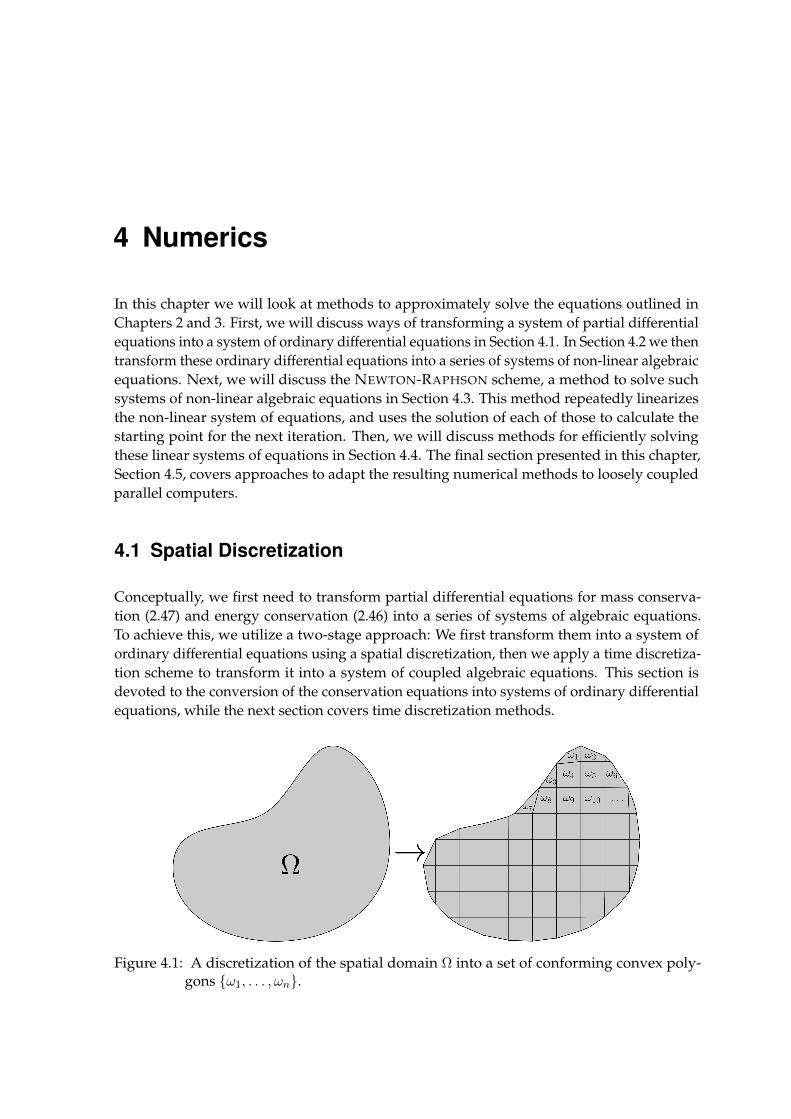
4 Numerics
In this chapter we will look at methods to approximately solve the equations outlined inChapters 2 and 3. First, we will discuss ways of transforming a system of partial differentialequations into a system of ordinary differential equations in Section 4.1. In Section 4.2 we thentransform these ordinary differential equations into a series of systems of non-linear algebraicequations. Next, we will discuss the NEWTON-RAPHSON scheme, a method to solve suchsystems of non-linear algebraic equations in Section 4.3. This method repeatedly linearizesthe non-linear system of equations, and uses the solution of each of those to calculate thestarting point for the next iteration. Then, we will discuss methods for efficiently solvingthese linear systems of equations in Section 4.4. The final section presented in this chapter,Section 4.5, covers approaches to adapt the resulting numerical methods to loosely coupledparallel computers.
4.1 Spatial Discretization
Conceptually, we first need to transform partial differential equations for mass conserva-tion (2.47) and energy conservation (2.46) into a series of systems of algebraic equations.To achieve this, we utilize a two-stage approach: We first transform them into a system ofordinary differential equations using a spatial discretization, then we apply a time discretiza-tion scheme to transform it into a system of coupled algebraic equations. This section isdevoted to the conversion of the conservation equations into systems of ordinary differentialequations, while the next section covers time discretization methods.
Figure 4.1: A discretization of the spatial domain Ω into a set of conforming convex poly-gons ω1, . . . , ωn.

50 Numerics
Quite a few spatial discretization schemes have been proposed to date. The ones which aremost widely used are based on the ideas of the finite volume [31], finite element [29, 81], anddiscontinuous GALERKIN approaches [5]. All of these methods share the property that thespatial domain Ω is partitioned into n smaller subdomains ω1, ω2, . . . , ωn. The individualsubdomains are called elements or cells, whilst the partition itself is called grid or mesh. In thecontext of this work, we assume that all elements of a grid are convex polygons, and that thegrid is conforming, i.e., that no vertex is located at any non-corner position of any element.Such a grid is depicted in Figure 4.1.
The fundamental idea for partitioning the domain Ω is the fact, that the solution for Ω maybe described as the superposition of the solutions of an arbitrary but fixed number subsetsof Ω, provided that these subsets do not overlap, and that Ω is fully covered by their union.We thus take advantage of the observation that the partial differential equations are valid forall elements individually. Taking this argument further, if we find approximate solutions forall individual subsets, we have found an approximate solution for the whole domain if wecombine them. Moreover, if we can make the difference between the approximate and theexact solution arbitrarily small, the approximate solution can be made to be equivalent tothe exact one and the discretization scheme is said to be convergent. Usually, reducing theaccuracy of the approximation requires to increase the number of elements of the partitioningof Ω [29].
To derive the spatial discretization scheme which we will use in the remainder of this work,we use the GAUSS theorem on the integral form of Equation 2.6 for all elements. This yields∫
ωi
∂
∂tbdx+
∫ωi
div(bv) dx−∫ωi
q dx =∫ωi
∂
∂tbdx+
∫∂ωi
ni · bv dy −∫ωi
q dx = 0
for each element ωi.
Since the EULERIAN approach uses an observation volume which is fixed in time, the timederivative and the spatial integral commute. Thus we get
∂
∂t
∫ωi
bdx+
∫∂ωi
ni · bv dy −∫ωi
q dx = 0 .
Taking advantage of the assumption that all elements are polyhedra which exhibit planarsurfaces, we may split the integral of the flux term into a sum of fluxes, one for each of thefaces ∂ωi,1, ∂ωi,2, . . . , ∂ωi,mi of the element:
∂
∂t
∫ωi
bdx+
mi∑j=1
(‖∂ωi,j‖ni,j ·
∫∂ωi,j
bv dy
)−∫ωi
q dx = 0 .
From this, we get the standard finite volume scheme by assuming that all quantities are

Spatial Discretization 51
Figure 4.2: Illustration of the finite volume discretization of a function b defined on a one-dimensional spatial domain: After discretizing the continuous spatial domain Ωinto multiple line segments ω1, ω2, . . . , ωn, the quantity b is assumed to be con-stant within each subvolume ωi, and thus we get discontinuities at the boundariesof the subdomains. For two and three-dimensional domains, the method worksin an analogous way.
constant within an element, i.e.,
‖ωi‖∂bi∂t
+
mi∑j=1
‖∂ωi,j‖ bi,jni,j · vi,j − ‖ωi‖qi = 0
holds, as illustrated in Figure 4.2 for the one dimensional case.
A problem specific to this scheme is the calculation of the quantities which are required onthe boundaries of the finite volumes since the quantities are discontinuous there. We dealwith these discontinuities using two approaches:
Averaging: Parameters that do not depend on the solution— like ones impressed externally—can be averaged. In the context of flows in porous media, this is the case for intrinsicpermeabilityK which needs to be averaged using the harmonic mean [40].
Upstreaming: Quantities fully determined by the solution must be upstreamed [40]. Up-streaming is the numerical equivalent of the fact that the flux of conservation quantitiesonly depends on the location where these quantities originate. An example are airflows: Whether a smell reaches an observer only depends on whether the air passes thecause of the smell before or after it reaches the observer—i.e., whether the observer is indownstream or in upstream direction. This correlation is illustrated in Figure 4.3.
In the context of flows in porous media, quantities that need to be upstreamed are therelative permeabilities kr,α, molar densities ρmol,α and mole fractions xκα.

52 Numerics
(a)
(b)
Figure 4.3: Illustration of the upstreaming concept: (a) The hunter is in the upstream winddirection relative to his prey, i.e., the air passes the hunter before it reaches thedeer, and the deer can thus percept the smell of the hunting party. (b) Thedeer is unsuspecting because the hunting party is in the direction of the wind,and the deer thus cannot smell it. (Images are based on works from http://openclipart.org.)
Flux Approximation
The final problem which needs to be solved if we use a finite volume method as spatialdiscretization is that we need a way to calculate spatial gradients at the boundaries of finitevolumes to obtain the filter velocities of the fluid phases. Again, this is only a problembecause the discretized solutions are discontinuous at the boundaries of the finite volumes.This means that, strictly speaking, spatial gradients within finite volumes are zero, whilstthey are undefined at their boundaries.
The most simple method to define these gradients is to apply the two-point gradient approx-

Spatial Discretization 53
Figure 4.4: Illustration of the two point gradient approximation: The centers of the two finitevolumes i and j are ∆x := ‖xj − xi‖ apart, while the difference of the quantity bfor which we seek the gradient at the interface is bj − bi.
Figure 4.5: The vertex-centered finite volume spatial discretization used for the numericalexamples of this thesis: The black lines correspond to the primary grid as describedin Section 4.1, areas of identical color are associated with a finite volume on whichthe conservation equations are considered. The finite volumes are constructed byassociating each point of the domain to the closest vertex of the primary grid.
imation scheme as illustrated in Figure 4.4. For this method we assume that the values forall quantities are given at the centers of the two finite volumes adjacent to the boundary forwhich the gradient needs to be calculated. If we further assume a linear gradient of thesequantities, we can approximate the gradient of b by
grad bi,j ≈bj − bi‖xj − xi‖
,
where bi and bj are the values for the quantities of the finite volumes i and j, and xi and xjare the positions of their centers.
Another method is to construct a dual grid. As illustrated in Figure 4.5, we define an elementof the dual grid to be the set of points for which a given vertex of the primary grid is thenearest one. The conservation equations are then solved for the volumes centered at thevertices of the original grid, and the gradients on the faces of the dual grid elements of thequantities we are interested in may be calculated using the gradients of the set of the linearfinite element shape functions defined on the primary grid. Since the finite volumes for

54 Numerics
which the conservation equations are solved can be uniquely identified by the vertex of theprimary grid, we call these discretizations vertex-centered finite volume methods [39].
In this context, we note that more elaborate gradient approximation schemes have beenproposed [1]. These have not been implemented for this work, though.
4.2 Time Discretization
Using the methods presented in the previous section, we can transform partial differentialequations of the form
∂b
∂t+ div(bv) = q
into a large coupled system of ordinary differential equations of the form
∂B
∂t= Q . (4.1)
We now need to transform it into a system of algebraic equations. This can be achievedby taking advantage of TAYLOR’s theorem: Any smooth function f which depends on thevariable t can be expressed by
f(t) =∞∑i=0
1
i!
∂if(te)
∂ti(t− te)i ,
where te is called the expansion point. This theorem also applies to vectorial functions likeEquation 4.1:
B(t) =∞∑i=0
1
i!
∂iB(te)
∂ti(t− te)i . (4.2)
Truncating the right-hand side of Equation 4.2 after the second term we get
B(t) = B(te) +∂B(te)
∂t(t− te) +O((t− te)2) .
Reordering and neglecting the O((t− te)2) error term—which is acceptable for small valuesof t− te—we get
∂B(te)
∂t≈ B(t)−B(te)
t− te.
For time discretization we now have two options: To advance one step from t[k] to t[k+1] :=
t[k] + ∆t[k], we can either discretize explicitly, i.e., exclusively using quantities for the alreadycalculated time t[k]; or we can discretize implicitly, i.e., also using quantities defined fortime t[k+1]. For the explicit approach we set the expansion point to te = t[k], and evaluateat t = t[k+1]; for the implicit approach, we use te = t[k+1] as expansion point and evaluate

Method of NEWTON and RAPHSON 55
at t = t[k]. This yields
B(t[k+1]) = B(t[k]) +∂B(t[k])
∂t∆t[k] (4.1)
= B(t[k]) + ∆t[k]Q(t[k])
as the rule of evolution for the explicit scheme, while we get
B(t[k+1]) = B(t[k]) +∂B(t[k+1])
∂t∆t[k] (4.1)
= B(t[k]) + ∆t[k]Q(t[k+1]) (4.3)
as the evolution law in the implicit case. Both methods are due to LEONHARD EULER, andboth have advantages and disadvantages when compared to each other [16]; since the implicittime discretizations exhibit better stability, and, given the fact that in both cases we to havesolve the algebraic systems iteratively because of their highly non-linear character, we willuse the implicit EULER method (4.3) as time discretization throughout the remainder of thisthesis.
It needs to be noted that there are more advanced time discretization methods which exhibitbetter convergence behavior like the backward differential formula approach [6] and RUNGE-KUTTA methods [16]. In this context, “better” convergence behavior means that the errorterm of the method is in O((t − te)
3). Most of these methods are based on the TAYLOR
expansion (4.2) but truncate the series differently than the EULER methods.
4.3 Method of NEWTON and RAPHSON
Instead of solving a system of coupled non-linear partial differential equations, we now haveto solve a sequence of much larger systems of non-linear algebraic equations. In this workwe use the NEWTON-RAPHSON method to accomplish this.
Let us first look at the simplest case: Solving the equation
f(x) = 0
featuring a smooth non-linear function f : R→ R. The idea is to start at an arbitrary initialvalue x[0]. Then we linearize the non-linear curve at this position. This means that we needto find the tangent for f(x[0]), and calculate the root of this tangent. We then use the value ofthis root as start value x[1] of the next iteration. The motivation for this is that x[1] is usuallycloser to the root of the non-linear function f than x[0]. As illustrated in Figure 4.6a, we oftencan get as close to the root of f as desired by repeating the described procedure.
Now, let us find the root of g[i], the tangent of f at x[i], defined as
g[i](x) = m[i] x+ c[i], with x,m[i], c[i] ∈ R . (4.4)
The slope of the tangent is determined by the derivative of f at the location of the NEWTON-RAPHSON iteration, i.e.,
m[i] =∂ f(x[i])
∂x.
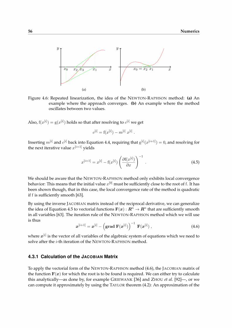
56 Numerics
x
y
x0 x1x2 x3
(a)
x
y
x0 = x2 x1
(b)
Figure 4.6: Repeated linearization, the idea of the NEWTON-RAPHSON method: (a) Anexample where the approach converges. (b) An example where the methodoscillates between two values.
Also, f(x[i]) = g(x[i]) holds so that after resolving to c[i] we get
c[i] = f(x[i])−m[i] x[i] .
Inserting m[i] and c[i] back into Equation 4.4, requiring that g[i](x[i+1]) = 0, and resolving forthe next iterative value x[i+1] yields
x[i+1] = x[i] − f(x[i])
(∂f(x[i])
∂x
)−1
. (4.5)
We should be aware that the NEWTON-RAPHSON method only exhibits local convergencebehavior: This means that the initial value x[0] must be sufficiently close to the root of f . It hasbeen shown though, that in this case, the local convergence rate of the method is quadraticif f is sufficiently smooth [63].
By using the inverse JACOBIAN matrix instead of the reciprocal derivative, we can generalizethe idea of Equation 4.5 to vectorial functions F(x) : Rn → Rn that are sufficiently smoothin all variables [63]. The iteration rule of the NEWTON-RAPHSON method which we will useis thus
x[i+1] = x[i] −(grad F(x[i])
)−1F(x[i]) , (4.6)
where x[i] is the vector of all variables of the algebraic system of equations which we need tosolve after the i-th iteration of the NEWTON-RAPHSON method.
4.3.1 Calculation of the JACOBIAN Matrix
To apply the vectorial form of the NEWTON-RAPHSON method (4.6), the JACOBIAN matrix ofthe function F(x) for which the root is to be found is required. We can either try to calculatethis analytically—as done by, for example GRIEWANK [36] and ZHOU et al. [92]—, or wecan compute it approximately by using the TAYLOR theorem (4.2): An approximation of the

Method of NEWTON and RAPHSON 57
partial derivative ∂F(x)/∂xj can be determined by truncating Equation 4.2 after the secondterm, and resolving for the derivative. Using this approach, we get
F(x[xj←xje ]) = F(x) +∂F(x)
∂xj(xje − xj) +O((xj − xje)2) .
Depending on whether we set the evaluation point xje for the j-th row of F to xj + ε or xj − ε(for some arbitrary but fixed small ε ∈ R+), we get the forward difference scheme
∂F(x)
∂xj=
F(x[xj←xj+ε])− F(x)
ε+O(ε2)
or the backward difference scheme
∂F(x)
∂xj=
F(x)− F(x[xj←xj−ε])
ε+O(ε2) .
A slightly more accurate method is to truncate the TAYLOR series only after the second term,expand it once at xj + ε and once at xj − ε, and subtract the equations from each other. Thisresults in the central difference scheme
∂F(x)
∂xj=
F(x[xj←xj+ε])− F(x[xj←xj−ε])
ε+O(ε3) ,
which exhibits an error term in O(ε3) because the second order terms of the TAYLOR seriescancel each other. Thus, the central difference scheme has a higher accuracy compared toforward or backward differences. Having noted this, the central difference scheme requiresa significantly higher computational effort compared to the one-sided variants, since forthis scheme F must be evaluated twice per derivative instead once for per derivative plusone time for the whole JACOBIAN. For the numerical examples shown in Chapter 6, wewill thus always use forward differences. Another reason for this is using for one-sidedfinite difference schemes, we can choose the value of ε small enough to achieve a sufficientaccuracy.
4.3.2 Discretized Partial Differential Equations
For systems of equations that stem from partial differential equations that where spatiallydiscretized using a grid based method, we can assemble the JACOBIAN matrix efficiently:For this, we take advantage of the observation that each row of F only interacts with a smallnumber of other rows. This is due to the fact that, for such grid based spatial discretizations,the direct influence of the value of a quantity at a position is limited to the element whichcontains this position and the neighbors of that element. This leads to a sparse JACOBIAN
matrix of F where most entries are zero, i.e., the number of non-zero entries of grad F isin O(n) with n being the number of rows in F. We can exploit this property by calculatingthe residual and its gradient for each element locally followed by summing them up to get asparse JACOBIAN matrix for F.

58 Numerics
4.4 Linear Solvers
At this point, we need to solve the sequence of systems of linear equations produced bythe NEWTON-RAPHSON method. To simplify the notation of this section, we discuss linearsystems of equations in the form
Ax = b , (4.7)
whereA ∈ Rn×n, b,x ∈ Rn and n ∈N . To adapt the iteration rule of the NEWTON-RAPHSON
scheme (4.6) to the notation used by the current section, we need to set x to x[i] − x[i+1], b toF(x[i]) andA to grad F(x[i]).
Many ways to solve such systems of equations have been proposed [70], but we can classifyall of these into two categories: Direct and iterative linear solvers. In the following, we willoutline the basic ideas of both of these classes.
4.4.1 Direct Solution
The canonical method to solve Equation 4.7 is to use GAUSS elimination. It is the “canonical”approach because it is guaranteed to work for all non-degenerate matricesA and all right-hand sides b, i.e., we do not need to assume any properties other thanA being non-degenerate.The basic approach of GAUSS elimination is to decomposeA into
A = LU (4.8)
where U is an upper diagonal matrix and L is a lower diagonal matrix.
This decomposition, which we call LU-decomposition, can be achieved using equivalencetransformations. The idea of these is that multiplying a line in L by a non-zero scalar value γ ∈R can be reversed by multiplying the same column in U with 1/γ. Similarly substituting arow by its sum with another row scaled by any factor does not change the solution of a linearsystem of equations. This way, by starting with L0 = A and U0 = I we can eliminate allentries on the upper right ofA as well as normalize its main diagonal.
Once we have calculated the LU-decomposition ofA, we get the inverse using
A−1 = (LU)−1 = U−1L−1 . (4.9)
Here, the factors L−1 and U−1 can be efficiently calculated using forward elimination fortriangular matrices.
Cost Analysis
Although direct methods to solve Equation 4.7 are versatile, in practice they are rarely used inunaltered form because of their high computational cost: To solve a linear system of equationswith n rows, we require O(n3) scalar operations and O(n2) scalars need to be stored [70] ifwe implement this method naively. Even worse, in the general case these estimates hold even

Linear Solvers 59
for sparse matrices [70]. For such matrices we have two options to tackle this problem: Wemay either try to re-order the linear system so that this problem gets reduced and the systemcan be solved much faster [70, 53, 71], or we can use an iterative solver as described in thenext section.
4.4.2 Iterative Solvers
In contrast to directly solving Equation 4.7, iterative solvers require additional properties ofthe linear system of equations to be solved [70]. This means that, using iterative linear solvers,we cannot guarantee to solve any non-degenerate linear system of equations. However, inpractice this constraint is not very relevant since the iterative solvers usually converge for thelinear systems of equations stemming from discretized partial differential equations.
The fundamental property upon which all iterative solvers rely, is that the matrix-vectorproduct
y = Ax
can be computed using O(n) scalar operations, provided thatA is sparse. In the followingsubsections we will illustrate how some widely used iterative linear solvers work.
4.4.2.1 Steepest Descent
The first solver which we investigate here, is the steepest descent solver. For it, we takeadvantage of the fact that for symmetric and positive definite matricesA, the minimum ofthe function
f(x) =1
2xTAx− xTb+ c (4.10)
corresponds to the solution of Equation 4.7. To see this, we set the JACOBIAN matrix of f tozero, and get
0!
= grad f (4.11)
=1
2
(xT grad(Ax) + grad
(xT)Ax)− b
=1
2
(xTA+Ax
)− b .
Since we assumed thatA is symmetric, i.e., that
xTA = ATx = Ax
holds, we find that Equation 4.7 is satisfied, if and only if, Equation 4.11 holds. Further, thesolution must be a minimum of Equation 4.10, because the gradient of Equation 4.11 is
grad(grad f) = grad(Ax− b) = A
60 Numerics
which is positive definite by assumption.
We can exploit these properties by starting at an arbitrary value x[0], and repeatedly calculatethe minimum along the line in the direction of the strongest decrease of f , i.e., the solver uses
x[k+1] = x[k] + α[k]grad f(x[k]) (4.12)
to find the next iterative value. To use this equation, now we need to minimize Equation 4.12with respect to α[k]. This yields
0!
=df(x[k+1])
dα[k]
= grad(
f(x[k+1])) dx[k+1]
dα[k]
= −r[k+1] · r[k]
=(b−Ax[k+1]
)· r[k]
= b · r[k] −A(x[k] + α[k]grad f(x[k])
)· r[k]
= b · r[k] −A(x[k] + α[k]r[k]
)· r[k] ,
where r[k] is called the linear residual, and is an abbreviation for grad f(x[k]) = Ax[k] − b.Resolving for α[k], we get
α[k] =
(Ax[k] − b
)· r[k](
Ar[k])· r[k]
=r[k] · r[k]
r[k] ·(Ar[k]
) . (4.13)
Using Equation 4.12 in conjunction with Equation 4.13 as iteration rule, we are able toapproximate the solution of the linear system of Equations 4.7 arbitrarily closely, as illustratedin Figure 4.7 for the case of two unknowns. Figure 4.7 also illustrates a major shortcomingof the steepest descent method; namely that convergence tends to be slow. This is because,although each two consecutive optimization directions grad f(x[k]) and grad f(x[k+1]) areorthogonal, the method optimizes into “almost” the same direction at steps k and k + 2.
4.4.2.2 Conjugate Gradients
If we can make sure that x[k] stays minimal for directions that we optimized for in previoussteps, this issue does not occur. Also, if the optimization directions are not linearly dependenton each other, we will reach the exact solution after at most n iterations. For symmetric,positive definite matrices A, we can achieve these properties by making the optimization

Linear Solvers 61
Figure 4.7: Illustration of the steepest descent algorithm: For any point x[k], the minimumof the function f along the negative direction of the gradient −grad f(x[k]) is thevalue of the next iterative solution x[k+1].
direction pairwiseA-orthogonal, i.e., requiring that
d[i]Ad[j] = 0
holds for any two distinct optimization directions d[i] and d[j]. It turns out [70] that we canuse
d[k+1] = r[k+1] +r[k+1] · r[k+1]
r[k] · r[k]
to calculate the next optimization direction d[k+1] at the end of iteration k, with
d[0] = r[0]
as the initial optimization direction, and
x[k+1] = x[k] + α[k]d[k], with α[k] =d[k] · r[k]
d[k] ·Ad[k](4.14)
as the iteration rule. Since A-orthogonal vectors are said to be conjugate, the linear solveremerging from using Equation 4.14 as iteration rule is called the conjugate gradient method.
4.4.2.3 Bi-Conjugate Gradients
The conjugate gradient method covered in the previous section only works well for symmetric,positive definite matrices. As an extension to unsymmetric matrices, the bi-conjugate gradientmethod has been proposed by VAN DER VORST [86]. The basic idea of this method is to findthe solution for a dual system
ATx? − b = 0
62 Numerics
in addition to the linear system Ax = b for which we actually seek the solution. The bi-conjugate gradient method works by executing the conjugate gradient algorithm on eachof those two systems separately, and ensuring that the search directions d[k] and d?[k] ofeach iteration are A-orthogonal to each other. Note that this method is equivalent to theconjugate gradient method for symmetric, positive definite matrices, albeit it requires twicethe computational cost in this case.
Since the bi-conjugate method cannot guarantee convergence for all matricesA, and is quiteunstable [70], several stabilized variants have been proposed [70]. The one which we will usefor the numerical examples presented in Chapter 6 is BiCGSTAB [70].
4.4.2.4 GMRES
The last iterative linear solver which we will cover in this work is the Gerneralized MinimalResidual (GMRES) method. This solver uses the initial optimization direction r[0] and theoptimization direction d[k] of iteration k is found by explicitly orthogonalizing r[k] withrespect to all previous optimization directions. The advantage of the GMRES method isthat it can be proved that—like bi-conjugate gradient based methods—it converges to thesolution of the linear system of equations after at most n iterations [70]. This comes at thedisadvantage that the memory requirement is in O(n2), and the number of scalar operationsis in O(n3) which is not better than if we would use a direct solution method based on GAUSS
elimination.
To avoid this issue, the GMRES method is usually restarted after a fixed number of iterations j.This has the effect that the memory consumption is in O(n · j), but has the disadvantage thatconvergence cannot be guaranteed anymore. In most cases, restarted GMRES is still morestable than a bi-conjugate gradient solver [70].
4.4.3 Preconditioners
Using preconditioners, we may get faster convergence of the iterative linear solvers. The ideaof preconditioners is to make the linear system of equations better suited for the linear solverby applying a computationally cheap preprocessing step in every iteration. Conceptually, wecan use preconditioners with any iterative linear solver using the relation
x[k+1] = P (y[k])
where x[k+1] is the start vector of iteration k + 1 of the linear solver, y[k] is the result of itera-tion k of the linear solver, and P is a computationally cheap function that is approximatelythe inverse ofA in some sense, i.e.,
grad P ≈ A−1 .

Parallelization 63
The JACOBI Preconditioner
A simple preconditioner, which outlines the basic idea of preconditioners quite well, is dueto CARL GUSTAV JACOB JACOBI. If we assume that all entries of the main-diagonal ofA arenon-zero, we may use the inverse of the main diagonal ofA, i.e., we get the preconditioner
P (y[k]) = (diag A)−1 y[k] .
Because of its simplicity, the JACOBI preconditioner does not require significant computationalcosts. Having said that, it also does not improve convergence much [70].
Other Preconditioners
We note that preconditioners are typically much more elaborate and exhibit much highercomputational costs than the JACOBI preconditioner. For example, if we use the LU decom-position presented in Section 4.4.1, but execute it only on the non-zero matrix entries, weget the incomplete LU (ILU) preconditioner [70]. Another approach is to create a hierarchyof matrices by successively merging rows and columns of the matrixA. This idea leads toalgebraic multi-grid preconditioners [82].
4.5 Parallelization
Now we are in a position to compute approximate solutions for a system of partial differentialequations. We will thus proceed briefly at how this process can be sped up by doing therequired computations in parallel. We will first discuss one of the fundamental techniquesto perform parallel computations, domain decomposition. Then, we will then present howwe can use this idea to parallelize the linearization process, and in Section 4.5.3 we willfinally look at how iterative linear solvers can be implemented on loosely coupled parallelcomputers.
4.5.1 Domain Decomposition Methods
Computations involving very large grids are usually performed on parallel computers thatfeature a large number of processors which are only connected by a network. The mathe-matical basis which allows to use such machines are domain decomposition methods [75].The general idea of these methods is to partition the grid for the whole spatial domain into anumber of smaller connected subgrids of approximately equal size followed by assigningeach subgrid to a processor. This processor then deals with discretizing and linearizing thesystem of partial differential equations on the subgrid using the methods which we discussedin Section 4.2. After each such step, we get a distributed linear system of equations which weneed to solve in a parallel manner.

64 Numerics
(a) Domain Decomposition
(b) Overlap of First Process
Figure 4.8: (a) Decomposition of the grid of a computational domain into four connected,approximately equally large subgrids. Each of the four subgrids can be treatedalmost independently which allows using loosely coupled parallel computations.(b) A domain overlap of three elements of the first process.
One major difficulty of this approach is the partitioning of the grid: In order to obtain good—i.e., compact and approximately equally large—subgrids, we generally have to use complexgraph processing algorithms that solve NP-complete problems [43, 66]. Since this partitioningprocess is not a focus of this work, we refer the interested reader to KARYPIS and KUMAR [43],PELLEGRINI and ROMAN [66], and to BURRI et al. [15]. An illustration of the idea of domaindecomposition is given in Figure 4.8a where a two-dimensional grid is partitioned into foursubgrids.
4.5.2 Distributed Linearization
To linearize the overall system of equations, we first linearize the individual subgrids inde-pendently. If there are so-called ghost elements, i.e., elements at the subgrid boundary whichare visible a processor but which are located within a neighboring subgrid, nothing elseneeds to be done. If no ghost elements are present, each processor must sum up the values ofthe matrix rows and the rows of the residual vector which represent entities adjacent to theboundary of the subgrid of the processor.

Parallelization 65
In both cases, we get a distributed version of the linearized system of equations
Ax = b , where (4.15)
A =
A1 0 0
0. . . 0
0 0 Ak
,
x = (x1, . . . ,xk)T and
b = (b1, . . . , bk)T
are distributed on k processors, i.e., processor i can only accessAi and the vectors xi and biwithout communication.
4.5.3 Parallel Iterative Linear Solvers
Now we have to efficiently solve the distributed linear system of equations (4.15) in parallel.For direct solvers this problem is much more complicated than for iterative ones [53, 71], sowe will concentrate on the latter. For these solvers, the only operations which we need toprovide for the global linear system of equations are matrix-vector products, scalar products,norms, and preconditioners.
Matrix-Vector Products
Parallel matrix-vector products can be implemented by local matrix-vector products, pro-vided that the domains overlap by at least one finite volume. After executing the localoperation, rows which correspond to finite volumes that are at the front of the overlap needto be synchronized by retrieving their values from the process which is associated with thesubgrid of the finite volume.
Scalar Products
We can compute all common scalar products in parallel by local scalar products followed bya summation of the results of all processors. For example, we can express the EUCLIDEAN
scalar product in CARTESIAN coordinates in terms of the local operation
pi · qi =
ni∑j=1
pijqij ,
followed by computing the sum of the results of all processes, i.e.,
p · q =
k∑i=1
pi · qi .
66 Numerics
Only the last step requires communication between the processes.
Norms
The norms of distributed vectors which we need for iterative linear solvers can be computedusing the corresponding scalar products. For example, the two-norm of a distributed vector pis given by
‖p‖ =√p · p .
Preconditioners
Preconditioners are the most challenging operations in the context of distributed iterativesolvers. This is due to the fact, that the result of the preconditioner may depend on theordering of the rows and columns ofA. For ordering independent preconditioners such asthe JACOBI method, it is sufficient to apply them locally for each subgrid. Unfortunately, wecannot use these preconditioners in practice, as the convergence rates of the iterative linearsolvers is much slower compared to more advanced preconditioners [70]. For preconditionersthat dependent on the ordering of the rows, we can provide a parallel version by applyingthe sequential preconditioner locally, followed by a synchronization of the result on theoverlapping rows—if the overlap regions are large enough. The synchronization is done byretrieving the values of the overlapping rows from the processes that are assigned to thesubgrids of the finite volumes associated with the rows.
4.6 Chapter Synopsis
In this chapter, we discussed numerical methods for finding approximate solutions of systemsof partial differential equations. The conceptual approach which we use is to first transforma relatively small system of partial differential equations
∂b(x, t)
∂t+ div(b(x, t) · v) = q(x, t)
into a much larger system of coupled ordinary differential equations
∂B(t)
∂t= Q(t)
using a space discretization method.
The space discretization methods which we discussed partitioned the spatial domain Ω into aset of smaller subdomains ω1, . . . , ωn, and represented any quantity b as piecewise constantfunctions on the subdomains. The value of an individual subdomain b(ωi) we interpreted asthe average of the quantity within ωi.

Chapter Synopsis 67
After the spatial discretization, we transformed the obtained system of ordinary differentialequations into a set of coupled non-linear algebraic equations. For this we truncated theTAYLOR series and obtained
B(t[k+1]) = B(t[k]) + (tk+1 − t[k])Q(t[k+1])
as the time stepping rule. At this point, we had to repeatedly solve coupled non-linearsystems of algebraic equations. To achieve this, we applied the NEWTON-RAPHSON methodwhich exhibits the iteration rule
x[i+1] = x[i] −(grad F(x[i])
)−1F(x[i]) ,
i.e., for each time step, we now needed to repeatedly linearize the non-linear algebraic systemof equations, and solve the corresponding linear systems of equations until the error wassmaller than the allowed tolerance.
The final piece of the numerical puzzle were ways to solve such linear systems of equations.For this, we discussed several direct and iterative approaches as well as preconditioners forthe iterative linear solvers.
To conclude this chapter, we briefly discussed how the steps of discretizing the partialdifferential equations, linearization of the resulting algebraic systems and solving the linearsystems of equations can be efficiently implemented on loosely coupled parallel computers.


5 Implementation Aspects
For this thesis, the methods which we discussed in the previous chapters have been imple-mented using the numerical C++ framework eWoms [30]. In this chapter, we will look atsome of the technical aspects of this implementation.
5.1 DUNE
The eWoms framework is based on the Distributed and Unified Numerics Environment(DUNE) [28]. As illustrated in Figure 5.1, DUNE provides a set of basic C++ classes whichsimplify the development of numerical schemes, but DUNE itself does not implement any ofthose. Instead, such methods have to be implemented by additional modules like eWoms.Currently, DUNE comprises the following core modules:
dune-common implements very basic abstractions like, for example, dense vector andmatrix classes, helper routines for parsing configuration files, exception handling, andlow-level macros for compiler abstraction.
dune-geometry provides a set of reference elements and the associated transformationsto convert these into the actual geometries required by the grid. Currently, the dune-geometry module supports line segments for one spatial dimension, triangles, andrectangles for two spatial dimensions, and tetrahedra, cubes, prisms, and pyramidsfor three dimensional grids. In addition, simplices and cubes are provided for higherspatial dimensions.
dune-grid defines an abstract interface for partitioning the spatial domain into a grid asdescribed in Section 4.1. The DUNE grid interface also supports parallel computationsbased on the domain decomposition concept which we discussed in Section 4.5. Besidesdefining a parallel programming interface for grids, this module also provides a fewsample implementations for CARTESIAN grids, and wrappers for external unstructuredgrid management libraries, such as ALUGrid [4], ALBERTA [3], and UG [85].
dune-localfunctions supplies finite-element shape functions based on the infrastructureof the grid and the geometry modules. The only shape functions used by eWoms arethose of linear finite elements. The reason for this is that these functions are used tocalculate the gradients of quantities on the dual-grid of vertex-centered finite volumemethods which we discussed in Section 4.1.
dune-istl stands for Iterative Solvers Template Library, and implements a superset of theiterative linear solvers and preconditioners which we described in Section 4.4.

70 Implementation Aspects
Figure 5.1: The software architecture of the DUNE C++ framework [28]. The core of eWomsrepresents an external module which implements discretization schemes and thenumerical problems which will be presented in Chapter 6 fall into the applicationscategory.
All DUNE modules use the C++ template mechanism extensively. The reason for this is tokeep the run-time overhead of the abstractions low, but it comes at the price of increasedcompilation time, and a relatively steep learning curve.
5.2 eWoms
Based on these DUNE modules, the eWoms framework implements discretization schemesand physical models which we will cover in greater detail in the following. But before wecan discuss these models, a rough overview of the general software architecture of eWoms isrequired.
5.2.1 General Structure
Conceptually, eWoms currently consists of the following parts:
The Time Loop deals with adapting time step sizes, simplifies implementing time-dependent problems, and runs the simulation from the initial time to the specified endtime. To actually advance the time level from t[k] to t[k+1], it calls the non-linear solver.
The NEWTON-RAPHSON Solver implements the non-linear solver for algebraic systems ofequations as discussed in Section 4.3. This part of the code calls the discretizationscheme to linearize the system of equations, and subsequently calls a linear solver tofind the solution of the linearized system of equations.
Discretization Schemes: Implement the fully implicit vertex-centered finite volume spacediscretization discussed in Section 4.1, and the implicit EULER time discretization ofSection 4.2. It is also the part of eWoms which uses the DUNE grid interface mostextensively.

eWoms 71
Flow Models: This part of eWoms is called by the discretization schemes, and specifiesthe conservation equations, i.e., it determines the function F of Equation 4.6. Theflow model also specifies the interpretation of its primary variables, and it providessome auxiliary methods like scaling parameters of the primary variables and of theconservation equations.
Problems: In eWoms, the purpose of problems is to describe the setup of a physical system.This includes the grid used by the simulation, boundary and initial conditions, as wellas spatially dependent parameters like the intrinsic permeability of the porous mediumor the value of the gravitational acceleration. The parameters of the problem are mostlyqueried by the flow model.
Material Framework: The purpose of the eWoms material framework is to provide materialspecific relations. Such relations include the thermodynamic relations of multi-phasemulti-component systems of fluids, capillary pressure and relative permeability rela-tionships.
Parallelization: This part of eWoms implements distributed overlapping linear systems ofequations with the required operations and synchronization algorithms for precondi-tioners of the iterative linear solvers. These linear systems of equations are then solvedusing one of the iterative linear solvers of dune-istl.
Auxiliary Infrastructure: eWoms also provides auxiliary code. Amongst other things, thiscode is used to specify simulation-wide parameters, comprises routines simplifying thestartup procedure, and classes providing checkpointing functionality as well as classesfor writing the solutions into file formats suitable for visualization.
5.2.2 Flow Models
Now that we have covered the general software design of eWoms, we will have a closer lookat the implementation aspects of the eWoms flow models in the following paragraphs. First,we will discuss how the flow models work in general, then we will consider the specificaspects of the individual flow models.
General Mode of Operation
The central part of all flow models is the code which defines of the local residual function,i.e., a class to compute the residual for a single element of the grid. After linearizing theselocal residuals for each element, the local linearized system of equations is transferred tothe linear system of equations for the full subgrid of the respective process. This processinvolves mapping the element-local indices of each finite volume to its respective index inthe subgrid, and summing them into a large vector. In eWoms, the local linearization and thetransfer from the element-local to the global system of equations is implemented genericallyby infrastructural code, so the only part which needs to be provided by a flow model is theelement-local residual.

72 Implementation Aspects
The flow models presented in this thesis use a multi-stage approach to define the localresidual of an element: First, the primary variables—which are defined as the quantitieswhich are contained in the solution vector x[i] of the NEWTON-RAPHSON method (4.6)—aretransformed into so-called volume variables. In eWoms, volume variables are quantities thatare independent of the state of the spatial neighborhood of a given point in the spatial domainlike, for example, temperature, pressures, and saturations.
The volume variables are then used to calculate flux variables. The flux variables represent allquantities which depend on the spatial neighborhood of a finite volume. They are mainlyrequired to calculate the divergence term of Equation 2.6. Quantities represented by the fluxvariables are, for example, the gradients of pressure and temperature.
Based on the flux and the volume variables, the local residual of a flow model then specifiesthe volumetric rate of each conservation quantity that is incorrectly added to or removed fromthe system for a given solution. For mass, eWoms uses either Equation 2.42 or Equation 2.47,and if energy is conserved, the local residual of the flow model also includes Equation 2.46.
The Immiscible Model
As covered in Section 3.5.1, the immiscible model assumes that the components do not mix,and that, as a consequence, each fluid phase comprises exactly one component. This modeluses Equation 2.42 as the equation for the conservation of mass in conjunction with themulti-phase version of DARCY’s law (2.37), i.e., the residual function Fα for the conservationof the mass of a component reads
∂φραSα∂t
− div
(ραkr,α
µαK (grad pα − gρα)
)− qα = Fα
!= 0 ,
where α is the fluid phase corresponding to the component.
The primary variables for this model are the pressure of the fluid phase with the lowest indexand the M − 1 saturations of the fluid phases associated with the lowest indices.
The PVS Model
The PVS model for M -phase, N -component flow in porous media which uses the primaryvariable switching conditions (3.31) as model assumptions is based on Equation 2.47, the mo-lar formulation of the component-wise mass conservation equation. The residual function Fκ
for the conservation of the mass of component κ is thus given by
∑α
∂φxκαρmol,αSα∂t
−∑α
div
(xκαρmol,α
kr,α
µαK (grad pα−gρα) +Dκ
pm.α grad xκα
)−qκ=Fκ
!=0 .
Compared to the immiscible model, the interpretation of the N primary variables is muchmore complicated:
eWoms 73
• The first primary variable always represents the pressure of the phase with the lowestindex.
• The nextM−1 primary variables represent the saturations of the phases if the respectivephase is present, or else the mole fraction of the component with the same index as theprimary variable in the corresponding to with the phase lowest index that in the set ofpresent phases.
• The final N −M primary variables represent the mole fractions of the N −M lastcomponents in the phase associated with the lowest index that is assumed to be present.
In this model, in addition to the N “real” primary variables, M boolean pseudo primaryvariables p1, . . . , pM are required to specify the set of fluid phases which are present at agiven spatial location. They are determined at the end of each NEWTON-RAPHSON iterationaccording to the following rules:
• If fluid phase α was assumed not to be present at the beginning of the current NEWTON-RAPHSON iteration and if the sum of the mole fractions of the phase is larger than orequal to 1 after updating the solution, for the next iteration we assume that phase α ispresent.
• If fluid phase α was assumed to be present for the current NEWTON-RAPHSON iterationand the saturation of phase α is smaller than 0, we assume that phase α is not presentin the next iteration.
After updating the pseudo primary variables, we need to adapt all “real” primary variablesto make the model consistent.
The NCP Model
Like the primary variable switching model, the model which directly embeds non-linearcomplementarity functions, uses Equation 2.47 as mass conservation equation. This meansthat it also uses the component-wise molar formulation of the conservation of mass inconjunction with DARCY’s law. In other words, the residual function Fκ which describes theconservation of component κ is also given by
∑α
∂φxκαρmol,αSα∂t
−∑α
div
(xκαρmol,α
kr,α
µαK (grad pα−gρα) +Dκ
pm.α grad xκα
)−qκ=Fκ
!=0 .
In addition to the mass conservation equations, the model explicitly includes theM non-linearcomplementarity functions of Equation 3.33.
Compared to the primary variable switching model, the set of primary variables for thismodel is quite simple:
• The first primary variable is the pressure of the phase associated with the lowest index.
• The next M − 1 primary variables are the saturations of the M − 1 phases with thelowest indices.

74 Implementation Aspects
Model SLOC Core SLOCImmiscible 720 297Black-Oil 1013 434NCP 1046 551PVS 1260 720
Table 5.1: Comparison of the number of source lines of C++ code (SLOC) implementingthe discussed model approaches in eWoms as determined by the SLOCCounttool [74]. The first number represents the total number of source code lines ofthe implementation of each model in eWoms, while the “Core SLOC” columnexcludes auxiliary code like the one for writing the solutions to the hard disk,making checkpoints et cetera.
• The final N primary variables represent the fugacities fκ of all components.
The Black-Oil Model
In addition to the generic models discussed in the previous model, the eWoms back-oil modelimplements the specialized approach covered in Section 3.5.4. From the software engineeringpoint of view, it is very similar to the model which assumes immiscibility. This is due to thefact that two of the three fluid phases are assumed to be immiscible. This allows the eWomsimplementation of the black-oil model to use the same primary variables as the immisciblemodel, i.e., the pressure and the saturation of the gas phase, in addition to the saturation ofthe water phase.
Compared to the immiscible model, the main differences of the black-oil model are that thequantities required for the mass conservation equations are calculated by directly using theblack-oil parameters, and that undersaturated oil phase needs special attention if we usethe aforementioned primary variables: Such oil is described by negative saturations of thegas phase, where the amount of “negative” gas is subtracted from the amount of the gascomponent which is dissolved in the oil phase. In this respect, the eWoms implementation ofthe black-oil model is similar to the negative saturations approach proposed by, for example,ABADPOUR and PANFILOV [2], with the differences that the composition of the gas and waterphases are known a priori, and that the black-oil model considers three instead of two fluidphases.
5.2.3 Implementational Complexity
When estimating the effort required to implement the discussed models in software, wecan use the number of lines of code required for each as a very rough indication. We haveto be aware though, that the complexity of the implementation is not linear to the numberof lines of code. This is due to the facts that tightly written source code packs much morefunctionality into the same number of lines than loosely written source code and that highlyconvoluted algorithms are much more difficult to implement than straightforward ones. In

eWoms 75
the case of the numerical models featured by eWoms, the density of the source code can beassumed to be similar for all models, but the inherent complexity of the primary-variableswitching model is higher than that of the other models.
These numbers of lines of source code needed to implement the individual models in eWomsare compared in Table 5.1. As this table indicates, the model which assumes immiscibilityis by far the simplest, followed by the black-oil model. Also clearly represented is the factthat the effort required to implement the model based on primary variable switching is muchhigher than for the model which directly incorporates non-linear complementarity functions.
From the point of view of the implementation, the main simplifying factor of the NCPmodel compared to the PVS model is the fact that the semantics of all primary variables areindependent of the state of the solution, i.e., no pseudo primary variables are required.


6 Numerical Applications
After briefly sketching the software implementation in the previous chapter, we will now com-pare the physical accuracy and the computational performance of the presented numericalmodels for fluid flow in porous media.
We roughly proceed in order of complexity of the examples: First, we compare the phys-ical and numerical performance of the primary-variable switching (PVS) approach withthe one based on non-linear complementarity problems (NCP) using a one-dimensionalnon-isothermal setup for which a semi-analytical solution is known. Then we discuss theresults and the computational performance of the immiscible, PVS, and NCP models for anisothermal, radially symmetric CO2 injection problem. In this section, we will also brieflyexamine the scalability of the domain decomposition parallelization approaches, and weanalyze the viability of using two-dimensional simulations for radially symmetric problems.
We then proceed with the ninth [45] and the fifth [46] benchmark problems specified by thesociety of petroleum engineers. The ninth benchmark problem is used to estimate merritsand drawbacks of the black-oil model versus fully compositional models and demonstratesthe computational instability of the PVS model. In contrast, the primary intention of the fifthSPE benchmark problem is to show the viability of the generic compositional multi-phasemodels for the complex cubic equations of state which we discussed in Sections 3.3.1 and 3.3.2.We conclude the chapter with a brief discussion of geological-scale simulations for the CO2injection research project in Ketzin/Havel, Germany.
6.1 The Heat-Pipe Problem
In this section, we will discuss the heat-pipe setup as proposed by UDELL [84]. The problemuses the spatial domain depicted in Figure 6.1: In the beginning, the domain is fully saturatedby liquid distilled water, and the domain is fully closed for mass flows except on the leftside, where it is open. Initially, and on the left boundary of the domain, the domain isfully saturated by liquid exhibiting a pressure pl of one bar. For energy, the domain is fullyclosed except on the left side, where it is assumed to be open, and on the right side, which isheated at a constant rate. The initial temperature and the permanent temperature on the leftboundary is 70 C.
In steady-state, this setup leads to a region that is only occupied by the liquid on the left wherethe temperature is too low to evaporate the liquid water, and the heat is thus exclusivelytransported by means of heat conduction. On the right side of the domain, the temperature ishigh enough to create a zone where only steam is present so that in this region energy can

78 Numerical Applications
qenergy
pl = 1 bar
T = 70 C
s
Figure 6.1: The spatial domain of the heat-pipe problem: The experiment consists of a tubeof 2 m length filled by a fully water-saturated porous medium. On the left side,the tube is open and exposed to atmospheric pressure; on the right, it is closedbut heated. Initially the temperature within the domain is T = 70 C.
Figure 6.2: Uniform extrusion of a one-dimensional grid to three spatial dimensions.
also only be transported by means of heat conduction. The most interesting part of this setuplies in between these two extremes: There, liquid water as well as steam is present. The liquidis drawn from left to right by the capillary pressure where the liquid is evaporated. Then,the material gets transported back to the left by a pressure gradient in the gas phase and itcondenses to liquid again.
6.1.1 Uniform Domain Extrusion
Since the mass and energy conservation equations (2.10, 2.23) are only valid for three spatialdimensions, we first have to become aware of their interpretation in the case of one space-dimension. The answer turns out to be quite simple: In order to apply Equations 2.10 and 2.46,the spatial domain can be extruded uniformly to three dimensions as depicted in Figure 6.2and the usual conservation equations thus apply.
6.1.2 Semi-Analytical Solution
Besides this small glitch in the interpretation of the results, the quasi one-dimensional natureof this setup allows us to derive a semi-analytical solution. To obtain it, we first suppose thesystem to be in steady-state. This means that there cannot be any net flux of mass along theaxis s of the tube, i.e.,
ρlkr,l
µlK∂ pl∂s
= −ρgkr,g
µgK∂ pg∂s
(6.1)
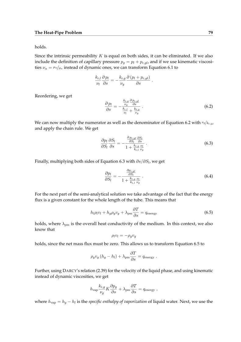
The Heat-Pipe Problem 79
holds.
Since the intrinsic permeability K is equal on both sides, it can be eliminated. If we alsoinclude the definition of capillary pressure pg = pl + pc,gl, and if we use kinematic viscosi-ties να = µα/ρα instead of dynamic ones, we can transform Equation 6.1 to
kr,l
νl
∂ pl∂s
= −kr,g
νg
∂ (pl + pc,gl)
∂s.
Reordering, we get
∂ pl∂s
= −kr,gνg
∂ pc,gl∂s
kr,lνl
+kr,gνg
. (6.2)
We can now multiply the numerator as well as the denominator of Equation 6.2 with νg/kr,g,and apply the chain rule. We get
∂pl∂Sl
∂Sl∂s
= −∂ pc,gl∂Sl
∂Sl∂s
1 +kr,gkr,l
νlνg
. (6.3)
Finally, multiplying both sides of Equation 6.3 with ∂s/∂Sl, we get
∂pl∂Sl
= −∂pc,gl∂Sl
1 +kr,gkr,l
νlνg
. (6.4)
For the next part of the semi-analytical solution we take advantage of the fact that the energyflux is a given constant for the whole length of the tube. This means that
hlρlvl + hgρgvg + λpm∂T
∂s= qenergy (6.5)
holds, where λpm is the overall heat conductivity of the medium. In this context, we alsoknow that
ρlvl = −ρgvg
holds, since the net mass flux must be zero. This allows us to transform Equation 6.5 to
ρgvg (hg − hl) + λpm∂T
∂s= qenergy .
Further, using DARCY’s relation (2.39) for the velocity of the liquid phase, and using kinematicinstead of dynamic viscosities, we get
hvapkr,g
νgK∂pg∂s
+ λpm∂T
∂s= qenergy ,
where hvap = hg − hl is the specific enthalpy of vaporization of liquid water. Next, we use the

80 Numerical Applications
chain rule and the definition of capillary pressure, so we get
hvapkr,g
νgK
(pl∂s
+∂pc,gl
∂Sl
∂Sl∂Sl
∂Sl∂s
)+ λpm
∂T
∂s= qenergy .
Multiplying both sides with ∂s/∂Sl leads us to
hvapkr,g
νgK
(∂pl∂Sl
+∂pc,gl
∂Sl
)+ λpm
∂T
∂Sl= qenergy
∂s
∂Sl. (6.6)
In Equation 6.6 we now observe that, since we expressed pg in terms of pl and pc,gl, theterm ∂pl/∂Sl is identical to zero, so that we get
hvapkr,g
νgK∂pc,gl
∂Sl+ λpm
∂T
∂Sl= qenergy
∂s
∂Sl.
Now, we apply the chain rule to the temperature term. We get
hvapkr,g
νgK∂pc,gl
∂Sl+ λpm
∂T
∂pg
∂(pl + pc,gl)
∂Sl= qenergy
∂s
∂Sl.
After some reordering, we get
∂s
∂Sl=∂pc,gl
∂Sl
hvapKkr,gνg
+ λpm∂T∂pg
qenergy.
Finally, we take advantage ofpg = pvap(T ) ,
i.e., the fact that the pressure of the gas phase is identical to the vapor pressure of water [88]at a given temperature in the two-phase, one-component case. This leads us to the secondequation of the semi-analytical solution
∂s
∂Sl=∂pc,gl
∂Sl
hvapKkr,gνg
+ λpm
(∂pvap∂T
)−1
qenergy. (6.7)
Together, Equations 6.4 and 6.7 form a coupled system of two ordinary differential equationswhich can be solved using the methods presented in Section 4.2.
6.1.3 Results
For the results presented in this section, the capillary pressure relation proposed by LEV-ERETT [51]
pc,gl = pc,gl,0 γ(1.263S3g − 2.120S2
g + 1.417Sg),

The Heat-Pipe Problem 81
s/cm]
Sl
1007550250
1
0.75
0.5
0.25
0
AnalyticNCPPVS50 elements100 elements200 elements400 elements800 elements1600 elements
(a) Liquid Saturation (b) Temperature
s/cm
T/K
1007550250
377
376
375
374
373
Figure 6.3: Comparison of the semi-analytical solution calculated using Equations 6.4 and 6.7(dotted) with results obtained by the numerical models using primary variableswitching (PVS, dashed) and non-linear complementary functions (NCP, non-dashed). The numerical models were run until t = 109 s with a uniform spatialresolution along the tube axis of 50, 100 200, 400, 800, and 1600 elements.
was applied, where γ = 0.05878 N/m represents the surface tension, and pc,gl,0 =√φ/K is the
scaling pressure. Further, the porosity φ is 0.4, and the intrinsic permeability K is 10−12 m2.
The overall heat conductivity λpm is approximated by the SOMERTON [76] relation
λpm = λpm,dry +√Sl (λpm,wet − λpm,dry) ,
where λpm,dry is the heat conductivity of the porous medium fully saturated by steamand λpm,wet is the heat conductivity of the porous medium when it is fully saturated byliquid water. For these parameters, we assume
λpm,dry = 1.85 W/K m2 and
λpm,wet = 2.67 W/K m2 .
Finally, the energy influx at the right side of the domain is qenergy = 200 W/m2.
Figure 6.3 shows the obtained results for the steady-state saturation of liquid water andthe temperature for the semi-analytical solution calculated using Equations 6.4 and 6.7 incomparison to the results of the finite-volume based numerical models. In this figure, theorigin of the spatial domain is set to the leftmost point where the saturation of the gas phasedeviates from zero.
Generally, it can be observed that both numerical solutions are identical up to roundingerrors, and that both converge to the semi-analytical solution when the grid gets refined.From these results, we can conclude that both numerical models and their implementationare correct in the sense that the discretization is convergent and that both models lead to
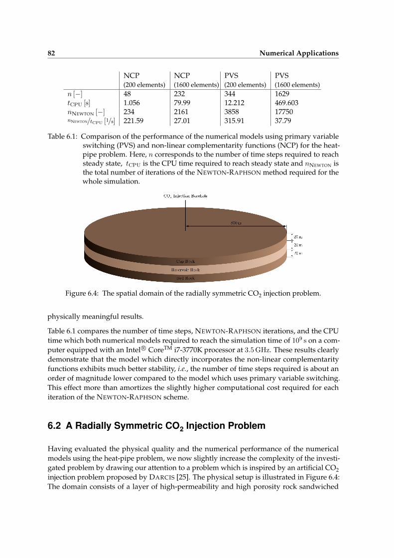
82 Numerical Applications
NCP(200 elements)
NCP(1600 elements)
PVS(200 elements)
PVS(1600 elements)
n [−] 48 232 344 1629tCPU [s] 1.056 79.99 12.212 469.603nNEWTON [−] 234 2161 3858 17750nNEWTON/tCPU [1/s] 221.59 27.01 315.91 37.79
Table 6.1: Comparison of the performance of the numerical models using primary variableswitching (PVS) and non-linear complementarity functions (NCP) for the heat-pipe problem. Here, n corresponds to the number of time steps required to reachsteady state, tCPU is the CPU time required to reach steady state and nNEWTON isthe total number of iterations of the NEWTON-RAPHSON method required for thewhole simulation.
Figure 6.4: The spatial domain of the radially symmetric CO2 injection problem.
physically meaningful results.
Table 6.1 compares the number of time steps, NEWTON-RAPHSON iterations, and the CPUtime which both numerical models required to reach the simulation time of 109 s on a com-puter equipped with an Intel R© CoreTM i7-3770K processor at 3.5 GHz. These results clearlydemonstrate that the model which directly incorporates the non-linear complementarityfunctions exhibits much better stability, i.e., the number of time steps required is about anorder of magnitude lower compared to the model which uses primary variable switching.This effect more than amortizes the slightly higher computational cost required for eachiteration of the NEWTON-RAPHSON scheme.
6.2 A Radially Symmetric CO2 Injection Problem
Having evaluated the physical quality and the numerical performance of the numericalmodels using the heat-pipe problem, we now slightly increase the complexity of the investi-gated problem by drawing our attention to a problem which is inspired by an artificial CO2injection problem proposed by DARCIS [25]. The physical setup is illustrated in Figure 6.4:The domain consists of a layer of high-permeability and high porosity rock sandwiched

A Radially Symmetric CO2 Injection Problem 83
Layer Parameter ValueCap rock K 10−17 Im2
Reservoir K 1.97 · 10−13 Im2
Bed rock K 10−17 Im2
Cap rock φ 4.6 %Reservoir φ 20 %Bed rock φ 4.6 %All pe 5 kPaAll λbc 2All Sr,l 25 %All Sr,g 2.5 %
Table 6.2: Parameters used for the radially symmetric CO2 injection problem. The quantity perepresents the entry pressure, and λbc stands for the shape parameter of theBROOKS-COREY capillary pressure relation (3.18). Further, Sr,l and Sr,g specify theresidual saturations of the liquid and gas phases [39].
Figure 6.5: Radial extrusion of a two-dimensional grid to three spatial dimensions.
between two layers of rock with low permeability and porosity. In the center of the domain,CO2 is injected into the reservoir layer for 20 years at a rate of 0.17 kg/s while on the outerboundary we assume the reservoir to be fully saturated with brine and that all fluids canflow freely. Finally, the material parameters used for this problem are given in Table 6.2.
6.2.1 Radial Domain Extrusion
One thing we notice immediately about this problem is that it is radially symmetric, so we areable to discretize the conservation equations (2.42, 2.46) using only two dimensions, providedthat we extrude the domain radially along the horizontal axis. In this case, we define theextrusion factor as
γ = 2πr ,
where r is the distance to the center of the bore hole of the well, i.e., the distance from the leftboundary of the spatial domain plus the radius of the bore hole of the injection well. Thisconcept is illustrated in Figure 6.5.
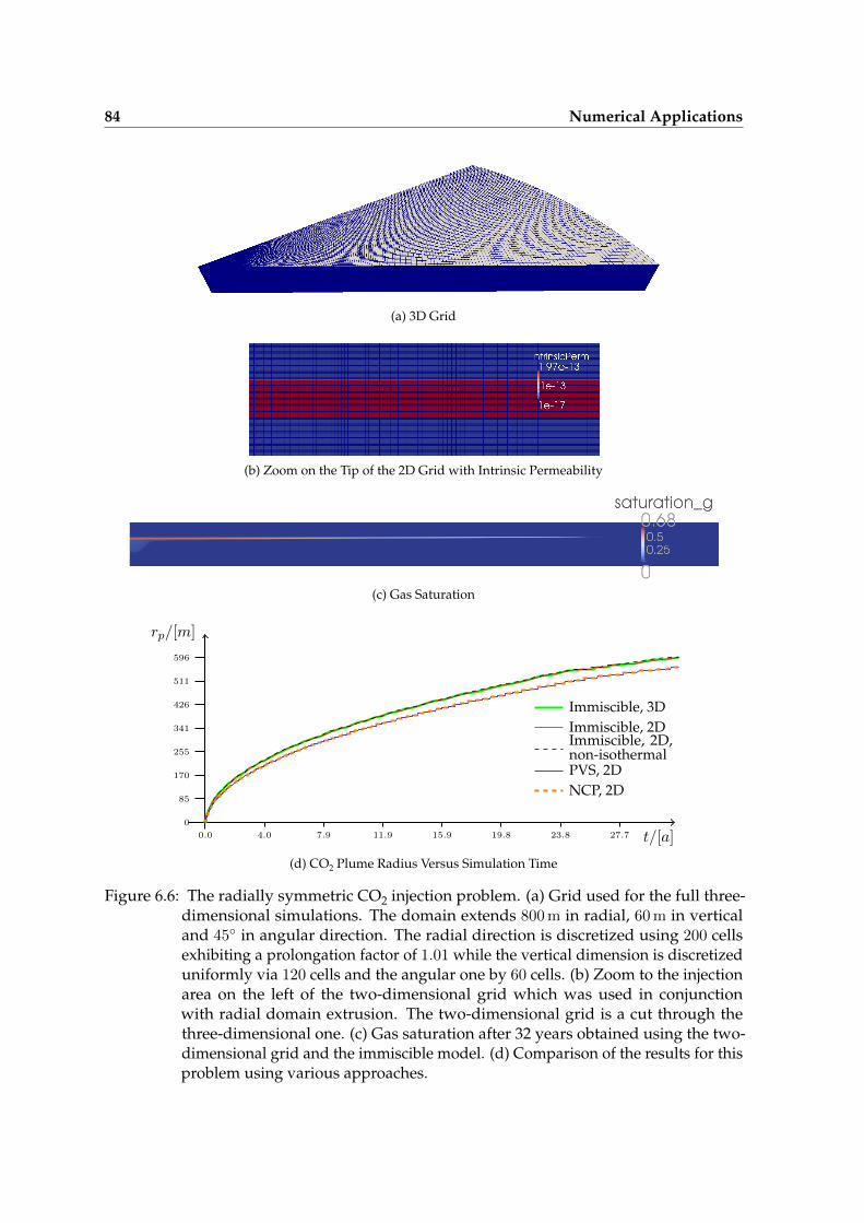
84 Numerical Applications
(a) 3D Grid
(b) Zoom on the Tip of the 2D Grid with Intrinsic Permeability
(c) Gas Saturation
t/[a]
rp/[m]
0.0 4.0 7.9 11.9 15.9 19.8 23.8 27.7
0
85
170
255
341
426
511
596
Immiscible, 3DImmiscible, 2DImmiscible, 2D,non-isothermalPVS, 2DNCP, 2D
(d) CO2 Plume Radius Versus Simulation Time
Figure 6.6: The radially symmetric CO2 injection problem. (a) Grid used for the full three-dimensional simulations. The domain extends 800 m in radial, 60 m in verticaland 45 in angular direction. The radial direction is discretized using 200 cellsexhibiting a prolongation factor of 1.01 while the vertical dimension is discretizeduniformly via 120 cells and the angular one by 60 cells. (b) Zoom to the injectionarea on the left of the two-dimensional grid which was used in conjunctionwith radial domain extrusion. The two-dimensional grid is a cut through thethree-dimensional one. (c) Gas saturation after 32 years obtained using the two-dimensional grid and the immiscible model. (d) Comparison of the results for thisproblem using various approaches.

A Radially Symmetric CO2 Injection Problem 85
6.2.2 Results
Now we are in a position to discuss results for this problem. In Figure 6.6, we outline theresults obtained using both, the radial domain extrusion method as well as the direct three-dimensional simulation approaches. As we can conclude from Figure 6.6d, the differenceof the radius of the CO2 plume for a full three dimensional simulation compared to that ofthe two-dimensional simulation is quite small, and probably below the discretization errorif we consider the fact that the sizes of the time steps are generally slightly smaller for thethree-dimensional grid compared to the two-dimensional one.
Further, we observe that the results do not differ significantly if energy is conserved comparedto neglecting this equation. Quite likely, we can attribute this to the fact that the CO2 is injectedat reservoir temperature.
Finally, the results obtained using the NCP model agree very well with the ones obtainedusing the PVS approach. This means that for this problem, the only significant differencesare between the results of models which incorporate miscibility and the results of the modelwhich assumes immiscibility.
Besides the quality of the results, the parallel performance of a simulator is of major interestfor large-scale problems. To investigate it, this problem was used in conjunction with thethree dimensional grid. The reason for this choice is that, on one hand, the problem is largeenough to keep the communication overhead of the processors reasonably low comparedto the local computational work of each processor in parallel simulations, but on the otherhand, it is still small enough to compute results on a single processor within a reasonabletime frame. Figure 6.7a shows the wall time required to linearize the non-linear system ofequations and the time to solve the resulting linear system of equations depending on thenumber of processors used. The linear solver used to obtain these results was a stabilizedBiCG method [86] in conjunction with an incomplete LU decomposition preconditioner [70].Also, the overlap of the linearization was chosen to be 10 cells.
The results of this are depicted in Figure 6.7 which shows the wall time of the simulations andthe parallel efficiency of the individual parts depending on the number of involved processors.There, the parallel efficiency αpar is defined as the CPU time required by a single processorto finish the simulation tseq divided by time the required by the parallel run tpar and by thenumber of processors ncores:
αpar =tseq
tpar · ncores.
A remarkable aspect of Figure 6.7b is the fact that the efficiency of the linearization process isnot dependent on the number of processors and is even sightly better for parallel runs thanfor sequential ones. The latter observation can probably be attributed to cache effects.
As clearly visible in Figure 6.7, the part of the simulations that does not scale well is the linearsolver: We can observe that the wall time required for the linear solver even increases for 8processes compared to 4. For more than 8 cores, the linear solver scales again, albeit its parallelefficency asymptotically decreases to zero. Quite likely, we can explain the former behaviorby the fact that the memory bandwidth of a single node of the used computer system is

86 Numerical Applications
ncores
tCPU/h
1 2 4 8 16 32 64 128 256
37.3
74.6
111.9
149.2
186.5
TotalLinear SolveAssemble
(a) Wall Time
ncores
αpar/%
1 2 4 8 16 32 64 128 256
20
40
60
80
100
AssembleLinear Solve
(b) Parallel Efficiency
Figure 6.7: Parallel performance of the CO2 injection problem simulated in three spatialdimensions using an isothermal model that assumes immiscibility. The problemwas simulated on a compute cluster equipped with dual-socket 2.83 GHz Intel R©
XeonTM E5440 CPUs. The simulation used a hexahedron grid featuring about 1.45million elements (200 cells in radial, 60 elements in angular, and 120 elements invertical direction).
shared amongst all eight processors on a single compute node. For more than four concurrentprocesses, the limiting factor of the linear solver thus becomes the available bandwidth to themain memory. Using more than eight processors then leads to a distribution of the simulationto more than one compute node, which increases the overall bandwidth to the main memory.If we continue to use more processors, the need for inter-node communication during thelinear solution process increases proportionally. In turn, this leads to the asymptotic decreaseof the parallel efficiency which is featured in Figure 6.7b.
The gist of Figure 6.7b is that, in the case of the synthetic CO2 injection problem, using morethan approximately 64 processors does not lead to sufficient performance improvements tojustify the additional computational resources. This situation might change if we could im-prove the parallel efficiency of the linear solution part of the simulation, for example by usingmore sophisticated linear solvers like multi-grid methods [82]; these are not investigated inthe context of this thesis, though.
Finally, Table 6.3 shows the CPU time required on a single core of a 3.5 GHz Intel R© CoreTM
i7-3770K CPU for various simulation approaches to this problem. As expected, the two-dimensional simulations which use radial domain extrusion are much faster than the fullythree-dimensional one. From this table, we can also conclude that in contrast to the heat-pipeproblem discussed in Section 6.1, the model which directly solves non-linear complementarityfunctions does not profit much from its increased robustness regarding changes of the phasepresence, but is obviously hit by increased costs for linearizing the non-linear system ofequations and solving the resulting linear systems of equations: If energy is conserved viaan additional equation, the model based on primary variable switching requires approxi-mately 70 % more time steps than the model which solves the non-linear complementarity

The Ninth SPE Benchmark Problem 87
Model Grid Time Steps NEWTON-Iterations
Wall Time /[h]
Immiscible 3D 133 1114 69.54Immiscible 2D 115 929 0.24Immiscible, non-isothermal 2D 115 932 0.49PVS 2D 1066 12278 7.21PVS, non-isothermal 2D 1744 20569 20.34NCP 2D 1032 11817 12.22NCP, non-isothermal 2D 1012 11503 17.43
Table 6.3: Performance metrics for various approaches on a single core of an 3.5 GHz Intel R©
CoreTM i7-3770K CPU.
functions directly, although this is only barely enough to compensate the additional costs ofthe additional equations required by the NCP model.
Summarizing this example, we can conclude that the most effective approach to modelradially symmetric problems is to use a two-dimensional grid in conjunction with radialdomain extrusion. Further, Figure 6.6d shows that the results obtained using models thatinclude miscibility are easily distinguishable from the ones neglecting it, even if miscibilityis quite low as is the case for CO2 injection scenarios. At the same time, it indicates thatwe do not need to consider energy as a conservation quantity for CO2 injection scenarios ifthe temperature of the injected CO2 is close to the temperature of the reservoir. Finally, weobserve that the scalability of parallel runs of such simulations usually is not very good, andthat this is primarily caused by the part which solves the linear systems of equations.
6.3 The Ninth SPE Benchmark Problem
The next setup which we will discuss is a slightly simplified version of the ninth benchmarkproblem of the society of petroleum engineers [45] (SPE-9): Instead of the 27 wells of theoriginal specification, the problem which we discuss has only one injection and one produc-tion well. The spatial domain is outlined in Figure 6.8. In planar direction, it is a rectangleof 2.2 km by 2.2 km, and exhibits a thickness of 110 m. The domain is skewed by 16 degreeswith its deepest point being at a depth of 3200 m. This domain is discretized using 24 times 24
rectangles in planar direction and 16 layers of varying thicknesses in depth direction. Theintrinsic permeabilityK varies widely within the spatial domain as outlined in Figure 6.8b.Initially, the pressure in the domain is 248 bar. Elements deeper than 3030 m are initially set tobe fully water saturated, while elements above that threshold exhibit an initial oil saturationof 100 %.
While all borders of the reservoir are assumed to be completely impermeable, the reservoir ispenetrated by the two boreholes mentioned above: The one used for the production of oil andgas is located at the center of the topmost and most north-eastern element. The well whichinjects water is assumed to be located at the center of the bottommost, most south-westernelement of the grid. Both wells are implemented as source terms using the PEACEMAN well

88 Numerical Applications
(a) The Grid, Initial Oil Saturation So and Well Locations
(b) Intrinsic Permeability ‖K‖/m2
(c) Oil Saturation After 9000 Days
(d) Oil Pressure po/Pa After 9000 Days
Figure 6.8: The simplified SPE-9 benchmark problem.
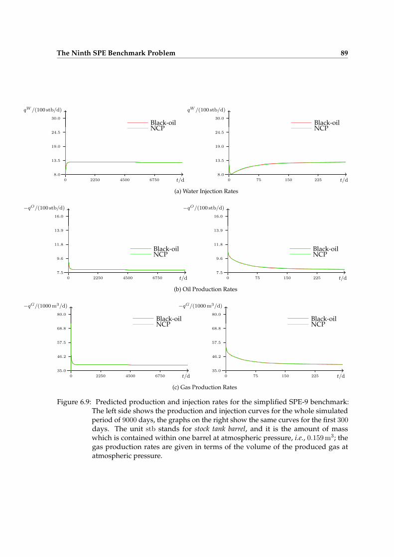
The Ninth SPE Benchmark Problem 89
t/d
qW /(100 stb/d)
Black-oilNCP
0 2250 4500 6750
8.0
13.5
19.0
24.5
30.0
t/d
qW /(100 stb/d)
Black-oilNCP
0 75 150 225
8.0
13.5
19.0
24.5
30.0
(a) Water Injection Rates
t/d
−qO/(100 stb/d)
Black-oilNCP
0 2250 4500 6750
7.5
9.6
11.8
13.9
16.0
t/d
−qO/(100 stb/d)
Black-oilNCP
0 75 150 225
7.5
9.6
11.8
13.9
16.0
(b) Oil Production Rates
t/d
−qG/(1000 m3/d)
Black-oilNCP
0 2250 4500 6750
35.0
46.2
57.5
68.8
80.0
t/d
−qG/(1000 m3/d)
Black-oilNCP
0 75 150 225
35.0
46.2
57.5
68.8
80.0
(c) Gas Production Rates
Figure 6.9: Predicted production and injection rates for the simplified SPE-9 benchmark:The left side shows the production and injection curves for the whole simulatedperiod of 9000 days, the graphs on the right show the same curves for the first 300days. The unit stb stands for stock tank barrel, and it is the amount of masswhich is contained within one barrel at atmospheric pressure, i.e., 0.159 m3; thegas production rates are given in terms of the volume of the produced gas atatmospheric pressure.

90 Numerical Applications
Figure 6.10: Typical behavior of the NEWTON-RAPHSON method for the SPE-9 problem ifusing the PVS model: The phase presence pseudo variables oscillate. The valuedisplayed χpp is calculated using
χpp := 20 · po + 21 · pw + 22 · pg
where pα is 1 if fluid phase α is present at a given spatial location, and zerootherwise. The phase presence initially displayed on the upper left is changedto the one on the upper right in the next NEWTON-RAPHSON iteration, then itassumes the value on the lower left, and finally goes back to the initial state asdisplayed on the lower right.
NCP Black-Oiln [−] 84 60nNEWTON [−] 536 327tCPU [h] 0.77 0.19
Table 6.4: Comparison of the performance of the numerical models using the specializedblack-oil model and the NCP model incorperating non-linear complementarityfunctions for the SPE-9 problem. Here, n corresponds to the number of time stepsrequired to simulate the setup for 9000 days, tCPU is the required computationtime of a single core of an Intel R© CoreTM i7-3770K CPU, and nNEWTON is the totalnumber of iterations of the NEWTON-RAPHSON method required for the wholesimulation.
model [19]. The parameters used are a skin factor of zero, a borehole radius of 7.5 cm, and abottom-hole pressure of 275 bar for the injection well and 206 bar for the production well.
This setup was simulated using the PVS and the NCP models as well as with the black-oil model. The obtained results for the water injection rate as well as for the oil and gasproduction rates agree very well as we can see in Figure 6.9. Inspecting this figure, we alsonote that the production and injection rates for the PVS model are not included. The reasonfor this is that the NEWTON-RAPHSON algorithm is very unstable for the SPE-9 problemwhen using the PVS model. This caused a non-recoverable breakdown at the beginning

The Fifth SPE Benchmark Problem 91
(a) (b)
(c) (d)
Figure 6.11: The SPE-5 benchmark problem: (a) The grid, initial oil phase saturation, andthe locations of the wells. (b) Oil phase saturation after three years of productionas seen from above. (c) The oil phase saturation after three years of productionas seen from below. (d) The water phase saturation after three years of only oilproduction and one subsequent year of water injection plus oil production as seenfrom below.
of the simulation. The reason for this is illustrated in Figure 6.10. It displays the valuesof the phase-presence pseudo primary variables for successive iterations of the NEWTON-RAPHSON algorithm of a failing time step: The presence of the phases keeps oscillatingbetween iterations instead of reaching a stable state. This behavior is likely caused by thesimilar values of the fugacity coefficients for components which are not preferred by the gasand the water phases. Since the NCP model directly embeds the presence of the fluid phasesin the non-linear system of equations to be solved, it is less vulnerable to this issue and doesnot suffer a breakdown.
Moreover, we can infer from Figure 6.9 that the production and the injection rates calculatedusing the specialized black-oil model agree quite well with the ones computed using thegeneric NCP model. As outlined in Table 6.4, the computational effort for the generic NCPmodel is higher, though.

92 Numerical Applications
Component 〈·〉κ pκcrit [bar] T κcrit[K] ωκ
Water (H2O) 220.64 647.10 0.344Methane (C1) 460.43 190.56 0.013Propane (C3) 424.92 369.83 0.1524Hexane (C6) 301.23 507.44 0.3007Decane (C10) 209.60 617.67 0.489Pentadecane (C15) 137.89 705.56 0.65Icosane (C20) 111.69 766.67 0.85
Table 6.5: PENG-ROBINSON parameters used for the fifth SPE benchmark problem. All binaryinteraction coefficients kκλα are zero, except for C1 interacting with C15 or C20, andC3 interacting with C15 or C20. In the former case, the interaction coefficient isassumed to be 0.05 while in the latter case kκλα = 0.005 is used.
6.4 The Fifth SPE Benchmark Problem
Let us now consider the problem specified by the fifth comparative solution project of theSociety of Petroleum Engineers [46]. This problem is the subject of Figure 6.11 and features asimple three-dimensional CARTESIAN grid exhibiting 7 by 7 by 3 elements with a total extendof 1067 m by 1067 m by 30.5 m, as outlined. The bottom of the domain is assumed to be ata depth of 2750 m which yields an initial pressure of 275 bar. Like for the simplified ninthbenchmark problem, the boundary of the domain is fully closed, and production and injectionare handled by vertical boreholes using the PEACEMAN well model [19]. For this problem,the injection well is located in the highest, most south-western cell, while the production wellis located in the deepest north-eastern cell, with a bottom hole pressure of 310 bar for theinjection well and 69 bar for the production well. Initially, the reservoir exhibits a uniformwater saturation of 20 % and an oil saturation of 80 %. Of the three scenarios described in thebenchmark specification [46], only the first is considered: This scenario specifies a period ofthree years where oil and gas is produced without any injection occuring. After that, waterand gas injections are alternated yearly. In this scenario, oil production and water injectionis capped at 12000 stock-tank barrels per day, while the injection rate of gas is limited to 12
thousand cubic feet at standard conditions per day.
The interesting part of the problem are the thermodynamics of the involved fluids: Likethe black-oil model, this problem assumes the potential presence of the three fluid phasesgas, oil, and water, but it specifies the thermodynamic properties using seven components,and the PENG-ROBINSON parameterization of the cubic equation of state. The parametersused for these thermodynamic relations are outlined in Table 6.5. Also, the problem appliesthe standard mixing rule (3.4). With this, we calculate the mass densities ρo and ρg of theoil and the gas phases. The fugacity coefficients for all components are calculated usingEquation 3.15 for the initial state and are then used throughout the simulations.
For this thesis, this problem was simulated using the PVS and NCP models. As we can inferfrom Figure 6.12, the predicted injection and production rates as well as the average pressurewithin the reservoir are virtually indistinguishable. Moreover, the computed rates and the

The Fifth SPE Benchmark Problem 93
t/a
−qO/(103 stb/d)
NCPPVS
0 4 8 12
1.0
3.8
6.5
9.2
12.0
(a) Oil Production Rates
t/a
−qG/(103 m3/d)
NCPPVS
0 4 8 12
110.0
145.0
180.0
215.0
250.0
(b) Gas Production Rates
t/a
−qW /(102 stb/d)
NCPPVS
0 4 8 12
0.0
5.0
10.0
15.0
20.0
(c) Water Production Rates
t/a
po/bar
NCPPVS
0 4 8 12
100.0
150.0
200.0
250.0
300.0
(d) Average Reservoir Pressure
Figure 6.12: Predicted production and injection rates for the SPE-5 benchmark. The rates foroil production and water injection are given in stock tank barrels per day (stb/d),the gas production rate is plotted in thousands of cubic feet per day (MCF/d).

94 Numerical Applications
NCP PVSn [−] 858 826
nNEWTON [−] 5334 4840tCPU [h] 0.67 0.50
nNEWTON/tCPU [1/s] 2.20 2.67
Table 6.6: Comparison of the performance of the numerical models using primary variableswitching (PVS) and non-linear complementarity functions (NCP) for the SPE-5benchmark problem. Like for the previously presented problems, n correspondsto the number of time steps required to simulate the problem for 17 years, tCPU isthe CPU time required for the simulation using an Intel R© CoreTM i7-3770K CPUrunning at a clock speed of 3.50 GHz. Further, nNEWTON is the total number ofiterations of the NEWTON-RAPHSON method.
average reservoir pressure agree very well with the results of most simulators publishedin the original specification [46]. If we consider the computational effort required for oursimulations as presented in Table 6.6. One aspect worth mentioning here is that the ratio ofthe computational costs per NEWTON-RAPHSON iteration for the PVS and the NCP models issmaller for the SPE-5 problem than for the setups discussed before. This is due to the factthat solving the local systems of equations for the PVS model is much more elaborate in thethree-phase case than if only two phases are involved. In conjunction with the large numberof components, this leads to the PVS-based simulation to exhibit high computational costsper NEWTON-RAPHSON iteration. Unlike for the previously presented examples, the numberof NEWTON-RAPHSON iterations required is higher for the NCP model than for the PVSmodel.
6.5 The Ketzin CO2 Storage Project
After investigating the physical accuracy and comparing the computational performanceof the flow models amongst each other, let us now have a brief look at a setup whichdescribes a large-scale real-world experiment – the German CO2 injection pilot site nearKetzin/Havel [55, 44, 49]. The geology of the site of this project features a dome-shapedreservoir formation which exhibits relatively a high permeability as well as high porosity,that is “sandwiched” between highly impermeable salt layers. Together with the intrinsicpermeability field of the reservoir, the shape of the reservoir formation is displayed inFigure 6.13. The capillary-pressure and relative permeability curves used for the simulationare presented in Figure 6.14.
The planar extend of this domain is a square of 5 km by 5 km, and the reservoir layer isabout 130 m thick. This domain is discretized by roughly 4 million tetrahedra using theDUNE-ALUGrid manager [4, 15]. The resulting grid is depicted in Figure 6.13.
Figure 6.15 shows the shape of CO2 plumes after injecting roughly 55 thousand tons of CO2over a period of slightly more than three years while Figure 6.16 shows the predicted share

The Ketzin CO2 Storage Project 95
(a) Grid and Intrinsic Permeability ‖K‖/Pa
(b) The Partition of the Grid Used for the Parallel Simulation
Figure 6.13: Discretization the Ketzin CO2 injection site.

96 Numerical Applications
Sl
pc,gl/kPa
0.0 0.1 0.2 0.4 0.5 0.6 0.8 0.9 1.0
0.0
49.8
99.6
149.4
199.2
249.0
298.8
348.6
(a) Capillary Pressure pc,gl
Sl
kr,α
0.0 0.1 0.2 0.4 0.5 0.6 0.8 0.9 1.0
0.0
0.1
0.3
0.4
0.6
0.7
0.9
1.0
kr,l
kr,g
(b) Relative Permeabilities
Figure 6.14: The material parameters used by the simulations of the Ketzin CO2 storageproject. It is assumed that these parameters only depend on the saturation of theliquid phase.

The Ketzin CO2 Storage Project 97
(a) Gas Saturation Predicted by the Model Assuming Immiscibility
(b) Gas Saturation Predicted by the NCP Model
Figure 6.15: The simulated gas-phase saturation for the Ketzin CO2 injection experiment afterinjecting about 55 thousand tons of CO2 during a three year period. The extend ofthe CO2 plume for the NCP case which includes miscibility is clearly smaller thanfor the case where miscibility is neglected. Both simulations assume the potentialpresence of the two phases “liquid” and “gas”, and use the two components brineand CO2 which are described using the relations provided by IAPWS [88], andSPAN and WAGNER [77]. Based on the conclusions of Section 6.2, energy is notconsidered as a conservation quantity in these simulations.

98 Numerical Applications
t/a
ml,CO2/mtot,CO2
0.00 0.46 0.92 1.38 1.83 2.29 2.75 3.21
0.00
0.09
0.18
0.27
0.36
0.45
0.54
0.63
Figure 6.16: Predicted share of CO2 dissolved in the brine phase for the Ketzin CO2 injectionexperiment. The brine-CO2 miscibility relations used in this simulation have beenproposed by SPYCHER and PRUESS [78].
of CO2 dissolved in the brine phase if using a model that considers miscibility (in this caseusing the NCP model).
In comparison to the synthetic CO2 injection problem which we discussed in Section 6.2,miscibility effects play a much more important role in this scenario, as 40 % to 60 % of theinjected CO2 are predicted to be dissolved in the brine. We can also clearly observe therelevance of miscibility by comparing the shape of the CO2 plume of Figure 6.15a to that ofFigure 6.15b. In this context we should be aware that—due to using finite volume methods asspatial discretizations for these simulations—the amount of dissolved CO2 is overestimatedsystematically. The reason for this is that finite volume discretizations use only a singlevalue to represent the conditions within an individual element. For large finite volumes,this leads to CO2 being assumed to be present in regions of the elements where it cannot bepresent in reality. This implies that the amount of brine which CO2 is assumed dissolve inis overestimated. In turn, this over-estimation of the amount of dissolved CO2 leads to anunderestimation of the gas phase saturation. In the case of the Ketzin project, this suppositionis supported by seismic evidence [55]. For this setup, we should also be aware that the inputparameters, like the intrinsic permeabilityK exhibit large uncertainties, so that the resultspresented in Figures 6.15 and 6.16 should be used with care.
Nevertheless, these simulations prove that the methods presented in this thesis can be usedfor large-scale geological applications and that miscibility is a factor which needs to beconsidered in many real-world applications.

7 Summary and Conclusion
In this thesis, we first motivated the continuum mechanical approach and derived theconservation equations for the physical quantities mass, momentum, and energy on this scale.After adapting the momentum conservation equations to the special case of NEWTONIAN
fluids, we used the obtained relations to derive the conservation equations for macro-scalefluid flow in porous media. We then discussed how we can close the system of equations in amathematical sense. It turned out that one relation per fluid phase needs to be defined usingmodel assumptions. For this purpose, we presented the assumptions of the well establishedimmiscibility model [39], primary variable switching model [23], and black-oil model [19] andintroduced a new set of model assumptions which are based on directly including non-linearcomplementarity problems into the system of equations to be solved [48].
Following this coverage of all relevant equations, we discussed how the resulting systems ofequations can be discretized and how the resulting algebraic non-linear systems of equationscan be solved. After briefly looking at the software which was used to implement theaforementioned concepts, we finally discussed some numerical examples.
The first of these was the heat-pipe setup proposed by UDELL [84]. This problem featuresa one-dimensional spatial domain occupied by water that evaporates and condenses. Forthis problem, we could derive a semi-analytical solution for the steady-state with whichwe compared to results obtained using the numerical models based on primary variableswitching (PVS) and non-linear complementarity problems (NCP) and observed that thenumerical results obtained using both models are identical up to rounding errors. We furtherobserved that the numerical solutions converged to the semi-analytical one as we increasedthe spatial resolution of the grid. This led us to the conclusion that from the point of viewof physical and numerical accuracy, both the NCP and the PVS models produce correctresults, and that thus the computational cost is the main factor for deciding which one touse. Analyzing this computational performance of both approaches, we found that for thisproblem, the NCP model required an order of magnitude fewer time steps than the PVSapproach. This increased robustness more than amortized higher costs per time-step of theNCP model.
After the heat-pipe problem, we compared the NCP and the PVS models with the immis-cible model for a synthetic CO2 injection problem. For this problem we used a radiallysymmetric domain which allowed us to compare the numerical results obtained using athree-dimensional simulation with the ones computed using radial domain extrusion inconjunction with a two-dimensional spatial domain. We found that the results of bothapproaches are comparable, but that the approach using radial domain extrusion is muchcheaper from the point of view of computational effort. We deduced that we should choose a2D approach in conjunction with radial domain extrusion if possible. For this problem, we

100 Summary and Conclusion
also compared the immiscible model with the ones that consider miscibility, and found thatthe results differed significantly. Having said that, the results obtained using the immisciblemodel should still be accurate enough for many purposes.
Since the three-dimensional grid used by this problem featured approximately 1.4 millionelements, it was large enough to apply domain decomposition methods on a parallel machine.Simultaneously, it was small enough to complete sequential simulations in an acceptable timeframe. For this reason, we used this problem to analyze the efficiency of the parallelization.In this context, we found that the computational time required for this simulation is clearlydominated by the procedure of solving the linearized systems of equations, and, even worse,that this procedure typically does not scale well with the number or processors involved.
Next, we compared the computational effort required for the three models for this problem.We found that the effort in terms of the number of time steps and NEWTON-RAPHSON
iterations is much lower for the immiscible model compared to the other two. For thetwo models that include miscibility, the NCP model requires fewer time steps and fewerNEWTON-RAPHSON iterations, but in terms of processing time, it is still slower than the PVSapproach. The reason for this is the fact that the discretization and linearization as well asthe linear solution processes are more elaborate for the NCP model. This is the case becauseit includes one additional equation and primary variable per phase compared to the PVSmodel. Further, in contrast to the heat-pipe problem, the determination of the presence ofthe fluid phases does not seem to be a major limiting factor of this problem when it comesto numerical performance, so the higher costs of each NEWTON-RAPHSON iteration are notamortized by the fewer required time-steps.
After the synthetic CO2 injection problem, we considered a slightly simplified version ofthe ninth benchmark problem of the society of petroleum engineers [45]. For this setup, wecompared the PVS and NCP models with the black-oil model. We found, that the PVS modelis incapable of simulating this setup, but that the NCP model and the black-oil model couldbe used. For this setup, we observed that the injection and production rates calculated usingthe two models agreed very well, but we also noted that the computational effort requiredfor the black-oil model was much lower.
This was followed by an investigation of the first scenario of the fifth benchmark problemof the society of petroleum engineers [46]. Like the ninth SPE benchmark problem, thisspecification originates from the field of oil reservoir engineering, and thus features thethree fluid phases oil, gas, and water. Compared to the ninth benchmark problem, it usesa simpler CARTESIAN grid with uniform material properties. The interesting part of thisproblem are its complicated thermodynamic relations which involve cubic equations of state.The predicted production and injection rates as well as the average pressure of the reservoirwhich we obtained for this problem using the PVS and NCP models were very similar. Fromthe point of view of the required computational effort, the NCP model was worse than thePVS model, but the on a per NEWTON-RAPHSON iteration basis the NCP model difference tothe PVS model was smaller than in the other examples. We attributed the latter observationto the relatively large number of components of this problem and to the observation thatthe systems of equations which need to be solved locally are relatively large for three-phaseproblems when using the PVS model compared to those which need to be solved for the NCP

Future Research 101
model.
Finally, we compared the results of the immiscible model and the ones of the NCP modelfor the CO2 injection experiment in Ketzin/Havel, Germany. For these simulations, anunstructured tetrahedral grid featuring roughly four million elements, and spatially varyingpermeability and porosity fields were used. The results obtained using a model whichassumes immiscibility differed considerably from the results produced by the NCP model.We found that the reason for this is that the share of CO2 which is predicted to dissolvein the liquid phase is quite significant in this case. However, in this context we noted thatthis is probably an overestimation which is due to the spatial discretization used. Even so,miscibility is often a relevant effect in large-scale geological applications, and should thusnot be neglected at the outset.
In summary, the NCP model has proven to be the most versatile as it performed reasonablywell for all problems presented in the context of this thesis. Further, from a computationalpoint of view, it is generally advisable to use a model that directly takes advantage ofadditional knowledge available for a given setting. For example, if miscibility of componentscan be neglected, using the immiscible model often leads to a large improvement of thecomputational performance. Another example is if the setup to be simulated can be assumedto be radially symmetric: Then, using a two-dimensional simulation in conjunction withradial domain extrusion exhibits much lower computational costs while the quality of theresults is basically identical compared to fully three-dimensional simulations.
Future Research
Like all scientific works, this thesis has only a limited scope, so there are plenty of topics ofinterest which could not be covered. In the following, we will outline a few of those.
Model Coupling
For many problems, we may benefit using different numerical models for parts of thesimulation that feature diverse characteristics. For example, we could use a model whichassumes immiscibility for periods of time where miscibility of components is unimportant,and use a more elaborate model for the remaining time [25].
Another situation for which coupling multiple models might be beneficial are multi-physicssituations [34]. For these problems, most of the spatial domain can be described well bya simple model, for example a model neglecting energy or only considering a subset ofall fluid phases, while a small part of the domain needs to be simulated using a morecomprehensive model. For the fully implicit methods which we covered in this thesis, theimplementational effort required for such schemes is quite high [34],and for this reasonmulti-physics approaches currently mostly use semi-implicit methods [34].
Also, we need to use several models for the spatial domain if the the flow characteristic isvastly different in various parts of the domain. For example, problems that incorporate a

102 Summary and Conclusion
part occupied by a porous medium and a part which features turbulent flows, like river-groundwater systems [37] or the soil-atmosphere interactions [57], require us to use a couplingbetween the models for the individual spatial subdomains.
Finally, we can also think of coupling the models for flow and transport in porous mediawhich we discussed in this thesis with geomechanical models [25] or with large-scale modelsfor global phenomena like climate.
Parameter Uncertainty
In the context of this work, we assumed the external parameters—like the intrinsic per-meability K—as quantities precisely known a priori. This is rarely the case for real-worldapplications. There, only rough indications about the distribution of these parameters, anda limited set of measured values are usually available for practical and economic reasons.This means that in reality all parameters used in our models feature an uncertainty which wewould need to quantify in order to obtain predictive results. This is a fulminant challenge,and we refer the interested reader to OLADYSHKIN et al. [62], CIRPKA et al. [21], and toBÁRDOSSY et al. [17].
Advanced Discretizations
For this thesis, only finite volume were used as spatial discretizations. While conceptuallyfinite volume schemes are easy to understand, locally conservative [31] as well as numericallystable [31], they also exhibit severe disadvantages. Amongst those are slow grid convergencerates and a large impact of the numerical dispersion effect [31]. It would thus be benefi-cial to investigate more sophisticated spatial discretizations like discontinuous GALERKIN
methods [5] or mimetic finite difference methods [12].
Also, as time discretization scheme, the implicit EULER method was exclusively used. Like inthe case of finite volume schemes for spatial discretization, this scheme is simple and exhibitsgood numerical stability [6], but its convergence rate tends to be low because of the relativelylarge error term. We could thus benefit from investigating better time discretization schemeslike implicit RUNGE-KUTTA methods [16] or backward differential formula methods [6].
Adaptivity
Adaptive methods are related to the advanced discretizations and multi-physics ap-proaches [26]. mentioned above. Generally speaking, there are two different approachesto adaptivity: For h-adaptive methods, more elements are added to (or removed from) thegrid as soon as the estimated error in the obtained solution is too large (or low enough). Forp-adaptive schemes [26], a spatial discretization with a better error term is used for regions ofthe domain for which a large error is detected.
Finally, h-p-adaptive schemes [26] are combining these two concepts. For them, a higher-order space discretization is used if it is computationally cheaper than refining the grid,

Future Research 103
else the resolution of the grid is locally increased. Typically, h-p-discretization schemes arechallanging to implement [26] since, in addition to error estimates for the refined grid andfor the solution with a locally better discretization, we need to find a balance between thetwo approaches in order to decide which one is better in a given situation.
Further Applications
The final item of this non-exhaustive list of topics that are not covered by this thesis is a closerinvestigation of additional applications of multi-phase flows in porous media. Amongstthese applications we find ground decontamination methods [22, 39], measures to controlsubsurface coal fires [24], polymer-electrolyte membrane fuel cells [7], and many otherchemical engineering applications [42].


A Reproducibility and Raw Data
For the interested and sufficiently determined reader, all results presented in this thesisare available at http://www.hydrosys.uni-stuttgart.de/institut/hydrosys/publikationen/phd_data/ in their raw and refined forms. The only exception is thedata for the Ketzin CO2 storage project discussed in Section 6.5, which is not included in itsraw form due to licensing reasons.
The source code of the software packages which were used to produce these results are alsoprovided. In addition to the raw data and the source code of the simulations which wediscussed within this thesis, the LATEX sources of this document, and editable versions of allpictures used within it, are available at this site.
The source code of the software is provided under the terms of the GNU General PublicLicense (GPL), version two—or, at your option—any newer version of the license. Thesources of this document and the raw data of the presented results are licensed under theCreative Commons Attribution Share-Alike 3.0 license. Further information on the usedlicenses can be found athttp://www.gnu.org/licenses/gpl-2.0.htmland athttp://creativecommons.org/licenses/by-sa/3.0/


Bibliography
[1] I. Aavatsmark. An Introduction to Multipoint Flux Approximations for QuadrilateralGrids. Computational Geosciences, 6:405–432, 2002.
[2] A. Abadpour and M. Panfilov. Method of Negative Saturations for Modeling Two-PhaseCompositional Flow with Oversaturated Zones. Transport in Porous Media, 79:197–214,2009.
[3] The ALBERTA Website: http://www.alberta-fem.de/.
[4] The ALU-Grid Website:http://www.mathematik.uni-freiburg.de/IAM/Research/alugrid/.
[5] D. N. Arnold, F. Brezzi, B. Cockburn, and L. D. Marini. Unified Analysis of Discon-tinuous Galerkin Methods for Elliptic Problems. SIAM Journal on Numerical Analysis,39(5):1749–1779, 2002.
[6] U. M. Ascher and L. R. Petzold. Computer Methods for Ordinary Differential Equations andDifferential-Algebraic Equations. Society for Industrial and Applied Mathematics, 1997.
[7] F. Barbir. PEM Fuel Cells - Theory and Practice. Elsevier, second edition, 2012.
[8] C. Bartels. Analyzing Biased Monte Carlo and Molecular Dynamics Simulations. Chemi-cal Physics Letters, 331(5-6):446–454, 2000.
[9] G. K. Batchelor. An Introduction to Fluid Dynamics. Cambridge University Press, 2000.
[10] A. Y. Beliaev and S. M. Hassanizadeh. A Theoretical Model of Hysteresis and DynamicEffects in the Capillary Relation for Two-Phase Flow in Porous Media. Transport inPorous Media, 43(3):487–510, 2001.
[11] P. Bobeck. The Public Fountains of the City of Dijon. Kendall/Hunt Publishing Company,2009. English Translation of H. Darcy’s 1856 Book Les Fontaines Publiques de la Ville deDijon.
[12] F. Brezzi, K. Lipnikov, and V. Simoncini. A Family of Mimetic Finite Difference Methodson Polygonal and Polyhedral Meshes. Mathematical Models and Methods in AppliedSciences, 15(10):1533–1551, 2005.
[13] R. H. Brooks and A. T. Corey. Hydraulic Properties of Porous Media. Hydrology Papers,Colorado State University, 1964.
[14] E. Buckingham. Studies on the Movement of Soil Moisture. United States Bureau of SoilsBulletin, 38:1–61, 1907.
108 Bibliography
[15] A. Burri, A. Dedner, R. Klöfkorn, and M. Ohlberger. An Efficient Implementation ofan Adaptive and Parallel Grid in DUNE. Proceedings of the Russian-German AdvancedResearch Workshop on Computational Science and High Performance Computing, 2:67–82,2006.
[16] J. C. Butcher. Numerical Methods for Ordinary Differential Equations. Wiley, 2003.
[17] A. Bárdossy, I. I. Bogardi, and W. E. Kelly. Imprecise (Fuzzy) Information in Geostatistics.Mathematical Geology, 20:287–311, 1988.
[18] R. Car and M. Parrinello. Unified Approach for Molecular Dynamics and Density-Functional Theory. Physical Review Letters, 55:2471–2474, 1985.
[19] Z. Chen, G. Huan, and Y. Ma. Computational Methods for Multiphase Flows in Porous Media.Society for Industrial and Applied Mathematics, 2006.
[20] T. J. Chung. General Continuum Mechanics. Cambridge University Press, second edition,2007.
[21] O. A. Cirpka, F. P. J. de Barros, G. Chiogna, M. Rolle, and W. Nowak. Stochastic Flux-Related Analysis of Transverse Mixing in Two-Dimensional Heterogeneous PorousMedia. Water Resources Research, 47(6), 2011.
[22] H. Class and R. Helmig. Numerical Simulation of Non-Isothermal Multiphase Multi-component Processes in Porous Media: 2. Applications for the Injection of Steam andAir. Advances in Water Resources, 25(5):551–564, 2002.
[23] H. Class, R. Helmig, and P. Bastian. Numerical Simulation of Non-Isothermal Multi-phase Multicomponent Processes in Porous Media: 1. An Efficient Solution Technique.Advances in Water Resources, 25(5):533–550, 2002.
[24] G. J. Colaizzi. Prevention, Control and/or Extinguishment of Coal Seam Fires UsingCellular Grout. International Journal of Coal Geology, 59(1–2):75 – 81, 2004.
[25] M. Darcis. Coupling Models of Different Complexity for the Simulation of CO2 Storage in DeepSaline Aquifers. PhD thesis, University of Stuttgart, 2012.
[26] L. Demkowicz. Computing with h-p Adaptive Finite Elements: One and Two-DimensionalElliptic and Maxwell Problems. CRC Press, 2006.
[27] A. H. Demond, F. N. Desai, and K. F. Hayes. Effect of Cationic Surfactants on OrganicLiquid-Water Capillary Pressure-Saturation Relationships. Water Resources Research,30(2):333–342, 1994.
[28] The DUNE Website: http://www.dune-project.org/.
[29] K. Eriksson, D. Estep, P. Hansbo, and C. Johnson. Computational Differential Equations,volume 7. Cambridge University Press, 1996.
[30] The eWoms Website: http://opm-project.org/ewoms.
[31] R. Eymard, T. Gallou, and R. Herbin. Finite Volume Methods, volume 7. Elsevier, 2000.

Bibliography 109
[32] A. Fischer. A Special Newton-Type Optimization Method. Optimization, 24(3-4):269–284,1992.
[33] P. A. Forsyth and R. B. Simpson. A Two-Phase, Two-Component Model for NaturalConvection in a Porous Medium. International Journal for Numerical Methods in Fluids,12(7):655–682, 1991.
[34] J. Fritz, B. Flemisch, and R. Helmig. Decoupled and Multiphysics Models for Non-Isothermal Compositional Two-Phase Flow in Porous Media. International Journal ofNumerical Analysis & Modeling, 9(1):17–28, 2011.
[35] W. G. Gray. A Derivation of the Equations for Multi-Phase Transport. Chemical Engineer-ing Science, 30(2):229–233, 1975.
[36] A. Griewank. Mathematical Programming: Recent Developments and Applications, pages83–108. Kluwer Academic Publishers, 1989.
[37] O. Gunduz and M. M. Aral. River Networks and Groundwater Flow: A SimultaneousSolution of a Coupled System. Journal of Hydrology, 301(1–4):216–234, 2005.
[38] S. M. Hassanizadeh, M. A. Celia, and H. K. Dahle. Dynamic Effect in the CapillaryPressure–Saturation Relationship and its Impacts on Unsaturated Flow. Vadose Zone,1(1):38–57, 2002.
[39] R. Helmig. Multiphase Flow and Transport Processes in the Subsurface: A Contribution to theModeling of Hydrosystems. Springer, first edition, 1997.
[40] R. Helmig and R. Huber. Comparison of Galerkin-Type Discretization Techniquesfor Two-Phase Flow in Heterogeneous Porous Media. Advances in Water Resources,21(8):697–711, 1998.
[41] J. Jaffré and A. Sboui. Henry’ Law and Gas Phase Disappearance. Transport in PorousMedia, 82:521–526, 2010.
[42] H. A. Jakobsen. Chemical Reactor Modeling: Multiphase Reactive Flows. Springer, 2008.
[43] G. Karypis and V. Kumar. METIS - Unstructured Graph Partitioning and Sparse MatrixOrdering System, Version 2.0. Technical report, 1995.
[44] T. Kempka, M. Kühn, H. Class, P. Frykman, A. Kopp, C. M. Nielsen, and P. Probst.Modelling of CO2 Arrival Time at Ketzin – Part I. International Journal of Greenhouse GasControl, 4(6):1007–1015, 2010.
[45] J. E. Killough. Ninth Comparative Solution Project: A Reexamination of Black-OilSimulation. Society of Petroleum Engineers, SPE 29110, 1995.
[46] J. E. Killough and C. A. Kossack. Fifth Comparative Solution Project: Evaluation ofMiscible Flood Simulators. Society of Petroleum Engineers, SPE 16000, 1987.
[47] J. Kool, J. C. Parker, and M. T. van Genuchten. Parameter Estimation for UnsaturatedFlow and Transport Models - A Review. Journal of Hydrology, 91:255–293, 1987.

110 Bibliography
[48] A. Lauser, C. Hager, R. Helmig, and B. Wohlmuth. A new Approach for Phase Transitionsin Miscible Multi-Phase Flow in Porous Media. Advances in Water Resources, 34(8):957–966, 2011.
[49] U. Lengler, M. D. Lucia, and M. Kühn. The Impact of Heterogeneity on the Distribution ofCO2: Numerical Simulation of CO2 Storage at Ketzin. International Journal of GreenhouseGas Control, 4(6):1016–1025, 2010.
[50] R. J. Lenhard, J. C. Parker, and S. Mishra. On the Correspondence Between Brooks-Coreyand van Genuchten Models. Journal of Irrigation and Drainage Engineering, 115(4):744–751,1989.
[51] M. C. Leverett. Capillary Behavior in Porous Solids. Technical report, AIME, 1940.
[52] M. C. Leverett and W. B. Lewis. Steady Flow of Gas-Oil-Water Mixtures ThroughUnconsolidated Sands. Transactions of AIME, 142(107):14, 1941.
[53] X. S. Li. An Overview of SuperLU: Algorithms, Implementation, and User Interface.ACM Transactions on Mathematical Software, 31(3):302–325, 2005.
[54] O. Lia, H. Omre, H. Tjelmeland, L. Holden, and T. Egeland. Uncertainties in ReservoirProduction Forecasts. AAPG Bulletin, 82(5):775–803, 1997.
[55] S. Martens, T. Kempka, A. Liebscher, S. Lüth, F. Möller, A. Myrttinen, B. Norden,C. Schmidt-Hattenberger, M. Zimmer, and M. Kühn. Europe’s Longest-Operating On-shore CO2 Storage Site at Ketzin, Germany: A Progress Report After Three Years ofInjection. Environmental Earth Sciences, 67(2):323–334, 2012.
[56] G. J. Martyna, D. J. Tobias, and M. L. Klein. Constant Pressure Molecular DynamicsAlgorithms. Journal of Chemical Physics, 101(5):4177 – 4189, 1994.
[57] K. Mosthaf, K. Baber, B. Flemisch, R. Helmig, T. Leijnse, I. Rybak, and B. Wohlmuth.A Coupling Concept for Two-Phase Compositional Porous-Medium and Single-PhaseCompositional Free Flow. Water Resources Research, 47(10), 2011.
[58] R. Neumann, P. Bastian, and O. Ippisch. Modeling and Simulation of Two-Phase Two-Component Flow with Disappearing Nonwetting Phase. Computational Geosciences,17:139–149, 2013.
[59] J. Niessner and S. M. Hassanizadeh. A Model for Two-Phase Flow in Porous MediaIncluding Fluid-Fluid Interfacial Area. Water Resources Research, 44(8), 2008.
[60] J. Nolen. Numerical Simulation of Compositional Phenomena in Petroleum Reservoirs.Society of Petroleum Engineers, SPE 4274, 1973.
[61] S. O. Ochs. Steam Injection into Saturated Porous Media: Process Analysis Including Experi-mental and Numerical Investigations. PhD thesis, University of Stuttgart, 2006.
[62] S. Oladyshkin, H. Class, R. Helmig, and W. Nowak. An Integrative Approach to RobustDesign and Probabilistic Risk Assessment for CO2 Storage in Geological Formations.Computational Geosciences, 15:565–577, 2011.

Bibliography 111
[63] J. M. Ortega and W. C. Rheinboldt. Iterative Solution of Nonlinear Equations in SeveralVariables. Society for Industrial and Applied Mathematics, 2000.
[64] A. M. Otten, A. Alphenaar, C. Pijls, F. Spuij, and H. de Wit. In Situ Soil Remediation.Springer, 1997.
[65] J. C. Parker, R. J. Lenhard, and T. Kuppusamy. A Parametric Model for ConstitutiveProperties Governing Multiphase Flow in Porous Media. Water Resources Research,23(4):618–624, 1987.
[66] F. Pellegrini and J. Roman. Scotch: A Software Package for Static Mapping by DualRecursive Bipartitioning of Process and Architecture Graphs. In High-PerformanceComputing and Networking, volume 1067 of Lecture Notes in Computer Science, pages493–498. Springer, 1996.
[67] M. Quintard and S. Whitaker. Transport in Ordered and Disordered Porous Media II:Generalized Volume Averaging. Transport in Porous Media, 14:179–206, 1994.
[68] R. C. Reid, J. M. Prausnitz, and B. E. Poling. The Properties of Gases and Liquids. McGraw-Hill, fourth edition, 1987.
[69] E. Rubin and H. de Coninck. IPCC Special Report on Carbon Dioxide Capture and Storage.Cambridge University Press, 2005.
[70] Y. Saad. Iterative Methods for Sparse Linear Systems. PWS Publishing, first edition, 1996.
[71] O. Schenk and K. Gärtner. Solving Unsymmetric Sparse Systems of Linear Equationswith PARDISO. Future Generation Computer Systems, 20(3):475–487, 2004.
[72] A. A. Shabana. Computational Continuum Mechanics. Cambridge University Press, secondedition, 2012.
[73] H. Y. She and B. E. Sleep. The Effect of Temperature on Capillary Pressure-SaturationRelationships for Air-Water and Perchloroethylene-Water Systems. Water ResourcesResearch, 34(10):2587–2597, 1998.
[74] D. M. Wheeler’s SLOCCount Website: http://www.dwheeler.com/sloccount.
[75] B. Smith, P. Bjørstad, and W. Gropp. Domain Decomposition: Parallel Multilevel Methodsfor Elliptic Partial Differential Equations. Cambridge University Press, 2004.
[76] W. H. Somerton, A. H. El-Shaarani, and S. M. Mobarak. High Temperature Behavior ofRocks Associated with Geothermal Type Reservoirs, volume SPE 4897. Society of PetroleumEngineers, 1974.
[77] R. Span and W. Wagner. A New Equation of State for Carbon Dioxide Covering theFluid Region from the Triple-Point Temperature to 1100 K at Pressures up to 800 MPa.Journal of Chemical and Physical Reference Data, 25(6):1509–1596, 1996.
[78] N. Spycher and K. Pruess. CO2-H2O Mixtures in the Geological Sequestration of CO2. II.Partitioning in Chloride Brines at 12–100C and Up to 600 bar. Geochimica et CosmochimicaActa, 69(13):3309 – 3320, 2005.
112 Bibliography
[79] H. L. Stone. Probability Model for Estimating Three-Phase Relative Permeability. Journalof Petroleum Technology, 22(2):214–218, 1970.
[80] H. L. Stone. Estimation of Three-Phase Relative Permeability and Residual Oil Data.Journal of Petroleum Technology, 12(4), 1973.
[81] W. G. Strang and G. J. Fix. An Analysis of the Finite Element Method. Prentice-Hall, 1973.
[82] K. Stüben. Algebraic Multigrid (AMG). An Introduction with Applications. GMDForschungszentrum Informationstechnik, 1999.
[83] J. A. Trangenstein and J. B. Bell. Mathematical Structure of the Black-Oil Model forPetroleum Reservoir Simulation. SIAM Journal on Applied Mathematics, 49(3), 1989.
[84] K. S. Udell. Heat Transfer in Porous Media Considering Phase Change and Capillarity –The Heat-Pipe Effect. International Journal of Heat and Mass Transfer, 28(2):485–495, 1985.
[85] The UG Website: http://atlas.gcsc.uni-frankfurt.de/~ug/.
[86] H. A. van der Vorst. BI-CGSTAB: A Fast and Smoothly Converging Variant of BI-CG forthe Solution of Non-symmetric Linear Systems. SIAM Journal on Scientific and StatisticalComputing, 13(2):631–644, 1992.
[87] M. T. van Genuchten. A Closed-Form Equation for Predicting the Hydraulic Conduc-tivity of Unsaturated Soils. Journal of the Soil Science Society of America, 44(5):892–898,1980.
[88] W. Wagner and A. Pruß. The IAPWS Formulation 1995 for the Thermodynamic Proper-ties of Ordinary Water Substance for General and Scientific Use. Journal of Chemical andPhysical Reference Data, 31(2):387–535, 2002.
[89] S. Whitaker. Flow in Porous Media I: A Theoretical Derivation of Darcy’s Law. Transportin Porous Media, 1(1):3–25, 1985.
[90] Wikipedia Article on Carbon Capture and Storage: http://en.wikipedia.org/wiki/Carbon_capture_and_storage. Article Date: January 18, 2013.
[91] Wikipedia Article on Petroleum Reservoirs: http://en.wikipedia.org/wiki/Petroleum_reservoir. Article Date: March 23, 2013.
[92] Y. Zhou, H. A. Tchelepi, and B. T. Mallison. Automatic Differentiation Frameworkfor Compositional Simulation on Unstructured Grids with Multi-Point DiscretizationSchemes. Society of Petroleum Engineers, SPE 141592, 2011.

Institut für Wasser- und Umweltsystemmodellierung Universität Stuttgart
Pfaffenwaldring 61 70569 Stuttgart (Vaihingen) Telefon (0711) 685 - 64717/64749/64752/64679 Telefax (0711) 685 - 67020 o. 64746 o. 64681 E-Mail: [email protected] http://www.iws.uni-stuttgart.de
Direktoren Prof. Dr. rer. nat. Dr.-Ing. András Bárdossy Prof. Dr.-Ing. Rainer Helmig Prof. Dr.-Ing. Silke Wieprecht Vorstand (Stand 19.08.2013) Prof. Dr. rer. nat. Dr.-Ing. A. Bárdossy Prof. Dr.-Ing. R. Helmig Prof. Dr.-Ing. S. Wieprecht Prof. Dr. J.A. Sander Huisman Jürgen Braun, PhD apl. Prof. Dr.-Ing. H. Class Dr.-Ing. H.-P. Koschitzky Dr.-Ing. M. Noack Jun.-Prof. Dr.-Ing. W. Nowak, M.Sc. Dr. rer. nat. J. Seidel Dr.-Ing. K. Terheiden Emeriti Prof. Dr.-Ing. habil. Dr.-Ing. E.h. Jürgen Giesecke Prof. Dr.h.c. Dr.-Ing. E.h. Helmut Kobus, PhD
Lehrstuhl für Wasserbau und Wassermengenwirtschaft Leiter: Prof. Dr.-Ing. Silke Wieprecht Stellv.: Dr.-Ing. Kristina Terheiden Versuchsanstalt für Wasserbau Leiter: Dr.-Ing. Markus Noack Lehrstuhl für Hydromechanik und Hydrosystemmodellierung Leiter: Prof. Dr.-Ing. Rainer Helmig Stellv.: apl. Prof. Dr.-Ing. Holger Class Jungwissenschaftlergruppe: Stochastische Modellierung von Hydrosystemen Leiter: Jun.-Prof. Dr.-Ing. Wolfgang Nowak, M.Sc. Lehrstuhl für Hydrologie und Geohydrologie Leiter: Prof. Dr. rer. nat. Dr.-Ing. András Bárdossy Stellv.: Dr. rer. nat. Jochen Seidel Hydrogeophysik der Vadosen Zone (mit Forschungszentrum Jülich) Leiter: Prof. Dr. J.A. Sander Huisman VEGAS, Versuchseinrichtung zur Grundwasser- und Altlastensanierung Leitung: Jürgen Braun, PhD, AD Dr.-Ing. Hans-Peter Koschitzky, AD
Verzeichnis der Mitteilungshefte
1 Röhnisch, Arthur: Die Bemühungen um eine Wasserbauliche Versuchsanstalt an
der Technischen Hochschule Stuttgart, und Fattah Abouleid, Abdel: Beitrag zur Berechnung einer in lockeren Sand geramm-ten, zweifach verankerten Spundwand, 1963
2 Marotz, Günter: Beitrag zur Frage der Standfestigkeit von dichten Asphaltbelägen
im Großwasserbau, 1964 3 Gurr, Siegfried: Beitrag zur Berechnung zusammengesetzter ebener Flächen-
tragwerke unter besonderer Berücksichtigung ebener Stauwände, mit Hilfe von Randwert- und Lastwertmatrizen, 1965
4 Plica, Peter: Ein Beitrag zur Anwendung von Schalenkonstruktionen im Stahlwas-
serbau, und Petrikat, Kurt: Möglichkeiten und Grenzen des wasserbaulichen Ver-suchswesens, 1966

2 Institut für Wasser- und Umweltsystemmodellierung * Universität Stuttgart * IWS 5 Plate, Erich: Beitrag zur Bestimmung der Windgeschwindigkeitsverteilung in der
durch eine Wand gestörten bodennahen Luftschicht, und Röhnisch, Arthur; Marotz, Günter: Neue Baustoffe und Bauausführungen für den Schutz der Böschungen und der Sohle von Kanälen, Flüssen und Häfen; Geste-hungskosten und jeweilige Vorteile, sowie Unny, T.E.: Schwingungs-untersuchungen am Kegelstrahlschieber, 1967
6 Seiler, Erich: Die Ermittlung des Anlagenwertes der bundeseigenen Bin-
nenschiffahrtsstraßen und Talsperren und des Anteils der Binnenschiffahrt an die-sem Wert, 1967
7 Sonderheft anläßlich des 65. Geburtstages von Prof. Arthur Röhnisch mit Beiträ-
gen von Benk, Dieter; Breitling, J.; Gurr, Siegfried; Haberhauer, Robert; Hone-kamp, Hermann; Kuz, Klaus Dieter; Marotz, Günter; Mayer-Vorfelder, Hans-Jörg; Miller, Rudolf; Plate, Erich J.; Radomski, Helge; Schwarz, Helmut; Vollmer, Ernst; Wildenhahn, Eberhard; 1967
8 Jumikis, Alfred: Beitrag zur experimentellen Untersuchung des Wassernachschubs
in einem gefrierenden Boden und die Beurteilung der Ergebnisse, 1968 9 Marotz, Günter: Technische Grundlagen einer Wasserspeicherung im natürlichen
Untergrund, 1968 10 Radomski, Helge: Untersuchungen über den Einfluß der Querschnittsform wellen-
förmiger Spundwände auf die statischen und rammtechnischen Eigenschaften, 1968
11 Schwarz, Helmut: Die Grenztragfähigkeit des Baugrundes bei Einwirkung vertikal
gezogener Ankerplatten als zweidimensionales Bruchproblem, 1969 12 Erbel, Klaus: Ein Beitrag zur Untersuchung der Metamorphose von Mittelgebirgs-
schneedecken unter besonderer Berücksichtigung eines Verfahrens zur Bestim-mung der thermischen Schneequalität, 1969
13 Westhaus, Karl-Heinz: Der Strukturwandel in der Binnenschiffahrt und sein Einfluß
auf den Ausbau der Binnenschiffskanäle, 1969 14 Mayer-Vorfelder, Hans-Jörg: Ein Beitrag zur Berechnung des Erdwiderstandes un-
ter Ansatz der logarithmischen Spirale als Gleitflächenfunktion, 1970 15 Schulz, Manfred: Berechnung des räumlichen Erddruckes auf die Wandung kreis-
zylindrischer Körper, 1970 16 Mobasseri, Manoutschehr: Die Rippenstützmauer. Konstruktion und Grenzen ihrer
Standsicherheit, 1970 17 Benk, Dieter: Ein Beitrag zum Betrieb und zur Bemessung von Hochwasser-
rückhaltebecken, 1970

Verzeichnis der Mitteilungshefte 3 18 Gàl, Attila: Bestimmung der mitschwingenden Wassermasse bei überströmten
Fischbauchklappen mit kreiszylindrischem Staublech, 1971, 19 Kuz, Klaus Dieter: Ein Beitrag zur Frage des Einsetzens von Kavitationserschei-
nungen in einer Düsenströmung bei Berücksichtigung der im Wasser gelösten Ga-se, 1971,
20 Schaak, Hartmut: Verteilleitungen von Wasserkraftanlagen, 1971 21 Sonderheft zur Eröffnung der neuen Versuchsanstalt des Instituts für Wasserbau
der Universität Stuttgart mit Beiträgen von Brombach, Hansjörg; Dirksen, Wolfram; Gàl, Attila; Gerlach, Reinhard; Giesecke, Jürgen; Holthoff, Franz-Josef; Kuz, Klaus Dieter; Marotz, Günter; Minor, Hans-Erwin; Petrikat, Kurt; Röhnisch, Arthur; Rueff, Helge; Schwarz, Helmut; Vollmer, Ernst; Wildenhahn, Eberhard; 1972
22 Wang, Chung-su: Ein Beitrag zur Berechnung der Schwingungen an Kegelstrahl-
schiebern, 1972 23 Mayer-Vorfelder, Hans-Jörg: Erdwiderstandsbeiwerte nach dem Ohde-
Variationsverfahren, 1972 24 Minor, Hans-Erwin: Beitrag zur Bestimmung der Schwingungsanfachungs-
funktionen überströmter Stauklappen, 1972, 25 Brombach, Hansjörg: Untersuchung strömungsmechanischer Elemente (Fluidik)
und die Möglichkeit der Anwendung von Wirbelkammerelementen im Wasserbau, 1972,
26 Wildenhahn, Eberhard: Beitrag zur Berechnung von Horizontalfilterbrunnen, 1972 27 Steinlein, Helmut: Die Eliminierung der Schwebstoffe aus Flußwasser zum Zweck
der unterirdischen Wasserspeicherung, gezeigt am Beispiel der Iller, 1972 28 Holthoff, Franz Josef: Die Überwindung großer Hubhöhen in der Binnenschiffahrt
durch Schwimmerhebewerke, 1973 29 Röder, Karl: Einwirkungen aus Baugrundbewegungen auf trog- und kastenförmige
Konstruktionen des Wasser- und Tunnelbaues, 1973 30 Kretschmer, Heinz: Die Bemessung von Bogenstaumauern in Abhängigkeit von
der Talform, 1973 31 Honekamp, Hermann: Beitrag zur Berechnung der Montage von Unterwasserpipe-
lines, 1973 32 Giesecke, Jürgen: Die Wirbelkammertriode als neuartiges Steuerorgan im Was-
serbau, und Brombach, Hansjörg: Entwicklung, Bauformen, Wirkungsweise und Steuereigenschaften von Wirbelkammerverstärkern, 1974

4 Institut für Wasser- und Umweltsystemmodellierung * Universität Stuttgart * IWS 33 Rueff, Helge: Untersuchung der schwingungserregenden Kräfte an zwei hinterein-
ander angeordneten Tiefschützen unter besonderer Berücksichtigung von Kavita-tion, 1974
34 Röhnisch, Arthur: Einpreßversuche mit Zementmörtel für Spannbeton - Vergleich
der Ergebnisse von Modellversuchen mit Ausführungen in Hüllwellrohren, 1975 35 Sonderheft anläßlich des 65. Geburtstages von Prof. Dr.-Ing. Kurt Petrikat mit Bei-
trägen von: Brombach, Hansjörg; Erbel, Klaus; Flinspach, Dieter; Fischer jr., Richard; Gàl, Attila; Gerlach, Reinhard; Giesecke, Jürgen; Haberhauer, Robert; Hafner Edzard; Hausenblas, Bernhard; Horlacher, Hans-Burkhard; Hutarew, An-dreas; Knoll, Manfred; Krummet, Ralph; Marotz, Günter; Merkle, Theodor; Miller, Christoph; Minor, Hans-Erwin; Neumayer, Hans; Rao, Syamala; Rath, Paul; Rueff, Helge; Ruppert, Jürgen; Schwarz, Wolfgang; Topal-Gökceli, Mehmet; Vollmer, Ernst; Wang, Chung-su; Weber, Hans-Georg; 1975
36 Berger, Jochum: Beitrag zur Berechnung des Spannungszustandes in rotations-
symmetrisch belasteten Kugelschalen veränderlicher Wandstärke unter Gas- und Flüssigkeitsdruck durch Integration schwach singulärer Differentialgleichungen, 1975
37 Dirksen, Wolfram: Berechnung instationärer Abflußvorgänge in gestauten Gerin-
nen mittels Differenzenverfahren und die Anwendung auf Hochwasserrückhalte-becken, 1976
38 Horlacher, Hans-Burkhard: Berechnung instationärer Temperatur- und Wärme-
spannungsfelder in langen mehrschichtigen Hohlzylindern, 1976 39 Hafner, Edzard: Untersuchung der hydrodynamischen Kräfte auf Baukörper im
Tiefwasserbereich des Meeres, 1977, ISBN 3-921694-39-6 40 Ruppert, Jürgen: Über den Axialwirbelkammerverstärker für den Einsatz im Was-
serbau, 1977, ISBN 3-921694-40-X 41 Hutarew, Andreas: Beitrag zur Beeinflußbarkeit des Sauerstoffgehalts in Fließge-
wässern an Abstürzen und Wehren, 1977, ISBN 3-921694-41-8, 42 Miller, Christoph: Ein Beitrag zur Bestimmung der schwingungserregenden Kräfte
an unterströmten Wehren, 1977, ISBN 3-921694-42-6 43 Schwarz, Wolfgang: Druckstoßberechnung unter Berücksichtigung der Radial- und
Längsverschiebungen der Rohrwandung, 1978, ISBN 3-921694-43-4 44 Kinzelbach, Wolfgang: Numerische Untersuchungen über den optimalen Einsatz
variabler Kühlsysteme einer Kraftwerkskette am Beispiel Oberrhein, 1978, ISBN 3-921694-44-2
45 Barczewski, Baldur: Neue Meßmethoden für Wasser-Luftgemische und deren An-
wendung auf zweiphasige Auftriebsstrahlen, 1979, ISBN 3-921694-45-0
Verzeichnis der Mitteilungshefte 5 46 Neumayer, Hans: Untersuchung der Strömungsvorgänge in radialen Wirbelkam-
merverstärkern, 1979, ISBN 3-921694-46-9 47 Elalfy, Youssef-Elhassan: Untersuchung der Strömungsvorgänge in Wirbelkam-
merdioden und -drosseln, 1979, ISBN 3-921694-47-7 48 Brombach, Hansjörg: Automatisierung der Bewirtschaftung von Wasserspeichern,
1981, ISBN 3-921694-48-5 49 Geldner, Peter: Deterministische und stochastische Methoden zur Bestimmung der
Selbstdichtung von Gewässern, 1981, ISBN 3-921694-49-3, 50 Mehlhorn, Hans: Temperaturveränderungen im Grundwasser durch Brauchwas-
sereinleitungen, 1982, ISBN 3-921694-50-7, 51 Hafner, Edzard: Rohrleitungen und Behälter im Meer, 1983, ISBN 3-921694-51-5 52 Rinnert, Bernd: Hydrodynamische Dispersion in porösen Medien: Einfluß von Dich-
teunterschieden auf die Vertikalvermischung in horizontaler Strömung, 1983, ISBN 3-921694-52-3,
53 Lindner, Wulf: Steuerung von Grundwasserentnahmen unter Einhaltung ökologi-
scher Kriterien, 1983, ISBN 3-921694-53-1, 54 Herr, Michael; Herzer, Jörg; Kinzelbach, Wolfgang; Kobus, Helmut; Rinnert, Bernd:
Methoden zur rechnerischen Erfassung und hydraulischen Sanierung von Grund-wasserkontaminationen, 1983, ISBN 3-921694-54-X
55 Schmitt, Paul: Wege zur Automatisierung der Niederschlagsermittlung, 1984, ISBN
3-921694-55-8, 56 Müller, Peter: Transport und selektive Sedimentation von Schwebstoffen bei ge-
stautem Abfluß, 1985, ISBN 3-921694-56-6 57 El-Qawasmeh, Fuad: Möglichkeiten und Grenzen der Tropfbewässerung unter be-
sonderer Berücksichtigung der Verstopfungsanfälligkeit der Tropfelemente, 1985, ISBN 3-921694-57-4,
58 Kirchenbaur, Klaus: Mikroprozessorgesteuerte Erfassung instationärer Druckfelder
am Beispiel seegangsbelasteter Baukörper, 1985, ISBN 3-921694-58-2 59 Kobus, Helmut (Hrsg.): Modellierung des großräumigen Wärme- und Schadstoff-
transports im Grundwasser, Tätigkeitsbericht 1984/85 (DFG-Forschergruppe an den Universitäten Hohenheim, Karlsruhe und Stuttgart), 1985, ISBN 3-921694-59-0,
60 Spitz, Karlheinz: Dispersion in porösen Medien: Einfluß von Inhomogenitäten und
Dichteunterschieden, 1985, ISBN 3-921694-60-4, 61 Kobus, Helmut: An Introduction to Air-Water Flows in Hydraulics, 1985,
ISBN 3-921694-61-2

6 Institut für Wasser- und Umweltsystemmodellierung * Universität Stuttgart * IWS 62 Kaleris, Vassilios: Erfassung des Austausches von Oberflächen- und Grundwasser
in horizontalebenen Grundwassermodellen, 1986, ISBN 3-921694-62-0 63 Herr, Michael: Grundlagen der hydraulischen Sanierung verunreinigter Poren-
grundwasserleiter, 1987, ISBN 3-921694-63-9 64 Marx, Walter: Berechnung von Temperatur und Spannung in Massenbeton infolge
Hydratation, 1987, ISBN 3-921694-64-7 65 Koschitzky, Hans-Peter: Dimensionierungskonzept für Sohlbelüfter in Schußrinnen
zur Vermeidung von Kavitationsschäden, 1987, ISBN 3-921694-65-5 66 Kobus, Helmut (Hrsg.): Modellierung des großräumigen Wärme- und Schadstoff-
transports im Grundwasser, Tätigkeitsbericht 1986/87 (DFG-Forschergruppe an den Universitäten Hohenheim, Karlsruhe und Stuttgart) 1987, ISBN 3-921694-66-3
67 Söll, Thomas: Berechnungsverfahren zur Abschätzung anthropogener Tempera-
turanomalien im Grundwasser, 1988, ISBN 3-921694-67-1 68 Dittrich, Andreas; Westrich, Bernd: Bodenseeufererosion, Bestandsaufnahme und
Bewertung, 1988, ISBN 3-921694-68-X, 69 Huwe, Bernd; van der Ploeg, Rienk R.: Modelle zur Simulation des Stickstoffhaus-
haltes von Standorten mit unterschiedlicher landwirtschaftlicher Nutzung, 1988, ISBN 3-921694-69-8,
70 Stephan, Karl: Integration elliptischer Funktionen, 1988, ISBN 3-921694-70-1 71 Kobus, Helmut; Zilliox, Lothaire (Hrsg.): Nitratbelastung des Grundwassers, Aus-
wirkungen der Landwirtschaft auf die Grundwasser- und Rohwasserbeschaffenheit und Maßnahmen zum Schutz des Grundwassers. Vorträge des deutsch-franzö-sischen Kolloquiums am 6. Oktober 1988, Universitäten Stuttgart und Louis Pas-teur Strasbourg (Vorträge in deutsch oder französisch, Kurzfassungen zwei-sprachig), 1988, ISBN 3-921694-71-X
72 Soyeaux, Renald: Unterströmung von Stauanlagen auf klüftigem Untergrund unter
Berücksichtigung laminarer und turbulenter Fließzustände,1991, ISBN 3-921694-72-8
73 Kohane, Roberto: Berechnungsmethoden für Hochwasserabfluß in Fließgewäs-
sern mit überströmten Vorländern, 1991, ISBN 3-921694-73-6 74 Hassinger, Reinhard: Beitrag zur Hydraulik und Bemessung von Blocksteinrampen
in flexibler Bauweise, 1991, ISBN 3-921694-74-4, 75 Schäfer, Gerhard: Einfluß von Schichtenstrukturen und lokalen Einlagerungen auf
die Längsdispersion in Porengrundwasserleitern, 1991, ISBN 3-921694-75-2 76 Giesecke, Jürgen: Vorträge, Wasserwirtschaft in stark besiedelten Regionen; Um-
weltforschung mit Schwerpunkt Wasserwirtschaft, 1991, ISBN 3-921694-76-0

Verzeichnis der Mitteilungshefte 7 77 Huwe, Bernd: Deterministische und stochastische Ansätze zur Modellierung des
Stickstoffhaushalts landwirtschaftlich genutzter Flächen auf unterschiedlichem Skalenniveau, 1992, ISBN 3-921694-77-9,
78 Rommel, Michael: Verwendung von Kluftdaten zur realitätsnahen Generierung von
Kluftnetzen mit anschließender laminar-turbulenter Strömungsberechnung, 1993, ISBN 3-92 1694-78-7
79 Marschall, Paul: Die Ermittlung lokaler Stofffrachten im Grundwasser mit Hilfe von
Einbohrloch-Meßverfahren, 1993, ISBN 3-921694-79-5, 80 Ptak, Thomas: Stofftransport in heterogenen Porenaquiferen: Felduntersuchungen
und stochastische Modellierung, 1993, ISBN 3-921694-80-9, 81 Haakh, Frieder: Transientes Strömungsverhalten in Wirbelkammern, 1993,
ISBN 3-921694-81-7 82 Kobus, Helmut; Cirpka, Olaf; Barczewski, Baldur; Koschitzky, Hans-Peter: Ver-
sucheinrichtung zur Grundwasser und Altlastensanierung VEGAS, Konzeption und Programmrahmen, 1993, ISBN 3-921694-82-5
83 Zang, Weidong: Optimaler Echtzeit-Betrieb eines Speichers mit aktueller Abflußre-
generierung, 1994, ISBN 3-921694-83-3, 84 Franke, Hans-Jörg: Stochastische Modellierung eines flächenhaften Stoffeintrages
und Transports in Grundwasser am Beispiel der Pflanzenschutzmittelproblematik, 1995, ISBN 3-921694-84-1
85 Lang, Ulrich: Simulation regionaler Strömungs- und Transportvorgänge in Karst-
aquiferen mit Hilfe des Doppelkontinuum-Ansatzes: Methodenentwicklung und Pa-rameteridentifikation, 1995, ISBN 3-921694-85-X,
86 Helmig, Rainer: Einführung in die Numerischen Methoden der Hydromechanik,
1996, ISBN 3-921694-86-8, 87 Cirpka, Olaf: CONTRACT: A Numerical Tool for Contaminant Transport and
Chemical Transformations - Theory and Program Documentation -, 1996, ISBN 3-921694-87-6
88 Haberlandt, Uwe: Stochastische Synthese und Regionalisierung des Niederschla-
ges für Schmutzfrachtberechnungen, 1996, ISBN 3-921694-88-4 89 Croisé, Jean: Extraktion von flüchtigen Chemikalien aus natürlichen Lockergestei-
nen mittels erzwungener Luftströmung, 1996, ISBN 3-921694-89-2, 90 Jorde, Klaus: Ökologisch begründete, dynamische Mindestwasserregelungen bei
Ausleitungskraftwerken, 1997, ISBN 3-921694-90-6, 91 Helmig, Rainer: Gekoppelte Strömungs- und Transportprozesse im Untergrund -
Ein Beitrag zur Hydrosystemmodellierung-, 1998, ISBN 3-921694-91-4,
8 Institut für Wasser- und Umweltsystemmodellierung * Universität Stuttgart * IWS 92 Emmert, Martin: Numerische Modellierung nichtisothermer Gas-Wasser Systeme
in porösen Medien, 1997, ISBN 3-921694-92-2 93 Kern, Ulrich: Transport von Schweb- und Schadstoffen in staugeregelten Fließge-
wässern am Beispiel des Neckars, 1997, ISBN 3-921694-93-0, 94 Förster, Georg: Druckstoßdämpfung durch große Luftblasen in Hochpunkten von
Rohrleitungen 1997, ISBN 3-921694-94-9 95 Cirpka, Olaf: Numerische Methoden zur Simulation des reaktiven Mehrkomponen-
tentransports im Grundwasser, 1997, ISBN 3-921694-95-7, 96 Färber, Arne: Wärmetransport in der ungesättigten Bodenzone: Entwicklung einer
thermischen In-situ-Sanierungstechnologie, 1997, ISBN 3-921694-96-5 97 Betz, Christoph: Wasserdampfdestillation von Schadstoffen im porösen Medium:
Entwicklung einer thermischen In-situ-Sanierungstechnologie, 1998, ISBN 3-921694-97-3
98 Xu, Yichun: Numerical Modeling of Suspended Sediment Transport in Rivers,
1998, ISBN 3-921694-98-1, 99 Wüst, Wolfgang: Geochemische Untersuchungen zur Sanierung CKW-
kontaminierter Aquifere mit Fe(0)-Reaktionswänden, 2000, ISBN 3-933761-02-2 100 Sheta, Hussam: Simulation von Mehrphasenvorgängen in porösen Medien unter
Einbeziehung von Hysterese-Effekten, 2000, ISBN 3-933761-03-4 101 Ayros, Edwin: Regionalisierung extremer Abflüsse auf der Grundlage statistischer
Verfahren, 2000, ISBN 3-933761-04-2, 102 Huber, Ralf: Compositional Multiphase Flow and Transport in Heterogeneous Po-
rous Media, 2000, ISBN 3-933761-05-0 103 Braun, Christopherus: Ein Upscaling-Verfahren für Mehrphasenströmungen in po-
rösen Medien, 2000, ISBN 3-933761-06-9 104 Hofmann, Bernd: Entwicklung eines rechnergestützten Managementsystems zur
Beurteilung von Grundwasserschadensfällen, 2000, ISBN 3-933761-07-7 105 Class, Holger: Theorie und numerische Modellierung nichtisothermer Mehrphasen-
prozesse in NAPL-kontaminierten porösen Medien, 2001, ISBN 3-933761-08-5
106 Schmidt, Reinhard: Wasserdampf- und Heißluftinjektion zur thermischen Sanie-
rung kontaminierter Standorte, 2001, ISBN 3-933761-09-3 107 Josef, Reinhold:, Schadstoffextraktion mit hydraulischen Sanierungsverfahren un-
ter Anwendung von grenzflächenaktiven Stoffen, 2001, ISBN 3-933761-10-7

Verzeichnis der Mitteilungshefte 9 108 Schneider, Matthias: Habitat- und Abflussmodellierung für Fließgewässer mit un-
scharfen Berechnungsansätzen, 2001, ISBN 3-933761-11-5 109 Rathgeb, Andreas: Hydrodynamische Bemessungsgrundlagen für Lockerdeckwer-
ke an überströmbaren Erddämmen, 2001, ISBN 3-933761-12-3 110 Lang, Stefan: Parallele numerische Simulation instätionärer Probleme mit adapti-
ven Methoden auf unstrukturierten Gittern, 2001, ISBN 3-933761-13-1 111 Appt, Jochen; Stumpp Simone: Die Bodensee-Messkampagne 2001, IWS/CWR
Lake Constance Measurement Program 2001, 2002, ISBN 3-933761-14-X 112 Heimerl, Stephan: Systematische Beurteilung von Wasserkraftprojekten, 2002,
ISBN 3-933761-15-8, 113 Iqbal, Amin: On the Management and Salinity Control of Drip Irrigation, 2002, ISBN
3-933761-16-6 114 Silberhorn-Hemminger, Annette: Modellierung von Kluftaquifersystemen: Geosta-
tistische Analyse und deterministisch-stochastische Kluftgenerierung, 2002, ISBN 3-933761-17-4
115 Winkler, Angela: Prozesse des Wärme- und Stofftransports bei der In-situ-
Sanierung mit festen Wärmequellen, 2003, ISBN 3-933761-18-2 116 Marx, Walter: Wasserkraft, Bewässerung, Umwelt - Planungs- und Bewertungs-
schwerpunkte der Wasserbewirtschaftung, 2003, ISBN 3-933761-19-0 117 Hinkelmann, Reinhard: Efficient Numerical Methods and Information-Processing
Techniques in Environment Water, 2003, ISBN 3-933761-20-4 118 Samaniego-Eguiguren, Luis Eduardo: Hydrological Consequences of Land Use /
Land Cover and Climatic Changes in Mesoscale Catchments, 2003, ISBN 3-933761-21-2
119 Neunhäuserer, Lina: Diskretisierungsansätze zur Modellierung von Strömungs-
und Transportprozessen in geklüftet-porösen Medien, 2003, ISBN 3-933761-22-0 120 Paul, Maren: Simulation of Two-Phase Flow in Heterogeneous Poros Media with
Adaptive Methods, 2003, ISBN 3-933761-23-9 121 Ehret, Uwe: Rainfall and Flood Nowcasting in Small Catchments using Weather
Radar, 2003, ISBN 3-933761-24-7 122 Haag, Ingo: Der Sauerstoffhaushalt staugeregelter Flüsse am Beispiel des
Neckars - Analysen, Experimente, Simulationen -, 2003, ISBN 3-933761-25-5 123 Appt, Jochen: Analysis of Basin-Scale Internal Waves in Upper Lake Constance,
2003, ISBN 3-933761-26-3

10 Institut für Wasser- und Umweltsystemmodellierung * Universität Stuttgart * IWS 124 Hrsg.: Schrenk, Volker; Batereau, Katrin; Barczewski, Baldur; Weber, Karolin und
Koschitzky, Hans-Peter: Symposium Ressource Fläche und VEGAS - Statuskol-loquium 2003, 30. September und 1. Oktober 2003, 2003, ISBN 3-933761-27-1
125 Omar Khalil Ouda: Optimisation of Agricultural Water Use: A Decision Support
System for the Gaza Strip, 2003, ISBN 3-933761-28-0 126 Batereau, Katrin: Sensorbasierte Bodenluftmessung zur Vor-Ort-Erkundung von
Schadensherden im Untergrund, 2004, ISBN 3-933761-29-8 127 Witt, Oliver: Erosionsstabilität von Gewässersedimenten mit Auswirkung auf den
Stofftransport bei Hochwasser am Beispiel ausgewählter Stauhaltungen des Ober-rheins, 2004, ISBN 3-933761-30-1
128 Jakobs, Hartmut: Simulation nicht-isothermer Gas-Wasser-Prozesse in komplexen
Kluft-Matrix-Systemen, 2004, ISBN 3-933761-31-X 129 Li, Chen-Chien: Deterministisch-stochastisches Berechnungskonzept zur Beurtei-
lung der Auswirkungen erosiver Hochwasserereignisse in Flussstauhaltungen, 2004, ISBN 3-933761-32-8
130 Reichenberger, Volker; Helmig, Rainer; Jakobs, Hartmut; Bastian, Peter; Niessner,
Jennifer: Complex Gas-Water Processes in Discrete Fracture-Matrix Systems: Up-scaling, Mass-Conservative Discretization and Efficient Multilevel Solution, 2004, ISBN 3-933761-33-6
131 Hrsg.: Barczewski, Baldur; Koschitzky, Hans-Peter; Weber, Karolin; Wege, Ralf:
VEGAS - Statuskolloquium 2004, Tagungsband zur Veranstaltung am 05. Oktober 2004 an der Universität Stuttgart, Campus Stuttgart-Vaihingen, 2004, ISBN 3-933761-34-4
132 Asie, Kemal Jabir: Finite Volume Models for Multiphase Multicomponent Flow
through Porous Media. 2005, ISBN 3-933761-35-2 133 Jacoub, George: Development of a 2-D Numerical Module for Particulate Contam-
inant Transport in Flood Retention Reservoirs and Impounded Rivers, 2004, ISBN 3-933761-36-0
134 Nowak, Wolfgang: Geostatistical Methods for the Identification of Flow and
Transport Parameters in the Subsurface, 2005, ISBN 3-933761-37-9 135 Süß, Mia: Analysis of the influence of structures and boundaries on flow and
transport processes in fractured porous media, 2005, ISBN 3-933761-38-7 136 Jose, Surabhin Chackiath: Experimental Investigations on Longitudinal Dispersive
Mixing in Heterogeneous Aquifers, 2005, ISBN: 3-933761-39-5 137 Filiz, Fulya: Linking Large-Scale Meteorological Conditions to Floods in Mesoscale
Catchments, 2005, ISBN 3-933761-40-9
Verzeichnis der Mitteilungshefte 11 138 Qin, Minghao: Wirklichkeitsnahe und recheneffiziente Ermittlung von Temperatur
und Spannungen bei großen RCC-Staumauern, 2005, ISBN 3-933761-41-7 139 Kobayashi, Kenichiro: Optimization Methods for Multiphase Systems in the Sub-
surface - Application to Methane Migration in Coal Mining Areas, 2005, ISBN 3-933761-42-5
140 Rahman, Md. Arifur: Experimental Investigations on Transverse Dispersive Mixing
in Heterogeneous Porous Media, 2005, ISBN 3-933761-43-3 141 Schrenk, Volker: Ökobilanzen zur Bewertung von Altlastensanierungsmaßnahmen,
2005, ISBN 3-933761-44-1 142 Hundecha, Hirpa Yeshewatesfa: Regionalization of Parameters of a Conceptual
Rainfall-Runoff Model, 2005, ISBN: 3-933761-45-X 143 Wege, Ralf: Untersuchungs- und Überwachungsmethoden für die Beurteilung na-
türlicher Selbstreinigungsprozesse im Grundwasser, 2005, ISBN 3-933761-46-8 144 Breiting, Thomas: Techniken und Methoden der Hydroinformatik - Modellierung
von komplexen Hydrosystemen im Untergrund, 2006, 3-933761-47-6 145 Hrsg.: Braun, Jürgen; Koschitzky, Hans-Peter; Müller, Martin: Ressource Unter-
grund: 10 Jahre VEGAS: Forschung und Technologieentwicklung zum Schutz von Grundwasser und Boden, Tagungsband zur Veranstaltung am 28. und 29. Sep-tember 2005 an der Universität Stuttgart, Campus Stuttgart-Vaihingen, 2005, ISBN 3-933761-48-4
146 Rojanschi, Vlad: Abflusskonzentration in mesoskaligen Einzugsgebieten unter
Berücksichtigung des Sickerraumes, 2006, ISBN 3-933761-49-2 147 Winkler, Nina Simone: Optimierung der Steuerung von Hochwasserrückhaltebe-
cken-systemen, 2006, ISBN 3-933761-50-6 148 Wolf, Jens: Räumlich differenzierte Modellierung der Grundwasserströmung allu-
vialer Aquifere für mesoskalige Einzugsgebiete, 2006, ISBN: 3-933761-51-4 149 Kohler, Beate: Externe Effekte der Laufwasserkraftnutzung, 2006,
ISBN 3-933761-52-2 150 Hrsg.: Braun, Jürgen; Koschitzky, Hans-Peter; Stuhrmann, Matthias: VEGAS-
Statuskolloquium 2006, Tagungsband zur Veranstaltung am 28. September 2006 an der Universität Stuttgart, Campus Stuttgart-Vaihingen, 2006, ISBN 3-933761-53-0
151 Niessner, Jennifer: Multi-Scale Modeling of Multi-Phase - Multi-Component Pro-
cesses in Heterogeneous Porous Media, 2006, ISBN 3-933761-54-9 152 Fischer, Markus: Beanspruchung eingeerdeter Rohrleitungen infolge Austrocknung
bindiger Böden, 2006, ISBN 3-933761-55-7

12 Institut für Wasser- und Umweltsystemmodellierung * Universität Stuttgart * IWS 153 Schneck, Alexander: Optimierung der Grundwasserbewirtschaftung unter Berück-
sichtigung der Belange der Wasserversorgung, der Landwirtschaft und des Natur-schutzes, 2006, ISBN 3-933761-56-5
154 Das, Tapash: The Impact of Spatial Variability of Precipitation on the Predictive
Uncertainty of Hydrological Models, 2006, ISBN 3-933761-57-3 155 Bielinski, Andreas: Numerical Simulation of CO2 sequestration in geological for-
mations, 2007, ISBN 3-933761-58-1 156 Mödinger, Jens: Entwicklung eines Bewertungs- und Entscheidungsunterstüt-
zungssystems für eine nachhaltige regionale Grundwasserbewirtschaftung, 2006, ISBN 3-933761-60-3
157 Manthey, Sabine: Two-phase flow processes with dynamic effects in porous
media - parameter estimation and simulation, 2007, ISBN 3-933761-61-1 158 Pozos Estrada, Oscar: Investigation on the Effects of Entrained Air in Pipelines,
2007, ISBN 3-933761-62-X 159 Ochs, Steffen Oliver: Steam injection into saturated porous media – process anal-
ysis including experimental and numerical investigations, 2007, ISBN 3-933761-63-8
160 Marx, Andreas: Einsatz gekoppelter Modelle und Wetterradar zur Abschätzung
von Niederschlagsintensitäten und zur Abflussvorhersage, 2007, ISBN 3-933761-64-6
161 Hartmann, Gabriele Maria: Investigation of Evapotranspiration Concepts in Hydro-
logical Modelling for Climate Change Impact Assessment, 2007, ISBN 3-933761-65-4
162 Kebede Gurmessa, Tesfaye: Numerical Investigation on Flow and Transport Char-
acteristics to Improve Long-Term Simulation of Reservoir Sedimentation, 2007, ISBN 3-933761-66-2
163 Trifković, Aleksandar: Multi-objective and Risk-based Modelling Methodology for
Planning, Design and Operation of Water Supply Systems, 2007, ISBN 3-933761-67-0
164 Götzinger, Jens: Distributed Conceptual Hydrological Modelling - Simulation of
Climate, Land Use Change Impact and Uncertainty Analysis, 2007, ISBN 3-933761-68-9
165 Hrsg.: Braun, Jürgen; Koschitzky, Hans-Peter; Stuhrmann, Matthias: VEGAS –
Kolloquium 2007, Tagungsband zur Veranstaltung am 26. September 2007 an der Universität Stuttgart, Campus Stuttgart-Vaihingen, 2007, ISBN 3-933761-69-7
166 Freeman, Beau: Modernization Criteria Assessment for Water Resources Plan-
ning; Klamath Irrigation Project, U.S., 2008, ISBN 3-933761-70-0

Verzeichnis der Mitteilungshefte 13 167 Dreher, Thomas: Selektive Sedimentation von Feinstschwebstoffen in Wechselwir-
kung mit wandnahen turbulenten Strömungsbedingungen, 2008, ISBN 3-933761-71-9
168 Yang, Wei: Discrete-Continuous Downscaling Model for Generating Daily Precipi-
tation Time Series, 2008, ISBN 3-933761-72-7 169 Kopecki, Ianina: Calculational Approach to FST-Hemispheres for Multiparametrical
Benthos Habitat Modelling, 2008, ISBN 3-933761-73-5 170 Brommundt, Jürgen: Stochastische Generierung räumlich zusammenhängender
Niederschlagszeitreihen, 2008, ISBN 3-933761-74-3 171 Papafotiou, Alexandros: Numerical Investigations of the Role of Hysteresis in Het-
erogeneous Two-Phase Flow Systems, 2008, ISBN 3-933761-75-1 172 He, Yi: Application of a Non-Parametric Classification Scheme to Catchment Hy-
drology, 2008, ISBN 978-3-933761-76-7 173 Wagner, Sven: Water Balance in a Poorly Gauged Basin in West Africa Using At-
mospheric Modelling and Remote Sensing Information, 2008, ISBN 978-3-933761-77-4
174 Hrsg.: Braun, Jürgen; Koschitzky, Hans-Peter; Stuhrmann, Matthias; Schrenk, Vol-
ker: VEGAS-Kolloquium 2008 Ressource Fläche III, Tagungsband zur Veranstal-tung am 01. Oktober 2008 an der Universität Stuttgart, Campus Stuttgart-Vaihingen, 2008, ISBN 978-3-933761-78-1
175 Patil, Sachin: Regionalization of an Event Based Nash Cascade Model for Flood
Predictions in Ungauged Basins, 2008, ISBN 978-3-933761-79-8 176 Assteerawatt, Anongnart: Flow and Transport Modelling of Fractured Aquifers
based on a Geostatistical Approach, 2008, ISBN 978-3-933761-80-4 177 Karnahl, Joachim Alexander: 2D numerische Modellierung von multifraktionalem
Schwebstoff- und Schadstofftransport in Flüssen, 2008, ISBN 978-3-933761-81-1 178 Hiester, Uwe: Technologieentwicklung zur In-situ-Sanierung der ungesättigten Bo-
denzone mit festen Wärmequellen, 2009, ISBN 978-3-933761-82-8 179 Laux, Patrick: Statistical Modeling of Precipitation for Agricultural Planning in the
Volta Basin of West Africa, 2009, ISBN 978-3-933761-83-5 180 Ehsan, Saqib: Evaluation of Life Safety Risks Related to Severe Flooding, 2009,
ISBN 978-3-933761-84-2 181 Prohaska, Sandra: Development and Application of a 1D Multi-Strip Fine Sedi-
ment Transport Model for Regulated Rivers, 2009, ISBN 978-3-933761-85-9
14 Institut für Wasser- und Umweltsystemmodellierung * Universität Stuttgart * IWS 182 Kopp, Andreas: Evaluation of CO2 Injection Processes in Geological Formations
for Site Screening, 2009, ISBN 978-3-933761-86-6 183 Ebigbo, Anozie: Modelling of biofilm growth and its influence on CO2 and water
(two-phase) flow in porous media, 2009, ISBN 978-3-933761-87-3 184 Freiboth, Sandra: A phenomenological model for the numerical simulation of
multiphase multicomponent processes considering structural alterations of po-rous media, 2009, ISBN 978-3-933761-88-0
185 Zöllner, Frank: Implementierung und Anwendung netzfreier Methoden im Kon-
struktiven Wasserbau und in der Hydromechanik, 2009, ISBN 978-3-933761-89-7
186 Vasin, Milos: Influence of the soil structure and property contrast on flow and
transport in the unsaturated zone, 2010, ISBN 978-3-933761-90-3 187 Li, Jing: Application of Copulas as a New Geostatistical Tool, 2010, ISBN 978-3-
933761-91-0 188 AghaKouchak, Amir: Simulation of Remotely Sensed Rainfall Fields Using Copu-
las, 2010, ISBN 978-3-933761-92-7 189 Thapa, Pawan Kumar: Physically-based spatially distributed rainfall runoff model-
ling for soil erosion estimation, 2010, ISBN 978-3-933761-93-4 190 Wurms, Sven: Numerische Modellierung der Sedimentationsprozesse in Retenti-
onsanlagen zur Steuerung von Stoffströmen bei extremen Hochwasserabflusser-eignissen, 2011, ISBN 978-3-933761-94-1
191 Merkel, Uwe: Unsicherheitsanalyse hydraulischer Einwirkungen auf Hochwasser-
schutzdeiche und Steigerung der Leistungsfähigkeit durch adaptive Strömungs-modellierung, 2011, ISBN 978-3-933761-95-8
192 Fritz, Jochen: A Decoupled Model for Compositional Non-Isothermal Multiphase
Flow in Porous Media and Multiphysics Approaches for Two-Phase Flow, 2010, ISBN 978-3-933761-96-5
193 Weber, Karolin (Hrsg.): 12. Treffen junger WissenschaftlerInnen an Wasserbauin-
stituten, 2010, ISBN 978-3-933761-97-2 194 Bliefernicht, Jan-Geert: Probability Forecasts of Daily Areal Precipitation for Small
River Basins, 2011, ISBN 978-3-933761-98-9 195 Hrsg.: Koschitzky, Hans-Peter; Braun, Jürgen: VEGAS-Kolloquium 2010 In-situ-
Sanierung - Stand und Entwicklung Nano und ISCO -, Tagungsband zur Veran-staltung am 07. Oktober 2010 an der Universität Stuttgart, Campus Stuttgart-Vaihingen, 2010, ISBN 978-3-933761-99-6

Verzeichnis der Mitteilungshefte 15 196 Gafurov, Abror: Water Balance Modeling Using Remote Sensing Information - Fo-
cus on Central Asia, 2010, ISBN 978-3-942036-00-9 197 Mackenberg, Sylvia: Die Quellstärke in der Sickerwasserprognose:
Möglichkeiten und Grenzen von Labor- und Freilanduntersuchungen, 2010, ISBN 978-3-942036-01-6
198 Singh, Shailesh Kumar: Robust Parameter Estimation in Gauged and Ungauged
Basins, 2010, ISBN 978-3-942036-02-3 199 Doğan, Mehmet Onur: Coupling of porous media flow with pipe flow, 2011,
ISBN 978-3-942036-03-0 200 Liu, Min: Study of Topographic Effects on Hydrological Patterns and the Implica-
tion on Hydrological Modeling and Data Interpolation, 2011, ISBN 978-3-942036-04-7
201 Geleta, Habtamu Itefa: Watershed Sediment Yield Modeling for Data Scarce Are-
as, 2011, ISBN 978-3-942036-05-4 202 Franke, Jörg: Einfluss der Überwachung auf die Versagenswahrscheinlichkeit von
Staustufen, 2011, ISBN 978-3-942036-06-1 203 Bakimchandra, Oinam: Integrated Fuzzy-GIS approach for assessing regional soil
erosion risks, 2011, ISBN 978-3-942036-07-8 204 Alam, Muhammad Mahboob: Statistical Downscaling of Extremes of Precipita-
tion in Mesoscale Catchments from Different RCMs and Their Effects on Local Hydrology, 2011, ISBN 978-3-942036-08-5
205 Hrsg.: Koschitzky, Hans-Peter; Braun, Jürgen: VEGAS-Kolloquium 2011 Flache
Geothermie - Perspektiven und Risiken, Tagungsband zur Veranstaltung am 06. Oktober 2011 an der Universität Stuttgart, Campus Stuttgart-Vaihingen, 2011, ISBN 978-3-933761-09-2
206 Haslauer, Claus: Analysis of Real-World Spatial Dependence of Subsurface
Hydraulic Properties Using Copulas with a Focus on Solute Transport Behav-iour, 2011, ISBN 978-3-942036-10-8
207 Dung, Nguyen Viet: Multi-objective automatic calibration of hydrodynamic mod-
els – development of the concept and an application in the Mekong Delta, 2011, ISBN 978-3-942036-11-5
208 Hung, Nguyen Nghia: Sediment dynamics in the floodplain of the
Mekong Delta, Vietnam, 2011, ISBN 978-3-942036-12-2 209 Kuhlmann, Anna: Influence of soil structure and root water uptake on flow in the
unsaturated zone, 2012, ISBN 978-3-942036-13-9
16 Institut für Wasser- und Umweltsystemmodellierung * Universität Stuttgart * IWS 210 Tuhtan, Jeffrey Andrew: Including the Second Law Inequality in Aquatic Ecody-
namics: A Modeling Approach for Alpine Rivers Impacted by Hydropeaking, 2012, ISBN 978-3-942036-14-6
211 Tolossa, Habtamu: Sediment Transport Computation Using a Data-Driven Adap-
tive Neuro-Fuzzy Modelling Approach, 2012, ISBN 978-3-942036-15-3 212 Tatomir, Alexandru-Bodgan: From Discrete to Continuum Concepts of Flow in
Fractured Porous Media, 2012, ISBN 978-3-942036-16-0 213 Erbertseder, Karin: A Multi-Scale Model for Describing Cancer-Therapeutic
Transport in the Human Lung, 2012, ISBN 978-3-942036-17-7 214 Noack, Markus: Modelling Approach for Interstitial Sediment Dynamics and Repro-
duction of Gravel Spawning Fish, 2012, ISBN 978-3-942036-18-4 215 De Boer, Cjestmir Volkert: Transport of Nano Sized Zero Valent Iron Colloids dur-
ing Injection into the Subsurface, 2012, ISBN 978-3-942036-19-1 216 Pfaff, Thomas: Processing and Analysis of Weather Radar Data for Use in Hydro-
logy, 2013, ISBN 978-3-942036-20-7 217 Lebrenz, Hans-Henning: Addressing the Input Uncertainty for Hydrological Model-
ing by a New Geostatistical Method, 2013, ISBN 978-3-942036-21-4 218 Darcis, Melanie Yvonne: Coupling Models of Different Complexity for the Simula-
tion of CO2 Storage in Deep Saline Aquifers, 2013, ISBN 978-3-942036-22-1 219 Beck, Ferdinand: Generation of Spatially Correlated Synthetic Rainfall Time Series
in High Temporal Resolution - A Data Driven Approach, 2013, ISBN 978-3-942036-23-8
220 Guthke, Philipp: Non-multi-Gaussian spatial structures: Process-driven natural
genesis, manifestation, modeling approaches, and influences on dependent pro-cesses, 2013, ISBN 978-3-942036-24-5
221 Walter, Lena: Uncertainty studies and risk assessment for CO2 storage in geologi-
cal formations, 2013, ISBN 978-3-942036-25-2 222 Wolff, Markus: Multi-scale modeling of two-phase flow in porous media including
capillary pressure effects, 2013, ISBN 978-3-942036-26-9 223 Mosthaf, Klaus Roland: Modeling and analysis of coupled porous-medium and free
flow with application to evaporation processes, 2014, ISBN 978-3-942036-27-6 224 Leube, Philipp Christoph: Methods for Physically-Based Model Reduction in Time:
Analysis, Comparison of Methods and Application, 2013, ISBN 978-3-942036-28-3 225 Rodríguez Fernández, Jhan Ignacio: High Order Interactions among environmental
variables: Diagnostics and initial steps towards modeling, 2013, ISBN 978-3-942036-29-0

Verzeichnis der Mitteilungshefte 17 226 Eder, Maria Magdalena: Climate Sensitivity of a Large Lake, 2013,
ISBN 978-3-942036-30-6 227 Greiner, Philipp: Alkoholinjektion zur In-situ-Sanierung von CKW Schadensherden
in Grundwasserleitern: Charakterisierung der relevanten Prozesse auf unter-schiedlichen Skalen, 2014, ISBN 978-3-942036-31-3
228 Lauser, Andreas: Theory and Numerical Applications of Compositional Multi-Phase
Flow in Porous Media, 2014, ISBN 978-3-942036-32-0 Die Mitteilungshefte ab der Nr. 134 (Jg. 2005) stehen als pdf-Datei über die Homepage des Instituts: www.iws.uni-stuttgart.de zur Verfügung.