theory and practice of molecular electronic...
TRANSCRIPT

CHEM 545Theory and Practice of
Molecular Electronic Structure
Anna I. Krylov
http://iopenshell.usc.edu/chem545
DON’T PANIC
USCFall 2016

"Every attempt to employ mathematical methods in the study of chemical questions must be considered profoundly irrational and contrary to the spirit of chemistry. Ifmathematical analysis should ever hold a prominent placein chemistry - an aberration which is happily almostimpossible - it would occasion a rapid and widespread degeneration of that science."
A. Comte (1830)

Contents
1 Introduction 71.1 Energy units . . . . . . . . . . . . . . . . . . . . . . . . . . . . . . . . 81.2 Energy range . . . . . . . . . . . . . . . . . . . . . . . . . . . . . . . 91.3 Adiabatic approximation . . . . . . . . . . . . . . . . . . . . . . . . . 10
1.3.1 Potential energy surfaces and the electronic Hamiltonian . . . 101.3.2 Non-Adiabatic Dynamics: An example . . . . . . . . . . . . . 141.3.3 Adiabatic approximation: Summary . . . . . . . . . . . . . . . 141.3.4 Potential energy surfaces: concepts and definitions . . . . . . . 14
1.4 Approximation in electronic problem . . . . . . . . . . . . . . . . . . 151.4.1 A valid many-electron function . . . . . . . . . . . . . . . . . 161.4.2 Towards the exact solution . . . . . . . . . . . . . . . . . . . . 191.4.3 The notion of a theoretical model chemistry . . . . . . . . . . 20
1.5 Calibration of electronic structure models . . . . . . . . . . . . . . . . 231.5.1 Benchmarks: computational details . . . . . . . . . . . . . . . 231.5.2 Measures of errors . . . . . . . . . . . . . . . . . . . . . . . . 24
2 Slater Rules and many electron wave-functions 292.1 Orbitals and many-electron wave-functions . . . . . . . . . . . . . . . 29
2.1.1 Orbitals: one-electron wave-functions . . . . . . . . . . . . . . 292.1.2 Two-electron wave-functions . . . . . . . . . . . . . . . . . . . 30
2.2 Slater determinants . . . . . . . . . . . . . . . . . . . . . . . . . . . . 302.2.1 Matrix elements of electronic Hamiltonian . . . . . . . . . . . 312.2.2 Slater rules for matrix elements . . . . . . . . . . . . . . . . . 322.2.3 Second Quantization formalism: a tool to derive electronic struc-
ture equations . . . . . . . . . . . . . . . . . . . . . . . . . . . 33
3 Hartree-Fock model: one-electron approximation 393.1 Non-interacting electron gas . . . . . . . . . . . . . . . . . . . . . . . 393.2 Interacting electrons: mean-field model . . . . . . . . . . . . . . . . . 403.3 Derivation of HF equations . . . . . . . . . . . . . . . . . . . . . . . . 42
3.3.1 Variational principle . . . . . . . . . . . . . . . . . . . . . . . 423.3.2 Expression for Hartree-Fock energy . . . . . . . . . . . . . . . 433.3.3 Derivation of Hartree-Fock equations . . . . . . . . . . . . . . 46
3.4 Orbital energies ✏i and Koopmans theorem . . . . . . . . . . . . . . . 473.5 Brillouin’s theorem . . . . . . . . . . . . . . . . . . . . . . . . . . . . 48
1

2 CONTENTS
3.6 Molecular Orbitals — Linear Combination of Atomic Orbitals (MOL-CAO) approach . . . . . . . . . . . . . . . . . . . . . . . . . . . . . . 483.6.1 Linear Variational Principle . . . . . . . . . . . . . . . . . . . 503.6.2 HF MO-LCAO equations using density matrices . . . . . . . . 51
3.7 How to solve it? . . . . . . . . . . . . . . . . . . . . . . . . . . . . . . 513.7.1 Connection to computation . . . . . . . . . . . . . . . . . . . 523.7.2 Tricks of the trade . . . . . . . . . . . . . . . . . . . . . . . . 533.7.3 Conclusions . . . . . . . . . . . . . . . . . . . . . . . . . . . . 53
4 Basis sets 554.1 Atomic orbitals: Slater type orbitals and contracted Gaussians . . . . 554.2 Extensions . . . . . . . . . . . . . . . . . . . . . . . . . . . . . . . . . 57
4.2.1 Non-isotropic e↵ects: multiple-zeta bases . . . . . . . . . . . . 574.2.2 Polarized basis sets . . . . . . . . . . . . . . . . . . . . . . . . 584.2.3 Di↵use functions . . . . . . . . . . . . . . . . . . . . . . . . . 59
5 H2 example 615.1 Symmetry and spin of an electronic wavefunction . . . . . . . . . . . 61
5.1.1 One- and two-electron spin functions . . . . . . . . . . . . . . 625.2 H2: Hartree-Fock wavefunction . . . . . . . . . . . . . . . . . . . . . 65
5.2.1 Analysis of Hartree-Fock wavefunction . . . . . . . . . . . . . 665.2.2 Unrestricted Hartree-Fock wavefunction . . . . . . . . . . . . 67
5.3 H2: an exact solution in the minimal basis set . . . . . . . . . . . . . 68
6 Qualitative molecular orbital theory 71
7 Performance of Hartree-Fock theory 737.1 Geometries . . . . . . . . . . . . . . . . . . . . . . . . . . . . . . . . 74
7.1.1 AHn molecules . . . . . . . . . . . . . . . . . . . . . . . . . . 747.1.2 AHnBHm molecules . . . . . . . . . . . . . . . . . . . . . . . . 747.1.3 Overall results for polyatomics . . . . . . . . . . . . . . . . . . 75
7.2 Harmonic vibrational frequencies . . . . . . . . . . . . . . . . . . . . 757.3 Relative energies . . . . . . . . . . . . . . . . . . . . . . . . . . . . . 76
7.3.1 Internal rotation . . . . . . . . . . . . . . . . . . . . . . . . . 767.3.2 Bond strength . . . . . . . . . . . . . . . . . . . . . . . . . . . 777.3.3 Isogyric & isodesmic reactions . . . . . . . . . . . . . . . . . . 77
7.4 Conclusions . . . . . . . . . . . . . . . . . . . . . . . . . . . . . . . . 78
8 Reduced density matrices and electronic density 818.1 Density matrices . . . . . . . . . . . . . . . . . . . . . . . . . . . . . 81
8.1.1 One-particle density matrix . . . . . . . . . . . . . . . . . . . 818.1.2 Two-particle density matrix . . . . . . . . . . . . . . . . . . . 818.1.3 K-particle density matrix . . . . . . . . . . . . . . . . . . . . . 828.1.4 Why do we need density matrices? . . . . . . . . . . . . . . . 82

CONTENTS 3
8.2 Using electronic density and density matrices for the analysis of elec-tronic structure calculations . . . . . . . . . . . . . . . . . . . . . . . 888.2.1 Multipole moments . . . . . . . . . . . . . . . . . . . . . . . . 898.2.2 Di↵erent orbitals . . . . . . . . . . . . . . . . . . . . . . . . . 898.2.3 Population analysis . . . . . . . . . . . . . . . . . . . . . . . . 908.2.4 Natural Bond Orbital program . . . . . . . . . . . . . . . . . 918.2.5 Partial charges and dipole moments: Formaldehyde example . 97
9 Practice of electronic structure calculations 1019.1 Packaged programs for electronic structure calculations . . . . . . . . 1019.2 Getting help . . . . . . . . . . . . . . . . . . . . . . . . . . . . . . . . 1019.3 How to run ab initio program? . . . . . . . . . . . . . . . . . . . . . . 102
9.3.1 Coordinates . . . . . . . . . . . . . . . . . . . . . . . . . . . . 1029.3.2 Charge . . . . . . . . . . . . . . . . . . . . . . . . . . . . . . . 1039.3.3 Spin Multiplicity . . . . . . . . . . . . . . . . . . . . . . . . . 1039.3.4 Basis Set . . . . . . . . . . . . . . . . . . . . . . . . . . . . . . 1039.3.5 Methods . . . . . . . . . . . . . . . . . . . . . . . . . . . . . . 104
9.4 Tricks of the trade . . . . . . . . . . . . . . . . . . . . . . . . . . . . 1049.5 Molecular properties . . . . . . . . . . . . . . . . . . . . . . . . . . . 1059.6 How to present results . . . . . . . . . . . . . . . . . . . . . . . . . . 105
10 Electron correlation 10710.1 Introduction of the correlation problem . . . . . . . . . . . . . . . . . 107
10.1.1 Chemical consequences of electron correlation . . . . . . . . . 10810.1.2 Dynamical and non-dynamical correlation . . . . . . . . . . . 10910.1.3 Conclusions . . . . . . . . . . . . . . . . . . . . . . . . . . . . 111
10.2 Structure of FCI matrix and di↵erent approaches to electron correlation11210.2.1 Intermediate normalization . . . . . . . . . . . . . . . . . . . . 11210.2.2 Summary . . . . . . . . . . . . . . . . . . . . . . . . . . . . . 114
10.3 Configurational interaction . . . . . . . . . . . . . . . . . . . . . . . . 11410.3.1 MCSCF model . . . . . . . . . . . . . . . . . . . . . . . . . . 11510.3.2 Truncated CI methods . . . . . . . . . . . . . . . . . . . . . . 118
10.4 Many-body perturbation theory . . . . . . . . . . . . . . . . . . . . . 11910.4.1 Derivation of MP2 correlation energy . . . . . . . . . . . . . . 11910.4.2 Computational cost of MP2 theory . . . . . . . . . . . . . . . 12310.4.3 Local MP2 . . . . . . . . . . . . . . . . . . . . . . . . . . . . . 12310.4.4 Limitations of MP2 theory and higher orders of MBPT . . . . 12310.4.5 Basis set and electron correlation methods . . . . . . . . . . . 12410.4.6 Performance of MP2 theory . . . . . . . . . . . . . . . . . . . 125
10.5 Coupled cluster theory . . . . . . . . . . . . . . . . . . . . . . . . . . 12610.5.1 Size-extensivity . . . . . . . . . . . . . . . . . . . . . . . . . . 12610.5.2 How to solve? . . . . . . . . . . . . . . . . . . . . . . . . . . . 12710.5.3 CCSD model . . . . . . . . . . . . . . . . . . . . . . . . . . . 12810.5.4 CCSD(T) model . . . . . . . . . . . . . . . . . . . . . . . . . 128
10.6 Approximation of coupled-cluster theory: quadratic CI (QCI) model . 129

4 CONTENTS
10.7 Seasoned coupled cluster methods . . . . . . . . . . . . . . . . . . . . 130
11 High accuracy quantum chemistry 13311.1 Overview . . . . . . . . . . . . . . . . . . . . . . . . . . . . . . . . . . 13311.2 Energy additivity schemes. Gaussian-1 / Gaussian-2 / Gaussian-3 theory133
11.2.1 Chemistry using G2(MP2) model . . . . . . . . . . . . . . . . 13411.2.2 A critique of G2(MP2) theory . . . . . . . . . . . . . . . . . . 13511.2.3 Getting better accuracy . . . . . . . . . . . . . . . . . . . . . 135
11.3 Alternatives to G2 theories . . . . . . . . . . . . . . . . . . . . . . . . 13611.3.1 Complete basis set (CBS) methods . . . . . . . . . . . . . . . 136
12 Density functional theory 13712.1 Hohenberg-Kohn theorems . . . . . . . . . . . . . . . . . . . . . . . . 137
12.1.1 Hohenberg-Kohn theorem I . . . . . . . . . . . . . . . . . . . 13812.1.2 Hohenberg-Kohn theorem II . . . . . . . . . . . . . . . . . . . 139
12.2 Kohn-Sham equations . . . . . . . . . . . . . . . . . . . . . . . . . . 13912.3 Approximations for Exc . . . . . . . . . . . . . . . . . . . . . . . . . . 141
12.3.1 Local Density Approximation . . . . . . . . . . . . . . . . . . 14112.3.2 Generalized Gradient Approximation . . . . . . . . . . . . . . 14212.3.3 Adiabatic connection methods and hybrid functionals . . . . . 143
12.4 Performance of DFT theory . . . . . . . . . . . . . . . . . . . . . . . 14312.5 Recent developments in DFT . . . . . . . . . . . . . . . . . . . . . . 144
12.5.1 Range-separated functionals . . . . . . . . . . . . . . . . . . . 14412.5.2 Empirical dispersion-corrected functionals . . . . . . . . . . . 14512.5.3 DFT benchmarks . . . . . . . . . . . . . . . . . . . . . . . . . 146
13 Excited States 14713.1 What is an excited state? . . . . . . . . . . . . . . . . . . . . . . . . 14713.2 Variational Principle for excited states . . . . . . . . . . . . . . . . . 14813.3 Example: excited states of H2 in the minimal basis . . . . . . . . . . 14813.4 Configuration Interaction Singles . . . . . . . . . . . . . . . . . . . . 151
13.4.1 Tamm-Danko↵ theorem . . . . . . . . . . . . . . . . . . . . . 15113.4.2 CIS model . . . . . . . . . . . . . . . . . . . . . . . . . . . . . 15213.4.3 Excited state character. . . . . . . . . . . . . . . . . . . . . . 15313.4.4 Performance of the CIS model . . . . . . . . . . . . . . . . . . 155
13.5 CIS(D) models . . . . . . . . . . . . . . . . . . . . . . . . . . . . . . 15613.6 Higher order CI . . . . . . . . . . . . . . . . . . . . . . . . . . . . . . 157
14 Equation-of-Motion methods for open-shell and electronically ex-cited species 15914.1 Introduction . . . . . . . . . . . . . . . . . . . . . . . . . . . . . . . . 15914.2 Equation-of-motion: A versatile electronic structure tool . . . . . . . 16114.3 The spin-flip method . . . . . . . . . . . . . . . . . . . . . . . . . . . 16314.4 The spin-flip method for bond-breaking: the ethylene torsional potential16514.5 The spin-flip method for diradicals . . . . . . . . . . . . . . . . . . . 166

CONTENTS 5
14.6 Trirdicals . . . . . . . . . . . . . . . . . . . . . . . . . . . . . . . . . 16714.7 Conclusions . . . . . . . . . . . . . . . . . . . . . . . . . . . . . . . . 168
15 Excited states: old notes 17315.1 Variational Principles for excited states . . . . . . . . . . . . . . . . . 173
15.1.1 VP for the ground state . . . . . . . . . . . . . . . . . . . . . 17315.1.2 Excited states from VP . . . . . . . . . . . . . . . . . . . . . . 173
15.2 MCSCF models for excited states . . . . . . . . . . . . . . . . . . . . 17815.3 Linear Response Formalism for Ground and Excited States . . . . . . 179
15.3.1 Time-dependent variational principles . . . . . . . . . . . . . . 17915.3.2 Linear response . . . . . . . . . . . . . . . . . . . . . . . . . . 17915.3.3 CIS by linear response . . . . . . . . . . . . . . . . . . . . . . 18015.3.4 EOM-CC: Excitation energies for the CC wavefunctions by lin-
ear response theory. CCD example . . . . . . . . . . . . . . . 181

6 CONTENTS

Chapter 1
Introduction
The Royal Swedish Academy of Sciences has awarded the 1998 Nobel Prize in Chem-istry in the area of quantum chemistry to Walter Kohn and John Pople. The prizewas awarded for pioneering contributions in developing methods that can be usedfor theoretical studies of the properties of molecules and the chemical processes inwhich they are involved. The prize was divided equally between: “Walter Kohn forhis development of the density-functional theory and John Pople for his developmentof computational methods in quantum chemistry”.
Why where advances in this field so highly recognized? What questions are coveredby electronic structure theory?
1. The equilibrium structures of molecules and their excited states;
2. Molecular properties: electrical, magnetic, optical, etc.;
3. Spectroscopy, from NMR to X-ray;
4. Intramolecular interactions, transition states, and reaction paths: reaction mech-anisms in chemistry and biochemistry;
5. Intermolecular interactions giving potentials which may be used to study macro-molecules, solvent e↵ects, crystal packing, etc.
Here we are concerned with two types of answers: quantitative and qualitative. Knowl-edge of the spectrum/geometry for some unstable radical can help to design experi-ment. On the other hand, calculations can help to interpret results of the experiment,e.g., to assign complicated spectra, or to establish mechanism of a reaction.
The goal of this class it to provide a guide to electronic structure calculations.More specifically, to ab initio calculations of electronic structure. “Ab initio” means“from first principles”. In this class we shall study:
• what are the 1-st principles?
• what approximations do we make?Ab initio = an art of approximation.
7

8 Introduction
• how to balance accuracy vs cost?
Today there are many packaged programs allowing to perform wide range of elec-tronic structure calculations, e.g., Q-Chem, Gaussian, GAMESS, PSI, ACES III andC4 (former ACES II), Spartan, Jaguar, MOLPRO, MOLCAS. General problem ishow to design calculations relevant to a particular problem. You can consult manualsand learn how to prepare a working input for these programs. By trying to run di↵er-ent calculations, you will learn about cost of calculations, for example, what kind ofcalculations you cannot a↵ord for your system. However, you cannot learn from themanual, or from o�cially looking output of the program with many digits in energywhat is an accuracy of your calculations, and whether this accuracy is su�cient foryour specific problem. That is why we have to study theory of electronic structurecalculations, namely, what are di↵erent approximation which we use, what are phys-ical considerations behind them, and what limitations they impose. We shall alsodesign and perform electronic structure calculations, and analyze their results.
Some general references: course textbook,1 advanced texts,2,3 prerequisites.4 Re-views on modern electronic structure theory,5,6 http://nobelprizes.com/nobel/nobel.html
1.1 Energy units
In electronic structure calculations we use atomic units. They are defined such thatelectron charge, electron mass, and Plank constant equal unity: e=1 (electron charge)& h=1 (Plank constant) & m=1 (electron mass). What are the advantages of theatomic units?
• Equations assume simpler form, e.g., the Schrodinger equation (SE) for thehydrogen atom in atomic units is:
(�1
2r2
r �1
2Mr2
R � 1
|R� r|) (r, R) = E (r, R) (1.1)
as compared to the SE in the SI units:
(� h2
2mer2
r �h2
2Mr2
R � e2
4⇡✏0|R� r|) (r, R) = E (r, R) (1.2)
• The results do not depend on accuracy to which the universal constants areknown, e.g., e, me and h. These constants have being permanently refined,and atomic units allow for comparing the results of calculations performed 30years ago and today. In order to compare the results of calculations presentedin SI units, one has to account for di↵erent numerical values of the universalconstants being used in the calculations.
In Szabo book, on page 42 you can find the conversion table of the atomic unitsto the SI units. Some important units to remember are listed in Table 1.1.

1.2 Energy range 9
Table 1.1: Atomic units: Important constants to remember.Quantity Atomic units Value
Length ao, or bohr 0.52918 ADipole moment 2 unit charges separated by ao 2.5418 Debyes (D)Energy hartree 27.211 eV
627.51 kcal/mole4.36·10�18J1.042·10�18cal2.195·105 cm�1
6.58·1015Hz3.158·105 K
Figure 1.1: Energy range relevant to chemistry and chemical physics.
1.2 Energy range
Let us consider what energy range is of interest for physical chemistry (see Table 1.2and Fig. 1.1).
Here (and always) we are interested in energy di↵erences, e.g., vibrational spec-troscopy measures energy spacings between vibrational levels, and so on. However, itis important to understand how these relative energies are related to the total energyof the chemical system.
Energy of the hydrogen atom is -0.5 hartree, energy of the ethylene molecule isabout -80 hartree, energy of hexatriene is already couple of hundreds hartree. Thatis one of the reasons why electronic structure calculations are so challenging: inorder to address chemical problems we need to achieve an incredible accuracy inrelative energetics relative to the total energy. For example, an error of one percentin total energy for the ethylene equals 8 hartree. If this error is not uniform upon

10 Introduction
Table 1.2: Energy ranges.Process Energy, hartree Experiment
Annihilation 104 elementary particles’ physicsRadioactivity 102 Messbauer, synchrotron,
gamma-electron spectroscopies1 photoelectron spectroscopy
Ionization, electronic excitation, 0.1-0.01 Electronic spectroscopydissociation (bond energy) chemistryMolecular vibrations 10�2-10�3 IR, RamanMolecular rotations 10�4-10�6 Far IR, radiofrequenciesSpin < 10�4 NMR, EPROrientation in molecular solids ultrasound
geometry changes, it can give the same error in vibrational levels, which means thatthe error would be 3 orders of magnitude larger than calculated quantity! That is whyelectronic structure calculation is an art of making balanced approximations whichresult in error cancellation.
1.3 Adiabatic approximation
1.3.1 Potential energy surfaces and the electronic Hamilto-nian
We start from the non-relativistic Schrodinger equation (SE) for the system of nelectrons and N nuclei. Exact many electron, many nuclei problem is described bythe following SE:
H i(r, R) = Ei i(r, R), (1.3)
where r = r1, r2, . . . , rn, R = R1, R2, . . . , RN represent the electron and nuclear coor-dinates, respectively, and
H = Te + Tn + Ven + Vee + Vnn (1.4)
The kinetic energy terms are:
Te = �nX
i
p2i2
& Tn = �NX
A
P 2A
2MA, (1.5)
where p2 = @2
@x2 +@2
@y2 +@2
@z2 = r2 = �.The Coulomb terms are:
Vee =1
2
nX
ij
1
|ri � rj|& Vnn =
1
2
NX
AB
ZAZB
|RA �RB|& Ven = �
nX
i
NX
A
ZA
|ri �RA|(1.6)

1.3 Adiabatic approximation 11
The solution of equation (1.3) yields wave functions that depend on the coordi-nates of all nuclei and all electrons. Intuitively, we feel that nuclear and electronicmotions are very di↵erent, because their masses are very di↵erent, e.g., the protonmass is 3 orders of magnitude larger than the electron mass. If the masses of nucleiwere infinite, equation (1.3) would reduce to the equation for interacting electronsmoving in the potential of fixed nuclei. Each nuclear configuration would producedi↵erent external potential, which means that electronic energies/wavefunction woulddepend on nuclear positions parametrically. We cannot, however, just set up M = 1(i.e., TN = 0), since then we would not be able to describe nuclear dynamics (therewould be no dynamics!). But since the nuclear motion is much slower relative toelectronic motion, we can expect that electrons can adjust almost simultaneously toany new position of nuclei. Let us see how we can separate nuclear and electronicmotion.
Let us define so-called electronic wavefunctions to be solutions of the electronicSE:
Hel�i(r;R) = Ui(R)�i(r;R) (1.7)
Hel ⌘ Te + Ven + Vee + Vnn (1.8)
We can solve this equation at each fixed geometry of nuclei, and resulting solution(U and �) will depend parametrically on nuclear geometry (we use ’;’ instead of ’,’ todistinguish between parametric and explicit dependence on R). Calculated adiabaticpotential energy curves Ui(R) of O2 molecule are shown in Fig. 1.2. We will see laterthat U(R) is a potential which governs nuclear motion (bound states — vibrationalmotion, unbound states — dissociation, etc). At each internuclear distance, the lowestenergy solution of the electronic SE gives ground state energy. Higher energy solutionsdescribe electronically excited states. Note that some of the states are unbound, i.e.,if molecule is excited to one of such states, it dissociates to two oxygen atoms.
Equation (1.8) is the equation of the electronic structure theory. This is what wesolve and this is our “first principle”.
Now we want to express solutions of full problem (1.3) in terms of the solutionsof the electronic problem. We can express the exact wavefunction as:
i(r, R) =X
j
�j(r;R)⇠ij(R) (1.9)
Here functions �j are used as a basis, and so called nuclear functions ⇠ij(R) areexpansion coe�cients to be determined. From now on, we will skip r, R, we will justremember that �j ⌘ �j(r;R) and ⇠ij ⌘ ⇠ij(R).
Now we want to derive equations for so defined ⇠ij. Substitute ansatz (1.9) intoSE (1.3):
(Hel + TN)X
j
�j⇠ij = Ei
X
j
�j⇠ij (1.10)
Multiply this equation by �k on the left, and integrate over the electronic coordinates:
X
j
< �k|Hel|�j >r ⇠ij +
X
j
< �k|TN |�j⇠ij >r= Ei
X
j
< �k|�j >r ⇠ij (1.11)

12 Introduction
Figure 1 displays a complete collection of the lower lying valence electronic states of O2and a number of the adiabatic potential energy curves which result from Rydberg-valenceinteractions. The states with the vibrational levels indicated by tick marks were calculated bythe RKR method. The dotted curves are the theoretical potentials generated by Saxon & Liu[1977] and the dashed curves are from Partridge et al. [1991] or Partridge [Private Comm.]. Thedot-dash curves are diabatic representations of the nl�g Rydberg states with n ⌥ 5.
Figure 1.2: Calculated adia-batic potential energy curves of O2
molecule. At each internuclear dis-tance, the lowest energy solution ofthe electronic SE gives ground stateenergy. Higher energy solutions de-scribe electronically excited states.Note that some of the states are un-bound, i.e., if molecule is excitedto one of such states, it dissociatesto two oxygen atoms. Reproducedfrom Morill et al., Review of elec-tronic structure of molecular oxy-gen, a web report published on theNIST website.
Let us analyze Eq. (1.11) term-by-term:
X
j
< �k|Hel|�j >r ⇠ij = Uk(R)⇠ik (1.12)
X
j
< �k|�j >r ⇠ij = ⇠ik (1.13)
in virtue of Eq. (1.8) and the orthonormality of the electronic functions �j. Thekinetic energy term:
�X
j
< �k|TN |�j⇠ij >r⌘
X
A
X
j
1
2MA< �k|rArA|�j⇠
ij >r=
X
A
X
j
1
2MA< �k|rA{(rA�j)⇠
ij + �jrA⇠
ij} >r=
X
A
X
j
1
2MA< �k|{(r2
A�j)⇠ij +rA�jrA⇠
ij +rA�jrA⇠
ij + �jr2
A⇠ij} >r=
X
A
1
2MA
0
@X
j
< �k|r2A�j >r ⇠
ij + 2
X
j
< �k|rA�j >r rA⇠ij +r2
A⇠ik
1
A (1.14)

1.3 Adiabatic approximation 13
Therefore we end up with the following set of equations for ⇠ij:
(TN + Uk(R)� Ei) ⇠ik =
X
A
1
2MA
0
@X
j
< �k|r2A�j >r ⇠
ij + 2
X
j
< �k|rA�j >r rA⇠ij
1
A
(1.15)If we could neglect terms on the right, we would end up with an eigenproblem for
nuclei moving in the potential Uk, which is mean field potential of electrons (electroncloud). For each Uk we can find nuclear eigenstates, and eigenstates for di↵erent Uk
are independent. In this case ansatz (1.9) assumes simpler form:
ik = �i⇠ik (1.16)
We can consider PES’s from Fig. 1.2. For bound states, there will be quantizedvibrational energy levels, and localized nuclear vibrational wavefunctions (similar toharmonic oscillator functions). Solution of the nuclear SE for unbound PES’s willproduce continuum energy levels and wave-like wavefunctions.
In the classical limit, we can consider nuclei as spheres moving on the given poten-tial Uk. Once nuclei are placed on the given Uk, they will stay on this surface forever:electronic state Uk cannot change to Ui upon nuclear motion. In other words, elec-trons can adjust to a new nuclear position simultaneously. They are infinitely fastrelative to nuclei. This is adiabatic (Born-Oppenheimer approximation).
Let us analyze terms on the right. What do they do? Consider their diagonalpart. Some correction to the energy, second is zero. Non-diagonal parts: they couplenuclear dynamics on di↵erent electronic states. Using classical language, due to thisterms electronic state can change upon the nuclear motion — there is a probability ofnon-adiabatic hops. When these terms can be large? When electronic wavefunctiondepend strongly on nuclear geometry (derivative terms)! Fig. 1.3 shows adiabaticPES’s for NaI. At equilibrium, the molecule is ionic. However, lowest energy gas phasedissociation channel is neutral one. Thus, the wavefunction changes its character fromionic to neutral, and the derivative coupling may be large. It is possible to consider socalled diabatic states, states that do not change their nature as a function of nucleargeometry. These states are no longer eigenstates of electronic SE. Thus, they arecoupled by a potential coupling, an o↵-diagonal matrix element of the Hamiltonian inthe basis of diabatic states.
Term < �k|r2A�j >r ⇠ij is just some potential coupling (acts as additional po-
tential for nuclei). To be important, it has to be large relative to diagonal parts ofthe Hamiltonian (potential Uk). So its importance is defined solely by the value ofthe integral < �k|r2
A�j >r and the potentials Uk. TermP
j < �k|rA�j >r rA⇠ij,however, is di↵erent. It has two parts: integral
Pj < �k|rA�j >r, and nuclear mo-
mentum rA⇠ij. Therefore, this term can become very large when nuclear velocity ishigh. Here we can discuss two limits: adiabatic limit: nuclei are very slow, electronsfollow nuclear motion and adjust to it. Nuclear are very fast — electrons cannotadjust to nuclear motion — non-adiabatic “hops”.
As a homework, use PT to analyze termP
j < �k|rA�j >r to understand whenit can be large (see Fig. 1.4).

14 Introduction
Figure 1.3: Adiabatic states change theircharacter from ionic to covalent (and vice-verse) upon dissociation, and thus inter-act strongly through the derivative cou-pling. Two diabatic states preserve thepurely ionic or covalent character. Theseare coupled by non-derivative, i.e., poten-tial, coupling, an o↵-diagonal matrix ele-ment of the Hamiltonian in the basis ofdiabatic states.
1.3.2 Non-Adiabatic Dynamics: An example
Consider photodissociation of bromacetil chloride (Br-CH2COCl).7 As summarizedin Fig. 1.5, once the molecule is photoexcited (with su�cient energy) into S1 state,there are two channels open for photodissociation: C-Br bond fission and C-Cl bondfission. The barrier for C-Br bond breaking channel is 10 kcal/mol lower than theC-Cl one, however, the branching ratio is 0.4:1.0 (in favor of the latter). Why? Non-adiabatic re-crossing — the NA couplings are much stronger for the C-Br channel,thus diabatic dynamics, repulsive wall, etc.
1.3.3 Adiabatic approximation: Summary
1. Electronic problem gives PES for ground and excited states.
2. Nuclear dynamics: Nuclear motion on BO surface (bound, unbound levels).Vibrations and rotations.
3. When Born-Oppenheimer approximation is valid?
4. What can happen when BO breaks?
5. How to solve the full problem (using el as a basis) ?
1.3.4 Potential energy surfaces: concepts and definitions
Consider a solution of electronic Schrodinger equation: E(R) ⌘ U(R). E(R) definesnuclear motion (in adiabatic approximation) and is called potential energy surface(PES).
Gradient (vector): gradR = rR = @@R1
, . . . , @@R3n
Hessian (matrix): HRi,Rj = rRirRj =@2
@Ri@Rj
Stationary points of PES ⌘ gradient vanishes in all directions: @E@Ri
= 0

1.4 Approximation in electronic problem 15
Figure 1.4: Thederivative couplingbecomes large whenPESs approach eachother. The probabilityof non-adiabatic tran-sitions are significantaround so-called conicalintersections.
• minimum (positive curvature in all directions, @2E@Ri@Rj
> 0) — stable molecularstructures
• maximum (negative curvature in all directions, @2E@Ri@Rj
< 0)
• saddle point of order m (negative curvature in only m directions, matrix @2E@Ri@Rj
has m negative roots) — transition structures connecting minima
Figs. 1.6,1.7 show PESs for the dissociation of cyclobutane to two ethylene molecules.Note minima corresponding to stable products and transition states. Minima are con-nected through transition states. Barriers define reaction rates.
Figs. 1.8-1.10 show PES’s for HNCO. Number of internal degrees of freedom: 3N-6, N=4. 6 internal degrees of freedom: RHN , RNC , RCO, ↵HNC , ↵NCO, and torsionangle (deviation from planarity). Fig. 1.8 is one dimensional diagram along minimalenergy paths connecting di↵erent isomers, e.g., HCNO and HOCN. Fig. 1.9 is a 2Dcontour plot, E(RHN ,↵NCO), all other degrees of freedom being frozen. There aretwo stable minima connected by transition state (saddle point), and a valley alongdissociation coordinate (also separated by transition states from the stable isomers).Fig. 1.10, E(RHN ,RNC), shows two dissociation channels.
1.4 Approximation in electronic problem
From now on, we shall use the following notations:
H ⌘ Hel & ⌘ �el(r;R) (1.17)

16 Introduction
1A’
1 1A’’
Non-adiabaticrecrossing
Adiabaticreaction
Laser at248 nm
C-Cl ruptureC-Br rupture
Br OC C
ClH H
Cl(2P) +
BrCH2CO(X 2A’) Br(2P) +
CH2COCl(X 2A’’)
2 1A’’
BrO
CC
ClHH
HH
Cl
BrO
CC
1A’
1 1A’’
Non-adiabaticrecrossing
Adiabaticreaction
Laser at248 nm
C-Cl ruptureC-Br rupture
Br OC C
ClH H
Cl(2P) +
BrCH2CO(X 2A’) Br(2P) +
CH2COCl(X 2A’’)
2 1A’’
BrO
CC
ClHH
HH
Cl
BrO
CC
Figure 1.5: Two competing channels found in the photodissociation of Br(CH2)nCOCl.Following photoabsorption, the molecule on the upper electronic surface can dissociatealong any of two bonds, either C-Cl or C-Br. In spite of the higher adiabatic barrier inthe first channel (0.4 eV di↵erence), the actual branching ratio 1:0.4 is in favor of thisreaction. The reason is that the second reaction is strongly non-adiabatic, such that themolecule fails to switch its initial bonding electronic configuration to the antibonding oneof the fragmentation products. As a result, the molecule rebounces from the potential walland recrosses back to the region of reagents even though it has enough energy to surmountthe adiabatic barrier. Conversely, the C-Cl bond cleavage does successfully proceed via theadiabatic route. Figure courtesy of Rosendo Valero and Don Truhlar.
Why cannot we solve electronic problem exactly?H = E , a di↵erential equation in many coordinates, is not directly available forcomputer solution !we must convert it to algebraic equation because we’d like to solve for numbers(expansion coe�cients) rather than functions ! =
Pi ci�i, where ci are expansion coe�cients and {�i} — set of many-electron
expansion functions.What are they?
1.4.1 A valid many-electron function
A valid many-electron function must be single-valued, continuous, and normalized:
< | >=Z +1
�1 ⇤(x) (x)dx (1.18)
It also should posses certain symmetries, i.e.:
• Permutational symmetry (electrons are indistinguishable, so nothing shouldchange if we swap two electrons).

1.4 Approximation in electronic problem 17
Figure 1.6: Schematic depiction oftwo possible pathways for ring open-ing in cyclobutane. The two di-agrams depict the transition stateand diradical mechanisms, respec-tively. Reproduced from S. Peder-sen, J.L. Herek, and A.H. Zewail,The validity of the “diradical” hy-pothesis: Direct femtosecond stud-ies of the transition-state structures,Science 266, 1359 (1994).
Figure 1.7: Schematic depiction of thediradical reaction for ring opening incyclobutane. Extrusion of the carbonmonoxide group from the parent moleculecan create a diradical (tetramethylene), ifthe dissociation is followed shortly by a ra-diationless transition to the ground elec-tronic state. Shown are the two chan-nels for product formation, closure of cy-clobutane or fragmentation to two ethy-lene molecules. Reproduced from S. Ped-ersen, J.L. Herek, and A.H. Zewail, Thevalidity of the “diradical” hypothesis: Di-rect femtosecond studies of the transition-state structures, Science 266, 1359 (1994).
• Spatial symmetry defined by the point group symmetry of the external potential,i.e., nuclei. For example, consider H2 molecule: nothing should change if weswap nuclei.
• Be an eigenfunction of spin-operators Sz and S2.
In all of the above, we used the following result from Quantum Mechanics: if a certainoperator A commutes with the Hamiltonian, i.e., if:
hH, A
i= 0, (1.19)
H and A have common eigenfunctions (eigenfunctions of H are also eigenfunctionsof A).
We shall discuss and use all of the above symmetries. Today we will talk onlyabout permutational symmetry, i.e., the Pauli principle.
Consider a system of indistinguishable particles, e.g., electrons of nuclei. [H,P ] =0, where P — permutation operator ! H,P have common eigenfunctions.

18 Introduction
on the PES and energies are shown to be essential for suchreactions as NH1CO, O1HCN, CH1NO, and N1HOC.Credibility of the theoretical approach is confirmed by thecomparison with the literature data for singlet @H,C,N,O# aswell as for PES of the NH1CO, O1HCN and O1HNCreactions. We applied the global features of the PES to char-acterize the CH1NO reaction. The global surfaces can bealso used to derive the PES profiles for all possible reactionsin this system, namely, H1NCO, N1HOC, OH1CN,C1HON, H1CNO, N1HCO, H1CON, and C1HNO.
The neutral @H,C,N.O# system is found to have on thesinglet and triplet potential energy surfaces 7 and 11 boundisomers, respectively. For both multiplicities, isocyanic acid,HNCO 1, is the most stable structure. For singlet, it is fol-lowed by cyanic acid 2 ~28.7 kcal/mol higher in energy than1!, fulminic acid 3 ~67.9 kcal/mol! and isofulminic acid ~87.1kcal/mol!. For triplet, the branched NC~H!O isomer 7 is al-most as stable as 1 ~0.3 kcal/mol relative to triplet HNCO!and it is followed by HOCN 2 ~27.9 kcal/mol! and HCNO 3~40.6 kcal/mol!. Isofulminic acid, HONC 4, does not exist onthe triplet PES. The barriers for intramolecular rearrange-ments within singlet and triplet @H,C,N,O# system are high,
and the isomerization in most cases cannot compete withfragmentation.
The thermal decomposition of isocyanic acid is shown tooccur via the lowest point on the singlet–triplet seam ofcrossing X1 and then via the barrier on the triplet surface.The activation energy, 92.7 kcal/mol, is equal to the energydifference between triplet TS1D2 and singlet 1. For theO(3P)1HCN reaction, the main products are likely to beH1NCO H1, with some contributions of the NH1CO D2channel involving the branched NC~H!O intermediate 7,while the OH1CN D3 and HCNO 3 product channels re-quire higher activation energies. For O(3P)1HNC, NH1COD2 are the major products, and H1NCO H1 as well asO1HCN O1 can also be produced with negative temperaturedependence. For the reaction of CH with NO, various chan-nels, such as N1HCO N1, O1HCN O1, H1NCO H1,OH1CN D3, NH1CO D2, O1HNC O2, etc., are exother-mic and have negative activation energies. More accuratecalculations at such a level as G240 or G2M41 will be re-quired for quantitative prediction of the reaction rate con-stants and product branching ratios.
FIG. 12. Profile of the potential energy surface for the CH~2P!1NO~2P! reaction, calculated at the B3LYP/6-311G(d ,p)1ZPE level.
6453Mebel et al.: Surfaces of the [H,C,N,O] system
J. Chem. Phys., Vol. 105, No. 15, 15 October 1996
Downloaded¬17¬Aug¬2010¬to¬128.125.8.144.¬Redistribution¬subject¬to¬AIP¬license¬or¬copyright;¬see¬http://jcp.aip.org/about/rights_and_permissions
Figure 1.8: Profile of PES for the CH(2⇧)+NO(2⇧) reaction. Note di↵erent isomers andtransition states. Reproduced from: A.M. Mebel, A. Luna, M.C. Lin, and K. Morokuma,A density functional study of the global potential energy surfaces of the [H,C,N,O] systemin singlet and triplet states, J. Chem. Phys. 105, 6439 (1996).
Consider P12 for 2-particle system:
P12 12 = � 12
P12P12 12 = 12 = �2 12 !�2 = 1 ! � = ±1 (1.20)
Bosons: P12 12 = 12 (symmetric w.f.).Fermions: P12 12 = � 12 (antisymmetric w.f.).
Naturally, in this class we are concerned about fermions and antisymmetric wavefunctions. What would be a simple and convenient ansatz for such a wave function?A determinant composed of one-electron functions (orbitals, or, more precisely, spin-orbitals).
Consider 2-electron system, e.g., He atom. Let us take the following ansatz:
(1, 2) = �1(1)�2(2), (1.21)
where �(1) is some one-electron function, e.g., a wave function for He+ system (e.g.,�1 = 1s↵ and �2 = 1s�). In order to make the wave function (1.21) a valid one, wehave to anti symmetrize it:
P12 (1, 2) = P12�1(1)�2(2) = ��1(2)�2(1) 6= � (1, 2) (1.22)

1.4 Approximation in electronic problem 19
328 J.-J. Klossika et a L / Chemical Physics Letters 276 (1997) 325-333
one side and H(2S) "1- NCO(1 A") on the other. (The free NCO molecule has 2II symmetry and is there- fore doubly degenerate at linear geometries. In C s symmetry the degeneracy is lifted leading to two states, one with A' symmetry (the ground state) and one with A" symmetry (the excited state). The $1 state of HNCO correlates with the latter.) A compa- rably deep potential well is located at close internu- clear separations. There is a small barrier present in the I-IN + CO channel, which probably has little influence on the bond rupture mechanism. However, a significantly higher barrier hinders direct breaking of the HN bond. These two transition states (TS) will be discussed in more detail below.
From this potential cut it appears as if the H + NCO channel is energetically higher than the NI-I(atA) + CO channel. However, this is a misap- prehension caused by fixing the bending angle aNC o. Along the minimum energy path the NCO fragment drastically changes its equilibrium geometry from bent NCO inside the well to linear NCO asymptoti- cally. This is best seen in Fig. 2 where we show a two-dimensional cut through the PES as function of the HN bond distance and the NCO bending angle for fixed RNC. In contrast to the electronic ground state, in which the NCO moiety is almost linear, in the excited state NCO is strongly bent. Actually, there are two pronounced minima, one for the t rans and one for the cis conformation. In order to leave
2 5 0 I I I ' I ~ __ I I
20O
150
IO0
I I I I I I I I I 1.5 2 2.5 3 3,5 4 4.5 5 5,5
RHa [8-0]
Fig. 2. Two-dimensional cut through the potential energy surface for RNC = 2.50 a o. For more details see Fig. 1.
250
200
o o
I
2 2.5 3 3.5 4 4.5 5 5.5 RN c [ao]
Fig. 3. Two-dimensional cut through the potential energy surface for RHN = 2.00 a0. For more details see Fig. 1.
either one of the two wells the molecule first has to drastically change its shape and to surpass a signifi- cant barrier before it reaches the H + NCO product channel. Note that the barrier is much smaller for the cis conformer. However, the photodissociation starts mainly in the t rans configuration (,~,(e) = 172o in ~NCO the ground state).
Along the other reaction path, leading to I-IN + CO, the variation of the NCO angle is less dramatic. In Fig. 3 we show a two-dimensional potential plot for RHN ---- 2.00 a 0. One clearly sees the maximum around a s c o ~- 180 ° and RNC = 3.3 a 0 caused by the conical intersection with a higher electronic state, the saddle point between the t rans and the cis wells and the transition states separating the bound regions from the HN(a1A)+ CO exit channel. The TS for cis HNCO is higher than for the t rans conformer.
Poten t i a l m in ima . On our 3D PES the minima are located at RNC ---- 2.638 a 0, RHN = 1.940 a 0 and aNC o = 125.1 ° for t rans HNCO and at RNC ---- 2.620 a 0, RHN = 1.914 a 0 and aNCO=230.2 ° for cis HNCO. The corresponding depths with respect to the H + NCO asymptotic minimum are 0.820 eV and 0.748 eV, respectively. This PES has been calculated with Rco and flasc being fixed at 2.25 a 0 and 110 °, respectively. Optimizing the potential in the (Rco,/3HNc)-plane around the t rans minimum yields equilibrium data of Rco = 2.266 a 0 and flHaC = 106.6 ° with the energy being lowered by approxi-
Figure 1.9: Two-dimensional cutthrough the PES of excited 1S1 stateof HNCO. The heavy dot marks theFranck-Condon point. Reproducedfrom: J.-J. Klossika, H. Flothmann,C. Beck, R. Schinke, K. Yamashita,The topography of the HNCO (S1)potential energy surface and its im-plications for photodissociation dy-namics, Chem. Phys. Lett. 276 325(1997).
However,
P12 [�1(1)�2(2)� �1(2)�2(1)] = �1(2)�2(1)� �1(2)�2(1) =
� [�1(1)�2(2)� �1(2)�2(1)] = � (1, 2) (1.23)
The above (anti-symmetrized) wave function can be compactly written as a determi-nant:
(1, 2) = det(�1�2) =✓�1(1) �2(1)�1(2) �2(2)
◆(1.24)
We should, of course, worry about proper normalization, but this is easy. For thesystem of n electrons, the normalization coe�cient is 1p
n! given that one-electronfunctions are normalized to one.
Thus, the simplest n-electron antisymmetric functions: determinant composed ofn di↵erent 1-electron functions:
| (x1x2 . . . xn) >=1pn!det{�1�2 . . .�n} =
1pn!
0
BBB@
�1(1) �2(1) . . . �n(1)�1(2) �2(2) . . . �n(2). . .�1(n) �2(n) . . . �n(n)
1
CCCA (1.25)
Note that electron labels include not only the coordinates of the electrons, ri, butalso spin, si. Thus we call the one-electron functions “spin-orbitals”.
1.4.2 Towards the exact solution
If we are given a set of M spin-orbitals, then

20 Introduction
J.-J. Klossika et al. / Chemical Physics Letters 276 (1997) 325-333 327
6 d orbitals were inactive but correlated. In order to save computer time a reference threshold was ap- plied, i.e., configuration state functions with norm < 0.05 were not taken into account. The Davidson correction was utilized in order to approximately account for the unlinked cluster effects of higher excitations. All calculations are performed with the MOLPRO package 2.
Altogether we have calculated about 5000 points on the S~ PES. RNc is varied from 1.80 a 0 to 10 a 0 with ARNc = 0.25 a 0, 0.5 a o, and 1 a 0 at small, medium and large values of the NC bond. The HN bond is varied between 1.3 a 0 and 8 a o with ARHN ----0.25 a 0, 0.5 %, and 1 % . The NCO angle aNc o is varied in the interval [700,270 °] with A a N c o = 10 ° for most of the points. At larger values of RHN and/or RNc, where the anisotropy is not so strong, A aNC o = 20 °. Angles < 180 ° represent trans HNCO whereas angles > 180 ° mimic the cis isomer. Be- cause of the presence of the H atom, the potential is not symmetric with respect to aNC o = 180 °, except in the H + NCO exit channel, where NCO is linear. The HNC angle /3nN c is frozen at 110 ° and the CO bond distance Rco is chosen to be 2.25 a 0. Both values are close to their values at the equilibrium of the S I PES.
In the regions of the two potential minima or along the two reaction paths, regions of the coordi- nate space most important for the dissociation dy- namics, the CASSCF calculations converged without problems. Serious convergence problems were en- countered only when the HN and the NC bonds were simultaneously elongated. However, this corre- sponded to regions of the coordinate space, where the energies are quite high and which are therefore not sampled in the dissociation process, provided one constrains the calculations to photolysis wavelengths used in the experiments. Because of a conical inter- section with a higher electronic state, particular care was required near linearity of the NCO entity. We found the calculations to be most stable when the NCO angle is varied for fixed bond distances. Prob-
2 MOLPRO is a package of ab initio programs written by H.-J. Werner and P.J. Knowles, with contributions from J. AlmiSf, R.D. Amos, M.J.O. Deegan, S.T. Eibert, C. Hampel, W. Meyer, K. Peterson, R. Pitzer, A.J. Stone and P.R. Taylor.
lematic points on the PES were subsequently modi- fied so that the potential energy surface was as smooth as possible was. Points in regions where both bond distances are large were determined by extrapo- lation. Finally, a three-dimensional cubic spline rou- tine was used for calculating energies between the grid points. Despite the numerical problems we are confident that the general topography of the PES is realistically described and the good agreement with known experimental data supports this. In what fol- lows the energy is normalized so that E = 0 corre- sponds to H + NCO with RNc at its asymptotic equilibrium value of 2.322 %, Rco = 2.25 a o and OtNC o ---- 180 °.
3. Results
Globalpotential energy surface. In Fig. 1 we show a two-dimensional cut through the calculated three-dimensional PES as function of RNc and RUN; the NCO bending angle is fixed at 140 °. The two chemically distinct product channels, NH + CO and H + NCO, are clearly seen as either the NC bond distance or the HN bond distance becomes large. The S I state correlates with NH(a lA)+ CO(XIE +) on
6
5.5
5
4.5
4
z ",- 3.5
3
2.5
2
1.5
2 2.5 3 3.5 4 4.5 5 5.5 6 RNC [aO]
Fig. I. Two-dimensional cut through the potential energy surface for a NCO angle of aNC o = 140 ° (/]HNC = 110° and Rco = 2.25 a0). Energy normalization is so that (e) H + NCO(RNc n ,aNC o = 180 °) corresponds to E ffi 0. The highest contour is E = 3 eV and the spacing is 0.2 eV. The heavy dot marks the Franck-Condon point.
Figure 1.10: Two-dimensionalcut through the PES of the ex-cited 1S1 state of HNCO. Theheavy dot marks the Franck-Condonpoint. Reproduced from: J.-J. Klossika, H. Flothmann, C. Beck,R. Schinke, K. Yamashita, The to-pography of the HNCO (S1) poten-tial energy surface and its implica-tions for photodissociation dynam-ics, Chem. Phys. Lett. 276 325(1997).
• The best solution we can obtain to an N -electron problem will be to combinetogether all valid determinants:
=X
i
ci�i (1.26)
and use the variational principle to minimize E.
• If those M spin-orbitals are flexible enough to describe any 1-electron function(“completeness”) then this will yield the exact solution!
Full Configurational Interaction (FCI) is what we have just described.FCI is exact solution of electronic Schrodinger equation in a given spin-orbital
basis.How many configurations? It is the number of ways we can draw N di↵erent
spin-orbitals from a pool of M , in a unique fashion:
#configurations = CNM =
M !
N !(M �N)!(1.27)
A relatively harmless-looking expression, but devastating in practice. Considerthat both N & M are proportional to the size of molecule
Exponential growth: CNM ⇡ 10N
Let us see what does it mean in terms of molecules:Today’s largest FCI calculations:8 methylene, CH2, in TZ2P basis, with core-
orbital frozen. Basis set is large enough to give accurate results, but is still far frombeing complete, e.g., errors in excitation energies are ⇡ 0.04 eV.
1.4.3 The notion of a theoretical model chemistry
We have reviewed how to solve the electronic problem exactly, and have declared itunfeasible, at least in general:

1.4 Approximation in electronic problem 21
Table 1.3: Number of configuration for the M/N=5N M CN
M
2 10 454 20 48456 30 5937758 40 7.7*107
10 50 1.0*1010
20 100 5.4*1020
Table 1.4: Number of electrons, N , in some simple moleculesMolecule NH2O 10C2H4 16C4H8 32
• for a fixed ratio N : M , we observe exponential growth in the number of con-figurations;
• to obtain completeness, M must become very large
There are hence two fundamental approximation that will be usually made inquantum chemistry:
• we find some way of reducing the number of configurations involved in wavefunction:
“we do not solve the exact equations”
“approximate treatments of electron-electron interactions, or electron correla-tion”
• We do not achieve completeness in the one-particle expansion space
“we do not solve inexact equation exactly”
“basis set truncation error”
These two approximations may be nicely summarized on a chart — first introducedby Pople in 1965 — a two-dimensional chart of quantum chemistry (see Fig. 1.11).
The one-configurational model is Hartree-Fock theory, the smallest feasible basisset is termed “minimal”, both these concepts will be discussed in details later.
A given entry on this chart defines a “theoretical model chemistry”, a model ofreality which can be used to make comparisons with experiment and predictions.9
To solve a given problem using electronic structure theory involves the selectionof a theoretical model which is
• feasible when applied to the problem
• su�ciently accurate that meaningful results are obtained

22 Introduction
Partial differential equations in 3n unknowns such as we havehere are completely intractable to solve exactly, and thereforetwo important approximations are usually made. Together theseapproximations will determine how closely a given calculationwill approach the exact result.The first approximation is that we do not attempt to solve
the exact equations. Instead, we solve related, but simpler, setsof equations. For example, it is desirable to reduce the functionof 3n variables to n functions (orbitals), each depending onlyon three variables. Each such molecular orbital (MO) woulddescribe the probability distribution of a single electron andwould be determined by the electron moving in the averagefield of all other electrons. Enforcing Fermion antisymmetryleads us to construct a trial wave function which is a determinantof molecular orbitals and obtain the optimum MO’s byvariationally minimizing the energy. This is the much used (andsometimes abused!) Hartree-Fock (HF) approximation,9,10which is the foundation of much of modern molecular orbitaltheory.The HF method is simply a mean field method applied to
the many-electron problem,11-13 and for this reason the HFsolution is often called the self-consistent field (SCF). As weshall see in section 4, density functional theories are in a senseimproved SCF methods. Approximations to the many-electronwave function that go beyond the HF level must include detailsof the instantaneous electron-electron correlations, which areaveraged out in the SCF. For this reason, in HF calculations,electrons approach each other a little too closely, and the HFwave function is slightly “too ionic” in character. Calculationswhich include electron-electron correlation can correct thisdeficiency and are discussed in section 3.The second approximation which is usually invoked is that
we solve the inexact equations (for example, the Hartree-Fockequations) inexactly. Because computers are far better at solvingalgebraic sets of equations rather than differential sets ofequations, it is advantageous to convert the HF equations intoa problem in linear algebra by expanding the unknown molecularorbital functions in terms of a given, fixed set of functions,whose number is finite.14 If the functions are wisely chosen,then as their number increases, increasingly accurate ap-proximate MO’s will be obtained. These functions are usuallycalled the atomic orbital (AO) basis, because they are atom-centered and resemble solutions to the HF problem for theconstituent atoms of a molecule. Standardized basis sets arenow available going under many different, seemingly obscureacronyms, and detailed reviews15,16 are available to help guideboth the uninitiated and the initiated through this aspect of anelectronic structure calculation.AO basis functions are Gaussian functions, or linear combi-
nations of Gaussians, since this form permits all required matrixelements to be evaluated analytically.17 The simplest widelyused basis sets are of the (aptly named) “minimal” type (oneAO per valence atomic orbital, or “single zeta”), while moreflexible sets are the “split valence” or “double zeta” type (twoAO’s per valence atomic orbital). It is possible to proceed totriple zeta and onward. The physical purpose of providingmultiple basis functions per atomic orbital is to allow the sizeof orbitals to increase (for example, along a bond axis) or
diminish (for example, perpendicular to a bond axis). It is alsocommon to enhance double or triple zeta basis sets withpolarization functions (one or more sets of d functions on first-row atoms, making basis sets of the form “DZP” or “TZ2P”,for example) to describe small displacements of the orbitals fromtheir atomic centers in the molecular environment and for thedescription of electron correlation via the methods of section3. Finally, for anions and Rydberg excited states, additionaldiffuse functions are necessary.The combination of the first approximation, which is to solve
a set of approximate equations, rather than the exact Schrodingerequation, and the second approximation, which is the use of anincomplete set of expansion functions for the MO’s, constitutes(at least in principle!) the sole sources of error in an ab initioelectronic structure calculation. All approximations can there-fore be conveniently represented on a two-dimensional chart,18where the two axes correspond to the correlation treatment andthe basis set. Such a chart is given in Figure 1 with a series ofstandard approximations listed on the two axes. The basis setentries on the horizontal axis were described above. We shalldiscuss the as-yet-undefined entries on the vertical axis in section3, as they represent increasing accuracy correlation treatments.An exact correlation treatment with an infinite (complete) basisset constitutes a restatement of the Schrodinger equation.So, what is a theoretical model chemistry, and how does it
connect to these two approximations and the diagram embodiedin Figure 1? Any entry in Figure 1 constitutes, in principle, amethod which can be applied to any molecule, to determine itsproperties such as structure, energetics, etc. Thus, if I apply agiven method, say HF, with a given basis set (for instance, the
H(r;R) ) -1
2∑i
n ( @2
@xi2
+@2
@xi2
+@2
@xi2) -∑
i
n
∑R
A ZR
|ri - RR|+
1
2∑i
n
∑j
n 1
|ri - rj|+1
2∑R
A
∑‚
A ZRZ‚
|RR - R‚|
Figure 1. A theoretical model chemistry is defined by the two mainapproximations that are made in order to make solution of the time-independent Schrodinger equation tractable. These are the level ofcorrelation treatment and the extent of completeness of the set of basisfunctions which are used to represent the molecular orbitals. The chartarranges approximations in order of increasing accuracy along the twoaxes, so that model chemistries toward the top right approach exactsolution of the Schrodinger equation. The horizontal axis contains aseries of basis sets of increasing quality (minimal, double zeta, doublezeta plus polarization, triple zeta plus double polarization functions,etc.; see ref 20 for details) as discussed in section 2. The vertical axiscontains a series of increasingly sophisticated models of electroncorrelation, as discussed in section 3. The accuracy of these methodsfor relative energies is discussed in section 3 and for the calculation ofmolecular properties such as geometries and vibrational frequencies insection 5. State-of-the-art density functional theory methods as discussedin section 4 lie roughly at the MP2 level of accuracy.
Quantum Chemistry and Molecular Processes J. Phys. Chem., Vol. 100, No. 31, 1996 13215
Figure 1.11: Two-dimensional chart of quan-tum chemistry. A theoretical model chem-istry is defined by the two main approxima-tions that are made in order to make solutionof the Schrodinger equation tractable.These arethe level of correlation treatment and the ex-tent of completeness of the set of basis func-tions which are used to represent molecular or-bitals. The chart arranges approximations inorder of increasing accuracy along the two axe,so that model chemistries toward the top rightapproach exact solution of the Schrodinger equa-tion (FCI in the complete basis set). The hor-izontal axis contains a series of (one-particle)basis sets of increasing complexity (minimal,double zeta, double-zeta plus polarization, etc).The vertical axis contains a series of increasinglysophisticated models of electron correlation. Re-produced from M. Head-Gordon, J. Phys.Chem.100, 13213 (1996).
Balancing these 2 factors is what I want you to get out of this course.Before we begin our studies of di↵erent theoretical model chemistries it is useful
to consider additional attributes that they should possess. These may seem obvious,but we shall find it is hard to satisfy them all.
1. feasibility (scaling & timing)
2. accuracy (error bars)
3. predictive
4. size-consistent (“size-extensive”)
5. variational
Scaling: how does cost of calculations increase with molecular size increase.Timing: how much time does it take for a particular system. See Fig. 1.12.
Predictive: no experimental input, or molecule-specific data beyond nuclear po-sitions, electron number, and state multiplicity should be required: “Electrons &nuclei in, energies out”. A model chemistry meeting this criterion can be applied inan unambiguous fashion to any molecule. Black-box tool.
Size-consistency (“size-extensivity”): The energy of a set of identical noninter-acting molecules should be proportional to their number. Again, obvious to state,because without this property we cannot reliably compare molecules of di↵erent sizes(e.g., we cannot look at processes which involve fusing or fragmenting molecules).But many common approximations are not size-consistent).
Variationality: “upper bound to the energy”.

1.5 Calibration of electronic structure models 23
compared with experimental infrared and Raman spectroscopy.The HF method is useful for vibrational frequencies, althoughit typically overestimates bond stretch vibrations by roughly10%, a trend that is sometimes corrected by scaling. KS-DFTwith today’s best functionals is a significant improvement overHF calculations, as is MP2 theory. For molecules where CCSD-(T) calculations are possible with large basis sets, sufficientaccuracy is obtained to usually permit unambiguous assignmentof experimental infrared and Raman transitions.50 A numberof misassignments of such transitions have been corrected byaccurate ab initio calculations!Similar progress is occurring in the use of electronic structure
methods to calculate the other properties delineated in Figure2. It is beyond my scope to review them in any detail at allhere, other than to note the exciting progress in calculating NMRproperties51 and electrical properties such as dipole momentsand electrostatic potentials. Induced electrical properties suchas static and frequency-dependent polarizabilities seem to posegreater challenges for electronic structure calculations,52 and todate ab initio quantum chemical methods have not played asignificant role in associated areas of chemistry such as thedesign of novel molecules for nonlinear optical applications.This is an area where we may expect progress in the future.There are beautiful connections between response theory for
static response properties, frequency-dependent properties, andexcitation energies because the same response matrices governall three classes of problem.12,53 In the case of excitationenergies, this gives us a simple and elegant method ofgeneralizing a successful ground state wave function ap-proximation to excited states. Imagine applying a time-dependent perturbation of adjustable frequency ˆ to a molecularsystem described by a ground state model chemistry andstudying the first-order response of the molecular wave functionas a function of applied frequency. At some particular frequen-cies, the response of the wave function will become very large,and diverge, and we can immediately identify such frequenciesas being the Bohr frequencies of the molecule within thetheoretical model chemistry! This is the physical basis forgeneralizations of the HF and CCSD methods to excitationenergy calculations and is another area where significantprogress is occurring. It permits us to imagine an analog ofFigure 1 for calculations of electronic excited states.
6. Bottlenecks to Treating Large Molecules
Someone looking at the electronic structure field from outsidemight rightly speculate that the widespread adoption of elec-tronic structure methods is in large measure a result of thedramatic progress that has occurred in the availability of veryhigh speed computing resources. Today’s high performanceworkstations are almost 3 orders of magnitude faster than theminicomputers and early workstations of 10-15 years ago. Inthe realm of supercomputing, we are just now witnessing theemergence of usable massively parallel computers which is anexciting development with strong implications for the future ofthis field.54 The future rate of improvement in computing(performance is currently doubling roughly every 2 years) mightwell appear to be the primary determinant of how the impactof electronic structure calculations will grow in the future.If this is not entirely the case, then what else is important?
In a related vein, is it or is it not feasible to think of ab initiocalculations on molecules the size of proteins by early in thenext century? In this part of the article we scratch beneath thesurface of the theoretical model chemistries enough to try toanswer these questions and, in the process of doing so, revealsome of the remarkable progress that has occurred in the
algorithms for much of electronic structure theory. We shallalso see, however, that in many areas equally remarkableprogress is still required in the future! As a rough guide to thepresent state of affairs, Figure 3 contains a summary of thecurrent scalings with molecular size of some of the theoreticalmodels discussed in sections 2-4 and estimates of the maximumsize of calculation feasible, subject to various assumptions.If we consider the series of theoretical models, HF (or KS-
DFT methods), MP2, CCSD, and CCSD(T), for a given sizebasis set and varying molecular size, M, then in the simplestanalysis their computational requirements scale as M4, M5, M6,and M7, respectively. For example, M5 scaling implies thatdoubling the size of the molecule leads to a calculation roughly32 times longer. Let me discuss the changing views ofcomputational bottlenecks in HF calculations (KS-DFT calcula-tions may be viewed essentially identically) as a first exampleto show some of what has been achieved and is being achieved.Two basic steps are involved, which are repeated iterativelyuntil the self-consistent field is achieved and the solutions nolonger change. The first step is the construction of the effectiveone-electron Hamiltonian matrix (usually termed the Fockmatrix), given a density matrix. The second is the generationof a new density matrix, usually via the generation of newmolecular orbitals or Kohn-Sham orbitals. How has our abilityto evaluate these two steps improved?The assertion that the HF method scales as the fourth power
of molecular size arises because of the evaluation of electron-electron interactions via four-center, two-electron integrals. Thedensity consists of sums of products of AO’s, and electron-electron interactions are thereby the sum of a quartic numberof Coulomb interactions between pairs of pairs of AO’s. ForGaussian AO’s these two-electron integrals can be analyticallyevaluated, and there is a large literature on the successful effortsto reduce their computational cost.55 More important, however,is the fact that the number of nonnegligible two-electron
Figure 3. Current scalings of electronic structure theory methods withmolecular size, M, and estimates of the maximum molecular sizes (interms of numbers of first-row non-hydrogen atoms) for which energyand gradient evaluations can be tackled by each method at present.The latter estimates are Very approximate because they depend criticallyon many variables beyond simply the size dependence of computationalcomplexity and the assumed availability of a high-end workstation.Other factors include the number of energy and gradient evaluationsrequired (assumed to be fewer than 10), the size of the basis set chosen(assumed to be DZP quality), molecular symmetry (none assumed),etc. Typical current calculations are of course on substantially smallermolecules at each level of theory. Nevertheless, the overall pattern ofsteep reduction in maximum feasible molecular size with increasinglysophisticated electron correlation treatments is an accurate reflectionof the current limits of electronic structure methods. It also illustratesthe need for new algorithms which scale more physically with molecularsize, as discussed in section 6.
13220 J. Phys. Chem., Vol. 100, No. 31, 1996 Head-Gordon
Figure 1.12: Scalings of electronic structure theorymethods with molecular size, M , and estimates of themaximum molecular sizes (in terms of numbers of first-row non-hydrogen atoms) for which energy and gradientevaluations can be tackled by each method at present(e.g., in 1996). The latter estimates are very approximatebecause they depend critically on many variables beyondsimply the size dependence of computational complexityand the assumed availability of a high-end workstation.Other factors include the number of energy and gradientevaluations required (assumed to be fewer than 10), thesize of the basis set chosen (assumed to be DZP qual-ity), molecular symmetry (none assumed), etc. Typicalcurrent calculations are of course on substantially smallermolecules at each level of theory. Nevertheless, the overallpattern of steep reduction in maximum feasible molecu-lar size with increasingly sophisticated electron correla-tion treatments is an accurate reflection of the currentlimits of electronic structure models. It also illustratesthe need for new algorithms which scale more physicallywith molecular size. Reproduced from M. Head-Gordon,J. Phys.Chem. 100, 13213 (1996).
1.5 Calibration of electronic structure models
How to characterize accuracy of electronic structure calculations? We do not attemptto obtain truly converged results for each specific molecule but rather are interested inblack-box methods which are not exact, but whose errors we can estimate. Therefore,it is very important to know what are intrinsic errors of approximate methods, i.e.,theoretical model chemistry (see Fig. 1.13). An apparent error of a theoretical modelchemistry (total error w.r.t. experiment) consists of the (one-particle basis) set errorand the N -electron error (correlation approximation). The error of a method in thecomplete basis set limit is method’s intrinsic error.
Statistics is essential! We adopt somewhat experimental approach: Let us studya large set of molecules, and statistically analyze errors of di↵erent methods — fromthese results we will see what kind of errors one can expect from a given model.
Today, we will discuss calibration results with respect to molecular equilibriumstructures. This is the easiest (for ab initio) part — frequencies, reaction energies,excited states are more challenging. Calibration results can be found in Refs.3,10,11
1.5.1 Benchmarks: computational details
The set of 19 closed-shell molecules containing first-row atoms have been used for cal-ibration of electronic structure methods w.r.t. equilibrium structures (see Fig 1.14).Note that the results do not necessarily carry over to open-shell molecules and

24 Introduction
ror is the difference from the exact result. The exact result isthe basis-set limit !the result obtained with a complete one-electron basis" for a full configuration-interaction !FCI" wavefunction and may here be viewed as the experimental resultcorrected for vibrational, nonadiabatic, relativistic, and othereffects, that is, effects neglected when the electronic Schro-dinger equation is solved in the Born–Oppenheimer approxi-mation. The basis-set error is the difference between theobtained result and the basis-set limit for the same wave-function model. The intrinsic error !or intrinsic N-electronerror" of the specific wave-function model is the differencebetween the basis-set limit and the exact result. Note that theapparent error is a sum of the basis-set error and the intrinsicerror. For completeness, we have depicted in Fig. 1 also theN-electron error, which represents the difference betweenthe result obtained using a given wave-function model andthe FCI model in the same basis.
Even for small systems, it is difficult to calculate thetotal electronic energy to an apparent error less than10mEh#26 kJ/mol—a large error compared with the accu-racy of many experimental measurements of properties likeatomization energies and reaction enthalpies. However,properties like atomization energies and reaction enthalpiesrepresent differences in energies of systems of similar struc-ture and some cancellation of errors can therefore be ex-pected when these properties are calculated. Moreover, eventhough the cancellation of errors may be expected to be largefor both atomizations and isogyric reactions, a difference isexpected since the number of paired electrons is conserved inthe isogyric reactions but not in the atomizations. The errorin the description of the Coulomb holes9 should therefore bemore similar for the reactants and products of the isogyric
reactions than of the atomizations, leading to a smaller over-all error in the calculated reaction enthalpies.
The Coulomb holes of a correlated wave function arisefrom the Coulomb forces among the electrons and are diffi-cult to describe by means of one-electron basis sets.10–13 Ifthe cancellation of errors when subtracting total energies isnot sufficiently strong to remove the deficiency in the de-scription of the Coulomb hole, explicitly correlated wavefunctions may be used to overcome this problem.14–16 How-ever, calculations with such wave functions are still non-standard and are typically used to establish basis-set limits inbenchmark calculations. One way to overcome the inaccu-rate description of the short range region of Coulomb holesis to employ basis-set extrapolation.17–22 Different ap-proaches have recently been proposed. The most successfulappears to be the linear two-point formula of Helgaker andco-workers,22,23 which is physically well motivated andbased on a careful study of the convergence of the total en-ergy. The two-point extrapolation formula can be used onlywith basis sets that systematically improve the description ofthe Coulomb hole as do the correlation-consistent basis setsof Dunning and co-workers. We here investigate the useful-ness of the two-point extrapolation formula for calculationsof atomization energies and reaction enthalpies. The calcula-tions employ correlation-consistent basis sets with the cardi-nal number x ranging from 2 to 6 !in standard terminology,D, T, and Q are used for the cardinal numbers 2, 3, and 4".3–7These calculations allow us to calculate accurately statisticalmeasures of the basis-set errors for the series of cc-pCVxZbasis sets with x$6. Further, from comparisons with experi-ment, statistical measures of the intrinsic errors are estab-lished for Hartree–Fock, MP2, CCSD, and CCSD!T" wave-function models as are the statistical measures of theapparent errors using the cc-pCVxZ basis sets. The correla-tion contributions from the core electrons are analyzed sepa-rately to establish their magnitude and their convergence as afunction of the cardinal number for atomization energies andreaction enthalpies. The two-point extrapolation scheme isalso used for the core-correlation contributions.
Related work on atomization energies has been pre-sented previously. For a set of 13 small molecules, Martinused the CCSD!T" method and valence correlation-consistent basis sets augmented for all but the hydrogenatoms.20 By extrapolation of the results for x!3, 4, and 5and by addition of core contributions, the mean and maxi-mum absolute errors of the atomization energies were foundto be 1.3 and 3.8 kJ/mol, respectively. The mean and maxi-mum absolute errors were later reduced to 0.5 and 1.8 kJ/molby Martin and Taylor by extrapolating the Hartree–Fock andthe valence-correlation contributions separately and by usinga correction term for bonds involving nitrogen.24 In an ex-tensive study covering several properties, Feller and Petersoncalculated atomization energies for a large number ofmolecules.25 In an extension of this work, Feller and Peter-son later calculated atomization energies for 73 small mol-ecules containing first- and second-row atoms; their best re-sults have mean and maximum absolute errors of 3 and 11kJ/mol.26 These results were obtained from valenceCCSD!T" calculations using aug-cc-pVxZ sets with x!3, 4,
FIG. 1. Schematic definition of the errors occurring in ab initio calculationswith finite basis sets and approximative N-electron wave functions models.
9230 J. Chem. Phys., Vol. 112, No. 21, 1 June 2000 Bak et al.
Downloaded 17 Aug 2010 to 128.125.8.144. Redistribution subject to AIP license or copyright; see http://jcp.aip.org/about/rights_and_permissions
Figure 1.13: Schematic definition of theerrors occurring in ab initio calculationswith finite basis set and approximate N -electron wavefunctions. Reproduced from:Bak et al., J. Chem. Phys. 112, 9229(2000).
molecules containing heavier elements. Moreover, we expect the performance to de-grade in case of not so well-behaved closed-shell molecules, such as singlet diradicals,molecules away from equilibrium (e.g. at transition states), etc.
For the molecules from Fig. 1.14, the following hierarchy of approximate (N-electron) methods have been tested: Hartree-Fock, Møller-Plesset PT (MP2, MP3,and MP4), CCSD, and CCSD(T). CISD have also been included — it is instructiveto compare this model vs. CCSD which is of approximately same complexity, but isa size-consistent method. For each approximate N-electron model, the series of one-particle basis sets of increasing complexity have been used to investigate the basis-setsaturation e↵ect (bases used for structures: cc-pVDZ, cc-pVTZ, cc-pVQZ).
1.5.2 Measures of errors
Let the calculated bond distances for a given method/basis set be denoted by Rcalci ,
and let the corresponding experimental numbers be Rexpi . The error is then given by:
�i = Rcalci �Rexp
i (1.28)
The following statistical measures of errors have been calculated: the mean error

1.5 Calibration of electronic structure models 25
successful of these new hierarchical basis sets are perhapsthe correlation-consistent sets developed by Dunning andco-workers.5–9 Thus, for all wave functions considered inthis study, we carry out calculations using the followingthree correlation-consistent sets: the correlation-consistentpolarized valence double-zeta ~cc-pVDZ! basis, thecorrelation-consistent polarized valence triple-zeta ~cc-pVTZ! basis, and the correlation-consistent polarized va-lence quadruple-zeta ~cc-pVQZ! basis. For a few selectedmolecules and wave functions, additional calculations havebeen carried out for even larger correlation-consistent basissets.
Perhaps the simplest N-electron hierarchy of wave-function models is that provided by Mo”ller–Plesset perturba-tion theory ~MPPT!, containing the models Hartree–Fock~HF!, second-order Mo”ller–Plesset ~MP2!, third-orderMo”ller–Plesset ~MP3!, and fourth-order Mo”ller–Plesset~MP4!, all of which have been included in this study. Analternative hierarchy is that based on the coupled-cluster~CC! representation of the electronic structure. This particu-lar hierarchy contains the models HF, MP2, CCSD, andCCSD~T!, where CCSD is the coupled-cluster singles anddoubles model10 and CCSD~T! corresponds to CCSD withperturbative triples corrections added.11 In addition to thesemodels, we have included in our study the configuration-interaction singles and doubles ~CISD! model. Although thismodel is considerably less important and less useful thanthose belonging to the MPPT and CC hierarchies, its histori-cal importance makes its inclusion in this study worthwhile.
Many investigations have appeared where the accuracyof molecular equilibrium geometries has been examined forthe standard wave function models.12–18 Our investigationdiffers from the previous studies in being more systematicwith regard to the approximations made in the one- andN-electron spaces, thereby making it easier to identify andseparate the errors introduced at the different levels oftheory. Previous studies have been less systematic in thisrespect and have in our opinion not always correctly sepa-rated the errors introduced in the one- and N-electron spaces,leading in some cases to incorrect conclusions concerningthe quality of the N-electron models. The number of mol-ecules considered in this investigation is also larger than inprevious studies and in a few cases new experimental resultshave been found, more recent and accurate than those used inprevious investigations, increasing the statistical significanceof the present study. It should be noted, however, that thepresent investigation concerns only closed-shell moleculescontaining first-row atoms. The results presented in this pa-per therefore do not necessarily carry over to open-shell mol-ecules or to molecules containing heavier elements such astransition-metal compounds.
II. COMPUTATIONAL DETAILS
Calculations of the molecular equilibrium geometrieshave been carried out for the 19 molecules in Table I usingthe HF, MP2, MP3, MP4, CCSD, CCSD~T!, and CISD wavefunctions. For all models, the calculations have been carried
out using the correlation-consistent cc-pVDZ, cc-pVTZ, andcc-pVQZ basis sets—the primary basis sets considered inthis investigation. To explore basis-set saturation further, ad-ditional calculations have been carried out in the larger cc-pV5Z basis for the three molecules N2, H2O, and N2H2. Thecorrelation-consistent sets provide a hierarchy of molecularbasis sets, where the occupied Hartree–Fock atomic orbitalsare systematically supplemented with correlating functionsdesigned for an accurate and balanced description of corre-lation effects in the atomic valence region.
In addition to exploring the convergence of the standardcorrelation-consistent hierarchy of basis sets cc-pVXZ, wehave for the three molecules N2, H2O, and N2H2 also con-sidered the performance of two related correlation-consistentbasis-set hierarchies: the augmented correlation-consistentsets aug-cc-pVDZ, aug-cc-pVTZ, aug-cc-pVQZ, and aug-cc-pV5Z; and the correlation-consistent core-valence sets cc-pCVDZ, cc-pCVTZ, and cc-pCVQZ. In the augmented basissets, the standard correlation-consistent basis sets have beenaugmented with diffuse functions so as to improve the rep-resentation of the outer regions of the electronic system.8 Inthe core-valence sets, the standard correlation-consistent ba-sis sets have been augmented with correlating functions oflarge exponents, as appropriate for a description of correla-tion effects in the inner-valence and core regions.9
The CISD calculations and the largest HF and MP2 cal-culations have been carried out using the Gaussianprogram.19 For the remaining calculations in this study, wehave used the ACESII program.20 The calculated electronicenergies and equilibrium structures for the 19 sample mol-ecules in Table I may be obtained upon request from theauthors. We note that, in all calculations, all electrons werecorrelated ~i.e., the 1s orbitals were not kept frozen!. Theexperimental bond distances for the 28 distinct bonds in the19 sample molecules are listed in Table II.
III. RESULTSA. Measures of errors
In order to quantify the errors in the calculations, wehave considered several statistical measures. Let the calcu-lated bond distances for a given method and for a given basisset be denoted by Ri
calc and let the corresponding experimen-tal numbers be Ri
exp . The error is then given by
D i5Ricalc2Ri
exp . ~1!
TABLE I. The 19 molecules, on which the statistical analysis is based.
HF, H2O, NH3, CH4, N2, CH2, CO, HCN, CO2, HNC, C2H2, CH2O, HNO,N2H2, O3, C2H4, F2, HOF, H2O2
6431Helgaker et al.: Molecular equilibrium structures
J. Chem. Phys., Vol. 106, No. 15, 15 April 1997
Downloaded¬17¬Aug¬2010¬to¬128.125.8.144.¬Redistribution¬subject¬to¬AIP¬license¬or¬copyright;¬see¬http://jcp.aip.org/about/rights_and_permissions
Figure 1.14: The 19 molecules (28 bond distances), on which the statistical analysis isbased. Reproduced from: Helgaker et al., J. Chem. Phys. 106, 6430 (1997).
�, the standard deviation in the errors �std, the mean absolute error �abs, and themaximum error �max:
� =1
n
nX
i
�i (1.29)
�std =
vuut 1
n� 1
nX
i
(�i � �)2 (1.30)
�abs =1
n
nX
i
|�i| (1.31)
�max = maxi|�i| (1.32)
Each measure characterizes a specific aspect of the performance. The mean errorand the standard deviation are most important — they show what the average error(remember about the sign!) is, and what is the width of the distribution. Theyquantify both systematic and non-systematic errors. What do we want the errordistribution to be? A delta-like function centered at zero (zero error vs. experiment)— thus, both � and �std should be small for a reliable method. The mean absoluteerror represents the typical magnitude of the errors in calculations, and �max givesthe largest error.
Mean errors and standard deviations are shown in Figs. 1.15,1.16. Note thatsmall mean errors can combined with large standard deviations (e.g., CISD in smallbasis sets). Another observation: mean error for MP2 is very similar to that of theCCSD(T), however the standard deviation of errors (in large basis sets) for these twomethods is quite di↵erent. Basis set convergence: (i) basis set e↵ects are larger formore correlated methods; and (ii) only CCSD(T) shows nice convergence towardsvery small �std.
A more pictorial view is given in Fig. 1.17. Note that HF does not become morepredictive in larger basis sets. CCSD(T) gives delta-like distribution in cc-pVTz basisset. MP2 is reasonably good, nice improvement over the Hartree-Fock model.
Mean absolute errors and maximum errors are shown in Figs. 1.18,1.19, respec-tively.

26 Introduction
We have, for each basis set and each method, calculated themean error D , the standard deviation in the errors Dstd , themean absolute error Dabs , and the maximum error Dmax forthe n528 bond distances,
D51n (
i51
n
D i , ~2!
Dstd5A 1n21 (
i51
n
~D i2D!2, ~3!
Dabs51n (
i51
n
uD iu, ~4!
Dmax5maxi
uD iu. ~5!
Each measure characterizes a specific aspect of the perfor-mance of the methods and the basis sets. Thus, the two firstmeasures D and Dstd characterize the distribution of errorsabout a mean value D for a given method and basis set, thusquantifying both systematic and nonsystematic errors. The
mean absolute error Dabs represents the typical magnitude ofthe errors in the calculations and Dmax gives the largest error.
B. Mean errors
We begin by considering the mean errors, which arelisted in Table III and plotted in Fig. 1. From Fig. 1, weconclude that improvements in the one-electron basis shortenthe bond lengths whereas improvements in the N-electrondescription usually ~but not invariably! increase the bondlengths. Thus, going from the cc-pVDZ basis to the cc-pVTZbasis, the bond lengths are on the average reduced by 0.8 pmat the Hartree–Fock level and by 1.6 pm at the correlatedlevels. Going from the cc-pVTZ basis to the cc-pVQZ basis,this contraction is much less pronounced—of the order of 0.1pm. Clearly, for most methods and most applications, thecc-pVTZ basis should provide results sufficiently close to thebasis-set limit.
For all basis sets, the bond distances increase in the se-quence HF, CISD, MP3, CCSD, MP2, CCSD~T!, and MP4.Moreover, the Hartree–Fock bond lengths are too short andthe MP4 bond lengths are too long relative to experiment.Thus, improvements in the description of correlation effectstend to increase the bond lengths. We note, however, the
TABLE II. Bond length of the molecules in Table I ordered according toincreasing experimental values.
Molecule Bond Experiment ~pm!
1 HF RFH 91.7a2 H2O RHO 95.7b3 HOF RHO 96.57c4 H2O2 RHO 96.7d5 HNC RHN 99.4e6 NH3 RHN 101.2f7 N2H2 RHN 102.8g8 C2H2 RCH 106.2h9 HNO RHN 106.3i10 HCN RCH 106.5j11 C2H4 RCH 108.1k12 CH4 RCH 108.6l13 N2 RNN 109.77a14 CH2O RCH 109.9m15 CH2 RCH 110.7n16 CO RCO 112.8a17 HCN RCN 115.3j18 CO2 RCO 116.0o19 HNC RCN 116.9e20 C2H2 RCC 120.3h21 CH2O RCO 120.3m22 HNO RNO 121.2i23 N2H2 RNN 125.2g24 O3 ROO 127.2p25 C2H4 RCC 133.4k26 F2 RFF 141.2a27 HOF RFO 143.5c28 H2O2 ROO 145.56d
aReference 32. iReference 26.bReference 33. jReference 38.cReference 28. kReference 39.dReference 31. lReference 40.eReference 34. mReference 41.fReference 35. nReference 42.gReference 36. oReference 43.hReference 37. pReference 44.
TABLE III. The mean deviations D relative to experiment in the calculatedbond distances ~pm!.
cc-pVDZ cc-pVTZ cc-pVQZ
HF 22.01 22.80 22.91MP2 1.29 20.15 20.26MP3 0.40 21.16 21.30MP4 1.77 0.30 0.24CCSD 0.96 20.72 20.89CCSD~T! 1.59 20.05 20.19CISD 0.11 21.57 21.80
FIG. 1. Mean errors D relative to experiment in the calculated bond dis-tances ~pm!.
6432 Helgaker et al.: Molecular equilibrium structures
J. Chem. Phys., Vol. 106, No. 15, 15 April 1997
Downloaded¬17¬Aug¬2010¬to¬128.125.8.144.¬Redistribution¬subject¬to¬AIP¬license¬or¬copyright;¬see¬http://jcp.aip.org/about/rights_and_permissions
Figure 1.15: Mean errors � relative to experiment in calculated bond distances, pm(10�12m=0.01 A). Reproduced from: Helgaker et al., J. Chem. Phys. 106, 6430 (1997).
oscillatory behavior of the Mo”ller–Plesset sequence—theMP2 bond lengths are intermediate between those obtainedat the MP3 and MP4 levels.
Since improvements in the one-electron and N-electrondescriptions affect the bond lengths in opposite directions,there is considerable scope for cancellation of errors in thecalculation of bond distances. For example, at the cc-pVDZlevel, the CISD bond lengths are in the mean extremely ac-curate with a mean deviation of only 0.1 pm, compared withthe CCSD~T! error of 1.6 pm, almost as large in magnitudeas the Hartree–Fock error of 22.0 pm for this basis set.However, as the description of the one-electron space is im-proved, the CISD bond distances shorten. At the cc-pVQZlevel, the CISD bond distances are much less accurate thanthe other correlated wave functions, with an average error of21.8 pm compared with the CCSD~T! error of 20.2 pm andthe Hartree–Fock error of 22.9 pm. A similar behavior isobserved for the MP3 bond distances, which are accurate ~inthe mean! at the cc-pVDZ level ~error 0.4 pm! but inaccurateat the more complete cc-pVQZ level ~error 21.3 pm!.
Clearly, the CISD and MP3 models are not of suffi-ciently high quality to yield accurate bond lengths for largebasis sets. The CISD and MP3 models should therefore notbe used for the calculation of molecular structures. Theirgood performance at the cc-pVDZ level is fortuitous anddoes not allow for an improvement of the one-electron de-scription. It does explain, however, the success of the CISDwave function in the 1970s for the calculation of molecularstructures for basis sets of polarized double-zeta quality.
At the cc-pVTZ level, two approximations stand outfrom the others: MP2 with a mean error of 20.15 pm andCCSD~T! with a mean error of 20.05 pm. At this level, theMP4 distances ~with a mean error of 10.30 pm! are alsoquite accurate, but less so than the simpler MP2 approxima-tion. Again, there appears to be a certain element of cancel-lation of error in these numbers. Thus, at the more elaboratecc-pVQZ level, the MP2 and CCSD~T! bond distances are,with mean errors of 20.26 and 20.19 pm, respectively, onthe average less accurate than at the cc-pVTZ level. Also, atthe cc-pVQZ level, the MP4 distances are finally slightlymore accurate than the MP2 distances ~errors 10.24 and20.26 pm, respectively!. We shall return to a discussion ofthe possible sources of errors in these numbers later.
C. Standard deviations
Having discussed the mean errors in the calculated bonddistances, it is appropriate also to consider the standard de-viations in the errors and thus more fully characterize thedistribution of errors in the calculations. The standard devia-tions are listed in Table IV and plotted in Fig. 2. Only forthree models does the standard deviation decrease with im-provements in the basis set: for MP2, for MP4, and in par-ticular for CCSD~T!. For MP3 and CCSD, the standard de-viation decreases from cc-pVDZ to cc-pVTZ but increases aswe go to cc-pVQZ. For the CISD wave function, the stan-dard deviation increases monotonically and for Hartree–Fock it is always large.
D. Normal distributions
In Fig. 3, we have, for each basis set and each N-particleapproximation, plotted the normal distributions
r~R !5Nc expF212 S R2D
DstdD 2G ~6!
based on the mean values and standard deviations in TablesIII and IV. In this expression, Nc is a normalization constant.Although we make no claim that the errors in the calculatedbond distances are indeed distributed according to the nor-mal distributions, these plots neatly summarize the perfor-mance of the various levels of theory.
We note that the Hartree–Fock wave function is charac-terized by broad distributions centered off the origin, andthat its performance does not improve upon improvement inthe basis set. In contrast, the Mo”ller–Plesset bond distancesare characterized by distributions that are sharper and locatedcloser to the origin. The relatively poor performance of theMP3 bond distances compared with MP2 and MP4 is evidentfrom these plots. We also note that the progression of theMP4 distribution as the basis set is improved is somewhatmore satisfactory than that of MP2 theory—both with re-spect to the position of the peak and its width—but onlyslightly so. Indeed, considering the significantly higher costof the MP4 calculations, the improvement of MP4 over MP2is rather disappointing.
The performance of the CCSD model is also somewhatdisappointing; its performance is intermediate between that
FIG. 2. Standard deviations Dstd in the errors relative to experiment in thecalculated bond distances ~pm!.
TABLE IV. Standard deviations Dstd in the calculated bond distances rela-tive to experiment ~pm!.
cc-pVDZ cc-pVTZ cc-pVQZ
HF 2.22 2.21 2.25MP2 0.77 0.73 0.67MP3 1.02 0.93 1.04MP4 0.84 0.65 0.54CCSD 0.78 0.68 0.79CCSD~T! 0.82 0.32 0.30CISD 1.23 1.31 1.48
6433Helgaker et al.: Molecular equilibrium structures
J. Chem. Phys., Vol. 106, No. 15, 15 April 1997
Downloaded¬17¬Aug¬2010¬to¬128.125.8.144.¬Redistribution¬subject¬to¬AIP¬license¬or¬copyright;¬see¬http://jcp.aip.org/about/rights_and_permissions
Figure 1.16: Standard deviations �std in the errors relative to experiment in calculatedbond distances, pm (10�12m=0.01 A). Reproduced from: Helgaker et al., J. Chem. Phys.106, 6430 (1997).

1.5 Calibration of electronic structure models 27
of MP2 and MP3. Clearly, the CCSD wave function is notparticularly well suited for the calculation of bond distances.Only with the addition of triples corrections at the CCSD~T!level does the coupled-cluster model yield satisfactory re-sults. Indeed, at the cc-pVTZ and cc-pVQZ levels, theCCSD~T! model performs excellently, with sharply peakeddistributions close to the origin. From these investigations, itappears that the inclusion of doubles amplitudes to secondorder at the MP2 level yields satisfactory results, but that theinclusion of doubles to higher orders ~as in MP3, CISD, andCCSD! without the simultaneous incorporation of triples @asin MP4 and CCSD~T!# yields bond distances in worse agree-ment with the exact solution. We finally note that CISD per-forms less satisfactorily than any other correlated method,with the possible exception of MP3.
E. Mean absolute deviations
We now consider the mean absolute deviations Dabslisted in Table V and plotted in Fig. 4. In Table VI, the mean
absolute deviations Dabs are scaled such that the CCSD~T!error in the cc-pVQZ basis is equal to one. With the obviousexceptions of MP3 and CISD at the cc-pVDZ level, Fig. 4 isvery similar to what we would obtain by plotting the abso-lute values of the mean values D ~compare with Fig. 1!,confirming the systematic nature of the errors usually ob-tained in ab initio calculations. From Fig. 4, the different
FIG. 3. Normal distributions r(R) for the errors in the calculated bond distances. The distributions have been calculated from the mean errors in Table III andthe standard deviations in Table IV ~pm!. For easy comparison, all distributions have been normalized to one and plotted on the same horizontal and verticalscales.
TABLE V. The mean absolute deviations Dabs relative to experiment for thecalculated bond distances ~pm!.
cc-pVDZ cc-pVTZ cc-pVQZ
HF 2.11 2.80 2.91MP2 1.29 0.58 0.54MP3 0.88 1.16 1.30MP4 1.77 0.51 0.41CCSD 1.09 0.72 0.89CCSD~T! 1.59 0.23 0.22CISD 0.93 1.57 1.80
6434 Helgaker et al.: Molecular equilibrium structures
J. Chem. Phys., Vol. 106, No. 15, 15 April 1997
Downloaded¬17¬Aug¬2010¬to¬128.125.8.144.¬Redistribution¬subject¬to¬AIP¬license¬or¬copyright;¬see¬http://jcp.aip.org/about/rights_and_permissions
Figure 1.17: Normal distributions for the errors in calculated bond distances. Reproducedfrom: Helgaker et al., J. Chem. Phys. 106, 6430 (1997).

28 Introduction
behavior of the wave functions at the cc-pVDZ level on oneside and the cc-pVTZ and cc-pVQZ levels on the other sideis quite evident. Among the correlated methods, the CISDand MP3 approximations perform best at the cc-pVDZ leveland worst at the cc-pVTZ and cc-pVQZ levels.
At this point, it is appropriate to comment on the relativeperformance of the Mo”ller–Plesset approximations. Compar-ing with Hartree–Fock theory, we note that, for the cc-pVDZbasis, the absolute mean errors relative to the uncorrelateddescription are 61%, 42%, and 84% at the MP2, MP3, andMP4 levels, respectively. Thus, for this basis set, the im-provements on the uncorrelated description are small and wenote that MP3 performs better than MP2 and MP4. At thecc-pVTZ level, the situation is reversed and the errors rela-tive to the Hartree–Fock description are 21%, 41%, and18%, respectively. Finally, for the cc-pVQZ basis, the errorsat the MP2, MP3, and MP4 levels are 19%, 45%, and 14%.
These examples demonstrate quite clearly the oscillatorybehavior of the Mo”ller–Plesset sequence and the inherentinadequacy of the cc-pVDZ basis set in recovering molecularelectronic correlation effects, indicating that any comparisonof the performance of correlated methods relative to experi-ment based on experience with the cc-pVDZ basis set shouldbe treated with caution as it may give a completely falseindication of the performance of the various models. Thesmall cc-pVDZ basis does not have the flexibility needed fora satisfactory description of the true correlation effects. Thecc-pVTZ basis, on the other hand, yields satisfactory resultsfor the bond distances and should be sufficient for most pur-poses.
F. Maximum errors
Finally, in Table VII and Fig. 5, we have listed andplotted the maximum errors for the various basis sets andN-electron approximations. These numbers are important inproviding worst-case errors for the different wave functionsand basis sets. Thus, we see that, for the cc-pVQZ basis, theHartree–Fock wave function may give errors as large as 8.5pm, and that the maximum CISD and MP3 errors are as largeas 5.7 and 4.2 pm, respectively. The CCSD wave function
may give errors as large as 3.1 pm at the cc-pVQZ level.Again, the best methods are MP2, MP4, and CCSD~T!,whose maximum errors are 1.7, 1.5, and 1.2 pm, respec-tively.
Some comments are in order for the maximum errors.First, these numbers are based on a rather small sample ofmolecules, containing elements from the first and secondrows only. Clearly, larger errors may be obtained in calcula-tions on other systems and in particular in calculations onmolecules involving heavier atoms. For example, for the ver-tical cyclopentadienyl–iron distance in ferrocene, theHartree–Fock wave function overestimates the distance by21 pm,21 MP2 underestimates the same distance by 19 pm,21whereas CCSD and CCSD~T! give distances within 1–2 pmof the experimental bond length.22 This particular exampleillustrates that, although less accurate for molecules involv-ing first- and second-row atoms, the CCSD wave functionappears to be more robust than MP2 theory for moleculescontaining heavier atoms. It should also be noted that themaximum errors in Table VII may be associated with errorsin the experimental measurements rather than errors in thecalculations, in particular for the most accurate methods. Weshall return to this point shortly.
G. Detailed plots
In Figs. 6–9, we have plotted the differences betweenthe calculated and experimental bond lengths for the differ-ent wave functions: HF in Fig. 6; MP2, MP3, and MP4 inFig. 7; CCSD and CCSD~T! in Fig. 8; and CISD in Fig. 9. Inthese plots, the 28 distinct bonds found in the 19 samplemolecules have been arranged in order of increasing experi-
FIG. 4. Mean absolute errors Dabs relative to experiment in the calculatedbond distances ~pm!.
TABLE VI. The mean absolute deviations Dabs in the calculated bond dis-tances relative to experiment in units of the deviation at the cc-pVQZCCSD~T! level.
cc-pVDZ cc-pVTZ cc-pVQZ
HF 9.40 12.49 12.98MP2 5.76 2.60 2.40MP3 3.94 5.17 5.80MP4 7.90 2.28 1.84CCSD 4.84 3.22 3.97CCSD~T! 7.10 1.04 1.00CISD 4.14 6.99 8.04
TABLE VII. The maximum absolute deviations Dmax in the calculated bonddistances relative to experiment ~pm!.
cc-pVDZ cc-pVTZ cc-pVQZ
HF 7.52 8.29 8.45MP2 3.16 1.62 1.67MP3 2.75 3.87 4.24MP4 3.84 1.77 1.48CCSD 1.98 2.62 3.07CCSD~T! 4.55 1.07 1.20CISD 3.89 5.19 5.72
6435Helgaker et al.: Molecular equilibrium structures
J. Chem. Phys., Vol. 106, No. 15, 15 April 1997
Downloaded¬17¬Aug¬2010¬to¬128.125.8.144.¬Redistribution¬subject¬to¬AIP¬license¬or¬copyright;¬see¬http://jcp.aip.org/about/rights_and_permissions
of MP2 and MP3. Clearly, the CCSD wave function is notparticularly well suited for the calculation of bond distances.Only with the addition of triples corrections at the CCSD~T!level does the coupled-cluster model yield satisfactory re-sults. Indeed, at the cc-pVTZ and cc-pVQZ levels, theCCSD~T! model performs excellently, with sharply peakeddistributions close to the origin. From these investigations, itappears that the inclusion of doubles amplitudes to secondorder at the MP2 level yields satisfactory results, but that theinclusion of doubles to higher orders ~as in MP3, CISD, andCCSD! without the simultaneous incorporation of triples @asin MP4 and CCSD~T!# yields bond distances in worse agree-ment with the exact solution. We finally note that CISD per-forms less satisfactorily than any other correlated method,with the possible exception of MP3.
E. Mean absolute deviations
We now consider the mean absolute deviations Dabslisted in Table V and plotted in Fig. 4. In Table VI, the mean
absolute deviations Dabs are scaled such that the CCSD~T!error in the cc-pVQZ basis is equal to one. With the obviousexceptions of MP3 and CISD at the cc-pVDZ level, Fig. 4 isvery similar to what we would obtain by plotting the abso-lute values of the mean values D ~compare with Fig. 1!,confirming the systematic nature of the errors usually ob-tained in ab initio calculations. From Fig. 4, the different
FIG. 3. Normal distributions r(R) for the errors in the calculated bond distances. The distributions have been calculated from the mean errors in Table III andthe standard deviations in Table IV ~pm!. For easy comparison, all distributions have been normalized to one and plotted on the same horizontal and verticalscales.
TABLE V. The mean absolute deviations Dabs relative to experiment for thecalculated bond distances ~pm!.
cc-pVDZ cc-pVTZ cc-pVQZ
HF 2.11 2.80 2.91MP2 1.29 0.58 0.54MP3 0.88 1.16 1.30MP4 1.77 0.51 0.41CCSD 1.09 0.72 0.89CCSD~T! 1.59 0.23 0.22CISD 0.93 1.57 1.80
6434 Helgaker et al.: Molecular equilibrium structures
J. Chem. Phys., Vol. 106, No. 15, 15 April 1997
Downloaded¬17¬Aug¬2010¬to¬128.125.8.144.¬Redistribution¬subject¬to¬AIP¬license¬or¬copyright;¬see¬http://jcp.aip.org/about/rights_and_permissions
Figure 1.18: Mean absolute errors �abs relative to experiment in calculated bond distances,pm (10�12m=0.01 A). Reproduced from: Helgaker et al., J. Chem. Phys. 106, 6430 (1997).
mental bond length as given in Table II. Each figure containsthree plots—one for each of cc-pVDZ, cc-pVTZ, and cc-pVQZ basis sets.
From Fig. 6, we note that the Hartree–Fock wavefunction—almost without exception—gives bond lengthsthat are too short compared with experiment. In contrast, theMP4 bond lengths in Fig. 7 are with very few exceptions toolong. The other models may give bond lengths that are eithertoo short or too long, with a predominance of too long bondsat the cc-pVDZ level and too short bonds at the cc-pVTZ andcc-pVQZ levels. In particular, at the cc-pVTZ and cc-pVQZlevels, the MP3, CCSD, and CISD models invariably givetoo short bond distances, whereas the cc-pVDZ CCSD~T!model gives bond distances that are too long.
For the Hartree–Fock function, the largest deviationsfrom experiment are found in O3 ~where two electronic con-figurations are important!, and for the electron-rich nonhy-drogen bonds in F2, HOF, H2O2, and N2H2. The MP2 modeldescribes these bonds surprisingly well, whereas the MP3model still has problems for these bonds. Similar problemsare experienced by the CISD model and to some extent bythe CCSD model. CCSD~T! describes these bonds quite ac-curately.
The CCSD~T! results with the cc-pVQZ basis in Fig. 8have a mean absolute deviation of 0.22 pm, smaller than theestimated error in many experimental investigations. Themaximum deviation for CCSD~T! in the cc-pVQZ basis oc-curs for the NH bond length in HNO, which is a factor of 5.5
larger than the mean error for this basis set and wave func-tion. In the other wave-function models, the correspondingfactors between the maximum and mean deviations are be-tween 2.9 and 3.6. The large maximum error in CCSD~T!compared with the mean error is probably due to an inaccu-rately determined experimental bond length for NH in HNO.This conjecture is substantiated by the fact that the remaining
FIG. 5. Maximum errors Dmax relative to experiment in the calculated bonddistances ~pm!.
FIG. 6. The errors in the calculated bond lengths at the Hartree–Fock level~pm!.
FIG. 7. Errors relative to experiment in the calculated bond lengths for theMo”ller–Plesset models ~pm!.
FIG. 8. Errors relative to experiment in the calculated bond distances at theCCSD and CCSD~T! levels ~pm!.
6436 Helgaker et al.: Molecular equilibrium structures
J. Chem. Phys., Vol. 106, No. 15, 15 April 1997
Downloaded¬17¬Aug¬2010¬to¬128.125.8.144.¬Redistribution¬subject¬to¬AIP¬license¬or¬copyright;¬see¬http://jcp.aip.org/about/rights_and_permissions
behavior of the wave functions at the cc-pVDZ level on oneside and the cc-pVTZ and cc-pVQZ levels on the other sideis quite evident. Among the correlated methods, the CISDand MP3 approximations perform best at the cc-pVDZ leveland worst at the cc-pVTZ and cc-pVQZ levels.
At this point, it is appropriate to comment on the relativeperformance of the Mo”ller–Plesset approximations. Compar-ing with Hartree–Fock theory, we note that, for the cc-pVDZbasis, the absolute mean errors relative to the uncorrelateddescription are 61%, 42%, and 84% at the MP2, MP3, andMP4 levels, respectively. Thus, for this basis set, the im-provements on the uncorrelated description are small and wenote that MP3 performs better than MP2 and MP4. At thecc-pVTZ level, the situation is reversed and the errors rela-tive to the Hartree–Fock description are 21%, 41%, and18%, respectively. Finally, for the cc-pVQZ basis, the errorsat the MP2, MP3, and MP4 levels are 19%, 45%, and 14%.
These examples demonstrate quite clearly the oscillatorybehavior of the Mo”ller–Plesset sequence and the inherentinadequacy of the cc-pVDZ basis set in recovering molecularelectronic correlation effects, indicating that any comparisonof the performance of correlated methods relative to experi-ment based on experience with the cc-pVDZ basis set shouldbe treated with caution as it may give a completely falseindication of the performance of the various models. Thesmall cc-pVDZ basis does not have the flexibility needed fora satisfactory description of the true correlation effects. Thecc-pVTZ basis, on the other hand, yields satisfactory resultsfor the bond distances and should be sufficient for most pur-poses.
F. Maximum errors
Finally, in Table VII and Fig. 5, we have listed andplotted the maximum errors for the various basis sets andN-electron approximations. These numbers are important inproviding worst-case errors for the different wave functionsand basis sets. Thus, we see that, for the cc-pVQZ basis, theHartree–Fock wave function may give errors as large as 8.5pm, and that the maximum CISD and MP3 errors are as largeas 5.7 and 4.2 pm, respectively. The CCSD wave function
may give errors as large as 3.1 pm at the cc-pVQZ level.Again, the best methods are MP2, MP4, and CCSD~T!,whose maximum errors are 1.7, 1.5, and 1.2 pm, respec-tively.
Some comments are in order for the maximum errors.First, these numbers are based on a rather small sample ofmolecules, containing elements from the first and secondrows only. Clearly, larger errors may be obtained in calcula-tions on other systems and in particular in calculations onmolecules involving heavier atoms. For example, for the ver-tical cyclopentadienyl–iron distance in ferrocene, theHartree–Fock wave function overestimates the distance by21 pm,21 MP2 underestimates the same distance by 19 pm,21whereas CCSD and CCSD~T! give distances within 1–2 pmof the experimental bond length.22 This particular exampleillustrates that, although less accurate for molecules involv-ing first- and second-row atoms, the CCSD wave functionappears to be more robust than MP2 theory for moleculescontaining heavier atoms. It should also be noted that themaximum errors in Table VII may be associated with errorsin the experimental measurements rather than errors in thecalculations, in particular for the most accurate methods. Weshall return to this point shortly.
G. Detailed plots
In Figs. 6–9, we have plotted the differences betweenthe calculated and experimental bond lengths for the differ-ent wave functions: HF in Fig. 6; MP2, MP3, and MP4 inFig. 7; CCSD and CCSD~T! in Fig. 8; and CISD in Fig. 9. Inthese plots, the 28 distinct bonds found in the 19 samplemolecules have been arranged in order of increasing experi-
FIG. 4. Mean absolute errors Dabs relative to experiment in the calculatedbond distances ~pm!.
TABLE VI. The mean absolute deviations Dabs in the calculated bond dis-tances relative to experiment in units of the deviation at the cc-pVQZCCSD~T! level.
cc-pVDZ cc-pVTZ cc-pVQZ
HF 9.40 12.49 12.98MP2 5.76 2.60 2.40MP3 3.94 5.17 5.80MP4 7.90 2.28 1.84CCSD 4.84 3.22 3.97CCSD~T! 7.10 1.04 1.00CISD 4.14 6.99 8.04
TABLE VII. The maximum absolute deviations Dmax in the calculated bonddistances relative to experiment ~pm!.
cc-pVDZ cc-pVTZ cc-pVQZ
HF 7.52 8.29 8.45MP2 3.16 1.62 1.67MP3 2.75 3.87 4.24MP4 3.84 1.77 1.48CCSD 1.98 2.62 3.07CCSD~T! 4.55 1.07 1.20CISD 3.89 5.19 5.72
6435Helgaker et al.: Molecular equilibrium structures
J. Chem. Phys., Vol. 106, No. 15, 15 April 1997
Downloaded¬17¬Aug¬2010¬to¬128.125.8.144.¬Redistribution¬subject¬to¬AIP¬license¬or¬copyright;¬see¬http://jcp.aip.org/about/rights_and_permissions
Figure 1.19: Maximum errors �max in calculated bond distances, pm (10�12m=0.01 A).Reproduced from: Helgaker et al., J. Chem. Phys. 106, 6430 (1997).

Chapter 2
Slater Rules and many electronwave-functions
Here we consider some general properties of many-electron wave-functions and howto work with them (formalisms).
A valid many-electron function must be normalized:
< | >=Z +1
�1 ⇤(x) (x)dx (2.1)
and must be antisymmetric to interchange of any 2 electrons — the Pauli principle.Simplest n-electron antisymmetric functions: determinant composed of n di↵erent
1-electron functions:
| (r) >=1pn!det{�1�2 . . .�n} =
1pn!
0
BBB@
�1(1) �2(1) . . . �n(1)�1(2) �2(2) . . . �n(2). . .�1(n) �2(n) . . . �n(n)
1
CCCA (2.2)
Note that electron labels include not only the coordinates of the electrons, ri, butalso spin, si. Thus we call the 1 electron functions “spin-orbitals”
2.1 Orbitals and many-electron wave-functions
2.1.1 Orbitals: one-electron wave-functions
One-electron wave-function is called orbital, more precisely, spin-orbital, since it de-pends on spacial and spin coordinates of the electron: (x) = �(r)s(�), where r —spacial coordinate of the electron, and � — spin coordinate of the electron.
Spacial part of the spin-orbital, �(r), is called spacial orbital. One-electron spin-functions s(�) are simple: ↵(�) corresponds to the spin up, �(�) — to the spin down.Spin-functions are orthonormal: < ↵|↵ >=< �|� >= 1, < ↵|� >= 0.
From the set of N spacial orbitals, {�i(r)}Ni , we can generate 2N set of spin-orbitals: {�i(r)↵,�i(r)�}Ni , ↵ and � subsets are mutually orthonormal.
29

30 Slater Rules and many electron wave-functions
2.1.2 Two-electron wave-functions
Let us compose two-electron wave-function from one-electron wave-functions: | (r, �) >=�1(1)�2(2).
Bosons and fermions
Bosons: symmetric 12:
| (r, �) >= Ps�1(1)�2(2) =1p2(�1(1)�2(2) + �1(2)�2(1)) (2.3)
Fermions: anti-symmetric 12:
| (r, �) >= Pas�1(1)�2(2) =1p2(�1(1)�2(2)� �1(2)�2(1)) (2.4)
Can two particles occupy the same spin-orbital? Let us look at | (r) > when�1 = �2 ⌘ �:
Bosons: | (r, �) >= �(1)�(2) — OKFermions: | (r, �) >⌘ 0 — NOT
Conclusion: there can be equivalent bosons in the system, but not equivalentfermions. There cannot be two electrons with the equivalent spacial and spin wave-functions (Pauli exclusion principle).
2.2 Slater determinants
Note that two-electron wave-function (2.4) can be written as the following determi-nant
| (r, �) >=1p2
✓�1(1) �2(1)�1(2) �2(2)
◆=
1p2(�1(1)�2(2)� �1(2)�2(1)) (2.5)
This result can be readily generalized to the case of n-electron wave-functions:
| (r) >=1pn!det{�1�2 . . .�n} =
|�1�2 . . .�n >=
1pn!
0
BBB@
�1(1) �2(1) . . . �n(1)�1(2) �2(2) . . . �n(2). . .�1(n) �2(n) . . . �n(n)
1
CCCA (2.6)
Such form of antisymmetric wave-function is called Slater determinant (SD). Notethat electron labels include not only the coordinates of the electrons, ri, but alsospin, si. Thus we call the 1-electron functions “spin-orbitals”
Note:

2.2 Slater determinants 31
• interchange of two rows of the SD ! interchange of two electrons ! changesign of the SD.
• if there are two equivalent columns/rows ! SD=0
• Scalar product of two SD composed from orthonormal orbitals: < �i|�j >= 0if �i,�j di↵er by at least one orbital; if orbital set is the same < �i|�j >= ±1
At home: demonstrate the last point using 2-electron wave-function.When we compare two SD, we reorder orbitals to be of the maximum coincidence,
and only then calculate di↵erences.Example: Compare |ijkl > and |alji >
1. Reorder second determinant: |alji >=-|alij >=. . .=-|ijal >.2. Compare: determinants are di↵erent by ONE orbital.
2.2.1 Matrix elements of electronic Hamiltonian
Electronic Hamiltonian (n electrons, N nuclei):
Hel = Vnn �nX
i
p
2i
2
�nX
i
NX
A
ZA
|ri �RA|+
nX
i>j
1
|ri � rj|=
Vnn +X
i
h(i) +1
2
nX
ij
v(i, j), (2.7)
where Vnn is nuclear repulsion energy (constant), h(i) = �12r2
i �P
AZA
|RA�ri| is a one-
electron operator (kinetic energy of electrons and Coulomb attraction to nuclei), andv(i, j) = 1
|ri�rj | is a two-electron operator (Coulomb electron-electron repulsion).Total electronic Hamiltonian can be written as follows:
H = O1 + O2 + Vnn (2.8)
O1 =nX
i
h(i) (2.9)
O2 =1
2
nX
ij
v(i, j) (2.10)
h(i) = �1
2r2
i �NX
A
ZA
|RA � ri|(2.11)
v(i, j) =1
|ri � rj|, (2.12)
where O1, O2 represent one- and two-electron parts of the electronic Hamiltonian,respectively, and Vnn is a nuclear repulsion energy.

32 Slater Rules and many electron wave-functions
Notations for matrix elements
Matrix elements of one- and two- electron operators are called one- and two- electronintegrals. We shall use so called physicist’s notations and use spin-orbitals. (Thereare also chemist’s notations, and, also, notations for integrals over spacial orbitals).
< i|h|j >⌘< �i(1)|h(1)|�j(1) >1=Z
dx�⇤i (x)h(r)�i(x) (2.13)
< ij|kl >⌘< �i(1)�j(2)|v(r12)|�k(1)�l(2) >1,2=Z
dx1dx2�⇤i (x1)�
⇤j(x2)v(r12)�k(x1)�l(x2)
< ij||kl >⌘< ij|kl > � < ij|lk > (2.14)
Permutational symmetry of integrals
Prove at home that:
< i|h|j >=< j|h|i >⇤ (2.15)
< ij|kl >=< ji|lk >=
< kl|ij >⇤=< lk|ji >⇤=
< ij||kl >=< ji||lk >=
< kl||ij >⇤=< lk||ji >⇤=
� < ij||lk >= � < ji||kl >=
� < lk||ij >⇤= � < kl||ji >⇤ (2.16)
2.2.2 Slater rules for matrix elements
Matrix elements between Slater determinants of n-electron systemCase(|K >, |L >) < K|O1|L > < K|O2|L >
|K >= | . . .mn . . . >PN
m < m|h|m > 12
PNm
PNn < mn||mn >
|L >= | . . .mn . . . >|K >= | . . .mn . . . > < m|h|p >
PNn < mn||pn >
|L >= | . . . pn . . . >|K >= | . . .mn . . . > 0 < mn||pq >|L >= | . . . pq . . . >|K >= | . . .mnl . . . > 0 0|L >= | . . . pqr . . . >
Don’t forget to reorder determinants to the maximum coincidence.Slater Rules give all the necessary tools to work with Slater Determinants. How-
ever, it is possible to introduce a more convenient formalism, namely, Second Quan-tization operators.

2.2 Slater determinants 33
2.2.3 Second Quantization formalism: a tool to derive elec-tronic structure equations
What’s for?Second quantization allows us (i) to work with many-particle system with an
arbitrary number of particles; and (ii) to transform (permutational) symmetry of thedeterminantal wave-function into algebraic equations.
1. With each spin-orbital �i associate a creation operator a+i . Definition of a+i : forany Slater determinant, |k . . . l >, operator a+i creates electron on i� th orbital:a+i |k . . . l >= |ik . . . l >.Consider two operators a+i and a+j :a+i a
+j |k . . . l >= |ijk . . . l >
a+j a+i |k . . . l >= |jik . . . l >= �|ijk . . . l >
Thus, anti-commutation relation:
{a+i , a+j } ⌘ a+i a+j + a+j a
+i = 0 (2.17)
Note, that a+i a+i = 0 (satisfy Pauli exclusion principle).
2. Annihilation operator ai is defined as an adjoint of the creation operator:ai = (a+i )
+
What does annihilation operator ai do? ai destroys electron on the orbital i:ai|ik . . . l >= |k . . . l >ai|ki . . . l >= �ai|ik . . . l >= �|k . . . l >Why adjoint?Consider |K >= |ij >= a+i |j >Take the adjoint of |K >: ((AB)+ = B+A+)(|K >)+ =< K| =< j|(a+i )+We must satisfy < K|K >= 1:< K|K >=< j|(a+i )+a+i |j >=< j|(a+i )+|ij >In order to satisfy < K|K >= 1 operator (a+i )
+ must delete electron on orbitali.
Anti-commutation relation:
{ai, aj} ⌘ aiaj + aj ai = 0 (2.18)
Note, that aiai = 0 — cannot delete electron twice.
3. Anti-commutator of a+i aj:
{a+i , aj} ⌘ a+i aj + aj a+i = �ij (2.19)
4. Vacuum state | > — empty state, no electrons. < | >= 1

34 Slater Rules and many electron wave-functions
Second Quantization: Summary
1. Vacuum state ⌘ empty state | >, < | >= 1
2. Creation operator a+i ⌘ creates electron on orbital i; a+i | >= |i >, a+i a+i = 0,
a+i |i >= 0,
3. Annihilation operator ai ⌘ destroys electron on orbital i; ai|i >= | >, aiai = 0,ai| >= 0
4. Anti-commutation relations:
(a+i )+ = ai
{a+i , a+j } ⌘ a+i a+j + a+j a
+i = 0
{ai, aj} ⌘ aiaj + aj ai = 0
{a+i , aj} ⌘ a+i aj + aj a+i = �ij (2.20)
5. Slater determinant, O1 and O2:
|ijk . . . l >= a+i a+j a
+k . . . a+l
O1 =MX
pq
< p|h|q > a+p aq
O2 =1
2
MX
pqrs
< pq|rs > a+p a+q asar =
1
4
X
pqrs
< pq||rs > a+p a+q asar, (2.21)
where M is number of spin-orbitals (sums run over the set of spin-orbitals).
Meaning of O1: it can change state of one electron. Thus, deletes one electron instate q, then creates electron in state p. Two-electron operator: change state of twoelectrons.
Now we can derive Slater rules, calculate overlap and matrix elements betweendi↵erent Slater determinants.
Second Quantization: Examples
How do we employ creation/annihilation operators? Let us consider several examples.From now on, I shall use following (simplified) notations:
p ⌘ ap (2.22)
p+ ⌘ a+p (2.23)
|i >⌘ |�i(x) > (2.24)
(2.25)

2.2 Slater determinants 35
Ani-commutation properties {i, j} = 0, {i+, j+} = 0 means that if we are given asequence of creation (or annihilation) operators, we can reorder them as we please (achange of sign must be accounted for):
ijkl = �jikl = jilk (2.26)
i+j+k+l+ = �j+i+k+l+ = j+i+l+k+ (2.27)
(2.28)
However, if we have a string of creation and annihilation operators, interchange is notthat simple:
ij+ = �ij � j+i (2.29)
How do we simplify expressions? We remember that certain combinations equal zero:i| >= 0, or < |i+ = 0.
What about determinants? Consider |� >= a+1 . . . a+n | >. p+|� > equals to zeroif orbital p is occupied in � (if operator p+ can be found in the string). Why? We canreorder creation operators as we want, then combination p+p+ will give zero. p|� >is zero is p is not occupied in � >, and non-zero otherwise. Similarly, we can workout rules for bra-determinants.
1. How to calculate overlap < �|� >?
< �|� >=< |an . . . a1a+1 . . . a+n | > (2.30)
Consider pair a1a+1 = 1� a+1 a1. Second term will give zero, since we can inter-
change a1 with all a+i , i 6= 1 until we have . . . a1| >, which is zero. Performingthe same procedure of with all the rest of pairs of operators we finally have< | >= 1.
2. Let us now consider some reference determinant:
|�0 >= a+1 . . . a+n | > (2.31)
I will call the orbitals present in |�0 > occupied, and I’ll use indexes i, j, k, l, . . .for them. I will call all the rest of orbitals virtual orbitals and will use a, b, c, d . . .for them. When I need to refer to the orbitals which can be either occupied orvirtual, I will use indexes p, q, r, s, . . ..
Now consider determinants generated from |�0 > by substituting one (occupied)orbital by a virtual orbital. |�a
i > stands for the determinant where all orbitalsare the same as in �0 > except for the orbital i which is replaced by orbital a.How do we describe this determinant by second quantization?
|�ai >= a+i|�0 > (2.32)
Similarly, doubly substituted determinants denoted:
|�abij >= a+ib+j|�0 >= �a+b+ij|�0 >= a+b+ji|�0 > . . . (2.33)

36 Slater Rules and many electron wave-functions
3. Excitation operators Cn: generate all possible n-tuple excitations from |�0 >with arbitrary amplitudes:
C1 =X
ia
cai a+i (2.34)
C2 =X
i<j,a<b
cabij a+b+ji =
1
4
X
ijab
cabij a+b+ji (2.35)
. . . (2.36)
Factor 14accounts for the fact that the sum over i, j ad a, b is unrestricted and
includes redundant cases, i.e., both i, j and j, i. That could be avoided byrestricting sum for i < j and a < b. That’s how they work:
C1�0 =X
ia
cai�ai (2.37)
C2�0 =1
4
X
ijab
cabij�abij (2.38)
4. Prove that two excitation operators commute.
5. Consider two determinants: |� >= a+1 . . . a+i . . . a+n | > and a single-substituteddeterminant �a
i = a+1 . . . a+a . . . a+n | >, in which ith orbital was replaced by athorbital. In a second quantization form, �a
i = a+i|� > (see above discussion).Overlap < �|�a
i >=< �|a+i|� >= 0 if a is not equal to i. a+i = �ai � ia+,where second term is zero.
6. Consider operator N =PM
p=0 p+p, M is number of spin-orbitals. For a general
n-electron normalized wave-function =P
L CL�L, show that < |N | >= n,where n is a number of electrons.
For a determinant �L:p+p�L is zero if p /2 �L and �L otherwise. Thus,
PMp=0 p
+p�L = n�L, since
n defines how many spin-orbitals are in �L. Thus, < |N |PL CL�L >=< |PL CLn�L >= n < |PL CL�L >= n < | >= n.
Operator N =PM
p=0 p+p is called a number operator.
7. Consider matrix elements of one-electron part of the Hamiltonian:
< �0|O1|�0 >=MX
pq
< p|h|q >< �0|p+q|�0 >=X
p2�0
< p|h|p >=X
i
< i|h|i >
(2.39)
8. Consider matrix elements of O1 between the reference and single-substituteddeterminants:
< �ai |O1|�0 >=
X
pq
< �0|i+ap+q|�0 >< p|h|q >=

2.2 Slater determinants 37
X
pq
< �0|i+(�ap � p+a)q|�0 >< p|h|q >=
X
pq
< �0|�ap(�iq � qi+)� i+p+(�aq � qa)|�0 >< p|h|q >=
< a|h|i > (2.40)
Term ...qi+ is zero because i is already occupied in �0. For the same reason,...i+p+... term is zero (can interchange two creation operators). Similarly, ...qa...is zero because a is not present in �0.

38 Slater Rules and many electron wave-functions

Chapter 3
Hartree-Fock model: one-electronapproximation
Now, when we have our tools, i.e., second quantization or Slater Rules, we can startto discuss approximations to electronic Schrodinger equation. Recall how we can findan exact solution: start from a complete 1-electron basis set, generate a complete n-electron basis set (Slater determinants), expand the wave-function over the n-electronbasis set, find expansion coe�cients from variational principle. This procedure isunrealistic. Thus, we introduce approximations to (i) 1-electron basis; and (ii) n-electron basis.
We start from considering the simplest and crudest approximation (ii) — whenwave-function is represented by a single Slater Determinant. We first consider whatis a physical meaning of such approximation and then we will discuss how to do it,i.e., how to find a Slater Determinant which is the best possible approximation to theexact wave-function.
References:.12,13 To do: find original Roothan paper.
3.1 Non-interacting electron gas
In your homework, you have seen that for the separable Hamiltonian H =Pn
i h(i)wave-function �(x1, . . . , xn) = �i(x1)�j(x2) . . .�k(xn), where one-particle functionsare eigenstates of one-particle Hamiltonian:
h(i)�k(xi) = ✏k�k(xi) (3.1)
with an energy E = ✏i + ✏j + . . .+ ✏k.Now let us consider system of n non-interacting electrons, i.e., O2=0:
H = O1 =nX
i
h(i) (3.2)
Using second quantization, we shall see that any Slater determinant composed of nspin orbitals which are eigenstates of h is an eigenstate of H.
39

40 Hartree-Fock model: one-electron approximation
First, let us analyze O1:
O1 =MX
pq
< p|h|q > p+q =MX
p
< p|h|p > p+p =MX
p
✏pp+p (3.3)
since orbitals p are eigenstates of h. Consider now H|� >=PM
p < p|h|p > p+p|� >=Pp2� < p|h|p > p+p|� >=
Pp2� < p|h|p > (1 � pp+|� >=
Pp2� < p|h|p > |� >=P
p2� ✏p|� >Ground state for the system of non-interacting electrons is given by SD in which
n lowest spin-orbitals are populated, �gs = �0. Excited states are given by excited(substituted) SD: �a
i ,�abij , . . .. Excitation energies are given by one-electron energies,
e.g., E(�0� > �ai ) = ✏a � ✏i. This is because electrons do not interact and therefore
excitation of one electron does not change states of other electrons.
3.2 Interacting electrons: mean-field model
If electrons interact very weakly, we can expect that a single SD will be a reason-able approximation to the wave-function. However, we want to account (somehow)for electron interaction. Let us consider one-electron approximation, but when one-electron operators h for each electron include mean-field of all other electrons. Thisis a simplest electronic structure model, and it is called Hartree-Fock (self-consistentfield) approximation: each electron moves in the mean-field of other electrons.
What other mean-field models do we know? Adiabatic approximation is a mean-field model: nuclei move in the mean-field of electrons. Recall:
(TN + U(R))⇠ = E⇠ (3.4)
U(R) =< �el|Hel|�el >r (3.5)
Can we justify mean-field model? In case of adiabatic approximation di↵erentvelocities of electronic and nuclear motion provide such justification. In case of elec-trons this is not applicable — all electrons move with a same speed. Moreover, pairCoulomb interactions 1
rijare strong interactions, and electron can “see” the di↵er-
ence in a local arrangement of other electrons. So why such an approximation maywork? Coulomb interactions are long range interactions. We can hope that long rangee↵ects summed over all electrons are strong enough to beat local pair (correlation)e↵ects. Also, one electron part of the Hamiltonian is quite large — at least Coulombinteraction with a nuclei has same order of magnitude.
Aside: Would it work for a system of bosons? He cluster? Are coordinatesimportant? Normal modes vs Cartesian (vibrational problem is separable in normalcoordinates and is not separable in Cartesian). Why?
So, what is one-particle approximation? It assumes separability of the wave-function in a sense that
�(1, . . . , n) = As (�1(1) . . .�n(n)) = |�1(1) . . .�n(n) >
Etot = ✏1 + . . .+ ✏nheff�i = ✏i�i (3.6)
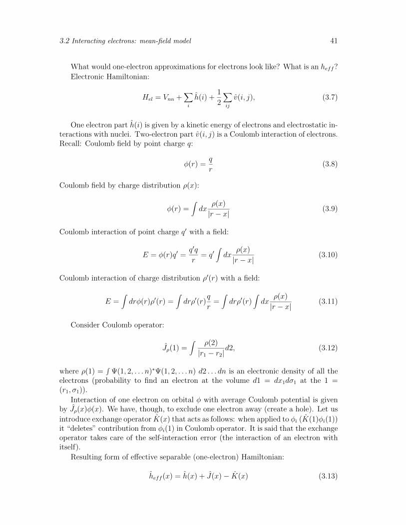
3.2 Interacting electrons: mean-field model 41
What would one-electron approximations for electrons look like? What is an heff?Electronic Hamiltonian:
Hel = Vnn +X
i
h(i) +1
2
X
ij
v(i, j), (3.7)
One electron part h(i) is given by a kinetic energy of electrons and electrostatic in-teractions with nuclei. Two-electron part v(i, j) is a Coulomb interaction of electrons.Recall: Coulomb field by point charge q:
�(r) =q
r(3.8)
Coulomb field by charge distribution ⇢(x):
�(r) =Zdx
⇢(x)
|r � x| (3.9)
Coulomb interaction of point charge q0 with a field:
E = �(r)q0 =q0q
r= q0
Zdx
⇢(x)
|r � x| (3.10)
Coulomb interaction of charge distribution ⇢0(r) with a field:
E =Zdr�(r)⇢0(r) =
Zdr⇢0(r)
q
r=Zdr⇢0(r)
Zdx
⇢(x)
|r � x| (3.11)
Consider Coulomb operator:
J⇢(1) =Z ⇢(2)
|r1 � r2|d2, (3.12)
where ⇢(1) =R (1, 2, . . . n)⇤ (1, 2, . . . n) d2 . . . dn is an electronic density of all the
electrons (probability to find an electron at the volume d1 = dx1d�1 at the 1 =(r1, �1)).
Interaction of one electron on orbital � with average Coulomb potential is givenby J⇢(x)�(x). We have, though, to exclude one electron away (create a hole). Let usintroduce exchange operator K(x) that acts as follows: when applied to �i (K(1)�i(1))it “deletes” contribution from �i(1) in Coulomb operator. It is said that the exchangeoperator takes care of the self-interaction error (the interaction of an electron withitself).
Resulting form of e↵ective separable (one-electron) Hamiltonian:
heff (x) = h(x) + J(x)� K(x) (3.13)

42 Hartree-Fock model: one-electron approximation
3.3 Derivation of HF equations
3.3.1 Variational principle
If we are given an ansatz (a functional form) for the wave-function, how do we find abest function in this class? For example, consider a one electron function (r;↵) =e�↵r that depends on a parameter ↵. The VP tells us that the “best” value of ↵ willminimize the expectation value E(↵) =< (↵)|H| (↵) >. Thus, the recipe is: (i)to obtain an analytic expression for the function E(↵); (ii) take derivative, @E
@↵ ; (iii)solve for @E
@↵ = 0.When we consider more complex parameterization (e.g., we can vary functions
themselves, and not just numeric coe�cients), this can be generalized by using theconcept of functional variation. Thus, the general form of the Rayleigh-SchrodingerVP is:
�
E =< �|H|� >
< �|� >
!
= 0 (3.14)
What does it mean? We can see that for the exact wave-function, this is equivalentto the Schrodinger equation. What else?
The rules for taking a variation are the same as for taking a derivative. By using⇣uv
⌘0= (u0v�uv0)
v2 and E = <�|H|�><�|�> we obtain:
< ��|H � E|� >
< �|� >+
< �|H � E|�� >
< �|� >= 0 (3.15)
For real-valued normalized wave-function this reduces to:
< ��|H � E|� >= 0 or < ��|H|� >= 0 (3.16)
What does that mean? Consider 3D space, {x, y, z} and some operator H oper-ating on 3D vectors, e.g., Hp = s (p, s are 3D vectors). This is shown in Fig. 3.1.Eigenproblem Hr = ✏r means that when H operates on vector r the result, i.e. vectorHr, is parallel to vector r. Thus:
Hr = ✏r < � > (Hr)||r < � > (s, Hr) = 0 < � > (�r, Hr) = 0 (3.17)
where s is any vector orthogonal to r. The last form uses the fact that a smallvariation is orthogonal to a vector.
Now consider 2D approximation (vector q from XY plane) of the vector r. How wecan rewrite the original 3D problem for 2D vector? First, note that we cannot satisfyHq = ✏q, since vector Hq has Z-component, and vector q does not. However, we canminimize a norm of the vector (Hq � ✏q). How to do that? Make (XY) componentof the vector Hq parallel to q. Thus, (�q, Hq) = 0, where �q is any allowed variationof q, i.e., it belongs to XY plane as well. This is explained in Fig. 3.2
This picture can be readily generalized to the case of non-linear spaces. Consider2D nonlinear manifold, e.g., a surface of sphere in 3D space (let us simply bend ourXOY plane). If we restrict our approximate function � to this manifold, than the

3.3 Derivation of HF equations 43
x
y
zr
H
s = Hr
rH s = Hr = !r
r
r’
"r
"r
Hr
("r,Hr)=0
("r,r)=0x
y
zr
H
s = Hr
rH s = Hr = !r
r
r’
"r
"r
Hr
("r,Hr)=0
("r,r)=0
Figure 3.1: Consider3D space and the opera-tor H which operates on3D vectors. For a vectorr which is an eigenvec-tor of operator H, i.e.,Hr = ✏r, the vector Hris parallel to the vectorr. Thus, it is orthogonalto any vector orthogo-nal to r. Therefore,it is also orthogonal toany small variation ofvector r (since smallvariations are orthogo-nal to a varied vec-tor). Thus, eigenprob-lem Hr = ✏r is equiv-alent to the followingcondition: (�r, Hr) = 0.
H� does not necessarily belongs to the manifold of trial functions — it will havetangential and orthogonal components. To minimize a di↵erence H�� ✏� by varying� within the manifold means to zero out a tangential component of this vector. This,< ��|H� >= 0, where �� is an allowed variation of �. Allowed variations leave �within the manifold, and thus are tangential to the manifold.
So, we shall approximate electronic wave-function by a single Slater determinantand vary orbitals such that the energy is minimal preserving ortho-normality of or-bitals:
{�i}ni=1, < �i|�j >= �ij| HF >= |�0 >= |1 . . . n >= a+1 . . . a+n
< �0| =< n . . . 1| = an . . . a1FIND min�(E({�i}n1 ) =< �0|H|�0 >)
HOLD < �0|�0 >= 1 (3.18)
3.3.2 Expression for Hartree-Fock energy
E({�i}n1 ) =< �0|H|�0 >=< �0|O1|�0 > + < �0|O2|�0 > (3.19)
One-electron terms:
< �0|O1|�0 >=X
pq
< �0|a+p aq|�0 >< p|h|q > (3.20)
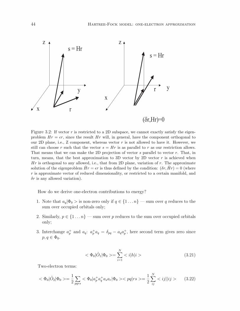
44 Hartree-Fock model: one-electron approximation
x
y
z
r
s = Hr
x
yr
s = Hr
(!r,Hr)=0
z
Figure 3.2: If vector r is restricted to a 2D subspace, we cannot exactly satisfy the eigen-problem Hr = ✏r, since the result Hr will, in general, have the component orthogonal toour 2D plane, i.e., Z component, whereas vector r is not allowed to have it. However, westill can choose r such that the vector s = Hr is as parallel to r as our restriction allows.That means that we can make the 2D projection of vector s parallel to vector r. That, inturn, means, that the best approximation to 3D vector by 2D vector r is achieved whenHr is orthogonal to any allowed, i.e., that from 2D plane, variation of r. The approximatesolution of the eigenproblem Hr = ✏r is thus defined by the condition: (�r, Hr) = 0 (wherer is approximate vector of reduced dimensionality, or restricted to a certain manifold, and�r is any allowed variation).
How do we derive one-electron contributions to energy?
1. Note that aq|�0 > is non-zero only if q 2 {1 . . . n} — sum over q reduces to thesum over occupied orbitals only;
2. Similarly, p 2 {1 . . . n} — sum over p reduces to the sum over occupied orbitalsonly;
3. Interchange a+p and aq: a+p aq = �pq � aqa+p , here second term gives zero sincep, q 2 �0.
< �0|O1|�0 >=NX
i=1
< i|h|i > (3.21)
Two-electron terms:
< �0|O2|�0 >=1
2
X
pqrs
< �0|a+p a+q asar|�0 >< pq|rs >=1
2
NX
ij
< ij||ij > (3.22)

3.3 Derivation of HF equations 45
Here we use indexes i, j instead of indexes p, q to emphasize that the indexesbelongs to the subspace of orbitals occupied in �0, i.e., i, j 2 �0.
Hartree-Fock energy is:
EHF =< �0|H|�0 >=NX
i=1
< i|h|i > +1
2
NX
ij
< ij||ij > (3.23)
We can treat HF energy as a sum of expectation values of one- and two-electronoperators. Let us analyze these operators.
One electron contributions arise from matrix elements of one-electron part of theHamiltonian, < i|h|i >. One electron operator h is simple: when applied to anelectron on the orbital |�i > it involves di↵erentiating the orbital (kinetic energy)and multiplying it by a number (potential energy of the interaction with nuclei).
Consider two electron integrals:
< ij|ij >=Zd1d2 �i(1)
⇤�j(2)⇤ 1
r12�i(1)�j(2) =
Zd1 �i(1)
⇤ Z
d2�j(2)⇤�j(2)
r12
!
�i(1) =< �i(1)|Jj|�i(1) > (3.24)
where we defined a Coulomb operator Jj (e↵ective one-electron operator) as:
Jj�(1) =Z�⇤j(2)r
�112 �j(2)d2 · �(1) (3.25)
Note that the Coulomb operator Jj is a local operator. It describes a Coulomb po-tential created by electron on the orbital j. The total Coulomb operator is:
J⇢ =Z ⇢(2)
|r1 � r2|d2 =
Zd2X
j
�⇤j(2)r
�112 �
⇤j(2) =
X
j
Jj (3.26)
Similarly,
< ij|ji >=Zd1d2 �i(1)
⇤�j(2)⇤ 1
r12�j(1)�i(2) =
Zd1 �i(1)
⇤ Z
d2�j(2)⇤�i(2)
r12
!
�j(1) =< �i(1)|Kj|�i(1) >, (3.27)
with an non-local exchange operator:
Kj�(1) =Z�⇤j(2)r
�112 �(2)d2 · �j(1) (3.28)
Why exchange? There is no classical analog. If we compare Jj�(x) and Kj�(x) wesee that Kj interchange orbitals �j and �i.
Thus, Hartree-Fock energy is:
EHF =X
i
< i|h|i > +1
2
X
ij
< i|Jj � Kj|i > (3.29)

46 Hartree-Fock model: one-electron approximation
I also define a Fock operator, an e↵ective one-electron operator, as:
F (1) = h(1) +X
j
hJj(1)� Kj(1)
i(3.30)
Fock operator includes one-electron terms (kinetic energy of electron and interactionwith nuclei), Coulomb interaction of an electron with the electron density of all elec-trons corrected by subtraction of self-interactions. It looks like one-electron operator,but it depends on the all others electrons as well. Thus, Fock operator is a non-linearoperator.
3.3.3 Derivation of Hartree-Fock equations
EHF =< �0|H|�0 >=NX
i=1
< i|h|i > +1
2
NX
ij
< ij||ij > (3.31)
Vary orbitals (i ! i+ �i), collect first order terms to get �E, then find conditionwhen �E = 0. Don’t forget to keep orbitals orthonormal, < i|j >= �ij, which satisfyortho-normality of the total wave-function (optimization with constraint).
Energy variation:
�E =X
i
[< �i|h|i > + < i|h|�i >] +
1
2
X
ij
[< �ij||ij > + < i�j||ij > +
< ij||�ij > + < ij||i�j >] (3.32)
Using permutational symmetry of 1- and 2-electron integrals and renaming sum-mation indexes:
�E =X
i
< �i|h|i > +X
ij
< �ij||ij > +(�E)⇤ (3.33)
Ortho-normality: restriction on variations �i. We shall use Lagrange multipliersto impose ortho-normality of the orbitals (< i|j >= �ij):
�E = 0 & < i|j > ��ij = 0 (3.34)
�
0
@E �X
ij
✏ij(< i|j > ��ij)1
A = 0 (3.35)
Note, that Lagrange multipliers compose a Hermitian matrix — since orbitaloverlap matrix < �i|�j > is a Hermitian matrix as well. In order to satisfy Nindependent conditions, we need to use N Lagrange multipliers.
0
@X
i
< �i|h|i > +X
ij
< �ij||ij > �X
ij
✏ij < �i|j >1
A+
{complex conjugate} = 0 (3.36)

3.4 Orbital energies ✏i and Koopmans theorem 47
Have to satisfy for both parts ! vary independentlyHave to satisfy for ANY �i !Result:
h|i > +X
j
hJj|i > �Kj|i >
i=X
j
✏ij|j >
F |i >=X
j
✏ij|j > (3.37)
Canonical Hartree-Fock equations
Consider unitary transformation Uof orbitals:
�i(x) =X
k
�k(x)Uki (3.38)
Thus, transformed row:
⇣�1(x) . . . �n(x)
⌘= (�1(x) . . .�n(x))U (3.39)
Transformed determinant is therefore:
|�| = |�U | (3.40)
Note that unitary transformation of occupied orbitals does not change �0, sincedet(AB) = detA ⇤ detB, and the determinant of unitary matrix equals unity. There-fore, we can look for such transformation of orbitals so that matrix ✏ij becomesdiagonal matrix:
F |i >= ✏i|i > (3.41)
This are canonical HF-equations.Equivalent form of HF equations:
< a|F |i >= 0, (3.42)
where i is an occupied orbital and a is any orbital orthogonal to the subspace ofoccupied orbitals, i.e., a virtual orbital.
What we have done? We transformed one many-particle equation into set ofcoupled one-particle equations.
3.4 Orbital energies ✏i and Koopmans theorem
HF-energy is:
EHF =NX
i=1
< i|h|i > +1
2
NX
ij
< ij||ij >=X
i
✏i �1
2
X
ij
< ij||ij >, (3.43)

48 Hartree-Fock model: one-electron approximation
where orbital energies ✏i are:
✏i =< i|h|i > +NX
j
< ij||ij > (3.44)
Note that Hartree-Fock energy is not a sum of e↵ective one-electron energies ✏i. Why?Formally, we have lost factor of 1
2when we di↵erentiated two-electron part of the
energy. But what is a physical meaning of this fact?To understand why Etot 6= ✏1 + . . . ✏n, where ✏i =< i|F |i >=< i|h|i > + < i|J |i >
� < i|K|i >, consider 2-electrons-on-2-orbitals i, j (✏i and ✏j). ✏i =< i|F |i >=<i|h|i > + < i|Jj|i > � < i|Kj|i > includes interaction of the electron on orbital iwith the electron on j. Similarly, ✏j includes interaction of the electron on j with anelectron on a. Hence, i� j interaction calculated twice.
Is there any physical meaning of orbital energies? Koopmans theorem says thatorbital energy ✏i gives an ionization potential from the orbital i in a frozen coreapproximation:
IP =N�1 Ei �N E0 = �✏i (3.45)
Frozen core approximation means that orbitals do not change when one electron isremoved from the molecule. At home: prove the Koopmans theorem by calculatingenergy di↵erences between systems of N and N � 1 electrons.
3.5 Brillouin’s theorem
Another important property of Hartree-Fock determinant �0 is that matrix elementsbetween HF determinant and any singly excited determinant are zero:
< �ai |H|�0 >= 0 (3.46)
Why? < �ai |H|�0 >=< a|F |i >= 0
Another way to prove it is (1) to show that for real-valued function < ��|H|�0 >=0 from VP, and (2) to show that first variation of the determinant ��0 is given by asingle excited determinants, i.e., ��0 =
Pia c
ai�
ai . Prove at home.
Aside: If we consider the entire space of many-electron wave-functions {�0, �ai ,
�abij }, in which subspace HF wave-function is defined? In a subspace of reference and
single excitations
3.6 Molecular Orbitals — Linear Combination ofAtomic Orbitals (MOLCAO) approach
Eq. (3.41) is an operator equation, i.e., di↵erential equation. As a next step, weare going to transform Eq. (3.41) to some set of linear equations. This will be doneby representing eigenstates of the Fock operators, �i (molecular orbitals) by a linearcombination of atomic orbitals (MOLCAO). There are several implementations of

3.6 Molecular Orbitals — Linear Combination of Atomic Orbitals (MOLCAO) approach49
MO-LCAO approach: (i) Hartree-Fock-Roothaan equations (RHF); (2) Pople-Nesbetequations (UHF); and (3) Restricted Open-Shell HF (ROHF).
Introduce AO basis: �i =P
µ Cµi⇠µ, µ = 1 . . .M, i = 1 . . . N . The matrix C iscalled molecular orbital matrix. It defines molecular orbitals as a linear combinationof atomic orbitals, Cµi is a coe�cient giving the contribution of AO µ to MO i. AO’s{⇠} are not orthonormal: < ⇠µ|⇠⌫ >= Sµ⌫ = Sµ⌫ , S is thus an overlap matrix foratomic orbitals {⇠}. MO {�} are orthonormal:
< �i|�j >= �ij =MX
µ=1
MX
⌫=1
Cµi < ⇠µ|⇠⌫ > C⌫j =
MX
µ=1
MX
⌫=1
CµiSµ⌫C⌫j =hC+SC
i
ij=>
C+SC = 1 (3.47)
To obtain equations for coe�cients C we apply a Linear Variational Principle(LVP). LVP answers the following question: what are best Ciµ? Variationally theyminimize E:
E =< �|H|� >
< �|� >(3.48)
Resulting MO-LCAO equations are:
FC = SCE (3.49)
C+SC = 1 (3.50)
where F is a matrix of Fock operator in AO basis:
Fµ⌫ = hµ⌫ +MX
��
< µ�||⌫� > P�� (3.51)
where P is a density matrix:
P�� =NX
i=1
C�iC�i (3.52)
Let us analyze Eqns. (3.49,3.50):
FC = SCE => C+FC = C+SCE => C+FC = E, (3.53)
Which means that Fock matrix is diagonal in the basis of final MOs. Thus, Eqns. (3.49,3.50)are nothing but generalized matrix eigenproblem.
Why P from Eq. (3.52) is called density matrix? Electronic density, i.e., proba-bility to find an electron at point x:
⇢(x1) =Z (x1, x2, . . . , xn) (x1, x2, . . . , xn)dx2 . . . dxn (3.54)

50 Hartree-Fock model: one-electron approximation
For ⌘ �0 (a single Slater determinant):
⇢(x1) =Z�0(x1, x2, . . . , xn)�0(x1, x2, . . . , xn)dx2 . . . dxn =
ZAs [�1(x1)�2(x2) . . .�n(xn)]⇥ As [�1(x1)�2(x2) . . .�n(xn)] dx2 . . . dxn =
NX
i=1
�2i (x1), (3.55)
where As is anti-symmetrizing operator. This is a very sensible result — for non-interacting electrons, the probability to find an electron is sum over one-electronprobabilities (electrons are independent, and so are the probabilities!).
By substituting �i =P
µ Cµi⇠µ into the above expression for density:
⇢(x) =NX
i=1
�2i (x) =
NX
i=1
MX
µ=1
MX
⌫=1
Cµi⇠µC⌫i⇠⌫ =X
µ⌫
Pµ⌫⇠µ⇠⌫ (3.56)
Matrix P thus tells us how to calculate electronic density once molecular orbitalcoe�cients are known.
3.6.1 Linear Variational Principle
Here is a brief description of LVP.
| >=X
k
Ck|⇠k >
E =< �|H|� >
< �|� >=
Pkl CkCl < ⇠k|H|⇠l >Pkl < ⇠k|⇠l > CkCl
(3.57)
Consider, when @E@Ci
= 0. Do this as an implicit derivative:
@E
@Ci=
1
(P
kl < ⇠k|⇠l > CkCl)2
2X
m
Ck < ⇠m|H|⇠i >X
kl
< ⇠k|⇠l > CkCl �
2X
m
< ⇠m|⇠i > Cm
X
kl
CkCl < ⇠k|H|⇠l > (3.58)
To satisfy @E@Ci
= 0, we need to zero numerator:
0 = 2X
m
Ck < ⇠m|H|⇠i >X
kl
< ⇠k|⇠l > CkCl �

3.7 How to solve it? 51
2X
m
< ⇠m|⇠i > Cm
X
kl
CkCl < ⇠k|H|⇠l >X
m
Cm < ⇠k|H|⇠i >= EX
m
< ⇠i|⇠m > Cm
HC = SCE (3.59)
3.6.2 HF MO-LCAO equations using density matrices
We can write HF energy using density matrix:
�i =X
µ
Cµi⇠µ, µ = 1 . . .M, i = 1 . . . N
Pµ⌫ =nX
i=0
CµiC⌫i
E =X
i
< i|h|i > +1
2
X
ij
(< ij|ij > � < ij|ji >) =
X
i
X
µ⌫
CµiC⌫i < µ|h|⌫ > +
1
2
X
ij
X
µ⌫��
< µ⌫|�� > CµiC⌫jC�iC�j �
1
2
X
ij
X
µ⌫��
< µ⌫|�� > CµiC⌫jC�iC�j =
X
i
X
µ⌫
CµiC⌫i < µ|h|⌫ > +
1
2
X
ij
X
µ⌫��
< µ⌫||�� > CµiC⌫jC�iC�j =
Tr[Pµ⌫hµ⌫ ] +1
2Tr[Pµ� < µ⌫||�� > P⌫�] =
Tr[Ph+1
2PIIP ] (3.60)
E = Tr[Ph] +1
2Tr[PIIP ] (3.61)
@E
@P= F = h+ IIP (3.62)
3.7 How to solve it?
How to chose an atomic orbital basis? We’ll discuss basis sets in details later. Themain idea is to take atomic functions from solutions of an atomic problem, i.e.,hydrogen-like atomic functions.

52 Hartree-Fock model: one-electron approximation
Once basis set is chosen, we have to solve somehow a nonlinear system of Roothanequations. It is done by iterative procedure, that’s why HF method is often referredto as self-consistent field.
The first step is to take some zero-order (guess) orbitals, C0. Once we havesome set of MO, we can calculate the Fock operator, our e↵ective one-particle Hamil-tonian. Once we have a Hamiltonian, how do we minimize the energy of the n-electron wavefunction? As in non-interacting electrons model, we diagonalize theone-particle Hamiltonian and occupy lowest n levels (this is called the Aufbau princi-ple). Note that for interacting electrons the Aufbau Principle does not always work,since EHF 6= P
i ✏i. Therefore, di↵erent electron occupations should be tested.Those new occupied orbitals (new molecular orbitals, C1) define new density ma-
trix, new Fockian, and new molecular orbitals from diagonalization of the new Fock-ian. If new molecular orbitals are the same as old MO’s, the equations have beensolved. This is a self-consistent procedure:
1. Input: nuclei, electrons & basis set;
2. Make initial guess for MO (e.g., diagonalize h);
3. Make density matrix from MO;
4. Make Fock operator (rate determining step);
5. Diagonalize F ;
6. Check whether MO’s have converged, i.e., if |Cn �Cn�1| < ✏. If not — go backto step 3.
Actually, such procedure almost never converges. Numerous enhancements areused in practice, i.e., computational methods for many-dimensional optimization (use“gradients” and “Hessians” of the energy with respect to orbital rotations; or DIISmethod — extrapolation by using data from previous iterations).
3.7.1 Connection to computation
Memory: need a bunch of matrices (F,H, S, etc) — say 4-8. Mem ⇡ 5*M2, M —basis set size.
Double is 8B. For 126 MB of memory — 18 M doubles (⇡ 18,000,000) — Mmax ⇡2, 000. How do we connect Mmax with molecular size? Depend on the basis. Inminimal basis set (1 function per atomic orbital) CH2 has 7 functions in minimalbasis, (CH2)300.
Computational part is dominated by Fock matrix computation: F=H+IIP:
Fµ⌫ = hµ⌫ +X
��
< µ⌫||�� > P�� (3.63)
Cost ⇡ (# iterations)xM4x(cost per integral) Cost per integral ⇡ 100 flop. #of iterations ⇡ 10-20. Cost ⇡ 103 � 104 ⇤ N4. For 100 basis functions: 1011 �1012 adds/mults. For computer 107 flops time is 104-105 seconds (few hours). Mycomputers (2003) — couple of minutes.

3.7 How to solve it? 53
3.7.2 Tricks of the trade
1. For very small molecules:
Use “in core integrals” — compute them once. This reduces cost per iterationto about 10 flops. However, need M4 memory (actually, M4/8). Often — “ondisk integrals”, then IO rate is important.
2. Large molecules:
Number of non-zero integrals grows as only O(M2) (= K2M2), where K ise↵ective # of neighbors. K ⇡ 100� 200.
3. Very large molecules:
Linear scaling models (M. Head-Gordon, G. Scuseria groups) (use multipoles,sparsity of density, avoid diagonalization).
PICTURE OF THE COST.Start see di↵erence for N ⇡ 200
3.7.3 Conclusions
• Large calculations with HF method are feasible
• You now can estimate whether YOUR HF calculation is feasible.
Note: all discussion was about single energy point. But we need at least optimizedgeometries, etc.

54 Hartree-Fock model: one-electron approximation

Chapter 4
Basis sets
Why do we use atomic basis set for molecules? Because we know that chemical bond-ing can be described qualitatively by considering linear combinations of atomic or-bitals. Consider H2 molecule. Wave functions for individual H-atoms are 1s-functions.From these two orbitals we can prepare two molecular orbitals:
�1(r) =1p
2 + sAB(1sA + 1sB) ⌘ �(r) (4.1)
�2(r) =1p
2� sAB(1sA � 1sB) ⌘ �⇤(r) (4.2)
� is so-called bonding orbital, and �⇤ is antibonding orbital. Hartree-Fock wavefunction for the H2 is:
�0 =1p2�(1)�(2)(↵� � �↵) (4.3)
And this is how Hartree-Fock model describes chemical bonding. We shall discuss H2
example in more details next time. Now we are concerned about atomic basis setsfor electronic structure calculations.
4.1 Atomic orbitals: Slater type orbitals and con-tracted Gaussians
What do we know about atomic wave functions? For hydrogen-like atom (one electronmoving in the Coulomb potential U(r) = �Z
r ) we can solve the Scarodinger equationanalytically:
En = � Z2
2n2(4.4)
�nlm(r, ✓,�) = exp(�⇠|r|)Pnl(r)Ylm(✓,�) (4.5)
The energy levels for the hydrogen-like atom are shown in Fig. 4.1.The radial part of the wave function (4.5) is called Slater type orbital, and its
important features are: (i) nuclear cusp; and (ii) asymptotic exponential decay. SeeFig. 4.2a.
55

56 Basis sets
Figure 4.1: Energy levels inhydrogen-like atoms: En = � Z2
2n2 .The degeneracy between the levelswith the same n but di↵erent l is aspecial feature of the Coulomb po-tential; it is lifted in other central-symmetric potentials.
Figure 4.2: Slater-typeversus Gaussian-type orbital.Note di↵erent shape at r=0and di↵erent asymptoticbehavior (at r ! 1). STOexhibits a cusp and a slowerdecay.
For many electron atoms there is no analytic solution, but asymptotic behavior(cusp and tail) are described correctly by Slater type functions. The structure ofenergy levels is also similar to those of the hydrogen atoms except for the fact thatthe degeneracy between levels with same principal quantum number n is removed,and levels with di↵erent angular momentum (l) are non-degenerate.
Thus, these hydrogenic atom solutions must be right form for atoms. Then we canmix them together to form molecular orbitals. However, these exponential functionsare intractable for practical calculations because we cannot calculate e�ciently the2-electron integrals (six-dimensional integrals). Contrary to Slater type functions,Gaussian functions 1s = e�⇠r
2are tractable (because product of two Gaussians is
a Gaussian centered in between), but they have (1) wrong shape at nuclei (nuclearcusp) and (2) have too rapid decay at large r. Fig. 4.2 compares STO with GTO.
The solution is to take fixed combination of several Gaussian functions (contrac-tions) to get roughly the right shape (including any radial nodes, etc):
⇠i(r) =mX
d=1
dime�↵mr2 , (4.6)
where ⇠i is an atomic basis function obtained by contraction ofm primitive Gaussians,and the coe�cients dim are frozen (i.e., not changed in SCF calculations).
STO-3G basis (introduced in 1969) (Slater-type-orbital (modeled by a contractionof) 3 Gaussian functions. STO-3G is called the minimal basis set. In the minimalbasis set we take only valence orbitals (1s for H atom, 1s, 2s and 2p for Li atom,

4.2 Extensions 57
Figure 4.3: Contracted Gaussianfunctions can approximate STO.The quality of fit can be system-atically improved by taking moreGaussians.
etc). This is a minimum required to qualitatively describe chemical bonding. Thecontraction scheme for STO basis for the C atom is (6s3p)/[2s1p]. A common way ofdetermining contractions is from results of atomic SCF calculations. In these atomiccalculations one uses a relatively large basis of uncontracted Gaussians, optimizes allexponents, and determines the SCF coe�cients of each of the derived atomic orbitals.Then these exponents are used in primitive Gaussians, and SCF coe�cients are usedto derive contraction coe�cients.
We can improve the description by taking (a) more Gaussians (STO-nG) (actually,3 is good enough!) (b) more basis functions.
4.2 Extensions
Basis set extensions: what if STO-3G is no good? In order to understand how toimprove it, we have to understand what e↵ects it may fail to describe.
4.2.1 Non-isotropic e↵ects: multiple-zeta bases
STO-3G mimics one Slater function with exponent zeta (STO can be called single-zetabasis). Therefore atoms stay isotropic in the molecule. To describe anisotropic e↵ects,we are “splitting the representation”: a “double zeta” basis supplies 2 functions(Slater) per atomic orbital called “inner” and “outer”. The “inner” AO is slightly lessdi↵use and the “outer” AO is slightly more di↵use than optimized STO functions.This allows the shape of AO to change upon going to the molecular environment.Example:HCN: pz ! � bondpx, py ! 2 ⇡ bonds⇡ bonds are more di↵use. In � “inner” orbital has more weight, in ⇡ — “outer”
These defines the following sequence of bases sets: Double-Zeta, Triple-Zeta, etc.Many basis sets were developed by Huzinaga and Dunning.
“Split-valence basis” of Pople is essentially the same — except that the core is

58 Basis sets
single zeta (assumes that the core orbitals do not change much upon chemical trans-formations.
A standard selection of split-valence, DZ basis sets is 3-21G: ’3’ — minimal corecomposed of 3 Gaussians; and ’-21’ — split-valence, valence orbitals are describedby inner orbital (composed of two Gaussians) and an outer orbital (composed of 1Gaussian). The general contraction scheme for carbon is (6s3p)/[3s2p].
You will now understand meaning of 6-31G, 4-31G — there have slightly moreGaussians, but no more contracted functions. Dunning DZ basis (9s5p)/[4s2p] isdi↵erent from 3-21G.
Triple-zeta: 3 (Slater) orbitals per AO. TZP, 6-311G basis
Also Quadrupole, Pentupole zeta.
It is dangerous, however, to increase only a number of s and p functions. Forexample, in the limit of a large number of s and p functions equilibrium geometryof the ammonia become planar. That is because so constructed basis set is not wellbalanced. What are e↵ects that are omitted in these basis sets? Polarization e↵ects —asymmetric distribution of the electron density around the nuclei in the asymmetricelectric field.
4.2.2 Polarized basis sets
Consider atom in an electric field: its electronic density is distorted, and it is nolonger possesses spherical symmetry (atom is polarized by an applied field). Atomsin molecules experience influence of an electric field, therefore, we have to account forthe polarization e↵ects.
“Polarization functions” are functions of the higher angular momentum and theirpurpose is to allow polarization of charge. An atomic orbital may be distorted bymixing with a higher angular momentum function:s+p ! “polarized” (distorted, shifted) s-level;p+d ! “polarized” p-level.
We can add higher angular momentum functions to a basis to permit the energylowering that results from polarization e↵ects.
Cases where polarization is important: (1) bonding in highly polar molecules(NH3) is a good example (2) strained ring system (C3, discuss hybridization, explainwhy strained, banana bonds) (3) hypervalency — expanded coordination shells forsecond row atoms and below (SF6).
Notations for polarized basis set: 6-31G*, 6-31G**,6-31G(d,p). d describes “heavy”atom polarization, p describes hydrogen atom polarization.
3-21G(*) basis: split valence plus polarization function on second row and below.Similar set of Dunning: DZP.
STO-3G* basis: minimal basis plus polarization function on second row and below.
Caveat: pure angular momentum (5d, 7f, . . .) polarization versus Cartesian (6d,8f, etc).

4.2 Extensions 59
4.2.3 Di↵use functions
A further split of the valence space to allow a good description of more di↵use chargedistribution (appropriate for anions, Rydberg states, electronically excited molecules,van der Waals clusters).
Notations: 6-31+G(*), 6-31++G, 6-311++G(d). ’+’ means that one set of di↵useorbitals is added to the basis. For H atom this is one di↵use s-orbital, and for secondrow atoms — one s and one p di↵use orbitals. When two sets of di↵use functions arerequested (’2+’), this means that two di↵use s functions are added for hydrogen, andtwo di↵use s and two di↵use p orbitals are added to second row atoms.

60 Basis sets
Chapter 5
H2 example
We shall consider a simple example: H2 molecule in a minimal basis set. We shallanalyze FCI solution (which is an exact solution in the given one electron basis set)and compare it with Hartree-Fock solution. Also, we shall discuss symmetry andspin-symmetry of the wavefunctions by using this simple example.
5.1 Symmetry and spin of an electronic wavefunc-tion
The exact wavefunction must possess proper point group and spin symmetries. Pointgroup symmetry is imposed by a point group symmetry of the external potential, e.g.,nuclear potential.
Since non-relativistic Hamiltonian commutes with a spin-operators, they have aset of common eigenstates. Concerning eigenstates of spin operators, we have twooperators: S2 and Sz. Exact wavefunctions are therefore eigenstates of S2 and Sz:
Sz|� >= mz|� > (5.1)
S2|� >= s(s+ 1)|� >, (5.2)
where |� > is a valid spin function, and mz gives projection of the spin on the z-axis,and s characterizes the absolute value of spin. Term multiplicity (number of stateswith the same s but di↵erent mz) is given by ⇤ = 2s+ 1 (because mz = �s . . . s).
However, in a case of approximate non-linear equations, such as HF equations,the approximate wavefunction does not necessarily possess these properties. We canimpose proper symmetry by restricting variations of the orbitals, which means thatthe solution may not be the best in a variational sense. What is better: correctsymmetry or best variational solution (Lowdin dilemma)? Hard question... Example:weakly interacting gas and its condensation.
Today we shall consider one- and two- electron spin functions. At home, youshall see that certain conditions must be imposed on the spatial part of the generaltwo-electron Hartree-Fock wavefunction in order to restrict it to the proper spin-symmetry.1
1Restricted HF: Sz, S2. Orbitals are forced to be the same for ↵ and � electrons: {�i(x)↵,�i(x)�}.
61

62 H2 example
5.1.1 One- and two-electron spin functions
One-electron spin functions are just familiar ↵ and � states:
|↵ >=✓10
◆|� >=
✓01
◆(5.3)
Cartesian components of one-electron spin operator are given by Pauli matrices:
�x =1
2
✓0 11 0
◆�y =
1
2
✓0 �ii 0
◆�z =
1
2
✓1 00 �1
◆(5.4)
Spin-operator, S, is given therefore by a vector composed of Pauli matrices:
S = ~S = ~ex�x + ~ey�y + ~ez�z (5.5)
Operator S2 for one electron is just a scalar product of S · S:
S2 = �2x + �2
y + �2z =
3
4E, (5.6)
where E is a unit matrix. Operator Sz = �z.We are interested in wavefunctions which are eigenstates of Sz and S2. Let us see
how Sz and S2 act on the |↵ > and |� > states:
Sz ↵ = �z|↵ >=1
2
✓1 00 �1
◆✓10
◆=
1
2
✓10
◆=
1
2|↵ >
Sz|� >= �z|� >=1
2
✓1 00 �1
◆✓01
◆= �1
2
✓01
◆= �1
2|� >
S2|↵ >=3
4|↵ >
S2|� >=3
4|� >
(5.7)
Thus, |↵ > and |� > are eigenstates of Sz with an eigenvalues 12and �1
2, respec-
tively, and eigenstates of S2 with an eigenvalue of 34.
We shall also need to know how operators �x and �y act on ↵ and � functions:
�x|↵ >=1
2|� > (5.8)
�x|� >=1
2|↵ > (5.9)
�y|↵ >=i
2|� > (5.10)
�y|� >= � i
2|↵ > (5.11)
(5.12)
Unrestricted HF: Sz is ok, S2 — not. Orbitals may di↵er for ↵ and � electrons: {�i(x)↵, i(x)�}.General HF: Sz, S
2 —not. Orbitals are complex and assumes a most general form: {�i(x)↵+ i(x)�}

5.1 Symmetry and spin of an electronic wavefunction 63
How do we construct two-electron wavefunctions and operators? Wavefunctionsare given by a linear combinations of products of ↵ and �. We shall find whatcombinations are legal. Two-electron spin operators are given by a sum of one-electron operators:
~S(1, 2) = ~S(1) + ~S(2) (5.13)
Sz(1, 2) = Sz(1) + Sz(2) (5.14)
S2(1, 2) =h~S(1) + ~S(2)
i2= (5.15)
S2(1) + S2(2) + 2~S(1) · ~S(2) = (5.16)3
2E + 2 [�x(1)�x(2) + �y(1)�y(2) + �z(1)�z(2)] (5.17)
Let us consider now the following two-electron wavefunctions: ↵(1) · ↵(2), �(1) ·�(2), and ↵(1) · �(2).
Applying Sz to ↵(1) · ↵(2):
Sz(1, 2)↵(1) · ↵(2)
�=
↵(2) ·sz(1)↵(1)
�+ ↵(1) ·
sz(2)↵(2)
�=
1 · [↵(1) · ↵(2)] (5.18)
Applying S2 to ↵(1) · ↵(2):
S2(1, 2)↵(1) · ↵(2)
�=
3
2E↵(1) · ↵(2)
�+ 2
�x(1)↵(1)
�·�x(2)↵(2)
�+
2�y(1)↵(1)
�·�y(2)↵(2)
�+ 2
�z(1)↵(1)
�·�z(2)↵(2)
�=
3
2·↵(1) · ↵(2)
�+ 2 · 1
4·⇢�(1) · �(2) + (�1)�(1) · �(2) + ↵(1) · ↵(2)
�=
2 · [↵(1) · ↵(2)] (5.19)
Conclusion: ↵(1) · ↵(2) is an eigenfunction of the operators Sz and S2 and itseigenvalues are respectively 1 and 2. Since 2 =< S2 >= s(s + 1), it follows thats = 1. The term multiplicity is defined as ⇤ = 2s + 1 and is equal to 3. Similarly,�(1) · �(2) is an eigenfunction of the operators Sz and S2 and their eigenvalues arerespectively -1 and 2. Since 2 =< S2 >= s(s + 1), it follows that s = 1. The termmultiplicity is 3.
Applying Sz to ↵(1) · �(2):
Sz(1, 2)↵(1) · �(2)
�= �(2) ·
�z(1)↵(1)
�+ ↵(1) ·
�z(2)�(2)
�=
↵(1) · �(2)� ↵(1) · �(2) = 0 · [↵(1) · �(2)] (5.20)
Applying S2 to ↵(1) · �(2):
S2(1, 2)↵(1) · �(2)
�=
3
2E↵(1) · �(2)
�+ 2
�x(1)↵(1)
�·�x(2)�(2)
�+

64 H2 example
2�y(1)↵(1)
�·�y(2)�(2)
�+ 2
�z(1)↵(1)
�·�z(2)�(2)
�=
3
2·↵(1) · �(2)
�+ 2 · 1
4·⇢�(1) · ↵(2) + i�(1) · (�i)↵(2) + ↵(1) · (�1)�(2)
�=
= [↵(1) · �(2)] + [�(1) · ↵(2)](5.21)
Conclusion: ↵(1) · �(2) is an eigenfunction of the operator Sz. The eigenvalueis 0. ↵(1) · �(2) is not an eigenfunction of the operator S2. We can calculate theexpectation value of < S2 >:
< S2 >=< ↵(1) · �(2)|S2|↵(1) · �(2) >=
< ↵(1) · �(2)|↵(1) · �(2) + �(1) · ↵(2) >= 1 (5.22)
Similarly, �(1) · ↵(2) is an eigenfunction of Sz and is not an eigenfunction of S2.We can consider linear combinations 1p
2(↵� ± �↵).
Applying Sz to 1p2[↵(1) · �(2) + �(1) · ↵(2)]:
Sz(1, 2)1p2
↵(1) · ↵(2) + �(1) · ↵(2)
�= 0 ·
↵(1) · ↵(2) + �(1) · ↵(2)
�
Applying S2 to 1p2[↵(1) · �(2) + �(1) · ↵(2)]:
S2(1, 2)1p2
↵(1) · �(2) + �(1) · ↵(2)
�= 2 ·
↵(1) · �(2) + �(1) · ↵(2)
�
Conclusion: 1p2[↵(1) · �(2) + �(1) · ↵(2)] is an eigenfunction of the operators Sz and
S2 with eigenvalues are respectively 0 and 2. s is 1, and multiplicity equals 3.Applying Sz to 1p
2[↵(1) · �(2)� �(1) · ↵(2)]:
Sz(1, 2)1p2
↵(1) · ↵(2)� �(1) · ↵(2)
�= 0 ·
↵(1) · ↵(2)� �(1) · ↵(2)
�
Applying S2 to 1p2[↵(1) · �(2)� �(1) · ↵(2)]:
S2(1, 2)1p2
↵(1) · �(2)� �(1) · ↵(2)
�= 0 ·
↵(1) · �(2) + �(1) · ↵(2)
�
Conclusion: 1p2[↵(1) · �(2)� �(1) · ↵(2)] is an eigenfunction of the operators Sz and
S2 with eigenvalues 0 and 0, respectively. s = 0 and the term multiplicity ⇤ = 1.To summarize, Table 5.1 gives valid spin-functions for two electrons.Note that multiplicity can define spatial symmetry. Triplet functions are symmet-
ric with respect to electron permutations, hence, must be combined with an antisym-metric spatial part. Singlets are antisymmetric, should be combined with symmetricspatial part.

5.2 H2: Hartree-Fock wavefunction 65
Table 5.1: Valid two-electron spin-functionsSz < S2 >= s(s+ 1) Multiplicity ⇤ = (2s+ 1)
↵(1)↵(2) 1 2 3 (triplet)�(1)�(2) -1 2 3 (triplet)1p2(↵(1)�(2) + �(1)↵(2)) 0 2 3 (triplet)
1p2(↵(1)�(2)� �(1)↵(2)) 0 0 1 (singlet)
5.2 H2: Hartree-Fock wavefunction
We have two atoms: HA & HB. In a minimal basis set there are two 1s orbitalscentered on each atom: 1sA & 1sB.
Here we shall restrict our HF wavefunction to be of correct symmetry. This leadsto restricted HF (usually it means spin-restricted HF, a model when HF wavefunctionhas correct spin symmetry).
General HF solution would be:
|�(1, 2) >= |�1�2 >=1p2
✓�1(1) �2(1)�1(2) �2(2)
◆, (5.23)
where �1, �2 can have any kind of spin or spatial partIf we require correct spin symmetry, we end up in forcing each orbital to have a
pure spin (↵ or �, but not a mixture), and spatial parts to be the same for ↵ and �spin-orbitals.
Such, for singlet function we end up with:
|�RHF (1, 2) >= |�↵ �� >=1p2
✓�(1)↵(1) �(1)�(1)�(2)↵(2) �(2)�(2)
◆=
1p2(�(1)�(2)↵(1)�(2)�
�(2)�(1)�(1)↵(2)) =1p2�(1)�(2) ⇤ [↵(1)�(2)� �(1)↵(2)] (5.24)
What is that? Properly anti-symmetrized doubly occupied orbital �, with a singletspin function.
What can � be for H2? Most general form:
� = c1sA + c2sBc21 + c22 + 2c1c2 < sa|sb >= 1 (5.25)
For this particular case there is no need to solve HF equations to find coe�cientsc1 and c2 if we require wavefunction to have correct symmetry.

66 H2 example
Consider now spatial symmetry of that wavefunction. Point group is C1v. Forthe minimal basis set we can disregard symmetry associated with rotations and theplane (1s functions are symmetric). The non-trivial symmetry element is an inversioncenter i. Wavefunction should be either gerade or ungerade symmetry. For �1(1)�2(2)wavefunction that means that orbitals �1 and �2 should have either gerade or ungeradesymmetry.
This means that we have restriction on coe�cients ci: c1 = ±c2 This results intwo orthogonal MO’s (we skip normalization factor of 1p
2(1±<sA|sB>)):
� = (sA + sB)
�⇤ = (sA � sB) (5.26)
Orbital � is gerade, �⇤ — ungerade. Wavefunctions: �(1)�(2), �⇤(1)�⇤(2) are gerade;�(1)�⇤(2)� �⇤(1)�(2), �(1)�⇤(2) + �⇤(1)�(2) are ungerade.
Energy of orbital � is lower than that of �⇤ We can see it from nodes. Or derivefrom integrals. Energy gap depends on overlap. For small distances, it is large.For large distances, when two-center integrals and overlap are zero, � and �⇤ aredegenerate.
That in conjunction with Aufbau principle gives for HF solution:
|�0 >=1p2�(1)�(2) [↵(1)�(2)� �(1)↵(2)] (5.27)
We can also show that HF energy of �2 is lower than energy of (�⇤)2 (when orbitalsare not degenerate). Orbital � is called bonding orbital, orbital �⇤ — antibonding.Chemical bond formation: electronic density between atoms. Di↵erential density.(Do at home).
5.2.1 Analysis of Hartree-Fock wavefunction
Now lets analyze spatial part of �0:
�0 = �� = (sA + sB)(sA + sB) =
sAsA + sBsB + sAsB + sBsA =
H�AH
+B +H+
AH�B +HAHB +HAHB (5.28)
Configurations H�AH
+B and H+
AH�B are ionic: they describe situation when both
electrons are localized near one of the H-atoms (there is unit probability to find bothelectrons near one H-atom).
Configuration HAHB is covalent: it describes situation when one electron is local-ized near one of the H-atoms, and second electron is localized near another H-atom(there is unit probability to find electrons near di↵erent atoms).�0 alone is a mixture of ionic and covalent configurations in a fixed proportion.
We have no variational freedom to vary degree of ionicity in HF wavefunction.Conclusions:

5.2 H2: Hartree-Fock wavefunction 67
• can be wrong for strongly ionic/strongly covalent situation;
• cannot describe ether neutral (H2 ! H + H), or ionic (H2 ! H+ + H�)dissociation.
This is very important limitation of the Hartree-Fock model: it cannot describechemical bond breaking.
5.2.2 Unrestricted Hartree-Fock wavefunction
What if we do not impose correct symmetry on the Hartree-Fock wavefunction? Theresulting model is called unrestricted Hartree-Fock. In this model we do not apply anyrestrictions on �0 — just looking for the lowest energy solution. In (spin) unrestrictedHF orbitals for ↵ and � electrons are di↵erent. As a result, �0 is eigenstate of Sz,but not an eigenstate of S2.
For the H2 molecule at the dissociation limit we have:
�UHF0 (r ! 1) = |sA↵sB� >=
1p2
✓sA(1)↵(1) sB(1)�(1)sA(2)↵(2) sB(2)�(2)
◆=
1p2(sA(1)↵(1)sB(2)�(2)�
sB(1)�(1)sA(2)↵(2))
(5.29)
This wavefunction does describe covalent dissociation (it does not have any ionic con-tributions in it). However, it does not possess proper symmetry. This wavefunctionis an eigenstate of Sz, but not an eigenstate of S2. We can calculate expectationvalue for S2: < S2 >=1, meaning that such wavefunction is a mixture of singlet(< S2 >=0) and triplet (< S2 >=2) states. It is said to be spin-contaminated.Spin-contamination means that approximate wavefunction does not give < S2 >corresponding to the pure spin-cases.
We can see that unrestricted HF wavefunction is a mixture of singlet and triplet byconsidering linear combination of covalent singlet and covalent triplet wavefunctions:
singletcov = (sAsB + sBsA)(↵� � �↵) =
(sA↵sB� � sB�sA↵) +
(sB↵sA� � sA�sB↵)
tripletcov = (sAsB � sBsA)(↵� + �↵) =
(sA↵sB� � sB�sA↵) +
(sA�sB↵� sB↵sA�)
UHF0 =
1p2( singlet
cov + tripletcov ) (5.30)

68 H2 example
�UHF0 is a mixture of singlet and triplet. Singlet and triplet are degenerate at the
dissociation limit, so energetically UHF is better that RHF. However, the lack ofproper symmetry is very serious problem.
Note that in this case UHF wavefunction does not have correct spatial symmetry:it is a mixture of gerade and ungerade functions.
Spin-contamination may occur not only at dissociation limit, but also at equilib-rium. One of the examples: HF for radicals.
PICTURE of alpha and beta MO’s hereTwo models are available: UHF and ROHF. For UHF calculations one has to
analyze what is < S2 >. For doublet radicals it should be 0.75. If it is much di↵erentfrom that — you have to be very cautious about the results. ROHF — not necessarilybetter... Radicals are more problematic for HF theory than closed-shell molecules.
5.3 H2: an exact solution in the minimal basis set
Let us construct now a multi-electron basis set for H2, and analyze FCI wavefunction.Consider single excitations:Excitation �� ! �⇤↵:
��⇤↵�� = |�↵, �⇤↵ >=
1p2
✓�(1)↵(1) �⇤(1)↵(1)�(2)↵(2) �⇤(2)↵(2)
◆=
1p2(�(1)�⇤(2)� �⇤(1)�(2))↵(1)↵(2) (5.31)
This is a triplet state (pure spin state).Similarly, excitation �↵ ! �⇤�:
��⇤��↵ = |��, �⇤� >=
1p2(�(1)�⇤(2)� �⇤(1)�(2)) �(1)�(2) (5.32)
Excitation �� ! �⇤�:
��⇤��� = |�↵, �⇤� >=
1p2
✓�(1)↵(1) �⇤(1)�(1)�(2)↵(2) �⇤(2)�(2)
◆=
1p2(�(1)�⇤(2)↵(1)�(2)�
�⇤(1)�(2)�(1)↵(2)) (5.33)
This is not a pure spin state (is not an eigenstate of S2).Similarly, excitation �↵ ! �⇤↵
��⇤↵�↵ = |��, �⇤↵ >=

5.3 H2: an exact solution in the minimal basis set 69
1p2
✓�(1)�(1) �⇤(1)↵(1)�(2)�(2) �⇤(2)↵(2)
◆=
1p2(�(1)�⇤(2)�(1)↵(2)�
�⇤(1)�(2)↵(1)�(2)) (5.34)
This is not a pure spin state (is not an eigenstate of S2).We can take linear combination of two last determinants:
��⇤��� + ��
⇤↵�↵ =
1p2(�(1)�⇤(2)� �⇤(1)�(2))
(↵(1)�(2) + �(1)↵(2)) (5.35)
��⇤��� � ��⇤↵
�↵ =
1p2(�(1)�⇤(2) + �⇤(1)�(2))
(↵(1)�(2)� �(1)↵(2)) (5.36)
Note that first linear combination is a pure triplet function (with < Sz >=0),whereas second is a pure singlet.
As a consequence of Pauli principle, spatial part of triplets is antisymmetric withrespect to electron interchange. Spatial part of singlets is symmetric.
Can last singlet be present in FCI wavefunction? No, because of symmetry con-siderations. It is of ungerade symmetry (gxu=u), when HF determinant is gerade.
FCI wavefunction: FCI = C0�0 + C1�1, (5.37)
where
�0 = �� [↵� � �↵] (5.38)
�2 = �⇤�⇤ [↵� � �↵] (5.39)
At equilibrium, when there is an energy gap between � and �⇤, �0 has energymuch lower than �2, and C0 is large.
At large rAB, when � and �⇤ are degenerate, coe�cients C0 and C1 are of thesame magnitude.
As we have shown in the previous section, �0 is a mixture of the ionic and covalentconfigurations in a fixed proportion:
�0 = �� = (sA + sB)(sA + sB) =
sAsA + sBsB + sAsB + sBsA =
H�AH
+B +H+
AH�B +HAHB +HAHB (5.40)
Similarly, �2 is given by:
�2 = �� = (sA � sB)(sA � sB) =
sAsA + sBsB � sAsB � sBsA =
H�AH
+B +H+
AH�B �HAHB �HAHB (5.41)

70 H2 example
Therefore, FCI has enough variational freedom to describe both ionic and covalentdissociation by mixing these two configurations:
�0 � �2 = HAHB +HBHA
�0 + �2 = H+AH
�B +H�
AH+B
(5.42)

Chapter 6
Qualitative molecular orbitaltheory
From the H2 example, we now understand how the Hartree-Fock model describesbonds in molecules: additional stabilization (w.r.t. individual fragments) is achievedby “sharing” the electrons which occupy molecular bonding orbitals (which have moredensity between the atoms).
It is possible to generalize many of the HF results in a qualitative picture whichcan be used to analyze bonding. There are numerous variants of such qualitative (oreven semi-quantitative) models. I am going to discuss the simplest variant and giveyou examples of how it can be used.
Qualitative molecular orbital theory rules:
1. MOs are formed only from AOs which are close in energy.
2. Two interacting AOs form bonding (lower energy, no node between fragments)and anti-bonding (higher energy, node) pair.
3. Bonding-antibonding splitting is proportional to the overlap between AOs andis zero when overlap is zero.
4. Overlap (and thus bonding-antibonding splittings) decrease in the followingsequence of MOs : � ! ⇡ ! � . . .
5. Bond energy (or stabilization energy w.r.t. fragments) is roughly equal to one-electron energies (sum of energies of occupied MOs) minus small electron re-pulsion (which only becomes important when orbitals are degenerate or nearlydegenerate).
6. Bond order equals 12(Nelectrons�on�bonding�orbitals�Nelectrons�on�anti�bonding�orbitals).
Related very useful qualitative tool: Huckel theory.Examples:1. O2 molecule: consider MOs, calculate bond order, define multiplicity. Relative
stability of the neutral, cation, and anion.
71

72 Qualitative molecular orbital theory
2. CH2Cl radical.14,15 Bond contraction relative to saturated compound, anoma-lous charge distributions. Excited states and their properties: lowest valence (⇡⇤ ! �⇤
transition) and Rydberg states.3. Why weakly bound covalent dimers are so weakly bound? Bond formed by
anti-bonding orbitals: NO and (NO)2. Mention multi-reference character.4. Al-ethylene dimer: covalently bound vs. van der Waals.16
5. Ethylene and twisted ethylene. Covalent nature of triplets. Singlet states.

Chapter 7
Performance of Hartree-Focktheory
Notation for a model chemistry: correlation treatment/basis set (correlation approx-imation/algebraic approximation — basis set truncation).
Hence, our first model is HF/STO-3G. There are two approaches how to obtainbelievable results form our calculations.
• for our molecule, apply a series of improved models until converged results areobtained: “molecule at a time approach”;
• for a given theoretical model, understand how it treats a whole range of chemicalproblems, and it will then acquire some predictive credibility.
The second approach is more powerful, as it permits us to study trends in a naturalway. We have already discussed these ideas in the beginning, when talking about abinitio “error bars”, predictability, and calibration of approximate models.
We will test performance of HF theory for:
1. Optimized molecular geometries (AHn, ABHn, first row atoms, second rowatoms);
2. Vibrational frequencies;
3. Relative energies:
• internal rotation;
• bond dissociation energies;
• transition states;
• isogyric reactions (conserve number of electron pairs);
• isodesmic reaction (conserve number of bonds of the same type).
73

74 Performance of Hartree-Fock theory
7.1 Geometries
Geometry optimization for closed shell, neutral molecules. Consider the sequenceSTO-3G ! 3-21G ! 6-31G*, i.e., single-zeta ! double-zeta ! double-zeta withpolarization.
7.1.1 AHn molecules
Molecules: H2, LiH, CH4, NH3, H2O, HF, NaH, SiH4, PH3, H2S, HCl. Total: 21 bondlengths, 8 angles. Results are in Table 7.1.
Table 7.1: Results for the 11 AHn moleculesBasis < |rcalc � rexp| >, A
STO-3G 0.0603-21G 0.0166-31G* 0.014
7.1.2 AHnBHm molecules
Consider AB bonds:
1. STO-3G:
• single bonds involving C are quite good (0.02-0.03 A);
• Single bonds between other elements show much larger errors;
• Multiple bonds not well described;
• Overall < |rcalc � rexp| >=0.082A.
2. 3-21G:
• Multiple bonds better described;
• Single bonds not uniformly improved;
• Overall < |rcalc � rexp| >=0.067A.
3. 6-31G*:
• Generally improved results except for bonds between electropositive ele-ments (first row atoms);
• Multiple bonds slightly underestimated ( 0.01-0.02 A);
• Overall estimate for accuracy for organic molecules approaches 0.01A, 1o.

7.2 Harmonic vibrational frequencies 75
Table 7.2: Overall results for polyatomics. (An average error in A).Basis Single bond Multiple bond All bonds
STO-3G 0.030 0.027 0.0293-21G 0.033 0.019 0.0293-21G* 0.015 0.018 0.0166-31G* 0.020 0.021 0.020
7.1.3 Overall results for polyatomics
Overall results for polyatomics are in Table 7.2. Examples for specific molecules aregiven in Table 7.3.
Is error a systematic? Not quite. In a Hartree-Fock limit — generally underesti-mated bond length. Why underestimates? HF is too ionic. Why STO — overesti-mates? No polarization. Angles change correspondingly.
Table 7.3: Composed table from Szabo (bond lengths are in bohr).Basis H2 N2 CO CH4 NH3 H20 FH
STO-3G 1.346 2.143 2.166 2.047 1.952 1.871 1.8074-31G 1.380 2.050 2.132 2.043 1.873 1.797 1.7426-31G* 2.039 2.105 2.048 1.897 1.791 1.7226-31G** 1.385 2.048 1.897 1.782 1.703NHFL 2.013 2.081 2.048 1.890 1.776 1.696Exp 1.401 2.074 2.132 2.050 1.912 1.809 1.733
Hyper-valent molecules: PF5, SF6, FClO2, FClO3 (results in Table 7.4).
Table 7.4: Hypervalent molecules: PF5, SF6, FClO2, FClO3.Basis < |rcalc � rexp| >
STO-3G 0.1253-21G* 0.0156-31G* 0.014
Overall: HF theory with DZ or DZP basis is quite accurate (0.01-0.02A, 1-2o) forcompounds with 1st and 2nd row atoms. Basis set convergence is fast.
7.2 Harmonic vibrational frequencies
STO-3G generally very poor — we shall not study it further. Results are in Table 7.5.Comparison with the experiment is di�cult, because experimental data include an-harmonicity, which tends to make results lower than if only the harmonic part of thepotential was used (see Fig. 7.1).

76 Performance of Hartree-Fock theory
Figure 7.1: Harmonic and anhar-monic potentials. All three poten-tials have identical harmonic part.Positive anharmonicity (i.e., !01 <!harm) is common in stretching vi-brations. Negative anharmonicity(i.e., !01 > !harm) may occur inbending, torsional, and out-of-planevibrations.
Table 7.5: Vibrational frequencies.Basis �⌫, %
AHn 3-21G 7.16-31G* 8.0
AHnBHn 3-21G 12.86-31G* 13.0
3-5% of the error may be anharmonicity. What do these percents mean? For⌫=1500cm�1 (C-C bond) 1% means 15 cm�1. Error is systematic, not random. Fre-quencies are too high. Overall: �⌫(3 � 21G) ⇡ �⌫(6 � 31G⇤)=11% larger thenobserved. Hence, can scale by 0.9 to empirically correct. This helps to calculatereliable zero-point energies in particular.
Why larger? HF is too ionic, bond strength is overestimated.
7.3 Relative energies
7.3.1 Internal rotation
Generally quite successful, because no bonds are made or broken (error cancellation).6-31G* is needed for reasonable treatment of conjugated molecules.

7.3 Relative energies 77
7.3.2 Bond strength
Generally a disaster.Cannot do directly — from H2 example must be clear that we cannot describe
dissociation curves & transition states.Can do indirectly, by calculating energy di↵erences: calculate AB, then separately
A and B and not non-interacting A B.AH bond energies: �E ⇡ 24-40 kcal/mol ⇡ 1-2 eV For the reference: typical AH
bond strength ⇡ 100 kcal/mol ⇡ 5 eV.AB bond strength: similarly, but errors are larger for all basis sets, up to 50
kcal/mol.Why so bad? Hydrogenation energies: slightly better (closed shell reactions).
7.3.3 Isogyric & isodesmic reactions
The origin of the worst failure we have seen in bond strength is not in the basisset: it is neglect of electron correlation due to making Hartree-Fock approximation.Correlation is largest for electrons close together. Hence, in bond breaking process— use isogyric reactions (conserve # of electron pairs).
Example: C-H bond strength.Reaction
CH4(1A1) ! CH3(
2A00
2) +H(2S) (7.1)
is non-isogyric.Reaction
CH4(1A1) +H(2S) ! CH3(
2A00
2) +H2(1⌃+
g ) (7.2)
is isogyric.Then can try to balance the chemistry more closely between left and right sides
of a reaction.Isodesmic reactions: conserve # of bonds of each formal type — only alter their
connectivity.Examples:
1. internal rotation;
2. many problems involving relative energetics of isomers;
3. bond separation reactions — separate all heavy atom linkages into 2 atom par-ents, balancing with 1 atom hydrides;
Example:
CH3 � CH = C = O + 2CH4 ! CH3 � CH3 +
CH2 = CH2 + CH2 = O (7.3)
even STO-3G is OK for molecules with a single dominant valence structure;

78 Performance of Hartree-Fock theory
4. heats of formation: combine known results with isodesmic reactions to predictunknowns.
Example: isomerization energy of CH3CH2OH ! CH3OCH3. Can be calculateddirectly (this is isogyric reaction), or by isodesmic reactions as follows:
CH3CH2OH + CH4 !CH3CH3 + CH3OH +BSE(CH3CH2OH) (7.4)
�H(CH3CH2OH) = �H(CH3CH3) +�H(CH3OH)��H(CH4)� BSE(CH3CH2OH) (7.5)
CH3OCH3 +H2O ! 2CH3OH +BSE(CH3OCH3) (7.6)
�H(CH3OCH3) = 2�H(CH3OH)��H(H2O)� BSE(CH3OCH3) (7.7)
Note: isomerization energy of CH3CH2OH ! CH3OCH3 is then much betterpredicted than by the direct (isogyric) energy di↵erence, especially with small basissets.
�E = �H(CH3OCH3)��H(CH3CH2OH) =
�H(CH3OH)��H(H2O)
��H(CH3CH3) +�H(CH4)
�BSE(CH3OCH3) + BSE(CH3CH2OH) (7.8)
The trick is general, can be used with more advanced methods.To conclude: while we can use simple tricks like isodesmic reactions to “dodge the
bullet” of electron correlation in some cases, it is also clear that we simply cannot getaway with Hartree-Fock theory in general, especially for molecules with non-classicalstructures. We must look into the problem of electron correlation.
7.4 Conclusions
1. Energy point: Scaling: N4. Memory: N2. Linear scaling models. Ratherfeasible. Gradients and frequencies are more expensive.
2. Accuracy?
• Geometries: HF theory with DZ or DZP basis is quite accurate (0.01-0.02A, 1-2o) for compounds with 1st and 2nd row atoms.

7.4 Conclusions 79
• Frequencies: �⌫(3 � 21G) ⇡ �⌫(6 � 31G⇤) = 11%. Error is systematic,can use scaling.
• Energetics:
– internal rotation: OK;
– bond strength — disaster (1-2) eV (for 5 eV AH bonds), and larger;
– dissociation and transition states — disaster;
– isogyric reactions — OK;
– isodesmic reactions — OK;
– When breaks: multireference, bond-breaking problem, radicals, dirad-icals.
3. Predictive: yes.
4. Size-extensive: yes (for two closed-shell fragments); (Size-consistent: no).
5. Variational: yes.

80 Performance of Hartree-Fock theory

Chapter 8
Reduced density matrices andelectronic density
Reduced density matrices are very important in electronic structure since they (i)allow for compressing information; (ii) are used to for wave function analysis; (iii)some results can be written in a general form using density matrices, i.e., independenton the ansatz we use.
8.1 Density matrices
Consider (1, . . . , N) normalized anti-symmetrized N-electron wave function, 1, . . . , Nspin and spacial coordinates of i-th electron, i ⌘ (ri, �i). Below we define functionswhich are called density matrices.
8.1.1 One-particle density matrix
One-particle density matrix (OPDM) is not a matrix, but a function of two arguments:
⇢1(10, 1) ⌘ N
Z ⇤(10, 2, . . . , N) (1, 2, . . . , N)d2 . . . dN (8.1)
Why is it called matrix? Does not really matter... It’s arguments, 10 and 1 whichrefer to coordinates of the first electron, make it look like a matrix.
Diagonal of one-particle density matrix:
⇢(1) ⌘ ⇢1(10, 1)|10=1 = N
Z ⇤(1, 2, . . . , N) (1, 2, . . . , N)d2 . . . dN (8.2)
⇢(1) is just electron density. Probability to find an electron in a volume dr is givenby
R⇢(r, �)d� = ⇢(r). Normalization results:
R⇢(1)d1 = N .
8.1.2 Two-particle density matrix
⇢2(10, 20, 1, 2) ⌘ N(N � 1)
2
Z ⇤(10, 20, 3, . . . , N) (1, 2, 3, . . . , N)d3 . . . dN (8.3)
81

82 Reduced density matrices and electronic density
Diagonal of two-particle density matrix:
⇢2(1, 2) ⌘ ⇢2(10, 20, 1, 2)|10=1,20=2 =
N(N � 1)
2
Z ⇤(1, 2, . . . , N) (1, 2, . . . , N)d3 . . . dN
(8.4)
8.1.3 K-particle density matrix
⇢K(10, 20, . . . , K 0, 1, 2, . . . , K) ⌘ Ck
N
Z ⇤(10, 20, . . . , K 0, . . . , N) (1, 2, . . . , K, . . . , N)dK+1 . . . dN
(8.5)Relation between K and K � 1 particle density matrix:
⇢K�1 =CK�1
N
CKN
Z⇢K(1
0, 20, . . . , K 0, 1, 2, . . . , K)|K0=KdK (8.6)
We always can perform integration over spin-coordinates and calculate spacialdensity matrix from spin density matrix.
8.1.4 Why do we need density matrices?
This is a way to compress information!
Diagonal OPDM
Diagonal OPDM defines number of electrons:Z⇢(r)dr = N (8.7)
Matrix elements of one-electron operators
For one-electron operator A =P
i hi, where hi is one-electron operator for i-th parti-cle:
< |A| >=NX
i=1
< |hi| >=
NX
i=1
Z ⇤(1, 2, . . . , N)hi (1, 2, . . . , N)d1 . . . dN =
NZ ⇤(1, 2, . . . , N)h1 (1, 2, . . . , N)d1 . . . dN =
Z[h1⇢1(1
0, 1)]10=1 d1 (8.8)
Here we use antisymmetry of : we permute i and 1 in both ⇤ and , andthis does not change the integral. Then we can rename variables under the integral(1 ! i, i ! 1), etc.
If A does not a↵ect spin, < |A| >=R[h1⇢1(r01, r1)]r01=r1
dr1.We have astonishing compression of information here: instead of general N -
electron wave function, we have function of two coordinates only, OPDM!

8.1 Density matrices 83
Matrix elements of two-electron operators
Similarly, for any B(1, 2):
< |B| >=Z
[B12⇢2(10, 20, 1, 2)]10=1,20=2 d1d2 (8.9)
For Coulomb interaction and the like (B12 = B(|r1�r2|), only diagonal part of TPDMis needed:
< |B| >=ZB12⇢2(r1, r2)dr1dr2 (8.10)
Actually, we need only radial part of the dependence of ⇢2 on r1 � r2.
Energy expression
For the electronic Hamiltonian:
Hel =X
i
Ti +X
i
vi +1
2
X
ij
1
rij(8.11)
total energy is given:
E = �1
2
Zr2
r⇢1(r0, r)|r0=rdr +
Zv(r)⇢1(r)dr +
Z ⇢2(r1, r2)
|r1 � r2|dr1dr2 (8.12)
Conclusion: to calculate energy we need only OPDM and TPDM!Can we rewrite Shrodinger equation for density only? Not quite. We’ll get set
of equations up two N-particle density matrix which is equivalent to the N-electronwave function... How to truncate? Unclear.
N-representation problem: unclear, how to find only densities which correspond toantisymmetric wave function. There are developments in these directions — di↵erentapproximations to truncation are used.
Matrix representation of density matrix
In practical implementations, we use matrix representations of operators and otherquantities. In the basis of molecular orbitals {�p}, the one-particle density matrix,⇢1(10, 1), is represented as follows:
⇢1(10, 1) =
X
pq
�pq�p(10)�q(1) (8.13)
where �pq is a matrix also called OPDM:
�pq =Z�p(1
0)⇢1(10, 1)�q(1)d1
0d1 (8.14)
⇢1(10, 1) and �pq are related to the density operator described below.

84 Reduced density matrices and electronic density
Density operator and matrix of density operator
Consider operator P (also called density matrix):
P�(1) =Z⇢1(1
0, 1)�(10)d10 = (1) (8.15)
P is one-electron operator, and ⇢1 is a kernel of integral operator P . We can calculatematrix of the operator P in the basis of molecular orbitals, e.g.:
�pq =Z�p(1)⇢1(1
0, 1)�q(10)d10d1 =< p|P |q > (8.16)
Can we represent density matrix operator in a second quantization? As any otherone-particle operator:
P =X
pq
�pqp+q (8.17)
�pq is a matrix representation of density matrix operator (in the basis of one-particlefunctions, e.g., spin-orbitals). �pq is also called density matrix! What is �pq, i.e., howcan we calculate it? We can use Eq. (8.16), or simply calculate:
�pq =< |p+q| >, (8.18)
where is N electron wave function. One can prove the above equation by combiningEq. (8.16) and Eq. (8.1):
�pq =< �p|P |�q >=Z�p(1
0)⇢1(10, 1)�q(1)d1
0d1 =
NZ�p(1
0) ⇤(10, 2, . . . , N) (1, 2, . . . , N)�q(1)d10d1d2 . . . dN =
NZ
d2 . . . dN✓Z
d10�p(10) ⇤(10, 2, . . . , N)
◆✓Zd1 (1, 2, . . . , N)�q(1)
◆(8.19)
What is an e↵ect ofRd1 (1, 2, . . . , N)�q(1)? Exactly as q| >! Annihilation of the
orbital �q from all the determinants in which contain this orbital, and annihilationof all the determinants which do not have it! Likewise,
Rd10�p(10) ⇤(10, 2, . . . , N) ⌘<
|p+|.
An important property of OPDM:
Tr[�] = N (8.20)
Recall the number operator,P
p p+p and use the definition of trace to prove it. Al-
ternatively, this can be proved by using Eq. (8.14):
Tr[�] =X
p
�pp =Z�⇤p(1
0)⇢1(10, 1)�p(1)d1
0d1 =
NZ�⇤p(1
0) ⇤(10, 2, . . . , N) (1, 2, . . . , N)�q(1)d10d1d2 . . . dN =
NZd2 . . . dN
✓Zd10�⇤
p(10) ⇤(10, 2, . . . , N)
◆✓Zd1 (1, 2, . . . , N)�p(1)
◆= N (8.21)

8.1 Density matrices 85
H2 example: Density Matrix for Hartree-Fock and FCI wave functions
Let us consider simple example: H2 molecule in the minimal basis set, and let uscalculate matrix of the operator P in the basis of �↵, ��, �⇤↵, and �⇤� orbitals forthe Hartree-Fock wave function and for the FCI wave function. We shall use secondquantization to do the job. An alternative derivation is given in the next section.
We shall first calculate density matrices for the general HF wave function:
�pq =< �0|p+q|�0 >=< �0|i+j|�0 >= �ij (8.22)
Here, as usual, p, q denote general (occupied or virtual) spin-orbitals, and i, j refer tospin-orbitals occupied in �0.
Thus, for the H2 the matrix of the operator R assumes the following form in thebasis of {�↵, ��, �⇤↵, �⇤�} orbitals:
� =
0
BBB@
1 0 0 00 1 0 00 0 0 00 0 0 0
1
CCCA (8.23)
The result is general in a sense that for any Slater determinant composed ofN spin-orbitals, OPDM consists of two blocks: one is diagonal unit matrix (in theoccupied-occupied block), and zero for virtual-virtual block. For example, for thedoubly excited determinant, �1 = (�⇤)2, we have:
� =
0
BBB@
0 0 0 00 0 0 00 0 1 00 0 0 1
1
CCCA (8.24)
For the FCI wave function, = C0�0 + C1�1, we have:
�pq =< |p+q| >= C20 < �0|p+q|�0 > +C2
1 < �1|p+q|�1 > +
C0C1 < �0|p+q|�1 > +C1C0 < �1|p+q|�0 > (8.25)
Last two terms are zero (because �1 and �0 do not share a single spin-orbital), thus:
� =
0
BBB@
C20 0 0 00 C2
0 0 00 0 C2
1 00 0 0 C2
1
1
CCCA (8.26)
Since C20 + C2
1 = 1 (normalization condition), we see that (i) eigenvalues of densitymatrix are non-negative and smaller or equal 1; (ii) they sum up to the number ofelectrons; (iii) they can be interpreted as populations of natural orbitals; and (iv)they bear some information about correlation e↵ects in a compact form.
Alternative derivation:

86 Reduced density matrices and electronic density
For the Hartree-Fock wave function, we have:
⇢1(10, 1) ⌘ N
Z�⇤
0(10, 2, . . . , N)�0(1, 2, . . . , N)d2 . . . dN =
X
i2�0
�⇤i (1
0)�i(1) (8.27)
Thus, for the H2 the matrix of the operator R assumes the following form in the basisof {�↵, ��, �⇤↵, �⇤�} orbitals:
� =
0
BBB@
1 0 0 00 1 0 00 0 0 00 0 0 0
1
CCCA (8.28)
We can see that Hartree-Fock orbitals are eigenvectors of the P , and that theireigenenergies are the same as populations of molecular orbitals in the Hartree-Fockwave function. They are greater or equal zero, and smaller or equal one. Their sum(or trace of the matrix of R) is equal to the number of electrons, two in the case ofH2.
Alternatively, for the doubly excited determinant, �1 = (�⇤)2 we have:
� =
0
BBB@
0 0 0 00 0 0 00 0 1 00 0 0 1
1
CCCA (8.29)
For the FCI wave function, = C0�0 + C1�1, we have:
⇢1(10, 1) ⌘ N(
ZC2
0�⇤0(1
0, 2, . . . , N)�0(1, 2, . . . , N)d2 . . . dN +ZC2
1�⇤1(1
0, 2, . . . , N)�1(1, 2, . . . , N)d2 . . . , dN) =
C20(�(1
0)↵(10)�(1)↵(1) + �(10)�(10)�(1)�(1)) +
C20(�
⇤(10)↵(10)�⇤(1)↵(1) + �⇤(10)�(10)�⇤(1)�(1)) (8.30)
Thus, matrix of P is:
� =
0
BBB@
C20 0 0 00 C2
0 0 00 0 C2
1 00 0 0 C2
1
1
CCCA (8.31)
Since C20 + C2
1 = 1 (normalization condition), we see that (i) eigenvalues of densitymatrix are non-negative and smaller or equal 1; (ii) they sum up to the number ofelectrons; (iii) they bear some information about correlation e↵ects in a compactform.
Natural orbitals and density matrices
We can generalize these observations. Below are listed several important propertiesof the density matrix operator P and corresponding density matrix �:

8.1 Density matrices 87
1. When acts of the function from L2, result is also L2;
2. P is a Hermitian operator, and � is a Hermitian matrix;
3. P has a complete set of eigenvectors {�i} with eigenvalues {ni}. �i are callednatural orbitals, ni — populations of natural orbitals. Matrix � is a diagonalmatrix in the basis of natural orbitals.
R⇢1(1)d1 =
Pi ni or Tr[�] =
Pi ni;
⇢1(10, 1) =P
i ni�⇤i (1
0)�i(1) =P
i ni|�i >< �i| or P =P
p nip+p;
� =
0
BBB@
n1 0 . . . 00 n2 . . . 0. . . . . . . . . . . .0 0 . . . ni
1
CCCA (8.32)
4. 0 ni 1. For a wave function that is a single Slater determinant all ni equal1 for the occupied orbitals, and zero for the virtual orbitals.
5.P
i ni = N .
About N-representation problem:Important property of the one-particle density is the following: If 0 ni 1 andP
i ni = N , then we can write
⇢1(10, 1) =
X
k
↵k⇢k1(1
0, 1) (8.33)
where ↵k > 0,P
k ↵k = 1 and ⇢k is OPDM for the Slater determinant composed of Nnatural orbitals �i.
On the other hand, any density ⇢(r) can represent (ifR⇢(r)dr = N):
⇢(r) =X
i
�i(r)2 (8.34)
Proof: Consider sphere ⌦ centered in the point A. Let us find such ⌦ thatZ
⌦1
⇢(r)dr = 1 (8.35)
Let us take �1 asp⇢ inside ⌦ and zero outside. Then can write
⇢(r) = �21(r) + ⇢1(r) (8.36)
where ⇢1(r) � 0 andR⇢1(r)dr = N � 1. Repeat N times and get ⇢(r) =
Pi �i(r)2.
Such functions are orthonormal: < �i|�j >= 0
Two-particle density matrix
�pqrs =< |p+q+sr| > (8.37)

88 Reduced density matrices and electronic density
Density matrices and expectation values
For one-particle operators:
< |O1| >= Tr[O1�] (8.38)
For two-particle operators:
< |O2| >=1
2Tr[O2�] (8.39)
Prove by using second quantization representation of both.
8.2 Using electronic density and density matricesfor the analysis of electronic structure calcu-lations
One-electron density characterizes electron distribution in the molecule, i.e., probabil-ity to find an electron at some point, and it is of the great quantitative and qualitativevalue.
Quantitative value: we need OPDM in order to calculate expectation values ofone-particle density matrices, e.g., multipole moments, or spatial extent of the wavefunction.
Qualitative value of density is that it helps to analyze wave function in terms offamiliar models of chemical bonding. Recall H2 example: we saw that bonding orbitalhas more density between atomic centers than just in case of non-interacting atoms.Later on we shall discuss how to get this type of information (Bader AIM analysis).
We also would like to relate density with some familiar models:
• Lewis structures: H:O:H + two lone pairs on oxygen. Lewis structure for wa-ter would be (core)2(�(OH))2(�(OH))2(n1)2(n2)2, where ni denotes lone pairs onoxygen. Deviations from Lewis structures are also interesting.
• Ionicity of the bond: H+�Cl��.
• Hybridization model: sp, sp2, sp3, and so on.
• Bond orders, e.g., single, double, triple bonds.
Such analysis is of great interest in cases where structure of the molecule is not trivial,e.g., radicals, clusters, highly energetic species (O4). That is why there are di↵erentschemes of wave function analysis.

8.2 Using electronic density and density matrices for the analysis of electronic structure calculations89
8.2.1 Multipole moments
Dipole moment characterizes charge separation in the molecule. Quadrupole momentsdescribe charge asymmetry (deviation from spherical symmetry).
The dipole moment operator is given by:
µ = �X
i
ri +X
A
ZARA (8.40)
Expectation value of this one-electron operator is:
< |µx| >=Z[x⇢(r0, r)]|r=r0dr = Tr[µx�] (8.41)
where � is a density matrix (matrix of the density operator P ) and µx is a matrix ofthe x-component of the dipole moment operator: µx
pq =< p|µx|q >.Usually it is convenient to calculate both µ and � in the atomic basis.The traceless quadrupole moment tensor is defined as:
Qij =X
l
ql(3(xi)l · (xj)l � r2�ij), (8.42)
where ij mark Cartesian components {XYZ} of the coordinate of the point chargeql. For electrons, all ql equal -1, and the electronic matrix elements of the quadrupoletensor are :
Q = 3 ·
0
B@< |x2 � r2| > < |xy| > < |xz| >< |yx| > < |y2 � r2| > < |yz| >< |zx| > < |zy| > < |x2 � r2| >
1
CA (8.43)
where r2 = x2 + y2 + z2. The x2, y2, xy, . . . operators are also one-electron operators.
The < |x2| >, < |y2| >, and < |z2| > matrix elements can be used toestimate the spatial extend of the wave function, e.g., in order to assign Rydberg orvalence character to excited states.
8.2.2 Di↵erent orbitals
There several types of orbitals we use in electronic structure calculations:
1. Initial non-orthogonal atomic orbitals (AOs) {�p}. Overlap matrix S is definedas Spq =< �p|�q >.
2. Orthogonalized atomic orbitals. We can orthogonalize any given basis set inseveral possible ways. Since the meaning of atomic orbitals is transparent, wewould like to orthogonalize AO set such that the deviation of the new set fromthe original one is minimal:
minT ||�� �T ||, T+ST = 1 (8.44)
where T is a transformation we seek. The result is T = S�1/2. This is calledsymmetric orthogonalization, or Lowdin orthogonalization.

90 Reduced density matrices and electronic density
3. Canonical Hartree-Fock orbitals (those which diagonalize Fock operator) —delocalized molecular orbitals (MOs). They are delocalized over the entiremolecule. Their energies gives IP’s and EA’s (Koopmans theorem).
4. Natural orbitals (NOs): those which diagonalize density operator (eigenvectorsof density operator).
⇢(10, 1) =X
i
ni�i(10)�i(1) (8.45)
P =X
p
npp+p (8.46)
Natural orbitals and their population give the information about correlation.NOs are the the most compact basis for representing density.
5. Localized orbitals. Why do we need them? In order to analyze wave function.For example, we would like to write down the wave function for water in termsin localized rather than delocalized orbitals. How to define localized orbitals?There is no unique scheme. In general, variational principle is used to definelocalization:
min(< �k�l|g|�k�l >) (8.47)
max(< �k�k|g|�k�k >) (8.48)
Or Boys localization: maximum separation of centroids???
8.2.3 Population analysis
Consider density matrix � in the AO basis set. Number of electrons is:
N =Z⇢(10, 1)|10=1d1 = Tr[�S], (8.49)
where � is a density matrix in the AO basis set, and S is an overlap matrix.Why?
⇢(10, 1) =X
µ⌫
�µ⌫⇠µ(10)⇠⌫(1) (8.50)
⇢(1) = ⇢(10, 1)|10=1 =X
µ⌫
�µ⌫⇠µ(1)⇠⌫(1) (8.51)
N =Zd1⇢(1) =
Zd1X
µ⌫
�µ⌫⇠µ(1)⇠⌫(1) =
X
µ⌫
�µ⌫Zd1⇠µ(1)⇠⌫(1) =
X
µ⌫
�µ⌫Sµ⌫ =
X
µ
(�S)µµ = Tr[�S] (8.52)

8.2 Using electronic density and density matrices for the analysis of electronic structure calculations91
It is possible to interpret [�S]µµ as a number of electrons associated with atomicorbital µ. This is called Mulliken population analysis:
qA = ZA �X
µ2A[�S]µµ (8.53)
where ZA is the charge of atomic nucleus A; the index of summation indicates thatwe only sum over the basis functions centered on A.
This definition is by no means unique. Since Tr[AB] = Tr[BA],
N = Tr[S↵�S1�↵] (8.54)
for any ↵. With ↵ = 12, we have:
N = Tr[S1/2�S1/2] = Tr[�0], (8.55)
where �0 is the density matrix in terms of symmetrically orthogonalized basis set.The diagonal elements of �0 are used for Lowdin population analysis:
qA = ZA �X
µ2A[S1/2�S1/2]µµ (8.56)
Thus, we see that both schemes involve arbitrariness. However, both can be usedto observe trends, e.g., changes of bond polarity as shown in Table 8.1. Note that,though the trend (more polar bonds for more electronegative atoms) is reproducedcorrectly, however, absolute values are questionable. Especially dangerous would beto compare results from the di↵erent basis sets, e.g., 6-31G* calculations on methanecompared to an STO-3G calculations on ammonia would predict that CH bond inthe latter is more polar than the NH bond in the former. Going from the 6-31G*to 6-31G** basis set, we add more functions on hydrogen, that is why populationanalysis assigns more electrons to the hydrogen in ** basis set. Another example: ifwe would calculate H2O in the very large basis set (up to complete basis set limit),but such that all functions are centered on oxygen, both population analysis wouldassign all electrons to the oxygen. Despite the ambiguity in so defined charges, thisis still a useful tool of analysis.
8.2.4 Natural Bond Orbital program
The NBO program17 is interfaced to the many electronic structure programs. Goal isto analyze electronic density in terms of Lewis structures and hybridization theory.Theory of NBO analysis is given in Ref. 18.
As input, the program uses density matrix in some basis set and these basis setorbitals. It is applicable to any wave function given that OPDM is calculated.
NBO performs series of transformations of the input basis set {�µ} to variouslocalized basis sets [natural atomic orbitals (NAOs), hybrid orbitals (NHOs), bondorbitals (NBOs), and localized molecular orbitals (NLMOs)]:input basis ! NAOs ! NHOs ! NBOs ! NLMOs.

92 Reduced density matrices and electronic density
Table 8.1: Mulliken and Lowdin SCF population analysisa. Net charge on hydrogenis shown.
Basis set CH4 NH3 H2O FHSTO-3G 0.06 0.16 0.18 0.214-31G 0.15 0.30 0.39 0.486-31G* 0.16 0.33 0.43 0.526-31G(*,*) 0.12 0.26 0.34 0.40STO-3G 0.03 0.10 0.13 0.154-31G 0.10 0.20 0.28 0.366-31G* 0.16 0.27 0.36 0.456-31G(*,*) 0.11 0.18 0.23 0.27
a composed table from Ref. 1.
The localized sets may be transformed to delocalized natural orbitals (NOs), orcanonical molecular orbitals (MOs).
Below we discuss how these transformation are performed, and how these localizedorbitals are defined. We shall also analyze Q-Chem output of NBO analysis for thewater molecule.
Occupancy-weighted symmetric orthogonalization
In the NAO procedure, non-orthogonal AOs {�µ} are transformed to correspond-ing orthonormal AOs {�µ} by the occupancy weighted symmetric orthogonalization(OWSO) procedure:
�µ =X
⌫
�⌫TOWSO⌫µ (8.57)
The transformation matrix TOWSO is found from variational principle. It minimizesthe occupancy weighted mean-squared deviation of the new orbitals {�µ} from theparent set of non-orthogonal orbitals {�µ}:
min{X
µ
!µ||�µ � �µ||}, (8.58)
where weighting factor !µ is taken as occupancy of �µ (diagonal expectation value ofthe density operator P :
!µ =< �µ|P |�µ >= [�S]µµ, (8.59)
where � is a density matrix in the parent basis set, and S is an overlap matrix. Suchvariational principle is a generalization of the Lowdin symmetric orthogonalizationprocedure, which corresponds to choosing !µ = 1 for each µ. In OWSO procedure,those orbitals having highest occupancy are most strongly preserved in their originalform, while orbitals of low occupancy can distort more freely to achieve orthonormal-ity. This procedure ensures stability in large basis sets. For small near-minimal basissets TOWSO is very close to the Lowdin transformation S�1/2.

8.2 Using electronic density and density matrices for the analysis of electronic structure calculations93
Natural orbitals and one-particle density matrix
Natural orbitals are defined as eigenstates of OPDM:
P�i = !i�i (8.60)
where !i are called populations or occupation numbers. By their definition, NAOshave an important optimum property that leads to the most rapid convergent expan-sion of the electron density ⇢(r) in a finite basis set:
⇢(r) ⇡nX
k=1
!k�k(r)2 (8.61)
Thus, NAO’s are the optimal basis set to represent one-electron density.
Natural atomic orbitals
Localized NAOs are obtained as eigenvectors of localized blocks of the density ma-trix. Procedure is the following: diagonalize block of OPDM associated with atomicfunctions localized on the given atom. Then remove interatomic overlap by OWSOprocedure. Orbitals centered on one atom are already orthogonal among themselves.
These orbitals are used to define NAO charges:
qA = �X
i
PAii + ZA (8.62)
They also are used to define natural atomic electronic configuration, e.g., (1s)1.99(2s)1.90 . . ..Such, inter- and intra- molecular charge transfer can be calculated. Moreover,
energy change associated with this charge transfer can be calculated as well.
Bond eigenvectors: natural hybrids and natural bond orbitals
In NAOs basis, density matrix has the following form: it is diagonal in localizedblocks, and it has non-diagonal non-zero blocks:
PICTURE OF P HEREWith the density matrix transformed to NAO basis, the NBO program begins
search for an optimal natural Lewis structure:
1. NAOs of high occupancy (> 1.999 e) are removed as unhybridized core orbitals.
2. NAO’s with an occupancy (> 1.90) are identified as lone pairs.
3. Two-centered blocks of density matrix (PAB) are analyzed: program searchesfor bond vectors �AB (� here is a generic notation for any occupied orbital, itcan refer to ⇡ bond as well) with high occupancy (> 1.90).
4. If insu�cient number of bonds is found, the program analyzes three-centeredblocks and looks for three-centered bonds.

94 Reduced density matrices and electronic density
5. Each �AB is decomposed into its normalized hybrid contributions hA and hB
from each atom:�AB = cAhA + cBhB, (8.63)
where hA, hB are so called natural hybrid orbitals composed of NAOs. Hybridsfrom each center participating in di↵erent bonds are symmetrically orthogonal-ized to remove intra-atomic overlap.
As a result, molecular wave function can be rewritten as “natural Lewis struc-ture”: (core)2(nA)2�2
AB. Generally, there is some deviation from the idealized Lewisstructure, e.g., not all population numbers are equal to 2. Total Lewis occupancy canbe calculated and the quantity called % of Lewis structure is then can be derived.Usually, this numbers are very high: more than 99%: for ethylene, % ⇢(Lewis) is99.74%, for benzene: 97.12%. Benzene has resonance structure, which reduce thedominant character of the localized Lewis structure.
Natural localized molecular orbitals
Since total occupancy of NBOs is not equal to the number of electrons, we have somecontribution of remaining weakly occupied NBOs. The most important of these areLewis anti-bonds �⇤
AB:�⇤AB = cAhA � cBhB, (8.64)
Don’t get confused by these anti-bonds – they are not the same as virtual orbitalsin HF theory. NBO analysis of HF wave function will produce some weakly populatednatural Lewis anti-bonds. Their presence is not related to the correlation e↵ects, butto the deviation of molecular wave function from the strictly localized Lewis structure.
Thus, these NLMOs are found by NBO program by minimizing ��⇤ couplingelements of the density matrix P .
Associated energy change can be calculated.
Hyper-conjugative interactions in NBO analysis
Hyper-conjugative interactions are defined as interactions not described by Lewisstructure. These are weak departures (� ! �⇤) from a strictly localized Lewis struc-ture. They are also called “non-covalent” e↵ects.
Natural energy decomposition
Total energy can be decomposed into several components associated with a particulartype of interactions.
Hartree-Fock calculations of water: NBO analysis
The current version of Q-CHEM supports only NBO analysis of SCF, DFT, orCC/EOM-CC wave functions. See the NBO tutorial on the web.

8.2 Using electronic density and density matrices for the analysis of electronic structure calculations95
NBO analysis: Formaldehyde example
Geometry:
----------------------------------------------------Standard Nuclear Orientation (Angstroms)
I Atom X Y Z----------------------------------------------------
1 C 0.000000 0.000000 0.5292372 O 0.000000 0.000000 -0.6729633 H 0.927500 0.000000 1.1041384 H -0.927500 0.000000 1.104138
----------------------------------------------------
HF/6-31G(d):
Natural PopulationNatural ---------------------------------------------
Atom No Charge Core Valence Rydberg Total--------------------------------------------------------------------
C 1 0.32443 1.99972 3.63992 0.03592 5.67557O 2 -0.58199 1.99982 6.55763 0.02454 8.58199H 3 0.12878 0.00000 0.86909 0.00213 0.87122H 4 0.12878 0.00000 0.86909 0.00213 0.87122
====================================================================* Total * 0.00000 3.99954 11.93574 0.06472 16.00000
Natural Population--------------------------------------------------------
Core 3.99954 ( 99.9884% of 4)Valence 11.93574 ( 99.4645% of 12)Natural Minimal Basis 15.93528 ( 99.5955% of 16)Natural Rydberg Basis 0.06472 ( 0.4045% of 16)
--------------------------------------------------------
Atom No Natural Electron Configuration----------------------------------------------------------------------------
C 1 [core]2s( 1.03)2p( 2.61)3s( 0.01)3p( 0.02)3d( 0.01)O 2 [core]2s( 1.71)2p( 4.85)3p( 0.01)3d( 0.02)H 3 1s( 0.87)H 4 1s( 0.87)
NATURAL BOND ORBITAL ANALYSIS:
Occupancies Lewis Structure Low HighOcc. ------------------- ----------------- occ occ
Cycle Thresh. Lewis Non-Lewis CR BD 3C LP (L) (NL) Dev

96 Reduced density matrices and electronic density
=============================================================================1(1) 1.90 15.89491 0.10509 2 4 0 2 0 0 0.05
-----------------------------------------------------------------------------
Structure accepted: No low occupancy Lewis orbitals
--------------------------------------------------------Core 3.99954 ( 99.988% of 4)Valence Lewis 11.89538 ( 99.128% of 12)
================== ============================Total Lewis 15.89491 ( 99.343% of 16)
-----------------------------------------------------Valence non-Lewis 0.08099 ( 0.506% of 16)Rydberg non-Lewis 0.02410 ( 0.151% of 16)
================== ============================Total non-Lewis 0.10509 ( 0.657% of 16)
--------------------------------------------------------
(Occupancy) Bond orbital/ Coefficients/ Hybrids-------------------------------------------------------------------------------
1. (2.00000) BD ( 1) C 1- O 2( 33.02%) 0.5747* C 1 s( 0.00%)p 1.00( 99.55%)d 0.00( 0.45%)
0.0000 0.0000 0.0000 0.0000 0.00000.0000 0.9961 -0.0570 0.0000 0.00000.0000 0.0000 -0.0671 0.0000 0.0000
( 66.98%) 0.8184* O 2 s( 0.00%)p 1.00( 99.57%)d 0.00( 0.43%)0.0000 0.0000 0.0000 0.0000 0.00000.0000 0.9978 -0.0062 0.0000 0.00000.0000 0.0000 0.0658 0.0000 0.0000
2. (1.99993) BD ( 2) C 1- O 2( 33.31%) 0.5771* C 1 s( 32.17%)p 2.10( 67.51%)d 0.01( 0.32%)
0.0000 -0.5626 -0.0718 -0.0052 0.00000.0000 0.0000 0.0000 0.8163 0.09320.0000 0.0000 0.0000 0.0082 -0.0560
( 66.69%) 0.8167* O 2 s( 42.56%)p 1.34( 56.92%)d 0.01( 0.52%)0.0000 -0.6519 -0.0248 0.0004 0.00000.0000 0.0000 0.0000 -0.7543 -0.01450.0000 0.0000 0.0000 0.0020 -0.0719
3. (1.99573) BD ( 1) C 1- H 3( 57.62%) 0.7591* C 1 s( 33.99%)p 1.94( 65.79%)d 0.01( 0.22%)
0.0000 0.5827 -0.0197 -0.0013 0.7060-0.0097 0.0000 0.0000 0.3992 0.00090.0000 0.0383 0.0000 0.0267 -0.0041
( 42.38%) 0.6510* H 3 s(100.00%)

8.2 Using electronic density and density matrices for the analysis of electronic structure calculations97
1.0000 0.00834. (1.99573) BD ( 1) C 1- H 4
( 57.62%) 0.7591* C 1 s( 33.99%)p 1.94( 65.79%)d 0.01( 0.22%)0.0000 0.5827 -0.0197 -0.0013 -0.70600.0097 0.0000 0.0000 0.3992 0.00090.0000 -0.0383 0.0000 0.0267 -0.0041
( 42.38%) 0.6510* H 4 s(100.00%)1.0000 0.0083
5. (1.99972) CR ( 1) C 1 s(100.00%)1.0000 0.0000 0.0000 0.0000 0.00000.0000 0.0000 0.0000 0.0000 0.00000.0000 0.0000 0.0000 0.0000 0.0000
6. (1.99981) CR ( 1) O 2 s(100.00%)p 0.00( 0.00%)1.0000 0.0003 0.0000 0.0000 0.00000.0000 0.0000 0.0000 -0.0002 0.00000.0000 0.0000 0.0000 0.0000 0.0000
7. (1.98780) LP ( 1) O 2 s( 57.45%)p 0.74( 42.48%)d 0.00( 0.07%)-0.0003 0.7578 -0.0143 0.0002 0.00000.0000 0.0000 0.0000 -0.6517 -0.00650.0000 0.0000 0.0000 0.0021 -0.0273
8. (1.91619) LP ( 2) O 2 s( 0.00%)p 1.00( 99.80%)d 0.00( 0.20%)0.0000 0.0000 0.0000 0.0000 0.9990
-0.0077 0.0000 0.0000 0.0000 0.00000.0000 0.0443 0.0000 0.0000 0.0000
....................................
The shapes of natural bond orbiltals are easier to interpret that the delocalized MOs.For exmaple, the lone pair NBO is not mixed with �CH , the �CH orbitals are localized,etc.
8.2.5 Partial charges and dipole moments: Formaldehyde ex-ample
One obvious way to judge the quality of partial atomic charges {qA} is to comparethe dipole moment computed as an expectation value for the given wave functionwith the dipole moment computed using partial charges derived from the same wavefunction:
µ =< |µ| >= Tr[�µ] (8.65)
µ =X
A
qARA (8.66)
If we use A to specify the coordinates, then the the conversion factor to Debye is1/0.52918 · 2.5418 = 4.803.

98 Reduced density matrices and electronic density
This is demonstrated for formaldehyde using HF in two di↵erent basis sets. Thegeometry is given above.
Results in 6-31G(d):
Ground-State Mulliken Net Atomic Charges
Atom Charge (a.u.)----------------------------------------
1 C 0.1344682 O -0.4277553 H 0.1466444 H 0.146644
----------------------------------------Sum of atomic charges = 0.000000
-----------------------------------------------------------------Cartesian Multipole Moments
-----------------------------------------------------------------Dipole Moment (Debye)
X 0.0000 Y 0.0000 Z 2.7570Tot 2.7570
..........................Natural Population
Natural ---------------------------------------------Atom No Charge Core Valence Rydberg Total
--------------------------------------------------------------------C 1 0.32443 1.99972 3.63992 0.03592 5.67557O 2 -0.58199 1.99982 6.55763 0.02454 8.58199H 3 0.12878 0.00000 0.86909 0.00213 0.87122H 4 0.12878 0.00000 0.86909 0.00213 0.87122
====================================================================* Total * 0.00000 3.99954 11.93574 0.06472 16.00000
The dipole moments computed using partial Mulliken and NBO charges are 3.27and 4.07 Debye, respectively.
Results in 6-311+G(d,p):
Ground-State Mulliken Net Atomic Charges
Atom Charge (a.u.)----------------------------------------
1 C 0.1064622 O -0.3083063 H 0.1009224 H 0.100922
----------------------------------------

8.2 Using electronic density and density matrices for the analysis of electronic structure calculations99
Sum of atomic charges = 0.000000
-----------------------------------------------------------------Cartesian Multipole Moments
-----------------------------------------------------------------Dipole Moment (Debye)
X 0.0000 Y 0.0000 Z 2.9443Tot 2.9443
...............................Natural Population
Natural ---------------------------------------------Atom No Charge Core Valence Rydberg Total
--------------------------------------------------------------------C 1 0.39789 1.99971 3.56085 0.04155 5.60211O 2 -0.57583 1.99978 6.55715 0.01889 8.57583H 3 0.08897 0.00000 0.90836 0.00267 0.91103H 4 0.08897 0.00000 0.90836 0.00267 0.91103
====================================================================* Total * 0.00000 3.99949 11.93472 0.06579 16.00000
The Mulliken and NBO dipole moments are 2.34 and 3.81 Debye, respectively.Note that the trend (the dipole moment increase in a larger basis set) is not repro-duced and the absolute values are quite o↵. However, the NBO dipoles are less basisset dependent.

100 Reduced density matrices and electronic density

Chapter 9
Practice of electronic structurecalculations
9.1 Packaged programs for electronic structure cal-culations
There are several widely (and sometimes wildly) used ab initio packages which focuson di↵erent methods. Every package has a homepage, where you can find a detailedinformation about its functionality.
We can consider GAUSSIAN as a standard for basic ab initio calculations: SCF,DFT, MP2, QCISD, CIS methods are implemented.
Q-CHEM package is an alternative to the Gaussian. It has similar functionality,and it has very powerful tools for linear scaling. It has a variety of CC and EOM-CCcodes.
GAMESS is non-commercial and it is the best MCSCF package.Former ACES II (non-commercial) is the most complete coupled-cluster package.
Now it is available as ACES III (Florida version) and C4 (Austin-Mainz-Budapest).PSI (non-commercial) has coupled-cluster methods, fancy CI, the best FCI code,
MCSCF.SPARTAN uses (dumbed-down) Q-CHEM engine and is famous for its excellent
graphics and user-friendly interface.In this course, we will use mostly Q-CHEM. We will begin by using WebMO
interface, but for production-level runs on HPC we will need to learn how to manuallyedit input files and submit jobs using batch files.
9.2 Getting help
Up-to-date materials relevant to this course are on the web:http://iopenshell.usc.edu/krylovgroup/chem545.html
Link “Practice of ab initio calculations” from this page contains some notes/linksabout performing and designing calculations using packaged programs. It also presents
101

102 Practice of electronic structure calculations
some site-specific tips, e.g., how to connect, computer usage policies, etc.I also recommend to read some general explanations about setting up ab initio
calculations. Check out the following links: “How to run a Quantum ChemistryProgram” and “How to construct a Z-Matrix”.
Q-CHEM manual can be downloaded in a PDF format. All manuals are availableas hard copies in SSC#409.
9.3 How to run ab initio program?
9.3.1 Coordinates
You must specify a geometry of the molecule you you wish to study. Generally, youhave two input choices:
• Cartesian: Specify the Atomic Symbol and the XYZ coordinates of the atom.
• Z-matrix: Specify the internal bond distances and angles between atoms. Aball and stick model is useful.
A simple way to perform transformation from Cartesian coordinates to intra-molecular is to use xmol program (installed on almaak) or jmol.
Sources of coordinates:
1. X-ray crystallography, NMR: X-Ray is good for solid phase structures and crys-tallized organics and proteins. NMR is useful for liquid phase structures.
2. Books - these will provide you with bond distances between di↵erent elements.However, you will still need to determine angles on your own.
3. Previous calculations - One can use a various set of software packages to getmolecular geometries.
Insight (tm) is one such useful package. You can build a molecule from fragmentsthen optimize the geometry with a classical force field algorithm. Also, you can usethe a semi-empirical method for structures such as AM1. Finally, you can use anynumber of ab initio packages to optimize a guess structure into a valid geometry.
Note that when you are performing accurate methods such as coupled-clustertheory, you should use the best geometry available, i.e., one from a SCF or MP2geometry optimization using a medium sized basis set.
Z-matrix
A Z-matrix is used to define connectivity between atoms in a molecule. The param-eters one needs are distances, angles and dihedral angles. We will show a few simpleexamples of how to make Z-matrices in this text. Sometimes it is a good idea to thinkbefore attempting to write a Z-matrix. What is it you are planning on doing with themolecule? If you are going to do a geometry optimization for the ground state, then
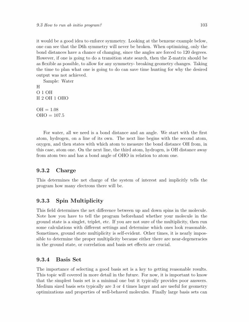
9.3 How to run ab initio program? 103
it would be a good idea to enforce symmetry. Looking at the benzene example below,one can see that the D6h symmetry will never be broken. When optimizing, only thebond distances have a chance of changing, since the angles are forced to 120 degrees.However, if one is going to do a transition state search, then the Z-matrix should beas flexible as possible, to allow for any symmetry- breaking geometry changes. Takingthe time to plan what one is going to do can save time hunting for why the desiredoutput was not achieved.
Sample: WaterHO 1 OHH 2 OH 1 OHO
OH = 1.08OHO = 107.5
For water, all we need is a bond distance and an angle. We start with the firstatom, hydrogen, on a line of its own. The next line begins with the second atom,oxygen, and then states with which atom to measure the bond distance OH from, inthis case, atom one. On the next line, the third atom, hydrogen, is OH distance awayfrom atom two and has a bond angle of OHO in relation to atom one.
9.3.2 Charge
This determines the net charge of the system of interest and implicitly tells theprogram how many electrons there will be.
9.3.3 Spin Multiplicity
This field determines the net di↵erence between up and down spins in the molecule.Note how you have to tell the program beforehand whether your molecule in theground state is a singlet, triplet, etc. If you are not sure of the multiplicity, then runsome calculations with di↵erent settings and determine which ones look reasonable.Sometimes, ground state multiplicity is self-evident. Other times, it is nearly impos-sible to determine the proper multiplicity because either there are near-degeneraciesin the ground state, or correlation and basis set e↵ects are crucial.
9.3.4 Basis Set
The importance of selecting a good basis set is a key to getting reasonable results.This topic will covered in more detail in the future. For now, it is important to knowthat the simplest basis set is a minimal one but it typically provides poor answers.Medium sized basis sets typically are 3 or 4 times larger and are useful for geometryoptimizations and properties of well-behaved molecules. Finally large basis sets can

104 Practice of electronic structure calculations
be on the order of 10+ times larger than a minimal set and they are useful for ”ultra-accurate” results.
9.3.5 Methods
One can choose from a multitude of methods which include:
1. SCF - Self Consistent Field theory (Ground State)
• Hartree - Fock theory : A starting point for correlated and excited statemethods;
• DFT - Density Functional Theory: A quick and reasonably accurate method.(Well, some people call it Dirty Fast Trick... Do not tell it to anybody!)
2. MP2 - Moller - Plesset perturbation theory (Ground State). This is the simplestcorrelation correction to the SCF energy and derivatives.
3. CCD, CCSD, CCSD(T), ... - Coupled-cluster theories. These are more ad-vanced forms of correlation corrections which correspondingly take longer toperform.
4. CI - Configuration interaction (Grd. State and Exc. State) CIS and CIS(D)are useful first approximations to excited states of molecules. Higher order CIsuch as CISDTQ can be useful a correlation correction to the ground state andexcited states.
5. Geometry optimizations. A molecule of interest can be optimized with respectto the electronic potential energy surface generated by SCF and MP2 calcula-tions.
6. Properties. Di↵erent programs o↵er a wide range of calculated properties ofmolecules. They include energies, dipoles, polarizabilities, vibrational frequen-cies, NMR shifts, ...
These are general notes about input. However, usually you have to specify muchmore information to set up calculations. Also, formats of input files are very di↵erent.
9.4 Tricks of the trade
Performing calculations is not simple. You can make mistakes in preparing input(most frequent problems) and program will either crush, or give an incorrect results.Therefore you have to always analyze output file. Also, it is good to perform somebenchmarks to make sure that everything is correct. When starting use of anotherpackage, it is always good to run some test problems in both packages to compareresults (must be same!). When starting to work on a new problem, good test is to runminimal basis set calculations in order to see that your input is correct , to analyzevalence MOs, etc.

9.5 Molecular properties 105
Why outputs are so large? Extra information is given to help you to check yourresults or to find out why the program does not work. Always look at Z-matrixprogram prints as an output to make sure it looks correct. Check symmetry. For thetest, nuclear repulsion energy is good, since it does not depend on basis set/model,but on geometry only. Good test for performing calculations of the same moleculewith di↵erent methods, bases, packages.
Then good thing to look at are molecular orbitals, analyze their symmetries andenergies. Sometimes SCF can converge to a wrong solution (since it is non-linearproblem). If you get occupied orbitals with positive energy, or virtual orbitals withnegative energy, or if the HOMO-LUMO gap is too small, possibly something is verywrong. However, sometimes it can be a correct answer. Which would mean that HFbreaking down. Why? Recall MP2 or H2 problem.
Frequencies: negative frequencies mean two things: this is not a minima, or HFwavefunction breaks symmetry, or is very poor.
9.5 Molecular properties
Atomic charges: characterize screening — how much density resides on atoms. Mul-tipole moments: dipoles, quadrupoles, etc. HF: Koopmans’ IP (orbital energies).Electronic spatial extent — how di↵use electron cloud is. Rydberg character. Ther-mochemical data — can calculate heats of formation, enthalpies. etc.
9.6 How to present results
Tables arranged as follows: Experiment: last line. Total energies are given in a firstcolumn. 6 digits in total energy is a standard. Good style is to provide nuclearrepulsion energy.

106 Practice of electronic structure calculations

Chapter 10
Electron correlation
References: 5, 6.
10.1 Introduction of the correlation problem
Electron correlation energy is defined as a di↵erence between Hartree-Fock energy inthe infinite basis set and the exact energy:
Ecorr = Eexact � EHF (10.1)
We also can define correlation energy in the given finite basis set:
Ecorr = EFCI � EHF , (10.2)
where EHF is Hartree-Fock energy in the given finite basis set, and EFCI is fullconfiguration interaction energy calculated in the same basis set.
What is a Hartree-Fock energy? Hartree-Fock problem is finding the best sin-gle determinant wavefunction in a self-consistent field procedure, which is repeateddiagonalization of an e↵ective one-electron Hamiltonian:
Fµ⌫ = hµ⌫ +X
��
< µ⌫||�� > P�� (10.3)
P�� =NX
i=1
C�iC�i (10.4)
This is a mean-field procedure. All electron interactions are averaged. Correlationsare averaged out and each electron moves in the average field of the others. Thismeans that electrons do not feel instantaneous positions of other electrons. Instead,they feel averaged in time positions of other electrons.
Our task is now to develop systematic improvements to the mean-field model.Why correlation energy is important? On the one hand, correlation energy is
usually smaller than 1% of the total electron energy. However, it is crucial becauseit changes in most chemical processes. Consider H2 dissociation: at equilibriumgeometry, electrons must be correlated. Their correlation energy is omitted from
107

108 Electron correlation
Hartree-Fock wavefunction. On the dissociation limit, there is no electron correlation:each atom has one electron. Hence, for each of the individual H-atoms one electronapproximation is exact. So correlation energy changes along dissociation curve fromsome finite value to zero. Rough order of magnitude for correlation energy is about 50-100 kJ/mol (0.5-1.0 eV) per electron pair. It is exactly the same order of magnitude aschemical transformation energies. Hence, Hartree-Fock energy for the H2 dissociationis wrong by about 0.5-1.0 eV, which is the same order of magnitude as H-H bondenergy.
Like energy itself, the correlation energy scales with the size of the molecule, it isan extensive property.
Bond energies are a leading manifestations of electron correlation, but there arepresumably a lot of other (may be less crucial) e↵ects on molecular structure.
10.1.1 Chemical consequences of electron correlation
In this section we consider qualitative chemical consequences of electron correlation.
Ionicity
The Hartree-Fock model lets electrons get slightly too close to each other (because ofaveraging out instantaneous repulsions). Therefore, polarity is slightly overestimatedby Hartree-Fock model. For example, calculated dipole moments at HF/6-31G* aretypically 20% too big.
We can demonstrate that Hartree-Fock wavefunction is too ionic by consideringH2 molecule in a minimal basis set:
�RHF = ��(↵� � �↵) =
(sA + sB)(sA + sB)(↵� � �↵) =
(sAsA + sBsB + sAsB + sBsA)(↵� � �↵) =
H�AH
+B +H+
AH�B +HAHB +HAHB (10.5)
Hartree-Fock wavefunction is a mixture of ionic and covalent pieces in a fixedproportion. This is always wrong, but it is especially bad as one approach dissociationwhen there should be zero probability of getting H+ and H�!
Bond lengths
Due to ionic character, bond lengths are generally underestimated. Correspondingly,frequencies are overestimated. As a result, molecules at Hartree-Fock level of theoryare too rigid.
Correlation treatment would decrease ionicity and will lead to the bond lengthincrease. Why? The Hartree-Fock model describes chemical bond by a formation ofbonding and antibonding orbitals, bonding orbitals being occupied, antibonding or-bitals completely unoccupied. Full configurational interaction wavefunction includesall possible excited determinants. Hence, “electron correlation” must be associated

10.1 Introduction of the correlation problem 109
with antibonding orbitals becoming fractionally occupied, due to other determinantsmixing with Hartree-Fock one. Hence, bond length will increase, and frequencies willdecrease.
Electron-molecule scattering
In the HF approximation molecule’s electron see the time averaged position of thescattering electron. In reality, the molecular electrons polarize in response to theinstantaneous position of the scattering electron.
Basic point: understanding the chemistry of Hartree-Fock model leads you to arough understanding of the role of correlation without any mathematics. It shouldalso give you some instinct for when to trust Hartree-Fock calculations and when notto.
10.1.2 Dynamical and non-dynamical correlation
We can distinguish, in general, two di↵erent e↵ects associated with electron corre-lation: dynamical and non-dynamical correlation. There is no rigorous definition ofthese two e↵ects. There is no rigorous way to separate these two e↵ects as well. Wedistinguish dynamical and non-dynamical correlation as two asymptotic cases.
The e↵ect of correlation is dual. Remember uncertainty principle? Is electron aparticle or a wave? We can measure electron di↵raction, when electrons behave aswaves. On the other hand, electrons can interact with individual molecules, and wecan count individual electrons when they hit luminescent screen (on impact, electronsinteract with an individual molecules). When we have electron localized in space,its momentum (and, hence, kinetic energy) is undefined. Similarly, when energy ofelectron is well defined, its position is undefined (they behave like a waves).
Dynamical correlation can be considered as a local interaction of two electrons,their energies undefined. Non-dynamical correlation is associated with degeneracy:interaction of two electrons (may be well separated in space) with a same energy.
Since, we did not define rigorously, how do we distinguish dynamical and nondy-namical correlation:
Ecorr 6= End + Edyn (10.6)
Later I’ll introduce rigorous definition of both components for which we’ll havethis hold:
Ecorr = End + Edyn (10.7)
Dynamical correlation
Dynamical correlation is the physical e↵ect associated with electrons avoiding eachother at short range and their fluctuations being correlated at long range. Thisis a mostly local (in space) e↵ect. But it is wide in energy coordinate: there arecontributions from electrons with very di↵erent energy (occupying well separated inenergy orbitals). Many small contributions sum up to the large quantity.

110 Electron correlation
Nondynamical correlation
Nondynamical correlation arises when two or more electronic states are nearly de-generate. The electrons fluctuate with frequencies proportional to the energy gapsbetween electronic states. If two or more states are nearly degenerate, we have alow frequency oscillations, hence, slow electron motions. For slow electrons mean-field would not work as good as for fast electrons. Another way to see it: kineticenergy of electrons (plus nuclear-electron interaction) against pair electron-electroninteractions. For slow electrons we have decrease of one-electron part of the totalHamiltonian.
Generally, degeneracy is an indication that non-dynamical correlation is impor-tant. As a pathological example, we consider electron scattering from the molecule.For a free electron which has a continuum of energy levels degeneracy is very high.As another example, consider H2 dissociation. On dissociation limit, bonding � andanti-bonding �⇤ orbitals become degenerate. As a result two Slater determinants (�)2
and (�⇤)2 become degenerate.So non-dynamical correlation is important in
1. electron-molecule scattering;
2. bond-dissociation;
3. anions;
4. molecules with several Lewis structures;
5. diradicals.
This e↵ect is non-local (electrons occupying degenerate orbitals can be far apartspatially), but narrow in energy coordinate (electrons occupy degenerate states).
In terms of FCI wavefunction:
= C0�0 + CL�L (10.8)
dynamical correlation is associated with a contributions from many excited deter-minants with a small coe�cients CL; non-dynamical correlation is associated with acontributions from several configurations with a large coe�cients.
Consider H2 dissociation. FCI wavefunction would be all double excitations fromthe reference configuration (�)2:
= C0(�)2 + C1(�
⇤)2 +X
i
Ci(�i)2 (10.9)
At equilibrium all coe�cients Ci are small. But the gross e↵ect can be large, whenwe sum contributions from many determinants. On dissociation, coe�cient C1 willbecome very large. As a result, contribution from a single (�⇤)2 configuration wouldbe large. Hence, we have dynamical correlation at equilibrium, and non-dynamicalcorrelation at dissociation limit. Which makes sense: at small distances, local e↵ectsprevail, whereas at large separations, we have non-local e↵ects.
Picture of MO of H2 here.

10.1 Introduction of the correlation problem 111
Unrestricted Hartree-Fock wavefunction as a tool to describe non-dynamicalcorrelation
The non-dynamical correlation is the e↵ect of mixing in a few other determinantsnecessary to get a qualitatively correct wavefunction (e.g. for dissociation). Thiscan be achieved e.g. by UHF, or, alternatively by mixing a couple of determinantstogether.
Qualitatively correct wavefunction for � bond dissociation:
= C0(�2) + C1(�
⇤)2, (10.10)
Unrestricted Hartree-Fock wavefunction has no restriction to be of correct sym-metry. Hence, variational principle will yield at dissociation limit molecular orbitals,which are localized near individual atoms, instead of delocalized molecular orbitals �and �⇤.
�UHF0 (r ! 1) = |sA↵sB� >=
1p2
✓sA(1)↵(1) sB(1)�(1)sA(2)↵(2) sB(2)�(2)
◆=
1p2(sA(1)↵(1)sB(2)�(2)� sB(1)�(1)sA(2)↵(2)) (10.11)
Hence, UHF wavefunction can describe electron localization near individual atoms.In contrast to the RHF-wavefunction, it corresponds to the pure covalent structure.However, it has incorrect symmetry. We can show that �UHF
0 is a mixture of singletand triplet states:
singletcov = (sAsB + sBsA)(↵� � �↵) =
(sA↵sB� � sB�sA↵) + (sB↵sA� � sA�sB↵) (10.12)
tripletcov = (sAsB � sBsA)(↵� + �↵) =
(sA↵sB� � sB�sA↵) + (sA�sB↵� sB↵sA�) (10.13)
UHF0 =
1p2( singlet
cov + tripletcov ) (10.14)
UHF-wavefunction is not an eigenstate of S2: < S2 >⌘< UHF |S2| UHF >=1 ondissociation limit. UHF is spin-contaminated. < S2 >=0 for singlet and 2 for triplet.
10.1.3 Conclusions
Electron correlation energy is defined as a di↵erence between exact and uncorrelatedmean-field Hartree-Fock model. Hartree-Fock, an one-electron, mean-field approx-imation, approximates many-electron wavefunction by a single Slater determinant.Hence, following e↵ects are omitted in Hartree-Fock model:
1. local interaction of electrons (dynamical correlation);
2. e↵ect of several nearly degenerate configurations (non-dynamical correlation).
112 Electron correlation
H2 example: at equilibrium, we want to include local e↵ect of electron repulsion.At dissociation, we need non-local e↵ects: two configuration (�)2 and (�⇤)2 are de-generate, we need two determinants to describe a wavefunction on dissociation limit.Hence, we have dynamical and non-dynamical correlation e↵ects. Consider two situ-ations for calculation of dissociation energy: Start: calculate EHF of H2 molecule atequilibrium. Then (i) calculate EHF of H2 molecule at large distance. In this casewe missed dynamical correlation at equilibrium and non-dynamical correlation at dis-sociation. (ii) Calculate EHF of each of H atoms. Then we missed only dynamicalcorrelation energy at equilibrium. Both are important
10.2 Structure of FCI matrix and di↵erent approachesto electron correlation
10.2.1 Intermediate normalization
It is convenient to employ so called intermediate normalization of the wavefunctioninstead of familiar normalization condition:
< | >= 1 (10.15)
Intermediate normalization requires that the weight of reference determinant (usually,Hartree-Fock determinant) equals unit:
< �0| >= 1 (10.16)
Thus, a general wavefunction assumes the following form:
FCI = �0 +X
L
CL�L (10.17)
With normalization condition (10.15), the energy is given by the familiar expectationvalue:
E =< |H| > (10.18)
With intermediate normalization (10.16) the energy expression assumes the followingform:
E =< �0|H| > (10.19)
To show that, consider matrix element < �0|H| > for the wavefunction which isan eigenfunction of H. Thus, energy calculated as (10.19) is the same as calculated by(10.18) for the exact wavefunction (but not the same for an approximate). However,for some approximate models (e.g., truncated CI) both equation give the same answer.
To proceed to di↵erent approaches for correlation energy calculation, consider FCIwavefunction and compare it against HF one. Lets think our basis is large enough tobe complete.
FCI = �0 +X
L
CL�L = (1 + C1 + C2 + . . . CN)�0, (10.20)

10.2 Structure of FCI matrix and di↵erent approaches to electron correlation 113
where operator CM excites M electrons in all possible ways from reference configura-tion �0:
C1 =X
i2occ,a2virttai a
+a ai
C2 =1
4
X
ij2occ,ab2virttabij a
+a a
+b aiaj (10.21)
Orbital picture here. (Occupied, virtuals, several excited determinants).FCI solution: in the basis of all �L, diagonalize matrix of the total Hamiltonian,
and find its eigenvalues and eigenvectors.How does the Hamiltonian matrix look like in the basis of excited determinants?FCI matrix picture here.....Several observations:
1. For intermediate normalization and for Hartree-Fock reference, we have:
E =< �0|H|(1+C1+C2+. . . CN)�0 >=< �0|H|�0 > + < �0|H|C2�0 >= E0+Ecorr,(10.22)
where E0 is Hartree-Fock energy, and correlation energy Ecorr depends explic-itly only on the amplitudes (weights) of doubly excited configurations. Thatdoes not mean, however, that we can disregard all other excitations, since theyare coupled through Hamiltonian with double excitations, and therefore definecoe�cients of doubly excited determinants in FCI wavefunction.
2. Correlation is associated with the population antibonding orbitals.
3. We can associate di↵erent orders in excitations with pair correlations, triplecorrelations, etc. (E.g., for H2 only single and double excitations are possible,hence, FCI is CISD). For HeH — only triple excitations, etc. Hence, we canhope that the weight of higher order excitations would die in a FCI wf.
4. Di↵erent determinants: a few degenerate contribute a lot (have large CI coe�-cients) into total energy. Or a lot of non-degenerate (with small CI coe�cients)contribute totally a lot into the energy. Again, first case is non-dynamicalcorrelation, second one — dynamical correlation.
Practical electron correlation methods. Idea — try to include e↵ects of pair-electron correlation first, then three-particle e↵ects, and so on.
1. MCSCF theory: no dynamical correlation. Exponential as it is FCI in a smallersubspace. For small active spaces (i.e., � � �⇤ and the like), scaling is just likefor the Hartree-Fock method: N2 �N3.
2. Superposition of configurations (configurational interaction)
3. Perturbation theory (MP2,MP3). MP2 (2nd order P.T.) — perturbative treat-ment of pair correlations. N4 �N5

114 Electron correlation
4. Coupled cluster theory with singles and doubles. Self-consistent treatment ofpair correlations. N6
5. The e↵ect of triple excitations CCSD(T) theory. Corrections for triple excita-tions. N7
6. Gaussian-2 theory and chemical accuracy
10.2.2 Summary
• Correlation energy: di↵erence between exact and uncorrelated (HF) model.HF is one-electron, mean-field approximation. E↵ects omitted: (1) local inter-action of electrons; (2) e↵ect of several nearly degenerate configurations. H2
example: at equilibrium, we want to include local e↵ect of electron repulsion.At dissociation, we need non-local e↵ects: two configuration (�)2 and (�⇤)2 aredegenerate, we need two determinants to describe a wavefunction on dissoci-ation limit. Hence, we have dynamical and non-dynamical correlation e↵ects.Consider two situations for calculation of dissociation energy: Start: calculateEHF of H2 molecule at equilibrium. Then (i) calculate EHF of H2 moleculeat large distance. In this case we missed dynamical correlation at equilibriumand non-dynamical correlation at dissociation. (ii) Calculate EHF of each of Hatoms. Then we missed only dynamical correlation energy at equilibrium. Bothare important...
• Intermediate normalization is more convenient in electronic structure: < �0| >=1 (amplitude of the reference determinant is unit). For so normalized wavefunc-tion energy is: E =< �0|H| >. By analyzing FCI matrix we get: E = E0+ <�0|H|C2�0 >. Hence, correlation energy is Ecorr =< �0|H|C2�0 >.
• Di↵erent determinants in FCI wavefunction: a few degenerate contribute a lot(have large CI coe�cients) into total energy. Or a lot of non-degenerate (withsmall CI coe�cients) contribute totally a lot into the energy. Again, first caseis non-dynamical correlation, second one — dynamical correlation.
10.3 Configurational interaction
Good review: 19.First ideas about electron correlation were associated with configurational inter-
action. If Hartree-Fock models is so good (gets 99% of the total energy), may beinclusion of several more important determinants will make it excellent? General CIwavefunction:
=X
L
CL�L (10.23)
Consideration (MCSCF and CI): (i) how do I select important configurations? (ii)can I include a systematically chosen set of configurations?

10.3 Configurational interaction 115
10.3.1 MCSCF model
Goal — to describe non-dynamical correlation (e↵ects of a small number of quasi-degenerate configurations). How to include important configurations? If we solveHartree-Fock problem and get �0, we can consider then excited determinants andselect several (using our chemical intuition) which are important for a particularcase. Then we can diagonalize Hamiltonian in the basis of this configurations. Thisis not a good approach. Why? Because orbitals were optimized in HF procedure togive a lowest energy for a single determinant! Hence, we have unbalanced description:orbitals are best for one of the determinants, and of poor quality for another. Hence,HF (SCF) model were generalized to MCSCF model, in which both orbitals and CIcoe�cients are optimized variationally to give a lowest energy for the wavefunction(10.23).
Consider �-bond dissociation in H2 molecule (Fig. 10.1). Simplest qualitatively
E
σ∗=s1−s2,
+ s1 s2
σ=s1+s2,
RH−H
Figure 10.1: Molecular orbital picture for H2 dis-sociation. At equilibrium, the two hydrogen s or-bitals form bonding � and anti-bonding �⇤ orbitalswhich are well separated in energy. The wave-function describing chemical bond formation canbe represented by doubly occupying the � orbital.For a large nuclear separation, when � and �⇤ aredegenerate, electrons are localized near individualH atoms and occupy orbitals s1 and s2.
correct wavefunction must include 2 determinants:
= C0 0 + C1 1 (10.24)
0 = (�)2
1 = (�⇤)2
Then we optimize both orbitals and CI coe�cient at each nuclear geometry. Wave-function (10.24), often referred as a two-configuration SCF (TCSCF) wavefunction,is the simplest example of a multi-configurational SCF (MCSCF) wavefunction. Inthis example the orbitals � and �⇤ define the active space (Fig. 10.2), which is the setof orbitals whose occupations vary among the di↵erent configurations included in anMCSCF wavefunction.
If a minimal basis set is used, then the � and �⇤ orbitals are determined by symme-try, and the two configurations (�)2 and (�⇤)2 are the only ones allowed by symmetry

116 Electron correlation
restricted virtual (non−valence)
active virtual (valence)
active occupied (valence)
restricted core
Figure 10.2: Schematic representation of ac-tive and restricted orbital spaces. Excita-tions are allowed within the window of ac-tive orbitals. Orbitals in each subspace aredefined variationally, by minimizing total en-ergy with respect to orbital rotations be-tween restricted/active subspaces.
for the ground state of H2. Hence, for this particularly simple example, the TC-SCF wavefunction (10.24) happens to be identical to a full configuration interaction(FCI) wavefunction in the active space of � and �⇤ orbitals. More generally, a FCIwavefunction defined in an active space of variationally optimized orbitals is called acomplete-active-space SCF (CASSCF) wavefunction,20 also known as full optimizedreaction space (FORS).21 For the H2 molecule, when there are only two valenceorbitals, wavefunction (10.24) recovers all non-dynamical correlation.22 For othermolecules, however, the valence space contains more orbitals. Then, although twoelectronic configurations of the form (�)2 and (�⇤)2 will dominate the dissociation of� bonds, other electronic configurations in the valence space can be important in thezero-order wavefunction. For instance, to describe the dissociation of each particularbond in a polyatomic molecule by a TCSCF wavefunction, di↵erent � and �⇤ orbitalsshould be included in the active space. However, describing the dissociation of two� bonds at the same time (or one double bond) requires an MCSCF wavefunctionincluding four electronic configurations. More generally, a zero-order wavefunctionwhich includes all electronic configurations that can be formed by distributing thevalence electrons among the valence orbitals (bonding, anti-bonding, and lone pairorbitals) is capable of describing the breaking of any type of chemical bond (double,triple, etc.) and, moreover, the simultaneous breaking of any number of bonds. Inother words, the non-dynamical correlation energy may be defined as the di↵erencebetween full configuration interaction within the space of all valence orbitals, and asingle determinant of molecular orbitals (Hartree-Fock theory).22 Hence, the CASSCFwavefunction incorporates all non-dynamical correlation when the full valence activespace is considered. Dynamical correlation energy, which is the di↵erence betweenthe FCI and CASSCF energies,22 can be included later. Unfortunately, the exact

10.3 Configurational interaction 117
calculation of non-dynamical correlation energy, as defined above, involves computa-tional complexity that grows exponentially with molecular size and is thus unfeasiblebeyond systems of just two or three heavy atoms.
One strategy to approximate non-dynamical correlation for larger systems is toperform CASSCF calculations in smaller active spaces. In that case, non-dynamicalcorrelation is no longer completely described in the zero-order wavefunction. Practi-cally, this approximation introduces arbitrariness into theoretical descriptions becausethe active space is no longer uniquely defined and must be chosen based on physicalconsiderations for each particular process. Often small active orbital spaces lead tosignificant errors, which cannot be completely recovered by subsequent calculations ofdynamical correlation. It has been shown by Davidson23 that CASSCF calculationsfor the Cope rearrangement performed in a ⇡-orbitals active space is qualitatively in-correct, and inclusion of �-⇡ correlation by subsequent CASMP2 calculations changesthe energetics along the reaction coordinate significantly. Another case where a largeactive space is necessary is reported by Chaban et.al.:24 their study of N2O2 isomersdemonstrated that the CASSCF space should include not only four NO bonds andone NN bond, but also the oxygen lone pairs. The resulting CASSCF space—14electrons distributed in 12 orbitals, denoted (14,12)—is very close to today’s limit forthe CASSCF method.
Next, we consider the torsional barrier in the ethylene molecule. This example,though simple, represents a wide class of chemically important problems such astransition states and diradicals.25,26 The molecular orbital picture of ethylene at theequilibrium geometry and along the twisting coordinate is sketched in Fig. 10.3. Atthe equilibrium geometry, the two carbon p orbitals perpendicular to the molecularplane form bonding ⇡ and anti-bonding ⇡⇤ orbitals. The ground state (labelled theN state) doubly occupies the ⇡-orbital. A ⇡ ! ⇡⇤ excitation results in the V state.Doubly occupying the ⇡⇤ orbital results in the Z state. As we twist ethylene aroundthe C–C bond, the overlap between the two p orbitals decreases and becomes zero at90o. Therefore, at 90o the ⇡ and ⇡⇤ orbitals become degenerate and the ⇡ bond isbroken. In order to describe twisted ethylene at 90o, we have to introduce the twoconfigurations (⇡)2 and (⇡⇤)2 consistently into our zero-order description.
Other examples: dissociation of double bond (C=C), or triple bond (N2). Discussminimal reasonable active space in each case.
Summary
MCSCF theory does not include dynamical correlation. The goal of MCSCF modelis to provide correct zero-order wavefunction. It includes one determinant for eachLewis structure. To achieve accurate results, the dynamical correlation should beincluded by other models, e.g., by perturbation theory.
CASSCF wavefunction is FCI defined in an active (orbital) space with orbitalsbeing variationally optimized. Both CI coe�cients and orbitals are defined variation-ally.
Qualitatively correct size-consistent zero-order wavefunction suitable for PES’s:CASSCF defined in a full valence space (all bonding, antibonding, and lone pairs

118 Electron correlation
E Z (π*)2 V (ππ*) π*
π N (π)2 0 90 180 Torsional angle
Figure 10.3: Schematic molecular or-bital picture of ground and excitedstates of ethylene along the torsionalcoordinate. Twisted ethylene at 90o
can be considered as a simple diradicaltransition state.
orbitals). It is well defined. Non-dynamical correlation energy can be defined as acorrelation energy of this wavefunction. We can define then the di↵erence betweenFCI and the so defined non-dynamical correlation energy. Thus:
Eex = End + Edyn (10.25)
Unfortunately, such calculations are unfeasible because of exponential scaling ofFCI expansion. Traditional approach is to take smaller active space based on physicalconsiderations. Criticism: MCSCF thus becomes “molecule-at-a-time”chemistry, dueto the need to pick configurations (active space). It will not be systematic and couldeven be worse than HF if done poorly.
Tradeo↵: flexibility vs. systematization. Tailored garments vs. o↵-the-shelf cloth-ing!
10.3.2 Truncated CI methods
Superposition of configurations (configurational interaction) CI is a brute force ap-proach, no chemical intuition necessary, no configuration selection should be done.
1. all double excitations? (CID)
CID = �0 + C2�0 = �0 +1
4
X
ijab
cabij�abij (10.26)

10.4 Many-body perturbation theory 119
2. all single and double excitations? (CISD)
CISD = (1 + C1 + C2)�0 =
�0 +X
ia
cai�ai +
1
4
X
ijab
cabij�abij (10.27)
No. Or at least not acceptably. Because of the size-consistency problem. CID,CISD, MCSCF are generally not size consistent. Results degrade as molecular sizeincreases.
E.g. CISD is exact for H2 (same as FCI), but for 2 separate H2, CISD is not exact,because the product wavefunction involves product of doubles (quadruples). That’swhy CISD (as any truncated CI method) is not size consistent. In a sense, it is worsethan HF!
Reminder: Size-consistency (size-extensivity) means that calculation on a systemof non-interacting fragments should give the same energy as the sum of energies fromseparate calculations on the individual fragments.
EAB = EA + EB (10.28)
HF is size-consistent when two closed-shell fragments are considered (for two H2
molecules, but not for two H-atoms!) FCI is size-consistent (just like nature!) Othertruncated CI methods are not. Why size-consistency is important even we do notdescribe bond-breaking? Because there are other manifestations, even at equilibriumgeometries. For example, quality of results degrade with molecular size increase forsize-inconsistent models.
We should consider theoretical model chemistries which are size-consistent! Sotoday we do not consider truncated CI models as a practical methods for electroniccorrelation. However, CI provides a convenient language for correlation problem.
10.4 Many-body perturbation theory
In this section we consider perturbative treatment of electron correlation. Idea: ifHF theory gets 99% of the way to the right energy, may be we can get the rest byperturbation theory. Goal of MP2 theory is to recover dynamical correlation when azero-order wavefunction, e.g., the Hartree-Fock wavefunction, is qualitatively correct.
10.4.1 Derivation of MP2 correlation energy
Second-order perturbation theory for many-electron wavefunction was introduced byC. Møller and M.S. Plesset.27 It is called MP2 (higher orders — MP3, MP4, etc.).
Let us recall 1-st and 2-nd orders of the Rayleigh-Schrodinger perturbation theory(with intermediate normalization of the wavefunction):
H0 (0)i = E(0)
i (0)i (10.29)
H = H0 + �V (10.30)

120 Electron correlation
< (0)i | (1)
i >= 0 (10.31)
E(1)i =< (0)
i |V | (0)i > (10.32)
⇣E(0)
i �H0
⌘| (1)
i >=⇣V � E(1)
i
⌘| (0)
i > (10.33)
E(2)i =< (0)
i |V | (1)i > (10.34)
How can we calculate PT corrections for the Hartree-Fock wavefunction? Whatis tricky here? To apply the RS perturbation theory we need exact solutions of somezero-order Hamiltonian. Can we find some Hamiltonian for which HF wavefunctionis an exact solution? Yes, this is Fock operator:
F�K =X
i2�K
✏i�K (10.35)
Note that the eigenenergy of |�0 > is not equal the Hartree-Fock energy. So, let usconsider this mean-field Fock operator as our zero-order Hamiltonian. Let us considerthe di↵erence between the exact Hamiltonian and the zero-order Hamiltonian:
V = H � F, (10.36)
where the perturbation V is fluctuation potential (contains electron correlations), His the exact Hamiltonian, and F is the mean-field Fock operator of HF theory.
Imagine the matrix of H in the basis of determinants. If our starting point is HF,then the question as far as PT goes — what is it coupled to?
Matrix elements of Fock operator in the basis of determinants is very simple:
< �L|F |�L >=X
i2�L
✏i (10.37)
< �L|F |�K >= 0, K 6= L (10.38)
So, the Fock operator is just a diagonal of the matrix. V has all non-diagonal blocks,some of them zero. Which blocks are zero? Reference – single excitations (Brillouintheorem). Also between blocks when excitation is di↵erent more than by 2. Groundstate is coupled through Hamiltonian to doubles. (Slater rules, pair interaction in theexact Hamiltonian).
!! Picture here: FCI matrix and Fock matrix !!Consider the exact problem for the ground state wavefunction:
H 0 = E 0 (10.39)
Then let us expand perturbation V and wavefunction 0 in series of �:
(F + �V )( (0)0 + � (1)
0 + �2 (2)0 + . . .)
= (E(0)0 + �E(1)
0 + �2E(2)0 + . . .)( (0)
0 + � (1)0 + �2 (2)
0 + . . .) (10.40)
Now lets collect terms proportional to the given power of �

10.4 Many-body perturbation theory 121
Zero order
Collect terms proportional to �0
F (0)0 = E(0)
0 (0)0
E(0)0 =< (0)
0 |F | (0)0 >=
occX
i
✏i (10.41)
So, as we expected, (0)0 ⌘ �0. But E
(0)0 6= EHF !
First order
Collect terms proportional to �1:
F (1)0 + V (0)
0 = E(0)0
(1)0 + E(1)
0 (0)0
E(1)0 =< (0)
0 |V | (0)0 >= �1
2
occX
ij
< ij||ij > (10.42)
This is the missing part of the Hartree-Fock energy! Thus:
EHF =< (0)0 |H| (0)
0 >= E(0)0 + E(1)
0 (10.43)
the HF energy is correct through 1st order in V!What does (1)
0 look like?
(F � E(0)0 ) (1)
0 = �(V � E(1)0 ) (0)
0 (10.44)
As usual (1)0 is orthogonal to the (0)
0 . Lets look in terms of determinants whatexcitations contribute to (1)
0 . We will write expression for (1)0 in our basis which is
all excited determinants:
(1)0 = (T1 + T2 + . . .)�0 =X
ia
tai�ai +
1
2
X
ijab
tabij�abij + . . . (10.45)
Now lets find coe�cients t by projecting (1) on di↵erent determinants:
< �ai |(F � E(0)
0 ) (1)0 >= tai (✏a � ✏i) =
< �ai |� (V � E(1))|�0 >=< �a
i |� (H � F � E(1))|�0 >= 0 (10.46)
< �ai |H|�0 >= 0 by the Brillouin theorem, < �a
i |F |�0 >= 0 because the Fockianis just diagonal matrix in the basis of determinants, and the last term is zero due toorthonormality (E(0) is just a number).
Therefore, there is no single excitations in first order PT corrections to the HFwavefunction.

122 Electron correlation
Double excitations
< �abij |F � E(0)| (1)
0 >= (✏a + ✏b � ✏i � ✏j)tabij =
< �abij |� (V � E(1))|�0 >=< �ab
ij |� (H � F )|�0 >=
� < �abij |H|�0 >= � < ij||ab > (10.47)
We get < �abij |H|�0 >=< ij||ab > by using the Slater rules. < �ab
ij |F |�0 > is zerofor the same reason as before: the Fockian is diagonal matrix (in the basis of exciteddeterminants). < �ab
ij |E(1)|�0 > is zero because E(1) is just a number, and exciteddeterminant is orthogonal to a reference one (Slater rules). Hence, the coe�cients infirst-order PT corrections to the wavefunction would be:
tabij = � < ij||ab >✏a + ✏b � ✏i � ✏j
(10.48)
Second order
The second-order energy (MP2 energy) is:
F (2) + V (1) = E(0) (2) + E(1) (1) + E(2) (0)
E(2) =< (0)|V | (1) > (10.49)
MP2 energy:
E(2) = �1
4
X
ijab
< ij||ab >2
✏a + ✏b � ✏i � ✏j(10.50)
We can represent it graphically, by looking at the FCI matrix.We should have expected this — only doubles coupled to HF determinant. Schemat-
ically, (1) =
X
d
td�d (10.51)
td = � Vod
E(0)d � E(0)
0
(10.52)
Here �d = �abij —doubly substituted determinants, and td = tabij are the amplitudes
(coe�cients) of double substitutions.
E(2) =X
d
� V 2od
E(0)d � E(0)
0
(10.53)
Contributions to correlation energy from all double excitations
1. “pair correlation theory” — there is a contribution to correlation energy whichcomes from each pair of electrons;
2. correlation energy is negative-definite;
3. correlation energy is size-consistent;
4. the energy is not variational.
10.4 Many-body perturbation theory 123
10.4.2 Computational cost of MP2 theory
E(2) =X
d
� V 2od
E(0)d � E(0)
0
= �1
4
X
ijab
< ij||ab >2
✏a + ✏b � ✏i � ✏j(10.54)
How many doubles are there? O2V 2. Number of occupied pairs times number ofvirtual pairs. Hence, there is quartic number of double excitations.
What is a cost of making the matrix elements < ij||ab >, two-electron integralsin the molecular orbitals basis?
Suppose we have AO integrals computed and stored. Then cost is that of trans-forming a 2-electron integrals from the original AO basis to the MO basis.
This is a sequence of matrix multiplies:
< ab||ij >=X
µ
Cµa
"X
⌫
C⌫b
"X
�
C�i
"X
�
C�j < µ⌫||�� >
###
(10.55)
Costs O(N5) to make O(N4) transformed integrals (N is number of basis func-tions).
Hence, HF theory scales approximately N2 � N3, and this is iterative procedure(we recalculate Fockian at each self-consistent field) iteration.
MP2 theory scales as N5, and this is non-iterative method.
10.4.3 Local MP2
For small systems, all double excitations (O2V 2) can contribute into the total energyfrom Eq. (10.50). For a large system, however, number of terms which contribute intoMP2 energy depend on how the orbitals are represented. The MO’s that diagonalizeF (canonical MO’s) are delocalized. This does not change as a system gets bigger.Hence, all determinants can contribute into MP2 energy.
We can find a transformation which localizes occupied and virtual orbitals. Thenwe have smaller number of determinants which contribute into MP2 energy. This isa basis of local MP2 theories. Local MP2 models has been developed in MHG groupbring MP2 down to quadratic (N2) scaling by solving the equations in terms of localatomic orbital quantities.
10.4.4 Limitations of MP2 theory and higher orders of MBPT
What correlation (dynamical or non-dynamical) is MP2 capable of describing? Dy-namical. The very idea of local MP2 assumes that e↵ect is local. MP2 energy, as aHF energy depends only on the subspaces of occupied and virtual orbitals. Hence,can find transformation to local orbitals.
MP2 is a complete failure in the cases when non-dynamical correlation is impor-tant. Why? Because degeneracy disable use of perturbation theory. We can see itfrom Eq. (10.50), which goes to the negative infinity when orbitals become degener-ate. Such, for H2 example:
EMP2 = �< ��||�⇤�⇤ >
✏� � ✏�⇤(10.56)

124 Electron correlation
On the dissociation limit, � and �⇤ are degenerate, hence... Other way to see it. PTassumes that perturbation V is small, and can be expanded in a small series of �.Hence, wavefunction also can be represented as
= (0) + � (1) + �2 (2) + . . . (10.57)
However, for the cases when nondynamical correlation is important, we have severaldeterminants in FCI expansion which have large expansion coe�cients. For H2 exam-ple, we have equal coe�cients for both determinants at the dissociation limit. Hence,assumption that � is a small parameter is not valid.
Collapse to the negative infinity on dissociation limit is a well-known behavior ofMP2 correlation energy.
Conclusion: MP2 theory would be a complete failure for the cases when non-dynamical correlation is important:
1. bond-breaking process and transition states;
2. molecules with several Lewis structures;
3. anions;
4. radicals and diradicals.
Higher orders of PT are not useful. Examples: bondlength and divergence of MPexpansions. References... MP3, MP4 are occasionly used, but if MP2 has troublethe best way to fix it is not usually higher orders of PT, but rather treating electroncorrelation self-consistently, not perturbatively.
H2: dissociation curve for H2 described by MP2 would be a complete failure. How-ever, we can achieve excellent results by doing PT on top of MCSCF wavefunction.
General consideration: include non-dynamical correlation into zero-order wave-function. Then rest of the e↵ects would be small, and we can make it by usingPT.
10.4.5 Basis set and electron correlation methods
Why did we need basis set larger then minimal atomic basis set for HF theory? Todescribe how orbitals change in a molecular environment (become more di↵use, po-larized in a chemical bond direction, etc). Hence, our consideration for basis setchoice for HF calculations was to have basis set flexible enough to describe well occu-pied subspace (bonding orbitals). Something new happens as we proceed to electroncorrelation in general and to MP2 theory in particular. Since electron correlation isassociated with antibonding and other virtual orbitals become fractionally occupied,we have represent both the virtual and occupied space accurately.
Se, we expect that there will be even more stringent requirements on the basis setthan were required in HF theory!
New e↵ects:
1. radial (in-out) correlation;

10.4 Many-body perturbation theory 125
2. angular correlation;
3. two-electron cusp;
Radial (in-out) correlation
When electron is near the nucleus, other will tend to stay relatively far away. Hence,we need multiple-zeta basis sets. The “correlation-consistent” basis set of Dunninget. al.28
!!Figure here!!!!! table here !!
Angular correlation
If we imagine subdividing an atom volume by angle, then there will be a tendencyfor stable configuration to involve electron that are in distinct angular segments.Describing this type of correlation requires higher angular momentum functions.
!! figure here!!
Two electron cusp
Similarly to electron-nuclear cusp, there is a electron-electron cusp due to Coloumbinteraction of two electrons. To describe it, we need large basis sets, since it is di�cultto approximate this two electron function by products of one-electron functions. Thisis one of the reasons for slower basis set convergence for correlated methods.
Conclusions
The smallest basis set suitable for use with correlation methods — DZP or 6-31G*size.
Larger basis sets such as “correlation consistent” basis sets yield further systematicimprovements: cc-pVDZ cc-pVTZ cc-pVQZ cc-pVPZ.
These bases are meant to be used with frozen core. For includig core correlatione↵ects, one needs cc-cVXZ series.
10.4.6 Performance of MP2 theory
Given an adequate basis set, MP2 is a systematic improvement over HF theory (incase that HF wavefunction is qualitatively correct). MP2 gives approximately 80%of correlation energy.
General performance of MP2:
• For geometries and frequencies errors significantly reduced (by factor 2-3);
• relative energetics is usually improved, but not nearly enough.

126 Electron correlation
10.5 Coupled cluster theory
Objective: a more satisfactory formulation of the Shrodinger equation than configu-ration interaction such that size-extensive truncation is possible.
In configuration interaction model wavefunction is represented as a linear super-position of Slater determinants:
= (1 + C1 + C2 + . . . Cn)�0, (10.58)
where Cm represents all possible n-fold excitations. We have seen that this is physi-cally inappropriate when truncated. Alternative form is to take an exponential:
= exp(T1 + T2 + . . .+ Tn)�0 (10.59)
Tn operators also represent n-fold excitations. Form of Tn:
T1 =X
ia
tai a+a ai =
X
ia
tai a+i
T2 =1
4
X
ijab
tabij a+a a
+b aiaj =
X
ijab
tabij a+b+ij (10.60)
Both anzats are exact when carried to n-fold excitations. We can expand exponentto see relation between CI operators and cluster operators:
exp(T1 + T2 + . . .+ Tn) = (1) + (T1 + T2 + . . .+ Tn) +1
2!(T1 + T2 + . . .+ Tn)
2 +
1
3!(T1 + T2 + . . .+ Tn)
3 + . . .(10.61)
C1 = T1
C2 = T2 +1
2T 21
C3 = T3 + T1T2 +1
3!T 31
C4 = T4 + T3T1 +1
2T 22 +
1
2T2T
21 +
1
4!T 41 (10.62)
Comparing the groups, we see that truncating CC at singles and doubles gives usan approximate description of all higher excitations through n-fold.
Physical meaning: for CCSD, correlation between pairs of electrons (T2T2) is in-cluded. These specific quadrupole excitations are analogous to simultaneous collisionof two pairs of electrons, and contributions from these events is more significant thatcontributions fro the collisions of four electrons.
10.5.1 Size-extensivity
Size-extensivity is immediate: product form for non-interacting fragments:
exp(A+B) = exp(A) exp(B) (10.63)
provided that the operators A and B commute: [A,B] = 0.

10.5 Coupled cluster theory 127
10.5.2 How to solve?
How can we determine the cluster coe�cients?
1. variationally? No — equations do not terminate:
< eT1+T2�|eT1+T2� >=< �|� > + < T1�|T1� > + < (T2+1
2T 21�)|(T2+
1
2T 21 )� > + . . .
(10.64)
2. Solve eigenvalue problem in a subspace:
(H � E) = 0 (10.65)
Satisfy this equation in the space of
• the HF determinant;< �0|H � E| >= 0 (10.66)
• all single substitutions:
< �ai |H � E| >= 0 (10.67)
• all double substitutions:
< �abij |H � E| >= 0 (10.68)
enough equations to determine:
• energy;
• single coe�cients;
• double coe�cients;
The above equations are very similar to the variational CISD equations. In fact,they are identical if one takes | >= (1+C1+C2)�0 and not | >= exp(T1+T2)�0.What does this similarity mean? CISD is derived by using the variational principle:
< � |H| >= 0 (10.69)
where � is any allowed variation of the wavefunction. For the CISD wavefunction:
� CISD 2 span{�0,�ai ,�
abij }, (10.70)
i.e., belongs to the linear subspace of the reference, single, and double excitations.For the CCSD wavefunction, � is defined as some curvilinear subspace of the samedimensionality (e.g., sphere vs. plane in 3-D space). We can approximate this morecomplicated manifold by the linear part:
� CCSD ⇡2 span{�0,�ai ,�
abij } (10.71)

128 Electron correlation
10.5.3 CCSD model
CCSD equations
= eT1+T2�0
< �0|H � E| >= 0
< �ai |H � E| >= 0
< �abij |H � E| >= 0 (10.72)
How the equations terminate in this case? Quite naturally, by Slater rules:
E =< �0|H|�0 > + < �0|H|(12T 21 + T2)�0 >= EHF + Ecorr
< �ai |H � E|(1 + T1 + T2 + T1T2 +
1
2T 21 +
1
6T 31 )|�0 >
< �abij |H � E|(1 + T1 + T2 + T1T2 +
1
2T 21 +
1
2T 21 T2
1
6T 31 +
1
24T 41 +
1
2T 22 )|�0 >(10.73)
(10.74)
Properties of CCSD
1. Size-extensive!
2. Exact for isolated pairs of electrons. A good sign since molecules consist ofinteracting pairs of electrons!
3. Non-variational.
4. Computational cost is N6 and iterative.
5. Fails for bond-breaking: explain imbalance.
Recovery of correlation energy
CCSD at equilibrium geometries recovers⇡ 95% of correlation energy. Is this enough?In general, not quite. Correlation energy is about 1 eV per local pair. This gives 4eV correlation energy for C atom (bound to 4 neighbors). We get 0.2 eV error per Catom. This is still not quite enough — but close!
10.5.4 CCSD(T) model
What is missing in CCSD model? It is the e↵ect of triple excitations. Let us estimatethis perturbatively:
< �abcijk |F |T3�0 > + < �abc
ijk |V |(T1 + T2)�0 >= 0 (10.75)
This is not PT corrections for CCSD, this is PH estimate of triples contributions.Anyway, leading contribution is due to triples.

10.6 Approximation of coupled-cluster theory: quadratic CI (QCI) model 129
method scaling iterative?HF N2-N3 yesMP2 N5 no (must do HF first)CCSD N6 yes (must do HF first)CCSD(T) N7 no (must do CCSD first)CCSDT N8 yes (must do HF first)
What is its e↵ect on the energy? Work by analogy with PT:
�ET =1
36
X
ijkabc
tabcijk < �abcijk |V |T2�0 > (10.76)
This method, CCSD(T), is
1. Size-extensive!
2. Computational cost is N7 and non-iterative. CCSD must be solved first.
3. Recovers ⇡ 99% of correlation energy for normal molecules. Hence can approachchemical accuracy!
4. Non-variational.
Accuracy of CCSD(T): bondlength: 0.002 A, frequencies: ⇡ 10 cm�1
Alternatively, one can consider PT corrections for the CCSD wavefunctions. Thesewill have both triples and quadruples! CCSD(2) method.
We can include e↵ect of triples non-perturbatively, hence, we’ll get CCSDT equa-tions. How? Lets write them in class.
Lets pause to consider where we are:Picture here: X-axis: min, DZ, DZP, 6-311G(2df) cc-pVDZ, cc-pVTZ, cc-pVQZ,
cc-pV5Z. Y-axis: HF, MP2, CCSD, CCSD(T), CCSDT.
10.6 Approximation of coupled-cluster theory: quadraticCI (QCI) model
QCISD method: Ref.29.QCI equation is an attempt to make truncated CI to be size-extensive. On the
other hand, QCI equations can be viewed as an approximation to CC equations. Insome cases QCI is equivalent to CC. For example, CID is the same as QCCD.
QCISD equations:
< �0|H � E| >= 0
< �ai |H � E|(1 + T1 + T2 + T1T2) >= 0
< �abij |H � E|(1 + T1 + T2 +
1
2T 22 ) >= 0 (10.77)

130 Electron correlation
QCISD equations contain important non-linear terms, We can prove that theQCI energy is size-extensive (due to this terms!). Note that there is no wavefunctionassociated with QCI model.
Scaling of QCI is the same as scaling for CCSD, but timings are much morefavorable.
10.7 Seasoned coupled cluster methods
1. Is CCSD size-extensive? Is it size-consistent? Explain.
2. Derivation of CCD equations. What is missing here? Orbital relaxation.
3. Brueckner CCD model. Optimized-orbitals CCD model. Relate to Hartree-Fock equations: < �a
i |H|�0 >= 0, or @E0@✓ia
= 0. E↵ect of single excitations inCCSD theory, T1 diagnostics.
4. Coupled cluster wavefunctions for multireference problem: VOOCCD model.Dissociation example. Ethylene example.
The excellent performance of the VOOCCD model for challenging multi-referenceproblems such as the torsion of ethylene and chemical bond breaking has been demon-strated in ref.30 (See Figs. 10.4-10.6). Recently, Sherrill et al. compared the perfor-mance of the VOOCCD, CASSCF (in the full valence active space), and TCSCF(CASSCF in 2x2 active space) models for several molecules with significant diradi-cal character, such as twisted ethylene, methylene, and ozone (Table 10.1 reproducesresults for the methylene). The comparison of optimized geometries, energies, andmolecular properties (e.g., dipole moments, frequencies and IR-intensities) has shownthat VOOCCD does accurately approximate the CASSCF wavefunction, while thealternative TCSCF approximation gives much larger errors (nearly same as Hartree-Fock model).

10.7 Seasoned coupled cluster methods 131
0 30 60 90 120 150 180Torsion angle, deg
−78.6
−78.4
−78.2
−78.0
Ener
gy, h
artre
e
CASSCFSCFDFTMP2CISDCCSD
Figure 10.4: Ethylene torsional barrierusing a DZP basis set. The RHF SCFenergy at for the planar structure is -78.049241 hartree.
0.0 50.0 100.0 150.0Torsion angle, deg
−78.19
−78.14
−78.09
Ener
gy, h
artre
e
CASSCF
VOO−CCD
TCSCF
Figure 10.5: The torsional barrier forethylene as computed by CASSCF(12,12),TCSCF [CASSCF(2,2)] and VOO-CCDusing a DZP basis set. An absolute er-ror of 0.113 hartree is subtracted from theTCSCF energy in order to compare allthree curves on the same scale. The VOO-CCD total energy is -78.188456 at equilib-rium and -78.061061 at the barrier.

132 Electron correlation
1.0 2.0 3.0RCH, A
−78.20
−78.15
−78.10
−78.05
−78.00
Ener
gy, h
artre
e
CASSCF
VOO−CCD
Figure 10.6: C-H bond dissociation inethylene using CASSCF(12,12) and VOO-CCD with a DZP basis set.
Table 10.1: Comparison of the restricted Hartree-Fock, TCSCF, and VOOCCD mod-els against CASSCF in the full valence active space. Total energies, dipole moments,equilibrium geometries, and harmonic vibrational frequencies and infrared intensities(in parentheses) are calculated for a1A1 CH2 using DZP and TZ2P basis setsa.
Method Energy µe re ✓e !1 (a1) !2 (a2) !3 (a3)DZP RHF -38.885 590 2.102 1.1005 103.74 3120 (61) 1490 (1) 3193 (96)DZP TCSCF -38.906 002 1.858 1.1035 102.72 3094 (68) 1512 (<1) 3158 (112)DZP VOOCCD -38.944 141 1.748 1.1333 100.65 2798 (84) 1413 (<1) 2863 (132)DZP CASSCF -38.944 322 1.742 1.1335 100.66 2795 (85) 1411 (<1) 2861 (133)TZ2P RHF -38.892 826 1.972 1.0945 103.73 3105 (64) 1503 (4) 3169 (77)TZ2P TCSCF -38.914 802 1.744 1.0967 102.99 3085 (67) 1527 (4) 3140 (92)TZ2P VOOCCD -38.953 446 1.657 1.1235 101.00 2797 (76) 1434 (<1) 2859 (103)TZ2P CASSCF -38.953 635 1.651 1.1238 100.98 2800 (74) 1435 (1) 2861 (102)
a Bond lengths in A, bond angles in degrees, dipole moments in Debye, frequencies in cm�1,and infrared intensities in km mol�1.

Chapter 11
High accuracy quantum chemistry
11.1 Overview
Chemical accuracy: errors about 1 kcal/mol ⇡ 0.05 eV.Approaches:
1. Complete basis extrapolation — Taylor style. (?) | ¯�E| ⇡ 0.2 kcal/mol. Tinysystems only.
2. Alternative methods to make the extrapolation from cheaper calculations...CBS models
3. Give up on extrapolation and adopt a more explicitly empirical approach,,,G1/G2 models.
4. G3 and G3S models.
Details: CBS style extrapolation — still somewhat empirical and hard to apply,but based on rigorous 2-e results
G2, G2-MP2: somewhat complicated, but e�cient.Final comments: research issues a) unphysical scaling; b) (L+ 1
2)�4convergence
11.2 Energy additivity schemes. Gaussian-1 / Gaussian-2 / Gaussian-3 theory
Gaussian-2 (G2) theory31 approximates a very high level calculations CCSD(T)/Infinitebasis by a series of lower level calculations that use finite basis sets and lower levels ofelectron correlation treatment in many cases. G3 and G3S theories32,33 are somewhatimproved modifications of G2 theory.
• Step 1: optimize molecular geometry. Note that low levels of theory work quitewell for this purpose, hence, can use MP2/6-31G*, which is not the full basisand highest level of correlation
133

134 High accuracy quantum chemistry
• Step 2: evaluate zero point energy at nuclear geometry (recall harmonic oscil-lator):
EZPE =1
2
modesX
↵
h!↵ (11.1)
Remember, that low-level theory was pretty good for frequencies. Hence, we useHF/6-31G* geometry and HF/6-31G* frequencies scaled by 0.893 to calculateEZPE.
• Step 3.: evaluate electronic energy at optimized geometry:
1. basic correlation energy calculation: QCISD(T)/6-311G(d,p). (QCISD(T)is a theory which can be viewed as a simplified version of CCSD(T). Itperforms quite similarly.)
2. e↵ect of basis set extensions from 6-311G(d,p) to 6-311+G(3df,2p)
�MP2 = MP2/6311 +G(3df, 2p)�MP2/6� 311G(d, p) (11.2)
We are using MP2 theory instead of full CCSD(T) (or QCISD(T)). This isbecause the e↵ect of such extensions is mostly to add high-energy unoccu-pied orbitals whose e↵ect can be estimated reasonably well by perturbationtheory. Remember, we do this for reasons of expediency only
3. e↵ect of basis set extensions from 6-311+G(3df,2p) to infinity. An empir-ical correction for the remaining basis set deficiencies is added:
�HLC = An↵ � Bn� (n↵ � n�) (11.3)
Value of B is the error in the energy of the H-atom. B=0.19 mhartree
Value of A is fitted to make mean derivation from experiment zero for55 well established heats of formation. A=4.81 mhartree (⌘ 0.13 eV perelectron pair)
This sizable correction per electron pair reinforces how hard it is to getcorrelation energies converged with respect to basis set.
Overall term:
E [G2(MP2)] = E [QCISD(T )/6� 311G(d, p)] + �MP2 + �HLC + �ZPE (11.4)
11.2.1 Chemistry using G2(MP2) model
Results for first and second row compounds. Average absolute deviation comparedto the experiment. MAD — mean absolute deviation
1. Dissociation energies: MAD=1.16 kcal/mol=0.050 eV.
2. Proton a�nities (M +H+ ! MH+): MAD=1.04 kcal/mol=0.045eV.

11.2 Energy additivity schemes. Gaussian-1 / Gaussian-2 / Gaussian-3 theory 135
3. Ionization energies (M ! M+ + e): MAD=1.24 kcal/mol=0.054 eV
4. Electron a�nities (M + e ! M�): MAD=1.29 kcal/mol=0.056 eV
Overall MAD=1.58 kcal/mol, which means uncertainty is ± 3 kcal/mol. Whatis a range of accessible chemistry? G2(MP2) theory can be applied up to systemcontaining about 7 first row atoms.
11.2.2 A critique of G2(MP2) theory
1. since it is based on single-reference models, it cannot describe non-dynamicalcorrelation. Therefore can be used only to describe molecules at equilibrium.Cannot apply to study inherently multi-reference situations, such as transitionstates along reaction coordinate;
2. higher level correction is empirical and cannot be fully transferable;
3. use of harmonic zero-point energies and empirically scaled HF frequencies;
4. approximations in all parts of the calculation are potentially suspect;
11.2.3 Getting better accuracy
If we still want better results then a more expensive G2 model is available. It replacesMP2 evaluation of the first basis set extension e↵ect with MP4 evaluations of basisset extension e↵ects in stages:
1. Di↵use:
�E(+) = E [MP4/6� 311 +G(d, p)]� E [MP4/6� 311G(d, p)] (11.5)
2. Higher polarization on non-H atoms:
�E(2df) = E [MP4/6� 311G(2df, p)]� E [MP4/6� 311G(d, p)] (11.6)
3. Extra polarization functions:
�E(3df) = E [MP2/6� 311 +G(3df, 2p)]� E [MP2/6� 311G(2df, p)]
�E [MP2/6� 311 +G(d, p)] + E [MP2/6� 311G(d, p)](11.7)
Overall e↵ect of basis set extension:
� = �E(+) +�E(2df) +�E(3df) (11.8)
Result: MAD=1.21 kcal/mol.A small but systematic improvement. Computation time is significantly increased
however.G3 theory and G3 theory using scaled energies32,33 G3: 1.01 kcal/mol, G3S: 0.99
kcal/mol. G3 includes spin-orbital corrections and uses larger basis sets.

136 High accuracy quantum chemistry
11.3 Alternatives to G2 theories
11.3.1 Complete basis set (CBS) methods
Instead of using higher-level correction to move to the complete basis set limit, onecan attempt to extrapolate calculations using features of the known pair correlationenergy function for He.
This leads to somewhat less expense and potentially less empiricism.References:.34–36
However, the reduction in expense for simple CBS models is accompanied by areduction in accuracy, and the reduction is relatively small.
CBS-4: MAD= 2 kcal/molCBS-q: MAD= 1.7 kcal/molCBS-Q: MAD= 1.0 kcal/molNote that empirical factors remain.

Chapter 12
Density functional theory
References: Reviews: Refs. 37, 38. DFT: Ref. 39. The Q-CHEM manual contains aconcise overview of the theory and di↵erent functionals. Excellent book: 40.
Outline:
• Return to density matrices;
• Basis of DFT: Hohenberg-Kohn theorems;
• Kohn-Sham equations;
• Approximate functionals: LDA, GGA, ADM (Hybrids);
• Performance and limitations, self-interaction errors;
• New range-separated functionals (wB97X and BNL);
• Empirical dispersion correction: ’-D’ methods.
12.1 Hohenberg-Kohn theorems
Exact electronic density, ⇢(r), of the ground state defines everything about molecule.Why? First,
R⇢(r) = N . Second, nuclear cusp positions define location of nuclei.
Third, gradient of density at nuclei defines nuclear charges (result from cusp condi-tion).
@
@ra⇢(ra)|ra=0 = �2Za⇢(0), (12.1)
where ⇢(ra) is a spherical average of ⇢(ra), a radial part of electronic density. There-fore, we know positions of nuclei, their charges and number of electrons. Hence, wecan write Shrodinger equation, solve it (in principle), get exact N-electron wavefunc-tion and exact energy. Which means that we know all about the system.
The reasoning presented above summarizes the so-called Wilson proof of DFT.Here are some recollections of Mel Levy:41 “During the conference [1979, shortlyafter Hohenberg-Kohn proof was presented], I had an interesting lunch with E. Bright
137

138 Density functional theory
Wilson. I was already aware of his unpublished density-functional type existencetheorem for Coulomb systems. As known from the work of Kato, the cusps of aneigenstate density determines the positions and charges on the nuclei, and hencev(r). Then, integration of the density gives T and Vee. Hence, an eigenstate Coulomb⇢ determines H, and thus, determines all the properties of the system. (Observe,however, that Wilson’s approach does not address directly variational calculations,in part because most trial densities do not belong to Coulomb eigenstates.)
What was particularly memorable for me was Wilson’s reaction to the conse-quences of his own beautiful proof. If I remember correctly, he expressed that heactually lost some interest in the HohenbergKohn theorem and felt less optimisticabout its practical implications after feeling that his proof for Coulomb densities wasessentially self-evident. I guess he was not the first to assume emotionally that thevalue of a theorem is necessarily proportional to its di�culty of proof. But that wasa long time ago.”
In the discussion below, we consider the following electronic Hamiltonian:
Hel =X
i
Ti +X
i
vi +1
2
X
ij
1
rij, (12.2)
where v = vi denotes one-particle potential operator often referred to as the “externalpotential”. In molecular applications, v is the electrostatic field due to the nuclei. Itis “external” with respect to the electrons.
12.1.1 Hohenberg-Kohn theorem I
The ground state electron density ⇢(r) determines the external potential v(r) uniquely(to within an additive constant C):
⇢(r) ! v(r) (unique) (12.3)
Proof (by contradiction, reductio ad absurdum): Let there be two external poten-tials v1(r), v2(r) arising from the same ⇢(r). Thus there will be two Hamiltonians,H1 and H2 with the same (ground state) density, but di↵erent wavefunctions 1 and 2:
Hi i = E0i i, i = 1, 2 (12.4)
We can use variational principle (VP) to make the following estimations for theground state energies:
E01 << 2|H1| 2 >=< 2|H2| 2 > + < 2|H1�H2| 2 >= E0
2+Z⇢(r)[v1(r)�v2(r)]dr
(12.5)Similarly,
E02 << 1|H2| 1 >=< 1|H1| 1 > + < 1|H2�H1| 1 >= E0
1+Z⇢(r)[v2(r)�v1(r)]dr
(12.6)

12.2 Kohn-Sham equations 139
Combining both inequalities together, we obtain contradiction:
E01 + E0
2 < E02 + E0
1 (12.7)
Hence, external potential is uniquely defined by ⇢(r).We can therefore represent energy as a functional of density:
E[⇢] = Vne[⇢] + T [⇢] + Vee[⇢] =Z⇢(r)v(r)dr + T [⇢] + Vee[⇢] (12.8)
We do not know what is T [⇢] and Vee[⇢] except for the fact that Vee[⇢] containsCoulomb interaction J [⇢]:
J [⇢] =1
2
Z ⇢(r1)⇢(r2)
r12dr1dr2 (12.9)
12.1.2 Hohenberg-Kohn theorem II
Introduces VP for the ground state density. Any approximate density, ⇢, defines someH and, therefore, . Using regular VP:
< |H| >= E[⇢] � E[⇢exact] (12.10)
We have equality only when ⇢ = ⇢exact.Hence, VP for the density:
�E[⇢]� µ�Z
⇢(r)dr �N�= 0 (12.11)
Can solve them to get density. The only catch is that we do not know is how towrite the functional, E[⇢]!
12.2 Kohn-Sham equations
E[⇢] = Ts[⇢] +Z⇢(r)v(r)dr +
1
2
Z ⇢(r1)⇢(r2)
|r1 � r2|+ Exc[⇢], (12.12)
where Ts is kinetic energy of non-interacting system with density ⇢(r) in the ap-propriate v(r). Here v(r) is just a Coulomb potential — this is a second term inthe equation. The third term is the classical Coulomb electron-electron interaction(which includes self-interaction). The last term is exchange-correlation energy, andit is defined by Eq. (12.12)
If Exc is ignored, we obtain Hartree approximation (not Hartree-Fock!).The Kohn-Sham equations use the fact that any density can be represented as:
⇢(r) =NX
i=1
�2i (r), (12.13)
where �2i (r) are some orthonormal orbitals (proof).

140 Density functional theory
Is there any relations between orbital �2i (r) and some real one-electron functions?
In some cases. Consider non-interacting electron gas (N electrons) in some externalfield v(r). Then wavefunction of the system is separable and is given by a single Slaterdeterminant composed of one-electron functions:
�(1, . . . N) = |�1 . . .�N >, (12.14)
where orbitals �i are solutions of one-electron problem with the Hamiltonian:
H =NX
i=1
(�1
2r2
i + v(ri)) (12.15)
This is an exact solution of Schrodinger equation for N non-interacting electrons inthe external field. Density ⇢(r) for the single Slater determinant is:
⇢(r) = NZ�2(1, . . . , N)d2 . . . dNd�1 =
NX
i=1
�2i (r) (12.16)
Hence, in a case of non-interacting gas, orbitals �i are one-electron wavefunctions.Kohn-Sham equations:
�1
2r2 + v(r) +
Z ⇢(r0)
|r � r0|dr0 + vxc � ✏i
!
�i(r) = 0 (12.17)
Here �i are just a set of one-electron functions. They are called Kohn-Shamorbitals. vxc is defined as follows:
vxc(r) ⌘�Exc[⇢(r)]
�⇢(r)(12.18)
Here vxc(r) depends on density ⇢(r) — if we change ⇢, vxc will change. However, wewrite vxc(r) because there is a value of vxc at point r defined, and we can use it asa local potential, that is, integrate it to get total Exc. vxc can be described as theone-electron operator for which the expectation value of the KS Slater determinantis Exc:
Exc[⇢(r)] =Z⇢(r)vxc[⇢(r)]dr (12.19)
Kohn-Sham energy is then:
E = ET + EV + EJ + EXC , (12.20)
where each term is a functional of ⇢(r) and can be expressed in terms of Kohn-Shamorbitals and density as:
ET =NX
i=1
�1
2< �i|r2
i |�i > (12.21)
EV = �MX
A=1
Z ZA⇢(r)
|r �RA|dr (12.22)
EJ =1
2
Z ⇢(r1)⇢(r2)
|r1 � r2|(12.23)
EXC =Z⇢(r)vxc[⇢(r)]dr =
Zf(⇢,r⇢, . . .)dr (12.24)

12.3 Approximations for Exc 141
Here there was no approximation done. Equation (12.20) is the exact equationgiven that the vxc is known. The equation is similar to Hartree-Fock equation. Or-bitals �i are called Kohn-Sham orbitals, and they just represent a basis to write thedensity ⇢(r).
If we neglect vxc, the resulting equation is Hartree approximating (non-interactingsystem of N particles, not anti-symmetrized). If we replace this term by an exactexchange:
Exc = �1
4
Z Z ⇢1(r, r0)2
|r � r0| drdr0 (12.25)
which will give Hartree-Fock approximation. Then KS orbitals will be HF orbitals.KS orbitals are of great qualitative value. For example, for isolated system, i.e.v(1) = 0, highest ✏i controls asymptotic decay of ⇢, and is negative of the exactmany-body ionization potential.
KS equations are in principle exact, if we use the exact vxc. On the other hand,when we use approximations for vxc, we do not have a systematic way to improvequality of our calculations. This is di↵erent from other electronic structure models,such as CI or CC, when we can get exact results if we have enough computer power.Conclusion: unclear how to get exact results from DFT.
How do we solve Kohn-Sham equations? As HF equations, by self-consistentprocedure in a basis set. Select basis set (usually, atomic basis), represent KS-orbitalsas a linear combination of basis orbitals, get equations for the expansion coe�cientsand solve self-consistent problem: guess for orbitals/density ! calculate e↵ectiveHamiltonian ! diagonalization ! check convergence ! next step. In fact, samecomputer code is often used for the DFT and SCF calculations, apart from the changesin integral evaluations (i.e., grid techniques are used for the DFT integrals).
12.3 Approximations for Exc
12.3.1 Local Density Approximation
For the uniform electron gas (called jellium) in the box with the density ⇢ whichis constant, and with positive background Eb, uniformly spread charge of the samedensity:
Exc = N✏xc(⇢) =Z✏xc(⇢)⇢dr, (12.26)
where ✏xc is exchange-correlation energy per electron, N is number of electrons. ✏xccan be evaluated with a high precision – there are analytical expressions for theexchange part and numerical (quantum Mote Carlo calculations) results for the cor-relation. LDA generalizes this equation to:
ELDAxc ⌘
Z✏xc[⇢(r)]⇢(r)dr, (12.27)
where ✏xc is the exchange-correlation energy per particle of a uniform interactingelectronic gas of density ⇢ (note, that ⇢ is constant for uniform gas). In LDA, the

142 Density functional theory
results for the uniform gas are modified in Eq. (12.27) where the constant ⇢ is replacedby a function ⇢(r). This assumes that actual density varies slowly (which is actuallyquite strange assumption when molecules are considered!). LDA is exact when lengthover which the density varies is much larger than the mean particle spacing.
Uniform electron gas exchange expression:
Ex[⇢(r)] = �9↵
8(3
⇡)13
Z⇢(r)
43dr (12.28)
For the uniform gas, ↵ = 2/3, for the so-called Slater exchange ↵ = 1, and for theDFT predecessor, the X↵ method, ↵ is empirically chosen to be 3/4. The Slaterexchange expression is derived assuming that exchange hole can be approximated bya sphere of constant potential with the radius depending on the density.
LDA (or LDSA) functionals: VWN (Vosko, Wilk, Nusair), SVWN (’S’ for ’Slater’).Vosko, Wilk, Nusair fit some functional form to the numerical results for the uniformgas, and used the uniform gas exchange functional given above. In SVWN, they useSlater exchange (same form, di↵erent ↵).
LDA does not have have correct asymptotic behavior. Why? because real densitychanges, hence, Exc should be corrected by terms depending on density gradients (likeTaylor expansion). KS orbitals of LDA are very close to the HF orbitals.
12.3.2 Generalized Gradient Approximation
GGA models correct LDA accounting for non-uniform density by introducing gradientof density into Exc:
EGGAxc =
Zf(⇢(r),r⇢(r))dr = ELDA
xc [⇢(r)] +�Exc[|r⇢|⇢4/3
] (12.29)
The last term depends on the dimensionless reduced gradient of density (how fast thedensity changes).
EGGAxc depends both on density and its gradient, and can reproduce correct asymp-
totic behavior of ⇢(r). Locality versus non-locality: r⇢(r) is a local quantity, butit allows us to get some information about density away from where we are (thinkTaylor expansion). What is f(⇢(r),r⇢(r)) then?
There are several flavors of GGA exchange. Becke (denoted by ’B’) has correctasymptotic behavior of energy density and includes one empirical parameter (op-timized for nobel gases). Similar exchange functionals: CAM, PW, FT97, mPW.Alternative exchange with no empirical parameters: B86, P, LG, PBE.
Correlation functionals in GGA: P86, PW91, B95. The most successful so faris Lee-Yang-Parr correlation potential (LYP). It has 4 empirical parameters and hasexact cancellation of SIE in one-electron systems (more on SIE later). LYP wasderived from an actual correlated wavefunction for two electron system (He atom).
A complete exchange correlation: B-LYP (Becke exchange + Lee-Yang-Parr cor-relation). Most commonly used GGA’s: BLYP, BP86, BPW91.

12.4 Performance of DFT theory 143
Criticism: most GGAs use empirical corrections. GGA is also local model, how-ever, real exchange/correlation are non-local. However, their is some error cancella-tion, exchange-correlation together are more local than each of them separately.
12.3.3 Adiabatic connection methods and hybrid functionals
One can consider a system with “tunable” electron-electron interaction. Let theparameter � define the strength of the interactions, e.g., � = 0 correspond to a non-interacting system, whereas � = 1 corresponds to the fully interacting system. Then,under certain assumptions, Exc for the interacting system is given by the followingintegral:
Exc =Z 1
0 (�)Vxc(�) (�)d�, (12.30)
where (�) is the exact wavefunction corresponding to �. We know what is Exc at� = 0 — it is just Hartree-Fock exchange. Thus,
Exc = EHFx + z(EDFT
ex � EHFx ), (12.31)
where EDFTex is the (unknown) DFT exchange-correlation functional for the fully in-
teracting system which we are after. This allows us to justify the following expressionfor Exc:
Exc = (1� a)EDFTxc + aEHF
x (12.32)
where a is a parameter 0 < a < 1 that controls the amount of the “Hartree-Fockexchange” (sometimes misleadingly referred to as “exact exchange”) in a functional.These functionals are called ’Hybrids’. One example is H&H (half-and-half) in whichthe fraction of HF exchange is 50%.
This idea was taken further and three-parameter hybrids were developed (e.g.,B3PW91), of which the most successful is B3LYP:
EB3LY P = (1� a)ELSDAx + aEHF
x + b�EBx + (1� c)ExLSDA + cELY P
c (12.33)
where a,b, and c have the same values as in B3PW91: a=0.2, b=0.72, c=0.81.
12.4 Performance of DFT theory
How the KS equations are solved? Using the same self-consistent procedure as inHF. The only di↵erence is evaluation of vxc integrals. Those are computed usingnumerical grids. The density of the grid, which can be controlled by the user, definesaccuracy. One should use tighter grids when performing finite-di↵erence calculationsof frequencies.
Some features of KS-DFT:
• Scaling is N3, very inexpensive. Forming “Fock” matrix is about N2. Also canbe formulated using local linear scaling formulation.
• Though potentially can be exact, unclear how to get exact solution.

144 Density functional theory
• Using empirical factors. As any empirical model, breaks in some cases unex-pectedly. Not an ab initio theory.
• Variational, but, since uses empirical corrections, is not related to the exactenergy.
• Geometries, frequencies: improvement over HF. Energetics: varies (MAE forB3LYP are 3 kcal/mol on the G2 set).
• Does not describe non-dynamical correlation (since using local approximations):fails for dissociation, transition states, diradicals. For energetics errors are about6 kcal/mol.
• Can be extended for excited states (via time-dependent formalism).
• Fails for weakly bound systems (van der Waals interactions, hydrogen bonding).
• Self-interaction error: H+2 example.
• Describes well structures, frequencies, and charge densities. Discuss tables here.
• Used for ab initio MD: Car-Parrinello and Born-Oppehneimer. Simultaneousdynamics of electrons and nuclei (CPMD and BOMD).
12.5 Recent developments in DFT
12.5.1 Range-separated functionals
These functionals attempt to mitigate SIE by using exact HF exchange for the long-range Coulomb interaction.42 Functionals along these lines are known variously as“Coulomb-attenuated” functionals, “range-separated” functionals, or (our preferreddesignation) “long-range-corrected” (LRC) density functionals. Whatever the nomen-clature, these functionals are all based upon a partition of the electron–electronCoulomb potential into long- and short-range components, using the error function(erf, see Fig. 12.1):
1
r12⌘ 1� erf(!r12)
r12+
erf(!r12)
r12, (12.34)
The first term on the right in Eq. (12.34) is singular but short-range, and decaysto zero on a length scale of ⇠ 1/!, while the second term constitutes a non-singular,long-range background. The basic idea of LRC-DFT is to utilize the short-rangecomponent of the Coulomb operator in conjunction with standard DFT exchange(including any component of Hartree–Fock exchange, if the functional is a hybrid),while at the same time incorporating full Hartree–Fock exchange using the long-range part of the Coulomb operator. This provides a rigorously correct description ofthe long-range distance dependence of charge-transfer excitation energies, but aimsto avoid contaminating short-range exchange–correlation e↵ects with extra Hartree–Fock exchange.

12.5 Recent developments in DFT 145
Figure 12.1: The error function(erf) is defined as: erf(x) =2⇡
R x0 e�t2dt. The compimentary er-
ror function, denoted by erfc, is de-fined as: erfc(x) = 1� erf(x).
Consider an exchange–correlation functional of the form
EXC = EC + EGGAX + CHF E
HFX , (12.35)
in which EC is the correlation energy, EGGAX is the (local) GGA exchange energy, and
EHFX is the (non-local) Hartree–Fock exchange energy. The constant CHF denotes the
fraction of Hartree–Fock exchange in the functional, therefore CHF = 0 for GGAs,CHF = 0.20 for B3LYP, CHF = 0.25 for PBE0, etc. The LRC version of the genericfunctional in Eq. (12.35) is
ELRCXC = EC + EGGA,SR
X + CHF EHF,SRX + EHF,LR
X , (12.36)
in which the designations “SR” and “LR” in the various exchange energies indicatethat these components of the functional are evaluated using either the short-range(SR) or the long-range (LR) component of the Coulomb operator. (The correlationenergy EC is evaluated using the full Coulomb operator.) The LRC functional inEq. (12.36) incorporates full Hartree–Fock exchange in the asymptotic limit via thefinal term, EHF,LR
X . To fully specify the LRC functional, one must choose a valuefor the range separation parameter ! in Eq. (12.34); in the limit ! ! 0, the LRCfunctional in Eq. (12.36) reduces to the original functional in Eq. (12.35), while the! ! 1 limit corresponds to a new functional, EXC = EC+EHF
X . It is well known thatfull Hartree–Fock exchange is inappropriate for use with most contemporary GGAcorrelation functionals, so the latter limit is expected to perform quite poorly. Valuesof ! > 1.0 bohr�1 are probably not worth considering.
There are several of these functionals in Q-CHEM. Our favorites are !B97X43 andBNL.44,45
12.5.2 Empirical dispersion-corrected functionals
This is a very simple trick46 that works surprisingly well: an empirical C6R6 poten-
tial terms are added to all atoms describing the dispersion interactions. Examples:B3LYP-D, BLYP-D, etc. Our favorite so far: !B97X-D (Ref. 43).

146 Density functional theory
12.5.3 DFT benchmarks
There are a lot of papers benchmarking di↵erent aspects of DFT using a varietyof datasets. This review gives a reasonable overview of benchmakring studies: Rf.47. Grimme’s paper48 is more recent, but he overlooked some of the best recentdevelopments. This paper of Head-Gordon is very useful.43
Figure 12.2: Independent com-parison of an established GGA(BLYP) against an establishedhybrid (B3LYP), a recent range-separated hybrid (!B97X), anda range-separated hybrid that in-cludes an empirical long-rangedispersion correction (!B97X-D).MAE (mean average errors) arecomputed for the atomization en-ergies (48 reactions comprisingthe G3/05 test set) and weakinteractions (25 intermolecularcomplex binding energies).43,49

Chapter 13
Excited States
13.1 What is an excited state?
What is an excited state? When a molecule absorbs a photon, it changes its energy.It can change energy of vibrations, or of the electronic state. To distinguish betweendi↵erent excitations, let us recall that we solve (in adiabatic approximation) theelectronic Shrodinger equation:
Hel k = Ek k (13.1)
The lowest eigenvalue E0 is electronic energy of the lowest electronic state, the groundstate. Higher eigenvalues correspond to excited states. We call these states electron-ically excited states.
How many excited states does a molecule have? Infinite number. We shoulddistinguish between the bound (with respect to electron detachment) and continuum(above the ionization threshold) states. In this chapter, we are concerned with thelow-lying electronically excited states that are below the ionization continuum.
In the two limiting cases, the excited states are simple.
If we consider the exact solution of the SE, FCI in CBS, then the lowest FCIeigenstate is our ground state, and higher FCI roots are our excited states. Groundand excited states are treated on the same footing (diagonalization of the Hamiltonianmatrix).
If we consider non-interacting electrons, then any Slater determinant composedfrom orbitals that are eigenstates of the one-electron Hamiltonian is an eigenstate ofthe full Hamiltonian. The Aufbau principle tells us what is the lowest-energy state.All other electron distributions give rise to excited states, and the respective excitationenergies are given by orbital di↵erences, e.g., the excitation energy for i ! a excitedstate is ✏a � ✏i.
What is di�cult, however, is developing approximate wave functions for inter-acting electrons. The two principal problems are: (i) limitations of VP; and (ii)open-shell character of the excited-state wave functions.
147

148 Excited States
13.2 Variational Principle for excited states
Recall that our approximate methods for ground-state wave functions were based onVP, e.g., the HF and KS equations were derived by applying VP, the existence of thedensity functional was proven via VP.
For the ground state energy, VP reads as following. For any trial wavefunction ,such that < | >= 1
E =< |H| >� E0 (13.2)
Moreover, if the E = E0, = . The closer E is to E0, the smaller is a di↵erence(in terms of the norm) between and .
Thus, we can say nothing about excited states energies, except for some specificcases. When the Hamiltonian matrix is block-diagonal because of symmetry (or spinsymmetry), then we can apply VP in each block separately, as demonstrated for theH2 example below.
13.3 Example: excited states of H2 in the minimalbasis
Recall H2 problem in a minimal basis set. Molecular orbitals in a minimal basis aredefined solely by symmetry:
� = (sA + sB)
�⇤ = (sA � sB) (13.3)
Orbital � is gerade, �⇤ — ungeradeWavefunctions: �(1)�(2), �⇤(1)�⇤(2) are gerade; �(1)�⇤(2)��⇤(1)�(2), �(1)�⇤(2)+
�⇤(1)�(2) are ungerade;Ground-state HF wavefunction:
|�0 >=1p2�(1)�(2) [↵(1)�(2)� �(1)↵(2)] (13.4)
This is singlet, gerade symmetry, ⌃ state: 1⌃+g . We have found from the symmetry
consideration that from all excited determinants only doubly excited one is of the samesymmetry and can be mixed with 0:
|�1 >=1p2�⇤(1)�⇤(2) [↵(1)�(2)� �(1)↵(2)] (13.5)
Solution of FCI problem in this basis will yield energies of two 1⌃+g states. Note
that determinant |�1 > is not an approximation to the second 1⌃+g state. VP only
states that energy of |�1 > configuration is upper bound of the ground state |�0 >.Recall singly excited states. They all are of ungerade symmetry and can be both
singlet and triplet. Some of the triplets are single-determinantal, whereas other arelinear combination of two Slater determinants.
We have the following singly excited determinants:

13.3 Example: excited states of H2 in the minimal basis 149
• Excitation �� ! �⇤↵:
��⇤↵�� = |�↵, �⇤↵ >=
1p2
✓�(1)↵(1) �⇤(1)↵(1)�(2)↵(2) �⇤(2)↵(2)
◆=
1p2(�(1)�⇤(2)� �⇤(1)�(2))↵(1)↵(2) (13.6)
This is a triplet state (pure spin state)
• Similarly, excitation �↵ ! �⇤�:
��⇤��↵ = |��, �⇤� >=
1p2(�(1)�⇤(2)� �⇤(1)�(2)) �(1)�(2) (13.7)
• Excitation �� ! �⇤�
��⇤��� = |�↵, �⇤� >=
1p2
✓�(1)↵(1) �⇤(1)�(1)�(2)↵(2) �⇤(2)�(2)
◆=
1p2(�(1)�⇤(2)↵(1)�(2)�
�⇤(1)�(2)�(1)↵(2)) (13.8)
This is not a pure spin state (is not an eigenstate of S2).
• Similarly, excitation �↵ ! �⇤↵
��⇤↵�↵ = |��, �⇤↵ >=
1p2
✓�(1)�(1) �⇤(1)↵(1)�(2)�(2) �⇤(2)↵(2)
◆=
1p2(�(1)�⇤(2)�(1)↵(2)�
�⇤(1)�(2)↵(1)�(2)) (13.9)
This is not a pure spin state (is not an eigenstate of S2).
We can take linear combination of the two Ms = 0 determinants:1p2
⇣��
⇤��� + ��
⇤↵�↵
⌘=
1
2(�(1)�⇤(2)� �⇤(1)�(2))
(↵(1)�(2) + �(1)↵(2)) (13.10)1
2
⇣��
⇤��� � ��⇤↵
�↵
⌘=
1
2(�(1)�⇤(2) + �⇤(1)�(2))
(↵(1)�(2)� �(1)↵(2)) (13.11)

150 Excited States
These combinations are eigen-states of S2.
The structure of FCI matrix is block-diagonal because: (i) the matrix elementsbetween gerade and ungerade determinants are zero; and (ii) the matrix elementsbetween di↵erent Ms determinants are zero.
One block contains two ⌃g determinants. One block has two ⌃u determinants.The high-spin ⌃u determinants form two more blocks. In each of the uncoupledblocks we can apply VP. Why? Because these states are orthogonal by symmetry(spin-symmetry) to the exact (FCI) lowest states of H2.
For example, for the triplet states:
< �T |H|�T >� E(3⌃+u ) (13.12)
However, for the singlet 1⌃u state, we cannot get anything useful from:
< �S|H|�S >� E(1⌃+u ) (13.13)
because the singlet wavefunction is a combination of the two Slater determinants.If we consider larger basis sets, the situation becomes more complicated as the
sizes of di↵erent symmetry blocks increase. However, we still can find wavefunctionsof the lowest triplet state by the HF procedure optimizing orbitals (which are notdefined by symmetry anymore) for the high-spin determinant. This is not true forthe lowest excited singlet state.
Conclusion: we cannot directly apply HF model for the excited states, exceptfor special cases when excited state have di↵erent symmetry/spin-symmetry. Just or-thogonality to an approximate ground-state wavefunction is not su�cient for accurateresults. Even though we can apply linear VP and solve CI problem in non-interactingblocks, we cannot expect a good error cancellation for energy di↵erences between thestates (excitation energies). Moreover, we know that the error cancellation can bevery poor (consider the high-spin 3⌃u and X1⌃g states).
As follows from the analysis of the 1⌃u wave function, the excited states areoften multi-configurational. For example, the Ms = 0 triplet and singlet ⌃u states arelinear combination of two determinants with equal weights, which is necessary to havecorrect spin. What are the implications of that? Consider two Ms = 0 determinants,�1 = |�↵�⇤� > and �2 = |���⇤↵ >. The Hamiltonian matrix in this basis is:
H =✓✏ �� ✏
◆, (13.14)
where ✏ =< �1|H|�1 >=< �2|H|�2 > and � =< �1|H|�2 >. The eigenstatesof this problem are the familiar ± combinations of the two determinants, and therespective eigenenergies are ✏±|�|. So what is the value of �? Using the Slater rulesto evaluate the matrix element, we obtain:
� = � < ��⇤|�⇤� > (13.15)

13.4 Configuration Interaction Singles 151
This is the exchange integral. For non-interacting electrons, there is no coupling (noCoulomb repulsion potential), and the spin coupling is not important, only the orbitalenergies matter. For the interacting electrons, the triplet and singlet states will besplit by 2�. How large could it be? Several eV are not uncommon.
13.4 Configuration Interaction Singles
The simplest excited-state theory is CIS (Configuration Interaction Singles). Theexcited states are described as linear combination of singly-excited determinants, andthe respective amplitudes are obtained by diagonalizing the Hamiltonian in the basisof all single excitations. Obviously, this approach can only describe the states whichdominated by one-electron excitations (singly-excited states).
The formal justification of CIS relies on the Brillouin theorem, i.e., that singleexcitations are not coupled to the HF wavefunction. More rigorously, CIS can bederived by using linear response formalism and the Tamm-Danko↵ theorem.50,51
CIS yields reasonable transition energies only when HF is a good approximationfor the ground-state wavefunction. We just solve the CI problem in a block of singleelectronic excitations. Note that we do not necessary obtain excited states energiesabove the ground HF state energy.
Implementations of CIS: see Refs. 52, 53.
13.4.1 Tamm-Danko↵ theorem
Consider ground state HF wavefunction �0. Hartree-Fock equations define set ofoccupied and virtual orbitals:
F |p >= ✏p|p > (13.16)
Consider all single excitations from |�0 >: given by |�ai >, i 2 OCC, a 2 V IRT .
The Brillouin theorem states that < �ai |H|�0 >= 0. which is a consequence of
variational derivation of HF energy (first variation of HF wavefunction includes singleexcitations – only them and all of them. Variational condition says that �E =<��0|H|�0 >= 0.
Hamiltonian projected to the subspace of HF wavefunction and single excitationsis then:
H =✓EHF 00 Ea
i
◆(13.17)
Note that VP does not imply that Ek � EHF ! When proving theorem for theexcited states, we used re-ordered approximate states.
However, if HF is a good wavefunction, in a sense that it it much lower in energythan any of Ek, we will have than:
EHF = E0 � E0 (13.18)
Ek � Ek (13.19)
Than we can hope that transitions energies would be OK.

152 Excited States
13.4.2 CIS model
This is the essence of CIS model — the eigenproblem for the Hamiltonian projectedinto the space of all single excitations is solved. The the resulting energies approxi-mate excited states.
HsCs = CsEs (13.20)
CIS =X
ia
Cai �
ai (13.21)
Note that CIS wavefunction includes some correlation e↵ects, since it is a linearcombination of the excited determinants. It is useful to analyze the di↵erence be-tween CIS energies and Koopmans theorem estimates (exchange and configurationinteraction).
Do we have diagnostics to predict when CIS breaks? Diagonal elements of <�a
i |H|�bj >, Hamiltonian projected into the space of single excitations are equal to
the sum of orbital energies from the given Slater determinant. Hence, di↵erencebetween Hartree-Fock determinant and the lowest diagonal value is Ea
i = ✏a � ✏i,where i, a correspond to the HOMO and LUMO. If this gap is large, diagonalizationof H probably would not make the lowest CIS energy lower than the HF energy.
CIS calculation of water
Consider CIS calculations for water with 6-31G*. The two lowest states are:
Excited state 1: excitation energy (eV) = 8.7533Total energy for state 1: -75.689068475536Multiplicity: TripletTrans. Mom.: 0.0000 X 0.0000 Y 0.0000 ZStrength : 0.0000D( 5) --> V( 1) amplitude = 0.9858
Excited state 2: excitation energy (eV) = 9.7107Total energy for state 2: -75.653883859812Multiplicity: SingletTrans. Mom.: 0.0000 X 0.2763 Y 0.0000 ZStrength : 0.0182D( 5) --> V( 1) amplitude = 0.9919
...................................................--------------------------------------------------------------
Orbital Energies (a.u.) and Symmetries--------------------------------------------------------------
Alpha MOs, Restricted-- Occupied --
-20.558 -1.346 -0.714 -0.571 -0.4981 A1 2 A1 1 B1 3 A1 1 B2

13.4 Configuration Interaction Singles 153
-- Virtual --0.213 0.307 1.032 1.133 1.168 1.178 1.385 1.4314 A1 2 B1 3 B1 5 A1 2 B2 6 A1 4 B1 7 A12.021 2.031 2.067 2.636 2.966 3.9788 A1 1 A2 3 B2 9 A1 5 B1 10 A1
Note the splitting between the singlet and triplet: 0.96 eV. The states have thesame orbital character, HOMO!LUMO excitation. The wave functions are domi-nated by this transition (99%). The Koopmans estimate of the excitation energy is0.71 hartree (19 eV)! Symmetry of these states: B2. What is the character of thesestates? We need to look at the orbital shapes.
13.4.3 Excited state character.
Valence versus Rydberg excited states – see Ref. 54.
Rydberg states: What are they?
Rydberg states in atoms are defined as electronically excited states derived by excitingone of the electrons into an orbital with a principal quantum number larger than thatof the valence shell.55 Because of the di↵use character of the target orbital, thesestates resemble the states of a hydrogen-like atom, and their energy levels behavesimilarly to hydrogen-like atomic levels. This is the essence of the Rydberg formula56
that describes the convergence of the Rydberg series in many-electron atoms to therespective ionization energies (IEs):
Eex = IE � Ryd
(n� �)2, (13.22)
where Eex is the excitation energy of the Rydberg state (in eV), Ryd = 13.61 eV, nis the principal quantum number, and � is the quantum defect parameter accountingfor the penetration of the excited Rydberg electron to the cation core.
The distinction between Rydberg and valence states in polyatomic molecules ismore qualitative. Molecular Rydberg states are excited states whose configurationalexpansion is dominated by configurations in which the excited electron occupies dif-fuse (Rydberg) orbitals. Similarly to atomic Rydberg states, molecular Rydbergstates can be described as having an ionized core with a weakly bound electron. Al-though the core is no longer spherically symmetric, the Rydberg formula can still beemployed to describe energy levels. The quantum defect �, which depends on the sizeand the shape of the molecule, usually has values of 0.9-1.2 for s-states, 0.3-0.9 forp-states, and smaller or equal to 0.1 for d-states.56 These ranges are much narrowerwithin a homologous series of molecules or radicals.54 The situation can be morecomplex in molecules with closely-lying ionized states due to, for example, more thanone Rydberg center. In CH3NH2 two Rydberg series are observed, one centered onthe carbon atom and the other on the nitrogen.57 Likewise, in vinyl radicals, one Ry-dberg series is obtained by exciting the unpaired electron to a Rydberg state, whereasanother involves excitation of the ⇡ bond.58

154 Excited States
In spite of these complications, the Rydberg formula can often be used as oneof the assignment criteria of electronically excited states of molecules and radicals.For example, if the quantum defect computed by using Eq. (13.22) with known IEand Eex falls within the � interval typical of a specific class of molecules, the statewith energy Eex can be defined as Rydberg (provided, of course, that the characterof the target MO is consistent with the suggested l,m quantum numbers). Largerdeviations of � from the characteristic values indicate interactions with nearby valencestates and/or strong perturbations by the core.
Because the molecular core is no longer symmetric, assigning s, p, or d characterto a molecular Rydberg state is only qualitative, and Rydberg states with di↵erentl but with the same symmetry can interact with each other. Nevertheless, visualinspection of MOs and wave function amplitudes shows that many molecular Rydbergstates can indeed be described as s or p or d states. Fig. 13.1 shows Dyson orbitals59
corresponding to the excited states of the NO dimer1. The orbitals are no longer atom-centered, and three p-orbitals are no longer degenerate due to the core asymmetry.However, because the spatial extent of the orbitals is very large relative to the dimercore, they preserve their hydrogen-atom like appearance. For example, one of the A1
state can be easily identified as an s-like Rydberg state, whereas another A1 and twoB2 states resemble p orbitals. Note that the spatial extent of the second B2 state isless than that of the A1 states, because of its interactions with the valence state ofthe same symmetry.
11B2
21B2
11A1
21A1
Figure 13.1: Dyson orbitals correspondingto the two B2 (left) and two A1 states of(NO)2 (the numbering of the states is notspectroscopic and is only used to distinguishthe states, e.g., 1A1 state is not the low-est A1 state of the dimer, rather, the lowestof the two A1 Rydberg states considered inthis example). The B2 states are of a mixedRydberg-valence character, whereas the A1
states are predominantly Rydberg. Note thesimilarity between the respective Dyson MOsand the hydrogen-atom like orbitals.
We note also the di↵erence in size of low-lying Rydberg and valence states, whichcan be quantified by expectation values of r2. < r2 > for valence states that involven, ⇡⇤ or �⇤ are very similar to the ground state values. The di↵erence between the< r2 > values for the ground and excited states, � < r2 >, provides a better measureof the extent of electronic density in the excited states than just the value of < r2 >,because the latter depends on the molecular size, whereas the former does not, which
1Dyson orbitals allow one to visualize di↵erences between correlated multi-configurational wavefunctions of the neutral species and the respective cations, and are particularly useful when analyzingelectron distributions in excited states.

13.4 Configuration Interaction Singles 155
enables comparisons between molecules of di↵erent sizes. In small molecules, thetypical values of < r2 > are 10-12 (A)2, and the change in < r2 > upon excitationfrom the ground to a valence state,� < r2 >, is less that 1 (A)2, whereas for the 3sor 3p Rydberg state � < r2 > are about 12 (A)2.
This can serve as another basis of identification and assignments of Rydberg states(see, for example, assignment of Rydberg and valence states of diazomethane in Ref.60). Rydberg-valence state interactions are expected to transpire in the region closestto the core, a↵ecting vibrational levels as well.
13.4.4 Performance of the CIS model
What are the limitation for CIS?
• Neglect of non-dynamical correlation for the ground state: as the HF model,CIS will break when HF description fails. Examples: dissociation curves byCIS.
PICTURE HERE
This is even more frustrating than HF behavior, because often excited statesminima corresponds to the significant geometry changes of the excited molecule,i.e., bond breaking. Hence, often CIS can break at the stationary points on theexcited state — even though HF would be a good wavefunction at the groundstate equilibrium geometry.
However, CIS includes some non-dynamical correlation, for example, it candescribe singly excited states which are linear combination of two determinants,such as singly excited ⌃u state of H2.
• Related problem arises when there is (near)-degeneracy obtained at CIS level.Nearly degenerate CIS states can strongly mix when correlation is included,hence, they can change considerably. Such states are of questionable accuracy.
• Cannot describe doubly and other multiply excited states. However, they areimportant. Also, they can mix with singly excited states and to change themconsiderably. Example: Ag, Bu states of butadiene and hexatriene.
• The lack of dynamical correlation. This can yield errors of 1 eV even if CISwavefunction is qualitatively correct. This e↵ect (changes in non-dynamicalcorrelation upon excitation) is called di↵erential correlation e↵ects. Why doesnon-dynamical correlation changes? We separate electron pair by promotingone electron up.
CIS is a semi-quantitative model. Errors can be as large as 1.5 eV, but the or-dering of the states is often OK. So, it is inexpensive (scaling is N5 due to integraltransformation) model for qualitative analysis.
The attractive features of CIS: the model is size-extensive (as the HF model itself)and predictive (does not require any extra input).

156 Excited States
Why is it size-extensive? Because we have only single excitations, and for theseparated fragments these excitations can be on one fragment only. It is variational— in some sense.
13.5 CIS(D) models
One possibility to improve CIS model is to include dynamical correlation correctionsimilar to MP2 model for the ground state.61,62 As far as PT is concerned, there aretwo distinct situations: degenerate and nondegenerate PT. In case of degeneracy, wecannot just correct energies of individual states, but have to re-diagonalize perturbeddegenerate blocks.
Consider first MP2 correction for the ground state energy:
E =< �0|V |T2�0 >, (13.23)
where V is a fluctuation potential (V = H�F ), and T2 are double excitation operator.We have seen that first order corrections to the zero-order wavefunction include onlyT2, and which are defined from:
< �abij |F + V � E0|T2�0 >= 0 (13.24)
Similarly, PT can be applied to CIS states ( CIS = U1�0 =P
ia uai�
ai ). CIS
equations are:< �a
i |F + V � E|U1�0 >= !uai (13.25)
Consider first CIS-MP2 corrections. This theory is based on the assumption thatsimilar physics holds for the excited states, with two modifications relative to MP2.First, double substitutions from CIS give triple excitations from the �0, and, second,Brillouin’s theorem does not hold for CIS, thus we must also include single substi-tutions from CIS, which are double excitations from the reference HF determinant.Corrections are:
ECIS�MP2 =< CIS|V |U2�0 > + < CIS|V |U3�0 > (13.26)
U2 and U3 equations are found from first order PT expressions for the CIs wavefunc-tions, and they a set of equations should be solved to define these amplitudes. This iscomputationally demanding (scaling is N6, as for CCSD). Moreover, these correctionsare not size-extensive!
CIS(D) model takes care of these problems. Again, we are considering non-degenerate case. CIS(D) approximates U3 term by product of T2U1, where T2 areground state MP2 amplitudes and U1 are CIS amplitudes, thus assuming that for“inactive” electrons correlation e↵ects do not change upon excitation.
ECIS(D) =< CIS|V |U2�0 > + < CIS|V |U1T2�0 > (13.27)
The scaling of CIS(D) is N5 and it is size-extensive!

13.6 Higher order CI 157
Performance of CIS(D) model is greatly improved. (DISCUSS TABLES). (02.-0.5eV for many cases where CIS errors were of 1.5 eV). There is, however, importantproblem associated with degeneracy. We do not expect this theory based on non-degenerate PT theory to work well when zero-order states are degenerate. What todo? This questions consists of two: (i) How do we know where CIS(D) unreliable?(ii) How do we correct it?
There is simple diagnostic (✓ diagnostic) for CIS(D) model. It estimates maximumpossible mixing of the zero-order CIS state with other states expressed in terms ofangle (Givens rotations). When this angle is large, then CIS(D) is unreliable.
Theory which corrects CIS(D) for degeneracy: CIS(D1) model. Performs betterfor degenerate situations.
SOS-CIS(D) method:63 very fast and surprisingly accurate.
13.6 Higher order CI
The question now is — can we systematically improve CIS model? Can we, forexample, include all double excitations as well?
PICTURE OF FCI AGAIN.The answer is not quite. Though from VP we know that by expanding our linear
subspace (defined by many electron basis set) we will get closer and closer to theexact energies, our transition energies can become worse. How? Because we knownothing about how fast each of the CI roots approaching exact solution. And thatis exactly the case. Consider CISD. Doubles are coupled to the �0. Which meansthat our CISD ground state wf will include all double excitations fro m �0. However,since triples are not included, excited state wavefunction does not include doubleexcitations. This results in non-balanced description of the excited and ground state.CIS excitation energies are usually much more accurate than those of CISD.

158 Excited States

Chapter 14
Equation-of-Motion methods foropen-shell and electronicallyexcited species
This chapter is based on References 64,65. There is a more recent and more focusedreview on EOM-CC approaches which I am going to use for lectures – Ref. 66.
14.1 Introduction
High-level calculations of closed-shell molecules can now be carried out almost rou-tinely due to the availability of e�cient and user-friendly electronic structure packagesfeaturing a hierarchy of “theoretical model chemistries”.9 The well-defined nature ofthese approximate methods of solving electronic Schrodinger equation enables theircalibration3 thus providing error bars for each model. By using these error bars ascriteria for balancing accuracy versus computational cost, a chemist can choose justthe right tool for a particular problem at hand, and use it in a “black box” fashion.
As defined by Pople, “theoretical model chemistry” consists of a pair of well-defined approximations to the exact wavefunction: correlation treatment and one-electron basis set.9 Fig. 14.1 summarizes a hierarchy of approximate methods forcorrelation treatment?, 3, 67 in the ground and excited states. Both the ground and ex-cited states’ series converge to the exact solution, and the accuracy of the descriptionimproves with each additional step of sophistication (at the price of increased compu-tational cost, of course). Fortunately, chemically and spectroscopically relevant an-swers can be obtained within computationally tractable (for moderate-size molecules)models. For example, the coupled-cluster model with single and double excitations68
augmented by triple excitations treated perturbatively [CCSD(T)]69 yields highlyaccurate structural (errors in bond lengths of 0.002-0.003 A) and thermochemical(errors of less than 1 kcal/mol in reaction enthalpies) data.3 Excitation energies canbe calculated with 0.1-0.3 eV accuracy70 by the excited states’ counterpart of CCSD,equation-of-motion for excitation energies (EOM-EE) CCSD method.71–73 Note thatmulti-configurational excited states, e.g., open-shell singlets, are correctly described
159

160Equation-of-Motion methods for open-shell and electronically excited species
Figure 14.1: The hierarchy of approximations to an N -electron wavefunction. Models of in-creasing complexity for ground and excited state wavefunctions are presented in the left andright panels, respectively. The simplest description of an N -electron wavefunction is givenby a single Slater determinant composed of spin-orbitals, i.e., states of pseudo-independentelectrons moving in the field of nuclei and a mean field of other electrons [self-consistent filed(SCF), or Hartree-Fock (HF) model]. The e↵ects of electron interaction, i.e., correlation,can gradually be turned on by including single, double, and higher excitations (T1, T2, etc).This can be done perturbatively, e.g., as in the Møller-Plesset theory (MP), or explicitly,e.g., as in coupled-cluster (CC) methods. The corresponding excited states’ models can bederived within the linear response (LR) or equation-of-motion (EOM) formalisms, in whichthe excited states are described as electronic excitations from approximate ground statewavefunctions (the operator Rm generates all possible m-electron excitations out of the ref-erence determinant �0). For example, the SCF analog for excited states, the configurationinteraction singles (CIS) model, describes excited states as a linear combination of all singlyexcited determinants. Similarly to the ground state models, accuracy can systematicallybe improved by including higher excitations. Both series converge to the exact solution ofthe Schrodinger equation (in a given one-electron basis set) — full configuration interaction(FCI), which, in turn, becomes exact in the limit of the complete one-electron basis set.
by the single-reference (SR) excited state models, provided that their wavefunctionsare dominated by single-electron excitations. For example, the two-configurational1,3⇡ ! ⇡⇤ excited states of ethylene are correctly described even at the CIS level,since both configurations, ⇡↵⇡⇤� and ⇡�⇡⇤↵, are single-electron excitations from theground state ⇡↵⇡� determinant.
Unfortunately, the above error bars are valid only for species whose ground statewavefunction is dominated by a single Slater determinant and for excited states dom-inated by single electron excitations. This restricted the mainstream applications ofSR models to well-behaved molecules such as closed-shell species at their equilib-rium geometries, some doublet radicals, or triplet diradicals, leaving many chemicallyimportant situations (e.g., transition states, bond-breaking, singlet diradicals74 andtriradicals) to the domain of multi-reference methods.75,76
To understand the origin of the breakdown of the SR methods away from equi-

14.2 Equation-of-motion: A versatile electronic structure tool 161
librium, consider the torsional potential in ethylene (Fig. 14.2). Whereas at its equi-librium geometry ethylene is a well-behaved closed-shell molecule whose ground and⇡-valence excited states can be described accurately by SR models (except for thedoubly excited Z-state), it becomes a diradical at the barrier, when the ⇡-bond iscompletely broken.77 Thus, at the twisted geometry all of ethylene’s ⇡-valence states(N , T , V , and Z) are two-configurational, except for the high-spin components of thetriplet.
The traditional recipe for computing ethylene’s torsional potential for the groundand excited states would involve state-by-state (or state-averaged) calculations withthe two-configurational SCF (TCSCF) method, the simplest variant of complete ac-tive space SCF (CASSCF) further augmented by perturbation theory (MRPT) orconfiguration interaction (MRCI) corrections.75 Similar ideas have also been exploredwithin CC formalism.30,78–80
Here we discuss an alternative strategy, the spin-flip (SF) approach, which is, asany EOM model, a multi-state method (i.e., yields several states in one computation),does not require an active space selection and orbital optimization (thus, is genuinelya robust “black-box” type SR method), and treats both non-dynamical and dynamicalcorrelation simultaneously (i.e., is not a two-step procedure).
As mentioned above, theMs=±1 components of the T -state of ethylene (Fig. 14.2)are single-determinantal at the ground state equilibrium geometry, and remain single-determinantal at all values of the twisting angle. Therefore, they can be accuratelydescribed by SR methods at all the torsional coordinates.81 Moreover, all the low-spin Ms=0 determinants from Fig. 14.2 are formally single-electron excitations fromthe high-spin triplet state involving a spin-flip of one electron. This immediatelysuggests employing EOM or LR formalism and describing the target Ms = 0 statesas spin-flipping excitations from the well-behaved high-spin reference state. This isthe essence of the SF approach82–88 described below.
14.2 Equation-of-motion: A versatile electronic struc-ture tool
EOM approach?,71,73,87,89–91 is a powerful and versatile electronic structure tool thatallows one to describe many multi-configurational wavefunctions within a single-reference formalism.92 Conceptually, EOM is similar to configuration interaction(CI): target EOM states are found by diagonalizing the so-called similarity trans-formed Hamiltonian H ⌘ e�THeT :
HR = ER, (14.1)
where T and R are general excitation operators w.r.t. the reference determinant|�0 >. Regardless of the choice of T , the spectrum of H is exactly the same as thatof the original HamiltonianH — thus, in the limit of the complete many-electron basisset, EOM is identical to FCI. In a more practical case of a truncated basis, e.g., when TandR are truncated at single and double excitations, the EOMmodels are numerically

162Equation-of-Motion methods for open-shell and electronically excited species
pp*
Torsion
V-state: Y~
-V-state: Y~
-T-state:YMs=0
~YMs=1
~YMs=-1
~
+T-state:YMs=0
~YMs=1
~YMs=-1
~
+
N-state: Y~
- lN-state: Y~
- l
Z-state: Y~
l+Z-state: Y~
l+
Figure 14.2: Around equilibrium, theground state (N -state) wavefunction ofethylene is dominated by the ⇡2 config-uration. However, as a degeneracy be-tween ⇡ and ⇡⇤ develops along the tor-sional coordinate, the importance of the(⇡⇤)2 configuration increases. At the bar-rier, where ⇡ and ⇡⇤ are exactly degen-erate, the qualitatively correct wavefunc-tion for the N -state must include bothconfigurations with equal weights. Thatis why the quality of the SR wavefunc-tions degrades as the molecule is twisted:even when the second configuration is ex-plicitly present in a wavefunction (e.g., asin the CCSD or CISD models), it is nottreated on the same footing as the refer-ence configuration, ⇡2. The singlet andtriplet ⇡⇡⇤ states (the V and T states, re-spectively) are formally single-electron ex-citations from the N -state, and are welldescribed by the SR excited states’ mod-els (despite the fact that both the singletand the Ms=0 component of the triplet aretwo-configurational and therefore are notaccessible by the ground state SR meth-ods). The Z-state, however, is formallya doubly-excited state with respect to theN -state, and therefore SR models will nottreat it accurately. Note that the high-spin Ms = ±1 components of the tripletT -state remain single-determinantal at allthe torsional angles. Moreover, all theMs = 0 configurations employed in theN , V , T , and Z states are formally single-electron excitations which involve a spin-flip of one electron with respect to any ofthe two high-spin triplet configurations.

14.3 The spin-flip method 163
superior to the corresponding CI models,93 because correlation e↵ects are “folded in”in the transformed Hamiltonian. Moreover, the truncated EOM models are rigorouslysize-extensive,94,95 provided that the amplitudes T satisfy the CC equations for thereference state |�0 >:
< �µ|H|�0 >, (14.2)
where �µ denotes µ-tuply excited determinants, e.g., {�ai ,�
abij } in the case of CCSD.
The computational scaling of EOM-CC and CI methods is identical, e.g., bothEOM-CCSD and CISD scale as N6. By combining di↵erent types of excitation op-erators and references |�0 >, di↵erent groups of target states can be accessed asexplained in Fig. 14.3. For example, electronically excited states can be describedwhen the reference |�0 > corresponds to the ground state wavefunction, and opera-tors R conserve the number of electrons and a total spin.71–73 In the ionized/electronattached EOM models,96–98 operators R are not electron conserving (i.e., include dif-ferent number of creation and annihilation operators) — these models can accuratelytreat ground and excited states of doublet radicals and some other other open-shellsystems. For example, singly ionized EOM methods, i.e., EOM-IP-CCSD and EOM-EA-CCSD, have proven very useful for doublet radicals whose theoretical treatmentis often plagued by symmetry-breaking. Finally, the EOM-SF method82,87 in whichthe excitation operators include spin-flip allows one to access diradicals, triradicals,and bond-breaking without using spin- and symmetry-broken UHF references.
To summarize, the EOM approach enables one to describe manymulti-configurationalwavefunctions within a single-reference formalism. The EOM models are rigorouslysize-extensive, and their accuracy can be systematically improved (up to the exactFCI results) by including higher excitations explicitly or perturbatively. Moreover,the EOM methods are multi-state schemes — several target states are obtained in thesingle diagonalization step. This results in an improved accuracy due to the built-inerror cancellation and greatly simplifies the calculation of coupling elements, suchas non-adiabatic or spin-orbit couplings, between the states. Simpler formalism alsofacilitates implementation of analytic gradients and properties calculations73,96,99,100
14.3 The spin-flip method
In traditional (non-SF) SR excited states EOM models, the excited state wavefunc-tions are parameterized as follows (see Fig. 14.1):
s,tMs=0 = RMs=0
sMs=0, (14.3)
where sMs=0 is a closed-shell reference wavefunction, and the operator R is an excita-
tion operator truncated at a certain level of excitation consistent with the theoreticalmodel employed to describe the reference state. Note that only excitation operatorsthat do not change the total number of ↵ and � electrons, i.e. Ms=0, need to beconsidered in Eq. (14.3).
As explained in the Introduction, this scheme breaks down both for ground and ex-cited states when orbitals from occupied and virtual subspaces become near-degenerate,

164Equation-of-Motion methods for open-shell and electronically excited species
e.g. at the dissociation limit or in diradicals (see Fig. 14.2). To overcome this prob-lem, the SF model employs a high-spin triplet reference state, which is accuratelydescribed by a SR wavefunction. The target states, closed- and open-shell singletsand triplets, are described as spin-flipping excitations:
s,tMs=0 = RMs=�1
tMs=+1, (14.4)
where tMs=+1 is the ↵↵ component of the triplet reference state, s,t
Ms=0 stands for the
final (Ms=0) singlet and triplet states, respectively, and the operator RMs=�1 is anexcitation operator that flips the spin of an electron. As can be seen from Fig. 14.2,all the configurations used to describe diradical-type wavefunctions (e.g., N , V , T ,and Z states of ethylene) are formally single excitations with respect to the high-spincomponent of the triplet (|⇡↵⇡⇤↵ >).
Fig. 14.4 shows the reference high-spin configuration and the spin-flipping singleand double excitations for four electrons in four orbitals system. The first configura-tion in the second row corresponds to a ground-state closed shell singlet. It is followedby the configuration that becomes degenerate with it at the dissociation limit. Twonext configurations complete a set necessary to describe all diradicals’ states, e.g.,states which can be derived by distributing two electrons over two (nearly) degener-ate orbitals (N , V , T , and Z states of twisted ethylene are of this type). It is easy tosee that these four configurations are treated on an equal footing in our model, andthat other configurations do not introduce imbalance in their treating.
Therefore, the SF ansatz (14.4) is su�ciently flexible to describe changes in groundstate wavefunctions along a single bond-breaking coordinate. Moreover, it treats bothclosed-shell (e.g., N and Z) and open-shell (V and T ) diradicals’ states in a balancedfashion, i.e., without overemphasizing the importance of one of the configurations.
Note that the SF set of determinants is not a spin-complete set. Whereas allthe closed-shell and open-shell diradical configurations appear as single excitations(first four in the second row in Fig. 14.4), the counterparts of other single SF deter-minants (i.e., those which include excitations of electrons from doubly occupied orto the unoccupied MO’s) are formally double or triple excitations. Thus, when allsingles and doubles are included into the SF model, the resulting wavefunctions arenot eigenstates of S2, i.e., are spin-contaminated. However, the spin-contaminationis rather small — because the SF excitations within the open-shell form a spin-complete set. For example, the values of < S2 > for the X3B1, a1A1, b1B1, and c1A1
states of methylene at their equilibrium geometries are 1.9991, -0.0011, -0.0007, and-0.0007, respectively, at the EOM-SF-CCSD/TZ2P level using UHF reference. Thespin-completeness of SF models can be achieved by including a subset of higher exci-tations.88 Although this increase a computational cost of a model, the scaling remainsthe same.88 Most importantly, the size-extensivity of SF models is not violated as aresult of extending the determinantal subspace.
Similarly to traditional excited state theories, the description of the final statescan be systematically improved by employing theoretical models of increasing com-plexity for the reference wavefunction as summarized in Fig. 14.5. For example, thesimplest SF model employs a Hartree-Fock wavefunction, and the operator R is then

14.4 The spin-flip method for bond-breaking: the ethylene torsional potential 165
truncated at single excitations (SF-CIS or SF-SCF).82,88 SF-CIS can be further aug-mented by perturbative corrections [SF-CIS(D) or SF-MP2].83 A yet more accuratedescription can be achieved by describing the reference wavefunction by a coupled-cluster model, e.g., CCSD87 or OO-CCD.82,101 In this case, the excitation operatorR consists of single and double excitation operators involving a flip of the spin of anelectron.82 Finally, inclusion of triple excitations in the EOM operator R results in theEOM-SF(2,3)102 model, which is capable of chemical accuracy. The corresponding SFequations in spin-orbital form are identical to those of traditional excited state the-ories, i.e., CIS, CIS(D), EOM-EE-CCSD or EOM-EE-OOCCD, and EOM-EE(2,3),however, they are solved in a di↵erent determinantal subspace: non-SF theories con-sider only Ms=0 excitation operators, whereas SF operates in the Ms=-1 subspace.The computational cost and scaling of the SF models are identical to those of thecorresponding non-SF excited state theories.
Two of the SF models, SF-CISD and SF-DFT, deserve special mention. By usingthe SF approach, CI can be formulated in a rigorously size-extensive way.84,88,94 Forexample, the SF-CISD model is (i) variational, (ii) size-consistent, and (iii) exact fortwo electrons thus simultaneously satisfying these three highly desirable properties.9
Lastly, the SF approach implemented within the time-dependent (TD) densityfunctional theory (DFT) extends DFT to multi-reference situations with no cost in-crease relative to the non-SF TD-DFT. Similarly to DFT and TD-DFT, the SF-DFTmodel86 is formally exact and therefore will yield exact answers with the exact den-sity functional. With the available inexact functionals, the SF-DFT represents animprovement over its non-SF counterparts, e.g., it yields accurate equilibrium prop-erties and singlet-triplet energy gaps in diradicals.86 All of the above SF models, aswell as the corresponding spin-conserving models and analytic gradients for SF-CIS,SF-TDDFT, and EOM-EE/SF-CCSD100 are implemented in the Q-CHEM electronicstructure package.103
14.4 The spin-flip method for bond-breaking: theethylene torsional potential
Fig. 14.6 shows the torsional potential calculated by the SF [SF-CIS, SF-CIS(D), andSF-OD] and non-SF (restricted and unrestricted HF and OD) methods.82,83,104 Allcurves are compared with the TC-CISD curve.83 The unbalanced treatment (withina single reference framework) of (⇡)2 and (⇡⇤)2 configurations results in unphysicalshapes of the PES, i.e., a cusp at 90o and large errors in barrier heights. The spin-unrestricted PESs are smooth; however, the barrier height is usually underestimated,even by the highly correlated methods.104 Moreover, the shape of the unrestrictedPES can be quite wrong, for example, the U-OD curve is too flat around the barrieras compared against the TC-CISD one (see Fig. 14.6). Also, the UHF based wave-functions are heavily spin-contaminated around the barrier even for highly correlatedmethods such as coupled-cluster models .104 All the SF models produce smooth PESs.Quantitatively, SF-SCF represents a definite advantage over both the RHF and UHF

166Equation-of-Motion methods for open-shell and electronically excited species
results. Similarly, the SF-OD curve is closer to our reference TC-CISD curve than ei-ther R-OD or U-OD. The SF-CIS(D) curve is very close to the more expensive SF-ODone. Similar performance of the SF methods has been observed for bond-breaking inHF, BH, and F2.82–84
14.5 The spin-flip method for diradicals
Diradicals25,74,105 represent the most clear-cut application of the SF approach be-cause in these systems the non-dynamical correlation derives from a single HOMO-LUMO pair (e.g., ⇡ and ⇡⇤ in twisted ethylene). In this section we present results fortrimethylenemethane (TMM), a very challenging case due to the exact degeneracy ofits frontier orbitals (for a detailed review of previous TMM studies, see Ref.106).
The ⇡-system of TMM is shown in Fig. 14.7: four ⇡-electrons are distributedover four molecular ⇡-type orbitals. Due to the exact degeneracy between the two e0
orbitals at the D3h structure, the ground state of TMM is a 3A02 state (similar to the
T -state in ethylene), in agreement with Hund’s rule predictions.The vertical excitation energies are summarized in Fig. 14.7 (with C2v symmetry
labels).85,106 The three lowest singlet states are the diradical singlet states (similarto the N , V , and Z states of ethylene). However, excited states that derive fromexcitations of other ⇡ electrons are also relatively low in energy. The first closed-shell singlet, 1A1 and the open-shell singlet 1B2 (similar to the N and V states ofethylene, respectively) are degenerate at the D3h geometry due to the degeneracyof a2 and 2b1 orbitals (note that CASSCF fails to reproduce this exact degeneracy,unless the state-averaged orbital optimization is performed). The second closed-shellsinglet 21A1 (an analog of the Z-state) is followed by a pair of degenerate triplets,3A1 and 3B2, obtained by excitation of one electron from the doubly occupied 1b1orbital to the a2 or 2b1 degenerate orbitals. Finally, there is a quintet 5B2 state inwhich all ⇡-orbitals are singly occupied. We do not discuss low-lying states derivedfrom electron excitations beyond the TMM’s ⇡-system. Several such states appearbetween the pair of degenerate triplets and the quintet state. The SF-OD and SF-CCSD models should be augmented by higher excitations to achieve a quantitativelyaccurate description of these states.102
In accordance with the Jahn-Teller theorem, the degeneracy between the degen-erate states (closed-shell and open-shell singlets, and a pair of triplets) can be liftedin lower symmetry. The closed-shell singlet is stabilized at the planar C2v geometry,with one short CC bond. The open-shell singlet prefers an equilibrium structure withone long CC bond and a twisted methylene group. The second 1A1 state prefers D3h
equilibrium geometry. The EOM-SF-CCSD/EOM-SF(2,3) adiabatic singlet-tripletenergy separations for the three lowest singlet states are 0.51/0.65 eV, 0.92/0.77 eV,and 4.34/4.03 eV for the 11B1, 11A1, and 21A1 states, respectively102 (in the basis setcomposed of the cc-pVTZ basis on carbons and the cc-pVDZ basis on hydrogens).These energies are very close to the MRPT values85 of 0.71 and 0.83 eV (for the11B1 and 11A1 states, respectively). With regard to experiment, the lowest adiabaticstate, 11B1, has not been observed in the photoelectron spectrum107 because of un-

14.6 Trirdicals 167
favorable Franck-Condon factors. The experimental adiabatic energy gap (includingZPE) between the ground triplet state and the 11A1 state is 0.70 eV. The estimatedexperimental Te is 0.79 eV, which is in excellent agreement with the EOM-SF(2,3)estimate.
In our detailed benchmarks study,85,102 we calculated the singlet-triplet energyseparations for a large number of systems, i.e., O,C, and Si atoms, O2, NH, NF, andOH+ diatomics, methylene isovalent series (CH2, NH
+2 , SiH2, and PH+
2 ), benzynes,and TMM. In all these cases, the SF models performed very well. The typical errorsfor EOM-SF-OD/EOM-SF-CCSD are less than 1 kcal/mol, and the maximum errorwas 3 kcal/mol, as compared to the experimental or highly accurate multi-referencevalues. Inclusion of triples in the EOM part brings the error bars down to hundredthsof eV.
14.6 Trirdicals
Triradicals108–111 — species with three unpaired electrons distributed over three nearlydegenerate orbitals — feature even more extensive electronic degeneracies than di-radicals. Fig. 14.8 shows valid triradical wavefunctions with a positive projectionof the total spin, i.e., with MS=+3
2, 12. Note that only the high-spin component of
the quartet state, the first configuration in Fig. 14.8, is single-configurational, whileall the low-spin states are multi-configurational and are, therefore, not accessible bythe traditional ground state single-reference methods. However, all these states canaccurately be described by the SF models as:
d,qMS=1/2 = RMS=�1
qMS=3/2, (14.5)
where qMS=3/2 is the ↵↵↵ high-spin reference determinant, RMS=�1 is an excitation
operator that flips the spin of an electron (↵ ! �), and d,qMS=1/2 stands for the
wavefunctions of the doublet and quartet target states. Since all the configurations(with MS = 1/2) present in the low-lying triradical states are formally obtained fromtheMS = 3/2 reference state by single excitations including a spin-flip, the SF methodprovides a balanced description of all the triradical states from Fig. 14.8.
Note that, although all the target states – the quartet, the open-shell doubletsand and the closed-shell doublets – are multi-configurational, they are treated by SFwithin a single-reference formalism.
The SF method enabled recent studies of electronic structure of triradicals.109–111
These works focused on interactions between the radical centers in finite size moleculesand structural, spectroscopic, and thermochemical signatures of these interactions.For example, we have found that there is a bonding interactions between radicalcenters in the C6H3 isomers that results in considerably tighter equilibrium geome-tries (i.e., the distance between radical centers contracts by 0.05 A relative to theparent benzene molecule) and higher vibrational frequencies.109,110 The energies ofthese interactions vary between 0.5 kcal/mol to up to 37 kcal/mol that constitutesapproximately one third of a normal chemical bond.110 These bonding interactions

168Equation-of-Motion methods for open-shell and electronically excited species
also determine the multiplicity of the ground state — in all three isomers, multiplicityof the ground state is doublet.
In the 5-dehydro-m-xylylene (DMX) triradical111 shown in Fig. 14.9, the interac-tion between radical centers is rather weak due to the �-⇡ character of the orbitalsthat host the unpaired electrons. Overall, the interaction between the centers resultsin an unusual electron arrangement — the ground state of DMX is an open-shelldoublet state, i.e., the three unpaired electrons are localized at their radical centers,and, contrary to Hund’s rule, are coupled antiferromagneticaly. Low lying electronicstates of DMX are shown in Fig. 14.10. The dense nature of the DMX electronicspectrum renders MR calculations of this system extremely di�cult.
14.7 Conclusions
The realm of HF!MP2!CCSD!CCSD(T)!CCSDT! . . . hierarchy of approxi-mations to the exact many-electron wavefunction ends when a wavefunction acquiresconsiderable multi-configurational character, e.g. due to small HOMO-LUMO gap ata dissociation limit, or in electronically excited states. Traditionally, these and otherchemically important situations were treated by multi-reference methods that mustbe tailored to suit a specific problem at hand. The single-reference EOM-CC theoryo↵ers an alternative approach to multi-configurational wavefunctions, which trulycomplies with a set of Pople’s attributes of a “theoretical model chemistry”. TheEOM-CC methods are rigorously size-extensive, include both dynamical and non-dynamical correlation in a balanced fashion, and describe several electronic statesin a single computational scheme. Recently, we introduced a new EOM method,EOM-SF, that extended the applicability of SR EOM-CC methods to bond-breaking,diradicals, and triradicals. Both closed and open shell type target states are describedwithin a single reference formalism as spin-flipping, e.g., ↵ ! �, excitations from thehigh-spin triplet (Ms=1) or quartet( Ms=3/2) reference state for which both dynami-cal and non-dynamical correlation e↵ects are much smaller than for the correspondinglow-spin states. Formally, the new theory can be viewed as an EOM model where theexcited states are sought in the basis of determinants conserving the total number ofelectrons but changing the number of ↵ and � electrons.

14.7 Conclusions 169
EOM-IP: !(N) =R(-1)!0(N+1)
!" !i !ij
a
EOM-EE: !(Ms=0) =R(Ms=0)!0(Ms=0)
!" !i
a !ijab!
" !ia !ij
ab
EOM-EA: !(N) =R(+1)!0(N-1)
!" !a !i
ab
!" !i
a
EOM-SF: !(Ms=0)=R(Ms=-1)!0(Ms=1)
Figure 14.3: In EOM formalism, target states are described as excitations from a refer-ence state 0: = R 0, where R is a general excitation operator. Di↵erent EOM modelsare defined by choosing the reference and the form of the operator R. In the EOM modelsfor electronically excited states (EOM-EE, upper panel), the reference is the closed-shellground state Hartree-Fock determinant, and the operator R conserves the number of ↵ and� electrons. Note that two-configurational open-shell singlets are correctly described byEOM-EE since both leading determinants appear as single electron excitations. However,EOM-EE fails when a small HOMO-LUMO gap causes the ground state wavefunction tobe a mixture of two closed-shell determinants (the reference and the doubly excited one):although both determinants may be present in the target wavefunction, they are not treatedon an equal footing. The second and third panels present the EOM-IP/EA models. Thereference states for EOM-IP/EA are determinants for N + 1/N � 1 electron states, andthe excitation operator R is ionizing or electron-attaching, respectively. Note that boththe EOM-IP and EOM-EA sets of determinants are spin-complete and balanced w.r.t. thetarget multi-configurational ground and excited states of doublet radicals. Finally, theEOM-SF method (the lowest panel) employs the hight-spin triplet state as a reference, andthe operator R includes spin-flip, i.e., does not conserve the number of ↵ and � electrons.All the determinants present in the target low-spin states appear as single excitations, whichensures their balanced treatment both in the limit of large and small HOMO-LUMO gaps.

170Equation-of-Motion methods for open-shell and electronically excited species
R1(Ms=-1) F0
F0
R2(Ms=-1) F0Figure 14.4: Four electrons in four orbitals system. Configuration �0 is the referenceconfiguration. Single-electron excitations with spin-flip produce configurations in the firstrow. Two-electron excitations with a single spin-flip produce configurations in the secondrow. Note that non-spin-flipping excitations or excitations that flip the spin of two electronsproduce Ms=±1 configurations, which do not interact through the Hamiltonian with thefinal Ms=0 states, and thus are not present in the model.
Reference:���������Method: Wavefunction:
SCF��������������������SF-SCF��(or�SF-CIS) R1 !0
MP2�������������������SF-MP2��[or�SF- CIS(D)]����������R1 !0 + T2 by�PTCCSD�����������������EOM-SF-CCSD������������������������(R1+R2)exp(T1+T2)!0
CCSDT EOM-SF-CCSDT (R1+R2+R3)exp(T1+T2 +T3)!0
................................................................................................................................
Figure 14.5: Hierarchy of the SFmodels. Similarly to the non-SF SRmethods, the SF models convergeto the exact n-electron wavefunc-tion when the spin-flipping opera-tor R includes up to n-tuple exci-tations. For example, the EOM-SF-CCSD model is exact for two elec-trons.
30 60 90 120 150Torsion angle, deg
0.02
0.04
0.06
0.08
0.10
0.12
0.14
0.16
0.18
Ener
gy, h
artre
e
TC−CISDRHFUHFR−ODU−ODSF−CISSF−CIS(D)SF−OD
Figure 14.6: Ethylene torsion, DZP basis.All curves are shifted such that the energyat 0o is zero. The spin-flip curves do notexhibit an unphysical cusp and are closerto the reference TC-CISD curve than thecorresponding spin-restricted and spin-unrestricted models.

14.7 Conclusions 171
Figure 14.7: On the right, the ⇡-system of TMM and the electronic configuration of theground state are shown (C2v labels are used). The left panel presents electronic states ofTMM at the ground state equilibrium D3h geometry, and at the two Jahn-Teller C2v dis-torted structures (equilibrium geometries of the 11B1 and 11A1 states). The correspondingadiabatic singlet-triplet gaps are also shown.
+2 -
+
+ + +
-
-
- - -!’
!’
!”
!”
!”’
!”’
Ms=1/2�quartet: "Open-shell"�Ms=1/2�doublets:
"Closed-shell"�Ms=1/2�doublets:
Spin-flip�quartet�reference "0(Ms=3/2)Figure 14.8: Triradicals’wavefunctions that are eigen-functions of S2. Note thatall the Ms = 1/2 configura-tions present in the low-lyingtriradical states are formallyobtained from the Ms = 3/2reference state by single ex-citations including a spin-flip.The coe�cients � that definethe mixing of closed-shell de-terminants depend on the en-ergy spacing between the or-bitals, while the coe�cientsof the open-shell determinantsare determined solely by thespin-symmetry requirements.Spatial symmetry determinesfurther mixing of the abovewavefunctions.

172Equation-of-Motion methods for open-shell and electronically excited species
s ( a1 )p ( b1 ) p* ( a2 )
Figure 14.9: Structure and molecular orbitals of DMX.
0
1
2
3
4
Excitation
energy,eV
sp p*sp p*
sp p*sp p*
sp p*sp p*sp p*sp p*sp p*
sp p*sp p*l
-- l
+
2
2
B
2
1
2
A
1
1
4
B
2
1
2
B
2
2
2
B
1
1
2
B
1
2
2
A
1
1
2
A
2
0
1
2
3
4
Excitation
energy,eV
sp p*sp p*sp p*sp p*
sp p*sp p*sp p*sp p*
sp p*sp p*sp p*sp p*sp p*sp p*sp p*sp p*sp p*sp p*
sp p*sp p*sp p*sp p*l
-- l
+
2
2
B
2
1
2
A
1
1
4
B
2
1
2
B
2
2
2
B
1
1
2
B
1
2
2
A
1
1
2
A
2 Figure 14.10: Lowlying electronic statesof DMX. Note thatthe closed-shell dou-blet (12B2 state) inwhich electrons are dis-tributed in accordancewith Aufbau principleis 2.5 eV above theground state. Anotherlikely candidate forthe ground state, thequartet 14B2 state,is 0.5 eV above theopen-shell doublet, thusviolating Hund’s rule.

Chapter 15
Excited states: old notes
15.1 Variational Principles for excited states
How can we estimate energies of the excited states?
15.1.1 VP for the ground state
For ground state energy, we have VP: for any trial wavefunction , such that < | >= 1
E =< |H| >� E0 (15.1)
Moreover, if the E = E0, = . The closer E is to E0, the smaller is a di↵erence(in terms of norm) between and .
15.1.2 Excited states from VP
Theorem 1
If we have 0, . . . , N , N exact lowest eigenvalues, and some which is orthogonalto these lowest exact eigenfunctions, < | >= 1 and < | k >= 0, k = 0, . . . , N ,then:
< |H| >� EN+1 (15.2)
Proof: if 0, . . . , N are exact eigenfunctions, then matrix of the Hamiltonian isblock-diagonal, there is no coupling between block of < k|H| l > and the rest of theHamiltonian. Then for orthogonal function we get a problem in orthogonal subspace,where EN+1 is the lowest eigenvalue. This problem is thus equivalent to the groundstate problem.
PICTURE HERE: block diagonal Hamiltonian.If the orthogonality to the exact ground state wavefunction is not satisfied, the
only thing we know for sure, that the energy of our trial wavefunction is an upperbound of the ground state energy.
This result is not practical, since we do not know exact ground state wavefunction,but an approximate one only.
173

174 Excited states: old notes
When it is useful? When there are symmetry restriction and when excited statesare orthogonal to the ground state due to specific symmetry. For example, we canalways calculate lowest triplet state for the molecules which ground state is singletstate because the triplet is always orthogonal to exact ground state singlet state dueto spin-symmetry. Such calculations can be done by Hartree-Fock model, or by otherground-state methods, exactly as we calculate ground states. The same approach canbe applied when when have point group symmetry involved. Consider, for example,water molecule. It belongs to c2v point group. For c2v we have the following irreduciblerepresentations (Table 15.1):
Table 15.1: Characters for irreducible representations for c2v point group. Moleculeis in the ZOX or ZOY plain such that OZ runs between two hydrogens.Irrep: E C2 (Z-axis) �v (ZOX) �0
v (ZOY )A1; z 1 1 1 1B2; y 1 -1 -1 1A2 1 1 -1 -1B1; x 1 -1 1 -1
In the minimal basis set, there are the following molecular orbitals: 1a1, 2a1, 1b1, 3a1, 1b2(occupied) and 4a1, 2b1 (virtual). These are valence orbitals, except for 1a1 which is acore 1s orbital of oxygen. Ground state belongs to the fully symmetric irrep A1 (thisis always a case for closed shell molecule — because doubly occupied orbital is al-ways fully symmetric). Consider now singly excited valence states. We shall use veryqualitative description and describe them as one-electronic excitations described by asingle substituted Slater determinant. Such description is very crude and would notgive even qualitatively correct energies (let alone that we disregard Rydberg states!),but we can use it to analyze symmetry of the valence states. Possible valence singleexcitations are listed in Table 15.2.
Table 15.2: Symmetries of valence single excitations in water molecule.Excitation Symmetry1b2 ! 4a1 B2
1b2 ! 2b1 A2
2(3)a1 ! 4a1 A1
2(3)a1 ! 2b1 B1
1b1 ! 4a1 B1
1b1 ! 2b1 1A1
Thus, the structure of the Hamiltonian in the basis of these determinants assumesthe block diagonal form, and we can use Hartree-Fock (and above) models to describestates of B1, B2, and A2 symmetry (for both singlet and for triplet states). Practically,it is very easy to do with PSI, where we can require proper electronic configurationmanually (by using docc input).

15.1 Variational Principles for excited states 175
This is not very general approach, since it is limited to the lowest states of thesymmetry (and spin-symmetry) other than ground state. Moreover, the quality ofsuch calculations is often lower than quality of the ground state calculations, andtherefore there can be very large errors in excitation energies (imbalance and no errorcancellation). Why does it happen? Because excited states are often inherently mul-tireference (open shell) states and cannot be described by a single reference models.
Theorem 2
There is, however, stronger result, for Ritz VP. Ritz VP is linear variational principle,when subspace of trial functions is a linear subspace:
=NX
k=1
Ck k (15.3)
Let us consider Hamiltonian H, projected Hamiltonian to the space of trial func-tions.
H = PHP (15.4)
P =NX
k=1
| k >< k| (15.5)
P ( k + ?) = k (15.6)
P is a projection operator into the space of { k}, P 2 = P . We can solve for projectedHamiltonian:
H k = Ek k (15.7)
Then we haveEk � Ek, (15.8)
where Ek are exact energies, and Ek is variational. This is important result which saysthat we do have some kind of variational estimation for the excited states. Namely,for any linear subspace formed by trial functions, eigenvalues of the Hamiltonian inthis subspace gives us upper bounds of corresponding sequential eigenstates of theexact Hamiltonian. Note, however, that exact states which are orthogonal to our trialstates will not be described, e.g., if we consider configuration interaction with singlyexcited states only, doubly excited states would be completely missed. Note also thatwe can tell nothing about transition energies, Ek � Ei, and transition energies arewhat we want to calculate.
Another result says that if we expand our linear space, our variational energiesgetting closer to the exact energies. Which means that we can improve our excitedstate energies by expanding subspace, and that, in principle, we can converge to theexact solutions.
In more rigorous formulation: let us expand our subspace by adding one morefunction, N+1, orthogonal to the “zero-order” set of trial functions k, k = 1, . . . , N .

176 Excited states: old notes
Let us call variational energies for the “zero-order” set of trial functions E0k , and new
variational energies Ek. The theorem says that
E0 E00 E1 . . . E0
N EN + 1 (15.9)
Proof: Consider our zero-order basis, set of N k. Let us call projected Hamiltonian(Hamiltonian in the basis of these functions), as H0:
H0 = PHP (15.10)
P =NX
k=1
| k >< k| (15.11)
(H0)ij =< i|H| j > (15.12)
We can diagonalize H0, and use a new set of its eigenfunctions instead of original k.Then
H0 =NX
k=1
| k >< k|E0k (15.13)
Secular problem now reads:
✓H0 a
a
+ b
◆✓C
0
C
◆= E
✓C
0
C
◆(15.14)
here H0 is the Hamiltonian projected into the space of zero-order trial functions, bis a matrix element for the new added trial function: b =< N+1|H| N+1 >, a
represents couplings: ak =< k|H| N+1 >, and coe�cients C
0, C are coe�cient ofthe new wavefunction:
=NX
k=1
C0k k + C N+1 (15.15)
This results in the following equations:
H0C0 + Ca = EC
0 (15.16)
a
+C
0 + bC = EC (15.17)
(15.18)
We can now find C
0 from the first equation, substitute into second, and cancelnumber C. Then we can use the fact that H0 is diagonal to take inverse operator:
C
0 = �(H0 � E)�1Ca (15.19)
Ca
+(E � H0)�1a+ bC = EC (15.20)
E = b+NX
k=1
a2kE � E0
k
(15.21)
We have equation of the type: E = f(E). We can solve it graphically: plot y = Eand y = f(E), and points where these two graphs cross are our solutions.

15.1 Variational Principles for excited states 177
PICTURE HERE
As a result, we have estimations:
Ek E0k (15.22)
which we wanted to prove — that expansion of the basis makes our estimations forexcited states better.
Now we have to prove that Ek Ek. How to do that? Let us start from the exactsolution, and then will decrease size of the space. With previous result by inductionwe prove Ek Ek.
This is important result showing that in principle we can describe excited states bya general CI model. However, practically, truncated CI models are not very accurate,and later we’ll see why. We shall see that often larger linear subspaces would yieldpoorer approximations to transition energies! Moreover, what if in our subspace thereis no vectors which can represent certain states??? For example, if for C2v molecule,we take A1 determinants only, then we will not even know that other excited statesexist. Likewise, at the CIS level, we remain blissfully unaware of doubly excitedstates!
Theorem 3
Now we shall consider so called minimax theorem, which does not require orthogo-nality to the exact ground state. It is though applicable to the linear spaces.
Minimax theorem says that if we consider variational estimation of the k � thstate of the Hamiltonian defined by:
Ek = min < |H| >
< | >(15.23)
< �i| >= 0, i = 1, . . . , k � 1 (15.24)
where {�i} are k�1 lowest exact eigenvalues of the Hamiltonian, the Ek can be foundfrom the following condition:
Ek = max�imin < |H| >
< | >(15.25)
< �i| >= 0, i = 1, . . . , k � 1 (15.26)
where �i are k � 1 some arbitrary functions.This means that: (i) we first fix {�i} and find minimum of E = < |H| >
< | > with
satisfying orthonormality condition < �i| >= 0; (ii) this E = E[{�i}] — is afunctional of {�i}. To find Ek, we have to find maximum of E[{�i}] by varying all{�i}.
Proof: The dimensionality of the subspace defined by {�i} is k�1. Therefore if weconsider k trial functions { i}, we can find at least one linear combination orthogonal

178 Excited states: old notes
to the subspace defined by {�i}. The energy of this function is:
E =< |H| >
< | >=
Pkl=1 |cl|2E 0
lPkl=1 |cl|2
E 0k (15.27)
Thus, it always lower that E 0k and equality can be achieved by finding maximum of all
minima. On the other hand, setting k�1 {�i} equal to exact k�1 lowest eigenstatesof H, we achieve equality.
15.2 MCSCF models for excited states
Because of the limitations of CIS (lack of non-dynamical correlation and ability todescribe doubly-excited electronic states), MCSCF methods are considered to be thebest today.
Ground state MCSCF wavefunction:
=X
L
CL�L, (15.28)
where L is usually small, and configurations are selected based on physical consider-ations. In MCSCF approach both coe�cients CL and orbitals are varied t optimizetotal energy of MCSCF wavefunction.
How can we describe excited states by MCSCF approach?Option 1: Take similar anzats, ⇤ =
PL⇤ CL⇤�L⇤ , and optimize energy (find best
orbitals and best coe�cients for this wavefunction). Problems:
• We will face same problems as with HF approximation: variational collapse tothe ground state when states are not orthogonal by symmetry/spin-symmetry.
• Such approach will result in di↵erent set of orbitals for each of the states (e.g.,group and excited). Non-orthogonal orbitals complicate significantly calculationof matrix elements between di↵erent states (e.g., transition dipole moments,non-adiabatic and spin-orbit couplings).
• Such approach su↵ers from arbitrariness in configuration selection. This prob-lem becomes even more complicated than for ground state. Reasons: (i) Whilefor the ground state valence configurations are of the major importance, ex-cited states often involve mixing with non-valence configurations, e.g., Rydbergstates. Besides, balanced description of two di↵erent states becomes merelyimpossible.
Option 2: Solve the problem for ground state. Describe excited states as higherCI roots. Not very good – since orbitals are optimized for ground state, hence,ground state is described much better than excited states. Non-balanced descriptionintroduces large errors into transition energies.

15.3 Linear Response Formalism for Ground and Excited States 179
Option 3: State-averaged procedure. Consider ground state and excited statefunctions written as:
=X
L
CL�L (15.29)
⇤ =X
L⇤CL⇤�L⇤ (15.30)
use the same set of orbitals for both states. Minimize averaged energy of both states:
E = n0E0 + n⇤E⇤ = n0 < |H| > +n⇤E⇤ < ⇤|H| ⇤ >, (15.31)
where n0, n⇤ some arbitrary weights.Both states are described equally poorly — neither of them is completely happy
with the orbitals. However, we do not have problems with non-orthogonal orbitalsand when states intersects.
Option 4: Describe excited state wavefunction by single excitations from the MC-SCF wavefunction. This is generalization of CIS model, which is possible due tothe variational nature of MCSCF wavefunction. Here we use generalized Brillouintheorem. This is most rigorous way to define excited states on top of MCSCF wave-function. However, it assumes that orbital relaxation is small for excited states, whichis not always the case. Such models (MCLR) were tested, and found to be not verye�cient.
Accurate theories: MCSCF corrected for dynamical correlation: CASPT2, etc.
15.3 Linear Response Formalism for Ground andExcited States
15.3.1 Time-dependent variational principles
Frenkel time-dependent variational principle:
< ��|H + V (t)� i@
@t|� >= 0 (15.32)
Explain meaning of this principle. In linear parameterizations — result is CI. Innon-linear parameterizations — more complicated.
15.3.2 Linear response
For non-variational methods can replace variation �� to some other subspace.Our starting point is time-dependent Schrodinger equation:
(H + �V (t))| (t) >= i@
@t| (t) > (15.33)
Since we do not know exact solution of the problem with time-independent Hamil-tonian H, we cannot apply standard time-dependent perturbation theory approach

180 Excited states: old notes
for the whole problem (15.33). Instead, we shall seek for the solution of Eq(15.33) inthe given finite subspace ⌦ defined by the some basis functions {�L}NL=1. To find asolution of Eq(15.33) in the subspace ⌦ we have to satisfy the following set of coupledequations:
< �L|
(H + �V (t))� i@
@t
!
| (t) >= 0, L = 1, . . . , N (15.34)
We shall solve projective equations (15.34) by means of perturbation theory. Zero-order solution (� = 0) shall define ground state energy and wavefunction. Polesof first order response equation will define resonances of ground state wavefunction,which correspond to excitation energies. Since resonance conditions in first orderequations must be satisfied at any perturbation V, hence, we must satisfy them forV = 0 as well. This means that we do not need to know what is an perturbation V.However, we can use some information about time-dependence of V in order to guessabout functional form of | (t) >. In other words, explicit form of V helps us to pickup a correct anzats for | (t) >.
15.3.3 CIS by linear response
Let us apply the linear response formalism to the Hartree-Fock wavefunction. Let usremember, that linear response will give us ground state and excited states energies.
To proceed with the derivation, we have to decide about basis |�L > (manyelectron basis) we will use. The basis is defined by the space in which wavefunctionis defined. Where HF wavefunction is defined? In a space of a single determinant?Yes, EHF =< �0|H|�0 >. Is that all? No, HF wavefunction is defined in a space ofsingle excitations as well:
F�i = ✏i�i (15.35)
< �ai |H|�0 >= 0 (15.36)
These are two equivalent forms of Hartree-Fock equations. First equation is whatwe derived, second equation is Brillouin theorem, an equivalent form of Hartree-Fockequations. The second equation shows that HF wavefunction is defined in a spaceof reference determinant and single excitations (VP results in the fact that singleexcitations do not mix with the HF reference).
We, hence, start from the following set of equations:
< �L|
H � i@
@t
!
| (t) >=< �L|�V (t)| (t) >, �L = {�0,�ai } (15.37)
Wavefunction is given:
(t) = �0e�iE0t + �T1�0e
�iE1t (15.38)
, where �0 is time-independent Slater determinant, E0 is energy of the ground state,and E1 is an energy of the excited state. Here we use “frozen-orbitals” approximation

15.3 Linear Response Formalism for Ground and Excited States 181
— we do not introduce time-dependence into the molecular orbitals, only into theamplitudes/phase of the wavefunction. For zero-order (�0) we have:
(0)(t) = �0e�iE0t (15.39)
< �L|(H � i@
@t)|�0e
�iE0t >= 0 (15.40)
which gives:
< �L|H|�0 > e�iE0t � E0 < �L|�0 > e�iE0t = 0 (15.41)
< �L|H|�0 >= E0 < �L|�0 > (15.42)
< �0|H|�0 >= E0 (15.43)
< �ai |H|�0 >= 0 (15.44)
(15.45)
These are Hartree-Fock equations! Now consider first order (�1):
(1)(t) = T1�0e�iE1t (15.46)
< �L|(H � i@
@t)|T1�0e
�iE1t >=< �L|V (t)|T1�0e�iE1t > (15.47)
(15.48)
Since we seek for the resonance conditions, we have to satisfy the equation for anyV , including V = 0. Hence,
< �L|(H � i@
@t)|T1�0e
�iE1t >= 0 (15.49)
< �L|H|T1�0 > e�iE1t � E1 < �L|T1�0 > e�iE1t = 0 (15.50)
< �L|H|T1�0 >= E1 < �L|T1�0 > (15.51)
< �0|H|T1�0 >= 0 (15.52)
< �ai |H|T1�0 >= E1t
ai (15.53)
(15.54)
These are CIS equations!
15.3.4 EOM-CC: Excitation energies for the CC wavefunc-tions by linear response theory. CCD example
Let us start from the general definition of the time-dependent coupled-cluster wave-function
| (t) >= eT (t)|�0 > e�iE(�,t) (15.55)
We introduce no time-dependence into |�0 > using frozen orbitals approximation.We will truncate operator T by including only single and double excitations. Forground state we will retain only double excitations (CCD model).
T (t) = T2 + �U1(t) + �U2(t) (15.56)
182 Excited states: old notes
For the sake of simplicity we make an assumption about form of the perturbationV:
�V (t) = �µ(ei!t + e�i!t) (15.57)
Form of perturbation Eq.(15.57) defines time-dependence in a wavefunction ampli-tudes in first-order response equations: time-dependence of amplitudes in linear re-sponse follows time-dependence of perturbation:
U1(t) = U1e�i!t
U2(t) = U2e�i!t (15.58)
The subspace ⌦ is defined by the truncation of operator T (15.56) in the wavefunc-tion (15.55): reference Hartree-Fock determinant, all single and double excitationsdefine a subspace for Eq.(15.34).
Zero-order solution of Eq(15.33) for CCD-wavefunction (15.55,15.56) yields equa-tions defining projective Brueckner CCD energy and wavefunction:
E(0) = ECCD =< �0|H|(1 + T2)�0 > (15.59)
< �ai |H|(1 + T2)�0 >= 0 (15.60)
< �abij |H|(1 + T2 +
1
2T 22 )�0 >= aabijECCD (15.61)
Since our ground state model is not projective Brueckner CCD, the linear responseequations for VBCCD can be di↵erent from equations below. For now, we will uselinear response equations for projective BCCD model as they are.
First order response equations results in:
< �ai |H|(U1 + U2 + U1T2)�0 >= ua
i (ECCD + !)(15.62)
< �abij |H|(U1 + U2 + U1T2 + U2T2)�0 > �aabij < �0|H|(U1 + U2)�0 >= uab
ij (ECCD + !)(15.63)

Bibliography
[1] A. Szabo and N.S. Ostlund, Modern Quantum Chemistry: Introduction to AdvancedElectronic Structure Theory. McGraw-Hill, New York, 1989.
[2] R. McWeeny, Methods of Molecular Quantum Mechanics. Academic Press, 2nd edi-tion, 1992.
[3] T. Helgaker, P. Jørgensen, and J. Olsen, Molecular electronic structure theory. Wiley& Sons, 2000.
[4] L.D. Landau and E.M. Lifshitz, Quantum Mechanics: Non-relativistic theory. Perg-amon, Oxford, 1977.
[5] M. Head-Gordon, Quantum chemistry and molecular processes, J. Phys. Chem. 100,13213 (1996).
[6] K. Raghavachari and J.B. Anderson, Electron correlation e↵ects in molecules, J.Phys. Chem. 100, 12960 (1996).
[7] L.J. Butler, Chemical dynamics beyond the Born-Oppenheimer approximation, Annu.Rev. Phys. Chem. 49, 125 (1998).
[8] C.D. Sherrill, M.L. Leininger, T.J. Van Huis, and H.F. Schaefer III, Structures andvibrational frequencies in the full configuration interaction limit: Predictions for fourelectronic states of methylene using triple-zeta plus double polarization (TZ2P) basis,J. Chem. Phys. 108, 1040 (1998).
[9] J.A. Pople, Theoretical models for chemistry, in Energy, Structure and Reactivity:Proceedings of the 1972 Boulder Summer Research Conference on Theoretical Chem-istry, edited by D.W. Smith and W.B. McRae, pages 51–61. Wiley, New York, 1973.
[10] T. Helgaker, J. Gauss, P. Jørgensen, and J. Olsen, The prediction of molecularequilibrium structures by the standard electronic wave functions, J. Chem. Phys.106, 6430 (1997).
[11] K.L. Bak, P. Jørgensen, J. Olsen T. Helgaker, and W. Klopper, Accuracy of atom-ization energies and reaction enthalpies in standard and extrapolated electronic wavefunction/basis set calculations, J. Chem. Phys. 112, 9229 (2000).
[12] D.R. Hartree, Proc. Camb. Phil. Soc. 24, 328 (1928).
[13] V.A. Fock, Z. Phys. 15, 126 (1930).
183

184 BIBLIOGRAPHY
[14] S.V. Levchenko and A.I. Krylov, Electronic structure of halogen-substituted methylradicals: Excited states of CH2Cl and CH2F, J. Chem. Phys. 115, 7485 (2001).
[15] S.V. Levchenko, A.V. Demyanenko, V. Dribinski, A.B. Potter, H. Reisler, and A.I.Krylov, Rydberg-valence interactions in CH2Cl ! CH2 + Cl photodissociation: De-pendence of absorption probability on ground state vibrational excitation, J. Chem.Phys. 118, 9233 (2003).
[16] A.M.C. Cristian and A.I. Krylov, Electronic structure of the ⇡-bonded Al-C2H4
complex: Characterization of the ground and low-lying excited states, J. Chem.Phys. 118, 10912 (2003).
[17] E.D. Glendening, J.K. Badenhoop, A.E. Reed, J.E. Carpenter, and F. Weinhold,NBO 4.0, Theoretical Chemistry Institute, University of Wisconsin, Madison, WI,1996.
[18] A.E. Reed, L.A. Curtiss, and F. Weinhold, Intermolecular interactions from a naturalbond orbital, donor-acceptor viewpoint, Chem. Rev. 88, 899 (1988).
[19] C.D. Sherrill and H.F. Schaefer III, The Configuration Interaction method: Advancesin highly correlated approaches, Adv. Quantum Chem. 34, 143 (1999).
[20] B.O. Roos, P.R. Taylor, and P.E.M. Siegbahn, A complete active space SCF method(CASSCF) using a density matrix formulated super-CI approach, Chem. Phys. 48,157 (1980).
[21] K. Ruedenberg, M.W. Schmidt, M.M. Gilbert, and S.T. Elbert, Are atoms intrinsicto molecular wavefunction? I. The FORS model., Chem. Phys. 71, 41 (1982).
[22] D.K.W. Mok, R. Neumann, and N. Handy, Dynamical and nondynamical correlation,J. Phys. Chem. 100, 6225 (1996).
[23] E.R. Davidson, The spatial extent of the V state of ethylene and its relation todynamic correlation in Cope rearrangement, J. Phys. Chem. 100, 6161 (1996).
[24] G. Chaban, M.S. Gordon, and K.A. Nguyen, Potential energy surfaces for dissociationreactions of high-energy isomers of N2O2, J. Phys. Chem. 101, 4283 (1997).
[25] W.T. Borden, editor, Diradicals. Wiley, New York, 1982.
[26] J. Michl and V. Bonacic-Koutecky, Electronic Aspects of Organic Photochemistry.Wiley, New York, 1990.
[27] C. Møller and M.S. Plesset, Phys. Rev. 46, 618 (1934).
[28] Woon and Dunning, J. Chem. Phys. 103, 4572 (1995).
[29] J.A. Pople, M. Head-Gordon, and K. Raghavachari, Quadratic configuration inter-action. a general technique for determining electron correlation energies, J. Chem.Phys. 87, 5968 (1987).
[30] A.I. Krylov, C.D. Sherrill, E.F.C. Byrd, and M. Head-Gordon, Size-consistent wave-functions for non-dynamical correlation energy: The valence active space optimizedorbital coupled-cluster doubles model, J. Chem. Phys. 109, 10669 (1998).

BIBLIOGRAPHY 185
[31] L.A. Curtiss, K. Raghavachari, G.W. Truks, and J.A. Pople, Gaussian-2 theory formolecular energies of first- and second-row compounds, J. Chem. Phys. 94, 7221(1991).
[32] L.A. Curtiss, K. Raghavachari, P.C. Redfern, V. Rassolov, and J.A. Pople, Gaussian-3 (G3) theory for molecules containing first and second-row atoms, J. Chem. Phys.109, 7764 (1998).
[33] L.A. Curtiss, K. Raghavachari, P.C. Redfern, and J.A. Pople, Gaussian-3 theory usingscaled energies, J. Chem. Phys. 112, 1125 (2000).
[34] J.A. Montgomery, M.J. Frisch, J.W. Ochterski, and G.A. Petersson, A complete basisset model chemistry. VII. Use of minimum population localization method, J. Chem.Phys. 112, 6532 (2000).
[35] J.W. Ochterski, G.A. Petersson, and J.A. Montgomery, A complete basis set modelchemistry. V. extensions to six or more heavy atoms, J. Chem. Phys. 104, 2598(1996).
[36] J.W. Ochterski, G.A. Petersson, and K.B. Wiberg, J. Am. Chem. Soc. 117, 11299(1995).
[37] W. Kohn, A.D. Becke, and R.G. Parr, Density functional theory of electronic struc-ture, J. Phys. Chem. 100, 12974 (1996).
[38] N.C. Handy, Density functional theory, in Lecture Notes in Quantum Chemistry II,edited by B.O. Roos. Springer-Verlag, Berlin, 1994.
[39] W. Yang, Direct calculation of electron density in density-functional theory, Phys.Rev. Lett. 66, 1438 (1991).
[40] W. Koch and M.C. Holthausen, A chemist’s guide to density functional theory.WILEY-VCH, 2001.
[41] M. Levy, On the simple constrained-search reformulation of the Hohenberg-Kohntheorem to include degeneracies and more (1964-1979), Int. J. Quant. Chem. 110,3140 (2010).
[42] H. Iikura, T. Tsuneda, T. Yanai, and K. Hirao, A long-range correction scheme forgeneralized-gradient-approximation exchange functionals, J. Chem. Phys. 115, 3540(2001).
[43] J.-D. Chai and M. Head-Gordon, Long-range corrected hybrid density functionalswith damped atom-atom dispersion interactions, Phys. Chem. Chem. Phys. 10, 6615(2008).
[44] R. Baer and D. Neuhauser, Density functional theory with correct long-range asymp-totic behavior, Phys. Rev. Lett. 94, 043002 (2005).
[45] E. Livshits and R. Baer, A well-tempered density functional theory of electrons inmolecules, Phys. Chem. Chem. Phys. 9, 2932 (2007).

186 BIBLIOGRAPHY
[46] S. Grimme, Accurate description of van der Waals complexes by density functionaltheory including empirical corrections, J. Comput. Chem. 25, 1463 (2004).
[47] S.F Sousa, P.A. Fernandes, and M.J. Ramos, General performance of density func-tionals, J. Phys. Chem. A 111, 10439 (2007).
[48] L. Goerigk and S. Grimme, A thorough benchmark of density functional methods forgeneral main group thermochemistry, kinetics, and noncovalent interactions, Phys.Chem. Chem. Phys. 13, 6670 (2011).
[49] J.-D. Chai and M. Head-Gordon, Systematic optimization of long-range correctedhybrid density functionals, J. Chem. Phys. 128, 084106 (2008).
[50] I. Tamm, J. Phys. USSR 9, 449 (1945).
[51] S.M. Danco↵, Non-adiabatic meson theory of nuclear forces, Phys. Rev. 78, 382(1950).
[52] J. A. Pople, Electron interaction in unsaturated hydrocarbons, Trans. Faraday Soc.49, 1375 (1953).
[53] J.B. Foresman, M. Head-Gordon, J.A. Pople, and M.J. Frisch, Toward a systematicmolecular orbital theory for excited states, J. Phys. Chem. 96, 135 (1992).
[54] H. Reisler and A.I. Krylov, Interacting Rydberg and valence states in radicals andmolecules: Experimental and theoretical studies, Int. Rev. Phys. Chem. 28, 267(2009).
[55] T.F. Gallagher, Rydberg Atoms, Cambridge Monographs on Atomic, Molecular andChemical Physics. Cambridge, 1994.
[56] G. Herzberg, Molecular spectroscopy and molecular structure; Electronic spectra endelectronic structure of polyatomic molecules, volume III. van Nostrand Reinhold: NewYork, 1966.
[57] Bernstein E. O Taylor D, Dion C, On the electronic states and photochemistry ofsimple alkyl amines., J. Chem. Phys. 106, 3512 (1997).
[58] L. Koziol, S.V. Levchenko, and A.I. Krylov, Beyond vinyl: Electronic structure of un-saturated propen-1-yl, propen-2-yl, 1-buten-2-yl, and trans-2-buten-2-yl hydrocarbonradicals, J. Phys. Chem. A 110, 2746 (2006).
[59] C.M. Oana and A.I. Krylov, Dyson orbitals for ionization from the ground and elec-tronically excited states within equation-of-motion coupled-cluster formalism: Theory,implementation, and examples, J. Chem. Phys. 127, 234106 (2007).
[60] I. Fedorov, L. Koziol, G. Li, J.A. Parr, A.I. Krylov, and H. Reisler, Theoretical and ex-perimental investigations of electronic Rydberg states of diazomethane: Assignmentsand state interactions, J. Phys. Chem. A 111, 4557 (2007).
[61] M. Head-Gordon, R.J. Rico, M. Oumi, and T.J. Lee, A doubles correction to elec-tronic excited states from configuration interaction in the space of single substitutions,Chem. Phys. Lett. 219, 21 (1994).

BIBLIOGRAPHY 187
[62] J.F. Stanton, J. Gauss, N. Ishikawa, and M. Head-Gordon, A comparison of singlereference methods for characterizing stationary points of excited state potential energysurfaces, J. Chem. Phys. 103, 4160 (1995).
[63] Y. Jung, R.C. Lochan, A.D. Dutoi, and M. Head-Gordon, Scaled opposite spin secondorder Moller-Plesset correlation energy: An economical electronic structure method,J. Chem. Phys. 121, 9793 (2004).
[64] A.I. Krylov, L.V. Slipchenko, and S.V. Levchenko, Breaking the curse of the non-dynamical correlation problem: the spin-flip method, in ACS Symposium Series,volume 958, pages 89–102, 2007.
[65] A.I. Krylov, The spin-flip equation-of-motion coupled-cluster electronic structuremethod for a description of excited states, bond-breaking, diradicals, and triradicals,Acc. Chem. Res. 39, 83 (2006).
[66] A.I. Krylov, Equation-of-motion coupled-cluster methods for open-shell and electron-ically excited species: The hitchhiker’s guide to Fock space, Annu. Rev. Phys. Chem.59, 433 (2008).
[67] R.J. Bartlett, How and why coupled-cluster theory became the preeminent method inab initio quantum chemistry, in Theory and Applications of computational chemistry,edited by C. Dykstra, G. Frenking, and G. Scuseria. Elsevier, 2005.
[68] G.D. Purvis and R.J. Bartlett, A full coupled-cluster singles and doubles model: Theinclusion of disconnected triples, J. Chem. Phys. 76, 1910 (1982).
[69] K. Raghavachari, G.W. Trucks, J.A. Pople, and M. Head-Gordon, A fifth-orderperturbation comparison of electron correlation theories, Chem. Phys. Lett. 157, 479(1989).
[70] H. Larsen, K. Hald, J. Olsen, and P. Jørgensen, Triplet excitation energies in fullconfiguration interaction and coupled-cluster theory, J. Chem. Phys. 115, 3015 (2001).
[71] H. Sekino and R.J. Bartlett, A linear response, coupled-cluster theory for excitationenergy, Int. J. Quant. Chem. 26, 255 (1984).
[72] H. Koch, H.J.Aa. Jensen, P. Jørgensen, and T. Helgaker, Excitation energies fromthe coupled clusters singles and doubles linear response functions (CCSDLR). Appli-cations to Be, CH+, CO, and H2O, J. Chem. Phys. 93, 3345 (1990).
[73] J.F. Stanton and R.J. Bartlett, The equation of motion coupled-cluster method. Asystematic biorthogonal approach to molecular excitation energies, transition proba-bilities, and excited state properties, J. Chem. Phys. 98, 7029 (1993).
[74] L. Salem and C. Rowland, The electronic properties of diradicals, Angew. Chem. Int.Ed. 11, 92 (1972).
[75] K. Hirao, editor, Recent Advances in Multi-reference Methods. World Scientific, 1999.
[76] Some of these situations can be described by SR models employing spin-symmetrybroken UHF references.?

188 BIBLIOGRAPHY
[77] Following Salem,74 we define diradicals as molecules with two electrons occupying two(near)-degenerate molecular orbitals. More loosely, Salem considers molecules with abroken bond as diradicals.
[78] C.D. Sherrill, A.I. Krylov, E.F.C. Byrd, and M. Head-Gordon, Energies and analyticgradients for a coupled-cluster doubles model using variational Brueckner orbitals:Application to symmetry breaking in O+
4 , J. Chem. Phys. 109, 4171 (1998).
[79] S.R. Gwaltney, C. D. Sherrill, M. Head-Gordon, and A. I. Krylov, Second orderperturbation corrections to singles and doubles coupled-cluster methods: Generaltheory and application the valence optimized doubles model, J. Chem. Phys. 113,3548 (2000).
[80] A.I. Krylov, C.D. Sherrill, and M. Head-Gordon, Excited states theory for optimizedorbitals and valence optimized orbitals coupled-cluster doubles models, J. Chem.Phys. 113, 6509 (2000).
[81] It is hardly surprising that the high-spin T state is not a↵ected by the ⇡-bond break-ing: indeed, since both ⇡ electrons in the T state are of the same spin, there is no ⇡bond in this state to begin with!
[82] A.I. Krylov, Size-consistent wave functions for bond-breaking: The equation-of-motion spin-flip model, Chem. Phys. Lett. 338, 375 (2001).
[83] A.I. Krylov and C.D. Sherrill, Perturbative corrections to the equation-of-motionspin-flip SCF model: Application to bond-breaking and equilibrium properties ofdiradicals, J. Chem. Phys. 116, 3194 (2002).
[84] A.I. Krylov, Spin-flip configuration interaction: An electronic structure model thatis both variational and size-consistent, Chem. Phys. Lett. 350, 522 (2001).
[85] L.V. Slipchenko and A.I. Krylov, Singlet-triplet gaps in diradicals by the spin-flipapproach: A benchmark study, J. Chem. Phys. 117, 4694 (2002).
[86] Y. Shao, M. Head-Gordon, and A.I. Krylov, The spin-flip approach within time-dependent density functional theory: Theory and applications to diradicals, J. Chem.Phys. 118, 4807 (2003).
[87] S.V. Levchenko and A.I. Krylov, Equation-of-motion spin-flip coupled-cluster modelwith single and double substitutions: Theory and application to cyclobutadiene, J.Chem. Phys. 120, 175 (2004).
[88] J.S. Sears, C.D. Sherrill, and A.I. Krylov, A spin-complete version of the spin-flipapproach to bond breaking: What is the impact of obtaining spin eigenfunctions?, J.Chem. Phys. 118, 9084 (2003).
[89] D.J. Rowe, Equations-of-motion method and the extended shell model, Rev. Mod.Phys. 40, 153 (1968).
[90] K. Emrich, An extension of the coupled-cluster formalism to excited states (I), Nucl.Phys. A351, 379 (1981).

BIBLIOGRAPHY 189
[91] J. Geertsen, M. Rittby, and R.J. Bartlett, The equation-of-motion coupled-clustermethod: Excitation energies of Be and CO, Chem. Phys. Lett. 164, 57 (1989).
[92] R.J. Bartlett, To multireference or not to multireference: That is the question?, Int.J. Mol. Sci. 3, 579 (2002).
[93] J. Olsen, The initial implementation and applications of a general active space coupledcluster method, J. Chem. Phys. 113, 7140 (2000).
[94] Size-extensivity of EOM deserves additional comments. Since unlinked diagrams arepresent in EOM equations, not all EOM solutions are size-extensive, as describedbelow. The EOM target states of two non-interacting fragments A and B consistof: (i) the EOM excited states of A, B being in the ground state; (ii) the EOMstates of B, A is in the ground state; and (iii) simultaneous excitations on A and B.Whereas the EOM excitation energies of states (i) and (ii) are exactly the same asthe EOM excitation energies of the individual fragments, the excitations energies of(iii) are not the sum of the corresponding excitation energies of A and B. Thus, onlythe energies of states from (i) and (ii) are size-extensive, provided that the referencewavefunction is size-extensive as well. For example, the EOM-EE-CCSD total energiesof the lowest excited states of Be and Ne, which are 100 A apart, are equal to theEOM total energies of the corresponding Be state plus the CCSD energy of Ne atom.However, states in which both Be and Ne are excited, are not size-extensive. Thus,size-extensivity of EOM is weaker than that of CC (e.g., total CCSD energy of Be-Neis the sum of the CCSD energies of monomers), but stronger that that of the truncatedCI (e.g., CISD excited states of Be are a↵ected by the Ne atom 100 A away). Thus,the quality of the EOM treatment does not degrade with the molecular size, providedthat the excited states are localized on chromophore groups, as, for example, in theCH2O!CH3CHO!CH3(CH2)nCHO series.
[95] L. Meissner and R.J. Bartlett, Transformation of the Hamiltonian in excitation en-ergy calculations: comparison between Fock-space multireference coupled-cluster andequation-of-motion coupled-cluster methods, J. Chem. Phys. 94, 6670 (1991).
[96] J.F. Stanton and J. Gauss, Analytic energy derivatives for ionized states describedby the equation-of-motion coupled cluster method, J. Chem. Phys. 101, 8938 (1994).
[97] M. Nooijen and R.J. Bartlett, Equation of motion coupled cluster method for electronattachment, J. Chem. Phys. 102, 3629 (1995).
[98] D. Sinha, D. Mukhopadhya, R. Chaudhuri, and D. Mukherjee, The eigenvalue-independent partitioning technique in Fock space: An alternative route to open-shellcoupled-cluster theory for incomplete model spaces, Chem. Phys. Lett. 154, 544(1989).
[99] J.F. Stanton, Many-body methods for excited state potential energy surfaces. I.General theory of energy gradients for the equation-of-motion coupled-cluster method,J. Chem. Phys. 99, 8840 (1993).
[100] S.V. Levchenko, T. Wang, and A.I. Krylov, Analytic gradients for the spin-conservingand spin-flipping equation-of-motion coupled-cluster models with single and doublesubstitutions, J. Chem. Phys. 122, 224106 (2005).

190 BIBLIOGRAPHY
[101] In the optimized orbitals CCD (OO-CCD or OD) model,68,78 the orbitals are opti-mized variationally to minimize the total energy of the OO-CCD wavefunction. Thisallows one to drop single excitations from the wavefunction. Conceptually, OO-CCDis very similar to the Brueckner CCD (B-CCD) method. Both OO-CCD and B-CCDperform similarly to CCSD in most cases.
[102] L.V. Slipchenko and A.I. Krylov, Spin-conserving and spin-flipping equation-of-motion coupled-cluster method with triple excitations, J. Chem. Phys. 123, 084107(2005).
[103] J. Kong, C.A. White, A.I. Krylov, C.D. Sherrill, R.D. Adamson, T.R. Furlani, M.S.Lee, A.M. Lee, S.R. Gwaltney, T.R. Adams, C. Ochsenfeld, A.T.B. Gilbert, G.S.Kedziora, V.A. Rassolov, D.R. Maurice, N. Nair, Y. Shao, N.A. Besley, P. Maslen,J.P. Dombroski, H. Daschel, W. Zhang, P.P. Korambath, J. Baker, E.F.C. Byrd,T. Van Voorhis, M. Oumi, C.-P. Hsu, S. Hirata, N. Ishikawa, J. Florian, A. Warshel,B.G. Johnson, P.M.W. Gill, M. Head-Gordon, and J.A. Pople, Q-Chem 2.0: A highperformance ab initio electronic structure program package, J. Comput. Chem. 21,1532 (2000).
[104] A.I. Krylov, Spin-contamination in coupled cluster wavefunctions, J. Chem. Phys.113, 6052 (2000).
[105] V. Bonacic-Koutecky, J. Koutecky, and J. Michl, Neutral and charged biradicals,zwitterions, funnels in S1, and proton translocation: Their role in photochemistry,photophysics, and vision, Angew. Chem. Int. Ed. 26, 170 (1987).
[106] L.V. Slipchenko and A.I. Krylov, Electronic structure of the trimethylenemethane di-radical in its ground and electronically excited states: Bonding, equilibrium structuresand vibrational frequencies, J. Chem. Phys. 118, 6874 (2003).
[107] P.G. Wenthold, J. Hu, R.R. Squires, and W.C. Lineberger, Photoelectron spec-troscopy of the trimethylenemethane negative ion. The singlet-triplet splitting oftrimethylenemethane, J. Am. Chem. Soc. 118, 475 (1996).
[108] A.I. Krylov, Triradicals, J. Phys. Chem. A 109, 10638 (2005).
[109] L.V. Slipchenko and A.I. Krylov, Electronic structure of the 1,3,5,-tridehydrobenzenetriradical in its ground and excited states, J. Chem. Phys. 118, 9614 (2003).
[110] A.M.C. Cristian, Y. Shao, and A.I. Krylov, Bonding patterns in benzene triradicalsfrom structural, spectroscopic, and thermochemical perspectives, J. Phys. Chem. A108, 6581 (2004).
[111] L.V. Slipchenko, T.E. Munsch, P.G. Wenthold, and A.I. Krylov, 5-dehydro-1,3-quinodimethane: A hydrocarbon with an open-shell doublet ground state, Angew.Chem. Int. Ed. 43, 742 (2004).