theory and practice of rapid elasticity in cloud applications
TRANSCRIPT
Theory and practice of rapid elasticity in cloud applications
Mika Majakorpi
MSc ThesisUNIVERSITY OF HELSINKIDepartment of Computer Science
Helsinki, April 14, 2013

Faculty of Science Department of Computer Science
Mika Majakorpi
Theory and practice of rapid elasticity in cloud applications
Computer Science
MSc Thesis April 14, 2013 70
cloud computing, scalability, elasticity
This thesis is a study of the theory of scalability and its application in an infrastructureas a service (IaaS) cloud context. The cloud based utility computing paradigm is presentedalong with how scalability principles are applied in the cloud. The differences of scalability ingeneral and the cloud concept of elasticity are discussed.
A quality of elasticity (QoE) metric is developed to facilitate factual discussion andcomparison of different cloud platforms’ elasticity capabilities and the effectiveness of elasticscaling strategies. The metric is based on business requirements expressed as preferencefunctions over a set of lower level metrics. Multi-criteria analysis is applied to these possiblyconflicting preferences to arrive at a unified value of utility based on weighting the sum of thepreferences. QoE reflects the utility of the system over time.
The concept of an elasticity controller application is presented and a prototype implemen-tation described in order to exercise the QoE metric. Two load testing scenarios are executedagainst a simple test application whose deployment is managed by the prototype controller.The elastic scaling behavior of the system is analyzed in terms of the QoE results to confirmthe prototype is functional and to find areas of improvement.
ACM Computing Classification System (CCS):
Networks → Cloud computingSoftware and its engineering → Software performanceComputer systems organization → ReliabilityGeneral and reference → Metrics
Tiedekunta — Fakultet — Faculty Laitos — Institution — Department
Tekijä — Författare — Author
Työn nimi — Arbetets titel — Title
Oppiaine — Läroämne — Subject
Työn laji — Arbetets art — Level Aika — Datum — Month and year Sivumäärä — Sidoantal — Number of pages
Tiivistelmä — Referat — Abstract
Avainsanat — Nyckelord — Keywords
Säilytyspaikka — Förvaringsställe — Where deposited
Muita tietoja — Övriga uppgifter — Additional information
HELSINGIN YLIOPISTO — HELSINGFORS UNIVERSITET — UNIVERSITY OF HELSINKI

Contents
1 Introduction 5
1.1 Cloud computing terminology . . . . . . . . . . . . . . . . . . 6
2 Scalability 8
2.1 Dimensions . . . . . . . . . . . . . . . . . . . . . . . . . . . . 9
2.2 Tradeoffs . . . . . . . . . . . . . . . . . . . . . . . . . . . . . 11
2.3 Bounds . . . . . . . . . . . . . . . . . . . . . . . . . . . . . . 13
3 Scalability in cloud infrastructures 16
3.1 Rapid elasticity . . . . . . . . . . . . . . . . . . . . . . . . . . 17
3.2 Virtual machine lifecycle . . . . . . . . . . . . . . . . . . . . . 18
3.3 Triggers and bounds - monitoring an elastic cloud deployment 21
4 Elasticity 22
4.1 Elasticity as a controlled process . . . . . . . . . . . . . . . . 23
4.2 Rules to satisfy requirements . . . . . . . . . . . . . . . . . . 25
4.3 Multi-criteria decision analysis . . . . . . . . . . . . . . . . . 26
4.4 Quality of elasticity . . . . . . . . . . . . . . . . . . . . . . . 26
4.5 Factors of quality of elasticity . . . . . . . . . . . . . . . . . . 28
4.6 Elastic application architecture . . . . . . . . . . . . . . . . . 31
5 Elastic scaling prototype 33
5.1 Business application . . . . . . . . . . . . . . . . . . . . . . . 34
5.2 Elasticity controller . . . . . . . . . . . . . . . . . . . . . . . . 37
6 Test results 43
6.1 Test scenarios . . . . . . . . . . . . . . . . . . . . . . . . . . . 43
6.2 Results: Scenario 1 . . . . . . . . . . . . . . . . . . . . . . . . 45
6.3 Results: Scenario 2 . . . . . . . . . . . . . . . . . . . . . . . . 46
2

6.4 Notes on quality of elasticity . . . . . . . . . . . . . . . . . . 49
7 Conclusion 50
A Figures for test scenario 1 52
B Figures for test scenario 2 57
References 62
3

For RashmiYour resolve inspires me
4

1 Introduction
Computer science is a discipline built on layers upon layers of abstraction. Webuild entire worlds out of combinations of binary states. When complexityincreases over a practical threshold, we apply another abstraction layer andcontinue until we face another technological or conceptual limit. Progresshappens when new abstractions emerge either leveraging existing ones orreplacing and simplifying them.
The context of this thesis is scalability in cloud computing, a recent abstrac-tion built on virtualization and distributed computing [30]. Technologiesrelated to cloud computing accelerate the provisioning of computing re-sources by several orders of magnitude compared to a non-virtualized process.Resources are provided to users as virtual units which draw on a pool ofdistributed physical resources collectively called a cloud. The lead time toacquire a virtual server instance is measured in seconds or minutes insteadof days or even weeks [46]. When the server is no longer needed or duringtimes of inactivity the resources reserved for the server are allocated to othervirtual resources or released back to the cloud as free capacity. This flexibilitydrives down costs and provides the possibility for new kinds of agile ICT.
The apparent unlimited supply and instant delivery of resources has inspiredresearchers to consider cloud computing as a utility similar to water andelectricity [15]; It’s ubiquitously available and billed based on usage. Theease at which cloud resources can be provisioned makes it possible to runapplications with an adjustable amount of server instances depending on thecurrent or anticipated usage level of the application. This flexibility and thespeed with which the deployment can be adjusted have enabled e.g. webapplications to scale from a handful of concurrent sessions to millions [11]and back without committing to a large amount of computing resourceswhich would remain deployed but unused during periods of low usage. Adeployment capable of serving millions of users is understandably expensiveto maintain, but the cloud approach with its prevalent pay per use pricingenables such scenarios to be realized without large upfront investment incomputing resources as would be the case with dedicated hardware servers.
The ability of an application deployment on a cloud platform to change insize dynamically at runtime is referred to as elasticity or rapid elasticity [49].
5

This capability to automatically scale the deployment in (smaller) or out(larger) depending on current demand is a major factor in the hype andsuccess [11] of cloud platforms in recent years.
The goal of this thesis is to explore the theory and practice of rapid elasticity.The concept of quality of elasticity is developed and put to test using aprototype implementation of an elasticity controller [60], a piece of cloudinfrastructure software whose responsibility is to decide on and implementcloud provisioning actions. The focus is on infrastructure as a service (IaaS)clouds and the provisioning of virtual machines in such clouds. The elasticitycontroller concept is a step towards a more service oriented cloud offering.Rather than provide infrastructure with an interface modeled exactly afterthe operations performed on IaaS VMs, a service-oriented approach aims toprovide more abstract interfaces which address the cloud customer’s problemdomain rather than the cloud provider’s. This includes e.g. cross-cloudcapabilities [53].
The thesis is structured as follows. Chapter 2 discusses the different formsof scalability in system and software architectures. Chapter 3 presentsscalability in cloud context. Chapter 4 discusses the theory of elastic scalingand develops a metric, quality of elasticity, for it. Architectural patterns totake full advantage of elasticity are also presented in this chapter. Chapter 5presents an elasticity controller prototype along with its requisite monitoringinfrastructure used in the thesis to put the theory to test in practice.
Results of two test load scenarios are presented in chapter 6. The twoscenarios compare quality of elasticity under a gradually growing load and asudden spike of load. Areas of further development are discussed based onthe findings of the tests. Finally, chapter 7 concludes the thesis.
1.1 Cloud computing terminology
Cloud computing is often referred to quite vaguely as a massively scalablemodel for infrastructure services in information technology. As academicresearch and practical use grows, more and more terms and conceptualframeworks related to cloud computing are emerging, some of them short livedor focused on marketing. Published taxonomies [36] offer a snapshot to a fastmoving target. The following terms for deployment models and abstraction
6

levels are fixed in common usage [49] [30] and essential to understanding thescope of cloud computing.
A cloud is public if it is available for the general public to access and privateif it is only available internally to some organization or selected groupof organizations. Obvious differences from a cloud user’s perspective arethe location of data and management of physical resources on which thevirtualization environment is built. Hybrid clouds are a combination of theabove such that a private cloud is bridged to another private or public cloud.They remain functionally independent but the private clouds gain benefits intolerance against hardware failure and resource exhaustion as workload (i.e.virtual machines) can be shifted elsewhere in case of a shortage of capacity.Such expansion of a private cloud is called cloudbursting [49]. When aprivate cloud is the actor in cloudbursting, it is considered functionallytransparent to the users of the cloud. The cloud user has a single interfacetowards the cloud which handles bursting behind the scenes. Bursting mayalso be implemented outside any cloud infrastructure layer, closer to theapplication. In this case bursting is typically handled by an applicationcontroller component in charge of elastic scaling (elasticity controller).
Varying the size of a deployment or the amount of resources reserved for atask is called scaling. Adding more resource instances (e.g. a virtual machine)is referred to as scaling out. Decreasing the amount of resource instancesis called scaling in. This is in contrast to modifying the capabilities of anexisting resource instance, which is referred to as scaling up for more andscaling down for less.
Customers can benefit from clouds at different levels of service. The simplestcase for a customer is using cloud deployed software as a service (SaaS)without having to consider any operative aspects of the software. Gmailis an example in this category. Google operates the service supposedlydeployed on their private cloud infrastructure and customers merely log into the service and use it over the Internet. Moving down to the next levelof service, customers can deploy their own applications to platform as aservice (PaaS) clouds like Heroku, Microsoft Azure or Google App Engine.The service provided is a platform for applications with related applicationprogramming interfaces (APIs) and services for managing and monitoringthe deployment. A PaaS cloud enables customers to focus on the application
7
instead of infrastructure at the cost of losing control and ownership of it. Onefurther level down, infrastructure as a service (IaaS) clouds enable customersto provision virtualized infrastructure resources (virtual machines, storage,network) to build their own infrastructure, platform and application. IaaSgives the most control on the deployment, but requires considerably moremanagement compared to the other service levels.
Cloud service levels form a hierarchy with infrastructure at the bottom, aplatform deployed on the infrastructure and software on the platform offeredas a service to customers. A new service or application may be built byleveraging any of these service levels. For example, the Heroku PaaS platformuses Amazon’s EC2 infrastructure and an application deployed on Herokuwill then complete the stack. On the other hand, an application could simplybe deployed on EC2, skipping the PaaS layer, if it was deemed beneficial togain additional control of the stack down to virtual infrastructure. Startingat a lower abstraction level increases the responsibilities of the application ororganization operating it to include infrastructure or platform managementas well as managing the application.
Ultimately all deployment models and service levels are meant to provide scal-able computing resources to customers. How to best benefit from scalabilityand what it actually means in each case is up to the customer.
2 Scalability
Scalability is one of the elusive “-ilities” in information systems, a qualityattribute whose importance for an application deployment is clearly demon-strated when the usage of a system grows and resource demands increase.Yet it is hard to pin down exactly what scalability means in each discussionof it [35].
Computing resources are limited and eventually any system which grows indata or usage will saturate the resources available to it. The system maythen also end up needlessly large or expensive in case resource requirementsdecrease afterwards. The resources in question may be e.g. processing ca-pacity for computationally intensive systems or storage capacity for dataintensive systems. Network capacity is a notable scalability point in dis-tributed systems. Structural scalability concerns the internal design of a
8
system and how the design lends itself to growth or shrinking of the system’sdata model or, for example, its deployment.
2.1 Dimensions
Scalability has multiple dimensions as illustrated in figure 1. Scaling is saidto be vertical if the scaling point or points in question are internal to a server.For example, the amount of RAM available to a specific server or its CPUspeed is a vertical scaling point in terms of that server. A vertically scaledsystem remains logically equivalent in the process of scaling. Scaling thisway is straightforward as software requires no changes to take advantage offurther resources on a system. In contrast, adding more server instances,horizontal scaling, is a more coarse grained operation and requires softwareto be written specifically to leverage the multiple servers by running tasks inparallel [16].
Switching to a higher level of abstraction in system design changes theviewpoint from horizontal to vertical. Horizontal scaling of nodes in a servercluster or cloud can be considered vertical scaling from the viewpoint ofthe utility provided (e.g. processing capacity) by it to a higher level systemusing it as a component. This is how infrastructure as a service (IaaS) andplatform as a service (PaaS) scaling viewpoints differ. Horizontal IaaS virtualmachine scaling is vertical platform capacity scaling from the viewpoint ofan application deployed on a PaaS cloud where the platform manages theinfrastructure.
The vertical dimension gets exponentially more expensive as the system sizeincreases. The scaled system needs to be changed to a more capable type ofserver as the need for more resources increases past what the current servercan physically support. This scaling path eventually leads to mainframes andsupercomputers. The limits for horizontal scaling, on the other hand, aretraditionally in the domain of data centers and the amount of servers thatcan fit on their racks. Horizontal scaling has been very common in Internetarchitectures since the early days of the network, but recently virtualizationhas made vertical scaling an important option to consider as well [60]. Withvertical scaling, system configuration can be adjusted dynamically at runtimein a matter of seconds, which is faster than the minute-or-two time frame of
9

horizontal scaling in a cloud. A combination of both scaling dimensions canbe used to implement a fine grained scaling solution.
Cloud computing pushes both scaling dimensions past their traditionalboundaries. Hybrid clouds and cloud interoperability make it possible toscale out a system past the boundaries of data centers and cloud providers.The network becomes the limiting factor here as the communication betweennodes in a system needs to be transmitted between clouds over the Internet.
A third dimension to consider is structural scalability which has to do withthe behavior of a piece of software as its data model, amount of data oramount of tasks to execute varies in size [16]. A requirement for scalablesoftware is to be internally efficient in terms of the asymptotic time and spacecomplexity of its algorithms [22] and additionally support parallel processingin terms of tasks and data [10].
<<software component>>
Structural scaling
within software
Vertical scaling
by adding more
resources to
existing nodes
<<baseline node>>
<<more powerful node>>
<<clone>>
...
<<clone>>
Horizontal scaling by cloning nodes
Figure 1: Three dimensions of scalability
Task parallelism is a feature of software systems which are capable of si-multaneously executing multiple tasks on the same or different data. Aserial program, in contrast, must proceed with a single task at a time. Taskparallel software lends itself well to horizontal scaling as separate tasks canbe executed on distributed nodes of a system. Vertical scaling, on the otherhand, can be applied to adjust the performance of each task independently.
Data parallelism is the capability of a software system to perform the sameoperation in parallel to different instances of data. In distributed systems,a large computing task is typically split into multiple independent tasks
10

which can be executed on separate server nodes simultaneously withoutcommunication between them. Results of the split tasks are then sent backto a controller which combines them and computes the final result. This wasdone in large scale already back in 1999 with the Seti@Home project. Sincethen millions of ordinary computer users have donated CPU time to searchfor extraterrestrial intelligence by running an application which analyzespieces of a large set of radio telescope data [43][2]. More recently Googleand e.g. the open source distributed database Hadoop have made use of theMapReduce programming model [50] for distributed data parallel computing.
Structural scalability is closely related to the horizontal scaling dimension.To take full advantage of horizontal scaling, the application has to supportparallel execution and minimize synchronization between the parallel threadsof execution. Depending on the use case, parallelism can be either task ordata based, but in both cases the notion of parallelism has to be built in tothe application.
2.2 Tradeoffs
Scaling a system is not without its negatives. Vertical scaling gets expen-sive at an exponential rate when the system grows in available resources.Horizontal scaling increases complexity of coordination between distributednodes. Structural scaling requires algorithm and data model design to fitthe chosen scaling mechanism.
Advances in computer science and technology have reduced the impact ofthese tradeoffs from what it used to be with older technology. Virtualizationand dynamic provisioning of virtual machines have made it possible touse computing resources more efficiently in a modern data center. Highcapacity servers are not kept idle waiting for spikes in system load. Virtualresources can be allocated dynamically based on demand at any given time.Nevertheless, for vertical scaling, the cost is still the definitive tradeoff.
With horizontal scaling, a common tradeoff point is the need for communica-tion between nodes in a distributed system. If such communication can beavoided or minimized, the software scales well; Adding servers does not causeexcessive use of network bandwidth and the benefit of additional servers doesnot decrease as the amount of servers increases. This could happen due to
11

increased processing needed for keeping the system’s increasingly complexstate synchronized. For data parallel computations, the MapReduce modelenables this on a massive scale but requires algorithms to fit its mold withtwo distinct phases, map and reduce [50]. The map phase distributes datato mapper nodes where it is processed. Intermediate results from the mapphase are fed to reducer nodes for another round processing which ends withthe final result. Both of the steps can be processed in parallel on distributedsystems. The model clearly requires a specific approach to algorithm imple-mentation in order to take advantage of parallel computation and is onlyapplicable to structurally similar problems which can be expressed in termsof the map and reduce functions.
Task parallel software can get congested due to synchronized access to com-mon data. ACID (Atomicity, Consistency, Isolation, Durability) transactionsare inherently serial in nature so a shared relational database, for example,quickly emerges as a bottleneck for scalability. To remedy this, databases canbe scaled by applying various techniques such as sharding [17]. Need for ACIDtransactions should also be scrutinized. Many highly scalable systems makedo with the BASE (Basically Available, Soft state, Eventually Consistent)consistency model in favor of the more strict ACID model [8][60][14].
When scaling in, the tradeoff is with ensuring performance and reliabilitywhile minimizing cost. When a deployment is at its minimum size, it’s difficultto reliably react to increased load without false positives and try to keep theapplication responsive. Scaling out to accommodate the load will take sometime, so the decision should be made early enough to keep the applicationresponsive during the scaling activity [54]. Ensuring performance, reliabilityand fault tolerance as required by e.g a service level agreement [29][38] setslimits for the minimum system configuration. A capacity buffer of appropriatesize has to be kept to allow time for scaling activities.
At code level, in addition to the need for communication between horizontalnodes, tradeoffs are made between the asymptotic complexity of algorithmsin terms of CPU time or data storage space needed for execution. Systemdesign principles are of key importance to minimize the impact of scalabilitytradeoffs.
Scalability should be considered in context. Discussing e.g. only the CPUcapacity of a system is a moot point if the system becomes overly complex
12

or expensive to maintain due to the increase in computational capacity.Designing a system with one scalability factor in mind may reduce scalabilityin terms of other factors. Tradeoffs like these are important to understandwhen designing systems. The relative importance of scalability factors canbe derived from the requirements of the system in question. By going afterthe most important factors, the utility (performance maintained by scalingwhich the stakeholders experience as a tangible benefit) [27] of the scalingeffort is the highest.
Scalability can be analyzed as a multi-criteria optimization problem where,given the priorities of the system in question, different scaling strategies willperform differently as the system grows. Multi-criteria analysis will help tochoose the correct scaling factors from both technical and stakeholder benefitviewpoints as shown by Duboc in her work on the subject [27]. Choosingthe strategy with the most utility for the system’s stakeholders should bethe goal.
2.3 Bounds
Scalability analysis in the design phase of a system can save effort and costsduring a system’s lifetime as changes are easiest and cheapest to make inthe beginning. Any real system will have its bounds set by its environmentand stakeholders through functional and non-functional requirements. Somerequirements are harder to meet than others and an understanding of thelaws of scalability helps in managing expectations and succeeding in systemimplementation. This chapter presents basic laws of scalability to establishthe limits within which scalability engineering takes place.
Typically a portion of any computation is not parallelizable. The size of thisportion determines the lower bound in terms of execution time for a programaccording to Amdahl’s law [9]. The law can be expressed as a function whichgives the maximum speedup S that can be achieved with N nodes workingin parallel,
S(N) = 1(1− P ) + P
N
, (1)
where P is the portion of the program that can be executed in parallel and
13

conversely (1− P ) the serial portion. As N tends to infinity, the speeduptends to 1/(1− P ).
For example, if a given computation has a serial part which is 10% of thecomplete computation, then the benefit of increasing parallelism for theremainder of the computation will tend towards zero as the number ofparallel nodes increases. The upper bound for S(N) in this case is 10. Thecomputation can be sped up at most by a factor of 10 regardless of theamount of parallel processors introduced to the system. This along withother values of P are illustrated in figure 2.
Before reaching the theoretical limit given by Amdahl’s law, typically apractical limit for evenly dividing P into parallel tasks or data sets would bereached. This implies that software design level structural scalability is veryimportant in order to keep the non-parallelizable code to a minimum.
20.00
18.00
16.00
14.00
12.00
10.00
8.00
6.00
4.00
2.00
0.00
Sp
ee
du
p
1 2 4 8
16
32
64
12
8
25
6
51
2
10
24
20
48
40
96
81
92
16
38
4
32
76
8
65
53
6
Number of Processors
Amdahl’s Law
Parallel Portion
50%
75%
90%
95%
Figure 2: Amdahl’s law states that the maximum speedup of a program whenrunning it on multiple processors is limited by the portion of the programthat can be run in parallel. (Image source: Wikimedia Commons [7])
Amdahl’s law underlines the importance of algorithmic optimization to
14

maximize the speedup achievable with parallel processing. However, althoughthe benefit of adding more parallel nodes tends to zero, the processing capacityof each of the nodes does not of course diminish in the process. In fact, theentire array of parallel nodes is idle for 1− P percent of the execution. Tomake efficient use of a horizontally scalable system, the problem thereforeneeds to be of a nature which benefits from a large number of N . That is,the portion of inherently serial code 1− P needs to be minimized and theproblem needs to be divisible to N or more parallel parts.
Dividing a fixed set of data or tasks can only be done in a limited numberof practical ways. Amdahl’s law assumes a static size and even division fordata over N nodes and gives the maximum proportional speed but does notconsider that more data or tasks can be processed in the same time. Inpractice, the benefit of parallel processing is larger given a problem withdynamic data or task set size. Having more data or tasks is key to beingable to split them N ways. With virtualization, N can also be adjusted tofit the input size.
Gustafson’s law [32] shows that parallel processing is efficient given the rightkind of problem. It assumes the serial fraction of computation α = 1 − Pis static while the divisible amount of data or tasks grows evenly with theamount of parallel nodes N . The speedup according to the law is then
S(N) = N − α(N − 1). (2)
In practice α will also grow due to overhead caused by increased parallelism,but as long as the overhead is insignificant, Gustafson’s law shows thatscaling horizontally is efficient up to large numbers of N if the data or tasksize grows with the system. This is illustrated in figure 3.
In contrast to Amdah’ls law, Gustafson shows that parallel computingin a dynamic environment (data divided into parts equal in amount tothat of computing nodes) scales very well. Recently multicore processorshave brought more possibilities to architecting scalability [34] but the basicprinciples from the 1960s still apply for computations done either withprocessor cores or virtual nodes on an elastic cloud platform. Similar highlevel algorithms work for both cases, and the source of computing resourcescan be thought of as an abstract concept.
15

Figure 3: Gustafson’s law states that speedup increases linearly given theamount of work grows evenly with the amount of nodes available to processit. (Image source: Wikimedia Commons [4])
3 Scalability in cloud infrastructures
Public infrastructure clouds (IaaS clouds) make computing resources availableto customers on a pay per use basis. Customers provision virtual servers,storage and networks from a pool of physical resources. Part of the allureof IaaS clouds is that the availability of further resources is made to seeminfinite. Cloud service providers do set limits to the size of deploymentunder a single account, but those limits can be raised by separate agreement.The initial limits are there more to avert denial of service attacks than tosafeguard against actual resource depletion.
It is apparent that clouds are massively scalable systems in terms of per-formance, reliability, cost, maintenance and a multitude of other qualityattributes when the size of deployment of physical hardware on which thevirtual resources are provisioned varies. Cloud computing takes distributedcomputing forward by increasing dynamism in the structure of distributed
16
systems. Virtualization enables quick provisioning and deprovisioning ofservers, storage and networks. Setting up a public cloud infrastructure for anew business can be accomplished in a matter of minutes or hours. The pay-per-use model enables quick responsiveness to change since adding servers tothe environment does not come with a large up front cost. Similarly, whenremoving servers from the system, the released capacity will not necessarilygo to waste. It becomes available to other users of the cloud.
This thesis focuses on the user level of IaaS clouds and the benefits attainableat that level for building scalable information systems. The underlyingphysical implementation of a cloud and scalability therein is left mostlyout of scope. Higher levels of the cloud service stack (PaaS, SaaS) are notdiscussed directly, but the elasticity measures presented in later chapters doapply to them as well.
In cloud context, the basic principles of scalability remain as discussedin chapter 2. Vertical scaling is achieved by adjusting the performance ofexisting virtual machines by changing the amount of available resources. Thiscan imply relocating the virtual machine to a different physical host if thecurrent host can’t accommodate the scaled up VM [62]. In practice, verticalscaling is currently slower than it could be due to limitations on adjustingCPU and RAM dynamically at runtime [60]. Changing these parametersrequires a restart and, for example on Amazon EC2, a newly provisionedVM instance will replace the old one. The process is heavy considering thegained benefit and as discussed above will grow exponentially expensive whenresource demands increase.
Horizontal scaling is where clouds excel. Virtual machines are cloned asneeded and load is balanced among them. Scaling the network, load balancersand other infrastructure tools like monitoring is needed when the systemgrows to surpass their capacity [60].
3.1 Rapid elasticity
A cloud is said to be elastic [49] if the resources it provides can be provisionedand deprovisioned dynamically and automatically. This implies the necessityto monitor the cloud so that provisioning decisions can be made based onperformance data. Provisioning must be automatic, i.e. decisions to scale
17

out or scale in should be acted on without human intervention. This impliesthe need for cloud customers to access a programmatic interface with whichcloud provisioning actions are carried out. The actions should resolve as fastas possible to enable constant matching of the size of deployment to servicedemand.
The benefit of elasticity is realized when the gap between demand and capacitycan be kept as small as possible (see figure 4). When demand increases andmore capacity is needed, rapid elasticity can enable the service to scale outquickly enough so that no requests need to be refused. Scaling in rapidlywhen demand decreases means unneeded resources are kept reserved for ashorter time and consequently less money is wasted on unused capacity. Theutilization rate of provisioned resources can be kept at a better level comparedto a system that would prepare for demand spikes by overprovisioningresources which then end up being idle during non peak demand.
Capacity
Time
Demand
Traditional
capacity
Cloud
capacity
Overprovisioned
capacity
Underprovisioned
capacity
Figure 4: Elastic scaling allows capacity to closely follow demand whereastraditional non-virtualized capacity is slower to provision and typicallyremains unused but reserved when demand decreases.
3.2 Virtual machine lifecycle
Rapid elasticity is all about adjusting the size of a system by instantiatingnew virtual machines (VMs) and terminating existing ones. This takes the
18

VMs through a lifecycle. Optimizing this lifecycle is key to successful rapidelasticity.
The VMs go through a number of phases during the lifecycle. The high levelphases from an application perspective are
• template preparation,
• instance configuration,
• instance start,
• instance contextualization,
• instance monitoring (running state) and
• instance termination.
In the template preparation phase, the virtual machine and its data isprepared up to a point from which it can be instantiated in the cloud. Thetemplate could be a basic installation of an operating system on virtualhardware or further specialized for a specific purpose. The tradeoff betweengeneric and specialized templates is the time it takes to configure andcontextualize an instantiated generic VM for a specific purpose and, on theother hand, the effort needed to maintain specialized templates which canbe applied quickly to newly provisioned VMs.
Instance configuration is the first phase on the way to instantiating a specificVM instance from the template. This phase may include steps like choosingthe size of the VM instance i.e. how much memory and CPU capacity theinstance will have. Network configuration is set at this phase as well as othervirtual hardware configuration. Security settings such as SSH access keysare configured in this phase before VM is started up.
With the template chosen and configuration set, the VM instance is ready tobe started. This phase is in the cloud provider’s domain, but customers needto be able to monitor the progress in order to have up to date information ontheir deployment. Behind the scenes, the cloud provider chooses a physicalserver on which to allocate the VM instance and makes the necessary changesin their system to allocate portions of physical CPU, memory, storage andother resources to the VM.
19

When the start is done, the customer system will learn of the availability ofthe new instance via some reporting mechanism offered by the cloud provider.This is typically an API query over HTTP, i.e. a request-response cycle. Anevent mechanism whereby the cloud notifies the customer would be preferredto shorten feedback time or the need to busy loop querying the status, butscalability and security considerations on the cloud provider side may preventsuch a scenario.
After starting up, the virtual machine needs to be contextualized for thedynamic runtime environment of the service it is part of. The VM couldbe added to a group of workers fetching work items from a queue or addedto a load balanced cluster of application servers, for example. Monitoringand other infrastructure services are configured with runtime informationat this point. To work around waiting time in a scenario where a controllercomponent would connect to the new VM to perform contextualizationtasks after it starts up, the virtual machine may be configured to pull itscontext from another server by executing a script at startup. Context mayadditionally be provided as a mountable block storage volume separate fromthe template. The Open Virtualization Format (OVF) standard advocatesthe use of ISO CD images for this purpose [24]. Amazon and Eucalyptusamong others provide a local network service for querying instance specificmetadata over HTTP.
There has been a lot of research activity regarding the contextualization phasein the form of describing one-off solutions to accomplish a specific goal likejoining instantiated VMs to a scientific computing cluster [41], standardizingan interface between VM instances and a configurator component to separateconcerns of the VM internal implementation and deployment configurationby the inversion of control principle [44] and using this phase to carry outtasks related to a higher level service management approach [53] [42] [18].
After contextualization, the VM instance is in the running state. The VMcarries out its tasks and reports its status as configured until, at some pointin time, the VM will be shut down. The termination phase is where the VMshould inform all related system components of its eventual termination sothat the system as a whole can react to it by e.g. removing a load balancingsetup or monitoring scope.
These phases need to be customizable so that cloud customers can add their
20

own logic in them. Template preparation, configuration, contextualizationand termination phases are the main customization points. Automation toolslike Puppet [6] and Chef [5] exist to help system administrators carry outconfiguration tasks. Claudia [53] proposes a new abstraction layer on top ofIaaS to enable more purposeful cloud service management including use ofmultiple cloud service providers.
3.3 Triggers and bounds - monitoring an elastic cloud de-ployment
Clouds have the capability to scale, but system specific logic is neededto make decisions on when and how to scale. Scaling decisions can bebased on the business requirements set for the system. Good requirementsare measurable and unambiguous. What is measurable depends on themonitoring capabilities of the cloud system. The monitoring subsystemneeds to be customizable so that service specific metrics can be included inthe data set and scaling logic. Cloud providers typically provide monitoringfacilities, but separate monitoring tools like Ganglia [48] serve this purposein hybrid or highly specialized configurations. With separate solutions, thecloud customer has full control over the monitoring subsystem and it can beused in private clouds as well as in hybrid configurations. The tradeoff ishaving to maintain the monitoring components if they are not provided as aservice.
Quality of monitoring data is important to make timely decisions. Withlarge deployments, the amount of data can be large and analyzing it all canput load on the system. Data is typically aggregated from service tiers orgroups of servers to reduce the amount of raw data that is to be processedby the monitoring subsystem. Another way to reduce monitoring load isto gather data at longer intervals. This quickly reduces the quality of thescaling metrics. Cloud systems aiming at just-in-time scalability alreadyhave to account for provisioning delays of tens of seconds or a few minutes.If the data on which scaling decisions are based is also a few minutes old,this makes the total reaction time sum up to e.g. 10 minutes. Balancingthe monitoring overhead and scaling reaction time is an exercise needed tooptimize each system.
21
The metrics used to make scaling decisions are typically related to perfor-mance or fault tolerance. CPU and network load and available storagecapacity are straightforward metrics on a subsystem level as well as a heart-beat metric indicating the live status of each VM. System-wide and servicespecific metrics like requests handled per second, time spent on each servicetier and the size of work queues are understandable by business stakeholdersand therefore usable for concretely agreeing on and discussing system perfor-mance. Such metrics are typical for quantifying the quality of service (QoS)and are referred to in service level agreements (SLA) [12] with specific thatshould not be crossed.
Operating a system has to be profitable or at least sustainable. Cost is oftenthe upper bound for scaling a system in the cloud. Business stakeholdersneed to set limits above which the system is not allowed to scale based oncost. The lower bound is set by technical limitations of system architectureor business requirements on fault-tolerance and availability. Understandingthe economics of IT systems deployed on clouds is a key success factor in thelong run [57]. Cloud adoption in enterprises begun with simple cost savinggoals but is moving towards enablement of lean enterprises capable of quickchanges in business direction [47].
Clouds are a technology which levels the IT system playing field considerablybetween startups and large corporations. With the pay-per-use model, largeup front investments in computing infrastructure are not required to starta business, yet the scalability is available in case the service popularityexplodes.
4 Elasticity
This chapter introduces a theory of elasticity based on the concept of acontrolled process loop governed by business requirements. Metrics areidentified as tools for defining rules that govern a system’s measures tostay conformant to the requirements. The concept of utility of a system’sperformance based on multi-criteria analysis of conflicting requirements isdeveloped. The overall utility over a range of time is introduced as qualityof elasticity, QoE and the ability of a system to maximize its utility withina defined range given a specific usage pattern is defined as the QoE score.
22

The fact that utility and QoE are based on business requirements is keyhere. Cloud adoption in enterprises is increasingly a step towards makingthe business more agile instead of saving on IT operations costs [11]. TheQoE concept facilitates measurement and scoring of system behavior given aset of business requirements. The system’s performance can be optimized byvarying either the cloud platform, the way the elastic scaling is handled orthe parallelizability of the application implementation. The direction andneed for optimizations originates from the business requirements and theQoE results are understandable by business stakeholders. This enables aquick feedback loop between business and IT stakeholders.
4.1 Elasticity as a controlled process
Efficient cloud deployed applications can change their deployment configura-tion in a matter of minutes if not seconds. To effectively manage a system atsuch speeds it is essential that reactions to regularly occurring or anticipatedevents are built in to the system and automated.
Concepts from process control theory and autonomic computing can beapplied to implement a cloud application system which knows its state andreacts to changes in it. An essential part of such a system is a controllercomponent external to the application itself. The responsibilities of suchan elasticity controller are to monitor the system, analyze the metrics,plan corrective actions and execute them. This is known as a MAPE-Kcontrol loop [37][51] named after its phases (Monitoring, Analysis, Planning,Execution, Knowledge). The knowledge in MAPE-K loops is shared databetween the actual MAPE phases. The loop is illustrated in figure 5.
The cloud application deployment is monitored and the configuration isadjusted based on metrics reported by monitoring agents (software com-ponents) attached to the application or its environment. This attachmentcan be non-intrusive, where the agent is located outside the application andmonitors external phenomena like network traffic or CPU load. Intrusivemonitor attachment works by instrumenting the execution environment orapplication itself for monitoring. For example, a Java virtual machine (JVM)can be instrumented using the java.lang.instrument API to monitor theinternal workings of the JVM. Aspect oriented programming can be used
23

to instrument at the application level to monitor metrics unique to theapplication or its business logic.
Application deployment
Sensors Effectors
Application deployment
Monitoring
Analysis Planning
Execution
Knowledge
Elasticity Controller
Application runtime environment
Figure 5: The elasticity controller’s functionality is modeled after theMAPE-K control loop.
Monitoring data is analyzed by the controller in the corresponding phase ofthe MAPE-K loop. The raw sensor data is turned into knowledge in thisphase. The MAPE-K knowledge can be an advanced modeled abstraction ofthe system where the data is fed into or simply a group of variables reflectingthe state of the monitored system now and the way it is changing over time.
Analysis of the system model may indicate that one or more criteria ofacceptable system behavior are no longer met (reactive trigger) or somemetric is about to exit its tolerated range (proactive trigger). Given such asituation, the controller will enter the planning phase with the purpose ofcreating a plan of action to bring the metric values back to or keep themin the tolerance zone. This plan can be based on a set of rules that governthe operation of the controller component or again a more elaborate modeldriven approach which approximates the behavior of the actual system.
The execution phase is where the controller or its delegate effector componentsinterface with the application and the cloud environment to carry out the
24

actions decided in the planning phase. This phase relies on automationAPIs available for the environment and the runtime configurability of theapplication.
The executed actions will cause changes in the behavior of the system whichare then reported back to the controller in subsequent control loops.
4.2 Rules to satisfy requirements
The control loop needs metrics that are relevant to the system in questionand bounds to specify acceptable value ranges for the metrics. Each metricand its acceptable range represent a requirement for the controller. Rulesfor controlling the system are created with the purpose of making sure thesystem will always meet these requirements.
Requirements expressed in terms of the implementation technology (systemload, network traffic, etc.) are straightforward to set up for monitoringand further processing. If non-technical stakeholders like business decisionmakers are involved in the requirements elicitation, technical requirementsmay be difficult to communicate understandably. Therefore higher levelrequirements (e.g. cost per visit to a website, type of user activity, etc.)expressed in business terms may be the starting point of defining the elasticityrequirements for a system.
To monitor and make scaling decisions based on metrics expressed in businessterms, it is necessary to instrument the application code or monitor the stateof the application’s domain model (database). This kind of monitoring takesmore effort compared to non-intrusive technical metrics since the monitoringhas to be customized for the application. The choice of customization orrelying on lower level metrics is a tradeoff one has to make when designingan elastic system. A mapping from business requirements to technicalrequirements [20][28][65][57] may be necessary to facilitate communicationof the requirements from their source down to the implementation of thecontroller.
25

4.3 Multi-criteria decision analysis
Often the requirements given for the performance of a system conflict eachother. If, for example, a system is optimized in terms of response timeby adding more virtual machines to the deployment, cost rises too high tooperate the system. Or if memory usage is minimized by writing data todisk, the performance may suffer due to increased access time to data. Therequirements may form a complex network of this kind of interdependencies.It quickly becomes difficult to specify simple rules for satisfying all therequirements simultaneously.
Multi-criteria decision analysis [27][40] is a method for finding an optimaldecision considering conflicting criteria. It can be applied here to formalizethe decision making under conflicting requirements.
The multiple criteria are considered together by the use of a utility function
U(X) =k∑
i=1wiPi(X) (3)
with a normalized range U(X) ∈ [0, 1] in the domain of real numbers, where avalue of 0 denotes the worst possible utility and 1 denotes that the system fullysatisfies its combined requirements. X is a set of j parameters {x1, . . . , xj}which are needed to calculate the utility. Metric values and other knowledgeof the system state are typical parameters. The utility function is a weightedsum of k preference functions Pi(X) with 1 ≤ i ≤ k. Each elasticity relatedrequirement is defined as a preference function Pi with a normalized rangePi(X) ∈ [0, 1], where a value of 0 denotes the worst possible preference forthis requirement and 1 denotes that the requirement has been optimallyfulfilled. The weights wi represent the relative importance of each preferencefunction to overall utility, with
∑ki=1wi = 1.
4.4 Quality of elasticity
The utility function (3), given business-related preferences, measures thebusiness utility of a system with regard to its performance metrics. Plottingthe utility over time as the usage pattern changes shows how the systemresponds to these changes. A perfectly elastic system would adjust its capacity
26

to match or slightly surpass the required level for maximum utility. Theaggregate measure of utility over time shows how well the system responds tochanges, i.e. how well the system scales out and in as a response to changesin its environment.
The quality of elasticity (QoE) for a system over time can be quantified asthe integral of the utility function from some moment of time a to time bdivided by the duration of the measurement b− a:
QoE =
b∫aU(X) dx
b− a(4)
The range for QoE is the same as that of the utility function, i.e. QoE ∈ [0, 1]in the domain of real numbers. Figure 6 illustrates the QoE concept as thearea on a graph between the values of U(X) and the x-axis over time.
U(X)
Time
QoE
1.0
0.0
Figure 6: Quality of elasticity is the integral of the utility function U(X)between two points in time.
For real systems the utility function is represented by monitored metricvalues gathered over time rather than a mathematical function. In thiscase the integral can be approximated by means of numerical analysis. Thetrapezoid method [55] is used for this as the step from each data point tothe next is linear and the method gives exact results in such a case.
The numerical trapezoid method version of the QoE formula is
27

b∫aU(X) dx
b− a≈
b−a2N
N∑k=1
(U(Xk−1) + U(Xk))
b− a=
h2
N∑k=1
(U(Xk−1) + U(Xk))
b− a(5)
where N is the amount of evenly spaced data point intervals and Xi withi ∈ [0, N ] is the set of monitored metric values for utility data point i.The spacing of data points is denoted by h = b−a
N which solves to 1 whenthe data is evenly spaced and available for each interval. Finally with allsimplifications applied, quality of elasticity is calculated with the followingformula:
QoE =
12
N∑k=1
(U(Xk−1) + U(Xk))
b− a(6)
QoE is a measure of the quality of the elasticity controller’s decision makingand execution capability in the specific environment it is in. The behavior ofthe measured application and the strictness of elasticity related requirementsgiven for the application influence QoE. The range of possible runtime QoEvalues has to be approximated or tested empirically by exercising the systemin order to use QoE as a tool to reason about elastic performance. A thresholdQoE value can be chosen so that whenever below that threshold, the elasticitycontroller will work to increase the system’s utility. Normalizing the QoEvalue between this threshold and the maximum 1.0 then gives a score for thesystem’s elasticity:
QoEScore = QoE −QoEmin
QoEmax −QoEmin(7)
4.5 Factors of quality of elasticity
Quality of elasticity depends on multiple factors which are are both technicaland business related in nature. These factors are discussed in the remainderof this chapter. Table 1 on page 31 collects the factors and attributes themto system components based on the components’ infuence on the factor.
For good elasticity, the elasticity controller has to be fed with timely and
28
correct information on the status of the system. The controller’s monitoringsubsystem has to be able to deliver relevant metrics quickly. The data shouldbe such that it can be reliably used to make scaling decisions. Data jittercan be a problem as well so often aggregate data is preferred so trends canbe analyzed. There is a clear tradeoff between how quickly the metrics showa trend change and how reliable that indication is. These issues related tometric data quality may need to be tuned specifically for each application.
With quality metric data, the next step is to react on results of data analysisquickly and correctly. These factors, namely speed of decision making andcorrectness of scaling decisions are up to the elasticity controller. Decisionmaking speed can vary based on the the implementation of the controller.Scaling decisions can be made reactively when metrics pass their thresholdsor predictively based on predictive algorithms. In simple cases the predictivealgorithm could be as simple as specifying time ranges throughout the dayand scaling out or in according to typical usage. Advanced algorithms doexist for more complicated usage patterns [38][58][54][19][64][25]. Predictivescaling is possible as long as there is some indicator in the metrics that canbe used to decide that higher load is about to come. For web sites, suddenspikes of activity like click throughs from a social media discussion (“Slashdoteffect”) with a link to some normally low usage server are impossible topredict. In such a case, the performance is up to how quickly the spike ofactivity is identified and whether the reaction to it matches the size of thespike.
Scaling out horizontally is helpful if the application is structured to takeadvantage of it. The level of parallelization exhibited by the application andits algorithms decides whether the elastic scaling will actually help with theapplication’s performance. The theory of scalability was discussed in detailin chapter 2.
Assuming the application is well parallelizable, the price - performance ratiothen quantifies the performance received for a certain expenditure relatedto scaling out the deployment infrastructure. The ratio is mainly affectedby the cloud provider as it sets the infrastructure pricing for its offeringand specifies the kind of resources available. The elasticity controller andthe application implementation also have a role considering the effectiveuse of the infrastructure. The controller should choose the amount and
29

type of VM instances to fit the scenario. The elastic application should beimplemented to use infrastructure resources in a way that matches the cloudprovider’s capabilities. Advanced optimizations in price - performance ratiomay increase coupling of the application to the infrastructure specifics of thecloud provider. This can lead to increased effort required if the applicationis ever deployed elsewhere, i.e. cloud vendor lock-in.
Further related to price, billing granularity affects QoE [13][39][45][59]. Theminimum price paid for a provisioned VM instance as well as the billinginterval in the pay-per-use model has an effect on economical use of theinfrastructure. Cost of instantiation or termination could discourage scalingout and increase the level of commitment to infrastructure. The billinginterval also relates to commitment. The typical hourly billing interval withno extra cost for instantiation or termination means it is irrelevant whetheran instance is running for a minute or just short of an hour. Effective use ofinfrastructure needs to reflect this characteristic of the billing model.
VM provisioning speed is a multi-faceted QoE factor. It concerns the effec-tiveness of VM lifecycle phases (see chapter 3.2) from configuration throughstart and contextualization to termination. An effectively configured VMimage will complete contextualization faster, so the choices made in theconfiguration phase affect provisioning speed. If a VM is provisioned with abaseline configuration of just the operating system, contextualization of theinstance has to include everything from installing application dependencies toconfiguring them and announcing the availability of the new instance to theapplication infrastructure. Moving some idempotent tasks like software andoperating system update installation from contextualization to configurationcan decrease provisioning time as configuration is done once before and theconfigured VM template image is cloned for each VM instance to use. Timespent in the starting and termination phases is up to the cloud provider asit is the provider’s responsibility to reserve and release physical resourcesfor the virtual machine. These phases are pure waiting time in terms of theelasticity controller and the application.
Finally the ultimate bounds for QoE are set by utility preferences. Thepreferences are modeled above as functions of metric data at a point intime. The definition of these functions determines the system’s utility. Thedefinitions of these functions need to be realistic and applicable to the
30

deployment environment. If the definitions are unrealistic, the system maynot exhibit any utility or quality of elasticity as defined here. The preferencesmay need to be defined together with technical and business stakeholdersto arrive at workable results. Preferences typically consider cost, responsetime, throughput and usage of storage space, memory or other resourcesbut could be anything that is measurable and for which measured trendscan be mapped to elastic scaling operations. An elicitation method likethe Architectural Tradeoff Analysis Method [21] can be used to elicit thepreferences from stakeholders. The ATAM method finds quality attributesthat are pivotal to the success of a system to its stakeholders, but appearsto require a lot of effort if applied to its full extent. Research on elicitingscalability preferences in particular also exists [26].
QoE Factor System ComponentElasticityController
CloudProvider
Application Businessmodeling
Price - performance ratio X X XInfrastructure pricing XBilling granularity XVM provisioning speed X X XMetric data quality X XDecision making speed XCorrectness of scaling decisions XLevel of parallelization XUtility preferences X
Table 1: QoE factors and the system components which can affect them.
4.6 Elastic application architecture
Successful deployment of applications and services on a cloud infrastructurerequires a scalable application architecture. The cloud is not a silver bulletfor scalable software. The software has to be built to take advantage of theenvironment.
Algorithms for parallel computation like MapReduce and architectural pat-terns like master/worker and cell based architecture are important buildingblocks of harnessing the processing power of a cloud service. The generalrule is to design the architecture so as to have as few as possible sharedcomponents in a deployment. Shared components will end up being thebottlenecks or hotspots when scaling out for two reasons; They get hit the
31

hardest from multiple other system components when the system is underheavy load and they are often harder to scale themselves [56]. Unavailabilityof a shared component can have far reaching effects on the whole application.Shared components are actually single points of failure [63].
Public cloud services are built on commodity hardware. The durability andserviceability of this kind of hardware is by no means in the same class asthat of mainframe hardware. The way to cope with failure of relatively cheaphardware is to accept it happens and design for failure [63]. Cloud resourcepricing is based on low margins and high volume and best practices advocate“buying insurance” by adding redundancy at every step [61].
Designing for failure implies automating infrastructure and application de-ployment and maintenance tasks as fully as possible. Automated recoveryfrom server failures can be implemented quite simply by terminating a mis-behaving server instance and provisioning another one to replace it. This isin fact one of the scenarios Amazon Web Services covers in their SLA [3].Notable omissions from the SLA are server instance uptime and performance.This underlines the design for failure philosophy of their cloud service offering.
Notable cloud applications apply this principle by making it standard practiceto simulate failures in the infrastructure. The streaming movie service Netflix,for example, has built and open sourced a component of their infrastructurecalled Chaos Monkey which randomly shuts down virtual machine instancesin their production environment. The existence of such a service focusesdevelopers to design fault tolerant solutions. Research on this kind of failureinjection frameworks has lead to e.g. the idea of a generic failure generationservice [31] which could be a standard part of a cloud provider’s services.
Knowledge of failures is key to the design for failure approach. Monitoringthe application and the infrastructure is therefore an important architecturalaspect. Cloud providers offer monitoring services that focus on the infras-tructure performance, but application specific monitoring has to be set up inorder to be able to handle failures from a business requirement and servicelevel agreement perspective as well as technically. An additional benefitof not relying on the cloud provider’s monitoring is avoiding cloud vendorlock-in [52]. With external services like the open source Ganglia monitoringsystem [48] or commercial alternatives like New Relic or AppDynamics, itremains possible to add redundancy to the architecture also at the cloud
32
provider level by deploying on more than one cloud.
Feeding the monitoring system with metrics from the application is a kind ofa glorified logging task. Aspect oriented programming can be used to injectmetrics to business logic without adding complexity. Manually written wrap-per classes with metrics instrumentation are another albeit more disruptiveapproach.
5 Elastic scaling prototype
This chapter details the elasticity controller prototype that was implementedfor this thesis as a tool to evaluate the controllability of scalable applicationdeployment on a cloud platform. The aim of the prototype implementationwas to
• find out what solutions exist to implement an elasticity controllerwithout depending on a specific cloud infrastructure provider’s elasticityservices,
• explore the real world problems of making elastic scaling decisions and
• test the QoE concept in practice.
The prototype was designed to be cloud provider agnostic. The AmazonEC2 service is used here as the deployment platform, but all components areimplemented using open source software with the intention of supporting anysingle cloud platform or multiple platforms at once. Deploying an applicationover multiple clouds serves to increase fault tolerance. Cloud vendor lock-incan be avoided if an application is not coupled to proprietary APIs supportedby a single cloud provider. Vendor lock-in could make migration to otherdeployment platforms cost-prohibitive in the long run [52].
The technologies and software components used in the implementation ofthe controller as well as the simple controlled application and environmentare presented in the following chapters.
33
5.1 Business application
The “business application” used for the tests is a simple Java servlet basedService Oriented Architecture (SOA) service implemented using the Springframework, version 3.1.1. Upon receiving a HTTP POST request, thebusiness service calculates a million random integers and returns the lastone as HTTP response header. The service is clearly useless for any realpurpose and is simply written to represent a CPU bound highly parallelizablecomputation task. The application does not store user state, which makes iteasy to spread the service requests among any number of servers runningthe same code. The deployment includes a load balancer node as a singlepoint of entry. Requests first arrive at the load balancer which allocatesthem to any number of configured application servers using a simple roundrobin algorithm.
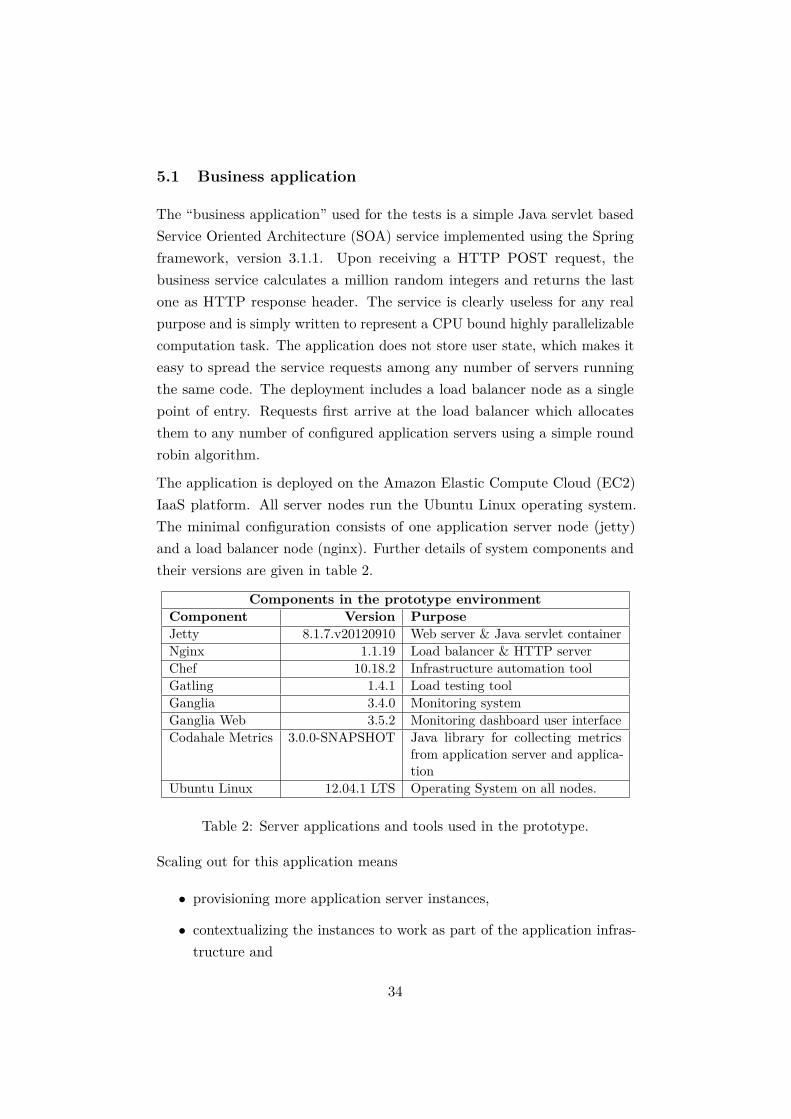
The application is deployed on the Amazon Elastic Compute Cloud (EC2)IaaS platform. All server nodes run the Ubuntu Linux operating system.The minimal configuration consists of one application server node (jetty)and a load balancer node (nginx). Further details of system components andtheir versions are given in table 2.
Components in the prototype environmentComponent Version PurposeJetty 8.1.7.v20120910 Web server & Java servlet containerNginx 1.1.19 Load balancer & HTTP serverChef 10.18.2 Infrastructure automation toolGatling 1.4.1 Load testing toolGanglia 3.4.0 Monitoring systemGanglia Web 3.5.2 Monitoring dashboard user interfaceCodahale Metrics 3.0.0-SNAPSHOT Java library for collecting metrics
from application server and applica-tion
Ubuntu Linux 12.04.1 LTS Operating System on all nodes.
Table 2: Server applications and tools used in the prototype.
Scaling out for this application means
• provisioning more application server instances,
• contextualizing the instances to work as part of the application infras-tructure and
34

• changing the infrastructure configuration to account for the newlyprovisioned instances.
Figure 7 shows the deployment diagram for the application along withelasticity controller components which will be discussed in chapter 5.2.
<<cloud provider>>
Amazon EC2
<<in
frast
ruct
ure
a
utom
atio
n>>
chef
serv
er
<<m
onito
ring>
>
gang
lia
<<cl
ient
>>
gatli
ng
Key:
UM
L 2.
0 an
d ad
ditio
nally
:
<<us
es>>
dep
ende
ncy:
<<el
astic
ity c
ontro
ller>
>
cont
rolle
r
<<lo
ad b
alan
cer>
>
ngin
xch
efcl
ient
gang
lia
repo
rter
<<ap
plic
atio
n se
rver
>>
(dyn
amic
ally
pro
visi
oned
, am
ount
v
arie
s)
jetty
gang
lia
repo
rter
chef
clie
nt
Figure 7: Prototype deployment diagram.
The QoE concept needs business requirements to determine the quality ofelasticity. Any requirement can be used as long as it is quantifiable and
35
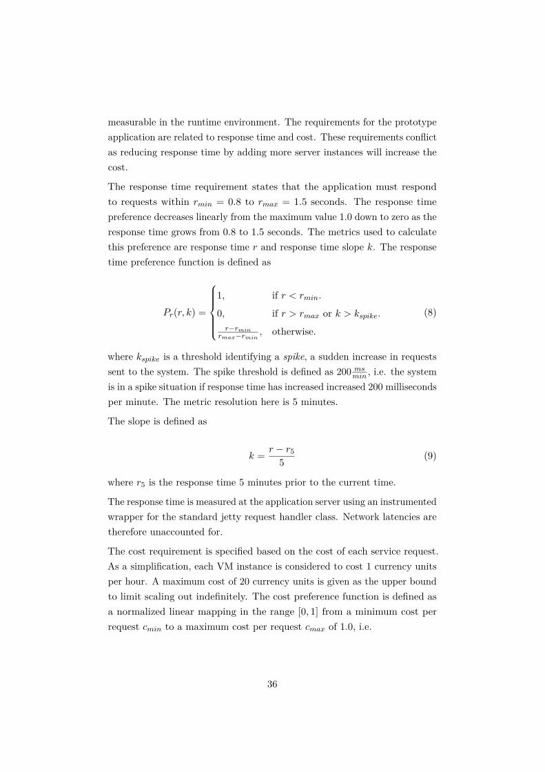
measurable in the runtime environment. The requirements for the prototypeapplication are related to response time and cost. These requirements conflictas reducing response time by adding more server instances will increase thecost.
The response time requirement states that the application must respondto requests within rmin = 0.8 to rmax = 1.5 seconds. The response timepreference decreases linearly from the maximum value 1.0 down to zero as theresponse time grows from 0.8 to 1.5 seconds. The metrics used to calculatethis preference are response time r and response time slope k. The responsetime preference function is defined as
Pr(r, k) =
1, if r < rmin.
0, if r > rmax or k > kspike.
r−rminrmax−rmin
, otherwise.
(8)
where kspike is a threshold identifying a spike, a sudden increase in requestssent to the system. The spike threshold is defined as 200 ms
min , i.e. the systemis in a spike situation if response time has increased increased 200 millisecondsper minute. The metric resolution here is 5 minutes.
The slope is defined as
k = r − r55 (9)
where r5 is the response time 5 minutes prior to the current time.
The response time is measured at the application server using an instrumentedwrapper for the standard jetty request handler class. Network latencies aretherefore unaccounted for.
The cost requirement is specified based on the cost of each service request.As a simplification, each VM instance is considered to cost 1 currency unitsper hour. A maximum cost of 20 currency units is given as the upper boundto limit scaling out indefinitely. The cost preference function is defined asa normalized linear mapping in the range [0, 1] from a minimum cost perrequest cmin to a maximum cost per request cmax of 1.0, i.e.
36

Pc(e, v, k, q, tvm) =
1, if c < cmin or v ≤ 1 or k > 50 or q > 0.
0, if c > cmax and v > 1.c−cmin
cmax−cmin, otherwise.
(10)
where e, v, k, q and tvm denote current arrival rate of requests, amountof application server VM instances currently in use, response time slope,average queue length at the application servers and maximum average serverthroughput (requests per second per VM instance) measured when theaverage response time is less than rmin, respectively. cmin is further definedas the cost per VM instance cvm divided by tvm , i.e.
cmin = cvm
tvm(11)
where tvm is measured only when r < rmin.
The application running on m1.small instances on Amazon EC2 will typicallyhandle approximately 3 requests per second with a response time less thanthe rmin of 0.8 seconds. This makes cmin roughly equal to 0.3 currency units.
5.2 Elasticity controller
The prototype elasticity controller and its monitoring and infrastructureautomation facilities are distributed between multiple server nodes in theenvironment as illustrated in figure 7. The controller exists to answer threebasic questions on elastic scaling, namely
• when to scale,
• how much and in which direction to scale and
• how to scale.
These questions map to the MAPE-K phases of analysis, planning and exe-cution. Here the deployment and implementation of the elasticity controlleris described in terms of the MAPE-K control loop (see figure 5 on page 24).An overview of the execution sequence is given in Algorithm 1 on page 38.
37
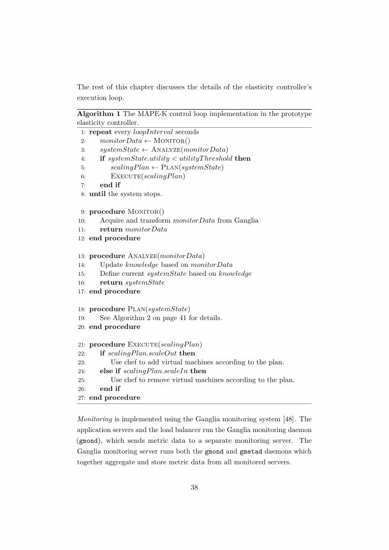
The rest of this chapter discusses the details of the elasticity controller’sexecution loop.
Algorithm 1 The MAPE-K control loop implementation in the prototypeelasticity controller.
1: repeat every loopInterval seconds2: monitorData← Monitor()3: systemState← Analyze(monitorData)4: if systemState.utility < utilityThreshold then5: scalingP lan← Plan(systemState)6: Execute(scalingP lan)7: end if8: until the system stops.
9: procedure Monitor()10: Acquire and transform monitorData from Ganglia11: return monitorData12: end procedure
13: procedure Analyze(monitorData)14: Update knowledge based on monitorData15: Define current systemState based on knowledge16: return systemState17: end procedure
18: procedure Plan(systemState)19: See Algorithm 2 on page 41 for details.20: end procedure
21: procedure Execute(scalingP lan)22: if scalingP lan.scaleOut then23: Use chef to add virtual machines according to the plan.24: else if scalingP lan.scaleIn then25: Use chef to remove virtual machines according to the plan.26: end if27: end procedure
Monitoring is implemented using the Ganglia monitoring system [48]. Theapplication servers and the load balancer run the Ganglia monitoring daemon(gmond), which sends metric data to a separate monitoring server. TheGanglia monitoring server runs both the gmond and gmetad daemons whichtogether aggregate and store metric data from all monitored servers.
38

The analysis and planning phases are the responsibility of an elasticity con-troller application written specifically for this prototype. The controllerqueries the Ganglia server for system state metrics every 20 seconds (loop-Interval in Algorithm 1) and calculates the utility based on the preferencefunctions defined for the business application. The controller first analyzesthe monitoring data together with other knowledge of the system to determinethe current system state. If utility (eq. 3 on page 26) is below a threshold of0.7 (utilityThreshold in Algorithm 1), the controller proceeds to the planningphase.
For the purpose of making a plan to scale the system either out or in, thecontroller application uses a scaling function S(X) to indicate the neededdirection and distance from optimal utility. The range of S(X) is [−1 . . . 1].A value of −1 represents the maximum impulse to scale in while a value of1 represents the maximum impulse to scale out. To factor in the directionof scaling, the preference functions are divided into two groups based onrequiring either scaling out or scaling in to improve their value. The scalingfunction then takes the form
S(X) =j∑
i=1win
i (−1 + P ini (X)) +
k∑i=1
wouti P out
i (X). (12)
where P ini denotes a preference which requires scaling in and P out
i denotes apreference which requires scaling out to improve. The weights win
i and wouti
are distributed among these two groups so thatj∑
i=1win
i = 1 andk∑
i=1wout
i = 1.
In practice the prototype used here has one preference (Pr) for scaling outand one (Pc) for scaling in, so both their weights are 1.0.
With the above definition of the scaling function S(X), it is possible thatpositive scale out preferences and negative scale in preferences cancel eachother out or interfere with each other at a time when the metrics clearlyindicate scaling is needed in a specific direction. For this reason, the costpreference is considered to be at its maximum in the following situations:
• If the slope kr is larger than 50 msmin . This indicates an increasing load
trend.
39

• If there are requests queued up at the application server(s), i.e. allavailable processing threads are processing a request and more requestsare waiting to be processed.
• If there is only one application server.
Similarly the response time preference function has one special case when itis set to minimum preference. This is when the response time slope indicatesa spike. The response time preference function then indicates the need toscale out regardless of the current response time value.
In addition to the scaling function, the elasticity controller detects trends inrequest response time by keeping track of it in a 5-minute moving window.The slope kr of response time is calculated based on the delta of the metricvalue 5 minutes ago and currently. If response time has grown more than200 ms per minute in the last 5 minutes, i.e. kr > 200 ms
min , the trend isconsidered a spike, a sudden large increase in activity.
With this information, the elasticity controller creates a scaling plan with thealgorithm given in Algorithm 2 on page 41. Scaling is done in the directionindicated by the value of the scaling function S(X) with regard to thethreshold parameters outThold and inThold. The amount of server instancesto add or remove depends on the system state. With gradual growth, theamount of application server nodes is increased by half (nonSpikeMultiplier).If the response time slope indicates a spike is underway, the amount of serverinstances to add is the current amount multiplied by three (spikeMultiplier).For scaling in, the amount is decided with the use of the cost preferencefunction Pc (eq. 10 on page 37). The cost preference is calculated withdecreasing instance count until it reaches the maximum preference value.Any instances above the count which yields maximum cost preference areterminated.
Further thresholds apply to the planning phase. In order to scale out, therequest rate needs to be larger than 2 requests/s (rrThold in Algorithm 2).To avoid repeatedly adjusting the size of the deployment, scaling in requiresthe scaling utility function value to be S(X) < −0.5, i.e. inThold is set to0.5.
The controller application delegates execution of the plan to an infrastructureautomation tool called Chef. It enables an infrastructure as code approach
40

Algorithm 2 The Planning phase of the MAPE-K loop in detail.1: procedure Plan(systemState)2: scalingUtility ← S(systemState) . See eq. 12 on page 393: if scalingUtility > outThold AND requestRate > rrThold then4: scaleOut← true5: if spike then6: addVMs← Ceil(currentV Ms ∗ spikeMultiplier)7: else8: addVMs← Ceil(currentV Ms ∗ nonSpikeMultiplier)9: end if
10: else if scalingUtility < inThold then11: scaleIn← true12: removeVMs← currentV Ms13: while Pc(removeVMs) < 1 do . See eq. 10 on page 3714: Decrement removeVMs15: end while16: removeVMs← currentV Ms− removeVMs17: end if18: return scalingP lan19: end procedure
to IT operations. All installation and configuration is done with scriptswritten in Ruby. In Chef terminology, these are referred to as recipes withincookbooks. Chef manages the state of the deployment on a separate serverwhich is a part of the infrastructure. Each server node managed by Chef runsthe chef-client daemon which periodically connects to the Chef server andconfigures the node to match the state received from the Chef server.
The MAPE-K knowledge is a shared concept between the controller appli-cation, Ganglia and the Chef server. The controller keeps track of trendaverages of metrics it fetches from Ganglia and system contextualization isdone based on system state information managed by Chef. The load balancerserver runs chef-client every 30 seconds. This is how knowledge of appli-cation servers is updated at the load balancer. Similarly the address of themonitoring server is read from Chef every time a new node is configured (andperiodically during the node’s lifetime). Any change in system configurationdue to scaling operations gets updated to live nodes in this way.
The elasticity controller’s decision making is influenced by a number ofparameters used in algorithms 1 and 2. The tests described in chapter 6 were
41

carried out with values chosen based on empirical tuning over 30 preliminarytest runs for the application under test. Table 3 lists the parameters, thevalues used in the reported tests and a summary of each parameter’s effecton the elasticity controller’s behavior.
Scaling decision parametersParameter Value used Purpose
loopInterval 20 sThe frequency at which the decision loopis executed. This needs to be larger thanthe monitoring system’s update frequency.
utilityThreshold 0.7 The value of U(X) below which planningof a scaling operation is started.
outThold 0.0 Scaling out is planned if S(X) is greaterthan this value.
inThold -0.5 Scaling in is planned if S(X) is less thanthis value.
rrThold 2.0 Scaling out is planned if requestRate isgreater than this value.
spike 200 msmin
The controller considers the system to beunder a spike load situation if the requestrate slope kr is greater than this value.
spikeMultiplier 3.0The spike multiplier determines how manynew virtual machines are added when scal-ing out in a spike situation
nonSpikeMultiplier 0.5The non spike multiplier determines howmany new virtual machines are addedwhen scaling out under normal load.
Pr(X) See eq. 8The response time preference function de-termines the business stakeholder prefer-ence value for a given response time.
Pc(X) See eq. 10The cost preference function determinesthe business stakeholder preference valuefor a given cost per request value.
Other preferencefunctions none
Further preference functions can be in-cluded in the calculation of utility U(X)and scaling utility S(X) to refine the con-troller’s behavior under varying businessrequirements.
Table 3: Parameters which influence the elasticity controller’s scaling deci-sions.
Although the monitoring system reports new values every 15 seconds, themoving average values for metrics take time to reflect a change in systemperformance. Response time, for example, is measured as a biased histogram
42

of 1028 data points. The histogram sample uses a forward-decaying algorithmwhich favors data from the past 5 minutes [23][33]. Averaged metrics areused to even out jitter (oscillation) in the measured values that could triggerunnecessary provisioning operations. The downside is that the metrics taketime to react to significant changes as well. To allow time for the metricsto react and stabilize after a provisioning operation, the system has a 3-minute quiet period after each provisioning completes. No new provisioningoperations are started during this time. This gives time for the metricsto stabilize for a new amount of virtual machines and e.g. data to startactually arrive from newly provisioned VMs, but also means the system isnot responsive to utility changes during this time. Responsiveness is furtherhindered by the time it takes to provision instances, as the total quiet periodconsists of first waiting for new instances and then waiting for metrics tostabilize.
6 Test results
This chapter discusses the performance of the elasticity controller prototypeand the test application in terms of utility preferences and the overallquality of elasticity for the application deployment described in chapter 5.Two different testing scenarios are presented along with results of how thecontroller responded to the request load generated by the scenarios. Qualityof elasticity is evaluated as a conclusion to the chapter.
6.1 Test scenarios
The elasticity controller was tested under two scenarios. Scenario 1 subjectedthe system to a gradually growing rate of requests while scenario 2 generateda sudden spike of requests. The scenarios were implemented using the Gatlingload testing tool [1].
Gatling simulates users making requests to the application. Each simulateduser sends equal requests, i.e. only one request type is used. The requesthandler calculates a million random integers and returns the last one. Afterreceiving a response, the user waits for a random amount of time between500 and 800 milliseconds before sending another request. This is repeated
43

for one hour. The actual time depends on response times and ramp downperiods.
The amount of users varies throughout the scenarios. The gradual growthscenario starts with six users and adds two more every 10 minutes. All usersfinish after one hour. The scenario steps with their timings for scenario 1are:
• 00:00 - 6 users ramp up in 30 seconds.
• 00:10 - 2 users ramp up in 1 second.
• 00:20 - 2 users ramp up in 1 second.
• 00:30 - 2 users ramp up in 1 second.
• 00:40 - 2 users ramp up in 1 second.
• 00:50 - 2 users ramp up in 1 second.
• 01:00 - 10 users ramp down in 1 second. The first 6 users ramp downin 30 seconds.
• 01:00:30 - Finished ramping down users.
The spike scenario starts with three users for five minutes, then graduallyadds six more users during a period of ten minutes and finally starts thespike of 30 users at 00:25. The spike nearly quadruples the user amountduring one minute. The spike lasts for 20 minutes until 00:45. At 00:55 Thesix user wave starts ramping down over the next 10 minutes, so that at 01:00,when the first 3 users ramp down, 3 users from the six user wave are stillramping down. Finally all users are ramped down at 01:05. The steps withtheir timings for scenario 2 are:
• 00:00 - 3 users ramp up in 5 seconds.
• 00:05 - 6 users ramp up in 600 seconds.
• 00:15 - 6 users fully ramped up.
• 00:25 - 30 users ramp up in 60 seconds (spike).
44

• 00:45 - 30 users ramp down in 60 seconds (spike ends).
• 00:55 - 6 users ramp down in 600 seconds.
• 01:00 - 3 users ramp down in 5 seconds.
• 01:05 - Finished ramping down users.
6.2 Results: Scenario 1
Scenario 1 exhibiting gradual growth in request rate was handled quite wellby the elasticity controller. Starting off with 1 application server instance and6 users, a reference throughput (tvm used in cost preference calculation) rateof 3.4 requests per second per server was established at 00:07 as show in figure19 on page 56. Utility (fig. 8 on page 52) stayed above the scaling triggervalue of 0.7 until the first two users were added at 00:10. The controller took6 minutes to react to the increased amount of users. At 00:16, utility fellbelow 0.7 due to an increase in response time (fig. 17 on page 55) to 1.2sand hence a drop in the corresponding preference function value (fig. 11 onpage 53) to 0.4. The MAPE-K planning phase was triggered and concludedwith a decision to provision one new VM instance as scaling utility (fig. 9on page 52) was positive at 0.6 at the time and response time slope (fig. 14on page 54) was under 200 indicating no spike was occurring.
Two application server instances were enough to satisfy utility for most ofthe test duration. Utility dropped below 0.7 briefly at 00:21 during thecontroller’s post provisioning quiet period. This utility fluctuation is causedby a drop in both response time and cost preference values (fig. 12 on page53). The metrics for request rate and response time fluctuated down andup at this time due to the system adjusting to the new virtual machine.Averaged metric values are affected immediately when a new instance showsup in the monitoring system (averaged system wide values are calculated bydividing a sum of each node’s metric value by the number of nodes). It takes2-3 minutes after this to start receiving actual correct data from the newnode and for 1-minute and 5-minute averaged metrics to react. The quietperiod accommodates this fluctuation and prevented a hasty further scalingdecision here.
The next significant change in utility was at 00:33. Request rate (fig. 13
45

on page 54) drops to 2 requests/s for no apparent reason but then recoversto 3 at 00:37. Response time reacts upward to nearly 1.2s a bit later at00:36 returning to 0.8s at 00:40. This appears likely to be a slow down inthe infrastructure as the request load did not change at the time. Responsetime reacts slower than request rate because it is calculated using a 5-minutemedian as opposed to a 1-minute mean for the request rate.
At 00:54, utility fell below 0.7 again. Response time had increased earlier andstarting from 00:50 request rate fell down to 4 from 6. This was likely anotherinfrastructure performance fluctuation as a comparable request rate changedid not happen after 00:40 when 2 more users started making requests justlike at 00:50. On the other hand, the effect of those additional users showsclearly in response time as it increases to 1 second after the user increase at00:40. With the response time increase followed by the request rate drop, theelasticity controller made a further scale out decision to add 1 VM instance.
The added VM arrived late for this scenario. Provisioning started at 00:54and continued until 00:59. The metrics show the VM coming properly onlinejust before the one hour mark at which the Gatling load script terminates.The completion of VM provisioning is seen in the response time preferencevalue as it increases quickly at the same time as the VM count metric (fig. 15on page 54) increases. Then response time preference decreases as the newVM starts reporting response times and takes time to get up to full speed.The scenario ends at 01:00 and the 1 minute average request rate metricreacts a minute later to drop utility below 0.7 again. This triggers anotherscaling decision whereby 2 virtual machines are terminated, returning thesystem to its original configuration of 1 application server instance.
The overall QoE value for this scenario is 0.86. The system performedrelatively well in terms of quality of elasticity. Normalizing QoE between aminimum of 0.7 and maximum of 1.0 (eq. 7 on page 28) yields a score of53% to the system given this elasticity scenario.
6.3 Results: Scenario 2
The second scenario tests the system’s behavior under a load which spikes,i.e. suddenly increases from 9 users to 39 users. Reference throughputused for cost calculation goes up to 3.6 this time at 00:12 (fig. 31 on page
46

61). The difference to the scenario 1 value of 3.4 has to be attributed tothe cloud infrastructure as the virtual machine instances are different andhence also the placement on physical hardware at Amazon’s data center ismost likely different. The maximum reference throughput was reached laterthan in scenario 1 due to the difference in user amounts. Scenario 2 has8 users making requests at 00:12 whereas scenario 1 reached its maximumthroughput with 6 users. The VM in scenario 2 could take on more load andstill perform as well as the scenario 1 VM. Performance is clearly differentbetween VM instantiations with the same specifications.
Utility (fig. 20 on page 57) was at maximum until the amount of usersreached 8. Response time had slowly increased from 00:08 with the gradualincrease of users and lead to utility dropping below the 0.7 threshold at 00:16.Provisioning of one VM instance was started and the VM became operationalat 00:20 returning utility above the threshold. The metrics jittered a lotduring the quiet period again as they adjusted to the new instance. Afterstabilizing, utility increased back to maximum at 00:26, just in time to receivethe spike.
The spike started at 00:25 with 30 additional users ramping up over thenext 60 seconds. The system was clearly not ready to handle this kind ofload as the application server request queues started filling up (fig. 30 onpage 60) which did not happen at all in scenario 1 (fig. 18 on page 55). At00:28 the response time preference (fig. 23 on page 58) quickly fell from 1.0to 0.0. Response time was increasing but the slope metric was close to 0as response time now and five minutes prior was nearly at the same level.Utility decreased below the threshold, but the elasticity controller failed todetect the spike because of the low slope value. Due to this, provisioning ofonly one additional VM instance was started at this time.
The spike continued while the single VM was being provisioned. Its intro-duction to the load balancing array understandably did nothing to make thisbetter and utility was flat at 0.5. Utility did not decrease further becausethe cost preference function was at maximum, i.e. the request rate (fig. 13on page 54) was high enough to keep cost per request low. At 00:34, sixminutes after the misfired single VM provisioning operation, the quiet periodended and the elasticity controller was able to add more VM instances. Thistime 9 more were added, as the controller is configured to triple the amount
47

of VMs if it detects a spike.
One of the 9 VMs failed in the contextualization phase and at 00:40, 8 newapplication server instances started receiving requests. During the quietperiod and even after it until 00:44, utility was below the 0.7 threshold, butno scaling operations were executed. The scaling utility metric (fig. 9 onpage 52), which indicates whether to add or remove instances, was negativebut not below 0.5, so scaling was not executed. Both the response time andcost preferences were below 0.8 at this time and they canceled each otherout in the calculation of scaling utility. The metric stabilization took longerthan previously due to the large amount of 8 new VMs, so the post scalingquiet period failed to protect the system. However as the metrics influencescaling utility in opposite directions, a further scaling operation was avoidedhere right before the spike ended.
The spike ended gradually between 00:45:00 and 00:45:30. The request ratemetric began to show this at 00:46. Cost preference decreased and responsetime preference increased to maximum. The cost increase triggered removalof 8 VMs at 00:46:30. The termination caused a sudden drop in request ratewhich brought utility down to 0.5 due to rising cost per request per server.This was during the quiet period, however, and the metrics stabilized priorto the end of the period.
With the spike over and 3 VM instances left, the system ran at approximately0.85 utility until 00:55. After this the 6 user “second wave” started rampingdown over the next 10 minutes. Utility slowly decreased due to this untila bigger impulse was given by the ramp down of the 3-user “first wave” at01:00. Metrics reacted to this at 01:00:30 and the controller brought thesystem down to its initial configuration of 1 application server instance. Theremaining second wave users finished their rampdown at 01:05 with utilityalready back at maximum since 01:02:30.
The overall QoE value for this scenario is 0.78. The system did not performwell with regard to the spike usage profile represented by this scenario. Thescaling threshold was set at 0.7. Normalizing QoE between a minimum of0.7 and maximum of 1.0 (eq. 7 on page 28) yields a score of 27% to thesystem given this elasticity scenario.
48

6.4 Notes on quality of elasticity
The QoE scores obtained in the tests were 53% for scenario 1 and 27% forscenario 2. The controller is better at managing elasticity when the metricschange slowly like in scenario 1. Main reasons for this are the delays observedafter a scaling decision execution was started. It took roughly 3-4 minutesfrom decision to the point where a new virtual machine was available toservice requests and another 3 minutes for the quiet period during whichmetrics were allowed to stabilize for the new configuration. The elasticitycontroller prototype took a simple approach to running the MAPE-K loop;it was run sequentially, one at a time. the total time between two controlloop executions could range from 20 seconds (no scaling decisions made) to6-7 minutes when the scaling plan execution phase waits to receive controlof new VM instances and contextualizes them. An improvement could be torun the control loop during provisioning and the quiet period and implementthe possibility to cancel an operation if the metrics start to give an oppositeindication while provisioning is in progress.
The metrics, which are polled every 15 seconds, are averaged for stabilitywhich makes the slower to react to changes. A 5-minute average for responsetime was used as it was readily available in the Coda Hale Metrics opensource project, but a faster metric could have helped with the reaction timeand allowed a shorter quiet period for the control loop. Similarly the responsetime slope metric was calculated over 5 minutes, which worked against spikedetection in scenario 2.
The cost metric is rather superficial in these tests as the size of the deploymentis small and hence small changes in user amount are percentually large. Inreal systems where this kind of calculation becomes relevant, there wouldbe a business case for the system and a reasonable cost preference couldbe derived from it [57]. Issues like billing period granularity, which thisprototype does not consider, then rise to a more important status. Thecontroller would then have to keep track of billing cycles and other real timecost factors to properly optimize QoE in terms of cost.
The cloud infrastructure itself played a variable role in the QoE results.Particularly in scenario 1, the request rate dropped twice for no apparentreason caused by the scenario. As the effect of this was to only reduce utility
49
within the threshold limit, these performance fluctuations reduced QoE withno reaction from the elasticity controller. In scenario 2, one of the total15 VM instance provisioning operations failed. This is notable because theoperations are automated and hence user error is eliminated as a possiblecause. Many things can still fail on many levels, as Amazon runs the EC2service on commodity hardware and the infrastructure is accessed over theInternet and provisioning relies on the availability of many other Internetservices like the Ubuntu package repositories.
As the cloud provider business model is based on guarantees of quantity overabsolute guarantees of quality, the design for failure approach [61] can beused to mitigate this kind of risk. Given the pay per use pricing model, it isinexpensive to overprovision by a certain percentage as an insurance againstfailed VM delivery or performance fluctuations.
The controller logic implemented for the prototype is based on a reactiveconcept. The controller analyzes historical data and makes decisions basedon that. Introducing a predictive analysis model could help maximize QoE[11] as the controller could know to prepare for future load before it arrives byeither provisioning new resources or deciding not to terminate old ones justbefore load is about to increase. In straightforward cases a simple schedulebased analysis could help as e.g. web applications typically have usageprofiles peaking when people work or are awake and periods of inactivityoutside of business ours or during the night.
7 Conclusion
This thesis presented an overview of cloud computing service levels andfocused on elasticity at the IaaS level. Theory of scalability was examined anddivided it into horizontal, vertical and structural (algorithmic) dimensions.Tradeoffs arising from designing applications for scalability were identifiedas difficulty of synchronizing state, use of unscalable shared resources whichquickly become bottlenecks, exponential cost of vertical scaling and designeffort for structural scalability.
The theory of horizontal scaling was examined further as that is the kind ofscaling most applicable to cloud applications. The limits of scalability werediscussed based on Amhdal’s law [9] and Gustafson’s law [32] in chapter 2.3.
50

Analysis of scalability based on multi criteria analysis of metrics was presentedbased on the work of Duboc [27].
The scalability theory was taken into cloud infrastructure context in chapter 3.The concept of rapid elasticity was introduced and the lifecycle of an elasticvirtual machine instance was walked through. Availability of data on thesystem’s performance and the quality of that data was identified as a keysuccess factor for cloud scalability.
Cloud platform and application elasticity was examined further from theviewpoint of a MAPE-K control loop in chapter 4. The concept of utility ofan application deployment was developed based on multi-criteria analysisof business requirements. Quality of Elasticity (QoE) was introduced as ametric of utility over time. To facilitate comparisons and contextualizationof QoE to a specific system in a specific environment, a QoE score metricwas defined as the normalized value of QoE between a deployment specificlower bound threshold and maximum.
Design principles of elastic application architectures were discussed brieflyin chapter 4.6. The design for failure philosophy is a key point in thinkingof the fitness for purpose of cloud provider SLAs. The cloud providerbusiness model and offering is fundamentally different from the traditionalIT operations without virtualization. Designing applications so that theycan handle infrastructure failures is key to success.
A prototype elasticity controller implementation is presented in chapter 5.The prototype is then put to test in chapter 6. The results confirm theapplicability of the controller to its purpose and indicate areas in need offurther study that have the potential to improve the QoE scores attainedwith the controller. In particular the quality and reactiveness of metrics, VMprovisioning speed and parallelization of the elasticity controller’s decisionmaking functionality are identified as areas of possible improvement. Thequality of the controller’s decisions could be improved by moving from areactive analysis model to a predictive one.
The QoE results correctly indicate that the elasticity controller handled testscenario 1 better than scenario 2 in terms of the business requirements usedto define QoE for the prototype. The QoE concept should be put to furthertest using varying business requirement definitions to determine its universalapplicability to measuring cloud elasticity.
51

A Figures for test scenario 1
����� ����� ����� ����� ����� ����� ����� ���������
����
����
����
����
����
�������
�����������������������
�����������
�����
������
����������� �������������� �������������� ��������������������
Figure 8: Utility during test scenario 1
����� ����� ����� ����� ����� ����� ����� ���������
����
����
����
����
�������
�������������������������������
�����������
�����
������
������������������� �������������� �������������� ��������������������
Figure 9: Scaling utility during test scenario 1
52
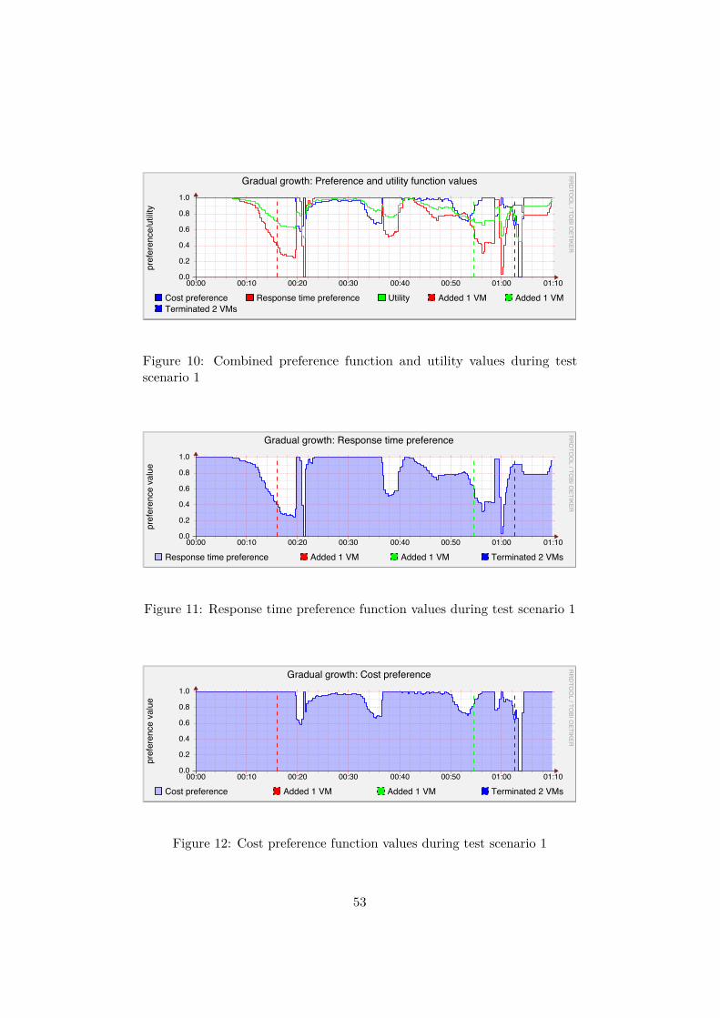
����� ����� ����� ����� ����� ����� ����� ���������
����
����
����
����
����
������������������
������������������������������������������������������
�����������
�����
������
������������������� ���������������������������� ����������� �������������� ��������������
��������������������
Figure 10: Combined preference function and utility values during testscenario 1
����� ����� ����� ����� ����� ����� ����� ���������
����
����
����
����
����
����������������
����������������������������������������
�����������
�����
������
���������������������������� �������������� �������������� ��������������������
Figure 11: Response time preference function values during test scenario 1
����� ����� ����� ����� ����� ����� ����� ���������
����
����
����
����
����
����������������
�������������������������������
�����������
�����
������
������������������� �������������� �������������� ��������������������
Figure 12: Cost preference function values during test scenario 1
53

����� ����� ����� ����� ����� ����� ����� ���������
����
����
����
����
����
����������
���������������������������������������������
�����������
�����
������
�������������������������������� ���������������������� �������������� ��������������
��������������������
Figure 13: Request rate during test scenario 1
����� ����� ����� ����� ����� ����� ����� ���������
����
����
����
����
����
����
������
��������������������������������������������
�����������
�����
������
����������������������� �������������� �������������� ��������������������
Figure 14: Response time slope during test scenario 1
����� ����� ����� ����� ����� ����� ����� ���������
����
����
����
������
������������������������������������������
�����������
�����
������
������������ �������������� �������������� ��������������������
Figure 15: Scaling utility during test scenario 1
54

����� ����� ����� ����� ����� ����� ����� ���������
����
����
����
����
�������������
�������������������������������������������
�����������
�����
������
������������������������������� �������������� �������������� ��������������������
Figure 16: Cost per request per second during test scenario 1
����� ����� ����� ����� ����� ����� ����� �����
������
������
������������
������������������������������������
�����������
�����
������
��������������������������������� �������������� �������������� ��������������������
Figure 17: Response time during test scenario 1
����� ����� ����� ����� ����� ����� ����� ���������
����
����
����
����
����
��������������������
������������������������������������
�����������
�����
������
�������������������������������� ���������������������� �������������� ��������������
��������������������
Figure 18: Application server request queue size during test scenario 1
55

����� ����� ����� ����� ����� ����� ����� �����
����
����
����
����������
����������������������������������������������������������������
�����������
�����
������
������������������������ �������������� �������������� ��������������������
Figure 19: Reference throughput during test scenario 1
56
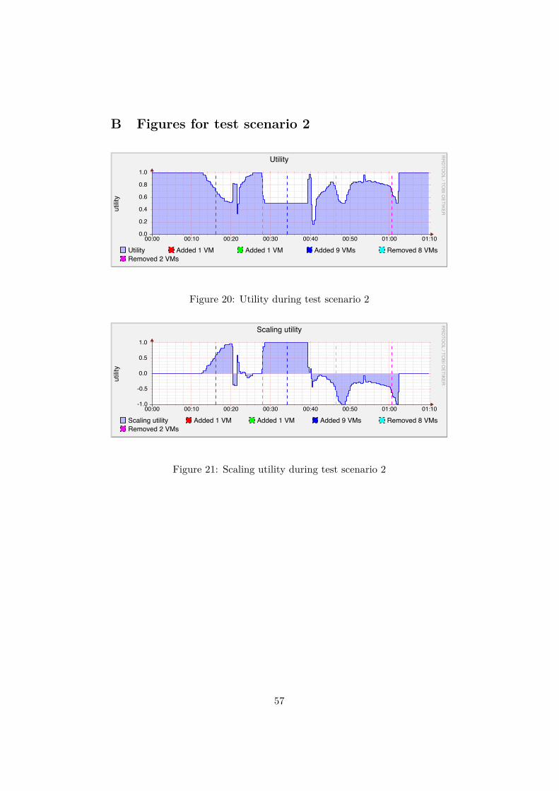
B Figures for test scenario 2
����� ����� ����� ����� ����� ����� ����� ���������
����
����
����
����
����
�������
�������
�����������
�����
������
����������� �������������� �������������� ��������������� �����������������
�����������������
Figure 20: Utility during test scenario 2
����� ����� ����� ����� ����� ����� ����� ���������
����
����
����
����
�������
���������������
�����������
�����
������
������������������� �������������� �������������� ��������������� �����������������
�����������������
Figure 21: Scaling utility during test scenario 2
57

����� ����� ����� ����� ����� ����� ����� ���������
����
����
����
����
����
������������������
��������������������������������������
�����������
�����
������
������������������� ���������������������������� ����������� �������������� ��������������
��������������� ����������������� �����������������
Figure 22: Combined preference function and utility values during testscenario 2
����� ����� ����� ����� ����� ����� ����� ���������
����
����
����
����
����
����������������
������������������������
�����������
�����
������
���������������������������� �������������� �������������� ���������������
����������������� �����������������
Figure 23: Response time preference function values during test scenario 2
����� ����� ����� ����� ����� ����� ����� ���������
����
����
����
����
����
����������������
���������������
�����������
�����
������
������������������� �������������� �������������� ��������������� �����������������
�����������������
Figure 24: Cost preference function values during test scenario 2
58

����� ����� ����� ����� ����� ����� ����� ���������
����
����
����
����
����������
�����������������������������
�����������
�����
������
�������������������������������� ���������������������� �������������� ��������������
��������������� ����������������� �����������������
Figure 25: Request rate during test scenario 2
����� ����� ����� ����� ����� ����� ����� �����
����
����
����
������
����������������������������
�����������
�����
������
������������������������ �������������� �������������� ��������������� �����������������
�����������������
Figure 26: Response time slope during test scenario 2
����� ����� ����� ����� ����� ����� ����� ���������
����
����
����
����
����
����
������
��������������������������
�����������
�����
������
������������ �������������� �������������� ��������������� �����������������
�����������������
Figure 27: Scaling utility during test scenario 2
59
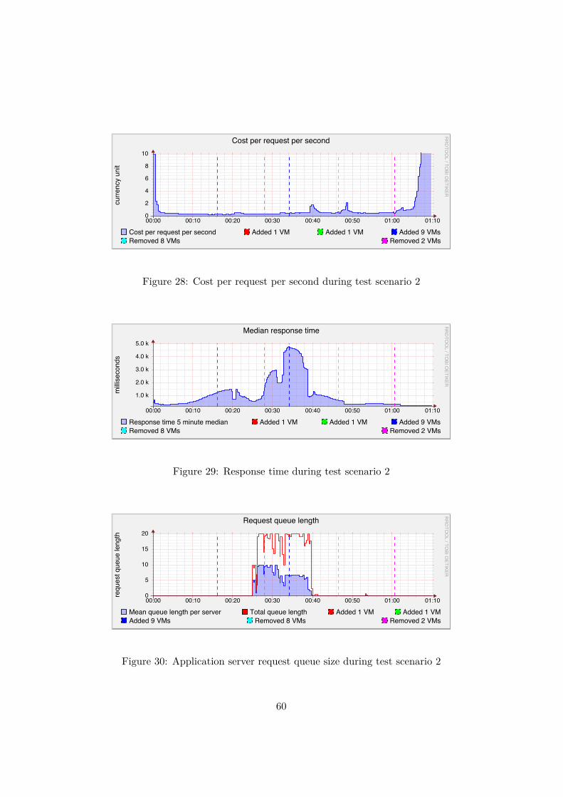
����� ����� ����� ����� ����� ����� ����� ���������
����
����
����
����
����
�������������
���������������������������
�����������
�����
������
������������������������������� �������������� �������������� ���������������
����������������� �����������������
Figure 28: Cost per request per second during test scenario 2
����� ����� ����� ����� ����� ����� ����� �����
������
������
������
������
������
������������
��������������������
�����������
�����
������
��������������������������������� �������������� �������������� ���������������
����������������� �����������������
Figure 29: Response time during test scenario 2
����� ����� ����� ����� ����� ����� ����� ���������
����
����
����
����
��������������������
��������������������
�����������
�����
������
�������������������������������� ���������������������� �������������� ��������������
��������������� ����������������� �����������������
Figure 30: Application server request queue size during test scenario 2
60

����� ����� ����� ����� ����� ����� ����� �����
����
����
����
����
����������
������������������������������������������������
�����������
�����
������
������������������������ �������������� �������������� ��������������� �����������������
�����������������
Figure 31: Reference throughput during test scenario 2
61

References
[1] Gatling Project - Stress Tool. http://gatling-tool.org/, visited on4.3.2013.
[2] SETI@home website. http://setiathome.berkeley.edu/, visited on18/03/12.
[3] Amazon EC2 Service Level Agreement, 2008. http://aws.amazon.com/
ec2-sla/, visited on 3.3.2013.
[4] File:Gustafson.png by Peahihawaii (Own work) [CC-BY-SA-3.0 (http://creativecommons.org/licenses/by-sa/3.0) or GFDL(http://www.gnu.org/copyleft/fdl.html)], via Wikimedia Commons, 2011.http://commons.wikimedia.org/wiki/File:Gustafson.png, visitedon 3.3.2013.
[5] OpsCode Chef website, 2012. http://www.opscode.com/chef/, visitedon 1st April, 2012.
[6] Puppet Labs website, 2012. http://puppetlabs.com/, visited on 1stApril, 2012.
[7] File:AmdahlsLaw.svg by Daniels220 at English Wikipedia(Own work based on: File:AmdahlsLaw.png) [CC-BY-SA-3.0(http://creativecommons.org/licenses/by-sa/3.0)], via WikimediaCommons, 2013. http://commons.wikimedia.org/wiki/File:
AmdahlsLaw.svg, visited on 3.3.2013.
[8] Ahola, Jukka, Ashraf, Adnan, Gupta, Bibha, Hassan, Usman, Har-tikainen, Mikko, Helenius, Marko, Heljanko, Keijo, Järvenpää, Jarkko,Kallio, Aleksi, Kannisto, Joona, Karppinen, Kaarina, Lafond, Sébastien,Lagerspetz, Eemil, Lehtonen, Tero, Lilius, Johan, Mikkonen, Tommi,Niemenmaa, Matti, Paksula, Matti, Palkosaari, Ville, Pietikäinen,Pekka, Porres, Ivan, Raivio, Yrjö, Repo, Petrus, Röning, Juha, Savola,Reijo, Schumacher, Andrée, Selänniemi, Johan, Smeds, Jens, Svan,Lauri, Svanfeldt-Winter, Olle, Syeed, Mahbubul, Takanen, Sami,Tarkoma, Sasu, Thi Thuy, Trang Tran, Tripathi, Abhishek, Uharani,Zineellabidine, Uusitalo, Ilkka, and Visuri, Miska: Best Practices forCloud Computing. Technical report, Tieto- ja viestintäteollisuuden
62

tutkimus TIVIT Oy, 2010. http://www.cloudsoftwareprogram.org/
rs/2234/9ed65124-0873-400e-bc8a-9c85c1f1afa8/63b/filename/
d1-1-2-techreportbestpracticesforcloudcomputing.pdf.
[9] Amdahl, Gene M: Validity of the single processor approach to achievinglarge scale computing capabilities. In Proceedings of the April 18-20,1967, spring joint computer conference, pages 483–485. ACM, 1967.
[10] Andrews, G R: Foundations of multithreaded, parallel, and distributedprogramming. Addison-Wesley, 2000, ISBN 9780201357523.
[11] Armbrust, Michael, Stoica, Ion, Zaharia, Matei, Fox, Armando, Grif-fith, Rean, Joseph, Anthony D., Katz, Randy, Konwinski, Andy, Lee,Gunho, Patterson, David, and Rabkin, Ariel: A view of cloud computing.Communications of the ACM, 53(4):50, April 2010, ISSN 00010782.http://portal.acm.org/citation.cfm?doid=1721654.1721672.
[12] Boloor, Keerthana, Chirkova, Rada, Salo, Tiia, and Viniotis, Yan-nis: Management of SOA-Based Context-Aware Applications Hostedin a Distributed Cloud Subject to Percentile Constraints. 2011 IEEEInternational Conference on Services Computing, pages 88–95, July2011. http://ieeexplore.ieee.org/lpdocs/epic03/wrapper.htm?
arnumber=6009248.
[13] Brebner, Paul C.: Is your cloud elastic enough? In Proceedingsof the third joint WOSP/SIPEW international conference on Per-formance Engineering - ICPE ’12, page 263, New York, New York,USA, 2012. ACM Press, ISBN 9781450312028. http://dl.acm.org/
citation.cfm?doid=2188286.2188334.
[14] Buyya, Rajkumar, Ranjan, Rajiv, and Calheiros, RodrigoN.: Inter-Cloud: Utility-Oriented Federation of Cloud Computing Environmentsfor Scaling of Application Services. In Hsu, Ching Hsien, Yang,LaurenceT., Park, JongHyuk, and Yeo, Sang Soo (editors): Algo-rithms and Architectures for Parallel Processing, volume 6081 of Lec-ture Notes in Computer Science, pages 13–31. Springer Berlin Heidel-berg, 2010, ISBN 978-3-642-13118-9. http://dx.doi.org/10.1007/
978-3-642-13119-6_2.
63
[15] Buyya, Rajkumar, Yeo, Chee Shin, Venugopal, Srikumar, Broberg,James, and Brandic, Ivona: Cloud computing and emerging IT plat-forms: Vision, hype, and reality for delivering computing as the5th utility. Future Generation Computer Systems, 25(6):599–616,June 2009, ISSN 0167739X. http://dl.acm.org/citation.cfm?id=
1528937.1529211.
[16] Cáceres, Juan, Vaquero, L.M., Rodero-Merino, L., Polo, Álvaro, andHierro, J.J.: Service Scalability Over the Cloud. In Handbook of CloudComputing, pages 357–377. Springer, 2010. http://www.springerlink.
com/index/MT877601J8700786.pdf.
[17] Cattell, Rick: Scalable SQL and NoSQL data stores. ACM SIGMODRecord, 39(4), 2011. http://dl.acm.org/citation.cfm?id=1978919.
[18] Chapman, Clovis, Emmerich, Wolfgang, Marquez, Fermin Galan, Clay-man, Stuart, and Galis, Alex: Elastic service definition in computationalclouds. 2010 IEEE/IFIP Network Operations and Management Sym-posium Workshops, pages 327–334, 2010. http://ieeexplore.ieee.
org/lpdocs/epic03/wrapper.htm?arnumber=5486555.
[19] Chen, Xi, Chen, Haopeng, Zheng, Qing, Wang, Wenting, and Liu,Guodong: Characterizing web application performance for maximiz-ing service providers’ profits in clouds. 2011 International Confer-ence on Cloud and Service Computing, pages 191–198, December2011. http://ieeexplore.ieee.org/lpdocs/epic03/wrapper.htm?
arnumber=6138519.
[20] Chen, Yuan, Iyer, Subu, Liu, Xue, Milojicic, Dejan, and Sahai,Akhil: Translating Service Level Objectives to lower level policiesfor multi-tier services. Cluster Computing, 11(3):299–311, July2008, ISSN 1386-7857. http://www.springerlink.com/index/10.
1007/s10586-008-0059-6.
[21] Clements, Paul, Kazman, Rick, and Klein, Mark: The ATAM - A Methodfor Architecture Evaluation. In Evaluating Software Architectures: Meth-ods and Case Studies, chapter 3, pages 43–84. Addison Wesley, 2002,ISBN 978-0201704822.
64

[22] Cormen, T H, Leiserson, C E, Rivest, R L, and Stein, C: IntroductionTo Algorithms. MIT Press, 2001, ISBN 9780262032933.
[23] Cormode, G, Shkapenyuk, V, Srivastava, D, and Xu, Bojian: ForwardDecay: A Practical Time Decay Model for Streaming Systems. In DataEngineering, 2009. ICDE ’09. IEEE 25th International Conference on,pages 138–149, 2009.
[24] Crosby, S, Doyle, R, Gering, M, and Gionfriddo, M: Open VirtualizationFormat Specification (OVF 1.1.0). Technical report, Distributed Manage-ment Task Force (DMTF), 2010. http://www.dmtf.org/standards/
ovf.
[25] Cunha, Matheus, Mendonca, Nabor, and Sampaio, Americo: Investi-gating the Impact of Deployment Configuration and User Demand ona Social Network Application in the Amazon EC2 Cloud. 2011 IEEEThird International Conference on Cloud Computing Technology andScience, (section IV):746–751, November 2011. http://ieeexplore.
ieee.org/lpdocs/epic03/wrapper.htm?arnumber=6133224.
[26] Duboc, Leticia, Letier, Emmanuel, Rosenblum, David S., and Wicks,Tony: A Case Study in Eliciting Scalability Requirements. 2008 16thIEEE International Requirements Engineering Conference, pages 247–252, September 2008. http://ieeexplore.ieee.org/lpdocs/epic03/
wrapper.htm?arnumber=4685677.
[27] Duboc, Leticia, Rosenblum, David, and Wicks, Tony: A frameworkfor characterization and analysis of software system scalability. InProceedings of the the 6th joint meeting of the European softwareengineering conference and the ACM SIGSOFT symposium on Thefoundations of software engineering - ESEC-FSE ’07, page 375, NewYork, New York, USA, 2007. ACM Press, ISBN 9781595938114. http:
//portal.acm.org/citation.cfm?doid=1287624.1287679.
[28] Emeakaroha, Vincent C., Brandic, Ivona, Maurer, Michael, and Dustdar,Schahram: Low level Metrics to High level SLAs - LoM2HiS framework:Bridging the gap between monitored metrics and SLA parametersin cloud environments. In 2010 International Conference on HighPerformance Computing & Simulation, pages 48–54. IEEE, June 2010,
65

ISBN 978-1-4244-6827-0. http://ieeexplore.ieee.org/xpls/abs_
all.jsp?arnumber=5547150http://ieeexplore.ieee.org/lpdocs/
epic03/wrapper.htm?arnumber=5547150.
[29] Funika, Wlodzimierz and Koperek, P: Scalable Resource Provision-ing in the Cloud Using Business Metrics. In ADVCOMP 2011,The Fifth International Conference on Advanced Engineering Com-puting and Applications in Sciences, number 1, pages 72–77, 2011,ISBN 9781612081724. http://www.thinkmind.org/index.php?view=
article&articleid=advcomp_2011_3_50_20173.
[30] Furht, Borko and Escalante, Armando (editors): Handbook ofCloud Computing. Springer, 2010, ISBN 978-1-4419-6523-3.http://www.springer.com/computer/communication+networks/
book/978-1-4419-6523-3.
[31] Gunawi, HS, Do, T, and Hellerstein, JM: Failure as a service (faas):A cloud service for large-scale, online failure drills. Technical report,EECS Department, University of California, Berkeley, 2011. http://
www.eecs.berkeley.edu/Pubs/TechRpts/2011/EECS-2011-87.pdf.
[32] Gustafson, John L: Reevaluating Amdahl’s law. Commun. ACM,31(5):532–533, 1988, ISSN 0001-0782. http://doi.acm.org/10.1145/
42411.42415.
[33] Hale, Coda: Coda Hale Metrics User Manual. http://metrics.
codahale.com/manual/core/#man-core-histograms, visited on4.3.2013.
[34] Hill, M D and Marty, M R: Amdahl’s Law in the Multicore Era. Com-puter, 41(7):33–38, 2008, ISSN 0018-9162.
[35] Hill, Mark D: What is scalability? ACM SIGARCH Computer Ar-chitecture News, 18(4):18–21, December 1990, ISSN 01635964. http:
//portal.acm.org/citation.cfm?doid=121973.121975.
[36] Höfer, C. N. and Karagiannis, G.: Cloud computing services: taxonomyand comparison. Journal of Internet Services and Applications, pages81–94, June 2011, ISSN 1867-4828. http://www.springerlink.com/
index/10.1007/s13174-011-0027-x.
66
[37] Huebscher, Markus C. and McCann, Julie a.: A survey of autonomiccomputing—degrees, models, and applications. ACM Computing Surveys,40(3):1–28, August 2008, ISSN 03600300. http://portal.acm.org/
citation.cfm?doid=1380584.1380585.
[38] Iqbal, Waheed, Dailey, Matthew N., Carrera, David, and Janecek, Paul:Adaptive resource provisioning for read intensive multi-tier applicationsin the cloud. Future Generation Computer Systems, 27(6):871–879, June2011, ISSN 0167739X. http://linkinghub.elsevier.com/retrieve/
pii/S0167739X10002098.
[39] Islam, Sadeka, Lee, Kevin, Fekete, Alan, and Liu, Anna: How a consumercan measure elasticity for cloud platforms. Proceedings of the third jointWOSP/SIPEW international conference on Performance Engineering- ICPE ’12, page 85, 2012. http://dl.acm.org/citation.cfm?doid=
2188286.2188301.
[40] Ke, Chih Kun, Lin, Zheng Hua, Wu, Mei Yu, and Chang, Shih Fang: AnOptimal Selection Approach for a Multi-tenancy Service Based on a SLAUtility. 2012 International Symposium on Computer, Consumer andControl, pages 410–413, June 2012. http://ieeexplore.ieee.org/
lpdocs/epic03/wrapper.htm?arnumber=6228333.
[41] Kijsipongse, Ekasit and Vannarat, Sornthep: Autonomic resource pro-visioning in rocks clusters using Eucalyptus cloud computing. In Pro-ceedings of the International Conference on Management of EmergentDigital EcoSystems - MEDES ’10, page 61, New York, New York,USA, 2010. ACM Press, ISBN 9781450300476. http://portal.acm.
org/citation.cfm?doid=1936254.1936265.
[42] Kirschnick, Johannes: Toward an Architecture for the AutomatedProvisioning of Cloud Services. IEEE Communications Magazine,(December):124–131, 2010.
[43] Korpela, E., Werthimer, D., Anderson, D., Cobb, J., and Leboisky,M.: SETI@home-massively distributed computing for SETI. Computingin Science & Engineering, 3(1):78–83, 2001, ISSN 15219615. http:
//ieeexplore.ieee.org/xpl/freeabs_all.jsp?arnumber=895191.
67
[44] Liu, Huan: Rapid application configuration in Amazon cloud using con-figurable virtual appliances. In Proceedings of the 2011 ACM Sym-posium on Applied Computing - SAC ’11, page 147, New York, NewYork, USA, March 2011. ACM Press, ISBN 9781450301138. http:
//dl.acm.org/citation.cfm?id=1982185.1982221.
[45] Mao, Ming and Humphrey, Marty: Auto-scaling to minimize costand meet application deadlines in cloud workflows. In Proceedingsof 2011 International Conference for High Performance Computing,Networking, Storage and Analysis on - SC ’11, page 1, New York,New York, USA, 2011. ACM Press, ISBN 9781450307710. http:
//dl.acm.org/citation.cfm?doid=2063384.2063449.
[46] Marshall, Paul, Keahey, Kate, and Freeman, Tim: Elastic Site: UsingClouds to Elastically Extend Site Resources. 2010 10th IEEE/ACMInternational Conference on Cluster, Cloud and Grid Computing, pages43–52, 2010. http://ieeexplore.ieee.org/lpdocs/epic03/wrapper.
htm?arnumber=5493493.
[47] Marston, Sean, Li, Zhi, Bandyopadhyay, Subhajyoti, Zhang, Juheng, andGhalsasi, Anand: Cloud computing — The business perspective. DecisionSupport Systems, 51(1):176–189, April 2011, ISSN 01679236. http:
//linkinghub.elsevier.com/retrieve/pii/S0167923610002393.
[48] Massie, Matthew L, Chun, Brent N, and Culler, David E: The gangliadistributed monitoring system: design, implementation, and experience.Parallel Computing, 30(7):817–840, July 2004, ISSN 01678191. http:
//linkinghub.elsevier.com/retrieve/pii/S0167819104000535.
[49] Mell, Peter and Grance, Timothy: The NIST Definition of CloudComputing, 2011. http://csrc.nist.gov/publications/nistpubs/
800-145/SP800-145.pdf.
[50] Middleton, AnthonyM.: Data-Intensive Technologies for CloudComputing. In Furht, Borko and Escalante, Armando (edi-tors): Handbook of Cloud Computing, pages 83–136. SpringerUS, 2010, ISBN 978-1-4419-6523-3. http://dx.doi.org/10.1007/
978-1-4419-6524-0_5.
68

[51] Müller, H, Kienle, H, and Stege, U: Autonomic Computing Now You SeeIt, Now You Don’t. In Software Engineering - International SummerSchools, ISSSE 2006-2008, Salerno, Italy, Revised Tutorial Lectures,volume 5413, pages 32–54. Springer Berlin Heidelberg, 2009. http:
//www.nature.com/nature/journal/v435/n7046/full/4351165a.
htmlhttp://www.springerlink.com/index/0k008550k285gq9v.pdf.
[52] Petcu, Dana, Macariu, Georgiana, Panica, Silviu, and Crăciun, Ciprian:Portable Cloud applications—From theory to practice. Future GenerationComputer Systems, pages 1–14, January 2012, ISSN 0167739X. http:
//linkinghub.elsevier.com/retrieve/pii/S0167739X12000210.
[53] Rodero-Merino, Luis, Vaquero, Luis M., Gil, Victor, Galán, Fer-mín, Fontán, Javier, Montero, Rubén S., and Llorente, Ignacio M.:From infrastructure delivery to service management in clouds. Fu-ture Generation Computer Systems, 26(8):1226–1240, October 2010,ISSN 0167739X. http://linkinghub.elsevier.com/retrieve/pii/
S0167739X10000294.
[54] Roy, Nilabja, Dubey, Abhishek, and Gokhale, Aniruddha: Efficient Au-toscaling in the Cloud Using Predictive Models for Workload Forecasting.2011 IEEE 4th International Conference on Cloud Computing, pages500–507, July 2011. http://ieeexplore.ieee.org/lpdocs/epic03/
wrapper.htm?arnumber=6008748.
[55] Stewart, J: Calculus: Early Transcendentals. Textbooks Availablewith Cengage YouBook Series. Brooks/Cole, 2010, ISBN 9780538497909.http://books.google.fi/books?id=QyOYWR9RLI8C.
[56] Stonebraker, Michael: The case for shared nothing. Database EngineeringBulletin, 9(1):4–9, 1986.
[57] Suleiman, Basem, Sakr, Sherif, Jeffery, Ross, and Liu, Anna: On un-derstanding the economics and elasticity challenges of deploying busi-ness applications on public cloud infrastructure. Journal of InternetServices and Applications, December 2011, ISSN 1867-4828. http:
//www.springerlink.com/index/10.1007/s13174-011-0050-y.
[58] Tan, Yongmin, Nguyen, Hiep, and Gu, Xiaohui: PREPARE: PredictivePerformance Anomaly Prevention for Virtualized Cloud Systems. Proc.
69

of ICDCS, (Vcl), 2012. http://www4.ncsu.edu/~ytan2/icdcs2012_
tan.pdf.
[59] Van den Bossche, Ruben, Vanmechelen, Kurt, and Broeckhove, Jan:Cost-Optimal Scheduling in Hybrid IaaS Clouds for Deadline ConstrainedWorkloads. 2010 IEEE 3rd International Conference on Cloud Comput-ing, pages 228–235, July 2010. http://ieeexplore.ieee.org/lpdocs/
epic03/wrapper.htm?arnumber=5557990.
[60] Vaquero, Luis M., Rodero-Merino, Luis, and Buyya, Rajkumar: Dynam-ically scaling applications in the cloud. ACM SIGCOMM ComputerCommunication Review, 41(1):45, January 2011, ISSN 01464833.http://doi.acm.org/10.1145/1925861.1925869http://portal.
acm.org/citation.cfm?doid=1925861.1925869.
[61] Varia, Jinesh: Architecting for the cloud: Best practices. TechnicalReport May, Amazon Web Services, 2010.
[62] Verma, Akshat, Kumar, Gautam, and Koller, Ricardo: The cost of recon-figuration in a cloud. Proceedings of the 11th International MiddlewareConference Industrial track on - Middleware Industrial Track ’10, pages11–16, 2010. http://portal.acm.org/citation.cfm?doid=1891719.
1891721.
[63] Wilder, B: Cloud Architecture Patterns. Oreilly and Associate Series.O’Reilly Vlg. GmbH & Company, 2012, ISBN 9781449319779. http:
//books.google.fi/books?id=ON1RoKiCBBkC.
[64] Wilkes, John: PRESS: PRedictive Elastic ReSource Scaling for cloudsystems. 2010 International Conference on Network and Service Man-agement, pages 9–16, October 2010. http://ieeexplore.ieee.org/
lpdocs/epic03/wrapper.htm?arnumber=5691343.
[65] Wu, Linlin, Garg, Saurabh Kumar, and Buyya, Rajkumar: SLA-BasedResource Allocation for Software as a Service Provider (SaaS) in CloudComputing Environments. 2011 11th IEEE/ACM International Sym-posium on Cluster, Cloud and Grid Computing, pages 195–204, May2011. http://ieeexplore.ieee.org/lpdocs/epic03/wrapper.htm?
arnumber=5948610.
70