theory manual english nov 2010 - deep excavation manual_… · deepxcav theory manual: ... rankine...
TRANSCRIPT

DeepXcav theory manual: Developed by Ce.A.S. srl, Italy and Deep Excavation LLC, U.S.A.
Page | 1
DEEPXCAV
A SOFTWARE FOR ANALYSIS AND DESIGN OF RETAINING WALLS
THEORY MANUAL
RELEASE 9.1.1.9 - November 2011

DeepXcav theory manual: Developed by Ce.A.S. srl, Italy and Deep Excavation LLC, U.S.A.
Page | 2
Table of Contents
Section Title Page 1 Introduction 4
2 General Analysis Methods 4
3 Ground water analysis methods 4
4 Undrained‐Drained Analysis for clays 4
5 Active and Passive Coefficients of Lateral Earth Pressures 5
5.1 Active and Passive Lateral Earth Pressures in Conventional Analyses
6
5.2 Active and Passive Lateral Earth Pressures in PARATIE module 6
5.3 Passive Pressure Equations 10
5.4 Classical Earth Pressure Options 11
5.4.1 Active & Passive Pressures for non‐Level Ground 11
5.4.2 Peck 1969 Earth Pressure Envelopes 13
5.4.3 FHWA Apparent Earth Pressures 14
5.4.4 FHWA Recommended Apparent Earth Pressure Diagram for Soft to Medium Clays
16
5.4.5 FHWA Loading for Stratified Soil Profiles 16
5.4.6 Modifications to stiff clay and FHWA diagrams 19
5.4.7 Verification Example for Soft Clay and FHWA Approach 22
5.4.8 Custom Trapezoidal Pressure Diagrams 24
5.4.9 Two Step Rectangular Pressure Diagrams 25
5.5 Vertical wall adhesion in undrained loading 26
6 Eurocode 7 analysis methods 27
6.1 Safety Parameters for Ultimate Limit State Combinations 28
6.2 Automatic generation of active and passive lateral earth pressure factors in EC7 type approaches.
35
6.3 Determination of Water Pressures & Net Water Pressure Actions in the new software (Conventional Limit Equilibrium Analysis)
36
6.4 Surcharges 37
6.5 Line Load Surcharges 38
6.6 Strip Surcharges 40
6.7 Other 3D surcharge loads 40
7 Analysis Example with EC7 42
8 Ground anchor and helical anchor capacity calculations Ground Anchor Capacity Calculations
61
8.1 Ground Anchor Capacity Calculations 61
8.2 Helical anchor capacity calculations 67

DeepXcav theory manual: Developed by Ce.A.S. srl, Italy and Deep Excavation LLC, U.S.A.
Page | 3
Section Title Page 9 Geotechnical Safety Factors 71
9.1 Introduction 71
9.1.1 Introduction 71
9.1.2 Cantilever Walls (conventional analysis) 72
9.1.3 Walls supported by a single bracing level in conventional analyses.
73
9.1.4 Walls supported by a multiple bracing levels (conventional analysis)
73
9.2 Clough Predictions & Basal Stability Index 74
9.3 Ground surface settlement estimation 76
10 Handling unbalanced water pressures in Paratie 78
11 Wall Types ‐ Stiffness and Capacity Calculations 79
12 Seismic Pressure Options 83
12.1 Selection of base acceleration and site effects 84
12.2 Determination of retaining structure response factor R 85
12.3 Seismic Thrust Options 87
12.3.1 Semirigid pressure method 87
12.3.2 Mononobe‐Okabe 88
12.3.3 Richards Shi method 89
12.3.4 User specified external 89
12.3.5 Wood Automatic method 90
12.3.6 Wood Manual 90
12.4 Water Behavior during earthquakes 90
12.5 Wall Inertia Seismic Effects 91
12.6 Verification Example 92
13 Verification of free earth method for a 10ft cantilever excavation
96
14 Verification of 20 ft deep single‐level‐supported excavation 100
15 Verification of 30 ft excavation with two support levels 105
Appendix A APPENDIX: Verification of Passive Pressure Coefficient Calculations
109
Appendix B APPENDIX: Sample Paratie Input File Generated by New Software Program
113

DeepXcav theory manual: Developed by Ce.A.S. srl, Italy and Deep Excavation LLC, U.S.A.
Page | 4
1. Introduction
This document briefly introduces the new DeepXcav‐Paratie combined software features, analysis
methods, and theoretical background. The handling of Eurocode 7 is emphasized through an
example of a simple single anchor wall.
2. General Analysis Methods
The combined DeepXcav‐Paratie software is capable of analyzing braced excavations with
“conventional” limit‐equilibrium‐methods and beam on elastic foundations (i.e. the traditional
PARATIE engine). An excavation can be analyzed in one of the following sequences:
a) Conventional analysis only
b) Paratie analysis only
c) Combined “Conventional”‐Paratie Analysis: 1st Conventional analysis with traditional safety
factors stored in memory. Once the traditional analysis is completed, then the Paratie
analysis is launched.
3. Ground water analysis methods
The software offers the following options for modeling groundwater:
a) Hydrostatic: Applicable for both conventional and Paratie analysis. In Paratie,
hydrostatic conditions are modeled by extending the “wall lining” effect to 100 times the
wall length below the wall bottom.
b) Simplified flow: Applicable for both conventional and Paratie analysis. This is a simplified
1D flow around the wall. In the Paratie analysis mode, the traditional Paratie water flow
option is employed.
c) Full Flow Net analysis: Applicable for both conventional and Paratie analysis. Water
pressures are determined by performing a 2D finite difference flow analysis. In PARATIE,
water pressures are then added by the UTAB command. The flownet analysis does not
account for a drop in the phreatic line.
d) User pressures: Applicable for both conventional and Paratie analysis. Water pressures
defined by the user are assumed. In PARATIE, water pressures are then added by the UTAB
command.
In contrast to PARATIE, conventional analyses do not generate excess pore pressures during
undrained conditions for clays.
4. Undrained‐Drained Analysis for clays
Clay behavior depends on the rate of loading (or unloading). When “fast” stress changes take place
then clay behavior is typically modeled as “Undrained” while slow stress changes or long term
conditions are typically modeled as “Drained”.
DeepXcav theory manual: Developed by Ce.A.S. srl, Italy and Deep Excavation LLC, U.S.A.
Page | 5
In the software, the default behavior of a clay type soil is set as “Undrained”. However, the final
Drained/Undrained analysis mode is controlled from the Analysis tab. The software offers the
following Drained/Undrained Analysis Options:
a) Drained: All clays are modeled as drained. In this mode, conventional analysis methods
use the effective cohesion c’ and the effective friction angle φ’ to determine the appropriate
lateral earth pressures. For clays, the PARATIE analysis automatically determines the effective
cohesion from the stress state history and from the peak and constant volume shearing friction
angles (φpeak’ and φcv’ respectively) and it does not use the defined c’ in the soils tab.
b) Undrained: All clays are modeled as undrained. In this mode, conventional analysis methods
use the Undrained Shear Strength Su and assume an effective friction angle φ’=0o to determine
the appropriate lateral earth pressures. For clays, the PARATIE analysis automatically
determines the Undrained Shear Strength from the stress state history of the clay element and
from the peak and constant volume shearing friction angles (φpeak’ and φcv’ respectively), but
limits the upper Su to the value in the soils tab.
c) Undrained for only initially undrained clays: Only clays whose initial behavior is set to
undrained (Soils form) are modeled as undrained as described in item b) above. All other clays
are modeled as drained.
In contrast to PARATIE, conventional analyses do not generate excess pore pressures during
undrained conditions for clays.
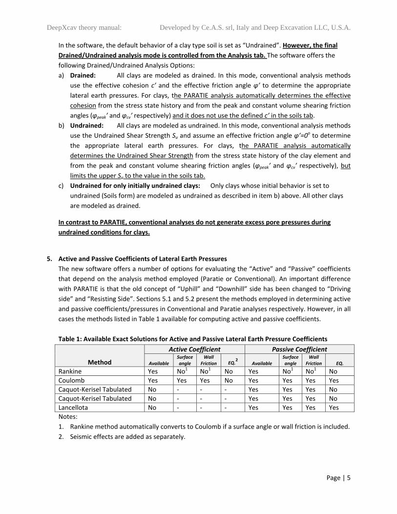
5. Active and Passive Coefficients of Lateral Earth Pressures
The new software offers a number of options for evaluating the “Active” and “Passive” coefficients
that depend on the analysis method employed (Paratie or Conventional). An important difference
with PARATIE is that the old concept of “Uphill” and “Downhill” side has been changed to “Driving
side” and “Resisting Side”. Sections 5.1 and 5.2 present the methods employed in determining active
and passive coefficients/pressures in Conventional and Paratie analyses respectively. However, in all
cases the methods listed in Table 1 available for computing active and passive coefficients.
Table 1: Available Exact Solutions for Active and Passive Lateral Earth Pressure Coefficients
Method
Active Coefficient Passive Coefficient
Available Surface angle
Wall Friction EQ.
2 Available
Surface angle
Wall Friction EQ.
Rankine Yes No1 No1 No Yes No1 No1 No
Coulomb Yes Yes Yes No Yes Yes Yes Yes
Caquot‐Kerisel Tabulated No ‐ ‐ ‐ Yes Yes Yes No
Caquot‐Kerisel Tabulated No ‐ ‐ ‐ Yes Yes Yes No
Lancellota No ‐ ‐ ‐ Yes Yes Yes Yes
Notes:
1. Rankine method automatically converts to Coulomb if a surface angle or wall friction is included.
2. Seismic effects are added as separately.

DeepXcav theory manual: Developed by Ce.A.S. srl, Italy and Deep Excavation LLC, U.S.A.
Page | 6
5.1 Active and Passive Lateral Earth Pressures in Conventional Analyses
In the conventional analysis the software first determines which side is generating driving earth
pressures. Once the driving side is determined, the software examines if a single ground surface
angle is assumed on the driving and on the resisting sides. If a single surface angle is used then the
exact theoretical equation is employed as outlined in. If an irregular ground surface angle is
detected then the program starts performing a wedge analysis on the appropriate side. Horizontal
ground earth pressures are then prorated to account for all applicable effects including wall
friction. It should be noted that the active/passive wedge analyses can take into account flownet
water pressures if a flownet is calculated.
The computed active and passive earth pressures are then modified if the user assumes another
type of lateral earth pressure distribution (i.e. apparent earth pressure diagram computed from
active earth pressures above subgrade, divide passive earth pressures by a safety factor, etc.).
All of the above Ka/Kp computations are performed automatically for each stage. The user has
only to select the appropriate wall friction behavior and earth pressure distribution.
5.2 Active and Passive Lateral Earth Pressures in PARATIE module
Paratie 7.0 incorporates the active and passive earth pressure coefficients within the soil data.
Hence, in the existing Paratie 7.0 even though Ka/Kp are in the soil properties dialog, the user has
to manually compute Ka/Kp and include wall friction and other effects (such as slope angle, wall
friction). If a slope angle surface change takes place on a subsequent stage, then the existing
Paratie user has to manually compute and change Ka/Kp to properly account for all required
effects. The new software offers a different, more rationalized approach.
In the new SW the default Ka/Kp (for both φpeak’ and φcv’) defined in the soils tab are by default
computed with no wall friction and for a horizontal ground surface. The user still has the ability to
use the default PARATIE engine Ka/Kp by selecting a check box in the settings (Tabulated Butee
values). This new approach offers the benefit that the same soil type can easily be reused in
different design sections without having to modify the base soil properties. Otherwise, while
strongly not recommended, wall friction and ground surface angle can be incorporated within the
default Ka/Kp values in the Soil Data Dialog. In general the layout logic in determining Ka and Kp is
described in Figure 1.

DeepXcav theory manual: Developed by Ce.A.S. srl, Italy and Deep Excavation LLC, U.S.A.
Page | 7
Options 1 2 3Default Ka, Kp = Rankine
(RECOMMENDED)Default engine Ka/Kp (Butee) for zero
wall friction and horizontal ground gives same numbers as Rankine
User defined Ka/Kp that can include slope and wall friction (NOT
RECOMMENDED)
Default KaBase, KpBase defined for each soil type
(Performed for each stage)
1. Default Option (YES) 2. NoSW automatically determines slope angle, wall friction, and other effects KaBaseOptions: A. Enable Kp changes for seismic effects (Default = Yes) KpBase
B. Enable Ka/Kp changes for slope angle (Default = Yes)C. Enable wall friction adjustments (Default = Yes)
For each stage then Options 1.1 and 1.2 are available:
Ka= Kabase x Ka(selected method, slope angle, wall friction)Ka Rankine (i.e. ground slope =0, wall friction = 0)
Kp= Kpbase x Kp(selected method, slope angle, wall friction, EQ)Kp Rankine (i.e. ground slope =0, wall friction = 0)
Ka= Ka(selected method, slope angle, wall friction)
Kp= Kp(selected method, slope angle, wall friction, EQ)
IMPORTANT LIMITATIONSA) Ka/Kp for irregular surfaces is not computed and is treated as horizontal.B) Seismic thrusts are not included in the default Ka calculations.
Sub option 1.2: Use Actual Ka/Kp as determined from Stage Methods and Equations (see Table 1)
3. Examine material changes. The latest Material change property will always override the above equations.
Soil Type Dialog/Base Ka-Kp
Enable automatic readjustment of Ka/Kp for slope angle, wall friction etc?
Sub option 1.1: Prorate base Ka/Kp for slope and other effects (Default)
*note wall friction can be independently selected on the driving or the resisting side. However, basic
wall friction modeling is limited to three options a) Zero wall friction, b) % of available soil friction,
and c) set wall friction angle.
Figure 1: Ka/Kp determination options for Paratie module in new software

DeepXcav theory manual: Developed by Ce.A.S. srl, Italy and Deep Excavation LLC, U.S.A.
Page | 8
When the software detects that the user is running an analysis with non‐horizontal soil layers
(i.e. custom line mode is turned on), the software will calculate the appropriate active and passive
lateral earth pressure coefficients by performing a series of wedge analysis. Each wedge analysis is
performed at the bottom elevation of each layer by assuming a linear wedge failure with no wall
friction. Then, if wall friction is assumed, the Ka and Kp values are prorated by the ratio of the horizontal
layer Ka with the selected method (Coulomb, Caquot, etc) to the Rankine Ka or Kp values. Last, the
computed Ka and Kp coefficients are multiplied or divided by the appropriate partial safety factors if a
EC7 type approach is selected. For clays, the wedge analysis is performed for both the peak and the
constant volume friction angle Ka and Kp values (KaCV, KpCV, KaPeak, KpPeak). More information about
the wedge analysis equations is presented in sections 5.4 and 5.5.
In most cases this approach yields good rough approximations to the actual Ka and Kp values in
complex geological stratigraphies. However, results should be more closely inspected as in some
conditions more conservative coefficients may be generated when block type failures are initiated. In
these cases, it might be more appropriate to define a custom increased Ka and decreased Kp from the
soils input dialog and the Resistance Tab. The program offers a way to quickly inspect the wedge analysis
values (without the wall friction prorating) by typing the following commands in the Command Prompt
text box:
GEN WEDGES 0 LEFT = Generates the equivalent Ka and Kp for the left side of the left wall
GEN WEDGES 0 RIGHT = Generates the equivalent Ka and Kp for the right side of the left wall
GEN WEDGES 1 LEFT = Generates the equivalent Ka and Kp for the left side of the right wall
GEN WEDGES1 RIGHT = Generates the equivalent Ka and Kp for the right side of the right wall
Note: The commands can be executed only when the excavation section has been analyzed at‐least
once.
The following example presents a case where the previous commands were verified with no wall
friction.
Figure 2.1.a: Wedge analysis example for non‐linear analysis

DeepXcav theory manual: Developed by Ce.A.S. srl, Italy and Deep Excavation LLC, U.S.A.
Page | 9
In this example the layer properties are:
For the Gen Wedges 0 Right command the following message will be produced:
For sand layers the reported KaWedge and KpWedge is also reported in the CV and Peak Values. For
clays, the KaWedge and KpWedge represent the values used in the limit equilibrium analysis, while the
KaCV, KpCV, KaPK, KpPK represent the values used in the non‐linear analysis (Paratie engine). Negative
and zero values are reported when a layer is not intersected by the wall. Upon closer inspection of the
previously presented results one can see that the calculated Ka and Kp values are very close to the
theoretical horizontal Ka and Kp Rankine values. Some expected small differences are also observed but
these are expected because the typically used Ka and Kp equations for multilayered soils assume a step‐
wise wedge failure (which is also a rough approximation) whereas the wedge analysis assumes a single
angle from the wall to the surface.

DeepXcav theory manual: Developed by Ce.A.S. srl, Italy and Deep Excavation LLC, U.S.A.
Page | 10
5.3 Passive Pressure Equations
This section outlines the specific theoretical equations used for determining the passive lateral
earth pressure coefficients within the software.
a) Rankine passive earth pressure coefficient: This coefficient is applicable only when no wall
friction is used with a flat passive ground surface. This equation does not account for seismic
effects.
b) Coulomb passive earth pressure coefficient: This coefficient can include effects of wall
friction, inclined ground surface, and seismic effects. The equation is described by Das on his
book “Principles of Geotechnical Engineering”, 3rd Edition, pg. 430 and in many other
textbooks:
Where α= Slope angle (positive upwards)
= Seismic effects = with
ax = horizontal acceleration (relative to g)
ay= vertical acceleration, +upwards (relative to g)
θ= Wall angle from vertical (0 radians wall face is vertical)
c) Lancellotta: According to this method the passive lateral earth pressure coefficient is given
by:
Where
And
d) Caquot‐Kerisel (Tab‐buttee): Refer to manual by Paratie and tabulated values.

DeepXcav theory manual: Developed by Ce.A.S. srl, Italy and Deep Excavation LLC, U.S.A.
Page | 11
5.4 Classical Earth Pressure Options
5.4.1 Active & Passive Pressures for non‐Level Ground Occasionally non‐level ground surfaces and benches have to be constructed. The current version
of DeepXcav can handle both single angle sloped surfaces (i.e single 10degree slope angle) and
complex benches with multiple points. DeepXcav automatically detects which condition applies.
For single angle slopes, DeepXcav will determine use the theoretical Rankine, Coulomb, or Caquot‐
Kerisel active, or passive lateral thrust coefficients (depending on user preference).
For non level ground that does not meet the single slope criteria, DeepXcav combines the
solutions from a level ground with a wedge analysis approach. Pressures are generated in a two
step approach: a) first, soil pressures are generated pretending that the surface is level, and then
b) soil pressures are multiplied by the ratio of the total horizontal force calculated with the wedge
method divided by the total horizontal force generated for a level ground solution. This is done
incrementally at all nodes throughout the wall depth summing forces from the top of the wall.
Wall friction is ignored in the wedge solution but pressures with wall friction according to
Coulomb for level ground are prorated as discussed.
This approach does not exactly match theoretical wedge solutions. However, it is employed
because it is very easy with the iterative wedge search (as shown in the figure below) to miss the
most critical wedge. Thus, when lateral active or passive pressures have to be backfigured from
the total lateral force change a spike in lateral pressure can easily occur (while the total force is
still the same). Hence, by prorating the active‐passive pressure solution a much smoother
pressure envelope is generated. In most cases this soil pressure envelope is very close to the
actual critical wedge solution. The wedge methods employed are illustrated in the following
figures.
Surcharge loads are not considered in the wedge analyses since surcharge pressures are derived
separately using well accepted linear elasticity equations.

DeepXcav theory manual: Developed by Ce.A.S. srl, Italy and Deep Excavation LLC, U.S.A.
Page | 12
Figure 2.1: Active force wedge search solution according to Coulomb.
Figure 2.2: Passive force wedge search solution according to Coulomb.

DeepXcav theory manual: Developed by Ce.A.S. srl, Italy and Deep Excavation LLC, U.S.A.
Page | 13
5.4.2 Peck 1969 Earth Pressure Envelopes After observation of several braced cuts Peck (1969) suggested using apparent pressure envelopes with the following guidelines:
is taken as the effective unit weight while water pressures are added separately (private communication with Dr.
Peck). Figure 2.3: Apparent Earth Pressures as Outlined by Peck, 1969
For mixed soil profiles (with multiple soil layers) DeepXcav computes the soil pressure as if each
layer acted only by itself. After private communication with Dr. Peck, the unit weight g represents
either the total weight (for soil above the water table) or the effective weight below the water
table. For soils with both frictional and undrained behavior, DeepXcav averages the "Sand" and
"Soft clay" or "Stiff Clay" solutions. Note that the Ka used in DeepXcav is only for flat ground
solutions. The same effect for different Ka (such as for sloped surfaces), can be replicated by
creating a custom trapezoidal redistribution of active soil pressures.

DeepXcav theory manual: Developed by Ce.A.S. srl, Italy and Deep Excavation LLC, U.S.A.
Page | 14
5.4.3 FHWA Apparent Earth Pressures
The current version of DeepXcav also includes apparent earth pressure with FHWA standards
(Federal Highway Administration). The following few pages are reproduced from applicable FHWA
standards.
Figure 2.4: Recommended apparent earth pressure diagram for sands according to FHWA

DeepXcav theory manual: Developed by Ce.A.S. srl, Italy and Deep Excavation LLC, U.S.A.
Page | 15
TOTAL LOAD (kN/m/meter of wall) = 3H2 to 6H2 (H in meters)
Figure 2.5: Recommended apparent earth pressure diagram for stiff to hard clays according to FHWA.
In both cases for figures 2.4 and 2.5, the maximum pressure can be calculated from the total force as:
a. For walls with one support: p= 2 x Load / (H +H/3)
b. For walls with more than one support: p= 2 x Load /{2 H – 2(H1 + Hn+1)/3)}
DeepXcav theory manual: Developed by Ce.A.S. srl, Italy and Deep Excavation LLC, U.S.A.
Page | 16
5.4.4 FHWA Recommended Apparent Earth Pressure Diagram for Soft to Medium Clays
Temporary and permanent anchored walls may be constructed in soft to medium clays (i.e. Ns>4)
if a competent layer of forming the anchor bond zone is within reasonable depth below the
excavation. Permanently anchored walls are seldom used where soft clay extends significantly
below the excavation base.
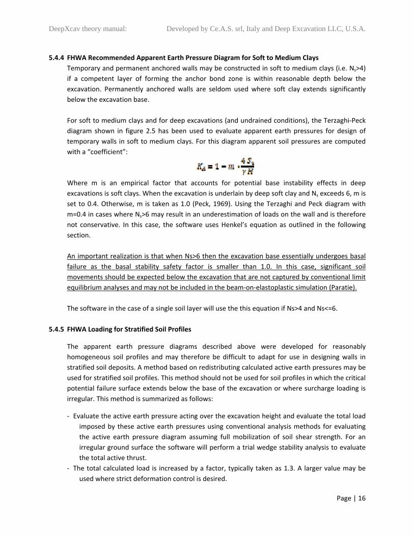
For soft to medium clays and for deep excavations (and undrained conditions), the Terzaghi‐Peck
diagram shown in figure 2.5 has been used to evaluate apparent earth pressures for design of
temporary walls in soft to medium clays. For this diagram apparent soil pressures are computed
with a “coefficient”:
Where m is an empirical factor that accounts for potential base instability effects in deep
excavations is soft clays. When the excavation is underlain by deep soft clay and Ns exceeds 6, m is
set to 0.4. Otherwise, m is taken as 1.0 (Peck, 1969). Using the Terzaghi and Peck diagram with
m=0.4 in cases where Ns>6 may result in an underestimation of loads on the wall and is therefore
not conservative. In this case, the software uses Henkel’s equation as outlined in the following
section.
An important realization is that when Ns>6 then the excavation base essentially undergoes basal
failure as the basal stability safety factor is smaller than 1.0. In this case, significant soil
movements should be expected below the excavation that are not captured by conventional limit
equilibrium analyses and may not be included in the beam‐on‐elastoplastic simulation (Paratie).
The software in the case of a single soil layer will use the this equation if Ns>4 and Ns<=6.
5.4.5 FHWA Loading for Stratified Soil Profiles
The apparent earth pressure diagrams described above were developed for reasonably
homogeneous soil profiles and may therefore be difficult to adapt for use in designing walls in
stratified soil deposits. A method based on redistributing calculated active earth pressures may be
used for stratified soil profiles. This method should not be used for soil profiles in which the critical
potential failure surface extends below the base of the excavation or where surcharge loading is
irregular. This method is summarized as follows:
‐ Evaluate the active earth pressure acting over the excavation height and evaluate the total load
imposed by these active earth pressures using conventional analysis methods for evaluating
the active earth pressure diagram assuming full mobilization of soil shear strength. For an
irregular ground surface the software will perform a trial wedge stability analysis to evaluate
the total active thrust.
‐ The total calculated load is increased by a factor, typically taken as 1.3. A larger value may be
used where strict deformation control is desired.

DeepXcav theory manual: Developed by Ce.A.S. srl, Italy and Deep Excavation LLC, U.S.A.
Page | 17
‐ Distribute the factored total force into an apparent pressure diagram using the trapezoidal
distribution shown in Figure 2.4.
Where potential failure surfaces are deep‐seated, limit equilibrium methods using slope stability
may be used to calculate earth pressure loadings.
The Terzaghi and Peck (1967) diagrams did not account for the development of soil failure below
the bottom of the excavation. Observations and finite element studies have demonstrated that
soil failure below the excavation bottom can lead to very large movements for temporary
retaining walls in soft clays. For Ns>6, relative large areas of retained soil near the excavation base
are expected to yield significantly as the excavation progresses resulting in large movements
below the excavation, increased loads on the exposed portion of the wall, and potential instability
of the excavation base. In this case, Henkel (1971) developed an equation to directly obtain KA for
obtaining the maximum pressure ordinate for soft to medium clays apparent earth pressure
diagrams (this equation is applied when FHWA diagrams are used and the program examines if
Ns>6):
Where m=1 according to Henkel (1971). The total load is then taken as:
Figure 2.6: Henkel’s mechanism of base failure
Figure 2.7 shows values of KA calculated using Henkel’s method for various d/H ratios. For results
in this figure Su = Sub. This figure indicates that for 4<Ns<6, the Terzaghi and Peck envelope with
m=0.4 is overly conservative relative to Henkel. Also, for Ns<5.14 the Henkel equation is not valid
and apparent earth pressures calculated using m=1.0 in the Terzaghi and Peck envelope are
unrealistically low. For the range 4<Ns<5.14, a constant value of Ka=0.22 should be used to
evaluate the maximum pressure ordinate for the soft to medium clay apparent earth pressure
envelope. At the transition between stiff‐hard clays to soft‐medium clays, i.e. Ns= 4, the total load

DeepXcav theory manual: Developed by Ce.A.S. srl, Italy and Deep Excavation LLC, U.S.A.
Page | 18
using the soft to medium apparent earth pressure diagram with Ka= 0.22 is 0.193 H2 resulting in a
maximum pressure p=0.26 H. Use of Ka= 0.22, according to FHWA, represent a rational transition
value for these cases.
Henkel’s method is limited to cases where the clays soils on the retained side of the excavation
and below the excavation can each be reasonably characterized using a constant value for
undrained shear strength. Where a more detailed shear strength profile is required, limit
equilibrium methods may be used to evaluate the earth pressure loadings on the wall described in
section 5.7.3 of the FHWA manual (not performed within the software).
Figure 2.7: Comparison of apparent lateral earth pressure coefficients with basal stability index
(FHWA 2004).
For clays the stability number is defined as:
Please note that software uses the effective vertical stress at subgrade to find an equivalent soil
unit weight, Water pressures are added separately depending on water condition assumptions.
This is slightly different from the approach recommended by FHWA, however, after personal
communication with the late Dr. Peck, has confirmed that users of apparent earth pressures
should use the effective stress at subgrade and add water pressures separately.
By ignoring the water table, or by using custom water pressures, the exact same numerical
solution as with the original FHWA method can be obtained.

DeepXcav theory manual: Developed by Ce.A.S. srl, Italy and Deep Excavation LLC, U.S.A.
Page | 19
5.4.6 Modifications to stiff clay and FHWA diagrams
Over the years various researchers and engineers have proposed numerous apparent lateral earth
pressure diagrams for braced excavations. Unfortunately, most lateral apparent pressure
diagrams have been taken out of context or misused. Historically, apparent lateral earth pressure
diagrams have been developed from measured brace reactions. However, apparent earth
pressure diagrams are often arbitrarily used to also calculate bending moments in the wall.
In excavations supporting stiff clays, many researchers have observed that the lower braces
carried smaller loads. This has misled engineers to extrapolate the apparent lateral earth pressure
to zero at subgrade. In this respect, many apparent lateral earth pressure diagrams carry within
them a historical unconservative oversight in the fact that the lateral earth pressure at subgrade
was never directly or indirectly measured. Konstantakos (2010) has proven that the zero apparent
lateral earth pressure at the subgrade level assumption is incorrect, unconservative, and most
importantly unsubstantiated. This historical oversight, can lead to severe underestimation of the
required wall embedment length and of the experienced wall bending moments.
If larger displacements can be tolerated or drained conditions are experienced the apparent earth
pressure diagrams must not, at a minimum, drop below the theoretical active pressure, unless soil
arching is carefully evaluated. Alternatively, in these cases, for fast calculations or estimates, an
engineer can increase the apparent earth pressure from 50% at midway between the lowest
support level and the subgrade to the full theoretical apparent pressure or the active pressure
limit at the subgrade level (see Figure 2.8). As always, these equations represent a simplification of
complex conditions.
If tighter deformation control is required or when fully undrained conditions are to be expected,
then the virtual reaction at the subgrade level has to take into account increased lateral earth
pressures that can even reach close to fifty percent of the total vertical stress at the subgrade
level. The initial state of stress has to be taken into consideration as overconsolidated soil strata
will tend to induce larger lateral earth stresses on the retaining walls. In such critical cases, a
design engineer must always compliment apparent earth pressure diagram calculations with more
advanced and well substantiated analysis methods.
The above modifications can be applied within the software by double clicking on the driving earth
pressure button when the FHWA or Peck method is selected.

DeepXcav theory manual: Developed by Ce.A.S. srl, Italy and Deep Excavation LLC, U.S.A.
Page | 20
Figure 2.8: Minimum lateral pressure option for FHWA and Peck apparent pressure diagrams (check
box).

DeepXcav theory manual: Developed by Ce.A.S. srl, Italy and Deep Excavation LLC, U.S.A.
Page | 21
Figure 2.9: Proposed modifications to stiff clay and FHWA apparent lateral earth pressure diagrams (Konstantakos 2010).

DeepXcav theory manual: Developed by Ce.A.S. srl, Italy and Deep Excavation LLC, U.S.A.
Page | 22
5.4.7 Verification Example for Soft Clay and FHWA Approach
A 10m deep excavation is constructed in soft clays and the wall is embedded 2m in a second soft
clay layer. The wall is supported by three supports at depths of 2m, 5m, and 8m from the wall top.
Assumed soil properties are:
Clay 1: From 0 to 10m depth, Su = 50 kPa 20 kN/m3
Clay 2: From 10m depth and below Su = 30 kPa 20 kN/m3
The depth to the firm layer from the excavation subgrade is assumed as d=10m (which is the
model base, i.e. the bottom model coordinate)
Figure 2.10: Verification example for FHWA apparent pressures with a soft clay
The total vertical stress at the excavation subgrade is:
v’20 kN/m3 x 10m =200 kPa
The basal stability safety factor is then:
FS= 5.7 x 30 kPa/ 200 kPa = 0.855 (verified from Fig. 2.10)
Then according to Henkel Ka is calculated as (m=1):
The total thrust above the excavation is then: Ptotal = 0.5 KA v’ x H = 647 kN/m
The maximum earth pressure ordinate is then:
p= 2 x Load /{2 H – 2(H1 + Hn+1)/3)} = 2 x 647 kN/m /{2 x 10m ‐2 x (2m +2m)/3}= 74.65 kPa

DeepXcav theory manual: Developed by Ce.A.S. srl, Italy and Deep Excavation LLC, U.S.A.
Page | 23
The software calculates 74.3 kPa and essentially confirms the results as differences are attributed
to rounding errors.
The tributary load in the middle support is then 3m x 74,3kPa = 222.9 kN/m (which is confirmed by
the program). When performing only conventional limit equilibrium analysis it is important to
properly select the number of wall elements that will generate a sufficient number of nodes. In
this example, 195 wall nodes are assumed. In general it is recommended to use at least 100 nodes
when performing conventional calculations while 200 nodes will produce more accurate results.
‐ Now examine the case if the soil was a sand with a friction angle of 30 degrees.
Figure 2.11: Verification example for FHWA soft clay analysis
In this case, the total active thrust is calculated as: Ptotal = 0.65 KA v’ x H = 432.9 kN/m
The maximum earth pressure ordinate is then:
p= 2 x Load /{2 H – 2(H1 + Hn+1)/3)} = 2 x 432.9 kN/m /{2 x 10m ‐2 x (2m +2m)/3}= 49.95 kPa
This apparent earth pressure value is confirmed by the software.
‐ Next, we will examine the same excavation with a mixed sand and clay profile.
Sand: From 0 to 5m depth, = 30o 20 kN/m3
Clay 1: From 5 to 10m depth, Su = 50 kPa 20 kN/m3
Clay 2: From 10m depth and below Su = 30 kPa 20 kN/m3
In this example, Ns=6.67. As a result we will have to use Henkel’s equation but average the effects
of soil friction and cohesion. This method is a rough approximation and should be used with
caution.
From 0m to 5m the friction force on a vertical face in Sand 1 can be calculated as:
Ffriction = 0.5 x 20 kN/m3 x 5m x tan(30 degrees) x 5m = 144.5 kN/m

DeepXcav theory manual: Developed by Ce.A.S. srl, Italy and Deep Excavation LLC, U.S.A.
Page | 24
The available side cohesion on layer Clay 1 is: 5m x 50 kPa = 250 kN/m
The total side resistance on the vertical face is then: 250 kN/m + 144.5 kN/m = 395.5 kN/m
The average equivalent cohesion can be computed as:
Su.ave= 395.5 kN/m / 10m = 39.55 kPa
Then according to Henkel Ka is calculated as (m=1):
The total thrust above the excavation is then: Ptotal = 0.5 KA v’ x H = 849 kN/m
The maximum earth pressure ordinate is then:
p= 2 x Load /{2 H – 2(H1 + Hn+1)/3)} = 2 x 647 kN/m /{2 x 10m ‐2 x (2m +2m)/3}= 98 kPa
This result is confirmed by the software that produces 99.2 kPa.
Figure 2.12: Verification example for FHWA mixed soil profile with soft clay and sand
5.4.8 Custom Trapezoidal Pressure Diagrams
With this option the apparent earth pressure diagram is determined as the product of the active
soil thrust times a user defined factor. The factor should range typically from 1.1 to 1.4 depending
on the user preferences and the presence of a permanent structure. The resulting horizontal
thrust is then redistributed as a trapezoidal pressure diagram where the top and bottom
triangular pressure heights are defined as a percentage of the excavation height.

DeepXcav theory manual: Developed by Ce.A.S. srl, Italy and Deep Excavation LLC, U.S.A.
Page | 25
5.4.9 Two Step Rectangular Pressure Diagrams
Very often, especially in the US, engineers are provided with rectangular apparent lateral earth
pressures that are defined with the product of a factor times the excavation height. Two factors
are usually defined M1 for pressures above the water table and M2 for pressures below the water
table. M1 and M2 should already incorporate the soil total and effective weight. Use of this option
should be carried with extreme caution. The following dialog will appear if the rectangular
pressure option is selected in the driving pressures button.
Figure 2.10: Two step rectangular earth pressure coefficients.

DeepXcav theory manual: Developed by Ce.A.S. srl, Italy and Deep Excavation LLC, U.S.A.
Page | 26
5.5 Vertical wall adhesion in undrained loading
Short term total stress conditions (i.e. undrained loading) represent the state in the soil before the
pore water pressures have had time to dissipate i.e. immediately after construction in a cohesive
soil. For total stress the horizontal active and passive pressures are calculated using the following
equations:
pa = Ka ( γ z+q) – Su Kac
pp = Kp( γ z+q) + Su Kpc
Where:
(γ z+q) represents the total overburden pressure
Ka = Kp = 1.0 for cohesive soils.
Design su= sud= sumc/ FSsu where Fssu is typically 1.5. The earth pressure coefficients, Kac and Kpc, make an allowance for wall /soil adhesion and are derived as follows:
Kac= Kpc= 2√(1+Swmax /Sud)
0.5
According to the Piling Handbook by Arcelor (2005), the limiting value of wall adhesion Swmax at
the soil/sheet pile interface is generally taken to be smaller than the design undrained shear
strength of the soil, sud, by a factor of 2 for stiff clays. i.e. Sw max = α x Sud, where α = 0.5. Lower
values of wall adhesion, however, may be realized in soft clays. In any case, the designer should
refer to the design code they are working to for advice on the maximum value of wall adhesion
they may use. Currently, these modifications can be used only in conventional limit equilibrium
analyses.

DeepXcav theory manual: Developed by Ce.A.S. srl, Italy and Deep Excavation LLC, U.S.A.
Page | 27
6. Eurocode 7 analysis methods
In the US practice excavations are typically designed with a service design approach while a
Strength Reduction Approach is used in Europe and in many other parts of the world. Eurocode 7
(strength design, herein EC7) recommends that the designer examines a number of different
Design Approaches (DA‐1, DA‐2, DA‐3) so that the most critical condition is determined. In
Eurocode 7 soil strengths are readjusted according to the material “M” tables, surcharges and
permanent actions are readjusted according to the action “A” tables, and resistances are modified
according to the “R” tabulated values. Hence, in a case that may be outlined as “A2” + “M2” +
“R2” one would have to apply all the relevant factors to “Actions”, “Materials”, and “Resistances”.
A designer still has to perform a service check in addition to all the ultimate design approach
cases. Hence, a considerable number of cases will have to be examined unless the most critical
condition can be easily established by an experienced engineer. In summary, EC7 provides the
following combinations where the factors can be picked from the tables in section 6.1:
Design Approach 1, Combination 1: A1 “+” M1 “+” R1
Design Approach 1, Combination 2: A2 “+” M2 “+” R1
Design Approach 2: A1* “+” M1 “+” R2
Design Approach 3: A1* “+” A2+ “+” M2 “+” R3
A1* = For structural actions or external loads, and A2+= for geotechnical actions
EQK (from EC8): M2 “+” R1
(The Italian code DM08 uses DA1‐1, DA1‐2, and EQK design approach methods only).
In the old Paratie (version 7 and before), the different cases would have been examined in many
“Load Histories”. The term “Load History” has been replaced in the new software with the concept
of “Design Section”. Each design section can be independent from each other or a Design Section
can be linked to a Base Design Section. When a design section is linked, the model and analysis
options are directly copied from the Base Design Section with the exception of the Soil Code
Options (i.e, Eurocode 7, DM08 etc).
In Eurocode 7, various equilibrium and other type checks are examined:
a) STR: Structural design/equilibrium checks
b) GEO: Geotechnical equilibrium checks
c) HYD: Hydraulic heave cases
d) UPL: Uplift (on a structure)
e) EQU: Equilibrium states (applicable to seismic conditions?)
The new software handles a number of STR, GEO, and HYD checks while it gives the ability to
automatically generate “all” Eurocode 7 cases for a model. Unfortunately, Eurocode 7 as a whole
is mostly geared towards traditional limit equilibrium analysis. In more advanced analysis methods
(such as in Paratie), Eurocode 7 can be handled according to “the letter of the code” only when
equal groundwater levels are assumed in both wall sides. However, much doubt exists as to the
DeepXcav theory manual: Developed by Ce.A.S. srl, Italy and Deep Excavation LLC, U.S.A.
Page | 28
most appropriate method to be employed when different groundwater levels have to be modeled.
Section 6.1 presents the safety/strength reduction parameters that the new software uses.
6.1 Safety Parameters for Ultimate Limit State Combinations
Table 2.1 lists all safety factors that are used in the new software and also provides the used
safety factors according to EC7‐2008. The last 4 table columns list the code safety factors for each
code case/scenario (i.e. in the first row Case 1 refers to M1, Case 2 refers to M2). Table 2.2 lists
the same factors for the Italian code NTC08, while tables 2.3, 2.4, and 2.5 list the safety factors for
the Greek, the French, and the German codes respectively.
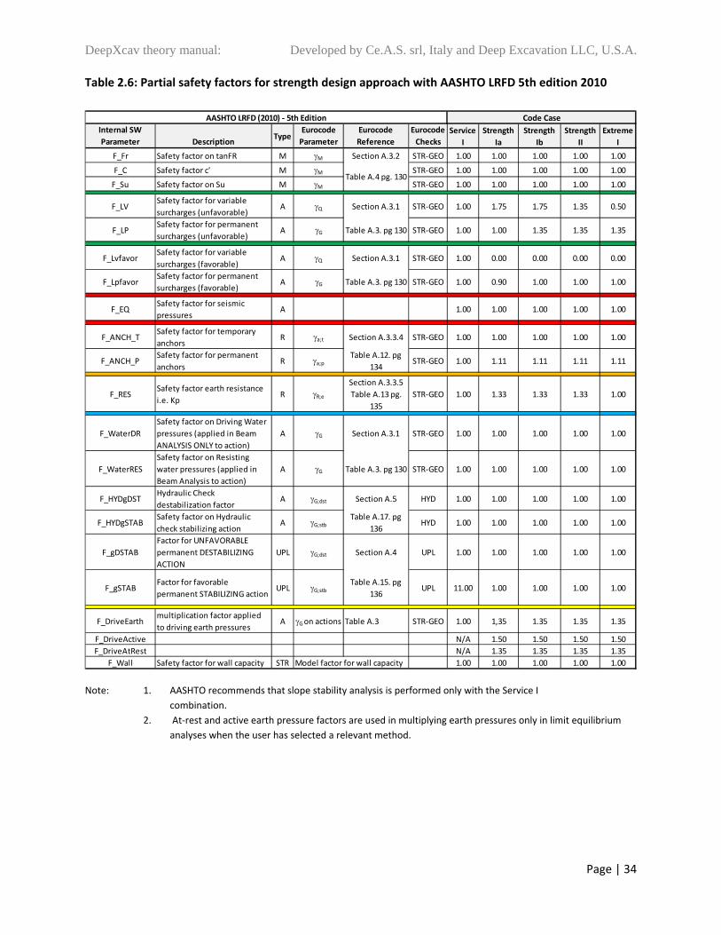
Last, table 2.6 presents the load combinations employed by AASHTO LRFD 5th edition (2010).
AASHTO slightly differs from European standards in that soil strength is not factored.

DeepXcav theory manual: Developed by Ce.A.S. srl, Italy and Deep Excavation LLC, U.S.A.
Page | 29
Table 2.1: List of safety factors for strength design approach according to Eurocode 7
Internal SW
Parameter Description
TypeEurocode
Parameter
Eurocode
Reference
Eurocode
Checks
Case 1
DA‐1:
comb1.
A1+M1+R1
Case 2
DA‐1:
comb2.
A2+M2+R1
Case 3
DA‐2:
A1+M1+R2
Case 4
DA‐1:
A1+M1+R1
EQU:
M2+R1
F_Fr Safety factor on tanFR M M Section A.3.2 STR‐GEO 1.00 1.25 1.00 1.25 1.25
F_C Safety factor c' M M STR‐GEO 1.00 1.25 1.00 1.25 1.25
F_Su Safety factor on Su M M STR‐GEO 1.00 1.40 1.00 1.40 1.40
F_LVSafety factor for variable
surcharges (unfavorable)A Q Section A.3.1 STR‐GEO 1.50 1.30 1.50 1.50 0.00
F_LPSafety factor for permanent
surcharges (unfavorable)A G Table A.3. pg 130 STR‐GEO 1.35 1.00 1.35 1.35 1.00
F_LvfavorSafety factor for variable
surcharges (favorable)A Q Section A.3.1 STR‐GEO 0.00 0.00 0.00 0.00 1.00
F_LpfavorSafety factor for permanent
surcharges (favorable)A G Table A.3. pg 130 STR‐GEO 1.00 1.00 1.00 1.00 1.00
F_EQSafety factor for seismic
pressuresA 0.00 0.00 0.00 0.00 1.00
F_ANCH_TSafety factor for temporary
anchorsR a;t Section A.3.3.4 STR‐GEO 1.10 1.10 1.10 1.00 1.10
F_ANCH_PSafety factor for permanent
anchorsR a;p
Table A.12. pg
134STR‐GEO 1.10 1.10 1.10 1.00 1.10
F_RESSafety factor earth resistance
i.e. KpR R;e
Section A.3.3.5
Table A.13 pg.
135
STR‐GEO 1.00 1.00 1.40 1.00 1.00
F_WaterDR
Safety factor on Driving Water
pressures (applied in Beam
ANALYSIS ONLY to action)
A G Section A.3.1 STR‐GEO 1.35 1.00 1.35 1.00 1.00
F_WaterRESSafety factor on Resisting
water pressures (applied in
Beam Analysis to action)
A G Table A.3. pg 130 STR‐GEO 1.00 1.00 1.00 1.00 1.00
F_HYDgDSTHydraulic Check
destabilization factorA G;dst Section A.5 HYD 1.35 1.35 1.35 1.35 1.00
F_HYDgSTABSafety factor on Hydraulic
check stabilizing actionA G;stb
Table A.17. pg
136HYD 0.90 0.90 0.90 0.90 0.90
F_gDSTABFactor for UNFAVORABLE
permanent DESTABILIZING
ACTION
UPL G;dst Section A.4 UPL 1.10 1.10 1.10 1.10 1.10
F_gSTABFactor for favorable
permanent STABILIZING actionUPL G;stb
Table A.15. pg
136UPL 0.90 0.90 0.90 0.90 0.90
F_DriveEarthmultiplication factor applied
to driving earth pressuresA G on actions Table A.3 STR‐GEO 1.35 1.00 1.35 1.00 1.00
F_DriveActive N/A N/A N/A N/A N/A
F_DriveAtRest N/A N/A N/A N/A N/A
F_Wall Safety factor for wall capacity STR Model factor for wall capacity 1.00 1.00 1.00 1.00 1.00
Table A.4 pg. 130
EUROCODE 7, EN 1997‐1: 2004 (2007) Code Case

DeepXcav theory manual: Developed by Ce.A.S. srl, Italy and Deep Excavation LLC, U.S.A.
Page | 30
Table 2.2: List of safety factors for strength design approach according to Italian NTC 2008 code
Internal SW
Parameter DescriptionType
Eurocode
Parameter
Eurocode
Reference
Eurocode
ChecksCase 1 Case 2 Case 3* Case 4 EQK
F_Fr Safety factor on tanFR M M Section A.3.2 STR‐GEO 1.00 1.25 1.25
F_C Safety factor c' M M STR‐GEO 1.00 1.25 1.25
F_Su Safety factor on Su M M STR‐GEO 1.00 1.40 1.4
F_LVSafety factor for variable
surcharges (unfavorable)A Q Section A.3.1 STR‐GEO 1.50 1.30 1
F_LPSafety factor for permanent
surcharges (unfavorable)A G
Table A.3. pg
130STR‐GEO 1.30 1.00 1
F_LvfavorSafety factor for variable
surcharges (favorable)A Q Section A.3.1 STR‐GEO 0.00 0.00 1
F_LpfavorSafety factor for permanent
surcharges (favorable)A G
Table A.3. pg
130STR‐GEO 1.00 1.00 1
F_EQSafety factor for seismic
pressuresA 0.00 0.00 1
F_ANCH_TSafety factor for temporary
anchorsR a;t
Section
A.3.3.4STR‐GEO 1.10 1.10 1.10 1.1
F_ANCH_PSafety factor for permanent
anchorsR a;p
Table A.12. pg
134STR‐GEO 1.20 1.20 1.20 1.2
F_RESSafety factor earth resistance
i.e. KpR R;e
Section
A.3.3.5 Table STR‐GEO 1.00 1.40 1
F_WaterDRSafety factor on Driving
Water pressures (applied in A G Section A.3.1 STR‐GEO 1.30 1.00 1
F_WaterRES
Safety factor on Resisting
water pressures (applied in
Beam Analysis to action)
A GTable A.3. pg
130STR‐GEO 1.00 1.00 ‐
F_HYDgDSTHydraulic Check
destabilization factorA G;dst Section A.5 HYD 1.35 ‐ ‐
F_HYDgSTABSafety factor on Hydraulic
check stabilizing actionA G;stb
Table A.17. pg
136HYD 0.90 ‐ ‐
F_gDSTAB
Factor for UNFAVORABLE
permanent DESTABILIZING
ACTION
UPL G;dst Section A.4 UPL 1.10 ‐ ‐
F_gSTAB
Factor for favorable
permanent STABILIZING
action
UPL G;stbTable A.15. pg
136UPL 0.90 ‐ ‐
F_DriveEarthmultiplication factor applied
to driving earth pressuresA G on actions Table A.3 STR‐GEO 1.30 1.00 1
F_Wall Safety factor for wall capacity STR Model factor for wall capacity 1.00 1.00 1
Table A.4 pg.
130
ITALIAN, NTC‐2008 Code Case
Note: F_Wall is not defined in EC7. These parameters can be used in an LRFD approach consistent with USA codes.

DeepXcav theory manual: Developed by Ce.A.S. srl, Italy and Deep Excavation LLC, U.S.A.
Page | 31
Table 2.3: List of safety factors for strength design approach Greek design code 2007
Internal SW
Parameter Description
Type Eurocode
Parameter
Eurocode
Reference
Eurocode
Checks
Case 1
DA‐2*:
A1+M1+R2
Case 2
DA‐3: A1‐
A2+M2+R1
EQU:
M2+R1
F_Fr Safety factor on tanFR M MSection
A.3.2STR‐GEO 1.00 1.25 1.25
F_C Safety factor c' M M STR‐GEO 1.00 1.25 1.25
F_Su Safety factor on Su M M STR‐GEO 1.00 1.40 1.40
F_LVSafety factor for variable
surcharges (unfavorable)A Q
Section
A.3.1STR‐GEO 1.50 1.50 1.00
F_LPSafety factor for permanent
surcharges (unfavorable)A G
Table A.3. pg
130STR‐GEO 1.35 1.35 1.00
F_LvfavorSafety factor for variable
surcharges (favorable)A Q
Section
A.3.1STR‐GEO 0.00 0.00 0.00
F_LpfavorSafety factor for permanent
surcharges (favorable)A G
Table A.3. pg
130STR‐GEO 1.00 1.00 1.00
F_EQSafety factor for seismic
pressuresA 0.00 1.00 1.00
F_ANCH_TSafety factor for temporary
anchorsR a;t
Section
A.3.3.4STR‐GEO 1.10 1.10 1.10
F_ANCH_PSafety factor for permanent
anchorsR a;p
Table A.12.
pg 134STR‐GEO 1.10 1.10 1.10
F_RESSafety factor earth resistance
i.e. KpR R;e
Section
A.3.3.5 Table
A.13 pg. 135
STR‐GEO 1.40 1.00 1.00
F_WaterDRSafety factor on Driving Water
pressures (applied in Beam
ANALYSIS ONLY to action)
A GSection
A.3.1STR‐GEO 1.35 1.35 1.00
F_WaterRES
Safety factor on Resisting
water pressures (applied in
Beam Analysis to action)
A GTable A.3. pg
130STR‐GEO 1.00 1.00 1.00
F_HYDgDSTHydraulic Check
destabilization factorA G;dst Section A.5 HYD 1.35 1.00 1.00
F_HYDgSTABSafety factor on Hydraulic
check stabilizing actionA G;stb
Table A.17.
pg 136HYD 0.90 0.90 0.90
F_gDSTAB
Factor for UNFAVORABLE
permanent DESTABILIZING
ACTION
UPL G;dst Section A.4 UPL 1.10 1.10 1.10
F_gSTABFactor for favorable
permanent STABILIZING actionUPL G;stb
Table A.15.
pg 136UPL 0.90 0.90 0.90
F_DriveEarthmultiplication factor applied
to driving earth pressuresA G on actions Table A.3 STR‐GEO 1.35 1.35 1.00
F_DriveActive N/A N/A N/A
F_DriveAtRest N/A N/A N/A
F_Wall Safety factor for wall capacity STR Model factor for wall capacity 1.00 1.00 1.00
EUROCODE 7, GREEK 2007 Code Case
Table A.4 pg.
130
Note: For slope stability the design approach is equivalent to EQU

DeepXcav theory manual: Developed by Ce.A.S. srl, Italy and Deep Excavation LLC, U.S.A.
Page | 32
Table 2.4: Partial safety factors for strength design approach with French codes XP240 and XP220
Case 1 Case 2 Case 3 Case 4 Case 5 Case 6 Case 7 Case 8
1‐2a
(stand)
2b
(sens)
1‐2a
(stand)
2b
(sens)
1‐2a
(stand)
2b
(sens)
1‐2a
(stand)
2b
(sens)
F_Fr Safety factor on tanFR M MSection
A.3.2STR‐GEO 1.25 1.25 1.25 1.25 1.25 1.25 1.25 1.25
F_C Safety factor c' M M STR‐GEO 1.25 1.25 1.25 1.25 1.25 1.25 1.25 1.25
F_Su Safety factor on Su M M STR‐GEO 1.40 1.40 1.40 1.40 1.40 1.40 1.40 1.40
F_LVSafety factor for variable
surcharges (unfavorable)A Q
Section
A.3.1STR‐GEO 1.33 1.33 1.00 1.00 1.33 1.33 0.00 0.00
F_LPSafety factor for permanent
surcharges (unfavorable)A G
Table A.3. pg
130STR‐GEO 1.00 1.00 1.00 1.00 1.00 1.00 1.00 1.00
F_LvfavorSafety factor for variable
surcharges (favorable)A Q
Section
A.3.1STR‐GEO 0.00 0.00 0.00 0.00 0.00 0.00 0.00 0.00
F_LpfavorSafety factor for permanent
surcharges (favorable)A G
Table A.3. pg
130STR‐GEO 0.90 0.90 0.90 0.90 0.90 0.90 0.90 0.90
F_EQSafety factor for seismic
pressuresA 1.00 1.00 1.00 1.00 1.00 1.00 1.00 1.00
F_ANCH_TSafety factor for temporary
anchorsR a;t
Section
A.3.3.4STR‐GEO 1.10 1.10 1.10 1.10 1.10 1.10 1.10 1.10
F_ANCH_PSafety factor for permanent
anchorsR a;p
Table A.12.
pg 134STR‐GEO 1.10 1.10 1.10 1.10 1.10 1.10 1.10 1.10
F_RESSafety factor earth resistance
i.e. KpR R;e
Section
A.3.3.5 Table
A.13 pg. 135
STR‐GEO 1.00 1.00 1.00 1.00 1.00 1.00 1.00 1.00
F_WaterDR
Safety factor on Driving Water
pressures (applied in Beam
ANALYSIS ONLY to action)
A GSection
A.3.1STR‐GEO 1.00 1.00 1.00 1.00 1.00 1.00 1.00 1.00
F_WaterRES
Safety factor on Resisting water
pressures (applied in Beam
Analysis to action)
A GTable A.3. pg
130STR‐GEO 1.00 1.00 1.00 1.00 1.00 1.00 1.00 1.00
F_HYDgDSTHydraulic Check destabilization
factorA G;dst Section A.5 HYD 1.35 1.35 1.35 1.35 1.35 1.35 1.35 1.35
F_HYDgSTABSafety factor on Hydraulic check
stabilizing actionA G;stb
Table A.17.
pg 136HYD 0.90 0.90 0.90 0.90 0.90 0.90 0.90 0.90
F_gDSTAB
Factor for UNFAVORABLE
permanent DESTABILIZING
ACTION
UPL G;dst Section A.4 UPL 1.10 1.10 1.10 1.10 1.10 1.10 1.10 1.10
F_gSTABFactor for favorable permanent
STABILIZING actionUPL G;stb
Table A.15.
pg 136UPL 0.90 0.90 0.90 0.90 0.90 0.90 0.90 0.90
F_DriveEarthmultiplication factor applied to
driving earth pressuresA G on actionsTable A.3 STR‐GEO 1.00 1.00 1.00 1.00 1.00 1.00 1.00 1.00
F_DriveActive N/A N/A N/A N/A N/A N/A N/A N/A
F_DriveAtRest N/A N/A N/A N/A N/A N/A N/A N/A
F_Wall Safety factor for wall capacity STR Model factor for wall capacity 1.00 1.00 1.00 1.00 1.00 1.00 1.00 1.00
Fundamental Accidental
Table A.4 pg.
130
EUROCODE 7,FRENCH 2007 Code Case
Internal SW
Parameter Description
Type
Eurocode
Parameter
Eurocode
Reference
Eurocode
Checks
XP‐240 XP‐220Fundamental Accidental
Note: French code standards are particularly important for soil nailing walls.

DeepXcav theory manual: Developed by Ce.A.S. srl, Italy and Deep Excavation LLC, U.S.A.
Page | 33
Table 2.5: Partial safety factors for strength design approach with German DIN 2005
Internal SW
Parameter Description
Type Eurocode
Parameter
Eurocode
Reference
Eurocode
Checks
Case 1
GZ2
(SLS)
Case 2
GZ1B
(LC1)
Case 3
GZ1B
(LC2)
Case 4
GZ1B
(LC3)
Case 5
GZ1C
(LC1)
Case 6
GZ1C
(LC2)
Case 7
GZ1C
(LC3)
F_Fr Safety factor on tanFR M MSection
A.3.2STR‐GEO 1.00 1.00 1.00 1.00 1.25 1.15 1.10
F_C Safety factor c' M M STR‐GEO 1.00 1.25 1.15 1.10 1.25 1.15 1.10
F_Su Safety factor on Su M M STR‐GEO 1.00 1.25 1.15 1.10 1.25 1.15 1.10
F_LVSafety factor for variable surcharges
(unfavorable)A Q
Section
A.3.1STR‐GEO 1.00 1.50 1.30 1.00 1.30 1.20 1.00
F_LPSafety factor for permanent
surcharges (unfavorable)A G
Table A.3.
pg 130STR‐GEO 1.00 1.00 1.00 1.00 1.00 1.00 1.00
F_LvfavorSafety factor for variable surcharges
(favorable)A Q
Section
A.3.1STR‐GEO 0.00 0.00 0.00 0.00 0.00 0.00 0.00
F_LpfavorSafety factor for permanent
surcharges (favorable)A G
Table A.3.
pg 130STR‐GEO 1.00 0.90 0.90 0.90 0.90 0.90 0.90
F_EQ Safety factor for seismic pressures A 1.00 0.00 0.00 0.00 1.00 1.00 1.00
F_ANCH_T Safety factor for temporary anchors R a;tSection
A.3.3.4STR‐GEO 1.00 1.10 1.10 1.10 1.10 1.10 1.10
F_ANCH_P Safety factor for permanent anchors R a;pTable A.12.
pg 134STR‐GEO 1.00 1.10 1.10 1.10 1.10 1.10 1.10
F_RES Safety factor earth resistance i.e. Kp R R;eSection
A.3.3.5
Table A.13
STR‐GEO 1.00 1.40 1.30 1.20 1.40 1.00 1.00
F_WaterDR
Safety factor on Driving Water
pressures (applied in Beam
ANALYSIS ONLY to action)
A GSection
A.3.1STR‐GEO 1.00 1.35 1.00 1.20 1.00 1.00 1.00
F_WaterRES
Safety factor on Resisting water
pressures (applied in Beam Analysis
to action)
A GTable A.3.
pg 130STR‐GEO 1.00 1.00 1.00 1.00 1.00 1.00 1.00
F_HYDgDSTHydraulic Check destabilization
factorA G;dst
Section
A.5HYD 1.00 1.00 1.00 1.00 1.00 1.00 1.00
F_HYDgSTABSafety factor on Hydraulic check
stabilizing actionA G;stb
Table A.17.
pg 136HYD 1.00 0.90 0.95 0.90 0.90 0.95 0.90
F_gDSTABFactor for UNFAVORABLE
permanent DESTABILIZING ACTIONUPL G;dst
Section
A.4UPL 1.00 1.00 1.00 1.00 1.00 1.00 1.00
F_gSTABFactor for favorable permanent
STABILIZING actionUPL G;stb
Table A.15.
pg 136UPL 1.00 0.90 0.95 0.90 0.90 0.95 0.90
F_DriveEarthmultiplication factor applied to
driving earth pressuresA G on actions Table A.3 STR‐GEO 1.00 1.35 1.20 1.00 1.00 1.00 1.00
F_DriveActive N/A N/A N/A N/A N/A N/A N/A
F_DriveAtRest N/A 1.20 1.10 N/A N/A N/A N/A
F_Wall Safety factor for wall capacity STR Model factor for wall capacity 1.00 1.00 1.00 1.00 1.00 1.00 1.00
EUROCODE 7, GERMAN 2005
Table A.4
pg. 130
Code Case
Note: 1. Case 5, 6, and 7 are only used in slope stability analysis in conjunction with cases 1, 2, and 3 respectively.
2. At‐rest earth pressure factor is used in multiplying earth pressures only in limit equilibrium analyses.
DeepXcav theory manual: Developed by Ce.A.S. srl, Italy and Deep Excavation LLC, U.S.A.
Page | 34
Table 2.6: Partial safety factors for strength design approach with AASHTO LRFD 5th edition 2010
Internal SW
Parameter DescriptionType
Eurocode
Parameter
Eurocode
Reference
Eurocode
Checks
Service
I
Strength
Ia
Strength
Ib
Strength
II
Extreme
I
F_Fr Safety factor on tanFR M M Section A.3.2 STR‐GEO 1.00 1.00 1.00 1.00 1.00
F_C Safety factor c' M M STR‐GEO 1.00 1.00 1.00 1.00 1.00
F_Su Safety factor on Su M M STR‐GEO 1.00 1.00 1.00 1.00 1.00
F_LVSafety factor for variable
surcharges (unfavorable)A Q Section A.3.1 STR‐GEO 1.00 1.75 1.75 1.35 0.50
F_LPSafety factor for permanent
surcharges (unfavorable)A G Table A.3. pg 130 STR‐GEO 1.00 1.00 1.35 1.35 1.35
F_LvfavorSafety factor for variable
surcharges (favorable)A Q Section A.3.1 STR‐GEO 1.00 0.00 0.00 0.00 0.00
F_LpfavorSafety factor for permanent
surcharges (favorable)A G Table A.3. pg 130 STR‐GEO 1.00 0.90 1.00 1.00 1.00
F_EQSafety factor for seismic
pressuresA 1.00 1.00 1.00 1.00 1.00
F_ANCH_TSafety factor for temporary
anchorsR a;t Section A.3.3.4 STR‐GEO 1.00 1.00 1.00 1.00 1.00
F_ANCH_PSafety factor for permanent
anchorsR a;p
Table A.12. pg
134STR‐GEO 1.00 1.11 1.11 1.11 1.11
F_RESSafety factor earth resistance
i.e. KpR R;e
Section A.3.3.5
Table A.13 pg.
135
STR‐GEO 1.00 1.33 1.33 1.33 1.00
F_WaterDR
Safety factor on Driving Water
pressures (applied in Beam
ANALYSIS ONLY to action)
A G Section A.3.1 STR‐GEO 1.00 1.00 1.00 1.00 1.00
F_WaterRES
Safety factor on Resisting
water pressures (applied in
Beam Analysis to action)
A G Table A.3. pg 130 STR‐GEO 1.00 1.00 1.00 1.00 1.00
F_HYDgDSTHydraulic Check
destabilization factorA G;dst Section A.5 HYD 1.00 1.00 1.00 1.00 1.00
F_HYDgSTABSafety factor on Hydraulic
check stabilizing actionA G;stb
Table A.17. pg
136HYD 1.00 1.00 1.00 1.00 1.00
F_gDSTAB
Factor for UNFAVORABLE
permanent DESTABILIZING
ACTION
UPL G;dst Section A.4 UPL 1.00 1.00 1.00 1.00 1.00
F_gSTABFactor for favorable
permanent STABILIZING actionUPL G;stb
Table A.15. pg
136UPL 11.00 1.00 1.00 1.00 1.00
F_DriveEarthmultiplication factor applied
to driving earth pressuresA G on actions Table A.3 STR‐GEO 1.00 1,35 1.35 1.35 1.35
F_DriveActive N/A 1.50 1.50 1.50 1.50
F_DriveAtRest N/A 1.35 1.35 1.35 1.35
F_Wall Safety factor for wall capacity STR Model factor for wall capacity 1.00 1.00 1.00 1.00 1.00
AASHTO LRFD (2010) ‐ 5th Edition Code Case
Table A.4 pg. 130
Note: 1. AASHTO recommends that slope stability analysis is performed only with the Service I
combination.
2. At‐rest and active earth pressure factors are used in multiplying earth pressures only in limit equilibrium
analyses when the user has selected a relevant method.

DeepXcav theory manual: Developed by Ce.A.S. srl, Italy and Deep Excavation LLC, U.S.A.
Page | 35
6.2 Automatic generation of active and passive lateral earth pressure factors in EC7 type
approaches.
Figure 3 outlines the calculation logic for determining the active and passive lateral earth pressure
coefficients. In conventional analyses, the resistance factor is applied by dividing the resisting
lateral earth pressures with a safety factor.
1: Get Base soil strength parameters
(Slope, wall friction, etc)
2. Modify soil properties according to the code 'M" case
3: Determine base Ka & Kp accordingSection 5.1 for Conventional Analysis
Section 5.2 for Paratie Analysis
4. Multiply/Divide Ka and Kp by Appropriate Factor
4.1 PARATIE ANALYSIS
Kp.Base
F_RES
In DA1‐1 the software uses internally FS_DriveEarth=1 and standardizes
the external loads by FS_DriveEarth. Then, at the end of the analysis,
wall moments, shear forces, and support reactions are multiplied by
FS_DriveEarth and the ultimate design values are obtained:
Wall moment MULT = MCALC x FS_DriveEarth
Wall Shear VULT = VCALC x FS_DriveEarth
Support Reaction RULT = RCALC x FS_DriveEarth
4.2 CONVENTIONAL ANALYSISKa.used = Ka.Base
Kp.used = Kp.Base
Determine Initial Driving and Resisting Lateral Earth Pressures
4.2.a: Final Driving Lateral Earth Pressures = Initial x FS_DriveEarth
(FS_DriveEarth =1 EC7, DM08)
4.2.b: Final Resisting Lateral Earth Pressures = Initial /F_RES
Kp.used = Ka.used = Ka.Base x FS_DriveEarth
Figure 3: Calculation logic for determining Ka and Kp and driving and resisting lateral earth pressures.

DeepXcav theory manual: Developed by Ce.A.S. srl, Italy and Deep Excavation LLC, U.S.A.
Page | 36
6.3 Determination of Water Pressures & Net Water Pressure Actions in the new software
(Conventional Limit Equilibrium Analysis)
The software program offers two possibilities for determining water actions on a wall when EC7 is
employed. In the current approach, the actual water pressures or water levels are not modified.
Option 1 (Default): Net water pressure method
In the default option, the program determines the net water pressures on the wall. Subsequently,
the net water pressures are multiplied by F_WaterDR and then the net water pressures are
applied on the beam action. The net water pressure results are then stored for reference checks.
Hence, this method can be outlined with the following equation:
Wnet = (Wdrive‐Wresist) x F_WaterDR
Option 2: Water pressures multiplied on driving and resisting sides (This Option is not yet
enabled.)
In this option, the program first determines initial net water pressures on the wall. Subsequently,
the net water pressures are determined by multiplying the driving water pressures by F_WaterDR
and by multiplying the resisting water pressures. The net water pressure results are then stored
for reference checks. Hence, this method can be outlined with the following equation:
Wnet= Wdrive x F_WaterDR ‐ Wresist x F_WaterRES
DeepXcav theory manual: Developed by Ce.A.S. srl, Italy and Deep Excavation LLC, U.S.A.
Page | 37
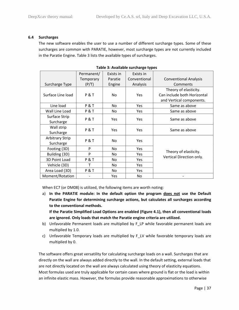
6.4 Surcharges
The new software enables the user to use a number of different surcharge types. Some of these
surcharges are common with PARATIE, however, most surcharge types are not currently included
in the Paratie Engine. Table 3 lists the available types of surcharges.
Table 3: Available surcharge types
Surcharge Type
Permanent/ Temporary
(P/T)
Exists in Paratie Engine
Exists in Conventional
Analysis Conventional Analysis
Comments
Surface Line load P & T No Yes Theory of elasticity.
Can include both Horizontal and Vertical components.
Line load P & T No Yes Same as above
Wall Line Load P & T No Yes Same as above
Surface Strip Surcharge
P & T Yes Yes Same as above
Wall strip Surcharge
P & T Yes Yes Same as above
Arbitrary Strip Surcharge
P & T No Yes
Theory of elasticity. Vertical Direction only.
Footing (3D) P No Yes
Building (3D) P No Yes
3D Point Load P & T No Yes
Vehicle (3D) T No Yes
Area Load (3D) P & T No Yes
Moment/Rotation ‐ Yes No ‐
When EC7 (or DM08) is utilized, the following items are worth noting:
a) In the PARATIE module: In the default option the program does not use the Default
Paratie Engine for determining surcharge actions, but calculates all surcharges according
to the conventional methods.
If the Paratie Simplified Load Options are enabled (Figure 4.1), then all conventional loads
are ignored. Only loads that match the Paratie engine criteria are utilized.
b) Unfavorable Permanent loads are multiplied by F_LP while favorable permanent loads are
multiplied by 1.0.
c) Unfavorable Temporary loads are multiplied by F_LV while favorable temporary loads are
multiplied by 0.
The software offers great versatility for calculating surcharge loads on a wall. Surcharges that are
directly on the wall are always added directly to the wall. In the default setting, external loads that
are not directly located on the wall are always calculated using theory of elasticity equations.
Most formulas used are truly applicable for certain cases where ground is flat or the load is within
an infinite elastic mass. However, the formulas provide reasonable approximations to otherwise

DeepXcav theory manual: Developed by Ce.A.S. srl, Italy and Deep Excavation LLC, U.S.A.
Page | 38
extremely complicated elastic solutions. When Poison's ratio is used the software finds and uses
the applicable Poisson ratio of v at each elevation.
Figure 4.1: Simplified Paratie load options Figure 4.2: Elasticity surcharge options
6.5 Line Load Surcharges
Line loads are defined with two components: a) a vertical Py, and b) a horizontal Px. It is important
to note that the many of the equations listed below are, only by themselves, applicable for a load
in an infinite soil mass. For this reason, the software multiplies the obtained surcharge by a factor
m that accounts for wall rigidity. The software assumes a default value m=2 that accounts for full
surcharge “reflection” from a rigid behavior. However, a value m=1.5 might be a reasonably less
conservative assumption that can account for limited wall displacement.
For line loads that are located on the surface (or the vertical component strip loads, since strip
loads are found by integrating with line load calculations), equations that include full wall rigidity
can be included. This behavior can be selected from the Loads/Supports tab as Figure 4.2
illustrates. In this case, the calculated loads are not multiplied by the m factor.
For vertical line loads on the surface: When the Use Equations with Wall Rigidity option is not
selected, the software uses the Boussinesq equation listed in Poulos and Davis, 1974, Equation
2.7a
Horizontal Surcharge

DeepXcav theory manual: Developed by Ce.A.S. srl, Italy and Deep Excavation LLC, U.S.A.
Page | 39
For a vertical surface line load, when the Use Equations with Wall Rigidity option is selected, the
software uses the Boussinesq equation as modified by experiment for ridig walls (Terzaghi, 1954).
For vertical line loads within the soil mass: The software uses the Melan’s equation listed in
Poulos and Davis, 1974, Equation 2.10b pg. 27
and m=(1‐v)/v
Horizontal Surcharge
For the horizontal component of a surface line load: The software uses the integrated Cerruti
problem from Poulos and Davis Equation 2.9b
Horizontal Surcharge
For the horizontal component of a line load within the soil mass: The software uses Melan’s
problem Equation 2.11b pg. 27, from Poulos & Davis
Horizontal Surcharge

DeepXcav theory manual: Developed by Ce.A.S. srl, Italy and Deep Excavation LLC, U.S.A.
Page | 40
6.6 Strip Surcharges
Strip loads in the new software can be defined with linearly varying magnitudes in both vertical
and horizontal directions. Hence, complicated surcharge patterns can be simulated. Surcharge
pressures are calculated by dividing the strip load into increments where an equivalent line load is
considered. Then the line load solutions are employed and numerically integrated to give the total
surcharge at the desired elevation. The software subdivides each strip load into 50 increments
where it performs the integration of both horizontal and vertical loads. On surface loads, the
vertical load is calculated from integration along x and not along the surface line.
6.7 Other 3D surcharge loads
The software offers the possibility to include other 3‐dimensional surcharges. In essence, all these
loads are extensions/integrations of the 3D point vertical load solution.
For 3D footings, the surcharge on the wall can be calculated in two ways:
a) By integrating the footing bearing pressure over smaller segments on the footing footprint. In
this case the footing is subdivided into a number of segments and the surcharge calculations
are slightly more time consuming.
b) By assuming that the footing load acts as a 3D point load at the footing center coordinates.
For loads that are located on the surface: The software program uses the Boussinesq equation.
Results from the following equations are multiplied by the elastic load adjustment factor m as
previously described.
The radial stress increment is then calculated as:
The hoop stress is defined as:
With the angles defined as:

DeepXcav theory manual: Developed by Ce.A.S. srl, Italy and Deep Excavation LLC, U.S.A.
Page | 41
Then, the horizontal component surcharge is:
For vertical point loads within the soil mass: The software uses the Mindlin solution as outlined by
Poulos and Davis, 1974 equations 2.4.a, and 2.4.g
6.8 Load behavior and factors when a design approach is used
When an analysis uses design approach such as EC7, each external load must be categorized as
favorable or unfavorable. In the default mode when no load combination is used, the software
program automatically categorizes loads as favorable or unfavorable based on their location and
direction relative to the wall and the excavation. Hence, loads that push the wall towards the
excavation are treated as unfavorable, while loads that push the wall towards the retained soil are
treated as favorable. In all design approach methods, favorable variable loads are ignored in the
analysis while favorable permanent loads are multiplied by a safety factor equal to 1. Unfavorable
loads get typically multiplied with factors ranging from 1 to 1.5 depending on the examined design
approach and the load nature (permanent vs. variable).
When a load combination is used, the user has the option to manually select the behavior of each
load.

DeepXcav theory manual: Developed by Ce.A.S. srl, Italy and Deep Excavation LLC, U.S.A.
Page | 42
7. Analysis Example with EC7
A simplified analysis example is presented in this section for the purpose of illustrating use of EC7
methods. The example involves the analysis of steel sheet pile wall supported by a single level of
tiebacks with the following assumptions:
‐ Retained ground surface level (uphill side) El. +200
‐ Maximum excavation level (downhill side) El. +191
‐ Water level on retained side El. +195
‐ Water level on excavated side El. +191
‐ Water density γWATER= 10kN/m3
‐ Soil properties: γTOTAL= 20kN/m3, γDRY= 19kN/m
3, c’= 3 kPa, φ= 32 deg,
Exponential soil model: Eload= 15000 kPa, Ereload = 45000 kPa, ah = 1 , av=0
KpBase =3.225 (Rankine), KaBase= 0.307 (Rankine)
Ultimate Tieback bond capacity qult = 150 kPa
User specified safety on bond values FS Geo= 1.5
‐ Tieback Data: Elevation El. +197,
Horizontal spacing = 2m
Angle = 30 deg from horizontal
Prestress = 400 kN (i.e. 200kN/m)
Structural Properties: 4 strands/1.375 cm diameter each,
Thus ASTEEL = 5.94 cm2
Steel yield strength Fy = 1862 MPa
Fixed body length LFIX = 9 m
Fixed body Diameter DFIX = 0.15m
‐ Wall Data: Steel Sheet pile AZ36, Fy = 355 MPa
Wall top. El. +200
Wall length 18m
Moment of Inertia Ixx = 82795.6 cm4/m
Section Modulus Sxx = 3600 cm3/m
‐ Surcharge: Variable triangular surcharge on wall
Pressure 5kPa at El. +200 (top of wall)
Pressure 0kPa at El. +195
The construction sequence is illustrated in Figures 4.1 through 4.4. For the classical analysis the
following assumptions will be made:
Rankine passive pressures on resisting side
Cantilever excavation: Active pressures (Free earth analysis)

DeepXcav theory manual: Developed by Ce.A.S. srl, Italy and Deep Excavation LLC, U.S.A.
Page | 43
Final stage: Apparent earth pressures from active x 1.3, redistributed top from 0 kPa at wall
top to full pressure at 25% of Hexc., Active pressures beneath subgrade.
Free earth analysis for single level of tieback analysis.
Water pressures: Simplified flow
Figure 5.1: Initial Stage (Stage 0, Distorted Scales)
Figure 5.2: Stage 1, cantilever excavation to El. +196.5 (tieback is inactive)
Figure 5.3: Stage 2, activate and prestress ground anchor at El. +197

DeepXcav theory manual: Developed by Ce.A.S. srl, Italy and Deep Excavation LLC, U.S.A.
Page | 44
Figure 5.4: Stage 3, excavate to final subgrade at El. +191
The first step will be to evaluate the active and passive earth pressures for the service case as illustrated in Figure 5.

DeepXcav theory manual: Developed by Ce.A.S. srl, Italy and Deep Excavation LLC, U.S.A.
Page | 45
Top triangular pressure height= 0.25 Hexc = 2.25 m Hexc= 9 mApparent Earth Pressure Factor: 1.3 (times active)
Eurocode Safety factors 1 1 1SOIL UNIT
WEIGHTDRY UNIT WEIGHT
WATER UNIT WEIGHT
WATER TABLE ELEV. φ Ka Kp c'
(kPa) (kPa) (kPa) (m) (deg) (kPa) (m) m m/m32 0.307 3.255 3 195 22 0.1818
20 19 10 195 32.00 0.307 3.255 3.000
ELEV.
TOTAL VERTICAL STRESS
WATER PRESSURE
EFFECTIVE VERTICAL STRESS
Acive LATERAL
SOIL STRESS
Apparent Earth
Pressures
TOTAL LATERAL STRESS
TOTAL VERTICAL STRESS
WATER PRESSURE
EFFECTIVE VERTICAL STRESS
LATERAL SOIL
STRESS
TOTAL LATERAL STRESS NET
(m) (kPa) (kPa) (kPa) (kPa) (kPa) (kPa) (kPa) (kPa) (kPa) (kPa)
200 0 0 0 0 0.00 0.00 0.00
199.43 10.82 0.00 10.82 0.00 -7.93 -7.93 -7.93
197.75 42.75 0.00 42.75 -9.81 -31.33 -31.33 -31.33
195 95 0 95 -25.86 -31.33 -31.33 -31.33
191 175 -32.7 142.3 -40.39 -31.33 -64.06 -64.06
191 175 -32.7 142.3 -40.39 -40.39 -73.12 0 0 0 10.82 10.82429 -62.3
182 355 -106.4 248.64 -73.07 -73.07 -179.43 180 106.4 73.64 250.48 356.84 177.4
Total active earth force above subgrade:
ΔFxFrom El. 200.00 to El. 199.43 0.0 kN/mFrom El. 199.43 to El. 197.75 8.2 kN/mFrom El. 197.75 to El. 195.00 49.1 kN/mFrom El. 195.00 to El. 191.00 132.5 kN/m
Sum= 189.8 kN/mFactored Forc 246.7
Max. Apparent Earth Pressure= 31.3 kPa
LEFT EXCAVATION SIDE PRESSURES RIGHT SIDE PRESSURES (PASSIVE)
Modified for calculation/Strength Reductions
Hydraulic travel length
Hydraulic loss gradient i
WATER TABLE ELEV.
180
182
184
186
188
190
192
194
196
198
200
202
-200 -100 0 100 200 300 400
EL
EV
AT
ION
(m)
LATERAL STRESS (kPa)
LEFT LAT SOIL
LEFT WATER
LEFT TOTAL
RIGHT LAT SOIL
RIGHT WATER
RIGHT TOTAL
NET
Figure 6: Calculation of lateral earth and water pressures for service case
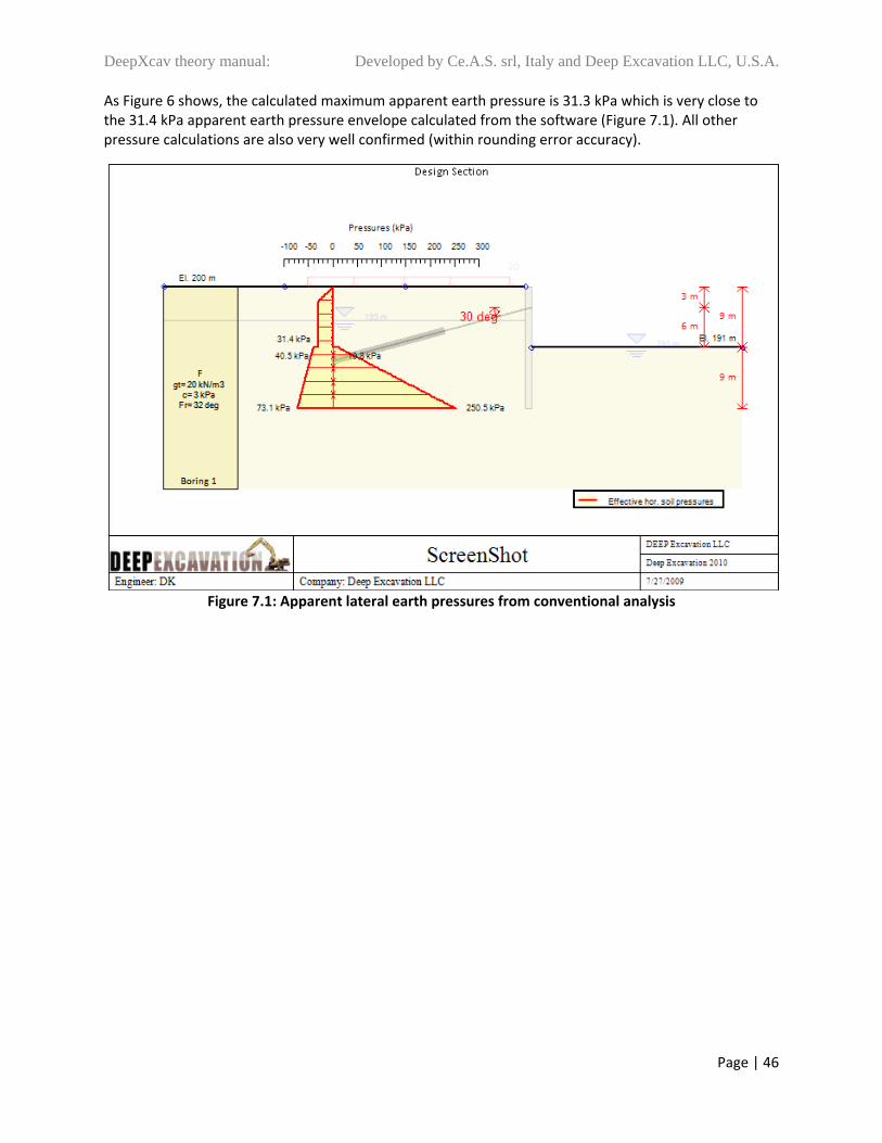
DeepXcav theory manual: Developed by Ce.A.S. srl, Italy and Deep Excavation LLC, U.S.A.
Page | 46
As Figure 6 shows, the calculated maximum apparent earth pressure is 31.3 kPa which is very close to the 31.4 kPa apparent earth pressure envelope calculated from the software (Figure 7.1). All other pressure calculations are also very well confirmed (within rounding error accuracy).
Figure 7.1: Apparent lateral earth pressures from conventional analysis

DeepXcav theory manual: Developed by Ce.A.S. srl, Italy and Deep Excavation LLC, U.S.A.
Page | 47
Figure 7.2: Simplified flow groundwater pressures from conventional analysis
Figure 7.3: Simplified flow net groundwater pressures from conventional analysis

DeepXcav theory manual: Developed by Ce.A.S. srl, Italy and Deep Excavation LLC, U.S.A.
Page | 48
Figure 7.4: Wall surcharge pressures (unfactored)
Figure 7.5: Wall displacements from conventional analysis (last stage)

DeepXcav theory manual: Developed by Ce.A.S. srl, Italy and Deep Excavation LLC, U.S.A.
Page | 49
Figure 7.6: Shear and moment diagrams with support reaction and stress checks drawn (red lines on
moment diagram show wall capacity).
Figure 7.7: Shear and moment diagram envelopes (for current design section only)

DeepXcav theory manual: Developed by Ce.A.S. srl, Italy and Deep Excavation LLC, U.S.A.
Page | 50
Next, the EC7 combination DA‐3 approach will be examined in detail. However, all EC7 design approaches will be analyzed simultaneously. The model is linked to the base design section.
Figure 8.1: General model for EC7 DA‐3 Approach The corresponding safety factors are:
FS(tan(φ)) = 1.25 FS(c’) = 1.25 FS(Su) = 1.5 (this is also used for the ultimate bond resistance) FS(Actions temp) = 1.3 FS(Anchors)= 1.1 FS(Water Drive)= 1.0 FS(Drive_Earth)= 1.0
Next the active and passive earth pressures, as well as the net water pressures for the DA3 approach will be calculated as illustrated in Figure 8.2. As Figures 8.3 through 8.4 demonstrate, the software calculates essentially the same lateral earth pressures as the spreadsheet shown in Figure 8.2.

DeepXcav theory manual: Developed by Ce.A.S. srl, Italy and Deep Excavation LLC, U.S.A.
Page | 51
Top triangular pressure height= 0.25 Hexc = 2.25 m Hexc= 9 m
Apparent Earth Pressure Factor: 1.3 (times active)
Eurocode Safety factors 1.25 1 1.25SOIL UNIT
WEIGHTDRY UNIT WEIGHT
WATER UNIT WEIGHT
WATER TABLE ELEV. φ Ka Kp c'
(kPa) (kPa) (kPa) (m) (deg) (kPa) (m) m m/m32 0.307 3.255 3 195 22 0.1818 1 1 1
20 19 10 195 26.56 0.382 2.618 2.400
ELEV.
TOTAL VERTICAL STRESS
UNFACTORED WATER
PRESSURE
EFFECTIVE VERTICAL STRESS
Acive LATERAL
SOIL STRESS
Apparent Earth
Pressures
TOTAL LATERAL STRESS (factored
earth)
TOTAL VERTICAL STRESS
WATER PRESSURE
EFFECTIVE VERTICAL STRESS
LATERAL SOIL
STRESS
TOTAL LATERAL STRESS
Net water pressure (factored) NET
(m) (kPa) (kPa) (kPa) (kPa) (kPa) (kPa) (kPa) (kPa) (kPa) (kPa) (kPa)
200 0 0 0 0 0.00 0.00 0 0.00
199.59 7.77 0.00 7.77 0.00 -7.37 -7.37 0 -7.37
197.75 42.75 0.00 42.75 -13.37 -40.60 -40.60 0 -40.60
195 95 0 95 -33.33 -40.60 -40.60 0 -40.60
191 175 -32.7 142.3 -51.39 -40.60 -73.33 -32.73 -73.3
191 175 -32.7 142.3 -51.39 -51.39 -84.11 0 0 0 7.77 7.765837 -32.73 -76.3
182 355 -106.4 248.64 -92.02 -92.02 -198.39 180 106.4 73.64 200.51 306.88 0.00 108.5
Total active earth force above subgrade:
ΔFxFrom El. 200.00 to El. 199.59 0.0 kN/mFrom El. 199.59 to El. 197.75 12.3 kN/mFrom El. 197.75 to El. 195.00 64.2 kN/mFrom El. 195.00 to El. 191.00 169.4 kN/m
Sum= 245.9 kN/mFactored Forc 319.7
Max. Apparent Earth Pressure= 40.60 kPa
Modified for calculation/Strength Reductions
LEFT EXCAVATION SIDE PRESSURES RIGHT SIDE PRESSURES (PASSIVE)
WATER TABLE ELEV.
Hydraulic travel length
Hydraulic loss gradient i
Safety factor on net water pressures
Safety factor on
earth pressures
Safety factor on Passive
Resistance
180
182
184
186
188
190
192
194
196
198
200
202
-300 -200 -100 0 100 200 300 400
EL
EV
AT
ION
(m)
LATERAL STRESS (kPa)
LEFT LAT SOIL
LEFT WATER
LEFT TOTAL
RIGHT LAT SOIL
RIGHT WATER
RIGHT TOTAL
NET Water
Net
Figure 8.2: Calculation of lateral earth and water pressures for DA3 Approach

DeepXcav theory manual: Developed by Ce.A.S. srl, Italy and Deep Excavation LLC, U.S.A.
Page | 52
Figure 8.2: Apparent lateral earth pressures for DA3 Approach (40.7 kPa pressure verified spreadsheet calculations)
Figure 8.3: Factored lateral surcharge pressures for DA3 Approach (7.5 kPa pressure = 5 kPa x 1.5)

DeepXcav theory manual: Developed by Ce.A.S. srl, Italy and Deep Excavation LLC, U.S.A.
Page | 53
Figure 8.4: Net Factored water pressures for DA3 Approach 32.73 kPa pressure = 32.73 kPa x 1.0 , 32.7 kPa from Figure 6.3
Spreadsheet calculation 32.7 kPa
Figure 8.5: Wall shear and moment for DA3 Approach

DeepXcav theory manual: Developed by Ce.A.S. srl, Italy and Deep Excavation LLC, U.S.A.
Page | 54
Next we examine the case of DA1‐1 where earth and water pressures are multiplied by safety factors while the soil strength parameters are maintained.
Top triangular pressure height= 0.25 Hexc = 2.25 m Hexc= 9 mApparent Earth Pressure Factor: 1.3 (times active)
Eurocode Safety factors 1 1 1SOIL UNIT
WEIGHTDRY UNIT WEIGHT
WATER UNIT WEIGHT
WATER TABLE ELEV. φ Ka Kp c'
(kPa) (kPa) (kPa) (m) (deg) (kPa) (m) m m/m32 0.307 3.255 3 195 22 0.1818 1.35 1.35 1
20 19 10 195 32.00 0.307 3.255 3.000
ELEV.
TOTAL VERTICAL STRESS
UNFACTORED WATER
PRESSURE
EFFECTIVE VERTICAL STRESS
Acive LATERAL
SOIL STRESS
Apparent Earth
Pressures
TOTAL LATERAL STRESS (factored
earth)
TOTAL VERTICAL STRESS
WATER PRESSURE
EFFECTIVE VERTICAL STRESS
LATERAL SOIL
STRESS
TOTAL LATERAL STRESS
Net water pressure (factored) NET
(m) (kPa) (kPa) (kPa) (kPa) (kPa) (kPa) (kPa) (kPa) (kPa) (kPa) (kPa)
200 0 0 0 0 0.00 0.00 0 0.00
199.43 10.82 0.00 10.82 0.00 -7.93 -10.71 0 -10.71
197.75 42.75 0.00 42.75 -9.81 -31.33 -42.30 0 -42.30
195 95 0 95 -25.86 -31.33 -42.30 0 -42.30
191 175 -32.7 142.3 -40.39 -31.33 -75.02 -44.18 -86.5
191 175 -32.7 142.3 -40.39 -40.39 -87.25 0 0 0 10.82 10.82429 -44.18 -87.9
182 355 -106.4 248.64 -73.07 -73.07 -205.01 180 106.4 73.64 250.48 356.84 0.00 151.8
Total active earth force above subgrade:
ΔFxFrom El. 200.00 to El. 199.43 0.0 kN/mFrom El. 199.43 to El. 197.75 8.2 kN/mFrom El. 197.75 to El. 195.00 49.1 kN/mFrom El. 195.00 to El. 191.00 132.5 kN/m
Sum= 189.8 kN/mFactored Forc 246.7
Max. Apparent Earth Pressure= 31.33 kPa
Safety factor on
earth pressures
Safety factor on Passive
Resistance
WATER TABLE ELEV.
Hydraulic travel length
Hydraulic loss gradient i
Modified for calculation/Strength Reductions
LEFT EXCAVATION SIDE PRESSURES RIGHT SIDE PRESSURES (PASSIVE)
Safety factor on net water pressures
180
182
184
186
188
190
192
194
196
198
200
202
-300 -200 -100 0 100 200 300 400
EL
EV
AT
ION
(m)
LATERAL STRESS (kPa)
LEFT LAT SOIL
LEFT WATER
LEFT TOTAL
RIGHT LAT SOIL
RIGHT WATER
RIGHT TOTAL
NET Water
Net
Figure 8.6: Calculation of lateral earth and water pressures for DA1‐1 Approach

DeepXcav theory manual: Developed by Ce.A.S. srl, Italy and Deep Excavation LLC, U.S.A.
Page | 55
Figure 8.7: Apparent lateral earth pressures for DA1‐1 Approach (42.4 kPa pressure verified spreadsheet calculations)
Figure 8.8: Net Factored water pressures for DA1‐1 Approach 44.18 kPa pressure = 32.73 kPa x 1.35 , 32.7 kPa from Figure 6.3
Spreadsheet calculation 44.18 kPa
In the following pages, the non‐linear solution to the same problem is briefly presented.

DeepXcav theory manual: Developed by Ce.A.S. srl, Italy and Deep Excavation LLC, U.S.A.
Page | 56
Figure 9.1: Wall bending moments and shear forces for Paratie Solution for service case.
Figure 9.2: Wall bending moments and shear forces for Paratie Solution for DA3 case.

DeepXcav theory manual: Developed by Ce.A.S. srl, Italy and Deep Excavation LLC, U.S.A.
Page | 57
Figure 9.3: Net water pressures for Paratie Solution for DA3 case (not yet factored)
Figure 9.4: Wall bending moments and shear forces for Paratie Solution for DA1‐1 case.
IMPORTANT For DA1‐1: In Paratie when Water Unfavorable or Earth Unfavorable are greater than 1, wall bending, wall shear, and support reaction results are obtained from an equivalent service analysis approach. In this approach, all surcharge magnitudes are standardized by Earth Unfavorable (1.35 in DA1‐1), thus, unfavorable variable loads will be multiplied by 1.5/1.35=1.111 while permanent loads by 1.35/1.35=1. When the analysis is completed the wall moment, wall shear, and support reaction results are multiplied x 1.35. The displacements however are not multiplied.

DeepXcav theory manual: Developed by Ce.A.S. srl, Italy and Deep Excavation LLC, U.S.A.
Page | 58
The tieback STR & GEO capacity calculations will be performed for Case DA1‐1:
R = 1.1 (temporary tieback)
SU = 1 (Shear strength also used for bond values) FS Geo = 1.0 User specified safety factor in this example,
recommended value 1.35 in other conditions.
Fixed body length LFIX = 9 m
Fixed body Diameter DFIX = 0.15m
Ultimate Skin friction qULT = 150 kPa
Then the ultimate geotechnical capacity is:
RULT.GEO = LFIX x π x DFIX x qULT/ R)
RULT.GEO = 578.33 kN per ground anchor
The design geotechnical capacity (for stress check ratios) is calculated as:
RDES.GEO = LFIX x π x DFIX x qULT/ R x SU xFS Geo) = 578.33 kN
The Ultimate Structural capacity can be calculated as:
RULT.STR = AFIX.STEEL x Fy/ M)
Note that 1/ M = φ in the EC = 0.87
RULT.STR = 0.87 AFIX.STEEL x Fy
RULT.STR = 0.87 x 5.94 cm2 x 1862 MPa = 961.8 kN
These results are verified by the software program:

DeepXcav theory manual: Developed by Ce.A.S. srl, Italy and Deep Excavation LLC, U.S.A.
Page | 59
Figure 9.6: Individual support reactions/capacity The tieback GEO capacity calculations for Case DA1‐2:
R = 1.1 (temporary tieback)
SU = 1.4 (Shear strength also used for bond values) FS Geo = 1.0 In M2 cases this factor is automatically set to 1.0 in
order to produce consistent capacities with available design charts for bond resistance of ground anchors (where an FS=2.0).
Fixed body length LFIX = 9 m
Fixed body Diameter DFIX = 0.15m
Ultimate Skin friction qULT = 150 kPa
Then the ultimate geotechnical capacity is:
RULT.GEO = LFIX x π x DFIX x qULT/ R x SU xFS Geo)
RULT.GEO = 578.33 kN per ground anchor
The design geotechnical capacity (for stress check ratios) is calculated as:
RDES.GEO = LFIX x π x DFIX x qULT/ R x SU xFS Geo) = 413.1 kN

DeepXcav theory manual: Developed by Ce.A.S. srl, Italy and Deep Excavation LLC, U.S.A.
Page | 60
Figure 9.7: Individual support reactions/capacity for DA1‐2

DeepXcav theory manual: Developed by Ce.A.S. srl, Italy and Deep Excavation LLC, U.S.A.
Page | 61
8. Ground anchor and helical anchor capacity calculations
8.1 Ground Anchor Capacity Calculations
A ground anchor has two forms of capacity, a geotechnical and a structural resistance. The
structural resistance of the tendons is defined by EC steel standards while the bonded zone has
to be examined for its pull‐out capacity (geotechnical check). The new software includes a
number of ground anchor (tieback) sections. Hence, a ground anchor section can be reused over
and over in many different support levels and in many different design sections (the same
approach is also utilized for steel struts, rakers (inclined struts), and concrete slabs). The tieback
capacities (ultimate and permissible) can be calculated using the following equations:
a) Ultimate geotechnical capacity used for the geotechnical yielding is:
RULT.GEO = LFIX x π x DFIX x qULT/ R)
b) The design geotechnical capacity (for stress check ratios) is calculated as:
RDES.GEO = LFIX x π x DFIX x qULT/ R x SU xFS Geo)
Where:
qULT = Ultimate Skin friction (options available) LFIX = Fixed body length
DFIX = Fixed body diameter (0.09m to 0.15m typically) FS Geo = 1.0 to 2.0 user specified safety factor.
FS Geo= 1.0 in M2 design approach methods.
R = 1 to 1.2 Resistance factor geotechnical capacity
SU = 1 to 1.4 (Shear strength, used for bond values)
Note that R and SU are by default 1, but take Eurocode or DM08 specified values when a design approach is used. c) The ultimate and design Structural capacity can be calculated as:
PULT.STR = φULT.CODE x (Area of Tendons) x Fy
φ ULT.CODE = Material strength reduction factor typically 0.9
PDES.STR = φDES x (Area of Tendons) x Fy
φ DES = Material strength reduction factor 0.6 to 0.9
The ultimate capacity is used to determine the structural yielding of the element while the
permissible is used for the stress checks. φULT.CODE is always picked up from the structural
code that is used. φDES can be specified by the user or can be set automatically when the
some code settings are specified. When Eurocodes are used φALL should be the same as
φULT.CODE.
Note that φ= 1/ M
In the default setting during a Paratie analysis, the new software models a tieback automatically
as a yielding element (Wire with yielding properties) with its yielding force determined as the

DeepXcav theory manual: Developed by Ce.A.S. srl, Italy and Deep Excavation LLC, U.S.A.
Page | 62
minimum STR or GEO capacity. A ground anchor can also be modeled as a non‐yielding wire
element by selecting the appropriate option in the Advanced Tab of the Tieback dialog.
However, it is felt that due to legal reasons it is better to include a tieback as yielding element by
default.
Figure 10.1 shows the main tieback section dialog. The main parameters of interest are the steel
material, the cross sectional area of the steel tendons, and the fixed body diameter (Dfix).
Figure 10.1: Main tieback section dialog (Elastic‐Wire command in Red)
The geotechnical capacity represents the capacity of the soil to resist the tensile forces
transferred by the steel strands to the grouted body. The new software subdivides the fixed
body into a number of elements were soil resistance is computed. As previously mentioned, the
geotechnical tieback capacity is evaluated for every stage. Within the current Paratie engine, it
is currently possible to change the yield limit of an ELPL spring from stage to stage. Initially, in
the Paratie mode the software uses the capacity at the stage of installation. The capacity is
adjusted at each stage and the final support check is performed for the actual capacity for each
stage. A number of options exist for defining the geotechnical capacity of a tieback:

DeepXcav theory manual: Developed by Ce.A.S. srl, Italy and Deep Excavation LLC, U.S.A.
Page | 63
a) Soil resistance is computed from frictional and cohesive components. For the frictional
component, DeepXcav uses the average of the vertical and lateral at‐rest stress times the
tangent of the friction angle. For the cohesive component, adhesion factors can be applied.
Furthermore, individual densification factors can be applied separately to the frictional and
cohesive components to simulate the effect of pressure grouting. End bearing at the start of
the grouted body is ignored. These calculations should be considered as a first order
estimate. Hence, in this case the ultimate skin friction can be defined as:
t ULT =F1 x 0.5 x (σ’V+ σ’H‐Ko) x tan (φ) + F2 x α x (c’ or SU)
In an undrained analysis the software will use SU and φ=0. For a drained analysis the
program will use φ and c’.
Where:
F1 = Frictional densification factor (default 1)
F2 = Cohesional densification factor (default 1)
α = Adhesion factor (default =1), but program also offers a dynamic tri‐linear
approach for defining this parameter based on c’ or Su. In this approach:
α = Value 1 = 0.8 if c’ or Su <= Climit1
α = Value 2 = 0.5 if c’ or Su >= Climit2
α = Linear interpolation for c’ or Su between Clim1 and Clim2.
b) User‐defined geotechnical capacity (and structural) defined from the advanced tieback tab.
Figure 10.2: Advanced tieback dialog tab

DeepXcav theory manual: Developed by Ce.A.S. srl, Italy and Deep Excavation LLC, U.S.A.
Page | 64
c) Ultimate specific bond resistance for tieback section.
t ULT = qULT in Geotechnical tab of tieback section
Figure 10.3: Geotechnical tieback dialog tab (Wire command in Red)
d) Ultimate bond resistance determined from integrating soil ultimate skin friction resistances
over the fixed length.
t ULT = qULT from Soil type (Bond Tab)
In this case, the skin friction can be determined from the Bustamante design charts (Fig.
10.5.1, 10.5.2) when pressuremeter test data are available.
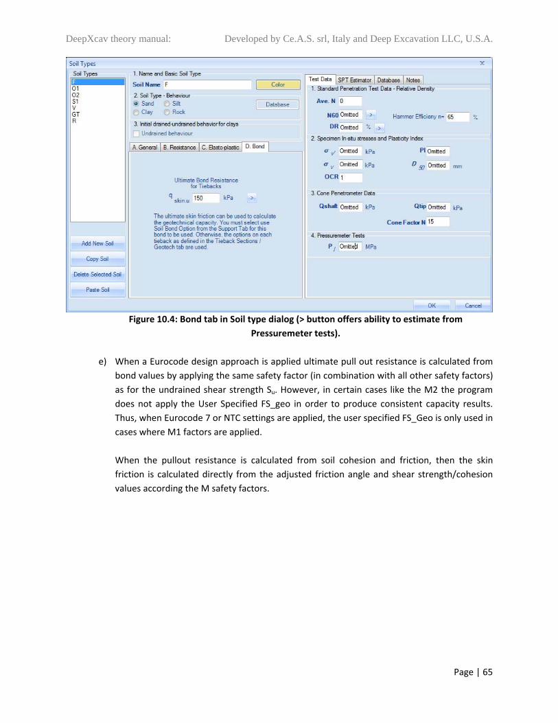
DeepXcav theory manual: Developed by Ce.A.S. srl, Italy and Deep Excavation LLC, U.S.A.
Page | 65
Figure 10.4: Bond tab in Soil type dialog (> button offers ability to estimate from
Pressuremeter tests).
e) When a Eurocode design approach is applied ultimate pull out resistance is calculated from
bond values by applying the same safety factor (in combination with all other safety factors)
as for the undrained shear strength Su. However, in certain cases like the M2 the program
does not apply the User Specified FS_geo in order to produce consistent capacity results.
Thus, when Eurocode 7 or NTC settings are applied, the user specified FS_Geo is only used in
cases where M1 factors are applied.
When the pullout resistance is calculated from soil cohesion and friction, then the skin
friction is calculated directly from the adjusted friction angle and shear strength/cohesion
values according the M safety factors.

DeepXcav theory manual: Developed by Ce.A.S. srl, Italy and Deep Excavation LLC, U.S.A.
Page | 66
Figure 10.5.1: Estimation of bond resistance for tiebacks from TA‐95 according to Bustamante.
Figure 10.5.2: Estimation of bond resistance for tiebacks from Pressuremeter tests FHWA and
French recommendations.

DeepXcav theory manual: Developed by Ce.A.S. srl, Italy and Deep Excavation LLC, U.S.A.
Page | 67
8.2 Helical anchor capacity calculations
A helical anchor/pile consists of one or more helix‐shaped bearing plates attached to a central shaft,
which is installed by rotating or "torqueing" into the ground. Each helix is attached near the tip, is
generally circular in plan, and formed into a helix with a defined pitch. Helical anchors/piles derive
their load‐carrying capacity through both end bearing on the helix plates and skin friction on the
shaft (Figure 10.6.1).
Figure 10.6.1: Typical helical anchor detail and geotechnical capacity behavior
According to IBC 2009, the allowable axial design load, Pa, of helical piles shall be determined as follows:
Pa = 0.5 Pu (IBC 2009 Equation 18‐4) Where Pu is the least value of:
1. Sum of the areas of the helical bearing plates times the ultimate bearing capacity of the soil or rock comprising the bearing stratum. 2. Ultimate capacity determined from well‐documented correlations with installation torque. 3. Ultimate capacity determined from load tests. 4. Ultimate axial capacity of pile shaft. 5. Ultimate capacity of pile shaft couplings. 6. Sum of the ultimate axial capacity of helical bearing plates affixed to pile.

DeepXcav theory manual: Developed by Ce.A.S. srl, Italy and Deep Excavation LLC, U.S.A.
Page | 68
An explanation and summary of each of the six design criterions required per the IBC for helical pile design have been listed below to better explain the design process and intent of the code. Item 1 is in reference to the Individual Bearing Method. This method requires prior knowledge of the soil properties at the site via a soils report or boring logs. Please note that most soil reports only report the allowable bearing capacity of a soil or stratum. This allowable capacity normally has a safety factor of two or three applied. Item 1 is in reference to the Individual Bearing Method. This method requires prior knowledge of the soil properties at the site via a soils report or boring logs. Please note that most soil reports only report the allowable bearing capacity of a soil or stratum. This allowable capacity normally has a safety factor of two or three applied. Applying another factor of safety of two per the IBC would be extremely conservative. Typical helical plate sizes are 8”, 10”, 12”, 14” and 16” in diameter. The maximum number of helical plates placed on a single pile is normally set at six (6). The central area of the shaft is typically omitted from the effective area of the helical plate when using the Individual Bearing Method. The total capacity of the anchor can be calculated as:
Qult = Qshaft + ΣQh where: Qult = Total Multi‐helix Anchor/Pile Ultimate Capacity Qh = Individual Helix Ultimate Capacity
Qh = Ah (Nc c + γ D Nq) ≤ Qh.str Qh = Ah (9 c + γ D Nq) ≤ Qh.str
where: Ah = Projected effective area of helix Nc = 9 for ratio of top helix depth to helix dia. > 5 (program assumes value =9) D = Depth of helix plate below ground line Nq = Bearing capacity factor for sand Qh.str = Upper mechanical limit determined by helix strength Qshaft= Geotechnical shaft resistance can be also included. Within the program, the shaft
resistance is calculated only within from the starting point of the fixed length of the anchor to the first encountered helical plate. In most cases, the shaft resistance is conservatively ignored.
The software program replaces the above γ D term with the vertical effective stress at each helix. According to a standard practice (AB Chance corporation presentation), Nq can be calculated as adapted from G. G. Meyerhof Factors for Driven Piles in his paper Bearing Capacity and Settlement of Pile Foundations, 1976 Equation:
Nq=0.5 (12*φ)φ/54
With a few exceptions, the shaft resistance can be calculated in a similar manner as the geotechnical capacity of ground anchors. When the capacity is calculated with side frictional methods, a distinction can be made between a grouted a non grouted shaft (i.e. a grouted shaft has friction of cement grout with soil while a non grouted shaft between steel and soil).

DeepXcav theory manual: Developed by Ce.A.S. srl, Italy and Deep Excavation LLC, U.S.A.
Page | 69
Item 2 is in reference to the Torque Correlation Method. The Torque Correlation Method is an empirical method that distinguishes the relationship between helical pile capacity and installation torque and has been widely used since the 1960’s. The process of a helical plate shearing through the soil or weathered bedrock in a circular motion is equivalent to a plate penetrometer test. The method gained notoriety based on the study performed by Hoyt and Clemence (1989). Their study analyzed 91 helical pile load tests at 24 different sites within various soil types ranging from sand, silt and clay soils. They demonstrated the direct correlation of the installation torque of a helical pile to its ultimate capacity in compression or tension. The common denominator discovered from the study was a parameter referred to as the torque correlation factor, Kt. The equation is:
Pu = Kt T Where:
Pu is the ultimate capacity of the helical pile or anchor [lb (kN)]. Kt is the empirical torque factor of the central shaft of the pile [ft‐1 (m‐1)]. T is the final installation torque [ft‐lb (m‐kN)].
It’s important to point out that the tests analyzed by Hoyt and Clemence (1989) were in tension. It was shown in sub‐sequential studies that the tension capacity of helical piles was 16 to 33 percent less than the measured compression capacity. The difference is attributed to the fact that the lead helical plate is bearing on relatively undisturbed soil in compression applications. In tension applications, the leading and trailing helical plates are bearing on soil affected by the installation of the helical plates. It has become common practice to use the same torque correlation factor for a helical pile of the same size for tension and compression and ignore the slight increase in compression capacity. This creates a more conservative compression capacity for helical piles when compared to the Individual Bearing Method. Also unlike the Individual Bearing Method, the number of helical plates on a pile is completely independent of the piles capacity based on the Torque Correlation Method.
Figure 10.6.2: Typical recommended torque factors
When helical anchors are used in a non‐linear analysis, the elastic behavior of the helical anchor must be first estimated. In most cases, the ultimate geotechnical pullout resistance of a helical anchor is controlled by the bearing at each helix. As a result, the ultimate resistance of a helical anchor is realized at much greater strains than shaft resistance, and may require as much displacement as 10% of the helix diameter. A reasonable, albeit rough assumption, is to use an additional displacement 4% of the largest helix diameter at 65% of the ultimate anchor capacity (Figure 10.6.3). This additional strain/displacement is added to the elastic anchor elongation and must be verified by load tests.

DeepXcav theory manual: Developed by Ce.A.S. srl, Italy and Deep Excavation LLC, U.S.A.
Page | 70
Figure 10.6.3: Elastic behavior of helical anchors – advanced tab

DeepXcav theory manual: Developed by Ce.A.S. srl, Italy and Deep Excavation LLC, U.S.A.
Page | 71
9. Geotechnical Safety Factors
9.1 Wall Embedment Stability (toe stability)
9.1.1 Introduction Support walls must be embedded sufficiently to prevent toe stability failure. DeepXcav uses
classical methods in determining the toe embedment depth for a safety factor of 1.0 and the
available safety factor. The following paragraphs describe the available methods for calculating toe
stability for cantilever, single support, and multiple level braced walls. The following safety factor
definitions are available:
1) Passive Resistance Safety Factor (Conventional Analysis):
2) Rotational Safety Factor (Conventional Analysis):
3) Length based (Conventional Analysis):
4) Mobilized passive resistance (PARATIE)
The mobilized passive resistance is currently calculated with conventional analysis methods
(that can include the effects of non‐linear ground surface).
5) Zcut method (PARATIE)
The internal Paratie engine gradually reduces the wall length until the wall collapses.
When both the conventional and PARATIE methods are used, the software first analyzes the model
with the conventional approach and stores the calculated conventional safety factors (Equations 9.1,
9.2, 9.3). Subsequently, once the PARATIE analysis is successfully performed, the software evaluates
the toe safety based on Eq. 9.4. In this way the user has the benefit of evaluating all conventional
safety factors while performing a PARATIE analysis at the same time.
Note that in equations 9.1 and 9.2 the water contribution is included as a net driving (i.e.
unfavorable) component in the denominator.

DeepXcav theory manual: Developed by Ce.A.S. srl, Italy and Deep Excavation LLC, U.S.A.
Page | 72
9.1.2 Cantilever Walls (conventional analysis)
For cantilever walls, on may use the "free" earth method or the "fixed" earth method as
illustrated in the figure below. The safety factor is defined as the available embedment depth over
the embedment depth for a safety factor of 1.0 using the given set of pressure assumptions. The
fixed earth method uses an iterative search solution to find the minimum depth were stability is
satisfied. Note that in some instances, the fixed earth method may fail to converge when very stiff
soils with high cohesion values are used. In such a case you might have to use the free earth method
to obtain results.
In the free earth method the software finds the depth of wall where the overturning moment is
equal to the resisting moment and this depth is then set as the FSrotation= 1.0 depth. In this
method, the horizontal forces are not balanced and for stable walls the passive resistance is greater
than the driving resistance (wall shear is not automatically balanced). The software then calculates a
safety factor for resisting to driving moments, and also an embedment safety factor just based on
depth (FS= Depth from subgrade to wall bottom / depth from subgrade to elevation of zero
moment). The overall reported safety factor is the minimum of the two values.
Figure 11.1: Fixed Earth Method for a cantilever wall

DeepXcav theory manual: Developed by Ce.A.S. srl, Italy and Deep Excavation LLC, U.S.A.
Page | 73
9.1.3 Walls supported by a single bracing level in conventional analyses.
For walls supported by a single level of bracing the software uses the free earth method as
illustrated below. For multiple support walls, moments are taken in the same fashion about the
lowest support level. However, only pressures below the lowest support level are considered. The
safety factor is defined as:
FS= Resisting Moment about anchor point/ Overturning Moment about anchor point
Figure 11.2: Free Earth Method for a wall supported by a single level of anchors
9.1.4 Walls supported by a multiple bracing levels (conventional analysis)
For walls supported by multiple braces the software can calculate both the horizontal force
safety factor and the rotational safety factor (Eq. 9.1 and 9.2):
FSrotation= Resisting Moment about lowest brace/ Overturning Moment about lowest brace
Only the force/pressures below the lowest brace are accounted in the above equation.
For the passive safety factor, the software offers two possibilities depending on how the support
forces are determined:
a) If the wall is analyzed with a beam analysis “Blum’s method”, then the software finds the
virtual net horizontal reaction that acts on the virtual fixity point beneath the subgrade. The
passive safety factor is then taken as:

DeepXcav theory manual: Developed by Ce.A.S. srl, Italy and Deep Excavation LLC, U.S.A.
Page | 74
a) If the support reactions are determined with the tributary area method, then the software
determines the apparent horizontal reaction that acts at the subgrade level (i.e. at the
excavation elevation). The passive safety factor is then taken as:
Driving pressures= Soil Pressure at driving side + Net Water Pressures
9.2 Clough Predictions & Basal Stability Index
Clough (Clough et. al., 1989) developed a method for predicting wall deflections based on a
normalized system using a stiffness factor and on a factor of safety for basal stability. Clough
defines the system stiffness factor as the product of the modulus of elasticity (E) times the inertia
(I) of the wall divided by the unit weight of water (W) times the average brace spacing. This
approach of predicting wall deflections has some obvious limitations when applied to stiff walls
because: a) the typical spacing between vertical supports varies little from project to project
(average 9ft to 12 ft) with 7ft minimum and 17ft maximum, b) the wall thickness typically varies
from 2’ to 3’, c) the effects of prestressing braces are totally ignored, and d) the effect of soil
conditions is partially accounted in the basal stability factor that is not directly applicable for the
majority of the walls that were keyed into a stiff stratum.
It is clear that the big limitation of the system stiffness approach is the generic assumption that
wall deflections are primarily related to deformations occurring between support levels. In
individual projects, there may be several length scales affecting the wall deflections depending on
the toe fixity of the wall, the depth to bedrock, the wall embedment below the base of the
excavation, the width of the excavation, the size of berms, and the initial unsupported excavation
depth. Furthermore, the proposed method of Clough et. al. [1989] takes not account of the
stiffness profile in the retained soil.
Recently, a much more detailed finite element study has carried out by Jen [1998]. These finite
analyses consisted of three main groups of parametric analyses to quantify the effects of
excavation geometry, soil profile, and support system. The parameters she studied included: I)
Geometry (wall length, excavation width, depth to bedrock), II) Soil Profile (overconsolidation
ratio of the clay, cohesionless layer over a clay stratum, presence of clay crust over low OCR clay
stratum), and III) Support System (stiffness of support wall, and bracing components).
Jen [1998] found that walls basically undergo three phases of deformation: i) Unsupported
cantilever deflections; ii) bulging (subgrade bending); and iii) toe kickout. She concluded that the
actual deformation phase was determined by the wall embedment depth. Wall stiffness was more
effective in reducing deformations for soft soils but had a smaller effect in stiffer soils. She also
found that the depth to bedrock had a significant impact on the surface settlement at a distance
from the excavation.

DeepXcav theory manual: Developed by Ce.A.S. srl, Italy and Deep Excavation LLC, U.S.A.
Page | 75
Figure 11.3: Predicted wall displacements versus system stiffness according to Clough et. al.
Table 4.1: Limit equilibrium calculations of base stability (after Terzaghi, 1943).
Nc sub __
FS= For D<(¨ 2 / 2) B
‐ sub /D Nc sub __
FS= For D>(¨ 2 / 2) B 2 suu
‐ ¨ 2 B
sub = undrained strength of basal clay suu = undrained strength of clay above the excavation grade B = Breadth of excavation D = Depth from excavation grade to firm stratum Nc = 5.4
Since multiple soil types can be included DeepXcav averages the undrained shear strength of the
soil below the subgrade within one excavation depth below subgrade or until a rock layer is
encountered. Note that the frictional component of a soil is included by adding to Su the sum of
the vertical effective stress times the tangent of the friction angle on the left and right wall side.

DeepXcav theory manual: Developed by Ce.A.S. srl, Italy and Deep Excavation LLC, U.S.A.
Page | 76
9.3 Ground surface settlement estimation Boone and Westland reported an interesting approach to estimating ground settlements. This
approach associates ground settlements to the basal stability index, a modified system stiffness
value, and individual wall displacement components as seen in the following figure. Wall
displacements and surface settlements are divided in two major categories:
a) Cantilever wall – generating the sprandel settlement volume trough Avs b) Bending wall movements – generating the concave settlement trough Avc The combination of sprandel and concave settlement troughs results in the combined total settlement profile. Both these areas Avs and Avc are taken as a certain percentage of the corresponding wall movements.
When a non‐linear solution is performed (beam on elastic foundations), DeepXcav offers the
ability to estimate surface settlements directly from computed wall displacements. In addition,
DeepXcav will add a component for toe translation to the concave settlement. This additional
volume is estimated as a triangle by extrapolating a line from the maximum displacement above
the wall toe to the displacement at the wall base. The following table provides detailed
information and recommendations about using this method.
If settlements are used, it is strongly recommended to enable the modifications from the
surface settlements tab in the main form (otherwise surface settlements may be greatly
overestimated).
Figure 11.4: Definitions of lateral and vertical displacement parameters: concave on left, sprandel on
right (after Boone 2003).

DeepXcav theory manual: Developed by Ce.A.S. srl, Italy and Deep Excavation LLC, U.S.A.
Page | 77
Table 4.2: Summary of displacement estimation equations based on curve fitting of non‐linear numerical modeling results.

DeepXcav theory manual: Developed by Ce.A.S. srl, Italy and Deep Excavation LLC, U.S.A.
Page | 78
10. Handling unbalanced water pressures in Paratie As discussed before, automatic handing of water pressures in Paratie when Eurocode is used can be a very tricky subject. The following paragraphs list some available options for reasonably modeling water in Paratie simulations: Automatic Generation: Alternative A: Inclusion of a model factor on wall and support results In this approach, wall bending/shear and support reactions are multiplied by a model factor to account for the additional net water forces. The software uses the safety factor on unfavorable earth resistance as the “model” factor which in all Eurocode 7 and DM08 approaches is equal to the water unfavorable factor. This philosophical contrast stems from the fact that, in this case, we would have gone through all the effort of readjusting soil properties, actions, etc. only to come at the end of our analysis and essentially use an allowable safety factor. This approach is used Manual Generation (Must be specified externally by user) Alternative B: Readjustment of water levels (Manual) From a theoretical standpoint, the most appropriate solution if the groundwater table is beneath the surface would be to simply raise the ground water elevation (but one should be careful not to elevate the ground water elevation above). However, in this approach an automatic groundwater elevation change might not make much sense all together in many cases. For example, in a 15 m excavation beneath the groundwater one would multiply the retained water height by 1,35 resulting in:
New water height H = 1.35 x 15 m = 20.25m It is obvious, that for a typical excavation elevating the water table by 5.25m would create unrealistic modeling of the soil stress‐state history. For example, if one were to do this in Milan (where there is a canal and the water table is 3 m below the street) then the simulated assumption would be that the water has raised 2.25 m above the street level, essentially flooding the entrance of many buildings. Thus, a reasonable automatic generation procedure for readjusting water levels can be very challenging and is not implemented within the software. Alternative C: Addition of net water pressures as external pressures In this approach, the additional net factored water pressures (above the normal water pressures calculated from groundwater flow analysis) are added automatically as an external surcharge. With this alternative additional water pressures should be accounted on every stage

DeepXcav theory manual: Developed by Ce.A.S. srl, Italy and Deep Excavation LLC, U.S.A.
Page | 79
11. Wall Types ‐ Stiffness and Capacity Calculations The new software offers a number of different wall options for calculating wall stiffness and wall capacity. The different wall types control also the manner by which soil and water pressures are accounted beneath the excavation subgrade (i.e. bottom of excavation). The following tables summarizes the basic stiffness calculations used for each different wall type.
Table 5.1: Wall Type and Automatic Stiffness Calculations – Soldier Pile & Sheet Pile Walls
Wall Type Subtype Wall Stiffness (Each Element)
Soldier Pile Wall and Lagging
With Steel H beam
The strong axis moment of inertia of the steel element Ixx
With Steel Pipe Only
For thread reduction please see table notes.
With Steel Pipe filled with Concrete
All properties same as above except:
Reinforced Concrete
(Only on reinforced piles, can also be defined by user)
Soil mix (only concrete)
(Only on reinforced piles, can also be defined by user)
Steel sheet piles
The moment of inertia of the sheet pile Ixx/unit length.
Notes: Often with steel pipes smaller elements have to be sequentially connected in order to form the full wall length. In this case, the joints between different segments are typically threaded.

DeepXcav theory manual: Developed by Ce.A.S. srl, Italy and Deep Excavation LLC, U.S.A.
Page | 80
These threads must be fully welded to provide the full pipe strength. Otherwise, the pipe strength (not stiffness) has to be empirically reduced by the thread reduction factor.
Table 5.2: Wall Type and Automatic Stiffness Calculations, Secant & Tangent Pile Walls
Wall Type Subtype Wall Stiffness (Each Element)
Secant Pile Walls
Effective concrete block
IUsedBlock= IBlock/4
Where Intersection angle in radians
With Steel H beam D= Beam Depth
The strong axis moment of inertia of the steel element Ixx is combined with Ceffect typically taken as 25% of the equivalent rectangular concrete block stiffness.
With Steel Pipe Only D= Pipe Diameter
For thread reduction please see table notes.
With Steel Pipe filled with Concrete D= Pipe Diameter
All properties same as above except:
Reinforced Concrete
D=W
(Only on reinforced piles, can also be defined by user)
Soil mix (only concrete)
D=W
(Only on reinforced piles, can also be defined by user)
Tangent Pile Walls Same as secant pile walls
Same as soldier pile walls but Effective width is limited to the flange size.

DeepXcav theory manual: Developed by Ce.A.S. srl, Italy and Deep Excavation LLC, U.S.A.
Page | 81
From version 8.0.9.33, for soldier pile and tangent pile walls, the software program offers the ability to model walls with piles that are offset in respect to the wall axis (as the following figure shows). The program offers the ability to include a stiffness increase that simulates the pile offset. In this case, the wall stiffness increase is accounted by:
Moment of inertia increase/pile = Effectiveness Factor (%) x Area x (Offset /2)2 The increase in moment of inertia is only accounted for the equivalent wall thickness (or wall stiffness) and not for the moment of inertia of each individual pile. Where: Area= Steel pile area for walls with steel members, or concrete area for concrete piles Effectiveness factor = The effectiveness factor (0 to 100%) for the stiffness increase due to the wall
offset. It is important to note, that a rigid pile cap connection must be utilized if this factor is included. In essence, the wall stiffness can be increased if there is sufficient friction between adjacent piles. A factor of 100% would imply that the wall is fully braced all along the whole length and especially at the top and bottom end points (a case that is not realistic in most conditions).

DeepXcav theory manual: Developed by Ce.A.S. srl, Italy and Deep Excavation LLC, U.S.A.
Page | 82
Table 5.3: Wall Type and Automatic Stiffness Calculations, Diaphragm and SPTC Walls
Wall Type Subtype Wall Stiffness (Each Element)
Always Reinforced Concrete
Only Concrete stiffness is considered by default.
However, note that while this value is automatically calculated
the program uses the specified Ixx within the Wall Sections
dialog.
SPTC Walls (Soldier Pile and Tremied Concrete)
Only pile stiffness is considered
Only pile stiffness is considered. Usually concrete is ignored as it is very weak, but the software program allows the user to include a percentage of the rectangular block stiffness thus:
Equivalent Thickness Calculations for Paratie:
The non‐linear module works with an equivalent stiffness approach where the wall thickness and the
material elasticity are defined. In this approach the wall is treated within the engine as a continuous slab
with an equivalent thickness Teq.
The equivalent thickness is calculated by using the Ixx defined in Tables 5.1 through 5.3 and dividing it
by the wall spacing S. Thus:
Typically in most cases
Ixx and S are always converted in consistent units. However, since a wall may be composite, the wall
thickness may be adjusted internally to account for the standard material that is being used for the wall.
The equivalent thickness and stiffness calculations are always reported in the paratie input file.

DeepXcav theory manual: Developed by Ce.A.S. srl, Italy and Deep Excavation LLC, U.S.A.
Page | 83
12. Seismic Pressure Options
Earth retaining structures such as braced excavations and anchored bulkheads experience
additional forces during seismic events. The true wall behavior is very complex and can rarely be truly
simulated for most earth retaining structures. Instead, engineers have long used widely acceptable
simplified models and methods that allow seismic effects to be added as external pressure diagrams.
These additional seismic pressures can be essentially divided in three parts:
a) The additional force due to the soil skeleton
b) The additional hydrodynamic forces.
c) Inertia effects on the retaining structure
Unyielding walls (i.e. rigid walls that do not move) experience greater forces compared to yielding
walls. Hence, permissible wall displacement influences the magnitude of the external forces that a wall
might experience during an earthquake. In an elastoplastic analysis (i.e. Paratie engine) an automatic
simplified procedure is available that gradually reduces pressures from the theoretical rigid wall limit as
the wall displaces. The details of this method are outside the scope of this text and are covered in the
Paratie engine theoretical manual.
Further, water in highly permeable soils may be free to move independently from the soil skeleton,
thus adding hydrodynamic pressures on a wall. Water above the ground surface will also add
hydrodynamic effects. The following sections provide full details for all available methods within the
new software. In general the following procedure has to be followed:
a) Determination of site factors, base acceleration.
b) Selection of the basic wall behavior (flexible or rigid). For rigid wall behavior the wood method is
selected and then we proceed to step e).
c) For flexible walls, determination of the structure response (R factor).
d) Selection of method for seismic pressures due to soil.
e) Option to select seismic pressures to be included for full wall height or just excavation height.
f) Selection of method for calculating hydrodynamic effects (if any).
g) Option to include inertia effects due to the wall mass.

DeepXcav theory manual: Developed by Ce.A.S. srl, Italy and Deep Excavation LLC, U.S.A.
Page | 84
Figure 12.1: Seismic options dialog
12.1 Selection of base acceleration and site effects
The horizontal design acceleration in most building codes is defined by determining the base
acceleration (at the bedrock base) and including adjustment factors that account for soil conditions, site
topography, structure behavior, and finally structure importance. The horizontal design acceleration is
generally defined as:
Where: AxDES = Maximum horizontal design acceleration ABASE = Base acceleration determined for a required return period SS = Soil type amplification factor (typical values 1 to 2)
ST = Topographic site amplification factor (valley, ridge, flat ground) typical values range from 1 to 1.4
I = Importance factor (depends on structure usage). 1 for typical structures, see individual building codes for actual values.
Some building codes (i.e. Italian) provide detailed methods for determining various factors
automatically (see 12.5).

DeepXcav theory manual: Developed by Ce.A.S. srl, Italy and Deep Excavation LLC, U.S.A.
Page | 85
12.2 Determination of retaining structure response factor R
For flexible walls (i.e. yielding walls) the software offers a number of options for calculating the
structure response factor R:
a) When the user site response option is selected, the permissible displacement and responsed
factor R can be defined according to Eurocode 8 and Simonella (2004).
Figure 12.2: Seismic response factor R according to Simonella 2004
b) Richards‐Elms displacement control based method: Richards and Elms (1979) outlined a
procedure for determining the design acceleration based on the acceptable permanent wall
displacement. This method is essentially summarized in the following equation:
Or
Where: PERM = Permanent horizontal design displacement
vmax = Maximum base velocity
MAX = Maximum surface ground acceleration (units of length/sec2)
that includes all site and importance effects.
X = Horizontal design acceleration including (units of length/sec2)
Kramer (1996) suggests the following preliminary values for vmax /MAX
Stratigraphy vmax /MAX
Rocks or rigid profiles 0.05 sec
Deformable layers over a rigid base 0.15 sec
c) Liao‐Whitman displacement control method:

DeepXcav theory manual: Developed by Ce.A.S. srl, Italy and Deep Excavation LLC, U.S.A.
Page | 86
Liao and Whitman provided an alternative way to calculate the design acceleration from the
permissible displacement.
d) Italian building code (NTC 2008) automatic procedure:
The Italian 20087 building code offers a straight forward manner for estimating the horitzontal
design seismic acceleration.
ah = kh·g = ··aMAX (NTC 2008 eq. 7.11.9)
amax = S·ag = SS· ST·ag (NTC 2008 eq. 7.11.10)
The software program then determines the design acceleration with:
The and parameters are determined with the aid of the following design charts where: H = Excavation height (automatically determined during analysis) us = design permanent wall displacement (defined by user)
Figure 12.3: Site response factor according to Italian building code NTC 2008

DeepXcav theory manual: Developed by Ce.A.S. srl, Italy and Deep Excavation LLC, U.S.A.
Page | 87
Figure 12.4: Site response factor according to Italian building code NTC 2008
12.3 Seismic Thrust Options
12.3.1 Semirigid pressure method
In the semirigid approach the seismic pressure is calculated as the product of the total
vertical stress at the bottom of the wall (or excavation subgrade depending on user
selection) times a factor B. The seismic thrust is then included as an external rectangular
pressure diagram.
Where:
B = Multiplication factor (typically 0.75, i.e. Hellenic Seismic Code)
VTOTAL = Total vertical stress at wall bottom or excavation subgrade
uTOP = Water pressure, if any, at the ground surface (if water is above ground
surface)

DeepXcav theory manual: Developed by Ce.A.S. srl, Italy and Deep Excavation LLC, U.S.A.
Page | 88
12.3.2 Mononobe‐Okabe
Okabe (1926) and Mononobe and Matsuo (1929) developed the basis of a pseudostatic
analysis of seismic earth pressures that has become popularly known at the Mononobe‐
Okabe (M‐O) method. The M‐O method is a direct extension of the static coulomb theory
that accounts for acceleration where seismic accelerations are applied to a Coulomb active
(or passive) wedge. The software program always includes seismic pressures calculated with
the M‐O method as external loads.
Where α= Slope angle (positive upwards)
= Seismic effects = Dry soil
Impervious soil = (EC. Eq. E.13)
Pervious soil = (EC. Eq. E.16)
X = horizontal acceleration (relative to g)
Y = vertical acceleration, +upwards (relative to g)
θ= Wall angle from vertical (0 radians wall face is vertical)
For a vertical wall the net seismic thrust is then calculated by:
The seismic thrust is then redistributed according to the Seed & Whitman (1970)
recommendation as an inverse trapezoid with the resultant force acting at 0.6H above the
wall bottom (or bottom of excavation depending on the selected height option). This results
in the pressure at the top and bottom being equal to:

DeepXcav theory manual: Developed by Ce.A.S. srl, Italy and Deep Excavation LLC, U.S.A.
Page | 89
12.3.3 Richards Shi method
The Richards‐Shi method (1994) provides an extension to the M‐O approach that includes
frictional soils that have cohesion. For free field conditions the proposed equation is
outlined as:
With zero acceleration the above equation becomes:
Where: = (1‐ Y) z ‐UTOP (program uses total vertical stress)
= z ‐UTOP (program uses total vertical stress)
XZ = ‐ X z
The program then calculates:
The net seismic thrust increase is then calculated as:
The seismic pressures are then redistributed as an inverse trapezoid in a similar manner
outlined for the M‐O method. In this approach, the soil is inherently treated as
impermeable. Inclusion of hydrodynamic pressures will always provide a conservative
approach. The software program always includes seismic pressures calculated with the
Richards‐Shi method as external loads.
12.3.4 User specified external
In this approach the user can directly input the seismic pressures as an external trapezoidal
or rectangular pressure diagram.

DeepXcav theory manual: Developed by Ce.A.S. srl, Italy and Deep Excavation LLC, U.S.A.
Page | 90
12.3.5 Wood Automatic method
In this approach the first step is to determine the average lateral thrust of the soil according
to the wood approach with:
Where APPLIED = Applicable soil unit weight with the following possibilities (also see 12.4): a) Dry above the water table
b) Total when the soil below the water table is treated as impervious, or
c) Total minus unit weight of water for soil below the water table that is
treated as pervious where water can move independently from the soil
skeleton.
Then the seismic pressures can be calculated as:
In the limit equilibrium approach the calculated pressures are applied directly on the wall.
Therefore with this approach the wall is implicitly assumed to be rigid.
Within the Paratie analysis these pressures are applied as the initial seismic thrust pressures
at zero additional seismic strain (i.e. rigid wall behavior when the seismic pressures are
initially applied). The initial seismic pressures are then gradually readjusted (typically
reduced) as the wall gradually displaces due to the additional seismic load until equilibrium
is reached. Details of this automatic procedure are fully outlined in the Paratie engine
theory manual.
12.3.6 Wood Manual
This approach behaves in exactly the same manner as the Automatic Wood Method with
the only difference being that the zero strain seismic pressures are defined directly by the
user.
12.4 Water Behavior during earthquakes
For retaining walls hydrodynamic water pressures are typically calculated with Westergaard’s
solution (Westergaard, 1931) and are always applied as external pressures to a wall where the
hydrodynamic pressure is calculated as:

DeepXcav theory manual: Developed by Ce.A.S. srl, Italy and Deep Excavation LLC, U.S.A.
Page | 91
For retained water above the ground surface external hydrodynamic pressures are included with
the previous equation. In case of water above the subgrade (excavation level) on the excavated
side, hydrodynamic relief pressures are also included in the excavated side in the direction of the
horizontal acceleration.
Depending on soil permeability, water within the soil can move with or independently from the
soil skeleton. When soil is treated as pervious hydrodynamic pressures from groundwater will be
added (on both retained an excavation side, but towards the same direction). The program offers
the following options:
a) All soils are treated as impervious. Water is not free to move independently, hydrodynamic
effects for groundwater are not included for any soils.
b) All soils are treated as pervious. Water is free to move independently, hydrodynamic effects
for groundwater are included for all soils.
c) Automatic determination of behavior according to Eurocode 8 recommendations. Soils with
permeability greater than 5 x 10‐4 m/sec are automatically treated as pervious while soils with
smaller permeability are treated as impermeable.
In case of water flow an alternative approach is to calculate the hydrodynamic pressure based on
the actual water pressures (Konstantakos, 2009):
Note: This equation is an extension of the Westegaard theory that is difficult to verify in real
projects. In steady flow conditions, the above equation will produce smaller pressures compared
to the traditional Westegaard equation.
12.5 Wall Inertia Seismic Effects
Traditionally wall inertia effects (acceleration of the wall mass directly) are not included for
flexible retaining structures. The program offers the ability to include these effects

DeepXcav theory manual: Developed by Ce.A.S. srl, Italy and Deep Excavation LLC, U.S.A.
Page | 92
12.6 Verification Example
Let’s imagine a wall that is 10m deep, with water at the same elevation on both sides of the wall.
The example involves the analysis of steel sheet pile wall supported by a single level of tiebacks
with the following assumptions:
‐ Retained ground surface level (uphill side) El. +0
‐ Maximum excavation level (downhill side) El. ‐10
‐ Water level on retained side El. 0
‐ Water level on excavated side El. 0
‐ Water density γWATER= 10kN/m3
‐ Horizontal design acceleration ax= 0.25g
‐ Vertical design acceleration az= 0.125g (upwards)
‐ Wall friction = 11 degress ‐ Soil properties: γTOTAL= 21.55kN/m
3, γDRY= 18.55kN/m3, c’= 0 kPa, φ= 32 deg,
Permeability Kx= 0.001 m/sec
Exponential soil model: Eload= 15000 kPa, Ereload = 45000 kPa, ah = 1 , av=0
KpBase =3.225 (Rankine), KaBase= 0.307 (Rankine)
Note that according to Coulomb with wall friction 11 degrees we obtain:
KpCoulomb =3.301, KaCoulomb= 0.278
Part A: Calculate the driving seismic thrust from soil and water and the corresponding pressures
with the Mononobe‐Okabe method assuming that the soil is pervious.
atand Ax
t w 1 Ay( )
for pervious soil
0 0deg 24.649deg
According to Mononobe Okabe if B < FR - THETA test1 test1 7.351deg
KAEsin 2
cos sin 2 sin 1 1sin 1 sin
sin 1 sin
0.5
2
KAE 0.756
In the horizontal direction KAE.h KAE cos
2 1
KAE.h 0.742

DeepXcav theory manual: Developed by Ce.A.S. srl, Italy and Deep Excavation LLC, U.S.A.
Page | 93
The effective vertical stress at the wall bottom is:
V’= z ‐U = 21.55 x 10 – 10 x 10 = 115.5 kN/m2
The net seismic thrust due to the soil force is then calculated as:
Fx.SoilEQ= (KAE.H x (1‐ay) –KA.Coul) V’ H/2 = 214.4 kN/m
Then the seismic soil pressure at the wall top and bottom can be calculated as:
= 8.57 kPa
The hydrodynamic pressure from one wall side at the wall botton is calculated as:
21.875kPa
Sincewaterisalsofoundontheexcavatedside,thehydrodynamicforcemustbeaccountedtwice,thus:
8.57 kPa + 2 x 21.875 kPa= 52.33 kPa
The program produces almost the same results:

DeepXcav theory manual: Developed by Ce.A.S. srl, Italy and Deep Excavation LLC, U.S.A.
Page | 94
Figure 12.5: Verification of MO seismic pressures with software, Part A, Automatic water
behavior (pervious in this case).
Part B: Next we will examine if the soil behaves in as impervious. In this case, hydrodynamic
pressures must be accounted only in the excavated side:
atant Ax
t w 1 Ay( )
for impervious soil
0 0deg 28.061deg
According to Mononobe Okabe if B < FR - THETA test1 test1 3.939deg
KAEsin 2
cos sin 2 sin 1 1sin 1 sin
sin 1 sin
0.5
2
KAE 0.936
In the horizontal direction KAE.h KAE cos
2 1
KAE.h 0.919
The net seismic thrust due to the soil force is then calculated as:
Fx.SoilEQ= (KAE.H x (1‐ay) –KA.Coul) V’ H/2 = 303.8 kN/m
= 12.15 kPa
12.15 kPa + 21.875 kPa= 34.02 kPa
These results are verified by the program, (note that the maximum pressure is found below the
wall top):

DeepXcav theory manual: Developed by Ce.A.S. srl, Italy and Deep Excavation LLC, U.S.A.
Page | 95
Figure 12.6: Verification of MO seismic pressures with software, Part B, impervious water
behavior.
Part C: Calculate the seismic thrust assuming the semirigid method with B=0.75 and no water on
both sides. In this case, the effective vertical stress at the wall bottom is:
V’= z ‐U = 18.55 x 10 ‐0= 185.5 kN/m2
Then the seismic thrust, as also verified by the software, is taken as a rectangular diagram equal
to:
Figure 12.7: Verification of MO seismic pressures with software, Part C, no water.
If a rigid behavior is assumed then

DeepXcav theory manual: Developed by Ce.A.S. srl, Italy and Deep Excavation LLC, U.S.A.
Page | 96
13. Verification of free earth method for a 10ft cantilever excavation
The purpose of this exercise is to calculate lateral stresses, toe embedment, and bending moments with
the free earth method for a 10 ft cantilever excavation. Pressure calculations and assumptions are:
Left Side El. = 0 FT Right Side El.= ‐10 FT Gen. Water El= ‐10 FT
Soil = 120 pcf Friction Angle=30 deg Water = 62.4 pcf
Active on left side ka= 0.333 Passive on right side kp=3
Figure 13.1: Cantilever excavation lateral pressure calculations

DeepXcav theory manual: Developed by Ce.A.S. srl, Italy and Deep Excavation LLC, U.S.A.
Page | 97

DeepXcav theory manual: Developed by Ce.A.S. srl, Italy and Deep Excavation LLC, U.S.A.
Page | 98
Figure 13.2: Output for 10ft cantilever excavation.
The same problem in DEEP can be seen in Figure 13.2. DEEP generates the same lateral pressures and
predicts FS. 1 embedment is EL. ‐24.5 ft. Our calculations have showed that the FS. 1 elevation is El. ‐
24.76 ft. DeepXcav essentially finds the same number. The difference stretches an important aspect of
how discretization (i.e. dividing the wall into many elements) can generate slight differences from the
actual solution.
The safety factor on embedment length is calculated as:
FSembed =40ft/ (‐10 ft – (‐24.5ft)) = 2.758

DeepXcav theory manual: Developed by Ce.A.S. srl, Italy and Deep Excavation LLC, U.S.A.
Page | 99
The embedment safety factor based on the horizontal forces is calculated by dividing the resisting
horizontal forces by the driving horizontal forces. DeepXcav calculates a safety factor of 4.136 whereas
the following calculation shows FS=2.213. The discrepancy is likely due to rounding errors as all the
significant digits are carried in internal calculations within DeepXcav.
The effective vertical stress at El. ‐10ft and at El. ‐50 ft is:
V‐10’= z ‐U = 0.120 kcf x 10 ft ‐0= 1.2 ksf
V‐50’= V‐10’ + (w)z = 1.2 ksf + (0.120‐0.0624) kcf x 40 ft = 3.504 ksf
However, the water is calculated with the net method where the right side water pressures are
subtracted from the left side water pressures. Hence, in this example the net water pressure is equal to
zero.
Driving force = 0.333 x 1.20 ksf x 10ft/2 + 0.333 x (1.2ksf + 3.504 ksf) x 40 ft/2 = 33.35 kips/ft
Resisting force = 3 x (0.120‐0.0624) kcf x 40 ft x 40ft/2 = 138.24 k/ft
Then the horizontal passive force safety factor is:
FSpas= 138.24/ 33.35 = 4.145 while the software produces 4.136
DeepXcav generates a bending moment of 22.4 k‐ft which verifies the calculated maximum moment
above. The slight discrepancy is because of rounding and because when the wall is divided into small
elements the exact maximum moment position will likely be missed by the wall node where the
maximum moment is reported.

DeepXcav theory manual: Developed by Ce.A.S. srl, Italy and Deep Excavation LLC, U.S.A.
Page | 100
14. Verification of 20 ft deep single‐level‐supported excavation
Using the same general parameters as in section 14.1, we will now verify analyze a problem of a 20 ft
excavation that is supported by a single support level at El. ‐10 ft (10 ft depth from top of wall). The aim
of this task will be to find the required toe‐embedment for a safety factor of 1.0, the support reaction,
and the maximum wall bending moment. Lateral pressures calculations are shown in Figure 1.
Figure 14.1: Lateral pressure calculations for 20 ft single level supported excavation.

DeepXcav theory manual: Developed by Ce.A.S. srl, Italy and Deep Excavation LLC, U.S.A.
Page | 101

DeepXcav theory manual: Developed by Ce.A.S. srl, Italy and Deep Excavation LLC, U.S.A.
Page | 102
Figure 14.2: DeepXcav output for 20 ft deep excavation with single support at 10 ft depth.
As we can see in Figure 2, DEEP predicts that the FS=1.0 elevation is at El. ‐35.75 ft while the previous
calculations show EL. ‐35.9 ft. Therefore, our calculations essentially confirm the numbers found by
DeepXcav.
The wall embedment safety factor based on length is calculated as:
FSembed.length= 30 ft/ (‐20ft – (‐35.75ft)= 1.904
DeepXcav finds the same number for the support reaction which is calculated at
Rsupport = 10.48 kips (per foot of wall length).
Using a commercial structural analysis software program we can input the parameters and calculate the
moment easily while we can also verify the calculated support reactions above. As it can be seen in
Figure 14.3, the calculated maximum moment is 45.9 k‐ft/ft while DeepXcav predicts a maximum
bending moment of 44.6 k‐ft/ft. Thus, DeepXcav predicts the maximum bending moment accurately.
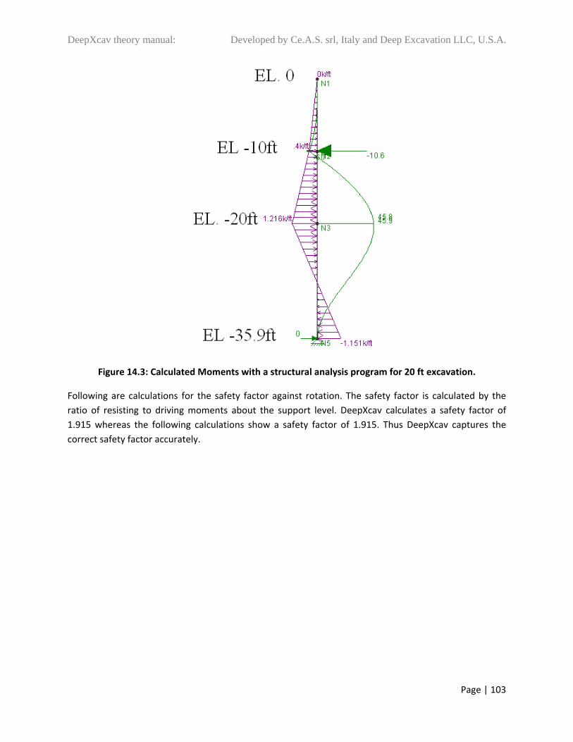
DeepXcav theory manual: Developed by Ce.A.S. srl, Italy and Deep Excavation LLC, U.S.A.
Page | 103
Figure 14.3: Calculated Moments with a structural analysis program for 20 ft excavation.
Following are calculations for the safety factor against rotation. The safety factor is calculated by the
ratio of resisting to driving moments about the support level. DeepXcav calculates a safety factor of
1.915 whereas the following calculations show a safety factor of 1.915. Thus DeepXcav captures the
correct safety factor accurately.

DeepXcav theory manual: Developed by Ce.A.S. srl, Italy and Deep Excavation LLC, U.S.A.
Page | 104
The hand calculations confirm the calculated rotational safety factor software calculates a rotational
safety factor of 1.915

DeepXcav theory manual: Developed by Ce.A.S. srl, Italy and Deep Excavation LLC, U.S.A.
Page | 105
15. Verification of 30 ft excavation with two support levels
This section verifies a 30 ft excavation with two support levels, one at 10 ft depth, and the second at 20
ft from the top of the wall. All other project parameters remain the same as in the previous two sections
(14.1 and 14.2). Figure 15.1 shows pressure calculations for the 30 ft excavation. DeepXcav calculates
the same lateral pressures as calculations in Figure 15.1.
SOIL UNIT WEIGHT
WATER UNIT WEIGHT
WATER TABLE ELEV. Ka Kp
WATER TABLE ELEV.
(kcf) (kcf) (FT) (FT)
0.12 0.0624 -10 0.333 3 -30
ELEV.
TOTAL VERTICAL STRESS
WATER PRESSURE
EFFECTIVE VERTICAL STRESS
LATERAL SOIL
STRESS
TOTAL LATERAL STRESS
TOTAL VERTICAL STRESS
WATER PRESSURE
EFFECTIVE VERTICAL STRESS
LATERAL SOIL
STRESS
TOTAL LATERAL STRESS NET
(FT) (ksf) (ksf) (ksf) (ksf) (ksf) (ksf) (ksf) (ksf) (ksf)
0 0 0 0 0 0 0
-10 1.2 0 1.2 -0.4 -0.4 -0.4
-20 2.4 -0.624 1.776 -0.592 -1.216 -1.216
-30 3.6 -1.248 2.352 -0.784 -2.032 0 0 0 0 0 -2.032
-43.22 5.186 -2.073 3.113 -1.038 -3.111 1.586 0.825 0.761 2.284 3.109 -0.001
-50 6 -2.496 3.504 -1.168 -3.664 2.4 1.248 1.152 3.456 4.704 1.04
LEFT EXCAVATION SIDE PRESSURES RIGHT SIDE PRESSURES
-60
-50
-40
-30
-20
-10
0
-5 -4 -3 -2 -1 0 1 2 3 4 5 6
EL
EV
AT
ION
(FT
)
LATERAL STRESS (KSF)
LEFT LAT SOIL
LEFT WATER
LEFT TOTAL
RIGHT LAT SOIL
RIGHT WATER
RIGHT TOTAL
NET
Figure 15.1: Lateral pressure calculations for a 30 ft excavation

DeepXcav theory manual: Developed by Ce.A.S. srl, Italy and Deep Excavation LLC, U.S.A.
Page | 106
Figure 15.2: Lateral pressures and bending moments for a 30ft deep excavation by DeepXcav.
Figure 15.3: 30ft Excavation modeled with a structural analysis software

DeepXcav theory manual: Developed by Ce.A.S. srl, Italy and Deep Excavation LLC, U.S.A.
Page | 107
The excavation has been modeled with an independent structural software program with a base support
at El ‐43.22 where the net pressure is equal to zero. Results from the independent software program are
shown in Figure 15.3. The software program results in wall moments of 72.5 k‐ft/ft at El. ‐20 ft and 65.0
k‐ft maximum positive on the right side. DeepXcav produces a moment of 72.6 k‐ft/ft at El. ‐20 and 65.0
k‐ft/ft on the right wall side. Support reactions in DEEP are ‐1.24 k/ft at the first support level and
32.01k/ft at the second support level (El. ‐20ft). Therefore, DeepXcav within acceptable accuracy levels
calculates moments and support reactions.
Figure 15.4: Wall embedment safety factors, wall moments, and support reactions by DEEP for a 30 ft
excavation example.
Now calculate the toe‐embedment safety factors.
Reaction at pin support at El -43.22 ft FB 9.000kip
Note that the pressure at El -43.22 is zero. Now calculate the net passive resistance to the bottom of the wall.
BOT 0.944ksf
Therefore, the next passive resisting force below El. -43.22 is
RNET 50ft 43.22ft( )BOT 1 ft
2 RNET 3.2kip
Passive force safety factor FSPASRNET
FB FSPAS 0.356
DeepXcav calculates 0.36 which verifies the hand calculated safety factor.

DeepXcav theory manual: Developed by Ce.A.S. srl, Italy and Deep Excavation LLC, U.S.A.
Page | 108
u30 1.248ksf
Moment for water from El. -20 to El. -30ft
M1w10 ft u20 10 ft
2
u30 u20 10 ft
2
10 ft 2
3
1 ft M1w 52kip ft
Below El. -30 the net water pressure has a rectangular distribution
unet u30 unet 1.248ksf and the moment contribution is
M2w unet 20 ft 10ft20ft
2
1 ft M2w 499.2kip ft
The driving moment is then: MDR MDRs M1w M2w
Resisting moment comes from a triangular pressure distribution pressure at bottom 3.456 ksfonky due to soil contribution as water moment is added as a net moment on the driving side
FR 3.456ksf 20 ft 1ft
2 MR FR 10ft 20ft
2
3
MR 806.4kip ft
Now we can calculate the rotational safety factor FSROTMR
MDR FSROT 0.814
Now calculate rotational safety factor about lowest support. In this method, driving and resistingmoments below the lowest support are calculated. The safety factor is then calculated at the ratio of resistring to driving moments. Note that moments above the lowest support are ignored.
Soil pressure at El- 20 DRs20 0.592ksfDRsbot 1.168ksfSoil pressure at bottom of left wall side El- 50ft
From the rectangular portion of the driving soil pressures
FDRrectS 30ft 1 ft DRs20 FDRrectS 17.76kip
MDRrectS FDRrectS 30ft
2 MDRrectS 266.4kip ft
From the triangular portion of the driving pressures
FDRtriS DRsbot DRs20 30 ft 1ft
2 FDRtriS 8.64kip
MDRtriS FDRtriS 30 ft2
3 MDRtriS 172.8kip ft
And total driving moment dueto soil pressures on left side
MDRs MDRrectS MDRtriS MDRs 439.2kip ft
Now calculate the net driving moment due to water below El. -20ft
u20 0.624ksf
As Figure 15.4 shows, DeepXcav calculates the same safety factor as calculated above.

DeepXcav theory manual: Developed by Ce.A.S. srl, Italy and Deep Excavation LLC, U.S.A.
Page | 109
A. APPENDIX: Verification of Passive Pressure Coefficient Calculations
KP1cos 2
cos 2 cos 2 cos 1 1sin 1 sin
cos 1 cos
0.5
2
KP KP1 1 Ay( ) KP 15.976
KPH KP cos 1 KPH 15.734
3. Calculate Kp according to Lancellotta 2007, note equation does not account for wall inclination
2 asinsin 1 sin
asinsin
sin
1 2 2 1.029
2 58.981deg1 1 Ay( )
2Ax
2
0.5 1 1.013
KPE cos 1 cos 1 sin 2 sin 1 2 0.5
cos sin 2 sin 2 0.5
e2 tan ( )
KPE 10.401
KPH.Lancellotta KPE 1 cos KPH.Lancellotta 10.477
KP.LancellottaKPH.Lancellotta
cos 1 KP.Lancellotta 10.639
1. Calculate Kp according to various equations, define basic parameters
Soil friction angle 40deg
Slope angle 15deg Note that positive slope angle is upwards
1 10degWall friction
Wall inclination 0deg Note vertical face angle theta is 0
Seismic accelerations
Ax 0.16 Ay 0
atanAx
1 Ay
0.159 9.09deg
2. Calculate Kp according to Coulomb, DAS pg. 430, Principles of Geotechnical Engineering
In the following page, the results by the software program are presented.
DeepXcav theory manual: Developed by Ce.A.S. srl, Italy and Deep Excavation LLC, U.S.A.
Page | 110
The soil Kp estimation form can be raised in two ways a) From the Soil Data dialog when the Paratie
analysis is selected, and b) by writing Kp Estimate in the text command and pressing
enter.

DeepXcav theory manual: Developed by Ce.A.S. srl, Italy and Deep Excavation LLC, U.S.A.
Page | 111

DeepXcav theory manual: Developed by Ce.A.S. srl, Italy and Deep Excavation LLC, U.S.A.
Page | 112

DeepXcav theory manual: Developed by Ce.A.S. srl, Italy and Deep Excavation LLC, U.S.A.
Page | 113
B. APPENDIX: Sample Paratie Input File Generated by New Software Program
** * PARATIE ANALYSIS FOR DESIGN SECTION:EC7, 2007: DA‐1, Combination 2: A2 + M2 + R1 *1: Define General Calculation Settings delta 0.2 unit m kN option param itemax 200 *2. ADD GENERAL WALLS & DIMESIONS wall Leftwall 0 182 200 *3.1 DEFINE SURFACE FOR LEFT WALL soil 0_L Leftwall 182 200 1 0 soil 0_R Leftwall 182 200 2 180 *4: DEFINE SOIL LAYER ELEVATIONS & STRENGTHS * BORING Boring 1 *DATA FOR LAYER: 1, SOIL TYPE= 1, F Ldata L1 200 weight 19 10 10 Resistance 3 32 0.307 3.255 atrest 0.47 0.5 1 Moduli 15000 3 0 1 100 0.5 permeabil 0.03048 Endl *5.1: DEFINE STRUCTURAL MATERIALS *START GENERAL MATERIALS * GENERAL CONCRETE MATERIALS ‐ CONVERTED TO CONSISTENT UNITS WITH FORCE/LENGTH^2 *Concrete material: 0 Name= 3 ksi Concrete, E= 21541.9MPa material CONC_0_3 21541900 *Concrete material: 1 Name= 4 ksi Conrete, E= 24874.5MPa material CONC_1_4 24874500 *Concrete material: 2 Name= 5 ksi Conrete, E= 27810.5MPa material CONC_2_5 27810500 * GENERAL STEEL MEMBER MATERIALS ‐ CONVERTED TO CONSISTENT UNITS WITH FORCE/LENGTH^2 *Steel material: 0 Name= Fe510, E= 206000MPa material STEEL_0_ 206000000 *Steel material: 1 Name= A‐50, E= 200100MPa material STEEL_1_ 200100000 * GENERAL REBAR MATERIALS ‐ CONVERTED TO CONSISTENT UNITS WITH FORCE/LENGTH^2, USED FOR ANCHORS *Rebar material: 0 Name= Grade 60, E= 200100MPa material REB_0_Gr 200100000 *Rebar material: 1 Name= Grade 75, E= 200100MPa material REB_1_Gr 200100000 *Rebar material: 2 Name= Grade 80, E= 200100MPa material REB_2_Gr 200100000 *Rebar material: 3 Name= Grade 150, E= 200100MPa material REB_3_Gr 200100000 *Rebar material: 4 Name= Strands 270 ksi, E= 200100MPa material REB_4_St 200100000 * USER DEFINED MATERIALS ‐ CONVERTED TO CONSISTENT UNITS WITH FORCE/LENGTH^2, USED FOR ANCHORS *User material: 0 Name= User mat 0, E= 1MPa material USER_0_U 1000 * END GENERAL MATERIALS * 5.2 Define a very stiff material for rigid supports mate stiffMAT 100000000000 * 6.1 LEFT WALL STRUCTURAL PROPERTIES *Calculate equivalent Steel Sheet Pile Ixx. x Wall Spacing

DeepXcav theory manual: Developed by Ce.A.S. srl, Italy and Deep Excavation LLC, U.S.A.
Page | 114
* Ewall= 206000 MPa, Stiffness Ixx= 82795.6 cm4/m x 1 m = 82795.6 cm4 * Iequivalent= Ewall x Ixx x ConvEI / (Estandard x ConvEL x Wall Spacing) => * Iequivalent= 206000 MPa x 82795.6 cm4/m x 1 m = 82795.6 cm4 x 1E‐08/ (206000 x 1 x 1)= 0.00083 (m^4/m) *Now calculate Equivalent Wall Thickness from Ixx/Length * Wall thick= (12 x Ixx/L)^(1/3) = (12 x 0.00083)^(1/3) = 0.21498 (m) BEAM Leftwall_BEAM Leftwall 182 200 STEEL_0_ 0.214979 00 00 *7.1: GENERATE SUPPORTS FOR LEFT WALL *Convert Tieback to Wire: Stiffness a/L= (Area/ConvA) / [Spacing x (Free Length + Fixed Length x Stiffness Ratio / 100] => *Stiffness a/L= (5.94cm2/10000cm2 /m2) /[2 m x (7 m + 50 x 9 m/100] = 2.58261E‐05 WIRE SPL_0 Leftwall 197 REB_4_St 2.58261E‐05 200 30 0 0 *8.1: ADD WALL LOADS & PRESCRIBED CONDITIONS FOR LEFT WALL NODE 0 Leftwall 195 * END OF NODE ADDITION * 9.A 1st wall compute external wall surcharges. Stage 0 * 9.A 1st wall compute external wall surcharges. Stage 1 * 9.A 1st wall compute external wall surcharges. Stage 2 * 9.A 1st wall compute external wall surcharges. Stage 3 * Stage: 3, examine surcharge load 0 1st point at Elev. 200, x= 0, qx = 5, qz= 0 * 2nd point at Elev. 195, x= 0, qx = 0, qz= 0 * Auto Procedure: Excavation on the right, load is pushing to the right. Load is treated as unfavorable variable load LF=1.3 ***** END determination of load factors for strip surcharge load 0 **************************************************************** * 10: GENERATE ALL STEP/STAGES ***************************************************************** *START DATA FOR STAGE: 0 Name: Stage 0 step 0 : Stage 0 *10.a: DESCRIBE Kp, Ka Changes for this stage due to Defined Wall Friction, Slope or Strength Code Changes * LAYER 1 Stage 0 *Standard Soil Code Used: EC7, 2007, Case:DA‐1, Comb. 2: A2 + M2 + R1 *FS_FR = 1.25, FS_c'= 1.25, FS_DriveEarth= 1, FS_gStab= 0.9, FS_RES= 1 *FS_LoadVar = 1.3, FS_LoadPerm= 1, FS Seismic= 0, FS_AnchPerm= 1.1, FS_AnchTemp= 1.1 * KaUH= KaHBase x FS_DriveEarth x [Rankine_Kah(deg FR= 26.56, DFR= 0, Asur= 0)] / [Rankine_Kah(deg FR= 32, DFR= 0, Asur= 0)]=> * KaDH = 0.307 x 1 x 0.382/0.307 = 0.382 * KpDH= [KpHBase /FS_Resist] x [Rankine_Kph(deg FR= 26.56, DFR= 0, Asur= 0)] / [Rankine_Kph(deg FR= 32, DFR= 0, Asur= 0)]=> * KpDH = [3.255 /1] x 2.618/3.255 = 2.618 * END LAYER 1 Stage : 0 * If Section 10.b is not specified then parameters are same as in previous stage. *END 10.a *10b: START GENERATE SOIL PROPERTY CHANGE COMMANDS FOR STAGE * These changes might be associated with the use of a Strength reduction code such as EUR 7 * or with the user changing from drained to undrained in this stage etc. change L1 u‐frict 26.56 Leftwall change L1 d‐frict 26.56 Leftwall change L1 u‐cohe 2.4 Leftwall change L1 d‐cohe 2.4 Leftwall change L1 u‐ka 0.381719868280688 Leftwall change L1 d‐ka 0.381719868280688 Leftwall change L1 u‐kp 2.61784906429131 Leftwall change L1 d‐kp 2.61784906429131 Leftwall *10a: END GENERATING CHANGES FOR STAGE. * DATA FOR LEFT WALL setwall Leftwall *10.1 Generate left wall water elevations for stage 0 geom 200 200 water 195 0 ‐3830 *11: ADD LEFT WALL SUPPORTS *13.1: ADD LEFT WALL SURCHARGES NOT FROM LOADS DIRECTLY LOADING THE WALL

DeepXcav theory manual: Developed by Ce.A.S. srl, Italy and Deep Excavation LLC, U.S.A.
Page | 115
*13.2.1: ADD LEFT WALL SURCHARGES CALCULATED OUTSIDE FROM PARATIE ENGINE *13.3: ADD WALL SURCHARGES THAT ARE DIRECTLY ON THE LEFT WALL *13.3: END ADDING WALL SURCHARGES ON LEFT WALL * END DATA FOR LEFT WALL *19.1 EXAMINE IF SUPPORTS ARE REMOVED FOR LEFT WALL * 19: END SUPPORT REMOVAL *20: ADD LATERAL LINE LOADS PLACED DIRECTLY ON WALL ENDSTEP *END DATA FOR STAGE 0 NAME: Stage 0 *************************************************************** ***************************************************************** *START DATA FOR STAGE: 1 Name: Stage 1 step 1 : Stage 1 *10.a: DESCRIBE Kp, Ka Changes for this stage due to Defined Wall Friction, Slope or Strength Code Changes * LAYER 1 Stage 1 *Standard Soil Code Used: EC7, 2007, Case:DA‐1, Comb. 2: A2 + M2 + R1 *FS_FR = 1.25, FS_c'= 1.25, FS_DriveEarth= 1, FS_gStab= 0.9, FS_RES= 1 *FS_LoadVar = 1.3, FS_LoadPerm= 1, FS Seismic= 0, FS_AnchPerm= 1.1, FS_AnchTemp= 1.1 * KaUH= KaHBase x FS_DriveEarth x [Rankine_Kah(deg FR= 26.56, DFR= 0, Asur= 0)] / [Rankine_Kah(deg FR= 32, DFR= 0, Asur= 0)]=> * KaDH = 0.307 x 1 x 0.382/0.307 = 0.382 * KpDH= [KpHBase /FS_Resist] x [Rankine_Kph(deg FR= 26.56, DFR= 0, Asur= 0)] / [Rankine_Kph(deg FR= 32, DFR= 0, Asur= 0)]=> * KpDH = [3.255 /1] x 2.618/3.255 = 2.618 * KaDH= KaHBase x FS_Drive x [Rankine_Kah(deg FR= 26.56, DFR= 0, Asur= 0)] / [Rankine_Kah(deg FR= 32, DFR= 0, Asur= 0)]=> * KaDH = 0.307 x 1 x 0.382/0.307 = 0.382 * KpUH= [KpHBase x /FS_Resist] x [Rankine_Kph(deg FR= 26.56, DFR= 0, Asur= 0)] / [Rankine_Kph(deg FR= 32, DFR= 0, Asur= 0)]=> * KpUH = [3.255 /1] x [2.618/3.255] = 2.618 * c'_Uphill= c_base / (FS_c x FS_DriveEarth) = 3/(1.25 x 1) = 2.4 * c'_Down= c_base / (FS_c x FS_Res) = 3/(1.25 x 1) = 2.4 * END LAYER 1 Stage : 1 * If Section 10.b is not specified then parameters are same as in previous stage. *END 10.a * DATA FOR LEFT WALL setwall Leftwall *10.1 Generate left wall water elevations for stage 1 geom 200 196.5 water 195 0 ‐3830 *11: ADD LEFT WALL SUPPORTS *13.1: ADD LEFT WALL SURCHARGES NOT FROM LOADS DIRECTLY LOADING THE WALL *13.2.1: ADD LEFT WALL SURCHARGES CALCULATED OUTSIDE FROM PARATIE ENGINE *13.3: ADD WALL SURCHARGES THAT ARE DIRECTLY ON THE LEFT WALL *13.3: END ADDING WALL SURCHARGES ON LEFT WALL * END DATA FOR LEFT WALL *19.1 EXAMINE IF SUPPORTS ARE REMOVED FOR LEFT WALL * 19: END SUPPORT REMOVAL *20: ADD LATERAL LINE LOADS PLACED DIRECTLY ON WALL ENDSTEP *END DATA FOR STAGE 1 NAME: Stage 1 *************************************************************** ***************************************************************** *START DATA FOR STAGE: 2 Name: Stage 2 step 2 : Stage 2

DeepXcav theory manual: Developed by Ce.A.S. srl, Italy and Deep Excavation LLC, U.S.A.
Page | 116
*10.a: DESCRIBE Kp, Ka Changes for this stage due to Defined Wall Friction, Slope or Strength Code Changes * LAYER 1 Stage 2 *Standard Soil Code Used: EC7, 2007, Case:DA‐1, Comb. 2: A2 + M2 + R1 *FS_FR = 1.25, FS_c'= 1.25, FS_DriveEarth= 1, FS_gStab= 0.9, FS_RES= 1 *FS_LoadVar = 1.3, FS_LoadPerm= 1, FS Seismic= 0, FS_AnchPerm= 1.1, FS_AnchTemp= 1.1 * KaUH= KaHBase x FS_DriveEarth x [Rankine_Kah(deg FR= 26.56, DFR= 0, Asur= 0)] / [Rankine_Kah(deg FR= 32, DFR= 0, Asur= 0)]=> * KaDH = 0.307 x 1 x 0.382/0.307 = 0.382 * KpDH= [KpHBase /FS_Resist] x [Rankine_Kph(deg FR= 26.56, DFR= 0, Asur= 0)] / [Rankine_Kph(deg FR= 32, DFR= 0, Asur= 0)]=> * KpDH = [3.255 /1] x 2.618/3.255 = 2.618 * KaDH= KaHBase x FS_Drive x [Rankine_Kah(deg FR= 26.56, DFR= 0, Asur= 0)] / [Rankine_Kah(deg FR= 32, DFR= 0, Asur= 0)]=> * KaDH = 0.307 x 1 x 0.382/0.307 = 0.382 * KpUH= [KpHBase x /FS_Resist] x [Rankine_Kph(deg FR= 26.56, DFR= 0, Asur= 0)] / [Rankine_Kph(deg FR= 32, DFR= 0, Asur= 0)]=> * KpUH = [3.255 /1] x [2.618/3.255] = 2.618 * DATA FOR LEFT WALL setwall Leftwall *10.1 Generate left wall water elevations for stage 2 geom 200 196.5 water 195 0 ‐3830 *11: ADD LEFT WALL SUPPORTS ADD SPL_0 *13.1: ADD LEFT WALL SURCHARGES NOT FROM LOADS DIRECTLY LOADING THE WALL *13.2.1: ADD LEFT WALL SURCHARGES CALCULATED OUTSIDE FROM PARATIE ENGINE *13.3: ADD WALL SURCHARGES THAT ARE DIRECTLY ON THE LEFT WALL *13.3: END ADDING WALL SURCHARGES ON LEFT WALL * END DATA FOR LEFT WALL *19.1 EXAMINE IF SUPPORTS ARE REMOVED FOR LEFT WALL * 19: END SUPPORT REMOVAL *20: ADD LATERAL LINE LOADS PLACED DIRECTLY ON WALL ENDSTEP *END DATA FOR STAGE 2 NAME: Stage 2 *************************************************************** ***************************************************************** *START DATA FOR STAGE: 3 Name: Stage 3 step 3 : Stage 3 *10.a: DESCRIBE Kp, Ka Changes for this stage due to Defined Wall Friction, Slope or Strength Code Changes * LAYER 1 Stage 3 *Standard Soil Code Used: EC7, 2007, Case:DA‐1, Comb. 2: A2 + M2 + R1 *FS_FR = 1.25, FS_c'= 1.25, FS_DriveEarth= 1, FS_gStab= 0.9, FS_RES= 1 *FS_LoadVar = 1.3, FS_LoadPerm= 1, FS Seismic= 0, FS_AnchPerm= 1.1, FS_AnchTemp= 1.1 * KaUH= KaHBase x FS_DriveEarth x [Rankine_Kah(deg FR= 26.56, DFR= 0, Asur= 0)] / [Rankine_Kah(deg FR= 32, DFR= 0, Asur= 0)]=> * KaDH = 0.307 x 1 x 0.382/0.307 = 0.382 * KpDH= [KpHBase /FS_Resist] x [Rankine_Kph(deg FR= 26.56, DFR= 0, Asur= 0)] / [Rankine_Kph(deg FR= 32, DFR= 0, Asur= 0)]=> * KpDH = [3.255 /1] x 2.618/3.255 = 2.618 * KaDH= KaHBase x FS_Drive x [Rankine_Kah(deg FR= 26.56, DFR= 0, Asur= 0)] / [Rankine_Kah(deg FR= 32, DFR= 0, Asur= 0)]=> * KaDH = 0.307 x 1 x 0.382/0.307 = 0.382 * KpUH= [KpHBase x /FS_Resist] x [Rankine_Kph(deg FR= 26.56, DFR= 0, Asur= 0)] / [Rankine_Kph(deg FR= 32, DFR= 0, Asur= 0)]=> * KpUH = [3.255 /1] x [2.618/3.255] = 2.618 * DATA FOR LEFT WALL setwall Leftwall *10.1 Generate left wall water elevations for stage 3 geom 200 191 water 195 4 *11: ADD LEFT WALL SUPPORTS *13.1: ADD LEFT WALL SURCHARGES NOT FROM LOADS DIRECTLY LOADING THE WALL *13.2.1: ADD LEFT WALL SURCHARGES CALCULATED OUTSIDE FROM PARATIE ENGINE
DeepXcav theory manual: Developed by Ce.A.S. srl, Italy and Deep Excavation LLC, U.S.A.
Page | 117
*13.3: ADD WALL SURCHARGES THAT ARE DIRECTLY ON THE LEFT WALL * Stage: 3, examine surcharge load 0 1st point at Elev. 200, x= 0, qx = 5, qz= 0 * 2nd point at Elev. 195, x= 0, qx = 0, qz= 0 * Auto Procedure: Excavation on the right, load is pushing to the right. Load is treated as unfavorable variable load LF=1.3 ***** END determination of load factors for strip surcharge load 0 dload step Leftwall 195 0 200 6.5 *13.3: END ADDING WALL SURCHARGES ON LEFT WALL * END DATA FOR LEFT WALL *19.1 EXAMINE IF SUPPORTS ARE REMOVED FOR LEFT WALL * 19: END SUPPORT REMOVAL *20: ADD LATERAL LINE LOADS PLACED DIRECTLY ON WALL ENDSTEP *END DATA FOR STAGE 3 NAME: Stage 3 *************************************************************** set country english * *