theory of the analytic hierarchy and analytic network

© Saaty Thomas L., 2003 Системні дослідження та інформаційні технології, 2003, № 2 7

TIДC

ПРОБЛЕМИ ПРИЙНЯТТЯ РІШЕНЬ І УПРАВЛІННЯ В ЕКОНОМІЧНИХ, ТЕХНІЧНИХ, ЕКОЛОГІЧНИХ І СОЦІАЛЬНИХ СИСТЕМАХ

UDC 519.5

THEORY OF THE ANALYTIC HIERARCHY AND ANALYTIC NETWORK PROCESS – EXAMPLES. PART 2.2

SAATY THOMAS L.

In this part we introduce the role of benefits, opportunities, costs and risks (BOCR) in decision-making and how to establish priorities for them. We give an example of a real life application of the US Congress acting on China joining the World Trade Organization (WTO) mailed to the US congressional committee before that deci-sion. We then introduce and apply the Analytic Network Process and its concept of a supermatrix to make decisions with dependence and feedback and illustrate its ap-plication for a single “control” criterion of market share. This will be followed in Part 2.3 by a full BOCR application in the context of the ANP.

1. EVALUATING THE BOCR MERITS THROUGH STRATEGIC CRITERIA USING RATINGS

This section was taken from an analysis carried out before the US Congress acted favorably on China joining the WTO and was hand-delivered to many of the members of the committee including its Chairperson [4]. Since 1986, China had been attempting to join the multilateral trade system, the General Agreement on Tariffs and Trade (GATT) and, its successor, the World Trade Organization (WTO)]. According to the rules of the 135-member nation WTO, a candidate member must reach a trade agreement with any existing member country that wishes to trade with it. By the time this analysis was done, China signed bilateral agreements with 30 countries — including the US (November 1999) — out of 37 members that had requested a trade deal with it.

As part of its negotiation deal with the US, China asked the US to remove its annual review of China’s Normal Trade Relations (NTR) status, until 1998 called Most Favored Nation (MFN) status. In March 2000, President Clinton sent a bill to Congress requesting a Permanent Normal Trade Relations (PNTR) status for China. The analysis was done and copies sent to leaders and some members in both houses of Congress before the House of Representatives voted on the bill, May 24, 2000. The decision by the US Congress on China’s trade-relations status will have an influence on US interests, in both direct and indirect ways. Direct impacts will include changes in economic, security and political relations between the two countries as the trade deal is actualized. Indirect impacts will occur when China becomes a WTO member and adheres to WTO rules and principles. China has said that it would join the WTO only if the US gives it Permanent Normal Trade Relations status.

Saaty Thomas L.

ISSN 1681–6048 System Research & Information Technologies, 2003, № 2 8

It is likely that Congress will consider four options, the least likely being that the US will deny China both PNTR and annual extension of NTR status. The other three options are:

1. Passage of a clean PNTR bill: Congress grants China Permanent Nor-mal Trade Relations status with no conditions attached. This option would allow implementation of the November 1999 WTO trade deal between China and the Clinton administration. China would also carry out other WTO principles and trade conditions.

2. Amendment of the current NTR status bill: This option would give China the same trade position as other countries and disassociate trade from other issues. As a supplement, a separate bill may be enacted to address other matters, such as human rights, labor rights, and environmental issues.

3. Annual Extension of NTR status: Congress extends China’s Normal Trade Relations status for one more year, and, thus, maintains the status quo.

The conclusion of the study is that the best alternative is granting China PNTR status. China now has that status.

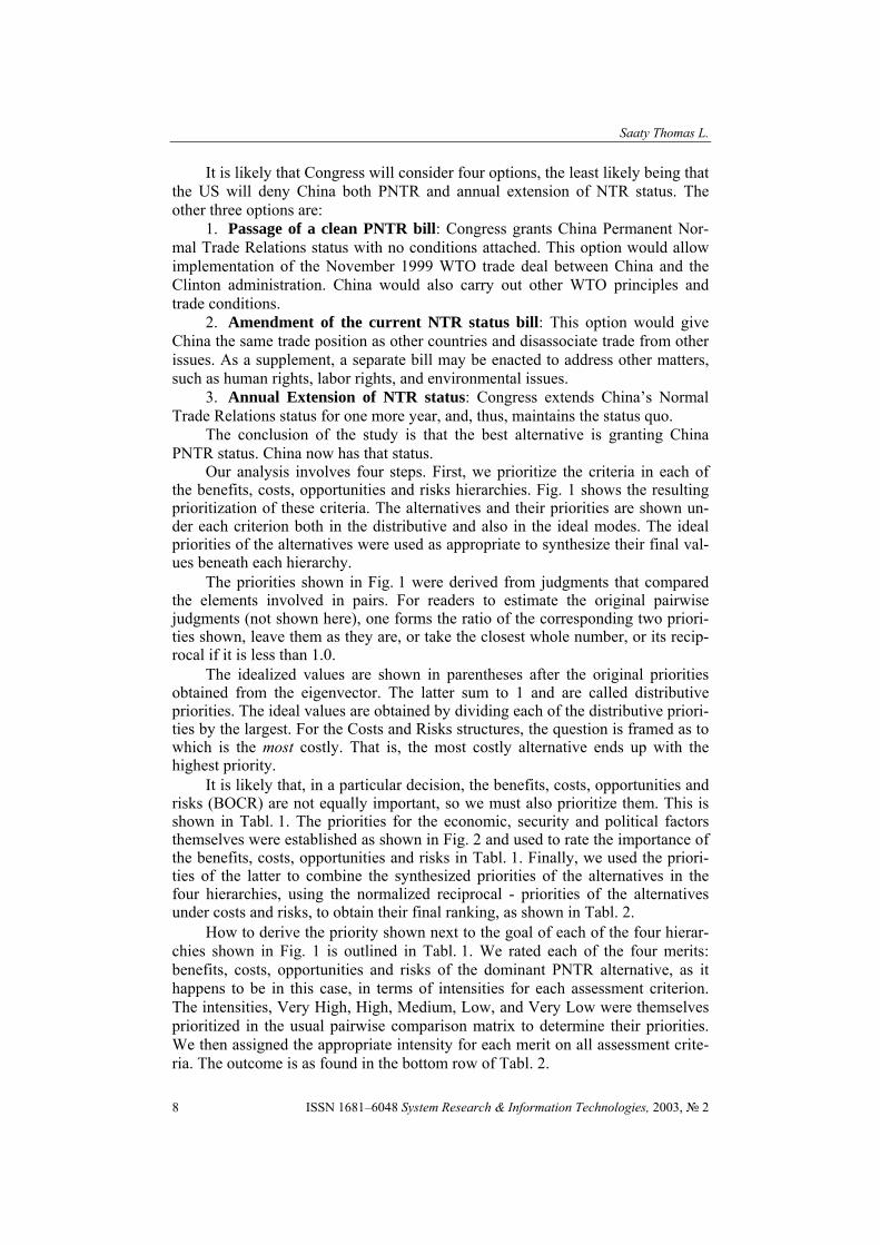
Our analysis involves four steps. First, we prioritize the criteria in each of the benefits, costs, opportunities and risks hierarchies. Fig. 1 shows the resulting prioritization of these criteria. The alternatives and their priorities are shown un-der each criterion both in the distributive and also in the ideal modes. The ideal priorities of the alternatives were used as appropriate to synthesize their final val-ues beneath each hierarchy.

The priorities shown in Fig. 1 were derived from judgments that compared the elements involved in pairs. For readers to estimate the original pairwise judgments (not shown here), one forms the ratio of the corresponding two priori-ties shown, leave them as they are, or take the closest whole number, or its recip-rocal if it is less than 1.0.

The idealized values are shown in parentheses after the original priorities obtained from the eigenvector. The latter sum to 1 and are called distributive priorities. The ideal values are obtained by dividing each of the distributive priori-ties by the largest. For the Costs and Risks structures, the question is framed as to which is the most costly. That is, the most costly alternative ends up with the highest priority.

It is likely that, in a particular decision, the benefits, costs, opportunities and risks (BOCR) are not equally important, so we must also prioritize them. This is shown in Tabl. 1. The priorities for the economic, security and political factors themselves were established as shown in Fig. 2 and used to rate the importance of the benefits, costs, opportunities and risks in Tabl. 1. Finally, we used the priori-ties of the latter to combine the synthesized priorities of the alternatives in the four hierarchies, using the normalized reciprocal - priorities of the alternatives under costs and risks, to obtain their final ranking, as shown in Tabl. 2.

How to derive the priority shown next to the goal of each of the four hierar-chies shown in Fig. 1 is outlined in Tabl. 1. We rated each of the four merits: benefits, costs, opportunities and risks of the dominant PNTR alternative, as it happens to be in this case, in terms of intensities for each assessment criterion. The intensities, Very High, High, Medium, Low, and Very Low were themselves prioritized in the usual pairwise comparison matrix to determine their priorities. We then assigned the appropriate intensity for each merit on all assessment crite-ria. The outcome is as found in the bottom row of Tabl. 2.

Theory of the analytic hierarchy and analytic network process – examples. Part 2.2

Системні дослідження та інформаційні технології, 2003, № 2 9

Bene

fits S

ynth

esis

(Ide

al):

P

NTR

1.0

0

Am

end

NTR

0.4

8

Ann

ual E

xten

sion

0.21

Cos

ts S

ynth

esis

(whi

ch is

mor

e cos

tly):

PN

TR 0

.31

Am

end

NTR

0.5

0

Ann

ual E

xten

sion

0.8

7 C

osts

Syn

thes

is (le

ss co

stly

, and

idea

lizin

g):

PN

TR 1

Am

end

NTR

0.6

1

Ann

ual E

xten

sion

0.3

5

Saaty Thomas L.


Opp

ortu

nitie

s Syn

thes

is (I

deal

): P

NT

R: 1

A

men

d N

TR

: 0.4

4

Ann

ual E

xten

sion

: 0.2

0

Ris

ks S

ynth

esis

(mor

e ri

sky,

Idea

l): P

NT

R

0.51

A

men

d N

TR

0.5

2 A

nnua

l Ext

ensi

on 0

.61

Ris

ks S

ynth

esis

(les

s ris

ky, I

deal

): P

NT

R 1

A

men

d N

TR

0.9

9

Ann

ual E

xten

sion

0.8

4

Fig.

1. H

iera

rchy

for R

atin

g B

enef

its, C

osts

, Opp

ortu

nitie

s, an

d R

isks



T a b l e 1 . Priority Ratings for the Merits: Benefits, Costs, Opportunities, and Risks Intensities: Very High (0.42), High (0.26), Medium (0.16), Low (0.1), Very Low (0.06)

Benefits Costs Opportunities Risks

Growth (0.19) High Very Low Medium Very Low Economic

(0.56) Equity (0.37) Medium High Low Low Regional (0.03) Low Medium Medium High

Non-Proliferation (0.08) Medium Medium High High Security

(0.32) Threat to US (0.21) High Very High High Very

High Constituencies (0.1) High Very High Medium High Political

(0.12) American Values (0.02) Very Low Low Low Medium

Priorities 0.25 0.31 0.20 0.24

We are now able to obtain the overall priorities of the three major decision alternatives listed earlier, given as columns in Tabl. 2 which gives three ways of synthesize for the ideal mode, we see in bold that PNTR is the dominant alterna-tive any way we synthesize as in the last four columns.

T a b l e 2 . Four Methods of Synthesizing BOCR Using the Ideal Mode

Alte

rnat

ives

Ben

efst

s

Opp

ortu

nitie

s

Cos

ts

Rec

ipro

cals

of

Cos

ts

Cos

ts (d

ivid

ed b

y la

rges

t rec

ipro

cal)

Ris

ks

Rec

ipro

cals

of

Ris

ks

Ris

ks (d

ivid

ed b

y la

rges

t rec

ipro

cal)

BO

/CR

bB +

oO

+

c(1

/C) +

r(11

-R)

bB +

oO

+

c(1

–C) +

r (1

–R)

bB +

oO

- cC

–

rR

(0.25) (0.20) (0.31) (0.24)

PNTR 1 1 0.31 3.23 1 0.51 1.96 1 1.65 1.01 0.78 0.23 Amend NTR 0.48 0.44 0.50 2.00 0.62 0.52 1.92 0.98 0.22 0.64 0.51 -0.07

Annual Exten. 0.21 0.20 0.87 1.15 0.36 0.61 1.64 0.84 0.03 0.41 0.28 -0.32

Factors for Evaluating the Decision

Economic: 0.56 – Growth (0.33) – Equity (0.67)

Security: 0.32 – Regional Security (0.09)– Non-Proliferation (0.24)– Threat to US (0.67)

Political: 0.12 – Domestic Constituencies (0.80) – American Values (0.20)

Fig. 2. Prioritizing the Strategic Criteria to be used in Rating the BOCR

Saaty Thomas L.


2. THE ANALYTIC NETWORK PROCESS (ANP)

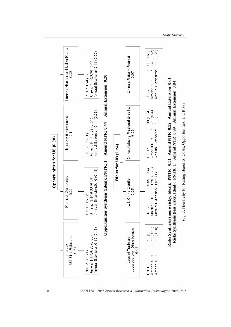
At present, in their effort to simplify and deal with complexity, people who work in decision-making use mostly very simple hierarchic structures consisting of a goal, criteria, and alternatives. Yet, not only are decisions obtained from a simple hierarchy of three levels different from those obtained from a multilevel hierar-chy, but also decisions obtained from a network can be significantly different from those obtained from a more complex hierarchy. We cannot collapse com-plexity artificially into a simplistic structure of two levels, criteria and alterna-tives, and hope to capture the outcome of interactions in the form of highly con-densed judgments that correctly reflect all that goes on in the world. We must learn to decompose these judgments through more elaborate structures and organ-ize our reasoning and calculations in sophisticated but simple ways to serve our understanding of the complexity around us. Experience indicates that it is not very difficult to do this although it takes more time and effort. Indeed, we must use feed-back networks to arrive at the kind of decisions needed to cope with the future.

The Analytic Network Process is a generalization of the Analytic Hierarchy Process. The basic structure is an influence network of clusters and nodes. Priori-ties are established in the same way they are in the AHP using pairwise compari-sons and judgment. Many decision problems cannot be structured hierarchically because they involve the interaction and dependence of higher-level elements in a hierarchy on lower-level elements. Not only does the importance of the criteria determine the importance of the alternatives as in a hierarchy, but also the impor-tance of the alternatives themselves determines the importance of the criteria. Two bridges, both strong, but the stronger is also uglier, would lead one to choose the strong but ugly one unless the criteria themselves are evaluated in terms of the bridges, and strength receives a smaller value and appearance a larger value be-cause both bridges are strong. Feedback enables us to factor the future into the present to determine what we have to do to attain a desired future.

The feedback structure does not have the top-to-bottom form of a hierarchy but looks more like a network, with cycles connecting its components of ele-ments, which we can no longer call levels, and with loops that connect a compo-nent to itself (Fig. 3). It also has sources and sinks. A source node is an origin of paths of influence (importance) and never a destination of such paths. A sink node is a destination of paths of influence and never an origin of such paths. A full network can include source nodes; intermediate nodes that fall on paths from source nodes, lie on cycles, or fall on paths to sink nodes; and finally sink nodes. Some networks can contain only source and sink nodes. Still others can include only source and cycle nodes or cycle and sink nodes or only cycle nodes. A deci-sion problem involving feedback arises often in practice. It can take on the form of any of the networks just described. The challenge is to determine the priorities of the elements in the network and in particular the alternatives of the decision and even more to justify the validity of the outcome. Because feedback involves cycles, and cycling is an infinite process, the operations needed to derive the pri-orities become more demanding than has been familiar with hierarchies.



To test for the mutual independence of elements such as the criteria, one proceeds as follows: Construct a zero-one matrix of criteria against criteria using the number one to signify dependence of one criterion on another, and zero oth-erwise. A criterion need not depend on itself as an industry, for example, may not use its own output. For each column of this matrix, construct a pairwise compari-son matrix only for the dependent criteria, derive an eigenvector, and augment it with zeros for the excluded criteria. If a column is all zeros, then assign a zero vector to represent the priorities. The question in the comparison would be: For a given criterion, which of two criteria depends more on that criterion with respect to the goal or with respect to a higher-order controlling criterion?

In Fig. 3, a view is shown of a hierarchy and a network. A hierarchy is com-prised of a goal, levels of elements and connections between the elements. These connections go only to elements in lower levels. A network has clusters of ele-ments, with the elements being connected to elements in another cluster (outer

L in e a r H ie ra rc h y

c o m p o n e n t,c lu s te r(L e v e l)

e le m e n t

A lo o p in d ic a te s th a t e a c he le m e n t d e p e n d s o n ly o n its e lf .

G o a l

S u b c rite r ia

C rite r ia

A lte rn a tiv e s

Feed back N etw ork w ith C om ponents ha vin g Inn er an d O u ter D epend en ce am on g T heir E lem en ts

C 4

C 1

C 2

C 3

Feedback

Loop in a com ponen t ind ica tes inner dependence o f the e lem en ts in tha t com ponentw ith respect to a com m on p rope rty.

A rc from com ponen tC 4 to C 2 ind ica tes theou te r dependence o f the e lem en ts in C 2 on thee lem en ts in C 4 w ith respectto a com m on p rope rty.

Fig. 3. How a Hierarchy Compares to a Network

Saaty Thomas L.


dependence) or the same cluster (inner dependence). A hierarchy is a special case of a network with connections going only in one direction. In a view of a hierar-chy, such as that shown in Fig. 3, the levels in the hierarchy correspond to clusters in a network. One example of inner dependence in a component consisting of a father mother and baby is whom does the baby depend on more for its survival, its mother or itself. The baby depends more on its mother than on itself. Again sup-pose one makes advertising by newspaper and by television. It is clear that the two influence each other because the newspaper writers watch television and need to make their message unique in some way, and vice versa. If we think about it carefully everything can be seen to influence everything including itself according to many criteria. The world is far more interdependent than we know how to deal with using our existing ways of thinking and acting. We know it but how to deal with it. The ANP appears to be a plausible logical way to deal with dependence.

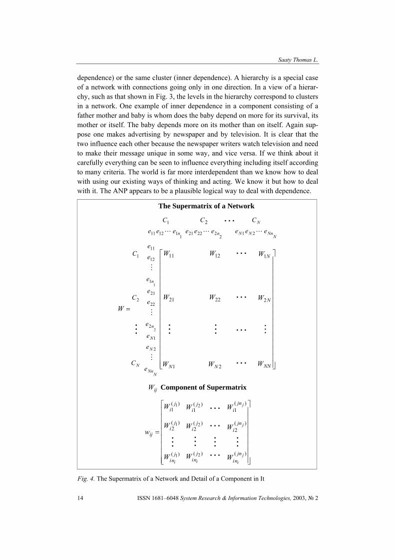
The Supermatrix of a Network

NNnNN

N

nn eee

C

eee

C

eee

C

212

222211

11211

1 2

⎥⎥⎥⎥⎥⎥⎥⎥⎥⎥⎥⎥⎥⎥⎥⎥

⎦

⎤

⎢⎢⎢⎢⎢⎢⎢⎢⎢⎢⎢⎢⎢⎢⎢⎢

⎣

⎡

=

NN

N

N

NN W

W

W

W

W

W

W

W

W

W

NNn

N

N

n

n

N e

e

e

e

e

e

e

e

e

C

C

C

2

1

2

22

12

1

21

11

2

1

2

22

21

1

12

11

2

1

2

1

ijW Component of Supermatrix

⎥⎥⎥⎥⎥⎥⎥⎥

⎦

⎤

⎢⎢⎢⎢⎢⎢⎢⎢

⎣

⎡

=

)(

)(2

)(1

)(

)(2

)(1

)(

)(2

)(1

2

2

2

1

1

1

ji

j

j

ii

jnni

jni

jni

jni

ji

ji

jni

ji

ji

ij

W

W

W

W

W

W

W

W

W

w

Fig. 4. The Supermatrix of a Network and Detail of a Component in It



The priorities derived from pairwise comparison matrices are entered as parts of the columns of a supermatrix. The supermatrix represents the influence priority of an element on the left of the matrix on an element at the top of the ma-trix. A supermatrix along with an example of one of its general entry matrices is shown in Fig. 4. The component iC in the supermatrix includes all the priority vectors derived for nodes that are “parent” nodes in the iC cluster. Fig. 5 gives the supermatrix of a hierarchy along with the kth power that yields the principle of hierarchic composition in its )1,(k position.

Hierarchic composition yields multilinear forms which are of course nonlin-ear and have the form

p

p

ip

ii

ii xxx∑,,

211

21 ,

Supermatrix of a Hierarchy

1

221

)1(1)1(

1

1

)2(1)2(

2

221

2

111

1

−

−

−−

−

−−

−

N

NN

nNN

NnN

NN

nNN

N

nn

ee

eeCC

eeС

eeС

eeС

⎥⎥⎥⎥⎥⎥⎥⎥⎥⎥⎥⎥

⎦

⎤

⎢⎢⎢⎢⎢⎢⎢⎢⎢⎢⎢⎢

⎣

⎡

=

−

−−

IW

W

W

W

e

e

e

ee

e

C

C

C

W

nn

nn

nN

N

n

n

N

N

0

0

0

0

0

0

0

0

0

0

0

0

0

0

0

0

0

0

0

0

1,

2,1

32

21

1

2

21

1

11

2

1

2

1

Supermatrix to nth Power Gives Hierarchical Synthesis

⎥⎥⎥⎥⎥⎥

⎦

⎤

⎢⎢⎢⎢⎢⎢

⎣

⎡

=

−−−−−−−−−− IWWWWWWWWWW nnnnnnnnnnnnnn

kW0

00

0

00

0

00

0

00

0

00

1,2,11,322,11,21322,11, ……

for 1−> nk Fig. 5. The Supermatrix of a Hierarchy with the Resulting Limit Matrix Corresponding to Hierarchical Composition

Saaty Thomas L.


where ji indicates the jth level of the hierarchy and the jx is the priority of an element in that level. The richer the structure of a hierarchy in breadth and depth, the more elaborate are the derived multilinear forms from it. There seems to be a good opportunity to investigate the relationship obtained by composition to co-variant tensors and their algebraic properties.

More concretely we have the covariant tensor

iiwwwwh

h

hhh i

NN

iiii

hii

hi ≡=

−

−

−−−∑

=

−1

1,,

1,,

211

11

121221

for the priority of the ith element in the hth level of the hierarchy. The composite vector hW for the entire hth level is represented by the vector with covariant ten-sorial components. Similarly, the left eigenvector approach to a hierarchy gives rise to a vector with contravariant tensor components.

The classical problem of relating space (geometry) and time to subjective thought can perhaps be examined by showing that the functions of mathematical analysis (and hence also the laws of physics) are derivable as truncated series from the above tensors by composition in an appropriate hierarchy. The foregoing is reminiscent of the theorem in dimensional analysis that any physical variable is proportional to the product of powers of primary variables.

Priority means dominance. If we know how capture dominance we would know how to obtain priorities. In the ANP we look for steady state priorities from a limit super matrix. To obtain the limit we must raise the matrix to powers. The outcome of the ANP is nonlinear and rather complex. The limit may not converge unless the matrix is column stochastic that is each of its columns sums to one. If the columns sum to one then from the fact that the principal eigenvalue of a ma-trix lies between its largest and smallest column sums, we know that the principal eigenvalue of a stochastic matrix is equal to one. Now we know, from a theorem due to J.J. Sylvester that when the multiplicity of each eigenvalue of a matrix W is equal to one that an entire function )(xf (power series expansion of )(xf con-verges for all finite values of (x) with x replaced by W , is given by

∑ ∏

∏

=≠

≠

−

−

==n

iij

ij

ijj

iii

AI

ZZfWf1 )(

)(

)(),()()(λλ

λ

λλλ ,

∑=

===n

iiijii ZZZZIZ

1

2 )()(,0)()(,)( λλλλλ ,

where I and 0 are the i dentity and null matrices respectively. A similar expression is also available when some or all of the eigenvalues

have multiplicities greater than one. The matrix A itself gives the direct domi-nance of an element on the left over another element on top. But an element can dominate another via a third element. Dominance of an element over another



through two step transitivities is obtained by squaring the matrix. Similarly all Nth order transitivities are obtained by raising the matrix to the Nth power which gives the dominance of one element over another in N steps. From each matrix we obtain the relative overall dominance of an element in steps equal to that power of the matrix by adding the coefficients in the row of the matrix corresponding to that element and dividing by the total. According to Cesaro summability, the limit

of the Cesaro sum ⎟⎟⎠

⎞⎜⎜⎝

⎛∑∑==∞→

N

k

TkN

k

TkN

eAeeAN00

/1lim , )1,...,1,1(=e that repre-

sents the average of all order dominance up to N, is the same as the limit of the sequence of the powers of the matrix i.e. TNTN

NeAeeA /lim

∞→ and thus we need

to calculate the limiting powers of A . How do we capture the priorities in the limit as the steady state priorities?

We see that if, as we need in our case, NWWf =)( , then Niif λλ =)( and as

∞→N the only terms that give a finite nonzero value are those for which the modulus of iλ is equal to one. The fact that W is stochastic ensures this. We have:

max11

max λ=≥∑∑== i

jn

jij

n

jij w

waa for iwmax ,

max11

min λ=≤∑∑== i

jn

jij

n

jij w

waa for iwmin .

Thus for a row stochastic matrix we have ∑=

≤≤=n

jija

1maxmin1 λ

∑=

=≤n

jija

11max , thus 1max =λ .

The same type of argument applies when a matrix that is column stochastic. For complete treatment, see this author’s 2001 book on the ANP [1], and also the manual for the ANP software [2].

The ANP Formulation of the Classic AHP School Example

We show in Fig. 6 below the hierarchy, the corresponding supermatrix, and its limit supermatrix to obtain the priorities of three schools involved in a decision to choose one for the author’s son. They are precisely what one obtains by hierarchic composition using the AHP. The priorities of the criteria with respect to the goal and those of the alternatives with respect to each criterion are clearly discernible in the supermatrix itself. Note that there is an identity submatrix for the alterna-tives with respect to the alternatives in the lower right hand part of the matrix. The level of alternatives in a hierarchy is a sink cluster of nodes that absorbs pri-orities but does not pass them on. This calls for using an identity submatrix for them in the supermatrix.

Saaty Thomas L.


The Investment Example with Criterion Weights Automatically Derived from the Supermatrix [3]

Let us revisit the investment example that appeared in my earlier exposition in Part 2.1 on the theory of the AHP/ANP. An individual has three alternate ways,

1A , 2A , and 3A , of investing a sum of money for the same period of time. There are two types of returns, 1C and 2C (for example, capital appreciation and inter-est), as shown in Tabl. 3. The question is, which is the best investment to make in terms of actual dollars earned?

Leaming Frends School Life

VocationalTraining

College Prep.

Music Classes

School A

School B

School C

Goal Satisfaction with School

Goal Learning Friends School life Vocational trainingCollege preparation Music classes A B CGoal 0 0 0 0 0 0 0 0 0 0

Learning 0 0 0 0 0 0 0 0 0 0Friends 0 0 0 0 0 0 0 0 0 0

School life 0 0 0 0 0 0 0 0 0 0Vocational training 0 0 0 0 0 0 0 0 0 0College preparation 0 0 0 0 0 0 0 0 0 0

Music classes 0 0 0 0 0 0 0 0 0 0Alternative A 0.3676 0.16 0.33 0.45 0.77 0.25 0.69 1 0 0Alternative B 0.3781 0.59 0.33 0.09 0.06 0.5 0.09 0 1 0Alternative C 0.2543 0.25 0.34 0.46 0.17 0.25 0.22 0 0 1

Goal Learning Friends School life Vocational trainingCollege preparation Music classes A B CGoal 0 0 0 0 0 0 0 0 0 0

Learning 0.32 0 0 0 0 0 0 0 0 0Friends 0.14 0 0 0 0 0 0 0 0 0

School life 0.03 0 0 0 0 0 0 0 0 0Vocational training 0.13 0 0 0 0 0 0 0 0 0College preparation 0.24 0 0 0 0 0 0 0 0 0

Music classes 0.14 0 0 0 0 0 0 0 0 0Alternative A 0 0.16 0.33 0.45 0.77 0.25 0.69 1 0 0Alternative B 0 0.59 0.33 0.09 0.06 0.5 0.09 0 1 0Alternative C 0 0.25 0.34 0.46 0.17 0.25 0.22 0 0 1

The School Hierarchy as Supermatrix

Limiting Supermatrix & Hierarchic Composition

Fig. 6. Supermatrix of School Choice Hierarchy gives same Result as Hierarchic Com-position



It is easy to calculate the actual total cost for each alternative by simply add-ing the two numbers; the relative cost is then obtained by normalizing as shown in the table.

T a b l e 3 . Calculating Returns Arithmetically

Alternatives Criterion C1

Unnormalized weight = 1.0

Criterion C2 Unnormalized weight = 1.0

Weighted Sum Unnormalized

Normalized or Relative values

A1 200 150 350 350/1300=0.269 A2 300 50 350 350/1300=0.269 A3 500 100 600 600/1300=0.462

Column Totals 1000 300 1300 1 Since we are dealing with tangibles we normalize each column to obtain the

priorities for the alternatives under each criterion. We also normalize each row to obtain the priorities of the criteria with respect to each alternative. We enter these in a supermatrix as shown in Tabl. 4; there is no need to weight the supermatrix because it is already column stochastic, so we can raise it to limiting powers and obtain the limit supermatrix in Tabl. 5 in which all the columns are identical. Be-cause the supermatrix is column stochastic the priorities for the alternatives and the criteria each add to 50% of the value in a column. We see that the supermatrix saves us the arithmetic of determining criteria weights based on the values of the alternatives under each criterion.

T a b l e 4 . The Unweighted Supermatrix of the Investment Example

Alternatives Criteria A1 A2 A3 C1 C2

A1 0.000 0.000 0.000 0.200 0.500 A2 0.000 0.000 0.000 0.300 0.167 Alternatives A3 0.000 0.000 0.000 0.500 0.333 C1 0.571 0.857 0.833 0.000 0.000

Criteria C2 0.429 0.143 0.167 0.000 0.000

T a b l e 5 . The Limit Supermatrix of the Investment Example

Alternatives Criteria A1 A2 A3 C1 C2

Alternatives A1 0.135 0.135 0.135 0.135 0.135 A2 0.135 0.135 0.135 0.135 0.135 A3 0.231 0.231 0.231 0.231 0.231

Criteria C1 0.385 0.385 0.385 0.385 0.385 C2 0.115 0.115 0.115 0.115 0.115

Saaty Thomas L.


Normalizing the results for the alternatives, that is, dividing by the sum of their values in Tabl. 5, which is .5, gives the same ratios we obtained for the over-all return for each investment in Tabl. 3.

3. TWO EXAMPLES OF ESTIMATING MARKET SHARE — THE ANP WITH A SINGLE BENEFITS CONTROL CRITERION

A market share estimation model is structured as a network of clusters and nodes. The object is to try to determine the relative market share of competitors in a par-ticular business, or endeavor, by considering what affects market share in that business and introducing them as clusters, nodes and influence links in a network. The decision alternatives are the competitors and the synthesized results are their relative dominance. The relative dominance results can then be compared against some outside measure such as dollars. If dollar income is the measure being used, the incomes of the competitors must be normalized to get it in terms of relative market share.

The clusters might include customers, service, economics, advertising, and quality of goods. The customers cluster might then include nodes for the age groups of the people that buy from the business: teenagers, 20–33 year olds, 34–55 year olds, 55–70 year olds, and over 70. The advertising cluster might include newspapers, TV, Radio, and Fliers. After all the nodes are created start by picking a node and linking it to the other nodes in the model that influence it. The “chil-dren” nodes will then be pairwise compared with respect to that node as a “par-ent” node. An arrow will automatically appear going from the cluster the parent node is in to the cluster with its children nodes. When a node is linked to nodes in its own cluster, the arrow becomes a loop on that cluster and we say there is inter-dependence.

The linked nodes in a given cluster are pairwise compared for their influence on the node they are linked from (the parent node) to determine the priority of their influence on the parent node. Comparisons are made as to which is more important to the parent node in capturing “market share”. These priorities are then entered in the supermatrix for the network.

The clusters are also pairwise compared to establish their importance with respect to each cluster they are linked from, and the resulting matrix of numbers is used to weight the components of the original unweighted supermatrix to give the weighted supermatrix. This matrix is then raised to powers until it converges to give the limit supermatrix. The relative values for the companies are obtained from the columns of the limit supermatrix that are all the same. Normalizing these numbers yields the relative market share.

If comparison data in terms of sales in dollars, or number of members, or some other known measures are available, one can use these relative values to validate the outcome. The AHP/ANP has a compatibility metric to determine how close the ANP result is to the known measure. It involves taking the Hadamard product of the matrix of ratios of the ANP outcome and the transform of the ma-trix of ratios of the actual outcome summing all the coefficients and dividing by n2. The requirement is that the value should be close to 1 and certainly not much more than 1.1.



We will give three examples of market share estimation showing details of the process in the first example and showing only the models and results in the second and third examples.

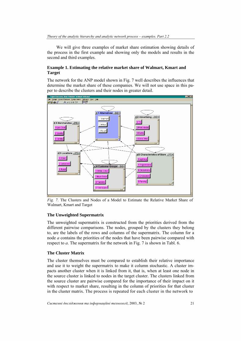
Example 1. Estimating the relative market share of Walmart, Kmart and Target

The network for the ANP model shown in Fig. 7 well describes the influences that determine the market share of these companies. We will not use space in this pa-per to describe the clusters and their nodes in greater detail.

The Unweighted Supermatrix

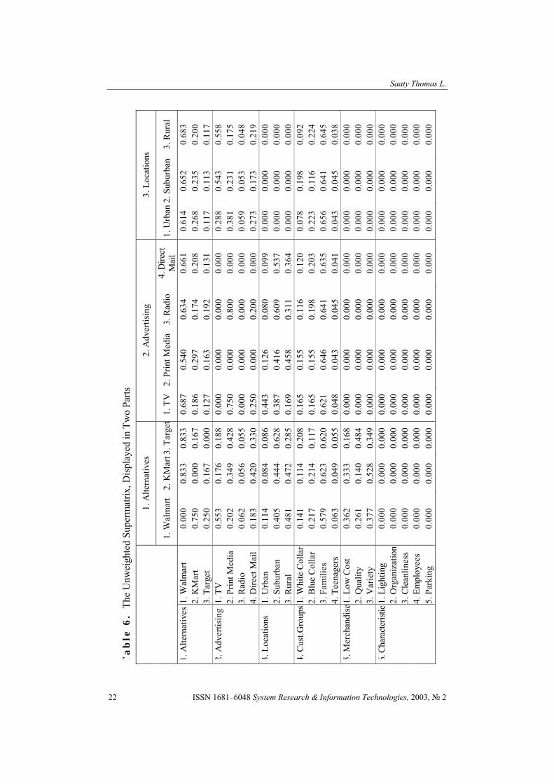
The unweighted supermatrix is constructed from the priorities derived from the different pairwise comparisons. The nodes, grouped by the clusters they belong to, are the labels of the rows and columns of the supermatrix. The column for a node a contains the priorities of the nodes that have been pairwise compared with respect to a. The supermatrix for the network in Fig. 7 is shown in Tabl. 6.

The Cluster Matrix

The cluster themselves must be compared to establish their relative importance and use it to weight the supermatrix to make it column stochastic. A cluster im-pacts another cluster when it is linked from it, that is, when at least one node in the source cluster is linked to nodes in the target cluster. The clusters linked from the source cluster are pairwise compared for the importance of their impact on it with respect to market share, resulting in the column of priorities for that cluster in the cluster matrix. The process is repeated for each cluster in the network to

Fig. 7. The Clusters and Nodes of a Model to Estimate the Relative Market Share of Walmart, Kmart and Target

Saaty Thomas L.


Ta

ble

6.

The

Unw

eigh

ted

Supe

rmat

rix, D

ispl

ayed

in T

wo

Parts

1.

Alte

rnat

ives

2.

Adv

ertis

ing

3. L

ocat

ions

1.

Wal

mar

t 2.

KM

art 3

. Tar

get

1. T

V

2. P

rint M

edia

3.

Rad

io

4. D

irect

M

ail

1. U

rban

2. S

ubur

ban

3. R

ural

1. A

ltern

ativ

es 1

. Wal

mar

t 0.

000

0.83

3 0.

833

0.68

7 0.

540

0.63

4 0.

661

0.61

4 0.

652

0.68

3 2.

KM

art

0.75

0 0.

000

0.16

7 0.

186

0.29

7 0.

174

0.20

8 0.

268

0.23

5 0.

200

3. T

arge

t 0.

250

0.16

7 0.

000

0.12

7 0.

163

0.19

2 0.

131

0.11

7 0.

113

0.11

7 2.

Adv

ertis

ing

1. T

V

0.55

3 0.

176

0.18

8 0.

000

0.00

0 0.

000

0.00

0 0.

288

0.54

3 0.

558

2. P

rint M

edia

0.

202

0.34

9 0.

428

0.75

0 0.

000

0.80

0 0.

000

0.38

1 0.

231

0.17

5 3.

Rad

io

0.06

2 0.

056

0.05

5 0.

000

0.00

0 0.

000

0.00

0 0.

059

0.05

3 0.

048

4. D

irect

Mai

l 0.

183

0.42

0 0.

330

0.25

0 0.

000

0.20

0 0.

000

0.27

3 0.

173

0.21

9 3.

Loc

atio

ns

1. U

rban

0.

114

0.08

4 0.

086

0.44

3 0.

126

0.08

0 0.

099

0.00

0 0.

000

0.00

0 2.

Sub

urba

n 0.

405

0.44

4 0.

628

0.38

7 0.

416

0.60

9 0.

537

0.00

0 0.

000

0.00

0 3.

Rur

al

0.48

1 0.

472

0.28

5 0.

169

0.45

8 0.

311

0.36

4 0.

000

0.00

0 0.

000

4. C

ust.G

roup

s 1. W

hite

Col

lar

0.14

1 0.

114

0.20

8 0.

165

0.15

5 0.

116

0.12

0 0.

078

0.19

8 0.

092

2. B

lue

Col

lar

0.21

7 0.

214

0.11

7 0.

165

0.15

5 0.

198

0.20

3 0.

223

0.11

6 0.

224

3. F

amili

es

0.57

9 0.

623

0.62

0 0.

621

0.64

6 0.

641

0.63

5 0.

656

0.64

1 0.

645

4. T

eena

gers

0.

063

0.04

9 0.

055

0.04

8 0.

043

0.04

5 0.

041

0.04

3 0.

045

0.03

8 5.

Mer

chan

dise

1. L

ow C

ost

0.36

2 0.

333

0.16

8 0.

000

0.00

0 0.

000

0.00

0 0.

000

0.00

0 0.

000

2. Q

ualit

y 0.

261

0.14

0 0.

484

0.00

0 0.

000

0.00

0 0.

000

0.00

0 0.

000

0.00

0 3.

Var

iety

0.

377

0.52

8 0.

349

0.00

0 0.

000

0.00

0 0.

000

0.00

0 0.

000

0.00

0 6.

Cha

ract

erist

ic 1

. Lig

htin

g 0.

000

0.00

0 0.

000

0.00

0 0.

000

0.00

0 0.

000

0.00

0 0.

000

0.00

0 2.

Org

aniz

atio

n 0.

000

0.00

0 0.

000

0.00

0 0.

000

0.00

0 0.

000

0.00

0 0.

000

0.00

0 3.

Cle

anlin

ess

0.00

0 0.

000

0.00

0 0.

000

0.00

0 0.

000

0.00

0 0.

000

0.00

0 0.

000

4. E

mpl

oyee

s 0.

000

0.00

0 0.

000

0.00

0 0.

000

0.00

0 0.

000

0.00

0 0.

000

0.00

0 5.

Par

king

0.

000

0.00

0 0.

000

0.00

0 0.

000

0.00

0 0.

000

0.00

0 0.

000

0.00

0



Te

rmin

atio

n

4 Cu

stom

. Gro

ups

5 M

erch

an-d

ise

6 Ch

arac

-teris

tics o

f Sto

re

1. W

hite

Co

llar

2. B

lue

Colla

r 3.

Fam

ilie

4. T

eens

1. L

ow C

ost

2. Q

ualit

y 3.

V

arie

ty

1. Li

ght’n

g 2.

Org

aniz.

3.

Cle

an

4. E

mp-

loye

es

5.

Park

1.

Alte

rnat

.. 1.

Wal

mar

t 0.

637

0.66

1 0.

630

0.69

1 0.

661

0.61

4 0.

648

0.66

7 0.

655

0.57

0 0.

644

0.55

8

2. K

Mar

t 0.

105

0.20

8 0.

218

0.14

9 0.

208

0.11

7 0.

122

0.11

1 0.

095

0.09

7 0.

085

0.12

2

3. T

arge

t 0.

258

0.13

1 0.

151

0.16

0 0.

131

0.26

8 0.

230

0.22

2 0.

250

0.33

3 0.

271

0.32

0 2.

Adv

ertis

. 1.

TV

0.

323

0.51

0 0.

508

0.63

4 0.

000

0.00

0 0.

000

0.00

0 0.

000

0.00

0 0.

000

0.00

0

2. P

rint M

ed.

0.21

4 0.

221

0.27

0 0.

170

0.00

0 0.

000

0.00

0 0.

000

0.00

0 0.

000

0.00

0 0.

000

3.

Rad

io

0.05

9 0.

063

0.04

9 0.

096

0.00

0 0.

000

0.00

0 0.

000

0.00

0 0.

000

0.00

0 0.

000

4.

Dire

ct M

ail

0.40

4 0.

206

0.17

3 0.

100

0.00

0 0.

000

0.00

0 0.

000

0.00

0 0.

000

0.00

0 0.

000

3. L

ocat

ions

1. U

rban

0.

167

0.09

4 0.

096

0.10

9 0.

268

0.10

5 0.

094

0.10

0 0.

091

0.09

1 0.

111

0.06

7

2. S

ubur

ban

0.83

3 0.

280

0.30

8 0.

309

0.11

7 0.

605

0.62

7 0.

433

0.45

5 0.

455

0.44

4 0.

293

3.

Rur

al

0.00

0 0.

627

0.59

6 0.

582

0.61

4 0.

291

0.28

0 0.

466

0.45

5 0.

455

0.44

4 0.

641

4.Cu

st. G

rps 1

. Whi

te C

ol.

0.00

0 0.

000

0.27

9 0.

085

0.05

1 0.

222

0.16

5 0.

383

0.18

7 0.

242

0.16

5 0.

000

2.

Blu

e Co

llar

0.00

0 0.

000

0.64

9 0.

177

0.11

2 0.

159

0.16

5 0.

383

0.18

7 0.

208

0.16

5 0.

000

3.

Fam

ilies

0.

857

0.85

7 0.

000

0.73

7 0.

618

0.56

6 0.

621

0.18

5 0.

583

0.49

4 0.

621

0.00

0

4. T

eena

gers

0.

143

0.14

3 0.

072

0.00

0 0.

219

0.05

3 0.

048

0.04

8 0.

043

0.05

6 0.

048

0.00

0 5.

Mer

chan

d. 1

. Low

Cos

t 0.

000

0.00

0 0.

000

0.00

0 0.

000

0.80

0 0.

800

0.00

0 0.

000

0.00

0 0.

000

0.00

0

2. Q

ualit

y 0.

000

0.00

0 0.

000

0.00

0 0.

750

0.00

0 0.

200

0.00

0 0.

000

0.00

0 0.

000

0.00

0

3. V

arie

ty

0.00

0 0.

000

0.00

0 0.

000

0.25

0 0.

200

0.00

0 0.

000

1.00

0 0.

000

0.00

0 0.

000

6. C

hara

cter

. 1. L

ight

ing

0.00

0 0.

000

0.00

0 0.

000

0.00

0 0.

000

0.00

0 0.

000

0.16

9 0.

121

0.00

0 0.

250

2.

Org

aniz

. 0.

000

0.00

0 0.

000

0.00

0 0.

000

0.00

0 0.

000

0.25

1 0.

000

0.57

5 0.

200

0.75

0

3. C

lean

li.

0.00

0 0.

000

0.00

0 0.

000

0.00

0 0.

000

0.00

0 0.

673

0.46

9 0.

000

0.80

0 0.

000

4.

Em

ploy

ee

0.00

0 0.

000

0.00

0 0.

000

0.00

0 0.

000

0.00

0 0.

000

0.30

8 0.

304

0.00

0 0.

000

5.

Par

king

0.

000

0.00

0 0.

000

0.00

0 0.

000

0.00

0 0.

000

0.07

5 0.

055

0.00

0 0.

000

0.00

0

Saaty Thomas L.


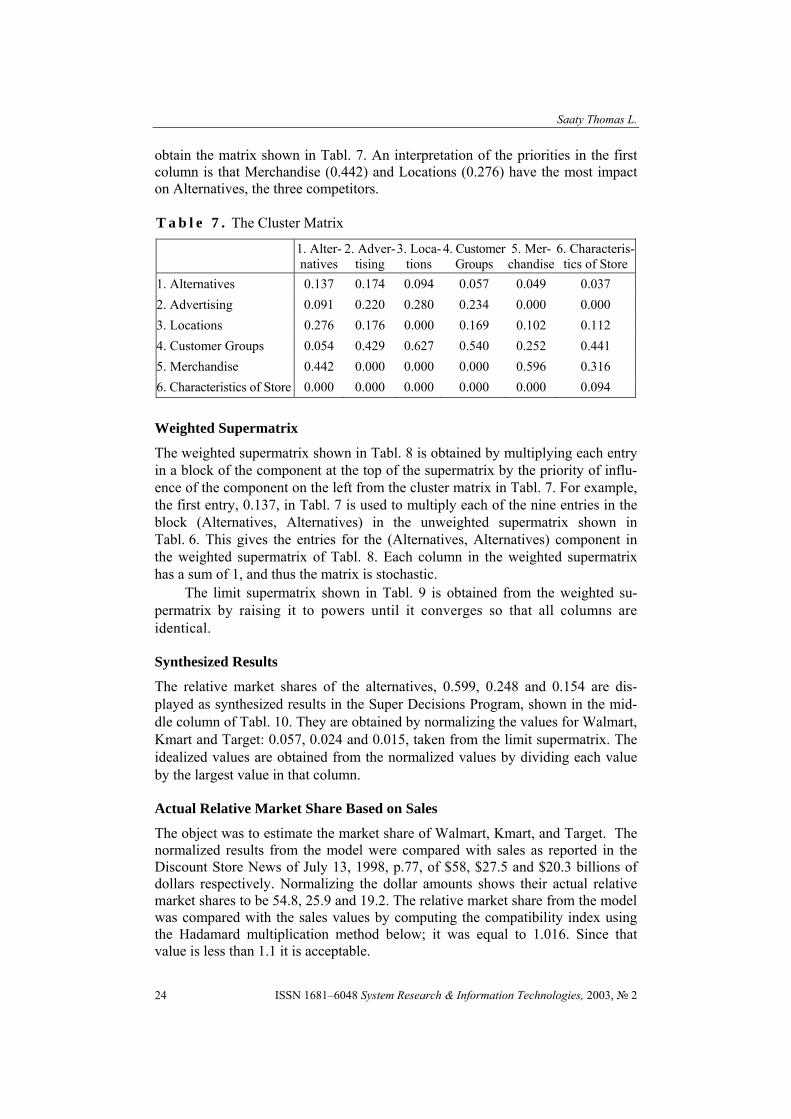
obtain the matrix shown in Tabl. 7. An interpretation of the priorities in the first column is that Merchandise (0.442) and Locations (0.276) have the most impact on Alternatives, the three competitors.

T a b l e 7 . The Cluster Matrix

1. Alter-natives

2. Adver-tising

3. Loca-tions

4. Customer Groups

5. Mer-chandise

6. Characteris-tics of Store

1. Alternatives 0.137 0.174 0.094 0.057 0.049 0.037 2. Advertising 0.091 0.220 0.280 0.234 0.000 0.000 3. Locations 0.276 0.176 0.000 0.169 0.102 0.112 4. Customer Groups 0.054 0.429 0.627 0.540 0.252 0.441 5. Merchandise 0.442 0.000 0.000 0.000 0.596 0.316 6. Characteristics of Store 0.000 0.000 0.000 0.000 0.000 0.094

Weighted Supermatrix

The weighted supermatrix shown in Tabl. 8 is obtained by multiplying each entry in a block of the component at the top of the supermatrix by the priority of influ-ence of the component on the left from the cluster matrix in Tabl. 7. For example, the first entry, 0.137, in Tabl. 7 is used to multiply each of the nine entries in the block (Alternatives, Alternatives) in the unweighted supermatrix shown in Tabl. 6. This gives the entries for the (Alternatives, Alternatives) component in the weighted supermatrix of Tabl. 8. Each column in the weighted supermatrix has a sum of 1, and thus the matrix is stochastic.

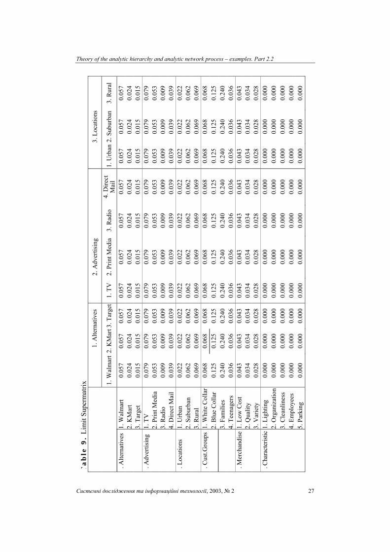
The limit supermatrix shown in Tabl. 9 is obtained from the weighted su-permatrix by raising it to powers until it converges so that all columns are identical.

Synthesized Results

The relative market shares of the alternatives, 0.599, 0.248 and 0.154 are dis-played as synthesized results in the Super Decisions Program, shown in the mid-dle column of Tabl. 10. They are obtained by normalizing the values for Walmart, Kmart and Target: 0.057, 0.024 and 0.015, taken from the limit supermatrix. The idealized values are obtained from the normalized values by dividing each value by the largest value in that column.

Actual Relative Market Share Based on Sales

The object was to estimate the market share of Walmart, Kmart, and Target. The normalized results from the model were compared with sales as reported in the Discount Store News of July 13, 1998, p.77, of $58, $27.5 and $20.3 billions of dollars respectively. Normalizing the dollar amounts shows their actual relative market shares to be 54.8, 25.9 and 19.2. The relative market share from the model was compared with the sales values by computing the compatibility index using the Hadamard multiplication method below; it was equal to 1.016. Since that value is less than 1.1 it is acceptable.



Ta

ble

8.

The

Wei

ghte

d Su

perm

atrix

, Dis

play

ed in

Tw

o Pa

rts

1.

Alte

rnat

ives

2.

Adv

ertis

ing

3.

Loc

ation

s

1.

Wal

mar

t 2.

KM

art

3. T

arge

t 1.

TV

2.

Prin

t M

edia

3.

Rad

io

4. D

irect

M

ail

1. U

rban

2.

Subu

rban

3.

Rur

al

. Alte

rnat

ives

1.

Wal

mar

t 0.

000

0.11

4 0.

114

0.12

0 0.

121

0.11

0 0.

148

0.05

8 0.

061

0.06

4 2.

KM

art

0.10

3 0.

000

0.02

3 0.

033

0.06

6 0.

030

0.04

7 0.

025

0.02

2 0.

019

3. T

arge

t 0.

034

0.02

3 0.

000

0.02

2 0.

037

0.03

3 0.

029

0.01

1 0.

011

0.01

1 . A

dver

tisin

g 1.

TV

0.

050

0.01

6 0.

017

0.00

0 0.

000

0.00

0 0.

000

0.08

0 0.

152

0.15

6 2.

Prin

t Med

ia

0.01

8 0.

032

0.03

9 0.

165

0.00

0 0.

176

0.00

0 0.

106

0.06

4 0.

049

3. R

adio

0.

006

0.00

5 0.

005

0.00

0 0.

000

0.00

0 0.

000

0.01

6 0.

015

0.01

4 4.

Dire

ct M

ail

0.01

7 0.

038

0.03

0 0.

055

0.00

0 0.

044

0.00

0 0.

076

0.04

8 0.

061

. Loc

atio

ns

1. U

rban

0.

031

0.02

3 0.

024

0.07

8 0.

028

0.01

4 0.

022

0.00

0 0.

000

0.00

0 2.

Sub

urba

n 0.

112

0.12

3 0.

174

0.06

8 0.

094

0.10

7 0.

121

0.00

0 0.

000

0.00

0 3.

Rur

al

0.13

3 0.

130

0.07

9 0.

030

0.10

3 0.

055

0.08

2 0.

000

0.00

0 0.

000

. Cus

t.Gro

ups

1. W

hite

Col

lar

0.00

8 0.

006

0.01

1 0.

071

0.08

6 0.

050

0.06

6 0.

049

0.12

4 0.

058

2. B

lue

Col

lar

0.01

2 0.

011

0.00

6 0.

071

0.08

6 0.

085

0.11

2 0.

140

0.07

3 0.

141

3. F

amili

es

0.03

1 0.

033

0.03

3 0.

267

0.35

6 0.

275

0.35

0 0.

411

0.40

2 0.

404

4. T

eena

gers

0.

003

0.00

3 0.

003

0.02

1 0.

024

0.01

9 0.

023

0.02

7 0.

028

0.02

4 . M

erch

andi

se 1

. Low

Cos

t 0.

160

0.14

7 0.

074

0.00

0 0.

000

0.00

0 0.

000

0.00

0 0.

000

0.00

0 2.

Qua

lity

0.11

5 0.

062

0.21

4 0.

000

0.00

0 0.

000

0.00

0 0.

000

0.00

0 0.

000

3. V

arie

ty

0.16

6 0.

233

0.15

4 0.

000

0.00

0 0.

000

0.00

0 0.

000

0.00

0 0.

000

. Cha

ract

erist

ic 1

. Lig

htin

g 0.

000

0.00

0 0.

000

0.00

0 0.

000

0.00

0 0.

000

0.00

0 0.

000

0.00

0 2.

Org

aniz

atio

n 0.

000

0.00

0 0.

000

0.00

0 0.

000

0.00

0 0.

000

0.00

0 0.

000

0.00

0 3.

Cle

anlin

ess

0.00

0 0.

000

0.00

0 0.

000

0.00

0 0.

000

0.00

0 0.

000

0.00

0 0.

000

4. E

mpl

oyee

s 0.

000

0.00

0 0.

000

0.00

0 0.

000

0.00

0 0.

000

0.00

0 0.

000

0.00

0 5.

Par

king

0.

000

0.00

0 0.

000

0.00

0 0.

000

0.00

0 0.

000

0.00

0 0.

000

0.00

0

Saaty Thomas L.


Te

rmin

atio

n

4.

Cus

tom

Gro

ups

5. M

erch

andi

se

6. C

hara

ctof

Sto

re

1

Whi

te

Col

lar

2 B

lue

Col

lar

3 Fa

mili

e 4

Teen

s 1

Low

Cos

t 2

Qua

lity

3 V

arie

ty

1 Li

ght’n

g 2

Org

an. 3

Cle

an

4 Em

p-lo

yees

5 Pk

g

.Alte

rnat

. 1.

Wal

mar

t 0.

036

0.03

8 0.

036

0.04

0 0.

033

0.03

0 0.

032

0.03

6 0.

024

0.03

1 0.

035

0.08

6 2.

KM

art

0.00

6 0.

012

0.01

2 0.

009

0.01

0 0.

006

0.00

6 0.

006

0.00

4 0.

005

0.00

5 0.

019

3. T

arge

t 0.

015

0.00

7 0.

009

0.00

9 0.

006

0.01

3 0.

011

0.01

2 0.

009

0.01

8 0.

015

0.04

9 . A

dver

tisin

g 1.

TV

0.

076

0.11

9 0.

119

0.14

8 0.

000

0.00

0 0.

000

0.00

0 0.

000

0.00

0 0.

000

0.00

0 2.

Prin

t Med

. 0.

050

0.05

2 0.

063

0.04

0 0.

000

0.00

0 0.

000

0.00

0 0.

000

0.00

0 0.

000

0.00

0 3.

Rad

io

0.01

4 0.

015

0.01

2 0.

023

0.00

0 0.

000

0.00

0 0.

000

0.00

0 0.

000

0.00

0 0.

000

4. D

irect

Mai

l 0.

095

0.04

8 0.

040

0.02

3 0.

000

0.00

0 0.

000

0.00

0 0.

000

0.00

0 0.

000

0.00

0 . L

ocat

ions

1. U

rban

0.

028

0.01

6 0.

016

0.01

8 0.

027

0.01

1 0.

010

0.01

6 0.

010

0.01

5 0.

018

0.03

1 2.

Sub

urba

n 0.

141

0.04

7 0.

052

0.05

2 0.

012

0.06

2 0.

064

0.07

1 0.

051

0.07

4 0.

073

0.13

5 3.

Rur

al

0.00

0 0.

106

0.10

1 0.

098

0.06

3 0.

030

0.02

9 0.

076

0.05

1 0.

074

0.07

3 0.

295

. Cus

t Grp

s 1.

Whi

te C

ol.

0.00

0 0.

000

0.15

1 0.

046

0.01

3 0.

056

0.04

2 0.

247

0.08

2 0.

156

0.10

7 0.

000

2. B

lue

Col

lar

0.00

0 0.

000

0.35

0 0.

096

0.02

8 0.

040

0.04

2 0.

247

0.08

2 0.

134

0.10

7 0.

000

3. F

amili

es

0.46

3 0.

463

0.00

0 0.

398

0.15

6 0.

143

0.15

7 0.

119

0.25

7 0.

318

0.40

0 0.

000

4. T

eena

gers

0.

077

0.07

7 0.

039

0.00

0 0.

055

0.01

3 0.

012

0.03

1 0.

019

0.03

6 0.

031

0.00

0 . M

erch

and

1. L

ow C

ost

0.00

0 0.

000

0.00

0 0.

000

0.00

0 0.

477

0.47

7 0.

000

0.00

0 0.

000

0.00

0 0.

000

2. Q

ualit

y 0.

000

0.00

0 0.

000

0.00

0 0.

447

0.00

0 0.

119

0.00

0 0.

000

0.00

0 0.

000

0.00

0 3.

Var

iety

0.

000

0.00

0 0.

000

0.00

0 0.

149

0.11

9 0.

000

0.00

0 0.

316

0.00

0 0.

000

0.00

0 . C

hara

ct.

1. L

ight

ing

0.00

0 0.

000

0.00

0 0.

000

0.00

0 0.

000

0.00

0 0.

000

0.01

6 0.

017

0.00

0 0.

097

2. O

rgan

iz.

0.00

0 0.

000

0.00

0 0.

000

0.00

0 0.

000

0.00

0 0.

035

0.00

0 0.

079

0.02

7 0.

290

3. C

lean

li.

0.00

0 0.

000

0.00

0 0.

000

0.00

0 0.

000

0.00

0 0.

092

0.04

4 0.

000

0.11

0 0.

000

4. E

mpl

oyee

0.

000

0.00

0 0.

000

0.00

0 0.

000

0.00

0 0.

000

0.00

0 0.

029

0.04

2 0.

000

0.00

0 5.

Par

king

0.

000

0.00

0 0.

000

0.00

0 0.

000

0.00

0 0.

000

0.01

0 0.

005

0.00

0 0.

000

0.00

0



Ta

ble

9.

Lim

it Su

perm

atrix

1. A

ltern

ativ

es

2.

Adv

ertis

ing

3.

Loc

atio

ns

1.

Wal

mar

t 2.

KM

art 3

. Tar

get

1. T

V

2. P

rint M

edia

3.

Rad

io

4. D

irect

M

ail

1. U

rban

2. S

ubur

ban

3. R

ural

. Alte

rnat

ives

1. W

alm

art

0.05

7 0.

057

0.05

7 0.

057

0.05

7 0.

057

0.05

7 0.

057

0.05

7 0.

057

2. K

Mar

t 0.

024

0.02

4 0.

024

0.02

4 0.

024

0.02

4 0.

024

0.02

4 0.

024

0.02

4 3.

Tar

get

0.01

5 0.

015

0.01

5 0.

015

0.01

5 0.

015

0.01

5 0.

015

0.01

5 0.

015

. Adv

ertis

ing

1. T

V

0.07

9 0.

079

0.07

9 0.

079

0.07

9 0.

079

0.07

9 0.

079

0.07

9 0.

079

2. P

rint M

edia

0.

053

0.05

3 0.

053

0.05

3 0.

053

0.05

3 0.

053

0.05

3 0.

053

0.05

3 3.

Rad

io

0.00

9 0.

009

0.00

9 0.

009

0.00

9 0.

009

0.00

9 0.

009

0.00

9 0.

009

4. D

irect

Mai

l 0.

039

0.03

9 0.

039

0.03

9 0.

039

0.03

9 0.

039

0.03

9 0.

039

0.03

9 . L

ocat

ions

1.

Urb

an

0.02

2 0.

022

0.02

2 0.

022

0.02

2 0.

022

0.02

2 0.

022

0.02

2 0.

022

2. S

ubur

ban

0.06

2 0.

062

0.06

2 0.

062

0.06

2 0.

062

0.06

2 0.

062

0.06

2 0.

062

3. R

ural

0.

069

0.06

9 0.

069

0.06

9 0.

069

0.06

9 0.

069

0.06

9 0.

069

0.06

9 . C

ust.G

roup

s 1.

Whi

te C

olla

r 0.

068

0.06

8 0.

068

0.06

8 0.

068

0.06

8 0.

068

0.06

8 0.

068

0.06

8 2.

Blu

e C

olla

r 0.

125

0.12

5 0.

125

0.12

5 0.

125

0.12

5 0.

125

0.12

5 0.

125

0.12

5 3.

Fam

ilies

0.

240

0.24

0 0.

240

0.24

0 0.

240

0.24

0 0.

240

0.24

0 0.

240

0.24

0 4.

Tee

nage

rs

0.03

6 0.

036

0.03

6 0.

036

0.03

6 0.

036

0.03

6 0.

036

0.03

6 0.

036

. Mer

chan

dise

1. L

ow C

ost

0.04

3 0.

043

0.04

3 0.

043

0.04

3 0.

043

0.04

3 0.

043

0.04

3 0.

043

2. Q

ualit

y 0.

034

0.03

4 0.

034

0.03

4 0.

034

0.03

4 0.

034

0.03

4 0.

034

0.03

4 3.

Var

iety

0.

028

0.02

8 0.

028

0.02

8 0.

028

0.02

8 0.

028

0.02

8 0.

028

0.02

8 . C

hara

cter

istic

1. L

ight

ing

0.00

0 0.

000

0.00

0 0.

000

0.00

0 0.

000

0.00

0 0.

000

0.00

0 0.

000

2. O

rgan

izat

ion

0.00

0 0.

000

0.00

0 0.

000

0.00

0 0.

000

0.00

0 0.

000

0.00

0 0.

000

3. C

lean

lines

s 0.

000

0.00

0 0.

000

0.00

0 0.

000

0.00

0 0.

000

0.00

0 0.

000

0.00

0 4.

Em

ploy

ees

0.00

0 0.

000

0.00

0 0.

000

0.00

0 0.

000

0.00

0 0.

000

0.00

0 0.

000

5. P

arki

ng

0.00

0 0.

000

0.00

0 0.

000

0.00

0 0.

000

0.00

0 0.

000

0.00

0 0.

000

Saaty Thomas L.


Te

rmin

atio

n

4. C

usto

mer

Gro

ups

5. M

erch

an-d

ise

6. C

hara

ct o

f Sto

re

1. W

hite

C

olla

r 2.

Blu

e C

olla

r 3.

Fa

mili

e 4.

Tee

ns

1. L

ow

Cos

t 2.

Qua

lity

3.

Var

iety

1.Li

ght’n

g 2.

O

rgan

iz.

3. C

lean

4. E

mp-

loye

es

5.

Park

ing

. Alte

rnat

ives

1. W

alm

art

0.05

7 0.

057

0.05

7 0.

057

0.05

7 0.

057

0.05

7 0.

057

0.05

7 0.

057

0.05

7 0.

057

2. K

Mar

t 0.

024

0.02

4 0.

024

0.02

4 0.

024

0.02

4 0.

024

0.02

4 0.

024

0.02

4 0.

024

0.02

4 3.

Tar

get

0.01

5 0.

015

0.01

5 0.

015

0.01

5 0.

015

0.01

5 0.

015

0.01

5 0.

015

0.01

5 0.

015

. Adv

ertis

ing

1. T

V

0.07

9 0.

079

0.07

9 0.

079

0.07

9 0.

079

0.07

9 0.

079

0.07

9 0.

079

0.07

9 0.

079

2. P

rint M

ed.

0.05

3 0.

053

0.05

3 0.

053

0.05

3 0.

053

0.05

3 0.

053

0.05

3 0.

053

0.05

3 0.

053

3. R

adio

0.

009

0.00

9 0.

009

0.00

9 0.

009

0.00

9 0.

009

0.00

9 0.

009

0.00

9 0.

009

0.00

9 4.

Dire

ct M

ail

0.03

9 0.

039

0.03

9 0.

039

0.03

9 0.

039

0.03

9 0.

039

0.03

9 0.

039

0.03

9 0.

039

. Loc

atio

ns

1. U

rban

0.

022

0.02

2 0.

022

0.02

2 0.

022

0.02

2 0.

022

0.02

2 0.

022

0.02

2 0.

022

0.02

2 2.

Sub

urba

n 0.

062

0.06

2 0.

062

0.06

2 0.

062

0.06

2 0.

062

0.06

2 0.

062

0.06

2 0.

062

0.06

2 3.

Rur

al

0.06

9 0.

069

0.06

9 0.

069

0.06

9 0.

069

0.06

9 0.

069

0.06

9 0.

069

0.06

9 0.

069

. Cus

t.Gro

ups

1. W

hite

Col

. 0.

068

0.06

8 0.

068

0.06

8 0.

068

0.06

8 0.

068

0.06

8 0.

068

0.06

8 0.

068

0.06

8 2.

Blu

e Co

llar

0.12

5 0.

125

0.12

5 0.

125

0.12

5 0.

125

0.12

5 0.

125

0.12

5 0.

125

0.12

5 0.

125

3. F

amili

es

0.24

0 0.

240

0.24

0 0.

240

0.24

0 0.

240

0.24

0 0.

240

0.24

0 0.

240

0.24

0 0.

240

4. T

eena

gers

0.

036

0.03

6 0.

036

0.03

6 0.

036

0.03

6 0.

036

0.03

6 0.

036

0.03

6 0.

036

0.03

6 . M

erch

andi

se 1

. Low

Cos

t 0.

043

0.04

3 0.

043

0.04

3 0.

043

0.04

3 0.

043

0.04

3 0.

043

0.04

3 0.

043

0.04

3 2.

Qua

lity

0.03

4 0.

034

0.03

4 0.

034

0.03

4 0.

034

0.03

4 0.

034

0.03

4 0.

034

0.03

4 0.

034

3. V

arie

ty

0.02

8 0.

028

0.02

8 0.

028

0.02

8 0.

028

0.02

8 0.

028

0.02

8 0.

028

0.02

8 0.

028

. Cha

ract

erist

i. 1.

Lig

htin

g 0.

000

0.00

0 0.

000

0.00

0 0.

000

0.00

0 0.

000

0.00

0 0.

000

0.00

0 0.

000

0.00

0 2.

Org

aniz

. 0.

000

0.00

0 0.

000

0.00

0 0.

000

0.00

0 0.

000

0.00

0 0.

000

0.00

0 0.

000

0.00

0 3.

Cle

anli.

0.

000

0.00

0 0.

000

0.00

0 0.

000

0.00

0 0.

000

0.00

0 0.

000

0.00

0 0.

000

0.00

0 4.

Em

ploy

ee

0.00

0 0.

000

0.00

0 0.

000

0.00

0 0.

000

0.00

0 0.

000

0.00

0 0.

000

0.00

0 0.

000

5. P

arki

ng

0.00

0 0.

000

0.00

0 0.

000

0.00

0 0.

000

0.00

0 0.

000

0.00

0 0.

000

0.00

0 0.

000



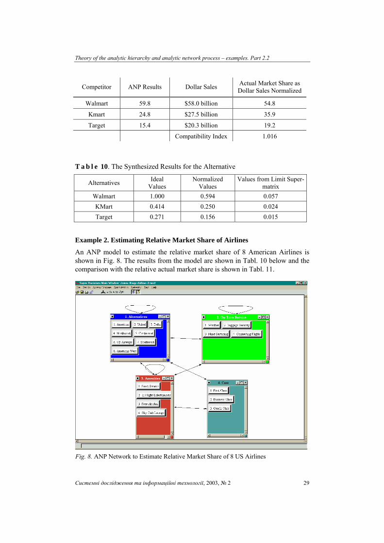
Competitor ANP Results Dollar Sales Actual Market Share as Dollar Sales Normalized

Walmart 59.8 $58.0 billion 54.8

Kmart 24.8 $27.5 billion 35.9

Target 15.4 $20.3 billion 19.2

Compatibility Index 1.016

T a b l e 10. The Synthesized Results for the Alternative

Alternatives Ideal Values

Normalized Values

Values from Limit Super-matrix

Walmart 1.000 0.594 0.057 KMart 0.414 0.250 0.024 Target 0.271 0.156 0.015

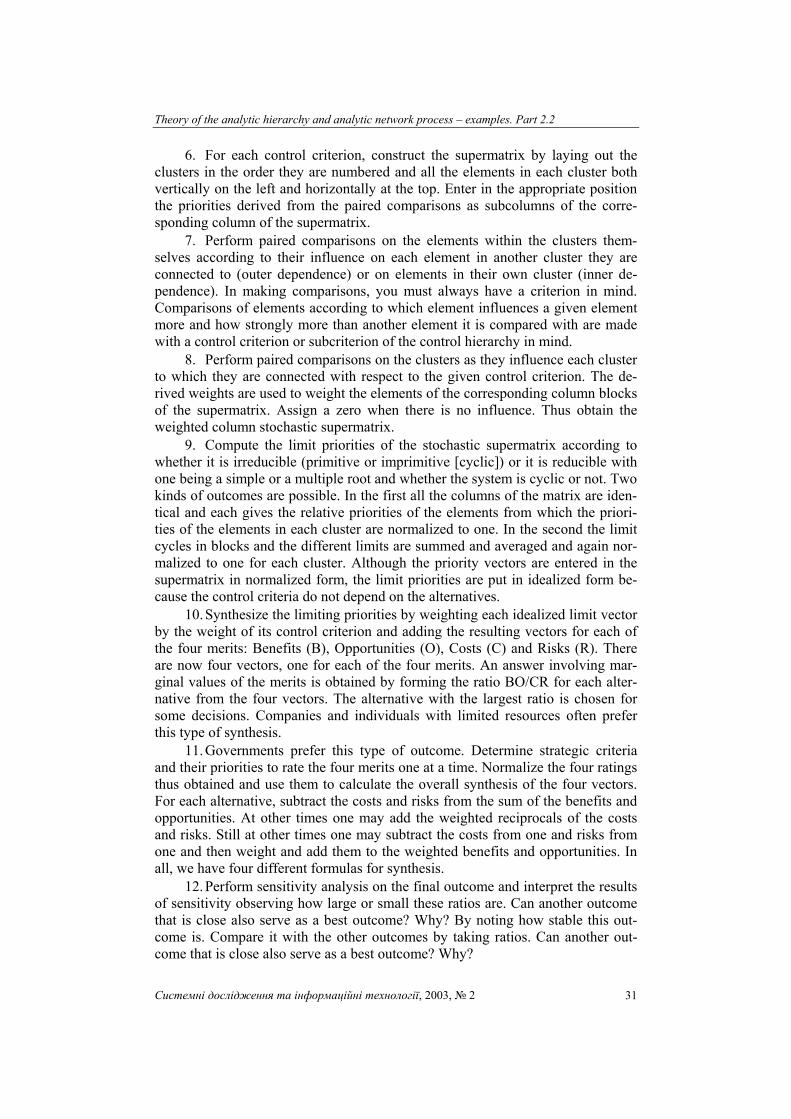
Example 2. Estimating Relative Market Share of Airlines

An ANP model to estimate the relative market share of 8 American Airlines is shown in Fig. 8. The results from the model are shown in Tabl. 10 below and the comparison with the relative actual market share is shown in Tabl. 11.

Fig. 8. ANP Network to Estimate Relative Market Share of 8 US Airlines

Saaty Thomas L.


T a b l e 11. Comparing Model Results with Actual Market Share Data

Model Results Actual Market Share (yr 2000) American 23.9 24.0

United 18.7 19.7 Delta 18.0 18.0

Northwest 11.4 12.4 Continental 9.3 10.0 US Airways 7.5 7.1 Southwest 5.9 6.4

American West 4.4 2.9 Compatibility Index 1.0247

We summarize by giving the reader a list of the steps we have followed in

applying the ANP.

4. OUTLINE OF THE STEPS OF THE ANP

1. Describe the decision problem in detail including its objectives, criteria and subcriteria, actors and their objectives and the possible outcomes of that deci-sion. Give details of influences that determine how that decision may come out.

2. Determine the control criteria and subcriteria in the four control hierar-chies one each for the benefits, opportunities, costs and risks of that decision and obtain their priorities from paired comparisons matrices. If a control criterion or subcriterion has a global priority of 3% or less, you may consider carefully elimi-nating it from further consideration. The software automatically deals only with those criteria or subcriteria that have subnets under them. For benefits and oppor-tunities, ask what gives the most benefits or presents the greatest opportunity to influence fulfillment of that control criterion. For costs and risks, ask what incurs the most cost or faces the greatest risk. Sometimes (very rarely), the comparisons are made simply in terms of benefits, opportunities, costs, and risks in the aggre-gate without using control criteria and subcriteria.

3. Determine the most general network of clusters (or components) and their elements that applies to all the control criteria. To better organize the devel-opment of the model as well as you can, number and arrange the clusters and their elements in a convenient way (perhaps in a column). Use the identical label to represent the same cluster and the same elements for all the control criteria.

4. For each control criterion or subcriterion, determine the clusters of the general feedback system with their elements and connect them according to their outer and inner dependence influences. An arrow is drawn from a cluster to any cluster whose elements influence it.

5. Determine the approach you want to follow in the analysis of each cluster or element, influencing (the preferred approach) other clusters and elements with respect to a criterion, or being influenced by other clusters and elements. The sense (being influenced or influencing) must apply to all the criteria for the four control hierarchies for the entire decision.



6. For each control criterion, construct the supermatrix by laying out the clusters in the order they are numbered and all the elements in each cluster both vertically on the left and horizontally at the top. Enter in the appropriate position the priorities derived from the paired comparisons as subcolumns of the corre-sponding column of the supermatrix.

7. Perform paired comparisons on the elements within the clusters them-selves according to their influence on each element in another cluster they are connected to (outer dependence) or on elements in their own cluster (inner de-pendence). In making comparisons, you must always have a criterion in mind. Comparisons of elements according to which element influences a given element more and how strongly more than another element it is compared with are made with a control criterion or subcriterion of the control hierarchy in mind.

8. Perform paired comparisons on the clusters as they influence each cluster to which they are connected with respect to the given control criterion. The de-rived weights are used to weight the elements of the corresponding column blocks of the supermatrix. Assign a zero when there is no influence. Thus obtain the weighted column stochastic supermatrix.

9. Compute the limit priorities of the stochastic supermatrix according to whether it is irreducible (primitive or imprimitive [cyclic]) or it is reducible with one being a simple or a multiple root and whether the system is cyclic or not. Two kinds of outcomes are possible. In the first all the columns of the matrix are iden-tical and each gives the relative priorities of the elements from which the priori-ties of the elements in each cluster are normalized to one. In the second the limit cycles in blocks and the different limits are summed and averaged and again nor-malized to one for each cluster. Although the priority vectors are entered in the supermatrix in normalized form, the limit priorities are put in idealized form be-cause the control criteria do not depend on the alternatives.

10. Synthesize the limiting priorities by weighting each idealized limit vector by the weight of its control criterion and adding the resulting vectors for each of the four merits: Benefits (B), Opportunities (O), Costs (C) and Risks (R). There are now four vectors, one for each of the four merits. An answer involving mar-ginal values of the merits is obtained by forming the ratio BO/CR for each alter-native from the four vectors. The alternative with the largest ratio is chosen for some decisions. Companies and individuals with limited resources often prefer this type of synthesis.

11. Governments prefer this type of outcome. Determine strategic criteria and their priorities to rate the four merits one at a time. Normalize the four ratings thus obtained and use them to calculate the overall synthesis of the four vectors. For each alternative, subtract the costs and risks from the sum of the benefits and opportunities. At other times one may add the weighted reciprocals of the costs and risks. Still at other times one may subtract the costs from one and risks from one and then weight and add them to the weighted benefits and opportunities. In all, we have four different formulas for synthesis.

12. Perform sensitivity analysis on the final outcome and interpret the results of sensitivity observing how large or small these ratios are. Can another outcome that is close also serve as a best outcome? Why? By noting how stable this out-come is. Compare it with the other outcomes by taking ratios. Can another out-come that is close also serve as a best outcome? Why?

Saaty Thomas L.


5. CONCLUSIONS

Complete examples applying the AHP to a decision involving BOCR can be found in references 1 and 2. Numerous other examples along with the software Super Decisions for the ANP can be obtained from [email protected]. The reader now should have a good idea as to how to use the process in a com-plex decision. The AHP and ANP have found application in practice by many companies and governments. My book Decision Making for Leaders is in more than a half a dozen languages. What is happening now is the wide interest shown in the ANP and its applicability to the long discussed project of building a Na-tional Missile Defense This application was done in September 2000 and pre-sented at the National Defense University in Washington, DC, in February 2002. Its conclusions were affirmed by President Bush’s decision of late December 2002 to construct such a system. Another recent policy study was done regarding whether the US should challenge Iraq directly or go through the UN. The admini-stration decided to go through the UN. There is also the hopeless Middle East conflict. An ANP analysis showed that the best option is for Israel and the US to help the Palestinians both set up a state and in particular achieve a viable econ-omy. There are two things to tell the reader about it in this regard. The ANP book is now translated to Russian and will soon appear and the manual for the Super Decisions sofware can be obtained by sending an email to [email protected]. My forthcoming book The Encyclicon will have nearly 100 examples of such applications and will be out in the near future.

As a final word, the AHP has developed a group of critics who think it can-not be used for multicriteria methods because it is simple. They say that it is lin-ear. I say it is non-linear. Hierarchic composition yields nonlinear forms that are dense in the space of polynomials (multinomials). According to the theorem of Weierstrasse the latter can be used to approximate a continuous function arbitrar-ily close. Multilinear forms and polynomials are intimately related, particularly when we see that we can identify all the variables into a single or into several variables raised to powers. Thus depending on how rich a hierarchic structure is, one can use hierarchic composition to come close to the real answer underlying a decision. This author, a mathematician, with a Ph.D. in mathematics from Yale University, and postdoctoral work at the Sorbonne in Paris, has written many first works in the field of Operations Research. Among them is Mathematical Methods of Operations Research, translated to many languages. Also, he has spent the first half of his career working at the Pentagon, the Navy Department, and the De-partment of State, all the time searching for and applying, when feasible, mathe-matical models of operations research. The biggest weakness of these methods is that they could only be understood by the experts and occasionally used by the practicing layman, with doubt and hesitation. As an adult I took it upon myself since my first involvement in research on negotiations between the US and the Soviet Union in Geneva in the 1960’s and after having written a book on the Mathematical Models of Arms Control and Disarmament in 1968, translated to Russian in 1977, to always try to simplify the AHP so that even a child can use it. And children have used it without the need to explain the mathematics but even if one has to, it is possible to do that with some patience but without a great deal of



prolixity and confusion. This is why the AHP and ANP are intentionally simple. More full blown decision examples will be given in Part 2.3.

REFERENCES

1. Saaty, Thomas L. The Analytic Network Process, RWS Publications, 4922 Ellsworth Avenue, Pittsburgh, Pa. 15213, 2001.

2. Saaty, Rozann W. Decision Making in Complex Environments: The Analytic Network Process (ANP) for Dependence and Feedback; a manual for the ANP Software; Creative Decisions Foundation, 4922 Ellsworth Avenue, Pittsburgh, PA 15213, 2002.

3. Saaty, Thomas L. Fundamentals of the Analytic Hierarchy Process, RWS Publica-tions, 4922 Ellsworth Avenue, Pittsburgh, Pa. 15413, 2000.

4. Saaty, Thomas L and Yeonmin Cho “The Decision by the US Congress on China’s Trade Status: A Multicriteria Analysis,” Socio-Economic Planning Sciences, 35(2001) 243-252.

Received 29.04.2003

theory of the analytic hierarchy and analytic network

Documents