thermal analysis of solid structures - infographdownload.infograph.de/en/solid_thermal.pdf · the...
TRANSCRIPT
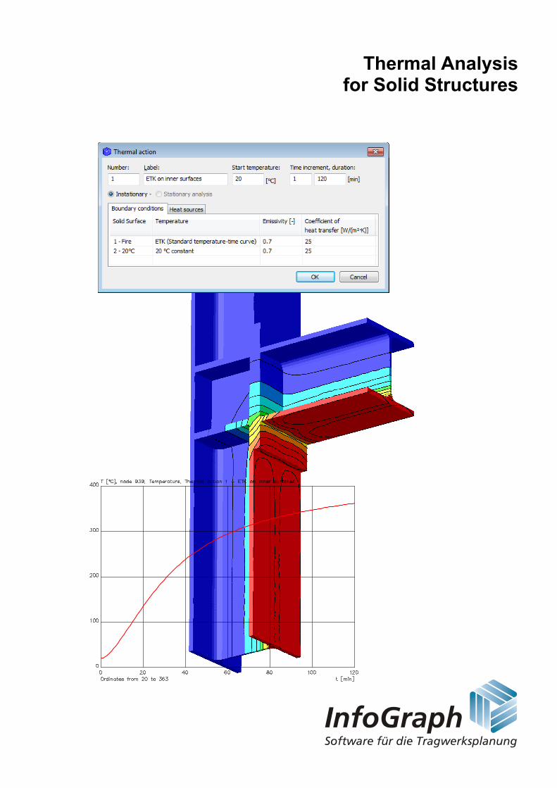
Thermal Analysisfor Solid Structures

The description of program functions within this documentation should not be considered a warranty of product features.All warranty and liability claims arising from the use of this documentation are excluded.
InfoGraph® is a registered trademark of InfoGraph GmbH, Aachen, Germany. The manufacturer and product namesmentioned below are trademarks of their respective owners.
This documentation is copyright protected. Reproduction, duplication, translation or electronic storage of this document orparts thereof is subject to the written permission of InfoGraph GmbH.
InfoGraph® Software uses Microsoft® MFC and Intel® MKL Libraries.
© 2019 InfoGraph GmbH, Aachen, Germany. All rights reserved.
Title image: Temperature distribution at the corner of a frame after 120 minutes of fire exposure on the inner surfaces.

1
Contents
© InfoGraph GmbH, August 2019
Contents
Area of Application 2
Basics 3
Input Data 5
Thermal Material Properties 5
Solid Surface 8
Thermal Actions 9
Thermal Analysis 10
Examples 11
Instationary Temperature Progression in an Angular Retaining Wall 11
Comparative Calculation with and without Radiation 14
Stationary Temperature Destribution 15
References 16
2
Thermal Analysis of Solid Structures
© InfoGraph GmbH, August 2019
Thermal Analysis of Solid Structures
Area of ApplicationThe Thermal analysis allows the analysis of stationary and instationary temperature distributions in solid structures oftetrahedron elements within the Finite Elements program systems. Any three-dimensional geometry can be analyzed.
The material properties are described in the section Thermal material properties.
The analysis can be divided up into the following steps:
• The structure geometry is described with model object Solid.
• Properties like material and presets for the mesh generation are assigned to each solid model object.
• The thermal material properties are defined in the section dialog.
• After selection of the surface of a solid a surface property can be assigned to it.
• In the dialog Thermal action thermal boundary conditions are assigned to the surfaces.
• After the definition of all properties which are relevant for the structure the finite element model is generated with themesh generator Tetrahedrons from Solid.
• Subsequently the thermal analysis is carried out.
• Additionally a static analysis can be performed considering the thermal strains due to a thermal action (load typeThermal action).
Multiple independent Thermal actions can be defined.
3
Basics
© InfoGraph GmbH, August 2019
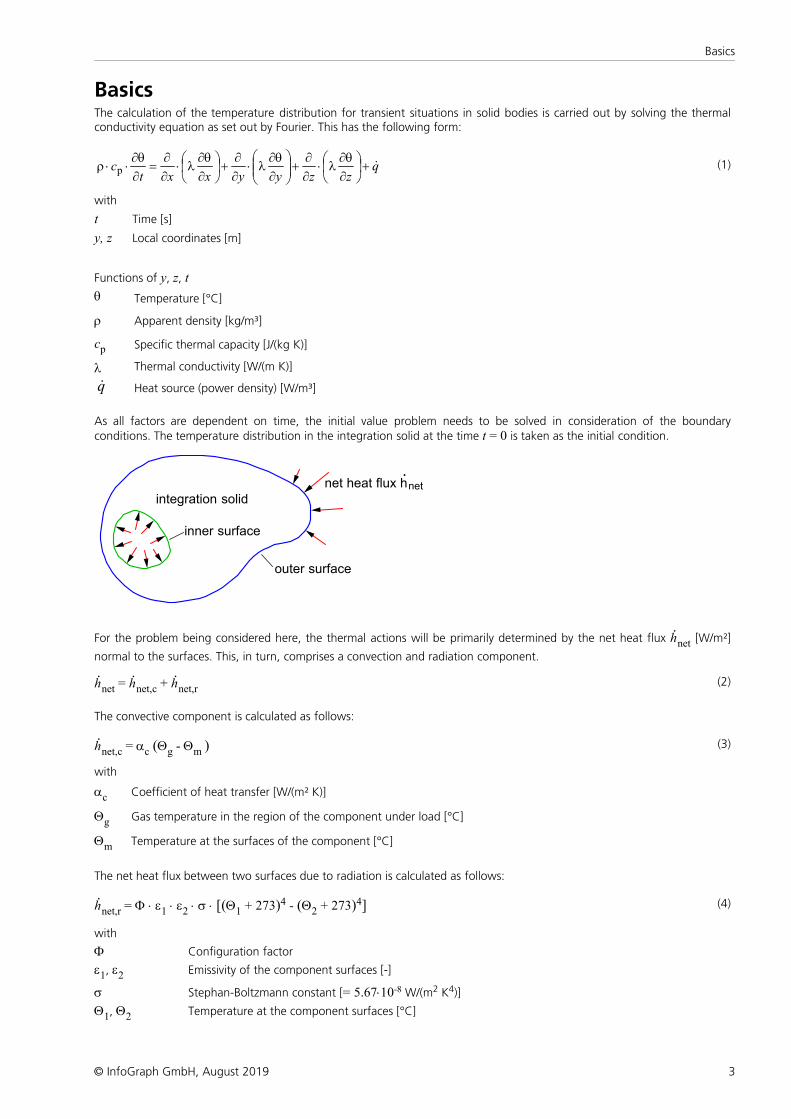
BasicsThe calculation of the temperature distribution for transient situations in solid bodies is carried out by solving the thermalconductivity equation as set out by Fourier. This has the following form:
qzzyyxxt
c &+÷ø
öçè
æ
q¶l×
¶+÷÷
ø
öççè
æ
q¶l×
¶+÷
ø
öçè
æ
q¶l×
¶=
q¶××r p (1)
with
t Time [s]
y, z Local coordinates [m]
Functions of y, z, t
q Temperature [°C]
r Apparent density [kg/m³]
cp Specific thermal capacity [J/(kg K)]
l Thermal conductivity [W/(m K)]
q& Heat source (power density) [W/m³]
As all factors are dependent on time, the initial value problem needs to be solved in consideration of the boundaryconditions. The temperature distribution in the integration solid at the time t = 0 is taken as the initial condition.
integration solid
inner surface
outer surface
net heat flux•
neth
For the problem being considered here, the thermal actions will be primarily determined by the net heat flux h×net [W/m²]
normal to the surfaces. This, in turn, comprises a convection and radiation component.
h×net = h
×net,c + h
×net,r
(2)
The convective component is calculated as follows:
h×net,c = ac (Qg - Qm ) (3)
with
ac Coefficient of heat transfer [W/(m² K)]
Qg Gas temperature in the region of the component under load [°C]
Qm Temperature at the surfaces of the component [°C]
The net heat flux between two surfaces due to radiation is calculated as follows:
h×net,r = F × e1 × e2 × s × [(Q1 + 273)4 - (Q2 + 273)4] (4)
with
F Configuration factor
e1, e2 Emissivity of the component surfaces [-]
s Stephan-Boltzmann constant [= 5.67×10⁻⁸ W/(m2 K4)]
Q1, Q2 Temperature at the component surfaces [°C]
4
Thermal Analysis of Solid Structures
© InfoGraph GmbH, August 2019
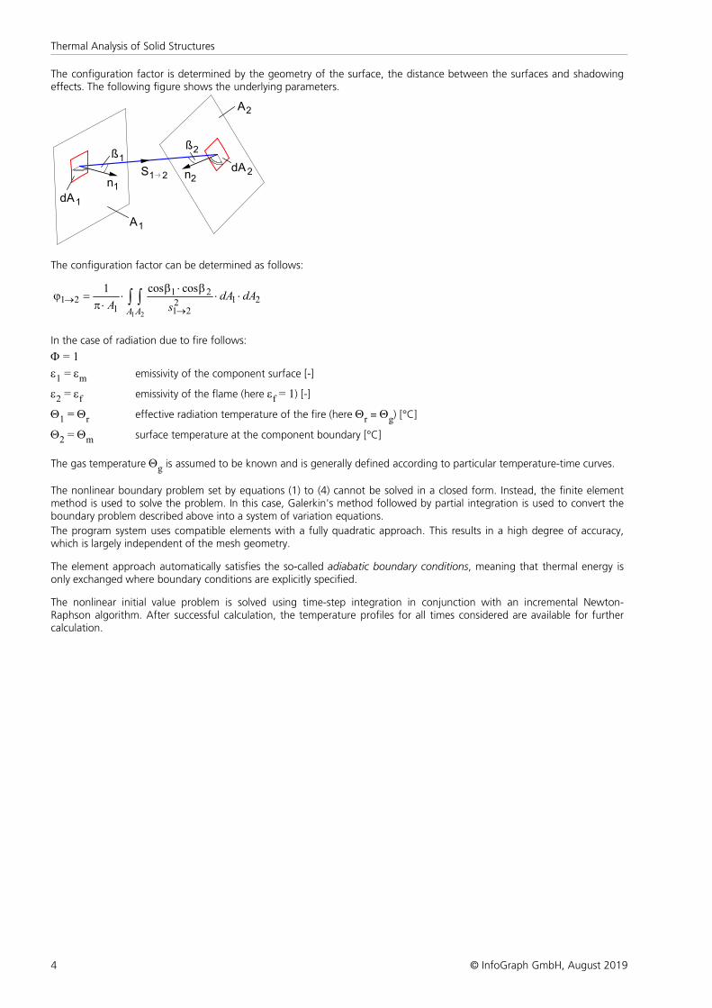
The configuration factor is determined by the geometry of the surface, the distance between the surfaces and shadowingeffects. The following figure shows the underlying parameters.
dA2
1dA
ß1
n1
ß2
n2
A1
A2
S1 2
The configuration factor can be determined as follows:
21221
21
121
1 2
coscos1dAdA
sAA A
××b×b
××p
=j ò ò®
®
In the case of radiation due to fire follows:
F = 1
e1 = em emissivity of the component surface [-]
e2 = ef emissivity of the flame (here ef = 1) [-]
Q1 = Qr effective radiation temperature of the fire (here Qr = Qg) [°C]
Q2 = Qm surface temperature at the component boundary [°C]
The gas temperature Qg is assumed to be known and is generally defined according to particular temperature-time curves.
The nonlinear boundary problem set by equations (1) to (4) cannot be solved in a closed form. Instead, the finite elementmethod is used to solve the problem. In this case, Galerkin's method followed by partial integration is used to convert theboundary problem described above into a system of variation equations.
The program system uses compatible elements with a fully quadratic approach. This results in a high degree of accuracy,which is largely independent of the mesh geometry.
The element approach automatically satisfies the so-called adiabatic boundary conditions, meaning that thermal energy isonly exchanged where boundary conditions are explicitly specified.
The nonlinear initial value problem is solved using time-step integration in conjunction with an incremental Newton-Raphson algorithm. After successful calculation, the temperature profiles for all times considered are available for furthercalculation.
5
Input Data
© InfoGraph GmbH, August 2019
Input Data
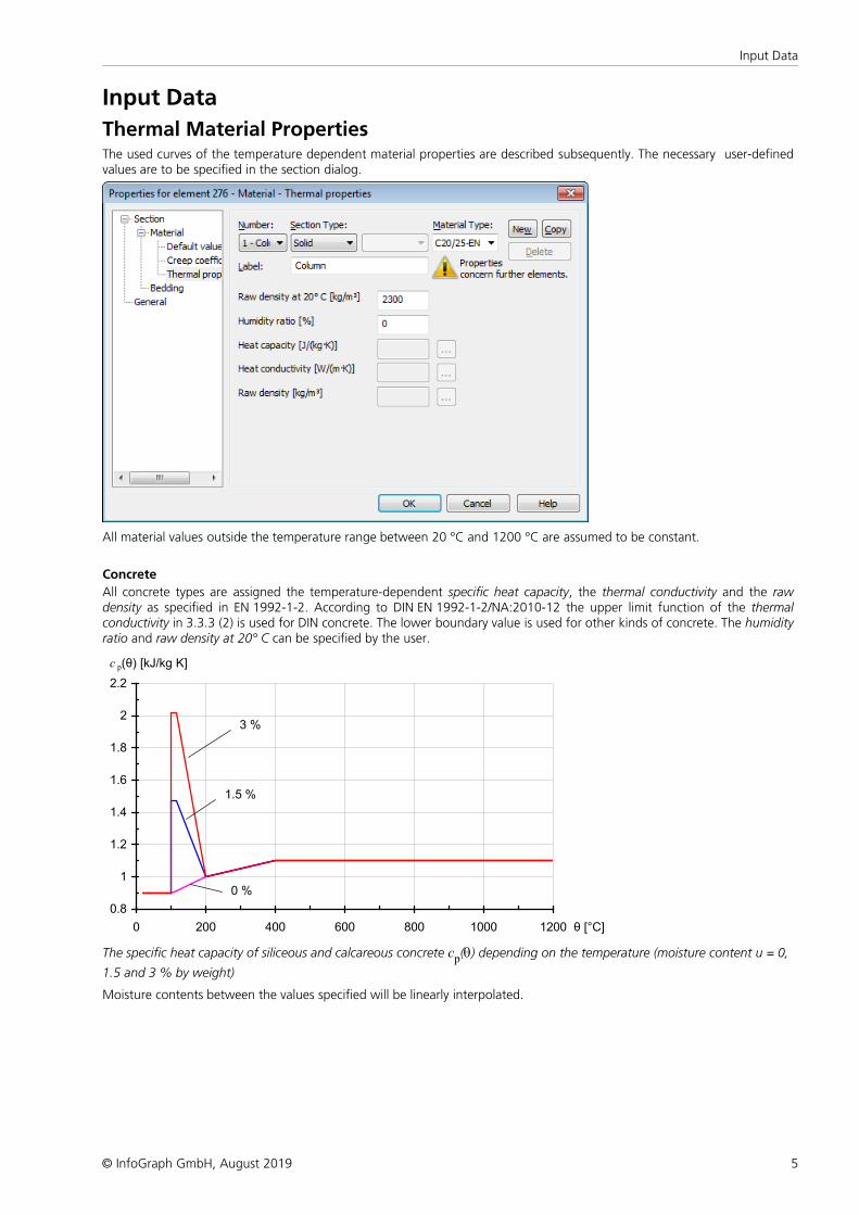
Thermal Material PropertiesThe used curves of the temperature dependent material properties are described subsequently. The necessary user-definedvalues are to be specified in the section dialog.
All material values outside the temperature range between 20 °C and 1200 °C are assumed to be constant.
Concrete
All concrete types are assigned the temperature-dependent specific heat capacity, the thermal conductivity and the rawdensity as specified in EN 1992-1-2. According to DIN EN 1992-1-2/NA:2010-12 the upper limit function of the thermalconductivity in 3.3.3 (2) is used for DIN concrete. The lower boundary value is used for other kinds of concrete. The humidityratio and raw density at 20° C can be specified by the user.
0.8
1
1.2
1.4
1.6
1.8
2
2.2
0 200 400 600 800 1000 1200 θ [°C]
c p(θ) [kJ/kg K]
3 %
0 %
1.5 %
The specific heat capacity of siliceous and calcareous concrete cp(q) depending on the temperature (moisture content u = 0,
1.5 and 3 % by weight)
Moisture contents between the values specified will be linearly interpolated.

6
Thermal Analysis of Solid Structures
© InfoGraph GmbH, August 2019
0.4
0.6
0.8
1
1.2
1.4
1.6
1.8
2
0 200 400 600 800 1000 1200 θ [°C]
l c [W/m K]
1
2
Temperature-dependent thermal conductivity 1: upper limit (DIN concrete); 2: lower limit
0.85
0.9
0.95
1
0 200 400 600 800 1000 1200 θ [°C]
rθ /r20 [-]
Temperature-dependent raw density ratio of concrete
Steel
All steel types are assigned the temperature-dependent specific heat capacity and the thermal conductivity as specified inEN 1993-1-2.
0
1000
2000
3000
4000
5000
0 200 400 600 800 1000 1200 θ [°C]
c a [J / kg K]
The temperature-dependent specific heat capacity for carbon steel
7
Input Data
© InfoGraph GmbH, August 2019
20
30
40
50
60
0 200 400 600 800 1000 1200 θ [°C]
l a [W/m K]
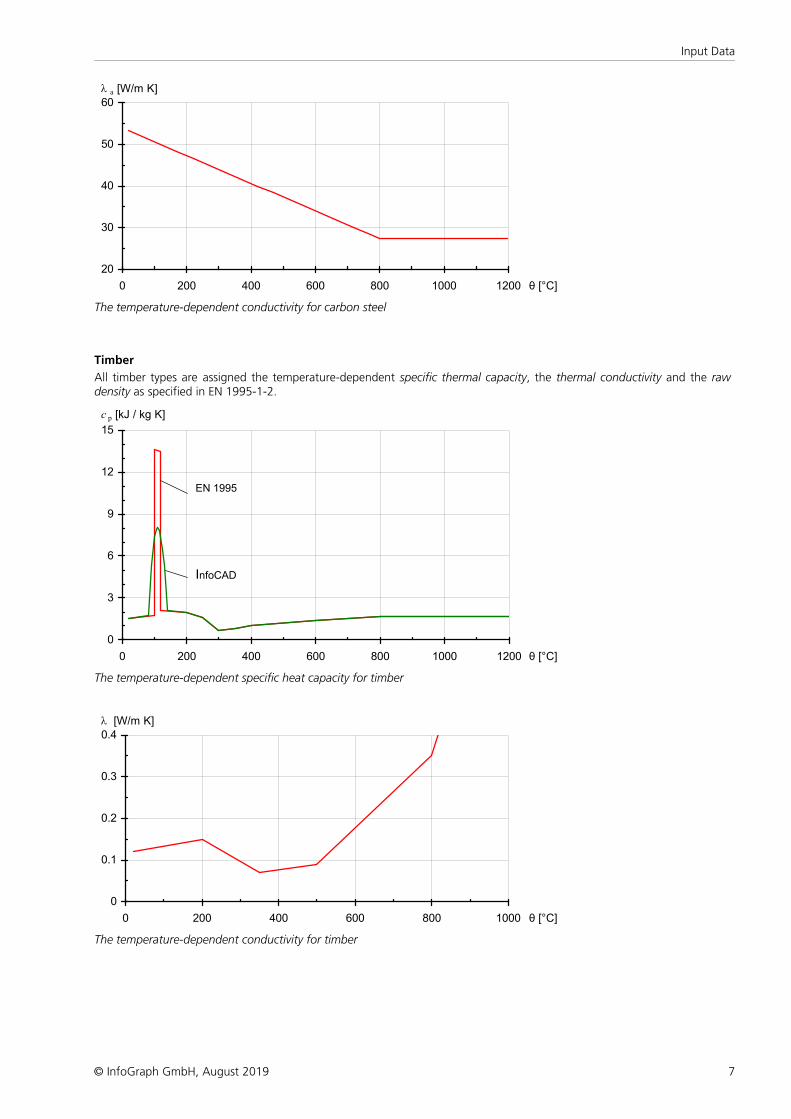
The temperature-dependent conductivity for carbon steel
Timber
All timber types are assigned the temperature-dependent specific thermal capacity, the thermal conductivity and the rawdensity as specified in EN 1995-1-2.
0
3
6
9
12
15
0 200 400 600 800 1000 1200 θ [°C]
c p [kJ / kg K]
EN 1995
InfoCAD
The temperature-dependent specific heat capacity for timber
0
0.1
0.2
0.3
0.4
0 200 400 600 800 1000 θ [°C]
l [W/m K]
The temperature-dependent conductivity for timber
8
Thermal Analysis of Solid Structures
© InfoGraph GmbH, August 2019
0
0.2
0.4
0.6
0.8
1
1.2
0 200 400 600 800 1000 1200 θ [°C]
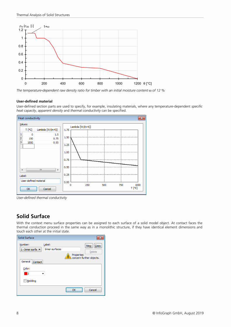
rθ /r20 [-] 1+w
The temperature-dependent raw density ratio for timber with an initial moisture content w of 12 %
User-defined material
User-defined section parts are used to specify, for example, insulating materials, where any temperature-dependent specificheat capacity, apparent density and thermal conductivity can be specified.
User-defined thermal conductivity
Solid SurfaceWith the context menu surface properties can be assigned to each surface of a solid model object. At contact faces thethermal conduction proceed in the same way as in a monolithic structure, if they have identical element dimensions andtouch each other at the initial state.
9
Input Data
© InfoGraph GmbH, August 2019
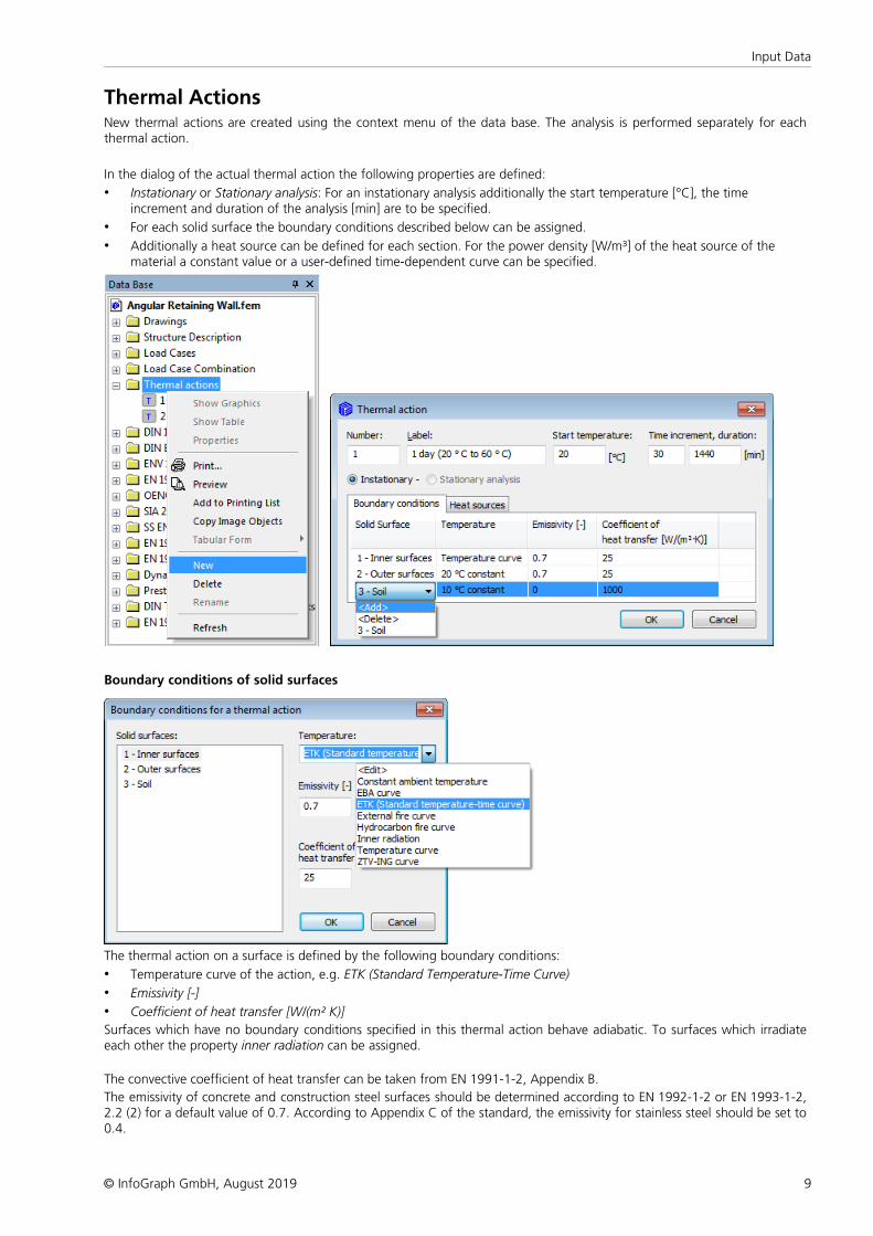
Thermal ActionsNew thermal actions are created using the context menu of the data base. The analysis is performed separately for eachthermal action.
In the dialog of the actual thermal action the following properties are defined:
• Instationary or Stationary analysis: For an instationary analysis additionally the start temperature [°C], the timeincrement and duration of the analysis [min] are to be specified.
• For each solid surface the boundary conditions described below can be assigned.
• Additionally a heat source can be defined for each section. For the power density [W/m³] of the heat source of thematerial a constant value or a user-defined time-dependent curve can be specified.
Boundary conditions of solid surfaces
The thermal action on a surface is defined by the following boundary conditions:
• Temperature curve of the action, e.g. ETK (Standard Temperature-Time Curve)
• Emissivity [-]
• Coefficient of heat transfer [W/(m² K)]
Surfaces which have no boundary conditions specified in this thermal action behave adiabatic. To surfaces which irradiateeach other the property inner radiation can be assigned.
The convective coefficient of heat transfer can be taken from EN 1991-1-2, Appendix B.
The emissivity of concrete and construction steel surfaces should be determined according to EN 1992-1-2 or EN 1993-1-2,2.2 (2) for a default value of 0.7. According to Appendix C of the standard, the emissivity for stainless steel should be set to0.4.
10
Thermal Analysis of Solid Structures
© InfoGraph GmbH, August 2019
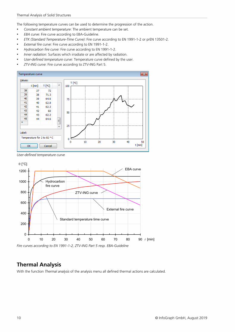
The following temperature curves can be used to determine the progression of the action.
• Constant ambient temperature: The ambient temperature can be set.
• EBA curve: Fire curve according to EBA-Guideline.
• ETK (Standard Temperature-Time Curve): Fire curve according to EN 1991-1-2 or prEN 13501-2.
• External fire curve: Fire curve according to EN 1991-1-2.
• Hydrocarbon fire curve: Fire curve according to EN 1991-1-2.
• Inner radiation: Surfaces which irradiate or are affected by radiation.
• User-defined temperature curve: Temperature curve defined by the user.
• ZTV-ING curve: Fire curve according to ZTV-ING Part 5.
User-defined temperature curve
0
200
400
600
800
1000
1200
0 10 20 30 40 50 60 70 80 90 t [min]
q [°C]
Hydrocarbon
fire curve
External fire curve
Standard temperature time curve
ZTV-ING curve
EBA curve
Fire curves according to EN 1991-1-2, ZTV-ING Part 5 resp. EBA-Guideline
Thermal AnalysisWith the function Thermal analysis of the analysis menu all defined thermal actions are calculated.
11
Examples
© InfoGraph GmbH, August 2019
ExamplesThe following examples shall demonstrate possible applications of the program and also be used for validation of theattained results.
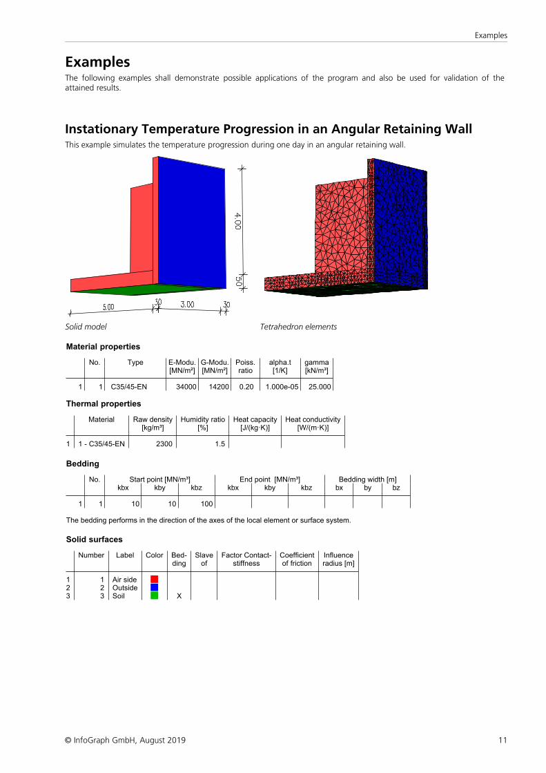
Instationary Temperature Progression in an Angular Retaining WallThis example simulates the temperature progression during one day in an angular retaining wall.
Solid model Tetrahedron elements
Material properties
No. Type E-Modu. G-Modu. Poiss. alpha.t gamma[MN/m²] [MN/m²] ratio [1/K] [kN/m³]
1 1 C35/45-EN 34000 14200 0.20 1.000e-05 25.000
Thermal properties
Material Raw density[kg/m³]
Humidity ratio[%]
Heat capacity[J/(kg·K)]
Heat conductivity[W/(m·K)]
1 1 - C35/45-EN 2300 1.5
Bedding
No. Start point [MN/m³] End point [MN/m³] Bedding width [m]kbx kby kbz kbx kby kbz bx by bz
1 1 10 10 100
The bedding performs in the direction of the axes of the local element or surface system.
Solid surfaces
Number Label Color Bed-ding
Slaveof
Factor Contact-stiffness
Coefficientof friction
Influenceradius [m]
1 1 Air side 2 2 Outside 3 3 Soil X
12
Thermal Analysis of Solid Structures
© InfoGraph GmbH, August 2019
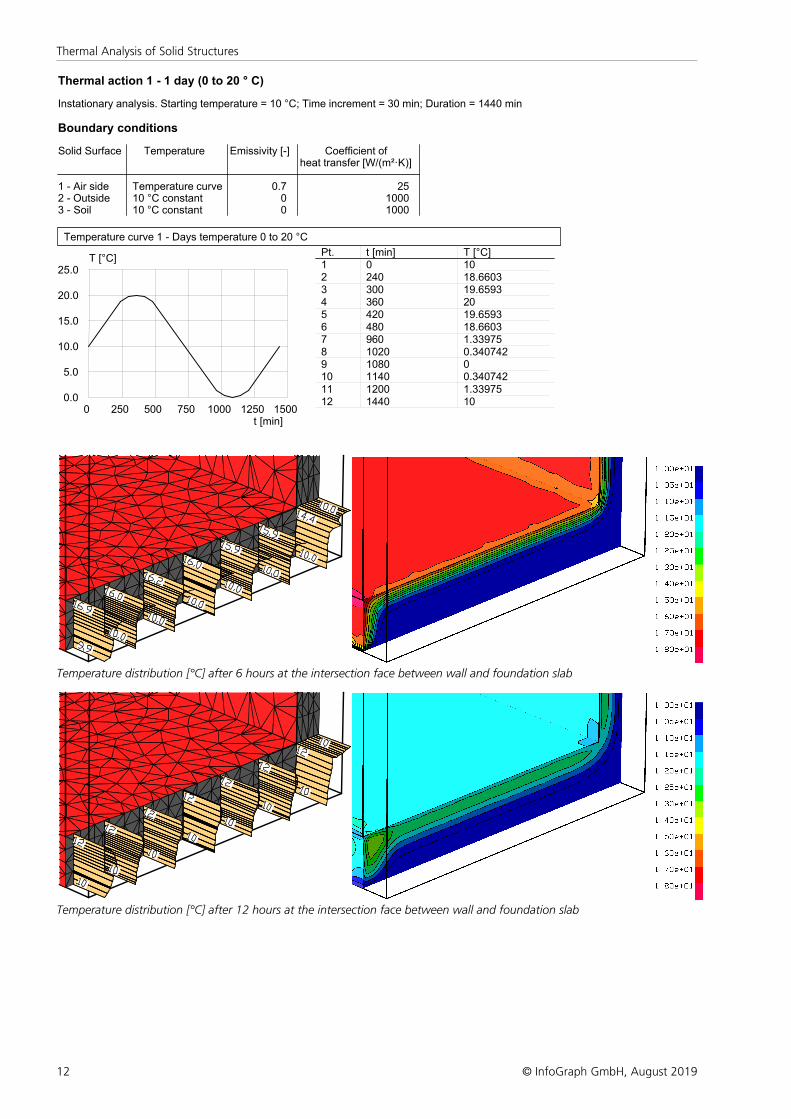
Thermal action 1 - 1 day (0 to 20 ° C)
Instationary analysis. Starting temperature = 10 °C; Time increment = 30 min; Duration = 1440 min
Boundary conditions
Solid Surface Temperature Emissivity [-] Coefficient of heat transfer [W/(m²·K)]
1 - Air side Temperature curve 0.7 25 2 - Outside 10 °C constant 0 1000 3 - Soil 10 °C constant 0 1000
Temperature curve 1 - Days temperature 0 to 20 °C
0 250 500 750 1000 1250 1500 0.0
5.0
10.0
15.0
20.0
25.0
t [min]
T [°C] Pt. t [min] T [°C] 1 0 10 2 240 18.6603 3 300 19.6593 4 360 20 5 420 19.6593 6 480 18.6603 7 960 1.33975 8 1020 0.340742 9 1080 0 10 1140 0.340742 11 1200 1.33975 12 1440 10
Temperature distribution [°C] after 6 hours at the intersection face between wall and foundation slab
Temperature distribution [°C] after 12 hours at the intersection face between wall and foundation slab
13
Examples
© InfoGraph GmbH, August 2019
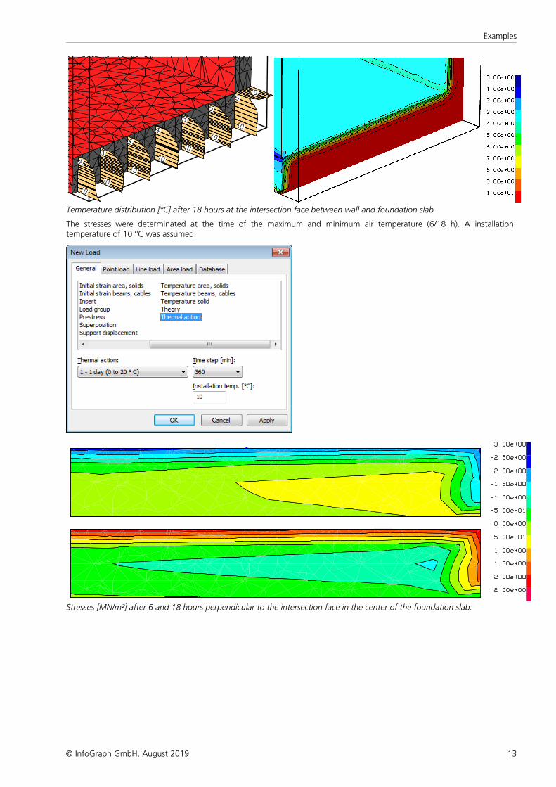
Temperature distribution [°C] after 18 hours at the intersection face between wall and foundation slab
The stresses were determinated at the time of the maximum and minimum air temperature (6/18 h). A installationtemperature of 10 °C was assumed.
Stresses [MN/m²] after 6 and 18 hours perpendicular to the intersection face in the center of the foundation slab.
14
Thermal Analysis of Solid Structures
© InfoGraph GmbH, August 2019
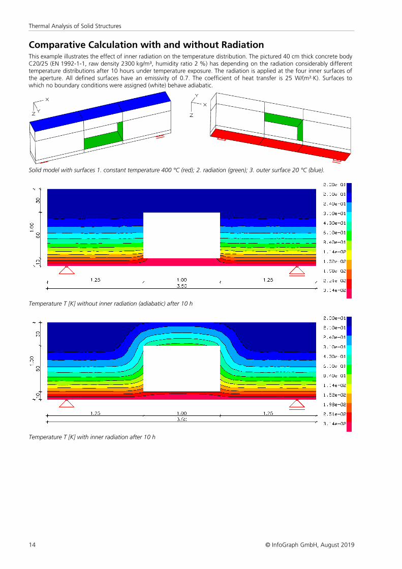
Comparative Calculation with and without RadiationThis example illustrates the effect of inner radiation on the temperature distribution. The pictured 40 cm thick concrete bodyC20/25 (EN 1992-1-1, raw density 2300 kg/m³, humidity ratio 2 %) has depending on the radiation considerably differenttemperature distributions after 10 hours under temperature exposure. The radiation is applied at the four inner surfaces ofthe aperture. All defined surfaces have an emissivity of 0.7. The coefficient of heat transfer is 25 W/(m²·K). Surfaces towhich no boundary conditions were assigned (white) behave adiabatic.
Solid model with surfaces 1. constant temperature 400 °C (red); 2. radiation (green); 3. outer surface 20 °C (blue).
Temperature T [K] without inner radiation (adiabatic) after 10 h
Temperature T [K] with inner radiation after 10 h
15
Examples
© InfoGraph GmbH, August 2019
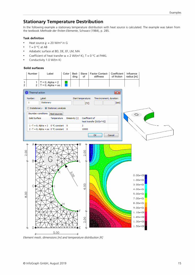
Stationary Temperature DestributionIn the following example a stationary temperature distribution with heat source is calculated. The example was taken fromthe textbook Methode der finiten Elemente, Schwarz (1984), p. 285.
Task definition
• Heat source q· = 20 W/m³ in G
• T = 0 °C at AB
• Adiabatic surface at BD, DE, EF, LM, MA
• Coefficient of heat transfer a = 2 W/(m²·K), T = 0 °C at FHIKL
• Conductivity 1.0 W/(m K)
Solid surfaces
Number Label Color Bed-ding
Slaveof
Factor Contact-stiffness
Coefficientof friction
Influenceradius [m]
1 1 T = 0; Alpha = 2 2 2 T = 0; Alpha = oo
Element mesh, dimensions [m] and temperature distribution [K]
16
Thermal Analysis of Solid Structures
© InfoGraph GmbH, August 2019
ReferencesDIN EN 1991-1-2/NA:2010-12
Nationaler Anhang – National festgelegte Parameter – (National Annex – Nationally Determined Parameters –).Eurocode 1: Einwirkungen auf Tragwerke – Teil 1-2: Allgemeine Einwirkungen - Brandeinwirkungen auf Tragwerke.(Eurocode 1: Actions on Structures – Part 1-2: General Actions – Actions on Structures exposed to Fire).Publisher: DIN Deutsches Institut für Normung e.V., Berlin. Beuth Verlag, Berlin 2010.
DIN EN 1992-1-2/NA:2010-12Nationaler Anhang – National festgelegte Parameter – (National Annex – Nationally Determined Parameters –)Eurocode 2: Bemessung und Konstruktion von Stahlbeton- und Spannbetontragwerken – Teil 1-2: Allgemeine Regeln - Tragwerksbemessung für den Brandfall.(Eurocode 2: Design of Concrete Structures – Part 1-2: General Rules – Structural Fire Design)Publisher: DIN Deutsches Institut für Normung e.V., Berlin. Beuth Verlag, Berlin 2010.
DIN EN 1993-1-2/NA:2010-12Nationaler Anhang – National festgelegte Parameter – (National Annex – Nationally Determined Parameters –)Eurocode 3: Bemessung und Konstruktion von Stahlbauten – Teil 1-2: Allgemeine Regeln - Tragwerksbemessung für den Brandfall.(Eurocode 3: Design of Steel Structures – Part 1-2: General Rules – Structural Fire Design)Publisher: DIN Deutsches Institut für Normung e.V., Berlin. Beuth Verlag, Berlin 2010.
DIN EN 1995-1-2/NA:2010-12Nationaler Anhang – National festgelegte Parameter – (National Annex – Nationally Determined Parameters –)Eurocode 5: Bemessung und Konstruktion von Holzbauten – Teil 1-2: Allgemeine Regeln - Tragwerksbemessung für den Brandfall.(Eurocode 5: Design of Timber Structures – Part 1-2: General Rules– Structural Fire Design)Publisher: DIN Deutsches Institut für Normung e.V., Berlin. Beuth Verlag, Berlin 2010.
EBA-RichtlinieAnforderungen des Brand- und Katastrophenschutzes an den Bau und den Betrieb von Eisenbahntunneln.(EBA-Guideline – Requirements of Fire and Disaster Prevention on Construction and Management of Railroads Tunnels)Publisher: Eisenbahnbundesamt. Date: 1.7.2008.
EN 1991-1-2:2010Eurocode 1: Actions on Structures – Part 1-1: General Actions – Actions on Structures exposed to Fire Publisher: CEN European Committee for Standardization, Brussels. Beuth Verlag, Berlin 2010.
EN 1992-1-2:2004/AC:2008 Eurocode 2: Design of Concrete Structures – Part 1-2: General Rules – Structural Fire DesignPublisher: CEN European Committee for Standardization, Brussels. Beuth Verlag, Berlin 2008.
EN 1993-1-2:2005/AC:2009 Eurocode 3: Design of Steel Structures – Part 1-2: General Rules – Structural Fire DesignPublisher: CEN European Committee for Standardization, Brussels. Beuth Verlag, Berlin 2009.
EN 1994-1-2:2005/AC:2008 Eurocode 4: Design of composite Steel and Concrete Structures – Part 1-2: General Rules – Structural Fire DesignPublisher: CEN European Committee for Standardization, Brussels. Beuth Verlag, Berlin 2010.
EN 1995-1-2:2010 Eurocode 5: Design of Timber Structures – Part 1-2: General Rules – Structural Fire DesignPublisher: CEN European Committee for Standardization, Brussels. Beuth Verlag, Berlin 2010.
Lienhard IV, J.H.; Lienhard V, J.H.A Heat Transfer Textbook.Phlogiston Press, Cambridge (Massachusetts) 2008.
Hosser, D. (Hrsg.)Leitfaden Ingenieurmethoden des Brandschutzes (Engineering Guide for Fire Protection),Technischer Bericht vfdb TB 04/01.Vereinigung zur Förderung des Deutschen Brandschutzes e. V. (vfdb), Altenberge 2006.
Schwarz, H. R.Methode der finiten Elemente (Method of finite elements).Teubner Studienbücher. Teubner Verlag, Stuttgart 1984.
Zehfuß, J.Bemessung von Tragsystemen mehrgeschossiger Gebäude in Stahlbauweise für realistische Brandbeanspruchung(Design of Load-Bearing Systems for Multi-Floor Buildings with Steel Construction for Realistic Fire Stress) (Dissertation).Technische Universität Braunschweig, Braunschweig 2004.
ZTV-INGZusätzliche Technische Vertragsbedingungen und Richtlinien für Ingenieurbauten, Teil 5 – Tunnelbau.(Additional Technical Contract Terms and Guidelines for Engineering Structures, Part 5 – Tunnel Construction)Publisher: Bundesanstalt für Straßenwesen (BASt). Date: 3/2012.


InfoGraph GmbH
www.infograph.eu
Kackertstrasse 10
52072 Aachen, Germany
Phone: +49 241 889980
Fax: +49 241 8899888