THERMAL CONTROL SYSTEMS FOR

LOW-TEMPERATURE HEAT REJECTION

ON A LUNAR BASE

K. R. Sridhar

Principal Investigator

and

Matthias Gottmann

Graduate Research Assistant

Department of Aerospace and Mechanical Engineering*

The University of Arizona

Tucson, AZ 85721

Semiannual Status Report

for Grant NAG5-1572

from NASA Goddard Space Flight Center

February 1 9 9 2

(NA.SA-CR-190G63) THERMAL CONTROL SYSTEMS N92-20269FOR LOW-TEMPERATURE HEAT REJECTION ON ALUNAR BASE Semiannual Status Report(Arizona Univ.) 35 p CSCL 06K Unclas

G3/54 0077032

https://ntrs.nasa.gov/search.jsp?R=19920011027 2018-05-07T09:38:59+00:00Z

Nomenclature

T — temperature

P — pressure

h — enthalpy

s — entropy

p — density

m — mass flow rate

V

Q

q

w

— volumetric flow rate

— heat load

— specific heat load

w —

compressor power

specific compressor power

COP — coefficient of performance

TI — efficiency

specific massm —

L — rejection loop pipe length

A — radiator area

H — radiator equivalent height

S — radiator array distance to lunar base

(Ty — material strength

d — inner pipe diameter

/ — pipe length

/ — friciton factor

v — fluid velocity

Be. — Reynolds number

cp — specific heat at constant pressure

fj, — dynamic viscosity

<T — Stefan Boltzmann constant

e — emissivity

M mass

PRECEDING PAGE BUNK NOT FILMED

1 Introduction

One of the important issues in the lunar base architecture is the design of a Thermal Control

System (TCS) to reject the low-temperature heat from the base. The TCS ensures that

the base and all the components inside are maintained within the operating temperature

range. The temperature of the lunar surface peaks to 400K during the 336 hour lunar day

and heat rejection from the base under such conditions is a technically challenging task.

Prior studies have shown that the overall mass of a TCS and its power supply for lunar

base applications can be significant. The single largest fraction of the overall mission cost

for any space mission is associated with the initial launch, which continues to be in the

vicinity of $ 5000/lb from Earth to LEO. The reduction of lift mass at launch is a key driver

in reducing the overall cost of space missions. In order to find the lowest mass for the TCS,

several options have been proposed. One option would be to store the waste heat deep in

lunar regolith [1]. A piping system working as a heat exchanger has to be buried in the soil.

The technical difficulties and uncertainties associated with large scale excavation on the

Moon, and lack of knowledge about the thermal properties of lunar regolith are primary

reasons for not pursuing this path presently. A significant portion of the total mass of

the TCS is due to the radiator. In order to reduce the mass of the radiator, the concept

of shaded light-weight radiators have been proposed [2]. Shading the radiator from the

sun and the hot lunar soil could decrease the radiator operating temperature significantly.

This technology requires shades built of specular surfaces. The degradation of the radiator

Lcool ^reject

Figure 1: Schematic Diagram of a TCS using a Heat Pump

surface properties with age in a lunar environment is not known. At least for the initial

cases, the prudent approach would be to employ systems that rely on proven technology.

The concept of using a heat pump fits this bill. In this concept, energy in the form of

heat or work, is supplied to the heat pump which collects heat from the low-temperature

source (the lunar base) and delivers it at a higher temperature to the radiator. The mass

of the radiator dissipating the high temperature heat would be significantly lower than

one operating without a temperature lift. A simplified block diagram of this concept is

illustrated in figure 1.

Heat pumps have been in use for terrestrial applications for a long time. Refrigeration

devices utilizing a thermodynamic cycle are essentially heat pumps. A vapor compression

cycle involving two constant pressure and two adiabatic processes is the most widely used.

It is also called a Rankine cycle and requires shaft work. Absorption cycles on the other

hand are heat driven and do not require high quality shaft power. The Stirling cycle consists

of two isothermal and two constant volume processes and promises a better efficiency than

the Rankine cycle. Theoretically, it reaches the same efficiency as the optimal Carnot cycle

but the processes are technically difficult to realize. Today, Stirling cycle coolers are used

in cryogenic applications. Experiments using this cycle for residential heat pumps show

promising results [3],[4], but but these heat pumps are yet to become technically reliable.

To optimize the mass of the heat pump augmented TCS, all promising options have

to be evaluated and compared. During these preliminary comparison studies, considerable

care is given to optimizing system operating parameters, working fluids and component

masses. However, to keep this preliminary study simple and concise, the following aspects

are not considered presently. The systems are modeled for full load operation and the im-

plications and power penalties at off-design and partial load conditions are not considered.

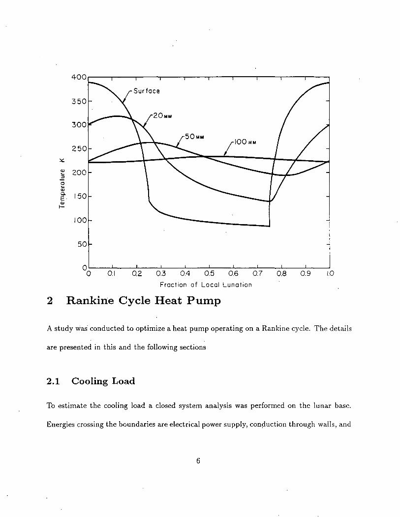
However, it is realized that the surface temperature of the lunar regolith varies consider-

ably during the lunar day as shown in figure 2 . This -variation in the regolith temperature

would indicate that the temperature lift and the load of the heat pump would vary as

a function of the time of the day. For this reason, the performance of the heat pump

at partial load conditions is important and will be studied in detail in the future. Also,

redundancy requirements are not considered presently. While evaluating system mass, the

control components are not accounted for since the variation in their masses for the various

cycles and working fluids would not be large. Issues such as these will be studied in detail

during the design of the actual system.

0. 0.2 0.3 0.4 0.5 0.6 0.7

Fraction of Local Lunation

0.8 0.9 1.0

2 Rankine Cycle Heat Pump

A study was conducted to optimize a heat pump operating on a Rankine cycle. The details

are presented in this and the following sections

2.1 Cooling Load

To estimate the cooling load a closed system analysis was performed on the lunar base.

Energies crossing the boundaries are electrical power supply, conduction through walls, and

heat removed by the acquisition loop. Within the system, heat generation can occur due

to human metabolic activity. The electrical power input for a first stage base is estimated

to be between 50 and 100 kW, more likely lOOkW ([1],[6], [7]). The conduction through the

walls depends on the insulation. Without significant mass penalties it is possible to reduce

heat gains or losses to a very small fraction of the electrical input, hence it is neglected.

Based on food consumption, a crew member produces an average of about 150W. For a

crew of six to eight members, the total heat generation would again be negligible, compared

to the electrical input. Therefore, the cooling load (the heat removed by the acquisition

loop) can be equated to the electrical input into the base. Stated differently, this implies

that all electrical input will finally be dissipated as heat. The value for the cooling load is

fixed at lOOkW for this study. When further details about the design and activities of the

base are known, these assumptions can be revisited and refined if necessary.

2.2 The Acquisition Loop

The acquisition loop collects the excess heat from the lunar base and transports it to the

heat pump. The acquisition loop consists of cold plates and a network of connecting pipes.

The heat is transported by a single phase fluid. Since the coolant in the acquisition loop

circulates in the habitation module nontoxicity is a necessity from safety considerations.

Water with certain trace additives to depress its freezing point would be a good candidate.

For this study, it was decided that one cooling loop operating at a single pre-designed

temperature would be used. This temperature was chosen to be 275K (the lower of the

two Space Station cooling loop temperatures). The variation in the temperature of the

coolant has to be small enough to provide isothermal cooling for small variations in the

load, yet large enough to keep the coolant flow rate within reasonable limits. The mass

flow rate in the acquisition loop is m = <5cooi/(cpAT). If water with trace additives were

used as the coolant and the temperature variation in the acquisition loop were taken to be

5K, the mass flow rate in the acquisition loop would be 4.8kg/s.

2.3 The Heat Pump

Two different heat pump setups were studied: In the first setup termed Case A the heat

pump is directly connected to the rejection loop. In this case the condenser of the heat

pump and the radiator are essentially the same device. The refrigerant circulating in the

heat pump condenses and rejects heat in the radiator. An alternative setup is to decouple

the heat pump and the rejection loop with a heat exchanger (Case B). Detailed analysis

of the two cases and their pros and cons will be discussed in the following sections.

2.4 Heat Pump Connected Directly to the Rejection Loop (Case A)

A simplified schematic of a heat pump configuration directly connected to the rejection

loop is illustrated in figure 3 The main parameters of interest in the design of a heat

8

Heat Pumpi :iiii

AcquisitionLoop 1

0 i@T ,'^cool^ cool1

1

1

1

\

t

-> N^l-Ix-x]1*Throttle

F

i

HeatExchanger

i

r^H

7 ~i41 11

1ii

12 I V

Radiator

^Q • @T •^ reject^ reject

^ | W

, Compressor |

1

Figure 3: Schematic Diagram of a Heat Pump directly connected to the Rejection Loop

pump used for cooling are the input heat load (Qcoo[) and its temperature (Tjow), the

temperature lift, and the coefficient of performance (COP}. The COP of a heat pump is

defined as

QcoolCOP =W

where W is the power consumed by the heat pump.

2.4.1 The Compressor

Figure 4 illustrates the Rankine cycle process in a pressure-enthalpy diagram. The working

fluid in the vapor state is compressed from P\ to P^. Ideally this process would be isentropic

(2S). Due to irreversibilities, the process is nonisentropic

"'ideal =

COJ-,

wCO

0.0 500.0 1000.0 1500.0

Enthalpy [kJ/kg]2000.0 2500.0

Figure 4: P - h Diagram of a Rankine Cycle for R717 (Tlow = 270K, Thigh = 360K)

where: P is the pressure, h is the specific enthalpy and the subscripts refer to the states

in figure 4. It is assumed that the compression would be performed in a single stage,

in order to limit the number of free parameters. Customarily airplane cooling systems

utilize multistage compression [8], but there is no intercooling between the stages. Hence,

effectively the compression can be modeled as a single stage process. The properties of

the refrigerant used for the calculation are obtained from [9] and a FORTRAN?? code

developed in-house [10]. Deviation from the ideal behavior in the compression occur due

to mechanical, electrical (motor), and electronic (controller) inefficiencies, and fluid friction.

The values for the efficiencies in state-of-the-art aircraft cooling equipment were obtained

10

from [11], and are as follows: 7;mech = 0.95, Electrical = °-94> ^electronic = 0.91,and

''fluid = 0-75. The overall efficiency of such a compressor would be the product of all

four efficiencies, about 61 percent in this case. The excess energy supplied to overcome

these inefficiencies will be converted to heat. Since the compressor would operate in a

high vacuum environment, radiation to the environment and convection of the heat by

the vapor flow inside are the only heat rejection mechanisms. An upper limit for the

amount of heat rejected by radiation can be obtained by modeling the compressor as a

black cube, 0.25m side, at 400K. Both, the surface properties and the temperature of the

surface are deliberately chosen to be well above the actual values to obtain a conservative

estimate . This heat is small compared to the compressor input power and can be neglected.

Therefore, it can be assumed that all the energy supplied to the compressor will be used

to compress and heat the refrigerant. It should be noted that the temperature of the

compressor can be maintained within operating limits by the use of a cold plate. However

this would not be required since the working fluid could convectively remove the excess

heat from the compressor.

The next step is a mass estimate for the compressor. In aircraft cooling, the compressor

mass is assumed to be proportional to the cooling load. One pound (0.454kg) per kilowatt

is the value suggested [11]. Our mass optimization is performed at maximum cooling load

(lOOkW) and this value remains unchanged in the optimization. The heat pump output

temperature and hence the total heat rejected by the heat pump is varied. Since the

11

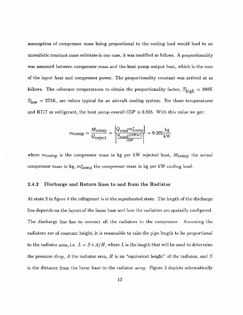
assumption of compressor mass being proportional to the cooling load would lead to an

unrealistic constant mass estimate in our case, it was modified as follows. A proportionality

was assumed between compressor mass and the heat pump output heat, which is the sum

of the input heat and compressor power. The proportionality constant was arrived at as

follows. The reference temperatures to obtain the proportionality factor, T^igh = 380K

Tjow = 275K, are values typical for an aircraft cooling system. For these temperatures

and R717 as refrigerant, the heat pump overall COP is 0.805. With this value we get:

= 0.202^reject

COPkW

where mcomp is the compressor mass in kg per kW rejected heat, Mcomp the actual

compressor mass in kg, mcomp the compressor mass in kg per kW cooling load.

2.4.2 Discharge and Return lines to and from the Radiator

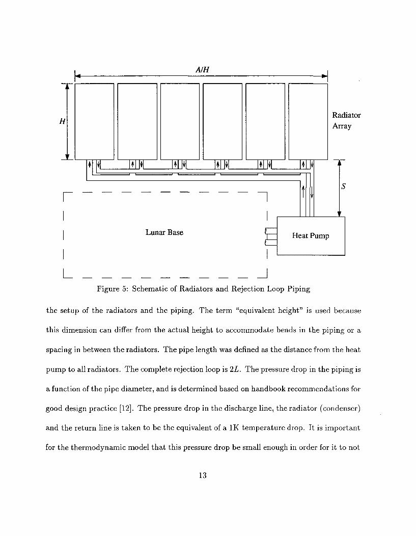
At state 2 in figure 4 the refrigerant is in the superheated state. The length of the discharge

line depends on the layout of the lunar base and how the radiators are spatially configured.

The discharge line has to connect all the radiators to the compressor. Assuming the

radiators are of constant height, it is reasonable to take the pipe length to be proportional

to the radiator area, i.e. L — S + A/H, where L is the length that will be used to determine

the pressure drop, A the radiator area, H is an "equivalent height" of the radiator, and S

is the distance from the lunar base to the radiator array. Figure 5 depicts schematically

12

H

AIM

ED*

r ~i

Lunar Base

Radiator

Array

Heat Pump

I I

Figure 5: Schematic of Radiators and Rejection Loop Piping

the setup of the radiators and the piping. The term "equivalent height" is used because

this dimension can differ from the actual height to accommodate bends in the piping or a

spacing in between the radiators. The pipe length was defined as the distance from the heat

pump to all radiators. The complete rejection loop is 2L. The pressure drop in the piping is

a function of the pipe diameter, and is determined based on handbook recommendations for

good design practice [12]. The pressure drop in the discharge line, the radiator (condenser)

and the return line is taken to be the equivalent of a IK temperature drop. It is important

for the thermodynamic model that this pressure drop be small enough in order for it to not

13

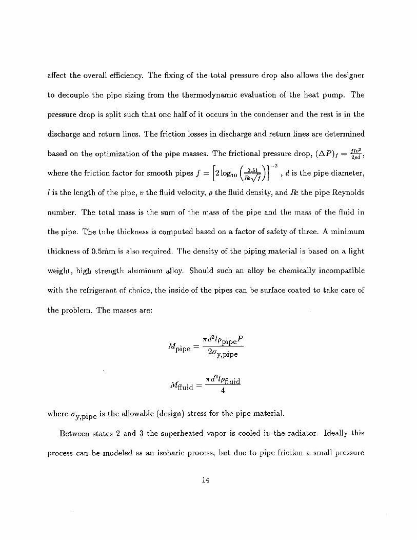
affect the overall efficiency. The fixing of the total pressure drop also allows the designer

to decouple the pipe sizing from the thermodynamic evaluation of the heat pump. The

pressure drop is split such that one half of it occurs in the condenser and the rest is in the

discharge and return lines. The friction losses in discharge and return lines are determined

based on the optimization of the pipe masses. The frictional pressure drop, (AP)/ = jj,

where the friction factor for smooth pipes / = 21og10 I 2 '5V-) , d is the pipe diameter,L \ f tv'/J

/ is the length of the pipe, v the fluid velocity, p the fluid density, and Be. the pipe Reynolds

number. The total mass is the sum of the mass of the pipe and the mass of the fluid in

the pipe. The tube thickness is computed based on a factor of safety of three. A minimum

thickness of 0.5mm is also required. The density of the piping material is based on a light

weight, high strength aluminum alloy. Should such an alloy be chemically incompatible

with the refrigerant of choice, the inside of the pipes can be surface coated to take care of

the problem. The masses are:

'pipe - 2(T •zcry,pipe

Mfluid = *±

where cry nine is the allowable (design) stress for the pipe material.

Between states 2 and 3 the superheated vapor is cooled in the radiator. Ideally this

process can be modeled as an isobaric process, but due to pipe friction a small pressure

14

drop would occur. Between states 3 and 4, the refrigerant is condensed to saturated liquid.

A finite pressure drop occurs in the condenser. The mass estimate for the condenser will be

discussed in the radiator section. The heat to be rejected by the radiator, <?reject = h-^ — h^.

From state 4 the saturated liquid is sent from the radiator to the throttle valve located at

the evaporator inlet, through the return line. The sizing of the return line is based on the

same guidelines described for the discharge line.

2.4.3 Evaporator and Throttle Valve

Between states 4 and 5 the fluid is adiabatically throttled. The mass of the throttle valve

is negligible compared to the mass of the other components of the heat pump. Between

states 5 and 1, the refrigerant absorbs heat from the primary coolant circulating in the

lunar base. The temperature difference between the primary coolant in the acquisition loop

and the boiling refrigerant in the evaporator is 5K. The heat removed, <?coo} = hi — h5.

The mass of the evaporator is obtained based on a suggested value of 2.72kg/kW [1].

2.4.4 Refrigerant

One of the important issues is the choice of refrigerant as the working medium for the

Rankine cycle. The refrigerants that are commonly used in terrestrial and aerospace ap-

plications, Rll, R12, R113, R114, and R717, were considered [8]. R113 and R114 were

eliminated from the list of potential refrigerants due to the possibility of condensation of

15

30.0 100.0 170.0

Enthalpy [kJ/kg]240.0 310.0

Figure 6: Rankine Cycle for R114. Tlow = 270K, Thigh = 360K

the vapor in the compressor (figure 6). Such condensation would be detrimental to the life

of the compressor. Among the remaining refrigerants, the selection was narrowed down

to Rll and R717, because R12 has a lower COP and a lower critical temperature (R717:

rcrit = 407K> R11: rcrit = 474K> R12: Tcrit = 385K)- The P - /i diagrams for R717 and

Rll are shown in figures 4 and 7 respectively. Safety considerations give an edge to Rll

due to its nontoxicity and noninflamability, but R717 offers lower overall system mass. The

thermodynamic properties of the refrigerants were obtained using the analytical functions

suggested in [9]. The COP can be expressed in terms of the specific enthalpies and for the

Rankine cycle:

COP =— h5

16

<DSH

3COOT 7(U O*-. ^

OU

0.0 70.0 140.0 210.0 280.0 350.0

Enthalpy [kJ/kg]Figure 7: Rankine Cycle for Rll. Tlow = 270K, Th[gh = 360K

Table 1 illustrates the COP calculation for a condenser temperature of T^^gh = 380K. The

overall COP was computed as a function of the condenser temperature and is plotted in

figure 8.

2.4.5 Implementation of Heat Pump and Piping Model

Values for COP and the mass of the piping were computed and tabulated for varying

rejection temperature using the models presented above. These tabulated values were

imported into the spreadsheet and linearly interpolated where necessary.

17

Refrigerant: R717state

12345

T[K]270626380380270

P[MPa]0.381

7.277.147.14

0.381

h[kj/kg]

158424191541893893

[kJ/kg]6.0466.6154.7883.0803.483

[kg/m3]3.08824.89

67.2436.56.725

COP = 0.829

Refrigerant: Rllstate

12345

T[K]270448380380270

P[MPa]0.0350.9640.9450.9450.035

h[kJ/kg]

249350301158158

[kJ/kg]0.9581

1.0510.93430.55650.6180

[kg/m3]2.1839.249.712554.22

COP = 0.914

Table 1: Properties in the Refrigeration Cycle for = 380K

2.5 Heat Pump Decoupled from the Rejection Loop with a

Heat Exchanger (Case B)

Connecting the heat pump directly to the radiator has inherent disadvantages. If the

refrigerant used in the Rankine cycle is not suitable for a heat transport loop, it can be

advantageous to separate the rejection loop from the heat pump with a heat exchanger.

This configuration of a heat pump augmented TCS is shown in figure 9. From a system

design perspective it is desirable to decouple subsystems that carry out different tasks.

The decoupled case would provide for better and simpler control of the TCS during partial

18

RefrigerantD=R110=R12V=R717

330.0 400.0

Figure 8: Variation of COP with Thi h = 270K of Rll, R12, and R717. Tlow = 270K

HeatPump _ _ _ _ _ _ _ _ Pump

AcquisitionLoop

Qcool@Tcool,

Throttle

HeatExchanger

HeatExchanger

Radiator

reject^- reject

Compressor |

I

Figure 9: Schematic Diagram of a Heat Pump decoupled from the Rejection Loop

load conditions. On the other hand, a heat exchanger between the two loops will cause a

temperature drop between the heat pump and the rejection loop and an associated mass

penalty. To compensate for the temperature drop the heat pump has to deliver the output

heat at a higher temperature and therefore operate at a lower COP. If the same fluid were

19

used in the Rankine cycle and in the rejection loop, the only foreseeable advantage of the

decoupled system would be the possibility of better and simpler control. However, other

advantages could emerge if two different fluids were used.

The thermodynamic and mass models for the heat pump with an output heat exchanger

(Case B) differs only in few aspects from the models presented for Case A (section 2.4).

Only these differences will be discussed in this section.

2.5.1 Condenser

In case B the condenser is a heat exchanger that decouples the rejection loop from the

heat pump. Both fluids undergo phase change in this heat exchanger. For a mass estimate

the value quoted in [1], 2.72 kg/kW was used. The thermodynamic performance of the

condenser is characterized by a pressure drop in each loop (heat pump and rejection loop)

and a temperature difference between both sides. Similar to the acquisition side, the

temperature difference is set to 5K. Consistent with case A, the pressure drop has to be

small enough, not to affect the heat pump performance. A pressure drop equivalent to IK

temperature drop has been assigned to the condenser.

2.5.2 Rankine Cycle Analysis

The cycle evaluation follows the same path outlined for Case A. The efficiencies and pres-

sure drops of the heat pump components are also the same as in Case A. The COP as a

20

(a)

Symbols:A R717-modelO Rll-model

R717-real fluid

(b)

320.0 340.0 360.0 380.0 320.0 340.0

' h i g h [K] h i g h

360.0

[K]380.0

Figure 10: Comparison of COP from Cycle Analysis and Approximation for Rll and R717.^evaporator = 270K

function of the output temperature Tnign was computed with a FORTRAN?? program

using real fluid properties from [9]. The implementation of this COP(T} into the spread-

sheet was realized with an approximate analytical function. For each refrigerant a fourth

order polynomial was fitted to the data computed with the FORTRAN?? code. The re-

sulting approximation yields an error of less then 0.3 percent for output temperatures from

^hieh = 320K to Tnjgn = 390K. Figures lOa and lOb show a comparison between the real

fluid model and the polynomial approximation. It can be seen that the results are almost

identical.

2.5.3 Rejection Loop

The decoupled rejection loop would require a pump to circulate the coolant fluid. This

pump and the power penalty associated with it have to be incorporated in the mass estimate

21

and optimization. The pump mass is estimated using a formula quoted by Dexter and

Haskin [13]/ . \ 0.75

Mpump = 5.61

where: m is the mass flow rate in Ib/hr, p is the density of the fluid in lb/ft3. The power

required for a liquid pump can be readily computed from

WpumpAPV

7/pump

where AP is the pressure differential across the pump, V the volume flow rate, and ?/pump

the pump efficiency. A conservative 7/pump = 0.25 as suggested by [13] was used. The

pressure drop was determined with the formulas presented for case A. The pipe thickness is

again determined based on the hoop stress or 0.5mm, whichever is larger. Masses included

in the estimate are due to pipes, coolant, pump, and the power supply. The decoupled

rejection loop does not affect the heat pump COP. The minimum mass for the loop may be

achieved by balancing pipe mass and the power penalty. This approach results in optimum

mass when the pipe diameters are relatively small and the pressure drop is large. However,

a large pressure drop in the vapor line would result in a large temperature drop and this is

accompanied by an increase in the radiator area and mass. While the pressure drop in the

liquid line can be compensated with the pump, if the pressure drop gets large, the pumping

power will become significant and add to the total heat rejection load.. Therefore, the mass

22

estimate for the piping has to be computed based on a limited pressure drop. Here again,

the pressure drop is specified in terms of an equivalent temperature drop and is set to 0.5K

in the vapor and l.OK in the liquid line. These values are chosen based on recommended

design practice [12]. The cooling fluid of choice is ammonia, which already demonstrated

its good performance as a heat transport fluid in Case A. The toxicity of ammonia will not

be a concern for the rejection loop as it is outside the habitation modules.

In Case A the piping mass was determined together with the heat pump estimate be-

cause they are coupled. Assuming values for the radiator height and distance from the base,

Case A yielded a model where the piping mass depends solely on the rejection temperature.

For Case B a model that makes use of the decoupling of heat pump characteristics and

the rejection loop was sought. For a given refrigerant and specified pressure drops in the

liquid and vapor lines, the rejection loop mass depends on three parameters: rejection heat

load Q reiect> rejection temperature Tre:ect, and pipe length L. Using the thermodynamic

properties from [9] the mass model was implemented into a FORTRAN?? code. Figures

11 and 12 show results obtained with the code. For use with a spreadsheet software it is

desirable to obtain an analytical expression for the mass. This was realized with a polyno-

mial which is second order in temperature, second order in length and linear in rejection

heat load:

^pipingi=0 j=0 k=0

The coefficients were determined with a least square error fit. The approximation is valid

23

oao~n QLkWJ.LIml

D= 150. lOT)O=150, 200A=250 , 100

= 250, 200

T[K],L[mlD = 340, 1000 = 340, 200A = 380, 100

= 380, 200

0 = 340, 250A = 380, 150

340.CB50.0 360.0 370.0 380.0 150.0175.0 300.0 225.0 350.0 100.0135.0 150.0 175.0 300.0

T [K] Q . , [kW] L , , [m]r e j ec t L -1 ^ re jec t L J r e j e c t L J

Figure 11: Mass of the Liquid Piping

in the following range: 340K < Treject < 380K, 150kW < Qreject < 250kW, and 100m <

L < 400m. The maximum error of the approximation is three percent.

2.6 Radiator Considerations

The function of the radiator is to reject the waste heat from the base. The heat rejected

by the radiator is given by Q — Acr)O'(T^ • . — T*- i ) where f. is the emissivity, 77 the

fin efficiency, TTe:ec^ and Tgj^ the radiator and sink temperatures. The estimated sink

temperature for a vertically mounted radiator at the lunar base is 32IK [6]. Most reviewed

sources suggest e = 0.8, and 77 = 0.7. Several estimates for the mass of a radiator are avail-

able in the literature ([1],[6],[14],[15]). The mass of a radiator is taken to be proportional

to its area and recent publications recommend a value of 5kg/m2 for a one sided radiator.

The vertical radiator is two sided and hence a mass estimate of 2.5kg/m2 is assumed. The

24

--D=15t). 100=150, 200

= 250, 100V=250 , 200

T[K],L[mlD = 340, 1000 = 340, 200A = 380, 100

T[K],Q[kW]D = 3T40, 150O = 340, 250

= 380, 150

340.0350.0 360.0 370.0 380.0 150.0175.0 300.0 325.0 350.0 100.0135.0 150.0 175.0 300.0

T r e j ec t M Q r c j c c t [kW] L r e ] ec t [m]

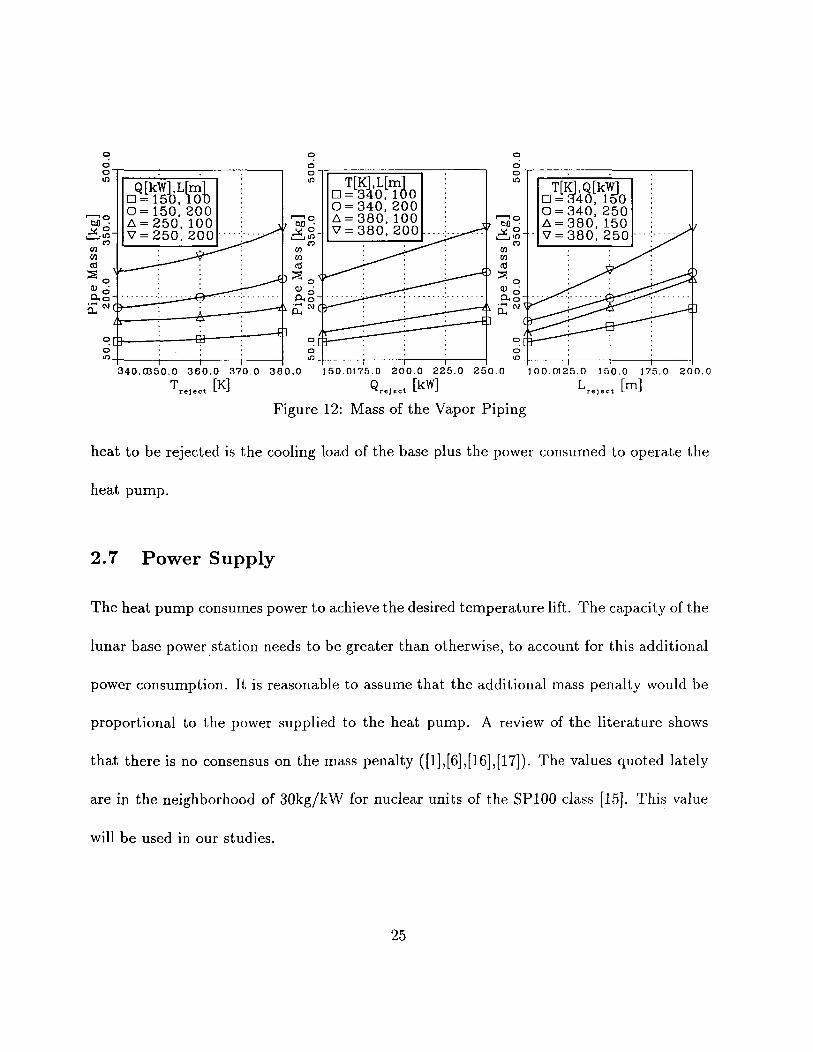
Figure 12: Mass of the Vapor Piping

heat to be rejected is the cooling load of the base plus the power consumed to operate the

heat pump.

2.7 Power Supply

The heat pump consumes power to achieve the desired temperature lift. The capacity of the

lunar base power station needs to be greater than otherwise, to account for this additional

power consumption. It is reasonable to assume that the additional mass penalty would be

proportional to the power supplied to the heat pump. A review of the literature shows

that there is no consensus on the mass penalty ([1],[6],[16],[17]). The values quoted lately

are in the neighborhood of 30kg/kW for nuclear units of the SP100 class [15]. This value

will be used in our studies.

25

3 Results

The overall mass optimization was performed in a spreadsheet. The heat pump output

temperature lift and hence the radiator temperature was varied and the variation of the

masses of the components and the TCS were computed using the mass models described

here. For the coupled TCS configuration, Case A, the analysis were performed for two

working fluids, Rll and R717 and the overall TCS mass variation as a function of radiator

temperature is shown in figure 13a. Similar analysis were performed for a the decoupled

configuration, Case B, and the results are shown in figure 13b. For Case B, Rll and R717

were used as working fluids for the heat pump, but R717 was used in the rejection loop

due to to its superior heat transport characteristics.

When Rll is used as the working fluid for the heat pump, the optimal TCS mass is

6108kg at a radiator temperature of 371K for the coupled situation, Case A. For Case B,

the optimal TCS mass is 5940kg at a radiator temperature of 362K. The radiator mass

in Case B is higher than for Case A due to its lower operating temperature. Also, the

presence of the heat exchanger between the heat pump and the rejection loop adds extra

mass to the Case B scenario. In spite of these mass penalties the optimal TCS system

mass for Case B is lower than that for Case A. This is due to the huge reduction in the

rejection loop piping mass for Case B. When R717 is used as the working fluid in the heat

pump, the optimal mass of the TCS is 5515kg at a radiator temperature of 362K for Case

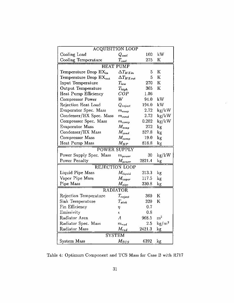
A. For Case B the corresponding values are 6392kg and 360K respectively. It is obvious

26

that Case B is more massive than Case A since the radiator temperature for Case B is

lower and also it has an additional heat exchanger.

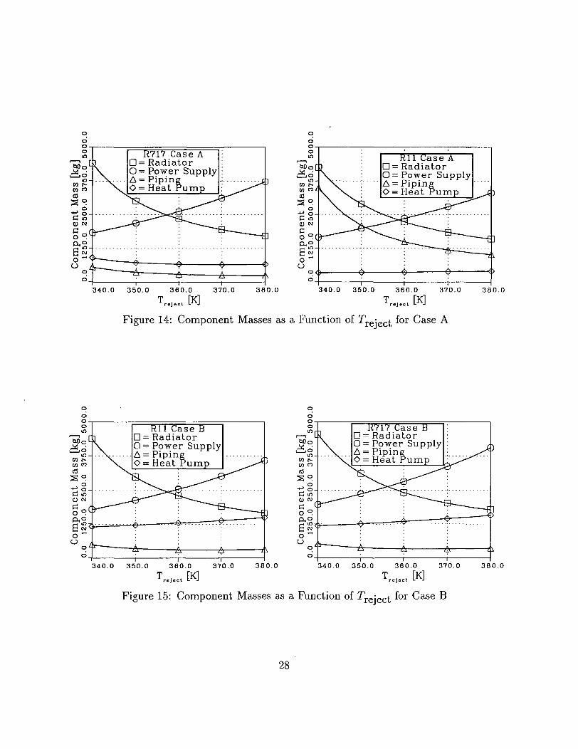
The mass of the individual components for Cases A and B are shown graphically in

figures 14 and 15 for a range of radiator temperatures and is listed in tables 2-5 for the

optimal radiator temperatures.

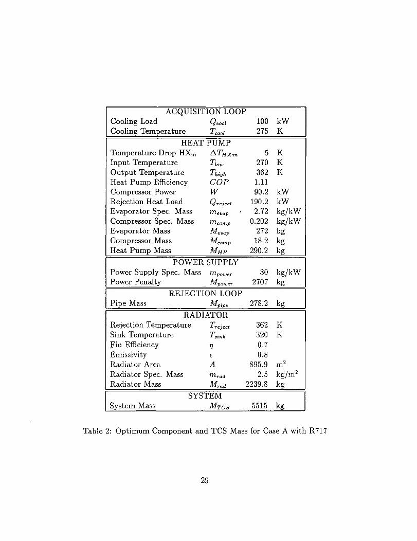
Among the cases considered R717 coupled TCS configuration offers the least mass of

5515kg. The best decoupled configuration would involve Rll as the working fluid for the

heat pump and R717 as the working fluid for the rejection loop. The optimal mass for this

configuration, as stated earlier, is 5940kg. In spite of the additional mass, the decoupled

system may offer the advantage of simpler and more reliable system control during partial

load operation. This issue will be examined in detail in the future.

°b °.

340.0 350.0 360.0 370.0

T . t [K]re ject L -I

380.0 340.0 350.0 360.0 370.0

T . [K]reject L -1

380.0

Figure 13: Overall TCS Mass as a Function of

27

R717 CaseD= RadiatorO= Power SupplyA= PipingO= Heat Pump

340.0 380.0

r e j e c

Rll Case AD= Radiator

= Power SupplyA = PipingO = Heat Pump

340.0 350.0 360.0 370.0 380.0

T , [K]re jec t L J

Figure 14: Component Masses as a Function of for Case A

Rll Case BD- RadiatorO= Power SupplyA= PipingO= Heat Pump

340.0 350.0 360.0 370.0 380.0

R717 CaseD= RadiatorO= Power SupplyA= PipingO= Heat Pump

340.0 350.0 360.0 370.0

Tr.,..t M

380.0

Figure 15: Component Masses as a Function of f°r Case B

28

ACQUISITION LOOPCooling Load QcooiCooling Temperature Tcooi

HEAT PUMPTemperature Drop HXin AT//xinInput Temperature TIOW

Output Temperature ThighHeat Pump Efficiency COPCompressor Power WRejection Heat Load QrejectEvaporator Spec. Mass mevap

Compressor Spec. Mass rncomp

Evaporator Mass Mevap

Compressor Mass Mcomp

Heat Pump Mass MHPPOWER SUPPLY

Power Supply Spec. Mass rnpower

Power Penalty Mpower

REJECTION LOOPPipe Mass Mpipe

RADIATORRejection Temperature Treject

Sink Temperature TsinkFin Efficiency TJEmissivity tRadiator Area ARadiator Spec. Mass rnrad

100275

52703621.1190.2

190.22.72

0.20227218.2

290.2

302707

278.2

3623200.70.8

895.92.5

Radiator Mass Mrad 2239.8SYSTEM

System Mass MTCS 5515

kWK

KKK

kWkWkg/kWkg/kWkgkgkg

kg/kWkg

kg

KK

m2

kg/m2

kg

kg

Table 2: Optimum Component and TCS Mass for Case A with R717

29

ACQUISITION LOOPCooling Load QcooiCooling Temperature Tcoo/

HEAT PUMPTemperature Drop HX;n AT//x.'nInput Temperature T\ow

Output Temperature ThighHeat Pump Efficiency COPCompressor Power WRejection Heat Load QrejectEvaporator Spec. Mass mevapCompressor Spec. Mass mcomp

Evaporator Mass Mevap

Compressor Mass Mcomp

Heat Pump Mass MJJPPOWER SUPPLY

Power Supply Spec. Mass mpower

Power Penalty Mpower

REJECTION LOOPPipe Mass Mpipe

RADIATORRejection Temperature Treject

Sink Temperature TSmfcFin Efficiency ?/Emissivity eRadiator Area ARadiator Spec. Mass rnradRadiator Mass MTad

SYSTEMSystem Mass MTCS

100275

5270371

1.0694.5

194.52.72

0.20227219.1

291.1

302836

1170.5

3713200.70.8

724.22.5

1810.5

6108

kWK

KKK

kWkWkg/kWkg/kWkgkgkg

kg/kWkg

kg

KK

m2

kg/m2

kg

kg

Table 3: Optimum Component and TCS Mass for Case A with Rll

30

ACQUISITION LOOPCooling Load QcoolCooling Temperature Tcooi

HEAT PUMPTemperature Drop HX;n AT#jf,-n

Temperature Drop HXout ^TjjxoutInput Temperature T/otu

Output Temperature ThighHeat Pump Efficiency COPCompressor Power WRejection Heat Load QrejectEvaporator Spec. Mass mevapCondenser/HX Spec. Mass mcondCompressor Spec. Mass rncomp

Evaporator Mass Mevap

Condenser/HX Mass McondCompressor Mass Mcomp

Heat Pump Mass MHP

POWER SUPPLYPower Supply Spec. Mass mpower

Power Penalty MpoweT

REJECTION LOOPLiquid Pipe Mass MnquidVapor Pipe Mass MvapOT

Pipe Mass Mpipe

RADIATORRejection Temperature Treject

Sink Temperature TsinkFin Efficiency 77Emissivity cRadiator Area ARadiator Spec. Mass rnTadRadiator Mass Mrad

SYSTEMSystem Mass MTCS

100275

55

2703651.0694.0

194.02.722.72

0.202272

527.819.0

818.8

302821.4

213.3117.5330.8

3603200.70.8

968.52.5

2421.3

6392

kWK

KKKK

kWkWkg/kWkg/kWkg/kWkgkgkgkg

kg/kWkg

kgkgkg

KK

m2

kg/m2

kg

kg

Table 4: Optimum Component and TCS Mass for Case B with R717

31

ACQUISITION LOOPCooling Load QcoolCooling Temperature Tcoo\

HEAT PUMPTemperature Drop HX;n ATj/xinTemperature Drop HXout . ATuxoutInput Temperature T\ow

Output Temperature ThighHeat Pump Efficiency COPCompressor Power WRejection Heat Load QrejectEvaporator Spec. Mass rnevap

Condenser/HX Spec. Mass mcondCompressor Spec. Mass rncomp

Evaporator Mass Mevap

Condenser/HX Mass McondCompressor Mass Mcomp

Heat Pump Mass MHP

POWER SUPPLYPower Supply Spec. Mass mpower

Power Penalty Mpower

REJECTION LOOPLiquid Pipe Mass MnquidVapor Pipe Mass Mvapor

Pipe Mass Afp,pe

RADIATORRejection Temperature Treject

Sink Temperature TsinkFin Efficiency rjEmissivity (.Radiator Area ARadiator Spec. Mass rnradRadiator Mass Mrad

SYSTEMSystem Mass MTCS

100275

55

2703671.1487.7

187.72.722.72

0.202272

510.617.7

800.3

302631.3

193.5104.8298.3

3623200.70.8

884.22.5

2210.4

5940

kWK

KKKK

kWkWkg/kWkg/kWkg/kW

kgkgkgkg

kg/kWkg

kgkgkg

KK

m2

kg/m2

kg

kg

Table 5: Optimum Component and TCS Mass for Case B with Rll

32

References

[1] Swanson, T. D., Radermacher, R., Costello, F. A., Moore, J. S., and Mengers, D. R.,

"Low-temperature thermal control for a lunar base", %(fh Intersociety Conference on

Environmental Systems, Williamsburg, Virginia, July 9-12, 1990, Publication SP-831,

pp. 39-53, SAE Paper No. 901242.

[2] Costello, F. A., and Swanson., T. D., "Lunar radiators with specular reflectors",

AIAA/ASME Thermophysics and Heat Transfer Conference, Seattle, Washington,

June 18-20, 1990, ASME Publication HTD-Vol. 135, pp. 145-150.

[3] Penswick, B., and Urieli, I., "Duplex Stirling machines", 19th Intersociety Energy

Conversion Engineering Conference, San Francisco, California, August 19-24, 1984,

pp. 1823-1828, SAE Paper No. 849045.

[4] Chen, F. C., Keshock, E. G., and Murphy, R. W., "Testing of a Stirling cycle

cooler," The Winter Annual Meeting of the American Society of Mechanical Engi-

neers, Chicago, Illinois, November 27-December 2, 1988, AES-Vol. 8, SED-Vol. 6, pp.

49-55.

[5] Cremers, C. J., Birkebak, R. C., and White, J. E., "Lunar Surface Temperatures from

Apollo 12," The Moon, Vol. 3, No. 3, December 1971, pp. 346-351.

33

[6] Ewert, M. K., Petete, P. P., and Dezenitis, J., "Active thermal control systems

for lunar and martian exploration," 2(fh Intersociety Conference on Environmental

Systems, Williamsburg, Virginia, July 9-12, 1990, Publication SP-831, pp. 55-65, SAE

Paper No. 901243.

[7] Waldron, R. D., "Lunar base power requirements, options and growth," Engineering,

Construction and Operations in Space 2, Albuquerque, New Mexico, April 22-26,

1990, Proceedings of Space 90, Part 2, pp. 1288-1297.

[8] Dexter, P. F., Watts, R. J., and Haskin, W. L., "Vapor cycle compressors for aerospace

vehicle thermal management," Aerospace Technology Conference and Exposition, Long

Beach, California, October 1-4, 1990, SAE Paper No. 901960.

[9] Reynolds, W. C., Thermodynamic Properties in SI, Published by the Department of

Mechanical Engineering, Stanford University, Stanford, California, 1979.

[10] Meitz, H., and Gottmann, M., FORTRAN77 library to compute real gas properties,

University of Arizona, Tucson, Arizona.

[11] Murray, R., AiResearch, Los Angeles, California, private communication, July 1991.

[12] Carrier Air Conditioning Company, Syracuse, New York, System Design Manual,

1972.

34

[13] Dexter, P. F., and Haskin, W. L., "Analysis of heat pump augmented systems for

spacecraft thermal control," AIAA 19th Thermophysics Conference, Snowmass, Col-

orado, June 25-28, 1984, AIAA Paper No. 84-1757.

[14] Guerra, L., "A commonality assessment of lunar surface habitation," Engineering,

Construction and Operations in Space, Albuquerque, New Mexico, August 29-31,

1988, Proceedings of Space 88, pp. 274-287.

[15] Drolen, B., "Heat pump augmented radiator for high power spacecraft thermal con-

trol," 21th Aerospace Science Meeting, Reno, Nevada, January 9-12, 1989, Paper No.

AIAA 89-0077.

[16] Landis, G. A., Bailey, S. G., Brinker, D. J., and Flood, D. J., "Photovoltaic power

for a lunar base," Acta Astronautica, Vol. 22, 1990, pp. 197-203.

[17] Roschke, E. J., and Wen, L. C., "Preliminary system definition study for solar thermal

dynamic space power systems," Technical Report D-4286, JPL, Pasadena, California,

June 15, 1987.

35