thermal image-based deer detection to reduce accidents … · thermal image-based deer detection to...

Thermal Image-Based Deer Detection to Reduce Accidents Due to Deer-Vehicle Collisions

Final Report

Prepared by:

Debao Zhou

Department of Mechanical and Industrial Engineering Northland Advanced Transportation Systems Research Laboratories

University of Minnesota Duluth

CTS 13-06

Technical Report Documentation Page 1. Report No. 2. 3. Recipients Accession No. CTS 13-06 4. Title and Subtitle 5. Report Date Thermal Image-Based Deer Detection to Reduce Accidents Due to Deer-Vehicle Collisions

January 2013 6.

7. Author(s) 8. Performing Organization Report No. Debao Zhou

9. Performing Organization Name and Address 10. Project/Task/Work Unit No. Department of Mechanical and Industrial Engineering University of Minnesota Duluth 1303 Ordean Court Duluth, MN 55812

CTS Project #2012013 11. Contract (C) or Grant (G) No.

12. Sponsoring Organization Name and Address 13. Type of Report and Period Covered Intelligent Transportation Systems Institute Center for Transportation Studies University of Minnesota 200 Transportation and Safety Building 511 Washington Ave. SE Minneapolis, Minnesota 55455

Final Report 14. Sponsoring Agency Code

15. Supplementary Notes http://www.its.umn.edu/Publications/ResearchReports/ 16. Abstract (Limit: 250 words) Deer-vehicle collision (DVC) is one of the most serious traffic issues in the Unite States. To reduce DVCs, this research developed a system using a contour-based histogram of oriented gradients algorithm (CNT-HOG) to identify deer through the processing of images taken by thermographic cameras. The system is capable of detecting deer in low visibility. Two motors are applied to enlarge the detection range and make the system capable of tracking deer by providing two degrees of freedom. The main assumption in the CNT-HOG algorithm is that the deer are brighter than their background in a thermo image. The brighter areas are defined as the regions of interest, or ROIs. ROIs were identified based on the contours of brighter areas. HOG features were then collected and certain detection frameworks were applied to the image portions in the ROIs instead of the whole image. In the detection framework, a Linear Support Vector Machine classifier was applied to achieve identification. The system has been tested in various scenarios, such as a zoo and roadways in different weather conditions. The influence of the visible percentage of a deer body and the posture of a deer on detection accuracy has been measured. The results of the applications on roadside have shown that this system can achieve high detection accuracy (up to 100%) with fast computation speed (10 Hz). Achieving such a goal will help to decrease the occurrence of DVCs on roadsides. 17. Document Analysis/Descriptors 18. Availability Statement Deer, Collisions, Thermal imagery, Tracking systems, Detection and identification

No restrictions. Document available from: National Technical Information Services, Alexandria, Virginia 22312

19. Security Class (this report) 20. Security Class (this page) 21. No. of Pages 22. Price Unclassified Unclassified 67

Thermal Image-Based Deer Detection to Reduce Accidents Due to Deer-Vehicle Collisions

Final Report

Prepared by:

Debao Zhou

Department of Mechanical and Industrial Engineering Northland Advanced Transportation Systems Research Laboratories

University of Minnesota Duluth

January 2013

Published by:

Intelligent Transportation Systems Institute Center for Transportation Studies

University of Minnesota 200 Transportation and Safety Building

511 Washington Ave. S.E. Minneapolis, Minnesota 55455

The contents of this report reflect the views of the authors, who are responsible for the facts and the accuracy of the information presented herein. This document is disseminated under the sponsorship of the Department of Transportation University Transportation Centers Program, in the interest of information exchange. The U.S. Government assumes no liability for the contents or use thereof. This report does not necessarily reflect the official views or policies of the University of Minnesota. The authors, the University of Minnesota, and the U.S. Government do not endorse products or manufacturers. Any trade or manufacturers’ names that may appear herein do so solely because they are considered essential to this report.

Acknowledgments

The author would like to thank Prof. Eil Kwon for his support to make this research possible. The author also would like to thank Mr. Jingzhou Wang, Mr. Matt Dillion, Prof. Shufang Wang and Prof. Hua Fang for the work they conducted in this research.

The study was funded by the Intelligent Transportation Systems (ITS) Institute, a program of the University of Minnesota’s Center for Transportation Studies (CTS). Financial support was provided by the United States Department of Transportation’s Research and Innovative Technologies Administration (RITA). The project was also supported by the Northland Advanced Transportation Systems Research Laboratories (NATSRL), a cooperative research program of the Minnesota Department of Transportation, the ITS Institute and the University of Minnesota Duluth College of Science and Engineering.

Table of Contents

Chapter 1. Introduction ................................................................................................. 1

Chapter 2. Literature Review ....................................................................................... 5

2.1 Thermographic Cameras ......................................................................................... 5

2.2 Image Processing Algorithm................................................................................... 6

Chapter 3. Deer Detection Methodology .................................................................... 13

3.1 Thermal EyeTM Thermographic Camera ............................................................... 13

3.2 System Setup ......................................................................................................... 13

3.3 Image Collection ................................................................................................... 14

3.4 ROI Finding .......................................................................................................... 17

3.5 Feature Vector Collection ..................................................................................... 20

3.6 Support Vector Machine (SVM) ........................................................................... 20

3.7 Multi-Scale Detection Framework ........................................................................ 21

Chapter 4. Deer Detection Results and Evaluation................................................... 23

4.1 Data Set Setup ....................................................................................................... 23

4.2 Intermediate Results in the Algorithm .................................................................. 24

4.3 Speed and Accuracy Tests .................................................................................... 28

4.4 Body Angle and Occlusion Tests .......................................................................... 29

4.5 System Capability Test ......................................................................................... 32

Chapter 5. On-Road Application ................................................................................ 35

Chapter 6. Conclusion and Future Recommendations ............................................. 39

References ..................................................................................................................... 41

Appendix A. Deer Mortality Statistic and Deer Pictures

List of Figures

Figure 1: A deer collided with a car. .............................................................................................. 1

Figure 2: Likelihood of DVCs in the U.S. ..................................................................................... 1

Figure 3: Electromagnetic spectrum diagram. ............................................................................... 5

Figure 4: Example of the application of a thermographic camera. ................................................ 6

Figure 5: R-HOG block (source from [38]). ................................................................................ 10

Figure 6: C-HOG block (source from [38]). ................................................................................ 10

Figure 7: SVM classifier hyper-plane. ......................................................................................... 11

Figure 8: Thermal Eye 3620AS camera....................................................................................... 13

Figure 9: Image acquisition system. ............................................................................................ 14

Figure 10: Connection of components illustration....................................................................... 14

Figure 11: Examples of the first group of deer images. ............................................................... 15

Figure 12: Examples of deer in different angles. ......................................................................... 16

Figure 13: Examples of the occlusion to deer’s body .................................................................. 16

Figure 14: Examples of deer in different sun conditions. ............................................................ 17

Figure 15: Images with different objects on road. ....................................................................... 17

Figure 16: ROI finding flow chart. .............................................................................................. 18

Figure 17: Intermediate results of finding the ROIs. ................................................................... 19

Figure 18: Deer with different size. ............................................................................................. 21

Figure 19: Deer detection algorithm flow chart. .......................................................................... 22

Figure 20: Example images from training data set. ..................................................................... 24

Figure 21: Plots of Gamma correction curves with different 𝜸 values. ....................................... 25

Figure 22: Gamma=1.0 (Original). .............................................................................................. 25

Figure 23: Gamma=0.5. ............................................................................................................... 25

Figure 24: Gamma=2.0. ............................................................................................................... 25

Figure 25: Histogram for Gamma=1.0 (Original)........................................................................ 25

Figure 26: Histogram for Gamma= 0.5........................................................................................ 25

Figure 27: Histogram for Gamma=2.0......................................................................................... 25

Figure 28: Final detection result. ................................................................................................. 26

Figure 29: Image after the illumination filter. ............................................................................. 26

Figure 30: All contours found. ..................................................................................................... 26

Figure 31: Image after the size filter. ........................................................................................... 27

Figure 32: Region of interest. ...................................................................................................... 27

Figure 33: Detection result........................................................................................................... 27

Figure 34: Original image. ........................................................................................................... 28

Figure 35: Region of interest 1. ................................................................................................... 28

Figure 36: Image after the size filter. ........................................................................................... 28

Figure 37: Region of interest 2. ................................................................................................... 28

Figure 38: Example 1 of misidentification. ................................................................................. 29

Figure 39: Example 2 of misidentification. ................................................................................. 29

Figure 40: Deer detection performance at different body angle. ................................................. 30

Figure 41: Deer detection performance with various occlusion percentages. ............................. 31

Figure 42: Detection accuracy to occlusion. ................................................................................ 33

Figure 43: Comparison between images taken in winter and summer. ....................................... 33

Figure 44: Comparison between images taken in sunny and cloudy day. ................................... 34

Figure 45: Example of detection in summer day. ........................................................................ 34

Figure 46: Road test location. ...................................................................................................... 35

Figure 47: Camera system setup. ................................................................................................. 35

Figure 48: Images taken in day time and night time by an optical camera. ................................ 35

Figure 49: Image taken by the thermographic camera at night. .................................................. 36

Figure 50: Deer images captured during road tests. .................................................................... 37

Figure 51: Images with people and house captured during road tests. ........................................ 38

Figure 52: Image with vehicles captured during road tests. ........................................................ 38

List of Tables

Table 1: Top 10 states for DVCs in 2010-2011. ............................................................................ 1

Table 2: Gradient computation operators. ..................................................................................... 9

Table 3: Block normalization scheme.......................................................................................... 10

Table 4: Table of detection accuracy to different occlusion percentage. .................................... 32

Table 5: Algorithm performance comparison between winter and summer. ............................... 33

Table 6: Road test detection accuracy and algorithm speed. ....................................................... 36

Executive Summary

Deer-vehicle collision (DVC) has been one of the top traffic accidents in North America and Europe for decades. Many researchers have been dedicated to reduce these occurrences, but limited success has been achieved due to various reasons, such as bad weather, low visibility, and huge computational and equipment cost.

To reduce the deer-vehicle collisions, this work developed a deer-detection system using the contour based histogram of oriented gradients algorithm (CNT-HOG) to identify deer through the processing of thermographic images.

The system has the capability of detecting deer in low visibility, such as lack of light, and in foggy, rainy, or snowy weather conditions. It is equipped with two motors, which enlarged the detection range and made the system capable of tracking a detected deer by providing two degrees of freedom.

In the CNT-HOG algorithm, HOG descriptors were employed to describe the common feature of targeted objects. The main assumption in the CNT-HOG algorithm was that the temperature of a deer is higher than the environment’s such that the deer is inside a bright area in the thermographic images. The portion of the images formed by the brighter areas is called region of interest (ROI). The regions of interest were identified based on the contours of brighter areas. Then in the ROI, the HOG feature was collected and a detection framework was applied to the image portions in the ROI instead of the whole image. In the detection framework, a Linear Support Vector Machine classifier was applied to achieve identification.

The system has been tested in various scenarios, including a zoo and roadways in different weather conditions for various purposes to verify the system capabilities, such as robustness, performance under occlusion, detection accuracy with different deer postures, etc. The test results have shown that this system can achieve high accuracy of deer detection with fast computation speed. When applied to roadsides, it will help to decrease the occurrence of DVCs.

1

Chapter 1. Introduction

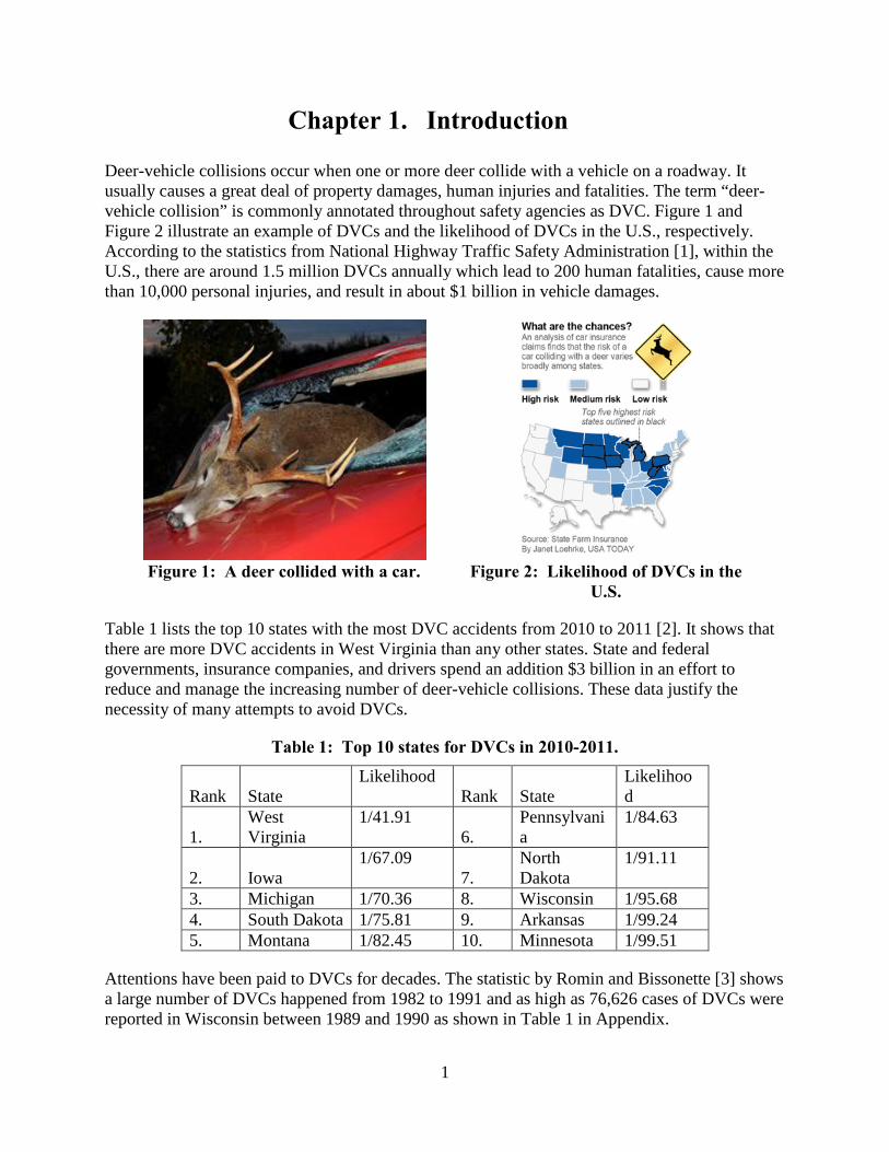
Deer-vehicle collisions occur when one or more deer collide with a vehicle on a roadway. It usually causes a great deal of property damages, human injuries and fatalities. The term “deer-vehicle collision” is commonly annotated throughout safety agencies as DVC. Figure 1 and Figure 2 illustrate an example of DVCs and the likelihood of DVCs in the U.S., respectively. According to the statistics from National Highway Traffic Safety Administration [1], within the U.S., there are around 1.5 million DVCs annually which lead to 200 human fatalities, cause more than 10,000 personal injuries, and result in about $1 billion in vehicle damages.

Figure 1: A deer collided with a car. Figure 2: Likelihood of DVCs in the

U.S.

Table 1 lists the top 10 states with the most DVC accidents from 2010 to 2011 [2]. It shows that there are more DVC accidents in West Virginia than any other states. State and federal governments, insurance companies, and drivers spend an addition $3 billion in an effort to reduce and manage the increasing number of deer-vehicle collisions. These data justify the necessity of many attempts to avoid DVCs.

Table 1: Top 10 states for DVCs in 2010-2011.

Rank State Likelihood

Rank State Likelihood

1. West Virginia

1/41.91 6.

Pennsylvania

1/84.63

2. Iowa 1/67.09

7. North Dakota

1/91.11

3. Michigan 1/70.36 8. Wisconsin 1/95.68 4. South Dakota 1/75.81 9. Arkansas 1/99.24 5. Montana 1/82.45 10. Minnesota 1/99.51

Attentions have been paid to DVCs for decades. The statistic by Romin and Bissonette [3] shows a large number of DVCs happened from 1982 to 1991 and as high as 76,626 cases of DVCs were reported in Wisconsin between 1989 and 1990 as shown in Table 1 in Appendix.

2

Many works have been carried out on reducing DVCs as shown in Table 2 in Appendix. These works are usually categorized into passive and active approaches based on how they functioned to keep drivers safe. Passive methods, using fencing or ultrasonic warning whistles, are now proved to be impractical and inefficient. For cost and simplicity, the most frequently used technique is deer crossing signs method which is a technique trying to inform drivers the existence of deer in range.

Active approaches for deer detection can be further grouped into ‘break-the-beam’ method (BTB) and ‘area-cover’ method. The key component in a BTB method is a beam which is formed by infrared light [4]. The blockage of the beam means there is an animal crossing the road, which results in the issuance of a warning signal. The BTB methods have the following drawbacks: (1) An object exiting from the road to roadside also activates the warning system; (2) Any object big enough to block the beam activates the warning system; (3) It is not capable of detecting the existence of roadside deer which may jump onto the roadway, which leaves passing drivers do not have enough time to react.

In an area-cover system, a camera, radar or an ultrasound system is used to detect the presence of deer. Once an object, such as a deer, is detected, a warning signal will be issued. Compared to a BTB method, it gives better accuracy and performs with more robustness in different scenarios. Examples of such applications are the systems in Box, Finland [5], Nugget Canyon, Wyoming, USA [6], Kootenay National Park, British Columbia, and Canada [7]. However, current existing cover systems still have drawbacks preventing them from being used widely in the world. As an example, the system shown in [7] was installed in May 2003 but removed in Oct. 2003 due to many problems encountered.

The existing approaches can also be categorized into roadside technologies and on-vehicle technologies according to where the detecting systems are placed. Roadside technologies include methods that either deter or detect the deer to avoid crashes. Deterrence roadside technologies have been researched to keep deer away from approaching traffic. Some of these technologies include animal reflectors [8], roadside reflectors [9], natural habitat prevention (predator scent [10], removal of roadside vegetation [11]) and electronic mats [11]. Although this idea is good theoretically, it has met with various difficult challenges in application. In addition to being difficult to implement, most proved to be ineffective. Experience shows that rather than attempting to deter deer, it may be more effective to detect deer and alert drivers. Detection roadside technologies developed usually have flashing signs to alert the driver when a deer is detected as a threat in the vicinity. On-vehicle technologies also aim at either deterring or detecting deer to avoid collisions. On-vehicle deterrence technologies include whistles [13] and TH - High Intensity Discharge lighting systems [14]. However, neither the audible nor visible methods of deterrence proved effective in any studies. On the other hand, current on-vehicle detection technologies, including forward-collision sensors [15], ultrasonic sensors [16], and thermographic cameras [17]- [18] that give the driver a thermographic image of the road ahead, only detect deer or big animals down the road direct to the front of vehicles passively and unfortunately ignore ones on the side of the road.

This research works used thermographic cameras to supervise the surroundings on highways. It belongs to active roadside detection technology. Compared to common optical cameras, thermographic cameras provide better performance in heavy fog and smoke. They function well

3

during day and night when there is little light. Through the mechanical design, the hardware system is also capable of working in rainy, snowy weather conditions. The system is also equipped with two step motors providing two degrees of freedom and making it possible to track deer when detected.

The algorithm selected to detect deer is motivated by the Histogram of Oriented Gradients (HOG) algorithm, proposed by Navneet Dalal in 2006 [19]. Based on this HOG algorithm, a new Contour-Based HOG algorithm (CNT-HOG) was designed in this research, which not only significantly improved the speed of the algorithm to make it possible for real-time detection, but also provided better performance in terms of detection accuracy. Descriptors employed here is an R-HOG descriptor, which demonstrates the best performance among C-HOG, Bar HOG and Center-surrounded HOG. Contours in the image were found out based on grayscale differences. In an image grabbed by a thermographic camera, the grayscale difference reflects the difference of temperature. Taking this advantage, the image can be segmented into several regions according to grayscale values. Considering that deer are warm-blooded animals and reflect more heat than most of the surroundings, the contour finding function can find out regions in the image with relatively high possibilities of deer existence. Comparing to the original algorithm performing HOG calculation on the whole image, by only applying the detection framework within the Regions of interest (ROIs), this contour based algorithm significantly reduces the running time. After HOG feature vectors are obtained, they will be sent into the detection framework for deer Identification. The classifier employed in the framework is a linear Support Vector Machine (SVM) classifier which was proposed by Vapnik and Corinna in1995 [20].

A significant amount of studies about the HOG and SVM methods have been carried out for object detection such as pedestrian identification, traffic identification, and object tracking [23], [22], [23]. However, there is no research about using HOG to detect deer with thermographic imaging devices. The combination of thermographic cameras and CNT-HOG algorithm provides this research with numerous advantages compared to current existing methods. In terms of hardware, the employment of thermographic cameras makes the system capable of functioning in bad weather conditions such as night, thick smoke and heavy fog, rain, snow, where common optical cameras don’t perform well due to the lack of visibility. In terms of algorithm, this Contour Based HOG algorithm works in real-time detection and simultaneously provides high detection accuracy.

Based on the identified deer in the thermographic images, a stereo thermographic camera system was designed to simulate the human eye system, and to estimate the distance from the deer to the camera. With the estimated distance, the function of showing the position of a deer on a road side LED map screen or in drivers’ GPS will be no more a dream.

In the remainder of this report, Chapter 2 will talk about the literature review about HOG, SVM classifier and contour finding methods; Chapter 3 will show the details of the research methodology; Deer detection results and evaluation will be presented in Chapter 4; The on-road application of the system and its performance evaluation will be described in Chapter 5; The conclusion is drawn and future work is illustrated in Chapter 6.

5

Chapter 2. Literature Review

This Chapter mainly concentrates on the review of the background knowledge including HOG algorithm, SVM classifier and contour finding methods.

2.1 Thermographic Cameras

The first thermographic camera was invented by a Hungarian physicist Kálmán Tihanyi for anti-aircraft defense in Britain in 1929. Similar to the common optical cameras which form images using visible light, a thermographic camera or infrared (IR) camera is a device that forms image using infrared radiation [24]. Figure 3 shows the location of infrared energy among the electromagnetic spectrum. It encompasses radiation from Gamma rays to radio waves. A certain amount of black body radiation will be emitted in a positive correlation with its temperature. This radiation can be detected by a thermographic camera via a special detector like the way in which optical cameras do with visible light. Since thermographic cameras take infrared radiation instead of light to form images, it works even in total darkness. This makes it especially useful when applied in night vision, firefighting, astronomy and underground detection. It can also be installed on vehicles to aid drivers. To the application of transportation, the first successful attempt was the installation on a 2000 Cadillac DeVille. Some physiological activities, particularly responses, in human beings and other warm-blooded animals can also be monitored with thermographic imaging.

Figure 3: Electromagnetic spectrum diagram.

Thermographic cameras are broadly divided into two types based on the detectors installed inside. One type is equipped with cooled infrared detectors. Cooled infrared cameras provide superior image quality compared to un-cooled ones, but the drawbacks are that cooling is power-

6

hungry and time-consuming and that they are expensive both to produce and to run. Compared to cooled infrared cameras, un-cooled infrared cameras are smaller and less costly. However, their resolution and image quality tend to be lower than cooled ones. This is due to the difference in their fabrication processes which is limited by available technology. Figure 4 shows one of the applications of thermal imaging technology where a thermographic camera is installed in airports to detect human temperature as an indication of possible H1N1virus.

Figure 4: Example of the application of a thermographic camera.

Thermal camera shows a visual picture of the temperature over a large area reflecting a clear temperature contrast. What is important to this research is that it can be used to measure or observe in areas inaccessible or hazardous for other methods and detect in dark areas as well as different environments with low visibility.

2.2 Image Processing Algorithm

In image processing, to realize object identification, detection, tracking, or classification task, many machine learning and pattern recognition algorithms can be employed.

2.2.1 Machine Learning and Pattern Recognition

Tom Mitchell has defined machine learning in reference [24]. Commonly used machine learning algorithms are categorized into supervised algorithms and unsupervised algorithms. Supervised algorithms, including back-propagation in artificial neural network [26], Bayesian statistics [27], decision trees [28], and support vector machine (SVM) [28], etc., focus on generating a function that can best match a given input to a desired output (label). Unsupervised algorithm refers to the problem of trying to find certain hidden structure in unlabeled data. Commonly used unsupervised algorithms are clustering [30], expectation-maximization [31], and some artificial neural network algorithms [31]. There are also hybrid algorithms using both labeled and unlabeled examples to generate an appropriate function or classifier.

Pattern recognition accomplishes the task of assigning a label to a specified given input. The typical pattern recognition methods include classification, regression, parsing, and sequence labeling. Commonly used algorithms include particle filters [34], Kalman filters [35], Gaussian process regression [36] and principal component analysis (PCA) [37], etc.

7

The contour based HOG algorithm developed in this research is a supervised method, which is motivated mainly by the HOG algorithm proposed by Navneet Dalal [19]. In this algorithm, HOG descriptor was selected to represent the edge information of deer, and then employed in a multi-scale detection framework to realize classification and identification. The classifier applied in the detection framework is a linear Support Vector Machine. To improve the accuracy and speed up the algorithm for real-time detection, a contour finding function is added to search for regions of interest (ROIs) where deer are most likely to appear. The collection of the HOG features and the identification of deer are considered only within the ROIs.

2.2.2 Histogram of Oriented Gradients (HOG)

The basic idea of transferring the chaos numerical data that represents an object in a digital image to a convenient pattern for computer comprehension is to find out a good transform to reveal the characteristics of the objects. HOG is such a transform that generates a feature descriptor (HOG descriptor) to represent the pattern of the objects. This descriptor was first proposed by two researchers- Navneet Dalal and Bill Triggs- from the French National Institute for Research in Computer Science and Control (INRIA) [38]. It can be used in computer vision areas such as identification, classification or object detection.

To form an HOG descriptor, the gradients of pixels are accumulated by its orientation into a histogram in a localized image area (cell). This is quite like edge orientation histograms and shape contexts. The difference is that after the formation of the local histogram, it will be further combined in a bigger area (block) and normalized in different overlapping blocks. The normalization improves its accuracy and resistance to illumination variance. The descriptor was first used in offline up-right people detection and later was expanded to do offline animal detection and vehicle detection.

Histogram of Oriented Gradient descriptors were designed based on the idea that an object’s appearance or shape information can be well described by the intensity gradients or edge directions. To implement the HOG descriptors in an image, the image should be first divided into a dense grid of uniformly spaced connected regions, called cells. Within each cell, local shape and edge information is represented by forming a histogram of the gradient of each pixel. Histogram is encoded by each pixel’s gradient orientation. To improve its invariance to illumination or shadowing, an overlapping contrast-normalization is employed in a larger region of the image, called “block”. Thus, an HOG descriptor is generated for a block. Normalized descriptors will be combined into a long feature vector in an even larger area, called window.

Compared with other frequently used descriptors in image processing such as Harr Wavelet [39], shape context [40], and PCA-SIFT [40], HOG descriptor has its own advantages [38]: First, the descriptor is obtained in cells. Hence, it provides a good invariance to the geometric and photometric transformations. Second, since an HOG descriptor is contrast-normalized in overlapping blocks, it has a better invariance to illumination or shading. Third, if the target object roughly keeps its posture, the movement of the target can be ignored. This makes it particularly suitable for object tracking.

8

Image Pre-Processing

An image pre-processing includes the work for geometric correction, histogram stretch, normalization, smoothing, and other image enhancement technologies. The aim of an image pre-processing is to increase the interpretability of the digital data and to facilitate the subsequent processes and to facilitate the image processing phase. Before collecting HOG descriptors in a given image, the image is first globally Gamma normalized (Power law compression, see following equation): r

out inV AV= . Gamma normalization is especially important in the case where displaying an image accurately on a computer screen is of concern. Images without gamma normalization may look either bleached out, or too dark. Gamma normalization enhances image quality in image contrast and its invariance to illumination. Since the way in which HOG descriptors are collected generates a good invariance to illumination or shading, instead of mandatory, gamma normalization can be optional in the image pre-processing phase in an HOG algorithm.

Gradient Computation

The first step in image processing phase in HOG algorithm is the gradient computation. Commonly used operators for gradient calculation in digital image processing are Sobel mask, Robert masks, 1-D mask, and Laplacian mask (see Table 2 for details). In Dalal and Triggs’s research [38], the preferable operator employed is the 1-D centered, point discrete derivative mask. According to their test, the performances tend to be poorer when more complex operators such as Sobel or Lplacian are employed.

9

Table 2: Gradient computation operators.

Sobel mask

-1 -2 -1 -1 0 1 0 0 0 -2 0 2 1 2 1 -1 0 1 Horizontal Vertical

Roberts cross mask

-1 0 0 -1

0 1 1 0

X-Dimension Y-Dimension

1-D mask

0 0 0 0 -1 0 -1 0 1 0 0 0 0 0 0 0 1 0 Horizontal Vertical

Laplacian mask (non-diagonal)

0 1 0 0 -1 0

1 -4 1 -1 4 -1

0 1 0 0 -1 0 Negative Positive

Laplacian mask (diagonal)

1 1 1 -1 -1 -1

1 -8 1 -1 8 -1

1 1 1 -1 -1 -1

Negative Positive

Orientation Binning

Orientation binning is applied in cells. A cell is a region in which the previous calculated gradients of each pixel is voted into a histogram. A cell can be either rectangular or circular and consists of numerous of pixels in a connected region. Gradients within a cell are voted into histogram based on its orientation. In an “unsigned” case, bins spread evenly from 0 to 180 degrees, while from 0 to 360 degrees in a “signed” case. Weights of these gradients are decided by their magnitudes or a certain function of their magnitudes such as square root. Experimental results from Dalal and Triggs’s research showed that magnitude itself is more preferable than its square or its square root, and a histogram with 9 bins gives the best performance on both human detection and deer detection. Taking aliasing into consideration, which happens at the image edge and the vibration of the image (a strong edge pixel in one cell may fall into a neighborhood in the next), a tri-linear interpolation, is applied to the histogram in a 3-D space when the weight of gradients is distributed into the pre-defined orientation bins.

10

Descriptor Blocks

In order to account for the changes in illumination and contrast, the gradient strengths must be locally normalized, which requires grouping the cells together into larger, spatially connected blocks. The HOG descriptor is then a vector formed by combining the normalized cell histograms within the block regions. Commonly used blocks are rectangular R-HOG blocks and circular C-HOG blocks. As discovered in Dalal’s research [38], a block with 3 x 3 cells and each cell with 6x6 pixels performs best on detection accuracy. Compared with R-HOG block, C-HOG block defines cell into log-polar shape. Figure 5 and Figure 6 illustrates the comparison between R-HOG and C-HOG.

Figure 5: R-HOG block (source from

[38]). Figure 6: C-HOG block (source from

[38]).

Block Normalization

Blocks typically overlap, meaning that each cell contributes more than once to the final descriptor for a window. To improve the performance of HOG descriptor, it will be contrast-normalized in overlapping areas. Dalal and Triggs’s research proved that a normalized block shows significantly improved performance over a non-normalized block. The reason is that in the local area where HOG is collected, the illumination variation and the difference in background-foreground contrast may cause the gradient magnitude vary over a huge range. Contrast-normalization helps to reduce the variation. Many normalization schemes can be employed, including L1-norm, L1-sqrt, L2-norm, and L2-Hys. Those for schemes are illustrated in Table 3.

Table 3: Block normalization scheme.

L1-norm 1 11

vfv e

=+

L2-norm 2 22

vfv e

=+

L1-sqrt 2 11

vfv e

=+

L2-hys L2-norm followed by clipping and renormalizing

In Table 3, v is the non-normalized vector containing all histograms in a given block, ||v||k is its k-norm for k = 1,2 and e is some small constant (the exact value, hopefully, is unimportant). Experimental results showed that L1-norm has some drawback on reliable performance compared with other normalization schemes, and the other 3 normalization schemes provide almost the same performance.

11

2.2.3 Linear Support Vector Machine

SVM classifier is a classification system with an optimal hyper-plane realizing the function of sorting input data into different categories. By feeding the data into the classifier, the hyper-plane will serve as a decision function and generate a bench mark for the input. Classification will be done according to the bench mark. It is a supervised learning method that used to analyze data and recognize patterns.

Before applying SVM classifier in an HOG algorithm, an optimal hyper-plane needs to be trained. The training data set for a binary classifier contains 2 classes. By feeding the training data set into the learning phase of the classifier, an optimal hyper-plane will be obtained. There are cases that with the training data set, the obtained hyper-plane is non-linear. To train a linear classifier, a kernel function will be introduced. Most frequently used Kernel function is the Gaussian function. Other kernels include homogeneous polynomial kernel, inhomogeneous polynomial kernel, and hyperbolic tangent kernel.

After the hyper-plane is obtained, a set of testing data can be sent into the classifier. It provides a bench mark as the output. The sign of the bench mark decides the class that the input belongs to.

The mathematical SVM model is a multi-dimensional space in which an example is represented by a point in the space. The aim of a learning phase is to separate points belonging to different categories with a clear gap as wide as possible. The classification phase is a prediction of a new, class unknown example to a certain category based on which side of the gap it falls on in the space. If training data D is a set of n points of the form

( ) { }{ }1

, , 1,1nP

i i i i iD x y x R y

== ∈ ∈ −

where the yi is either 1 or −1, indicating the class to which the point xi belongs. Each xi is a p-dimensional real vector. Any hyper-plane can be expressed by the following function:

0b⋅ − =w x

where · denotes the dot product and w and x, and b is the bias. Figure 7 illustrates the math model of a linear SVM classifier. The goal is to find out a vector w to maximize 2/||w||, i.e. to minimum w.

Figure 7: SVM classifier hyper-plane.

http://en.wikipedia.org/wiki/File:Svm_max_sep_hyperplane_with_margin.png

12

As we also have to prevent data points from falling into the margin, we add the following constraint: for each either

1b⋅ − ≥w x for xi of the first class

or

1b⋅ − ≤ −w x for xi of the second class

Once trained on images containing some particular object, the SVM classifier can make decisions regarding the presence of an object, such as a human being, in additional test images.

2.2.4 Contour Finding

Contour finding methods are used in the domain of image processing to locate the contour of a target. They were mainly based on edge detection via edge linking. Early contour findings methods are applied by detecting object edges with Roberts, Sobel, and Canny detectors [47]. One drawback of earlier methods is that the contour found may not be continuous. To improve on this point, in 1987, Michael Kass, et al. suggested a “snakes” method to find contours [42]. This method proved to be flexible for many image processing problems [43] and it sparkled several researches at that time. Based on this snake model, the balloon model [48] and greedy snake model [49] were developed.

13

Chapter 3. Deer Detection Methodology

3.1 Thermal EyeTM Thermographic Camera

Thermographic camera applied in this research is a Thermal Eye 3620AS provided by Thermal EyeTM Company as shown in Figure 8. The Thermal-Eye 3620AS is a camera core with best-in-class power consumption. This camera core utilizes Amorphous Silicon Microbolometer detector technology (30-micron 160x120 pixel array). It has been utilized in security, military, public safety and other applications. This thermal camera has the following features and advantages [50]: (1) Small size and best-in-class power consumption at 2.4 watts; (2) Advanced image processing for best-in-class image quality at all times; (3) Flexible with sophisticated GUIs for OEM customization; and (4) Seal-ready optics housing and optics assemblies for easy OEM integration. More technical specifications can be found from [51].

Figure 8: Thermal Eye 3620AS camera.

3.2 System Setup

Infrared images were collected with the equipment shown in Figure 9. The image acquisition system contains two thermalcameras which are designed to take video of the surroundings and to simulate human visual system to realize the function of distance measurement. Videos taken by the stereo camera system are grabbed using a Sensory S2255 image grabbing card [52] which connects the cameras and computer. It transfers data from the cameras to our computer. Image grabbing card S2255 connects cameras via two BNC wires and connects to computer using a single USB port. The stereo camera system is equipped with two stepper motors which provide two degrees of freedom: the yaw and pitch motions, making the camera capable of rotating both vertically and horizontally to track detected targets. The range of the yaw and pitch rotation is, relative to the front direction of the box, ±180° and ±45° individually. Those motors incorporate with a motion control card which connects to a computer through a serial port. Thus the computer is able to control the motion of the motor using a negative feedback system. The motors are designed to be driven by 110 volts AC power supply. The stereo camera system is powered by either AC power supply or 9 volts DC battery, which facilitates the outdoor test of the camera without AC power supply. Connection of components in this image acquisition system is illustrated in Figure 10.

14

Figure 9: Image acquisition system.

Figure 10: Connection of components illustration.

The frame grabber used to capture the video from the thermal camera is a Sensory 2255 image grabbing card. The card is able to acquire and capture frames from up to four video inputs, which means the ability of processing signals from up to 4 cameras simultaneously. The acquisition speed of the card can reach a maximum of 30 fps, which guaranties the fluency of the grabbed image flow. Captured images can be either colorful or monochrome, depending on users’ choices.

3.3 Image Collection

To create data sets for training and testing, in total 3 groups of deer images were collected. These images contain deer in winter, summer, in both sunny and cloudy days, on roads, vehicles, people and other animal influence. Collected images would be re-organized later to facilitate system performance test.

15

The first group of deer images was acquired in the Lake Superior Zoo in Duluth, Minnesota USA on January 20th, 2011. The outdoor temperature was -20°F and the distance from the camera to the deer was about 50m. A total of 3000 images were obtained with deer in different postures. Images in this group have a very strong contrast between deer and background and have very little inference from heated objects such as rocks, houses, vehicles, and human beings. Examples are shown in Figure 11 (a) to Figure 11 (f).

On May 5, June 7 and 27, 2011, deer images collections were carried out again in the Lake Superior Zoo, mainly containing images with deer in all angles, in both sunny and cloudy day, and also deer under different percentage of occlusion. Example images with deer at different angles are shown in Figure 12 (a) to Figure 12 (b). Example images of occlusion are shown in Figure 13 (a) to Figure 13 (d). Comparison between a sunny day image and a cloudy day image are shown in Figure 14 (a) and Figure 14 (b).

(a): Example 1 (b): Example 2 (c): Example 3

(d): Example 4 (e): Example 5 (f): Example 6

Figure 11: Examples of the first group of deer images.

16

(a): Example 1 (b): Example 2

(c): Example 3 (d): Example 4

Figure 12: Examples of deer in different angles.



Figure 13: Examples of the occlusion to deer’s body

17

(a): Image in sunny day (b): Image in cloudy day

Figure 14: Examples of deer in different sun conditions.

(a): Multi deer (b): Vehicle (c): People

Figure 15: Images with different objects on road.

The third time of image collection was carried out from March 8th to March15th, 2012. This group of images was collected to testify its on-roadside real-time detection performance. This data set includes images with only deer, images with only people, images with vehicles, images with single deer and images with multiple deer. These images contain many interference factors, such as people, buildings, vehicles, other animals, etc. Example images are shown in Figure 15.

3.4 ROI Finding

Contour finding plays an important role in image pre-processing phase in this research. Through the experiment, it was discovered that original HOG algorithm takes around 3.7s to process a single static image with size 640 by 480 pixels, and around 2.3s for 320 by 240 pixels. This speed is too slow compared to the image grabbing speed (up to 30 fps, i.e. 0.033s per image). Neither the output would be fluent for human to perceive. To carry out the algorithm in real-time detection task, Navneet Dalal proposed histogram of oriented flow and appearance algorithm. The drawback of this algorithm is that the speed up is at the cost of a fall in detection accuracy. This research aims at using infrared thermal imaging method to achieve real-time detection of the presence of deer in the surroundings. Since Navneet Dalal’s method uses a sliding window to scan the whole image, calculate the HOG descriptors, and then make decisions, processing time per image is mainly consumed in calculating massive HOG descriptors. The bigger the scan region is the more HOG descriptors it calculates, the longer it takes. Considering that calculating HOG descriptors in regions without deer generates no added value to the detection job and

18

sometimes even generates wrong detections, a smaller scan region will be more preferable. Motivated from this, the pre-processing phase of the original algorithm is modified by adding a contour finding function block. Results prove that it contributed a great part in balancing the speed and accuracy and made the algorithm capable of real-time detecting simultaneously.

The first step of contour finding is to build an illumination filter. The image sent to computer for detection is in grayscale. As a property of thermal images, intensity of the image reflects temperature difference in the real world. Since deer are warm-blooded animals, their temperature tends to remain stable and will be different from most of the background. Hence, based on the gray scale property of the IR thermal images, if a grayscale value range of a deer can be found, most background information (lower temperature objects and extra high temperature ones) could be separated. Thus, regions with temperature lying in the range would be emphasized. Originated from this idea, attempts have been made to find out the upper boundary and lower boundary of the deer grayscale value in the image. Experimental results show that the boundary varies as the environment changes, due to the self-adjustment function of the camera itself. Hence, only a lower boundary, which is 165 throughout the experiment, was selected to filter out some background information. Once the computer reads an image in, the algorithm would first scan the whole image and automatically reset image by assigning pixels with grayscale value lower than the pre-defined threshold value (lower boundary of the range) to be zero. Thus, most of regions without deer are filtered out. This is called an illumination filter in this research, and it can be expressed by following function:

>

=otherwise

thresholdxxjif

,0,

),(

After assigning the lower intensity pixels to 0 through the illumination filter, the raw image shown in Figure 17 (a) will be turned into the image shown in Figure 17 (b), with all contours of the bright region labeled by white rectangles. Contours were searched using their edge information. In this stage, from this image it can be found that: 1.most parts of the image without a presentence of deer are filtered; 2.however, there are still bright regions without deer. To increase the algorithm speed, the algorithm is supposed to be carried out in an as small as possible potential region with the presence of deer. Hence, the problem left was to further filter out as many as possible portions in which there are no deer.

Figure 16: ROI finding flow chart.

19

(a): Raw image (b): Result after illumination filter with all

contours found

(c): Result after size filter (d): Regions of interest

Figure 17: Intermediate results of finding the ROIs.

To filter out as many as possible portions without deer, a size filter was designed. Taking into consideration that the deer has greater chance of showing up in its side view, the training data set was collected consisting of mostly side-view deer and little front or rear view deer. Hence the algorithm is good at detecting side-view deer. Based on this point, to realize the size filter, two criteria were employed: (1) size of the contour, which restricts size of deer to be neither too big nor too small, and (2) ratio of width to height of a contour, which is designed to detect deer in a side view. Thus, some of the areas will be eliminated from the candidate pool (white rectangles shown in Figure 17 (b)). Rectangles those pass the size filter are further enlarged to regions of interest (ROIs) by expanding on each direction. Figure 17 (c) illustrates the output of the size filter. And based on Figure 17 (c), ROIs are obtained and shown in Figure 17 (d). Flow chart of contour finding is shown in Figure 16.

As a drawback of the combination of sliding window technique and HOG descriptor, objects of small size could be neglected. In this research, some deer in distance within certain ROIs have high possibilities to be ignored due to its small size. To avoid the misdetection and increase the accuracy, those ROIs would be zoomed in as a new input to detect. This will be further introduced in multi-scale detection framework section.

20

3.5 Feature Vector Collection

In this research, after the image pre-processing phase, four stages were used to calculate HOG features. Firstly, a Sobel mask was used to compute the gradients of each pixel. The gradient contains both magnitude and orientation information. They capture contour, silhouette and some texture information, while providing further resistance to illumination variations. Then, gradients of pixels were voted into a local 1-D histogram using its orientation information in a region called ‘cell’, which is composed of several connected pixels. The orientation is voted into a fixed number of pre-determined bins. Commonly used number is either 9 or 18, corresponding to [0°, 180°] and [0°, 360°] separately. The weight of each gradient is decided by a function of its magnitude. In this research, the orientation was divided into 9 bins from 0° to 180° evenly, and the magnitude itself was chosen as the voting weight. These 1-D histograms formed the basic representation of the orientation histogram and were taken as the default set for descriptor throughout the whole experiment. The third stage was to combine and normalize those histograms, which introduces better invariance to illumination, shadowing, and edge contrast according to Navneet Dalal’s research [38]. Normalization was carried out in regions called “blocks” which is composed of several cells. It is performed by accumulating a measure of local histogram “energy” in the block. Thus, the normalization is block-dependent, and since each cell is shared between several blocks, a single cell histogram appears several times in the final descriptor of a window. This, as turned out in the result from Navneet Dalal, improved the performance. The normalization scheme chosen in this experiment was L-2 form. Finally, the HOG descriptors were collected from all blocks of a dense overlapping grid of blocks covering the detection window into a combined feature vector for further use in the classifier. In this research, default window size was 144 by 104 pixels. Within a window, each block contained 2 by 2 cells while each cell was composed of 8 by 8 pixels. Hence, a feature vector of a given window is of size 1 by 6480.

3.6 Support Vector Machine (SVM)

Linear Support Vector Machine was employed in this research to generate a detector and then use it to classify given descriptors. Based on the functionality, an SVM classifier can be divided into two phases— training phase and classification phase. In the training phase, a training data set is taken as input and a detector will be provided as output. In the classification phase, a test data will be sent into the classifier to generate a bench mark based on which it will be categorized.

In this research, to train the detector for classification, a training data set containing both positive and negative examples was collected first. Positive examples were created by selecting images with side-view deer and cropping out windows with deer located in the center. Those windows were then resized to be 144 by 104 in pixel, which is the same as defined before in feature vector collection. Negative examples were collected by randomly cropping out a window of size 144 by 104 without deer in those training images. HOG feature vector calculation was applied to both of the data sets. Then, positive and negative examples together generated the initial training data set. By sending the training data set into the SVM classifier, processing each example in the training phase, an initial detector of size 1*6481 will be given.

21

According to many studies on SVM classifier, a better detector than the initial one can be achieved by its second training. This is performed by sending feature vectors for both images with and without deer into the classifier. False positives in the result of classification phase were collected and labeled as hard examples to update original negative examples. Thus, an updated training data set was established, the final detector was updated by sending the updated data set into the classification phase.

3.7 Multi-Scale Detection Framework

A multi-scale detection framework was designed in this research to detect deer of various sizes in an image. As shown in Figure 18, targets may spread in different locations and are of varying sizes. Navneet Dalal has tried to detect targets of different sizes by resizing the image iteratively and merging all the results from all iterations. This method not only helps to detect multi-scale deer, but also helps to eliminate some false positives and increase accuracy. In this research, some modifications were added to the original framework to improve its performance. After ROIs were obtained in the pre-processing phase, a separation would be applied based on the size of the ROI. Once the area of an ROI was less than 2500, it would be taken as a region where deer of very small size may exist. For such ROIs, they were resized by 3 times of its original size, and the original framework proposed by Navneet Dalal would be applied. For other ROIs, original framework would be directly employed. In the framework, a scale factor 1.05 was selected to resize the image iteratively for detection. Illustration for the algorithm is shown in Figure 19.

Figure 18: Deer with different size.

22

Figure 19: Deer detection algorithm flow chart.

23

Chapter 4. Deer Detection Results and Evaluation

To test the performance of the proposed system and algorithm, evaluations on many aspects have been carried out, including accuracy test, speed test, rotation and occlusion test, performance comparison between winter and summer, performance under different weather. Also, performance comparison between original HOG algorithm and the CNT-Hog algorithm will be shown in this Chapter.

4.1 Data Set Setup

To facilitate the research, all the images collected during the whole research period were re-organized into the training data set and testing data set. To form the training data set, since images taken in winter tend to show a greater contrast between deer and non-deer objects than other groups, as shown in Figure 20, and greater contrast emphasizes deer edge, images selected to generate training data set were mainly from images collected in the Lake Superior Zoo in 2011 winter. Considering that the negative examples from those images are monotonous only with trees and snow, additional examples generated from images collected in summer in the zoo and images collected on road, including people, buildings, vehicles, roads, and other animals were added. More examples of training data set are shown in Figure A1 in Appendix. From the training data set, 900 positive examples and 1200 negative ones were first generated. The number of hard examples generated by SVM classifier first training was 604 and they were further added into negative training data set for SVM classifier second training. The SVM classifier selected is a linear SVM classifier, called LightSVM [53]. Positive examples and negative examples are shown in Figure A2 and Figure A3 in Appendix.

Test data set was divided into 5 groups to give a full evaluation on the method performance in different scenarios. Group I is composed of image samples from all images collected in both winter and summer, in zoo and on road. It was created for general test on accuracy, algorithm speed, and comparison between different algorithms. Group II contains images in which deer are of different postures. This group was collected to test algorithm performance to rotation. Group III consists of images in which body of deer is partially blocked. This group of data would be later employed to give an evaluation on detection accuracy under occlusion. Group IV mainly includes images taken on road to show the algorithm’s ability in real-time on road detection. Images in Group V were taken both in winter and summer to show the algorithm and camera performance under different weather. Example images from each group of test data are shown in Figure A1 and Figure A4 to Figure A7 in Appendix A.

24

(a): example image 1 taken in winter (b): example image 2 taken in winter

(c): example image taken in cloudy

summer (d): example image taken in sunny summer

Figure 20: Example images from training data set.

Figure 20 (a) to (d) show 4 example images served as SVM classifier training data. (a) and (b) were taken in winter, while (c) and (d) were taken in summer. As shown, it can be found out that image (a) and (b) has the best contrast between background and deer. Image (c) was taken in a cloudy summer day. Compared with image (d), which was taken in a hot sunny summer day, low temperature tends to give a better contrast.

4.2 Intermediate Results in the Algorithm

Gamma correction was applied as the first step in image pre-processing phase. Figure 21 shows the performance curve of gamma correction with different 𝛾 values. More gamma corrected images with different gamma value are shown in Figure A8 in Appendix. Taking image shown in Figure 22 as an example, Figure 23 shows the effect of gamma correction with γ = 0.5 while Figure 24 is the result when γ = 2.0. Figure 25 to Figure 27 show relative histograms. From those histogram figures it can be concluded that 𝛾 = 2.0 has the best contrast between background and deer. It makes the darker part of the image (background) even darker and thus stretched the histogram distribution, making it much easier to separate deer and background.

25

Figure 21: Plots of Gamma correction curves with different 𝜸 values.

Figure 22: Gamma=1.0

(Original). Figure 23: Gamma=0.5. Figure 24: Gamma=2.0.

Figure 25: Histogram for Gamma=1.0 (Original).

Figure 26: Histogram for Gamma= 0.5.

Figure 27: Histogram for Gamma=2.0.

Gamma corrected image with 𝛾 = 2.0 was sent to the illumination filter to filter out useless background information. An example of the output image of the filter is shown in Figure 29. After this step, useful information (deer existence) only lies in regions labeled with white rectangles as shown in Figure 30. White rectangles in Figure 30 represent all contours found based on Figure 29. The output of illumination filter was then sent to size filter where further selection of regions where deer might exist would be carried out. Result is shown as Blue rectangle in Figure 31. Then the blue rectangle will be resized and cropped out to serve as an ROI image, shown in Figure 32. Compared with the result after illumination filter, most regions without deer were filtered out. Regions left in Figure 31 were then enlarged on each direction to generate corresponding ROIs as shown in Figure 32. As long as ROIs of an image were obtained, detection would be carried out only within them. Until now, the pre-processing phase of the algorithm is finished. In the processing phase, the detection frame work was applied to ROIs

26

only. Detection results was first obtained in each ROI image, and then combined into the original image. Detection results are shown in Figure 28. The red rectangle labels out the detected deer. The Blue one shows the contour that passed the size filter, which is identical to that in Figure 31. The green rectangle is the ROI in this image which is obtained based on the blue rectangle.

Figure 28: Final detection result.

During this image pre-processing phase, deer may be separated into several different regions due to the illumination change on its body surface. This affects the performance of the algorithm by generating different detection results on the same objects since different ROIs would be introduced from the white rectangle or by missing the detection since the deer was divided into parts that are so small that would be further filtered out through seize filter in next step. Figure 34 to Figure 37 illustrates an example of this. Figure 34 shows the original image. Figure 36 illustrates the result after illumination filter and size filter. Figure 35 is the ROI generated from the top blue rectangle in Figure 36 while Figure 37 is generated from the bottom one. Figure 33 is the detection results. The same deer is identified twice in two different ROIs.

Figure 29: Image after the illumination

filter. Figure 30: All contours found.

27

Figure 31: Image after the size filter. Figure 32: Region of interest.

Figure 33: Detection result.

28

Figure 34: Original image. Figure 35: Region of interest 1.

Figure 36: Image after the size filter. Figure 37: Region of interest 2.

4.3 Speed and Accuracy Tests

This test was carried out with test data set Group I. The data set contains images with deer in different postures under different weather conditions, and images without deer but consist of many non-deer objects that may affect the detection, such as humans, animals, cars, bicycles, buildings. There are also images in this group containing multiple deer of various sizes.

4.3.1 Speed Test

The computation speed of the algorithm varies with different numbers of ROIs. Generally speaking, to process an ROI with size around 160 by 120 pixels usually takes less than 0.05s. Although the number of ROIs differs and the size of ROIs may change, by running the algorithm to process 1500 images of size 320 by 240 pixels, the time consumed was found to be 251s in total, i.e. 0.167s/image, meaning the average computation speed reached 5.988fps.

4.3.2 Accuracy Test

The following equation was employed to test the accuracy of the proposed algorithm:

%100)( 21

NnnN +−

=η,

29

where N is the total number of the targets in images, n1 is the number of the detected non-deer objects and n2 is the number of deer where misidentifications happen. Among 1500 images in this Group I of test data, there were 54 deer that were not detected and 32 non-deer objects that were misidentified as deer. The total number of deer was 1473. One thing to note here would be that, multi-detection results on one single deer introduced by different ROIs covering the same deer are counted as only one correct detection result. This results in an accuracy of 94.16% from the testing set of only deer that were side-on to the system. By further analyzing those images, it is found that most of wrong identified objects are big heated rocks on the ground or buildings that look like deer body without legs as shown in Figure 38. There were also some other (less than 5) false-positives generated by an object within which a darker area looks much like a deer instead of a brighter area. This shows that the HOG descriptor has the adaptability to a contrast-conversed feature. The reason is that during forming the HOG descriptor, the orientation range was set to [0°, 180°] rather than [0°, 360°]. An example is shown in Figure 39. It was also noticed that, most of the misdetection were introduced by occlusion and rotation of body angle since the training data set to generate the detector for SVM classifier were mainly formed by side view deer images without occlusion.

Figure 38: Example 1 of

misidentification. Figure 39: Example 2 of

misidentification.

4.4 Body Angle and Occlusion Tests

It is observed in accuracy tests that when deer postures were at certain angle with respective to the camera and/or when part of the body of deer was behind a tree, i.e. blocked from the camera view, they are harder to detect. Test data sets Group II and Group III were then employed to further evaluate the performance of the algorithm when deer body is at different angles and part of the body is occluded.

4.4.1 Body Angle Test

To test the detailed accuracy in different rotation angles, a series of detections were carried out on images with deer at different angles. Noted is that since most of the positive training samples were side view deer, the detector trained in the SVM classifier was good for the detection of side view deer.

30

In this research, right-head side view of a deer is defined as 0°, back view as 90°, left-head side view as 180° and front view as 270°. Figure 40 shows some of the results at different angles. By running detection in the Group II, it was found that when the angle of the deer falls in the range of [70°, 110°] and [250°, 290°] (estimated values), deer tended to be difficult to detect. More examples are shown in Figure A10 in Appendix.

This, however, can be improved in future work. Once training samples with deer posture angles falling in the range of [70°, 110°] and [250°, 290°] are added to the SVM classifier training phase and a new classification category was created for front-rear-view deer, the algorithm would have the capability to detect these deer.

(a): Deer detected at 115° (b): Deer detected at 110°

(c): Deer detected at 90° (d): Deer detected at 0°

Figure 40: Deer detection performance at different body angle.

4.4.2 Occlusion Test

It is a common scenario in image processing that part of the body of an object is behind certain obstacle. This made occlusion a common difficulty to deal with in many object detection and tracking tasks. Difficulty increases as the body shown percentage decreases. Body shown percentage means the percentage of the target object shown in the images relative to its whole body in one posture. It equals to 100 percentages minus occlusion percentage. Deer can be easily blocked by obstacles such as trees, rocks, buildings, or vehicles. In such cases, only part of the deer’s body is shown.

31

To evaluate algorithm performance to occlusion, a total of 700 images with different deer body shown percentage from Group III have been selected. The tests were performed in several scenarios with different parts of the deer body occluded. A series of results are shown in Figure A9 in Appendix.

(a): More front body left (b): Less front body left

(c): More rear body left (d): Less rear body left

Figure 41: Deer detection performance with various occlusion percentages.

It is observed that the occlusion of the head and the front part of a deer influence detection accuracy much greater than the occlusion of the rear part of the body. As shown in Figure 41, if the head and the front body are not covered, the deer can be easily detected. On the other hand, without the information of the front of deer, the identification accuracy will drop. Noted is that if the deer bodies are in perfect side view posture (0° or 180°), the identification rate can reach 100%. In Figure 41, blue rectangles are the ROIs detected while red rectangles represent the detection results. In Figure 41 (b), in total 3 ROIs were found, among which 2 of them contains no deer and one contains deer head. In the ROI with deer head, if a special detector can be trained for the detection of deer head, possibly the deer can be identified. Following Table 4 shows the detailed results of performance results to occlusion. Figure 42 provides the performance curve to occlusion percentage.

32

Table 4: Table of detection accuracy to different occlusion percentage.

Occlusion Percentage Accuracy

Front body

0 100 10 92.0 20 84.0 25 80.0 30 74.0 35 55.0 40 42.0

Rear body

0 100 10 96.0 20 92.0 25 88.0 30 82.0 35 68.0 40 46.0

4.5 System Capability Test

To test the capability of the camera, the algorithm was applied on Group V of the test data set. Group V contains different images taken both in winter and summer, daytime and night time. Following Figure 43 shows a comparison example between winter and summer, while Figure 44 shows the difference between images taken during sunny summer day and cloudy summer day. Result shows that images in winter provides stronger contrast between deer and background, which saves a lot of time in running the detection and helps in increasing the detection accuracy. Images taken in a sunny summer day contains many bright dots in the background and many black dots on deer body, and the deer in the image didn’t show as much difference as it is in the images taken in cloudy summer day. One reason was that the environment temperature in a sunny summer is higher and the sunshine is stronger. Another reason is the self-adjustment function embedded in the thermal camera itself. The camera was designed with this function to provide a better reflection of the heat distribution in the image and protect the camera core, but results turned out that it killed the contrast between deer and background.

33

Figure 42: Detection accuracy to occlusion.

O l i

Table 5: Algorithm performance comparison between winter and summer.

Winter Summer Detection accuracy 97.2% 89.3% Algorithm speed 7.33 fps 5.12 fps

(a): Example image taken in winter (b): Example image taken in summer

Figure 43: Comparison between images taken in winter and summer.

Although the illumination contrast in summer, especially on sunny summer days, was weaker than images taken in winter, the algorithm was still capable of detecting deer. Disadvantage of the low contrast is that it brought in many difficulties in image pre-processing phase, especially in the contour finding process. The final ROI found here

34

tends to be of bigger size and amount. The running time is thus increased a little bit while the detection accuracy is decreased. An example of detection results obtained using summer taken images is shown in Figure 45. A comparison of the algorithm performance between winter and summer was given in Table 5. Accuracy and speed was obtained by the same method used in accuracy and speed test section.

(a): Example image taken in sunny summer

day (b): Example image taken in cloudy

summer day

Figure 44: Comparison between images taken in sunny and cloudy day.

Figure 45: Example of detection in summer day.

The blue rectangle is the contour passed both illumination filter and size filter. Area within the green rectangle is the ROI. Red rectangle gives the detection result.

35

Chapter 5. On-Road Application

To test the system performance in real-time application, a series of road tests have been carried out from March 8th to March15th, 2012. All the road tests were carried out at Old Howard Mill Rd Duluth MN, as shown in Figure 46. The camera system was setup as illustrated in Figure 47. The camera box was mounted on the top of a street light pole which is 6-inch tall. The surrounding in daytime is shown in Figure 48 (a). Figure 48 (b) shows the surrounding environment at night, where the drawback of optical camera can be easily observed. As a comparison, Figure 49 shows the effect of the thermographic used in this research. Since thermographic cameras capture the heat of an object, lacking of light doesn’t affect its functionality.

Figure 46: Road test location. Figure 47: Camera system setup.

(a): Image taken at day time (b): Image taken at night time

Figure 48: Images taken in day time and night time by an optical camera.

36

Figure 49: Image taken by the thermographic camera at night.

In the images captured on roadside, there are more heated objects such as houses, human, small animals, vehicles, etc. than those grabbed in the zoo. These heated objects will influence the detection accuracy. There are also more occlusions by houses and trees. The environment is more complicated than the zoo setup and it may result in lower detect accuracy as a result.

Figure 51 shows a collection of frame samples from one of the road test videos. Frames 1 to 6 illustrate the capability of detecting deer with various postures. Frames 7 to 10 demonstrate the influence of occlusion. Frames 11 and 12 show that the algorithm is not good at rear-view detections. Frame 13 is an example of multi detection results on one deer due to multi ROIs. Frame 14 shows that the system is capable of detecting multi deer in one frame. Frame 15 and frame 16 show the misdetection and wrong detection, respectively.

By analyzing the detection results, the computation speed and detection accuracy were obtained and shown in Table 6. Noted is that the algorithm computation speed is the average speed over 12 hours. Due to the fact that in most of the images, there are no deer and even no ROI, the speed is significantly improved from 5.988 fps to 22.403 fps. Also noted is that the detection accuracy is calculated the same way as expressed in Chapter 4. The decrease on the detection accuracy from 94.16% to 91.2% is due to more complicated environment such as more occlusions and more heated objects.

From these results, it is also found that an up-right human body hardly affects the detection. But houses with light sending out from window occasionally were identified as deer. Examples are shown in Figure 51 (a) to (d). It is also found that the vehicle doesn’t affect the deer detection as shown in Figure 52.

Table 6: Road test detection accuracy and algorithm speed.

Accuracy Speed On Road Application 91.2% 22.403 fps

37

Example frame 1 Example frame 2 Example frame 3 Example frame 4




Figure 50: Deer images captured during road tests.

38



Figure 51: Images with people and house captured during road tests.

Figure 52: Image with vehicles captured during road tests.

39

Chapter 6. Conclusion and Future Recommendations

Thermal imaging has shown promising results in the identification of deer to help reduce accidents from deer-vehicle collisions. In this research, based on the traditional HOG descriptor and SVM classifier, a contour based HOG method has been developed for deer identification to present deer-vehicle collisions. From the testing results provided in this research, it can be concluded that this method has reduced the time for object identification and improved the detection accuracy compared with the traditional HOG method. Since the computation time on one image reaches 0.13s, on average, the method is suitable to be used in real-time deer tracking and identification. Road test results confirmed its good performance in on-road application.

Compared with the Original HOG method using optical camera, this thermographic image-based CNT-HOG algorithm has the following advantages:

1. Image grab ability in low-visibility environment: as a property of thermographic camera, it forms images using the heat it sensed. Hence, it has the ability to form a visible image in dark night, foggy, rainy, and snowy weather, which makes the system especially suitable for working in low-visibility area, while an optical camera does not.

2. A balance between fast computation speed and high accuracy: Based on the same data set used in the accuracy tests section, a comparison between original HOG algorithm and CNT-HOG algorithm has been done. The computation speed improved to 5.988 frames per second (fps). In term of the detection accuracy, there was a 5.09 percentage-point improvement, from 89.07% to 94.16%. The contour finding and ROI selection in the image pre-processing contributed a lot.

3. Stable on-road deer detection: Road test results showed that the detection system can reach a computation speed as high as 22.403 fps, which is supposed to be fast enough for a real-time detection task. Although there is a small decrease on the detection compared with that for the data collected in the Lake Superior Zoo, 91.2% is still a satisfying result considering so many occlusions and deer body rotations.

Although the detection is speedy with high accuracy in both the road tests and zoo tests, there are still drawbacks that presents it for achieving better performance. These are listed below and corresponding future recommendations are given as a solution.

1. As a drawback of the thermographic camera, the image grabbed is insufficiently clear compared with images grabbed by the optical camera. The image can easily be influenced by the environmental temperature since the camera has an embedded self-adjustment function. This problem can be solved by employing a better camera and de-function self-adjustment.

2. Wrong detection, Misdetection, and Multi-detections on one target: as shown in the results part, there are various detection faults introduced by all kinds of reasons. Wrong detections are mostly introduced by heated objects that look much like a deer body without a head and legs. Since most heated objects tend to stay unchanged with their location, if detection results from consequent frames can be fused, these wrong detections can be filtered. Misdetections usually happen because of occlusion or rotation. Misdetections caused by occlusion can be avoid by introducing a part-based detection

40

framework, while those caused by rotation can be avoided by changing the SVM classifier into a three-class classifier by adding new training examples. Multi-detections on one deer usually happen when there are two or more ROI identified on one deer. This can be improved by a suitable fusion.

Except for the drawbacks that can be improved, there are also extension functions that can be added to this system, such as stereo distance measurement functions, object location in Google map, multi-work stations communication, etc.

41

References

1. R. Doyle, “Deer-car collisions increase this time of year,” USA Today, http://www. Usatoday.Com/news/nation/story/2011-10-31/deer-car-accidents-rise/51019604/1, accessed January 16, 2013.

2. State Farm Insurance, “Likelihood of collision with deer,” http://www.statefarm. com/aboutus/_pdf/deer-chart-2011.pdf, accessed January 16, 2013.

3. L. Romin and J. Bissonette, “Deer: vehicle collisions: status of state monitoring activities and mitigation effort,” Wildlife Society Bulletin, Vol. 24, no. 2, 276-283, June 1996.

4. M.P. Huijser, P.T. McGowen, W. Camel, A. Hardy, P. Wright, A.P. Clevenger, L. Salsman and T. Wilson, “Animal vehicle crash mitigation using advanced technology phase i: review, design and implementation”, Oregon Department of Transportation Research Unit, Oregon, August 2006.

5. K. Taskula, “The moose ahead”, Traffic Technology International, 170-173, 1997. 6. K.M. Gordon and M. C. McKinstry and S. H. Anderson, “Motorist response to a deer sensing

warning system”, Wildlife Society Bulletin, The Wildlife Society, 32: 565-573. 7. N.J. Newhouse, “The wildlife protection system: early successes and challenges using

infrared technology to detect deer, warn drivers, and monitor deer behavior”, in Proceedings of the International Conference on Ecology and Transportation, Lake Placid, New York, pp. 390-391, 2003.

8. I.B. Pless, “Collisions with animals”, Lancet, Elsevier Limited, vol. 53, no. 30, pp. 348-492, 1996.

9. G.J. D'angelo, J.G. D'angelo, G.R. Gallagher, D.A. Osborn, K.V. Miller and R. J. Warren, “Evaluation of Wildlife Warning Reflectors for Altering White-Tailed Deer Behavior Along Roadways”, Wildlife Society Bulletin, The Wildlife Society, vol. 34 no. 4, pp. 1175-1183, 2006.

10. T.W. Seamans, B. F. Blackwell and J.D. Cepek, “Coyote hair as an area repellent for white-tailed deer”, International Journal of Pest Management, Taylor & Francis Publisher, vol. 48, no 4, pp.301-306, 2002.

11. R. Wangersky, Canadian Geographic, Royal Canadian Geographical Society (RCGS), pp. 44-56, 2000.

12. T.W. Seamans and H.A. David, “Evaluation of an electrified mat as a white-tailed deer (odocoileus virginianus) barrier”, International Journal of Pest Management, Taylor & Francis publisher, vol. 54, no.1, pp. 89-94, 2008.

13. E. Weir, “Collisions with wildlife: the rising toll”, Canadian Medical Association Journal, Canadian Medical Association (CMA), vol. 166, no. 6, pp. 775, 2002.

14. B.F. Blackwell and W.S. Thomas, Enhancing the Perceived Threat of Vehicle Approach to Deer, Journal of Widlife Management, Wiley publisher, vol. 73, no. 1, pp. 128-135, 2009.

15. C.J. Murray, “Auto industry bows technology to avoid collisions”, Electronic Engineering Times, UBM Electronics, a division of United Business Media, vol. 24, pp. 4, September 2001.

16. Rational consumer, “Just Click to Park,” Economist, The Economist Group, vol. 390, no. 8621, 2009.

17. T.W. Seamans and D.A. Helon, “Evaluation of an electrified mat as a white-tailed deer (odocoileus virginianus) barrier,” International Journal of Pest Management, Taylor & Francis publisher, vol. 54, no. 1, pp. 89-94, 2008.

42

18. H.A. Jacobson, J.C. Kroll, R.W. Browning, B.H. Koerth and M.H. Conway, “Infrared-Triggered Cameras for Censusing White-Tailed Deer”, Wildlife Society Bulletin, The Wildlife Society, vol. 25, no. 2, pp. 547-556, 1997.

19. N. Dalal and B. Triggs, “Histograms of oriented gradients for human detection,” IEEE Computer Society Conference on Computer Vision and Pattern Recognition, San Diego, CA, vol.1, pp.886-893, 25-25 June 2005.

20. C. Cortes and V. Vapnik, “Support-vector networks,” Machine Learning, Springer Publisher, vol. 20, pp. 273-297, Sep 1995.

21. H. Son, S. Lee, J. Choi and K. Min, “Efficient pedestrian detection by Bin-interleaved Histogram of Oriented Gradients,” IEEE Region 10 Conference TENCON 2010, Fukuoka Japan, pp.2322-2325, Nov. 2010.

22. L. Mao, M. Xie, Y. Huang and Y. Zhang, “Preceding vehicle detection using Histograms of Oriented Gradients,” 2010 International Conference on Communications, Circuits and Systems (ICCCAS), Chengdu City, Sichuan, Province, China, pp.354-358, July 2010.

23. J. Ge, Y. Luo and G. Tei, “Real-Time Pedestrian Detection and Tracking at Nighttime for Driver-Assistance Systems,” IEEE Transactions on Intelligent Transportation Systems, IEEE Intelligent Transportation Systems Society, vol.10, no.2, pp.283-298, June 2009.

24. T. Williams, Thermal imaging cameras characteristics and performance, Boca Raton, Taylor & Francis, p. 218, 2009.

25. T. Mitchell, Machine Learning, Edition of book: Boston, WCB/McGraw-Hill Francis, p. 414, 1997.

26. S. Lo, S. Lou, J. Lin, M.T. Freedman, M.V. Chien and S.K. Mun, “Artificial convolution neural network techniques and applications for lung nodule detection,” IEEE Transactions on Medical Imaging, IEEE Publisher, vol.14, no.4, pp.711-718, Dec 1995.

27. N. Bergman, L. Ljung and F. Gustafsson, “Terrain navigation using Bayesian statistics,” Control Systems, IEEE Publisher, vol.19, no.3, pp.33-40, Jun 1999.

28. Y. Li, M. Dong and R. Kothari, “Classifiability-based omnivariate decision trees,” IEEE Transactions on Neural Networks, IEEE publisher, vol.16, no.6, pp.1547-1560, Nov. 2005.

29. Y. Wang, S. Wang and K.K. Lai, “A new fuzzy support vector machine to evaluate credit risk,” IEEE Transactions on Fuzzy Systems, IEEE publisher, vol.13, no.6, pp. 820- 831, Dec. 2005.

30. V.S. Tseng and C.P. Kao, “A Novel Similarity-Based Fuzzy Clustering Algorithm by Integrating PCM and Mountain Method,” IEEE Transactions on Fuzzy Systems, IEEE publisher, vol.15, no.6, pp.1188-1196, Dec. 2007.

31. P. Stoica and Y. Selen, “Cyclic minimizers, majorization techniques, and the expectation-maximization algorithm: a refresher,” Signal Processing Magazine, IEEE Publisher, vol.21, no.1, pp. 112- 114, Jan 2004.

32. G.P.J. Schmitz, C. Aldrich and F.S. Gouws, “ANN-DT: an algorithm for extraction of decision trees from artificial neural networks,” IEEE Transactions on Neural Networks, IEEE Publisher, vol.10, no.6, pp.1392-1401, Nov 1999.

33. D. Corcoran, Pattern Recognition, ASIN: 1408022664, Penguin publisher, pp. 223, 1971. 34. O. Ozdemir, R. Niu and P.K. Varshney, “Tracking in Wireless Sensor Networks Using

Particle Filtering: Physical Layer Considerations,” IEEE Transactions on Signal Processing, IEEE Publisher, vol.57, no.5, pp.1987-1999, May 2009.

35. F. Daum, “Nonlinear filters: beyond the Kalman filter,” Aerospace and Electronic Systems Magazine, IEEE Publisher, vol.20, no.8, pp.57-69, Aug. 2005.

43

36. T. Yoshioka and S. Ishii, “Fast Gaussian process regression using representative data,” in Proceedings of the International Joint Conference on Neural Networks, Brisbane, Australia, vol.1, pp.132-137, 2001.

37. S. Ghosh-Dastidar, H. Adeli and N. Dadmehr, “Principal Component Analysis-Enhanced Cosine Radial Basis Function Neural Network for Robust Epilepsy and Seizure Detection,” IEEE Transactions on Biomedical Engineering, IEEE Publisher, vol.55, no.2, pp.512-518, Feb. 2008.

38. D. Navneet, “Finding People in Images and Videos”, PhD Thesis, Institute National Polytechnique de Grenoble / INRIA Grenoble, Grenoble, July 2006.

39. G. Luo, H. Fang, Z.L. Fang and G.G. Mu, “Method for the deviation inspection of integrated circuit chip pin based on Harr wavelet transform,” Optical Engineering, SPIE, vol. 39, pp. 1712-1716, Jun 2000.

40. F. Su, T. Lu and R. Yang, “Symbol Recognition by Multiresolution Shape Context Matching,” 2011 International Conference on Document Analysis and Recognition (ICDAR), Beijing, China, vol., no., pp.1319-1323, Sept. 2011.

41. K. Yan and R. Sukthankar, “PCA-SIFT: a more distinctive representation for local image descriptors,” Proceedings of the 2004 IEEE Computer Society Conference on Computer Vision and Pattern Recognition, Washington, DC, vol.2, pp. II-506- II-513 Vol.2, July 2004.

42. M. Kass, A. Witkin and D. Terzopoulos, Snakes: Active contour models, International journal of computer vision, IEEE computer Society Press, pp. 259-268, 1987.

43. M. Xiao, Y.Q. Shi, D. Kristol, L. Horn and P. Englet, “Contour extraction from HVEM image of microvessel using active contour models”, Bioengineering Conference, Springfield, MA, pp. 1-2, 1994.

44. F. Jin, A. Zheng and S. Wang, “Pedestrian detection based on active contour models”, in Proceedings of the 2010 Third International Symposium on Information Processing (ISIP), Qingdao, China, pp. 121-125, 2010.

45. G.I. Chiou and J.N. Hwang, “A neural network based stochastic active contour model (NNS-Snake) for contour finding of distinct features”, IEEE Transactions on Image Processing, 4, pp. 1407-1416, 1995.

46. B. Xiong, W. Yu and C. Chareonsak, “Face contour extraction using Snake”, in the Proceedings of the 2004 IEEE International Workshop on Biomedical Circuits and Systems, Singapore, pp: S3/22 - S35-8, 2004.

47. D. Marr and E. Hildreth, “Theory of edge detection,” in the Proceedings of the Royal Society of London Series B Biological Sciences, Royal Society of London, vol. 207, pp. 187-218, 1980.

48. C. Laurent, “On active contour models and balloons,” CVGIP: Image Understanding, ScienceDirect.com, Volume 53, Issue 2, pp 211-218, March 1991.

49. C. Xu and J.L. Prince, “Snakes, shapes, and gradient vector flow,” IEEE Transactions on Image Processing, IEEE Publisher, vol.7, no.3, pp.359-369, March 1998.

50. L-3 Communications Inc., http://www.thermal-eye.com/products/3600as.htm, accessed June 18, 2012.

51. L-3 Communications Inc., http://www.thermal-eye.com/pdf/3600AS_DS_Jan08.pdf, accessed June 18, 2012.

52. Sensoray Inc, http://www.sensoray.com/products/2255.htm, accessed June 18, 2012. 53. T. Joachims, http://svmlight.joachims.org/, accessed June 18, 2012.

Appendix A. Deer Mortality Statistic and Deer Pictures

A-1

Table A1: Change in deer mortality on highways by state during 1982-1991 as derived from a questionnaire survey of natural resource agencies in October 1992.

State No. deer killed (year)

Lowest Year Highest Year Alabama no data Alaska

51-77/year

Arizona

no response Arkansas 3,603 (1990)

4,200(1989)

California

15,000/year Colorado 5,202 (1983)

7,296(1991)

Connecticut 1,429(1982)

2,423(1986) Delaware 103(1982)

268(1991)

Florida

no data Georgia

50,000/year

Hawaii

no response Idaho

no data

Illinois 2,797 (1982)

15,560(1991) Indiana 2,858(1982)

12,671(1991)

Iowa 4,805(1982)

9,248(1988) Kansas 2,492(1982)

3536(1991)

Kentucky 1,490(1982)

4,677(1990) Louisiana

1,500/year

Maine 2,000(1980’s)

3,500(1990’s) Maryland

no response

Massachusetts

no data Michigan 18,045(1982)

44,374(1991)

Minnesota 11,471(1982)

16,280(1991) Mississippi

no data

Missouri 1,261(1982)

3,341(1991) Montana

no response

Nebraska 1,261(1982)

3,341(1991) Nevada

no response

New Hampshire 455(1982)

1,000(1990) New Jersey 455(1982)

10,494(1986)

New Mexico

no data New York 7,269(1984)

10,978(1986)

North Carolina

5,000-8,000/year

North Dakota 2,500(1980's)

3,000(1990's)

A-2

Ohio 8,587(1982)

20,215(1991) Oklahoma 450(1985)

495(1983)

Oregon

no data Pennsylvania 24,648(1983)

43,002(1990)

Rhode Island

no response South Carolina 840(1982)

3,689(1991)

South Dakota 2,166(1982)

3,363(1991) Tennessee

no response

Texas

(19,000/year) Utah 1,826(1980-81)

5,502(1988-89)

Vermont 1,105(1982-83)

1,514(1990-91) Virginia 1,446(1982)

3,427(1990)

Washington

no response West Virginia 3,844(1985)

9,515(1991)

Wisconsin 28,878(1982-83)

76,626(1989-90) Wyoming 987(1988)

1,756(1982)

A-3

Table A2: Techniques used to reduce deer mortality on highways in the United States as reported by natural resource agencies in an October 1992 survey.

State Technique

FC UO CS LS MR SR HL WW HA HZ PR Alabama

X X

X

Alaska

X

X Arizona no response

Arkansas

X California

X X

X

X X

Colorado X X X

X X X X X X X Connecticut

X

X

Delaware

X Florida no data

Georgia

X

X

X Hawaii no response

Idaho X X X X

X Illinois

X

X X

X

X

Indiana

X

X

X Iowa X

X

X

X X

Kansas

X

X Kentucky

X

X

X

X

Louisiana

X X Maine

X

X

Maryland no response Massachusetts

X X

X

Michigan

X

X Minnesota X X X

X X

X X

Mississippi

X

X X

X

X Missouri

X

X X

X

X

Montana

X

X Nebraska

X

X

X

X

Nevada no response New Hampshire

X

New Jersey

X X

X

X

X New Mexico

X

X

New York

X X

X X

X North Carolina

X

X

X

North Dakota X

X

X

X

X

A-4

Ohio

X

X

X

X Oklahoma

X X

Oregon X

X

X X Pennsylvania X

X

X

X

Rhode Island no response South Carolina

X

South Dakota X X X

X

X

X Tennessee no response Texas

X

Utah X X X

X

X

X Vermont

X

X

X

Virginia X

X

X

X

X Washington no response West Virginia X

X X

X

X X

Wisconsin

X

X

X X

X Wyoming X X X X

X X X

X X

Total 11 7 40 7 11 22 2 20 6 3 22

FC=fencing, UO=underpasses or overpass, CS=deer crossing signs, LS=lower speed limit, MR=mirrors, SR=swareflex reflectors, HL=highway Lighting, WW=ultrasonic warning whistles, HA=habitat alteration, HZ=hazing, PR=public awareness programs. X indicates use by state.

A-5

Example 1 Example 2 Example 3 Example 4




Figure A1: Training data set examples (also can be used as testing data).

A-6





Figure A2: Positive examples for SVM detector training

A-7





Figure A3: Negative examples for SVM detector training.

A-8





Figure A4: Examples of testing data set Group II.

A-9





Figure A5: Examples of testing data set Group III.

A-10





Figure A6: Examples of testing data set Group IV.

A-11





Figure A7: Examples of testing data set Group V.

A-12

Gamma=0.05 Gamma=0.15 Gamma=0.30 Gamma=0.50



Figure A8: Gamma corrected images.

A-13

Figure A9: Deer detection under occlusion.

A-14

Figure A10: Deer detection at multiple angles.

thermal image-based deer detection to reduce accidents … · thermal image-based deer detection to...

Documents