thermoacoustic riemann solver finite volume method with

University of Central Florida University of Central Florida

STARS STARS

Electronic Theses and Dissertations, 2004-2019

2013

Thermoacoustic Riemann Solver Finite Volume Method With Thermoacoustic Riemann Solver Finite Volume Method With

Application To Turbulent Premixed Gas Turbine Combustion Application To Turbulent Premixed Gas Turbine Combustion

Instability Instability

Perry Johnson University of Central Florida

Part of the Mechanical Engineering Commons

Find similar works at: https://stars.library.ucf.edu/etd

University of Central Florida Libraries http://library.ucf.edu

This Masters Thesis (Open Access) is brought to you for free and open access by STARS. It has been accepted for

inclusion in Electronic Theses and Dissertations, 2004-2019 by an authorized administrator of STARS. For more

information, please contact [email protected].

STARS Citation STARS Citation Johnson, Perry, "Thermoacoustic Riemann Solver Finite Volume Method With Application To Turbulent Premixed Gas Turbine Combustion Instability" (2013). Electronic Theses and Dissertations, 2004-2019. 2717. https://stars.library.ucf.edu/etd/2717

https://stars.library.ucf.edu/



https://stars.library.ucf.edu/etd

http://network.bepress.com/hgg/discipline/293?utm_source=stars.library.ucf.edu%2Fetd%2F2717&utm_medium=PDF&utm_campaign=PDFCoverPages

https://stars.library.ucf.edu/etd

http://library.ucf.edu/

mailto:[email protected]

https://stars.library.ucf.edu/etd/2717?utm_source=stars.library.ucf.edu%2Fetd%2F2717&utm_medium=PDF&utm_campaign=PDFCoverPages



Thermoacoustic Riemann Solver Finite Volume Method withApplication to Turbulent Premixed Gas Turbine Combustion

Instability

by

Perry L. JohnsonB.S. Mechanical Engineering, University of Central Florida, 2011

A thesis submitted in partial fulfillment of the requirementsfor the degree of Master of Science

in the Department of Mechanical and Aerospace Engineeringin the College of Engineering and Computer Science

at the University of Central FloridaOrlando, Florida

Spring Term2013

Major Professor: Jayanta Kapat

c© 2013 by Siemens Energy Inc.

ii

ABSTRACT

This thesis describes the development, verification, and validation of a three dimen-

sional time domain thermoacoustic solver. The purpose of the solver is to predict the frequen-

cies, modeshapes, linear growth rates, and limit cycle amplitudes for combustion instability

modes in gas turbine combustion chambers. The linearized Euler equations with nonlinear

heat release source terms are solved using the finite volume method. The treatment of mean

density gradients was found to be vital to the success of frequency and modeshape predic-

tions due to the sharp density gradients that occur across deflagration waves. In order to

treat mean density gradients with physical fidelity, a non-conservative finite volume method

based on the wave propagation approach to the Riemann problem is applied. For modelling

unsteady heat release, user input flexibility is maximized using a virtual class hierarchy

within the OpenFOAM C++ library. Unsteady heat release based on time lag models are

demonstrated. The solver gives accurate solutions compared with analytical methods for

one-dimensional cases involving mean density gradients, cross-sectional area changes, uni-

form mean flow, arbitrary impedance boundary conditions, and unsteady heat release in

a one-dimensional Rijke tube. The solver predicted resonant frequencies within 1% of the

analytical solution for these verification cases, with the dominant component of the error

coming from the finite time interval over which the simulation is performed. The linear

iii

growth rates predicted by the solver for the Rijke tube verification were within 5% of the

theoretical values, provided that numerical dissipation effects were controlled. Finally, the

solver is then used to predict the frequencies and limit cycle amplitudes for two lab scale

experiments in which detailed acoustics data are available for comparison. For experiments

at the University of Melbourne, an empirical flame describing function was provided. The

present simulation code predicted a limit cycle of 0.21 times the mean pressure, which was

in close agreement with the estimate of 0.25 from the experimental data. The experiments

at Purdue University do not yet have an empirical flame model, so a general vortex-shedding

model is proposed on physical grounds. It is shown that the coefficients of the model can

be tuned to match the limit cycle amplitude of the 2L mode from the experiment with the

same accuracy as the Melbourne case. The code did not predict the excitation of the 4L

mode, therefore it is concluded that the vortex-shedding model is not sufficient and must be

supplemented with additional heat release models to capture the entirety of the physics for

this experiment.

iv

ACKNOWLEDGMENTS

Thanks to Dr. Jay Kapat for the years of inspiration and introduction to advanced topics in

mechanical and aerospace engineering, as well as his guidance and support in my developing

career. Thanks to Dr. Enrique Portillo for his oversight and guidance in my thesis work at

Siemens. He took a true interest in the details of my developments and the development

of my personal abilities as an engineer. Thanks also to Dr. Rajesh Rajaram, for insightful

discussions contributing to the development and presentation of this work. Thanks to Jared

Pent, for the teamwork at Siemens that greatly enhanced this thesis. Dr. Aleksander

Jemkov and Dr. Hrvoje Jasak of Wikki, Ltd. contributed much of the source code as well

as vital insight into OpenFOAM code development. Thanks to Dr. Sen Shivamoggi for two

interesting courses in theoretical fluid dynamics as well as many office hours of mathematical

correction, career guidance, and philisophical meanderings. Thanks to Drs. Subith Vasu and

Marcel Ilie for discussions and lectures in combustion and turbulence, respectively, as well

as for sitting on my thesis committee. Thanks to Roberto Claretti, Greg Natsui, Lucky

Tran, and others in the CATER group for countless entertaining and wonderful discussions.

Thanks to Lance Olimb and Ande Johnson, for their refreshing guidance in my life’s journey

these past six years at UCF. Thanks to my wife, Cara Johnson, for being my indispensible

partner, displaying unyielding humility, grace, and sanity.

v

TABLE OF CONTENTS

LIST OF FIGURES . . . . . . . . . . . . . . . . . . . . . . . . . . . . . . . . . . . xix

LIST OF TABLES . . . . . . . . . . . . . . . . . . . . . . . . . . . . . . . . . . . . xxviii

NOMENCLATURE . . . . . . . . . . . . . . . . . . . . . . . . . . . . . . . . . . . xxxii

CHAPTER 1 INTRODUCTION . . . . . . . . . . . . . . . . . . . . . . . . . . . 1

1.1 Linear Behavior . . . . . . . . . . . . . . . . . . . . . . . . . . . . . . . . 4

1.2 Finite Amplitude Effects . . . . . . . . . . . . . . . . . . . . . . . . . . . . 8

1.2.1 Boundary Damping . . . . . . . . . . . . . . . . . . . . . . . . . . 8

1.2.2 Non-Linear Flame Response . . . . . . . . . . . . . . . . . . . . . . 9

1.2.3 Non-Linear Acoustics and Loss of Orthogonality . . . . . . . . . . 9

1.2.4 Limit Cycle Amplitudes . . . . . . . . . . . . . . . . . . . . . . . . 10

1.3 Some Example Feedback Mechanisms . . . . . . . . . . . . . . . . . . . . 12

vi

1.4 Mitigation of Large Amplitude Limit Cycles . . . . . . . . . . . . . . . . . 15

1.5 Predictive Tools for Combustion Instabilities . . . . . . . . . . . . . . . . 16

1.5.1 Transfer Matrix Approach . . . . . . . . . . . . . . . . . . . . . . . 16

1.5.2 Modal Expansion with Spatial Averaging . . . . . . . . . . . . . . 16

1.5.3 Large Eddy Simulation . . . . . . . . . . . . . . . . . . . . . . . . 18

1.5.4 Other Methods . . . . . . . . . . . . . . . . . . . . . . . . . . . . . 19

1.5.5 Motivation for the Present Work . . . . . . . . . . . . . . . . . . . 20

1.6 Thesis Contributions . . . . . . . . . . . . . . . . . . . . . . . . . . . . . . 21

1.7 Thesis Outline . . . . . . . . . . . . . . . . . . . . . . . . . . . . . . . . . 22

CHAPTER 2 GOVERNING EQUATIONS . . . . . . . . . . . . . . . . . . . . . . 24

2.1 Governing Equations of Fluid Flow . . . . . . . . . . . . . . . . . . . . . . 24

2.1.1 Conservative Form Equations . . . . . . . . . . . . . . . . . . . . . 24

2.1.2 Non-Conservative Form Equations . . . . . . . . . . . . . . . . . . 25

2.2 Expansion and Linearization . . . . . . . . . . . . . . . . . . . . . . . . . 26

vii

2.2.1 Decomposition . . . . . . . . . . . . . . . . . . . . . . . . . . . . . 27

2.2.2 Mean Equations . . . . . . . . . . . . . . . . . . . . . . . . . . . . 28

2.2.3 Acoustic Equations . . . . . . . . . . . . . . . . . . . . . . . . . . 29

2.2.4 Reference Parameters . . . . . . . . . . . . . . . . . . . . . . . . . 30

2.2.5 Perturbation Parameters . . . . . . . . . . . . . . . . . . . . . . . 31

2.2.6 Mean Field Parameters . . . . . . . . . . . . . . . . . . . . . . . . 31

2.2.7 Estimates of Terms in Acoustic Equations . . . . . . . . . . . . . . 32

2.3 Linear Acoustic Equations . . . . . . . . . . . . . . . . . . . . . . . . . . . 33

2.4 Isentropic Linear Acoustic Equations . . . . . . . . . . . . . . . . . . . . . 36

2.5 Classical Acoustic Equations . . . . . . . . . . . . . . . . . . . . . . . . . 37

CHAPTER 3 NUMERICAL APPROACH . . . . . . . . . . . . . . . . . . . . . . 39

3.1 Numerical Considerations . . . . . . . . . . . . . . . . . . . . . . . . . . . 39

3.2 Governing Equations as a Three Dimensional Hyperbolic System . . . . . 41

3.3 Finite Volume Formulation for an Unstructured Grid . . . . . . . . . . . . 44

viii

3.3.1 Wave Structure of the Governing Equations . . . . . . . . . . . . . 46

3.3.2 Conservative Flux Formulation . . . . . . . . . . . . . . . . . . . . 50

3.3.3 Non-conservative Flux Formulation . . . . . . . . . . . . . . . . . . 50

3.3.4 Extension to Second-Order Method . . . . . . . . . . . . . . . . . 52

3.4 Practical Considerations . . . . . . . . . . . . . . . . . . . . . . . . . . . . 53

3.4.1 Initialization . . . . . . . . . . . . . . . . . . . . . . . . . . . . . . 53

3.4.2 Calculation of Resonant Frequencies . . . . . . . . . . . . . . . . . 53

3.4.3 Calculation of Modeshapes . . . . . . . . . . . . . . . . . . . . . . 54

3.4.4 Calculation of Growth Rates . . . . . . . . . . . . . . . . . . . . . 56

CHAPTER 4 VERIFICATION . . . . . . . . . . . . . . . . . . . . . . . . . . . . 57

4.1 Acoustic Verification . . . . . . . . . . . . . . . . . . . . . . . . . . . . . . 58

4.1.1 1D Acoustics in a Uniform Duct . . . . . . . . . . . . . . . . . . . 60

4.1.2 1D Acoustics with a Linear Temperature Distribution . . . . . . . 62

4.1.3 1D Acoustics with an Acoustically Compact Temperature Rise . . 68

ix

4.1.4 1D Acoustics with a Uniform Mean Flow . . . . . . . . . . . . . . 72

4.1.5 1D Acoustics with Temperature Jump and Mean Flow . . . . . . . 75

4.1.6 1D Acoustics with an Exponential Cross-sectional Area Distribution 78

4.1.7 1D Acoustics with an Acoustically Compact Area Change . . . . . 83

4.1.8 Three-Dimensional Acoustics in a Circular Cylinder . . . . . . . . 87

4.1.9 Three Dimensional Acoustics in an Annular Cylinder . . . . . . . . 94

4.2 Boundary Conditions Verification . . . . . . . . . . . . . . . . . . . . . . . 101

4.2.1 Real Constant Impedance . . . . . . . . . . . . . . . . . . . . . . . 103

4.2.2 Complex Impedance as a Function of Frequency . . . . . . . . . . 107

4.3 Thermoacoustic Verification . . . . . . . . . . . . . . . . . . . . . . . . . . 112

4.3.1 Rijke Tube: Pressure Mechanism . . . . . . . . . . . . . . . . . . . 112

4.3.2 Rijke Tube: Velocity Mechanism . . . . . . . . . . . . . . . . . . . 114

4.4 Numerical Damping . . . . . . . . . . . . . . . . . . . . . . . . . . . . . . 116

4.4.1 1D Uniform Duct . . . . . . . . . . . . . . . . . . . . . . . . . . . 118

x

4.4.2 Area Expansion . . . . . . . . . . . . . . . . . . . . . . . . . . . . 121

4.4.3 3D Circular Cylinder . . . . . . . . . . . . . . . . . . . . . . . . . 123

4.4.4 Rijke Tube . . . . . . . . . . . . . . . . . . . . . . . . . . . . . . . 125

4.5 Parallel Computation Verification . . . . . . . . . . . . . . . . . . . . . . . 131

4.5.1 1D Uniform Duct . . . . . . . . . . . . . . . . . . . . . . . . . . . 131

4.5.2 Area Jump . . . . . . . . . . . . . . . . . . . . . . . . . . . . . . . 133

CHAPTER 5 VALIDATION . . . . . . . . . . . . . . . . . . . . . . . . . . . . . . 135

5.1 University of Melbourne Bluff Body Combustor . . . . . . . . . . . . . . . 135

5.1.1 Validation Case Selection . . . . . . . . . . . . . . . . . . . . . . . 137

5.1.2 Summary of Simulation Approach . . . . . . . . . . . . . . . . . . 138

5.1.3 RANS Simulation of Mean Flow . . . . . . . . . . . . . . . . . . . 139

5.1.4 Comparison of Frequencies and Modeshapes . . . . . . . . . . . . . 145


5.1.6 Nonlinear Heat Release Model . . . . . . . . . . . . . . . . . . . . 153

xi

5.2 Purdue University Dump Combustor . . . . . . . . . . . . . . . . . . . . . 158

5.2.1 Validation Case Selection . . . . . . . . . . . . . . . . . . . . . . . 160

5.2.2 Summary of Simulation Approach . . . . . . . . . . . . . . . . . . 161

5.2.3 RANS Simulation for Mean Flow . . . . . . . . . . . . . . . . . . . 162

5.2.4 Grid Resolution Study . . . . . . . . . . . . . . . . . . . . . . . . . 163

5.2.5 RANS Results . . . . . . . . . . . . . . . . . . . . . . . . . . . . . 166

5.2.6 Comparison of Frequencies and Modeshapes . . . . . . . . . . . . . 169


5.2.8 Linear Heat Release Model . . . . . . . . . . . . . . . . . . . . . . 176

5.2.9 Non-linear Heat Release Model . . . . . . . . . . . . . . . . . . . . 181

5.2.10 Sensitivity to Model Constants . . . . . . . . . . . . . . . . . . . . 187

5.2.11 Cost of Simulations . . . . . . . . . . . . . . . . . . . . . . . . . . 190

5.2.12 Conclusion . . . . . . . . . . . . . . . . . . . . . . . . . . . . . . . 191

APPENDIX A DERIVATION OF GOVERNING EQUATIONS . . . . . . . . . . 198

xii

A.1 Conservation of Mass . . . . . . . . . . . . . . . . . . . . . . . . . . . . . 199

A.2 Conservation of Momentum . . . . . . . . . . . . . . . . . . . . . . . . . . 201

A.3 Equation of State . . . . . . . . . . . . . . . . . . . . . . . . . . . . . . . 202

A.4 Conservation of Energy . . . . . . . . . . . . . . . . . . . . . . . . . . . . 204

A.4.1 Kinetic Energy Equation . . . . . . . . . . . . . . . . . . . . . . . 205

A.4.2 Work . . . . . . . . . . . . . . . . . . . . . . . . . . . . . . . . . . 205

A.4.3 Heat . . . . . . . . . . . . . . . . . . . . . . . . . . . . . . . . . . . 206

A.4.4 Various Forms of the Energy Equation . . . . . . . . . . . . . . . . 207

APPENDIX B RIEMANN SOLVER APPROACH TO FINITE VOLUME METH-

ODS FOR HYPERBOLIC EQUATIONS . . . . . . . . . . . . . . . . . . . . . . . . 210

B.1 Advection Equation . . . . . . . . . . . . . . . . . . . . . . . . . . . . . . 211

B.1.1 General Solution . . . . . . . . . . . . . . . . . . . . . . . . . . . . 211

B.1.2 Initial Value Problem . . . . . . . . . . . . . . . . . . . . . . . . . 212

B.1.3 Riemann Problem . . . . . . . . . . . . . . . . . . . . . . . . . . . 213

xiii

B.2 Hyperbolic Systems of Equations . . . . . . . . . . . . . . . . . . . . . . . 214

B.2.1 Transformation to Decoupled Equations . . . . . . . . . . . . . . . 215

B.2.2 General Solution . . . . . . . . . . . . . . . . . . . . . . . . . . . . 218

B.2.3 Initial Value Problem . . . . . . . . . . . . . . . . . . . . . . . . . 218

B.2.4 Riemann Problem . . . . . . . . . . . . . . . . . . . . . . . . . . . 220

B.3 Finite Volume Formulation . . . . . . . . . . . . . . . . . . . . . . . . . . 222

B.3.1 One-Dimensional Upwind Formulation . . . . . . . . . . . . . . . . 222

B.3.2 System of Hyperbolic Equations: Godunov Method . . . . . . . . . 224

B.3.3 Extension to Higher Order Methods . . . . . . . . . . . . . . . . . 226

APPENDIX C ANALYTICAL SOLUTIONS TO VERIFICATION CASES . . . . 228

C.1 One-Dimensional Acoustics in a Duct . . . . . . . . . . . . . . . . . . . . 229

C.1.1 Closed-Closed Boundary Conditions . . . . . . . . . . . . . . . . . 231

C.1.2 Closed-Open Boundary Conditions . . . . . . . . . . . . . . . . . . 232

C.2 One-Dimensional Acoustics with a Linear Temperature Distribution . . . 233

xiv

C.3 One-Dimensional Acoustics with an Acoustically Compact Temperature Rise 237



C.4 One-Dimensional Acoustics with an Exponential Cross-sectional Area Distri-

bution . . . . . . . . . . . . . . . . . . . . . . . . . . . . . . . . . . . . . . . . . . 241

C.5 One-Dimensional Acoustics with an Acoustically Compact Area Change . 244



C.6 One-Dimensional Acoustics with a Uniform Mean Flow . . . . . . . . . . . 247



C.7 Three-dimensional Acoustics in a Circular Cylinder . . . . . . . . . . . . . 250

C.7.1 Longitudinal Modes . . . . . . . . . . . . . . . . . . . . . . . . . . 251

C.7.2 Tangential and Radial Modes . . . . . . . . . . . . . . . . . . . . . 254

xv

C.7.3 Combined Modes . . . . . . . . . . . . . . . . . . . . . . . . . . . . 258

C.8 Three Dimensional Acoustics in an Annular Cylinder . . . . . . . . . . . . 259

C.8.1 Longitudinal Modes . . . . . . . . . . . . . . . . . . . . . . . . . . 260

C.8.2 Tangential and Radial Modes . . . . . . . . . . . . . . . . . . . . . 260

C.8.3 Combined Modes . . . . . . . . . . . . . . . . . . . . . . . . . . . . 264

C.9 General Rijke Tube Formulation . . . . . . . . . . . . . . . . . . . . . . . 264

C.9.1 Governing Equations . . . . . . . . . . . . . . . . . . . . . . . . . . 265

C.9.2 General Solution . . . . . . . . . . . . . . . . . . . . . . . . . . . . 266

C.9.3 Boundary Conditions . . . . . . . . . . . . . . . . . . . . . . . . . 269

C.9.4 Interface Conditions . . . . . . . . . . . . . . . . . . . . . . . . . . 271

C.9.5 Heat Release Model . . . . . . . . . . . . . . . . . . . . . . . . . . 275

C.9.6 Example . . . . . . . . . . . . . . . . . . . . . . . . . . . . . . . . 279

APPENDIX D ANALYTICAL SPATIAL AVERAGING OF RIJKE TUBE CASES 281

D.1 Modified Spatial Averaging Procedure for the Acoustic Wave Equation . . 284

xvi

D.1.1 Derivation of the Governing Wave Equation . . . . . . . . . . . . . 284

D.1.2 General Solution to the Homogeneous Problem . . . . . . . . . . . 286

D.1.3 Application of Spatial Averaging . . . . . . . . . . . . . . . . . . . 291

D.2 Application to Rijke Tube Problem . . . . . . . . . . . . . . . . . . . . . . 295

D.2.1 Analytical Solution . . . . . . . . . . . . . . . . . . . . . . . . . . 296

D.2.2 Estimation by Spatial Averaging . . . . . . . . . . . . . . . . . . . 297

D.2.3 Clarification of Dowling’s Results . . . . . . . . . . . . . . . . . . . 302

D.2.4 Clarification of Culick’s Diagnosis . . . . . . . . . . . . . . . . . . 302

D.2.5 Conclusions . . . . . . . . . . . . . . . . . . . . . . . . . . . . . . . 304

APPENDIX E BOUNDARY CONDITIONS . . . . . . . . . . . . . . . . . . . . . 306

E.1 Simple Boundary Conditions . . . . . . . . . . . . . . . . . . . . . . . . . 307

E.1.1 Closed BC . . . . . . . . . . . . . . . . . . . . . . . . . . . . . . . 307

E.1.2 Open BC . . . . . . . . . . . . . . . . . . . . . . . . . . . . . . . . 308

E.1.3 Choked BC . . . . . . . . . . . . . . . . . . . . . . . . . . . . . . . 309

xvii

E.2 Arbitrary Impedance Boundary Conditions . . . . . . . . . . . . . . . . . 310

E.2.1 Real Pole . . . . . . . . . . . . . . . . . . . . . . . . . . . . . . . . 316

E.2.2 Complex Conjugate Pair of Poles . . . . . . . . . . . . . . . . . . . 318

E.2.3 Real Pole and Complex Conjugate Pair of Poles . . . . . . . . . . . 320

E.3 Characteristic Boundary Conditions . . . . . . . . . . . . . . . . . . . . . 321

E.3.1 Closed Inlet . . . . . . . . . . . . . . . . . . . . . . . . . . . . . . . 325

E.3.2 Closed Outlet . . . . . . . . . . . . . . . . . . . . . . . . . . . . . . 327

E.3.3 Open Inlet . . . . . . . . . . . . . . . . . . . . . . . . . . . . . . . 328

E.3.4 Open Outlet . . . . . . . . . . . . . . . . . . . . . . . . . . . . . . 330

E.3.5 Slip Wall . . . . . . . . . . . . . . . . . . . . . . . . . . . . . . . . 331

E.3.6 Arbitrary Real Constant Impedance Inlet . . . . . . . . . . . . . . 333

E.3.7 Arbitrary Real Constant Impedance Outlet . . . . . . . . . . . . . 334

LIST OF REFERENCES . . . . . . . . . . . . . . . . . . . . . . . . . . . . . . . . 336

xviii

LIST OF FIGURES

Figure 1.1 Temperature-entropy diagram showing the ideal Brayton cycle along with a

cycle accounting for entropy production in the compressor and turbine. . . . . . . 2

Figure 1.2 Schematic emphasizing the closed loop feedback processes leading to combustion

instabilities. . . . . . . . . . . . . . . . . . . . . . . . . . . . . . . . . . . . . . . . 3

Figure 1.3 Acoustic energy gains and losses as a function of oscillation amplitude. 11

Figure 1.4 Idealization of the evolution of a combustion instability, from exponential growth

in the linear regime to limit cycle amplitude in the non-linear regime. . . . . . . . 11

Figure 1.5 Cost vs. fidelity comparison for combustion instability predictive tools. 21

Figure 3.1 Characteristic diagram at a face in the tacFoam hyperbolic system. . . 47

Figure 3.2 Schematic showing the flux calculation using (a) Roe’s method – conservative

formulation and (b) non conservative formulation. . . . . . . . . . . . . . . . . . . 52

Figure 3.3 Flowchart showing the strategy for obtaining resonant frequencies and mode-

shapes from tacFoam simulations. . . . . . . . . . . . . . . . . . . . . . . . . . . . 55

Figure 4.1 The mesh for uniform duct verification. . . . . . . . . . . . . . . . . . 60

Figure 4.2 Resonant frequencies for uniform one-dimensional duct. . . . . . . . . 61

xix

Figure 4.3 Relative frequency errors for uniform one-dimensional duct. . . . . . . 62

Figure 4.4 Pressure modeshapes for uniform one-dimensional duct. Solid lines are analyti-

cal solutions, symbols are tacFoam solutions. . . . . . . . . . . . . . . . . . . . . . 63

Figure 4.5 Mean (a) temperature and (b) density profiles for the linear temperature veri-

fication case; here a temperature ratio of eight is shown. . . . . . . . . . . . . . . . 64

Figure 4.6 Linear temperature case (a) resonant frequencies and (b) relative frequency

errors. Solid lines are analytical solutions, symbols are tacFoam solutions. . . . . . 66

Figure 4.7 Modeshapes for first five longitudinal modes for the linear temperature verifi-

cation case; a temperature ratio of eight is shown here. Solid lines are analytical solutions,

symbols are tacFoam solutions. . . . . . . . . . . . . . . . . . . . . . . . . . . . . . 67

Figure 4.8 Mean (a) temperature and (b) density profiles for the compact temperature rise

verification case. . . . . . . . . . . . . . . . . . . . . . . . . . . . . . . . . . . . . . 69

Figure 4.9 Compact temperature rise (a) frequencies and (b) relative errors. Solid lines are

analytical solutions, symbols are tacFoam solutions. . . . . . . . . . . . . . . . . . 71

Figure 4.10 Modeshapes for first five modes of the compact temperature rise case. Solid

lines are analytical solutions, symbols are tacFoam solutions. . . . . . . . . . . . . 72

Figure 4.11 Uniform mean flow (a)frequencies and (b) relative errors. Solid lines are ana-

lytical solutions, symbols are tacFoam solutions. . . . . . . . . . . . . . . . . . . . 74

Figure 4.12 Two temperature with mean flow: (a)relative frequency errors and (b) growth

rates. Solid lines are TMA solutions, symbols are tacFoam solutions. . . . . . . . . 77

xx

Figure 4.13 Two temperature with mean flow: growth rates from simulation including source

terms previously neglected. Solid lines are TMA solutions, symbols are tacFoam solutions.

78

Figure 4.14 The (mesh for the exponentially-varying cross-sectional area verification case.

80

Figure 4.15 Resonant frequencies for first five modes for the exponentially-varying cross-

sectional area case. Solid lines are analytical solutions, symbols are tacFoam solutions.

81

Figure 4.16 Relative frequency error for first five modes for the exponentially-varying cross-

sectional area case. . . . . . . . . . . . . . . . . . . . . . . . . . . . . . . . . . . . 82

Figure 4.17 Modeshapes for first five modes of the exponential area verification case. Solid

lines are analytical solutions, open symbols are tacFoam solutions. . . . . . . . . . 82

Figure 4.18 The (a) domain and (b) mesh for area discontinuity verification. . . . 84

Figure 4.19 Resonant frequencies for first five modes for the area discontinuity case. Solid

lines are analytical solutions, symbols are tacFoam solutions. . . . . . . . . . . . . 85

Figure 4.20 Relative frequency errors for first five modes for the area discontinuity case.

86

Figure 4.21 Modeshapes for first five modes of the area discontinuity case. Solid lines are

analytical solutions, symbols are tacFoam solutions. . . . . . . . . . . . . . . . . . 86

Figure 4.22 The (a) domain and (b) mesh for circular cylinder verification. . . . . 88

xxi

Figure 4.23 All resonant frequencies under 500 Hz for cylindrical case: (a) closed-closed, (b)

closed-open. . . . . . . . . . . . . . . . . . . . . . . . . . . . . . . . . . . . . . . . 90

Figure 4.24 Relative error in resonant frequency prediction for the closed-closed and closed-

open boundary conditions of the cylindrical verification case. . . . . . . . . . . . . 91

Figure 4.25 First pure axial mode, 1L, (a) amplitude and (b) phase. . . . . . . . . 92

Figure 4.26 First pure tangential mode, 1T, (a) amplitude and (b) phase. . . . . . 92

Figure 4.27 First pure radial mode, 1R, (a) amplitude and (b) phase. . . . . . . . 93

Figure 4.28 Combined axial-tangential mode, 2L-2T, (a) amplitude and (b) phase. 93

Figure 4.29 Combined axial-radial mode, 1L-1R, (a) amplitude and (b) phase. . . 94

Figure 4.30 The (a) domain and (b) mesh for annular cylinder verification. . . . . 95


open boundary conditions of the annular verification case. . . . . . . . . . . . . . . 97


open boundary conditions of the annular verification case. . . . . . . . . . . . . . . 98

Figure 4.33 First pure axial mode, 1L, (a) amplitude and (b) phase. . . . . . . . . 98

Figure 4.34 First pure tangential mode, 1T, (a) amplitude and (b) phase. . . . . . 99

Figure 4.35 First pure radial mode, 1R, (a) amplitude and (b) phase. . . . . . . . 99

Figure 4.36 Combined axial-tangential mode, 1L-3T, (a) amplitude and (b) phase. 100

Figure 4.37 Combined radial-tangential mode, 1T-1R, (a) amplitude and (b) phase. 100

xxii

Figure 4.38 As a function of frequency for Z = 3, the reflection coefficient (a) magnitude

and (b) phase. . . . . . . . . . . . . . . . . . . . . . . . . . . . . . . . . . . . . . . 105

Figure 4.39 Average reflection coefficients as a function of impedance for the 1D case. 106

Figure 4.40 Reflection coefficients as a function of impedance for the 3D cylinder and square

cases. . . . . . . . . . . . . . . . . . . . . . . . . . . . . . . . . . . . . . . . . . . . 107

Figure 4.41 Curve fits for complex impedance example with a single real pole. . . 109

Figure 4.42 Curve fits for complex impedance example with a single pair of complex conju-

gate poles. . . . . . . . . . . . . . . . . . . . . . . . . . . . . . . . . . . . . . . . . 110

Figure 4.43 Curve fits for complex impedance example with a real pole and a pair complex

conjugate poles. . . . . . . . . . . . . . . . . . . . . . . . . . . . . . . . . . . . . . 111

Figure 4.44 Growth rates for the first three modes in the Rijke tube verification case. Solid

lines are analytical solution and symbols are the tacFoam solution. . . . . . . . . . 114

Figure 4.45 Growth rates for the first three modes in the velocity mechanism Rijke tube

verification case. Solid lines are analytical solution and symbols are the tacFoam solution.

116

Figure 4.46 Numerical damping coefficients as a function of (a) cells per wavelength (at

unity Courant number) and (b) Courant number at 133 cells per wavelength. . . . 120

Figure 4.47 Comparison of numerical damping coefficients for the single mode initialization

(2L mode) and the white noise initialization for two different boundary configurations. 121

xxiii

Figure 4.48 Numerical damping coefficients for various resolution of the area jump. Legend

denotes the cells per wavelength measure for each symbol. . . . . . . . . . . . . . . 122

Figure 4.49 Numerical damping as a function of grid resolution for modes less than 500 Hz

in the cylindrical verification case. . . . . . . . . . . . . . . . . . . . . . . . . . . . 124

Figure 4.50 Growth rates for modes 4 and 5 in the pressure mechanism Rijke tube verification

case. Solid lines are analytical solution and symbols are the tacFoam solution. . . 126

Figure 4.51 Growth rates for modes 4-5 in the pressure mechanism Rijke tube case, corrected

for numerical damping. Solid lines are analytical solution and symbols are the tacFoam

solution. . . . . . . . . . . . . . . . . . . . . . . . . . . . . . . . . . . . . . . . . . 127

Figure 4.52 Growth rates for modes 4-5 in the pressure mechanism Rijke tube case, using a

10x refined grid. Solid lines are analytical solution and symbols are the tacFoam solution.

128

Figure 4.53 Growth rates for the fourth and fifth modes in the velocity mechanism Rijke tube


129

Figure 4.54 Growth rates, corrected for numerical damping, for modes 4-5 in the velocity

mechanism Rijke tube case. Solid lines are analytical solution and symbols are the tacFoam

solution. . . . . . . . . . . . . . . . . . . . . . . . . . . . . . . . . . . . . . . . . . 130

Figure 4.55 Parallelization accuracy for (a) frequency error and (b) damping coefficient.

132

xxiv

Figure 4.56 The (a) frequency and (b) numerical damping coefficient of the two area case

with various number of processors. . . . . . . . . . . . . . . . . . . . . . . . . . . . 134

Figure 5.1 University of Melbourne experimental test section: (a) isometric view, (b) slice

of internal view. . . . . . . . . . . . . . . . . . . . . . . . . . . . . . . . . . . . . . 136

Figure 5.2 Melbourne bluff body combustor, RANS (a) domain and (b) finite volume mesh.

141

Figure 5.3 Translucent iso-surfaces of reaction progress variable outlining the spatial struc-

ture of the flame. Flow is bottom to top as shown by arrows. . . . . . . . . . . . . 142

Figure 5.4 Center-plane of Melbourne case RANS results: (a) temperature [K] and (b)

axial velocity [m/s] and (c) heat release [W/m3]. . . . . . . . . . . . . . . . . . . . 144

Figure 5.5 Melbourne bluff body combustor acoustic simulation (a) domain and (b) finite

volume mesh. . . . . . . . . . . . . . . . . . . . . . . . . . . . . . . . . . . . . . . 146

Figure 5.6 Melbourne rig acoustic velocity (u’) and pressure (p’) mode amplitudes on a

color scale of blue (zero amplitude) to red (max amplitude) : (a) 1L, (b) 2L, (c) 3L. 150

Figure 5.7 Pressure time histories for a simulation probe near the bluff body : (a) coarse

grid, (b) fine grid . . . . . . . . . . . . . . . . . . . . . . . . . . . . . . . . . . . . 156

Figure 5.8 Pressure time histories for the experimental probe near the bluff body, from

Hield et al. . . . . . . . . . . . . . . . . . . . . . . . . . . . . . . . . . . . . . . . . 157

Figure 5.9 Purdue University experimental test section. . . . . . . . . . . . . . . 159

Figure 5.10 Purdue dump combustor RANS (a) domain and (b) finite volume mesh. 165

xxv

Figure 5.11 Translucent iso-surfaces of reaction progress variable outlining the spatial struc-

ture of the flame. Flow from left to right as shown by the arrows. . . . . . . . . . 166

Figure 5.12 Centerplane of Purdue RANS results for the finest mesh: (a) temperature [K]

and (b) axial velocity [m/s] and (c) heat release [W/m3]. . . . . . . . . . . . . . . 168

Figure 5.13 Purdue dump combustor acoustic simulation (a) domain and (b) finite volume

mesh. . . . . . . . . . . . . . . . . . . . . . . . . . . . . . . . . . . . . . . . . . . . 171

Figure 5.14 Purdue rig normalized acoustic pressure mode amplitudes on a color scale of

blue (zero amplitude) to red (max amplitude) : (a) 1L, (b) 2L, (c) 3L, (d) 4L. . . . 173

Figure 5.15 Normalized acoustic pressure fluctuation amplitude for the first four modes along

the center-line of the domain. . . . . . . . . . . . . . . . . . . . . . . . . . . . . . . 174

Figure 5.16 Mean heat release fields on the center-plane after mapping from RANS solution

onto tacFoam grid : (a) no refinement, (b) one level of refinement . . . . . . . . . . 180

Figure 5.17 Pressure time histories for a simulation probe near the exit of the domain : (a)

no grid refinement, (b) one level of grid refinement . . . . . . . . . . . . . . . . . . 182

Figure 5.18 Rayleigh index (W · Pa/m3) field for 2L frequency on two grids: (a) no refine-

ment, (b) one level of refinement . . . . . . . . . . . . . . . . . . . . . . . . . . . . 185

Figure 5.19 Rayleigh index (W ·Pa/m3) field for 4L frequency on two grids: (a) coarse grid,

(b) fine grid . . . . . . . . . . . . . . . . . . . . . . . . . . . . . . . . . . . . . . . 186

Figure 5.20 Sensitivity analysis for adjustable parameters in non-linear vortex shedding

model. . . . . . . . . . . . . . . . . . . . . . . . . . . . . . . . . . . . . . . . . . . 189

xxvi

Figure D.1 Comparison of frequency shift when unsteady heat release is added with the

given u′ mechanism. . . . . . . . . . . . . . . . . . . . . . . . . . . . . . . . . . . . 305

Figure E.1 Curve fits for complex impedance example. . . . . . . . . . . . . . . . 317



xxvii

LIST OF TABLES

Table 2.1 Reference parameters useful for analysis of acoustic equations. . . . . . 30

Table 2.2 Reference parameters useful for analysis of acoustic equations. . . . . . 31

Table 2.3 Definitions of mean field parameters for analysis of acoustic oscillations. 32

Table 2.4 Estimations for terms in mass equation . . . . . . . . . . . . . . . . . . 34

Table 2.5 Estimations for terms in momentum equation . . . . . . . . . . . . . . 35

Table 2.6 Estimations for terms in energy (pressure) equation . . . . . . . . . . . 36

Table 4.1 Reference conditions for uniform duct verification. . . . . . . . . . . . . 59

Table 4.2 Reference conditions for uniform duct verification. . . . . . . . . . . . . 60

Table 4.3 Reference conditions for linear temperature verification case. . . . . . . 64

Table 4.4 Reference conditions for compact temperature rise verification. . . . . . 69

Table 4.5 Reference conditions for uniform mean flow verification. . . . . . . . . . 73

Table 4.6 Reference conditions for mean flow temperature jump verification. . . . 75

Table 4.7 Reference conditions for exponential cross-sectional area verification. . 79

Table 4.8 Reference conditions for sudden area change verification. . . . . . . . . 83

Table 4.9 Reference conditions for circular cylinder verification. . . . . . . . . . . 87

xxviii

Table 4.10 Reference conditions for annular cylinder verification. . . . . . . . . . . 95

Table 4.11 Reference conditions for mean flow temperature jump verification. . . . 103

Table 4.12 Reference conditions for uniform mean flow verification. . . . . . . . . . 112

Table 4.13 Four grids used for circular cylinder numerical damping study. . . . . . 123

Table 5.1 Reference conditions for liquified petroleum gas bluff body combustor at the

University of Melbourne. . . . . . . . . . . . . . . . . . . . . . . . . . . . . . . . . 137

Table 5.2 Flow conditions for liquified petroleum gas bluff body combustor at the University

of Melbourne. . . . . . . . . . . . . . . . . . . . . . . . . . . . . . . . . . . . . . . 138

Table 5.3 Summary of simulations for Hield bluff body combustor. . . . . . . . . 139

Table 5.4 Grid characteristics for thermoacoustic grids of Melbourne experiment. 145

Table 5.5 Resonant frequencies (Hz) for first three modes with perfectly-reflecting bound-

aries. The GIM results are the unshifted frequency, which is the appropriate comparison

here. . . . . . . . . . . . . . . . . . . . . . . . . . . . . . . . . . . . . . . . . . . . 148

Table 5.6 Numerical damping coefficient (1/sec) for first three modes. . . . . . . 149

Table 5.7 Boundary damping coefficient (1/sec) for first three modes (“choked”), compared

with numerical damping (“closed”). . . . . . . . . . . . . . . . . . . . . . . . . . . 153

Table 5.8 Frequency (Hz) and limit cycle amplitude (p′/p) for 2L mode, compared with

experiment as well as the simulation of and Hield et al. . . . . . . . . . . . . . . . 158

xxix

Table 5.9 Reference conditions for natural gas dump combustor at Purdue University.

160

Table 5.10 Flow conditions for natural gas dump combustor at Purdue University. 161

Table 5.11 Summary of simulations for Purdue dump combustor. . . . . . . . . . . 161

Table 5.12 Results from the grid resolution study for the validation with the Purdue dump

combustor experiment. . . . . . . . . . . . . . . . . . . . . . . . . . . . . . . . . . 164

Table 5.13 Grid characteristics for thermoacoustic grids of Purdue experiment. . . 170

Table 5.14 Resonant frequencies (Hz) for first four modes with perfectly-reflecting bound-

aries. . . . . . . . . . . . . . . . . . . . . . . . . . . . . . . . . . . . . . . . . . . . 170

Table 5.15 Numerical damping coefficient (1/sec) for first four modes. . . . . . . . 171

Table 5.16 Resonant frequencies (Hz) and damping coefficients (1/sec) for first four modes

with choked boundaries. . . . . . . . . . . . . . . . . . . . . . . . . . . . . . . . . 176

Table 5.17 Resonant frequencies (Hz) and linear growth rate (1/sec) for the linear heat

release model simulation. . . . . . . . . . . . . . . . . . . . . . . . . . . . . . . . . 179

Table 5.18 Limit cycle amplitudes (mbar) for first four modes. . . . . . . . . . . . 183

Table 5.19 Volume integrated Rayleigh index (W · Pa) for first four modes. . . . . 184

Table 5.20 Parameter variation for sensitivity analysis. . . . . . . . . . . . . . . . 188

Table 5.21 Comparison of computational resources for tacFoam and LES analysis of Purdue

dump combustor. . . . . . . . . . . . . . . . . . . . . . . . . . . . . . . . . . . . . 190

xxx

Table C.1 Roots of the first order Bessel function or the first kind, J1(ζ(1)n ) = 0 . . 256

Table C.2 Roots of the first order Bessel function or the first kind, dJ1

dr(ξ

(m)1 ) = 0 . 258

Table E.1 Complex frequency-domain impedance data for example curve fit . . . 316

Table E.2 Results from curve fitting code . . . . . . . . . . . . . . . . . . . . . . . 316



Table E.5 Results from curve fitting code . . . . . . . . . . . . . . . . . . . . . . . 320

xxxi

NOMENCLATURE

Symbol Name Units

A area m2

a sound speed m/s

A≈

x-oriented flux Jacobian −

AR cross-sectional area ratio −

B≈

y-oriented flux Jacobian −

cp specific heat at constant pressure J/(kgK)

cv specific heat at constant volume J/(kgK)

C≈

z-oriented flux Jacobian −

Co Courant number −

E2n orthonormal scaling factor m3

e internal energy per unit mass J/kg

f frequency Hz

f˜ x-flux function −

fface flux at finite volume face −

F momentum source per volume, force N/m3

g˜ y-flux function −

xxxii

H21 transfer function −

h enthalpy per unit mass J/kg

h source term for spatial averaging kg/(ms4)

h˜ z-flux function −

H enthalpy of reaction per unit mass m2/s2

Jn nth order first kind Bessel function −

j electrical current density A/m2

J≈

arbitrarily-oriented flux Jacobian −

k wave number 1/m

L≈

left eigenvector matrix −

L length of a duct m

l˜ left eigenvector −

Lr acoustic reference length m

L[] Sturm-Liouville operator −

M Mach number = u/a −

M mass source per volume kg/(m3s)

n any integer −

n unit normal vector −

p pressure Pa

Q heat release per unit area W/m2

q heat release per unit volume W/m3

xxxiii

Q heat addition per unit volume W/m3

R gas constant J/(kgK)

R(ω) reflection coefficient −

R≈

right eigenvector matrix −

r˜ right eigenvector −

S cross-sectional area of a duct m2

s entropy per unity mass J/(kgK)

S˜ hyperbolic system source vector −

S entropy source per volume W/(m3K)

T temperature K

t time s

TR temperature ratio −

u x-velocity, velocity in general m/s

u˜ velocity vector m/s

V volume m3

v y-velocity m/s

w z-velocity m/s

w˜ characteristic variables −

W work done per unit volume W/m3

W˜ wave strength vector −

x˜ position vector m

xxxiv

x x-position m

Yn nth order second kind Bessel function −

y x-position m

Z acoustic impedance −

z x-position m

α linear growth rate 1/s

α wave strength coefficient −

γ specific heat ratio = cp/cv −

δ Dirac delta function 1/m

δij Kronecker delta −

ε acoustic smallness parameter −

η temporal dependence of thermoacoustics −

Λ≈

diagonal eigenvalue matrix −

λ eigenvalue −

λ acoustic wavelength 1/m

µ fluid dynamic viscosity Pa s

µ mean flow scaling parameter −

ν fluid kinematic viscosity m2/s

ν mean gradient scaling parameter −

ρ fluid mass density kg/m3

ρelec electrical resistivity Ωm

xxxv

σ orthogonality weight function −

Ψ total variation diminishing slope limiter −

ψ normalized modeshape −

φ arbitrary solution variable −

Ω complex frequency rad/s

ω frequency, real part of Ω rad/s

ω reaction rate kg/(m3s)

t

Ω

dV control volume integral m3

s

∂Ω

dS bounding surface integral m2

Subscripts

L left side of Riemann problem

R right side of Riemann problem

r reference value

xxxvi

CHAPTER 1INTRODUCTION

Gas turbine engines are widely used for both power generation and propulsion. Land-

based power generation gas turbines are designed to produce electrical power by converting

the chemical energy stored in a fuel into thermal and flow energy through a combustion

process. Prior to combustion, a series of compressor stages bring the intake air up to pres-

sure many times the atmospheric pressure. After the combustion, the flow’s energy is then

converted into work through rows of turbine blades before exhausting back to the ambient

surroundings. In modern power plants, a combined cycle can be utilized, in which the hot

exhaust from the gas turbine is used to preheat steam for a steam cycle. In this way, com-

bined cycle power plants can achieve impressive efficiencies in the neighborhood of 60% [1].

Thermodynamically, the physics of a power generation gas turbine engine can be described

to first order by the ideal Brayton cycle with small deviations accounting for non-isentropic

processes [2]. The Brayton cycle is sketched in Fig. 1.1 in therms of an entropy-temperature

diagram. From 1→ 2 the compressor adds work to the flow. The flow then enters the com-

bustion chamber, where the exothermic reaction adds heat to the flow from 2 → 3 (nearly

isobaric). Then the flow enters the turbine where the rotors extract energy from the flow,

1

3→ 4, converting it rotational energy which is transferred to electrical energy via a generator

(not shown).

s

T

1

2

3

4

2s

4s

Q

W

W

Figure 1.1: Temperature-entropy diagram showing the ideal Brayton cycle along with a cycle

accounting for entropy production in the compressor and turbine.

Nitrogen oxides NOx, primary pollutants formed during the combustion processes

of gas turbine engines [3], are heavily-regulated due to environmental concerns [4]. The

chemical effects of NOx in the atmosphere are discussed in [5]. In the past, gas turbine

engines used diffusion flames for combustion due to their stability [3]. Recent regulations

have pushed gas turbine designs toward use of lean, premixed flames, which produce much

less NOx via the thermal mechanism [6]. Such lean, premixed flames, however, have proven

much more sensitive to acoustic disturbances [7]. In this way, the mitigation of combustion

instabilities has become a key design task in the development of clean engine technology.

2

The term “combustion instability” refers to the presence of large amplitude acoustic

motions which develop inside combustion chambers, driven by the positive feedback inter-

action between the unsteady acoustic motions and the unsteady heat release of the flame.

Combustion instabilities are not unique to gas turbines, but have also been observed in

other scenarios such as liquid rockets, solid rockets, ramjets, and afterburners [8]. Unsteady

flames can be viewed as acoustic sources, adding energy to acoustic modes of the enclosed

chamber. The unsteady motions of the flames can themselves be driven by acoustic motion,

directly or indirectly through acoustically altered hydrodynamic effects. These effects form

a closed feedback loop, Fig. 1.2, by which acoustic disturbances can grow. Theoretically,

in the linear (small signal) limit, the acoustic modes can grow unbounded. In reality, large

amplitude effects and non-linearities quickly intervene to bring the system to a limit cycle.

Chamber Acousticsp’, u’

Unsteady Heat Releaseq’

Figure 1.2: Schematic emphasizing the closed loop feedback processes leading to combustion

instabilities.

3

1.1 Linear Behavior

A mathematically concise way to capture the physical behavior in the linear limit is

easy to obtain using the method of modal expansion and spatial averaging [8]. Derivation

and discussion of this method is reserved for Chapter 2 and Appendix D. The generalized

results are shown here for introducing the physical behavior in the linear limit. Using η

to describe the temporal evolution of a given mode’s amplitude (specifically, the acoustic

pressure mode), depending on the nature of the relationship between the acoustic variables

and the heat release (feedback mechanism), the temporal evolution can be written as

η − αη + (ωn − ωsh)η = 0. (1.1)

To a certain extent, Eq. (1.1) relies on the assumptions of the weighted residual

method used to generate it, but in a loose, general sense, conveys the basic physics that

lead to combustion instabilities. For example, aside from the details of the weighted resid-

ual method, a simple derivation of Eq. (1.1) starts with the temporal evolution for linear

acoustics

η + ωnη = 0 (1.2)

supplied with an arbitrary forcing term, F , coming from the unsteady heat release of com-

bustion

η + ωnη = F. (1.3)

4

For a given feedback mechanism, the temporal evolution of forcing term will be a

function of the temporal evolution of the acoustic variables and their time derivatives.

F = F (η, η, η) (1.4)

Neglecting, again, non-linear interactions (small signal assumption), the forcing func-

tion can be written as a linear combination of the three

F = c1η + c2η + c3η. (1.5)

Substituting Eq. (1.5) into the forced oscillator equation, Eq. (1.3) and organizing

all terms to the left hand side

(1− c3)η − c2η + (ωn − c1)η = 0. (1.6)

Thus, the forcing term, depending on its exact form, accomplishes on of three effects.

First, the heat release can cause a shift in the frequency (c1) of the oscillation away from

the natural frequency of the linear acoustic mode. Second, the heat release may introduce

and (negative) damping term (c2) into the oscillator equation, which serves to augment or

attenuate the acoustic fluctuations in time. Finally, the third term (c3) works to adjust the

inertia of the oscillating system. Normalization of Eq. (1.6) leads to Eq. (1.1) with the

following relationships for the growth rate and frequency shift

α =c2

1− c3

(1.7)

ωsh = ωn −ωn − c1

1− c3

. (1.8)

5

The general solution to Eq. (1.1) is

η(t) = exp(αt)

cos(ωn − ωsh)

sin(ωn − ωsh)

. (1.9)

Hence, the main two physical effects of unsteady heat release are (1) to shift the

frequency, and (2) to cause exponential growth/decay. The nature of the feedback mechanism

between the acoustic motions and the unsteady heat release determines the degree to which

either of these two effects is manifest.

The conditions for the unsteady heat release to cause an exponential growth or decay

in the linear acoustics was first spelled out by Lord Rayleigh [9]: “If heat be periodically

communicated to, and abstracted from, a mass of air vibrating in a cylinder bounded by a

piston, the effect produced will depend upon the phase of the vibration at which the transfer

of heat takes place. If heat be given to the air at the moment of greatest condensation or

to be taken from it at the moment of greatest rarefaction, the vibration is encouraged. On

the other hand, if heat be given at the moment of greatest rarefaction, or abstracted at the

moment of greatest condensation, the vibration is discouraged.”

In essence, this quote was the first understanding of what has become known as

Rayleigh’s Criterion. When the unsteady heat release is in phase with the acoustic pressure

oscillations, the maximum mode growth occurs. When the two are 180o out of phase, the

maximum mode damping occurs. At phases greater than −90o and less than 90o, the mode

will grow exponentially. Modes with phases outside this range will be attenuated. A phase

relationship of ±90o between acoustic pressure and unsteady heat release indicates marginal

6

stability. A concise mathematical statement often used to summarize Rayleigh’s Criterion

for the growth of acoustic modes is

t0+T∫t0

y

Ω

p′q′dV dt > 0 (1.10)

where T is the period of oscillation. For this reason, pressure-based mechanisms with no time

lag or spatial dependence will lead to maximum growth of the mode. This global measure can

be calculated for a domain with known pressure and heat release field histories. Additionally,

by leaving out the volume integration, a local value, sometimes referred to as a Rayleigh Index

(R.I.) can be calculated at all points in the domain. This value is essentially the correlation

between the pressure and heat release signals at that point. A positive correlation indicates

local contribution to the growth of the mode, while a negative contribution indicates local

contribution to the damping of the mode. Such a calculation for a known pressure and heat

release field history can reveal regions of the flame which contribute to damping the mode

and regions which tend to excite the mode. This can provide insight to underlying feedback

mechanisms. A proper understanding of physical feedback mechanisms can aid designers in

mitigating combustion instabilities through manipulation of design variables to shift phases

in a way so as to discourage positive Rayleigh indices.

As a corollary to Rayleigh’s criterion, it can be stated that phase relationships of ±90o

lead to maximum frequency shifts. For this reason, acoustic velocity-based mechanisms with

no time lag of spatial dependence will lead to no growth rate, but maximum frequency

shift. So, the phase relationship between the acoustic pressure and unsteady heat release

determines the relative magnitude of the frequency shifts and damping caused by the flame.

7

The linear growth rate (α) or alternatively the Rayleigh criterion can be used to determine

whether a mode will grow or decay in the linear limit. The sign of the linear growth rate

predicts the absence or presence of a strong acoustic oscillation at a given mode.

1.2 Finite Amplitude Effects

The previous discussion was encapsulated by the linear acoustic assumption, that is,

that the acoustic oscillations remain infinitesimally small. For modes with positive linear

growth rates, one can see that linear theory predicts the exponential growth of that mode.

Hence, after a finite amount of time, the amplitude of the oscillation will no longer be

negligible. The consequences of finite amplitudes are now explored.

1.2.1 Boundary Damping

The perfectly reflecting boundary condition (rigid wall or pressure release) is an ideal

approximation of real boundaries. This approximation becomes even worse when the assump-

tions of linear acoustics break down (finite amplitude signal). For example, walls enclosing

the combustion chamber become less rigid in the presence of finite amplitude oscillations.

Near wall boundaries, the viscosity and conductivity of the gas will play a larger role (in

the boundary layer). The inviscid and non-conducting assumptions of classical acoustics are

no longer valid. These viscous and conducting effects will tend to remove acoustic energy

8

from the system. Additionally, the inlet (for gas turbines, from the compressor exit) and the

outlet (to the turbine inlet) or the combustion chamber will be a boundary through which

acoustic energy can escape. As the acoustic fluctuations become large, the loss of acoustic

energy through the boundaries will also increase, tending to slow the growth of the mode.

1.2.2 Non-Linear Flame Response

A linear flame response indicates that as the acoustic oscillations increase, the heat

release oscillations increase proportionally. In reality, this is not the case [10]. The oscillation

of the flame will be limited by viscous and heat conduction effects as well as kinematic

restoration. Hence, for larger amplitude oscillations, the feedback mechanism driving the

instability will not be able to keep up. Therefore, the non-linear nature of the flame response

will tend to slow the growth of the mode as acoustic oscillation amplitudes become large.

1.2.3 Non-Linear Acoustics and Loss of Orthogonality

Another physical effect that comes into play at large enough amplitudes is the non-

linear interaction of acoustic motions. Linear acoustics assumes small enough motions such

that any terms higher than first order in fluctuating variables can be neglected. Such terms

can no longer be neglected once a given mode becomes large enough. When the non-linear

effects are included, the acoustic modes are no longer orthogonal. The loss of the orthogo-

9

nality property means that the acoustic modes can now interact with other acoustic modes.

For example, modes that are damped can steal acoustic energy from growing modes. In this

way, the growth of the mode is also slowed by non-linear mode interactions.

1.2.4 Limit Cycle Amplitudes

Ultimately, these finite amplitude effects which append themselves to linear acoustic

theory slow the growth of an excited mode. Eventually, the growth levels off to a steady limit

cycle in which the amplitude is large but constant [8]. A visualization of this is shown in

Fig. 1.3. The acoustic energy gain from the unsteady flame is initially (for lower amplitude

oscillations) greater than the losses from the effects described above. As the amplitude

then increases, the non-linear flame response (gain), the increasing losses from other effects

becomes dominant. The intersection of these two curves identifies the limit cycle amplitude,

that is, where the gains and losses of acoustic energy are in equilibrium.

The amplitude of the limit cycle is often what is sought in engineering analysis of gas

turbines, since this is what is of concern to the steady operation of the engine. Figure 1.4

illustrates the progression from the linear regime to the limit cycle as acoustic amplitudes

increase. These last two figures are a simplification of the physical behavior in some real cases,

since non-linear effects can lead to chaotic behavior of the oscillation amplitude envelope [11],

rather than the constant amplitude limit cycle shown in the figure.

10

Fluctuation Level

∆(E

ne

rgy)

Limit Cycle Amplitude

Line

ar T

heor

y

GAINS

LOSSES

Figure 1.3: Acoustic energy gains and losses as a function of oscillation amplitude.

eαt

Limit cyclep’

t

Figure 1.4: Idealization of the evolution of a combustion instability, from exponential growth

in the linear regime to limit cycle amplitude in the non-linear regime.

11

It is somewhat reasonable, yet optimistic, that limit cycle amplitudes would be cor-

related (proportional) to the relative magnitude of the linear growth rate. For example,

by decreasing the linear growth rate of a mode through manipulation of time lags, it is

reasonable to think that the limit cycle amplitude would be lowered. In fact, some studies

have suggested a rough correspondence [12]. Such a correspondence gives utility to the use

of linear theory in analyzing combustion instabilities. It should be stressed, however, that

the use of linear theory comes with a number of assumptions that render any such analysis

method a first order approximation.

1.3 Some Example Feedback Mechanisms

In the present discussion, the feedback mechanism refers to the physical process (or

chain of processes) by which the acoustic fluctuations affect the unsteady heat release in

the flame. From the governing equations, as shown in Chapter 2, the influence of the heat

release on the acoustics is clear. The unsteady heat release appears as a source term in the

linearized energy equation. To close the feedback loop for complete coupling, however, it is

necessary to specify the physical mechanism by which the acoustics affect the heat release. In

reality, the manner in which the unsteady heat release is influenced by the chamber acoustics

is exceedingly complex, given that the such a relationship is governed by the multi-species

reacting Navier-Stokes equations. This set of equations is highly non-linear and turbulent

for any realistic engine conditions. It is the goal of first order analysis to characterize the

12

flame behavior simply. With this goal in mind, vast simplifications of the combustion physics

are simplified into a flame transfer function (FTF), time lag model [13], or flame describing

function (FDF) [14]. Flame describing functions differ from flame transfer functions in that

they include non-linear effects in the flame response [1]. For the simulation code developed

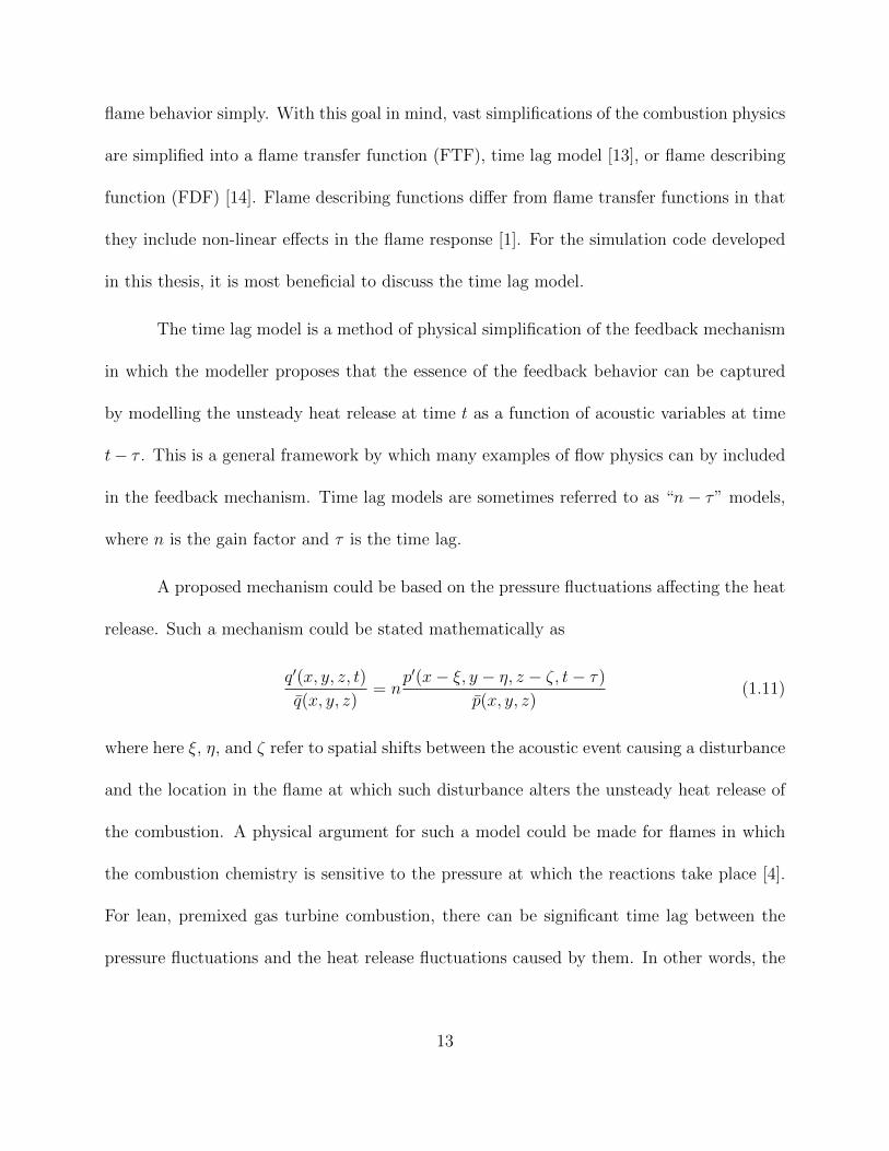
in this thesis, it is most beneficial to discuss the time lag model.

The time lag model is a method of physical simplification of the feedback mechanism

in which the modeller proposes that the essence of the feedback behavior can be captured

by modelling the unsteady heat release at time t as a function of acoustic variables at time

t− τ . This is a general framework by which many examples of flow physics can by included

in the feedback mechanism. Time lag models are sometimes referred to as “n− τ” models,

where n is the gain factor and τ is the time lag.

A proposed mechanism could be based on the pressure fluctuations affecting the heat

release. Such a mechanism could be stated mathematically as

q′(x, y, z, t)

q(x, y, z)= n

p′(x− ξ, y − η, z − ζ, t− τ)

p(x, y, z)(1.11)

where here ξ, η, and ζ refer to spatial shifts between the acoustic event causing a disturbance

and the location in the flame at which such disturbance alters the unsteady heat release of

the combustion. A physical argument for such a model could be made for flames in which

the combustion chemistry is sensitive to the pressure at which the reactions take place [4].

For lean, premixed gas turbine combustion, there can be significant time lag between the

pressure fluctuations and the heat release fluctuations caused by them. In other words, the

13

lean premixed flame chemistry does not necessarily respond instantaneously to the pressure

oscillations at frequencies typically seen [10].

Another scenario in which the acoustic pressure can be the primary property in the

feedback mechanism occurs when the injection of unburned mixture into the chamber occurs

transverse to the direction of acoustic oscillation for a given mode. In this case, the oscillating

pressure in the chamber gives oscillating resistance to the injection path. In this way, the

oscillating pressure seen by the injection causes an oscillation in the flow rate, leading to

pulsing of the injected flow. The pulsing can then be linked to mass conversion rate of the

combustion process and coherent structures created from the lip of the injector [15].

Another acoustic variable which can have a significant impact on the unsteady heat

release is the acoustic velocity. The mathematical expression relating to this mechanism

could be

q′(x, y, z, t)

q(x, y, z)= n

u′(x− ξ, y − η, z − ζ, t− τ)

u(x, y, z). (1.12)

Note that in regions of low Mach number, the mean velocity in the denominator could

cause a large predicted growth rate. Instead, the model could be normalized by the local

sound speed, which would in effect multiply the gain by the local Mach number. Superposed

on the mean and turbulent velocities, the acoustic velocity aerodynamically changes the

shape of the flame. Additionally, the flame can be locally wrinkled by the acoustic velocity,

causing local increases in the heat release due to surface area enhancement. Aside from

direct modification of the flame shape, the acoustic velocity can also trigger vortex shedding

14

from the lip of a backward facing step. The vortex that is shed then convects at a speed

related to the mean velocity and wrinkles the flame. This mechanism is commonly proposed

for dump combustors [16].

A final mechanism can for feedback coupling in premixed flames is based on equiva-

lence ratio fluctuations [17]. The pressure and velocity oscillations at the fuel injection site

can cause the local equivalence ratio to vary, as well as the level of unmixedness. For lean

premixed flames near the blow-off limit, small changes in equivalence ratio can have large

effects. This mechanism is not applicable to scenarios in which the premixing takes place in

a volume acoustically isolated from the combustion.

1.4 Mitigation of Large Amplitude Limit Cycles

Passive and active control of combustion instabilities is an open and very active

topic of research [18]. Aside from modifying designs to adjust time lag relationships and

hence diminish instability mechanisms, passive and active components can be added to the

combustion system to mitigate large amplitude limit cycles. While effective active controls

have been demonstrated [18], they often require too much input energy or increase the level of

pollutants such that their implementation in engines is not justified. The most common type

of passive control for mitigating combustion acoustics is an acoustically absorbing combustor

liner or resonators [19, 20]. When multiple acoustic modes are excited by the unsteady heat

release in a combustor, multiple resonators tuned to different frequencies can be used [21].

15

1.5 Predictive Tools for Combustion Instabilities

1.5.1 Transfer Matrix Approach

On of the most common approaches to predicting linear stability is the use of transfer

matrices [22] to represent volume elements, connected at nodes where acoustic variables are

specified. The transfer matrix on an element relates the acoustic variables on either of its

sides based on solutions to the linearized Euler equations. A given geometry can be broken

piecewise into many elements and an overall transfer matrix with boundary conditions can

be solved numerically for the complex eigenfrequencies. Flame elements can be used which

introduce time lag heat release models as source terms to the linearized Euler equations. The

imaginary part of the eigenfrequencies, which is introduced mainly through a flame element,

indicates the linear stability of the system. This tools is subject to the assumption of one-

dimensional acoustic propagation. It is limited to evaluating the stability of longitudinal

modes. Additionally, the flame dynamics must be captured by a one-dimensional flame

transfer function.

1.5.2 Modal Expansion with Spatial Averaging

Application of the method of spatial averaging for approximate treatment of com-

bustion instabilities was introduced by Culick in his doctoral thesis [23]. The method was

16

recently summarized by [8]. In this approach, the acoustic wave equation is solved with

source terms on the right hand side accounting for heat release and mean flow effects. An

approximate solution is constructed by using the modeshapes (eigenfunctions) from the ho-

mogeneous problem as basis functions for an eigenfunction expansion. A weighted residual

method is then used, with the homogeneous modeshapes as the weighting functions, to in-

tegrate the wave equation spatially and obtain a second-order ODE in time. This ODE

resembles a simple harmonic oscillator with source terms stemming from heat release, mean

flow, and boundary effects. A numerical ODE solver is used to obtain the temporal devel-

opment of a given mode. Depending on the type of model, linear or non-linear, a linear

growth rate or limit cycle amplitude can be approximated with this method. This predic-

tive methodology is subject to its assumption that the heat release, from the supplied flame

response function, is weak relative to the acoustic behavior of the chamber. Appendix D

provides further details into the possible shortcomings of this method, as pointed out by

[24]. This approximate treatment of combustion instabilities was implemented in the Gen-

eralized Instability Model [25], which runs on the MATLAB platform. GIM is a pseudo-3D

implementation, but does not allow the accurate treatment of three-dimensional acoustics

in complex geometries. It primarily targets longitudinal modes, but can also predict trans-

verse modes in geometries with constant cross-sectional areas. Cross-sections are limited to

circular and annular shapes [26].

17

1.5.3 Large Eddy Simulation

A computationally-intensive approach to combustion instability simulation is the di-

rect solution of the Navier-Stokes equations subject to a spatial filter. With large-eddy

simulations (LES), the large turbulent motions are resolved spatially and temporally, and

the smaller eddies that are physically present in the real flow are modelled. With a fine

enough grid, a large percentage of the turbulent kinetic energy can be resolved, while the

prohibitively large computational expense of direct numerical simulation (DNS) is avoided.

Large-eddy simulations were first introduced in the context of meteorology by Smagorin-

sky [27]. With the rapid advance of modern computing power, the large-eddy simulation

has become a staple tool in just about all applications of fluid dynamics. Combustion and

thermoacoustics is no exception [28].

Two primary means of utilizing LES for insight into thermoacoustic instabilities are

the forced response method [29, 30, 1] and the self-excited method [31, 32, 33]. The forced

response method provides artificial acoustic forcing of a simulated flame and extracts the

resulting heat release fluctuations. From the simulation, a flame transfer or non-linear flame

describing function can be constructed [1]. The flame describing function is then useful for

lower order methods, such as the transfer matrix approach or spatial averaging procedure in

performing quick parametric sweeps of operating conditions and flow variables. Self-excited

LES refers to a simulation in which no artificial forcing is introduced. Instead, should

the physics be modelled correctly, the acoustic fluctuations develop on their own with in

18

the simulation. This method targets a physically accurate representation of a combustion

instability. Such self-excited simulations are generally costly, as an entirely new simulation

must be run for any change in flow or boundary conditions. The LES approach to combustion

instabilities, forced response or self-excited, is a promising research field. However, it remains

too time-consuming for complete integration into the current engineering design environment.

1.5.4 Other Methods

Now that some of the predominant methods of analysis for combustion instabilities

have been discussed, a few others are worth mentioning. A quick, low-fidelity method of

predicting combustion instabilties using Green’s functions [23, 34] is related to the devel-

opment of the spatial averaging technique [8]. Dowling [24] showed that this method does

not accurately account for the effect of heat release on the oscillation frequency when such

effects are not small.

A method based on a conservation equation for acoustic energy was developed re-

cently [35]. The conservation equation for acoustic energy is derived from the governing

equations, but much care must be take to accurately model each term. The capacity to

model viscous and boundary losses is built into the method. The method provides the

ability to approximate acoustic gains and losses at any frequency, regardless of the natural

acoustic frequencies of the chamber.

19

Other numerical approaches include the use of existing commercial software for acous-

tic predictions, such as Virtual Lab [36]. Such software provides a frequency-domain solution

to the acoustics in the combustion chamber with the ability to incorporate inhomogeneous

media effects and mean flow. While this is useful for predicting the frequencies at which

combustion instabilities are possible, it has no way to predict the stability of any modes.

Finally, most related to this thesis, Jemkov [37] solved the thermoacoustic equations

on a Cartesian finite volume mesh for a Rijke tube. To some extent, this thesis is an extension

of this method for unstructured grids with an improved flux calculation to correctly account

for density gradients.

1.5.5 Motivation for the Present Work

Examining the predictive tools described above, two fundamental approaches can

be seen. The first is the approximate and one-dimensional methods, such as the transfer

matrix approach and GIM. These approaches offer quick turn-around times and convenient

“back-of-the-envelope” approximations. A much greater degree of fidelity is achieved with

LES, which resolves the full three-dimensional geometry, as well as the large-scale turbulent

dynamics of the fluid flow and flame. The LES approach suffers from long turn-around

times which becomes prohibitive for parametric studies required for design. The present

work attempts to fill the gap in between the rough, quick methods and the thorough, costly

20

methods with a predictive tool representative (tacFoam) of a compromise in computational

cost and physical fidelity, Fig. 1.5.

tacFoam

GIM/TMA

LESIn

cre

ase

d F

ide

lity

Increased Cost

Figure 1.5: Cost vs. fidelity comparison for combustion instability predictive tools.

1.6 Thesis Contributions

The main contributions of this thesis to the state of the art are summarized as follows:

(1) Development, verification, and validation of a novel simulation technique in which

pre-computed three-dimensional mean flows are mapped onto an unstructured finite volume

mesh, where the linear Euler equations are solved with non-linear heat release models for

arbitrary three-dimensional geometries with a broad range of time lag based heat release

models. The three-dimensionality of mean field quantities (heat release, density, velocity,

21

etc...) as well as acoustic quantities are resolved in this method without the computational

expense of a full Navier-Stokes solver (LES).

(2) Extension of a high-resolution non-conservative second-order total variation di-

minishing Godunov flux calculation method based on the wave propagation method of [38] to

arbitrarily-oriented faces in an unstructured finite volume mesh suitable for complex engine

geometries.

1.7 Thesis Outline

This thesis is organized as follows:

Chapter 2: Derivation the linear thermoacoustic equations from the governing equa-

tions of fluid flow.

Chapter 3: Derivation of the wave structure of linear acoustics in inhomogeneous

media for an arbitrarily-oriented face. Application of these derivations in the development

of a non-conservative flux formulation for unstructured finite volume meshes.

Chapter 4: Verification of the present implementation of the numerical approach in

open source software. Comparison with various academic problems with analytical solution

demonstrating the ability of the solver to model the basic physics involved in thermoacoustic

instabilities.

22

Chapter 5: Application and validation of the present implementation of the numerical

method to laboratory-scale experiments. Demonstration of the code’s ability to utilize exist-

ing empirically-correlated non-linear heat release functions as well as its ability to implement

a physics-based vortex shedding model.

23

CHAPTER 2GOVERNING EQUATIONS

2.1 Governing Equations of Fluid Flow

The governing equations of fluid flow are the starting point for arriving at the gov-

erning equations for thermoacoustics. Appendix A provides a detailed derivation of these

equations. For the purposes of this thesis, thermoacoustics relating to the combustion of

premixed gases, the mass source is neglected, M = 0. As viscous forces tend to play a

small role in linear acoustics, forces other than the pressure force is neglected, (Fi = 0).

Accordingly, the contribution of viscous dissipation to the energy equation. The heat release

term on the right hand side of the energy equation is not neglected, Q 6= 0, as it plays a

defining role in the development of thermoacoustic instabilities. The resulting equations for

fluid flow are summarized below in both conservative and non-conservative form.

2.1.1 Conservative Form Equations

Mass:

∂ρ

∂t+∂(ρuj)

∂xj= 0 (2.1)

24

Momentum:

∂(ρui)

∂t+∂(ρujui + pδij)

∂xj= 0 (2.2)

Energy:

∂[ρ(e+ 12uiui)]

∂t+∂[ρuj(e+ 1

2uiui + p

ρ)]

∂xj= Q (2.3)

Pressure (energy):

∂[p+ 12(γ − 1)ρuiui]

∂t+∂[γujp+ 1

2(γ − 1)ρujuiui]

∂xj= (γ − 1)q (2.4)

2.1.2 Non-Conservative Form Equations

Density (Mass):

∂ρ

∂t+ ρ

∂uj∂xj

+ uj∂ρ

∂xj= 0 (2.5)

Velocity (Momentum):

ρ∂ui∂t

+ ρuj∂ui∂xj

+∂p

∂xjδij = 0 (2.6)

Temperature (Energy):

ρcv∂T

∂t+ ρcvuj

∂T

∂xj= −p∂uj

∂xj+ q (2.7)

or

ρcp∂T

∂t+ ρcpuj

∂T

∂xj=∂p

∂t+ uj

∂p

∂xj+ q (2.8)

25

Pressure (Energy):

∂p

∂t+ uj

∂p

∂xj+ γp

∂uj∂xj

= (γ − 1)q (2.9)

2.2 Expansion and Linearization

The equations summarized above represent equations for the instantaneous variables

of the flow. For acoustic analysis, the mean flow is not the primary interest, but rather the

small signal perturbations on the mean flow. For this reason, the governing equations listed

above are decomposed into mean and fluctuating (acoustic) parts and expanded about the

mean using a perturbation parameter (ε). The equations can then be linearized by keeping

only first order terms in ε. In the linearization process, other parameters appear in connection

with mean flow velocity as well as mean property and flow gradients. In the following, the

pressure form of the energy equation will be used, because acoustics is generally expressed

primarily in terms of pressure and velocity. Temperature is then expressed through the

equation of state.

26

2.2.1 Decomposition

First, each of the variables are split into mean and fluctuating (acoustic) quantities

ρ = ρ+ ρ′

u = u+ u′

p = p+ p′

q = q + q′

(2.10)

Despite its resemblance to the Reynolds averaging procedure in the analysis of tur-

bulent fluctuations, this decomposition in terms of acoustics is performed here without any

regard for turbulent fluctuations. Key distinctions between turbulence and acoustics is the

magnitude of the fluctuations for different quantities and the spectral nature of the phenom-

ena. Turbulence is by nature dissipative and broadband, while acoustics (in the linear sense)

is conservative and occurs at discrete frequencies. This simplistic view of the physics of

turbulent flows with acoustics, namely the lack of interaction between the two fields, is jus-

tified primarily by two facts in field of combustion instabilities. First, the turbulent sources

of noise are overwhelmingly small compared to the combustion sources. Secondly, in the

linearization process, the acoustic disturbances are assumed very small compared to their

mean properties, hence the acoustic field is not strong enough to influence the turbulence,

except perhaps to trigger the laminar-to-turbulent transition. Substitution of Eq. (2.10) into

the governing equations, Eqs. (2.1) - (2.4), and algebraic manipulation yields the expanded

forms of these equations.

27

Mass:

∂ρ∂t

+ ∂ρ′

∂t+ ρ

∂uj∂xj

+ ρ∂u′j∂xj

+ ρ′∂uj∂xj

+ ρ′∂u′j∂xj

+uj∂ρ∂xj

+ uj∂ρ′

∂xj+ u′j

∂ρ∂xj

+ u′j∂ρ′

∂xj= 0

(2.11)

Momentum:

ρ∂ui∂t

+ ρ∂u′i∂t

+ ρ′ ∂ui∂t

+ ρ′∂u′i∂t

+ρuj∂ui∂xj

+ ρuj∂u′i∂xj

+ ρu′j∂ui∂xj

+ ρ′uj∂ui∂xj

+ρu′j∂u′i∂xj

+ ρ′uj∂u′i∂xj

+ ρ′u′j∂ui∂xj

+ ρ′u′j∂u′i∂xj

+ ∂p∂xi

+ ∂p′

∂xi= 0

(2.12)

Energy (Pressure):

∂p∂t

+ ∂p′

∂t

+uj∂p∂xj

+ uj∂p′

∂xj+ u′j

∂p∂xj

+ u′j∂p′

∂xj

+γp∂uj∂xj

+ γp∂u′j∂xj

+ γp′∂uj∂xj

+ γp′∂u′j∂xj

= (γ − 1)Q+ (γ − 1)q′

(2.13)

2.2.2 Mean Equations

The equations for the mean flow are obtained by taking only the terms that are zeroth

order in fluctuating parameters. In the limit ε→ 0, all other terms become vanishingly small.

Mass:

∂ρ

∂t+ ρ

∂uj∂xj

+ uj∂ρ

∂xj= 0 (2.14)

28

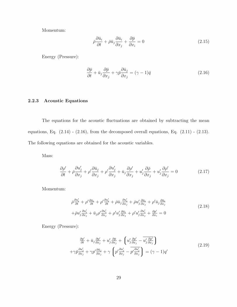
Momentum:

ρ∂ui∂t

+ ρuj∂ui∂xj

+∂p

∂xi= 0 (2.15)

Energy (Pressure):

∂p

∂t+ uj

∂p

∂xj+ γp

∂uj∂xj

= (γ − 1)q (2.16)

2.2.3 Acoustic Equations

The equations for the acoustic fluctuations are obtained by subtracting the mean

equations, Eq. (2.14) - (2.16), from the decomposed overall equations, Eq. (2.11) - (2.13).

The following equations are obtained for the acoustic variables.

Mass:

∂ρ′

∂t+ ρ

∂u′j∂xj

+ ρ′∂uj∂xj

+ ρ′∂u′j∂xj

+ uj∂ρ′

∂xj+ u′j

∂ρ

∂xj+ u′j

∂ρ′

∂xj= 0 (2.17)

Momentum:

ρ∂u′i∂t

+ ρ′ ∂ui∂t

+ ρ′∂u′i∂t

+ ρuj∂u′i∂xj

+ ρu′j∂ui∂xj

+ ρ′uj∂ui∂xj

+ρu′j∂u′i∂xj

+ ujρ′ ∂u′i∂xj

+ ρ′u′j∂ui∂xj

+ ρ′u′j∂u′i∂xj

+ ∂p′

∂xi= 0

(2.18)

Energy (Pressure):

∂p′

∂t+ uj

∂p′

∂xj+ u′j

∂p∂xj

+u′j ∂p′∂xj

− u′j∂p′

∂xj

+γp

∂u′j∂xj

+ γp′∂uj∂xj

+ γ

p′ ∂u′j∂xj− p′ ∂u

′j

∂xj

= (γ − 1)q′(2.19)

29

The above equations are large and contain many terms that are, in general, difficult

to model. From here, the task at hand is judging the relative importance of the terms in each

of the equations. With such judgements in hand, for a given application and desired fidelity,

many of the terms in Eqs. (2.17) - (2.19) can be omitted. In the following three section,

parameters are defined which allow for the quantitative analysis of the relative magnitude

of the terms in the acoustic equations above.

2.2.4 Reference Parameters

In order to proceed with asymptotic analysis of the non-linear acoustic equations

stated above, a number of expansion parameters are now defined. These parameters can be

given precise definitions, by which they relate the relative importance of the terms in Eq.

(2.17) - (2.19). To reduce the number of parameters and simplify the analysis, the practical

approach is to group the expansion parameters by orders of magnitude. It is first useful

to establish reference values to which the expansion parameters can be compared, given in

Table 2.1.

Table 2.1: Reference parameters useful for analysis of acoustic equations.

Length Velocity Time Density Pressure Heat Release

SI Units m m/s sec kg/m3 Pa W/m3

Reference Lr ar tr ∼ Lrar

ρr pr ∼ ρra2r qr

30

2.2.5 Perturbation Parameters

The mean quantities from Eq. (2.10) are, by definition, on the same order of mag-

nitude as the reference quantities specified above. The fluctuating quantities defined in Eq.

(2.10) are now related to the reference quantities (and, hence, the mean quantities). These

are denoted as perturbation parameters, because typical analysis treats them as overwhelm-

ingly small compared to unity. Analysis, then, is often performed in their limit approaching

zero. The relevant perturbation quantities are given in Table 2.2.

Table 2.2: Reference parameters useful for analysis of acoustic equations.

Pressure Velocity Density Heat Release

εp εu ερ εq

p′

pru′

ar

ρ′

ρr

q′

qr

2.2.6 Mean Field Parameters

The mean flow and mean gradients are completely independent of the acoustic vari-

ables, and hence must be characterized by a separate group of parameters unrelated to the

perturbation parameters. These are differentiated from perturbation parameters in that they

are not a specification of acoustic disturbance magnitudes, but rather a specification of the

influence of mean flow and mean gradients on the acoustic behavior. Therefore, the main

31

result of these parameters is the ability to compare the relative importance (or negligibility)

of terms arising in the acoustic equations containing these mean flow quantities.

Table 2.3: Definitions of mean field parameters for analysis of acoustic oscillations.

Mean Flow Mean Flow Gradient Mean Density Gradient Mean Pressure Gradient

µ νu νρ νp

uar

Lru∂u∂x

Lrρ∂ρ∂x

Lrp∂p∂x

2.2.7 Estimates of Terms in Acoustic Equations

The reference definitions allow for the temporal and spatial derivatives of acoustic

variables to be estimates as

∂

∂t∼ 1

tr∼ arLr

(2.20)

and

∂

∂x∼ 1

Lr. (2.21)

Based on the acoustic equations to first order in these perturbation parameters, Eqs.

(2.17) - (2.19), it is possible to collapse the acoustic description into a single perturbation

parameter

ε ∼ εp ∼ εu ∼ ερ. (2.22)

32

Culick [8] collapses these into a single parameter µ by arguing their relations through

the mean equations. This assumes that each term in the mean equations is equally important,

which may not be the case depending on the flow. Instead, it is enough to evaluate an

estimate for the mean heat release, starting with

q ∼ ρucp∆T (2.23)

and assuming that, for a deflagration wave, the temperature rise across a flame translates

into a density drop with negligible change in pressure

q ∼ µνρρra3r (2.24)

indicating that a consistent evaluation of thermoacoustics typically should include at least

first order terms in µ and νρ. The exception would be situations with strong flame transfer

functions, where εq ∼ 1 >> ε. Each term for the mass, momentum, and energy equations

are analyzed using the parameters established above in Table 2.4, Table 2.5, and Table 2.6.

2.3 Linear Acoustic Equations

Neglecting all terms which are of order ε2 or higher, the equations become linearized

in terms of the acoustic variables. Also, the mean flow is assumed to change very slowly

compared to the acoustic fluctuations, so the time derivative of any mean flow variables is

negligible as well.

33

Table 2.4: Estimations for terms in mass equation

Term Estimation Order

∂ρ′

∂t∼ ε ρr arL O(ε)

ρ∂u′j∂xj

∼ ε ρr arL O(ε)

ρ′∂uj∂xj

∼ µνuερr arL O(µνuε)

ρ′∂u′j∂xj

∼ ε2 ρr arL O(ε2)

uj∂ρ′

∂xj∼ µε ρr arL O(µε)

u′j∂ρ∂xj

∼ νρερr arL O(νρε)

u′j∂ρ′

∂xj∼ ε2 ρr arL O(ε2)

Mass:

∂ρ′

∂t+ ρ

∂u′j∂xj

+ ρ′∂uj∂xj

+ uj∂ρ′

∂xj+ u′j

∂ρ

∂xj= 0 (2.25)

Momentum:

ρ∂u′i∂t

+ ρuj∂u′i∂xj

+ ρu′j∂ui∂xj

+ ρ′uj∂ui∂xj

+∂p′

∂xi= 0 (2.26)

Energy (Pressure):

∂p′

∂t+ uj

∂p′

∂xj+ u′j

∂p

∂xj+ γp

∂u′j∂xj

+ γp′∂uj∂xj

= (γ − 1)q′ (2.27)

34

Table 2.5: Estimations for terms in momentum equation


ρ∂u′i∂t

∼ ε ρr a2r

L O(ε)

ρ′∂u′i∂t

∼ ε2 ρr a2r

L O(ε2)

ρuj∂u′i∂xj

∼ µε ρr a2r

L O(µε)

ρu′j∂ui∂xj

∼ µνuερr a2

r

L O(µνuε)

ρ′uj∂ui∂xj

∼ µ2νuερr a2

r

L O(µ2νuε)

ρu′j∂u′i∂xj

∼ ε2 ρr a2r

L O(ε2)

ujρ′ ∂u′i∂xj

∼ µε2 ρr a2r

L O(µε2)

ρ′u′j∂ui∂xj

∼ µνuε2 ρr a

2r

L O(µνuε2)

ρ′u′j∂u′i∂xj

∼ ε3 ρr a2r

L O(ε3)

∂p′

∂xi∼ ε prL ∼ ε ρr a

2r

L O(ε)

35

Table 2.6: Estimations for terms in energy (pressure) equation


∂p′

∂t∼ ε pr arL O(ε)

uj∂p′

∂xj∼ µε pr arL O(µε)

u′j∂p∂xj

∼ νpεpr arL O(νpε)

u′j∂p′

∂xj∼ ε2 pr arL O(ε2)

γp∂u′j∂xj

∼ ε pr arL O(ε)

γp′∂uj∂xj

∼ µνuεpr arL O(µνuε)

γp′∂u′j∂xj

∼ ε2 pr arL O(ε2)

(γ − 1)q′ ∼ µνρεqpr arL O(µνρεq)

2.4 Isentropic Linear Acoustic Equations

Use of the isentropic signal assumption, that the entropy fluctuation is everywhere

zero, a relation between p′ and ρ′ can be derived.

ρ′ =p′

a2. (2.28)

This relation precludes the necessity of the linearized mass equation, Eq. (2.25).

Instead, Eq. (2.28) is substituted into Eqs. (2.26) and (2.27), forming a closed set of four

equations which can be solved for the acoustic pressure and acoustic velocity.

36

Momentum:

∂u′i∂t

+ uj∂u′i∂xj

+ u′j∂ui∂xj

+ p′ujγp

∂ui∂xj

+1

ρ

∂p′

∂xi= 0 (2.29)

Energy (Pressure):

∂p′

∂t+ uj

∂p′

∂xj+ u′j

∂p

∂xj+ γp

∂u′j∂xj

+ γp′∂uj∂xj

= (γ − 1)q′ (2.30)

Equations (2.29) and (2.30) are the governing equations used by the present form

of tacFoam. The most serious limitations from the use of these equations is the isentropic

assumption of Eq. (2.28). This precludes the solver from capturing physical effects of entropy

waves on thermoacoustic behavior. To include entropy wave effects, Eqs. (2.25), (2.26), and

(2.27) must be used. This would represent an increase in cost from four to five equations

that must be solved numerically.

2.5 Classical Acoustic Equations

Furthermore, neglecting all terms relating to mean flow and mean property gradients,

the equations of classical acoustics are obtained, with the obvious exception of retaining the

source term in the energy equation.

Mass:

∂ρ′

∂t+ ρ

∂u′j∂xj

= 0 (2.31)

37

Momentum:

ρ∂u′i∂t

+∂p′

∂xi= 0 (2.32)

Energy (Pressure):

∂p′

∂t+ γp

∂u′j∂xj

= (γ − 1)q′ (2.33)

The wave equation for the acoustic pressure and velocity can be obtained using only

the momentum and energy equations, Eq. (2.32) and Eq. (2.19), respectively. The wave

equation for the acoustic pressure is built by differentiating Eq. (2.33) in time and differen-

tiating Eq. (2.32) in space and subtracting the results.

∂2p′

∂t2+γp

ρ

∂2p

∂xj= (γ − 1)

∂q′

∂t(2.34)

The heat release term has been carried through to illustrate a main idea in combustion

acoustics. The unsteady heat release related to fluctuations in the flame from chemical and

fluid dynamical effects acts as a forcing term in the acoustic wave equation. While it is true

that many of the terms neglected to obtain the wave equation above can play significant

roles in the acoustic behavior of combustion chambers, the main point remains. A physical

correlation between the heat release fluctuations and the acoustic variables may provide a

feedback pathway by which the acoustic field can be excited or damped.

38

CHAPTER 3NUMERICAL APPROACH

3.1 Numerical Considerations

The design of a numerical method for a given purpose relies heavily on the goals and

challenges for its particular set of predictive uses. In the case of tacFoam, the prediction

of thermoacoustic instabilities includes accounting for a number of physics which may drive

or damp a particular mode. These physical effects include unsteady heat release, boundary

conditions, viscous diffusion, and mean flow interactions. While the governing equations may

be adjusted based on the physics one may attempt to capture, the delicate balance between

driving and damping forces means that the effects of numerical dissipation are particularly

unwanted. Numerical dissipation, common to any stable approach to computational fluid

dynamics, can pollute the physical insight of the solution if its magnitude is not managed to

be much lower than the operating physical mechanisms. To this end, the present numerical

method is designed for low numerical dissipation.

An additional consideration for the numerical method design at hand is the goal of

applying the predictive tool to the complex geometries of gas turbine combustion chambers.

This application makes the use of structured grids difficult; the construction of a structured

39

or block-structured grid represents a bottleneck in the user time needed to extract a useful

solution from such a scheme. For this reason, many production level codes have resorted to

unstructured finite volume methods, including OpenFOAM [39]. Such a method provides

the necessary flexibility in domain definition and mesh construction for efficient application

of numerical methods to complex geometries.

There are two main approaches in computational fluid dynamics to designing nu-

merical schemes with low dissipation: high-order methods and high-resolution methods.

High-order methods, here in reference to spatial discretization of fourth order or higher, can

be used to construct low dissipation schemes, but can encounter difficulties at sharp gradi-

ents of solution variables or media [40]. Additionally, in the context of unstructured finite

volume methods, the application of higher-order methods is particularly difficult. On the

other hand, the high-resolution approach is very attractive. High-resolution approaches use

the generalized Riemann problem to construct low dissipation schemes with second-order

accuracy. This approach is easily applicable to unstructured finite volume methods and is

particularly well-suited for wave propagation in discontinuous media, such as the large mean

density gradients present across a flame. An introduction to the basics of the Riemann solver

approach is given in [41, 40], with the main ideas summarized in Appendix B of this thesis.

40

3.2 Governing Equations as a Three Dimensional Hyperbolic System

The governing equations are derived in the preceding chapter, Eqs. (2.29) and (2.30).

In order to phrase these as a linear hyperbolic system, the terms related to gradients of mean

quantities are move to the right hand side to be treated as source terms.

∂p′

∂t+ uj

∂p′

∂xj+ γp

∂u′j∂xj

= (γ − 1)q′ − u′j∂p

∂xj− γp′∂uj

∂xj(3.1)

∂u′i∂t

+ uj∂u′i∂xj

+1

ρ

∂p′

∂xi= −u′j

∂ui∂xj− p′ uj

γp

∂ui∂xj

(3.2)

The system of hyperbolic equations for tacFoam contains four equations.

∂p′

∂t+ u

∂p′

∂x+ v

∂p′

∂y+ w

∂p′

∂z+ γp

∂u′∂x

+∂v′

∂y+∂w′

∂z

=

(γ − 1)q′ −u′ ∂p

∂x+ v′

∂p

∂y+ w′

∂p

∂z

− γp′∂u∂x

+∂v

∂y+∂w

∂z

(3.3)

∂u′

∂t+ u

∂u′

∂x+ v

∂u′

∂y+ w

∂u′

∂z+

1

ρ

∂p′

∂x=

−u′∂u

∂x+ v′

∂u

∂y+ w′

∂u

∂z

− p′

γp

u∂u∂x

+ v∂u

∂y+ w

∂u

∂z

(3.4)

∂v′

∂t+ u

∂v′

∂x+ v

∂v′

∂y+ w

∂v′

∂z+

1

ρ

∂p′

∂y=

−u′ ∂v

∂x+ v′

∂v

∂y+ w′

∂v

∂z

− p′

γp

u ∂v∂x

+ v∂v

∂y+ w

∂v

∂z

(3.5)

∂w′

∂t+ u

∂w′

∂x+ v

∂w′

∂y+ w

∂w′

∂z+

1

ρ

∂p′

∂z=

−u′∂w

∂x+ v′

∂w

∂y+ w′

∂w

∂z

− p′

γp

u∂w∂x

+ v∂w

∂y+ w

∂w

∂z

. (3.6)

41

For three dimensional equations, a system of hyperbolic equations can be written in

the form

∂φ˜∂t

+f˜(φ˜)

∂x+g˜(φ˜)

∂y+h˜(φ˜)

∂z= S≈

(φ˜) (3.7)

where f , g, and h are the flux functions in each of the three Cartesian directions. The

Jacobian matrix in each direction can be constructed such that

A≈

= ∂f˜/∂φ˜ (3.8)

B≈

= ∂g˜/∂φ˜ (3.9)

C≈

= ∂h˜/∂φ˜ (3.10)

and the hyperbolic system can be rewritten in non-conservative form as

∂φ˜∂t

+ A≈

∂φ˜∂x

+B≈

∂φ˜∂y

+ C≈

∂φ˜∂z

= S≈

(φ˜). (3.11)

The tacFoam equations from Eqs. (3.3) - (3.6) constitute a 4x4 hyperbolic system in

the form of Eq. (3.11). The vector of solution variables is

φ˜ =

p′

u′

v′

w′

(3.12)

42

and the Jacobian matrices in each direction are

A≈

=

u γp 0 0

1ρ

u 0 0

0 0 u 0

0 0 0 u

(3.13)

B≈

=

v 0 γp 0

0 v 0 0

1ρ

0 v 0

0 0 0 v

(3.14)

C≈

=

w 0 0 γp

0 w 0 0

0 0 w 0

1ρ

0 0 w

(3.15)

and the source vector is

S˜(φ˜) =

(γ − 1)q′ −u′ ∂p

∂x+ v′ ∂p

∂y+ w′ ∂p

∂z

− γp′∂u∂x

+ ∂v∂y

+ ∂w∂z

−u′ ∂u

∂x+ v′ ∂u

∂y+ w′ ∂u

∂z

− p′

γp

u∂u∂x

+ v ∂u∂y

+ w ∂u∂z

−u′ ∂v

∂x+ v′ ∂v

∂y+ w′ ∂v

∂z

− p′

γp

u ∂v∂x

+ v ∂v∂y

+ w ∂v∂z

−u′ ∂w

∂x+ v′ ∂w

∂y+ w′ ∂w

∂z

− p′

γp

u∂w∂x

+ v ∂w∂y

+ w ∂w∂z

. (3.16)

43

3.3 Finite Volume Formulation for an Unstructured Grid

Most modern CFD codes with heavy use in industry employ unstructured finite vol-

ume methods. This method allows great flexibility in terms of mesh topology and domain

geometry. The OpenFOAM C++ libraries are written for finite volume methods with un-

structured grids. Therefore, it is necessary to write the hyperbolic systems with an unstruc-

tured grid in mind. For a finite volume method, the governing equations are integrated over

an arbitrary control volume, Ω, to yield

y

Ω

∂φ˜∂tdV +

y

Ω

A≈ ∂φ˜∂x +B≈

∂φ˜∂y

+ C≈

∂φ˜∂z

dV =y

Ω

S≈

(φ˜)dV. (3.17)

For constant coefficient equations, the coefficient matrices (Jacobians) can be taken

inside the derivatives

y

Ω

∂φ˜∂tdV +

y

Ω

∂A≈φ˜∂x +∂B≈φ˜

∂y+∂C≈φ˜

∂z

dV =y

Ω

S≈

(φ˜)dV. (3.18)

The divergence theorem can now be implemented to convert the second volume inte-

gral on the left hand side into a surface integral. For an arbitrarily oriented face with unit

normal vector given by

n = (nx, ny, nz)T (3.19)

this term can be written as

∂A≈φ˜

∂x+∂B≈φ˜

∂y+∂C≈φ˜

∂z=

(J≈φ˜)j

∂xj(3.20)

44

where the Jacobian is given by

J≈

= A≈nx +B

≈ny + C

≈nz. (3.21)

Using the divergence theorem, the second volume integral of Eq. (3.18) then becomes

y

Ω

∂A≈φ˜∂x +∂B≈φ˜

∂y+∂C≈φ˜

∂z

dV =x

∂Ω

J≈φ˜ · ndS. (3.22)

For the arbitrarily-oriented face, this Jacobian matrix is now the equivalent flux

matrix as for a one-dimensional case. Analysis to calculate the flux from this matrix proceeds

as for the one-dimensional case. For the tacFoam hyperbolic set, the Jacobian is given by

J≈

=

U γpnx γpny γpnz

nxρ

U 0 0

nyρ

0 U 0

nzρ

0 0 U

(3.23)

where the face-normal mean velocity is given by

U = u˜ · n = unx + vny + wnz. (3.24)

The flux at a cell face is given by

f˜face =J≈φ˜face

(3.25)

the total flow through the cell face is given by the integration over the surface

F˜ face =x

face

J≈φ˜dS = f˜faceAface (3.26)

45

using a constant flux approximation for the integration. Likewise, the temporal derivative

is approximated by

y

Ω

∂φ˜∂tdV =

dφ˜centerdt

Vcell (3.27)

and the source term is similarly integrated using the cell-centered values

y

Ω

S≈

(φ˜)dV = S≈

(φ˜center)Vcell. (3.28)

The time advancement at each cell is made by

dφ˜centerdt

= S≈

(φ˜center)−Nfaces∑

i

AiVcell

fi (3.29)

using a four stage explicit Runge-Kutta method. The fluxes f through each face are cal-

culated using a second-order TVD high-resolution upwind method via the Riemann solver

approach.

3.3.1 Wave Structure of the Governing Equations

The eigenvalues of the Jacobian are found by solving

det(J≈− λI

≈) = 0 (3.30)

where I≈

is the identity matrix. This yields the characteristic equation

(U − λ)4 − (n2x + n2

y + n2z)γp

ρ(U − λ)2 = 0. (3.31)

46

Noting the unit normal has a magnitude of one, n2x +n2

y +n2z = 1, the solution to this

equation yields the eigenvalues, λ, which are the wave speeds for a given cell discontinuity

λ1 = U − a λ2 = λ3 = U λ4 = U + a (3.32)

where a = γp/ρ represents the sound speed. These represent a backward travelling acoustic

wave, two transverse component convective waves, and a forward travelling acoustic wave,

respectively. These waves are shown in a characteristic diagram in Fig. 3.1 under the

assumption that the mean face-normal velocity is left to right.

n

>

t

L

*1*3

λ=U

λ=U+a

λ=U-a

R

0

Figure 3.1: Characteristic diagram at a face in the tacFoam hyperbolic system.

The related right eigenvector matrix is

R≈

=

−ZL 0 0 ZR

nx 1 0 nx

ny 0 1 ny

nz −nxnz−nynz

nz

(3.33)

47

where ZL = ρLaL is the acoustic impedance on the left side of the face and ZR = ρRaR is the

acoustic impedance on the right side. Notice here that variation of the mean density and

sound speed across the face is accounted for, whereas such gradients were not allowed in the

application of the divergence theorem leading to Eq. (3.20). Inverting this matrix gives the

left eigenvector matrix

R≈−1 = L

≈=

1

ZR + ZL

−1 ZRnx ZRny ZRnz

0 (ZR + ZL)(n2y + n2

z) −(ZR + ZL)nxny −(ZR + ZL)nxnz

0 −(ZR + ZL)nxny (ZR + ZL)(n2x + n2

z) −(ZR + ZL)nynz

1 ZLnx ZLny ZLnz

.

(3.34)

The characteristic variables are then

w˜ = R≈−1φ˜ =

−p′+ZRU ′ZR+ZL

u′ − nxU ′

v′ − nyU ′

p′+ZLU′

ZR+ZL

(3.35)

where

U ′ = u˜′ · n = u′nx + v′ny + w′nz. (3.36)

48

The wave strengths are then

α˜ = w˜R − w˜L =

−(p′R−p′L)+ZR(U ′R−U

′L)

ZR+ZL

(u′R − u′L)− nx(U ′R − U ′L)

(v′R − v′L)− ny(U ′R − U ′L)

(p′R−p′L)+ZL(U ′R−U

′L)

ZR+ZL

. (3.37)

Multiplying the wave strengths by the right eigenvalues results in the wave vectors.

W˜1 = α1r˜1 =

p′∗1 − p′L

u′∗1 − u′L

v′∗1 − v′L

w′∗1 − w′L

=

ZLZR+ZL

(p′R − p′L)− ZLZRZR+ZL

(U ′R − U ′L)

− nxZR+ZL

(p′R − p′L) + nxZRZR+ZL

(U ′R − U ′L)

− nyZR+ZL

(p′R − p′L) + nyZRZR+ZL

(U ′R − U ′L)

− nzZR+ZL

(p′R − p′L) + nzZRZR+ZL

(U ′R − U ′L)

(3.38)

W˜2 +W˜3 = α2r˜2 + α3r˜3 =

p′∗3 − p′∗1

u′∗3 − u′∗1

v′∗3 − v′∗1

w′∗3 − w′∗1

=

0

(u′R − u′L)− nx(U ′R − U ′L)

(v′R − v′L)− ny(U ′R − U ′L)

(w′R − w′L)− nz(U ′R − U ′L)

(3.39)

W˜4 = α4r˜4 =

p′∗1 − p′L

u′∗1 − u′L

v′∗1 − v′L

w′∗1 − w′L

=

ZRZR+ZL

(p′R − p′L) + ZLZRZR+ZL

(U ′R − U ′L)

nxZR+ZL

(p′R − p′L) + nxZLZR+ZL

(U ′R − U ′L)

nyZR+ZL

(p′R − p′L) + nyZLZR+ZL

(U ′R − U ′L)

nzZR+ZL

(p′R − p′L) + nzZLZR+ZL

(U ′R − U ′L)

. (3.40)

49

3.3.2 Conservative Flux Formulation

To calculate the fluxes for the conservative formulation, the only remaining step is

the use of Roe’s method

f˜face =1

2A≈

(φ˜L + φ˜R)−m∑p=1

|λp|W˜p (3.41)

with the wave speeds and wave vectors of the tacFoam Riemann problem, Eqs. (3.32), (3.38),

(3.39), (3.40). If the coefficients of the non-conservative hyperbolic system present in the

matrices of Eqs. (3.13), (3.14), and (3.15) are not constant in space, the divergence theorem

used in Eq. (3.20) is not applicable because the coefficients cannot be brought inside the

spatial derivatives.

3.3.3 Non-conservative Flux Formulation

If the coefficients of the non-conservative hyperbolic system present in the matrices

of Eqs. (3.13), (3.14), and (3.15) are not constant in space, the divergence theorem used

in Eq. (3.20) is not applicable because the coefficients cannot be brought inside the spatial

derivatives. Instead of this approach, a better formulation is inspired by the wave propa-

gation forms put forward by LeVeque, originally in [38] and more completely in [40]. The

key step for this non-conservative flux formulation is the assumption of piecewise constant

coefficients (mean variables). The coefficients are constant except at each face, where they

50

undergo an finite jump over an infinitesimal distance. The preceding wave analysis remains

valid except at the face, where the discontinuity needs to be taken into account. One minor

change is the use of two different mean velocities. The wave speeds given by Eq. (3.32)

become

λ1 = UL − aL λ2 = λ3 = U+ λ4 = UR + aR (3.42)

where U+ indicates the left mean velocity UL if the face-normal mean velocity is right to

left and UR if the face-normal mean velocity is left to right. The major change in this

formulation only concerns the last step of the previous derivation. Instead of using Roe’s

method to calculate a single flux through the face, it is recognized that two different fluxes

are needed, one for either side of the face. Therefore, the left flux is calculated using

f˜face,L = J≈Lφ˜L +

m∑p=1

(λp)−W˜p (3.43)

and the right flux is calculated using

f˜face,R = J≈Rφ˜R −

m∑p=1

(λp)+W˜p. (3.44)

The non-conservative finite volume formulation uses the left flux when computing the

surface integrals of Eq. (3.22) for the cell on the left of the face and the right flux when

computing the surface integrals for the cell on the right side of the face. Second order TVD

extrapolation is used to obtain the left and right solution variables at each face from the

cell-centered values. It is important to note that, because of the assumption of piecewise

constant mean variables, no extrapolation of the mean variables (pressure, velocity, density)

51

to the faces is performed. The differences between the conservative and non-conservative for-

mulations are depicted in Fig. 3.2. The current version of tacFoam uses this non-conservative

formulation, because verification cases that included mean density gradients (shown in the

next chapter) failed when the conservative formulation was used.

fface,L

n

fface,R

fRfL

fface

n

fRfL

(a) (b)

Figure 3.2: Schematic showing the flux calculation using (a) Roe’s method – conservative

formulation and (b) non conservative formulation.

3.3.4 Extension to Second-Order Method

Second-order methods can be constructed by evaluating the gradient of each solution

variable at each cell center and extrapolating the cell center variables to either side of the

face using this gradient. For a given variable

φL = φL,center + Ψ∂φ

∂n

∣∣∣∣L

(x˜face − x˜center) (3.45)

52

and

φR = φR,center + Ψ∂φ

∂n

∣∣∣∣R

(x˜face − x˜center) (3.46)

where Ψ is a total variation diminishing (TVD) slope limiter. That is, when the solution

varies smoothly, Ψ = 1 and the method is second-order. When there is a sharp gradient in

the solution near a face, 0 < Ψ < 1 and the method is reduced to first-order. The limiter of

Barth and Jespersen [42] is used for tacFoam.

3.4 Practical Considerations

3.4.1 Initialization

With no forcing, the numerical scheme must initialized with noise in order to provide

acoustic energy for modes in the frequency of interest. This can be done either by specifying

initial conditions with spatial white noise or by adding a forcing term in a region of the

domain for a given startup time. After the startup time is complete, the forcing is turned

off and the main part of the simulation can be started.

3.4.2 Calculation of Resonant Frequencies

The solver advances the solution for a satisfactory amount of time with probes placed

in locations away from any expected pressure nodes. The probes read pressure data at a

53

single point in the domain for each time step and write to a file. The probe signals are

analyzed in the frequency domain after performing a fast-Fourier transform (FFT) on the

data. Since the initial conditions contain wavenumbers (and hence, frequencies) across the

entire spectrum, those corresponding to the resonant frequencies of the domain dominate the

spectrum from the transformed probe data. Sharp peaks in the spectrum mark the resonant

frequencies, which are calculated with a frequency domain resolution inversely proportional

to the total time of the simulation.

3.4.3 Calculation of Modeshapes

Modeshapes can be calculated from the tacFoam solver using a discrete Fourier trans-

fer (DFT) calculation which is calculated during the simulation time. The DFT is carried

out as a numerical integration (or summation) which is updated at each time step for each

cell in the domain. Because a DFT can be very costly when calculated at each cell in a large

domain, it is more efficient to calculate the DFT for only a few frequencies rather than the

whole spectrum. In general, a second simulation is required to calculate the modeshapes for

a given domain, because the user must know the resonant frequencies a-priori in order to

specify the frequencies for the DFT calculation. In most cases, the DFT is costly enough

such that running two simulations with negligible computational effort spent on the DFT for

only a few frequencies on interest (Fig. 3.3a) is much faster than the expense of computing

the DFT for a single simulation over the entire frequency domain (Fig. 3.3b). The results

54

of the DFT give the amplitude and phase of fluctuation for a given resonant frequency as

a function of space, which is the acoustic modeshape. As a final note, when the resonant

frequencies are known a-priori (e.g. from an analytical solution), the verification may be

performed in one simulation if the tacFoam code proves that it can match the analytical fre-

quencies, which are specified by the user prior to the first simulation. If small errors in the

tacFoam frequencies exist, an additional simulation may be needed with updated frequencies

to extract the modeshapes from the time domain solver (Fig. 3.3c).

Geometry,

Initial Conditions,

Boundary Conditions

Simulation 1:

Find resonant

frequencies

Simulation 2:

DFT of resonant

frequencies

(a)

(b)

Geometry,

Initial Conditions,

Boundary Conditions

Simulation 1:

DFT of all frequencies,

Find resonant frequencies

Geometry,

Initial Conditions,

Boundary Conditions

Simulation 1:

DFT guess frequencies,

Find resonant frequencies

Simulation 2:

DFT of resonant frequencies(c)

Guess frequencies

=

Resonant frequencies?

No.

Yes.

Done.

Figure 3.3: Flowchart showing the strategy for obtaining resonant frequencies and mode-

shapes from tacFoam simulations.

55

3.4.4 Calculation of Growth Rates

Growth rates for a particular mode can also be calculated from the time domain

data. First, the time domain data from a point probe is filtered with a narrow bandpass

filter (±5Hz) so that only information from the desired mode is retained. Second, the

extrema are selected from the data. Finally, an exponential curve fit is performed through

the absolute values of the extrema. The exponent from this curve fit provides the growth

rate. It is recommended that R2 values are checked to ensure that the fit is appropriate and

a visual inspection of the data is quickly performed if the R2 value is low.

56

CHAPTER 4VERIFICATION

In this chapter, the tacFoam solver is verified for a number of simple problems with

analytical solutions. Key phenomena which tacFoam attempts to account for include mean

flow, mean flow gradients, density gradients, three-dimensional geometries, acoustic bound-

ary conditions, and unsteady heat release. The verification of the solver includes test cases

designed to demonstrate the ability of the solver to accurately capture the physical effects

of these phenomena when compared with known analytical solutions. Derivations of the

analytical solutions corresponding to each verification case can be found in the appendix.

Aside from verification with respect to physical phenomena, the solver is tested for

accuracy in parallel computation. It is important that the numerical solution be indepen-

dent of parallelization across many processors. Finally, the behavior of numerical damping

is quantified with respect to the most influential parameters. The possible pitfalls from

uncontrolled numerical damping are illustrated with suggestions for avoiding them.

57

4.1 Acoustic Verification

The main objective of pure acoustic testing is to verify that the solver produces the

correct resonant frequencies, modeshapes, and/or linear growth rates for problems with the

various important phenomena. A number of simple cases are presented, ranging from one-

dimensional to three-dimensional, in which the solver is tested for its ability to correctly

capture the acoustic behavior for a number of physical effects that are important for the

present application to gas turbine combustion. The resonant frequencies and modeshapes

are used as the metric for the assessment of accuracy.

First, the solver is verified for one-dimensional acoustics in a very simple test. The

first one-dimensional test is a duct with uniform properties and zero mean flow. The objective

of this test is to verify the ability of the solver to replicate results from classical acoustics.

Then the solver is tested in a one-dimensional duct with linearly varying mean temperature

and constant mean pressure. This second test has a smooth variation of mean properties

inside the domain, which provides a first test of the solvers ability to handle density gradients.

Afterwards, the solver is tested with the same one-dimensional duct but with an acoustically-

compact temperature rise. This “thin flame simulation” with steady heat release tests the

ability of the solver to correctly simulate the effect of sharp density gradients on acoustic

modes. The final one-dimensional test returns to a duct with uniform mean properties, but

adds a mean flow.

58

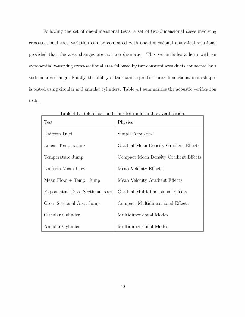
Following the set of one-dimensional tests, a set of two-dimensional cases involving

cross-sectional area variation can be compared with one-dimensional analytical solutions,

provided that the area changes are not too dramatic. This set includes a horn with an

exponentially-varying cross-sectional area followed by two constant area ducts connected by a

sudden area change. Finally, the ability of tacFoam to predict three-dimensional modeshapes

is tested using circular and annular cylinders. Table 4.1 summarizes the acoustic verification

tests.

Table 4.1: Reference conditions for uniform duct verification.

Test Physics

Uniform Duct Simple Acoustics

Linear Temperature Gradual Mean Density Gradient Effects

Temperature Jump Compact Mean Density Gradient Effects

Uniform Mean Flow Mean Velocity Effects

Mean Flow + Temp. Jump Mean Velocity Gradient Effects

Exponential Cross-Sectional Area Gradual Multidimensional Effects

Cross-Sectional Area Jump Compact Multidimensional Effects

Circular Cylinder Multidimensional Modes

Annular Cylinder Multidimensional Modes

59

4.1.1 1D Acoustics in a Uniform Duct

A one-dimensional grid was constructed for the domain (Fig. 4.1) with 100 cells. The

physical parameters of the simulation are shown in Table 4.2.

Table 4.2: Reference conditions for uniform duct verification.

R[J/kg −K] γ p[kPa] ρ[kg/m3] T [K] a[m/s] L[m] f −Range[Hz]

287 1.40 100 1.17 298 346 1.0 87-865

Figure 4.1: The mesh for uniform duct verification.

Linear acoustics in a one-dimensional uniform duct is governed by the wave equation,

resulting in sinusoidal modeshapes. Both closed-closed and closed-open boundary conditions

were simulated. The pressure modeshapes for closed-closed boundaries are given by [43]

ψ(z) = cos(nπz/L) (4.1)

with corresponding frequencies (in Hz) of

fn =na

2L(4.2)

For closed-open boundaries, the modeshapes become

ψ(z) = cos((n− 1/2)πz/L) (4.3)

60

with resonant frequencies given (in Hz) by

fn =(n− 1

2)a

2L. (4.4)

The resonant frequencies for the first five modes found by the solver are compared

in Fig. 4.2 with the analytical values from Eqs. (4.2) and (4.4). As shown in Fig. 4.3, the

frequency errors were less than 0.6%, mostly falling within the resolution uncertainty of the

FFT. Figure 4.4 shows the comparison of pressure modeshapes for tacFoam DFT solution

against the analytical modeshapes from Eqs. (4.1) and (4.3).

0

200

400

600

800

1000

1 2 3 4 5

Mode

Fre

quency (

Hz)

Theory (Closed-Closed)

tacFoam (Closed-Closed)

Theory (Closed-Open)

tacFoam (Closed-Open)

Figure 4.2: Resonant frequencies for uniform one-dimensional duct.

The ability of the solver to match frequencies and modeshapes with classical acoustic

theory is no surprise, but provides a first check that the numerical algorithm contains no

fatal flaws in its development or implementation.

61

0.0001

0.001

0.01

0.1

1

1 2 3 4 5Mode

Rela

tive F

requency E

rror tacFoam (Closed-Closed)

tacFoam (Closed-Open)

Figure 4.3: Relative frequency errors for uniform one-dimensional duct.

4.1.2 1D Acoustics with a Linear Temperature Distribution

An important physical effect for modelling thermoacoustics in gas turbine combustors

is the effect of inhomogeneous media. The first test applied to tacFoam involving mean

density gradients is a one-dimensional duct with a linear temperature profile and constant

mean pressure. The mean density profile was calculated from the ideal gas equation (p =

ρRT ) and the sound speed is given by a =√γRT . Mathematically, the temperature profile

is given by

T (z) = Tinlet +mz (4.5)

where m is the temperature gradient given by

m =Texit − Tinlet

L. (4.6)

62

-1

-0.75

-0.5

-0.25

0

0.25

0.5

0.75

1

0 0.2 0.4 0.6 0.8 1

z (m)

Norm

aliz

ed M

odeshape

1L

2L

3L

4L

5L

1L

2L

3L

4L

5L

(a)

-1

-0.75

-0.5

-0.25

0

0.25

0.5

0.75

1

0 0.2 0.4 0.6 0.8 1

z (m)

Norm

aliz

ed M

odeshape

1L

2L

3L

4L

5L

1L

2L

3L

4L

5L

(b)

Figure 4.4: Pressure modeshapes for uniform one-dimensional duct. Solid lines are analytical

solutions, symbols are tacFoam solutions.

63

The boundary conditions are closed at the inlet and open at the exit. The same

domain and grid shown in Fig. 4.1 was used for this case. The acoustics were simulated in

this problem for a range of temperature gradients. The parameters for the simulations are

given in Table 4.3. Example temperature and density profiles for a temperature ratio of 8

are given in Fig. 4.5.

Table 4.3: Reference conditions for linear temperature verification case.

R [J/kg-K] γ p [kPa] Tinlet [K] Texit [K] Texit/Tinlet L [m] f -Range [Hz]

287 1.40 100 298 298-2384 1-8 1.0 86.5-1496

Temperature Profile

0500

10001500200025003000

0 0.2 0.4 0.6 0.8 1z (m)

Tem

pera

ture

(K

)

Density Profile

0

0.5

1

1.5

0 0.2 0.4 0.6 0.8 1z (m)

Density (

kg/m

^3)

(a) (b)

Figure 4.5: Mean (a) temperature and (b) density profiles for the linear temperature verifi-

cation case; here a temperature ratio of eight is shown.

With closed-open boundaries, the analytical modeshapes derived in Appendix C are

given by

ψ(z) = −Y1

2ω√Tinlet

|m|√γR

J0

2ω√Tinlet +mz

|m|√γR

64

+ J1

2ω√Tinlet

|m|√γR

Y0

2ω√Tinlet +mz

|m|√γR

(4.7)

where the frequencies ω satisfy the characteristic equation

Y1

2ω√Tinlet

|m|√γR

J0

2ω√Texit

|m|√γR

− J1

2ω√Tinlet

|m|√γR

Y0

2ω√Texit

|m|√γR

= 0. (4.8)

This characteristic equation can be solved with an appropriate root-finding numerical

scheme for the resonant frequencies of the duct.

The resonant frequencies found by tacFoam are compared with theoretical values

from Eq. (4.8) in Fig. 4.6. The relative errors for this test case, plotted in Fig. 4.6b, were

less than or equal to the relative error from the first case. The first verification case is the

same as the temperature ratio of unity case shown here. The corresponding modeshapes are

shown in Fig. 4.7 for a temperature ratio of eight, compared with the analytical modeshapes

from Eq. (4.7).

As with the first verification case, the analytically-derived frequencies and mode-

shapes are matched accurately by the tacFoam solutions. This confirms that mean density

gradients are treated properly by the tacFoam solver.

65

0

200

400

600

800

1000

1200

1400

1600

1 2 3 4 5 6 7 8

Temperature Ratio

Fre

quency (

Hz)

1L

2L

3L

4L

5L

1L

2L

3L

4L

5L

(a)

0.00001

0.0001

0.001

0.01

0.1

1

0 1 2 3 4 5 6 7 8 9

Temperature Ratio

Rela

tive F

requency E

rror

1L

2L

3L

4L

5L

(b)

Figure 4.6: Linear temperature case (a) resonant frequencies and (b) relative frequency

errors. Solid lines are analytical solutions, symbols are tacFoam solutions.

66

-1

-0.75

-0.5

-0.25

0

0.25

0.5

0.75

1

0 0.2 0.4 0.6 0.8 1z (m)

Norm

aliz

ed M

odeshape

1L

2L

3L

4L

5L

1L

2L

3L

4L

5L

Figure 4.7: Modeshapes for first five longitudinal modes for the linear temperature verifi-

cation case; a temperature ratio of eight is shown here. Solid lines are analytical solutions,

symbols are tacFoam solutions.

67

4.1.3 1D Acoustics with an Acoustically Compact Temperature Rise

Motivated by the nature of density gradients within typical gas turbine combustion

chambers, namely their relatively thin nature, another density gradient test is simulated

with tacFoam and compared with analytical solution. For this case the linear tempera-

ture distribution is concentrated in an infinitessimal region at the center of the domain

(z = b = 0.5m), with constant temperature regions on either side of the temperature discon-

tinuity. Acoustically, because the flame thickness is much less than the wavelength of the

first few acoustic modes, the density gradient appears as a discontinuity. Mathematically,

an equivalent statement for the compactness of the flame is

t << L (4.9)

where t is the thickness of the flame region and L = 1.0m is the length of the duct, which is

the length scale for the acoustic wavelengths. The analytical solution is found by matching

two acoustic waves from constant density regions using interface conditions at the flame.

In most gas turbine combustors for power generation, the flames are acoustically compact

[10]. This verification case is carried out with temperature ratio of eight for various grid

resolutions to quantify any effect of resolving the thin density gradient region. With 100

cells (∆ = 0.01m), this mesh represents the case in which the flame is not resolved at all,

appearing as a discontinuity to the mesh. Therefore, the effective thickness of the flame is

assumed to be t < 0.01m. The temperature and density profiles are shown in Fig. 4.8.

68

Table 4.4: Reference conditions for compact temperature rise verification.

R [J/kg-K] γ p [kPa] Tinlet [K] Texit [K] t [m] L [m] b [m] f -Range [Hz]

287 1.40 100 298 2384 0.010 1.00 0.50 152-1182

Temperature Profile

100

900

1700

2500

0 0.5 1z (m)

Te

mp

era

ture

(K

)

Density Profile

0.1

0.4

0.7

1

1.3

0 0.5 1z (m)

Density (

kg/m

^3)

(a) (b)

Figure 4.8: Mean (a) temperature and (b) density profiles for the compact temperature rise

verification case.

69

The analytical modeshapes for closed-open boundaries are given by

ψ(z) =

cos

ω√γRTinlet

z

z b

(4.10)

where the resonant frequencies, ω, satisfy the characteristic equation

tan

ω√γRTexit

(L− b) tan

ω√γRTinlet

b

−√TexitTinlet

= 0 (4.11)

The resonant frequencies for the first five modes are plotted in Fig. 4.9a as a function

of the resolution of the flame.

Not only does tacFoam correctly match the trends, the relative errors in the frequen-

cies remain below one percent for all cases simulated. The modeshapes for the TR = 8 case

are shown in Fig. 4.10. As before, the modeshapes match their analytical counterparts.

The suitability for tacFoam to handle flame-like thin density gradient regions is sup-

ported by this verification case. Such ability is important for the design environment for

which it is intended, namely, lean premixed flames in gas turbine engines for power genera-

tion.

70

0

200

400

600

800

1000

1200

1400

1 2 3 4 5 6 7 8

Temperature Ratio

Fre

quency (

Hz)

1L

2L

3L

4L

5L

1L

2L

3L

4L

5L

(a)

0.00001

0.0001

0.001

0.01

0.1

1

1 2 3 4 5 6 7 8

Temperature Ratio

Rela

tive F

requency E

rror

1L

2L

3L

4L

5L

Figure 4.9: Compact temperature rise (a) frequencies and (b) relative errors. Solid lines are

analytical solutions, symbols are tacFoam solutions.

71

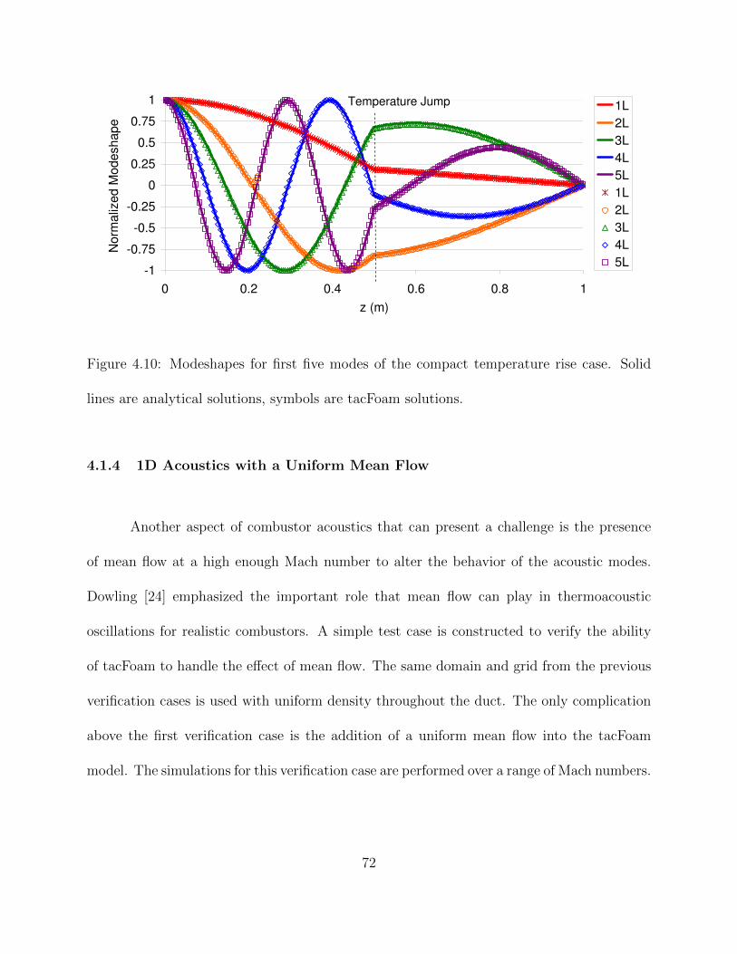
-1

-0.75

-0.5

-0.25

0

0.25

0.5

0.75

1

0 0.2 0.4 0.6 0.8 1

z (m)

Norm

aliz

ed M

odeshape

1L

2L

3L

4L

5L

1L

2L

3L

4L

5L

Temperature Jump

Figure 4.10: Modeshapes for first five modes of the compact temperature rise case. Solid

lines are analytical solutions, symbols are tacFoam solutions.

4.1.4 1D Acoustics with a Uniform Mean Flow

Another aspect of combustor acoustics that can present a challenge is the presence

of mean flow at a high enough Mach number to alter the behavior of the acoustic modes.

Dowling [24] emphasized the important role that mean flow can play in thermoacoustic

oscillations for realistic combustors. A simple test case is constructed to verify the ability

of tacFoam to handle the effect of mean flow. The same domain and grid from the previous

verification cases is used with uniform density throughout the duct. The only complication

above the first verification case is the addition of a uniform mean flow into the tacFoam

model. The simulations for this verification case are performed over a range of Mach numbers.

72

The details of the model parameters are recorded in Table 4.5. Note that the M = 0.0 case

is identical to the verification case from the first section.

Table 4.5: Reference conditions for uniform mean flow verification.

R [J/kg-K] γ p [kPa] T [K] a [m/s] u [m] M f -Range [Hz]

287 1.40 100 298 346 0-312 0.0-0.9 16-779

For this verification case, closed-open boundaries are used. As shown in Appendix C,

the analytical frequencies are

fn =(n− 1

2)a

2L(1− M2) (4.12)

Note that this is the same as the resonant frequencies for the uniform duct in Eq. (4.4),

except for the added factor (1 − M2), which reduces the frequency as the Mach number is

increased.

The resonant frequencies for the tacFoam simulations with uniform mean flow in the

constant property duct are shown in Fig. 4.11a along with the analytical solutions. The

relative error in the tacFoam simulations, Fig. 4.11b, remains below 0.6%. This verifies that

no significant additional error is added by the presence of a mean flow.

73

0

100

200

300

400

500

600

700

800

900

0 0.2 0.4 0.6 0.8 1

Mach Number

Fre

quency (

Hz)

1L

2L

3L

4L

5L

1L

2L

3L

4L

5L

(a)

0.00001

0.0001

0.001

0.01

0.1

1

0 0.2 0.4 0.6 0.8 1

Mach Number

Rela

tive F

requency E

rror

5L

4L

3L

2L

1L

(b)

Figure 4.11: Uniform mean flow (a)frequencies and (b) relative errors. Solid lines are ana-

lytical solutions, symbols are tacFoam solutions.

74

4.1.5 1D Acoustics with Temperature Jump and Mean Flow

A combination of the previous two cases involves a one-dimensional flow with a tem-

perature jump normal to the flow. This roughly simulates the physics present in the com-

bustion chambers of gas turbine engines. From a physical point of view, the key addition for

this verification case is the presence of a mean flow gradient, caused by the jump in density

and the necessity to conserve mass flow rate. In the interest of brevity, only one tempera-

ture ratio was simulated, with a range of Mach numbers. The conditions used are shown in

Table 4.6. The same domain and grid are used as in all the previous one-dimensional cases.

Acoustic boundary conditions are closed at the inlet and open at the outlet.

Table 4.6: Reference conditions for mean flow temperature jump verification.

R [J/kg-K] γ p [kPa] Tinlet [K] Texit/Tinlet Minlet f -Range (Hz)

287 1.40 100 298 8 0.0-0.25 152-1182

The frequencies and growth rates found are compared with those obtained from the

Transfer Matrix Approach (TMA) [44]. First, a simulation is performed in which the source

terms on the right hand side of Eqs. (3.1) and (3.2) are neglected. These terms contain

the physical effects of mean velocity gradients, therefore neglecting them should be fatal to

the accuracy of the simulation. The relative frequency error as a function of inlet Mach

number is shown in Fig. 4.12. The relative errors in frequency are small (below one percent)

for small inlet Mach numbers (0.05 and below). As the inlet Mach number increases, and

75

hence the velocity gradient at the flame increases, the relative error increases. By an inlet

Mach number of 0.2, the relative error in frequency is as high as 10%. The errors are more

dramatic for the growth rate. The zero Mach number case has no growth rate. With finite

Mach number, the velocity gradient at the flame works to damp or excite acoustic modes.

This effect is completely missing from the tacFoam solution, which only shows the numerical

damping (comparatively very small). These results are not surprising given that the terms

necessary to capture the physical effects of mean velocity gradients on acoustics are missing

from the governing equations used.

In a follow-up simulation, the source terms related to mean flow gradients are added

back into the governing equations of the code and the above simulation is repeated. As

expected based on the analytical solutions shown in Fig. 4.12, strong damping of the modes

becomes evident. The results are shown for two low Mach number cases in Fig. 4.13.

The presence of strong damping in the time domain simulation become problematic for

post-processing at higher Mach numbers. Because the modes die out quickly, the filtering

and curve-fitting technique used to extract growth rates no longer yields quality results.

Therefore, the figure shows only the small Mach number, low damping rate cases.

The agreement is excellent for the limited number of cases for which comparison is

available. Relative errors remain under 5%, even for Mach = 0.025 when the damping rates

become ∼ 40 rad/s. This verification case concludes that the mean velocity gradient source

terms are effective in modelling the interaction between gradients in the mean velocity field

and acoustics.

76

0.0001

0.001

0.01

0.1

1

0 0.05 0.1 0.15 0.2 0.25

Inlet Mach Number

Rela

tive F

requency E

rror

1L

2L

3L

4L

5L

(a)

-800

-700

-600

-500

-400

-300

-200

-100

0

0 0.05 0.1 0.15 0.2 0.25 0.3

Inlet Mach Number

Gro

wth

Rate

(1/s

ec)

1L

2L

3L

4L

5L

1L

2L

3L

4L

5L

(b)

Figure 4.12: Two temperature with mean flow: (a)relative frequency errors and (b) growth

rates. Solid lines are TMA solutions, symbols are tacFoam solutions.

77

-80

-70

-60

-50

-40

-30

-20

-10

0

0 0.005 0.01 0.015 0.02 0.025

Inlet Mach NumberG

row

th R

ate

(1/s

ec)

1L

2L

3L

4L

5L

1L

2L

3L

4L

5L

Figure 4.13: Two temperature with mean flow: growth rates from simulation including source

terms previously neglected. Solid lines are TMA solutions, symbols are tacFoam solutions.

4.1.6 1D Acoustics with an Exponential Cross-sectional Area Distribution

With the previous verification cases covering important phenomena for modeling gas

turbine combustors with regard to the flow variables, the other significant influence on the

thermoacoustics in combustors is multi-dimensional effects. In some cases, only longitudinal

modes are of interest. Longitudinal modes, in this context, are defined as modes in which

the wavenumber vector is approximately aligned with the streamlines of the mean flow.

If only longitudinal modes are of concern and the cross-sectional area varies little relative

to the length of the duct, a one-dimensional approach may be maintained analytically for

approximating the acoustic behavior. The next set of verification cases includes two dimen-

78

sional geometries in which only longitudinal modes are concerned. The solutions provided by

tacFoam are compared with analytical solutions using the one-dimensional approximation.

The first such case is of the exponentially-varying cross-sectional area. Simulations

are run in tacFoam for a number of exit-to-inlet area ratios with constant mean properties

and no mean flow. The simulation parameters are given in Table 4.7. Note that the cross-

sectional areas are given in meters because the simulation is two-dimensional in nature. A

unit depth in the third direction could be assumed to make the units m2. Also note that area

ratios up to 64 are simulated. At these higher area ratios, the one-dimensional assumption

inherent in the analytical solution becomes inaccurate. Closed-closed boundary conditions

are used and the area ratio of unity is equivalent to the first verification case.

Table 4.7: Reference conditions for exponential cross-sectional area verification.

R [J/kg-K] γ p [kPa] T [K] Sinlet [m/s] Sexit [m] f -Range [Hz]

287 1.40 100 298 0.01 0.01-0.64 173-873

The domain and mesh for a typical case (AR = 16) is shown in Fig. 4.14. The

transverse direction is meshed with 20 cells and the longitudinal direction is meshed with

the number of cells necessary for an aspect ratio of unity.

The cross-section area is given by

S(z) = Sinletemz (4.13)

79

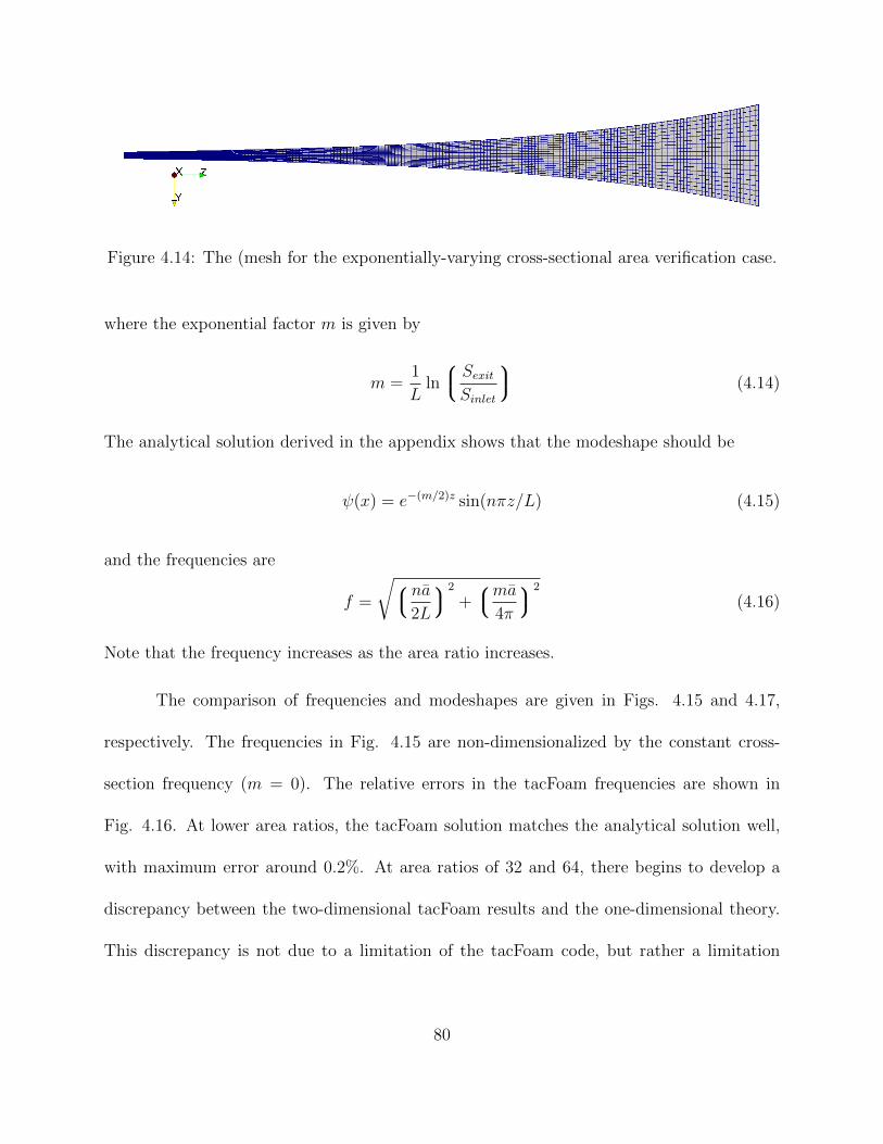
Figure 4.14: The (mesh for the exponentially-varying cross-sectional area verification case.

where the exponential factor m is given by

m =1

Lln

SexitSinlet

(4.14)

The analytical solution derived in the appendix shows that the modeshape should be

ψ(x) = e−(m/2)z sin(nπz/L) (4.15)

and the frequencies are

f =

√na

2L

2

+ma

4π

2

(4.16)

Note that the frequency increases as the area ratio increases.

The comparison of frequencies and modeshapes are given in Figs. 4.15 and 4.17,

respectively. The frequencies in Fig. 4.15 are non-dimensionalized by the constant cross-

section frequency (m = 0). The relative errors in the tacFoam frequencies are shown in

Fig. 4.16. At lower area ratios, the tacFoam solution matches the analytical solution well,

with maximum error around 0.2%. At area ratios of 32 and 64, there begins to develop a

discrepancy between the two-dimensional tacFoam results and the one-dimensional theory.

This discrepancy is not due to a limitation of the tacFoam code, but rather a limitation

80

of the one-dimensional theory of describing acoustics in ducts when the cross-sectional area

varies dramatically.

0.98

1

1.02

1.04

1.06

1.08

1.1

1.12

1.14

1.16

1.18

1.2

1 10 100

Area Ratio

Non-D

imensio

nal F

requency 1L

2L

3L

4L

5L

1L

2L

3L

4L

5L

Figure 4.15: Resonant frequencies for first five modes for the exponentially-varying cross–

sectional area case. Solid lines are analytical solutions, symbols are tacFoam solutions.

The modeshapes shown in Fig. 4.17 are shown for the example case of area ratio

(Sexit/Sinlet) of 16. This was the highest area ratio at which the simulations matched the

frequency of the analytical solution. As a note, the modeshapes were taken from a line

probe through the center of the duct. No observations were made of any possible transverse

variation in the modeshape because the comparison at hand is made with one-dimensional

theory.

The conclusion of this test is that, as far as possible, tacFoam shows agreement with

analytical frequencies and modeshapes. When the assumptions of the analytical solution

81

0.000001

0.00001

0.0001

0.001

0.01

0.1

1

1 10 100

Area Ratio

Rela

tive F

requency E

rror

5L

4L

3L

2L

1L

Figure 4.16: Relative frequency error for first five modes for the exponentially-varying cross–

sectional area case.

-1

-0.75

-0.5

-0.25

0

0.25

0.5

0.75

1

0 0.2 0.4 0.6 0.8 1

z (m)

Norm

aliz

ed M

odeshape

1L

2L

3L

4L

5L

1L

2L

3L

4L

5L

Figure 4.17: Modeshapes for first five modes of the exponential area verification case. Solid

lines are analytical solutions, open symbols are tacFoam solutions.

82

breakdown, tacFoam predictably fails to replicate the limited analytical solutions outside of

the their range of applicability.

4.1.7 1D Acoustics with an Acoustically Compact Area Change

While the previous verification case showed that tacFoam could handle smooth changes

in cross-sectional area, it is worthwhile to pursue the question of more sudden area changes.

In combustor geometries, sudden area changes are often used as part of the scheme to anchor

the flame. Therefore, the most relevant verification case is two constant area ducts joined

by an area discontinuity. The parameters for this case are given in Table 4.8. Closed-open

boundary conditions are used. The area ratios for this test case were not chosen as large

as the previous test case, since the limits of the one-dimensional theory had already been

tested.

Table 4.8: Reference conditions for sudden area change verification.

R [J/kg-K] γ p [kPa] T [K] Sinlet [m/s] Sexit [m] f -Range [Hz]

287 1.40 100 298 0.01 0.01-0.08 87-828

The domain for the area ratio of four case is shown in Fig. 4.18a. The one-dimensional

acoustic theory gives a good approximation of this geometry because the total area change

is much less than the length of the duct (wavelength). A close-up snapshot of the mesh

near the discontinuity is shown in Fig. 4.18b. Upstream, the mesh includes 20 cells in the

83

transverse direction. Downstream, the cell size remains constant and hence the number of

transverse cells scales with the area expansion ratio. The longitudinal resolution was chosen

to give aspect ratios near unity.

(a)

(b)

Figure 4.18: The (a) domain and (b) mesh for area discontinuity verification.

The analytical modeshapes for closed-open boundaries, constructed by matching con-

stant area duct solutions at the interface, are

ψ(z) =

cos(kz) x b

(4.17)

The resonant frequencies can be solved for numerically from the following characteristic

equation

tanωa

(L− b) tan

ωab− Sexit

Sinlet= 0 (4.18)

84

The frequencies found by the tacFoam solver are compared with the analytical fre-

quencies in Fig. 4.19. The trends in frequency are matched. Note that, as the area ratio

tends to infinity, the acoustic frequencies become those of half the duct. Figure 4.20 shows

that the frequency error is this verification case remains below 1%.

0

100

200

300

400

500

600

700

800

900

1 2 3 4 5 6 7 8Area Ratio

Fre

quency (

Hz)

1L

2L

3L

4L

5L

1L

2L

3L

4L

5L

Figure 4.19: Resonant frequencies for first five modes for the area discontinuity case. Solid

lines are analytical solutions, symbols are tacFoam solutions.

The comparison between the 1D analytical solution and tacFoam modeshapes is

shown in Fig. 4.21. As with the previous case, the modeshapes are taken from a line probe

along the centerline of the two-dimensional tacFoam domain. Any transverse variation is

not explored.

85

0.00001

0.0001

0.001

0.01

0.1

1

1 2 3 4 5 6 7 8

Area Ratio

Re

lative

Fre

qu

en

cy E

rro

r

1L

2L

3L

4L

5L

Figure 4.20: Relative frequency errors for first five modes for the area discontinuity case.

-1

-0.8

-0.6

-0.4

-0.2

0

0.2

0.4

0.6

0.8

1

0 0.2 0.4 0.6 0.8 1

z (m)

Norm

aliz

ed M

odeshape

1L

2L

3L

4L

5L

1L

2L

3L

4L

5L

Area Discontinuity

Figure 4.21: Modeshapes for first five modes of the area discontinuity case. Solid lines are

analytical solutions, symbols are tacFoam solutions.

86

4.1.8 Three-Dimensional Acoustics in a Circular Cylinder

All the previous verification cases shown above investigate frequencies and mode-

shapes for acoustic propagation in one-dimension. The final two cases show the ability of

the solver to reproduce three-dimensional modes. The first example is the circular cylinder,

which is solved analytically in Appendix C. The circular cylinder is a good approximation

of the shape of a combustion chamber for can-annular engine configurations. The particular

circular cylinder chosen for the verification case had a length of one meter, consistent with

the previous verification cases. The radius of the circular cross-section was a half meter. The

domain and mesh constructed in OpenFOAM using the blockMesh utility is shown in Fig.

4.22. The basic information about the case is tabulated in Table 4.9.

Table 4.9: Reference conditions for circular cylinder verification.

R [J/kg-K] γ p [kPa] T [K] Radius [m] Length [m] f -Range [Hz]

287 1.40 100 298 0.5 1.0 87-496

The three-dimensional modeshapes are found via separation of variables to be

φmn(r)χm(θ)ψj(z) (4.19)

where the axial component of the modeshape is

ψ(z) = A1 cos(kzz) + A2 sin(kzz) (4.20)

87

and the transverse component of the modeshape is

χm(θ)φm1(r) = cos(mθ)Jm

ξ(m)1

r

R

. (4.21)

(a) (b)

Figure 4.22: The (a) domain and (b) mesh for circular cylinder verification.

Note, for these modeshapes, the radial boundary has been assumed to be closed,

while the axial boundary has been left arbitrary. For more details on this solution, please

consult the appropriate section of Appendix C. The resonant frequencies from the analytical

solution are

ωjmn = a√

(kr)2mn + (kz)2

j (4.22)

88

where the axial wave number for closed-closed boundary conditions is

(kz)j =jπ

L(4.23)

or for closed-open boundary conditions is

(kz)j =(j − 1/2)π

L(4.24)

and the radial wavenumber is

(kr)mn =ξ

(m)n

R. (4.25)

Therefore, the frequencies and modeshapes are easily plotted using tabulated roots

of the Bessel functions and derivatives. All modes with frequencies under 500 Hz will be

evaluated. The resonant frequencies of the tacFoam simulations are given in Fig. 4.23. The

solver found all the relevant frequencies for both sets of boundary conditions using white

noise initial conditions. It should be noted that some of the amplitudes were larger than

others, which led to a large amount of noise in the smaller amplitude modes coming through

the signal filtering operations.

The relative error in the simulation frequencies for the closed-closed and closed-open

boundary conditions is shown in Fig. 4.24. All frequency errors were below 1% and there

is no visible trend with respect to grid resolution. The lack of a trend with resolution

highlights the fact that the main source of frequency error was the resolution uncertainty

of the FFT. These simulations were run for one second, giving a resolution of 1 Hz, or a

resolution uncertainty of 0.5 Hz. This was the dominant source of error in almost all of the

verification cases.

89

0

100

200

300

400

500

600

1L 2L 1T 2T 3T 1R 1T-1L 2T-1L 3T-1L 1R-1L 1T-2L 2T-2L

Fre

quency (

Hz)

Theory

tacFoam

(a)

0

100

200

300

400

500

600

1L 2L 3L 1T-1L 2T-1L 3T-1L 1R-1L 1T-2L 2T-2L 1R-2L 1T-3L

Fre

quency (

Hz)

Theory

tacFoam

(b)

Figure 4.23: All resonant frequencies under 500 Hz for cylindrical case: (a) closed-closed,

(b) closed-open.

90

0.0001

0.001

0.01

0.1

1

10 100 1000

Cells per Wavelength

Rela

tive F

requency E

rror

Figure 4.24: Relative error in resonant frequency prediction for the closed-closed and

closed-open boundary conditions of the cylindrical verification case.

The next set of figures shows the three-dimensional modeshapes resulting from the

cell-by-cell DFT calculation. The first pure axial mode (1L) is shown in Fig. 4.25. The first

pure tangential mode is shown in Fig. 4.26. The first pure radial mode (1R) is shown in

Fig. 4.27. A combined axial-tangential mode (2L-2T) is shown in Fig. 4.28. A combined

axial-radial mode (1L-1R) is shown in Fig. 4.29. These figures are not a comprehensive set

of all the modes shown in the Figs. 4.23 and 4.24, but rather a sampling to show the ability

of the solver to capture three-dimensional modeshapes. All the other modes, not shown for

brevity, were also captured correctly. Due to the randomness of the initial conditions, some

modes were not as strong as other modes, hence a higher presence of noise polluted the DFT

signal in these weaker mode cases. The DFT magnitudes are not normalized in order that

the reader can observe the variation in strength of different modes.

91

(a) (b)

Figure 4.25: First pure axial mode, 1L, (a) amplitude and (b) phase.

(a) (b)

Figure 4.26: First pure tangential mode, 1T, (a) amplitude and (b) phase.

92

(a) (b)

Figure 4.27: First pure radial mode, 1R, (a) amplitude and (b) phase.

(a) (b)

Figure 4.28: Combined axial-tangential mode, 2L-2T, (a) amplitude and (b) phase.

93

(a) (b)

Figure 4.29: Combined axial-radial mode, 1L-1R, (a) amplitude and (b) phase.

4.1.9 Three Dimensional Acoustics in an Annular Cylinder

Similar to the previous verification case, this case involves three-dimensional mode-

shapes in an annular cylinder. This geometry is also very relevant to real engine configura-

tions, as many gas turbine engines use annular combustion configurations. The analytical

solution can be found in Appendix C. The particular annular cylinder chosen for the verifi-

cation case had a length of one meter, consistent with the previous verification cases. The

inner radius of the annular cross-section was a quarter meter and the outer radius was three

quarters of a meter. The domain and mesh constructed in OpenFOAM using the blockMesh

94

utility is shown in Fig. 4.30. The basic information about the case is tabulated in Table

4.10.

(a) (b)

Figure 4.30: The (a) domain and (b) mesh for annular cylinder verification.

Table 4.10: Reference conditions for annular cylinder verification.

R [J/kg-K] γ p [kPa] T [K] Inner/Outer R [m] Length [m] f -Range [Hz]

287 1.40 100 298 0.25/0.75 1.0 173-400

The modeshapes are expressed in a similar fashion to the circular cylinder

φmn(r)χm(θ)ψj(z) (4.26)

95

where the axial component of the modes are unaffected by the change from circular to annular

cross-section

ψ(z) = A1 cos(kzz) + A2 sin(kzz). (4.27)

The circumferential component of the modes is given by

χm(θ) = cos(mθ) (4.28)

and the radial component is given by

φmn(r) = Y ′m((kr)mnRinner)J′m((kr)mnr)− J ′m((kr)mnRinner)Y

′m((kr)mnr). (4.29)

The frequency for any given combination

ωjmn = a√

(kr)2mn + (kz)2

j (4.30)

where the axial wave number is found the same as before and the radial wave number is

found by solving

J1(krRouter)Y1(krRinner)− J1(krRinner)Y1(krRouter) = 0. (4.31)

As with the circular cylinder, closed boundaries have been assumed at the radial

boundaries. Only the closed-closed boundary conditions is used for the annular geometry. All

frequencies under 400 Hz are analyzed. The frequencies for all such modes are shown in Fig.

4.31. Once again, the simulation produces peaks in the FFT at all frequencies corresponding

to resonant frequencies. The relative error of these frequencies is shown in Fig. 4.32. The

errors remain well below 1% and once again are dominated by the resolution of the FFT in

96

the frequency domain, which is 1 Hz as before. The dominance of the frequency resolution

error is manifest in the lack of trends for frequency error versus cells per wavelength.

0

50

100

150

200

250

300

350

400

450

1L 2L 1T 2T 3T 4T 1R 1T-1L 2T-1L 3T-1L 1R-1L 1T-2L 1T-

1R

Fre

quency (

Hz)

Theory

tacFoam


closed-open boundary conditions of the annular verification case.

As with the circular cylinder, a cell-by-cell calculation of the DFT is performed,

resulting in three-dimensional modehshapes. The 1L, 1T, and 1R modes are shown in shown

in Fig. 4.33, 4.34, and 4.35, respectively. Combined modes are also resolved. The 1L-

3T mode is shown in Fig. 4.36 and the 1T-1R is shown in Fig. 4.37. These figures are

not comprehensive for all modes shown in the Figs. 4.31 and 4.32, but rather provide a

sample of a few modes to demonstrate the ability of the solver to capture three-dimensional

modeshapes. As with the circular cylinder, the DFT magnitudes are not normalized in

order that the reader can observe the variation in strength of different modes. The various

strengths are indicative of the white noise initial conditions used to trigger all modes.

97

0.0001

0.001

0.01

0.1

1

10 100 1000


Rela

tive F

requency E

rror


closed-open boundary conditions of the annular verification case.

(a) (b)

Figure 4.33: First pure axial mode, 1L, (a) amplitude and (b) phase.

98

(a) (b)

Figure 4.34: First pure tangential mode, 1T, (a) amplitude and (b) phase.

(a) (b)

Figure 4.35: First pure radial mode, 1R, (a) amplitude and (b) phase.

99

(a) (b)

Figure 4.36: Combined axial-tangential mode, 1L-3T, (a) amplitude and (b) phase.

(a) (b)

Figure 4.37: Combined radial-tangential mode, 1T-1R, (a) amplitude and (b) phase.

100

For the geometry shown, the focus was kept on modes in the hundreds of Hertz.

Higher frequency modes can be captured in a similar way to the verification cases above,

provided that the proper grid resolution is supplied and the time step provides a low Courant

number for stability. This may increase the computational cost for tangential and radial

modes in higher aspect ratio geometries due to the difference in time scale between the

longitudinal and transverse frequencies.

4.2 Boundary Conditions Verification

Common acoustic boundary conditions include closed, open, and choked. These

acoustic boundary conditions can be generalized to specifying the acosutic impedance at

the boundary. The acoustic impedance is defined as the ratio of the acoustic pressure to the

acoustic velocity normal to the boundary

Z(ω) =p

ρaun(4.32)

where

p ∼ exp(iωt) (4.33)

u ∼ exp(iωt). (4.34)

A closed boundary (un = 0) represents the limit as Z →∞ while an open boundary

represents the limit as Z → 0. A choked boundary is in between these limits, the specific

value depending on the Mach number of the mean flow in the chamber. These three simple

101

boundary conditions have real values of impedance that are independent of frequency. In

general, the impedance of an arbitrary boundary is a complex quantity, with both magnitude

and phase being a function of frequency.

Two different boundary conditions are developed for the tacFoam solver. The first

boundary condition, designed for real impedances only, uses the mixed value boundary con-

dition from OpenFOAM with a value fraction tuned to give the appropriate reflection coef-

ficient for a given impedance. The second boundary condition applies a piecewise constant

approximation for calculating the convolution integral. The numerical details of the bound-

ary conditions are given in Appendix E.

For this test, rather than follow the procedure used for previous tests, a procedure for

determining the reflection coefficient of the boundary is used. One boundary is forced with an

overlay of sinusoidal signals with random phase. The other boundary is given the arbitrary

real, constant impedance. Two pressure probes at designated locations capture pressure

signals. The two-microphone method [45] is used to measure the reflection coefficient of the

boundary. The reflection coefficient from the two-microphone method is calculated by

R(ω) =H21 − exp(−iks)exp(iks)−H21

exp(i2kL) (4.35)

where k = ω/a is the wavenumber, s is the distance between the microphones, L is the

distance from the boundary to the midpoint between the two microphones and H21 is the

transfer function between the two signals given by

H21 =p2

p1

(4.36)

102

The subscript 2 denotes the microphone closer to the boundary of interest and the subscript

1 denotes the microphone further away. The value calculated from Eq. (4.35) is compared

with the analytical value of the reflection coefficient, given by

R =Z − 1

Z + 1(4.37)

4.2.1 Real Constant Impedance

The first test is of the boundary condition written to handle real impedance (no

imaginary component) that is constant over all frequencies.

4.2.1.1 1D Acoustic Boundary

A one-dimensional domain, the same as used in previous tests, is initialized to zero.

The reference conditions for this verification case are provided in Table 4.11.

Table 4.11: Reference conditions for mean flow temperature jump verification.

R [J/kg-K] γ p [kPa] T [K] Z f -Range (Hz)

287 1.40 100 298 0-∞ 10-1000

Over the entire frequency range forced by the opposite boundary condition, the re-

flection coefficient was found to be constant, as specified. An example is shown in Fig. 4.38

where the impedance of the boundary was set at Z = 3, so a reflection coefficient of R = 0.5

103

was expected, per Eq. (4.37). Some minor noise was seen in the data, which is attributed

to the signal processing. Also, a minor shift in phase (< 5o) is noticed at high frequencies,

which can be attributed to the zeroth order interpolation done by the numerical probes (slight

discrepancy in the distance separating the probes from the boundary).

The impedance set at the boundary was adjusted from 0 to ∞. An impedance of

zero corresponds to the fully-reflective (R = −1) open boundary condition. The other limit,

Z → ∞, corresponds to the fully reflective (R = 1) closed boundary. These two limits

were check and verified with error below 0.1% for the one-dimensional case. Intermediate

impedances were also simulated, and the average reflection coefficient over all frequencies

for each impedance is plotted against the expected relationship, Eq. (4.37). The reflection

coefficient for this plot was calculated from the average magnitude, |Z|, and average phase,

∠Z, by

Z = |Z| cos(∠Z) (4.38)

The relative error of impedance for this plot was less than 0.6% for all calculations.

104

0

0.1

0.2

0.3

0.4

0.5

0.6

0.7

0.8

0.9

1

0 200 400 600 800 1000

Frequency

Reflection C

oeffic

ient

Magnitude

(a)

-180

-120

-60

0

60

120

180

0 200 400 600 800 1000

Frequency

Reflection C

oeffic

ient P

hase

(b)

Figure 4.38: As a function of frequency for Z = 3, the reflection coefficient (a) magnitude

and (b) phase.

105

-1

-0.75

-0.5

-0.25

0

0.25

0.5

0.75

1

1.00E-02 1.00E-01 1.00E+00 1.00E+01 1.00E+02

Z

Reflection C

oeffic

ient

tacFoam

analytical

Figure 4.39: Average reflection coefficients as a function of impedance for the 1D case.

4.2.1.2 3D Acoustic Boundary

The one-dimensional real impedance test showed that the implementation gave ex-

cellent results. The same test was also preformed in three-dimensions using the three di-

mensional circular cylinder from section 4.1.8. Additionally, the test was performed on a

similar geometry that was square rather than circular in cross-section. Figure 4.40 shows

that excellent agreement was again achieved for these tests. There is almost no difference

between the circular and square cross-section results, indicating that the application of this

boundary condition has low sensitivity to the geometrical shape.

106

-1

-0.75

-0.5

-0.25

0

0.25

0.5

0.75

1

0.01 0.1 1 10 100

Z

Reflection C

oeffic

ient

analytical

tacFoam box

tacFoam cyl

Figure 4.40: Reflection coefficients as a function of impedance for the 3D cylinder and square

cases.

4.2.2 Complex Impedance as a Function of Frequency

A curve fitting procedure for the magnitude and phase of complex impedance bound-

ary conditions is shown in Appendix E. Three example curve fits with input values for

tacFoam’s complex impedance boundary conditions are given. Preliminary results of this

boundary condition in terms of complex reflection coefficient are now shown. The reflection

coefficient is determined by the two-microphone method using a one-dimensional grid as

shown above for the real impedance boundary condition.

107

4.2.2.1 Real Pole

The reflection coefficient magnitude and phase of a complex impedance boundary with

only a single real pole is shown in Fig. 4.41 compared to the analytical value. Magnitude

and phase are matched in the low frequency limit, but at relevant frequencies, the changes

magnitude and phase with increasing frequency are under-predicted.

4.2.2.2 Complex Conjugate Poles

The reflection coefficient magnitude and phase of a complex impedance boundary

with only a single pair of complex conjugate poles is shown in Fig. 4.42 compared to the

analytical value. Magnitude and phase are matched in the low frequency limit, but at relevant

frequencies, the changes magnitude and phase with increasing frequency are under-predicted.

4.2.2.3 Real Pole and Complex Conjugate Poles

The reflection coefficient magnitude and phase of a complex impedance boundary

with both a real pole and a pair of complex conjugate poles is shown in Fig. 4.43 compared

to the analytical value. Magnitude and phase are matched in the low frequency limit, but

at relevant frequencies, the changes magnitude and phase with increasing frequency are

under-predicted.

108

0

0.1

0.2

0.3

0.4

0.5

0.6

0.7

0.8

0.9

0 200 400 600 800 1000

Frequency (Hz)

Reflection C

oeff. M

agnitude

Fit

Input Data to Curve Fit

tacFoam

(a)

-180

-160

-140

-120

-100

-80

-60

-40

-20

0

20

0 200 400 600 800 1000

Frequency (Hz)

Reflection C

oeff. P

hase

Fit


tacFoam

(b)

Figure 4.41: Curve fits for complex impedance example with a single real pole.

109

0

0.5

1

1.5

2

2.5

0 200 400 600 800 1000

Frequency (Hz)

Reflection C

oeff. M

agnitude

Fit


tacFoam

(a)

-180

-160

-140

-120

-100

-80

-60

-40

-20

0

20

0 200 400 600 800 1000

Frequency (Hz)

Reflection C

oeff. P

hase

Fit


tacFoam

(b)

Figure 4.42: Curve fits for complex impedance example with a single pair of complex conju-

gate poles.

110

0

0.5

1

1.5

2

2.5

0 200 400 600 800 1000

Frequency (Hz)

Reflection C

oeff. M

agnitude

Fit


tacFoam

(a)

-180

-160

-140

-120

-100

-80

-60

-40

-20

0

0 200 400 600 800 1000

Frequency (Hz)

Reflection C

oeff. P

hase

Fit


tacFoam

(b)

Figure 4.43: Curve fits for complex impedance example with a real pole and a pair complex

conjugate poles.

111

4.3 Thermoacoustic Verification

The vital verification that needs to be addressed in this work is that of the unsteady

heat release models. For these verification cases, the n − τ family of heat release models

are used. This family of models is based on the time lag theory proposed by [46] and

used heavily since then in describing combustion instability mechanisms [8]. These cases

used the conditions from the TR = 8 temperature jump case, which represent an extreme

operating condition. The flame is located over two cells (0.01m long), where the mean heat

release is placed and the density drops from the reactant density to the product density.

Key parameters for these cases are listed in Table 4.12. The solutions by which the solvers

results were benchmarked are found using the method described in Appendix C, which is

similar to that described by Dowling [24].

Table 4.12: Reference conditions for uniform mean flow verification.

R [J/kg-K] γ p [kPa] T [K] TR Q [W/m2] q [W/m3] f -Range [Hz]

287 1.40 100 298 8.0 2.45e6 2.45e8 152-1183

4.3.1 Rijke Tube: Pressure Mechanism

The first heat release model is based on a relationship between the acoustic pressure

oscillations and the heat release oscillations. Mathematically, the pressure mechanism can

112

be written as

q′(x, t) = n(x)q

pp′sender(t− τ) (4.39)

where p′sender denotes the acoustic pressure at the location where the mechanism is caused and

the n(x) is the gain distribution which identifies the region where the mechanism for unsteady

heat release takes effect. For this case, the sender region is the flame region itself. The gain

is set to unity in the flame region and zero outside the flame region. The frequency shifts

caused by this mechanism, given that it is a weak mechanism, are very small and typically

on the order of magnitude of the frequency resolution of the FFT (1Hz). Therefore, the

useful comparisons of tacFoam with theory are in terms of growth rate.

The results from the baseline simulation are shown in Fig. 4.44. At zero time lag, the

pressure and heat release fluctuations are in phase, leading to maximum growth rate. For

each mode, depending on the frequency of the mode, as the time lag increases, the pressure

slowly moves out of phase and the growth rate reaches a minimum with the heat release

when the time lag is one half of the period. When the time lag reaches a full period, the heat

release and pressure are once again in phase and the growth rate reaches another maximum.

Hence, the growth rate for each mode displays a sinusoidal patter with respect to time lag,

with the period of the sinusoid equal to the period of the mode.

The modes are plotted in two different graphs to indicate an important dichotomy.

Figure 4.44, shows the first three modes. These modes are such that, at the given resolution,

the numerical damping coefficient measured by a q′ = 0 simulation is order of magnitudes

113

less than the growth rates shown in the figure

|αnumerical| << |αq′ |. (4.40)

-8

-6

-4

-2

0

2

4

6

8

0 0.001 0.002 0.003 0.004 0.005 0.006 0.007

Time Lag (sec)

Gro

wth

Rate

(1/s

ec)

1L

2L

3L

1L

2L

3L

Figure 4.44: Growth rates for the first three modes in the Rijke tube verification case. Solid

lines are analytical solution and symbols are the tacFoam solution.

The simulation predicts the stability map very accurately, with growth rate errors

less than 5% for these first three modes. The inequality shown in Eq. (4.40) is vital for this

accurate prediction, as will be demonstrated in a later section.

4.3.2 Rijke Tube: Velocity Mechanism

The other heat release model tested here is based on a relationship between the

acoustic velocity oscillations and the heat release oscillations. Mathematically, the velocity

114

mechanism can be written as

q′(x, t) = n(x)q

au′sender(t− τ) (4.41)

where u′sender denotes the acoustic velocity at the location where the mechanism is caused

and the n(x) is the gain distribution which identifies the region where the mechanism for

unsteady heat release takes effect. For this case, the sender region is set to the region

just prior to the flame, to conform as closely as possible to the model in the theoretical

development. Across the flame, with non-zero unsteady heat release, there is a jump in

acoustic velocity. Therefore, since the pre-flame acoustic velocity is desired for the model,

the sender region and flame region must not overlap. The gain is set to unity in the flame

region and zero outside the flame region. As for the pressure mechanism, comparisons of

tacFoam with theory are in terms of growth rate due to the weak mechanism. The results

from the baseline simulation are shown in Fig. 4.45.

At zero time lag, the velocity and heat release fluctuations are in phase. For slightly

perturbed acoustic waves, the velocity and pressure are 90o, which means that the pressure

and heat release are 90o out of phase. This makes the zero time lag case marginally stable,

i.e. the growth rate is zero. For each mode, depending on the frequency of the mode, as the

time lag increases, the phase between the pressure and heat release slowly changes in the

same sinusoidal manner as in the pressure mechanism case above. Hence, the growth rate for

each mode also displays a sinusoidal patter with respect to time lag, with the period of the

sinusoid equal to the period of the mode. The errors are again small due to the negligibility

of numerical damping with respect to the growth rate from the heat release mechanism.

115

-6

-4

-2

0

2

4

6

0 0.001 0.002 0.003 0.004 0.005 0.006 0.007

Time Lag (sec)

Gro

wth

Rate

(1/s

ec)

1L

2L

3L

1L

2L

3L

Figure 4.45: Growth rates for the first three modes in the velocity mechanism Rijke tube


4.4 Numerical Damping

Since the tacFoam solver applies TVD limiters to the second order flux calculation

in which solution variables are extrapolated from cell centers to faces, numerical diffusion

is introduced in the effort to maintain solution stability and limit overshoot [41, 40]. Such

numerical diffusion damps existing acoustic waves in a tacFoam solution, which can pollute

the numerical estimation of growth rates. One of the main target capabilities of tacFoam

is the prediction of linear growth rates for combustor geometries. In order to ensure the

suitability of tacFoam for that task, it is vital to understand its numerical damping behavior.

116

Placing a probe in the domain and extracting time series data from the simulation as

before, the results gave a damped oscillation. By extracting the extrema and curve fitting

with an exponential curve fit, the growth rate α of the oscillations can be found, where

p′ ∼ exp(αt). (4.42)

The numerical damping rate is given by −α and quantifies the amount of numerical

damping present in the simulation. The spatial and temporal resolution of the mode is

important in determining the numerical damping in a given simulation for a given mode.

The spatial resolution of a given mode is best quantified by measuring the number of cells

within a wavelength of oscillation. This can be calculated locally as

cells per wavelength =λ

∆z=

a

f∆z(4.43)

where λ is the wavelength given by a/f and ∆z is the length of the cell in the direction of

the wave vector.

The temporal resolution can likewise be measured quantitatively by the number of

time steps in one period of oscillation, or

time steps per period =T

∆t=

1

f∆t(4.44)

where T is the period of oscillation, f is the frequency in Hertz and ∆t is the time step of

the simulation. The dimensionless number most often associated with numerical simulations

of fluids is the Courant number, which is contructed by dividing Eq. (4.43) by Eq. (4.44).

This results in

Co =a∆t

∆z. (4.45)

117

Note that in the presence of mean flow, a better metric for spatial resolution is given

by

cells per wavelength =u+ a

f∆z(4.46)

which gives a Courant number of

Co =(u+ a)∆t

∆z. (4.47)

For this thesis, the cells per wavelength and Courant number will be used to report

dimensionless spatial and temporal resolution (noting that the actual temporal resolution is

best represented by the product of the cells per wavelength and the Courant number).

4.4.1 1D Uniform Duct

To begin the exploration of numerical damping, the uniform duct from section 4.1.1

is excellent. Instead of exciting the simulation with white noise, the initial conditions are

carefully prescribed using sine or cosine waves to be one of the modeshapes of the duct.

In this case, the second mode was chosen and the velocity was initialized with the corre-

sponding modeshape (derivative of the pressure modeshape). With closed-open boundaries

(differentiating Eq. (4.3) and normalizing, with n = 2), the velocity initial conditions were

w′(z, 0) = w0 sin(1.5πz/L) (4.48)

where the frequency and numerical damping rate of the solver should be insensitive to the

wave magnitude w0. For this case, the length of the duct was L = 1m and the initial

118

magnitude of the velocity mode was w0 = 0.25m/s, which for the given conditions (Table

4.2) gave a pressure fluctuation magnitude of around 100Pa.

For the simple duct verification case at hand, the effect of spatial and temporal

resolution on damping coefficient is given in Fig. 4.46. First, the temporal resolution has

little to no effect on the damping in comparison with the spatial resolution. The exception

to this rule is at Courant numbers close to 2, where the numerical damping is elevated.

Notice that a special procedure was used for initialization for the first numerical

damping test. Because for a given complex geometry, the modeshapes will not be known

a-priori, the numerical damping should be determined from a simulation starting with a

more generic initial condition (e.g. white noise) than the precise modeshape. In this way,

the numerical damping for all modes can be determined from a single simulation within the

strategy outlined in Fig. 3.3. A bandpass filter with bandwidth of 5 Hz was used to filter

the pressure signal at the frequencies of each of the first five resonant modes. The same

exponential curve fitting procedure was then used to calculate a growth rate for each of the

modes. The results are plotted against the previous “2L mode only” simulation in Fig. 4.47.

There are two important consequences stemming from this figure. First, notice that

for 133 cells per wavelength, the closed-open 2L modes matches numerical damping coefficient

regardless of the initialization method and whether filtering of the signal needs to be applied.

This validates the bandpass filtering approach to acquiring numerical damping coefficients.

Secondly, the rest of the data is not completely colinear.

119

0.00001

0.0001

0.001

0.01

0.1

1

10

100

10 100 1000 10000

Cells/Wavelength

Dam

pin

g C

oeffic

ient (1

/sec)

(a)

0.00001

0.0001

0.001

0.01

0.1

1

10

100

0 1 2Courant Number

Dam

pin

g C

oeffic

ient (1

/sec)

(b)

Figure 4.46: Numerical damping coefficients as a function of (a) cells per wavelength (at

unity Courant number) and (b) Courant number at 133 cells per wavelength.

120

Therefore, the numerical damping is not simply a function of spatial resolution only.

Nonetheless, as will be shown more fully later, the general trend of numerical damping vs

cells per wavelength holds regardless of whether the wavelength or the number of cells is

varied.

0.00001

0.0001

0.001

0.01

0.1

1

10

100

10 100 1000

Cells/Wavelength

Dam

pin

g C

oeffic

ient (1

/sec) closed-closed

closed-open2L mode only

Figure 4.47: Comparison of numerical damping coefficients for the single mode initialization

(2L mode) and the white noise initialization for two different boundary configurations.

4.4.2 Area Expansion

This verification case provided an excellent opportunity to study the behavior of nu-

merical damping when effected by geometrical features (in this case, an area expansion). In

addition to the cells per wavelength measure introduced in the one-dimensional verification

cases, another important parameter for this case is the cells per step height. This parame-

121

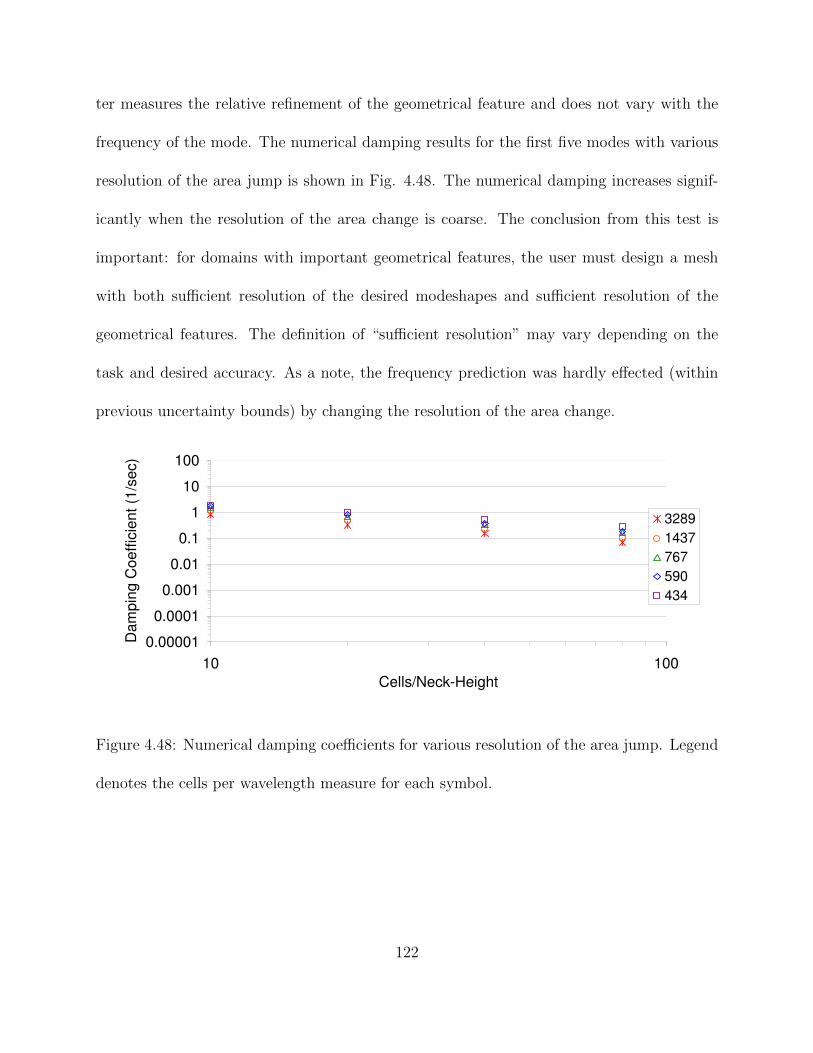
ter measures the relative refinement of the geometrical feature and does not vary with the

frequency of the mode. The numerical damping results for the first five modes with various

resolution of the area jump is shown in Fig. 4.48. The numerical damping increases signif-

icantly when the resolution of the area change is coarse. The conclusion from this test is

important: for domains with important geometrical features, the user must design a mesh

with both sufficient resolution of the desired modeshapes and sufficient resolution of the

geometrical features. The definition of “sufficient resolution” may vary depending on the

task and desired accuracy. As a note, the frequency prediction was hardly effected (within

previous uncertainty bounds) by changing the resolution of the area change.

0.00001

0.0001

0.001

0.01

0.1

1

10

100

10 100

Cells/Neck-Height

Dam

pin

g C

oeff

icie

nt

(1/s

ec)

3289

1437

767

590

434

Figure 4.48: Numerical damping coefficients for various resolution of the area jump. Legend

denotes the cells per wavelength measure for each symbol.

122

4.4.3 3D Circular Cylinder

The numerical damping for the modes analyzed above was calculated from probe data

for the following simulations: (1) a closed-closed boundary condition set on the baseline grid,

(2) a closed-open boundary condition set on the baseline grid, (3) a closed-closed boundary

condition set with 2x local hanging node refinement for 0.7 > z > 1.0, and (4) a closed-open

boundary condition set with 4x global refinement. Note that for the 2x local refinement, the

cells per wavelength calculation ignored the local refinement. This case tested the effect of

local refinement, most importantly its effect on numerical damping. The 4x global refinement

case did recalculate the cells per wavelength based on the refined grid size, since this grid

size was everywhere applicable. This global refinement case enabled testing of numerical

damping at high cells per wavelength. The four grids are summarized in Table 4.13.

Table 4.13: Four grids used for circular cylinder numerical damping study.

Refinement Boundary Conditions Title

1x Closed-Closed “Closed-Closed Uniform Grid”

1x Closed-Open “Closed-Open Uniform Grid”

2x, 0.7 < z < 1.0 Closed-Closed “Closed-Closed Non-Uniform Grid”

4x, Global Closed-Open “Closed-Open Fine Grid”

The results in Fig. 4.49 show that the local refinement had little effect on the nu-

merical damping when the larger (unrefined) cell size was used to calculate the cells per

123

wavelength measure. The results for all four cases seem to follow a second order decrease in

damping with respect to grid resolution, as would be expected from the numerical method.

The amount of scatter amongst this second order descent is due to the difficulty of precisely

measuring cells per wavelength in each direction, particularly the radial and tangential di-

rections. In these directions, the grid lines do not follow the wave vector lines, hence the

cells per wavelength is an estimate at best. Nonetheless, there is still a noticeable 2nd order

trend.

0.00001

0.0001

0.001

0.01

0.1

1

10

100

10 100 1000


Da

mp

ing

Co

eff

icie

nt

(1/s

ec)

Closed-Closed Uniform GridClosed-Closed Non-uniform GridClosed-Open Uniform GridClosed-Open Fine Grid2nd-order slope

Figure 4.49: Numerical damping as a function of grid resolution for modes less than 500 Hz

in the cylindrical verification case.

124

4.4.4 Rijke Tube

In order to show the reason for such a detailed look into numerical damping, it is

instructive to consider again the Rijke tube example from section 4.3. Figure 4.50 shows the

fourth and fifth mode, for which the numerical damping is on the same order of magnitude

as the theoretical growth rate

|αnumerical| ∼ |αq′|. (4.49)

The difference in the quality of prediction between Fig. 4.44 for the first three modes

and Fig. 4.50 for the fourth and fifth modes is remarkable. The first three modes exhibit

relative errors less than 5%, but the errors in the fourth and fifth modes are on the order of

100%. The cause is simple. When the numerical damping is large enough to compete with

the heat release forcing term, large errors in the prediction will occur. When the numerical

damping is too small to compete, the solver produces an accurate result for the growth rate.

For this reason, careful quantitative characterization and control of the numerical damping

in vital for each application.

To further understand the role of numerical damping in polluting the growth rate

predictions, the values of numerical damping calculated from the zero heat release case are

added to the results of each time-lag simulation. This effectively shifts the growth rate curve

to correct for numerical damping. The results of this shift are shown in Fig. 4.51. Indeed

the shift improves the simulation results dramatically, but there are still noticeable errors

and a few points for which the sign of the growth rate is incorrect. Therefore, while shifting

125

to correct for the numerical damping is a realistic strategy for users to employ, and it is

seen that such a strategy dramatically improves the stability predictions, it is recommended

that the numerical damping is mitigated rather than corrected for. Mitigation of numerical

damping can be accomplished through an increase in grid refinement. This results in an

increase in computational cost.

-3

-2

-1

0

1

2

3

0 0.001 0.002 0.003 0.004 0.005 0.006 0.007

Time Lag (sec)

Gro

wth

Rate

(1/s

ec)

4L

5L

4L

5L

Figure 4.50: Growth rates for modes 4 and 5 in the pressure mechanism Rijke tube verifica-

tion case. Solid lines are analytical solution and symbols are the tacFoam solution.

To illustrate strategies for reducing the numerical damping, the resolution of the grid

was increased by 10x (2000 cells). The numerical damping was dramatically reduced by this

ten-fold increase in cells per wavelength, as shown in the previous verification cases dealing

with numerical damping. The result is shown in Fig. 4.52. The relative errors are now with

5%, as with the lower frequency modes. This effectively shows that, by reducing numerical

126

damping such that it is overwhelmed by the growth rate due to heat release, the linear

growth rates can be accurately predicted.

-2

-1.5

-1

-0.5

0

0.5

1

1.5

2

0 0.001 0.002 0.003 0.004 0.005 0.006 0.007

Time Lag (sec)

Gro

wth

Rate

(1/s

ec)

4L

5L

4L

5L

Figure 4.51: Growth rates for modes 4-5 in the pressure mechanism Rijke tube case, corrected

for numerical damping. Solid lines are analytical solution and symbols are the tacFoam

solution.

The same dichotomy noted in the pressure mechanism case is again observed for the

velocity mechanism. The first three modes, shown in Fig. 4.45 give good agreement with the

theoretical solution. The errors are within 10%, which is impressively small given that the

sender region was offset by a finite length in order to incorporate the same physics and the

theoretical model. When the numerical damping becomes large enough to compete with the

growth rates for the fourth and fifth modes, the simulation does not produce accurate results,

Fig. 4.53. This can be partially overcome by shifting the results to correct for numerical

damping, shown in Fig. 4.54, but the results still contain noticeable errors. Such practice

127

is not recommended. Rather, it is recommended to increase the grid refinement (at more

computational cost) to obtain a more accurate solution.

-3

-2

-1

0

1

2

3

0 0.001 0.002 0.003 0.004 0.005 0.006 0.007

Time Lag (sec)

Gro

wth

Rate

(1/s

ec)

4L

5L

4L

5L

Figure 4.52: Growth rates for modes 4-5 in the pressure mechanism Rijke tube case, using

a 10x refined grid. Solid lines are analytical solution and symbols are the tacFoam solution.

There is no easy rule of thumb for determining the grid resolution necessary for

a given scenario. The numerical damping for a given resolution can be approximated by

calculating the cells per wavelength using Eq. (4.43) and the approximate “cells per step

height” (cells per relevant geometric feature length) and using Figs. 4.49 and 4.48 as a

guide. In most cases, the numerical damping can be calculated using the bandpass filtering

and curve fitting method described at the end of chapter 3 from an initial “no unsteady heat

release” simulation. Such a simulation is also useful for determining the resonant frequencies

and modeshapes of the geometry. Once the numerical damping for each targeted mode is

determined, one must compare that damping coefficient to an expected growth rate, which

128

will likely be much less than the frequency of the mode in rad/sec. If results show that the

apriori estimates for the necessary grid resolution yield a numerical damping coefficient near

the same order of magnitude as physical sources of growth or damping, then the grid should

be refined and the simulation process iterated.

-6

-4

-2

0

2

4

6

0 0.001 0.002 0.003 0.004 0.005 0.006 0.007

Time Lag (sec)

Gro

wth

Rate

(1/s

ec)

4L

5L

4L

5L

Figure 4.53: Growth rates for the fourth and fifth modes in the velocity mechanism Rijke tube


129

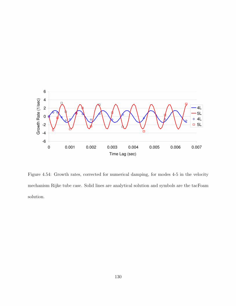
-6

-4

-2

0

2

4

6

0 0.001 0.002 0.003 0.004 0.005 0.006 0.007

Time Lag (sec)

Gro

wth

Rate

(1/s

ec)

4L

5L

4L

5L

Figure 4.54: Growth rates, corrected for numerical damping, for modes 4-5 in the velocity

mechanism Rijke tube case. Solid lines are analytical solution and symbols are the tacFoam

solution.

130

4.5 Parallel Computation Verification

Another important feature of the solver is the ability to calculate spatio-temporal

acoustic fields in parallel. In order to compute acoustic fields in larger, more complex ge-

ometries, larger numbers of cells with smaller time steps will be necessary. For this tool to

be useful for practical engineering design and analysis, the simulation code must be paral-

lelized. The code must give the same answer with the same numerical damping regardless

of the number of processors used to compute the simulation.

4.5.1 1D Uniform Duct

The uniform duct case from section 4.1.1, using the procedure described in Fig. 3.3,

was run multiple times, varying the number of processors used for the computation. The

resulting frequency errors and numerical damping coefficients are shown in Fig. 4.55 as a

function of number of processors used. As desired, the simulation did not show any variation

with number of processors.

131

0.00001

0.0001

0.001

0.01

0.1

1

1 10 100

Processors

Fre

quency E

rror

(a)

0.00001

0.0001

0.001

0.01

0.1

1

10

100

1 10 100

Processors

Da

mp

ing

Co

eff

icie

nt

(1/s

ec)

(b)

Figure 4.55: Parallelization accuracy for (a) frequency error and (b) damping coefficient.

132

4.5.2 Area Jump

While parallel computation was verified for the one-dimensional case with 100 cells, it

was also thought wise to check parallelization behavior for a multi-dimesional case with many

more cells. The 2D simulation with acoustically-compact area change from section 4.1.7 was

chosen to suit this purpose. The grid with 10 cells per neck height (15,000 cells) was chosen

and run on various numbers of processors, from 1 to 12. The frequency and numerical

damping coefficient was monitored. As shown in Fig. 4.56, no changes in frequency or

numerical damping coefficient were observed. These two tests were sufficient for verifying

the successful parallelization of the code. Due to constraints in present computing resources,

no scaling tests were performed to determine the efficiency of the parallelization.

133

0

100

200

300

400

500

600

700

800

900

0 2 4 6 8 10 12 14

Processors

Fre

quency (

Hz) 1L

2L

3L

4L

5L

(a)

0

0.5

1

1.5

2

2.5

0 2 4 6 8 10 12 14

Processors

Dam

pin

g C

oeffic

ient (1

/sec)

1L

2L

3L

4L

5L

(b)

Figure 4.56: The (a) frequency and (b) numerical damping coefficient of the two area case

with various number of processors.

134

CHAPTER 5VALIDATION

The previous chapter included numerous verification cases by which the integrity of

the solver was established for simple academic cases. This chapter focuses on extending

the use of the solver to physically relevant cases. Specifically, this chapter predicts the

thermoacoustic instabilities for two lab scale experiments.

5.1 University of Melbourne Bluff Body Combustor

The first validation case is a simulation of a laboratory combustor at the University

of Melbourne [47, 48]. A schematic of the combustion chamber from the experimental study

is reproduced in Fig. 5.1, whjch is reproduced from [47]. Premixed air and fuel enter the

one-meter-long circular cylinder test section through a choke plate. The fuel is liquified

petroleum gas with composition of 98% propane. Upstream of the choke plate, the fuel and

air is allow to completely mix. The upstream mixing region is acoustically isolated from

the combustion region. The flame is anchored by a bluff body located at the approximate

center of the meter-long duct. Downstream of the flame, the combustion chamber walls were

fused silica to allow optical access for chemiluminescence measurements. The diameter of

135

the combustion chamber is 0.05 meters and the diameter of the bluff body is 0.025 meters.

The length of the bluff body is 0.06 meters, and the length downstream of the bluff body to

the open exit is 0.45 meters. The 20:1 aspect ratio of the combustion chamber is designed

to investigate longitudinal modes. The limit cycle pressure amplitudes are measured at a

probe aligned with the center of the bluff body.

the entropy fluctuation appears to be important, as also shown in

other studies [5,47].

In this paper, the flame behaviour in a laboratory combustor

will be examined experimentally and related to the velocity fluctu-

ations at the flameholder. For the combustor used here, the param-

eters n and s will be shown to depend on the amplitude of the

acoustic velocity fluctuations, over a range of operating conditions

and for a number of combustor exit nozzles including a choked exit

operating point, suggesting a novel nonlinear form of Crocco and

Cheng’s flame model.

Dowling’s [2] low-order thermoacoustic model is then extended

to include entropy fluctuations downstream of the flame, enabling

the effect of a choked exit nozzle to be examined. A nonlinear

flame model is developed based on the experimental results and

integrated into the thermoacoustic model. The model is then used

to investigate the limit cycles formed for both an open and a

choked combustor exit operating point. The simulation results

show good agreement with the experimental results presented

here and in other studies of the same combustor [42,48]. In partic-

ular, the effect of choking the combustor exit is captured, with the

model simulating the transition from an acoustically driven insta-

bility to a low-frequency, entropically driven instability.

2. Experimental methods

2.1. The experimental rig

The experimental rig is shown in Fig. 1. The combustion cham-

ber is a 1-m long section of pipe with an axially mounted flame-

holder at the midpoint. A 450 mm long section of the duct

downstream of the flame is constructed of quartz tubing, allowing

optical access to the flame. The combustion chamber inlet is

choked, and consists of a plate with an array of 15 holes of 2 mm

diameter, so as to promote uniform flow a short distance down-

stream of the inlet. In this study four combustor exit nozzles were

used, with area ratios (defined as the ratio of the cross-sectional

area of the throat to that of the combustor) of 1.0, 0.4, 0.2 and

0.1. The flow was choked at the combustor exit for the last of these

nozzles. The combustor was fed with air from a dedicated 60 hp

Sullair compressor, and liquified petroleum gas (LPG, 98% propane)

from cylinders. The fuel was injected into the air flow sufficiently

far upstream of the combustor to allow for complete mixing before

the combustor inlet. See [48] for further details of the rig.

A large number of operating conditions were studied. These

conditions included traversing the combustor’s flammability limits

in Mach number and equivalence ratio for the four different com-

bustor exit nozzles discussed above (e.g. Fig. 2). This range of oper-

ating conditions yielded widely varying limit cycle behaviour, as is

shown later in this paper.

2.2. Measurement techniques

The acoustic pressure was measured at two locations upstream

of the flame using two Kulite type WCT 312 M fast response pres-

sure transducers mounted at points x1 and x2 upstream of the

flameholder (see Fig. 1). The pressure measurements act as a phase

reference for the optical signals, and also allow the acoustic veloc-

ity at the flameholder to be calculated.

The acoustic velocity calculation was based on that described by

Chung [49], but extended to include the mean flow. More detail is

given in [48]. The integration performed as part of the acoustic

velocity calculation had the effect of amplifying the low-frequency

noise contained in the pressure transducer signals. For this reason,

the pressure transducer signals were high-pass filtered by remov-

ing the frequency components below 60 Hz from the pressure

transducer spectra before the acoustic velocity was calculated. This

cut-off frequency was chosen because it is sufficiently far below

the lowest frequency peak in the measured pressure transducer

spectra (85 Hz for an operating point of AR = 0.1, M ¼ 0:034, /

= 0.78), but high enough to remove the frequencies amplified by

Fig. 1. (a) Isometric view of the experimental setup for optical measurements and (b) partial cross-section of the working section showing the coordinate system used in the

calculation of the acoustic velocity at the flameholder.

P.A. Hield et al. / Combustion and Flame 156 (2009) 1683–1697 1685

Figure 5.1: University of Melbourne experimental test section: (a) isometric view, (b) slice

of internal view.

136

5.1.1 Validation Case Selection

The experimental test matrix [47, 48] included varying the equivalence ratio, inlet

Mach number, and exit boundary condition. The open exit test case, with unity equivalence

ratio, provided the best validation case for the present code. The reference conditions of this

experiment are given in Table 5.1. Other tests ran had different exit geometries, including a

choked boundary. This experiment resulted in a large amplitude mode at the second resonant

frequency of the duct (three-quarter wave frequency). This 2L mode was the only dominant

frequency observed in the experiment.

Table 5.1: Reference conditions for liquified petroleum gas bluff body combustor at the

University of Melbourne.

φ Tpreheat[K] p[kPa] m[kg/m3] f [Hz]

1.0 345 101 0.029 364

The flow conditions upstream and downstream of the flame are given in Table 5.2.

The mean pressure was approximately constant across the flame and equal to the atmospheric

pressure imposed at the exit boundary. The temperature shown here is the calculated adi-

abatic flame temperature, though some heat transfer did occur through the sides of the

combustor due to the fused silica walls. The RANS simulation did account for small pres-

sure changes and heat release through the walls. The Mach number remains low, indicating

that mean velocity influences on the acoustics may be small.

137

Table 5.2: Flow conditions for liquified petroleum gas bluff body combustor at the University

of Melbourne.

Section T [K] p[kPa] ρ[kg/m3] V [m/s] M

Products 345 101 1.0 15 0.04

Reactants 2425 101 0.16 92 0.10

This experiment was also simulated by [47, 48] using the matrix approach of [49] and

by [50, 1] using the Generalized Instability Model (GIM) of [25]. These two one-dimensional

simulations provide a nice context for the present prediction code.

5.1.2 Summary of Simulation Approach

For this case, a RANS simulation and four tacFoam simulations are run. The purpose

of each tacFoam simulation is to build upon the knowledge of the other simulations and reveal

a particular behavior of the model. The simulations for this case are summarized in Table

5.3.

138

Table 5.3: Summary of simulations for Hield bluff body combustor.

Solver Type Purpose

RANS To obtain the mean flow

tacFoam no q’, closed BC to evaluate numerical damping

tacFoam no q’, choked BC to evaluate boundary damping

tacfoam non-linear q’, choked BC to predict limit cycle amplitude

5.1.3 RANS Simulation of Mean Flow

The Reynolds Averaged Navier Stokes (RANS) equations were solved using the finite

volume method in OpenFOAM. The k-ω SST model was used for turbulence closure [51].

The combustion was modelled using a single-step reaction tracked by a reaction progress

variable b. Chemical closure was obtained through a turbulent flame speed correlation [52]

using a laminar flame speed calculated from a network reactor modelling tool in Cantera

[53].

The velocity, turbulent quantities, and temperature were specified at the inlet with

zero pressure gradient and the pressure was specified at the outlet with zero gradient for all

other variables. The wall used the no slip condition with wall functions for the turbulent

quantities. While the boundary condition for the wall in terms of the energy equation is

not clear from the experiments, the RANS simulation used a constant temperature wall at

the pre-heat temperature. This essentially assumes that the walls are steady at the pre-heat

139

temperature before ignition, and they rise in temperature only negligibly after the flame is

ignited.

The domain for the RANS study began at the inlet choke point and ended at the

open exit, Fig 5.2. A fully hexahedral mesh was created using the snappyHexMesh utility

in OpenFOAM with a STL file of the cylinder and bluff body dimensions given in Hield’s

thesis [48]. Two different grids were run (125k cells, 275k cells) and the results of the finer

resolution mesh were taken for interpolation to the acoustic mesh. The differences between

the simulations were judged to be insignificant for the current purposes (extracting a realistic

temperature and heat release field). It is emphasized that the purpose of the RANS was

not to focus on providing a high-fidelity mean field, but rather to quickly produce realistic

mean fields for the acoustic simulation. Thus, the RANS simulation was “quick-and-dirty”

as compared to a formal RANS investigation, including a formal grid resolution study. An

example of a grid resolution study is shown for the Purdue University validation case.

The simulation was advanced to a steady solution using OpenFOAM’s bi-conjugate

gradient solver. The simulation converged to a steady-state solution when the residuals

dropped by three or more orders of magnitude and simulation variables from point probes

showed negligible changes. The flame is anchored by the recirculation region in the wake

of the bluff body and propagates toward the outer walls downstream. Three-isosurfaces of

reaction progress variable (at b = 0.25, 0.5, 0.75) are shown in Fig. 5.3, outlining the main

reaction region. The flame extends about 20 centimeters downstream of the bluff body, close

to half of the downstream section of the chamber.

140

0.49 m 0.45 m

0.05 m0.025 m

Velocity Inlet Pressure OutletBluff Body Flameholder

0.06 m

(a)

(b)

Figure 5.2: Melbourne bluff body combustor, RANS (a) domain and (b) finite volume mesh.

141

Figure 5.3: Translucent iso-surfaces of reaction progress variable outlining the spatial struc-

ture of the flame. Flow is bottom to top as shown by arrows.

142

The variables relevant to the thermoacoustic simulation are shown in Fig. 5.4 along

the center-plane of the duct. The temperature determines the sound speed, while the velocity

determines the extent to which the mean flow affects the acoustic behavior of the duct. The

temperature increases dramatically across the flame and remains close to the adiabatic flame

temperature in the center of the pipe. Near the edges, the cooling at the wall produces lower

temperatures. The transfer of heat from the combusted flow plays an important role in

determining the acoustic behavior downstream. Closely tied to the temperature and also

affecting the propagation of the acoustic waves is the mean velocity, Fig. 5.4b. The flow

accelerates after the flame due to the drop in density (increase in temperature). The local

Mach number exceeds the mean Mach number due to non-uniformity of temperature and

velocity in the cross-section. The Mach number, however, remains modest (< 0.15). The

heat release is also an important quantity to be mapped from the RANS solution. It provides

a main factor in determining the location and intensity of heat release oscillations.

143

(a)

(b)

(c)

Figure 5.4: Center-plane of Melbourne case RANS results: (a) temperature [K] and (b) axial

velocity [m/s] and (c) heat release [W/m3].

144

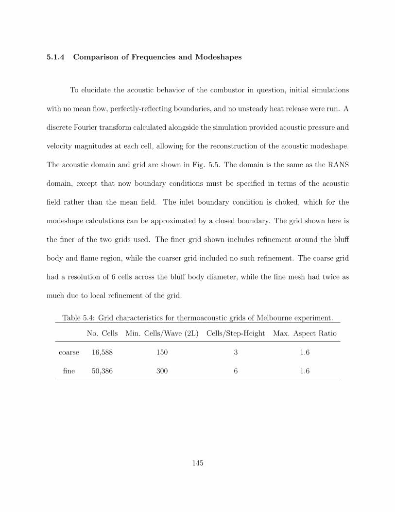
5.1.4 Comparison of Frequencies and Modeshapes

To elucidate the acoustic behavior of the combustor in question, initial simulations

with no mean flow, perfectly-reflecting boundaries, and no unsteady heat release were run. A

discrete Fourier transform calculated alongside the simulation provided acoustic pressure and

velocity magnitudes at each cell, allowing for the reconstruction of the acoustic modeshape.

The acoustic domain and grid are shown in Fig. 5.5. The domain is the same as the RANS

domain, except that now boundary conditions must be specified in terms of the acoustic

field rather than the mean field. The inlet boundary condition is choked, which for the

modeshape calculations can be approximated by a closed boundary. The grid shown here is

the finer of the two grids used. The finer grid shown includes refinement around the bluff

body and flame region, while the coarser grid included no such refinement. The coarse grid

had a resolution of 6 cells across the bluff body diameter, while the fine mesh had twice as

much due to local refinement of the grid.

Table 5.4: Grid characteristics for thermoacoustic grids of Melbourne experiment.

No. Cells Min. Cells/Wave (2L) Cells/Step-Height Max. Aspect Ratio

coarse 16,588 150 3 1.6

fine 50,386 300 6 1.6

145

0.49 m 0.45 m

0.05 m0.025 m

Choked Inlet Open OutletBluff Body Flameholder

0.06 m

(a)

(b)

Figure 5.5: Melbourne bluff body combustor acoustic simulation (a) domain and (b) finite

volume mesh.

146

This initial simulation has no acoustic damping or growth sources except for the

grid-dependent damping of the numerical method. Because of this, it provides a convenient

quantification of the numerical damping for the two grids. For the present analysis, the first

three modes are the only modes of interest, the second mode being the excited mode in the

experiments. The first three resonant frequencies for the two acoustic grids based on this

initial simulation are shown in Table 5.5. Note that there is significant over-prediction of the

frequency (more than 8% error) for the second mode. Similar over-prediction can be seen

in previous analytical predictions based on one-dimensional analysis with compact flames,

including that of the experimentalist himself [47, 1]. It is postulated here that the over-

prediction is a result of the flame dynamics discussed by the experimentalist. A large periodic

fluctuation of the flame length occurred over the acoustic period of oscillation. During this

cycle, the flame changed from very short to very long, even as long as the entire length of

the downstream section. Because of this, the extent of the downstream hot products region

may be severely shortened during some phases of the cycle, leading to lower overall sound

speeds and a lower frequency. Such unsteady (non-turbulent) fluid mechanical behavior is

not captured by the steady RANS calculation nor is there currently a method of including it

within the current thermoacoustic simulation methodology. Other possibilities include the

under-prediction of heat transfer by the RANS model, as well as a poor prediction of the

mean flame position. It is unclear whether the first and third mode frequencies are correctly

predicted because these modes were stable in the experiment.

147

The prediction of the GIM code from [50] shows better agreement than the present

code. It is observed, however, that the lower frequency in this prediction is caused by a lower

prediction of the adiabatic flame temperature than the RANS procedure used here and a

different placement of the bluff body location (evidently in conflict with the location shown

by [48]). The simulation from [47] did not give an “unshifted frequency”, therefore it is not

included here. In this context, “unshifted” refers to the natural frequency of the domain

without any frequency shifts caused by the unsteady flame.

Table 5.5: Resonant frequencies (Hz) for first three modes with perfectly-reflecting bound-

aries. The GIM results are the unshifted frequency, which is the appropriate comparison

here.

1L 2L 3L

(Exp.) – 364 –

coarse 137 397 578

fine 138 396 578

(GIM [50]) 86 382 629

The numerical damping coefficient for the first three modes on each of the two acoustic

grids is shown in Table 5.6. These damping coefficients are clearly orders of magnitude less

than the frequency, but the more important comparison is with the physical sources of

acoustic damping (here, the choked boundary). The damping follows the expect trends,

148

namely, that the increase in grid resolution decreases the numerical damping and that the

increase in frequency (moving to higher modes) results in an increase in numerical damping.

Table 5.6: Numerical damping coefficient (1/sec) for first three modes.

1L 2L 3L

coarse 8.6 5.9 10.8

fine 4.9 4.3 6.9

The pressure modeshapes are shown in Fig. 5.6 for the first three modes. The images

shown are taken from the fine grid with a slice through the mid-plane. No color scale appears

on these figures because the modeshapes are typically normalized by the maximum value.

The color red represents anti-nodes (maximum fluctuation) while the color blue denotes

nodes (zero fluctuation). The first mode is the quarter wave mode, with maximum at the

closed inlet and minimum (zero) at the open outlet. As such, the large pressure fluctuations

for this mode occur upstream of the combustion. The potential of the coupling of pressure

and heat release fluctuations necessary to drive mode growth is severely limited for this

mode because its amplitude is relatively small in the combustion region. The second mode

is the three-quarter wave mode. The combustion region is more advantageously placed for

the growth of this mode. Meanwhile, the third mode contains a pressure maximum in the

combustion region, leading to the highest possibility of mode growth from the point of view

of the pressure modeshape.

149

u’

p’

(a)

u’

p’

(b)

u’

p’

(c)

Figure 5.6: Melbourne rig acoustic velocity (u’) and pressure (p’) mode amplitudes on a

color scale of blue (zero amplitude) to red (max amplitude) : (a) 1L, (b) 2L, (c) 3L.

150

For this validation case, however, the unsteady heat release mechanism is based on

velocity fluctuations. Therefore, the velocity modeshape is just as influential in determining

the outcome of the stability analysis. Figure 5.6 also shows the axial velocity modeshape

for the first three modes. The first mode contains large velocity fluctuations in the flame

region, leading to the possibility of a strong mechanism. However, the fact that the heat

release is located at a pressure minimum, any unsteady heat release generated by the 1L

velocity fluctuations cannot couple with pressure and therefore cannot drive instability. The

second mode also shows relatively strong velocity fluctuations in the flame region. The third

mode, which contained a pressure anti-node at the flame region, contains a velocity node.

Because the unsteady heat release is dependent on the acoustic velocity, which is taken from

the flame region, there is little opportunity for the growth of the third mode. Therefore,

based on preliminary analysis of the modeshapes, it can be concluded that the most likely

mode to exhibit thermoacoustic instability is the second mode.


Before simulating the heat release model developed with the experiment [47, 48], it is

instructive to assess the damping extent of the choked inlet. The first simulation replaced the

choked inlet with a closed inlet so that the impact of numerical damping on baseline acoustic

modes could be assessed. For a second simulation, a choked inlet boundary is restored, with

the reflection coefficient given by [24]

151

Rinlet =1− M1 + M

(5.1)

For this case, with Mach number of 0.04, the reflection coefficient is 0.923. Note that

this reflection coefficient is valid only in the absence of entropy waves [54]. However, because

the current simulation ignores entropy waves, this formula is appropriate here.

In the second simulation, the presence of the absorbing boundary condition adds

damping to the system. It is important that this damping is not overwhelmed by the

numerical damping. The first three frequencies for this second solution did not change by

more than a couple Hz, as expected due to the small Mach number. The damping coefficient

for the first three modes on each of the two acoustic grids is shown in Table 5.7. The

boundary damping for all three modes is indeed greater than the numerical damping, but

not quite by an order of magnitude. In fact, the influence of numerical damping on these

results is evident in the noticeable drop in damping coefficient from the coarser to finer grid

( 10%-30%). Therefore, the numerical damping for these two grids is expected to assert

some effect on the final heat release simulation.

152

Table 5.7: Boundary damping coefficient (1/sec) for first three modes (“choked”), compared

with numerical damping (“closed”).

1L 2L 3L BC

coarse 29.3 21.0 23.2 choked

fine 24.9 18.9 18.1 choked

coarse 8.6 5.9 10.8 closed

fine 4.9 4.3 6.9 closed

5.1.6 Nonlinear Heat Release Model

The non-linear heat-release model proposed by Hield et al. was given in the frequency

domain [47, 48].

q′ = nF (ω)q

uu′(t− τ) (5.2)

with non-linear n and τ given by 1

n = 1.6 exp(−0.2u′RMS) + 0.225 (5.3)

τ = 0.0075 exp(−0.0744u′RMS) + 0.0025 (5.4)

1Note that the experimentalist’s paper [47] contains a typo in the time lag formula. The leading coefficientin the time lag correlation is given as 0.075 by Hield et al., but the Fig. 10c of [47] shows that the time lagshould be 0.01 in the zero amplitude limit. Therefore, the leading coefficient should be 0.0075 as shown inEq .(5.4)

153

The function F (ω) in Eq. (5.2) is a second-order low-pass filter given by

ω2co

ω2co + 2iζωcoω − ω2

(5.5)

where ωco is the cut-off frequency and ζ is the damping coefficient. For this model, Hield

et al. suggested ωco = 350Hz and ζ = 0.5. For the implementation of this model, it was

necessary to transform this filter into a state space model so that the filter could be applied

in the time domain. The discrete state space model is given by

xñ = A≈xñ−1 +B˜un−1 (5.6)

yn = C˜ · xñ +Dun (5.7)

Equation (5.6) updates the state variables given by the vector x˜ based on its previous

value and the value of the input. Then, Eq. (5.7) generates the output based on the state

variables and the input. For a discretized version of the filter proposed by [47], the coefficients

A, B, C, and D are

A≈

=

1 ωcoδt

−ωcoδt 1− 2ζωcoδt

(5.8)

B˜ = (0 ωcoδt)T (5.9)

C˜ = (10)T (5.10)

D = 0 (5.11)

Of course, this is a crude filter, and more advanced filters (e.g. Chebyshev filters) can

be constructed in state space and applied in the same manner. In the interest of matching

154

the experiment, the above second-order filter is applied. This heat release model is applied

to the present case for a third simulation. The velocity fluctuations are taken just behind

the bluff body, with the heat release applied to the region downstream of the bluff body.

Note also that the RMS velocity fluctuation needed for these non-linear models is estimated

using an exponentially weighted averaging technique. Therefore, the influence of past values

on the current estimation of the RMS value decays exponentially.

The temporal evolution of a the pressure for the non-linear heat release simulations

is shown in Fig. 5.7. The two grids show similar histories, which is expected since the

numerical and boundary damping for each was similar. At first, the 3L mode begins to grow

rapidly at about 0.2 seconds, but then abruptly disappears. The 1L mode then replaces it

and exhibits a transient large amplitude fluctuation from about 0.25 to 0.5 seconds in both

simulations. Then, the 1L dies out and the 2L grows to a steady limit cycle amplitude. This

switching of modes is due to the non-linear time lag which can bring the modes in and out

of phase based on the relationship between the present time lag and the frequency of the

mode. Finally, both simulations settle on a limit cycle amplitude about 20% of the mean

pressure. The coarse grid limit cycle had a dominant frequency of 410Hz and the refined

grid had a dominant frequency of 412Hz. For comparison in terms of limit cycle amplitude,

a time history of the experimental data is reproduced from [48] in Fig. 5.8.

Table 5.8 gives the quantitative comparison of limit cycle amplitude for the two

simulations with experimental data for these flow conditions. The experimental limit cycle

is based on an approximation made by the experimentalists [47], noting that there is not

155

a clean limit cycle amplitude visible in Fig. 5.8. Even with the approximation of the

experimentalists, the calculation is within 20% of the experimental limit cycle. The under-

prediction of the limit cycle amplitudes is foreseeable given the impact of the numerical

damping noted in Table 5.7.

0.2 0.4 0.6 0.8 1 1.2−0.4

−0.2

0

0.2

0.4

p’/p

Bar

time (sec)

2L1L3L

0.2 0.4 0.6 0.8 1 1.2−0.4

−0.2

0

0.2

0.4

p’/p

Bar

time (sec)

3L 1L 2L

(a) (b)

Figure 5.7: Pressure time histories for a simulation probe near the bluff body : (a) coarse

grid, (b) fine grid

It is interesting to compare the results of the present simulations to previous 1D

simulations in the open literature for this case. The simulations of [47] also under-predict

the limit cycle amplitude and over-predict the frequency. In fact, for this simulation, the

agreement is worse on both counts. The GIM simulations performed by [50] also over-predict

the frequency, but to a lesser extent than the present simulations. The explanations for this

have already been discussed in terms of the “unshifted” frequency in Table 5.5. The limit

cycle amplitude is over-predicted by the GIM model, with about the same percent error as

156

the present simulation. It is worth noting that the non-linear heat release model used in

the GIM simulation only included the non-linearity in gain factor. A constant time lag was

used, perhaps contributing to the over-prediction of limit cycle amplitude.

Figure 5.8: Pressure time histories for the experimental probe near the bluff body, from

Hield et al.

Overall, the agreement with experiment for the present simulation is acceptable for the

scope of the predictive tool. The thermoacoustic simulation correctly predicted the existence

of the 2L mode limit cycle and the absence of the other modes. The predicted limit cycle

amplitude was within 20% error of the experimental limit cycle amplitude approximation.

Other simulations verified that the low-pass filter operated correctly by lowering the cut-off

frequency to 100 Hz (from 350 Hz). This lead to the existence of only a 1L mode at a limit

cycle amplitude of 4.3 millibars, much smaller than the 200+ millibar limit cycles seen for

the 2L mode in Table 5.8.

157

Table 5.8: Frequency (Hz) and limit cycle amplitude (p′/p) for 2L mode, compared with

experiment as well as the simulation of and Hield et al.

2L Unshifted Freq Shifted Freq Amplitude

(Exp.) – 364 0.25

coarse 396 410 0.21

fine 397 412 0.21

(GIM ) 424 399 0.06

(Sim. [47]) – 450 0.18

5.2 Purdue University Dump Combustor

The second validation case is a simulation of a lab-scale dump combustor experiment

preformed at Purdue University [55]. A schematic of the test section is shown in Fig. 5.9 with

dimensions shown in millimeters. Premixed air and natural gas (92% methane) enter the test

section through a choke plate. The choke plate is an orifice plate with multiple holes through

which the incoming flow enters. By choking the flow at the inlet (M = 1), the upstream duct

is isolated from the acoustics within the combustion chamber, eliminating the possibility of

equivalence ratio driven mechanisms. The dump plane is located approximately 1.4 meters

downstream of the choke plate. The duct connecting the choke plate to the dump plane has

a square cross-section with sides approximately 3.8 centimeters in length. The dump plane

is a square-square expansion with an area ratio of four. The flame is ignited at the dump

158

plane and is anchored by the recirculation region in the outer part of the downstream duct.

The combustion chamber duct downstream of the dump plane has sides of 7.6 centimeters

and extends about 2.1 meters in length. At the end of the combustion chamber, a nozzle

chokes the flow again, providing well-defined acoustic boundary conditions at the exit. Thus,

the rig is designed to investigate longitudinal modes with choked inlet and outlet boundary

conditions. More detailed information regarding the experimental rig is given by [55].

Figure 5.9: Purdue University experimental test section.

159

5.2.1 Validation Case Selection

Of the test cases performed on this rig, one operating condition is selected for valida-

tion of the present numerical code. Table 5.9 gives the operating conditions for the test. The

design of the rig was such that the even numbered longitudinal modes contained pressure

anti-nodes (velocity nodes) at the dump plane while the odd numbered modes contained

pressure nodes (velocity anti-nodes) at the dump plane. In this way, the flame was located

in a low pressure oscillation region for the odd modes and a high pressure oscillation regions

for the even modes. Therefore, the even modes showed the strongest tendency for high limit

cycle amplitudes. In particular, this test show limit cycle amplitudes at 189 and 382 Hz,

which are the second and fourth modes, respectively.

Table 5.9: Reference conditions for natural gas dump combustor at Purdue University.

φ Tpreheat[oC] p[bar] m[kg/s] f [Hz]

0.64 399 7.83 0.40 189, 382

The flow conditions upstream and downstream of the flame are given in Table 5.10.

For this table, the mean pressure is assumed constant across the flame and the adiabatic

flame temperature calculated from an equilibrium chemistry code is reported for the mean

temperature downstream of the flame. In reality, there was some pressure drop due and

friction and significant heat transfer through the combustion chamber walls, as shown in the

RANS results to be shown later.

160

Table 5.10: Flow conditions for natural gas dump combustor at Purdue University.

Section T [oC] p[bar] ρ[kg/m3] V [m/s] M

Products 399 7.83 4.1 68 0.13

Reactants 1767 7.83 1.5 46 0.056

5.2.2 Summary of Simulation Approach

For this case, a RANS simulation and four tacFoam simulations are run. The purpose

of each tacFoam simulation is to build upon the knowledge of the other simulations and reveal

a particular behavior of the model. The simulations for this case are summarized in Table

5.11.

Table 5.11: Summary of simulations for Purdue dump combustor.

Solver Type Purpose

RANS To obtain the mean flow

tacFoam no q’, no mean flow, closed BC to evaluate numerical damping

tacFoam no q’, mean flow, choked BC to evaluate boundary damping

tacFoam linear q’, no mean flow, closed BC to evaluate linear growth rate

tacFoam non-linear q’, mean flow, choked BC to predict limit cycle amplitude

161

5.2.3 RANS Simulation for Mean Flow

The Reynolds Averaged Navier Stokes (RANS) equations were solved using the finite

volume method in OpenFOAM. The k-ω SST model was used for turbulence closure [51].

The combustion was modelled using a single-step reaction tracked by a reaction progress

variable b. Chemical closure was obtained through a turbulent flame speed correlation [52]

using a laminar flame speed calculated from a network reactor modelling tool in Cantera

[53]. The mass flow and total temperature were specified at the inlet from Table 5.9 with

zero gradient pressure. The turbulent intensity and length scale (estimated as one fourth

of the hydraulic diameter) were used to specify inlet conditions for the turbulent kinetic

energy and dissipation rate. The pressure was specified at the exit with zero gradient for

the velocity, temperature, and turbulent quantities.

The walls were assumed to be at the preheat temperature. A rough one-dimensional

heat transfer calculation using the lumped capacitance model (valid in this case due to the low

Biot number) showed a maximum increase of about 50 K over the duration of the experiment,

while a thermocouple on the outside of the chamber walls verified this estimation. The single

thermocouple also showed that the walls were not even close to a thermal steady state. The

specification of the fixed wall temperature as preheat temperature is the best approximation

for RANS boundaries because the temperature of the walls rises slowly but steadily during

the extent of the experiment. The grid resolution was controlled so as to keep the first cell

in the so-called “log-law” region. Wall functions were used for wall boundary conditions for

162

the turbulence quantities. The velocity at the wall was set to zero (no-slip) and the pressure

was set to zero gradient.

The simulation was advanced to a steady solution using OpenFOAM’s bi-conjugate

gradient solver. The simulation converged to a steady-state solution when the residuals

dropped by three or more orders of magnitude and simulation variables from point probes

showed negligible changes.

5.2.4 Grid Resolution Study

The RANS simulation was performed on three grids in order to apply the Richardson

extrapolation procedure for estimating numerical discretization uncertainty [56]. The finest

grid has been shown in Fig. 5.10. The uncertainty of the RANS simulation was judged

in terms of the flame length, exit bulk temperature, and center-line velocity at the dump

plane. These three quantities were judged to be the most influential quantities on the

acoustic simulation. The flame length describes the location of the heat release that is

driving any instabilities as well as the sharp density gradient that accompanies the flame.

The maximum dump plane velocity describes the velocity profile seen by the flame for a

given flow rate, which influences the acoustic wave propagation speed, flame length, and

recirculation length. The exit bulk temperature is the most convenience measure of the

amount of heat transfer through the chamber walls. For an ideal gas, the temperature

163

determines the sound speed. Table 5.12 summarizes the results from the grid resolution

study, including the Grid Convergence Index (GCI) [56] for judging numerical uncertainty.

Table 5.12: Results from the grid resolution study for the validation with the Purdue dump

combustor experiment.

No. Cells Flame Length [m] Max Dump Plane Vel. [m/s] Exit Bulk Temp. [K]

194,400 0.628 85.1 1409

449,280 0.642 85.5 1426

1,001,640 0.666 85.9 1441

GCI [56] 5.8% 10.3% 8.4%

The uncertainties were relatively high if the study were to focus on the details of

the RANS solution. For the present purposes, the RANS simulation serves only the pur-

pose of providing the acoustic simulation with an approximate backdrop on which to study

thermoacoustic stability. Other uncertainties, such as turbulence closure and flame speed

closure, likely play are large role in reducing the overall accuracy of the RANS approach. In

addition, the RANS simulation provides Favre-averaged variables, whereas the derivation in

previous chapters showed that the thermoacoustic simulation requires simple mean variables

(not density weighted). In view of these technicalities, the RANS simulation should be seen

as a “quick-and-dirty” method by which the mean fields are estimated for the thermoacoustic

simulation.

164

1.4 m 2.1 m

0.038 m 0.076 mMass Flow Inlet Pressure OutletDump Plane

(a)

(b)

Figure 5.10: Purdue dump combustor RANS (a) domain and (b) finite volume mesh.

165

5.2.5 RANS Results

The mean fields, as resolved by the RANS simulation are now briefly shown. Figure

5.11 shows iso-surfaces of reaction progress variable (at b = 0.25, 0.5, and 0.75). Such iso-

surfaces mark the location of the flame spatially. The flame is cone-shaped and symmetric

with respect to the transverse directions. The heat release occurs in a relatively compact

region of the domain, where the gas composition transitions from premixed air and fuel

reactants to high temperature burnt combustion products.

Figure 5.11: Translucent iso-surfaces of reaction progress variable outlining the spatial struc-

ture of the flame. Flow from left to right as shown by the arrows.

166

The variables relevant to the tacFoam simulation (after mapping) are shown in Fig.

5.12 along the center-plane of the duct. The temperature determines the sound speed, while

the velocity determines the extent to which the mean flow affects the acoustic behavior of

the duct. The temperature increases dramatically across the flame then slowly drops due to

heat transfer through the combustion chamber walls. The amount of heat transfer predicted

by the RANS is important in determining the sound speed and hence natural frequencies

of the test section. The heat release, however, is the most important field to be mapped,

because it contains the spatial information about the mean heat release, from which the heat

release model will obtain its spatial information.

167

(a)

(b)

(c)

Figure 5.12: Centerplane of Purdue RANS results for the finest mesh: (a) temperature [K]

and (b) axial velocity [m/s] and (c) heat release [W/m3].

168

5.2.6 Comparison of Frequencies and Modeshapes

An initial tacFoam simulation was run with perfectly reflecting boundaries and no

mean velocity effects. This simulation provides baseline frequencies and modeshapes of the

expected acoustic modes while also allowing to test the numerical damping from the finite

volume method. The RANS simulation is interpolated to an acoustic grid, which is much

coarser than the RANS meshes discussed above. The domain and grid for the tacFoam

simulations is shown in Fig. 5.13. The extent of the domain is the same as in the RANS

simulations, but the inlet and outlet boundaries are now specified in terms of acoustics.

Three different grids were constructed for the tacFoam simulations to explore the effect of

grid resolution, especially at the step change in area and in the flame region. The resolution

of the step change in area has a large effect on the numerical damping of a given mode, while

the resolution of the flame region affects the fidelity with which the mean field (particularly,

the heat release) is translated to the thermoacoustic solver. Grid refinement is only preformed

in the region containing the dump plane and the flame. The details of the grids are given in

Table 5.13.

The resonant frequencies of the domain were found to be relatively insensitive to the

resolution of the grid, see Table 5.14. The frequencies for the second and fourth modes

were matched with less than 2% error. The main effect of grid refinement was a drop in

numerical damping. As shown in Table 5.15, the 2L and 4L modes have much lower damping

coefficients than the odd-numbered modes. In other words, the presence of the area change

169

adds a significant amount of damping to the 1L and 3L modes, but not for the 2L and 4L

modes. The even-numbered modes have a velocity node at the dump plane, but the odd-

numbered modes have a velocity anti-node. The amplitude of velocity fluctuations at the

dump plane likely controls the amount of numerical damping added by the area change for

a mode. The reason for this is that the velocity is a vector quantity, requiring an abrupt

change in direction at the dump plane. Modes with a high velocity component at the dump

plane are then more sensitive to the grid resolution in that region.

Table 5.13: Grid characteristics for thermoacoustic grids of Purdue experiment.

No. Cells Min. Cells/Wave (2L) Cells/Step-Height Max. Aspect Ratio

coarse 10,560 207 2 1.6

medium 35,760 207 4 1.6

fine 206,896 207 8 1.6

Table 5.14: Resonant frequencies (Hz) for first four modes with perfectly-reflecting bound-

aries.

1L 2L 3L 4L

(Exp.) – 189 – 382

coarse 92 189 275 377

medium 92 189 276 376

fine 92 189 276 376

170

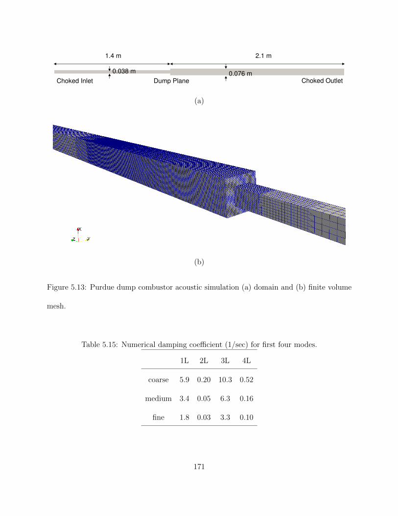
1.4 m 2.1 m

0.038 m 0.076 mChoked Inlet Choked OutletDump Plane

(a)

(b)

Figure 5.13: Purdue dump combustor acoustic simulation (a) domain and (b) finite volume

mesh.

Table 5.15: Numerical damping coefficient (1/sec) for first four modes.

1L 2L 3L 4L

coarse 5.9 0.20 10.3 0.52

medium 3.4 0.05 6.3 0.16

fine 1.8 0.03 3.3 0.10

171

The pressure modeshapes on a cut-plane through the center of the domain are shown

in Fig. 5.14. For this figure, no color scale is necessary, since it is customary to discuss

acoustic modes in terms of normalized amplitudes. The blue regions of this figure correspond

to a normalized amplitude of zero and the red regions correspond to a normalized amplitude

of one. It can be seen from this figure that the modes contain little variation in the transverse

direction. In view of this fact, the modes are best presented in a one-dimensional manner,

as done in Fig. 5.15.

The odd-numbered modes have low normalized amplitudes in the combustion cham-

ber, while the even-numbered modes have approximately equal amplitude in the regions

upstream and downstream of the dump plane. Also, the even-numbered modes have pres-

sure anti-nodes at the dump plane which the odd-numbered modes have pressure nodes. In

the view that acoustic modes are fed energy via the coupling of heat release and pressure

oscillations (Rayleigh’s criterion), the above reasons suggest that the even-numbered acous-

tic modes will be much more likely excited than the odd-numbered modes. This is, in fact,

what the experiment observed.

172

0

0.5

1

0.0 0.5 1.0 1.5 2.0 2.5 3.0 3.5

z

(a)

z0

0.5

1

0.0 0.5 1.0 1.5 2.0 2.5 3.0 3.5

(b)

z0

0.5

1

0.0 0.5 1.0 1.5 2.0 2.5 3.0 3.5

(c)

z0

0.5

1

0.0 0.5 1.0 1.5 2.0 2.5 3.0 3.5

(d)

Figure 5.14: Purdue rig normalized acoustic pressure mode amplitudes on a color scale of

blue (zero amplitude) to red (max amplitude) : (a) 1L, (b) 2L, (c) 3L, (d) 4L.

173

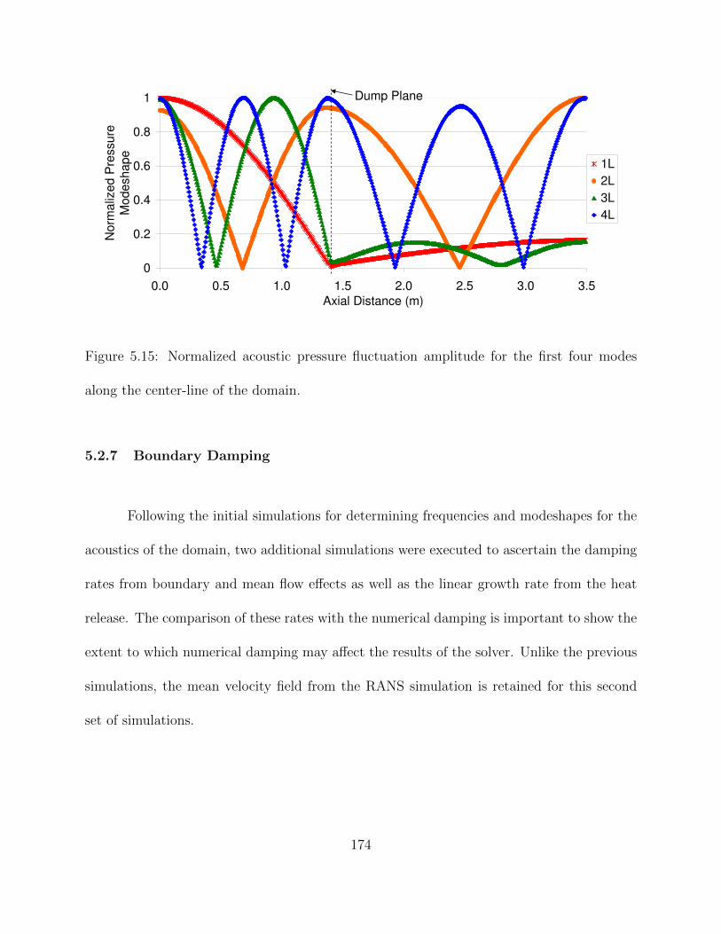
0

0.2

0.4

0.6

0.8

1

0.0 0.5 1.0 1.5 2.0 2.5 3.0 3.5

Axial Distance (m)

Norm

aliz

ed P

ressure

Modeshape

1L

2L

3L

4L

Dump Plane

Figure 5.15: Normalized acoustic pressure fluctuation amplitude for the first four modes

along the center-line of the domain.


Following the initial simulations for determining frequencies and modeshapes for the

acoustics of the domain, two additional simulations were executed to ascertain the damping

rates from boundary and mean flow effects as well as the linear growth rate from the heat

release. The comparison of these rates with the numerical damping is important to show the

extent to which numerical damping may affect the results of the solver. Unlike the previous

simulations, the mean velocity field from the RANS simulation is retained for this second

set of simulations.

174

First, without adding any heat release to the simulation, the perfectly-reflecting

boundary conditions are replaced by a choked inlet [24] and choked outlet boundaries [54].

Without taking into account entropy waves, the reflection coefficients for these boundaries

are given by Eqs. (5.1) and (5.12)

Routlet =1− γM + (γ − 1)M2

1 + γM + (γ − 1)M2(5.12)

These reflection coefficient formulae are used to set the boundary impedance at the

inlet and outlet to the domain. For this particular case, the reflection coefficient of the

choked inlet is 0.764 and the reflection coefficient of the outlet is 0.985. The purpose of

this simulation is to quantify the damping of the acoustic modes due to acoustic energy

flux through the boundaries and through interaction with the mean flow. The resulting

frequencies and damping coefficients are given in Table 5.16 respectively. Because the odd-

numbered modes are dominant in the upstream region, the reflection coefficient at the inlet

has a larger effect on these modes. In fact the peaks for the 1L and 3L modes are absent

from the results of this simulation. A small shift in the frequencies were observed, but the 2L

and 4L modes are still predicted with less than 3% error from the experimental frequencies.

The damping coefficient (negative growth rate) is now much higher than in the previous

simulation (Table 5.15). Because of this, the influence of numerical damping on the values

in Table 5.16 is negligible and these values can be interpreted as the damping rate associated

with the loss of acoustic energy through the boundaries and to the mean flow.

175

Table 5.16: Resonant frequencies (Hz) and damping coefficients (1/sec) for first four modes

with choked boundaries.

2L frequency 2L damping 4L frequency 4L damping

(Exp.) 189 – 382 –

coarse 188 10.1 374 12.4

medium 188 11.3 373 15.3

fine 188 10.6 373 13.2

5.2.8 Linear Heat Release Model

For the third simulation of this geometry, the mean velocity is once again removed and

the boundaries are reset to perfectly-reflecting conditions. After eliminating those sources of

damping, a linear heat release model is implemented. This simulation, therefore, measures

the linear growth rate due to heat release. The comparison of growth rate due to heat release

and damping due to acoustic energy losses indicates the linear stability of a mode. The linear

stability of a mode could be determined with one simulation rather than two by including

both heat release and loss mechanisms in a single simulation. For illustrative purposes, the

simulations were performed separately.

For flames anchored by a backward-facing step or sudden area change, a vortex shed-

ding model is common for capturing the physics of the acoustics-heat release feedback loop

176

[57]. With this in mind the Strouhal numbers of the 2L and 4L modes are 0.053 and 0.107,

respectively. Here, Strouhal number is defined as

StH =fH

U0

(5.13)

where H is the step height and U0 is the approaching velocity. The experiments of [58]

found a dominant frequency of vortex shedding with StH = 0.07. Large-eddy simulations of

the same geometry and flow conditions [59] found StH = 0.09 was the dominant frequency

of vortex shedding. Meanwhile, other experiments [60] found that the drag for a backward

facing step is minimum with local forcing at StH = 0.27. Appealing to [61], the authors

argue that this represents the vortex shedding frequency of the backward-facing step. The

spectra from their measurements, however, reveal peaks at StH/4 and StH/2, suggesting

that the actual dominant frequency of the step may be lower, with the minimal drag forcing

frequency of StH = 0.27 being a higher harmonic of the base frequency. Reynolds number

dependence is the other likely explanation for the disagreement.

Apparently, the frequencies of the 2L and 4L modes in the Purdue experiment lay in

the approximate region necessary for interaction with vortex shedding from the dump plane.

A sophisticated heat release model for vortex shedding combustion instability has been de-

veloped, leading to a kicked oscillator equation [16]. For the present purposes (demonstrating

a numerical technique), a simpler model is constructed. In this model the shedding pattern

of vortices promotes a sinusoidal heat release pattern in time. The release of a vortex occurs

at an acoustic pressure minimum at the dump plane and the vortex travels downstream at a

half of the mean flow velocity upstream of the dump plane [16]. The heat release maximum

177

occurs at the center of the vortex. This leads to the mathematical phrasing

q′(x, y, z, t) = −nq(x, y, z)

p0

p′0(t− τ(z)) (5.14)

where the time lag

τ(z) =z − z0

0.5U0

(5.15)

represents the time it takes for the vortex to travel from the dump plane to the location of

the heat release. The subscript 0 represents the value at the dump plane. The negative sign

represents the fact that this model predicts that the vortex release (maximum heat release)

occurs at an acoustic pressure minimum at the dump plane. For the linear heat release

model, the gain factor n is assumed independent of the acoustic variables. A value of n = 25

is used for the present case, but this value would likely need to be tuned to experimental

results to result in accurate reproduction of linear growth rate or limit cycle amplitude (for a

non-linear model). For this simulation, the 2L mode grew rapidly, drowning out any growth

of the 4L mode. For this reason, Table 5.17 reports values for only the 2L mode. Because

the two previous simulations indicated that the numerical damping would not play a large

role in determining accuracy of growth rates, the finest mesh was not simulated.

The frequency errors are again less that 3%. However, the linear growth rates for

the two mesh resolutions are quite different. The previous discussion ruled out numerical or

boundary damping as a reason for such a discrepancy. The numerical damping for the 2L

mode was much to small to create the difference shown here, and the boundary damping

was very similar for these two meshes. There is significant difference in the grid resolution

178

as it relates to the flame thickness, however, suggesting that the discretization as it relates

to heat release plays an important role in the determination of the linear growth rate. To

illustrate this point, Fig. 5.16 shows the heat release distribution on a cut plane for the

two tacFoam meshes. Qualitatively, the heat release distributions are very different, since

they are both mapping from a one million cell RANS mesh that is much finer in resolution.

When coupled with a heat release model that is dependent on distance from the dump plane,

it is no surprise that this difference leads to the difference in linear growth rates shown in

Table 5.17. Consequently, this also leads to the expectation that there may be a noticeable

difference in limit cycle amplitude when a non-linear model of the same type is used.

Table 5.17: Resonant frequencies (Hz) and linear growth rate (1/sec) for the linear heat

release model simulation.

2L frequency 2L amplitude

(Exp.) 189 –

coarse 192 27.8

medium 193 15.7

179

(a)

(b)

Figure 5.16: Mean heat release fields on the center-plane after mapping from RANS solution

onto tacFoam grid : (a) no refinement, (b) one level of refinement

180

5.2.9 Non-linear Heat Release Model

For a final simulation set with non-linear heat release model, the time lag calculation

is not changed from Eq. (5.14) and Eq (5.15). Only the gain factor n becomes a function of

the acoustic pressure amplitude. In particular, the form

n = Ane−Bnp′RMS + Cn (5.16)

is used, as was the form for the Hield et al. [47] validation case. Here, the values chosen

for the constants An, Bn, Cn are not from an experimental correlation. For the present

demonstrations, the values taken are

An = −24 (5.17)

Bn = 0.00011

Pa(5.18)

Cn = −1 (5.19)

The values An and Cn add to −25, so that the small signal limit yields the same gain

factor (n = −25) as the linear model. The negative value reflects that the model assumes that

the vortex is released at the pressure minimum and the maximum heat release corresponds

to the location of the vortex as it convects downstream. The value for Bn (specifically, its

multiplicative inverse) sets the characteristic pressure value at which the non-linearities of

the flame become manifest. As previously mentioned, a complete model would require the

tuning of these constants to a specific configuration, as done by [47, 48] for a bluff body

stabilized flame.

181

The temporal evolution of acoustic pressure for the non-linear heat release simulations

is shown in Fig. 5.17. The mode from the medium grid grows more slowly than that from

the coarsest grid. This observation is consistent with the lower linear growth rate observed

in Table 5.17 for the medium grid. The limit cycle amplitude reached is also lower for the

simulation with the refined grid. This shows the proportionality of linear growth rate and

limit cycle amplitude [12] for the two different grids.

0.5 1 1.5 2

−100

−50

0

50

100

pres

sure

(m

bar)

time (sec)0.5 1 1.5 2

−100

−50

0

50

100

pres

sure

(m

bar)

time (sec)

(a) (b)

Figure 5.17: Pressure time histories for a simulation probe near the exit of the domain : (a)

no grid refinement, (b) one level of grid refinement

Table 5.18 gives the comparison of limit cycle amplitude for the two simulations

with experimental data for these flow conditions. Note that for both the experimental and

numerical data, the limit cycle amplitude is an average of amplitudes from five pressure

probes placed along the length of the combustor (downstream of the flame). The probe

locations for the experiment and simulation were identical. Both simulations under-predict

182

the limit cycle amplitude of the 2L mode, but are of the right order of magnitude. The 4L

mode, while very strong in the experiment is absent from the simulation.

Table 5.18: Limit cycle amplitudes (mbar) for first four modes.

2L frequency 2L limit cycle 4L frequency 4L limit cycle

(Exp.) 189 54 382 279

coarse 189 123 374 0.2

medium 190 59 375 0.3

The Rayleigh index (RI), defined in Eq. (5.20), is calculated over the course of each

equation at each cell. The Rayleigh index calculation is done in the frequency domain, so

that the index is available as a function of frequency. The results of such a calculation gives

insight into what regions of the domain are driving or damping a given mode. Negative

values indicate that the heat release at that point, over the course of the simulation, tends

to remove acoustic energy from the domain. On the other hand, positive values indicate the

addition of acoustic energy by the unsteady heat release.

RI =

∫p′q′dt (5.20)

The comparison in Figs. 5.18 and 5.19 highlight the effect of grid resolution on

the stability of the mode. The Rayleigh index shows an alternating pattern of damping

and driving regions. Physically, this represents the vortex, shed from the dump plane at a

pressure minimum, convecting downstream. The continuing acoustic oscillations bring the

183

vortex (positive heat release fluctuation) in an out of phase with the pressure, leading to the

pattern seen in Fig. 5.18 for the 2L frequency. A similar pattern is seen in Fig. 5.19 for the

4L frequency, except that the phase of the vortex is altered at a higher frequency than the

2L mode.

While the 2L and 4L modes display the same pattern, the results showed that only

the 2L mode was excited to a large amplitude limit cycle. The overall excitation of the mode

is related to the Rayleigh criterion, which is determined by the integration of the Rayleigh

index over the entire domain. The 2L integrated Rayleigh index shows an increase by three

to four orders of magnitude over the 4L, while the odd numbered modes are even much below

that. The integrated Rayleigh index for the 2L decreases from the coarse grid to the fine

grid, which was manifest in the decrease of the limit cycle amplitude from 36 millibar to 21

millibar. The 4L mode integrated Rayleigh index increases as the mesh is refined, however.

Table 5.19: Volume integrated Rayleigh index (W · Pa) for first four modes.

1L 2L 3L 4L

coarse – 4.29E+05 – 6.55E+01

medium 6.90E-01 1.57E+05 1.12E-01 2.75E+02

184

(a)

(b)

Figure 5.18: Rayleigh index (W · Pa/m3) field for 2L frequency on two grids: (a) no refine-

ment, (b) one level of refinement

185

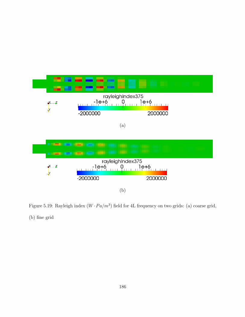
(a)

(b)

Figure 5.19: Rayleigh index (W ·Pa/m3) field for 4L frequency on two grids: (a) coarse grid,

(b) fine grid

186

5.2.10 Sensitivity to Model Constants

The experimental study of this combustor did not result in an empirical flame model

as provided by Hield et al. [47]. Because of this, the constants (An, Bn, Cn, and α) used for

the heat release model were determined in a somewhat arbitrary way. The least arbitrary

of the coefficients is the vortex convection speed coefficient α, which is typically close to the

average of the two velocities in a shear layer. In this case, the average between the jet flow

and the recirculation region yields and value of α = 0.5 if the recirculation region is assumed

to be approximately stagnant compared to the velocity of the jet.

A sensitivity analysis of these model parameters provides information about how the

choice of parameters affects the limit cycle amplitude prediction. The goal is to show that

the model parameters can be tuned (e.g. as a function of equivalence ratio and pre-heat

temperature) so as to match experimental limit-cycle amplitudes. The sensitivity analysis

was performed simply by varying one parameter at a time from the baseline values that

produced the results in Table 5.18. The values used in the sensitivity analysis are shown in

Table 5.20.

The results are shown in Fig. 5.20. The three first three parameters have clear trends,

while the trend is less clear for the vortex convection speed coefficient. The pre-multiplier

value An directly controls the low amplitude limit of the heat release model. As An increases,

the value of the gain coefficient given by Eq. (5.16) increases for a given value of pressure

amplitude. As a result, the limit cycle amplitude prediction is increased for an increasing

187

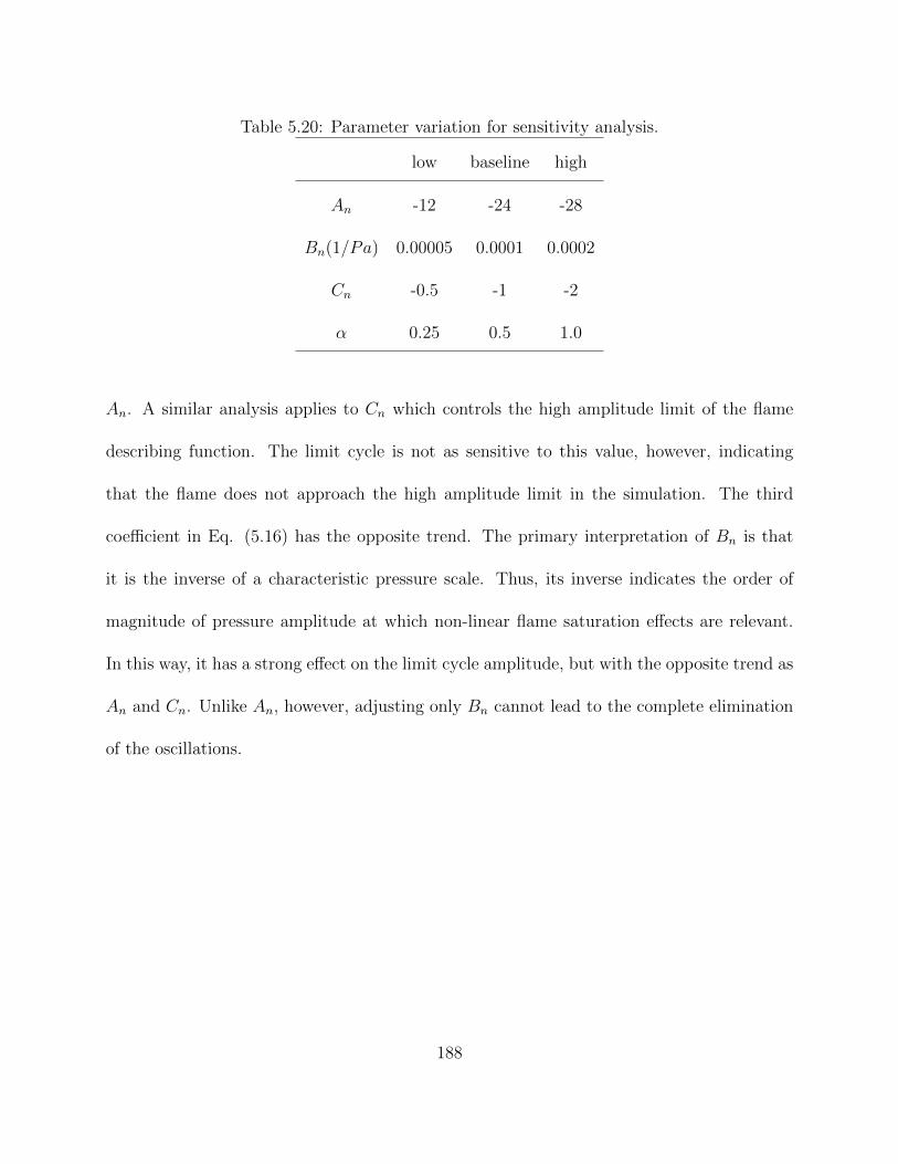
Table 5.20: Parameter variation for sensitivity analysis.

low baseline high

An -12 -24 -28

Bn(1/Pa) 0.00005 0.0001 0.0002

Cn -0.5 -1 -2

α 0.25 0.5 1.0

An. A similar analysis applies to Cn which controls the high amplitude limit of the flame

describing function. The limit cycle is not as sensitive to this value, however, indicating

that the flame does not approach the high amplitude limit in the simulation. The third

coefficient in Eq. (5.16) has the opposite trend. The primary interpretation of Bn is that

it is the inverse of a characteristic pressure scale. Thus, its inverse indicates the order of

magnitude of pressure amplitude at which non-linear flame saturation effects are relevant.

In this way, it has a strong effect on the limit cycle amplitude, but with the opposite trend as

An and Cn. Unlike An, however, adjusting only Bn cannot lead to the complete elimination

of the oscillations.

188

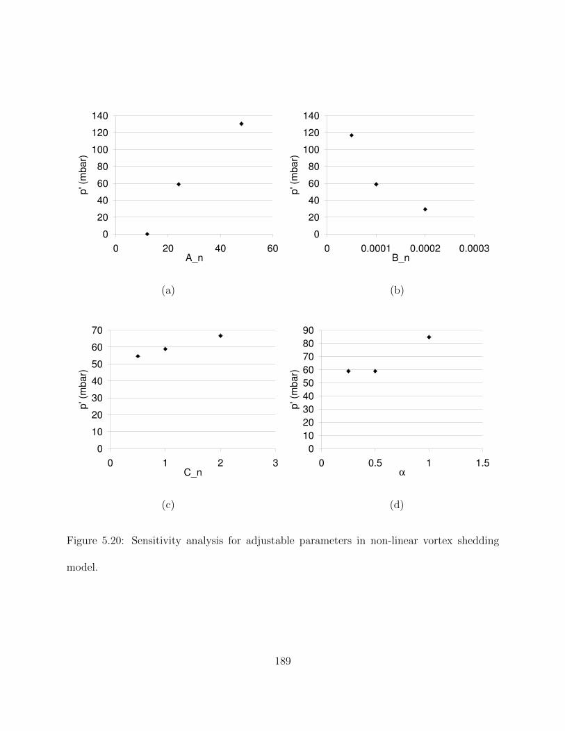
0

20

40

60

80

100

120

140

0 20 40 60A_n

p' (

mb

ar)

0

20

40

60

80

100

120

140

0 0.0001 0.0002 0.0003B_n

p' (

mb

ar)

(a) (b)

0

10

20

30

40

50

60

70

0 1 2 3C_n

p' (

mb

ar)

0

10

20

30

40

50

60

70

80

90

0 0.5 1 1.5α

p' (

mb

ar)

(c) (d)

Figure 5.20: Sensitivity analysis for adjustable parameters in non-linear vortex shedding

model.

189

5.2.11 Cost of Simulations

As a final note, it is instructive to compare the computational resources necessary

for tacFoam simulations with that of LES simulations. This validation case is optimal for

such comparisons due to the availability of LES work on this very same geometry [62]. As

discussed above, two different grids were run for the tacFoam case. The first was a baseline

coarse mesh with no refinement. The second mesh was refined in the flame region. Similarly,

the LES study used two grids, one coarse and one refined. A comparison in computational

cost is shown in Table 5.21.

Table 5.21: Comparison of computational resources for tacFoam and LES analysis of Purdue

dump combustor.

tacFoam coarse tacFoam fine LES coarse LES fine

cells 10,560 35,680 840,200 2,986,748

time step (sec) 1e-5 5e-6 5e-7 4e-7

total time (sec) 1.2 1.2 0.5 0.5

processors 4 12 240 240

wall-time (hours) 2.75 15.6 120 336

190

5.2.12 Conclusion

In conclusion, the Purdue dump combustor experiments were modelled by the present

thermoacoustic simulation code. The numerical damping for the 2L and 4L modes was

much less than the boundary damping and linear growth rates provided by the choked

boundaries and non-linear flame describing function, respectively. A physically motivated

vortex shedding model was used for the unsteady heat release based on mean heat release

profiles mapped from a RANS solution. A high amplitude limit cycle was observed for the 2L

mode, but the 4L mode was not present, most likely due the model or the model’s constants.

The amplitude of the 2L mode was on the same order of magnitude as the experiment, but

the coefficients used in the model would need to be tuned to match the experiment (similar

to that done by Hield et al. [47, 48]). The absence of the 4L mode from the simulation

was in contrast to the experiment, where the 4L mode was a greater amplitude than the 2L

mode. This result suggests that the vortex-based heat release model, while shown plausible

for the 2L mode, is not plausible in its current form for the 4L mechanism. Further research

and simulation is needed to determine other possible mechanisms for the 4L mode. One

possibility is that two different sets of tuned coefficients would be necessary to capture both

modes with the vortex model. Another possibility is to vary phase relationships could be

employed with respect to the pressure fluctuations at the dump plane. The most important

characteristic of the above model is its explicit dependence on dump plane pressure rather

than velocity. Velocity dependence, in this case, would most likely lead to strong 1L and

191

3L coupling, since these modes have pressure nodes and velocity anti-nodes at the dump

plane. Pressure dependence, however, gives the desired strength to 2L coupling, which has

a pressure anti-node and a velocity node at the dump plane.

The necessity of tuning the constants underscores a major limitation in the present

approach to modelling the unsteady heat release of a turbulent flame under the influence of

acoustic perturbations. Further work with modelling the Purdue experiments could include

tuning the coefficients (or phase relationship between the dump plane pressure and the release

of a vortex). The coefficients could also be tuned with variables such as pre-heat temperature

and equivalence ratio to model lean blow-off effects. This limitation is a natural consequence

of its standing on the cost versus accuracy scale. Just as many RANS models rely on

constants tuned for various canonical flows but by no means universal. In the same way,

constants could be tuned for a particular flame and used for predicting trends on similar

flames, but lack on universality is certainly expected for n − /tau heat release models. For

simulations requiring less constants (or less influential constants), large-eddy simulations can

be performed, albeit at a significant cost increase. The tuning of constants for appropriate

time lag models is out of the scope of this work.

192

CONCLUSION

Summary

In this thesis, the development of a novel three-dimensional linear thermoacoustic

solver was presented. The solver was written using the OpenFOAM C++ libraries for un-

structured finite volume meshes. The solution process includes interpolating a known mean

field solution onto the finite volume mesh intended for the acoustic solution. The linearized

Euler equations with a source term for unsteady heat release are discretized and solved using

a fourth-order Runge-Kutta method and second-order total variation diminishing Godunov

flux calculation. The Riemann solution for acoustics in inhomogeneous media is utilized at

each numerical face in a non-conservative flux scheme, allowing for accurate high-resolution

capturing of variations in both acoustic and pre-computed mean field data. For applica-

tion to gas turbine combustors, it was shown that the accurate representation of the effect

of density gradients on acoustic waves is vital to the successful prediction of resonant fre-

quencies and modeshapes. The thin premixed flames appear as sharp density gradients,

greatly altering the acoustic behavior of the combustion chamber. The governing equations

require an unsteady heat release model based on acoustic velocity or acoustic pressure to

close the system and provide a feedback path between the acoustic and heat release oscilla-

193

tions. The modelling success of the simulation relies heavily on the physical fidelity of the

heat release model. Indeed, a major ability of this code is to test such models in a complex

three-dimensional geometry with accurate mean fields. In this way, physical insight can be

gained through the comparison of various heat release models with known results. In addi-

tion, models constants can be tuned to match experiments for exploring operating ranges and

parametric effects. A number of verification tests were run to identify to validity of the solver

for various simple “academic” problems. The solver successfully reproduced analytical solu-

tions for one-, two-, and three-dimensional acoustics, gradual and sharp density gradients,

subsonic mean flow, arbitrary (real, constant) impedance boundary conditions (e.g. choked),

and linear growth rates in a Rijke tube with simple n-τ heat release model. These tests were

designed to verify the ability of the solver to account for the important physics governing

the development of large amplitude acoustic oscillations in gas turbine combustors. Finally,

the solver was validated with two different laboratory-scale combustors. First, a bluff body

stabilized flame experiment at the University of Melbourne provided an excellent validation

case. The experimental study performed in Melbourne used chemiluminescence data over

a range of operating conditions to establish a non-linear heat release law in which the gain

and time lag were dependent on the amplitude of oscillation. The descrease in gain with

increasing acoustic amplitude, along with choked boundaries, allowed for the development

of a limit cycle in the linear simulation. The limit cycle amplitude found reproduced the

experimental limit cycle accurately. The second validation case involved a recent dump com-

bustor experiment at Purdue University. No empirical heat release was developed by the

194

experimentalists in this case. Instead, a physically motivated vortex shedding model was

used for the simulation. With arbitrary (untuned) coefficients in the model, a limit cycle of

the same order of magnitude as the experiments was obtained was obtained for one of the

modes but not for the other. The effect of grid resolution for RANS and acoustics were also

explored.

Further Work

The following steps are recommended for further development of the numerical sim-

ulation procedure described in this thesis.

(1) For this thesis, the solver was limited to analytical and laboratory-scale scenarios.

The solver remains to be tested in a full-scale engine geometry with comparison to engine

data. This is the end goal of the solver and represents the most obvious extension of the

work in this thesis.

(2) The governing equations used for this thesis solved for acoustic velocity and

pressure, relying on the isentropic signal assumption to account for acoustic density. In real

combustors, an unsteady flame generates entropy waves which convect downstream with the

mean flow. These entropy waves can play an important role not only in the effecting acoustic

propagation, but also in the exit boundary conditions, where the interaction of entropy waves

with the boundary can produce an upstream-travelling acoustic wave. In addition to the

four linearized equations solve in this thesis, the inclusion of a fifth equation for the acoustic

195

density fluctuations would give the solver the ability to account for entropy waves. While

causing additional cost to the simulation, this enhancement would add important physical

fidelity to the model. The choked outlet case from the University of Melbourne experiments

could be used to validate the ability of the code to capture entropy waves, since the observed

instabilities in that case were due to the propagation of entropy waves and generation of an

acoustic wave at the choked exit.

(3) The solver developed in this thesis is designed to play a role in the design and

development process between one-dimensional thermoacoustic tools and large-eddy simula-

tions. Based on the three-dimensional modeshapes that can be found by the finite volume

solver, a weighted-residuals approximation method can be developed within the OpenFOAM

framework. This extension would allow for quick solution including only evaluation of three-

dimensional integrals over the domain and solution to the resulting ODE. Sophisticated ODE

solvers, such as Runge-Kutta methods, are already available in the OpenFOAM libraries.

Many of the mean flow and boundary effects could be easily accounted for in an accurate

three-dimensional manner by integrating over the finite volume domain otherwise used to

solve the full system of PDEs. Such a weighted residual method would offer a quick, approx-

imate solution that would have advantages over one-dimensional tools, but have a solution

time orders of magnitude less than the full thermoacoustic solution. This would allow for

parametric sweeps of important variables or of hypothesized heat release models.

(4) The boundary conditions for the solver developed in this thesis accounted for tra-

ditional acoustic boundary conditions (no mean flow, etc...). Improved boundary conditions

196

using a characteristic approach similar to the LODI approach of compressible DNS/LES

would allow for more accurate representation of boundary conditions in a more complex, in-

homogeneous field. Additionally, the initial success of the time-domain complex impedance

boundary conditions was limited. Additional testing and research into the implementation

of this boundary condition is suggested.

197

APPENDIX ADERIVATION OF GOVERNING EQUATIONS

198

APPENDIX ADERIVATION OF GOVERNING EQUATIONS

Starting with the general governing equations for the continuum model of fluid flow,

this section will develop the equations of motion by which thermoacoustic phenomena can

be modelled. The physical principles applicable to the continuum model of gas dynamics are

the conservation equations of mass, momentum, energy, and entropy, as well as an equation

of state to close the system.

A.1 Conservation of Mass

The conservation of mass, or continuity equation, simply states that the rate of change

of mass inside a fixed control volume in laboratory coordinates is equal to the difference

between the incoming and outgoing mass, adding any mass sources or sinks. For an arbitrary

control volume

∂

∂t

y

Ω

ρdV = −x

∂Ω

ρujdAj +y

Ω

MdV (A.1)

where the outward pointing normal has been used to define the differential surface area dAi

and M is the mass source/sink density. In Eq. (A.1), M represents any source of mass

present within a given control volume. For example, the evaporation of liquid droplets into

199

gas can be modelled simply by this term. Applying the divergence theorem to the first term

on the right hand side bringing the time derivative inside the integration on the left hand

side

y

Ω

∂ρ

∂tdV = −

y

Ω

∂(ρuj)

∂xjdV +

y

Ω

MdV. (A.2)

This is the integral form of the mass conservation, provided the differentiability con-

siderations for the divergence theorem are satisfied and the interchangeability of differentia-

tion in time and integration in space is valid. In some fluid flows, such as those containing

shock waves, the differentiability considerations are not met and the solution must be sought

in terms of the integral form. Such solutions are often referred to as weak solutions [41, 40].

Disregarding these cases, requiring that Eq. (A.2) be satisfied for any and all control volumes

results in the criteria that the integrands must be satisfied at all locations

∂ρ

∂t+∂(ρuj)

∂xj=M. (A.3)

This is the conservative form of the partial differential equation describing the con-

servation of mass. It can also be written in non-conservative form

∂ρ

∂t+ ρ

∂uj∂xj

+ uj∂ρ

∂xj=M (A.4)

which is sometimes useful for analysis and manipulation.

200

A.2 Conservation of Momentum

The conservation of momentum, also known as Newton’s second law of motion,

equates the forces acting on a control volume with the change in momentum within the

control volume. For the Newtonian formulation of the continuum model for fluid mechanics,

the change of momentum within the volume is equal to the net amount of momentum flow-

ing into the volume plus the forces acting on the volume. In three-dimensional space, the

conservation of momentum is expressed by three equations, which can be written concisely

using summation notation

∂

∂t

y

Ω

ρuidV = −x

∂Ω

ρuiujdAj +y

Ω

FidV. (A.5)

Assuming differentiability, the divergence theorem is applied to the first term on the

right hand side, as in the mass equation. Also, the interchange of time differentiation and

volume integration is performed on the left hand side, leading to

y

Ω

∂(ρui)

∂tdV = −

y

Ω

∂(ρujui)

∂xjdV +

y

Ω

FidV (A.6)

and equating the integrands gives

∂(ρui)

∂t+∂(ρujui)

∂xj= F surfacei + F bodyi . (A.7)

In Eqs. (A.5)-(A.7), Fi represents any forces acting on the fluid. In Eq. (A.7), the

forces are split into surface forces F surfacei and body forces F bodyi . The surface forces can be

further divided into normal and shear forces. The normal surface forces are due to the local

201

pressure, while the shear forces are due to the local viscosity

F surfacei = Fnormali + F sheari = − ∂p

∂xjδij +

∂

∂xj

µ∂ui∂xj

. (A.8)

For convenience the viscous terms are combined with the body force terms into a

general term Fi, which accounts for all forces except the pressure forces. The momentum

conservation equation becomes

∂(ρui)

∂t+∂(ρujui)

∂xj+

∂p

∂xjδij = Fi. (A.9)

Momentum conservation can also be written in non-conservative form in order to

express the equation in terms of the primitive variable, velocity. Multiplying ui to Eq. (A.3)

and subtracting this from Eq. (A.9) yields

ρ∂ui∂t

+ ρuj∂ui∂xj

+∂p

∂xjδij = Fi − uiM. (A.10)

A.3 Equation of State

The state postulate of thermodynamics ensures that any unknown intensive property

of a fluid can be determined from two known independent intensive properties. This is often

useful for achieving closure to a set of fluid mechanical equations. In the mass and momen-

tum equations discussed above, two intensive thermodynamic quantities have already been

introduced: p and ρ. From knowledge of these two quantities, any other intensive thermody-

namic quantity can be deduced, provided a physically accurate model for the thermodynamic

202

behavior of the fluid. In this thesis, the topic at hand (pre-mixed combustion) deals almost

exclusively with gases well-approximated by the ideal gas equation of state

p = ρRT. (A.11)

Furthermore, the internal energy e and the enthalpy h of an ideal gas is a function of

temperature only

e(Tstate) = e(Tref ) +

Tstate∫Tref

cvdT (A.12)

and

h(Tstate) = h(Tref ) +

Tstate∫Tref

cpdT. (A.13)

Note that the definitions of internal energy and enthalpy are therefore arbitrary to an

additive constant based on the reference temperature chosen. Choosing a constant specific

heat with a convenient reference condition, Eqs. (A.12) and (A.13) can be written simply as

e = cvT (A.14)

and

h = cpT. (A.15)

Substituting Eq. (A.14) into Eq. (A.11), the equation of state for an ideal gas with

constant specific heat can be written as

e =p

(γ − 1)ρ(A.16)

where

γ =cpcv. (A.17)

203

A.4 Conservation of Energy

The conservation of energy, also known as the first law of thermodynamics, states

that the change in energy content of a mass is equal to the heat addition to the mass minus

the work done by the mass. For a fluid control volume, the rate of change of the energy

within the volume is equal to the net energy flow into the volume plus the net heat addition

to the volume minus the net work done by the volume. For an arbitrary control volume in

laboratory coordinates

∂∂t

t

Ω

ρ(e+ 12uiui)dV =

−s

∂Ω

ρ(e+ 12uiui)ujdAj +

t

Ω

QdV −t

Ω

WdV

(A.18)

where Q is the volumetric heat to the system andW is the volumetric work from the system.

Performing the same manipulations as before

t

Ω

∂[ρ(e+ 12uiui)]

∂tdV =

−t

Ω

∂[ρuj(e+12uiui)]

∂xjdV +

t

Ω

QdV −t

Ω

WdV

(A.19)

the partial differential equation for energy conservation is acquired by requiring Eq. (A.19)

to be satisfied for any arbitrary control volume

∂[ρ(e+ 12uiui)]

∂t+∂[ρuj(e+ 1

2uiui)]

∂xj= Q−W . (A.20)

This equation describes the total sensible energy of the system, which is the sum of

internal energy (e) and kinetic energy (12uiui).

204

A.4.1 Kinetic Energy Equation

An equation for the kinetic energy of the flow can be developed by multiplying Eq.

(A.10) by ui and noting that ui∂ui = ∂(12uiui) and uiδij = uj

∂(12uiui)

∂t+ ρuj

∂(12uiui)

∂xj+ uj

∂p

∂xj= uiF − uiuiM. (A.21)

This equation can be used to manipulate Eq. (A.20) conservation equation.

A.4.2 Work

The work term W represents the work done by the gas and is composed of the work

done by the pressure gradient on the moving fluid (force times velocity, with force equal

to the negative pressure gradient) and the thermodynamic expansion work done by the gas

(pressure times change in specific volume)

W = −W∇p +Wexpansion −Wother

= uj∂p∂xj

+ ρpD 1ρ

Dt− ujFj.

(A.22)

The second term can be simplified using the chain rule

ρpD1

ρ

Dt

= −ρp 1

ρ2

Dρ

Dt= −p

ρ

Dρ

Dt. (A.23)

205

Using the non-conservative form of the mass equation, Eq. (A.4), the material deriva-

tive of the density can be substituted, yielding

ρpD1

ρ

Dt

= p∂uj∂xj− p

ρM. (A.24)

Substituting this result into Eq. (A.22) gives

W = uj∂p∂xj

+ p∂uj∂xj− p

ρM− ujFj

=∂(puj)

∂xj− p

ρM− ujFj

. (A.25)

A.4.3 Heat

The heat term Q represents both the heat transferred into the control volume via

conduction and the heat produced in the control volume via electrical dissipation or chemical

reaction. Mathematically, the expression for the heat is

Q = Qconduction +Qelectrical +Qchemical

= ∂∂xj

k ∂T∂xj

+ j2ρelec + ωH(A.26)

where k is the thermal conductivity, ρelec is the electrical resistivity, j is the electrical current

density, ω is the mass conversion rate of a chemical reaction, andH is the enthalpy of reaction

per unit mass. At this point, the heat term will be left in the equation as is, though later,

the chemical source of heat will be crucial. This term models the energy added to the flow

by combustion.

206

A.4.4 Various Forms of the Energy Equation

Substituting the formulation for the work term W from Eq. (A.25) into Eq. (A.20)

and rearranging

∂[ρ(e+ 12uiui)]

∂t+∂[ρuj(e+ 1

2uiui + p

ρ)]

∂xj= Q+

p

ρM+ ujFj. (A.27)

This is the conservation form of the energy equation often employed in computational

fluid dynamics. Defining the enthalpy as h = e+ pρ, this equation can be rephrased as

∂[ρ(e+ 12uiui)]

∂t+∂[ρuj(h+ 1

2uiui)]

∂xj= Q+

p

ρM+ ujFj. (A.28)

Even more concisely, the kinetic energy can be absorbed into the definitions of eo =

e+ 12uiui and ho = h+ 1

2uiui

∂(ρeo)

∂t+∂(ρujh

o)

∂xj= Q+

p

ρM+ ujFj. (A.29)

From this equation, subtracting eo multiplied by the conservative form of the mass

equation, Eq. (A.3), then also subtracting the kinetic energy equation, Eq. (A.21), a non-

conservative energy equation can be written in terms of the evolution of internal energy

ρ∂e

∂t+ ρuj

∂e

∂xj= −p∂uj

∂xj+Q+

p

ρ+

1

2uiui − e

M. (A.30)

Using a constant specific heat model for the fluid, e = cvT , this equation can be

phrased in terms of temperature

ρcv∂T

∂t+ ρcvuj

∂T

∂xj= −p∂uj

∂xj+Q+

p

ρ+

1

2uiui − e

M. (A.31)

207

This is the form used by Culick (2006). Alternatively, from Eq. (A.29), subtracting

ho multiplied by Eq. (A.3) and subtracting the kinetic energy equation, a non-conservative

enthalpy equation can be written

ρ∂h

∂t+ ρuj

∂h

∂xj=∂p

∂t+ uj

∂p

∂xj+Q+

1

2uiui − e

M. (A.32)

Using a constant specific heat model for the fluid, h = cpT , this equation can be

phrased in terms of temperature

ρcp∂T

∂t+ ρcpuj

∂T

∂xj=∂p

∂t+ uj

∂p

∂xj+Q+

1

2uiui − e

M. (A.33)

Using the ideal gas equation of state (A.11), an substituting for T in Eq. (A.33)

ρcpDTDt

= ρcpR

D(p/ρ)Dt

= cpRDpDt

+ ρcpp

RD(1/ρ)Dt

= γγ−1

DpDt− cpp

ρRDρDt

= γγ−1

DpDt

+ γγ−1

p∂uj∂xj− γ

γ−1pρM

(A.34)

where Eq. (A.4) has been used to simplify the material derivative of density. Substituting

Eq. (A.34) into Eq. (A.33) and multiplying by γ − 1 leads to a non-conservative energy

equation in terms of pressure

∂p

∂t+ uj

∂p

∂xj+ γp

∂uj∂xj

= (γ − 1)Q+

1

2(γ − 1)uiui − (γ − 1)e− γp

ρ

M. (A.35)

The pressure form of the energy equation is very useful in the field of thermoacoustics,

because it is natural to treat acoustic fields in terms of pressure and velocity. A pressure form

208

of the energy equation can also be derived by substituting Eq. (A.16) into the conservative

formulation of the energy conservation, Eq. (A.27), which results in

∂[p+ 12(γ − 1)ρuiui]

∂t+∂[γujp+ 1

2(γ − 1)ρujuiui]

∂xj= (γ − 1)(Q+

p

ρM). (A.36)

209

APPENDIX BRIEMANN SOLVER APPROACH TO FINITE VOLUME

METHODS FOR HYPERBOLIC EQUATIONS

210

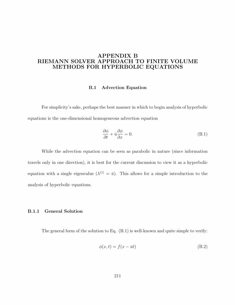
APPENDIX BRIEMANN SOLVER APPROACH TO FINITE VOLUME

METHODS FOR HYPERBOLIC EQUATIONS

B.1 Advection Equation

For simplicity’s sake, perhaps the best manner in which to begin analysis of hyperbolic

equations is the one-dimensional homogeneous advection equation

∂φ

∂t+ u

∂φ

∂x= 0. (B.1)

While the advection equation can be seen as parabolic in nature (since information

travels only in one direction), it is best for the current discussion to view it as a hyperbolic

equation with a single eigenvalue (λ(1) = u). This allows for a simple introduction to the

analysis of hyperbolic equations.

B.1.1 General Solution

The general form of the solution to Eq. (B.1) is well-known and quite simple to verify:

φ(x, t) = f(x− ut) (B.2)

211

where f(x) is any differentiable function. Differentiating Eq. (B.2) in time and space, re-

spectively, yields

∂φ∂t

= −uf ′(x− ut)

∂φ∂x

= f ′(x− ut)(B.3)

Simple substitution the verifies that Eq. (B.1) is satisfied.

B.1.2 Initial Value Problem

For an initial value problem in which no physical boundaries play a significant role,

the analysis can be further clarified. Using initial data

φ(x, 0) =o

φ(x) (B.4)

the general function f(x) can be found by setting t = 0

φ(x, 0) = f(x) =o

φ(x) (B.5)

which yields the IVP solution to the advection equation

φ(x, t) =o

φ(x− ut). (B.6)

Physically, the insight offered by Eq. (B.6) is as follows. The initial data provided to

the system simply translates (advects) with the characteristic speed u.

212

B.1.3 Riemann Problem

It is in this simple context that the Riemann problem can be first introduced. The

Riemann problem is a specific type of initial value problem in which the initial conditions are

piecewise constant with a single discontinuity at the origin (x = 0). The initial conditions

can be stated in terms of the two constant values: to the left of the origin (φL) and to the

right of the origin (φR)

o

φ(x) =

φL : x < 0

φR : x ≥ 0

. (B.7)

Applying the general solution to the hyperbolic IVP, Eq. (B.6), the solution to the

Riemann problem for the advection equation is simply

φ(x, t) =

φL : x− ut < 0

φR : x− ut ≥ 0

(B.8)

or

φ(x, t) =

φL : x < ut

φR : x ≥ ut

(B.9)

or, finally

φ(x, t) =

φL : u > x

t

φR : u ≤ xt

(B.10)

This final form of the solution is perhaps the most useful moving forward, since it relates

the discontinuity location in terms of the eigenvalue (u) and the similarity variable (xt). As

a final note, a value of importance later is the solution to the Riemann problem at the origin

213

for finite positive time

φ(0, t) =

φL : u > 0

φR : u ≤ 0

(B.11)

Noting that the solution at the origin is not a function of time for linear systems, we follow

the nomenclature of LeVeque (2002) to denote the solution at the origin

φ↓(φL, φR) =

φL : u > 0

φR : u ≤ 0

(B.12)

This has a simple interpretation that the solution at the origin is equal to the upwind

initial condition. Later, this will be and important starting place for a class of finite volume

numerical methods.

B.2 Hyperbolic Systems of Equations

A natural extension of the above discussion for a single hyperbolic equation is a

system of m hyperbolic equations defined by

∂φ˜∂t

+f˜(φ˜)

∂x= 0 (B.13)

where subscripts are used to denote partial differentiation, φ is the vector of solution variables

φ˜ =

φ1

φ2

...

φm

(B.14)

214

and the f is the flux vector given by

f˜ =

f1(φ1, φ2, , φm)

f2(φ1, φ2, , φm)

...

fm(φ1, φ2, , φm)

(B.15)

Applying the chain rule to the flux in Eq. (B.13), the system of equations can be rewritten

as

∂φ˜∂t

+ A≈

∂φ˜∂x

= 0 (B.16)

where A≈

is the Jacobian matrix given by

A≈

= ∂f˜/∂φ˜ =

∂f1/∂φ1 ∂f1/∂φ2 · · · ∂f1/∂φm

∂f2/∂φ1 ∂f2/∂φ2 · · · ∂f2/∂φm

......

. . ....

∂fm/∂φ1 ∂fm/∂φ2 · · · ∂fm/∂φm

(B.17)

B.2.1 Transformation to Decoupled Equations

Equation (B.13) is a system of m coupled PDEs. Next, it is useful to decouple

these into m independent PDEs. In the event that the entries in the Jacobian matrix A≈

,

Eq. (B.17), are constant functions of the variables φ˜, it is useful to consider the eigenvalue

215

problem related to the Jacobian matrix, namely

A≈R≈

= R≈

Λ≈

(B.18)

where R≈

is the right eigenvector matrix associated with the diagonal eigenvalue matrix Λ≈

.

Λ≈

=

λ1 0 · · · 0

0 λ2 · · · 0

......

. . ....

0 0 · · · λm

(B.19)

R≈

=[r˜1 r˜2 · · · r˜m] (B.20)

where r˜p is the pth eigenvector and λp is its corresponding pth eigenvalue. In this way, each

eigenvalue-eigenvector pair satisfies the relationship

A≈r˜p = λpr˜p. (B.21)

Rearranging Eq. (B.18), it is evident that the Jacobian can be diagonalized if its

eigenvalues are real

A≈

= R≈

Λ≈R≈−1 (B.22)

.

Similarly, the left eigenvectors matrix L≈

is defined as

L≈A≈

= Λ≈L≈

(B.23)

216

and is populated with the left eigenvectors as row vectors

L≈

=

l˜1l˜2...

l˜m

. (B.24)

Rearranging Eq. (B.23), the A matrix can also be written as

A≈

= L≈−1Λ≈L≈. (B.25)

Equating Eq. (B.22) with Eq. (B.25) shows the following relationship between the

left and right eigenvector matrices

L≈

= R≈−1. (B.26)

The system of partial differential equations is called hyperbolic provided that the

eigenvalues of the Jacobian are real. The term strictly hyperbolic refers to a system in which

the real eigenvalues are distinct. Assuming the Jacobian matrix to be constant in space and

time, except for its dependence on the variables φ˜, Eq. (B.22) can be substituted into Eq.

(B.16) giving

∂φ˜∂t

+R≈

Λ≈R≈−1∂φ˜∂x

= 0

R≈−1∂φ˜∂t

+ Λ≈R≈−1∂φ˜∂x

= 0

∂(R≈−1φ˜)

∂t+ Λ≈

∂(R≈−1φ˜)

∂x= 0

∂w˜∂t

+ Λ≈

∂w˜∂x

= 0 (B.27)

217

where a new set of transformed variables w˜ is defined by

w˜ = R≈−1φ˜ = L

≈φ˜

w˜p = l˜p · φ˜(B.28)

such that the coupled system of m equations given by Eq. (B.16) is transformed into m

independent equations, the pth equation given by

∂wp

∂t+ λp

∂wp

∂x= 0 (B.29)

.

B.2.2 General Solution

Each of the decoupled equations resulting from the above transformation can be

solved separately following the procedure shown for the advection equation. Each solution

consists of a wave, with the corresponding eigenvalue giving the speed of propagation. The

general solution to each independent equation is, by analogy with Eq. (B.2)

wp(x, t) = f(x− ut). (B.30)

B.2.3 Initial Value Problem

When the initial conditions of a system are given by

φ˜(x, 0) =o

φ˜(x) (B.31)

218

the initial conditions for the decoupled system can be found using the same transformation

as Eq. (B.28)

ow˜(x) = R

≈−1

o

φ˜(x) = L≈

o

φ˜(x)

o

wp(x) = l˜p · oφ˜(x)

(B.32)

where

o

wp(x) = wp(x, 0) (B.33)

and the solution is found for each advection-like equation for the transformed variables

wp(x, t) =o

wp(x− λpt). (B.34)

After each independent equation is solved using Eq. (B.34), the desired solution in

terms of φ˜ can be found by reversing the transformation in Eq. (B.28)

φ˜(x, t) = R≈w˜(x, t)

=m∑p=1

wp(x, t)r˜p=

m∑p=1

owp(x− λpt)r˜p

=m∑p=1

l˜p · oφ˜(x− λpt) r˜p

. (B.35)

Hence, the hyperbolic system can be described by m independently propagating

waves, with strengths in terms of original variables determined by the eigenvectors of the

Jacobian.

219

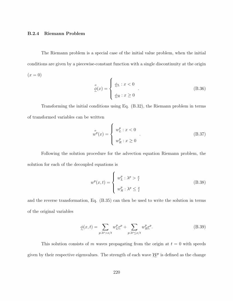
B.2.4 Riemann Problem

The Riemann problem is a special case of the initial value problem, when the initial

conditions are given by a piecewise-constant function with a single discontinuity at the origin

(x = 0)

o

φ˜(x) =

φ˜L : x < 0

φ˜R : x ≥ 0

. (B.36)

Transforming the initial conditions using Eq. (B.32), the Riemann problem in terms

of transformed variables can be written

o

wp(x) =

wpL : x < 0

wpR : x ≥ 0

. (B.37)

Following the solution procedure for the advection equation Riemann problem, the

solution for each of the decoupled equations is

wp(x, t) =

wpL : λp > x

t

wpR : λp ≤ xt

(B.38)

and the reverse transformation, Eq. (B.35) can then be used to write the solution in terms

of the original variables

φ˜(x, t) =∑

p:λp>x/t

wpLr˜p +∑

p:λp≤x/t

wpRr˜p. (B.39)

This solution consists of m waves propagating from the origin at t = 0 with speeds

given by their respective eigenvalues. The strength of each waveW˜p is defined as the change

220

in the original variables across the wave ∆(φ˜)p. From Eq. (B.39), the change in the original

variables across a wave is given by

W˜p = ∆(φ˜)p = (wpR − wpL)r˜p = αpr˜p (B.40)

where αp is the strength coefficient for the pth wave. Equation (B.40) can be considered as

the mathematical definition of αp. The values for αp can be found by considering the change

in original variables across all of the waves is the sum of the individual changes shown in

Eq. (B.40)

φ˜R − φ˜L =m∑p=1

r˜pαp = R≈α˜. (B.41)

Inverting this equation to solve for α

α˜ = w˜R − w˜L = R≈−1(φ˜R − φ˜L) = L

≈(φ˜R − φ˜L)

αp = wpR − wpL = l˜p · (φ˜R − φ˜L)

. (B.42)

Given this definition for the wave strength, the solution to the Riemann problem,

first given by Eq. (B.39), can also be written as

φ˜(x, t) = φ˜L +∑

p:λp≤x/t

W˜p

= φ˜R −∑

p:λp>x/t

W˜p

=1

2(φ˜L + φ˜R) +

1

2

∑p:λp≤x/t

W˜p −∑

p:λp>x/t

W˜p

. (B.43)

Finally, the value on the origin, useful in the next section, is easily found

φ˜(0, t) = φ˜↓(φ˜L, φ˜R) =1

2(φ˜L + φ˜R) +

1

2

∑p:λp≤0

W˜p −∑p:λp>0

W˜p

. (B.44)

221

B.3 Finite Volume Formulation

The solutions to hyperbolic initial value problems, specifically Riemann problems,

are useful in establishing numerical methods for calculating the flux through an internal face

between two numerical cells. At a given time step, the values from the two neighboring

cells provide the left and right initial conditions for the Riemann problem. The flux through

the face can then be calculated using the solution to the Riemann problem on the face (at

x = 0). The finite volume formulation for using the Riemann solution for flux calculations

is presented first in one dimension for a single advection equation and then expanded to a

system of hyperbolic equations. At first, focus is put on first order upwind methods, with

extension to higher-order methods reserved for later.

B.3.1 One-Dimensional Upwind Formulation

To introduce the use of the Riemann problem for numerical methods, first consider

a single advection equations, given by Eq. (B.1). For a one-dimensional finite volume

method, consider a face connecting to neighboring cells. At a given time step n, the right

and left cells contain a single value for each of the solution variables at the cell center. As

a first approximation, assume that such cell-centered values are constant over the entire cell

volume. In this way, using the values at time n as initial conditions, the problem resembles

the Riemann problem described above in Eq. (B.7). The flux through the face (for a constant

222

u) is defined as

f(φ) = uφ. (B.45)

Defining a coordinate system to reflect the relationship of the finite volume problem

with the Riemann problem, set the origin x = 0 at the face where the discontinuity occurs.

At the face, the solution variable φ transitions from the left cell center’s value to the right

cell-center’s value. The numerical flux, vital for finite volume calculations, is given by

fface = uφ(0, t). (B.46)

Using the results from the above solution to the one-dimensional advection equation

for the Riemann problem, the flux through the face is

fface = uφ↓(φL, φR) = u−φR + u+φL (B.47)

where the plus and minus superscripts denote

u+ = max(u, 0) u− = min(u, 0). (B.48)

Furthermore, it is useful to describe this in terms of the wave strengthW = φR−φL.

There is only one wave in this case, of course. The flux at the face can also be given by

uφ↓(φL, φR) = uφL − u−W = uφR − u+W . (B.49)

This is merely a mathematical way to describe that, for a given direction of the

wave propagation velocity (eigenvalue), the value of the solution variable used at the face

to calculate the flux comes from the upstream side. For the single variable linear advection

223

equation, as shown, the results is quite simply the first-order upwind method. This method is

stable, but highly diffusive, especially when used for a non-linear term, such as the advection

term in the momentum equations of fluid flow. This task of this thesis is solely concerned

with linearized equations, so further discussion of non-linearity is not needed.

B.3.2 System of Hyperbolic Equations: Godunov Method

The extension of the upwind flux calculation method introduced above to systems of

linear equations makes use of the previously discussed theory. Such an extension is quite

straight-forward. Under the assumption of constant coefficients

f˜(φ˜) = A≈φ˜. (B.50)

Therefore, proceeding as above, the flux at the face for each of the variables in the φ˜vector can be written as

f˜face = A≈φ˜(0, t) (B.51)

where again the face between two adjacent one-dimensional cells is placed at the origin

(x = 0). As foreshadowed, Eq. (B.43) is now extremely useful for defining the flux through

the face. The first expression of Eq. (B.43) at the face becomes

f˜face = A≈φL +

∑p:λp<0

A≈W˜p. (B.52)

This essentially states that the variables at the face can be calculated as the values

at the left cell center plus the changes across each wave propagating to the left. Noting from

224

Eq. (B.40) that the wave strength vectorW˜p is a multiple of the pth eigenvector, Eq. (B.52)

can be rewritten, using Eq. (B.18), as

f˜face = A≈φL +

∑p:λp<0

λpW˜p (B.53)

or, using the notation developed in Eq. (B.48), as

f˜face = A≈φL +

m∑p=1

(λp)−W˜p. (B.54)

Likewise, the flux at the face can be calculated coming from the right using the second

expression from Eq. (B.43)

f˜face = A≈φR −

∑p:λp>0

A≈W˜p. (B.55)

Here, the face fluxes are calculated using the cell center values from the right cell

minus the changes across each of the waves propagating to the right. Using the definition of

the eigenvectors here as on the left side

f˜face = A≈φR −

m∑p=1

(λp)+W˜p. (B.56)

For constant coefficient linear problems, Eqs. (B.54) and (B.56) give the same value.

A convenient way to calculate this value is found by averaging these two equations (that is,

multiplying each by 1/2 and adding).

f˜face =1

2A≈

(φ˜L + φ˜R)−m∑p=1

[(λp)+ − (λp)−

]W˜p. (B.57)

Noting from Eq. (B.48) the identity

λ+ − λ− = |λ| (B.58)

225

the so-called Roe’s method for calculating face fluxes is given most succinctly by

f˜face =1

2A≈

(φ˜L + φ˜R)−m∑p=1

|λp|W˜p. (B.59)

In the context of using this flux calculation to support a finite volume calculation, this

first-order upwind method is known as Godunov’s method. As mentioned with the simple

advection equation, such upwinding is highly diffusive. Therefore, extension to higher orders

is necessary for useful in the present context (linear growth rates and limit cycle amplitudes

for combustion instabilities). Prediction of thermoacoustic stability is polluted if numerical

diffusion adds significant damping to the acoustic modes of interest.

B.3.3 Extension to Higher Order Methods

Second-order methods can be constructed by evaluating the gradient of each solution

variable as each cell center and extrapolating the cell center variables to the either side of

the face using such gradient. For a given variable

φL = φL,center +∂φ

∂xL

∆Lx

2(B.60)

and

φR = φR,center −∂φ

∂xR

∆Rx

2. (B.61)

The extrapolated values on either side then serve as the initial condition for the

Riemann problem and the fluxes can be calculated using Eq. (B.54), (B.56), or (B.59). This

226

often leads in the best case to spurious oscillations in the solution and in the worst case to

numerical instability. To mitigate such factors that arise when the solution varies rapidly,

the theory of total variation diminishing (TVD) gradient limiters has been heavily developed

within the CFD community [41]. Applying a TVD limiter to the gradients calculated for

each cell center, Eqs. (B.60) and (B.61) can be used to develop a second-order Godunov

type approach to the finite volume method. Of course, in the neighborhood of sharp changes

in solution variables, the method reduces to first order. This is unavoidable, however, in this

context, if a stable, total variation diminishing solution is desired. This TVD-based approach

with piecewise linear reconstruction of the solution in space gives a so-called “high-resolution”

method for solving the hyperbolic system of equations. Such high-resolution methods are

known to give much less numerical diffusion than more traditional CFD flux calculations

involving simple interpolation between two cell centers. This comes at a price, however,

as the solution to the Riemann problem creates additional operations at each cell for each

iteration. Nevertheless, the extra computing time is often worth it in simulations sensitive

to numerical diffusion.

227

APPENDIX CANALYTICAL SOLUTIONS TO VERIFICATION CASES

228

APPENDIX CANALYTICAL SOLUTIONS TO VERIFICATION CASES

The purpose of this appendix is to show the derivation of the analytical solutions used

for verification cases for the tacFoam solver. For a general background in acoustic analysis,

the author recommends [43].

C.1 One-Dimensional Acoustics in a Duct

The simplest verification for an acoustics solver is the one-dimensional duct with no

mean flow and no mean property gradients. In this case, the linearized momentum and

energy conservation laws for classical acoustics in one spatial dimension (z) can be applied

∂u′

∂t+ 1

ρ∂p′

∂z= 0

∂p′

∂t+ γp∂u

′

∂z= 0

(C.1)

For the constant area, constant property, zero flow duct, the eigenfrequencies are those of

classical acoustics. The conservation laws of Eq. (C.1) can be combined to form the classical

wave equation for the acoustic pressure with wave speed a =√

γpρ

, which is the isentropic

speed of sound in an ideal gas

∂2p′

∂t2− a2∂

2p′

∂z2= 0 (C.2)

229

The separation of variables technique suggests

p′ = ψ(z)h(t) (C.3)

Substitution of Eq. (C.3) into Eq. (C.2) gives

d2h/dt2

ah=d2ψ/dz2

ψ= −k2 (C.4)

Because the first statement in Eq. (C.4) is a function of time only and the second is a

function of space only, the only scenario in which their equality can be upheld is their

mutual equality with a constant, here labelled −k2. The temporal evolution equation gives

the harmonic oscillator equation

d2h

dt2+ ω2h = 0 (C.5)

where

ω2 = k2a2 (C.6)

The solution to Eq. (C.5) is a linear superposition of sine and cosine functions defined by the

initial conditions. For this case, the exact form of the temporal behavior is not important,

since this analysis is ambivalent to the initial conditions. Separation of variables, in this case,

is equivalent to the assumption that p′ ≈ exp(iωt). The spatial ODE from the separation of

variables in Eq. (C.4) is also a harmonic oscillator form

d2ψ

dz2+ k2ψ = 0 (C.7)

The solution to this equation for the modeshape ψ is

ψ(z) = C1 cos(kz) + C2 sin(kz) (C.8)

230

Hence, there are two arbitrary constants to be determined by the boundary conditions.

Two basic boundary conditions are used here. First, the open boundary condition, also

referred to as a pressure release boundary, is defined by the absence of pressure fluctuations:

p′ = 0. Assuming harmonic temporal behavior, p′(x, t) = ψ(z) exp(iωt), the open boundary

is described by the homogeneous Dirichlet condition ψ = 0. The second boundary condition

is the closed boundary condition, in which the velocity normal to the boundary vanishes:

u′ = 0. The momentum equation can be used to state the closed boundary condition in

terms of pressure

∂u′

∂t= −1

ρ

∂p′

∂z(C.9)

Substituting the harmonic behavior in time, u′(z, t) = U ′(z) exp(iωt), p′(z, t) = ψ(z) exp(iωt)

into Eq. (C.9) yields

iωU ′(z) = −1

ρ

dψ

dz(C.10)

Requiring that the velocity modeshape vanish at a closed boundary thus gives the homoge-

neous second kind boundary condition: dψdz

= 0.

C.1.1 Closed-Closed Boundary Conditions

For closed boundaries in a one-dimensional domain 0 ≤ z ≤ L, the boundary condi-

tions are

dψdz

(0) = 0

dψdz

(L) = 0

(C.11)

231

Substitution of the first condition into Eq. (C.8) gives C2 = 0 and

ψ(z) = C1 cos(kz) (C.12)

Substitution of the second boundary condition yields the eigenfrequencies

fn =na

2L(C.13)

where the frequency in Hertz is fn = ωn/2π and n = 1, 2, ,∞ denotes the mode number.

The corresponding acoustic pressure modeshapes are given by Eq. (C.12), where C1 is an

arbitrary scaling factor and

kn = nπ/L (C.14)

C.1.2 Closed-Open Boundary Conditions

For a closed boundary at z = 0 and an open boundary at z = L, the boundary

conditions are

dψdz

(0) = 0

ψ(L) = 0

(C.15)

Substitution of the first condition into Eq. (C.8) gives C2 = 0 and

ψ(z) = C1 cos(kz) (C.16)

Substitution of the second boundary condition yields the eigenfrequencies

fn =(n− 1

2)a

2L(C.17)

232

where the frequency in Hertz is fn = ωn/2π and n = 1, 2, ,∞ denotes the mode number.

The corresponding acoustic pressure modeshapes are given by Eq. (C.16), where C1 is an

arbitrary scaling factor and

kn =(n− 1

2)π

L(C.18)

C.2 One-Dimensional Acoustics with a Linear Temperature Distribution

Another scenario with an accessible exact solution involving mean temperature and

density gradients is the case of a linear temperature distribution over the entire domain. The

following solution was first posed by [63]. The wave equation constructed from the linearized

momentum and energy equations, accounting for the existence of mean density gradients is

∂2p′

∂t2+a2

ρ

∂ρ

∂z

∂p′

∂z− a2∂

2p′

∂z2= 0 (C.19)

or

∂2p′

∂z2− 1

ρ

∂ρ

∂z

∂p′

∂z− 1

a2

∂2p′

∂t2= 0 (C.20)

The separation of variables technique suggests

p′ = ψ(z)h(t) (C.21)

Substitution of Eq. (C.3) into Eq. (C.20) gives

d2h/dt2

h= a2d

2ψ/dz2 − (1/ρ)(dρ/dz)(dψ/dz)

ψ= −ω2 (C.22)

Because the first statement in Eq. (C.4) is a function of time only and the second is a

function of space only, the only scenario in which their equality can be upheld is their

233

mutual equality with a constant, here labelled −ω2 to denote that this constant represents

the eigenfrequencies. The temporal evolution equation gives the harmonic oscillator equation

d2h

dt2+ ω2h = 0 (C.23)

The solution to Eq. (C.5) is a linear superposition of sine and cosine functions defined by the

initial conditions. For this case, the exact form of the temporal behavior is not important,

since this analysis is ambivalent to the initial conditions. Separation of variables, in this case,

is equivalent to the assumption that p′ ≈ exp(iωt). The spatial ODE from the separation of

variables in Eq. (C.4) is also a harmonic oscillator form

d2ψ

dz2− 1

ρ

dρ

dz

dψ

dz+

ω2

γRTψ = 0 (C.24)

From the equation of state for an ideal gas, p = ρRT , the density and temperature gradients

can be related under constant mean pressure by

1

ρ

dρ

dz= − 1

T

dT

dz(C.25)

Substitution of Eq. (C.25) into Eq. (C.24) yields

d2ψ

dz2+

1

T

dT

dz

dψ

dz+

ω2

γRTψ = 0 (C.26)

This spatial ODE is not directly solvable in the present form due to the variable coefficients

arising from the temperature gradient. The situation is improved, however, by transforma-

tion of dependent variable from x to T .

dψ

dz=dψ

dT

dT

dz(C.27)

234

d2ψ

dz=d2ψ

dT 2

dTdz

2

+dψ

dT

d2T

dz2(C.28)

Under this transformation, the modeshape ODE becomes

T

dz

2d2ψ

dT 2+

1

T

d

dz

T dTdz

dψ

dT+

ω2

γRTψ = 0 (C.29)

The temperature in the domain 0 ≤ z ≤ L is given by

T (z) = T0 +mz (C.30)

such that the temperature gradient is constant given by dT /dz = m. Substitution of this

temperature profile into Eq. (C.29) gives

m2 d2ψ

dT 2+

1

Tm2 dψ

dT+

ω2

γRTψ = 0 (C.31)

or

d2ψ

dT 2+

1

T

dψ

dT+ω2/m2

γRTψ = 0 (C.32)

The solution to the equation remains elusive at this step, but becomes visible with one more

transformation of the dependent variable.

τ = 2

√ω2

m2γRT (C.33)

dψ

dT=dψ

dτ

dτ

dT=

√ω2

m2γRT

dψ

dτ=

1

2

τ

T

dψ

dτ(C.34)

d2ψ

dT 2=

d

dT

dψdτ

dτ

dT

=d2ψ

dτ 2

dτ

dT

2

+dψ

dτ

d2τ

dT 2=

1

4

τ 2

T 2

d2ψ

dτ 2− 1

4

τ

T 2

dψ

dτ(C.35)

Substitution of these transformation relations into the governing ODE, Eq. (C.32) leads to

1

4

τ 2

T 2

d2ψ

dτ 2+

1

4

τ

T 2

dψ

dτ+

1

4

τ 2

T 2ψ = 0 (C.36)

235

or

τ 2d2ψ

dτ 2+ τ

dψ

dτ+ τ 2ψ = 0 (C.37)

While Eq. (C.37) has variable coefficients, it is now recognizable as Bessel’s equation with

order zero. The solution is a linear combination of the first and second kind Bessel functions

of order zero.

ψ(τ) = C1J0(τ) + C2Y0(τ) (C.38)

or, reversing the two transformations

ψ(z) = C1J0

2ω

|m|√γR

√T0 +mz

+ C2Y0

2ω

|m|√γR

√T0 +mz

(C.39)

The derivative of the modeshape, useful for applying boundary conditions, is given by

ψ(z) = −C1mω

|m|√γR(T0+mz)

J1

2ω|m|√γR

√T0 +mz

−C2

mω

|m|√γR(T0+mz)

Y1

2ω|m|√γR

√T0 +mz

(C.40)

For this example, only the solution for closed-open boundary conditions is shown, though

the process is similar for other boundary conditions. The closed-open boundary conditions

are, as before

dψdz

(0) = 0

ψ(L) = 0

(C.41)

Application of the first boundary conditions gives

C1J1

2ω√T0

|m|√γR

+ C2Y1

2ω√T0

|m|√γR

= 0 (C.42)

The second boundary condition gives

C1J0

2ω√TL

|m|√γR

+ C2Y0

2ω√TL

|m|√γR

= 0 (C.43)

236

where TL = T (L) = T0 + mL. Simultaneous solution of these two equations yields the

following characteristic equation

Y1

2ω√T0

|m|√γR

J0

2ω√TL

|m|√γR

− J1

2ω√T0

|m|√γR

Y0

2ω√TL

|m|√γR

= 0 (C.44)

with modeshapes given by

ψ(z) = −Y1

2ω√T0

|m|√γR

J0

2ω√T0+mz

|m|√γR

+J1

2ω√T0

|m|√γR

Y0

2ω√T0+mz

|m|√γR

(C.45)

C.3 One-Dimensional Acoustics with an Acoustically Compact Temperature

Rise

When an acoustically compact temperature jump is present in a one-dimensional

duct at x = b, there are two different sound speeds on either side of the jump. This

example is a simple model for an acoustically compact deflagration wave, where the pressure

is (approximately) constant across the flame and the density and temperature change rapidly.

The acoustic behavior can be constructed piecewise from classical acoustics. On either side

of the rapid temperature (density) change, the acoustic motions are describe as in classical

acoustics if no entropy waves are generated by the flame. This is assured by requiring that

the unsteady heat input be zero. On either side of the flame, the analysis from the previous

237

problem holds and the pressure modeshape is given by

ψ(z) =

A1 cos(k1z) +B1 sin(k1z) : z b

(C.46)

Note that the basis functions for the z > b domain have been shifted to simplify the use of

the boundary conditions. The interface conditions require the continuity of acoustic pressure

(momentum conservation) and acoustic velocity (from the energy equation)

p′(b−) = p′(b+)

u′(b−) = u′(b+)

(C.47)

Assuming a time harmonic solution is assumed at the eigenfrequencies, p′(x, t) = ψ(x)eiωt, u′(x, t) =

U ′(x)eiωt, and using the acoustic momentum equation from Eq. (C.1) to relate the acoustic

velocity to the acoustic pressure given by Eq. (C.50), the interface conditions from Eq.

(C.47) become

ψ(b−) = ψ(b+)

1ρ1

dψdz

(b−) = 1ρ2

dψdz

(b+)

(C.48)


For closed conditions at z = 0 and z = L, the boundary conditions can be stated as

before

dψdz

(0) = 0

dψdz

(L) = 0

(C.49)

238

Applying the first boundary condition to Eq. (C.46) gives B1 = 0 and applying the second

boundary conditions gives B2 = 0. The modeshape for these boundary conditions is given

by

ψ(z) =

A1 cos(k1z) : x b

(C.50)

where ki and Ai are the wavenumber and relative magnitude of the ith segment, respectively.

The wavenumbers in Eq. (C.50) are related to the eigenfrequencies by

ki = ωai

ai =√γRTi

(C.51)

Substituting the modeshape from Eq. (C.50) into the two relationships from Eq. (C.48) the

following characteristic equation can be found

tan

ω√γRT2

(L− b)+

√T1

T2

tan

ω√γRT1

b

= 0 (C.52)

Equation (C.52) has an infinite set of roots, each representing an eigenfrequency of the duct.

The roots can be found by a suitable numerical method and substituted back into Eq. (C.50)

for the modeshape, using Eq. (C.51) for the wavenumbers. The ratio of wave amplitudes

can also be derived from the two relationships in Eq. (C.48)

A1

A2

=cos[k2(L− b)]

cos(k1b)(C.53)

239

For closed condition at z = 0 and open boundary at z = L, the boundary conditions

can be stated as before

dψdz

(0) = 0

ψ(L) = 0

(C.54)


boundary conditions gives A2 = 0. The modeshape for these boundary conditions is given

by

ψ(z) =

A1 cos(k1z) : z b

(C.55)

where ki and Ai are the wavenumber and relative magnitude of the ith segment, respectively.

Substituting the modeshape from Eq. (C.55) into the two relationships from Eq. (C.48) the

following characteristic equation can be found

tan

ω√γRT2

(L− b) tan

ω√γRT1

b

−√T2

T1

= 0 (C.56)

Equation (C.56) has an infinite set of roots, each representing an eigenfrequency of the duct.

The roots can be found by a suitable numerical method and substituted back into Eq. (C.55)

for the modeshape, using Eq. (C.51) for the wavenumbers. The ratio of wave amplitudes

can also be derived from the two relationships in Eq. (C.48)

A1

B2

=− sin[k2(L− b)]

cos(k1b)(C.57)

240

C.4 One-Dimensional Acoustics with an Exponential Cross-sectional Area

Distribution

Another example problem in which a simple analytical solution exists for one-dimensional

acoustics with cross-sectional area changes is the exponential horn. In contrast to a sudden

expansion or contraction, this problem has smooth area variation. The cross-sectional area,

as a function of axial location z, is given by

S(z) = S0emz (C.58)

The equations for one-dimensional acoustics with variation in cross-sectional area are

1

S(z)

∂

∂z

S(z)∂p′

∂z

− 1

a2

∂2p′

∂t2= 0 (C.59)

which can be rewritten

∂2p′

∂z2+

1

S(z)

∂S

∂z

∂p′

∂z− 1

a2

∂2p′

∂t2= 0 (C.60)

or

∂2p′

∂z2+∂ ln(S)

∂z

∂p′

∂z− 1

a2

∂2p′

∂t2= 0 (C.61)

Substituting Eq. (C.58) into Eq. (C.61), the governing equation becomes

∂2p′

∂z2+m

∂p′

∂z− 1

a2

∂2p′

∂t2= 0 (C.62)

where m is a constant. Using the technique of separation of variables, the solution can be

written as

p′(z, t) = ψ(z)h(t) (C.63)

241

Substitution of Eq. (C.63) into Eq. (C.62) and rearrangement leads to

d2ψ/dz2 +m(dψ/dz)

ψ/a2=d2h/dt2

h= −ω2 (C.64)

The first term is a function of x only, while the second term is a function of time only.

Therefore, the eigenvalue ω2 is a constant. This fact splits the PDE into two ODEs. The

temporal evolution of a mode is given by

∂2h

∂t2+ ω2h = 0 (C.65)

which is simply the harmonic oscillator equation. Because initial conditions are not relevant

to the current goals, the solution to Eq. (C.65) can be written as

h(t) = eiωt (C.66)

The spatial ODE from Eq. (C.64) is

∂2ψ

∂z2+m

∂ψ

∂z+ω2

a2ψ = 0 (C.67)

This is a constant coefficient second-order homogeneous ODE which can be solved by as-

suming solutions of the form

ψ(z) = enx (C.68)

Substitution of this form into Eq. (C.67) leads to values of n satisfying

n2 +mn+ω2

a2= 0 (C.69)

Using the quadratic formula

n = −m2± i√ω

a

2

−m

2

2

(C.70)

242

and

ψ(z) = e−(m/2)z(A+e−ikz + A−eikz) (C.71)

with

k =

√ωa

2

−m

2

2

(C.72)

This problem is solved here only for open-open boundaries, which are given by

p′(0, t) = 0

p′(L, t) = 0

(C.73)

or

ψ(0) = 0

ψ(L) = 0

(C.74)

Using the first boundary condition, ψ(0) = 0, with Eq. (C.71), the following is found

A+ = −A− = A (C.75)

Then, using the second boundary condition, ψ(L) = 0, the following characteristic equation

is found

e−ikL = eikL (C.76)

By noting that e−i(2πn) = 1 for integer n, Eq. (C.76) can be rewritten

e−ikL = eikL−2πn (C.77)

or

− kL = kL− 2πn (C.78)

243

using Eq. (C.72)

k =

√ωa

2

−m

2

2

=πn

L(C.79)

which gives frequencies of

ω =

√nπaL

2

+ma

2

2

(C.80)

The equations for the modeshapes, Eq. (C.71), with Eq. (C.75), simplifies to

ψ(x) = e−(m/2)z sin(kz) (C.81)

C.5 One-Dimensional Acoustics with an Acoustically Compact Area Change

The duct with an area discontinuity at x = b in the absence of property variation

and mean flow can be solved in the same piecewise manner as above. On either side of the

rapid cross-sectional area change, the acoustic motions are describe as in classical acoustics

with no duct area changes. On either side of the discontinuity, the analysis from classical

acoustics in a constant area duct holds and the pressure modeshape is given by

ψ(z) =

A1 cos(kz) +B1 sin(kz) : z b

(C.82)

Note that the sound speed is not changed by the area discontinuity, therefore the wavenum-

bers of the two sections are equal. Also, note that the basis functions for the z > b domain

have again been shifted to simplify the use of the boundary conditions. The interface con-

ditions require the continuity of acoustic pressure (momentum conservation) and acoustic

244

volume flux (from the energy equation)

p′(b−) = p′(b+)

S1u′(b−) = S2u

′(b+)

(C.83)

where Si is the cross-sectional area of the ith section. Assuming a time harmonic solution

is assumed at the eigenfrequencies, p′(x, t) = ψ(x)eiωt, u′(x, t) = U ′(x)eiωt, and using the

acoustic momentum equation from Eq. (C.1) to relate the acoustic velocity to the acoustic

pressure given by Eq. (C.82), the interface conditions from Eq. (C.47) become

ψ(b−) = ψ(b+)

S1dψdx

(b−) = S2dψdx

(b+)

(C.84)


For closed condition at z = 0 and z = L, the boundary conditions can be stated as

before

dψdz

(0) = 0

dψdz

(L) = 0

(C.85)


boundary conditions gives B2 = 0. The modeshape for these boundary conditions is given

by

ψ(z) =

A1 cos(kz) : x b

(C.86)

245

Substituting Eq. (C.86) into these the two interface conditions of Eq. (C.84), the following

characteristic equation is found

tanωa

(L− b)+

S1

S2

tanωab = 0 (C.87)

As with Eq. (C.56), the infinite zeros of Eq. (C.87), representing the eigenfrequencies of

the duct, can be found using a suitable root solver. The modeshapes are then given by

substituting the eigenfrequencies back into Eq. (C.86) using the relation k = ω/a. Also

derived from Eq. (C.84) is the ratio of wave amplitudes

A1

A2

=cos[k(L− b)]

cos(kb)(C.88)


For closed condition at z = 0 and open boundary at z = L, the boundary conditions

can be stated as before

dψdz

(0) = 0

ψ(L) = 0

(C.89)


boundary conditions gives A2 = 0. The modeshape for these boundary conditions is given

by

ψ(z) =

A1 cos(kz) : x b

(C.90)

246

Substituting Eq. (C.90) into these the two interface conditions of Eq. (C.84), the following

characteristic equation is found

tanωa

(L− b) tan

ωab− S2

S1

= 0 (C.91)

As with Eq. (C.56), the infinite zeros of Eq. (C.91), representing the eigenfrequencies of

the duct, can be found using a suitable root solver. The modeshapes are then given by

substituting the eigenfrequencies back into Eq. (C.90) using the relation k = ω/a. Also

derived from Eq. (C.84) is the ratio of wave amplitudes

A1

B2

=− sin[k(L− b)]

cos(kb)(C.92)

C.6 One-Dimensional Acoustics with a Uniform Mean Flow

For the constant area, constant property duct with a subsonic mean flow (M < 1),

the linearized conservation laws for momentum and energy become

∂u′

∂t+ u∂u

′

∂z+ 1

ρ∂p′

∂z= 0

∂p′

∂t+ u∂p

′

∂z+ γp∂u

′

∂z= 0

(C.93)

The solution to this system of hyperbolic equations is given by a superposition of forward

and backward travelling waves with propagation speeds

λ± = u± a (C.94)

and wavenumbers

k± =ω

λ±(C.95)

247

The general acoustic pressure modeshape before the application of boundary conditions ca

be written as

p′(x, t) = A+ei(ωt−k+x) + A−ei(ωt−k

−x) (C.96)

Substituting Eq. (C.96) into the energy conservation Eq. (C.93) and simplifying yields the

general acoustic velocity modeshape

u′(x, t) =A+

Z0

ei(ωt−k+x) − A−

Z0

ei(ωt−k−x) (C.97)

where Z0 = ρa is the characteristic impedance of the gaseous medium.


Applying the closed inlet boundary condition u′(0, t) = 0, Eq. (C.97) reduces to

A+ = A− = A (C.98)

Substituting Eq. (C.98) into the pressure modeshape, Eq. (C.96), and applying the open

exit boundary condition u′(L, t) = 0, leads to the characteristic equation

e−ik+L − e−ik−L = 0 (C.99)

Noting that ei(2n)π = 1 and equating the exponents

k+L− k−L = (2n)π (C.100)

Using Eq. (C.94) and Eq. (C.95) the characteristic equation can be solved analytically

fn =na

2L(1− M2) (C.101)

248

where M = ua. Note that this reduces to the classical acoustic frequencies in the absence of

mean flow (M = 0).


Applying the closed inlet boundary condition u′(0, t) = 0, Eq. (C.97) reduces to

A+ = −A− = A (C.102)

Substituting Eq. (C.102) into the pressure modeshape, Eq. (C.96), and applying the open

exit boundary condition p′(L, t) = 0, leads to the characteristic equation

e−ik+L + e−ik

−L = 0 (C.103)

Noting that ei(2n−1)π = −1 and equating the exponents

k+L− k−L = (2n− 1)π (C.104)

Using Eq. (C.94) and Eq. (C.95) the characteristic equation can be solved analytically

fn =(n− 1

2)a

2L(1− M2) (C.105)

where M = ua. Note that this reduces to the classical acoustic frequencies in the absence of

mean flow (M = 0).

249

C.7 Three-dimensional Acoustics in a Circular Cylinder

For simple geometries, three-dimensional modeshapes can be constructed by sepa-

ration of variables, allowing for the calculation of frequencies for transverse, radial, and

combined modes in addition to the longitudinal modes found above. The equation for three-

dimensional acoustics in the absence of mean flow, mean property gradients, and non-linear

effects is given by

∂2p′

∂x2i

− 1

a2

∂2p′

∂t2= 0 (C.106)

For cylindrical coordinates, the Laplacian term in Eq. (C.106) is written as

∂2p′

∂x2i

=1

r

∂

∂r

r∂p′∂r

+1

r2

∂2p′

∂θ2+∂2p′

∂z2=∂2p′

∂r2+

1

r

∂p′

∂r+

1

r2

∂2p′

∂θ2+∂2p′

∂z2(C.107)

Performing separation of variables for all four independent variables

p′(r, θ, z, t) = φ(r)χ(θ)ψ(z)h(t) (C.108)

Substituting Eq. (C.108) into Eq. (C.106) and rearranging

d2φ/dr2

φ+

1

r

dφ/dr

φ+

1

r2

dχ/dθ

χ+d2ψ/dz2

ψ=

1

a2

d2h/dt2

h= −k2 (C.109)

Using the same arguments used in one dimension, with constant speed of sound, the temporal

ODE is as before

d2h

dt2+ k2a2h =

d2h

dt2+ ω2h = 0 (C.110)

250

In the present derivation, the initial conditions are not important and only the frequencies

and modeshapes are sought. Hence the solution to Eq. (C.110) is simply written as

h(t) = eiωt (C.111)

F Next, the spatial components in Eq. (C.109) can be separated one at a time.

C.7.1 Longitudinal Modes

First, rearranging Eq. (C.109)

d2φ/dr2

φ+

1

r

dφ/dr

φ+

1

r2

dχ/dθ

χ+ k2 = −d

2ψ/dz2

ψ= k2

z (C.112)

The left hand side is a function of r and θ only, while the middle is a function of z only,

making them both equal to a constant, here labelled k2z , since it will be related to the axial

component of the wave number. The axial ODE is then

d2ψ

dz2+ kzψ = 0 (C.113)

which is the same as the modes from the simple 1D acoustic duct with constant tempera-

ture and cross-section without mean flow. The general solution to Eq. (C.113) is a linear

combination of sine and cosine waves

ψ(z) = A1 cos(kzz) + A2 sin(kzz) (C.114)

The coefficients A1 and A2 can be found by using boundary conditions at z = 0 and z = L.

The following is a summary of modeshapes and axial wavenumbers for different boundary

251

conditions, along with frequencies for pure longitudinal modes. Details of the derivation of

these are in previous sections.

C.7.1.1 Closed-Closed Boundary Conditions

Modeshape:

ψj(z) = cos

jπzL

(C.115)

Wave-number:

(kz)j =jπ

L(C.116)

Pure longitudinal frequency:

ωj =jπa

L(C.117)

C.7.1.2 Open-Open Boundary Conditions

Modeshape:

ψj(z) = sin

jπzL

(C.118)

Wave-number:

(kz)j =jπ

L(C.119)


ωj =jπa

L(C.120)

252

C.7.1.3 Closed-Open Boundary Conditions

Modeshape:

ψj(z) = cos

(j − 1/2)πz

L

(C.121)

Wave-number:

(kz)j =(j − 1/2)π

L(C.122)


ωj =(j − 1/2)πa

L(C.123)

C.7.1.4 Open-Closed Boundary Conditions

Modeshape:

ψj(z) = sin

(j − 1/2)πz

L

(C.124)

Wave-number:

(kz)j =(j − 1/2)π

L(C.125)


ωj =(j − 1/2)πa

L(C.126)

253

C.7.2 Tangential and Radial Modes

Re-arranging Eq. (C.112)

r2d2φ/dr2

φ+ r

dφ/dr

φ+ r2(k2 − k2

z) = −dχ/dθχ

= m2 (C.127)

Again, because the left side is a function of r only and the middle is a function of θ only, the

right hand side is a constant, here denoted as m2 given the fact that it does not represent a

physical wave number. The boundary conditions in the circumferential direction are periodic,

thus there cannot be pure circumferential modes due to the singularity at r = 0. Instead,

m must be an dimensionless integer. Therefore, the circumferential modeshape must be

combined with a radial modeshape for the creation of a tangential mode. The circumferential

ODE is

d2χ

dθ2+m2χ = 0 (C.128)

whose solution is

χ(θ) = B1 cos(mθ) +B2 sin(mθ) (C.129)

The coefficients B1 and B2 can be set arbitrarily by the alignment of the mode due to radial

symmetry. Setting

k2 = k2r + k2

z (C.130)

and applying this to Eq. (C.127)

r2d2φ/dr2

φ+ r

dφ/dr

φ+ (r2k2

r −m2) = 0 (C.131)

254

which can be recognized as an mth order Bessel equation. The solution to Eq. (C.131) is

given by a linear superposition of first and second kind Bessel functions

φ(r) = C1Jm(krr) + C2Ym(krr) (C.132)

For circular cylinders, the second kind Bessel function Ym(krr) has a singularity at r = 0

and hence cannot contribute to the solution of Eq. (C.131). Eliminating this term from Eq.

(C.133)

φ(r) = Jm(krr) (C.133)

C.7.2.1 Radial Modes

Pure radial modes are constructed from the above whenm = 0 and the circumferential

modeshape χ is a constant. Similarly, kz = 0 and the longitudinal modeshape is a constant,

which means that the frequency is, using Eq. (C.130) given by

ω = ka = kra (C.134)

and the modeshape from Eq. (C.133) with m = 0

φ(r) = J0(krr) (C.135)

For cylindrical combustion systems, the relevant radial boundary condition is closed, u′ = 0

and dp/dr = 0, thus dφ/dr = 0 at r = R. Differentiation of the modeshape gives

dφ

dr= −krJ1(krr) (C.136)

255

and substitution of the homogeneous boundary condition yields the characteristic equation

for the frequencies

J1(krR) = 0 (C.137)

Denoting ζ(m)n as the nth root of the mth order first-kind Bessel function, the solution to Eq.

(C.137) is

(kr)n =ζ

(1)n

R(C.138)

ωn =ζ

(1)n a

R(C.139)

where for any integer n

Jm(ζ(m)n ) = 0 (C.140)

and the modeshapes are given by

φ0n(r) = J0

ζ(1)n

r

R

(C.141)

The first five roots, ζ(1)n are tabulated in Table C.1.

Table C.1: Roots of the first order Bessel function or the first kind, J1(ζ(1)n ) = 0

n 1 2 3 4 5

ζ(1)n 3.832 7.016 10.173 13.324 16.471

256

C.7.2.2 Tangential Modes

For tangential modes, the approach is similar, except the absence of circumferential

variation (m = 0) is no longer required. For arbitrary integer m

χ(θ) = cos(mθ + Φ) (C.142)

where Φ is an arbitrary phase which controls a particular circumferential alignment. The

value of Φ is irrelevant to the frequencies, therefore, the angle θ can be defined with reference

such that the circumferential component of the tangential mode is

χ(θ) = cos(mθ) (C.143)

Requiring a closed boundary, dφ/dr = 0 at r = R

dJm(krr)

dr|r=R = 0 (C.144)

Letting ξ(m)n denote the nth root of the derivative of the first-kind Bessel function of order

m, the solution to Eq. (C.144) is

(kr)mn =ξ

(m)n

R(C.145)

ωmn =ξ

(m)n a

R(C.146)

radial component of the tangential mode is given by

φmn(r) = Jm

ξ(m)n

r

R

(C.147)

257

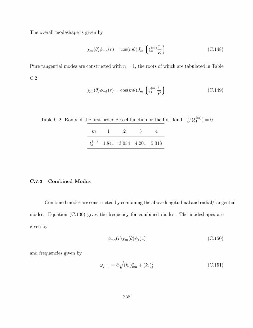
The overall modeshape is given by

χm(θ)φmn(r) = cos(mθ)Jm

ξ(m)n

r

R

(C.148)

Pure tangential modes are constructed with n = 1, the roots of which are tabulated in Table

C.2

χm(θ)φm1(r) = cos(mθ)Jm

ξ(m)1

r

R

(C.149)

Table C.2: Roots of the first order Bessel function or the first kind, dJ1

dr(ξ

(m)1 ) = 0

m 1 2 3 4

ξ(m)1 1.841 3.054 4.201 5.318

C.7.3 Combined Modes

Combined modes are constructed by combining the above longitudinal and radial/tangential

modes. Equation (C.130) gives the frequency for combined modes. The modeshapes are

given by

φmn(r)χm(θ)ψj(z) (C.150)

and frequencies given by

ωjmn = a√

(kr)2mn + (kz)2

j (C.151)

258

Note that m = 0 and n = 0 with j = 1, 2, 3, gives pure longitudinal modes; m = 0 and

j = 0 with n = 1, 2, 3, gives pure radial modes; n = 1 and j = 0 with m = 1, 2, 3 gives pure

tangential modes. Also note that

ζ(1)n = ξ(0)

n (C.152)

C.8 Three Dimensional Acoustics in an Annular Cylinder

Similar to the previous discussion of the circular cylinder, acoustics in an annular

cylinder can be described using separation of variables. Many of the mathematical details

are the same as those above. Starting with the acoustic pressure wave equation

∂2p′

∂x2i

− 1

a2

∂2p′

∂t2= 0 (C.153)

With the above equation written in cylindrical coordinates, performing separation of vari-

ables for all four independent variables

p′(r, θ, z, t) = φ(r)χ(θ)ψ(z)h(t) (C.154)

Substituting Eq. (C.154) into Eq. (C.153) and rearranging

d2φ/dr2

φ+

1

r

dφ/dr

φ+

1

r2

dχ/dθ

χ+d2ψ/dz2

ψ=

1

a2

d2h/dt2

h= −k2 (C.155)

Skipping intermediate steps shown above, the temporal evolution is described by the har-

monic oscillator equation, with solution

h(t) = eiωt (C.156)

259

As with the circular cylinder, each coordinate direction can now be separated into its own

ODE.

C.8.1 Longitudinal Modes

First, rearranging Eq. (C.155)

d2φ/dr2

φ+

1

r

dφ/dr

φ+

1

r2

dχ/dθ

χ+ k2 = −d

2ψ/dz2

ψ= k2

z (C.157)

which, by intermediate steps shown in more detail for the circular cylinder, leads to the

harmonic oscillator ODE in the axial direction, with solution

ψ(z) = A1 cos(kzz) + A2 sin(kzz) (C.158)

As before, the coefficients A1 and A2 are dependent on the boundary conditions at z = 0

and z = L. The results are identical to the circular cylinder, since no fundamental change

has occurred in the axial direction. The modeshapes and frequencies for longitudinal modes

are the same as the circular cylinder, and there is no need to repeat them here.

C.8.2 Tangential and Radial Modes

Re-arranging Eq. (C.112)

r2d2φ/dr2

φ+ r

dφ/dr

φ+ r2(k2 − k2

z) = −dχ/dθχ

= m2 (C.159)

260

This further separation of variables leads the harmonic oscillator ODE in the circumferential

direction, whose solution is

χ(θ) = B1 cos(mθ) +B2 sin(mθ) (C.160)

This solution must satisfy periodic boundary conditions. The coefficients B1 and B2 can be

set arbitrarily by the alignment of the mode due to radial symmetry. Setting

k2 = k2r + k2

z (C.161)

and applying this to Eq. (C.159)

r2d2φ/dr2

φ+ r

dφ/dr

φ+ (r2k2

r −m2) = 0 (C.162)

which can be recognized as an mth order Bessel equation. The solution to Eq. (C.162) is

given by a linear superposition of first and second kind Bessel functions

φ(r) = C1Jm(krr) + C2Ym(krr) (C.163)

The second-kind Bessel function cannot be eliminated, as with the circular cylinder, because

the location r = 0 is not in the annular domain. Instead, the coefficients C1 and C2 are

found for a particular annulus by setting boundary conditions at r = Rinner and r = Router,

the inner and outer radii.

C.8.2.1 Radial Modes

Pure radial modes are constructed from the above whenm = 0 and the circumferential

modeshape χ is a constant. Similarly, kz = 0 and the longitudinal modeshape is a constant,

261

which means that the frequency is, using Eq. (C.130) given by

ω = ka = kra (C.164)

and the modeshape from Eq. (C.163) with m = 0

φ(r) = C1J0(krr) + C2Y0(krr) (C.165)

the derivative of which is

dφ

dr= −C1krJ1(krr)− C2krY1(krr) (C.166)

Requiring a closed boundary (wall) at both inner and outer radii, dφ/dr = 0 at r = Rinner

and r = Router, leads to the characteristic equation

J1(krRouter)Y1(krRinner)− J1(krRinner)Y1(krRouter) = 0 (C.167)

This equation has an infinite number of solutions, (kr)0n (n = 1, 2, 3,), and can be solved

numerically for the frequencies using a root finder. The frequencies and modeshapes are

then given by

ω0n = (kr)0n a (C.168)

φ0n(r) = Y1((kr)0nRinner)J0((kr)0nr)− J1((kr)0nRinner)Y0((kr)0nr) (C.169)

262

C.8.2.2 Tangential Modes

For m 6= 0 and n = 1, pure tangential modes can be constructed. As discussed for

the circular cylinder, the circumferential contribution to the modeshape is

χm(θ) = cos(mθ) (C.170)

Requiring closed boundaries, dφ/dr = 0 at r = Rinner and r = Router, the characteristic

equation becomes

J ′m(krRouter)Y′m(krRinner)− J ′m(krRinner)Y

′m(krRouter) = 0 (C.171)

where the prime denotes differentiation of the Bessel function. The zeros of this function

can be found using a suitable numerical root finder and labelled here as (kr)mn for the nth

root with mth order Bessel functions. In general frequencies and modeshapes are given by

ωmn = (kr)mn a (C.172)

φmn(r) = Y ′m((kr)mnRinner)J′m((kr)mnr)− J ′m((kr)mnRinner)Y

′m((kr)mnr) (C.173)

For pure tangential modes, n = 1, the first solution to the characteristic equation is taken

ωm1 = (kr)m1 a (C.174)

φm1(r) = Y ′m((kr)m1Rinner)J′m((kr)m1r)− J ′m((kr)m1Rinner)Y

′m((kr)m1r) (C.175)

263

C.8.3 Combined Modes

Combined modes, as with the circular cylinder, are constructed by combining the

above longitudinal and radial/tangential modes. Equation (C.161) gives the frequency for

combined modes. The modeshapes are given by

φmn(r)χm(θ)ψj(z) (C.176)

and frequencies given by

ωjmn = a√

(kr)2mn + (kz)2

j (C.177)

Note that m = 0 and n = 0 with j = 1, 2, 3, gives pure longitudinal modes; m = 0 and

j = 0 with n = 1, 2, 3, gives pure radial modes; n = 1 and j = 0 with m = 1, 2, 3 gives pure

tangential modes.

C.9 General Rijke Tube Formulation

A Rijke tube presents an idealized thermoacoustic flow with all of the basic physics

of combustion instability problems. All motions are assumed one-dimensional from z = 0 to

z = L, with constant mean flow and mean variables on either side of an infinitesimally thin

flame sheet at z = L. The heat release is thus modelled as

q(z) = Qδ(z − b) (C.178)

q′(z, t) = Q′(t)δ(z − b) (C.179)

264

The region 0 < z < b is given the subscript 1 and the region b < z < L is given the subscript

2. The deflagration flame is modelled to have no effect on the mean pressure. The mean

fields are thus described by

p(z) = p1 = p2 = p (C.180)

T (z) = T1 +H(z − b)(T2 − T1) (C.181)

ρ(z) = ρ1 +H(z − b)(ρ2 − ρ1) (C.182)

u(z) = u1 +H(z − b)(u2 − u1) (C.183)

The mean continuity equation relates the mean densities and velocities as follows

ρ1u1 = ρ2u2 (C.184)

C.9.1 Governing Equations

On either side of the discontinuity at x = b, the mean gradients are zero and there is

no heat release. In this case, the governing equations are Mass:

∂ρ′

∂t+ ρ

∂u′

∂z+ u

∂ρ′

∂z= 0 (C.185)

Momentum:

∂u′

∂t+ u

∂u′

∂z+

1

ρ

∂p′

∂z= 0 (C.186)

Energy (Pressure):

∂p′

∂t+ u

∂p′

∂z+ γp

∂u′

∂z= 0 (C.187)

265

These can be written in vector form as

∂q˜∂t

+ A≈

∂q˜∂z

= 0 (C.188)

with

q˜ = (ρ′ u′ p′)T (C.189)

and

A≈

=

u ρ 0

0 u 1ρ

0 γp u

(C.190)

C.9.2 General Solution

The eigenvalues of the flux matrix A≈

are

λ− = u− a (C.191)

λs = u (C.192)

λ+ = u+ a (C.193)

where a is the sound speed on either side of the flame given by

a =

√γp

ρ(C.194)

The left eigenvectors are

l˜− = (0 − ρa 1) (C.195)

266

l˜s = (−a2 0 1) (C.196)

l˜+ = (0 ρa 1) (C.197)

Hence, the waves for a harmonic signal with complex frequency (Ω = ω − iα) propagate as

p− ∼ exp

[Ω

t− z

u− a

] (C.198)

ps ∼ exp[Ωt− z

u

] (C.199)

p+ ∼ exp

[Ω

t− z

u+ a

] (C.200)

with strengths given by

p− = p− ρau (C.201)

ps = p− a2ρ (C.202)

p+ = p+ ρau (C.203)

Rearranging these relations, the fluctuation of primitive variables can be written as

p =1

2

p+ + p− (C.204)

u =1

2ρa

p+ − p− (C.205)

ρ =1

2a2

p+ + p−− 1

a2ps (C.206)

In terms of wave amplitudes (A−, As, and A+), write

p− = 2A− exp

[Ω

t− z

u− a

] (C.207)

ps = As exp[Ωt− z

u

] (C.208)

267

p+ = 2A+ exp

[Ω

t− z

u+ a

] (C.209)

Combination of the previous six equations gives

p′(z, t) = A+ exp

[Ω

t− z

u+ a

]+ A− exp

[Ω

t− z

u− a

] (C.210)

ρau′(z, t) = A+ exp

[Ω

t− z

u+ a

]− A− exp

[Ω

t− z

u− a

] (C.211)

a2ρ′(z, t) = A+ exp

[Ω

t− z

u+ a

]+ A− exp

[Ω

t− z

u− a

]− As exp[Ωt− z

u

](C.212)

Note that if the entropy wave is zero (As = 0), then the density is related to the

pressure via the isentropic relation

ρ′ =p′

a2(C.213)

Writing Eqns. (C.210) - (C.212) for either side of the flame

p′1(z, t) = A+1 exp

[Ω

t− z

u1 + a1

]+ A−1 exp

[Ω

t− z

u1 − a1

] (C.214)

ρau′1(z, t) = A+1 exp

[Ω

t− z

u1 + a1

]− A−1 exp

[Ω

t− z

u1 − a1

] (C.215)

a2ρ′1(z, t) = A+1 exp

[Ω

t− z

u1 + a1

]+ A−1 exp

[Ω

t− z

u1 − a1

]− As1 exp

[Ω

t− z

u1

] (C.216)

and

p′2(z, t) = A+2 exp

[Ω

t− z − Lu2 + a2

]+ A−2 exp

[Ω

t− z − Lu2 − a2

] (C.217)

ρau′2(z, t) = A+2 exp

[Ω

t− z − Lu2 + a2

]− A−2 exp

[Ω

t− z − Lu2 − a2

] (C.218)

268

a2ρ′2(z, t) = A+2 exp

[Ω

t− z − Lu2 + a2

]+ A−2 exp

[Ω

t− z − Lu2 − a2

]− As2 exp

[Ω

t− z − Lu2

] (C.219)

Note that the wave structure on the downstream side of the flame is written in terms of a

shifted variable z − L, which conveniently goes to zero at the outlet boundary. Finally, we

also assume harmonic dependence on time for the unsteady heat release

1

aQ′(t) = AQ exp(iΩt) (C.220)

In this way, the original problem in terms of the seven primitive variables (ρ′1, u′1, p′1, ρ′2,

u′2, p′2, q′) has been rephrased in terms of seven wave strengths (A−1 , As1, A+1 , A−2 , As2, A+

2 ,

AQ). The advantage we have gained in doing this, by assuming the space-time behavior of

the solution, is that boundary conditions and interface matching conditions can now provide

algebraic relations for the new unknowns and matrix methods can be employed to reach the

solution.

C.9.3 Boundary Conditions

The three most common acoustic boundary conditions are

Closed:

u′ = 0 (C.221)

Open:

p′ = 0 (C.222)

269

Choked:

ρ′u+ ρu′ = 0 (C.223)

In addition to an acoustic boundary provided at the inlet and outlet, a boundary condition

for the incoming entropy wave must be provided to the inlet. The most common and easiest

to implement is the isentropic assumption, hence

p′ − a2ρ′ = 0 (C.224)

Substituting Eqns. (C.214) - (C.212) into the boundary conditions at the inlet Closed inlet:

u′1(0, t) = A+1 exp(iΩt)− A−1 exp(iΩt) = 0 (C.225)

A−1 − A+1 = 0 (C.226)

Open inlet:

p′1(0, t) = A+1 exp(iΩt) + A−1 exp(iΩt) = 0 (C.227)

A−1 + A+1 = 0 (C.228)

Isentropic inlet:

p′1(0, t)− a2ρ′1(0, t) = As1 exp(iΩt) = 0 (C.229)

As1 = 0 (C.230)

Isentropic choked inlet:

ρ′1(0, t)u1 + ρ1u′1(0, t) = (1 + M)A+

1 exp(iΩt)− (1− M)A−1 exp(iΩt) = 0 (C.231)

(1 + M1)A+1 − (1− M1)A−1 = 0 (C.232)

270

Similarly, the substitution of Eqns. (C.217) - (C.219) into the exit boundary conditions

Closed outlet:

u′2(0, t) = A+2 exp(iΩt)− A−2 exp(iΩt) = 0 (C.233)

A−2 − A+2 = 0 (C.234)

Open outlet:

p′2(0, t) = A+2 exp(iΩt) + A−2 exp(iΩt) = 0 (C.235)

A−2 + A+2 = 0 (C.236)

Choked outlet:

ρ′2(0, t)u2 + ρ2u′2(0, t) = (1 + M)A+

2 exp(iΩt)− (1− M)A−2 exp(iΩt)− MAs2 exp(iΩt) = 0

(C.237)

(1 + M)A+2 − (1− M)A−2 − MAs2 = 0 (C.238)

Note that the choked outlet allows the entropy wave to interact with the acoustic waves

at the outlet boundary, which could provide another means of feedback to the combustion

oscillations.

C.9.4 Interface Conditions

Across the discontinuity at the flame, the conservative form of the governing equations

are used to construct interface matching conditions for the acoustic waves and entropy wave.

271

The conservative form of the equations are

Mass:

∂ρ

∂t+∂(ρu)

∂z= 0 (C.239)

Momentum:

∂(ρu)

∂t+∂(ρu2 + pδij)

∂z= 0 (C.240)

Energy:

∂[ρ(e+ 12u2)]

∂t+∂[ρu(e+ 1

2u2 + p

ρ)]

∂z= q (C.241)

Rewriting the energy in terms of pressure (using the perfect gas equations of state):

∂[p+ 12(γ − 1)ρu2]

∂t+∂[γup+ 1

2(γ − 1)ρu3]

∂z= (γ − 1)q (C.242)

Satisfying the integral form of these equations amounts to considering an infinitessimal vol-

ume straddling the discontinuity and integrating the above equations. The following interface

relations are found

Mass:

ρ2u2 − ρ1u1 = 0 (C.243)

Momentum:

(p2 + ρ2u22)− (p1 + ρ1u

21) = 0 (C.244)

Pressure:

γu2p2 +1

2(γ − 1)ρ2u

32

−γu1p1 +1

2(γ − 1)ρ1u

31

=

∫ b+

b−

(γ − 1)q(z)dz (C.245)

272

With Eq. (C.178), the pressure equations becomesγu2p2 +1

2(γ − 1)ρ2u

32

−γu1p1 +1

2(γ − 1)ρ1u

31

= (γ − 1)Q (C.246)

Equations (C.243), (C.244), and (C.246) give the relations for the behavior of instantaneous

values across the flame. In the absence of fluctuations, these govern the fluid dynamical

behavior of a laminar flame, hence aid in the calculation of laminar flame speeds and det-

onation speeds. For the present purposes, the these equations are perturbed and linearized

to find the interface conditions for the acoustic fluctuations.

Mass:

(ρ′2u2 + ρ2u′2)− (ρ′1u1 + ρ1u

′1) = 0 (C.247)

Momentum:

(p′2 + ρ′2u22 + 2ρ2u2u

′2)− (p′1 + ρ′1u

21 + 2ρ1u1u

′1) = 0 (C.248)

Pressure: γu′2p2 + γu2p′2 +

1

2(γ − 1)ρ′2u

32 +

3

2(γ − 1)ρ2u

22u′2

−γu′1p1 + γu1p

′1 +

1

2(γ − 1)ρ′1u

31 +

3

2(γ − 1)ρ1u

21u′1

= (γ − 1)Q′ (C.249)

Substitution of Eqns. (C.214) - (C.220) into these three interface conditions yields

Mass: (1 + M1)e+1 A

+1 − (1− M1)e−1 A

−1

− a1

a2

(1 + M2)e+2 A

+2 − (1− M2)e−2 A

−2 − M2e

s2A

s2

= 0 (C.250)

Momentum: (1 + M1)2e+1 A

+1 + (1− M1)2e−1 A

−1

273

−(1 + M2)2e+

2 A+2 + (1− M2)2e−2 A

−2 − M2

2 es2A

s2

= 0 (C.251)

Pressure: 1 + γM1 +3

2(γ − 1)M2

1 +1

2(γ − 1)M3

1

e+1 A

+1

−1− γM1 +

3

2(γ − 1)M2

1 −1

2(γ − 1)M3

1

e−1 A−1

− a2

a1

1 + γM2 +3

2(γ − 1)M2

2 +1

2(γ − 1)M3

2

e+2 A

+2

+a2

a1

1− γM2 +3

2(γ − 1)M2

2 −1

2(γ − 1)M3

2

e−2 A−2

+a2

a1

1

2γM3

2 es2A

s2 + (γ − 1)AQ = 0 (C.252)

In the above three equations, the following shorthand has been used for the exponential

terms

e−1 = exp

Ωb

u1 − a1

(C.253)

e+1 = exp

Ωb

u1 + a1

(C.254)

e−2 = exp

Ωb− Lu2 − a2

(C.255)

es2 = exp

Ωb− Lu2

(C.256)

e+2 = exp

Ωb− Lu2 + a2

(C.257)

Thus, Eqns (C.250) - (C.252) give the three interface conditions for the system.

274

C.9.5 Heat Release Model

The general solution contains seven unknown wave strengths. Three boundary con-

ditions and three interface conditions give six independent equations. Hence, one more

equation is needed for closure. This equation is provided by the heat release model. The

heat release model relates the unsteady heat release to the acoustic density, velocity and

pressure fields.

C.9.5.1 Pressure Mechanism

In some cases, the heat release behavior may be modeled by

Q′(t)

Q= n

p′1(t− τ)

p1

(C.258)

When the mean heat release is written as

Q = ρ1u1cp(T2 − T1) (C.259)

this pressure-coupled mechanism model becomes

Q′(t) = nγ

γ − 1M1(TR− 1)a1p

′1(t− τ) (C.260)

where TR = T2/T1 is the temperature ratio across the flame. Substitution of Eqs. (C.214)

and (C.220) gives

nγM1(TR− 1)(e+1 A

+1 + e−1 A

−1 )− (γ − 1) exp(iΩτ)AQ = 0 (C.261)

275

which closes the set of equations for this model.

C.9.5.2 Weak Velocity Model

While the first model predicts that the heat release oscillations are coupled to acoustic

pressure oscillations, an alternate model couples the heat release fluctuations to acoustic

velocity fluctuations

Q′(t)

Q= n

u′1(t− τ)

a1

(C.262)

With the mean heat release from Eq (C.259), this velocity-coupled model becomes

Q′(t) = n1

γ − 1M1(TR− 1)p1u

′1(t− τ) (C.263)

Substitution of Eqs. (C.215) and (C.220) gives

nM1(TR− 1)(e+1 A

+1 − e−1 A−1 )− (γ − 1) exp(iΩτ)AQ = 0 (C.264)

C.9.5.3 Strong Velocity Mechanism

Note that the denominator in Eq. (C.262) is chosen as the sound speed (the rele-

vant velocity scale for the acoustic fluctuations). The flame could also respond to velocity

fluctuations related to the order of the mean flow

Q′(t)

Q= n

u′1(t− τ)

u1

(C.265)

276

This heat release model is stronger than the previous by the factor M−11 . For most gas

turbine combustors, this is a rather large factor. In this case the heat release fluctuations

can be written as

Q′(t) = n1

γ − 1(TR− 1)p1u

′1(t− τ) (C.266)

which, in terms of wave strengths, gives the equation

n(TR− 1)(e+1 A

+1 − e−1 A−1 )− (γ − 1) exp(iΩτ)AQ = 0 (C.267)

Note that, with this model, the strength of the heat release AQ is on the same order as the

acoustic wave strengths A−1 , A+1 . This is in contrast to the first two models, where the heat

release is O(M) compared to the acoustic wave strengths. Hence, this mechanism is referred

to as a ‘strong’ model.

C.9.5.4 Mass Flow Rate Mechanism

The heat release could also be modelled as responsive to fluctuations in the mass flow

rate

Q′(t)

Q= n

m′(t− τ)¯m

(C.268)

or

Q′(t)

Q= n

ρ′1(t− τ)

ρ1

+u′1(t− τ)

u1

(C.269)


Q′(t) = n1

γ − 1(TR− 1)

u1ρ′1(t− τ) + ρ1u

′1(t− τ)

(C.270)

277

Substitution of Eqs. (C.215), (C.216) and (C.220) gives

n(TR− 1)(1 + M1)e+

1 A+1 − (1− M1)e−1 A

−1 )− (γ − 1) exp(iΩτ)AQ = 0 (C.271)

Because there is no entropy wave entering the domain at the inlet, the density and pressure

on the upstream side of the flame are related via the isentropic relation. The mass flow rate

mechanism is thus a combination of the pressure mechanism O(M1) and the strong velocity

mechanism O(1). For small Mach numbers, this is approximately equivalent to the strong

velocity mechanism.

C.9.5.5 No Entropy Wave Mechanism

A final simple model worth mentioning is one that produces no entropy wave (for

n = 1)

Q′(t)

Q= n

p′1(t− τ)

p1

+u′1(t− τ)

u1

(C.272)


Q′(t) = n1

γ − 1(TR− 1)

ρ1u1

p1

p′1(t− τ) + ρ1u′1(t− τ)

(C.273)

Substitution of Eqs. (C.214), (C.215) and (C.220) gives

n(TR− 1)(1 + γM1)e+

1 A+1 − (1− γM1)e−1 A

−1 )− (γ − 1) exp(iΩτ)AQ = 0 (C.274)

278

C.9.6 Example

To show how this procedure can be used to solve a Rijke tube problem for the fre-

quency and growth rate, we consider a Rijke tube with a choked isentropic inlet, Eq. (C.232),

open outlet, Eq. (C.236), the three fixed interface conditions, Eqs. (C.250), (C.9.4), (C.252),

and a mean flow rate mechanism, Eq. (C.268). This problem was explored by [24]. Since

the incoming entropy wave is zero, we have 6 unknowns with 2 boundary conditions, 3 in-

terface conditions, and a heat release model. Stacking these six algebraic equations into a

6x6 matrix

M≈A˜ = 0˜ (C.275)

where the vector of wave strengths is

A˜ = (A+1 A−1 A+

2 A−2 As2 AQ) (C.276)

and the coefficient matrix is

M≈

=

(1 + M1) −(1− M1) 0 0 0 0

(1 + M1)e+1 −(1− M1)e−1 − a1

a2(1 + M2)e+

2a1

a2(1− M2)e−2

a1

a2M2e

s2 0

(1 + M1)2e+1 (1− M1)2e−1 −(1 + M2)2e+

2 −(1− M2)2e−2 M22 e

s2 0

p+1 e

+1 −p−1 e−1 − a2

a1p+

2 e+2

a2

a1p−2 e

−2

12a2

a1γM3

2 es2 (γ − 1)

0 0 1 1 0 0

q+1 e

+1 −q−1 e−1 0 0 0 −1

(C.277)

279

where the abbreviated polynomials are

p+1 = 1 + γM1 +

3

2(γ − 1)M2

1 +1

2(γ − 1)M3

1 (C.278)

p−1 = 1− γM1 +3

2(γ − 1)M2

1 −1

2(γ − 1)M3

1 ) (C.279)

p+2 = 1 + γM2 +

3

2(γ − 1)M2

2 +1

2(γ − 1)M3

2 ) (C.280)

p−2 = 1− γM2 +3

2(γ − 1)M2

2 −1

2(γ − 1)M3

2 ) (C.281)

q+1 =

n(TR− 1)

γ − 1(1 + M1) exp(−iΩτ) (C.282)

q−1 =n(TR− 1)

γ − 1(1− M1) exp(−iΩτ) (C.283)

and the abbreviated exponentials are given in the interface conditions section. As suggested

by Eq. (C.275), a non-trivial solution for the wave amplitudes can only be achieved when the

determinant of M≈

vanishes. A standard numerical root solver coupled with a determinant

calculation can be used to quickly solve for the frequencies. In general, no analytical solution

exists, but this matrix can be simplified to the temperature jump, mean flow, and simple duct

acoustics problems shown in previous sections of this appendix. Under such simplifications,

the solutions derived in previous sections can be recovered from this more general method.

280

APPENDIX DANALYTICAL SPATIAL AVERAGING OF RIJKE TUBE

CASES

281

APPENDIX DANALYTICAL SPATIAL AVERAGING OF RIJKE TUBE

CASES

Application of the method of spatial averaging for approximate treatment of com-

bustion instabilities was introduced by Culick in his doctoral thesis [23]. The method was

recently summarized by [8]. Recently, Dowling [24] used the method for a simple one-

dimensional Rijke tube geometry for which there exists an analytical solution. The result of

this paper’s comparison showed a large discrepancy between the predicted frequency shift

from the spatial averaged approximation and the analytical solution. Dowling concluded

that this is an inherent limitation of the method. Recently, however, Culick [64] has argued

that the large disagreement between theory and approximation for the simplified problem

introduced by Dowling was due to her neglect of the mean density gradient term in the

governing equations. In fact, a more thorough derivation of the spatial averaging process

for the proposed geometry, boundary conditions, and heat release model was given by Palm

[65]. Palm’s solution showed better agreement with the analytical solution, ascribing the

success of his reworked model to the inclusion of the mean density gradient term previously

neglected by Dowling.

It turns out that neither Dowling nor Palm do proper justice to the problem at hand.

It is shown here that the error committed by Dowling was unrelated to any of the density

282

gradient terms in the governing equations. In fact, Dowling’s procedure is equivalent to

Palm’s with respect to the mean density gradient effects. Though not shown explicitly by

Dowling, the spatial averaging equations she used properly account for the effect of the

density gradient. It is also shown that in Palm’s solution, while extra care is taken not to

leave out any important mean density gradient terms, the terms stemming from the density

gradient terms cancel in the final frequency shift formula. Palm’s failure to recognize this

fact led Culick to incorrectly identify the source of Dowling’s error. In fact, the difference

between the solution of Dowling and Palm arises from differing approximations of the acoustic

velocity fluctuations (u′) in terms of the acoustic pressure fluctuations (p′).

This paper derives a more robust method of spatial averaging using the acoustic pres-

sure wave equation, incorporating the density gradient within the Sturm-Liouville operator.

In this method, it is shown that the harmonic oscillation equations are obtained in the same

form and Culick [8], but without any source terms relating to the mean density gradient.

The equivalence of the results of this derivation with Dowling’s spatial averaging equations

is then demonstrated. The solution to this method is shown using two different relations

for the acoustic velocity in terms of acoustic pressure. The first method uses the linearized

acoustic momentum equation and results in the estimations of Dowling. The second method

uses the linearized energy equation and results in the frequency shift shown by Palm. After

deriving each of the two results, the key error of Dowling is highlighted, as well as the error

in Culick’s diagnosis of Dowling’s poor estimation.

283

D.1 Modified Spatial Averaging Procedure for the Acoustic Wave Equation

In the following, a spatial averaging procedure very similar to that of Dowling [24],

Culick [8] and Palm [65] is derived from the linearized Euler equations by combining them into

the acoustic pressure wave equation. Where applicable, the relationship with this derivation

and others is explained. The key difference in this derivation is the natural inclusion of

mean density gradients within the Sturm-Liouville eigenvalue problem. This leads to clear

understanding where other previous methods (see [65]) have led to confusion.

D.1.1 Derivation of the Governing Wave Equation

The linearized equations for acoustic momentum and energy are, respectively

ρ∂u′i∂t

+ ρuj∂u′i∂xj

+ ρu′j∂ui∂xj

+ ρ′uj∂ui∂xj

+∂p′

∂xi= 0 (D.1)

∂p′

∂t+ uj

∂p′

∂xj+ u′j

∂p

∂xj+ γp

∂u′j∂xj

+ γp′∂uj∂xj

= (γ − 1)q′ (D.2)

Rewriting these equations to put mean flow and mean pressure gradient effects, which are

viewed as perturbations to the equations of classical acoustics, on the right hand side

∂u′i∂t

+1

ρ

∂p′

∂xi= −uj

∂u′i∂xj− u′j

∂ui∂xj− ρ′

ρuj∂ui∂xj

(D.3)

∂p′

∂t+ γp

∂u′j∂xj

= (γ − 1)q′ − uj∂p′

∂xj− u′j

∂p

∂xj− γp′∂uj

∂xj(D.4)

284

Differentiating Eq. (D.4) in time and subtracting γp times the divergence of Eq. (D.3)

results in

∂2p′

∂t2− γp ∂

∂xj

1

ρ

∂p′

∂xj

= h (D.5)

where the source term h is given by

h = (γ−1)∂q′

∂t−∂u′j∂t

∂p

∂xj−uj

∂2p′

∂t∂xj−γ ∂p

′

∂t

∂uj∂xj

+γp∂

∂xi

uj ∂u′i∂xj

+ u′j∂ui∂xj

+ρ′

ρuj∂ui∂xj

(D.6)

As an aside, it is at this point that Culick [8] further simplifies the spatial derivatives on the

left hand side of Eq. (D.5) using

γp∂

∂xj

1

ρ

∂p′

∂xj

=γp

ρ

∂2p′

∂x2j

+ γp∂(1/ρ)

∂xj

∂p′

∂xj= a2∂

2p′

∂x2j

− a2

ρ

∂ρ

∂xj

∂p′

∂xj(D.7)

Substituting Eq. (D.7) into Eq. (D.5) and moving the ∂ρ∂xj

term to the right hand side,

Culick [8] arrives at his form of the wave equation for acoustic pressure

∂2p′

∂t2− γp

ρ

∂2p′

∂xj∂xj= hCulick (D.8)

where his source term hCulick is given by

hCulick = (γ − 1)∂q′

∂t− a2

ρ

∂ρ

∂xj

∂p′

∂xj−∂u′j∂t

∂p

∂xj− uj

∂2p′

∂t∂xj− γ ∂p

′

∂t

∂uj∂xj

+ γp∂

∂xi

uj ∂u′i∂xj

+ u′j∂ui∂xj

+ρ′

ρuj∂ui∂xj

(D.9)

Therefore, the difference between the current derivation in Eq. (D.5) and Culick’s in Eq.

(D.9) is the position of the mean density gradient effects. Culick views these on the right

hand side as a perturbation to the wave equation, while the current derivation includes them

in the spatial operator in the wave equation.

285

D.1.2 General Solution to the Homogeneous Problem

Returning to the derivation at hand, the weighting and expansion functions are found

via solution to the unperturbed problem

∂2p′

∂t2− γp ∂

∂xj

1

ρ

∂p′

∂xj

= 0 (D.10)

which can be solved via separation of variables. Substitution of

p′ = ψn(xj)ηn(t) (D.11)

leads to the following to ordinary differential equations

ηn + ω2nηn = 0 (D.12)

γp∂

∂xj

1

ρ

∂ψn∂xj

+ ω2nψn = 0 (D.13)

where ω2n is the eigenvalue. Performing the same operations which led from Eq. (D.5) to

Eq. (D.8) can reformulate this spatial ODE in the form similar to Palm’s [65] solution

∂2ψn∂xj∂xj

+ k2nψn =

1

ρ

∂ρ

∂xj

∂ψn∂xj

(D.14)

Here, the density gradient is again moved to the right hand side and viewed as a perturbation

to the homogeneous Helmholtz equation with eigenvalue k2n = ω2

n

a2 . The drawback is that

viewing the mean density gradient as a perturbation to wave equation rather than as part

of the spatial operator causes one to miss some nice results from the three-dimensional

extension of Sturm-Liouville theory. Note that Eq. (D.13), can be rephrased as

∂

∂xj

(γp)refρ

∂ψn∂xj

+ ω2n

(γp)refγp

ψn = 0 (D.15)

286

where (γp)ref represents reference values of specific heat and pressure that are not a function

of space. It is recognized that, though deflagration waves in premixed combustion cause

changes mostly in mean density, that small changes in mean pressure and specific heat are

also incurred. With the use of reference values, Eq. (D.15) is of Sturm-Liouville form in its

three-dimensional extension

L[ψn(xj)] + λnσ(xj)ψn(xj) = 0 (D.16)

where the linear differential operator is

L[ψn] =∂

∂xj

(γp)refρ

∂ψn∂xj

(D.17)

the eigenvalue is

λn = ω2n (D.18)

and the weighting function for orthogonality is

σ(xj) =(γp)ref

γ(xj)p(xj)(D.19)

In the context of extending Sturm-Liouville, it is useful to discuss Green’s formula. Note

that the inclusion of the surface discontinuities, which are important for applications with

acoustically compact flames, is calculated from the use of the divergence theorem in the

derivation of Green’s formula. For a vector field Fj in the domain Ω with boundaries ∂Ω and

K surface discontinuities marked by gk(xj) = 0 with k = 1, 2, , K the divergence theorem

becomes

y

Ω

∂Fj∂xj

dV =x

∂Ω

FjnjdS −K∑k=1

x

gk=0

∆(Fj)njdS

(D.20)

287

where ∆(Fj) represents the instantaneous change in the vector across the surface in the

direction of the normal vector nj. Green’s formula for the linear operator is then

y

Ω

ψnL[ψm]− ψmL[ψn] dV =

(γp)refx

∂Ω

[1

ρ

ψn∂ψm∂xj

− ψm∂ψn∂xj

]njdS− K∑k=1

x

gk=0

∆

[1

ρ

ψn∂ψm∂xj

− ψm∂ψn∂xj

]njdS(D.21)

In order to evaluate the right hand side integrals for surface discontinuities, inter-

face conditions for flame interfaces are necessary. For a flame interface, from the acoustic

momentum equation, Eq. (D.3), neglecting mean flow and mean pressure gradients

∂u′i∂t

+1

ρ

∂p′

∂xi= 0 (D.22)

Integrating across an infinitesimally thin control volume surrounding the surface discontinu-

ity described by g(xj) = 0 leads to

p′(g+)− p′(g−) = 0 (D.23)

or

∆(p′) = 0 (D.24)

The second interface condition is provided by the non-homogeneous wave equation, Eq.

(D.5), only accounting for the heat release and neglecting the contributions of mean flow

and mean pressure gradient

∂2p′

∂t2− γp ∂

∂xj

1

ρ

∂p′

∂xj

= (γ − 1)∂q′

∂t(D.25)

288

where the heat release function for a flame discontinuity on the surface g(xj) = 0 is given by

q′(xj, t) = Q′(t)δ(g(xj)) (D.26)

where δ is the Dirac delta function. When Eq. (D.25) is integrated over an infinitesimal

control volume around the surface discontinuity g(xj) = 0, yields

1

ρ

∂p′

∂xj

nj

∣∣∣∣g+

− 1

ρ

∂p′

∂xj

nj

∣∣∣∣g−

= −γ − 1

γp

dQ′

dt(D.27)

or

∆

1

ρ

∂p′

∂xj

nj = −γ − 1

γp

dQ′

dt(D.28)

Interface conditions for the acoustic modeshapes ψn can be derived from the homogeneous

form of Eq. (D.3) and the spatial ODE Eq. (D.15). Substituting the separation of variables

in Eq. (D.11) into Eq. (D.22)

∂u′i∂t

+1

ρ

∂ψn∂xi

ηn = 0 (D.29)

and integrating across the flame at g(xj) = 0, gives

ψn(g+)− ψn(g−) = 0 (D.30)

or

∆(ψn) = 0 (D.31)

Similarly, integrating Eq. (D.15) across a discontinuity at g = 0

1

ρ

∂ψn∂xj

nj

∣∣∣∣g+

− 1

ρ

∂ψn∂xj

nj

∣∣∣∣g−

= 0 (D.32)

289

or

∆

1

ρ

∂ψn∂xj

nj = 0 (D.33)

Based on the interface relations from Eq. (D.31) and (D.33), the latter integral on the right

hand side of Eq. (D.21) vanishes. If homogeneous first, second, or third kind boundary

conditions are used, the boundary integration also vanishes. With these conditions, the

right hand side of Eq. (D.21) vanishes and the linear operator is self-adjoint

y

Ω

ψnL[ψm]− ψmL[ψn] dV = 0 (D.34)

Note that the linear differential operator is not self-adjoint when considering the acous-

tic pressure field, as pointed out by [66]. The interface condition given by Eq. (D.28) is

non-homogeneous, the heat release term preventing the operator from being self-adjoint.

Substituting Eq. (D.16) into Eq. (D.34) and simplifying yields

(ω2n − ω2

m)y

Ω

(γp)refγp

ψnψm

dV = 0 (D.35)

This shows the orthogonality of the modeshapes found from solving Eq. (D.15).

y

Ω

(γp)refγp

ψmψndV =

E2n m = n

0 m 6= n

(D.36)

where E2n are the normalization constant for the modeshapes.

290

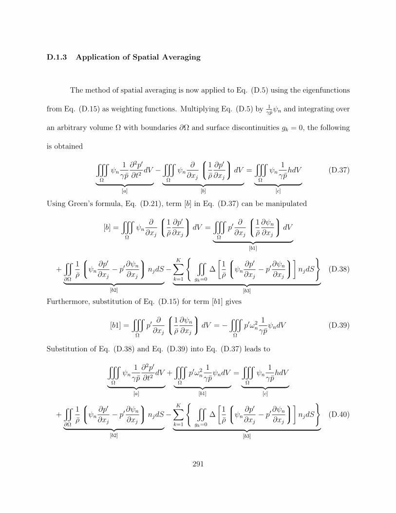
D.1.3 Application of Spatial Averaging

The method of spatial averaging is now applied to Eq. (D.5) using the eigenfunctions

from Eq. (D.15) as weighting functions. Multiplying Eq. (D.5) by 1γpψn and integrating over

an arbitrary volume Ω with boundaries ∂Ω and surface discontinuities gk = 0, the following

is obtained

y

Ω

ψn1

γp

∂2p′

∂t2dV︸︷︷︸

[a]

−y

Ω

ψn∂

∂xj

1

ρ

∂p′

∂xj

dV︸︷︷︸[b]

=y

Ω

ψn1

γphdV︸︷︷︸

[c]

(D.37)

Using Green’s formula, Eq. (D.21), term [b] in Eq. (D.37) can be manipulated

[b] =y

Ω

ψn∂

∂xj

1

ρ

∂p′

∂xj

dV =y

Ω

p′∂

∂xj

1

ρ

∂ψn∂xj

dV︸︷︷︸[b1]

+x

∂Ω

1

ρ

ψn ∂p′∂xj− p′∂ψn

∂xj

njdS︸︷︷︸[b2]

−K∑k=1

x

gk=0

∆

[1

ρ


∂xj

]njdS︸︷︷︸[b3]

(D.38)

Furthermore, substitution of Eq. (D.15) for term [b1] gives

[b1] =y

Ω

p′∂

∂xj

1

ρ

∂ψn∂xj

dV = −y

Ω

p′ω2n

1

γpψndV (D.39)

Substitution of Eq. (D.38) and Eq. (D.39) into Eq. (D.37) leads to

y

Ω

ψn1

γp

∂2p′

∂t2dV︸︷︷︸

[a]

+y

Ω

p′ω2n

1

γpψndV︸︷︷︸

[b1]

=y

Ω

ψn1

γphdV︸︷︷︸

[c]

+x

∂Ω

1

ρ


∂xj


−K∑k=1

x

gk=0

∆

[1

ρ


∂xj

]njdS︸︷︷︸[b3]

(D.40)

291

Then replacing the acoustic pressure p′ by a series expansion on the basis functions ψm

p′ = pref

∞∑m=0

ψm(xj)ηm(t) (D.41)

such that

∂2p′

∂t2= pref

∞∑m=0

ψm(xj)ηm(t) (D.42)

then Eq. (D.40) becomes

y

Ω

ψn1

γppref

∞∑m=0

ψmηm dV︸︷︷︸[a]

+y

Ω

pref

∞∑m=0

ψmηmω2n

1

γpψndV︸︷︷︸

[b1]

=

y

Ω

ψn1

γphdV︸︷︷︸

[c]

+x

∂Ω

1

ρ


∂xj


−K∑k=1

x

gk=0

∆

[1

ρ


∂xj

]njdS︸︷︷︸[b3]

(D.43)

interchanging integration and summation

∞∑m=0

ηm y

Ω

prefγp

ψmψndV

︸︷︷︸[a]

+ω2n

∞∑m=0

ηm y

Ω

prefγp

ψmψndV

︸︷︷︸[b1]

=

y

Ω

ψn1

γphdV︸︷︷︸

[c]

+x

∂Ω

1

ρ


∂xj


−K∑k=1

x

gk=0

∆

[1

ρ


∂xj

]njdS︸︷︷︸[b3]

(D.44)

292

Using the orthogonality property, Eq. (D.36), then

y

Ω

prefγp

ψmψndV =1

γref

y

Ω

(γp)refγp

ψmψndV =

E2n/γref m = n

0 m 6= n

(D.45)

which simplifies Eq. (D.44) to

E2n

γrefηn︸︷︷︸

[a]

+E2n

γrefω2nηn︸︷︷︸

[b1]

=y

Ω

ψn1

γphdV︸︷︷︸

[c]

+x

∂Ω

1

ρ


∂xj


−K∑k=1

x

gk=0

∆

[1

ρ


∂xj

]njdS︸︷︷︸[b3]

(D.46)

where E2n is the normalization constant for the orthogonality statement. Rearranging, this

leads to the non-homogeneous harmonic oscillator equations

ηn︸︷︷︸[a]

+ω2nηn︸︷︷︸[b1]

=1

prefE2n

y

Ω

h(γp)refγp

ψndV︸︷︷︸[c]

+1

prefE2n

x

∂Ω

(γp)refρ


∂xj


− 1

prefE2n

K∑k=1

x

gk=0

∆

[(γp)refρ


∂xj

]njdS︸︷︷︸[b3]

(D.47)

Up to this point, the substitution of Eq. (D.41) has not been used for the boundary and

interface surface integrals on the right hand side of the integrated equations. In fact, if

the substitution is made and ψn is constructed with homogeneous boundary conditions, the

two integrals will vanish. This is not desirable for the sake of the approximation method,

because there is no other way to account for the effect of non-homogeneous boundary condi-

tions appearing as a perturbation to the homogeneous problem. The interface discontinuity

293

integrals, arising from the heat release zones, should be left out, however. The effect of the

heat release perturbation to the homogeneous problem is included in the source term h, and

therefore need not be included in the surface integrals at discontinuities. With this logic, the

substitution of Eq. (D.41) into term [b3] of Eq .(D.47) is made, thus causing this term to

vanish for heat release driven discontinuities. The final form of the forced harmonic oscillator

equation is then

ηn︸︷︷︸[a]

+ω2nηn︸︷︷︸[b1]

=1

prefE2n

y

Ω

h(γp)refγp

ψndV︸︷︷︸[c]

+1

prefE2n

x

∂Ω

(γp)refρ


∂xj


(D.48)

As shown in Appendix D, the accuracy of this method depends on the relation used to put

u′ in terms of η. When the momentum equation is used, the results resemble those of [24],

which are highly inaccurate. If the homogeneous energy equation is used, as suggested by [8],

then the method gives remarkably accurate results. In general, the sensitivity of the results

is due to the fact that the unsteady heat release for the model used is of the same order of

magnitude as the acoustics itself, see Appendix C for discussion of weak and strong velocity

mechanism. Suppose a time lag was used such that the heat release was not in phase with

the velocity. This would make the Rayleigh criterion for a velocity based method non-zero

(it is zero if the time lag is zero). Then, for the strong velocity model, the approximation

α << ω would not hold and the underpinning of the weighted residual method (treating the

heat release as a small perturbation on the homogeneous acoustic solution) would not be a

reasonable assumption.

294

D.2 Application to Rijke Tube Problem

The example problem originally introduced by [24] is now considered with the above

derivation of the spatial averaged equations. The geometry is one-dimensional from x = 0

to x = L with a flame discontinuity at x = b. The heat release is given by a Dirac delta

function.

q′(x, t) = Q′(t)δ(x− b) (D.49)

On either side of the discontinuity, the flow properties are constant and there is no mean

flow. For the model problem, the specific heats and mean pressure are constant across the

heat input, hence only the mean density and mean temperature change. The subscript 1

is used to denote properties in the region 0 ≤ x < b and the subscript 2 is used to denote

properties in the region b < x ≤ L.

u(x, t) = 0 (D.50)

p(x, t) = pref (D.51)

γ(x, t) = γref (D.52)

T = T1 + (T2 − T1)H(x− b) (D.53)

ρ = ρ1 + (ρ2 − ρ1)H(x− b) (D.54)

where H represents the Heavyside step function. From the ideal gas equation

ρ1

ρ2

=T2

T1

= TR (D.55)

295

and sound speeds given by

a1 =√γRT1

a2 =√γRT2 (D.56)

and wave numbers given by

kn1 =ωna1

kn2 =ωna2

(D.57)

The boundary conditions are closed-open

∂p′

∂x

∣∣∣∣x=0

= 0 (D.58)

p′(L) = 0 (D.59)

The heat release is given by the model

Q′(t) = ρ1cp(T2 − T1)u′(b−, t) (D.60)

D.2.1 Analytical Solution

The analytical solution is derived by both [24] and [65]. This can also be derived

from the matrix method presented in the last section of Appendix C. The frequencies for

the homogeneous problem, Eq. (D.10), satisfy the following characteristic equation

tan(kn1b) tan(kn2(L− b)) =√TR (D.61)

296

with modeshapes given by

ψn =

cos(kn1x) 0 ≤ x < b

cos(kn1b)sin(kn2(L−b)) sin(kn2(L− x)) b < x ≤ L

(D.62)

The frequencies to the problem with unsteady heat release given by Eq. (D.60) satisfy the

following characteristic equation

tan(kn1b) tan(kn2(L− b)) =√TR−1 (D.63)

D.2.2 Estimation by Spatial Averaging

To simplify Eq. (D.48) for the given problem, it is recognized that the homogeneous

boundary conditions given by Eq. (D.58) and (D.59) cause the boundary integration term

[b2] to vanish.

[b2] =1

prefE2n

x

∂Ω

(γp)refρ


∂xj

njdS = 0 (D.64)

Because the problem is one-dimensional by definition, the following simplifications hold

y

Ω

dV →L∫

0

dx (D.65)

x

∂Ω

dS →∣∣∣L

0(D.66)

Finally, with no mean pressure gradients or mean flow, the source term h becomes

h = (γ − 1)∂q′

∂t(D.67)

297

With these simplifications, the spatial averaged equations become

ηn + ω2nηn =

γ − 1

pE2n

L∫0

∂q′

∂tψndx (D.68)

which is the starting point for Dowling’s solution process. Note that the mean density

gradient terms are not explicitly present, but rather have been accounted for in the definition

of the weighting function ψn. Palm [65] includes the mean density gradient term at this point

in his analysis and concludes along with Culick [64], that the absence of the mean density

gradient term in Eq. (D.68) is the cause for Dowling’s error. The following analysis shows

that no such error has been committed in the derivation of Eq. (D.68).

The ωn in Eq. (D.68) comes from the solution to the unperturbed problem given by

Eq. (D.61). Using Eqs. (D.49) and (D.60), the unsteady heat release is written as

q′(x, t) = ρ1cp(T2 − T1)u′(b−, t)δ(x− b) (D.69)

Substitution of Eq. (D.69) into Eq. (D.68) gives

ηn + ω2nηn =

(γ − 1)cpρ1(T2 − T1)

pE2n

∂u′

∂t(b−)ψn(b) (D.70)

With some rearranging

ηn + ω2nηn =

a21(TR− 1)ρ1

pE2n

∂u′

∂t(b−)ψn(b) (D.71)

The next step is the approximation of u′ in terms of the weighting functions. First, the

homogeneous momentum or energy equations are used to write u′ in terms of p′. Then, Eq.

(D.41) converts this to an expressing in ψn. The choice of whether to use the momentum or

energy equation is crucial. As will be shown, one choice will lead to a poor approximation,

while the other leads to an excellent one.

298

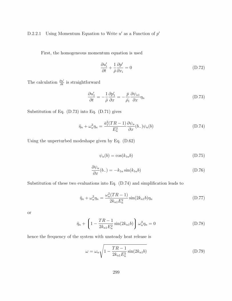
D.2.2.1 Using Momentum Equation to Write u′ as a Function of p′

First, the homogeneous momentum equation is used

∂u′i∂t

+1

ρ

∂p′

∂xi= 0 (D.72)

The calculation ∂u′

∂tis straightforward

∂u′1∂t

= −1

ρ

∂p′1∂x

= − p

ρ1

∂ψn1

∂xηn (D.73)

Substitution of Eq. (D.73) into Eq. (D.71) gives

ηn + ω2nηn =

a21(TR− 1)

E2n

∂ψn∂x

(b−)ψn(b) (D.74)

Using the unperturbed modeshape given by Eq. (D.62)

ψn(b) = cos(k1nb) (D.75)

∂ψn∂x

(b−) = −k1n sin(k1nb) (D.76)

Substitution of these two evaluations into Eq. (D.74) and simplification leads to

ηn + ω2nηn =

ω2n(TR− 1)

2kn1E2n

sin(2kn1b)ηn (D.77)

or

ηn +

1− TR− 1

2kn1E2n

sin(2kn1b)

ω2nηn = 0 (D.78)

hence the frequency of the system with unsteady heat release is

ω = ωn

√1− TR− 1

2kn1E2n

sin(2kn1b) (D.79)

299

This is the shifted frequency equivalent to that of Dowling’s solution. It generates an esti-

mation of frequency shift that is very poor, dropping to zero before a temperature ratio of

four.

D.2.2.2 Using Unperturbed Energy Equation to Write u′ as a Function of p′

Alternatively, the unperturbed energy equation can be used to write ∂u′

∂tin terms of

ψn. In one dimension

∂p′

∂t+ γp

∂u′

∂x= 0 (D.80)

Rearranging

∂u′

∂x= − 1

γp

∂p′

∂t(D.81)

Integrating this expression in x

u′ = − 1

γp

∫∂p′

∂tdx (D.82)

Differentiating in time

∂u′

∂t= − 1

γp

∫∂2p′

∂t2dx (D.83)

Substituting the expansion Eq. (D.41)

∂u′

∂t= −1

γ

∫ ψndx

ηn (D.84)

This is inconvenient because it contains the integration of the modeshape, hence use Eq.

(D.15) to substitute for ψn

∂u′

∂t=

1

γω2n

[∫∂

∂x

γpρ

∂ψn∂x

dx

]ηn (D.85)

300

Simplifying this

∂u′

∂t=

1

γk2n

∂ψn∂x

ηn (D.86)

This is of the form used by Palm [65] in his analysis and suggested in general by Culick

[8]. Note that the heat release in now proportional to the second derivative in time, hence

suggesting interpretation of adding inertia to the system. Substituting Eq. (D.86) into Eq.

(D.71) leads to

ηn + ω2nηn =

(TR− 1)

k2n1E

2n

∂ψn∂x

(b−)ψn(b)ηn (D.87)

Using Eq. (D.75) and (D.76) to substitute

ηn + ω2nηn = −(TR− 1)

2kn1E2n

sin(2kn1b)ηn (D.88)

or 1 +(TR− 1)

2k1nE2n

sin(2kn1b)

ηn + ω2nηn = 0 (D.89)

finally

ηn +ω2n

1 + (TR−1)2kn1E2

nsin(2kn1b)

ηn = 0 (D.90)

This indicates a shifted frequency given by

ω = ωn

√1

1 + (TR−1)2kn1E2

nsin(2kn1b)

(D.91)

This frequency gives identical results to Palm’s solution, and in fact it will be shown later

that Palm’s solution can be reduced to this form.

301

D.2.3 Clarification of Dowling’s Results

Now that the solution has been carried out for the method derived here, in what the

author believes to be a very clear and concise manner, it is worthwhile to consider the cause

of the poor estimation in Dowling’s case. The previous section showed that Dowling’s error

was not caused by neglecting mean density gradients. In fact, her solution is equivalent to

that obtained by use of the linearized momentum equation to relate u′ to the expansion

functions. This is not the actual error committed by Dowling, however. Dowling, indeed

uses Eq. (D.86) to estimate ∂u′

∂t, but then quickly follows this with the substitution

ηn = −ω2nηn (D.92)

which is directly inconsistent with the starting equation, Eq. (D.68). In fact, the above

derivation shows that this substitution is entirely unneceesary. With this substitution, the

results are the same as if the momentum equation had been used to relate u′ to ψ.

D.2.4 Clarification of Culick’s Diagnosis

It is also worthwhile to discuss Palm’s solution, which caused Culick to conclude that

the exclusion of the density gradient term from the right hand side of the wave equation

was Dowling’s crucial mistake. As shown above, no mean density gradient term is needed

to derive a frequency shift in agreement with Palm’s solution. One may note that the

302

mathematical form of Palm’s frequency (for κ = 1) is

ω = ωn

√√√√√ 1− 1kn1E2

n

β1−β3

2ln(TR)

1 + 1kn1E2

n

β1(TR− 1)− β1−β3

2ln(TR)

(D.93)

which indeed contains terms related to the density gradient. The portions of Eq. (D.93)

stemming from the inclusion of the mean density gradient term can be recognized as those

proportional to (β1 − β3). These two terms are given by

β1 = cos(kn1b) sin(k1nb) (D.94)

β3 =√TR

cos2(kn1b)

tan(√

(TR−1)kn1(L− b))(D.95)

Evaluating their difference

β1 − β3 = cos(kn1b) sin(kn1b)−√TR

cos2(kn1b)

tan(√

(TR−1)kn1(L− b))(D.96)

Noting that

√TR−1kn1 = kn2 (D.97)

then

β1 − β3 =cos2(kn1b)

tan(kn2(L− b))

tan(kn1b) tan(kn2(L− b))−√TR = 0 (D.98)

which is identically zero using Eq. (D.61) for the definition of the unperturbed frequency

and wave numbers. Therefore, the terms in Palm’s solution which he gains by including

the density gradient term on the right hand side actually cancel in the final equation. The

frequency from Palm’s solution with κ = 1 can then be reduced to

ω = ωn

√1

1 + 1kn1E2

nβ1(TR− 1)

(D.99)

303

or, with the substitution of Eq.(D.94) for β1

ω = ωn

√1

1 + (TR−1)2kn1E2

nsin(2kn1b)

(D.100)

which is in complete agreement with Eq. (D.91), resulting from the derivation using the

unperturbed energy equation to write u′ in terms of ψn.

D.2.5 Conclusions

In addition to the above derivations, the geometry was solved using a numerical

integration in the Generalized Instability Model (GIM) [25]. Note that in this code, the

discontinuity in mean density is smoothed using a Gaussian cumulative distribution function

and the differentiation of the modeshapes is accomplished via a five point scheme. In this way,

the precise mathematics of integrating over a Dirac delta function is lost. The comparison

of the frequency shift from all these methods is shown in Fig. D.1.

It is interesting to note that the plot shown by Palm gives a different curve for his

results. The present paper shows that Palm’s solution is in much better agreement than

Palm recognized. Notice that, as discussed above, the present derivation using unperturbed

energy equation for relating u′ to ψn agrees exactly with Palm’s results. This is, as discussed

above, Palm’s solution can be reduced to agree mathematically with the present derivation.

Such reduction of the frequency shift statement shows that the terms gained by including

the right hand side density gradient term in fact cancel in the final form. Also, the present

304

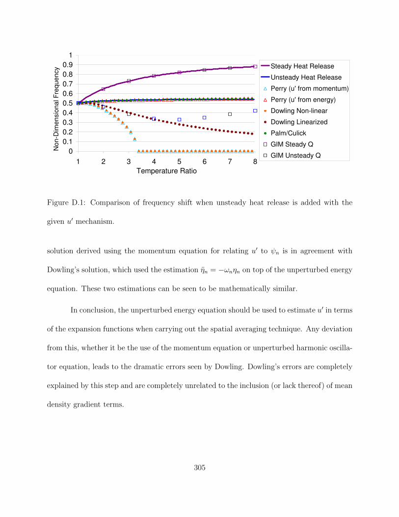
0

0.1

0.2

0.3

0.4

0.5

0.6

0.7

0.8

0.9

1

1 2 3 4 5 6 7 8

Temperature Ratio

No

n-D

ime

nsio

na

l F

req

ue

ncy Steady Heat Release

Unsteady Heat Release

Perry (u' from momentum)

Perry (u' from energy)

Dowling Non-linear

Dowling Linearized

Palm/Culick

GIM Steady Q

GIM Unsteady Q

Figure D.1: Comparison of frequency shift when unsteady heat release is added with the

given u′ mechanism.

solution derived using the momentum equation for relating u′ to ψn is in agreement with

Dowling’s solution, which used the estimation ηn = −ωnηn on top of the unperturbed energy

equation. These two estimations can be seen to be mathematically similar.

In conclusion, the unperturbed energy equation should be used to estimate u′ in terms

of the expansion functions when carrying out the spatial averaging technique. Any deviation

from this, whether it be the use of the momentum equation or unperturbed harmonic oscilla-

tor equation, leads to the dramatic errors seen by Dowling. Dowling’s errors are completely

explained by this step and are completely unrelated to the inclusion (or lack thereof) of mean

density gradient terms.

305

APPENDIX EBOUNDARY CONDITIONS

306

APPENDIX EBOUNDARY CONDITIONS

E.1 Simple Boundary Conditions

There are three simple boundary conditions commonly used for acoustics, particularly

aeroacoustics and thermoacoustics: closed, open, and choked. Before a discussion of more

complicated boundary conditions is

E.1.1 Closed BC

The closed boundary condition in acoustics refers to

u′n(t) = 0 (E.1)

Physically, this represents a rigid wall (the normal component of velocity vanishes). Because

the no-slip condition is often ignored in first-order acoustics, this boundary condition for

the acoustic velocity is best represented by the “slip” boundary condition in OpenFOAM,

in which the tangential velocity components have zero-gradient conditions at the boundary.

The boundary condition for the pressure at a closed boundary is obtained substituting Eq.

307

(E.1) into the normal component of Eq. (2.26) and rearranging to form a third-kind BC

∂p′

∂xn+uja

∂un∂xj

p′ = −ρuj∂u′n∂xj− ρu′j

∂un∂xj

(E.2)

In the absence of mean flow gradients ( ∂ui∂xj

= 0), the assumptions leading to the current

equations of tacFoam hold. The pressure boundary condition for a closed boundary becomes

∂p′

∂xn= −ρuj

∂u′n∂xj

(E.3)

Note that this form is consistent with the current equations of tacFoam, but Eq. (E.2) is

consistent with the physics of linear acoustics. Finally, if the mean flow is negligible all

together, the closed boundary condition for pressure takes on its classical form

∂p′

∂xn= 0 (E.4)

E.1.2 Open BC

The open boundary condition in acoustics refers to

p′(t) = 0 (E.5)

Physically, this represents a pressure release boundary, such as the ideal behavior of an exit

from a confined duct into a large ambient space. The open boundary condition for velocity is

found by substituting Eq. (E.5) into Eq. (2.27) and rearranging (assuming there is no heat

release at the boundary; indeed, placing an open boundary condition near a heat release

308

location is numerically ill-advised)

∂u′j∂xj

+1

γp

∂p

∂xju′j = − uj

γp

∂p′

∂xj− p′

p

∂uj∂xj

(E.6)

This form is consistent with the physics of linear acoustics. To be consistent with the current

version of tacFoam, the mean velocity and mean pressure gradients must be ignored

∂u′j∂xj

= − ujγp

∂p′

∂xj(E.7)

For classical acoustics with no mean flow, the pressure release (or open) boundary condition

for velocity is given by

∂u′j∂xj

= 0 (E.8)

Note that in these equations, the divergence contains transverse derivatives of velocity com-

ponents transverse to the boundary normal. These terms should be move to the RHS of the

equation, which gives the normal derivative of the normal velocity at the boundary. The

transverse derivatives, for lack of other easy way to specify BC, can be given zero gradient

boundary conditions.

E.1.3 Choked BC

The choked boundary condition refers to an acoustic boundary condition applied at

the choke point (Mach = 1) of a flow. Because of the nature of choked flows, this dictates

that the mass flow remains constant at the throat, hence, for a given area

ρ(t)un(t) = constant (E.9)

309

for linearized acoustics

ρ′un + ρu′n = 0 (E.10)

which can be rearranged, using the isentropic signal assumption, to

p′

γp+u′nun

= 0 (E.11)

or

p′ +γp

unu′n = 0 (E.12)

Equation (E.6) or (E.2) along with zero gradient BC for the components tangential to the

surface can then be used to close the system for the four variables on the boundary.

E.2 Arbitrary Impedance Boundary Conditions

For arbitrary impedance (Z), the boundary condition is given by

p′ − Zρau′n = 0 (E.13)

The closed boundary condition is the limit Z →∞ and the open boundary condition

is the limit when Z → 0. In the limit of small Mach number, the choked boundary impedance

also tends to infinity, hence behaves similarly to a closed boundary. Anything in between

can be considered arbitrary impedance. That is, any boundary to an acoustic domain not

behaving like an open or closed boundary is in this group. A number of practical scenarios in

gas turbines give rise to the necessity of arbitrary impedance boundary conditions [67]. Most

310

obviously, the inlet and outlet of the combustion chamber, namely the compressor exit and

the turbine inlet, respectively. Also, common acoustic mitigation techniques such as wall

liners and absorbing Helmholtz resonators are also of this type. These boundaries do not fall

conveniently as open, closed, or choked boundaries. Also, they typically exhibit reactance

behavior as well as resistance. Thus, in mathematical terms, their impedance is complex,

having both real and imaginary components. To make matters worse, the impedance of

combustor boundaries have impedances that are a function of frequency. For this reason,

the discussion must begin in the complex frequency plane.

p(ω) = Z(ω)ρaun(ω) (E.14)

where the hat symbol designates the Fourier transform of a variable as a function of time.

p(ω) =1

2π

∞∫−∞

p′(t) exp(−iωt)dt (E.15)

un(ω) =1

2π

∞∫−∞

u′n(t) exp(−iωt)dt (E.16)

The relationship between the acoustic pressure and acoustic velocity in time can be written

by performing an inverse Fourier transform on Eq. (E.14).

p′(t) =

∞∫−∞

p(ω) exp(iωt)dω (E.17)

p′(t) =

∞∫−∞

Z(ω)ρaun(ω) exp(iωt)dω (E.18)

Using the convolution theorem

p′(t) =

∞∫−∞

Z(τ)ρau′n(t− τ)dτ (E.19)

311

where

Z(t) =

∞∫−∞

Z(ω) exp(iωt)dω (E.20)

and

u′n(t) =

∞∫−∞

un(ω) exp(iωt)dω (E.21)

In order to prevent violation of the causality principle, based on Eq. (E.19), the

function Z(t) should be exactly zero for all negative values of t. This effectively requires

that the poles of the function Z(ω) lie in the upper half of the complex frequency plane.

From input complex impedance data, the basis functions for a curve fit can be chosen such

that causality is upheld and the inverse Fourier transform of the impedance, Eq. (E.20), can

be performed analytically prior to the simulation. The pressure-velocity relationship at the

boundary can be calculated within the simulation by numerically approximating

p′(t) =

t∫0

Z(τ)ρau′n(t− τ)dτ (E.22)

Note that the negative τ region of the integral is eliminated by the causality principle,

namely, that the present value of acoustic pressure cannot depend on future values of the

acoustic velocity. Secondly, for the sake of a finite simulation in time, the integration can

only be performed up to τ = t, since no values of acoustic velocity are available from before

the start of the simulation. As with the choked boundary condition, either Eq. (E.2) or (E.6)

can be used with zero gradient conditions on the transverse acoustic velocities to provide a

closed system of equations for the boundary.

312

The approach for implementing this time-domain complex impedance boundary con-

dition for a broadband impedance model requires a curve fitting technique for translating

Z(ω) data into a function with form such that it can be transformed analytically and causal-

ity can be upheld. The approach used here is that described by [68] and implemented for

aeroacoustic applications in [69]. The curve fit uses bases functions in the form

Z(ω) =A

iω + λ(E.23)

where the residue (A) and the pole location (ω = iλ) are constants to be determined by the

curve fitting algorithm. These constants are either real or complex conjugates. In the case

they are complex conjugates

Z(ω) =A+ iB

iω + (α + iβ)+

A− iBiω + (α− iβ)

(E.24)

It is more convenient to write

Z(ω) =iωC +D

(iω + α)2 + β2(E.25)

where the residue is A± iB and the pole location is ω = iλ = i(α ± iβ). The relationships

are

C = 2A

D = 2Aα + 2Bβ

(E.26)

As discussed by [70], in order for the convolution integral, Eq. (E.19), to depend only

on past values of acoustic velocity (i.e. not on future values of acoustic velocity, to satisfy

causality), the transformed function Z(t) must be zero for all negative values of t. Thus, the

313

lower bound on the integral in Eq. (E.19) can be set to 0. Note, for finite time simulations,

the upper bound on the convolution integral is simply the time duration of the simulation.

Thus, Eq. (E.22) is recovered for implementation into tacFoam. For Z(t) = 0∀t < 0, the

poles of the function Z(ω) must all lie in the upper half of the ω-plane. Any poles in the

lower-half plane will contribute non-zero values to the negative t part of the impedance,

which violates causality. Poles in the upper-half plane contribute to the positive t part of

Z(t), which satisfies causality. Therefore, for basis functions defined by Eqs. (E.23) and

(E.25) to satisfy causality, the imaginary part of their pole location (specifically, λ or α)

must be positive. Performing the transform, Eq. (E.20), for Eqs. (E.23) and (E.25), the

time domain impedance functions are respectively given by

Z(t) = A exp(−λt)H(t) (E.27)

Z(t) = exp(−αt)C cos(βt) +

D − αCβ

sin(βt)

H(t) (E.28)

whereH is the Heaviside step function, which explicitly shows that these impedance functions

satisfy causality. For a curve fit to arbitrary data in the frequency domain, a summation of

these basis functions can be used and the constants can be chosen so as to optimized the

accuracy of the fit.

Z(ω) =J∑j=1

Ajiω + λj

+K∑k=1

iωCk +Dk

(iω + αk)2 + β2k

(E.29)

314

where the λj and αk values are positive to enforce causality. The transformed impedance in

the time domain is then given by

Z(t) =

[J∑j=1

Aj exp(−λjt) +K∑k=1

exp(−αkt)Ck cos(βkt) +

Dk − αkCkβk

sin(βkt)

]H(t)

(E.30)

Substitution of Eq. (E.30) into Eq. (E.22) provides the boundary condition for

the time domain solver. Alternatively, the admittance Y (ω) could be used to write the

acoustic velocity in terms of the acoustic pressure. The only remaining numerical issue is

the calculation of the integral. For this task, the recursive convolution method of [71] with

piecewise linear reconstruction of the time history is used. Further details of the methods

are available in [68]. As recommended by [69], the vector fitting method from [72], [73], and

[74] is used as provided online [75].

Note that the code provides a curve fit of the form

Z(ω) =J∑j=1

Ajiω − λj

(E.31)

with complex conjugates sometimes resulting for Aj and λj. Notice the subtraction in the

denominator instead of addition as in Eq. (E.29).

315

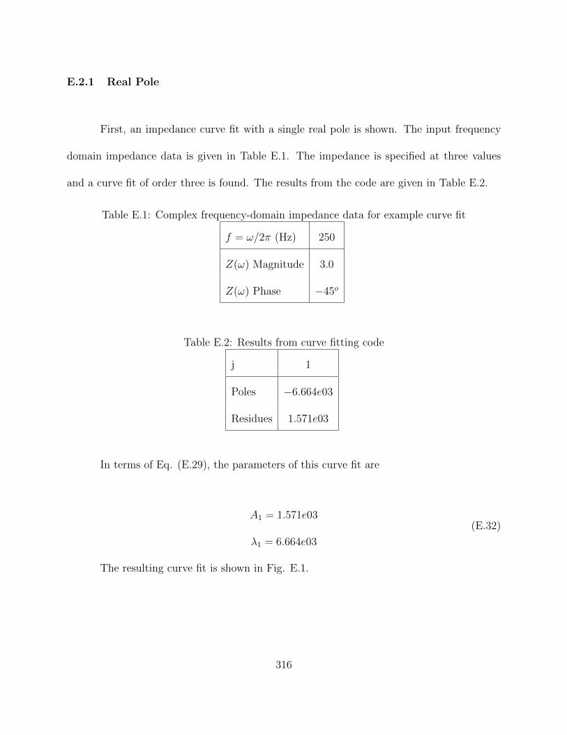
E.2.1 Real Pole

First, an impedance curve fit with a single real pole is shown. The input frequency

domain impedance data is given in Table E.1. The impedance is specified at three values

and a curve fit of order three is found. The results from the code are given in Table E.2.

Table E.1: Complex frequency-domain impedance data for example curve fit

f = ω/2π (Hz) 250

Z(ω) Magnitude 3.0

Z(ω) Phase −45o

Table E.2: Results from curve fitting code

j 1

Poles −6.664e03

Residues 1.571e03

In terms of Eq. (E.29), the parameters of this curve fit are

A1 = 1.571e03

λ1 = 6.664e03

(E.32)

The resulting curve fit is shown in Fig. E.1.

316

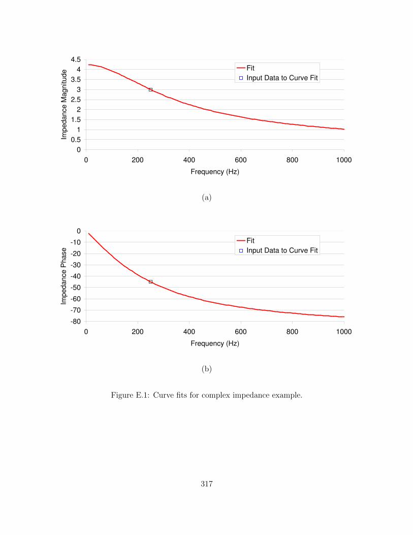
0

0.5

1

1.5

2

2.5

3

3.5

4

4.5

0 200 400 600 800 1000

Frequency (Hz)

Impedance M

agnitude Fit


(a)

-80

-70

-60

-50

-40

-30

-20

-10

0

0 200 400 600 800 1000

Frequency (Hz)

Impedance P

hase

Fit


(b)

Figure E.1: Curve fits for complex impedance example.

317

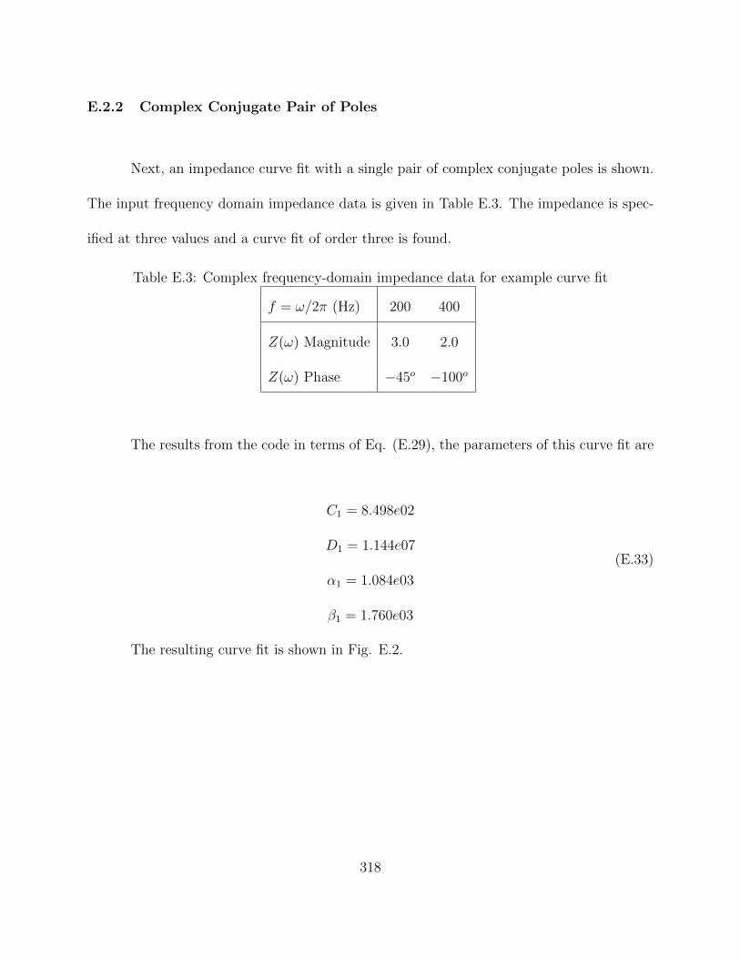
E.2.2 Complex Conjugate Pair of Poles

Next, an impedance curve fit with a single pair of complex conjugate poles is shown.

The input frequency domain impedance data is given in Table E.3. The impedance is spec-

ified at three values and a curve fit of order three is found.


f = ω/2π (Hz) 200 400

Z(ω) Magnitude 3.0 2.0

Z(ω) Phase −45o −100o

The results from the code in terms of Eq. (E.29), the parameters of this curve fit are

C1 = 8.498e02

D1 = 1.144e07

α1 = 1.084e03

β1 = 1.760e03

(E.33)


318

0

0.5

1

1.5

2

2.5

3

3.5

0 200 400 600 800 1000

Frequency (Hz)

Imp

ed

an

ce

Ma

gn

itu

de Fit


(a)

-160

-140

-120

-100

-80

-60

-40

-20

0

0 200 400 600 800 1000

Frequency (Hz)

Impedance P

hase

Fit


(b)


319

E.2.3 Real Pole and Complex Conjugate Pair of Poles

Finally, an example curve fit is shown for a complex impedance containing a real pole

and a complex conjugate pair of poles. The input frequency domain impedance data is given

in Table E.4. The impedance is specified at three values and a curve fit of order three is

found. The results from the code are given in Table E.5.


f = ω/2π (Hz) 100 300 500

Z(ω) Magnitude 0.9 0.5 0.4

Z(ω) Phase −50o −120o −140o

Table E.5: Results from curve fitting code

j 1 2 3

Poles −1.290e05 −5.224e02 + i5.410e02 −5.224e02− i5.410e02

Residues −4.315e04 3.868e02− i1.900e02 3.868e02 + i1.900e02

In terms of Eq. (E.29), the parameters of this curve fit are

320

A1 = −4.315e04

λ1 = 1.290e05

C2 = 7.736e02

D2 = 6.097e05

α2 = 5.224e02

β2 = 5.410e02

(E.34)


321

0

0.1

0.2

0.3

0.4

0.5

0.6

0.7

0.8

0.9

1

0 200 400 600 800 1000

Frequency (Hz)

Impedance M

agnitude Fit


(a)

-180

-160

-140

-120

-100

-80

-60

-40

-20

0

0 200 400 600 800 1000

Frequency (Hz)

Impedance P

hase

Fit


(b)


322

E.3 Characteristic Boundary Conditions

As with direct numerical simulations (DNS) and highly-resolved large-eddy simula-

tions (LES), the numerical boundary conditions of acoustic solvers must also be given with

care. The Navier-Stokes Characteristic Boundary Condition (NSCBC) approach given by

Poinsot and Lele [76] uses the Local One-Dimensional Inviscid approximation. A similar ap-

proach can be taken to develop characteristic boundary conditions for the acoustic equations

used in tacFoam. In the above formulation of the boundary conditions, as in Eq. (E.2) or Eq.

(E.6), the second boundary condition (“soft” BC) is derived from the physical BC using one

of the governing equations. The above formulation then gives boundary conditions for one

acoustic variable in terms of the normal derivative of the other acoustic variables. These then

must be approximated from the solution internal to the numerical domain. In reality, these

partially depend on waves entering the domain from the outside, however. Thus, estimation

of such derivatives for the above BC is inaccurate. An alternate, more involved formulation

of boundary conditions follows the procedure outlined in the definition of NSCBC for DNS

and LES calculations. First, assume that there is no heat release at the boundary and no

gradients of mean velocity or mean pressure. (This is good modelling practice, anyhow).

The governing equations become

∂p

∂t+ u

∂p

∂x+ v

∂p

∂y+ w

∂p

∂z+ γp

∂u∂x

+∂v

∂y+∂w

∂z

= 0 (E.35)

∂u

∂t+ u

∂u

∂x+ v

∂u

∂y+ w

∂u

∂z+

1

ρ

∂p

∂x= 0 (E.36)

323

∂v

∂t+ u

∂v

∂x+ v

∂v

∂y+ w

∂v

∂z+

1

ρ

∂p

∂y= 0 (E.37)

∂w

∂t+ u

∂w

∂x+ v

∂w

∂y+ w

∂w

∂z+

1

ρ

∂p

∂z= 0 (E.38)

With the x-direction normal to the boundary, the related Local One-Dimensional Inviscid

(LODI) equations are

∂p

∂t+ u

∂p

∂x+ γp

∂u

∂x= 0 (E.39)

∂u

∂t+ u

∂u

∂x+

1

ρ

∂p

∂x= 0 (E.40)

∂v

∂t+ u

∂v

∂x= 0 (E.41)

∂w

∂t+ u

∂w

∂x= 0 (E.42)

The LODI system has eigenvalues

λ1 = u− a, λ2 = λ3 = u, λ4 = u+ a (E.43)

left eigenvectors

l1 = (1 − ρa 0 0) (E.44)

l2 = (0 0 1 0) (E.45)

l3 = (0 0 0 1) (E.46)

l4 = (1 ρa 0 0) (E.47)

which leads to wave strengths of

L1 = (u− a)

∂p

∂x− ρa∂u

∂x

(E.48)

324

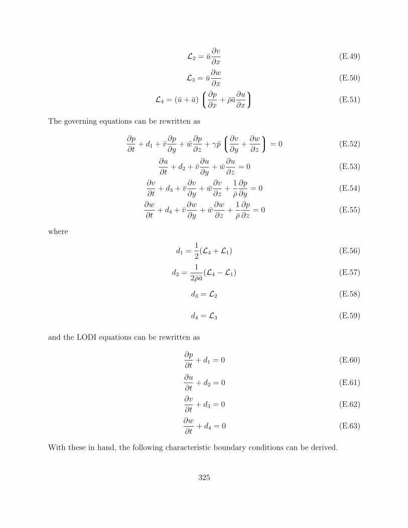
L2 = u∂v

∂x(E.49)

L3 = u∂w

∂x(E.50)

L4 = (u+ a)

∂p

∂x+ ρa

∂u

∂x

(E.51)

The governing equations can be rewritten as

∂p

∂t+ d1 + v

∂p

∂y+ w

∂p

∂z+ γp

∂v∂y

+∂w

∂z

= 0 (E.52)

∂u

∂t+ d2 + v

∂u

∂y+ w

∂u

∂z= 0 (E.53)

∂v

∂t+ d3 + v

∂v

∂y+ w

∂v

∂z+

1

ρ

∂p

∂y= 0 (E.54)

∂w

∂t+ d4 + v

∂w

∂y+ w

∂w

∂z+

1

ρ

∂p

∂z= 0 (E.55)

where

d1 =1

2(L4 + L1) (E.56)

d2 =1

2ρa(L4 − L1) (E.57)

d3 = L2 (E.58)

d4 = L3 (E.59)

and the LODI equations can be rewritten as

∂p

∂t+ d1 = 0 (E.60)

∂u

∂t+ d2 = 0 (E.61)

∂v

∂t+ d3 = 0 (E.62)

∂w

∂t+ d4 = 0 (E.63)

With these in hand, the following characteristic boundary conditions can be derived.

325

E.3.1 Closed Inlet

The physical boundary condition is

u(y, z, t) = 0 (E.64)

The soft boundary conditions must determine p(y, z, t). The L1 wave is outgoing and hence

can be approximated from the interior solution. The other three waves (L2,L3,L4) are

incoming and must be specified. For closed conditions, it is best to specify that there are

no incoming convective waves, i.e. L2 = L3 = 0. This effectively enforces zero gradient

boundary conditions on the transverse acoustic velocity components.

∂v

∂x=∂w

∂x= 0 (E.65)

Thus, only the pressure boundary condition remains unknown.

E.3.1.1 Step 1

Eliminate the velocity equations from the governing equations. Retain only the pres-

sure equation.

326

E.3.1.2 Step 2

With fixed u, use the LODI equation

∂u

∂t+ d2 = 0 (E.66)

which gives d2 = 0 or L4 = L1, hence d1 = L1.

E.3.1.3 Step 3

The remaining equation to be solved on the boundary is

∂p

∂t+ d1 + v

∂p

∂y+ w

∂p

∂z+ γp

∂v∂y

+∂w

∂z

= 0 (E.67)

where d1 = L1, which given by Eq. (E.48) and can be approximated from the interior

solution.

E.3.2 Closed Outlet


u(y, z, t) = 0 (E.68)

The soft boundary conditions must determine p(y, z, t), v(y, z, t), w(y, z, t). The L1 wave is

incoming and hence unknown to the interior solution. The other three waves (L2,L3,L4)

are outgoing and can be properly estimated from the interior solution.

327

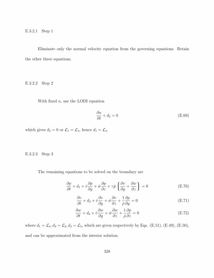
E.3.2.1 Step 1

Eliminate only the normal velocity equation from the governing equations. Retain

the other three equations.

E.3.2.2 Step 2


∂u

∂t+ d2 = 0 (E.69)


E.3.2.3 Step 3

The remaining equations to be solved on the boundary are

∂p

∂t+ d1 + v

∂p

∂y+ w

∂p

∂z+ γp

∂v∂y

+∂w

∂z

= 0 (E.70)

∂v

∂t+ d3 + v

∂v

∂y+ w

∂v

∂z+

1

ρ

∂p

∂y= 0 (E.71)

∂w

∂t+ d4 + v

∂w

∂y+ w

∂w

∂z+

1

ρ

∂p

∂z= 0 (E.72)

where d1 = L4, d3 = L2, d4 = L3, which are given respectively by Eqs. (E.51), (E.49), (E.50),

and can be approximated from the interior solution.

328

E.3.3 Open Inlet


p(y, z, t) = 0 (E.73)

The soft boundary conditions must determine u(y, z, t). The L1 wave is outgoing and hence

can be approximated from the interior solution. The other three waves (L2,L3,L4) are

incoming and must be specified. As with closed conditions, it is best to specify that there

are no incoming convective waves, i.e. L2 = L3 = 0. This effectively enforces zero gradient


∂v

∂x=∂w

∂x= 0 (E.74)

Thus, only the normal velocity boundary condition remains unknown.

E.3.3.1 Step 1

Eliminate the pressure and tangential velocity equations from the governing equa-

tions. Retain only the normal velocity equation.

329

E.3.3.2 Step 2

With fixed p, use the LODI equation

∂p

∂t+ d1 = 0 (E.75)

which gives d1 = 0 or L4 = −L1, hence d2 = −L1/(ρa).

E.3.3.3 Step 3


∂u

∂t+ d2 + v

∂u

∂y+ w

∂u

∂z= 0 (E.76)

where d2 = −L1/(ρa), which can be approximated from the interior solution using Eq.

(E.48).

E.3.4 Open Outlet


p(y, z, t) = 0 (E.77)

The soft boundary conditions must determine u(y, z, t), v(y, z, t), w(y, z, t). The L1 wave is



330

E.3.4.1 Step 1

Eliminate only the pressure equation from the governing equations. Retain the three

velocity equations.

E.3.4.2 Step 2


∂p

∂t+ d1 = 0 (E.78)

which gives d1 = 0 or L1 = −L4, hence d2 = L4/(ρa).

E.3.4.3 Step 3


∂u

∂t+ d2 + v

∂u

∂y+ w

∂u

∂z= 0 (E.79)

∂v

∂t+ d3 + v

∂v

∂y+ w

∂v

∂z= 0 (E.80)

∂w

∂t+ d4 + v

∂w

∂y+ w

∂w

∂z= 0 (E.81)

where d2 = L4/(ρa), d3 = L2, d4 = L3, which are given respectively by Eqs. (E.51), (E.49),

(E.50), and can be approximated from the interior solution.

331

E.3.5 Slip Wall

Note: here, the slip wall is oriented as an outlet, such that the outward pointing

normal of the boundary is in the positive x direction. The physical boundary condition is

u(y, z, t) = 0 (E.82)

The soft boundary conditions must determine p(y, z, t), v(y, z, t), w(y, z, t). The L1 wave

is incoming and hence unknown to the interior solution. The L4 wave is outgoing and can

be properly estimated from the interior solution. The two convective waves, based on the

impermeability condition (u = 0), have zero strength, i.e. L2 = L3 = 0.

E.3.5.1 Step 1

Eliminate only the normal velocity equation from the governing equations. Retain

the other three equations.

E.3.5.2 Step 2


∂u

∂t+ d2 = 0 (E.83)


332

E.3.5.3 Step 3


∂p

∂t+ d1 + v

∂p

∂y+ w

∂p

∂z+ γp

∂v∂y

+∂w

∂z

= 0 (E.84)

∂v

∂t+ v

∂v

∂y+ w

∂v

∂z+

1

ρ

∂p

∂y= 0 (E.85)

∂w

∂t+ v

∂w

∂y+ w

∂w

∂z+

1

ρ

∂p

∂z= 0 (E.86)

where d1 = L4, which is given by Eq. (E.51) and can be approximated from the interior

solution.

E.3.6 Arbitrary Real Constant Impedance Inlet


p(y, z, t) = Zu(y, z, t) (E.87)

where Z is a real constant. For example, a choked inlet could be enforced by setting Z =

−γp/u. The soft boundary conditions must determine u(y, z, t). The L1 wave is outgoing

and hence can be approximated from the interior solution. The other three waves (L2,L3,L4)

are incoming and must be specified. As previously for inlets, it is best to specify that there

are no incoming convective waves, i.e. L2 = L3 = 0. This effectively enforces zero gradient


∂v

∂x=∂w

∂x= 0 (E.88)

333

Thus, only the normal velocity boundary condition remains unknown.

E.3.6.1 Step 1

Eliminate the pressure and tangential velocity equations from the governing equa-

tions. Retain only the normal velocity equation.

E.3.6.2 Step 2


∂p

∂t+ d1 = 0 (E.89)

which gives d1 = −Z∂u/∂t or L4 = −L1 − 2Z∂u/∂t, hence d2 = −(L1 + Z∂u/∂t)/(ρa).

E.3.6.3 Step 3


∂u

∂t+ d2 + v

∂u

∂y+ w

∂u

∂z= 0 (E.90)

where d2 = −(L1 + Z∂u/∂t)/(ρa), which can be approximated from the interior solution

using Eq. (E.48).

334

E.3.7 Arbitrary Real Constant Impedance Outlet


p(y, z, t) = Zu(y, z, t) (E.91)

The soft boundary conditions must determine u(y, z, t), v(y, z, t), w(y, z, t). The L1 wave is



E.3.7.1 Step 1

Eliminate only the pressure equation from the governing equations. Retain the three

velocity equations.

E.3.7.2 Step 2


∂p

∂t+ d1 = 0 (E.92)

which gives d1 = −Z∂u/∂t or L1 = −L4 − 2Z∂u/∂t, hence d2 = (L4 + Z∂u/∂t)/(ρa).

335

E.3.7.3 Step 3


∂u

∂t+ d2 + v

∂u

∂y+ w

∂u

∂z= 0 (E.93)

∂v

∂t+ d3 + v

∂v

∂y+ w

∂v

∂z= 0 (E.94)

∂w

∂t+ d4 + v

∂w

∂y+ w

∂w

∂z= 0 (E.95)

where d2 = L4/(ρa), d3 = L2, d4 = L3, which are given respectively by Eqs. (E.51), (E.49),

(E.50), and can be approximated from the interior solution.

336

LIST OF REFERENCES

[1] H. Krediet, Prediction of Limit Cycle Pressure Oscillations in Gas Turbine CombustionSystems Using the Flame Describing Function. PhD thesis, University of Twente, 2012.

[2] Y. A. Cengel and M. A. Boles, Thermodynamics: An Engineering Approach. New York,NY: McGraw-Hill, 6 ed., 2008.

[3] Y. Huang and V. Yang, “Dynamics and stability of lean-premixed swirl-stabilized com-bustion,” Progress in Energy and Combustion Science, vol. 35, pp. 293–364, 2009.

[4] I. Glassman and R. Yetter, Combustion. Academic Press, 4 ed., 2007.

[5] P. Leighton, Photochemistry of air pollution, vol. 9. Academic Press, 1961.

[6] J. Zeldovich, “The oxidation of nitrogen in combustion and explosions,” Acta Physic-ochimica, vol. 21, no. 4, pp. 577–628, 1946.

[7] T. Lieuwen, V. Yang, and F. Lu, Combustion instabilities in gas turbine engines: op-erational experience, fundamental mechanisms and modeling. American Institute ofAeronautics and Astronautics, 2005.

[8] F. E. C. Culick, “Unsteady Motions in Combustion Chambers for Propulsion Systems,”tech. rep., NATO RTO, 2006. AGARDograph RTO-AG-AVT-039.

[9] J. W. S. Rayleigh, “The explanation of certain acoustical phenomena,” vol. 18, pp. 319–321, 1878.

[10] T. Lieuwen, “Modeling premixed combustion – acoustic wave interactions: a review,”AIAA Journal of Propulsion and Power, vol. 19, no. 5, pp. 765–781, 2003.

[11] A. Fichera, C. Losenno, and A. Pagano, “Clustering of chaotic dynamics of a leangas-turbine combustor,” Applied Energy, vol. 69, no. 2, pp. 101–117, 2001.

[12] W. Krebs, H. Krediet, S. Hermeth, T. Poinsot, and E. Portillo, “Comparison of nonlinearto linear thermoacoustic stability analysis of a gas turbine combustion system,” ASMETurbo Expo, 2012. GT2012-69477.

[13] L. Crocco and S. Cheng, Theory of Combustion Instability in Liquid Propellant RocketMotors. London: Butterworths Science Publication, 1956. AGARDograph 8.

337

[14] A. Gelb and W. E. VanderVelde, Multiple-Input Describing Functions and NonlinearSystem Design. New York, NY: McGraw-Hill Book Co., 1968.

[15] J. OConnor and T. Lieuwen, “Disturbance field characteristics of a transversely excitedburner,” Combustion Science and Technology, pp. 427–443, 2011.

[16] K. I. Matveev and F. E. C. Culick, “A model for combustion instability involving vortexshedding,” Combustion Science and Technology, vol. 175, no. 6, pp. 1059–1083, 2003.

[17] T. Lieuwen, Investigation of combustion instability mechanisms in premixed gas tur-bines. PhD thesis, Georgia Institute of Technology, 1999.

[18] A. P. Dowling and A. S. Morgans, “Feedback control of combustion oscillations,” AnnualReview of Fluid Mechanics, vol. 57, pp. 151–182, 2005.

[19] D. L. Gysling, G. S. Copeland, D. C. McCormick, and W. M. Proscia, “Combustionsystem damping augmentation with helmholtz resonators,” Journal of engineering forgas turbines and power, vol. 122, no. 2, pp. 269–274, 2000.

[20] V. Bellucci, P. Flohr, C. O. Paschereit, and F. Magni, “On the use of helmholtz res-onators for damping acoustic pulsations in industrial gas turbines,” Journal of engi-neering for gas turbines and power, vol. 126, no. 2, pp. 271–275, 2004.

[21] D. Zhao and A. S. Morgans, “Tuned passive control of combustion instabilities usingmultiple helmholtz resonators,” Journal of Sound and Vibrations, vol. 320, no. 4.

[22] T. Sattelmayer and W. Polifke, “Assessment of methods for the computation of thelinear stability of combustors,” Combustion Science and Technology, vol. 175, no. 3,pp. 453–476, 2003.

[23] F. E. C. Culick, High Frequency Pressure Oscillations in Liquid Rockets. ScD Thesis,Massachusetts Institute of Technology, 1961. Department of Aeronautics and Astro-nautics.

[24] A. P. Dowling, “The calculation of thermoacoustic oscillations,” Journal of Sound andVibration, vol. 180, no. 4, pp. 557–581, 1995.

[25] J. E. Portillo, J. C. Sisco, M. J. Corless, W. E. Anderson, and V. Sankaran, “Generalizedcombustion instability model,” AIAA/ASME/SAE/ASEE Joint Propulsion Conference,2006. AIAA-2006-4889.

[26] J. Pent, B. F. Kock, W. Krebs, and J. E. Portillo, “Application of a generalized in-stability model to industrial annular combustion chambers,” AIAA Aerospace SciencesMeeting, 2012. AIAA 2012-0010.

338

[27] J. Smagorinsky, “General circulation experiments with the primitive equations, i: Thebasic experiment,” Monthly Weather Review, vol. 91, no. 3, pp. 99–164, 1963.

[28] T. Poinsot and D. Veynante, Theoretical and Numerical Combustion. R. T. Edwards,Inc., 2005.

[29] A. Giauque, L. Selle, T. Poinsot, H. Buechner, P. Kaufmann, and W. Krebs, “Sys-tem identification of a large-scale swirled partially premixed combustor using les andmeasurements,” Journal of Turbulence, vol. 6, no. 21, 2005.

[30] J. F. van Kampen, Acoustic Pressure Oscillations Induced by Confined Turbulent Pre-mixed Natural Gas Flames. PhD thesis, University of Twente, 2006.

[31] A. Roux, L. Y. M. Gicquel, S. Reichstadt, N. Bertier, G. Staffelback, F. Vuillot, andT. J. Poinsot, “Analysis of unsteady reacting flows and impact of chemistry descriptionin large eddy simulations of side-dump ramjet combustors,” Combustion and Flame,vol. 157, no. 1, pp. 176–191, 2010.

[32] C. Stone and S. Menon, “Open-loop control of combustion instabilities in a model gasturbine combustor,” Journal of Turbulence, vol. 4, no. 1, 2003.

[33] P. Chatterjee, U. Vandsburger, W. R. Saunders, V. K. Khanna, and W. T. Baumann,“On the spectral characteristics of a self-excited rijke tube combustor - numerical sim-ulation and experimental measurements,” Journal of Sound and Vibration, vol. 283,pp. 573–588, 2005.

[34] U. G. Hedge, D. Reuter, B. T. Zinn, and B. R. Daniel, “Fluid mechanically coupled com-bustion instabilities in ramjet combustors,” AIAA Aerospace Sciences Meeting, 1987.AIAA-87-0216.

[35] Z. M. Ibrahim, F. A. Williams, S. G. Buckley, and C. Z. Twardochleb, “An acoustic-energy method for estimating the onset of acoustic instabilities in premixed gas-turbinecombustors,” ASME Journal of Engineering for Gas Turbines and Power, vol. 130,no. 5, 2008.

[36] “Lms engineering innovation.” http://www.lmsintl.com/simulation/virtuallab, May2011.

[37] A. Jemcov and B. Jojic, “Numerical modelling of combustion instability in rijke tubes,”(Kingston, Canada), 14th Annual Conferfence of CFD Society of Canada, July 2006.CFD2006.

[38] R. J. LeVeque, “Wave propagation algorithm for multidimensional hyperbolic systems,”Journal of Computational Physics, vol. 131, pp. 327–353, 1997.

339

[39] OpenFOAM, The Open Source CFD Toolbox: User Guide. OpenFOAM Foundation,2011. Available online: www.openfoam.org.

[40] R. J. LeVeque, Finite Volume Methods for Hyperbolic Problems. Cambridge, UK: Cam-bridge University Press, 2002.

[41] E. F. Toro, Riemann Solvers and Numerical Methods for Fluid Dynamics. New York,NY: Springer-Verlag, 1999.

[42] T. Barth and D. Jespersen, “The design and application of upwind schemes on unstruc-tured meshes,” 1989. AIAA-89-0366.

[43] D. G. Blackstock, Fundamentals of Physical Acoustics. New York, NY: John Wiley andSons, Inc., 2000.

[44] J. Lepers, R. Roper, and T. Sockheim, “Combustion stability code manual.” InternalReport, June 2003. Siemens Energy Inc.

[45] “Acoustics – determination of sound absorption coefficient and impedance in impedancetubes – part 2: Transfer-function method.” ISO 10534-2:1998(E).

[46] M. Summerfield, “A theory of unstable propulsion in liquid propellant rocket systems,”ARS J., vol. 21, no. 5, pp. 108–114, 1951.

[47] P. A. Hield, M. J. Braer, and S. H. Jin, “Thermoacoustic limit cycles in a premixedlaboratory combustor with open and choked exits,” Combustion and Flame, vol. 156,pp. 1683–1691, 2009.

[48] P. A. Hield, An Experimental and Theoretical Investigation of Thermoacoustic Insta-bility in a Turbulent Premixed Laboratory Combustor. PhD thesis, University of Mel-bourne, 2007.

[49] A. P. Dowling, “Nonlinear self-excited oscillations of a ducted flame,” Journal of FluidMechanics, vol. 346, pp. 271–290, 1997.

[50] H. Krediet, W. Krebs, E. Portillo, and J. Kok, “Prediction of thermoacousticlimit cycles during premixed combustion using the modified galerkin approach,”AIAA/ASME/SAE/ASEE Joint Propulsion Conference, 2010. AIAA 2010-7150.

[51] F. Menter and T. Esch, “Elements of industrial heat transfer prediction,” 2001. 16thBrazilian Congress of Mechanical Engineering (COBEM).

[52] D. Bradley, “How fast can we burn?,” Proceedings of the Combustion Institute, vol. 24,pp. 247–262, 1992.

340

[53] D. Goodwin, “Cantera: An object-oriented software toolkit for chemical kinetics, ther-modynamics, and transport processes.” Caltech, Pasadena, 2009. [Online]. Available:http://code.google.com/p/cantera.

[54] S. R. Stow, A. P. Dowling, and T. P. Hynes, “Reflection of circumferential modes in achoked nozzle,” Journal of Fluid Mechanics, vol. 467, 2002.

[55] C. Fugger, Y. Yu, Y. Matsutomi, W. Anderson, J. Pent, W. Krebs, and E. Por-tillo, “Investigation of a premixed reacting jet in an unstable transverse flow field,”AIAA/ASME/SAE/ASEE Joint Propulsion Conference, 2011. AIAA-2011-5703.

[56] I. B. Celik, U. Ghia, P. J. Roache, C. J. Freitas, H. Coleman, and P. E. Raad, “Procedurefor estimation and reporting of uncertainty due to distretization in cfd applications,”ASME Journal of Fluids Engineering, vol. 130, 2008. 078001-1.

[57] K. Schadow and E. Gutmark, “Combustion instability related to vortex shedding indump combustors and their passive control,” Progress in Energy and Combustion Sci-ence, vol. 18, pp. 117–132, 1992.

[58] J. K. Eaton and J. P. Johnston, “Turbulent flow re-attachment: An experimental studyof the flow and structure behind a backward-facing step,” Stanford University Report,1980.

[59] A. S. Neto, D. Grand, L. Metais, and M. Lesieur, “A numerical investigation of thecoherent vortices in turbulence behind a backward-facing step,” Journal of Fluid Me-chanics, vol. 256, pp. 1–25, 1993.

[60] K. B. Chun and H. J. Sung, “Control of turbulent separated flow over a backward-facingstep by local forcing,” Experiments in Fluids, vol. 21, pp. 417–426, 1996.

[61] L. W. Sigurdson, “The structure and control of a turbulent reattaching flow,” Journalof Fluid Mechanics, vol. 298, pp. 139–165, 1995.

[62] J. Pent, “Lessons learned for numerical modeling using self-excited large eddy simula-tions in openfoam.” Internal Report, 2013. Siemens Energy Inc.

[63] R. I. Sujith, G. A. Waldherr, and B. T. Zinn, “An exact solution for one-dimensionalacoustic fields in ducts with an axial temperature gradient,” Journal of Sound andVibration, vol. 183, no. 3, pp. 389–402, 1995.

[64] F. E. C. Culick, “Spatial averaging combined with perturbation/iteration procedure,”International Journal of Spray and Combustion Dynamics, vol. 4, no. 3, pp. 185–216,2012.

[65] S. Palm, PLIF for Thermoacoustics. PhD Thesis, California Institute of Technology,2013. Department of Aerospace Engineering (not yet published).

341

[66] K. Balasubramanian and R. I. Sujith, “Non-normality and nonlinearity in combustion-acoustic interaction in diffusion flames,” Journal of Fluid Mechanics, vol. 594, pp. 29–57,2008.

[67] N. Lamarque and T. Poinsot, “Boundary conditions for acoustic eigenmode computa-tions in gas turbine combustion chambers,” AIAA J., vol. 46, no. 9, pp. 2282–2292,2008.

[68] Y. Reymen, M. Baelmans, and W. Desmet, “Time-domain impedance formulation basedon recursive convolution,” 12th AIAA/CEAS Aeroacoustics Conference, May 2006.AIAA 2006-2685.

[69] Y. Reymen, M. Baelmans, and W. Desmet, “Time-domain impedance formulationsuited for broadband simulations,” 13th AIAA/CEAS Aeroacoustics Conference, May2007. AIAA 2007-3519.

[70] K. Y. Fung and H. Ju, “Time-domain impedance boundary conditions for computationalacoustics and aeroacoustics,” International Journal of Computational Fluid Dynamics,vol. 18, no. 6, pp. 503–511, 2004.

[71] D. F. Kelley and R. J. Luebbers, “Piecewise linear recursive convolution for dispersivemedia using fdtd,” International Journal of Computational Fluid Dynamics, vol. 18,no. 6, pp. 503–511, 2004.

[72] B. Gustavsen and A. Semlyen, “Rational approximation of frequency domain responsesby vector fitting,” IEEE Trans. Power Delivery, vol. 14, no. 3, pp. 1052–1061, 1999.

[73] B. Gustavsen, “Improving the pole relocating properties of vector fitting,” IEEE Trans.Power Delivery, vol. 21, no. 3, pp. 1587–1592, 2006.

[74] T. D. D. Deschrijver, M. Mrozowski and D. D. Zutter, “Macromodeling of multiportsystems using a fast implementation of the vector fitting method,” IEEE Microwaveand Wireless Components Letters, vol. 18, no. 6, pp. 383–385, 2008.

[75] “The vector fitting website.” http://www.energy.sintef.no/Produkt/VECTFIT/index.asp.

[76] T. J. Poinsot and S. K. Lele, “Boundary conditions for direct simulations of compressibleviscous flows,” Journal of Computational Physics, vol. 101, no. 1, pp. 104–129, 1992.

342

thermoacoustic riemann solver finite volume method with

Documents