thermosyphon flooding in reduced gravity environments · thermosyphon flooding in reduced gravity...
TRANSCRIPT
Marc Andrew GibsonGlenn Research Center, Cleveland, Ohio
Thermosyphon Flooding in Reduced Gravity Environments
NASA/TM—2013-216536
September 2013
https://ntrs.nasa.gov/search.jsp?R=20140010152 2020-04-08T17:43:36+00:00Z
������������ ��������������
�������������������������������������������������������� ����������������������������������������������������������������������� ���������!���� ����"����#�"��������������������� �������������� ���������
���������������� �������������������������������������"�$�������� �����%����������������������&�������������������������������� �����������'����������������������� ����������������������������������������������(����������������������������������������������������)��������������������������������������������������������������������������������������������*����)�����������������������������+�������������������"����������������������)�����������*���������������������*���������"���, .� �4$7��$�8��9:8�$���%���)�������
� ����������������� �;������������������ ������������������������������������������ ���������������<����������������������������"��������������� ���������������������������������������������������������� �������� ������������������������������������������������������+����*���� ������������������������������������������� ���������� ���������������������<��������������������������
.� �4$7��$�8�=4=%)��(9=������������
���������������������������������� ���"�� ����������&������������������>���#�������� ������*#���������������������������������������� ��� �������������(��������������<������������"����
.� $%��)�$�%)�)4�%)�����������������
�������������������"�����+������� ��������������������
.� $%�?4)4�$4��9:8�$���%���$��������������� �������������������������������������" �������� ����������� �������������������������"������
.� ��4$��8��9:8�$���%��������������
������������������������ ������ � �������� ����;���������� ���������������������*�������;���������������������������������������
.� �4$7��$�8��)���8���%���4������+
���������������������������������������������������� ����������������������'�� ������
��������&����������������������������������� ����������������������� �&������������������&���������������������������������
?� ����� �������������������������� �������������*���,
.� ����������������������� �� ����������http://www.sti.nasa.gov
.� 4+ ����"��>���������[email protected] .� ?�<�"��>����������������������
��� �����(��#����@@BCDHDCHIJB .� ��������������������� �����(��#���� @@BCDHDCHIJK .� L�����,
������������������ �����(��# �����$������������������ ���������������DOOH���������(��������������7������=(�KOJDPCOBKJ
Marc Andrew GibsonGlenn Research Center, Cleveland, Ohio
Thermosyphon Flooding in Reduced Gravity Environments
NASA/TM—2013-216536
September 2013
����������������������������� ���������
Q�����)�������$���� $����������%���@@OBH
Acknowledgments
��*������#��������#������������ ���� "�*���������������������������������������������������������������� ������������������"�����(������������������������������������������������������U���������*#���<��������������������� ����'����������������8���=���������������������������������� �����������������������<��� �������������������������� ������*���������������������������������*������������U������� ���������%���<��� ����U�������*V�W� ����&���(� ��8;�������������(��W�*�#����������<���������������*#��������� �������"���������������������������Q�����)�������$���������������������������� ���� ������� ��������������������� ������?������%�������������� �����������������������U���������������������� � ���������)�������Q����"�%����������������������� ���������������������U��������������
�����������
�����$������������������ ����DOOH���������(���7������=(�KOJDPCOBKJ
��������������������� �����������HBJO����*����)��
���<�������X��KKBOK
���������������������"��������,YY***������������
Level of Review,������ ��������������������������"�����*����"����������� ����� �����
NASA/TM—2013-216536 iii
Contents Abstract ......................................................................................................................................................... 1 1.0 Introduction ............................................................................................................................................ 1
1.1 Heat Rejection of Nuclear Power Systems for Planetary Surface Applications ........................... 1 1.2 Thermosyphons, Heat Pipes, and the Effects of Gravity .............................................................. 4 1.3 Thermosyphon Limits ................................................................................................................... 5
1.3.1 The Flooding Limit Literature Survey .............................................................................. 5 1.3.2 One Dimensional Model of the Flooding Limit ................................................................ 9 1.3.3 Other Thermosyphon Heat Transfer Limitations ............................................................ 10
2.0 Experiment Design and Hardware ........................................................................................................ 12 2.1 Reduced Gravity Testing and Vehicles ....................................................................................... 12 2.2 Experiment Design ...................................................................................................................... 12 2.3 Instrumentation ........................................................................................................................... 16
3.0 Ground Testing in Earth’s Gravity ....................................................................................................... 18 3.1 Test Methods and Procedures ..................................................................................................... 18 3.2 Data Analysis .............................................................................................................................. 19
4.0 Reduced Gravity Testing ...................................................................................................................... 23 4.1 The 2011 and 2012 Flight Campaigns ........................................................................................ 23 4.2 Reduced Gravity Data Analysis .................................................................................................. 25
5.0 Data Correlation ................................................................................................................................... 28 5.1 Non-Dimensional Analysis and Data Correlation....................................................................... 28 5.2 Conclusion .................................................................................................................................. 32
Appendix A.—Symbols and Acronyms...................................................................................................... 33 Appendix B.—One Dimensional Analysis ................................................................................................. 35 Appendix C.—Error Analysis ..................................................................................................................... 39 Appendix D.—Test Equipment Data Package ............................................................................................ 45 Bibliography ............................................................................................................................................... 90
List of Tables Table 2.1.—Instrumentation List ................................................................................................................ 16 Table 2.2.—Thermocouple ID and location ............................................................................................... 16 Table C.1.—Lunar parabolic flight data and statistical analysis................................................................. 43 Table C.2.—1g Laboratory data and statistical analysis ............................................................................. 43
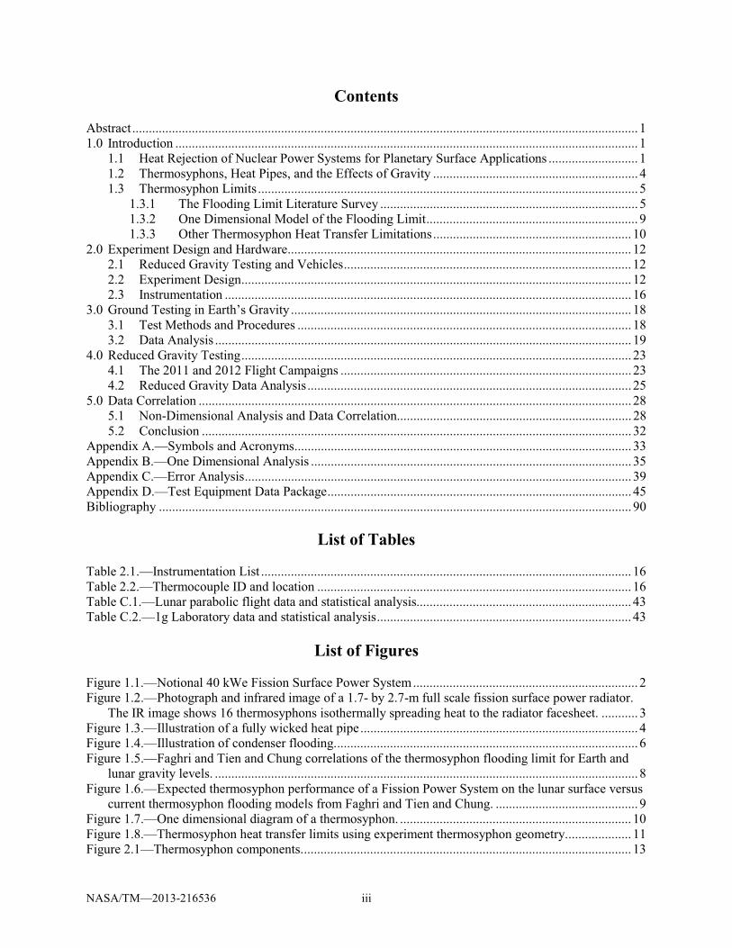
List of Figures Figure 1.1.—Notional 40 kWe Fission Surface Power System .................................................................... 2 Figure 1.2.—Photograph and infrared image of a 1.7- by 2.7-m full scale fission surface power radiator.
The IR image shows 16 thermosyphons isothermally spreading heat to the radiator facesheet. ........... 3 Figure 1.3.—Illustration of a fully wicked heat pipe .................................................................................... 4 Figure 1.4.—Illustration of condenser flooding. ........................................................................................... 6 Figure 1.5.—Faghri and Tien and Chung correlations of the thermosyphon flooding limit for Earth and
lunar gravity levels. ................................................................................................................................ 8 Figure 1.6.—Expected thermosyphon performance of a Fission Power System on the lunar surface versus
current thermosyphon flooding models from Faghri and Tien and Chung. ........................................... 9 Figure 1.7.—One dimensional diagram of a thermosyphon. ...................................................................... 10 Figure 1.8.—Thermosyphon heat transfer limits using experiment thermosyphon geometry. ................... 11 Figure 2.1—Thermosyphon components. ................................................................................................... 13
NASA/TM—2013-216536 iv
Figure 2.2.—Top: National Instruments PXI Data System and electrical controls; Bottom: Screen shot of flight software showing critical information and controls for all 12 thermosyphons. .......................... 14
Figure 2.3.—Thermosyphon flooding experiment payload. ....................................................................... 15 Figure 2.4.—Thermocouple location diagram. ........................................................................................... 17 Figure 3.1.—Graphical representation of two different methods used to approach the flooding limit. ..... 18 Figure 3.2.—Typical 1-g flooding event using the constant power method.. ............................................. 19 Figure 3.3.—Initial 1g test data showing scattered results caused by fluid charge differences. ................. 20 Figure 3.4.—Initial individual thermosyphon flooding limits showing dissimilar results during fluid
charge investigation. ............................................................................................................................. 21 Figure 3.5.—Effect of fluid charge on thermosyphon flooding limit. ........................................................ 21 Figure 3.6.—Flooding limit of correctly filled thermosyphons using 2.0 g of water. ................................ 22 Figure 4.1.—G-Force One aircraft and 2011 research teams. .................................................................... 23 Figure 4.2.—Pre-flight test readiness review at the reduced gravity office, Ellington Field. ..................... 24 Figure 4.3.—Thermosyphon flooding experiment. .................................................................................... 25 Figure 4.4.—Flooding event data of thermosyphon number 8 taken during Martian and lunar gravity
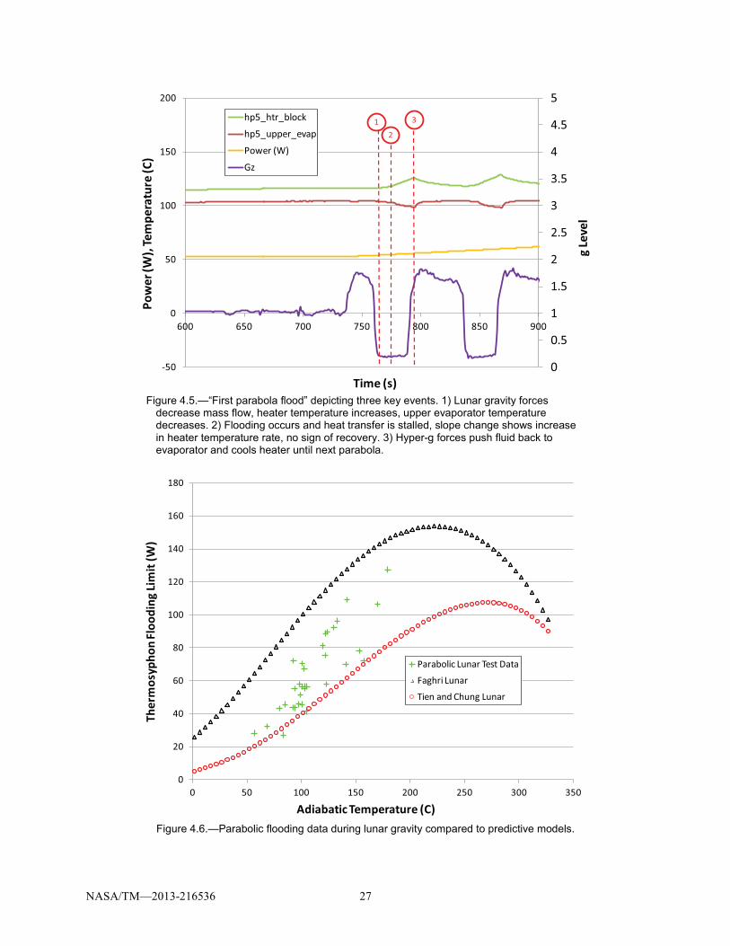
parabolas in September 2011................................................................................................................ 26 Figure 4.5.—“First parabola flood” depicting 3 key events. 1) Lunar gravity forces decrease mass flow,
heater temperature increases, upper evaporator temperature decreases. 2) Flooding occurs and heat transfer is stalled, slope change shows increase in heater temperature rate, no sign of recovery. 3) Hyper-g forces push fluid back to evaporator and cools heater until next parabola. ........................... 27
Figure 4.6.—Parabolic flooding data during lunar gravity compared to predictive models. ...................... 27 Figure 5.1.—Non-dimensional parameter q from the original Faghri model versus non-dimensional q test
data at 1g, top, and lunar gravity, bottom. ............................................................................................ 29 Figure 5.2.—New non-dimensional flooding correlation “q” showing gravity independence. .................. 30 Figure 5.3.—New thermosyphon flooding correlation versus parabolic lunar test data. ............................ 30 Figure 5.4.—New thermosyphon flooding correlation versus 1g test data. ................................................ 31 Figure 5.5.—New thermosyphon flooding model, expected performance of an FPS thermosyphon on the
lunar surface, and existing flooding models ......................................................................................... 32 Figure B.1.—One dimensional diagram of the thermosyphon ................................................................... 35 Figure B.2.—Top: One dimensional analysis of the thermosyphon axial power limits versus several ��
ratios. Bottom: Non-dimensional power parameter “q” from the one dimensional analysis as compared to different values of �� and the latest flooding model. ....................................................... 38
Figure C.1.—Standard deviation of the 1g and lunar test data compared to the new flooding model. ...... 40 Figure C.2.—Three axis accelerometer data during typical lunar gravity parabolas. ................................. 41 Figure C.3—The 95 percent confidence interval for the 1g and lunar model ............................................ 42
NASA/TM—2013-216536 1
Thermosyphon Flooding in Reduced Gravity Environments
Marc Andrew Gibson National Aeronautics and Space Administration
Glenn Research Center Cleveland, Ohio 44135
Abstract An innovative experiment to study the thermosyphon flooding limits was designed and flown on a
parabolic flight campaign to achieve the Reduced Gravity Environments (RGE) needed to obtain empirical data for analysis. Current correlation models of Faghri and Tien and Chung do not agree with the data. A new model is presented that predicts the flooding limits for thermosyphons in Earth’s gravity and lunar gravity with a 95 percent confidence level of ± 5 W.
1.0 Introduction 1.1 Heat Rejection of Nuclear Power Systems for Planetary Surface Applications
Fission Power Systems (FPS) have long been recognized as potential multi-kilowatt power solutions for lunar, Martian, and extended planetary surface missions. Current heat rejection technology associated with fission surface power systems has focused on titanium water thermosyphons embedded in carbon composite radiator panels. The thermosyphons, or wickless heat pipes, are used as a redundant and efficient way to spread the waste heat from the power conversion unit(s) over the radiator surface area where it can be rejected to space. It is well known that thermosyphon performance is reliant on gravitational forces to keep the evaporator wetted with the working fluid. One of the performance limits that can be encountered, if not understood, is the phenomenon of condenser flooding. This occurs when the gravity forces acting on the condensed fluid cannot overcome the shear forces created by the vapor escaping the evaporator throat. When this occurs, the heat transfer process is stalled and may not re-stabilize to effective levels without corrective control actions. The flooding limit in Earth’s gravity environment has been studied as experimentation is readily accessible, but when the environment and gravity change relative to other planetary bodies, experimentation becomes difficult.
Fission power can provide decades of uninterrupted power, day or night, making them especially attractive where solar intensity is limited or non-existent. Typically, 30 to 40 percent of the reactor heat gets converted to electricity and the remaining 60 to 70 percent gets rejected to space through large surface area heat rejection radiators. Figure 1.1 provides a graphical representation of a potential 40-kWe, 186-kWt, Moon-based Fission Surface Power (FSP) system (1) that has a total heat rejection surface area of 184 m2 with over 300 thermosyphons. Unique to surface power systems, when compared to in-space power systems, is the presence of gravity. Gravitational forces are a significant variable in fluid system design and directly impact the amount of power produced and rejected in a FSP system. A pumped water loop is used to transfer the waste heat from the cold side of the Stirling power conversion system to a total quantity of 20 (1.7- by 2.7-m) radiators. The radiators are equipped with heat exchangers to transfer the heat from the pumped water to the individual thermosyphon evaporators. The closed two phase thermosyphons are separate, cylindrical pressure vessels with the sole purpose of transferring the heat from the evaporator to the condenser where an attached fin can radiate the heat to the space environment. This heat transfer is accomplished using the saturated vapor, generated in the evaporator, to create the needed pressure difference to force the vapor up the tube where it can lose its latent heat to the cooler condenser wall. The heat transport capability of the saturated vapor can travel several meters from the evaporator to the condenser making the thermal conductance of thermosyphons several thousand times better than the most conductive materials. This high thermal conductance provides a near isothermal temperature throughout the condenser and allows the heat to be spread over several square meters of
NASA/TM—2013-216536 2
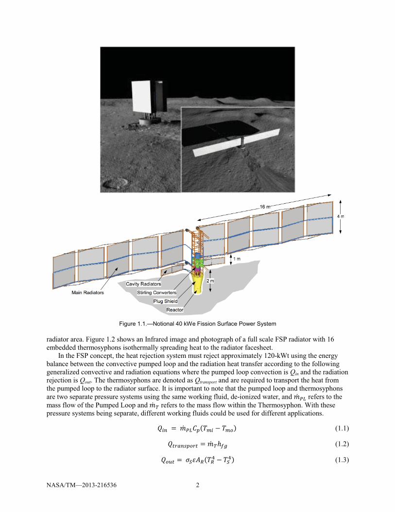
Figure 1.1.—Notional 40 kWe Fission Surface Power System
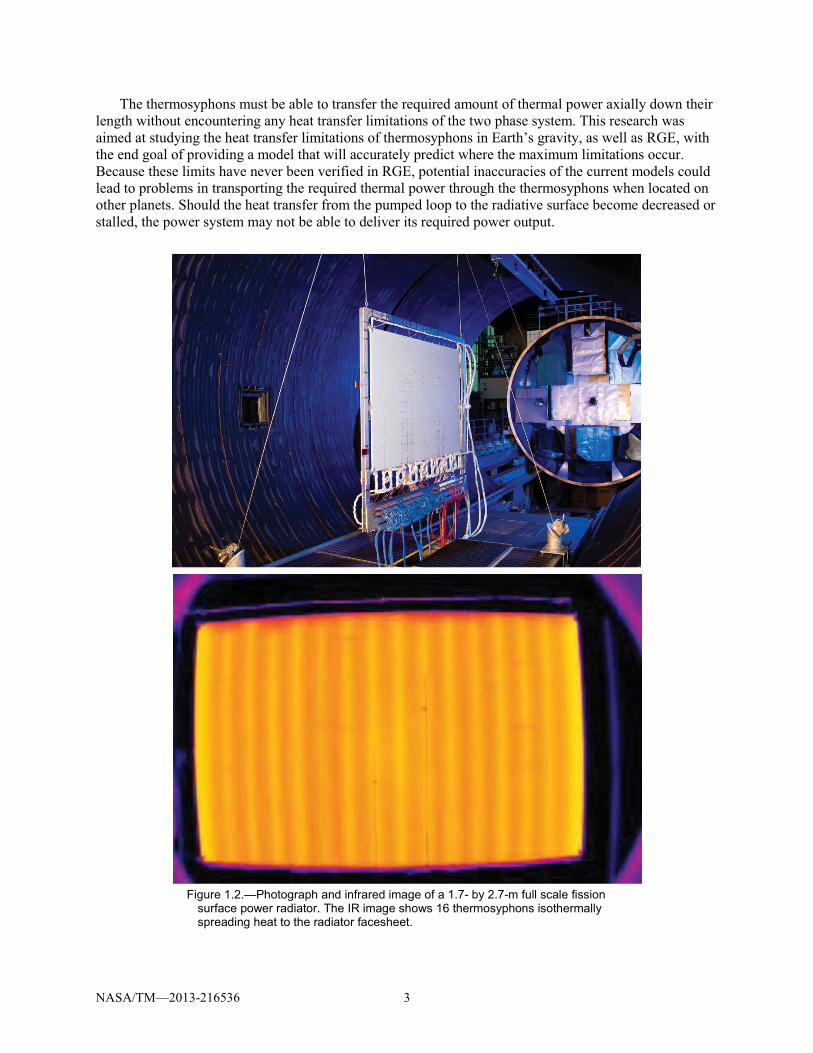
radiator area. Figure 1.2 shows an Infrared image and photograph of a full scale FSP radiator with 16 embedded thermosyphons isothermally spreading heat to the radiator facesheet.
In the FSP concept, the heat rejection system must reject approximately 120-kWt using the energy balance between the convective pumped loop and the radiation heat transfer according to the following generalized convective and radiation equations where the pumped loop convection is Qin and the radiation rejection is Qout. The thermosyphons are denoted as Qtransport and are required to transport the heat from the pumped loop to the radiator surface. It is important to note that the pumped loop and thermosyphons are two separate pressure systems using the same working fluid, de-ionized water, and �� �� refers to the mass flow of the Pumped Loop and �� � refers to the mass flow within the Thermosyphon. With these pressure systems being separate, different working fluids could be used for different applications.
� = �� ��� (�� � ���) (1.1)
����� ��� = �� ���� (1.2)
��� = �����(��� � ��
�) (1.3)
NASA/TM—2013-216536 3
The thermosyphons must be able to transfer the required amount of thermal power axially down their length without encountering any heat transfer limitations of the two phase system. This research was aimed at studying the heat transfer limitations of thermosyphons in Earth’s gravity, as well as RGE, with the end goal of providing a model that will accurately predict where the maximum limitations occur. Because these limits have never been verified in RGE, potential inaccuracies of the current models could lead to problems in transporting the required thermal power through the thermosyphons when located on other planets. Should the heat transfer from the pumped loop to the radiative surface become decreased or stalled, the power system may not be able to deliver its required power output.
Figure 1.2.—Photograph and infrared image of a 1.7- by 2.7-m full scale fission
surface power radiator. The IR image shows 16 thermosyphons isothermally spreading heat to the radiator facesheet.
NASA/TM—2013-216536 4
1.2 Thermosyphons, Heat Pipes, and the Effects of Gravity
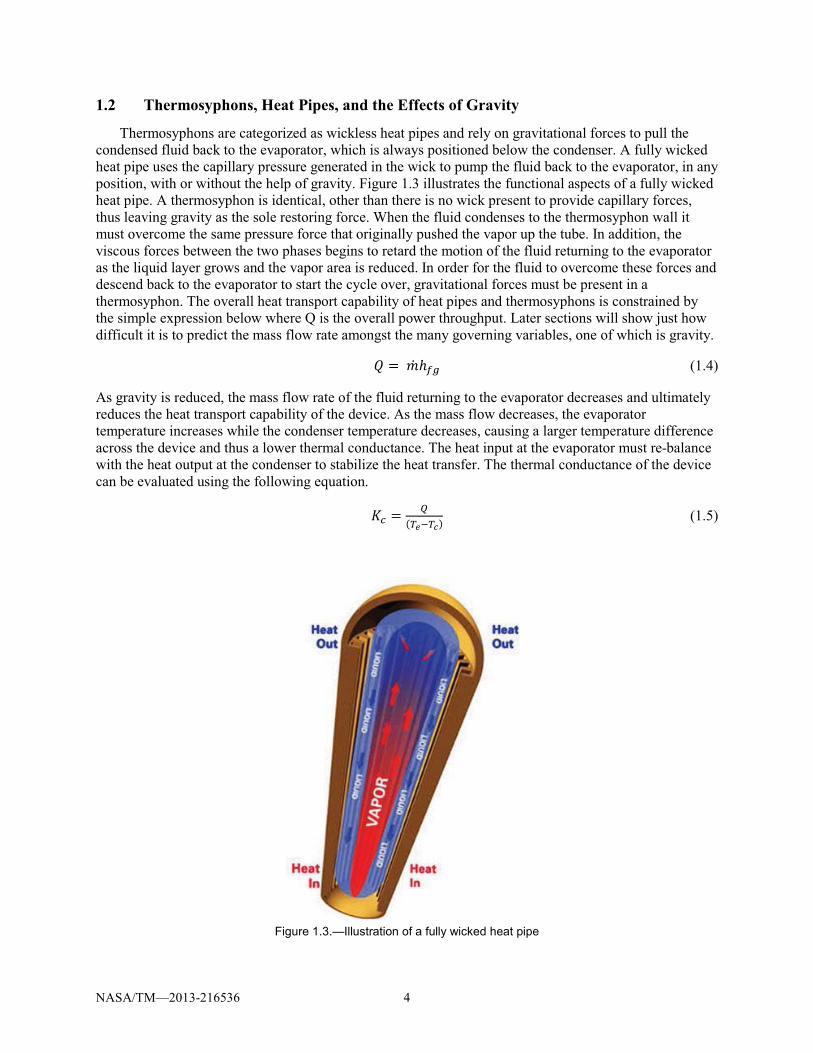
Thermosyphons are categorized as wickless heat pipes and rely on gravitational forces to pull the condensed fluid back to the evaporator, which is always positioned below the condenser. A fully wicked heat pipe uses the capillary pressure generated in the wick to pump the fluid back to the evaporator, in any position, with or without the help of gravity. Figure 1.3 illustrates the functional aspects of a fully wicked heat pipe. A thermosyphon is identical, other than there is no wick present to provide capillary forces, thus leaving gravity as the sole restoring force. When the fluid condenses to the thermosyphon wall it must overcome the same pressure force that originally pushed the vapor up the tube. In addition, the viscous forces between the two phases begins to retard the motion of the fluid returning to the evaporator as the liquid layer grows and the vapor area is reduced. In order for the fluid to overcome these forces and descend back to the evaporator to start the cycle over, gravitational forces must be present in a thermosyphon. The overall heat transport capability of heat pipes and thermosyphons is constrained by the simple expression below where Q is the overall power throughput. Later sections will show just how difficult it is to predict the mass flow rate amongst the many governing variables, one of which is gravity.
= �� ��� (1.4)
As gravity is reduced, the mass flow rate of the fluid returning to the evaporator decreases and ultimately reduces the heat transport capability of the device. As the mass flow decreases, the evaporator temperature increases while the condenser temperature decreases, causing a larger temperature difference across the device and thus a lower thermal conductance. The heat input at the evaporator must re-balance with the heat output at the condenser to stabilize the heat transfer. The thermal conductance of the device can be evaluated using the following equation.
!" = #(�$%�&) (1.5)
Figure 1.3.—Illustration of a fully wicked heat pipe
NASA/TM—2013-216536 5
The thermosyphon working fluid is specifically chosen, based on its thermophysical properties, to operate in the desired temperature range, typically determined through trade studies of the total system specific power (W/kg) of the system. When gravity forces are present, such as on the surface of the Moon or Mars, thermosyphons can trade better than heat pipes because they do not have a wick structure in the condenser and may ultimately have a lower mass. This trade must be taken into careful consideration as the additional mass of the heat pipe wick can be balanced by the increased power the wick gives the heat pipe in reduced gravity.
1.3 Thermosyphon Limits
There are a few main heat transfer limits that will influence the amount of thermal power that can be transferred by thermosyphon. The boiling limit, viscous limit, sonic limit, and flooding limit are the most important recognized limitations that have been extensively studied and have been included for a full evaluation. It is important to evaluate each heat transfer limit to fully understand the results and determine what limit the thermosyphons reach during the experiment. The flooding limit will be extensively discussed in Sections 1.3.1 and 1.3.2 as it is the main focus of this research. A generalized discussion and analysis of the other limitations will also be included in Section 1.3.3 to give the reader adequate background information that may influence other thermosyphon designs and applications.
1.3.1 The Flooding Limit Literature Survey The flooding limit is heavily influenced by gravity forces and can stall the heat transfer process of a
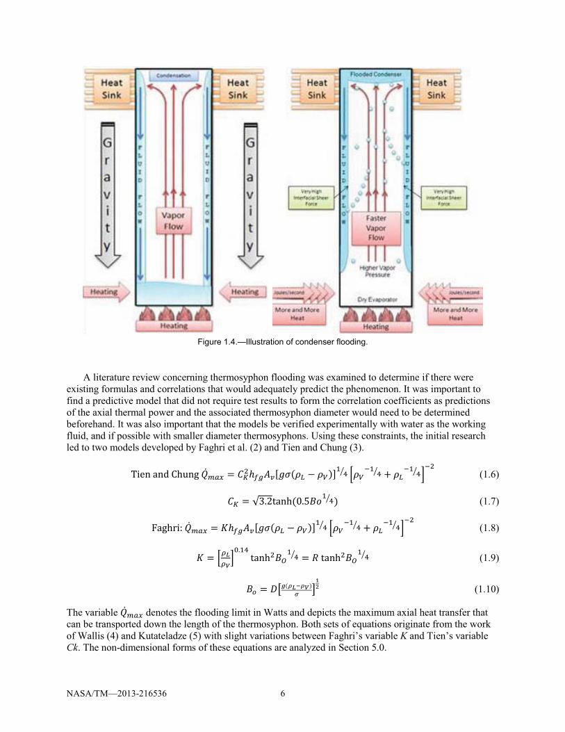
thermosyphon during operation. Flooding can typically occur throughout the majority of the thermosyphon temperature range making it the most often encountered heat transfer limit. The flooding limit occurs when the shear forces from the counter current flow between the vapor and liquid overpowers the gravity forces required to keep the evaporator wetted with the working fluid. This will occur near the top of the evaporator were the liquid layer is at its thickest point and the vapor is traveling through the local minimized cross sectional area at its peak velocity (Figure 1.4). This creates a liquid orifice that will eventually be broken by the vapor shear force interacting with the liquid boundary. When this occurs, the fluid can form wave instabilities which can then become torn away from the liquid layer and be transported up to the condenser. This phenomenon has been called flooding because it floods the condenser with the working fluid. When wicks are present, a similar event occurs, identified as entrainment, that differs only in the fact that the capillary effect of the wick can influence the wave instability and make it harder for the vapor to rip the liquid from the wick structure. In some cases reports have indicated that this entrained fluid can be heard as the fluid particles hit the end cap. With small diameter thermosyphons, it may also be possible that the instabilities of the liquid layer near the flooding limit may cause the fluid to close off the vapor space. This would cause all the fluid in the adiabatic and condenser sections to flood the condenser and be held there until the pressure in the evaporator subsides, allowing the fluid to return to the condenser. In either case, flooding will cause a stall in the mass flow rate allowing the evaporator to overheat and dryout. When this happens the evaporator temperatures can rapidly increase and cause high pressure conditions inside the thermosyphon which may eventually lead to a rupture in the container wall. During experimentation, careful detection methods must be used to keep the evaporator temperature limits within manageable levels.
NASA/TM—2013-216536 6
Figure 1.4.—Illustration of condenser flooding.
A literature review concerning thermosyphon flooding was examined to determine if there were existing formulas and correlations that would adequately predict the phenomenon. It was important to find a predictive model that did not require test results to form the correlation coefficients as predictions of the axial thermal power and the associated thermosyphon diameter would need to be determined beforehand. It was also important that the models be verified experimentally with water as the working fluid, and if possible with smaller diameter thermosyphons. Using these constraints, the initial research led to two models developed by Faghri et al. (2) and Tien and Chung (3).
Tien and Chung ���' = �*+����,[-�(.� � ./)]0
�1 2./%0
�1 + .�%0
�1 4%+
(1.6)
�* = 53.2tanh (0.5;<0�1 ) (1.7)
Faghri: ���' = !����,[-�(.� � ./)]0�1 2./
%0�1 + .�
%0�1 4
%+ (1.8)
! = 2?@?A
4B.0�
tanh+;D0
�1 = E tanh+;D0
�1 (1.9)
;� = GHI(J@KJA)L M
NO (1.10)
The variable ���' denotes the flooding limit in Watts and depicts the maximum axial heat transfer that can be transported down the length of the thermosyphon. Both sets of equations originate from the work of Wallis (4) and Kutateladze (5) with slight variations between Faghri’s variable K and Tien’s variable Ck. The non-dimensional forms of these equations are analyzed in Section 5.0.
NASA/TM—2013-216536 7
The Wallis correlation used a balance between inertia and hydrostatic forces of open two-phase systems to determine the available axial thermal power in countercurrent flow. The empirically dimensionless constants m and Cw are functions of the fluid properties with reported values typically between 0.7 and 1.0. The values PQ and P, are the liquid and vapor volumetric flow rates divided by the vapor area of the thermosyphon.
(1.11)
(1.12)
(1.13)
Wallis determined that flooding would occur when PQ = 1 and P, = 0. In the case of a closed thermosyphon system, �� Q = �� , = R
���1 where q is the heat flux in S/�+and Av is the cross sectional area of the
vapor passage. The Wallis correlation for flooding is:
Wallis = VXYZO \^I_�`(?b%?X)?X
c0fj?X ?b1 kN m1
oO (1.14)
The Kutateladze number ! is a balance between the dynamic head, surface tension, and gravitational force. The Kutateladze correlation assumes:
(!,)0+1 + (!Q)0
+1 = �* (1.15)
(1.16)
Tien and Chung combined the Wallis and Kutateladze correlations assuming that PQ = 0 and Ck = 53.2 based on letting D equal the critical wavelength of the Taylor Instability. The hyperbolic tangent in Tien and Chung’s equation comes from the experimental results of Wallis and Makkenchery (6) in which the Kutateladze number decreases to the dimensionless diameter, or Bond number, giving Cw as seen in Equation (1.11). The Tien and Chung correlation was shown to be accurate within 15 percent based on water as the working fluid but was not as accurate for other fluids.
Faghri took note of the fact that the flooding limit with other fluids needed a new dimensionless group as a ratio of the density of the fluid over the density of the vapor. Faghri recombined the correlations to predict the flooding phenomenon per Equation (1.8).
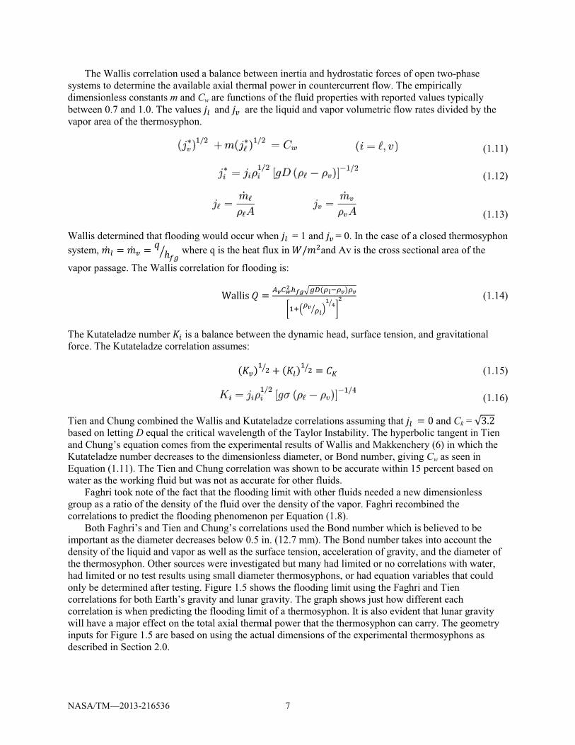
Both Faghri’s and Tien and Chung’s correlations used the Bond number which is believed to be important as the diameter decreases below 0.5 in. (12.7 mm). The Bond number takes into account the density of the liquid and vapor as well as the surface tension, acceleration of gravity, and the diameter of the thermosyphon. Other sources were investigated but many had limited or no correlations with water, had limited or no test results using small diameter thermosyphons, or had equation variables that could only be determined after testing. Figure 1.5 shows the flooding limit using the Faghri and Tien correlations for both Earth’s gravity and lunar gravity. The graph shows just how different each correlation is when predicting the flooding limit of a thermosyphon. It is also evident that lunar gravity will have a major effect on the total axial thermal power that the thermosyphon can carry. The geometry inputs for Figure 1.5 are based on using the actual dimensions of the experimental thermosyphons as described in Section 2.0.
NASA/TM—2013-216536 8
Figure 1.5.—Faghri and Tien and Chung correlations of the thermosyphon flooding
limit for Earth and lunar gravity levels.
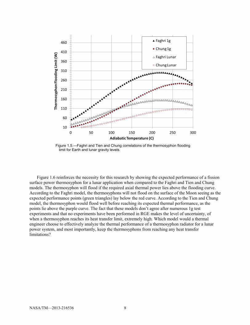
Figure 1.6 reinforces the necessity for this research by showing the expected performance of a fission surface power thermosyphon for a lunar application when compared to the Faghri and Tien and Chung models. The thermosyphon will flood if the required axial thermal power lies above the flooding curve. According to the Faghri model, the thermosyphons will not flood on the surface of the Moon seeing as the expected performance points (green triangles) lay below the red curve. According to the Tien and Chung model, the thermosyphon would flood well before reaching its expected thermal performance, as the points lie above the purple curve. The fact that these models don’t agree after numerous 1g test experiments and that no experiments have been performed in RGE makes the level of uncertainty, of when a thermosyphon reaches its heat transfer limit, extremely high. Which model would a thermal engineer choose to effectively analyze the thermal performance of a thermosyphon radiator for a lunar power system, and most importantly, keep the thermosyphons from reaching any heat transfer limitations?
10
60
110
160
210
260
310
360
410
460
0 50 100 150 200 250 300
Ther
mos
ypho
n Fl
oodi
ng Li
mit
(W)
Adiabatic Temperature (C)
Faghri 1g
Chung 1g
Faghri Lunar
Chung Lunar
NASA/TM—2013-216536 9
Figure 1.6.—Expected thermosyphon performance of a Fission Power System on the lunar surface
versus current thermosyphon flooding models from Faghri and Tien and Chung.
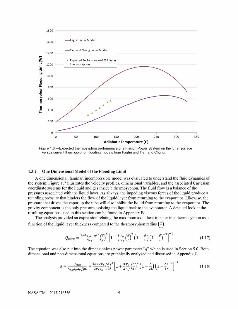
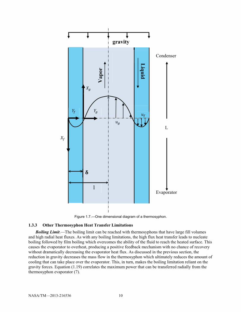
1.3.2 One Dimensional Model of the Flooding Limit A one dimensional, laminar, incompressible model was evaluated to understand the fluid dynamics of
the system. Figure 1.7 illustrates the velocity profiles, dimensional variables, and the associated Cartesian coordinate systems for the liquid and gas inside a thermosyphon. The fluid flow is a balance of the pressures associated with the liquid layer. As always, the impeding viscous forces of the liquid produce a retarding pressure that hinders the flow of the liquid layer from returning to the evaporator. Likewise, the pressure that drives the vapor up the tube will also inhibit the liquid from returning to the evaporator. The gravity component is the only pressure assisting the liquid back to the evaporator. A detailed look at the resulting equations used in this section can be found in Appendix B.
The analysis provided an expression relating the maximum axial heat transfer in a thermosyphon as a function of the liquid layer thickness compared to the thermosyphon radius jp
Qk.
��' = +q\^I?^�Qv
wx^jp
Qk
wy1 + w
+xI
x^jp
Qk
+j1 � p
wQk j1 � p
Qk
%w{
%0 (1.17)
The equation was also put into the dimensionless power parameter “q” which is used in Section 5.0. Both dimensional and non-dimensional equations are graphically analyzed and discussed in Appendix C.
R = #|}~\^I?IVX_�`
= Q_�`?^
wx^?Ijp
Qk
wy1 + w
+xI
x^jp
Qk
+j1 � p
wQk j1 � p
Qk
%w{
%0 (1.18)
0
200
400
600
800
1000
1200
1400
1600
1800
0 50 100 150 200 250 300 350
Ther
mos
ypho
n Fl
oodi
ng Li
mit
(W)
Adiabatic Temperature (C)
Faghri Lunar Model
Tien and Chung Lunar Model
Expected Performance of FSP Lunar Thermosyphon
NASA/TM—2013-216536 10
Figure 1.7.—One dimensional diagram of a thermosyphon.
1.3.3 Other Thermosyphon Heat Transfer Limitations Boiling Limit.—The boiling limit can be reached with thermosyphons that have large fill volumes
and high radial heat fluxes. As with any boiling limitations, the high flux heat transfer leads to nucleate boiling followed by film boiling which overcomes the ability of the fluid to reach the heated surface. This causes the evaporator to overheat, producing a positive feedback mechanism with no chance of recovery without dramatically decreasing the evaporator heat flux. As discussed in the previous section, the reduction in gravity decreases the mass flow in the thermosyphon which ultimately reduces the amount of cooling that can take place over the evaporator. This, in turn, makes the boiling limitation reliant on the gravity forces. Equation (1.19) correlates the maximum power that can be transferred radially from the thermosyphon evaporator (7).
Vap
or
Liquid
��
�� ��
��
��
��
�
l
gravity
Evaporator
Condenser
L
NASA/TM—2013-216536 11
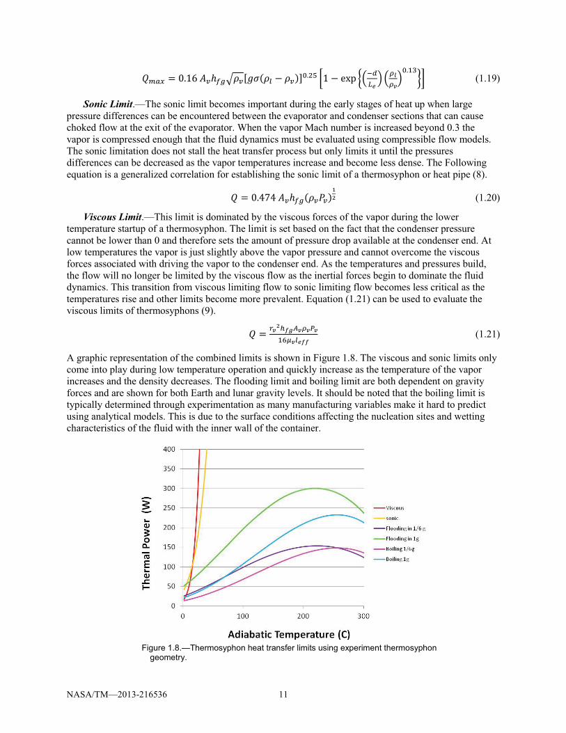
��' = 0.16 �,���_.,[-�(.Q � .,)]B.+� y1 � exp �j%��$
k j?b?X
kB.0w
�{ (1.19)
Sonic Limit.—The sonic limit becomes important during the early stages of heat up when large pressure differences can be encountered between the evaporator and condenser sections that can cause choked flow at the exit of the evaporator. When the vapor Mach number is increased beyond 0.3 the vapor is compressed enough that the fluid dynamics must be evaluated using compressible flow models. The sonic limitation does not stall the heat transfer process but only limits it until the pressures differences can be decreased as the vapor temperatures increase and become less dense. The Following equation is a generalized correlation for establishing the sonic limit of a thermosyphon or heat pipe (8).
= 0.474 �,���(.,�,)NO (1.20)
Viscous Limit.—This limit is dominated by the viscous forces of the vapor during the lower temperature startup of a thermosyphon. The limit is set based on the fact that the condenser pressure cannot be lower than 0 and therefore sets the amount of pressure drop available at the condenser end. At low temperatures the vapor is just slightly above the vapor pressure and cannot overcome the viscous forces associated with driving the vapor to the condenser end. As the temperatures and pressures build, the flow will no longer be limited by the viscous flow as the inertial forces begin to dominate the fluid dynamics. This transition from viscous limiting flow to sonic limiting flow becomes less critical as the temperatures rise and other limits become more prevalent. Equation (1.21) can be used to evaluate the viscous limits of thermosyphons (9).
= �XO\^IVX?X�X
0��XQ$^^ (1.21)
A graphic representation of the combined limits is shown in Figure 1.8. The viscous and sonic limits only come into play during low temperature operation and quickly increase as the temperature of the vapor increases and the density decreases. The flooding limit and boiling limit are both dependent on gravity forces and are shown for both Earth and lunar gravity levels. It should be noted that the boiling limit is typically determined through experimentation as many manufacturing variables make it hard to predict using analytical models. This is due to the surface conditions affecting the nucleation sites and wetting characteristics of the fluid with the inner wall of the container.
Figure 1.8.—Thermosyphon heat transfer limits using experiment thermosyphon
geometry.
NASA/TM—2013-216536 12
2.0 Experiment Design and Hardware 2.1 Reduced Gravity Testing and Vehicles
NASA has established numerous methods to study Reduced Gravity Environments (RGE) in an effort to provide research opportunities for developing gravity influenced technologies at an affordable cost. The current Flight Opportunities Program, or FOP, is run through NASA’s Office of the Chief Technologist (OCT) under the Game Changing Development (GCD) program. The FOP sends out solicitations for proposals and awards flights to the technologies that align with the current OCT technology roadmap. The FOP has established a number of Suborbital Re-useable Launch Vehicles (SrLV) which are chosen depending on the research payload and RGE requirements. This fleet of vehicles currently includes conventional aircraft, sounding rockets, and other suborbital launch vehicles to provide parabolic and suborbital flight platforms that can provide a wide range of RGE for various levels of research.
Initially, research flight requirements start with the desired time at the specific gravity level needed to perform the research. The FOP has a diverse set of flight vehicles to allow several options when considering the total research objectives. After careful examination, the FOP determines which vehicle best suits the payload objectives and can award the flight. Using this approach, FOP provided a parabolic flight campaign to conduct this research with the Zero G Corporation using a Boeing 727 named G-Force One, based on the need for lunar and Martian gravity and the size of the experiment.
2.2 Experiment Design
In order to fly the experiment on G-Force One, a number of requirements had to be met to ensure safe operations while in flight. The experiment would be strictly investigated during internal and external Test Readiness Reviews (TRR) for safe operations of both mechanical and electrical systems before being allowed to fly. The Test Equipment Data Package listed in Appendix D gives specific details of the experiment under the FOP guidelines and operational procedures. These safety requirements typically drive the engineering constraints for the experiment and would ultimately limit the size and power of the experiment. Within these constraints, the experiment would need to successfully determine the heat transfer limits of the thermosyphons and would require innovative techniques to design the experiment and acquire the needed data.
The NASA Glenn Research Center has a long history of parabolic flights and microgravity research which helped acquire a flight chassis to house the experiment. The chassis had already been structurally proven through other parabolic flights and would become the geometric constraints of the system with dimensions 24- by 24- by 42-in.
Next, the electrical system and thermosyphon design would have to be specified to meet the aircraft’s strict electrical requirements. It was imperative that the experiment be designed to meet the requirements of the 1g laboratory testing as well as the parabolic flight testing, to minimize any error associated with the hardware. For the flight, a baseline of 2 kW at 115 V was used as the maximum electrical constraint for the experiment based on the aircraft’s available power. For laboratory 1g testing, the experiment would have to provide almost three times that power to simultaneously achieve the heat transfer limits of all twelve thermosyphons.
The next consideration was to determine the number and size of thermosyphons to meet the electrical constraints while still being able to reach the desired flooding limit. Knowing that the flooding limit was going to be extremely difficult to obtain in parabolic flight, it was determined that 12 thermosyphons, if possible, would be a good balance between getting multiple chances at capturing the flooding event while keeping in mind the electrical constraints. Using 12 thermosyphons, each heater would have a total of 165 W of supply power while in reduced gravity.
Faghri’s Equation (1.8) was used for early predictions as it represented the more conservative approach to staying within the aircraft electrical budget. The diameter of the thermosyphon would be
NASA/TM—2013-216536 13
estimated by graphically evaluating the flooding limit of 165 W and a lunar gravity value of 1.622 m/s2. Both lunar and Martian gravity environments were analyzed but the lesser lunar gravity was chosen as the desired target because it would allow a wider range of data for the intended correlation, as well as require less heater power. The decision to test mostly in lunar gravity, as opposed to half lunar and half Martian, was due to the fact that during the parabolic flights only a limited number of parabolas are dedicated to reduced gravity and the experiment needed as much time as possible to pass through a flooding event. After careful examination, the final decision was to design the experiment with a total of 12 thermosyphons made from 0.25 by 0.035 in. (6.35 by 0.889 mm) wall titanium tube using water as the working fluid. The total thermosyphon length of 24 in. (60 cm) was built with a 2.5 in. (6.35 cm) evaporator, a 2.5 in. (6.35 cm) adiabatic section, and a 19 in. (45.7 cm) condenser, providing a length to diameter (L/D) ratio of 130, similar to the thermosyphons designed for the fission surface power system in Figure 1.1. Two wraps of 100-mesh titanium screen were used in the evaporator section to increase fluid flow during nucleation and prevent dryout. The condenser was designed to be air cooled, using a finned aluminum tube that would enhance heat transfer and allow the internal fluid temperature to be altered via a variable speed fan. Combination of these components would allow testing over a wide range of expected heat transfer limitations that would provide new data for the research community.
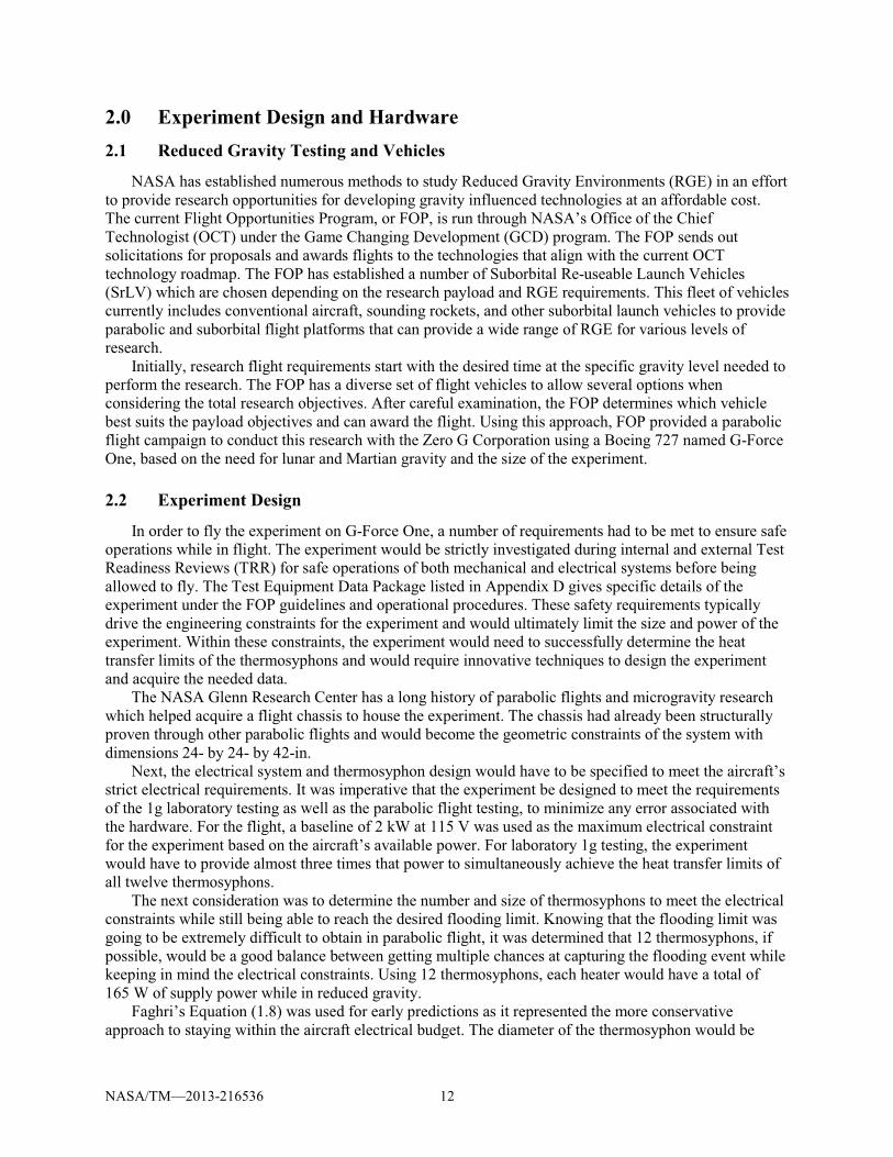
Extreme caution was used at the higher temperatures due to the pressure increase of the saturated vapor within each thermosyphon. Each thermosyphon would require proof pressure testing as well as extended temperature testing to adequately prove they would not rupture during any portion of the experiment. Photos of the thermosyphon components are shown in Figure 2.1.
When reaching any of the heat transfer limits, it is known that the heater temperatures will rapidly increase based on the associated power level. This drove the most important control system decision which required that the heater power interlock have double redundancy to protect the heater from running away during the experiment. The control system relied on several thermocouples to provide the necessary information to appropriately shut down the heaters should the operator miss the runaway event.
Figure 2.1—Thermosyphon components.
NASA/TM—2013-216536 14
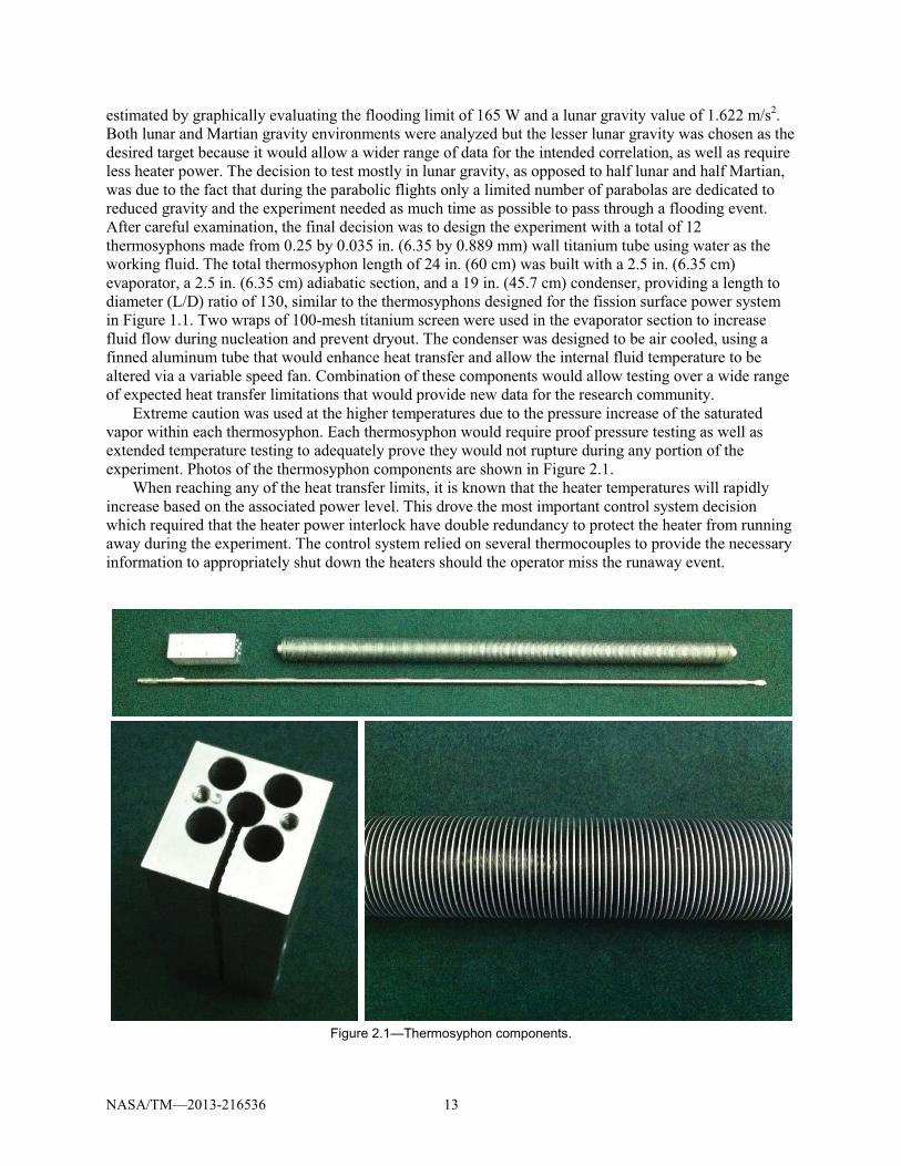
Figure 2.2.—Top: National Instruments PXI Data System and electrical controls; Bottom: Screen shot of flight
software showing critical information and controls for all 12 thermosyphons.
The data acquisition and control (DAC) system was accomplished using a National Instruments PXI chassis and real-time controller with customized Labview programming to provide the system logic and user interface functions. The end product used a laptop computer that was linked to the PXI controller inside the flight rack and let the operator view and collect data signals, control the heater power, view alarms, and record notes. Several revisions of the DAC system were implemented to establish a streamline process that allowed quick communication and control needed during parabolic maneuvers. Pictures of the experiment hardware can be seen in Figure 2.2 and Figure 2.3. More detail relating to each individual component can be seen in the TEDP in Appendix D.
NASA/TM—2013-216536 15
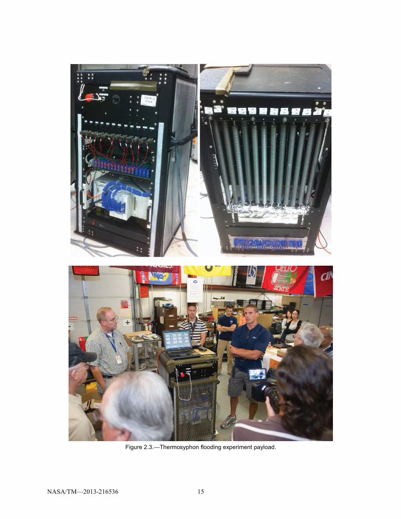
Figure 2.3.—Thermosyphon flooding experiment payload.
NASA/TM—2013-216536 16
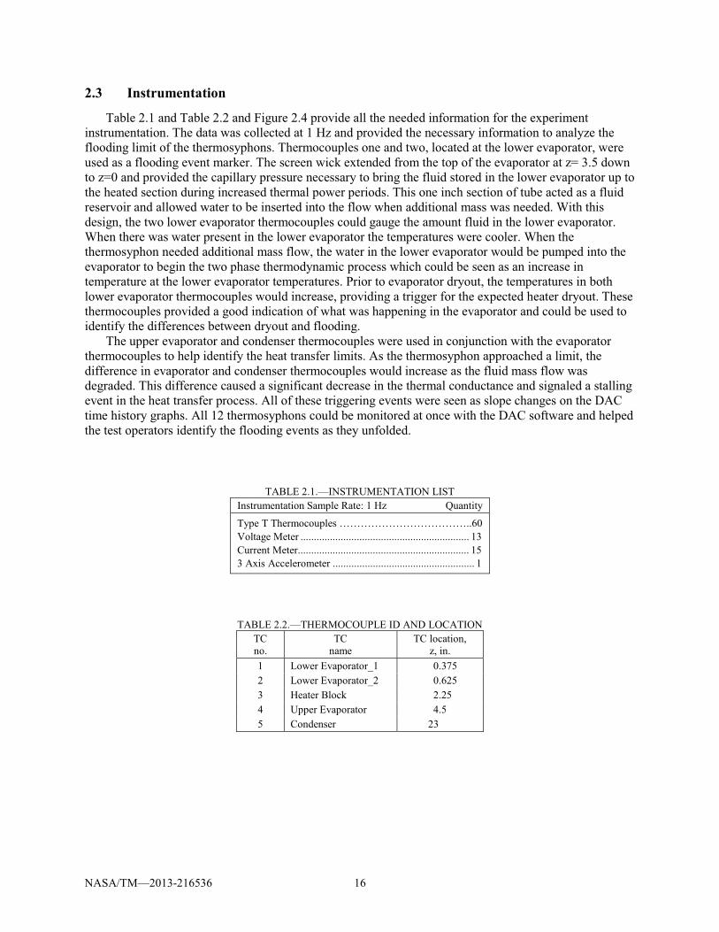
2.3 Instrumentation
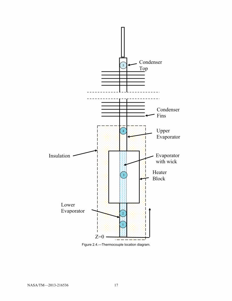
Table 2.1 and Table 2.2 and Figure 2.4 provide all the needed information for the experiment instrumentation. The data was collected at 1 Hz and provided the necessary information to analyze the flooding limit of the thermosyphons. Thermocouples one and two, located at the lower evaporator, were used as a flooding event marker. The screen wick extended from the top of the evaporator at z= 3.5 down to z=0 and provided the capillary pressure necessary to bring the fluid stored in the lower evaporator up to the heated section during increased thermal power periods. This one inch section of tube acted as a fluid reservoir and allowed water to be inserted into the flow when additional mass was needed. With this design, the two lower evaporator thermocouples could gauge the amount fluid in the lower evaporator. When there was water present in the lower evaporator the temperatures were cooler. When the thermosyphon needed additional mass flow, the water in the lower evaporator would be pumped into the evaporator to begin the two phase thermodynamic process which could be seen as an increase in temperature at the lower evaporator temperatures. Prior to evaporator dryout, the temperatures in both lower evaporator thermocouples would increase, providing a trigger for the expected heater dryout. These thermocouples provided a good indication of what was happening in the evaporator and could be used to identify the differences between dryout and flooding.
The upper evaporator and condenser thermocouples were used in conjunction with the evaporator thermocouples to help identify the heat transfer limits. As the thermosyphon approached a limit, the difference in evaporator and condenser thermocouples would increase as the fluid mass flow was degraded. This difference caused a significant decrease in the thermal conductance and signaled a stalling event in the heat transfer process. All of these triggering events were seen as slope changes on the DAC time history graphs. All 12 thermosyphons could be monitored at once with the DAC software and helped the test operators identify the flooding events as they unfolded.
TABLE 2.1.—INSTRUMENTATION LIST Instrumentation Sample Rate: 1 Hz Quantity
Type T Thermocouples ………………………………..60 Voltage Meter ............................................................... 13 Current Meter ................................................................ 15 3 Axis Accelerometer ..................................................... 1
TABLE 2.2.—THERMOCOUPLE ID AND LOCATION TC no.
TC name
TC location, z, in.
1 Lower Evaporator_1 0.375 2 Lower Evaporator_2 0.625 3 Heater Block 2.25 4 Upper Evaporator 4.5 5 Condenser 23
NASA/TM—2013-216536 17
Figure 2.4.—Thermocouple location diagram.
Insulation
Z=0
Heater Block
Upper Evaporator
Condenser Fins
Condenser Top
Evaporator with wick
Lower Evaporator
5
4
2
1
3
NASA/TM—2013-216536 18
3.0 Ground Testing in Earth’s Gravity 3.1 Test Methods and Procedures
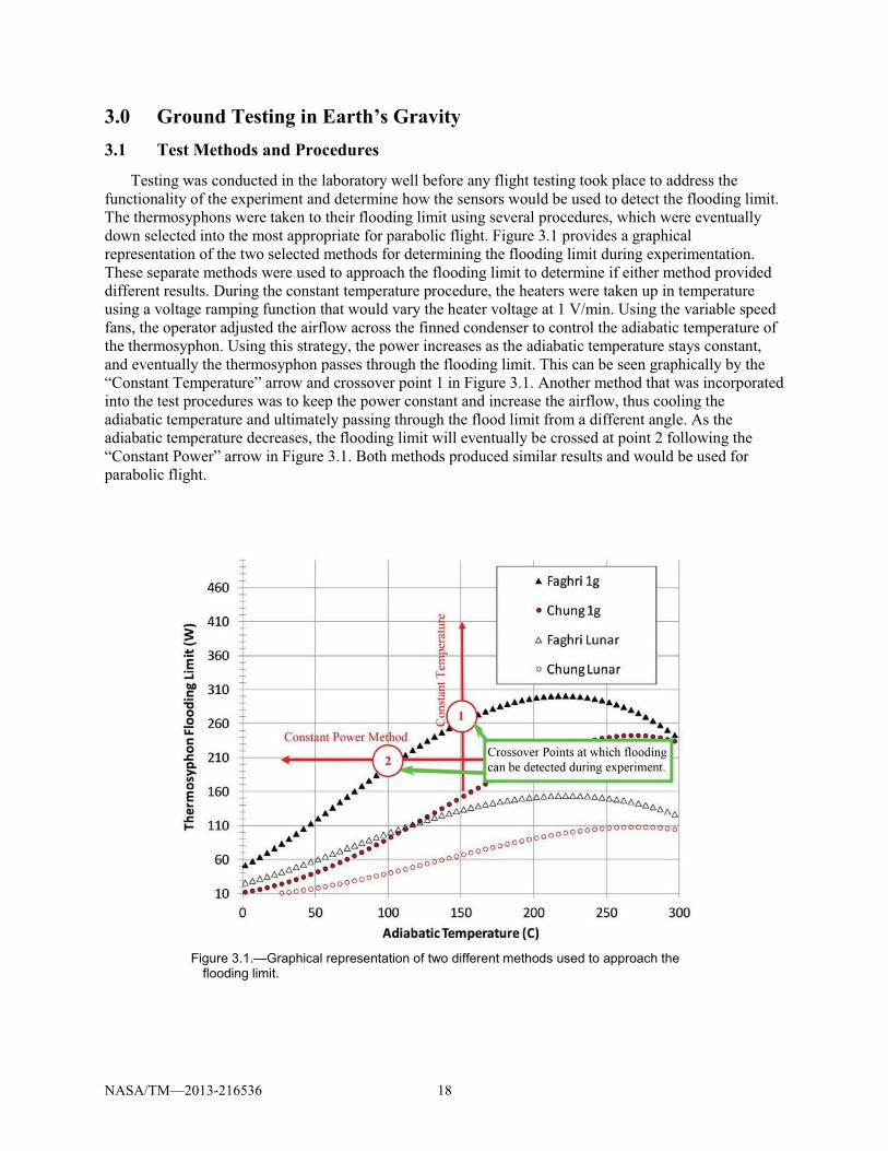
Testing was conducted in the laboratory well before any flight testing took place to address the functionality of the experiment and determine how the sensors would be used to detect the flooding limit. The thermosyphons were taken to their flooding limit using several procedures, which were eventually down selected into the most appropriate for parabolic flight. Figure 3.1 provides a graphical representation of the two selected methods for determining the flooding limit during experimentation. These separate methods were used to approach the flooding limit to determine if either method provided different results. During the constant temperature procedure, the heaters were taken up in temperature using a voltage ramping function that would vary the heater voltage at 1 V/min. Using the variable speed fans, the operator adjusted the airflow across the finned condenser to control the adiabatic temperature of the thermosyphon. Using this strategy, the power increases as the adiabatic temperature stays constant, and eventually the thermosyphon passes through the flooding limit. This can be seen graphically by the “Constant Temperature” arrow and crossover point 1 in Figure 3.1. Another method that was incorporated into the test procedures was to keep the power constant and increase the airflow, thus cooling the adiabatic temperature and ultimately passing through the flood limit from a different angle. As the adiabatic temperature decreases, the flooding limit will eventually be crossed at point 2 following the “Constant Power” arrow in Figure 3.1. Both methods produced similar results and would be used for parabolic flight.
Figure 3.1.—Graphical representation of two different methods used to approach the
flooding limit.
NASA/TM—2013-216536 19
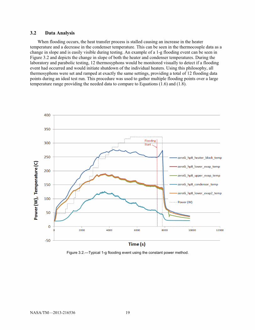
3.2 Data Analysis
When flooding occurs, the heat transfer process is stalled causing an increase in the heater temperature and a decrease in the condenser temperature. This can be seen in the thermocouple data as a change in slope and is easily visible during testing. An example of a 1-g flooding event can be seen in Figure 3.2 and depicts the change in slope of both the heater and condenser temperatures. During the laboratory and parabolic testing, 12 thermosyphons would be monitored visually to detect if a flooding event had occurred and would initiate shutdown of the individual heaters. Using this philosophy, all thermosyphons were set and ramped at exactly the same settings, providing a total of 12 flooding data points during an ideal test run. This procedure was used to gather multiple flooding points over a large temperature range providing the needed data to compare to Equations (1.6) and (1.8).
Figure 3.2.—Typical 1-g flooding event using the constant power method.
NASA/TM—2013-216536 20
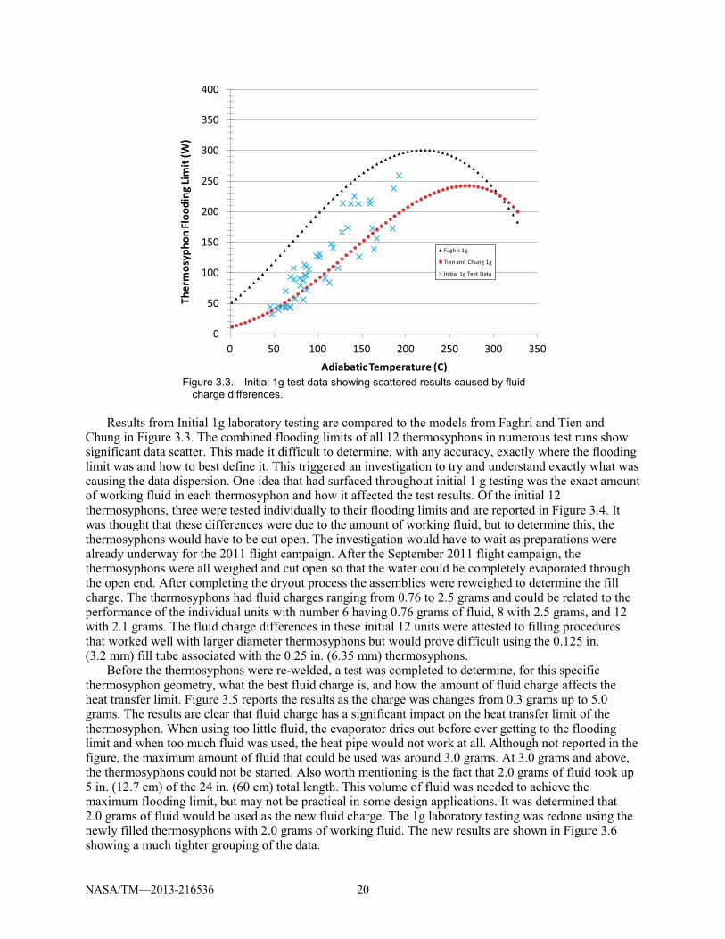
Figure 3.3.—Initial 1g test data showing scattered results caused by fluid
charge differences. Results from Initial 1g laboratory testing are compared to the models from Faghri and Tien and
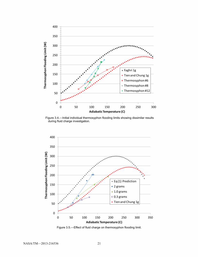
Chung in Figure 3.3. The combined flooding limits of all 12 thermosyphons in numerous test runs show significant data scatter. This made it difficult to determine, with any accuracy, exactly where the flooding limit was and how to best define it. This triggered an investigation to try and understand exactly what was causing the data dispersion. One idea that had surfaced throughout initial 1 g testing was the exact amount of working fluid in each thermosyphon and how it affected the test results. Of the initial 12 thermosyphons, three were tested individually to their flooding limits and are reported in Figure 3.4. It was thought that these differences were due to the amount of working fluid, but to determine this, the thermosyphons would have to be cut open. The investigation would have to wait as preparations were already underway for the 2011 flight campaign. After the September 2011 flight campaign, the thermosyphons were all weighed and cut open so that the water could be completely evaporated through the open end. After completing the dryout process the assemblies were reweighed to determine the fill charge. The thermosyphons had fluid charges ranging from 0.76 to 2.5 grams and could be related to the performance of the individual units with number 6 having 0.76 grams of fluid, 8 with 2.5 grams, and 12 with 2.1 grams. The fluid charge differences in these initial 12 units were attested to filling procedures that worked well with larger diameter thermosyphons but would prove difficult using the 0.125 in. (3.2 mm) fill tube associated with the 0.25 in. (6.35 mm) thermosyphons.
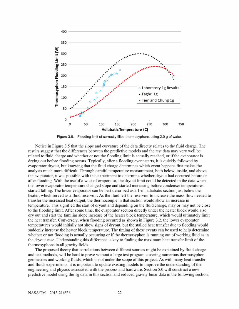
Before the thermosyphons were re-welded, a test was completed to determine, for this specific thermosyphon geometry, what the best fluid charge is, and how the amount of fluid charge affects the heat transfer limit. Figure 3.5 reports the results as the charge was changes from 0.3 grams up to 5.0 grams. The results are clear that fluid charge has a significant impact on the heat transfer limit of the thermosyphon. When using too little fluid, the evaporator dries out before ever getting to the flooding limit and when too much fluid was used, the heat pipe would not work at all. Although not reported in the figure, the maximum amount of fluid that could be used was around 3.0 grams. At 3.0 grams and above, the thermosyphons could not be started. Also worth mentioning is the fact that 2.0 grams of fluid took up 5 in. (12.7 cm) of the 24 in. (60 cm) total length. This volume of fluid was needed to achieve the maximum flooding limit, but may not be practical in some design applications. It was determined that 2.0 grams of fluid would be used as the new fluid charge. The 1g laboratory testing was redone using the newly filled thermosyphons with 2.0 grams of working fluid. The new results are shown in Figure 3.6 showing a much tighter grouping of the data.
0
50
100
150
200
250
300
350
400
0 50 100 150 200 250 300 350
Ther
mos
ypho
n Fl
oodi
ng Li
mit
(W)
Adiabatic Temperature (C)
Faghri 1g
Tien and Chung 1g
Initial 1g Test Data
NASA/TM—2013-216536 21
Figure 3.4.—Initial individual thermosyphon flooding limits showing dissimilar results
during fluid charge investigation.
Figure 3.5.—Effect of fluid charge on thermosyphon flooding limit.
0
50
100
150
200
250
300
350
400
0 50 100 150 200 250 300
Ther
mos
ypho
n Fl
oodi
ng Li
mit
(W)
Adiabatic Temperature (C)
Faghri 1gTien and Chung 1gThermosyphon #6Thermosyphon #8Thermosyphon #12
0
50
100
150
200
250
300
350
400
0 50 100 150 200 250 300 350
Ther
mos
ypho
n Fl
oodi
ng Li
mit
(W)
Adiabatic Temperature (C)
Eq (1) Prediction2 grams1.0 grams0.3 gramsTien and Chung 1g
NASA/TM—2013-216536 22
Figure 3.6.—Flooding limit of correctly filled thermosyphons using 2.0 g of water.
Notice in Figure 3.5 that the slope and curvature of the data directly relates to the fluid charge. The
results suggest that the differences between the predictive models and the test data may very well be related to fluid charge and whether or not the flooding limit is actually reached, or if the evaporator is drying out before flooding occurs. Typically, after a flooding event starts, it is quickly followed by evaporator dryout, but knowing that the fluid charge determines which event happens first makes the analysis much more difficult. Through careful temperature measurement, both below, inside, and above the evaporator, it was possible with this experiment to determine whether dryout had occurred before or after flooding. With the use of a wicked evaporator, the dryout limit could be detected in the data when the lower evaporator temperature changed slope and started increasing before condenser temperatures started falling. The lower evaporator can be best described as a 1-in. adiabatic section just below the heater, which served as a fluid reservoir. As the fluid left the reservoir to increase the mass flow needed to transfer the increased heat output, the thermocouple in that section would show an increase in temperature. This signified the start of dryout and depending on the fluid charge, may or may not be close to the flooding limit. After some time, the evaporator section directly under the heater block would also dry out and start the familiar slope increase of the heater block temperature, which would ultimately limit the heat transfer. Conversely, when flooding occurred as shown in Figure 3.2, the lower evaporator temperatures would initially not show signs of dryout, but the stalled heat transfer due to flooding would suddenly increase the heater block temperature. The timing of these events can be used to help determine whether or not flooding is actually occurring or if the thermosyphon is running out of working fluid as in the dryout case. Understanding this difference is key to finding the maximum heat transfer limit of the thermosyphons in all gravity fields.
The proposed theory that correlations between different sources might be explained by fluid charge and test methods, will be hard to prove without a large test program covering numerous thermosyphon geometries and working fluids, which is not under the scope of this project. As with many heat transfer and fluids experiments, it is important to update existing models to improve the understanding of the engineering and physics associated with the process and hardware. Section 5.0 will construct a new predictive model using the 1g data in this section and reduced gravity lunar data in the following section.
0
50
100
150
200
250
300
350
400
0 50 100 150 200 250 300 350
Ther
mos
ypho
n Fl
oodi
ng L
imit
(W)
Adiabatic Temperature (C)
Laboratory 1g ResultsFaghri 1gTien and Chung 1g
NASA/TM—2013-216536 23
4.0 Reduced Gravity Testing 4.1 The 2011 and 2012 Flight Campaigns
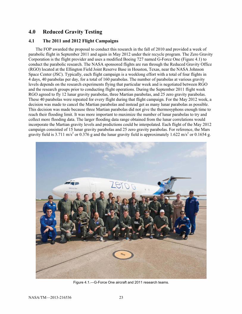
The FOP awarded the proposal to conduct this research in the fall of 2010 and provided a week of parabolic flight in September 2011 and again in May 2012 under their recycle program. The Zero Gravity Corporation is the flight provider and uses a modified Boeing 727 named G-Force One (Figure 4.1) to conduct the parabolic research. The NASA sponsored flights are run through the Reduced Gravity Office (RGO) located at the Ellington Field Joint Reserve Base in Houston, Texas, near the NASA Johnson Space Center (JSC). Typically, each flight campaign is a weeklong effort with a total of four flights in 4 days, 40 parabolas per day, for a total of 160 parabolas. The number of parabolas at various gravity levels depends on the research experiments flying that particular week and is negotiated between RGO and the research groups prior to conducting flight operations. During the September 2011 flight week RGO agreed to fly 12 lunar gravity parabolas, three Martian parabolas, and 25 zero gravity parabolas. These 40 parabolas were repeated for every flight during that flight campaign. For the May 2012 week, a decision was made to cancel the Martian parabolas and instead get as many lunar parabolas as possible. This decision was made because three Martian parabolas did not give the thermosyphons enough time to reach their flooding limit. It was more important to maximize the number of lunar parabolas to try and collect more flooding data. The larger flooding data range obtained from the lunar correlations would incorporate the Martian gravity levels and predictions could be interpolated. Each flight of the May 2012 campaign consisted of 15 lunar gravity parabolas and 25 zero gravity parabolas. For reference, the Mars gravity field is 3.711 m/s2 or 0.376 g and the lunar gravity field is approximately 1.622 m/s2 or 0.1654 g.
Figure 4.1.—G-Force One aircraft and 2011 research teams.
NASA/TM—2013-216536 24
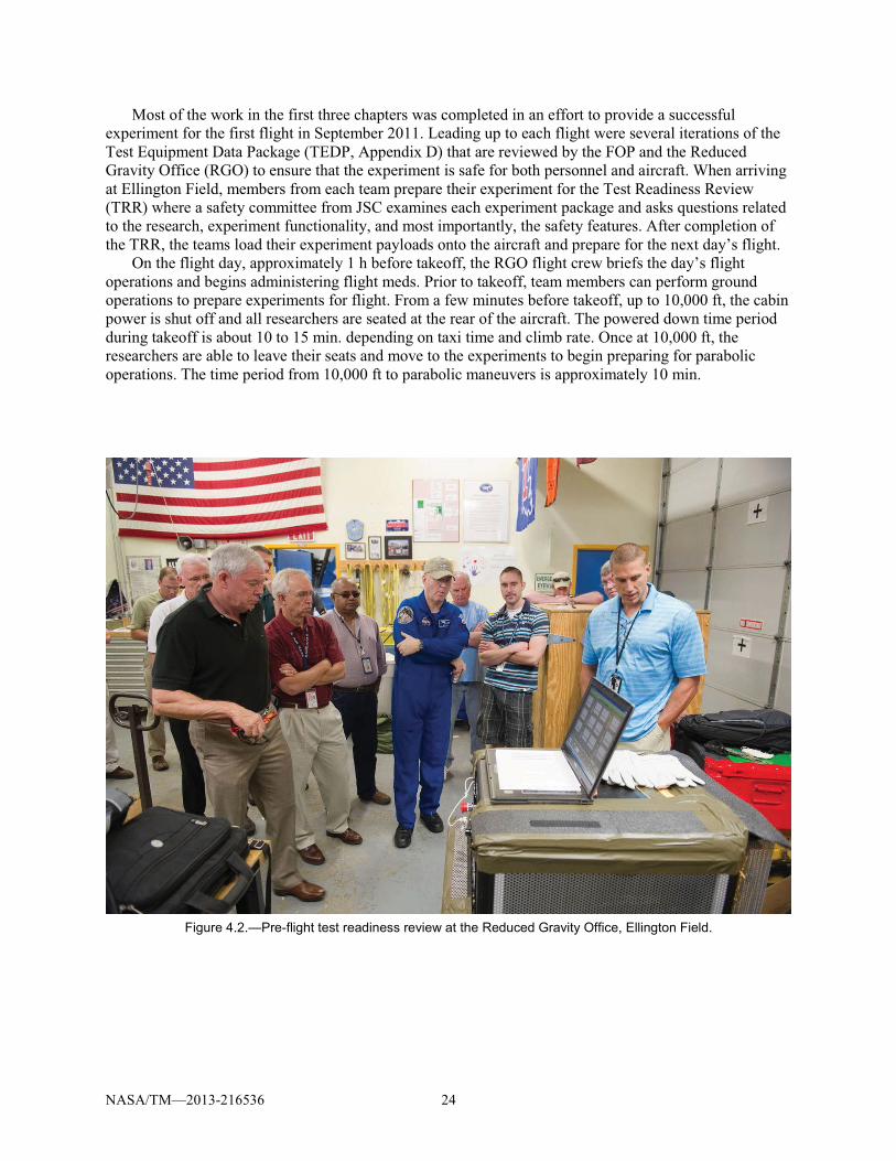
Most of the work in the first three chapters was completed in an effort to provide a successful experiment for the first flight in September 2011. Leading up to each flight were several iterations of the Test Equipment Data Package (TEDP, Appendix D) that are reviewed by the FOP and the Reduced Gravity Office (RGO) to ensure that the experiment is safe for both personnel and aircraft. When arriving at Ellington Field, members from each team prepare their experiment for the Test Readiness Review (TRR) where a safety committee from JSC examines each experiment package and asks questions related to the research, experiment functionality, and most importantly, the safety features. After completion of the TRR, the teams load their experiment payloads onto the aircraft and prepare for the next day’s flight.
On the flight day, approximately 1 h before takeoff, the RGO flight crew briefs the day’s flight operations and begins administering flight meds. Prior to takeoff, team members can perform ground operations to prepare experiments for flight. From a few minutes before takeoff, up to 10,000 ft, the cabin power is shut off and all researchers are seated at the rear of the aircraft. The powered down time period during takeoff is about 10 to 15 min. depending on taxi time and climb rate. Once at 10,000 ft, the researchers are able to leave their seats and move to the experiments to begin preparing for parabolic operations. The time period from 10,000 ft to parabolic maneuvers is approximately 10 min.
Figure 4.2.—Pre-flight test readiness review at the Reduced Gravity Office, Ellington Field.
NASA/TM—2013-216536 25
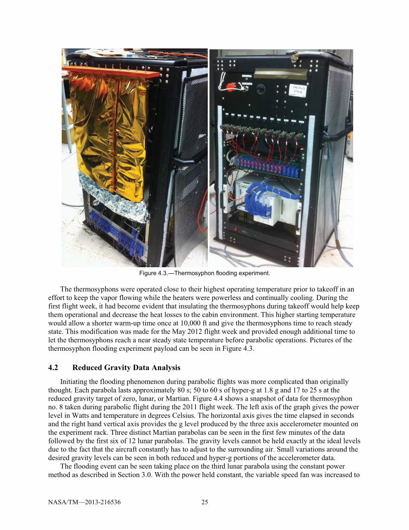
Figure 4.3.—Thermosyphon flooding experiment.
The thermosyphons were operated close to their highest operating temperature prior to takeoff in an
effort to keep the vapor flowing while the heaters were powerless and continually cooling. During the first flight week, it had become evident that insulating the thermosyphons during takeoff would help keep them operational and decrease the heat losses to the cabin environment. This higher starting temperature would allow a shorter warm-up time once at 10,000 ft and give the thermosyphons time to reach steady state. This modification was made for the May 2012 flight week and provided enough additional time to let the thermosyphons reach a near steady state temperature before parabolic operations. Pictures of the thermosyphon flooding experiment payload can be seen in Figure 4.3.
4.2 Reduced Gravity Data Analysis
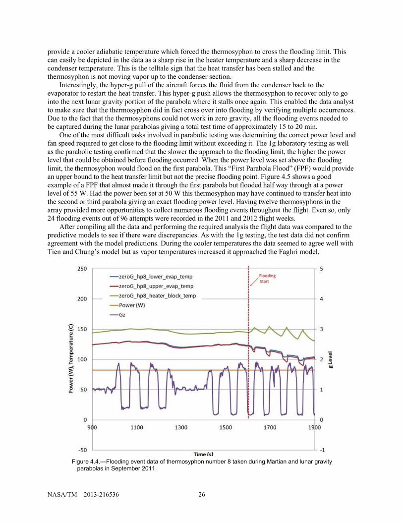
Initiating the flooding phenomenon during parabolic flights was more complicated than originally thought. Each parabola lasts approximately 80 s; 50 to 60 s of hyper-g at 1.8 g and 17 to 25 s at the reduced gravity target of zero, lunar, or Martian. Figure 4.4 shows a snapshot of data for thermosyphon no. 8 taken during parabolic flight during the 2011 flight week. The left axis of the graph gives the power level in Watts and temperature in degrees Celsius. The horizontal axis gives the time elapsed in seconds and the right hand vertical axis provides the g level produced by the three axis accelerometer mounted on the experiment rack. Three distinct Martian parabolas can be seen in the first few minutes of the data followed by the first six of 12 lunar parabolas. The gravity levels cannot be held exactly at the ideal levels due to the fact that the aircraft constantly has to adjust to the surrounding air. Small variations around the desired gravity levels can be seen in both reduced and hyper-g portions of the accelerometer data.
The flooding event can be seen taking place on the third lunar parabola using the constant power method as described in Section 3.0. With the power held constant, the variable speed fan was increased to
NASA/TM—2013-216536 26
provide a cooler adiabatic temperature which forced the thermosyphon to cross the flooding limit. This can easily be depicted in the data as a sharp rise in the heater temperature and a sharp decrease in the condenser temperature. This is the telltale sign that the heat transfer has been stalled and the thermosyphon is not moving vapor up to the condenser section.
Interestingly, the hyper-g pull of the aircraft forces the fluid from the condenser back to the evaporator to restart the heat transfer. This hyper-g push allows the thermosyphon to recover only to go into the next lunar gravity portion of the parabola where it stalls once again. This enabled the data analyst to make sure that the thermosyphon did in fact cross over into flooding by verifying multiple occurrences. Due to the fact that the thermosyphons could not work in zero gravity, all the flooding events needed to be captured during the lunar parabolas giving a total test time of approximately 15 to 20 min.
One of the most difficult tasks involved in parabolic testing was determining the correct power level and fan speed required to get close to the flooding limit without exceeding it. The 1g laboratory testing as well as the parabolic testing confirmed that the slower the approach to the flooding limit, the higher the power level that could be obtained before flooding occurred. When the power level was set above the flooding limit, the thermosyphon would flood on the first parabola. This “First Parabola Flood” (FPF) would provide an upper bound to the heat transfer limit but not the precise flooding point. Figure 4.5 shows a good example of a FPF that almost made it through the first parabola but flooded half way through at a power level of 55 W. Had the power been set at 50 W this thermosyphon may have continued to transfer heat into the second or third parabola giving an exact flooding power level. Having twelve thermosyphons in the array provided more opportunities to collect numerous flooding events throughout the flight. Even so, only 24 flooding events out of 96 attempts were recorded in the 2011 and 2012 flight weeks.
After compiling all the data and performing the required analysis the flight data was compared to the predictive models to see if there were discrepancies. As with the 1g testing, the test data did not confirm agreement with the model predictions. During the cooler temperatures the data seemed to agree well with Tien and Chung’s model but as vapor temperatures increased it approached the Faghri model.
Figure 4.4.—Flooding event data of thermosyphon number 8 taken during Martian and lunar gravity
parabolas in September 2011.
NASA/TM—2013-216536 27
Figure 4.5.—“First parabola flood” depicting three key events. 1) Lunar gravity forces
decrease mass flow, heater temperature increases, upper evaporator temperature decreases. 2) Flooding occurs and heat transfer is stalled, slope change shows increase in heater temperature rate, no sign of recovery. 3) Hyper-g forces push fluid back to evaporator and cools heater until next parabola.
Figure 4.6.—Parabolic flooding data during lunar gravity compared to predictive models.
0
0.5
1
1.5
2
2.5
3
3.5
4
4.5
5
-50
0
50
100
150
200
600 650 700 750 800 850 900
g Le
vel
Pow
er (W
), Te
mpe
ratu
re (C
)
Time (s)
hp5_htr_block
hp5_upper_evap
Power (W)
Gz
12
3
0
20
40
60
80
100
120
140
160
180
0 50 100 150 200 250 300 350
Ther
mos
ypho
n Fl
oodi
ng Li
mit
(W)
Adiabatic Temperature (C)
Parabolic Lunar Test Data
Faghri Lunar
Tien and Chung Lunar
NASA/TM—2013-216536 28
5.0 Data Correlation 5.1 Non-Dimensional Analysis and Data Correlation
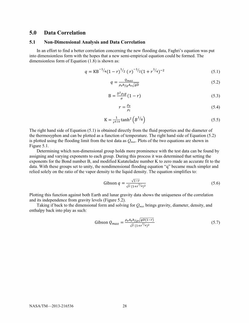
In an effort to find a better correlation concerning the new flooding data, Faghri’s equation was put into dimensionless form with the hopes that a new semi-empirical equation could be formed. The dimensionless form of Equation (1.8) is shown as:
R = KB%0�1 (1 � �)0
+1 ( �)%0+1 (1 + �0
�1 )%+ (5.1)
R = #|}~?X\^IVX_�`
(5.2)
B = `O?b��
(1 � �) (5.3)
� = ?X?b
(5.4)
K = 0��.Nm tanh+ j;0
�1 k (5.5)
The right hand side of Equation (5.1) is obtained directly from the fluid properties and the diameter of the thermosyphon and can be plotted as a function of temperature. The right hand side of Equation (5.2) is plotted using the flooding limit from the test data as Qmax. Plots of the two equations are shown in Figure 5.1.
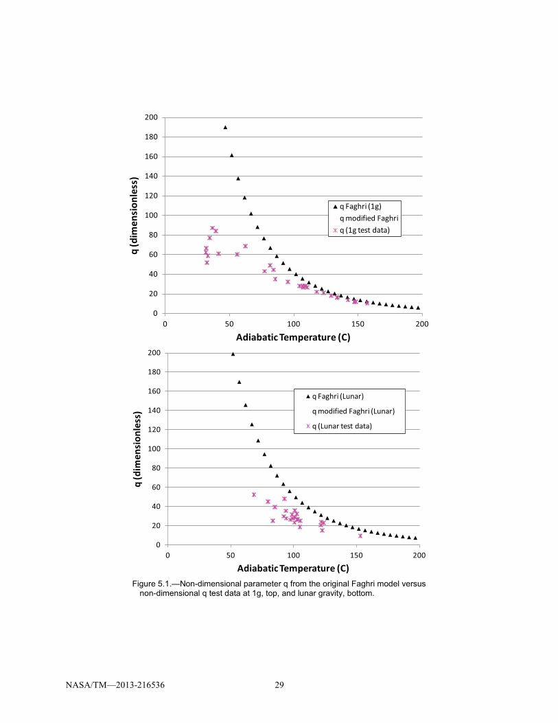
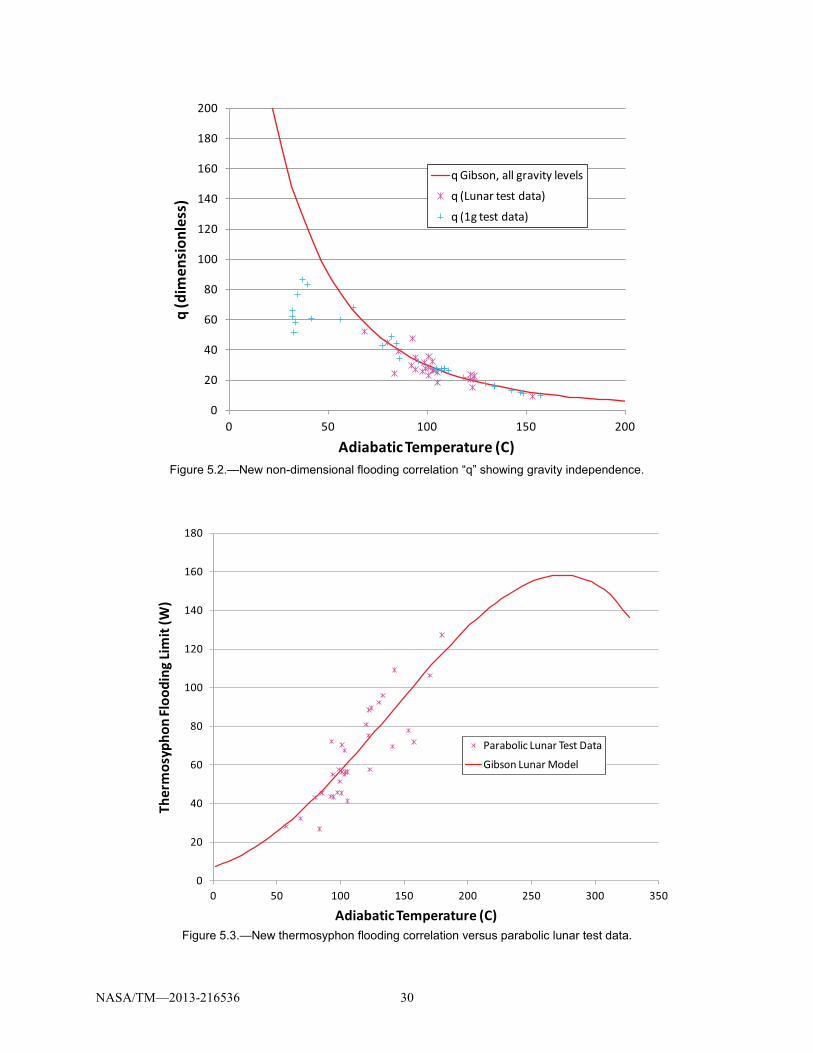
Determining which non-dimensional group holds more prominence with the test data can be found by assigning and varying exponents to each group. During this process it was determined that setting the exponents for the Bond number B, and modified Kutateladze number K to zero made an accurate fit to the data. With these groups set to unity, the nondimensional flooding equation “q” became much simpler and relied solely on the ratio of the vapor density to the liquid density. The equation simplifies to:
Gibson R = 50%�
5� (0f�N m1 )O
(5.6)
Plotting this function against both Earth and lunar gravity data shows the uniqueness of the correlation and its independence from gravity levels (Figure 5.2).
Taking if back to the dimensional form and solving for Qmax brings gravity, diameter, density, and enthalpy back into play as such:
Gibson ��' = ?XVX\^I_�`(0%�)
5� (0f�N m1 )O
(5.7)
NASA/TM—2013-216536 29
Figure 5.1.—Non-dimensional parameter q from the original Faghri model versus
non-dimensional q test data at 1g, top, and lunar gravity, bottom.
0
20
40
60
80
100
120
140
160
180
200
0 50 100 150 200
q (d
imen
sion
less
)
Adiabatic Temperature (C)
q Faghri (1g)q modified Faghriq (1g test data)
0
20
40
60
80
100
120
140
160
180
200
0 50 100 150 200
q (d
imen
sion
less
)
Adiabatic Temperature (C)
q Faghri (Lunar)
q modified Faghri (Lunar)
q (Lunar test data)
NASA/TM—2013-216536 30
Figure 5.2.—New non-dimensional flooding correlation “q” showing gravity independence.
Figure 5.3.—New thermosyphon flooding correlation versus parabolic lunar test data.
0
20
40
60
80
100
120
140
160
180
200
0 50 100 150 200
q (d
imen
sion
less
)
Adiabatic Temperature (C)
q Gibson, all gravity levels
q (Lunar test data)
q (1g test data)
0
20
40
60
80
100
120
140
160
180
0 50 100 150 200 250 300 350
Ther
mos
ypho
n Fl
oodi
ng Li
mit
(W)
Adiabatic Temperature (C)
Parabolic Lunar Test Data
Gibson Lunar Model
NASA/TM—2013-216536 31
Figure 5.4.—New thermosyphon flooding correlation versus 1g test data.
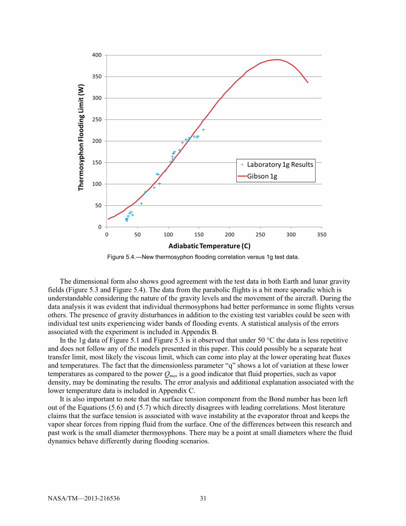
The dimensional form also shows good agreement with the test data in both Earth and lunar gravity fields (Figure 5.3 and Figure 5.4). The data from the parabolic flights is a bit more sporadic which is understandable considering the nature of the gravity levels and the movement of the aircraft. During the data analysis it was evident that individual thermosyphons had better performance in some flights versus others. The presence of gravity disturbances in addition to the existing test variables could be seen with individual test units experiencing wider bands of flooding events. A statistical analysis of the errors associated with the experiment is included in Appendix B.
In the 1g data of Figure 5.1 and Figure 5.3 is it observed that under 50 °C the data is less repetitive and does not follow any of the models presented in this paper. This could possibly be a separate heat transfer limit, most likely the viscous limit, which can come into play at the lower operating heat fluxes and temperatures. The fact that the dimensionless parameter “q” shows a lot of variation at these lower temperatures as compared to the power Qmax is a good indicator that fluid properties, such as vapor density, may be dominating the results. The error analysis and additional explanation associated with the lower temperature data is included in Appendix C.
It is also important to note that the surface tension component from the Bond number has been left out of the Equations (5.6) and (5.7) which directly disagrees with leading correlations. Most literature claims that the surface tension is associated with wave instability at the evaporator throat and keeps the vapor shear forces from ripping fluid from the surface. One of the differences between this research and past work is the small diameter thermosyphons. There may be a point at small diameters where the fluid dynamics behave differently during flooding scenarios.
0
50
100
150
200
250
300
350
400
0 50 100 150 200 250 300 350
Ther
mos
ypho
n Fl
oodi
ng Li
mit
(W)
Adiabatic Temperature (C)
Laboratory 1g ResultsGibson 1g
NASA/TM—2013-216536 32
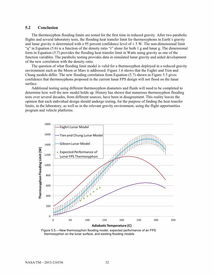
5.2 Conclusion
The thermosyphon flooding limits are tested for the first time in reduced gravity. After two parabolic flights and several laboratory tests, the flooding heat transfer limit for thermosyphons in Earth’s gravity and lunar gravity is determined with a 95 percent confidence level of ± 5 W. The non-dimensional limit “q” in Equation (5.6) is a function of the density ratio “r” alone for both 1 g and lunar g. The dimensional form in Equation (5.7) provides the flooding heat transfer limit in Watts using gravity as one of the function variables. The parabolic testing provides data in simulated lunar gravity and aided development of the new correlation with the density ratio.
The question of what flooding limit model is valid for a thermosyphon deployed in a reduced gravity environment such as the Moon or Mars is addressed. Figure 1.6 shows that the Faghri and Tien and Chung models differ. The new flooding correlation from Equation (5.7) shown in Figure 5.5 gives confidence that thermosyphons proposed in the current lunar FPS design will not flood on the lunar surface.
Additional testing using different thermosyphon diameters and fluids will need to be completed to determine how well the new model holds up. History has shown that numerous thermosyphon flooding tests over several decades, from different sources, have been in disagreement. This reality leaves the opinion that each individual design should undergo testing, for the purpose of finding the heat transfer limits, in the laboratory, as well as in the relevant gravity environment, using the flight opportunities program and vehicle platforms.
Figure 5.5.—New thermosyphon flooding model, expected performance of an FPS
thermosyphon on the lunar surface, and existing flooding models
0
200
400
600
800
1000
1200
1400
1600
1800
0 50 100 150 200 250 300 350
Ther
mos
ypho
n Fl
oodi
ng Li
mit
(W)
Adiabatic Temperature (C)
Faghri Lunar Model
Tien and Chung Lunar Model
Gibson Lunar Model
Expected Performance of Lunar FPS Thermosyphon
NASA/TM—2013-216536 33
Appendix A.—Symbols and Acronyms g acceleration of gravity (m/s2), grams ��� heat of vaporization i subscript used to denote individual variables for certain nomenclature l thermosyphon inner radius P Wallis velocity parameter (m/s) �� mass flow rate (kg/s) q dimensionless power r density ratio, ., .Q� � velocity (m/s) z statistical parameter � area �, vapor area ;� Bond number �* dimensionless constant, Tien and Chung �� dimensionless constant, Wallis D thermosyphon inner diameter DAC Data Acquisition and Control FOP Flight Opportunities Program FPF First Parabola Flood FPS Fission Power System FSP Fission Surface Power GCD Game Changing Development GRC NASA Glenn Research Center JSC NASA Johnson Space Center !" thermal conductance (W/K) K dimensionless constant, Kutateladze and Faghri L thermosyphon length N statistical sample size OCT Office of the Chief Technologist P pressure Q thermal power (W) RGE Reduced Gravity Environment RGO Reduced Gravity Office SrLV Suborbital re-useable Launch Vehicle T temperature TC thermocouple TEDP Test Equipment Data Package TRL Technology Readiness Level TRR Test Readiness Review
NASA/TM—2013-216536 34
W thermosyphon width � confidence parameter � liquid thickness (m) � emissivity � dynamic viscosity (Pa s) � kinematic viscosity (m2/s) .� density of the liquid ./ density of the vapor � surface tension (N/m) �� standard deviation �� Stefan Boltzmann constant (5.67×10⁻⁸ W/m2K4) � shear stress (Pa) �(�) cumulative normal distribution function
NASA/TM—2013-216536 35
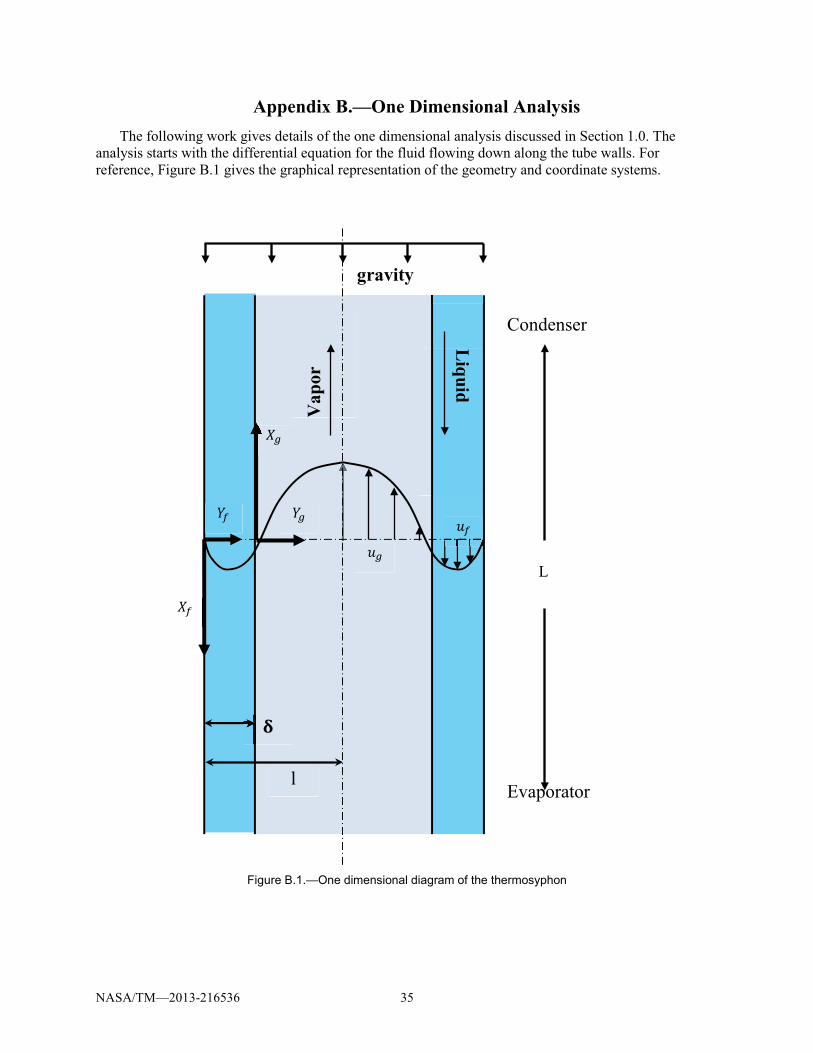
Appendix B.—One Dimensional Analysis The following work gives details of the one dimensional analysis discussed in Section 1.0. The
analysis starts with the differential equation for the fluid flowing down along the tube walls. For reference, Figure B.1 gives the graphical representation of the geometry and coordinate systems.
Figure B.1.—One dimensional diagram of the thermosyphon
Vap
or
Liquid
��
�� ��
��
��
��
�
l
gravity
Evaporator
Condenser
L
NASA/TM—2013-216536 36
�� �O�^
�¡^O¢ � ��
�'^+ .�- = 0 (B.1)
;�. 1 �� = 0 @ ¤� = 0 (B.2)
;�. 2 ����^
�¡^@ � = ��� = � ¥�
�(� � �) (B.3)
Integrating twice using the given boundary conditions provides the desired fluid velocity profile as:
�� = ¡^
+�^2.�-¦2� � ¤�§ � ¥�
�¦2� � ¤�§4 (B.4)
��p = p+�^
2.�-(�) � ¥��
(2� � �)4 (B.5)
In order to obtain the mass flow rate of the fluid, the velocity is integrated over the fluid thickness between zero and delta and multiplied by the fluid density, giving the mass flow rate per unit width as:
�� � = Qv
x^jp
Qk
+¨?^�p
wQ� ©�
+�j1 � p
wQkª (B.6)
Similar equations are developed for the vapor traveling up the center of the tube with the fluid as its boundary. The differential equation gives the following relationships:
�� �O�I
�¡IO¢ + ©�
�= 0 (B.7)
;�. 1 �� = ��� @ ¤� = 0 (B.8)
;�. 2 ��I
�¡I= 0 @ ¤� = � � � (B.9)
Integrating to find the velocity profile of the gas gives:
�� = ©��
¡I
+�IH2(� � �) � ¤�M + p
+�^2©�
�(2� � �) � .�-�4 (B.10)
Integrating the vapor velocity between � and (� � �) and multiplying by the vapor density gives the mass flow rate per width as:
�� � = ©��
Qv
xIy0
wj1 � p
Qk
w+ �I
�^
pQ
j1 � pQk j1 � p
+Qk � ?I�Qv
+x^jp
Qk
+j1 � p
Qk{ (B.11)
The �I
�^ term drops out as it is << 1 giving:
�� � = ©��
Qv
xIy0
wj1 � p
Qk
w� ?I�Qv
+x^jp
Qk
+j1 � p
Qk{ (B.12)
Continuity ensures that the mass flows must be equal between the fluid and vapor. Setting the mass flow �>��������>�����������������������������P/L gives:
©��
=Nv?^�j«
b kv
¬^¬I
Nvj0%«
b kv
fNOj«
b kO
j0% «vbk
(B.13)
NASA/TM—2013-216536 37
Equation (1.04) can be applied to the following one dimensional analysis as follows:
�� � = �� � = #+q\^I
(B.14)
Inserting ©��
back into the fluid mass flow Equation (B.6), and plugging into (B.14) gives an expression
relating Q as a function of � �1 as:
#|}~x^
+q\^I?^�Qv = 0w
jpQk
wy1 + w
+xI
x^jp
Qk
+j1 � p
wQk j1 � p
Qk
%w{
%0 (B.15)
Assuming negligible differences between the rectangular and cylindrical dimensions of the tube wall, a change is made to try and match the non-dimensional power parameter “q” as described in Section 5.0. In order to achieve this, the following assumptions are made:
2 = 2®�; Area of the vapor = �, = ®�+
R = #|}~\^I?IVX_�`
= Q_�`?^
wx^?Ijp
Qk
wy1 + w
+xI
x^jp
Qk
+j1 � p
wQk j1 � p
Qk
%w{
%0 (B.16)
The following one dimensional work was left out of the data analysis sections of the paper because it was not found to be entirely accurate when compared to the data, but it did give insight into the fluid dynamics associated with the liquid vapor shear in thermosyphons. A graph of the thermosyphon axial thermal power, Qmax in Equation (B.15), versus several values of � �1 for the 1g laboratory case is shown in Figure B.2. Values were chosen that accurately scaled the curves with the latest model produced from this research. The curve that best represents the 1g model has a � �1 value of 0.04 which corresponds to a water fluid charge of approximately 0.8 grams, assuming all the fluid is in motion. As described in the paper, a fluid charge of 2.0 grams was found to give the best results. The equation gives a good representation of the flooding limit but determination of the correct � �1 ratio that would allow the model to be used as a predictive tool would be difficult.
The non-dimensional form from Equation (B.16) was also compared to the latest model using representative values of p
Q. The results are shown in figure B.2 and give a good approximation to the shape
and scale of the latest model representing the test data.
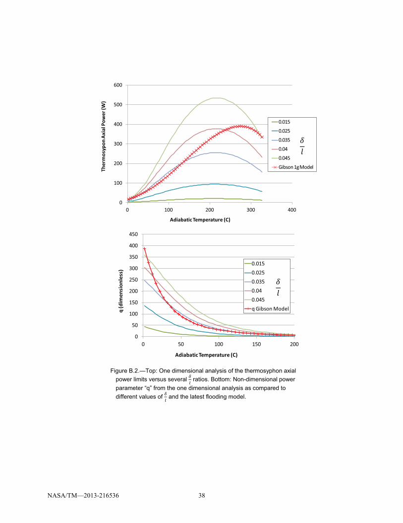
NASA/TM—2013-216536 38
Figure B.2.—Top: One dimensional analysis of the thermosyphon axial
power limits versus several pQ ratios. Bottom: Non-dimensional power
parameter “q” from the one dimensional analysis as compared to different values of p
Q and the latest flooding model.
0
100
200
300
400
500
600
0 100 200 300 400
Ther
mos
ypon
Axi
al P
ower
(W)
Adiabatic Temperature (C)
0.015
0.025
0.035
0.04
0.045
Gibson 1g Model
0
50
100
150
200
250
300
350
400
450
0 50 100 150 200
q (d
imen
sion
less
)
Adiabatic Temperature (C)
0.0150.0250.0350.040.045q Gibson Model
��
��
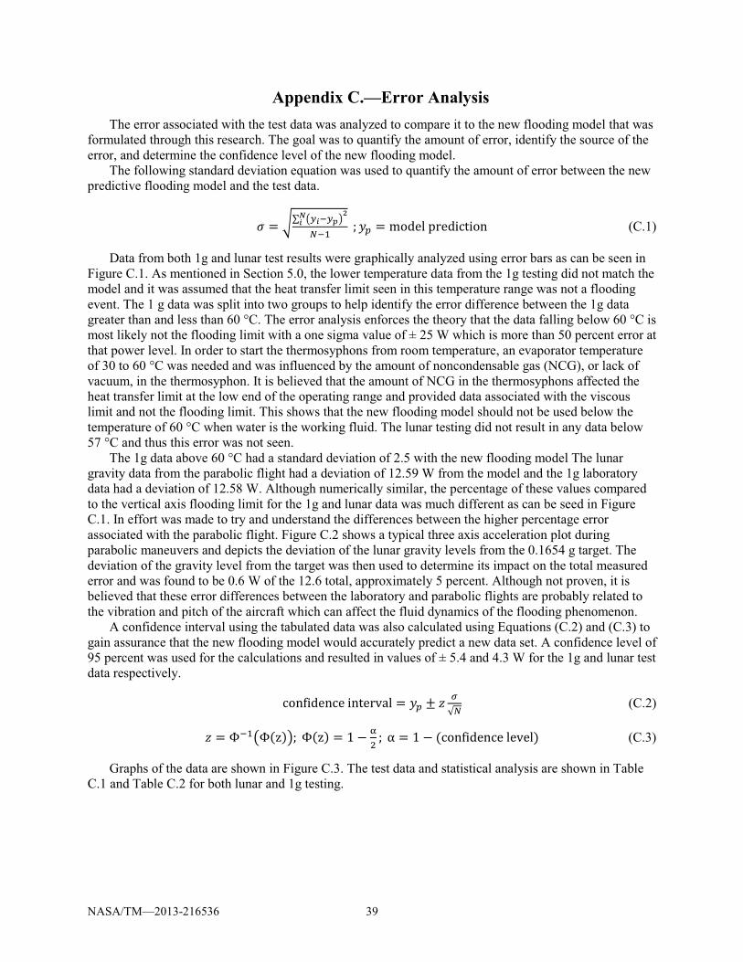
NASA/TM—2013-216536 39
Appendix C.—Error Analysis The error associated with the test data was analyzed to compare it to the new flooding model that was
formulated through this research. The goal was to quantify the amount of error, identify the source of the error, and determine the confidence level of the new flooding model.
The following standard deviation equation was used to quantify the amount of error between the new predictive flooding model and the test data.
� = ³´ ¦¡µ%¡¶§O·
µ¸%0
; ¤ = model prediction (C.1)
Data from both 1g and lunar test results were graphically analyzed using error bars as can be seen in Figure C.1. As mentioned in Section 5.0, the lower temperature data from the 1g testing did not match the model and it was assumed that the heat transfer limit seen in this temperature range was not a flooding event. The 1 g data was split into two groups to help identify the error difference between the 1g data greater than and less than 60 °C. The error analysis enforces the theory that the data falling below 60 °C is most likely not the flooding limit with a one sigma value of ± 25 W which is more than 50 percent error at that power level. In order to start the thermosyphons from room temperature, an evaporator temperature of 30 to 60 °C was needed and was influenced by the amount of noncondensable gas (NCG), or lack of vacuum, in the thermosyphon. It is believed that the amount of NCG in the thermosyphons affected the heat transfer limit at the low end of the operating range and provided data associated with the viscous limit and not the flooding limit. This shows that the new flooding model should not be used below the temperature of 60 °C when water is the working fluid. The lunar testing did not result in any data below 57 °C and thus this error was not seen.
The 1g data above 60 °C had a standard deviation of 2.5 with the new flooding model The lunar gravity data from the parabolic flight had a deviation of 12.59 W from the model and the 1g laboratory data had a deviation of 12.58 W. Although numerically similar, the percentage of these values compared to the vertical axis flooding limit for the 1g and lunar data was much different as can be seed in Figure C.1. In effort was made to try and understand the differences between the higher percentage error associated with the parabolic flight. Figure C.2 shows a typical three axis acceleration plot during parabolic maneuvers and depicts the deviation of the lunar gravity levels from the 0.1654 g target. The deviation of the gravity level from the target was then used to determine its impact on the total measured error and was found to be 0.6 W of the 12.6 total, approximately 5 percent. Although not proven, it is believed that these error differences between the laboratory and parabolic flights are probably related to the vibration and pitch of the aircraft which can affect the fluid dynamics of the flooding phenomenon.
A confidence interval using the tabulated data was also calculated using Equations (C.2) and (C.3) to gain assurance that the new flooding model would accurately predict a new data set. A confidence level of 95 percent was used for the calculations and resulted in values of ± 5.4 and 4.3 W for the 1g and lunar test data respectively.
confidence interval = ¤ ± � �5¸
(C.2)
� = �%0¦�(z)§; �(z) = 1 � ½+
; � = 1 � (confidence level) (C.3)
Graphs of the data are shown in Figure C.3. The test data and statistical analysis are shown in Table C.1 and Table C.2 for both lunar and 1g testing.
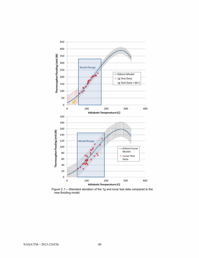
NASA/TM—2013-216536 40
Figure C.1.—Standard deviation of the 1g and lunar test data compared to the
new flooding model.
0
50
100
150
200
250
300
350
400
450
0 100 200 300 400
Ther
mos
ypho
n Flo
odin
g Lim
it (W
)
Adiabatic Temperature (C)
Gibson Model1g Test Data1g Test Data < 60 C
Model Range
0
20
40
60
80
100
120
140
160
180
200
0 100 200 300 400
Ther
mos
ypho
n Flo
odin
g Lim
it (W
)
Adiabatic Temperature (C)
Gibson lunar Model
Lunar Test Data
Model Range
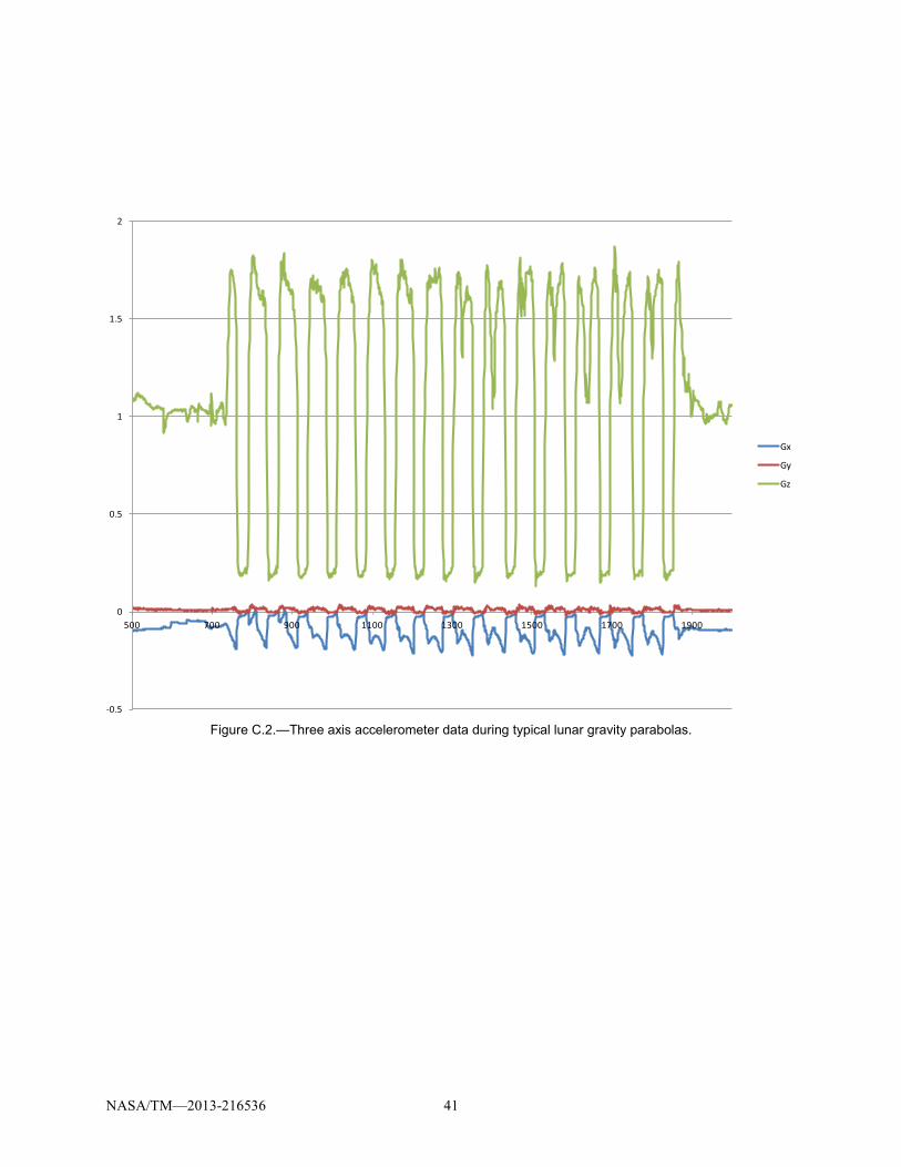
NASA/TM—2013-216536 41
Figure C.2.—Three axis accelerometer data during typical lunar gravity parabolas.
-0.5
0
0.5
1
1.5
2
500 700 900 1100 1300 1500 1700 1900
Gx
Gy
Gz
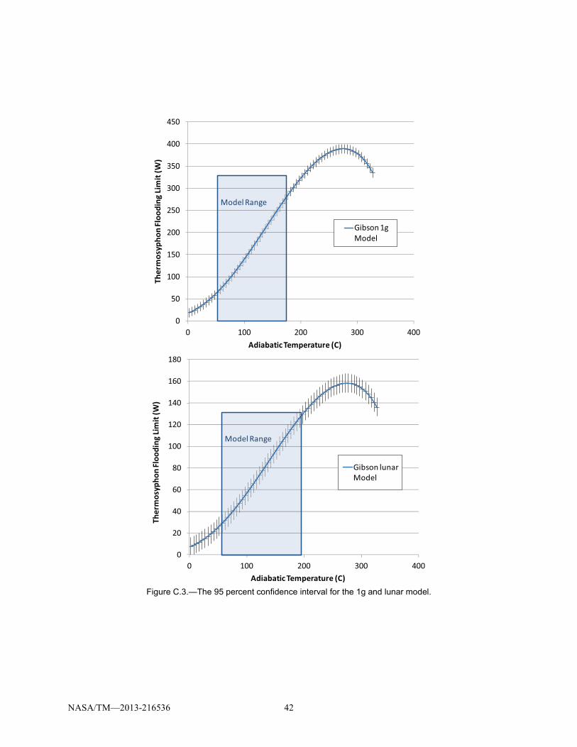
NASA/TM—2013-216536 42
Figure C.3.—The 95 percent confidence interval for the 1g and lunar model.
0
50
100
150
200
250
300
350
400
450
0 100 200 300 400
Ther
mos
ypho
n Fl
oodi
ng L
imit
(W)
Adiabatic Temperature (C)
Gibson 1g Model
Model Range
0
20
40
60
80
100
120
140
160
180
0 100 200 300 400
Ther
mos
ypho
n Fl
oodi
ng Li
mit
(W)
Adiabatic Temperature (C)
Gibson lunar Model
Model Range
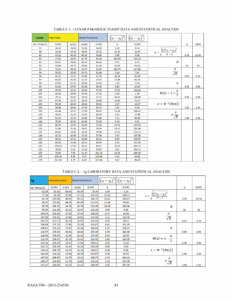
NASA/TM—2013-216536 43
TABLE C.1.—LUNAR PARABOLIC FLIGHT DATA AND STATISTICAL ANALYSIS
TABLE C.2.—1g LABORATORY DATA AND STATISTICAL ANALYSIS

NASA/TM—2013-216536 44
NASA/TM—2013-216536 45
Appendix D.—Test Equipment Data Package
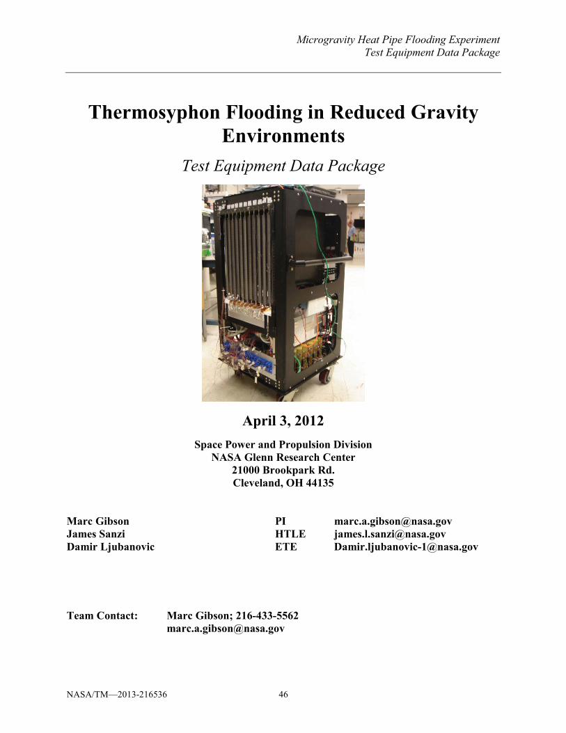
Microgravity Heat Pipe Flooding Experiment Test Equipment Data Package
NASA/TM—2013-216536 46
Thermosyphon Flooding in Reduced Gravity Environments
Test Equipment Data Package
April 3, 2012
Space Power and Propulsion Division NASA Glenn Research Center
21000 Brookpark Rd. Cleveland, OH 44135
Marc Gibson PI [email protected] James Sanzi HTLE [email protected] Damir Ljubanovic ETE [email protected] Team Contact: Marc Gibson; 216-433-5562 [email protected]
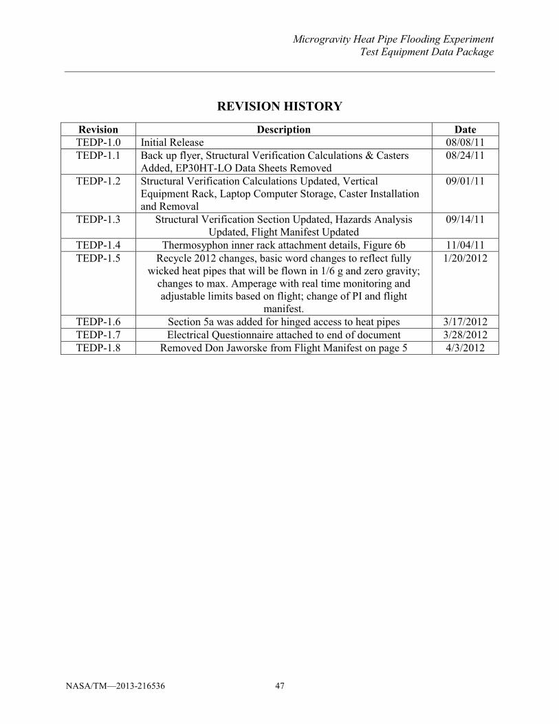
Microgravity Heat Pipe Flooding Experiment Test Equipment Data Package
NASA/TM—2013-216536 47
REVISION HISTORY
Revision Description Date TEDP-1.0 Initial Release 08/08/11 TEDP-1.1 Back up flyer, Structural Verification Calculations & Casters
Added, EP30HT-LO Data Sheets Removed 08/24/11
TEDP-1.2 Structural Verification Calculations Updated, Vertical Equipment Rack, Laptop Computer Storage, Caster Installation and Removal
09/01/11
TEDP-1.3 Structural Verification Section Updated, Hazards Analysis Updated, Flight Manifest Updated
09/14/11
TEDP-1.4 Thermosyphon inner rack attachment details, Figure 6b 11/04/11 TEDP-1.5 Recycle 2012 changes, basic word changes to reflect fully
wicked heat pipes that will be flown in 1/6 g and zero gravity; changes to max. Amperage with real time monitoring and adjustable limits based on flight; change of PI and flight
manifest.
1/20/2012
TEDP-1.6 Section 5a was added for hinged access to heat pipes 3/17/2012 TEDP-1.7 Electrical Questionnaire attached to end of document 3/28/2012 TEDP-1.8 Removed Don Jaworske from Flight Manifest on page 5 4/3/2012
Microgravity Heat Pipe Flooding Experiment Test Equipment Data Package
NASA/TM—2013-216536 48
QUICK REFERENCE DATA SHEET
Principal Investigator: Marc Gibson
Contact Information: [email protected], (216) 433-5562
Experiment Title: Thermosyphon Flooding in Reduced Gravity Environments
Work Breakdown Structure (WBS): 887359.04.01.05.03
Flight Date(s):
Overall Assembly Weight: 275 [lb]
Assembly Dimensions (L, W, H): 24.0, 24.0, 42.19 [in]
Equipment Orientation Requests: The zero-g flight approved Vertical Equipment Rack which holds the experiment equipment will be bolted to the floor of the aircraft. Heat Pipe side of experiment will face toward cabin wall.
Proposed Floor Mounting Strategy (Bolts/Studs or Straps): Bolts
Gas Cylinder Requests (Type & Quantity): No
Overboard Vent Request (Yes or No): No
Power Requirement (Voltage and Current Required): 115 VAC, 20 amps (Max amperage is monitored and adjustable for each flight to accommodate RGO requirements. In past flights RGO gave us limits that we verified before each flight.
Free Float Experiment (Yes or No): No
Flyer Names for Each Proposed Flight Day: Marc Gibson, Damir Ljubanovic, Jim Sanzi as follows: Flt. Day 1: MG, DL, JS; Flt Day 2: MG, DL, JS, Flt Day 3: MG, DL,JS; Flt. Day 4: MG, DL,JS
Camera Pole and/or Video Support: No
Microgravity Heat Pipe Flooding Experiment Test Equipment Data Package
NASA/TM—2013-216536 49
Table of Contents
1. ............................................................................................................................... FLIGHT MANIFEST....................................................................................................................................................... 50
2. EXPERIMENT BACKGROUND ......................................................................................... 50
3. EXPERIMENT DESCRIPTION ........................................................................................... 51
4. EQUIPMENT DESCRIPTION ............................................................................................. 52
5. STRUCTURAL VERIFICATION ........................................................................................ 65
6. ELECTRICAL ANALYSIS/VERIFICATION ..................................................................... 71
7. PRESSURE VESSEL/SYSTEM ........................................................................................... 79
8. PARABOLA DETAILS AND GROUND CREW ASSITANCE ......................................... 79
9. HAZARD ANALYSIS .......................................................................................................... 80
10. TOOL REQUIREMENTS ................................................................................................. 80
11. AIRCRAFT LOADING..................................................................................................... 81
12. GROUND SUPPORT REQUIREMENTS ........................................................................ 82
13. MATERIAL SAFETEY DATA SHEETS......................................................................... 83
14. EQUIPMENT PROCEDURE DOCUMENTATION ........................................................ 86
15. ELECTRICAL QUESTIONNAIRE .................................................................................. 88
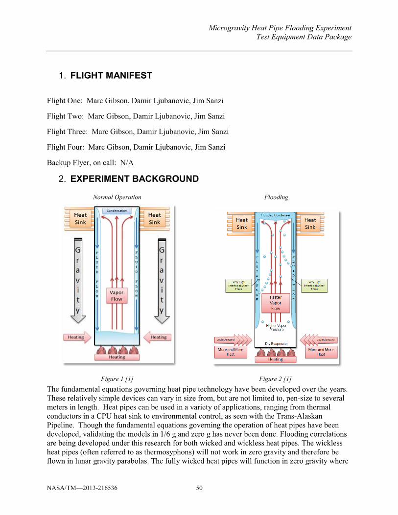
Microgravity Heat Pipe Flooding ExperimentTest Equipment Data Package
NASA/TM—2013-216536 50
FLIGHT MANIFEST 1.
Flight One: Marc Gibson, Damir Ljubanovic, Jim Sanzi
Flight Two: Marc Gibson, Damir Ljubanovic, Jim Sanzi
Flight Three: Marc Gibson, Damir Ljubanovic, Jim Sanzi
Flight Four: Marc Gibson, Damir Ljubanovic, Jim Sanzi
Backup Flyer, on call: N/A
EXPERIMENT BACKGROUND 2.
Normal Operation Flooding
Figure 1 [1] Figure 2 [1] The fundamental equations governing heat pipe technology have been developed over the years. These relatively simple devices can vary in size from, but are not limited to, pen-size to several meters in length. Heat pipes can be used in a variety of applications, ranging from thermal conductors in a CPU heat sink to environmental control, as seen with the Trans-Alaskan Pipeline. Though the fundamental equations governing the operation of heat pipes have been developed, validating the models in 1/6 g and zero g has never been done. Flooding correlations are being developed under this research for both wicked and wickless heat pipes. The wickless heat pipes (often referred to as thermosyphons) will not work in zero gravity and therefore be flown in lunar gravity parabolas. The fully wicked heat pipes will function in zero gravity where
Microgravity Heat Pipe Flooding Experiment Test Equipment Data Package
NASA/TM—2013-216536 51
their heat transport limits will be studied. There will be 8 thermosyphons and 4 heat pipes flown under this research flight campaign. The thermosyphons will be turned off for the zero gravity parabolas.
Heat pipes, while simple, are constrained by heat transfer limits associated with the flow of the working fluid through its thermodynamic cycle. One of the more common limits for thermosyphons in reduced gravity is the flooding limit. The limit that occurs most often with wicked heat pipes in microgravity is the capillary limit. This research effort will continue the thermosyphon flooding limits performed in lunar gravity during the 2011flight campaign as well as address the capillary limits of heat pipes in zero gravity. This will be accomplished by flying both thermosyphons and heat pipes, with the only difference being the wick structure in the heat pipe specimens. The capillary limit occurs in microgravity when the amount of power applied to the heat pipe exceeds the pumping capacity of the heat pipe wick structure to return liquid from the condenser, in essence starving the evaporator. The capillary limit is influenced not just by the design of the heat pipe but also by gravitational acceleration. For instance, a heat pipe with specific dimensions and 100 Watts of power flowing through it might not hit the limit here on Earth; however, if it were placed in a microgravity environment the same heat pipe could exceed its capillary limit. The Low-g flight experiment will allow us to compare a numerical model that predicts heat pipe limits with real life results in order to validate the model.
EXPERIMENT DESCRIPTION 3. Purpose: The purpose of this experiment is to study the effect that gravitational acceleration has heat transfer limits of two-phase heat pipes.
Objective: The recorded data will be used to determine whether or not our numerical model is accurate in predicting heat pipe flooding.
Layout: The experiment consists of twelve, nineteen inch long heat pipes, mounted to an internal rack that fits into a Zero-G flight approved vertical equipment rack, which will be bolted to the floor. Also in this rack, there are the 12 power supplies, which are bolted to a ¼ in. aluminum plate located at the lowest region on the rack.
Experiment: A range of power will be applied over the twelve heat pipes. For instance, if 100 W were applied to the first heat pipe and 144 W applied to the twelfth, the step, or interval, between each heat pipe would be 12 W. This will, in a sense, create a spectrum which can be adjusted by increasing or decreasing the power, along with adjusting the change in power between the heat pipes. The maximum power going through a heat pipe will not exceed 200 W. Heat is removed from the system via forced air cooling and a range of cooling can be applied by incrementing fan speed.
Thermocouples, strategically placed on all 12 heat pipes, will relay information to a data acquisition system. Temperature and acceleration data will be gathered each second along the parabolic trajectory of the Zero-G aircraft and will be sent to a laptop computer in order to observe the effect that gravity has on heat pipe flooding. Under normal operation, the heat pipes
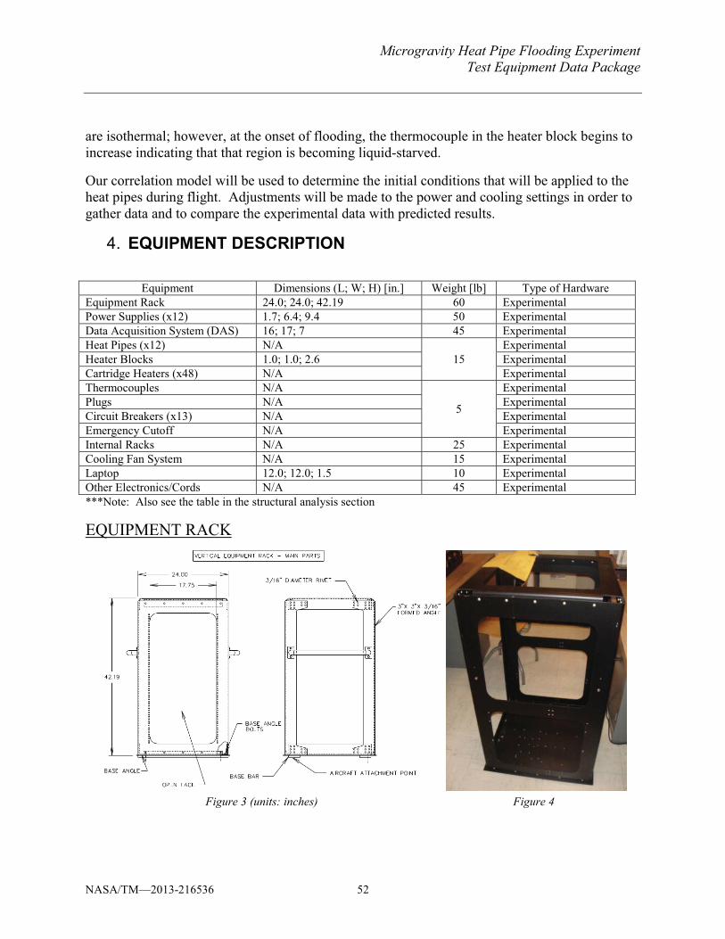
Microgravity Heat Pipe Flooding Experiment Test Equipment Data Package
NASA/TM—2013-216536 52
are isothermal; however, at the onset of flooding, the thermocouple in the heater block begins to increase indicating that that region is becoming liquid-starved.
Our correlation model will be used to determine the initial conditions that will be applied to the heat pipes during flight. Adjustments will be made to the power and cooling settings in order to gather data and to compare the experimental data with predicted results.
EQUIPMENT DESCRIPTION 4.
Equipment Dimensions (L; W; H) [in.] Weight [lb] Type of Hardware Equipment Rack 24.0; 24.0; 42.19 60 Experimental Power Supplies (x12) 1.7; 6.4; 9.4 50 Experimental Data Acquisition System (DAS) 16; 17; 7 45 Experimental Heat Pipes (x12) N/A
15 Experimental
Heater Blocks 1.0; 1.0; 2.6 Experimental Cartridge Heaters (x48) N/A Experimental Thermocouples N/A
5
Experimental Plugs N/A Experimental Circuit Breakers (x13) N/A Experimental Emergency Cutoff N/A Experimental Internal Racks N/A 25 Experimental Cooling Fan System N/A 15 Experimental Laptop 12.0; 12.0; 1.5 10 Experimental Other Electronics/Cords N/A 45 Experimental ***Note: Also see the table in the structural analysis section
EQUIPMENT RACK
Figure 3 (units: inches) Figure 4
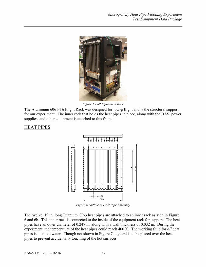
Microgravity Heat Pipe Flooding Experiment Test Equipment Data Package
NASA/TM—2013-216536 53
Figure 5 Full Equipment Rack
The Aluminum 6061-T6 Flight Rack was designed for low-g flight and is the structural support for our experiment. The inner rack that holds the heat pipes in place, along with the DAS, power supplies, and other equipment is attached to this frame.
HEAT PIPES
Figure 6 Outline of Heat Pipe Assembly
The twelve, 19 in. long Titanium CP-3 heat pipes are attached to an inner rack as seen in Figure 6 and 6b. This inner rack is connected to the inside of the equipment rack for support. The heat pipes have an outer diameter of 0.247 in, along with a wall thickness of 0.032 in. During the experiment, the temperature of the heat pipes could reach 400 K. The working fluid for all heat pipes is distilled water. Though not shown in Figure 7, a guard is to be placed over the heat pipes to prevent accidentally touching of the hot surfaces.
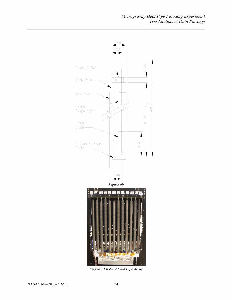
Microgravity Heat Pipe Flooding Experiment Test Equipment Data Package
NASA/TM—2013-216536 54
Figure 6b
Figure 7 Photo of Heat Pipe Array
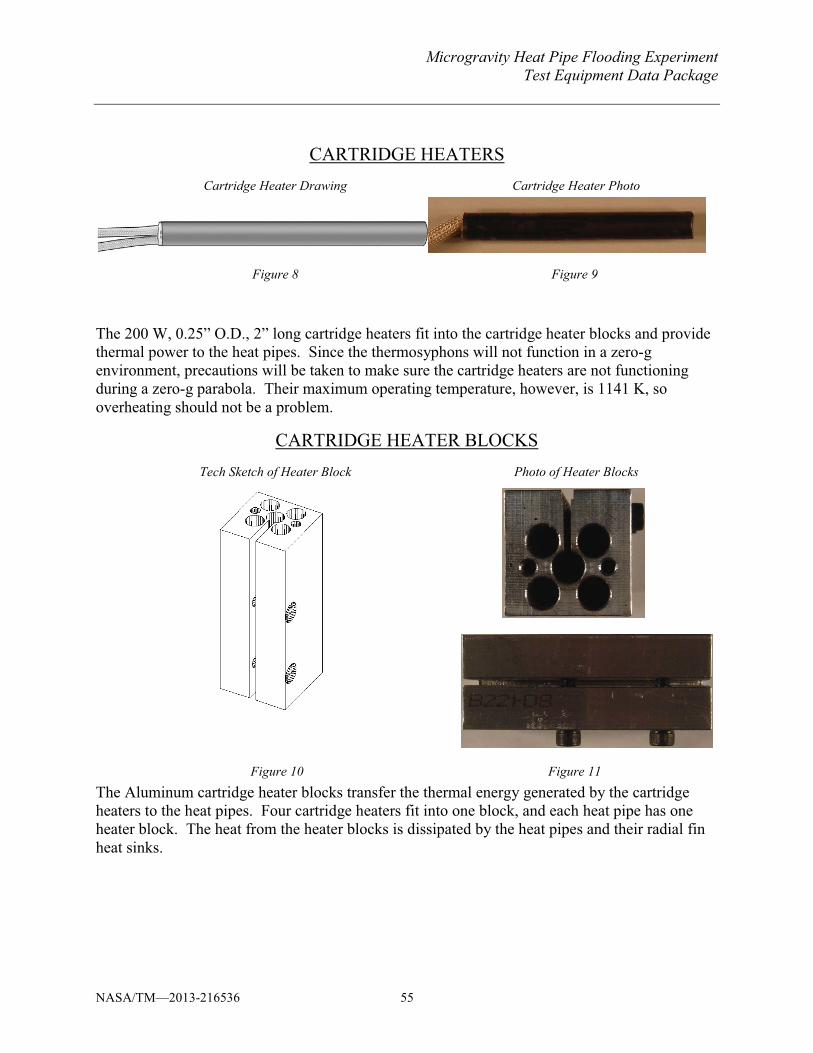
Microgravity Heat Pipe Flooding Experiment Test Equipment Data Package
NASA/TM—2013-216536 55
CARTRIDGE HEATERS Cartridge Heater Drawing Cartridge Heater Photo
Figure 8 Figure 9 The 200 W, 0.25” O.D., 2” long cartridge heaters fit into the cartridge heater blocks and provide thermal power to the heat pipes. Since the thermosyphons will not function in a zero-g environment, precautions will be taken to make sure the cartridge heaters are not functioning during a zero-g parabola. Their maximum operating temperature, however, is 1141 K, so overheating should not be a problem.
CARTRIDGE HEATER BLOCKS Tech Sketch of Heater Block Photo of Heater Blocks
Figure 10 Figure 11 The Aluminum cartridge heater blocks transfer the thermal energy generated by the cartridge heaters to the heat pipes. Four cartridge heaters fit into one block, and each heat pipe has one heater block. The heat from the heater blocks is dissipated by the heat pipes and their radial fin heat sinks.
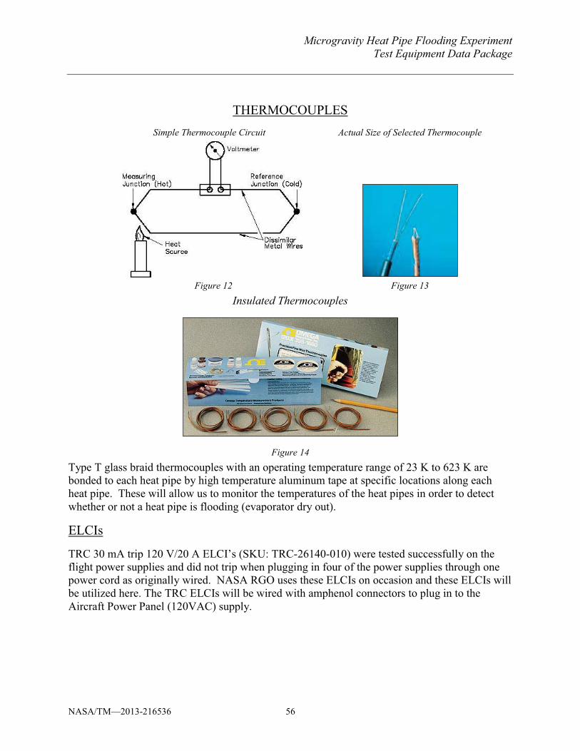
Microgravity Heat Pipe Flooding ExperimentTest Equipment Data Package
NASA/TM—2013-216536 56
THERMOCOUPLES Simple Thermocouple Circuit Actual Size of Selected Thermocouple
Figure 12 Figure 13
Insulated Thermocouples
Figure 14
Type T glass braid thermocouples with an operating temperature range of 23 K to 623 K are bonded to each heat pipe by high temperature aluminum tape at specific locations along each heat pipe. These will allow us to monitor the temperatures of the heat pipes in order to detect whether or not a heat pipe is flooding (evaporator dry out).
ELCIs
TRC 30 mA trip 120 V/20 A ELCI’s (SKU: TRC-26140-010) were tested successfully on the flight power supplies and did not trip when plugging in four of the power supplies through one power cord as originally wired. NASA RGO uses these ELCIs on occasion and these ELCIs will be utilized here. The TRC ELCIs will be wired with amphenol connectors to plug in to the Aircraft Power Panel (120VAC) supply.
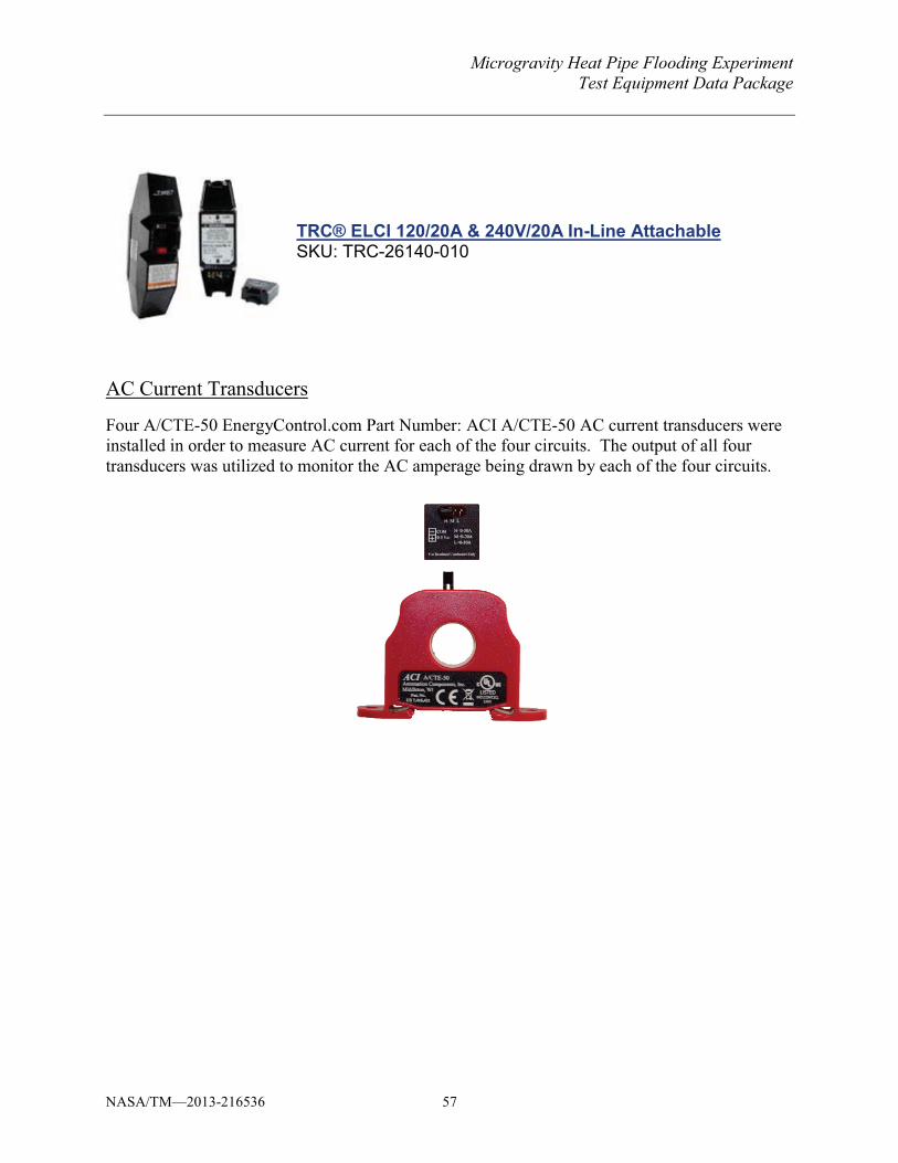
Microgravity Heat Pipe Flooding ExperimentTest Equipment Data Package
NASA/TM—2013-216536 57
TRC® ELCI 120/20A & 240V/20A In-Line Attachable SKU: TRC-26140-010
AC Current Transducers
Four A/CTE-50 EnergyControl.com Part Number: ACI A/CTE-50 AC current transducers were installed in order to measure AC current for each of the four circuits. The output of all four transducers was utilized to monitor the AC amperage being drawn by each of the four circuits.
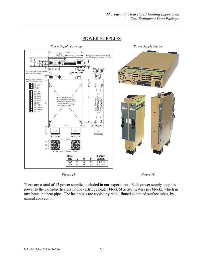
Microgravity Heat Pipe Flooding Experiment Test Equipment Data Package
NASA/TM—2013-216536 58
POWER SUPPLIES Power Supply Drawing Power Supply Photos
Figure 15 Figure 16
There are a total of 12 power supplies included in our experiment. Each power supply supplies power to the cartridge heaters in one cartridge heater block (4 active heaters per block), which in turn heats the heat pipe. The heat pipes are cooled by radial finned extended surface tubes, by natural convection.
Microgravity Heat Pipe Flooding Experiment Test Equipment Data Package
NASA/TM—2013-216536 59
POWER SUPPLY SPECIFICATIONS
Input Voltage: 90-265 VAC, 49-420 Hz, single phase, or 110-350 Vdc. 208 VAC 3-phase is also available (see Options). AC input (maximum): 8A (WL7 case), 12A (WL9 case) DC input (maximum): 5.75A (WL7 case), 8.8A (WL9 case). DC input may be connected without regard to polarity.
Inrush current: Cold start, (thermistor limiter) 33A peak @115 VAC (typical); 65A peak @ 230 VAC (typical).
Startup Time: 800 mS (typical).
Input Undervoltage: An input of less than 90 VAC will not damage power supply.
Power Factor:0.99 (typical) at 115 VAC, 60 Hz and full load. Complies with EN61000-3-2.
Regulation (in constant voltage mode): Line Regulation: ±0.05% Load Regulation: ±0.05%
Regulation, Ripple (in constant current mode): Line Regulation: ±0.2% or 30 mA. Load Regulation: ±0.5% or 100 mA. Current Ripple: 0.5% rms.
Ambient Operating Temperature: 0 to +71 °C.
Temperature Coefficient (after 30 minute warm-up): Voltage mode: ±0.02%/°C (typical). Current mode: ±0.1%/°C (typical).
Drift (voltage mode or current mode): ±0.1% (typical) over 8 hours, after 30 minute warmup.
Storage Temperature: –40 to +85°C.
Holdup Time: 20 mS minimum with full load.
Transient Response: 300 μS to return to ±1% of output setting. Maximum of ±3% output excursion following a load step change from 50 to 100%.
Polarity: Output is floating and may be used in either polarity.
Remote Sensing: Compensates up to 0.5 V drop per output line.
Output Adjustment: Voltage and current output adjustments are located on the front. Output adjustment may also be controlled by using remotely located potentiometers.
Output Programming: The output voltage and current may be programmed from 0 to full rating by means of control voltage inputs of 0 to +10 Vdc (0 to +5 Vdc for models with option “C5”). Voltage mode accuracy: 0.5%. Current mode accuracy: 3% for models with greater than 10 amps
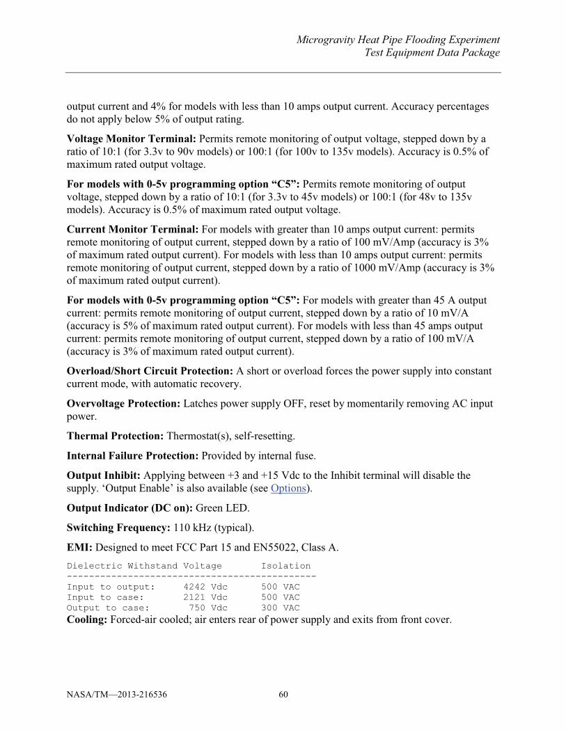
Microgravity Heat Pipe Flooding Experiment Test Equipment Data Package
NASA/TM—2013-216536 60
output current and 4% for models with less than 10 amps output current. Accuracy percentages do not apply below 5% of output rating.
Voltage Monitor Terminal: Permits remote monitoring of output voltage, stepped down by a ratio of 10:1 (for 3.3v to 90v models) or 100:1 (for 100v to 135v models). Accuracy is 0.5% of maximum rated output voltage.
For models with 0-5v programming option “C5”: Permits remote monitoring of output voltage, stepped down by a ratio of 10:1 (for 3.3v to 45v models) or 100:1 (for 48v to 135v models). Accuracy is 0.5% of maximum rated output voltage.
Current Monitor Terminal: For models with greater than 10 amps output current: permits remote monitoring of output current, stepped down by a ratio of 100 mV/Amp (accuracy is 3% of maximum rated output current). For models with less than 10 amps output current: permits remote monitoring of output current, stepped down by a ratio of 1000 mV/Amp (accuracy is 3% of maximum rated output current).
For models with 0-5v programming option “C5”: For models with greater than 45 A output current: permits remote monitoring of output current, stepped down by a ratio of 10 mV/A (accuracy is 5% of maximum rated output current). For models with less than 45 amps output current: permits remote monitoring of output current, stepped down by a ratio of 100 mV/A (accuracy is 3% of maximum rated output current).
Overload/Short Circuit Protection: A short or overload forces the power supply into constant current mode, with automatic recovery.
Overvoltage Protection: Latches power supply OFF, reset by momentarily removing AC input power.
Thermal Protection: Thermostat(s), self-resetting.
Internal Failure Protection: Provided by internal fuse.
Output Inhibit: Applying between +3 and +15 Vdc to the Inhibit terminal will disable the supply. ‘Output Enable’ is also available (see Options).
Output Indicator (DC on): Green LED.
Switching Frequency: 110 kHz (typical).
EMI: Designed to meet FCC Part 15 and EN55022, Class A. Dielectric Withstand Voltage Isolation --------------------------------------------- Input to output: 4242 Vdc 500 VAC Input to case: 2121 Vdc 500 VAC Output to case: 750 Vdc 300 VAC Cooling: Forced-air cooled; air enters rear of power supply and exits from front cover.
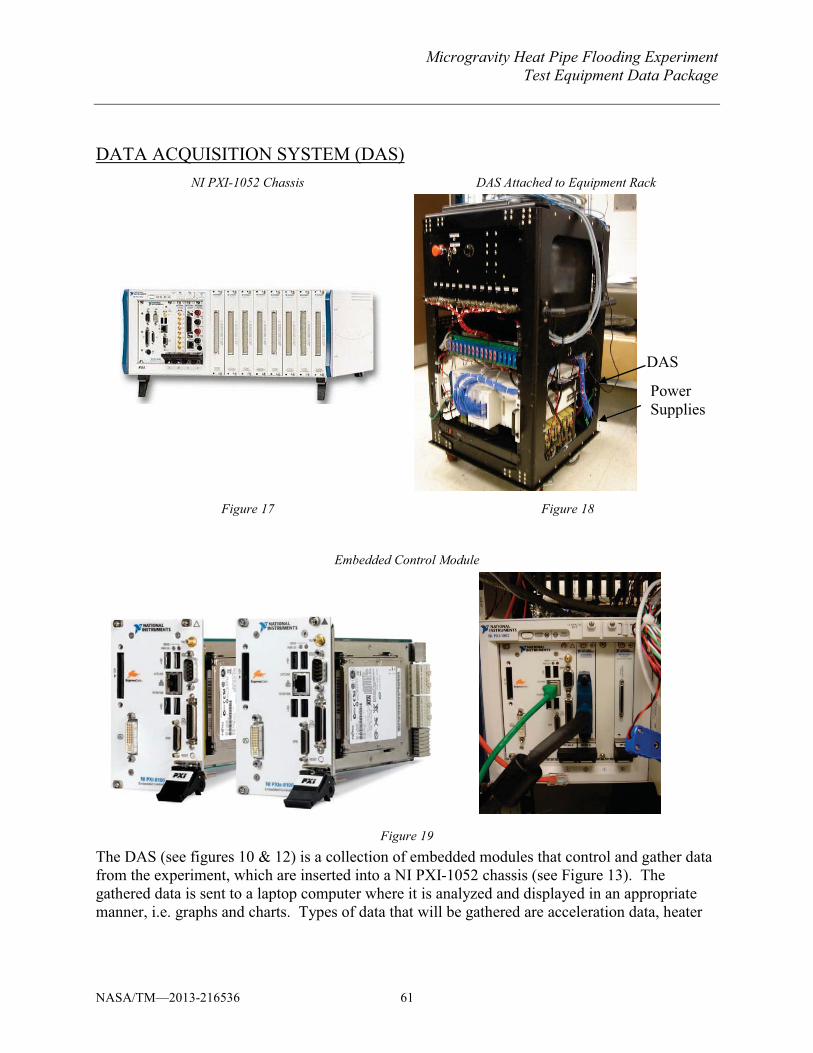
Microgravity Heat Pipe Flooding ExperimentTest Equipment Data Package
NASA/TM—2013-216536 61
DATA ACQUISITION SYSTEM (DAS) NI PXI-1052 Chassis DAS Attached to Equipment Rack
Figure 17 Figure 18
Embedded Control Module
Figure 19
The DAS (see figures 10 & 12) is a collection of embedded modules that control and gather data from the experiment, which are inserted into a NI PXI-1052 chassis (see Figure 13). The gathered data is sent to a laptop computer where it is analyzed and displayed in an appropriate manner, i.e. graphs and charts. Types of data that will be gathered are acceleration data, heater
DAS
Power Supplies
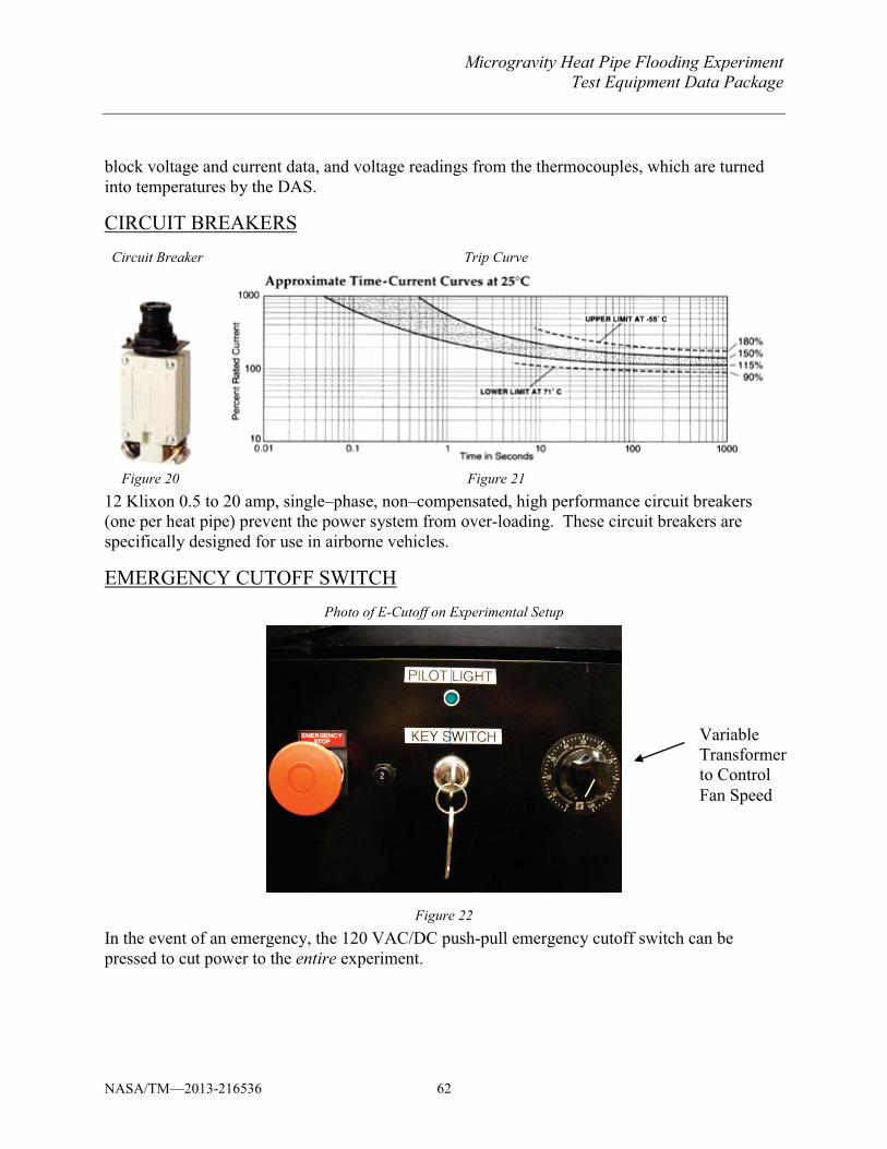
Microgravity Heat Pipe Flooding ExperimentTest Equipment Data Package
NASA/TM—2013-216536 62
block voltage and current data, and voltage readings from the thermocouples, which are turned into temperatures by the DAS.
CIRCUIT BREAKERS Circuit Breaker Trip Curve
Figure 20 Figure 21 12 Klixon 0.5 to 20 amp, single–phase, non–compensated, high performance circuit breakers (one per heat pipe) prevent the power system from over-loading. These circuit breakers are specifically designed for use in airborne vehicles.
EMERGENCY CUTOFF SWITCH Photo of E-Cutoff on Experimental Setup
Figure 22 In the event of an emergency, the 120 VAC/DC push-pull emergency cutoff switch can be pressed to cut power to the entire experiment.
Variable Transformer to Control Fan Speed
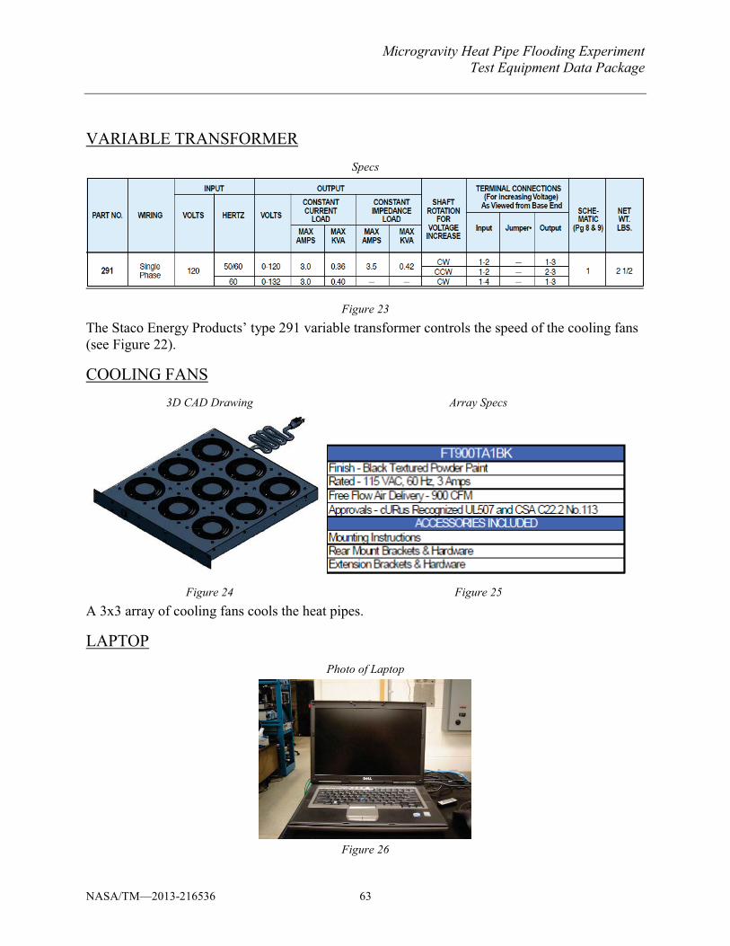
Microgravity Heat Pipe Flooding ExperimentTest Equipment Data Package
NASA/TM—2013-216536 63
VARIABLE TRANSFORMER Specs
Figure 23
The Staco Energy Products’ type 291 variable transformer controls the speed of the cooling fans (see Figure 22).
COOLING FANS3D CAD Drawing Array Specs
Figure 24 Figure 25 A 3x3 array of cooling fans cools the heat pipes.
LAPTOP Photo of Laptop
Figure 26
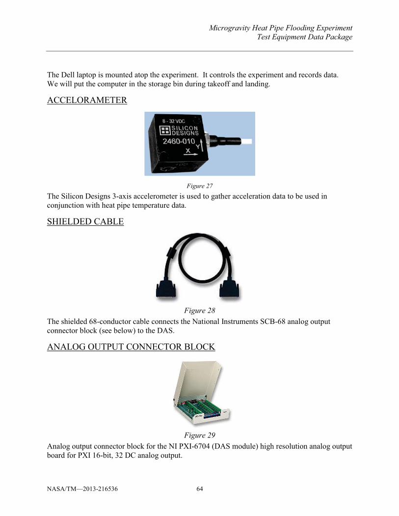
Microgravity Heat Pipe Flooding ExperimentTest Equipment Data Package
NASA/TM—2013-216536 64
The Dell laptop is mounted atop the experiment. It controls the experiment and records data. We will put the computer in the storage bin during takeoff and landing.
ACCELORAMETER
Figure 27
The Silicon Designs 3-axis accelerometer is used to gather acceleration data to be used in conjunction with heat pipe temperature data.
SHIELDED CABLE
Figure 28 The shielded 68-conductor cable connects the National Instruments SCB-68 analog output connector block (see below) to the DAS.
ANALOG OUTPUT CONNECTOR BLOCK
Figure 29
Analog output connector block for the NI PXI-6704 (DAS module) high resolution analog output board for PXI 16-bit, 32 DC analog output.
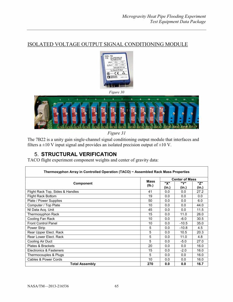
Microgravity Heat Pipe Flooding ExperimentTest Equipment Data Package
NASA/TM—2013-216536 65
ISOLATED VOLTAGE OUTPUT SIGNAL CONDITIONING MODULE
Figure 30
Figure 31 The 7B22 is a unity gain single-channel signal conditioning output module that interfaces and filters a ±10 V input signal and provides an isolated precision output of ±10 V.
STRUCTURAL VERIFICATION 5.TACO flight experiment component weights and center of gravity data:
Thermosyphon Array in Controlled Operation (TACO) ~ Assembled Rack Mass Properties
Component Mass (lb.)
Center of Mass "X" "Y" "Z" (in.) (in.) (in.)
Flight Rack Top, Sides & Handles 41 0.0 0.0 27.2 Flight Rack Bottom 19 0.0 0.0 0.0 Plate / Power Supplies 50 0.0 0.0 6.0 Computer / Top Plate 10 0.0 0.0 44.0 NI Data Acq. Unit 45 0.0 0.0 11.5 Thermosyphon Rack 15 0.0 11.0 26.0 Cooling Fan Rack 10 0.0 -6.0 30.5 Front Control Panel 10 0.0 -10.5 35.0 Power Strip 5 0.0 -10.8 4.5 Rear Upper Elect. Rack 5 0.0 10.5 20.3 Rear Lower Elect. Rack 5 0.0 11.0 4.8 Cooling Air Duct 5 0.0 -5.0 27.0Plates & Brackets 20 0.0 0.0 16.0 Electronics & Fasteners 15 0.0 -2.0 16.0 Thermocouples & Plugs 5 0.0 0.0 16.0 Cables & Power Cords 10 0.0 0.0 16.0
Total Assembly 270 0.0 0.0 16.7
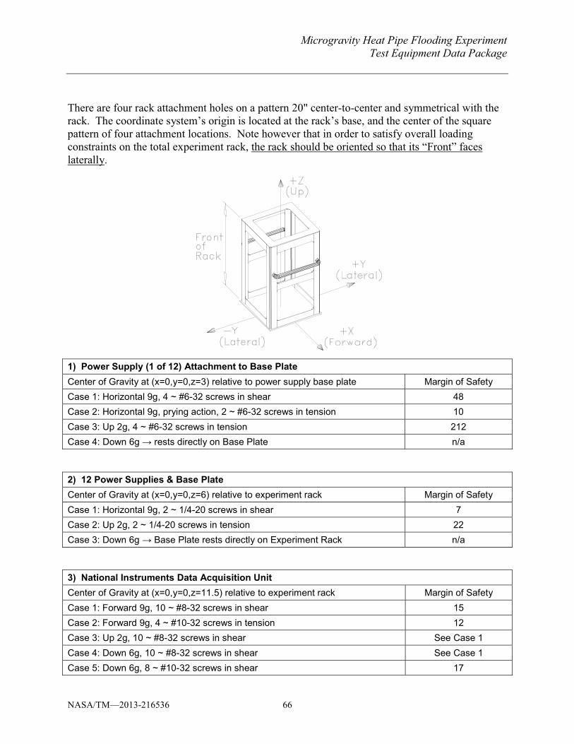
Microgravity Heat Pipe Flooding Experiment Test Equipment Data Package
NASA/TM—2013-216536 66
There are four rack attachment holes on a pattern 20" center-to-center and symmetrical with the rack. The coordinate system’s origin is located at the rack’s base, and the center of the square pattern of four attachment locations. Note however that in order to satisfy overall loading constraints on the total experiment rack, the rack should be oriented so that its “Front” faces laterally.
1) Power Supply (1 of 12) Attachment to Base Plate Center of Gravity at (x=0,y=0,z=3) relative to power supply base plate Margin of Safety Case 1: Horizontal 9g, 4 ~ #6-32 screws in shear 48 Case 2: Horizontal 9g, prying action, 2 ~ #6-32 screws in tension 10 Case 3: Up 2g, 4 ~ #6-32 screws in tension 212 ����������� ������������������������������� n/a
2) 12 Power Supplies & Base Plate Center of Gravity at (x=0,y=0,z=6) relative to experiment rack Margin of Safety Case 1: Horizontal 9g, 2 ~ 1/4-20 screws in shear 7 Case 2: Up 2g, 2 ~ 1/4-20 screws in tension 22 ����������� ����������������������������������������������� n/a
3) National Instruments Data Acquisition Unit Center of Gravity at (x=0,y=0,z=11.5) relative to experiment rack Margin of Safety Case 1: Forward 9g, 10 ~ #8-32 screws in shear 15 Case 2: Forward 9g, 4 ~ #10-32 screws in tension 12 Case 3: Up 2g, 10 ~ #8-32 screws in shear See Case 1 Case 4: Down 6g, 10 ~ #8-32 screws in shear See Case 1 Case 5: Down 6g, 8 ~ #10-32 screws in shear 17
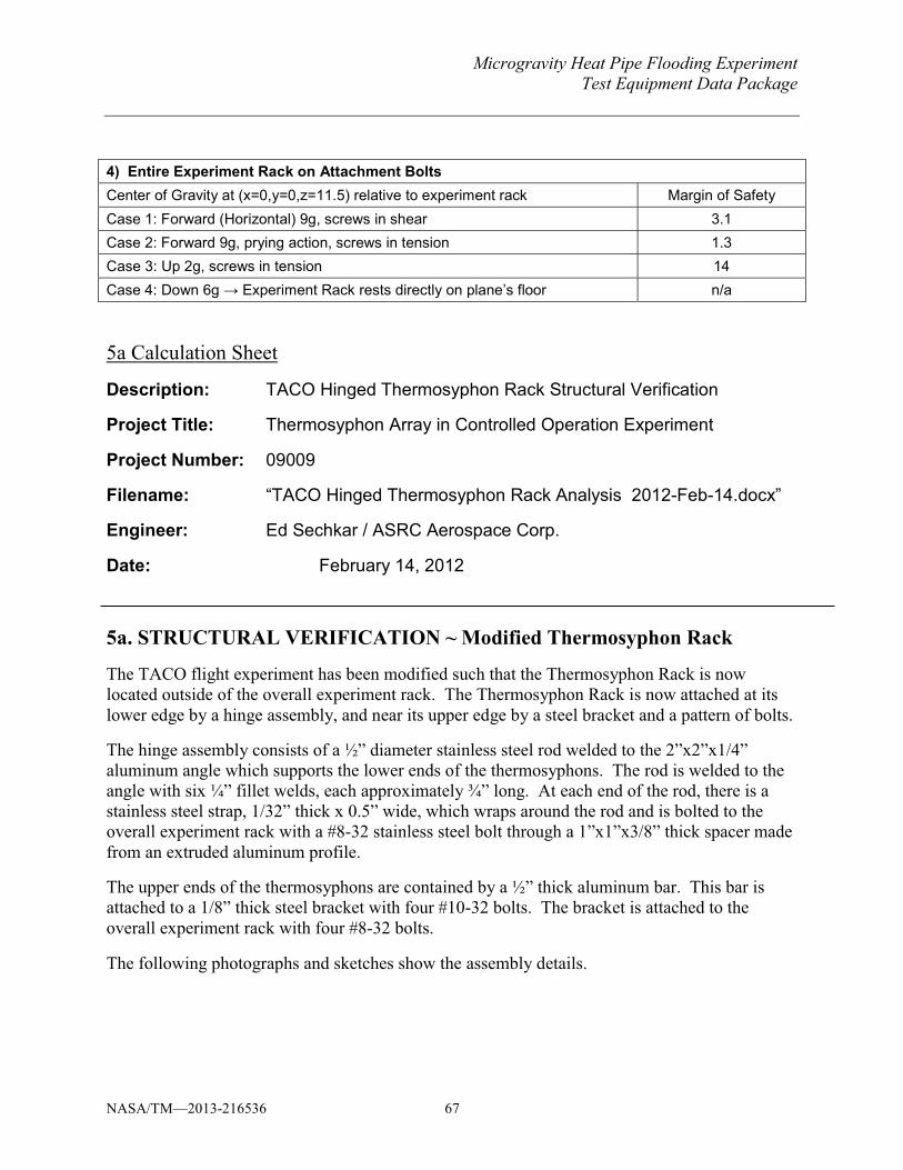
Microgravity Heat Pipe Flooding Experiment Test Equipment Data Package
NASA/TM—2013-216536 67
4) Entire Experiment Rack on Attachment Bolts Center of Gravity at (x=0,y=0,z=11.5) relative to experiment rack Margin of Safety Case 1: Forward (Horizontal) 9g, screws in shear 3.1 Case 2: Forward 9g, prying action, screws in tension 1.3 Case 3: Up 2g, screws in tension 14 ����������� ������������������������������������������!��"�� n/a
5a Calculation Sheet
Description: TACO Hinged Thermosyphon Rack Structural Verification
Project Title: Thermosyphon Array in Controlled Operation Experiment
Project Number: 09009
Filename: “TACO Hinged Thermosyphon Rack Analysis 2012-Feb-14.docx”
Engineer: Ed Sechkar / ASRC Aerospace Corp.
Date: February 14, 2012
5a. STRUCTURAL VERIFICATION ~ Modified Thermosyphon Rack
The TACO flight experiment has been modified such that the Thermosyphon Rack is now located outside of the overall experiment rack. The Thermosyphon Rack is now attached at its lower edge by a hinge assembly, and near its upper edge by a steel bracket and a pattern of bolts.
The hinge assembly consists of a ½” diameter stainless steel rod welded to the 2”x2”x1/4” aluminum angle which supports the lower ends of the thermosyphons. The rod is welded to the angle with six ¼” fillet welds, each approximately ¾” long. At each end of the rod, there is a stainless steel strap, 1/32” thick x 0.5” wide, which wraps around the rod and is bolted to the overall experiment rack with a #8-32 stainless steel bolt through a 1”x1”x3/8” thick spacer made from an extruded aluminum profile.
The upper ends of the thermosyphons are contained by a ½” thick aluminum bar. This bar is attached to a 1/8” thick steel bracket with four #10-32 bolts. The bracket is attached to the overall experiment rack with four #8-32 bolts.
The following photographs and sketches show the assembly details.
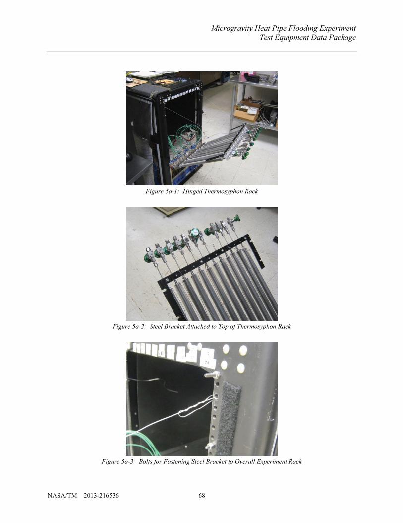
Microgravity Heat Pipe Flooding Experiment Test Equipment Data Package
NASA/TM—2013-216536 68
Figure 5a-1: Hinged Thermosyphon Rack
Figure 5a-2: Steel Bracket Attached to Top of Thermosyphon Rack
Figure 5a-3: Bolts for Fastening Steel Bracket to Overall Experiment Rack
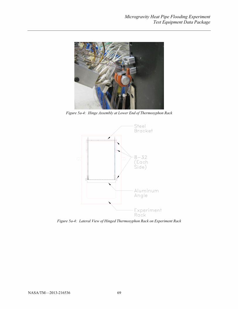
Microgravity Heat Pipe Flooding Experiment Test Equipment Data Package
NASA/TM—2013-216536 69
Figure 5a-4: Hinge Assembly at Lower End of Thermosyphon Rack
Figure 5a-4: Lateral View of Hinged Thermosyphon Rack on Experiment Rack
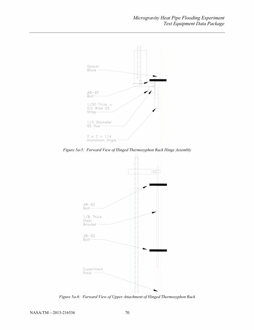
Microgravity Heat Pipe Flooding Experiment Test Equipment Data Package
NASA/TM—2013-216536 70
Figure 5a-5: Forward View of Hinged Thermosyphon Rack Hinge Assembly
Figure 5a-6: Forward View of Upper Attachment of Hinged Thermosyphon Rack
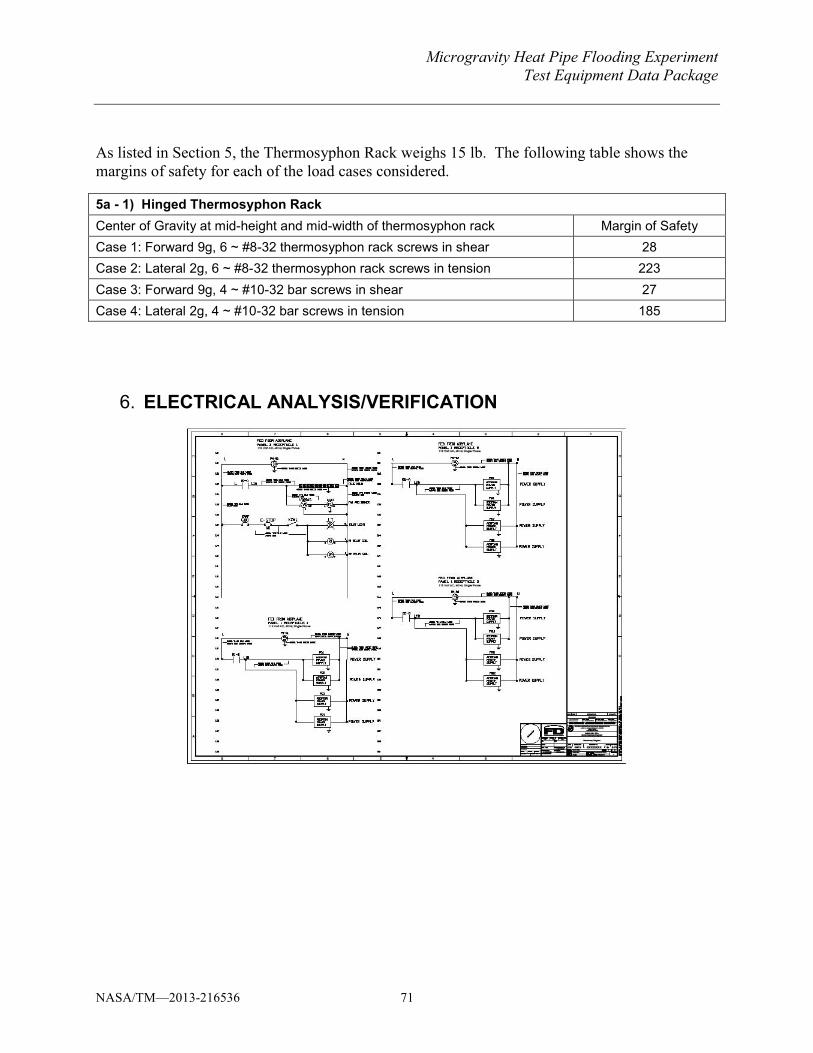
Microgravity Heat Pipe Flooding Experiment Test Equipment Data Package
NASA/TM—2013-216536 71
As listed in Section 5, the Thermosyphon Rack weighs 15 lb. The following table shows the margins of safety for each of the load cases considered.
5a - 1) Hinged Thermosyphon Rack Center of Gravity at mid-height and mid-width of thermosyphon rack Margin of Safety Case 1: Forward 9g, 6 ~ #8-32 thermosyphon rack screws in shear 28 Case 2: Lateral 2g, 6 ~ #8-32 thermosyphon rack screws in tension 223 Case 3: Forward 9g, 4 ~ #10-32 bar screws in shear 27 Case 4: Lateral 2g, 4 ~ #10-32 bar screws in tension 185
ELECTRICAL ANALYSIS/VERIFICATION 6.
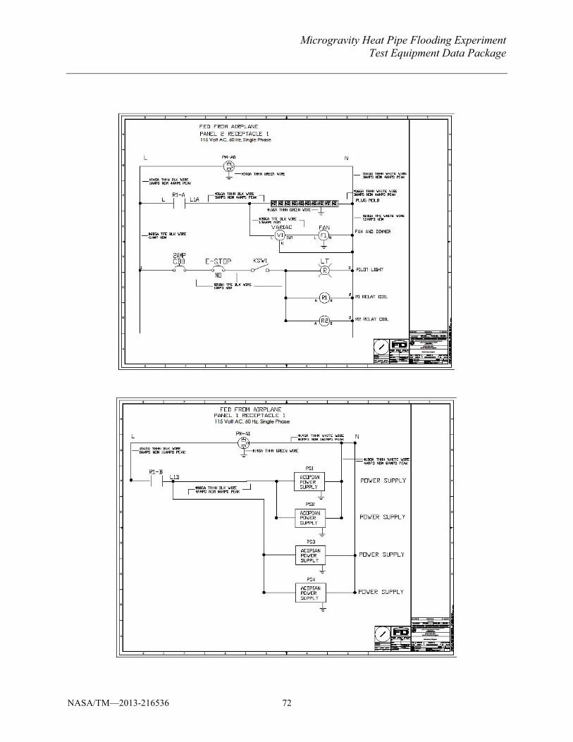
Microgravity Heat Pipe Flooding Experiment Test Equipment Data Package
NASA/TM—2013-216536 72
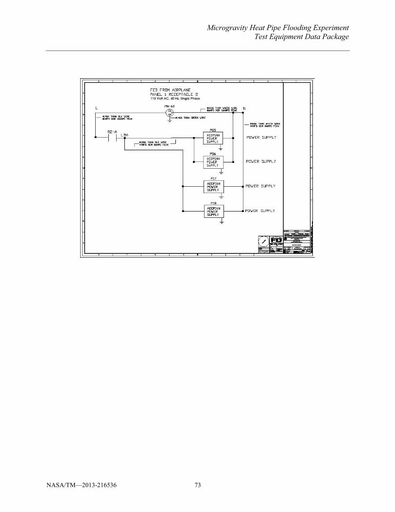
Microgravity Heat Pipe Flooding Experiment Test Equipment Data Package
NASA/TM—2013-216536 73
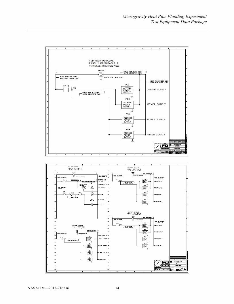
Microgravity Heat Pipe Flooding Experiment Test Equipment Data Package
NASA/TM—2013-216536 74
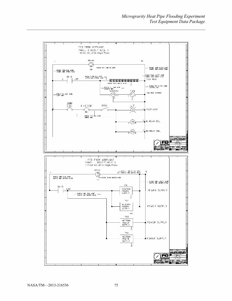
Microgravity Heat Pipe Flooding Experiment Test Equipment Data Package
NASA/TM—2013-216536 75
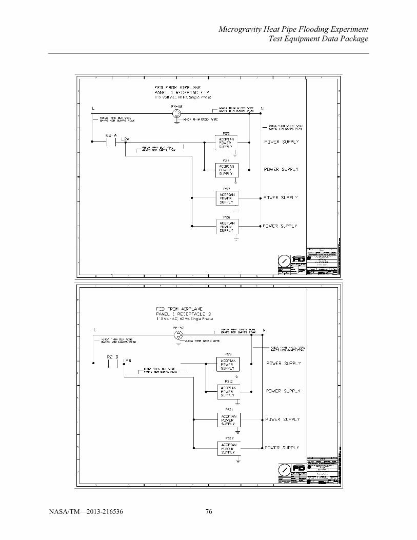
Microgravity Heat Pipe Flooding Experiment Test Equipment Data Package
NASA/TM—2013-216536 76
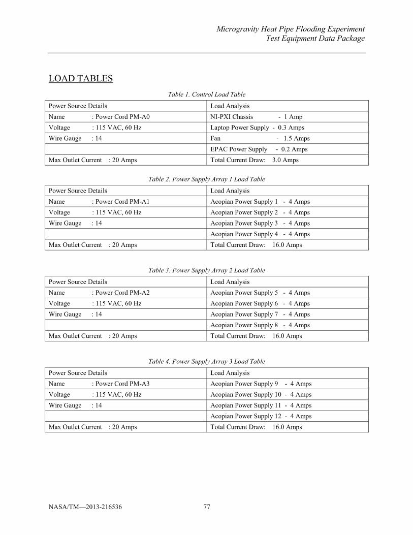
Microgravity Heat Pipe Flooding Experiment Test Equipment Data Package
NASA/TM—2013-216536 77
LOAD TABLES Table 1. Control Load Table
Power Source Details Load Analysis Name : Power Cord PM-A0 NI-PXI Chassis - 1 Amp Voltage : 115 VAC, 60 Hz Laptop Power Supply - 0.3 Amps Wire Gauge : 14 Fan - 1.5 Amps EPAC Power Supply - 0.2 Amps Max Outlet Current : 20 Amps Total Current Draw: 3.0 Amps
Table 2. Power Supply Array 1 Load Table
Power Source Details Load Analysis Name : Power Cord PM-A1 Acopian Power Supply 1 - 4 Amps Voltage : 115 VAC, 60 Hz Acopian Power Supply 2 - 4 Amps Wire Gauge : 14 Acopian Power Supply 3 - 4 Amps Acopian Power Supply 4 - 4 Amps Max Outlet Current : 20 Amps Total Current Draw: 16.0 Amps
Table 3. Power Supply Array 2 Load Table
Power Source Details Load Analysis Name : Power Cord PM-A2 Acopian Power Supply 5 - 4 Amps Voltage : 115 VAC, 60 Hz Acopian Power Supply 6 - 4 Amps Wire Gauge : 14 Acopian Power Supply 7 - 4 Amps Acopian Power Supply 8 - 4 Amps Max Outlet Current : 20 Amps Total Current Draw: 16.0 Amps
Table 4. Power Supply Array 3 Load Table
Power Source Details Load Analysis Name : Power Cord PM-A3 Acopian Power Supply 9 - 4 Amps Voltage : 115 VAC, 60 Hz Acopian Power Supply 10 - 4 Amps Wire Gauge : 14 Acopian Power Supply 11 - 4 Amps Acopian Power Supply 12 - 4 Amps Max Outlet Current : 20 Amps Total Current Draw: 16.0 Amps
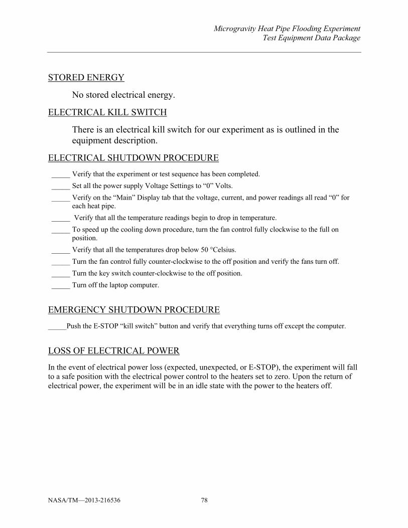
Microgravity Heat Pipe Flooding Experiment Test Equipment Data Package
NASA/TM—2013-216536 78
STORED ENERGY
No stored electrical energy.
ELECTRICAL KILL SWITCH
There is an electrical kill switch for our experiment as is outlined in the equipment description.
ELECTRICAL SHUTDOWN PROCEDURE
_____ Verify that the experiment or test sequence has been completed. _____ Set all the power supply Voltage Settings to “0” Volts. _____ Verify on the “Main” Display tab that the voltage, current, and power readings all read “0” for
each heat pipe. _____ Verify that all the temperature readings begin to drop in temperature. _____ To speed up the cooling down procedure, turn the fan control fully clockwise to the full on
position. _____ Verify that all the temperatures drop below 50 °Celsius. _____ Turn the fan control fully counter-clockwise to the off position and verify the fans turn off. _____ Turn the key switch counter-clockwise to the off position. _____ Turn off the laptop computer.
EMERGENCY SHUTDOWN PROCEDURE
_____Push the E-STOP “kill switch” button and verify that everything turns off except the computer.
LOSS OF ELECTRICAL POWER
In the event of electrical power loss (expected, unexpected, or E-STOP), the experiment will fall to a safe position with the electrical power control to the heaters set to zero. Upon the return of electrical power, the experiment will be in an idle state with the power to the heaters off.
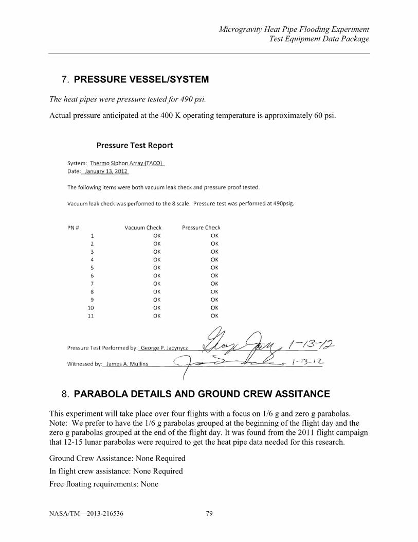
Microgravity Heat Pipe Flooding ExperimentTest Equipment Data Package
NASA/TM—2013-216536 79
PRESSURE VESSEL/SYSTEM 7.
The heat pipes were pressure tested for 490 psi.
Actual pressure anticipated at the 400 K operating temperature is approximately 60 psi.
PARABOLA DETAILS AND GROUND CREW ASSITANCE 8.
This experiment will take place over four flights with a focus on 1/6 g and zero g parabolas. Note: We prefer to have the 1/6 g parabolas grouped at the beginning of the flight day and the zero g parabolas grouped at the end of the flight day. It was found from the 2011 flight campaign that 12-15 lunar parabolas were required to get the heat pipe data needed for this research.
Ground Crew Assistance: None Required In flight crew assistance: None Required Free floating requirements: None
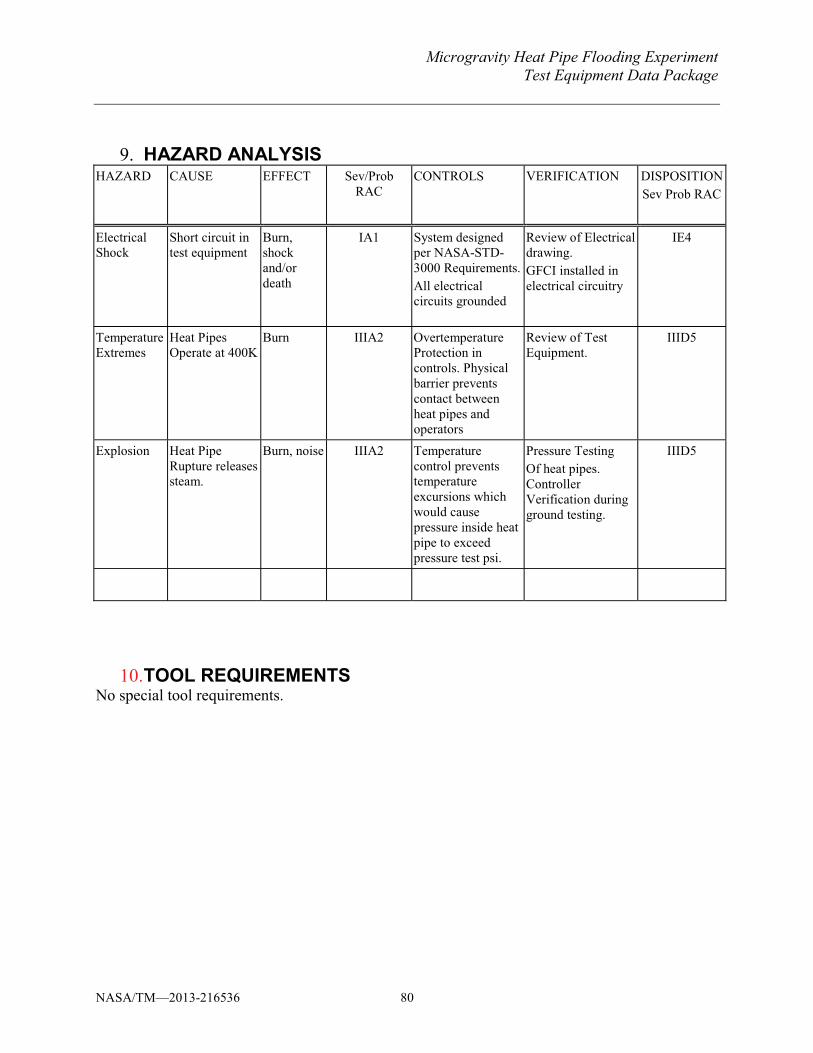
Microgravity Heat Pipe Flooding Experiment Test Equipment Data Package
NASA/TM—2013-216536 80
HAZARD ANALYSIS 9.HAZARD CAUSE EFFECT Sev/Prob
RAC CONTROLS VERIFICATION DISPOSITION
Sev Prob RAC
Electrical Shock
Short circuit in test equipment
Burn, shock and/or death
IA1 System designed per NASA-STD-3000 Requirements. All electrical circuits grounded
Review of Electrical drawing. GFCI installed in electrical circuitry
IE4
Temperature Extremes
Heat Pipes Operate at 400K
Burn IIIA2 Overtemperature Protection in controls. Physical barrier prevents contact between heat pipes and operators
Review of Test Equipment.
IIID5
Explosion Heat Pipe Rupture releases steam.
Burn, noise IIIA2 Temperature control prevents temperature excursions which would cause pressure inside heat pipe to exceed pressure test psi.
Pressure Testing Of heat pipes. Controller Verification during ground testing.
IIID5
TOOL REQUIREMENTS 10.No special tool requirements.
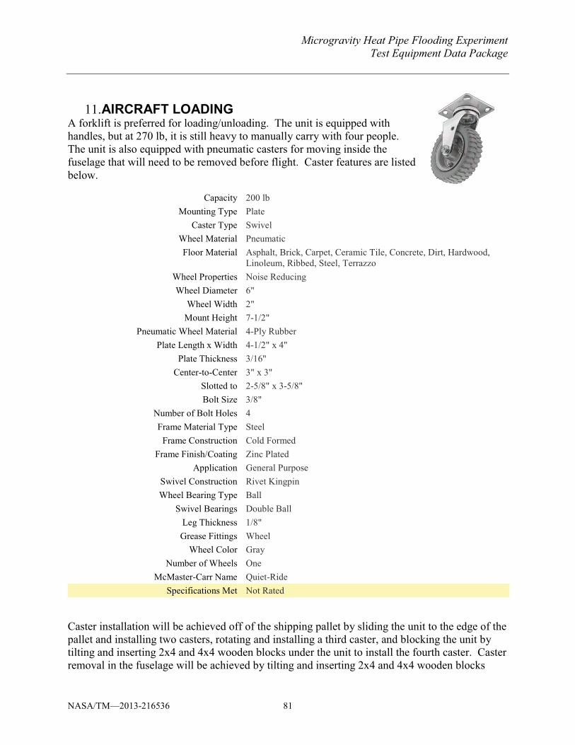
Microgravity Heat Pipe Flooding Experiment Test Equipment Data Package
NASA/TM—2013-216536 81
AIRCRAFT LOADING 11.A forklift is preferred for loading/unloading. The unit is equipped with handles, but at 270 lb, it is still heavy to manually carry with four people. The unit is also equipped with pneumatic casters for moving inside the fuselage that will need to be removed before flight. Caster features are listed below.
Capacity 200 lb Mounting Type Plate
Caster Type Swivel Wheel Material Pneumatic Floor Material Asphalt, Brick, Carpet, Ceramic Tile, Concrete, Dirt, Hardwood,
Linoleum, Ribbed, Steel, Terrazzo Wheel Properties Noise Reducing Wheel Diameter 6"
Wheel Width 2" Mount Height 7-1/2"
Pneumatic Wheel Material 4-Ply Rubber Plate Length x Width 4-1/2" x 4"
Plate Thickness 3/16" Center-to-Center 3" x 3"
Slotted to 2-5/8" x 3-5/8" Bolt Size 3/8"
Number of Bolt Holes 4 Frame Material Type Steel
Frame Construction Cold Formed Frame Finish/Coating Zinc Plated
Application General Purpose Swivel Construction Rivet Kingpin Wheel Bearing Type Ball
Swivel Bearings Double Ball Leg Thickness 1/8" Grease Fittings Wheel
Wheel Color Gray Number of Wheels One
McMaster-Carr Name Quiet-Ride Specifications Met Not Rated
Caster installation will be achieved off of the shipping pallet by sliding the unit to the edge of the pallet and installing two casters, rotating and installing a third caster, and blocking the unit by tilting and inserting 2x4 and 4x4 wooden blocks under the unit to install the fourth caster. Caster removal in the fuselage will be achieved by tilting and inserting 2x4 and 4x4 wooden blocks
Microgravity Heat Pipe Flooding Experiment Test Equipment Data Package
NASA/TM—2013-216536 82
under the unit with subsequent tilting and removal of the wooden blocks until the unit is at floor level.
GROUND SUPPORT REQUIREMENTS 12.Four 120v power outlets will be required on site in order to warm up the heat pipes. During the 2011 flight campaign, we were placed in the high bay were we could use the simulated aircraft power supplies which was needed for our special ground fault interrupter circuits listed above.
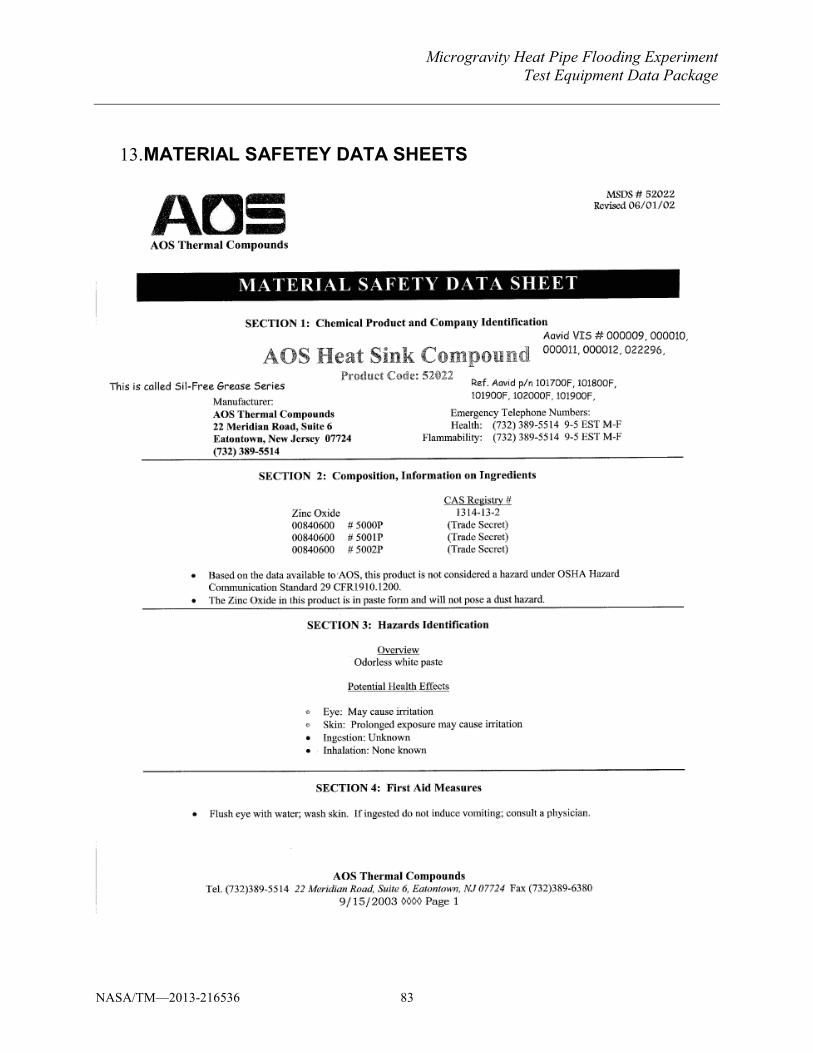
Microgravity Heat Pipe Flooding ExperimentTest Equipment Data Package
NASA/TM—2013-216536 83
MATERIAL SAFETEY DATA SHEETS 13.
Microgravity Heat Pipe Flooding ExperimentTest Equipment Data Package
NASA/TM—2013-216536 84
Microgravity Heat Pipe Flooding ExperimentTest Equipment Data Package
NASA/TM—2013-216536 85
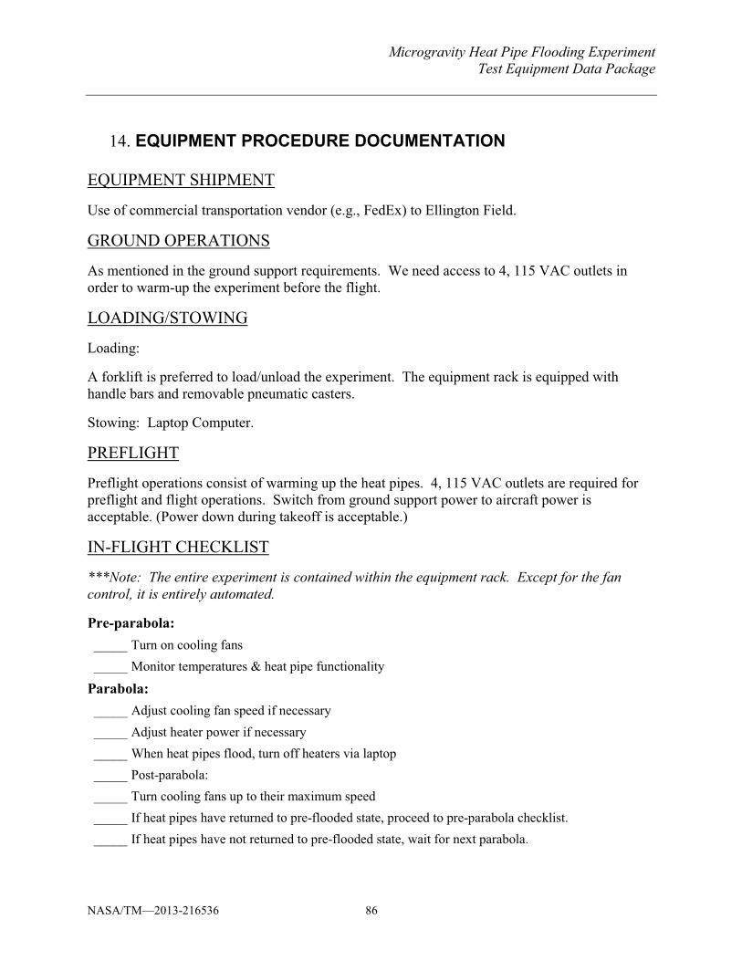
Microgravity Heat Pipe Flooding Experiment Test Equipment Data Package
NASA/TM—2013-216536 86
EQUIPMENT PROCEDURE DOCUMENTATION 14. EQUIPMENT SHIPMENT
Use of commercial transportation vendor (e.g., FedEx) to Ellington Field.
GROUND OPERATIONS
As mentioned in the ground support requirements. We need access to 4, 115 VAC outlets in order to warm-up the experiment before the flight.
LOADING/STOWING
Loading:
A forklift is preferred to load/unload the experiment. The equipment rack is equipped with handle bars and removable pneumatic casters.
Stowing: Laptop Computer.
PREFLIGHT
Preflight operations consist of warming up the heat pipes. 4, 115 VAC outlets are required for preflight and flight operations. Switch from ground support power to aircraft power is acceptable. (Power down during takeoff is acceptable.)
IN-FLIGHT CHECKLIST
***Note: The entire experiment is contained within the equipment rack. Except for the fan control, it is entirely automated.
Pre-parabola: _____ Turn on cooling fans _____ Monitor temperatures & heat pipe functionality
Parabola: _____ Adjust cooling fan speed if necessary _____ Adjust heater power if necessary _____ When heat pipes flood, turn off heaters via laptop _____ Post-parabola: _____ Turn cooling fans up to their maximum speed _____ If heat pipes have returned to pre-flooded state, proceed to pre-parabola checklist. _____ If heat pipes have not returned to pre-flooded state, wait for next parabola.
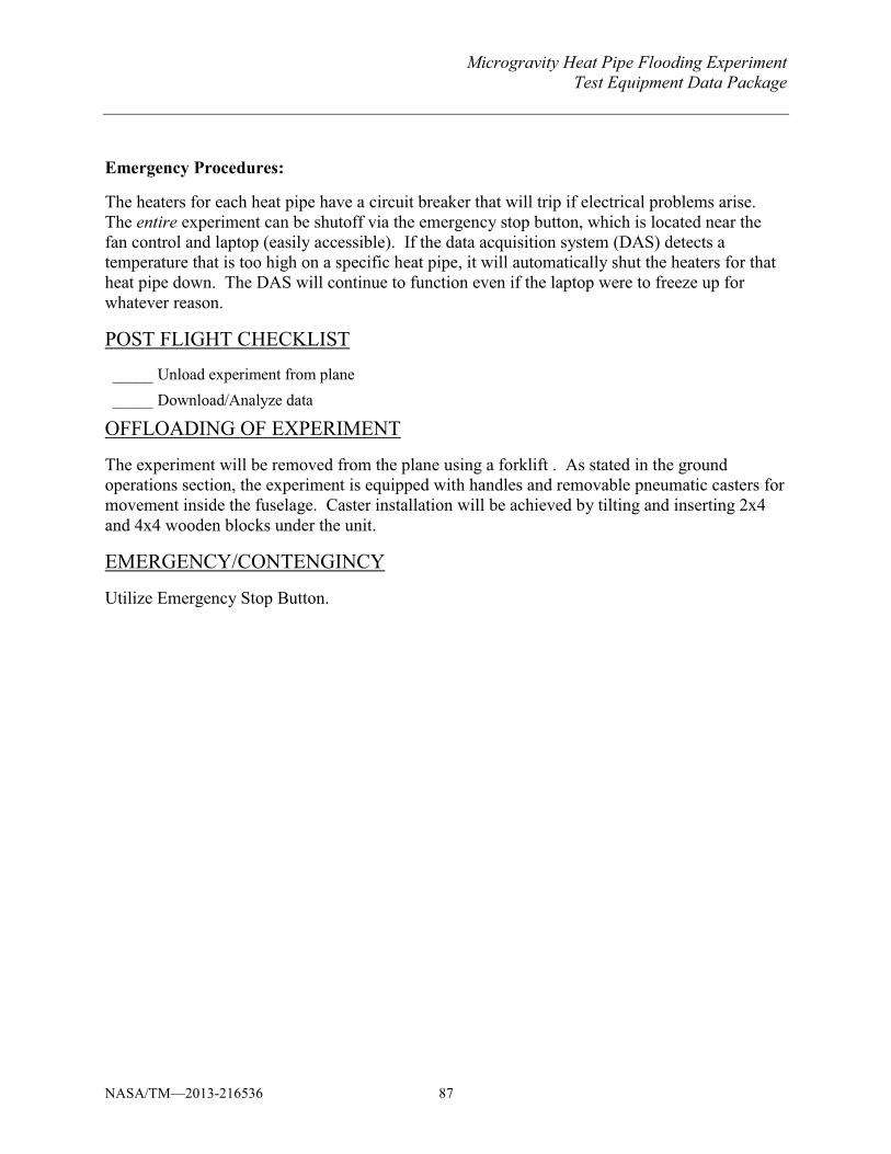
Microgravity Heat Pipe Flooding Experiment Test Equipment Data Package
NASA/TM—2013-216536 87
Emergency Procedures:
The heaters for each heat pipe have a circuit breaker that will trip if electrical problems arise. The entire experiment can be shutoff via the emergency stop button, which is located near the fan control and laptop (easily accessible). If the data acquisition system (DAS) detects a temperature that is too high on a specific heat pipe, it will automatically shut the heaters for that heat pipe down. The DAS will continue to function even if the laptop were to freeze up for whatever reason.
POST FLIGHT CHECKLIST
_____ Unload experiment from plane _____ Download/Analyze data
OFFLOADING OF EXPERIMENT
The experiment will be removed from the plane using a forklift . As stated in the ground operations section, the experiment is equipped with handles and removable pneumatic casters for movement inside the fuselage. Caster installation will be achieved by tilting and inserting 2x4 and 4x4 wooden blocks under the unit.
EMERGENCY/CONTENGINCY
Utilize Emergency Stop Button.
Microgravity Heat Pipe Flooding Experiment Test Equipment Data Package
NASA/TM—2013-216536 88
ELECTRICAL QUESTIONNAIRE 15. For completion by research teams flying on RGO Aircraft through the Flight Opportunities Program
Please answer the following question with verified and measured parameters:
1. Organization Name:____________NASA GRC FP06__________________
2. Contact Name:__Marc Gibson________________________Phone:__216-433-5562___
Email:[email protected]________________
3. Aircraft Electrical Power Requirements (actual measured ):
a. 115VAC: Normal Current:___16A______ Max Current:____20A____
Phase:__Single___
b. 28VDC: Normal Current:____N/A_____ Max Current:____N/A____
4. Emergency Shut Down Capability with kill switch in easy access location?
_____YES____
5. Grounding: Exposed metal surfaces were adequately grounded to prevent electrical
shock. Y/N:___Y____
6. Electromagnetic Compatibility:
a. Wireless device usage Y/N: __N__; Model:____N/A___ Manuf:________ N/A
________
b. Frequency:____ N/A ____ RF Transmit Power:___ N/A __ FCC approved:
Y/N:____ N/A _
c. Maximum voltage and current generate if
applicable:_____75VDC___3.8ADC_______
d. Motor usage Y/N: __N___ Motor type:_____ N/A _____Model:______ N/A
__________
Brushed Motor Y/N:__N_____EMI checked Y/N:_____N/A________
e. High voltage generator (spark)? Y/N:___N___ Max Voltage and Current:_____
N/A ___
f. EMI checked Y/N:__N/A__
Microgravity Heat Pipe Flooding Experiment Test Equipment Data Package
NASA/TM—2013-216536 89
7. Battery type: _____ N/A _________ Specification:_____ N/A
_______________________________
8. Circuit breaker Y/N:__Y___ Specification:____2 and_4ADC_, 20A
ELCI______________
9. Potential liquid in contact with electrical circuitry Y/N: __N____ Mitigation Y/N:____
N/A _____
10. Identified other potential electrical hazard and safety that was not identified in the TEDP
Y/N: __N__ If yes, provide description
___________________________________________
________________________________________________________________________
________________________________________________________________________
If you have questions, please contact: Cap V. Nguyen, [email protected]
NASA/TM—2013-216536 90
Bibliography 1. Mason, Lee, Poston, David and Qualls, Louis. System Concepts for Affordable Fission Surface Power. Cleveland : NASA/TM, 2008. TM. 2008-215166. 2. Heat Transfer Characteristics in Two-Phase Closed Conventional And Concentric Annular Thermosyphons. Faghri, A., Chen, M. M. and Morgan, M. Houston : ASME, 1998. 1988 National Heat Transfer Conference. pp. 291-303. 3. Entrainment Limits in Heat Pipes. Tien, C. L. and Chung, K. S. 1979, AIAA, pp. 643-646. 4. Wallis, G. B. One-Dimensional Two-Phase Flow. New York : McGraw-Hill, 1969. 5. Elements of Hydrodynamics of Gas-Liquid Systems. Kutateladze, S. S. 1972, Fluid Mechanics-Soviet Research, pp. 29-50. 6. The Hanging Film Phenomenon in Vertical Annular Two-Phase Flow. Wallis, G. B. and Makkenchery, S. 1974, J. Fluids Eng., pp. 297-298. 7. Critical heat flux in two phase closed thermosyphons. Imura, H., et al. 1983, J. Heat Mass Transfer, pp. 1181-1188. 8. Dunn, P D and Reay, D A. Heat Pipes. New York : Pergamon Press Inc., 1982. 9. Theory of the Ultimate Heat Transfer Limit of Cylindrical Heat Pipes. Busse, C. A. 1973, Int. J. Heat Mass Transfer, pp. 169-186. 10. Faghri, Amir. Heat Pipe Science and Technololgy. New York, NY 10001 : Taylor and Frances, 1995. 11. Vapor Flow Considerations in Conventional and Gravity-Assisted Heat Pipes. Kemme, J. E. Bologna : s.n., 1976. Proc. 2cd Intl. Heat Pipe Conf. pp. 11-22. 12. Theorecticl Investigation of Heat Pipes Operating at Low Vapor Pressures. Levy, E. K. 1968, ASME J. Engineering Industry, Vol. 90, pp. 547-552. 13. A Visualization Study of Flooding and Entrainment in a closed Two-Phase Thermosyphon. Shatto, D. P., Besly, J. A. and Peterson, G. P. New Orleans, LA : AIAA, 1996. 31st Thermophysics Conference. 14. Performance Limits of Gravity-Assisted HEat Pipes. Prenger, F. C. 1984, Proc. 5th Int. Heat Pipe Conf. , pp. 1-5. 15. An analytical study on the critical heat flux of countercurrent boiling in a vertical tube with a closed bottom. Katto, Y. and Watanabe, K. 1992, Int. J. Heat Mass Transfer, pp. 3021-3028. 16. Summary of the Manufacture, Testing, and Model Valication of a Full-Scale Radiator for Fission Surface Power Applications. Ellis, David, Calder, James and Siamidis, John. Albuquerque : s.n., 2011. Proc. of Nuclear and Emerging Technologies for Space.

