Calhoun: The NPS Institutional Archive

Theses and Dissertations Thesis Collection

1990-06

The exploration of an alternative to acceptance sampling

Hammons, Craig A.

Monterey, California: Naval Postgraduate School

http://hdl.handle.net/10945/27752

AD-A237 602iiiIIU11IE~II I ill

NAVAL POSTGRADUATE SCHOOLMonterey, California T c

IW

_.STT JUN 2 199 1

THESIS

TIHE EXPLORATION OF AN ALTERNATIVE

TO ACCEPTANCE SAMPLING

by

Craig A. Ilammons

June 1990

Thesis Advisor G. F. Lindsay

Approved for public release; distribution is unlimited.

91-03061I'lll ill!1UlII~(49l !illIl

Unclassifiedsecurity classification of tis pae

REPORT' 0UC\ ENTATION PAGEI a Report Security Classification Unclassified l b Restrictive m arkings

2a Security Clwzsiftcation Authority 3 Distribution Availability of Report2b Declassification Do%% nirading Schedule Approved for public release: dlistribution is unlimited..4 Performing Organization Rcport Numiber(s) 5 Monitoring Organization Report Number(s)

~aNm fPromn raiain6b Office Symbol -7i.Name of Monitoiing-OrganizatonNaval Postgraduate School fif applicable) 30 iNaval Postgraduate School ~

(-c Address (cry, state, and ZIP code) 7b Addrebs (cin, state, and ZIP code,'Monterey. CA 93943-5000 Mlonterev. CA 93943-5000Sa Name of Funding Sponsoring Organization 8b Office S~inbul -9Rcurenjqi.t lnsyuinent Identification Number

I(if apIkahle ____________________________________________

Sc Address (city, stt, and ZiI' codep It) Source of Funding Numbers___________________________________________________Program Element No IProtect \o Il1ask No Iwork Unit Accession No

I1 I ItWe I n, 111d srrufir cka7yra i, 1T1lE FNl'l OR.\l 10N 01 AN AL-IlFR1N~\ IVE '10 ACCEPTANCE SAMPLING12 Plersoila! Author(s) Crai2 A. Iiasnrnons13a1 1 ype of Report 13b Iline covc.'ed 1.4 Date of Report (Year, mionth, daY,' 153 Page CouItMast~er's Thesis IFrom Tro T une Fl90 I (,I

1-~ mn;r \outtw T[he \ ie, expiet ed in this thesis aie those of the author and do not reflct the officiatl policy or po-sition of the Depaittnent of Dlei.nso oi the *.S. Governinent.

- Cosati Codc' IS~ Subje~t I erm ci o~nine oti reircs U/ neeessam and id kf i block ,~l~

Fild irou:' Suc vrord processing. Script. GMIL, text processhIn.

19 :\hstraCt o .?!.u n rcversp I ,ilc'aa denlyl1- ii : nuoabe?I hi thesis consideis the probkni of e~aluating, a producer's prounam in statistical process control, fromn tile standpoint

of the conwirir A model is po, tulatcd rclkacing2 the xariability, in proportion nonconforming of a process and the chiarac-teritics of the fial contiol jiart in thle ProLCeS. Flom this the stead, -state solution to a *\arko% chiain is used to find theoutput proportion nonconlbnning of the process.

21) Distribution Aw aiiabrlrt% of \b~tr.aci 21 Abstra,:, Sceurit ClassificationLITICIRS5ified V11ilr'tCd 0 S s rerOrt D 1) 1 IC tlqorq t. nelasilied

2-a N ame of Responsie lnd;\idurd 2.,0 1 clennone znucArt'a Q(, --c olice Sym(1 olG. F. I indsav (40S) 6 46-2N'% 541 ,

DD) FORMl 1473.&; MIAR 1,3 AP'R cdit,on ma\ bv, used unti! c~husted seu ~C~mislicationl of tis page'All otlhcr eultions are obsuiev:

Unclassified

Approved for public release; distribution is unlimited.

The Exploration of an Alternative

to Acceptance Sampling

by

Craig A. HammonsLieutenant, United States Navy

B.S., Oklahoma State University, 1984

Submitted in partial fulfillment of the

requirements for the degree of

MASTER OF SCIENCE IN OPERATIONS RESEARCH

from the

NAVAL POSTGRADUATE SCHOOLJune 1990

Author:

C)Craig Hanunons

Approved bF:

W. M. Woods, Second Reader

Peter Purdue, Chairman,

Department of Operations Research

ABSTRACT

This thesis considers the problem of evaluating a producer's program in statistical

process control, from the standpoint of the consumer. A model is postulated reflecting

the variability in proportion nonconforming of' a process and the characteristics of the

final control chart in the process, From this the steady-state solution to a Markov chain

is used to find the output proportion nonconforming of the process.

W2

* V

* !oa

THESIS DISCLAIMER

The reader is cautioned that computer programs developed in this research may not

have been exercised for all cases of interest. While every effort has been made, within

the time available, to ensure that the programs are free of computational and logic er-

roi s, they cannot be considered validated. Any application of these programs without

additional verification is at the risk of the user.

iv

TABLE OF CONTENTS

1. INTRODUCTION ............................................. 1I

11. ACCEPTANCE SAMPLING: DESCRIPTION AND ANALYSIS.......... 3

A. MIL-STT) 105D SAMPLING PLANS............................3

B. MIL-STD 414 SAMPLING PLANS..............................6

C. MvEASURING THE PERFORMANCE OF A SAMPLING PLAN ....... 8

111. A DIFFERENT APPROACH - DESCRIPTION AND ANALYSIS....... 10

A. STATISTICAL QUALITY CONTROL VERSUS STATISTICAL PROC-

ESS CONTROL ............................................. 10

B. CONT*ROL CHARTiS AS A.MEANS OFIPROCESS CONTIROL........ 12

C. MEASURING TH-E EFFECTIVENESS OF CONTROL CHARTS...... 15

1). A MODEL OF A MANUFACTh RING PROCESS..................I1

E. CALCULATION OF STEADY-STATE PROBABILITIES USING

MIARKO\V CH-AIN PIROI)ERTlII:.S................................21

F. ANALYZING SOMEvl- RESULTS OF AN IMPLEMENTED CONTROL

CHART AT TIlE END 01: A' PROCESS............................26

IN". COMPARISON OF THlE REL.IANCE ON ACCEPTANCE SAMPIILIN\G

VERSUS A CONTROL CH-ARTr PROCEDURE.........................29

A. COST CO.MPARISON ...................................... 29

B. EFFECTIVENESS CO.MPARISON ............................. 30

V. SU \"ARY PAND SUGGESTrIONS FOR FURThiER STIUDY ............ 3

APPENLX A.................................. ............... 37

APP'ENDIX B .................................. ............. 2

LIST OF REFERENCES .. . . . . . . . . . . . .. . . . . ... .

INITIAL DISTRIBUTION LIST....................................51

LIST OF TABLES

Table 1. SUMMARY OF MODEL PROBABILITIES .................... 22

Table 2. RESULTS OF LEAST SQUARES FIT TO DATA ............... 27Table 3. AOQ VALUES FOR A MIL-STD 105D SAMPLING PLAN WITFH

A Q L = .0 15 ............ .................................. 31

vii

LIST OF FIGURES

Figure 1. Acceptance Sampling OC Curve..............................

Figure 2. An Example of a p-chart .................................. 14

Figure 3. p-chart OC Curve ........................................ 16

Figure 4. ARL Curve........................................... 17

Figure 5. Graphical Representation of Model ........................... 20

Figure 6. Comparison of the Effect of the Two Methods on AOQ of Process ... 32

NUi

I. iNTRODUCTION

The commander of the Naval Weapons Support Center in Cranc, Indiana is con-

cerned with the quality level of projectiles stored at this base. A projected manpower

shortage there may require the use of" alernative methods to assure the quality of these

projectiles with fewer personnel. The base commnander also questions the capability of

the current methods being employed to provide him with accurate estimates of quality.

For many years. acceptance sampling has been employed as a primary tool to pro-

vide assurance that high quality of goods is accepted by the military. Some military

standards provide the sampling procedure, sample size, and decision rules by which a

given shipment of goods. usually called a lot, is either accepted or rejected. These

standards typically require that the saample or samples be drawn randonly from the lot

of goods. These methods have several weaknesses. One drawback is that an entire lot

must have been produced belore a decision can be made to accept or reject it. Ifa lot

is rejected, delays may occur belore acceptable goods can be acquired. In some cases

the producer's own quality programs are so effective that acceptance sampling may be

unneccssary due to such a high rate of acceptance. One alternati'e to acceptance sam-

pling is to conduct a program that reviews and evaluates the quality control procedures

already in place at the manulhcturer's facility. If the quality personnel at the Navy base

approve the procedures used by the manuflcturer, then they may choose to accept the

goods from the manulacturer's operation without further inspection. In this thesis we

examine one method for evaluating a quality control procedure. Approval ol'a pro-

ducer's quality control procedures could be as effiective as acceptance sampling in pro-

viding quality to the Navy and might reduce the number of quality assurance personnel

needed at the Naval Weapons Support Center.

In Chapter 1I we examine the current quality methods that are being used at the

base for acceptance sampling.

In Chapter III. we discuss the differences between statistical quality control and

statistical process control. This leads us to the exploration of using control charts as a

means of helping to control the level of quality in a process. To exaline the effect of

a control chart on a t1pical manuflacturing process, we first create a stochastic model

of a manuflacturing process. The model employs a Markov chain to describe how the

behavior of mle process is affected when a control chart procedure is imposed on it. The

decision rules of the control chart are embedded in the model. A small computer pro-

gram encodes the model. Given the necessary inputs, one can use this program to

compute the output quality level of the manufacturing process. The results of the pro-

gram are included in this thesis. They provide a rough measure of how the process and

control chart parameters might impact the quality of the output of the manufacturing

process.

In Chapter IV. cost and effectiveness measures are used to determine whether or not

the proposed method of statistical process control could be more desirable than the,.urrent method of statistical quality control. The cost comparison is essentially a qual-

itative argument. The effectiveness comparison is quantitative.

In Chapter V the results of the study are summarized and recomnendations are

made pertaining to the use of alternative quality assurance methods at the NavalWeNapons Support Center.

: 2

-A

II. ACCEPTANCE SAMPLING: DESCRIPTION AND ANALYSIS

In this chapter, the importance of an effective quality assurance program is ad-

dressed. Also, current methods used in acceptance sampling are explored with the pri-

mary focus being on MIL-STD 105D. MIL-STD 414, another set of acceptancesampling plans, is also discussed and comparisons are made between MIL-STD 105D

and MIL-STD 414.Acceptance sampling may be used by a consumer in deciding to accept or reject a

shipment of goods from a manufacturer. If the shipment of goods is rejected, it will of-

ten be sent back to the manufacturer. If a manufacturer's product is being rejected at

a high rate, one of two things may happen. The manufacturer may take steps to im-

prove his production methods, or the customer may find a better source of supply. Be-sides helping to ensure quality in accepted goods, acceptance sampling indirectly

improves quality of production through its encouragement of good quality by requiring

a high rate of acceptance.

A. MIL-STD 105D SAMPLING PLANS

Some of the most popular acceptance sampling plans are those in .MIL-STD 105D..MIL-STi) 105D was developed in 1950. Many of the sampling tables and procedures

used in MIL-STD 105 were derived from the Army Service Forces Tables developed in

1942 by Bell Telephone Laboratories for the Ordnance Department of the United StatesArmy. Another source for the development of MIL-STD 105 was the JAN (Joint Army

and Navy) Standard 105 Statistical Sampling Tables and Procedures originally developed

for the Navy by the Statistical Research Group of' Columbia University in 1945.

MIL-STD 105D. the fourth revision to the standard. was adopted in 1963 by the ABCWorking Group. a committee made up of members from the military agencies of the

United States, Great Britain. and Canada. This was the last revision to the standard.

[Ref. 1]MIL-STD 105D is essentially a collection of sampling plans or a sampling scheme.

The plans in this standard only use attributes data. The focal point of the standard is

the acceptable quality level or AQL. The AQL is "the maximum percent defective (or

the maximum number of defects per hundred units) that. for purposes of sampling in-

spection. caii be considered satisfactory as a process average " [Ref. 2]. In applying the

standard, it is expected that there will exist a clear understanding between the producer

and the customer as to what the customer considers the acceptable quality level for a

given product. Although an obvious purpose of an acceptance sampling plan is to en-

sure that the customer receives a product of at least acceptable quality, an effect of using

the plan "is in general to Force the supplier to submit product of such a quality that a

small percentage of the lots submitted for inspection are rejected" [Ref. 11.

Another characteristic of the standard is inspection level. The inspection level de-

termines the relationship between lot size and sample size. Three general levels of in-

spection are ofl'hred. Under ordinary circumstances, Level 11 is used. In instances,

where the quality of goods is high. we may spec;fy Level I, which will proxide less dis-

crinination via a smaller sample size. When the quality of goods is low, we may specify

Level III, which will provide more discrimination via a larger sample size. There are also

four special inspection levels offered: SI, S2. S3. and S.4. which ofler smaller sample sizes

than Level I. These special levels max be used where relatively small sample sizes are

necessary and large sampling risks can or must be tolerated. The inspection level is

adopted at the initiation of the sampling program and is generally not changed there-

after. IRef. 21MIL-STD 105D also offers three different types of sampling plans to choose fiom:

single sampling, double sampling, and multiple sampling plans. Il he choice of a plan is

frequently based on cost comparisons between the difficultiCs in conducting the plans

and the average sample sizes of the plans. The average sample size for single plans is

generally greater than that of either double or multiple plans. Howecr. the adminis-

trative diflicultV and average cost per unit of the sample are usually less with the single

plan than with either the double or multiple plans. [Ref. !] We only consider single

sampling plans in this thesis.

I or a specified AQL. inspection level, and lot size. MI I.- STID I U5D gives a normal

sampling plan that is to be used as long as the supplier is producing a product of AQLquality or better. It also gives a tightened plan to shift to if there is eN idence that a de-

terioiation in quality has occurred. The rule is that a switch iom the normal plan to

the tightened plan will be made if two out of five consecutiNe lots have been rejected on

original inspection. Normal inspection is re-instituted iffihc consecutive lots have been

accepted on original insrection. If ten consecutive lots remain under a tightened plan.inspection is stopped pending action on quality. [Rcf. I] Similarily, NIIL-STD 105D

calls for shifts to reduced inspection if the qualitx is observed to be especiall good. The

rule here is that production must have been running at a steady rate and tho last IQ lots

must ha e been accepted on original normal inspection. In order to shift to reduced

.4

inspection, the cumulative number of defecti~e items in the last 10 samples must be lessthan the value set forth in the MIL-STD 105D table pertaining to limit numbers for re-duced inspection. [Ref. 1] The basic idea of reduced inspection is to save the consumer

money when quality has been ?onsistently high.

The following is an example of one sampling plan from NI1L-STD 105D. Supposelots of size 1000 have been specified, an AQL of 1.5 percent has been agreed to, and adiscrimination Level II is desired. For lot sizes of 1000, the single sampling plans set

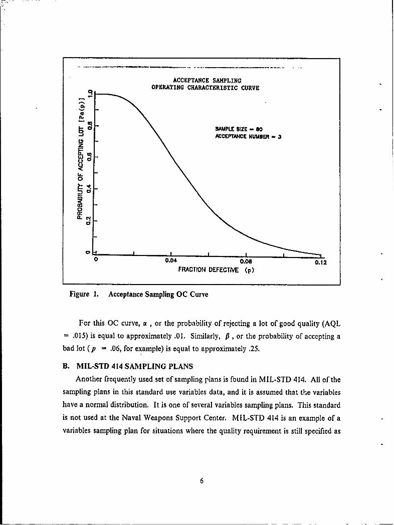
forth in MIL-STD 1051) require a sample of size SO. The lot is accepted if there are 3or fewer defective items in the sample and rejected if there are 4 or more defective items[Ref. 3]. Each sampling plan in MIL-STD 105D generates an operating characteristic(OC) curve. An OC curve gives the probability of accepting a lot of a given quality.Just as with any OC curve, there are Type I and Type I1 errors involved. In our case,the probability of a Type I error is the probability of rejecting a lot as a function of the

quality of the lot (proportion non-conforming). The probability of a Type II error is theprobability of accepting a bad lot. where "bad" corresponds to a larger proportionnonconforming that the specified A\QL. The OC curve for our exaimple is shown in

ligure I.

ACCEPTANCE SAMPLINGOPERATING CHARACTERISTIC CURVE

SAMPLE SIZE - 80ACCEPTACE NUMBER 3

0

OH

0 0.04 0.08 0.12FRACTIO14 DEFECTIVE (p)

Figure 1. Acceptance Sampling OC Curve

For this OC curve, o , or the probability of rejecting a lot of good quality (AQL- .015) is equal to approximately .01. Similarly, P , or the probability of accepting a

bad lot (p = .06, for example) is equal to approximately .25.

B. MIL-STD 414 SAMPLING PLANS

Another frequently used set of sampling plans is found in MIL-STI) 414. All of thesampling plans in this standard use variables data, and it is assumed that the variables

have a normal distribution. It is one of several variables sampling plans. This standard

is not used at the Naval Weapons Support Center. MIL-STD 414 is an example of avariables sampling plan for situations where the quality requirement is still specified as

6

specified as a percent nonconforming. [Ref. 4]

Some points of similarity between MIL-STD 105D and MIL-STD 414 are:

* both are based on the concept of AQL,

* both pertain to lot-by-lot acceptance inspection,

* both provide procedures for normal, tightened, and reduced inspection,

* both provide 9everal inspection levels,

* in both sets of plans, the sample size is greatly influenced by lot size, and

* in both sets of plans, all plans are identified by a sample size code letter.

MIL-STD 414 is also similar to MIL-STD 105D in that in both sets of plans sampling

plans under normal inspection were designed to protect the producer by rejecting with

small probability those lots which have a percent defective no larger than the specified

AQL. Just as in MIL-STD 105D. the protection to the customer depends largely on the

use of tightened inspection whenever the process average appears to be unsatisfactory

or there are other reasons to be suspicious of the process. [Ref 3]

The primary advantage of using MIL-STD 414 is that the same OC curve can be

obtained with a smaller sample size than is required by Standard 105D. The precise

measurements required by a plan from Standard 414 will probably cost more than the

simple classification of' items required by a plan from M I L-STD 105D. but the reduction

in sample size will hopefully offset this extra expense. For example, a plan from

MIL-STD 105D may require a sample of 50, but a comparable plan from Standard 414

requires a sample of only 30. If the unit cost of measurement is less than 5 3 times that

of simply classifying the items, the MIL-STD 414 sampling plan will eff'ct a savings.

[Ref. 3] Such savings may be especially significant if inspection is destructive and the

item is expensive.

The primary disadvantage of a sampling plan from MIL-STID 414 is that a separate

plan must be employed for each quality characteristic that is being inspected. For ex-

ample, if an item is to be inspected for five quality characteristics, then it would be nec-

essary to have five separate inspection plans from MIL-STD 414: whereas, acceptance

or rejection of the lot as a whole could be based on a single sampling plan from Standard

105D. Also, it is theoretically possible. although unlikely, that under a variables plan a

lot will be rejected by the variables criteria, even though the sample actually contains

no defective items. Another disadvantage of a variables sampling plan is that the quality

characteristic must come from a normal distribution. Since thc quality characteristics

7

being sampled will not always be normally distributed, the use of MIL-STD 414 will not

always be appropriate.

Due to the higher degree of popularity and use of MIL-STD 105D as opposed to

MIL-STD 414. plus the fact that Standard 105D is used at the Naval Weapons Support

Center, MIL-STD 105D will be used as the benchmark with which to compare any

proposed methods in later chapters.

C. MEASURING THE PERFORMANCE OF A SAMPLING PLANThe most basic measure of a sampling plan's performance in monitoring quality is

its OC curve, which shows the probability that a lot of given quality will be accepted.

It is also useful to have a measure of the quality of the product that will reach the con-

sumer's shelves after acceptance sampling has taken place.

We will assume that rectifying inspection is employc n the sampling process.

What is meant by this is that all rejected lots will be inspect -ercent and noncon-

forming items will be replaced by good ones. Thus, with th' Imption. as lots of size

L pass through the sampling process, one of the following scenarios will occur:

1. The lot is accepted, or

2. The lot is initially rejected; but. is subjected to 100 percent inspection and bad itemsare replaced with good ones. The lot is then accepted.

The sample s will eventually contain no defective items since all defects in the

sample are replaced by good ones. The same is true for the lot if it is initially rejected.

It will then be inspected 100 percent with the bad items being replaced by good ones.

If the lot is initially accepted, it will contain p(L - s) defective items, where p is the

proportion of defective items in the lot. This will occur Pa proportion of the time.

Thus, the sampling plan will on the average, turn out lots that contain PaIp(L- S))

defective items (Pa is the probability" of accepting a lot and is tatlen from the OC curve

for the sampling plan). Ifiwe divide by the lot size, L we can express this average out-

going quality as a fraction defective as follows:

AO00 Pa(p(L - s)) [Ref. 1].L

Thus, this concept of average outgoing quality, or AOQ, gives us a method of examining

the effect that a particular acceptance sampling plan has on product quality. AOQ is a

function of p . It has a maximum value which is called the average outgoing quality

limit, AOQL. Tables are provided in MIL-STD 105D that give the factors with which

8

the AOQL values for specific sampling plans can be calculated. The AOQL is a value

representing the worst case AOQ For a particular sampling plan. The value of p cor-

responding to the AOQL is of particular importance. This subject will be addressed

further in Chapter IV.

A producer may depend on either his or a consumer's quality control department forpost-production inspection of his products. This inspection results in nonconforming

items being screened out and replaced by conforming items. Often, this is how samplingplans such as MIL-STD 105D are used in a manulacturing operation. However, this

post-production type of inspection is wasteful because it allows time and materials to be

invested in products which are not always saleable.

One way to solve this problem, is to adopt an inspection strategy wherein a productcan be inspected For quality in the early and middle stages of production. A second way

of solving this problem is the adoption of a strategy of prevention. Clearly. it is much

more effective to avoid waste by not producing unsaleable output to begin with. What

follows in the next chapter is the basis for such a strategy.

9

III. A DIFFERENT APPROACH - DESCRIPTION AND ANALYSIS

In this chapter, the differences between statistical quality control and statistical

process control are addressed. These diflkrences lead to another outlooK .vw, ards quality

assurance and an alternate method of dealing with it which is set forth in this chapter.

The fundamental idea of the alternate method is the use of control charts by the pro-

ducer to gain statistical control of the manufacturing process with the result ultimately

being better quality in the product. Since a control char' is a fbrm of control based upon

sampling rather than 100 percent inspection, the quality of process output will depend

not only on the control chart, but upon the characteristics of the process which cause

its likelihood to produce deflcts to vary over umnc. Thus, a model will be proposed to

estimate the performance of the manufacturing process and a Ma:..ov chain will be used

to develop a measure of process output. Both of these will be presented in detail.

A somewhat similar study was conducted by Brugeer and is detailed in his technical

paper [Ref. 51. Brugger did use a Markov chain approach; however, his study was fo-

cused on modeling an acceptance sampling procedure vice a control chart procedure.

A. STATISTICAL QUALITY CONTROL VERSUS STATISTICAL PROCESS

CONTROL

Quality assurance will now be approached in a diflerent manner than in acceptance

sampling. It will be addressed firom the manufacturer's point of view. Aside from rec-

tif ing inspection, quality cannot be inspected into an item after it has been manufac-

tured. Because of this we will focus our attention on the manufacturing process. If this

different viewpoint seems to the reader to be a ninor point, then it should bc pointed

out that it changes entir how an analyst will approach the problem and ,,vhat tech-

niques he must use to solve it. Instead of a statistical quality control (SQC) problem,

we are now faced with a statistical process control (SPC) problem. SQC involves a large

amount of inspection. This inspection is usually conducted on final product. However,

at this point in the process it is too late to make corrections or adjustments to the

process which can correct for the mistakes already made: although, it will certainly be a

necessary task if quality is to be improved in future items. SPC methods are based upon

the exanination of finished and semi-finished product at an early stage with some

means of rapid and effective feedback. Rapid feedback gives tighter control, sa es add-

ing value to defecti e items, saves time, and reduces the impact of defectix e ,naterial on

10

scheduling and resulting output. Effective feedback can only be achieved by the use of

statistically based process quality control methods [Ref. 6]. SPC methods will allow the

quality of the product to be controlled by allowing the process to constantly monitor

itself. This means that the operator or technician in charge of the process examines the

product as it comes through the process to make sure that it meets the required specifi-

cations. He does this by using a sampling procedure which tells him exactly how often

to take a sample and how many items to sample. The sampling must of course be con-

ducted randomly.

SPC methods are often very simple when implemented in a manufacturing process.

As an example, suppose a quality problem arises within a process. The problem will be

noticed rasonably quickly if the process is monitored correctly. After becoming aware

of the problem. with minimum delay, the cause is determined and the problem is cor-

rected. The procedure just described is a routine one and occurs frequently in a manu-

fhcturing process. The use of SPC methods allows the frequent occurrence of procedures

such as the one mentioned above to be dealt with promptly and efficiently.

Problems with quality in a manufacturing process in which SQC procedures are be-

ing employed are not always as straight Forward. In SQC, a quality problem is some-

times discovered after the product is out of the manufacturer's factory and has been

delivered to the customer. If through acceptance sampling procedures, the lot is re-

jected. then not only has the manufacturer lost money but he has a defective product

and it is conceivable that he may not even know why.

The companies that have used SPC procedures over the years have found that

qualizy costs related to SPC are usually known and low. Once SPC procedures are im-

plemented by a company, they tend to remain in use because they are found to be of

considerable benefit. Unfortunately, the number of companies that are actually making

widespread use of SPC methods in their operation is relatively low when one considers

the benefits that SPC methods offer. The major reason fbund for this low usage is a lack

of knowledge, particularly among senior managers, Although these senior managers

sometimes recognize quality as being an important part of corporate strategy, they do

not appear .o know what effective steps to take in order to carry out the strategy, Too

often quality is seen as an abstract property and ijot as a measurable and controllable

parameter. [Ref. 6]

* 11

B. CONTROL CHARTS AS A MEANS OF PROCESS CONTROL

Assuming we do not want to conduct 100 percent inspection on the process we need

to devise a sampling procedure or some other method that will tell us when the quality

in our manufacturing process begins to deteriorate. In addition, we would like the

method to be more versatile than just being able to tell us when we are producing ex-

cessive defective products. We would like the method to be useful in helping us control

the process, and a control chart is a widely used statistical method tlat is well-suited for

this task.

The control chart is considered to be a very important tool in statistical process

control. Manuflcturerz readily accept the fact that the measured quality of their prod-

uct is always subject to a certain amount of random variation which can be attributed

to chance. T pically. some inherent random error is present in any process. Variation

within the process will, therefore, be inevitable. The control chart is a tool which gives

the producer the capability to detect any excessive variation in the process which may

be attributed to assignable causes. Such assignable causes may be: differences among

machines. materials, or workers, or a number of other flhctors related to the pcrormance

of the process. The reason for the excessive variation is then determined and corrected.

Thus. use of the control gises the producer the capability to diagnose and correct many

production poblems and often brings substantial improvements in product quality.

Furthermore. bN identiying certain quality variations as chance variations, the control

chait tells us when to lea\e a process alone, thereby preventing unnecessary and frequentadjustments thuit tend to inciease the variability of the process rather than decrease it.

One Nersatile and widely used control chart is the p-chart. It is the control chartfor proportion defective, or fraction defecti'e. which is designated by p . A p-chart

works as follows. A sample of a predetern-ined size is take2n at a predeterminfed interval.

The number of items in the sample that are defective, x . is then compared with the

sample size. s . to form our iatio "X , or our sample fraction defective which we will

refer to as ff . This value is then compared to the control limits on the control chart toget an idea of how the process is performing at the time of the sample being taken. The

p-chart can be constructed using data that are already available for other purposes or

can readily be made available.

We will use the p-chart in our quality method. Before we can use the p-chart, we

must have an estimate of the fraction defective of the process. We will assume that weare able to obtain this estimate without a great deal of difliculty. Now we have nearly

all of the information we need to construct the p-chart. Simple statistical calculations

* 12

can be used to provide control limits that tell whether assignable causes for variation

appear to be present or whether the variations from lot to lot are explainable by means

of chance occurrence. We will concern ourselves only with an upper control limit, since

a lower control limit on fraction defective is a self-defeating purpose. The upper control

limit can be calculated as follows:

UCL = + 3oF [Ref. 3].

We should be able to get an estimate for p from past data on the process. We will

denote this estimate as '. We will use the value for ' as the centerline on the control

chart. Also, since, ff is based on the binomial distribution, we are able to estimate

dr as follows:

As can be seen u; is dependent on the sample size, s , which will vary from control chart

to control chart. Thus, oTF will also vary from control chart to control chart.

For illustration purposes, suppose our sampling frequency, m , or the number of

items produced between samples being taken, is 1000 . Also, assume our sample size,

s ,is 80 and our estimate ' of the process fraction defective p is .015. We can now

calculate oF as follows:

/.015(.985)o. = 80

= .0136.

Now that we have a value for ,r , we can calculate UCL, or the upper control limit

for the process as follows:

UC4 = .015 + 3(.0136)= .0558

13

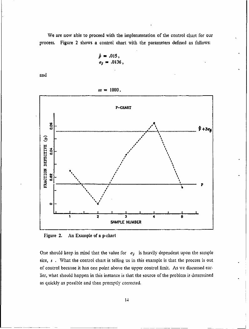
We are now able to proceed with the implementation of the control chart for our

process. Figure 2 shows a control chart with the parameters defined as follows:

- .015,- .0136,

and

= 1000.

P-CHART

W'a , I +.............. ..... ................... .................................... .............. ........ + 'w0

Z 4k

so

I

0I

2 3.4 5

I III I

I# I

Fiur 2. A3 Exml5f -

One should keep in mind that the value for cr; is heavily dependent upon the sample

size, s . WVhat the control chart is telling us in this example is that the process is out

of control because it has one point above the upper control limit. As we discussed ear.

lier, what should happen in this instance is that the source of the problem is determined

as quickly as possible and then promptly corrected.

14

C. MEASURING THE EFFECTIVENESS OF CONTROL CHARTSTaking the concept of control charts one step further, we would like the consumer

to be able to determine the effect that using a control chart at the end of a process will

have on the quality of the output. The consumer can then judge for himself whether

or not acceptance sampling is needed. Once again, the consumer's primary concern iswhether or not either procedure will function adequately to furnish product of accepta-

ble quality.

One commonly used measure of control chart performance is the chart's operating

characteristic curve or OC curve. A control chart's OC curve gives the probability that(for a given firaction defective) the process is declared under control based on a sample

result. Being declared under control is essentially the acceptance of the null hypothesis

that the process fraction defective is / ,the value based upon past data of the process.This probability as a function of the current process fraction defective p is denoted

Pa,(p) .

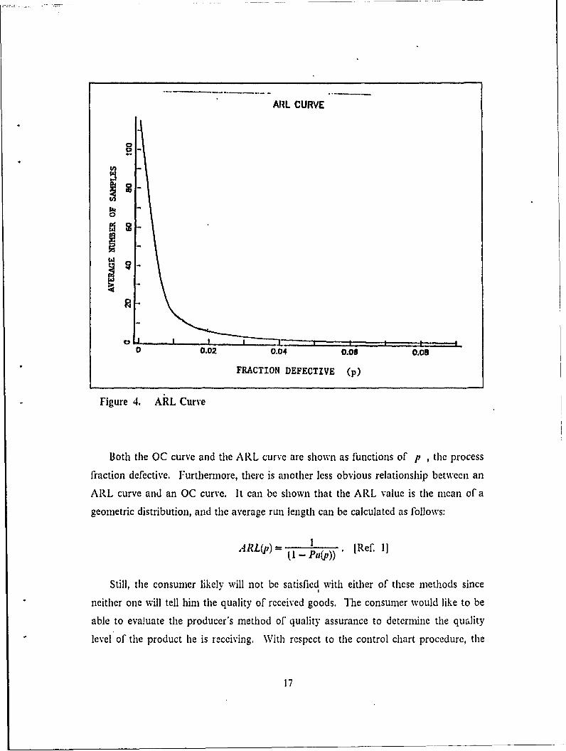
Another wtll-known measure of control chart perfomance within quality circles isthe average run length curve or ARL curve. The ARL curve 2ics, for a particular

ftaction defective, the average number of samples that would ha'.e to be taken before the

process was determined to be out of control. [Refl 1] Figure 3 shows an example of a

p-chart OC curve and Figure 4 shows an example of an ARL curve.

15

CONTROL CHART PROCEDUREOPERATING CHARACTERISTIC CURVE

0.

04 SAMPLE SIZE-SO0ACCEPTrANCE NUMBER -3

C,

U

0

0 0.04 0.08 0.12

FRACTION DEFECTIVE (p)

Figure 3. p-chart OC Curve

16

ARL CURVE

a

19-

0 0.02 0.04 0.06 0.08

FRACTION DEFECTIVE (p)

Figure 4. ARL Curve

Both the OC curve and the ARL curve are shown as functions of p , the process

fraction defective. Furthermore, there is another less obvious relationship between an

ARL curve and an OC curve. It can be shown that the ARL value is the mean of a

geometric distribution, and the average run length can be calculated as follows:

ARL(p) = (I - Pap)) Ref. 1

Still, the consumer likely will not be satisfied with either of these methods since

neither one will tell him the quality of received goods. The consumer would like to be

able to evaluate the producer's method of quality assurance to determine the quality

level of the product he is receiving. With respect to the control chart procedure, the

17

question now becomes: how does the consumer judge a manufacturer's control chart?

Upon initial examination of a p-chart one notices the following:

I. The sample size,

2. The sampling interval,

3. The upper control limit, which is a function of the centerline and sample size, and

4. The steps to be taken by the producer in the event the process is determined to beout of control , i.e., when the sample proportion is found to be outside the control

limits on the control chart.

The customer's concern is that none of above listed factors gives him any direct infor-

mation about the quality of product that he will receive.

In addition to these factors, it is clear that product quality lcavina a final control

chart will depend upon how the characteristics which are the primary cause for defects

in the process change over time. Clearly, these characteristics will vary from process to

process, and in some instances may be unknown or difficult to estimate. In the next

section. we will give one simple model of a manufacturing process in which p varies

over time. The model will be used to demonstrate the effectiveness of the control chart

procedure, and to provide a basis for computing a measure of the quality of goods re-

ceived by the consumer.

D. A MODEL OF A MANUFACTURING PROCESSThe next step in this approach to our problem is to devise a vay of approximating

or estimating the performance of the manufacturing process with respect to quality. The

simple process we will model is one where a final control chart is emp . ed for overall

fraction defective. We shall assume that when the control chart shows that the process

is out of control, corrections are made before additional items are produced, and the

process fraction defective returns inmediately to a lower base value. This base value is

the iesult of inherent. random errors within the process.

WNhen devising this model, one must include the effect that various factors have on

the quality of a product. One of these factors is the aging of elements used in the process

(machinery, tooling, etc.). Another factor is the random way in which defecti\ e products

occur and how we record them; e.g.. by attributes or by variables. In our model, items

are scored by attributes only; that is each item is classified into one of two categories:

defective or non-defective.

Another modeling problem that must be addressed is: what happens when the

process is determined to be out of control or producing an excessive amount of dcfecti\ e

18

products. Typically, some form of corrective action is taken to get the process back

under control. At times, this corrective action may involve such measures as shuttingthe process down until the problem can be determined and corrected. Drastic measures

such as this are usually not required since the probem can often be corrected without

noticeably slowing down production. For modeling purposes, we will assume that whenthe process is back in control as a result of the necessary corrections being made, the

process fraction defective immediately reverts back to a value which is a result of the

occurence of inherent, random errors in the process. This seems to be a reasonable as-

sumption when considering the reasons listed above for occurrence of defects in a

product. The assumption of the process firaction defective reverting back to its inherent

value or state along with the general nature of a manufacturing process allows us to

model the process performance as a stochastic process. First, let us suppose we divideup the daily production output quantity of the process into it increments of size / .

This can be done on a shift basis instead of a daily basis if the producer so desires. This

gives us our sampling fiequency. In our example we will arbitrarily choose 6 as the

value of' n . Thus, we have six production periods per day or per shift and a sample

will be taken after e cry n units of production. Let a be defined as the probabilitythat an item produced by the process when under control is defective dt.C only to the

inherent random error within the process. Whenever we have determined the process tohe out of control, the model allows the process to become under control again by per-

mitting the probability of producing a defective item to immediately revert back to a

The assumption is made that the problem causing the process to be out of control can

be determined and corrected. Also. let us define b a., the rate per item produced atwhich the probability of occurrence of a defective item increases with respect to pro-

duction. We now have the basis for our process model which'is shown in graphical form

in Figure 5.

It should be pointed out that in a real world manufacturing process. the parametersa and b will not only be unknown but they will probably be very diflicult to estimate.

If they were known, then we would have no reason to employ a control chart on the

process since we would know when to make the necessary adjustments to the process to

keep it producing goods of an acceptable quality. Likewise. we would ha'e no use fora sampling plan if we had available to us known values for a and b . By using oui

model we hope to ha e a rough means of portraying a change in p over time.

19

PROCESS BEHAVIOR WITHCONTROL CHART IMPLEMENTATION

a+6ba

aiSbu

a+4be --

a+3bu ,..f - - -

a--- i -4- a b

S I I 11, IC a 2a 3n 4a 5m 6M

NUMBER OF ITEMS PRODUCED

Figure 5. Graphical Representation of Model

In Figure 5 we show the defect rate increasing linearly with the number of items

produced. Sampling inspection will take place after every in items are produced.

When the process is determined to be out of control via use of the control chart, the

defect rate immediately returns to the point designated in the figure by the coordinates

(0 , a). The process essentially starts over at this point. Moving along with the model,

let Pa; equal the probability of concluding that the prdcess is under control at level

a + ibm where i is the period number and a + ibm is the process defect rate at the

end of period i . The probability Pa, can be obtained from from the OC curve for the

control chart. We can think of /nt as the number of items produced since the last time

the process was determined to be out of control and at which time the probability of

producing a defective item was returned to (0, a). If we let P equal the fraction

20

defective for the quantity of goods produced during period i ,then we can calculate this

value for each period as

Pi =a +2i - 1hP,=-a + n

As we noted earlier, we have built-in to our model the control chart decision rules.

An important point is that without these decision rules in our model the process fraction

defective, p , will increase linearly without bound. This is due to the fhct that the con-

trol chart is the only measure we are using to decide whether or not the process is under

control or not. However, as we indicated earlier the purpose of the model is simply to

give us a rough idea of how a manufacturing process performs when a control chart is

imposed on it.

E. CALCULATION OF STEADY-STATE PROBABILITIES USING MARKOV

CHAIN PROPERTIESGenerally, if and when the manufacturing process reaches a level with defective rate

a + 6bin in our example. the probability that we conclude the process is under control

will be extremely small. Therefore. we will assume that Pa6 is equal to zero. This as-

sumption gives us the capability to approximate the behavior of the process with a

Markov chain with a finite number of states (six). A Markov chain can describe a

process which moves from one state to the next in such a way that the probability of

going to one of the next states only depends on the fact that it is presently in a given

state and does not depend on any prior states [Ref. 7]. We can summarize what we

know thus far in Table 1. which follows.

21

Table 1. SUMMARY OF MODEL PROBABILITIES

Period Probability of a Probability ofPerod Prbalt O fi at Concluding that Process Fraction Defectiveor Defect Occuring at is Under Control in Period i, P,

State the end of Period i at Level a + ibm

11 a+bm Pa a + -b

2 a + 2bin Pa2 a+ 7 bi

a+3bn Pa3 a + "bm

2

,.a+bni Pa4 a +2"-bm

55+bn Pas a-'--2-bin

6 a + 6bm 0 a + bm

The six states in the model correspond to the ends of the six periods listed ill Table

1. State 1 is the end of Period I where the defect rate is a + bin. The Markov chain

reaches State I as a result of the process being determined to be out of control. When

this occurs, corrective action is taken on the process which takes the process defect rate

back to a , and then with certainty to a + bin at the end of Period !.

Referring to Figure 5. one can see the pattern which is a result of the model being

a .Markov chain. In State 1. the process can only transit to State 2 if it is concluded that

the process is under control or to a if it is concluded that the process is out of control.

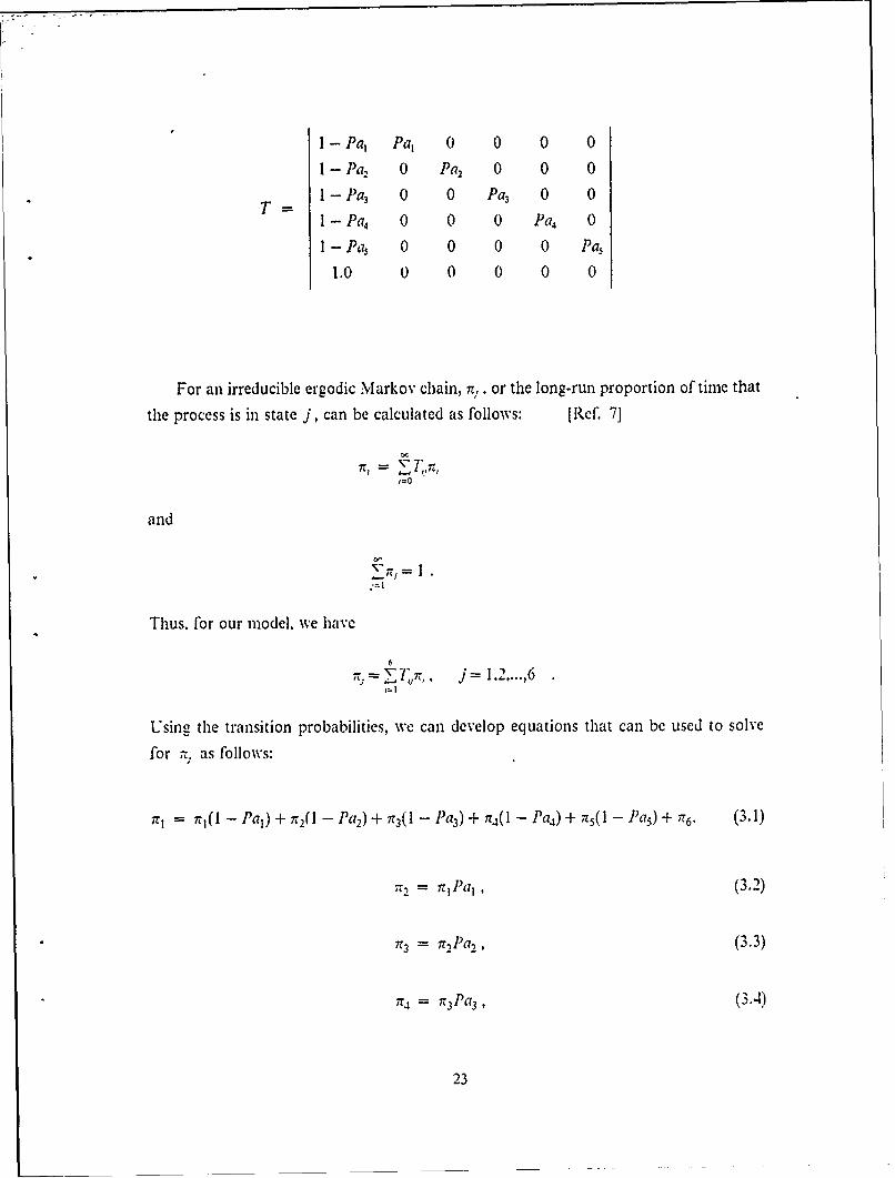
Sinilarily, in State 2. the process can only transit to State 3 or to a . Let the matrix

T , which follows, represent the transition probabilities. This 6 x 6 transition proba-

bilitv matrix shows the probabilities of transitioning to states represented by the col-

umns, given one is in a state represented by one of the six rows. Note that the transition

probabilities are either 0 . 1.0 . or are from the OC curve from the control chart of the

process.

22

I - Pal Pal 0 0 0 0

1 - Pa2 0 Pa2 0 0 0

1 - Pa 0 0 Pa3 0 0

1 - Pa 0 0 0 Pa4 0

I - Pa 0 0 0 0 Pa,

1.0 0 0 0 0 0

For an irreducible ergodic Markov chain, it,. or the long-run proportion of time that

the process is in state j, can be calculated as follows: [Ref. 71

1=0

and

vit,= I

Thus. for our model, we have

6

7' 7I , j

Using the transition probabilities, we can develop equations that can be used to solve

for , as follows:

r = it1(I - Pal) + r' 2(l - Pa2) + ,t3(1 - Pa3) + rn4(l - Pa4 ) + ,t5(l - Pa) + 'T6. (3.1)

'42 = IrIpa41 (3.2)

773 = it2Pa,, (3.3)

174 = 7T3Pa3 , (3.-)

23

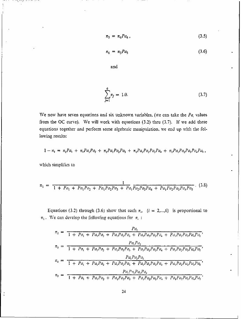
IT5 nr4Pa 4 , (3.5)

n6 = 7 5Pa5 (3.6)

and

6

= 1.0. (3.7))--1

We now have seven equations and six unknown variables. (we can take the Pa, values

from the OC curve). We will work with equations (3.2) thru (3.7). If we add theseequations together and perform some algebraic manipulation. we end up with the fol-

lowing results:

1 - -, = irPa, + 7rPaPa2 + 7rPaPa,Pa, + 7zPaPaPa3Pa, + ir2Pa2Pa,Pa3P1Pa,

which simplifies to

7rT = 1 + Pa1 + Pa1 Pa2 + PaPa2 Pa3 + PaPa2Pa3Pa.4 + P)a1 Pa:2 Pa3Pa.Pa5 ' (38)

Equations (3.2) through (3.6) show that each 7,, (i = 2,...,6) is proportional to

. We can develop the following equations for it,

Pa

1 + Pal + PaPa, + lPa,1 a,Pa + Pa,Pal(3aP4 + Pa,1Pa,PaPaP,'

Pa, Pa71 + Pa + a,1P, + Pa P 11Pa3 + PaPaj1'a3Pa, + PaPa.Pa131aa Pa,

Pa2 iaPa31 + 1)a1 + Pallpa 2 + Pa,Pa,13 + PaPa,Pa3Paa + lPa,Pa,a 3PaPa,

PaP,PaPa1 + Pa + PaPa2 + PaIPa,Pa3 + Pa Pa,Pa Pa + Paa,lla,,aPa,' "

24

and

PaPaPaPaPa,iT6 = 1 + Pal + PaPa2 + PaPa2Pa3 + PaPa2Pa3Pa4 + 1aPaPaPaPa"

Now that we have determined the long run proportion of time the process spends

in each state, and Table I shows the fraction defective in each state, we can calculate the

fraction deflective of the process as determined by the model. We will denote the model's

resulting value for the process fraction defective as p'.

We can compute p' as follows:

p' = t7,(a + - bin) + irT(a + 3 bin) + ;(a + - bin) + ,(a + -7 bn)

+ r(a + 9 bin) + (a + -U- bin).

lfwe collect the common terms, we end up with the fbllowing equation for fraction de-

fizctive as computed -vith the use of our model: [Ref. 71

6

= a + bm Iri( 2i 2 (39)i--I

The expression br p' in Equation (3.9) provides a way to compute a value for the

output fraction defective of the simple process we have modeled. The six nir values

may be obtained from solution of Equation (3.8) for 7r , and successive solution of

Equations (3.2) through (3.6) for n, through n. . Solving these equations requires five

values: Pal, Pa. Pa3, Pa, and Pa. . These values can be obtained from the control chart

for the manufacturing process.

An important point to note is that p' may not accurately reflect the level of quality

in the product as it ends up in the consumer's warehouse. This is because the model

does not consider how the quality level in the product is affected b, shipping, . onloading.

25

offloading, etc.. Despite the model's limitations, it gives us a rough estimate of a proc-

ess' fraction defective when a control chart is employed.

The end result of the model is the value of the manufacturing process' output frac-

tion defective, or more simply put, an estimate of the level of quality in the product

produced by the process when there is a control chart at the end. This value p' can

be thought of as a means of measuring the effectiveness of the control chart procedure.

Furthermore, this value can be compared to the AOQ value of an acceptance sampling

procedure to get an idea of which method is more effective. This will be addressed in the

next chapter.

F. ANALYZING SOME RESULTS OF AN IMPLEMENTED CONTROL CHART

AT THE END OF A PROCESS

It should be clear that the parameters of the model can be changed as necessary in

order to estimate the performance of a variety of manufacturing processes. The program

listed in Appendix A was written so we would have a means of testing the model with

respect to its ability to estimate the output of the process with a control chart. The

program allows the user to judge the sensitivity of the model with respect to variation

of its parameters a and b , as well as the control chart characteristics LUCLi, sample

size s, and sampling interval in. By varying these factors we are able to get a better

understanding as to which ones are the most critical in computing the process output

averace fraction defective. p'.

The program was applied to cases where a varied from 0 to 0.0075. b from

0.000001 to 0.000005, ' from 0.001 to 0.01, sample size s from 50 to 150, and sampling

frequency in from 500 to 2000.Some results of the computer program (see Appendix B). suggest that. over the

range of parameter values used, the estimate of average fi action defectix e fluctuated the

most as the parameters b and in were varied. I lence, b and In or their product appear

to have the most influence on the estimate of the output quality of the process. This

seems logical when one recalls that m is the sample firequency and b is the rate at which

the process performance deteriorates. If a process has a high rate of deterioration, then

it is clear that its average fraction defective will be higher as a result even with the use

of a control chart. Still, it will be significantly lower when using a control chart than

when not using one. Intuitively. this will be true of any manufacturing process in a real

world environment and. as explained earlier, it is true by design in our model. This is

because our model cannot operate without a control chart. Also. if qual.t problems

26

are occurring within a process, the more frequently samples are taken, the greater the

frequency of detecting and correcting those problems becomes.

Taking our analysis one step further, we will now focus our attention on a portion

of the data. For the cases where the sampling frequency is in = 1000 ( one third of the

data), using the data in Appendix B, we further find that the process fraction defective

is most dependent on the process characteristics, a and b . and the sampling frequency

i . This was determined by obtaining a linear fit for the data. In particular, the process

fraction defective after one period. (a + bm) reflects both the process characteristics and

the sampling frequency. Using this as one variable and the control chart rule (UCL) as

the other, we applied a least squares fit to our data. The result for the S1 data points

where in = 1000 was

p' = 0.0005 + 1.0094(a + bin) + 0.0733(UCL)

This reflects, for this set of data. the clear influence of process characteristics and sam-

pling frequency. Some values of interest for the in = 1000 set of data arc shown in

Table 2 which follows. Note that this is not a statistical regression analysis, but simply

an efl'ort to fit a linear function to a set of data.

Table 2. RESULTS OF LEAST SQUARES FIT TO DATA

Nlinimuin MaximuniValue V.alue

a + bin (.)0)1 0.)125

U:C'LF o.oo7 0(.0522

p 0.0023 0.019

P fom 0.00212 0.0)169linear lit

Reidua! .0.0(0416 0.0 I0415

As stated earlier, the purpose of the computer program shown in Appcidix A was

simply to demonstrate the el'cctixeness of a final control chart on process output as a

function of process parameters and control chart characteristiks. It is belicvd that if

27

one examines the output, its effectiveness will become apparent. After close examina-

tion, one can also get an understanding of the sensitivities of the model to specific pa-

rameters. This information can be useful to a quality manager when he is attempting

to improve his operation.

Although, the computer program provides a means of evaluating the effectiveness

of the control chart procedure, what is really desired is a method of comparing, from the

consumer's point of view, reliance on a final control chart to acceptance sampling. This

issue is addressed in Chapter IV.

28

IV. COMPARISON OF THE RELIANCE ON ACCEPTANCE SAMPLING

VERSUS A CONTROL CHART PROCEDURE

In this chapter, we will look at various means of comparing acceptance samplingwith statistical process control, wherein acceptance sampling would not be employed.

First, a qualitative comparison of the corresponding costs of each method will be per-

formed followed by a comparison of the effectiveness of each method.

A. COST COMPARISONThe cost comparison will be approached from the perspective of the base

commander. From his viewpoint, any alternative that reduces his costs and maintains

or increases current levels of' efl'ccti\ eness will attract his interest. Since the proposed

alternative may reduce the the number of quality assurance personnel required to be

stailed at the base, the base commander will at least reap the amount of savings resulting

from this. IIowever. the biggest savings in using a method of quality assurance involving

control charts vice acceptance sampling is what results from the elimination of sampling

inspection and rectifying inspection.

An outsider may argue that even though in this case the Naval Weapons Support

Center is saving money. the overall cost to the )epartment of Defense is the same.

While it is true that there is a shift in cost from the naval base to the defense contractor,

there still may be a significant savings involved with the control chart procedure. First

of all. the defiense contractor should have no need to hire additional personnel when he

implements this method. This is because it is necessary and fundamental to the success

of the process control method that the technicians and operators on the production line

should be the personnel who are carrying out the methods of the control chart 'proce-

dure. This is where training of personnel is important. It may be necessary to train all

of the technicians and machine operators associated with the manul'cturing process in

the fundamentals of statistical process control and the use of'control charts. 'he major

impact of training costs will be felt in the beginning while the changeo\ er to reliance on

the control chart procedure is being made. Training will still have to be conducted,

though to a lesser degree. on a continual basis. This will be one of the two primary costs

of changing the emphasis from an acceptance sampling pro.Ledure to a control chart

procedure. The other cost is associated with instances when it is necessary to stop the

process to determine the reason for the process being out of control. T[his resulting

2()

downtime in production can be very costly and can quickly cut into the defense con-

tractor's profit margin.

The cost considerations discussed above are difficult to quantify. Why these costs

which primarily affect the manufacturer are of concern to the base commander is that

he will see them reflected in his contract with the manufacturer. Due to the factors

mentioned above, the base commander may see a reduction in his costs when the con-

tract is written if a control chart procedure is used.

B. EFFECTIVENESS COMPARISON

Having concluded that elimination of acceptance sampling may result in a cost

savings, we now to focus our attention on the effectiveness of a control chart procedure

as opposed to an acceptance sampling procedure. One way of examining the effective-

ness of each procedure is to look at the efflect of each on the AOQ or average outgoing

quality of the process and the quality components.

With the concept of AOQ, we will assume a scheme of 100 percent inspection of

rejected lots and that any defective items discovered within the rejected lot will be re-

placed by good items. Another assumption is that the 100 percent inspection of the re-

jected lots will ultimately result in 100 percent quality of those lots. Finally, in our

analysis. we will assume that the number of defects in our sample is binomially distrib-

uted with a mean equal to sp . or the product of the sample size s and lot quality p.

We will now show how average outgoing quality is related to p.

Recall that in Chapter 11. the AOQ for a process in which a sampling plan and 100

percent rectilication are implemented was defined as follows:

Pa(p(L - s))

For illustration purposes. we will use the same M1L-STD 105D sampling plan that

we used earlier as an example. Its parameters are as follows:

lot size (L = 1000),

sample size (s = 80),

acceptable quality level (AQL = .015 and

acceptance number (c 3).

30

(Note: MIL-STD 105D uses the following letter designations: Nfor lot size (vice L) and n for sample size (vice s). Different

designations are used in this thesis to clarify the difference in the

parameters used in the model and the parameters used in MIL-105D.)

Using various values for the quality of incoming product, p, we summarize the re-

sulting AOQ values for the different values of p in Table 3. The values for Pa were

taken from the OC curve for this plan shown earlier in Chapter II.

Table 3. AOQ VALUES FOR A MIL-STD 105D SAMPLING PLAN WITHAQL=.015

p Pa AOQ

.01 .991 .0091

.015 .966 .0137

.020 .921 .0169

.025 .857 .0197

.030 .779 .0215

.035 .692 .0223

.o-10 .603 .0222

.045 .515 .0213

.050 .433 .0199

.055 .359 .0182

.060 .294 .0162.065 .238 .0142

.070 .191 .0 12 3

.075 .1 51 .0104

.080 .117 .0086

As can be seen the maximum AOQ value s about .0223. This AOQ value is known

as the AOQL. or Average Outgoing Quality Limit. The corresponding value of p at

which this maximum AOQ occurs is .035. Simply put, the process with use of this par-

31

i

ticular sampling plan is ultimately producing its worst level of quality, orAOQL - .0223, when p, the lot quality, is equal to .035. In effect, we can considerthis to be the worst case performance of this MIL-STD 105D sampling plan when rec-tifying inspection is employed.

Under the proposed method of using control charts to gain statistical control of theprocess, our argument is a very simple one. The process long-run average performancep will simply be equal to the estimate p' of the process average fraction defective ob-tained ftom the modcl. Figure 6 shows the effiect of each method on the AOQ of the

process.

AOQ CURVE

a-

2-40

CY

0

o - ICCEMANJCE SIING PROCEDUREI N I .- LOWER BOUND FOR CONTROL CW"TA PROCEDURE

o - UPPER BOUND FOR CON1TRO CKAfl PROC.1UURE

0 I I.. .. ... .. .. .. ... .. .. .. ... .. .. . I

0 0 0.02 0.04 0.06 0.08

FRACTION DEFECTIVE (p)

Figure 6. Comparison of the Effect of the Two Methods on AOQ of Process

It can he seen from the figure that at times, MIL-SID 105D pcrforms better and

at other times it does worse. In this example the worst case performance is better with

-- 32

the control chart method. The MIL-STD 105D AOQ curve is for the same sampling

plan we have been using as an example throughout this thesis. Once again its parame-ters are shown below:

L= 1000,

s= 80,

and

AQL =.015.

The two dashed lines in the figure representing the upper and lower bounds on p' for

the proposed method were computed using the following parameters in the model:

n 6.

= 1000,

a= .007i.

b = .000001 (for the lower bound).

b = .000005 (For the upper bound).

s= 80,

and

P = .015.

As we have already established, p' is dependent upon the parameters used in the

model. Hlowever. in this example the values for the model's parameteCrs were chosen so

that the two methods will be operating on processes with roughly the same character-

istics. The same value that was used for lot size in the xrilitary standard was chosen as

33

sampling frequency in the model. Also, it was decided it was best to use the same sample

size in each method. The inherent probability that the process will produce a defective

item a was arbitrarily chosen to be half of the AQL value. It is believed that for most

manufacturing processes this is an overstatement of the tendency for the process to

produce a defective item. The rate at which this probability of producing a defective

item increases with time b was chosen to take on two values for illustrations purposes

due to its uncertainty. The lower bound value represents what is believed to be a rea-

sonable deterioration rate for the process; whereas, the upper bound represents an ap-

proximation of a worst case scenario. It is difficult to compare the two methods on a

equal basis; however, it is believed that the estimates made here are conservative and

provide for a rough, but reasonable comparison of the two methods.

Hence, we conclude that by using this means of comparison, it is reasonably evidentthat implementation of the proposed method of reliance on a control chart procedure

should be given consideration because it will likely result in a cost savings. Also, ouranalN sis has shown that it some cases it can be at least as effcctive as the current method

of acceptance sampling which is being used.

In the following chapter. we will surmarize our study and make further conclusionswith regard to what we believe the efl'ect of a control chart procedure similar to the one

presented here will have on a manufacturing process if implemented.

34

V. SUMMARY AND SUGGESTIONS FOR FURTHER STUDY

The purpose of this thesis was to conduct research into the area of quality assurance

and to determine whether or not there might exist a feasible alternative to ensuring

quality in military systems as compared to the methods being used today. Specifically,

the Commanding Officer of the Naval Weapons Support Center in Crane, Indiana,

would like to know if it would be feasible for him to rely only on the manufacturer's

operation and quality assurance methods to ensure an acceptable level of quality in the

product he is receiving from the manufacturer, and how he could evaluate these meth-

ods. Since there seems to be a slow but sure shift in the manufacturing industry towards

statistical process control, it was decided that this thesis would concentrate on an alter-

native of this nature.

Acceptance sampling conducted by the consumer requires that the military agency

staff a group of personnel knowledgeable in quality assurance methods. The method

presented in this thesis, consistent with the fundamental concept of statistical process

control, shifts the emphasis of product quality back to the manufacturer where ideally

problems in quality are detected early and corrected on the spot. In order for the cus-

tomer to shift from the reliance on acceptance sampling to reliance on control charts at

the manufacturing operation, is necessary to show that upon consideration of the pro-

ducer's quality program, the product he will receive without acceptance sampling is sat-

isfactory. To do this, dn effective measure is needed to compare the alternatives of

acceptance sampling and control charts.

As a way of measuring the effectiveness of the control chart on the output of a

manufacturing operation, a model of a manufacturing process was developed. The pri-

mary assumption made in constructing the model was that a linear deterioration rate

over time existed with respect to quality. Another assumption made was that when the

process is determined to be out of control, the problem can be determined and corrected.

Upon correcting the problem, the value for the rate at which defects occur returns im-

mediately to a value that is due only to the random error present within the process.

The model requires inputs for sample frequency; sample size; the probability of a defect

occurring due to inherent or random error present within the process; the rate at which

the probability of the occurance of a defect increases with time; and the centerline value

for the control chart to be used. The output p' of the model is an estimate of the

35

process average output fraction defective when the control chart is in use. The

paramters in the model that were determined to be the most influential in this estimate

were the sample frequency and the rate at which the probability of an occurence of a

defective product increased with respect to time.

Although, the main purpose of the model is to show one way to evaluate the effec-

tiveness of a control chart, a quality manager may be able to use it as a decision aid ifcontrol charts are being employed in his operation and if he believes his manufacturing

process possesses the necessary characteristics (i.e., linear deterioration rate, etc.). The

manager will have to be able to estimate within reasonable accuracy the parameters in

the model as they apply to his process in order for the model to provide him with useful

information. The quality manager will be able to derive his estimates from existing data

concerning past performance of the process. Even if useful data does exist on the per-

formance of the process, the parameters in question will probably be difficult to estimate

due to the uncertainty of their behavior, as will probably be borne out by the data.

Clearly, if the manager were to have at his disposal estimates of these parameters which

involved little or no uncertainty then he would have no use for a control chart to begin

with. Nonetheless, if the quality manager is able to obtain estimates of a and b then

he may be able to use the model as a decision aid to assist him in improving the effi-

ciency of his process.

In Chapter IV, the argument was made that even if reliance on a control chart

without acceptance sampling resulted in approximately the same level of quality in the

product. it would result in a cost savings because it would reduce the need for staffing

of quality assurance personnel by the customer. We also argued that the proposed

procedure would reduce costs because a manufacturer is much better equipped to per-

form a quality assurance operation than the consumer. For statistical process control

to be effective, the quality assurance methods must be performed by the manufacturer.

There is much room for improvement in manufacturing methodologies and quality

assurance techniques. It is recormmended that this research be taken further by ap-

proaching it slightly differently. An alternative approach to the problem is to model the

manufacturing process using two rates of average fraction defective and the time be-

tween the process changing between the two would be exponential. There are many

manufacturing systems that would lend themselves to this type of model.

It is sincerely hoped that the methods and procedures presented in this thesis will

be useful in helping the Naval Weapons Support Center and other Department of De-

fense agencies in dealing with quality assurance issues.

36

APPENDIX A.

Program to Generate OC Curve Probabilities

INTEGER M(1:10),MM,N,S(1:10),SS,AA,BB,C,ICOUNT,PP,NLINEREAL PA(i: 10),PI(1: 10),FRADEF(1: i0),SUM,A(l h10),B(1: 10)REAL PTOTAL,CL(1: 10),UCL(1: 10,1: 10) ,DENOM(i: 10) ,DSUNREAL PPRIHE(1: 10,1: 10,1: 10,: 10,1: 10)

* ********************************* ** l//Ill/lllI//ll/lII/ll/lII/l////I** II II ** // The purpose of this program is to demonstrate the // ** // effectiveness of a control chart procedure when it is // ** // imposed upon a manufacturing process. This is done by // ** // evaluating a model of the process. Given the necessary // ** // inputs, the OC curve probabilities are calculated. // ** // Since, the process is modeled via the use of a markov // ** // chain, the steady-state probabilities are then // ** // calculated. These calculations allow for the // *

// computation of an estimate of a fraction defective // ** // for the process in question. // ** II II **II II *

* * ,* * ** *,* * * * * ** **** * * * * * * * d * * * * *

CCC Prompt the user for data entry.C

PRINT *, 'To check the sensitivity of the model to each parameter'PRINT *, 'enter the number of different values you would like to'PRINT , enter for each parameter.'PRINT *READ * NUMPRINT *PRINT *, 'Enter the value for the number of periods, n.PRINT *, 'This value will not vary. To change it you must'PRINT *, 'run the program again.PRINTREAD *, NPRINTDO 5 I = I,NUM

PRINT 'PRINT *, 'Enter the value for the sampling frequency, m.PRINT *READ *, M(I)PRINT *PRINT *, 'Enter the value for the sample size, s.'PRINT *

37

READ *, S(I)PRINT *PRINT *, 'Enter the value for a, the probability the process'PRINT *, 'will produce a defective item when it is performi g'PRINT *, 'at peak efficiency.'PRINT *READ *, A(I)PRINT *PRINT *, 'Enter the value for B which is the rate at which'PRINT * 'the probabilty of producing a defective item'PRINT *, 'increases with respect to time.'PRINT *READ *, B(I)PRINT *PRINT *, 'Enter the value for the centerline on the control'PRINT *, 'chart.'PRINT *READ *, CL(I)PRINT *

5 CONTINUEICOUNT = 0NLINE = 0DO 60 MM = 1,NUM

DO 55 SS = l,NUMDO 50 AA = 1,NUM

DO 45 BB = 1,NUMDO 40 PP = 1,NUM

CCC Calculate the upper control limit for the control chartC

UCL(PP,SS) = CL(PP) + 3 * SQRT(CL(PP) * (1 - CL(PP))+ / S(SS))

C = S(SS) * UCL(PP,SS)CCC Use the subroutine POISS to calculate the OC curve probabilities.C

DO 10 I = 1,NCALL POISS(A,B,I,M,S,PA,AA,BB,MM,SS,C)

10 CONTINUECCC Calculate the steady-state probabilities.C

PTOTAL = 0DSUM = 1.0DO 20 J = N,2,-l

DENOM(J) = 1.0DO 15 I = J-l,l,-l

DENOM(J) = DENOM(J) * PA(I)15 CONTINUE

DSUM = DSUM + DENOM(J)20 CONTINUE

P(1) = I / DSUMPTOTAL = PTOTAL + PI(1)

38

DO 25 I = 2,NPI(I) = PI(I-1) * PA(I-I)PTOTAL = PTOTAL + PI(I)

25 CONTINUECCC Scale the probabilities to ensure that they sum to one.C

DO 30 1= ,NPI(I) = Pl(I) / PTOTAL

30 CONTINUECCC Calculate the fraction defective for each period.C

SUM = 0DO 35 1 = 1,N

FRADEF(I) = PI(I) * ((2*1 - 1) / 2)SUM = SUM + FRADEF(I)

35 CONTINUECCC Calculate the average fraction defective for the process.C

PPRIME(PP,BB,AA,SS,MM) = A(AA) + (B(BB) * M(MM) * SUM)40 CONTINUE45 CONTINUE50 CONTINUE55 CONTINUE60 CONTINUE

CCC Print out a definition list of the parameters.C

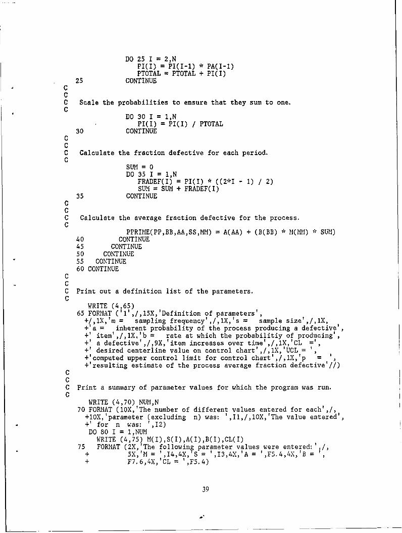
WRITE (4,65)65 FORMAT ('l',/,l5X,'Definition of parameters',+/,iX,'m = sampling frequency',/,lX,'s = sample size',/,lX,+1a = inherent probability of the process producing a defective',+' item',/,lX,'b = rate at which the probabilitiy of producing',+' a defective',/,9X,'item increases over time',/,lX,'CL ',+' desired centerline value on control chart',/,IX,'UCL =+'computed upper control limit for control chart',/,IX,'p =+'resulting estimate of the process average fraction defective'//)

CCC Print a summary of parameter values for which the program was run.C

WRITE (4,70) NUM,N70 FORMAT (lOX,'The number of different values entered for each',/,+1OX,'parameter (excluding n) was: ',Il,/,10X,'The value entered',+' for n was: ',12)DO 80 I = 1,NUM

WRITE (4,75) M(I),S(I),A(I),B(I),CL(I)75 FORMAT (2X,'The following parameter values were entered:',/,+ 5X,'M = ',14,4X, S = ',13,4X,'A = ',FS.4,4X,'B =+ F7.6,4X,'CL = ',F5.4)

39

80 CONTINUECCC Printout column headings for table.C

WRITE (4,85?85 FORMAT (2X Case',5X,'m',7X 's',6X,'a',9X,'b',9x,+ 'CL' 7X UCL ,7Xsp ,2X, , --- x, 1 ------+ '" .3X---X,' --------- 4X '----,,3X,'-.......-',I,+ t .. . . 1/)+

CCC Print out all calculated values.C

DO 120 MM = 1,NUMDO 115 SS = 1,NUM

DO 110 AA = 1,NUMDO 105 BB = I,NUM

DO 100 PP = 1,NUMICOUNT = ICOUNT + 1NLINE = NLINE + 1IF (NLINE .LT. 40) GOTO 90WRITE (4,65)WRITE (4,85)NLINE = 0

90 WRITE (4,95) ICOUNT,M(MM),S(SS),A(AA),B(BB),CL(PP),+ UCL(PP,SS),PPRIME(PP,BB,AA,SS,MM)

95 FORMAT (2X,14,2X,15,4X,14,3X,F5.4,3X,+ F9.8,3X,F5.4,3X,FS.4,3X,F7.6)

100 CONTINUE105 CONTINUE110 CONTINUE115 CONTINUE120 CONTINUE

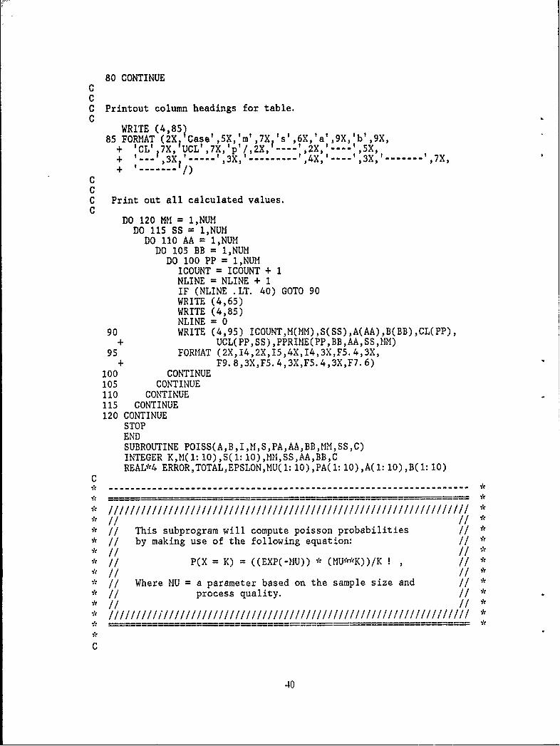
STOPENDSUBROUTINE POISS(A,B,I,M,S,PA,AA,BB,MM,SS,C)INTEGER K,M(l: l0),S(l: 10),MM,SS,AA,BB,CREAL*4 ERROR,TOTAL,EPSLON,MU(l: 10),PA(i: l0),A(l: l0),B(1: 10)

C

* IIIIIIIIIIIIIIIIIIIIIIIIIIIIIIIIII** // // *

* // This subprogram will compute poisson probabilities // ** // by making use of the following equation: // ** II I/ *

* // P(X = K) = ((EXP(-MU)) * (MU**K))/K , // ** I/ II *

I // Where MU = a parameter based on the sample size and // ** // process quality. //* II II ** ///11i/1/1/1/1/1//I//1/1////////1/*

C

40

MU(I) = S(SS) * (A(AA) + (I-1) * B(BB) * M(MM))CCC Initialize variablesC

K= 0CC When K = 0, to avoid division by 0, the 'prob' for K =0 is simplyC EXP(-MU)C

PA(I) = EXP(-MU(I))TOTAL = 0.

CCC Begin summing the probabilities to find the cumulative probability.C

TOTAL = TOTAL + PA(I)5 IF ((K .GE. C ) .OR. (TOTAL .GT. .99999)) GOTO 10

KK+ 1CCC Calculate the probability of exactly K occurrences.C

PA(I) = (PA(I) * MU(I)) / KCCC Continue summing the probabilities to find the cumulative probabilityC

TOTAL = TOTAL + PA(I)GOTO 5

Cr

- C Set Pa(i) equal to the cumulative probability and return to mainC programC10 PA(I) = TOTAL

END

41

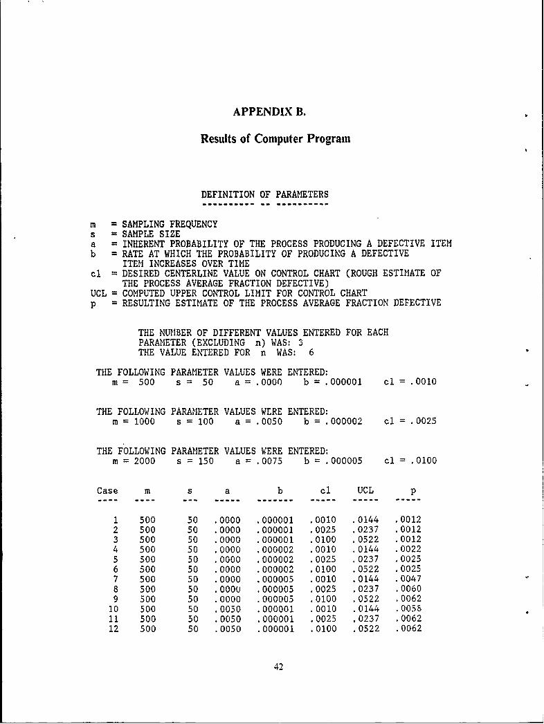
APPENDIX B.

Results of Computer Program

DEFINITION OF PARAMETERS

m = SAMPLING FREQUENCYs = SAMPLE SIZEa = INHERENT PROBABILITY OF THE PROCESS PRODUCING A DEFECTIVE ITEMb = RATE AT WHICH THE PROBABILITY OF PRODUCING A DEFECTIVE

ITEM INCREASES OVER TIMEcl = DESIRED CENTERLINE VALUE ON CONTROL CHART (ROUGH ESTIMATE OF

THE PROCESS AVERAGE FRACTION DEFECTIVE)UCL = COMPUTED UPPER CONTROL LIMIT FOR CONTROL CHARTp = RESULTING ESTIMATE OF THE PROCESS AVERAGE FRACTION DEFECTIVE

THE NUMBER OF DIFFERENT VALUES ENTERED FOR EACHPARAMETER (EXCLUDING n) WAS: 3THE VALUE ENTERED FOR n WAS: 6

THE FOLLOWING PARAMETER VALUES WERE ENTERED:m = 500 s = 50 a = .000 b = .000001 cl = .0010

THE FOLLOWING PARAMETER VALUES WERE ENTERED:m = 1000 s = 100 a = .0050 b = .000002 cl = .0025

THE FOLLOWING PARAMETER VALUES WERE ENTERED:

m 2000 s = 150 a .0075 b = .000005 cl = .0100

Case m s a b cl UCL p

1 500 50 .0000 .000001 .0010 .0144 .00122 500 50 .0000 .000001 .0025 .0237 .00123 500 50 .0000 .000001 .0100 .0522 .00124 500 50 .0000 .000002 .0010 .0144 .00225 500 50 .0000 .000002 .0025 .0237 .00256 500 50 .0000 .000002 .0100 .0522 .00257 500 50 .0000 .000005 .0010 .0144 .00478 500 50 .0000 .000005 .0025 .0237 .00609 500 50 .0000 .000005 .0100 .0522 .0062

10 500 50 .0050 .000001 .0010 .0144 .005811 500 50 .0050 .000001 .0025 .0237 .006212 500 50 .0050 .000001 .0100 .0522 .0062

42

13 500 50 .0050 .000002 .0010 .0144 .006614 500 50 .0050 .000002 .0025 .0237 .007415 500 50 .0050 .000002 .0100 .0522 .007516 500 50 .0050 .000005 .0010 .0144 .008417 500 50 .0050 .000005 .0025 .0237 .010618 500 50 .0050 .000005 .0100 .0522 .011119 500 50 .0075 .000001 .0010 .0144 .008220 500 50 .0075 .000001 .0025 .0237 .008621 500 50 .0075 .000001 .0100 .0522 .008722 500 50 .0075 .000002 .0010 .0144 .008823 500 50 .0075 .000002 .0025 .0237 .009824 500 50 .0075 .000002 .0100 .0522 .010025 500 50 .0075 .000005 .0010 .0144 .010426 500 50 .0075 .000005 .0025 .0237 .012827 500 50 .0075 .000005 .0100 .0522 .013528 500 100 .0000 .000001 .0010 .0105 .001229 500 100 .0000 .000001 .0025 .0175 .001230 500 100 .0000 .000001 .0100 .0398 .001231 500 100 .0000 .000002 .0010 .0105 .002432 500 100 .0000 .000002 .0025 .0175 .002433 500 100 .0000 .000002 .0100 .0398 .002534 500 100 .0000 .000005 .0010 .0105 .005535 500 100 .0000 .000005 .0025 .0175 .005536 500 100 .0000 .000005 .0100 .0398 .006237 500 100 .0050 .000001 .0010 .0105 .006138 500 100 .0050 .000001 .0025 .0175 .0061

43

DEFINITION OF PARAMETERS

m = SAMPLING FREQUENCYs = SAMPLE SIZEa = INHERENT PROBABILITY OF THE PROCESS PRODUCING A DEFECTIVE ITEMb = RATE AT WHICH THE PROBABILITY OF PRODUCING A DEFECTIVE

ITEM INCREASES OVER TIMEcl = DESIRED CENTERLINE VALUE ON CONTROL CHART (ROUGH ESTIMATE OF

THE PROCESS AVERAGE FRACTION DEFECTIVE)UCL = COMPUTED UPPER CONTROL LIMIT FOR CONTROL CHARTp = RESULTING ESTIMATE OF THE PROCESS AVERAGE FRACTION DEFECTIVE

Case m s a b cl UCL p

39 500 100 .0050 .000001 .0100 .0398 .006240 500 100 .0050 .000002 .0010 .0105 .007041 500 100 .0050 .000002 .0025 .0175 .007042 500 100 .0050 .000002 .0100 .0398 .007543 500 100 .0050 .000005 .0010 .0105 .009344 500 100 .0050 .000005 .0025 .0175 .009345 500 100 .0050 .000005 .0100 .0398 .011146 500 100 .0075 .000001 .0010 .0105 .008447 500 100 .0075 .000001 .0025 .0175 .008448 500 100 .0075 .000001 .0100 .0398 .008749 500 100 .0075 .000002 .0010 .0105 .009250 500 100 .0075 .000002 .0025 .0175 .009251 500 100 .0075 .000002 .0100 .0398 .010052 500 100 .0075 .000005 .0010 .0105 .011253 500 100 .0075 .000005 .0025 .0175 .011254 500 100 .0075 .000005 .0100 .0398 .013455 500 150 .0000 .000001 .0010 .0087 .001256 500 150 .0000 .000001 .0025 .0147 .001257 500 150 .0000 .000001 .0100 .0344 .001258 500 150 .0000 .000002 .0010 .0087 .002459 500 150 .0000 .000002 .0025 .0147 .002560 500 150 .0000 .000002 .0100 .0344 .002561 500 150 .0000 .000005 .0010 .0087 .004962 500 150 .0000 .000005 .0025 .0147 .005863 500 150 .0000 .000005 .0100 .0344 .006264 500 150 .0050 .000001 .0010 .0087 .005965 500 150 .0050 .000001 .0025 .0147 .006266 500 150 .0050 .000001 .0100 .0344 .006267 500 150 .0050 .000002 .0010 .0087 .006668 500 150 .0050 .000002 .0025 .0147 .007269 500 150 .0050 .000002 .0100 .0344 .007570 500 150 .0050 .000005 .0010 .0087 .008271 500 150 .0050 .000005 .0025 .0147 .009872 500 150 .0050 .000005 .0100 .0344 .011273 500 150 .0075 .000001 .0010 .0087 .008274 500 150 .0075 .000001 .0025 .0147 .008575 500 150 .0075 .000001 .0100 .0344 .008776 500 150 .0075 .000002 .0010 .0087 .008777 500 150 .0075 .000002 .0025 .0147 .0095

44

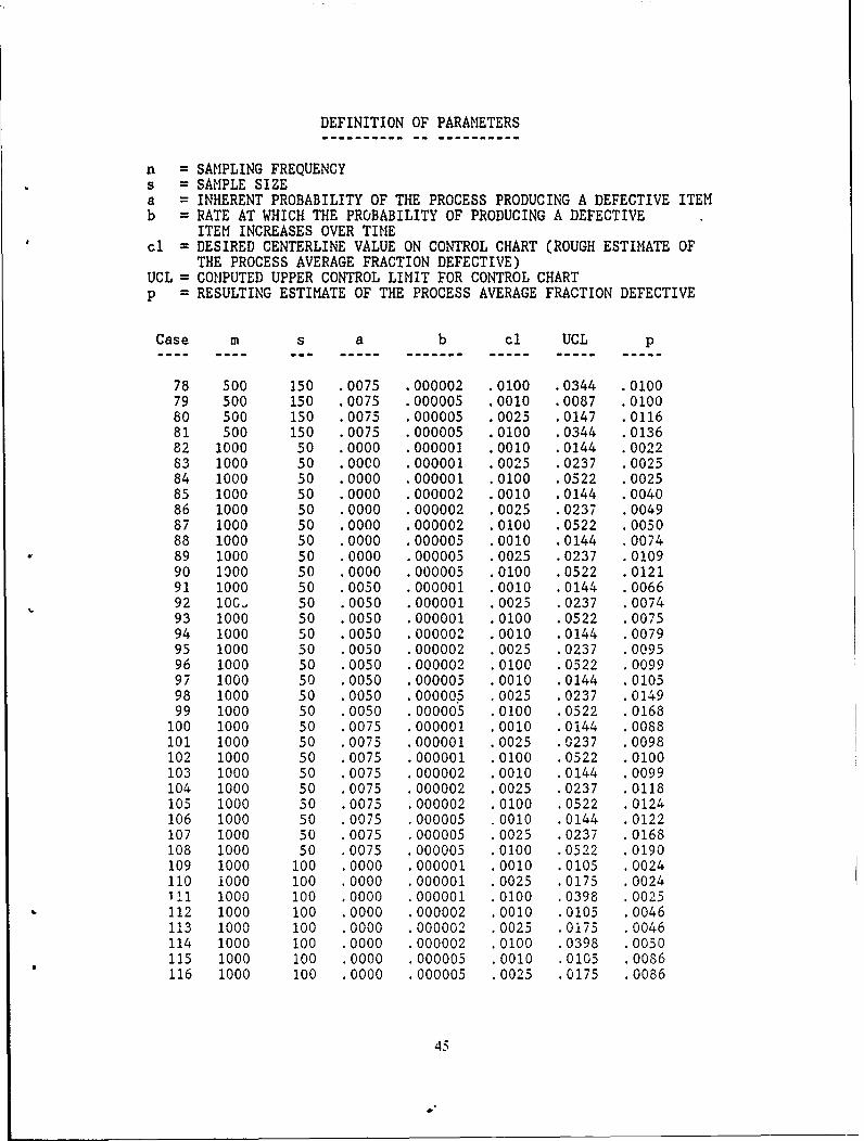
DEFINITION OF PARAMETERS

n = SAMPLING FREQUENCYs = SAMPLE SIZEa = INHERENT PROBABILITY OF THE PROCESS PRODUCING A DEFECTIVE ITEMb = RATE AT WHICH THE PROBABILITY OF PRODUCING A DEFECTIVE

ITEM INCREASES OVER TIMEcl = DESIRED CENTERLINE VALUE ON CONTROL CHART (ROUGH ESTIMATE OF

THE PROCESS AVERAGE FRACTION DEFECTIVE)UCL = COMPUTED UPPER CONTROL LIMIT FOR CONTROL CHARTp = RESULTING ESTIMATE OF THE PROCESS AVERAGE FRACTION DEFECTIVE

Case m s a b cl UCL p

78 500 150 .0075 .000002 .0100 .0344 .010079 500 150 .0075 .000005 .0010 .0087 .010080 500 150 .0075 .000005 .0025 .0147 .011681 500 150 .0075 .000005 .0100 .0344 .013682 1000 50 .0000 .000001 .0010 .0144 .002283 1000 50 .0000 .000001 .0025 .0237 .002584 1000 50 .0000 .000001 .0100 .0522 .002585 1000 50 .0000 .000002 .0010 .0144 .004086 1000 50 .0000 .000002 .0025 .0237 .004987 1000 50 .0000 .000002 .0100 .0522 .005088 1000 50 .0000 .000005 .0010 .0144 .007489 1000 50 .0000 .000005 .0025 .0237 .010990 1000 50 .0000 .000005 .0100 .0522 .012191 1000 50 .0050 .000001 .0010 .0144 .006692 lOG, 50 .0050 .000001 .0025 .0237 .007493 1000 50 .0050 .000001 .0100 .0522 .007594 1000 50 .0050 .000002 .0010 .0144 .007995 1000 50 .0050 .000002 .0025 .0237 .009596 1000 50 .0050 .000002 .0100 .0522 .009997 1000 50 .0050 .000005 .0010 .0144 .010598 1000 50 .0050 .000005 .0025 .0237 .014999 1000 50 .0050 .000005 .0100 .0522 .0168

100 1000 50 .0075 .000001 .0010 .0144 .0088101 1000 50 .0075 .000001 .0025 .0237 .0098102 1000 50 .0075 .000001 .0100 .0522 .0100103 1000 50 .0075 .000002 .0010 .0144 .0099104 1000 50 .0075 .000002 .0025 .0237 .0118105 1000 50 .0075 .000002 .0100 .0522 .0124106 1000 50 .0075 .000005 0010 .0144 .0122

107 1000 50 .0075 .000005 .0025 .0237 .0168108 1000 50 .0075 .000005 .0100 .0522 .0190109 1000 100 .0000 .000001 .0010 .0105 .0024110 iOO 100 .0000 .000001 .0025 .0175 .0024ill 1000 100 .0000 .000001 .0100 .0398 .0025112 1000 100 .0000 .000002 .0010 .0105 .0046113 1000 100 .0000 .000002 .0025 .0175 .0046114 1000 100 .0000 .000002 .0100 .0398 .0050115 1000 100 .0000 .000005 .0010 .0105 .0086116 1000 100 .0000 .000005 .0025 .0175 .0086

45

DEFINITION OF PARAMETERS

m = SAMPLING FREQUENCYs = SAMPLE SIZEa = INHERENT PROBABILITY OF THE PROCESS PRODUCING A DEFEC"TVE ITEMb = RATE AT WHICH THE PROBABILITY OF PRODUCING A DEFECTIVE

ITEM INCREASES OVER TIMEcl = DESIRED CENTERLINE VALUE ON CONTROL CHART (ROUGH ESTIMATE OF

T-;E PROCESS AVERAGE FRACTION DEFECTIVE)UCL = COMPUTED UPPER CONTROL LIMIT FOR CJNTROL CHARTp = RESULTING ESTIMATE OF THE PROCESS AVERAGE FRACTION DEFECTIVE

Case m s a b cl UCL p

117 1000 100 .0000 .000005 .0100 .0398 .0119118 1000 100 .0050 .000001 .0010 .0105 .0070119 1000 100 .0050 .000001 .002 .0175 .0070120 1000 100 .0050 .1. 0001 .0100 .0398 .0075121 1000 100 .0050 .0,0002 .0010 .0105 .0086122 1000 100 .0050 .000002 .0025 .0175 .0086123 1000 100 .0050 .000002 .0100 .0398 .0099124 1000 100 .0050 .000005 .0010 .0105 .0117125 1000 100 .0050 .000005 .0025 .0175 .0117126 1000 100 .0050 .000005 .0100 .0398 .0162127 1000 100 .0075 .000001 .0010 .0105 .0092128 1000 100 .0075 .000001 .0025 .0175 .0092129 1000 100 .0075 .000001 .0100 .0398 .0100130 1000 100 .0075 .000002 .0010 .0105 .0106131 1000 100 .0075 .000002 .0025 .0175 .0106132 1000 100 .0075 .000002 .0100 .0398 .0123133 1000 100 .0075 .000005 .0010 .0105 .0132134 1000 100 .0075 .000005 .0025 .0175 .0132135 VO0 100 .0075 .000005 .0100 .0398 .0182136 A0 150 .0000 .000001 .0010 .0087 .0024137 lu00 150 .0000 .000001 .0025 .0147 .0025138 1000 150 .0000 .000001 .0100 .0344 .0025139 1000 150 .0000 .000002 .0010 .0087 .0042140 1000 150 .0000 .000002 .0025 .0147 .0048141 1000 150 .0000 .000002 .0100 .0344 .0050142 1000 150 .0000 .000005 .0010 .0087 .0069143 1000 ]50 .0000 .000005 .0025 .0147 .0092144 1000 150 .0000 .000005 .0100 .0344 .0122145 1000 150 .0050 .000001 .0010 .0087 .0066146 1000 150 .0050 .000001 .0025 .0147 .0072147 1000 150 .0050 .000001 .0100 .0344 .0075148 1000 150 .0050 .000002 .0010 .0087 .00784 1000 150 .0050 .000002 .0025 .0147 .0090150 1000 150 .0050 .000002 .0100 .0344 .0100151 1000 150 .0050 .000005 .0010 .0087 .0098152 1000 150 .0050 .000005 .0025 .0147 .0122153 1000 150 .0050 .000005 .0100 .0344 .0167154 1000 150 .0075 .000001 .0010 .0087 .0087155 1000 150 .0075 .000001 .0025 .0147 .0095

46

DEFINITION OF PARAMETERS

m = SAMPLING FREQUENCYs = SAMPLE SIZEa = INHERENT PROBABILITY OF THE PROCESS PRODUCING A DEFECTIVE ITEMb = RATE AT WHICH THE PROBABILITY OF PRODUCING A DEFECTIVE

ITEM INCREASES OVER TIMEcl = DESIRED CENTERLINE VALUE ON CONTROL CHART (ROUGH ESTIMATE OF

THE PROCESS AVERAGE FRACTION DEFECTIVE)UCL = COMPUTED UPPER CONTROL LIMIT FOR CONTROL CHARTp = RESULTING ESTIMATE OF THE PROCESS AVERAGE FRACTION DEFECTIVE

Case m s a b cl UCL p

156 1000 150 .0075 .000001 .0100 .0344 .0100157 1000 150 .0075 .000002 .0010 .0087 .0096158 1000 150 .0075 .000002 .0025 .0147 .0110159 1000 150 .0075 .000002 .0100 .0344 .0124160 1000 150 .0075 .000005 .0010 .0087 .0113161 1000 150 .0075 .000005 .0025 .0147 .0137162 1000 150 .0075 .000005 .0100 .0344 .0189163 2000 50 .0000 .000001 .0010 .0144 .0040164 2000 50 .0000 .000001 .0025 .0237 .0049165 2000 50 .0000 .000001 .0100 .0522 .0050166 2000 50 .0000 .000002 .0010 .0144 .0065167 2000 50 .0000 .000002 .0025 .0237 .0091168 2000 50 .0000 .000002 .0100 .0522 .0098169 2000 50 .0000 .000005 .0010 .0144 .0108

170 2000 50 .0000 .000005 .0025 .0237 .0172171 2000 50 .0000 .000005 .0100 .0522 .0217172 2000 50 .0050 .000001 .0010 .0144 .0079173 2000 50 .0050 .000001 .0025 .0237 .0095174 2000 50 .0050 .000001 .0100 .0522 .0099175 2000 50 .0050 .000002 .0010 .0144 .0097176 2000 50 .0050 .000002 .0025 .0237 .0133177 2000 50 .0050 .000002 .0100 .0522 .0146178 2000 50 .0050 .000005 .0010 .0144 .0134179 2000 50 .0050 .000005 .0025 .0237 .0203180 2000 50 .0050 .000005 .0100 .0522 .0254181 2000 50 .0075 .000001 .0010 .0144 .0099182 2000 50 .0075 .000001 .0025 .0237 .0118183 2000 50 .0075 .000001 .0100 .0522 .0124184 2000 50 .0075 .000002 .0010 .0144 .0115185 2000 50 .0075 .000002 .0025 .0237 .0153186 2000 50 .0075 .000002 .0100 .0522 .0169187 2000 50 .0075 .000005 .0010 .0144 .0149188 2000 50 .0075 .000005 .0025 .0237 .0218189 2000 50 .0075 .000005 .0100 .0522 .0272190 2000 100 .0000 .000001 .0010 .0105 .0046191 2000 100 .0000 .000001 .0025 .0175 .0046192 2000 100 .0000 .000001 .0100 .0398 .0050193 2000 100 .0000 .000002 .0010 .0105 .0076194 2000 100 .0000 .000002 .0025 .0175 .0076

47

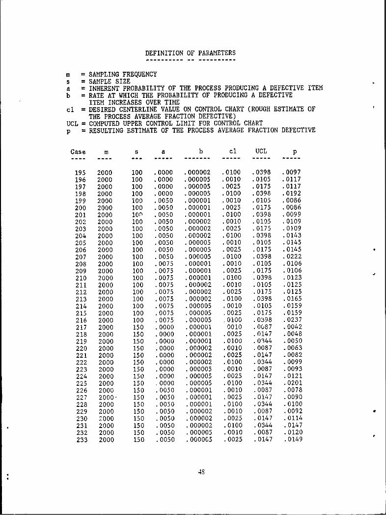
DEFINITION OF PARAMETERS

m = SAMPLING FREQUENCYs = SAMPLE SIZEa = INHERENT PROBABILITY OF THE PROCESS PRODUCING A DEFECTIVE ITEMb = RATE AT WHICH THE PROBABILITY OF PRODUCING A DEFECTIVE

ITEM INCREASES OVER TIMEcl = DESIRED CENTERLINE VALUE ON CONTROL CHART (ROUGH ESTIMATE OF

THE PROCESS AVERAGE FRACTION DEFECTIVE)UCL = COMPUTED UPPER CONTROL LIMIT FOR CONTROL CHARTp = RESULTING ESTIMATE OF THE PROCESS AVERAGE FRACTION DEFECTIVE

Case m s a b cl UCL p

195 2000 100 .0000 .000002 .0100 .0398 .0097196 2000 100 .0000 .000005 .0010 .0105 .0117197 2000 100 .0000 .000005 .0025 .0175 .0117198 2000 100 .0000 .000005 .0100 .0398 .0192199 2000 100 .0050 .000001 .0010 .0105 .0086200 2000 100 .0050 .000001 .0025 .0175 .0086201 2000 1Ol .0050 .000001 .0100 .0398 .0099202 2000 100 .0050 .000002 .0010 .0105 .0109203 2000 100 .0050 .000002 .0025 .0175 .0309204 2000 100 .0050 .000002 .0100 .0398 .0143205 2000 100 .0050 .000005 .0010 .0105 .0145206 2000 100 .0050 .000005 .0025 .0175 .0145207 2000 100 .0050 .000005 .0100 .0398 .0222208 2000 100 .0075 .000001 .0010 .0105 .0106209 2000 100 .0075 .000001 .0025 .0175 .0106210 2000 100 .0075 .000001 .0100 .0398 .0123211 2000 100 .0075 .000002 .0010 .0105 .0125212 2000 100 .0075 .000002 .0025 .0175 .0125213 2000 100 .0075 .000002 .0100 .0398 .0165214 2000 100 .0075 .000005 .0010 .0105 .0159215 2000 100 .0075 .000005 .0025 .0175 .0159216 2000 100 .0075 .000005 .0100 .0398 .0237217 2000 150 .0000 .000001 0010 .0087 .0042218 2000 150 .0000 .000001 .0025 .0147 .0048219 2000 150 .0000 .000001 .0100 .0344 .0050220 2000 150 .0000 .000002 .0010 .0087 .0063221 2000 150 .0000 .000002 .0025 .0147 .0082222 2000 150 .0000 .000002 .0100 .0344 .0099223 2000 150 .0000 .000005 .0010 .0087 .0093224 2000 150 .0000 .000005 .0025 .0147 .0121225 2000 150 .0000 .000005 .0100 .0344 .0201

226 2000 150 .0050 .000001 .0010 .0087 .0078227 2000' 150 .0050 .000001 .0025 .0147 .0090228 2000 150 .0050 .000001 .0100 .0344 .0100229 2000 150 .0050 .000002 .0010 .0087 .0092230 2000 150 .0050 .000002 .0025 .0147 .0114231 2000 150 .0050 .000002 .0100 .0344 .0147232 2000 150 .0050 .000005 .0010 .0087 .0120233 2000 150 .0050 .000005 .0025 .0147 .0149

48

DEFINITION OF PARAMETERS

m = SAMPLING FREQUENCYs = SAMPLE SIZEa = INHERENT PROBABILITY OF THE PROCESS PRODUCING A DEFECTIVE ITEMb = RATE AT WHICH THE PROBABILITY OF PRODUCING A DEFECTIVE

ITEM INCREASES OVER TIMEcl = DESIRED CENTERLINE VALUE ON CONTROL CHART (ROUGH ESTIMATE OF

THE PROCESS AVERAGE FRACTION DEFECTIVE)UCL = COMPUTED UPPER CONTROL LIMIT FOR CONTROL CHARTp = RESULTING ESTIMATE OF THE PROCESS AVERAGE FRACTION DEFECTIVE

Case m s a b cl UCL p

234 2000 150 .0050 .000005 .0100 .0344 .0231235 2000 150 .0075 .000001 .0010 .0087 .0096236 2000 150 .0075 .000001 .0025 .0147 .0110237 2000 150 .0075 .000001 .0100 .0344 .0124238 2000 150 .0075 .000002 .0010 .0087 .0108239 2000 150 .0075 .000002 .0025 .0147 .0130240 2000 150 .0075 .000002 .0100 .0344 .0169241 2000 150 .0075 .000005 .0010 .0087 .0133242 2000 150 .0075 .000005 .0025 .0147 .0162243 2000 150 .0075 .000005 .0100 .0344 .0246

49

LIST OF REFERENCES

1. Duncan, Acheson J., Qualitv Control and Industrial Statistics. Richard D. Irwin,

Inc., Homewvood, Illinois, 1974.

2. Department of Defense Military Standard MIL-STD 105D, Sainplinq Procedures

and Tables-for Inspection bv Attributes, 1961.

3. Grant, Eugene L. and Leavenworth, Richard S., Statistical Quality Control

McGraw-Hill, Inc., New York, New York, 1980.

4. Department of Defense Military Standard M I L-STD 414, Sa,,zplhni Procedures and

Tables fbr Inspection by Variables fbr Percent Defective, 1957.

5. Brugger, Richard M., ",4 Simplifled ? Iarkov Chain A4nalysis of AXSI .41SOC ZI.4

U sed WJithout Limit Numbers", Journal of Quality Technology- , April 1989,

pp.97-102.

6. Oakland, John S.. Statistical Process Control. John WNiley and Sons. Inc.. New

York, New York, 1986.

7. Ross, Sheldon M., Introduction to Probabilitr Models. Academic Press, Inc., San

Diego, California. 1985.

50

INITIAL DISTRIBUTION LIST

No. Copies

1. Defense Technical Information Center 2Cameron StationAlexandria, VA 22304-6145

2. Library, Code 0142 2Naval Postgraduate SchoolMonterey, CA 93943-5002

3. Professor Glen Lindsay. Code 55Ls 2I)epartment of Operations ResearchNaval Postgraduate SchoolMonterey, CA 93943-5000

4. Professor Michael Bailey, Code 55Ba 2I)epartment of Operations ResearchNaval Postgraduate SchoolMonterey. CA 93943-5000

5. Mr. John Bowden 2Ordnance Engineering Department. Code 50Naval Weapons Support CenterCrane, IN 47522-5050

6. Ms. Glatha Ilemne 2Pacific Miesile Test CenterCruise Weapons DivisionAttn: Code 1070Pt. MagL. CA 93042-5000

7. Mr. Dan Cuhna 2General DvnanicsConvair DivisionPost Office Box 85357Department 613-0 ' MZ-546130San Diego, CA 92138-5357

8. Department of Industrial Engineering and Management 2Oklahoma State UniversityStillwater, OK 74078

9. LT Greg DevogelNaval Postgraduate SchoolSMC 1803Monterey, CA 93943

51

10. Mr. JI Roy Hammnons 2P.O. Box 571Thomas, OK 73669

52