thesis (4.4-es pont)
DESCRIPTION
A STUDY IN HEBREWPARAPHRASE IDENTIFICATIONTRANSCRIPT

Ben-Gurion University of the Negev
Faculty of Natural Science
Department of Computer Science
A STUDY IN HEBREW
PARAPHRASE IDENTIFICATION
Thesis submitted as part of the requirements for the
M.Sc. degree of Ben-Gurion University of the Negev
by
Gabriel Stanovsky
December 2012

Subject: A Study in Hebrew Paraphrase Identi�cation
Writen By: Gabriel Stanovsky
Advisor: Professor Michael Elhadad
Department: Computer Science
Faculty: Natural Science
Ben-Gurion University of the Negev
Signatures:
Author: Gabriel Stanovsky Date
Advisor: Professor Michael Elhadad Date
Dept. Committee Chairman Date
I

Contents
1 Introduction 1
1.1 Formal De�nitions . . . . . . . . . . . . . . . . . . . . . . . . . . . . . . . . . 2
1.1.1 Textual Entailment . . . . . . . . . . . . . . . . . . . . . . . . . . . . . 2
1.1.2 Paraphrase . . . . . . . . . . . . . . . . . . . . . . . . . . . . . . . . . 2
1.1.3 Related Shared Tasks . . . . . . . . . . . . . . . . . . . . . . . . . . . 3
1.1.4 Paraphrasing in Hebrew . . . . . . . . . . . . . . . . . . . . . . . . . . 3
1.2 Motivation . . . . . . . . . . . . . . . . . . . . . . . . . . . . . . . . . . . . . 3
2 Research Questions and Objectives 5
2.1 Research Questions . . . . . . . . . . . . . . . . . . . . . . . . . . . . . . . . . 5
2.1.1 Hebrew Speci�c properties . . . . . . . . . . . . . . . . . . . . . . . . . 5
2.1.2 Hebrew Datasets for Paraphrasing . . . . . . . . . . . . . . . . . . . . 6
2.1.3 Method Adaptation for Hebrew . . . . . . . . . . . . . . . . . . . . . . 6
2.1.4 Producing Hebrew Resources for Other NLP Uses . . . . . . . . . . . 6
2.2 Objectives . . . . . . . . . . . . . . . . . . . . . . . . . . . . . . . . . . . . . . 6
3 Previous Work 7
3.1 Paraphrase Identi�cation . . . . . . . . . . . . . . . . . . . . . . . . . . . . . 7
3.2 Paraphrase Generation . . . . . . . . . . . . . . . . . . . . . . . . . . . . . . . 8
3.3 Paraphrases Extraction . . . . . . . . . . . . . . . . . . . . . . . . . . . . . . 8
3.4 Hebrew Paraphrasing . . . . . . . . . . . . . . . . . . . . . . . . . . . . . . . . 9
4 Linguistic Background 10
4.1 Is Paraphrasing Possible? . . . . . . . . . . . . . . . . . . . . . . . . . . . . . 10
4.2 Levels of Paraphrasing . . . . . . . . . . . . . . . . . . . . . . . . . . . . . . . 10
4.3 Explaining Paraphrases: What Motivates Deviation from Convention . . . . . 12
4.4 Syntax and Paraphrases . . . . . . . . . . . . . . . . . . . . . . . . . . . . . . 13
4.4.1 Phrase Structure Grammar . . . . . . . . . . . . . . . . . . . . . . . . 14
4.4.2 Dependency Grammar . . . . . . . . . . . . . . . . . . . . . . . . . . . 15
4.4.3 Examples of Paraphrases Pair in Phrase Structure Grammar vs De-
pendency Grammar . . . . . . . . . . . . . . . . . . . . . . . . . . . . 16
II

4.4.4 Discussion . . . . . . . . . . . . . . . . . . . . . . . . . . . . . . . . . . 18
5 Methodology 21
5.1 Plan of Work . . . . . . . . . . . . . . . . . . . . . . . . . . . . . . . . . . . . 21
5.2 Learning Methods . . . . . . . . . . . . . . . . . . . . . . . . . . . . . . . . . 23
5.2.1 Neural Networks . . . . . . . . . . . . . . . . . . . . . . . . . . . . . . 23
5.2.1.1 Outline . . . . . . . . . . . . . . . . . . . . . . . . . . . . . . 23
5.2.1.2 Neuron . . . . . . . . . . . . . . . . . . . . . . . . . . . . . . 23
5.2.1.3 Weights . . . . . . . . . . . . . . . . . . . . . . . . . . . . . . 24
5.2.1.4 Network Computation . . . . . . . . . . . . . . . . . . . . . . 24
5.2.1.5 Learning . . . . . . . . . . . . . . . . . . . . . . . . . . . . . 24
5.2.1.6 Backpropogation . . . . . . . . . . . . . . . . . . . . . . . . . 24
5.2.1.7 Layered Networks . . . . . . . . . . . . . . . . . . . . . . . . 25
5.2.2 Deep Learning . . . . . . . . . . . . . . . . . . . . . . . . . . . . . . . 25
5.2.2.1 Curriculum Learning . . . . . . . . . . . . . . . . . . . . . . 25
5.2.2.2 Multi Task Learning . . . . . . . . . . . . . . . . . . . . . . . 26
5.2.2.3 Word Embeddings . . . . . . . . . . . . . . . . . . . . . . . . 26
5.2.3 Auto Encoders . . . . . . . . . . . . . . . . . . . . . . . . . . . . . . . 26
5.2.3.1 Outline . . . . . . . . . . . . . . . . . . . . . . . . . . . . . . 27
5.2.3.2 Neural Network . . . . . . . . . . . . . . . . . . . . . . . . . 27
5.2.3.3 Encoding . . . . . . . . . . . . . . . . . . . . . . . . . . . . . 27
5.2.3.4 Decoding . . . . . . . . . . . . . . . . . . . . . . . . . . . . . 28
5.2.3.5 Uses in NLP . . . . . . . . . . . . . . . . . . . . . . . . . . . 28
5.2.4 Tree Matching . . . . . . . . . . . . . . . . . . . . . . . . . . . . . . . 28
5.2.4.1 De�nition . . . . . . . . . . . . . . . . . . . . . . . . . . . . . 28
5.2.4.2 Tree Match Score . . . . . . . . . . . . . . . . . . . . . . . . 29
5.2.4.3 Tree Matching is NP-Complete . . . . . . . . . . . . . . . . . 29
5.3 Hebrew Paraphrasing . . . . . . . . . . . . . . . . . . . . . . . . . . . . . . . . 30
5.3.1 Producing Deep Learning Embedding for Hebrew . . . . . . . . . . . . 30
5.3.1.1 Overview . . . . . . . . . . . . . . . . . . . . . . . . . . . . . 30
5.3.1.2 Preprocessing and Hebrew Adaptation . . . . . . . . . . . . . 31
5.3.1.3 Language Model . . . . . . . . . . . . . . . . . . . . . . . . . 31
5.3.1.4 Curriculum Learning . . . . . . . . . . . . . . . . . . . . . . 32
5.3.1.5 Stochastic Sampling of the Error Function . . . . . . . . . . 32
5.3.1.6 Deep Learning Structure . . . . . . . . . . . . . . . . . . . . 33
5.3.2 Binarizing Parse Trees . . . . . . . . . . . . . . . . . . . . . . . . . . . 34
5.3.2.1 Overview . . . . . . . . . . . . . . . . . . . . . . . . . . . . . 34
5.3.2.2 Binarization of Constituency Parse Trees . . . . . . . . . . . 35
5.3.2.3 Binarization of Dependency Parse Trees . . . . . . . . . . . . 36
III

5.3.3 Learning to Parse on Embeddings Using Autoencoders . . . . . . . . . 36
5.3.3.1 Overview . . . . . . . . . . . . . . . . . . . . . . . . . . . . . 36
5.3.3.2 Training Process . . . . . . . . . . . . . . . . . . . . . . . . . 37
5.3.4 Tree Matching . . . . . . . . . . . . . . . . . . . . . . . . . . . . . . . 38
5.3.4.1 Overview . . . . . . . . . . . . . . . . . . . . . . . . . . . . . 38
5.3.4.2 Finding Tree Matching . . . . . . . . . . . . . . . . . . . . . 38
5.4 Experiments . . . . . . . . . . . . . . . . . . . . . . . . . . . . . . . . . . . . . 38
5.4.1 Testing Embeddings . . . . . . . . . . . . . . . . . . . . . . . . . . . . 38
5.4.1.1 Improving POS tagging . . . . . . . . . . . . . . . . . . . . . 39
5.4.2 Testing Tree Matching as Paraphrase Indicator . . . . . . . . . . . . . 39
5.4.3 Testing Dependency vs Constituency Parse Trees . . . . . . . . . . . . 39
6 Experimental Setting and Results 40
6.1 Experimental Setting . . . . . . . . . . . . . . . . . . . . . . . . . . . . . . . . 40
6.1.1 Embeddings Generation Corpus . . . . . . . . . . . . . . . . . . . . . . 40
6.1.2 Autoencoding of Parse Trees Training Corpus . . . . . . . . . . . . . . 40
6.1.3 Labeled Paraphrase Corpus . . . . . . . . . . . . . . . . . . . . . . . . 41
6.2 Results . . . . . . . . . . . . . . . . . . . . . . . . . . . . . . . . . . . . . . . . 41
6.2.1 Embeddings . . . . . . . . . . . . . . . . . . . . . . . . . . . . . . . . . 41
6.2.1.1 Annotations . . . . . . . . . . . . . . . . . . . . . . . . . . . 41
6.2.2 English POS Tagging . . . . . . . . . . . . . . . . . . . . . . . . . . . 41
6.2.2.1 Corpus . . . . . . . . . . . . . . . . . . . . . . . . . . . . . . 41
6.2.2.2 Experiments . . . . . . . . . . . . . . . . . . . . . . . . . . . 41
6.2.2.3 Discussion . . . . . . . . . . . . . . . . . . . . . . . . . . . . 42
6.2.3 Hebrew POS Tagging . . . . . . . . . . . . . . . . . . . . . . . . . . . 42
6.2.3.1 Corpora . . . . . . . . . . . . . . . . . . . . . . . . . . . . . . 42
6.2.3.2 Analysis of Corpora . . . . . . . . . . . . . . . . . . . . . . . 43
6.2.3.3 Experiments . . . . . . . . . . . . . . . . . . . . . . . . . . . 44
6.2.3.4 Discussion . . . . . . . . . . . . . . . . . . . . . . . . . . . . 46
6.2.4 Paraphrasing . . . . . . . . . . . . . . . . . . . . . . . . . . . . . . . . 46
6.2.4.1 Corpus . . . . . . . . . . . . . . . . . . . . . . . . . . . . . . 46
6.2.4.2 Paraphrase Identi�cation . . . . . . . . . . . . . . . . . . . . 48
6.2.4.3 Discussion . . . . . . . . . . . . . . . . . . . . . . . . . . . . 48
7 Conclusion 49
Bibliography 51
A Proof of Tree Matching NP Completeness 55
IV

B Paraphrase Tagging Guidelines 58
B.1 Goal . . . . . . . . . . . . . . . . . . . . . . . . . . . . . . . . . . . . . . . . . 58
B.2 Rules for Tagging . . . . . . . . . . . . . . . . . . . . . . . . . . . . . . . . . . 58
B.2.1 Paraphrase . . . . . . . . . . . . . . . . . . . . . . . . . . . . . . . . . 58
B.2.1.1 Restrictions . . . . . . . . . . . . . . . . . . . . . . . . . . . . 58
B.2.2 Partial Paraphrase . . . . . . . . . . . . . . . . . . . . . . . . . . . . . 59
B.2.3 Negative . . . . . . . . . . . . . . . . . . . . . . . . . . . . . . . . . . . 59
B.3 Examples . . . . . . . . . . . . . . . . . . . . . . . . . . . . . . . . . . . . . . 59
V

List of Tables
5.1 Baseline results for English paraphrase recognition on the MSRP corpus . . . 22
6.1 Size of the Di�erent Corpora used for Embeddings computation . . . . . . . . 40
6.2 Experimental Results for English POS Tagging . . . . . . . . . . . . . . . . . 42
6.3 Hebrew corpora statistics. Values show size in #tokens and #sequences . . . 43
6.4 Unknown Token Percentage . . . . . . . . . . . . . . . . . . . . . . . . . . . . 43
6.5 Percentage of Ambiguous Tokens . . . . . . . . . . . . . . . . . . . . . . . . . 44
6.6 Hebrew Baseline Results. Values show Acc / F1 . . . . . . . . . . . . . . . . . 45
6.7 Hebrew Embeddings Results. Values show Acc / F1. . . . . . . . . . . . . . . 46
6.8 Category Distribution Over the Paraphrase Corpus . . . . . . . . . . . . . . . 47
6.9 Category Distribution Over the Paraphrase Corpus . . . . . . . . . . . . . . . 47
6.10 Tree Matching Algorithm Performance . . . . . . . . . . . . . . . . . . . . . . 48
VI
List of Figures
4.1 Constituent Parse Tree for the Hebrew Sentence �no bears and no forest� . . 15
4.2 Dependency Parse Tree for the Hebrew Sentence �no bears and no forest� . . 16
4.3 Constituency Emphasis Paraphrasing Example . . . . . . . . . . . . . . . . . 19
4.4 Dependency Emphasis Paraphrasing Example . . . . . . . . . . . . . . . . . . 19
4.5 Constituent Transliteration Paraphrasing Example . . . . . . . . . . . . . . . 19
4.6 Dependency Transliteration Paraphrasing Example . . . . . . . . . . . . . . . 20
4.7 Constituent Participle and Reported Speech Paraphrasing Example . . . . . . 20
4.8 Dependency Participle and Reported Speech Paraphrasing Example . . . . . 20
5.1 Deep Network Structure . . . . . . . . . . . . . . . . . . . . . . . . . . . . . . 33
5.2 Constituency Binarization Paraphrasing Example . . . . . . . . . . . . . . . . 35
5.3 Dependency Binarization Paraphrasing Example . . . . . . . . . . . . . . . . 35
5.4 Encoding of a Binary Dependency Tree . . . . . . . . . . . . . . . . . . . . . 37
5.5 Possible Match of a Paraphrase Pair . . . . . . . . . . . . . . . . . . . . . . . 39
6.1 Tag Distribution Histogram . . . . . . . . . . . . . . . . . . . . . . . . . . . . 43
6.2 Ambiguous Tokens Distribution Histogram . . . . . . . . . . . . . . . . . . . 44
6.3 Hebrew Baseline Accuracy Percentage on Di�erent Corpora and Feature Set . 45
6.4 Hebrew Baseline F1 Percentage on Di�erent Corpora and Feature Set . . . . 45
VII

Chapter 1
Introduction
The topic of this research is the processing and generation of natural language paraphrases
from an algorithmic point of view. Focusing mainly on the implication of adapting and
applying such algorithms to the Hebrew language.
Paraphrasing is the action of restating sentences or paragraphs using di�erent sentence
structures or di�erent choice of words, while keeping similar meaning. Paraphrases are used
by an author of a single text in order to elaborate on a given subject, to provide examples,
or to explain a topic by using a di�erent approach while conveying the same message. When
comparing text written by di�erent authors describing similar events, one will also �nd
occurrences of paraphrases, re�ecting style di�erences between the authors.
Paraphrase identi�cation is the task of determining whether two given texts stand in a
relation of paraphrasing. Paraphrase generation is the task of producing a paraphrase given
an original sentence.
While it is natural for native speakers to either paraphrase a given sentence or to deter-
mine if a given pair of text fragments are a paraphrase, an algorithmic formulation of the
tasks is quite challenging.
For example, the following two news snippets (dated from 14.11.11) from two di�erent
News web sites can be considered paraphrases:
(aixrn) y"aa ifkxnd x`ecd wpa sipqa ccey lr ehlzyd gha`ne gxf` �
� A citizen and a guard took over a robber at the general post o�ce in Beer-Sheva. (The
city name appears here as an abbreviation)
(zepexg` zerici) ray x`aa x`ec sipq cecyl dvxy mc` lr ehlzyd gha`ne gxf` �
� A citizen and a guard took over a man who tried to rob the post o�ce in Beer-Sheva.
1

1.1 Formal De�nitions
Recent research in the �eld of paraphrasing in English has yielded the formulation of the
following de�nitions [2][4]:
1.1.1 Textual Entailment
Given two text fragments A,B, determine if one could be inferred from the other. A will
entail B if a human being who trusts A, on all its parts, will consequently have to trust that
B is also true.
For example:
dtexi` zetil`a dnir cgi dkfe qewiipz`pt zveawl 2000 zpya ribd yhw oexec �
� Doron Katash joined the Panathinaikos team in 2000, and won the European cham-
pionship with it.
2000 zpya dtexi` zetil`a dzkf qewiipz`pt zveaw �
� The Panathinaikos team won the European championship in 2000.
For the comprehensive de�nition of textual entailment, see [4].
1.1.2 Paraphrase
Paraphrase is commonly de�ned as bidirectional textual entailment. For example, given two
text fragments (A,B), it could be said that A entails B and vice-versa. A few restrictions
upon these texts have been de�ned:
� This bidirectional entailment can rely also on knowledge which is considered to be
common:
diqex mr xgq mkqdl dribd oiq –
� China has reached a trading agreement with Russia
diqex mr xgq mkqdl dribd mlera zqlke`nd dpicnd –
� The world most populated nation has reached a trading agreement with Russia
� Yet the entailment must not rely solely on prior knowledge:
diqex mr xgq mkqdl dribd oiq –
� China has reached a trading agreement with Russia
mlera zqlke`nd dpicnd `id oiq –
� China is the most populated nation.
A complete de�nition of Hebrew paraphrase is given in appendix B.
2

1.1.3 Related Shared Tasks
Following these de�nitions, several shared tasks have been de�ned and proposed to the
attention of the research community, amongst them:
- Novelty Detection [4], Given a fraction T of text and a corpus C - determine if T
contains new information with respect to C.
- Knowledge Base Population [3], Given a list of entities and a corpus C, extract values
for a pre-de�ned set of attributes (a.k.a. �slots�) corresponding to those entities.
1.1.4 Paraphrasing in Hebrew
We are not aware of previous e�ort in studying paraphrasing in Hebrew - either linguistically
or computationally. The closest e�ort has been that of [29] who have applied the technique of
MultiWordnet to construct an electronic thesaurus in Hebrew; the work does not speci�cally
address the task of paraphrasing detection or generation.
We expect that the speci�c properties of the Hebrew language � speci�cally the pos-
sibility to agglutinate function words (prepositions, conjunctions and articles) with other
words, the relatively free word order syntax, the productive noun-compounding mechanism
(smixut) and several productive word derivation mechanisms (verb constructions - binyanim)
� produces rich opportunities for paraphrasing.
1.2 Motivation
The tasks of generation and identi�cation of paraphrases help in various Natural Language
Processing (NLP) �elds, such as:
- Automatic Text Generation, data from a knowledge base can be expressed in a variety
of forms using paraphrases. The capability of producing text variability is important
for text generators to adapt the generated text to various target audience needs, by
varying the style of the text, its complexity and its level of detail.
- Automatic Summarization, while scanning through a document, paraphrases found in
text body could be detected, and then omitted, in order to provide a shorter version
of the document. This is particularly important in the context of multi-document
summarization: in this task, several similar documents (describing the same events)
are taken as input, and we expect them to contain many paraphrases. The summary
of the cluster of documents should avoid repetitions and contain only one instance of
each group of paraphrases from the source documents.
- Automatic Construction of Thesaurus, identifying paraphrases from freely occurring
text in conjunction with exploiting knowledge of the sentence structure can be used
3

to yield a bank of Hebrew words which are, with high probability, synonyms. The
result of such analysis would lead to automatic construction of a thesaurus in Hebrew,
similar to the Wordnet [16] resource available in English.
4

Chapter 2
Research Questions and Objectives
2.1 Research Questions
As part of this work, we address the research questions related to analysis of paraphrasing
in Hebrew:
2.1.1 Hebrew Speci�c properties
Are there speci�c properties of the Hebrew language that allow paraphrasing?
- Morphological derivation (e.g., using participle forms to operate as nouns, or
verbs). For example, the following pair of sentences is a case of a participle taking
form of a verb to create a paraphrase of a given sentence:
.zelwa mincxp md mitiirzn micliyk -
- When children get tired, they will fall asleep easily.
.zelwa mincxp mitiir micli -
- Tired children fall asleep easily.
- Syntactic variations exploiting free-word order in Hebrew. Sentences in He-
brew may be expressed in di�erent word orderings, as a tool to emphasize di�erent
notions within the same occurrence, which is a common target of paraphrasing:
.dberd z` izpkd ip` -
- I made the cake.
.izpkd dberd z` -
- The cake, I made.
- Lexical replacement. Replacing a Hebrew word with another derived from another
language with transliterations, with another part of speech.
5

dpe`za oihelgl dqxdp zipeknd -
- The car was completely ruined during the accident.
dpe`zd zeawra qel-l`heh dxar zipeknd -
- Because of the accident, the car is a total loss.
2.1.2 Hebrew Datasets for Paraphrasing
Which datasets can be used to collect and identify a database of paraphrases in Hebrew?
The objective is to identify pairs of naturally occurring sentences which are paraphrases
with high likelihood. We still need to manually assess the level of paraphrasing, but we
would like to mine existing text repositories to extract likely candidates.
2.1.3 Method Adaptation for Hebrew
Could approaches taken on other languages (especially English) for paraphrasing identi�ca-
tion and generation be applied on Hebrew? What aspects of the methods must be adapted
to account for speci�c properties of Hebrew?
- Word agglutination
- High morphological ambiguity
- Free-word order syntax
2.1.4 Producing Hebrew Resources for Other NLP Uses
Can the process of learning paraphrases yield resources applicable for other NLP Hebrew
tasks? Recent research in the �eld of NLP tries to reuse training information and share it
across common NLP tasks (this is known as �Deep Learning�). Can such information be
obtained and encoded in such a way to aid other Hebrew NLP tasks?
2.2 Objectives
The overall objective of this work is to develop computational methods to identify para-
phrases in Hebrew text. As part of this objective, we construct a dataset of paraphrase
pairs in Hebrew, we build reusable resources for Hebrew processing (word embeddings) and
measure their impact on other NLP tasks: Parts of Speech (POS) Tagging and Parsing.
6

Chapter 3
Previous Work
Relatively recent research has explored the possibility to learn paraphrases ([6, 33, 32, 25,
21]). These could be divided into three main categories [25]:
- Identi�cation of a paraphrase.
- Generation of paraphrases
- Extraction of paraphrases from large texts.
We review work done in each of these interconnected �elds in the rest of this chapter,
given de�ntions formulated in previous chapters.
3.1 Paraphrase Identi�cation
This task involves receiving a pair of text fragments and determining if the pair consti-
tutes a paraphrase. Barzilay and McKeown [6] have developed an unsupervised paraphrase
identi�cation algorithm. Their dataset consists of multiple English translations of foreign
books (e.g., books that were translated into English more than once). Their assumption
was that di�erent translators will introduce paraphrases when translating the same source
text. First they used the alignment method of [17] to align the corresponding translations.
They continued by applying an iterative model for extracting paraphrases features from the
aligned sentences. The iteration starts with a simple rule, which extracts the surroundings
of identical words (namely a number of tokens before and after an identical word) in both
sentences. From these surroundings they code a "contextual rule", by exploiting the sur-
rounding words parts of speech. They continue by reapplying the new rules learned in the
previous iteration upon their corpus once more, allowing for a prede�ned number of sepa-
rating tokens to appear, thus allowing new rules to arise. This process ends when no more
rules are discovered during a single iteration. During these iterations a classi�er is trained
from the examples extracted from the text.
7
Socher et al [33] created a system for paraphrase identi�cation composed of two parts:
the �rst is an autoencoder [31], trained to compress setences taken from the WSJ corpus
and which were syntactically parsed using an automatic parser (the Stanford parser). The
leaves (representing original words in the sentence, preserving the original word order) were
replaced by 100 dimensional number vector embeddings of the words (obtained by a sta-
tistical language model, [13, 38]). The autoencoder then traverses the tree in a bottom-up
manner, at each step saving the encoding of two already computed nodes at their parent
node. Thus, the system outputs a tree in which each node contains an encoding (a 100
dimensional vector) of the subtree which it spans.
The second part of their system (after the autoencoder has been trained), receives a
sentence pair and computes two parsed auto-encoded trees, as explained above. The eu-
clidean distance between each node i of the �rst sentence, and every node j in the second
is then computed to form a similarity matrix. Since this matrix is not of a �xed size (be-
cause sentence pairs are not of �xed size), this matrix is then sampled by running a sliding
window of �xed, predetermined size, over it and picking the minimum of every window into
a �dynamic-pooling� matrix. This matrix, now being of �xed size, can be fed to another
classifer trained to distinguish between paraphrases pair pooling matrix and non-paraphrase
pair pooling matrix.
This system provides state-of-the-art accuracy in paraphrase identi�cation in English as
of 2012 and seems to be quite robust across domains.
3.2 Paraphrase Generation
Paraphrase Generation is the task of generating a paraphrase of a given text fragment. The
Microsoft NLP team [32] created a system to produce paraphrases of an input English sen-
tence. Their system gathered a large automated training set from news sites, upon which
they performed subsequently: sentence alignment, word alignment and phrasal replacement
identi�cation. They eventually learned a "phrasal translation database" from this dataset.
To create this database they have used methods from the area of Statistical Machine Trans-
lation (SMT). Given an input sentence, they create a "generation lattice" which describes
all possible paraphrases for each possible phrasal alignment where each label is marked with
a probability assigned by the system. The lattice is then exploited to generate traversal
paths which can be ranked by probability.
3.3 Paraphrases Extraction
The task of extracting parphrases from a large given corpus. In the �eld of paraphrase
extraction, [20] is a typical example: they developed a system for extraction of Japanese
paraphrases from the web. They begin by scanning the web for what they call a "de�nition
8

sentence", a sentence which describes a term. This is done by searching for a certain sequence
of part of speech tags which according to their hypothesis de�nition sentence are likely to
adhere to. All the de�nitions of the same terms are considered candidate paraphrases. These
possible paraphrases are parsed for dependency structures using an automated parser and
classi�ed by a Support Vector Machine (SVM) classi�er to decide which candidate should
be declared as a paraphrase. Using this method they have achieved a large collection of
300K paraphrases with estimated precision of 94%.
3.4 Hebrew Paraphrasing
In comparison to the vast research e�orts invested in English paraphrasing, very little work
has been done in the �eld of Hebrew paraphrase. [29] have developed a medium scale
Wordnet for Hebrew, consisting of 5300 groups of synonymous lexical items (synsets).
The approach they have taken was to form the Wordnet by aligning English and Hebrew
expressions, and infer relations from the English available Wordnet onto their created Hebrew
Wordnet. They state that this method (called MultiWordNet) is preferable over building
the Wordnet from scratch since the Hebrew language is poor on computational linguistic
resources. The lack of monolingual dictionaries in Hebrew is given as an example of such
resource.
9

Chapter 4
Linguistic Background
4.1 Is Paraphrasing Possible?
It is unclear whether two sentences can really be considered �equivalent�. This question is for-
mulated clearly in Clark's Principle of Conventionality and Principle of Contrast ([12][11]):
Principle of Conventionality: In every language community, there are certain mean-
ings for which there exist conventional words used to express these meanings.
Principle of Contrast: �Every two forms contrast in meaning�. That is, when there is
a deviation from the conventional word used to express a meaning, a member of the language
community will assume the speaker is seeking to convey a (perhaps slightly) di�erent notion
than that of the conventional meaning.
In other words, following the general approach of minimal distinctive pairs adopted
in structuralist linguistics, any paraphrase pair must be explained by a deviation in meaning.
Many experiments in the linguistic �eld were conducted to provide empirical evidence of
the validity of these two principles. Among these were studies of the way children acquire
language (and seemingly avoid attaching two di�erent words to the same meaning), and
studies across di�erent language communities speaking the same language (showing di�erent
conventional names for the same meaning). Experiments supporting these principles were
also conducted among Hebrew native speakers [15].
If every two forms of words indeed di�er in meaning as research suggests, one can induce
that two di�erent phrases must also di�er in meaning. Thus complete and true meaning
preserving paraphrase does not exist. Still, di�erent linguistic theories attempt to de�ne
�near equivalence� through di�erent ways. We review two such attempts below.
4.2 Levels of Paraphrasing
Halliday in [19] has developed a version of functionalist linguistics which puts emphasis on
the notion of paraphrasing. This perspective sees language as a tool which provides its
10

speakers with a system of choices with which to transfer meaning between the partici-
pants of a conversation. The set of choices available to a speaker are often called linguistic
devices. The functionalist theory enumerates linguistic devices at di�erent levels which,
together, contribute to the expression of meaning in context. For example, Halliday classi�es
linguistic devices in terms on their relation to three main dimensions:
Field Who does what to whom?
Tenor What is the relationship between the speakers?
Mode What theme and register is taken by the speaker?
Meaning is thus transformed from the speaker intention into natural language by deciding
on a set of linguistic choices. Analyzing text, according to this school, is trying to recover
from a sentence the decisions which produced it.
In this perspective, paraphrases are two sentences which are produced by �almost the
same intentions� conveyed using di�erent linguistic devices. Analyzing each of the sentences
in a functionalist point of view is discerning the �input� to the linguistic functions. Pick [30]
gives the following paraphrases as example:
� I �Julius Caesar was assassinated by Brutus�
II �Julius Caesar lay dead at the hands of Brutus�
� I �John lent Mary the book�
II �Mary had the book on loan from John�
According to Pick both sentences of each pair consist of the same functional elements.
But the linguistic devices used to convey this similar meaning are di�erent: with di�erent
syntactic structures and di�erent lexical elements used in each sentence.
Interestingly, some of the decisions taken while producing an utterance are dictated
directly by the speaker intentions, while others are imposed as a consequence of earlier
decisions. For example, when a speaker decides to use a speci�c verb (like �assassinate�),
together with this decision comes the requirement to use a subject and an object. In contrast,
if the predicate �lay dead� is selected, the �agent� of the action does not need to be expressed.
One could just say: �Julius Ceasar lay dead.�
In addition, for some verbs, the speaker must further decide whether to use the verb in
the passive or active voice (�assassinate�) while this option does not exist for others (�lay
dead�).
Accordingly, when one analyzes the set of decisions taken in order to produce two closely
related sentences (a pair of sentences candidate as paraphrases), one must identify the base
decisions which explain the contrast between the two sentences. Those decisions which
derive from other decisions are not necessarily meaningful to the same level. Accordingly,
11
one may distinguish di�erent levels of paraphrasing between pairs of sentences � in other
words, paraphrasing is not a binary relation, but is more a gradable relation between pairs
of sentences.
4.3 Explaining Paraphrases: What Motivates Deviation
from Convention
Based on the principle of conventionality, it is generally assumed that expressions of a given
meaning can be ranked in terms of their conventionality. More conventional expressions
bring less �surprise�. When a deviation from conventional expression is detected, linguists
are often interested in �explaining� the deviation (which is a source of meaning).
For example, Hirst [21] proposes a classi�cation of paraphrases as small scale and large
scale paraphrasing. Small scale paraphrases are two phrases which are identical except for a
few words exchanged for near synonyms. Following the principle of contrast, this divergence
between otherwise identical phrases indicates the speaker intention to give the phrase a
di�erent meaning. For example:
I Yossi bought a carpet at the market
weya gihy dpw iqei �
weya caxn dpw iqei �
� The word �shatiach� in the �rst sentence is substituted with the word �marvad� in
the second. �Shatiah� is the Hebrew contemporary conventional word for carpet.
The deviation in the latter may suggest that Yossi bought a rather exclusive artifact
instead of a usual rug.
II The destruction of the building occurred last year
dxary dpya dxw oiipad qxd �
dxary dpya dxw oiipad oaxeg �
� The word �herez� in the �rst sentence is substituted with the word �hurban� in the
second. As before, The former being the Hebrew contemporary conventional word
for destruction. The deviation in the latter may suggest that the speaker would
like to convey a sense of grief related to the destruction, as opposed to the latter,
which may sound as a more objective description.
III The last few days indicate that the �ghting is over
zeaxwd seq lr micirn mipexg`d minid �
zeaxwd uw lr micirn mipexg`d minid �
12

� The word �sof� in the �rst sentence is substituted with the word �ketz� in the
second. Again, the former being the Hebrew contemporary conventional word for
ending. The deviation in the latter may suggest that the speaker believes that the
break in the �ghting is a more constanst state, as oppose to the former, which may
be understood as a less de�nite state.
Large scale paraphrasing, according to Hirst's division, is the act of di�erent phrasing of
full sentences or paragraphs. This instance of paraphrasing can be found when an author,
either consciously or unconsciously, inserts his own ideology and perception into the details
of an occurrence. For example:
I Emphasis
.dberd z` izpkd ip` �
� I made the cake.
.izpkd dberd z` �
� The cake, I made.
The latter emphasizes the product of the baking (the cake), while the former emphasizes
the maker (I made the cake).
II Ideology
(29.2.2012 ,ux`d) .oeilrd ze`iypn zyxet yipiia �
� Dorit Beinish retires from Supreme Court. (Haaret'z, 29.2.2012)
(28.2.2012 ,zayd xkik) .dziad zkled yipiia zixec �
� Dorit Beinish goes home. (Kikar Hashabat, 28.2.2012)
Although the two news snippets above report the same occurrence - the retirement of
Dorit Beinish from the Supreme Court, it is safe to say that the latter phrase takes a
more supporting approach to her departure.
In general, one can explain the distinction between paraphrases in terms of (1) which level
of linguistic expression di�ers (a single word or the syntactic structure) and (2) what moti-
vates the deviation from one form to another (put emphasis, express additional connotation,
avoid expressing a part of the meaning, indicate di�erent levels of social appreciation).
4.4 Syntax and Paraphrases
One of the main linguistic sources of paraphrasing consists of altering the syntactic structure
of a sentence. For example, one can change a sentence from active to passive voice:
1. The cat eats the mouse.
13

2. The mouse is eaten by the cat.
Many similar syntactic alternations have been identi�ed which can be used as sources
of paraphrasing. When combined with other sources of paraphrasing (such as replacing a
word with a quasi-synonym or with a pronoun), one obtains a large range of variants from
a base sentence:
1. The cat eats the mouse.
2. The mouse is eaten by the cat.
3. It is devoured by the felin.
Parsing (also known as syntax analysis) is the process that maps an input sentence to
the syntactic tree representing the relation among words within the sentence. The syntactic
structure is usually not visible explicitly within the sentence � one must recover it using
the rules of grammar and knowledge of typical relations among speci�c words. Parsing is a
necessary step to assess whether two sentences are syntactic variants, or to align paraphrase
candidates so that each part of the sentence can be further analyzed in terms of lexical
similarity. In the example above, parsing is necessary to discover that �the felin� must be
compared with �the cat� and �devour� with �eat�.
Computational techniques for automatic parsing have seen tremendous progress in the
past decade. We survey two common approaches, phrase structure grammar (constituent
grammar), and dependency grammar. We focus mainly on instances of paraphrases pairs,
and review the resulting parse trees in each of the approaches. From here on, when speaking
of constituents of parse trees we will refer to a part of sentence which can be seen as single
unit in parse tree, i.e., a subtree of a parse tree.
4.4.1 Phrase Structure Grammar
Phrase structure grammar, also known as constituent grammar, is the grammar originally
de�ned by Chomsky[10] as part of the generative school. A Phrase structure grammar is
formally de�ned as a 4-tuple G = (N,T, S, P ) where
I N⋂T = ∅, N - The non-terminal set, T - the terminal set
II S ∈ N , S being the start symbol
III P = {(u, v) : u, v ∈ (N⋃T )∗}, P is �nite and called the production rules
According to these grammars, the leaves (terminals) of the parse tree are the words of the
original sentence, appearing in the original sentence order. Accordingly, the leftmost word
will be represented by the leftmost leaf, and so forth. The rules by which an input sentence
is parsed onto a parse tree are de�ned via a transformational grammar. Computational
14

Figure 4.1: Constituent Parse Tree for the Hebrew Sentence �no bears and no forest�
tools which parse input sentences onto a possible constituent parse tree were devised with
good results for Hebrew and English languages ([9],[18], respectively). Figure 4.1 shows a
constituent parse tree of the Hebrew sentence �No bears and no forest�.
4.4.2 Dependency Grammar
Dependency grammars in modern linguistics date to the work of Tesni`re (1959) [27]. This
approach towards parsing views the syntax analysis of a sentence as consisting of binary
asymmetrical relations between words. In each of these relations there is a word which
functions as a head (also known as governor, regent) and a second word which functions
as a dependent. The relation between the two words is called a dependency. According to
this linguistic theory, the speaker of a language analyzes syntax by perceiving connections
between words, the dependency relation aims at modeling this connection. This binary re-
lation of head - dependent will appear in the parse tree as father - son relation.
This de�nition suggests that dependency parse trees will be formed of words in the sentence.
As opposed to the constituency grammar trees, words in the dependency tree will appear
also as the inner nodes, and not only as terminals. Because of this property, dependency
trees will be of smaller size as that of the matching constituency tree, in which syntactic
nodes are present in addition to the original words of the sentence. As an example of this,
the dependency parse tree for the sentence �no bears and no forest�, which was shown pre-
viously for constituency tree, is shown in �gure 4.2 (18 nodes in constituency tree versus 5
nodes in the dependency tree) .
The root of every subtree will represent the head (and will normally be a verb) of that
subtree (by transitivity), where his direct dependents will be his sons.
15

Figure 4.2: Dependency Parse Tree for the Hebrew Sentence �no bears and no forest�
Various de�nitions exist for determining when two words will appear in a dependency
relation, yet, as is often the case with NLP, none of the rules cover all cases. Following are
a few of these de�nitions [27] (where: H marks the head, D marks the dependent, and C
marks their relation) :
� H determines the syntactic category of C and can often replace C.
� H determines the semantic category of C, D gives semantic speci�cation.
� H is obligatory, D may be optional.
� The form of D depends on H.
� The linear position of D is speci�ed with reference to H.
These should be seen as guidelines for identifying words in dependency relation: failure to
satisfy one of these rules does not necessarily indicate the pair of words is not in a depen-
dency relation. Accordingly, success to satisfy a rule does not necessarily deem the pair as
being in a dependency relation.
As for Constituency parsing, tools to automatically parse a dependency structure of a sen-
tence were devised ([23],[18]).
4.4.3 Examples of Paraphrases Pair in Phrase Structure Grammar
vs Dependency Grammar
In the following section we review paraphrase pairs' parse trees in both formats de�ned
above (i.e, constituency and dependency).
1. A simple example of paraphrase pair was described before, as a pair which demonstrate
the change of emphasis:
.dberd z` izpkd ip` �
� I made the cake.
16
.izpkd dberd z` �
� The cake, I made.
Figure 4.3 and 4.4 show the corresponding constituent and dependency parse trees of
both sentences. In �g. 4.3 we can see the same constituents appearing as subtrees
of both sentences, while in �g. 4.4 we can see that �the cake� in the latter sentence
receives a higher node in the parse tree, when comparing to the former sentence. This
may correspond to its increased emphasis in the second sentence.
2. Recall the example of Hebrew paraphrasing arising from replacing a term with its
transliterated equivalent:
dpe`za oihelgl dqxdp zipeknd �
� The car was completely ruined during the accident.
dpe`zd zeawra qel-l`heh dxar zipeknd �
� Because of the accident, the car is a total loss.
Figure 4.5 and 4.6 show the corresponding constituent and dependency parse trees of
both sentences.
In �g. 4.5 we can see that the general structure is similar within the trees (with
respect to the inner nodes structure and type). There is a change in one constituent
S ⇒ PP ⇒ PP on the right is substituted with S ⇒ ADV P ⇒ RB on the left.
This can be seen as a substitution of the Hebrew �lahalutin� (completely) with the
transliterated term �total loss�.
In �g. 4.6 The governor of the sentence is changed from �neherza� (wrecked), on the
left, to �avra� (su�ered, in this context) on the right. Apart from that we see, again,
the subtree of �lahalutin� (completely) on the left, changed with �total loss� on the
right.
3. In this example we examine a relatively complicated example of paraphrasing, which
includes participles changing part of speech between the two sentences and reported
speech.
i`kf `ed ik eizeprh zexnl ,my` ceygd ik meid eraw mihtey �
� Judges have decided today that the defendant is guilty, although he claimed being
not guilty.
i`kf `edy zexnl eze` mihtey ik xn` meid my`edy ceygd �
� The defendant that was accused today said that he was not guilty.
Figure 4.7 and 4.8 show the corresponding constituent and dependency parse trees of
both sentences.
17

In �g. 4.7 a few similarities can be found, although not as easily as in previous
examples. The �rst level below the root is almost identical, and the prepositional
phrase is also similar.
In �g. 4.8 it is hard to �nd any similarities between the parse trees, nor to map
between matching constituents.
In both �gures it can be seen that the participle �shoftim� (judge) indeed appear in
di�erent nodes in the parse tree.
4.4.4 Discussion
As a conclusion of this section, we notice a few relevant observations with regards to both
formats of parse tree which were shown, within the scope of the task of paraphrase identi�-
cation:
� Dependency parsing yields a tree with signi�cantly less nodes when comparing to
constituency parsing.
� A change in a dependency parse tree due to paraphrasing can in�ict a change in higher
nodes than that of a constituency parse tree.
� Dependency parse trees seem more sensitive to changes in the sentence structure.
� A note on binarization of parse trees: While the binarization of a constituency parse
tree is rather straightforward, this is not the case when binarizing dependency parse
trees. This topic is elaborated in 5.3.2.
18
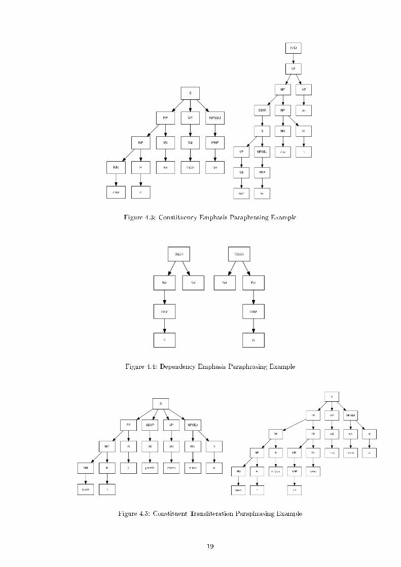
Figure 4.3: Constituency Emphasis Paraphrasing Example
Figure 4.4: Dependency Emphasis Paraphrasing Example
Figure 4.5: Constituent Transliteration Paraphrasing Example
19
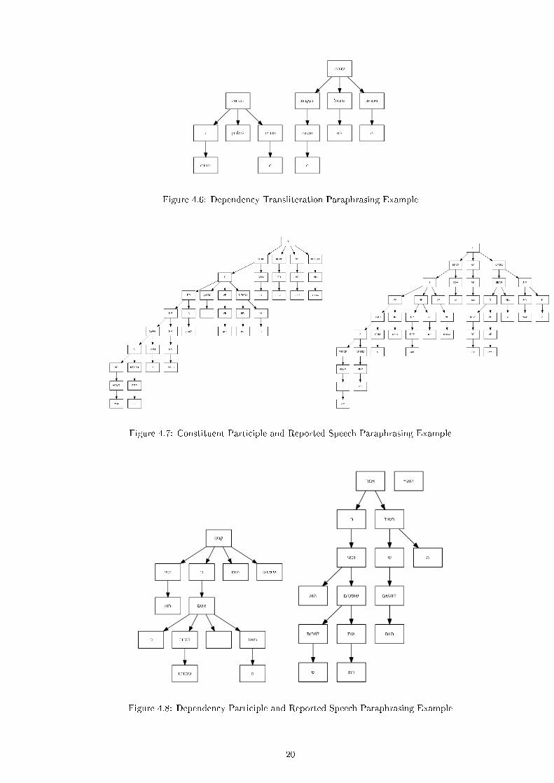
Figure 4.6: Dependency Transliteration Paraphrasing Example
Figure 4.7: Constituent Participle and Reported Speech Paraphrasing Example
Figure 4.8: Dependency Participle and Reported Speech Paraphrasing Example
20

Chapter 5
Methodology
This chapter covers the main methods of learning which are applied in this work, description
of the adaption technique and proposed hypotheses, and �nally the experiments taken to
prove those hypotheses.
The structure of this chapter is as follows: In Section 5.1, we describe the method and
outline of the work in general lines. Section 5.2 reviews the methods of learning applied in
NLP which are relevant to the task of paraphrasing. Section 5.3 contains an in depth plan
for adapting the algorithms discussed to answer the research questions posed in previous
chapter. Section 5.4 concludes this chapter by depicting the experiments by which we test
correctness of the methods proposed.
5.1 Plan of Work
The target of this work is to face the task of paraphrase recognition in Hebrew. To attack
this problem, we apply, adapt, and devise methods of machine learning (neural networks,
autoencoders), and computational linguistics (language models, automatic parsing). Since
this task has not yet been addressed in Hebrew, it is missing comparative benchmark results
and adequate corpora. Thus, we must collect and publish such a corpus. Datasets consist
of a monolingual Hebrew parallel corpus of paraphrases. These are acquired in an unsuper-
vised manner by obtaining hourly news �ashes and corresponding news stories from leading
Israeli News sites. Each news �ash in the dataset is aligned against an assumed matching
news �ash from the other websites. This yields a method for obtaining an automatically
growing dataset. These datasets will be hand tagged by human judges in order to obtain a
baseline comparable corpus, guidelines for formally de�ning what is considered as an Hebrew
paraphrase will also be published as part of this work (see Appendix B). The methods and
hypotheses raised in this work are trained and tested against this corpus. The desired size of
the corpus is 6000 sentences, with 67% of the pairs being in a paraphrase relationship. These
numbers are an Hebrew equivalent of the Microsoft Research Paraphrase Corpus (MSRP
21

Model ACC F1
Wan et al. (2006) 75.6 83.0
Das and Smith (2009) 76.1 82.7
Socher et al. (2011) 76.8 83.6
Table 5.1: Baseline results for English paraphrase recognition on the MSRP corpus
corpus [1]). Recent research in the �eld of English paraphrase uses this corpus as baseline
comparative parallel corpus.
In order to recognize Hebrew paraphrases, we go along the lines of [33] that used auto
encoders on embedded parse trees of the input sentences. They have used word feature vector
representation of the words, as obtained from a deep learning approach. In the course of
this work we reproduce the settings described in that paper for the English language. We
o�er some deviation and improvement of the algorithms they have used, introducing a new
search problem on the pair of trees. Following the reproduction of that experiment we
implement it for the Hebrew language. This implementation requires generating resources
not yet available for the Hebrew language, such as Hebrew word embeddings, binarization
of dependency parse trees, and the parallel paraphrase corpus already mentioned above.
We test both Socher's implementation's equivalent , as well as the proposed improvement
of it, on the Hebrew corpus. The main experiment is the task of identifying paraphrase
identi�cation as described in the previous section. The baseline results of several English
applications on the MSRP corpus appear in Table 5.1.
22

5.2 Learning Methods
Learning methods applied in Arti�cial Intelligence (AI) in general are used to detect some
recurring pattern in input data. If the process of learning is supervised then the pattern is
�rst learned from labeled training data (by adjusting the speci�c parameters of the learning
model). Then the model is tested on an unlabeled, and previously unseen test data, to
measure its ability to infer and deduce from the training phase. We hope that by properly
modeling the input data and correctly adjusting the model parameters during training we
will learn the real underlying pattern embedded in the data.
In Natural Language Processing (NLP) in particular, these methods are employed over
natural language corpora. Training data may be labeled for the speci�c tasks - i.e., pairs of
sentences are marked manually as being paraphrase or not. Additional labels on input data
may include semantic information, which is naturally not present in raw natural language.
These may include Part of Speech (POS) tags, parsing of the sentences, anaphora resolution,
to name a few. Over this data and possibly additional labels, learning methods are used to
explore recurring patterns in the input text. We review below the main learning methods
applied in this work to identify recurring patterns in Hebrew paraphrases.
5.2.1 Neural Networks
5.2.1.1 Outline
The concept of neural networks is to try and imitate the function of neurons in an intelligent
being's brain. Each neuron is modeled as a predetermined di�erentiable function which
receives a predetermined number of inputs. Neurons are connected to other neurons, forming
what can be seen as a graph whose vertices are the neurons, and whose edges are the
connections among those neurons. The topology of this graph is determined a priori. A
neuron network is the set of neurons and their connections. A special case of neurons are
the input neurons - which receive their input from an input instance of predetermined format,
and output neurons which output the result of the total network. Most of the information
in this section is based on the book [34].
5.2.1.2 Neuron
The function of a speci�c neuron can be seen as composition of two functions:
� Integration function: I : Rn → R - receives as input the incoming edges of this neuron
and outputs a single output.
� Activation function: A : R → R - receives the output of the integration function and
returns the �nal output of this neuron.
23
Thus, the function of this neuron can be seen as A ◦ I . The activation function can make
the behavior of the neuron non-linear.
5.2.1.3 Weights
As we've seen, the output of a neuron is in turn part of the input of another neuron. Two
neurons are connected by an edge in the network graph on which the information �travels�.
As part of this model, the graph is seen as a weighted graph. Each of the edges e has
a weight we ∈ R, the information x traveling an edge e is multiplied by we to reach the
integration function as the input x · we.
5.2.1.4 Network Computation
Neural network computation is the process of giving an input instance to the input neurons,
continuing by computing at each step the neuron function, and transferring their output to
their connected neighbors. The process is terminated when the output neurons output a
value. This vector of values is the output of the network and the result of its computation
on the input.
5.2.1.5 Learning
Most of the parameters of the network are predetermined, decided upon during design time,
and remain constant throughout all iterations of network computations. These parameters
are the neural network graph, including the number of neurons and their connections, and the
neuron functions (both integration and activation). The learning is achieved by modifying
the previously mentioned weights of the edges, these change during a number of iterations
which is called �training� in which tagged input (i.e., that the desired output for this input
is known), is fed into the system. Knowing the desired outcome can yield an error value
for this speci�c computation, by means of a distance metric. Thus, after a number of these
iterations, the value of an error function is known at speci�c points of input space. This
error function can be seen as a function of the weighted edges existing in the system, as
these are the only values which can be modi�ed according to the neural network model.
Thus by summing the received errors of all inputs we can arrive at an error value for these
weights. Changing the network weights and recalculating the error yields an error function
in weight space whose values are known at speci�c points. We can search for the minimum
of this error function using numerical methods such as the discrete gradient of the network
function.
5.2.1.6 Backpropogation
Learning in a neural network can thus be reduced to calculating partial derivatives of the
error function over weight space, in order to perform gradient descent on it, and minimizing
24

the error on the training dataset. A common way to calculate these partial derivatives is
Backpropogation. This method exploits the chain rule that applies in calculating derivatives,
and stores the derivative of its input during network computation. After the computation
step begins a backpropogation step which starts from the output nodes, traveling the network
backward, multiplying at each neuron the saved value of the derivative. Thus, the derivative
of the network is obtained at the input neurons.
5.2.1.7 Layered Networks
A special case of neural networks, and one of common use in machine learning is the case
of n layered networks. Several extra restrictions are applied on these networks:
� The Neuron vertices V of the graph can be seen as a union of disjoint sets: V =
V1
⋃...⋃Vn , Vi
⋂Vj = ∅. In layered networks the inner layers: V2, ..., Vn−1 are
referred to as �hidden layers�, and their respective neurons are referred to as �hidden
units�.
� Edges between neurons can be set only between nodes of adjacent groups, i.e, the
edge set E of the graph can be seen as E = E1
⋃...
⋃En−1 , Ei
⋂Ej = ∅, such that
Ei = {(vi, vi+1)|vi ∈ Vi, vi+1 ∈ Vi+1}
� Normally all neurons in a layer are connected to all neurons of adjacent layers.
Special optimizations for calculating the backpropogation step on layered networks exist,
and we use this type of networks throughout this work.
5.2.2 Deep Learning
Recent research in AI has yielded the approach of deep learning [7]. This approach aims at
modeling the human perception of complicated notions in several levels of representation.
This approach is implemented using several neural networks connected in such a way that
one network output is transferred to another network input. Backpropogation is carried
across networks, starting from the topmost network to the bottom. This process can give
�exibility in determining the networks parameters according to their location and dedicated
task.
5.2.2.1 Curriculum Learning
As part of the model of deep learning, the concept of curriculum learning [8] was established.
This approach claims that by giving the deep learning networks inputs in an increasing order
of complexity (as one teaches a child), the model will be able to obtain better results. This
is due to establishing �rmer representations on the �simple� samples, and improving that
solid ground when facing higher degrees of complexity in the input.
25

5.2.2.2 Multi Task Learning
It is common in recent research to attack several tasks at once, when using deep learning.
[13, 14] created an architecture where the lower levels of the deep learning extract features
of the input text, and embed these features in multidimensional vectors - these vectors are
the output of the bottom networks. These bottom networks are shared across higher-level
tasks (POS tagging, Semantic Role Labeling, Chunking, Name Entity Recognition, and
Language Model calculation). The upper levels, which are task speci�c classi�ers take as
input these embeddings instead of the original text. Thus the lower levels change during
training (which is done in an interleaved manner) of all these tasks. The rationale is that
information learned for one task for representing feature embedding, may be useful for a
second task which classi�es according to the same feature - thus the tasks classi�ers �pro�t�
from the multi training.
This work is impressive in that it achieves state of the art results on a wide range of
natural language tasks using a single uniform feature representation and learning method
for all tasks.
5.2.2.3 Word Embeddings
As a by-product of this process - The embeddings [13] of words were published for English
dictionaries [38] to use as a plug-in enhancer for use in many NLP tasks which treated words
simply as index to a �nite dictionary.
As part of this work, we use a deep learning architecture to learn a Hebrew language
model from a large corpora of unlabeled text. This yields a dictionary of Hebrew word
embeddings which aids the process of paraphrase identi�cation. This dictionary can also
be published to aid other research in the �eld of Hebrew NLP. The language model and
embedding networks are presented with dictionaries of growing size (words are ordered from
the common to the less common), according to the curriculum learning concept.
5.2.3 Auto Encoders
A major drawback on the model of neural networks as presented above is the constant size
of the network, on all its parts. These must be de�ned during the design of the system, and
determine the topology of the network. This constant size of input and inner representations
(known as the connectionist approach) does not the �t the nature of most AI tasks, for which
the instances of a task are not of constant bounded size. NLP tasks possess this property as
well. The instances of natural texts are of variable size and unbounded length � no known
bounds exist for word length, nor for sentence length, nor paragraph length. Speci�cally in
this work, it is easy to observe from the examples given in previous chapters that paraphrases
must not be of identical length, although by de�nition they convey the same amount of
26

information. This property seems to limit, or cancel the use of neural networks in the �eld
of variable length instances, such as NLP.
To attack this problem, several connectionist systems were devised to cope with the
unbounded input size. We review here the approach of Recursive Auto-Associative Memory
(RAAM [31]), also known and extended in later papers as Auto Encoders.
5.2.3.1 Outline
Auto Encoders aim at creating recursive �xed size representations of variable size input.
The input is assumed to be a variable length list of �xed size elements (a character string
for example), mark each element representation size as K. They do so by going over the
input instance of size K ·n and �encoding� every pair of consecutive input elements onto one
compressed representation. Thus obtaining a second level of representation of size K · n2 ,
this process is repeated until the last level contains one element of �xed size which represent
the entire variable size input, in a �xed size representation.
5.2.3.2 Neural Network
The system Pollack [31] devised was composed of two concatenated neural networks:
� Encoder - a neural network composed of an input layer of 2K elements fully connected
to an output layer of K elements.
� Decoder - a neural network composed of an input layer of K elements fully connected
to an output layer of 2K elements.
These two networks are trained concurrently as a single network: a network of 2K input
elements, K hidden units in one hidden layer, and 2K elements in the output layer. During
training on an input element, the element itself is presented as the network desired outcome
- thus training the network to output the input it received, after going through the hidden
layer. The hidden layer (recall that this is actually the output layer of the encoder), now
holds a compact representation of the input. In other words, the auto-encoders �learns� the
identity function while going through a compressed representation of the input space.
5.2.3.3 Encoding
Encoding of a variable size length input is giving to every two consecutive elements (con-
catenated to get 2K elements) to the encoder network, thus producing an element of size K,
this is marked as the father of the two nodes which it encodes. This process repeats until
we are left with one element of size K. This process yields a binary tree of the elements,
in which the leaves are the original input and the inner nodes are representing some subtree
they encode. If the encoding phase is �awless one can reconstruct the entire input sentence
given only the root of this binary tree.
27

5.2.3.4 Decoding
The process of decoding consists of taking the root of the previously mentioned binary tree,
and passing its K elements to the decoder network to receive 2K elements (the decoded
representations of its sons). This process is repeated on the sons until the full tree is
obtained again, and the input sentence is reconstructed.
5.2.3.5 Uses in NLP
Applications for such a system in the NLP �eld consist of taking a natural text structure,
such as a parse tree, and encoding it. Later stages of the algorithms can refer to the entire
structure, or parts of it, as a �xed size input.
[33, 36] have used autoencoders in two NLP applications:
� Predicting sentiment distributions ([36]) : Input sentences were encoded, and during
training the inner representations of the tree were learned, as indicators for sentiment
classi�cation of the sentences.
� Identifying paraphrases ([33]) : Each sentence of the given input sentence were en-
coded. Afterwords, the inner representations were compared and an euclidean distance
was computed across the encoded representations, to train as indicators of paraphras-
ing.
In this work we train an Auto Encoder for Hebrew parsed sentences, and try to compare
inner representations as indicators for paraphrasing. The words in the leaves are replaced
by their multi-dimensional vector embeddings.
5.2.4 Tree Matching
Tree matching is a new concept which we introduce to better exploit the usage of autoen-
coders, compared with the approach taken in [33].
5.2.4.1 De�nition
Consider two binary trees - t1, t2 (corresponding to sentences s1, s2, and obtained from them
by auto encoding) in which the leaves contain word embeddings and the inner nodes contain
encoding of the subtree they span. De�ne a �Tree Match� M , to be a set of tuples (n1, n2),
where n1, n2 are nodes of t1, t2 accordingly, s.t. for every word w in s1(s2), M contains
exactly one tuple which contains a node in the path from w to the root of t1 (t2). For
instance the tuple which contains the root of both sentences is always a match.
This de�nition captures the idea that a paraphrase pair consists of sentences whose
parts are interchangeable, from the sentence level down to the word level (including word-
reordering).
28

5.2.4.2 Tree Match Score
Following this de�nition, a score of a match can be de�ned:
S(M) =∑
(n1,n2)∈M
(||n1, n2|| · (number of spanned leaves by n1 and n2))
During training, a simple classi�er can learn the threshold below which minimal matches
represents pairs which are paraphrases. After training, the classi�er would hopefully yield
not only a binary value, but also signi�cant matching between the pair, "explaining" why
they are a paraphrase.
5.2.4.3 Tree Matching is NP-Complete
It can be shown that Tree Matching, as de�ned above, is an NP-Complete problem by
showing:
Positive SubsetSum ≤p Tree Matching
For proof, see Appendix A.
29

5.3 Hebrew Paraphrasing
This section describes the speci�c algorithms, modi�cations and adaptations, taken in the
course of this work to answer the research questions. The general approach for paraphrase
identi�cation is as follows:
� Given an input pair (s1, s2) of sentences in He-
brew.
� Parse them for dependency / constituency to re-
ceive two trees (t′1, t′2).
� Binarize these trees to obtain two binary parse
trees (t1, t2). (explained in section 5.3.2). Bi-
narization is important to allow us to use auto-
encoders over the binary trees.
� Change the leaves of the trees to contain Col-
lobert & Weston language model embeddings.
(explained in section 5.3.1)
� Use an auto encoder to receive compact represen-
tations at each of the inner nodes. (explained
in section 5.3.3)
� Search for a minimal Tree Matching on those two
trees, and use its value to decide if the pair is a
paraphrase. (explained in section 5.3.4)
input pair
parse
binarize
embed the leaves dictionary
encode using AE
extract minimal match
pass through classi�er
yes/no
The rest of this section explains each of these in detail. The chapter follows a pipeline
architecture � every section's output is the next section's input. Every section start with a
�black box� examination of the currently described logic, and its part in the overall process.
5.3.1 Producing Deep Learning Embedding for Hebrew
5.3.1.1 Overview
As described above, word embeddings are mapping from a �nite word dictionary D onto
a d - dimensional feature numerical vector space. Each word w ∈ D is mapped onto a
vector rw ∈ Rd. It is hoped that the structure of this vector space re�ects word similarity,
so that if two words are �similar� (along multiple linguistic dimensions, meaning, spelling,
morphology, parts of speech etc), their vector encoding will be �close� in Rd.
30

This mapping is produced as a by product of deep learning architecture, and can be seen
as a goal on its own in order to provide a plug-in enhancer for common NLP tasks. As part
of this work, we provide such a resource for Hebrew by learning a language model over a
large Hebrew corpus. The language model on its own won't be used for further tasks, but
the embeddings extracted from the architecture are published, and their ability to enhance
NLP tasks is tested on a common NLP task (POS tagging) in the course of this work.
5.3.1.1.1 Input Dictionaries are pre-constructed in a curriculum learning approach.
These are used to �lter an n-gram corpus, by selecting from the corpus only n-grams which
consist of words from the dictionary. These �ltered n - grams are the input for this stage.
5.3.1.1.2 Output For each word in the dictionary an embedding is produced onto a
100-dimensional hyperplane. This embedding encompasses an encoding of richer features
other than just index into a dictionary, as is usually the case in NLP applications. These
embeddings will serve the next stages by replacing each word by its embedding representa-
tion.
5.3.1.2 Preprocessing and Hebrew Adaptation
The corpus is pretagged with Adler's analyzer [5] for POS, and tokenization. The prepro-
cessing steps taken on this corpus are:
� We take into account only the segmentation of the words � the following Hebrew pre-
�xes appear on their own as a di�erent word:
y,e,d,n,l,k,a
In, As, To, From, The, And, That
� Number tokens appear as NUMBER
After applying this segmentation on the corpus, we obtain a corpus with 131M tokens.
5.3.1.3 Language Model
Language models try to give a score to a phrase in a speci�c language. This score represent
the model's estimation of the phrase being a valid phrase in this language. We build a
probabilistic language model based on a large corpus of 131 million tokens obtained from
news wire information. The language model is built using a neural network, which is trained
to separate between positive and negative examples of n-grams. The correct n - grams
are taken directly from the corpus. The negative examples (termed �corrupt� n - grams)
are created arti�cially, by introducing noise into positive examples. The requirement of
the language model is that it can separate between positive and negative examples by a
31

di�erence score of at least 1.
Therefore, we would like to minimize the following expression:
∑x∈S
∑w∈D
max(0, 1− f(s) + f(sw))
S being the pool of all available overlapping n - grams which are composed only of words
in the current dictionary D. f is a network computation function, and sw is the correct
n - gram, where we corrupt the last word of it with the word w. Minimizing this aims at
ensuring a di�erence of 1 between the score of a valid n - gram, and that of all �corrupt�
ones.
5.3.1.4 Curriculum Learning
Following the curriculum learning doctrine [8], we want to present the language model
learning environment with samples in an increasing order of complexity. The complexity of
the samples in the language model learning context, is in terms of the probability of the
appearance of a word in the corpus. E.g., a more common word is considered as a �simple�
example, whereas a less common word is considered a �complicated � example.
Thus the learning is carried out in iterations:
� In the �rst iteration, start from random word embeddings in the range of [−0.01, 0.01]
and train only on n - grams which contain words from a dictionary of the 5000 most
common words.
� In the next iterations, initialize the embeddings as those achieved in the previous step,
and increase the dictionary size to 10K, 30K, 50K and �nally 100K.
5.3.1.5 Stochastic Sampling of the Error Function
The calculation of an error function of the model, as described above, is a computationally
heavy task, as it involves iterating over all the dictionary on every n - gram update. This
fact will make training an unfeasible task when reaching large dictionary sizes. In order to
make the task possible, even on large sizes of the dictionary, we instead sample the error
function using only one corrupt n - gram at each update. Thus stochastically �peeking� into
the model's behavior instead of directly calculating it (this approach is taken by [13]). The
error function for a single iteration on the n - gram s is:
max(0, 1− f(s) + f(sw)) (5.1)
Where w is a word chosen uniformly at random from the dictionary.
This term is then backpropogated through the network to alter its parameters accordingly.
32

Figure 5.1: Deep Network Structure
5.3.1.6 Deep Learning Structure
This section describes in greater detail the neural network structure devised in order to
achieve a model which is capable of computing the language model score according to the
requirements described above. As a by product of the language model training, d - dimen-
sional Hebrew word embeddings will be created in the deep structure hidden layers. Figure
4.1 graphically shows the structure described below.
� Embedding networks - These are |D| distinct neural networks with input and output
layers of size d, and no hidden layers. Each of which can be seen as a matrix M ∈ Rdxd
of the network's weight.
� Embedding Dictionary - This will be the output of the embedding network com-
putation - the mapping between words onto the feature vectors:
� Its keys are the words w of the current dictionary D
� Its values are (vw ∈ Rd,Mw ∈ Rdxd). These represent an initial word embedding
vw and a matrix of weights � this is adjusted during the embedding networks
training phase.
To obtain the embedding of w, one can perform vw ·Mw. We will mark the embedding
of a word w as emb(w) and the embedding of an n gram G = (w1, ..., wn) as emb(G) =
(emb(w1), ..., emb(wn))
� Language model network - A neural network with:
� d · n input neurons (recall that we are looking at n-grams from the corpus, and
would like to obtain an embedding of d features for each word in the dictionary).
This will be used to input the network the current n-gram representation.
33

� An hidden sigmoid layer of 100 hidden units.
� An output layer of 1 neuron - this will be used to calculate the score for this
n-gram.
� Complete deep network The complete deep learning network computation is as
follows:
� Input: G = (w1, ..., wn) - a valid n - gram from the corpus.
� Algorithm:
* Obtain a random word w̃ from the dictionary to create the corrupt n-gram
G̃ = (w1, ..., wn−1, w̃)
* Pass G through the embedding dictionary to receive emb(G), concatenate
the vectors to receive a d · n length vector - pass this vector through the
Language model network to obtain a score SG.
* Perform the same operations on G̃ to obtain SG̃
* Backpropogate the error in formula (4.1) through through the Language
model network to obtain an error elm ∈ Rd·n at its input nodes.
* split elm to n vectors: (elm1, ..., elmn
), where elmi∈ Rd
* backpropogate elmi through the appropriate embedding dictionary item (e.g,
wi) and update wi's embedding.
This algorithm is run for every n-gram in the corpus.
5.3.2 Binarizing Parse Trees
5.3.2.1 Overview
Neither constituency parse trees nor dependency parse trees are necessarily binary, as seen
in the examples shown in Chapter 4. This presents a problem if one wishes to perform
autoencoding of those parse trees. This is due to the fact that the autoencoding of a tree
structure representation of data requires a �xed size number of sons for each node. This
limitation is a derivation of the �xed size limitation of neural networks, as stated in section
5.2.1.
Therefore, in order to be able to autoencode parse tree of both formats, some sort of �bina-
rization� process of each format needs to be formulated.
5.3.2.1.1 Input The �ltered n-grams mentioned in section 5.3.1 are pre parsed (using
Goldberg's parser [18]), which yields a parse tree. This parse tree is further processed to
replace the leaves (the original words) with their corresponding embedding. That is, each
leaf wi ∈ (w1, ..., wn) is preprocessed to obtain emb(w1). Thus the input of this stage is a
parse tree T whose leaves were changed to the corresponding embedding.
34

Figure 5.2: Constituency Binarization Paraphrasing Example
Figure 5.3: Dependency Binarization Paraphrasing Example
5.3.2.1.2 Output A binary tree representing the same information as T is output.
5.3.2.2 Binarization of Constituency Parse Trees
The binarization of constituency parse trees is done in a rather simple approach, when
compared with binarization of dependency parse trees. This is due to the fact that the
words of the original sentence are already present in the tree leaves. Intuitively, binarization
of such tree T over n nodes, is generating for each node which has m > 2 sons � a hierarchy
of sons which introduces O(logm) new synthetic nodes, each of which having only two sons.
The obvious setback with this approach is the increase in the size of the parse tree by a
factor of log(n). Figure 5.2 revisits Figure 4.5, this time the trees are binarized. Notice the
number of synthetic nodes inserted into the trees � these are marked to indicate the pair of
sons which were originally at that level of the tree.
35

5.3.2.3 Binarization of Dependency Parse Trees
The binarization of dependency parse trees is not an intuitive task, in contrast to binarization
of constituency parse trees. No known method was found to propose an algorithm for such
binarization. There are several special features that would be desired from the parse tree,
output by a binarization algorithm for this task:
� The words of the sentence must appear only at the nodes of the tree, as opposed to
the general de�nition of dependency parse trees (which was given at chapter 4). This
is due to the fact that we employ autoencoding on this tree.
� Keep the head-dependency relation embedded in the format of the tree.
� Linear ordering of the leaves.
� Keep high nodes in the original dependency tree also high on the binary tree. This
requirement is due to the fact that higher nodes in the parse tree are more likely to
be encoded better. Since they are involved in less encodings, less noise is added along
their way to the �nal encoding of the root of the tree. Naturally, it is desired that
primary notions in the sentence (such as the head of relations), be encoded better.
Examples of the binary trees output by this process appear in 5.3 (again, a revision of Figure
4.6). Notice the added syntactic leaves, marked with a running index (the index only for
convenience of reference, and does not mark any other information encoded in that node).
It can be seen that in this binary example of a paraphrase pair, transformed from dependency
relation, we can still see the matching subtrees across the pair, as was discussed in section
4.4.2.
5.3.3 Learning to Parse on Embeddings Using Autoencoders
5.3.3.1 Overview
This section explains the process of training autoencoders on binary parse trees. The leaves
of the trees are replaced with the embedding of an input sentence, as was described in the
previous section. The target of this is to generate �xed size encodings of constituents of the
parse trees. Later stages can use this encoding of a subtree as a way to reference a subtree
of variable size using a �xed size vector encoding.
5.3.3.1.1 Input The binary parse trees which were the output of section 5.3.2 serve as
input for this stage.
5.3.3.1.2 Output An autoencoder encoding from 200 to 100 features is trained on the
set of all input binary n-grams parse trees. This autoencoder is later used to obtain �xed size
36

Figure 5.4: Encoding of a Binary Dependency Tree
representations of higher nodes in the parse tree, these serve in giving a metric to compare
inner nodes between a given test pair.
5.3.3.2 Training Process
For an input binary tree T , the process of training is as follows:
� Initialize an autoencoder network which encodes from 2d to d (and naturally decodes
back from 2d to d), as was described in 5.2.3
� Encode each pair of sibling leaves of the parse tree, and put the result encoding in the
father.
� Continue by encoding inner nodes of which both sons were encoded.
� At the end of this process, all nodes of the parse tree contain an encoding of its spanned
subtree.
Along this process many encodings are performed, use these encodings to train the autoen-
coder, again as described in 5.2.3. Thus at the end of this process we obtain an autoencoder
which is trained in e�ciently encoding a parse tree in such a form to best reconstruct it
during decoding. Since we parsed along a parse tree of linguistic meaning, the root of sub-
tree contain encoding of the constituent they represent, hopefully encompassing interesting
features of the constituent, in a �xed size notation.
Figure 5.4 shows an example of such an encoding. Dotted edges (u1, v), (u2, v) mark that
the encoding of u1u2 will appear at the data of v.
37

5.3.4 Tree Matching
5.3.4.1 Overview
As described in section 5.2.4, tree matching is a new concept described in this work. It aims
at formulating a paraphrase pair in terms of a matching function between subtrees of the
parse trees, in which the words were changed for their embedding, binarized, and autencoded.
Upon this matching a score is de�ned. This score tries to predict the probability of the given
pair being in paraphrase relation, based on the given matching. The hypothesis claims that
the problem of paraphrase identi�cation reduces to �nding a best match between two given
texts' parse trees, and deciding on a score threshold below which the texts are considered
to be paraphrases.
5.3.4.1.1 Input A parsed, binarized, and autoencoded pair of texts is the input of this
section.
5.3.4.1.2 Output The score of theminimal match is output. On a given training set, a
classi�er can then be trained to �nd a threshold in the data below which pairs are considered
to be paraphrases. Thus yielding paraphrase identi�cation.
5.3.4.2 Finding Tree Matching
Since tree matching is an NP-Complete problem, we use a very simple heuristic. Exhaus-
tively searching the possible matches and recording the best one found. In order to reduce
this exponential run time, we stop the search after a prede�ned number of iterations, and
output the minimal match found thus far. Figure 5.5 depicts a possible (and probably de-
sired) match - nodes framed in box of the same color are matched against each other. It
can be seen that this matching in accordance with the de�nition given for tree matching at
section 5.2.4.
5.4 Experiments
This section describes the experiments which were conducted in order to assess the validity
of the hypotheses that were introduced in the course of this work. These are targeted to
test the separate contribution of each of the sections of the work.
5.4.1 Testing Embeddings
Collobert & Weston embeddings were shown to enhance the performance of many NLP tasks
in English [13, 8, 38]. Although in the original design [13] the embeddings were designed to
change during the simultaneous supervised training process of the NLP tasks (thus exploiting
the training process of one task to serve another's), it has been shown that these embeddings
38

Figure 5.5: Possible Match of a Paraphrase Pair
may as well serve as an o�-the-shelf �plug-in� enhancer for many distinct NLP tasks [38].
This approach takes an already proven system for a common NLP task which treats words
simply as index to a lexicon (thus using a very sparse representation), and exchanging its
representation for words with the corresponding embedding (thus using a more condensed,
linguistically based, encoding).
We test the �plug in� approach, testing the improvement over the task of POS tagging.
5.4.1.1 Improving POS tagging
We test a Conditional Random Field (CRF) [24, 35] model performance, when changing the
words indexes for our Hebrew embeddings over labeled data. We compare against baseline
of using the same CRF model without the embeddings, and against state of the art Hebrew
POS tagging [5].
5.4.2 Testing Tree Matching as Paraphrase Indicator
In order to test if tree matching reduction of paraphrasing is indeed a a valid hypothesis,
we test its validity using a common train-test partition of a paraphrase corpus.
5.4.3 Testing Dependency vs Constituency Parse Trees
As was discussed throughout the work, there are several possible de�nitions of parse trees.
We have focused on dependency and constituency parse trees. In addition we have de�ned
a binarization on both formats, which is an obligatory stage in order to later autoencode
the trees. In order to compare both formats and their respective binarization, we run the
previous tests both on binary dependency and binary constituency parse trees.
39

Chapter 6
Experimental Setting and Results
This chapter gives practical information regarding the corpora on which experiments are
conducted, and the results obtained.
6.1 Experimental Setting
This section describes in detail the corpora used for training models in this work, by means
of its statistical distribution and its size.
6.1.1 Embeddings Generation Corpus
The corpus used for the embeddings generation is a large corpus of the news domain. The
details of this corpus are given in table 6.1. This corpus is divided into 5 sections ordered
by complexity (how common the words are).
6.1.2 Autoencoding of Parse Trees Training Corpus
The same corpus described in Section 6.1.1 is used for the training of parse trees. Since this
corpus is formed from natural language sentences, we can parse it and use it as a training
corpus for sentences, as opposed to the previous section which took it as a source for 5-grams.
Table 6.1: Size of the Di�erent Corpora used for Embeddings computation
Dictionary Size (in tokens)
Full 131M
5K 63.6M
10K 110.3M
40

6.1.3 Labeled Paraphrase Corpus
This corpus is used for testing the proposed method for paraphrase identi�cation in a su-
pervised manner. It is composed of matched headlines from leading news sites. The size of
the overall news wire corpus, before searching for paraphrases is of size of about 1.4 Million
news headlines.
6.2 Results
Each of the following sections deals with the expected results of a single experiment:
6.2.1 Embeddings
This experiment sets out to test the improvement of using the generated embeddings on
a general NLP task. The task we test is POS tagging. We use the CRFSuite package
[28] to train and test a POS classi�er, with and without embedding features, and record
the embeddings improvement over the test set. We start by testing the equivalent C&W
embeddings on the task of English POS tagging, to achieve baseline expected enhancement
measures, and continue by testing the same on Hebrew POS tagging task.
6.2.1.1 Annotations
These are the notations used throughout this section when describing CRF feature sets:
� w[i] - The word located at the i'th location within a given sequence.
� l[i] - The POS tag of w[i].
� e[i][j] - The j'th embedding feature of w[i].
6.2.2 English POS Tagging
6.2.2.1 Corpus
The dataset used for English is the CoNLL 2000 dataset. This dataset consists of approxi-
mately 220K words (organized in 9K sequences) for training, and 50K words (organized in
2K sequences) for testing. Each word is tagged for POS and BIO tags.
6.2.2.2 Experiments
Upon this dataset, two experiments were run. The results are summarized in Table 6.2.
Following is a description of each of the experiments:
Baseline: This experiment aims at setting baseline results for the next experiment. The
feature set for tag located at position t within a sequence is:
41

� w[t− 2]
� w[t− 1]
� w[t]
� w[t + 1]
� w[t + 2]
� w[t− 1]|w[t]
� w[t]|w[t + 1]
� l[−1]
� A special start | end of sequence symbol.
CW: This experiment aims at testing the improvement induced by Collobert and Weston
(CW) embeddings upon the baseline results. The CRF features for word located at
index t within a sequence were those of previous experiment, in addition to:
� e[t][0]− e[t][99]
These features were added where embeddings exists for w[t]
Table 6.2: Experimental Results for English POS Tagging
Experiment Acc F1
Baseline 0.928 0.870
CW 0.961 0.926
6.2.2.3 Discussion
Turian [38] did not include this task in his article, while C&W did - although in their
experiment the embeddings changed in the course of the POS training, as part of the deep
learning architecture. It seems that C&W word embeddings are capable of signi�cantly
improving (3% in accuracy, and 6% in F1) POS tagging task also as a CRF plug-in enhancer.
6.2.3 Hebrew POS Tagging
6.2.3.1 Corpora
Three corpora were used to measure the improvement of word embeddings. TB1 and A7
are two di�erent corpora, while All is the concatenation of them. All of these were tagged
for POS and segmented. The size statistics of these datasets are shown in table 6.3. A tag
histogram is shown in �gure 6.1.
42

Table 6.3: Hebrew corpora statistics. Values show size in #tokens and #sequences
Corpus Training Testing
TB1 91K / 4K 18K / 750
A7 104K / 5K 21K / 1K
All 195K / 9K 40K / 2K
Figure 6.1: Tag Distribution Histogram
6.2.3.2 Analysis of Corpora
Several experiments were conducted to measure relevant statistics with regards to these
corpora. For comparison, the same statistics were measured also against the CoNLL corpus.
6.2.3.2.1 Unknown Tokens This experiment measures the percentage of occurrences
of tokens for which there is no embedding available. Results are given in Table 6.4. Note that
the unknown words rate is much higher in the Hebrew corpora than in English (re�ection of
the larger number of word forms in Hebrew than in English, because of the rich morphology
in Hebrew, and the smaller corpus sizes that we have available).
Table 6.4: Unknown Token Percentage
Corpora Train Test
TB1 27.334 % 27.723 %
A7 21.604 % 21.473 %
All 24.324 % 24.114 %
CoNLL 2.0 % 2.362 %
6.2.3.2.2 Ambiguous Tokens This experiment measures the percentage of occurrences
which appear in the corpora with several di�erent POS tags. The results are grouped by
the number of di�erent possible tags for a single token. Results, in the form of an histogram
per corpus, are shown in �gure 6.2. A rougher division can part each corpus entry as either
43
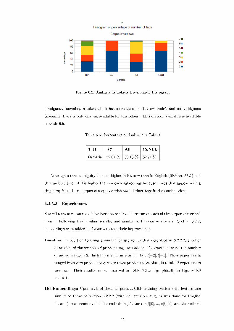
Figure 6.2: Ambiguous Tokens Distribution Histogram
ambiguous (meaning, a token which has more than one tag available), and un-ambiguous
(meaning, there is only one tag available for this token). This division statistics is available
in table 6.5.
Table 6.5: Percentage of Ambiguous Tokens
TB1 A7 All CoNLL
66.24 % 32.67 % 69.18 % 32.71 %
Note again that ambiguity is much higher in Hebrew than in English (69% vs. 33%) and
that ambiguity on All is higher than on each sub-corpus because words that appear with a
single tag in each subcorpus can appear with two distinct tags in the combination.
6.2.3.3 Experiments
Several tests were ran to achieve baseline results. These ran on each of the corpora described
above. Following the baseline results, and similar to the course taken in Section 6.2.2,
embeddings were added as features to test their improvement.
Baseline: In addition to using a similar feature set to that described in 6.2.2.2, another
dimension of the number of previous tags was added. For example, when the number
of previous tags is 2, the following features are added: l[−2], l[−1]. These experiments
ranged from zero previous tags up to three previous tags, thus, in total, 12 experiments
were ran. Their results are summarized in Table 6.6 and graphically in Figures 6.3
and 6.4.
HebEmbeddings: Upon each of these corpora, a CRF training session with feature sets
similar to those of Section 6.2.2.2 (with one previous tag, as was done for English
dataset), was conducted. The embedding features e[t][0], ..., e[t][99] are the embed-
44

Table 6.6: Hebrew Baseline Results. Values show Acc / F1
Num of previous tags 0 1 2 3
TB1 0.867 / 0.725 0.879 / 0.735 0.881 / 0.740 0.881 / 0.748
A7 0.909 / 0.696 0.910 / 0.701 0.910 / 0.703 0.910 / 0.698
All 0.861 / 0.644 0.866 / 0.662 0.868 / 0.660 0.869 / 0.664
Figure 6.3: Hebrew Baseline Accuracy Percentage on Di�erent Corpora and Feature Set
Figure 6.4: Hebrew Baseline F1 Percentage on Di�erent Corpora and Feature Set
45

ding calculated during the course of this work and available online [37]. Results are
summarized in Table 6.7
Table 6.7: Hebrew Embeddings Results. Values show Acc / F1.
without embeddings with embeddings
TB1 0.879 / 0.735 0.900 / 0.804
A7 0.910 / 0.701 0.940 / 0.821
All 0.866 / 0.662 0.880 / 0.723
6.2.3.4 Discussion
Several observations can be made, based on the Hebrew experiments:
� In all cases, the Hebrew embeddings enhanced performance, both in accuracy measure
(1% - 3%), as well as in F1 measure (6% - 12%). This is in accordance with the
previously shown English results.
� There is less improvement found in TB1 and All corpora (see table 6.7). This can
be associated with the fact that the maximum number of unknown tokens is found in
TB1 (see table 6.4). In fact, there is a correlation between the percentage of known
tokens and the rate of improvement gained by the addition of embeddings.
� There is a drop in performance when testing the All corpus, in comparison to testing
its two components. The drop is mainly in F1 measure. We hypothesize this is due to
di�erent conventions and guidelines used for tagging POS of TB1 and A7 corpora. A
supporting evidence for this can be the fact that the percentage of ambiguous tokens
reaches its maximum in All corpus (see table 6.5), this is due to the fact that about
7K non-ambiguous tokens in TB1 and A7 receive di�erent tags in both corpora - thus
rendering them ambiguous in All.
6.2.4 Paraphrasing
6.2.4.1 Corpus
A corpus of 1.6K pairs of sentences was collected from matching news articles from di�erent
Hebrew news sites. The average sentence length was 9.6 words. These pairs were manually
annotated by two human taggers as being either Paraphrase, Partial Paraphrase, or Nega-
tive, according to the Tagging Guidelines which appear as an Appendix.
The corpus can be divided into three categories according to the human tagging:
46

� AGREE - Pairs on which both taggers gave the exact same tagging.
� MISMATCH - Pairs on which taggers did not agree, yet one of the taggers tagged as
"Partial Paraphrase�.
� DISAGREE - Pairs which do not fall to any of the above categories, i.e pairs on which
human taggers tagged the opposite.
The distribution of the corpus according to these terms is shown in table 6.8.
Table 6.8: Category Distribution Over the Paraphrase Corpus
Category Percent
AGREE 70%
MISMATCH 29%
DISAGREE 1%
A couple of examples of pairs of sentences which belong to the DISAGREE category
follow:
I The Saudi stock market had lost 6.8% vs The Saudi stock market had lost
6.78%
6.87 % - a dgpv zicerqd dqxead �
6.8 % - a dgpv zicerqd dqxead �
II The High Court to the State Attorney: Explain the mistakes done in the
dealing with Galant's lands vs The High Court to the State Attorney: Ex-
plain the correction of mistakes done in the dealing with Galant's lands
hplb zerwxwa letiha zeierhd z` xaqd : y"nreil u"ba �
hplb zerwxw zyxta zeierhd oewiz lr xaqd : y"nreil u"ba �
When taking into account only pairs which belong to the AGREE category, we get the
paraphrase corpus which consists of 1273 pairs. The tag distribution over this corpus is
given in Table 6.9. The following experiments are conducted over this corpus.
Tag Percent
Paraphrase 43.3%
Partial 25.2%
Negative 31.5%
Table 6.9: Category Distribution Over the Paraphrase Corpus
47

6.2.4.2 Paraphrase Identi�cation
We tested the Tree Matching algorithm described in this work over the corpus described
in the previous section. Best results were obtained using dependency parsing, and after
training the classi�er for 50 epochs. The results are shown in Table 6.10
Table 6.10: Tree Matching Algorithm Performance
Parse Type Performance(ACC/F1)
Dependency 74.38 / 80.35
Constituency 69.20 / 74.83
6.2.4.3 Discussion
The results are compatible with the obtained state of the art results for the English task
(about 2% lower), which is a positive result in applying Hebrew adapted paraphrase identi�-
cation algorithms. The decrease in performance when using constituency trees can perhaps
be explained due to the much larger trees which are produced by this parsing method.
Such an increase in size can produce more noise to the system, and a consecutive drop in
performance.
48

Chapter 7
Conclusion
The objective of this work is to research the �eld of paraphrasing in Hebrew, providing �rst
results in a �eld in which English research has gained a lot of interest and focus in recent
years. The focus was set on the task of paraphrase identi�cation.
We developed a method to identify if an input pair is in a paraphrase relationship, via
adapting English state of the art algorithms, and providing modi�cation of these.
The datasets we use are:
� A large news wire corpus, preprocessed with POS information, and segmentation.
� A large corpus of Hebrew paraphrases, formed in a parallel corpus of news wire head-
lines. This corpus was obtained in an unsupervised manner, by scraping major Hebrew
news sites.
We run several experiments on these datasets, aiming at proving the hypotheses raised
during the course of this work. The main experiment aims at assessing the validity of the
proposed system as Hebrew paraphrase identi�er. This consists of splitting the corpus of
paraphrases in a train-test split and checking it performance via the standard statistical
metrics.
The results indicate that Hebrew paraphrase identi�cation is a feasible task, when com-
paring against result in the English equivalent �eld.
The main contributions of this work is:
� Showing the feasibility of paraphrase identi�cation in Hebrew, and establishing �rst
results close to state of the art levels in English.
� Providing Hebrew resources for later paraphrasing tasks (a paraphrase corpus), as well
as for more general Hebrew NLP tasks (Collobert and Weston embeddings as a plug
in enhancer).
As future work, we would like to further the research in the following optional directions:
49

� Explore the usage of the products of this work as tools for other paraphrase related
tasks, such as paraphrase generation, and textual entailment.
� Test the paraphrasing identi�er as a component in a more complex system of NLP or
NLG, such as automatic multi-text text summarization, text generation system which
is targeted for a speci�c audience.
� Use the word embeddings produced in this work in other NLP tasks.
50

Bibliography
[1] Microsoft research paraphrase corpus, http://research.microsoft.com/en-us/.
Technical report.
[2] Textual entailment search pilot, guidelines. Technical report, 5th Textual Entail-
ment Challenge, 2009.
[3] Knowledge base population validation task, guidelines. Technical report, 7th
Textual Entailment Challenge, 2011.
[4] Main task and novelty detection subtask, guidelines. Technical report, 7th Textual
Entailment Challenge, 2011.
[5] Meni Adler. Hebrew Morphological Disambiguation: An Unsupervised Stochastic
Word-based Approach. PhD thesis, Ben-Gurion University of the Negev, Beer-
Sheva, Israel, 2007.
[6] Regina Barzilay and Kathleen R. Mckeown. Extracting paraphrases from a par-
allel corpus. In In Proc. of the ACL/EACL, pages 50�57, 2001.
[7] Yoshua Bengio. Learning deep architectures for ai. Foundations and Trends in
Machine Learning, 2(1):1�127, 2009.
[8] Yoshua Bengio, Jérôme Louradour, Ronan Collobert, and Jason Weston. Cur-
riculum learning. In ICML, page 6, 2009.
[9] Eugene Charniak and Mark Johnson. Coarse-to-�ne n-best parsing and maxent
discriminative reranking. In ACL. The Association for Computer Linguistics,
2005.
[10] Noam Chomsky. Three models for the description of language. IRE Transactions
on Information Theory, 2:113�124, 1956.
[11] E V Clark.
[12] Eve V. Clark. On the logic of contrast. Journal of Child Language, 15:317�335,
1988.
51

[13] Ronan Collobert and Jason Weston. A uni�ed architecture for natural language
processing: deep neural networks with multitask learning. In Proceedings of the
25th international conference on Machine learning, ICML '08, pages 160�167,
New York, NY, USA, 2008. ACM.
[14] Ronan Collobert, Jason Weston, Léon Bottou, Michael Karlen, Koray
Kavukcuoglu, and Pavel P. Kuksa. Natural language processing (almost) from
scratch. CoRR, abs/1103.0398, 2011.
[15] Gil Diesendruck. The principles of conventionality and contrast in word learning:
An empirical examination. Developmental Psychology, 41(3):451�463, 2005.
[16] Christiane Fellbaum, editor.WordNet: An Electronic Lexical Database (Language,
Speech, and Communication). The MIT Press, illustrated edition edition, May
1998.
[17] William A. Gale and Kenneth W. Church. A program for aligning sentences in
bilingual corpora. Computational Linguistics, 1993.
[18] Yoav Goldberg and Michael Elhadad. Easy-�rst dependency parsing of modern
hebrew. In Proceedings of the NAACL HLT 2010 First Workshop on Statistical
Parsing of Morphologically-Rich Languages, pages 103�107, Los Angeles, CA,
USA, June 2010. Association for Computational Linguistics.
[19] R. Harman and University of Massachusetts Amherst. Education. Systemic Func-
tional Linguistics and the Teaching of Literature in Urban School Classrooms.
University of Massachusetts Amherst, 2008.
[20] Chikara Hashimoto, Kentaro Torisawa, Stijn De Saeger, Jun'ichi Kazama, and
Sadao Kurohashi. Extracting paraphrases from de�nition sentences on the web.
In ACL, pages 1087�1097, 2011.
[21] Graeme Hirst. Paraphrasing paraphrased. Technical report, University of Toronto,
2003.
[22] R. Karp. Reducibility among combinatorial problems. In R. Miller and
J. Thatcher, editors, Complexity of Computer Computations, pages 85�103.
Plenum Press, 1972.
[23] Dan Klein and Christopher D. Manning. Accurate unlexicalized parsing. In IN
PROCEEDINGS OF THE 41ST ANNUAL MEETING OF THE ASSOCIATION
FOR COMPUTATIONAL LINGUISTICS, pages 423�430, 2003.
[24] John D. La�erty, Andrew McCallum, and Fernando C. N. Pereira. Conditional
random �elds: Probabilistic models for segmenting and labeling sequence data.
52

In Proceedings of the Eighteenth International Conference on Machine Learning,
ICML '01, pages 282�289, San Francisco, CA, USA, 2001. Morgan Kaufmann
Publishers Inc.
[25] Prodromos Malakasiotis and Ion Androutsopoulos. A generate and rank approach
to sentence paraphrasing. In EMNLP, pages 96�106, 2011.
[26] Marie-Francine Moens and Stan Szpakowicz, editors. ROUGE: A Package for
Automatic Evaluation of Summaries, Barcelona, Spain, July 2004. Association
for Computational Linguistics.
[27] Joakim Nivre. Dependency grammar and dependency parsing. Technical report,
Växjö University: School of Mathematics and Systems Engineering, 2005.
[28] Naoaki Okazaki. Crfsuite: a fast implementation of conditional random �elds
(crfs), 2007.
[29] Noam Ordan, Bar Ilan, Noam Ordan, and Shuly Wintner. S.: Hebrew wordnet:
a test case of aligning lexical databases across languages. International Journal
of Translation, 19:39�58, 2007.
[30] Anthony Pick. Discourse and Function. A Framework of Sentence Structure.
http://www.discourseandfunction.com, 2009.
[31] Jordan B. Pollack. Recursive distributed representations. Arti�cial Intelligence,
46:77�105, 1990.
[32] Chris Quirk, Chris Brockett, and William Dolan. Monolingual machine trans-
lation for paraphrase generation. In In Proceedings of the 2004 Conference on
Empirical Methods in Natural Language Processing, pages 142�149, 2004.
[33] Richard Socher and Eric H. Huang and Je�rey Pennington and Andrew Y. Ng
and Christopher D. Manning. Dynamic Pooling and Unfolding Recursive Autoen-
coders for Paraphrase Detection. In Advances in Neural Information Processing
Systems 24. 2011.
[34] Raul Rojas. Neural Networks: A Systematic Introduction. Springer, 1 edition,
July 1996.
[35] Fei Sha and Fernando C. N. Pereira. Shallow parsing with conditional random
�elds. In HLT-NAACL, 2003.
[36] Richard Socher, Je�rey Pennington, Eric H. Huang, Andrew Y. Ng, and Christo-
pher D. Manning. Semi-Supervised Recursive Autoencoders for Predicting Senti-
ment Distributions. In Proceedings of the 2011 Conference on Empirical Methods
in Natural Language Processing (EMNLP), 2011.
53

[37] Gabriel Stanovsky. Hebrew cw embeddings for plugin enhancment -
http://www.cs.bgu.ac.il/ gabriels/paraphrasesite/main.htm, 2012.
[38] Joseph Turian, Lev Ratinov, and Yoshua Bengio. Word representations: a simple
and general method for semi-supervised learning. In Proceedings of the 48th An-
nual Meeting of the Association for Computational Linguistics, ACL '10, pages
384�394, Stroudsburg, PA, USA, 2010. Association for Computational Linguistics.
54
Appendix A
Proof of Tree Matching NP
Completeness
This section provides a proof for the NP completeness of tree matching as described in
section 5.2.4. We will do this by showing that
I Tree Matching ∈ NP
II Positive SubsetSum ≤p Tree Matching
Since Positive SubsetSum (PS) is an NP-Complete problem (is a variation of one of Karp's 21
NP-Complete problems[22]), proving these yields that Tree Matching (TM) is NP-Complete.
We continue by formally de�ning the PS decision problem, and the TM decision problem.
De�nition Given a set of k positive integers S = (n1, ..., nk) and a target positive integer
t, the PS decision problem is �nding if there is a subset of S which sums exactly to t.
Formally:
PS = { ({n1, ..., nk} ∈ Nk, t ∈ N ) | ∃ T ⊆ [1, k] :∑j∈T
nj = t }
De�nition Given a two binary trees T1, T2 which each nodes contain a 100 dimensional
vector of numbers, and a target positive integer t, the TM decision problem is �nding if there
is a Tree Matching M of T1, T2 for which S(M) = t. (Recall section 5.2.4 for de�nitions)
Formally:
TM = { ((T1, T2), t ∈ N ) | ∃M a match of T1, T2 : S(M) = t }
Proof. Following these de�nitions we go on to prove that:
I TM ∈ NP A straight forward approach can yield a simple linear veri�cation algorithm
which receives a pair of trees (T1, T2), a target integer t, and a match M . The algorithm
will compute the score of M (denoted S(M)) and will output �YES� i� S(M) = t.
55
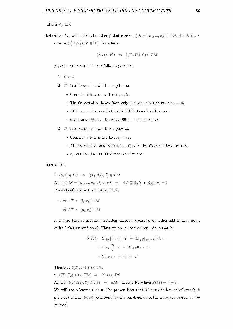
APPENDIX A. PROOF OF TREE MATCHING NP COMPLETENESS 56
II PS ≤p TM
Reduction: We will build a function f that receives ( S = {n1, ..., nk} ∈ Nk, t ∈ N ) and
returns ( (T1, T2), t′ ∈ N ) for which:
(S, t) ∈ PS ⇔ ((T1, T2), t′) ∈ TM
f produces its output in the following manner:
1. t′ ← t
2. T1 is a binary tree which complies to:
* Contains k leaves, marked l1, ..., lk.
* The fathers of all leaves have only one son. Mark them as p1, ..., pk.
* All inner nodes contain ~0 as their 100 dimensional vector.
* li contains (ni
2 , 0, ..., 0) as its 100 dimensional vector.
2. T2 is a binary tree which complies to:
* Contains k leaves, marked r1, ..., rk.
* All inner nodes contain (0, t, 0, ..., 0) as their 100 dimensional vector.
* ri contains ~0 as its 100 dimensional vector.
Correctness:
1. (S, t) ∈ PS ⇒ ((T1, T2), t′) ∈ TM
Assume (S = {n1, ..., nk}, t) ∈ PS ⇒ ∃ T ⊆ [1, k] : Σi∈T ni = t
We will de�ne a matching M of T1, T2:
� ∀i ∈ T : (li, ri) ∈M
� ∀i /∈ T : (pi, ri) ∈M
It is clear that M is indeed a Match, since for each leaf we either add it (�rst case),
or its father (second case). Thus, we calculate the score of the match:
S(M) = Σi∈T ||li, ri|| · 2 + Σi/∈T ||pi, ri|| · 3 =
= Σi∈Tni
2· 2 + Σi/∈T 0 · 3 =
= Σi∈T ni = t = t′
Therefore ((T1, T2), t′) ∈ TM
2. ((T1, T2), t′) ∈ TM ⇒ (S, t) ∈ PS
Assume ((T1, T2), t′) ∈ TM ⇒ ∃M a Match, for which S(M) = t′ = t.
We will use a lemma that will be proven later that M must be formed of exactly k
pairs of the form (∗, ri) (otherwise, by the construction of the trees, the score must be
greater).

APPENDIX A. PROOF OF TREE MATCHING NP COMPLETENESS 57
Following the lemma it is clear that M = M1
⋃M2, where M1 contains only pairs of
the form (li, rj) and M2 = M \M1 = { (xi, rj) ∈M : xi /∈ {l1, ..., lk} }. Thus:
t = S(M) = Σ(li,rj)∈M1||li, rj || · 2 + Σ(xi,rj)∈M2
||xi, rj || · 3 =
= Σ(li,rj)∈M1||li, rj || · 2 = Σ(li,rj)∈M1
ni
We see there is a subset of S which sums to t ⇒ (S, t) ∈ PS
Lemma A.1 S(M) = t ⇒ M must be formed of exactly k pairs of the form (∗, ri)
Proof. Assume by negation that there exists a match M of T1, T2, for which S(M) = t and
that there exists a pair (x, y) ∈M s.t
x ∈ T1, y ∈ T2, y /∈ {r1, ..., rk}
Mark as c > 2 - the number of spanned leaves by x and y.
Note, that by the formation of the trees, we get ||x, y|| =√
(t− 0)2 + ∗ ≥ t
Thus:
S(M) ≥ ||x, y|| · c ≥ ||x, y|| · 2 ≥ 2t > t
In contradiction with the assumption that S(M) = t .

Appendix B
Paraphrase Tagging Guidelines
B.1 Goal
The goal of tagging is to �nd sentences and parts of sentences which convey identical, or
near-identical, information, articulated in di�erent forms.
B.2 Rules for Tagging
Given two sentences S1, S2, the annotator should decide between the following options:
B.2.1 Paraphrase
the pair would be considered a paraphrase in the following case:
1. A human who fully accepts S1, must therefore accept S2 as a whole.
2. The same holds for the second direction as well. Namely, accepting S2, must yield
acceptance of S1.
B.2.1.1 Restrictions
� The acceptance can derive also by former knowledge, yet it must not be based solely
on it. (examples 1,2)
� The pair will be considered as a paraphrase, when there is su�cient con�dence that
they indeed convey the same information. (example 3)
� Given a pair for which their meaning is ambiguous (for example - there is not enough
information to be certain regarding the identities which appear in them). One must
assume that the ambiguity is solved in such a way that the pair relate to same incident.
(example 4)
58

APPENDIX B. PARAPHRASE TAGGING GUIDELINES 59
� The pair should be judged from a timeless point of view. Namely, if the pair relate
the same information, yet treat it from a di�erent point in time - it should be tagged
as paraphrase.
� The pair should be judges from a location-less point of view. Namely, if the same
incident is reported, yet it is regarded from a di�erent relative point of view, it should
be considered paraphrase.
� If one of the sentences, or both of them, contain additional information, or contradic-
tory information, the pair should not be tagged as a paraphrase.
B.2.2 Partial Paraphrase
If S1, S2 are not paraphrases, by the de�nition given above, yet certain clauses can be
removed to form a paraphrase, then S1, S2 should be tagged as partial paraphrases. The
additional clauses should be annotated as such. (example 6)
B.2.3 Negative
A catch-all rule. If S1, S2 do not fall under any of the previous tags, then they should be
tagged as Negative, meaning they do not convey any shared information.
B.3 Examples
1. S1 - .diqex mr htp xgq mkqdl dribd oiq
China has reached an oil trade contract with Russia
S2 - .diqex mr htp xgqn mkqd lr dnzg mlera zqlke`nd dpicnd
The world most populated nation has reached an oil trade contract with Russia
Tag: Paraphrase.
(It is of common knowledge that China is the world most populated nation)
2. S1 - .diqex mr htp xgq mkqdl dribd oiq
China has reached an oil trade contract with Russia
S2 - .mlera zqlke`nd dpicnd `id oiq
China is the world most populated nation.
Tag: Negative.
(Although the second sentence is true, it does not follow from the �rst, nor does the
second derives the �rst).
3. S1 - .dixeqa zexixbyd dxbq a"dx`
USA has closed its embassy in Syria.

APPENDIX B. PARAPHRASE TAGGING GUIDELINES 60
S2 - .dixeqn dxixby z` dxifgd a"dx`
USA has called its ambassador back from Syria.
Tag: Paraphrase.
(It is very probable to assume that closing the embassy yields calling back the ambas-
sador, and vice versa)
4. S1 - .dixeqa mipexg`d mirex`d z` dxwiq zyxd
The network has covered latest events in Syria.
S2 - .dixeqa zepexg`d zeieygxzdd lr dgeeic dxif'bl` zyx
Al Jazira network has passed reports of the latest happenings in Syria.
Tag: Paraphrase.
(It should be assumed that the network mentioned in the second sentence is the same
network mentioned in the �rst sentence)
5. S1 - .oey`x meia ray x`al ewd z` ziayz zakxd
Trains will not work on the line to Beer Sheva this Sunday, due to strike.
S2 - .ray x`al ewd z` xgn wiqtz zakxd
Trains will not work on the line to Beer Sheva tomorrow, due to strike.
Tag: Paraphrase.
(Although the pair convey the same information from di�erent points in time, it should
be regarded as paraphrase)
6. S1 - .ux`l xfg okn xg`le ,iqexd ezinr mr ybtp edipzp oinipa
Benyamin Netanyahu has met with his Russian counterpart, an later returned to Israel.
S2 - .miycgd milerd ziibeq z` eipta oiive ,iqexd eliawn mr crep edipzp oinipa
Benyamin Netanyahu has met with his Russian counterpart, and mentioned to him
the issue of Israeli immigrants from Russia.
Tag: Partial Paraphrase.
(Without the marked parts, the pair consists a paraphrase)
7. S1 - .mixirvd miqiibznd ipta m`p wxa ced`
Ehud Barak spoke in front of new army recruits.
S2 - .d`ad divpcwl ezecnren yibdl hilgd wxa ced`
Ehud Barak decided to run for the next elections.
Tag: Negative.
(Both sentences do not convey the same information, nor can any clauses can be
removed from them so that they do)