thesis
TRANSCRIPT
ANALYSIS, DESIGN AND CONTROL OF
PERMANENT MAGNET SYNCHRONOUS MOTORS
FOR WIDE-SPEED OPERATION
Liu QinghuaB.Eng., Huazhong University of Science & TechnologyM.Eng., Huazhong University of Science & Technology
A THESIS SUBMITTED
FOR THE DEGREE OF DOCTOR OF PHILOSOPHY
DEPARTMENT OF ELECTRICAL ENGINEERING
NATIONAL UNIVERSITY OF SINGAPORE
2005
Summary
This thesis presents aspects of analysis, design and control of permanent magnet
synchronous motors (PMSMs) for wide-speed operations.
An analytical method has been developed based on d- and q- axis equivalent
circuit model of interior PMSMs, which is used to determine the influence of motor
parameters and inverter power rating on motor output power capability. This
analysis provides design criteria to obtain optimal combination of motor parameters
in order to achieve a wide speed range of constant power operation.
Response surface methodology (RSM) has been used to build the second-order
empirical model for the estimation of motor parameters. Numerical experiments
were designed using modified central composite design and have been conducted
using finite element software to fit the second-order model. The developed model
by RSM provides an accurate description of effects of rotor geometric design on
the motor parameters. The RSM models were then used for the optimization of an
interior PMSM for wide speed operation.
The combination of RSM models which are used for estimation of motor
parameters, and genetic algorithms which is used for searching method, provides
i
an effective methodology for the interior PMSM design optimization. Compared to
traditional analytical methods, the proposed computational method improves the
accuracy of estimating motor parameters, and at the same time reduces computing
time and effort in the optimization process. The optimized values were verified
using an FEM software.
An experimental method for the determination of d- and q-axis inductances
has been proposed based on the load test with rotor position feedback. The accurate
measurement of motor parameters not only validate the developed numerical design
approach, but also improve the speed and torque control performance over a wide
speed range.
The conventional current vector control of interior PMSMs has been imple-
mented for a smooth and accurate speed and torque control. The advantages and
disadvantages on the control performance were investigated through theoretical
analysis and experimental work. It was noted that the flux-weakening performance
of current vector control deteriorates because of the saturation effects of current
regulator in the high speed and high current conditions.
Stator flux based modified direct torque control by using space vector mod-
ulation has been proposed to overcome the difficulties met in the current vector
control. The application of modified direct torque control for interior PMSM drives
has been developed through analysis and experimental implementation. Important
conditions which are necessary for the applicability of direct torque control to an
interior PMSM has been put forward. Compared to conventional current vector
control, the proposed control scheme improves the dynamic response on speed

and torque control on the wide-speed operation. Current regulator saturation, the
worst degrading factor of torque production in the extended flux-weakening range,
is eliminated. The experimental results show modified direct torque control is more
suitable for the applications on extended speed range for interior PMSMs.

Acknowledgments
I would like to express my sincere gratitude and appreciation to my supervisors Dr.
M. A. Jabbar and Dr. Ashwin M. Khambadkone for their help and advice. Their
invaluable and insightful guidance, support and encouragement inspired me in my
work.
I am also thankful to Dr. Sanjib Kumar Panda, Head of Electrical Machines
and Drives Lab, for his suggestions and help to this work in all possible aspects.
I would like to express my sincere gratitude to Mr. Y. C. Woo, Principal
Laboratory Technologist, for his help. In addition, we want to thank Mr. M.
Chandra in Electrical Machines and Drives Lab for his constant and immediate
help in the mechanical arrangements for my experimental setup.
I would like to thank my colleagues in the laboratory, Mr. Tripathi Anshu-
man, for his smart ideas and valuable discussions on the motion control application
for my work. I also owe many thanks to my friends in the lab: Mr. Liang Zhihong,
Mr. Wang Zhongfang, Mr. Shi Chunming, Mr. Zhang Yanfeng, Mr. Nay Lin Htun
Aung, Ms. Wu Mei, Mr. Azmi Bin Azeman, Ms. Dong Jing, Ms. Hla Nu Phyu,
Ms. Qian Weizhe, Mr. Sahoo Sanjib Kumar and Mr. Ho Chin Kian Ivan for their
iv

v
precious help with my study at NUS.
I wish to acknowledge the financial support provided by National University
of Singapore in the form of a Research Scholarship.
Finally, my dedication is due to my wife and my parents, for their constant
support and encouragement.
Contents
Summary i
Acknowledgments iv
List of Symbols xiii
List of Acronyms xvii
List of Figures xix
List of Tables xxvi
1 Introduction 1
1.1 Permanent Magnet Motors . . . . . . . . . . . . . . . . . . . . . . . 2
1.2 PM motors in Variable Speed Drives . . . . . . . . . . . . . . . . . 3
1.3 Characteristics of PM Materials . . . . . . . . . . . . . . . . . . . . 5
1.4 Structure of PMSMs . . . . . . . . . . . . . . . . . . . . . . . . . . 7
vi
vii
1.5 Literature Review . . . . . . . . . . . . . . . . . . . . . . . . . . . . 10
1.5.1 Constant Power Operation of PMSM Drives . . . . . . . . . 10
1.5.2 The Design of PMSMs . . . . . . . . . . . . . . . . . . . . . 12
1.5.3 Numerical Optimization . . . . . . . . . . . . . . . . . . . . 14
1.5.4 The Control of PMSMs . . . . . . . . . . . . . . . . . . . . . 18
1.6 Research Goals and Methodology . . . . . . . . . . . . . . . . . . . 21
1.6.1 Analysis of Constant Power Speed Range for IPMSM Drive . 22
1.6.2 Design Optimization of Interior PMSM . . . . . . . . . . . . 23
1.6.3 Control of IPMSM in Wide Speed Operation . . . . . . . . . 24
1.7 Outline of the Thesis . . . . . . . . . . . . . . . . . . . . . . . . . . 25
2 Analysis of Interior Permanent Magnet Synchronous Motors forWide-Speed Operation 27
2.1 Introduction . . . . . . . . . . . . . . . . . . . . . . . . . . . . . . . 27
2.2 Mathematical Modelling . . . . . . . . . . . . . . . . . . . . . . . . 28
2.3 Theoretical Analysis of Steady-State Operation . . . . . . . . . . . 33
2.3.1 Current limited maximum torque operation . . . . . . . . . 34
2.3.2 Current and voltage limited maximum poweroperation . . . . . . . . . . . . . . . . . . . . . . . . . . . . 36
2.3.3 Voltage limited maximum power operation . . . . . . . . . . 38

viii
2.3.4 Optimum current vector trajectory . . . . . . . . . . . . . . 41
2.4 Effects of Motor Parameters on Torque-Speed Characteristics . . . . 44
2.5 Design Considerations on Constant Power Speed Range . . . . . . . 46
2.6 Conclusions . . . . . . . . . . . . . . . . . . . . . . . . . . . . . . . 48
3 Determination of Motor Parameters in Interior PMSMs 50
3.1 Introduction . . . . . . . . . . . . . . . . . . . . . . . . . . . . . . . 50
3.2 Design of The Stator Winding . . . . . . . . . . . . . . . . . . . . . 51
3.3 Selection of The Rotor Design Variables . . . . . . . . . . . . . . . 55
3.4 Determination of Motor Parameters . . . . . . . . . . . . . . . . . . 59
3.4.1 Analytical Method . . . . . . . . . . . . . . . . . . . . . . . 59
3.4.1.1 Stator permanent magnet flux linkage . . . . . . . 59
3.4.1.2 Calculation of inductances . . . . . . . . . . . . . . 62
3.4.2 Finite Element Method . . . . . . . . . . . . . . . . . . . . . 66
3.4.3 Response Surface Method . . . . . . . . . . . . . . . . . . . 68
3.4.3.1 Building empirical models . . . . . . . . . . . . . . 68
3.4.3.2 Estimation of the regression coefficients . . . . . . 70
3.4.3.3 Fitting the second-order model . . . . . . . . . . . 72
3.4.3.4 Model adequacy checking . . . . . . . . . . . . . . 74

ix
3.5 Design of The Rotor Structure . . . . . . . . . . . . . . . . . . . . . 75
3.6 Conclusion . . . . . . . . . . . . . . . . . . . . . . . . . . . . . . . . 83
4 Numerical Optimization of an Interior PMSM for Wide ConstantPower Speed Range 84
4.1 Introduction . . . . . . . . . . . . . . . . . . . . . . . . . . . . . . . 84
4.2 Optimization Method . . . . . . . . . . . . . . . . . . . . . . . . . . 85
4.2.1 Formulation of the design optimization . . . . . . . . . . . . 85
4.2.2 Description of genetic algorithms . . . . . . . . . . . . . . . 88
4.3 Implementation of Proposed Design Optimization Procedure . . . . 93
4.4 Numerical Results and Discussions . . . . . . . . . . . . . . . . . . 93
4.5 Conclusion . . . . . . . . . . . . . . . . . . . . . . . . . . . . . . . . 103
5 Tests and Performance of the Prototype Interior PMSM 105
5.1 Introduction . . . . . . . . . . . . . . . . . . . . . . . . . . . . . . . 105
5.2 The Prototype Interior PMSM . . . . . . . . . . . . . . . . . . . . . 106
5.3 Experimental Interior PMSM Drive System . . . . . . . . . . . . . 108
5.3.1 DS1102 controller board . . . . . . . . . . . . . . . . . . . . 111
5.3.2 PWM voltage source inverter . . . . . . . . . . . . . . . . . 112
5.3.3 Integrated interface platform . . . . . . . . . . . . . . . . . . 112

x
5.3.4 Current sensor . . . . . . . . . . . . . . . . . . . . . . . . . 114
5.3.5 Loading system . . . . . . . . . . . . . . . . . . . . . . . . . 115
5.4 Experimental Determination of Motor Parameters . . . . . . . . . 116
5.4.1 Permanent magnet flux linkage λm . . . . . . . . . . . . . . 116
5.4.2 Torque angle measurement . . . . . . . . . . . . . . . . . . . 117
5.4.3 Load test to measure Ld and Lq . . . . . . . . . . . . . . . . 120
5.5 Experimental Evaluation of Wide Speed Operation Performance . . 122
5.5.1 Torque and Power Capability . . . . . . . . . . . . . . . . . 123
5.5.2 Efficiency and Power Factor . . . . . . . . . . . . . . . . . . 125
5.5.3 Performance under Reduced DC Link Voltages . . . . . . . . 128
5.6 Conclusion . . . . . . . . . . . . . . . . . . . . . . . . . . . . . . . . 131
6 Control of The Prototype Interior Permanent Magnet SynchronousMotor 133
6.1 Introduction . . . . . . . . . . . . . . . . . . . . . . . . . . . . . . . 133
6.2 Field Oriented Current Control Scheme . . . . . . . . . . . . . . . . 134
6.2.1 Description and features of the current control scheme . . . 134
6.2.2 Discussions on current control schemes . . . . . . . . . . . . 139
6.3 Space Vector Modulation based Direct Torque Control Scheme . . . 140
6.3.1 Principle of torque production in interior PMSMs . . . . . . 140
xi
6.3.2 Stator flux control in DTC-SVM . . . . . . . . . . . . . . . 142
6.3.3 Calculation of switching on time . . . . . . . . . . . . . . . . 145
6.3.3.1 Normal modulation range . . . . . . . . . . . . . . 147
6.3.3.2 In overmodulation range . . . . . . . . . . . . . . . 148
6.3.4 Stator flux estimation . . . . . . . . . . . . . . . . . . . . . 149
6.3.5 Operating Limits for DTC-SVM scheme in IPMSM drives . 150
6.3.6 Current Constraints . . . . . . . . . . . . . . . . . . . . . . 152
6.3.7 Proposed Wide Speed Operation . . . . . . . . . . . . . . . 155
6.4 Description and Features of the Proposed Scheme . . . . . . . . . . 158
6.4.1 Speed Range for Operation at Constant Torque . . . . . . . 158
6.4.2 Operating in flux-weakening speed range . . . . . . . . . . . 160
6.5 Experimental Results and Discussions . . . . . . . . . . . . . . . . . 160
6.6 Conclusion . . . . . . . . . . . . . . . . . . . . . . . . . . . . . . . . 168
7 Discussions and Conclusions 171
7.1 Discussions of Major Work . . . . . . . . . . . . . . . . . . . . . . . 171
7.1.1 Analysis of constant power operation . . . . . . . . . . . . . 171
7.1.2 Design optimization methodology . . . . . . . . . . . . . . . 173
7.1.3 Steady state tests of the prototype interior PMSM . . . . . . 175
xii
7.1.4 Speed and torque control by DTC-SVM . . . . . . . . . . . 176
7.2 Major Contributions of the Thesis . . . . . . . . . . . . . . . . . . . 177
7.3 Suggestions for Future Research . . . . . . . . . . . . . . . . . . . . 178
A Design Details for The Prototype Interior PMSM 195
B Additional Experimental Data 198

List of Symbols
Az cross area of winding conductor
B damping coefficient
Bad flux density in air gap due to d-axis armature MMF
Baq flux density in air gap due to q-axis armature MMF
BD knee flux density
Bg peak flux density in air gap due to magnets
Br remanent flux density
Bs air gap flux density due to armature reaction
B1g rms value of fundamental flux density in air gap due to magnets
D inner diameter of stator frame
dc bare diameter of conductor
E rms value of phase back EMF
ecoil back EMF in one coil
Fad d-axis armature MMF
Faq q-axis armature MMF
Fa1, Fb1, Fc1 phase fundamental MMF
xiii

xiv
F total value of fundamental MMF
f electrical frequency
fs slot space factor
ge air gap length including magnet thickness
g actual uniform air gap length
g′ effective air gap length
Hc coercive magnetizing force
Ia,b,c phase armature current
Id,q d- and q-axis current
Iph phase current
Is current space vector
Ism current constraints
J inertial of the rotor
Jc current density in conductor
K1s rms value of linear current density
kc Carter’s effect coefficient
kd d-axis inductance factor
kq q-axis inductance factor
kω winding factor
Laa,bb,cc phase self inductance
Lab,ac,bc phase mutual inductance

xv
L stator stack length
Lad d-axis magnetizing inductance
Laq q-axis magnetizing inductance
Ls synchronous inductance
lm magnet thickness
Ncoil number of turns per phase in equivalent full pitch winding
Nph number of turns per phase in actual winding
P number of poles
Pin motor input power
Po motor output power
pc crossover probability
pm mutation probability
Rs phase resistance
S number of slots
Sa slot area
Te motor electromagnetic torque
Tl motor loading torque
t time, second
Va,b,c phase terminal voltage
Vs voltage space vector
Vsm voltage constraints
x1, x2, x3 scaled design variables
Xs synchronous reactance
xvi
ϕ electrical angle in rotor w.r.t d-axis
θ rotor position angle w.r.t phase A axis
λm stator permanent magnet flux linkage
λa,b,c phase flux linkage
β current angle
λma,mb,mc phase flux linkage provided by rotor magnets
λd,q d- and q-axis flux linkage
ωs electrical velocity
δ torque angle
ωr mechanical velocity
ωb base speed
ωc crossover speed
ωmax maximum speed for rated power operation
ωp minimum speed for the voltage-limited maximum output power opration
βb current angle for maximum torque operation
α magnet pole angle
γ magnet position
φ flux in one full pitch winding
µ0 permeability in air gap
µr relative permeability in magnets
ε voltage adjusting coefficient

List of Acronyms
AC Alternating Current
AM Analytical Method
BLDC Brushless DC
CPSR Constant Power Speed Range
CVC Current Vector Control
DC Direct Current
DFC Direct Flux Control
DSP Digital Signal Processor
DTC Direct Torque Control
EMF Electro-motive Force
FEM Finite Element Method
GA Genetic Algorithms
MMF Magneto-motive Force
xvii
xviii
MTPA Maximum Torque Per Ampere
PI Proportional Integral
PM Permanent Magnet
PMSM Permanent Magnet Synchronous Motor
PWM Pulse Width Modulation
RMS Root Mean Square
RSM Response Surface Methodology
SD Slot Depth
SWF Slot Width Factor
SVM Space Vector Modulation
THD Total Harmonic Distortion
List of Figures
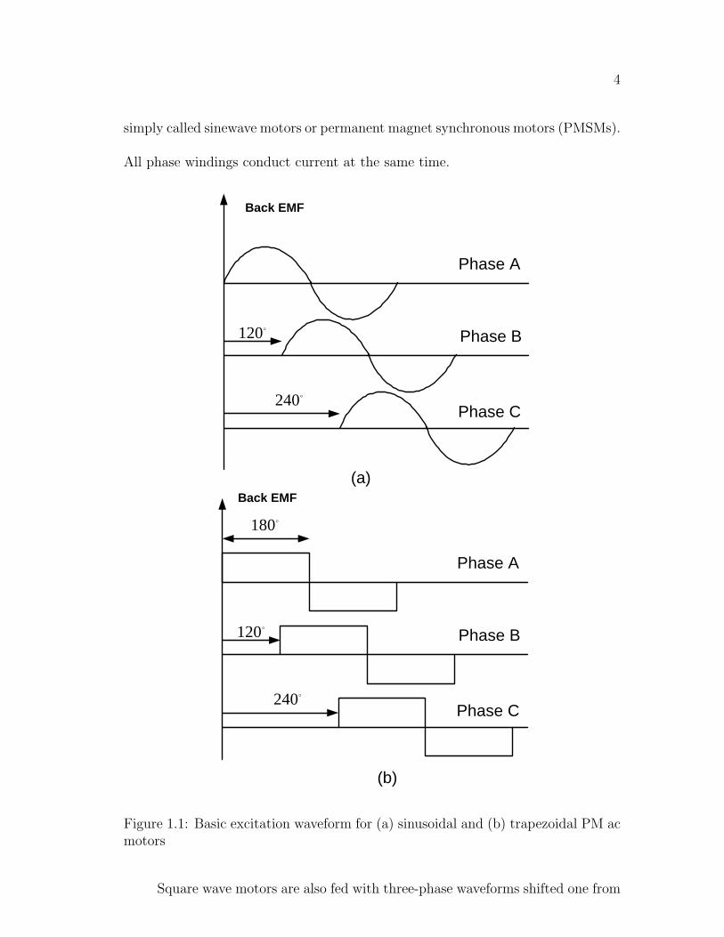
1.1 Basic excitation waveform for (a) sinusoidal and (b) trapezoidal PM
ac motors . . . . . . . . . . . . . . . . . . . . . . . . . . . . . . . . 4
1.2 Characteristics of Permanent Magnet Materials . . . . . . . . . . . 6
1.3 Structures for exterior permanent magnet motors . . . . . . . . . . 8
1.4 Structures for interior permanent magnet motors . . . . . . . . . . 8
1.5 Ideal Torque vs. speed characteristics for variable speed AC drives . 10
1.6 Cross section of axially laminated rotor for interior PMSM [16] . . . 13
1.7 Cross section of rotor with Lq/Ld < 1 for interior PMSM [17] . . . . 14
1.8 Two-part rotor with Lq/Ld < 1 for interior PMSM [18] . . . . . . . 15
2.1 Permanent magnet synchronous motor . . . . . . . . . . . . . . . . 29
2.2 Equivalent Circuit of an interior PMSM . . . . . . . . . . . . . . . 31
2.3 The stator flux linkage in the dq reference frame . . . . . . . . . . 32
xix

xx
2.4 The current limit circle and voltage limit ellipse for interior PMSMs 34
2.5 The optimum current vector trajectory in the d-q coordinate plane
for λm < LdIsm . . . . . . . . . . . . . . . . . . . . . . . . . . . . . 40
2.6 The optimum current vector trajectory in the d-q coordinate plane
for λm > LdIsm . . . . . . . . . . . . . . . . . . . . . . . . . . . . . 43
2.7 The maximum obtainable torque vs. speed profile . . . . . . . . . . 43
2.8 Torque vs. speed characteristics with optimum current vector tra-
jectory . . . . . . . . . . . . . . . . . . . . . . . . . . . . . . . . . . 44
2.9 Torque-speed characteristics with different magnet flux linkages . . 45
2.10 Torque-speed characteristics with different q-axis inductance . . . . 46
2.11 Torque-speed characteristics with different d-axis inductances . . . . 47
2.12 Comparison of power vs. speed characteristics for 5 designs . . . . . 48
3.1 Stator frame structure . . . . . . . . . . . . . . . . . . . . . . . . . 52
3.2 Stator and rotor structure for interior PMSMs . . . . . . . . . . . . 56
3.3 Permanent magnet excitation flux plot . . . . . . . . . . . . . . . . 56
3.4 Permanent magnet excited flux distribution in the air gap . . . . . 57
3.5 Rotor configuration of the interior PMSM . . . . . . . . . . . . . . 58
3.6 Actual and effective air gap flux density . . . . . . . . . . . . . . . 60

xxi
3.7 Air gap flux distribution due to permanent magnet . . . . . . . . . 61
3.8 MMF distribution of an interior PMSM over 180◦ . . . . . . . . . . 63
3.9 Air gap profile along the rotor surface . . . . . . . . . . . . . . . . . 64
3.10 Central composite design for second-order model . . . . . . . . . . . 73
3.11 λm as a function of rotor geometry . . . . . . . . . . . . . . . . . . 81
3.12 Ld as a function of rotor geometry . . . . . . . . . . . . . . . . . . . 82
3.13 Lq as a function of rotor geometry . . . . . . . . . . . . . . . . . . . 83
4.1 Determination of maximum power capability w.r.t to motor speed . 87
4.2 Main steps of genetic algorithms technique . . . . . . . . . . . . . . 89
4.3 Example of one individual of design variable . . . . . . . . . . . . . 91
4.4 Schematic samples of crossover and mutation process . . . . . . . . 92
4.5 Flowchart for the proposed design optimization of the interior PMSM 94
4.6 Average and maximum CPSR trend combining GA and RSM . . . 95
4.7 Effects of magnetic saturation on Ld and Lq . . . . . . . . . . . . . 97
4.8 Permanent magnet excited flux distribution in the air gap . . . . . 98
4.9 Air gap flux density curve with maximum flux-weakening condition
β = 180 degree . . . . . . . . . . . . . . . . . . . . . . . . . . . . . 98

xxii
4.10 The stator flux linkage in the dq reference frame . . . . . . . . . . 99
4.11 The optimum current vector trajectory in the d-q coordinate plane
for λm > LdIsm . . . . . . . . . . . . . . . . . . . . . . . . . . . . . 100
4.12 Torque vs. current angle β characteristics for FEM and RSM . . . . 100
4.13 Stator flux vs. current angle β characteristics for FEM and RSM . . 101
4.14 Power capability vs speed characteristics for the optimized design
by FEM and RSM . . . . . . . . . . . . . . . . . . . . . . . . . . . 101
4.15 Comparison of optimal design with other design cases . . . . . . . . 103
5.1 Hardware schematic of the interior PMSM drive system . . . . . . . 106
5.2 The optimized rotor structure for the prototype interior PMSM . . 107
5.3 Standard stator and designed rotor for the prototype interior PMSM 107
5.4 Experimental set-up for the interior PMSM drive system . . . . . . 108
5.5 dSPACE DS1102 based integrated PMSM drive test platform . . . 109
5.6 Configuration of the controller board used for hardware implemen-
tation . . . . . . . . . . . . . . . . . . . . . . . . . . . . . . . . . . 110
5.7 Interfacing the controller board with the control circuit . . . . . . . 113
5.8 Configuration for the interior PMSM loading system . . . . . . . . . 115
5.9 PMSM generator phasor diagram for testing . . . . . . . . . . . . . 118
xxiii
5.10 Experimental measurement of d-axis position . . . . . . . . . . . . . 118
5.11 Experimental measurement of load angle . . . . . . . . . . . . . . . 119
5.12 Experimental results for the maximum torque capability vs. speed . 125
5.13 Experimental results for the maximum power capability vs. speed . 126
5.14 Experimental results for the efficiency for constant current and full
voltage operation . . . . . . . . . . . . . . . . . . . . . . . . . . . . 127
5.15 Experimental results for the power factor for constant current and
full voltage operation . . . . . . . . . . . . . . . . . . . . . . . . . . 128
5.16 Experimental results for the torque capability for constant current
and reduced DC link voltage operation . . . . . . . . . . . . . . . . 129
5.17 Experimental results for the power capability for constant current
and reduced DC link voltage operation . . . . . . . . . . . . . . . . 130
5.18 Experimental results for the efficiency for constant current and re-
duced DC link voltage operation . . . . . . . . . . . . . . . . . . . . 130
5.19 Experimental results for the power factor for constant current and
reduced DC link voltage operation . . . . . . . . . . . . . . . . . . . 131
6.1 The optimum current profile in the d-q coordinate plane for λm >
LdIsm . . . . . . . . . . . . . . . . . . . . . . . . . . . . . . . . . . . 135
6.2 Block diagram of current controlled IPMSM drive system . . . . . . 135
6.3 Current regulator with decoupling feedforward compensation . . . . 137
xxiv
6.4 The stator flux linkage in the dq reference frame . . . . . . . . . . 141
6.5 The steady state operation of stator flux control . . . . . . . . . . 144
6.6 Three-phase converter and phase voltage . . . . . . . . . . . . . . . 146
6.7 Switching state vectors in the α− β plane . . . . . . . . . . . . . . 146
6.8 Space vector modulation with switching state vectors . . . . . . . . 147
6.9 Modified voltage model for flux estimation . . . . . . . . . . . . . . 149
6.10 The torque vs. load angle characteristics . . . . . . . . . . . . . . . 151
6.11 The phase current vs. load angle characteristics . . . . . . . . . . . 153
6.12 The comparison of maximum load angle: δm0 and δm1 Vs. λs . . . . 154
6.13 The characteristics of torque capability vs. stator flux linkage . . . 156
6.14 The Stator Flux Reference Profile: (a) Constant torque operation
with MTPA control; (b) Flux-weakening Operation . . . . . . . . . 157
6.15 Block diagram of IPMSM drive system . . . . . . . . . . . . . . . . 159
6.16 Current Control: The dynamic response with step speed change in
the normal range . . . . . . . . . . . . . . . . . . . . . . . . . . . . 162
6.17 SVM based DTC: The dynamic response with step speed change in
the normal range . . . . . . . . . . . . . . . . . . . . . . . . . . . . 162
6.18 Current Control: The dynamic response with step loading torque
change in constant torque speed range . . . . . . . . . . . . . . . . 163
xxv
6.19 SVM based DTC: The dynamic response with step loading torque
change in constant torque speed range . . . . . . . . . . . . . . . . 164
6.20 Current Control: The dynamic response with step speed change in
flux-weakening range . . . . . . . . . . . . . . . . . . . . . . . . . . 165
6.21 SVM based DTC: The dynamic response with step speed change in
flux-weakening range . . . . . . . . . . . . . . . . . . . . . . . . . . 166
6.22 Dynamic response of the IPMSM drive system in transition from
constant torque to flux-weakening regions . . . . . . . . . . . . . . . 167
6.23 Flux Weakening Operation with the variation of DC link voltage . . 167
6.24 Transient performances of flux and voltage for step speed change in
flux-weakening range . . . . . . . . . . . . . . . . . . . . . . . . . . 168
6.25 Torque performance of SVM based DTC and Current Control for a
wide speed operation . . . . . . . . . . . . . . . . . . . . . . . . . . 169
6.26 Power performance of SVM based DTC and Current Control for a
wide speed operation . . . . . . . . . . . . . . . . . . . . . . . . . . 170
A.1 Rotor mechanical design drawing . . . . . . . . . . . . . . . . . . . 195
A.2 Stator winding distribution . . . . . . . . . . . . . . . . . . . . . . . 196
A.3 Magnet design specification . . . . . . . . . . . . . . . . . . . . . . 197

List of Tables
1.1 Comparison between PMSMs with exterior and interior magnets . . 9
2.1 Motor parameters for 5 Interior PMSMs . . . . . . . . . . . . . . . 48
3.1 Stator frame data for the prototype interior PMSM . . . . . . . . . 53
3.2 Specifications of the Interior PMSM . . . . . . . . . . . . . . . . . . 53
3.3 Winding specifications for the prototype interior PMSM . . . . . . 55
3.4 Data for multiple linear regression . . . . . . . . . . . . . . . . . . . 71
3.5 The domain of design variables in the rotor structure . . . . . . . . 75
3.6 Central composite design for the design example of interior PMSM . 76
3.7 Comparison of results with AM, FEM and RSM . . . . . . . . . . . 79
3.8 Residual for the fitted second-order RSM model . . . . . . . . . . . 80
3.9 Test of adequacy for the fitted second-order RSM model . . . . . . 80
xxvi

xxvii
4.1 The domain of design variables in the rotor structure . . . . . . . . 90
4.2 Optimized design values and motor parameters . . . . . . . . . . . 96
4.3 Comparison of motor parameters with GA+RSM and FEM . . . . . 96
4.4 Comparison of flux distribution for open circuit and flux-weakening
condition . . . . . . . . . . . . . . . . . . . . . . . . . . . . . . . . . 99
4.5 Comparison of 9 design cases . . . . . . . . . . . . . . . . . . . . . 102
5.1 Experimental measurements of back EMF and calculated values of λm117
5.2 Experimental measurements of Ld and Lq . . . . . . . . . . . . . . 121
5.3 Comparison of motor parameters with The Commercial and The
Prototype . . . . . . . . . . . . . . . . . . . . . . . . . . . . . . . . 123
5.4 Test Condition with The Commercial and The Prototype . . . . . . 124
6.1 Base values of motor parameters . . . . . . . . . . . . . . . . . . . . 161

Chapter 1
Introduction
Permanent magnet synchronous motors (PMSMs) are increasingly used in variable
speed industrial drives. New developments and applications have been greatly
accelerated by improvements in permanent magnet (PM) materials, especially rare-
earth magnets. While the methods for analysis and design of conventional AC
electrical machines are becoming mature, extensive research is still required to
develop a systematic methodology for analysis, design and control of PMSMs.
In this thesis, a design and control method for PMSMs is developed based
on the analysis of PMSMs with different rotor structures. The prototype PMSM
was designed to achieve a wide-speed and constant power operation. Tests made
on the fabricated prototype motor prove the validity of the design optimization
methodology and control algorithm developed.
1
2
1.1 Permanent Magnet Motors
The use of permanent magnets (PM) in construction of electrical machines brings
the following benefits [1]:
• no electrical energy is absorbed by the field excitation system and thus there
are no excitation losses which means substantial increase in the efficiency
• higher torque and output power per unit volume compared to electromagnetic
excitation
• better dynamic performance than motors with electromagnetic excitation
(higher magnetic flux density in the air gap)
• simplification of construction and maintenance
• reduction of lifetime cost for some types of machines.
Cage induction motors have been the most popular electric motors in the 20th
century. Recently, owing to the fast progress made in the field of power electronics
and control technology, the applications of induction motors to electrical drives
have increased. The main advantages of cage induction motors are their simple
construction, easy maintenance, no commutator or slip rings, low price and high
reliability. The disadvantages are their lower efficiency and poorer power factor
than PM synchronous motors.

3
The use of PM motors in electrical drives has become a more attractive option
than induction motors. The improvements made in the field of semiconductor
drives mean that the control of PM motors has become easier and cost effective with
the possibility of operating the motor over a large speed range and still maintaining
a good efficiency and power factor. The price of rare earth magnets are also coming
down making these motors more popular.
1.2 PM motors in Variable Speed Drives
In a variable-speed drive or servo drive system, a speed or position feedback is used
for precision control of motors. The response time and the accuracy with which
the motor follows the speed and position commands are important performance
parameters. A power electronic converter interfaces the power supply and the
motor. Industrial drives technology has changed in recent years from conventional
DC or two-phase AC motor drives to new maintenance-free brushless three-phase
vector-controlled AC drives for all motor applications where quick response, light
weight and large continuous and peak torques are required.
Permanent magnet ac motors combine some of the desirable advantages of
conventional induction and synchronous motors and deserve special attention. Per-
manent magnet motors can be classified into two categories, one group is sinu-
soidally excited and the other is square wave (trapezoidally excited) motors [2].
Motors with a sinusoidal excitation are fed with three-phase sinusoidal waveforms
(Fig. 1.1 (a)) and operate on the principle of a rotating magnetic field. They are
4
simply called sinewave motors or permanent magnet synchronous motors (PMSMs).
All phase windings conduct current at the same time.
o120
o240
Phase A
Phase C
Phase B
(a)
o120
o240
Phase A
Phase C
Phase B
o180
(b)
Back EMF
Back EMF
Figure 1.1: Basic excitation waveform for (a) sinusoidal and (b) trapezoidal PM acmotors
Square wave motors are also fed with three-phase waveforms shifted one from

5
another by 120◦, but these waveshapes are rectangular or trapezoidal as shown in
Fig. 1.1 (b). Such a shape is produced when armature current (MMF) is precisely
synchronized with the rotor instantaneous position and frequency (speed) [3]. The
most direct and popular method of providing the required rotor position informa-
tion is to use an angular position sensor mounted on the rotor shaft. Such a control
scheme or electronic commutation is functionally equivalent to the mechanical com-
mutation in DC motors. This explains why motors with squarewave excitation are
called brushless DC motors (BLDC). These two kinds of permanent magnet motors
are different in performance and control. In this research, the emphasis was placed
on permanent magnet synchronous motors.
PMSMs have been broadly developed for industrial applications such as servo
motors, elevator drive motors, and electric vehicle traction motors [4]. At the same
time, the development in high-strength rare-earth permanent magnet materials,
especially neodymuim alloyed with iron and boron (NdFeB), have greatly enhanced
the potential applications of PMSMs. Before discussing design configurations of
PMSMs, it is necessary to understand the characteristics of permanent magnet
materials used in electric motors for excitation.
1.3 Characteristics of PM Materials
The development of permanent magnets with high flux density and large coercive
force resulted in the wide use of PMSM drives with high performance. Three main
magnetic materials are used in PMSM. They are: Ferrite, samarium-cobalt and
6
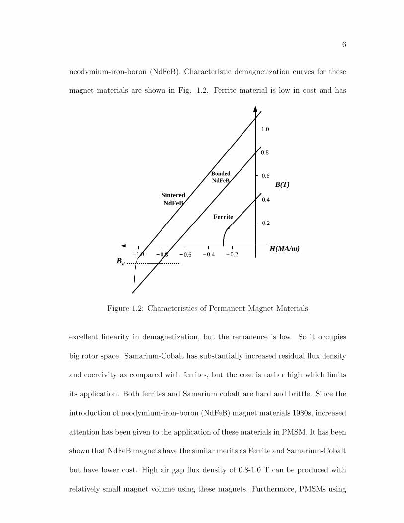
neodymium-iron-boron (NdFeB). Characteristic demagnetization curves for these
magnet materials are shown in Fig. 1.2. Ferrite material is low in cost and has
B(T)
H(MA/m)
SinteredNdFeB
BondedNdFeB
Ferrite
dB2.0−0.1− 8.0− 6.0− 4.0−
0.1
2.0
4.0
6.0
8.0
Figure 1.2: Characteristics of Permanent Magnet Materials
excellent linearity in demagnetization, but the remanence is low. So it occupies
big rotor space. Samarium-Cobalt has substantially increased residual flux density
and coercivity as compared with ferrites, but the cost is rather high which limits
its application. Both ferrites and Samarium cobalt are hard and brittle. Since the
introduction of neodymium-iron-boron (NdFeB) magnet materials 1980s, increased
attention has been given to the application of these materials in PMSM. It has been
shown that NdFeB magnets have the similar merits as Ferrite and Samarium-Cobalt
but have lower cost. High air gap flux density of 0.8-1.0 T can be produced with
relatively small magnet volume using these magnets. Furthermore, PMSMs using

7
NdFeB are well suited for high performance and variable speed drives because of
their high peak torque capability and their linear relationship between torque and
stator current. Some potential limitations of NdFeB material in comparison with
other high energy magnets are its relatively low temperature limit and vulnerability
to corrosion [5].
1.4 Structure of PMSMs
The stator of a PMSM is essentially of the same structure as that of an induction
motor or a synchronous motor. Three phase stator windings produce an approx-
imately sinusoidal distribution of rotating MMF in the air gap. There are many
rotor configurations for PMSMs. Depending on the location of the magnets on the
rotor, typical PMSMs can be divided into two kinds: Exterior Permanent Magnet
(EPM) motors which have the permanent magnets directly facing to the air gap
and stator armature winding, Fig. 1.3, and Interior Permanent Magnet (IPM)
motors in which the permanent magnets are hidden inside the rotor, Fig. 1.4.
The surface-mounted PMSM (Fig. 1.3 a) in EPM motors can have magnets
magnetized radially. An external high conductivity non-ferromagnetic cylinder can
used to protects the magnets against the demagnetizing action of armature reaction
and centrifugal forces and provides an asynchronous starting torque, and also acts
as a damper [6].
In the inset-type motors (Fig. 1.3 b) permanent magnets are magnetized

8
(a) Surface Mounted (b) Inset
Figure 1.3: Structures for exterior permanent magnet motors
(a) Spoked (b) Buried
Figure 1.4: Structures for interior permanent magnet motors
radially and embedded in shallow slots. The rotor magnetic circuit can be lami-
nated or made of solid steel. With the existence of permanent magnets, the d-axis
synchronous reactance is lower than that in the q-axis. Because of the leakage flux
in rotor, the back EMF induced by the permanent magnets is lower than that in
surface-mounted PM rotors.

9
The spoked-magnet rotor in IPM motors has circumferentially magnetized
magnets embedded in deep slots (Fig. 1.4 a). The application of a non-ferromagnetic
shaft is essential.
The buried-magnet rotor in IPM motors has alternately poled magnets (Fig.
1.4 b). Since the magnet pole area is smaller than that at the rotor surface, the air
gap flux density on open circuit is less than the flux density in the magnet. The
synchronous reactance in d−axis is smaller than that in q−axis since the q−axis
armature flux can pass through the steel pole pieces without crossing the PMs.
The magnets are very well protected against centrifugal forces [7].
A brief comparison between exterior and interior magnet synchronous motors
is given in Table 1.1.
Table 1.1: Comparison between PMSMs with exterior and interior magnets
Exterior PMSMs Interior PMSMs
Simple motor construction Relatively complicated motor construction
Air gap magnetic flux density Air gap magnetic flux density
is smaller than Br can be greater than Br
Small armature reaction flux Higher armature reaction flux
PMs not protected against armature field PMs protected against armature field
Low PM flux leakage Higher PM flux leakage
Poor flux-weakening capability Large flux-weakening capability
Medium speed range Wide speed range

10
1.5 Literature Review
1.5.1 Constant Power Operation of PMSM Drives
Most drives for electric automobiles, trains, buses and off-road vehicles are designed
to provide a constant drive torque up to a base speed and then to provide torque
which is inversely proportional to speed up to a maximum speed as shown in Fig.
1.5 [8]. This constant power range of operation is determined by the limitation of
energy supply system and motor properties [9].
power
torque
bωmax
ω
constanttorque region
flux weakeningoperation
Figure 1.5: Ideal Torque vs. speed characteristics for variable speed AC drives
Commutator type DC motors have long been used for traction drives. Nor-
mally, full field current is used up to the base speed. Then, holding the armature
current constant, the field is weakened in inverse proportion to speed to provide
11
the constant power range [10]. For a variable speed AC drive fed from a voltage
source and PWM controlled inverter, a constant torque region occurs from zero
to base speed ωb as shown in Fig 1.5. The rated voltage limit is reached at base
speed. In the subsequent region, the motor voltage has to be maintained at this
rated voltage, hence the maximum torque capability of this drive decreases. Since
the back EMF is proportional to speed, flux weakening needs to be carried out if
the back EMF has to be maintained constant [11].
In recent years, there has been considerable interest in employing PMSMs
for traction applications. Since most PMSMs tend to have essentially constant
magnetic flux because of the properties of PM materials, the direct control of
magnet flux is not possible. The air-gap flux, however, can be weakened by applying
a large demagnetizing current in the d-axis of the permanent magnets [13, 12].
In Schiferl’s work [14], the limiting torque-speed envelope that can be achieved
with a given PMSM and a source voltage under optimum flux-weakening condi-
tions is determined by the machine parameters. More specifically, the interrela-
tionships between magnet flux λm and the machine inductance values and saliency
ratio (Lq/Ld) are critical to determining the high-speed torque production capabil-
ities. Achieving constant power operation may require machine design tradeoffs. A
number of PM motor structures have been proposed to improve the flux-weakening
capability and to extend the constant power speed range by Miller, Soong and
Bianchi[15, 16, 17, 18].

12
1.5.2 The Design of PMSMs
Considerable work has been done in the past on the design of PMSMs with different
rotor configurations. For exterior PMSMs, some basic design models for torque
capability, loss calculation, thermal properties and magnet protection have been
set up by Slemon [19, 20]. A detail design example of surface-mounted PMSM is
given by Panigrahi [21]. The design procedure proposed in these papers developed
approximate relations for determining the major motor dimensions to meet a design
specification. These relations are useful in obtaining an estimation of what can be
achieved before detailed motor design is carried out. However, most of the design
relations are expressed in the form which are independent of the characteristics of
the inverter supply to the motor. These PM motors are capable of very high torque
and acceleration, particularly in the normal speed range, but they are not suitable
for high speed operation because of poor magnet protection and flux-weakening
capability.
In contrast, interior PMSMs with rotor saliency (Lq/Ld > 1) can offer appeal-
ing performance characteristics, providing flexibility for adopting a variety of rotor
geometries including spoked or buried magnets as alternatives to exterior PMSMs
[22]. Burying the magnets inside the rotor provides the basis for mechanically
robust rotor construction capable of high speeds since the magnets are physically
contained and protected inside rotor. In electromagnetic terms the introduction
of steel pole pieces fundamentally alters the machine magnetic circuits changing
the motor’s torque production characteristics. The rotor saliency can be employed

13
to reduce the PM excitation flux requirements in the interior PMSMs in order to
achieve extended-speed operating ranges [23, 24].
For conventional design of interior PMSMs (Fig. 1.4 b), the ratio of rotor
saliency is as high as 2 to 3 [11]. The required motor parameters can be achieved
through a number of unconventional rotor configurations [16, 17, 18, 25]. It is
proven that a very high saliency ratio and a low PM excitation flux can be achieved
by sandwiching flexible sheets of magnets between axial laminations as shown in
Fig. 1.6 [16]. An advantage of this construction resides in its low PM flux and
large constant power speed range.
Figure 1.6: Cross section of axially laminated rotor for interior PMSM [16]
Previous design studies have considered only saliency ratios greater than
unity. Nevertheless, constructions with Lq/Ld < 1 are possible either by em-
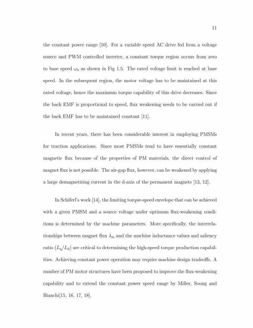
ploying single or multiple q−axis flux barriers [17] (Fig. 1.7) or by using a rotor
14
with two axial parts: one non-salient (exterior PMSM) and the other of the syn-
chronous reluctance type [18] (Fig. 1.8). It is shown that this kind of motor allows
a lower value of rated current and exhibits a larger speed range for flux-weakening
operation. However, both the rotors with low and high saliency ratios have the
specific disadvantages that the mechanical structure limits the maximum speed
and requires unconventional manufacturing technology.
Magnet
d
q
FluxBarrier
Figure 1.7: Cross section of rotor with Lq/Ld < 1 for interior PMSM [17]
1.5.3 Numerical Optimization
The design objective of an interior PMSM is to achieve constant power operation
over an extended speed range by appropriate selection of design variables. Opti-
mization methods can be used to find the optimal solution under constraints on
the design variables.
In the optimization of electromagnetic devices the objective function can
be computed using either the classical (equivalent circuit) approach or a numeri-

15
Reluctance Part Permanent Magnet Part
Figure 1.8: Two-part rotor with Lq/Ld < 1 for interior PMSM [18]
cal field computation approach, such as finite element method (FEM). The FEM
is more accurate than the classical approach but it requires substantially more
sophisticated software and computational time. In numerical field computations
the standard prerequisites of local optimization, such as convexity, differentiability
and accuracy of the objective function, are usually not guaranteed [28]. Deter-
ministic optimization tools for solving local optimization, such as steepest-descent,
conjugate gradient and quasi-Newton methods, are not ideally suited to numeric
electromagnetic problems [29]. Recently, stochastic methods of optimization have
become more popular due to their simplicity and high probability of finding global

16
minima and their simplicity [30]. Stochastic methods such as genetic algorithms
(GA) [31, 32], simulated annealing [33] and evolution strategies [34] have been
successfully used for different aspects of electrical machine design.
Optimization techniques have been applied to the design work of PMSMs in
order to meet particular performance requirements. An optimization method for
exterior PMSMs design has been presented by Higuchi [35]. The procedure inte-
grates analytical method and finite element method (FEM) to refine the design
specifications. In reference [36], a PMSM is optimized with respect to maximum
power output and minimum magnet volume. The problem is treated as a vector
optimization problem and is solved directly without any scalar transformation by
a stochastic search algorithm. A new approach to the design optimization of ex-
terior PMSMs is presented in [32]. The novelty lies in combining a motor analysis
procedure with GA to optimize an objective function such as the motor torque, the
efficiency, the material cost or other motor figures or a combination of these. It has
been observed that the GA generally requires a higher number of iterations with
respect to other conventional techniques. However, the GA method of optimiza-
tion is able to find the global optimum avoiding the local ones. In Lahteenmaki’s
work [37], GA method is chosen to optimize the high-speed PMSM motors with
the modelling of FEM and thermal network analysis. The main drawback with
the present optimization method is that the FEM has to be applied to the nu-
meric field computation at each stage of the optimization, which requires a lengthy
computation time.

17
In order to overcome the problem of time-consuming computation with GA
method, response surface methodology (RSM) was introduced to the numerical
optimization of exterior PMSMs. The response surface methodology (RSM) is a
collection of mathematical and statistical techniques that are useful for evaluat-
ing response, i.e., the objective physical quantities (motor parameters), which are
influenced by several design variables [38, 39]. By careful design of the FEM experi-
ments, RSM can be used to build the empirical model that is finally employed as an
objective function or constraints in an optimization process. As the response sur-
face is often described by polynomial representations (determinative equations), we
can save computational time for optimization process by evaluating the objective
physical quantities by the response surface instead of by the FEM analysis [38, 39].
RSM has been successfully applied to the design optimization of electromagnetic
devices [40, 41, 42, 43].
Although numerical optimization is currently considered indispensable for
PMSMs design, it is, however, difficult to design the interior PMSMs because of the
complicated rotor configurations and the complex influence of magnetic saturation
[44]. Till now, there is not much work that has been done on the optimization
of rotor geometric parameters for interior PMSMs which require a wide constant
power speed range.

18
1.5.4 The Control of PMSMs
Control techniques are critical to exploit the power capability of PMSMs over the
entire speed range. The torque is usually controlled by controlling the phase current
based on the fact that the electromagnetic torque is proportional to the motor
current [45]. The current control is normally executed in the rotor oriented system,
where the d-axis is along the permanent magnet. A rotor position sensor is required
to achieve high-performance current control with the PMSMs. The rotor position
feedback is needed to continuously perform the self-synchronization function, which
is significantly more demanding than other AC machines [47]. Hence, an absolute
or incremental encoder providing high resolution is typically required with PMSMs.
High-quality current vector control was first proposed by Jahns [7] and Rah-
man [49] for achieving high-performance motion control with PMSMs. By mapping
the torque command into values for the d-q axis current component commands,
then controlling the d-q axis current to follow the commands using field-oriented
current controller, we can obtain the the maximum torque for a given motor phase
current, which is generally named as maximum-torque-per-amp (MTPA) control.
By using MTPA control we can ensure maximizing operating efficiency [7]. In
order to apply the MTPA control in PMSM drives, the d-axis and q-axis current
commands have to be accurately calculated based on the motor parameters [49].
Separate current trajectories are identified for the exterior and interior PMSMs
[50, 51, 52]. However, these methods are extremely sensitive to the accuracy of
the motor parameters used in the controllers [53, 55]. Mademlis investigated the

19
influence of Lq variation on maximum torque to current controlled interior PMSM
drives and it is shown, for a given load torque, that the stator current requirement
of a saturated motor is around 15 percent higher [56]. Therefore, the respective
efficiency is lower compared to an unsaturated motor. Bodson proposed modified
maximum torque to current control that takes into account magnetic saturation,
however the air-gap flux linkage variation effect is not considered [59]. Zhu de-
scribed an enhanced online optimal control strategy which enables the maximum
power capability of an interior PMSM to be achieved independent of any variation
in its parameters [61], but the control performance was degraded at fast dynamic
conditions.
The problem of flux-weakening using current control was first highlighted
by Jahns. He proposed a corrective method of control to the standard vector
control architecture [13]. A feedback of current controller error in the synchronous
coordinates was regulated to zero through a PI-controller by reducing the d-axis
current Id and subsequently obtaining the q-axis current Iq. Another method
presented by Sul using a PI control of the voltage error between the saturated
voltage and the output voltage command of PI current controller to adjust d−axis
current command [52, 64]. On the other hand, the scheme presented by Morimoto
looks at voltage reference to determine the control modes between constant torque
and flux-weakening [51]. These templates are generated from motor’s steady state
characteristics, while the dynamic characteristics are either taken into account
merely by the constant voltage margin or they are implicitly solved by the current

20
controller. These schemes based on the static approach have at least two more
drawbacks: deviations from the prescribed control trajectories occur during the
transients, whereas in the steady state the available voltage of the voltage source
inverter is not completely exploited [67, 68].
In order to overcome these problems, direct torque control (DTC) has been
applied to PMSMs in the last decade [69, 70, 71]. DTC was first used in induction
motor drives [72, 73]. The basic principle of DTC is to directly select stator volt-
age vectors according to the differences between the reference and actual torque
and stator flux linkage. Unlike current control, DTC does not require any cur-
rent regulator, coordinate transformation or PWM signal generator. In spite of its
simplicity, DTC allows a fast torque response in steady-state and transient oper-
ating condition to be obtained. In addition, this controller is less influenced by
the parameter detuning in comparison with current control [74]. Although DTC
has many advantages over current control, it still has some disadvantages, such
as high current ripples, variable switching frequency and difficulty in controlling
torque and flux at very low speed.
In recent years, many researchers have tried to reduce the torque ripple and
fix the switching frequency of the DTC scheme. With multi-level inverter proposed
by Vas and Martins, there will be more voltage space vectors available to control
the flux and torque. Therefore, a smoother torque can be expected [75, 76]. How-
ever, more power switches are needed to achieve a lower ripple and almost fixed
switching frequency. Modified DTC schemes with constant switching frequency and

21
low torque ripple were reported by others [77, 78, 79], where space vector modu-
lation (SVM) is incorporated with DTC for induction motor drives to provide a
constant inverter switching frequency, and the torque ripple is significantly reduced
for invoking zero inverter switching state within every switching period of inverter
control. However, they are either motor parameter dependent or quite complicated
with two PI controllers which need to be tuned properly [80, 81]. There are still
drawbacks in present speed and torque control schemes that require corrections:
• DTC scheme does not include direct current control. The current protection is
realized by precalculated torque profile, which is motor parameter dependent.
The motor current may exceed the current constraints in the fast dynamics
or flux-weakening speed range due to variation of motor parameters;
• The transition between constant torque control and flux-weakening control
is determined by motor speed and constant inverter voltage, in which the
inverter voltage capability is not properly exploited;
• There is no feedback flux-weakening control.
1.6 Research Goals and Methodology
Permanent magnet synchronous motors have many advantages as mentioned in
the previous sections. These features permit this machine to be operated not
only in the constant torque region but also in the constant power region up to a
high speed by flux-weakening. However, considering the drawbacks listed in above

22
literature survey for PMSM drives, it is understood that further improvements
in the design and control techniques of PMSMs for constant power operation are
possible. Therefore, the objectives of this research are:
• Analysis of constant power speed range for IPMSM Drives;
• Design optimization of a prototype interior PMSM;
• Control of the prototype interior PMSM in wide speed operation.
1.6.1 Analysis of Constant Power Speed Range for IPMSMDrive
An accurate mathematical modelling of PMSMs provides a foundation for the de-
sign and control of PMSMs. The accuracy of the model directly affects the outcome
of the design and control. A two-phase PMSM equivalent circuit model in the ro-
tor d-q reference frame has been widely adopted by Pillay [2], Sebastian [82] and
Rahman [83] due to its relatively simple composition and reasonable accuracy. The
d-q model, also known as the analytical model, can be derived directly from d- and
q-axis magnetic circuits or can be obtained from the three phase model of a PMSM
by using Park’s transformation [84].
One objective of this research is to determine the relationship between steady
state equivalent circuit parameters of interior PMSMs and their power capability
over a wide speed range. In all cases it will be assumed that the motor is supplied
from a variable frequency inverter with current and rotor position feedback so that

23
both current magnitude and phase angle of current vector can be independently
controlled. The system performance will be investigated primarily by the shape of
the motor power capability curve which is a plot of the maximum power attain-
able versus motor speed subject to current and voltage magnitude constraints. A
simple equivalent circuit model, which takes account of saturation effect in q-axis
inductance, will be used in order to determine the best choice of motor parameters
necessary for maximum power capability over a wide speed range.
1.6.2 Design Optimization of Interior PMSM
While the design process for conventional exterior PMSMs is well developed in
Slemon and Panigrahi’s works [19, 21], it is hard to borrow these experiences to
the design of interior PMSMs because of their complicated rotor structures and
complex influence of magnetic saturation. In the modelling and computing pro-
cess, FEM can be used to accurately compute the air gap flux density and ro-
tor magnetic saliency ratio that are nonlinear functions of the machine flux level.
However, applying FEM in the every stage of design and optimization process is
time-consuming, and sometimes not practical.
In this work, the design procedure combines the FEM and RSM for the mag-
netic analysis, and genetic algorithms (GA) are used as a search method in the
optimization procedure. The effects of a wide range of geometric variables on the
performance of PMSM are investigated and the optimum design is selected for
further studies. Using the proposed design methodology, a 400 W prototype in-
24
terior PMSM with the optimum constant power speed range has been designed
and manufactured. Various steady state tests are conducted to verify the design
optimization method. Test results are compared with those from the numerical
analysis. The close agreement validates the proposed RSM model for the accurate
estimation of motor parameters. The tests also provided an understanding of the
performance of the prototype PMSM and laid a foundation for the control of the
PMSM drive system.
1.6.3 Control of IPMSM in Wide Speed Operation
For a PMSM drive the speed is determined by the frequency of its power supply
and the torque is determined by both the magnitude of the stator current and
the torque angle. The PMSMs can be controlled at constant torque below the
base speed and at constant power above the base speed. However, without proper
control strategy, the PMSM drives cannot exploit its potential power capability
even with a well designed motor.
In this research, a conventional current vector control strategy is imple-
mented. The performances on constant torque and constant power operations are
investigated, and their advantages and disadvantages are examined. A novel mod-
ified DTC scheme based on stator flux control is also proposed. The experimental
results confirm that the new control strategy not only improves the torque capa-
bility in the flux-weakening range, but also extends the speed range at constant
power operation.
25
1.7 Outline of the Thesis
The contents of the thesis are organized as follows:
In Chapter 2, a constant parameter equivalent circuit model is used to deter-
mine the power capability of interior PMSMs in variable speed drive application,
which is depend on the motor parameters, such as d-q axis inductances and stator
PM flux linkage. A simple relationship between the power capability and motor pa-
rameters is derived in order to obtain the theoretical foundation for optimal motor
designs that extend their constant power speed range.
In Chapter 3, the effect of geometric parameters on the motor parameters
of interior PMSMs has been investigated using both analytical method and finite
element method. In order to achieve a computationally simple and accurate mo-
tor parameters determination in the iterative process of numerical optimization,
an effective computational approach which combines magnetic field analysis and
analytical equations by response surface methodology (RSM) was proposed for the
prediction of motor parameters in interior PMSMs. The polynomial representation
of motor parameters (Ld, Lq and λpm) by RSM are derived and their accuracy in
selected geometric space of rotor structure are validated by FEM.
In Chapter 4, the numerical optimization methodology is developed for inte-
rior PMSMs. The design criteria and optimization objective in this thesis are to
extend the constant power speed range. The combination of FEM and RSM is used
26
for an investigation into the effect of a wide range of geometric variables, and GA
is applied as the search method to look for the optimum rotor geometric design.
In Chapter 5, results of various steady-state tests on the prototype interior
PMSM are presented, which include no-load and load test, torque-speed character-
istics, and efficiency and power factor measurements. The test results are compared
with those collected from the commercial interior PMSM with same power rating.
The tests also provide accurate measurement of the values for motor parameters
including magnet flux linkage and d-q axis inductances of prototype PMSM and
hence laid a foundation for the control of the interior PMSM drive system.
In Chapter 6, various aspects of the PMSM control system are discussed.
Hardware and software considerations and operations of the control system are
presented. A conventional current vector control strategies is implemented and
compared. Space vector modulation based modified DTC scheme is also proposed
to eliminate the drawbacks of current vector control scheme. The experimental
results confirm the advantages of new control method for the constant power op-
eration over a wide speed range.

Chapter 2
Analysis of Interior PermanentMagnet Synchronous Motors forWide-Speed Operation
2.1 Introduction
When permanent magnets are buried inside the rotor core, the motor not only
provides mechanical ruggedness but also opens a possibility of increasing its power
capability over a wide speed range. This class of interior PMSMs can be considered
as reluctance synchronous motors and PM motors combined together. Convention-
ally, a two phase equivalent circuit model (d-q axis model) has been used to analyze
reluctance synchronous machines and induction machines. This same technique is
now applied in the analysis of interior PMSMs in this chapter.
The steady state performance of interior PMSMs can be modelled by circuit
equations with stator PM flux linkage and d- and q-axis inductances that are non-
linear functions of the machine flux level. However, it is critical to note important
27

28
assumptions that have been made in this analysis.
First, the simplification of the interior PMSM’s equivalent circuits will include
only three parameters hence that all electrical loss components are ignored. This
includes both the stator copper loss, as well as hysteresis and eddy-current losses
in the machine iron. Iron losses gradually increase as the speed increases because
both of these iron loss components increase with frequency. Interior PMSMs are
typically designed with small iron loss at rated frequency, so ignoring these losses
is not expected to affect any of the major predicted trends.
Therefore, in this chapter lossless equivalent circuit model of the interior
PMSMs is used to investigate the influence of machine parameters on motor per-
formances. The purpose of this analysis is to determine the optimal set of equivalent
circuit parameters to obtain output power at high speed. Steady state maximum
output power versus speed curves can be derived for interior PMSMs over the whole
speed range.
2.2 Mathematical Modelling
The d- and q-coordinate based equivalent circuit model is used for the modelling of
PMSMs. Fig. 2.1 illustrates a conceptual cross-sectional view of a 3-phase, 2-pole
interior PMSM along with two reference frames. To show the inductance difference
(Lq > Ld), rotor is drawn with saliency.
The electrical dynamic equation in terms of phase variables can be written

29
θ
q-axis
d-axis
a-axis
b-axis
c-axis
S
N
a
'a
b
'b
c
'c
Figure 2.1: Permanent magnet synchronous motor
as:
Va = RsIa +dλa
dt(2.1)
Vb = RsIb +dλb
dt(2.2)
Vc = RsIc +dλc
dt(2.3)
where (Va, Vb, Vc), (Ia, Ib, Ic) and Rs refer to phase voltage, current and resistance,
respectively. The phase flux linkage (λa, λb, λc) equations are [81]:
λa = LaaIa + LabIb + LacIc + λma (2.4)
λb = LabIa + LbbIb + LbcIc + λmb (2.5)
λc = LacIa + LbcIb + LccIc + λmc (2.6)
30
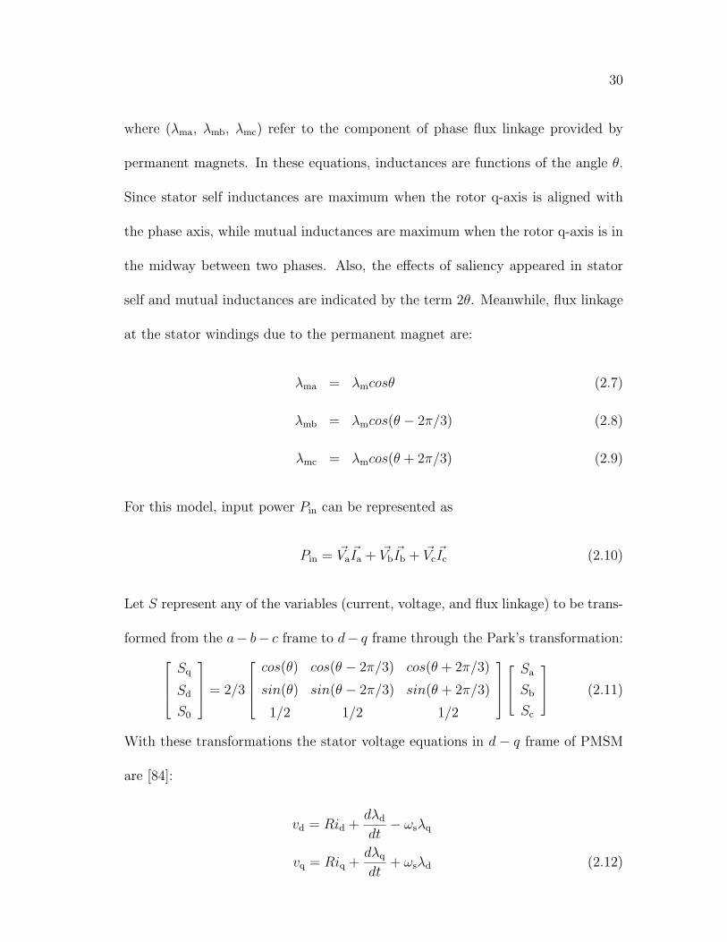
where (λma, λmb, λmc) refer to the component of phase flux linkage provided by
permanent magnets. In these equations, inductances are functions of the angle θ.
Since stator self inductances are maximum when the rotor q-axis is aligned with
the phase axis, while mutual inductances are maximum when the rotor q-axis is in
the midway between two phases. Also, the effects of saliency appeared in stator
self and mutual inductances are indicated by the term 2θ. Meanwhile, flux linkage
at the stator windings due to the permanent magnet are:
λma = λmcosθ (2.7)
λmb = λmcos(θ − 2π/3) (2.8)
λmc = λmcos(θ + 2π/3) (2.9)
For this model, input power Pin can be represented as
Pin = ~Va~Ia + ~Vb
~Ib + ~Vc~Ic (2.10)
Let S represent any of the variables (current, voltage, and flux linkage) to be trans-
formed from the a− b− c frame to d− q frame through the Park’s transformation:Sq
Sd
S0
= 2/3
cos(θ) cos(θ − 2π/3) cos(θ + 2π/3)
sin(θ) sin(θ − 2π/3) sin(θ + 2π/3)
1/2 1/2 1/2
Sa
Sb
Sc
(2.11)
With these transformations the stator voltage equations in d− q frame of PMSM
are [84]:
vd = Rid +dλd
dt− ωsλq
vq = Riq +dλq
dt+ ωsλd (2.12)
31
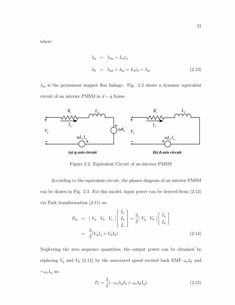
where
λq = λaq = Lqiq
λd = λad + λm = Ldid + λm (2.13)
λm is the permanent magnet flux linkage. Fig. 2.2 shows a dynamic equivalent
circuit of an interior PMSM in d− q frame.
sR qL
mωλ
dd ILωqV
qI
sR dL
qq ILωdV
dI
(a) q-axis circuit (b) d-axis circuit
Figure 2.2: Equivalent Circuit of an interior PMSM
According to the equivalent circuit, the phasor diagram of an interior PMSM
can be drawn in Fig. 2.3. For this model, input power can be derived from (2.12)
via Park transformation (2.11) as:
Pin = [ Va Vb Vc ]
Ia
Ib
Ic
=3
2[ Vq Vd ]
[Iq
Id
]
=3
2(VqIq + VdId) (2.14)
Neglecting the zero sequence quantities, the output power can be obtained by
replacing Vq and Vd (2.12) by the associated speed excited back EMF ωsλd and
−ωsλq as:
Po =3
2(−ωsλqId + ωsλdIq) (2.15)
32
mλ
sλsV
sI
δ
qλ
dλ
q
d
qI
dI
β
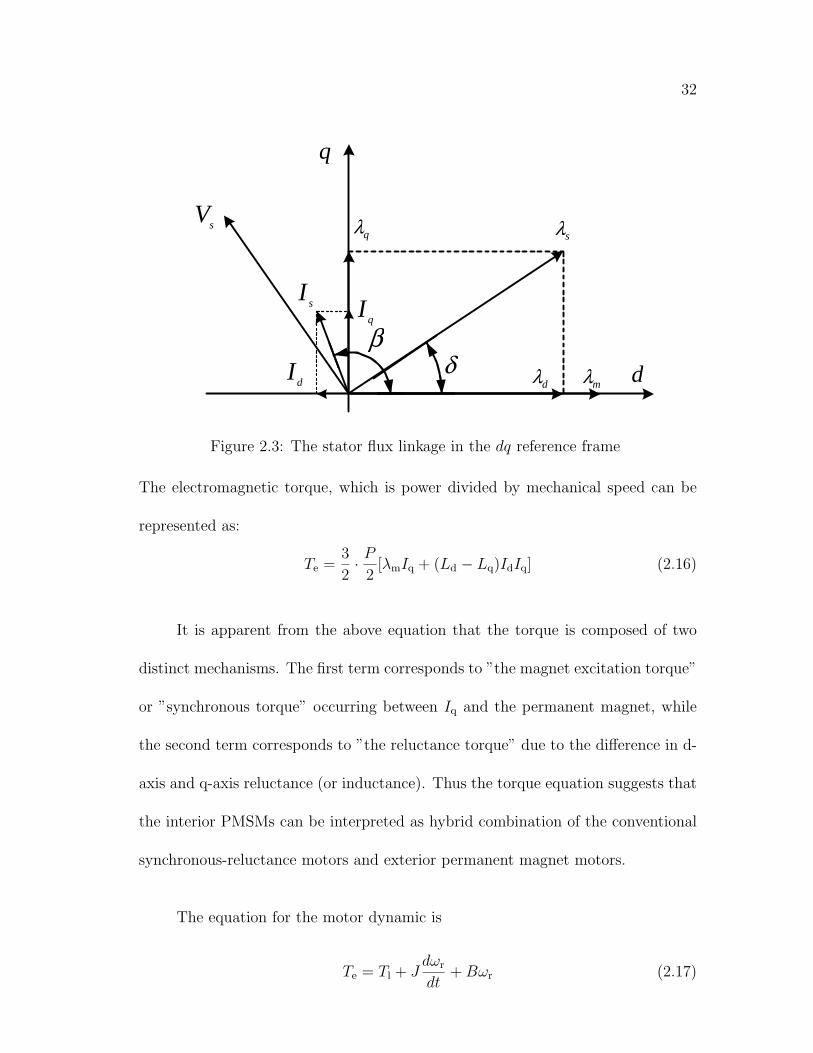
Figure 2.3: The stator flux linkage in the dq reference frame
The electromagnetic torque, which is power divided by mechanical speed can be
represented as:
Te =3
2· P
2[λmIq + (Ld − Lq)IdIq] (2.16)
It is apparent from the above equation that the torque is composed of two
distinct mechanisms. The first term corresponds to ”the magnet excitation torque”
or ”synchronous torque” occurring between Iq and the permanent magnet, while
the second term corresponds to ”the reluctance torque” due to the difference in d-
axis and q-axis reluctance (or inductance). Thus the torque equation suggests that
the interior PMSMs can be interpreted as hybrid combination of the conventional
synchronous-reluctance motors and exterior permanent magnet motors.
The equation for the motor dynamic is
Te = Tl + Jdωr
dt+ Bωr (2.17)

33
where J is the inertia of the rotor and the connected load. Because we are concerned
primarily with motor action, the torque Tl is positive for a torque load. The
constant B is a damping coefficient associated with the rotational system of the
machine and the mechanical load.
2.3 Theoretical Analysis of Steady-State Opera-
tion
In variable speed drives, PMSMs are fed from inverters. The power rating of
inverter is usually matching the power rating of motor in order to save the cost.
Considering this voltage and current constraints due to power rating limitation, the
armature current Is and the terminal voltage Vs (neglecting winding resistance) are
limited as follows:
Is =√
I2d + I2
q ≤ Ism (2.18)
Vs = ωs ·√
λ2d + λ2
q ≤ Vsm (2.19)
From (2.19), we have the voltage limitation related to the Id and Iq:
√(LdId + λm)2 + (LqIq)2 ≤ Vsm
ωs
(2.20)
The maximum current Ism is the continuous armature current rating in steady state
operation of motor. The maximum voltage Vsm is the maximum available output
voltage from the inverter depending on the dc-link voltage. The critical condition
of (2.18) and (2.31)is shown in Id − Iq plane, Fig. 2.4.
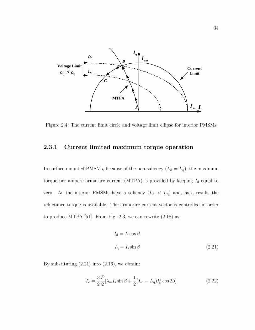
34
MTPA
CurrentLimit
smI
smI
qI
dI
Voltage Limit
12ωω > 2
ω
1ω
A
B
C
Figure 2.4: The current limit circle and voltage limit ellipse for interior PMSMs
2.3.1 Current limited maximum torque operation
In surface mounted PMSMs, because of the non-saliency (Ld = Lq), the maximum
torque per ampere armature current (MTPA) is provided by keeping Id equal to
zero. As the interior PMSMs have a saliency (Ld < Lq) and, as a result, the
reluctance torque is available. The armature current vector is controlled in order
to produce MTPA [51]. From Fig. 2.3, we can rewrite (2.18) as:
Id = Is cos β
Iq = Is sin β (2.21)
By substituting (2.21) into (2.16), we obtain:
Te =3
2
P
2[λmIs sin β +
1
2(Ld − Lq)I
2s cos 2β] (2.22)
35
The relationship between the amplitude of the stator current and the current angle
β can be derived by setting the derivative of (2.22) with respect to β to zero:
dTe
dβ=
3
2
P
2[λmIs cos β + (Ld − Lq)I
2s cos 2β] = 0 (2.23)
By substituting (2.21) into (2.23), we obtain
(Ld − Lq)I2d + λmId − (Ld − Lq)I
2q = 0 (2.24)
From (2.24), we can get
Id =λm
2(Lq − Ld)−
√√√√ λ2m
4(Lq − Ld)2+ I2
q (2.25)
This relationship is shown as the MTPA trajectory in Fig.2.4. The peak torque Tm
is produced when Is =√
I2d + I2
q = Ism considering the continuous current rating.
The current vector (Id, Iq) producing this peak torque Tm is the intersection point
of the MTPA trajectory and the current-limit circle, which corresponds to point B
in Fig. 2.4. The d- and q-axis currents Idm and Iqm are derived from (2.25) and√I2d + I2
q = Ism:
Idm =λm
4(Lq − Ld)−
√√√√ λ2m
16(Lq − Ld)2+
I2sm
2
Iqm =√
I2sm − I2
dm (2.26)
Thus, the current angle β for this peak torque is obtained as:
βb = arctan(Iqm
Idm
) (2.27)
Therefore, the peak torque Tm can be written as:
Tm =3
2· P
2[λmIqm + (Ld − Lq)IdmIqm] (2.28)

36
Until the terminal voltage Vs reaches its limited value Vsm at ωs = ωb, which is
defined as the base speed, the motor can be accelerated by this peak torque Tm.
The highest speed (base speed) under this constant torque is given by:
ωb =Vsm√
(LdIdm + λm)2 + (LqIqm)2(2.29)
2.3.2 Current and voltage limited maximum poweroperation
Inverter fed PMSM drives exhibit a constant torque region, from zero to the base
speed with increasing voltage. Then a decreasing torque region follows with a
constant voltage which extends up to the maximum operational speed. The high-
speed constant voltage operation is accomplished by reducing the stator flux linkage
through an appropriate stator current distribution and thus it is generally called
“flux-weakening region”.
The critical condition of (2.18) and (2.19) under flux-weakening operation is
given by the voltage-limit ellipse in the Id − Iq plane as shown in Fig. 2.4 by the
dashed lines. The voltage-limit ellipse becomes smaller as the speed increases and,
as a result, the current vector producing peak torque Tm cannot satisfy the voltage
constraint above the base speed. The d- and q-axis components of the armature
current are controlled in order to keep Vs equal to Vsm in the flux-weakening region
as shown in (2.30):
√λ2
d + λ2q =
√(LdId + λm)2 + (LqIq)2 =
Vsm
ωs
(2.30)

37
Substitute (2.13) into (2.30), we get the relationship between Id and Iq for voltage
constraint:
Id = −λm
Ld
+1
Ld
√(Vsm
ωs
)2 − (LqIq)2 (2.31)
Substituting (2.18) into (2.31), we can get the equation for Id with respect to motor
speed ωs for current and voltage limited maximum power operation (above the base
speed):
(L2d − L2
q)I2d + 2LdλmId + λ2
m + L2qI
2sm − (
Vsm
ωs
)2 = 0 (2.32)
Assuming
a = L2d − L2
q
b = 2Ldλm
c = λ2m + L2
qI2sm − (
Vsm
ωs
)2 (2.33)
then (2.32) can be rewritten as:
aI2d + bId + c = 0 (2.34)
Therefore, the solution for (2.34) is
Idn =−b +
√b2 − 4ac
2a
=−2Ldλm +
√(2Ldλm)2 − 4(L2
d − L2q)(λ
2m + L2
qI2sm − (Vsm
ωs)2)
2(L2d − L2
q)(2.35)
Finally, Iq can be solved as:
Iqn =√
I2sm − I2
dn (2.36)
Substitute (2.35) and (2.36) into (2.16), we can get the maximum torque withrespect to motor speed ωs under current and voltage constraints, which is shown
38
is (2.37).
Tn =32· P
2[λmIqn + (Ld − Lq)IdnIqn]
=32· P
2[λm +
−2Ldλm +√
(2Ldλm)2 − 4(L2d − L2
q)(λ2m + L2
qI2sm − (Vsm
ωs)2)
2(Ld + Lq)]Iqn(2.37)
and motor speed ωs satisfies the following voltage equation:
ωs =Vsm√
(LdIdn + λm)2 + (LqIqn)2(2.38)
2.3.3 Voltage limited maximum power operation
From (2.22), (2.18) and (2.19), the armature current vector (Id, Iq) producing max-
imum output torque under the voltage-limit condition is derived as follows where
the current-limit condition is not considered.
The voltage equation for interior PMSMs above the base speed is derived as:
(λm + LdId)2 + (LqIq)
2 = (Vsm
ωs
)2 (2.39)
and the torque equation is:
Te =3
2· P
2[λmIq + (Ld − Lq)IdIq] (2.40)
Rewriting (2.39) as:
λm + LdId =Vsm
ωs
cos α
LqIq =Vsm
ωs
sin α (2.41)
Subsequently, we get:
Id =Vsm
ωsLd
cos α− λm
Ld
Iq =Vsm
ωsLq
sin α (2.42)
39
where α is an interim variable. Thus, with
dTe
dα= λm
Vsm
ωsLq
cos α + (Ld − Lq) ·Vsm
ωsLd
· (− sin α) · Vsm
ωsLq
sin α
+ (Ld − Lq) ·Vsm
ωsLd
· (cos α) · Vsm
ωsLq
cos α = 0 (2.43)
we can get
2(Ld−Lq)·Vsm
ωsLd
· Vsm
ωsLq
cos2 α+Lq
Ld
·λmVsm
ωsLq
cos α−(Ld−Lq)·Vsm
ωsLd
· Vsm
ωsLq
= 0 (2.44)
Assuming
A = (Ld − Lq) ·Vsm
ωsLd
· Vsm
ωsLq
B =Lq
Ld
λmVsm
ωsLq
(2.45)
then (2.44) can be rewritten as:
2A cos2 α + B cos α− A = 0 (2.46)
Therefore,
cos α =−B −
√B2 + 8A2
4A(2.47)
Substituting (2.45) into (2.47) with simplifications, we can obtain:
cos α =−ρλm +
√(ρλm)2 + 8(1− ρ)2(Vsm/ωs)2
4(1− ρ)(Vsm/ωs)(2.48)
and
ρ = Lq/Ld > 1 (2.49)
By substituting (2.48) into (2.42), we can get the solution of Id which produce
maximum power under voltage limit:
Idp = −λm
Ld
−−ρλm +
√(ρλm)2 + 8(ρ− 1)2(Vsm/ωs)2
4(ρ− 1)Ld
(2.50)
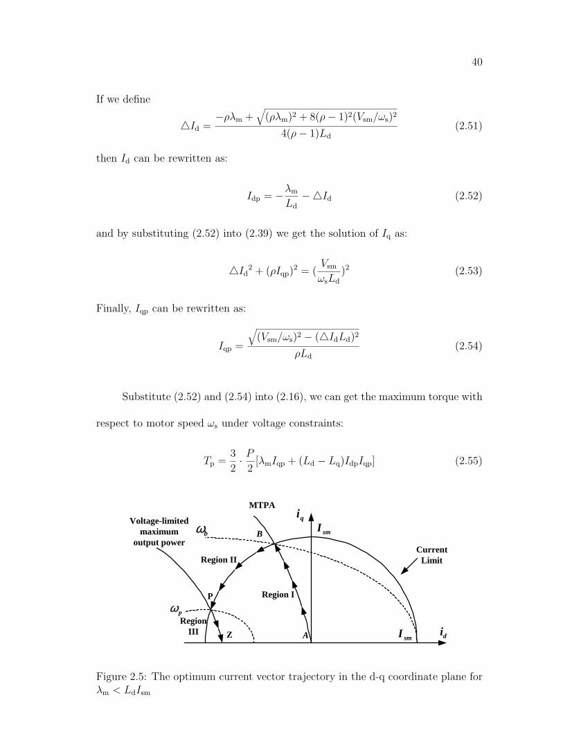
40
If we define
4Id =−ρλm +
√(ρλm)2 + 8(ρ− 1)2(Vsm/ωs)2
4(ρ− 1)Ld
(2.51)
then Id can be rewritten as:
Idp = −λm
Ld
−4Id (2.52)
and by substituting (2.52) into (2.39) we get the solution of Iq as:
4Id2 + (ρIqp)
2 = (Vsm
ωsLd
)2 (2.53)
Finally, Iqp can be rewritten as:
Iqp =
√(Vsm/ωs)2 − (4IdLd)2
ρLd
(2.54)
Substitute (2.52) and (2.54) into (2.16), we can get the maximum torque with
respect to motor speed ωs under voltage constraints:
Tp =3
2· P
2[λmIqp + (Ld − Lq)IdpIqp] (2.55)
CurrentLimit
smI
smI
qi
di
bω
A
B
MTPA
Voltage-limitedmaximum
output power
pωP
Z
Region I
Region II
RegionIII
Figure 2.5: The optimum current vector trajectory in the d-q coordinate plane forλm < LdIsm
41
The current vector trajectory of the voltage-limited maximum output power
is shown in Fig. 2.5. This current vector approaches the point P as the rotor speed
increases and reaches the current-limit circle at ωs = ωp. The rotor speed ωp is the
minimum speed for the voltage-limited maximum output power operation. Below
this speed, the voltage-limited maximum output power trajectory intersects the
voltage-limit ellipse outside the current limit circle. The direct solution of ωp from
(2.52), (2.54) and (2.18) is difficult. Alternatively, numerical computation can be
used to obtain ωp by solving the following equations:
Idp = −λm
Ld
−−ρλm +
√(ρλm)2 + 8(ρ− 1)2(Vsm/ωs)2
4(ρ− 1)Ld
Iqp =
√(Vsm/ωs)2 − (4IdLd)2
ρLd
Ism =√
I2dp + I2
qp (2.56)
Therefore, ωp is derived as:
ωp =Vsm√
(LdIdp + λm)2 + (LqIqp)2(2.57)
2.3.4 Optimum current vector trajectory
To produce the maximum output power in all speed ranges considering the con-
ditions of both the current and the voltage limits, the optimum current vector is
chosen as follows:
Region I (ωs ≤ ωb): Id and Iq are constant values given by (2.26). The
current vector is fixed at point B in Fig. 2.5.
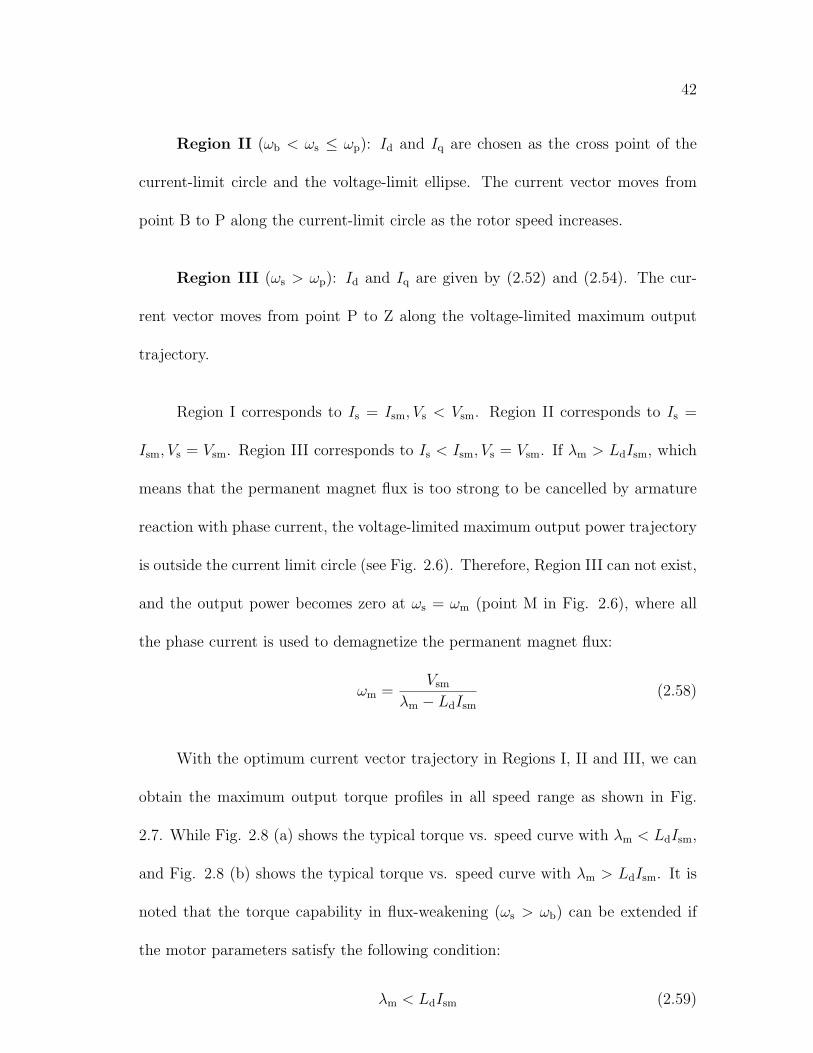
42
Region II (ωb < ωs ≤ ωp): Id and Iq are chosen as the cross point of the
current-limit circle and the voltage-limit ellipse. The current vector moves from
point B to P along the current-limit circle as the rotor speed increases.
Region III (ωs > ωp): Id and Iq are given by (2.52) and (2.54). The cur-
rent vector moves from point P to Z along the voltage-limited maximum output
trajectory.
Region I corresponds to Is = Ism, Vs < Vsm. Region II corresponds to Is =
Ism, Vs = Vsm. Region III corresponds to Is < Ism, Vs = Vsm. If λm > LdIsm, which
means that the permanent magnet flux is too strong to be cancelled by armature
reaction with phase current, the voltage-limited maximum output power trajectory
is outside the current limit circle (see Fig. 2.6). Therefore, Region III can not exist,
and the output power becomes zero at ωs = ωm (point M in Fig. 2.6), where all
the phase current is used to demagnetize the permanent magnet flux:
ωm =Vsm
λm − LdIsm
(2.58)
With the optimum current vector trajectory in Regions I, II and III, we can
obtain the maximum output torque profiles in all speed range as shown in Fig.
2.7. While Fig. 2.8 (a) shows the typical torque vs. speed curve with λm < LdIsm,
and Fig. 2.8 (b) shows the typical torque vs. speed curve with λm > LdIsm. It is
noted that the torque capability in flux-weakening (ωs > ωb) can be extended if
the motor parameters satisfy the following condition:
λm < LdIsm (2.59)
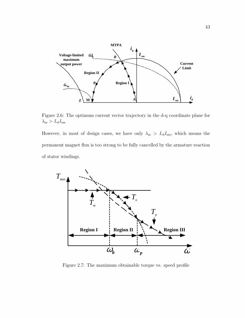
43
CurrentLimit
smI
smI
qi
di
bω
A
B
MTPA
Voltage-limitedmaximum
output power
mω P
MZ
Region I
Region II
Figure 2.6: The optimum current vector trajectory in the d-q coordinate plane forλm > LdIsm
However, in most of design cases, we have only λm > LdIsm, which means the
permanent magnet flux is too strong to be fully cancelled by the armature reaction
of stator windings.
ω
maxT
bω pω
mT nT
pT
Region I Region II Region III
Figure 2.7: The maximum obtainable torque vs. speed profile

44
T
ω
maxT
pT
bω pω
T
maxT
mω
(a)
(b)bω ω
smd IL<λ
smd IL>λ
Figure 2.8: Torque vs. speed characteristics with optimum current vector trajectory
2.4 Effects of Motor Parameters on Torque-Speed
Characteristics
In Fig. 2.8 (a) and (b), with the same current and voltage limits, it shows that
torque vs. speed characteristics are different for λm < LdIsm and λm > LdIsm.
This fact suggests that the detail investigation needs to be conducted in order to
analyze the effects of motor parameters on the performance of machine torque-
speed characteristics.
With voltage and current constraints (2.18) and (2.19) we obtain the torque
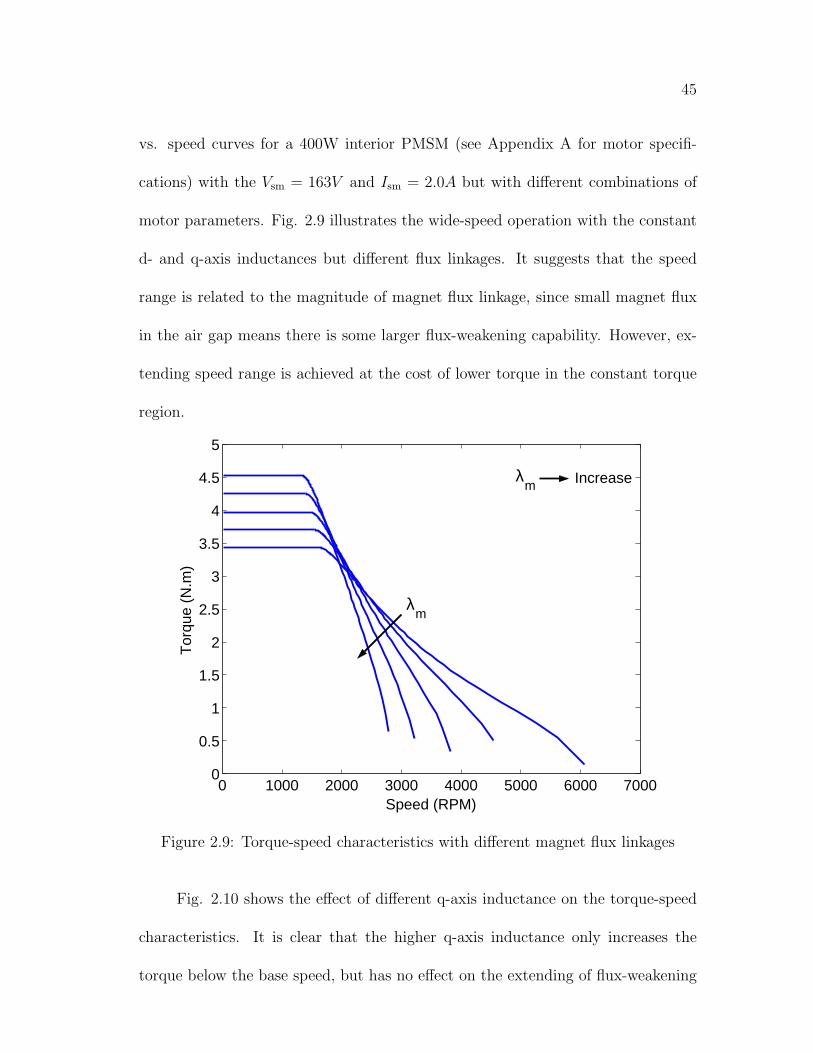
45
vs. speed curves for a 400W interior PMSM (see Appendix A for motor specifi-
cations) with the Vsm = 163V and Ism = 2.0A but with different combinations of
motor parameters. Fig. 2.9 illustrates the wide-speed operation with the constant
d- and q-axis inductances but different flux linkages. It suggests that the speed
range is related to the magnitude of magnet flux linkage, since small magnet flux
in the air gap means there is some larger flux-weakening capability. However, ex-
tending speed range is achieved at the cost of lower torque in the constant torque
region.
0 1000 2000 3000 4000 5000 6000 70000
0.5
1
1.5
2
2.5
3
3.5
4
4.5
5
Speed (RPM)
Tor
que
(N.m
)
λm
λm
Increase
Figure 2.9: Torque-speed characteristics with different magnet flux linkages
Fig. 2.10 shows the effect of different q-axis inductance on the torque-speed
characteristics. It is clear that the higher q-axis inductance only increases the
torque below the base speed, but has no effect on the extending of flux-weakening

46
speed range.
0 500 1000 1500 2000 2500 30000
1
2
3
4
5
6
Speed (rpm)
Tor
que
(N.m
) Lq
Lq Increase
Figure 2.10: Torque-speed characteristics with different q-axis inductance
Fig. 2.11 describes the effect of different d-axis inductances on the wide-
speed operation. It has the similar effect as the flux linkage on the constant torque
region, but higher d-axis inductance value extends the flux weakening speed range
significantly.
2.5 Design Considerations on Constant Power Speed
Range
A constant power speed range (CPSR) is defined as the speed range at which the
motor drive can maintain rated power with voltage and current constraints, which
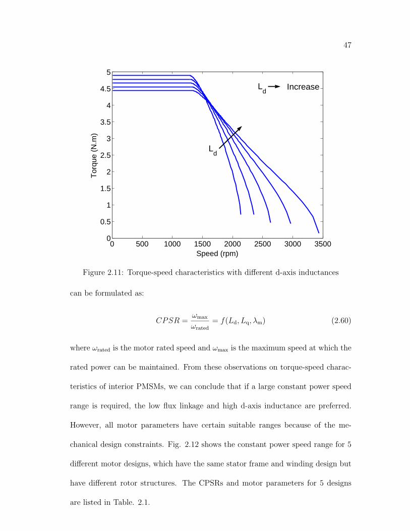
47
0 500 1000 1500 2000 2500 3000 35000
0.5
1
1.5
2
2.5
3
3.5
4
4.5
5
Speed (rpm)
Tor
que
(N.m
)
Ld
Ld Increase
Figure 2.11: Torque-speed characteristics with different d-axis inductances
can be formulated as:
CPSR =ωmax
ωrated
= f(Ld, Lq, λm) (2.60)
where ωrated is the motor rated speed and ωmax is the maximum speed at which the
rated power can be maintained. From these observations on torque-speed charac-
teristics of interior PMSMs, we can conclude that if a large constant power speed
range is required, the low flux linkage and high d-axis inductance are preferred.
However, all motor parameters have certain suitable ranges because of the me-
chanical design constraints. Fig. 2.12 shows the constant power speed range for 5
different motor designs, which have the same stator frame and winding design but
have different rotor structures. The CPSRs and motor parameters for 5 designs
are listed in Table. 2.1.
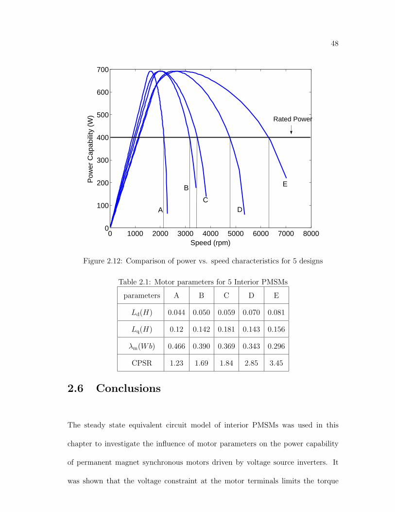
48
0 1000 2000 3000 4000 5000 6000 7000 80000
100
200
300
400
500
600
700
Speed (rpm)
Pow
er C
apab
ility
(W
)
A
B
C D
E
Rated Power
Figure 2.12: Comparison of power vs. speed characteristics for 5 designs
Table 2.1: Motor parameters for 5 Interior PMSMs
parameters A B C D E
Ld(H) 0.044 0.050 0.059 0.070 0.081
Lq(H) 0.12 0.142 0.181 0.143 0.156
λm(Wb) 0.466 0.390 0.369 0.343 0.296
CPSR 1.23 1.69 1.84 2.85 3.45
2.6 Conclusions
The steady state equivalent circuit model of interior PMSMs was used in this
chapter to investigate the influence of motor parameters on the power capability
of permanent magnet synchronous motors driven by voltage source inverters. It
was shown that the voltage constraint at the motor terminals limits the torque

49
output at high speed. For most designs this constraint causes the torque to drop
to zero and limit the speed range. This constant power speed range can be the-
oretically extended if the motor is designed with optimum combination of Ld, Lq
and λm. All of the above conclusions address the theoretical limits of operation of
lossless, linear model of interior type PMSMs. The practical interior PMSMs have
complicated rotor structures and complex influence of magnetic saturation. Cal-
culation and selection of optimum motor parameters require effective computation
and optimization approach which is discussed in the following chapter.

Chapter 3
Determination of MotorParameters in Interior PMSMs
3.1 Introduction
In order to extend the constant power speed range whilst keeping an economic
inverter rating for PMSM drives, the optimum combination of motor parameters
(Ld, Lq and λm) in an interior PMSM is necessary as discussed in Chapter 2. This
chapter discusses the determination of motor parameters in the machine design
stage.
The parameters in equivalent circuit model of an interior PMSM with fixed
stator windings are dependent on the configurations of the permanent magnets in
the rotor and the geometrical profile of the air gap. The design objective is to select
the appropriate geometry for the machine to obtain the optimum combination of
motor parameters to achieve a larger constant power speed range. The additional
design goals are high efficiency and power factor.
50
51
The motor parameters can be calculated by analytical equations derived from
generalized electrical machine theory, which is computationally simple and quick,
and it allows a wide range of design variables to be evaluated. However, it is dif-
ficult to use this method to calculate the performance of the machine taking into
account the effect of magnetic saturation and complex rotor configurations. Nu-
merical techniques have been recognized as practical and accurate methods of field
computation to aid in the electrical design. Finite element method has emerged as
a suitable technique for computation of motor parameters and performance evalu-
ation. But design optimization based on finite element solutions is time-consuming
process. In order to achieve a computationally simple and accurate prediction,
an effective computational approach which combines magnetic field analysis and
analytical equations by response surface methodology (RSM) is proposed for the
determination of motor parameters in interior PMSMs.
3.2 Design of The Stator Winding
The motor parameters (Ld, Lq and λm) in an interior PMSM depend on the detail
of stator winding and rotor structure. The stator of an existing 400W induction
motor is used in this work, which is shown in Fig. 3.1, and the geometry of stator
structure is listed in Table 3.1.
The design procedure of winding distribution for the prototype interior PMSM
is similar as the induction motor. Therefore, a simplified design example of phase
winding is listed as follows:

52
R 37.50mm
R 60.00mm
Figure 3.1: Stator frame structure
• If the required output power Pout = 400 W , the rms value of linear current
density:
K1s =Pout · 2p
πB1gD2Lωs
= 13.206(kA/m) (3.1)
where, ωs = 2πf = 100π rad/s and B1g is selected as 0.4 Tesla.
• Ampere turns per phase:
NphIph = (K1s/kw)πD/6 = 557.6(AT ) (3.2)
where, kw is the winding factor, Nph is the stator turns per phase and Iph is
the phase current.
• Current density in conductor:
Jc =Ks
fs · SWF · SD= 4.618(A/mm2) (3.3)
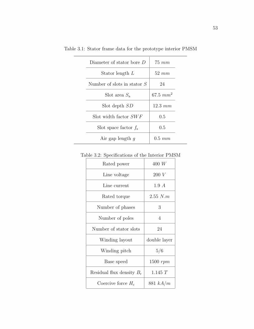
53
Table 3.1: Stator frame data for the prototype interior PMSM
Diameter of stator bore D 75 mm
Stator length L 52 mm
Number of slots in stator S 24
Slot area Sa 67.5 mm2
Slot depth SD 12.3 mm
Slot width factor SWF 0.5
Slot space factor fs 0.5
Air gap length g 0.5 mm
Table 3.2: Specifications of the Interior PMSM
Rated power 400 W
Line voltage 200 V
Line current 1.9 A
Rated torque 2.55 N.m
Number of phases 3
Number of poles 4
Number of stator slots 24
Winding layout double layer
Winding pitch 5/6
Base speed 1500 rpm
Residual flux density Br 1.145 T
Coercive force Hc 881 kA/m
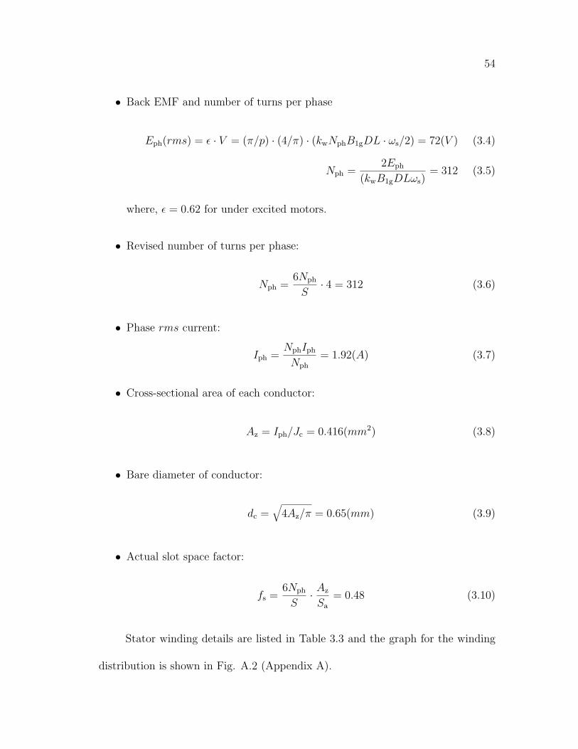
54
• Back EMF and number of turns per phase
Eph(rms) = ε · V = (π/p) · (4/π) · (kwNphB1gDL · ωs/2) = 72(V ) (3.4)
Nph =2Eph
(kwB1gDLωs)= 312 (3.5)
where, ε = 0.62 for under excited motors.
• Revised number of turns per phase:
Nph =6Nph
S· 4 = 312 (3.6)
• Phase rms current:
Iph =NphIph
Nph
= 1.92(A) (3.7)
• Cross-sectional area of each conductor:
Az = Iph/Jc = 0.416(mm2) (3.8)
• Bare diameter of conductor:
dc =√
4Az/π = 0.65(mm) (3.9)
• Actual slot space factor:
fs =6Nph
S· Az
Sa
= 0.48 (3.10)
Stator winding details are listed in Table 3.3 and the graph for the winding
distribution is shown in Fig. A.2 (Appendix A).

55
Table 3.3: Winding specifications for the prototype interior PMSM
Slots per phase 8
Phase spread 60◦ elec.
Coils per phase 8
Turns per coil 39
Turns per phase 312
Conductors per slot 78
Winding factor 0.933
Wire diameter 0.65 mm
Slot space factor 0.48
3.3 Selection of The Rotor Design Variables
As discussed in Chapter 1, the PMSM configuration chosen for this research have
a structure with NdFeB permanent magnets, as shown in Fig. 3.2.
The stator frame of a standard induction machine has been used in interior
PMSMs. The stator windings layout and ratings designed in previous section re-
main unchanged for different sample rotors. The design specifications of the interior
PMSM stator and permanent magnet material are listed in Table. 3.2.
Once the stator geometry and winding layout are determined, the motor
parameters are determined by the design variables in the rotor geometry. By FEM
computation, the flux plot for one pole produced by permanent magnet is shown
in Fig. 3.3 and flux density in the air gap for one pole pair is plotted in Fig.
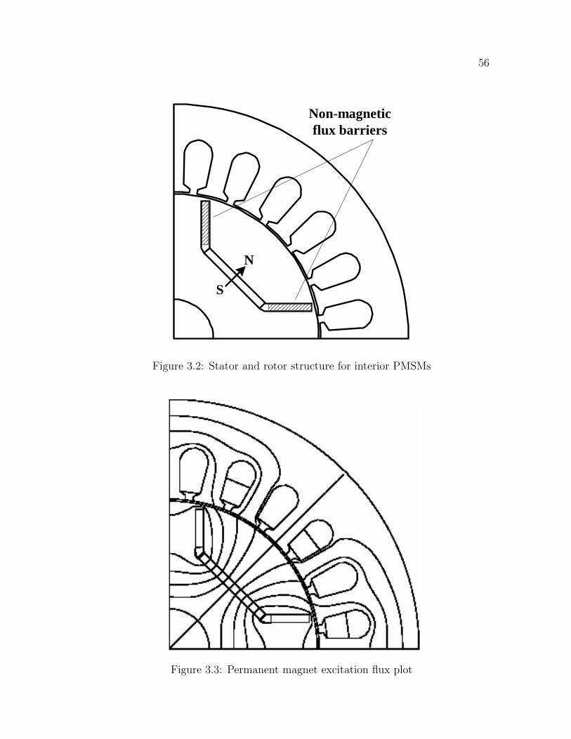
56
Non-magneticflux barriers
N
S
Figure 3.2: Stator and rotor structure for interior PMSMs
Figure 3.3: Permanent magnet excitation flux plot
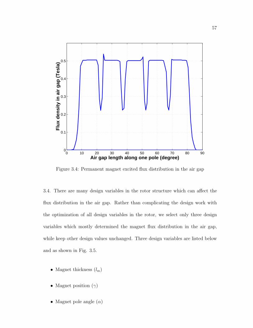
57
0 10 20 30 40 50 60 70 80 900
0.1
0.2
0.3
0.4
0.5
Air gap length along one pole (degree)
Flu
x d
ensi
ty in
air
gap
(T
esla
)
Figure 3.4: Permanent magnet excited flux distribution in the air gap
3.4. There are many design variables in the rotor structure which can affect the
flux distribution in the air gap. Rather than complicating the design work with
the optimization of all design variables in the rotor, we select only three design
variables which mostly determined the magnet flux distribution in the air gap,
while keep other design values unchanged. Three design variables are listed below
and as shown in Fig. 3.5.
• Magnet thickness (lm)
• Magnet position (γ)
• Magnet pole angle (α)
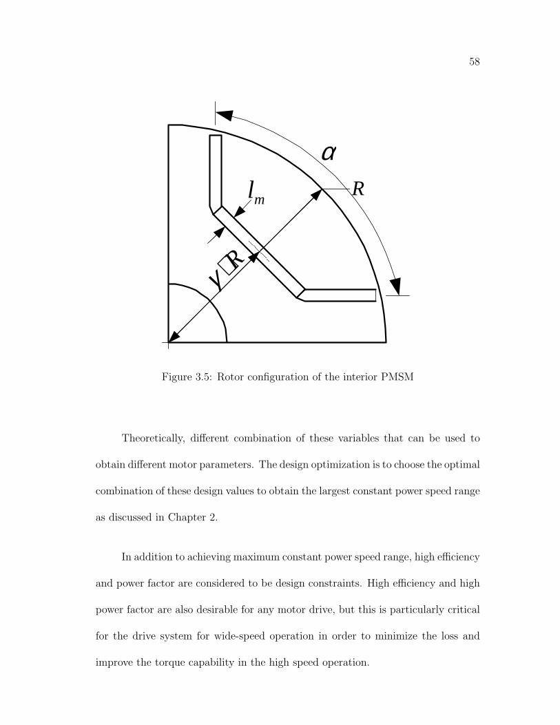
58
Rml
α
R⋅γ
Figure 3.5: Rotor configuration of the interior PMSM
Theoretically, different combination of these variables that can be used to
obtain different motor parameters. The design optimization is to choose the optimal
combination of these design values to obtain the largest constant power speed range
as discussed in Chapter 2.
In addition to achieving maximum constant power speed range, high efficiency
and power factor are considered to be design constraints. High efficiency and high
power factor are also desirable for any motor drive, but this is particularly critical
for the drive system for wide-speed operation in order to minimize the loss and
improve the torque capability in the high speed operation.

59
The NdFeB magnets are the most expensive material in the PMSM. In order
to reduce the overall cost of the interior PMSM, it is important to minimize the
volume of the permanent magnets, and also to use commercially available perma-
nent magnet blocks. The short time overload capacity of the interior PMSM is
constrained by the maximum current that can be carried by the stator winding
without permanently demagnetizing the magnets in the rotor.
3.4 Determination of Motor Parameters
3.4.1 Analytical Method
The analytical model of an interior PMSM is derived from generalized electrical
machine theory [84]. The magnetomotive force due to a stator winding excitation is
expressed in terms of the space distribution and current excitation of the winding.
Then the flux of one pole pitch, as a function of stator angle, is calculated by the
integral of flux density around the air gap. Finally, the flux linkages of the stator
windings are obtained by an integral of the flux multiplied by winding density.
Self-inductances and mutual inductances are given by the flux linkage divided by
the corresponding current excitation.
3.4.1.1 Stator permanent magnet flux linkage
The chosen magnet material is NdFeB which has a demagnetization characteristics
of the form shown in Fig. 1.2. The air gap flux density Bg above the magnets can
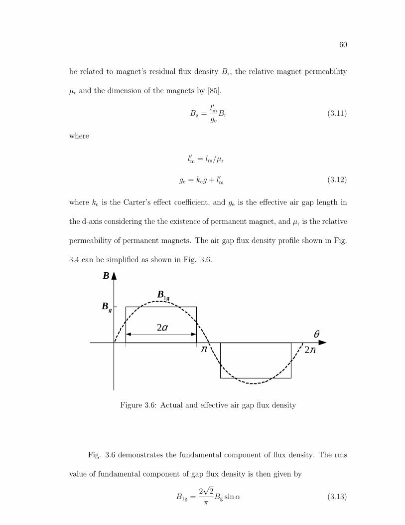
60
be related to magnet’s residual flux density Br, the relative magnet permeability
µr and the dimension of the magnets by [85].
Bg =l′mge
Br (3.11)
where
l′m = lm/µr
ge = kcg + l′m (3.12)
where kc is the Carter’s effect coefficient, and ge is the effective air gap length in
the d-axis considering the the existence of permanent magnet, and µr is the relative
permeability of permanent magnets. The air gap flux density profile shown in Fig.
3.4 can be simplified as shown in Fig. 3.6.
πθ
gB1
gB
π2
α2
B
Figure 3.6: Actual and effective air gap flux density
Fig. 3.6 demonstrates the fundamental component of flux density. The rms
value of fundamental component of gap flux density is then given by
B1g =2√
2
πBg sin α (3.13)

61
The fundamental flux density B1g considering the time component is written
as:
B1g(t, θ) = B1g cos(ωst + θ) (3.14)
As shown in Fig. 3.7, t = 0 is the instant as the rotor field axis or d-axis coincides
with the phase A axis. θ is defined as the electrical angle in the stator from A-axis.
B1g is the peak value of fundamental flux density in the air gap. ωs is the electrical
velocity of rotating flux. The flux in one full pitch coil can be expressed as:
N
S N
S
A-axis d-axistsω
θ
0 π π2
gstator
rotor
∧
gB1
t
Figure 3.7: Air gap flux distribution due to permanent magnet
φ =∫ π
0
B1g cos(ωst + θ)
P·DLdθ (3.15)
where D is the inner diameter of stator frame, L is the stator stack length and P
is the number of poles. Therefore,
φ =2DL
PB1g sin ωst (3.16)
Back EMF in one coil can be written as:
ecoil =dφ
dt=
2DL
PB1gωs cos ωst (3.17)

62
The RMS value of total induced voltage per phase for rotating flux is derived from
(3.17):
E = Nc ·√
2DL
PB1gωs = 4.44fNcΦ (3.18)
where
Nc = kωNph
ωs = 2πf
Φ =2DL
PB1g (3.19)
Nc is defined as the number of turns per phase in equivalent full pitch winding,
and Nph is the number of turns per phase in actual winding. kω is the winding
factor and Φ is the peak flux passing through one full pitch coil. The stator PM
flux linkage λm can be derived from (3.18):
λm =
√2E
ωs
=2DL
PB1g · kωNph (3.20)
3.4.1.2 Calculation of inductances
Fig. 3.8 shows a full-pitch armature winding coil in a P-pole machine which has
one such coil for each pair of poles.
If the coil has Nc turns and θ is the space angle in electrical degree measured
from a coil side, the MMF wave form can be represented by the Fourier series:
Fa(θ) =NcIa
P· 4
π[sin θ +
1
3sin 3θ + · · ·+ 1
(2n− 1)sin (2n− 1)θ] (3.21)
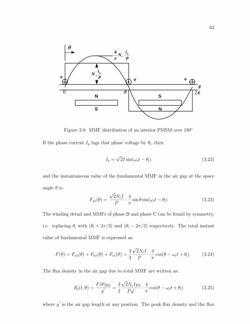
63
a P
iN a
c ⋅
g
a'a
0 π π2
θ
P
iN a
c ⋅π4
N
S N
S
Figure 3.8: MMF distribution of an interior PMSM over 180◦
If the phase current Ia lags that phase voltage by θi, then
Ia =√
2I sin(ωst− θi) (3.22)
and the instantaneous value of the fundamental MMF in the air gap at the space
angle θ is:
Fa1(θ) =
√2NcI
P· 4
πsin θ sin(ωst− θi) (3.23)
The winding detail and MMFs of phase B and phase C can be found by symmetry,
i.e. replacing θi with (θi + 2π/3) and (θi − 2π/3) respectively. The total instant
value of fundamental MMF is expressed as:
F (θ) = Fa1(θ) + Fb1(θ) + Fc1(θ) =3
2
√2NcI
P· 4
πcos(θ − ωst + θi) (3.24)
The flux density in the air gap due to total MMF are written as:
Bs(t, θ) =F (θ)µ0
g′ =3
2
√2NcIµ0
Pg′ · 4
πcos(θ − ωst + θi) (3.25)
where g′is the air gap length at any position. The peak flux density and the flux
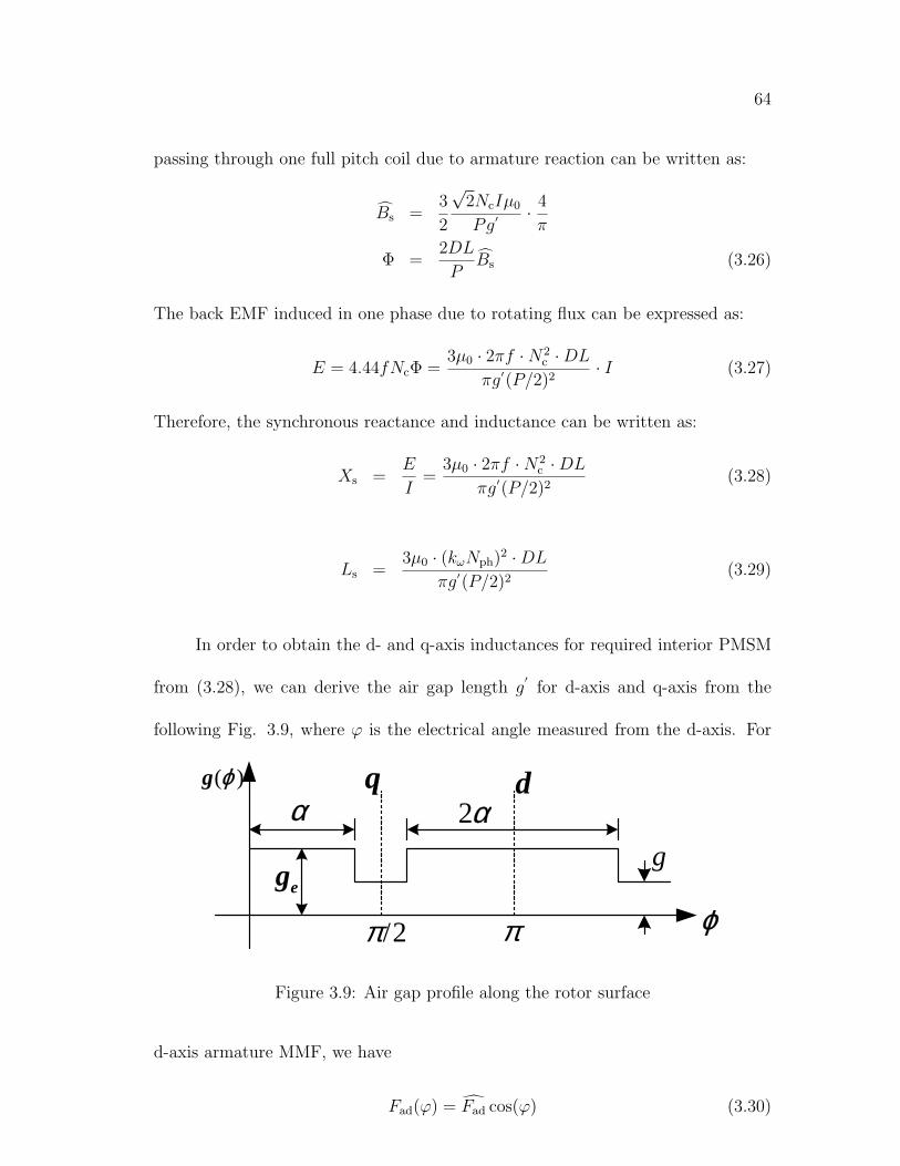
64
passing through one full pitch coil due to armature reaction can be written as:
Bs =3
2
√2NcIµ0
Pg′ · 4
π
Φ =2DL
PBs (3.26)
The back EMF induced in one phase due to rotating flux can be expressed as:
E = 4.44fNcΦ =3µ0 · 2πf ·N2
c ·DL
πg′(P/2)2· I (3.27)
Therefore, the synchronous reactance and inductance can be written as:
Xs =E
I=
3µ0 · 2πf ·N2c ·DL
πg′(P/2)2(3.28)
Ls =3µ0 · (kωNph)
2 ·DL
πg′(P/2)2(3.29)
In order to obtain the d- and q-axis inductances for required interior PMSM
from (3.28), we can derive the air gap length g′
for d-axis and q-axis from the
following Fig. 3.9, where ϕ is the electrical angle measured from the d-axis. For
egg
π2/π
α α2)(ϕg
ϕ
q d
Figure 3.9: Air gap profile along the rotor surface
d-axis armature MMF, we have
Fad(ϕ) = Fad cos(ϕ) (3.30)
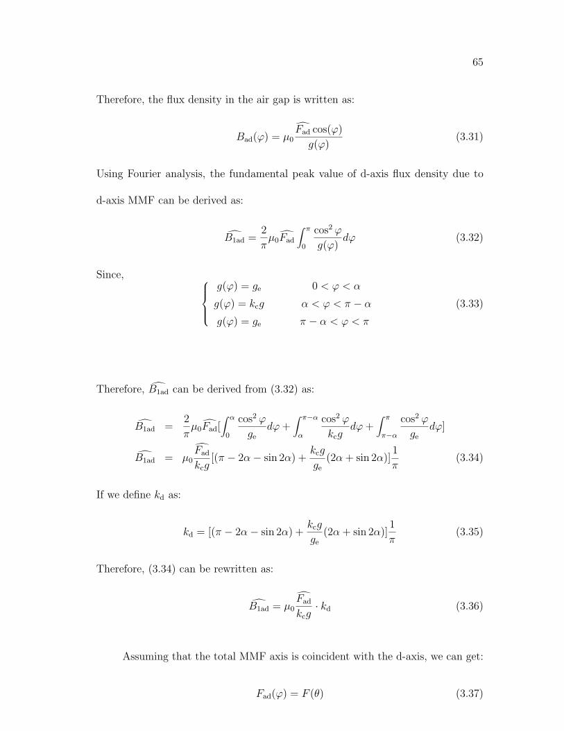
65
Therefore, the flux density in the air gap is written as:
Bad(ϕ) = µ0Fad cos(ϕ)
g(ϕ)(3.31)
Using Fourier analysis, the fundamental peak value of d-axis flux density due to
d-axis MMF can be derived as:
B1ad =2
πµ0Fad
∫ π
0
cos2 ϕ
g(ϕ)dϕ (3.32)
Since, g(ϕ) = ge 0 < ϕ < α
g(ϕ) = kcg α < ϕ < π − α
g(ϕ) = ge π − α < ϕ < π
(3.33)
Therefore, B1ad can be derived from (3.32) as:
B1ad =2
πµ0Fad[
∫ α
0
cos2 ϕ
ge
dϕ +∫ π−α
α
cos2 ϕ
kcgdϕ +
∫ π
π−α
cos2 ϕ
ge
dϕ]
B1ad = µ0Fad
kcg[(π − 2α− sin 2α) +
kcg
ge
(2α + sin 2α)]1
π(3.34)
If we define kd as:
kd = [(π − 2α− sin 2α) +kcg
ge
(2α + sin 2α)]1
π(3.35)
Therefore, (3.34) can be rewritten as:
B1ad = µ0Fad
kcg· kd (3.36)
Assuming that the total MMF axis is coincident with the d-axis, we can get:
Fad(ϕ) = F (θ) (3.37)
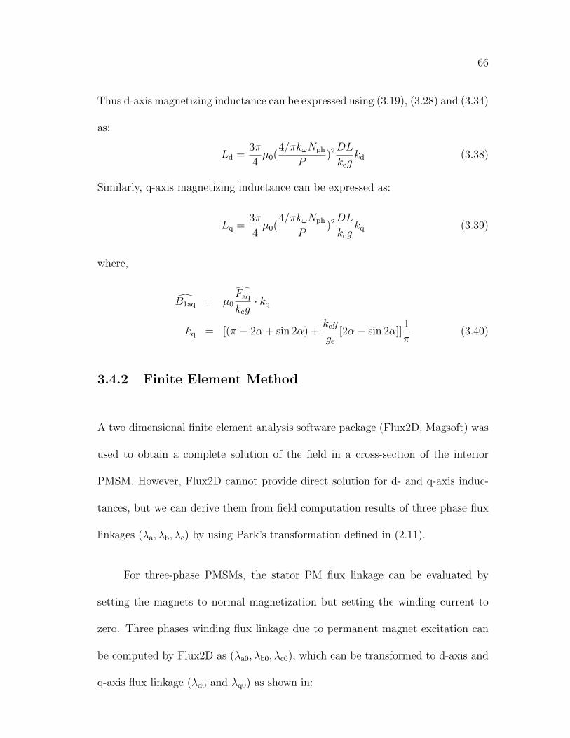
66
Thus d-axis magnetizing inductance can be expressed using (3.19), (3.28) and (3.34)
as:
Ld =3π
4µ0(
4/πkωNph
P)2DL
kcgkd (3.38)
Similarly, q-axis magnetizing inductance can be expressed as:
Lq =3π
4µ0(
4/πkωNph
P)2DL
kcgkq (3.39)
where,
B1aq = µ0Faq
kcg· kq
kq = [(π − 2α + sin 2α) +kcg
ge
[2α− sin 2α]]1
π(3.40)
3.4.2 Finite Element Method
A two dimensional finite element analysis software package (Flux2D, Magsoft) was
used to obtain a complete solution of the field in a cross-section of the interior
PMSM. However, Flux2D cannot provide direct solution for d- and q-axis induc-
tances, but we can derive them from field computation results of three phase flux
linkages (λa, λb, λc) by using Park’s transformation defined in (2.11).
For three-phase PMSMs, the stator PM flux linkage can be evaluated by
setting the magnets to normal magnetization but setting the winding current to
zero. Three phases winding flux linkage due to permanent magnet excitation can
be computed by Flux2D as (λa0, λb0, λc0), which can be transformed to d-axis and
q-axis flux linkage (λd0 and λq0) as shown in:
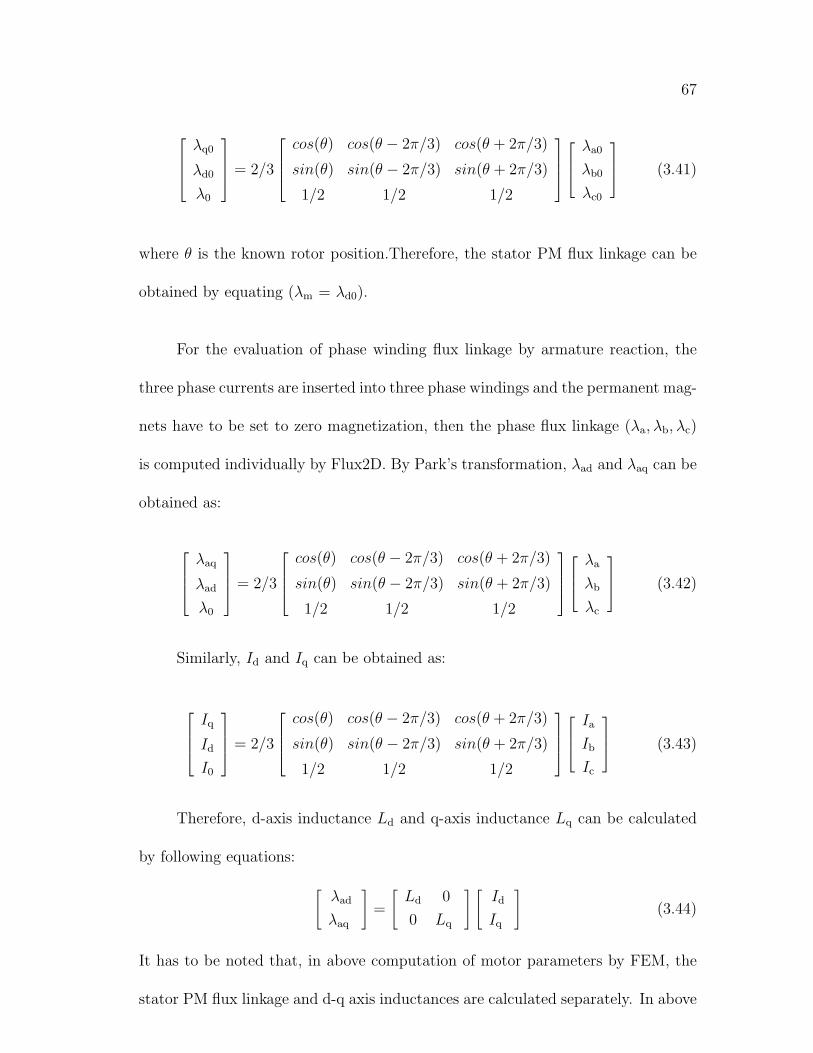
67
λq0
λd0
λ0
= 2/3
cos(θ) cos(θ − 2π/3) cos(θ + 2π/3)
sin(θ) sin(θ − 2π/3) sin(θ + 2π/3)
1/2 1/2 1/2
λa0
λb0
λc0
(3.41)
where θ is the known rotor position.Therefore, the stator PM flux linkage can be
obtained by equating (λm = λd0).
For the evaluation of phase winding flux linkage by armature reaction, the
three phase currents are inserted into three phase windings and the permanent mag-
nets have to be set to zero magnetization, then the phase flux linkage (λa, λb, λc)
is computed individually by Flux2D. By Park’s transformation, λad and λaq can be
obtained as:
λaq
λad
λ0
= 2/3
cos(θ) cos(θ − 2π/3) cos(θ + 2π/3)
sin(θ) sin(θ − 2π/3) sin(θ + 2π/3)
1/2 1/2 1/2
λa
λb
λc
(3.42)
Similarly, Id and Iq can be obtained as:
Iq
Id
I0
= 2/3
cos(θ) cos(θ − 2π/3) cos(θ + 2π/3)
sin(θ) sin(θ − 2π/3) sin(θ + 2π/3)
1/2 1/2 1/2
Ia
Ib
Ic
(3.43)
Therefore, d-axis inductance Ld and q-axis inductance Lq can be calculated
by following equations:
[λad
λaq
]=
[Ld 0
0 Lq
] [Id
Iq
](3.44)
It has to be noted that, in above computation of motor parameters by FEM, the
stator PM flux linkage and d-q axis inductances are calculated separately. In above
68
analysis, the effects of stator and rotor flux saturation are considered negligible.
In practice, the stator and rotor flux include both of armature reaction flux and
magnet flux, hence the saturation effect is more serious. Therefore, the calculated
motor parameters by above FEM method may not accurate enough in heavy loading
condition.
3.4.3 Response Surface Method
The response surface methodology (RSM) is a collection of mathematical and statis-
tical techniques that are useful for evaluating responses, i.e., the objective physical
quantities (motor parameters), which are influenced by several design variables.
As the response surface is often described by polynomial representations (deter-
minative equations), we can save computational time for optimization process by
evaluating the objective physical quantities by the response surface instead of by
the FEM analysis.
3.4.3.1 Building empirical models
In the practical application of RSM in the design optimization of interior PMSM, it
is necessary to develop an approximating model to evaluate the motor parameters
(λm, Ld, Lq) based on design variables (lm, γ, α). Since the true response function
between the motor parameters and the input design variables is unknown, we can
develop an approximation of it. Usually, a lower-order polynomial in some relatively
small region of the independent variable space is appropriate. In many cases, either

69
a first-order or a second-order model is used. In this work, the second-order
model is used for several reasons:
• The second order model is very flexible. It can take on a wide variety of
function forms, so it will often work well as an approximation to the true
response surface.
• It is not too difficult to estimate the parameters in the second-order model.
The method of least squares can be used for this purpose.
• There is considerable practical experience indicating that second-order mod-
els work well in solving real response surface problems.
A typical second-order response model with three design variables is listed as
follows:
y = β0 +β1x1 +β2x2 +β3x3 +β11x21 +β22x
22 +β33x
23 +β12x1x2 +β13x1x3 +β23x2x3 +ε
(3.45)
where y is the response which can be stator PM flux linkage (λm) or d- or q-axis
inductances (Ld, Lq); the β values are the regression coefficients; (x1, x2, x3) are
coded design variables for (lm, γ, α); ε is the estimation error. In RSM work it
is convenient to transform the natural design variables to coded variables, which
are usually defined to be dimensionless with mean zero and the same spread or
standard deviation. The coding rule is explained as follows:
x1 =lm − [max(lm) + min(lm)]/2
[max(lm)−min(lm)]/2(3.46)
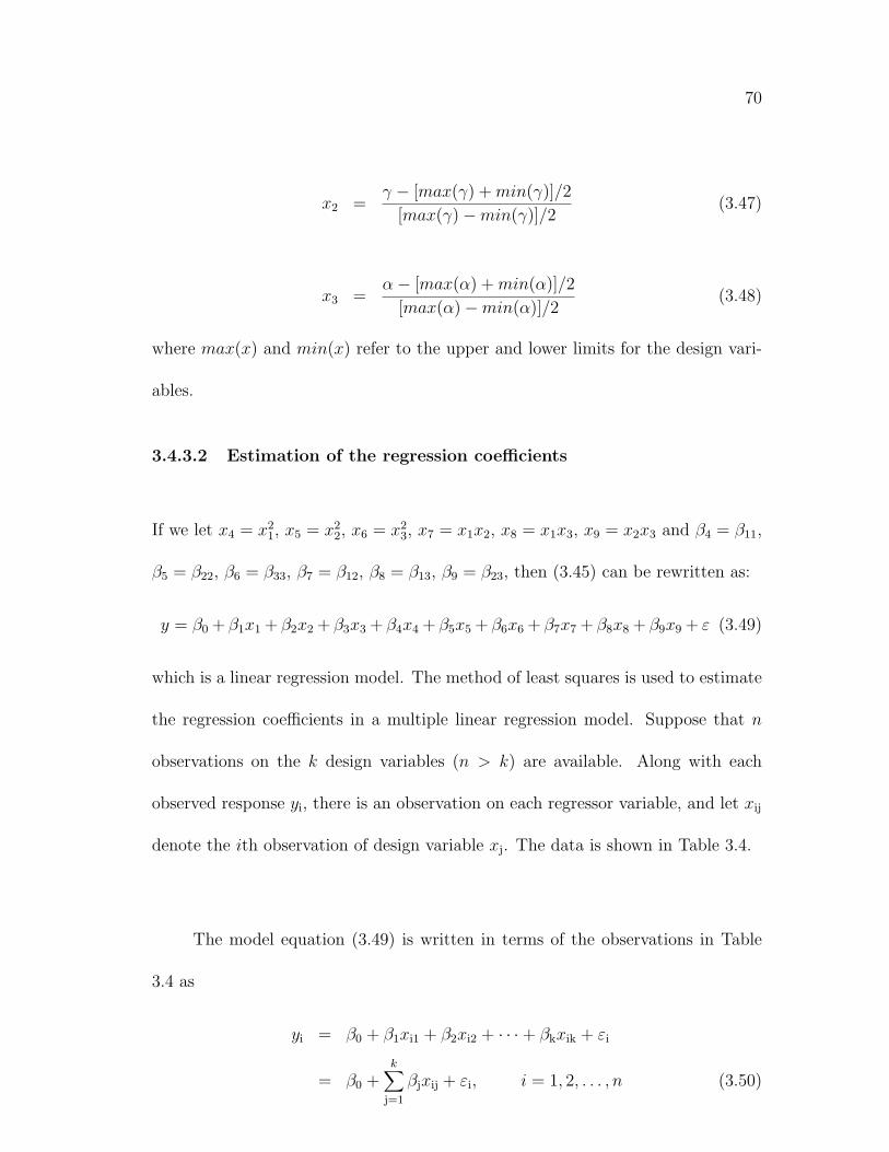
70
x2 =γ − [max(γ) + min(γ)]/2
[max(γ)−min(γ)]/2(3.47)
x3 =α− [max(α) + min(α)]/2
[max(α)−min(α)]/2(3.48)
where max(x) and min(x) refer to the upper and lower limits for the design vari-
ables.
3.4.3.2 Estimation of the regression coefficients
If we let x4 = x21, x5 = x2
2, x6 = x23, x7 = x1x2, x8 = x1x3, x9 = x2x3 and β4 = β11,
β5 = β22, β6 = β33, β7 = β12, β8 = β13, β9 = β23, then (3.45) can be rewritten as:
y = β0 + β1x1 + β2x2 + β3x3 + β4x4 + β5x5 + β6x6 + β7x7 + β8x8 + β9x9 + ε (3.49)
which is a linear regression model. The method of least squares is used to estimate
the regression coefficients in a multiple linear regression model. Suppose that n
observations on the k design variables (n > k) are available. Along with each
observed response yi, there is an observation on each regressor variable, and let xij
denote the ith observation of design variable xj. The data is shown in Table 3.4.
The model equation (3.49) is written in terms of the observations in Table
3.4 as
yi = β0 + β1xi1 + β2xi2 + · · ·+ βkxik + εi
= β0 +k∑
j=1
βjxij + εi, i = 1, 2, . . . , n (3.50)

71
Table 3.4: Data for multiple linear regression
y x1 x2 · · · xk
y1 x11 x12 · · · x1k
y2 x21 x22 · · · x2k
......
......
...
yn xn1 xn2 · · · xnk
The method of least squares chooses the βj (j = 0 to k) in (3.50) so that the sum
of the squares of the errors, εi, are minimized. The error least square function is:
L =n∑
i=1
ε2i =
n∑i=1
(yi − β0 −k∑
j=1
βjxij)2 (3.51)
The model in terms of the observations (3.50) can be written in matrix no-
tation as:
y = Xβ + ε (3.52)
where
y =
y1
y2
...yn
, X =
1 x11 x12 · · · x1k
1 x12 x22 · · · x2k
......
......
...
1 xn1 xn2 · · · xnk
, β =
β0
β1
...
βk
, and ε =
ε0
ε1
...εk
In general, y is an n×1 vector of the observations, X is an n×(k + 1) matrix
of the levels of the independent variables, β is a (k +1)× 1 vector of the regression
coefficients, and ε is an n× 1 vector of random errors. In order to find the vector
of least squares estimators that minimizes
L =n∑
i=1
ε2i = ε
′ε = (y −Xβ)
′(y −Xβ)

72
= y′y − β
′X
′y − y
′Xβ + β
′X
′Xβ
= y′y − 2β
′X
′y + β
′X
′Xβ (3.53)
where β′, ε
′and X
′are transpose of (β, ε and X). Since β
′X
′y is a 1×1 matrix,
or scalar, and its transpose (β′X
′y)
′= y
′Xβ is the same scalar. The least squares
estimators must satisfy:
∂L
∂β|b = −2X
′y + 2X
′Xb = 0 (3.54)
which simplifies to
X′Xb = X
′y (3.55)
where b is the solution of β. Therefore, the least squares estimator of β is
b = (X′X)−1X
′y (3.56)
The fitted regression model is
y = Xb (3.57)
In scalar notation, the fitted model is
yi = b0 +k∑
j=1
bjxij, i = 1, 2, · · · , n (3.58)
The difference between the observation yi and the fitted value yi is a residual, say
ei = yi - yi. The n× 1 vector of residuals is denoted by
e = y − y (3.59)
3.4.3.3 Fitting the second-order model
The regression coefficients are dependent on observations. It is desirable to make
the number of experiments carried out by the FEM analysis as small as possible.

73
The appropriate selection of the points for experiments can reduce the variance
of the coefficients, which make the resulting response surface more reliable. The
central composite design (CCD) has been widely used for fitting a second-order
response surface. The design consists of eight runs at the corner of a cubic, plus
six runs at the center of its six faces, plus one run at the cubic center. In terms
of the coded variables the corners of the cubic are (x1, x2, x3)=(-1,-1,-1),(1,-1,-1),
(-1,1,-1),(-1,-1,1),(1,1,-1),(1,-1,1),(-1,1,1),(1,1,1); the six face center points are at
(x1, x2, x3) = (-1,0,0),(1,0,0),(0,-1,0),(0,1,0),(0,0,-1),(0,0,1); and the cubic center
point is at (x1, x2, x3)=(0,0,0) as shown in Fig. 3.10.
3x2x
1x0 1-1
11
-1-1
Figure 3.10: Central composite design for second-order model

74
3.4.3.4 Model adequacy checking
It is necessary to examine the fitted response surface model to ensure that it pro-
vides an adequate approximation to the true system. The residuals from the least
squares fit, defined in (3.59), play an important role in judging model adequacy.
The sum of squares of the residuals is defined as:
SSE =n∑
i=1
(yi − yi)2 =
n∑i=1
e2i = e′e (3.60)
Substituting e = y − y = y −Xb and X ′Xb = X ′y, we can get
SSE = y′y − b′X ′y (3.61)
The total sum of squares is defined as:
SST =n∑
i=1
(yi − y)2 =n∑
i=1
y2i − (
n∑i=1
yi)2/n = y′y − (
n∑i=1
yi)2/n (3.62)
Equation (3.61) can be rewritten as:
SSE = y′y − (n∑
i=1
yi)2/n− [b′X ′y − (
n∑i=1
yi)2/n] (3.63)
or
SSE = SST − SSR (3.64)
Therefore, the regression sum of squares is
SSR = b′X ′y − (n∑
i=1
yi)2/n (3.65)
The coefficient of multiple determination R2 is defined as:
R2 =SSR
SST
= 1− SSE
SST
(3.66)
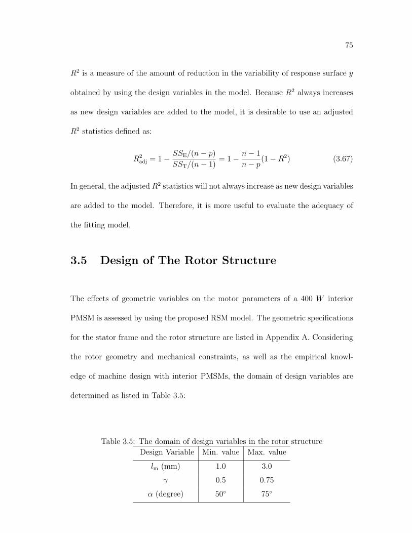
75
R2 is a measure of the amount of reduction in the variability of response surface y
obtained by using the design variables in the model. Because R2 always increases
as new design variables are added to the model, it is desirable to use an adjusted
R2 statistics defined as:
R2adj = 1− SSE/(n− p)
SST/(n− 1)= 1− n− 1
n− p(1−R2) (3.67)
In general, the adjusted R2 statistics will not always increase as new design variables
are added to the model. Therefore, it is more useful to evaluate the adequacy of
the fitting model.
3.5 Design of The Rotor Structure
The effects of geometric variables on the motor parameters of a 400 W interior
PMSM is assessed by using the proposed RSM model. The geometric specifications
for the stator frame and the rotor structure are listed in Appendix A. Considering
the rotor geometry and mechanical constraints, as well as the empirical knowl-
edge of machine design with interior PMSMs, the domain of design variables are
determined as listed in Table 3.5:
Table 3.5: The domain of design variables in the rotor structure
Design Variable Min. value Max. value
lm (mm) 1.0 3.0
γ 0.5 0.75
α (degree) 50◦ 75◦
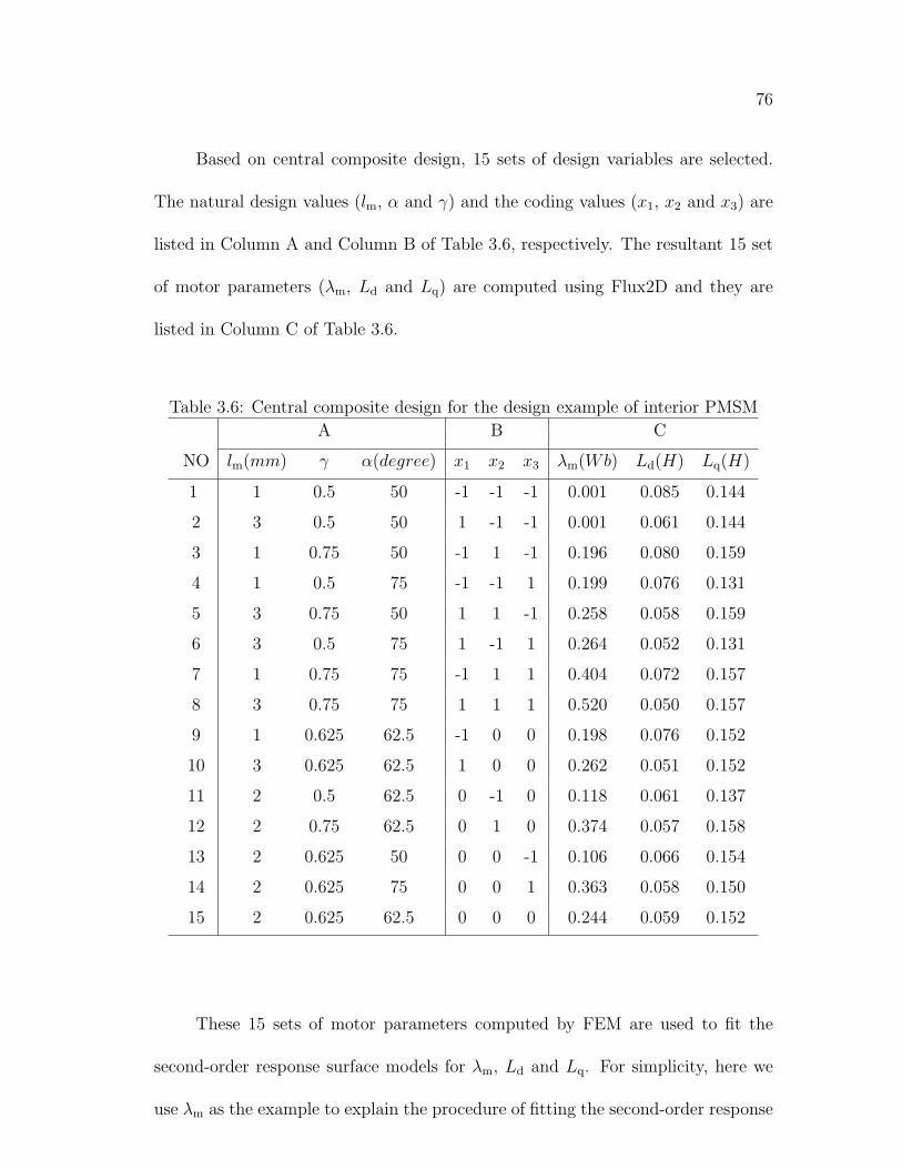
76
Based on central composite design, 15 sets of design variables are selected.
The natural design values (lm, α and γ) and the coding values (x1, x2 and x3) are
listed in Column A and Column B of Table 3.6, respectively. The resultant 15 set
of motor parameters (λm, Ld and Lq) are computed using Flux2D and they are
listed in Column C of Table 3.6.
Table 3.6: Central composite design for the design example of interior PMSM
A B C
NO lm(mm) γ α(degree) x1 x2 x3 λm(Wb) Ld(H) Lq(H)
1 1 0.5 50 -1 -1 -1 0.001 0.085 0.144
2 3 0.5 50 1 -1 -1 0.001 0.061 0.144
3 1 0.75 50 -1 1 -1 0.196 0.080 0.159
4 1 0.5 75 -1 -1 1 0.199 0.076 0.131
5 3 0.75 50 1 1 -1 0.258 0.058 0.159
6 3 0.5 75 1 -1 1 0.264 0.052 0.131
7 1 0.75 75 -1 1 1 0.404 0.072 0.157
8 3 0.75 75 1 1 1 0.520 0.050 0.157
9 1 0.625 62.5 -1 0 0 0.198 0.076 0.152
10 3 0.625 62.5 1 0 0 0.262 0.051 0.152
11 2 0.5 62.5 0 -1 0 0.118 0.061 0.137
12 2 0.75 62.5 0 1 0 0.374 0.057 0.158
13 2 0.625 50 0 0 -1 0.106 0.066 0.154
14 2 0.625 75 0 0 1 0.363 0.058 0.150
15 2 0.625 62.5 0 0 0 0.244 0.059 0.152
These 15 sets of motor parameters computed by FEM are used to fit the
second-order response surface models for λm, Ld and Lq. For simplicity, here we
use λm as the example to explain the procedure of fitting the second-order response
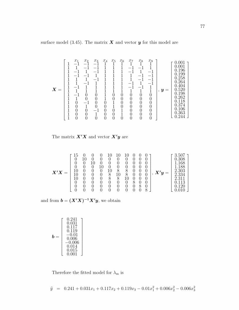
77
surface model (3.45). The matrix X and vector y for this model are
X =
x1 x2 x3 x4 x5 x6 x7 x8 x91 −1 −1 −1 1 1 1 1 1 11 1 −1 −1 1 1 1 −1 −1 11 −1 1 −1 1 1 1 −1 1 −11 −1 −1 1 1 1 1 1 −1 −11 1 1 −1 1 1 1 1 −1 −11 1 −1 1 1 1 1 −1 1 −11 −1 1 1 1 1 1 −1 −1 11 1 1 1 1 1 1 1 1 11 −1 0 0 1 0 0 0 0 01 1 0 0 1 0 0 0 0 01 0 −1 0 0 1 0 0 0 01 0 1 0 0 1 0 0 0 01 0 0 −1 0 0 1 0 0 01 0 0 1 0 0 1 0 0 01 0 0 0 0 0 0 0 0 0
, y =
0.0010.0010.1960.1990.2580.2640.4040.5200.1980.2620.1180.3740.1060.3630.244
The matrix X ′X and vector X ′y are
X ′X =
15 0 0 0 10 10 10 0 0 00 10 0 0 0 0 0 0 0 00 0 10 0 0 0 0 0 0 00 0 0 10 0 0 0 0 0 010 0 0 0 10 8 8 0 0 010 0 0 0 8 10 8 0 0 010 0 0 0 8 8 10 0 0 00 0 0 0 0 0 0 8 0 00 0 0 0 0 0 0 0 8 00 0 0 0 0 0 0 0 0 8
, X ′y =
3.5070.3081.1681.1882.3032.3342.3110.1130.1200.010
and from b = (X ′X)−1X ′y, we obtain
b =
0.2410.0310.1170.119−0.010.006−0.0060.0140.0150.001
Therefore the fitted model for λm is
y = 0.241 + 0.031x1 + 0.117x2 + 0.119x3 − 0.01x21 + 0.006x2
2 − 0.006x23
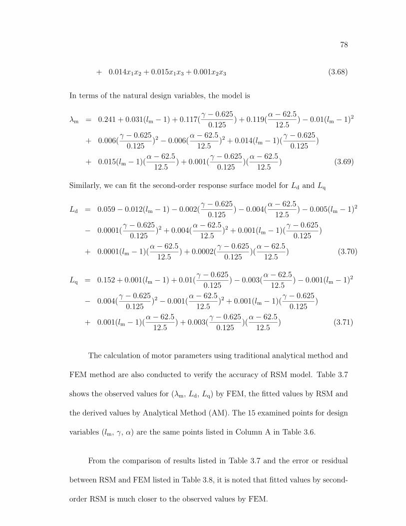
78
+ 0.014x1x2 + 0.015x1x3 + 0.001x2x3 (3.68)
In terms of the natural design variables, the model is
λm = 0.241 + 0.031(lm − 1) + 0.117(γ − 0.625
0.125) + 0.119(
α− 62.5
12.5)− 0.01(lm − 1)2
+ 0.006(γ − 0.625
0.125)2 − 0.006(
α− 62.5
12.5)2 + 0.014(lm − 1)(
γ − 0.625
0.125)
+ 0.015(lm − 1)(α− 62.5
12.5) + 0.001(
γ − 0.625
0.125)(
α− 62.5
12.5) (3.69)
Similarly, we can fit the second-order response surface model for Ld and Lq
Ld = 0.059− 0.012(lm − 1)− 0.002(γ − 0.625
0.125)− 0.004(
α− 62.5
12.5)− 0.005(lm − 1)2
− 0.0001(γ − 0.625
0.125)2 + 0.004(
α− 62.5
12.5)2 + 0.001(lm − 1)(
γ − 0.625
0.125)
+ 0.0001(lm − 1)(α− 62.5
12.5) + 0.0002(
γ − 0.625
0.125)(
α− 62.5
12.5) (3.70)
Lq = 0.152 + 0.001(lm − 1) + 0.01(γ − 0.625
0.125)− 0.003(
α− 62.5
12.5)− 0.001(lm − 1)2
− 0.004(γ − 0.625
0.125)2 − 0.001(
α− 62.5
12.5)2 + 0.001(lm − 1)(
γ − 0.625
0.125)
+ 0.001(lm − 1)(α− 62.5
12.5) + 0.003(
γ − 0.625
0.125)(
α− 62.5
12.5) (3.71)
The calculation of motor parameters using traditional analytical method and
FEM method are also conducted to verify the accuracy of RSM model. Table 3.7
shows the observed values for (λm, Ld, Lq) by FEM, the fitted values by RSM and
the derived values by Analytical Method (AM). The 15 examined points for design
variables (lm, γ, α) are the same points listed in Column A in Table 3.6.
From the comparison of results listed in Table 3.7 and the error or residual
between RSM and FEM listed in Table 3.8, it is noted that fitted values by second-
order RSM is much closer to the observed values by FEM.
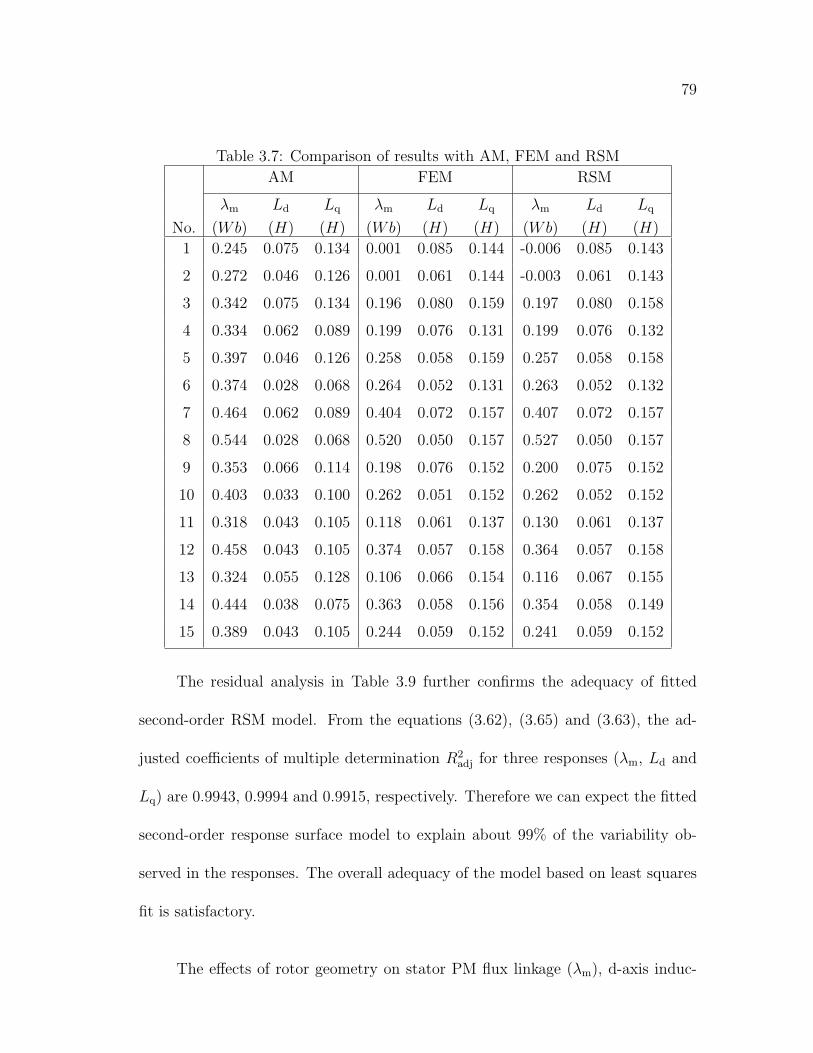
79
Table 3.7: Comparison of results with AM, FEM and RSM
AM FEM RSM
λm Ld Lq λm Ld Lq λm Ld Lq
No. (Wb) (H) (H) (Wb) (H) (H) (Wb) (H) (H)
1 0.245 0.075 0.134 0.001 0.085 0.144 -0.006 0.085 0.143
2 0.272 0.046 0.126 0.001 0.061 0.144 -0.003 0.061 0.143
3 0.342 0.075 0.134 0.196 0.080 0.159 0.197 0.080 0.158
4 0.334 0.062 0.089 0.199 0.076 0.131 0.199 0.076 0.132
5 0.397 0.046 0.126 0.258 0.058 0.159 0.257 0.058 0.158
6 0.374 0.028 0.068 0.264 0.052 0.131 0.263 0.052 0.132
7 0.464 0.062 0.089 0.404 0.072 0.157 0.407 0.072 0.157
8 0.544 0.028 0.068 0.520 0.050 0.157 0.527 0.050 0.157
9 0.353 0.066 0.114 0.198 0.076 0.152 0.200 0.075 0.152
10 0.403 0.033 0.100 0.262 0.051 0.152 0.262 0.052 0.152
11 0.318 0.043 0.105 0.118 0.061 0.137 0.130 0.061 0.137
12 0.458 0.043 0.105 0.374 0.057 0.158 0.364 0.057 0.158
13 0.324 0.055 0.128 0.106 0.066 0.154 0.116 0.067 0.155
14 0.444 0.038 0.075 0.363 0.058 0.156 0.354 0.058 0.149
15 0.389 0.043 0.105 0.244 0.059 0.152 0.241 0.059 0.152
The residual analysis in Table 3.9 further confirms the adequacy of fitted
second-order RSM model. From the equations (3.62), (3.65) and (3.63), the ad-
justed coefficients of multiple determination R2adj for three responses (λm, Ld and
Lq) are 0.9943, 0.9994 and 0.9915, respectively. Therefore we can expect the fitted
second-order response surface model to explain about 99% of the variability ob-
served in the responses. The overall adequacy of the model based on least squares
fit is satisfactory.
The effects of rotor geometry on stator PM flux linkage (λm), d-axis induc-

80
Table 3.8: Residual for the fitted second-order RSM modele(λm) e(Ld) e(Lq)
No. Wb ×10−3H ×10−3H
1 0.007 -0.063 0.030
2 0.004 0.086 0.030
3 -0.001 -0.108 0.030
4 -0.001 -0.123 -0.030
5 0.001 0.116 0.030
6 0.001 0.101 -0.030
7 -0.004 -0.09 -0.030
8 -0.007 0.056 -0.030
9 -0.002 0.338 0.000
10 0.001 -0.358 0.000
11 -0.012 0.000 0.000
12 0.011 0.030 0.000
13 -0.011 -0.030 -1.200
14 0.010 0.060 1.200
15 0.002 -0.060 0.000
Table 3.9: Test of adequacy for the fitted second-order RSM model
Response SSE SSR SST R2adj
λm 5.92× 10⁻⁴ 0.2909 0.2915 0.9943
Ld 3.62× 10⁻⁷ 0.0018 0.0018 0.9994
Lq 3.82× 10⁻⁶ 0.0012 0.0013 0.9915
tance (Ld) and q-axis inductance (Lq) as calculated by the fitted second-order RSM
model are shown in Fig. 3.11, Fig. 3.12 and Fig. 3.13. The following observations
are made from these results.
• The stator PM flux linkage can be changed by changing the volume of per-
manent magnets. Modifying the magnet pole angle is more effective than
81
magnet pole angle (degree)
αmagnet thickness
(mm)ml
)(Wbmλ
Figure 3.11: λm as a function of rotor geometry
changing the magnet thickness;
• The d-axis inductance can be increased by reducing the magnet thickness.
Changing lm has little effects on the q-axis inductance;
• The q-axis inductance can be changed by changing the magnet position in the
rotor. Higher magnet position provides larger q-axis inductance, but exposes
permanent magnets to higher demagnetizing fields.
The fitted second-order model not only gives a clear representation of the
motor parameters of the interior PMSM as a function of design variables, but
also allows the optimization process to evaluate the objective physical quantity
(constant power speed range) in a much shorter time. Based on the RSM models
82
)(HLd
magnet pole angle (degree)α
magnet thickness (mm)
ml
Figure 3.12: Ld as a function of rotor geometry
(3.69, 3.70 and 3.71) of motor parameters (λm, Ld and Lq) as well as the known
constraints of voltage and current, we can obtain the maximum power capability
over a wide speed range, which has been described in Chapter 2. Therefore, in
the numerical optimization process, the objective quantity (constant power speed
range) can be evaluated by the polynomial functions instead of the iterative field
calculation. As a result, we can achieve an overall increase in the optimization
speed. The detail optimization process based on RSM will be developed in Chapter
4.
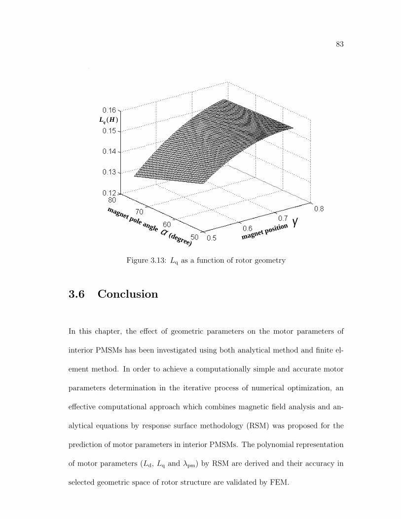
83
)(HLq
magnet pole angle (degree)
αmagnet position γ
Figure 3.13: Lq as a function of rotor geometry
3.6 Conclusion
In this chapter, the effect of geometric parameters on the motor parameters of
interior PMSMs has been investigated using both analytical method and finite el-
ement method. In order to achieve a computationally simple and accurate motor
parameters determination in the iterative process of numerical optimization, an
effective computational approach which combines magnetic field analysis and an-
alytical equations by response surface methodology (RSM) was proposed for the
prediction of motor parameters in interior PMSMs. The polynomial representation
of motor parameters (Ld, Lq and λpm) by RSM are derived and their accuracy in
selected geometric space of rotor structure are validated by FEM.

Chapter 4
Numerical Optimization of anInterior PMSM for WideConstant Power Speed Range
4.1 Introduction
Numerical computation using finite element method (FEM) is considered indis-
pensable for electrical machine design. However, it is difficult to carry out iterative
field computation in every step of an optimization process. In order to save the
computation time, an effective computational approach was developed in Chapter
3, which applies the response surface methodology (RSM) in stead of FEM to de-
termine motor parameters (λm, Ld and Lq) in interior PMSMs. Based on the motor
parameters using RSM, we can obtain the maximum power capability for a wide
speed range as described in Chapter 2. In this chapter we develop an numerical
optimization process using genetic algorithm (GA) to search for an optimum rotor
structure (lm, γ and α) for a 400 W interior PMSM, which has the largest constant
power speed range (CPSR) under certain constraints.
84

85
4.2 Optimization Method
The design objective of an interior PMSM is to find the optimum rotor structure
which can achieve the largest constant power speed range (CPSR) under certain
constraints. Therefore, optimization technique has to be applied to look for the
maximum of the objective function, which is also the global maximum of the func-
tion. The Genetic Algorithm (GA) technique has proved to be an effective tool
for motor design optimization as it allows a search in a wide region and a global
optimization to be performed [86]. However, GA requires the objective function
to be computed several times (especially when FEM is adopted to improve the
accuracy of the evaluation) and thus requires substantially more computational
time than other optimization techniques. In this work, we adopt the fitted second-
order model by RSM as the evaluation tool for the objective function and apply
GA as the search method. This enables us to save the computational time in the
design optimization process but without losing the accuracy in the evaluation of
the objective function.
4.2.1 Formulation of the design optimization
The task of the design optimization of an interior PMSM is to find a vector of
design variables X = (x1, x2, x3), which represents the natural design variables
(lm, γ, α), each of them bounded by ximin < xi < ximax, i = 1, 2, 3, so that the
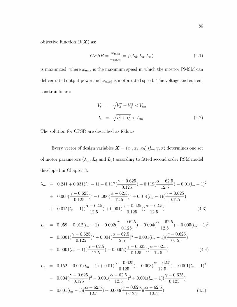
86
objective function O(X) as:
CPSR =ωmax
ωrated
= f(Ld, Lq, λm) (4.1)
is maximized, where ωmax is the maximum speed in which the interior PMSM can
deliver rated output power and ωrated is motor rated speed. The voltage and current
constraints are:
Vs =√
V 2d + V 2
q < Vsm
Is =√
I2d + I2
q < Ism (4.2)
The solution for CPSR are described as follows:
Every vector of design variables X = (x1, x2, x3) (lm, γ, α) determines one set
of motor parameters (λm, Ld and Lq) according to fitted second order RSM model
developed in Chapter 3:
λm = 0.241 + 0.031(lm − 1) + 0.117(γ − 0.625
0.125) + 0.119(
α− 62.5
12.5)− 0.01(lm − 1)2
+ 0.006(γ − 0.625
0.125)2 − 0.006(
α− 62.5
12.5)2 + 0.014(lm − 1)(
γ − 0.625
0.125)
+ 0.015(lm − 1)(α− 62.5
12.5) + 0.001(
γ − 0.625
0.125)(
α− 62.5
12.5) (4.3)
Ld = 0.059− 0.012(lm − 1)− 0.002(γ − 0.625
0.125)− 0.004(
α− 62.5
12.5)− 0.005(lm − 1)2
− 0.0001(γ − 0.625
0.125)2 + 0.004(
α− 62.5
12.5)2 + 0.001(lm − 1)(
γ − 0.625
0.125)
+ 0.0001(lm − 1)(α− 62.5
12.5) + 0.0002(
γ − 0.625
0.125)(
α− 62.5
12.5) (4.4)
Lq = 0.152 + 0.001(lm − 1) + 0.01(γ − 0.625
0.125)− 0.003(
α− 62.5
12.5)− 0.001(lm − 1)2
− 0.004(γ − 0.625
0.125)2 − 0.001(
α− 62.5
12.5)2 + 0.001(lm − 1)(
γ − 0.625
0.125)
+ 0.001(lm − 1)(α− 62.5
12.5) + 0.003(
γ − 0.625
0.125)(
α− 62.5
12.5) (4.5)
87
Every set of motor parameters (λm, Ld and Lq) determines maximum torque-
speed profile as follows:
Tmax =
Tm 0 < ωs < ωb
Tn ωb < ωs < ωp
Tp ωs > ωp
(4.6)
where Tm (2.28) is the peak torque produced by rated current; Tn (2.37) and Tp
(2.55) are current and voltage limited maximum torque, respectively, which are the
functions of motor parameters (λm, Ld and Lq) and motor speed ωs as described
in Chapter 2. Therefore, we can obtain the maximum power capability curve with
respect to speed according to torque-speed profile using following equation:
0 1000 2000 3000 4000 50000
100
200
300
400
500
600
700
Speed (rpm)
Max
imum
Pow
er C
apab
ility
(W
)
CPSR
Rated Power
Figure 4.1: Determination of maximum power capability w.r.t to motor speed
Power = Tmax · ωs (4.7)
The maximum power capability profile (shown in Fig. 4.1) is a discrete curve
with respect to motor speed (constant torque speed range and flux-weakening speed
88
range), which has no direct solution of constant power speed range (CPSR). There-
fore, computer programming is used to obtain the CPSR by enumerative algorithm.
4.2.2 Description of genetic algorithms
The genetic algorithm is one of the most up-to-date artificial intelligence techniques.
It is a search procedure emulating the mechanism of natural selection and natural
genetics. When applied to motor design optimization, the GA explores the space
of motor design variables and searches for the best motor design.
To apply the GA approach, a fitness function F (X) has to be defined to
evaluate how good each motor design is. This fitness function often coincides with
the objective function. Strings of binary digits (representing sets of values of motor
design variables) are manipulated by GA that measure the strength of each string
by a fitness value given by the value of the fitness function. The fittest strings
advance and mate with other strings to produce offsprings.
The main steps of GA optimization applied to the interior PMSM design are
shown in Fig. 4.2 and are described as follow:
The first step is to define the fitness function or objective function as listed
in (4.1). The maximum speed for rated power operation is derived from motor
parameters and equations.
A population of N different motor designs is generated randomly. Each indi-

89
Initial Population
Evaluation ofFitness &
Average Fitness
Avg. FitnessCheck
ReproductionCrossoverMutation
New Generation
Final Results
Figure 4.2: Main steps of genetic algorithms technique
vidual is characterized by a string of digits: zeros and ones. The string is composed
of three substrings, each of them describing a design variable, which is coded in
binary form using a binary substring (ai,n−1, ai,n−2, · · · , ai,1, ai,0), with ai,j ∈ {0, 1},
related to the value of xi by
xi = ximin +(ximax − ximin)
2n − 1
n−1∑j=0
ai,j2j (4.8)
The length n of each substring depends on the desired resolution ν which results,
2−n ≤ ν ≤ 2−n+1.
As described in Chapter 3, the RSM model of motor parameters (λm, Ld and
Lq) is validated in certain domain as listed in Table 4.1:

90
Table 4.1: The domain of design variables in the rotor structure
Design Variable Min. value Max. value
lm (mm) 1.0 3.0
γ 0.5 0.75
α (degree) 50◦ 75◦
There are many geometrical variables in the rotor design; optimization of
all the variables is impractical and may not be necessary. In the Chapter 3, it
has been shown through theoretical analysis that, if stator structure and winding
are fixed, the motor parameters are determined only by the flux distribution in
rotor core (3.18), (3.28). Using analytical model of electrical machines and finite
element analysis, we have concluded that magnet thickness lm, magnet angle α
and magnet position in rotor γ are most significant factors, that affect the flux
distribution in rotor core. Hence, only these three design parameters can be used
for the optimization work.
The design space for design variables (lm, γ, α) are limited by rotor geometry
and mechanical constraints, which are determined by the power rating we choose
to design; The modelling of motor parameters using RSM is based on such design
constraints. When using GAs to search the optimal design, we have to make sure
the search space does not exceed the design space. Therefore, the search domain
using GA is kept same as the domain of design variables in Table. 4.1.
An example of an individual set of design variables is shown in Fig. 4.3, where
the values of natural design variables (lm, γ and α) are calculated by (4.8). Each

91
)68.2(1 mmlx m = )64.0(2 =γx )67.66(3
o=αx
1 0 11111111 00000000
Figure 4.3: Example of one individual of design variable
individual in the population is evaluated by (4.6) and (4.7). For this purpose, an
analysis is carried out to predict their performance. The best fitness, CPSRmax,
is calculated. The average fitness CPSRavg of the population and the sum fitness
of all individuals are found from:
CPSRsum =N∑i=1
CPSR(Xi)
CPSRavg = CPSRsum/N (4.9)
At this stage, the rules of GA apply to reproduce a new population still of N
individuals. The reproduction process is composed of the following three phases:
• Selection: Individuals of the old population (last population of motor de-
signs) are selected and put in the new one, with preference given to the
fittest. The selection is a stochastic sampling (by which the best individ-
ual is selected several times, while the worst one is excluded, according to a
selection probability expressed as pi = CPSR(Xi)/CPSRsum).
• Crossover: Two randomly selected strings, among those selected in the pre-
vious step, are mated. A position along one string is again randomly selected
and all binary digits following this position are swapped with those of second
string. The the two entirely new strings move on to the new generation. It is

92
worth noting that the crossover process elaborates the already existing values.
This operation takes place with a defined probability pc which statistically
represents the number of individuals involved in the crossover process. Fig.
4.4a gives a schematic sample of crossover process.
1 11111111111111
0 00000000000000
1 11111
0 00000
000000000
111111111
1 11111 000000000
1 11111 000000010
(a) (b)
Figure 4.4: Schematic samples of crossover and mutation process
• Mutation: A bit of a string of the new population is randomly selected,
according to a defined probability pm, and its value is swapped from 1 to 0 or
vice versa. This process explores new solution in the search space, to avoid
any loss of useful genetic information. Fig. 4.4b shows a schematic sample
of the mutation process.
At this point a new population is achieved; all individuals are evaluated, as
described in step III, and the subsequent steps are repeated. The procedure is
stopped after a prefixed number of generation Ng or when the best or the average

93
fitness values have reached a satisfied level.
4.3 Implementation of Proposed Design Optimiza-
tion Procedure
To use the GA to search the optimal design of the rotor structure for the interior
PMSM, each of the three design variables (lm, γ, α) is coded into a 15 bit string
segments using binary coding as described in (4.8). The first population is gener-
ated by selecting randomly each bit of the strings. The fitted second-order RSM
models are used to determine the motor parameters (λm, Ld, Lq) according to the
input design variables. These motor parameters together with the voltage and cur-
rent constraints (4.2) are used to evaluate the final objective function CPSR (4.1).
The FEM is applied to verify the final design results. The whole flowchart for the
proposed design optimization procedure is shown in Fig. 4.5.
4.4 Numerical Results and Discussions
The GA combined with RSM has been applied to the design optimization of an
interior type PMSM with a rated power rating of 400 W . The GA technique has
been tested by computer simulations. The size of the population greatly affects
the quality of the result and the computation time. In addition, different choices
of crossover probability pc and mutation probability pm have been compared. It
is worth noting that the crossover operator searches in new parts of the variables
domain, a low pc causes a contracted search that can be ineffective. The mutation

94
Determine rotorconfiguration
Select 15 sets of points
for experiments by CentralComposite Design
Apply GA to search optimalCPSR with RSM model
Initial Population
FitnessAverage Fitness
Avg. Fitness
ReproductionCrossoverMutation
New Generation
StopEvaluate optimalCPSR by FEM
END
FEM experimentsfor calculating
mλ dL qL
Obtain the determinativmodel ofby RSM
mλ dL qL
( , , )ml γ α
Figure 4.5: Flowchart for the proposed design optimization of the interior PMSM
operator explores new points out the solution space and a high pm produces many
mutated strings in the new population which can alter the selection process of the
algorithm. Therefore, good GA performance requires the choice of a high pc, a low

95
pm (inversely proportional to the population size), and a moderate population size.
Following these instructions the following parameters have been adopted for the
computer simulation.
pm = 0.02
pc = 0.6
popsize = 60 (4.10)
For all the simulations, 30 generations have been considered. With this value a
good convergence has been obtained. The values of the maximum and average
CPSR for every generation are plotted in Fig. 4.6. The preferred solution is first
achieved at the 25th generation. The data of the best observed motor design are
reported in Table 4.2.
It has to be pointed out that this solution is near optimal but may not be
the true optimal because not all domains of design variables have been explored.
The fact is that GAs have no convergence guarantees in arbitrary problems. But
they do sort out interesting areas of a space quickly and provide solution close to
the global optimal.
The FEM is applied to verify the optimized results with the preferred design
values of rotor geometry. Table 4.3 indicates the validity of the proposed approach:
the motor parameters approximated by the RSM in the GA optimization process
are in good agreement with those recalculated by the FEM with 5% error.
Fig. 4.7 illustrates the d- and q-axis inductance variations with the armature
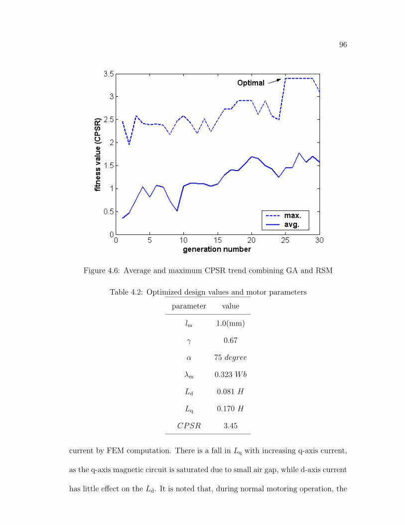
96
Figure 4.6: Average and maximum CPSR trend combining GA and RSM
Table 4.2: Optimized design values and motor parameters
parameter value
lm 1.0(mm)
γ 0.67
α 75 degree
λm 0.323 Wb
Ld 0.081 H
Lq 0.170 H
CPSR 3.45
current by FEM computation. There is a fall in Lq with increasing q-axis current,
as the q-axis magnetic circuit is saturated due to small air gap, while d-axis current
has little effect on the Ld. It is noted that, during normal motoring operation, the

97
Table 4.3: Comparison of motor parameters with GA+RSM and FEM
parameter GA+RSM FEM
λm(Wb) 0.323 0.312
Ld(H) 0.081 0.085
Lq(H) 0.170 0.165
q-axis current is usually less or equal than the rated current (2A). Therefore, it is
reasonable to use constant Lq to estimate the motor performance in the proposed
approach.
-3 -2 -1 0 1 2 30
0.04
0.08
0.12
0.16
0.2
Current (A)
Indu
ctan
ce (
H)
dL
qL
Figure 4.7: Effects of magnetic saturation on Ld and Lq
The flux distributions in the stator and air gap for the final prototype ma-
chine design have been evaluated from the FEM analysis (Flux2D). Fig. 4.9 shows
the flux density in the air gap at maximum flux-weakening condition. The corre-

98
sponding flux density in the air gap with open circuit condition is given in Fig. 4.8.
From the numerical analysis listed in Table. 4.4, it is obvious that the flux in the
air gap is seriously weakened by the armature reaction.
0 20 40 60 80 100 120 140 160 180
−0.6
−0.4
−0.2
0
0.2
0.4
0.6
Air gap length along one pole pair (degree)
Flu
x de
nsity
in a
ir ga
p (T
esla
)
Figure 4.8: Permanent magnet excited flux distribution in the air gap
Table 4.4: Comparison of flux distribution for open circuit and flux-weakeningcondition
Bg Open Circuit Flux-weakening
Fundamental value 0.564 T 0.209 T
Total R.M.S value 0.632 T 0.298 T
It is difficult to verify the final objective quantity value of CPSR directly by
FEM because of the coupling of the motor and the inverter system. Alternatively,
torque and stator flux linkage versus current angle β characteristics calculated by
FEM can provide the information of power capability in a wide speed range, Fig.
4.12 and Fig. 4.13 . The current angle β is defined as the angle of stator current

99
0 20 40 60 80 100 120 140 160 180
−0.6
−0.4
−0.2
0
0.2
0.4
0.6
Air gap length along one pole pair (degree)
Flu
x de
nsity
in a
ir ga
p (T
esla
)
Figure 4.9: Air gap flux density curve with maximum flux-weakening conditionβ = 180 degree
vector and the d-axis, as shown in Fig. 4.10. Since λm > LdIsm in the optimized
design , as introduced in Fig. 4.11 in Chapter 2, the maximum output torque under
different speed range is produced in Regions I and II only when current vector
(Id, Iq) is moving from point A (β = arctan(Idm/Iqm)) to point M (β = 180◦).
With the computation results by FEM and equation (4.6), the steady state
output power capability vs speed characteristics for the optimized rotor design are
shown in Fig. 4.14. The power vs. speed characteristics as well as the torque
vs. current angle characteristics further confirm that the estimated results by the
proposed RSM+GA approach is close to the field computation results by FEM.
The small discrepancy can be explained by the error of fitted RSM model and
effects of magnetic saturation.
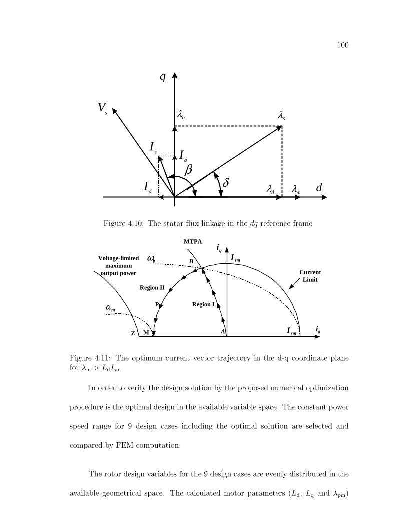
100
mλ
sλsV
sI
δ
qλ
dλ
q
d
qI
dI
β
Figure 4.10: The stator flux linkage in the dq reference frame
CurrentLimit
smI
smI
qi
di
bω
A
B
MTPA
Voltage-limitedmaximum
output power
mω P
MZ
Region I
Region II
Figure 4.11: The optimum current vector trajectory in the d-q coordinate planefor λm > LdIsm
In order to verify the design solution by the proposed numerical optimization
procedure is the optimal design in the available variable space. The constant power
speed range for 9 design cases including the optimal solution are selected and
compared by FEM computation.
The rotor design variables for the 9 design cases are evenly distributed in the
available geometrical space. The calculated motor parameters (Ld, Lq and λpm)

101
0 20 40 60 80 100 120 140 160 180-0.5
0
0.5
1
1.5
2
2.5
3
3.5
4
Current angle (degree)
Tor
que
(N.m
)
β
RSM+GA
FEM
Figure 4.12: Torque vs. current angle β characteristics for FEM and RSM
0 20 40 60 80 100 120 140 160 1800
0.1
0.2
0.3
0.4
0.5
0.6
0.7
current angle (degree)
stat
or fl
ux li
nkag
e (
Wb)
β
RSM + GA
FEM
Figure 4.13: Stator flux vs. current angle β characteristics for FEM and RSM
for the selected 9 design cases are listed in Table 4.5.
Fig. 4.15 shows the maximum power capability for 9 selected design cases. It
illustrates that the different design of rotor structures will produce different con-

102
0 1000 2000 3000 4000 5000 60000
100
200
300
400
500
600
700
speed (rpm)
Max
imum
pow
er c
apab
ility
(W
)
RSM+GA
FEM
ωmax
ωrated
CPSR
Rated Power
Figure 4.14: Power capability vs speed characteristics for the optimized design byFEM and RSM
Table 4.5: Comparison of 9 design cases
Case lm γ α Ld Lq λpm CPSR
(mm) (Degree) (H) (H) (Wb)
A 1 0.67 75 0.081 0.170 0.323 3.45
B 2 0.67 75 0.065 0.158 0.394 1.81
C 3 0.67 75 0.054 0.149 0.426 1.43
D 1 0.75 75 0.081 0.158 0.407 1.96
E 2 0.75 75 0.057 0.142 0.453 1.34
F 3 0.75 75 0.045 0.126 0.473 1.20
G 2 0.75 60 0.065 0.159 0.339 2.73
H 3 0.75 60 0.057 0.158 0.371 1.98
J 2 0.70 70 0.063 0.158 0.383 1.96

103
0 1000 2000 3000 4000 5000 60000
100
200
300
400
500
600
700
Speed (rpm)
Max
imum
Pow
er C
apab
ility
A
B C
D E F
G
H
J
Rated Power CPSR
ωrated
ωmax
Figure 4.15: Comparison of optimal design with other design cases
stant speed range. The optimal solution (Case A) by RSM together GAs method
has the largest CPSR (3.45), which validate the proposed numerical optimization
approach.
4.5 Conclusion
In this chapter, the effect of geometric parameters on the constant power operation
of interior PMSMs has been investigated using both analytical method and finite
element method. In order to design an interior PMSM with an optimal constant
power speed range, an efficient design optimization approach is proposed and im-
plemented. The combination of Response Surface Methodology, Genetic Algorithm
and Finite Element Analysis has proved an effective and practical tool for numer-

104
ical simulation and optimization process. This approach enables a fast design and
an accurate performance prediction as demonstrated by comparing the numerical
results obtained from this new method and conventional methods. The design
optimization methodology was illustrated by a design example for the prototype
interior PMSM.
Chapter 5
Tests and Performance of thePrototype Interior PMSM
5.1 Introduction
The prototype interior PMSM was tested using a motor-generator set. The test
equipment included a 750W/5A/350V IGBT PWM voltage source inverter, the pro-
totype interior PMSM, a torque transducer, a 1.1kW separately excited dc genera-
tor and a resistor bank to provide a load on the generator, as shown schematically
in Fig. 5.1. The digital signal processor (DSP) control board and an integrated
interface platform to provide interface between the digital and analog systems. The
inverter and the control system adjusted the speed, current and torque angle of the
drive system according to a command. The field excitation and load resistor of the
dc generator were adjusted to vary the mechanical loading of the PMSM.
A range of tests were conducted on the prototype PMSM. These tests served
three purposes:
105
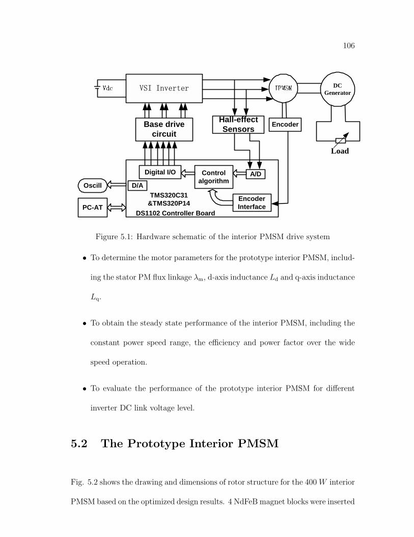
106
VSI InverterVdc IPMSM
Base drivecircuit
Hall-effectSensors
Encoder
Digital I/O Controlalgorithm
A/D
EncoderInterface
D/A
PC-AT
Oscill
DS1102 Controller Board
TMS320C31&TMS320P14
DCGenerator
Load
Figure 5.1: Hardware schematic of the interior PMSM drive system
• To determine the motor parameters for the prototype interior PMSM, includ-
ing the stator PM flux linkage λm, d-axis inductance Ld and q-axis inductance
Lq.
• To obtain the steady state performance of the interior PMSM, including the
constant power speed range, the efficiency and power factor over the wide
speed operation.
• To evaluate the performance of the prototype interior PMSM for different
inverter DC link voltage level.
5.2 The Prototype Interior PMSM
Fig. 5.2 shows the drawing and dimensions of rotor structure for the 400 W interior
PMSM based on the optimized design results. 4 NdFeB magnet blocks were inserted

107
in rotor slots. The stator frame is same with the standard induction motor and
the winding is rewound according to the design specifications (see Appendix A for
detail). The actual structures of the stator and rotor are shown in Fig. 5.3.
R 37.0mm
R10.0mm
24.8mm
o75=α
1.00mm
Figure 5.2: The optimized rotor structure for the prototype interior PMSM
Figure 5.3: Standard stator and designed rotor for the prototype interior PMSM

108
Tests were conducted on the prototype interior PMSM in order to evaluate
its performance, to verify the proposed optimization approach and to validate the
design.
5.3 Experimental Interior PMSM Drive System
An experimental set-up for the interior PMSM drive system has been built with the
dSPACE DS1102 controller board. An experimental set-up for the drive system is
shown in Fig. 5.4 and Fig. 5.5.
DCGenerator
TorqueTransducer
PrototypeIPMSM
Encoder
Figure 5.4: Experimental set-up for the interior PMSM drive system
As shown in these figures, the experimental system consists of the following
units:
• A PC for software programming, debugging and real-time control.

109
Figure 5.5: dSPACE DS1102 based integrated PMSM drive test platform
• A dSPACE DS1102 controller board for executing control programs, gener-
ating control signals, performing A/D and D/A conversions, and communi-
cating with the PC.
• A PWM voltage-source inverter for driving the interior PMSM.
• An integrated interface platform for performing logic operations, inverter
control, buffering, isolation, protection, etc.
• The prototype interior PMSM with exterior incremental encoder for position
sensing.
• Two current sensors for measuring the phase currents in two motor phases
and voltage sensor for measuring the DC link voltage.
• A loading system for producing load torque to the interior PMSM.

110
• A torque transducer for measuring the actual motor torque.
TMS320C31
JTAG Interface
128K×32 Static RAM Zero wait state
JTAG Connector
Serial Interface
PCI BUS
Host Interface
IncrementalEncoder Interface 1
TMS320P14Digital I/O
16-bit ADC 1
16-bit ADC 2
12-bit ADC 3
12-bit ADC 4
12-bit DAC 1
12-bit DAC 2
12-bit DAC 3
12-bit DAC 4
IncrementalEncoder Interface 2
Noise Filter
Noise Filter
Analog/Digital I/O Connector
26
Figure 5.6: Configuration of the controller board used for hardware implementation

111
5.3.1 DS1102 controller board
The dSPACE DS1102 controller board is specifically designed for the development
of high-speed multi variable digital controllers and real-time simulations in various
fields such as motor drives. The board consists of a floating-point DSP TMS320C31,
a micro controller TMS320P14 acting as a slave-DSP for the digital I/O subsystem,
A/D and D/A converters, and encoder interfaces.
The main DSP processes the numerically intensive algorithms at a speed of
60 MHz per instruction cycle. The slave-DSP performs digital I/O and PWM
generation. The A/D converters convert the analog feedback signals of ± 10V
into digital format so that the DSP can read in the measured quantity. Such
conversions are used on the measured stator current or motor torque feedback
signals. Conversely, the D/A converters convert the digital signals in the DSP into
analog signals of ± 10V so that they can be displayed on an analog CRO. The
encoder interface provides the interfacing of the DSP with the incremental encoder
so that the output of the incremental encoder, which is in discrete pulses, can
be quantized into digital form; hence, the data on the rotor-position is acquired.
The DS1102 controller board is designed like a PC expansion card so that it can be
inserted into the PCI slot of the PC, together with the PC video card or sound card.
Using the appropriate software for communication between the PC and the DSP,
users can debug the user-program that is loaded in the DSP (via C-programming
and the Texas Instruments C-Compiler), tune the experimental parameters on-line
or display the experimental variables in real-time.
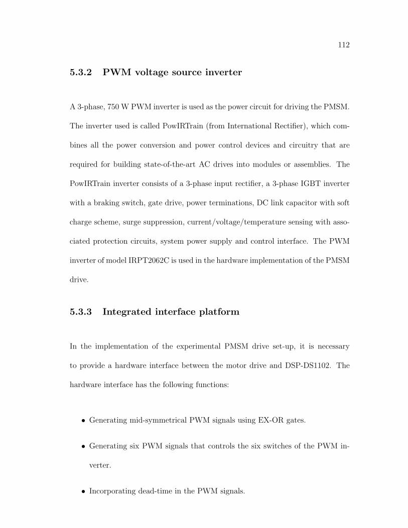
112
5.3.2 PWM voltage source inverter
A 3-phase, 750 W PWM inverter is used as the power circuit for driving the PMSM.
The inverter used is called PowIRTrain (from International Rectifier), which com-
bines all the power conversion and power control devices and circuitry that are
required for building state-of-the-art AC drives into modules or assemblies. The
PowIRTrain inverter consists of a 3-phase input rectifier, a 3-phase IGBT inverter
with a braking switch, gate drive, power terminations, DC link capacitor with soft
charge scheme, surge suppression, current/voltage/temperature sensing with asso-
ciated protection circuits, system power supply and control interface. The PWM
inverter of model IRPT2062C is used in the hardware implementation of the PMSM
drive.
5.3.3 Integrated interface platform
In the implementation of the experimental PMSM drive set-up, it is necessary
to provide a hardware interface between the motor drive and DSP-DS1102. The
hardware interface has the following functions:
• Generating mid-symmetrical PWM signals using EX-OR gates.
• Generating six PWM signals that controls the six switches of the PWM in-
verter.
• Incorporating dead-time in the PWM signals.

113
• Setting the over-current/over-voltage protections and RESET/STOP func-
tions of the inverter.
• Buffering the pulse signals generated from the incremental encoder.
• Provide filtering of the measured current and torque signals.
Mid-symmetrical PWM Signals
EX-OR
Setting Dead-time 2µs
Opto-couplers
PWM_A2
From Stator Windings
ResetStop
Current/Voltage Sensors
isa isb
uiA
From Encoder
Buffers Encoder Interface
uiB
PWM_A1
PWM_B1PWM_B2PWM_C1PWM_C2
PWM Inverter
ADC 1
ADC 2
PWM_0 PWM_1 PWM_2 PWM_3 PWM_4 PWM_5
DS1102 Interface
Break
UFB
UREF
Reset Stop
IREF
Filter IFB
Motor & Encoder
Fault Display
ADC 3ADC 4 usa,b
Figure 5.7: Interfacing the controller board with the control circuit
The block diagram of the peripheral interface circuit is shown in Fig. 5.7.
Signals of the six PWM channels, which are ch0 and ch1 for phase A, ch2 and
ch3 for phase B, and ch4 and ch5 for phase C, are EX-ORed and become three
mid-symmetrical PWM signals. Another three complementary signals are obtained

114
from three logic inverters. Proper ”dead time” is then incorporated into these six
PWM signals to avoid ”mutual-ON” of the upper and lower switches on the same
phase of the inverter. The opto-couplers transfer the six PWM signals and isolate
the low-side circuit from the high-side circuit. The six PWM signals are inverted
into ”low-active” signals as required by the inverter and then sent to the inverter.
Signals of ”Reset” and ”Stop” are also sent through opto-couplers to control the
inverter. Voltage comparators are used to detect over voltage and over current.
”Fault” signals generated by the inverter and the voltage comparators are sent
through opto-couplers to the low-side circuit to inhibit the transfer of the PWM
signals. The installed current sensors and resistors convert the current signals
into voltage signals for the use of A/D converters of DS1102. Signals from the
incremental encoder are sent through buffers to shape the waveforms and to drive
the encoder interface circuit of ds1102.
5.3.4 Current sensor
Sufficiently accurate measurements of the motor phase currents are essential to
ensure high-performance in the PMSM drive system. In the experimental set-
up, two current sensors are utilized to measure the phase-a and b currents. The
measured currents are converted into voltage signals scaled to the range ± 10V by
using resistors of appropriate resistances. These voltage signals are then fed into
the A/D converters of the DS1102. In the PMSM experimental set-up, the LEM
module LA 25-NP current sensors are used. The current sensors, resistors and the
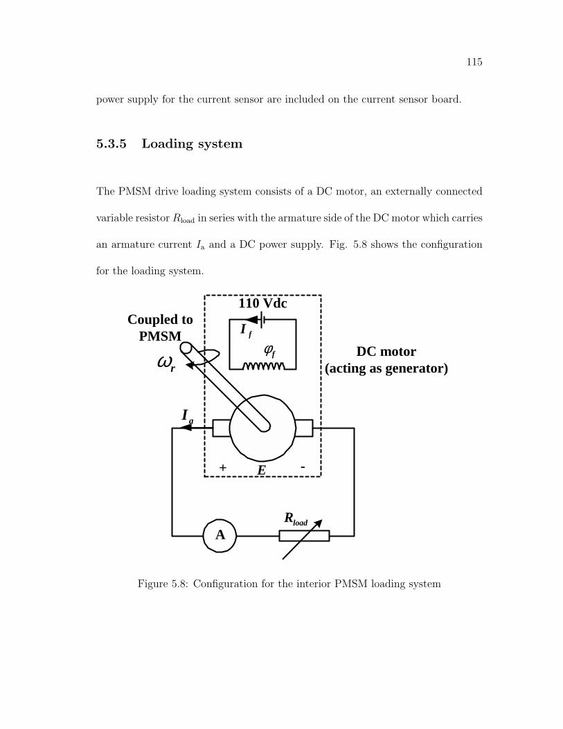
115
power supply for the current sensor are included on the current sensor board.
5.3.5 Loading system
The PMSM drive loading system consists of a DC motor, an externally connected
variable resistor Rload in series with the armature side of the DC motor which carries
an armature current Ia and a DC power supply. Fig. 5.8 shows the configuration
for the loading system.
Coupled toPMSM
+ -E
loadRA
rωfI
110 Vdc
fφ
aI
DC motor(acting as generator)
Figure 5.8: Configuration for the interior PMSM loading system
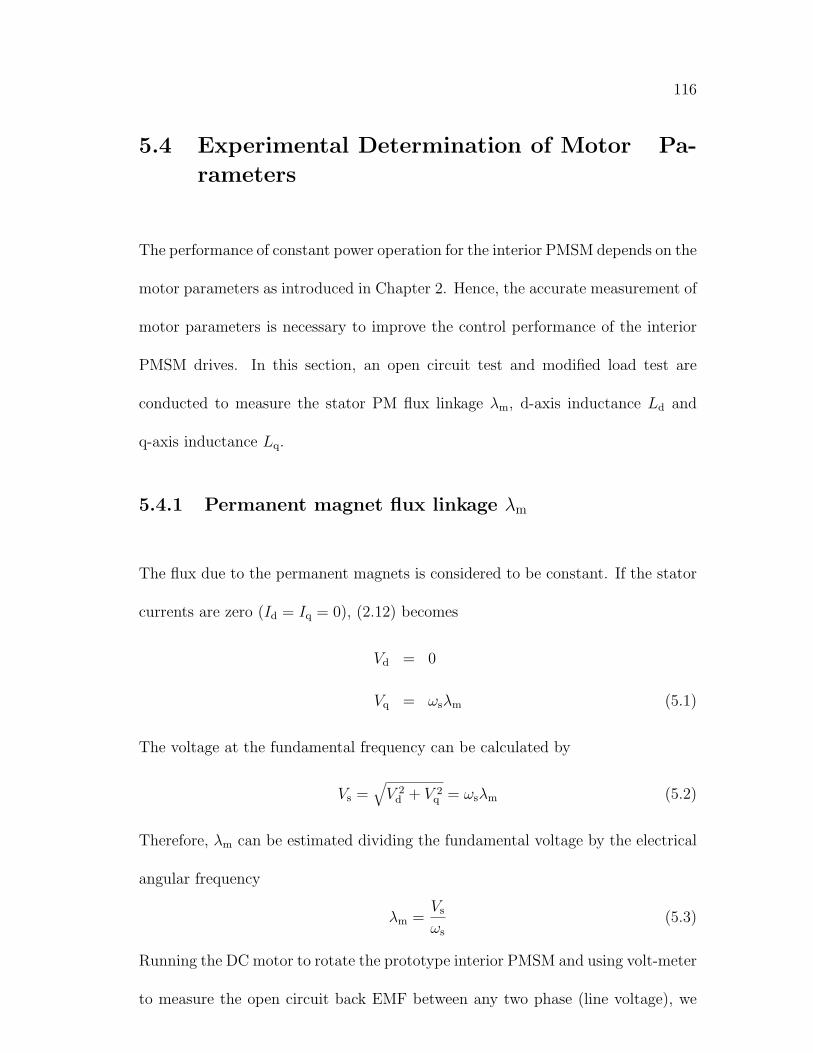
116
5.4 Experimental Determination of Motor Pa-
rameters
The performance of constant power operation for the interior PMSM depends on the
motor parameters as introduced in Chapter 2. Hence, the accurate measurement of
motor parameters is necessary to improve the control performance of the interior
PMSM drives. In this section, an open circuit test and modified load test are
conducted to measure the stator PM flux linkage λm, d-axis inductance Ld and
q-axis inductance Lq.
5.4.1 Permanent magnet flux linkage λm
The flux due to the permanent magnets is considered to be constant. If the stator
currents are zero (Id = Iq = 0), (2.12) becomes
Vd = 0
Vq = ωsλm (5.1)
The voltage at the fundamental frequency can be calculated by
Vs =√
V 2d + V 2
q = ωsλm (5.2)
Therefore, λm can be estimated dividing the fundamental voltage by the electrical
angular frequency
λm =Vs
ωs
(5.3)
Running the DC motor to rotate the prototype interior PMSM and using volt-meter
to measure the open circuit back EMF between any two phase (line voltage), we

117
get following results as listed in Table 5.1.
Table 5.1: Experimental measurements of back EMF and calculated values of λm
speed (rpm) line back EMF in rms (V) λm(Wb)
600 45.6 0.296
900 68.7 0.298
1200 91.4 0.297
1500 114.1 0.297
average 0.297
5.4.2 Torque angle measurement
The torque angle of a synchronous machine is defined as the angular displacement
between the magnet excitation voltage E0 and the terminal voltage Vs, as shown
in Fig. 5.9.
The magnet excitation voltage E0 and terminal phase voltage Vs can not be
measured at the same time. An alternative procedure depends on the position
measurement by incremental encoder. We can find out the position of d-axis of
the rotor with respect to phase A axis. The procedure is described in the following
steps:
I. The increment encoder was installed on the prototype motor shaft. The index
channel signal of incremental encoder is sent to the digital oscilloscope. We take
phase A voltage as the reference signal for the same digital oscilloscope.
II. Running the DC motor to drive the prototype motor at no-load. Then two
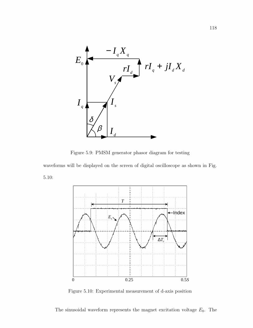
118
βδ
sI
sV
dI
qI
ddq XjIrI +qq XI−
0EdrI
Figure 5.9: PMSM generator phasor diagram for testing
waveforms will be displayed on the screen of digital oscilloscope as shown in Fig.
5.10:
T
0EIndex
0T∆
0 25.0 S5.0
Figure 5.10: Experimental measurement of d-axis position
The sinusoidal waveform represents the magnet excitation voltage E0. The
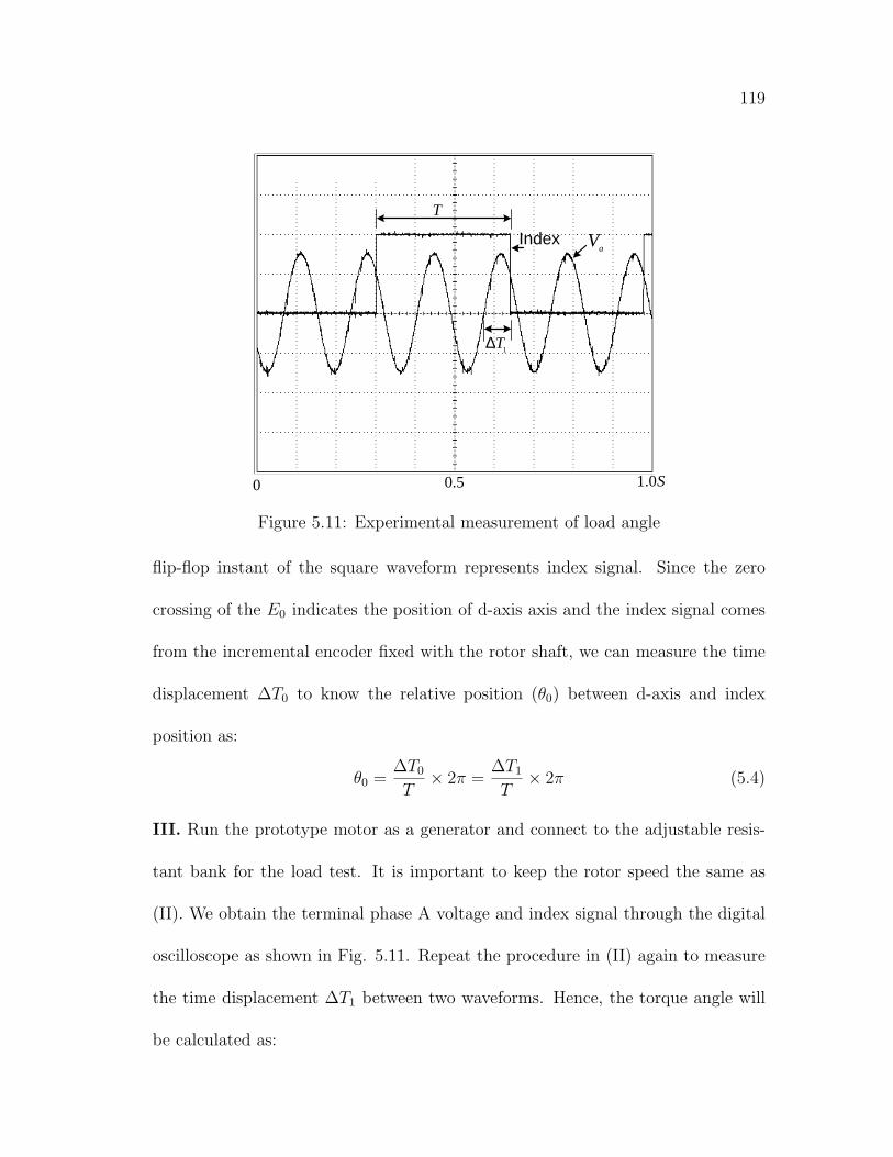
119
T
aV
1T∆
Index
0 5.0 S0.1
Figure 5.11: Experimental measurement of load angle
flip-flop instant of the square waveform represents index signal. Since the zero
crossing of the E0 indicates the position of d-axis axis and the index signal comes
from the incremental encoder fixed with the rotor shaft, we can measure the time
displacement ∆T0 to know the relative position (θ0) between d-axis and index
position as:
θ0 =∆T0
T× 2π =
∆T1
T× 2π (5.4)
III. Run the prototype motor as a generator and connect to the adjustable resis-
tant bank for the load test. It is important to keep the rotor speed the same as
(II). We obtain the terminal phase A voltage and index signal through the digital
oscilloscope as shown in Fig. 5.11. Repeat the procedure in (II) again to measure
the time displacement ∆T1 between two waveforms. Hence, the torque angle will
be calculated as:
120
δ =∆T0 −∆T1
T× 2π (5.5)
5.4.3 Load test to measure Ld and Lq
In the load test, the prototype interior PMSM is rotated by DC motor as a PMSM
generator, and the motor terminals are connected with the three phase resistor bank
which acting as an adjusted resistive load. In this measurement, it is not possible
to isolate the stator leakage reactance from the total d-axis and q-axis reactance. It
is common practice to lump the leakage inductance into the synchronous reactance,
which leads to the modified phasor diagram as shown in Fig. 5.9.
From the phasor diagram, the following can be obtained as
Vs sin δ = XqIq − rId
Vs cos δ = E0 −XdId − rIq (5.6)
where r is phase resistance which is assumed a constant dc value and E0 = λmωs .
It is noted that once the data of output voltage Vs, current Is, and torque angle δ
are known from the load test, other quantities in (5.6) can be obtained as
Xd =E0 − rIs cos δ − Vs cos δ
I sin δ
Xq =Vs sin δ + rIs sin δ
I cos δ(5.7)
and
Ld =Xd
ωs
Lq =Xq
ωs
(5.8)

121
Table 5.2 lists the experimental results of load test for different speeds and loading
conditions. The values of Ld in the IPM motor are affected at light load, and these
are not affected significantly at high values of load.
Table 5.2: Experimental measurements of Ld and Lq
speed Vs Is δ Ld Lq
(rpm) (V ) (A) (degree) (H) (H)
600 23.84 0.493 20.2 0.074 0.156
1200 49.42 0.616 25.2 0.079 0.160
1500 64.09 0.269 13.5 0.113 0.186
1500 62.76 0.525 22.5 0.086 0.164
1500 51.04 1.476 53.1 0.083 0.168
1500 48.27 1.588 58.5 0.086 0.184
In Table 5.1 and 5.2 the measured motor parameters (λm, Ld and Lq) for the
prototype motor through experiments show significant variation and discrepancy
with those expected by RSM+GA method. The major reasons for such difference
are listed as follows:
(1) The material characteristics used in FEM and RSM are slightly different
with those actually used in the fabrication of prototype motors. For example, the
measured remanence flux of permanent magnet was found to be less than the value
given by the manufacturing data sheet. This explains why λm is less than the
expected value.
(2) In the proposed design methodology, the unsaturated linear model are

122
used to estimated the motor parameters. However, the key machine parameters
are non-linear functions of design variables and the load condition. Therefore, the
performance of the machine is a non-linear function of these parameters. This is
another reason why measured performance of the prototype is below the design
values.
The major reason for this discrepancy seems to be the use of unsaturated
model. Hence a saturated model of motor parameters will give better estimate the
machine performance under saturation effect.
5.5 Experimental Evaluation of Wide Speed Op-
eration Performance
Tests have been conducted to evaluate the machine operation performance in a wide
speed range. The performance tests include the verification of torque and power
vs. speed characteristics, as well as the efficiency and power factor for different
operating conditions.
In order to validate the optimal design objective of prototype interior PMSM,
the wide speed operation performance for the prototype interior PMSM is compared
with a commercial 400W interior PMSM. The comparison is based on the same
drive system configuration and control scheme. The motor parameters for these
two motors are listed in Table 5.3.
In the tests of the prototype interior PMSM, torque, shaft power, input power
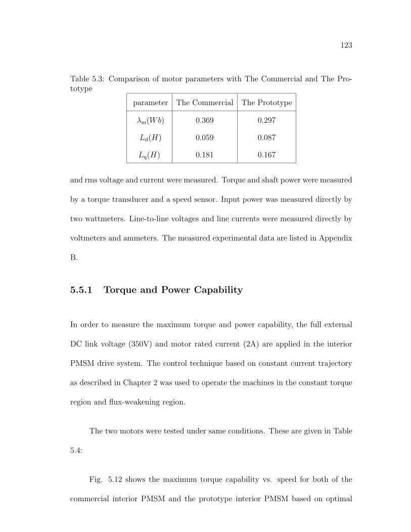
123
Table 5.3: Comparison of motor parameters with The Commercial and The Pro-totype
parameter The Commercial The Prototype
λm(Wb) 0.369 0.297
Ld(H) 0.059 0.087
Lq(H) 0.181 0.167
and rms voltage and current were measured. Torque and shaft power were measured
by a torque transducer and a speed sensor. Input power was measured directly by
two wattmeters. Line-to-line voltages and line currents were measured directly by
voltmeters and ammeters. The measured experimental data are listed in Appendix
B.
5.5.1 Torque and Power Capability
In order to measure the maximum torque and power capability, the full external
DC link voltage (350V) and motor rated current (2A) are applied in the interior
PMSM drive system. The control technique based on constant current trajectory
as described in Chapter 2 was used to operate the machines in the constant torque
region and flux-weakening region.
The two motors were tested under same conditions. These are given in Table
5.4:
Fig. 5.12 shows the maximum torque capability vs. speed for both of the
commercial interior PMSM and the prototype interior PMSM based on optimal

124
Table 5.4: Test Condition with The Commercial and The Prototype
Specifications The Commercial The Prototype
Power Rating (W) 400 400
Rated Line Voltage (V) 310 310
Rated Line Current (A) 1.2 1.2
Airgap Flux Density (Tesla) 0.5 0.5
Hardware Drive Circuit Same Same
Firmware Control Algorithms Same Same
Measurement Device Same Same
design. The torque capability for the prototype motor is slightly lower than the
commercial motor, however, the prototype motor has higher torque over the flux-
weakening region than the commercial one. This shows that the flux-weakening
capability for the prototype motor is superior to the commercial one.
Fig. 5.13 compares the maximum power capability and constant power speed
range for the prototype and commercial interior PMSMs.
The range of constant power operation achieved is around the ratio of 1 : 2.6,
which is also superior to the commercial motor (1:1.77). It is noted that the actual
constant speed range for the prototype interior PMSM is lower than the expected
value 1:3.6 by numerical analysis. The excessive friction loss and iron loss causes the
drop in the power capability in the high speed range. Considering the limitation
of numerical analysis method, total loss cannot be computed accurately. Hence
the actual constant power speed range is less than the predicted. However, the
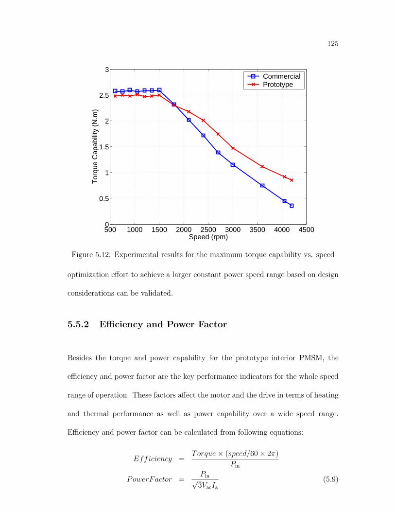
125
500 1000 1500 2000 2500 3000 3500 4000 45000
0.5
1
1.5
2
2.5
3
Speed (rpm)
Tor
que
Cap
abili
ty (
N.m
)
CommercialPrototype
Figure 5.12: Experimental results for the maximum torque capability vs. speed
optimization effort to achieve a larger constant power speed range based on design
considerations can be validated.
5.5.2 Efficiency and Power Factor
Besides the torque and power capability for the prototype interior PMSM, the
efficiency and power factor are the key performance indicators for the whole speed
range of operation. These factors affect the motor and the drive in terms of heating
and thermal performance as well as power capability over a wide speed range.
Efficiency and power factor can be calculated from following equations:
Efficiency =Torque× (speed/60× 2π)
Pin
PowerFactor =Pin√3VacIa
(5.9)
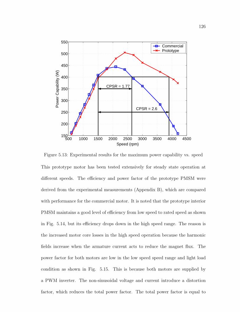
126
500 1000 1500 2000 2500 3000 3500 4000 4500150
200
250
300
350
400
450
500
550
Speed (rpm)
Pow
er C
apab
ility
(W
)
CommercialPrototype
CPSR = 1.77
CPSR = 2.6
Figure 5.13: Experimental results for the maximum power capability vs. speed
This prototype motor has been tested extensively for steady state operation at
different speeds. The efficiency and power factor of the prototype PMSM were
derived from the experimental measurements (Appendix B), which are compared
with performance for the commercial motor. It is noted that the prototype interior
PMSM maintains a good level of efficiency from low speed to rated speed as shown
in Fig. 5.14, but its efficiency drops down in the high speed range. The reason is
the increased motor core losses in the high speed operation because the harmonic
fields increase when the armature current acts to reduce the magnet flux. The
power factor for both motors are low in the low speed speed range and light load
condition as shown in Fig. 5.15. This is because both motors are supplied by
a PWM inverter. The non-sinusoidal voltage and current introduce a distortion
factor, which reduces the total power factor. The total power factor is equal to
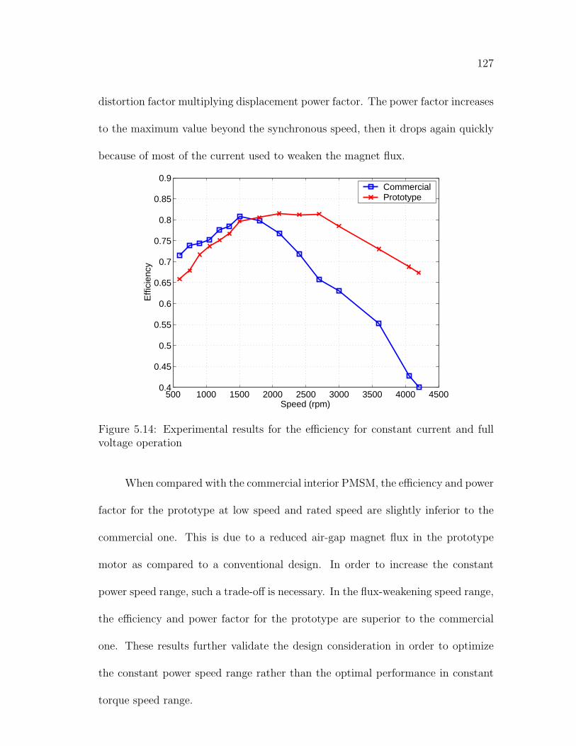
127
distortion factor multiplying displacement power factor. The power factor increases
to the maximum value beyond the synchronous speed, then it drops again quickly
because of most of the current used to weaken the magnet flux.
500 1000 1500 2000 2500 3000 3500 4000 45000.4
0.45
0.5
0.55
0.6
0.65
0.7
0.75
0.8
0.85
0.9
Speed (rpm)
Effi
cien
cy
CommercialPrototype
Figure 5.14: Experimental results for the efficiency for constant current and fullvoltage operation
When compared with the commercial interior PMSM, the efficiency and power
factor for the prototype at low speed and rated speed are slightly inferior to the
commercial one. This is due to a reduced air-gap magnet flux in the prototype
motor as compared to a conventional design. In order to increase the constant
power speed range, such a trade-off is necessary. In the flux-weakening speed range,
the efficiency and power factor for the prototype are superior to the commercial
one. These results further validate the design consideration in order to optimize
the constant power speed range rather than the optimal performance in constant
torque speed range.

128
500 1000 1500 2000 2500 3000 3500 4000 45000.45
0.5
0.55
0.6
0.65
0.7
0.75
0.8
0.85
0.9
0.95
Speed (rpm)
Pow
er F
acto
r
CommercialPrototype
Figure 5.15: Experimental results for the power factor for constant current and fullvoltage operation
5.5.3 Performance under Reduced DC Link Voltages
In practical application of interior PMSM drives, the input DC link voltage might
be decreased due to the uncertainty with external power network. Furthermore,
due to the large current change in the dynamics, the dc-link voltage drop on the
capacitor is larger than usual. All these unexpected variations can reduce the
maximum available voltage in the motor winding terminals and deteriorate the
operational performance of the machines. Therefore, tests under reduced DC link
voltages are necessary to evaluate the performance of machine to cope with the
reduced DC link voltage.
Figs. 5.16 and 5.17 show that the torque and power capability for the pro-
totype motor at 75 percent of the full DC link voltage (262.5V) and at 50 percent
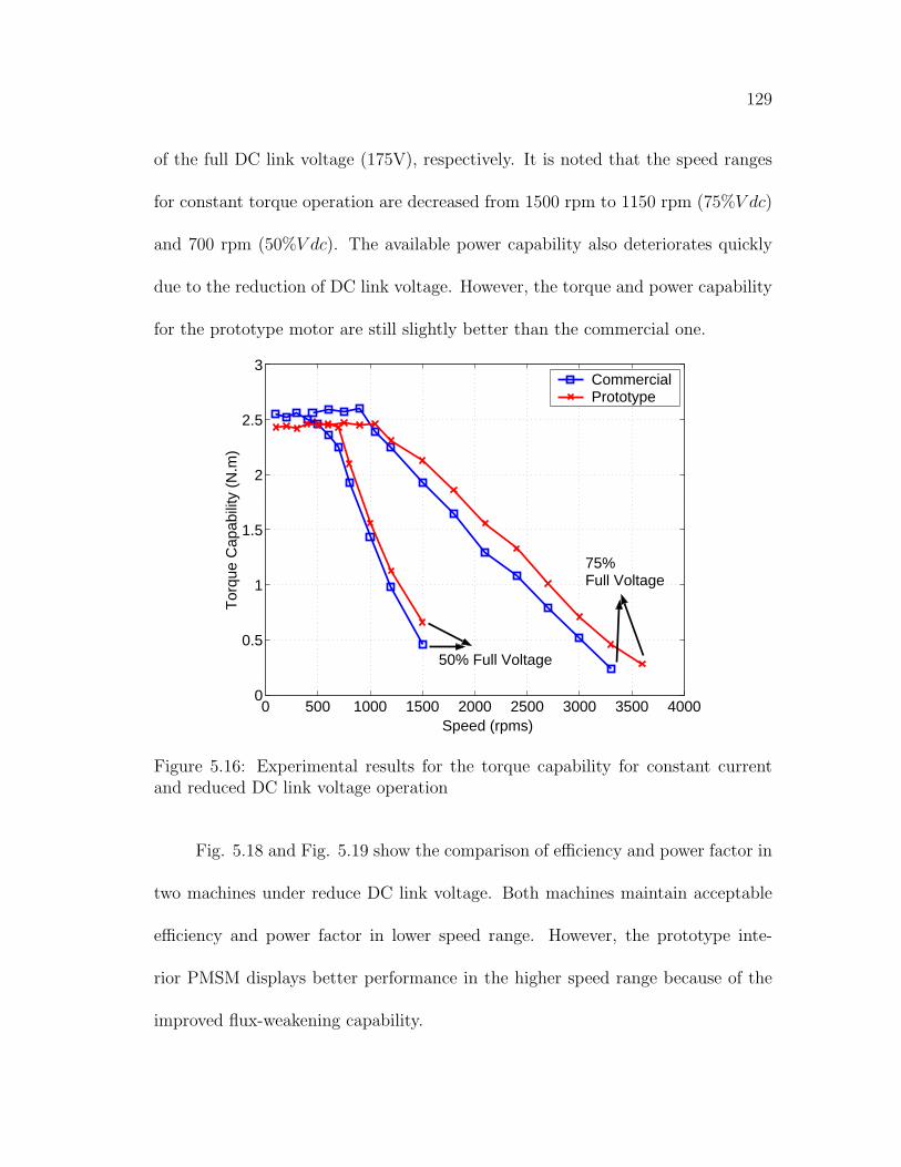
129
of the full DC link voltage (175V), respectively. It is noted that the speed ranges
for constant torque operation are decreased from 1500 rpm to 1150 rpm (75%V dc)
and 700 rpm (50%V dc). The available power capability also deteriorates quickly
due to the reduction of DC link voltage. However, the torque and power capability
for the prototype motor are still slightly better than the commercial one.
0 500 1000 1500 2000 2500 3000 3500 40000
0.5
1
1.5
2
2.5
3
Speed (rpms)
Tor
que
Cap
abili
ty (
N.m
)
CommercialPrototype
75% Full Voltage
50% Full Voltage
Figure 5.16: Experimental results for the torque capability for constant currentand reduced DC link voltage operation
Fig. 5.18 and Fig. 5.19 show the comparison of efficiency and power factor in
two machines under reduce DC link voltage. Both machines maintain acceptable
efficiency and power factor in lower speed range. However, the prototype inte-
rior PMSM displays better performance in the higher speed range because of the
improved flux-weakening capability.
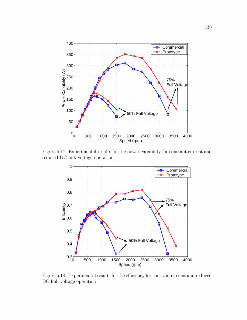
130
0 500 1000 1500 2000 2500 3000 3500 40000
50
100
150
200
250
300
350
400
Speed (rpm)
Pow
er C
apab
ility
(W
)
CommercialPrototype
50% Full Voltage
75% Full Voltage
Figure 5.17: Experimental results for the power capability for constant current andreduced DC link voltage operation
0 500 1000 1500 2000 2500 3000 3500 40000.3
0.4
0.5
0.6
0.7
0.8
0.9
1
Speed (rpm)
Effi
cien
cy
CommercialPrototype
50% Full Voltage
75% Full Voltage
Figure 5.18: Experimental results for the efficiency for constant current and reducedDC link voltage operation
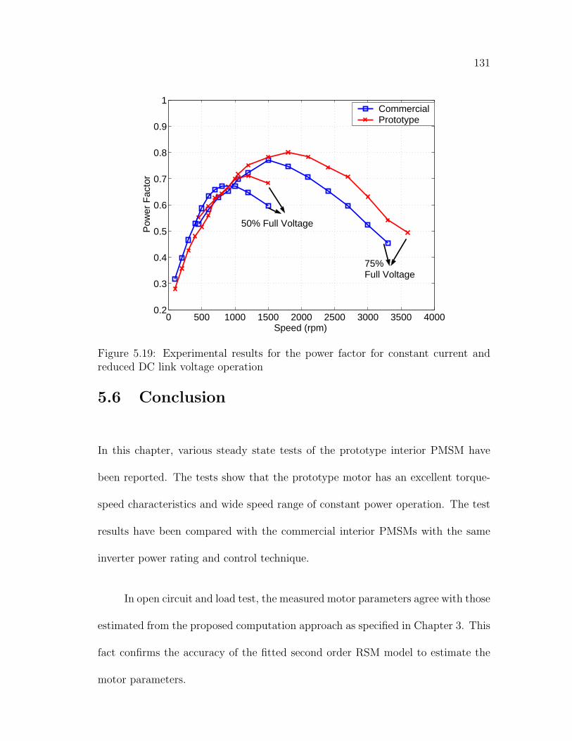
131
0 500 1000 1500 2000 2500 3000 3500 40000.2
0.3
0.4
0.5
0.6
0.7
0.8
0.9
1
Speed (rpm)
Pow
er F
acto
r
CommercialPrototype
50% Full Voltage
75% Full Voltage
Figure 5.19: Experimental results for the power factor for constant current andreduced DC link voltage operation
5.6 Conclusion
In this chapter, various steady state tests of the prototype interior PMSM have
been reported. The tests show that the prototype motor has an excellent torque-
speed characteristics and wide speed range of constant power operation. The test
results have been compared with the commercial interior PMSMs with the same
inverter power rating and control technique.
In open circuit and load test, the measured motor parameters agree with those
estimated from the proposed computation approach as specified in Chapter 3. This
fact confirms the accuracy of the fitted second order RSM model to estimate the
motor parameters.

132
The efficiency and power factor of the prototype interior PMSM have been
measured and compared with those of a commercial 400 W interior PMSM. The
comparison indicates that the optimized design realizes the wide-speed constant
power operation with no trade-off of its performance on the rated operation.
Chapter 6
Control of The Prototype InteriorPermanent Magnet SynchronousMotor
6.1 Introduction
While the design of an interior PMSM for extended speed operation poses sev-
eral technical challenges, the success of the complete drive system depends on the
availability of an appropriate control algorithm that can extract the full perfor-
mance capabilities from the machine. In particular, special flux weakening control
techniques are necessary to achieve constant power operation over a wide speed
range. Interior PMSMs are suitable for wide speed operation by flux-weakening
method because this kind of machine has a relatively large armature inductance,
and as a result, enough flux-weakening effect due to the d-axis armature reaction.
The design optimization of interior PMSMs further improves the machines’ flux
weakening capability and extends the constant power speed range, as discussed in
Chapter 3.
133

134
Control technique is critical to exploit the power capability of PMSMs in all
speed ranges. This chapter first discusses the control performance of traditional
field oriented current control scheme for interior PMSMs. More detailed descrip-
tions of this control system are given. The advantages and disadvantages using
current regulator in this control method are investigated with theoretical analy-
sis and experimental results. For better speed and torque control performance in
the wide-speed range, an improved speed and torque control method for interior
PMSMs is proposed in this chapter, and detail comparisons with field oriented
current control are presented with experimental results.
6.2 Field Oriented Current Control Scheme
The mathematical model of interior PMSMs in the synchronous d-q coordinates
have been presented in Chapter 2 with equations (2.1-2.16). The principle of cur-
rent control scheme is to force the current vector (Id, Iq) to follow the optimum
current vector trajectory as shown in Fig. 6.1, where the optimal current profile
with λm > LdIsm is used. Therefore, there are only two operating region divided
by the MTPA line (AB) and the current limit line (BM).
6.2.1 Description and features of the current control scheme
Fig. 6.2 illustrates a block diagram of the speed control system implemented with
current vector control algorithm [52], which includes three parts: current command
generator, current regulator, and flux-weakening voltage controller.
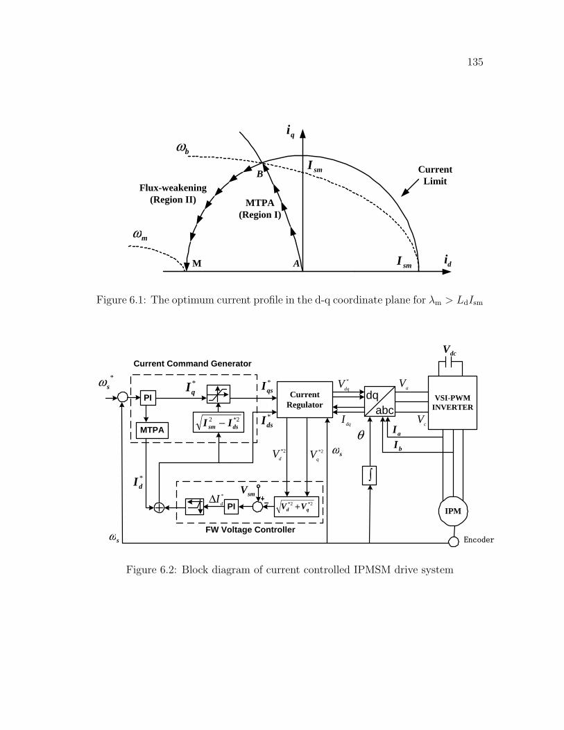
135
CurrentLimit
smI
smI
qi
di
bω
A
B
MTPA(Region I)
mω
M
Flux-weakening(Region II)
Figure 6.1: The optimum current profile in the d-q coordinate plane for λm > LdIsm
Encoder
PI
MTPA
PI 2*2*qd VV +
smV
2*2dssm II −
CurrentRegulator
*dsI
*qsI
*dI
*qI
sω
*sω
*
dI∆
VSI-PWMINVERTER
IPM
dcV
aI
bI
∫
θ
dqabc
aV
cV
2*
dV 2*
qV
*
dqV
dqI
sω
Current Command Generator
FW Voltage Controller
Figure 6.2: Block diagram of current controlled IPMSM drive system

136
The current command generator provides the reference q-axis current I∗q and
the reference d-axis current I∗d. I∗
q is decided from the speed error (ω∗s −ωs) through
the proportional-integral controller. The d-axis current command I∗d is decided by
(6.1) in the MTPA line (Region I) until the current regulator begins to saturate.
I∗d =
λm
2(Lq − Ld)−
√√√√ λ2m
4(Lq − Ld)2+ I∗
q2 (6.1)
Fig. 6.3 shows the details of current regulator. The d- and q-axis currents
cannot be controlled independently by Vd and Vq because of the cross-coupling
effects such as ωsLdId and ωsLqIq as shown in (2.12). The cross-coupling effects of
the interior PMSM are dominant because the interior PMSMs have relatively large
inductances. These effects increase as the speed increases. Therefore, it seems
that the current responses as well as torque response are affected by the cross-
coupling effects in the high-speed flux-weakening region. The cross-coupling effects
can be cancelled by the feed forward compensation as shown in Fig. 6.3. The
voltage commands are decided by the PI controller and decoupling feed forward
compensation, thus the d- and q-axis current control loops can be linearized by the
above decoupling current control.
Without a proper flux-weakening operation, the current regulator would be
saturated and lose its controllability at a higher speed. Since the onset of the
current regulator saturation varies according to load condition and the machine
parameters, the beginning point of flux weakening and the flux level should be
changed. A delay in flux-weakening may result in undesired output torque drop

137
PI
ddsmsq ILV ωλω +=0
qqsd ILV ω−=0
PI
dI
qI
*dI
*qI
sω
+
+
++
++ *
qV
*dV
Figure 6.3: Current regulator with decoupling feedforward compensation
according to the saturation of the current regulator, but an early start deteriorates
the acceleration performance. Therefore, it is desirable to change the onset point
of flux-weakening according to load condition and the machine parameters.
The main idea of flux-weakening voltage controller in current control scheme
is the use of the output reference voltage of the synchronous PI current regulator
to identify the onset of the flux-weakening. As the speed of the interior PMSM gets
higher during acceleration, the output of the current regulator, especially the q-axis
current regulator, increases and approaches to the boundary of the pulse width
modulator. Without a proper counter measure, the performance of the current
regulator gets worse due to the reduced margin of the voltage and finally it loses its
controllability. As shown in Fig. 6.2, the voltage regulator ensures the margin of the
voltage and increases the d-axis current towards the negative direction to prevent
saturation of the current regulators. With this outer voltage regulating loop the
flux level is inherently adjusted and the flux-weakening operation is accomplished
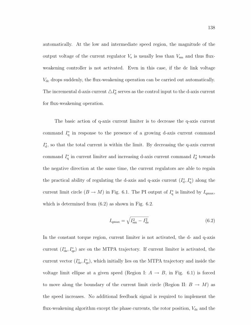
138
automatically. At the low and intermediate speed region, the magnitude of the
output voltage of the current regulator Vs is usually less than Vsm and thus flux-
weakening controller is not activated. Even in this case, if the dc link voltage
Vdc drops suddenly, the flux-weakening operation can be carried out automatically.
The incremental d-axis current4I∗d serves as the control input to the d-axis current
for flux-weakening operation.
The basic action of q-axis current limiter is to decrease the q-axis current
command I∗q in response to the presence of a growing d-axis current command
I∗d, so that the total current is within the limit. By decreasing the q-axis current
command I∗q in current limiter and increasing d-axis current command I∗
d towards
the negative direction at the same time, the current regulators are able to regain
the practical ability of regulating the d-axis and q-axis current (I∗d, I
∗q) along the
current limit circle (B → M) in Fig. 6.1. The PI output of I∗q is limited by Iqmax,
which is determined from (6.2) as shown in Fig. 6.2.
Iqmax =√
I2sm − I2
ds (6.2)
In the constant torque region, current limiter is not activated, the d- and q-axis
current (I∗ds, I
∗qs) are on the MTPA trajectory. If current limiter is activated, the
current vector (I∗ds, I
∗qs), which initially lies on the MTPA trajectory and inside the
voltage limit ellipse at a given speed (Region I: A → B, in Fig. 6.1) is forced
to move along the boundary of the current limit circle (Region II: B → M) as
the speed increases. No additional feedback signal is required to implement the
flux-weakening algorithm except the phase currents, the rotor position, Vdc and the

139
speed feedback, which are already available for the speed control in the constructed
system as shown in Fig. 6.2.
6.2.2 Discussions on current control schemes
The current vector control scheme for flux-weakening does not utilize the model
of interior PMSM but the reference output voltage of the synchronous PI cur-
rent regulator and the outer voltage control loop, and thus it is robust and less
sensitive to load condition and the machine parameters. The current control algo-
rithm described above, works well under the voltage and current limit from zero to
base speed. This method can theoretically achieve effective flux-weakening control
because it attempts to stop voltage saturation and expand the operating range.
However, the voltage references produced by this method must pass the saturated
voltage region. Consequently, the original reference output voltages by the current
control loop must be replaced by references with modified overmodulation strat-
egy. This result effectively changes the current controller to an unknown stability
and performance characteristics, and may not achieve the original control objec-
tives. Therefore, all the four PI gains must be selected appropriately to ensure
stability in the voltage saturation region. Generally, current control schemes based
on the approach with optimal current profile have at least two more drawbacks:
deviations from the prescribed control trajectories due to saturation of current reg-
ulator, whereas in the dynamics the available power capability of the inverter is
not completely exploited.

140
6.3 Space Vector Modulation based Direct Torque
Control Scheme
In order to overcome some problems in current vector control, we proposed an
improved space vector modulation (SVM) based DTC (DTC-SVM) scheme method
for IPMSM drive operating not only in constant torque region but also in the
flux weakening region. The proposed scheme uses constant switching frequency
operation similar to the modulation algorithms discussed by [90]. In addition,
using maximum voltage vector with over modulation technique, it provides a faster
torque control during dynamic operation and larger constant power speed range in
steady state operation.
6.3.1 Principle of torque production in interior PMSMs
The basic idea of the proposed scheme is in the control of the stator flux vector (in
amplitude and angular position) with feedback of observed torque and stator flux
from measured voltages and currents from motor terminals. The stator flux linkage
vector λs and rotor flux linkage vector λm can be drawn in the d − q coordinate,
Fig. 6.4. The angle between the stator and rotor flux linkages, δ, is the load angle
or torque angle.
The IPMSM stator flux linkage and electromagnetic torque equations in the
d− q coordinate are as follows:
λd = Ldid + λm
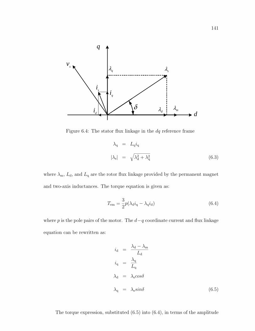
141
mλ
sλsv
si
δ
qλ
dλ
q
d
qi
di
Figure 6.4: The stator flux linkage in the dq reference frame
λq = Lqiq
|λs| =√
λ2d + λ2
q (6.3)
where λm, Ld, and Lq are the rotor flux linkage provided by the permanent magnet
and two-axis inductances. The torque equation is given as:
Tem =3
2p(λdiq − λqid) (6.4)
where p is the pole pairs of the motor. The d−q coordinate current and flux linkage
equation can be rewritten as:
id =λd − λm
Ld
iq =λq
Lq
λd = λscosδ
λq = λssinδ (6.5)
The torque expression, substituted (6.5) into (6.4), in terms of the amplitude
142
of the stator flux linkage and its angle with respect to rotor flux linkage is as follows:
Tem =3
2p · |λs|
2LdLq
[2λmLq sin δ − |λs|(Lq − Ld) sin 2δ] (6.6)
We can seen from (6.6) that by controlling the torque angle between stator and
rotor flux, and the magnitude of the stator flux, the electromagnetic torque can be
changed accordingly. The torque angle can be changed by changing the position of
the stator flux vector with respect to permanent magnet flux vector using the actual
voltage vector supplied by PWM inverter. In the steady state, δ is constant and
corresponds to a load torque, whereas stator and rotor fluxes rotate at synchronous
speed. In transient or dynamic operation, δ varies and the stator and rotor fluxes
rotate at different speeds.
6.3.2 Stator flux control in DTC-SVM
In stator coordinate (α−β axis) the stator flux linkage and current can be expressed
as:
λs = λα + jλβ
is = iα + jiβ (6.7)
Rewriting (6.4) in terms of α − β components the following torque expression is
obtained:
Tem = Im{3
2p(λs × is)} =
3
2p(λαiβ − λβiα) (6.8)
The major difference between DTC-SVM and conventional current vector
control lies in the absence of the current regulator in the flux and torque control.
143
Thus, the stator flux components are directly driven by the stator voltage vector
in the stator coordinate. The stator flux linkage of a PMSM that can be expressed
in the stationary reference frame is
λs =∫
(vs − rsis)dt (6.9)
During the switching interval, each voltage vector is constant, and (6.9) is then
written as:
λs = vst− rs
∫isdt + λs|t=0 (6.10)
The initial value of λs|t=0 is not zero for PMSM’s because of the existence of
permanent magnet. It can be obtained from the initial rotor positions. In digital
implementation the integration of the stator flux is as follows:
λα(k) = [vα(k)− riα(k)]Ts + λα(k − 1)
λβ(k) = [vβ(k)− riβ(k)]Ts + λβ(k − 1) (6.11)
where Ts is the sampling period and k represents the actual discrete time. The
α− β components of the command stator flux can be written as:
λ∗α(k) = λ∗
s (k) cos(θs(k) + ωs(k)Ts + ∆δ(k))
λ∗β(k) = λ∗
s (k) sin(θs(k) + ωs(k)Ts + ∆δ(k)) (6.12)
where ωs(k) is the present speed of stator flux and ∆δ(k) is the change of torque
angle; θs(k) is the position of the present stator flux linkage vector as shown in Fig.
6.5, which can be estimated by the present α− β component of stator flux vector:
θs(k) = arctan(λβ(k)
λα(k)) (6.13)

144
av
bv
aatv
bbtv
sλ∆ γ
mλ
sλ
s*λ s
λ∆
rθ
δ
α
β
γ
β
αδω ∆+
ssT
sθ
Figure 6.5: The steady state operation of stator flux control
The flux error between the command stator flux vector and actual stator flux
vector can be obtained by:
∆λα(k) = λ∗α(k)− λα(k)
∆λβ(k) = λ∗β(k)− λβ(k)
∆λs(k) = ∆λα(k) + j∆λβ(k) (6.14)
In stator flux control, we strive to achieve zero error for the stator flux vector in
one sampling time. This condition gives us the requirements for the on-time and
choice of the switching state vectors of a voltage source inverter.
∆λs(k) = vata + vbtb (6.15)
where va and vb are the voltage vectors produced by adjacent active switching
states of a three phase voltage source inverter as shown in Fig. 6.5; ta and tb are
the switching on time of two adjacent active voltage vectors.
For dynamic operations, the reference stator flux vector is forced to rotate
faster than rotor flux. Meanwhile, it is important that the magnitude of stator flux
145
vector is increased in the constant torque operation to achieve maximum torque
per ampere (MTPA) as described in [91], while in the flux weakening region, the
magnitude of stator flux vector has to be reduced as the speed increases. The prin-
ciple to adjust stator flux amplitude in different operating region will be discussed
later.
6.3.3 Calculation of switching on time
A three-phase machine being fed from a switched power converter, Fig. 6.6 (a),
have the switch pairs S1− S4 (S2− S5, and S3− S6) form half-bridge; one, and
only one switch in a half-bridge is closed at a time. The waveform of the phase
voltage (Va, Vb and Vc) is displayed in the upper trace of Fig. 6.6 (b) and the
peak value of phase voltage is 23Vdc. Therefore, there are six active switching state
vectors as shown in Fig. 6.8, where in brackets the switching polarities of three
half-bridge are indicated. The switching state vectors describe the inverter output
voltages. At operation with PWM waveforms, the two zero vectors V0 and V7 are
included in the pattern in Fig. 6.8 which are associated with those inverter states
with all upper or all lower half-bridge switches closed, respectively [92].
The modulation index is the normalized fundamental voltage, define as:
m =Vs
Vsmax
(6.16)
where Vs is the fundamental voltage of the modulated switching sequence and Vsmax
is the fundamental voltage at six-step operation as shown in Fig. 6.6 (b), which is

146
dcV
1S
2S
3S
4S 5
S6
S
aV
bV c
V
dcV
32
dcV
3
2−
aV
bV
cV
π2
π2
π2
(a) (b)
Figure 6.6: Three-phase converter and phase voltage
β
αdc
V3
2
(+ - -)
(+ + -)(- + - )
(- + +)
(- - +) (+ - +)
1v
2v
3v
4v
6v5
v 7v (+ + +)
0v (- - -)
Figure 6.7: Switching state vectors in the α− β plane
calculated by Fourier transformation as:
Vsmax =2
πVdc (6.17)

147
Using space vector modulation technique, we can achieve 0 ≤ m ≤ 1, and unity
modulation index can be obtained only in six-step mode. As the maximum power
of a PWM converter is proportional to the maximum power voltage at the ac side,
the maximum modulation index mmax constitutes an important utilization factor
of the equipment.
6.3.3.1 Normal modulation range
In the normal modulation range, the reference voltage vector Vs is always within
the hexagon as shown in Fig. 6.8 (a).
α
β
av
bv
γ 3π
sssTv λ∆=
aatv
bbtv
α
β
av
bv
γ 3π
sssTv λ∆=
aatv
bbtv
(a) (b)
Figure 6.8: Space vector modulation with switching state vectors
Based on geometric relationship in triangle, we can obtain the following equations:
|vata||∆λs|
=sin(π/3− γ)
sin(π/3)
|vbtb||∆λs|
=sin γ
sin(π/3)(6.18)

148
where |va| = |vb| = 23Vdc; γ is the position of stator flux error vector ∆λs, which
can be estimated as:
γ = arctan(∆λβ
∆λα
) (6.19)
Hence the switching on-times of the respective vectors are given as:
ta =3
2Vdc
· |∆λs|sin(π/3− γ)
sin(π/3)
tb =3
2Vdc
· |∆λs|sin(γ)
sin(π/3)
t0 = Ts − ta − tb (6.20)
6.3.3.2 In overmodulation range
As the angular velocity of stator flux ωs is increased, |∆λs| increases. The on-
times of active states could be so large that no zero vector can be switched, which
means that the reference voltage vector eventually touches the boundary of the
hexagon as shown in Fig. 6.8 (b). The controllable range of linear modulation
methods terminates at this point. Further increasing the modulation index up to
1, overmodulation technique has to be applied [92]. On the hexagon sides, the
stator flux error amplitude can be obtained as:
|∆λs| =Ts|va| sin(π/3)
sin(π/3 + γ)(6.21)
Hence, the modified switching on time of active voltage states are derived by sub-
stituting (6.21) into (6.20):
ta =Ts sin(π/3− γ)
sin(π/3 + γ)
tb = Ts − ta (6.22)
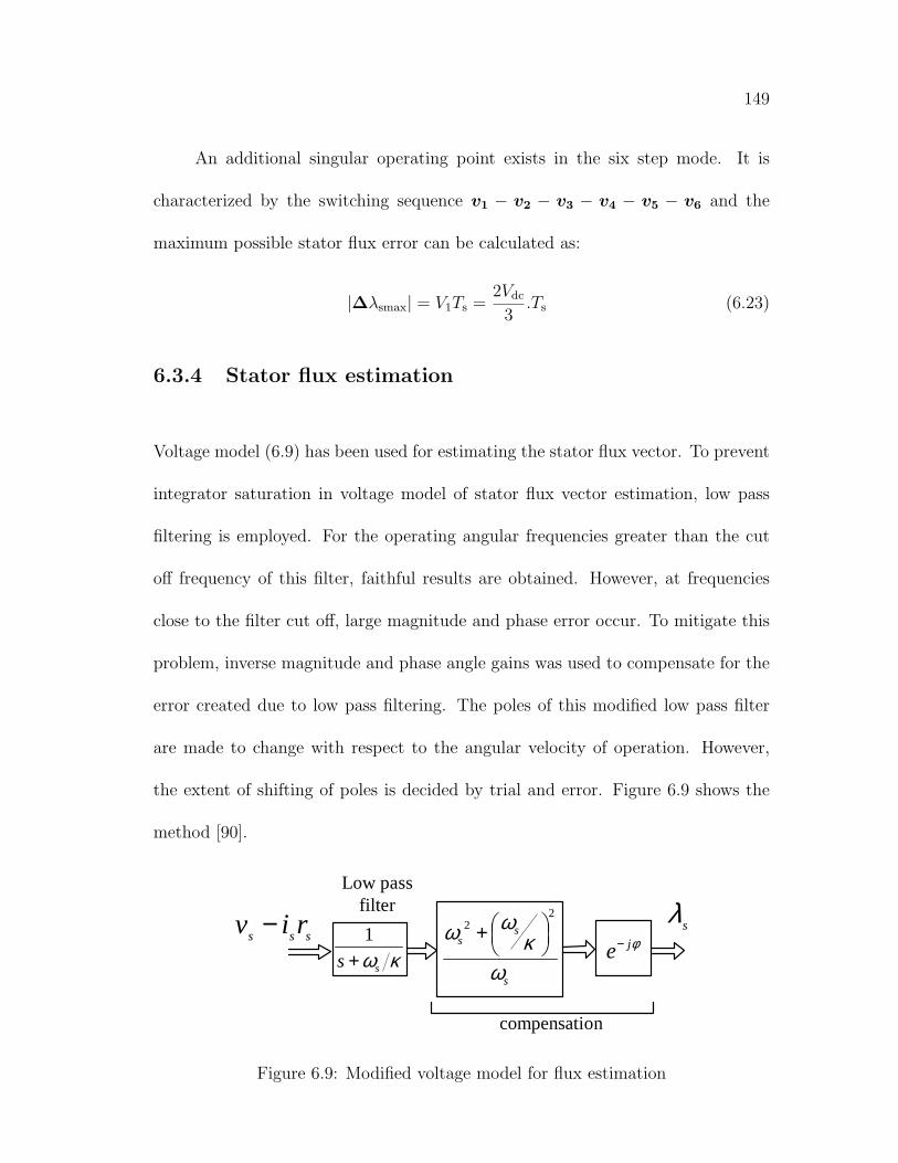
149
An additional singular operating point exists in the six step mode. It is
characterized by the switching sequence v1 − v2 − v3 − v4 − v5 − v6 and the
maximum possible stator flux error can be calculated as:
|∆λsmax| = V1Ts =2Vdc
3.Ts (6.23)
6.3.4 Stator flux estimation
Voltage model (6.9) has been used for estimating the stator flux vector. To prevent
integrator saturation in voltage model of stator flux vector estimation, low pass
filtering is employed. For the operating angular frequencies greater than the cut
off frequency of this filter, faithful results are obtained. However, at frequencies
close to the filter cut off, large magnitude and phase error occur. To mitigate this
problem, inverse magnitude and phase angle gains was used to compensate for the
error created due to low pass filtering. The poles of this modified low pass filter
are made to change with respect to the angular velocity of operation. However,
the extent of shifting of poles is decided by trial and error. Figure 6.9 shows the
method [90].
sλκωss +
1
s
ss
ωκ
ωω2
2
+ φje−
Low passfilter
compensation
sss riv −
Figure 6.9: Modified voltage model for flux estimation

150
Compensation in the magnitude and angle of the stator flux vector is done
after low pass filtering. This method is good at discarding high frequency noise
but the dc-offset still appears at the output of the filter, specially at very low
operating velocities. Moreover, the closed loop operation at speeds around zero
will depend upon the parameter κ which needs to be tuned by trial and error.
Following equation is used for stator flux estimation,
λs =∫{(1− jκsign(ωs))(vs − rsis)− κωsλs}dt (6.24)
here, ωs is the synchronous speed (angular velocity) and κ is a tuning parameter.
The poles of the resulting low pass filter will change corresponding to the operating
angular velocity. This model will work well only if the following two conditions are
satisfied. (a) amount of dc-offset is same for the sensed currents and (b) analog
gains provided by the anti noise/aliasing filters are exactly equal. Implementation
of the modified voltage model helps to deal with the problems of noise and drift.
6.3.5 Operating Limits for DTC-SVM scheme in IPMSMdrives
The critical condition for DTC which can be applied to IPMSM drive system is
that a positive dTem/dδ should be ensured within the normal operating condition
of the motor [69].
dTem
dδ=
3
2p · |λs|
LdLq
[λmLq cos δ − |λs|(Lq − Ld) cos 2δ] ≥ 0 (6.25)
According to (6.6), the torque vs. load angle characteristic with respect to different
stator flux amplitude is plotted in Fig. 6.10 (motor parameters are given in Table

151
5.3). The derivative of torque w.r.t δ near the region where δ = 0◦ is negative when
−150 −100 −50 0 50 100 150−15
−10
−5
0
5
10
15
Load Angle δ (degree)
Tor
que
(N.m
)λ
s = 3λ
m
δm0
−δm0
dT/dδ<0
λs = 2.5λ
m
λs = 2λ
m
λs = 1.5λ
m
λs = λ
m
λs = 0.5λ
m
Figure 6.10: The torque vs. load angle characteristics
the stator flux |λs| = 3λm, which will cause unstable operation of IPMSM drive by
using direct torque control.
Therefore, by (6.25), the condition for positive dTem/dδ around δ = 0◦ is
given by:
|λs| <Lq
Ld − Lq
λm (6.26)
Meanwhile, the maximum allowable angle δm0 which ensure a positive dTem/dδ can
be obtained by solving (6.25) as:
3
2p · |λs|
LdLq
[−2|λs|(Lq − Ld) cos2 δ + λmLq cos δ + |λs|(Lq − Ld)] ≥ 0 (6.27)
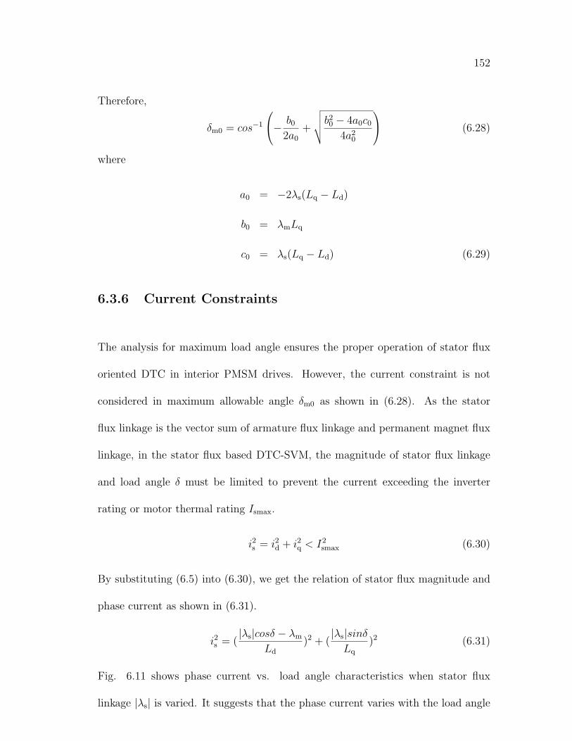
152
Therefore,
δm0 = cos−1
− b0
2a0
+
√√√√b20 − 4a0c0
4a20
(6.28)
where
a0 = −2λs(Lq − Ld)
b0 = λmLq
c0 = λs(Lq − Ld) (6.29)
6.3.6 Current Constraints
The analysis for maximum load angle ensures the proper operation of stator flux
oriented DTC in interior PMSM drives. However, the current constraint is not
considered in maximum allowable angle δm0 as shown in (6.28). As the stator
flux linkage is the vector sum of armature flux linkage and permanent magnet flux
linkage, in the stator flux based DTC-SVM, the magnitude of stator flux linkage
and load angle δ must be limited to prevent the current exceeding the inverter
rating or motor thermal rating Ismax.
i2s = i2d + i2q < I2smax (6.30)
By substituting (6.5) into (6.30), we get the relation of stator flux magnitude and
phase current as shown in (6.31).
i2s = (|λs|cosδ − λm
Ld
)2 + (|λs|sinδ
Lq
)2 (6.31)
Fig. 6.11 shows phase current vs. load angle characteristics when stator flux
linkage |λs| is varied. It suggests that the phase current varies with the load angle
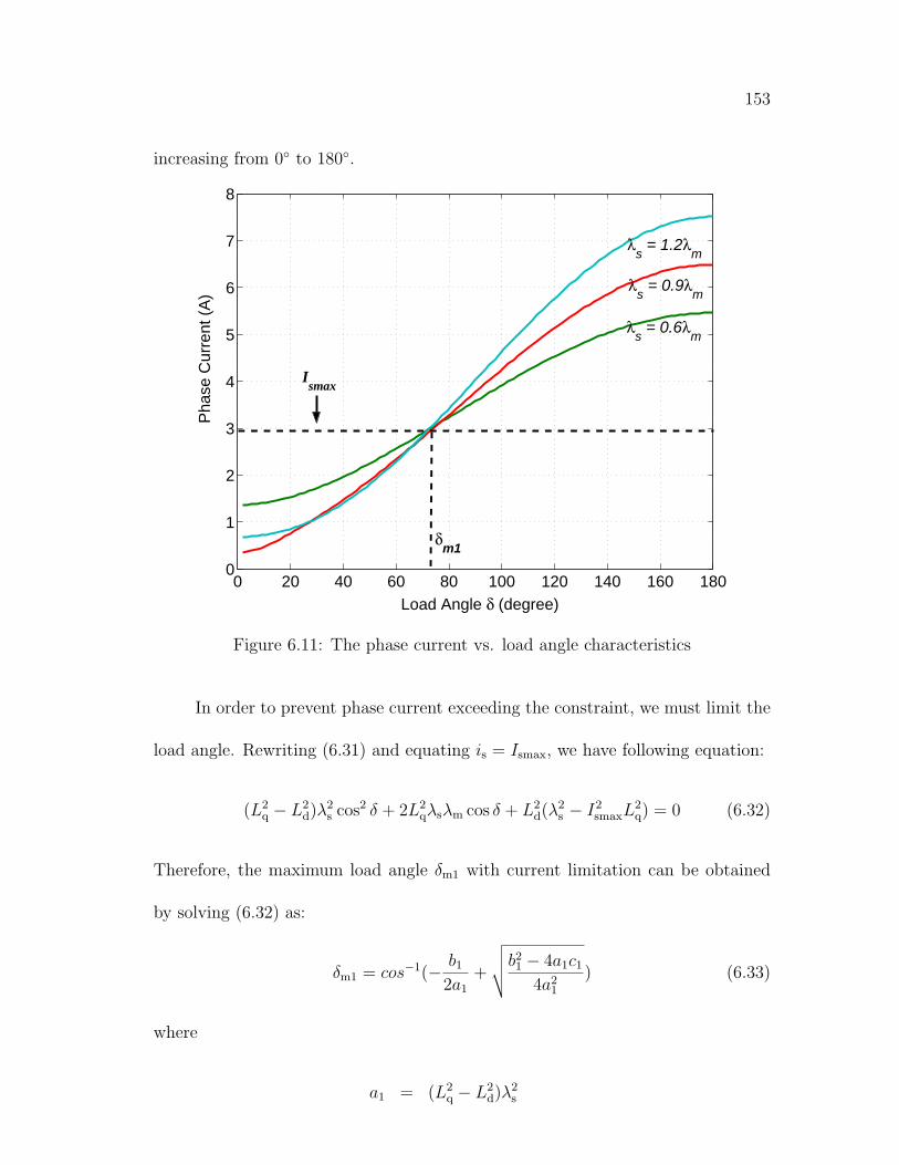
153
increasing from 0◦ to 180◦.
0 20 40 60 80 100 120 140 160 1800
1
2
3
4
5
6
7
8
Load Angle δ (degree)
Pha
se C
urre
nt (
A)
Ismax
δm1
λs = 1.2λ
m
λs = 0.9λ
m
λs = 0.6λ
m
Figure 6.11: The phase current vs. load angle characteristics
In order to prevent phase current exceeding the constraint, we must limit the
load angle. Rewriting (6.31) and equating is = Ismax, we have following equation:
(L2q − L2
d)λ2s cos2 δ + 2L2
qλsλm cos δ + L2d(λ
2s − I2
smaxL2q) = 0 (6.32)
Therefore, the maximum load angle δm1 with current limitation can be obtained
by solving (6.32) as:
δm1 = cos−1(− b1
2a1
+
√√√√b21 − 4a1c1
4a21
) (6.33)
where
a1 = (L2q − L2
d)λ2s

154
b1 = 2L2qλsλm
c1 = L2d(λ
2s − I2
smaxL2q) (6.34)
The two maximum load angle curves with respect to stator flux linkage for
positive dTem/dδ requirement and current limitation requirement can be plotted in
the same graph as shown in Fig. 6.12. The two trajectories cross at point(λs0, δm),
and divide the λs-δ plane into four regions. It is obvious that IPMSM drive can
only operate inside region 1 in Fig. 6.12, which ensures both current limitation
and positive dTem/dδ requirement.
0 0.1 0.2 0.3 0.4 0.5 0.680
90
100
110
120
130
140
150
Stator Flux Linkage λs (Wb)
Load
Ang
le δ
(de
gree
)
δm0
δm1
δm
ψs0
1
2 is > I
smax
dTem
/dδ <0
dTem
/dδ >0 is < I
smax
3 4
dTem
/dδ >0
dTem
/dδ < 0
is > I
smax
is < I
smax
Figure 6.12: The comparison of maximum load angle: δm0 and δm1 Vs. λs

155
6.3.7 Proposed Wide Speed Operation
In interior PMSM drives, operating in constant torque region, the torque capability
is limited by current constraint only. The maximum torque per ampere (MTPA)
control has been applied to field oriented current controlled IPMSM drives in con-
stant torque operation as described in [7]. In space vector modulation based DTC
scheme, the direct control of current is not possible. However, the stator flux link-
age is produced by both of armature flux and permanent magnet flux. Therefore,
the stator flux reference can be selected to realize the MTPA control indirectly. Fig.
6.13 illustrates the characteristics of torque capability with respect to stator flux
reference and load angle. The constant current trajectory described in pervious
section is also plotted in the same graph with the dash lines. Fig. 6.13 is used to
determine the maximum torque capability for different current ratings. Conversely,
the optimal stator flux reference for MTPA control is determined for certain torque
reference.
In many applications such as electric traction drives, the flux weakening is
required due to increasing motor speed or decreasing dc link voltage. The torque
capability in flux weakening operation is limited by both current and voltage con-
straints. In order to extract the full performance capabilities from the machine
and achieve fast speed and torque control dynamics, the proposed flux weakening
control technique is based on feed forward stator flux control. In the flux weakening
operation, the stator flux level is reduced by the increment of motor speed.
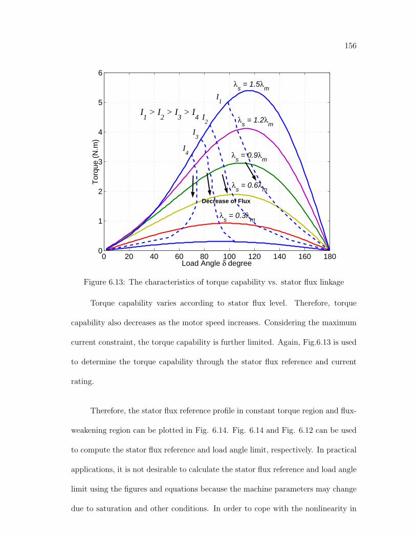
156
0 20 40 60 80 100 120 140 160 1800
1
2
3
4
5
6
Load Angle δ degree
Tor
que
(N.m
)λ
s = 1.5λ
m
Decrease of Flux
I1
I2
I3
I4
λs = 1.2λ
m
λs = 0.9λ
m
λs = 0.6λ
m
λs = 0.3λ
m
I1 > I
2 > I
3 > I
4
Figure 6.13: The characteristics of torque capability vs. stator flux linkage
Torque capability varies according to stator flux level. Therefore, torque
capability also decreases as the motor speed increases. Considering the maximum
current constraint, the torque capability is further limited. Again, Fig.6.13 is used
to determine the torque capability through the stator flux reference and current
rating.
Therefore, the stator flux reference profile in constant torque region and flux-
weakening region can be plotted in Fig. 6.14. Fig. 6.14 and Fig. 6.12 can be used
to compute the stator flux reference and load angle limit, respectively. In practical
applications, it is not desirable to calculate the stator flux reference and load angle
limit using the figures and equations because the machine parameters may change
due to saturation and other conditions. In order to cope with the nonlinearity in

157
(a)
sλ
mλ
emTmaxT
maxsλ
(b)
sλ
maxsλ
minsλ
sω
bω maxω
Figure 6.14: The Stator Flux Reference Profile: (a) Constant torque operationwith MTPA control; (b) Flux-weakening Operation
interior PMSMs, the stator flux reference and load angle limit can be derived from
tables which include the measured values from off-line experiments.
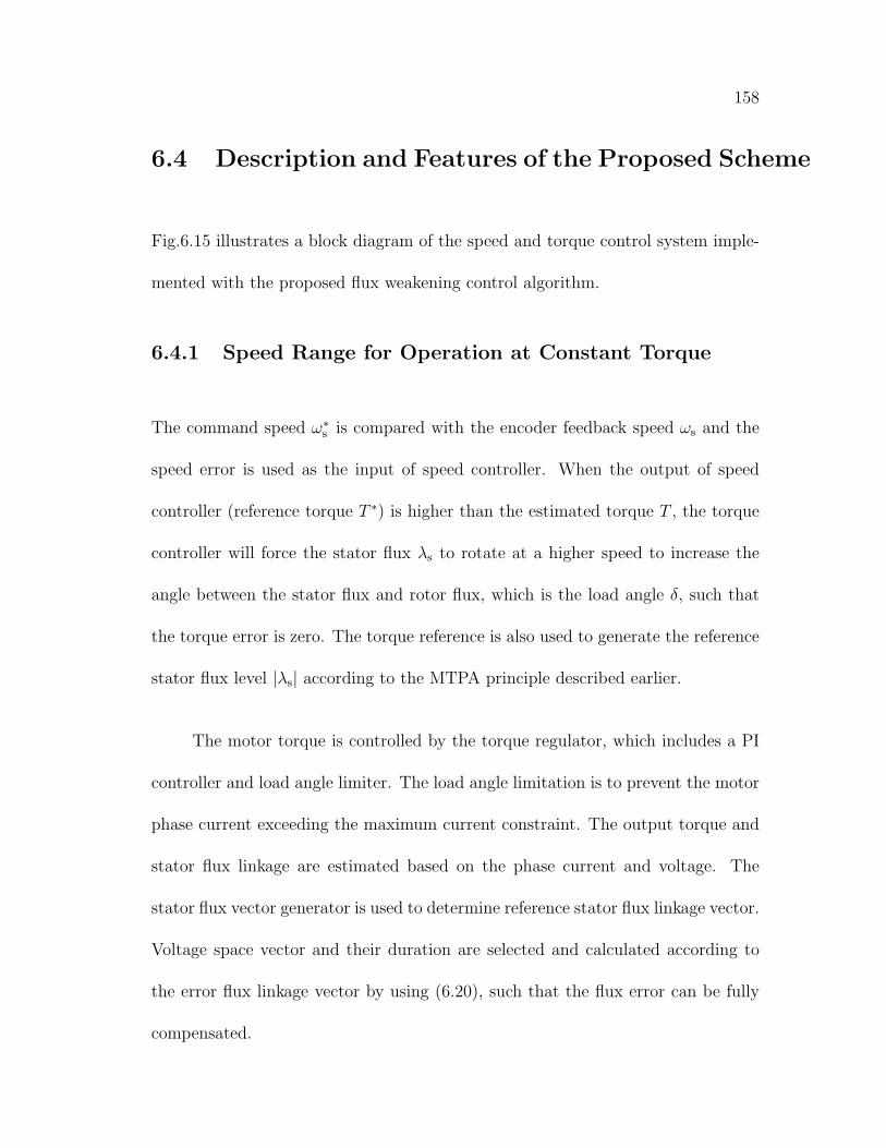
158
6.4 Description and Features of the Proposed Scheme
Fig.6.15 illustrates a block diagram of the speed and torque control system imple-
mented with the proposed flux weakening control algorithm.
6.4.1 Speed Range for Operation at Constant Torque
The command speed ω∗s is compared with the encoder feedback speed ωs and the
speed error is used as the input of speed controller. When the output of speed
controller (reference torque T ∗) is higher than the estimated torque T , the torque
controller will force the stator flux λs to rotate at a higher speed to increase the
angle between the stator flux and rotor flux, which is the load angle δ, such that
the torque error is zero. The torque reference is also used to generate the reference
stator flux level |λs| according to the MTPA principle described earlier.
The motor torque is controlled by the torque regulator, which includes a PI
controller and load angle limiter. The load angle limitation is to prevent the motor
phase current exceeding the maximum current constraint. The output torque and
stator flux linkage are estimated based on the phase current and voltage. The
stator flux vector generator is used to determine reference stator flux linkage vector.
Voltage space vector and their duration are selected and calculated according to
the error flux linkage vector by using (6.20), such that the flux error can be fully
compensated.

159
PI
PI
Stat
or F
lux
Vec
tor
Gen
erat
or
PI
SVM
IPM
*ω
ω*
T
T
δ∆
* sλ∆−
*
0sλ
max
sλ∆
sλ∆
* sλ
sλ
sλ∆=
≈
ωF
lux
and
Tor
que
Est
imat
or
sisv
*
2 sλ
∫rθ
dcV
÷max
sV
Spee
d an
d T
orqu
eC
ontr
olle
r
Flu
x W
eake
ning
Con
trol
ler
ω
max
eT
max
eT−
MT
PA
∗ 1sλ)
,m
in(
21
∗∗
ss
λλ
∗ sλ
δ
αβ
Stat
or F
lux
Lev
elC
alcu
lato
r
∗ sλ
sθ
Figure 6.15: Block diagram of IPMSM drive system
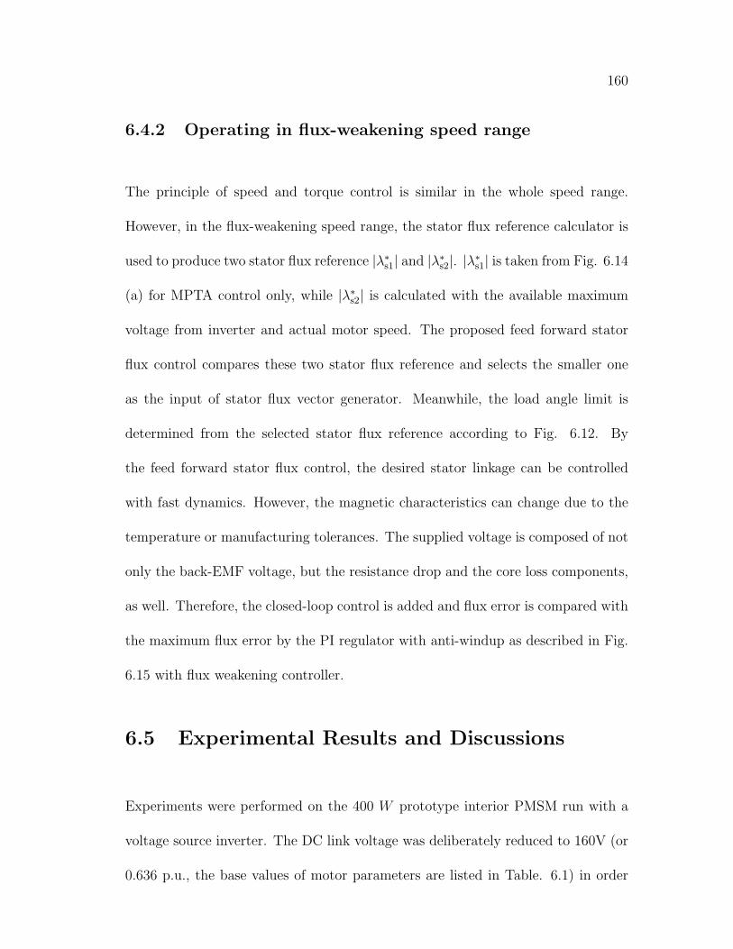
160
6.4.2 Operating in flux-weakening speed range
The principle of speed and torque control is similar in the whole speed range.
However, in the flux-weakening speed range, the stator flux reference calculator is
used to produce two stator flux reference |λ∗s1| and |λ∗
s2|. |λ∗s1| is taken from Fig. 6.14
(a) for MPTA control only, while |λ∗s2| is calculated with the available maximum
voltage from inverter and actual motor speed. The proposed feed forward stator
flux control compares these two stator flux reference and selects the smaller one
as the input of stator flux vector generator. Meanwhile, the load angle limit is
determined from the selected stator flux reference according to Fig. 6.12. By
the feed forward stator flux control, the desired stator linkage can be controlled
with fast dynamics. However, the magnetic characteristics can change due to the
temperature or manufacturing tolerances. The supplied voltage is composed of not
only the back-EMF voltage, but the resistance drop and the core loss components,
as well. Therefore, the closed-loop control is added and flux error is compared with
the maximum flux error by the PI regulator with anti-windup as described in Fig.
6.15 with flux weakening controller.
6.5 Experimental Results and Discussions
Experiments were performed on the 400 W prototype interior PMSM run with a
voltage source inverter. The DC link voltage was deliberately reduced to 160V (or
0.636 p.u., the base values of motor parameters are listed in Table. 6.1) in order
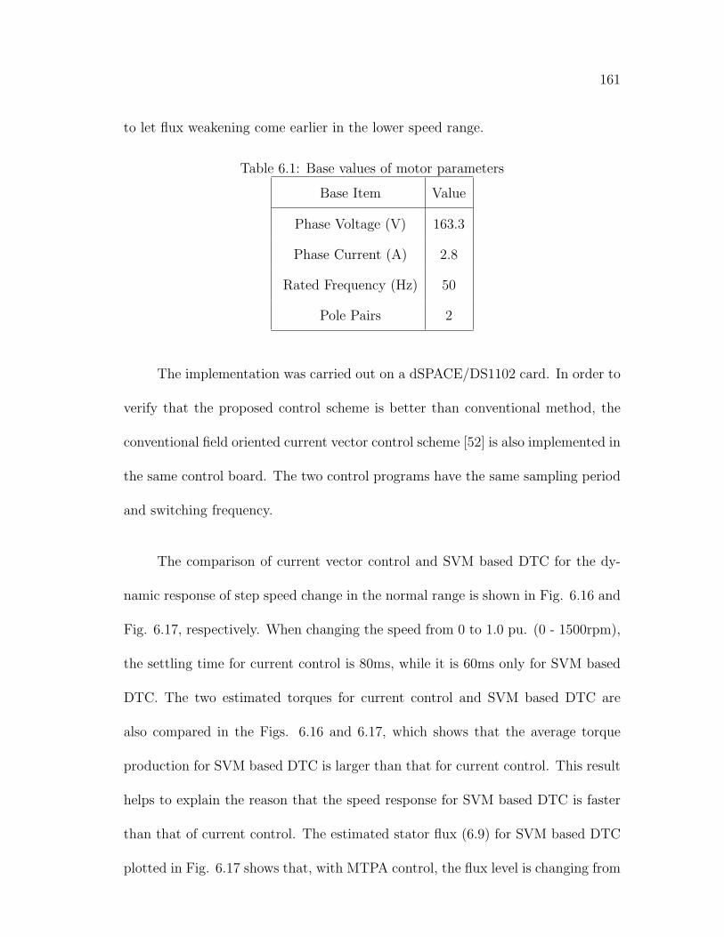
161
to let flux weakening come earlier in the lower speed range.
Table 6.1: Base values of motor parameters
Base Item Value
Phase Voltage (V) 163.3
Phase Current (A) 2.8
Rated Frequency (Hz) 50
Pole Pairs 2
The implementation was carried out on a dSPACE/DS1102 card. In order to
verify that the proposed control scheme is better than conventional method, the
conventional field oriented current vector control scheme [52] is also implemented in
the same control board. The two control programs have the same sampling period
and switching frequency.
The comparison of current vector control and SVM based DTC for the dy-
namic response of step speed change in the normal range is shown in Fig. 6.16 and
Fig. 6.17, respectively. When changing the speed from 0 to 1.0 pu. (0 - 1500rpm),
the settling time for current control is 80ms, while it is 60ms only for SVM based
DTC. The two estimated torques for current control and SVM based DTC are
also compared in the Figs. 6.16 and 6.17, which shows that the average torque
production for SVM based DTC is larger than that for current control. This result
helps to explain the reason that the speed response for SVM based DTC is faster
than that of current control. The estimated stator flux (6.9) for SVM based DTC
plotted in Fig. 6.17 shows that, with MTPA control, the flux level is changing from

162
1.0 to 1.4 p.u. with respect to 1.0 p.u. torque production in the dynamics.
sω
∧
emT
si
p.u.
1.0
0
1.0
0
1.0
0
0 0.1 0.2 0.3 0.4 0.5 s
80 ms
Figure 6.16: Current Control: The dynamic response with step speed change inthe normal range
p.u.
1.0
0
1.0
0
1.0
0
sω
∧
emT
s
Λ
λ
60 ms
0 0.1 0.2 0.3 0.4 0.5 s
Figure 6.17: SVM based DTC: The dynamic response with step speed change inthe normal range
Fig. 6.18 and Fig. 6.19 show the dynamic response for the loading torque
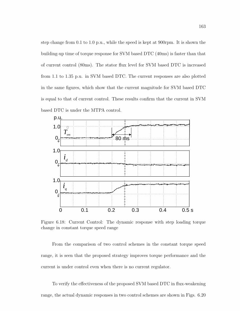
163
step change from 0.1 to 1.0 p.u., while the speed is kept at 900rpm. It is shown the
building-up time of torque response for SVM based DTC (40ms) is faster than that
of current control (80ms). The stator flux level for SVM based DTC is increased
from 1.1 to 1.35 p.u. in SVM based DTC. The current responses are also plotted
in the same figures, which show that the current magnitude for SVM based DTC
is equal to that of current control. These results confirm that the current in SVM
based DTC is under the MTPA control.
∧
emT
di
qi
p.u.
1.0
0
1.0
0
1.0
0
0 0.1 0.2 0.3 0.4 0.5 s
80 ms
Figure 6.18: Current Control: The dynamic response with step loading torquechange in constant torque speed range
From the comparison of two control schemes in the constant torque speed
range, it is seen that the proposed strategy improves torque performance and the
current is under control even when there is no current regulator.
To verify the effectiveness of the proposed SVM based DTC in flux-weakening
range, the actual dynamic responses in two control schemes are shown in Figs. 6.20
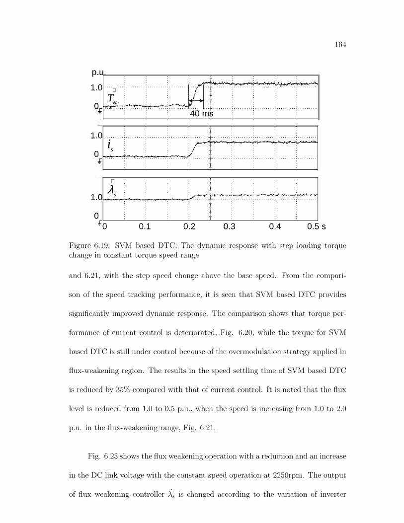
164
p.u.
1.0
0
1.0
0
1.0
0
∧
emT
si
∧
sλ
0 0.1 0.2 0.3 0.4 0.5 s
40 ms
Figure 6.19: SVM based DTC: The dynamic response with step loading torquechange in constant torque speed range
and 6.21, with the step speed change above the base speed. From the compari-
son of the speed tracking performance, it is seen that SVM based DTC provides
significantly improved dynamic response. The comparison shows that torque per-
formance of current control is deteriorated, Fig. 6.20, while the torque for SVM
based DTC is still under control because of the overmodulation strategy applied in
flux-weakening region. The results in the speed settling time of SVM based DTC
is reduced by 35% compared with that of current control. It is noted that the flux
level is reduced from 1.0 to 0.5 p.u., when the speed is increasing from 1.0 to 2.0
p.u. in the flux-weakening range, Fig. 6.21.
Fig. 6.23 shows the flux weakening operation with a reduction and an increase
in the DC link voltage with the constant speed operation at 2250rpm. The output
of flux weakening controller λs is changed according to the variation of inverter
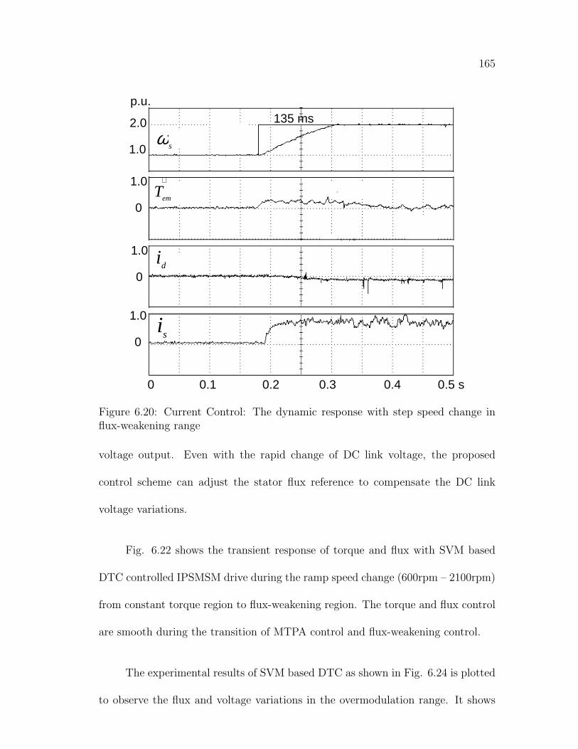
165
sω
∧
emT
di
si
0 0.1 0.2 0.3 0.4 0.5 s
p.u.
2.0
1.0
1.0
0
1.0
0
1.0
0
135 ms
Figure 6.20: Current Control: The dynamic response with step speed change influx-weakening range
voltage output. Even with the rapid change of DC link voltage, the proposed
control scheme can adjust the stator flux reference to compensate the DC link
voltage variations.
Fig. 6.22 shows the transient response of torque and flux with SVM based
DTC controlled IPSMSM drive during the ramp speed change (600rpm – 2100rpm)
from constant torque region to flux-weakening region. The torque and flux control
are smooth during the transition of MTPA control and flux-weakening control.
The experimental results of SVM based DTC as shown in Fig. 6.24 is plotted
to observe the flux and voltage variations in the overmodulation range. It shows

166
sω
∧
emT
ms100
0 0.1 0.2 0.3 0.4 0.5 s
∧
sλ
p.u.
2.0
1.0
1.0
0
si
1.0
0
1.0
0
Figure 6.21: SVM based DTC: The dynamic response with step speed change influx-weakening range
that when there is large step change in speed (from 900rpm to 1800rpm), the
system automatically comes into six step mode operation to provide faster dynamic
response.
Fig. 6.25 and Fig. 6.26 illustrates the operation performance under full DC
link voltage (350V) in a wide speed range with respect to two control schemes:
SVM based DTC and Field Oriented Current Control. As shown in Fig. 6.25, the
maximum torque capability for current control scheme in constant torque region is
better than SVM based DTC scheme, since with field oriented control, the current
vector can be properly controlled (without the voltage saturation) to fully exploit
the reluctance torque and magnet torque. However, the wide speed operation

167
p.u.
2.0
0
1.0
0
1.0
0
ConstantTorque
Operation
Flux-WeakeningOperation
sω
∧
emT
s
Λ
λ
0 0.1 0.2 0.3 0.4 0.5 s
Figure 6.22: Dynamic response of the IPMSM drive system in transition fromconstant torque to flux-weakening regions
dcVV200
V100∧
sλ
sω
0 1.0 2.0 3.0 4.0 5.0 s
p.u.1.0
0.5
2.0
1.0
0
Figure 6.23: Flux Weakening Operation with the variation of DC link voltage

168
αλβλ
aV
0 1.0 S2.0
Figure 6.24: Transient performances of flux and voltage for step speed change influx-weakening range
performance for SVM based DTC is superior than current control as shown in Fig.
6.26 because of the excellent flux-weakening control performance in the SVM based
DTC scheme.
6.6 Conclusion
In this chapter, a novel control strategy for speed and torque control of in interior
PMSM drives has been presented and compared with traditional current vector
control. The control scheme is derived from the basic direct torque control scheme;
it has the advantages of constant switching frequency and reduced torque and flux
ripples. The application of SVM based DTC for interior PMSM drives was inves-
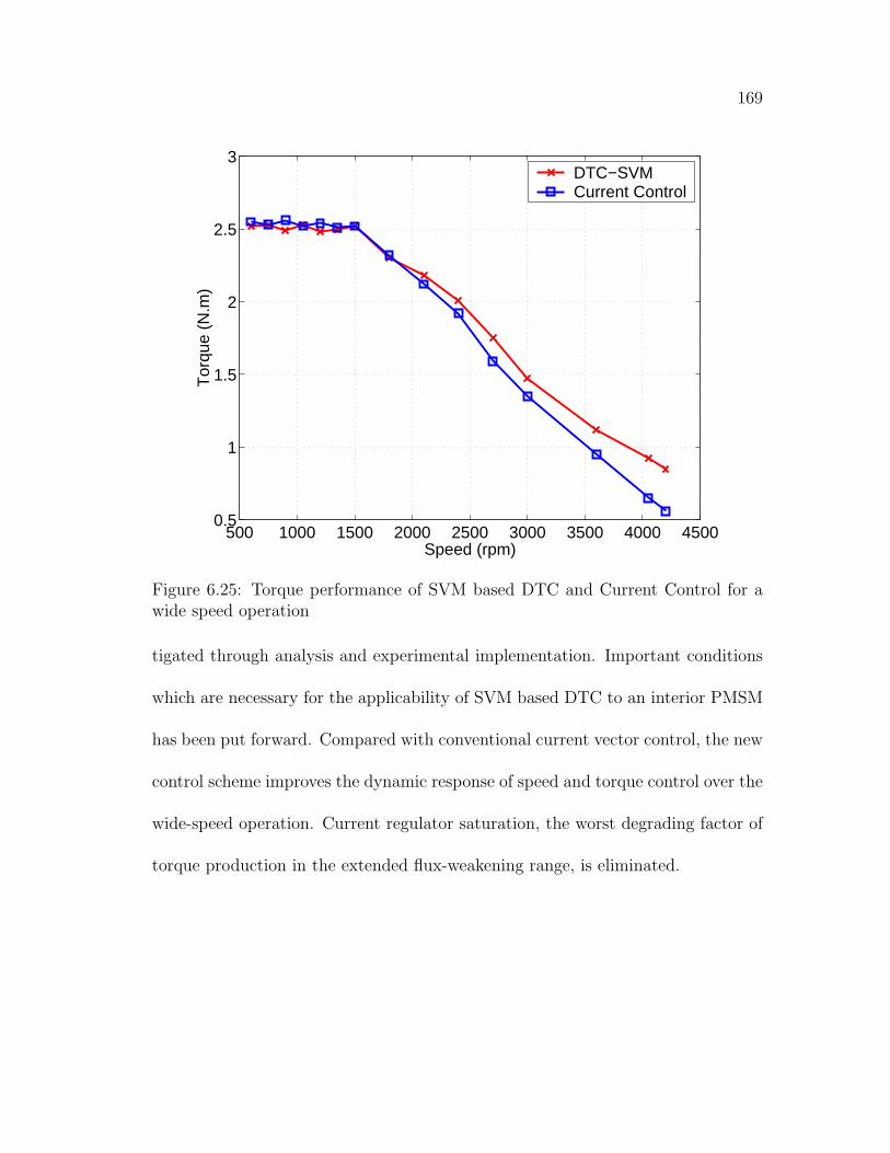
169
500 1000 1500 2000 2500 3000 3500 4000 45000.5
1
1.5
2
2.5
3
Speed (rpm)
Tor
que
(N.m
)
DTC−SVMCurrent Control
Figure 6.25: Torque performance of SVM based DTC and Current Control for awide speed operation
tigated through analysis and experimental implementation. Important conditions
which are necessary for the applicability of SVM based DTC to an interior PMSM
has been put forward. Compared with conventional current vector control, the new
control scheme improves the dynamic response of speed and torque control over the
wide-speed operation. Current regulator saturation, the worst degrading factor of
torque production in the extended flux-weakening range, is eliminated.

170
500 1000 1500 2000 2500 3000 3500 4000 4500150
200
250
300
350
400
450
500
550
Speed (rpm)
Pow
er C
apab
ility
(W
)
DTC−SVMCurrent Control
Figure 6.26: Power performance of SVM based DTC and Current Control for awide speed operation
Chapter 7
Discussions and Conclusions
This thesis examined various aspects of design and control applied to interior
PMSM drive, which required for a wide speed constant power operation. The
two main topics of discussion are the design optimization of a 400W prototype
interior PMSM and the control techniques to exploit the power capability of the
prototype.
7.1 Discussions of Major Work
7.1.1 Analysis of constant power operation
In order to match the interior PMSM with the variable speed control system, an
analysis of the effect of motor parameters on the steady state performance was pre-
sented in Chapter 2. The main purpose is to find out how the parameters affect the
constant power speed range. The torque-speed characteristics under three differ-
ent operating regions (current limited constant torque region, voltage and current
171

172
limit region, and voltage limited maximum power region) were introduced. Based
on the analysis, the constant power speed range of an interior PMSM drive can
be estimated from the motor parameters (Ld, Lq and λm) and voltage and current
constraints. It was suggested that the constant power speed range can be theoret-
ically extended if the interior PMSM is designed with an optimum combination of
motor parameters.
In the mathematical analysis presented, the steady state performance of an
interior PMSM was modelled by constant motor parameters. However, λm, Ld,
and Lq are nonlinear functions of the machine flux level. The simplification of
the interior PMSM’s equivalent circuits to include only three parameters means
that all electrical loss components were ignored. This included both the stator
resistance, as well as hysteresis and eddy-current losses in the machine. The impact
of neglecting iron losses gradually increases as the speed increases because these
iron loss components increase with speed. Magnetic saturation effects were not
included in the analysis. This has particular relevance for interior PMSMs with
high saliency ratios for which q-axis inductance can be significantly affected by
saturation. Therefore, the availability using constant motor parameters in the
analysis has to be justified by following assumptions in the design procedure:
• The prototype interior PMSM was designed with small iron loss at rated
speed, so ignoring these losses did not affect the major predicted trends.
• The developed design methodology was presented with the understanding

173
that the saturation is not dominant effect in the prototype interior PMSM.
7.1.2 Design optimization methodology
In order to design an interior PMSM with the optimum constant power speed
range under certain constraints, an effective design methodology was introduced
in Chapter 3. The key element of the proposed approach is the determination of
motor parameters (Ld, Lq and λm) based on design variables (lm, γ and α), which
was developed using fitted second order RSM models instead of FEM computation.
Hence the time for iterative field computation can be reduced significantly in the
design procedure. These RSM models were built by central composite design with
15 sets of FEM numerical results. Motor parameters (Ld, Lq and λm) obtained by
conventional analytical models and RSM models were compared with the numerical
results by FEM. It was noted that the results by RSM models agree well with
that by FEM. The residual analysis shows the fitted second-order RSM model can
explain about 99% of the variability observed in the responses.
Although the overall accuracy is satisfactory in the design of the prototype in-
terior PMSM, it has to be reminded that this is only valid when the available design
area is relatively small because of a cubic CCD is used to fit the second order RSM
models. The potential optimal solution could be missed by such simplifications.
In order to select appropriate design area, the empirical knowledge from previous
designs can be used to determine the the appropriate range of design variables.
174
Evolution computation is an optimization technique based on ideas of adap-
tation and evolution, which uses primarily real-vector coding, mutation, recombi-
nation, and selection as its primary operators. Mutation is performed by adding
a gaussian distributed random value. The step size (ie. the variance of this dis-
tribution) is usually adapted during the optimization, which should keep the evo-
lutionary process within the Evolution Window. The evolution strategy is robust
and efficient to locate the global optimal area for most complex optimization prob-
lem, however the implementation of such method is complicated and it would take
lots of time to develop the programming and parameter tuning work. The ma-
jor objective of my thesis is to develop a systematic technique which combines
the RSM methodology and optimization algorithms to design the rotor structure.
Using analytical model and numerical analysis, we have concluded that the mo-
tor parameters which determine the motor performances are sigificantly affected
by only three design variables (lm, γ, α). Therefore, considering the simplicity of
optimization work in our application, the basic GAs can fulfil this task to look
for the optimal design. The FEM verifications also confirm the optimal results
provided by the proposed design methodology. However, evolution computation
is more suitable for the design optimization which includes more design variables,
especially for the non-linear model of motor parameters.
The basic Genetic algorithms were used as the optimization technique to
search for the optimum rotor structure which can realize the largest constant power
speed range under voltage and current constraints. The objective function (con-
175
stant power speed range) was calculated from the motor parameters (Ld, Lq and
λm), which was determined by fitted RSM models. It is important to note that the
solution by GAs can be near the optimal but may not be the true optimal because
not all domain of design variables have been explored. The fact is that GAs have
no convergence guarantees in arbitrary problems. But they do sort out interesting
areas of a space quickly and provide solution close to the global optimal. On the
other hand, in this thesis work, we have only three design variables (lm, γ and α)
and the search space is 32 × 32 × 32. The GAs may not be the most efficient op-
timization method to deal with such an simple design case. However, considering
the increased design variables or larger search space in the future work, the GAs
together with RSM models may show their advantages to locate the optimum area
quickly.
7.1.3 Steady state tests of the prototype interior PMSM
A 400W prototype interior PMSM has been fabricated based on the optimized
design described in Chapter 4. Various steady state tests of the prototype interior
PMSM have been reported in Chapter 5. For open circuit and load test, the
measured motor parameters have only 5% variation from those estimated from the
proposed computational approaches as specified in Chapter 3 and Chapter 4. This
fact validates the fitted second order RSM model to estimate the motor parameters.
The tests show that the prototype motor has better torque-speed characteristics
and larger wide speed range of constant power operation than commercial interior
176
PMSM. However, when compared with those predicted from the analysis of the
steady state operation, it has to be pointed out that the experimental constant
power speed range is less than the predicted one. This can be explained as the iron
loss and magnetic saturation were neglected in the design procedure.
The efficiency and power factor of the prototype interior PMSM have been
measured and compared with those of a commercial 400 W interior PMSM. The
comparison indicates that the optimized design realizes the wide-speed constant
power operation with little trade-off in its performance on the rated operation.
7.1.4 Speed and torque control by DTC-SVM
An improved control strategy for speed and torque control of interior PMSM drives
using space vector modulation based on direct torque control in Chapter 6, was pre-
sented and compared with traditional current vector control. The control scheme
is derived from the basic direct torque control scheme; it has the advantages of con-
stant switching frequency and reduced torque and flux ripple. The maximum torque
per ampere control and flux-weakening control using proposed control scheme was
investigated through analysis and experimental implementation in the prototype
interior PMSM. Important conditions which are necessary for the applicability of
SVM based DTC to an interior PMSM has been put forward. Compared with
conventional current vector control, the new control scheme improves the dynamic
response (25% more) on speed and torque control over the wide-speed operation.
However, the selection of stator flux reference level has to be based on the accu-

177
racy of motor parameters under different loading condition, which requires off-line
measurements. Hence, it is also difficult to tune the flux weakening controller.
7.2 Major Contributions of the Thesis
• Analytical model has been developed based on equivalent circuit model of
interior PMSMs, which was used to determine the influence of motor pa-
rameters and inverter power rating on motor output power capability over a
wide speed range. This analysis provides design criterion to obtain optimal
combination of motor parameters in order to achieve a wide speed range of
constant power operation.
• A fitted second-order response surface model for the estimation of motor
parameters has been established based on the central composite design of
finite element computations. The developed RSM model provides an accurate
description of effects of rotor geometric design of the motor parameters of
interior PMSMs.
• A design methodology that combines the RSM model with the GA technique
has been proposed and implemented for the design optimization of an inte-
rior PMSM to realize an optimal constant power speed range. Compared
to traditional analytical methods and finite element methods, the new com-
putational method reduce computing time and effort in estimation of motor
parameters.
• An experimental method for the determination of d- and q-axis inductances

178
has been proposed based on the load test with rotor position feedback. The
measurement of motor parameters not only validate the developed numeri-
cal computation approach, but also improves the speed and torque control
performance of interior PMSMs over a wide speed range.
• The conventional current vector control of interior PMSMs has been imple-
mented for a smooth and accurate stator current control. This method is
particularly suitable for DSP based speed and torque control and leads to
improved torque capability below the rated speed. It is noted that the field-
weakening performance of current vector control is deteriorated because of
the saturation effects of current regulator in the high speed and high current
condition.
• Space vector modulation based direct torque control has been proposed to
overcome the difficulties met in the current vector control. The application of
SVM based DTC for the prototype interior PMSM drive has been investigated
through analysis and experimental implementation. Important conditions
which are necessary for the applicability of SVM based DTC in an interior
PMSM has been put forward.
7.3 Suggestions for Future Research
There are many aspects relevant to permanent magnet synchronous motors that
need to be explored in the future. The following suggestions are made based on
the developments reported in this thesis research:
179
• In Chapter 2 of this thesis, the analysis of interior PMSMs for constant power
operation is based on the theoretical steady state operation of lossless, linear
model of interior type PMSMs. However, actual power capability is limited,
especially at high speed, by motor core losses. Stator core loss has strong
influence on the time harmonics of stator flux density. These harmonic fields
increase as the armature current acts to reduce the magnet flux. Therefore,
a numerical model to calculate the stator core loss is required for accurate
prediction of the power capability of interior PMSMs over a wide speed range.
The second or higher order response surface model may be used to build the
empirical model of stator loss estimation based on the selected design of finite
element experiments.
• In Chapter 3, motor parameters are estimated using fitted second order RSM
models, which are based on geometrical variables only. However, the satu-
rated model of motor parameters are not considered. The potential optimal
design may be missed because of such simplification. Therefore, a saturated
model of motor parameters is necessary for the estimation of saturation ef-
fect due to armature reaction. More design variables including the armature
current can be considered in the fitted RSM models.
• The idea of hybrid optimization method may be used in the similar research.
We can start the search using a genetic algorithm to sort out the interesting
peaks in the problem. Once the GA finds out the best regions, then a locally
convergent scheme can be used to climb the local peaks. In this way, we can

180
combine the globality and parallelism of the GA with the more convergent
method by the local technique.
• In the proposed space vector modulation based direct torque control of in-
terior PMSM presented in Chapter 6, the stator flux linkage is selected to
realize the maximum output torque with minimum input armature current.
The selection is actually an off-line calculation based on the motor parame-
ters, which is seriously parameter dependent and may not result in an ideal
control performance over a wide speed range. The intelligent optimal con-
trol theory may be applied in the control algorithms to select the stator flux
linkage with on-line calculations.

Reference
[1] J. F. Gieras and M. Wing, Permanent Magnet Motor Technology (Design and
Application). Marcel. Dekker, Inc, second edition, revised and expanded ed.,
2002.
[2] P. Pillay and R. Krisnan, “Modeling, simulation, and analysis of perma-
nent magnet motor drives,” IEEE Trans. on Industry Application, vol. IA-25,
pp. 265–279, March/April 1989.
[3] T.-S. Low, M. A. Jabbar, and M. A. Rahman, “Permanent-magnet motors for
brushless operation,” IEEE Transactions on Industry Applications, vol. 26,
pp. 124–129, Jan/Feb 1990.
[4] T. M. Jahns, “Motion control with permanent-magnet ac machines,” Proceed-
ings of The IEEE, vol. 82, pp. 1241–1252, August 1994.
[5] G. R. Slemon, “Electrical machines for variable-frequency drives,” Proceedings
of The IEEE, vol. 82, pp. 1123–1139, August 1994.
[6] M. Satoh, M. Tomita, and S. Kanedo, “Comparison between spm motors and
ipm motors for compressors of air-conditioners,” IPEC, Tokyo, pp. 1286–1289,
2000.
181

182
[7] T. M. Jahns, “Interior permanent-magnet synchronous motors for adjustable-
speed drives,” IEEE Transactions on Industry Application, vol. IA-22,
pp. 738–746, July/August 1986.
[8] G. R. Slemon, Electric Machines and Drives. Addison Wesley, 1992.
[9] T. J. E. Miller, Brushless permanent-magnet and reluctance motor drive. Ox-
ford, London: Claredon Press, 1989.
[10] P. C. Sen, Principles of electric machines and power electronics. New York:
J. Wiley and Sons, second ed., 1997.
[11] R. Krishnan, Electric Motor Drives: Modeling, Analysis, and Control. Prentice
Hall, 2001.
[12] B. Stumberger, A. Hamler, M. Trlep, and M. Jesenik, “Analysis of interior
permanent magnet synchronous motor designed for flux weakening operation,”
IEEE Tranaction on Magnetics, vol. 37, pp. 3644–3647, September 2001.
[13] T. M. Jahns, “Flux-weakening regime operation of an interior permanent-
magnet synchronous motor drive,” IEEE Transaction on Industry Application,
vol. IA-23, pp. 681–689, July/August 1987.
[14] R. F. Schiferl and T. A. Lipo, “Power capability of salient pole permanent mag-
net synchronous motors in variable speed drive applications,” IEEE Transac-
tions on Industry Applications, vol. 26, pp. 115–123, January/February 1990.
[15] D. M. Ionel, J. F. Eastham, T. J. E. Miller, and E. Demeter, “Design consid-
erations for pm synchronous motors for flux weakening applications,” Inter-

183
national Conference on Electrical Machines and Drives, no. 444, pp. 371–375,
1997.
[16] W. L. Soong, D. A. Staton, and T. J. E. Miller, “Design of a new axially-
laminated interior permanent magnet motor,” IEEE Transaction on Industry
Application, vol. 31, pp. 358–367, Mar/Apr 1995.
[17] D. M. Ionel, J. F. Eastham, and T. Betzer, “Finite element analysis of a novel
brushless dc motor with flux barriers,” IEEE Transacion of Magnetics, vol. 31,
pp. 3749–3751, November 1995.
[18] N. Bianchi, S. Bolognani, and B. J. Chalmers, “Salient-rotor pm synchronous
motors for an extended flux-weakening operation range,” IEEE Transaction
on Industry Application, vol. 36, pp. 1118–1125, July/August 2000.
[19] G. R. Slemon, “On the design of high-performance surface-mounted pm mo-
tors,” IEEE Transaction on Industry Application, vol. 30, pp. 134–140, Jan-
uary 1994.
[20] G. R. Slemon and X. Liu, “Modelling and design optimization of permanent
magnet motors,” Electric Machines and Power Systems, vol. 20, pp. 71–92,
1992.
[21] B. P. Panigrahi and K. C. Patra, “Design of a permanent magnet synchronous
motor,” Electric Machine and Power System, vol. 27, pp. 771–779, 1999.
[22] L. Qinghua, M. A. Jabbar, and A. M. Khambadkone, “Design optimisation of
wide-speed permanent magnet synchronous motors,” in Proceedings of Inter-

184
national Conference on Power Electronics, Machines and Drives, (Bath, UK),
pp. 404–408, April 2002.
[23] L. Qinghua, M. A. Jabbar, and A. M. Khambadkone, “Design optimisation of
interior permanent magnet synchronous motors for wide-speed operation,” in
Proceedings of The 4th IEEE International Conference on Power Electronics
and Drive Systems, (Bali, Indonesia), pp. 475–478, October 2001.
[24] L. Xu and L. Ye, “A new design concept of permanent magnet machine for
flux weakening operation,” IEEE Transaction on Industry Application, vol. 31,
pp. 373–378, March/April 1995.
[25] J. C. Teixeira, C. Chillet, and J. P. Yonnet, “Structure comparison of buried
permanent magnet synchronous motors for flux weakening operation,” Inter-
national Conference on Electrical Machines and Drives, pp. 365–370, 1993.
[26] M. Hippner and R. G. Harley, “Looking for an optimal rotor for high speed
permanent magnet synchronous machine,” Industry Applications Society An-
nual Meeting, vol. 1, pp. 265–270, 1992.
[27] Z. P. M. A. Rahman and M. A. Jabbar, “Field circuit analysis of perma-
nent magnet synchronous motors,” IEEE Transaction on Magnetics, vol. 30,
pp. 1350–1359, July 1994.
[28] O. A. Mohammed and G. F. Uler, “A hybrid technique for the optimal design
of electromagnetic devices using direct search and genetic algorithms,” IEEE
Transaction on Magnetics, vol. 33, pp. 1892–1895, May 1997.

185
[29] A. Gottvald, K. Preis, C. Magele, O. Biro, and A. Savini, “Global optimization
methods for comutational electromagnetics,” IEEE Transaction on Magnetics,
vol. 28, pp. 1537–1540, Mar 1992.
[30] N. Bianchi and S. Bolognani, “Brushless dc motor design: an optimization
procedure using genetic algorithms,” in Proceedings of IEE Electrical machines
and drives conference, (Cambridge, UK), pp. 16–20, IEE, September 1997.
[31] G. F. Uler, O. A. Mohammed, and C.-S. Koh, “Utilizing genetic algorithms
for the optimal design of electromagnetic devices,” IEEE Transaction on Mag-
netics, vol. 30, pp. 4296–4298, November 1994.
[32] N. Bianchi and S. Bolonani, “Design optimization of electric motors by ge-
netic algorithms,” IEE Proceeding on Electric and Power Application, vol. 145,
pp. 475–483, September 1998.
[33] T. Renyuan and Y. Shiyou, “Combined strategy of improved simulated an-
nealing and genetic algorithm for inverse problem,” in 10th Conference on the
Computation of Electromagnetic Fields COMPUMAG’95, (Berlin, Germany),
pp. 196–197, 1995.
[34] M. Kasper, “Shape optimization of by evolution strategy,” IEEE Transaction
on Magnetics, vol. 28, pp. 1556–1560, Mar 1992.
[35] T. Higuchi, J. Oyama, and E. Yamada, “Optimization procedure of surface pm
synchronous motors,” IEEE Transaction on Magnetics, vol. 33, pp. 1943–1946,
March 1997.

186
[36] C. Schatzer and A. Binder, “Design optimization of a high-speed permanent
magnet machine with the vekopt algorithms,” Industry Application Confer-
ence, IEEE, vol. 1, pp. 439–444, 2000.
[37] J. K. Lahteenmaki, “Optimization of high-speed motors using a genetic al-
gorithm,” International Conference on Electric Machines and Drives, IEE,
vol. 1, pp. 26–30, September 1997.
[38] R. H. Myers and D. C. Montgomery, Response Surface Methodology, Press and
Product Optimization Using Designed Experiments. JOHN WILEY SONS,
INCQ, 2002.
[39] A. I. Khuri and J. A. Cornell, Response Surfaces, Designs and Analysis. Marcel
Dekker, Inc, 1996.
[40] R. Rong and D. A. Lowther, “Applying response surface methodology in the
design and optimization of electromagnetic devices,” IEEE Transaction on
Magnetics, vol. 33, pp. 1916–1919, March 1997.
[41] F. Gillon and P. Brochet, “Screening and response surface method applied to
the numerical optimization of electromagnetic devices,” IEEE Transaction on
Magnetics, vol. 36, pp. 1163–1167, July 2000.
[42] G. X. Ke, T. S. Low, L. Z. Jie, and C. S. Xin, “Robust design for torque op-
timization using response surface methodology,” IEEE Transaction on Mag-
netics, vol. 38, pp. 1141–1144, March 2002.

187
[43] Y. Fujishima, S. Wakao, A. Yamashita, and T. Katsuta, “Design optimization
of a permanent magnet synchronous motor by the response surface methodol-
ogy,” Journal of Applied Physics, vol. 91, pp. 8305–8307, May 2002.
[44] D.-H. Cho, H.-K. Jung, and D.-J. Sim, “Multiobjective optimal design of
interior permanent magnet synchronous motors considering improved core loss
formula,” IEEE Transaction on Energy Conversion, vol. 14, pp. 1347–1352,
December 1999.
[45] B. K. Bose, “A high-performance inverter-fed drive system of an interior pm
synchronous machine,” IEEE Transaction on Industry Application, vol. 24,
pp. 987–997, Nov/Dec 1988.
[46] A. B. Kulkarni and M. Ehsani, “A novel position sensor elimination technique
for the interior pm synchronous motor drive,” IEEE IAS Annual Meeting
Record, pp. 773–779, 1989.
[47] G. R. Slemon, “Operating limits of inverter-driven permanent magnet motor
drives,” IEEE Transaction on Industry Applications, vol. IA-23, pp. 327–332,
March/April 1987.
[48] M. P. Kaxmeirkowski and M. A. Dzieniakowski, “Novel current regulator
for vsi-pwm inverters,” Proceed of European Power Electronics Conference,
Aachen, 1989.

188
[49] M. N. Uddin, T. S. Radwan, G. H. George, and M. A. Rahman, “Performance
of current controllers for vsi-fed ipmsm drives,” IEEE Transaction on Industry
Applications, vol. 36, pp. 1531–1538, November/December 2000.
[50] S. Morimoto, Y. Takeda, and T. Hirasa, “Current phase control methods
for permanent magnet synchronous motors,” IEEE Trans. Power Electronics,
vol. 5, pp. 133–139, Apr. 1990.
[51] S. Morimoto, M. Sanada, and Y. Takeda, “Wide-speed operation of interior
permanent magnet synchronous motors with high-performance current regu-
lator,” IEEE Trans. Ind. Applicat., vol. 30, pp. 920–926, July/Aug 1994.
[52] J. M. Kim and S. K. Sul, “Speed control of interior permanent magnet syn-
chronous motor drive for the flux weakening operation,” IEEE Transaction on
Industry Applications, vol. 33, pp. 43–48, January/February 1997.
[53] B. J. Chalmers, “Influence of saturation in brushless permanent-magnet motor
drives,” IEE Proc., vol. 139, pp. 51–52, Jan 1992.
[54] B. J. Chalmers, R. Akmese, and L. Musada, “Validation of procedure for
prediction of field-weakening performance of brushless synchronous machines,”
Proc. ICEM 1998, Istanbul, Turkey, vol. 1, pp. 320–323, 1998.
[55] E. C. Lovelance, T. M. Jahns, and J. H. Lang, “Impact of saturation and
inverter cost on interior pm synchronous machine drive optimization,” IEEE
Trans. Ind. Applicat., vol. 36, pp. 723–729, MAY/JUNE 2000.

189
[56] C. Mademlis and V. G. Agelidis, “On considering magnetic saturation with
maximum torque to current control in interior permanent magnet synchronous
motor drives,” IEEE Trans. on Energy Conversion, vol. 16, pp. 246–252,
September 2001.
[57] J. H. Song, J. M. Kim, and S. K. Sul, “A new robust spmsm control to param-
eter variations in flux weakening region,” IEEE IECON, vol. 2, pp. 1193–1198,
1996.
[58] H. Le-Huy, K. Slimani, and P. Viarouge, “A predictive current controller for
synchronous motor drives,” Proceeding of EPE Conf., vol. 2, pp. 114–119,
1991.
[59] A. Verl and M. Bodson, “Torque maximization for permanent magnet syn-
chronous motors,” IEEE Trans. Contr. Syst. Technol., vol. 6, pp. 740–745,
Nov. 1998.
[60] E. Cerruo, A. Consoli, A. Raciti, and A. Testa, “Adaptive fuzzy control of
high performance motion systems,” IEEE Proceeding of Industrial Electronics
Conf. (IECON), pp. 88–94, 1992.
[61] Z. Q. Zhu, Y. S. Chen, and D. Howe, “Online optimal flux-weakening control of
permanent-magnet brushless ac drives,” IEEE Trans. on Ind. Applicat, vol. 36,
pp. 1661–1668, Nov/Dec 2000.

190
[62] S. Henneberger, U. Pahner, and R. Belmans, “Computation of a highly sat-
urated permanent magnet synchronous motor for a hybrid electric vehicle,”
IEEE Trans. Magnetics, vol. 33, Sept 1997.
[63] R. B. Colby and D. W. Novotny, “An efficiency-optimizing permanent magnet
synchronous motor drive,” IEEE Trans. Industry Appliations, vol. 24, pp. 462–
469, May/June 1988.
[64] J.-J. Chen and K.-P. Chin, “Minimum copper loss flux-weakening control of
surface mounted permanent magnet synchronous motors,” IEEE Transactions
on Power Electronics, vol. 18, pp. 929–936, July 2003.
[65] S. Morimoto, T. Ueno, and M. Sanada, “Effects and compensation of mag-
netic saturation in permanent magnet synchronous motor drives,” IEEE IAS
Annual Meeting, vol. 3, no. 6, pp. 59–64, 1993.
[66] R. B. Sepe and J. H. Lang, “Real-time adaptive control of the permanent
magnet synchronous motor,” IEEE Trans. Ind. Applicat, vol. 27, pp. 706–714,
July/Aug 1991.
[67] J. K. Seok and S.-K. Sul, “A new overmodulation strategy for induction motor
drive using space vector pwm,” Proc. IEEE APEC, vol. 1, pp. 211–216, Mar
1995.
[68] J. Shi and Y. S. Lu, “Field-weakening operation of cylindrical permanent-
magnet motors,” Proc. IEEE Int. Conf. Contr. Applicat, pp. 864–869, Sept.
1996.

191
[69] L. Zhong, M. F. Rahman, W. Y. Hu, and K. W. Lim, “Analysis of direct torque
control in permanent magnet synchronous motor drives,” IEEE Transaction
on Power Electronics, vol. 12, pp. 528–536, May 1997.
[70] M. F. Rahman, L. Zhong, and K. W. Lim, “A direct torque-controlled interior
permanent magnet synchronous motor drive incorporating field weakening,”
IEEE Transaction on Industry Application, vol. 34, pp. 1246–1253, Novem-
ber/December 1998.
[71] J. Faiz and S. H. Mohseni-Zonoozi, “A novel technique for estimation and
control of stator flux of a salient-pole pmsm in dtc method based on mtpf,”
IEEE Transaction on Industrial Electronics, vol. 50, pp. 262–271, April 2003.
[72] I. Takahashi and T. Noguchi, “A new quick-response and high-efficiency con-
trol strategy of an induction motor,” IEEE Transaction on Industry Applica-
tion, vol. 22, pp. 820–827, September/October 1986.
[73] M. Depenbrock, “Direct self-controlled (dsc) of inverter fed induction ma-
chine,” IEEE Transaction on Power Electronics, vol. 3, pp. 420–429, October
1988.
[74] D. Casadei, F. Profumo, G. Serra, and A. Tani, “Foc and dtc: Two viable
scheme for induction motors torque control,” IEEE Transaction on Power
Electronics, vol. 17, pp. 779–787, September 2002.
[75] P. Vas, Sensorless Vector and Direct Torque Control. Oxford University Press,
1998.
192
[76] C. Martins, X. Roboam, T. A. Meynard, and A. S. Caryalho, “Switching
frequency imposition and ripple reduction in dtc drives by using a multilevel
converter,” IEEE Transaction on Power Electronics, vol. 17, March 2002.
[77] C. Lascu, I. Boldea, and F. Blaabjerg, “A modified direct torque control for
induction motor sensorless drive,” IEEE Transaction on Industry Application,
vol. 36, pp. 122–130, Jan/Feb 2000.
[78] Y. S. Lai and J. H. Chen, “A new approach of induction motor drives for con-
stant inverter switching frequency and torque ripple reduction,” IEEE Trans-
action on Energy Conversion, vol. 16, pp. 220–227, September 2001.
[79] C. E. Moucary, E. Mendes, and A. Razek, “Decoupled direct control for pwm
inverter-fed induction motor drives,” IEEE Transaction on Industry Applica-
tions, vol. 38, pp. 1307–1315, September 2002.
[80] D. Novotny and T. Lipo, Vector control and dynamics of AC drives. London:
Clarendon Press, 1996.
[81] L. W. Matsch and J. D. Morgan, Electromagnetic and Electromechanical Ma-
chines. John Wiley and Sons, thrid ed., 1986.
[82] T. Sebastian, G. R. Slemon, and M. A. Rahman, “Modelling of permanent
magnet synchronous motors,” IEEE Transaction on Magnetics, vol. Mag-22,
pp. 1069–1071, September 1986.

193
[83] M. A. Rahman and A. M. Osheiba, “Performance of large line-start permanent
magnet synchronous motors,” IEEE Transaction on Energy Conversion, vol. 5,
pp. 211–217, March 1990.
[84] P. C. Krause, O. Wasynczuk, and S. D. Sudhoff, Analysis of Electric Machinery
and Drive Systems. IEEE Press: Wiley-Interscience, second ed., 2002.
[85] T. Sebastian, G. R. Slemon, and M. A. Rahman, “Design consideration for
variable speed permanent magnet motors,” Proceedings, International Confer-
ence on Electrical Machines, pp. 1099–1102, September 1986.
[86] D. E. Goldberg, Genetic Algorithms in Search, Optimization and Machine
Learning. MA: Addison Wesley, 1989.
[87] L. Tang, L. Zhong, M. F. Rahman, and Y. Hu, “An investigation of a modified
direct torque control strategy for flux and torque ripple reduction for induction
machine drive system with fix switching frequency,” in Conf. Rec. IAS’02, 37th
IEEE IAS Annual Meeting, (Pittsburgh, USA), 13-18 Oct. 2002.
[88] M. Fu and L. Xu, “A sensorless direct torque control technique for perma-
nent magnet synchronous motors,” in Industry Applications Conference, 1999.
Thirty-Fourth IAS Annual Meeting. Conference Record of the 1999 IEEE,
vol. 1, pp. 159–164, 3-7 Oct 1999.
[89] L. Tang, L. Zhang, M. F. Rahman, and Y. Hu, “A novel direct torque con-
trolled interior permanent magnet synchronous machine drive with low ripple

194
in flux and torque and fixed switching frequency,” Power Electronics, IEEE
Transactions on, vol. 2, pp. 346–354, March 2004.
[90] A. Tripathi, A. M. Khambadkone, and S. K. Panda, “Predictive stator flux
cotnrol with overmodulation and dynamic torque control at constant switching
frequency in ac drives,” in Conf. Rec. IECON’02, pp. 1219–1224, Nov 30- Dec
4 2002.
[91] L. Qinghua, A. M. Khambadkone, and M. A. Jabbar, “Direct flux control of
interior permanent magnet synchronous motors for wide-speed operation,” in
Power Electronics and Drive Systems, 2003. PEDS 2003. The Fifth Interna-
tional Conference on, vol. 2, pp. 1680 – 1685, NOV. 2003.
[92] A. M. Khambadkone and J. Holtz, “Compenstated synchronous pi current
controller in overmodulation range and six-step operation of space-vector-
modulation-based vector-controlled drives,” IEEE Transaction on Industrial
Electronics, vol. 49, pp. 574–579, June 2002.

Appendix A
Design Details for The PrototypeInterior PMSM
52.00mm
74.00mm
D: (4.7, 30.3)mm
B: (4.7, 35.7)mm
A: (3.6, 35.7)mm
C: (3.6, 29.9)mm
H: (30.3, 4.7)mm
F: (35.7, 4.7)mm
E: (35.7, 3.6)mm
G: (29.9, 3.6)mm
Tolerence mm10.±A B
C D
E
F
G
H
R 10.00mm
R 37.00mm
20.00mm
1/4 rotor
(0,0)
36.20mm
1.0mm
Figure A.1: Rotor mechanical design drawing
195

196
12
34
56
78
910
1112
1314
1516
1718
1920
2122
2324
3 ph
ase,
24
slot
s, 4
pol
e,D
oubl
e L
ayer
Lap
Win
ding
RS
BF
YSB
SR
FYF
Figure A.2: Stator winding distribution
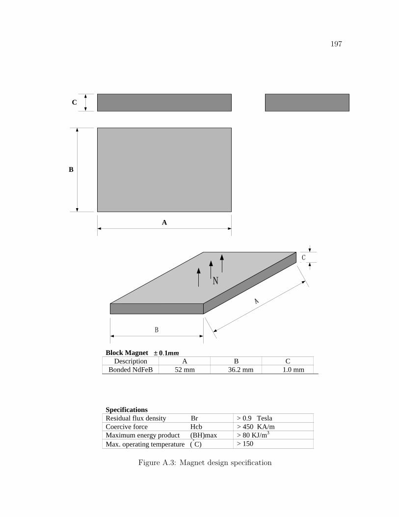
197
A
B
C
C
B
A
N
Block MagnetDescription A B C
Bonded NdFeB 52 mm 36.2 mm 1.0 mm
SpecificationsResidual flux density Br > 0.9 TeslaCoercive force Hcb > 450 KA/mMaximum energy product (BH)max > 80 KJ/m3
Max. operating temperature (°C) > 150
mm10.±
Figure A.3: Magnet design specification
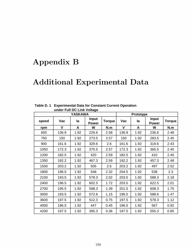
Appendix B
Additional Experimental Data
Table D. 1 Experimental Data for Constant Current Operationunder Full DC Link Voltage
YASKAWA Prototype
speed Vac IaInput
PowerTorque Vac Ia
Input Power
Torque
rpm V A W N.m V A W N.m600 136.9 1.92 226.6 2.58 136.9 1.92 236.6 2.48
750 150 1.92 273.5 2.57 150 1.92 283.5 2.45
900 161.6 1.92 329.6 2.6 161.6 1.92 319.6 2.43
1050 172.3 1.92 375.5 2.57 172.3 1.92 365.5 2.45
1200 182.5 1.92 420 2.59 182.5 1.92 410 2.45
1350 192.2 1.92 467.3 2.59 192.2 1.92 457.3 2.48
1500 203.2 1.92 505 2.6 203.2 1.92 497 2.52
1800 196.5 1.92 548 2.32 204.5 1.92 538 2.3
2100 193.5 1.92 578.3 2.02 203.5 1.92 588.3 2.18
2400 196.5 1.92 602.5 1.72 203.5 1.92 622.5 2.01
2700 195.5 1.92 598.3 1.39 201.5 1.92 608.3 1.75
3000 193.5 1.92 572.6 1.15 196.5 1.92 588.6 1.47
3600 197.5 1.92 512.3 0.75 197.5 1.92 578.3 1.12
4050 196.5 1.92 447 0.45 196.5 1.92 567 0.92
4200 197.5 1.92 395.3 0.36 197.5 1.92 555.3 0.85
198

199
Table D. 2 Experimental Data for Constant Current Operationunder 75% Full DC Link Voltage
YASKAWA Prototype
speed Vac IaInput
PowerTorque Vac Ia
Input Power
Torque
rpm V A W N.m V A W N.m450 116.5 1.92 204.2 2.56 106.5 1.92 195.5 2.48600 135 1.92 262.1 2.59 125 1.92 247.5 2.45750 150.2 1.92 313.6 2.57 140.2 1.92 295.6 2.47900 165.1 1.92 358.7 2.6 155.1 1.92 345 2.45
1050 163.6 1.92 380 2.39 163.6 1.92 390 2.461200 162.3 1.92 390.3 2.25 162.3 1.92 405.3 2.311500 163.6 1.92 419.6 1.93 163.6 1.92 425.6 2.131800 167.4 1.92 415.6 1.65 167.4 1.92 445.6 1.862100 163 1.92 382.5 1.29 163 1.92 424.5 1.562400 165.4 1.92 358.6 1.08 165.4 1.92 408.6 1.332700 163.9 1.92 325.4 0.79 163.9 1.92 385.4 1.013000 168.4 1.92 293.5 0.52 168.4 1.92 353.5 0.713300 169.3 1.92 255.2 0.24 169.3 1.92 305.2 0.463600 167.8 1.92 275.7 0.28
Table D. 3 Experimental Data for Constant Current Operationunder 50% Full DC Link Voltage
YASKAWA Prototype
speed Vac IaInput
PowerTorque Vac Ia
Input Power
Torque
rpm V A W N.m V A W N.m100 75.5 1.92 79.5 2.55 83.5 1.92 77.6 2.43200 85.6 1.92 113.5 2.52 94.7 1.92 112.7 2.44300 93.7 1.92 145.3 2.56 102.9 1.92 146 2.42400 102.5 1.92 180.5 2.5 113.6 1.92 181.6 2.46500 105.3 1.92 205.6 2.46 123.8 1.92 212.3 2.45600 109.5 1.92 230.5 2.36 128.5 1.92 239.1 2.46700 118.3 1.92 258.5 2.25 131.5 1.92 274 2.43800 120.5 1.92 269.2 1.93 130.5 1.92 279.2 2.1
1000 118.5 1.92 265 1.43 119.5 1.92 278 1.561200 117.3 1.92 253 0.98 111.3 1.92 263 1.131500 113.4 1.92 225 0.46 103.4 1.92 235 0.66
List of Publications
Conferences
1. Jabbar, M.A.; Khambadkone, A.M. and Liu Qinghua, “Design and Analysis
of Exterior and Interior Type High-Speed Permanent Magnet Motors”, Aus-
tralasian Universities Power Engineering Conference (AUPEC), Sep-2001,
Pages: 472-476
2. Liu Qinghua; Jabbar, M.A. and Khambadkone, A.M., “Design optimization
of interior permanent magnet synchronous motors for wide- speed operation”,
The 4th IEEE International Conference on Power Electronics and Drive Sys-
tems, 2001. Proceedings Volume: 2 , 22-25 Oct. 2001, Pages:475 - 478
3. Liu Qinghua; Jabbar, M.A. and Khambadkone, A.M., “Design optimization
of wide-speed permanent magnet synchronous motors”; International Confer-
ence on Power Electronics, Machines and Drives, PEMD2002. (Conf. Publ.
No. 487) , 4-7 June 2002 Pages:404-408
4. Liu Qinghua; Khambadkone A.M. and Tripathi A. and Jabbar M.A., “Torque
Control of IPMSM Drives using Direct Flux Control for Wide Speed Oper-
ation,” IEEE International Electric Machines and Drives Conference, June
200
201
2003, Pages: 188 - 193.
5. Liu Qinghua; Khambadkone, A.M. and Jabbar, M.A., “Direct flux control
of interior permanent magnet synchronous motor drives for wide-speed op-
eration” The Fifth International Conference on Power Electronics and Drive
Systems, 2003, PEDS 2003. Volume: 2 , 17-20 Nov. 2003 Pages:1680 - 1685
6. Liu Qinghua; Jabbar, M.A. and Khambadkone, A.M., “Response surface
methodology based design optimisation of interior permanent magnet syn-
chronous motors for wide-speed operation”, The Second International Con-
ference on Power Electronics, Machines and Drives (PEMD 2004), Conf.
Publ. No. 498 ,Volume: 2 , March 31, - April 2, 2004 Pages:546 - 551
Submitted for Review
1. Liu Qinghua; Jabbar, M.A. and Khambadkone, A.M., “Design And Exper-
imental Verification Of An Interior Permanent Magnet Synchronous Motor
For Wide Speed Operation”, IEE Journal on Electric Power Applications
To be Submitted
1. Liu Qinghua; Jabbar, M.A.; and Khambadkone, A.M., “Response Surface
Methodology Based Design Optimisation of Interior Permanent Magnet Syn-
chronous Motors for Wide-Speed Operation ”, IEE Journal on Electric Power
Applications

202
2. Liu Qinghua; Jabbar, M.A. amd Khambadkone, A.M., “Space Vector Mod-
ulation based Direct Torque Control of Interior Permanent Magnet Syn-
chronous Motor Drives for the Flux Weakening Operation”, IEEE Trans-
actions on Energy Conversion