THESIS

AN OBSERVATIONAL CLIMATOLOGY OF MIDLATITUDE MESOSCALE 

CONVECTIVE VORTICES

Submitted by

Eric James

Department of Atmospheric Science

In partial fulfillment of the requirements

For the Degree of Master of Science

Colorado State University

Fort Collins, Colorado

Spring 2009

1

COLORADO STATE UNIVERSITY

January 29, 2009

WE HEREBY RECOMMEND THAT THE THESIS PREPARED UNDER OUR SUPERVISION BY ERIC JAMES ENTITLED AN OBSERVATIONAL CLIMATO­LOGY OF MIDLATITUDE MESOSCALE CONVECTIVE VORTICES BE ACCEP­TED AS FULFILLING IN PART REQUIREMENTS FOR THE DEGREE OF MASTER OF SCIENCE.

Committee on Graduate Work

___________________________________________Committee Member Dr. Steven Rutledge

___________________________________________Outside Committee Member Dr. Jorge Ramirez

___________________________________________Advisor  Dr. Richard Johnson

___________________________________________Department Head  Dr. Richard Johnson

2

ABSTRACT OF THESIS

AN OBSERVATIONAL CLIMATOLOGY OF MIDLATITUDE MESOSCALE 

CONVECTIVE VORTICES

Climatological   characteristics   of   45   mesoscale   convective   vortices   (MCVs) 

occurring over the state of Oklahoma during the late spring and summer of four years are 

summarised.    The MCV cases are selected based on vortex detection by an objective 

algorithm operating on analyses from the Rapid Update Cycle model.  Consistent with a 

previous study, true MCVs represent ~20% of the relative vorticity maxima detected by 

the   algorithm.     The   MCVs   have   a   broad   range   of   radii   and   intensities,   and   MCV 

longevities range between one and 54 h.  The median radius is ~200 km, and the median 

mid­level relative vorticity is ~1x10­5  s­1.   Approximately 40% of the MCVs generate 

secondary convection within their circulations, and MCVs with secondary convection last 

~5 h longer, on average, than those without secondary convection.  

The mean synoptic­scale MCV environment is determined through constructing a 

composite of all 45 cases at four different stages in the MCV evolution, defined based on 

their detection by the objective algorithm.  MCV initiation is closely tied to the diurnal 

3

cycle of convection over the Great Plains, with MCVs forming in the early morning, near 

the time of maximum extent of nocturnal mesoscale convective systems (MCSs).   The 

most significant feature later in the MCV life cycle is a persistent mesoscale trough in the 

mid­level height field.  

Five repeating patterns of precipitation organisation and surface pressure effects 

are defined based on observations from the Next Generation Weather Radar Network and 

the Oklahoma Mesonet.    Three of  these MCV types,  comprising 28 of  the 45 cases, 

involve well­defined surface mesolows in the vicinity of the vortex.  Eight of the 45 cases 

are classified as “collapsing stratiform region MCVs”.   These MCVs arise from small 

and asymmetric parent MCSs.  As the stratiform region of the MCS weakens, a large and 

broad   mesolow   appears   beneath   its   dissipating   remnants   due   to   broad   subsidence 

warming, and at the same time the mid­level vortex spins up due to column stretching. 

Nineteen of  the 45 cases are classified as “rear   inflow jet  MCVs”, and tend to form 

within large and intense asymmetric MCSs.  Rear inflow into the MCS, enhanced by the 

development of an MCV on the northern side, produces a rear inflow notch and a distinct 

wake  low at   the  back  edge of   the  stratiform region.    One of   the  45  cases,  called  a 

“surface­penetrating   MCV”,   contains   a   large   and   well­defined   surface   mesolow   and 

associated cyclonic circulation, apparently due to the strength of the mid­level warm core 

and the weakness of the low­level cold pool.  Three of the 45 cases are classified as “cold 

4

pool dominated MCVs”; these cases contain significant precipitation but no discernable 

surface   pressure   perturbations.     The   remaining   14   cases   are   classified   as   “remnant 

circulation   MCVs”   containing   no   significant   precipitation   and   producing   no   surface 

pressure effects.

Eric JamesDepartment of Atmospheric Science

Colorado State UniversityFort Collins, CO  80523

Spring 2009

5

TABLE OF CONTENTS

I. Introduction.............................................................................................7

II. Data Sources.........................................................................................27

III. Methodology.......................................................................................42

IV. MCV Climatology..............................................................................62

V. MCV Types.........................................................................................96

VI. Discussion........................................................................................145

VII. Conclusions.....................................................................................161

References............................................................................................. 167

6

I. INTRODUCTION

a. Mesoscale Convective Vortices

Mesoscale   convective   vortices   (MCVs)   are   a   commonly   observed   and   well­

documented feature of mature to decaying mesoscale convective systems (MCSs) in both 

the midlatitudes  (e.g.,  Ogura and Liou 1980; Johnston 1982; Smull and Houze 1985; 

Menard et al. 1986; Leary and Rappaport 1987; Stirling and Wakimoto 1989; Johnson et 

al. 1989; Smith and Gall 1989; Murphy and Fritsch 1989; Tollerud et al. 1989; Brandes 

1990; Verlinde and Cotton 1990; Hales 1990; Biggerstaff and Houze 1991; Wang et al. 

1993; Fritsch et al. 1994; Scott and Rutledge 1995; Bartels et al. 1997; Trier and Davis 

2002; Knievel and Johnson 2002; Galarneau and Bosart  2005; Davis and Trier 2007; 

Trier and Davis 2007; Schumacher and Johnson 2008) and the tropics (e.g., Houze 1977; 

Leary 1979; Fortune 1980; Gamache and Houze 1982, 1985; Houze and Rappaport 1984; 

Wei and Houze 1987; Chong et al. 1987; Kuo and Chen 1990; Chen and Liang 1992; 

Keenan and Rutledge 1993; Jou and Yu 1993; Harr and Elsberry 1996; Yu et al. 1999; 

Chong and Bousquet  1999;  Bousquet  and Chong 2000;  Litta  et  al.  2007;  May et  al. 

2008).    They are quasi­steady, mesoscale,  cyclonic circulations  that form in the mid­

troposphere within the stratiform regions of MCSs, often persisting after the dissipation 

7

of   the  parent  MCS.    MCVs  have  been  documented  at  a  wide   range  of  vertical  and 

horizontal scales, but in general they are on the order of a few hundred kilometres in 

radius,  attaining   their  maximum relative  vorticity  near   the  melting   level   in   the  mid­

troposphere (typically between 600 and 500 hPa), with a corresponding anticyclone at 

upper levels (above 500 hPa) (Johnson and Bartels 1992).  It has been demonstrated that 

they are sometimes responsible for the repeated generation of convection in long­lived 

and serial MCSs (Bosart 1986; Fritsch et al. 1994), which in turn occasionally produce 

flash flooding (Bosart  and Sanders  1981).    A subset of MCSs, mesoscale  convective 

complexes (MCCs; Maddox 1980), has been extensively studied both in the United States 

and abroad (e.g., Maddox 1983; Cotton et al. 1983, 1989; Wetzel et al. 1983; Velasco and 

Fritsch  1987;  Miller  and Fritsch  1991;  Laing  and Fritsch  1993a,b).    There  are  some 

indications that MCVs are a fundamental feature of MCCs, causing their quasi­circular 

shape   and   contributing   to   their   longevity   (Velasco   and   Fritsch   1987;   Leary   and 

Rappaport  1987;  Menard  and  Fritsch  1989;  Olsson  and  Cotton  1997a,b).     It   is   also 

possible   that   the   frequently   observed   “asymmetric”   structure   of   leading­line/trailing­

stratiform mid­latitude MCSs (Houze et  al.  1990)  is  a  manifestation of an embedded 

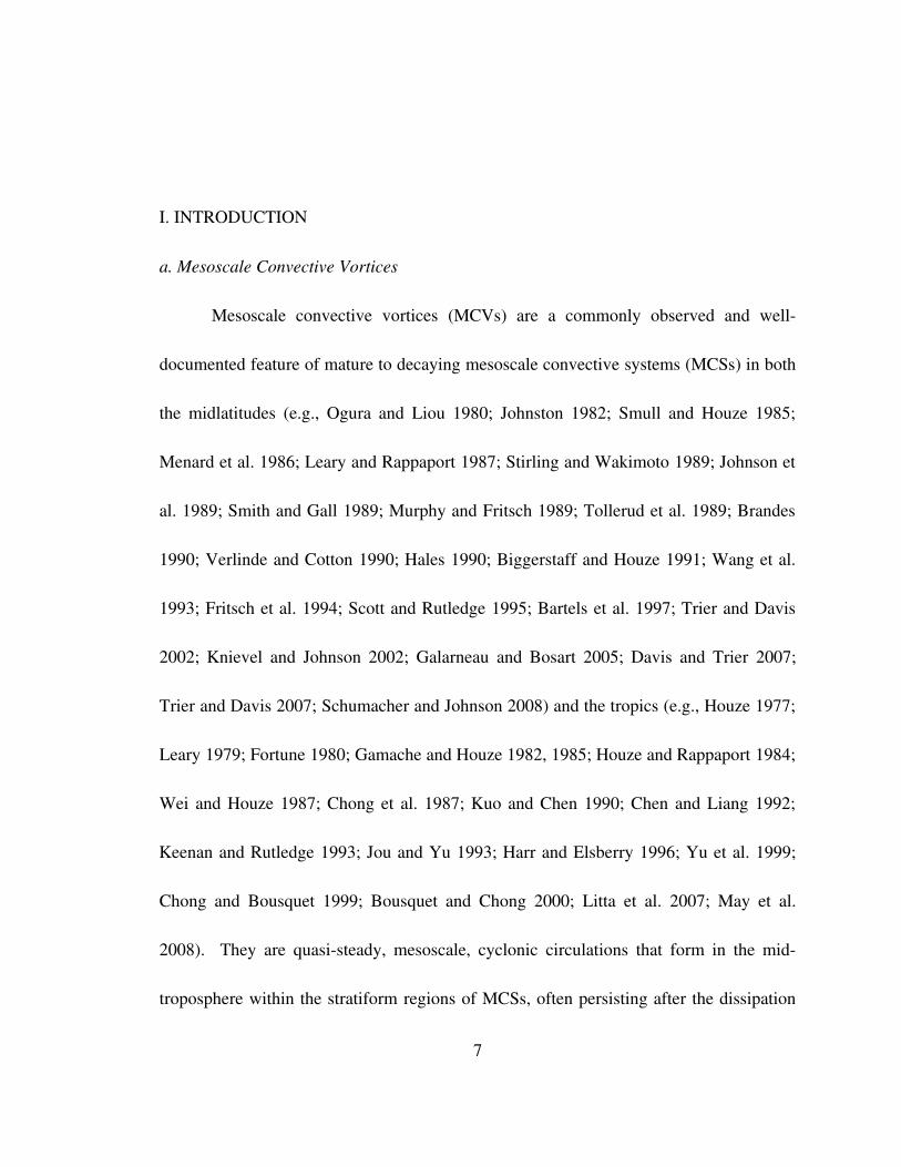
MCV (Houze et al. 1989; Pandya et al. 2000; see Figure 1.1).  

While not the primary focus of such experiments, MCVs have been documented 

in connection with many meteorological field programmes in the tropics and sub­tropics

8

Figure  1.1:  Conceptual  model  of  a  mid­level  horizontal  cross­section   through  (a)  an approximately   two­dimensional   squall   line,  and   (b)  a   squall   line  with  a  well­defined mesoscale vortex in the stratiform region (from Houze et al. 1989).

over   the   last   few   decades.     A   review   of   progress   arising   from   the   1974   Global 

Atmospheric   Research   Programme   (GARP)   Atlantic   Tropical   Experiment   (GATE; 

Kuettner et al.  1974) by Houze and Betts (1981) suggests that cyclonic vortices are a 

frequent   if   not   fundamental   characteristic   of   MCSs   in   the   eastern   tropical   Atlantic. 

Tropical  MCVs were  also  observed  during   the  Convection  Profonde  Tropicale  1981 

(COPT 81; Sommeria and Testud 1984) experiment in continental West Africa (Chong et 

al.   1987;   Chong   and   Hauser   1989,   1990),   in   the   1987   Taiwan   Area   Mesoscale 

Experiment   (TAMEX; Kuo and Chen 1990)  and  the  2008 Terrain­Induced  Monsoon 

Rainfall Experiment (TIMREX; R. Johnson, personal communication) in the vicinity of 

9

Taiwan (Chen and Liang 1992; Jou and Yu 1993; Yu et al.  1999), in  the 1988­1990 

Down Under Doppler and Electricity Experiment (DUNDEE; Rutledge et al. 1992) and 

the 2006 Tropical  Warm Pool International  Cloud Experiment (TWP­ICE; May et al. 

2008) in northern Australia (Keenan and Rutledge 1993), and in the 1992­1993 Tropical 

Ocean Global Atmosphere Coupled Ocean­Atmosphere Response Experiment  (TOGA 

COARE; Webster et al. 1992) in the western tropical Pacific (Chong and Bousquet 1999; 

Bousquet and Chong 2000).   Some studies have appeared in the Chinese and Japanese 

literature regarding the role of the “southwest vortex” in heavy rain producing MCSs in 

southern China (Huang 1986, Huang and Xiao 1989); the “southwest vortex” appears to 

be   at   least   partially   generated  by   the   terrain   of   the  Tibetan  plateau,   but   is   perhaps 

enhanced by MCV dynamics (Tao and Ding 1981; Kuo et al. 1986; Ma and Bosart 1987; 

Wang and Orlanski 1987; Wang 1987; Wang et al. 1993).   These findings demonstrate 

that  MCVs are  a  widespread  phenomenon,  apparently  occurring   in  all  areas   that  are 

climatologically   susceptible   to  organised  convection   in   the   tropics  and  subtropics,   in 

addition to the lower mid­latitudes.   There have also been a large number of numerical 

modeling studies of MCVs (e.g.,  Chen and Dell'Osso 1984; Zhang and Fritsch 1985, 

1986, 1987, 1988a,b,c; Dell'Osso and Chen 1986; Kuo et al. 1988; Zhang 1992; Chen and 

Frank 1993; Weisman et al.  1993; Davis and Weisman 1994; Skamarock et al.  1994; 

Zhang and Harvey 1995; Zhang and Bao 1996a,b; Weisman and Davis 1998; Trier et al. 

10

2000a; Rogers and Fritsch 2001; Cram et al. 2002; Davis and Trier 2002; Hawblitzel et 

al.  2007; Conzemius  et  al.  2007) over   the past  ~20 years,  some of which have been 

motivated   by   the   possibility   of   improving   warm   season   quantitative   precipitation 

forecasts (QPF) by successfully resolving and predicting the evolution of MCVs (e.g., see 

Zhang and Fritsch 1986, 1988c; Hawblitzel et al. 2007).  

b. Proposed Formation and Maintenance Mechanisms

Local increases and decreases of cyclonic or anticyclonic relative vorticity are 

described by the vorticity equation.  A number of formation mechanisms for MCVs have 

been proposed  in   the  literature,  based on  the various   terms  in  the vorticity  equation. 

These   include   the   concentration   of   planetary   vorticity   by   stretching   or   convergence 

(Bartels and Maddox 1991; Davis and Weisman 1994; Skamarock et al. 1994; Weisman 

and Davis 1998), the tilting of ambient horizontal relative vorticity (Zhang 1992; Brandes 

and Ziegler 1993; Chong and Bousquet 1999; Cram et al. 2002), and the convergence of 

ambient vertical relative vorticity (Brandes 1990; Johnson and Bartels 1992; Bousquet 

and Chong 2000).  Additionally, the reduction of the local Rossby radius of deformation 

due to the low static stability in the moist stratiform regions of MCSs may be necessary 

for   MCV   formation   (Chen   and  Frank  1993;   Yu   et   al.   1999).     Recent   studies   have 

suggested that MCVs may follow a variety of developmental paths (Kirk 2003, 2007).  

11

Observations generally support the notion that MCVs are warm core (Bartels et 

al. 1997).  In terms of potential vorticity (PV) thinking, MCVs are the balanced response 

to   the   increasing   latent  heating  with  height  associated  with   the  stratiform regions  of 

MCSs (Hertenstein and Schubert  1991; Davis and Trier 2002) (see Figure 1.2).   This 

profile of heating generates a local maximum in PV at the mid levels, which appears to 

be another distinguishing feature of MCVs (Fritsch et al. 1994).   This PV anomaly can 

interact with vertical wind shear in such a way that the resulting balanced lifting locally 

favours the regeneration of convection just downshear of the vortex, thereby intensifying 

the latent heat release and strengthening the vortex (Raymond and Jiang 1990; Jiang and 

Raymond 1995; Hawblitzel et al. 2007), as well as producing torrential rain (Trier and 

Davis 2002; Schumacher and Johnson 2008).  A recent modeling study by Conzemius et 

al.  (2007) demonstrates that this mechanism is capable of generating and maintaining 

mid­level   PV   anomalies   in   the   typical   environmental   conditions   of   an   MCV.     The 

evolution   of   the   mass   and   flow   fields   around   MCVs   thus   appears   to   be   driven   by 

horizontal and vertical gradients of latent heating.  Similarly, surface signatures of MCVs 

must depend on the integrated characteristics of the overlying atmosphere.  

The balanced nature of MCVs can allow them to persist for a long time, as long as 

the deleterious  effect of vertical  wind shear   is minimised in  the environment.     If   the 

MCV's environment remains otherwise favourable for convection, the MCV can generate

12

Figure   1.2:   (top)   Vertical   section   of   heating   function   (K/h;   contour   interval   1   K/h, negative heating contours dashed) representing stratiform heating, and (bottom) resulting dimensionless   PV   distribution   (contour   interval   0.2)   in   the   wake   of   this   heating propagating from X=0 to X=200 km within semigeostrophic model (from Hertenstein and Schubert 1991).

new   MCSs   by   the   above­described   mechanism   involving   the   PV   anomaly.     Each 

sequential   MCS   strengthens   the   vortex   by   intensifying   latent   heat   release,   further 

13

prolonging the MCV life span.  This process can continue for several days, as MCSs are 

generated and dissipate during each diurnal cycle.  Convection is generally most vigorous 

during the nighttime, dissipates in the morning, and regenerates in the late afternoon and 

evening.   One of these so­called serial MCSs, containing an MCV, was responsible for 

the 19­20 July 1977 Johnstown, Pennsylvania flood (Bosart and Sanders 1981).  

c. Previous Studies

There have been several climatological studies of MCVs over  the past several 

decades.  Early work by Bartels and Maddox (1991) focused on the synoptic environment 

of MCVs detected over the United States in eight years of satellite imagery.  They found 

that MCVs are favoured in situations with weak flow, weak vertical wind shear, weak 

background   relative  vorticity,   and   intense  vertical   and  horizontal  moisture   gradients. 

Trier et al. (2000b) undertook a climatology of MCVs for one warm season in the central 

United States, using a variety of observational platforms.  They found a relatively large 

number of long­lived MCVs, which appeared to be favoured under low vertical wind 

shear.   Regeneration of convection occurred in more than half of their identified cases. 

Davis et al. (2002) investigated MCV detection and prediction using the Rapid Update 

Cycle   (RUC)  model.    They  developed   an   automated   algorithm  which   is   capable   of 

distinguishing MCVs from dynamically different vortex types in hourly RUC analyses, 

14

and demonstrated its ability to detect MCVs over the Great Plains during a warm season. 

Using   this   algorithm,   they   summarised   some   climatological   aspects   of   midwestern 

MCVs.     It  was   found   that  MCVs  constitute   fewer   than  half  of  mid­level  mesoscale 

vortices during the season of interest.  They also found that there is a significant positive 

relationship between MCV intensity and longevity.   The RUC appears to be devoid of 

skill at predicting the development of MCVs in advance.  

Upper­air   observations   of   MCVs   since   the   early   1990s   have   been   greatly 

facilitated   by   the   implementation   of   the   National   Oceanic   and   Atmospheric 

Administration   (NOAA)   Profiler   Network   (NPN)   in   the   midwestern   United   States. 

Numerous detailed studies of the kinematic  structure of MCVs have been undertaken 

using   these  data.     Johnson and  Bartels   (1992)   studied  an  MCV over  Oklahoma  and 

Kansas on 23­24 June 1985.  They described the vertical structure of the vortex in some 

detail  using  a  variety  of  observing  platforms,   including  NPN data.    The  vortex  was 

100­200 km in horizontal scale, extending over 3­8 km altitude, with maximum relative 

vorticity near the melting layer.    In general the MCV was warm core,  with the most 

significant warm anomaly at low levels, associated with a descending  inflow jet.  Bartels 

et  al.   (1997) examined an MCV over northeastern Colorado on 8 June 1988, finding 

values of mid­level relative vorticity greater than three times the local Coriolis parameter. 

They used gradient wind balance to derive a balanced temperature field associated with 

15

the MCV, which implied a warm core over cold core thermodynamic structure.  Knievel 

and Johnson (2002) used wind profiler data to derive the synoptic and mesoscale flow 

features associated with an MCV observed in Oklahoma and Kansas on 1 August 1996. 

This  MCV grew  to  a  depth  of  12  km.   They  recorded   the  presence  of  a  mesoscale 

updraught   and  a  mesoscale   downdraught,   as  well   as   upper­   and   low­level   divergent 

outflow.   In a subsequent study (Knievel and Johnson 2003), the authors constructed a 

scale­discriminating   relative   vorticity   budget   for   this   MCV,   finding   that   the   MCV 

deepened and strengthened during the dissipation of the parent MCS due to convergence 

of absolute vorticity by the mesoscale wind.  A final investigation of this case (Knievel et 

al. 2004) sought to determine the extent of hydrostatic and gradient wind balance in the 

MCV, finding that the MCV was at least partially unbalanced.  

Two more recent studies have been based on observations from the Bow Echo 

and Mesoscale Convective Vortex Experiment (BAMEX) of 2003 (Davis et al. 2004). 

This  experiment   is   so  far   the  only   field  programme designed specifically   to  observe 

MCVs.     It   focussed  on  upper­air   observations   from dropsondes,  wind  profilers,   and 

aircraft, rather than on dense surface observations, so most studies stemming from this 

experiment have likewise dealt with the upper­level characteristics of MCVs.  Trier and 

Davis   (2007)   and Davis  and  Trier   (2007)   summarised  some  initial   results   from five 

BAMEX intensive observing periods (IOPs) focusing on MCVs.  They described a very 

16

wide variety of structures among the mature vortices examined.   In general the MCVs 

were observed to arise from the stratiform precipitation regions of MCSs.  They were 5­8 

km deep,  attaining  their  maximum relative vorticity  between 600 and 550 hPa.    The 

MCVs had varying degrees of tilt with the environmental shear; one case they examined 

appeared to be resilient and resisted tilting in shear.  Vortex penetration into the boundary 

layer appeared to require weak low­level wind shear.  They also found that, on average, 

outbreaks  of   secondary   convection  are   favoured   in   the  downshear   right   quadrant   of 

MCVs, due to a favourable kinematic and thermodynamic environment.  

There have been abundant studies examining the surface features of MCSs and 

general   convection   over   the   past   70   years.     Specific   subjects   have   included   the 

hydrostatically­induced mesohigh beneath the convection (e.g., Sawyer 1946; Schaffer 

1947;   Williams   1948,   1953;   Fujita   1951,   1955,   1959;   Brunk   1953;   Purdom   1973; 

Fankhauser 1974), the density current­like gust front at the leading edge of the mesohigh 

(e.g., Freeman 1950; Newton 1950; Tepper 1950, 1955; Charba 1974; Goff 1976; Miller 

and Betts 1977; Wakimoto 1982; Roux et al. 1982, 1984; Mueller and Carbone 1987; 

Nicholls et al. 1988), the pre­squall mesolow induced by subsidence warming aloft ahead 

of  the active convection  (Feteris  1961, 1978; Hoxit  et  al.  1976, 1977; Sanders 1977; 

Fritsch and Chappell 1980a,b), the wake low induced by subsidence warming within a 

descending rear inflow jet (Brunk 1949; Williams 1954; Magor 1958; Charba and Sasaki 

17

1971; Menard et al. 1988; Gallus 1996; Wicker and Skamarock 1996; Johnson 2001), 

surface   flow  through   these  pressure   features   (Garratt   and  Physick  1983;  Vescio  and 

Johnson  1992),   the   “squall  wake”  due   to   a   shallow   layer   of   cool,  moist   convective 

outflow behind the active convection (Zipser 1977; Johnson and Nicholls 1983), pressure 

responses to gravity waves (Haertel and Johnson 1998, 2000), transitory pressure features 

(Knievel  and Johnson 1998),  and non­hydrostatic  effects  (Levine  1942; Mal and Rao 

1945;   Marwitz   1972).     However,   to   date   there   have   been   relatively   few   studies 

investigating the particular surface features that accompany MCVs.  This may be partly 

due to the lack of sufficiently dense surface observing networks, or the paucity of field 

programmes designed to observe MCVs.  

The   Oklahoma­Kansas   Preliminary   Regional   Experiment   for   Storm­Scale 

Operational and Research Meteorology (OK PRE­STORM; Cunning 1986) provided the 

first  high resolution surface observations  of MCSs and their  associated MCVs in  the 

summer of 1985, motivating numerous studies of the surface features of MCSs (Johnson 

and Hamilton 1988; Johnson and Gallus 1988; Zhang et al. 1989; Zhang and Gao 1989; 

Smull and Jorgensen 1990; Stumpf et al. 1991; Smull et al. 1991; Nachamkin et al. 1994; 

Loehrer and Johnson 1995), and several studies specifically addressing surface features 

of MCVs.  An investigation of the 23­24 June 1985 OK PRE­STORM MCS by Johnson 

et al. (1989) found several interesting surface features associated with the decay of the 

18

MCS and the development  of a mid­level  circulation.    There was a strong mesohigh 

situated beneath the stratiform rain portion of the MCS during the system's mature phase. 

As the stratiform rain degenerated, this mesohigh transformed into a strong mesolow (see 

Figure 1.3).  This transformation was coincident with the development of a well­defined 

cyclonic vortex,  visible  in satellite   imagery.    The authors proposed that  the mesolow 

formed from hydrostatic effects due to warming and drying within a region of strong 

mesoscale   subsidence   in   the   absence   of   any   precipitation;   this   warm   subsiding   air 

actually produced localised “heat bursts” at several mesonet sites (Bernstein and Johnson 

1994).   It was unclear if there was any connection between the mesolow and the MCV 

development.  The existence of unsaturated downdraughts driven by rainfall evaporation 

has been demonstrated in a well­known modeling study (Brown 1979), and is understood 

to  be  the mechanism for  both microbursts   (Fujita  and Wakimoto  1981;  Brown et  al. 

1982; McNulty 1991) and heat bursts (Johnson 1983).  Brandes (1990) and Brandes and 

Ziegler   (1993)   studied   the  6­7  May 1985 OK PRE­STORM MCS and  its  associated 

MCV.   They found that the MCV focused and intensified a descending rear inflow jet 

into the southern portion of the system.   This descending air current apparently led to 

strong   low­level   subsidence   warming   and   drying,   producing   a   mesolow   with   a 

perturbation pressure anomaly of ­4 hPa (see Figure 1.4).  Again, it is unknown to what 

extent the MCV was responsible for the production of this mesolow.   They also found

19

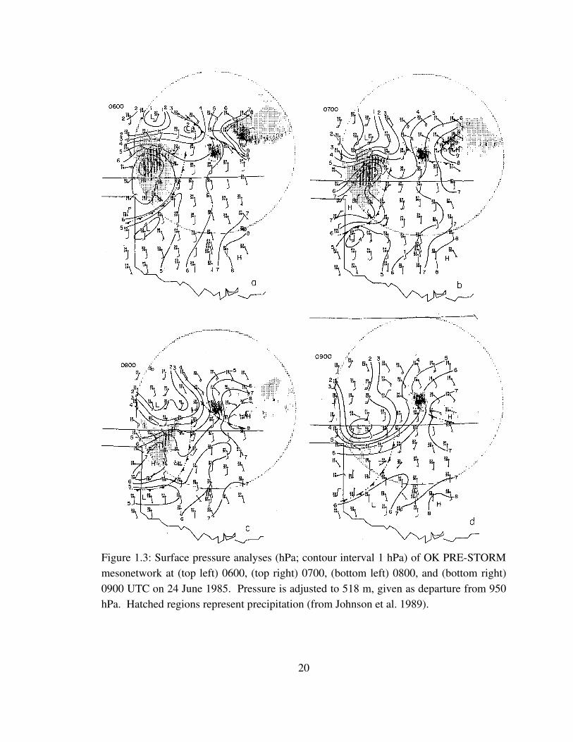
Figure 1.3: Surface pressure analyses (hPa; contour interval 1 hPa) of OK PRE­STORM mesonetwork at (top left) 0600, (top right) 0700, (bottom left) 0800, and (bottom right) 0900 UTC on 24 June 1985.  Pressure is adjusted to 518 m, given as departure from 950 hPa.  Hatched regions represent precipitation (from Johnson et al. 1989).

20

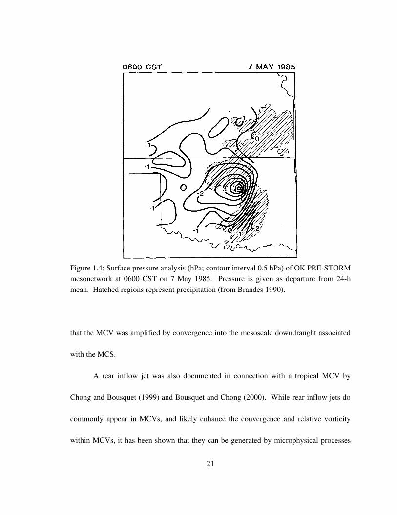
Figure 1.4: Surface pressure analysis (hPa; contour interval 0.5 hPa) of OK PRE­STORM mesonetwork at 0600 CST on 7 May 1985.   Pressure is given as departure from 24­h mean.  Hatched regions represent precipitation (from Brandes 1990).

that the MCV was amplified by convergence into the mesoscale downdraught associated 

with the MCS.  

A rear inflow jet  was also documented in connection with a tropical MCV by 

Chong and Bousquet (1999) and Bousquet and Chong (2000).  While rear inflow jets do 

commonly appear in MCVs, and likely enhance the convergence and relative vorticity 

within MCVs, it has been shown that they can be generated by microphysical processes 

21

unrelated to MCV dynamics (Braun and Houze 1997).   The rear inflow mechanism for 

mesolow generation consists of concentrated descent within the inflow being forced by 

evaporational   cooling­induced   subsidence  at   the   rear  of   the   stratiform  region,  which 

eventually becomes unsaturated and warms adiabatically, hydrostatically forming a wake 

low (Johnson and Hamilton 1988; Stumpf et  al.  1991).   A modeling study by Gallus 

(1996) suggests that this mechanism will only form a mesolow if the evaporating rainfall 

is decreasing in intensity, as occurs during the dissipation stage of an MCS; only under 

this condition will the adiabatic warming due to subsidence outweigh the cooling due to 

the evaporation of  the precipitation.    A study by Fortune et  al.   (1992) addressed  the 

tendency for MCSs to evolve in a manner resembling the frontal­wave pattern observed 

in synoptic­scale extratropical cyclones, using data collected in four OK PRE­STORM 

MCSs.   They found indications  that   this  pattern is  not  related to   the development of 

cyclonic mesoscale relative vorticity.   Their mesoanalyses of the MCSs revealed fairly 

well­defined mesohighs and mesolows; however, these MCSs did not appear to contain 

well­defined MCVs.  

d. The Tropical Cyclogenesis Problem

The specific mechanisms involved in the process of tropical cyclogenesis remain 

elusive   despite   much   focused   research.     Some   notable   similarities   between   tropical 

22

cyclones   and  MCVs  suggest   that  MCVs  may  be   a  necessary   ingredient   in   incipient 

tropical cylones (Zhang and Fritsch 1987; Keenan and Rutledge 1993; Fritsch et al. 1994; 

Ritchie et al. 1995; Zhang and Bao 1996a,b; Harr et al. 1996a,b; Simpson et al. 1997; 

Davis  et  al.  2004).    Two main   tropical  cyclogenesis  hypotheses  have  been  proposed 

recently, both of which may be active in different cyclogenesis cases.  One theory is that 

an initially mid­level vortex, consisting of a PV maximum above a low­level cold pool, 

can gradually build downward toward the surface through strengthening and deepening 

of the PV maximum by repeated MCS generation and dissipation (Fritsch et al. 1994; 

Rogers  and Fritsch  2001;  Trier  and  Davis  2002).    Such a   transformation   likely  also 

requires significant sensible and latent heat fluxes from the ocean surface, which may 

explain the rarity of sustained convectively­induced mesolows over land and over cool (< 

26  ºC)   waters.   In an extension of this theory, Mapes and Houze (1995) propose that 

several  anomalous  characteristics  of  divergence  profiles  within   tropical  MCSs would 

favour downward development of an initially elevated cyclonic circulation.  They present 

evidence,   from  the  TOGA COARE MCS of  6  February  1992,  of   low­   to  mid­level 

divergence and near­surface convergence, as well as adiabatic subsidence, all of which 

would act to lower the relative vorticity maximum and destroy the low­level cold pool. 

The   other   cyclogenesis   hypothesis   is   that   low­level   PV   generation   by   developing 

convection in the form of vortical hot towers spins up the vortex, with an MCV providing 

23

a   favourable   environment   with   weak   background   cyclonic   relative   vorticity 

(Montgomery   and   Enagonio   1998;   Reasor   et   al.   2005).     Several   studies   have   used 

numerical modeling to explicitly investigate the role of observed mid­level mesovortices 

during   the  genesis   stage  of   tropical   cyclones   (Ritchie   and Holland  1997;  Bister   and 

Emanuel  1997; Montgomery and Enagonio 1998; Kieu and Zhang 2008).    It  remains 

unclear which hypothesis is more realistic, but MCVs may play a key role in the tropical 

cyclogenesis process.  

There have been a number of documented cases of tropical cyclones developing 

from MCSs moving offshore.  The Johnstown MCV, in July 1977, actually intensified to 

tropical storm strength after emerging off the coast into the Atlantic (Bosart and Sanders 

1981).   This tropical cyclogenesis was confirmed in more recent model simulations by 

Zhang and Bao  (1996a,b).    Another   interesting  case  was  observed  during   the   recent 

TWP­ICE campaign in tropical Australia.  A large MCS formed as the monsoon trough 

retreated northward away from Australia in late January 2006, and clear cyclonic rotation 

was observed in the cloud field as the MCS emerged over water.  The system deepened to 

999 hPa as it made landfall southwest of Darwin, and continued to intensify to 988 hPa 

over land, maintaining its convection and spiral cloud structure for two days (May et al. 

2008).  Other systems similar to this have been observed over northern Australia, and are 

locally known as “landphoons”.  Emanuel et al. (2008) have proposed that these cyclones 

24

are maintained by strong vertical heat fluxes from the underlying hot desert soil which 

has been moistened by the first rains of the approaching system.  Climatological studies 

of global MCC populations in the Americas (Velasco and Fritsch 1987),   the western 

Pacific (Miller and Fritsch 1991), southern Asia (Laing and Fritsch 1993a), and Africa 

(Laing and Fritsch 1993b) have found numerous cases of tropical cyclones developing 

from MCCs, presumably due to the presence of embedded MCVs.  

While  true tropical  cyclogenesis   is only possible  over warm water,   there have 

been several observed cases of significant MCV­induced surface mesolows over land, as 

summarised   above.     Zhang   and   Harvey   (1995)   describe   a   real­case   simulation 

demonstrating  enhancement  of  extratropical  cyclogenesis  by a  convectively­generated 

mesovortex.  Rogers and Fritsch (2001) describe another real­case simulation in which a 

pronounced mesolow forms beneath an MCV over land after three cycles of convective 

redevelopment.  Since surface observations are very sparse over the oceans in regions of 

frequent tropical cyclogenesis, surface observations over land beneath MCVs may be the 

best source of observational evidence to support one of the theories of cyclogenesis.  

e. Objectives

The   goal   of   this   study   is   to   provide   a   broad   climatological   overview  of   the 

structure and evolution of midlatitude MCVs by using relatively dense surface and upper­

25

air observations of a large number of MCVs occurring during the late spring and summer 

months of four years over the state of Oklahoma.  It is hoped that such a climatology will 

facilitate generalisations about the physical characteristics of MCVs which will help to 

synthesise and solidify the conclusions reached in the large number of individual MCV 

case studies summarised above.  It is also anticipated that the large population of MCVs 

investigated herein will provide a statistically robust basis for validation of numerical 

simulations of MCVs, from both the numerical weather prediction (NWP) and general 

circulation   modeling   (GCM)   perspectives.     An   additional   important   objective   is   the 

documentation of MCV penetration to the surface and the proposal of some mechanisms 

for this phenomenon, which may be active in the tropical cyclogenesis process.  

The remainder of this paper is organised as follows.  The data sources used, and 

their   strengths   and  weaknesses,   are  described   in   section  2.    Section  3  describes   the 

methodology   followed   for   selecting   and   analysing   the   individual   MCV   cases,   and 

constructing the various composites.   Results are presented in sections 4 and 5, and are 

discussed in section 6.  Section 7 contains the conclusions of the study.  

26

II. DATA SOURCES

A variety of observational and model datasets are used in this study.  Model data 

are used in the detection of MCV cases, and to provide a synoptic­scale context for the 

analysis of each case.  Observational data are used to investigate the mesoscale structure 

of the MCVs in more detail.   This section provides descriptions of the various datasets 

used in this study, and highlights potential quality problems unique to each dataset.  

a. The Rapid Update Cycle

The   RUC   (Benjamin   et   al.   2004)   is   a   high­resolution   model   analysis   and 

forecasting  system designed  to aid  in short­term operational  forecasting of hazardous 

weather situations.   The RUC system is an assimilation­forecast cycle: thus, each new 

analysis is based on a background field derived from the model's earlier forecast for that 

time.  The horizontal and vertical grid spacing of the model have been upgraded several 

times; the current operational version of the model has a horizontal grid spacing of 20 km 

and  50  vertical   levels.     In   addition   to   the   standard   synoptic   observations,   the  RUC 

assimilates a wide variety of asynoptic data types to improve the quality of its hourly 

analyses (see Figure 2.1).  Two of the most important asynoptic data sources for the RUC

27

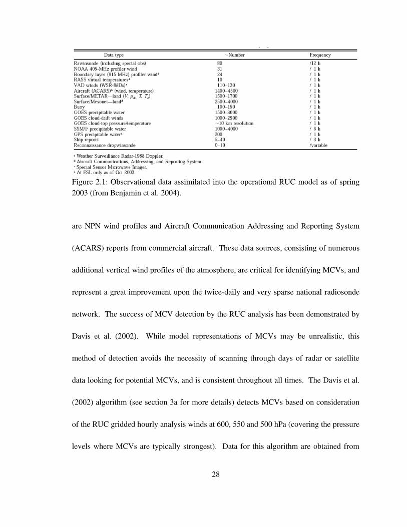
Figure 2.1: Observational data assimilated into the operational RUC model as of spring 2003 (from Benjamin et al. 2004).

are NPN wind profiles and Aircraft Communication Addressing and Reporting System 

(ACARS) reports from commercial aircraft.  These data sources, consisting of numerous 

additional vertical wind profiles of the atmosphere, are critical for identifying MCVs, and 

represent a great improvement upon the twice­daily and very sparse national radiosonde 

network.  The success of MCV detection by the RUC analysis has been demonstrated by 

Davis  et  al.   (2002).    While  model   representations  of  MCVs may be  unrealistic,   this 

method of detection avoids the necessity of scanning through days of radar or satellite 

data looking for potential MCVs, and is consistent throughout all times.  The Davis et al. 

(2002) algorithm (see section 3a for more details) detects MCVs based on consideration 

of the RUC gridded hourly analysis winds at 600, 550 and 500 hPa (covering the pressure 

levels where MCVs are typically strongest).   Data for this algorithm are obtained from 

28

the NOAA National Operational Model Archive and Distribution System, and consist of 

zonal and meridional wind data at these three levels over the late spring and summer 

(May­August) of the years 2002­2005, over the entire RUC domain (the continental USA 

and immediate  surroundings).   The operational  version of the RUC during these four 

years, the RUC­236, had a horizontal grid spacing of 40 km.  The years examined have a 

varying   amount   of   missing   data.     The   2002   data   are   39%   complete,   2003   is   87% 

complete, 2004 is 91% complete, and 2005 is 38% complete.  It is likely that numerous 

MCVs were not detected in 2002 and 2005, but this will not affect the conclusions drawn 

about the successfully detected systems.   For each of the MCV cases analysed in this 

study, the full RUC data (all variables and all levels) are obtained in order to perform a 

more detailed analysis of each case.  The vertical spacing of the RUC­236 data is 50 hPa, 

from 1000 to 100 hPa.   Variables retrieved include surface­based convective available 

potential energy (CAPE) and convective inhibition (CIN); column­integrated precipitable 

water; 2­m temperature, pressure, mean sea level pressure, and relative humidity; 10­m 

zonal and meridional wind speed; and pressure­level geopotential  height, temperature, 

relative humidity, pressure vertical velocity, and zonal and meridional wind speed.  The 

pressure vertical velocity variable in the RUC is only available at certain pressure levels 

(850, 700, 500, 300, and 200 hPa), and the relative humidity variable is only available 

every 50 hPa at and below 500 hPa.   A variety of other variables are derived from the 

29

RUC   variables,   including   vapour   pressure,   saturation   vapour   pressure,   mixing   ratio, 

saturation  mixing ratio,  dewpoint   temperature,  divergence,   relative  vorticity,  potential 

temperature,   equivalent   potential   temperature,   and   absolute   vorticity   at   2   m   and   at 

constant pressure levels, as well as PV at constant pressure levels.  RUC data are missing 

or incomplete for all times of the 3 June 2002, 4­5 June 2002, and 9­10 June 2002 cases, 

and for 11 hours of the 20 June 2004 case, four hours of the 3 June 2003 case, three hours 

of the 24­25 June 2003 case, two hours of the 19 June 2004 case, and one hour of the 10 

June 2005 case.  

While model fields are very convenient and attractive due to their completeness 

and their organisation on a regular grid, all models have major shortcomings.   It was 

found   by   Davis   et   al.   (2002)   that   the   RUC   has   virtually   no   skill   in   predicting   the 

formation of MCVs 12 h in advance.   This is likely due to the inherent unpredictable 

nature of the convection which produces MCVs.  While this study does not make use of 

any  RUC  forecasts,   the  design  of   the  RUC model   as   an   assimilation­forecast   cycle 

implies   that   RUC   forecasts   do   have   an   influence   on   the   hourly   analyses.     Thus, 

unrealistic model physics may negatively impact the analysis representations of MCVs. 

This problem can be exacerbated by sparse observations being ingested into the RUC.  If 

there happen to be no useful asynoptic data available for assimilation at a particular time, 

the   background   field   derived   from   the   RUC   forecast   will   be   almost   unmodified   to 

30

produce the final 0­h analysis.  In extreme situations (such as a lack of any new analysis 

data), the RUC analyses can progressively become farther and farther from reality with 

each hour that passes.   Another problem associated with the RUC analyses is aliasing 

associated with time windows for observations.  The asynoptic observations assimilated 

into the RUC are generally not valid at exactly the same time as the analysis time; thus, 

some error is introduced into the analysis by allowing a finite window of time in which 

observations will be incorporated.  Finally, the RUC analyses can suffer simply from the 

relatively  coarse   resolution  of   the  model  grid;  40  km may be   insufficient   to   resolve 

features on the small side of the mesoscale.  Due to these inherent deficiencies with the 

RUC analyses, these data are only used to describe the synoptic­scale environment of 

MCVs.    Conclusions  drawn about   the  mesoscale   structure  of  MCVs based  on  RUC 

analyses should be treated with caution.  

b. The NOAA Profiler Network

The primary upper­air observations used in this study are taken from the NPN 

(Weber et al. 1990).   The NPN is a network of 404­MHz (74.3­cm wavelength) radar 

wind  profilers   concentrated   in   the  midwestern  USA  (see  Figure  2.2).    The  profilers 

operate   with   three   upward   pointing   beams   directed   by   a   large,   fixed,   phased­array 

antenna: one vertical beam, one pointing north at 73.7º elevation angle, and one pointing

31

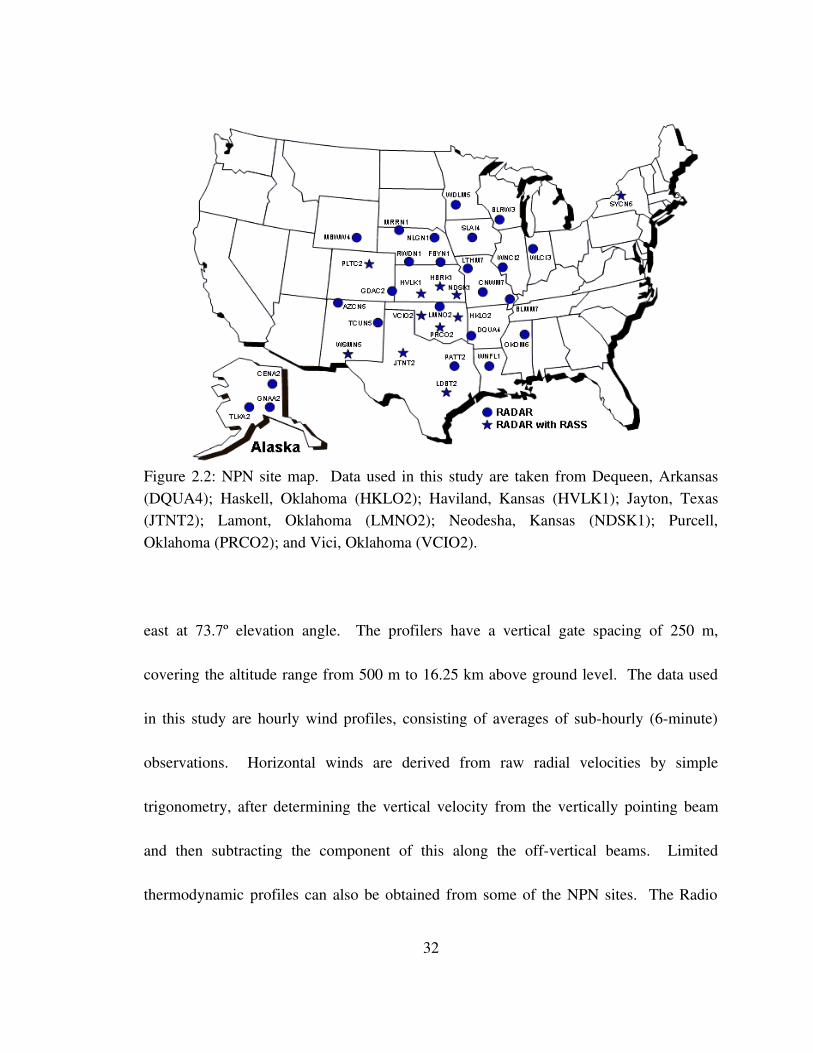
Figure 2.2: NPN site map.   Data used in this study are taken from Dequeen, Arkansas (DQUA4);  Haskell,  Oklahoma  (HKLO2);  Haviland,  Kansas   (HVLK1);   Jayton,  Texas (JTNT2);   Lamont,   Oklahoma   (LMNO2);   Neodesha,   Kansas   (NDSK1);   Purcell, Oklahoma (PRCO2); and Vici, Oklahoma (VCIO2).

east   at  73.7º  elevation  angle.    The  profilers  have  a  vertical  gate   spacing  of  250 m, 

covering the altitude range from 500 m to 16.25 km above ground level.  The data used 

in this study are hourly wind profiles, consisting of averages of sub­hourly (6­minute) 

observations.     Horizontal   winds   are   derived   from   raw   radial   velocities   by   simple 

trigonometry, after determining the vertical velocity from the vertically pointing beam 

and   then   subtracting   the   component   of   this   along   the   off­vertical   beams.     Limited 

thermodynamic profiles can also be obtained from some of the NPN sites.   The Radio 

32

Acoustic Sounding System (RASS; North et al. 1973) technique makes use of the fact 

that air compression and rarefaction by sound waves alters the dieletric constant of the 

medium, causing a partial reflection of electromagnetic energy from a radar.  An acoustic 

source sends out a sound wave into the atmosphere, which can then be tracked by the 

radar.  The speed of the sound wave can be related to the virtual temperature of the layer 

through which the wave passes; thus it is possible to derive a virtual temperature profile 

of the lower atmosphere.  A major advantage of RASS is its high temporal sampling; it is 

possible to continuously monitor the virtual temperature profile.  Hourly profiler data are 

obtained for each MCV case from the NOAA NPN online archive.  Wind profiles from 

the   following   profiler   sites   are   obtained:   Dequeen,   Arkansas;   Haskell,   Oklahoma; 

Haviland,  Kansas;   Jayton,  Texas;  Lamont,  Oklahoma;  Purcell,  Oklahoma;  Neodesha, 

Kansas; and Vici, Oklahoma.  RASS equipment is installed at all eight of these profiler 

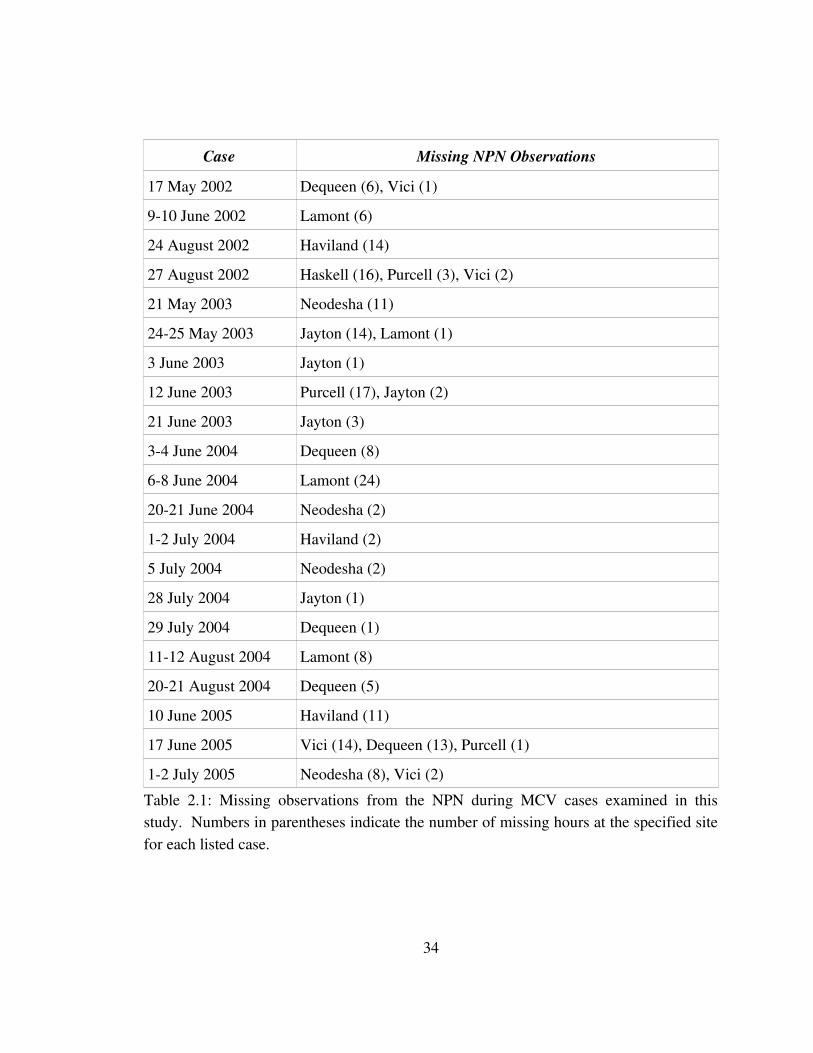
sites except Dequeen, Arkansas, and Lamont, Oklahoma.  Table 2.1 lists the MCV cases 

for which some profiler data were missing, and the number of missing hours at  each 

profiler site during these cases.  

Wind   profiler   data   quality   can   become   an   issue   under   certain   conditions. 

Specifically, convective precipitation (Wuertz et al. 1988) and gravity waves (Nastrom 

and  Vanzandt  1996)  can  violate   the   fundamental  horizontal  homogeneity  assumption 

(beam spacing is several kilometres at high altitudes), and migrating songbirds can cause

33

Case Missing NPN Observations

17 May 2002 Dequeen (6), Vici (1)

9­10 June 2002 Lamont (6)

24 August 2002 Haviland (14)

27 August 2002 Haskell (16), Purcell (3), Vici (2)

21 May 2003 Neodesha (11)

24­25 May 2003 Jayton (14), Lamont (1)

3 June 2003 Jayton (1)

12 June 2003 Purcell (17), Jayton (2)

21 June 2003 Jayton (3)

3­4 June 2004 Dequeen (8)

6­8 June 2004 Lamont (24)

20­21 June 2004 Neodesha (2)

1­2 July 2004 Haviland (2)

5 July 2004 Neodesha (2)

28 July 2004 Jayton (1)

29 July 2004 Dequeen (1)

11­12 August 2004 Lamont (8)

20­21 August 2004 Dequeen (5)

10 June 2005 Haviland (11)

17 June 2005 Vici (14), Dequeen (13), Purcell (1)

1­2 July 2005 Neodesha (8), Vici (2)Table  2.1:  Missing  observations   from  the  NPN during  MCV cases  examined   in   this study.  Numbers in parentheses indicate the number of missing hours at the specified site for each listed case.

34

unrealistic  wind speeds  and directions   in   low­level  profiler  observations   in   the  early 

morning during the migration season (spring or autumn) (Wilczak et  al.  1995).   This 

study uses only data passing a bird contamination check (Wilczak et al. 1995) and a time­

height  continuity  check (Weber et  al.  1993),  so  these problems should not  affect   the 

results of this study.   Errors in the RASS measurement of virtual temperature can be 

introduced by the presence of vertical velocity, or by an inaccurate measurement of the 

sound pulse velocity (particularly at low signal­to­noise ratios, which can occur at long 

range).   All RASS data used in this study have passed the time­height continuity check 

(Weber et al. 1993).   However, through manual inspection of the data, it became clear 

that   some   quality   issues   remained.     Specifically,   the   RASS   temperature   profiles 

occasionally  contained   layers  of  varying   thickness  with  unrealistically  and uniformly 

high virtual temperatures.  In the most extreme cases, the profiles consisted of near 40 ºC 

virtual temperatures at all range gates between the surface and 500 hPa.   Fortunately, 

these   erroneous   temperatures   are   easily   detectable   by   an   automated   process.     The 

Fortran­77 programme written to analyse the profiler data thus includes a simple quality 

control check consisting of a range of allowed virtual temperatures at each height.  Data 

falling below the minimum allowed virtual temperature or above the maximum allowed 

virtual temperature at each height are changed to missing data.   The allowable virtual 

temperature range is 20  ºC at each height,  centred on realistic values for the summer 

35

season in Oklahoma.   This simple algorithm appears to have removed erroneous data 

from consideration.  

c. The Oklahoma Mesonet

Mesoscale surface observations in this study consist of data from the Oklahoma 

Mesonet   (McPherson   et   al.   2007).     This   network  of   high­quality   automated   surface 

weather stations is made up of 127 sites distributed around the state (see Figure 2.3).  The 

mesonet was established in 1994, and its data have been used in a variety of applications 

including   public   safety,   emergency   management,   education,   resource   management, 

agriculture, industry, and research.  Data are recorded every five minutes, resulting in a 

very high spatial and temporal resolution representation of the state of the environment. 

Strict   standardisation   of   the   station   siting   and   instrumentation,   as   well   as   extensive 

quality control, ensure high data quality.  A large number of variables are measured; the 

relevant variables for this study are 1.5­m air temperature and relative humidity, surface 

rainfall,   surface   pressure,   and   10­m   wind   speed,   wind   direction,   and   wind   gusts. 

Historically,   there   have   been   very   few   high­quality   surface   mesonets,   despite   their 

demonstrated importance in improving our understanding of MCSs and their governing 

dynamics.   Prior to the establishment of the Oklahoma Mesonet, most mesonets were 

associated   with   specific   field   campaigns   (such   as   OK   PRE­STORM),   and

36

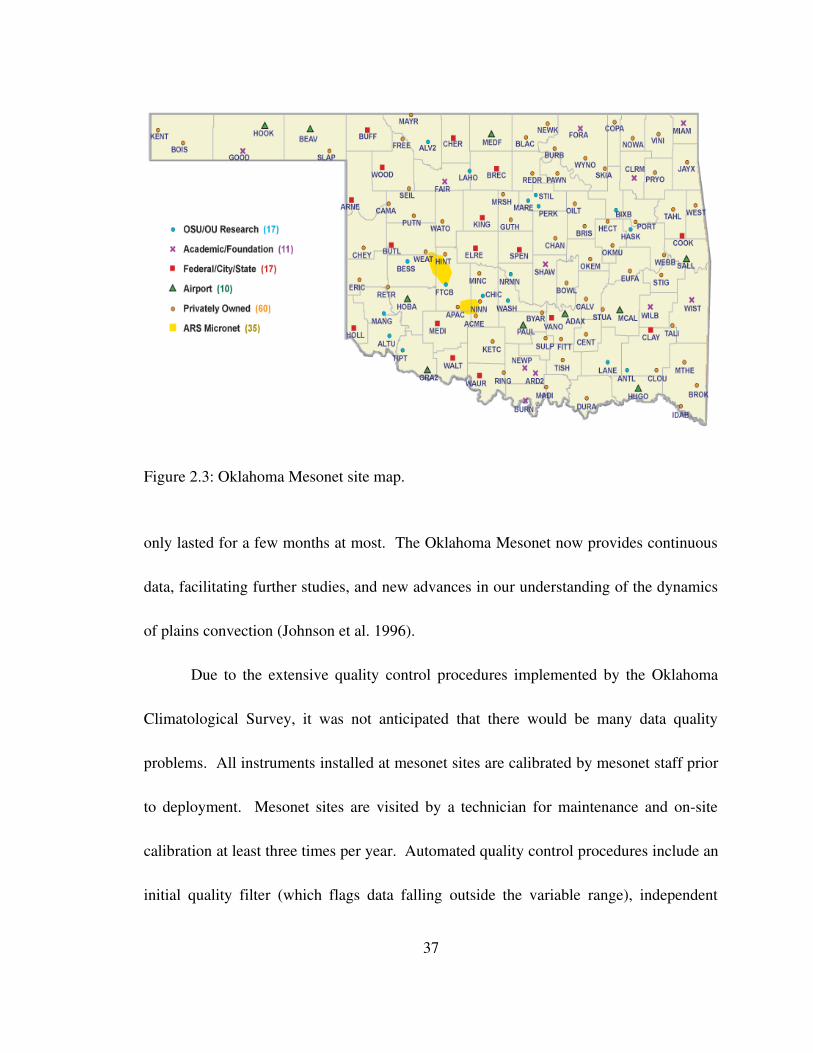
Figure 2.3: Oklahoma Mesonet site map.

only lasted for a few months at most.  The Oklahoma Mesonet now provides continuous 

data, facilitating further studies, and new advances in our understanding of the dynamics 

of plains convection (Johnson et al. 1996).  

Due to the extensive quality control procedures implemented by the Oklahoma 

Climatological  Survey,   it  was  not  anticipated   that   there  would  be  many data  quality 

problems.  All instruments installed at mesonet sites are calibrated by mesonet staff prior 

to deployment.   Mesonet sites are visited by a technician for maintenance and on­site 

calibration at least three times per year.  Automated quality control procedures include an 

initial  quality  filter   (which flags  data  falling  outside the variable  range),   independent 

37

algorithms (including step, persistence, and spatial tests), and a quality decision maker 

algorithm (which assigns a final flag to the observation).  Manual quality control is also 

implemented.    The  data  used   in   this   study,   from May   through  August   of   the  years 

2002­2005, appear to have no quality problems.  One or two sites are sometimes missing 

data, but this in no way affects the overall mesoanalyses contained herein.  

d. The Next Generation Weather Radar Network

One of the primary data sources for investigating the evolution of MCSs and their 

MCVs   in   this   study   is   the  Next  Generation  Weather  Radar   (NEXRAD)  network  of 

Weather  Surveillance   Radars   1988­Doppler   (WSR­88Ds).     This   national   network   of 

Doppler radar installations provides complete coverage of the state of Oklahoma.   The 

individual   radars   operate   at   10   cm   wavelength,   and   are   optimised   for   observing 

precipitation.     Therefore   they   are   a   powerful   tool   for   observing   the   development, 

movement,   and   evolution   of   precipitation   systems   such   as   MCSs.     For   this   study, 

NEXRAD Level 3 data are obtained for each MCV case in order to provide a background 

field for subsequent analysis.   Reflectivity composite images (the maximum reflectivity 

observed at any level at each gridpoint) are obtained at 15­minute intervals during each 

case from WSI Corporation.   Level 3 reflectivity data are also obtained for individual 

Oklahoma radar sites in order to track the heading and speed of the MCVs.  The specific 

38

radar sites used are Frederick,  Oklahoma (FDR); Inola, Oklahoma (INX); Fort Smith, 

Arkansas (SRX); Twin Lakes, Oklahoma (TLX); and Vance Air Force Base, Oklahoma 

(VNX).  These data are retrieved from the National Climatic Data Center (NCDC).  

Radar observation in meteorology has a long history, and many potential quality 

issues have been highlighted by both the research and the operational communities in the 

past several decades.  Many of these problems are associated with the observation of the 

Doppler velocity.  The WSR­88Ds' Doppler capability allows determination of the radial 

velocity of meteorological targets; this information is not used in this study.  Rather, this 

study   utilises   the   most   basic   radar­observed   quantity:   the   radar   reflectivity.     Radar 

reflectivity  within  a  distribution  of  meteorological   targets  depends  upon a  variety  of 

factors, including characteristics of both the radar and the contents of the target volume. 

The radar reflectivity is proportional to the diameter of the scatterers to the sixth power, 

and thus is highly sensitive to large scatterers.  10­cm, or S­band, radars are sensitive to 

precipitation­sized   particles   (typically   several   mm   in   diameter),   so   the   NEXRAD 

reflectivity data are a proxy for precipitation intensity.  In some instances, the reflectivity 

measurement can be affected by the presence of ice (including snow, graupel, ice pellets, 

and hail) but in the warm season this effect is usually fairly minor.  Radar reflectivity can 

also be contaminated by antenna sidelobes, as well as by ground clutter; these issues are 

largely resolved by operational algorithms.   In this study, the radar reflectivity is used 

39

only in a qualitative sense, to distinguish between the stratiform and convective regions 

of MCSs and to determine the relative intensities of areas of convection.  

e. Miscellaneous Data

Several other data sources are used in the analysis of MCV cases.   The primary 

source of information concerning the synoptic­scale context for each case is the standard 

operational radiosonde network.  This network, which covers the continental USA with a 

reasonable station spacing (~70 stations), gives a broad overview of the upper­level flow 

patterns   within   which   MCVs   are   situated.     Soundings   are   launched   twice   daily,   at 

synoptic   times   0000   and   1200   universal   coordinated   time   (UTC).     The   individual 

soundings from Norman, Oklahoma, and surrounding sites are occasionally examined in 

more detail when they were taken in the immediate vicinity of passing MCVs.  Individual 

soundings, as well as upper­air analyses produced by the NOAA Storm Prediction Center 

(SPC),  are  accessed   through  the  National  Center   for  Atmospheric  Research   (NCAR) 

Mesoscale and Microscale Modeling (MMM) Division's online image archive.  

Satellite   imagery   from   the   Geostationary   Operational   Environmental   Satellite 

(GOES) platforms covering the eastern and western portions of the country is used to 

ascertain   the extent  and  type of cloud cover  associated  with  the MCVs.   During  the 

daytime,  visible   imagery  is  examined,  and during nighttime,   infrared  (IR)   imagery is 

40

used.  Knowledge of the presence and type of cloud cover in different regions of MCVs 

is helpful in determining possible dynamics of some observed surface features.  Satellite 

imagery is also obtained through MMM's online image archive.  

The Department of Energy (DOE) Atmospheric Radiation Measurement (ARM) 

programme runs a permanent observing facility in north­central Oklahoma: the Southern 

Great Plains (SGP) Cloud and Radiation Testbed (CART) site.  In addition to a variety of 

cloud   remote  sensors  and  surface  observing   instruments,   the   site   is   equipped with  a 

radiosonde launcher, and soundings are launched every six hours (more frequently during 

special observing periods).   Each available sounding taken from this site (near Lamont, 

Oklahoma) during the passage of an MCV through Oklahoma is obtained from the ARM 

data   archive.     These   supplemental   soundings   provide   valuable   additional   upper­air 

kinematic and thermodynamic information.  

41

III. METHODOLOGY

This   section   provides   details   of   the   methodology   used   in   the   selection   and 

analysis of individual MCV cases, as well as in the construction of MCV composites. 

Case analyses and compositing are carried out using both observational and model­based 

(RUC) data.  

a. Case Selection

To facilitate  generalisations   about   the   structure  and  dynamics  of  MCVs,   it   is 

important to obtain a large number of MCV cases to examine in detail.  Several possible 

detection methods have been proposed in the literature in the past few decades.    The 

subjective   method   of   Bartels   and   Maddox   (1991)   involves   searching   4­km   visible 

satellite imagery for systems which exhibit well­defined cloud bands for more than one 

hour, whose “shape and pattern suggest cyclonic rotation, even when viewed on a single 

satellite image”.  This method, applied by Bartels and Maddox (1991) to approximately 

eight   years   of   satellite   imagery   over   the   central   USA,   appeared   to   significantly 

underestimate the total number of MCVs occurring.  This is likely due to the limitations 

of   the satellite   imagery;  MCVs were only detected  if   they had well­defined  cyclonic 

42

curvature in the mid­ and low­level clouds, with limited obstructing upper­level cirrus. 

They found 24 events over an eight­year period.   A more recent study by Trier et al. 

(2000b)   used   a   larger   variety   of   observational   platforms   in   their   MCV   detection, 

including   radar   reflectivity,   IR   satellite   imagery,   and   NPN   wind   profiles.     They 

considered   an   MCV   to   exist   whenever   a   circulation  was   indicated   by   any   of   these 

platforms after the dissipation of convection associated with the parent MCS.  Using this 

method, Trier et al. (2000b) detected 16 MCVs during the warm season of 1998.  A third 

MCV detection methodology, involving analyses from the RUC model, was developed 

by Davis et al. (2002).  Their algorithm, which requires relative vorticity maxima to pass 

a variety of tests in order to be considered MCVs, provides an objective means of MCV 

detection.    While   this  method is  based on model  data,  and thus may be occasionally 

inaccurate, it is consistent among all times, and can be automated, thus reducing the time 

required for finding cases.   Based on these advantages, and the limitations associated 

with the earlier two methods, the Davis et al. (2002) algorithm is used to detect MCVs in 

this study.  

The Davis et al. (2002) algorithm detects MCV within a gridded field of vertical 

relative vorticity (Figure 3.1).   In order to focus on MCVs, which are typically most 

intense in the mid­troposphere, the relative vorticity input to the algorithm is calculated 

(using centred­differencing) from the gridded wind field at each level between 600 and

43

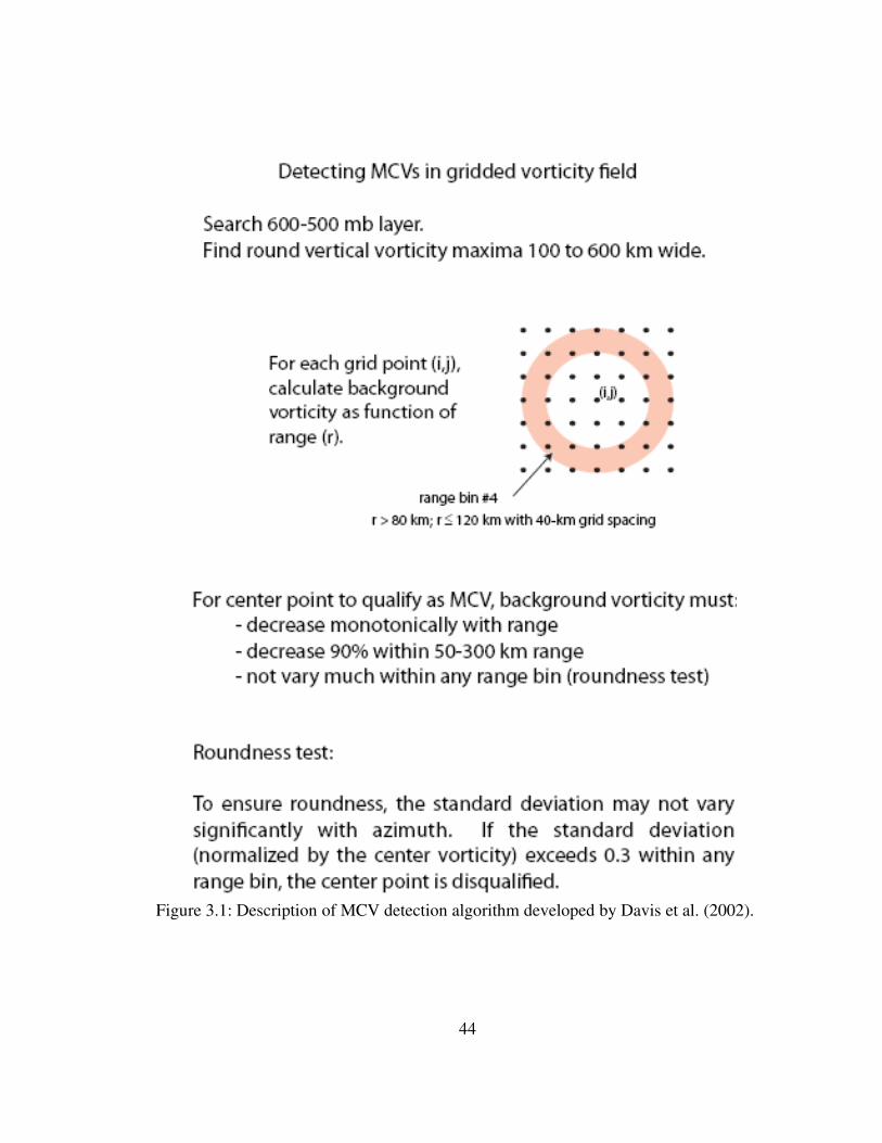
Figure 3.1: Description of MCV detection algorithm developed by Davis et al. (2002).

44

500  hPa,   and   then   averaged  over   that   layer.    The   first   step   in   the   algorithm   is   the 

identification of relative vorticity maxima, defined as gridpoints where the Laplacian of 

the relative vorticity is negative.  The next step filters out horizontally elongated vorticity 

features, which are quite common but non­convective in origin.  To do this, the algorithm 

calculates   several  metrics   associated  with   the   radial   distribution  of   relative  vorticity 

around   each   vorticity   maximum.     The   radial   distribution   of   relative   vorticity   is 

determined   by   taking   the   azimuthal   mean   of   all   the   gridpoints   within   a   series   of 

increasingly distant range bins of radial width 40 km (equal to the spacing of the RUC 

grid).    The radius R of  the vortex  is  defined as  the radius  bin annulus  in which the 

azimuthal mean relative vorticity decreases to less than 10% of its maximum (central) 

value.  For each radius bin within R, the standard deviation of relative vorticity about the 

azimuthal   mean   relative   vorticity   is   calculated.     Horizontally   elongated   features   are 

removed by excluding all  vortices  whose relative vorticity  standard deviation (in any 

range bin) is above 30% of the maximum (central) relative vorticity.  The algorithm also 

requires that the azimuthal mean relative vorticity decrease monotonically out to radius 

R,   which   excludes   vorticity   lobes   attached   to   larger­scale   maxima.     The   radial 

distribution of relative vorticity is only determined out to seven range bins.  The seventh 

range  bin corresponds   to  an  average   radius  of  262 km;   thus,   larger  vortices  are  not 

detected by the algorithm.  This filters out synoptic­scale vorticity anomalies, and keeps 

45

the   focus  on   the  mesoscale.    The  original   algorithm was  written   in  Fortran  77;   the 

algorithm used in this study was developed in Matlab, based on the original algorithm 

provided by David Ahijevych.  The presence of numerous times in the RUC data when at 

least   one   of   the   three   pressure   levels   was   missing   prompted   a   modification   of   the 

algorithm to search for MCVs based on only one or two levels.   The final algorithm is 

run  on   the  available  gridded  wind  fields   for   the  months  of  May  through  August  of 

2002­2005, over the entire RUC domain.  For the purposes of this study, output is only 

examined over the central USA, particularly in the vicinity of Oklahoma.  

Once the algorithm has detected all the MCV­like vortices present in the RUC 

analyses, it remains to determine which of them are actually MCVs.  Davis et al. (2002) 

report that the algorithm detects dry vortices in addition to MCVs; they suggest that these 

could be topographically generated since they tend to be concentrated in the immediate 

lee of the Rocky Mountains.   For each vortex detected within a latitude­longitude box 

containing   Oklahoma   and   part   of   the   Texas   panhandle,   archived   radar   and   satellite 

imagery  are  examined.    Vortices  are  classified  as  MCVs only   if   they  are  embedded 

within,  or  arising from, significant  stratiform precipitation  and anvil  cloud associated 

with deep convection.   This definition is inevitably subjective, but the vast majority of 

the   vortices   detected   by   the   algorithm   are   clearly   MCVs   or   clearly   not.     Vortices 

associated with convection, but in the absence of any stratiform precipitation, are also 

46

separately noted; these are fairly rare.  All the MCVs detected by this algorithm over the 

state   of   Oklahoma   are   recorded,   and   each   is   examined   in   more   detail   using   both 

observations and model data.  

b. Mesonet and Profiler Analyses

For  the  purposes  of   this  study,   it   is   important   to  examine   individual  cases   in 

detail.   To this end, gridded mesoscale analyses are constructed for each case based on 

data from the Oklahoma Mesonet and the NPN.   It has been noted in several previous 

mesoscale   analysis   studies   (e.g.,  Fujita  1955,  Bartels  et  al.  1997)   that,  under  certain 

conditions, the density of observations in the vicinity of a moving feature of interest can 

be   artificially   increased   by   employing   a   time­space   transformation.     This   involves 

determining the speed and direction of the motion of the feature being tracked.  Once this 

is known, and assuming the feature is in a steady state (i.e., not changing significantly 

over the time separating observations), previous and subsequent observations at a point 

can be “transformed” from time to space.  The additional observations are plotted along a 

line oriented along the direction of motion of the feature, and their separation distance 

from  the  original  observation  point  depends  on   the   speed  of   the   feature  of   interest. 

Obviously, this approach introduces some error into a dataset.  However, it can be quite 

useful   in   an   environment   of   sparse   observations,   as   long   as   the   steady­state 

47

approximation is not grossly violated.  For this study, MCVs are the feature of interest, 

and it  can be argued that  they are at  least  approximately in steady state.    Their very 

nature,  as  quasi­balanced systems,   suggests   that   they  evolve  very slowly,  and  this   is 

supported by the numerous reported cases of long­lived MCVs (e.g., Bosart and Sanders 

1981,  Fritsch et  al.  1994,  Galarneau et  al.  2005;  see also section  4a).    A  time­space 

transformation is carried out both for the Oklahoma Mesonet data and the NPN data.  In 

order to avoid clear violations of the steady­state approximation, the transformation is 

only applied over a limited area surrounding the MCV.   This area is a 3º  latitude by 3º 

longitude box, centred over the MCV and moving with it through the state of Oklahoma. 

The size of the box was determined by trial and error, roughly guided by the fact that an 

MCV might  be expected to  influence its  environment out  to approximately a Rossby 

radius of deformation (~280 km in a typical MCS environment; Chen and Frank 1993). 

The speed and heading of each MCV are determined by the motion of the vortex in radar 

imagery.    The Advanced Weather Interactive Processing System (AWIPS) software is 

used to display Level 3 radar data, and the AWIPS “distance­speed tool” is used to find 

the heading and speed of the vortices.  All the MCV cases examined contain some radar 

echoes in their vicinity,  which can be seen rotating around the vortex.     Heading and 

speed are determined for two­hour periods throughout the passage of the system through 

Oklahoma,  allowing a  time­space  transformation   to  be carried  out   for   the same  time 

48

period.    While  it  is likely that  the heading and speed determined in  this way are not 

always perfect, experimentation with differences in the system velocity have confirmed 

that the general mesoanalyses are not greatly affected by small changes in heading and 

speed.  The time­space transformation for the Oklahoma Mesonet surface observations is 

carried out using the system speed for the two­hour period containing the observation 

time.  For each observation, the two previous observations (five and ten minutes before) 

and the two following observations (five and ten minutes later) are transformed.   The 

same method   is  used   for   the  NPN upper­air  observations,   except  only  one  previous 

observation   (one   hour   earlier)   and   one   subsequent   observation   (one   hour   later)   are 

transformed.   Figure 3.2 shows an example of the additional observations that can be 

obtained using this method.  

With all the actual and artificial observations available,  the actual analyses are 

carried out using multiquadratic interpolation.  The characteristics and advantages of this 

method  of   analysis   have  been  described   in   some  detail   by  Nuss   and  Titley   (1994). 

Multiquadratic analysis utilises radial basis functions to interpolate scattered observations 

onto a regular grid.  The interpolation equation is

H X =∑i=1

N

iQ X−X i ,

where H(X)  is some spatially varying field,  Q(X­Xi)  is a radial basis function where the

49

Figure  3.2:  Observed NPN 700 hPa wind barbs  and RASS virtual   temperatures   (ºC) overlaid on NEXRAD composite radar reflectivity (colours; dBZ) at 1500 UTC on 24 May 2003.

argument represents the vector between an observation point Xi and any other point in the 

domain,  and i are weighting factors   to  be determined from the observations.    The 

basis functions are hyperboloids, given by the equation

Q X−X i=−∥X−X i∥2

c21.0 ,

where c is a tunable parameter (the multiquadratic parameter).  In matrix notation, when 

50

observational error is considered and accounted for, the final interpolation equation is 

H j=[QijN i2 ij] i ,

where Hj is the analysed field, Qij is the set of basis functions at each observation point, 

N  is   the   number   of   observations, is   another   tunable   parameter   (the   smoothing 

parameter), i2 is the mean­squared observation error, ij is the Kronecker delta, and

i are the coefficients determined from the observations.  Historically, this method of 

analysis has not been much used in the field of meteorology, but the study by Nuss and 

Titley  (1994)  confirms   that   it   is  actually   superior   to   two more  popular  methods:   the 

Barnes and Cressman methods.  Their study also demonstrates the influences of the two 

tunable   parameters,   the  muliquadratic   parameter   and   the   smoothing  parameter.    The 

multiquadratic parameter, c, serves to keep the multiquadratic basis function from having 

discontinuous   derivatives.     It   determines   the   sharpness   of   the   curvature   of   the 

hyperboloids used in the interpolation.   If  c  is small,  the hyperboloids will have very 

sharp curvature, and thus tight gradients can be easily represented.  Low values of c can 

also cause  individual  observations  to  affect  only  their   immediate  vicinity   in   the final 

analysis.  If c is large, flat hyperboloids are used and the interpolation may have trouble 

with closely spaced observations and tight gradients.   In this study, the multiquadratic 

parameter   was   extensively   modified   to   find   the   optimal   setting   by   trial   and   error. 

51

Optimal results are obtained with c=1.5, and this setting is used for all analyses in this 

study.  The smoothing parameter, , has the effect of reducing the small­scale noise in 

the final analysis.   If is small, the analysis will retain a large amount of the noise 

arising from the original observations.  If is large, it acts as a spectral low­pass filter 

to reduce the number of small­scale features and remove structure at short horizontal 

wavelengths.  Once again, the smoothing parameter was chosen by trial and error.  Small 

values of result in unrealistic values in data­sparse regions, due to the extrapolation 

of gradients by the interpolation technique.  Very large values of result in excessive 

smoothing of real gradients associated with the MCVs.   The best balance is achieved 

using =0.000005 for the mesonet analyses, and =0.0001 for the profiler analyses, 

and these values are used throughout this study.  Different values of are used for the 

mesonet and profiler analyses due to the different inherent spacing of the observations in 

both cases.   It was found that slight changes in these values do not greatly affect the 

analysis   results,  so  the analyses can be viewed with some confidence.    Analyses are 

carried  out  on a 0.1º  latitude  by 0.1º  longitude grid covering the state  of Oklahoma. 

Mesonet analyses cover the Oklahoma panhandle, whereas the profiler analyses do not.  

Using the multiquadratic interpolation technique,  a variety  of surface plots  are 

created   from   the   Oklahoma   Mesonet   data.     Plots   are   created   for   every   15   minutes 

throughout the MCV case analysis period.  The 15­minute temporal resolution is dictated 

52

by the background composite radar images obtained from WSI Corporation; these images 

are available only every 15 minutes.  Analysis fields are overlaid on these radar images to 

provide a useful context for the observations.   Mesonet observations that are analysed 

include the relative humidity (%), 1.5­m air temperature (ºC), 10­m wind speed (m/s), 10­

m wind direction  (º),  10­m wind gusts   (m/s),  accumulated  rainfall   (mm),  and station 

pressure   (hPa).     From   these   variables,   several   others   are   determined.     The   vapour 

pressure (e; hPa) is given by

e=0.06112 RH exp 17.67 TT243.49 ,

where  RH  is the relative humidity (%), and  T  is the 1.5­m air temperature (ºC).   The 

mixing ratio (r; g/kg) is given by

r=622 ep−e

,

where  p  is the station pressure (hPa).   The dewpoint temperature (Td;  ºC) is calculated 

from the equation

T d= 1273

−0.0001844 ln e6.112

−1

−273.15 .  

The station pressure variable is modified by removing the diurnal cycle of pressure from 

the raw observations.   This is achieved by subtracting, for each station and for each 5­

53

minute observation during the day, the averaged pressure at that station and time of day 

over the month of interest.  Pressure is also corrected to a constant elevation of 356.6 m, 

which is the average elevation of all the Oklahoma Mesonet stations.  This is achieved by 

the equation

p '=pexp z−356.6

29.3[T 273.15][10.6112r

1000] ,

where  z  is   the  station  elevation  (m),  and  p'  is   the  corrected  356.6­m pressure (hPa). 

Equivalent potential temperature ( e ; K) is then determined from the equation

e=T273.15Lv r

1000 c pd 1000

p l 0.286

,

where Lv is the latent heat of vapourisation of water (2.5x106 J/kg) and cpd is the specific 

heat capacity of dry air at constant pressure (1004 JK­1kg­1).  10­m divergence ( ; s­1) 

and relative vorticity ( ; s­1) are calculated from the 10­m wind field by the equations

=∂u∂ x

∂ v∂ y

and

=∂v∂ x

−∂ u∂ y

,

using centred­differencing.  Finally, the accumulated rainfall variable is converted to a 5­

min rainfall amount.  Plots are created every 15 minutes of the observed 10­m wind barbs 

54

and gusts  at  mesonet   stations,  and  the  analysed  10­m divergence,  10­m wind speed, 

station pressure corrected to 356.6­m elevation, 1.5­m relative humidity, 10­m streamline 

analysis, 1.5­m air temperature, 1.5­m dewpoint temperature, 1.5­m equivalent potential 

temperature, and 10­m relative vorticity.  In addition to these surface maps, meteograms 

are also constructed for each individual mesonet station for the period of interest during 

each   case.     These   meteograms   display   the   1.5­m   air   temperature   and   dewpoint 

temperature, 356.6­m pressure, 10­m wind barbs, 10­m wind speed and gusts, and 5­min 

accumulated rainfall.  

Profiler   fields  are  only  available  every  hour;   thus   the  pressure­level  plots  are 

overlaid  on  hourly   composite   radar   reflectivity   images.    Directly  observed  variables 

include wind speed (m/s) and direction (º) at 250­m vertical resolution, as well as RASS 

virtual temperatures (ºC) in the lower troposphere at certain profiler sites.  These data are 

linearly   interpolated   to   constant  pressure   levels   at  25­hPa   intervals.     In   cases  where 

several hours of profiler data are missing, but with valid profiles before and after, the 

data are linearly interpolated in time.   In addition to these directly observed variables, 

divergence   (s­1)   and   relative   vorticity   (s­1)   are   determined   on   each   25­hPa   level   by 

centred­differencing.   Plots are created every hour of the observed wind barbs at all of 

the   eight   profiler   sites,   as   well   as   the   analysed   divergence,   wind   speed,   streamline 

analysis, virtual temperature, and relative vorticity, at 850, 700, 500, 300, and 200 hPa.  

55

Various types of plots are also created for each individual profiler site.   Virtual 

temperature anomalies are calculated throughout the period of analysis for each MCV 

case at each RASS­equipped site.  These are determined by subtracting the mean virtual 

temperature (determined separately for each level)  over the analysis period from each 

individual virtual temperature observation.  This provides an easy way to visualise virtual 

warming  and cooling   in   the  column above  each  profiler   site,  and  can  often  provide 

guidance as to the mechanisms for surface effects around MCVs.  Time­height sections 

of   this   virtual   temperature   anomaly,   overlaid   on   profiler   wind   observations,   are 

constructed for each profiler site and for each case.   Skew­T/Log­p diagrams are also 

plotted  for  each profiler  site  at  each analysis   time.    While   the virtual   temperature   is 

strictly   not   equivalent   to   the   actual   air   temperature,   skew­T  diagrams  of   the  virtual 

temperature profile can give a basic sense of the state of the atmosphere.  Hodographs are 

also constructed for each profiler site at each analysis time.  

Finally, divergence and vorticity profiles, derived from the pressure­level gridded 

profiler analyses, are plotted through the centre of the MCV at each hour.   The MCV 

positions used for these profiles are determined from the RUC analyses, as described in 

section 3c.  These profiles can be compared with collocated ones from the RUC analyses 

to get a sense of the dynamics of the MCVs at various stages in their life cycle, as well as 

the performance of the RUC model.  

56

c. RUC Analyses

For each MCV case, a variety of variables derived from the hourly RUC analyses 

are plotted.  Some variables are directly included in the RUC data; others can be derived 

from the given variables.  Each RUC analysis includes the following variables which are 

plotted each hour: surface­based CAPE (J/kg) and CIN (J/kg); surface mean sea level 

pressure (hPa); column­integrated precipitable water (mm); 2­m relative humidity (%) 

and temperature (ºC); 10­m zonal and meridional wind speed (m/s); and pressure­level 

geopotential height (m), temperature (ºC), relative humidity (%), zonal and meridional 

wind speed (m/s), and pressure vertical velocity (Pa/s).  Derived variables that are plotted 

each hour include 10­m and pressure­level divergence (s­1) and relative vorticity (s­1); 2­

m and pressure­level  dewpoint   temperature   (ºC)  and equivalent  potential   temperature 

(K);   and   pressure­level   mixing   ratio   (g/kg)   and   PV   (PVU=10­6  Km2kg­1s­1).     PV   is 

calculated by the following equation:

PV=1

f ⋅∇ ,

where  is the air density (kg/m3), is the potential temperature, and

f=7.292×10−5 sin

is   the  Coriolis  parameter   (s­1),  where is   the   latitude   (º).     If  we   assume   that   the 

gradient  of potential  temperature is strictly  in the vertical,   then,  using the hydrostatic 

57

equation, we find that

PV=−gf ∂

∂ p ,

where g is the acceleration of gravity (9.8 m/s2).   Now, using the definition of potential 

temperature

=T 1000p Rcp

where R is the gas constant for dry air (287 JK­1kg­1) and T is in Kelvin, and substituting 

in numerical values, we find that, in units of PVU,

PV=−9.8×106 f {∂T

∂ p 1000p

0.286

−0.286 1000p

−0.714

10 Tp2 } ,

where we have used the chain rule to evaluate the partial derivative of with respect to 

p.  All moisture­related fields are derived from relative humidity, as shown in section 3b. 

In general, surface fields are overlaid on mean sea level pressure contours, and 

pressure­level fields are overlaid on geopotential height contours.  All of the above plots 

are created for each hour of the analysis period for each MCV.  In addition, if the MCV is 

detected by the RUC algorithm before or after it moves through Oklahoma (i.e., before 

the beginning or after  the end of  the mesonet and profiler  analysis  period),  plots  are 

created for each of these times.  Thus we can obtain an overview of the entire MCV life 

span with the RUC fields.  

58

To   aid   in   visualising   the   structure   of   the   MCVs   and   their   synoptic­scale 

environment,   east­west   and  north­south  cross­sections  of   some  variables   through   the 

centre of the MCV are constructed.    These variables include divergence,  PV, relative 

humidity,  equivalent  potential   temperature,  zonal  and meridional  wind speed,   relative 

vorticity, and mixing ratio.  These cross­sections are overlaid on isentropes, which give a 

sense of the thermal structure of the system.  

Finally,  vertical  profiles of several variables  through the MCV centre  are also 

constructed.    The profile  variables  are divergence,  relative vorticity,  PV, and relative 

humidity.     These   profiles   provide   a   means   of   following   the   evolution   of   MCV 

intensification and weakening by summarising the vertical structure of the vortices with 

regard to these variables.  

d. Composite MCV Construction

Numerous past studies of individual MCVs have demonstrated that these systems 

pass  through a predictable  evolution during their  lifetimes,  and that  the structure and 

intensity of a single MCV can vary greatly from one period to another (Fritsch et al. 

1994; Rogers and Fritsch 2001).  Thus, it would be advantageous to identify the life cycle 

evolution of the MCV cases studied here.   Ideally, pure observations could be used to 

track the intensity of the vortex,  and some criteria could be used to define life cycle 

59

stages.   However, the observations available in this study are quite sparse.   Due to the 

varying degree of resolution of MCV circulations by the profiler network, the evolution 

of the analysed relative vorticity may be different from the evolution of the real relative 

vorticity.  For example, when an MCV passes through the core of the profiler network its 

relative vorticity is likely to be fairly well resolved, but if a mature MCV passes along 

the  edge of   the  network  its   relative  vorticity  may be analysed  as  much smaller   than 

reality.   It is thus difficult to unambiguously identify the time of the MCV's maximum 

relative  vorticity  using   the  profiler  analyses.    To circumvent   these   issues,   this   study 

utilises the RUC model to follow the evolution of MCVs throughout their life cycles. 

RUC data are used to define four different life cycle stages.  MCV initiation is defined as 

the hour at  which  the MCV is   first  detected  by  the  objective  algorithm described   in 

section 3a.  MCV maturity is defined as the hour at which the MCV attains its maximum 

relative vorticity at any level between 600 and 500 hPa inclusive.   MCV dissipation is 

defined   as   the  hour   at  which   the  MCV   is   last   detected  by   the  objective   algorithm. 

Finally,  MCV  development   is   defined   as   the   analysis   hour   that   is   halfway  between 

initiation and maturity (rounded up).  While these stages of the life cycle of an MCV are 

admittedly arbitrary,  they are at least  consistent, and should be expected to provide a 

basic sense of the evolution of different MCVs.  The RUC certainly has deficiencies in its 

representation of MCVs, due to issues discussed in section 2a.  However, the advantage 

60

of using the RUC is its consistency among all times, allowing an unbiased comparison of 

the longevity and evolution of different MCVs.  

Using   these   four   life   stage   definitions,   it   is   possible   to   construct   composite 

analyses for each of them.  RUC data are used to create synoptic­scale composites of the 

initiation, developing, mature, and dissipation stages of MCV evolution.  Each MCV case 

with valid RUC data at the times of interest is included in these composites.  The RUC 

grids are shifted such that the vortices are all centred in Oklahoma (at 33.5º north, 97.5º 

west).  The shifting of the vortices is accomplished based on the position of the 500 hPa 

relative   vorticity   maximum   associated   with   each   MCV   at   each   analysis   time.     The 

horizontal position of the MCVs should not vary significantly between 600 and 500 hPa, 

so the composite fields should faithfully represent the MCV environment relative to the 

mid­level vortex centre.   Due to the coarseness of the RUC data, these composites are 

mostly  of  use for   investigating   the  synoptic  scale  environment  of  MCVs at  different 

stages of their life cycles.  

61

IV. MCV CLIMATOLOGY

This section presents the first part of the results of this study, summarising the 

main   findings   concerning   mid­latitude   MCV   climatology   and   the   synoptic­scale 

environment of these MCVs.  

a. Climatological Characteristics

The results of the MCV detection algorithm over the study period of May­August 

2002­05   are   presented   in   Table   4.1,   and   are   compared   with   results   from   previous 

climatological studies of MCVs.  It should be noted that the detection methodologies of 

the previous studies have been of variable sophistication and efficiency, as discussed in 

section 3a.   It is also important to recognise the differences in the experimental design 

between this study and that of Davis et al. (2002), despite the use of the same algorithm. 

Davis et al. (2002) ran the algorithm on 3­hourly RUC analyses, whereas hourly analyses 

are used in this study.  Additionally, Davis et al. (2002) documented vortices throughout 

the   Great   Plains   (see   Figure   4.1),   whereas   this   study   documents   vortices   only   in 

Oklahoma and the Texas panhandle.  Thus, some differences in the frequency of MCVs 

are to be expected among these studies.  

62

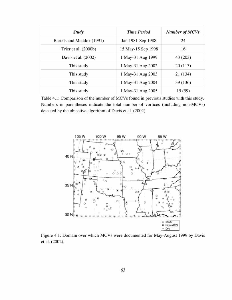
Study Time Period Number of MCVs

Bartels and Maddox (1991) Jan 1981­Sep 1988 24

Trier et al. (2000b) 15 May­15 Sep 1998 16

Davis et al. (2002) 1 May­31 Aug 1999 43 (203)

This study 1 May­31 Aug 2002 20 (113)

This study 1 May­31 Aug 2003 21 (134)

This study 1 May­31 Aug 2004 39 (136)

This study 1 May­31 Aug 2005 15 (59)Table 4.1: Comparison of the number of MCVs found in previous studies with this study.Numbers   in  parentheses   indicate   the   total  number  of  vortices   (including  non­MCVs) detected by the objective algorithm of Davis et al. (2002).

Figure 4.1: Domain over which MCVs were documented for May­August 1999 by Davis et al. (2002).

63

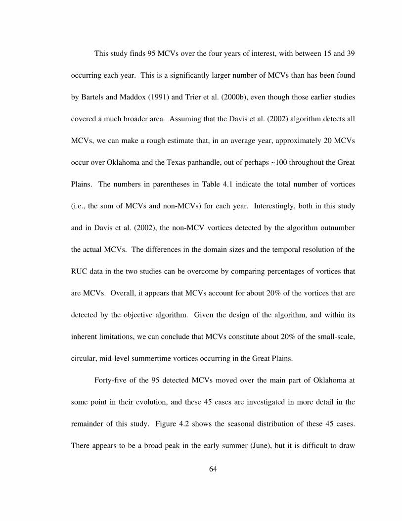
This study finds 95 MCVs over the four years of interest, with between 15 and 39 

occurring each year.  This is a significantly larger number of MCVs than has been found 

by Bartels and Maddox (1991) and Trier et al. (2000b), even though those earlier studies 

covered a much broader area.  Assuming that the Davis et al. (2002) algorithm detects all 

MCVs, we can make a rough estimate that, in an average year, approximately 20 MCVs 

occur over Oklahoma and the Texas panhandle, out of perhaps ~100 throughout the Great 

Plains.   The numbers in parentheses in Table 4.1 indicate the total number of vortices 

(i.e., the sum of MCVs and non­MCVs) for each year.   Interestingly, both in this study 

and in Davis et al. (2002), the non­MCV vortices detected by the algorithm outnumber 

the actual MCVs.  The differences in the domain sizes and the temporal resolution of the 

RUC data in the two studies can be overcome by comparing percentages of vortices that 

are MCVs.  Overall, it appears that MCVs account for about 20% of the vortices that are 

detected by the objective algorithm.   Given the design of the algorithm, and within its 

inherent limitations, we can conclude that MCVs constitute about 20% of the small­scale, 

circular, mid­level summertime vortices occurring in the Great Plains.  

Forty­five of the 95 detected MCVs moved over the main part of Oklahoma at 

some point in their evolution, and these 45 cases are investigated in more detail in the 

remainder of this study.   Figure 4.2 shows the seasonal distribution of these 45 cases. 

There appears to be a broad peak in the early summer (June), but it is difficult to draw

64

Figure  4.2:  Seasonal  distribution  of  MCV cases   (by  week)   detected  over  Oklahoma during May­August 2002­05.

any firm conclusions about the seasonality of MCVs because of the extensive periods of 

missing RUC data (and  thus likely  missing MCVs) during  the years 2002 and 2005. 

Figure 4.3 shows the seasonal distribution of available RUC data over the four years of 

interest, in terms of the number of available analysis hours per day.  Note that a date with 

complete RUC data over all four years will contain (24x4) 96 analysis hours.  Four years 

is likely insufficient to determine a climatological seasonal cycle.  

For the MCV cases having valid RUC analyses at their initiation and dissipation, 

it is possible to determine the MCV longevity.  This is defined as the number of hourly

65

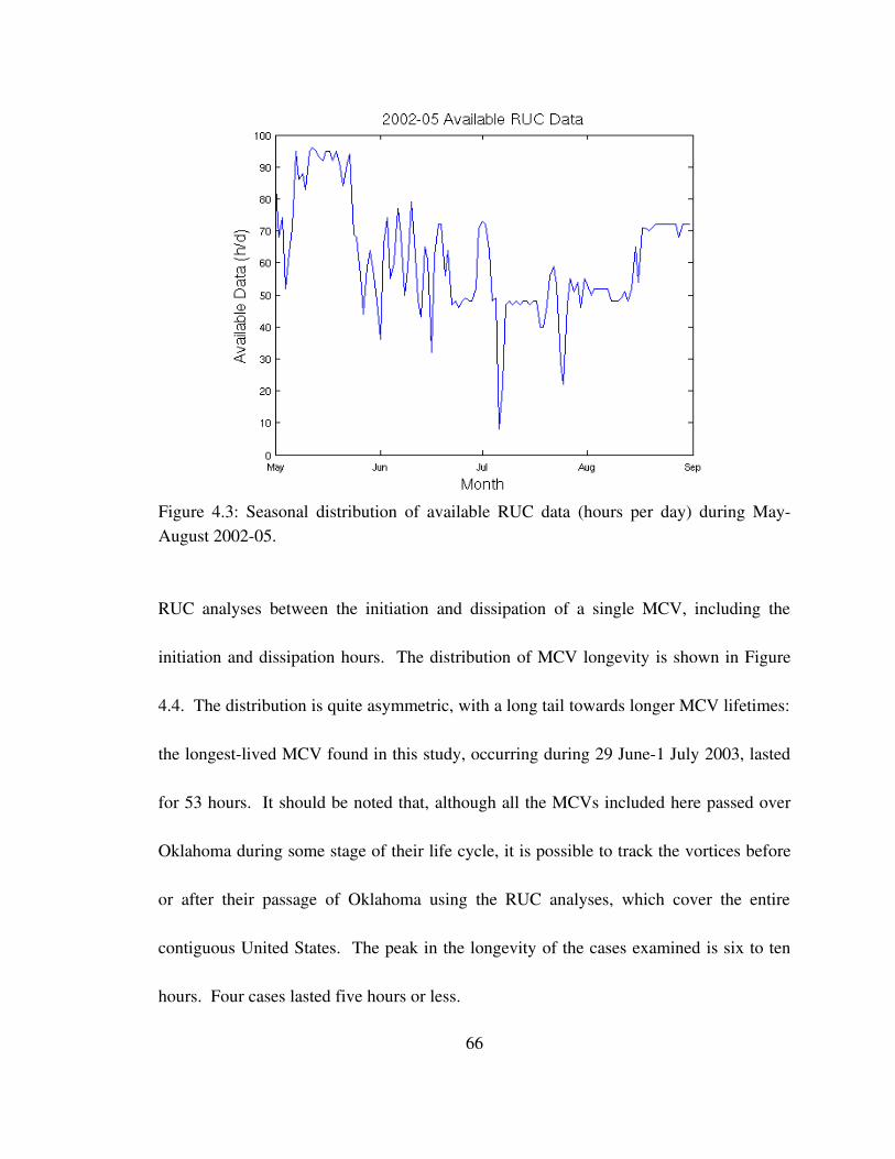
Figure 4.3: Seasonal distribution of available  RUC data (hours per day) during May­August 2002­05.

RUC analyses  between  the  initiation  and dissipation  of  a  single MCV,  including   the 

initiation and dissipation hours.   The distribution of MCV longevity is shown in Figure 

4.4.  The distribution is quite asymmetric, with a long tail towards longer MCV lifetimes: 

the longest­lived MCV found in this study, occurring during 29 June­1 July 2003, lasted 

for 53 hours.  It should be noted that, although all the MCVs included here passed over 

Oklahoma during some stage of their life cycle, it is possible to track the vortices before 

or  after   their  passage  of  Oklahoma using   the  RUC analyses,  which  cover   the  entire 

contiguous United States.  The peak in the longevity of the cases examined is six to ten 

hours.  Four cases lasted five hours or less.  

66

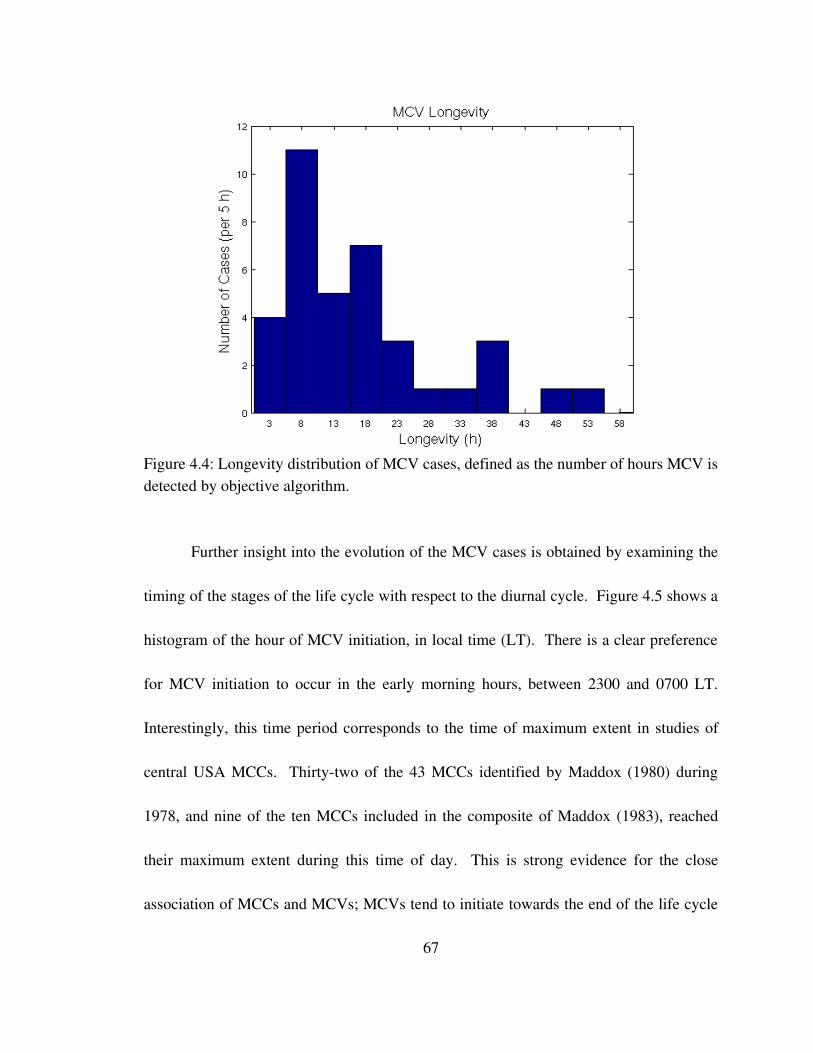
Figure 4.4: Longevity distribution of MCV cases, defined as the number of hours MCV is detected by objective algorithm.

Further insight into the evolution of the MCV cases is obtained by examining the 

timing of the stages of the life cycle with respect to the diurnal cycle.  Figure 4.5 shows a 

histogram of the hour of MCV initiation, in local time (LT).  There is a clear preference 

for MCV initiation to occur in the early morning hours, between 2300 and 0700 LT. 

Interestingly, this time period corresponds to the time of maximum extent in studies of 

central USA MCCs.   Thirty­two of the 43 MCCs identified by Maddox (1980) during 

1978, and nine of the ten MCCs included in the composite of Maddox (1983), reached 

their maximum extent during this  time of day.   This  is strong evidence for  the close 

association of MCCs and MCVs; MCVs tend to initiate towards the end of the life cycle

67

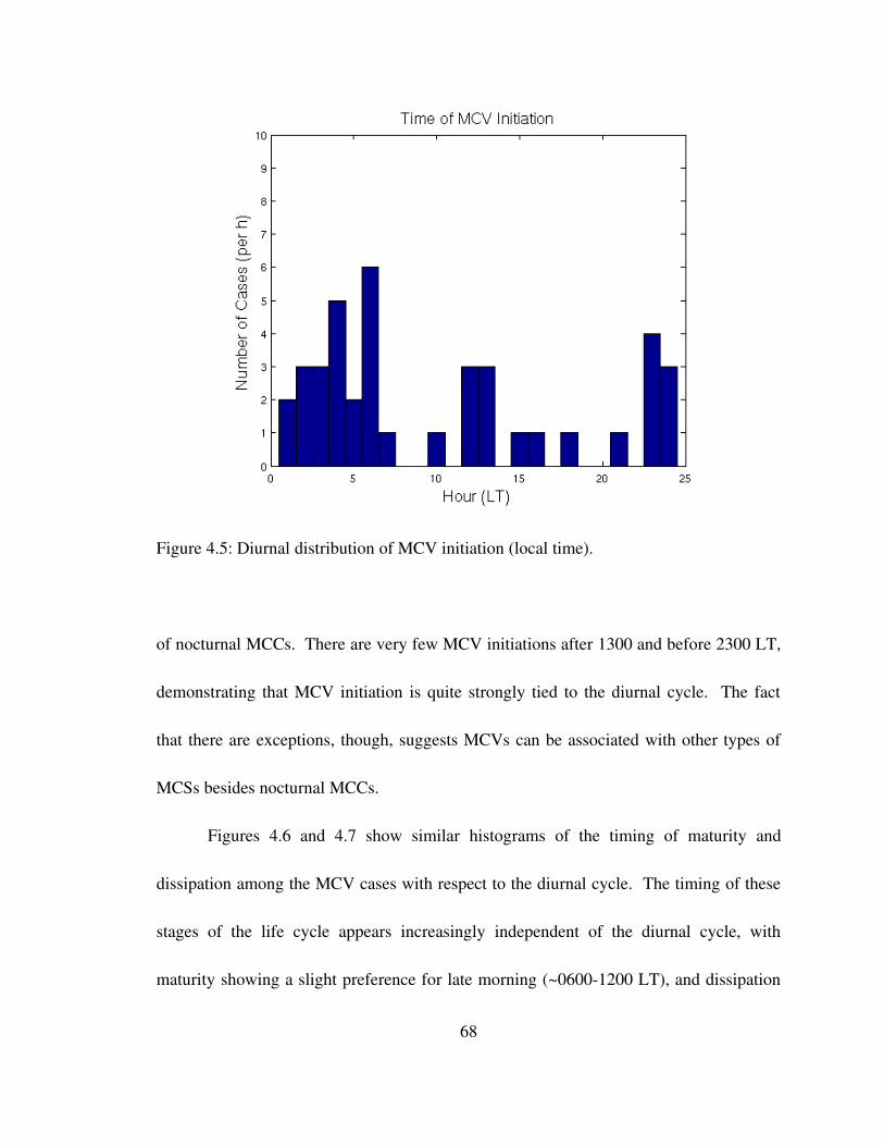
Figure 4.5: Diurnal distribution of MCV initiation (local time).

of nocturnal MCCs.  There are very few MCV initiations after 1300 and before 2300 LT, 

demonstrating that MCV initiation is quite strongly tied to the diurnal cycle.   The fact 

that there are exceptions, though, suggests MCVs can be associated with other types of 

MCSs besides nocturnal MCCs.  

Figures   4.6   and   4.7   show   similar   histograms   of   the   timing   of   maturity   and 

dissipation among the MCV cases with respect to the diurnal cycle.  The timing of these 

stages   of   the   life   cycle   appears   increasingly   independent   of   the   diurnal   cycle,   with 

maturity showing a slight preference for late morning (~0600­1200 LT), and dissipation

68

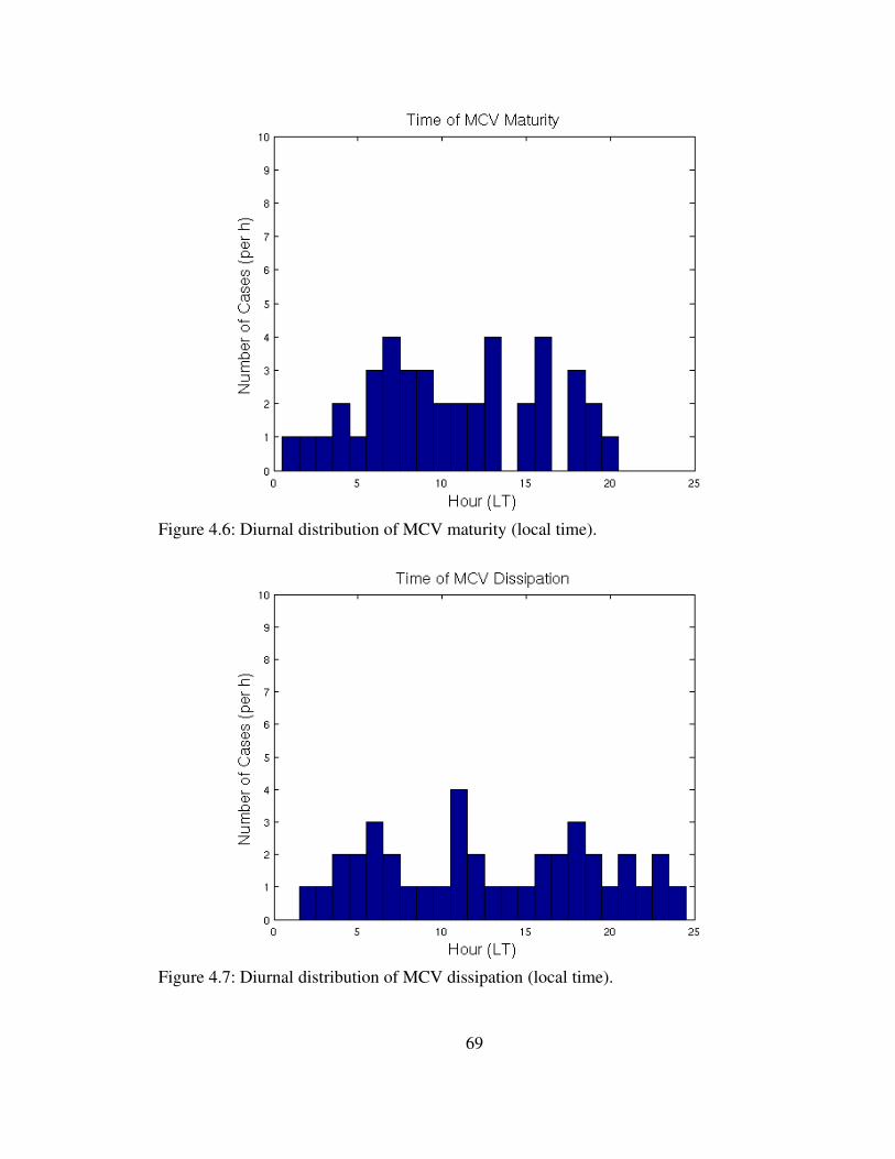
Figure 4.6: Diurnal distribution of MCV maturity (local time).

Figure 4.7: Diurnal distribution of MCV dissipation (local time).

69

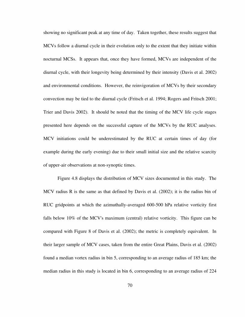
showing no significant peak at any time of day.  Taken together, these results suggest that 

MCVs follow a diurnal cycle in their evolution only to the extent that they initiate within 

nocturnal MCSs.  It appears that, once they have formed, MCVs are independent of the 

diurnal cycle, with their longevity being determined by their intensity (Davis et al. 2002) 

and environmental conditions.  However, the reinvigoration of MCVs by their secondary 

convection may be tied to the diurnal cycle (Fritsch et al. 1994; Rogers and Fritsch 2001; 

Trier and Davis 2002).   It should be noted that the timing of the MCV life cycle stages 

presented here depends on the successful capture of the MCVs by the RUC analyses. 

MCV   initiations   could   be   underestimated   by   the   RUC   at   certain   times   of   day   (for 

example during the early evening) due to their small initial size and the relative scarcity 

of upper­air observations at non­synoptic times.  

Figure 4.8 displays the distribution of MCV sizes documented in this study.  The 

MCV radius R is the same as that defined by Davis et al. (2002); it is the radius bin of 

RUC gridpoints at which the azimuthally­averaged 600­500 hPa relative vorticity first 

falls below 10% of the MCV's maximum (central) relative vorticity.  This figure can be 

compared with Figure 8 of Davis et al. (2002); the metric is completely equivalent.   In 

their larger sample of MCV cases, taken from the entire Great Plains, Davis et al. (2002) 

found a median vortex radius in bin 5, corresponding to an average radius of 185 km; the 

median radius in this study is located in bin 6, corresponding to an average radius of 224

70

Figure 4.8: Distribution of MCV radius at system maturity, defined as the radius bin at which the MCV's azimuthally­averaged 600­500 hPa relative vorticity first falls below 10% of the central (maximum) relative vorticity.  Bins 2­7 correspond to average radii of 49, 97, 142, 185, 224, and 262 km, respectively.

km.   It is not known if this is a real difference between the year 1999 and the mean of 

2002­05,  a   result  of   the  different   regions  covered   in   the   two studies,  or  a   statistical 

artifact.  Both studies demonstrate that the median MCV radius is within bin 7 (262 km), 

indicating that the cut­off radius of 300 km used in the MCV detection algorithm is likely 

appropriate.  The distribution of intensity of the MCV cases is shown in Figure 4.9.  For 

the purposes of this study, MCV intensity is defined as the mean 600­500 hPa relative 

vorticity at system maturity.  MCV intensity varies between 2x10­5 and 2x10­4 s­1, with a 

broad peak between 9x10­5 and 1.4x10­4 s­1.   This distribution of MCV relative vorticity

71

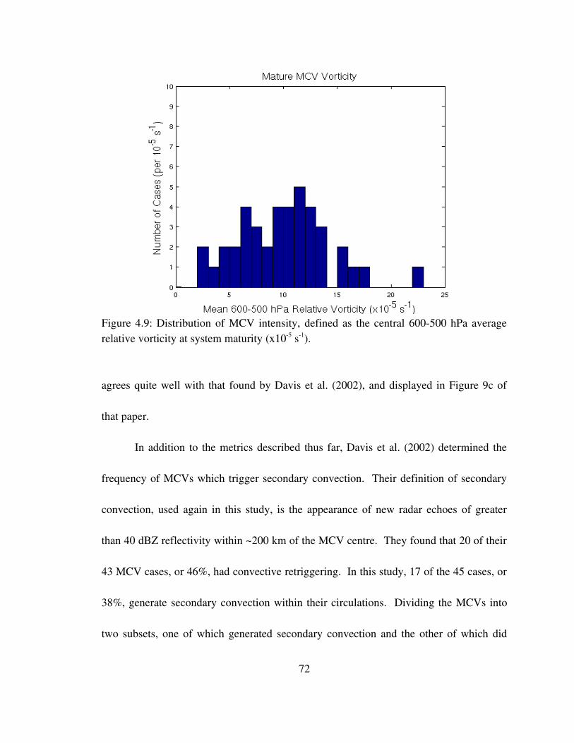
Figure 4.9: Distribution of MCV intensity, defined as the central 600­500 hPa average relative vorticity at system maturity (x10­5 s­1).

agrees quite well with that found by Davis et al. (2002), and displayed in Figure 9c of 

that paper.  

In addition to the metrics described thus far, Davis et al. (2002) determined the 

frequency of MCVs which trigger secondary convection.   Their definition of secondary 

convection, used again in this study, is the appearance of new radar echoes of greater 

than 40 dBZ reflectivity within ~200 km of the MCV centre.  They found that 20 of their 

43 MCV cases, or 46%, had convective retriggering.  In this study, 17 of the 45 cases, or 

38%, generate secondary convection within their circulations.   Dividing the MCVs into 

two subsets, one of which generated secondary convection and the other of which did 

72

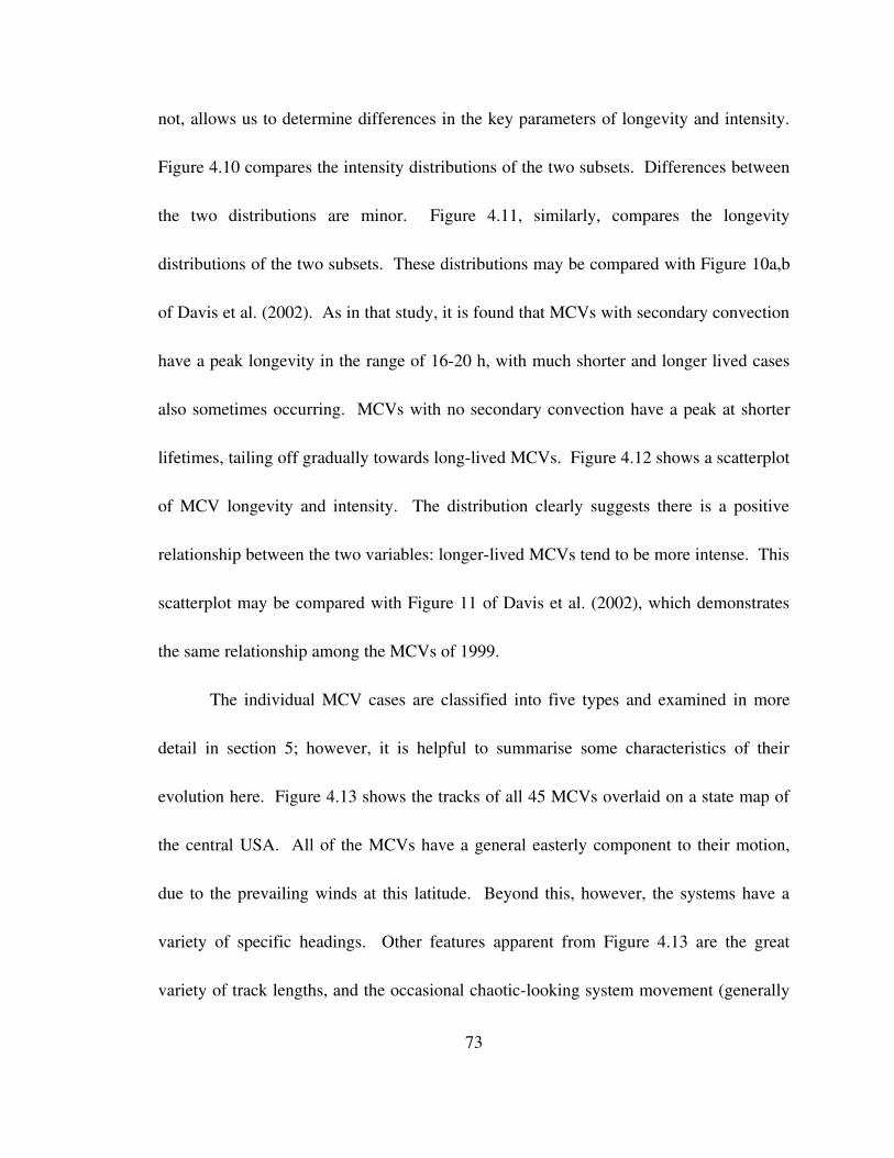
not, allows us to determine differences in the key parameters of longevity and intensity. 

Figure 4.10 compares the intensity distributions of the two subsets.  Differences between 

the   two   distributions   are   minor.     Figure   4.11,   similarly,   compares   the   longevity 

distributions of the two subsets.  These distributions may be compared with Figure 10a,b 

of Davis et al. (2002).  As in that study, it is found that MCVs with secondary convection 

have a peak longevity in the range of 16­20 h, with much shorter and longer lived cases 

also sometimes occurring.   MCVs with no secondary convection have a peak at shorter 

lifetimes, tailing off gradually towards long­lived MCVs.  Figure 4.12 shows a scatterplot 

of MCV longevity and intensity.    The distribution clearly suggests there is a positive 

relationship between the two variables: longer­lived MCVs tend to be more intense.  This 

scatterplot may be compared with Figure 11 of Davis et al. (2002), which demonstrates 

the same relationship among the MCVs of 1999.  

The individual MCV cases are classified into five types and examined in more 

detail   in  section  5;  however,   it   is  helpful   to   summarise   some characteristics  of   their 

evolution here.  Figure 4.13 shows the tracks of all 45 MCVs overlaid on a state map of 

the central USA.   All of the MCVs have a general easterly component to their motion, 

due to the prevailing winds at this latitude.   Beyond this, however, the systems have a 

variety  of specific  headings.    Other   features  apparent  from Figure 4.13 are   the great 

variety of track lengths, and the occasional chaotic­looking system movement (generally

73

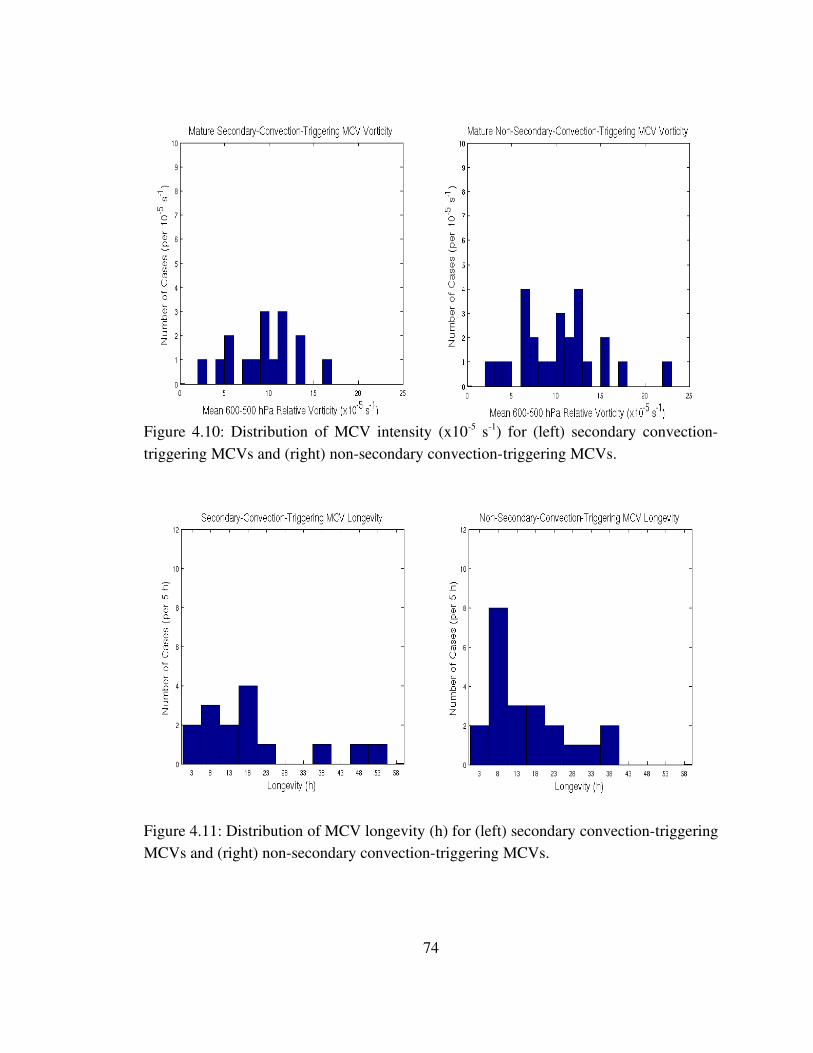
Figure 4.10: Distribution of MCV intensity (x10­5  s­1)  for (left) secondary convection­triggering MCVs and (right) non­secondary convection­triggering MCVs.

Figure 4.11: Distribution of MCV longevity (h) for (left) secondary convection­triggering MCVs and (right) non­secondary convection­triggering MCVs.

74

Figure 4.12: Scatterplot of MCV longevity (h) versus intensity (x10­5 s­1).

Figure  4.13:  MCV tracks  overlaid  on  state  map  of   the  south­central  USA.    Colours indicate the five MCV types identified in this study, as described in section 5a.

75

indicative of a nearly stationary MCV).  Some of the track irregularities are likely due to 

the limitations of the RUC analyses, and their failure to always resolve the MCVs in the 

correct locations.  

Figure 4.14 shows the relative vorticity evolution of the 45 MCV cases.   It  is 

difficult  to generalise this evolution in any sense beyond the obvious tendency for an 

initial increase, followed by a decrease leading up to system dissipation.  Several of the 

MCVs last sufficiently long to have several cycles of reintensification and weakening.  It 

is beyond the scope of this study to rigourously assess the statistical significance of the 

relationship between these intensification periods and the vigour of secondary convection 

in the vicinity of the MCV, but there does appear to be an association based on a casual 

inspection.  

Examination of surface pressure mesoanalyses for all 45 MCV cases reveals that 

28  of   the  45  vortices  have  significant   surface  mesolows  associated  with   them.    The 

varying sizes, strengths, and relative locations of the mesolows in each case suggest that 

no single mechanism is responsible for producing them.  Figure 4.15 shows the tracks of 

the primary mesolows with respect to the vortex centre, for each case with a significant 

mesolow.    The mesolow positions  are  plotted  relative   to   the vortex centre;   thus,   the 

ground­relative mesolow tracks will differ from those in Figure 4.15 depending on the 

motion of the parent MCVs.   The mesolows occur at varying times in the parent MCV

76

Figure 4.14: MCV mean 600­500 hPa relative vorticity (x10­5  s­1) evolution.    Colours indicate the five MCV types identified in this study, as described in section 5a.

Figure 4.15: MCV primary mesolow track, with respect to MCV centre at 600­500 hPa. Colours indicate the five MCV types identified in this study, as described in section 5a.

77

life cycle, and have varying durations.  In general, Figure 4.15 shows that the mesolows 

tend to remain fairly close to the MCV centre.   There is a slight tendency for mesolow 

displacement relative to the MCV centre to be more in the zonal than in the meridional 

direction.  The individual tracks tend to be oriented east­west, and their centroid is shifted 

slightly south of the MCV centre.  

The vortex centres in Figure 4.15 have been determined based on the average 

relative vorticity over the 600­500 hPa layer; plotting the mesolow tracks with respect to 

the relative vorticity maximum at a single level produces different individual tracks in the 

many cases where the MCV is tilted to some extent, but the basic nature of the track 

distribution is unchanged.  It is beyond the scope of this study to determine if the tilt of 

the MCVs in the RUC analyses is a real phenomenon, or a result of shortfalls in the RUC 

model.    The separation frequently  seen between the mid­level vortex and the surface 

mesolow   suggests   that,   at   least   in  many   cases,   the   surface  mesolow  is   not   a   direct 

downward penetration of the MCV.  It is possible that MCV tilting in vertical wind shear 

plays a role in the positioning of the surface low pressure centre; significant tilt has been 

observed in real MCVs (e.g., Davis and Trier 2007).  As will be shown in more detail in 

section 5, the mesolow does not appear to be a direct downward penetration of the MCV 

circulation in many of the cases examined in this study.  

78

b. Composite MCV

Figures 4.16­4.19 show the mid­level (500 hPa) geopotential height and relative 

vorticity fields for the four life cycle stages defined in section 3d.   A state map of the 

central USA is overlaid to provide a reference scale; it should be kept in mind that the 

composite construction involved shifting all MCVs to be centred in Oklahoma, so the 

map corresponds only to an average position of features among the different cases.  It is 

apparent from Figure 4.16 that the mean MCV initiation location is downstream from a 

mid­level ridge and upstream from a mid­level trough.  This positioning agrees well with 

that found by Bartels and Maddox (1991), as shown in Figure 4.20, despite the fewer 

cases identified in  that study.    The 500 hPa relative vorticity  field  at  MCV initiation 

shows weak anticyclonic relative vorticity in the environment of the MCV, particularly 

upstream; this  is associated with the anticyclonic flow around the nearby ridge.   The 

MCV itself appears as a concentrated, circular region of cyclonic relative vorticity.   At 

this   initial   time,   there   appears   to  be  minimal  deformation  of   the  geopotential  height 

contours in the vicinity of the MCV.  In the developing and mature composites, shown in 

Figures   4.17   and   4.18,   respectively,   the   MCV's   relative   vorticity   intensifies   and 

concentrates, while the environmental relative vorticity remains anticyclonic.  The MCV 

becomes   detectable   as   a   mesoscale   trough   in   the   geopotential   height   field.     At   the 

dissipation   stage   (Figure  4.19),   this  mesoscale   trough   remains  well   defined,   but   the

79

Figure   4.16:   Initiating   MCV   composite   (for   MCV   at   35.5ºN,   97.5ºW)   of   500   hPa geopotential height (m; contour interval 10 m) and relative vorticity (colours; s­1).

Figure  4.17:  Developing  MCV composite   (for  MCV at  35.5ºN,  97.5ºW)  of  500 hPa geopotential height (m; contour interval 10 m) and relative vorticity (colours; s­1).

80

Figure   4.18:   Mature   MCV   composite   (for   MCV   at   35.5ºN,   97.5ºW)   of   500   hPa geopotential height (m; contour interval 10 m) and relative vorticity (colours; s­1).

Figure  4.19:  Dissipating  MCV composite   (for  MCV at  35.5ºN,  97.5ºW)  of  500  hPa geopotential height (m; contour interval 10 m) and relative vorticity (colours; s­1).

81

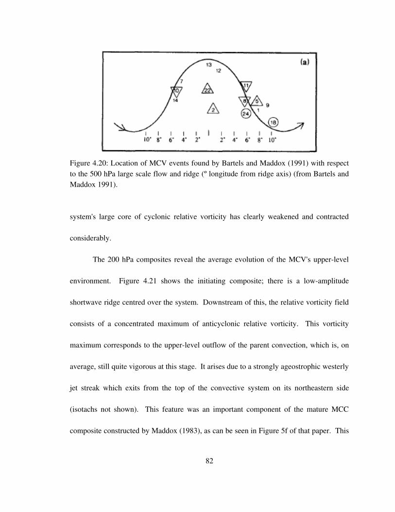
Figure 4.20: Location of MCV events found by Bartels and Maddox (1991) with respect to the 500 hPa large scale flow and ridge (º longitude from ridge axis) (from Bartels and Maddox 1991).

system's large core of cyclonic relative vorticity  has clearly weakened and contracted 

considerably.

The 200 hPa composites reveal the average evolution of the MCV's upper­level 

environment.     Figure   4.21   shows   the   initiating   composite;   there   is   a   low­amplitude 

shortwave ridge centred over the system.  Downstream of this, the relative vorticity field 

consists  of a concentrated maximum of anticyclonic  relative vorticity.    This  vorticity 

maximum corresponds to the upper­level outflow of the parent convection, which is, on 

average, still quite vigorous at this stage.  It arises due to a strongly ageostrophic westerly 

jet  streak which exits   from the  top of  the convective system on  its  northeastern side 

(isotachs not shown).   This feature was an important  component of the mature MCC 

composite constructed by Maddox (1983), as can be seen in Figure 5f of that paper.  This

82

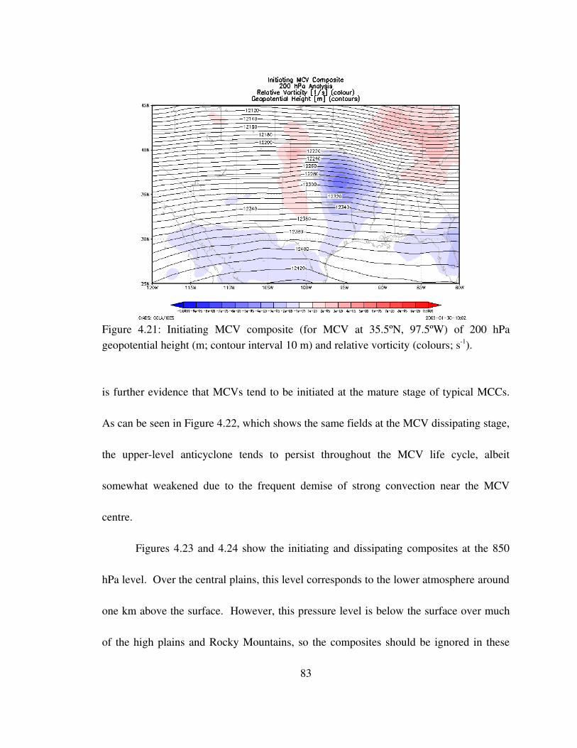
Figure   4.21:   Initiating   MCV   composite   (for   MCV   at   35.5ºN,   97.5ºW)   of   200   hPa geopotential height (m; contour interval 10 m) and relative vorticity (colours; s­1).

is further evidence that MCVs tend to be initiated at the mature stage of typical MCCs. 

As can be seen in Figure 4.22, which shows the same fields at the MCV dissipating stage, 

the   upper­level   anticyclone   tends   to   persist   throughout   the   MCV   life   cycle,   albeit 

somewhat  weakened due  to   the frequent  demise of  strong convection  near   the  MCV 

centre.  

Figures 4.23 and 4.24 show the initiating and dissipating composites at the 850 

hPa level.  Over the central plains, this level corresponds to the lower atmosphere around 

one km above the surface.  However, this pressure level is below the surface over much 

of the high plains and Rocky Mountains, so the composites should be ignored in these

83

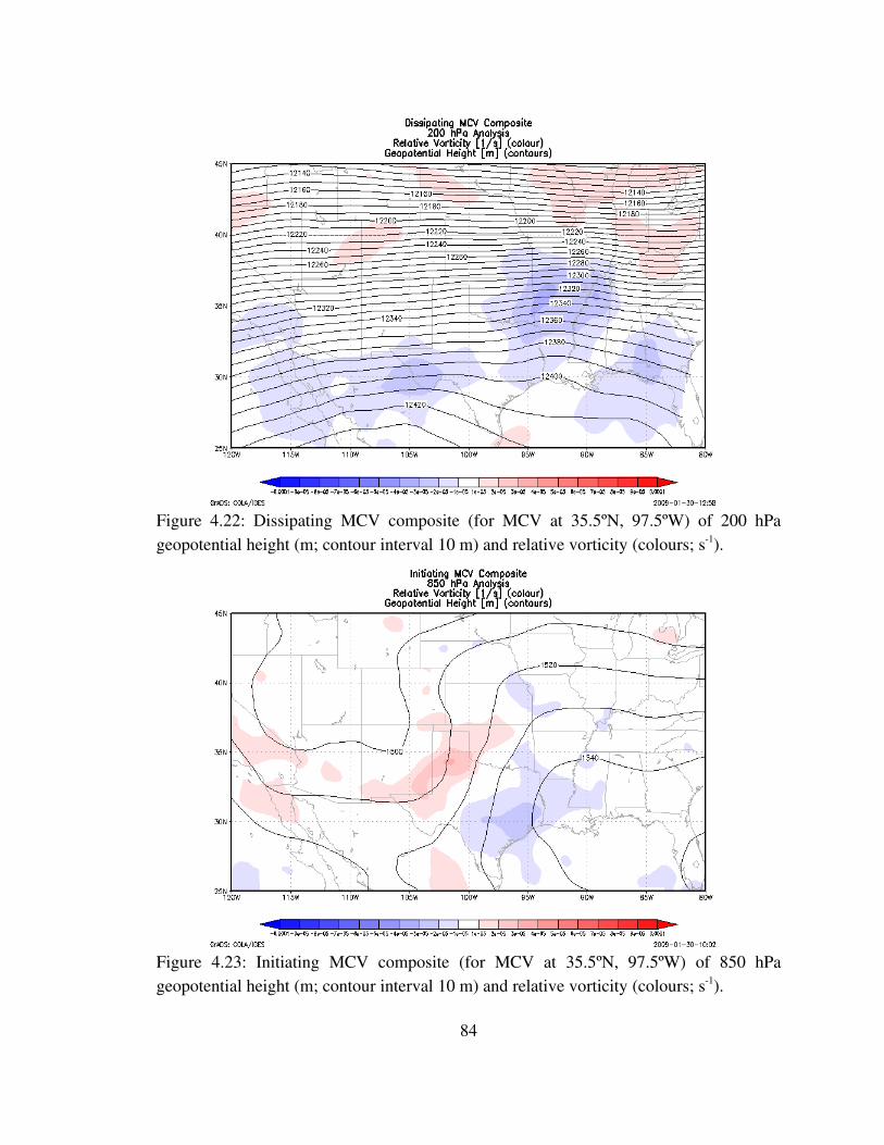
Figure  4.22:  Dissipating  MCV composite   (for  MCV at  35.5ºN,  97.5ºW)  of  200  hPa geopotential height (m; contour interval 10 m) and relative vorticity (colours; s­1).

Figure   4.23:   Initiating   MCV   composite   (for   MCV   at   35.5ºN,   97.5ºW)   of   850   hPa geopotential height (m; contour interval 10 m) and relative vorticity (colours; s­1).

84

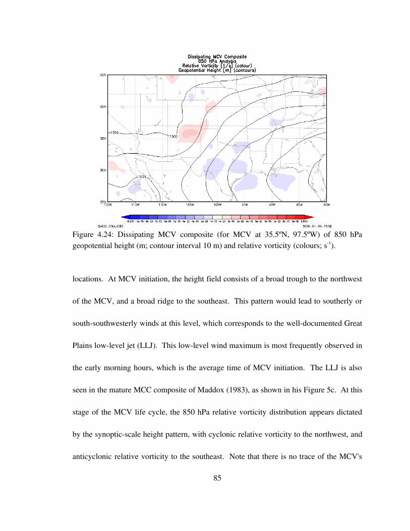
Figure  4.24:  Dissipating  MCV composite   (for  MCV at  35.5ºN,  97.5ºW)  of  850  hPa geopotential height (m; contour interval 10 m) and relative vorticity (colours; s­1).

locations.  At MCV initiation, the height field consists of a broad trough to the northwest 

of the MCV, and a broad ridge to the southeast.  This pattern would lead to southerly or 

south­southwesterly winds at this level, which corresponds to the well­documented Great 

Plains low­level jet (LLJ).  This low­level wind maximum is most frequently observed in 

the early morning hours, which is the average time of MCV initiation.  The LLJ is also 

seen in the mature MCC composite of Maddox (1983), as shown in his Figure 5c.  At this 

stage of the MCV life cycle, the 850 hPa relative vorticity distribution appears dictated 

by the synoptic­scale height pattern, with cyclonic relative vorticity to the northwest, and 

anticyclonic relative vorticity to the southeast.  Note that there is no trace of the MCV's 

85

relative vorticity at this level, indicating that the MCV is confined to the mid levels at this 

time.   At MCV dissipation, as shown in Figure 4.24, a similar height pattern persists, 

although the orientation of the height contours has shifted such that the 850 hPa winds 

are more veered (i.e., southwesterly).  This corresponds to the average diurnal weakening 

of the LLJ, which can also be seen in the MCC decay composite of Maddox (1983; his 

Figure   6c).     There   is   still   no   cyclonic   relative   vorticity   evident   at   850   hPa   in   the 

immediate vicinity of the MCV.  

Initiating and dissipating MCV composites at the surface are shown in Figures 

4.25 and 4.26.    At both  times,   the surface  pressure gradient  points   towards  the east, 

between a large region of low pressure over the high terrain southwest of the MCV and 

the western edge of the Bermuda high encroaching on the eastern USA.  This produces 

southeasterly flow at the surface.  The surface dewpoint temperature field shows a large­

scale   moistening   over   the   course   of   the   MCV   life   cycle.     However,   this   apparent 

moistening is likely an artificial effect arising from the compositing process.   Since, on 

average, the MCVs move eastwards, they tend to be in a moister environment at their 

dissipation   than   at   their   initiation.     During   the   compositing   process,   this   moisture 

signature is shifted westward, leading to an apparent moistening over the Great Plains.  

Profiles of variables through the composite MCV centre reveal several interesting 

features of the vertical structure.  Figure 4.27 shows the vertical structure of the low­ to

86

Figure 4.25: Initiating MCV composite (for MCV at 35.5ºN, 97.5ºW) of mean sea level pressure (hPa; contour interval 0.5 hPa) and 2­m dewpoint temperature (colours; ºC).

Figure 4.26: Dissipating MCV composite (for MCV at 35.5ºN, 97.5ºW) of mean sea level pressure (hPa; contour interval 0.5 hPa) and 2­m dewpoint temperature (colours; ºC).

87

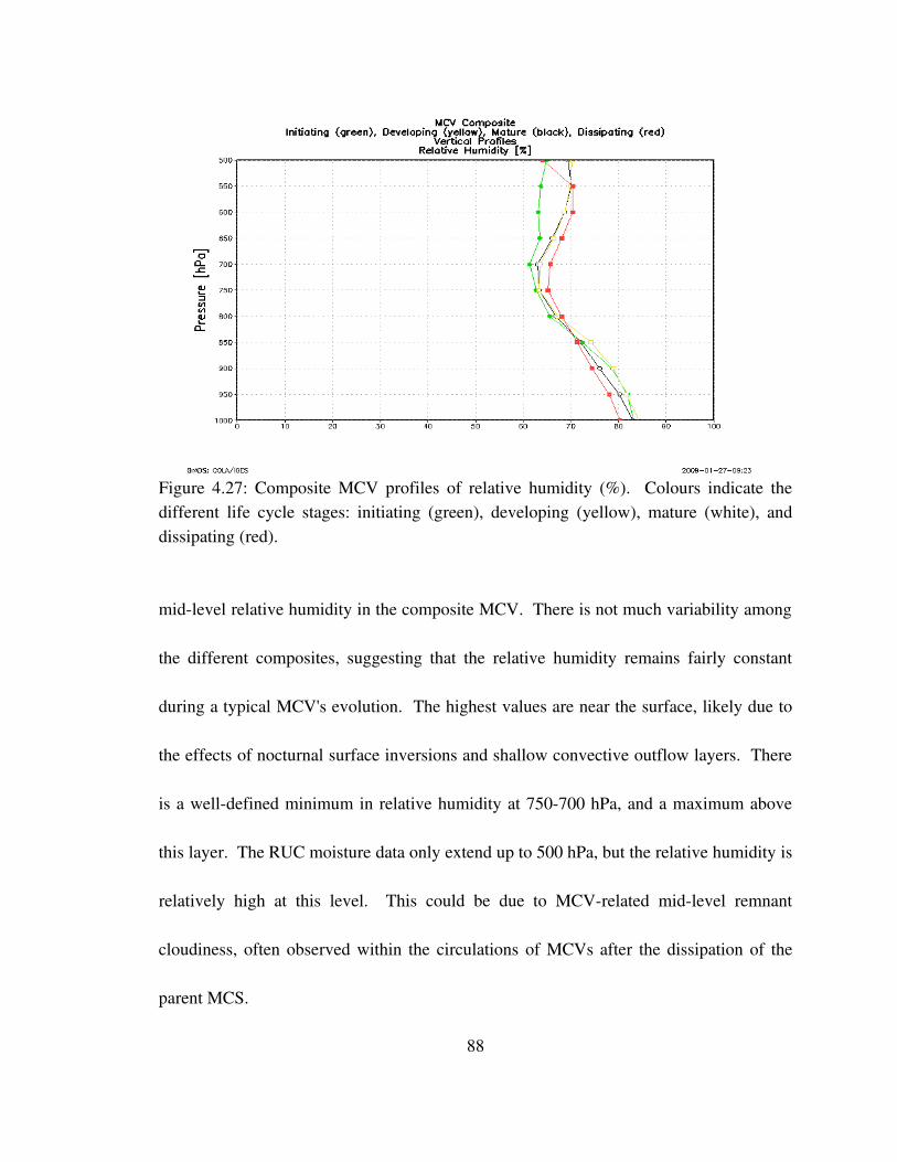
Figure 4.27: Composite MCV profiles of relative humidity (%).   Colours indicate the different  life cycle stages: initiating (green),  developing (yellow),  mature (white),  and dissipating (red).

mid­level relative humidity in the composite MCV.  There is not much variability among 

the different  composites,  suggesting that  the relative humidity  remains  fairly  constant 

during a typical MCV's evolution.  The highest values are near the surface, likely due to 

the effects of nocturnal surface inversions and shallow convective outflow layers.  There 

is a well­defined minimum in relative humidity at 750­700 hPa, and a maximum above 

this layer.  The RUC moisture data only extend up to 500 hPa, but the relative humidity is 

relatively  high   at   this   level.    This   could  be  due   to  MCV­related  mid­level   remnant 

cloudiness, often observed within the circulations of MCVs after the dissipation of the 

parent MCS.

88

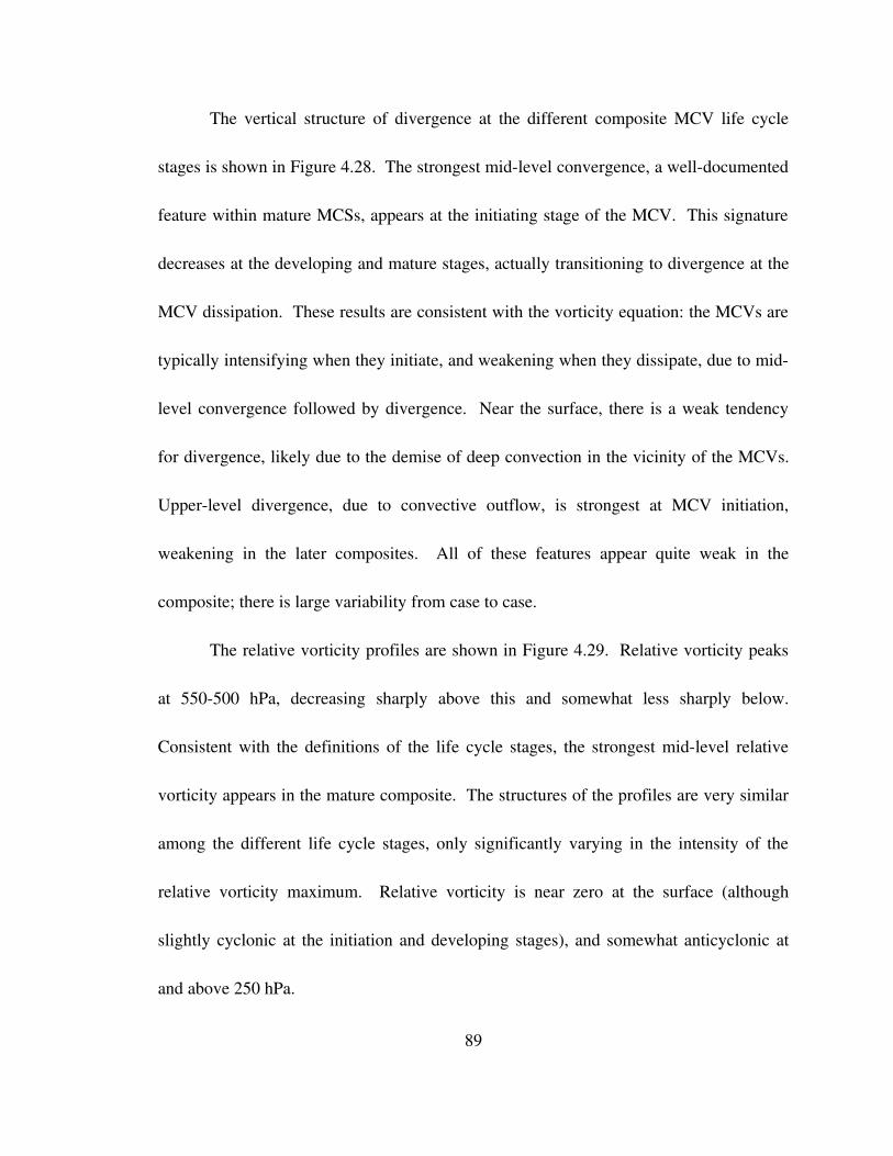
The vertical structure of divergence at the different composite MCV life cycle 

stages is shown in Figure 4.28.  The strongest mid­level convergence, a well­documented 

feature within mature MCSs, appears at the initiating stage of the MCV.  This signature 

decreases at the developing and mature stages, actually transitioning to divergence at the 

MCV dissipation.  These results are consistent with the vorticity equation: the MCVs are 

typically intensifying when they initiate, and weakening when they dissipate, due to mid­

level convergence followed by divergence.   Near the surface, there is a weak tendency 

for divergence, likely due to the demise of deep convection in the vicinity of the MCVs. 

Upper­level   divergence,   due   to   convective   outflow,   is   strongest   at   MCV   initiation, 

weakening   in   the   later   composites.    All   of   these   features   appear   quite  weak   in   the 

composite; there is large variability from case to case.  

The relative vorticity profiles are shown in Figure 4.29.  Relative vorticity peaks 

at   550­500   hPa,   decreasing   sharply   above   this   and   somewhat   less   sharply   below. 

Consistent with the definitions of the life cycle stages, the strongest mid­level relative 

vorticity appears in the mature composite.  The structures of the profiles are very similar 

among the different life cycle stages, only significantly varying in the intensity of the 

relative  vorticity  maximum.    Relative  vorticity   is  near   zero  at   the   surface   (although 

slightly cyclonic at the initiation and developing stages), and somewhat anticyclonic at 

and above 250 hPa.  

89

Figure 4.28: Composite MCV profiles of divergence (s­1).  Colours indicate the different life cycle stages: initiating (green), developing (yellow), mature (white), and dissipating (red).

Figure 4.29: Composite MCV profiles of relative vorticity  (s­1).    Colours indicate  the different  life cycle stages: initiating (green),  developing (yellow),  mature (white),  and dissipating (red).

90

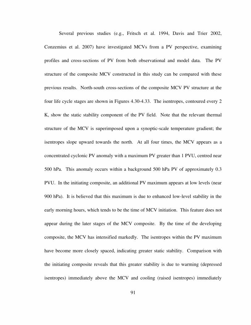
Several   previous   studies   (e.g.,   Fritsch   et   al.   1994,   Davis   and   Trier   2002, 

Conzemius   et   al.   2007)  have   investigated  MCVs   from a  PV perspective,   examining 

profiles  and cross­sections  of  PV from both  observational  and model  data.    The PV 

structure of the composite MCV constructed in this study can be compared with these 

previous results.   North­south cross­sections of the composite MCV PV structure at the 

four life cycle stages are shown in Figures 4.30­4.33.  The isentropes, contoured every 2 

K, show the static stability component of the PV field.   Note that the relevant thermal 

structure of the MCV is superimposed upon a synoptic­scale temperature gradient; the 

isentropes slope upward towards the north.   At all four times, the MCV appears as a 

concentrated cyclonic PV anomaly with a maximum PV greater than 1 PVU, centred near 

500 hPa.   This anomaly occurs within a background 500 hPa PV of approximately 0.3 

PVU.  In the initiating composite, an additional PV maximum appears at low levels (near 

900 hPa).  It is believed that this maximum is due to enhanced low­level stability in the 

early morning hours, which tends to be the time of MCV initiation.  This feature does not 

appear during the later stages of the MCV composite.   By the time of the developing 

composite, the MCV has intensified markedly.  The isentropes within the PV maximum 

have become more closely spaced, indicating greater static stability.   Comparison with 

the initiating composite reveals that this greater stability is due to warming (depressed 

isentropes)   immediately  above  the  MCV and cooling   (raised   isentropes)   immediately

91

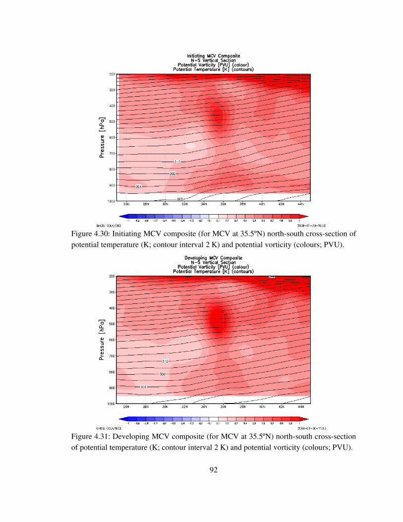
Figure 4.30: Initiating MCV composite (for MCV at 35.5ºN) north­south cross­section of potential temperature (K; contour interval 2 K) and potential vorticity (colours; PVU).

Figure 4.31: Developing MCV composite (for MCV at 35.5ºN) north­south cross­section of potential temperature (K; contour interval 2 K) and potential vorticity (colours; PVU).

92

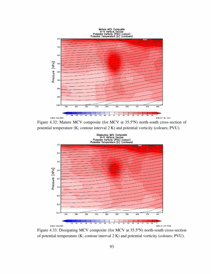
Figure 4.32: Mature MCV composite (for MCV at 35.5ºN) north­south cross­section of potential temperature (K; contour interval 2 K) and potential vorticity (colours; PVU).

Figure 4.33: Dissipating MCV composite (for MCV at 35.5ºN) north­south cross­section of potential temperature (K; contour interval 2 K) and potential vorticity (colours; PVU).

93

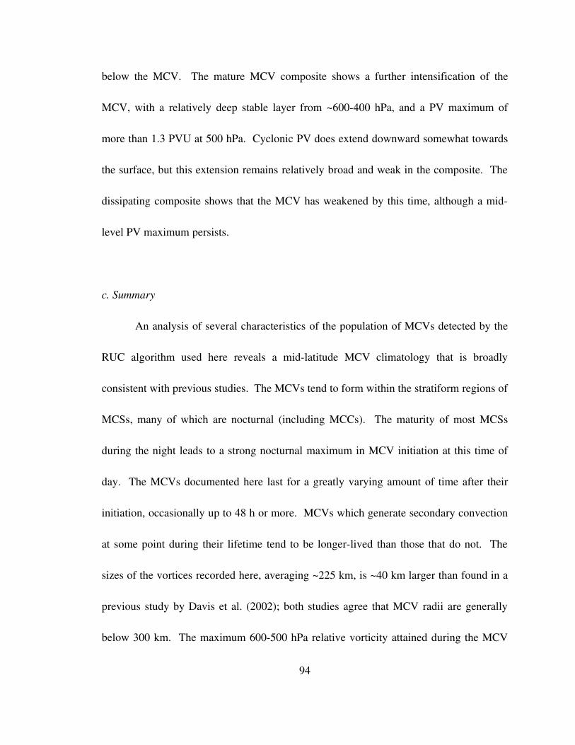
below the MCV.   The mature  MCV composite  shows a further   intensification of  the 

MCV, with a relatively deep stable layer from ~600­400 hPa, and a PV maximum of 

more than 1.3 PVU at 500 hPa.  Cyclonic PV does extend downward somewhat towards 

the surface, but this extension remains relatively broad and weak in the composite.  The 

dissipating composite shows that the MCV has weakened by this time, although a mid­

level PV maximum persists.  

c. Summary

An analysis of several characteristics of the population of MCVs detected by the 

RUC   algorithm   used   here   reveals   a   mid­latitude   MCV   climatology   that   is   broadly 

consistent with previous studies.  The MCVs tend to form within the stratiform regions of 

MCSs, many of which are nocturnal (including MCCs).   The maturity of most MCSs 

during the night leads to a strong nocturnal maximum in MCV initiation at this time of 

day.   The MCVs documented here last for a greatly varying amount of time after their 

initiation, occasionally up to 48 h or more.  MCVs which generate secondary convection 

at some point during their lifetime tend to be longer­lived than those that do not.   The 

sizes of the vortices recorded here, averaging ~225 km, is ~40 km larger than found in a 

previous study by Davis et al. (2002); both studies agree that MCV radii are generally 

below 300 km.  The maximum 600­500 hPa relative vorticity attained during the MCV 

94

events  varies  between 2x10­5  s­1  and  2x10­4  s­1.    The  MCV tracks  show a  variety  of 

orientations,  but   all   have   an  easterly   component   to   their  motion.    For   the  28   cases 

containing a significant surface mesolow, the low tends to be located near and slightly 

south of the MCV centre.  

The synoptic­scale  environment of  the MCVs is  further  examined through the 

construction of a composite MCV.  Although there is much variability among the cases, 

MCVs tend to   initiate  downstream of  a  mid­level   ridge and upstream of a mid­level 

trough,   in   agreement  with  Bartels   and  Maddox   (1991).    At  MCV   initiation,   several 

features of the parent MCS appear, including upper­level divergence associated with an 

ageostrophic jet streak, mid­level convergence, and a LLJ at 850 hPa.  Later in the MCV 

life  cycle,  these features weaken, but a mid­level  pressure  trough persists until  MCV 

dissipation.  

95

V. MCV TYPES

This section presents the remainder of the results of the study, summarising the 

repeating   patterns   of   organisation   and   surface   effects   observed   among   the   cases 

investigated.     Representative   cases   of   each   type   are   described   in   detail,   along   with 

hypotheses for the physical mechanisms involved in each type.  

a. MCV Types

Table 5.1 presents a list of all 45 MCV cases documented in this study, classified 

according to the types that are defined in this section.  Note that the single MCV of the 

third type, occurring on 29 July 2004, is omitted from Table 5.1.   The first repeating 

pattern of MCV organisation recognised in this study is termed the “collapsing stratiform 

region MCV”.  Eight of these MCVs are documented during the period of study.  In these 

MCVs,   a   surface   mesolow   develops,   which   will   be   later   attributed   to   large­scale 

subsidence warming within the dissipating stratiform region of the parent MCS.   The 

second type of MCV recorded here is named the “rear inflow jet MCV”.   This type of 

MCV   is   the  most   common:   19  of   the   45   cases   studied   herein   adhere   to   this   basic 

evolution.  These MCVs are characterised by a mesolow developing due to concentrated

96

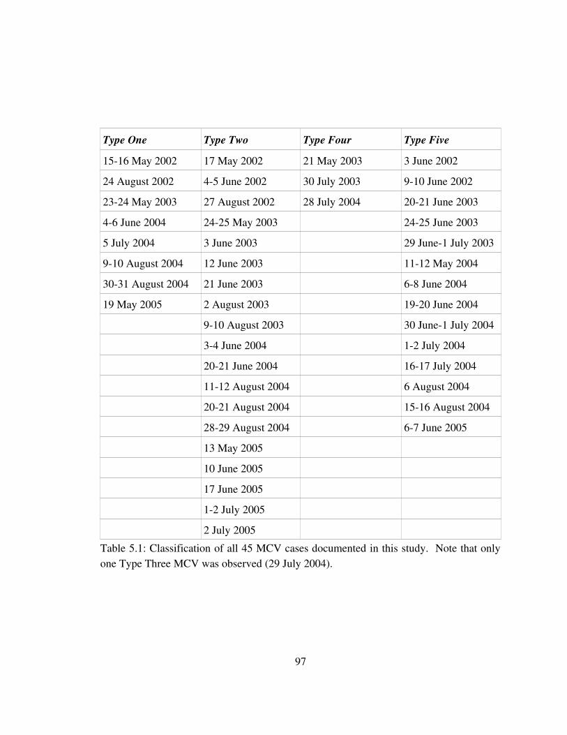
Type One Type Two Type Four Type Five

15­16 May 2002 17 May 2002 21 May 2003 3 June 2002

24 August 2002 4­5 June 2002 30 July 2003 9­10 June 2002

23­24 May 2003 27 August 2002 28 July 2004 20­21 June 2003

4­6 June 2004 24­25 May 2003 24­25 June 2003

5 July 2004 3 June 2003 29 June­1 July 2003

9­10 August 2004 12 June 2003 11­12 May 2004

30­31 August 2004 21 June 2003 6­8 June 2004

19 May 2005 2 August 2003 19­20 June 2004

9­10 August 2003 30 June­1 July 2004

3­4 June 2004 1­2 July 2004

20­21 June 2004 16­17 July 2004

11­12 August 2004 6 August 2004

20­21 August 2004 15­16 August 2004

28­29 August 2004 6­7 June 2005

13 May 2005

10 June 2005

17 June 2005

1­2 July 2005

2 July 2005Table 5.1: Classification of all 45 MCV cases documented in this study.  Note that only one Type Three MCV was observed (29 July 2004).

97

subsidence warming within a descending rear  inflow jet  in a strong MCS, as will  be 

shown later.    The  third kind of MCV seen among the cases examined is   termed  the 

“surface­penetrating MCV”.  Only one of the cases documented here displays this type of 

pattern.  In this case, the MCV appears to penetrate to the surface, leading to a large and 

strong surface mesolow and a well­defined surface cyclonic circulation.   The last two 

types of MCVs contain no significant surface mesolow.   The fourth type is called the 

“cold pool dominated MCV”, of which three are documented in Oklahoma during the 

period of study.   The fifth and final type of MCV observed in this study is called the 

“remnant   circulation  MCV”.    This   type  of   MCV   evolution   appears   to   be   relatively 

common; 14 of the 45 cases studied herein display this behaviour.  

b. Collapsing Stratiform Region MCV

The   first   type   of   MCV   observed   is   termed   the   “collapsing   stratiform   region 

MCV”, due to the apparent role of the dissipating stratiform region in the development of 

a   surface  mesolow.    Several   interesting   features   emerge   in   the  climatology  of   these 

events.   Figure 5.1 shows the mean radius of the five MCV types identified here at the 

four different life cycle stages (initiation, development, maturity, and dissipation).  In the 

mean, collapsing stratiform region MCVs (Type one) appear smaller in scale than the 

other MCV types examined here.   Figure 5.2, which shows the mean mid­level relative

98

Figure 5.1: Mean MCV radius evolution by MCV type. Life cycle stage one corresponds to initiation, two: development, three: maturity, and four: dissipation.   Colours indicate the five MCV types identified in this study, as described in section 5a.

Figure 5.2: As in Figure 5.1, but mean MCV 600­500 hPa relative vorticity (x10­5 s­1).

99

vorticity at each of the four times, reveals that these MCVs are also significantly weaker 

than the other types.  The reduced radius and intensity of these MCVs is likely related to 

the relatively small size of the parent MCS in each case.  

The eight  collapsing stratiform region MCV cases examined here all   follow a 

similar evolution.   The small initial MCS is characterised by a broad mesohigh at the 

surface (due to cooling from precipitation).   Interestingly, the MCSs have a preference 

for southeastward movement (six of the eight cases move south or southeast; see Figure 

5.3), and tend to exhibit a similar reflectivity structure consisting of a small, disorganised 

convective region, with stratiform precipitation off to the left of the system movement. 

This is similar to the “parallel stratiform” organisation of Parker and Johnson (2000), but 

the convection is not always in a well­defined line or oriented perpendicular to system 

motion.  After the peak intensity of the MCS convection, the mesohigh, initially centred 

within the stratiform region, shifts towards the front of the precipitation, and then out 

ahead of the precipitation.   Meanwhile, a mesolow begins to develop at the rear of the 

now­dissipating stratiform region.  This behaviour has not been documented heretofore, 

although pre­squall mesohighs have been reported prior to bowing in the bow echo cases 

studied by Adams­Selin and Johnson (2008).  Over the next few hours, during which the 

associated   MCV   is   first   detected,   the   stratiform   region   of   the   MCS   dissipates,   the 

mesohigh   weakens,   and   the   mesolow   moves   forward   into   the   dissipating   stratiform

100

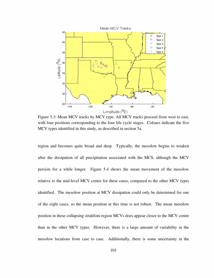
Figure 5.3: Mean MCV tracks by MCV type. All MCV tracks proceed from west to east, with four positions corresponding to the four life cycle stages.  Colours indicate the five MCV types identified in this study, as described in section 5a.

region and becomes quite broad and deep.   Typically, the mesolow begins to weaken 

after   the dissipation of all  precipitation  associated with  the MCS, although  the MCV 

persists   for   a  while   longer.    Figure  5.4   shows  the  mean  movement  of   the  mesolow 

relative to the mid­level MCV centre for these cases, compared to the other MCV types 

identified.  The mesolow position at MCV dissipation could only be determined for one 

of the eight cases, so the mean position at this time is not robust.   The mean mesolow 

position in these collapsing stratifom region MCVs does appear closer to the MCV centre 

than in the other MCV types.   However, there is a large amount of variability in the 

mesolow locations  from case  to  case.    Additionally,   there   is  some uncertainty  in   the

101

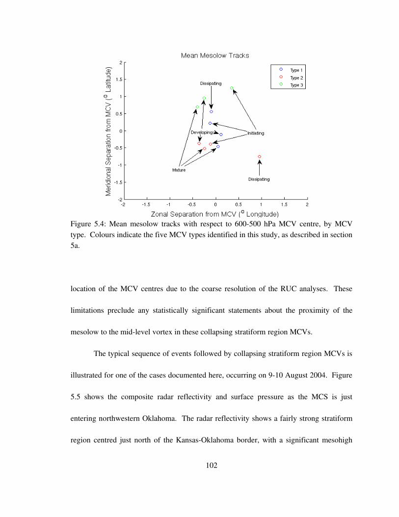
Figure 5.4: Mean mesolow tracks with respect to 600­500 hPa MCV centre, by MCV type.  Colours indicate the five MCV types identified in this study, as described in section 5a.

location of the MCV centres due to the coarse resolution of the RUC analyses.   These 

limitations  preclude any statistically  significant  statements  about   the proximity of  the 

mesolow to the mid­level vortex in these collapsing stratiform region MCVs.  

The typical sequence of events followed by collapsing stratiform region MCVs is 

illustrated for one of the cases documented here, occurring on 9­10 August 2004.  Figure 

5.5   shows   the   composite   radar   reflectivity   and   surface  pressure   as   the  MCS  is   just 

entering northwestern Oklahoma.  The radar reflectivity shows a fairly strong stratiform 

region centred just north of the Kansas­Oklahoma border, with a significant mesohigh

102

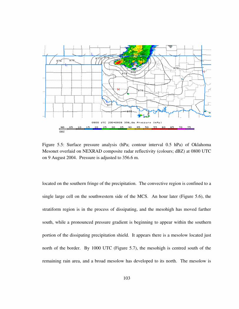
Figure   5.5:   Surface   pressure   analysis   (hPa;   contour   interval   0.5   hPa)   of   Oklahoma Mesonet overlaid on NEXRAD composite radar reflectivity (colours; dBZ) at 0800 UTC on 9 August 2004.  Pressure is adjusted to 356.6 m.

located on the southern fringe of the precipitation.  The convective region is confined to a 

single large cell on the southwestern side of the MCS.   An hour later (Figure 5.6), the 

stratiform region is in the process of dissipating, and the mesohigh has moved farther 

south, while a pronounced pressure gradient is beginning to appear within the southern 

portion of the dissipating precipitation shield.  It appears there is a mesolow located just 

north of the border.   By 1000 UTC (Figure 5.7), the mesohigh is centred south of the 

remaining rain area, and a broad mesolow has developed to its north.   The mesolow is

103

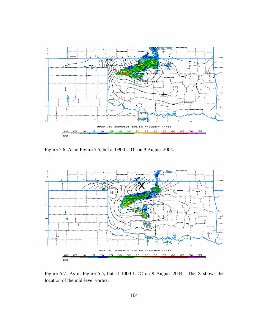
Figure 5.6: As in Figure 5.5, but at 0900 UTC on 9 August 2004.

Figure 5.7: As in Figure 5.5, but at 1000 UTC on 9 August 2004.   The X shows the location of the mid­level vortex.

104

approximately   centred   behind   the   largely   dissipated   stratiform   region.     The   MCV 

associated with the system is first detected by the objective algorithm at this time, located 

directly over the southern portion of the mesolow; its position is marked in Figure 5.7. 

By 1100 UTC (Figure 5.8), the stratiform precipitation has completely dissipated, leaving 

a   large and relatively  deep mesolow centred  in  northern Oklahoma and a weakening 

mesohigh to its south.  At later times, the mesohigh and the mesolow continue to move 

slowly southward, gradually weakening (not shown).   The surface wind field, shown in 

Figure 5.9 at 1100 UTC, shows light and variable winds, with some indications of weak 

convergence into the mesolow.  

Figure 5.10 shows a meteogram for the Breckinridge mesonet station, located just 

southwest of the mesolow centre at 1100 UTC.  The pressure trace shows the passage of 

a well­defined mesolow of ~4 hPa depth, lasting ~3 h and reaching maximum depth at 

1100 UTC.   While the magnitude of the pressure gradient between the mesohigh and 

mesolow is fairly significant (~6 hPa (100 km)­1), the observed winds at the surrounding 

mesonet   stations   remain   quite   low.     This   is   presumably   due   to   the   transient   and 

unbalanced nature  of  the pressure field,  as  described by Vescio and Johnson (1992). 

Another notable feature of Figure 5.10 is the minimal temperature and dewpoint variation 

during the passage of the mesolow; throughout the early part of the analysis period, the 

near­surface air remains relatively cool and moist.   The evolution of the 9­10 August

105

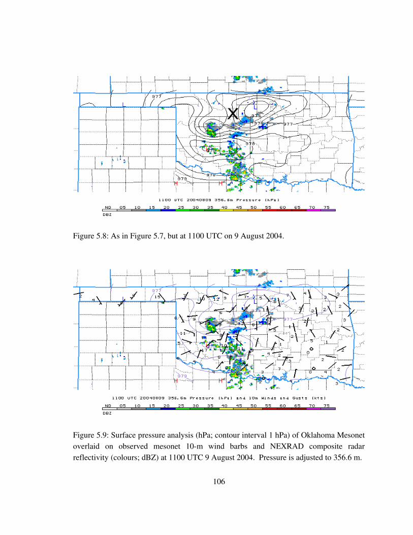
Figure 5.8: As in Figure 5.7, but at 1100 UTC on 9 August 2004.

Figure 5.9: Surface pressure analysis (hPa; contour interval 1 hPa) of Oklahoma Mesonet overlaid   on   observed   mesonet   10­m   wind   barbs   and   NEXRAD   composite   radar reflectivity (colours; dBZ) at 1100 UTC 9 August 2004.  Pressure is adjusted to 356.6 m.

106

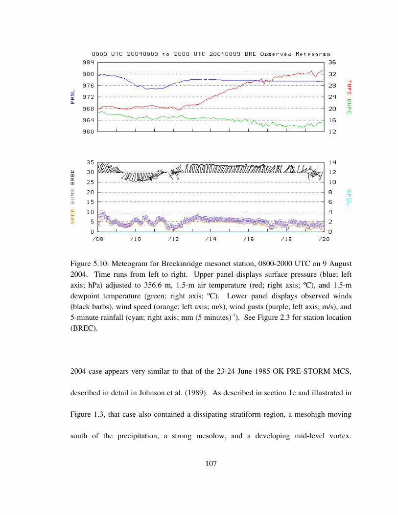
Figure 5.10: Meteogram for Breckinridge mesonet station, 0800­2000 UTC on 9 August 2004.   Time runs from left to right.   Upper panel displays surface pressure (blue; left axis; hPa) adjusted to 356.6 m, 1.5­m air temperature (red; right axis;  ºC), and 1.5­m dewpoint   temperature   (green;   right  axis;   ºC).    Lower  panel  displays  observed  winds (black barbs), wind speed (orange; left axis; m/s), wind gusts (purple; left axis; m/s), and 5­minute rainfall (cyan; right axis; mm (5 minutes)­1).  See Figure 2.3 for station location (BREC).

2004 case appears very similar to that of the 23­24 June 1985 OK PRE­STORM MCS, 

described in detail in Johnson et al. (1989).  As described in section 1c and illustrated in 

Figure 1.3, that case also contained a dissipating stratiform region, a mesohigh moving 

south   of   the   precipitation,   a   strong   mesolow,   and   a   developing   mid­level   vortex. 

107

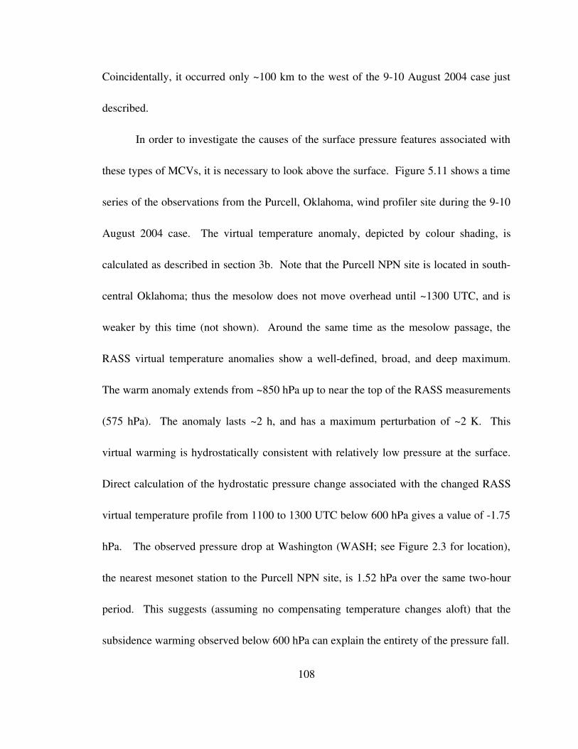
Coincidentally, it occurred only ~100 km to the west of the 9­10 August 2004 case just 

described.  

In order to investigate the causes of the surface pressure features associated with 

these types of MCVs, it is necessary to look above the surface.  Figure 5.11 shows a time 

series of the observations from the Purcell, Oklahoma, wind profiler site during the 9­10 

August  2004 case.    The virtual   temperature  anomaly,  depicted  by colour  shading,   is 

calculated as described in section 3b.  Note that the Purcell NPN site is located in south­

central Oklahoma; thus the mesolow does not move overhead until ~1300 UTC, and is 

weaker by this time (not shown).   Around the same time as the mesolow passage, the 

RASS virtual temperature anomalies show a well­defined, broad, and deep maximum. 

The warm anomaly extends from ~850 hPa up to near the top of the RASS measurements 

(575 hPa).   The anomaly lasts ~2 h, and has a maximum perturbation of ~2  K.   This 

virtual warming is hydrostatically consistent with relatively low pressure at the surface. 

Direct calculation of the hydrostatic pressure change associated with the changed RASS 

virtual temperature profile from 1100 to 1300 UTC below 600 hPa gives a value of ­1.75 

hPa.   The observed pressure drop at Washington (WASH; see Figure 2.3 for location), 

the nearest mesonet station to the Purcell NPN site, is 1.52 hPa over the same two­hour 

period.   This suggests (assuming no compensating temperature changes aloft) that the 

subsidence warming observed below 600 hPa can explain the entirety of the pressure fall. 

108

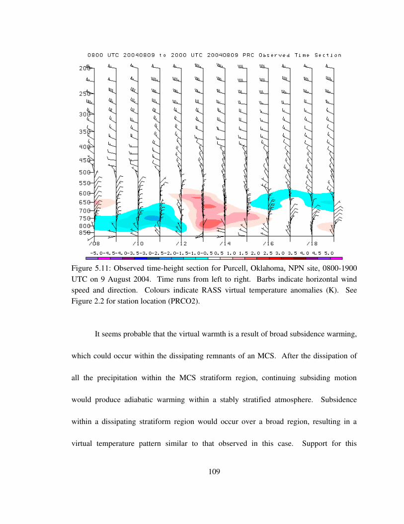
Figure 5.11: Observed time­height section for Purcell, Oklahoma, NPN site, 0800­1900 UTC on 9 August 2004.   Time runs from left to right.   Barbs indicate horizontal wind speed and direction.    Colours  indicate  RASS virtual   temperature anomalies  (K).    See Figure 2.2 for station location (PRCO2).

It seems probable that the virtual warmth is a result of broad subsidence warming, 

which could occur within the dissipating remnants of an MCS.  After the dissipation of 

all   the   precipitation  within   the   MCS   stratiform   region,   continuing   subsiding  motion 

would  produce  adiabatic  warming  within  a   stably   stratified  atmosphere.    Subsidence 

within a dissipating stratiform region would occur over a broad region, resulting in a 

virtual   temperature   pattern   similar   to   that   observed   in   this   case.     Support   for   this 

109

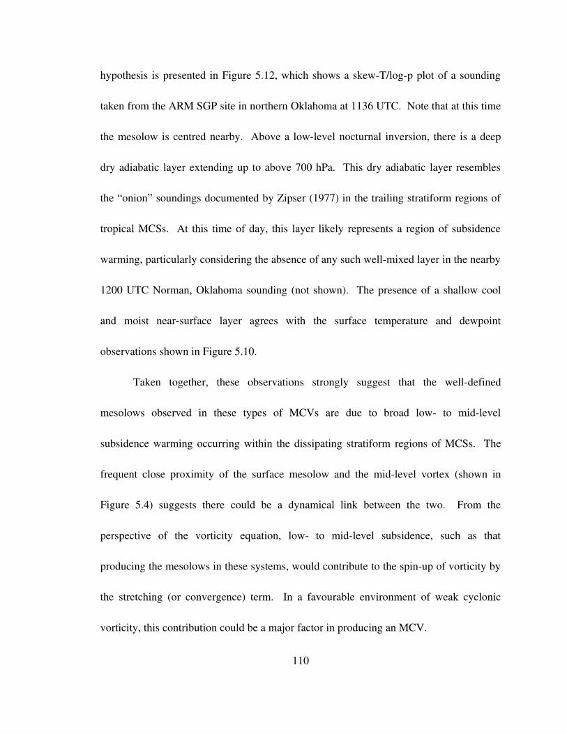
hypothesis is presented in Figure 5.12, which shows a skew­T/log­p plot of a sounding 

taken from the ARM SGP site in northern Oklahoma at 1136 UTC.  Note that at this time 

the mesolow is centred nearby.   Above a low­level nocturnal inversion, there is a deep 

dry adiabatic layer extending up to above 700 hPa.   This dry adiabatic layer resembles 

the “onion” soundings documented by Zipser (1977) in the trailing stratiform regions of 

tropical MCSs.   At this time of day, this layer likely represents a region of subsidence 

warming, particularly considering the absence of any such well­mixed layer in the nearby 

1200 UTC Norman, Oklahoma sounding (not shown).   The presence of a shallow cool 

and   moist   near­surface   layer   agrees   with   the   surface   temperature   and   dewpoint 

observations shown in Figure 5.10.  

Taken   together,   these   observations   strongly   suggest   that   the   well­defined 

mesolows   observed   in   these   types   of   MCVs   are   due   to   broad   low­   to   mid­level 

subsidence warming occurring within the dissipating stratiform regions of MCSs.   The 

frequent  close proximity  of   the  surface mesolow and the mid­level  vortex (shown in 

Figure   5.4)   suggests   there   could   be   a   dynamical   link   between   the   two.     From   the 

perspective   of   the   vorticity   equation,   low­   to   mid­level   subsidence,   such   as   that 

producing the mesolows in these systems, would contribute to the spin­up of vorticity by 

the stretching (or  convergence)   term.    In  a favourable environment of weak cyclonic 

vorticity, this contribution could be a major factor in producing an MCV.  

110

Figure 5.12: Skew­T/log­p plot of radiosonde from ARM SGP site at 1136 UTC on 9 August 2004.  See Figure 2.2 for station location (co­located with NPN station LMNO2).

111

c. Rear Inflow Jet MCV

The second kind of MCV repeatedly seen in this study is referred to as the “rear 

inflow jet MCV”.   These types of MCVs, several of which have been documented in 

previous studies (e.g., Brandes 1990, Brandes and Ziegler 1993, Knievel and Johnson 

2002), generally conform to the conceptual model of Houze et al. (1989) in which the 

vortex spins up within the stratiform region of an asymmetric MCS (Figure 1.1).  Figures 

5.1  and 5.2 show that   these MCVs (Type two) tend  to  be larger   than the collapsing 

stratiform region MCVs, and that, on average, they are the most intense class of MCVs. 

The mean track of  the mesolows associated with these MCVs (Figure 5.4) is  located 

slightly to the south of the MCV centre, which is believed to be due to the mechanism for 

these mesolows, to be described in this section.   Again, the location of the mesolow at 

MCV dissipation should be viewed with skepticism as it is only based on two cases.  

In rear inflow jet MCVs, the parent MCS tends to be fairly large and intense.  The 

associated MCV is generally first detected while the parent MCS remains quite vigorous. 

As the MCS begins to wane and the MCV intensifies during the next few hours, the 

surface pressure field, initially consisting of a strong surface mesohigh, begins to show a 

mesolow developing at the rear edge of the stratiform precipitation.  The back edge of the 

precipitation shield sometimes becomes deformed into a well­defined rear inflow notch, 

with the mesolow being located at the apex of this low­reflectivity region.  After this, the 

112

parent MCS tends to dissipate, while the MCV persists for a variable amount of time. 

Meteograms tend to show a sharp mesolow occurring near the time of the cessation of 

stratiform rainfall.  

The   MCV   of   24­25   May   2003,   occurring   during   the   BAMEX   campaign,   is 

described in detail here as a representative case of this type of MCV.  Figure 5.13 shows 

the composite radar reflectivity and surface pressure as the parent MCS is approaching 

northern  Oklahoma.     It   can  be  seen   that   the  MCS  is  organised   in  a   rather  complex 

manner.   There is an extensive region of stratiform rain in northeastern Oklahoma and 

southeastern Kansas, while on the south side of this there is a small but intense band of 

deep convection oriented northeast­southwest.   This convective line produced a 33 m/s 

wind gust at the Red Rock mesonet site a few minutes before this time (see Figure 2.3 for 

REDR   station   location).     At   the   surface,   there   is   a   well­defined   mesohigh   on   the 

southwestern end of this convective line.  An hour later, at 1500 UTC (Figure 5.14), the 

convective line has continued to surge southeastward on the western side of the large 

stratiform region.  The reflectivity field shows a developing rear inflow notch to the north 

of the convection, suggesting the presence of a strong rear inflow jet impinging on the 

back   of   the   stratiform   region   behind   the   convection.     The   surface   pressure   field   is 

relatively  flat  within  the MCS, with  the exception  of   the  mesohigh  remaining  at   the 

southwestern end of the convective line.    At 1600 UTC (Figure 5.15),  the associated

113

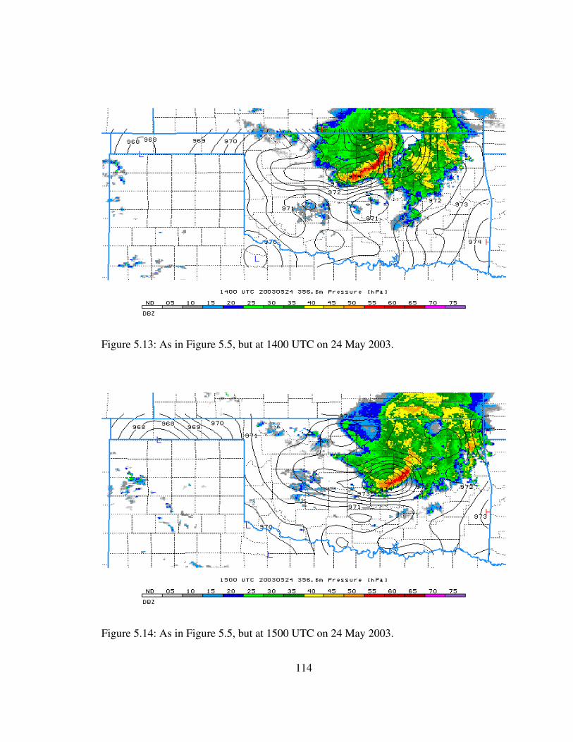
Figure 5.13: As in Figure 5.5, but at 1400 UTC on 24 May 2003.

Figure 5.14: As in Figure 5.5, but at 1500 UTC on 24 May 2003.

114

Figure 5.15: As in Figure 5.7, but at 1600 UTC on 24 May 2003.

MCV is first detected by the objective algorithm; its location is marked in the figure.  By 

this time, the convective line is becoming weaker, while the stratiform region is taking on 

a cyclonically curved shape.   South of the MCV, within the stratiform region, a weak 

mesolow has appeared.   The mesolow is centred at the front of the reflectivity gradient 

associated with the back edge of the stratiform region.  By 1700 UTC (Figure 5.16), the 

mesolow is quite concentrated and deep.  The stratiform region appears to be eroded on 

its back edge to the south of the MCV, and the mesolow is located near the apex of this 

rear inflow notch.   The presence of strong rear inflow is demonstrated in Figure 5.17, 

which shows the observed NPN winds at the 700 hPa level.  The corresponding surface

115

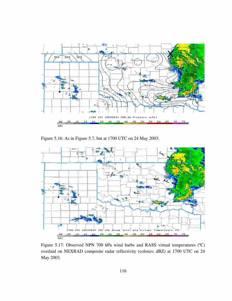
Figure 5.16: As in Figure 5.7, but at 1700 UTC on 24 May 2003.

Figure 5.17: Observed NPN 700 hPa wind barbs and RASS virtual temperatures (ºC) overlaid on NEXRAD composite radar reflectivity (colours; dBZ) at 1700 UTC on 24 May 2003.

116

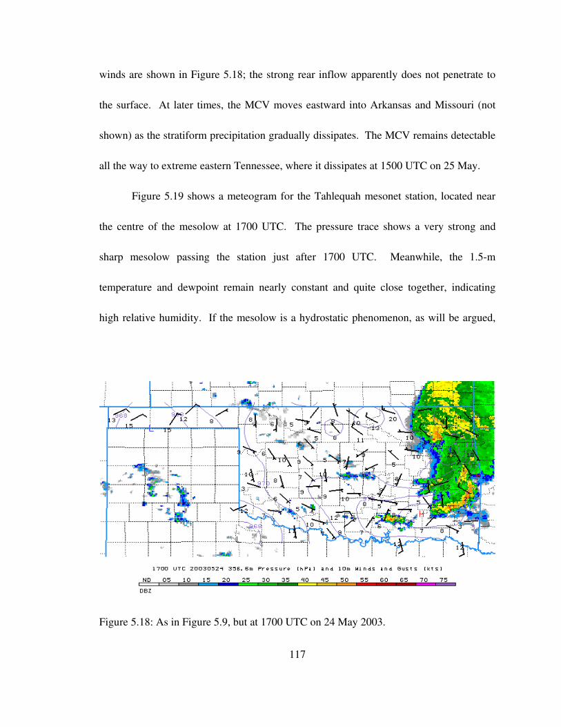
winds are shown in Figure 5.18; the strong rear inflow apparently does not penetrate to 

the surface.   At later times, the MCV moves eastward into Arkansas and Missouri (not 

shown) as the stratiform precipitation gradually dissipates.  The MCV remains detectable 

all the way to extreme eastern Tennessee, where it dissipates at 1500 UTC on 25 May.  

Figure 5.19 shows a meteogram for the Tahlequah mesonet station, located near 

the centre of the mesolow at 1700 UTC.   The pressure trace shows a very strong and 

sharp   mesolow   passing   the   station   just   after   1700   UTC.     Meanwhile,   the   1.5­m 

temperature  and dewpoint  remain  nearly constant and quite  close together,   indicating 

high relative humidity.  If the mesolow is a hydrostatic phenomenon, as will be argued,

Figure 5.18: As in Figure 5.9, but at 1700 UTC on 24 May 2003.

117

Figure 5.19:  Meteogram for  Tahlequah mesonet  station,  0700­2100 UTC on 24 May 2003.   Time runs from left to right.   Upper panel displays surface pressure (blue; left axis; hPa) adjusted to 356.6 m elevation, 1.5­m air temperature (red; right axis; ºC), and 1.5­m dewpoint   temperature   (green;   right   axis;   ºC).    Lower  panel  displays  observed winds (black barbs), wind speed (orange; left axis; m/s), wind gusts (purple; left axis; m/s),  and 5­minute  rainfall   (cyan;   right  axis;  mm (5 minutes)­1).    See Figure 2.3  for station location (TAHL).

the associated temperature perturbations must be confined to regions above the surface, 

similar to the collapsing stratiform region MCVs.  The mesolow occurs at the same time 

as the cessation of the stratiform rainfall, as noted in several other studies (Johnson and 

Hamilton 1988, Stumpf et al. 1991).  In this case, the 10­m winds respond strongly to the 

118

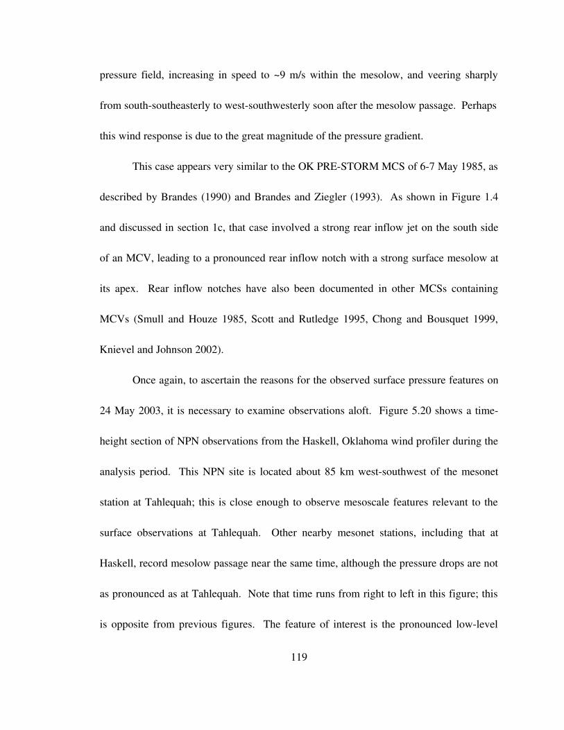
pressure field, increasing in speed to ~9 m/s within the mesolow, and veering sharply 

from south­southeasterly to west­southwesterly soon after the mesolow passage.  Perhaps

this wind response is due to the great magnitude of the pressure gradient.  

This case appears very similar to the OK PRE­STORM MCS of 6­7 May 1985, as 

described by Brandes (1990) and Brandes and Ziegler (1993).   As shown in Figure 1.4 

and discussed in section 1c, that case involved a strong rear inflow jet on the south side 

of an MCV, leading to a pronounced rear inflow notch with a strong surface mesolow at 

its  apex.    Rear  inflow notches have also been documented in other MCSs containing 

MCVs (Smull and Houze 1985, Scott and Rutledge 1995, Chong and Bousquet 1999, 

Knievel and Johnson 2002).  

Once again, to ascertain the reasons for the observed surface pressure features on 

24 May 2003, it is necessary to examine observations aloft.   Figure 5.20 shows a time­

height section of NPN observations from the Haskell, Oklahoma wind profiler during the 

analysis period.   This NPN site is located about 85 km west­southwest of the mesonet 

station at Tahlequah; this is close enough to observe mesoscale features relevant to the 

surface  observations   at  Tahlequah.    Other  nearby  mesonet   stations,   including   that  at 

Haskell, record mesolow passage near the same time, although the pressure drops are not 

as pronounced as at Tahlequah.  Note that time runs from right to left in this figure; this 

is opposite from previous figures.   The feature of interest is the pronounced low­level

119

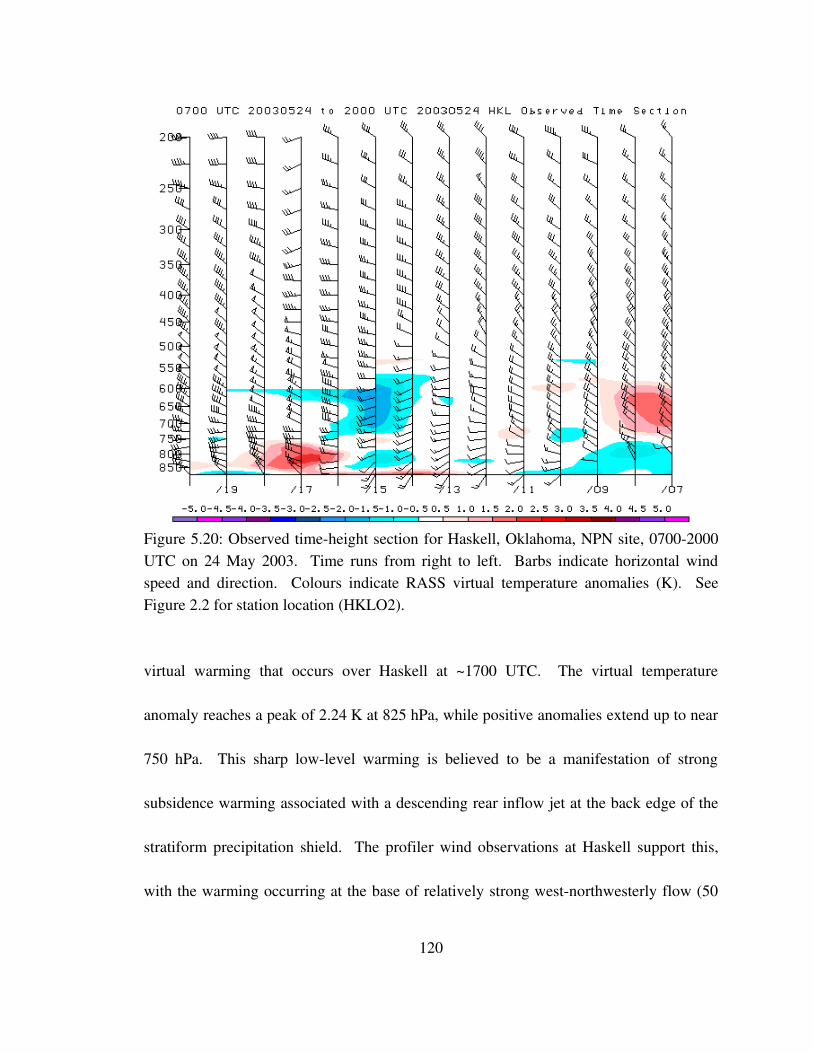
Figure 5.20: Observed time­height section for Haskell, Oklahoma, NPN site, 0700­2000 UTC on 24 May 2003.   Time runs from right to left.   Barbs indicate horizontal wind speed and direction.    Colours  indicate  RASS virtual   temperature anomalies  (K).    See Figure 2.2 for station location (HKLO2).

virtual   warming   that   occurs   over   Haskell   at   ~1700   UTC.     The   virtual   temperature 

anomaly reaches a peak of 2.24 K at 825 hPa, while positive anomalies extend up to near 

750 hPa.    This  sharp   low­level  warming   is  believed   to  be  a  manifestation  of   strong 

subsidence warming associated with a descending rear inflow jet at the back edge of the 

stratiform precipitation shield.   The profiler wind observations at Haskell support this, 

with the warming occurring at the base of relatively strong west­northwesterly flow (50 

120

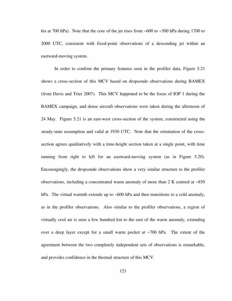
kts at 700 hPa).  Note that the core of the jet rises from ~600 to ~500 hPa during 1700 to 

2000   UTC,   consistent   with   fixed­point   observations   of   a   descending   jet   within   an 

eastward­moving system.  

In order to confirm the primary features seen in  the profiler data, Figure 5.21 

shows a cross­section of this MCV based on dropsonde observations during BAMEX 

(from Davis and Trier 2007).  This MCV happened to be the focus of IOP 1 during the 

BAMEX campaign, and dense aircraft observations were taken during the afternoon of 

24 May.   Figure 5.21 is an east­west cross­section of the system, constructed using the 

steady­state assumption and valid at 1930 UTC.   Note that the orientation of the cross­

section agrees qualitatively with a time­height section taken at a single point, with time 

running   from   right   to   left   for   an   eastward­moving   system   (as   in   Figure   5.20). 

Encouragingly, the dropsonde observations show a very similar structure to the profiler 

observations, including a concentrated warm anomaly of more than 2 K centred at ~850 

hPa.  The virtual warmth extends up to ~600 hPa and then transitions to a cold anomaly, 

as in  the profiler  observations.    Also similar  to  the profiler  observations,  a region of 

virtually cool air is seen a few hundred km to the east of the warm anomaly, extending 

over  a  deep   layer  except   for  a   small  warm pocket  at  ~700 hPa.    The  extent  of   the 

agreement between the two completely independent sets of observations is remarkable, 

and provides confidence in the thermal structure of this MCV.  

121

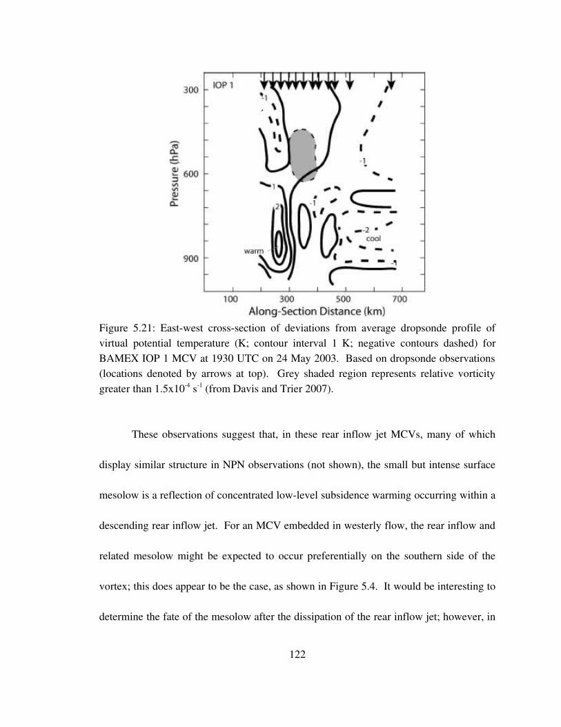
Figure  5.21:  East­west  cross­section  of  deviations  from average  dropsonde profile  of virtual  potential   temperature   (K;  contour   interval  1  K;  negative  contours  dashed)   for BAMEX IOP 1 MCV at 1930 UTC on 24 May 2003.  Based on dropsonde observations (locations denoted by arrows at top).   Grey shaded region represents relative vorticity greater than 1.5x10­4 s­1 (from Davis and Trier 2007).

These observations suggest that, in these rear inflow jet MCVs, many of which 

display similar structure in NPN observations (not shown), the small but intense surface 

mesolow is a reflection of concentrated low­level subsidence warming occurring within a 

descending rear inflow jet.  For an MCV embedded in westerly flow, the rear inflow and 

related mesolow might be expected to occur preferentially on the southern side of the 

vortex; this does appear to be the case, as shown in Figure 5.4.  It would be interesting to 

determine the fate of the mesolow after the dissipation of the rear inflow jet; however, in 

122

the majority of the cases documented here, the MCVs move out of Oklahoma while the 

rear inflow is still quite vigorous.  It is left to future studies to investigate this question.  

d. Surface­penetrating MCV

The third kind of MCV seen among the cases examined is termed the “surface­

penetrating MCV”.  Only one of the cases documented here displays this type of pattern: 

that of 29 July 2004.  The name chosen for this case is appropriate, because it appears to 

be the only case where the mid­level vortex produces a genuine surface reflection (i.e., an 

associated low­level vortex).  Figures 5.1 and 5.2 show the radius and vorticity evolution 

of this MCV case, compared with the other MCV types.  It can be seen that the radius of 

this MCV is larger than the mean radii of the other MCV classifications.   Radius bin 

seven corresponds to an average radius of 262 km.  The vorticity evolution of this case, 

however, is unexceptional in comparison with the other MCV types.   The northeasterly 

track of the vortex centre in this case can be seen in Figure 5.3, and the surface mesolow 

track with respect to the mid­level vortex appears in Figure 5.4.  The surface mesolow is 

initially located northeast of the mid­level vortex, and gradually shifts to the northwest of 

the vortex centre with time.  

The MCV initiates   in   far  northern  Texas,  subsequently  moving northeastward 

through   southeastern   Oklahoma  until   its   dissipation   in   northwestern  Arkansas.    The 

123

surface   mesolow   remains   in   fairly   close   proximity   to   the   mid­level   vortex.     The 

distinguishing   feature  of   this   case   is   the  persistent   and   relatively   large­scale   surface 

mesolow attendant   to   the  mid­level   circulation.    Figure  5.22  shows  the  precipitation 

structure and surface pressure field at 1300 UTC on 29 July 2004, as the main rain shield 

associated with the MCV moves northeastward into Oklahoma.   The mid­level  MCV 

centre is just south of the analysis domain at this time.   Note that the rain area appears 

quite disorganised; the strongest radar echoes in the composite reflectivity only reach 40 

dBZ,   and   these   regions   are   distributed   throughout   the   precipitation   region.     The 

precipitation appears to be completely stratiform in nature, with the possible exception of 

some convective showers on the northwestern periphery of the circulation.   The MCS 

which apparently generated the MCV occurred in north­central Texas on the previous 

afternoon, dissipating before this time.  The pressure field at this time shows a large and 

broad mesolow just southwest of the precipitation shield.  An hour later (Figure 5.23), the 

mesolow   has   consolidated   further,   and   the   entire   rain   shield   is   beginning   to   rotate 

cyclonically  around the mesolow.   This rotation  is  clearly  seen when subsequent  15­

minute radar images are animated on the computer screen.  By 1500 UTC (Figure 5.24), 

the system has continued to drift slowly north­northeastward into Oklahoma, with the 

mesolow remaining  well­defined.    The mesolow and MCV continue  drifting   through 

eastern Oklahoma over the next several hours (Figure 5.25), with the mesolow beginning

124

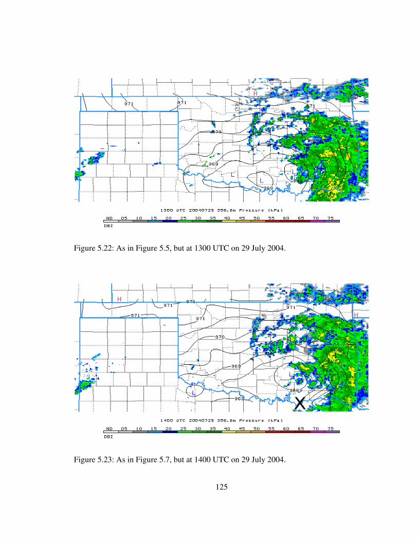
Figure 5.22: As in Figure 5.5, but at 1300 UTC on 29 July 2004.

Figure 5.23: As in Figure 5.7, but at 1400 UTC on 29 July 2004.

125

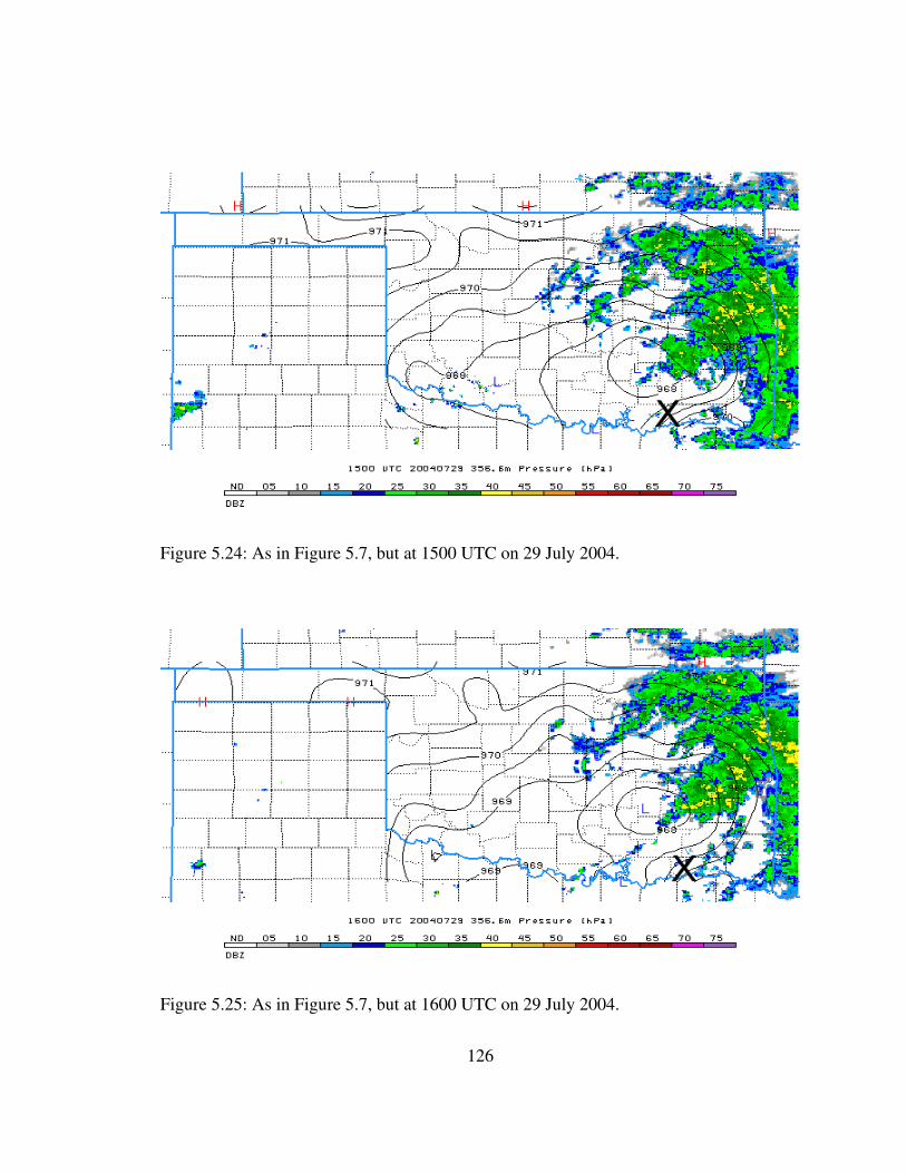
Figure 5.24: As in Figure 5.7, but at 1500 UTC on 29 July 2004.

Figure 5.25: As in Figure 5.7, but at 1600 UTC on 29 July 2004.

126

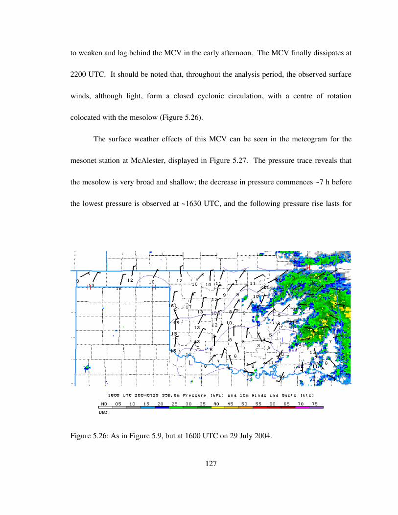
to weaken and lag behind the MCV in the early afternoon.  The MCV finally dissipates at 

2200 UTC.  It should be noted that, throughout the analysis period, the observed surface 

winds,   although   light,   form   a   closed   cyclonic   circulation,   with   a   centre   of   rotation 

colocated with the mesolow (Figure 5.26).  

The surface weather effects of this MCV can be seen in the meteogram for the 

mesonet station at McAlester, displayed in Figure 5.27.   The pressure trace reveals that 

the mesolow is very broad and shallow; the decrease in pressure commences ~7 h before 

the lowest pressure is observed at ~1630 UTC, and the following pressure rise lasts for

Figure 5.26: As in Figure 5.9, but at 1600 UTC on 29 July 2004.

127

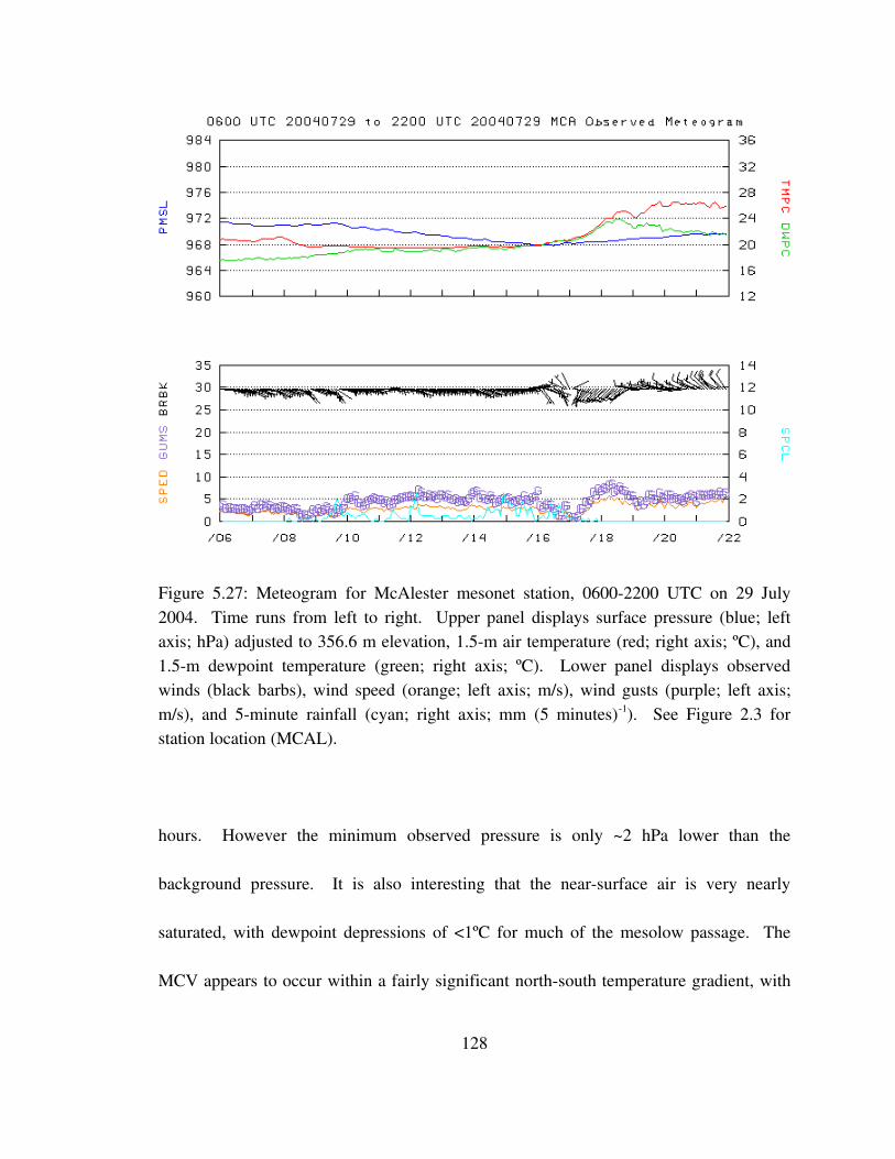
Figure  5.27:  Meteogram for  McAlester  mesonet   station,  0600­2200 UTC on 29 July 2004.   Time runs from left to right.   Upper panel displays surface pressure (blue; left axis; hPa) adjusted to 356.6 m elevation, 1.5­m air temperature (red; right axis; ºC), and 1.5­m dewpoint   temperature   (green;   right   axis;   ºC).    Lower  panel  displays  observed winds (black barbs), wind speed (orange; left axis; m/s), wind gusts (purple; left axis; m/s),  and 5­minute  rainfall   (cyan;   right  axis;  mm (5 minutes)­1).    See Figure 2.3  for station location (MCAL).

hours.     However   the   minimum   observed   pressure   is   only   ~2   hPa   lower   than   the 

background   pressure.     It   is   also   interesting   that   the   near­surface   air   is   very   nearly 

saturated, with dewpoint depressions of <1ºC for much of the mesolow passage.   The 

MCV appears to occur within a fairly significant north­south temperature gradient, with 

128

the temperature rising ~4ºC over ~2 h; this temperature gradient seems to be associated 

with a weak surface warm front.  While the winds clearly show the passage of a cyclonic 

circulation at ~1630 UTC, the wind speeds remain generally below 5 m/s.  Also note that 

a   ten­hour   period   of   stratiform   rainfall   occurs   prior   to   the   passage   of   the   surface 

mesolow.  

Figure 5.28 shows a time­height section of profiler and RASS observations from 

the  NPN site  at  Purcell,  Oklahoma.    Note   that   in   this   figure   the  virtual   temperature 

anomaly contour interval has been decreased by a factor of five from that in previous 

figures,   in  order   to   illustrate   the  patterns  associated  with   the  very  weak  temperature 

variations seen in this case.   The weakness of the virtual temperature anomalies in this 

case is notable; during the passage of the MCV (~1100­1900 UTC), the warm anomaly 

reaches a peak of 0.72 K at 650 hPa (at 1500 UTC).  Note as well that the warm anomaly 

is relatively shallow, and there appear to be cool anomalies above and below.  Overall, it 

appears that the virtual temperature profile is only weakly perturbed in the vicinity of the 

MCV.  It may be significant that the warm anomaly occurs near the time that the MCV is 

closest (~1400), and that a relatively deep cool anomaly occurs before the arrival of the 

MCV.  

Unfortunately,   the   six  RASS observation   sites   are   too   sparsely  distributed   to 

enable a detailed three­dimensional analysis of the temperature perturbations associated

129

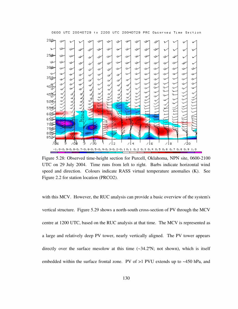
Figure 5.28: Observed time­height section for Purcell, Oklahoma, NPN site, 0600­2100 UTC on 29 July 2004.   Time runs from left to right.   Barbs indicate horizontal wind speed and direction.    Colours  indicate  RASS virtual   temperature anomalies  (K).    See Figure 2.2 for station location (PRCO2).

with this MCV.  However, the RUC analysis can provide a basic overview of the system's 

vertical structure.  Figure 5.29 shows a north­south cross­section of PV through the MCV 

centre at 1200 UTC, based on the RUC analysis at that time.  The MCV is represented as 

a large and relatively deep PV tower, nearly vertically aligned.   The PV tower appears 

directly  over   the  surface  mesolow at   this   time  (~34.2ºN;  not   shown),  which   is   itself 

embedded within the surface frontal zone.  PV of >1 PVU extends up to ~450 hPa, and

130

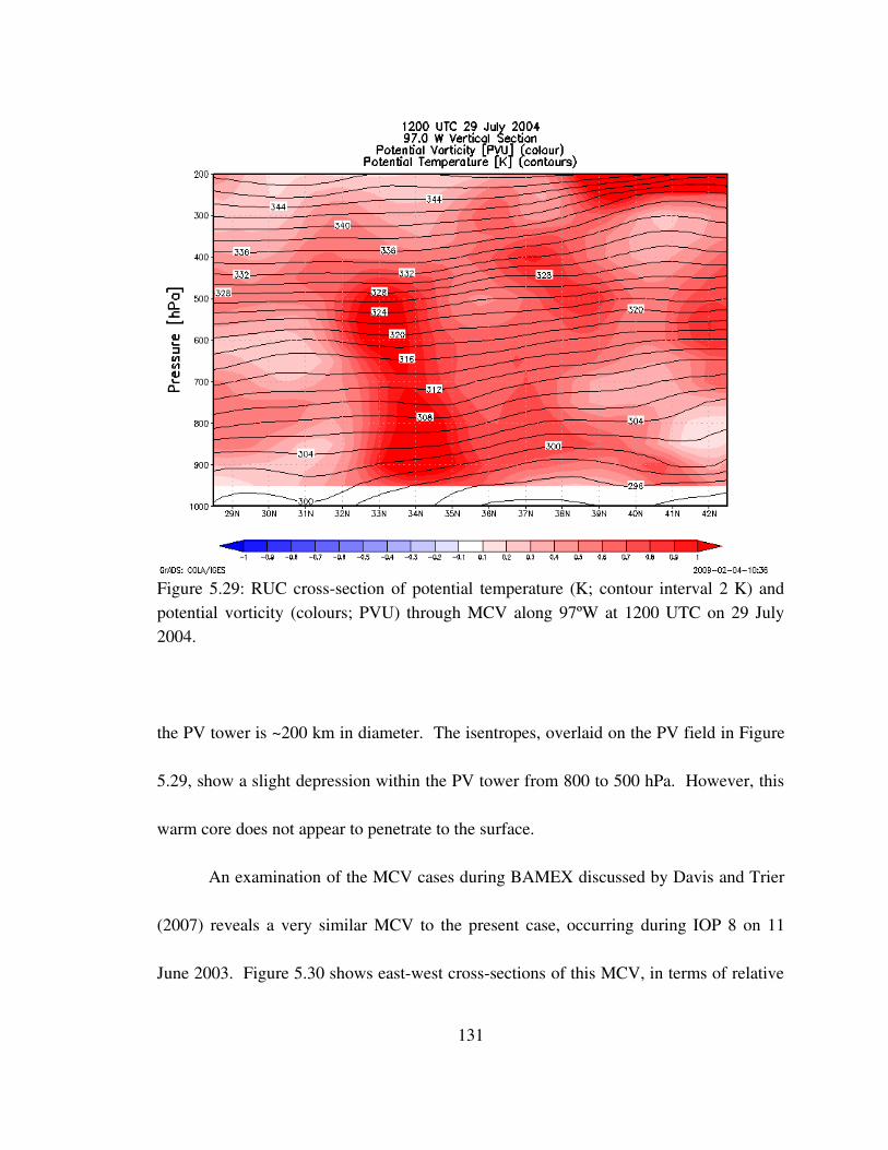
Figure 5.29: RUC cross­section of potential temperature (K; contour interval 2 K) and potential vorticity (colours; PVU) through MCV along 97ºW at 1200 UTC on 29 July 2004.

the PV tower is ~200 km in diameter.  The isentropes, overlaid on the PV field in Figure 

5.29, show a slight depression within the PV tower from 800 to 500 hPa.  However, this 

warm core does not appear to penetrate to the surface.  

An examination of the MCV cases during BAMEX discussed by Davis and Trier 

(2007) reveals a very similar MCV to the present case, occurring during IOP 8 on 11 

June 2003.  Figure 5.30 shows east­west cross­sections of this MCV, in terms of relative

131

Figure 5.30: East­west cross­section of (left) relative vorticity (x10­5 s­1; contour interval 5x10­5  s­1)   and   (right)  deviations   from average  dropsonde  profile  of  virtual  potential temperature   (K;  contour   interval  1  K;  negative  contours  dashed)   for  BAMEX IOP 8 MCV at 1730 UTC on 11 June 2003.  In left panel, heavy dashed line represents vortex axis, and stippled region represents standard deviation of relative vorticity greater than half   of   the   maximum  value.     In   right   panel,   grey   shaded   region   represents   relative vorticity   greater   than   2x10­4  s­1.     Virtual   potential   temperature   deviations   based   on dropsonde observations (locations denoted by arrows at top; from Davis and Trier 2007).

vorticity and virtual potential temperature anomaly.   The relative vorticity cross­section 

shows   a   coherent   and  vertically   stacked  vortex,  with   strong  vorticity   (>1.5x10­4  s­1) 

extending up to ~400 hPa.  While relative vorticity is not equivalent to PV, the shape and 

depth of the relative vorticity maximum is remarkably similar to the PV tower seen in the 

29 July 2004 case (Figure 5.29).   Another similarity emerges in the right­hand panel of 

Figure 5.30, which shows that the virtual potential temperature anomalies in the vicinity 

of   this   BAMEX   MCV   are   minimal.     The   occurrence   of   such   an   MCV   during   the 

132

BAMEX campaign, displaying marked similarities to the case documented here, supports 

the classification of these MCVs in their own category.  

The question arises as to what mechanism is responsible for the development of 

low pressure at the surface in these interesting cases.  The presence of a warm front in the 

29   July  2004  case  may   suggest  baroclinic   forcing  as   an  explanation   for   the   surface 

cyclone; however, such an extratropical cyclone would possess significant vertical tilt, 

with the surface low occurring downstream of the mid­level PV maximum.  Such tilt is 

not seen here.  The vertical coherence of the cyclonic PV anomaly in these cases, as well 

as the proximity of the surface mesolow to the centre of the PV tower, suggests that the 

mesolow may be due to a developing, deep warm core within the MCV.   Such a warm 

core   could   be   produced   by   the   diabatic   heating   occurring   within   the   persistent 

precipitation   shield   in   the   vicinity   of   the   MCV.     In   the   29   July   2004   case,   the 

precipitation shield itself, occurring on the east side of the vortex, is likely due to the 

balanced lifting mechanism proposed by Raymond and Jiang (1990) acting on the north­

south temperature gradient associated with the warm front.  The extension of the MCV to 

the surface in these cases is likely enabled by the relative lack of a surface­based cold 

pool, which could occur in a very moist environment.  The 29 July 2004 case does occur 

within   an   anomalously   moist   environment;   according   to   the   RUC   analyses,   the 

precipitable water in the vicinity of the vortex reaches a maximum of ~5.75 cm.   This 

133

mechanism of surface  low development  due to   the strengthening  and deepening  of  a 

warm core has been documented in prior studies of MCVs (Fritsch et al. 1994; Rogers 

and Fritsch 2001; Trier and Davis 2002).  

e. Cold Pool Dominated MCV

The   fourth   type   of   MCV   observed   in   this   study   is   termed   the   “cold   pool 

dominated MCV”.  Three of these MCVs are documented in Oklahoma during the period 

of  study.   The mean radius  and relative  vorticity  evolution  of  these cases   is  seen  in 

Figures 5.1 and 5.2, respectively.  It can be seen that these MCVs have near­average radii 

and relative vorticity.  Like most of the other types, the individual cases move generally 

eastward, as seen in Figure 5.3.  The distinguishing feature of these cases is the presence 

of significant reflectivity (i.e., an active MCS) during part of the MCV lifetime, but the 

absence of any significant surface mesolow.  

The evolution of these cases is illustrated here based on a representative case from 

30 July 2003.  The MCS which produces this MCV initiates along the Cheyenne Ridge, 

in   the  high  plains   of   southeastern  Wyoming,   in   the   late  morning   of   29   July.     The 

convection  is   initially  disorganised,  moving southeastward in a  large cluster  of small 

cells.  In the evening, as the convection moves through southwestern Kansas, a stratiform 

region begins to develop to the west of the active convection.  The MCV is first detected 

134

within this stratiform region at 0600 on 30 July.  Figure 5.31 shows the surface pressure 

and  composite   reflectivity   in   the  early  morning  of  30   July,   as   the  MCS  is   entering 

northwestern Oklahoma.   It can be seen that the pressure gradients are fairly weak; the 

main   feature   is   the  mesohigh  centred  within   the  stratiform region.    Two hours   later 

(Figure 5.32), the MCS continues slowly moving through northern Oklahoma.   By this 

time, relatively high pressure extends throughout the MCS and its immediate vicinity; 

this is due to the widespread presence of low­level cool air.  During the next few hours 

(Figures 5.33­5.35), the convection weakens, followed by the dissipation of the stratiform 

precipitation, as the MCV continues moving through Oklahoma.   The surface pressure 

field  remains  relatively  flat,  with no mesolow forming near  or  within  the dissipating 

MCS.  The surface temperature field at 1700 UTC (the time of MCV dissipation; Figure 

5.36) shows that a pool of cold air persists beneath the dissipating MCS.   Such a cold 

pool would act to raise the surface pressure hydrostatically.   It would also restrict the 

downward development of a warm core within the MCV, another possible mechanism 

for mesolow formation.  

f. Remnant Circulation MCV

The fifth and final type of MCV observed in this study is called the “remnant 

circulation MCV”.  This type of MCV evolution appears to be relatively common; 14 of

135

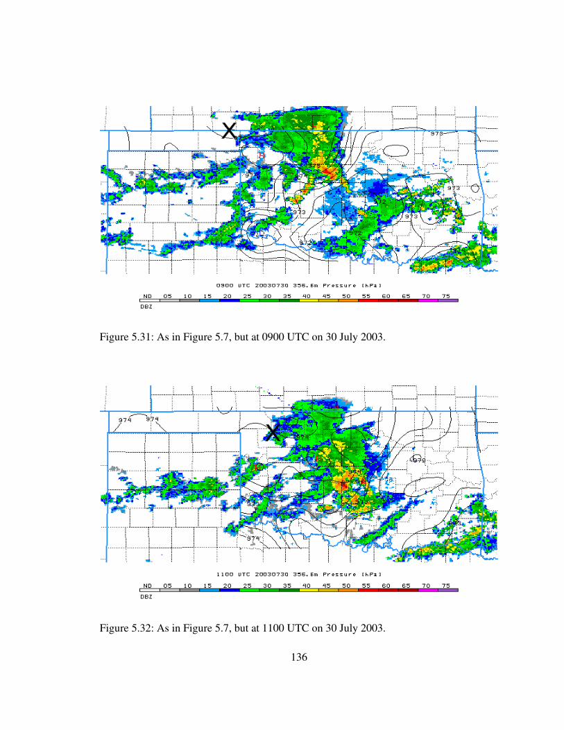
Figure 5.31: As in Figure 5.7, but at 0900 UTC on 30 July 2003.

Figure 5.32: As in Figure 5.7, but at 1100 UTC on 30 July 2003.

136

Figure 5.33: As in Figure 5.7, but at 1300 UTC on 30 July 2003.

Figure 5.34: As in Figure 5.7, but at 1500 UTC on 30 July 2003.

137

Figure 5.35: As in Figure 5.7, but at 1700 UTC on 30 July 2003.

Figure   5.36:   2­m   air   temperature   analysis   (ºC;   contour   interval   1ºC)   of   Oklahoma Mesonet overlaid on NEXRAD composite radar reflectivity (colours; dBZ) at 1700 UTC on 30 July 2003.

138

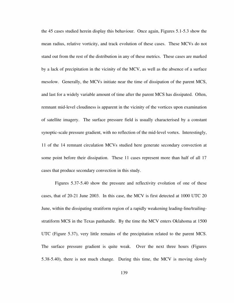
the 45 cases studied herein display this behaviour.  Once again, Figures 5.1­5.3 show the 

mean radius, relative vorticity, and track evolution of these cases.   These MCVs do not 

stand out from the rest of the distribution in any of these metrics.  These cases are marked 

by a lack of precipitation in the vicinity of the MCV, as well as the absence of a surface 

mesolow.  Generally, the MCVs initiate near the time of dissipation of the parent MCS, 

and last for a widely variable amount of time after the parent MCS has dissipated.  Often, 

remnant mid­level cloudiness is apparent in the vicinity of the vortices upon examination 

of satellite imagery.    The surface pressure field is usually characterised by a constant 

synoptic­scale pressure gradient, with no reflection of the mid­level vortex.  Interestingly, 

11 of the 14 remnant circulation MCVs studied here generate secondary convection at 

some point before their dissipation.   These 11 cases represent more than half of all 17 

cases that produce secondary convection in this study.  

Figures 5.37­5.40 show the pressure and reflectivity  evolution of one of  these 

cases, that of 20­21 June 2003.  In this case, the MCV is first detected at 1000 UTC 20 

June, within the dissipating stratiform region of a rapidly weakening leading­line/trailing­

stratiform MCS in the Texas panhandle.  By the time the MCV enters Oklahoma at 1500 

UTC (Figure 5.37), very little remains of the precipitation related to the parent MCS. 

The   surface   pressure   gradient   is   quite   weak.     Over   the   next   three   hours   (Figures 

5.38­5.40),   there  is  not much change.    During  this   time,   the MCV is moving slowly

139

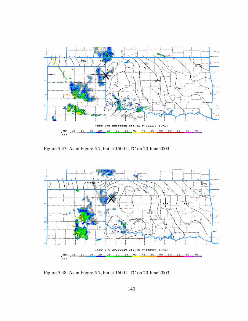
Figure 5.37: As in Figure 5.7, but at 1500 UTC on 20 June 2003.

Figure 5.38: As in Figure 5.7, but at 1600 UTC on 20 June 2003.

140

Figure 5.39: As in Figure 5.7, but at 1700 UTC on 20 June 2003.

Figure 5.40: As in Figure 5.7, but at 1800 UTC on 20 June 2003.

141

southeastward   through  western  Oklahoma,  but   there   is  no   trace  of   the  vortex  at   the 

surface.   The surface pressure field consists of a nearly uninterrupted eastward­directed 

pressure gradient.  A time series of observations from the Vici wind profiler observations 

(Figure 5.41) shows the wind field and the thermal structure associated with the MCV, 

which passes near this station at ~2200 UTC.   At low levels, the winds remain south­

southeasterly throughout the analysis period, only showing the presence of a vortex at the 

mid   levels.     Meanwhile,   the   virtual   temperature   anomalies   are   very   weak   and 

disorganised.  This case is representative of many of this type of MCV.  It appears that 

the development of a surface mesolow associated with an MCV requires at least some 

precipitation in the vicinity of the vortex.  In the absence of this precipitation, there will 

not be strong subsidence to generate warming in unsaturated downdraughts (such as seen 

in the collapsing stratiform region and rear inflow jet MCVs), nor will there be diabatic 

heating to generate a deep warm core (as seen in the deep surface­penetrating MCV).  

g. Summary

Five distinct repeating patterns of precipitation organisation and surface pressure 

features appear among the 45 mid­latitude MCVs analysed in this study.  Three of these 

patterns   involve   the   development   of   well­defined   surface   mesolows;   the   other   two 

patterns lack any significant surface mesolows.  Collapsing stratiform region MCVs and

142

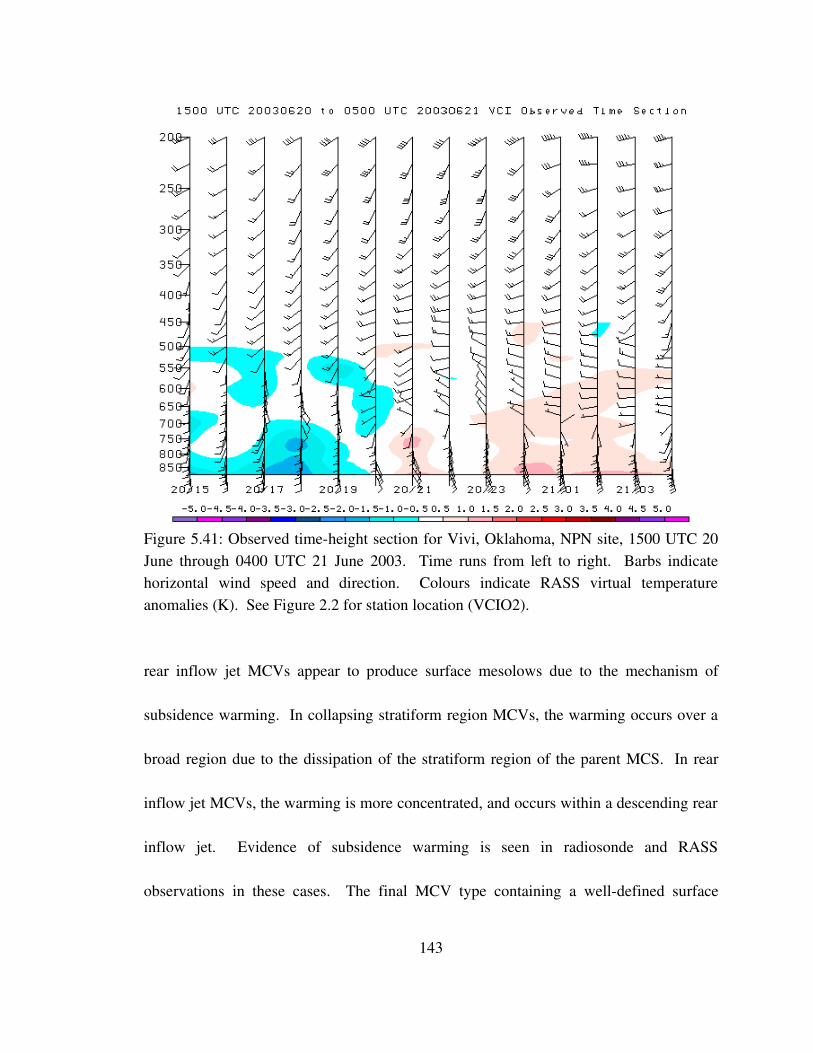
Figure 5.41: Observed time­height section for Vivi, Oklahoma, NPN site, 1500 UTC 20 June through 0400 UTC 21 June 2003.   Time runs from left to right.   Barbs indicate horizontal   wind   speed   and   direction.     Colours   indicate   RASS   virtual   temperature anomalies (K).  See Figure 2.2 for station location (VCIO2).

rear   inflow jet  MCVs appear   to  produce surface mesolows due  to   the mechanism of 

subsidence warming.  In collapsing stratiform region MCVs, the warming occurs over a 

broad region due to the dissipation of the stratiform region of the parent MCS.   In rear 

inflow jet MCVs, the warming is more concentrated, and occurs within a descending rear 

inflow   jet.     Evidence   of   subsidence   warming   is   seen   in   radiosonde   and   RASS 

observations   in   these  cases.    The   final  MCV  type  containing  a  well­defined   surface 

143

mesolow is termed the surface­penetrating MCV.  In these cases, the surface low appears 

related to the presence of a deep warm core within the MCV.  This warm core produces a 

hydrostatic pressure fall at the surface; thus, these cases can be described as MCVs which 

penetrate to the surface.   In some cases, MCVs contain significant precipitation but no 

well­defined surface mesolow; these cases are classified as cold pool dominated MCVs. 

Surface pressure falls  do not occur,  due to  the strength of  the low­level cold air  and 

mesohigh.  The fifth type of MCV is the remnant circulation MCV, in which the vortex 

contains little or no precipitation in its vicinity, and the surface pressure and flow fields 

are undisturbed by the MCV.  

144

V. DISCUSSION

This study has documented both a climatology of MCVs over Oklahoma and the 

surrounding region and the relationship between MCVs and their surface pressure fields. 

This   section   summarises   some   of   the   more   significant   results,   and   highlights   their 

applicability with regard to continuing research on mesoscale meteorology.  

In terms of the climatological characteristics of mid­latitude MCVs, this study has 

firmly established the close association of MCVs with MCSs.  The initiation of MCVs is 

tied to the early morning maximum extent of MCCs and MCSs in the central USA, and 

several  common features  appear  both in composites of mature MCC structure and of 

initiating  MCV structure.     It   has  been  hypothesised   (Velasco  and Fritsch  1987)   that 

MCVs are a fundamental component of MCC structure; this remains to be confirmed by 

future studies.  At the present time, the observational network, even within focussed field 

campaigns,   remains   too   limited   to   detect  MCVs  within  MCCs  with   total   efficiency, 

particularly considering the large range of MCV sizes and intensities documented here. 

On the other hand, it has been pointed out that the MCC size and duration thresholds 

introduced by Maddox (1980) are somewhat arbitrary, and important dynamical features 

of   MCCs   (including   MCVs)   are   often   present   in   smaller   and   shorter­lived   MCSs; 

145

examples  of   such  cases  have  been  shown  in   this   study.    Notwithstanding   remaining 

avenues of research in this area, it is at least clear that MCVs are generated by regions of 

organised convection with associated stratiform precipitation.  

As in a previous climatology of MCVs based on the RUC model (Davis et al. 

2002), it  is found that true MCVs only account for ~20% of the mid­level mesoscale 

vortices   occurring  during   the   summertime  over   the  Great  Plains   downstream  of   the 

Rocky Mountains.   Davis et al. (2002) have suggested that many of the other vortices 

may be topographically generated due to their concentration in the immediate lee of the 

Rocky Mountains.  These “dry vortices” are also widespread in the domain delineated in 

this study.   It is possible that other mechanisms, such as local instabilities of the mean 

flow, could produce these localised relative vorticity maxima.  

Distributions   of   the   structural   characteristics   of   the   MCVs   documented   here, 

particularly   vortex   radius   and   intensity,   show   considerable   breadth.     Vortex   radius 

(determined within the limitations of the RUC grid) ranges from ~150 to ~250 km, with a 

median radius of 224 km.  This is slightly larger than the 185 km median radius found by 

Davis   et   al.   (2002).     Similarly,   vortex   intensity   varies   by   more   than   an   order   of 

magnitude, from 2x10­5 s­1 to 2.3x10­4 s­1.  The median intensity is ~1.15x10­4 s­1.  These 

radius  and  intensity  values  could prove useful   for  verifying   the realism of  simulated 

MCVs,   in   both   NWP   and   GCM   applications.     Similarly,   the   distribution   of   MCV 

146

longevities,   ranging  up  to  54 h,  can provide  a  basis   for  validating   the  life  cycles  of 

simulated  MCVs.    The   frequency  of   secondary   convection   (a   second   cycle   of   deep 

convective activity during the MCV lifetime) associated with the MCV circulations in 

this study is ~40%, which agrees reasonably well with 46% from Davis et al. (2002). 

The median lifetime of MCVs which trigger secondary convection is ~10 h greater than 

the   lifetime   of   MCVs   with   no   secondary   convection;   this   result   is   in   qualitative 

agreement with theories regarding MCV intensification by secondary convection (e.g., 

Rogers and Fritsch 2001).  

The synoptic­scale environment of the MCVs recorded here is representative of 

the general situation favouring MCVs in the central USA (Bartels and Maddox 1991).  In 

the mean, that environment consists of west­northwesterly flow downstream of a mid­

level ridge and upstream of a mid­level trough.   Features related to the structure of the 

parent  MCS or  MCC,   such  as   an  upper­level   ageostrophic   jet   streak  and  associated 

divergence,  as  well  as  mid­level  convergence  and ascent  within   the  MCV stratiform 

region, tend to be strongest at the initiating stage of the MCV, and weaken at later stages. 

This is due to the typical waning of convection and dissipation of precipitation after the 

generation of the MCV.  On average, there does not appear to be a strong signal of the 

presence of an MCV in the synoptic­scale environment after the dissipation of the parent 

MCS.   The single notable feature at the mid levels is the development of a pronounced 

147

mesoscale trough in the height field, which remains significant throughout the lifetime of 

the composite MCV.  

The appearance of a mid­level mesoscale trough can be understood from both 

hydrostatic and dynamic perspectives.  Such a feature would be produced by warming at 

higher levels in the atmosphere.    This warming is achieved initially by latent heating 

within the parent MCS; the balanced nature of the resulting MCV (i.e., the radius of the 

vortex being larger than the Rossby radius of deformation) keeps this warm core intact 

within the vortex for a long period of time.  Dynamically, the increase of latent heating 

with height in the stratiform region of an MCS will lead to a positive midtropospheric 

PV anomaly (Raymond and Jiang 1990; Hertenstein and Schubert 1991).   While it  is 

likely   that  MCVs  of   varying   strengths   also  have   coherent  mid­level  warm  cores   of 

varying persistence and intensity, the appearance of this feature in the composite suggests 

that this is a common feature of MCVs.  

Additional interesting features appear in the composite in the lower levels of the 

atmosphere.    The appearance of  the LLJ is  noticeable at  850 hPa.    The LLJ is  most 

intense at the MCV initiating stage, weakening and veering at later times in the MCV life 

cycle.  This is likely unrelated to the actual evolution of the MCV, and is rather a result 

of the preferential initiation of MCVs in the early morning hours, at a time when the LLJ 

is climatologically at its strongest.   Previous studies have suggested that the LLJ may 

148

often play a role in flash flood situations involving MCVs (Bosart and Sanders 1981; 

Davis and Trier 2002; Schumacher and Johnson 2008).   The LLJ acts to transport high 

equivalent potential temperature air into the vicinity of the vortex; this air is then lifted, 

which  destabilises   the environment  and results   in   localised  deep  convection.    Lifting 

mechanisms can include low­level gravity waves, density currents,  or balanced lifting 

within the thermal structure of the MCV.  

The most important contribution of this study is the classification of MCVs into 

several   types  involving recurring  patterns  of organisation  and surface effects.     In  the 

majority of the cases documented here, MCVs particularly represent one of five types: 

the collapsing stratiform region MCV, the rear inflow jet MCV, the surface­penetrating 

MCV, the cold pool dominated MCV, and the remnant circulation MCV.  The remainder 

of this section describes these five types, and presents conceptual models of two of the 

three MCV types containing significant surface mesolows.  Only one surface­penetrating 

MCV was observed; thus, despite its many interesting features and potential relevance to 

tropical cyclogenesis, a conceptual model is not developed based upon this single case.  

The   eight   collapsing   stratiform   region   MCVs   documented   here   display   the 

strongest similarities of all the MCV types.  Figure 6.1 shows a basic conceptual model 

of the evolution of the collapsing stratiform region MCV.  The left panel represents the 

mature stage of the parent MCS; these MCSs often display a very specific organisation of 

149

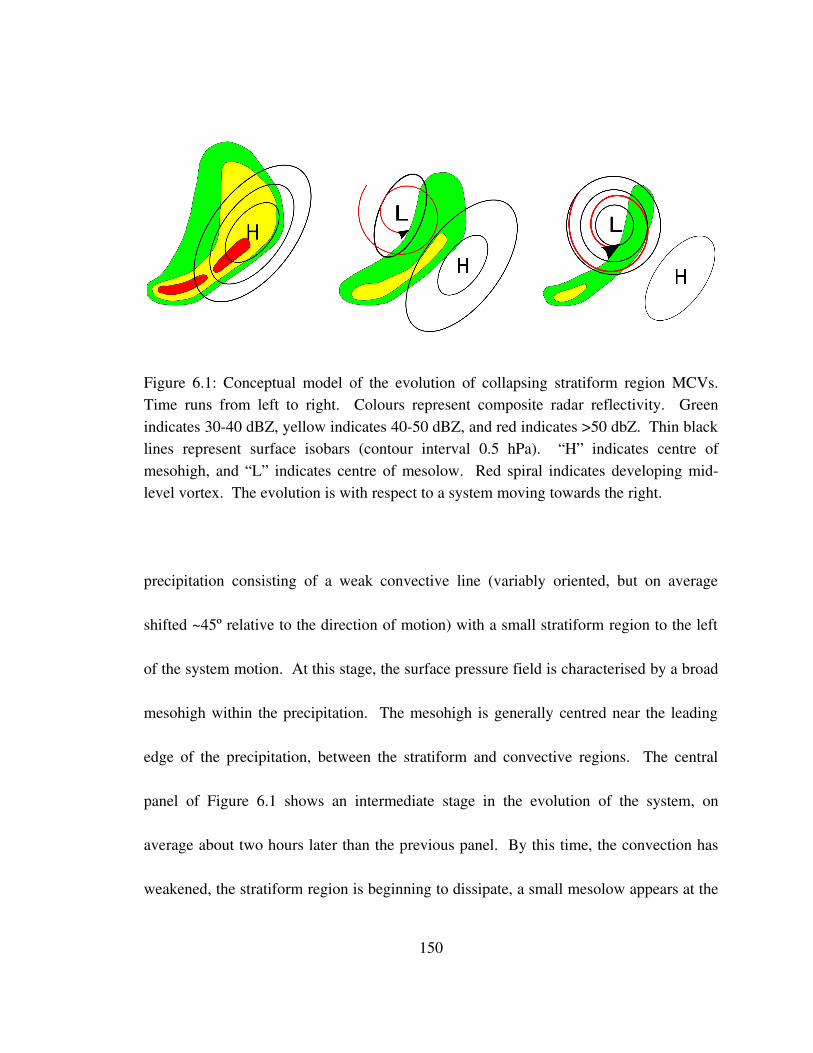
Figure 6.1: Conceptual  model of the evolution of collapsing stratiform region MCVs. Time runs from left   to   right.    Colours represent  composite   radar   reflectivity.    Green indicates 30­40 dBZ, yellow indicates 40­50 dBZ, and red indicates >50 dbZ.  Thin black lines   represent   surface   isobars   (contour   interval   0.5   hPa).     “H”   indicates   centre   of mesohigh, and “L” indicates centre of mesolow.   Red spiral indicates developing mid­level vortex.  The evolution is with respect to a system moving towards the right.

precipitation  consisting  of  a  weak convective   line   (variably  oriented,  but  on average 

shifted ~45º relative to the direction of motion) with a small stratiform region to the left 

of the system motion.  At this stage, the surface pressure field is characterised by a broad 

mesohigh within the precipitation.   The mesohigh is generally centred near the leading 

edge of the precipitation,  between the stratiform and convective regions.   The central 

panel  of  Figure  6.1   shows  an   intermediate   stage   in   the  evolution  of   the   system,  on 

average about two hours later than the previous panel.  By this time, the convection has 

weakened, the stratiform region is beginning to dissipate, a small mesolow appears at the 

150

rear of the stratiform region, and the surface mesohigh is beginning to move out ahead of 

the   precipitation   and   weaken.     The   mid­level   vortex   generally   becomes   sufficiently 

intense to be first detected by the objective algorithm a few hours after this time.   The 

right panel in Figure 6.1 shows the final stage in the evolution of these MCVs, occurring 

about another two hours later.  By this time, the broadening and deepening mesolow has 

moved into the dissipating remnants of the stratiform region, and the weak mesohigh has 

almost disappeared.  In seven of the eight cases, the mid­level MCV is first detected by 

the objective algorithm before, or less than two hours after, this time.  The formation of 

both the MCV and the surface mesolow occur during the weakening stage of the parent 

MCS.   As was shown in Figures 4.15 and 5.4, the surface mesolow in these types of 

MCVs tends to be quite close to the mid­level vortex; the extent of the collocation is 

slightly greater than in the other MCV types.  However, the difference is not statistically 

significant, and it is difficult to draw conclusions about the relative locations of the MCV 

and mesolow due to the coarse grid of the RUC analyses.  

All   eight   collapsing   stratiform   region   MCVs   contain   a   developing   mesolow 

towards   the   rear   of   the   stratiform   region   as   it   dissipates,   which   then   broadens   and 

deepens as the precipitation diminishes and the parent MCS weakens.  This indicates that 

the evolution of the precipitation structure of these systems influences the evolution of 

the   surface  pressure   field.    As  demonstrated   in   a  modeling   study by  Gallus   (1996), 

151

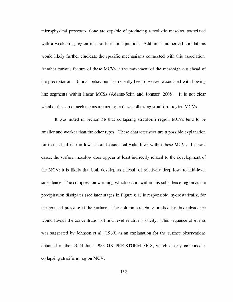
microphysical processes alone are capable of producing a realistic mesolow associated 

with a weakening region of stratiform precipitation.   Additional numerical simulations 

would likely further elucidate the specific mechanisms connected with this association. 

Another curious feature of these MCVs is the movement of the mesohigh out ahead of 

the precipitation.  Similar behaviour has recently been observed associated with bowing 

line  segments  within   linear  MCSs  (Adams­Selin  and Johnson 2008).     It   is  not  clear 

whether the same mechanisms are acting in these collapsing stratiform region MCVs.  

It  was noted  in  section 5b  that  collapsing  stratiform region  MCVs tend  to be 

smaller and weaker than the other types.  These characteristics are a possible explanation 

for the lack of rear inflow jets and associated wake lows within these MCVs.   In these 

cases, the surface mesolow does appear at least indirectly related to the development of 

the MCV: it is likely that both develop as a result of relatively deep low­ to mid­level 

subsidence.  The compression warming which occurs within this subsidence region as the 

precipitation dissipates (see later stages in Figure 6.1) is responsible, hydrostatically, for 

the reduced pressure at the surface.   The column stretching implied by this subsidence 

would favour the concentration of mid­level relative vorticity.   This sequence of events 

was suggested by Johnson et al. (1989) as an explanation for the surface observations 

obtained   in   the  23­24 June  1985 OK PRE­STORM MCS, which  clearly  contained  a 

collapsing stratiform region MCV.  

152

Rear   inflow   jet  MCVs  are   the   second  MCV   type   containing  marked   surface 

pressure perturbations.  In these cases, the development of low surface pressure seems to 

occur   due   to   the  well­documented  wake   low mechanism,  whereby   a   rear   inflow  jet 

flowing   into   an  MCS  stratiform   region  descends   strongly,   producing   a   concentrated 

region  of   subsidence   warming   at   low   levels   where   the   precipitation  has   evaporated 

(Johnson and Hamilton 1988).   Figure 6.2 shows a conceptual diagram of the evolution 

of these MCVs, based on the 19 cases of this type documented during this study.  The left 

panel of Figure 6.2 represents the mature stage of the parent MCS.  These MCSs show a 

wide variety of organisations, but one of the most frequent is the leading­line trailing­

stratiform MCS (Parker  and Johnson 2000).    The surface  pressure   field  at   this   time 

consists of a broad mesohigh within the precipitation.   The middle panel of Figure 6.2 

shows a later stage of development, on average about two hours later.  By this time, the 

precipitation structure is starting to take on pronounced asymmetry,  with the southern 

portion of the stratiform region beginning to erode due to the development of rear inflow 

on the south side of the incipient MCV.   A small mesolow appears behind this eroded 

portion of the stratiform region.  On average, the MCV is first detected by the objective 

algorithm near this time.  The final stage, depicted in the right panel of Figure 6.2, occurs 

on average about two hours after the intermediate stage.  By this time, the convective line 

has weakened and the stratiform region has been largely shunted to the left.  The MCV is

153

Figure 6.2: As in Figure 6.1, but of the evolution of rear inflow jet MCVs.

intensifying in the remaining portion of the stratiform region.  Meanwhile, a concentrated 

and intense mesolow has formed just behind the eroded southern portion of the stratiform 

region.  Often, this mesolow forms near the apex of a reflectivity notch in the back edge 

of the precipitation.  

The organisation of many of these rear inflow jet MCVs (and, to a lesser extent, 

that of the collapsing stratiform region MCVs) strongly resembles an asymmetric squall 

line (Houze et  al.  1990),  but with an embedded MCV in the northern portion of  the 

system, as introduced by Houze et al. (1989; see Figure 1.1b).   A similar asymmetric 

precipitation   structure  has  been  documented  among   the  OK PRE­STORM MCSs  by 

Loehrer and Johnson (1995; see their Figure 22b), but with a mesolow occurring behind 

the trailing stratiform region on the north side of the system rather than on the south side 

154

(as  shown in Figure 6.1).    Mesolows do occur   in   this  position   in   two of   the  MCVs 

examined here; these MCVs are classified as rear inflow jet MCVs due to the positioning 

of the mesolow just behind the stratiform precipitation.  This subset of the rear inflow jet 

MCVs may have distinct features, and merits further study.  

The role of the MCV in these cases is somewhat obscure; perhaps it influences the 

positioning and strength of the rear inflow jet.    Brandes (1990) argued that the MCV 

within   the   6­7   May   1985   OK   PRE­STORM   MCS   enhanced   the   rear   inflow   on   its 

southern   side;   this   MCV   displayed   many   similarities   to   the   rear   inflow   jet   MCVs 

described in this study.  In that case, as well as in the cases documented here, the location 

of  the mesolow appears  to be determined by the location  of  the rear   inflow jet  with 

respect to the stratiform region.  The mesolow does not form directly beneath the MCV 

(see Figure 4.15); rather, it forms directly beneath the descending rear inflow jet, which 

tends to be on the southern side of the MCV.  

The deep surface­penetrating MCV observed in this study, on 29 July 2004, has 

several unique characteristics  compared with the other MCV types.    The breadth and 

persistence of the mesolow suggest that different dynamics are active than in the other 

cases.     Upper­air   observations   from   the   NPN   do   not   reveal   any   obvious   low­level 

warming such as would be expected   in  the vicinity  of MCVs of  the first   two  types. 

However, analyses from the RUC model do indicate a relatively deep warm core at the 

155

mid   levels,   associated  with   a   coherent   tower  of  high  PV.    The   surface  mesolow  is 

apparently a hydrostatic result of the mesoscale warm core associated with the MCV.  It 

is not immediately obvious why the warm core is so much stronger in this case than in 

other cases; perhaps it is related to the longevity of the associated precipitation shield and 

its associated diabatic heating.  Moderate rainfall occurs on the eastern flank of the MCV 

throughout its lifetime, and rainfall occurs associated with the parent MCS throughout 

the previous day.  While the warm core does not appear to extend to the surface, it is also 

apparent that there is no well­defined surface cold pool.  The weakness of the cold pool 

may be the defining feature allowing such a strong mesolow to form.   The situation is 

complicated by the apparent presence of a warm front beneath the MCV; however, the 

weakness of the front, together with the circular shape of the mesolow and the associated 

cyclonic   surface  wind   circulation,   suggest   that   it   is  not  playing  a  major   role   in   the 

development of the mesolow.  

It is tempting to compare the surface­penetrating MCV with an incipient tropical 

cyclone.   The similarities are considerable: there is a closed surface circulation with a 

well­defined low pressure centre, a coherent and deep tower of high PV extending into 

the mid to upper troposphere,  and an extremely moist environment.    The lack of any 

significant organisation of the precipitation field, as well as the weakness of the surface 

wind field, may be related to the fact that the system is in its early stages of development. 

156

Soundings taken in the environment of the 29 July 2004 MCV reveal that the atmosphere 

is nearly saturated, with a nearly moist adiabatic lapse rate.  Figure 6.3 shows the 1200 

UTC radiosonde taken from Fort Worth, Texas.   This sounding contains a precipitable 

water value of 5.45 cm.  In the lowest ~80 hPa, though, there is a nearly isothermal layer; 

this   layer  effectively  caps  the atmosphere  to surface­based convection.    This  shallow 

layer of cool air is likely responsible for the lack of organised surface­based convection 

near  the centre of circulation,  such as one would expect within a developing tropical 

cyclone.  The lack of strong surface fluxes from an underlying warm ocean could explain 

the persistence of the cool layer and the failure of tropical cyclogenesis (Fritsch et al. 

1994).  While the low­level cold air is not as deep or extensive as is typical of MCS cold 

pools, and it is apparently weak enough to allow a well­defined surface reflection of the 

mid­level warm core, this cool layer prevents surface­based convection from developing 

within the circulation.  Surface fluxes from a warm ocean surface would further weaken 

the cold pool, and would likely allow the MCV to transition to a true tropical cyclone 

(Rogers and Fritsch 2001).   A recent study by Emanuel et al. (2008) suggests another 

means   by   which   MCVs   could   become   genuinely   surface­based.     Addressing   the 

frequently observed regeneration of tropical cyclones over the hot deserts of northern 

Australia several days after landfall, Emanuel et al. (2008) find that the extreme heat flux 

from  the  hot   and  wet   soil   can  become   sufficient   to  maintain   a   cyclone  of  minimal

157

Figure 6.3: Skew­T/log­p plot of radiosonde from Dallas­Fort Worth (KFWD) at 1200 UTC on 29 July 2004.  

hurricane intensity.  Numerical simulations would enable these hypotheses to be tested in 

the 29 July 2004 case, using a variety of surface flux sensitivity experiments.  

The final   two types  of MCVs documented in   this  study represent   the vortices 

which   fail   to   develop   significant   surface   pressure   perturbations.     The   mesolow 

158

development mechanisms active in the previous cases are not present in these MCVs for 

a   variety   of   possible   reasons.     The   cold   pool   dominated   MCVs   contain   significant 

precipitation,  but it  is likely that the deep and extensive surface cold pool masks any 

potential pressure perturbations due to warming aloft.   The remnant circulation MCVs 

lack   significant   precipitation   in   their   vicinity;   precipitation   is   required   for   the 

hypothesised mesolow development mechanisms active in the other MCV types.  

Several important limitations to this classification of the MCVs should be kept in 

mind when considering these results.  The main potential issue is the limited extent of the 

study domain (i.e., the state of Oklahoma).  Nearly all of the 45 MCVs documented here 

moved outside of the state at some point during their life cycle; during these times it was 

impossible to determine the surface pressure field associated with the vortices.   Thus, 

aspects of the MCV types that deal with the evolution of the surface pressure field are 

based only on the period during which the MCV is within the Oklahoma Mesonet.   In 

some cases, it is possible that MCVs transition between types during different stages of 

their   life   cycle.    This   limitation   introduces   some  uncertainty   into   the  classifications. 

However, the availability of radar reflectivity data over a much larger region does allow 

tracking   of   the   precipitation   structure   of   the   vortices   outside   of   Oklahoma.     In   the 

majority of the cases documented here, it is believed that MCVs particularly resemble 

one of the five types throughout their life cycle.  It should also be kept in mind that the 

159

detection of the MCVs by the objective algorithm is wholly based on their presence in the 

RUC analyses.  

It   is  beyond the scope of  this study to determine the reasons for  the different 

developmental evolution of the different MCV types.   It is left to future research, both 

observational and modelling work, to confirm the processes described in this study, and 

to seek an explanation for  the variety  of precipitation structures  and surface pressure 

patterns observed.   The improved understanding resulting from this research will allow 

for a more coherent and full understanding of the complete life cycles of MCSs, and will 

ultimately lead to improved forecasting of hazardous convective weather.  

160

VI. CONCLUSIONS

This study has described a number of characteristics of mid­latitude MCVs based 

on a fairly large sample of cases (45) observed over the state of Oklahoma during four 

years.    MCV case  detection  was  achieved  with  an  objective  algorithm developed   to 

operate on hourly analyses from the operational RUC model, as described by Davis et al. 

(2002).   The use of this algorithm has allowed a meaningful comparison of the derived 

climatological aspects of MCVs with the Davis et al. (2002) study.   It was found that 

MCVs are a mesoscale phenomenon, having a typical radius of ~200 km, and achieving 

their maximum relative vorticity (of ~1x10­5 s­1) in the mid troposphere (from 600 to 500 

hPa).  As found in previous studies, the longevity of the MCVs varies widely, with some 

systems only detected for one hour, and others lasting for more than 48 h.  The vortices 

arise from MCSs displaying a large variety of organisations; however, all parent MCSs 

contained significant stratiform precipitation.  The frequency of secondary convection (a 

second period of deep convective activity during the MCV life cycle) associated with the 

MCVs was found to be ~40%, consistent with previous studies.   MCVs with secondary 

convection   are   more   likely   to   be   long­lived   than   MCVs   generating   no   secondary 

convection.  

161

A composite  of the synoptic­scale environment of the MCV cases reveals  that 

MCVs tend to initiate within mature, nocturnal MCCs and MCSs.  Features common to 

composites of both initiating MCVs and mature MCCs include an ageostrophic upper­

level jet streak and associated divergence, mid­level convergence and ascent within the 

precipitation system, and a south­southwesterly LLJ.   The initiation of the MCVs thus 

appears  tied to the diurnal cycle.    Cross­sections of PV through the composite  MCV 

reveal   that   the   vortex   circulation   is,   on   average,   confined   to   the   mid   levels.     The 

concentration of PV in the MCV interior is due to both the locally high relative vorticity 

and the high static stability arising from strong diabatic heating.   The development of a 

system­scale  warm core   is  seen   in   the  gradual  depression of   the  mid­   to  upper­level 

isentropes within the cyclonic PV anomaly.  

Five repeating patterns of precipitation structure and surface pressure evolution 

have been identified based on the cases considered here.   Collapsing stratiform region 

MCVs  (comprising eight cases, or 18% of the total)  are smaller and weaker  than the 

average   of   the   MCV   population,   and   their   parent   MCSs   often   display   a   peculiar 

precipitation structure and a tendency for southeastward movement.  These MCVs form 

within the dissipating stratiform regions of relatively small MCSs, and their formation is 

coincident with surface mesolow development in the centre of the dissipating stratiform 

region.   Evidence has been presented supporting the idea that the surface mesolow is a 

162

result of broad subsidence warming within a large downdraught after the dissipation of 

the  precipitation.     It   is   also   likely   that   the   spin­up of   the  MCV is   enhanced  by   the 

stretching   term   due   to   this   low­   to  mid­level   subsidence.    These   results   imply   that 

forecasters should be vigilant for MCV development, which may influence convective 

potential in the region over the next ~24 h, when a broad and deep mesolow forms within 

the collapsing stratiform region of an MCS.  

Rear inflow jet MCVs (19 cases, or 42% of the MCVs) are generally produced by 

large  and  intense MCSs.    These MCSs  tend  to  adhere   to   the  asymmetric  squall   line 

structure   (Houze et  al.  1990),  with a  mid­level  circulation  embedded  in   the  northern 

portion of the system (Houze et al. 1989).  The rear inflow, which develops in response to 

the  strong   latent  heating,   flows   into   the  MCS stratiform  region   (Pandya  and  Durran 

1996), eventually descending towards the surface.   This descending rear inflow jet can 

lead to pronounced subsidence warming in areas where the evaporation of precipitation is 

insufficient to offset the dry adiabatic warming due to compression.  As the MCS begins 

to weaken and the stratiform region is eroded from the rear, a strong mesolow forms due 

to low­level subsidence warming at the back edge of the stratiform rainfall.   The MCV 

first appears near this time.  The MCV may play a role in directing and intensifying the 

rear inflow current in these systems.   The strong surface pressure gradients associated 

with wake lows are generally  not associated with severe surface winds, but  there are 

163

exceptions  (Johnson et  al.  1996).    Additionally,  strong  low­level  wind shear   is  often 

found in the vicinity of these mesolows, and can pose a major aviation hazard (Johnson 

2001).  Thus, perhaps the detection of an MCV within a large and vigorous MCS could 

alert forecasters to the possibility of wake low development and the associated hazards.  

Surface penetrating MCVs, of which only one is documented in this study, occur 

within exceptionally moist environments; this factor limits the extent and strength of the 

surface­based cold pool due to the parent MCS.   When this situation occurs coincident 

with a persistent and large region of  latent heating due to stratiform precipitation,  an 

MCV with a relatively deep warm core can form in the mid to upper levels.   The weak 

surface cold pool allows a large and strong surface mesolow to develop in response to the 

warming aloft; however, the cool near­surface air also prevents surface­based convection 

from   forming   near   the   mesolow.     The   development   of   such   convection   near   the 

circulation centre would likely be a first step towards tropical cyclogenesis were such 

systems to occur over a warm ocean.  

Cold pool dominated MCVs  (3 cases, or 7% of the MCVs) lack any significant 

surface  pressure  perturbations  despite   having  widespread  precipitation.    The   lack  of 

mesolows in these MCVs appears to be due to deep and extensive low­level cold pools.  

Remnant circulation MCVs (14 cases, or 31% of the MCVs) are characterised by 

a lack of precipitation in the vicinity of the vortex; such MCVs generally produce no 

164

effect   on   the   surface   pressure,   and   the   low­level   synoptic­scale   flow   remains 

uninterrupted.  

Several avenues of future research are suggested by the findings of this study. 

Further   observations   of   MCVs   are   needed;   specifically,   high­resolution   upper­air 

observations,   such   as   can  be  obtained  with  dropsonde­equipped  aircraft  during   field 

campaigns, would be helpful in diagnosing the detailed structure of MCVs.  It would also 

be interesting to compare MCV climatologies from different locations around the world. 

Numerical simulations of MCV evolution in a variety of environments could confirm the 

mesolow formation mechanisms proposed in this study.   In addition, such simulations 

may   elucidate   the   underlying   causes   for   the   wide   variety   of   MCV   structures   and 

evolutions   observed.     Specific   remaining   questions   include   the   effects   of   the 

environment, including wind shear, in determining MCV evolution, the role of surface 

fluxes   on   the   downward   penetration   of   MCVs,   and   the   influence   of   MCV­induced 

mesolows upon secondary convection.  

The goal of this study is to contribute to the small but growing body of research 

on   the   dynamics   of   MCVs.    Remarkably   little   is   known   about   the   details   of   these 

systems, despite their demonstrated importance to convective initiation, flash flooding, 

and warm season precipitation predictability.  This study could provide a basis for further 

investigations on many aspects of MCVs, particularly those making use of increasingly 

165

sophisticated numerical models, and it is anticipated that continuing research in this area 

will eventually lead to marked improvements in warm season forecast skill in the mid 

latitudes.  

166

REFERENCES

Adams­Selin,   R.   D.,   and   R.   H.   Johnson,   2008:  Investigation   of   mesoscale   surfacepressure and temperature features associated with bow echoes.  Mon. Wea. Rev.,in press.

Bartels,   D.   L.,   and   R.   A.   Maddox,   1991:   Midlevel   cyclonic   vortices   generated   bymesoscale convective systems. Mon. Wea. Rev., 119, 104­118.

­­­­­­­­,  J.  M. Brown, and E. I.  Tollerud,  1997: Structure of a midtropospheric vortexinduced by a mesoscale convective system. Mon. Wea. Rev., 125, 193­211.

Benjamin, S. G., D. Dévényi, S. S. Weygandt, K. J. Brundage, J. M. Brown, G. A. Grell,D. Kim, B. E. Schwartz, T. G. Smirnova, T. L. Smith, and G. S. Manikin, 2004:An hourly assimilation­forecast cycle: The RUC. Mon. Wea. Rev., 132, 495­518.

Bernstein, B. C., and R. H. Johnson, 1994: A dual­Doppler radar study of an OK PRE­STORM heat burst event. Mon. Wea. Rev., 122, 259­273.

Biggerstaff, M. I., and R. A. Houze, Jr., 1991: Midlevel vorticity structure of the 10­11June 1985 squall line. Mon. Wea. Rev., 119, 3066­3079.

Bister, M., and K. A. Emanuel, 1997: The genesis of Hurricane Guillermo: TEXMEXanalyses and a modeling study. Mon. Wea. Rev., 125, 2662­2682.

Bosart, L. F., 1986: Kinematic vertical motion and relative vorticity profiles in a long­lived midlatitude convective system. J. Atmos. Sci., 43, 1297­1299.

­­­­­­­­,   and   F.   Sanders,   1981:   The   Johnstown   flood   of   July   1977:   A   long­livedconvective system. J. Atmos. Sci., 38, 1616­1642.

Bousquet,   O.,   and   M.   Chong,   2000:   The   oceanic   mesoscale   convective   system   andassociated   mesovortex   observed   12   December   1992   during   TOGA­COARE.Quart. J. Roy. Meteor. Soc., 126, 189­211.

Brandes, E. A., 1990: Evolution and structure of the 6­7 May 1985 mesoscale convectivesystem and associated vortex. Mon. Wea. Rev., 118, 109­127.

­­­­­­­­, and C. L. Ziegler, 1993: Mesoscale downdraft influences on vertical vorticity in amature mesoscale convective system. Mon. Wea. Rev., 121, 1337­1353.

Braun, S. A., and R. A. Houze, Jr., 1997: The evolution of the 10­11 June 1985 PRE­STORM squall line: Initiation, development of rear inflow, and dissipation. Mon.Wea. Rev., 125, 478­504.

167

Brown, J. M., 1979: Mesoscale unsaturated downdrafts driven by rainfall evaporation: Anumerical study. J. Atmos. Sci., 36, 313­338.

­­­­­­­­, K. R. Knupp, and F. Caracena, 1982: Destructive winds from shallow, high­basedcumulonimbus. Preprints,  12th Conf. on Severe Local Storms,  San Antonio, TX,Amer. Meteor. Soc., 272­275.

Brunk, I. W., 1949: The pressure pulsation of 11 April 1944. J. Meteor., 6, 181­187.­­­­­­­­, 1953: Squall lines. Bull. Amer. Meteor. Soc., 34, 1­9.Charba,  J.,  1974: Application  of gravity  current  model   to analysis  of squall­line gust

front. Mon. Wea. Rev., 102, 140­156.­­­­­­­­, and Y. Sasaki, 1971: Structure and movement of the severe thunderstorms of 3

April  1964 as revealed from radar and surface meso­network data analysis.  J.Meteor. Soc. Japan, 49, 191­214.

Chen, G. T.­J., and C.­Y. Liang, 1992: A midlevel vortex observed in the Taiwan AreaMesoscale Experiment (TAMEX). J. Meteor. Soc. Japan, 70, 25­41.

Chen, S.­J., and L. D. Dell'Osso, 1984: Numerical prediction of the heavy rainfall vortexover the eastern Asia monsoon region. J. Meteor. Soc. Japan, 62, 730­747.

Chen, S. S., and W. M. Frank, 1993: A numerical study of the genesis of extratropicalconvective   mesovortices.   Part   I:   Evolution   and  dynamics.  J.   Atmos.   Sci.,  50,2401­2426.

Chong, M., and O. Bousquet, 1999: A mesovortex within a near­equatorial  mesoscaleconvective system during TOGA COARE. Mon. Wea. Rev., 127, 1145­1156.

­­­­­­­­,   and   D.   Hauser,   1989:  A   tropical   squall   line  observed   during   the   COPT  81experiment in West Africa. Part II: Water budget. Mon. Wea. Rev., 117, 728­744.

­­­­­­­­,   and   ­­­­­­­­,   1990:   A   tropical   squall   line   observed   during   the   COPT   81experiment in West Africa. Part III: Heat and moisture budgets. Mon. Wea. Rev.,118, 1696­1706.

­­­­­­­­, P. Amayenc, G. Scialom, and J. Testud, 1987: A tropical squall line observedduring   the   COPT  81   experiment   in   West  Africa.   Part   I:   Kinematic   structureinferred from dual­Doppler radar data. Mon. Wea. Rev., 115, 670­694.

Conzemius, R. J., R. W. Moore, M. T. Montgomery, and C. A. Davis, 2007: Mesoscaleconvective vortex formation in a weakly sheared moist neutral environment.  J.Atmos. Sci., 64, 1443­1466.

Cotton,  W. R.,  R.  L.  George,  P.  J.  Wetzel,  and R. L.  McAnelly,  1983:  A long­livedmesoscale convective complex. Part I: The mountain­generated component. Mon.Wea. Rev., 111, 1893­1918.

168

­­­­­­­­, M.­S. Lin, R. L. McAnelly, and C. J. Tremback, 1989: A composite model ofmesoscale convective complexes. Mon. Wea. Rev., 117, 765­783.

Cram, T. A., M. T. Montgomery,  and R. F. A. Hertenstein,  2002: Early evolution ofvertical vorticity in a numerically simulated idealized convective line.  J. Atmos.Sci., 59, 2113­2127.

Cunning,   J.   B.,   1986:   The   Oklahoma­Kansas   Preliminary   Regional   Experiment   forSTORM­Central. Bull. Amer. Meteor. Soc., 67, 1478­1486.

Davis, C. A., and S. B. Trier,  2002: Cloud­resolving simulations of mesoscale vortexintensification and its effect on a serial mesoscale convective system. Mon. Wea.Rev., 130, 2839­2858.

­­­­­­­­, and ­­­­­­­­, 2007: Mesoscale convective vortices observed during BAMEX. PartI: Kinematic and thermodynamic structure. Mon. Wea. Rev., 135, 2029­2049.

­­­­­­­­, and M. L. Weisman, 1994: Balanced dynamics of mesoscale vortices produced insimulated convective systems. J. Atmos. Sci., 51, 2005­2030.

­­­­­­­­, D. A. Ahijevych, and S. B. Trier, 2002: Detection and prediction of warm seasonmidtropospheric vortices by the Rapid Update Cycle. Mon. Wea. Rev., 130, 24­42.

­­­­­­­­, and Coauthors, 2004: The Bow Echo and MCV Experiment: Observations andopportunities. Bull. Amer. Meteor. Soc., 85, 1075­1093.

Dell'Osso, L. D., and S.­J. Chen, 1986: Numerical experiments on the genesis of vorticesover the Qinghai­Tibet plateau. Tellus, 38A, 236­250.

Emanuel, K. E., J. Callaghan, and P. Otto, 2008: A hypothesis for the redevelopment ofwarm­core cyclones over northern Australia. Mon. Wea. Rev., 136, 3863­3872.

Fankhauser,  J.  C.,  1974: The derivation of consistent  fields of wind and geopotentialheight from mesoscale rawinsonde data. J. Appl. Meteor., 13, 637­646.

Feteris, P. J., 1961: The influence of the circulation around cumulonimbus clouds on thesurface humidity pattern. Swiss Aero Rev., 36, 626­630.

­­­­­­­­, 1978: Comments on “Formation of mesolows or pressure troughs in advance ofcumulonimbus clouds”. Mon. Wea. Rev., 106, 1031­1034.

Fortune, M. A., 1980: Properties of African squall lines inferred from time­lapse satelliteimagery. Mon. Wea. Rev., 108, 153­168.

­­­­­­­­, W. R. Cotton, and R. L. McAnelly, 1992: Frontal­wave­like evolution in somemesoscale convective complexes. Mon. Wea. Rev., 120, 1279­1300.

Freeman, J. C., Jr., 1950: Map analysis in the vicinity of a pressure jump.  Bull. Amer.Meteor. Soc., 31, 324­325.

Fritsch, J. M., and C. F. Chappell, 1980a: Numerical prediction of convectively driven

169

mesoscale pressure systems. Part I: Convective parameterization.  J. Atmos. Sci.,37, 1722­1733.

­­­­­­­­,   and   ­­­­­­­­,   1980b:   Numerical   prediction   of   convectively   driven   mesoscalepressure systems. Part II: Mesoscale model. J. Atmos. Sci., 37, 1734­1762.

­­­­­­­­, J. D. Murphy, and J. S. Kain, 1994: Warm core vortex amplification over land. J.Atmos. Sci., 51, 1780­1807.

Fujita, T. T., 1951: Microanalytical study of thunder­nose. Geophys. Mag. Tokyo, 22, 78­88.

­­­­­­­­, 1955: Result of detailed synoptic studies of squall lines. Tellus, 7, 405­436.­­­­­­­­, 1959: Precipitation and cold air production in mesoscale thunderstorm systems.

J. Meteor., 16, 454­466.­­­­­­­­, and R. M. Wakimoto, 1981: Five scales of airflow associated with a series of

downbursts on 16 July 1980. Mon. Wea. Rev., 109, 1438­1456.Galarneau, T. J., and L. F. Bosart, 2005: An examination of the long­lived MCV of 10­13

June   2003.   Preprints,  11th  Conf.   on   Mesoscale   Processes,  Albuquerque,   NM,Amer. Meteor. Soc., 5­7.

Gallus, W. A., Jr., 1996: The influence of microphysics in the formation of intense wakelows: A numerical modeling study. Mon. Wea. Rev., 124, 2267­2281.

Gamache,  J. F., and R. A. Houze, Jr.,  1982: Mesoscale air  motions associated with atropical squall line. Mon. Wea. Rev., 110, 118­135.

­­­­­­­­, and ­­­­­­­­, 1985: Further analysis of the composite wind and thermodynamicstructure of  the 12 September GATE squall   line.  Mon. Wea. Rev.,  113,  1241­1259.

Garratt, J. R., and W. L. Physick, 1983: Low­level wind response to mesoscale pressuresystems. Bound.­Layer Meteor., 27, 69­87.

Goff, R. C.., 1976: Vertical structure of thunderstorm outflows.  Mon. Wea. Rev.,  104,1429­1440.

Haertel, P. T., and R. H. Johnson, 1998: The dynamics of surface pressure within squallsystems. Preprints,  19th Conf. on Severe Local Storms,  Minneapolis, MN, Amer.Meteor. Soc., 392­394.

­­­­­­­­, and ­­­­­­­­, 2000: The linear dynamics of squall line mesohighs and wake lows.J. Atmos. Sci., 57, 93­107.

Hales, J. E., 1990: An examination of the development and role of a mesoscale vorticitycenter in the Council Bluffs tornado on 15 July 1988. Preprints,  16th  Conf. onSevere Local Storms,  Kananaskis Park, AB, Canada, Amer. Meteor. Soc., 446­

170

449.Hane, C. E., C. J. Kessinger, and P. S. Ray, 1987: The Oklahoma squall line of 19 May

1977. Part II: Mechanisms for maintenance of the region of strong convection. J.Atmos. Sci., 44, 2866­2883.

Harr,  P.  A.,   and  R.  L.  Elsberry,   1996:  Structure   of   a  mesoscale   convective   systemembedded in Typhoon Robyn during TCM­93. Mon. Wea. Rev., 124, 634­652.

­­­­­­­­, ­­­­­­­­, and J. C. L. Chan, 1996a: Transformation of a large monsoon depressionto a tropical storm during TCM­93. Mon. Wea. Rev., 124, 2625­2643.

­­­­­­­­, M. S. Kalafsky, and R. L. Elsberry, 1996b: Environmental conditions prior toformation of a midget  tropical  cyclone during TCM­93.  Mon. Wea. Rev.,  124,1693­1710.

Hawblitzel, D. P., F. Zhang, Z. Meng, and C. A. Davis, 2007: Probabilistic evaluation ofthe dynamics and predictability of the mesoscale convective vortex of 10­13 June2003. Mon. Wea. Rev., 135, 1544­1563.

Hertenstein, R. F. A., and W. H. Schubert, 1991: Potential vorticity anomalies associatedwith squall lines. Mon. Wea. Rev., 119, 1663­1672.

Houze, R. A., Jr., 1977: Structure and dynamics of a tropical squall­line system.  Mon.Wea. Rev., 105, 1540­1567.

­­­­­­­­, and A. K. Betts, 1981: Convection in GATE.  Rev. Geophys. Space Phys.,  19,541­576.

­­­­­­­­, and E. N. Rappaport, 1984: Air motions and precipitation structure of an earlysummer squall line over the eastern tropical Atlantic. J. Atmos. Sci., 41, 553­574.

­­­­­­­­,   S.  A.   Rutledge,  M.   I.   Biggerstaff,   and   B.   F.   Smull,   1989:   Interpretation   ofDoppler  weather   radar   displays  of  midlatitude  mesoscale   convective   systems.Bull. Amer. Meteor. Soc., 70, 608­619.

­­­­­­­­,   B.   F.   Smull,   and   P.   Dodge,   1990:   Mesoscale   organization   of   springtimerainstorms in Oklahoma. Mon. Wea. Rev., 118, 613­654.

Hoxit, L. R., C. F. Chappell, and J. M. Fritsch, 1976: Formation of mesolows or pressuretroughs in advance of cumulonimbus clouds. Mon. Wea. Rev., 104, 1419­1428.

­­­­­­­­, ­­­­­­­­, and ­­­­­­­­, 1977: Reply and corrigendum.  Mon. Wea. Rev.,  105, 1063­1066.

Huang, F.­J., 1986: A composite analysis of the southwest vortex.  Sci. Atmos. Sin.,  10,402­408.

­­­­­­­­, and H.­D. Xiao, 1989: Mesoscale characteristics of a heavy precipitation eventproduced by a southwest­vortex. Meteorology, 15, 3­8.

171

Jiang, H., and D. J. Raymond, 1995: Simulation of a mature mesoscale convective systemusing a non­linear balance model. J. Atmos. Sci., 52, 161­175.

Johnson, B. C., 1983: The heat burst of 29 May 1976. Mon. Wea. Rev., 111, 1776­1792.Johnson, R. H., 2001: Surface mesohighs and mesolows.  Bull. Amer. Meteor. Soc.,  82,

13­31.­­­­­­­­,   and   D.   L.   Bartels,   1992:   Circulations   associated   with   a   mature­to­decaying

midlatitude  mesoscale   convective   system.  Part   II:   Upper­level   features.  Mon.Wea. Rev., 120, 1301­1320.

­­­­­­­­, and W. A. Gallus, Jr., 1988: The wake structure of an intense midlatitude squallline   in   OK   PRE­STORM.   Preprints,  Eighth   Conf.   on   Numerical   WeatherPrediction and 15th Conf. on Severe Local Storms, Baltimore, MD, Amer. Meteor.Soc., 229­232.

­­­­­­­­,  and P. J. Hamilton,  1988: The relationship of surface pressure features to theprecipitation  and airflow structure  of  an   intense  midlatitude  squall   line.  Mon.Wea. Rev., 116, 1444­1472.

­­­­­­­­,   and   M.   E.   Nicholls,   1983:   A   composite   analysis   of   the   boundary   layeraccompanying a tropical squall line. Mon. Wea. Rev., 111, 308­319.

­­­­­­­­, S. Chen, and J. J. Toth, 1989: Circulations associated with a mature­to­decayingmidlatitude mesoscale  convective  system. Part   I:  Surface features—heat  burstsand mesolow development. Mon. Wea. Rev., 117, 942­959.

­­­­­­­­,  E.  R. Hilgendorf,  and K. C. Crawford,  1996: Study of midwestern mesoscaleconvective   systems   using   new   operational   networks.   Preprints,  18th  Conf.   onSevere Local Storms, San Francisco, CA, Amer. Meteor. Soc., 308­312.

Johnston,  E.  C.,   1982:  Mesoscale  vorticity   centers   induced  by  mesoscale   convectivecomplexes. Preprints, Ninth Conf. On Weather Analysis and Forecasting, Seattle,WA, Amer. Meteor. Soc., 196­200.

Jou,   B.   J.­D.,   and   C.­K.   Yu,   1993:   Structure   of   a   tropical   convective   system   andassociated vortex: A TAMEX case study.  Proc. 26th  Int. Radar Conf.,  Norman,OK, Amer. Meteor. Soc., 65­67.

Keenan,   T.   D.,   and   S.   A.   Rutledge,   1993:   Mesoscale   characteristics   of   monsoonalconvection and associated stratiform precipitation. Mon. Wea. Rev., 121, 352­374.

Kessinger, C. J., P. S. Ray, and C. E. Hane, 1987: The Oklahoma squall line of 19 May1977. Part I: A multiple Doppler analysis of convective and stratiform structure.J. Atmos. Sci., 44, 2840­2864.

Kieu,  C. Q., and D.­L. Zhang, 2008: Genesis  of Tropical  Storm Eugene (2005) frommerging vortices  associated  with  ITCZ breakdowns.  Part   I:  Observational  and

172

modeling analyses. J. Atmos. Sci., 65, 3419­3439.Kirk, J. R., 2003: Comparing the dynamical development of two mesoscale convective

vortices. Mon. Wea. Rev., 131, 862­890.­­­­­­­­, 2007: A phase­plot method for diagnosing vorticity concentration mechanisms in

mesoscale convective vortices. Mon. Wea. Rev., 135, 801­820.Knievel, J. C., and R. H. Johnson, 1998: Pressure transients within MCS mesohighs and

wake lows. Mon. Wea. Rev., 126, 1907­1930.­­­­­­­­,   and   ­­­­­­­­,   2002:   The   kinematics   of   a   midlatitude,   continental   mesoscale

convective system and its mesoscale vortex. Mon. Wea. Rev., 130, 1749­1770.­­­­­­­­, and ­­­­­­­­, 2003: A scale­discriminating vorticity budget for a mesoscale vortex

in a midlatitude, continental mesoscale convective system. J. Atmos. Sci, 60, 781­794.

­­­­­­­­, D. S. Nolan, and J. P. Kossin, 2004: Imbalance in a mesoscale vortex within amidlatitude, continental mesoscale convective system.  J. Atmos. Sci.,  61,  1827­1832.

Kuettner,   J.  P.,  D.  E.  Parker,  D.  R.  Rodenhuis,  H.  Hoeber,  H.  Kraus,  and  S.  G.  H.Philander, 1974: GATE: Final international scientific plans. Bull. Amer. Meteor.Soc., 55, 711­744.

Kuo,   Y.­H.,   and   G.   T.­J.   Chen,   1990:   The   Taiwan   Area   Mesoscale   Experiment(TAMEX): An overview. Bull. Amer. Meteor. Soc., 71, 488­503.

­­­­­­­­,   L.   Cheng,   and   R.   A.   Anthes,   1986:   Mesoscale   analyses   of   Sichuan   floodcatastrophe, 11­15 July 1981. Mon. Wea. Rev., 114, 1984­2003.

­­­­­­­­, ­­­­­­­­, and J.­W. Bao, 1988: Numerical simulation of the 1981 Sichuan flood.Part 1: Evolution of a mesoscale southwest vortex.  Mon. Wea. Rev.,  116,  2481­2504.

Laing, A. G., and J. M. Fritsch, 1993a: Mesoscale convective complexes over the Indianmonsoon region. J. Climate, 6, 911­919.

­­­­­­­­, and ­­­­­­­­, 1993b: Mesoscale convective complexes in Africa. Mon. Wea. Rev.,121, 2254­2263.

Leary, C. A., 1979: Behavior of the wind field in the vicinity of a cloud cluster in theintertropical convergence zone. J. Atmos. Sci., 36, 631­639.

­­­­­­­­, and E. N. Rappaport, 1987: The life cycle and internal structure of a mesoscaleconvective complex. Mon. Wea. Rev., 115, 1503­1527.

Levine, J., 1942: Effect of vertical accelerations on pressure during thunderstorms. Bull.Amer. Meteor. Soc., 23, 52­61.

173

Litta,  A.   J.,  B.  Chakrapani,  and  K.  Mohankumar,  2007:  Mesoscale   simulation  of   anextreme rainfall event over Mumbai, India, using a high­resolution MM5 model.Meteor. Appl., 14, 291­295.

Loehrer, S. M., and R. H. Johnson, 1995: Surface pressure and precipitation life cyclecharacteristics of PRE­STORM mesoscale convective systems.  Mon. Wea. Rev.,123, 600­621.

Ma, K.­Y., and L. F. Bosart, 1987: A synoptic overview of a heavy rain event in southernChina. Wea. Forecasting, 2, 89­112.

Maddox, R. A., 1980: Mesoscale convective complexes.  Bull. Amer. Meteor. Soc.,  61,1374­1387.

­­­­­­­­,   1983:   Large­scale   meteorological   conditions   associated   with   midlatitude,mesoscale convective complexes. Mon. Wea. Rev., 111, 1475­1493.

Magor, B. W., 1958: A meso­low associated with a severe storm.  Mon. Wea. Rev.,  86,81­90.

Mal,   S.,   and   Y.   P.   Rao,   1945:   Effect   of   vertical   accelerations   on   pressure   duringthunderstorms. Quart. J. Roy. Meteor. Soc., 71, 419­421.

Mapes, B. E., and R. A. Houze, Jr., 1995: Diabatic divergence profiles in western Pacificmesoscale convective systems. J. Atmos. Sci., 52, 1807­1828.

Marwitz,   J.   D.,   1972:   Non­hydrostatic   pressures   in   severe   thunderstorms.   Preprints,Eighth Conf. on Severe Local Storms, Denver, CO, Amer. Meteor. Soc., 14­17.

May, P. T., J. H. Mather, G. Vaughan, C. Jakob, G. M. McFarquhar, K. N. Bower, and G.G. Mace, 2008: The Tropical Warm Pool International Cloud Experiment.  Bull.Amer. Meteor. Soc., 89, 629­645.

McNulty,   R.   P.,   1991:   Downbursts   from   innocuous   clouds:   An   example.  Wea.Forecasting, 6, 148­154.

McPherson,   R.   A.,   and   Coauthors,   2007:   Statewide   monitoring   of   the   mesoscaleenvironment: A technical update on the Oklahoma Mesonet.  J. Atmos. OceanicTechnol., 24, 301­321.

Menard,  R.  D.,  and  J.  M.  Fritsch,  1989:  A mesoscale  convective  complex­generatedinertially stable warm core vortex. Mon. Wea. Rev., 117, 1237­1261.

­­­­­­­­,   J.  H.  Merritt,   J.  M.  Fritsch,   and  P.  A.  Hirschberg,  1986:  Mesoanalysis  of   aconvectively   generated,   inertially   stable   mesovortex.   Preprints,  11th  Conf.   onWeather Forecasting and Analysis,  Kansas City, MO, Amer. Meteor. Soc., 194­199.

­­­­­­­­, D. L. Sims, and J. M. Fritsch, 1988: Case example of the effect of a wake low on

174

subsequent   convective   events.   Preprints,  15th  Conf.   on   Severe   Local   Storms,Baltimore, MD, Amer. Meteor. Soc., 225­228.

Miller,  D.,  and  J.  M.  Fritsch,  1991:  Mesoscale  convective  complexes   in   the  westernPacific region. Mon. Wea. Rev., 119, 2978­2992.

Miller, M. J., and A. K. Betts, 1977: Traveling convective storms over Venezuela. Mon.Wea. Rev., 105, 833­848.

Montgomery,  M.  T.,   and   J.  Enagonio,   1998:  Tropical   cyclogenesis   via   convectivelyforced  vortex  Rossy  waves   in  a   three­dimensional  quasigeostrophic  model.  J.Atmos. Sci., 55, 3176­3207.

Mueller, C. K., and R. E. Carbone, 1987: Dynamics of a thunderstorm outflow. J. Atmos.Sci., 44, 1879­1898.

Murphy, J.  D., and J. M. Fritsch,  1989: Multiple  production of mesoscale convectivesystems by a convectively­generated mesoscale vortex. Preprints,  12th  Conf. onWeather Analysis and Forecasting, Monterey, CA, Amer. Meteor. Soc., 68­73.

Nachamkin, J. E., R. L. McAnelly, and W. R. Cotton, 1994: An observational analysis ofa developing mesoscale convective complex. Mon. Wea. Rev., 122, 1168­1188.

Nastrom, G. D., and T. E. VanZandt, 1996: Biases due to gravity waves in wind profilermeasurements of winds. J. Appl. Meteor., 35, 243­257.

Newton, C. W., 1950: Structure and mechanism of the prefrontal squall line. J. Meteor.,7, 210­222.

Nicholls,   M.   E.,   R.   H.   Johnson,   and   W.   R.   Cotton,   1988:   The   sensitivity   of   two­dimensional   simulations   of   tropical   squall   lines   to   environmental   profiles.  J.Atmos. Sci., 45, 3625­3649.

North, E. M., A. M. Peterson, and H. D. Parry, 1973: RASS, a remote sensing system formeasuring low­level temperature profiles. Bull. Amer. Meteor. Soc., 54, 912­919.

Nuss,   W.   A.,   and   D.   W.   Titley,   1994:   Use   of   multiquadratic   interpolation   formeteorological objective analysis. Mon. Wea. Rev., 122, 1611­1631.

Ogura, Y., and M.­T. Liou, 1980: The structure of a midlatitude squall line: A case study.J. Atmos. Sci., 37, 553­567.

Olsson,  P.  Q.,  and  W.  R.  Cotton,  1997a:  Balanced  and  unbalanced  circulations   in  aprimitive   equation   simulation   of   a   midlatitude   MCC.   Part   I:   The   numericalsimulation. J. Atmos. Sci., 54, 457­478.

­­­­­­­­, and ­­­­­­­­, 1997b: Balanced and unbalanced circulations in a primitive equationsimulation of a midlatitude MCC: Part II: Analysis of balance. J. Atmos. Sci., 54,479­497.

175

Pandya, R. E., and D. R. Durran, 1996: The influence of convectively generated thermalforcing on the mesoscale circulation around squall lines. J. Atmos. Sci., 53, 2924­2951.

­­­­­­­­, ­­­­­­­­, and M. L. Weisman, 2000: The influence of convective thermal forcingon the three­dimensional circulation around squall lines. J. Atmos. Sci., 57, 29­45.

Parker, M. D., and R. H. Johnson, 2000: Organizational modes of midlatitude mesoscaleconvective systems. Mon. Wea. Rev., 128, 3413­3436.

Purdom, J. F. W., 1973: Meso­highs and satellite imagery.  Mon. Wea. Rev.,  101,  180­181.

Raymond,  D.   J.,   and  H.   Jiang,   1990:  A   theory   for   long­lived  mesoscale   convectivesystems. J. Atmos. Sci., 47, 3067­3077.

Reasor, P. D., M. T. Montgomery, and L. F. Bosart, 2005: Mesoscale observations of thegenesis of Hurricane Dolly (1996). J. Atmos. Sci., 62, 3151­3171.

Ritchie,  E.  A.,   and  G.   J.  Holland,   1997:  Scale   interactions  during   the   formation  ofTyphoon Irving. Mon. Wea. Rev., 125, 1377­1396.

­­­­­­­­, ­­­­­­­­, and J. Simpson, 1995: Contributions by mesoscale convective systems tothe development of Tropical Cyclone Oliver. Preprints, 21st Conf. on Hurricanesand Tropical Meteorology, Miami, FL, Amer. Meteor. Soc., 570­572.

Rogers, R. F., and J. M. Fritsch, 2001: Surface cyclogenesis from convectively drivenamplification of midlevel mesoscale convective vortices.  Mon. Wea. Rev.,  129,605­637.

Roux,   F.,   J.   Testud,   M.   Payen,   and   B.   Pinty,   1984:   West   African   squall­linethermodynamic   structure   retrieved   from   dual­Doppler   radar   observations.  J.Atmos. Sci., 41, 3104­3121.

­­­­­­­­, ­­­­­­­­, B. Pinty, and J. P. Chalon, 1982: Dual­Doppler radar and surface networkobservations  of a West­African squall   line during the “COPT 81” experiment.Preprints, Conf. Cloud Physics, Chicago, IL, Amer. Meteor. Soc., 547­550.

Rutledge, S. A., E. A. Williams, and T. D. Keenan, 1992: The Down Under Doppler andElectricity   Experiment   (DUNDEE):   Overview   and   preliminary   results.  Bull.Amer. Meteor. Soc., 73, 3­16.

Sanders, F., 1977: Comments on “Formation of mesolows or pressure troughs in advanceof cumulonimbus clouds”. Mon. Wea. Rev., 105, 1061­1063.

Sawyer,  J.  S.,  1946:  Cooling by rain as   the cause of  the pressure rise   in  convectivesqualls. Quart. J. Roy. Meteor. Soc., 72, 168.

Schaffer, W., 1947: The thunderstorm high. Bull. Amer. Meteor. Soc., 28, 351­355.

176

Schumacher,   R.   S.,   and   R.   H.   Johnson,   2008:   Mesoscale   processes   contributing   toextreme rainfall in a midlatitude warm­season flash flood. Mon. Wea. Rev.,  136,3964­3986.

Scott,  J.  D., and S. A. Rutledge,  1995: Doppler  radar observations  of an asymmetricmesoscale convective system and associated vortex couplet. Mon. Wea. Rev., 123,3437­3457.

Simpson, J., E. A. Ritchie, G. J. Holland, J. Halverson, and S. Stewart, 1997: Mesoscaleinteractions in tropical cyclone genesis. Mon. Wea. Rev., 125, 2643­2661.

Skamarock, W. C., M. L. Weisman, and J. B. Klemp, 1994: Three­dimensional evolutionof simulated long­lived squall lines. J. Atmos. Sci., 51, 2563­2584.

Smith, W. P., and R. L. Gall, 1989: Tropical squall lines of the Arizona monsoon. Mon.Wea. Rev., 117, 1553­1569.

Smull, B. F., and R. A. Houze, Jr., 1985: A midlatitude squall line with a trailing regionof stratiform rain: Radar and satellite observations.  Mon. Wea. Rev.,  113,  117­133.

­­­­­­­­, and D. P. Jorgensen, 1990: Pressure and buoyancy perturbations near an intensewake low in a midlatitude mesoscale convective system. Preprints, Fourth Conf.on Mesoscale Processes, Boulder, CO, Amer. Meteor. Soc., 214­215.

­­­­­­­­, ­­­­­­­­, and C. E. Hane, 1991: Comparison of retrieved pressure and buoyancyperturbations with in situ observations of an intense wake low in a midlatitudemesoscale convective system. Preprints,  25th  Int.  Conf. on Radar Meteorology,Paris, France, Amer. Meteor. Soc., 135­138.

Sommeria, G., and J. Testud, 1984: COPT 81: A field experiment designed for the studyof  dynamics   and  electrical   activity  of   deep   convection   in   continental   tropicalregions. Bull. Amer. Meteor. Soc., 65, 4­10.

Stirling, J., and R. M. Wakimoto, 1989: Mesoscale vortices in the stratiform region of adecaying mid­latitude squall line. Mon. Wea. Rev., 117, 452­458.

Stumpf, G. J., R. H. Johnson, and B. F. Smull, 1991: The wake low in a midlatitudemesoscale   convective   system   having   complex   convective   organization.  Mon.Wea. Rev., 119, 134­158.

Tao, S.­Y. and Y.­H. Ding, 1981: Observational evidence of the influence of the Qinghai­Xizang (Tibet)  plateau on the occurrence of heavy rain and severe convectivestorms in China. Bull. Amer. Meteor. Soc., 62, 23­30.

Tepper,  M., 1950: A proposed mechanism of squall  lines: The pressure jump line.  J.Meteor., 7, 21­29.

­­­­­­­­,  1955:  On  the generation  of  pressure­jump lines  by  the  impulsive addition  of

177

momentum to simple current systems. J. Meteor., 12, 287­297.Tollerud,  E.  I.,  J.  M. Brown, and D.  L.  Bartels,  1989: Structure of an MCS­induced

mesoscale   vortex   as   revealed   by   VHF   profiler,   Doppler   radar,   and   satelliteobservations.   Preprints,  12th  Conf.   on   Weather   Analysis   and   Forecasting,Monterey, CA, Amer. Meteor. Soc., 81­86.

Trier, S. B., and C. A. Davis, 2002: Influence of balanced motions on heavy precipitationwithin a long­lived convectively generated vortex. Mon. Wea. Rev., 130, 877­899.

­­­­­­­­, and ­­­­­­­­, 2007: Mesoscale convective vortices observed during BAMEX. PartII: Influences on secondary deep convection. Mon. Wea. Rev., 135, 2051­2075.

­­­­­­­­, ­­­­­­­­, and W. C. Skamarock, 2000a: Long­lived mesoconvective vortices andtheir  environment.  Part   II:   Induced  thermodynamic  destabilization   in   idealizedsimulations. Mon. Wea. Rev., 128, 3396­3412.

­­­­­­­­, ­­­­­­­­, and J. D. Tuttle, 2000b: Long­lived mesoconvective vortices and theirenvironment. Part I: Observations from the central United States during the 1998warm season. Mon. Wea. Rev., 128, 3376­3395.

Velasco, I., and J. M. Fritsch, 1987: Mesoscale convective complexes in the Americas. J.Geophys. Res., 92, 9591­9613.

Verlinde, J., and W. R. Cotton, 1990: A mesoscale vortex couplet observed in the trailinganvil of a multicellular convective complex. Mon. Wea. Rev., 118, 993­1010.

Vescio,   M.   D.,   and   R.   H.   Johnson,   1992:   The   surface­wind   response   to   transientmesoscale pressure fields associated with squall lines. Mon. Wea. Rev., 120, 1837­1850.

Wakimoto,  R.  M.,  1982:  The   life   cycle  of   thunderstorm gust   fronts   as  viewed  withDoppler radar and rawinsonde data. Mon. Wea. Rev., 110, 1060­1082.

Wang,  B.,  1987:  The development  mechanism for  Tibetan  plateau  warm vortices.  J.Atmos. Sci., 44, 2978­2994.

­­­­­­­­, and I. Orlanski, 1987: Study of a heavy rain vortex formed over the eastern flankof the Tibetan plateau. Mon. Wea. Rev., 115, 1370­1393.

Wang, W., Y.­H. Kuo, and T. T. Warner, 1993: A diabatically driven mesoscale vortex inthe lee of the Tibetan plateau. Mon. Wea. Rev., 121, 2542­2561.

Weber, B. L., D. B. Wuertz, D. C. Welsh, and R. McPeek, 1993: Quality controls forprofiler   measurements   of   winds   and   RASS   temperatures.  J.   Atmos.   OceanicTechnol., 10, 452­464.

­­­­­­­­, and Coauthors, 1990: Preliminary evaluation of the first NOAA demonstrationnetwork wind profiler. J. Atmos. Oceanic Technol., 7, 909­918.

178

Webster, P. J., and R. Lukas, 1992: TOGA COARE: The Coupled Ocean­AtmosphereResponse Experiment. Bull. Amer. Meteor. Soc., 73, 1377­1416.

Wei,  T.,   and  R.  A.  Houze,   Jr.,   1987:  The  GATE  squall   line  of   9­10  August   1974.Advances in Atmospheric Sciences, 4, 85­92.

Weisman, M. L., and C. A. Davis, 1998: Mechanisms for the generation of mesoscalevortices within quasi­linear convective systems. J. Atmos. Sci., 55, 2603­2622.

­­­­­­­­, W. C. Skamarock, J. B. Klemp, and C. Davis, 1993: The generation of mesoscaleconvective vortices within long­lived convective systems. Preprints, 20th Conf. onHurricanes and Tropical  Meteorology,  San Antonio,  TX, Amer.  Meteor.  Soc.,120­123.

Wetzel,   P.   J.,   W.   R.   Cotton,   and   R.   L.   McAnelly,   1983:   A   long­lived   mesoscaleconvective complex. Part II: Evolution and structure of the mature complex. Mon.Wea. Rev., 111, 1919­1937.

Wicker, L. J., and W. C. Skamarock, 1996: The dynamics governing surface pressurefields in mesoscale convective systems. Preprints,  Seventh Conf. on MesoscaleProcesses, Reading, United Kingdom, Amer. Meteor. Soc., 476­478.

Wilczak, J. M., R. G. Strauch, F. M. Ralph, B. L. Weber, D. A. Merritt, J. R. Jordan, D.E. Wolfe, L. K. Lewis, D. B. Wuertz, and J. E. Gaynor, 1995: Contamination ofwind   profiler   data   by   migrating   birds:   characteristics   of   corrupted   data   andpotential solutions. J. Atmos. Oceanic Technol., 12, 449­467.

Williams, D. T., 1948: A surface micro­study of squall­line thunderstorms.  Mon. Wea.Rev., 76, 239­246.

­­­­­­­­, 1953: Pressure wave observations in the central Midwest, 1952. Mon. Wea. Rev.,81, 278­289.

­­­­­­­­, 1954: A surface study of a depression­type pressure wave.  Mon. Wea. Rev.,  82,289­295.

Wuertz, D. B., B. L. Weber, R. G. Strauch, A. S. Frisch, C. G. Little, D. A. Merritt, K. P.Moran, and D. C. Welsh, 1988: Effects of precipitation on UHF wind profilermeasurements. J. Atmos. Oceanic Technol., 5, 450­465.

Yu, C.­K., B. J.­D. Jou, and B. F. Smull, 1999: Formative stage of a long­lived mesoscalevortex observed by airborne Doppler radar. Mon. Wea. Rev., 127, 838­857.

Zhang,   D.­L.,   1992:   The   formation   of   a   cooling­induced   mesovortex   in   the   trailingstratiform region of a midlatitude squall line. Mon. Wea. Rev., 120, 2763­2785.

­­­­­­­­, and N. Bao, 1996a: Oceanic cyclogenesis as induced by a mesoscale convectivesystem moving offshore. Part I: A 90­h real­data simulation. Mon. Wea. Rev., 124,

179

1449­1469.­­­­­­­­, and ­­­­­­­­, 1996b: Oceanic cyclogenesis as induced by a mesoscale convective

system  moving  offshore.  Part   II:  Genesis   and   thermodynamic   transformation.Mon. Wea. Rev., 124, 2206­2225.

­­­­­­­­,  and  J.  M.  Fritsch,  1985:  Numerical   simulation  of  a  meso­ß  scale  warm­corevortex over land. Preprints,  14th Conf. on Severe Local Storms,  Indianapolis, IN,Amer. Meteor. Soc., 29­32.

­­­­­­­­,   and   ­­­­­­­­,   1986:   Numerical   simulation   of   the   meso­ß  scale   structure   andevolution of the 1977 Johnstown flood. Part I: Model description and verification.J. Atmos. Sci., 43, 1913­1943.

­­­­­­­­,   and   ­­­­­­­­,   1987:   Numerical   simulation   of   the   meso­ß  scale   structure   andevolution of the 1977 Johnstown flood. Part II: Inertially stable warm­core vortexand the mesoscale convective complex. J. Atmos. Sci., 44, 2593­2612.

­­­­­­­­, and ­­­­­­­­, 1988a: Numerical sensitivity experiments of varying model physicson the structure, evolution and dynamics of two mesoscale convective systems. J.Atmos. Sci., 45, 261­293.

­­­­­­­­,   and   ­­­­­­­­,   1988b:  Numerical   simulation  of   the  meso­ß  scale   structure   andevolution of the 1977 Johnstown flood. Part III: Internal gravity waves and thesquall line. J. Atmos. Sci., 45, 1252­1268.

­­­­­­­­,   and   ­­­­­­­­,   1988c:   A   numerical   investigation   of   a   convectively   generated,inertially stable, extratropical warm­core mesovortex over land. Part I: Structureand evolution. Mon. Wea. Rev., 116, 2660­2687.

­­­­­­­­, and K. Gao, 1989: Numerical simulation of an intense squall line during 10­11June 1985 PRE­STORM. Part II: Rear inflow, surface pressure perturbations andstratiform precipitation. Mon. Wea. Rev., 117, 2067­2094.

­­­­­­­­, and R. Harvey, 1995: Enhancement of extratropical cyclogenesis by a mesoscaleconvective system. J. Atmos. Sci., 52, 1107­1127.

­­­­­­­­, K. Gao, and D. B. Parsons, 1989: Numerical simulation of an intense squall lineduring 10­11 June 1985 PRE­STORM. Part   I:  Model  verification.  Mon.  Wea.Rev., 117, 960­994.

Zipser, E. J., 1977: Mesoscale and convective­scale downdrafts as distinct components ofsquall­line structure. Mon. Wea. Rev., 105, 1568­1589.

180