Mixing In Jet-Stirred Reactors With Different Geometries

Thesis by

Wassim W. Ayass

In Partial Fulfillment of the Requirements

For the Degree of

Master of Science

King Abdullah University of Science and Technology

Thuwal, Kingdom of Saudi Arabia

December 2013

2

The thesis of Wassim W. Ayass is approved by the examination committee.

Committee Chairperson: S. Mani Sarathy - Assistant Professor

Committee Members: Ingo Pinnau - Professor

Committee Members: Klaus-Viktor Peinemann - Professor

Committee Members: Aamir Farooq - Assistant Professor

3

© December 2013

Wassim W. Ayass

All Rights Reserved

4

ABSTRACT

Mixing In Jet-Stirred Reactors With Different Geometries

Wassim W. Ayass

This work offers a well-developed understanding of the mixing process inside Jet-

Stirred Reactors (JSR’s) with different geometries. Due to the difficulty of

manufacturing these JSR’s made in quartz, existing JSR configurations were assessed

with certain modifications and optimal operating conditions were suggested for each

reactor. The effect of changing the reactor volume, the nozzle diameter and shape on

mixing were both studied. Two nozzle geometries were examined in this study, a

crossed shape nozzle and an inclined shape nozzle. Overall, six reactor configurations

were assessed by conducting tracer experiments - using the state-of-art technologies of

high-speed cameras and laser absorption spectroscopy- and Computational Fluid

Dynamics (CFD) simulations. The high-speed camera tracer experiment gives unique

qualitative information – not present in the literature – about the actual flow field. On

the other hand, when using the laser technique, a more quantitative analysis emerges

with determining the experimental residence time distribution (RTD) curves of each

reactor. Comparing these RTD curves with the ideal curve helped in eliminating two

cases. Finally, the CFD simulations predict the RTD curves as well as the mixing levels

of the JSR’s operated at different residence times. All of these performed studies

suggested the use of an inclined nozzle configuration with a reactor diameter D of 40mm

and a nozzle diameter d of 1mm as the optimal choice for low residence time operation.

However, for higher residence times, the crossed configuration reactor with D=56mm

and d=0.3mm gave a nearly perfect behavior.

5

ACKNOWLEDGEMENTS

I would like to thank my committee chair and members for their guidance and support

throughout the course of this research.

My appreciation also goes to my cousin Lana Yassine, my friends Rawand Madi and

Philippe Saliba who helped me in proofreading this thesis and to all my KAUST

colleagues who offered help and advice: Amjad Shaarawi, Ehson Nasir, and Dr. Paul

Arias.

And last but not least, I dedicate this work to my mother, brother, grandparents and

opera music! I also thank them for their constant encouragement and unconditional

support.

6

TABLE OF CONTENTS

Examination Committee Approvals Form ....................................................................................... 2

Copyright Page ................................................................................................................................. 3

Abstract ............................................................................................................................................ 4

Acknowledgments ............................................................................................................................ 5

Table of Contents ............................................................................................................................. 6

List of Abbreviations ........................................................................................................................ 8

List of Illustrations ........................................................................................................................... 9

List of Tables .................................................................................................................................. 13

Chapter 1 Introduction ................................................................................................... 14

1.1. Research Motivation and Objective ................................................................................... 16

1.2. Thesis Layout ...................................................................................................................... 17

Chapter 2 Comprehensive Literature Review .............................................................. 19

2.1. Combustion in JSR .............................................................................................................. 19

2.2. Ideal Reactors ...................................................................................................................... 27

2.3. Non-Ideal Reactors .............................................................................................................. 28

2.4. Theory ................................................................................................................................. 30

2.5. The Stirred Tank in Series Model ....................................................................................... 34

2.6. Previous Mixing Studies in Different Jet-Stirred Reactors ................................................. 36

2.6.1. Reactor Configuration 1: .............................................................................................. 36

2.6.2. Reactor Configuration 2: .............................................................................................. 37

2.6.3. Reactor Configuration 3: .............................................................................................. 38

2.7. JSR Operating Conditions ................................................................................................... 40

2.8. Suggested designs ............................................................................................................... 41

2.9. Micromixing ........................................................................................................................ 45

REFERENCES ........................................................................................................................... 46

Chapter 3 Experimental Methods .................................................................................. 49

7

3.1. Experimental set-up ............................................................................................................. 49

3.2. Experiment 1: flow visualization using a high-speed camera ............................................. 50

3.2.1. Experimental procedure ............................................................................................... 50

3.2.2. Results and Discussion ................................................................................................. 52

3.2.3. Conclusion .................................................................................................................... 59

3.3. Experiment 2: tracer experiment using a laser absorption spectroscopy technique ............ 60

3.3.1. Experimental Procedure ............................................................................................... 60

3.3.2. Results and Discussion ................................................................................................. 61

3.3.3. Conclusion .................................................................................................................... 72

REFERENCES ........................................................................................................................... 73

Chapter 4 CFD Simulations Versus Experiments ........................................................ 74

4.1. Introduction ......................................................................................................................... 74

4.2. Mathematical Modeling ...................................................................................................... 74

4.3. Steady-State Solution .......................................................................................................... 76

4.4. Transient Solution ............................................................................................................... 79

4.5. Results and Discussion ........................................................................................................ 81

4.5.1. Effect of the nozzle configuration and diameter on mixing ......................................... 81

4.5.2. Effect of the reactor volume and nozzle configuration (d=0.3mm) on mixing ............ 85

REFERENCES ........................................................................................................................... 87

Chapter 5 Summary of Thesis Contributions ............................................................... 88

Chapter 6 Future Work .................................................................................................. 92

APPENDIX A ............................................................................................................................... 96

APPENDIX B ................................................................................................................................ 97

APPENDIX C ............................................................................................................................. 102

8

LIST OF ABBREVIATIONS

JSR Jet-Stirred Reactor

CFD Computational Fluid Dynamics

RCM Rapid Compression Machine

HCCI Homogenous Charge Compression Ignition

CSTR Continuous Stirred Tank Reactor

ML Mixing Level

RTD Residence Time Distribution D Reactor diameter d Nozzle or jet diameter

9

LIST OF ILLUSTRATIONS

Figure 2-1: Reactant and products mole fraction profiles of the methyl decanoate oxidation in a JSR. Dots represent the experimental results against the model results represented by a line  ............................................................................................................................................  23  

Figure 2-2: Mole fraction profiles of the oxidation of a blend of n-heptane and toluene (80–20 mol%) in a JSR using FTIR  ..........................................................................................  24  

Figure 2-3: JSR coupled to RTOF-MS at the National Synchrotron Radiation Laboratory, China  ............................................................................................................................................  25  

Figure 2-4: Mole fraction profiles of hydroperoxides and ketohydroperoxides detected during the oxidation of n-butane at low-temperature (P=106 kPa, a residence time of 6 s, fuel and oxygen inlet mole fractions of 0.04 and 0.26, respectively)  ...............................................  25  

Figure 2-5: cw-CRDS coupled with a JSR  .................................................................................  26  

Figure 2-6: Mole fraction profiles obtained when oxidizing methane in a JSR coupled with cw-CRDS and GC (P=106 KPa , residence time of 2 s and fuel and oxygen inlet mole fractions of 0.0625)  ...........................................................................................................................  27  

Figure 2-7: schematic diagram showing the responses of a pulse input experiment and negative (-) step input experiment at the inlet and outlet of a reactor.  ...............................................  30  

Figure 2-8: RTD curves for the N-CSTR model  ........................................................................  35  

Figure 2-9: A schematic of a JSR of configuration 1  .................................................................  36  

Figure 2-10: A schematic of a JSR of configuration 2  ...............................................................  38  

Figure 2-11: A JSR of crossed configuration with a preheating zone  ........................................  38  

Figure 2-12 : An exploded view of the JSR (left) and a schematic of the fluid motion inside the reactor (right)  .....................................................................................................................  39  

Figure 2-13 CAD design of the reactors  .....................................................................................  44  

Figure 2-14 JSR with nozzle configuration 1 (right) and 2 (left)  ................................................  44  

Figure 3-1: experimental set-up for experiment 1 and 2  .............................................................  49  

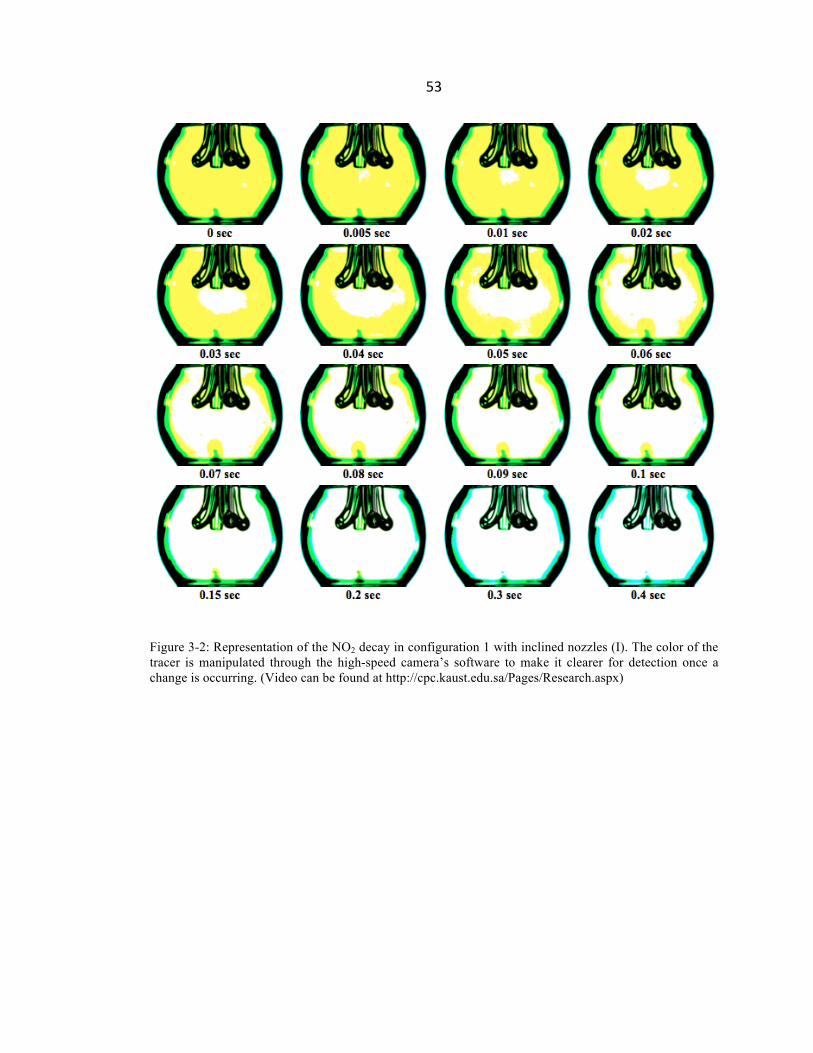
Figure 3-2: Representation of the NO2 decay in configuration 1 with inclined nozzles (I). The color of the tracer is manipulated through the high-speed camera’s software to make it clearer for detection once a change is occurring. (Video can be found at http://cpc.kaust.edu.sa/Pages/Research.aspx)  ......................................................................  53  

10

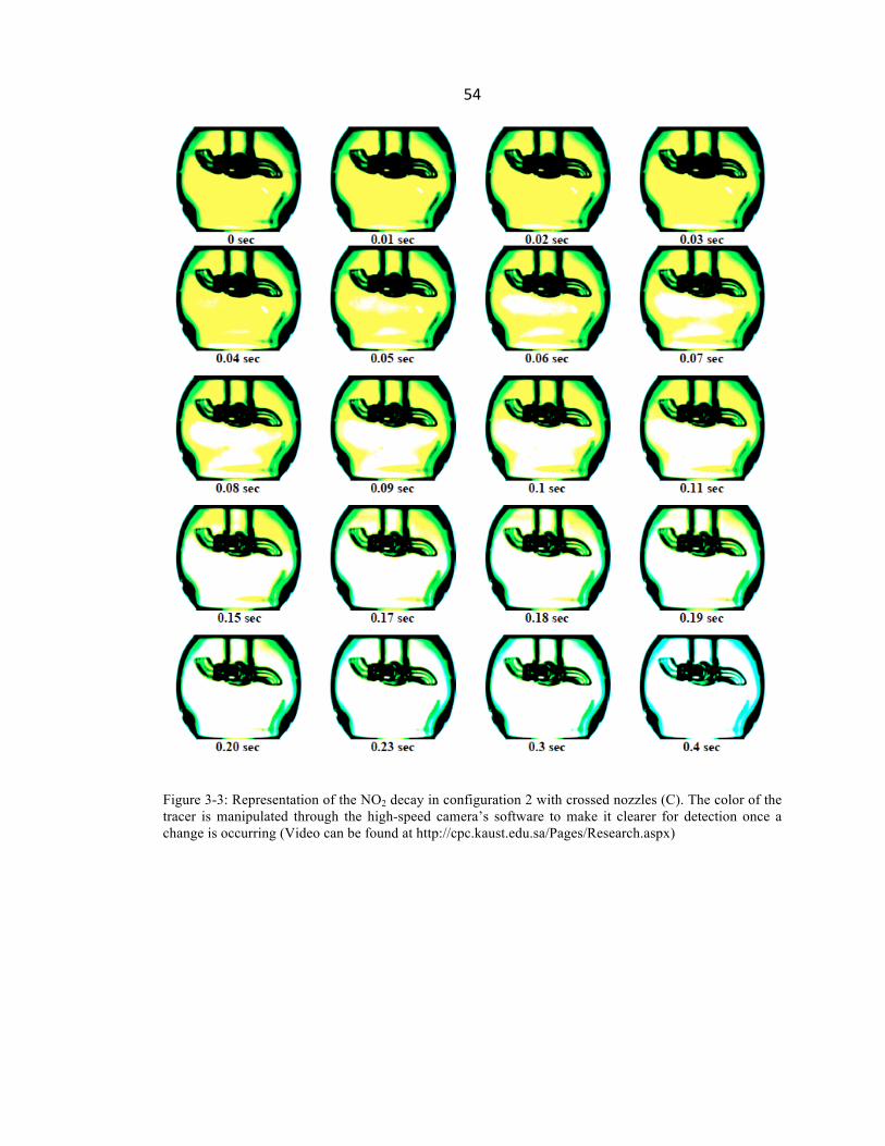
Figure 3-3: Representation of the NO2 decay in configuration 2 with crossed nozzles (C). The color of the tracer is manipulated through the high-speed camera’s software to make it clearer for detection once a change is occurring (Video can be found at http://cpc.kaust.edu.sa/Pages/Research.aspx)  ......................................................................  54  

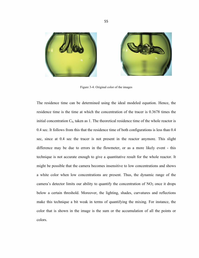
Figure 3-4: Original color of the images  .....................................................................................  55  

Figure 3-5: Five points or small control volumes studied along with their residence time in ms  57  

Figure 3-6: Plot of the change in color intensity in both reactors versus the number of frames  .  57  

Figure 3-7: Plots showing the exponential decay, as expected, representing the NO2 concentration versus time (ms) when purged with nitrogen (M=Middle, T=Top, B= Bottom, R=Right, and L=Left)  .........................................................................................................  58  

Figure 3-8: A plot of CO2 and H2O absorbance versus a frequency range (cm-1)  ......................  61  

Figure 3-9: A plot of normalized absorbance versus time (s)  .....................................................  62  

Figure 3-10: RTD E(t) curves for 1(I),40,1,GPE shown with a repeatability of three measurements per case. The upper and lower dashed lines represent the region containing all the experimental data (Appendix B)  ..............................................................................  64  

Figure 3-11: RTD E(t) curves for 2(C),40,1,GPE  .......................................................................  64  

Figure 3-12: RTD E(t) curves for 1(I),40,0.3,GPE and 2(C),40,0.3,GPE  ...................................  65  

Figure 3-13: RTD E(t) curves for 2(C),40,0.3,VERAL  ..............................................................  65  

Figure 3-14: RTD E(t) curves for 2(C),56,0.3,VERAL  ..............................................................  66  

Figure 3-15: RTD F(t) curves for 1(I),40,1,GPE shown with a repeatability of three measurements per case. The upper and lower dashed lines represent the region containing all the experimental data (Appendix B)  ..............................................................................  66  

Figure 3-16: RTD F(t) curves for 2(C),40,1,GPE  .......................................................................  67  

Figure 3-17: RTD F(t) curves for 1(I),40,0.3,GPE and 2(C),40,0.3,GPE  ...................................  67  

Figure 3-18: RTD F(t) curves for 2(C),40,0.3,VERAL  ..............................................................  68  

Figure 3-19: Figure 3-20: RTD E(t) curves for 2(C),56,0.3,VERAL  ..........................................  68  

Figure 3-21 CHEMKIN-PRO simulation  ...................................................................................  70  

Figure 3-22: F(t) curves versus times with the tank in series models curves  ..............................  71  

Figure 4-1: Vector maps, generated from the steady state solution, of the reactor’s cross-section (0,1,0) showing the circular movement of the flow and its direction.  .................................  79  

11

Figure 4-2: ML(%) versus time  ...................................................................................................  81  

Figure 4-3: Figure showing the simulated tracer concentration decay in a cross-section of the reactor (configuration 1, d=1mm and D=40mm) with respect to time related to the computed CFD residence time. The red and blue colors correspond to a mole fraction of 1 and 0 respectively. The mixing level ML is also reported. The plane cut is of coordinate [x(1,0,0) ; y(0,1,0) ; z(0,0,0)].  .............................................................................................  82  

Figure 4-4:  Figure showing the simulated tracer decay in a cross-section of the reactor (configuration 1, d=0.3mm and D=40mm) with respect to time related to the computed CFD residence time. The red and blue colors correspond to a mole fraction of 1 and 0 respectively. The mixing level ML is also reported. The plane cut is of coordinate [x(1,0,0) ; y(0,1,0) ; z(0,0,0)].  ............................................................................................................  83  

Figure 4-5: Figure showing the simulated tracer decay in a cross-section of the reactor (configuration 2, d=1mm and D=40mm) with respect to time related to the computed CFD residence time. The red and blue colors correspond to a mole fraction of 1 and 0 respectively. The mixing level ML is also reported. The plane cut is of coordinate [x(1,0,0) ; y(0,1,0) ; z(0,0,0)].  ............................................................................................................  84  

Figure 4-6: Figure showing the simulated tracer decay in a cross-section of the reactor (configuration 2, d=0.3mm and D=40mm) with respect to time related to the computed CFD residence time. The red and blue colors correspond to a mole fraction of 1 and 0 respectively. The plane cut is of coordinate [x(1,0,0) ; y(0,1,0) ; z(0,0,0)].  ........................  84  

Figure 4-7: Figure showing the simulated tracer decay in a cross-section of the reactor (configuration 1, d=0.3 mm and D=56mm) with respect to time related to the computed CFD residence time. The red and blue colors correspond to a mole fraction of 1 and 0 respectively. The plane cut is of coordinate [x(1,0,0) ; y(0,1,0) ; z(0,0,0)].  ........................  85  

Figure 4-8: Figure showing the simulated tracer decay in a cross-section of the reactor (configuration 2, d=0.3 mm and D=56mm) with respect to time related to the computed CFD residence time. The red and blue colors correspond to a mole fraction of 1 and 0 respectively. The plane cut is of coordinate [x(1,0,0) ; y(0,1,0) ; z(0,0,0)].  ........................  86  

Figure 5-1: Simulated, experimental and theoretical RTD curves  ..............................................  89  

Figure 5-2: Simulated, experimental and theoretical RTD curves  ..............................................  89  

Figure 5-3: Simulated, experimental and theoretical RTD curves  ..............................................  90  

Figure 5-4: Simulated, experimental and theoretical RTD curves  ..............................................  90  

Figure 6-1: Illustration of the molecular-beam sampling concept  ..............................................  92  

Figure 6-2: A sketch describing the different section of the furnace  ..........................................  93  

12

Figure A-3: Calibration Curve  ....................................................................................................  96  

Figure B-4: Raw intensity of the signal recorded versus time (s)  ...............................................  98  

Figure B-5: Absorbance versus time (s). The time delay due to piping connections is subtracted (¼ inch tube were used in all experiments performed)  ......................................................  98  

Figure B-6: Normalized absorbance versus time (s) represented with the fitting of the signal  ...  99  

Figure B-7: Figure 6-8: RTD E(t) curves for 1(I),40,1,GPE  .....................................................  101  

Figure C-9: F(t) curves of the ideal, experimental and 2-CSTR’s in series models  .................  102  

Figure C-10: F(t) curves of the ideal, experimental and 2-CSTR’s in series models  ...............  102  

Figure C-11: F(t) curves of the ideal, experimental and 2-CSTR’s in series models  ...............  103  

13

LIST OF TABLES

Table 2-1: show some of the reaction conditions of oxygenate fuels combustion in JSR ............. 19

Table 2-2: Table showing the different cases treated in this thesis, (I= inclined nozzles, C= crossed nozzles). GPE and VERAL manufactured the crossed nozzles differently: the bending angle of each jet and the nozzles volume occupied in the reactor differed in each case due to some manufacturing errors. ................................................................................. 42

Table 2-3: operating and designed conditions of the designed JSR at ambient temperature ......... 43

Table 2-4: operating and designed conditions of the designed JSR with Argon as a the flowing gas at 723 K and 105 Pa, A=0.785, the specific weight and the dynamic viscosity of argon are equal to 0.71 kg·m−3 and 4.23·10−5 Pa.s respectively ...................................................... 43

Table 3-1: Table showing the experimental residence times, the degree of micromixing and macromixing (Appendix B shows sample calculations) ........................................................ 63

Table 4-1: Boundary conditions and the main simulation parameters ........................................... 77

14

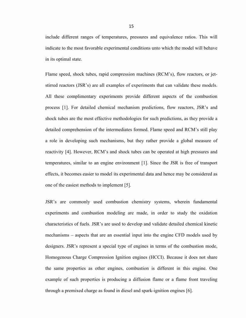
Chapter 1 Introduction

Combustion processes are taking place every day, whether in power plants, heating

applications or transportation medians (engines of vehicles), amongst other examples.

One of the ultimate goals associated with combustion processes, is the reduction of gas

emissions (NOx, SOx, etc.), and hence increasing the efficiency of the combustion

process. Consequently, understanding the nature of the fuel and its combustion route is

essential, and thus working with a fuel that is fully understood and developed is a crucial

requirement for engine manufacturers to properly design their systems. This can be

either achieved by conducting experiments, or by developing predictive models from

fundamental experiments. For example, using analytical spectroscopic techniques to

detect intermediate products of an oxidation reaction in a jet-stirred reactor (JSR) is a

fundamental experiment to help in developing or validating a chemical kinetic

mechanism [1].

Simulations, like computational fluid dynamics (CFD) coupled with a developed kinetic

mechanism, are excellent for providing a general model that can be applied in several

applications. Ultimately, this reduces the number of experiments performed; hence a lot

of effort is spent on such computational tools. Subsequently, extensive chemical reaction

mechanisms have been developed to model the combustion of light hydrocarbons (C-3,

C-4) [2]. These mechanisms are a collection of elementary steps that transform reactants

into products on the molecular level. Also, mechanisms for higher hydrocarbons and for

certain bio-fuels have been developed recently (up to C-20) [3]. In order to validate

these models, experiments should be done over a wide range of physical conditions, to

15

include different ranges of temperatures, pressures and equivalence ratios. This will

indicate to the most favorable experimental conditions unto which the model will behave

in its optimal state.

Flame speed, shock tubes, rapid compression machines (RCM’s), flow reactors, or jet-

stirred reactors (JSR’s) are all examples of experiments that can validate these models.

All these complimentary experiments provide different aspects of the combustion

process [1]. For detailed chemical mechanism predictions, flow reactors, JSR’s and

shock tubes are the most effective methodologies for such predictions, as they provide a

detailed comprehension of the intermediates formed. Flame speed and RCM’s still play

a role in developing such mechanisms, but they rather provide a global measure of

reactivity [4]. However, RCM’s and shock tubes can be operated at high pressures and

temperatures, similar to an engine environment [1]. Since the JSR is free of transport

effects, it becomes easier to model its experimental data and hence may be considered as

one of the easiest methods to implement [5].

JSR’s are commonly used combustion chemistry systems, wherein fundamental

experiments and combustion modeling are made, in order to study the oxidation

characteristics of fuels. JSR’s are used to develop and validate detailed chemical kinetic

mechanisms – aspects that are an essential input into the engine CFD models used by

designers. JSR’s represent a special type of engines in terms of the combustion mode,

Homogenous Charge Compression Ignition engines (HCCI). Because it does not share

the same properties as other engines, combustion is different in this engine. One

example of such properties is producing a diffusion flame or a flame front traveling

through a premixed charge as found in diesel and spark-ignition engines [6].

16

HCCI is a combustion process that is chemically controlled with a low temperature. It

combines both spark-ignition and diesel compression ignition technology. Fuel is mixed

homogenously with air in the combustion chamber; as the piston reaches the top dead

center, the air and fuel mixture auto-ignites. The auto-ignition of the mixture not only

results in a reduction in exhaust emissions, particulate matter emissions and NOx

emissions, but also gives higher thermal efficiency and saves energy [6].

JSR’s have been widely used in studying high and low temperature combustion

processes [7]. Similar to a continuous stirred-tank reactor (CSTR), the JSR is designed

to behave in an ideal fashion where reactants are perfectly stirred, leading to a uniform

composition throughout at a certain time over the reactor residence time. However, in

the JSR only a limited range of residence time ensure a perfectly mixed environment

depending on its geometry [7].

1.1. Research Motivation and Objective

There are several configurations for JSR’s of which their primary differences lie in the

volume of the reactor as well as the geometry of the four injection nozzles that include

outlets at the equatorial plane. Each nozzle has a different outlet direction, ensuring

overall a near perfectly mixed environment inside the reactor. Various injection

apparatuses and reactor geometries have been adopted [8-12]. Moreover, many

researchers have found it useful and implementable to assume that is it is an ideal

reactor (chapter 2) [8].

17

Thus, the broad questions that this thesis addresses are:

• To what extent has the design objective been realized in reactors of various

geometries? In other words, how ideal is the JSR?

• In what ways, if any, do the configuration of the jets or the geometry of the JSR

affect the mixing level?

1.2. Thesis Layout

In order to answer these questions, two experiments are performed to study and analyze

the mixing process taking place in the JSR. Both experiments use a tracer decay

technique, but the technology used to detect the change of decay differs. This technique

is then followed by fluid dynamics computations on fluent ANSYS, mainly undergone

to predict the mixing level (ML). Below is a list of objectives for each chapter:

Chapter 1 Introduction and aims of this thesis

Chapter 2 Comprehensive literature review

Chapter 3 Experimental methods: flow visualization using a high-speed camera and tracer experiment using a laser absorption spectroscopy technique

Chapter 4 Computational methods (CFD simulations) versus experimental methods

Chapter 5 Summary of the contributions of this thesis

Chapter 6 Future work

18

REFERENCES

[1] F. Battin-Leclerc, J.M. Simmie, E. Blurock, Cleaner Combustion, Springer Verlag,

2013.

[2] P. Dagaut , Physical Chemistry Chemical Physics. 4 (2002), 2079-94.

[3] S.M. Sarathy, C.K. Westbrook, M. Mehl, W.J. Pitz, C. Togbe, P. Dagaut, et al.

Combustion and Flame. 158 (2011), 2338-57.

[4] J.M. Simmie, Prog Energ Combust. Sci. 29 (2003), 599–634 [5] P. Dagaut , M. Cathonnet , J.P. Rouan, R. Foulatier, A. Quilgars, J.C. Boettner, F. Gaillard, H. James, J. Phys. E: Sci. Instrum. 19 (1986), 207-209. [6] U.S. department of Energy report, 2001 [7] P. G. Lignola, E. Reverchon, Combust. Sci. Technol. 60 (1988), 319-333.

[8] W. Bartok, C.E. Heath, M.A.Weiss, AIChE J. 6 (1960), 685-589

[9] A.Y. Abdalla, D. Bradley, S.B. Chin, Choi Lam, Symp. Comb. Inst. (1982), p.495.

[10] D.R. Jenkins, V.S. Yumlu, D.B. Spalding, Symp. Comb. Inst. (1967), p.779.

[11] J.E. Nenninger, A. Kridiotis, J. Chomiak, J.P. Longwell, A.F. Sarofim, Symp.

Comb. Inst. (1984), 473-479

[12] D. Matras, J. Villerrnaux, Chem. Engng. Sci. 28 (1973), 129-137

19

Chapter 2 Comprehensive Literature Review

2.1. Combustion in JSR  

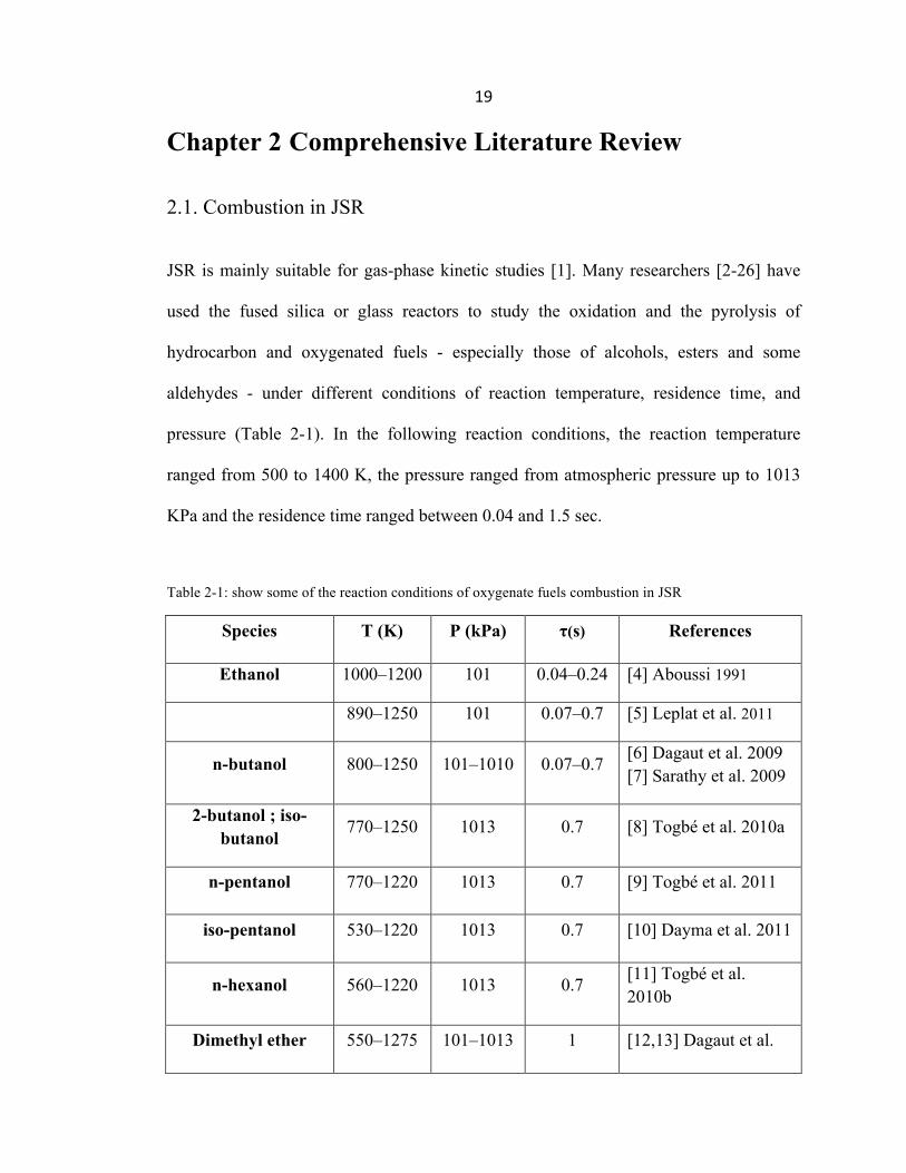
JSR is mainly suitable for gas-phase kinetic studies [1]. Many researchers [2-26] have

used the fused silica or glass reactors to study the oxidation and the pyrolysis of

hydrocarbon and oxygenated fuels - especially those of alcohols, esters and some

aldehydes - under different conditions of reaction temperature, residence time, and

pressure (Table 2-1). In the following reaction conditions, the reaction temperature

ranged from 500 to 1400 K, the pressure ranged from atmospheric pressure up to 1013

KPa and the residence time ranged between 0.04 and 1.5 sec.

 

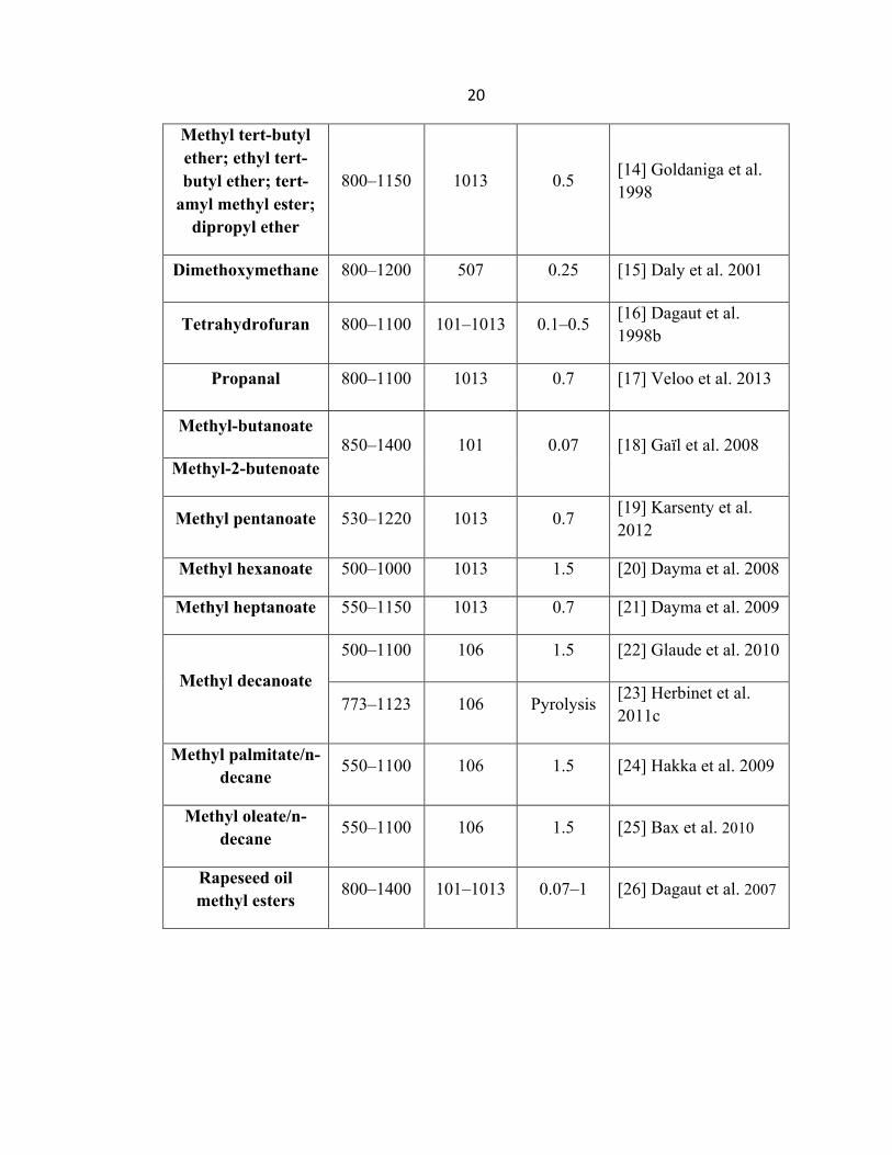
Table 2-1: show some of the reaction conditions of oxygenate fuels combustion in JSR

Species T (K) P (kPa) τ(s) References

Ethanol 1000–1200 101 0.04–0.24 [4] Aboussi 1991

890–1250 101 0.07–0.7 [5] Leplat et al. 2011

n-butanol 800–1250 101–1010 0.07–0.7 [6] Dagaut et al. 2009 [7] Sarathy et al. 2009

2-butanol ; iso-butanol 770–1250 1013 0.7 [8] Togbé et al. 2010a

n-pentanol 770–1220 1013 0.7 [9] Togbé et al. 2011

iso-pentanol 530–1220 1013 0.7 [10] Dayma et al. 2011

n-hexanol 560–1220 1013 0.7 [11] Togbé et al. 2010b

Dimethyl ether 550–1275 101–1013 1 [12,13] Dagaut et al.

20

Methyl tert-butyl ether; ethyl tert-butyl ether; tert-

amyl methyl ester; dipropyl ether

800–1150 1013 0.5 [14] Goldaniga et al. 1998

Dimethoxymethane 800–1200 507 0.25 [15] Daly et al. 2001

Tetrahydrofuran 800–1100 101–1013 0.1–0.5 [16] Dagaut et al. 1998b

Propanal 800–1100 1013 0.7 [17] Veloo et al. 2013

Methyl-butanoate 850–1400 101 0.07 [18] Gaïl et al. 2008

Methyl-2-butenoate

Methyl pentanoate 530–1220 1013 0.7 [19] Karsenty et al. 2012

Methyl hexanoate 500–1000 1013 1.5 [20] Dayma et al. 2008

Methyl heptanoate 550–1150 1013 0.7 [21] Dayma et al. 2009

Methyl decanoate

500–1100 106 1.5 [22] Glaude et al. 2010

773–1123 106 Pyrolysis [23] Herbinet et al. 2011c

Methyl palmitate/n-decane 550–1100 106 1.5 [24] Hakka et al. 2009

Methyl oleate/n-decane 550–1100 106 1.5 [25] Bax et al. 2010

Rapeseed oil methyl esters 800–1400 101–1013 0.07–1 [26] Dagaut et al. 2007

21

Other studies include the kinetic study of nitrous oxides formation and destruction [27],

and the study of stationary-state and oscillatory ignition phenomena in fuel

oxidation [28, 29]. Low temperature oxidation of hydrocarbons [30, 31], and the

cracking kinetics of biomass vapors [32] were studied in metallic JSR’s. A few studies

in JSR’s also focus on the oxidation of ethers, cyclic ethers, ketones and aldehydes.

Species such as ketones and aldehydes are an important field of study – usually formed

as intermediate combustion products - in order to better understand the intermediate

reactions of the combustion of hydrocarbons and oxygenates. [33].

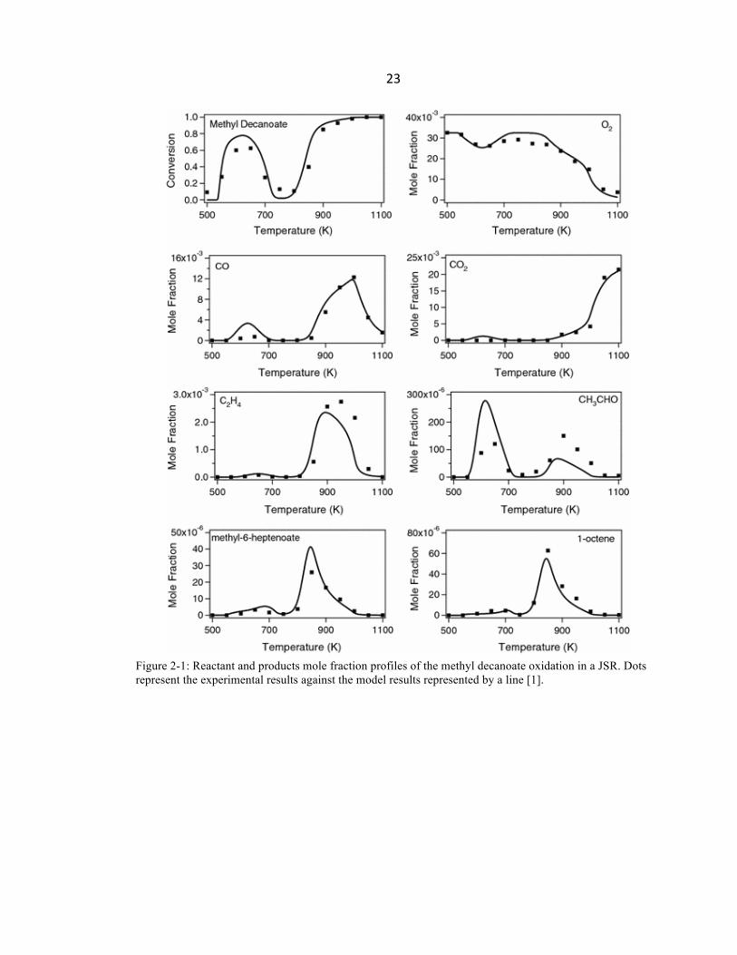
Most of the JSR experiments aim to help in understanding the intermediates or products

formed by recording the conversion of the reactants and the mole fractions of the

reaction products as a function of different reaction conditions [1]. In order to quantify

the species formed, spectroscopic techniques should be used. The classical technique

used to analyze gas phase species is gas chromatography (GC) coupled with a flame-

ionized detector (FID) and thermal conductivity detector (TCD), which well detect the

most stable molecules (Hydrocarbons and permanent gases respectively). In some cases,

the GC is coupled with a mass spectrometer (MS). An experimental study of the methyl

decanoate oxidation in a JSR done by Glaude et al. used the GC technique to quantify

the mole fractions of the reactants and products presented in Figure 2-1 [22].

22

In cases where radicals or unstable molecules like hydoperoxides - intermediates usually

formed in low temperature hydrocarbon oxidation - need to be detected, GC-TCD-FID

would not be enough. Fortunately, the JSR is very easy to couple with a variety of

analytical devices. Additionally, in the case of water and formaldehyde species

quantification, it is more suitable to couple the JSR to a Fourier transform infrared

spectroscopy. For this reason, coupling the JSR to different and new analytical devices

(e.g. infrared spectroscopy (IR) [34], synchrotron vacuum ultra violet (SVUV) photo-

ionization [2, 35, 36] and Cavity Ring-down Spectroscopy (CRDS) [37-39]) will yield to

a better comprehension of the species formed.

23

Figure 2-1: Reactant and products mole fraction profiles of the methyl decanoate oxidation in a JSR. Dots represent the experimental results against the model results represented by a line [1].

 

 

 

 

24

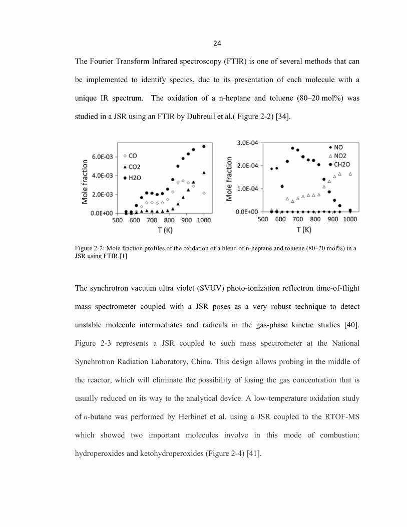
The Fourier Transform Infrared spectroscopy (FTIR) is one of several methods that can

be implemented to identify species, due to its presentation of each molecule with a

unique IR spectrum. The oxidation of a n-heptane and toluene (80–20 mol%) was

studied in a JSR using an FTIR by Dubreuil et al.( Figure 2-2) [34].

 

Figure 2-2: Mole fraction profiles of the oxidation of a blend of n-heptane and toluene (80–20 mol%) in a JSR using FTIR [1]

 

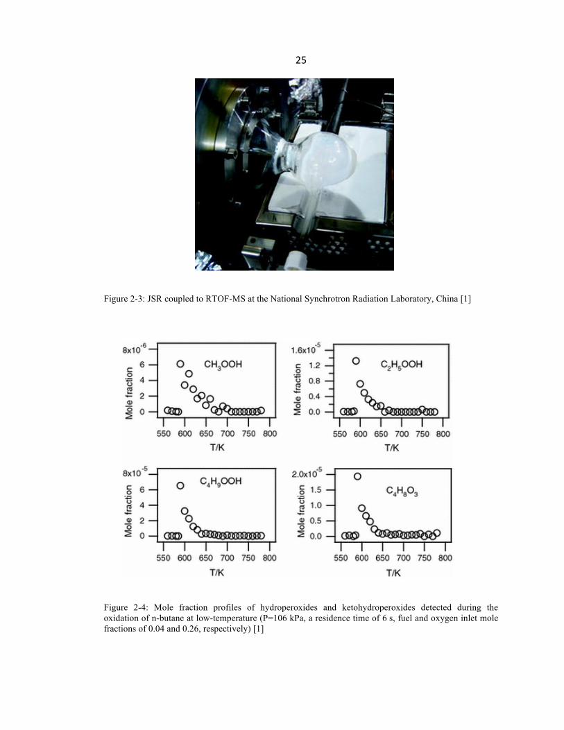
The synchrotron vacuum ultra violet (SVUV) photo-ionization reflectron time-of-flight

mass spectrometer coupled with a JSR poses as a very robust technique to detect

unstable molecule intermediates and radicals in the gas-phase kinetic studies [40].

Figure 2-3 represents a JSR coupled to such mass spectrometer at the National

Synchrotron Radiation Laboratory, China. This design allows probing in the middle of

the reactor, which will eliminate the possibility of losing the gas concentration that is

usually reduced on its way to the analytical device. A low-temperature oxidation study

of n-butane was performed by Herbinet et al. using a JSR coupled to the RTOF-MS

which showed two important molecules involve in this mode of combustion:

hydroperoxides and ketohydroperoxides (Figure 2-4) [41].

25

 

Figure 2-3: JSR coupled to RTOF-MS at the National Synchrotron Radiation Laboratory, China [1]

 

 

Figure 2-4: Mole fraction profiles of hydroperoxides and ketohydroperoxides detected during the oxidation of n-butane at low-temperature (P=106 kPa, a residence time of 6 s, fuel and oxygen inlet mole fractions of 0.04 and 0.26, respectively) [1]

26

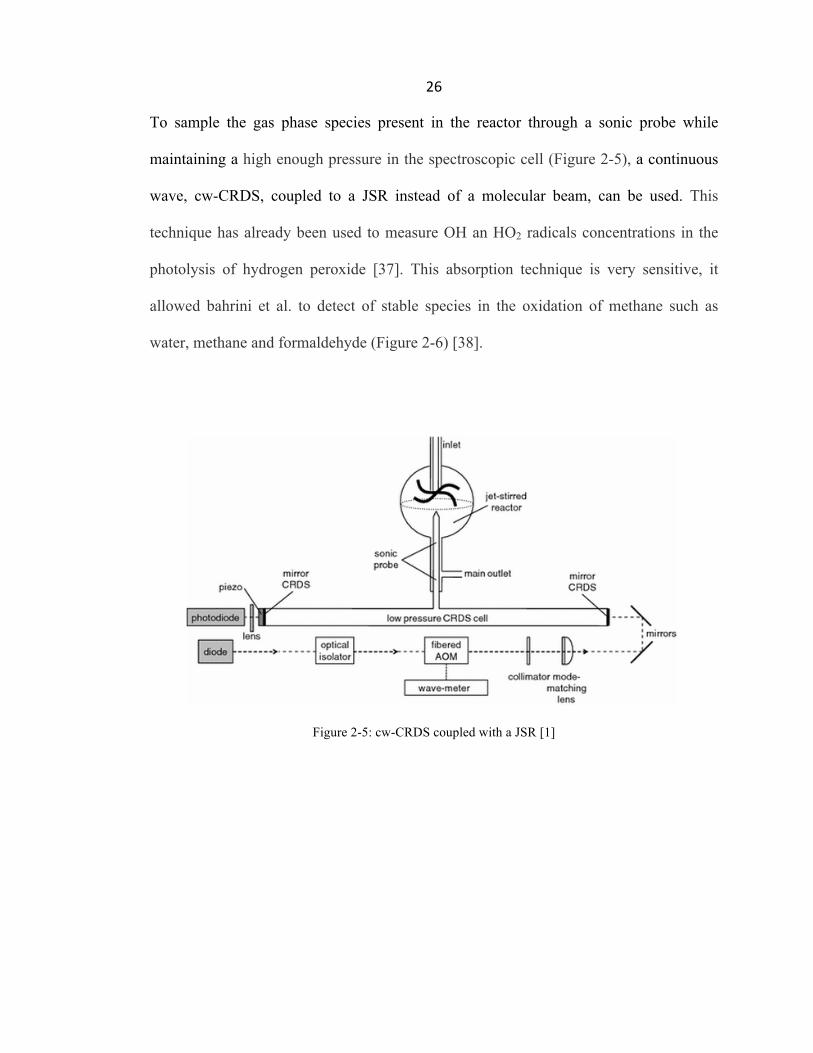
To sample the gas phase species present in the reactor through a sonic probe while

maintaining a high enough pressure in the spectroscopic cell (Figure 2-5), a continuous

wave, cw-CRDS, coupled to a JSR instead of a molecular beam, can be used. This

technique has already been used to measure OH an HO2 radicals concentrations in the

photolysis of hydrogen peroxide [37]. This absorption technique is very sensitive, it

allowed bahrini et al. to detect of stable species in the oxidation of methane such as

water, methane and formaldehyde (Figure 2-6) [38].

 

Figure 2-5: cw-CRDS coupled with a JSR [1]

27

 

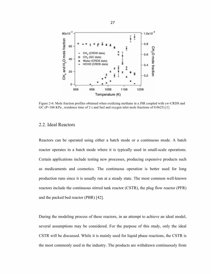
Figure 2-6: Mole fraction profiles obtained when oxidizing methane in a JSR coupled with cw-CRDS and GC (P=106 KPa , residence time of 2 s and fuel and oxygen inlet mole fractions of 0.0625) [1]

2.2. Ideal Reactors

Reactors can be operated using either a batch mode or a continuous mode. A batch

reactor operates in a batch mode where it is typically used in small-scale operations.

Certain applications include testing new processes, producing expensive products such

as medicaments and cosmetics. The continuous operation is better used for long

production runs since it is usually run at a steady state. The most common well-known

reactors include the continuous stirred tank reactor (CSTR), the plug flow reactor (PFR)

and the packed bed reactor (PBR) [42].

During the modeling process of these reactors, in an attempt to achieve an ideal model,

several assumptions may be considered. For the purpose of this study, only the ideal

CSTR will be discussed. While it is mainly used for liquid phase reactions, the CSTR is

the most commonly used in the industry. The products are withdrawn continuously from

28

the effluent. With a mechanical stirrer that ensures a proper mixing process, the CSTR is

assumed to be a perfectly mixed reactor. Thus, the concentration, temperature and

reaction rate inside the reactor are identical at any location at a certain time. This

assumption is only valid in a perfectly mixed environment. The basic design equation of

the CSTR can help in determining the optimum volume of the reactor V when the

reaction rate, r, of a species i is known, along with the initial and the effluent molar flow

rate F0 and F,

This design equation is derived by applying a simple mass balance on species i.

The following assumptions are considered: the system is operating at a steady state and

no spatial variations exist in the parameters of concentration, temperature and reaction

rate throughout the vessel [42].

2.3. Non-Ideal Reactors

All industrial reactors deviate from ideality (i.e. perfect mixing) due to many reasons

such as axial dispersion, bypassing and dead volume [42]. Many methods exist to

characterize the varying mixing levels of non-ideal reactors. In order to assess these non-

ideal mixing levels, these methods will have to be examined. This study is of extreme

importance to industries, as the reactor mixing level is directly proportional to the

production rate or the conversion of the reactants. As mentioned earlier, the objective is

to determine the extent to which the JSR is ideal. Therefore, similar methods will be

implemented to study the mixing level in the JSR. These experimental methods will be

explained in the following sections and can include, tracer experiment, flow

V =F0 −F−ri

29

visualization, determining the residence time distribution (RTD) E(t) and the mixing

level (ML).

The two experiments performed in this study aim to assess the mixing process inside the

JSR using the same concept of a tracer experiment. A tracer experiment or a pulse-input

experiment is done usually by pulsing a tracer, which can be a dye, an invisible gas, a

colored gas or a radioactive tracer, into the reactor while having an inert gas flowing.

Then, the concentration decay of the tracer is measured to compare it with an ideal

model. An adequate device or detector should be used to measure this concentration

decay or a physical property proportional to it. The type of the tracer used and its

properties dictate the technique used. Some examples would be using a mass

spectroscopy technique, scintillation probes, high-speed cameras to visualize the flow,

laser absorption spectroscopy technique or a thermo-conductivity technique. The two

techniques adopted in this study are using a high-speed camera and a laser absorption

technique. In certain cases, it is difficult to manipulate the tracer due to its problematic

physical properties such as toxicity or radioactivity, as well as due to detection limits

dictated by the technique used. Therefore, the same concept can be applied in a different

way. In this case, the tracer flows continuously in the reactor allowing the system to

reach steady state. Then, the tracer is purged by an inert gas and the decay of its

concentration is detected. This negative step input method is adopted in the experiments

presented in chapter 3.

30

 

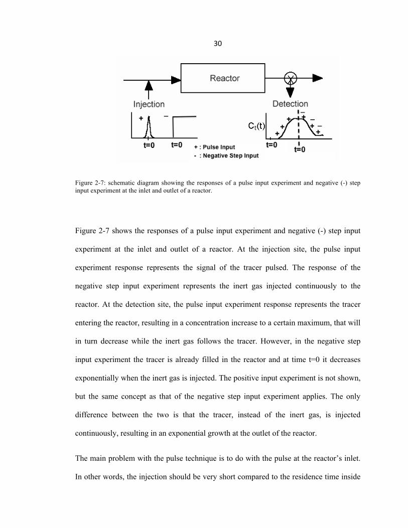
Figure 2-7: schematic diagram showing the responses of a pulse input experiment and negative (-) step input experiment at the inlet and outlet of a reactor.  

Figure 2-7 shows the responses of a pulse input experiment and negative (-) step input

experiment at the inlet and outlet of a reactor. At the injection site, the pulse input

experiment response represents the signal of the tracer pulsed. The response of the

negative step input experiment represents the inert gas injected continuously to the

reactor. At the detection site, the pulse input experiment response represents the tracer

entering the reactor, resulting in a concentration increase to a certain maximum, that will

in turn decrease while the inert gas follows the tracer. However, in the negative step

input experiment the tracer is already filled in the reactor and at time t=0 it decreases

exponentially when the inert gas is injected. The positive input experiment is not shown,

but the same concept as that of the negative step input experiment applies. The only

difference between the two is that the tracer, instead of the inert gas, is injected

continuously, resulting in an exponential growth at the outlet of the reactor.

The main problem with the pulse technique is to do with the pulse at the reactor’s inlet.

In other words, the injection should be very short compared to the residence time inside

31

the reactor in a way that dispersion of the tracer injected would be impossible [42]. Once

this problem is solved, obtaining the RTD curves would be direct and simple. The

positive step input experiment, on the other hand, is easier to conduct experimentally,

particularly since the amount of tracer in the feed doesn’t have to be known. One

drawback of this technique is that sometimes it is difficult to maintain a constant tracer

concentration in the feed. In that case a negative step input would solve the problem.

Another drawback will occur if the tracer used is expensive, since this technique

requires a large amount of tracer. In this case, using a pulse technique would be a better

choice to minimize the required costs [42].

In the conducted experiments, a solenoid valve with a response time of 20 ms was used

in order to prevent time delays as much as possible. Additionally, the choice for using

negative step input instead of a positive step input is for greater experimental

convenience, since a positive step input required the difficult step of maintaining a

constant NO2 tracer concentration in the feed stream. NO2 gas was synthesized in situ

and it was difficult to control its concentration.

2.4. Theory

Modeling the ideal CSTR behavior in a negative step input experiment is important to

predict ideal behavior of the reactor. This will be compared to the non-ideal reactor

behavior. In an ideal CSTR, the concentration at the effluent (Cout) is equal to the

concentration inside the reactor at a certain time. If a tracer is injected into the CSTR at

t=0, an inert gas is injected to purge the tracer. Performing a general tracer mass balance

in the CSTR yields,

32

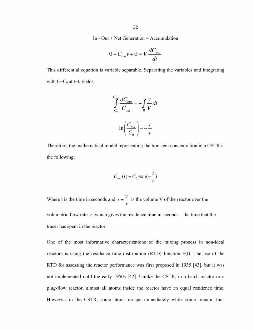
In - Out + Net Generation = Accumulation

This differential equation is variable separable. Separating the variables and integrating

with C=C0 at t=0 yields,

Therefore, the mathematical model representing the transient concentration in a CSTR is

the following,

Cout (t) =C0 exp(−tτ)

Where t is the time in seconds and is the volume V of the reactor over the

volumetric flow rate , which gives the residence time in seconds – the time that the

tracer has spent in the reactor.

One of the most informative characterizations of the mixing process in non-ideal

reactors is using the residence time distribution (RTD) function E(t). The use of the

RTD for assessing the reactor performance was first proposed in 1935 [43], but it was

not implemented until the early 1950s [42]. Unlike the CSTR, in a batch reactor or a

plug-flow reactor, almost all atoms inside the reactor have an equal residence time.

However, in the CSTR, some atoms escape immediately while some remain, thus

0−Coutv+ 0 =VdCout

dt

dCout

CoutC0

Cout

∫ = −vVdt

0

t

∫

ln Cout

C0

!

"#

$

%&= −

tτ

τ =Vv

v

33

creating a residence time distribution between the atoms. There are two limiting

processes, which cause a distribution of residence time within a reactor. The first

process is the flow pattern that the fluid elements follow without mutual mixing on the

microscopic scale, such as the laminar flow. Another one is the presence of fluid

elements with different mixing ages. A good example for the latter case would be the

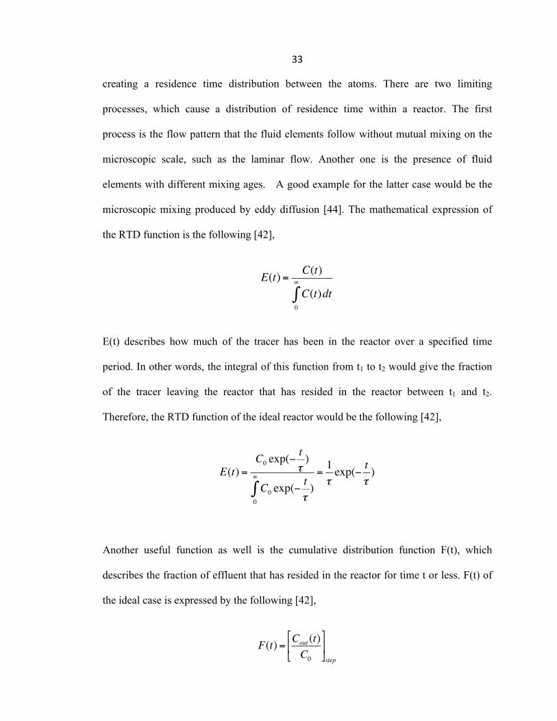
microscopic mixing produced by eddy diffusion [44]. The mathematical expression of

the RTD function is the following [42],

E(t) describes how much of the tracer has been in the reactor over a specified time

period. In other words, the integral of this function from t1 to t2 would give the fraction

of the tracer leaving the reactor that has resided in the reactor between t1 and t2.

Therefore, the RTD function of the ideal reactor would be the following [42],

E(t) =C0 exp(−

tτ)

C0 exp(−tτ)

0

∞

∫=1τexp(− t

τ)

Another useful function as well is the cumulative distribution function F(t), which

describes the fraction of effluent that has resided in the reactor for time t or less. F(t) of

the ideal case is expressed by the following [42],

E(t) = C(t)

C(t)dt0

∞

∫

F(t) = Cout (t)C0

!

"#

$

%&step

34

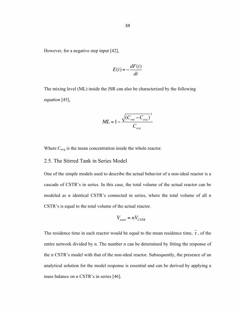
However, for a negative step input [42],

The mixing level (ML) inside the JSR can also be characterized by the following

equation [45],

Where Cavg is the mean concentration inside the whole reactor.

2.5. The Stirred Tank in Series Model

One of the simple models used to describe the actual behavior of a non-ideal reactor is a

cascade of CSTR’s in series. In this case, the total volume of the actual reactor can be

modeled as n identical CSTR’s connected in series, where the total volume of all n

CSTR’s is equal to the total volume of the actual reactor.

The residence time in each reactor would be equal to the mean residence time, , of the

entire network divided by n. The number n can be determined by fitting the response of

the n CSTR’s model with that of the non-ideal reactor. Subsequently, the presence of an

analytical solution for the model response is essential and can be derived by applying a

mass balance on n CSTR’s in series [46].

E(t) = − dF(t)dt

ML =1−(Cout −Cavg )

2

Cavg

Vtotal = nVCSTR

τ

35

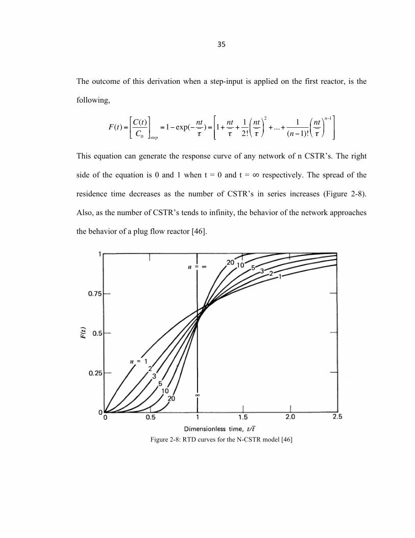
The outcome of this derivation when a step-input is applied on the first reactor, is the

following,

F(t) = C(t)C0

!

"#

$

%&step

=1− exp(− ntτ) = 1+ nt

τ+12!

ntτ

(

)*

+

,-2

+...+ 1(n−1)!

ntτ

(

)*

+

,-n−1!

"##

$

%&&

This equation can generate the response curve of any network of n CSTR’s. The right

side of the equation is 0 and 1 when t = 0 and t = ∞ respectively. The spread of the

residence time decreases as the number of CSTR’s in series increases (Figure 2-8).

Also, as the number of CSTR’s tends to infinity, the behavior of the network approaches

the behavior of a plug flow reactor [46].

 Figure 2-8: RTD curves for the N-CSTR model [46]

 

 

36

2.6. Previous Mixing Studies in Different Jet-Stirred Reactors

Three JSR configurations are presented below, at the same time acknowledging that the

first two nozzle configurations presented here are considered for this study since they

are the most commonly used recently [47,48,1].

2.6.1. Reactor Configuration 1:

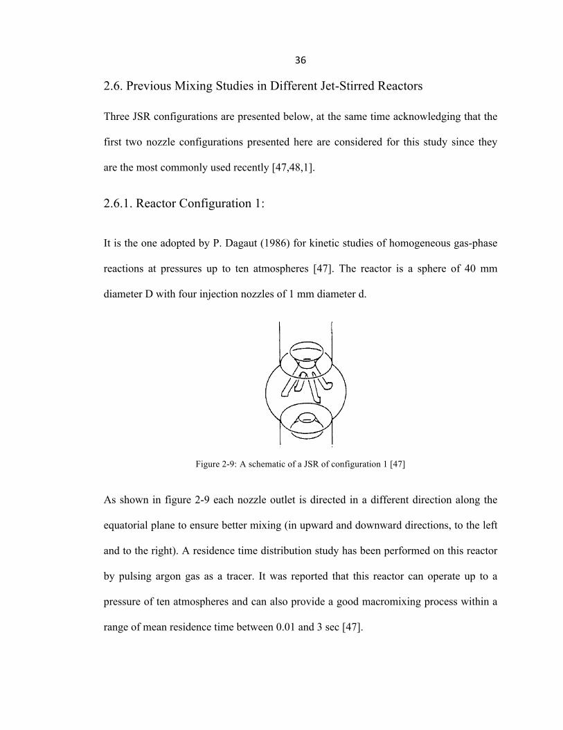
It is the one adopted by P. Dagaut (1986) for kinetic studies of homogeneous gas-phase

reactions at pressures up to ten atmospheres [47]. The reactor is a sphere of 40 mm

diameter D with four injection nozzles of 1 mm diameter d.

 

Figure 2-9: A schematic of a JSR of configuration 1 [47]

As shown in figure 2-9 each nozzle outlet is directed in a different direction along the

equatorial plane to ensure better mixing (in upward and downward directions, to the left

and to the right). A residence time distribution study has been performed on this reactor

by pulsing argon gas as a tracer. It was reported that this reactor can operate up to a

pressure of ten atmospheres and can also provide a good macromixing process within a

range of mean residence time between 0.01 and 3 sec [47].

37

A CFD study suggests that this reactor is a suitable reactor for studying the kinetics of

flames since the mixing level is close to 1. It is reported that this reactor has a mixing

level of around 94 % at a residence time of 160 ms, which decreases steadily to reach

93% at a residence time of 400 ms [45]. The simulation was performed using this reactor

configuration with a volume of 32.8 cm3. The temperature of the reactor walls is at 1305

K due to the combustion of methane: this study is done in the presence of a chemical

reaction [45]. For more information about the quality of the mesh and the method of

analysis please refer to reference [45].

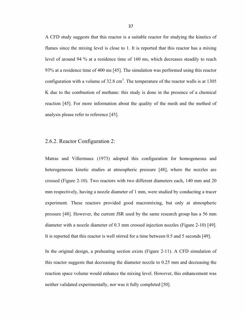
2.6.2. Reactor Configuration 2:

Matras and Villermaux (1973) adopted this configuration for homogeneous and

heterogeneous kinetic studies at atmospheric pressure [48], where the nozzles are

crossed (Figure 2-10). Two reactors with two different diameters each, 140 mm and 20

mm respectively, having a nozzle diameter of 1 mm, were studied by conducting a tracer

experiment. These reactors provided good macromixing, but only at atmospheric

pressure [48]. However, the current JSR used by the same research group has a 56 mm

diameter with a nozzle diameter of 0.3 mm crossed injection nozzles (Figure 2-10) [49].

It is reported that this reactor is well stirred for a time between 0.5 and 5 seconds [49].

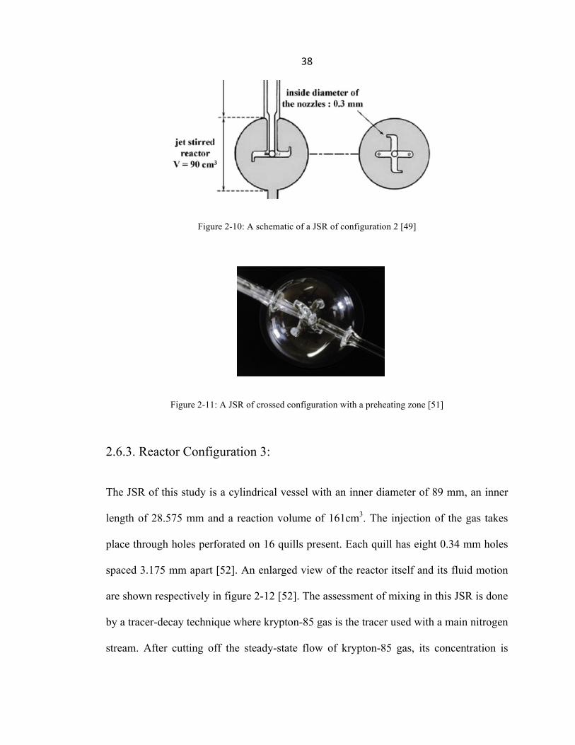
In the original design, a preheating section exists (Figure 2-11). A CFD simulation of

this reactor suggests that decreasing the diameter nozzle to 0.25 mm and decreasing the

reaction space volume would enhance the mixing level. However, this enhancement was

neither validated experimentally, nor was it fully completed [50].

38

 

Figure 2-10: A schematic of a JSR of configuration 2 [49]

 

Figure 2-11: A JSR of crossed configuration with a preheating zone [51]

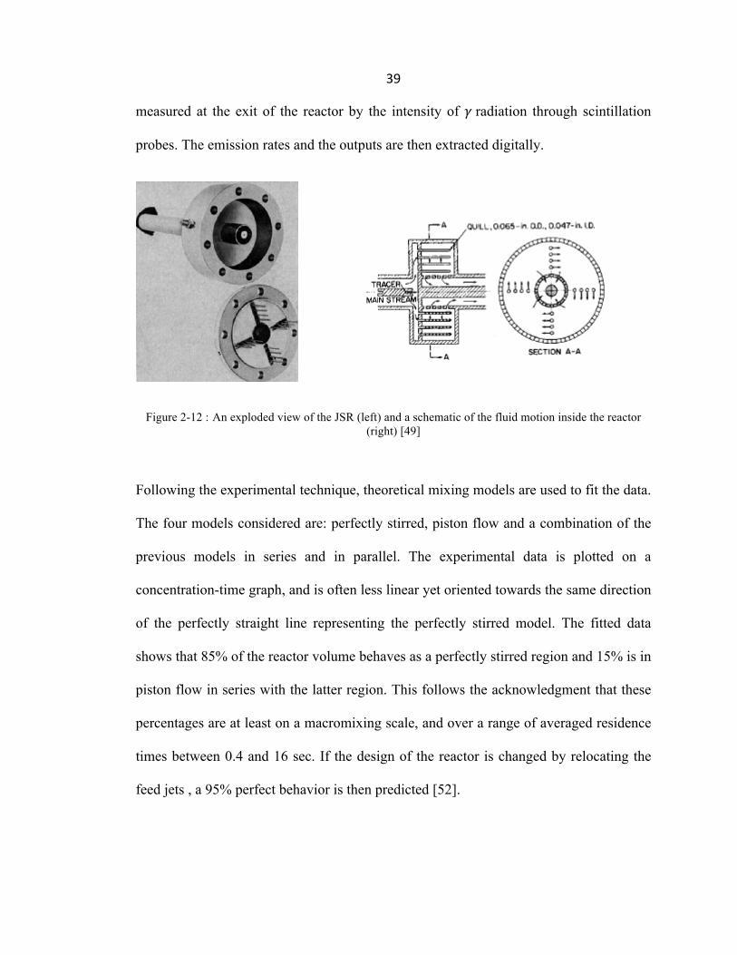
2.6.3. Reactor Configuration 3:

The JSR of this study is a cylindrical vessel with an inner diameter of 89 mm, an inner

length of 28.575 mm and a reaction volume of 161cm3. The injection of the gas takes

place through holes perforated on 16 quills present. Each quill has eight 0.34 mm holes

spaced 3.175 mm apart [52]. An enlarged view of the reactor itself and its fluid motion

are shown respectively in figure 2-12 [52]. The assessment of mixing in this JSR is done

by a tracer-decay technique where krypton-85 gas is the tracer used with a main nitrogen

stream. After cutting off the steady-state flow of krypton-85 gas, its concentration is

39

measured at the exit of the reactor by the intensity of 𝛾  radiation through scintillation

probes. The emission rates and the outputs are then extracted digitally.

 

Figure 2-12 : An exploded view of the JSR (left) and a schematic of the fluid motion inside the reactor (right) [49]

Following the experimental technique, theoretical mixing models are used to fit the data.

The four models considered are: perfectly stirred, piston flow and a combination of the

previous models in series and in parallel. The experimental data is plotted on a

concentration-time graph, and is often less linear yet oriented towards the same direction

of the perfectly straight line representing the perfectly stirred model. The fitted data

shows that 85% of the reactor volume behaves as a perfectly stirred region and 15% is in

piston flow in series with the latter region. This follows the acknowledgment that these

percentages are at least on a macromixing scale, and over a range of averaged residence

times between 0.4 and 16 sec. If the design of the reactor is changed by relocating the

feed jets , a 95% perfect behavior is then predicted [52].

40

One important result obtained from this study is the independence of mixing from the

residence time as long as turbulent conditions are satisfied. In other words, the geometry

is the critical aspect in turbulent mixing [52].

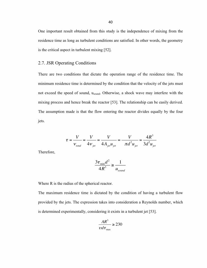
2.7. JSR Operating Conditions There are two conditions that dictate the operation range of the residence time. The

minimum residence time is determined by the condition that the velocity of the jets must

not exceed the speed of sound, usound. Otherwise, a shock wave may interfere with the

mixing process and hence break the reactor [53]. The relationship can be easily derived.

The assumption made is that the flow entering the reactor divides equally by the four

jets.

 

 

Therefore,

3τmind2

4R3≥

1usound

 

Where R is the radius of the spherical reactor.

The maximum residence time is dictated by the condition of having a turbulent flow

provided by the jets. The expression takes into consideration a Reynolds number, which

is determined experimentally, considering it exists in a turbulent jet [53].

AR3

υdτmax≥ 230  

 

41

 

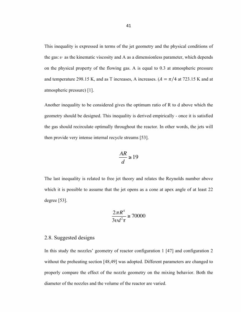
This inequality is expressed in terms of the jet geometry and the physical conditions of

the gas: as the kinematic viscosity and A as a dimensionless parameter, which depends

on the physical property of the flowing gas. A is equal to 0.3 at atmospheric pressure

and temperature 298.15 K, and as T increases, A increases. (𝐴 = 𝜋 4 at 723.15 K and at

atmospheric pressure) [1].  

Another inequality to be considered gives the optimum ratio of R to d above which the

geometry should be designed. This inequality is derived empirically - once it is satisfied

the gas should recirculate optimally throughout the reactor. In other words, the jets will

then provide very intense internal recycle streams [53].

 

The last inequality is related to free jet theory and relates the Reynolds number above

which it is possible to assume that the jet opens as a cone at apex angle of at least 22

degree [53].

2.8. Suggested designs

In this study the nozzles’ geometry of reactor configuration 1 [47] and configuration 2

without the preheating section [48,49] was adopted. Different parameters are changed to

properly compare the effect of the nozzle geometry on the mixing behavior. Both the

diameter of the nozzles and the volume of the reactor are varied.

υ

ARd≥19

2πR4

3υd 2τ≥ 70000

42

First, a similar reactor of the same dimensions of reactor configuration 1 [47] was

manufactured (D = 40mm, d=1mm). In order to compare the effect of the nozzles on

mixing, another reactor of the same dimensions, but with the crossed nozzle geometry of

reactor configuration 2 was manufactured. This will permit the study of an existing

reactor geometry used [47] with inclined nozzles, in order to then compare its mixing

behavior experimentally when changing the nozzle shape to a crossed geometry.

Another copy of the two reactors is manufactured with a nozzle diameter of 0.3 mm

while maintaining a constant reactor volume, since some CFD simulations suggested

that a smaller nozzle diameter provides better mixing for the reactor [50]. Finally, the

last reactor had a higher volume (D=56mm) and a constant nozzle diameter d of 0.3 mm.

The reactor of the same dimensions having the nozzles of configuration 1 is simulated

on CFD. This will permit to study an existing reactor geometry used with crossed

configuration of figure 2-10 (D=56 mm, d=0.3mm) [49] and compare its mixing

behavior computationally when changing the nozzle shape to an inclined geometry.

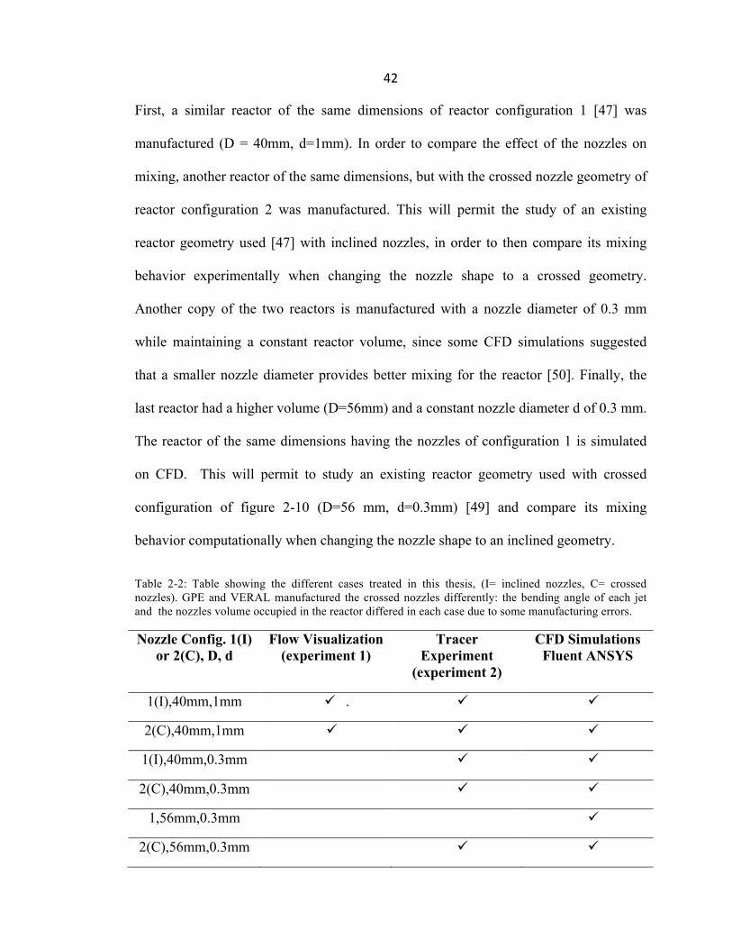
Table 2-2:   Table showing the different cases treated in this thesis, (I= inclined nozzles, C= crossed nozzles). GPE and VERAL manufactured the crossed nozzles differently: the bending angle of each jet and the nozzles volume occupied in the reactor differed in each case due to some manufacturing errors.

Nozzle Config. 1(I) or 2(C), D, d

Flow Visualization (experiment 1)

Tracer Experiment

(experiment 2)

CFD Simulations Fluent ANSYS

1(I),40mm,1mm ü . ü ü

2(C),40mm,1mm ü ü ü

1(I),40mm,0.3mm ü ü

2(C),40mm,0.3mm ü ü

1,56mm,0.3mm ü

2(C),56mm,0.3mm ü ü

43

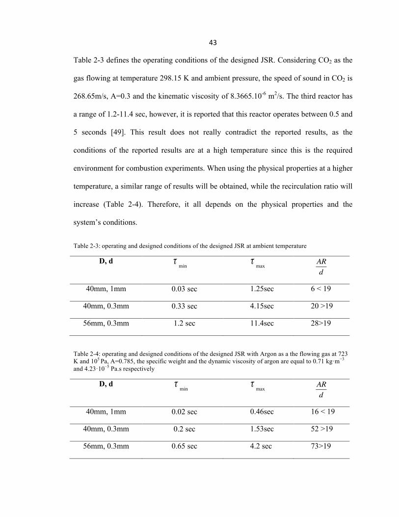
Table 2-3 defines the operating conditions of the designed JSR. Considering CO2 as the

gas flowing at temperature 298.15 K and ambient pressure, the speed of sound in CO2 is

268.65m/s, A=0.3 and the kinematic viscosity of 8.3665.10-6 m2/s. The third reactor has

a range of 1.2-11.4 sec, however, it is reported that this reactor operates between 0.5 and

5 seconds [49]. This result does not really contradict the reported results, as the

conditions of the reported results are at a high temperature since this is the required

environment for combustion experiments. When using the physical properties at a higher

temperature, a similar range of results will be obtained, while the recirculation ratio will

increase (Table 2-4). Therefore, it all depends on the physical properties and the

system’s conditions.

Table 2-3:  operating and designed conditions of the designed JSR at ambient temperature  

D, d min max

40mm, 1mm 0.03 sec 1.25sec 6 < 19

40mm, 0.3mm 0.33 sec 4.15sec 20 >19

56mm, 0.3mm 1.2 sec 11.4sec 28>19

Table 2-4: operating and designed conditions of the designed JSR with Argon as a the flowing gas at 723 K and 105 Pa, A=0.785, the specific weight and the dynamic viscosity of argon are equal to 0.71 kg·m−3 and 4.23·10−5 Pa.s respectively

D, d min max

40mm, 1mm 0.02 sec 0.46sec 16 < 19

40mm, 0.3mm 0.2 sec 1.53sec 52 >19

56mm, 0.3mm 0.65 sec 4.2 sec 73>19

τ τ ARd

τ τ ARd

44

 

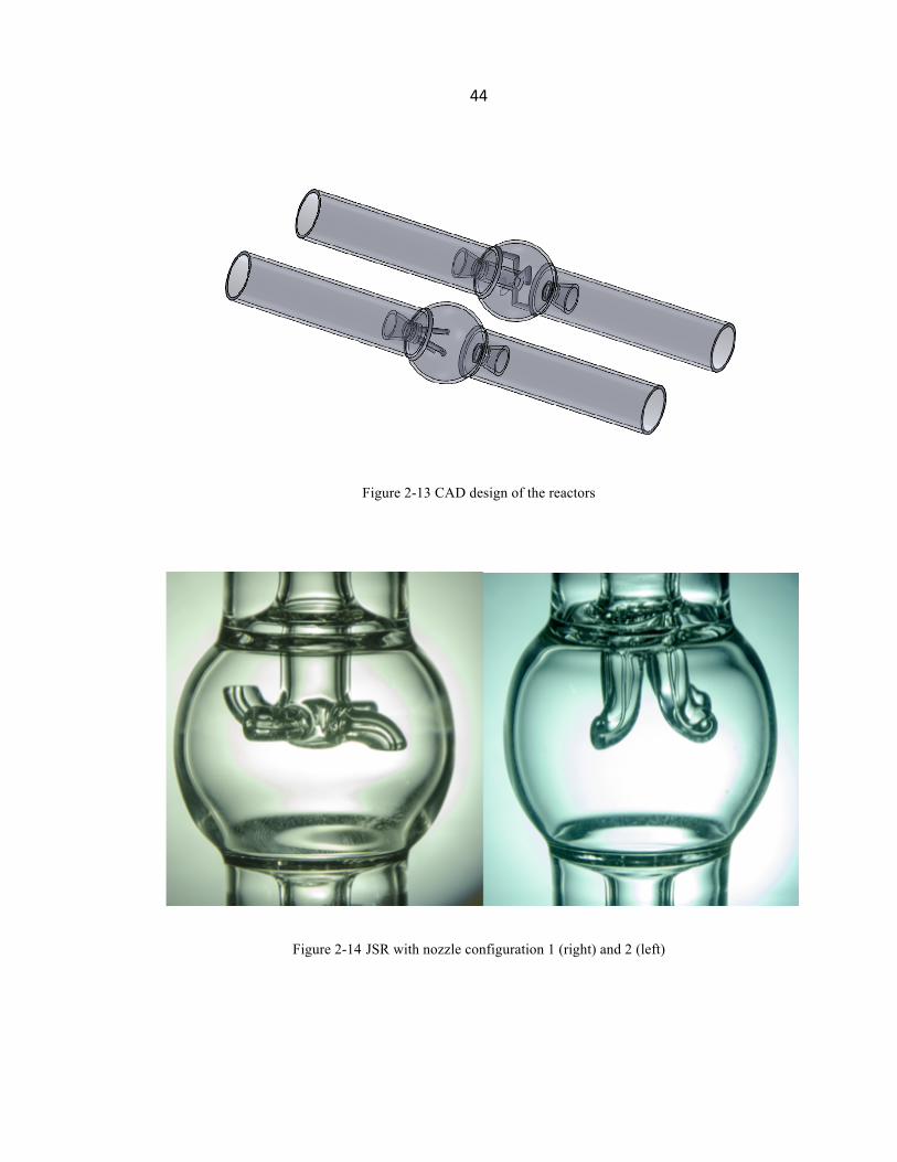
Figure 2-13 CAD design of the reactors

 

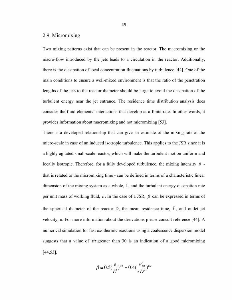
Figure 2-14 JSR with nozzle configuration 1 (right) and 2 (left)

 

 

 

45

2.9. Micromixing Two mixing patterns exist that can be present in the reactor. The macromixing or the

macro-flow introduced by the jets leads to a circulation in the reactor. Additionally,

there is the dissipation of local concentration fluctuations by turbulence [44]. One of the

main conditions to ensure a well-mixed environment is that the ratio of the penetration

lengths of the jets to the reactor diameter should be large to avoid the dissipation of the

turbulent energy near the jet entrance. The residence time distribution analysis does

consider the fluid elements’ interactions that develop at a finite rate. In other words, it

provides information about macromixing and not micromixing [53].

There is a developed relationship that can give an estimate of the mixing rate at the

micro-scale in case of an induced isotropic turbulence. This applies to the JSR since it is

a highly agitated small-scale reactor, which will make the turbulent motion uniform and

locally isotropic. Therefore, for a fully developed turbulence, the mixing intensity -

that is related to the micromixing time - can be defined in terms of a characteristic linear

dimension of the mixing system as a whole, L, and the turbulent energy dissipation rate

per unit mass of working fluid, .  In the case of a JSR, can be expressed in terms of

the spherical diameter of the reactor D, the mean residence time, , and outlet jet

velocity, u.  For more information about the derivations please consult reference [44]. A

numerical simulation for fast exothermic reactions using a coalescence dispersion model

suggests that a value of greater than 30 is an indication of a good micromixing

[44,53].

β ≅ 0.5( εL2)1/3 = 0.4(

ujet2

τD2 )1/3

 

β

ε β

τ

βτ

46

REFERENCES  

[1] F. Battin-Leclerc, J.M. Simmie, E. Blurock, Cleaner Combustion, Springer Verlag, 2013.

[2] F. Battin-Leclerc, O. Herbinet , P.A. Glaude , Angew. Chem. 122 (2010), 3237–3240

[3] P.M. Marquaire, G.M. Côme, React. Kinet. Catal. Lett. 9 (1978), 165–169

[4] B. Aboussi, PhD dissertation (1991), University of Orleans, France

[5] N. Leplat, P. Dagaut, C. Togbé et al, Combust. Flame. 158 (2011), 705–725

[6] P. Dagaut , S.M. Sarathy , M.J. Thomson, Proc Combust. Inst. 32 (2009), 229–237

[7] S.M. Sarathy, M.J. Thomson, C. Togbé et al, Combust Flame, 156 (2009), 852–864

[8] C. Togbé, A. Mzé-Ahmed, P. Dagaut, Energ. Fuel. 24 (2010a), 5244–5256

[9] C. Togbé, F. Halter, F. Foucher, C. Mounaim-Rousselle et al, Proc. Combust. Inst. 33 (2011), 367–374

[10] G. Dayma , C. Togbé , P. Dagaut, Energ. Fuel. 25 (2011), 4986–4998

[11] C. Togbé, P. Dagaut, A. Mzé-Ahmed et al, Energ. Fuel. 24 (2010b), 5859–5875

[12] P. Dagaut, J.C. Boettner, M. Cathonnet, Symp. Comb. Inst. (1996), 627–32

[13] P. Dagaut, C. Daly, J.M. Simmie et al, Symp. Comb. Inst. (1998a), 361–69

[14] A. Goldaniga, T. Faravelli, E. Ranzi et al, Symp. Comb. Inst. (1998), 353–60

[15] C.A. Daly, J.M. Simmie, P. Dagaut et al, Combust. Flame. 125 (2001), 1106–1117

[16] P. Dagaut, M. McGuinness, J.M. Simmie et al, Combust. Sci. Tech. 135 (1998b), 3–29

[17] P.S. Veloo PS, P. Dagaut, C. Togbé et al, Combust. Inst. 34 (2013), 599–606

[18] S. Gaïl, S.M. Sarathy, M.J. Thomson et al, Combust. Flame.155 (2008), 635–650

[19] F. Karsenty, S.M. Sarathy, C. Togbé et al, Energ Fuel. 26 (2012), 4680–4689

[20] G. Dayma, S. Gaïl, P. Dagaut, Energ Fuel. 22 (2008), 1469–1479

[21] G. Dayma, C. Togbé, P. Dagaut, Energ Fuel. 23 (2009), 4254–4268

[22] P.A. Glaude, O. Herbinet, S. Bax et al, Combust. Flame. 157 (2010), 2035–2050

47

[23] O. Herbinet, P.A. Glaude, V. Warth V et al, Combust. Flame. 158 (2011c), 1288–1300

[24] M.H. Hakka, P.A. Glaude, O. Herbinet et al, Combust. Flame. 156 (2009), 2129–2144

[25] S. Bax , M.H. Hakka, P.A. Glaude et al, Combust. Flame. 157 (2010), 1220–1229

[26] P. Dagaut, S. Gaïl, M. Sahasrabudhe, Proc. Combust. Inst. 31 (2007), 2955–2961

[27] G. Dayma , P. Dagaut, Combust. Sci. Tech. 178 (2006), 1999–2024

[28] D.L. Baulch, J.F. Griffiths, A.J. Pappin et al, Combust. Flame. 73 (1988), 163–185

[29] J.F. Griffiths, T. Inomata, J. Chem. Soc. Faraday. T. 88(1992), 3153–3158

[30] A. Cavaliere, A. Ciajolo, A. D’Anna et al, Combust. Flame. 93 (1993), 279–286

[31] A. Ciajolo, A. D’Anna, Combust. Flame. 112 (1998), 617–622

[32] S. Baumlin, F. Broust, M. Ferrer et al, Chem. Eng. Sci. 60 (2005), 41–55

[33] A. Piperel, P. Dagaut, X. Montagne, Combust. Sci. Technol. 32(2009), 2861–2868

[34] A. Dubreuil, F. Foucher , C. Mounaïm-Rousselle et al, Proc. Combust. Inst. 31(2007), 2879–2886

[35] N. Hansen, T.A. Cool, P.R. Westmoreland et al, Prog. Energy. Combust. Sci. 35(2009), 168–191

[36] Y. Li Y, F. Qi, Acc. Chem. Rev. 43 (2010), 68–78

[37] A.E. Parker, C. Jain, C. Schoemaecker et al, Appl. Phys. B. 103(2011), 725–733

[38] C. Bahrini, O. Herbinet , P.A. Glaude et al, Chem. Phys. Lett. 534(2012a), 1–7

[39] C. Bahrini, O. Herbinet, P.A. Glaude et al, J. Am. Chem. Soc. 134 (2012b), 11944–11947

[40] F. Qi, Proc Combust. Inst. 34(2013), 33–63

[41] O. Herbinet, F. Battin-Leclerc, S. Bax et al, Phys. Chem. Chem. Phys. 13(2011a), 296–308

[42] H.S. Fogler, Elements of Chemical Reaction Engineering Fourth Edition, Prentice Hall: Upper Saddle River,NJ,2006

[43] R.B. MacMullin, M. Wehcr. Jr., Trans. Am. Inst. Chem. Eng. 31 (1935), 409-458

48

[44] J. J. Evangelista, R. Shinnar, S. Katz , Symp. Comb. Inst. (1969), 901-912

[45] I. Gil, P. Mocek, Chem. Process Eng. 33 (2012), 397-410

[46] C.G. Hill, An Introduction to Chemical Engineering Kinetics & Reactor Design, John Wiley & Sons, 1977.

[47] P. Dagaut , M. Cathonnet , J.P. Rouan, R. Foulatier, A. Quilgars, J.C. Boettner, F. Gaillard, H. James, J. Phys. E: Sci. Instrum. 19 (1986), 207-209.

[48] D. Matras, J. Villerrnaux, Chem. Engng. Sci. 28 (1973), 129-137

[49] O. Herbinet, P.M. Marquaire, F. Battin-Leclerc, R. Fournet, J. Anal. Appl. Pyrolysis. 78 (2007) 419-429

[50] G.Mittal, 31st Annual Combustion Research Meeting.

[51] F.Battin-Leclerc, E. Blurock, R. Bounaceur, R.Fournet, P.A. Glaude, O.Herbinet et al, Chem. Soc. Rev. 40 (2011), 4762-4782

[52] W. Bartok, C.E. Heath, M.A.Weiss, AIChE J. 6 (1960), 685-589

[53] P. G. Lignola, E. Reverchon, Combust. Sci. Technol. 60:4-6 (1988), 319-333.

 

 

 

49

Chapter 3 Experimental Methods

3.1. Experimental set-up

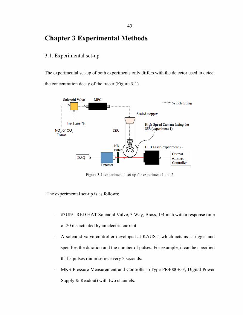
The experimental set-up of both experiments only differs with the detector used to detect

the concentration decay of the tracer (Figure 3-1).

Figure 3-1: experimental set-up for experiment 1 and 2

The experimental set-up is as follows:

- #3Ul91 RED HAT Solenoid Valve, 3 Way, Brass, 1/4 inch with a response time

of 20 ms actuated by an electric current

- A solenoid valve controller developed at KAUST, which acts as a trigger and

specifies the duration and the number of pulses. For example, it can be specified

that 5 pulses run in series every 2 seconds.

- MKS Pressure Measurement and Controller (Type PR4000B-F, Digital Power

Supply & Readout) with two channels.

50

- Mass flow controllers (MFC’s): MKS (1179A) 5 SLM and MKS (1159A) 50

SLM depending on the desired residence time (Calibration curves found in

Appendix A)

- Jet-stirred reactors

- High-speed camera FASTCAM SA3. The maximum capabilities of the camera

used can reach towards capturing 120,000 frames/sec (experiment 1)

- A Nanoplus Distributed Feedback (DFB) 2679 nm (3733 cm-1) laser. Product

number: 522-2679-2, serial number: 430/23-3 (experiment 2)

- ILX-3724C current and temperature controller to tune the laser frequency

- Neutral Density filter to reduce the incident laser intensity

- PVI-3TE-4 IR detector from Vigo Systems with a signal bandwidth of 10 MHz

to detect the laser intensity. Active area: 2 mm x 2 mm

- National Instruments PCI-6133 8-channel Data Acquisition (DAQ card)

System, which had a maximum sampling rate of 2.5 million samples per second,

providing very fine time resolution for even the smallest of residence times in

the conducted experiments

3.2. Experiment 1: flow visualization using a high-speed camera

3.2.1. Experimental procedure

Both reactors used are manufactured to be spherical in shape, with a diameter of 4 cm,

an approximate volume of 31.6 cm3 and each containing 4 nozzles of 1 mm inner

diameter for each nozzle, used primarily for the admission of the reactants. In this

experiment, the only variable in the design is the nozzle configuration geometry. This

51

enables us to study the effect of the nozzle’s geometry on the flow behavior or mixing.

The experiment is conducted at atmospheric pressure and temperature using a tracer-

decay technique with NO2 - a colored gas. The gas is synthesized in-situ while running

the experiment by adding nitric acid on copper wires inside a sealed flask. Once it is

depressurized, NO2 escapes to the jet-stirred reactor. The system is then allowed to reach

steady state. A solenoid valve cuts off the NO2 flow and enables a continuous flow of

nitrogen having a volumetric flow rate of 79 cm3/sec. A fast change of the red-brownish

color of NO2 is observed. The color is supposed to disappear after 0.4 sec; 0.4 sec being

the theoretical average residence time.

While the main purpose of this experiment is to visualize the flow dynamics inside the

reactor or the change of color within this short period of time, a high-speed camera is

essential in order to obtain such visuals. The high-speed camera used is FASTCAM

SA3, which is a “state-of-art” engineering technology with the ability to slow down and

observe high-speed dynamic bodies with a megapixel resolution. The camera was

controlled by PFV (Photron FASTCAM Viewer) software. The number of frames

captured is 1000 frames/sec, although maximum capabilities of the camera used can

reach towards capturing 120,000 frames/sec. Usually, the nature of the experiment and

its time frame dictates the number of frames that should be used.

52

Furthermore, the resolution is an important factor to consider as it decreases with the

increase of number of frames. That is why an appropriate lighting is included in the set-

up – a 350 W metal-halide lamp (Sumita Optical Glass, Inc.) - to enhance the quality of

the image. The frames extracted from PFV are then inputted to Avizo® where the

images are processed. In other words, the intensity of color can be correlated with the

concentration change of NO2. Once a region within the reactor is selected, the software

can track the decay of color within that region.

3.2.2. Results and Discussion

Consider the idea that the dynamics of a fast flow in a JSR has never been done before

and the technique is shown to reveal interesting findings and phenomena. Figure 3-2 and

3-3 show the dynamics of the flow, in both reactors, from the steady state time (t = 0)

until the disappearance of the color. The original tracer gas color shown in Figure 3-4, is

altered to a combination of yellow, green, and blue colors to aid in visualization.

If the reactor is perfectly mixed, the concentration C(t) of the tracer with time will

behave according to the following equation:

Cout (t) =C0 exp(−tτ)

Where C0 is the initial concentration, t is the time and τ is the average residence time,

which is the volume of the reactor over the volumetric flow rate.

53

Figure 3-2: Representation of the NO2 decay in configuration 1 with inclined nozzles (I). The color of the tracer is manipulated through the high-speed camera’s software to make it clearer for detection once a change is occurring. (Video can be found at http://cpc.kaust.edu.sa/Pages/Research.aspx)

54

Figure 3-3: Representation of the NO2 decay in configuration 2 with crossed nozzles (C). The color of the tracer is manipulated through the high-speed camera’s software to make it clearer for detection once a change is occurring (Video can be found at http://cpc.kaust.edu.sa/Pages/Research.aspx)

55

Figure 3-4: Original color of the images

 

The residence time can be determined using the ideal modeled equation. Hence, the

residence time is the time at which the concentration of the tracer is 0.3678 times the

initial concentration C0, taken as 1. The theoretical residence time of the whole reactor is

0.4 sec. It follows from this that the residence time of both configurations is less than 0.4

sec, since at 0.4 sec the tracer is not present in the reactor anymore. This slight

difference may be due to errors in the flowmeter, or as a more likely event - this

technique is not accurate enough to give a quantitative result for the whole reactor. It

might be possible that the camera becomes insensitive to low concentrations and shows

a white color when low concentrations are present. Thus, the dynamic range of the

camera’s detector limits our ability to quantify the concentration of NO2 once it drops

below a certain threshold. Moreover, the lighting, shades, curvatures and reflections

make this technique a bit weak in terms of quantifying the mixing. For instance, the

color that is shown in the image is the sum or the accumulation of all the points or

colors.

56

However, one of the most interesting results of this work was the ability to visualize the

dynamics of the flow experimentally, as shown in figures 3-2 and 3-3. The yellow color

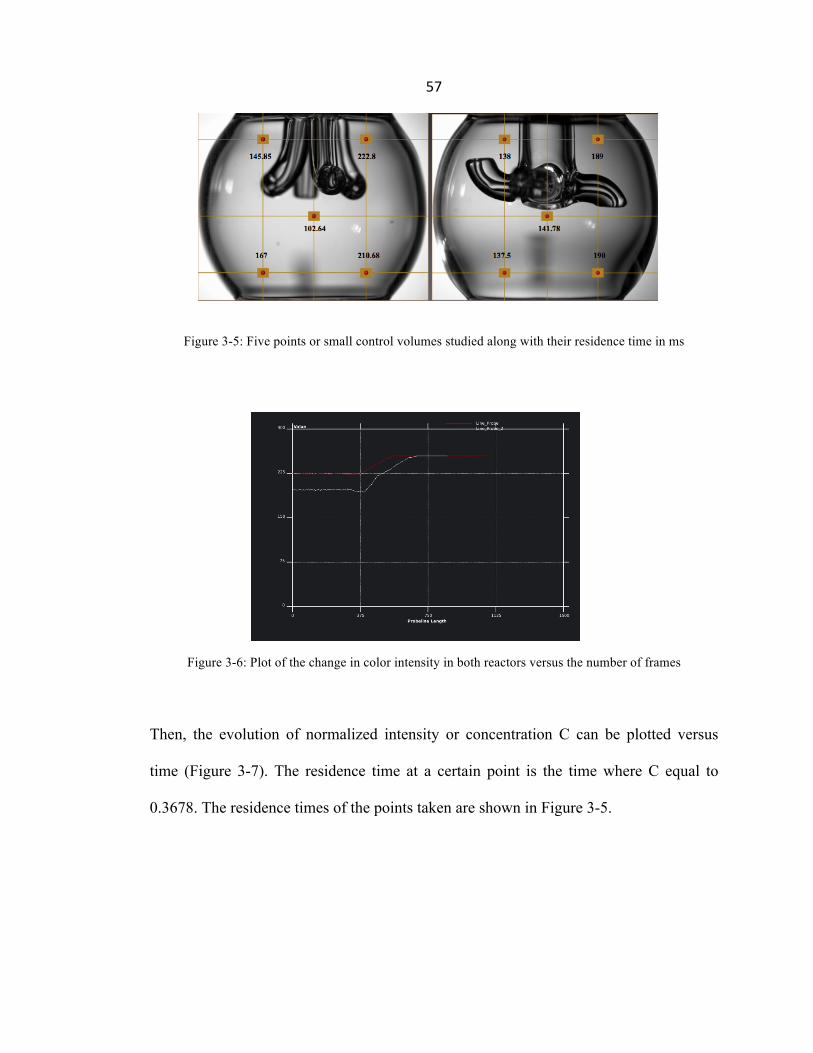
first clears at around 0.2 seconds for both reactors and then the colors remain changing

until 0.4 seconds is reached. It is important to note that the green color as well is turning

into blue. Before 0.2 seconds, the decay of the tracer in configuration 2 starts at the

bottom of the reactor then it goes to the top. On the other hand, in configuration 1, the

tracer decay starts from the middle and then expands. This shows how the geometry of

the nozzles affects the flow dynamics inside the JSR and thus affects the mixing

dynamics and the residence time.

In order to determine the experimental residence time of the reactor, usually the

concentration of the tracer is measured with time at the output of the reactor and then

plotted against time or normalized time. However, in this experiment, controlling the

NO2 proved a challenging task. Therefore, the change in color with time is transformed

to a change in a normalized intensity or concentration ranging from 0 to 1.

The frames extracted from the high-speed cameras are inputted to Avizo®. To quantify

certain regions of the JSR and compare it to the ideal model, 5 points, or small control

volumes in different areas of the reactor, are taken into account (Figure 3-5). The change

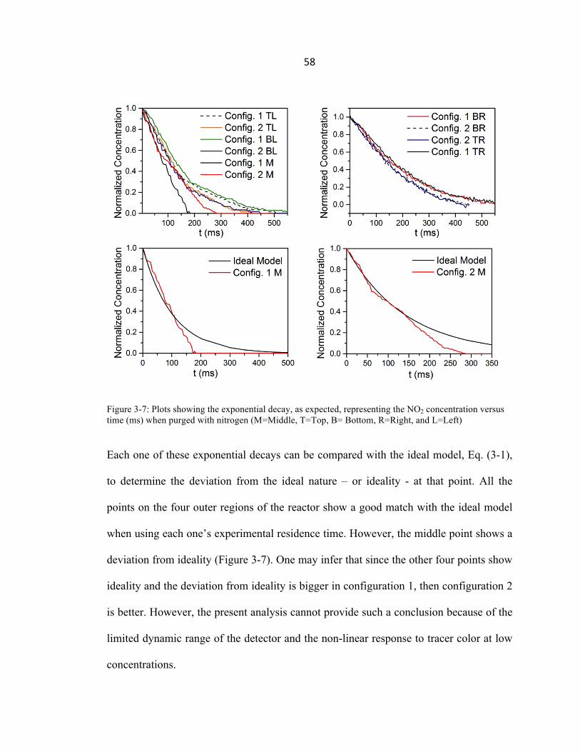
of color is observed through these points on Avizo®. Figure 3-6 show the change in

color intensity in both reactors versus the probeline length or number of frames.

57

Figure 3-5: Five points or small control volumes studied along with their residence time in ms

Figure 3-6: Plot of the change in color intensity in both reactors versus the number of frames

 

Then, the evolution of normalized intensity or concentration C can be plotted versus

time (Figure 3-7). The residence time at a certain point is the time where C equal to

0.3678. The residence times of the points taken are shown in Figure 3-5.

58

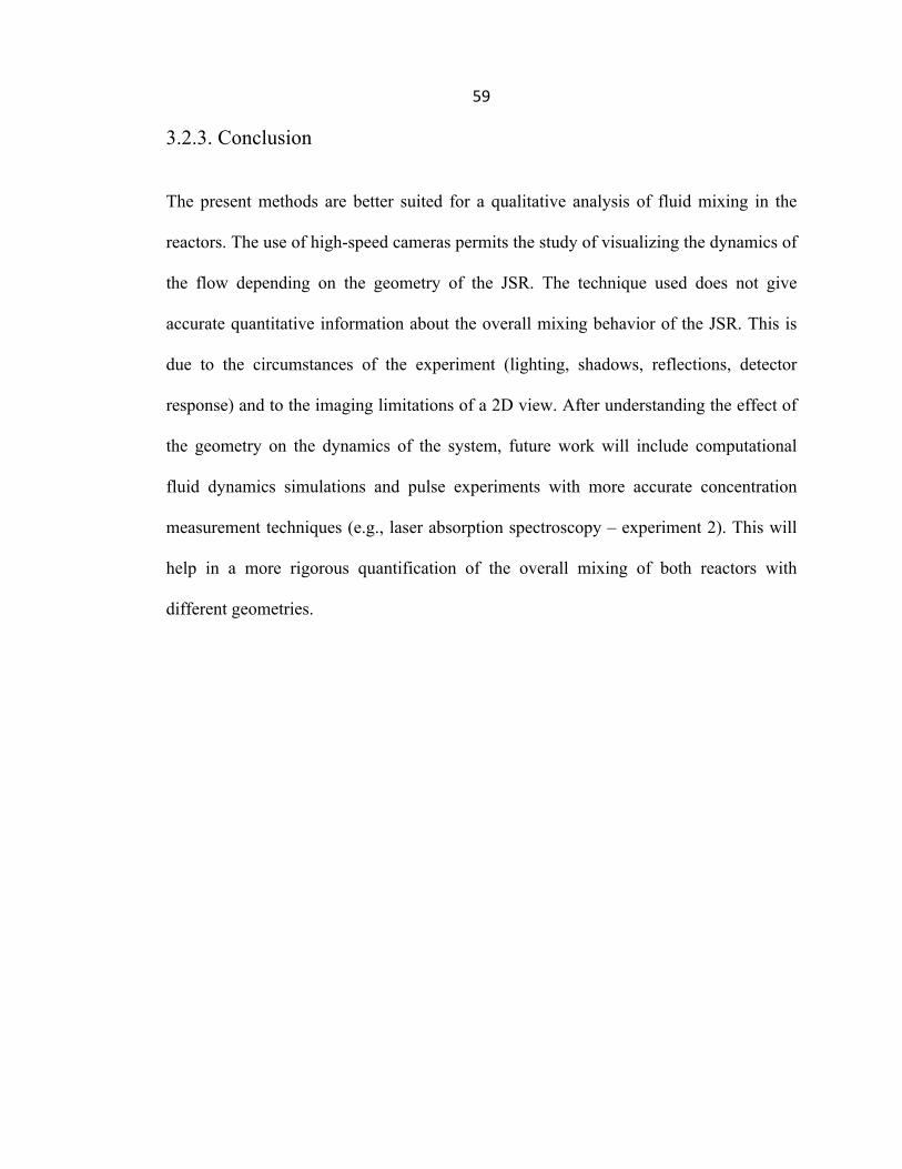
Figure 3-7: Plots showing the exponential decay, as expected, representing the NO2 concentration versus time (ms) when purged with nitrogen (M=Middle, T=Top, B= Bottom, R=Right, and L=Left)

Each one of these exponential decays can be compared with the ideal model, Eq. (3-1),

to determine the deviation from the ideal nature – or ideality - at that point. All the

points on the four outer regions of the reactor show a good match with the ideal model

when using each one’s experimental residence time. However, the middle point shows a

deviation from ideality (Figure 3-7). One may infer that since the other four points show

ideality and the deviation from ideality is bigger in configuration 1, then configuration 2

is better. However, the present analysis cannot provide such a conclusion because of the

limited dynamic range of the detector and the non-linear response to tracer color at low

concentrations.

59

3.2.3. Conclusion

The present methods are better suited for a qualitative analysis of fluid mixing in the

reactors. The use of high-speed cameras permits the study of visualizing the dynamics of

the flow depending on the geometry of the JSR. The technique used does not give

accurate quantitative information about the overall mixing behavior of the JSR. This is

due to the circumstances of the experiment (lighting, shadows, reflections, detector

response) and to the imaging limitations of a 2D view. After understanding the effect of

the geometry on the dynamics of the system, future work will include computational

fluid dynamics simulations and pulse experiments with more accurate concentration

measurement techniques (e.g., laser absorption spectroscopy – experiment 2). This will

help in a more rigorous quantification of the overall mixing of both reactors with

different geometries.

60

3.3. Experiment 2: tracer experiment using a laser absorption spectroscopy technique

Due to the lack of residence time distribution (RTD) data in JSR’s, it was recommended

to perform mixing studies and tracer experiments in these reactors to compare with the

stirred tank reactor data [1]. Table 2-2 shows the reactor tested in this experiment.

3.3.1. Experimental Procedure

The same concept of the tracer experiment is performed as described in experiment 1.

However, instead of NO2, the tracer gas used is CO2. The system is then allowed to reach

steady state. A solenoid valve cuts off the CO2 flow and enables a continuous flow of

nitrogen with different volumetric flow rates depending on the desired residence time.

CO2 concentration was monitored by laser absorption in the v1+v3 band of CO2 at 2.7

µm. The R26 transition at 3733.47 cm-1 is utilized for laser absorption as it is free from

interference due to H2O transitions as discussed in this reference [2]. The experiments

were performed at ambient air temperature and pressure (298 K, 1 atm).

HITRAN simulations were performed in order to obtain expected absorbance levels of

CO2 and interference from ambient air. Figure 3-8 shows the frequency range that can

be covered by the laser used. This range has lines from the v1+v3 band of CO2. The

R(26) line was used based on expected interference predicted by the HITRAN

simulation. Lines adjacent to R(26) showed some interference from ambient water vapor

which would become significant as the CO2 in the JSR is purged. The path length (L) of

absorbing species is taken to be as the JSR outlet (~1 cm) and a path length of 7 cm

represents the distance where the laser is present in ambient air.

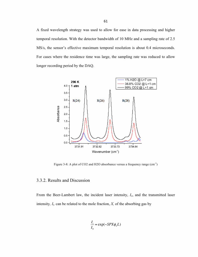
61

A fixed wavelength strategy was used to allow for ease in data processing and higher

temporal resolution. With the detector bandwidth of 10 MHz and a sampling rate of 2.5

MS/s, the sensor’s effective maximum temporal resolution is about 0.4 microseconds.

For cases where the residence time was large, the sampling rate was reduced to allow

longer recording period by the DAQ.

 

Figure 3-8: A plot of CO2 and H2O absorbance versus a frequency range (cm-1)

 

3.3.2. Results and Discussion

From the Beer-Lambert law, the incident laser intensity, Io, and the transmitted laser

intensity, It, can be related to the mole fraction, X, of the absorbing gas by

ItI0= exp(−SPXφnL)  

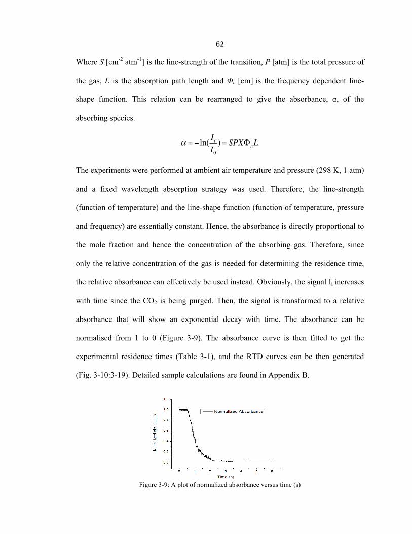
62

Where S [cm-2 atm-1] is the line-strength of the transition, P [atm] is the total pressure of

the gas, L is the absorption path length and Φυ [cm] is the frequency dependent line-

shape function. This relation can be rearranged to give the absorbance, α, of the

absorbing species.

α = − ln( ItI0) = SPXΦnL

The experiments were performed at ambient air temperature and pressure (298 K, 1 atm)

and a fixed wavelength absorption strategy was used. Therefore, the line-strength

(function of temperature) and the line-shape function (function of temperature, pressure

and frequency) are essentially constant. Hence, the absorbance is directly proportional to

the mole fraction and hence the concentration of the absorbing gas. Therefore, since

only the relative concentration of the gas is needed for determining the residence time,

the relative absorbance can effectively be used instead. Obviously, the signal It increases

with time since the CO2 is being purged. Then, the signal is transformed to a relative

absorbance that will show an exponential decay with time. The absorbance can be

normalised from 1 to 0 (Figure 3-9). The absorbance curve is then fitted to get the

experimental residence times (Table 3-1), and the RTD curves can be then generated

(Fig. 3-10:3-19). Detailed sample calculations are found in Appendix B.

 Figure 3-9: A plot of normalized absorbance versus time (s)

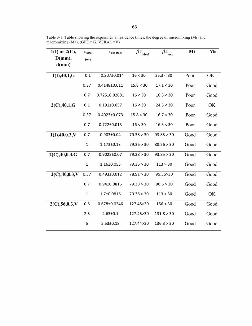
63

Table 3-1: Table showing the experimental residence times, the degree of micromixing (Mi) and macromixing (Ma), (GPE = G, VERAL =V)

1(I) or 2(C), D(mm), d(mm)  

τ Ideal  

(sec)  τexp  (sec)   βτ

ideal βτ

exp   Mi Ma

1(I),40,1,G 0.1   0.207±0.014    16  <  30   25.3  <  30   Poor OK

  0.37   0.4148±0.011   15.8  <  30   17.1  <  30   Poor Good

  0.7   0.725±0.02681   16  <  30   16.3  <  30   Poor Good

2(C),40,1,G 0.1   0.191±0.057   16  <  30   24.5  <  30   Poor OK

  0.37   0.4023±0.073   15.8  <  30   16.7  <  30   Poor Good

  0.7   0.722±0.013   16  <  30   16.3  <  30   Poor Good

1(I),40,0.3,V 0.7   0.903±0.04   79.38  >  30   93.85  >  30   Good Good

  1   1.173±0.13   79.36  >  30   88.26  >  30   Good Good

2(C),40,0.3,G 0.7   0.9023±0.07   79.38  >  30   93.85  >  30   Good Good

  1   1.16±0.053   79.36  >  30   113  >  30   Good Good

2(C),40,0.3,V 0.37   0.493±0.012   78.91  >  30   95.56>30   Good Good

0.7   0.94±0.0816   79.38  >  30   96.6  >  30   Good Good

1   1.7±0.0816   79.36  >  30   113  >  30   Good OK

2(C),56,0.3,V 0.5   0.678±0.0246   127.45>30   156  >  30   Good Good

2.5   2.63±0.1   127.45>30   131.8  >  30   Good Good

5   5.53±0.18   127.44>30   136.3  >  30   Good Good

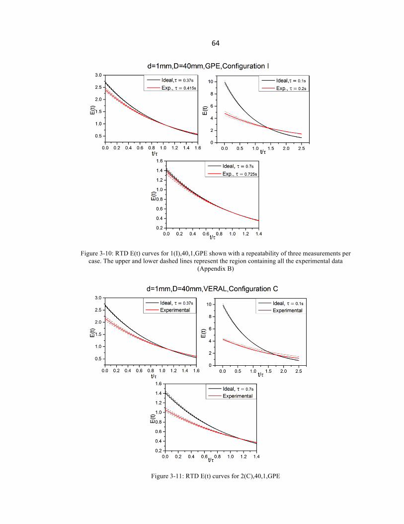
64

Figure 3-10: RTD E(t) curves for 1(I),40,1,GPE shown with a repeatability of three measurements per

case. The upper and lower dashed lines represent the region containing all the experimental data (Appendix B)

Figure 3-11: RTD E(t) curves for 2(C),40,1,GPE

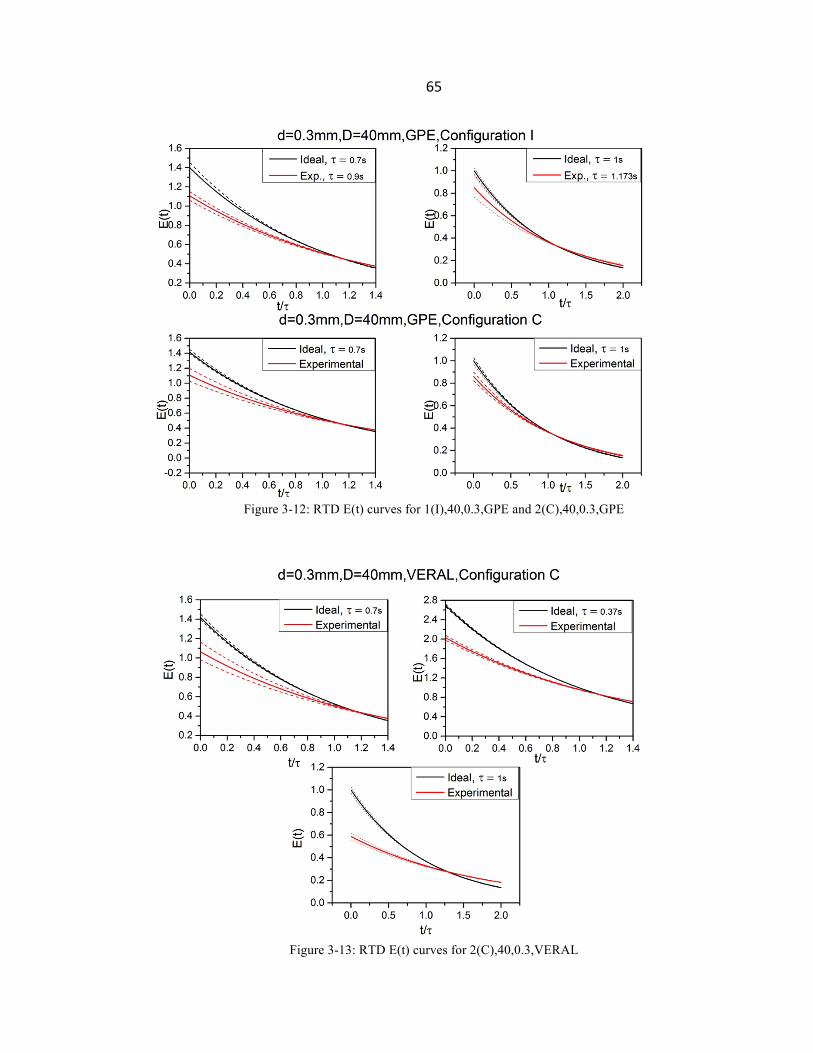
65

Figure 3-12: RTD E(t) curves for 1(I),40,0.3,GPE and 2(C),40,0.3,GPE

Figure 3-13: RTD E(t) curves for 2(C),40,0.3,VERAL

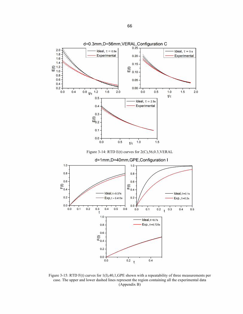
66

Figure 3-14: RTD E(t) curves for 2(C),56,0.3,VERAL

Figure 3-15: RTD F(t) curves for 1(I),40,1,GPE shown with a repeatability of three measurements per case. The upper and lower dashed lines represent the region containing all the experimental data

(Appendix B)

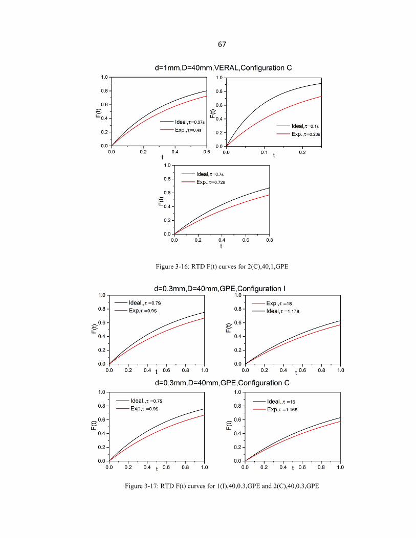
67

Figure 3-16: RTD F(t) curves for 2(C),40,1,GPE

Figure 3-17: RTD F(t) curves for 1(I),40,0.3,GPE and 2(C),40,0.3,GPE

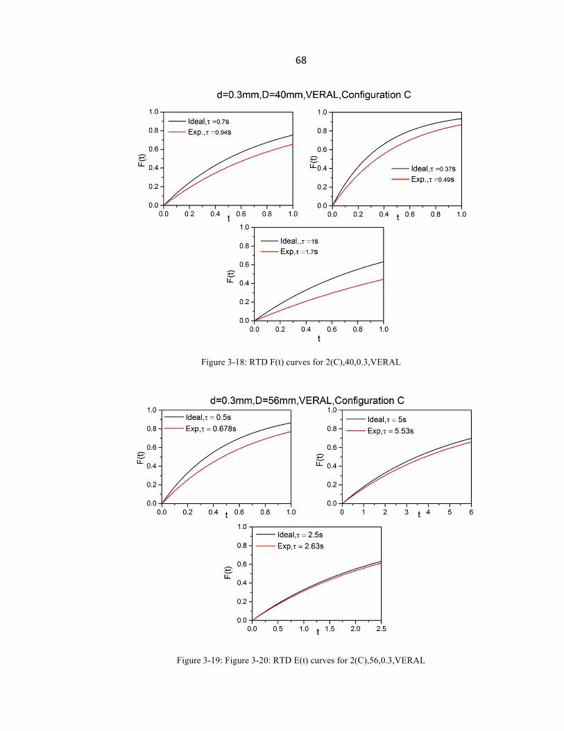
68

Figure 3-18: RTD F(t) curves for 2(C),40,0.3,VERAL

Figure 3-19: Figure 3-20: RTD E(t) curves for 2(C),56,0.3,VERAL

69

Most of the fitted experimental RTD curves followed the same trend as the ideal curves.

The criterion of a good macromixing is defined when the ideal and the experimental

RTD curve are equal at a time equal to the residence time. This criterion is present in

most of the cases even though in some cases bigger deviations are seen overall.

Mixing was not expected to be of high quality in the following particular geometry -

D=40mm and d=1mm - since the optimal recirculation criterion is not satisfied.

However, with the nozzle configuration 1 or the inclined nozzles, a better macromixing

is observed than the reactor with crossed nozzles, when operating at 0.37s and 0.7s,

since the experimental RTD is closer to the ideal RTD. Therefore, the reactor pertaining

to these dimensions with a crossed nozzle configurations can be eliminated from this

analysis, but will still be simulated using CFD (chapter 4). Both configurations show

poor macromixing at low residence times (0.1s), and this might be due to experimental

errors or certain leakages in the system that can take place only at high flow rates,

possibly caused by the stopper. However, finding a better way to seal the reactor

properly can reduce this error.

When keeping the volume constant and decreasing the nozzle diameter d to 0.3 mm,

both nozzle configurations seem to agree with the ideal curves. However, the crossed

reactors manufactured by GPE seem to give better results for middle and high residence

times than the ones made by VERAL – only for this specific reactor volume (D=40mm).

Even though, when using a bigger volume (D=56mm, d=0.3mm) – manufactured by

VERAL –the RTD shows excellent agreement with the ideal curves at high residence

times. It is not odd that the mixing of the latter reactor deviates from ideality at 0.5 sec,

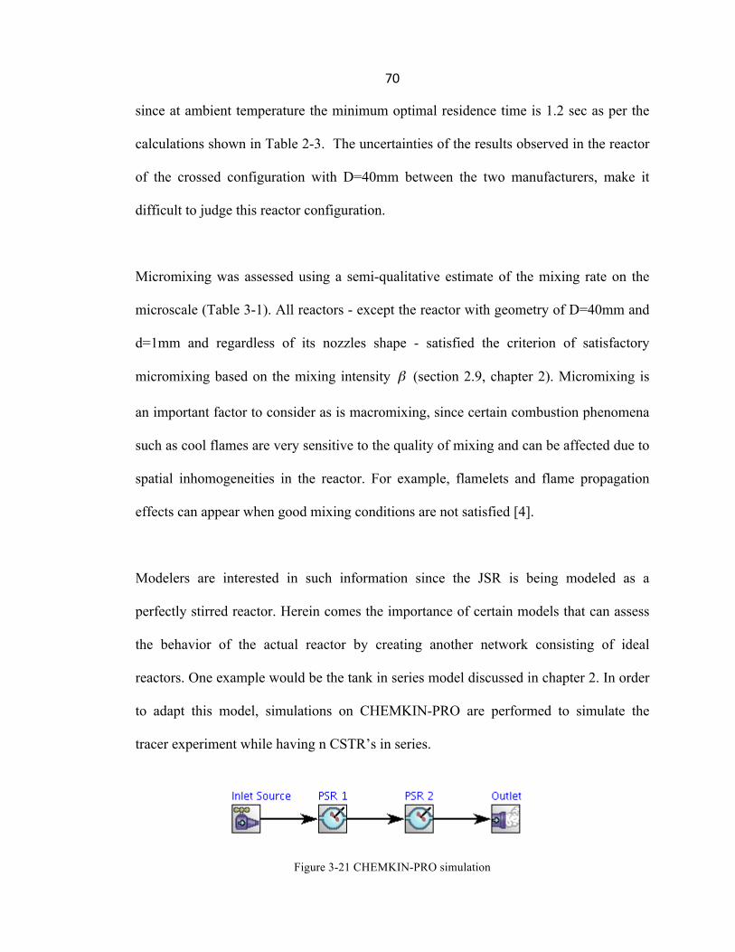
70

since at ambient temperature the minimum optimal residence time is 1.2 sec as per the

calculations shown in Table 2-3. The uncertainties of the results observed in the reactor

of the crossed configuration with D=40mm between the two manufacturers, make it

difficult to judge this reactor configuration.

Micromixing was assessed using a semi-qualitative estimate of the mixing rate on the

microscale (Table 3-1). All reactors - except the reactor with geometry of D=40mm and

d=1mm and regardless of its nozzles shape - satisfied the criterion of satisfactory

micromixing based on the mixing intensity (section 2.9, chapter 2). Micromixing is

an important factor to consider as is macromixing, since certain combustion phenomena

such as cool flames are very sensitive to the quality of mixing and can be affected due to

spatial inhomogeneities in the reactor. For example, flamelets and flame propagation

effects can appear when good mixing conditions are not satisfied [4].

Modelers are interested in such information since the JSR is being modeled as a

perfectly stirred reactor. Herein comes the importance of certain models that can assess

the behavior of the actual reactor by creating another network consisting of ideal

reactors. One example would be the tank in series model discussed in chapter 2. In order

to adapt this model, simulations on CHEMKIN-PRO are performed to simulate the

tracer experiment while having n CSTR’s in series.

 Figure 3-21 CHEMKIN-PRO simulation

β

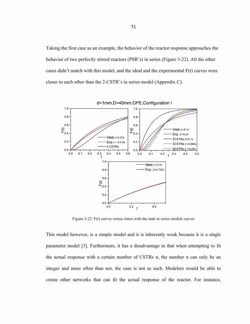
71

 

Taking the first case as an example, the behavior of the reactor response approaches the

behavior of two perfectly stirred reactors (PSR’s) in series (Figure 3-22). All the other

cases didn’t match with this model, and the ideal and the experimental F(t) curves were

closer to each other than the 2-CSTR’s in series model (Appendix C).

Figure 3-22: F(t) curves versus times with the tank in series models curves

This model however, is a simple model and it is inherently weak because it is a single

parameter model [3]. Furthermore, it has a disadvantage in that when attempting to fit

the actual response with a certain number of CSTRs n, the number n can only be an

integer and more often than not, the case is not as such. Modelers would be able to

create other networks that can fit the actual response of the reactor. For instance,

72

modeling the same case (τ=0.1s) with two PSR’s in parallel with a residence time of 0.4

sec each would give the same fitted experimental response.

3.3.3. Conclusion The laser absorption spectroscopy experiment gives a better understanding of the

micromixing and macromixing through the computed mixing intensity, , and the RTD

curves respectively. Through the different RTD’s, different reactors’ geometry exhibit

different behavior. For the smaller reactor with nozzle diameter 1 mm it is shown that

the inclined configuration performs better at moderate-high residence times. For the

bigger volume reactor, the response curves match with the ideal curves at moderate-high

residence times. However, this technique does not have the ability to determine the

mixing level ML of the reactor that can confirm the reactor choice made based on the

RTD curves analysis. This parameter can be computed by CFD simulations (Chapter 4).

β

73

REFERENCES  

[1] J. J. Evangelista, R. Shinnar, S. Katz, Symp. Comb. Inst. (1969), 901-912

[2] L. Joly, B. Parvitte, V. Zeninari, G. Durry, Appl. Phys. B (2007), 743–748

[3] C.G. Hill, An Introduction to Chemical Engineering Kinetics & Reactor Design, John Wiley & Sons, 1977.

[4] P. G. Lignola, E. Reverchon, Combust. Sci. Technol. 60 (1988), 319-333.

74

Chapter 4 CFD Simulations Versus Experiments

4.1. Introduction

Computational Fluid Dynamics (CFD) is the science used to predict phenomena such as

fluid flow field, heat and mass transfer, as well as chemical reactions and combustions in

engines. Used for a multitude of uses, this tool has offered a great advantage to the

scientific community. CFD can be used for the studying of new conceptual designs with

an optimized and detailed product development, and more importantly, allows the

reduction of total costs and efforts required for experimentation and data acquisition.

ANSYS CFD solvers are based on the finite control volume method; therefore the

studied geometry is first meshed. The domain is then discretized into a finite set of

control volumes, after which based on them, the general transport conservation

equations for mass, momentum, energy and species are solved. The general equation

includes an unsteady term, a convection term, a diffusion term and a generation term.

The conservation equations for each quantity are developed in the mathematical

modeling section. The partial differential equations are then discretized into a system of

algebraic equations, which are then solved numerically.

4.2. Mathematical Modeling The residence time and the RTD can be predicted using computational fluid dynamics

(CFD). The Mathematical modeling of the problem is normally shaped and conditioned

by the total mass balance, the momentum balance (Navier-Stokes N-S equations) and

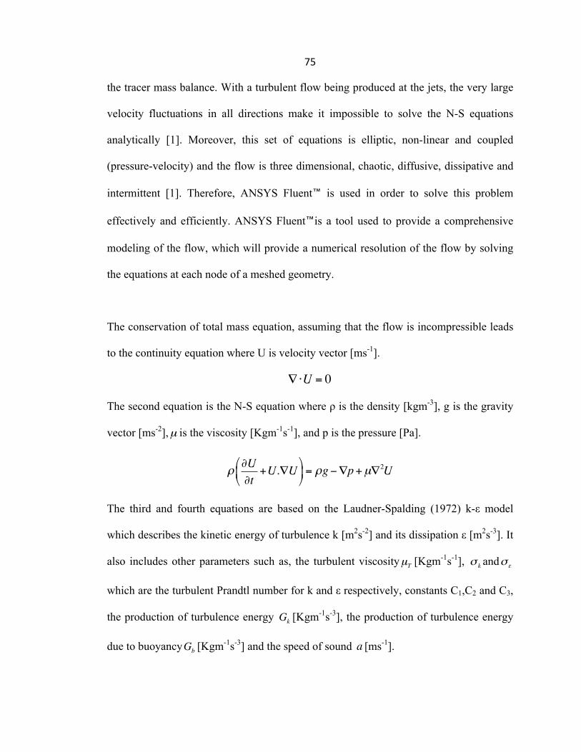
75

the tracer mass balance. With a turbulent flow being produced at the jets, the very large

velocity fluctuations in all directions make it impossible to solve the N-S equations

analytically [1]. Moreover, this set of equations is elliptic, non-linear and coupled

(pressure-velocity) and the flow is three dimensional, chaotic, diffusive, dissipative and

intermittent [1]. Therefore, ANSYS Fluent™ is used in order to solve this problem

effectively and efficiently. ANSYS Fluent™is a tool used to provide a comprehensive

modeling of the flow, which will provide a numerical resolution of the flow by solving

the equations at each node of a meshed geometry.

The conservation of total mass equation, assuming that the flow is incompressible leads

to the continuity equation where U is velocity vector [ms-1].

∇⋅U = 0

The second equation is the N-S equation where ρ is the density [kgm-3], g is the gravity

vector [ms-2],µ is the viscosity [Kgm-1s-1], and p is the pressure [Pa].

ρ∂U∂t

+U.∇U#

$%

&

'(= ρg−∇p+µ∇2U

The third and fourth equations are based on the Laudner-Spalding (1972) k-ε model

which describes the kinetic energy of turbulence k [m2s-2] and its dissipation ε [m2s-3]. It

also includes other parameters such as, the turbulent viscosityµT [Kgm-1s-1], σ k andσε

which are the turbulent Prandtl number for k and ε respectively, constants C1,C2 and C3,

the production of turbulence energy Gk [Kgm-1s-3], the production of turbulence energy

due to buoyancyGb [Kgm-1s-3] and the speed of sound a [ms-1].

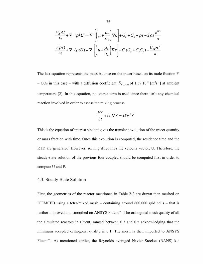
76

∂(ρk)∂t

+∇⋅ (ρkU) =∇⋅ µ +µTσ k

$

%&

'

()∇k

*

+,

-

./+Gk +Gb + ρε − 2ρε

k0.5

a

∂(ρε)∂t

+∇⋅ (ρεU) =∇⋅ µ +µTσε

$

%&

'

()∇ε

*

+,

-

./+C1(Gk +C3Gb )−

C2ρε2

k

The last equation represents the mass balance on the tracer based on its mole fraction Y

– CO2 in this case – with a diffusion coefficient DCO2−air of 1.39.10-5 [m2s-1] at ambient

temperature [2]. In this equation, no source term is used since there isn’t any chemical

reaction involved in order to assess the mixing process.

∂Y∂t

+U.∇Y = D∇2Y  

 This is the equation of interest since it gives the transient evolution of the tracer quantity

or mass fraction with time. Once this evolution is computed, the residence time and the

RTD are generated. However, solving it requires the velocity vector, U. Therefore, the

steady-state solution of the previous four coupled should be computed first in order to

compute U and P.

4.3. Steady-State Solution  

First, the geometries of the reactor mentioned in Table 2-2 are drawn then meshed on

ICEMCFD using a tetra/mixed mesh – containing around 600,000 grid cells – that is

further improved and smoothed on ANSYS Fluent™. The orthogonal mesh quality of all

the simulated reactors in Fluent, ranged between 0.3 and 0.5 acknowledging that the

minimum accepted orthogonal quality is 0.1. The mesh is then imported to ANSYS

Fluent™. As mentioned earlier, the Reynolds averaged Navier Stockes (RANS) k-ε

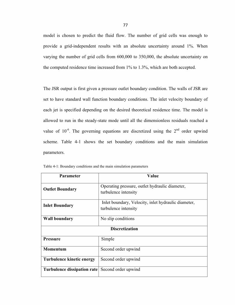
77

model is chosen to predict the fluid flow. The number of grid cells was enough to

provide a grid-independent results with an absolute uncertainty around 1%. When

varying the number of grid cells from 600,000 to 350,000, the absolute uncertainty on

the computed residence time increased from 1% to 1.3%, which are both accepted.

The JSR output is first given a pressure outlet boundary condition. The walls of JSR are

set to have standard wall function boundary conditions. The inlet velocity boundary of

each jet is specified depending on the desired theoretical residence time. The model is

allowed to run in the steady-state mode until all the dimensionless residuals reached a

value of 10-6. The governing equations are discretized using the 2nd order upwind

scheme. Table 4-1 shows the set boundary conditions and the main simulation

parameters.

Table 4-1: Boundary conditions and the main simulation parameters

Parameter Value

Outlet Boundary Operating pressure, outlet hydraulic diameter, turbulence intensity

Inlet Boundary Inlet boundary, Velocity, inlet hydraulic diameter, turbulence intensity

Wall boundary No slip conditions

Discretization

Pressure Simple

Momentum Second order upwind

Turbulence kinetic energy Second order upwind

Turbulence dissipation rate Second order upwind

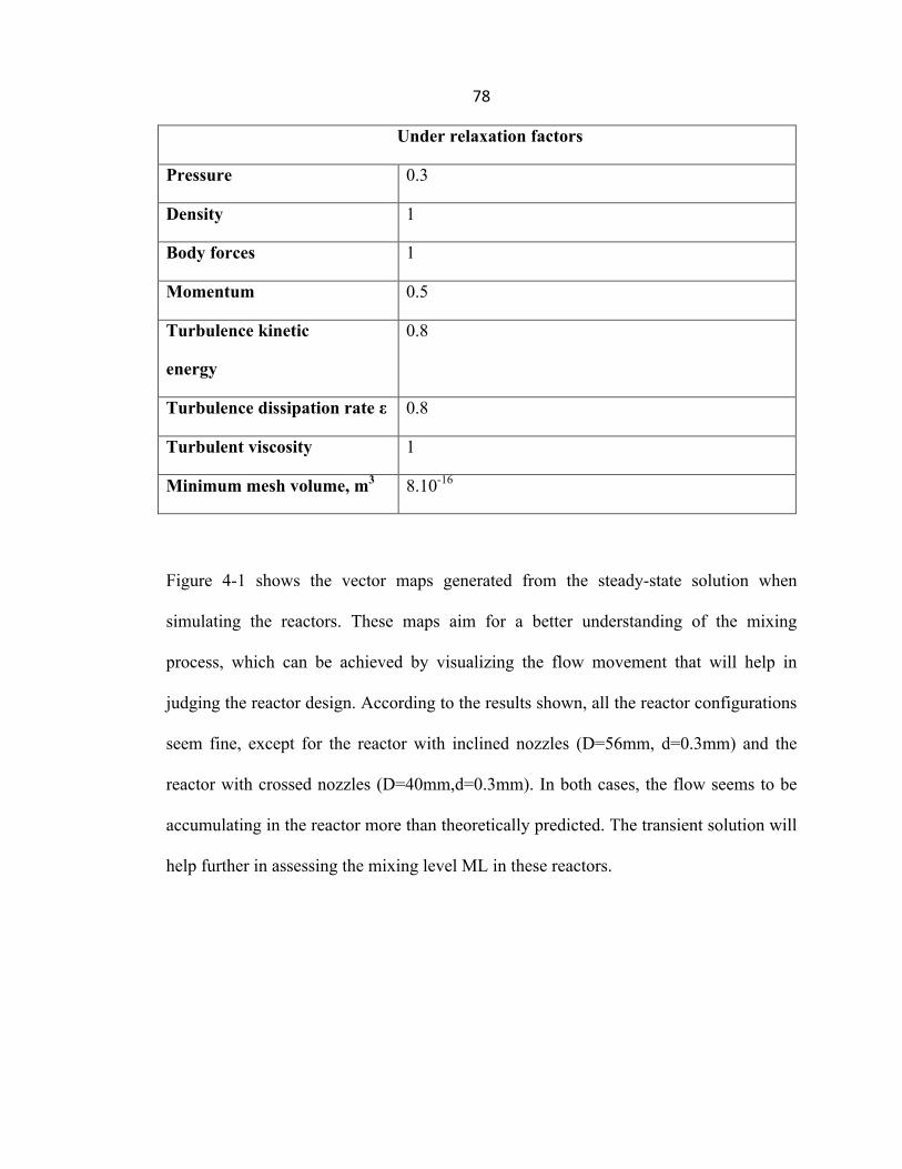
78

Under relaxation factors

Pressure 0.3

Density 1

Body forces 1

Momentum 0.5

Turbulence kinetic

energy

0.8

Turbulence dissipation rate ε 0.8

Turbulent viscosity 1

Minimum mesh volume, m3 8.10-16

Figure 4-1 shows the vector maps generated from the steady-state solution when

simulating the reactors. These maps aim for a better understanding of the mixing

process, which can be achieved by visualizing the flow movement that will help in

judging the reactor design. According to the results shown, all the reactor configurations

seem fine, except for the reactor with inclined nozzles (D=56mm, d=0.3mm) and the

reactor with crossed nozzles (D=40mm,d=0.3mm). In both cases, the flow seems to be

accumulating in the reactor more than theoretically predicted. The transient solution will

help further in assessing the mixing level ML in these reactors.

79

 

Figure 4-1: Vector maps, generated from the steady state solution, of the reactor’s cross-section (0,1,0) showing the circular movement of the flow and its direction.

 

4.4. Transient Solution

The tracer decay is modeled by using the flow field U computed from the fluid flow

field A user-defined scalar (UDS) is created to model the concentration of CO2. In order

to simulate the negative step input of CO2 done experimentally, the initial concentration

inside the reactor is initialized to be equal to 1 with a specified value of zero at the four

injection nozzle inlets. The boundary condition at the surface outlet is set to be 0 since it

is assumed that CO2 will be diluted with air by then. The simulation was allowed to run

20 iterations for each time step set. While iterating the solution, the averaged

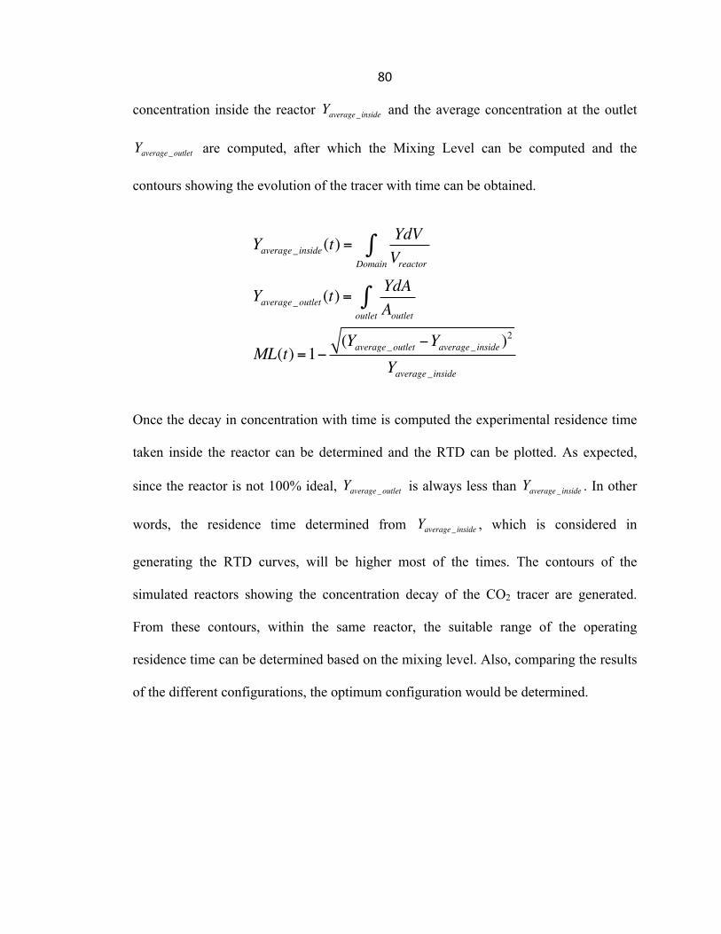
80

concentration inside the reactor Yaverage_ inside and the average concentration at the outlet

Yaverage_outlet are computed, after which the Mixing Level can be computed and the

contours showing the evolution of the tracer with time can be obtained.

Yaverage_ inside(t) =YdVVreactorDomain

∫

Yaverage_outlet (t) =YdAAoutletoutlet

∫

ML(t) =1−(Yaverage_outlet −Yaverage_ inside )

2

Yaverage_ inside

Once the decay in concentration with time is computed the experimental residence time

taken inside the reactor can be determined and the RTD can be plotted. As expected,

since the reactor is not 100% ideal, Yaverage_outlet is always less than Yaverage_ inside . In other

words, the residence time determined from Yaverage_ inside , which is considered in

generating the RTD curves, will be higher most of the times. The contours of the

simulated reactors showing the concentration decay of the CO2 tracer are generated.

From these contours, within the same reactor, the suitable range of the operating

residence time can be determined based on the mixing level. Also, comparing the results

of the different configurations, the optimum configuration would be determined.

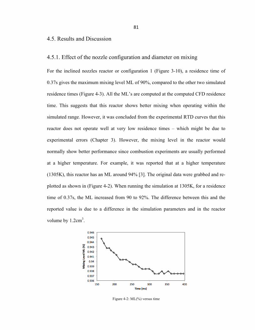
81

4.5. Results and Discussion  

4.5.1. Effect of the nozzle configuration and diameter on mixing

For the inclined nozzles reactor or configuration 1 (Figure 3-10), a residence time of

0.37s gives the maximum mixing level ML of 90%, compared to the other two simulated

residence times (Figure 4-3). All the ML’s are computed at the computed CFD residence

time. This suggests that this reactor shows better mixing when operating within the

simulated range. However, it was concluded from the experimental RTD curves that this

reactor does not operate well at very low residence times – which might be due to

experimental errors (Chapter 3). However, the mixing level in the reactor would

normally show better performance since combustion experiments are usually performed

at a higher temperature. For example, it was reported that at a higher temperature

(1305K), this reactor has an ML around 94% [3]. The original data were grabbed and re-

plotted as shown in (Figure 4-2). When running the simulation at 1305K, for a residence

time of 0.37s, the ML increased from 90 to 92%. The difference between this and the

reported value is due to a difference in the simulation parameters and in the reactor

volume by 1.2cm3.

 

Figure 4-2: ML(%) versus time

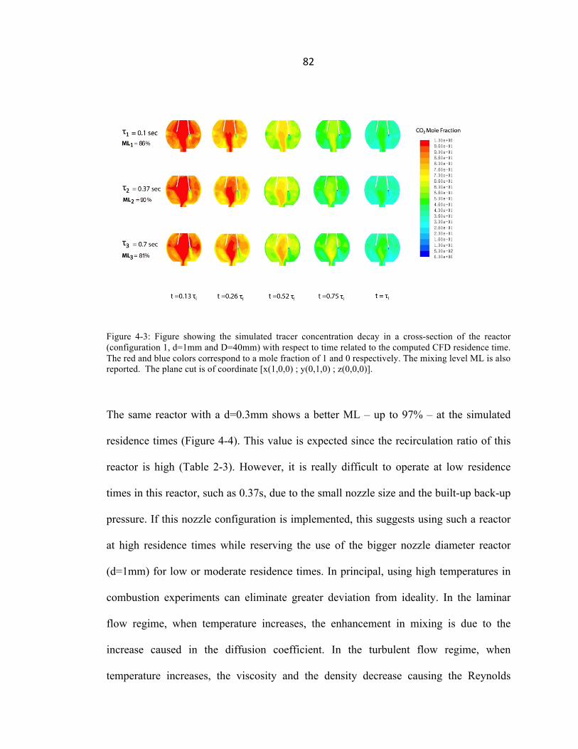
82

 Figure 4-3: Figure showing the simulated tracer concentration decay in a cross-section of the reactor (configuration 1, d=1mm and D=40mm) with respect to time related to the computed CFD residence time. The red and blue colors correspond to a mole fraction of 1 and 0 respectively. The mixing level ML is also reported. The plane cut is of coordinate [x(1,0,0) ; y(0,1,0) ; z(0,0,0)].  

 

The same reactor with a d=0.3mm shows a better ML – up to 97% – at the simulated

residence times (Figure 4-4). This value is expected since the recirculation ratio of this

reactor is high (Table 2-3). However, it is really difficult to operate at low residence

times in this reactor, such as 0.37s, due to the small nozzle size and the built-up back-up

pressure. If this nozzle configuration is implemented, this suggests using such a reactor

at high residence times while reserving the use of the bigger nozzle diameter reactor

(d=1mm) for low or moderate residence times. In principal, using high temperatures in

combustion experiments can eliminate greater deviation from ideality. In the laminar

flow regime, when temperature increases, the enhancement in mixing is due to the

increase caused in the diffusion coefficient. In the turbulent flow regime, when

temperature increases, the viscosity and the density decrease causing the Reynolds

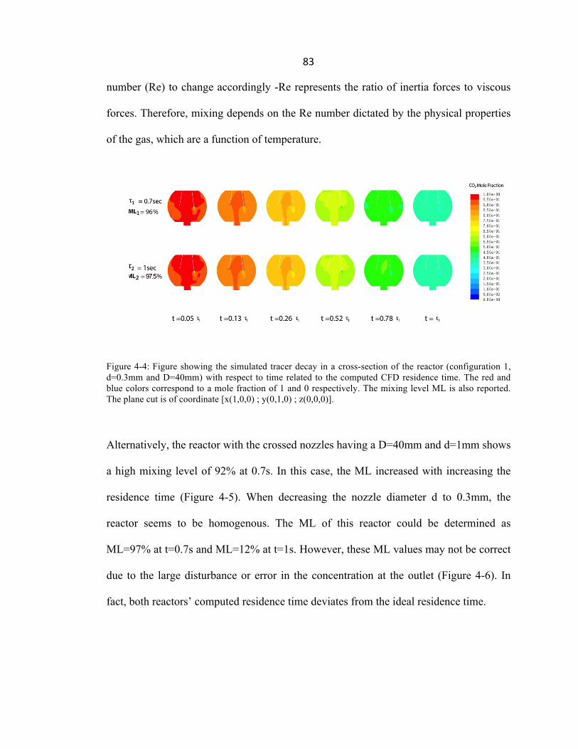
83

number (Re) to change accordingly -Re represents the ratio of inertia forces to viscous

forces. Therefore, mixing depends on the Re number dictated by the physical properties

of the gas, which are a function of temperature.

 Figure 4-4:  Figure showing the simulated tracer decay in a cross-section of the reactor (configuration 1, d=0.3mm and D=40mm) with respect to time related to the computed CFD residence time. The red and blue colors correspond to a mole fraction of 1 and 0 respectively. The mixing level ML is also reported. The plane cut is of coordinate [x(1,0,0) ; y(0,1,0) ; z(0,0,0)].

 

Alternatively, the reactor with the crossed nozzles having a D=40mm and d=1mm shows

a high mixing level of 92% at 0.7s. In this case, the ML increased with increasing the

residence time (Figure 4-5). When decreasing the nozzle diameter d to 0.3mm, the

reactor seems to be homogenous. The ML of this reactor could be determined as

ML=97% at t=0.7s and ML=12% at t=1s. However, these ML values may not be correct

due to the large disturbance or error in the concentration at the outlet (Figure 4-6). In

fact, both reactors’ computed residence time deviates from the ideal residence time.

 

 

 

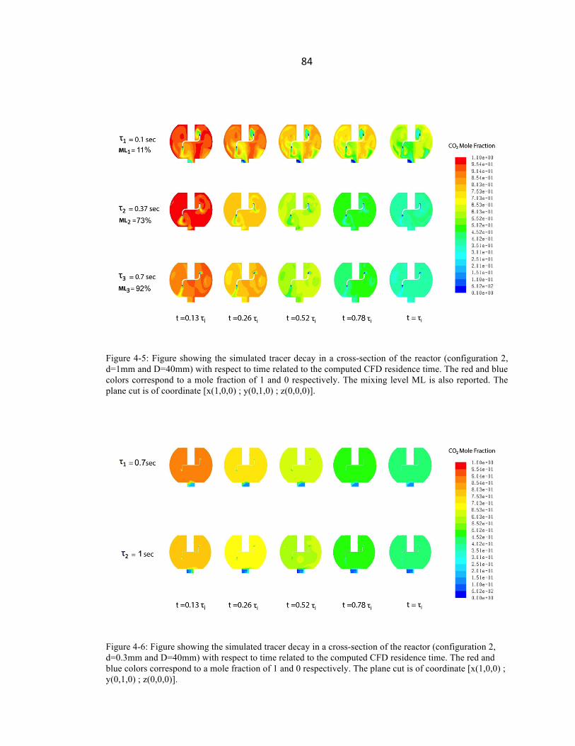
84

 

 

Figure 4-5: Figure showing the simulated tracer decay in a cross-section of the reactor (configuration 2, d=1mm and D=40mm) with respect to time related to the computed CFD residence time. The red and blue colors correspond to a mole fraction of 1 and 0 respectively. The mixing level ML is also reported. The plane cut is of coordinate [x(1,0,0) ; y(0,1,0) ; z(0,0,0)].

 

 

Figure 4-6: Figure showing the simulated tracer decay in a cross-section of the reactor (configuration 2, d=0.3mm and D=40mm) with respect to time related to the computed CFD residence time. The red and blue colors correspond to a mole fraction of 1 and 0 respectively. The plane cut is of coordinate [x(1,0,0) ; y(0,1,0) ; z(0,0,0)].

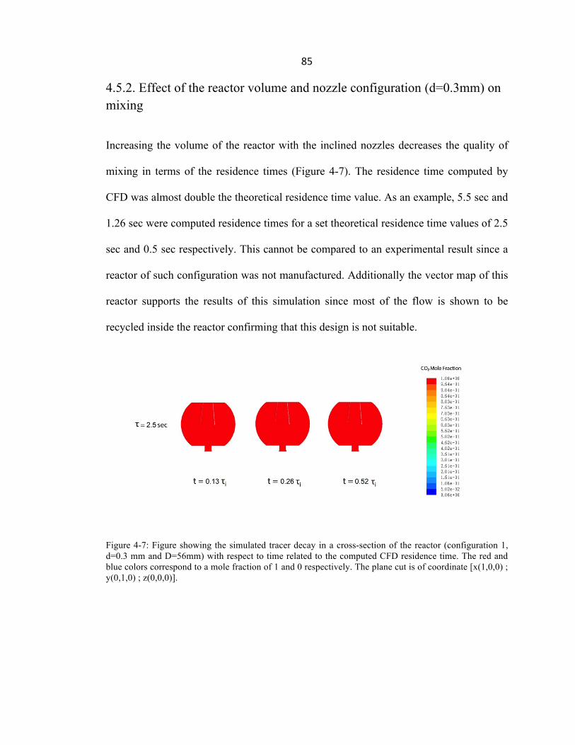
85

4.5.2. Effect of the reactor volume and nozzle configuration (d=0.3mm) on mixing  

Increasing the volume of the reactor with the inclined nozzles decreases the quality of

mixing in terms of the residence times (Figure 4-7). The residence time computed by

CFD was almost double the theoretical residence time value. As an example, 5.5 sec and

1.26 sec were computed residence times for a set theoretical residence time values of 2.5

sec and 0.5 sec respectively. This cannot be compared to an experimental result since a

reactor of such configuration was not manufactured. Additionally the vector map of this

reactor supports the results of this simulation since most of the flow is shown to be

recycled inside the reactor confirming that this design is not suitable.

 

Figure 4-7: Figure showing the simulated tracer decay in a cross-section of the reactor (configuration 1, d=0.3 mm and D=56mm) with respect to time related to the computed CFD residence time. The red and blue colors correspond to a mole fraction of 1 and 0 respectively. The plane cut is of coordinate [x(1,0,0) ; y(0,1,0) ; z(0,0,0)].

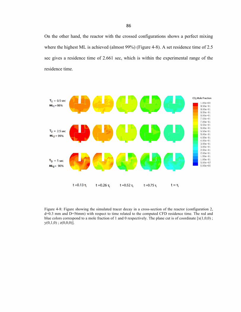
86

On the other hand, the reactor with the crossed configurations shows a perfect mixing

where the highest ML is achieved (almost 99%) (Figure 4-8). A set residence time of 2.5

sec gives a residence time of 2.661 sec, which is within the experimental range of the

residence time.

 

Figure 4-8: Figure showing the simulated tracer decay in a cross-section of the reactor (configuration 2, d=0.3 mm and D=56mm) with respect to time related to the computed CFD residence time. The red and blue colors correspond to a mole fraction of 1 and 0 respectively. The plane cut is of coordinate [x(1,0,0) ; y(0,1,0) ; z(0,0,0)].

 

 

 

 

 

87

REFERENCES [1] T. Saad, Turbulence Modeling Report

[2] M. K. Dubey, H. Ziock, G. Rueff, S. Elliott,W. S. Smith . Prepr. Pap. - Div. Fuel

Chem. 47(2002), 81-84

[3] I. Gil, P. Mocek, Chem. Process Eng. 33 (2012), 397-410

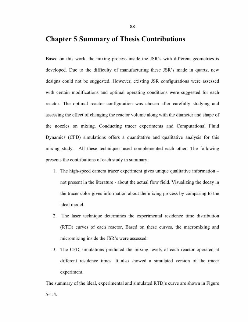
88

Chapter 5 Summary of Thesis Contributions Based on this work, the mixing process inside the JSR’s with different geometries is

developed. Due to the difficulty of manufacturing these JSR’s made in quartz, new

designs could not be suggested. However, existing JSR configurations were assessed

with certain modifications and optimal operating conditions were suggested for each

reactor. The optimal reactor configuration was chosen after carefully studying and

assessing the effect of changing the reactor volume along with the diameter and shape of

the nozzles on mixing. Conducting tracer experiments and Computational Fluid

Dynamics (CFD) simulations offers a quantitative and qualitative analysis for this

mixing study. All these techniques used complemented each other. The following

presents the contributions of each study in summary,

1. The high-speed camera tracer experiment gives unique qualitative information –

not present in the literature - about the actual flow field. Visualizing the decay in

the tracer color gives information about the mixing process by comparing to the

ideal model.

2. The laser technique determines the experimental residence time distribution

(RTD) curves of each reactor. Based on these curves, the macromixing and

micromixing inside the JSR’s were assessed.

3. The CFD simulations predicted the mixing levels of each reactor operated at

different residence times. It also showed a simulated version of the tracer

experiment.

The summary of the ideal, experimental and simulated RTD’s curve are shown in Figure

5-1:4.

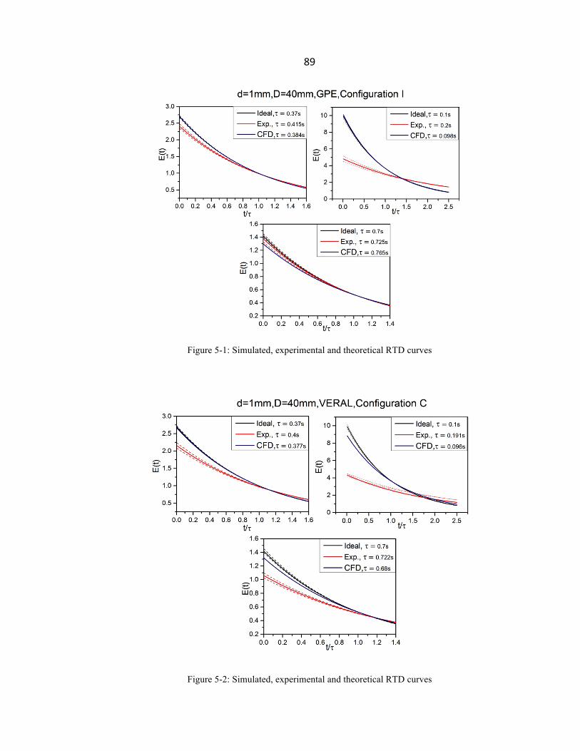
89

 Figure 5-1: Simulated, experimental and theoretical RTD curves

 

 

Figure 5-2: Simulated, experimental and theoretical RTD curves

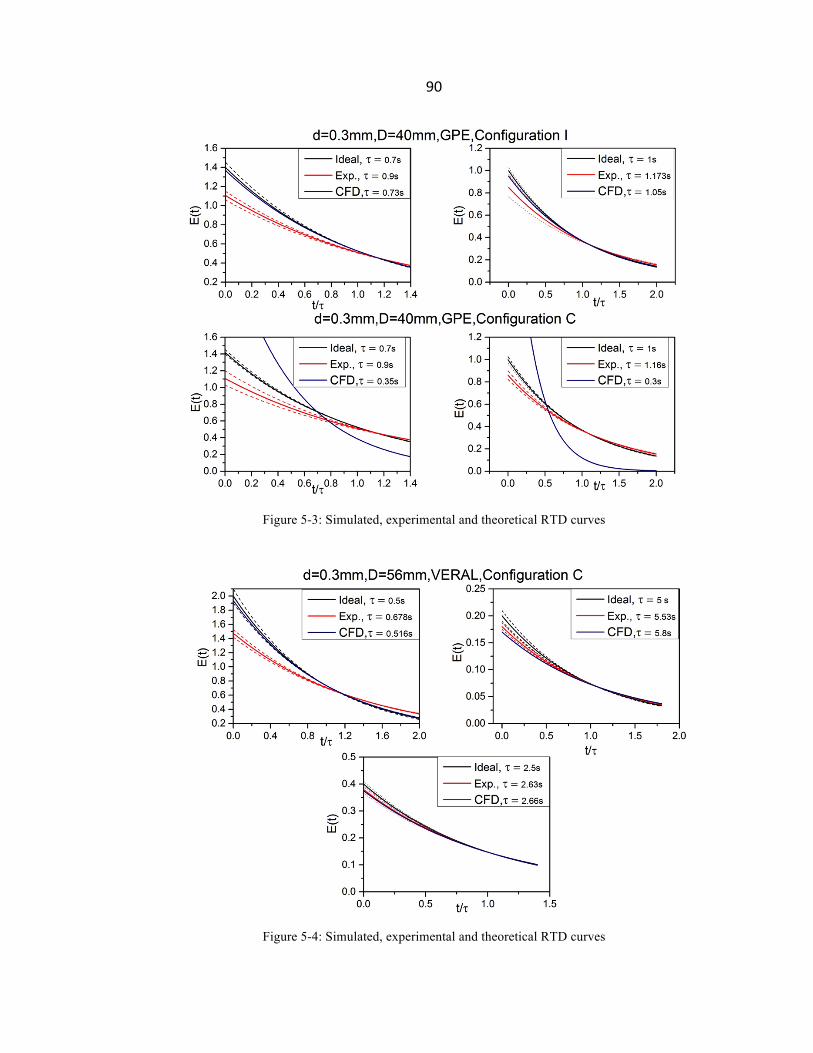
90

 

Figure 5-3: Simulated, experimental and theoretical RTD curves

 Figure 5-4: Simulated, experimental and theoretical RTD curves

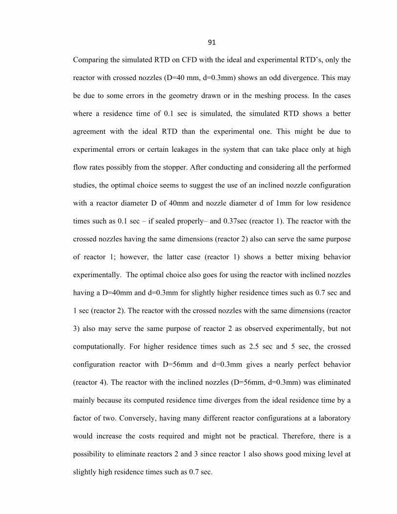
91

Comparing the simulated RTD on CFD with the ideal and experimental RTD’s, only the

reactor with crossed nozzles (D=40 mm, d=0.3mm) shows an odd divergence. This may

be due to some errors in the geometry drawn or in the meshing process. In the cases

where a residence time of 0.1 sec is simulated, the simulated RTD shows a better

agreement with the ideal RTD than the experimental one. This might be due to

experimental errors or certain leakages in the system that can take place only at high

flow rates possibly from the stopper. After conducting and considering all the performed

studies, the optimal choice seems to suggest the use of an inclined nozzle configuration

with a reactor diameter D of 40mm and nozzle diameter d of 1mm for low residence

times such as 0.1 sec – if sealed properly– and 0.37sec (reactor 1). The reactor with the

crossed nozzles having the same dimensions (reactor 2) also can serve the same purpose

of reactor 1; however, the latter case (reactor 1) shows a better mixing behavior

experimentally. The optimal choice also goes for using the reactor with inclined nozzles

having a D=40mm and d=0.3mm for slightly higher residence times such as 0.7 sec and

1 sec (reactor 2). The reactor with the crossed nozzles with the same dimensions (reactor

3) also may serve the same purpose of reactor 2 as observed experimentally, but not

computationally. For higher residence times such as 2.5 sec and 5 sec, the crossed

configuration reactor with D=56mm and d=0.3mm gives a nearly perfect behavior

(reactor 4). The reactor with the inclined nozzles (D=56mm, d=0.3mm) was eliminated

mainly because its computed residence time diverges from the ideal residence time by a

factor of two. Conversely, having many different reactor configurations at a laboratory

would increase the costs required and might not be practical. Therefore, there is a

possibility to eliminate reactors 2 and 3 since reactor 1 also shows good mixing level at

slightly high residence times such as 0.7 sec.

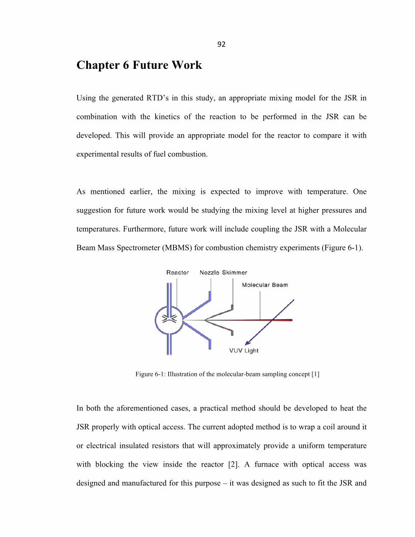
92

Chapter 6 Future Work Using the generated RTD’s in this study, an appropriate mixing model for the JSR in

combination with the kinetics of the reaction to be performed in the JSR can be

developed. This will provide an appropriate model for the reactor to compare it with

experimental results of fuel combustion.

As mentioned earlier, the mixing is expected to improve with temperature. One

suggestion for future work would be studying the mixing level at higher pressures and

temperatures. Furthermore, future work will include coupling the JSR with a Molecular

Beam Mass Spectrometer (MBMS) for combustion chemistry experiments (Figure 6-1).

 

Figure 6-1: Illustration of the molecular-beam sampling concept [1]

In both the aforementioned cases, a practical method should be developed to heat the

JSR properly with optical access. The current adopted method is to wrap a coil around it

or electrical insulated resistors that will approximately provide a uniform temperature

with blocking the view inside the reactor [2]. A furnace with optical access was

designed and manufactured for this purpose – it was designed as such to fit the JSR and

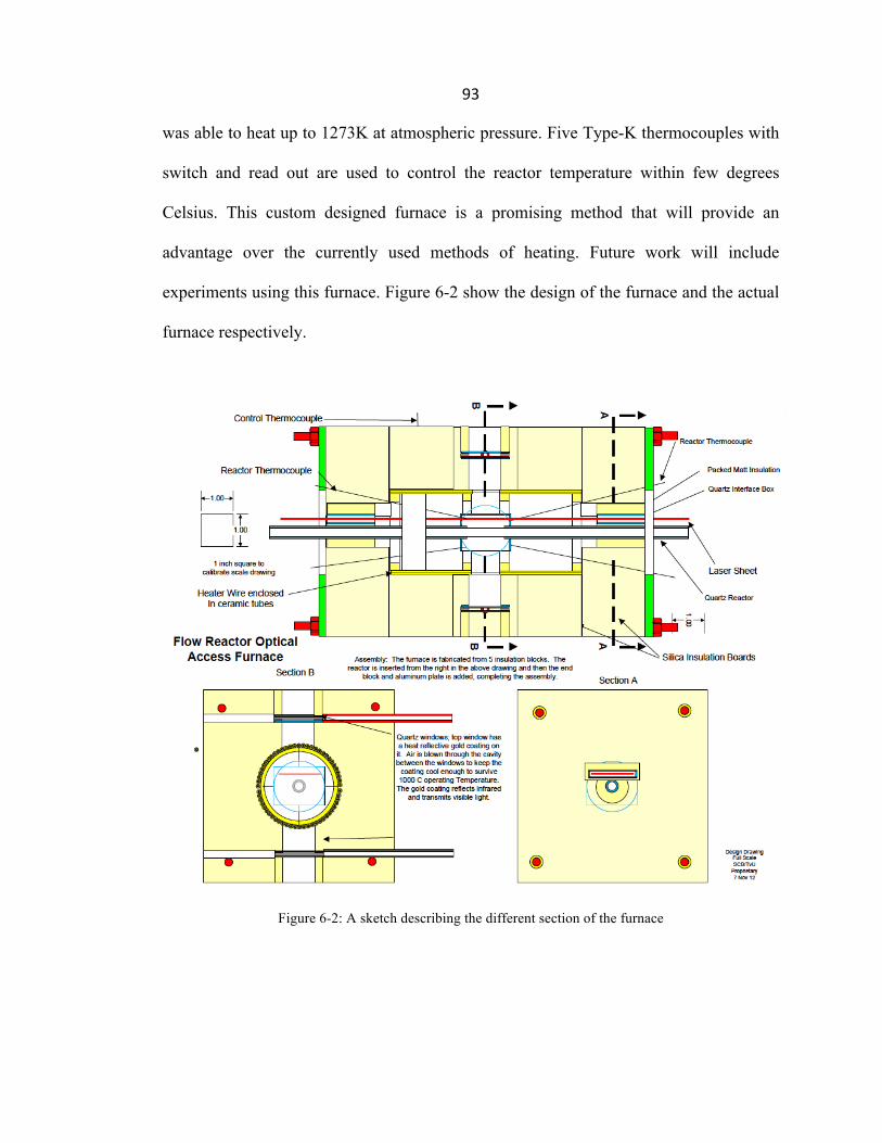
93

was able to heat up to 1273K at atmospheric pressure. Five Type-K thermocouples with

switch and read out are used to control the reactor temperature within few degrees

Celsius. This custom designed furnace is a promising method that will provide an

advantage over the currently used methods of heating. Future work will include

experiments using this furnace. Figure 6-2 show the design of the furnace and the actual

furnace respectively.

 

Figure 6-2: A sketch describing the different section of the furnace

94

The furnace was tested in order to check its suitability for future research. The fused

silica reactor was first inserted in the furnace with two thermocouples. The first

thermocouple (1) was placed inside the reactor center, near the nozzles. The second

thermocouple was placed at the outer wall of the spherical reactor. When setting the

desired temperature, a maximum step of 50°C is allowed. Therefore, if the desired

temperature is 500°C, a step-wise or gradual ramp of 50°C should be used. Both

thermocouples reached the set point within few degrees Celsius. Thermocouple (2)

reaches the set point faster than thermocouple (1).

95

REFERENCES [1] F. Qi, Proc. Combust. Inst. (2012)

[2] P. Dagaut, M. Cathonnet, J.P. Rouan, R. Foulatier, A. Quilgars, J.C. Boettner, F.

Gaillard, H. James, J. Phys. E: Sci. Instrum. 19 (1986), 207-209.

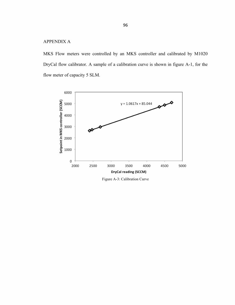
96

APPENDIX A MKS Flow meters were controlled by an MKS controller and calibrated by M1020

DryCal flow calibrator. A sample of a calibration curve is shown in figure A-1, for the

flow meter of capacity 5 SLM.

 Figure A-3: Calibration Curve

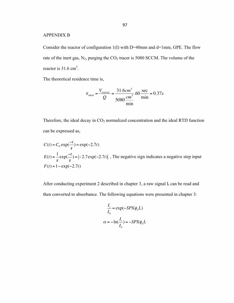
97

APPENDIX B Consider the reactor of configuration 1(I) with D=40mm and d=1mm, GPE. The flow

rate of the inert gas, N2, purging the CO2 tracer is 5080 SCCM. The volume of the

reactor is 31.6 cm3.

The theoretical residence time is,

τ ideal =VreactorQ

=31.6cm3

5080 cm3

min

.60 secmin

= 0.37s

Therefore, the ideal decay in CO2 normalized concentration and the ideal RTD function

can be expressed as,

C(t) =C0 exp(−tτ) = exp(−2.7t)

E(t) = 1τexp(−t

τ) = −2.7exp(−2.7t)

F(t) =1− exp(−2.7t)

, The negative sign indicates a negative step input

After conducting experiment 2 described in chapter 3, a raw signal It can be read and

then converted to absorbance. The following equations were presented in chapter 3:

ItI0= exp(−SPXφnL)  

α = − ln( ItI0) = −SPXφnL  

     

 

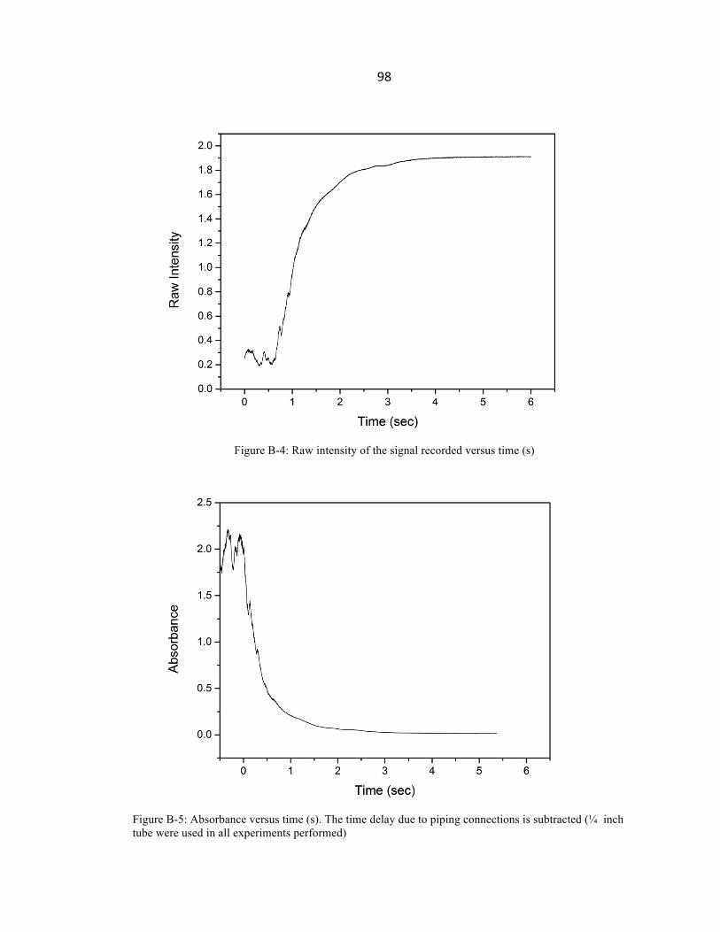
98

Figure B-4: Raw intensity of the signal recorded versus time (s)

Figure B-5: Absorbance versus time (s). The time delay due to piping connections is subtracted (¼ inch tube were used in all experiments performed)

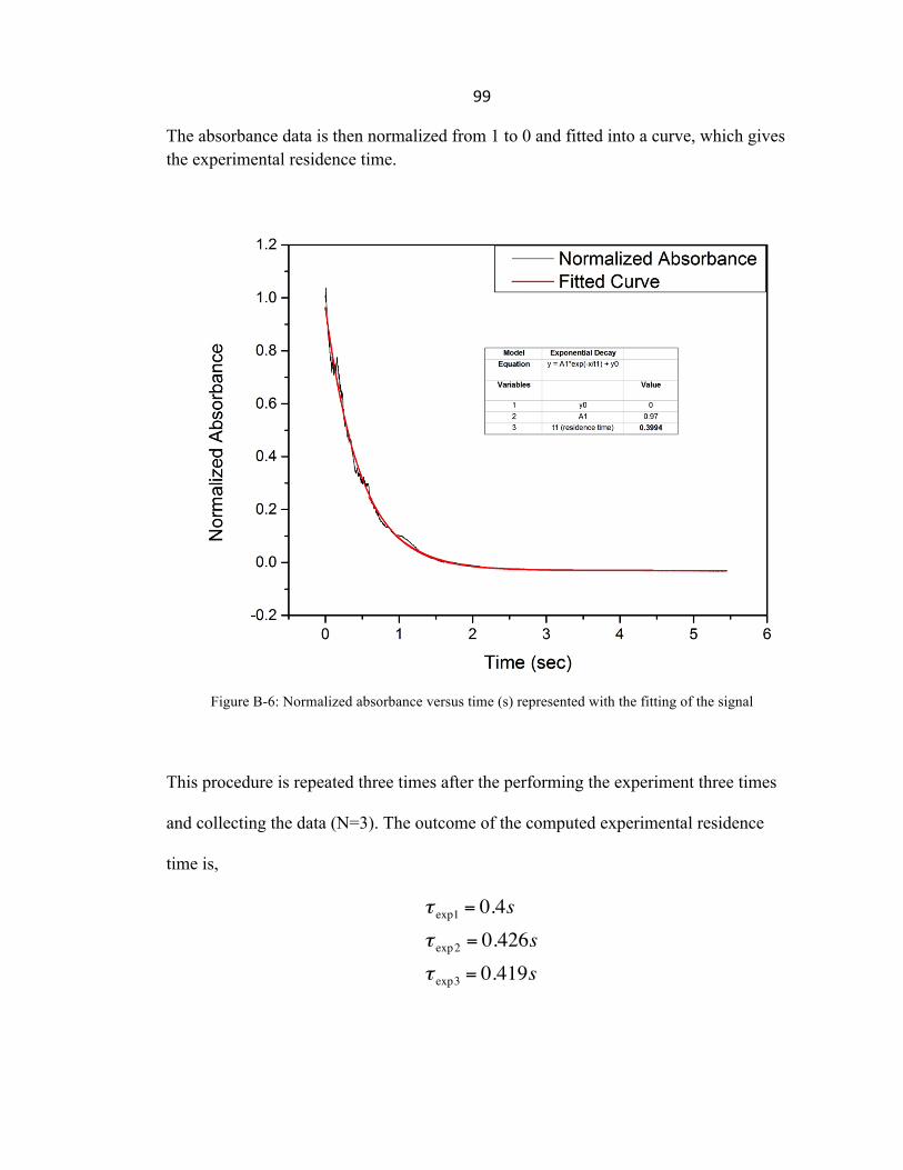
99

The absorbance data is then normalized from 1 to 0 and fitted into a curve, which gives the experimental residence time.

Figure B-6: Normalized absorbance versus time (s) represented with the fitting of the signal

This procedure is repeated three times after the performing the experiment three times

and collecting the data (N=3). The outcome of the computed experimental residence

time is,

τ exp1 = 0.4sτ exp2 = 0.426sτ exp3 = 0.419s

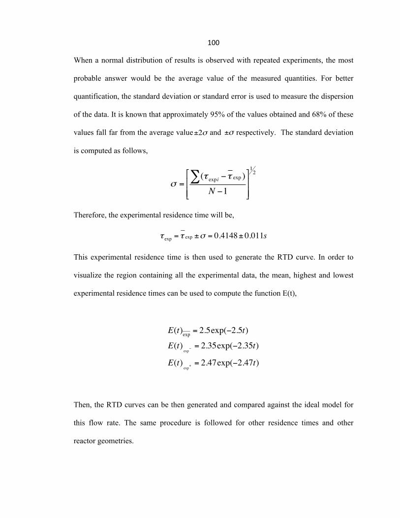
100

When a normal distribution of results is observed with repeated experiments, the most

probable answer would be the average value of the measured quantities. For better

quantification, the standard deviation or standard error is used to measure the dispersion

of the data. It is known that approximately 95% of the values obtained and 68% of these

values fall far from the average value±2σ and ±σ respectively. The standard deviation

is computed as follows,

σ =(τ expi∑ −τ exp )N −1

#

$%%

&

'((

12

 

Therefore, the experimental residence time will be,

τ exp = τ exp ±σ = 0.4148± 0.011s

This experimental residence time is then used to generate the RTD curve. In order to

visualize the region containing all the experimental data, the mean, highest and lowest

experimental residence times can be used to compute the function E(t),

E(t)exp = 2.5exp(−2.5t)

E(t)exp

− = 2.35exp(−2.35t)

E(t)exp

+ = 2.47exp(−2.47t)

Then, the RTD curves can be then generated and compared against the ideal model for

this flow rate. The same procedure is followed for other residence times and other

reactor geometries.

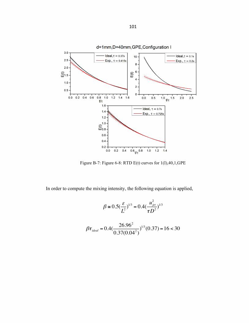
101

 Figure B-7: Figure 6-8: RTD E(t) curves for 1(I),40,1,GPE

In order to compute the mixing intensity, the following equation is applied,

β ≅ 0.5( εL2)1/3 = 0.4(

ujet2

τD2 )1/3

 

βτ ideal = 0.4(26.962

0.37(0.042 ))1/3(0.37) =16 < 30

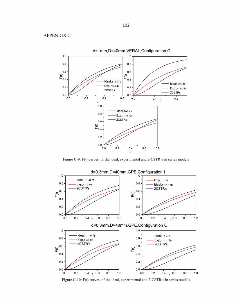
102

APPENDIX C

 Figure C-9: F(t) curves of the ideal, experimental and 2-CSTR’s in series models

 Figure C-10: F(t) curves of the ideal, experimental and 2-CSTR’s in series models

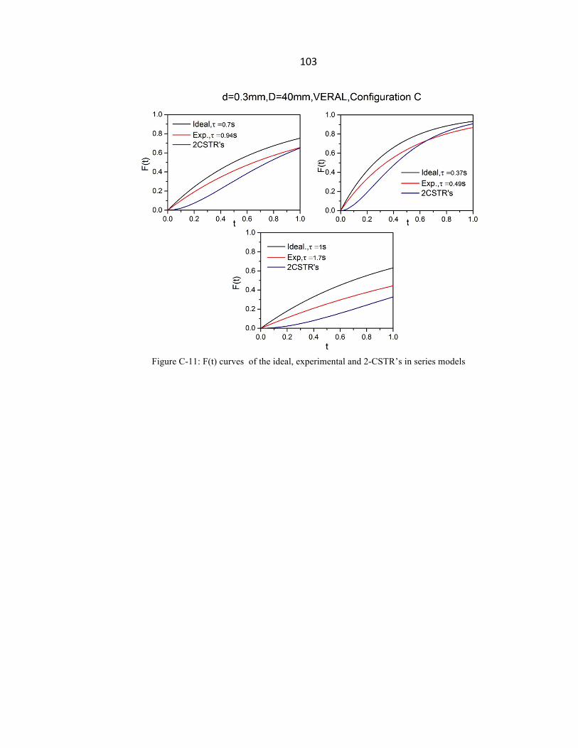
103

 Figure C-11: F(t) curves of the ideal, experimental and 2-CSTR’s in series models