COMPENSATION LAWS

‘ Thesis for the Degree of Ph. D.

MICHIGAN STATE UNIVERSITY

INDUR M. G'OKLANY

1973. '

L 1B RA R Y

Michigan State

University

This is to certify that the

thesis entitled

COMPENSATION LAWS

presented by

Indur M. Goklany

has been accepted towards fulfillment

of the requirements for

Ph.D. degree in Electrical

Engineering & Systems Science

Wm!Major professor

Date February 9, 1973

0-7639

magma IN I?

”053 & SUNS'

BUIIK F'NDEIIY INC.:7 lem 'E‘Y rFINGERS

.3; MICIIGAJI

ABSTRACT

COMPENSATION LAWS

BY

Indur M. Goklany

This thesis concerns itself mainly with linear enthalpy-entrOpy

relationships which give rise to compensation laws.

In Chapter II, we show that eXperimentally determined conductivi-

ties in biological and organic molecules can be as high as 10 to 12

orders of magnitude larger than can be expected from normal solid state

physics. We postulate that there is a change in the frequency spectrum

of lattice vibrations due to distortions in the lattice (i.e., conforma-

tional changes in biological parlance) when charge carriers are created.

We show that this can increase the number of states available into which

charge carriers may be excited, leading to a large increase in conduc-

tivity. This increase in conductivity is due to an entropic increase,

and is achieved at the expense of increasing the activation energy by

the amount of enthalpy required to create the conformational changes.

We then show on the basis of an Einstein oscillator model, that the

entrOpy and enthalpy terms are linearly related, giving rise to a com-

pensation law for conductivity in biological materials.

In Chapter III, we deal with the compensation law in single solute-

single solvent systems. Since the late 1930's it has been known that

the entrOpy of solution could be proportional to the enthalpy of

Indur M. Goklany

solution in such systems. However, the interpretation of the compensa-

tion law has been obscure, partly because there has never been a statis-

tical model that has given rise to a compensation law. Accordingly we

set up a model that leads to the compensation law. In this model we

postulate that the presence of a solute molecule influences the parti-

tion function of neighboring solvent molecules identically. We then

calculate the enthalpy and the entrOpy of solution from Henry's Law and

obtain a compensation law for them. We also note that the compensation

temperature (Tc) and the experimental temperature (T) cannot be

identically equal. If they were identical we arrive at the paradox that

the compensation law would not be observable. The compensation law for

the enthalpies and entrOpies of transferring a given solute from H O to

2

D20 is also examined.

In Chapter IV, we examine how the compensation law fits into the

structure of statistical mechanics. We note that the total change in

entrOpy on solution differs from the change in entrOpy as calculated by

the compensation law by the mixing entropy. This is the physical basis

for not expecting Tc identically equal to T. Also, we note that TC

can be defined as the ratio of the difference in entropy to the differ-

ence in enthalpy for different sets of ensembles. This is akin to the

definition of the experimental temperature defined for an ensemble. We

derive the form the density of states should exhibit for a compensation

law to obtain, and show that the models of Chapter II and III satisfy

this derived relationship.

COMPENSATION LAWS

By {'

Indur MJrCoklany

A THESIS

Submitted to

Michigan State University

in partial fulfillment of the requirements

for the degree of

DOCTOR OF PHILOSOPHY

Department of Electrical Engineering and Systems Science

1973

I9

,@0

(rib

ACKNOWLEDGEMENTS

Of the many years I have been a student, these last fifteen months

spent on the preparation of this thesis have been the most enjoyable and

also the most educational: it being an unfortunate fact of life that

enjoyment and education are not mutually inclusive. For this happy, and

unusual, set of occurrences I am grateful, among others, to Dr. Gabor

Kemeny and Prof. Barnett Rosenberg. Dr. Kemeny's help, advice and vast

donations of time have helped shape this thesis into what it now is. I

also thank Prof. B. Rosenberg for a number of valuable discussions,

lists of references and for granting me the run of his personal library.

My thanks are due Prof. T. H. Edwards for suggesting improvements

in the manuscript. I am also grateful to Dr. P. D. Fisher for his

encouragement.

I am indebted to the U. S. Atomic Energy Commission (AEC AT 11-1-1714)

which provided partial support during my years as a graduate student.

ii

LIST OF

Chapter

I.

II.

III.

IV.

V.

TABLE OF CONTENTS

TABLES O O O O O O O O O O O O O I O O O 0

THE COMPENSATION LAW 0 O O O O O O O O O O O O .

CONFORMONS AND ELECTRICAL CONDUCTIVITY IN BIOLOGICAL

MATERIALS 0 O O C O C C O O O O O O I O C C O O O O

2.1 Introduction . . . . . . . . . . . . . . . . . . . .

2.2 Electrical Conductivity and Conformation . . . . . .

2.3 Electrons and Holes in Semiconductors with Conforma-

tional Changes . . . . . . . . . . . . . . . . . . .

2.4 Conformons in Biological Molecules . . . . . . . .

2.5 Oscillator Model of Activation Energy and Entropy of

Conformons . . . . . . . . . . . . . . . . . . . . .

2.6 Conductivity on the Polaron and Conformon Models . .

2.7 The Compensation Rule . . . . . . . . . . . . . . .

2.8 General Observations on Conformons . . . . . . . . .

SINGLE SOLUTE - SINGLE SOLVENT SYSTEMS . . . . . .

3.1 Introduction . . . . . . . . . . . . . . . . . .

3.2 Single Solute, Single Solvent Model . . . . .

3.3 Enthalpy and Entropy of Solution Using Solubility

Data . . . . . . . . . . . . . . . . . . . . . .

3.4 Interpretation of TC . . . . . . . . . . . . .

3.5 Thermodynamics of Transfer from H20 to D20 . .

3.6 Generalization of the Model . . . . . . . . . .

THEORETICAL FOUNDATIONS . . . . . . . . . . . . . .

4.1 Introduction . . . . . . . . . . . . . . . . .

4.2 The Origin of the Difference between the Temperature

and the Compensation Temperature . . . . . . . . . .

4. 3 Densities of States and the Compensation Law . . . .

4. 4 Partition Function for Individual Degrees of Freedom

CONCLUS ION 0 O O O O O O O O O O O O O O O O O O 0

LIST OF REFERENCES 0 O O O O O O I O O O O I O O O O O O O

Page

iv

14

16

19

25

28

28

28

31

38

44

48

52

52

52

57

62

65

68

LIST OF TABLES

Table Page

1- Conformational Enthalpies and Entrepies at TC 23

iv

CHAPTER I

THE COMPENSATION LAW

There are numerous phenomena in physics, chemistry and biologyl’2

which can be represented by a relationship of the type

K = K; exp [-AG/(RTH (1)

where K could be the solubility if we are concerned with solution

chemistry, it could be the conductivity in semiconductor theory or it

could be the rate in the theory of absolute reaction rates, etc. AG is

a change in Gibbs free energy, this being the free energy required for a

solute molecule to go into solution (in solubility) or it could be the

energy required to activate a charge carrier (in semiconductor theory)

or it may be the free energy of the activated state with reference to

the free energy of the reactants (in absolute reaction rate theory); k

is Boltzmann's constant and T is the absolute temperature at which the

experiments are carried out; K; is a factor, generally algebraic,

which depends on the process in question.

The free energy can be written as2

AG = .AH - T AS (2)

where IQH and A5 are the changes in enthalpy and entrOpy, respec-

tively. Substituting Eq. (2) into Eq. (1) we get

K = KO exp I-AH/(RTH (3)

where

KO = K; exp [AS/k] . (4)

K0 will be referred to as the pre-exponential factor. In many

instances a plot of ln K vs T~1 gives a straight line. This is an

Arrhenius plot. This implies that (3H and zAS are independent of T.

From Eq. (3) we see, therefore, that the $10pe on a Arrhenius plot will

be fiLH/k. Hence, it is possible to calculate AH. To calculate (is

we have to use Eqs. (1) and (2) with the known value of AH.

There is no known thermodynamic or statistical mechanical relation-

ship between AH and .AS or .AH and 1n Ko yet in a number of situa-

tions a linear relationship seems to exist between these termsB-ll, such

that as AH increases so does AS (or In KO). We can see by an exami-

nation of Eq. (2) that a linear rAH 'AAS relationship can lead to a

situation where changes in AC are much smaller than changes in either

.AH or AS since the AH and -T.AS terms compensate for each other.

For this reason, linear AH - AS relationships are often said to lead

to compensation laws. Similarly linear AH - 1n Ko relationships also

compensate in AC.

The slope on a .AH - AS or .AH - 1n K.o plot has units of tempera-

ture and for linear plots is known as the compensation temperature Tc'

Surprisingly, though it's been known since the 1930's that compen-

sation laws exist, there has been quite a bit of skepticism among the

general scientific community to accept compensation laws as genuine phy-

sical phenomenalz-Ia. Skepticism revolves around two basic objections.

The first reason for skepticism is that the measured quantity is AC

or K. AH is calculated from the slope of the K vs T.1 curves

whereas AS is calculated from Eq. (2). There is no independent method

of measuring AS directly. Hence, it has been asserted that an error

in the calculation of AH will automatically result in a compensating

error in AS. In this interpretation the compensation, therefore, is

regarded as a compensation of errors. However, recently Exnerm-16 has

developed stringent statistical tests to be applied to data which leads

to compensation laws. His results indicate that in certain cases the

compensation law is a genuine physical phenomenon.

The second objection arises from the fact that no one has given a

statistical mechanical or model calculation that leads to a compensation

law. In the absence of such a theory it is not possible to say why and

how a compensation law arises and the interpretation, if any, of Tc is

unknown3’4’7’13’17. Recently17 there has been a derivation of a compen-

sation law for solubility. We will examine this in detail. Our analy-

sis, however, indicates that compensation in solutions comes from a

source different from the one outlined in Ref. 17 (Chapters III and IV).

It is the intention of this thesis to devise model systems that

lead to compensation laws. To the extent that this can be done we shall

have successfully been able to refute the second objection outlined

above and gained some understanding of how and why compensation laws

occur and perhaps obtain an interpretation of the constant of prepor-

tionality Tc'

Models will be set up specifically for the case of conductivity in

biological substances (Chapter II) and for solubility (Chapter III).

The reason for choosing the conductivity is that it was in this context

that we were introduced to the compensation law. Conductivity in some

biological substances also exhibits the extremely interesting (and unex-

plained) feature of having an enormously large pre-exponential factor.

4

We hOpe to be able to explain this, too. One reason for choosing to

examine the compensation law in solubility was that this was, as far as

we know, the simplest compensation law in chemistry.

CHAPTER II

CONFORMONS AND ELECTRICAL CONDUCTIVITY IN BIOLOGICAL MATERIALS

2.1 INTRODUCTION

Any theory of the electrical conductivity of organic and biological

semiconductors has to contend with two major problems: In many of these

substances 1) the conductivity is many orders of magnitude higher than

predicted by conventional semiconductor theory for the observed high

activation energies and 2) the pre-exponential factor itself is an eXpo-

nential function of the activation energy, leading to the compensation

law.

Since the mobility of these substances is known to be quite low, a

high density of activated charge carriers is the only possible way to

explain high conductivities. Mechanisms familiar from solid state phy-

sics do not provide for the requisite charge carrier density. We have,

therefore, assumed that the effective density of states for activated

charge carriers is greatly increased by the interaction of the activated

carriers with other degrees of freedom of the molecules. This provides

for an activation entropy which, under appropriate circumstances, is pro-

portional to the activation energy, leading to the compensation 1aw19.

A recent communication by Volkenstein20 introduced similar ideas,

but for different purposes, specifically excluding semiconductivity from

his range of applications. He considered the interaction of an electron

with a biological macromolecule. Such an interaction may lead to the

6

transconformation of the macromolecule. The electron plus the conforma-

tional change he called the conformon.

Volkenstein's mechanism and ours are very similar from the point of

view of statistical mechanics. In both cases there is a relationship

between an activation energy or enthalpy and activation entrepy. The

entropy can take on substantial values because energy can be distributed

over many degrees of freedom. We allow these degrees of freedom to

spread over one or more molecules if necessary. Although the applica-

tions may be different it seems reasonable to retain Volkenstein's term

and we will call the activated carrier plus the accompanying changes

carrying energy and entropy the conformon.

Objections have been raised against the experimental background on

which this theory rests because 1) the activation energy appears to be

too high and 2) the charge carriers may be not electrons and holes, but

ions. The experimental background, however, is quite solid. The elec-

tronic nature of the charge carriers and the high activation energies

have been well documented in several instances. Even if the charge car-

riers are ionic the same experimental facts, i.e., high conductivity and

the compensation law, still must be explained. Our present theory is

formulated for electrons and holes, but it would be easy to reformulate

it to apply to ions or protons. The concept of the conformon is a

generalization of the small polaron concept. A small polaron is formed

if an electron is trapped by its own polarization field21. The small

polaron can move by thermally activated happing or by tunnelling22’23.

It was suggested by Kemeny and Rosenberg24 that small polaron tunnelling

can account for some of the semiconductive prOperties of biological sub-

stances. The explanations so obtained were neither complete nor free

from objections (see Section 2.6). In the present paper we h0pe to

overcome both types of limitations using a new mechanism. This mechan-

ism could be called conformon hOpping and it does not involve tunnel-

ling. The small polaron concept does not involve entrOpy changes while

the conformon concept does. Herein lies the generalization.

2.2 ELECTRICAL CONDUCTIVITY AND CONFORMATION

If one examines the data on biological semiconductorle’ZS-27 one

is struck by the values quoted for 06 which often lie above 1010 and

can be as large as 1022 mho-cm-1. By usual semiconductor theory the

conductivity 0 is given as

U = 06 exp(-BE/2) (l)

where

00 = NGLI : (2)

and E is the gap energy, or alternatively the negative slape in a

In 0 vs l/2kT plot, N, e and n being the total density of charge

carriers, the electronic charge and the mobility, respectively. The

5largest mobility found to date is of the order of 10 cm2(v-sec)-1 in

lnSb. N is given by

N = NADn/M (3)

where N M, D and n are Avogadro's number, the molecular weight,A,

the density and the number of charge carriers available for excitation

per molecule of substance. Taking N = NA’

estimate, we get the maximum possible value of 06 as 1010 mho-cm-

which is likely an over-

1

which implies that in some cases the experimental values of ob are

larger than this by as much as ten or twelve orders of magnitude (this

8

point was repeatedly stressed by Prof. H. Kallmann: private communica-

tion by Prof. B. Rosenberg). This is in spite of the fact that we have

here used a mobility of 105 cm?’(V-sec)-1 whereas for most organic or

biological semiconductors it should be taken as 10 or even as low as

10'5 (Ref. 28).

The observed large value of ob, therefore, must be associated

with a large density of activated charge carriers. Unfortunately we

know of no feature in solid state physics that enables us to increase

the number of activated charge carriers by several orders of magnitude.

Thus, we were led to search for an explanation outside the domain of

solid state physics. We postulated that changes in conformation and/or

coordination in the molecular system are responsible for increasing the

effective number of excited electronic stateslg.

The creation of charge carriers in intrinsic semiconductors occurs

in pairs, i.e., an electron and a hole are created simultaneously.

These carriers move far from each other in the conduction process and

thus one positively and one negatively charged macromolecule is present

for each electron-hole pair. We shall assume that one or both of these

molecular ions can exist in various conformations and/or coordinations.

Due to the large statistical weight associated with the electron-hole

pair, i.e., the large entropy of the activated state, the number of

activated charge carriers is very large. This will account for the high

conductivity, provided the above mechanism does not decrease the mobil-

ity. It may be pointed out that even if the electron and hole were

separated far enough within the same molecule, the same argument could

be applied for an increase in the entropy.

9

A lowering of the mobility could be caused in two ways. A molecule

has to change its conformation and/or coordination both when the elec-

tron (or hole) reaches it and when it passes on. The conformational

change may require either activation or tunnelling through some barriers.

If both these processes are difficult the mobility will decrease, per-

haps offsetting the gain in activated states. We will see later on that

conformational activation will not raise any problems in this reapect.

It is necessary to present here some theoretical developments of a

general nature before returning to the Specific prOperties of the sub-

stances in question.

2.3 ELECTRONS AND HOLES IN SEMICONDUCTORS WITH CONFORMATIONAL CHANGES

Let us consider an ordinary intrinsic semiconductor first with N

molecules. Each molecule has one conduction and one valence state and

one electron on the average. Thus the system has a total of 2N states

and N electrons. If we place the zero of energy in the middle of the

gap the conduction levels are at energy a, the valence levels at -€.

The grand canonical partition function Q is given by

Q = [1 + q exp<-ec> + q epoee) + <12)” . (4)

Here N represents the number of molecules, 1 that no electron is

at +fiepresent, qe- that one electron is in the conduction level, qe

that one is in the valence level and q2 that there is one electron in

. 2each. The expectation value for the number of electrons is 9:

n = (Q, M Q <1 eer-fitL + (1 email“) I

8 q dq N[1+q eXP('B€) 1+q eXp(BC) o (5)

Writing

q = eXP(Bu) . (6)

10

where u is the chemical potential and demanding

n = N (7)

one finds

u = 0 . (8)

The above treatment becomes awkward if conformational changes are

allowed. It requires that the above grand partition function be gener-

alized by the inclusion of conformational effects. Eq. (4), however,

allows unphysical states, i.e., states which do not have the correct

number of electrons. In order to avoid the question of how to general-

ize the unphysical terms in Eq. (4) and still retain the advantages of

the grand canonical formulation we introduce a new grand partition func-

tion Q' using the definition

a . - N

Q = [1 + q eXP(-2be)] . (9)

The first term on the right represents no particle present and the

second one stands for one electron in the conduction level and one hole

in the valence level. The first term, of course, can just as well be

interpreted as one electron in the valence level and one hole in the

conduction level. The number of electrons in the conduction level is

then

r _ l U n ._ N q. CXBL-ZECL

ne — q 83'1“ Q - 1+q' exp(-2fie) ‘ (10)

n; has to be equal to the number of conduction electrons ne calcu-

lated from Eq. (4), which is

. _ N q eXPHBQ

ne - l+q exp(-B€) (11)

as can be seen from Eq. (5). Comparisons of Eqs. (10) and (11) show

11

that

q' = eXP(B€) . (12)

If the electron in question is in the valence state certain molecular

conformations are possible and if it is in the conduction state some

other conformations are allowed. A conformational partition function is

necessary for both. Thus the complete partition function is

H _ U N

Q - IQV + QC q exp(-2ee)1 , (13)

where Qc and Qv stands for the conformational partition functions of

the reapective levels. The number of electrons in the conduction levels

is

Qc q' eXP(-2B€)

c ‘ N QV +Qc q' exp(-2ee)

(14)

For Qc = Qv this reduces to Eq. (10) as required. If the fraction of

excited electrons is not too large then

Qc

0" = N'-- eXP(-B€) . (15)c Q

v

where Eq. (12) has been utilized. If we introduce the conformational

free energy difference between the two electron states by

Q

52- = eXP(-SAF) (16)

V

and the corresponding conformational enthalpies and entropies by

AH - TAS , (17)AF

then

edflfl .AS

C N exp(- ~13- k . (18)=- u

12

Thus the number of activated electrons (and of holes, which is the same)

is given not by the electronic activation energy alone, which would be

2C, but must also include the conformational enthalpy. Also the con-

formational entrOpy must be considered. The experimentally measured

activation energy for semiconduction includes the effect of rAH auto-

matically, but it may include thermal effects on the mobility also, and

therefore cannot simply be read off from Eq. (18). A large value of .AS

would increase n: and thus the conductivity. This, of course, was the

purpose of the whole exercise.

2.4 CONFORMONS IN BIOLOGICAL MOLECULES

We require now some sort of a model which provides for a great rise

in entrepy in the presence of an activated charge carrier. Since not

enough is known at this time concerning the nature of the forces in the

systems under consideration one can only assert that such an idea is

quite acceptable in related contexts. Volkenstein20 suggested that in

certain cases the free energy of an electronic transition is lowered

considerably by conformational changes accompanying such a transition.

We invoke this concept for conductivity. The energy available for con-

formational changes in the conductivity problem is comparable to the

energy in other situations. The activation energy is generally 2eV or

higher, sometimes as high as 4eV 30. It seems possible, therefore,

that the process of activation could involve setting the molecules "free"

if there were sufficient gain in entropy to warrant it.

When a dielectric (e.g., water) is mixed in with the solid, the

dielectric screens the effect of the charge. Thus the disruptive effect

of the charge on the structure would have a.shorter range. Hence as

more dielectric is introduced, the disorganization due to charges is

l3

reduced. Thus the increase in entropy is less in the presence of a

dielectric.

Incidentally, the dielectric also has another effect. The charge

polarizes the dielectric, which in turn produces a field that traps the

charge itself. The decrease of energy due to the charge-dielectric

interaction is the polaron binding energy W .

So far we have stated that an entrepy.factor is essential to

eXplain the high values of oh and also we have postulated a general

model by which the entrOpy could increase. We now attempt to estimate

the increase in entropy.

Let us consider a more Specific model in which the molecule is

rigidly bound in the solid prior to the arrival (or creation) of the

charge carrier. The partition function (Qv) is unity and it has no

entrepy associated with it. After introduction of the charge carrier in

this molecule, the molecule becomes "free" in a 3-dimensional infinite

square well since we have given it enough energy to overcome the attrac-

tive forces. Qc is given by29

Qc = (Zflkaaz/h2)3/2 (19)

where m, k and h are the mass of the molecule, Boltzmann's constant

and Planck's constant, and a the width of the well. Since the entr0py

in the rigid conformation was zero, the increase in entropy is given by

the entrOpy as calculated from Qc' Using the standard recipe for

finding the entropy from a partition function we get

AS = k In Qc + 3k/2 . (20)

Taking the molecular weight as 400, which is close to that of oxidized

14

o

cholesterol, T=300°K and a=5A we get

AS/k = 15.31 . (21)

This gives us an enhancement of ob by exp (15.31) or 106°65. However,

calculations of 06 for oxidized cholesterol show that the experimental

value is about 1011'9 above the calculated value (see Table I in Section

2.7 below). Hence we have to either increase the width of the potential

well or we have to have an extra "free" molecule. If we have only one

"free” molecule we need a22822 to give the right result which is

absurdly large. However, two "free" molecules (one each due to the

electron and the hole) could give the correct entropy factor taking

a=2.92 for each molecule

2.5 OSCILLATOR MODEL OF ACTIVATION ENERGY AND ENTROPY OF CONFORMONS

Let us consider a different picture of what may be going on in a

biological semiconductor. Part of the activation energy can be con-

ceived as being distributed among a number of harmonic oscillators which

correSpond to degrees of freedom of the biological molecules and the

dielectric molecules. Let there be m such "molecular" oscillators,

and d ”dielectric" oscillators. We shall for sake of simplicity

assume that each of the m oscillators is identical with each quantum

having energy Em. Similarly the d dielectric oscillators have each

quantum of energy equal to 6d.

If energy

E = n e + n C (22)

m

has to be distributed among these m+d modes with nm and n being

d

the respective number of quanta, then the number of ways of distributing

E is given by

15

(nm+m-l)i (nd+d-l)1

W = nm1(m-1)L nd1(d-l)! ° (23)

Fowler31 has worked out a similar problem. We shall assume, for simpli-

city, that em and ed have no common divisor. Using the method of

Lagrange Multipliers, with Eq. (22) as the auxiliary condition, we find

the maximum of In W. This yields

eXp(X€ ) exp(x€ )

] +(d-l) ln[ deXP(l“d)-1]’

ln Wmax = (nm€m+nded)-+(m-l) ln[ . (24)exp(xem)-l

where I is the Lagrange Multiplier, Em and Ed denote the most

probable number of quanta in the m and d oscillators, respectively.

I has to satisfy the two equations

hm +-m-l

kem = ln[ fi ](25)

m

and

5d + d-l

he = ln[ _ ] . (26)

d nd

It should be added that we need Stirling's approximation to evaluate Eq.

(24).

Equating In W to S/k and substituting Eq. (22) into Eq. (24)

max

we obtain

exp(lc ) exp(led)

S/k = IE + (m-l) 1n[exp(l€m)-l] + (d-l) 1n[exp(lcd)-l] (27)

Using Eq. (22), (25) and (26) we get

(m-l)e (d-l)€

m d . (28)

exp(iem)-1 T exp(1ed)-1

16

So far we have taken no approximations (barring Stirling's approxi-

mation). We will now assume that the number of quanta in the d oscil-

lators is low. This implies that the second term in Eq. (28) can be neg-

lected. Eq. (28) can therefore be written as

(m-l)cm

. (29)exp(l€m)-l

This assumption is valid if the energy e >>€m or d<<m. We expect

d

€d>>€m because the mass of the dielectric molecules (generally water)

is much less than that of the molecules, furthermore the interaction of

the charge with the dielectric is expected to be strong leading to a

large spring constant. Under these conditions we could neglect the last

term in Eq. (27). Combining the resulting equation with Eq. (29) we get

S/k = 5m ln[l +%:1-1 + (m-l) ln[l +27%] , (30)

where

am = E/em . (31)

Substituting Eq. (31) into Eq. (30) gives us

(m-l)€m E

S/k = E/em ln[l +--——E———J +-(m-l) ln[l +-a;:fy:;] . (32)

We will show below that the dependence of the entrOpy on m, as given

by Eq. (30), or on E, as given by Eq. (32), can lead to a compensation

rule.

2.6 CONDUCTIVITY ON THE POLARON AND CONFORMON MODELS

24,32Kemeny and Rosenberg have shown that small polaron formation

occurs in biological semiconductors. The evidence for such a claim can

17

be based upon: (a) the fact that the experimental activation energy

drOps as additives of high dielectric constant are introduced into the

biological material, the drOp in the activation energy being prOpor-

tional to the inverse of the dielectric constant33; and (b) calculations

by Kemeny and Rosenberg15 which indicate that the effective electronic

mass may be as high as 100 me (me being the electron mass). Kemeny and

Rosenberg24 assumed that the polarons moved by tunnelling rather than

happing. This gave a compensation rule for the conductivity. The com-

pensation temperature Tc was interpreted as 9D/2 where 0D is the

Debye temperature. However, at temperatures greater than 9D/4 the

polaron motion is expected to be by hopping rather than tunnelling34.

This implies that if the data were gathered at temperatures greater than

Tc/2, as indeed they were, polaron motion would not explain the compen-

sation rule. Furthermore, the Tc as calculated in the theory, was a

function of the additive rather than being dependent on the biological

molecule only, and this is contrary to experimental results.

We will combine small polaron hopping with the harmonic oscillator

model develOped in the previous section to give a comprehensive explana-

tion of biological semiconduction including the large number of acti-

vated charge carriers and the compensation rule. We shall use the

results for small polaron hOpping in the adiabatic approximation as des-

cribed by Austin and Mott23. Extension of the results to the non-

adiabatic approximation is trivial and we shall not do it here. The

results, however, should be qualitatively similar.

The mobility in the adiabatic approximation is given as

2 .

u = ea wofi exp(-BWp/2) (33)

18

where a is the hOpping distance, (no the optical vibrational fre-

quency B=l/(kT) and Wp/Z is the activation energy required for the

polaron to hep. Wp is the polaron binding energy. The conductivity 0

is given by

0‘ = ngeu ,(34)

where n: is the number of activated electrons as given by Eq. (18) and

e is the electronic charge. Using Eq. (18), (33) and (34) we get

0 = Nezaamoa exp[-B(E+Z§H)/2] exp(-B WP/Z) eprAS/k) . (35)

It should be pointed out that E=2€ is the minimum energy required to

separate the electron from the hole. AH is the enthalpy term that

comes from the conformational changes, and AS the entrOpy correspon-

ding to this. So that the formulae be less cumbersome, we shall assume

that in the absence of dielectric there is no polaron formation (i.e.,

Wp=0). From now on quantities with a superscript 0 will mean that no

dielectric has been added.

The conductivity in the absence of dielectric 0'0 is given by,

0° = Nezazwofi exp[-e (EO+2AHo)/2] exp(2\s°/k) . (36)

The eXperimentally determined activation energy (Eoexp) is, therefore,

given by

_ o oE exp - E /2 +-AH. . (37)

In the presence of dielectric the energy to separate the electron

and the hole decreases by 2Wp, that being the polaron binding energy

of the electron plus the hole. Hence,

E = E - 2w (3s)

l9

and the conductivity 0 is given by Eq. (35) and (38) as

2 2 o

o = Ne a «58 exp[-B (E -Wp+ZAH)/2] exp(AS/k) . (39)

The activation energy determined experimentally (Eexp) in the presence

of dielectric is thus

_ 0

Eexp - E /2 + (AH-wp/Z) . (40)

Eq. (39) is the general eXpression for the conductivity. In the

next section we shall use this in conjunction with the expressions for

the entrOpy to derive a compensation rule.

2.7 THE COMPENSATION RULE

In Section V we derived the entrOpy resulting from distributing a

fixed amount of energy among m molecular oscillators. In the absence

of dielectric E0exp is composed of two terms, Eo/2 and AHO, as can

be seen from Eq. (37). Here EO/2 is the energy required to separate

the electron-hole pair and AH0 is the energy distributed to the mo

oscillators, where m=m° in the absence of dielectric.

In the presence of dielectric the energy distributed to the molecu-

lar oscillators is AH by Eq. (40). (EC-WP)/2 is the sum of the

energy required to create the electron-hole pair in the dielectric and

the energy required to enable the polaron to hop. For this case we take

the number of molecular oscillators as m.

The dielectric effectively screens off the effects of the charge

carriers, and one could, therefore, expect the conformational changes to

be of a smaller magnitude, i.e., AH<AH° and AS<ASO. By the same

token, as the dielectric constant is increased by adding dielectric Wp

increases. It has been shown35 that Wp increases linearly with the

20

concentration of dielectric. If we now make the assumption that the

. 0 . . .

decrease in the enthalpy term, i.e., AH - AH, 13 also linear with the

amount of dielectric we can write

AH = 241° - wp/r (41)

where l/f is a positive number. We will show this assumption leads to

the compensation rule. Whereas this is no justification in itself it is

consistent with the qualitative arguments laid out at the beginning of

this paragraph.

We will now look at two Specific models each of which leads to a

compensation rule.

Model I. In this model we assume that as dielectric is added to

the biological substance, the screening effects will reduce the number

of participating molecular oscillators from m0 to m. However, each

participating oscillator has to be excited to the same level whether or

not the dielectric is present, i.e., each oscillator has the same number

of quanta (say r) present.

From Eq. (30) we obtain

A80 o 0---l o rmo

T = rm 1n (1+In )+(m-l) ln (1+ ) , (42)o o

rm m -l

and

AS _ m-l rmL

T - rm 1n (1 + rm) +(m-1) 1n (1 + m_-l) , (43)

where rm0 and rm are the total number of quanta in the absence and

presence of a dielectric, respectively. Here

rmo€m = ABC (44)

and

me = AH . (45)

21

Combining Eq. (43) with (45) we get

CH/(re )-1 AH/GLS __ AH m AH m

"12' ‘ :- 1“ (1 + ar- re ) + (a? '1) 1“ (1 +AH/(re >-1) ' “‘6’m m m m

From Eq. (42) and (44) the expression for ASo/k is similar formally,

except that all the AH in Eq. (46) are replaced by AHO.

The logarithmic terms in Eq. (46) are weakly dependent on AH/cm,

hence we could write Eq. (46) as,

AS/k = cAH/em + b , (47)

where

AH-re

_ m l_ rAHc — ln (1 +-eEEE-) + r 1n (1 +~ZEEEZ;? (48)

and

b - ln (1 +AH-rem) (49)

with c and b approximately constant.

Similarly,

ASo/k = c AHo/ém + b . (50)

Substituting the expressions for entrOpy Eq. (47) into the conduc-

tivity expression Eq. (39) and eliminating Wp with Eq. (41) we obtain

2 2 o o

G = Ne a.de exp[-B (E -fAH +(f+2)AH)/2] exp(eAH/€m) exp(b). (51)

Eq. (51) can be Specialized to the case where no dielectric is present by

substituting AHO for AH.

We can reorganize Eq. (51) into the form

0 on exp[Eexp(kT kT)] ’ ()2)

22

where

2 2 o o ,

o; = Ne a(noB exp(b) expf—(E - fldH )/2kFC] , (53)

E = Eo/2 +AH - w /2 (54)

9-K!) p

and

l _ 2c

T51“- ' (f+2)e (55)c m

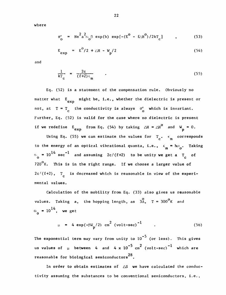
Eq. (52) is a statement of the compensation rule. Obviously no

matter what Eexp might be, i.e., whether the dielectric is present or

not, at T = TC the conductivity is always a; which is invariant.

Further, Eq. (52) is valid for the case where no dielectric is present

if we redefine Eexp from Eq. (54) by taking AH = AH0 and WP = 0.

Using Eq. (55) we can estimate the values for Tc. em corresponds

to the energy of an optical vibrational quanta, i.e., em = hmo. Taking

ab = 1014 sec-1 and assuming 2c/(f+2) to be unity we get a Tc of

7200K. This is in the right range. If we choose a larger value of

2c’(f+2), TC is decreased which is reasonable in view of the experi-

mental values.

Calculation of the mobility from Eq. (33) also gives us reasonable

0

values. Taking a, the hopping length, as 3A, T = 3000K and

14(so = 10 , we get

2 -l

u = 4 exp(-BWp/2) cm (volt-sec) . (56)

The exponential term may vary from unity to 10-.5 (or less). This gives

5us values of u between 4 and 4 x 10- cm2 (volt-sec)-1 which are

reasonable for biological semiconductorszg.

In order to obtain estimates of AS we have calculated the conduc-

tivity assuming the substances to be conventional semiconductors, i.e.,

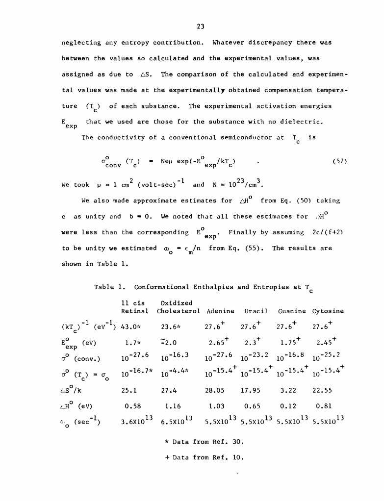
23

neglecting any entrOpy contribution. Whatever discrepancy there was

between the values so calculated and the experimental values, was

assigned as due to AS. The comparison of the calculated and experimen-

tal values was made at the experimentally obtained compensation tempera-

ture (TC) of each substance. The experimental activation energies

E that we used are those for the substance with no dielectric.

exp

The conductivity of a conventional semiconductor at TC is

, _ _ o

Oconv (TC) — Neu exp( E exp/ch) . (57)

We took u = 1 cm2 (volt-sec).1 and N = 1023/cm3.

We also made approximate estimates for AHO from Eq. (50) taking

c as unity and b - 0. We noted that all these estimates for AND

were less than the corresponding E°exp. Finally by assuming 2c/(f+2)

to be unity we estimated mo = em/n from Eq. (55). The results are

shown in Table 1.

Table l. Conformational Enthalpies and EntrOpies at Tc

11 cis Oxidized

Retinal Cholesterol .Adenine Uracil Guanine: Cytosine

(kTC)-1 (ev"1) 43.0* 23.6* 27.6+ 27.6+ 27.6+ 27.6+

szp (eV) 1.7* $2.0 2.65+ 2.3+ 1.75+ 2.45+

go (conv.) 10-27.6 10-16.3 10-27.6 10-23.2 10-16.8 10-25.2

06 (TC) = 0. 10-16.7* 10-4.4* 1045.4+ 1045.4+ 1045.4+ 1045.4+

LSD/k 25.1 27.4 28.05 17.95 3.22 22.55

2H° (eV) 0.58 1.16 1.03 0.65 0.12 0.81

o.O (see'l) 3.6x1013 6.5x1013 5.5x1013 5.5x1013 5.5x1013 5.5x1013

* Data from Ref. 30.

+ Data from Ref. 10.

24

It should be noticed that the constant 2c/(f+2) and em are both

characteristics of the molecular substance. From Eq. (55), therefore,

it is clear that Tc is a function of the intrinsic biological semicon-

ductor. This feature also tallies with eXperimental results.

Model II. In this model introduction of the dielectric does not

change the number of molecular oscillators. It merely changes the total

energy to be distributed among the oscillators. The entropy in such a

situation is given by Eq. (32) where we have to remember that m is

invariant. AS could therefore be written as

"»

2. c€/_\.H +b' ,

m

AS (58)

where c' and b' are slowly varying functions of AH. analogous with

Eqs. (48) and (49) in the previous model. This will also give a compen-

sation rule for conductivity, and the final results will be similar to

those depicted by Eqs. (52) through (55). In fact, numerically, it is

hard to distinguish the two models.

However, we may point out that this model exhibits a very curious

feature if

(m-l)<<Em = aa/em , (59)

i.e., each oscillator contains many quanta. In this case examination of

Eq. (32) shows that

AH/em

AS/k m_1 (m-l) [l + 1n (1 + )1 , (60)

that is

'1

AS/k constant . (61)

25

This means that the entrOpic advantage will be unchanged whether or

not dielectric is present. This means that for this regime we have no

compensation rule, but we could get a 06 much larger than expected.

As far as we are aware, experimentally there is no such material, i.e.,

when we have a large 06, we also seem to have a compensation rule.

But the result, in any case, is very intriguing.

Also, when m = 0, from Eq. (60) we see that we get no entropic

advantage. This is the situation for conventional semiconductors.

2.8 GENERAL OBSERVATIONS ON CONFORMONS

The semiconductive processes of biological substances have so far

seemed to be a matter of solid state physics, a problem isolated from

the physical chemistry of these substances. The solid state properties

were historically related to Bloch waves, which required long range

order in crystalline substances, while physical chemistry dealt with the

local interactions and conformational changes of the biological mole-

cules. This view of solid state physics is outdated, partially because

small polaron formation has been increasingly incorporated into the stan-

dard ideas of solid state physics. Now that conformational change is

implicated in the semiconductive preperties of biological molecules the

solid state physics and the physical chemistry of these substances

become indistinguishable. It seems that conductivity and other trans-

conformation processes only differ in the number of individual steps

involved in transferring a charge from one place to another and not in

the nature of the mechanisms involved.

We have shown that the large values of the pre-exponential factor

in the conductivity is a consequence of the entrOpic advantage derived

from conformational changes induced by the presence of charges. Further,

26

as dielectric is added to the biological substance, the activation

energy dr0ps, increasing the conductivity. Simultaneously, the entrOpic

advantage tends to decrease thus reducing the conductivity. At a parti-

cular temperature (Tc), known as the compensation temperature, these

two effects precisely cancel each other, thus leading to a compensation

rule. Further, the compensation temperature is shown to be a character-

istic of the biological substance as a consequence of the assumption that

the number of quanta in the oscillators correSponding to the degrees of

freedom of the dielectric are much fewer than the number in those oscil-

lators correSponding to the degrees of freedom of the molecules. How-

ever, if the converse were true, i.e., if the number of quanta in the

molecular oscillators was much fewer than the number in the dielectric

oscillators, we could derive a compensation temperature (Tc) which is

a characteristic of the dielectric.

It should be pointed out that there are a few activation phenomena

that exhibit a compensation rule with a TC characteristic of the

dielectric (generally water3). We feel that these phenomena could be

explained in the manner outlined above.

A point that deserves to be investigated experimentally is whether

there are materials which exhibit a large 06, but do not show a com-

pensation rule.

Since we have shown that in general the number of activated charge

carriers includes a free energy term we are led to ask why this term is

not evident in all semiconduction. One would expect that semiconductors,

in which the molecules are small and held together by covalent bonds,

are not likely to be subjected to local disruption as easily as in those

materials in which the molecules are held together by weak forces. We

27

also expect that at higher temperatures the entropic advantage due to

charge creation is going to be less evident, local disruption being

already present due to thermal effects.

CHAPTER III

SINGLE SOLUTE - SINGLE SOLVENT SYSTEMS

3.1 INTRODUCTION

In this chapter we will deal with compensation laws for enthalpies

and entropies of solution for homologous series of non-electrolytic sol-

utes in single solvent systems. The existence of such compensation laws

has been known since the 1930'33’6-8’36-40. However, as far as we are

aware, there has never been a satisfactory statistical mechanical deri-

vation for the compensation laws in such systems. We will set up models

that lead to linear .AH vs. AS relationships and Show that though the

constant of prOportionality may be temperature dependent it is not, in

fact, the experimental temperature. We also expect this approach to

shed light as to when one can or cannot expect a compensation law to be

valid.

3.2 SINGLE SOLUTE, SINGLE SOLVENT MODEL

Let us consider a solution containing n solute and N solvent

molecules. Each solute molecule perturbs the energy levels of the sur-

rounding solvent molecules. One would expect that the further a solvent

molecule is from the solute molecule the less is the effect of this per-

turbation on its energy spectrum. Let each solute molecule perturb A

solvent molecules. We, therefore, have two types of solvent molecules:

those that are perturbed and those that are not. We will assume that

each perturbed molecule is perturbed identically. We shall examine this

assumption in the subsequent sections.

28

29

We shall now distribute the n + N molecules into M 2_N + n equi-

valent cells. Let the partition function for each of the unperturbed

and perturbed solvent molecule be denoted by Q0 and Q1, respectively,

and let q be the partition function of each solute molecule in the sol-

vent. If we were to calculate q, Qo and Q1 we should have to

restrict the spatial coordinates to the dimensions of each cell. To

avoid proliferation of partition functions we shall assume that the solu-

tion is going to be dilute enough to neglect solute-solute interactions.

The canonical partition function for the system outlined above is

_ M1 N-An An n

Qc (n,N) - n1 N1 (M-N-n)! Q0 Q1 q ' (1)

We will now set up a grand canonical partition function Qg where

we can vary both n and N up to a maximum M. This gives

M M-N

_ M1 N-An An n

where A0, A and A are the fugacities of the unperturbed solvent,

1

perturbed solvent and solute molecules such that

A, = exp (sec) . (3.)

A1 = exp (BI-11) 9 (3b)

and

l = exp (Bu) . (30)

Here “0’ “1’ and u are the corresponding chemical potentials and H

is (kT)-1. We should note that in the summation for n, if n > M/(A+l)

then the number of perturbed solvent molecules is going to be less than

An. In effect, Qg has not been set up exactly, but if the solution is

dilute enough we would expect the terms for n > M/(A+l) to contribute

30

negligibly to the summation over n. Using the multinomial theorem we

sum the right hand side in Eq. (2) to give us

AQA M

Q = [1+A00Q +iq(—-1-—1)1 . (4)

8 AOQO

. . 12,27U31ng the standard methods of statistical mechanics we get

31’- = 1n = M1n11+n000 +1(—-1—-—Q:>A1 (5)

- 5‘1“ Q ) AlQl A -1N0 = A0 A0 = M [AOQo - AXq (AMQ) l D . (6a)

8(1n Q ) A Q- _ 1 l A -1N1 - A1 -—:gqfii- - MAIq (AoQo) D , (6b)

and

5(1n Q ) A Q- _ _ 1 1 A -l

n - l.--§§Cii‘ - qu (AoQo) D 3 (66)

where

A Q

— .1.“D - 1 +-AOQO + iq (AOQO) (6d)

and N0, N1 and h are the average numbers of unperturbed solvent,

perturbed solvent and solute molecules, reSpectively. From this point

on we shall drOp the bar to denote averages, since we will only be

dealing with averages. We should note that N1 = An, since that is how

we set up our grand canonical ensemble. It should be pointed out that

not all cells (A) influenced by a solute molecule need necessarily be

occupied by solvent molecules all the time, although it is assumed here

to be so. Such a formulation would result in an average number A' of

perturbed solvent molecules per solute molecule such that A' < A with

31

A' being non-integral in general. Such a calculation has been done in

Section 3.6 and shown to give results qualitatively similar in nature to

those derived from the present model.

Manipulation of Eqs. (6) using the fact that No + N1 = N leads to

_ _ N ,

AoQo - M-N-n (7d)

and

A Q1 1 A n

M (w) = “- - (7b)AOQO M N n

From Eqs. (3) and (7) and utilizing the fact that the chemical poten-

tials for a solvent molecule, whether perturbed or not, are identical,

1.6., no = “I we gEt

Llo

RT. - ln M;N-n - ln Qo (8a)

and

Q

U _ _..n___ .. .1 -kT — 1n M-N-n A ln (Q0) ln q . (8b)

This completes our considerations of the solution by itself. We will

include a treatment of the gas phase in the next section.

3.3 ENTHALPY AND ENTROPY OF SOLUTION USING SOLUBILITY DATA

If the solute in solution is in equilibrium with its pure form then

the chemical potentials in the two phases are identical. We will assume

that the solute in the pure form is an ideal gas. The chemical potential

of the solute in the gaseous phase 1541

11(3) 1150)

RE. = KT- + 1n P , (9)

where

32

“(0) h3 5,- = 1n -‘— ln RT (10)

kr (2nm)372 2

and P is the pressure of the gas phase, m is the mass of a solute

molecule and h is Planck's constant. We have assumed that the solute

molecule is structureless.

(8)Equating u to the chemical potential of the solute in solution

u given by Eq. (8b) we get

~9— —- p 1 +A1 /)-l (-——N+n)+fl'$)l (11)N+n _ exp [ n q n (Q1 Q0 n M-N-n kT °

The left hand side is the concentration c of the solution. We

could rewrite Eq. (11) as

c = P eXP [-846] . (12)

where

as = kT 1n (Mfgfn) - n(°) - kT in q - A kT 1n (01/00). (13)

AG is generally referred to as the free energy of solution. If

the volume of solution does not change much with pressure, i.e., the com-

pressibility is very small, then for very dilute solutions we can assume

the number of cells M to be fixed and also consider the volume of each

cell to be invariant with pressure. Hence, the partition functions Q0,

Q1 and q are going to be independent of pressure. Further, for very

dilute solutions, i.e., n<<N, we can safely assume that

M-N-n M-N

Under these circumstances BAG, for a particular temperature, is going

to be independent of P and c. Eq. (11) is Henry's Lawél.

We shall now cast Eq. (13) into a form more suitable for examining

linear enthalpy-entropy relationships. If we imagine that a solute

33

molecule behaves as a structureless particle in a 3-dimensional box of

the size of a cell then the partition function q is

Px2+Py2+Pzz

exp (- 2m kT ) . (14)

Z

z

Px,Py,P

where momenta in the x, y and 2 directions are given by

nz . (15)

Here n , n and n are the quantum numbers and l , l and l are

x y z x y z

the dimensions of the box in the x, y and 2 directions. Therefore

Eq. (14) can be rewritten as

2 2 2

h2 nx n nz

q = 2 exp [- 8ka (*5- + L2 + —-§-)] . (16)

n an an 1 1

x y z x z

If h2/(8mlx2kT) is much smaller than unity then we can replace the sum-

0

mation over nx by an integration. Taking 1x = 1A, m = 10 x mass of

a proton and T = 3000 K.

h2/8 mlxz kT 2 10'1 . (17)

Hence, replacing the summation by an integration seems valid. This gives

US

3/2

1n q = 1n v +-%-ln kT + 1n [3335%r—-q , (18)

n

where v is the volume of the cell.

Substituting Eq. (10) and (18) into (13) we get

BAG = 1n (fi¥fi) + 1n kT - 1n v - A 1n (01/00) . (19)

34

Let us now examine what happens when the solute is a member of a

homologous series, e.g., methane, ethane or n - propane, etc., and the

solvent is water (for example). We expect that any water molecule that

is adjacent to methane (say) will have its original energy levels

shifted due to the "perturbation" we Spoke of earlier. Any other water

molecule adjacent to the methane molecule would have similar variations

in its energy Spectrum and we would expect the partition function of any

perturbed water molecule to be the same. If we now substitute ethane

for methane, because of the similarity in structure of these molecules,

we would expect that once again adjacent water molecules would be per-

turbed similarly, i.e., Q1 is the same whether methane or ethane is the

solute. For that matter, Q1 should be the same for the entire homolo-

gous series. This argument though applicable for non-electrolytic sol-

utes would not hold for electrolytic solutes because of the complica-

tions of charged entities. From an elementary consideration of Gauss'

Law we could consider that the electrostatic interaction between a

charged solute and water to be approximated by that of a point charge at

the center of the solute and water dipoles. The larger the size of the

charge, the further is the nearest water molecule and less the electro-

static effect and, hence, perturbation of the energy spectrum of the

water molecule. Therefore, we would not expect the partition function

of perturbed water molecules to be the same if we replace one electro-

lytic solute with another if their sizes were different.

To go back to the consideration of a non-electrolytic homologous

series of solutes - we would expect that as we go up the series to

larger molecules it would be possible for more water molecules to be

accommodated at the surface of the solute molecule, i.e., A increases.

35

It should be pointed out that the so-called "two state theories" of

wateraz"44 in which the addition of a solute facilitates the conversion

of one form of "ice" to another, or one species of water to another, fits

in with our statement that each solute molecule from a homologous series

affects each water molecule identically (when it is affected at all).

We only add the proviso that the number of water molecules so affected

depends on the size of the solute molecule. The formation of clath-

rates45 could also be interpreted as being consistent with our formula-

tion, to a certain extent. Both the clathrate theory and the two-state

theories are pictorial in nature and neither are essential to our formu-

lation. Our theory does not depend on the precise change in water struc-

ture due to the addition of non-electrolytic solutes. We are content to

state that the presence of the solute affects the states of water mole-

cules and whatever this change might be, it is represented entirely by

changing the partition function from Qo to Q1.

However, the manner in which we have set up this model with equi-

valent cells makes it hard for us to imagine how the number of cells

adjacent to a solute molecule could change if any solute molecule

(whether methane or ethane) occupies only one cell. We could have set

up a model in which a solute molecule could have occupied more than one

cell and thereby we could have changed A, the number of solvent mole-

cules affected by a solute molecule. Higher members of a homologous

series would occupy more cells and hence, have a larger A. This would

complicate the mathematics, but the principles would not be changed.

We will now compare the free energy, enthalpy and entropy of solu-

tion for a homologous series of solutes. We will denote all quantities

pertaining to the i-th member of the series by a subscript i. From Eq.

36

(19) the free energy of solution for the i-th member is given by

N

BACi - ln (fi:fi) + 1n kT - 1n vi - Ai 1n (Ql/Qo) . (20)

. . . 41The enthalpy of solution 13 def1ned by

. _ 2 54H1 - H [E ”*6in . (21)

However, Q1 and Q0 in Eq. (20) are functions of T and vi, the

volume of a cell. If we assume that vi does not change appreciably

with temperature at any pressure, i.e., the coefficient of eXpansion of

the liquid is small, then we can neglect terms that contain Bvi/BT in

calculating Hi' The AHi so calculated does not include the contribu-

tion of the change in volume of the liquid phase. However, the major

change in volume is going to occur in the gas phase and the above proce-

dure would not result in any serious error. The enthalpy so calculated

is

2.111 = -kT + A1 (111 - U0) (22a)

where U is defined by

u = -kT2 5% (-ln Q) . (22b)

The entropy of solution is defined as

Asi- = - Tr = '_—-_T' ' ' ' o (23)

From Eqs. (20), (22) and (23) we get

. .. .. ._ .11. ..451 — k(1 + 1n kT) + k In vi k 1n (M-N) +-Ai (Si So)’ (24a)

where S is defined by

37

S = - (1 + T g?) [- k 1n Q] . (24b)

We now rewrite ‘AHi and AS1 in a form more suitable for examina-

tion of compensation phenomena, viz.

(0)2.11. = AH. + A. AU (25)

1 1 1

and

As = 25(0) +A As (26)i i i ’

where

an?) -kT , (27)

(0) _. __ _ .1.451 - k (l + 1n kT) + k 1n vi k In (M-N , (28)

AU = U1 - UO , (29)

and

AS = S1 - So . (30)

Let us now compare the enthalpies and entrOpies of solution for

i = j and k. From Eqs. (25) — (30) we get

AHj - AHk = (Aj - Ak) AU (31)

and

v _ . = , (o) _ , (o) _ASJ. Ask ASj ASk + (Aj Ak) AS . (32)

If the first two terms of Eq. (32) cancel each other out, then a plot of

AHi versus L51 for different i, i.e., for different members of a

homologous series, will result in a straight line with a slepe (AUAAS of

the dimension of temperature. The slope, generally referred to as the

compensation temperature, is given by

38

2 5

T = QLI. = T 5:}: I1n(Q1/Qo)] (33)

c AS ’

(1 + T 3;) [1n (Q1/0011

where we used Eqs. (22), (24), (29) and (30). From Eq. (28) the condi-

tion that the first two terms of Eq. (32) cancel, is

In (vj/vk) = 0 . (34)

If each solute molecule occupies only one cell regardless of the size of

the molecule then, obviously, Eq. (34) is correct but, as we pointed out

earlier this is probably too simplistic a model and that we should allow

a molecule to occupy more than one cell. However, as long as v1 is

only an algebraic function of the size of the molecule the above approxi-

mation is valid.

3.4 INTERPRETATION OF Tc

Tc is the ratio of the change in enthalpy and entropy of a single

solvent molecule when it is perturbed and when it is not. If a compensa-

tion phenomenon exists we do not expect Q1 = Q0 so that (AU and .13

are finite and non-zero.

Tc is in general dependent on the experimental temperature T,

but we do not expect the two to be identical. If Tc = T then the

terms containing AU and AS would cancel and the free energy of solu-

tion from Eqs. (25) and (26) would be

2.61 = Allie) - TASE'O) . (35)

This implies that the solubility for any solute of the homologous series

would be substantially constant if the pressure and temperature of mea-

surement were not changed.

39

This peculiar result of the constancy of solubility is not specific

to our model. Let us examine a situation where a compensation law is

valid for a process K. K may be the solubility, the rate constant or

conductivity for a semiconductor. The compensation law is observed by

plotting the enthalpy of the process versus its entrOpy for different x,

where x is the parameter that has to be varied to obtain a linear

enthalpy-entrepy relationship. The parameter x could characterize the

dielectric constant as in semiconductivity or even different members of a

homologous series as presently under discussion. Let us assume that all

the eXperiments were carried out at the same experimental temperature T.

Since the compensation law is valid the enthalpy and entrOpy for the pro-

cess K can be written as,

211 (T,x) = AH(O) (T) +TC AS' (T,x) (36)

and

AS(T,x) = AS(O)(T) +As' (T,x) , (37)

where AH(O) (T) and as“) (T) are independent of x. Eqs. (36) and

(37) are general enough to include the possibility of a compensation tem-

perature Tc. The free energy for process K, therefore, is

AG (T,x) = All“) (T) - 238(0) (T) + (Tc-T) 48' (T.x) . (38)

If now, Tc = T then the last term in the above expression vanishes,

i.e.,

AG (T,x) AH<O> (T) - T as“) (T) . (39)

If Tc and T are identically equal then for any experimental tempera-

ture the right hand side, and hence AG (T,x), is independent of x.

The extent of process K being given by an equation of the form

40

K (T.X) ~ eXP (“BQGWJD (40)

then implies K is also independent of x. Experimentally, however, we

know that the solubility, for instance, is different for different x,

i.e., size of solute, even when a compensation law holds.

Another important corollary follows if T = Tc. Since K (T,x) is

independent of x we would have only one curve to represent all x on

a 1n K(T,x) vs. T.1 plot. Therefore we would have only one enthalpy

and entrOpy for the process K, no matter what the x, if this infor-

mation were derived from the ln K vs. T-1 plot. Therefore, if we plot

AH versus A5 for different x and a fixed T, then we would not

have a straight line but a single point. Hence, AS' (T,x) in Eqs. (36)

and (37) would be zero.

We therefore assert that if’ AH and AS are derived from an ex-

pression like Eq. (40) then a linear AH versus AS plot will not be

observable if Tc is generally identical to the experimental temperature.

Ben Naim18 has derived a compensation law for a two state model of

water, with Tc = T. In his model, the presence of a solute molecule

causes a crossover of water molecules from one component to another.

The free energy, enthalpy and entropy per solute molecule are given by

1 = (56) +( - HENL)’s 5111— N ,N “L “11 SIT N (41)

s L H s w

H - (5“) + - 8N1)3 ‘ Sit—N ,N (H1. “11) (B—N—N (42)

s L H s w

and

83 SN

m

I

s " (Si—>11 N +(SL'SH) (ENE)N ’ (43)s L’ H s w

41

where all symbols have their usual significance and the subscripts s,

W, L and H refer to the solute, water and the two components of

water, respectively. Since the chemical potentials of the two compo-

nents of water have to be identical, i.e.,

”L = “H (44)

he gets

“S = (éfiifiNL’NH = H: . (45)

Further, since

“L = HL - TSL , (46)

and similarly for component H of water, he obtains

HL - HH = T (SL-SH) . (47)

Hence, the last two terms in Eqs. (42) and (43) cancel each other in the

free energy with the experimental temperature masquerading as the com-

pensation temperature. This suffers from exactly the same objections as

we outlined earlier in this section.

The compensation law that we have derived comes from a Slightly dif-

ferent source than Ben Naim's. In our formulation, recalling that Ben

Naim's “S is our u, we obtain from Eqs. (3) and (7)

— n _ _ -

u - kT 1n M_N_n kT ln q AkT 1n (Ql/Qo) + A (no 111) , (48)

where

ONL

A = - (SN—)N . (49)

s w

3':

Hence, in Ben Naim's notation “s is identifiable with the first three

42

terms on the right hand side of Eq. (48) and the compensation, that we

*

talk of, is in this us term and not the A(uo-p term, as he has it.1)

In fact, this term being zero, the enthalpy and entropy of solution, if

derived from Henry's Law, as noted earlier, will not include terms

derived from A(uo-p1).

If the experimental temperature is changed, Q1 and Q0 are going

to change accordingly. This means that there is going to be a change in

the occupation numbers of the states available to perturbed and unper-

turbed solvent molecules and in general, AU and AS as given by Eqs.

(29) and (30) will change. It is therefore, not surprising that TC

(Eq. (33)) is not temperature invariant. Under very Special circum-

stances Tc may be independent of temperature.

Comparing our treatment with that of Frank and Evans'8, we would

like to point out that they did not derive a compensation law. In their

formulation the entire change in entrOpy was related to a change in free

volume. To quote Frank6, "free volume is an auxiliary concept, with

only such meaning as is put into it by the definition adopted". The

free volume change, therefore, would also contain entrOpy changes due to

solute-solvent interaction, i.e., the entrOpy changes which we represent

as arising due to the change in the partition function of solvent mole-

cules from Qo to Q1. However, the manner in which they set up their

statistical mechanics gives us no prior reason to believe that AS is

linear in. AH. They assumed the validity of the compensation law

(Barclay-Butler rule)6"8 and from that derived that the free volume

change was exponential in AH. Their physical picture of non-

electrolytes "freezing" the water around them is similar to our model

(and the two state model) though we hesitate to go as far as stating

43

that the solute merely stabilizes one of the already existing "struc-

tures" of water. The latter statement is not essential to the argument

we have presented.

We would like to emphasize that in deriving Henry's Law, Eq. (11),

we separated out the ln n/(N+n) and In P terms. Therefore, AG is

not the total change in free energy of the system due to the solution

process but somewhat different from it. Also, the terms AU and AS

that lead to compensation have no mixing terms involved. In fact exami-

nation of Eqs. (25)-(30) show that the mixing terms are absent from

enthalpies and entrOpies which occur in the compensation law. The funda-

mental significance of this point will be examined in Chapter IV.

We would not expect compensation if the number of solute molecules

n is so large that the number of solvent molecules N<An. In fact,

mathematically, as has already been stated, the summation to evaluate Qg

breaks down if M<(A+l) n. At about this point we would expect solute-

solute interactions to play a larger role and this is one more factor

that would be reSponsible for not having a compensation law.

Let us examine what happens if we retain the same solvent and use a

different homologous series of solutes. In general for two different

series of solutes, Q1 would be different and hence, we would have in

general two different compensation temperatures.

However, if the solvent is water and the series are the aliphatic

hydrocarbons and the alcohols, since the difference between CH OH and

3

CZHSOH is similar to the difference between CH4 and C2H6’ it is not

surprising that the Tea for these series are almost identica138’39.

The starting point for both these series is different because of the

difference in head groups. Hence, a plot of AH versus ,QS for these

44

series gives parallel but not identical straight lines. A rigid inter-

pretation of the two state theories of water whereby the only effect of

the solute is to change one species of water (or ice) to another, would

give identical straight lines. However, a less rigid interpretation, as

has been noted earlier, is consistent with but not essential to our form-

ulation.

Since solute-solvent forces in the case of nonelectrolytes and water

are essentially similar, it is not too surprising that different homolo-

gous series of nonelectrolytes give similar Tea in water.

Similarly the hydrocarbons (or alcohols) in D 0 would give rise

2

to a compensation phenomenon. But since D20 is not quite the same as

H20, the strength of the deuterium bond being different from that of

the H - bond, etc., we would not expect the compensation temperature

for H20 and D20 to be identical. We will deal with the thermodynam-

ics of transfer from H20 to D20 in the next section.

3.5 THERMODYNAMICS OF TRANSFER FROM H20 TO D20

36,37

There is plenty of experimental evidence that the enthalpy and

entropy of transfer of electrolytic or non-electrolytic solutes from H20

to D20 exhibit a linear relationship. We will only comment on the

transfer of non-electrolytes.

We have seen in the previous section how it is possible to get a

compensation law for a non-electrolytic homologous series in H20 and/or

D20. All quantities that have been defined previously will have a sub-

script H or D depending on whether the solvent is H20 or D20. If

a subscript already exists, then H or D shall be the second subscript.

We will use as the reference state the vapor phase at a particular pres-

sure and assume that the experimental temperature is the same for all

cases.

45

The enthalpy and entrOpy of solution in H20 for the i th solute

of a homologous series is given by Eq. (25) and (26) as

_ (0)AHiH AHH + AH AUI_I (50)

and

= (0) .ASiH ASH + AH ASH (51)

where the superscript (0) once again denotes the part that does not

change with the solute. Similarly for D20, we replace the subscript

H by D.

The enthalpy of transfer is therefore

_ (o) . (o) _AHt - AHD - AHH + AD AUD AH AUH (52)

and the entropy of transfer is

= . (o) , (o) _Last AsD ASH + AD ASD AH ASH . (53)

where AH and AD are the number of H20 and D20 molecules per-

turbed by the solute. Normally we would expect these to be identical,

but we will keep our options Open.

Recalling that the compensation law holds for H O as well as D O2 2

we have the two compensation temperatures TCH and TCD given by

TcD = AUb/ASD (54)

and

TCH = [Juli/[ASH o(5 S)

From Eqs. (52)-(55) we get

= ,(o) (o) , _ . .AH: Ann AHH +AD TCD ASD AH rcH ASH . (56)

46

We will now assign the prescript l and m for the 1th and mth

0)solutes in a homologous series. The compensation temperatures, .AHé(H)

(0)ASD(H), D(H)’ AUD(H) and AMD(H) 'will not be affected at all, but

AH and AD will be different for the two solutes. Hence, we get

AS

mtfléo)-mAHI({O)-1A(o)+1AHl({o) =0 , (57)

i.e., the terms with superscript (o), the parts that do not change

with the solute will be absent when the difference in the enthalpy of

transfer is considered. A similar statement is valid for the terms in

the entropy which are invariant of the solute.

From Eqs. (52) - (56) we get the difference in the enthalpy and

entrOpy of transfer, for the 1th and mth solute as

m gut - 1 AHt = QAD(m,1) th ASD - AAH(m.1) Tc}, as“ (58)

and

m‘QSt - 1 ASt = AAD(m,l) ASD - AAH(m,l) ASH (59)

where

A plot of AHt versus ASt would therefore have a slope

(111,1) '1? As - (m.1) T AS

Tct(m’1) = AAD cD D DAH CH H . (61)

AA.D(m,l) ASD- A%(m,l) AsH

To have a straight plot, i.e., a compensation law, Tct(m’1) should

be independent of m and 1. On the right hand side of Eq. (58) all the

quantities are independent of m and 1 except AAD(m,l) and AAH(m,l).

Therefore to have a constant Tct’ AAD and AAH must be linearly

related by a constant independent of m or 1. Letting

47

AAD(m,l) = cAAH(m,l) (62)

and substitute Eq. (62) into (61) we get

c Tc0 ASD ' TcH.ASH

eASD - ash,

T = Tct(m’1)

ct (63)

Let us examine Eqs. (62) and (63) in greater detail. First of all, if

the number of H O or D O molecules affected by a solute molecule is

2 2

precisely the same, then c = 1. Further, if TCD = TcH are identical,

then Tct = TCH = TcD' However TCD and Tell are defined by Eq. (33) as

AU T25 [1pm /Q )1D 2?? 1D 00

TcD = :s" = a , <64)D (1+1: 5-5) I1n(Q1D/Q0D)l

similarly for TcH we replace subscript D 137 H everywhere.

Hence, if TCD = TcH then QlD/QoD = Q /Q0H and going back to

1H

Eq. (54)-(60), (22), (24), (29) and (30) we see that

ASD = ASH , (65a)

AUD = AUH , (65b)

m AHt - 1 AHt - 0 (65C)

and

AS - AS 7 0 (65d)

and we no longer have a compensation rule. Hence, the conditions c = l

and TCH B TCD do not lead to compensation phenomena. We see, on fur-

ther examination, that if c i l and TcH = TcD then we have compensa-

tion with Tc identical to the two compensation temperatures. Also,

T

if c = 1, then TcH # TcD gives rise to a compensation phenomenon such

48

that Tct # TcD or TcH' However, TcH = TcD 1mpl1es QlD/QoD = QlH/QoH

which does not seem reasonable since H20 and D20, though similar, are

not quite the same, and we would expect that the partition function of an

H20 molecule to be different from that of a D20 molecule. In fact we

would eXpect that any finite, measureable difference in the enthalpy

(entrepy) of solution in D20 and H20 to be reflected in different

partition functions, rather than in a change of c, though this possi-

bility cannot be ruled out entirely. If we had allowed the existence of

holes next to the solute molecule (see Appendix) then the number of H20

(or D20) molecules affected would be dependent on the partition func-

tions of the H20 (or D20) molecules in the presence or absence of the

solute molecule. Hence, c, QlD/QoD and QlH/QoH are correlated, and

the compensation temperature for transfer processes would best be written

as in Eq. (61), which, as we have already mentioned, may not be identical

to eithe o .r TCD r TCH

3.6 GENERALIZATION OF THE MODEL

In the previous model (Section 2.2) we assumed that each solute

molecule "perturbed" A sites and all these A sites were occupied by

solvent molecules. In this model we will not require occupation of all

these A sites, hence for each solute molecule we will have less than A

perturbed solvent molecules. We will see that this model also leads to

results similar to those derived for the previous model. The symbols

used in this section are identical, and have the same significance, as

in the previous model.

The canonical partition function (Qc) is given by,

= A..- . ACM'AD'ID '- . (An) 1 N0 N1 n

QC 2 [nl(M-n)1 N {(M-An-n-N )1 N1!(An-N1)1 Q0 Q1 q l ' (66)

N=N1+No ° 0

N1=An

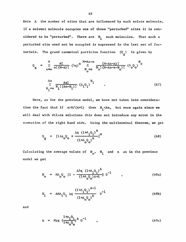
49

Here A the number of sites that are influenced by each solute molecule.

If a solvent molecule occupies one of these "perturbed" sites it is con-

sidered to be "perturbed". There are N1 such molecules. That such a

perturbed site need not be occupied is expressed in the last set of fac-

torials. The grand canonical particion function (Qg) is given by

M=An-n N

M

E

_ M! n (M-An-n)! o

Qg - n=o n1(M-n)1 (lq) NZ;0 Nol(M-An-n-No)1 (AoQo)

0

An N

An! 1

Z t I (A Q ) . (67)N1=o N1.(An-N1). l 1

Here, as for the previous model, we have not taken into considera-

tion the fact that if n>M/(A+l) then N1<An, but once again since we

will deal with dilute solutions this does not introduce any error in the

summation of the right hand side. Using the multinominal theorem, we get

Iq (1+A1Q1)A M

Q = [1+AOQo + A ] (68)

g (1+AOQO)

Calculating the average values of N0’ N1 and n as in the previous

model we get

AAM (1+A1Q1) _1

N6 = MAoQo [1 ' (1+AOQO)A+1 ] D ’ (69a)

(1+A101)A'1 _1

N1 = AMAIQI iq A D (69b)

(1+AOQO)

and

1+A Qn = 1 1 A D-I , (69c)

MN (m)

50

where

m (1+A1Q1)A

D = 1 + AOQ + A . (69d)

(1+AOQ0)

Manipulation of Eqs. (69) gives us

N

A Q = ---—------o(708)

o o M-An-n-No ’

Nl

AlQl - An-N1 ’ (70b)

and

An-N

_ n M-n-An A+l l A

lq — M-n M-n-An-No] [ An I ' (70C)

From Eqs. (70) the chemical potential of the solute in solution is

— n - -

u - kT [1n fi:H-+-(A+l) 1n (1+AOQO) A 1n (1+A1Q1) ln q] . (71)

Proceeding as in Section 3,3, we derive Henry's Law for equilibrium

of the solute in solution with its vapor phase. We get

6 = P exp (-BAG) . (72)

where

kT

BAG = -A In (Q1/Qo) +A ln (pl/p0) + 1n (:7)

with

= .A9_.p 1+AQ . (74)

p1 (p0) being the probability that a water molecule occupies a "per-

turbed" ("unperturbed") site. Clearly, p1 and po are less than one.

51

For a homologous series of solutes we would not expect

ln (Qo pl/Q1 p0) to change drastically as we vary solutes, but we would

expect A to change. If these changes in A In (Q0 Pl/Ql P0) are much

greater than the changes in the other terms in AG, then, once again,

we have a compensation law. We would like to remark that for very

dilute solutions the changes in the last two terms will be negligible if

we change solutes. In any case, the changes in the last three terms of

Eq. (74) are logarithmic.

CHAPTER IV

THEORETICAL FOUNDATIONS

4.1 INTRODUCTION

In Chapter III we examined single solute-single solvent systems and

the conditions under which they lead to a compensation law. In the pre-

sent chapter we will delve deeper into the theoretical foundations of

the compensation law. We will examine the underlying physical basis for

having the compensation temperature different from the experimental

temperature.

We will give an exposition of the compensation law as it fits into

the structure of statistical mechanics. This will lead us to a density

of states relationship that has to be satisfied if the compensation law

is to hold. Finally, we will prove that the models of Chapters II and

III invoked to explain the compensation laws for biological conductors

and for single solute-single solvent systems satisfy this density of

states relationship.

4.2 THE ORIGIN OF THE DIFFERENCE BETWEEN THE TEMPERATURE AND THE

COMPENSATION TEMPERATURE

In statistical mechanics the prOperties of a system are examined by

constructing an ensemble of identical systems and averages are calculated

over the ensemble. In a canonical ensemble the derivative of the entrapy

with respect to the energy is the reciprocal of the absolute temperature

_.1.—--T . (1)

52

53

This, in fact, is the definition of the absolute temperature scale46.

Eq. (1) is an energy-entrepy relationship of a kind, but it is not a

compensation law. Nevertheless, it contributes to the confusion. We

will show now how this confusion comes about. This point was also

touched upon in the previous chapter (page 43). We will in this chapter

ignore the difference between enthalpy and energy since it is not impor-

tant for our purpose.

Let us consider the equilibrium of a solute between two solvents,

or between a pure solute and its solution. We may also consider the

equilibrium of one substance, e.g., water, between two forms. In any

one of these cases the chemical potentials of two subsystems will be

equal:

“1 = “II ' (2)

We may write

u = H - T8 (3)

and thus

HI - TSI = HII = TSII (4)

or

as. ._.. 3.5.5.1.; = .1. (5)AH HI - HII T

The above formula was given by Ben Naimla. This enthalpy-entropy rela-

tionship leads to the experimental temperature and not to a compensation

temperature. This is to be expected because Eq. (5) is derived on a

basis very similar to the derivation of Eq. (1). As shown by Landau and

Lifschitza6, Eq. (1) follows from the requirement that a closed system

consisting of two subsystems, which can exchange energy with each other,

54

should be in equilibrium. Each one of the three systems above have two

subsystems, designated by I and II, which can exchange energy with each

other.

It is evident that the compensation law must have another basis.

In fact the compensation law cannot be derived by the examination of a

single system. It is a consequence of the examination of a set of

related systems. In other words, it is not enough to consider one

ensemble, but it is necessary to consider a set of ensembles. Curiously,

quantities defined over a set of related ensembles resemble those

defined over a single ensemble. We shall show that while ensembles lead

to the conventional statistical mechanical quantities, sets of ensembles

lead to closely analogous quantities related to the compensation law.

Let us consider specifically the equilibrium of a solute in solu-

tion and in the gas phase. The chemical potential of the solute in solu-

tion can be written as

- (0)“II “II + RT ln c , (6)

where c is the mole fraction concentration of the solution and “IIO)

is concentration-independent, the solution being considered to be ideal.

The chemical potential of a solute molecule in the gaseous phase, also

assumed to be ideal, is given by

“I = B(T) + RT In P , (7)

where P is the pressure of the gas phase and B(T) is a temperature

dependent factor.

Equating the two chemical potentials we can derive Henry's law, i.e.,

(0)1 - B(T>>/RT1 . <8)0 = P eXP [-(uI

55

The concentration c being an equilibrium constant, we can use the

van't Hoff relationship to calculate the enthalpies and entrOpies of

solution. Recasting Eq. (8) as

c = exp ['(“1i0) - uI)/RT] , (9)

the free energy of solution is

as“) = Q? - pl (10)

and the enthalpy and entrepy of solution are given by

(0)

- <0) .. 2.9. .‘_..__.Ru - - RT dT (“in ) (11)

and

\ (0) (0)

as“) = AH :12“; , (12)

reSpectively.

We will now compare ‘AH(°) and 08(0) with AH and ‘AS. To

facilitate comparison we first obtain from Eqs. (3) and (6) the relation-

ship

(0) a _ _“II HII TsII RT In C . (13)

From Eqs. (3), (10) and (13) we have

. (0) = _ _ _AG HII TSII HI + TSI RT ln c . (14)

Using Eq. (5) this reduces to

ac(°) = AH - Tlas - RT ln c . (15)

From Eqs. (11), (12) and (15) the enthalpy and entrOpy of solution are,

respectively,

56

mm) = an (16)

and

(o) = AS-I—Rlnc . (17)LS

Hence, from Eqs. (16) and (17)

AH(0) = AH 1 . (18)

58(0) A3 + R n c

Comparing QH(o)/AS(O) with AH/AS, i.e., Eqs. (18) and (5), we see

that, in general, {AH(°)/AS(O) cannot be identical to T. The differ-

ence between the two ratios being due to the R In c term. In fact the

R ln c term is comparable in magnitude to the as term. As an example,

for butane37 at 25°C and 1 atm. pressure the concentration of solution

is about 10.5. The calculated 138(0) is about 40 e.u. and the R ln c

term about -23 e.u.. It is interesting to note from Eq. (17) that aS(o)

is always less than AS.

The .AH(°) and aS(°) calculated above are for a single solution.

To talk of a compensation law we should compare the AH(°) and QS(°)

for a series of solutions, i.e., a set of ensembles. We will assume all

(0) (0)the LH and .AS are calculated for experiments done at the same

experimental temperature T and pressure P. Obviously, a plot of

111(0) versus AS(°) for arbitrary solute-solvent pairs should result

in no discernible pattern.

However, we do know that if we examine Afl‘o) and ¢S(o) for a

particular set of solute-solvent pairs we get straight lines and then we

have a compensation law. The lepe of this line is given by

an?” - AH(°)L i.

T , (19)

L48 (0) - AS (0)

J i

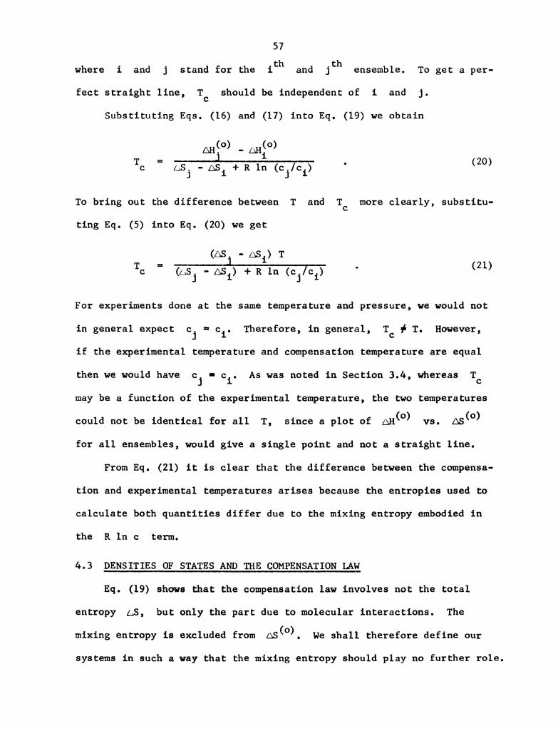
57

. . th .thwhere 1 and J stand for the i and J ensemble. To get a per-

fect straight line, Tc should be independent of i and j.

Substituting Eqs. (16) and (17) into Eq. (19) we obtain

AH‘O) - AH(O)

T = J 1c Lfij - AS + R ln (cj/c

. (20)

1 1)

To bring out the difference between T and TC more clearly, substitu-

ting Eq. (5) into Eq. (20) we get

T = (251- A51) T

C (Lfij ' A51) +-R.ln (cj/ci) ' (21)

For experiments done at the same temperature and pressure, we would not

in general expect cj = c1. Therefore, in general, Tc # T. However,

if the experimental temperature and compensation temperature are equal

then we would have cj - c1. As was noted in Section 3.4, whereas Tc

may be a function of the experimental temperature, the two temperatures

could not be identical for all T, since a plot of afl‘o) vs. AS(°)

for all ensembles, would give a single point and not a straight line.

From Eq. (21) it is clear that the difference between the compensa-

tion and experimental temperatures arises because the entropies used to

calculate both quantities differ due to the mixing entrOpy embodied in

the R ln c term.

4.3 DENSITIES OF STATES AND THE COMPENSATION LAW

Eq. (19) shows that the compensation law involves not the total

entrepy 45, but only the part due to molecular interactions. The

(0)mixing entropy is excluded from [AS . We shall therefore define our

systems in such a way that the mixing entrapy should play no further role.

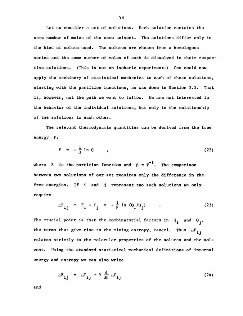
58

Let us consider a set of solutions. Each solution contains the

same number of moles of the same solvent. The solutions differ only in

the kind of solute used. The solutes are chosen from a homologous

series and the same number of moles of each is dissolved in their reSpec-

tive solutions. (This is not an isobaric experiment.) One could now

apply the machinery of statistical mechanics to each of these solutions,

starting with the partition functions, as was done in Section 3.2. That

is, however, not the path we want to follow. We are not interested in

the behavior of the individual solutions, but only in the relationship

of the solutions to each other.

The relevant thermodynamic quantities can be derived from the free

energy F:

—..}.F - B In Q , (22)

where Z is the partition function and B = T-l. The comparison

between two solutions of our set requires only the difference in the

free energies. If i and j represent two such solutions we only

require

AFij = Fi - Fj - l’ln (Qi/Qj) . (23)

B

The crucial point is that the combinatorial factors in Q1 and Qj’

the terms that give rise to the mixing entropy, cancel. Thus dFij

relates strictly to the molecular prOperties of the solutes and the sol-

vent. Using the standard statistical mechanical definitions of internal

energy and entropy we can also write

. .§_ ,LE1]. Afij + 6 dB AF” (24)

and

As. = 8 --AF.. . (25)

Let us now drOp the subscripts and consider AF, DE and AS in an

idealized way as possibly continuous variables. We are then talking

about a set of ensembles because these quantities represent differences

between ensembles. Let us now construct a theory for the set of ensem-

bles by analogy to the theory of ensembles. In analogy with Eq. (1) we

write

. (26)

ELL;

.1.

Tc

This is a definition. If it is valid we have a compensation law and Tc

is the compensation temperature. This is fairly obvious by comparison

with the Chapter III and will also be shown below. It is also obvious

that Tc is not the experimental temperature T, because the latter

quantity refers to a single ensemble and Tc to a set of ensembles.

This is not to say that Tc is independent of T, but the two tempera-

tures are clearly different concepts.

In order to show that Eq. (26) represents a compensation law, and

for other purposes, we shall solve this equation. Utilizing Eqs. (23) -

(26) we can write

2 d

3 “AF

dad = ac . (27)

(1+8 5'5) AF

We shall introduce AZ by the definition

AF = -%lnAQ . (28)

AZ is the ratio of two Q's, not their difference. Substitution of Eq.

(28) into Eq. (26) yields

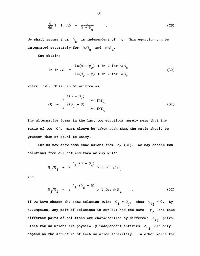
60

ld _ ——c—-——-

35 ln ln AQ — B - “c (29)

We shall assume that BC is independent of B. This equation can be

integrated separately for byflc and O<Bc.

One obtains

ln(B - BC) + 1n e for B>Bc

ln ln AQ = (30)

ln(Bc - B) + ln 6 for B<3c

where e>0. This can be written as

em - BC)e for B>Bc

so = emc - a) (31)e for B<B

c

The alternative forms in the last two equations merely mean that the

ratio of two Q's must always be taken such that the ratio should be

greater than or equal to unity.

Let us now draw some conclusions from Eq. (31). We may choose two

solutions from our set and then we may write

e -U (B BC)Qi/Q. = eJ > 1 for b>BC

and

€ ~(B - B)

Qj/Q. = e i] C > 1 for B<Bc . (32)1

If we have chosen the same solution twice Qi = Qj’ thus eij = 0. By

assumption, any pair of solutions in our set has the same Sc and thus

different pairs of solutions are characterized by different Cij pairs.

Since the solutions are physically independent entities €ij can only

depend on the structure of each solution separately. In other words the

61

number of independent eij is equal to the number of different solu-

tions and not to the number of pairs of such solutions. This means that

e = e, - e, . (33)

These e's can be put into a monotonic sequence such that

e > e. , (34)

so that Eij > O is always satisfied.

To verify that the compensation law is satisfied, we can write

E..(B - B)_ 1] c

Qj — e Qi . (35)

Using again the standard formulae of statistical mechanics we find

E. = e. +E. , (36)

S. = B E , + S , (37)

which lead to

43 _ .1-

as — TC - (38)

as required. We emphasize again that the differences in energy and

entropy are taken between two ensembles (leading to TC) and not within

the same ensemble (which would lead to T).

We can answer one more question here, namely what conclusions can

one reach with regard to the density of states of each solution? We may

write

Qi(fi) = I e'flE R1(E)dE . (39>

R(E) will vanish below some lower bound. Since the compensation law is

62

not going to give any information concerning the mixing terms we may as

well regard Qi and R1 as defined without them. Substituting Eq. (39)

for both i and j into Eq. (35) we obtain

.5 eij

RJ. (Efiij) e c . (40)R1 (B)

As expected we only get information concerning the relationship

among R's, but not of the individual R's. Going from one solution to

another in the sequence the density of states is rigidly displaced along

the energy axis and its scale is changed by an exponential function of

this displacement. The proportionality factor in the exponent is BC.

Finally we point out that if the compensation temperature were the

experimental temperature the entire deve10pment would be meaningless,

beginning with Eq. (24).

4.4 PARTITION FUNCTION FOR INDIVIDUAL DEGREES OF FREEDOM

We will now show that one method of satisfying Eq. (40), and hence

the compensation law, is to change the number of units or degrees of

freedom involved in the process (for which we have compensation) as we

th

change ensembles. Let the i ensemble have n degrees of freedom

1

affected in a certain way so as to change the partition function for an

affected degree of freedom from qo to ql. Let there be a total of n

such degrees altogether such that ni<n for any 1. Setting up the

total partition function for the ensemble i we obtain

q. n.

Qi = 0§°) qo“ (3&9 1 . (41)O

.t . . . .

For the J h ensemble we shall have a Similar expreSSIOn. Taking the

ratios Qj/Qi we get

63

(o) (o) ql “j'ni0 o = O a —_ O 42QJ/Q1L <01 /QJ ><qo) < )

QED) and QED) is the combined partition function of those degrees of

freedom that are not capable of being affected. We would expect

ng) = ng) and, hence

1 J

n,-ni

We could write q1 and q0 as

(11 = e (44a)

and

q = e . (44b)

Substituting Eqs. (44) into Eq. (43) we obtain

qi = qj eeij(5 - BC) ’ (45)

where

eij = (nj - n1) LR: , (46a)

BC = LS/L‘xu (46b)

and

f1 - f0 = [_,f = Au - (AS/B . (46c)

Eqs. (45) and (35) are identical. Hence, a model of the kind described

above will lead to a compensation law. Such a model will also automatic-

ally satisfy the requirement upon the density of states embodied in Eq.

(40). Further, the compensation temperature in this model is decided by

the ratio of the change in internal energy to the change in entropy for

64

a single participating unit, i.e., for each degree of freedom whose par-

tition function is changed [Eq. (46b)]. This model is a generalization

of the models devised in Chapter III and Model I of Section 2.7.

CHAPTER V

CONCLUSION

In the introduction we had stated that our aim was to set up model

systems that could lead to compensation laws. This, besides being an

end to itself, was undertaken with the intention of understanding of how

and why compensation laws occur and of the physical significance of Tc'

We succeeded in this undertaking by setting up models which led to com-

pensation in conductivity of biological substances (Chapter II) and solu-

bility of nonelectrolytic homologous series in a particular solvent

(Chapter III).

For the conductivity case we postulated that creation of a charge

carrier led to distortions of the lattice (or conformational changes in

the system). We showed that these conformational changes would contri-

bute an extra free energy term in the conductivity. This free energy

term can be split into an entrOpy term and an enthalpy term. The

measured activation energy would therefore consist of at least two con-

tributions, one arising from the above-mentioned enthalpy and the second

contribution coming from the energy required to Create the charge carrier.

A third contribution may be present arising from the mobility. The

entrOpy term would boost the pre-exponential factor. This would explain

the large pre-exponential factors found for the conductivity of biologi-

cal substances.

65

66

The compensation law for conductivity in biological substances can

be explained by a linear enthalpy-entrOpy relationship for the conforma-

tional changes. Tc’ in this case, can be interpreted as a local tem-

perature different from the temperature of the entire system (i.e.,

experimental temperature). Conformational changes occur because of

fluctuations in the energy in the environment of charge carriers.

From the model for the compensation law in solubility, Tc can be

interpreted as the ratio of the change in enthalpy to the change in

entrOpy of a solvent molecule when it is "perturbed" by a solute mole-

cule. Tc is therefore a characteristic of the molecular interactions

in a solution before and after the solute molecule is introduced. Unfor-

tunately, it is not possible to evaluate Tc since an a priori calcula-

tion of the partition function for a solvent molecule when it is per-

turbed or unperturbed is not possible.

We also showed that in general T and Tc would not be identical.

Ben Naim's derivation of the compensation law would give T and Tc

identical. However, we showed that the source of compensation for

single solute-single solvent systems was not the same as that of Ben

Naim's.

We identified why exactly T and Tc would not be identical. The

origin of this difference lay in that the total change in entropy of the

system was different from the change in entropy as calculated by Henry's

Law because of the R 1n c term.

We derived a density of states relationship which would hold if a

compensation law was valid. Finally, we showed that a model in which

different degrees of freedom were perturbed identically (the number of

perturbed degrees of freedom depending on the change in parameter which

67

results in the compensation law) satisfied the compensation law. This

model was general enough to include the models for the compensation law

in conductivity as well as solubility.

We think that the Einstein oscillator-like model develOped for the

conductivity could be applied to any activated phenomenon that exhibits

a compensation law. The interpretation of Tc as a local temperature

would once again be valid.

We think it is necessary at all times to keep in mind that a compen-

sation law occurs not for the enthalpy and entrOpy changes in a parti-

cular system, but rather when the enthalpy and entrOpy changes of dif-

ferent systems are compared. It is our feeling that if we have a set of

processes, each process involving a large number of degrees of freedom

(not necessarily identical degrees of freedom) then comparison between

different members of the set (of processes) could lead to a compensation

law. This point deserves careful attention and might make possible a

general derivation for the compensation law.

LI ST OF REFERENCES

10.

ll.

12.

13.

14.

15.

16.

17.

18.

LIST OF REFERENCES

F. Reif, "Fundamentals of Statistical and Thermal Physics" (McGraw-

Hill Book Co., New York, 1965).

S. Classtone, K. J. Laidler and H. Eyring, "The Theory of Rate Pro-

cesses" (McGraw-Hill Book Co., New York, 1941).

R. Lumry and S. Rajender, BiOpolymers 9, 1125 (1970).

J. W. Larson and L. G. Hepler in "Solute-Solvent Interactions" ed.

by J. F. Coetzee and C. D. Ritchie (Marcel Dekker, New York, 1969).

J. E. Leffler and E. Grunwald, "Rates and Equilibria of Organic

Reactions" (John Wiley and Sons, Inc., New York, 1963).

H. 8. Frank, J. Chem. Phys. 13, 478 (1945).

H. S. Frank, J. Chem. Phys. 13, 493 (1945).

H. 8. Frank and M. W. Evans, J. Chem. Phys. 13, 507 (1945).

M. G. Evans and M. Polanyi, Trans. Far. Soc. 32, 1333 (1936).

M. E. Burnel, D. D. Eley and V. Subramanyan, Ann. N. Y. Acad. Sci.

158, 191 (1969).

J. A. V. Butler, "Chemical Thermodynamics" (MacMillan and Co., Ltd.,

New York, 1960).

Meeting Report on the Mechanism of Enzyme Catalysis, FEBS Letters 10,

209 (1970).

L. A. Blyumenfel'd, Biofizika 16, 724 (1971).

O. Exner, Nature 201, 488 (1964).

O. Exner, Nature 227, 366 (1970).

O. Exner, Coll. Czech. Chem. Comm. 37, 1425 (1972).

M. Pope and H. Kallmann, Disc. Far. Soc. 51, 7 (1971).

A. Ben Naim, A Mixture Model Approach to the Theory of Classical

Fluids III. Application to Aqueous Solutions of Nonelectrolytes.

To be published. We are obliged to Dr. Ben Naim for the preprint.

68

19.

20.

21.

22.

23.

24.

25.

26.

27.

28.

29.

30.

31.

32.

33.

34.

35.

36.

37.

38.

39.

40.

69

C. Kemeny, Unpublished lecture notes, Department of BiOphysics,

Michigan State University (1972).

M. V. Volkenstein, J. Theor. Biol. 34, 193 (1972).

L. D. Landau, Phys. Z. Sowj. Un. 3, 664 (1933).

T. Holstein, Ann. Phys. (N.Y.) 8, 343 (1959).

I. G. Austin and N. F. Mott, Adv. Phys. 18, 41 (1969).

C. Kemeny and B. Rosenberg, J. Chem. Phys. 53, 3549 (1970).

D. D. Eley and W. P. Williams, Trans. Far. Soc. 64, 1528 (1968).

D. D. Eley, A. S. Fawcett and M. R. Willis, Trans. Far. Soc. 64,

1513 (1968).

J. R. McKellar, J. A. Weightman and R. J. P. Williams, Disc. Far.

Soc. 51, 179 (1971).

F. Guttman and L. E. Lyons, "Organic Semiconductors" (New York,

John Wiley, 1967).

K. V. Huang, "Statistical Mechanics" (John Wiley and Sons, Inc.,

New York, 1963).

B. Rosenberg, B. B. Bhowmik, H. C. Harder and E. Postow, J. Chem.

Phys. 49, 4108 (1968).

R. H. Fowler, "Statistical Mechanics" 2nd Ed. (Cambridge University

Press, Cambridge, U.K., 1966).

G. Kemeny and B. Rosenberg, J. Chem. Phys. 52, 4151 (1970).

B. Rosenberg and E. Postow, Ann. N. Y. Acad. Sci. 158, 161 (1969).

A. J. Bosman and H. J. van Daal, Adv. Phys. 19, l (1970).

B. Rosenberg, J. Chem. Phys. 36, 816 (1962).

E. M. Arnett and D. R. McKelvey in Solute-Solvent Interactions, Eds.,

J. F. Coatzee and C. D. Ritchie (Marcel Dekker, New York, 1969).

G. C. Kresheck, H. Schneider and H. A. Scheraga, J. Phy. Chem. 69,

3132 (1965).

W. F. Claussen and M. F. Polglase, J. Am. Chem. Soc. 74, 4817

(1952).

R. Aveyard and A. S. C. Lawrence, Trans. Far. Soc. 60, 2265 (1964).

I. M. Barclay and J. A. V. Butler, Trans. Far. Soc. 34, 1445 (1938).

41.

42.

43.

44.

45.

46.

70

A. H. Wilson, "Thermodynamics and Statistical Mechanics" (Cambridge

Univ. Press, London, 1966).

M. S. Jhon and H. Eyring, Chem. Phys. Letters, 13, 36 (1972).

G. Wada, Bull. Chem. Soc. Japan, 34, 955 (1961).

A. Ben Naim, Trans. Far. Soc., 66, 2749 (1970).

C. A. Jeffrey and R. K. McMullan, Progr. Inorg. Chem. 8, 43 (1967).

L. D. Landau and E. M. Lifschitz, "Statistical Physics" (Addison-

Wesley Publishing Co., Inc., Reading, Mass., 1958).