thesis jose estevez

Geothermal Power Plant Projects in

Central America: Technical and Financial Feasibility

Assessment Model

José Roberto Estévez Salas

Faculty of Industrial Engineering, Mechanical

Engineering and Computer Science

University of Iceland 2012

Geothermal Power Plant Projects in

Central America: Technical and Financial Feasibility

Assessment Model

José Roberto Estévez Salas

60 ECTS thesis submitted in partial fulfillment of a Magister Scientiarum

Advisors:

Dr. Páll Jensson Dr. Páll Valdimarsson

Faculty Representative:

Dr. Halldór Pálsson

Faculty of Industrial Engineering, Mechanical Engineering and Computer Science

School of Engineering and Natural Sciences University of Iceland

Reykjavík, 2012

Geothermal Power Plant Projects in Central America: Technical and Financial Feasibility Model Assessment 60 ECTS thesis submitted in partial fulfillment of a Magister Scientiarum Copyright © 2012 José Roberto Estévez All rights reserved. Faculty of Industrial Engineering, Mechanical Engineering and Computer Science School of Engineering and Natural Sciences University of Iceland Sæmundargötu 2 101 Reykjavík Iceland Telephone: 525 4000 Bibliographic information: Estevez, 2012. Geothermal Power Plant Projects in Central America: Technical and

Financial Feasibility Model Assessment, M.Sc thesis, Faculty of Industrial Engineering, Mechanical Engineering and Computer Science, University of Iceland Printing by Háskólaprent ehf. Reykjavík, Iceland, April 2012

Dedication

This thesis is dedicated to the memory of

Raúl E. Gálvez Nessi (1949-2011),

for inspiring my fascination in humanism, science and literature

Abstract

The geothermal resource potential makes the Central American region a prime candidate for investment in electricity power plant projects. In this study, the technical and financial feasibility of developing geothermal power plant projects in Central America is conducted. Three thermodynamic models of two groups of conventional power plants are evaluated for a range of possible values of geothermal resource temperatures (100-340°C) and mass flow rates (100-1,000 kg/s) in order to examine multiple expected scenarios. The main results are presented as contour maps of the internal rate of return (IRR) of free cash flow to equity (FCFE), net power plant output and the probability of success of accomplishing the minimum rate of return required by private investors. By using these maps, geothermal developers, who already characterize the quality of resources for geothermal projects, could identify technically and financially viable projects in terms of temperature and mass flow rate, taking into account the assumptions and limitations considered in the models. The results indicate that the geothermal power plant’s size, profitability indicators and the probability of success of geothermal power development arise from an increase in the temperature of the geothermal resource and mass flow rate. As a result, geothermal power development projects in Central America for a small power plant are not attractive to private investors, when taking into account the project’s cost of exploration and confirmation, drilling of an unknown field, and construction of the power plant and transmission line.

vii

Contents

List of Figures ...................................................................................................................... x

List of Tables ...................................................................................................................... xii

Nomenclature .................................................................................................................... xiv

Acknowledgements ........................................................................................................... xvi

1 Introduction ................................................................................................................... 17

2 Central American data ................................................................................................. 19

2.1 Power production status ........................................................................................ 19

2.2 Electricity market .................................................................................................. 20

2.2.1 Guatemala .................................................................................................... 20

2.2.2 El Salvador ................................................................................................... 20

2.2.3 Honduras ...................................................................................................... 21

2.2.4 Nicaragua ..................................................................................................... 22

2.2.5 Costa Rica .................................................................................................... 22

2.2.6 Panama ......................................................................................................... 23

2.2.7 Regional market ........................................................................................... 24

2.2.8 Market analysis ............................................................................................ 24

2.3 Corporate tax ......................................................................................................... 25

2.4 Tax incentives for renewable energy..................................................................... 25

2.4.1 Guatemala .................................................................................................... 26

2.4.2 El Salvador ................................................................................................... 26

2.4.3 Honduras ...................................................................................................... 26

2.4.4 Nicaragua ..................................................................................................... 26

2.4.5 Costa Rica .................................................................................................... 26

2.4.6 Panama ......................................................................................................... 26

2.5 Clean Development Mechanism ........................................................................... 27

2.6 Climatic factors ..................................................................................................... 28

3 Central American geothermal energy development .................................................. 31

3.1 Geothermal resources ............................................................................................ 31

3.1.1 Guatemala .................................................................................................... 32

3.1.2 El Salvador ................................................................................................... 32

3.1.3 Honduras ...................................................................................................... 33

3.1.4 Nicaragua ..................................................................................................... 33

3.1.5 Costa Rica .................................................................................................... 33

3.1.6 Panama ......................................................................................................... 34

4 Geothermal electrical power assessment .................................................................... 35

4.1 Power plant models ............................................................................................... 35

4.1.1 Single flash................................................................................................... 35

viii

4.1.2 Double flash ................................................................................................. 40

4.1.3 Organic Rankine cycle ................................................................................. 41

4.2 Simulation and optimization .................................................................................. 44

4.2.1 Assumptions and limitations ....................................................................... 44

4.2.2 Design variables and constraints ................................................................. 45

4.3 Results .................................................................................................................... 46

4.3.1 Single flash .................................................................................................. 46

4.3.2 Double flash ................................................................................................. 47


4.3.4 Comparison of power output between SF, DF and ORC ............................ 50

5 Cost estimation model of geothermal power development ........................................ 53

5.1 Geothermal development project phases ............................................................... 53

5.2 Exploration and confirmation ................................................................................ 53

5.3 Drilling ................................................................................................................... 54

5.4 Power plant ............................................................................................................ 55

5.4.1 Heat exchangers ........................................................................................... 55

5.4.2 Turbine - Generator ..................................................................................... 57

5.4.3 Compressor .................................................................................................. 58

5.4.4 Pumps .......................................................................................................... 58

5.4.5 Cooling tower .............................................................................................. 59

5.4.6 Separation station ........................................................................................ 59

5.4.7 PEC of single flash power plant .................................................................. 59

5.4.8 PEC of double flash power plant ................................................................ 60

5.4.9 PEC of organic Rankine cycle power plant ................................................. 60

5.4.10 Comparison of PEC between SF, DF and ORC .......................................... 61

5.4.11 Equipment and construction ........................................................................ 62

5.4.12 Steam gathering ........................................................................................... 62

5.4.13 Power transmission lines ............................................................................. 62

5.5 Operation and maintenance .................................................................................... 63

5.6 Capital cost of geothermal development ................................................................ 63

5.6.1 Capital cost of single flash power plant ....................................................... 64

5.6.2 Capital cost of double flash power plant ..................................................... 64

5.6.3 Capital cost of organic Rankine cycle power plant ..................................... 65

5.6.4 Comparison of capital costs between SF, DF and ORC .............................. 66

5.6.5 Literature review of capital costs of development ....................................... 67

6 Financial feasibility assessment modeling ................................................................... 69

6.1 Theory .................................................................................................................... 69

6.1.1 Definition ..................................................................................................... 69

6.1.2 Criteria for economic profitability analysis ................................................. 70

6.2 Model structure ...................................................................................................... 71

6.2.1 Input and assumptions ................................................................................. 72

6.2.2 Investment and financing ............................................................................. 72

6.2.3 Operating statement ..................................................................................... 73

6.2.4 Balance sheet ............................................................................................... 73

6.2.5 Cash flow ..................................................................................................... 73

6.2.6 Profitability .................................................................................................. 73

6.3 Model inputs .......................................................................................................... 74

ix

6.4 Model outputs for two resource scenarios and one power plant technology ........ 77

6.4.1 Cash Flows ................................................................................................... 77

6.4.2 Internal Rate of Return................................................................................. 78

6.4.3 Accumulated Net Present Value .................................................................. 79

6.4.4 Allocation of funds ...................................................................................... 80

6.5 Results for multiple resource scenarios and three power plant technologies ........ 81

6.5.1 Single flash................................................................................................... 82

6.5.2 Double flash ................................................................................................. 83


6.6 Impact of tax on geothermal development ............................................................ 84

6.7 Impact of CDM on geothermal development ........................................................ 86

7 Risk analysis .................................................................................................................. 87

7.1 Sensitivity analysis ................................................................................................ 87

7.2 Monte Carlo simulation ......................................................................................... 89

7.3 Results for multiple resource scenarios and three power plant technologies ........ 91

7.3.1 Single flash................................................................................................... 91

7.3.2 Double flash ................................................................................................. 92


8 Summary and conclusions............................................................................................ 95

9 References ...................................................................................................................... 98

Appendix .......................................................................................................................... 106

x

List of Figures

Figure 1: Central America. Net injection by source in 2010; electricity generation capacity by country .......................................................................................... 19

Figure 2: Guatemala: Net injection by source in 2010; installed electricity generation capacity 1990-2010 ....................................................................... 20

Figure 3: El Salvador: Net injection by source in 2010; installed electricity generation capacity 1990-2010 ........................................................................ 21

Figure 4: Honduras: Net injection by source in 2010; installed electricity generation capacity 1990-2010 ........................................................................ 21

Figure 5: Nicaragua: Net injection by source in 2010; installed electricity generation capacity 1990-2010 ........................................................................ 22

Figure 6: Costa Rica: Net injection by source in 2010; installed electricity generation capacity 1999-2010 ........................................................................ 23

Figure 7: Panama: Net injection by source in 2010; installed electricity generation capacity 1990-2010 .......................................................................................... 23

Figure 8: Central America: Annual energy prices in the wholesale market for years 1998-2010 ......................................................................................................... 24

Figure 9: Central American corporate tax income rates 2010 ......................................... 25

Figure 10: Central America: average air dry temperature and locations of main geothermal areas ............................................................................................... 29

Figure 11: Location of the geothermal fields in operation, and main geothermal areas in Central America ................................................................................. 31

Figure 12: Central America: Geothermal installed electricity generation capacity vs. Most probable geothermal potential ................................................................ 32

Figure 13: Single flash cycle schematic ............................................................................. 35

Figure 14: T-s diagram of single flash cycle ..................................................................... 36

Figure 15: Double flash cycle schematic ........................................................................... 40

Figure 16: T-s diagram for double flash ............................................................................ 41

Figure 17: ORC cycle with regeneration schematic .......................................................... 42

Figure 18: T-s diagram of an ORC cycle (Isopentane) with regeneration ......................... 43

xi

Figure 19: Specific net power output and separator pressure of SF cycle ......................... 46

Figure 20: Specific net power output and steam quality of turbine output of SF cycle ..... 46

Figure 21: Specific net power output and separator pressure from DF cycle .................... 47

Figure 22: Specific net power output and steam quality of turbine output from DF cycle .................................................................................................................. 47

Figure 23: Specific net power output from ORC using different working fluids .............. 49

Figure 24: Boiler pressure from ORC using different working fluids ............................... 49

Figure 25: Temperature – Heat transfer diagram between geothermal resource and working fluid for pre-heater and boiler ............................................................ 50

Figure 26: Comparison of specific power output from SF, DF and ORC power plants ................................................................................................................. 50

Figure 27: Geothermal developmental project phases ....................................................... 53

Figure 28: Specific net power output and specific PEC of SF power plant ....................... 59

Figure 29: Specific net power output and specific PEC of DF power plant ...................... 60

Figure 30: Specific net power output and specific PEC, from ORC power plant ............. 60

Figure 31: Comparison of specific PEC from SF, DF and ORC power plants .................. 61

Figure 32: Cost breakdown for SF geothermal development in % of total........................ 63

Figure 33: Specific capital cost of geothermal development for SF power plant .............. 65

Figure 34: Specific capital cost of geothermal development for DF power plant ............. 65

Figure 35: Specific capital cost of geothermal development for ORC power plant .......... 66

Figure 36: Comparison of specific capital costs of geothermal development as a function of resource temperature ...................................................................... 67

Figure 37: Literature review: specific capital cost of geothermal developments as function of resource temperature (2010 USD) ................................................. 67

Figure 38: Main components of the financial model and their relationships ..................... 72

Figure 39: CCF and FCFE ................................................................................................. 78

Figure 40: IRRs for project and equity............................................................................... 79

Figure 41: Accumulated net present value ......................................................................... 80

Figure 42: Allocation of funds ........................................................................................... 81

xii

Figure 43: Contour map of IRR of FCFE from single flash power plant .......................... 82

Figure 44: Contour map of IRR of Equity from double flash power plant ........................ 83

Figure 45: Contour map of IRR of Equity from ORC power plant ................................... 84

Figure 46: Impact of taxation on IRR of Equity for geothermal development .................. 85

Figure 47: Impact of CDM on IRR of Equity for geothermal development .................... 86

Figure 48: Sensitivity of the IRR of Equity: cost and operation inputs ............................. 86

Figure 49: Sensitivity of the IRR of Equity: financial inputs ............................................ 88

Figure 50: Density and cumulative probability distribution of IRR of Equity for SF geothermal power plant .................................................................................... 90

Figure 51: Contour map of probability of IRR of Equity ≥ 20%; SF power plant ............ 91

Figure 52: Contour map of probability of IRR of Equity ≥ 20%; DF power plant ........... 92

Figure 53: Contour map of probability of IRR of Equity ≥ 20%; ORC power plant ........ 93

List of Tables

Table 1: Central America: CDM Geothermal projects ................................................... 27

Table 2: Central American geothermal power plants in 2011 ........................................ 34

Table 3: Parameters and boundary conditions of the power plant models ..................... 45

Table 4: Design variables and constraints ...................................................................... 45

Table 5: Organic working fluids properties .................................................................... 48

Table 6: Average values for 31 geothermal fields .......................................................... 54

Table 7: Drilling costs from 1997 to 2000 for Central America and the Azores ........... 54

Table 8: Overall heat transfer coefficients ..................................................................... 56

Table 9: Estimation of equipment and construction cost in terms of PEC and DC ....... 62

Table 10: Specific cost of power transmission line .......................................................... 63

Table 11: Estimated cost of geothermal power plant development for single flash ......... 64

xiii

Table 12: Literature review: specific capital costs of geothermal development .............. 68

Table 13: Risk input variables .......................................................................................... 74

Table 14: Impact of taxation on IRR of Equity for geothermal development ................. 85

Table 15: Impact of CDM on IRR of Equity for geothermal development ..................... 86

Table 16: Input risk variables ........................................................................................... 89

xiv

Nomenclature

�� Heat exchanger area [ft2]

� Heat exchanger area [m2]

�� Base cost [USD]

CE Cost index [-]

�� Cash flow [USD]

�� Motor cost [USD]

� Specific heat [kJ/kg K]

� Material correction factor [-]

FOB Free on board [USD]

� Operating pressure correction factor [-]

ℎ Enthalpy [kJ/kg]

IRR Internal rate of return [%]

Life of the investment of project [years]

� Molar mass [g/mol]

�� Mass flow [kg/s]

NPV Net present value [USD]

� Pressure [Pa]

PEC Purchased equipment cost [USD]

� Ideal gas constant [J/kg K]

� Discount rate [%]

s Entropy [J kg-1 °C-1]

� Overall heat transfer coefficient [W/m2 K]

� Steam quality [-]

xv

Greek Symbols

η Efficiency

Δp Pressure drop [Pa]

ΔT Temperature difference [°C]

Nomenclature in Figures

CCF Capital Cash Flow

CER Certified Emission Reductions

DF Double Flash

EBITDA Earnings before Interest, Taxes, Depreciation, and Amortization

FCF Free Cash Flow

FCFE Free Cash Flow to Equity

HP High Pressure

kW Kilowatt

LP Low Pressure

MARR Minimum Attractive Rate of Return

MW Megawatt (electric)

NZD New Zealand Dollar

O&M Operations and Maintenance

ORC Organic Rankine Cycle

PDD Project Design Document

SCC Specific Capital Cost

SF Single Flash

USD United States Dollar

WACC Weighted Average Cost of Capital

xvi

Acknowledgements

My gratitude to the United Nations University Geothermal Training Programme (UNU- GTP) through it's Director Dr. Ingvar Birgi Fridleifsson for funding my Master's studies at the University of Iceland.

Special thanks to my supervisors Dr. Páll Jensson and Dr. Páll Valdimarsson for their wise guidance, support and patience, as well as for the encouragement throughout the project. I extend my gratitude to Dr. Halldór Pálsson for their excellent geothermal lectures.

My grateful thanks also go to people at UNU-GTP: Mr. Lúdvík Georgsson, Ms. Thórhildur Ísberg, Ms. Málfrídur Omarsdóttir, Mr. Markus Wilde and Mr. Ingimar Haraldsson for their enthusiastic help and support during this period.

I want to thank my employer LaGeo S.A de C.V. in El Salvador for allowing me to receive the UNU-GTP scholarship under such favorable conditions. My gratitude to the people who gave me their invaluable support in the process: Mr. Rodolfo Herrera, Mr. Jorge Burgos, Mr. Ricardo Escobar and Mr. José Luis Henríquez.

Last but not least, I owe my deepest gratitude to A. Joko, A. Kurti, A. Monroy, A. Rodríguez, B. M. Júlíusson, B. Martínez, C. A. Lagos, D. Cea, J. A. Rodríguez, J. L. Henríquez, J. Renderos, K. Padilla, L. Aguirre, M. A. Sandoval, M. Teke, M. Vilhjálmsdóttir, O. Calvo, R. Mora, R. N. Escobar, S. Ghiraldo, T. Mutia, W. Hernández for help me with technical information, scientific articles, comment my manuscript and answer my questions.

17

1 Introduction

Recent research on renewable energies by the International Energy Agency (2011) illustrates that renewable sources are the third largest contributors to global electricity production. They accounted for 19.3% of world generation in 2009, after coal (40.4%) and slightly behind gas (21.4%), but ahead of nuclear (13.4%) and oil (5.2%). Geothermal, solar and wind energies accounted for only 1.8% of world electricity production in 2009.

In 2009, electricity was produced from geothermal energy in 24 countries, increasing by 20% from 2004 to 2009 (as cited in Fridleifsson et al., 2011). The countries with the highest geothermal installed capacity (MW) were USA (3,093 MW), Philippines (1,197 MW), Indonesia (1,197 MW), Mexico (958 MW) and Italy (843 MW). In terms of the percentage of the total electricity production, the top five countries were Iceland (25 %), El Salvador (25 %), Kenya (17 %), Philippines (17 %) and Costa Rica (12 %) (Bertani, 2010).

Central America is geopolitically constituted by seven countries: Belize, Guatemala, El Salvador, Honduras, Nicaragua, Costa Rica, and Panama. Central America makes up most of the tapering isthmus that separates the Pacific Ocean to the west from the Caribbean Sea. It extends in an arc roughly 1,835 km long from the northwest to the southeast (Britannica, 2011). Each of these countries, with the possible exception of Belize, possesses actual or potential resources for geothermal power generation estimated at 4,000 MW or more (Lippmann, 2006). However, for many reasons, only 506 MW of the region’s enormous geothermal resources have been harnessed. The actual installed electric capacity in Central America is 53.8% thermal, 40% hydro, 4.5% geothermal and 1.6% wind. The massive unexploited geothermal resource potential in Central America promotes candidature for further investment in geothermal energy power plants projects. As a capital intensive undertaking, it is prudent to carry out a prior technical and financial assessment to assess the viability of the project. A viable project should be able to persuade investors to participate in the development. This thesis is intended to answer the question of how geological factors (temperature resource and mass flow rate) and economic conditions affect the viability of geothermal plant projects in Central America. For answer the aforementioned question the feasibility analysis as an analytical tool are using from the technical and financial perspectives. Nevertheless, since the available geothermal resource in the region has not yet been fully characterized or published, this analysis thus considers a range of possible values of geothermal resource temperatures and flow rates to examine and establish a number of possible expected scenarios upon using different technologies in geothermal power plant projects. In Central America, due its small geographic region divided politically into many territories; there exist similar economic and climatic conditions for the design of geothermal plants. On the other hand, geothermal reservoirs and well properties differ from

18

site to site, and require serious attention during the design process as these properties are critical optimization parameters. In this analysis, power plant models were designed based on the same technical parameters for each case and similar climatic conditions of the region. In Central America, the temperature range of the geothermal heat sources is large. Therefore, in order to examine the electric power potential of the geothermal resource, thermodynamic models for two groups of conventional power plants were developed: two steam cycles using resource temperatures ranging from 160 to 340°C and a binary cycle using resource temperatures ranging from 100 to 180°C. A financial feasibility analysis was developed from modeling the initial investment and subsequent operations of the project. The financial model was used for each geothermal resource scenario under a base case which used common economic data from Central American countries. Given the wide range of the economic assumptions, the model can be used as a kind of laboratory allowing studies for per example taxation, dividend payments, interest, carbon bonds, etc. The methods and approach conducted to accomplish the project objectives are summarized as follows:

• Obtain the main data related to the energy electricity market of the region

• Obtain the main data related to the main geothermal resources of the region

• Develop a power plant base model for three common geothermal technologies

• Simulate and optimize models for different resource temperatures

• Estimate cost for development of the geothermal resources

• Develop a financial assessment model

• Conduct a financial analysis of the geothermal resource as a function of its quality

• Develop a risk assessment

After this introduction, Chapter 2 addresses the Central American data in order to examine all the factors that influence the technical and financial analysis, such as the electricity energy markets, tax policies, the clean development mechanism and climatic factors. Chapter 3 shows the current geothermal development, and indicates the regions which have the greatest available geothermal energy resources. Chapter 4 concentrates on modeling, simulation and optimization of the thermodynamic power plant cycles. Chapter 5 covers the estimation of capital costs, and cost-affecting factors of each phase of a new power plant’s geothermal development. Chapter 6 is dedicated to financial modeling in order to evaluate different models of power plant technologies for different reservoir temperatures and the expected mass flow of the resource. The chapter provides an analysis performed as if the predictions were deterministic, using a predicted routine of the geothermal development over the project’s life. Chapter 7 offers an examination of the stochastic nature of the predictions made in Chapter 6 using a selection of risk analysis techniques. Lastly, Chapter 8 provides summary and conclusions.

19

2 Central American data

2.1 Power production status

According to CEPAL (2011), the annual electricity generation in the six Central American countries raised to 40,386.3 GWh in 2010, 2.1% more than the energy registered in 2009. As Figure 1 shows, such energy was generated from the following sources: hydraulic (54%), thermal (37%), geothermal (8%) and wind (1%). Costa Rica has the largest installed capacity and is the largest producer in the region. Nicaragua is the smallest. After Hydro, Geothermal is the primary renewable energy in the region. Costa Rica and Nicaragua are the only countries with installed wind power. As Figure 1 shows, at the end of 2010, the installed capacity for Central America was 11,212.1 MW, 53.8% from thermal (6,033.5 MW), 40% from hydro (4,489 MW), 4.5% from geothermal (506.8 MW) and 1.6% from wind (182.6 MW).

Figure 1: Central America. Net injection by source in 2010; electricity generation capacity

by country

Based on the data presented in Figure 1, thermal makes up more than half of the installed capacity in most of the countries, not counting Costa Rica. The strong dependency on hydrocarbons exposes the entire region to the impact of increased international prices for petroleum. Central America counts on the high potential of hydroelectric and geothermal resources. In both cases, only a small percentage has been exploited, 17% of the hydroelectric potential (22,000 MW) and 13% of the geothermal potential (4,000 MW).

The Central American region has made important reforms regarding electricity. Since the end of the 1980s, electricity production under centralized control of the state´s companies was integrated into liberalized markets, particularly with regard to generation activities. Guatemala, El Salvador, Nicaragua and Panama made profound changes in a relatively short period of time in their policies regarding generation, transmission and distribution. In Honduras and Costa Rica, changes were limited in form and only concerned generation. In the four countries that reconstructed their policies, the generation market operates well. In Honduras, a model of a single buyer was created, and in Costa Rica, private participation was opened for developing renewable energy resources of limited capacity (ICE, 2009).

0

500

1000

1500

2000

2500

3000

Co

sta

Ric

a

El S

alv

ad

or

Gu

ate

ma

la

Ho

nd

ura

s

Nic

ara

gu

a

Pa

na

má

MW

Wind Thermal Geothermal Hydro

INSTALLED ELECTRICITY GENERATION CAPACITY (2010)

Hydro

20,954 GWh

54%

Geothermal

3,124 GWh

8%

Thermal

14,197 GWh

37%

Wind

518 GWh

1%

NET INJECTION BY SOURCE (2010)

20

2.2 Electricity market

2.2.1 Guatemala

In 1996, Guatemala’s Congress voted to reform the electric power market, allowing the private sector to participate in a number of projects. The reforms gave private companies unrestricted access to the power grid, distributors, and wholesale customers, providing a general unbundling of generation, transmission, and distribution. The AMM (Administrador del Mercado Mayorista) is the wholesale market administrator, which is a private entity responsible for dispatching and programming the operation and coordination of the National Power Grid (CNEE, 2010).

Figure 2: Guatemala: Net injection by source in 2010; installed electricity generation

capacity 1990-2010

In 2010, the total installed capacity across all available resource types in Guatemala was 2,474.5 MW and peak demand was 1,467.9 MW. Thermal had the largest installed capacity 62.3%, hydroelectric 35.8% and geothermal 2.0 %. Figure 2 shows that in terms of evolution, installed capacity has almost tripled in the last 20 years (CEPAL, 2011). Figure 2 shows the yearly demand in 2010 was 8,276.21 GWh, generated from 45.5% is hydro, 47% thermal, 3.1% geothermal and 4.4% from imports (AMM, 2011). In Guatemala, the largest share of net injection (69.8%) came from private hands (CEPAL, 2011).

2.2.2 El Salvador

The local Salvadoran electricity market was liberalized in 1998. Distribution was sold to foreign investors, as was thermal generation. The system operation was separated from CEL (Comisión Ejecutiva Hidroeléctrica del Río Lempa) and given to a private entity, the UT (Unidad de Transacciones S.A. de C.V.), which operates the Contracts Market and the System Regulating Market (MRS). The transmission company was spun off from CEL, as was geothermal generation. In 2010, the total installed capacity across all available resource types in El Salvador was 1,480.3 MW and peak demand was 948 MW. Thermal had the largest installed capacity of 53.7%, hydroelectric 32.3% and geothermal 14%. Figure 3 shows that the evolution of the installed capacity has almost doubled in the last 20 years (SIGET, 2010). Yearly demand

0

500

1,000

1,500

2,000

2,500

3,000

19

90

19

95

20

00

20

04

20

05

20

06

20

07

20

08

20

09

20

10

MW

Hydro Geothermal Thermal

INSTALLED ELECTRICITY GENERATION CAPACITY (1990 - 2010)

Hydro

3,767.0 GWh

45.5%

Geothermal

259.3 GWh

3.1%

Thermal

3,887.5 GWh

47%

Imports

362.3 GWh

4.4%


21

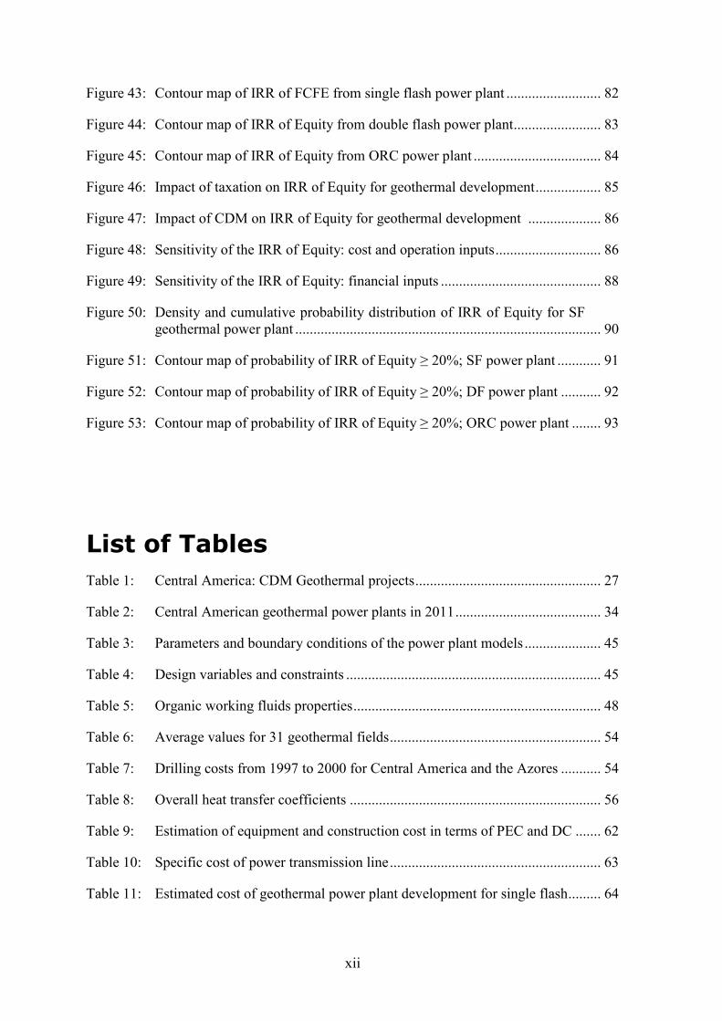
was 5,735.6 GWh, generated from 37.5% thermal, 36.2% hydro, 24.8% geothermal and 1.5% from imports. In El Salvador, the largest share of net injection (63%) came from private hands (CEPAL, 2011).

Figure 3: El Salvador: Net injection by source in 2010; installed electricity generation

capacity 1990-2010

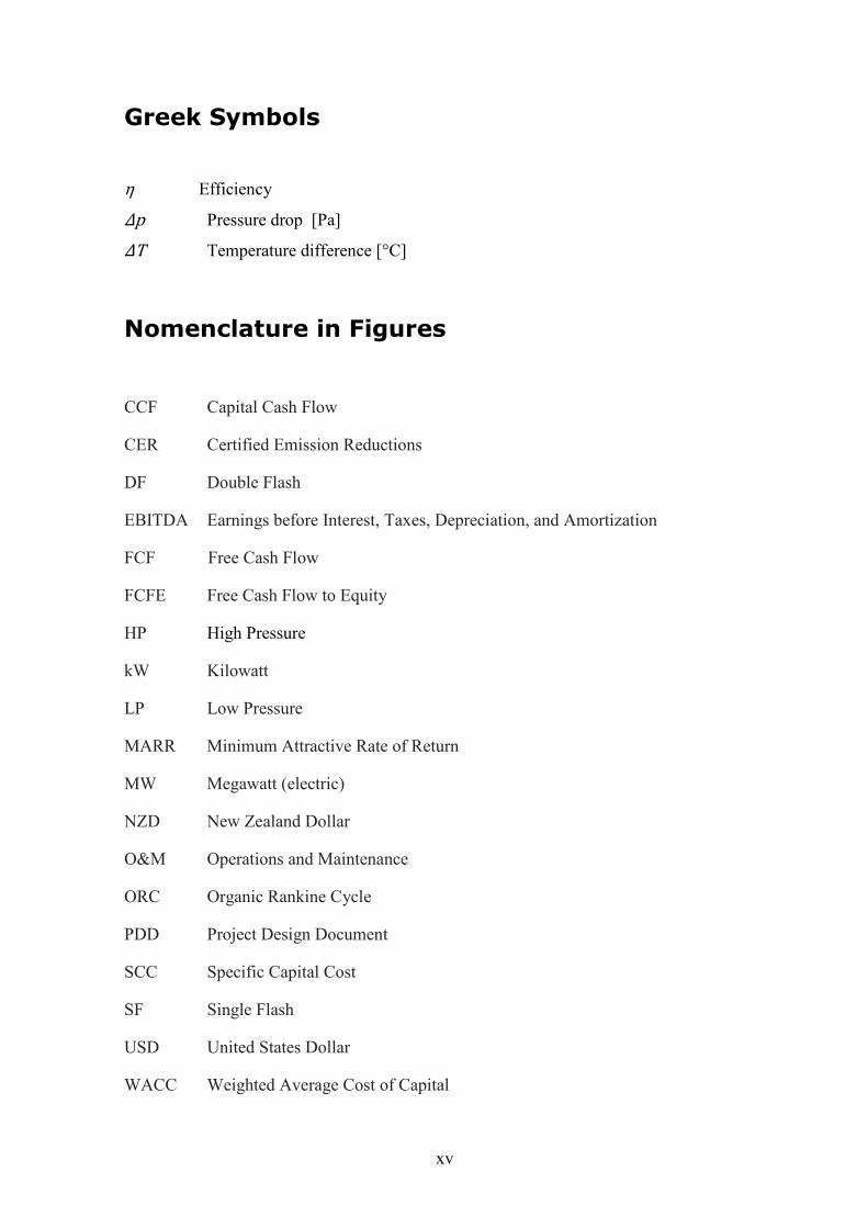
2.2.3 Honduras

The Honduran electricity market sustains itself via the electric law approved in 1994. It promotes competition in the wholesale market of median energy by the separation of generation, transmission and distribution, and the supply of electricity services by private agents. However, according to the consulting firm Pampagrass (2009), ENEE (Empresa

Nacional de Energía Eléctrica) converted itself into the only buyer for the entire system and kept its dominating presence in the sector. The opportunity market is very marginal even though legislation gives them options to participate; independent commercial agents and the activity of larger consumers are marginal.

Figure 4: Honduras: Net injection by source in 2010; installed electricity generation

capacity 1990-2010

In 2010, the total installed capacity across all available resource types in Honduras was 1,610.4 MW and peak demand was 1,245.0 MW. Thermal had the largest installed capacity 67.3% and hydroelectric 32.7%. Figure 4 shows that, in terms of evolution, installed capacity has almost tripled in the last 20 years. Yearly demand was 6,743.9 GWh,

0

200

400

600

800

1,000

1,200

1,400

1,600

19

90

19

94

19

96

19

98

20

00

20

02

20

04

20

06

20

08

20

10

MW

Hydro Geothermal Thermal


Hydro

2,079.1 GWh

36.2%

Geothermal

1,421.1 GWh

24.8%

Thermal

2,150.2 GWh

37.5%

Imports

85.2 GWh

1.5%


0

200

400

600

800

1,000

1,200

1,400

1,600

1,800

19

90

19

95

20

00

20

04

20

05

20

06

20

07

20

08

20

09

20

10

MW

Hydro Thermal


Hydro

3,080.2 GWh

45.7 %

Thermal

3,641.6 GWh

54.0%

Imports

22.1 GWh

0.3 %


22

generated from 54% thermal, 45.7% hydro and 0.3% from imports. In Honduras, the largest share of net injection (59.3%) was from private hands (CEPAL, 2011).

2.2.4 Nicaragua

INE (Instituto Nicaragüense de Energía) is in charge of the general direction of policies concerning electricity and is the national electricity regulator. According to Steinsdóttir and Ketilsson (2008), INE applies the policies defined by the government and is in charge of regulation and taxation. INE supervises the price purchase agreement (PPA) between the distributor and the developer. When the developer receives the exploration concession and has ascertained the base load, the developer applies to INE for a tariff. The developer can sell excess generation on the public market.

Figure 5: Nicaragua: Net injection by source in 2010; installed electricity generation

capacity 1990-2010

In 2010, the total installed capacity across all available resource types in Nicaragua was 1,067.6 MW and peak demand was 538.9 MW. Thermal had the largest installed capacity 76.1%, hydroelectric 9.8%, geothermal 8.2% and wind 5.9%. Figure 5 shows that, in terms of evolution, installed capacity has almost tripled in the last 20 years. Yearly demand was 3,304.7 GWh, generated from 71.9% thermal, 14.9% hydro, 8.1 % geothermal, 4.8% wind and 0.3% from imports. In Nicaragua, the largest share of net injection (80%) was from private hands (CEPAL, 2011).

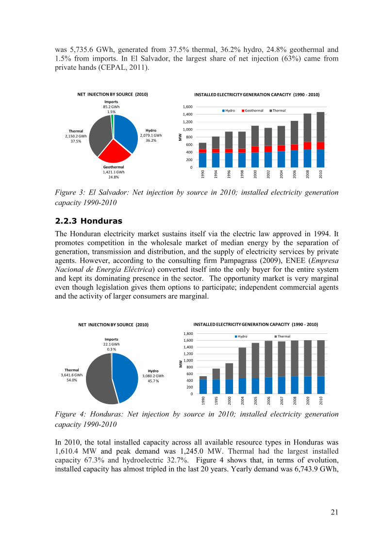
2.2.5 Costa Rica

Power service in Costa Rica is largely under the control of ICE (Instituto Costarricense de

Electricidad) which acts as an administrator and planner of short term policies, depending on the necessity of the electric system. ICE is the only buyer and owner of the electric transmission lines. From the capacity installed, ICE operates at 79.5% with proper plants and at 13.8% with hired plants with independent private generators (Grupo ICE, 2009). In 2010, the total installed capacity across all available resource types in Costa Rica was 2,605.3 MW and peak demand was 1,535.6 MW. Hydropower had the largest installed capacity 59.6%, 29.4% thermal, 6.4% geothermal and 4.6% wind. Figure 6 shows that, in terms of evolution, installed capacity has almost doubled in the last 10 years. Yearly demand was 9,565.2 GWh, generated from 75.9% hydro, 12.3% geothermal, 7.4% thermal,

0

200

400

600

800

1,000

1,200

19

90

19

95

20

00

20

04

20

05

20

06

20

07

20

08

20

09

20

10

MW

Hydro Geothermal Wind Thermal


Hydro

495.0 GWh

14.9 %

Geothermal

268.2 GWh

8.1%

Thermal

2,375.0 GWh

71.9%

Imports

10.2 GWh

0.3 %

Wind

159.8 GWh

4.8 %


23

3.8% wind and 0.6% from imports. In Costa Rica, the largest share of net injection (80%) was from public hands (CEPAL, 2011).

Figure 6: Costa Rica: Net injection by source in 2010; installed electricity generation

capacity 1999-2010

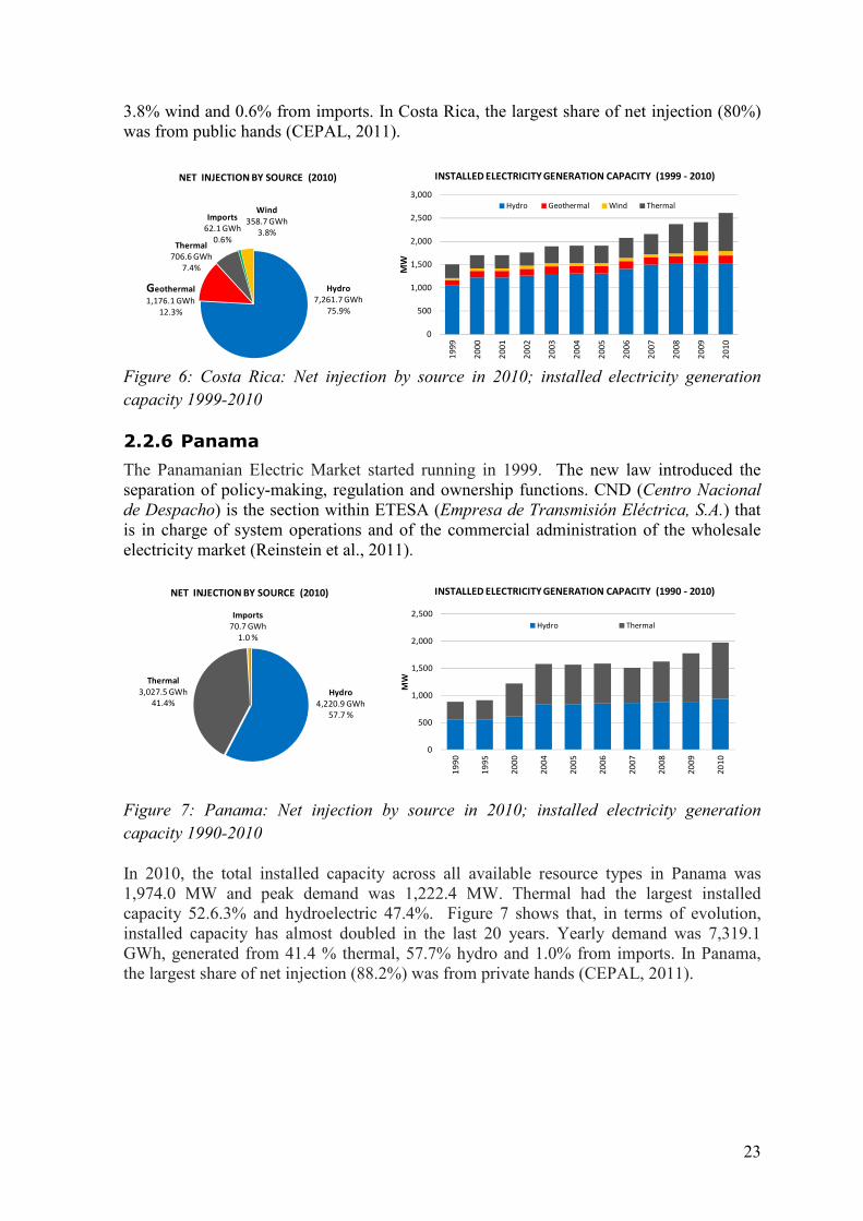
2.2.6 Panama

The Panamanian Electric Market started running in 1999. The new law introduced the separation of policy-making, regulation and ownership functions. CND (Centro Nacional

de Despacho) is the section within ETESA (Empresa de Transmisión Eléctrica, S.A.) that is in charge of system operations and of the commercial administration of the wholesale electricity market (Reinstein et al., 2011).

Figure 7: Panama: Net injection by source in 2010; installed electricity generation

capacity 1990-2010

In 2010, the total installed capacity across all available resource types in Panama was 1,974.0 MW and peak demand was 1,222.4 MW. Thermal had the largest installed capacity 52.6.3% and hydroelectric 47.4%. Figure 7 shows that, in terms of evolution, installed capacity has almost doubled in the last 20 years. Yearly demand was 7,319.1 GWh, generated from 41.4 % thermal, 57.7% hydro and 1.0% from imports. In Panama, the largest share of net injection (88.2%) was from private hands (CEPAL, 2011).

0

500

1,000

1,500

2,000

2,500

3,000

19

99

20

00

20

01

20

02

20

03

20

04

20

05

20

06

20

07

20

08

20

09

20

10

MW

Hydro Geothermal Wind Thermal


Hydro

7,261.7 GWh

75.9%

Geothermal

1,176.1 GWh

12.3%

Thermal

706.6 GWh

7.4%

Imports

62.1 GWh

0.6%

Wind

358.7 GWh

3.8%


0

500

1,000

1,500

2,000

2,500

19

90

19

95

20

00

20

04

20

05

20

06

20

07

20

08

20

09

20

10

MW

Hydro Thermal


Hydro

4,220.9 GWh

57.7 %

Thermal

3,027.5 GWh

41.4%

Imports

70.7 GWh

1.0 %


24

2.2.7 Regional market

In 1996, the signing of the Marco Treaty of the Electrical Market of Central America and of its two protocols fixated the legal framework for developing the project of the Central America Electric Interconnection system (SIEPAC). The project has 2 levels: the creation of a sub regional market of electricity, and the construction of a transmission line of 230 kV, 18,000 kilometers in length along the isthmus, which will allow the interchange of 300 MW between countries. The MER is the seventh market, superimposed over the six markets or existing national systems, with regional regulation, in which the agents of EOR (Ente Operador Regional) make international transactions of electrical energy in the Central American region. It is expected that the SIEPAC project will begin operating in 2013, expanding the potential of regional energy trade and the regional development of renewable generation.

2.2.8 Market analysis

In El Salvador, Guatemala, Nicaragua and Panama, generation costs are determined by the sum of the costs of energy production and the capacity of energy supply contracts in the long term (competitive bidding) and the cost of the purchasing spot market (economic dispatch based on the cost), with some leveling mechanism to mitigate the volatility of generation costs. Spot prices in wholesale markets competitive in the region increased significantly after 2004 due to soaring bunker prices. In Honduras and Costa Rica, generation costs used to regulate retail prices were lower and more stable than in Panama, Nicaragua and El Salvador. These three countries were faced with a tight balance between supply and demand in 2006 and 2007. The spot price increase was more pronounced as they were dispatched by less efficient generating plants and so were more expensive; as a result, the annual average spot price increased by approximately 140 USD/MWh (Lecaros et al., 2010).

Figure 8: Central America: Annual energy prices in the wholesale market for years 1998-

2010; Note: a) Costa Rica: average price paid to private geothermal generator Miravalles III. b) Honduras: projected short-term marginal costs

0

25

50

75

100

125

150

175

200

225

250

19

98

19

99

20

00

20

01

20

02

20

03

20

04

20

05

20

06

20

07

20

08

20

09

20

10

US

$ /

MW

h

Averague El Salvador Guatemala Nicaragua

Honduras Costa Rica Panama MER

25

Due to the fact that most of the regulators in the region do not publish the prices of their contracts, this market analysis is based on historical prices, statistics collected from managers of the wholesale market of each country as shown in Figure 8. Based on this data, in this study an average price of 115 USD/MWh in the wholesale market in the Central American countries was estimated for year 2010 with an expected growth rate of 5%.

2.3 Corporate tax

The Central American countries’ tax system is based on the territoriality principle, and all standard deductions are allowed in determining taxable income. As shown in Figure 9, the corporate tax rates in these countries are around 25% and 30% (Deloitte, 2010). In this analysis, 30% as corporate tax is used.

Figure 9: Central American corporate tax income rates 2010

Central American countries, with the exception of El Salvador, have a common practice of allowing companies to carry forward losses, although compensation rules vary from one country to another. Depreciation is allowed for a standard range of fixed assets and is generally on a straight line basis. Each country has different annual depreciation rates for the major groups, and the most similar standard rates are 5% for buildings, 20% for machinery, 25% for vehicles, 25% for software, and 50% for other movable assets (UN, 2010).

2.4 Tax incentives for renewable energy

In the last decade (2000-2010), Central American countries have created public incentives regarding the development of renewable energy. In this section a summary is presented of the main laws that support and promote the development of new power generation projects from renewable sources for each country, highlighting income tax incentives and particular conditions.

0%

5%

10%

15%

20%

25%

30%

35%

Co

sta

Ric

a

El S

alv

ad

or

Gu

ate

ma

la

Ho

nd

ura

s

Nic

ara

gu

a

Pa

na

ma

Corporate Income Tax

26

2.4.1 Guatemala

The Law of Incentives for the Development of Renewable Energy Projects Decree 52-2003 (Ministerio de Energía y Minas, 2003) establishes the exemption in customs duties for imports, including Value Added Tax (VAT) charges and fees on imports of machinery and teams. In addition, there is an exemption on income tax for a period of 10 years. These incentives are effective from the exact date the project begins commercial operation.

2.4.2 El Salvador

The Law of Fiscal Incentives for the Promotion of Renewable Energies in Electricity Generation (Decreto Legislativo No. 462, 2007) states that for those projects up to 20 MW, there is an exemption for a period of 10 years on tariffs on imports of machinery, equipment, materials and supplies for the stages of pre-investment and investment in the construction of power plants, including sub-transmission lines. There is an exemption on income tax for a period of 10 years for projects up to 10 MW of capacity. For projects of 10 to 20 MW, this exemption shall be for a period of 5 years. All income derived from the disposal of primary Certified Emissions Reductions (CERs) are tax exempt.

2.4.3 Honduras

The Incentives Act on Generation with Renewable Resources (Decreto 70-2007, 2007) establishes an exemption in import duties and taxes during the period of study and construction. There is an exemption in income tax, solidarity contribution, temporary tax on net assets, and those related to income taxes for a period of 10 years from the date of commencement of commercial operation, for projects with an installed capacity of up 50 MW.

2.4.4 Nicaragua

The Law for the Promotion of Energy Generation with Renewable Sources (Normas Jurídicas de Nicaragua, 2005) provides tax incentives such as an exemption on import duties and Value Added Tax for the work of pre-investment and construction, on machinery, equipment, materials and supplies, including sub-transmission lines. There is also an exemption on income tax for a period of 7 years from the project’s start of operations. During that same period, there shall be an exemption on income tax derived from revenues from the sale of carbon bonds.

2.4.5 Costa Rica

Under the current Costa Rican legal framework, the use of the geothermal resource can only be done by ICE; therefore, this is the only renewable source of energy that cannot be tapped for power generation by a private developer.

2.4.6 Panama

The incentives granted to the generators of energy from renewable sources were established by Law 45 (Ley No. 45, 2004). There are exemptions in taxes and duties associated with the importation of equipment and materials needed for construction, operation and maintenance. There is a fiscal incentive (as cited in Giardinella et al., 2010)

27

Country

Baseline

Emission

Factor

(tCO2-eq/MWh)

Project

Emissions

(tCO2/MWh)

Geothermal Project

PDD

Reference

El Salvador 0.612 0.028 Berlin Geothermal Project, Phase Two (UNFCCC, 2006)

El Salvador 0.693 0.000 Berlin Binary Cycle Power Plant (UNFCCC, 2007)

Guatemala 0.646 0.134 Amatitlan Geothermal Project (UNFCCC, 2008)

Costa Rica 0.152 − − (UNFCCC, 2004)

Nicaragua 0.754 0.074 San Jacinto Tizate Geothermal Project. (UNFCCC, 2005)

Honduras 0.555 − − (UNFCCC, 2005)

Panama 0.771 − − (UNFCCC, 2005)

for new and renewable energy projects of over 10 MW installed capacity, equivalent up to twenty five percent (25%) of direct investment, based on equivalent tonnes of CO2 emission reductions per year calculated for the term of the license or concession, which can only be used for payment of up to fifty percent (50%) of the revenue tax during the first 10 years of commercial operation, as long as the project is not benefitting from other incentives.

2.5 Clean Development Mechanism

The Clean Development Mechanism (CDM) is one of the three flexibility mechanisms of the Kyoto Protocol under the United Nations Framework Convention on Climate Change (UNFCCC). According to the UNFCCC (2011), the CDM allows emission reduction projects in developing countries by developed countries to earn Certified Emission Reduction (CER) credits, each equivalent to one tonne of CO2 reduced. These CERs can be traded and sold, and used by industrialized countries which have ratified the Kyoto protocol to meet part of their emission reduction targets under the Protocol. The crediting period for a CDM project has two options: fixed for a maximum period of 10 years or; renewable for a single crediting period of a maximum of 7 years and may be renewed at most 2 times. Central American countries are candidates for applying this mechanism for development of geothermal prospects. As shown in Table 1, there are already four geothermal projects in Central America that are register as CDM. Most of the geothermal projects in Central America, with the exception of Costa Rica, could replace electricity from relatively carbon intensive grids. The combined margin emission factor (CM) for Central American countries is in the range 0.152 to 0.771 tCO2-eq/MWh for a grid with a mix of thermal and non thermal power plants. It is important to note that these emission factors vary in each country according to the baseline year in the PDD, data and the number of the clean energy sources commissioned. According to Quinlivan et al. (2006), the baseline emissions are calculated as Project MWh x CM, and project CERs as:

�� = �� !"# ��"��"$#� − &�$' �(��"��"$#� − &�$' �() �*�+ ,"-�#./,1/

Table 1: Central America: CDM Geothermal projects

28

According to Delivand et al. (2011) the revenue from CER can be estimated by multiplying the carbon emission reduction (Eq. 1) by the price of carbon credit. There is not a fixed carbon trade price, and the price changes daily (see http://www.bluenext.eu/). This recent study (Delivand et al., 2011) considered price per CER at 11.93 Euro (15.66 USD) for the year 2011. This compares quite well with Angantýsson (2011) who showed that the average closing price of CERs from the date of January to August 2011 was 15.59 USD. CER price in the spot market is volatile, making it difficult to make the right decision in a future investment when the future price of carbon credit is highly uncertain (Retamal, 2009). A table in a price forecasting study from various institutes shows that CER prices by the year 2030 might be 34-50 Euro/tonne (GreenMarket, 2011). When registering a geothermal project under the CDM, the project developer needs to cover the costs accruing during the steps of the CDM project cycle. According to the CDM Rulebook (Baker & McKenzie, 2011), a registration fee which has applied since February 2010 is calculated using the following scale: 0.10 USD per certified emission reduction issued for the first 15,000 tonnes of CO2 equivalent for which issuance is requested in a given year; 0.20 USD per certified emission reduction issued for any amount in excess of 15,000 tonnes of CO2 equivalent for which issuance is requested in a given year. This registration fee scale is used in this analysis. The basic financial model does not consider the revenue of the CER sales. However, the CERs factor affects the operation statement and, therefore, is considered a potential impact on the IRR for geothermal development projects (Section 6.7). The emissions factor is critical to the volume of CERs produced from a geothermal power plant. In this study, the baseline emission factors evaluated are 0.2 tCO2-eq/MWh (for a grid based on renewable resources such as in Costa Rica), 0.5 tCO2-e/MWh (for a grid based on mixed renewable and fuel resources such as in Guatemala, El Salvador and Honduras) and 0.8 tCO2-eq/MWh (for a grid dominated by fuel resources such as in Panama and Nicaragua). Other assumptions for calculations are project emissions of 0.06 tCO2/MWh, and a CERs price of 15 USD/tCO2 with a growth rate of 5%.

2.6 Climatic factors

As seen in Figure 10, the regions in Central America where most geothermal areas coincide with higher temperatures (23°C and above) are found south of Guatemala, in southern El Salvador, in southwest Nicaragua and northwest Costa Rica. According to PREVDA (2010), in Central America average annual temperature values for the Pacific coast are between 26 and 27°C, with maximums of 28°C in parts of Guatemala, Honduras, Nicaragua and northwest Costa Rica.

Altitude is the factor that exerts the greatest influence on the thermal regime in Central America. In the Pacific and Caribbean sides of the areas located between an elevation of sea level and 600 meters, the average annual temperature varies between 24 and 27°C. The intermediate parts of the ridges and mountains, ranging in altitude between 600 and 1,200 meters, present mean annual temperatures of between 19 and 23 °C, while for the territories located between 1,200 and 1,800 meters, the average annual temperature ranges

29

from 17 to 20°C. Mainly, these ranges in average air temperature can be observed in the central areas of Nicaragua, Honduras, El Salvador and Panama. According to some of the national weather offices in Central American countries (e.g. SNET, INSIVUMEH, SERNA), the relative humidity varies from 60 to 85%, with an average of 80%. In this study, for calculations in the power plant model, a maximum dry air temperature of 28°C and relative humidity of 80% are used.

Figure 10: Central America: average air dry temperature and locations of main

geothermal areas; Figure modified from PREVDA (2010)

Annual Mean

Temperature

(°C)

31

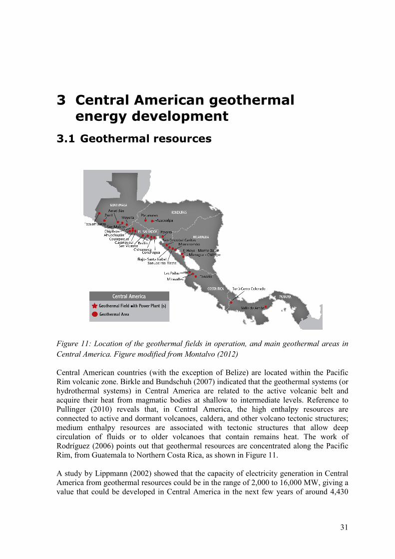
3 Central American geothermal energy development

3.1 Geothermal resources

Figure 11: Location of the geothermal fields in operation, and main geothermal areas in

Central America. Figure modified from Montalvo (2012)

Central American countries (with the exception of Belize) are located within the Pacific Rim volcanic zone. Birkle and Bundschuh (2007) indicated that the geothermal systems (or hydrothermal systems) in Central America are related to the active volcanic belt and acquire their heat from magmatic bodies at shallow to intermediate levels. Reference to Pullinger (2010) reveals that, in Central America, the high enthalpy resources are connected to active and dormant volcanoes, caldera, and other volcano tectonic structures; medium enthalpy resources are associated with tectonic structures that allow deep circulation of fluids or to older volcanoes that contain remains heat. The work of Rodríguez (2006) points out that geothermal resources are concentrated along the Pacific Rim, from Guatemala to Northern Costa Rica, as shown in Figure 11. A study by Lippmann (2002) showed that the capacity of electricity generation in Central America from geothermal resources could be in the range of 2,000 to 16,000 MW, giving a value that could be developed in Central America in the next few years of around 4,430

32

WM (Figure 12). However, only a relatively minor amount has been developed for power production; in a region endowed with an abundance of geothermal resources, the installed capacity by year 2010 was only 506.8 MW, as described in Chapter 2.

Figure 12: Central America: Geothermal installed electricity generation capacity

(CEPAL, 2010) vs. Most probable geothermal potential (Lippmann, 2002)

3.1.1 Guatemala

The geothermal power plant Zunil (25.2 MW) and Amatitlán (24 MW) supply approximately 3.1% of Guatemala´s electricity. Zunil I, drilled in 1991, identified a single phase 300°C resource. Amatitlán, an exploration well drilled in 1993, confirmed the existence of a deep chloride rich geothermal system with a temperature of 285°C (Asturias, 2008).

Asturias and Grajeda (2010) reported that evaluation of the Moyuta area in 1990 indicated that the reservoir consists of two subsystems with expected temperatures of 210 and 170°C. The results of the regional reconnaissance in 1981 identified 13 geothermal areas, of which 7 areas were selected with temperatures from 230 to 300°C. Listed in order of decreasing priority they are: Amatitlán, Tecuamburro, Zunil I, Zunil II, San Marcos, Moyuta, and Totonicapán. Second priority areas with low temperature resources are: Los Achiotes, Palencia, Retana, Ayarza, Atitlán, Motagua and Ipala.

3.1.2 El Salvador

El Salvador is the largest producer of geothermal energy in Central America (by year 2010); the power plants Ahuachapán (95 MW) and Berlín (109.4 MW) supply approximately 25% of El Salvador’s electricity.

Herrera et al. (2010) reported the temperatures of geothermal resources as being 250°C in Ahuachapán, 300°C in Berlín, 230°C in San Vicente, 240°C in Chinameca, and there are several resources below 200°C all along the volcanic chain. Depths range from as little as 600 m in the shallow areas of Ahuachapán, to about 2,800 m in the deep parts of Berlín. Pullinger (2009) reported that another area with a possible high enthalpy resource is the

0

200

400

600

800

1000

1200

1400

1600

1800

2000

Co

sta

Ric

a

El S

alv

ad

or

Gu

ate

ma

la

Ho

nd

ura

s

Nic

ara

gu

a

Pa

na

má

MW

Installed Capacity Potential

33

Coatepeque geothermal field, where an initial pre-feasibility study in the mid 1990s identified a possible resource with temperatures of around 220°C. Medium enthalpy resources such as Conchagua, Chilanguera and Obrajuelo geological, geochemical and geophysical field studies have identified resources with estimated temperatures of 180 to 220°C.

3.1.3 Honduras

Platanares is the only geothermal project under development in Honduras where performed studies showed that a potential of 35 MW could be achieved. Pavana and Azacualpa projects are under study.

Lagos and Gomez (2010) reported that, in the evaluation of Platanares, higher temperatures between 160 and 165°C were found at shallow depths and geothermometers suggested resource temperatures of between 200 and 225°C. Updated studies show a potential of 23 MW in Azacualpa with temperatures between 170 and 180°C, and 18 MW in Pavana with temperatures between 140° and 150°C. The main geothermal areas identified during the surface exploration in the 1970s are Platanares, San Ignacio, Azacualpa, Sambo Creek, Pavana, El Olivar and El Tigre Island.

3.1.4 Nicaragua

The Momotombo plant has 70 MW of installed capacity; however, there have been declines in the output levels. In year 2010, INE reported that the installed capacity available was 26.5 MW. San Jacinto Tizate (in year 2011) was operating at 10 MW and is under a two phase 72 MW expansion. In Momotombo, more than 44 exploration wells have been drilled (up to 2,500 m in depth), encountering temperatures in excess of 330°C (Mostert, 2007). Pullinger (2009) reported that in San Jacinto Tizate geothermal area, several wells were drilled (up to 2,200 m in depth) and confirmed the existence of temperatures from 260 to 290°C; and in El Hoyo Monte Galán geothermal area, temperatures of 220°C (at 2,000 m) were identified. Zúñiga (2005) pointed out that there were more promising geothermal areas: Managua-Chiltepe and Masaya-Granada-Nandaime. Other areas with possible high enthalpy resources mentioned in Nicaragua´s Geothermal Master Plan (2001) are Casita-San Cristobal volcano and Concepción volcano on the island of Ometepe.

3.1.5 Costa Rica

According to Projekt Consult GmbH and Loy D. (2007), the potential geothermal power in Costa Rica is estimated by some sources to be as high as 900 MW; nevertheless, ICE assumes a potential of only 235MW, as its analysis takes into account certain restrictive factors (large numbers of the suitable sites are located in national parks and the operation of such facilities at these locations is prohibited by law). Miravalles (165.5 MW) is the first operational geothermal power plant in Costa Rica since 1994. Las Pailas (35 MW) geothermal power plant, located at the Rincón de La Vieja Volcano, started in 2011 (GRC, 2011). Miravalles geothermal field presents a water dominated reservoir with an average temperature of 240°C. Las Pailas geothermal field,

34

during feasibility studies, confirmed the existence of a geothermal reservoir with temperatures near 260°C (Protti, 2010). Fung (2008) reported a geothermal area under feasibility studies at Borinquen where a production well was drilled with the highest measured bottom hole temperature (275°C) in Costa Rica. Tenorio and Nuevo Mundo geothermal areas are under pre-feasibility studies; Pocosol and the northern part of the Rincón de la Vieja volcano are under reconnaissance studies. In Pocosol, geothermometers suggested a reservoir temperature of 183 to 217°C. Other potential geothermal areas identified around the volcanoes are Platanar, Poás, Barva, Irazú and Turrialba.

3.1.6 Panama

The potential for geothermal power in Panama has been studied on several occasions since the 1970s, and five main areas for potential geothermal power generation have been evaluated since: Barú-Colorado, Valle de Antón, Coiba Island, Tonosí and Chitre de Calobre. The different studies varied in conclusions, placing the entire geothermal potential for Panama between 100 MW and 450 MW (Giardinella et al., 2011). In August 2006, the firm West Japan Engineering Consultants, Inc., in the framework of the Puebla-Panama Plan, presented the most recent preliminary estimate of the geothermal potential of Panama for the Baru-Colorado area as 24 MW, and for the Valle de Anton area 18 MW (ETESA, 2011).

Table 2: Central American geothermal power plants in 2011

Country Type of

Unit

Total

Installed

Capacity

MW

Ahuachapan Unit 1-2 Single Flash 30.0

Ahuachapan Unit 3 Double Flash 35.0

Berlin Unit 1-2 Single Flash 28.0

Berlin Unit 3 Single Flash 44.0

Berlin Unit 4 Binary 9.4

Orzunil Unit 1-7 Binary 24.0

Ortitlan Unit 1 Binary 25.2

Miravalles Unit 1-2 Single Flash 55.0

Miravalles Unit 3 Single Flash 29.5

Miravalles Unit 5 Binary 21.0

Miravalles WHU 1 BackPressure 5.0

Pailas Pailas I Binary 41.0

Momotombo Unit 1-2 Single Flash 35.0

Momotombo Unit 3 Binary 7.5

San Jacinto Tizate Unit 1-2 BackPressure 5.0

Costa Rica

El Salvador

Power Plant Name

Nicaragua

Guatemala

35

4 Geothermal electrical power assessment

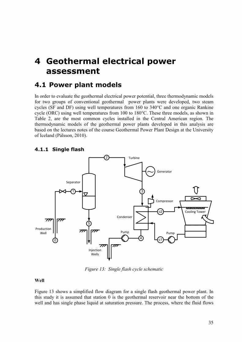
4.1 Power plant models

In order to evaluate the geothermal electrical power potential, three thermodynamic models for two groups of conventional geothermal power plants were developed, two steam cycles (SF and DF) using well temperatures from 160 to 340°C and one organic Rankine cycle (ORC) using well temperatures from 100 to 180°C. These three models, as shown in Table 2, are the most common cycles installed in the Central American region. The thermodynamic models of the geothermal power plants developed in this analysis are based on the lectures notes of the course Geothermal Power Plant Design at the University of Iceland (Pálsson, 2010).

4.1.1 Single flash

Figure 13: Single flash cycle schematic

Well

Figure 13 shows a simplified flow diagram for a single flash geothermal power plant. In this study it is assumed that station 0 is the geothermal reservoir near the bottom of the well and has single phase liquid at saturation pressure. The process, where the fluid flows

0

1

2

~

5

3

4

Production

Well

c1

c2

Injection

Wells

Separator

Turbine

Generator

Condenser

Cooling Tower

PumpPump

Compressor

36

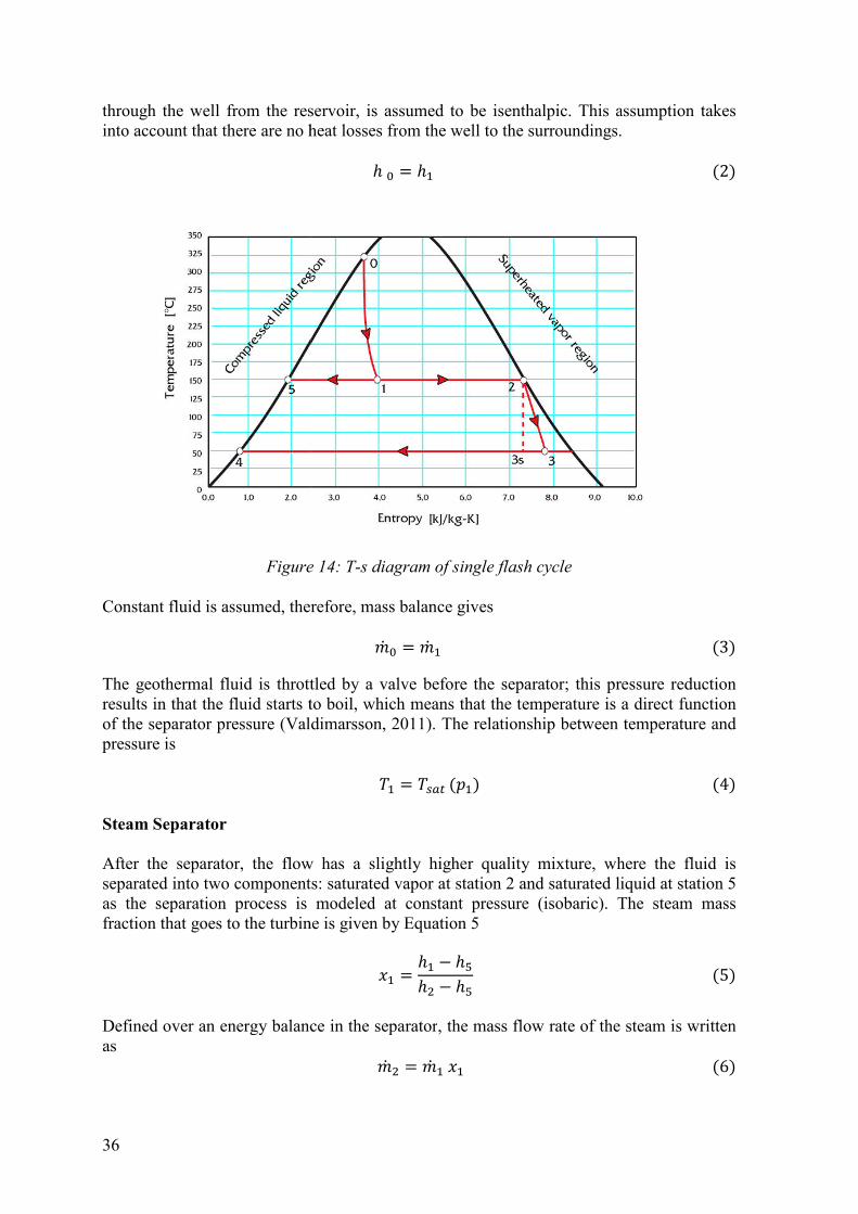
through the well from the reservoir, is assumedinto account that there are no heat losses fr

Figure

Constant fluid is assumed, therefore, mass balance gives

The geothermal fluid is throttled by a valve before results in that the fluid starts to boilof the separator pressure (Valdimarsson, 2011pressure is

Steam Separator

After the separator, the flowseparated into two components: as the separation process is fraction that goes to the turbine

Defined over an energy balance in the separatoras

om the reservoir, is assumed to be isenthalpic. This assumption takes into account that there are no heat losses from the well to the surroundings.

ℎ1 = ℎ2

Figure 14: T-s diagram of single flash cycle

therefore, mass balance gives

�� 1 = �� 2is throttled by a valve before the separator; this pressure reduction starts to boil, which means that the temperature is a direct function

(Valdimarsson, 2011). The relationship between temperature and

32 = 3456,�2/

the flow has a slightly higher quality mixture, where the fluid separated into two components: saturated vapor at station 2 and saturated liquid at station s the separation process is modeled at constant pressure (isobaric). The steam

fraction that goes to the turbine is given by Equation 5

�2 = ℎ2 − ℎ7ℎ8 − ℎ7 energy balance in the separator, the mass flow rate of the steam is written

�� 8 = �� 2�2

. This assumption takes om the well to the surroundings.

,2/

,3/ this pressure reduction

that the temperature is a direct function een temperature and

,4/

a slightly higher quality mixture, where the fluid is 2 and saturated liquid at station 5

The steam mass

,5/ of the steam is written

,6/

37

Turbine

Saturated steam, which is a small fraction of the total geothermal fluid, is expanded in the turbine, where some of the steam energy is transformed into mechanical energy in the shaft. In an ideal turbine, it is assumed to be a constant entropy process (isentropic) from the inlet at station 2 to the ideal exit at point 3s. The isentropic enthalpy at 3s is then calculated from the pressure at point 3 and the entropy at point 2. The expansion is irreversible, and the steam entropy is higher. Turbines are classified with an isentropic efficiency parameter that is given by the manufacturer, defined as

>6 = ℎ8 − ℎ?ℎ8 − ℎ?,4 ,7/ From Equation 7 above, the real turbine exit at station 3 can be calculated. The total power output of the turbine is given by B6 = �� 8,ℎ8 −ℎ?/,8/ The total electricity generated is equal to the work output of the turbine multiplied by the generator efficiency, written as

BD = >EB6,9/ The net contribution of that power plant to the electric grid can be calculated by subtracting all internal power consumption to the generator output.

Condenser with heat exchange

Steam exhaust from the turbine is cooled without mixing using water from the cooling tower in a surface type condenser. The goal is to condense this steam by extracting energy because it requires less work to pump an incompressible liquid than compressible gas or steam at state 4. The energy extracted is calculated by using the mass flow of steam and the enthalpy difference at stations 3 and 4, as follows GH =�� 8,ℎ? −ℎI/,10/ Equation 11, based on the energy balance in the exchanger, is �� 8,ℎ? −ℎI/ = �� K,ℎH8 −ℎH2/,11/ The heat exchange is determined by the temperature difference; therefore, the maximum temperature of the cooling water must not exceed the condensation temperature in the condenser. According to Pálsson (2010) there should be at least 5°C difference between those numbers, written as follows

3H8 = 3? − 5,12/

38

Assuming that condensation takes place at a constant temperature, a simplified equation can be given as 3I = 3?,13/ Since a temperature value is fixed on the design for the inlet cooling water temperature, all temperature variables can be identified. Therefore, Equation 11 can be used to calculate the required flow rate of the cooling water at station c1.

Gas extraction

The geothermal steam includes non condensable gases all the time. Carbon dioxide is typically about 98% of the gas content and is released to the atmosphere in most geothermal power plants (Thorhallsson, 2005). In this analysis, the composition of the non-condensable gases is assumed to be 100 % CO2. Non condensable gases cause a problem in the condenser; while the steam is condensed and pumped out, the gases are kept on in gaseous form producing an increase in the pressure in the condenser. A possible solution to this problem is to compress the gases and suck them out of the condenser. In the extraction process, some amount of steam will always be included since the steam is mixed with other gases inside. Hence, the gas mixture is then assumed to be saturated with steam when it is sucked out from the condenser. According to Pálsson (2010) the mass of steam extracted can be defined as

�� L = �L�4�5,�H − �4/�� 5,14/

where �L is the mass molar mass of water and �5 is the mass molar mass of gases, �4 is the saturation pressure of steam at the gas outlet temperature, �H is the condenser pressure and �� 5 is the mass flow of gases into the condenser.

The energy required for the pump is calculated by an ideal isentropic process between the condenser pressure and the atmospheric pressure. The mixture properties are calculated as follows

� = �5 + ,�L −�5/ �4�L�H,�5 +�L/,15/

� = �5 + ,�L − �5/ �4�L�H,�5 +�L/,16/ where � is the specific heat of the gas and the vapor mixture that is pumped out of the condenser, and R is the ideal gas constant for the mixture. The ideal enthalpy change of the fluid when compressed to atmospheric pressure can be written as

39

∆ℎ = �34 OP�56Q�H R SHT − 1U,17/ Including the compressor efficiency>H, the demanding power for the pump can be calculated as

BH = ,�� 5 +�� L/∆ℎ>H ,18/ Cooling tower

In this case, air cooling in a forced flow cooling tower is used to accommodate the heat load from the condensing steam. A cooling tower is an evaporative heat transfer device in which atmospheric air cools warm water with direct contact between the water and the air, by evaporating part of the water (Siregar, 2004). As shown in Figure 13, the cooling water is pumped from the pond to the condenser at station 1; after this, warm water at station c2 is cooled by being sprayed into the tower where it falls through; using fans at the top of the tower, an air stream is drawn into the tower at station c3, and flows out at station c4.

According to Pálsson (2010) it can be assumed that the relative humidity of the outlet (c4) is 100% if the tower is satisfactorily large. In regards to a mixture of air and water, with their respectively molar masses being Ma and Mw, the partial pressures of the air and water are defined as

�5 = � ∗ .5,19/ �K = � ∗ .K,20/

Then, taking into account the saturation pressure of water at given pressure �4, the relative humidity is denoted as

W = �K�4 ,21/ The humidity ratio is defined as

X = �K ∗ W ∗ �4�5 ∗ ,� − �4/,22/ Overall, cooling tower balance equations are formulated in order to find the required mass flow rate. Mass balance for dry air (Eq. 19) and water (Eq. 20) are given by

�� 5,H? = �� 5,HI = �� 5,23/ �� K,H2 +�� K,H? = �� K,H8 + �� K,HI,24/

And the energy balance equation is

ℎK,H2�� K,H2 + ℎK,H?�� K,H? + ℎ5,H?�� 5,H? = ℎK,H2�� K,H2 + ℎK,H?�� K,H? + ℎ5,H?�� 5,H?,25/

40

Introducing �� K,H? =X?�� 5,H? and �� K,HI =X?�� 5,HI into Equations 19 and 20, then solving the system for �� 5 , Equation 25 becomes

�� 5 = YℎK,H2 − ℎK,H8Z�K,H2ℎK,H8,XH? − XHI/ + ℎ5,HI + XHIℎK,HI– ,ℎ5,H? +X?ℎK,?/,26/ The amount of air for the cooling tower can be used to estimate the necessary power for drive fans and consequently estimate their cost.

4.1.2 Double flash

Figure 15 shows a simplified flow diagram of a double flash geothermal power plant. This process is called a second flashing process because it includes a secondary pressure step, which utilizes the waste heat in the geothermal brine from the high pressure (HP) separator. Saturated steam extracted from the second low pressure (LP) separator is mixed with other wet steam from the high pressure turbine to obtain greater steam quality. The extra steam gained passes through a low pressure turbine, and additional power is produced from the generator coupled with the second turbine (Dagdas, 2007). Thermodynamic equations presented in Section 4.1.1 for the single flash process are valid for modeling a double flash cycle. Figure 15 shows the schematic process of a double flash cycle.

Figure 15: Double flash cycle schematic

Low Pressure Separator

The brine from the high pressure separator is at station 3, and is throttled down to a lower pressure level at station 4. Assuming an isenthalpic process gives

0

1

2

3

8

9

6

10

5 7

c1

c2

Production

Well

HP

Turbine

Injection

Wells

HP

Separator

LP

Separator

LP

Turbine

Compressor

PumpPump

Cooling Tower

Generator

Condenser4

~

After second flashing the resulting saturated steam at station 5 is mixed with exhaust steam from station 6. The mixing takes ,

Figure

Low Pressure Turbine

The single steam flow at stationthe low pressure part of the turbine can be calculated as

The total electricity generated generator efficiency, as shown tower, gas extraction system, condenser and pumps are done in a similar procedurethe single flash process described

4.1.3 Organic Rankine c

In an organic Rankine cycle (ORC) unit the heat of the geothermal water is transferred to a secondary working fluid, usually an organic fluid that has a low boiling point and high vapor pressure when compared to water at a given temperature. The cooled geothermal water is then returned to the ground to recharge the reservoir ( Boiler

According to Valdimarsson the well at the source inlet temperature at

ℎ? = ℎIresulting saturated steam at station 5 is mixed with exhaust steam

from station 6. The mixing takes places while conserving energy, and can be written as

,�� 7 +�� \/ℎ] =�� \ℎ\ +�� ]ℎ]

Figure 16: T-s diagram for double flash

at station 7 is led to the low pressure turbine. The power output of pressure part of the turbine can be calculated as

B^� = ,�� 7 +�� \/,ℎ] −ℎ_/he total electricity generated is equal to the work output of the turbine multiplied

iency, as shown in Equation 9. Calculations for the HP turbine, cooling on system, condenser and pumps are done in a similar procedurecess described in Section 4.1.1.

Organic Rankine cycle

ycle (ORC) unit the heat of the geothermal water is transferred to a working fluid, usually an organic fluid that has a low boiling point and high

vapor pressure when compared to water at a given temperature. The cooled geothermal water is then returned to the ground to recharge the reservoir (Franco and Villani

Valdimarsson (2010), the geothermal fluid (frequently liquid waterthe well at the source inlet temperature at station 9 (Figure 17) and, if the pressu

41

,27/ resulting saturated steam at station 5 is mixed with exhaust steam

places while conserving energy, and can be written as

,28/

The power output of

,29/ work output of the turbine multiplied by the

HP turbine, cooling on system, condenser and pumps are done in a similar procedure as for

ycle (ORC) unit the heat of the geothermal water is transferred to a working fluid, usually an organic fluid that has a low boiling point and high

vapor pressure when compared to water at a given temperature. The cooled geothermal Franco and Villani, 2009).

frequently liquid water) enters f the pressure is kept

42

sufficiently high, any non-condensable gases will be released from the liquid; therefore, a gas extraction system is not required. The geothermal fluid is then cooled down in the boiler and heater, and sent to re-injection at station 11.

Figure 17: ORC cycle with regeneration schematic

The reason for separating the fluid in the heat exchanger and the brine into two parts is a potential minimum temperature difference within the heat exchanger. This minimum (or pinch point) is located at point 4 where the working fluid starts to boil (Pálsson, 2010). Assuming that point 4 is the minimum, this gives 321 = 3I +3,30/ The energy balance equation of boiler can then be determined as �� `,ℎ` − ℎ21/ = �� ?,ℎ7 − ℎI/,31/

9

~

7

1

10

5

4

11

6

2

3

Turbine

Condenser

Pump

Recuperator

Boiler

Pre-heater

Production

Well

Injection

Well

c1

c2 Cooling Tower

Pump

Recuperator

Valdimarsson (2010) concludes that the regeneration process serves only to move the highest power production towards can help in the case of a lower limit on the geothermal fluid temperature imposed by chemistry or by the requirements of a secondary process. The temperature at the temperature. Therefore, this temperature difference can be utilized for heating the working fluid at the entrance to the be described as follows

Figure 18: T-s diagram of an ORC cycle (Isopentane) with

Condenser

For the binary condensercondensation. Therefore, the process has tsuperheated vapor can be described

�̅ Second, condensation of the working fluid vapor �̅b3 where h]d2 is the enthalpy of the working fluid pinch point in the condenser

Valdimarsson (2010) concludes that the regeneration process serves only to move the highest power production towards a higher geothermal return temperature; regeneration can help in the case of a lower limit on the geothermal fluid temperature imposed by

the requirements of a secondary process.

the turbine outlet is somewhat higher that this temperature difference can be utilized for heating the working

the pre-heater. The energy balance equation for the

,ℎ\ − ℎ]/ = ,ℎ? − ℎ8/

diagram of an ORC cycle (Isopentane) with regeneration

binary condenser, the superheated vapor it must be cooledcondensation. Therefore, the process has to be divided into two steps. First

can be described as

�̅b3Heef�gE�� H2 = �� 7,ℎ] − ℎ]d2/

the working fluid vapor can be calculated as

b3HeghDg4�gE�� H2 = �� 7,ℎ]d2 − ℎ]/

is the enthalpy of the working fluid in a saturated vapor state, where pinch point in the condenser is located.

43

Valdimarsson (2010) concludes that the regeneration process serves only to move the higher geothermal return temperature; regeneration

can help in the case of a lower limit on the geothermal fluid temperature imposed by

turbine outlet is somewhat higher that the condensation this temperature difference can be utilized for heating the working

heater. The energy balance equation for the recuperator can

,32/

regeneration

be cooled previous to two steps. First, cooling the

,33/

,34/

saturated vapor state, where the

44

4.2 Simulation and optimization

Central America is a small geographic region divided politically into many territories. There exist similar economic and climatic conditions for the design of geothermal plants. However, geothermal reservoir and well properties differ from site to site and, as such, require serious attention during the design process as they are critical parameters for optimization. In this analysis, power plant models for Central America were designed based on the technical parameters which do not change from case to case and on the similar climatic conditions of the region. The methodology applies the fundamental principles of thermodynamics to the components of the cycle and to the cycle itself to form a system of non linear equations as developed in Section 4.1. The optimization process was solved by using the mathematical environment called Engineering Equation Solver (EES) which also evaluates thermodynamic properties and solves a system of non linear equations. The optimization process was done over three types of energy conversion systems: single flash (SF), double flash (DF) and organic Rankine cycle (ORC). For each of these cycles design variables and constraints were defined. The optimization constraints were applied by setting boundaries on each variable. In this analysis, the optimization process was carried out on the design variables using a direct search algorithm called the grid search method. According to Rao (2009) the method involves setting up a suitable grid in the design space, evaluating the objective function at all the grid points, and the point corresponding to the best objective function value is considered the optimum solution. The power output optimization process was repeated several times in each case for different resource temperatures and mass flows.

4.2.1 Assumptions and limitations

Simulation of the models of the energy conversion systems described in Section 4.1 required assumptions for a wide range of behavior of the geothermal system and technical characteristics of the power plant equipment. Table 3 gives a summary of assumptions used as input in this analysis. Some important assumptions not used as input for the analysis are:

• Well production is not dependent on wellhead pressure

• Evaporation of the cooling water is neglected

• The fluid chemistry is neglected

• Pressure losses in pipelines and other equipment are neglected

45

Power cycle Variable Contraint

SF Separator pressure Turbine exhaust dryness ≥ 0.85

HP Separator presure Turbine exhaust dryness ≥ 0.85

Turbine exhaust dryness ≥ 0.85

Pressure ≥ 75 kPa

Pinch at boiler ≥ 5°C

Pinch at recuperator ≥ 5°C

LP Separator presureDF

Boiler Pressure ORC

Table 3: Parameters and boundary conditions of the geothermal power plant models

4.2.2 Design variables and constraints

Basic components of an optimization problem involve an objective function expressing the main aim of the model which has to be minimized or maximized, a set of unknowns or variables which control the value of the objective function, and a set of constraints that allow unknowns to take on certain values but exclude others (Kumar, 2010).

In this analysis, the objective function is net power output per mass flow of geothermal fluid. Table 4 shows the optimization variables and constraints selected for the energy conversion systems. The optimization variables are independent design variables of each system. For SF and DF, separator pressure is considered the design variable, and for ORC the boiler pressure is used.

Table 4: Design variables and constraints

Unit Low High

Geothermal fluid

Maximum well head pressure kPa 100.0 3500.0

Non condensable gases in well mass flow % 0.5 0.5

Temperature of resource °C 100.0 340.0

Efficiencies

Turbine isentropic efficiency % 0.9 0.9

Compressor isentropic efficiency % 0.7 0.7

Pumps isentropic efficiency % 0.7 0.7

Fan efficiency % 0.7 0.7

Cooling system

Operating condenser pressure - Flash units kPa 10.0 10.0

Operating condenser pressure - ORC units kPa 140.0 600.0

Minimum pinch temperature in condenser °C 5.0 5.0

Increasing temperature of cooling water °C 12.0 12.0

Air dry temperature °C 28.0 28.0

Relative humidity % 0.8 0.8

Power

Plant

Geothermal

Reservoir

System Parameter Values

46

0.70

0.75

0.80

0.85

0.90

0.95

1.00

0

50

100

150

200

250

300

160 180 200 220 240 260 280 300 320 340

Ste

am

qu

ali

ty

[ -

]

Sp

eci

fic

ne

t p

ow

er

ou

tpu

t [

kW

/kg

/s

]

Resource temperature [ °C ]

Specific net power output Steam quality at turbine output

0

100

200

300

400

500

600

700

800

0

50

100

150

200

250

300

160 180 200 220 240 260 280 300 320 340

Sep

ara

tor

pre

ssu

re [

kP

a ]

Spe

cifi

c p

ow

er

ou

tpu

t [

kW

/kg

/s

]

Resource temperature [°C]

Specific net power output Separator pressure

4.3 Results

In this section SF, DF and ORC power plant cycles are evaluated for different resource temperatures (°C). The results present the optimum specific net power output (kW/kg/s) and the optimum working pressures (kPa) in the separator for SF and DF cases and in the boiler for the ORC case. In order to simplify reading from the graphs, the optimum net power output (kW) for a unit mass flow rate is used; the total power output can be obtained for each specific case simply by multiplying this by the actual mass flow rate in kg/s.

4.3.1 Single flash

The selection of the separator pressure has an important effect on the overall plant performance in terms of power output. High separator pressures result in higher working potential steam at the turbine inlet, a lower quality of steam in the turbine exhaust and higher injection temperature. Lower separator pressures increase the mixture quality in the separator, which means that more steam can be produced, but the specific available energy of the steam flow would decline.

Figure 19: Specific net power output and separator pressure of SF cycle

Figure 20: Specific net power output and steam quality of turbine output of SF cycle

47

The optimization routine is relatively simple since there is only one optimization variable and it can be determined by varying the value of the wellhead pressure to locate the power output maximum (Karlsdóttir, 2008). The results of the optimization process are presented in Figure 20 as the optimum specific net output and the separator pressure (kPa) as a function of the resources temperature. The specific net power output is directly proportional to the resource temperature. The separator pressure increases for a resource temperature ranging from 160 to 280°C; for higher resource values it is constant as the constraints of the steam quality of the turbine exhaust cannot be lower than 0.85, as seen in Figure 20.

4.3.2 Double flash

In the optimization process of a DF cycle, the maximum power output is gotten by adjusting the value of the high pressure (HP) and low pressure (LP) separators. Also, in a DF cycle, as in a SF cycle, the steam quality of the turbine exhaust is a constraint in the optimization process, in this case for two stations at the exhaust of LP and HP turbines.

Figure 21: Specific net power output and separator pressure from DF cycle

Figure 22: Specific net power output and steam quality of turbine output from DF cycle

0

500

1000

1500

2000

2500

3000

3500

4000

0

50

100

150

200

250

300

160 180 200 220 240 260 280 300 320 340

Se

pa

rato

r p

ress

ure

[k

Pa

]

Sp

eci

fic

Ne

t P

ow

er

Ou

tpu

t [

kW

]


Specific net power output HP Separator LP Separator

0.70

0.75

0.80

0.85

0.90

0.95

1.00

0

50

100

150

200

250

300

160 180 200 220 240 260 280 300 320 340

Ste

am

qu

ali

ty

[ -

]

Sp

eci

fic

ne

t p

ow

er

ou

tpu

t [

kW

/kg

/s

]


Specific net power output LP Steam quality at turbine output

48

Figure 21 shows the optimum specific net output and pressure separation for different resource temperatures. The specific net power output and the optimum pressure value of the HP separator are directly proportional to the temperature resource. In the DF system, as shown in Table 3, the maximum well head pressure was set at 3500 kPa, corresponding to the HP separator pressure at 340°C. Where limits for the maximum well head pressure are set lower, the pressure increases until it reaches the maximum limit, and for higher values of a temperature resource, the optimum pressure for the HP separator remains constant.

4.3.3 Organic Rankine cycle

In the optimization process of the ORC, the boiler pressure is chosen as the variable to maximize the specific net power output; compared to flashing technologies, in the ORC optimization there is no constraint related to the vapor quality at the turbine exhaust due to characteristics of the organic working fluid. Wet fluids like water usually need to be superheated, while many organic fluids, which may be dry or isentropic, do not need superheating (Andersen and Bruno, 2005). In addition, a recent study by Chen et al. (2010) concluded that superheating has a negative effect on cycle efficiency when dry fluids are used in ORC; therefore, superheating is not recommended.

Table 5: Organic working fluids properties (Dipippo, 2007)

As shown in Table 5, four isentropic fluids (isobutane, n-butane, isopentane and n-pentane) are considered as candidates in this study. It is quite clear that the selection of the working fluid plays a key role in ORC performance, where the critical temperature of fluid is a factor. For each working fluid, the optimum specific power output is plotted against the resource temperature as illustrated in Figure 23.

The optimum value of the specific net power output (Figure 23) and the corresponding boiler pressure (Figure 24) are proportional to a resource temperature of 100 to 180°C for ORC operating with n-butane, isopentane or n-pentane, and from 100 to 160°C for ORC operating with isobutane.

An ORC cycle run with isobutene for resource temperatures below 160°C gives a slightly higher power output compared with the rest of the working fluids. For temperatures above 160°C, the maximum working pressure for isobutane with 3200 kPa is reached at 86% of the critical pressure. The resulting shift of the pinch point, from the inlet of the boiler to the inlet of the preheater (Figure 25), leads to higher efficiency compared to the other working fluids. Heberle et al. (2011) made it clear that this effect takes place because the maximum processing pressure of the ORC fluid is reached, which leads to a high quantity of thermal energy coupled to the cycle. As a result, operating ORC with isobutane cools the geothermal resource most effectively; however, there is a reduction in the temperature of the reinjection temperature, close to the working fluid input temperature (Figure 25).

Working fluid Critical Temperature (°C) Critical Pressure (kPa)

isobutane 135.92 3,685

n-butane 150.98 3,718

isopentane 187.8 3,409

n-pentane 193.9 3,204

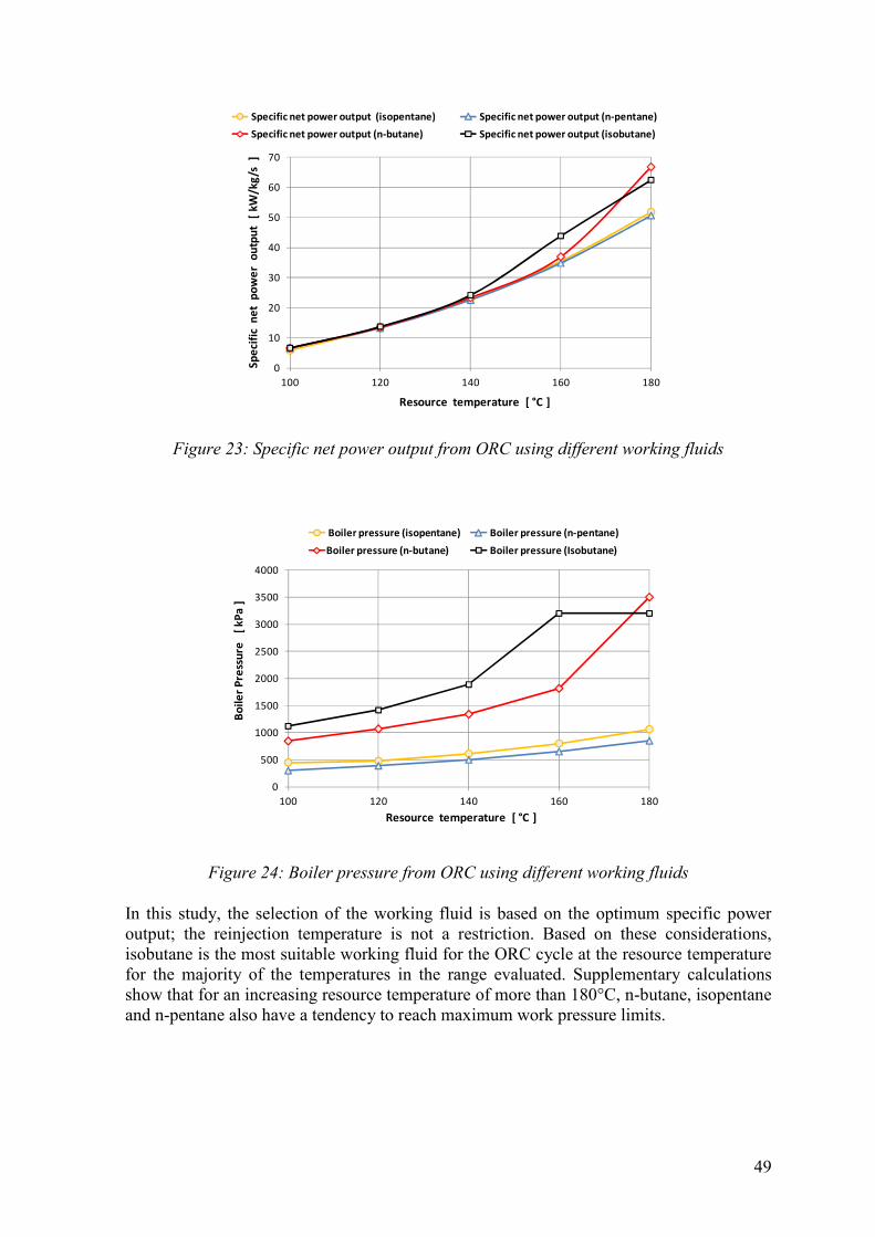
49

0

500

1000

1500

2000

2500

3000

3500

4000

100 120 140 160 180

Bo

ile

r P

ress

ure

[

kP

a ]


Boiler pressure (isopentane) Boiler pressure (n-pentane)

Boiler pressure (n-butane) Boiler pressure (Isobutane)

Figure 23: Specific net power output from ORC using different working fluids

Figure 24: Boiler pressure from ORC using different working fluids

In this study, the selection of the working fluid is based on the optimum specific power output; the reinjection temperature is not a restriction. Based on these considerations, isobutane is the most suitable working fluid for the ORC cycle at the resource temperature for the majority of the temperatures in the range evaluated. Supplementary calculations show that for an increasing resource temperature of more than 180°C, n-butane, isopentane and n-pentane also have a tendency to reach maximum work pressure limits.

0

10

20

30

40

50

60

70

100 120 140 160 180

Sp

eci

fic

ne

t p

ow

er

ou

tpu

t [

kW

/kg

/s

]


Specific net power output (isopentane) Specific net power output (n-pentane)

Specific net power output (n-butane) Specific net power output (isobutane)

50

0 50000 100000 150000 200000 25000040

60

80

100

120

140

160

qvap[i]

tcvap[i], thvap[i]

0 20000 40000 60000 80000 100000 120000 140000 16000040

60

80

100

120

140

160

180

qvap[i]

tcvap[i], thvap[i]

Figure 25: Temperature – Heat transfer diagram between geothermal resource (blue line)

and working fluid (black line) for pre-heater and boiler. Inlet temperature of geothermal

resource, working fluid: (a) 160°C,isobutene (b) 180°C,isobutene (c) 160°C,n-butane (d)

180°C, n-butane.

4.3.4 Comparison of power output between SF, DF and ORC

Figure 26: Comparison of specific power output from SF, DF and ORC power plants

0

50

100

150

200

250

300

100 120 140 160 180 200 220 240 260 280 300 320 340

Sp

eci

fic

ne

t p

ow

er

ou

tpu

t [

kW

/kg

/s

]


Single Flash Double Flash ORC (Isobutane)

0 50000 100000 150000 200000 250000 300000 35000040

60

80

100

120

140

160

180

qvap[i]

tcvap[i], thvap[i]

0 5000 10000 15000 20000 25000 30000 35000 40000 4500040

60

80

100

120

140

160

qvap[i]

tcvap[i], thvap[i]

a b

c d

51

Figure 26 presents a comparison of the optimal power outputs of the three power technologies operating at different geothermal resource temperatures. It can be seen that the size of power plants is determined principally by geothermal resource characteristics, but these are not the only factors that affect it.

In this study, flashing technologies are evaluated for resource temperatures between 160 and 340°C. As shown in Figure 23, the specific power output of a DF power plant is higher with respect to the SF power plant. DF is more effective than SF because a larger portion of the resource is utilized for electricity generation. It is important to note that in SF and DF cycles at lower temperatures the steam fraction becomes smaller and only a small fraction of the energy in the geothermal fluid can be utilized for electricity generation. However, also under consideration at temperatures between 100 and 180°C is an ORC operated with a secondary working fluid (isobutane) which has a low boiling point and high vapor pressure at low temperatures in contrast to steam. When comparing these processes with regard to the net power output at lower temperatures between 160 and 180°C, the regenerated ORC results in a higher power output than the SF and DF systems.

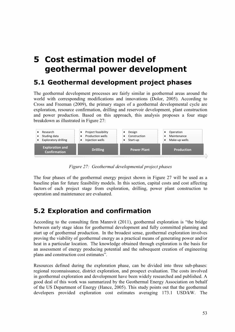
53

5 Cost estimation model of geothermal power development

5.1 Geothermal development project phases

The geothermal development processes are fairly similar in geothermal areas around the world with corresponding modifications and innovations (Dolor, 2005). According to Cross and Freeman (2009), the primary stages of a geothermal developmental cycle are exploration, resource confirmation, drilling and reservoir development, plant construction and power production. Based on this approach, this analysis proposes a four stage breakdown as illustrated in Figure 27:

Figure 27: Geothermal developmental project phases

The four phases of the geothermal energy project shown in Figure 27 will be used as a baseline plan for future feasibility models. In this section, capital costs and cost affecting factors of each project stage from exploration, drilling, power plant construction to operation and maintenance are evaluated.

5.2 Exploration and confirmation

According to the consulting firm Mannvit (2011), geothermal exploration is “the bridge between early stage ideas for geothermal development and fully committed planning and start up of geothermal production. In the broadest sense, geothermal exploration involves proving the viability of geothermal energy as a practical means of generating power and/or heat in a particular location. The knowledge obtained through exploration is the basis for an assessment of energy producing potential and the subsequent creation of engineering plans and construction cost estimates”. Resources defined during the exploration phase, can be divided into three sub-phases: regional reconnaissance, district exploration, and prospect evaluation. The costs involved in geothermal exploration and development have been widely researched and published. A good deal of this work was summarized by the Geothermal Energy Association on behalf of the US Department of Energy (Hance, 2005). This study points out that the geothermal developers provided exploration cost estimates averaging 173.1 USD/kW. The

Research

Studing data

Exploratory drilling

Exploration and

Confirmation

Project feasibility

Production wells

Injection wells

Drillling

Design

Construction

Start-up

Power Plant

Operation

Maintenance

Make-up wells

Production

54

Depth

Interval

(km)

Number

of

Wells

Total

Cost

(MUSD)

Average

Depth

(km)

Average

Cost/Well

(MUSD)

0.00–0.38 1 0.33 0.21 0.33

0.38–0.76 8 12.34 0.60 1.54

0.76–1.14 0 0.00 0.00 0.00

1.14–1.52 5 12.87 1.31 2.57

1.52–2.28 24 77.13 1.77 3.21

2.28–3.04 20 81.57 2.55 4.08

3.04–3.81 3 13.62 3.35 4.54

1.89 3.24Total

confirmation phase is defined as drilling additional production wells and testing their flow rates until approximately 25% of the resource capacity needed by the project is achieved. An average cost of 346 USD/kW was suggested when the confirmation phase was considered in tandem with the exploration phase. Using 2010 USD values as an input in the present analysis, the cost in USD/kW was inflated according to the US BLS (2011) inflation calculator.

5.3 Drilling

Cost related to drilling is usually the single largest cost and a highly risky component in any geothermal development. Given the circumstances, it is expected that the cost of drilling will be very variable; while this is certainly true to some degree, there are general tendencies. This analysis of drilling costs in Central America is based on the statistical method for estimating drilling investments in unknown geothermal fields presented by Stefansson (2001) who made a statistical study of drilling results in 31 high temperature fields around the world. Using these world average results, and combining them with data from Central America (Bloomfield and Laney, 2005), it is possible to estimate the expected value and its limits of error for drilling investment in this region. Stefansson (2001) stated that the average yield of wells in any particular geothermal field is fairly constant after passing through a certain learning period and gaining sufficient knowledge of the reservoir to site the wells so as to achieve the maximum possible yield. The average power output (MW) per drilled kilometer in geothermal fields is shown as a function of the number of wells in each field.

Table 6: Average values for 31 geothermal fields (as cited by Stefansson, 2001)

For this estimation, it is assumed that the average depth of the wells is 1,890 m, and that the average cost of such wells is 3.24 million USD as presented in Table 2 (drilling costs in Central America as reported by Bloomfield and Laney, 2005).

Table 7: Drilling costs from 1997 to 2000 for Central America and the Azores in 2010

USD (Bloomfield and Laney, 2005)

Average MW per well 4.2 ± 2.2

Average MW per drilled km 3.4 ± 1.4

Average number of wells before max. yield achieved 9.3 ± 6.1

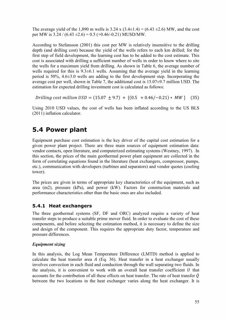
55

The average yield of the 1,890 m wells is 3.24 x (3.4±1.4) = (6.43 ±2.6) MW, and the cost per MW is 3.24 / (6.43 ±2.6) = 0.5 (+0.46/-0.21) MUSD/MW. According to Stefansson (2001) this cost per MW is relatively insensitive to the drilling depth (and drilling cost) because the yield of the wells refers to each km drilled; for the first step of field development, the learning cost has to be added to the cost estimate. This cost is associated with drilling a sufficient number of wells in order to know where to site the wells for a maximum yield from drilling. As shown in Table 6, the average number of wells required for this is 9.3±6.1 wells. Assuming that the average yield in the learning period is 50%, 4.6±3.0 wells are adding to the first development step. Incorporating the average cost per well, shown in Table 7, the additional cost is 15.07±9.7 million USD. The estimation for expected drilling investment cost is calculated as follows: i�"!!"#+�$�(�"!!"$#�ji = ,15.07 ± 9.7/ + [,0.5 + 0.46/−0.21/ ∗ �B],35/

Using 2010 USD values, the cost of wells has been inflated according to the US BLS (2011) inflation calculator.

5.4 Power plant

Equipment purchase cost estimation is the key driver of the capital cost estimation for a given power plant project. There are three main sources of equipment estimation data: vendor contacts, open literature, and computerized estimating systems (Westney, 1997). In this section, the prices of the main geothermal power plant equipment are collected in the form of correlating equations found in the literature (heat exchangers, compressor, pumps, etc.), communication with developers (turbines and separators) and vendor quotes (cooling tower). The prices are given in terms of appropriate key characteristics of the equipment, such as area (m2), pressure (kPa), and power (kW). Factors for construction materials and performance characteristics other than the basic ones are also included.

5.4.1 Heat exchangers

The three geothermal systems (SF, DF and ORC) analyzed require a variety of heat transfer steps to produce a suitable prime mover fluid. In order to evaluate the cost of these components, and before selecting the estimation method, it is necessary to define the size and design of the component. This requires the appropriate duty factor, temperature and pressure differences.

Equipment sizing

In this analysis, the Log Mean Temperature Difference (LMTD) method is applied to calculate the heat transfer area � (Eq. 36). Heat transfer in a heat exchanger usually involves convection in each fluid and conduction through the wall separating two fluids. In the analysis, it is convenient to work with an overall heat transfer coefficient � that accounts for the contribution of all these effects on heat transfer. The rate of heat transfer G� between the two locations in the heat exchanger varies along the heat exchanger. It is

56

necessary to work with the Logarithmic Mean Temperature Difference ∆3fQ (Eq. 37), which is an equivalent mean temperature difference between two fluids for an entire heat exchanger (Cengel and Turner, 2005).

The overall heat exchange surface expressed as a function ofG� , � and ∆3fQ can be written as

� = G��∆3fQ ,36/

where

∆3fQ = b32 − b38ln, b32b38/

,37/

In Equation 37, b32 and b38 represent the temperature differences between the two fluids at the inlet and outlet. Table 8 shows the overall heat transfer coefficients used in the analysis of a heat exchanger.

Table 8: Overall heat transfer coefficients (Valdimarsson, 2011)

Estimated equipment cost

Numerous methods in relation to the cost of heat exchangers can be found in the literature. Most of them are presented in the form of graphs and equations for FOB purchase cost as a function of one or more equipment size factors. The equipment cost equation presented by Seider et al. (2003) is incorporated into the calculations here. The equations are based on common construction materials, and for other materials a correction factor is applied. The input parameters are: heat exchanger surface area�� in ft, design pressure &h in psig, heat exchanger type and material of construction. The base cost (��/ can be calculated as follows

�� = exp{11.0545 − 0.9228ulnY��Zv + 0.09861ulnY��Zv8-$�-"� wℎ �w,38/

�� = exp{11.967 − 0.8197ulnY��Zv + 0.09005ulnY��Zv8-$�* ((! � x$"! �,39/ This base cost calculation counts for certain base case configurations including a carbon steel heat exchanger with 100 psig (690 kPa) pressure with a heat exchanger surface between 150 ft2 (13.9 m2) and 12,000 ft2 (1,114.8 m2). Correction factors for a different specific heat exchanger are introduced, and the FOB purchase cost for this type of heat exchanger is given by

Fluids U [W/m2

. K]

Water - Water 2000

Steam - Water 2000

Water - Isopentane 1200

Isopentane - Isopentane 1200

57

�� = ��̂ � (40) For different materials the factor � is introduced

� = � + P i100R

y ,41/ For different operating pressure the factor � is introduced

� = 0.9803 + 0.018 P &h100R + 0.0017 P &h100R8 ,42/

The base heat exchanger purchase cost equation is based on the CE index cost in mid year 2000 (CE=394).

Correcting equipment cost for inflation

Because the cost literature reflects equipment from some time in the past, it is necessary to correct for the cost of inflation. There are several inflation or cost indices in use; here the Chemical Engineering Plant Cost Index (CE index) is used in this analysis. The Chemical Engineering magazine (CHE) publishes the CE index regularly for correcting equipment costs for inflation; the CE indices for December 2010 are used in this analysis (CHE, 2011).

In order to obtain the current cost value of equipment �8 we use an inflation index z8 as given by Equation 43 (Silla, 2003)

�8 = �2 z8z2 ,43/

5.4.2 Turbine - Generator

If a new piece of equipment is similar to one of another capacity for which cost data is available, then it follows that the estimated cost for turbines can be obtained from a scaling factor by using the logarithmic relationship known as the six tenths factor rule. According to Peters et al. (2003) if the cost of a given unit at one capacity is known, then the cost of a similar unit with X times the capacity of the first is approximately ,X/N times the cost of the initial unit. The value of the cost exponent N varies depending upon the class of equipment being represented; the value of n for different equipment is often around 0.6. The typical value of cost exponent N for the steam turbine included in this analysis is 0.6.

Input parameters: cost and power of know turbine, capacity of estimated turbine

�$�($- }~"�� #(8�$�($- }~"�� #(2 = P��"(. }~"�� #(8��"(. }~"�� #(2R�,44/

58

This method is used in combination with the cost indices described in Section 5.3.1. Personal conversations with geothermal developers indicate that recent references (2010) used in the estimated purchasing cost for a turbine generator in a single flash process is around 13 million USD for 30 MW, and for double flash an additional 15% of the SF cost is considered. In a recent ORC development in Costa Rica, Marcos (2007) quoted a turbine cost of around 4 million USD for 7.5 MW.

5.4.3 Compressor

The FOB purchase cost for a typical centrifugal compressor is based on an equation from Seider (2003) where the base cost is given as a function of consumed power. The input parameters are: consumed power&H in HP and material of construction. The base cost (��/ is calculated as �� = exp{7.2223 + 0.80[ln,&H/]-$�� #(�"-~+�!�$�� $�,45/ This base cost calculation counts for certain base case configurations including an electrical motor drive and carbon steel construction. For other materials, a correction factor � is included. For geothermal purposes, stainless steel is used (� = 2.5/.

�� = �� (46)

The base purchase cost equation for the compressor has a CE index of 394. To correct the equipment cost for inflation, compressor CE indices (CE=903) for December 2010 are included (CHE, 2011).

5.4.4 Pumps

The technical literature for the cost of equipment offers several equations for calculating the approximate cost for centrifugal pumps, but the limitation is the flow range that the cooling water pumps operate in the geothermal power plant. The FOB purchase cost for the centrifugal pump is based on the equation equipment cost presented by Walas (1990). The input parameters are: flow rate GHKin gpm and material of construction. The base cost for a pump (��/ is calculated by �� = 20,GHK/1.]_-$�� ("��!��"�!-!$�,47/ Base cost calculations do not include the cost of the motor and are only valid for a flow range between 1,000

gpm and 130,000 gpm. The material correction factor for stainless steel is (� = 2/. The cost of the motor is calculated by Equation 48. The input parameter is: consumed power&H in HP. The cost of the motor (��/ is calculated as �� = 1.2exp[5.318 + 1.084ln,&H/ + 0.056 ln,&H/8],48/ These cost calculations are for a motor type which is totally enclosed, fan-cooled and 3,600 rpm.

59

5.4.5 Cooling tower

An online vendor quote is easy to get from many companies (e.g. Cooling Tower Systems, Delta Cooling Tower, Cooling Tower Depot). The only requirements are the cooling tower design and operating conditions. In this analysis, the six tenths factor rule is applied, and the cost reference is based on the cost quoted by Cooling Tower Depot (2011). The typical value of cost exponent N for the cooling tower included in this analysis is 0.9 (Bejan et al., 1996).

5.4.6 Separation station

A personal conversation with geothermal developers indicated that the cost estimation of a separator can be made based on the mass flow rate capacity of the station. Recent references (2010) gave a cost of 400,000 USD for a mass flow rate capacity of 200 kg/s. Based on this information, in this study the calculation for another separator capacity was obtained using the six tenths factor rule described in Section 5.4.2.

5.4.7 PEC of single flash power plant

The assessment of cost estimation of power plant components is done in order to develop the overall plant capital costs for each scenario. PEC is defined as the summation of all purchase costs of main equipment. In the case of a single flash cycle, the main equipment includes a turbine-generator unit, a condenser, cooling tower, cooling water circulation pumps, a separator and a gas extraction system. Figure 28 illustrates that there is an inverse relationship between the specific PEC for SF and a resource temperature between 160 and 340°C. Also, there is an inverse relationship between the specific PEC of SF and the mass flow rate. It should be noted that the specific PEC presents a 7% variation from a low (300 kg/s) to a high (1,000 kg/s) mass flow rate. The specific PEC of SF is between 1021 and 732 USD/kW for 300 kg/s; between 1,061 and 768 USD/kW for 600 kg/s; between 991 and 718 USD/kW for 1,000 kg/s.

Figure 28: Specific net power output and specific PEC of SF power plant

450

600

750

900

1050

1200

1350

1500

0

50

100

150

200

250

300

160 180 200 220 240 260 280 300 320 340

Sp

eci

fic

P

EC

[U

SD

/kW

]

Sp

eci

fic

ne

t p

ow

er

ou

tpu

t [

kW

/kg

/s ]


Specific net power output Specific PEC (600 kg/s)

Specific PEC (300 kg/s) Specific PEC (1000 kg/s)

60

5.4.8 PEC of double flash power plant

For a double flash cycle, the main equipment includes a turbine-generator unit, a condenser, a cooling tower, cooling water circulation pumps, a HP separator, a LP separator and a gas extraction system. Figure 29 illustrates that there is an inverse relationship between the specific PEC for DF and the resource temperature between 160 and 340°C. Also, there is an inverse relationship between the specific PEC of SF and the mass flow rate. It should be noted that when comparing the double flash to the single flash scenario, specific PEC presents an 18% difference from low (300 kg/s) to high (1,000 kg/s) mass flow rates. The specific PEC of DF is between 1,195 and 652 USD/kW for 300 kg/s; between 1,086 and 603 USD/kW for 600 kg/s; between 991 and 718 USD/kW for 1,000 kg/s.

Figure 29: Specific net power output and specific PEC of DF power plant

5.4.9 PEC of organic Rankine cycle power plant

Figure 30: Specific net power output and specific PEC, from ORC power plant

450.0

600.0

750.0

900.0

1050.0

1200.0

1350.0

1500.0

0

50

100

150

200

250

300

160 180 200 220 240 260 280 300 320 340S

pe

cifi

c

PE

C

[US

D/k

W]

Sp

eci

fic

ne

t p

ow

er

ou

tpu

t [

kW

/kg

/s ]


Specific net power output PEC (600kg/s)

PEC (1000kg/s) PEC (300kg/s)

450

600

750

900

1050

1200

1350

1500

0

50

100

150

200

250

300

100 120 140 160 180

Sp

eci

fic

P

EC

[U

SD/k

W]

Sp

eci

fic

ne

t p

ow

er

ou

tpu

t [

kW

/kg

/s ]


Specific net power output (isobutane) Specific PEC (300 kg/s)

Specific PEC (600 kg/s) Specific PEC (1000 kg/s)

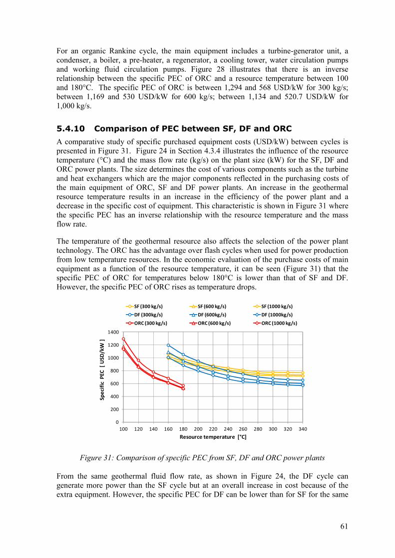
61

For an organic Rankine cycle, the main equipment includes a turbine-generator unit, a condenser, a boiler, a pre-heater, a regenerator, a cooling tower, water circulation pumps and working fluid circulation pumps. Figure 28 illustrates that there is an inverse relationship between the specific PEC of ORC and a resource temperature between 100 and 180°C. The specific PEC of ORC is between 1,294 and 568 USD/kW for 300 kg/s; between 1,169 and 530 USD/kW for 600 kg/s; between 1,134 and 520.7 USD/kW for 1,000 kg/s.

5.4.10 Comparison of PEC between SF, DF and ORC

A comparative study of specific purchased equipment costs (USD/kW) between cycles is presented in Figure 31. Figure 24 in Section 4.3.4 illustrates the influence of the resource temperature (°C) and the mass flow rate (kg/s) on the plant size (kW) for the SF, DF and ORC power plants. The size determines the cost of various components such as the turbine and heat exchangers which are the major components reflected in the purchasing costs of the main equipment of ORC, SF and DF power plants. An increase in the geothermal resource temperature results in an increase in the efficiency of the power plant and a decrease in the specific cost of equipment. This characteristic is shown in Figure 31 where the specific PEC has an inverse relationship with the resource temperature and the mass flow rate.

The temperature of the geothermal resource also affects the selection of the power plant technology. The ORC has the advantage over flash cycles when used for power production from low temperature resources. In the economic evaluation of the purchase costs of main equipment as a function of the resource temperature, it can be seen (Figure 31) that the specific PEC of ORC for temperatures below 180°C is lower than that of SF and DF. However, the specific PEC of ORC rises as temperature drops.

Figure 31: Comparison of specific PEC from SF, DF and ORC power plants

From the same geothermal fluid flow rate, as shown in Figure 24, the DF cycle can generate more power than the SF cycle but at an overall increase in cost because of the extra equipment. However, the specific PEC for DF can be lower than for SF for the same

0

200

400

600

800

1000

1200

1400

100 120 140 160 180 200 220 240 260 280 300 320 340

Sp

eci

fic

PE

C

[ U

SD

/kW

]


SF (300 kg/s) SF (600 kg/s) SF (1000 kg/s)

DF (300kg/s) DF (600kg/s) DF (1000kg/s)

ORC (300 kg/s) ORC (600 kg/s) ORC (1000 kg/s)

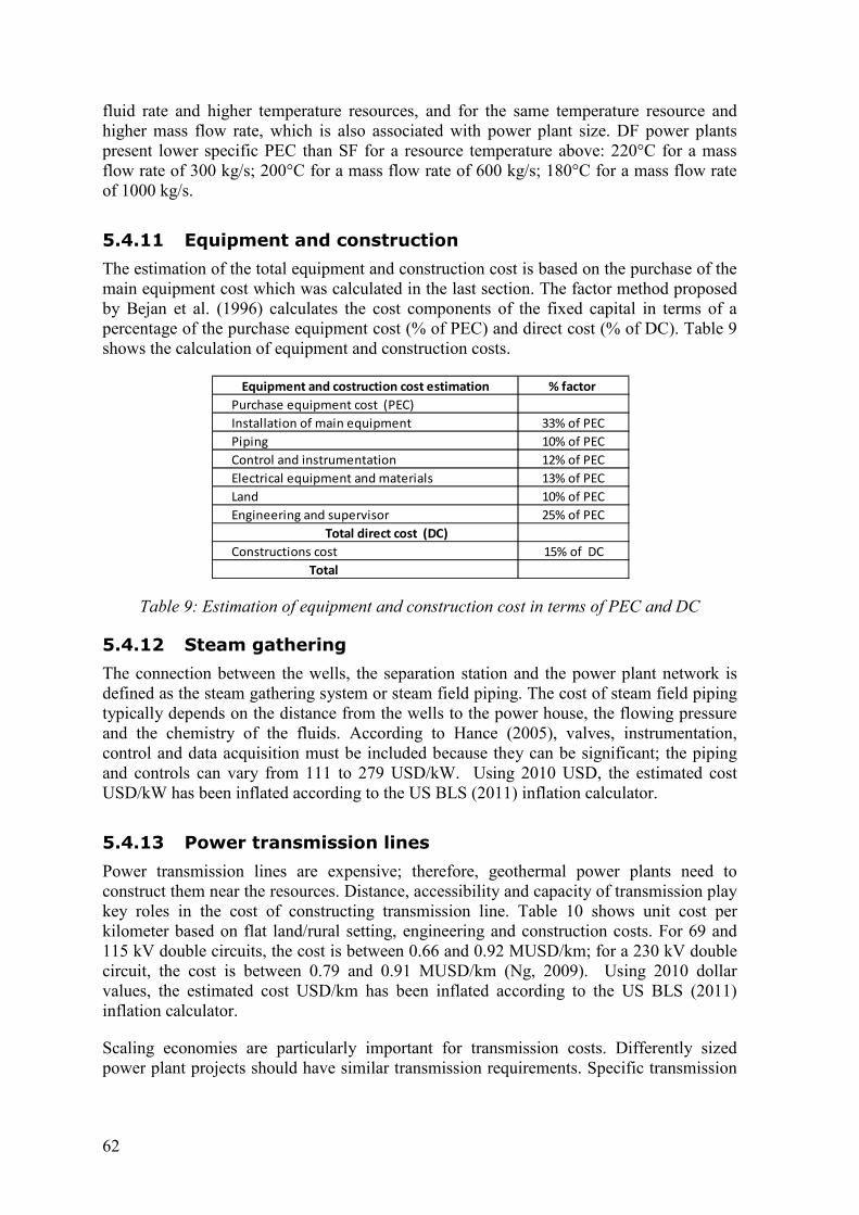
62

fluid rate and higher temperature resources, and for the same temperature resource and higher mass flow rate, which is also associated with power plant size. DF power plants present lower specific PEC than SF for a resource temperature above: 220°C for a mass flow rate of 300 kg/s; 200°C for a mass flow rate of 600 kg/s; 180°C for a mass flow rate of 1000 kg/s.

5.4.11 Equipment and construction

The estimation of the total equipment and construction cost is based on the purchase of the main equipment cost which was calculated in the last section. The factor method proposed by Bejan et al. (1996) calculates the cost components of the fixed capital in terms of a percentage of the purchase equipment cost (% of PEC) and direct cost (% of DC). Table 9 shows the calculation of equipment and construction costs.

Table 9: Estimation of equipment and construction cost in terms of PEC and DC

5.4.12 Steam gathering

The connection between the wells, the separation station and the power plant network is defined as the steam gathering system or steam field piping. The cost of steam field piping typically depends on the distance from the wells to the power house, the flowing pressure and the chemistry of the fluids. According to Hance (2005), valves, instrumentation, control and data acquisition must be included because they can be significant; the piping and controls can vary from 111 to 279 USD/kW. Using 2010 USD, the estimated cost USD/kW has been inflated according to the US BLS (2011) inflation calculator.

5.4.13 Power transmission lines

Power transmission lines are expensive; therefore, geothermal power plants need to construct them near the resources. Distance, accessibility and capacity of transmission play key roles in the cost of constructing transmission line. Table 10 shows unit cost per kilometer based on flat land/rural setting, engineering and construction costs. For 69 and 115 kV double circuits, the cost is between 0.66 and 0.92 MUSD/km; for a 230 kV double circuit, the cost is between 0.79 and 0.91 MUSD/km (Ng, 2009). Using 2010 dollar values, the estimated cost USD/km has been inflated according to the US BLS (2011) inflation calculator.

Scaling economies are particularly important for transmission costs. Differently sized power plant projects should have similar transmission requirements. Specific transmission

Equipment and costruction cost estimation % factor

Purchase equipment cost (PEC)

Installation of main equipment 33% of PEC

Piping 10% of PEC

Control and instrumentation 12% of PEC

Electrical equipment and materials 13% of PEC

Land 10% of PEC

Engineering and supervisor 25% of PEC

Total direct cost (DC)

Constructions cost 15% of DC

Total

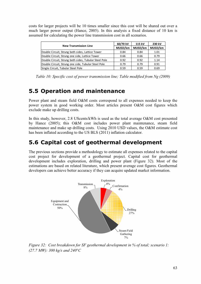
63

Exploration 4%

Confirmation 4%

Drilling 27%

Steam Field Gathering

7%

Equipment and Costruction

50%

Transmission8%

costs for larger projects will be 10 times smaller since this cost will be shared out over a much larger power output (Hance, 2005). In this analysis a fixed distance of 10 km is assumed for calculating the power line transmission cost in all scenarios.

Table 10: Specific cost of power transmission line; Table modified from Ng (2009)

5.5 Operation and maintenance

Power plant and steam field O&M costs correspond to all expenses needed to keep the power system in good working order. Most articles present O&M cost figures which exclude make up drilling costs.

In this study, however, 2.8 UScents/kWh is used as the total average O&M cost presented by Hance (2005); this O&M cost includes power plant maintenance, steam field maintenance and make up drilling costs. Using 2010 USD values, the O&M estimate cost has been inflated according to the US BLS (2011) inflation calculator.

5.6 Capital cost of geothermal development

The previous sections provide a methodology to estimate all expenses related to the capital cost project for development of a geothermal project. Capital cost for geothermal development includes exploration, drilling and power plant (Figure 32). Most of the estimations are based on related literature, which present average cost figures. Geothermal developers can achieve better accuracy if they can acquire updated market information.

Figure 32: Cost breakdown for SF geothermal development in % of total; scenario 1:

(27.7 MW): 300 kg/s and 240°C

60/70 kV 115 kV 230 kV

MUSD/km MUSD/km MUSD/km

Double Circuit, Strung both sides, Lattice Tower 0.84 0.84 1.01

Double Circuit, Strung one side, Lattice Tower 0.66 0.66 0.79

Double Circuit, Strung both sides, Tubular Steel Pole 0.92 0.92 1.14

Double Circuit, Strung one side, Tubular Steel Pole 0.79 0.79 0.91

Single Circuit, Tubular Steel Pole 0.59 0.59 0.69

New Transmission Line

64

Table 11 shows a summary of costs for scenario 1 (SF, 300 kg/s, 240°C) calculated as explained in previous sections. The capital costs estimated according to this methodology for a different geothermal resource (mass flow and temperature) and different power plant technology will be used as input in the financial modeling in Section 6. Figure 32 illustrates the breakdown of the total capital cost of geothermal development for scenario1. This includes all the costs associated with total investment where the plant cost is approximately 50%, the drilling cost is 27%, exploration and confirmation costs total 8%, the power line transmission cost is 8% and the steam gathering system cost is 7%.

Table 11: Estimated cost of geothermal power plant development for single flash scenario

1 (27.7 MW): 300 kg/s and 240°C

5.6.1 Capital cost of single flash power plant

Figure 33 shows the specific capital cost (SCC) of SF in USD/kW for exploration and confirmation, drilling and power plant as a function of the resource temperature for different mass flows. The SCC decreases as the resource temperature increases from 160 to 340°C. SCC for SF power plants varies from 3,474 to 2,028 USD/kW for 300 kg/s; from 2,928 to 2,002 USD/kW for 600 kg/s; from 2,736 to 2,000 USD/kW for 1,000 kg/s. SCC for SF drilling varies from 2,090 to 721 USD/kW for 300 kg/s; from 1,295 to 610 USD/kW for 600 kg/s; from 977 to 566 USD/kW for 1,000 kg/s.

5.6.2 Capital cost of double flash power plant

Figure 34 shows the specific capital cost (SCC) of DF in USD/kW for exploration and confirmation, drilling and power plant as a function of the resource temperature for different mass flows. The specific costs decrease as the resource temperature increases from 160 to 340°C. SCC for DF power plants varies from 3,761 to 1,745 USD/kW for 300 kg/s; from 3,070 to 1,616 USD/kW for 600 kg/s; from 2,736 to 1,594 USD/kW for 1,000 kg/s. SCC for DF drilling varies from 1,893 to 701 USD/kW for 600 kg/s; from 1,196 to 600 USD/kW for 600 kg/s; from 1,025 to 560 USD/kW for 1,000 kg/s.

Value Units

Exploration 173 USD/kw

Confirmation 173 USD/kw

Total Exploration 346 USD/kw

Known Field 504 USD/kw

Unknown Field 1,047 USD/kw

Total Drilling 1,047 USD/kw

Steam Gathering 279 USD/kw

Equipment and Costruction 1,964 USD/kw

Transmission Power Line 840,000 USD/km

Total Power Plant 2,546 USD/kw

O&M Total O&M 2.8 USD¢/kwh

Power Plant

Category Sub-Category Nominal Value

Exploration

Drilling

65

0

500

1,000

1,500

2,000

2,500

3,000

3,500

4,000

160 180 200 220 240 260 280 300 320 340

Sp

eci

fic

Ca

pit

al

Co

st

[U

SD

/kW

]


Plant (300 kg/s) Plant (600 kg/s) Plant (1000 kg/s)

Drilling (300 kg/s) Drilling (600 kg/s) Drilling (1000 kg/s)

Expl. & Conf.

Figure 33: Specific capital cost of geothermal development for SF power plant

Figure 34: Specific capital cost of geothermal development for DF power plant

5.6.3 Capital cost of organic Rankine cycle power plant

Figure 35 shows the specific capital cost (SCC) in USD/kW for exploration and confirmation, drilling and power plant as a function of the resource temperature for different mass flows. The specific costs decrease as the resource temperature increases from 100 to 180°C. SCC for ORC power plants varies from 3,020 to 1,325 USD/kW for

0

500

1,000

1,500

2,000

2,500

3,000

3,500

4,000

160 180 200 220 240 260 280 300 320 340

Sp

eci

fic

Ca

pit

al

Co

st

[U

SD

/kW

]


Plant (300 kg/s) Plant (600 kg/s) Plant (1000 kg/s)

Drilling (300 kg/s) Drilling (600 kg/s) Drilling (1000 kg/s)

Expl. & Conf.

66

300 kg/s; from 2,729 to 1,223 USD/kW for 600 kg/s; from 2,646 to 1,215 USD/kW for 1,000 kg/s. SCC for ORC drilling varies from 8,103 to 1,305 USD/kW for 300 kg/s; from 4,302 to 902 USD/kW for 600 kg/s; from 2,781 to 741 USD/kW for 1,000 kg/s.

Figure 35: Specific capital cost of geothermal development for ORC power plant

5.6.4 Comparison of capital costs between SF, DF and ORC

Figure 36 compares the specific capital cost as a function of the resource temperature for different mass flow rates and power plant technologies. As shown in the figure, all the technologies in this study anticipate that a larger sized power plant has more cost effective values than smaller sized plants as reflected by scaling economies. The specific capital cost (SCC) for ORC ranging between 11,400 and 2,300 USD per installed kW, for the resource temperature (100-180°C), and mass flow rate (300 kg-1,000 kg/s) was examined. The SCC of ORC rises quickly, exponentially, as the resource temperature and mass flow rate decrease (as a result of small power output). This occurs because the cost is affected by drilling and transmission line costs. For 300 kg/s at 180°C, the cost of drilling is 35% and transmission lines 13% of the total; at 100°C, drilling costs are 52% and transmission lines 26% of the total. The SCC for SF, which ranges between 5,910 and 2,940 USD per installed kW, and the SCC for DF, which ranges between 6,000 and 2,500 USD per installed kW at resource temperature (160-340°C) and mass flow rate (300-1,000 kg/s), were examined. The SCC of DF presents lower values than SF for a resource temperature above 200°C at all the mass flow rate scenarios. For resource temperatures between 220 and 180°C, the SCC of SF presents lower values than DF. Finally, for resource temperatures between 180 and 160°C, the SCC of ORC has lower values than either SF or DF.

0

1,000

2,000

3,000

4,000

5,000

6,000

7,000

8,000

100 120 140 160 180

Sp

eci

fic

Ca

pit

al

Co

st

[U

SD

/kW

]


Drilling (300 kg/s) Drilling (600kg/s) Drilling (1000kg/s)

Plant (300 kg/s) Plant (600kg/s) Plant (1000kg/s)

Expl. & Conf.

67

Figure 36: Comparison of specific capital costs of geothermal development as a function

of resource temperature

5.6.5 Literature review of capital costs of development

Figure 37: Literature review (EPRI, 1996; SKM, 2009): specific capital cost of geothermal

developments as function of resource temperature (2010 USD); Note: the specific capital cost from: a) EPRI (1996): 129-300°C resource/50MW plant size. b) SKM (2009): 230°C resource/20MW plant size; 260-300°C resource/ 50MW plant size; values from low enveloped wells; 0.7 as NZD/USD exchange rate (year 2007)

0

1,000

2,000

3,000

4,000

5,000

6,000

7,000

8,000

9,000

10,000

11,000

12,000

100 120 140 160 180 200 220 240 260 280 300 320 340

Sp

eci

fic

Ca

pit

al

Co

st

[ U

SD

/kW

]


SF (300 kg/s) SF (600 kg/s) SF (1000 kg/s)

DF (300kg/s) DF (600kg/s) DF (1000kg/s)

ORC (300 kg/s) ORC (600 kg/s) ORC (1000 kg/s)

0

1,000

2,000

3,000

4,000

5,000

6,000

7,000

8,000

9,000

10,000

11,000

12,000

100 120 140 160 180 200 220 240 260 280 300 320 340

Sp

eci

fic

Ca

pit

al

Co

st

[ U

SD

/kW

]


SF (SKM, 2009) DF (EPRI, 1996) DF (SKM, 2009)

ORC (EPRI, 1996) ORC (SKM, 2009)

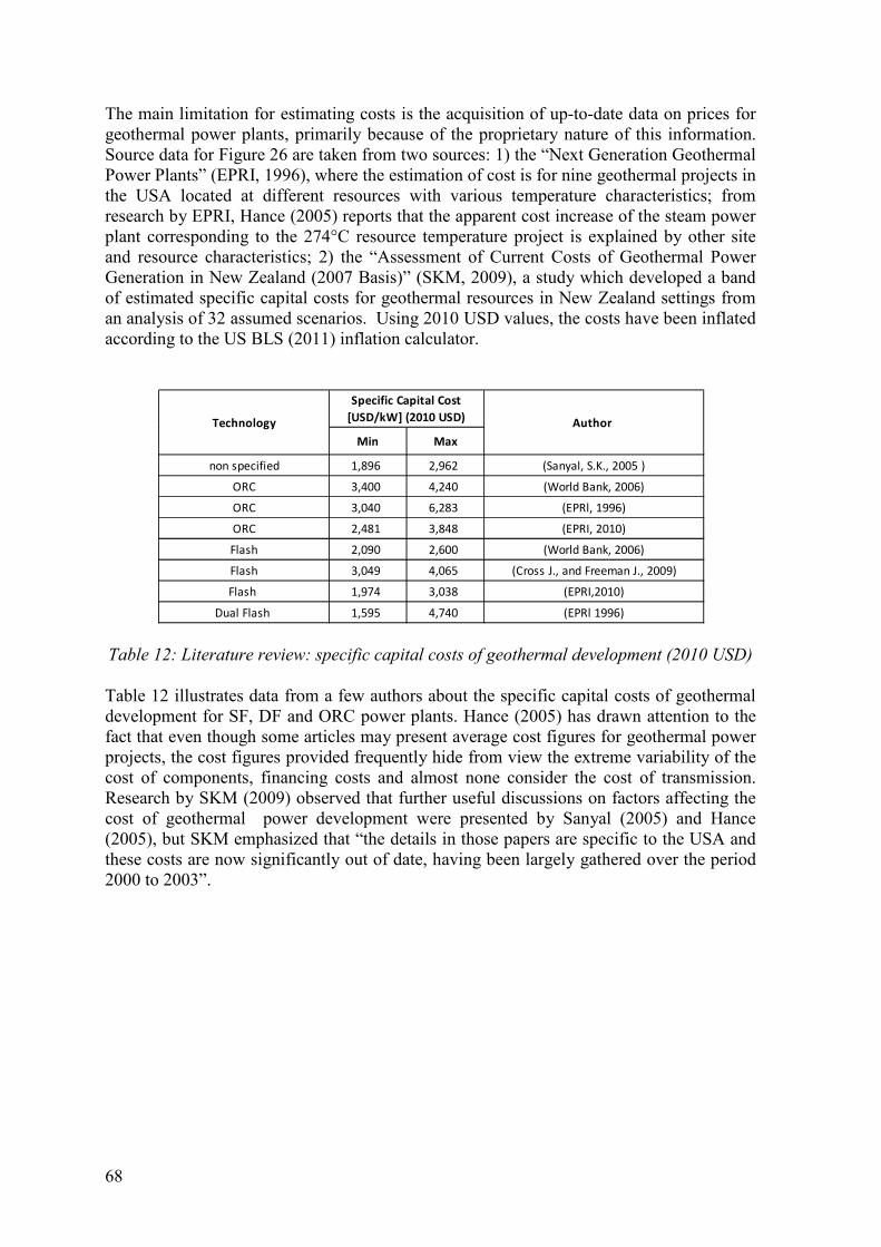
68

The main limitation for estimating costs is the acquisition of up-to-date data on prices for geothermal power plants, primarily because of the proprietary nature of this information. Source data for Figure 26 are taken from two sources: 1) the “Next Generation Geothermal Power Plants” (EPRI, 1996), where the estimation of cost is for nine geothermal projects in the USA located at different resources with various temperature characteristics; from research by EPRI, Hance (2005) reports that the apparent cost increase of the steam power plant corresponding to the 274°C resource temperature project is explained by other site and resource characteristics; 2) the “Assessment of Current Costs of Geothermal Power Generation in New Zealand (2007 Basis)” (SKM, 2009), a study which developed a band of estimated specific capital costs for geothermal resources in New Zealand settings from an analysis of 32 assumed scenarios. Using 2010 USD values, the costs have been inflated according to the US BLS (2011) inflation calculator.

Table 12: Literature review: specific capital costs of geothermal development (2010 USD)

Table 12 illustrates data from a few authors about the specific capital costs of geothermal development for SF, DF and ORC power plants. Hance (2005) has drawn attention to the fact that even though some articles may present average cost figures for geothermal power projects, the cost figures provided frequently hide from view the extreme variability of the cost of components, financing costs and almost none consider the cost of transmission. Research by SKM (2009) observed that further useful discussions on factors affecting the cost of geothermal power development were presented by Sanyal (2005) and Hance (2005), but SKM emphasized that “the details in those papers are specific to the USA and these costs are now significantly out of date, having been largely gathered over the period 2000 to 2003”.

Min Max

non specified 1,896 2,962 (Sanyal, S.K., 2005 )

ORC 3,400 4,240 (World Bank, 2006)

ORC 3,040 6,283 (EPRl, 1996)

ORC 2,481 3,848 (EPRI, 2010)

Flash 2,090 2,600 (World Bank, 2006)

Flash 3,049 4,065 (Cross J., and Freeman J., 2009)

Flash 1,974 3,038 (EPRI,2010)

Dual Flash 1,595 4,740 (EPRl 1996)

Specific Capital Cost

[USD/kW] (2010 USD) Author Technology

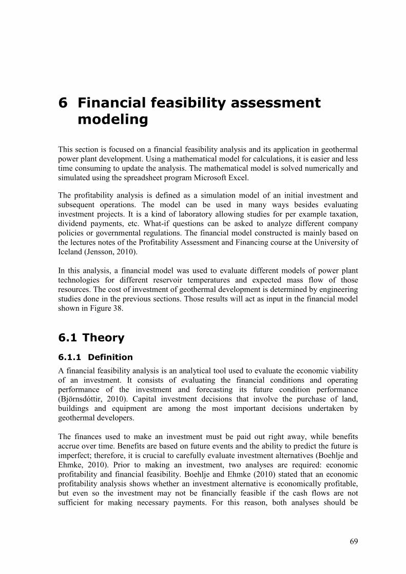
69

6 Financial feasibility assessment modeling

This section is focused on a financial feasibility analysis and its application in geothermal power plant development. Using a mathematical model for calculations, it is easier and less time consuming to update the analysis. The mathematical model is solved numerically and simulated using the spreadsheet program Microsoft Excel.

The profitability analysis is defined as a simulation model of an initial investment and subsequent operations. The model can be used in many ways besides evaluating investment projects. It is a kind of laboratory allowing studies for per example taxation, dividend payments, etc. What-if questions can be asked to analyze different company policies or governmental regulations. The financial model constructed is mainly based on the lectures notes of the Profitability Assessment and Financing course at the University of Iceland (Jensson, 2010). In this analysis, a financial model was used to evaluate different models of power plant technologies for different reservoir temperatures and expected mass flow of those resources. The cost of investment of geothermal development is determined by engineering studies done in the previous sections. Those results will act as input in the financial model shown in Figure 38.

6.1 Theory

6.1.1 Definition

A financial feasibility analysis is an analytical tool used to evaluate the economic viability of an investment. It consists of evaluating the financial conditions and operating performance of the investment and forecasting its future condition performance (Björnsdóttir, 2010). Capital investment decisions that involve the purchase of land, buildings and equipment are among the most important decisions undertaken by geothermal developers. The finances used to make an investment must be paid out right away, while benefits accrue over time. Benefits are based on future events and the ability to predict the future is imperfect; therefore, it is crucial to carefully evaluate investment alternatives (Boehlje and Ehmke, 2010). Prior to making an investment, two analyses are required: economic profitability and financial feasibility. Boehlje and Ehmke (2010) stated that an economic profitability analysis shows whether an investment alternative is economically profitable, but even so the investment may not be financially feasible if the cash flows are not sufficient for making necessary payments. For this reason, both analyses should be

70

completed previous to making a decision for accepting or rejecting a particular project. This section includes an overview of the basic concepts and elements used in the financial model.

6.1.2 Criteria for economic profitability analysis

Various techniques can be used to evaluate the economic profitability of an investment project. According to OXERA (2003), the internal rate of return (IRR) and the net present value (NPV) are the appropriate measures, commonly accepted and well established methods for measuring the profitability of an activity.

Both methods take into account the inflows and outflow of an activity over time and reflect the economic principle of time preference of money. OXERA (2003) reports that they are also the two most widely used techniques for investment appraisal in the business world. In this study, the IRR and NPV cash flow based techniques are used for evaluating the geothermal investment projects.

Net Present Value (NVP)

Hillier et al. (2010) stated that the basic quantitative technique for financial decision making is the net present value analysis. NVP is the present value of future cash flows minus the present value of the cost of investment. The net present value formula for an investment that generates cash flow C� in the future period is

�&� = � ��,1 + �/��

��1,49/

The basic investment rule can be generalized thus:

• Accept a project if the NPV is greater than zero

• Reject a project if NPV is less than zero

The numerator of Equation 49 is usually understood as being the expected time cash flow, and the discount rate � in the denominator. The calculation of the net present value (NPV) requires a value for the discount rate � and its selection is the main difficulty for this method. Crundwell (2008) argued that the discount rate value selection is essentially a strategic function and is done from the viewpoint of the entire organization; and the value of the discount rate that is used can be the financial cost of capital, the economic cost of capital or the risk adjusted discount rate.

Internal Rate of Return (IRR)

According to Benninga (2008) the internal rate of return (IRR) is defined as the compound rate of return � that makes the NPV equal to zero, which is expressed as

71

� ��,1 + �∗/��

��1= 0,50/

The general investment rule is clear:

• Accept the project if the IRR is greater than the MARR.

• Reject the project if the IRR is less than the MARR.

The IRR is about as close as you can get to NPV without essentially being NPV. Hillier et al. (2010) argued that “the basis rationale behind the IRR method is that it offers a single number summarizing the merits of a project. That number does not depend on the interest rate prevailing in the capital market”. This is why it is called the internal rate of return: the number is internally intrinsic to the project and independent except for the cash flow of the project. In this analysis, to evaluate capital expenditures the IRR is calculated on both project and equity. Minimum Acceptable Rate of Return (MARR)

According to Hillier et al. (2010) the discount rate on a risky project is the return that one can look forward to earning on a financial asset of equivalent risk, often referred to as an opportunity cost because corporate investment in the project takes away the shareholder's opportunity to invest the dividend in a financial asset. Crundwell (2008) indicated that the opportunity cost of capital is the return on the most profitable project that is not accepted; this is the Minimum Attractive Rate of Return (MARR). The opportunity cost of capital and MARR are terms that mean the same thing. The MARR for both project and equity needs to be determined by the project owners. Björnsdóttir (2010) pointed out that the MARR for a project is frequently the rate of return of the most preferable alternative investment, and the MARR for equity is usually the same as the investor’s cost of capital. Therefore, the lowest acceptable limit for IRR should be greater than MARR. In Section 6.3.7, the selection of a discount rate is discussed.

6.2 Model structure

The financial feasibility assessment model is based on several different modules done on separate worksheets, each representing different functions of the model. These worksheets are interconnected in a workbook. Figure 38 shows the main components of the model and their relationship. In order to perform the financial feasibility analysis, the model created projected financial reports such as an income statement, balance sheet and a cash flow statement. Crundwell (2008) indicated that these three financial statements represent three views of the company: the balance sheet represents the assets and liabilities of the company, that is, the value of the company; the income statement represents the revenue, costs and profit of the company, that is, the productive effort of the company; and the cash flow statement

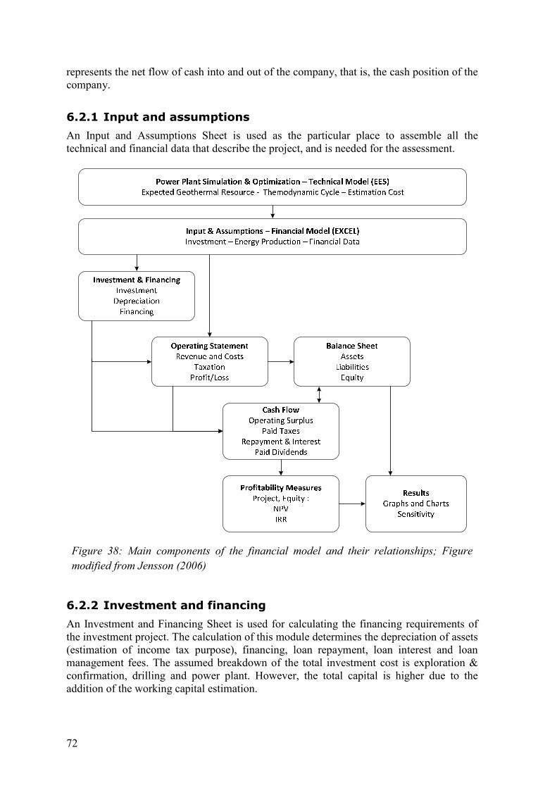
72

represents the net flow of cash into and out of the company, that is, the cash position of the company.

6.2.1 Input and assumptions

An Input and Assumptions Sheet is used as the particular place to assemble all the technical and financial data that describe the project, and is needed for the assessment.

Figure 38: Main components of the financial model and their relationships; Figure

modified from Jensson (2006)

6.2.2 Investment and financing

An Investment and Financing Sheet is used for calculating the financing requirements of the investment project. The calculation of this module determines the depreciation of assets (estimation of income tax purpose), financing, loan repayment, loan interest and loan management fees. The assumed breakdown of the total investment cost is exploration & confirmation, drilling and power plant. However, the total capital is higher due to the addition of the working capital estimation.

73

6.2.3 Operating statement

An Operating Statement or Income Statement Sheet is used for calculating the revenue and expenses over a specific period. The income statement includes several sections. One of particular importance is EBITDA (Earnings before Interests, Taxes, Depreciation and Amortization) or operating surplus, which summarizes earnings before taxes and financing costs. EBITDA is calculated by subtracting production costs from revenue. EBIT (Earnings before Interest and Taxes) can then be calculated by extracting depreciation and amortization from the EBITDA. Profit before tax is calculated by extracting the interest on the loan from EBIT. Income tax is a percentage of the taxable profit, in this analysis loss transfer is not considered, therefore, profit before tax is considered as the taxable profit. Appropriation of profit (dividends) is calculated as a percentage of the profit after tax. The last item on the statement is net profit/loss, calculated by extracting the dividends from the profit after tax.

6.2.4 Balance sheet

In this model, the balance sheet is used as a corroborative instrument as many logical errors would result in a difference between total assets and total debt and capital.

6.2.5 Cash flow

The Cash Flow Sheet for calculation requires information from investment & financing, an operating statement and a balance sheet. Cash flow before tax is calculated by subtracting debtor and creditor changes (changes in working capital) from EBITDA. Cash flow after taxes is calculated by subtracting the taxes that are paid a year later from Cash flow before tax. Cash flow after taxes together with the total invested capital (equity and the loan) is a measure of the profitability of the project regardless of how it will be financed.

Net cash flow or free cash flow (FCF) is calculated by subtracting the financing cost (interest and loan management fees) and the repayment of loans from the cash flow after tax. Net cash flow is used to measure the profitability of the equity. The last item on the statement is cash movements, which are calculated by adding the difference between financing (drawdown of equity and loans) and capital expenditure (i.e. the Working Capital) to the net cash flow, and then subtracting the paid dividend. The FCF calculation in this model can be summarized as

FCF = EBITDA − ∆WorkingCapital − Taxes − FinancialCost − Repayments,51/ Hillier et al. (2010) pointed out that the name (FCF) refers to the cash that the firm is free to distribute to creditors and shareholders because is it not needed for working capital or investment.

6.2.6 Profitability

The profitability sheet calculates the NPV and the IRR. The profitability measures for evaluating the project and equity are calculated from these two relevant cash flow series:

• Capital Cash Flow (CCF)

• Free Cash Flow to Equity (FCFE)

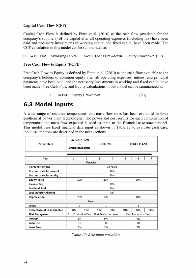
74

Parameters

Year 1 2 3 4 5 6 7

Planning Horizon

Discount rate for project

Discount rate for equity

Equity Ratio

Income Tax

Dividend Paid

Loss Transfer Allowed

Depreciation

Loans

Percentage of Loan Granted 50% 50% 50% 50% 40% 40% 20%

First Repayment

Interest

Loan Life

Loan Fees

32 Years

Financial

Loans

2% 2%

16%

20%

30%

30%

9%

10

2%

10 10

9% 9%

No

First Production Year First Production Year

1 1

First Production Year

1

EXPLORATION

&

CONFIRMATION

POWER PLANT DRILLING

25% 5% 10%

30% 30% 30%

Capital Cash Flow (CFF)

Capital Cash Flow is defined by Pinto et al. (2010) as the cash flow (available for the company´s suppliers) of the capital after all operating expenses (including tax) have been paid and necessary investments in working capital and fixed capital have been made. The CCF calculation in this model can be summarized as

CCF = EBITDA− ∆WorkingCapital − Taxes + LoansDrawdown + EquityDrawdown,52/ Free Cash Flow to Equity (FCFE)

Free Cash Flow to Equity is defined by Pinto et al. (2010) as the cash flow available to the company´s holders of common equity after all operating expenses, interest and principal payments have been paid, and the necessary investments in working and fixed capital have been made. Free Cash Flow and Equity calculations in this model can be summarized as

FCFE = FCF + EquityDrawdown,53/ 6.3 Model inputs

A wide range of resource temperatures and mass flow rates has been evaluated in three geothermal power plant technologies. The power and cost results for each combination of temperature and mass flow expected is used as input to the financial assessment model. This model uses fixed financial data input as shown in Table 13 to evaluate each case. Input assumptions are described in the next sections.

Table 13: Risk input variables

75

Geothermal resources

In this study, resource temperatures between 160 and 340°C are evaluated for flash technologies, and resource temperatures between 100 and 180°C are evaluated for binary technologies. Both technologies are evaluated for mass flow rates between 100 and 1,000 kg/s. Geothermal resources in Central American countries are described in Chapter 3. Power plant

The power plant availability factor is assumed as 90%, over a one year period. The net power output is calculated by subtracting all auxiliary loads to the total power output as described in Section 4.1. Market

In this study, the average price of 115 USD/MWh for the year 2010 was assumed for the wholesale market in Central American countries with an expected growth rate of 5%. Electricity market research is described in Section 2.2.8. Capital cost

The geothermal development capital cost includes exploration and confirmation, drilling and power plant. Capital cost is calculated as described in Chapter 5. Operation and maintenance cost

O&M cost is assumed as 2.8 UScents/kWh with an expected growth rate of 4 %. The cost of O&M for a power plant and for a steam field is described in Section 5.5. Structure of geothermal financing

The literature review (Battocletti et al., 1999; Hance, 2005; Rodríguez and Henríquez, 2007; Long, 2009; Salmon et al., 2011) illustrates values between 15% and 50% for the equity component in financing geothermal development. Lenders will normally require an equity percentage to ensure the sponsor’s continued commitment. For the exploration phase of the project, it is frequently used as the developer risks his own money on an indirect assessment of resource potential. Based on a survey of the literature, this analysis assumes 30% equity. Discount rates

Elíasson and Valdimarsson (2005) argued that the interest rate required from a geothermal project investment, often referred to as MARR, is defined by the company in order to undertake a project. It is similar to WACC if the project bears in itself the same or similar risk as the average risk from the normal operation of the company. The MARR can be in the range of 5-25% depending on the risk of the project. Ormat, a leading player in the geothermal market uses 12-18% as their target for a feasible project in developing countries (as cited in Broniki, 2004). According to Gordon (2009) risk capital comes at a

76

high cost, and most investors require a 20% return on investment, depending on the project and perceived risk.

In the Central American region, J. A. Rodríguez explained that the MARR for an investor in the geothermal development has increased in the last couple of years, in response to the jurisdiction and personal insecurities of these countries. The minimum IRR used to be 10% or 11% but is now 15% or 16%. The ROE (or equity IRR) that is normal requested is usually around 20% (personal communication, November 14, 2011). In Honduras, the second largest country of Central America, according to C.A. Lagos, from the point of view of private geothermal developers, the commonly used value (like MARR) for a project is between 10% to 14% and the MARR for equity is between 12% to 18%, both considering a period of 20 years (personal communication, November 11, 2011).

The Central American region´s values are in contrast with that of other developing countries such as Indonesia and Kenya. An Indonesia project appraisal document from World Bank (2008) pointed out that various reports and discussions with investors indicated that the capital cost for a geothermal Independent Power Producer is somewhere between 14 to 16%. In Kenya, the Government requires a ROE of 15%, while private investors would normally ask between 18% and 23% but it is not unusual to get higher requests (Ngugi, 2012). These figures vary with respect to the data from developed countries such as Iceland. According to B. M. Júlíusson, the minimum WACC that is used for geothermal projects in Iceland is 8% and the minimum rate of return on equity is 12%. The expected rate of return on equity for Landsvirkjun on new projects is 12 - 15% (personal communication, November 11, 2011).

Hance (2005) has drawn attention to the fact that in case of project failure, the geothermal equity holders are the last to recover their investment, therefore, to recompense risk they expect high rates of return from 16 to 20%. Based on the above information, 16% is used as the MARR for projects and 20% is used as the MARR for equity. Interest on loans

Fleischmann (2007) included in the financing issues for independent geothermal developers items such as: construction financing (interest rates may be up to 10% or more and the construction lender requires a take-out guarantee at commissioning); and term financing (usually based on 30% equity, IRR in the high teens, interest 7% or more for 15 years). Hance (as cited in IEA, 2011) states that when considering geothermal development, in some countries such as the United States, interest rates from 6% to 8% is usually requested for debt lenders. The IEA (2011) in its recent report indicated an assumed 10% interest rate assumed for the production cost calculations related to geothermal heat and power technologies. In a study of cost/size/risk analysis of geothermal projects (Elíasson and Smith, 2011), calculations assumed that first time projects require 30% equity, a 7% interest rate on 12 year majority with a 3 year grace period on the first project loan, and 25% equity, 6% interest and the same majority for subsequent projects. It is clear that different types of financing options (loans) may have different interest rates and terms. The work of Rodríguez and Henríquez (2005) revealed that, in Central America, all of the financing options: equity financing, bank financing (private banks and

77

multilateral institutions) and debenture through the stock exchange, are used to some extent by different developers. In this study, a 9 % interest is assumed in the three loans considered for geothermal development. Depreciation

A straight line depreciation method is assumed, as defined in Section 2.3. Dividends

The policy of dividend payments to owners is assumed to be 30% of the net income at the end of the financial year. Corporate tax

A corporate tax of 30% is assumed is defined in Section 2.3. As explained in Section 2.4, in Central America each country has different tax incentive schemes for the development of renewable energies. The impact of the tax incentives on the financial returns of geothermal projects is discussed in Section 6.7. Loss transfer

In this study, loss transfer is not allowed.

6.4 Model outputs for two resource scenarios

and one power plant technology

6.4.1 Cash Flows

In this analysis, two cash flows are considered: CCF and FCFE. Two different sizes of investments are discussed, as results of two different geothermal resources expected. In the next section, a wide range of temperature resources and mass flow have been evaluated. Figure 39 shows the cash flows for two single flash power plant projects: scenario 1 for 240°C, and 300 kg/s (27.7 MW); and scenario 2 for 240°C, and 300 kg/s (55.5 MW). As Figure 39 indicates, the geothermal development project has negative cash flows during the first 7 years, largely as a consequence of significant capital expenditures. Most of the high initial fixed costs occur during the drilling and power plant construction phases. During this period, geothermal development projects finance a high proportion of their investment needs with debt. In this analysis, debt financing helps to obtain better IRR of Equity; this is because it is assumed in the model that the payment of interest is tax deductible. FCFE reflects to the equity investor the effect of changes in the levels of debt, and repaying the principal on existing debt represents an outflow in the estimation of FCFE. After the geothermal power plant construction period, when commercial production starts, the revenue is spread out over the subsequent years; hence, the project shows positive cash flows. Note that after the debt repayment period payment is concluded, FCFE is similar to the CCF.

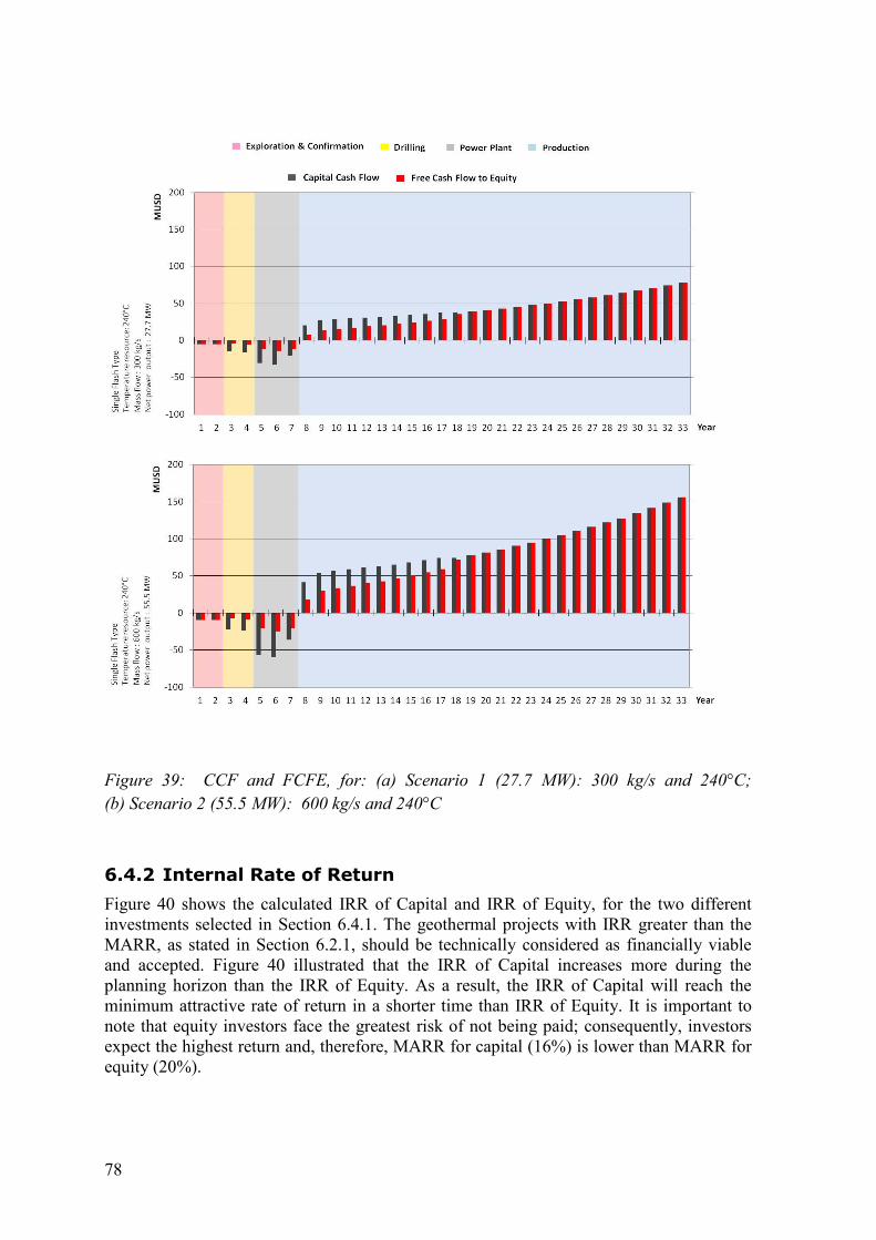
78

Figure 39: CCF and FCFE, for: (a) Scenario 1 (27.7 MW): 300 kg/s and 240°C;

(b) Scenario 2 (55.5 MW): 600 kg/s and 240°C

6.4.2 Internal Rate of Return

Figure 40 shows the calculated IRR of Capital and IRR of Equity, for the two different investments selected in Section 6.4.1. The geothermal projects with IRR greater than the MARR, as stated in Section 6.2.1, should be technically considered as financially viable and accepted. Figure 40 illustrated that the IRR of Capital increases more during the planning horizon than the IRR of Equity. As a result, the IRR of Capital will reach the minimum attractive rate of return in a shorter time than IRR of Equity. It is important to note that equity investors face the greatest risk of not being paid; consequently, investors expect the highest return and, therefore, MARR for capital (16%) is lower than MARR for equity (20%).

79

0%

5%

10%

15%

20%

25%

30%

1 2 3 4 5 6 7 8 9 10 11 12 13 14 15 16 17 18 19 20 21 22 23 24 25 26 27 28 29 30 31 32 33

IRR

Year

Sin

gle

Fla

sh C

ycle

Te

mp

era

ture

Re

sou

rce

: 24

0°C

Ma

ss F

low

: 6

00

kg

/s

Ne

t p

ow

er

Ou

tpu

t :

55

.5 M

W

0%

5%

10%

15%

20%

25%

30%

1 2 3 4 5 6 7 8 9 10 11 12 13 14 15 16 17 18 19 20 21 22 23 24 25 26 27 28 29 30 31 32 33

IRR

Year

IRR Capital IRR Equity

Sin

gle

Fla

sh C

ycle

Te

mp

era

ture

Re

sou

rce

: 2

40

°C

Ma

ss F

low

: 3

00

kg

/s

Ne

t p

ow

er

Ou

tpu

t :

27

.7 M

W

Figure 40: IRRs for project and equity for: a) Scenario 1 (27.7 MW): 300 kg/s and 240°C;

b) Scenario 2 (55.5 MW): 600 kg/s and 240°C

As shown in Figure 40, IRRs reach the MARRs in fewer years for a bigger sized development. The magnitude of the geothermal development will affect the years horizon considered for reaching the MARR. It is important to note that the planning horizon could be reduced, and it is still possible to reach the MARR. The IRR graph could help to define the horizon plan needed for consideration of a viable project. As shown in Figure 40, IRR rises rapidly in the beginning, then slows down and in the end remains the same year after year. This planning horizon analysis also can be done using the NPV charts, because the IRR is a related concept to NPV; IRR is defined as the discount rate for when NPV is equal to zero.

6.4.3 Accumulated Net Present Value

The accumulated NPVs are shown in Figure 41. In this analysis, future cash flows are discounted by appropriate discount rates. Discounting the CCFs with the MARR for a project reflects the NPV of the investment at the firm level and discounting the FCFEs with the MARR of equity reflects the NPV of the investment at the equity level.

80

-140

-120

-100

-80

-60

-40

-20

0

20

40

60

1 2 3 4 5 6 7 8 9 10 11 12 13 14 15 16 17 18 19 20 21 22 23 24 25 26 27 28 29 30 31 32

MU

SD

Year

Sin

gle

Fla

sh C

ycle

Te

mp

era

ture

Re

sou

rce

: 24

0°C

Ma

ss F

low

: 6

00

kg

/s

Ne

t p

ow

er

Ou

tpu

t :

55

.5

MW

As seen in Figure 40, a large size project will first reach a positive NPV, and indicates that this project has a lower risk. The NPV of CCF and NPV of FCFE are positive over the planning horizon for the two different sized developments. In both geothermal developments the loan received, which is for 70% of the investment cost and working capital, is paid over 10 years after operations begin, but the two geothermal developments meet the return requirement at different periods of time. The necessary payback period for recovering investments is lower for the project than for the equity investors.

6.4.4 Allocation of funds

Figure 42 illustrates the allocation of funds from the initial year through the planning horizon. The allocation of funds is illustrated for two single flash power plant projects: scenario 1 for 240°C, and 300 kg/s (27.7 MW); and scenario 2 for 240°C, and 300 kg/s (55.5 MW). The chart shows how paid taxes, financial cost, repayments, paid dividend and cash movement change over the planning horizon of 32 years.

Figure 41: Accumulated net present value for: a) Scenario 1 (27.7 MW): 300 kg/s and

240°C; b) Scenario 2 (55.5 MW): 600 kg/s and 240°C

-140

-120

-100

-80

-60

-40

-20

0

20

40

60

1 2 3 4 5 6 7 8 9 10 11 12 13 14 15 16 17 18 19 20 21 22 23 24 25 26 27 28 29 30 31 32

MU

SD

Year

NPV Capital Cash Flow 16% NPV Net Cash Flow 20%

Sin

gle

Fla

sh C

ycle

Te

mp

era

ture

Re

sou

rce

: 24

0°C

Ma

ss F

low

: 3

00

kg

/s

Ne

t p

ow

er

Ou

tpu

t :

27

.7 M

W

81

0

50

100

150

200

250

1 2 3 4 5 6 7 8 9 10 11 12 13 14 15 16 17 18 19 20 21 22 23 24 25 26 27 28 29 30 31 32

MU

SD

Year

Sin

gle

Fla

sh C

ycl

e

Te

mp

era

ture

Re

sou

rce

: 24

0°C

Ma

ss F

low

: 6

00

kg

/s

Ne

t p

ow

er

Ou

tpu

t :

55

.5 M

W

0

50

100

150

200

250

1 2 3 4 5 6 7 8 9 10 11 12 13 14 15 16 17 18 19 20 21 22 23 24 25 26 27 28 29 30 31 32

MU

SD

Year

Paid Taxes Financial Costs Repayment Paid Dividend Cash Movement

Sin

gle

Fla

sh C

ycl

e

Te

mp

era

ture

Re

sou

rce

: 24

0°C

Ma

ss F

low

: 3

00

kg

/s

Ne

t p

ow

er

Ou

tpu

t :

27

.7 M

W

Figure 42: Allocation of funds for: a) Scenario 1 (27.7 MW): 300 kg/s and 240°C;

b) Scenario 2 (55.5 MW): 600 kg/s and 240°C

6.5 Results for multiple resource scenarios and

three power plant technologies

Knowledge of the quality and quantity of the geothermal resources in question is key to the success of geothermal projects. A major problem for investors is that the quality and quantity of a resource can only be estimated and not proven before explorative drilling. In the early stages of geothermal energy projects, the risk of the resource is very high, and explorative drilling is very expensive (Wendel and Hiegl, 2010). In consequence, the feasibility of a project can only be recognized if the coupled flow rate and temperature accomplish the expectations of the investors.

82

The contour maps of IRRs of FCFE from three technologies of power plant investment are presented in this section. This kind of contour map can be a practical tool for decision makers in order to evaluate the project profitability for different expected geothermal resources. Based on the contour lines, an investor who knows the results of a geothermal field evaluation can identify the profitability measures. Previously selected as the discount rate in Section 6.3.7, the MARR for equity required for a geothermal investor is 20%; the MARR for a geothermal project is 16%.

6.5.1 Single flash

Figure 43 shows the contour map of IRR of Free Cash Flow to Equity (%), and the power plant size (MW) for a single flash power plant development. The color of the contour lines is used to illustrate: black for the IRR of FCFE, and red for the power plant size. The geothermal resource temperature examined is between 160 and 340°C, and the mass flow rate examined is between 100 and 1000 kg/s.

Figure 43: Contour map of IRR of FCFE from single flash power plant

For single flash power plants, the results of IRRs of FCFE for multiple power plant sizes suggest profitable indicators for specific geothermal resource temperatures and mass flow rates. From Figure 43, it is possible to conclude that in order to achieve profitable indicators, a resource temperature greater than or equal to 280°C demands a mass flow rate lower than or equal to 150 kg/s; this means roughly 21 MW or less capacity. A resource temperature greater than or equal to 240°C demands a mass flow rate lower than or equal to 230 kg/s; this means roughly 21 MW or less capacity. A resource temperature greater than or equal to 200°C demands a mass flow rate lower than or equal to 400 kg/s; this roughly means 23 MW or less capacity. Finally, a resource temperature equal to 160°C demands a mass flow greater than or equal to 900 kg/s; this roughly means 30 MW.

Re

sou

rce

te

mp

era

ture

[ °

C ]

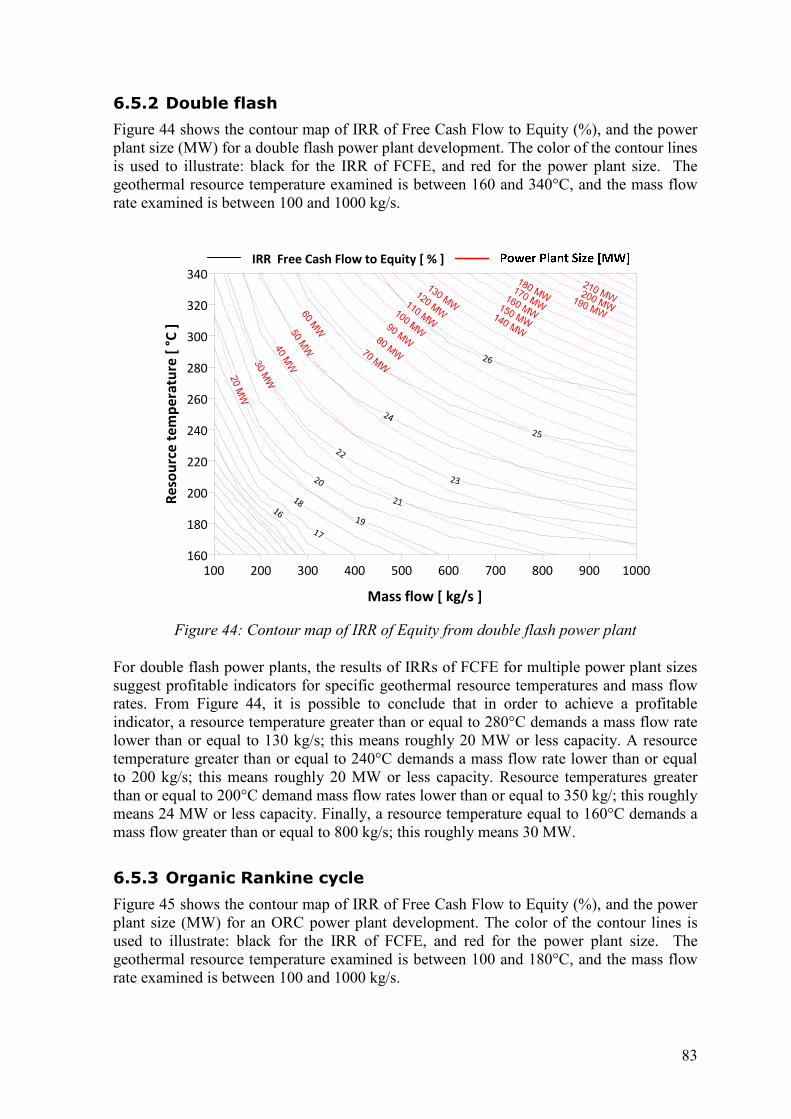
83

6.5.2 Double flash

Figure 44 shows the contour map of IRR of Free Cash Flow to Equity (%), and the power plant size (MW) for a double flash power plant development. The color of the contour lines is used to illustrate: black for the IRR of FCFE, and red for the power plant size. The geothermal resource temperature examined is between 160 and 340°C, and the mass flow rate examined is between 100 and 1000 kg/s.

Figure 44: Contour map of IRR of Equity from double flash power plant

For double flash power plants, the results of IRRs of FCFE for multiple power plant sizes suggest profitable indicators for specific geothermal resource temperatures and mass flow rates. From Figure 44, it is possible to conclude that in order to achieve a profitable indicator, a resource temperature greater than or equal to 280°C demands a mass flow rate lower than or equal to 130 kg/s; this means roughly 20 MW or less capacity. A resource temperature greater than or equal to 240°C demands a mass flow rate lower than or equal to 200 kg/s; this means roughly 20 MW or less capacity. Resource temperatures greater than or equal to 200°C demand mass flow rates lower than or equal to 350 kg/; this roughly means 24 MW or less capacity. Finally, a resource temperature equal to 160°C demands a mass flow greater than or equal to 800 kg/s; this roughly means 30 MW.


Figure 45 shows the contour map of IRR of Free Cash Flow to Equity (%), and the power plant size (MW) for an ORC power plant development. The color of the contour lines is used to illustrate: black for the IRR of FCFE, and red for the power plant size. The geothermal resource temperature examined is between 100 and 180°C, and the mass flow rate examined is between 100 and 1000 kg/s.

100 200 300 400 500 600 700 800 900 1000

Mass flow [ kg/s ]

160

180

200

220

240

260

280

300

320

340

Re

sou

rce

te

mp

era

ture

[ °

C ]

IRR Free Cash Flow to Equity [ % ]

84

For organic Rankine cycle power plants, the results of IRRs of FCFE for multiple power plant sizes suggest profitable indicators for specific geothermal resource temperatures and mass flow rates. From Figure 45, it is possible to conclude that in order to achieve a profitable indicator, a resource temperature greater than or equal to 180°C demands a mass flow rate lower than or equal to 250 kg/s; this means roughly 15 MW or less capacity. A resource temperature greater than or equal to 140°C demands a mass flow rate lower than or equal to 650 kg/s; this means roughly 16 MW or lesser capacity. A resource temperature greater than or equal to 130°C demands a mass flow rate lower than or equal to 900 kg/s; this roughly means 18 MW or less capacity.

Figure 45: Contour map of IRR of Equity from ORC power plant

6.6 Impact of tax on geothermal development

Tax incentives enhance the financial returns of geothermal projects by offsetting tax liabilities. Important elements of tax related incentives for geothermal projects in Central American countries are included in Table 14. Figure 46 shows the impact of taxation on the IRR of Equity for the development of geothermal resources. Incentive laws of tax exemption for the development of renewable energy projects are not large enough to enhance the internal rate of returns required by investors, when small size power plant projects are conducted: for flash technologies, power plant sizes smaller than or equal to 20 MW; and for ORC technology, power plant sizes smaller than or equal to 10 MW. Comparing the Central American countries, Nicaragua and Guatemala tax incentive laws are favorable to the profitability of geothermal development. This compares quite well with Guidos and Burgos (2012) who

Re

sou

rce

te

mp

era

ture

[ °

C ]

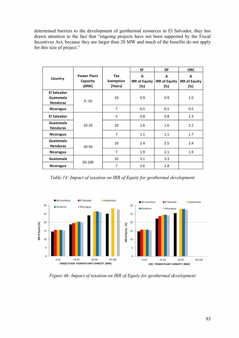
85

0

5

10

15

20

25

30

0-10 10-20 20-50 50-100

IRR

of

Eq

uit

y

[%]

ORC POWER PLANT CAPACITY [MW]

No Incentives El Salvador Guatemala

Honduras Nicaragua

determined barriers to the development of geothermal resources in El Salvador, they has drawn attention to the fact that “ongoing projects have not been supported by the Fiscal Incentives Act, because they are larger than 20 MW and much of the benefits do not apply for this size of project.”

Table 14: Impact of taxation on IRR of Equity for geothermal development

Figure 46: Impact of taxation on IRR of Equity for geothermal development

Δ

IRR of Equity

[%]

Δ

IRR of Equity

[%]

Δ

IRR of Equity

[%]

El Salvador

Guatemala

Honduras

10 0.9 0.9 1.0

Nicaragua 7 0.5 0.5 0.5

El Salvador 5 0.8 0.8 1.3

Guatemala

Honduras10 1.6 1.6 2.2

Nicaragua 7 1.1 1.1 1.7

Guatemala

Honduras10 2.4 2.5 2.4

Nicaragua 7 1.9 2.1 1.9

Guatemala 10 3.1 3.3

Nicaragua 7 2.6 2.8

Country Power Plant

Capacity

[MW]

Tax

Exemption

[Years]

SF DF ORC

0 -10

10-20

20-50

50-100

0

5

10

15

20

25

30

0-10 10-20 20-50 50-100

IRR

of

Eq

uit

y [

%]

SINGLE FLASH POWER PLANT CAPACITY [MW]

No Incentives El Salvador Guatemala

Honduras Nicaragua

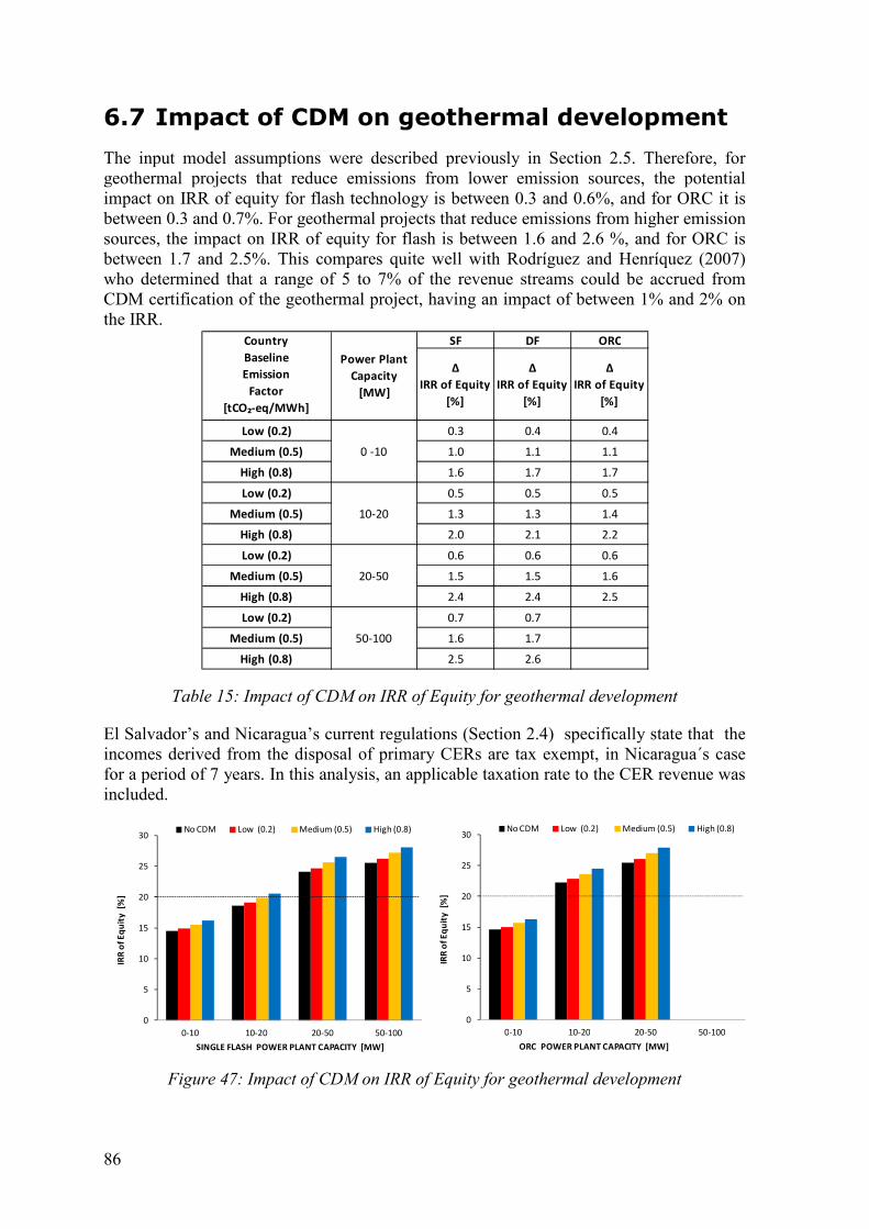
86

0

5

10

15

20

25

30

0-10 10-20 20-50 50-100

IRR

of

Eq

uit

y [

%]

ORC POWER PLANT CAPACITY [MW]

No CDM Low (0.2) Medium (0.5) High (0.8)

0

5

10

15

20

25

30

0-10 10-20 20-50 50-100

IRR

of

Eq

uit

y [

%]

SINGLE FLASH POWER PLANT CAPACITY [MW]

No CDM Low (0.2) Medium (0.5) High (0.8)

Δ

IRR of Equity

[%]

Δ

IRR of Equity

[%]

Δ

IRR of Equity

[%]

Low (0.2) 0.3 0.4 0.4

Medium (0.5) 1.0 1.1 1.1

High (0.8) 1.6 1.7 1.7

Low (0.2) 0.5 0.5 0.5

Medium (0.5) 1.3 1.3 1.4

High (0.8) 2.0 2.1 2.2

Low (0.2) 0.6 0.6 0.6

Medium (0.5) 1.5 1.5 1.6

High (0.8) 2.4 2.4 2.5

Low (0.2) 0.7 0.7

Medium (0.5) 1.6 1.7

High (0.8) 2.5 2.6

50-100

20-50

10-20

0 -10

Country

Baseline

Emission

Factor

[tCO₂-eq/MWh]

Power Plant

Capacity

[MW]

SF DF ORC

6.7 Impact of CDM on geothermal development

The input model assumptions were described previously in Section 2.5. Therefore, for geothermal projects that reduce emissions from lower emission sources, the potential impact on IRR of equity for flash technology is between 0.3 and 0.6%, and for ORC it is between 0.3 and 0.7%. For geothermal projects that reduce emissions from higher emission sources, the impact on IRR of equity for flash is between 1.6 and 2.6 %, and for ORC is between 1.7 and 2.5%. This compares quite well with Rodríguez and Henríquez (2007) who determined that a range of 5 to 7% of the revenue streams could be accrued from CDM certification of the geothermal project, having an impact of between 1% and 2% on the IRR.

Table 15: Impact of CDM on IRR of Equity for geothermal development

El Salvador’s and Nicaragua’s current regulations (Section 2.4) specifically state that the incomes derived from the disposal of primary CERs are tax exempt, in Nicaragua´s case for a period of 7 years. In this analysis, an applicable taxation rate to the CER revenue was included.

Figure 47: Impact of CDM on IRR of Equity for geothermal development

87

7 Risk analysis

The investment decision presented in Chapter 6 for geothermal power plant projects is based on cash flow analysis, such as NPV and IRR. The analysis is first performed using predicted routines of the project over the project life as if the predictions were deterministic. As a second step, the stochastic nature of these predictions are handled using a selection of risk analysis techniques (O’Donnell et al., 2002). In this analysis, the risk technique analyses include: single parameter sensitivity analysis and Monte Carlo simulation.

7.1 Sensitivity analysis

According to the Asian Development Bank (ADB, 2009), a sensitivity analysis is a technique for investigating the impact of changes in project variables for the base case. The purpose of a sensitivity analysis is: to help identify the key variables which influence the project cost and benefit streams. This method, determining how sensitive the financial model outputs are, changes the model inputs. The sensitivity is the rate of change of a variable with respect to the change of another variable with the values of all other variables held constant (Crundwell, 2008). This concept is expressed by Equation 54 as the partial derivative of the first variable with respect to the second one, as follows

j = � x,54/

where � and x are dependent and independent variables, and j is the sensitivity of � with respect to x. This analysis considers the effects of likely changes in the key variables on the IRR of Equity of scenario 1 (SF, 27.7MW, 240°C, 300 kg/s) for a geothermal power plant project. The key variables included are divided into two groups: cost and operation inputs, and financial data inputs. As shown in Figure 48, cost and operation inputs included in the sensitivity analysis are energy price, the availability factor, O&M costs, exploration and confirmation costs, drilling costs and power plant costs. Figure 49 illustrates the financial data inputs which include the equity ratio, corporate tax, loan interest, loan life and depreciation of equipment. Figure 48 shows how cost and operation input variables affect the IRR of Equity. Figure 46 shows how financial input variables affect the IRR of Equity. These inputs are changed from –50% of the base value to +50% of the base value, and the effect of the change on the IRR of Equity is then calculated. Figure 48 shows the sensitivity of IRR of Equity to the cost and operation inputs, where the IRR of Equity is most sensitive to the energy price and availability factor. The influence of these parameters is positive; an increase in the

88

energy price or availability factor indicates an increase in the IRR of Equity. The rest of the variables have a negative sensitivity. An increase in the cost of O&M, exploration and confirmation, drilling, and power plant means a decrease in the IRR of Equity.

Figure 48: Sensitivity of the IRR of Equity for scenario 1: cost and operation inputs

Figure 49 shows the sensitivity of the IRR of Equity to the financial inputs, where the IRR of Equity is most sensitive to the loan interest, equity ratio and corporate tax. The influence of these parameters is negative; an increase in these variables indicates a decrease in the IRR of Equity. The rest of the variables have positive sensitivity. An increase in the loan life or depreciation equipment means a decrease in the IRR of Equity.

Figure 49: Sensitivity of the IRR of Equity for scenario 1: financial inputs

8%

10%

12%

14%

16%

18%

20%

22%

24%

26%

28%

30%

32%

-50% -40% -30% -20% -10% 0% 10% 20% 30% 40% 50%

IRR

of

Eq

uit

y

Deviation

Energy Price Availability Factor O&M Expl. & Conf. Drilling Power Plant

19%

20%

21%

22%

23%

24%

25%

-50% -40% -30% -20% -10% 0% 10% 20% 30% 40% 50%

IRR

of

Eq

uit

y

Deviation

Equity Ratio Corporate Tax Loan Interest Loan Life Depreciation Equipment

89

From all the variables analyzed, the energy price and the available plant factor are identified as the critical values which could change the decision to another course of action. For this purpose, the critical values as they affect the project decision, here IRR of Equity, are first obtained.

7.2 Monte Carlo simulation

The Monte Carlo simulation, in the use of risk analysis, adds the dimension of dynamic analysis to investment assessment by building models of possible results by substituting a range of values, a probability distribution function (PDF), for any factor that has inherent uncertainty (Palisade, 2011). Various options of the mathematical technique are available for using Monte Carlo simulations in computers; @RISK software from Palisade is used in this analysis.

Symmetrical distributions as normal, uniform and PERT are used in the Monte Carlo simulations. According to Savvides (1994) symmetrical distributions allocate probability symmetrically across the defined range but with varying degrees of concentration towards the mean values. Palisade (2011) states that normally distributed variables are characterized by mean and standard deviations, where the values in the middle near the mean are most likely to occur; uniform distribution gives equal chance of occurring, which is defined by minimum and maximum; PERT distribution is rather like a triangular distribution, in that it is defined by minimum, most likely, and maximum; however, values between the most likely and extremes are more likely to occur than in the triangular distribution.

Table 16: Input risk variables for scenario 1

Variables Units Min. Mean Max. Fix. Val. St. Dev. Distribution

a m b

Gross Capacity MW 55.0

Resource Temperature °C 240.0

Mass Flow Rate kg/s 300.0

Availability Factor % 0.8 0.9 0.95 PERT

Exploration Cost USD/kW 138.4 173.0 207.6 Uniform

Confirmation Cost USD/kW 138.4 173.0 207.6 Uniform

Drilling Cost USD/MW 0.3 0.5 1.0 PERT

First Development Cost MUSD 5.3 15.1 24.8 PERT

Steam Gathering Cost USD/kW 223.2 279.0 334.8 Uniform

Equipment and Construction Cost MUSD 120.6 150.8 181.0 Uniform

Transmission Power Line Distance km 1.0 10.0 12.0 PERT

Transmission Power Line Cost USD/km 590000.0 840000.0 920000.0 PERT

O&M Cost USD¢/kwh 2.2 2.8 3.4 Uniform

O&M Annual Growth % 4.0 3 Normal

Initial Energy Price USD/MWh 90.0 116.0 170.0 PERT

Energy Price Annual Growth % 5.0 3 Normal

Loan Interest % 8.0 9.0 11.0 PERT

POWER PLANT SPECIFICATION

EXPLORATION AND CONFIRMATION

DRILLING

POWER PLANT

FINANCIAL

90

The second phase entails the selection of selection as “one which is critical to the viability of the project in the sense that a deviation from its projected value is both probable and potentially damaging to the project’s worth”. The simulated factor, exploration and confirmation cost, drilling costgathering cost, equipment and construction costtransmission power line cost, O&M costannual growth and loan interest Table 16 shows the risk variables for scenario 1 (SF, on this information, the risk analysis tool has the basic inputs to execute the Monte Carlo simulation; results are generated using 1,000 iterations. The variability informationthe study of variations in the IRR of Evariable.

Figure 50: Density and cumu

geothermal power plant with resource characteristics: (a)

and 240°C; (b) Scenario 2 (55.5 MW)

Figure 50 shows the density andscenarios 1 and 2. Using the IRR of Equity for Scenario probability of success for an IRR58.8% chance of the project exThe internal rate of return of equity some probability of being negative; investor.

entails the selection of the risk variables. Savvides (1994) one which is critical to the viability of the project in the sense that a

deviation from its projected value is both probable and potentially damaging to the The simulated risk variables shown in Table 16 includ

factor, exploration and confirmation cost, drilling cost, first development cosequipment and construction cost, transmission power line distance

ssion power line cost, O&M cost, O&M annual growth, energy price,annual growth and loan interest.

shows the risk variables for scenario 1 (SF, 27.7 MW, 240°C, 300 kg/s). Based this information, the risk analysis tool has the basic inputs to execute the Monte Carlo

simulation; results are generated using 1,000 iterations. The variability informationin the IRR of Equity due to the predicted variation of each risk

cumulative probability distribution of IRR of E

resource characteristics: (a) Scenario 1 (27.7 MW

Scenario 2 (55.5 MW): 600 kg/s and 240°C

density and cumulative probability distribution of IRR financial model, the expected or deterministic 1 is 21.3 %. The results of the risk analysis illustrate theIRR of Equity greater or equal to 20% to be 0.58

project exceeding the minimum rate of return expected internal rate of return of equity shows some probability of being positive as well as

negative; hence the decision rests on the risk aversion

s. Savvides (1994) defined this one which is critical to the viability of the project in the sense that a small

deviation from its projected value is both probable and potentially damaging to the include availability

first development cost, steam transmission power line distance,

energy price, energy price

240°C, 300 kg/s). Based this information, the risk analysis tool has the basic inputs to execute the Monte Carlo

simulation; results are generated using 1,000 iterations. The variability information permits quity due to the predicted variation of each risk

of Equity for SF

(27.7 MW): 300 kg/s

of IRR of Equity for the expected or deterministic result for the

analysis illustrate the 0.58, signifying a

return expected by investors. shows some probability of being positive as well as

rests on the risk aversion of the

91

7.3 Results for multiple resource scenarios and

three power plant technologies

The contours maps of the probability of success for an IRR of Equity greater or equal to 20%, from three technologies of power plant investment, are presented in this section. This kind of contour map can be a practical tool for decision makers in order to evaluate the profitability of success for different expected geothermal resources. Based on the contour lines, investors can identify the project risk for different resource scenarios.

7.3.1 Single flash

Figure 51 shows the contour map of the probability of success (%) for IRR of Equity greater or equal to 20%, and the power plant size (MW) for an SF power plant development. The color of the contour lines is used to illustrate: black for the probability of success, and red for the power plant size. The geothermal resource temperature examined is between 160 and 340°C, and the mass flow rate examined is between 100 and 1000 kg/s. In Chapter 6, Figure 43 illustrated that single flash development had a profitable indicator for plant capacity above 23 MW. The analysis of the data from Figure 51 suggests that the probability of success is roughly 50% for 23 MW of power plant capacity. It is important to note that there is a high risk associated with geothermal projects. For example, 70% of the probability of success of the MARR for equity would require a power plant size greater than 70 MW.

Figure 51: Contour map of probability of IRR of Equity ≥ 20%; SF power plant

100 200 300 400 500 600 700 800 900 1000

Mass flow [ kg/s ]

160

180

200

220

240

260

280

300

320

340

Re

sou

rce

te

mp

era

ture

[ °

C ]

Probability IRR of Equity > 20 [ % ]

92

7.3.2 Double flash

Figure 52 shows the contour map of the probability of success (%) for IRR of Equity greater or equal to 20%, and the power plant size (MW) for DF power plant development. The color of the contour lines is used to illustrate: black for the probability of success, and red for the power plant size. The geothermal resource temperature examined is between 160 and 340°C, and the mass flow rate examined is between 100 and 1000 kg/s. In Chapter 6, Figure 44 illustrated that double flash development had a profitable indicator for plant capacity above 25 MW. The analysis of the data from Figure 52 suggests that the probability of success is roughly 50% for an 18 MW power plant capacity. For example, 40% of the probability of success of the MARR for equity would require a power plant size greater than 60 MW.

Figure 52: Contour map of probability of IRR of Equity ≥ 20%; DF power plant


Figure 53 shows the contour map of the probability of success (%) for IRR of Equity greater or equal to 20%, and the power plant size (MW) for an ORC power plant development. The color of the contour lines is used to illustrate: black for the probability of success, and red for the power plant size. The geothermal resource temperature examined is between 100 and 180°C, and the mass flow rate examined is between 100 and 1000 kg/s. In Chapter 6, Figure 45 illustrated that organic Rankine cycle development had a profitable indicator for plant capacity above 25 MW. The analysis of the data from Figure 52 suggests that the probability of success is roughly 50% for a 25 MW power plant capacity.

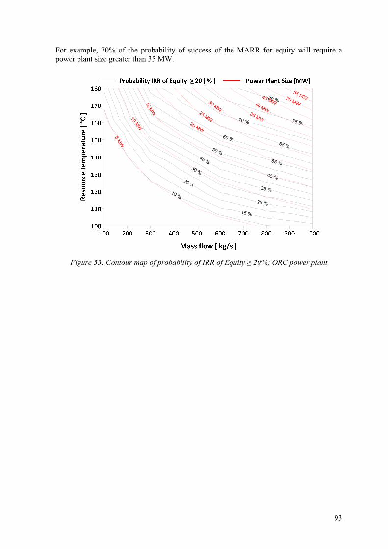
93

For example, 70% of the probability of success of the MARR for equity will require a power plant size greater than 35 MW.

Figure 53: Contour map of probability of IRR of Equity ≥ 20%; ORC power plant

95

8 Summary and conclusions

The present study indicates that geothermal power plant size, profitability indicators and probability of success of geothermal power development arise from an increase in the temperature of a geothermal resource and the mass flow rate. As a result, geothermal power development projects in Central America for small sized power plant are not attractive for private investors when the project considers the cost of exploration and confirmation, drilling an unknown field, power plant and transmission lines. The analysis suggests that geothermal development projects in Central America have profitable indicators starting from a specific power plant capacity, dependent upon the power plant technology selected. Three thermodynamic cycles were evaluated from mass flow rates ranging from 100 to 1,000 kg/s. The two steam cycles were evaluated for reservoir temperatures ranging from 160 to 340°C, and the organic Rankine cycle was evaluated for reservoir temperatures ranging from 100 to 180°C. In the case of the flash systems, the projects had profitable indicators for similar power plant sizes. The results suggested projects with profitable indicators for a power plant size greater than 24 MW for resource temperatures greater than or equal to 200°C. For flash power plant developments, using resource temperatures lower than 200°C demanded a mass flow rate higher than 400 kg/s, and the minimum power plant size required could extend to 30 MW. The difference between single flash and double flash is the amount of mass flow required to achieve the capacity needed. For a single flash system, between 10% and 20% more mass flow is needed. In the case of an organic Rankine cycle, the results suggested projects with profitable indicators for power plant sizes greater than 18 MW for resource temperatures greater than or equal to 130°C. For organic Rankine Cycle power plant development, using a resource temperature lower than 130°C demanded a mass flow rate higher than 900 kg/s. The study identified high technical and financial risks associated with small geothermal projects which were suggested with profitability indicators in the economic analysis. For flash projects less than 24 MW and ORC projects less than 18MW, the probability of success is around 50% for achieving the minimum attractive rate of return required by investors. Risk analysis suggests that the most important financial factor that affects project profitability is the energy price and the plant availability factor more than drilling and power plant costs.

Investment costs for typical geothermal development suggest extreme variability in the cost of components when all project costs (exploration and confirmation, drilling an unknown field, power plant and transmission line) are considered. The variability of the specific capital cost is inversely affected by the resource temperature and the mass flow rate. Based on the geothermal resource quality considered for each technology, the estimated cost for single flash ranges from 2,912 to 5,910 USD2010/kW, for double flash from 2,500 to 6,000 USD2010/kW, and for the organic Rankine cycle the cost ranges from 2,302 to 11,469 USD2010/kW. The range of results matches the costs presented in literature

96

where the temperature range is concentrated, for example in the case of the flash systems, when temperature range is reduced to 200-300°C from 160-340°C, and in the binary system when temperature range is reduced to 140-180°C from 100-180°C. Larger size development of geothermal power plants gives more cost effective values than smaller power plant sizes due to economies of scale. The cost of development for small geothermal power projects depends significantly on drilling cost, transmission cost and resource quality. A critical case is small ORC development: the specific capital cost rises quickly, as resource temperature and mass flow rate decrease (as a result of small power output). Size of power plants is determined principally by geothermal resource characteristics. The power output per unit mass flow produced by a double flash power plant is higher with respect to the single flash power plant. Double flash is more effective than single flash because a larger portion of the resource is utilized for electrical generation. However, for temperatures below 180°C, the regenerated ORC which was operated with a secondary working fluid resulted in a much higher power output than either of the flash systems.

The internal rate of return is offset by the volume of Certificated Emissions Reductions produced. The Clean Development Mechanism that allows developed countries to continue emitting greenhouse gases, developing countries with high baseline emission factors can benefit from this mechanism, producing a higher volume of CERs than countries with low baseline emission factors. In Central America, Costa Rica has a lower baseline emission factor of 0.15 tCO2-eq/MWh, and the rest of the countries are between 0.555 and 0.771 tCO2-eq/MWh. For geothermal power plant projects that reduce emissions from lower emission sources (such as Costa Rica), the potential impact of CDM on IRR of equity is between 0.3 and 0.6%. For projects that reduce emissions from medium emission sources (such as Guatemala, El Salvador and Honduras), the impact of CDM on IRR of equity is between 1.0 and 1.7%. For projects that reduce emissions from higher emission sources (such as Nicaragua and Panama), the impact is between 1.6 and 2.6 %.

Incentive laws of tax exemption for the development of renewable energy projects do not give large enough exemptions to enhance the internal rate of returns required by investors when small sized power plant projects are conducted: in a case of flash technologies, power plant size smaller than or equal to 20 MW; and for ORC technology, power plant sizes smaller than or equal to 10 MW. When comparing the Central American countries, Nicaragua and Guatemala tax incentive laws are more favorable to the profitability of geothermal development. The study shows that in Central American countries, the development of geothermal projects is limited by the internal rates of return demanded by private investors, common values for risk investments in developing countries. Hence, regulations of the energy sector could be reviewed. Important factors where the government could help to generate a positive impact on profitability and risk of the investment are: energy price, taxes, and steam development costs. Numerous alternatives could be evaluated such as: improved tax incentive laws, large period energy contracts, and public funds for exploration and confirmation phases.

97

Lack of integration of geothermal energy data from Central America is the main limitation of this study. Central America is a small geographic region divided politically into many territories, and there is a concentration of companies and institutions related to geothermal research. Hence, initiatives for developing the interconnection of companies and institutions in the Central American countries must be an important agenda for their governments. Based on recent experience of developed countries, as Iceland, with geothermal resources, one proposal to analyze could be the creation of a Central American Geothermal Cluster. Further research done by geothermal developers in Central America would improve the accuracy of results. Further studies might consider particular geothermal reservoirs and well properties such as fluid chemistry and well production curves from a specific geothermal field. Additionally, real market costs of components could be used for estimation processes, more easily obtained for geothermal developers.

98

9 References

ADB, 1999: Handbook for the economic analysis of water supply projects. Website: http://www.adb.org/Documents/Handbooks/Water_Supply_Projects/

AMM, 2011: Informe Estadístico 2010. AMM website: http://www.amm.org.gt

Andersen, W. and Bruno, T., 2005: Rapid screening of fluids for chemical stability in organic Rankine cycle applications. Industrial and Engineering Chemistry Research,

Volume 44, No 15, 5560–5566 pp. Angantýsson, A., 2011: Geothermal Power Plants as CDM Projects – The Financial

Premise for Registering Geothermal Power Plants as CDM Projects. University of Iceland, Reykjavik, MSc thesis, 102 pp.

Asturias, F. and Grajeda E., 2010: Geothermal Resources and Development in Guatemala Country Update, Proceedings World Geothermal Congress, Bali, Indonesia, April 25-30, 2010. Asturias, F., 2008: Geothermal Resources and Development in Guatemala. Papers

presented at the 30th Anniversary Workshop of the United Nations University Geothermal

Training Programme, UNU-GTP, Reykjavík, August 26-27, 2008. Barker & McKenzie, 2012: CDM Rulebook. Website: http://cdmrulebook.org/

Bejan, A., Tsatsaronis, G., Mora, M., 1996: Thermal Design and Optimization. John Wiley & Sons, Inc, Publication. New York, 522 pp.

Benninga, S., 2008: Financial Modeling. The MIT Press, 3rd Ed., Cambridge, MA, 1132 pp. Bertani, R., 2010: Geothermal power generation in the world. 2005-2010 update report. Proceedings World Geothermal Congress 2010, Bali, Indonesia, April 25-30, 2010. Birkle, P., Bundschuh, J., 2007: High and low enthalpy geothermal resources and potentials. In: Bundschuh, J. & G.E. Alvarado (editor): Central America: Geology,

Resources and Hazards. Taylor and Francis/CRC Press, Publisher, The Netherlands. 705-776 pp. Björnsdóttir, A.R., 2010: Financial Feasibility Assessments: Building and Using

Assessment Models for Financial Feasibility Analysis of Investment Projects. University of Iceland, Reykjavik, MSc thesis, 66 pp.

99

Bloomfield, K.K. and Laney, P.T., 2005: Estimating well costs for enhanced geothermal

system applications. Idaho Falls, Idaho, USA, Idaho National Laboratory for the US DOE. BLS, 2011: CPI Inflation Calculator. Website: http://www.bls.gov/data/inflation_calculator.htm

Britannica, 2012: Britannica Online Encyclopedia. Website: http://www.britannica.com/

Bronicki, L., 2004: Accelerating Development of Geothermal Energy in Developing Countries. Day of Geothermal Power, organized by UNEP Energy, BGR, Rödl & Patner,

GtV, GFZ and others, Bonn, Germany, June 1-4, 2004. Cengel, Y. and Tuner, R., 2005: Fundamentals of Thermal-fluid Sciences. 2nd ed., McGraw-Hill, New York. CEPAL, 2010: CentroAmérica: Estadísticas del subsector eléctrico, 2009. United Nations, Comisión Económica para América Latina y el Caribe, Sede Subregional en Mexico,79 pp. CEPAL, 2011: Centroamérica: Mercados mayoristas de electricidad y transacciones en el

mercado eléctrico regional, 2010. México, D.F. CEPAL, 2011. CHE, 2011: Economics Indicators. Vol. 118, No. 4, April 2011. CHE website: http://www.che.com/

Chen, H., Goswami, D., Stefanakos E., 2010: A review of thermodynamic cycles and working fluids for the conversion of low-grade heat. Renewable and Sustainable Energy

Reviews, Volume 14, 3059-3067 pp., 2010. CNE, 2001: Geothermal master plan of Nicaragua. Comisión Nacional de Energía. CNEE, 2011: Perspectivas de mediano plazo (2010-2015) para el suministro de

electricidad del sistema eléctrico nacional. Planes de expansión del sistema eléctrico guatemalteco. Website: http://www.cnee.gob.gt/PEG/Docs/Perspectivas%20PEG.pdf

Cooling Tower Depot, 2011: online tool for design, pricing, selection and optimization of cooling tower. Website: http://www.ctdepotinc.com/content/cooling-towers

Cross, J. and Freeman, J., 2009: 2008 Geothermal Technologies Market Report. NREL Report No. TP-6A2-46022, 46 pp. Crundwell, F.K., 2008: Finance for Engineers: Evaluation and Funding of Capital

projects. Springer-Verlag, London, UK, 622 pp. Decreto Legislativo No.462, 2007: Diario Oficial No. 238, Tomo 377 del 20 de Diciembre

del 2007, San Salvador, El Salvador. Decreto No.70-2007, 2007: La Gaceta No.31, 422 del 2 de Octubre del 2007, Tegucigalpa, Honduras.

100

Delivand, M., Barz, M., Garivait, S., 2011: Overall Analyses of Using Rice Straw Residues for Power Generation in Thailand - Project Feasibility and Environmental GHG Impacts Assessment. Journal of Sustainable Energy & Environment, Special Issue (2011), 39-46 pp. Deloitte, 2010: Sintesis Fiscal Iberoamericana 2010. Website: http://www.deloitte.com

Dipippo, R., 2008: Geothermal power plants. Principles, applications, case studies and

environmental impact. Elsevier Ltd., Kidlington, UK, 493 pp.

Dolor, F., 2006: Phases of geothermal development in the Philippines. Papers presented at

Workshop for Decision Makers on Geothermal Projects and Management. Organized by UNU-GTP and KengGen, Naivasha, Kenya, November 14-18, 2005. Elíasson, L. and Smith, C., 2011: When Smaller is Better: Cost/Size/Risk Analysis of Geothermal Projects. Proceedings Kenya Geothermal Conference, Nairobi, Kenya, November 21-22, 2011. Elíasson, L. and Valdimarsson, P., 2005: Economic Evaluation of Power Production from a Geothermal Reservoir. Proceedings World Geothermal Congress, Antalya, Turkey, April 24-29, 2011. EPRI, 1996: Next Generation Geothermal Power Plants. Electric Power Research Institute. Report EPRI TR-106223. EPRI, 2010: Geothermal Power: Issues, Technologies, and Opportunities for Research,

Development, Demonstration, and Deployment. Website: http://www.gtherm.net/downloads/EPRI_Geothermal_WhitePaper.pdf

ETESA, 2011: Empresa de Transmisión de Energía Eléctrica S.A.: Potencial Geotérmico. Website: http://www.etesa.com.pa/estudios.php?act=geotermico

F-Chart Software, 2002: EES, Engineering equation solver. F-Chart Software internet. Website: http://www.fchart.com/ees/ees.shtml

Fleischmann, D., 2007: Getting Geothermal Electricity Projects Online. Presentation by ORMAT Nevada, Inc., July 23, 2007. Franco, A. and Vaccaro, M., 2011: An integrated “Reservoir-Plant” strategy for a sustainable and efficient use of geothermal resources. Energy, Volume 37, 299-310 pp. Franco, A., and Villani, M., 2009: Optimal design of binary cycle power plants for water-dominated, medium-temperature geothermal fields. Geothermics, Volume 38, 379-391 pp. Fridleifsson, I.B., and Haraldsson, I.G., 2011: Geothermal energy in the world with special reference to Central America. Presented at the Short Course on Geothermal

Drilling, Resource Development and Power Plants, organized by UNU-GTP and LaGeo in

Santa Tecla, El Salvador, January 16-22, 2011.

101

Fung, A., 2008: Geothermal resources development in Costa Rica. Papers presented at the

30th Anniversary Workshop of the United Nations University Geothermal Training

Programme, UNU-GTP, Reykjavík, August 26-27, 2008. Giardinella, S., Baumeister, B., Da Silva, C., 2011: Status of the Development of Renewable Energy Projects in the Republic of Panama. Papers presented at International

Conference on Renewable Energies and Power Quality, Las Palmas de Gran Canaria, April 13-15, 2011. GreenMarket, 2011: Trading in EUAs and CERs. Key information on spot trading on

greenmarket. Website: http://www.greenmarket-exchange.com

Grupo ICE, 2009: Plan de Expansión de la Generación Eléctrica Periodo 2010-2021. Website: http://www.grupoice.com

Hance, C.N., 2005: Factors Affecting Costs of Geothermal Power Development. Geothermal Energy Association, Washington DC. Heberle, F., Preibinger, M., Bruggemann, D., 2011: Thermoeconomic evaluation of combined heat and power generation for geothermal applications. Proceedings World

Renewable Energy Congress, Linkoping, Sweden, May 9-13, 2011. Herrera, R., Montalvo, F., Herrera, A., 2010: El Salvador Country Update, Proceedings

World Geothermal Congress, Bali, Indonesia, April 25-30, 2010. Hillier, D., Ross, S., Westerfield, R., Jaffe, J., and Jordan, B., 2010: Corporate Finance. European Ed., McGraw-Hill Higher Education, London, 897 pp. IEA, 2011: Renewables Information. 2011 Ed., OECD/IEA, Paris. IEA, 2011: Technology Roadmap: Geothermal Heat and Power. OECD/IEA, Paris. Jensson, P., 2006: Profitability assessment model. Faculty of Engineering, University of Iceland, Reykjavík, 2006.

Jensson, P., 2010: Profitability assessment and financing. Profitability assessment and financing lecture notes, University of Iceland, Reykjavík, 2010.

Karlsdóttir, M.R., 2008: Utilization of geothermal brine for electrical power production. University of Iceland, Reykjavik, MSc thesis, 92 pp.

Kumar, D., 2010: Optimization Problem and Model Formulation. Optimization methods: Introduction and basic concepts, Module 1, Lecture Notes 2, Indian Institute of Science, India. Lagos, C.A. and Gomez, R., 2010: Honduras Country Update, Proceedings World

Geothermal Congress, Bali, Indonesia, April 25-30, 2010.

102

Lecaros, F., Cayo, J., Dussan, M., 2010: Estudio Programático Regional para el Sector

Energético de América Central: Aspectos Generales y Opciones. Departamento de Desarrollo Sostenible Región de América Latina y el Caribe. Website: www.sica.int/

Ley No.45, 2004: Gaceta Oficial No.25, 112 del 10 de Octubre del 2004, Ciudad de Panamá, Panamá. Lippmann, M. J., 2006: United Nations Millennium development goals and geothermal development in Central America. Workshop for Decision Makers on Geothermal Projects

in Central America, organized by UNU-GTP and LaGeo in San Salvador, El Salvador, 26 November to 2 December 2006. Mannvit, 2011: Geothermal Exploration. Website: http://www.mannvit.com

Marcos, A.G., 2007: Technical-Economic Feasibility Analysis of a Geothermal Power

Plant Based in Latinoamerica. Universidad Pontifica Comillas, Spain, BS thesis, 120 pp. Mayorga, G., 2010: Desarrollo de la energía geotérmica: caso de Costa Rica. Presented at I

Taller Regional de Electricidad “Perspectivas de la Utilización de las Energías

Renovables” organized by OLADE and Viceministerio de Minas y Energía del Paraguay,

in Asunción, Paraguay, May 26–27, 2010. Ministerio de Energía y Minas, 2003: Decreto #52-2003, Ley de Incentivos para el

Desarrollo de Proyectos con Energía Renovable. Congreso de la República 2003, Guatemala. Montalvo, F.E., 2012: Current status of geothermal resources development in Central America. Presented at Short Course on Geothermal Development and Geothermal Wells,

organized by UNU-GTP and LaGeo, in Santa Tecla, El Salvador, March 11-17, 2012. Mostert, W., 2007: Unlocking Potential, Reducing Risk Renewable Energy Policies for

Nicaragua. WorldBank/ESMAP, Washington DC, 2007. Ng, P., 2009: Draft Unit Cost Guide for Transmission Lines. Presented at Stakeholder

Meeting, Folsom, CA. Website: http://www.caiso.com/2360/23609c2864470.pdf Ngugi, P.K., 2012: What Does Geothermal Cost? The Kenya Experience. Presented at

Short Course on Geothermal Development and Geothermal Wells, organized by UNU-

GTP and LaGeo, in Santa Tecla, El Salvador, March 11-17, 2012. Normas Jurídicas de Nicaragua, 2005: Ley No. 532, Ley para la Promoción de Generación Eléctrica con Fuentes Renovables. La Gaceta No. 102 del 27 de Mayo del 2005, Managua, Nicaragua. O´Donell, B., Hickner, M., and Barna, B., 2002: Economic Risk Analysis: Using Analytical and Monte Carlo Techniques. Chemical Engineering Education, Volume 36, pp

94-107, 2002.

103

OXERA, 2003: Assessing profitability in competition policy analysis. Economic Discussion Paper No 6, a report prepared for the Office of Fair Trading, website: http://www.oft.gov.uk/shared_oft/reports/comp_policy/oft657.pdf Palisade Corp., 2011: @RISK Decision Tools Industrial Edition Software. Version 5.7. Palisade Corporation. Pálsson, H., 2010: Utilization of geothermal energy for power productions. Geothermal power development lecture notes, University of Iceland, Reykjavík, 2010.

Pampagrass, 2009: Análisis del Mercado de energía renovable en Honduras. Proyecto Acelerando las Inversiones en Energía Renovable en Centroamérica y Panamá. Website: http://www.proyectoareca.org/uploaded/content/article/2037190973.pdf

Peters, M.S. and Timmerhaus, K.D., 2003: Plant Design and Economics for Chemical

Engineers, 5th ed., McGraw-Hill Companies, Inc., New York. Pinto, J., Henry E., Robinson, T., Stowe, J., 2010: Equity asset valuation. 2nd ed., John Wiley and Sons, Inc. PREVDA, 2010: Atlas Centroamericano para la Gestión Sostenible del Territorio. Website: http://www.cathalac.org/atlas_prevda/ Projekt Consult GmbH and Loy, D., 2007: Energy-policy Framework Conditions for Electricity Markets and Renewable Energies a 23 country analysis. Deutsche Gesellschaft für Technische Zusammenarbeit (GTZ) GmbH, Division Environment and Infrastructure, Germany. Protti, A., 2010: Costa Rica Country Update Report, Proceedings World Geothermal

Congress, Bali, Indonesia, April 25-30, 2010. Pullinger, C., 2009: Geothermal development in Central America: Opportunities and difficulties. Presented at Short Course on Surface Exploration for Geothermal Resources, organized by UNU-GTP and LaGeo, in Ahuachapán and Santa Tecla, El Salvador, 17-30 October, 2009. Quinlivan, P., Muir, J., Randle, J., 2006: Clean Development Mechanism. Geothermal Project Experience with CDM, Proceedings 28th NZ geothermal Workshop, 2006. Randle, J.B., 2005: Financial Modeling of Geothermal Projects. Proceedings World

Geothermal Congress 2005, Antalya, Turkey, 24-29 April 2005. Rao, S.R., 2009: Engineering Optimization Theory and Practice. 4th ed., John Wiley and Sons, Inc. Reinstein, D., Mateos, A., Brugman, A., Johnson, T., Berman L., 2011: Regional power

integration: structural and regulatory challenges. Energy Unit Sustainable Development Department Latin America and Caribbean Region, the World Bank, Report No.58934– LAC.

104

Rodríguez, J.A. and Henríquez, J.L., 2007: Economics and financing for geothermal projects in Central America. In: Rodríguez, J.A., (lecturer), Lectures on geothermal in

Central America. UNU-GTP, report 2, 33-37. Sanyal, S., 2005: Cost of Geothermal Power and Factors that Affect it. Proceedings World

Geothermal Congress, Antalya, Turkey, April 24-29, 2005. Savvides, S., 1994: Risk Analysis in Investment Appraisal. Project Appraisal, Vol. 9,

Number 1, 1-30 pp. Seider, W.D., Seader, J.D., Lewin, D.R., 2003: Product and Process Design Principles:

Synthesis, Analysis, and Evaluation. 2nd ed., New York, NY: Wiley, 2003. SIGET, 2010: Boletín de Estadísticas Eléctricas No 12 2010. Gerencia de Electricidad, San Salvador. Siregar, P., 2004: Optimization of electrical power production process for Sibayak geothermal field, Indonesia. Report 16 in: Geothermal Training Iceland 2004. UNU-GTP, Iceland, 349-376. SKM, 2009: Assessment of Current Costs of Geothermal Power Generation in New

Zealand (2007 basis). Report by SKM for New Zealand Geothermal Association. Sinclair Knight Merz, Auckland. Website: www.nzgeothermal.org.nz\industry_papers.html. Stefansson, V., 2002: Investment Cost for Geothermal Power Plants. Geothermics, Volume

31, 263-272 pp. Steinsdóttir, G., and Ketilsson, J., 2008: Visit to Nicaragua July 2008. Geothermal Legal

Environment in Nicaragua. Report No: OS-2008/006, prepared for Iceland GeoSurvey. Website: http://www.os.is/gogn/Skyrslur/OS-2008/OS-2008-006.pdf

Thorhallsson, S., 2006: Common problems faced in geothermal generation and how to deal with them. Presented at the Workshop for Decision Makers on Geothermal Projects in

Central America, organized by the UNU-GTP and LaGeo in San Salvador, El Salvador, 26 November to 2 December 2006, 12 pp. UNFCCC, 2004: La Joya Hydroelectric Project , Version 2. Clean Development Mechanism, Project Design Document Form (CDM-PDD). Website: http://cdm.unfccc.int/Projects/DB/AENOR1154424472.86/view UNFCCC, 2005: La Esperanza Hydroelectric Project. Clean Development Mechanism, Project Design Document Form (CDM-PDD). Website: http://cdm.unfccc.int/Projects/DB/DNV-CUK1098894708.4

UNFCCC, 2005: Los Algarrobos Hydroelectric Project (Panama), Version 1. Clean Development Mechanism, Project Design Document Form (CDM-PDD). Website: http://cdm.unfccc.int/Projects/DB/AENOR1124809177.22/view

105

UNFCCC, 2005: San Jacinto Tizate geothermal project , Version 2. Clean Development Mechanism, Project Design Document Form (CDM-PDD). Website: http://cdm.unfccc.int/Projects/DB/DNV-CUK1135673240.22/view UNFCCC, 2006: LaGeo, S. A. de C. V., Berlin Geothermal Project, Phase Two, PDD

Number Version 18. Clean Development Mechanism, Project Design Document Form (CDM-PDD). Website: http://cdm.unfccc.int/Projects/DB/DNV-CUK1141464500.33/view UNFCCC, 2007: Berlin Binary Cycle power plant, Version 3.2. Clean Development Mechanism, Project Design Document Form (CDM-PDD). Website: http://cdm.unfccc.int/Projects/DB/DNV-CUK1182851006.68/view UNFCCC, 2008: Amatitlan Geothermal Project, Version 7. Clean Development Mechanism, Project Design Document Form (CDM-PDD). Website: http://cdm.unfccc.int/Projects/DB/DNV-CUK1218173149.57 UNFCCC, 2011: Clean development mechanism. Website: cdm.unfccc.int/index.html.

Valdimarsson, P., 2011: Basic concepts of thermoeconomics. Presented at Short Course

on Geothermal Drilling, Resource Development and Power Plants, organized by UNU-

GTP and LaGeo, in Santa Tecla, El Salvador, January 16-22, 2011. Valdimarsson, P., 2011: Geothermal power plant cycles and main components. Presented

at Short Course on Geothermal Drilling, Resource Development and Power Plants,

organized by UNU-GTP and LaGeo, in Santa Tecla, El Salvador, January 16-22, 2011. Walas, S.M., 1990: Chemical Process Equipment: Selection and Design. Butterworth-Heinemann, Boston. Wendel, M. and Hiegl, M., 2010: GEOFAR: Financing Geothermal Energy in European Regions. Proceedings World Geothermal Congress, Bali, Indonesia, April 25-29, 2010. Westney, R., 1997: The Engineer’s Cost Handbook Tools for managing Project Cost. Marcel Dekker, Inc., New York, 749 pp. World Bank, 2006: Technical and Economic Assessment of Grid, Mini-Grid and Off-

Grade Electrification Technologies. Website: http://www.worldbank.org/

World Bank, 2008: Project Appraisal Document on a Proposed Global Environment

Facility (GEF) Grant of US$ Million to the Republic of Indonesia for a Geothermal Power

Generation Development Project. Report No: 41420-ID. Website: http://www-

wds.worldbank.org/external/default/WDSContentServer/WDSP/IB/2008/05/14/000333037

_20080514235757/Rendered/PDF/414200PAD0P09910810011110Box327374B.pdf

Zuñiga, A., 2005: Nicaragua country update. Proceedings of the World Geothermal

Congress 2005, Antalya, Turkey, 5 pp.

106

Appendix

Financing Model Sheet

Summary of financial model

Total

Capital Equity(Project) (Equity)

NPV of Cash Flow 47 22 Disc Rate (MARR) 16% 20%

Internal Rate of return 19.85% 23.93% Planning Horizon 32 years

S.F. A.1 A.2 B.1 B.2 C.1 C.2 C.3

Disc Rate (MARR) Year S.F. 2010 1 2 3 4 5 6 7

Plant Life Time 25 Years Exploration % 50% 50%

Gross Capacity 55.473 MW Drilling % 50% 50%

Power Plant Type Single Flash Power Plant % 40% 40% 20%

Exploration 100% 19 MUSD Exploration MUSD 9.6 9.6

Drilling 100% 43.0 MUSD Drilling MUSD 21.5 21.5

Power Plant 100% 117 MUSD Power Plant MUSD 47.0 47.0 23.5

Total 100% 179.7 MUSD Total Invest. MUSD 9.6 9.6 21.5 21.5 47.0 47.0 23.5

Working Capital 100% 23.0 Working Capital MUSD 0.5 0.5 0.5 2.0 4.0 6.5 9.0

Total Financing 100% 202.7 MUSD Total Financing MUSD 10.1 10.1 22.0 23.5 51.0 53.5 32.5 0.0

MUSD 0.0 0.0 -0.3 -1.7 -3.6 -6.5 -9.2

Number of Loans 3 Equity Ratio % 100% 100% 30% 30% 30% 30% 30%

Loan Repay. 100% 10 10 10 10 10 10 10

Minimum Cash account 0.50 MUSD Loan Interest % 100% 0.03 0.03 0.09 0.09 0.08 0.08 0.08

Initial Operation Year 2017 Year Loan Fees % 100% 0.02 0.02 0.02 0.02 0.02 0.02 0.02

Variable Cost 100%

Fixed Cost 100% 12.2 MUSD/year Quantity MWh 100% 0 0 0 0 0 0 0 437,349

Inventory Build-up 100% Price USD/MWh 100% 116.0 121.8 127.9 134.3 141.0 148.0 155.5 163.2

Debtors 100% 25% of turnover

Creditors 100% 15% of V. C.

Dividend 100% 30% of profit

Depreciation Development 100% 25%

Depreciation Drilling 100% 5%

Depreciation Power Plant 100% 10%

Income Tax 100% 30% Variable 0.0%

Variable 0.0 MUSD Fixed 15.0%

Fixed 542.6 MUSD Paid Tax 18.5%

Paid Tax 667.3 MUSD Loan Interes 2.2%

Loan Interes 81.0 MUSD Repayments 3.5%

Repayments 127.8 MUSD Paid Dividend 16.6%

Paid Dividend 600.6 MUSD Cash Account 44.1%

Cash Account 1592.0 MUSD 100.0%

3611.3

Availability Factor 100% 0.9

Plant Net Capacity 100% 55.0 MW

PEC 100% 64.6 MUSD

Steam Gathering 100% 279.0 USD/kW

Transmission line distance 100% 8.8 Km

Transmission line cost 100% 811666.7 USD/Km

Exploration 100% 173.0

Confirmation 100% 173.0

Average cost of such well 100% 3.2 MUSD

Average depth of well A 100% 1.9 Km

Average MWe per drilled km 100% 3.4 MW/Km

Learning period 100% 0.5

O&M 100% 2.8 USD¢/kWh

O&M Annual Growth 100% 4%

POWER PLANT

EXPLORATION

DRILLING

O&M

BREAKDOWN

SALES

LOAN

OPERATION

RESULT

PROJECT

INVESTMENT

FINANCING

PLAN

INVESTMENT

Variable

Fixed

Paid Tax

Loan Interes

Repayments

Paid Dividend

Cash Account

107

Income Statement

Investment and Financing

INCOME STATEMENT

2010 2011 2012 2013 2014 2015 2016 2017 2018 2019 2020 2021 2022 2023 2024 2025 2026 2027 2028 2029 2030 2031 2032 2033 2034 2035 2036 2037 2038 2039 2040 2041 2042

OPERATIONS Sales 0 0 0 0 0 0 0 437,349 437,349 437,349 437,349 437,349 437,349 437,349 437,349 437,349 437,349 437,349 437,349 437,349 437,349 437,349 437,349 437,349 437,349 437,349 437,349 437,349 437,349 437,349 437,349 437,349 437,349

Price 116 121.8 127.89 134.28 141 148.05 155.5 163.22 171.38 179.95 188.95 198.4 208.32 218.74 229.67 241.16 253.21 265.87 279.17 293.13 307.78 323.17 339.33 356.3 374.11 392.82 412.46 433.08 454.73 477.47 501.35 526.41 552.73

Revenue 0.0 0.0 0.0 0.0 0.0 0.0 71.4 75.0 78.7 82.6 86.8 91.1 95.7 100.4 105.5 110.7 116.3 122.1 128.2 134.6 141.3 148.4 155.8 163.6 171.8 180.4 189.4 198.9 208.8 219.3 230.2 241.7

Variable Cost 0 0 0 0 0 0 0 0 0 0 0 0 0 0 0 0 0 0 0 0 0 0 0 0 0 0 0 0 0 0 0 0 0

Net profit contribution 0.0 0.0 0.0 0.0 0.0 0.0 71.4 75.0 78.7 82.6 86.8 91.1 95.7 100.4 105.5 110.7 116.3 122.1 128.2 134.6 141.3 148.4 155.8 163.6 171.8 180.4 189.4 198.9 208.8 219.3 230.2 241.7

Fixed Cost 12.2 0.0 0.0 0.0 0.0 0.0 0.0 12.2 12.7 13.2 13.8 14.3 14.9 15.5 16.1 16.8 17.4 18.1 18.9 19.6 20.4 21.2 22.1 22.9 23.9 24.8 25.8 26.8 27.9 29.0 30.2 31.4 32.6

Diverse Taxes

Operating Surplus (EBITDA) 0.0 0.0 0.0 0.0 0.0 0.0 59.1 62.2 65.5 68.9 72.4 76.2 80.2 84.3 88.7 93.3 98.2 103.2 108.6 114.2 120.1 126.4 132.9 139.8 147.0 154.6 162.6 171.0 179.8 189.1 198.8 209.1

Inventory Movement 0

Depreciation 0.0 0.0 0.0 0.0 0.0 0.0 18.7 18.7 18.7 18.7 13.9 13.9 13.9 13.9 13.9 2.2 2.2 2.2 2.2 2.2 2.2 2.2 2.2 2.2 2.2 2.2 0.0 0.0 0.0 0.0 0.0 0.0

Operating Gain/Loss (EBIT) 0.0 0.0 0.0 0.0 0.0 0.0 40.4 43.5 46.8 50.2 58.5 62.3 66.3 70.4 74.8 91.2 96.0 101.1 106.4 112.1 118.0 124.2 130.7 137.6 144.8 152.4 162.6 171.0 179.8 189.1 198.8 209.1

Financial cost (interest of loan) 0.0 0.0 0.3 1.7 3.6 6.5 9.2 10.5 9.7 8.6 7.6 6.5 5.5 4.4 3.3 2.3 1.2 0.2 0.0 0.0 0.0 0.0 0.0 0.0 0.0 0.0 0.0 0.0 0.0 0.0 0.0 0.0 0.0

Profit before Tax 0.0 0.0 -0.3 -1.7 -3.6 -6.5 -9.2 29.9 33.9 38.1 42.6 52.0 56.9 61.9 67.1 72.5 89.9 95.8 101.1 106.4 112.1 118.0 124.2 130.7 137.6 144.8 152.4 162.6 171.0 179.8 189.1 198.8 209.1

Loss Transfer N/A 0 0.0 0.0 0.0 0.0 0.0 0.0 0.0 0.0 0.0 0.0 0.0 0.0 0.0 0.0 0.0 0.0 0.0 0.0 0.0 0.0 0.0 0.0 0.0 0.0 0.0 0.0 0.0 0.0 0.0 0.0 0.0 0.0 0.0

Taxable Profit 0.0 0.0 0.0 0.0 0.0 0.0 0.0 29.9 33.9 38.1 42.6 52.0 56.9 61.9 67.1 72.5 89.9 95.8 101.1 106.4 112.1 118.0 124.2 130.7 137.6 144.8 152.4 162.6 171.0 179.8 189.1 198.8 209.1

Income Tax 25% 0.0 0.0 0.0 0.0 0.0 0.0 0.0 7.5 8.5 9.5 10.7 13.0 14.2 15.5 16.8 18.1 22.5 24.0 25.3 26.6 28.0 29.5 31.1 32.7 34.4 36.2 38.1 40.6 42.7 45.0 47.3 49.7 52.3

Profit after Tax 0.0 0.0 -0.3 -1.7 -3.6 -6.5 -9.2 22.4 25.4 28.6 32.0 39.0 42.6 46.4 50.3 54.4 67.4 71.9 75.8 79.8 84.0 88.5 93.2 98.1 103.2 108.6 114.3 121.9 128.2 134.9 141.8 149.1 156.8

Dividend 30% 0.0 0.0 0.0 0.0 0.0 0.0 0.0 6.7 7.6 8.6 9.6 11.7 12.8 13.9 15.1 16.3 20.2 21.6 22.7 23.9 25.2 26.5 27.9 29.4 31.0 32.6 34.3 36.6 38.5 40.5 42.5 44.7 47.0

Net Profit/Loss 0.0 0.0 -0.3 -1.7 -3.6 -6.5 -9.2 15.7 17.8 20.0 22.4 27.3 29.8 32.5 35.2 38.1 47.2 50.3 53.1 55.9 58.8 61.9 65.2 68.6 72.2 76.0 80.0 85.4 89.8 94.4 99.3 104.4 109.8

INVESTMENT AND FINANCING INVESTMENT Op.

2010 2011 2012 2013 2014 2015 2016 2017 2018 2019 2020 2021 2022 2023 2024 2025 2026 2027 2028 2029 2030 2031 2032 2033 2034 2035 2036 2037 2038 2039 2040 2041 2042

1 2 3 4 5 6 7 8 9 10 11 12 13 14 15 16 17 18 19 20 21 22 23 24 25 26 27 28 29 30 31 32

Investment:

Exploration 10 10 0 0 0 0 0 0 0 0 0 0 0 0 0 0 0 0 0 0 0 0 0 0 0 0 0 0 0 0 0 0 0

Drilling 22 22 0 0 0 0 0 0 0 0 0 0 0 0 0 0 0 0 0 0 0 0 0 0 0 0 0 0 0 0 0

Power Plant 47 47 23 0 0 0 0 0 0 0 0 0 0 0 0 0 0 0 0 0 0 0 0 0 0 0 0 0 0

10 10 22 22 47 47 23 0 0 0 0 0 0 0 0 0 0 0 0 0 0

Booked Value of fixed assests:

Exploration 10 19 19 19 19 19 19 14 10 5 0 0 0 0 0 0 0 0 0 0 0 0 0 0 0 0 0 0 0 0 0 0 0

Drilling 0 0 22 43 43 43 43 41 39 37 34 32 30 28 26 24 22 19 17 15 13 11 9 6 4 2 0 0 0 0 0 0 0

Power Plant 0 0 0 0 47 94 117 106 94 82 70 59 47 35 23 11.7 11.7 11.7 11.7 11.7 11.7 11.7 11.7 11.7 11.7 11.7 11.7 11.7 11.7 11.7 11.7 11.7 11.7

Booked Value 10 19 41 62 109 156 180 161 142 124 105 91 77 63 49 35 33 31 29 27 25 23 20 18 16 14 12 12 12 12 12 12 12

Depreciation:

Depreciation Exploration 25% 0 0 0 0 0 0 0 4.8 4.8 4.8 4.8 0.0 0.0 0.0 0.0 0.0 0.0 0.0 0.0 0.0 0.0 0.0 0.0 0.0 0.0 0.0 0.0 0.0 0.0 0.0 0.0 0.0 0.0

Depreciation Drilling 5% 0 0 0 0 0 0 0 2.2 2.2 2.2 2.2 2.2 2.2 2.2 2.2 2.2 2.2 2.2 2.2 2.2 2.2 2.2 2.2 2.2 2.2 2.2 2.2 0.0 0.0 0.0 0.0 0.0 0.0

Depreciation Power Plant 10% 0 0 0 0 0 0 0 11.7 11.7 11.7 11.7 11.7 11.7 11.7 11.7 11.7 0.0 0.0 0.0 0.0 0.0 0.0 0.0 0.0 0.0 0.0 0.0 0.0 0.0 0.0 0.0 0.0 0.0

Total Depreciation 0.0 0.0 0.0 0.0 0.0 0.0 18.7 18.7 18.7 18.7 13.9 13.9 13.9 13.9 13.9 2.2 2.2 2.2 2.2 2.2 2.2 2.2 2.2 2.2 2.2 2.2 0.0 0.0 0.0 0.0 0.0 0.0

FINANCING: A.1 A.2 B.1 B.2 C.1 C.2 C.3

Equity Percentage 100% 100% 30% 30% 30% 30% 30%

Loans Percentage 0% 0% 70% 70% 70% 70% 70%

Total Financing 10.1 10.1 22.0 23.5 51.0 53.5 32.5 0.0 0.0 0.0 0.0 0.0 0.0 0.0 0.0 0.0 0.0 0.0 0.0 0.0 0.0 0.0 0.0 0.0 0.0 0.0 0.0 0.0 0.0 0.0 0.0 0.0 0.0

Equity 10.1 10.1 6.6 7.1 15.3 16.0 9.7

Loans 0.0 0.0 15.4 16.5 35.7 37.4 22.7

A.1 Repayment 10 0 0.0 0.0 0.0 0.0 0.0 0.0 0.0 0.0 0.0 0.0 0.0 0.0 0.0 0.0 0.0 0.0 0.0 0.0 0.0 0.0 0.0 0.0 0.0 0.0 0.0 0.0 0.0 0.0 0.0 0.0 0.0

A.1 Principal 0.0 0.0 0.0 0.0 0.0 0.0 0.0 0.0 0.0 0.0 0.0 0.0 0.0 0.0 0.0 0.0 0.0 0.0 0.0 0.0 0.0 0.0 0.0 0.0 0.0 0.0 0.0 0.0 0.0 0.0 0.0 0.0 0.0

A.1 Interest Loan 3% 0.0 0.0 0.0 0.0 0.0 0.0 0.0 0.0 0.0 0.0 0.0 0.0 0.0 0.0 0.0 0.0 0.0 0.0 0.0 0.0 0.0 0.0 0.0 0.0 0.0 0.0 0.0 0.0 0.0 0.0 0.0 0.0

A.1 Loan Fees 2% 0.0

A.2 Repayment 10 0.0 0.0 0.0 0.0 0.0 0.0 0.0 0.0 0.0 0.0 0.0 0.0 0.0 0.0 0.0 0.0 0.0 0.0 0.0 0.0 0.0 0.0 0.0 0.0 0.0 0.0 0.0 0.0 0.0 0.0 0.0

A.2 Principal 0.0 0.0 0.0 0.0 0.0 0.0 0.0 0.0 0.0 0.0 0.0 0.0 0.0 0.0 0.0 0.0 0.0 0.0 0.0 0.0 0.0 0.0 0.0 0.0 0.0 0.0 0.0 0.0 0.0 0.0 0.0 0.0

A.2 Interest Loan 3% 0.0 0.0 0.0 0.0 0.0 0.0 0.0 0.0 0.0 0.0 0.0 0.0 0.0 0.0 0.0 0.0 0.0 0.0 0.0 0.0 0.0 0.0 0.0 0.0 0.0 0.0 0.0 0.0 0.0 0.0 0.0

A.2 Loan Fees 2% 0.0

B.1 Repayment 10 0 0.0 0.0 0.0 1.5 1.5 1.5 1.5 1.5 1.5 1.5 1.5 1.5 1.5 0.0 0.0 0.0 0.0 0.0 0.0 0.0 0.0 0.0 0.0 0.0 0.0 0.0 0.0 0.0 0.0

B.1 Principal 15.4 15.4 15.4 15.4 15.4 13.9 12.3 10.8 9.2 7.7 6.2 4.6 3.1 1.5 0.0 0.0 0.0 0.0 0.0 0.0 0.0 0.0 0.0 0.0 0.0 0.0 0.0 0.0 0.0 0.0 0.0

B.1 Interest Loan 9% 1.4 1.4 1.4 1.4 1.4 1.2 1.1 1.0 0.8 0.7 0.6 0.4 0.3 0.1 0.0 0.0 0.0 0.0 0.0 0.0 0.0 0.0 0.0 0.0 0.0 0.0 0.0 0.0 0.0 0.0

B.1 Loan Fees 2% 0.3

B.2 Repayment 10 0 0.0 0.0 0.0 1.6 1.6 1.6 1.6 1.6 1.6 1.6 1.6 1.6 1.6 0.0 0.0 0.0 0.0 0.0 0.0 0.0 0.0 0.0 0.0 0.0 0.0 0.0 0.0 0.0 0.0

B.2 Principal 16.5 16.5 16.5 16.5 14.8 13.2 11.5 9.9 8.2 6.6 4.9 3.3 1.6 0.0 0.0 0.0 0.0 0.0 0.0 0.0 0.0 0.0 0.0 0.0 0.0 0.0 0.0 0.0 0.0 0.0

B.2 Interest Loan 9% 1.5 1.5 1.5 1.5 1.3 1.2 1.0 0.9 0.7 0.6 0.4 0.3 0.1 0.0 0.0 0.0 0.0 0.0 0.0 0.0 0.0 0.0 0.0 0.0 0.0 0.0 0.0 0.0 0.0

B.2 Loan Fees 2% 0.3

C.1 Repayment 10 0 0.0 3.6 3.6 3.6 3.6 3.6 3.6 3.6 3.6 3.6 3.6 0.0 0.0 0.0 0.0 0.0 0.0 0.0 0.0 0.0 0.0 0.0 0.0 0.0 0.0 0.0 0.0

C.1 Principal 35.7 35.7 35.7 32.1 28.6 25.0 21.4 17.8 14.3 10.7 7.1 3.6 0.0 0.0 0.0 0.0 0.0 0.0 0.0 0.0 0.0 0.0 0.0 0.0 0.0 0.0 0.0 0.0 0.0

C.1 Interest Loan 8% 2.9 2.9 2.9 2.6 2.3 2.0 1.7 1.4 1.1 0.9 0.6 0.3 0.0 0.0 0.0 0.0 0.0 0.0 0.0 0.0 0.0 0.0 0.0 0.0 0.0 0.0 0.0 0.0

C.1 Loan Fees 2% 0.7

C.2 Repayment 10 0 3.7 3.7 3.7 3.7 3.7 3.7 3.7 3.7 3.7 3.7 0.0 0.0 0.0 0.0 0.0 0.0 0.0 0.0 0.0 0.0 0.0 0.0 0.0 0.0 0.0 0.0

C.2 Principal 37.4 37.4 33.7 30.0 26.2 22.5 18.7 15.0 11.2 7.5 3.7 0.0 0.0 0.0 0.0 0.0 0.0 0.0 0.0 0.0 0.0 0.0 0.0 0.0 0.0 0.0 0.0 0.0

C.2 Interest Loan 8% 3.0 3.0 2.7 2.4 2.1 1.8 1.5 1.2 0.9 0.6 0.3 0.0 0.0 0.0 0.0 0.0 0.0 0.0 0.0 0.0 0.0 0.0 0.0 0.0 0.0 0.0 0.0


C.3 Repayment 10 0.0 2.3 2.3 2.3 2.3 2.3 2.3 2.3 2.3 2.3 2.3 0.0 0.0 0.0 0.0 0.0 0.0 0.0 0.0 0.0 0.0 0.0 0.0 0.0 0.0 0.0

C.3 Principal 22.7 22.7 20.5 18.2 15.9 13.6 11.4 9.1 6.8 4.5 2.3 0.0 0.0 0.0 0.0 0.0 0.0 0.0 0.0 0.0 0.0 0.0 0.0 0.0 0.0 0.0 0.0

C.3 Interest Loan 8% 1.8 1.8 1.6 1.5 1.3 1.1 0.9 0.7 0.5 0.4 0.2 0.0 0.0 0.0 0.0 0.0 0.0 0.0 0.0 0.0 0.0 0.0 0.0 0.0 0.0 0.0


Total Repayment 0.0 0.0 0.0 0.0 0.0 0.0 10.5 12.8 12.8 12.8 12.8 12.8 12.8 12.8 12.8 12.8 2.3 0.0 0.0 0.0 0.0 0.0 0.0 0.0 0.0 0.0 0.0 0.0 0.0 0.0 0.0 0.0

Total Principal 0.0 0.0 15.4 31.9 67.6 105.0 127.8 117.3 104.5 91.7 78.9 66.2 53.4 40.6 27.8 15.1 2.3 0.0 0.0 0.0 0.0 0.0 0.0 0.0 0.0 0.0 0.0 0.0 0.0 0.0 0.0 0.0 0.0

Total Interest Loan 0.0 0.0 0.0 1.4 2.9 5.7 8.7 10.5 9.7 8.6 7.6 6.5 5.5 4.4 3.3 2.3 1.2 0.2 0.0 0.0 0.0 0.0 0.0 0.0 0.0 0.0 0.0 0.0 0.0 0.0 0.0 0.0 0.0

Total Loan Fees 0.0 0.0 0.3 0.3 0.7 0.7 0.5 0.0 0.0 0.0 0.0 0.0 0.0 0.0 0.0 0.0 0.0 0.0 0.0 0.0 0.0 0.0 0.0 0.0 0.0 0.0 0.0 0.0 0.0 0.0 0.0 0.0 0.0

108

Cash Flow

Balance Sheet

Profitability

CASH FLOW

2010 2011 2012 2013 2014 2015 2016 2017 2018 2019 2020 2021 2022 2023 2024 2025 2026 2027 2028 2029 2030 2031 2032 2033 2034 2035 2036 2037 2038 2039 2040 2041 2042 Total

Cash Flow

Operating Surplus (EBITDA) 0.0 0.0 0.0 0.0 0.0 0.0 0.0 59.1 62.2 65.5 68.9 72.4 76.2 80.2 84.3 88.7 93.3 98.2 103.2 108.6 114.2 120.1 126.4 132.9 139.8 147.0 154.6 162.6 171.0 179.8 189.1 198.8 209.1 3106.1

Debtor Changes 0.0 0.0 0.0 0.0 0.0 0.0 17.8 0.9 0.9 1.0 1.0 1.1 1.1 1.2 1.3 1.3 1.4 1.5 1.5 1.6 1.7 1.8 1.9 1.9 2.0 2.1 2.3 2.4 2.5 2.6 2.7 2.9 60.4

Creditor Changes 0.0 0.0 0.0 0.0 0.0 0.0 0.0 0.0 0.0 0.0 0.0 0.0 0.0 0.0 0.0 0.0 0.0 0.0 0.0 0.0 0.0 0.0 0.0 0.0 0.0 0.0 0.0 0.0 0.0 0.0 0.0 0.0 0.0

Cash Flow before Tax 0.0 0.0 0.0 0.0 0.0 0.0 0.0 41.3 61.3 64.5 67.9 71.4 75.1 79.0 83.1 87.5 92.0 96.8 101.8 107.1 112.6 118.5 124.6 131.0 137.8 144.9 152.4 160.3 168.6 177.3 186.5 196.1 206.2 3045.7

Paid Taxes 0 0 0 0 0 0 0 7 8 10 11 13 14 15 17 18 22 24 25 27 28 29 31 33 34 36 38 41 43 45 47 50 667

Cash Flow after Tax 0.0 0 0 0 0 0 0 41 54 56 58 61 62 65 68 71 74 74 78 82 86 90 95 100 105 111 116 122 128 135 142 149 157 929

Financial Costs 0.0 0 0 2 4 6 9 11 10 9 8 7 5 4 3 2 1 0 0 0 0 0 0 0 0 0 0 0 0 0 0 0 0 81

Repayment 0.0 0.0 0.0 0.0 0.0 0.0 0.0 10.5 12.8 12.8 12.8 12.8 12.8 12.8 12.8 12.8 12.8 2.3 0.0 0.0 0.0 0.0 0.0 0.0 0.0 0.0 0.0 0.0 0.0 0.0 0.0 0.0 0.0 128

Free (Net) Cash Flow 0.0 0.0 -0.3 -1.7 -3.6 -6.5 -9.2 20 31 35 38 41 44 48 52 56 60 72 78 82 86 90 95 100 105 111 116 122 128 135 142 149 157 2170

Paid Dividend 0 0 0 0 0 0 0 7 8 9 10 12 13 14 15 16 20 22 23 24 25 27 28 29 31 33 34 37 38 40 43 45 601

Financing - Expenditure (working capital) 0.5 0.5 0.5 2.0 4.0 6.5 9.0 0.0 0.0 0.0 0.0 0.0 0.0 0.0 0.0 0.0 0.0 0.0 0.0 0.0 0.0 0.0 0.0 0.0 0.0 0.0 0.0 0.0 0.0 0.0 0.0 0.0 0.0 23

Cash Movement 0.5 0.5 0.2 0.3 0.4 0.0 -0.2 20.3 24.7 27.1 29.4 31.9 32.2 34.8 37.6 40.5 43.5 51.6 56.3 59.0 62.1 65.2 68.5 72.0 75.7 79.6 83.6 87.9 91.4 96.1 101.1 106.3 111.8 1592

SOURCE AND ALLOCATION OF FUNDS

2010 2011 2012 2013 2014 2015 2016 2017 2018 2019 2020 2021 2022 2023 2024 2025 2026 2027 2028 2029 2030 2031 2032 2033 2034 2035 2036 2037 2038 2039 2040 2041 2042 Total

Source of Funds

Profit before Tax 0 0 0 -2 -4 -6 -9 30 34 38 43 52 57 62 67 73 90 96 101 106 112 118 124 131 138 145 152 163 171 180 189 199 209 2857

Depreciation 0 0 0 0 0 0 0 19 19 19 19 14 14 14 14 14 2 2 2 2 2 2 2 2 2 2 2 0 0 0 0 0 0 168

Funds from Operations 0 0 0 -2 -4 -6 -9 49 53 57 61 66 71 76 81 86 92 98 103 109 114 120 126 133 140 147 155 163 171 180 189 199 209 3025

Loan Drawdown 0 0 15 16 36 37 23 0 0 0 0 0 0 0 0 0 0 0 0 0 0 0 0 0 0 0 0 0 0 0 0 0 0 128

Equity Drawdown 10 10 7 7 15 16 10 0 0 0 0 0 0 0 0 0 0 0 0 0 0 0 0 0 0 0 0 0 0 0 0 0 0 75

Funds for allocation 10 10 22 22 47 47 23 49 53 57 61 66 71 76 81 86 92 98 103 109 114 120 126 133 140 147 155 163 171 180 189 199 209 3228

Alloction of Funds

Investment 10 10 22 22 47 47 23 0 0 0 0 0 0 0 0 0 0 0 0 0 0 0 0 0 0 0 0 0 0 0 0 0 0 180

Repayment 0 0 0 0 0 0 0 11 13 13 13 13 13 13 13 13 13 2 0 0 0 0 0 0 0 0 0 0 0 0 0 0 0 128

Paid Taxes 0 0 0 0 0 0 0 0 7 8 10 11 13 14 15 17 18 22 24 25 27 28 29 31 33 34 36 38 41 43 45 47 50 667

Paid Dividend 0 0 0 0 0 0 0 0 7 8 9 10 12 13 14 15 16 20 22 23 24 25 27 28 29 31 33 34 37 38 40 43 45 601

Total allocation 10 10 22 22 47 47 23 11 27 29 31 33 37 40 42 45 47 45 46 48 51 53 56 59 62 65 69 72 77 81 85 90 94 1575

Changes Net Curr. Assets 1 1 0 0 0 0 0 38 26 28 30 33 33 36 39 42 45 53 58 61 64 67 70 74 78 82 86 90 94 99 104 109 115 1652

Analysis of Changes

Current Assets

Cash at start of year 0 1 1 1 1 2 2 2 22 47 74 103 135 167 202 240 280 324 375 432 491 553 618 686 759 834 914 997 1085 1177 1273 1374 1480 14651

Cash at end of year 1 1 1 1 2 2 2 22 47 74 103 135 167 202 240 280 324 375 432 491 553 618 686 759 834 914 997 1085 1177 1273 1374 1480 1592 16243

Changes in Cash 1 1 0 0 0 0 0 20 25 27 29 32 32 35 38 41 44 52 56 59 62 65 69 72 76 80 84 88 91 96 101 106 112 1592

Debtor changes 0 0 0 0 0 0 0 18 1 1 1 1 1 1 1 1 1 1 1 2 2 2 2 2 2 2 2 2 2 2 3 3 3 60

Stock Movements 0 0 0 0 0 0 0 0 0 0 0 0 0 0 0 0 0 0 0 0 0 0 0 0 0 0 0 0 0 0 0 0 0 0

Changes in Current Assets 1 1 0 0 0 0 0 38 26 28 30 33 33 36 39 42 45 53 58 61 64 67 70 74 78 82 86 90 94 99 104 109 115 1652

Liabilities

Creditor changes 0 0 0 0 0 0 0 0 0 0 0 0 0 0 0 0 0 0 0 0 0 0 0 0 0 0 0 0 0 0 0 0 0 0

Changes Net Curr. Assets 0.5 0.5 0.2 0.3 0.4 0.0 -0.2 38.1 25.6 28.0 30.4 32.9 33.3 36.0 38.8 41.8 44.9 53.0 57.7 60.6 63.7 66.9 70.3 73.9 77.7 81.6 85.8 90.2 93.7 98.6 103.7 109.0 114.6 1652

Error 0 0 0 0 0 0 0 0 0 0 0 0 0 0 0 0 0 0 0 0 0 0 0 0 0 0 0 0 0 0 0 0 0

2010 2011 2012 2013 2014 2015 2016 2017 2018 2019 2020 2021 2022 2023 2024 2025 2026 2027 2028 2029 2030 2031 2032 2033 2034 2035 2036 2037 2038 2039 2040 2041 2042

BALANCE SHEET

ASSETS

Cash Account 0 0.5 1.0 1.2 1.5 1.9 1.9 1.7 22.0 46.7 73.7 103.1 135.0 167.2 202.1 239.7 280.2 323.8 375.3 431.6 490.7 552.7 617.9 686.5 758.5 834.2 913.8 997.5 1085.4 1176.8 1272.9 1373.9 1480.2 1592.0

Debtors (Accounts Receivables) 25% 0.0 0.0 0.0 0.0 0.0 0.0 0.0 17.8 18.7 19.7 20.7 21.7 22.8 23.9 25.1 26.4 27.7 29.1 30.5 32.0 33.7 35.3 37.1 39.0 40.9 42.9 45.1 47.4 49.7 52.2 54.8 57.6 60.4

Stock (Inventory) 0 0 0 0 0 0 0 0 0 0 0 0 0 0 0 0 0 0 0 0 0 0 0 0 0 0 0 0 0 0 0 0 0 0

Current Assets 0.5 1.0 1.2 1.5 1.9 1.9 1.7 39.8 65.4 93.4 123.8 156.7 190.0 226.0 264.8 306.6 351.4 404.4 462.1 522.7 586.4 653.3 723.6 797.5 875.2 956.8 1042.6 1132.7 1226.5 1325.1 1428.7 1537.8 1652.4

Fixed Assets (Booked value) 9.6 19.2 40.7 62.2 109.2 156.2 179.7 161.0 142.3 123.6 104.9 91.0 77.1 63.2 49.3 35.4 33.3 31.1 29.0 26.8 24.7 22.5 20.4 18.2 16.1 13.9 11.7 11.7 11.7 11.7 11.7 11.7 11.7

Total Assets 10.1 20.2 41.9 63.7 111.1 158.1 181.5 200.9 207.7 217.0 228.7 247.8 267.1 289.2 314.1 342.0 384.7 435.5 491.1 549.5 611.0 675.8 743.9 815.7 891.2 970.7 1054.3 1144.5 1238.2 1336.8 1440.5 1549.5 1664.2

DEBTS

Dividend Payable 0.0 0.0 0.0 0.0 0.0 0.0 0.0 6.7 7.6 8.6 9.6 11.7 12.8 13.9 15.1 16.3 20.2 21.6 22.7 23.9 25.2 26.5 27.9 29.4 31.0 32.6 34.3 36.6 38.5 40.5 42.5 44.7 47.0

Taxes Payable 0.0 0.0 0.0 0.0 0.0 0.0 0.0 7.5 8.5 9.5 10.7 13.0 14.2 15.5 16.8 18.1 22.5 24.0 25.3 26.6 28.0 29.5 31.1 32.7 34.4 36.2 38.1 40.6 42.7 45.0 47.3 49.7 52.3

Creditors 15% 0.0 0.0 0.0 0.0 0.0 0.0 0.0 0.0 0.0 0.0 0.0 0.0 0.0 0.0 0.0 0.0 0.0 0.0 0.0 0.0 0.0 0.0 0.0 0.0 0.0 0.0 0.0 0.0 0.0 0.0 0.0 0.0 0.0

Next Year Repayment 0.0 0.0 0.0 0.0 0.0 0.0 10.5 12.8 12.8 12.8 12.8 12.8 12.8 12.8 12.8 12.8 2.3 0.0 0.0 0.0 0.0 0.0 0.0 0.0 0.0 0.0 0.0 0.0 0.0 0.0 0.0 0.0 0.0

Current Liabilities (short term) 0.0 0.0 0.0 0.0 0.0 0.0 10.5 27.0 28.9 30.9 33.0 37.5 39.8 42.2 44.6 47.2 45.0 45.5 48.0 50.6 53.2 56.0 59.0 62.1 65.4 68.8 72.4 77.2 81.2 85.4 89.8 94.4 99.3

Long Term Loans 0.0 0.0 15.4 31.9 67.6 105.0 117.3 104.5 91.7 78.9 66.2 53.4 40.6 27.8 15.1 2.3 0.0 0.0 0.0 0.0 0.0 0.0 0.0 0.0 0.0 0.0 0.0 0.0 0.0 0.0 0.0 0.0 0.0

Total Debt 0.0 0.0 15.4 31.9 67.6 105.0 127.8 131.5 120.6 109.8 99.2 90.9 80.4 70.0 59.7 49.5 45.0 45.5 48.0 50.6 53.2 56.0 59.0 62.1 65.4 68.8 72.4 77.2 81.2 85.4 89.8 94.4 99.3

Equity 0 10.1 20.2 26.8 33.9 49.2 65.2 75.0 75.0 75.0 75.0 75.0 75.0 75.0 75.0 75.0 75.0 75.0 75.0 75.0 75.0 75.0 75.0 75.0 75.0 75.0 75.0 75.0 75.0 75.0 75.0 75.0 75.0 75.0

Net Profit & Loss Balance 0 0.0 0.0 -0.3 -2.0 -5.6 -12.1 -21.3 -5.6 12.2 32.2 54.6 81.9 111.8 144.3 179.5 217.6 264.8 315.1 368.1 424.0 482.9 544.8 610.0 678.6 750.9 826.9 907.0 992.3 1082.1 1176.5 1275.7 1380.1 1489.9

Total Capital 10.1 20.2 26.5 31.8 43.5 53.1 53.7 69.4 87.2 107.2 129.6 156.9 186.7 219.2 254.4 292.5 339.7 390.0 443.1 499.0 557.8 619.7 685.0 753.6 825.8 901.9 981.9 1067.3 1157.0 1251.4 1350.7 1455.1 1564.8

Debts and Capital 10 20 42 64 111 158 181 201 208 217 229 248 267 289 314 342 385 436 491 550 611 676 744 816 891 971 1054 1144 1238 1337 1440 1550 1664

Error Check 0 0 0 0 0 0 0 0 0 0 0 0 0 0 0 0 0 0 0 0 0 0 0 0 0 0 0 0 0 0 0 0 0

PROFITABILITY0 1 2 3 4 5 6 7 8 9 10 11 12 13 14 15 16 17 18 19 20 21 22 23 24 25 26 27 28 29 30 31 32

2010 2011 2012 2013 2014 2015 2016 2017 2018 2019 2020 2021 2022 2023 2024 2025 2026 2027 2028 2029 2030 2031 2032 2033 2034 2035 2036 2037 2038 2039 2040 2041 2042

PROFITABILITY MEASUREMENTSNPV and IRR of Total Cash Flow

Cash Flow after Taxes 0.0 0.0 0.0 0.0 0.0 0.0 0.0 41.3 53.9 56.1 58.3 60.8 62.1 64.8 67.7 70.7 73.9 74.3 77.8 81.8 86.0 90.4 95.1 100.0 105.1 110.5 116.2 122.2 128.0 134.6 141.5 148.8 156.5

Loans 0.0 0.0 -15.4 -16.5 -35.7 -37.4 -22.7 0.0 0.0 0.0 0.0 0.0 0.0 0.0 0.0 0.0 0.0 0.0 0.0 0.0 0.0 0.0 0.0 0.0 0.0 0.0 0.0 0.0 0.0 0.0 0.0 0.0 0.0

Equity -10.1 -10.1 -6.6 -7.1 -15.3 -16.0 -9.7 0.0 0.0 0.0 0.0 0.0 0.0 0.0 0.0 0.0 0.0 0.0 0.0 0.0 0.0 0.0 0.0 0.0 0.0 0.0 0.0 0.0 0.0 0.0 0.0 0.0 0.0

Total Cash Flow & Capital -10 -10 -22 -24 -51 -53 -32 41 54 56 58 61 62 65 68 71 74 74 78 82 86 90 95 100 105 111 116 122 128 135 142 149 157

NPV Total Cash Flow 16% -10 -19 -35 -50 -78 -104 -117 -103 -86 -71 -58 -46 -36 -26 -18 -10 -3 2 8 13 17 21 25 28 31 34 36 38 40 42 44 45 47

IRR Total Cash Flow 0% 0% 0% 0% 0% 0% 0% 0% 0% 0% 1% 6% 9% 11% 13% 14% 16% 16% 17% 17% 18% 18% 19% 19% 19% 19% 19% 19% 20% 20% 20% 20% 20%

EXTERNAL Rate of Return (MIRR) -100% -100% -14% -2% 4% 8% 11% 13% 14% 15% 15% 16% 16% 16% 17% 17% 17% 17% 17% 17% 17% 17% 17% 17% 17% 17% 17% 17%

NPV and IRR of Net Cash Flow

Free (Net) Cash Flow 0 0 0 -2 -4 -6 -9 20 31 35 38 41 44 48 52 56 60 72 78 82 86 90 95 100 105 111 116 122 128 135 142 149 157

Equity -10 -10 -7 -7 -15 -16 -10 0 0 0 0 0 0 0 0 0 0 0 0 0 0 0 0 0 0 0 0 0 0 0 0 0 0

Net Cash Flow & Equity -10 -10 -7 -9 -19 -23 -19 20 31 35 38 41 44 48 52 56 60 72 78 82 86 90 95 100 105 111 116 122 128 135 142 149 157

NPV Net Cash Flow 20% -10 -19 -23 -28 -37 -47 -53 -47 -40 -33 -27 -21 -17 -12 -8 -4 -1 2 5 7 10 12 13 15 16 17 18 19 20 21 21 22 22

IRR Net Cash Flow 0% 0% 0% 0% 0% 0% 0% 0% 0% 0% 5% 10% 13% 16% 17% 19% 20% 21% 21% 22% 22% 23% 23% 23% 23% 23% 24% 24% 24% 24% 24% 24% 24%