thesis paper edit 6 6 - skemman
TRANSCRIPT

Multi-Criteria Wind Energy Siting Assessment: A Case Study in the West Fjords
by
Renata Stefanie Bade Barajas
Thesis of 60 ECTS credits submitted to the School of Science and Engineering
at Reykjavík University in partial fulfillment of the requirements for the degree of
Master of Science (M.Sc.) in Sustainable Energy Engineering
June 2019
Supervisors:
Ármann Gylfason. Supervisor Assistant Professor, School of Science and Engineering, Reykjavík University, Iceland
Samuel Perkin, Supervisor System Operations Specialist, Landsnet, Iceland Stefán Kári Sveinbjörnsson. Supervisor Project Manager, Landsvirkjun, Iceland
Examiner:
Ágúst Valfells, Examiner Faculty President, School of Science and Engineering, Reykjavik University, Iceland

ii

Copyright
Renata Stephanie Bade Barajas
June 2019

iv

Multi-Criteria Wind Energy Siting Assessment: A Case Study in the West Fjords
Renata Stefanie Bade Barajas
June 2019
Abstract
Visualizing data through maps may aid in the strategic implementation of wind energy. Strategic implementation refers to holistic, multi-faceted site selection that addresses the common issues associated with wind energy generation. Current siting methods emphasize cost and prediction of power production. This study will expand on the state-of-the-art by addressing the effects of power generation on the transmission system and displaying results in user-friendly visuals. This research identifies locations best suited for wind energy implementation in the West Fjords of Iceland based on eight criteria: diesel use, electricity use, population size, predicted power, icing, maximum potential generation input, expected power losses, and cost. A multi-criteria assessment method is used to systematically determine ideal wind energy locations in the West Fjords. A sensitivity analysis is conducted as to evaluate the impact of the various input variables on the cumulative score used for site selection. The study found that the Southeastern part of the West Fjords is best suited for developing wind energy when all input variables are weighted equally. It is recommended that a holistic study, such as the one presented in this thesis, is first performed to identify a set of high-value regions which may then be the focus of feasibility studies.

vi

Multi-Criteria Wind Energy Siting Assessment: A Case Study in the West Fjords
Renata Stefanie Bade Barajas
júní 2019
Útdráttur
Sjónræn greining gagna með hjálp kortagrunna er gagnleg við heildræna ákvarðanatöku vegna uppbyggingu vindorkuvera. Heildræn ákvörðunataka byggir á vali á virkjunarstað með tilliti til margvíslegra þátta sem jafnan reynast erfiðir eða umdeildir við slíka uppbyggingu. Oft á tíðum eru ákvarðanir um virkjunarkosti teknar á grunni kostnaðar og orkuvinnslu. Í þessu verkefni er tekið tillit til fleiri þátta, og áhrifa raforkuframleiðslunnar á raforkukerfið, og er leitast við að setja niðurstöður fram á sjónrænan hátt. Verkefnið snýst um að finna hentug svæði til vindorkuframleiðslu á Vestfjörðum að teknu tilliti til átta áhrifaþátta: notkun dísel í raforkuframleiðslu, raforkunotkun, fólksfjölda, framleiðslugetu, ísingu, flutningsgetu, tapa í raforkukerfi, og kostnað. Lagðar eru til ákjósanlegar staðsetningar sem byggja á áhrifaþáttunum sem nefndir eru að ofan, ásamt því sem næmnigreining er sett fram til að meta áhrif hverrar breytu fyrir sig, og óvissu í gildum þeirra á heildarniðurstöðu verkefnissins. Meginniðurstaða verkefnissins er að suðausturhluti Vestfjarða þykir best til þess fallinn að byggja upp vindorkuver, þegar áhrif hverrar breytu fyrir sig eru metin með jöfnu vægi. Mælt er með að við val á ákjósanlegum stöðum til virkjunarframkvæmda á sé farið í heildræna greiningu sem þessa til að finna safn af mögulegum svæðum sem nánar eru skoðuð með tilliti til fýsileika og hagkvæmni.

viii

Multi-Criteria Wind Energy Siting Assessment: A Case Study in the West Fjords
Renata Stefanie Bade Barajas
Thesis of 60 ECTS credits submitted to the School of Science and Engineering at Reykjavík University in partial fulfillment of
the requirements for the degree of Master of Science (M.Sc.) in Sustainable Energy Engineering
June 2019
Student:
Renata Stefanie Bade Barajas
Supervisor:
Ármann Gylfason
Supervisor:
Samuel Perkin Supervisor:
Stefán Kári Sveinbjörnsson
Examiner:
Ágúst Valfells

x

The undersigned hereby grants permission to the Reykjavík University Library to reproduce single copies of this Thesis entitled Multi-Criteria Wind Energy Siting Assessment: A Case Study in the West Fjords and to lend or sell such copies for private, scholarly or scientific research purposes only. The author reserves all other publication and other rights in association with the copyright in the Thesis, and except as herein before provided, neither the Thesis nor any substantial portion thereof may be printed or otherwise reproduced in any material form whatsoever without the author’s prior written permission.
date
Renata Bade Barajas Master of Science in Sustainable Energy Engineering – Iceland School of Energy

xii

I dedicate this to the planet for letting us live here

xiv
Acknowledgements
This work was funded by 2019 Energy Research fund of Landsvirkjun.
I would like to formally acknowledge and thank my three supervisors Ármann Gylfason,
Samuel Perkin, and Stefán Kári Sveinbjörnsson for their guidance and support through all
stages of this project.
I would also like to express gratitude to Ragnar Kristjánsson from Reykjavik University for
giving me a crash course on power flow analysis and Birgir Hrafn Hallgrimsson from EFLA
for sharing his knowledge on power engineering standards.
Lastly, I would like to express gratitude for my friends and family for their unwavering faith
and encouragement. I would like to give a special shout out to Paula Rondon for her patience
and grammatical support.


xvi
Preface
This dissertation is original work by the author, Renata Stefanie Bade Barajas.

xvii
Contents
Acknowledgements ...................................................................................................... xiv
Preface .......................................................................................................................... xvi
Contents ...................................................................................................................... xvii
List of Figures .............................................................................................................. xix
List of Tables ................................................................................................................ xxi
List of Symbols ........................................................................................................... xxii
1 Introduction ................................................................................................................. 1 1.1 Overview ............................................................................................................ 1 1.2 Wind Energy and Current Siting Methods .......................................................... 3
1.2.1 Wind Energy in Iceland .......................................................................... 6 1.2.2 Terrain .................................................................................................... 8 1.2.3 Cold Climate Considerations .................................................................. 9 1.2.4 Weather Phenomena in Iceland ............................................................. 12
1.3 Power Systems ................................................................................................. 13 1.3.1 The Icelandic Grid ................................................................................ 14 1.3.2 Power System in the West Fjords.......................................................... 14 1.3.3 West Fjords Economy........................................................................... 17 1.3.4 Disturbance History .............................................................................. 17 1.3.5 Cost ...................................................................................................... 19 1.3.6 Power Flow .......................................................................................... 21 1.3.7 The Per Unit system ............................................................................. 24
2 Methods ...................................................................................................................... 25 2.1 Disqualifying Factors ....................................................................................... 26 2.2 Identifying Inputs ............................................................................................. 27 2.3 Status Quo ........................................................................................................ 28
2.3.1 Potential Power Analysis ...................................................................... 28 2.3.2 Icing ..................................................................................................... 29
2.4 Power System Considerations ........................................................................... 30 2.4.1 Base case .............................................................................................. 30 2.4.2 Calculating Line Parameters ................................................................. 30 2.4.3 Maximum Potential Generation Input ................................................... 32 2.4.4 Power Loss Analysis ............................................................................ 33 2.4.5 Cost Analysis ....................................................................................... 33 2.4.6 Weighing input variables ...................................................................... 33
2.5 Sensitivity Analysis .......................................................................................... 34 2.5.1 Social Considerations ........................................................................... 35 2.5.2 State-of-the-art ....................................... Error! Bookmark not defined. 2.5.3 Power System Integration ..................................................................... 36

xviii
3 Results ........................................................................................................................ 38 3.1 Base Map ......................................................................................................... 38 3.2 Eliminating ineligible points ............................................................................. 39
3.2.1 Elevation .............................................................................................. 39 3.2.2 Natural Sites ......................................................................................... 40 3.2.3 Population ............................................................................................ 41
3.3 Evaluating Different Criteria ............................................................................ 43 3.3.1 Diesel Generators ................................................................................. 43 3.3.2 Power Consumption ............................................................................. 45 3.3.3 Population ........................................................................................... 47
3.4 Status Quo ........................................................................................................ 48 3.4.1 Wind Energy ........................................................................................ 48 3.4.2 Icing ..................................................................................................... 53
3.5 Power System considerations ............................................................................ 54 3.5.1 Maximum Generation Input .................................................................. 55 3.5.2 Power Loss Evaluation ......................................................................... 56 3.5.3 Transmission Cost ................................................................................ 59
3.6 Cumulative Score ............................................................................................. 60 3.7 Sensitivity Analysis .......................................................................................... 64 3.8 Summary .......................................................................................................... 64
4 Conclusion .................................................................................................................. 70 4.1 Recommendations ............................................................................................ 70
5 References .................................................................................................................. 72
6 Appendix .................................................................................................................... 75
xix
List of Figures
Figure 1: Power Curve for a Siemens Wind Turbine ........................................................... 5 Figure 2: Average world wind speeds at 100m height ........................................................ 7 Figure 3: Effect of different icing types on wind turbines ................................................. 10 Figure 4: The impact of ice on the power curves of a ....................................................... 11 Figure 5: Example of the effects of extreme weather ........................................................ 13 Figure 6: A simplified visual representation of the ........................................................... 14 Figure 7: The power system in the West Fjords including ................................................ 15 Figure 8: Forecast of total electricity generation from ...................................................... 16 Figure 9: Energy Consumption per resident in the ............................................................ 17 Figure 10: Number of disturbances in the transmission .................................................... 18 Figure 11: Number of disruptions in the distribution ........................................................ 19 Figure 12: LCOE of wind from 2009-2017 [34, p. 8] ........................................................ 20 Figure 13: Example of a single line diagram .................................................................... 22 Figure 14: Possible line configurations [42, p. 7] ............................................................. 23 Figure 15: Base map of the West Fjords with ................................................................... 39 Figure 16: Map of the West Fjords elevation with ............................................................ 40 Figure 17: Natural noteworthy sites in the West ............................................................... 41 Figure 18: Heat map of populated areas in the ................................................................... 42 Figure 19: Color Key for the following maps, plots .......................................................... 43 Figure 20: Heat map highlighting the magnitude of .......................................................... 44 Figure 21: Diesel generator grade evaluating which ......................................................... 45 Figure 22: Power consumption heat map at the ................................................................. 46 Figure 23: Transmission substation grade favoring ........................................................... 47 Figure 24: Population grade favoring locations far ............................................................ 48 Figure 25: Weibull Probability Density Functions ............................................................ 49 Figure 26: Wind capacity factor heat map in the ............................................................... 50 Figure 27: Potential Predicted Power Grade in ................................................................. 51 Figure 28: Evaluation of locations in the .......................................................................... 52 Figure 29: Heat map representing icing classes ................................................................. 53 Figure 30: Icing grade depicting the areas ........................................................................ 54 Figure 31: Simplified single line diagram ......................................................................... 55 Figure 32: Maximum allowable input grade ...................................................................... 56 Figure 33: Power losses at all evaluation locations . .......................................................... 57 Figure 34: Power losses between Isafjordur ..................................................................... 58 Figure 35: Transmission system power loss ..................................................................... 59 Figure 36: Cost grade depicting the cost of ...................................................................... 60 Figure 37: Total cumulative grade depicting the ............................................................... 61 Figure 38: Cumulative social subsection grade in ............................................................. 62 Figure 39: Cumulative status quo subsection grade .......................................................... 63 Figure 40: Cumulative power system subsection .............................................................. 64 Figure 41: Sensitivity analysis showing the effect ............................................................ 65 Figure 42: Power system integration subsection ............................................................... 66 Figure 43: (a) Cumulative grade for the power . ................................................................ 66 Figure 44: Sensitivity analysis showing effect .................................................................. 67

xx
Figure 45: Sensitivity analysis showing effect .................................................................. 67 Figure 46: Sensitivity analysis showing effect .................................................................. 68 Figure 47: Map of the West Fjords depicting ................................................................... 75 Figure 48: Cumulative grade combining eight .................................................................. 86

xxi
List of Tables
Table 1.1 Wind Surface Roughness Classification [22] ......................................................... 8 Table 1.2 IEA ice classification illustrating the m ............................................................... 10 Table 1.3 Estimated total cost of power system cables [38] ................................................. 21 Table 2.1 Input variable weights used to determine cumulative .......................................... 34 Table 3.1 Population and coordinates of towns in the West Fjords [46] ............................... 42 Table 3.2 Diesel Generator coordinates and average usage over ......................................... 44 Table 3.3 Coordinates for the top five overall wind generation site locations....................... 61 Table 4.1 Grading breakdown for each evaluation site showing all ..................................... 76

xxii
List of Symbols
A Area
B Shunt Admittance
C Capacitance
CapEx Capital Expenditure
CC Cold Climate
CF Capacity Factor
CP Power Coefficient
CPF continuous Power Flow
D Diameter
dk phase angle
DSO Distribution System Operator
f Frequency
ft feet
IC Icing Climate
IEA International Energy Agency
IEC International Electrotechnical Commission
kV Kilovolts
kW Kilowatts
LCOE Levelized Cost of Electricity
m meter
m/s meters per second
MVA Apparent Power
MW Megawatt
MWh Megawatt hour
NIMBY Not in my back yard
OpEx Operational Expenses
OPF Optimal Power Flow
OV Orkubu Vestfjarða
PDF Probability Distribution Function
PF Power Flow
Pk Real Power

xxiii
QGIS Quantum Geographic Information System
Qk Reactive Power
R Resistance
Sbase Complex Power
T Temperature
TIN Triangulated Irregular Network
TSO Transmission System Operator
U Wind Speed
UC Unit Commitment
V Voltage
Vbase Base Voltage
Vk Voltage Magnitude
WECS Wind Energy Conversion System
W/m2 Watts per square meter
WTG Wind Turbine Generator
X Inductive Resistance
Zbase Impedance
ρ Air Density


1
Chapter 1
1Introduction
1.1 Overview
As climate change becomes more prominent within the global conversation, countries are
collectively working to reduce their carbon footprint whilst developing technology to maintain
modern lifestyles. If “the promotion of low carbon energy and associated infrastructures for
tackling climate change is a central task for governments worldwide” as noted by the Energy
Policy Journal [1], energy production must undergo major changes.
Iceland is paving the road to a renewable energy model, with a power system that runs on
hydropower and geothermal energy [2]. Though green electricity is favored, some parts of
Iceland depend on diesel for generating reserve power to provide electricity. The West Fjords
is one of these areas and is noteworthy because grid disturbances are more frequent due to
extreme weather [3]. The West Fjords is a remote area of Iceland located in the North Western
part of the country and has a population of approximately 7,000 [4]. Implementing wind energy
production may reduce diesel consumption by decreasing the region’s dependence on the
national power grid.
Of the renewable-based electricity generation sources available globally, wind energy is
growing the fastest (as of 2017) [5]. Social studies have been conducted to determine public
sentiment towards wind turbines since it is understood that public perception of renewable
energy technologies is important. Despite the public inclination towards general understanding
and acceptance of wind energy, opposition arises when new energy projects are proposed [1].
Ultimately, power generation projects should benefit the population consuming the electricity
and the affected public is in the right to voice concerns regarding proposed projects. Energy
producers should identify the aspects of wind energy that the population opposes [1]. This
study begins to account for local population concerns by using reoccurring social concerns as
location siting criteria [6].

2 CHAPTER 1: INTRODUCTION
This study acknowledges that wind energy is variable and intermittent. Wind energy is also
criticized as causing unnecessary fluctuations and disturbances in electrical grids. Eight criteria
are analyzed to address these concerns rather than dismiss them. By beginning to analyze the
effects of intermittent generation on a power system, system improvements and the
implementation of more effective precautions become increasingly more possible.
This project aims to use data collected by Landsvirkjun, Landsnet, Orkubu Vestfjarda and
other organizations to systematically determine the most effective locations for wind energy
generation. In order to redefine the traditional interpretation of effective wind energy
generation siting, this study utilizes an interdisciplinary approach to bring seemingly unrelated
perspectives together and introduces new factors for consideration to create a holistic, multi-
faceted approach. To accomplish this, eight criteria are analyzed: diesel use, electricity use,
population size, predicted power, icing, maximum potential generation input, expected power
losses, and cost.
This thesis addresses the following research questions:
1. What additional criteria should be considered when siting wind energy generation?
2. Which locations are best suited for wind energy generation implementation?
a. What locations are most desirable when considering a social lens?
b. Identify the highest ranked locations when analyzing sites according to the
status quo.
c. What areas of the West Fjords would benefit the most from wind energy
generation input into the power system?
3. How should potential wind energy generation sites be scored?
4. When considering an overall score, what is the impact of each research criterion on the
cumulative grade?
The study’s general outline is as follows:
Chapter 1 conducts a literature review describing how wind energy is captured, standard siting
procedures, the Icelandic power system, the issues it faces, and the costs associated with
transmission.
Chapter 2 describes the factors that disqualify evaluation locations. Once locations have been
filtered, this section outlines how each criterion’s score is calculated.
Chapter 3 displays the score of each potential site location according to the eight evaluation

1.2 WIND ENERGY AND CURRENT SITING METHODS 3
criteria as well as additional analysis.
Chapter 4 concludes the study and identifies recommended next steps.
1.2 Wind Energy and Current Siting Methods
The planning and design of new energy generation infrastructure is complex, encompassing
many factors. These commonly include: load forecasting, generation system reliability,
generation system cost, power-flow, transmission system reliability, land use availability,
environmental impact, socioeconomic impact assessments, site engineering, construction, and
site security [7]. In contrast, wind energy emphasizes potential power production and terrain,
a notably narrower breadth of considerations. Though state-of-the-art standards must be
considered, Wind Energy Conversion System (WECS) siting methods should expand their
focus.
To begin, power production methods will be outlined. Estimating potential power production
of WECS depends on location. Wind speed is the variable that contributes most to energy
output. But before wind speed and power production can be predicted, one must have a greater
understanding on wind itself.
Wind is created when solar radiation reflects and absorbs sunlight differently off the Earth [8].
More solar radiation is absorbed at the equator than at the poles. This spatial variation, the
planet’s rotation, and changes in seasons cause air to travel from high pressure to low pressure.
A boundary layer is also created by friction between air and the earth’s surface [8]. Changes
in pressure lead to kinetic energy that can be transferred into mechanical and electrical energy
using a turbine [8].
Probability density functions (PDF) are often used to characterize wind speed and frequency
distributions [9]. A PDF is a function of a continuous random variable that gives the probability
of occurrence. In other words, taking the integral across an interval is the probability that the
random variable lies within said interval [10]. The Weibull and Rayleigh distribution functions
are currently the most widely accepted PDFs used to characterize wind [11].
The Weibull distribution curve is frequently used and will be used in this study to form wind
speed predictions. The Weibull Distribution function is described by [12]:

4 CHAPTER 1: INTRODUCTION
Where f is a function of some random variable x and c is the shape parameter, b is the scale
parameter. The shape parameter, c, is sometimes referred to as the Weibull slope because when
observing a Weibull curve in a probability plot, c is the rate of change. The shape parameter is
dimensionless. The scale parameter, b, can stretch, shrink, increase, and decrease the height of
the curve [12].
The aim of extracting power from wind is to maximize energy produced; turbine choice has a
considerable impact on this. Each turbine has set specifications that directly determine the
amount of extractable power from a given wind resource. The important factors when choosing
a wind turbine type are cut-in speed, rated speed, furling speed, and capacity factor [13].
The cut-in speed is the change of distance over time at which turbines begin to generate
electricity [14]. Before the wind reaches this speed, the turbine is not operational and as
Eisenhut [15] describes “the rotor blades are in feathered pitch position”. Figure 1 displays the
relationship between wind speed and the performance of a wind turbine rated at 3.6 MW
(megawatts). Note that the power coefficient and the power produced are zero until wind speed
reaches this turbine’s cut-in speed of 3 m/s (meters per second).
𝑓(𝑥|𝑏, 𝑐) = 𝑒𝑥𝑝 − ; 𝑏, 𝑐𝜖ℝ ; 1-1

1.2 WIND ENERGY AND CURRENT SITING METHODS 5
Figure 1: Power Curve for a Siemens Wind Turbine rated at 3.6 MW and a hub height of 107 m [16]
Furling speed refers to the wind speed at which wind turbine blades furl and brakes are applied
to prevent spin [14]. Improving wind energy technology, often refers to reducing the cut in
speed and increasing the furling speed. The larger the range for which the turbine may operate,
the more electricity may be produced. There is a sudden drop from maximum production to no
electricity when wind speeds reach the furling speed — as evidenced in Figure 1 when
windspeeds reach 26 m/s.
The rated power is when the generator has reached its maximum capacity and can therefore
generate no additional power although windspeed may continue to increase. Using Figure 1 as
an example, when the speed of wind is between 16 m/s and 25 m/s the turbine will produce
3.6 MW, the highest amount of power this turbine can produce.
The capacity factor can be calculated using:
In this equation, 𝑃 refers to average wind turbine power and 𝑃 is the rated power of a given
turbine [8].
𝐶𝐹 = . 1-2

6 CHAPTER 1: INTRODUCTION
With a better understanding of how to deduce relevant variables, the theoretical limit of power
that can be generated from a wind turbine will be discussed. An ideal wind turbine assumes no
losses and the power coefficient Cp is equal to the Betz limit or 1627, where the power
coefficient is:
Above, P refers to power, the denominator is the power in the wind with 𝜌 representing air
density, U is wind speed, and A is area [8]. The Betz limit is derived using One-Dimensional
Momentum theory and refers to the maximum convertible power from wind. The following is
used to calculate the theoretical limit of power use:
where ρ, A, U, and Cp have been previously defined, and Cp is set to the Betz limit [8]. Though
a turbine with a larger radius will produce a larger power output, it can be deduced from
Equation 1-4 that wind speed is the most influential exogeneous factor as Aerodynamics of
Wind Turbines, Second Edition [17] puts it “power increases with the cube of the wind speed
and only linearly with density and area.” Due to the level of influence wind speed has on the
function, it is one of the main factors considered when siting locations. It is accepted that if a
location does not have adequate wind speeds, a turbine should not be installed there.
1.2.1 Wind Energy in Iceland
Iceland’s geographic location near “major low-pressure systems that cross the North Atlantic,”
as mentioned by Landsnet Icegrid [18], makes it particularly suitable for wind power
generation. The presence of a temperature gradient is also responsible for high winds because
it induces convection – which produces wind. The temperatures of the ocean surrounding
Iceland vary. Warm currents travel from the south and west while cold currents are present in
the north and east. The winter sea ice in northwest Iceland also contributes to surface heating
variations that eventually lead to wind formation.
Iceland has onshore wind conditions comparable to offshore wind values for other countries –
which typically exceed onshore values – making Iceland an optimal location for wind energy
𝑃 = 𝜌𝐴𝑈 𝐶𝑝 , 1-4
𝐶 = . 1-3

1.2 WIND ENERGY AND CURRENT SITING METHODS 7
generation [19]. Figure 2 shows global mean wind speeds recorded at 100 m above sea level
with an enlarged snapshot of Iceland. As one can see, Iceland shows promising land-based
wind energy generation with mean wind speeds reaching over 9.5 m/s. Though offshore wind
is also very promising, this study focuses solely on land-based wind power generation in the
West Fjords (circled in Figure 2).
Figure 2: Average world wind speeds at 100m height with Iceland highlighted in a box and the West Fjords circled on the map [20]
In addition to weather fronts creating high average wind speeds, there are several other reasons
to incorporate wind energy in Iceland. Specifics regarding the Icelandic grid will be touched
upon in the next section. As wind turbines have smaller sized equipment and foundation, their
installation periods are much shorter than that of hydropower and geothermal power plants.
Upon completion of project lifetimes, decommission is relatively hassle free and the land used
for generation can be reclaimed. Though all generation affects land through construction of
access roads and cables, the on-site equipment left is a concrete foundation which can be
removed. Wind turbines themselves do not emit any greenhouse gases during operation and
take less than half a year to “repay its energy footprint” from manufacturing as stated in the
Búrfellslundur report by Landsvirkjun [21].

8 CHAPTER 1: INTRODUCTION
1.2.2 Terrain
Wind speed can be affected by topography, meaning terrain is a factor often considered when
choosing wind energy turbine location. Terrain can be considered flat if it meets the following
conditions as set by A Siting handbook for Small Wind Energy Conversion systems [22]:
1. the elevation difference between the site and the surrounding terrain is less than 200 ft
(feet) for 2 to 3 miles in any direction; 2. the ratio of change in height over length is less than
0.03 (that is, a 3% grade).
WECSs favor flat terrain because installation is easier, and flatness is associated with lower
surface roughness. Surface roughness leads to larger boundary layers and reduced wind speeds
at low heights due to friction created by trees, buildings, etc. The different roughness categories
and the effects on wind speed can be seen in Table 1.1 [22].
Table 1.1 highlights the importance of strategically implementing wind energy in a location
that maximizes wind speed at the proposed hub height. The values within the matrix refer to
the ratio relating wind speed extrapolated at various heights as compared to wind speeds
recorded at 30 feet over flat terrain of uniform roughness. Wind speeds are significantly lower
in suburbs than in flat terrain at 20 ft, but this trend flips at higher heights.
Table 1.1 Wind Surface Roughness Classification [22, p. 8]

1.2 WIND ENERGY AND CURRENT SITING METHODS 9
1.2.3 Cold Climate Considerations
Extreme climate may also affect the amount of power that may be extracted using a WECS.
The West Fjords is subject to inclement weather that may be described as a Cold Climate (CC).
Cold climate is defined by IEA Wind as [23]:
Regions that experience frequent atmospheric icing or periods with temperatures below the
operational limits of standard IEC (International Electrotechnical Commission) 61400-1 ed3
Icing Climate (IC) is a region that experiences meteorological icing more than 0.5% of the
year and/or instrumental icing more than 1% of the year [23].
Atmospheric icing is the period where ice and snow can accrue on structures exposed to the
atmosphere. Atmospheric icing types that are most likely to impact wind turbine performance
are rime ice, glaze ice, and precipitation icing. IEA Wind [23] describes rime ice as
“supercooled liquid water droplets from clouds or fog [that] are transported by the wind” and
glaze ice as “smooth, transparent, and homogenous ice layer with a strong adhesion on a
structure”. Precipitation icing is also referred to as wet snow.
Atmospheric icing can have the following effects on a turbine:
- Icing can affect wind measurements, degrading the integrity of the values recorded.
- Noise levels can increase due to iced-up blades/cylindrical sound propagation.
- Ice being thrown off turbine blades can become a safety issue.
- Iced rotor blades can lead to stunted energy production, producing less than the
anticipated yield.
- Sites prone to icing are subject to higher uncertainty in calculating energy production.
- Icing can lead to shorter turbine lifespans because the mass balances have been
compromised. The effects and severity of different icing types on wind turbines is
shown in Figure 3.

10 CHAPTER 1: INTRODUCTION
- Maintenance is more difficult when icing is present.
In order to analyze the severity of icing the IEA (International Energy Agency) has developed
an icing classification system. Classes are divided based on long term icing conditions that can
partially be determined using icing maps [23]. Icing maps can be used as rough indicators to
later be refined with more information. The meteorological and instrumental icing bounds for
the five icing classes are displayed in Table 1.2.
Table 1.2 IEA ice classification illustrating the meteorological and instrumental icing that occurs in each icing class [23, p. 17]
IEA Ice Class Meteorological Icing (% of year)
Instrumental Icing (% of year)
Icing Loss (% of gross annual production)
5 >10 >20 >20 4 5-10 10-30 10-25 3 3-5 6-15 3-12 2 0.5-3 1-9 0.5-5 1 0-0.5 <1.5 0-0.5
Because of the damage CC can cause on standard wind turbines, it is important to make sure
to use turbines that are certified to operate under cold climate conditions. Though once
standards are developed by the International Electrotechnical Commission (IEC) to regulate
implementation of turbines in CC conditions, wind energy applications in this climate may
increase. Interest is present and shown by actions taken in industry. For example, a new CC
Figure 3: Effect of different icing types on wind turbines [23, p. 14]

1.2 WIND ENERGY AND CURRENT SITING METHODS 11
turbine class was proposed in IEC 61400-1 ed4 and turbine design load cases are being defined
for icing [23].
Cold Climate sites seem to be the middle of the road between offshore wind and onshore
temperate climates in terms of cost and power potential. IEA Wind [23] notes “an increase in
experience and knowledge, combined with improvements in technology focused on CC
conditions, has enabled such projects to become more competitive when compared to onshore
projects with low wind resources and offshore projects that are built at higher costs.”
Installing standard turbines in CC areas is challenging because they are faced with production
losses, increased loads due to icing, increased risk of mechanical failure, and financial losses
[23]. Figure 4 shows how power production is reduced from the optimal predictions when
icing is present. The level of icing, or the higher the icing class, the more power reduction is
expected. Production losses resulting from icing occurs due to compromises in blade and
turbine rotor optimum. Blades subject to ice buildup have an increase in drag, meaning lift is
reduced and in turn power output is also reduced and can potentially stop altogether. Icing has
a larger interannual variability than wind speed, meaning predicting power production
accurately in areas subject to icing is more complex. In order to estimate power production
losses, one should consider the icing intensity, duration, type, and frequency [23].
Figure 4: The impact of ice on the power curves of a 3MW wind turbine used in creating the Finnish icing atlas [23, p. 37]

12 CHAPTER 1: INTRODUCTION
1.2.4 Weather Phenomena in Iceland
Iceland is located on top of the North Atlantic Ridge’s rift zone, near a polar weather front,
and in the path of major low-pressure systems that cross the North Atlantic [24].
Earthquakes, volcanic eruptions, high winds, precipitation, icing, meltwater floods, and
avalanches are natural hazards that can occur in Iceland. In the 20th century alone, 164 lives
have been claimed due to snow related incidents, 107 of which were linked to avalanches.
Crust separation of the North American and the European tectonic plates is the cause of the
volcanic activity and earthquakes. Iceland’s proximity to low pressure systems triggers high
rainfall, icing, meltwater floods and avalanches. After extensive data collection, natural
hazards like volcanic eruptions become categorized as ‘low-frequency’ and hazards like icing
can be labelled ‘high frequency’ [24].
This study will focus on the climate conditions that can negatively impact the power system.
When volcanic eruptions occur in glacial areas, the ice melts at a rapid rate and can cause a
melt water flood. In 1996, volcanic-induced glacial melt from the Grimsvotn volcano in the
Vatnajokull Ice cap destroyed 24 towers of a 132kV transmission line. The West Fjords has
many towns located in fjord/valley-landscapes, making them avalanche-prone areas [24]. For
example, large avalanches took place in Súðavík and Flateyri in 1995 that took 34 lives,
marking a change in the way Icelander’s viewed the threat of avalanches [25], [26]. Avalanches
can take down buildings and power lines and there are hundreds of avalanches and landslides
registered annually [24].
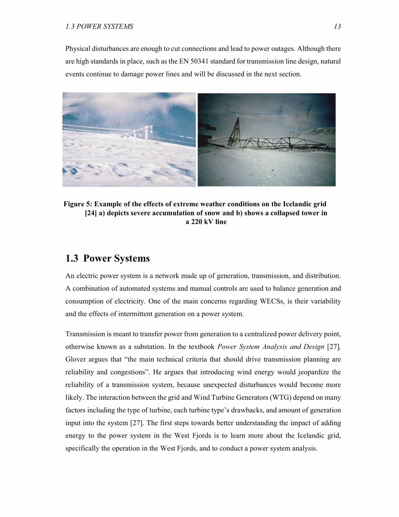
Winter can also stress power lines when there is localized accumulation of snow that creates
overloading and in some cases outages through high winds or icing. Figure 5 depicts two
examples of the damage power lines can suffer at the hands of inclement weather. Damage can
be expected, in some capacity, annually. But on average, major failures only happen once
every 10 years – the most recent major incidents recorded in 1987, 1991, and 1995 [24].
1.3 POWER SYSTEMS 13
Physical disturbances are enough to cut connections and lead to power outages. Although there
are high standards in place, such as the EN 50341 standard for transmission line design, natural
events continue to damage power lines and will be discussed in the next section.
1.3 Power Systems
An electric power system is a network made up of generation, transmission, and distribution.
A combination of automated systems and manual controls are used to balance generation and
consumption of electricity. One of the main concerns regarding WECSs, is their variability
and the effects of intermittent generation on a power system.
Transmission is meant to transfer power from generation to a centralized power delivery point,
otherwise known as a substation. In the textbook Power System Analysis and Design [27],
Glover argues that “the main technical criteria that should drive transmission planning are
reliability and congestions”. He argues that introducing wind energy would jeopardize the
reliability of a transmission system, because unexpected disturbances would become more
likely. The interaction between the grid and Wind Turbine Generators (WTG) depend on many
factors including the type of turbine, each turbine type’s drawbacks, and amount of generation
input into the system [27]. The first steps towards better understanding the impact of adding
energy to the power system in the West Fjords is to learn more about the Icelandic grid,
specifically the operation in the West Fjords, and to conduct a power system analysis.
Figure 5: Example of the effects of extreme weather conditions on the Icelandic grid [24] a) depicts severe accumulation of snow and b) shows a collapsed tower in
a 220 kV line

14 CHAPTER 1: INTRODUCTION
1.3.1 The Icelandic Grid
The Icelandic grid is made up of a 132 kV ring that connects to 66 kV distribution lines
responsible for sending power to end users throughout the country [28]. There are also 220kV
lines responsible for transmitting power to heavy industrial loads [28]. The transmission
system can be seen in Figure 6. Generation primarily occurs in two areas - the south-west and
the north-east [28]. The transmission lines are mainly overhead because implementing
underground cables is not feasible in many parts of Iceland [28]. Electricity demands grow
with increases in population, industry, and technology use.
Figure 6: A simplified visual representation of the Icelandic grid [29]
In addition to necessary grid updates, the transmission of the Icelandic power system is
impacted significantly by the natural hazards described previously. These forces of nature can
cause a lot of damage to the transmission system. Transmission line disturbances are often
higher and more frequent during the winter mainly due to damage caused to lines and cables
[24].
1.3.2 Power System in the West Fjords
The power grid in the West Fjords is run by Landsnet, the national transmission company and
Orkubu Vestfjarda (OV), a local distribution company. Figure 7 shows the combined
Transmission System Operator (TSO) and Distributions System Operator (DSO) system [29].

1.3 POWER SYSTEMS 15
There is a higher risk for natural hazards to affect the transport of energy over long
transmission distances. Implementation of wind energy as primary resources in different
sections of the country can help to minimize these losses by reducing transport distances. The
incorporation of wind energy feeding electricity into the main grid can help guarantee energy
demand is sufficiently met. A drawback is that a decentralized power system, where generation
is located in the West Fjords as opposed to the typical generation locations, will require more
robust controls to ensure stability and reliability [30].
Figure 7: The power system in the West Fjords including both the transmission and distribution systems [30, p. 30]

16 CHAPTER 1: INTRODUCTION
Before considering the effect a new power generation project will have on the grid, one must
assess demand. According to Orkustofnun, power demand in Iceland is estimated to increase
[31]. The estimated growth in electricity usage in Iceland up until the year 2050 is displayed
in Figure 8. 2005 to 2008 are marked by a period of rapid growth. The decrease in the growth
rate after 2008 can be attributed to the financial crisis that Iceland underwent during that time.
Conservative growth is thus predicted from the years 2019 to 2050.
Population growth and an increase in individual consumption has resulted in an increase of
energy use [31]. In the West Fjords, usage per capita is shown to have increased ~20,000 kWh
from the years 1987 to 2017, and ~30,000 kWh when comparing 1978 to 2017 (displayed in
Figure 8).
Figure 8: Forecast of total electricity generation from the years 2015-2015 as well as the electricity generation from 1995 to 2014 [31, p. xv], Rauntölur refers to recorded
power consumption , Spátimabil means predicted power consumption, frá virkjunum means from the power plant, frá flutningskerfinu means from the transmission
system, Inn á dreifikerfið refers to the energy from the distribution system, orkunotkun is power consumption and ár is year

1.3 POWER SYSTEMS 17
1.3.3 West Fjords Economy
There seems to be a direct correlation between an improved economy and per capita energy
usage. The economy of the West Fjords is mostly supported by tourism and fishing industries.
Tourism has increased in recent years; 2017 saw 106 cruise ships docked in Ísafjörður during
the summer, while only 15 were recorded during the summer of 2000. Cruise ships pose an
interesting challenge to the northern part of the power system, as the arrival of a cruise ship
can double the town’s population over a short time period [32].
Another source of income are the fishing and fish farming industries. The main company in
the West Fjords is Fiskvinnslan Íslandssaga hf, which operates under the Icelandic Saga
corporation and exports fish like haddock, catfish, and cod to the United Kingdom, the United
States, France, and Germany [33].
1.3.4 Disturbance History
Energy security and stability becomes more important as a result of an increase in electricity
dependence. Ensuring minimal disturbances in the power system becomes vital. To
understand, and eventually prevent future grid failures, past trends should be investigated.
First, the frequency of power disturbances system in the West Fjords is analyzed. Electricity
Figure 9: Energy Consumption per resident in the West Fjords from the years 1978-2017 [30, p. 10] kWst/ibua means kWh per capita, hiti means heat, and
translates to general

18 CHAPTER 1: INTRODUCTION
is consumed through central heating (as the West Fjords does not use geothermal energy to
heat homes as the rest of Iceland) and through the electrical system [30].
The causes, locations, and frequency of grid disturbances will be investigated. Figure 10 shows
the number of disturbances in the transmission and supply system in 2017 separated by devices
in which they occured. The majority of disturbances in 2017 were caused by issues with the
overheard lines, this is expected because as was mentioned earlier, the West Fjords is
vulnerable to inclement weather that can take down transmission lines [30].
Figure 10: Number of disturbances in the transmission and supply system of the electricity supply in 2017 planned (light blue) unplanned (dark blue) [30, p.
29]
Having established that transmission lines are the cause of most grid disturbances in the West
Fjords, the locations at which the issues arise are then identified. Figure 11 shows that more
than half of the disturbances that occurred in 2017 were in Patreksfjodur, which is the
westernmost town in the West Fjords. Patreksfjordur may have been subject to the most
disturbances because it is connected via long, vulnerable power lines.
0
10
20
30
40
50
60
70
Overhead Line Substation UndergroundCable
Sea Cable Unknown
Number of interruptions in the power transmission and distribution system 2017
Unplanned Planned

1.3 POWER SYSTEMS 19
Figure 11: Number of disruptions in the distribution system of electric utilities 2017 [30, p. 29]
1.3.5 Cost
Equipped with greater knowledge around disturbances in the grid, we can now consider costs
of renewable energy. Of the renewable energy production methods, wind energy saw the most
global growth in 2017 with indications of continuing rapid growth [34]. According to the 2015
Wind Technologies Market Report published by the U.S. Department of Energy, wind turbine
prices have dropped significantly since 2008 [35]. The high influx of wind power production
may be attributed to economies of scale [36]. A typical method for determining electricity
costs is the Levelized Cost of Electricity (LCOE). LCOE or average cost electricity must be
sold to break-even over the project lifetime and is often used to evaluate energy production
cost. The LCOE is defined by The University of Texas at Austin [37] as:
Estimated amount of money that it takes a particular electricity generation plant to produce a
MWh of electricity over its expected lifetime.
The advantage of using LCOE is that it creates a consistent format for evaluating costs at
different time periods and for different generation methods. Lazard published an extensive
study discussing the LCOE of various energy generation sources, some of which included coal,
nuclear, geothermal, solar, and wind. Figure 12 displays the trend over an eight-year timeframe
showing wind energy production LCOE has dropped by 67% [35].
Key factors affecting the total direct and indirect costs of generating and delivering electricity
0
2
4
6
8
10
12
14
Number of power supply interruptions in the distribution system 2017
Unplanned Planned

20 CHAPTER 1: INTRODUCTION
include transmission, distribution and administration costs, generation type, connectivity
infrastructure, expected consumption, capital costs, operation and management costs,
regulation taxes and subsidies, environment, human health impact, and local socio-economics.
The emphasis of this section will be cost comparison of transmission rather than trying to
determine a definitive predicted cost. Project installation costs are assumed to be comparable
between the sites analyzed and therefore negligible. Transmission costs include construction
and operation costs. Overhead lines require Capital Expenditure (CapEx) and Operational
Expenses (OpEx). Landvernd produced a study estimating the full life-cycle cost of a 120 km
line operating for 60 years [38]. These values were compared to results from a study conducted
by EFLA and Landsnet that estimated the life-cycle cost from project inception to
decommissioning [39]. Landsnet used a cost risk assessment to produce an upper and lower
bound on cost. Though this study more thoroughly analyzed potential costs, the report
Figure 12: LCOE of wind from 2009-2017 [35, p. 8]

1.3 POWER SYSTEMS 21
commissioned by Landvernd was ultimately used to estimate power line costs. This was done
because relative cost is the input criterion analyzed. The calculated costs for overhead lines
and underground cables at two different voltage ratings are displayed in Table 1.3.
Underground cables are typically more costly because installation costs are higher.
Underground cables are less susceptible to climate induced disturbances but experience higher
losses [38], [39].
Table 1.3 Estimated total cost of power system cables [38]
Total Costs Overhead (million €) Overhead (ISK) 132 kV 6.76 ∙ 10 9.22 ∙ 10 220 kV 9.68 ∙ 10 1.32 ∙ 10
With a deeper knowledge of the grid in Iceland, the issues it faces, and expected costs, this
study will now present a systematic approach to understanding power systems.
1.3.6 Power Flow
Power flow analysis is defined by Glover [27], as:
The computation of voltage magnitude and phase angle at each bus in a power system under
balanced three-phase steady-state conditions.
This research study assumes the power system is operating under these conditions, which
insinuates certain criteria must be met.
The grid must be balanced, in other words, generation equals demand plus losses. As specified
by Glover [27], “the generators operate within specific real and reactive power limits and
transmission lines and transformers are not overloaded.” Meaning the bus voltage must remain
within the allowed constraints making sure not to deviate too much from the rated values [27].
Power flow is often represented visually, such as in the single-line diagram in Figure 13. The
variable 𝑉 refers to voltage magnitude, phase angle is 𝛿 , net real power Pk, and reactive
power supplied to the is bus Qk. This type of diagram can be used to calculate real and reactive
power flows and losses in transmission lines and transformers and will be built to model the
West Fjords’ transmission system in this study.

22 CHAPTER 1: INTRODUCTION
For any given bus, it is typical to view power flow in terms of real power (MW), P and reactive power (Mvar), Q.
In power flow, generators are considered as power sources and demand is referred to as a load.
Power System Analysis and Design [27], shows that there are algorithms that solve for the
“voltage magnitude and angle at each bus in a power system, real and reactive power flows for
all equipment interconnecting the buses, as well as equipment losses.” These calculations rely
on the Gauss-Seidel and Newton Raphson methods.
The main deliverable of this research study is a visual representation of the optimum locations
for wind energy generation within the West Fjords. One of the major components of this study
is measuring the effects of wind energy integration to the Icelandic power system. Two main
modelling software were used, PowerWorld and MATPOWER. In the spirit of
communicability, the PowerWorld simulator is used in this project to visualize and simulate
the transmission system in the West fjords. The PowerWorld Simulator website [40] states that
“PowerWorld Simulator is an interactive power system simulation package designed to
simulate high voltage power system operation on a time frame ranging from several minutes
to several days. The software contains a highly effective power flow analysis package capable
of efficiently solving systems of up to 250,000 buses.” MATPOWER is Matlab language used
to simulate power flow. MATPOWER is used in this study to conduct a similar analysis as
𝑃 = 𝑃 − 𝑃 1-5
𝑄 = 𝑄 − 𝑄 1-6
Figure 13: Example of a single line diagram illustrating power flow [27, p. 326]

1.3 POWER SYSTEMS 23
with PowerWorld. Though MATPOWER is less visual than PowerWorld, its connection to
Matlab allows for automation [41].
A computational bus is defined as the part to which generators, feeders, loads, and other power
components are connected [27]. The quantities associated with a bus are: the magnitude of
voltage, the phase angle of voltage, real power and reactive power. There are three bus types:
a slack bus, a load bus, and a voltage-controlled bus.
The slack bus can also be referred to as the swing or reference bus and is a theoretical concept
used to model power flow. Because the total losses of a system are not initially known, a
reference must be set to initiate a simulation. The slack bus has a fixed voltage set to 1.0 pu
and a phase angle of voltage usually set to zero. The slack bus is treated as a free-variable in
the power-flow algorithm used to absorb or emit the active or reactive power from the power
system depending on what is needed [27].
The load bus is also referred to as the P-Q bus because the active power P and the reactive
power Q are specified and are to be injected into the system. The load bus is connected to
areas that are consuming electricity. On the opposite spectrum there is the generation bus,
which is also referred to as the P-V bus because the active power P and the voltage magnitude
is specified.
When referring to line type, three wires are required because there are three phases. Possible
line configurations are trefoil formation and flat formation. Both formations are shown in
Figure 14.
The XLPE Land Cable Systems: User’s Guide [42] iterates that “the choice depends on several
factors like screen bonding method, conductor area and available space for installation.”
Trefoil phase formation is typically used for voltage applications up to 132kV. This formation
is easy to install, does not require a lot of space, and the magnetic field and circular currents
are the same for each of the three cable phases because each cable is the same distance apart.
Flat phase formation is favorable for high voltage cables because as the XLPE Land Cable
Systems: User’s Guide [42] states “the mounting centers allow for sufficient heat-dissipation.”
Figure 14: Possible line configurations [42, p. 7]

24 CHAPTER 1: INTRODUCTION
The disadvantage of this formation is that the uneven spacing causes the middle cable to heat
up faster than the side cables. This disparity in temperature leads to voltage imbalances [42] .
1.3.7 The Per Unit system
Calculations dealing with power system values such as voltage, current, power, and impedance
are often conducted with the per-unit equivalents of these values. This is done to create
simplified, unitless transformer equivalent circuits to the point that voltages, currents, and
impedances do not change from one side of the transformer to the other. Per unit quantities
can be calculated as follows [27]:
The base value of quantity is also often referred to as the impedance or Zbase. In order to reach
the Zbase value for a single-phase circuit or for one phase of a three-phase circuit, the base
voltage VbaseLN and the base complex power Sbase1 are used [27]:
It is generally accepted that base quantities follow certain constraints so per-unit impedances
will remain unchanged on either side of a transformer. The constraints are that the base
complex power is the same for the entire system, and “the ratio of voltage bases is selected to
be the same as the ratio of the transformer voltage ratings [27].”
𝑍 =𝑉
𝑆 1-8
𝑝𝑒𝑟 − 𝑢𝑛𝑖𝑡 𝑞𝑢𝑎𝑛𝑡𝑖𝑡𝑦 = 𝑎𝑐𝑡𝑢𝑎𝑙 𝑞𝑢𝑎𝑛𝑡𝑖𝑡𝑦
𝑏𝑎𝑠𝑒 𝑣𝑎𝑙𝑢𝑒 𝑜𝑓 𝑞𝑢𝑎𝑛𝑡𝑖𝑡𝑦 1-7

25
Chapter 2
2Methods
This project aims to systematically determine the most effective locations for wind generation.
The project will analyze the potential for wind energy production implementation in the West
Fjords specifically, as the previous sections illustrated the need for renewably-sourced power
in this area. One of research outputs of this project will be the coordinates of locations best
suited for wind energy implementation in the West Fjords. Along with this information, a
detailed breakdown of the different variables that contributed to this conclusion will be
provided.
The information will be presented visually—a user-friendly mode of presentation may
encourage implementing this information in future energy projects. The information will be
calculated using MATLAB, MATPOWER, JAVA, and Excel. Once computed the data will
be presented on a map using QGIS.
In the process of determining the most promising wind energy locations in the West Fjords, a
method will be developed that will systematically evaluate and compare locations given
different input variables.
Lastly a sensitivity analysis will be conducted as to evaluate the impact of the various input
variables. This is necessary because it will help eliminate author bias when weighing
individual variables for the final all-inclusive evaluation as well as allow the method to be
customized to the land area in question.
The final deliverable will be a map showing the locations best suited to produce wind energy
based on the factors that will be described in the following paragraphs. QGIS, an open source
geographic information system was used to map disqualifying factors, input variables and
ultimately to evaluate potential power producing sites.

26 CHAPTER 2: METHODS
2.1 Disqualifying Factors
The first step in the mapping location is identifying locations where wind turbines may not be
installed under any circumstances, as grading them under other criteria would be inefficient.
The constraints leading to area exclusion identified are as follow:
Nature reserves
Topographic elevation
Population buffer zone
Non-viable wind resource
The objective of this study is to aid in the West Fjord’s transition to sustainability. One
objective of sustainability is environmental protection and conservation. The implementation
of wind turbines should not interrupt the nature of this region, especially protected natural
areas. Outstanding natural fixtures and preservation sites were identified and evaluation points
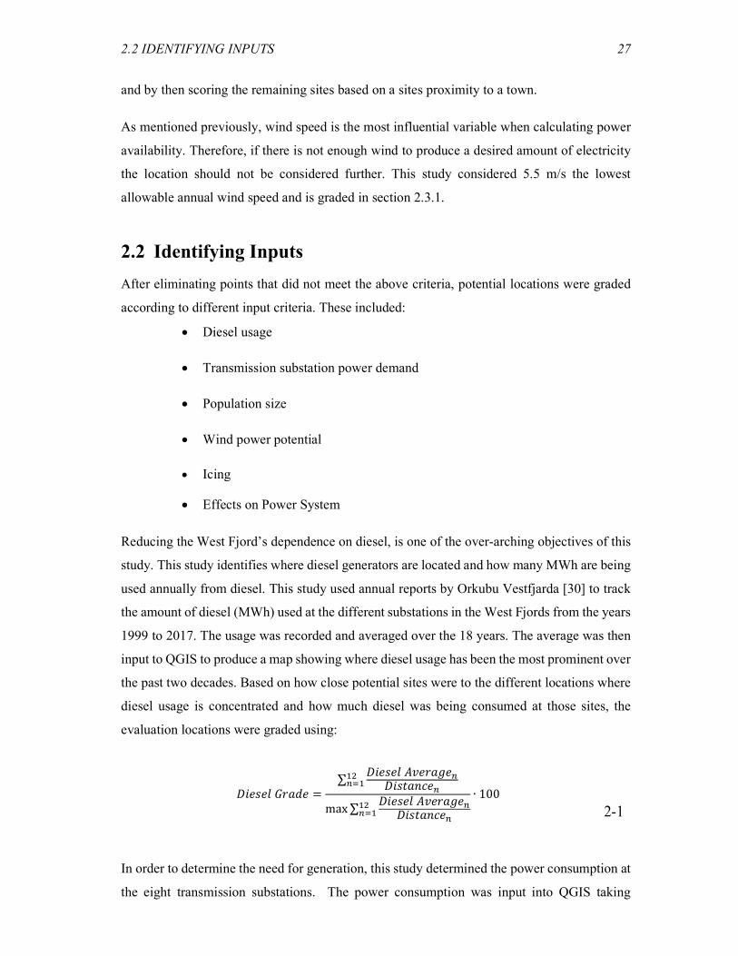
that coincided were subsequently eliminated.
The sites identified were Drangajokull, Hornstrandir, Dynjandi, Hrisey, Surtarbrandsgil, and
Vatnsfjordur. Drangajokull is Iceland’s northern-most glacier that spans an area of
approximately 200 km2 and has an altitude of 925m. Hornstrandir is a nature reserve that was
established in 1975 and is made up of approximately 260 species of plants and ferns. There
are cliffs designated for watching the 30 species of birds that nest in this area. Apart from birds,
the area houses many arctic foxes [43]. Dynjandi or Fjallafoss, is a series of connected
waterfalls that at the highest point measure to be approximately 100m.
Though elevation is considered when siting wind turbine locations, this study will place more
emphasis on variation of elevation, or slope. In the event of a large elevation gradient,
installation becomes difficult due to lack of infrastructure combined with the need to transport
large machinery. Large slope can also act as a high surface roughness, acting as a barrier to
wind and decreasing the speed. Slope is visually assessed, and areas located on high sloping
terrain are eliminated.
As an attempt to address Not in MY Backyard (NIMBY) and help close the social gap often
present when constructing wind energy turbines, this study has taken specific precaution to
avoid installation in close proximity to cities or towns by creating a 2 km elimination buffer
2.2 IDENTIFYING INPUTS 27
and by then scoring the remaining sites based on a sites proximity to a town.
As mentioned previously, wind speed is the most influential variable when calculating power
availability. Therefore, if there is not enough wind to produce a desired amount of electricity
the location should not be considered further. This study considered 5.5 m/s the lowest
allowable annual wind speed and is graded in section 2.3.1.
2.2 Identifying Inputs
After eliminating points that did not meet the above criteria, potential locations were graded
according to different input criteria. These included:
Diesel usage
Transmission substation power demand
Population size
Wind power potential
Icing
Effects on Power System
Reducing the West Fjord’s dependence on diesel, is one of the over-arching objectives of this
study. This study identifies where diesel generators are located and how many MWh are being
used annually from diesel. This study used annual reports by Orkubu Vestfjarda [30] to track
the amount of diesel (MWh) used at the different substations in the West Fjords from the years
1999 to 2017. The usage was recorded and averaged over the 18 years. The average was then
input to QGIS to produce a map showing where diesel usage has been the most prominent over
the past two decades. Based on how close potential sites were to the different locations where
diesel usage is concentrated and how much diesel was being consumed at those sites, the
evaluation locations were graded using:
In order to determine the need for generation, this study determined the power consumption at
the eight transmission substations. The power consumption was input into QGIS taking
𝐷𝑖𝑒𝑠𝑒𝑙 𝐺𝑟𝑎𝑑𝑒 =∑
𝐷𝑖𝑒𝑠𝑒𝑙 𝐴𝑣𝑒𝑟𝑎𝑔𝑒𝐷𝑖𝑠𝑡𝑎𝑛𝑐𝑒
max ∑𝐷𝑖𝑒𝑠𝑒𝑙 𝐴𝑣𝑒𝑟𝑎𝑔𝑒
𝐷𝑖𝑠𝑡𝑎𝑛𝑐𝑒
∙ 100
2-1

28 CHAPTER 2: METHODS
account of consumption magnitude and location. Potential sites were evaluated based on the
distance to high energy usage. The equation below was used to assess the locations.
Population is the last social criterion considered. As discussed previously, this study looks to
address NIMBY by making sure wind farms are not constructed within a 4 km radius of towns
as well as evaluating locations farthest from all population as most desirable. The formula
below shows how the population grade was calculated.
2.3 Status Quo
The main contributing factors to current siting methods include determining how much power
can be produced, making sure the terrain is maneuverable, and in cold climate locations, icing.
This study acknowledges the importance of the current criteria considered and will therefore
consider them as well.
2.3.1 Potential Power Analysis
This study received data from Landsvirkjun outlining information on 1400 locations. The
information included: potential power production, annual estimated production, capacity
factor and Weibull parameters. Weather data was collected over the years 1995 to 2015. The
information recorded was wind speed and direction.
Equation 2-4 illustrates how to calculate average wind speed, where N is number of wind speed
observations.
Once the average wind speed is known, the power output at average wind speed can be
simplified to the equation below. Where 𝜌 is density, and D is wind turbine diameter.
𝑇𝑟𝑎𝑛𝑠𝑚𝑖𝑠𝑠𝑖𝑜𝑛 𝐺𝑟𝑎𝑑𝑒 =∑
𝑇𝑟𝑎𝑛𝑠𝑚𝑖𝑠𝑠𝑖𝑜𝑛𝐷𝑖𝑠𝑡𝑎𝑛𝑐𝑒
max ∑𝑇𝑟𝑎𝑛𝑠𝑚𝑖𝑠𝑠𝑖𝑜𝑛
𝐷𝑖𝑠𝑡𝑎𝑛𝑐𝑒
∙ 100
2-2
𝑃𝑜𝑝𝑢𝑙𝑎𝑡𝑖𝑜𝑛 𝐺𝑟𝑎𝑑𝑒 =min ∑ 𝑝𝑜𝑝𝑢𝑙𝑎𝑡𝑖𝑜𝑛 ∙ 𝑑𝑖𝑠𝑡𝑎𝑛𝑐𝑒
∑ 𝑝𝑜𝑝𝑢𝑙𝑎𝑡𝑖𝑜𝑛 ∙ 𝑑𝑖𝑠𝑡𝑎𝑛𝑐𝑒∙ 100
2-3
𝑈 = 1
𝑁𝑈
2-4

2.3 STATUS QUO 29
Energy from a wind machine is described in the formula below. Where Pw (Ui) is the power
output calculated from wind speed Ui, and ∆𝑡 is change in time referring to one year in this
case. [44]:
Landsvirkjun analyzes data every 2500 m [45]. In order to evaluate the criteria at the locations
this project is analyzing, a continuous interpolation of the data is created by making a new
raster layer using the Triangulated Irregular Network (TIN) method [46]. This method uses the
Delaunay triangulation algorithm which creates triangles surrounding the nearest data points
[46]. These triangles are created using the intersections of circumcircles drawn around sample
points. Once the raster layer is made, a function in QGIS is used to extract data at the
coordinates where the study’s evaluation locations are. The Weibull parameters, capacity
factors, and predicted power production are then determined from this. To verify that the power
production is accurate, the Weibull probability density function for all the evaluation locations
are plotted using the extracted Weibull parameters. The plots with the highest and the lowest
mean are then examined further. The power curve for a turbine determined as favorable for
cold climate conditions is plotted along with the Weibull curve. To determine power
production, the power production at specific wind speeds is multiplied by the chance that the
wind speed would occur (shown in the Weibull curve). The power production grade was
determined using:
2.3.2 Icing
Icing affects the West Fjords and must therefore be considered. As mentioned in Section 1.2.3
there are five Icing classes. The classes depend on meteorological icing and instrumental icing.
Based on icing magnitude provided by Landsvirkjun each evaluation location is graded on
unitless scale using favoring locations with low icing frequency:
𝑃 = 𝜌2
3𝐷 𝑈 2-5
𝐸 = 𝑃 (𝑈 )(∆𝑡) 2-6
𝑃𝑜𝑤𝑒𝑟 𝑃𝑟𝑜𝑑𝑢𝑐𝑡𝑖𝑜𝑛 𝐺𝑟𝑎𝑑𝑒 =𝑃𝑜𝑤𝑒𝑟 𝑃𝑟𝑜𝑑𝑢𝑐𝑡𝑖𝑜𝑛
max (𝑃𝑜𝑤𝑒𝑟 𝑃𝑟𝑜𝑑𝑢𝑐𝑡𝑖𝑜𝑛)∙ 100 2-7

30 CHAPTER 2: METHODS
2.4 Power System Considerations
One of the main concerns with implementing intermittent power generation such as wind
energy is its effect on the power system. As such it is important to conduct a power flow
analysis. In this section PowerWorld Simulator and MATPOWER were used to understand the
effect of implementing wind energy at each potential site location.
2.4.1 Base case
This study assumes steady state conditions and begins with a base model of the power system
of the West Fjords modelled in PowerWorld [47]. For the case of one wind farm it is assumed
that generation will be connected to a transmission substation, as it is required for any
generation greater than or equal to 10 MW to be hooked up to the transmission network. For
this scenario, the model was then simplified to only include the transmission system, as this
study assumes power generation would not be connected to a distribution substation. Once the
model was simplified, four of the suggested wind energy generation locations were
individually modelled in PowerWorld. The aim is to find a limit on how much generation can
be implemented at the given locations. Once a visual was created to aid in understanding the
model an analysis of all the evaluation locations was conducted in MATPOWER. A base case
was provided by Landsnet and used to conduct further analysis.
2.4.2 Calculating Line Parameters
Before conducting any analysis on new generation, the line parameters resistance R, inductive
reactance X, and shunt admittance B must be calculated.
The ground, ambient, and conductor temperatures must be set. These values are based on
location averages and in the case of the West Fjords power system the ground temperature is
set to 1.1°C. The ambient temperature is set to 10 ° C and the conductor temperature is set to
65° C.
The power phase formation chosen is trefoil phase because the cables have a voltage magnitude
equal to or less than 132kV. The apparent power is set to that of the nearest transmission
𝐼𝑐𝑖𝑛𝑔 𝐺𝑟𝑎𝑑𝑒 =min (𝑖𝑐𝑖𝑛𝑔)
𝑖𝑐𝑖𝑛𝑔 2-8

2.4 POWER SYSTEM CONSIDERATIONS 31
substation using:
Where Imax refers to the maximum current, S is the apparent power and V is voltage. A land
cable systems user’s guide is used to adjust the thermal resistivity using a rating factor of 0.84.
Once the current has been adjusted the resistance at the conductor temperature can determined
using [48]:
R65 refers to the resistance at the conductor temperature, R20 is the base resistance given by the
tables at 20°C. T65 is a 65°C, T20 is 20°C, and α is the thermal coefficient of resistance. Once
the resistance has been adjusted, it will be changed into its per unit equivalent so that it can be
input into MATPOWER. The formula for the impedance is shown in Equation 1-8. Once the
impedance is found, the per-unit resistance can be calculated using the following equation.
Once the per-unit equivalent for resistance is found, the inductive reactance is computed
using:
Where x refers to the inductive reactance, f is the frequency, which in Iceland is set to 50Hz,
and L is the inductance which can be found in the tables. To finalize the value for inductive
reactance the value found above was multiplied by the length of the proposed line and
converted into the per-unit equivalent as can be done using. [40]
Lastly, the shunt admittance was calculated as:
𝐼 = 𝑆
𝑉√3 2-9
𝑅 = 𝑅 [1 + 𝛼(𝑇 − 𝑇 )] 2-10
𝑅 =𝑅
𝑍 2-11
𝑥 = 2𝜋𝑓𝐿
1000 2-12
𝑥 = 𝑥 ∙ 𝑙𝑒𝑛𝑔𝑡ℎ
𝑍 2-13

32 CHAPTER 2: METHODS
Where B is the shunt admittance and C is capacitance that was found in the XLPE tables. This
value is multiplied by 10 to the third power because the value returns Farads per meter, and
the desired format is in Farads per kilometer. The following equation was used to find the per-
unit equivalent of the shunt admittance.
The method for finding line parameters was automated for the remaining 482 potential wind
energy production sites using python. The script read in the Apparent Power (MVA) of the
nearest substation as well as the distance between the proposed site and the nearest substation
in order to calculate the R, X, and B line parameters for all the locations and output these
values in an excel sheet.
Because there are many potential wind siting locations a MATLAB code was written to
iteratively go through all 482 site scenarios. The code began by running a power flow analysis
on the base case. Once the base case ran successfully, new buses were added and analyzed one
at a time. Similarly, lines with line parameters corresponding the specific site were attached to
the new bus. A generator was then added to the bus.
2.4.3 Maximum Potential Generation Input
Generation was increased until the maximum viable input value was reached. In order to find
the threshold between a working system and a broken one, power flow analysis was conducted
and then run again to identify changes in the system. Voltage magnitude at the different busses
were analyzed to verify that it lay within the Icelandic voltage constraint of ± 0.1. The MVA
was also used to constrain the potential power generation. Each line has an MVA rating,
meaning it cannot transport electricity with a higher MVA.
Where i represents evaluation location.
𝐵 = 2𝜋𝑓𝐶 ∗ 10 2-14
𝑏 = 𝑏
𝑍 2-15
𝐺𝑒𝑛𝑒𝑟𝑎𝑡𝑖𝑜𝑛 𝐺𝑟𝑎𝑑𝑒 = 𝑃𝑜𝑡𝑒𝑛𝑡𝑖𝑎𝑙 𝐺𝑒𝑛𝑒𝑟𝑎𝑡𝑖𝑜𝑛
𝑀𝑎𝑥( 𝑃𝑜𝑡𝑒𝑛𝑡𝑖𝑎𝑙 𝐺𝑒𝑛𝑒𝑟𝑎𝑡𝑖𝑜𝑛)∙ 100 2-16

2.4 POWER SYSTEM CONSIDERATIONS 33
2.4.4 Power Loss Analysis
After the maximum amounts of wind generation that could be applied to the power system at
each location were determined, the losses were analyzed. The power losses of wind energy
generation integrated to the power system at each location is calculated and compared to the
current losses of the transmission system. Losses are computed on both on a binary scale and
evaluated to determine a grade. In terms of the binary scale 0 represents increased losses and
a 1 delimits reduced losses. To grade the power losses, loss will be compared to the minimum
non-zero loss. This will be done according to:
2.4.5 Cost Analysis
The last evaluation parameter for the power systems portion is transmission cost. Transmission
costs were estimated using the estimated full life-cycle costs for overhead lines in Iceland
(shown in 1.3.5). Only transmission cost is considered because it is assumed that installation
costs would be comparable at all evaluation locations. The infrastructure costs being
considered is installation of new power lines to connect the proposed wind farm to the nearest
substation. The full life time of overhead lines is assumed to be 60 years and will be scaled
down to represent the cost of transmission over the assumed life time of a wind turbine which
is 20 years. Lines considered are either rated at 66 kV or 132 kV. If the lines are rated at 132
kV the study conducted by Landvernd approximated, it would cost 25,578 ISK/m [38]. For the
66 kV lines the cost was scaled down from the study and estimated to be 12,676 ISK/m. There
is an inverse relationship between cost and grade that is shown:
2.4.6 Weighing input variables
All the criteria graded have the goal of addressing siting issues; both those considered standard
as well as others attempting to systematically address reoccurring concerns. Once all variables
have been individually assessed, they will be weighted, and given a combined score. There
will be three sub-categories: social considerations, status quo, and power system integration.
𝑃𝑜𝑤𝑒𝑟 𝐿𝑜𝑠𝑠 𝐺𝑟𝑎𝑑𝑒 =(min (𝑙𝑜𝑠𝑠)
𝑙𝑜𝑠𝑠∙ 100 2-17
𝐶𝑜𝑠𝑡 𝐺𝑟𝑎𝑑𝑒 =min (𝑐𝑜𝑠𝑡)
c𝑜𝑠𝑡∙ 100 2-18

34 CHAPTER 2: METHODS
Each of the subcategories are made up of three of evaluation criteria as seen in Table 2.1.
Table 2.1 Input variable weights used to determine cumulative score at each evaluation location
Category Criteria Weight Social Considerations Diesel Dependence 1/8 Social Considerations Energy Usage 1/8 Social Considerations Population 1/8 Status Quo Power Potential 1/8 Status Quo Icing 1/8 Power System Integration Maximum Allowable Input 1/8 Power System Integration Transmission Based Power Loss 1/8 Power System Integration Cost 1/8
2.5 Sensitivity Analysis
Once all input variables are considered and given a weight, a sensitivity analysis is conducted
to identify the trend between each variable and the overall score. In order to determine the
effect of each variable on the cumulative system evaluation, each criterion was analyzed
separately. One location is chosen, and random normal distributions are generated to
encompass possible values for each criterion. For example, the random normal distribution for
the cost criterion represents all potential costs at the site location. The normal distribution is
often denoted as:
Where N is a normal distribution with expected value 𝜇 and standard deviation 𝜎 [48].
The expectation is derived from data collected throughout the study and the standard deviation
ranges between 10-30% to mimic each criterion’s range. The randomly generated set of data
is put through the grading calculations described in previous sections to produce a raw score.
Raw score refers to a score with units unique to the criterion being analyzed. Once all random
sets have been evaluated, they are normalized, weighted, and combined to produce an overall
score. Each criterion’s raw score is then plotted versus the final score in order to understand
the influence each variable has on the final score. Finally, each normalized score is plotted
against the final score.
𝑁(𝜇, 𝜎 ) 2-19

2.5 SENSITIVITY ANALYSIS 35
2.5.1 Social Considerations
The social consideration evaluations are all distance dependent. To determine possible raw
scores for the diesel criterion, a random normal distribution is generated for each of the 12
diesel generators analyzed. The distribution is set up to reflect the possible diesel consumption
at each generator. To do this, mean is set to the average diesel consumption at each generator
(later mentioned in Table 3.2). There is minimal consumption variation over the 18 years
analyzed. To reflect limited consumption fluctuation, the standard deviation is set to 10%.
Once a mean, standard deviation, and random normal distribution are established, a program
was written in MATLAB that iterates through each possible amount of diesel consumption (as
represented by the normal distribution) and a raw score was calculated by taking the sum of
diesel consumed and then divided by the sum of the distance between the reference location
and each generator.
The raw score is then nondimensionalized using Eq. 2-1. A similar approach is taken to analyze
the effects of transmission on the overall score. A random normal distribution is created for
the eight transmission substations in the West Fjords. Variability in energy consumption may
be attributed to increased technology use and tourism. Though fluctuation is expected, there
are power system limits that deter fluctuations from exceeding a certain point. To illustrate this
energy consumption standard deviation σ, is set to 20% and the mean μ is based on estimated
consumption at each substation from Landsnet. These values are entered into MATLAB and a
script is written to iterate through the equation below 500 times.
Where transmission consumption is the independent variable.
The population sensitivity analysis simulated the change in population of 16 towns. The
normal distributions are generated by setting the current population of each town, seen in Table
3.1 Population and coordinates of towns in the West Fjords , as the mean for each distribution. In
other words, there are 16 random normal distributions generated representing the change in
population at each town. Standard deviation is fixed at 10% as previous census reports show
𝐷𝑖𝑒𝑠𝑒𝑙 𝑅𝑎𝑤 𝑆𝑐𝑜𝑟𝑒 =𝑁(𝑑𝑖𝑒𝑠𝑒𝑙 𝑎𝑣𝑒𝑟𝑎𝑔𝑒, 0.1 )
𝐷𝑖𝑠𝑡𝑎𝑛𝑐𝑒
2-20
𝑇𝑟𝑎𝑛𝑠𝑚𝑖𝑠𝑠𝑖𝑜𝑛 𝑅𝑎𝑤 𝑆𝑐𝑜𝑟𝑒 =𝑁(𝑡𝑟𝑎𝑛𝑠𝑚𝑖𝑠𝑠𝑖𝑜𝑛, 0.2 )
𝐷𝑖𝑠𝑡𝑎𝑛𝑐𝑒 2-21

36 CHAPTER 2: METHODS
2-23
nominal variation in the West Fjords population. This is input into MATLAB and each
potential population scenario is run through the following:
2.5.2 Status Quo
In this study, status quo refers to the potential power that can be produced at each evaluation
location and icing each location experiences. Sensitivity analyses at one location are carried
out in order to understand the effect these criteria have on the overall score. The range of
anticipated potential wind power production is simulated using a normal distribution. Mean μ
is set to the average wind speed at location analyzed. Standard deviation σ is set to 20%. The
values generated from the distribution are the raw score for potential power.
The expectation derived for the icing normal distributions are similarly based on collected
information provided by Landsvirkjun. The icing at one location is used as the mean. Based
on the information provided by Landsvirkjun, icing is expected to vary widely on a year to
year basis, so the standard deviation is set to 30%.
2.5.3 Power System Integration
The sensitivities calculated in the power systems section rely on the power flow analysis
conducted in section 1.3.6. The maximum power potential criteria will be described first. A
random normal distribution is generated by setting expectation μ to the maximum potential
input power at the analysis location. The potential power input is expected to be between 40
and 104 MW and is therefore set to a standard deviation of 20%. and cost.
𝑃𝑜𝑝𝑢𝑙𝑎𝑡𝑖𝑜𝑛 𝑅𝑎𝑤 𝑆𝑐𝑜𝑟𝑒 =𝑁(𝑝𝑜𝑝𝑢𝑙𝑎𝑡𝑖𝑜𝑛, 0.1 )
𝐷𝑖𝑠𝑡𝑎𝑛𝑐𝑒 2-22
𝐼𝑐𝑖𝑛𝑔 𝑅𝑎𝑤 𝑆𝑐𝑜𝑟𝑒 ~ 𝑁(𝑖𝑐𝑖𝑛𝑔, 0.3 )
𝑃𝑜𝑤𝑒𝑟 𝑃𝑟𝑜𝑑𝑢𝑐𝑡𝑖𝑜𝑛 𝑅𝑎𝑤 𝑆𝑐𝑜𝑟𝑒 ~ 𝑁(𝑝𝑜𝑤𝑒𝑟 𝑝𝑟𝑜𝑑𝑢𝑐𝑡𝑖𝑜𝑛, 0.2 )
2-24
𝑀𝑎𝑥 𝑃𝑜𝑤𝑒𝑟 𝐼𝑛𝑝𝑢𝑡 𝑅𝑎𝑤 𝑆𝑐𝑜𝑟𝑒 ~ 𝑁(𝑚𝑎𝑥 𝑝𝑜𝑤𝑒𝑟 𝑖𝑛𝑝𝑢𝑡, 0.2 ) 2-25

2.5 SENSITIVITY ANALYSIS 37
The power loss input is the most variable as will be later seen in the Results chapter and as
such has its corresponding standard deviation set to 30%.
The cost criterium is set to have a standard deviation of 10% because the current transmission
infrastructure does not allow for a large expected range.
Because the overall score is dimensionless, the raw score of each criterion is normalized. To
further facilitate comparison the unitless scores are set on a scale from 0 to 100 and compared
to the overall score. Once all scores are unitless they can be averaged together to create the
overall score.
𝐶𝑜𝑠𝑡 𝑅𝑎𝑤 𝑆𝑐𝑜𝑟𝑒 ~ 𝑁(𝑐𝑜𝑠𝑡, 0.1 ) 2-27
𝑃𝑜𝑤𝑒𝑟 𝐿𝑜𝑠𝑠 𝑅𝑎𝑤 𝑆𝑐𝑜𝑟𝑒 ~ 𝑁(𝑝𝑜𝑤𝑒𝑟 𝑙𝑜𝑠𝑠, 0.3 ) 2-26

38
Chapter 3
3Results
This part of the study presents the final deliverables of the siting evaluation. First, the analysis
set up is explained. The factors that render a site unsuitable are then stated. Sites subject to
these factors are eliminated. Once only eligible sites remain, the study presents the score of
each evaluation criterion visually. The size of the circle indicates the score. Further analysis is
presented for the predicted power production criterion and the power system integration
subsection. After the criteria scores are presented individually, they are weighted and presented
cumulatively. Lastly, the sensitivity analysis is presented, showing the effect of the criteria on
the overall score.
3.1 Base Map
Analysis began by rendering a base map. The base map shown in Figure 15 was made in QGIS
by creating a polygon that outlines the West Fjords and creating a set of 580 points evenly
spaced points every 4km contained within the polygon.

3.2 ELIMINATING INELIGIBLE POINTS 39
Figure 15: Base map of the West Fjords with evaluation sites located every 4000m
3.2 Eliminating ineligible points
To reduce the number of locations graded and avoid analyzing unsuitable sites, areas excluded
are determined based on change in elevation of the surrounding area, interference with natural
sites, and proximity to populated areas. If a site is determined unsuitable it is removed and not
analyzed further.
3.2.1 Elevation
High slope is a disqualifying factor that is evaluated using elevation. Information about the
elevation was found on Landmælingar Íslands from there contour lines were plotted with
darker greens indicating higher elevation using QGIS [46].

40 CHAPTER 3: RESULTS
Figure 16: Map of the West Fjords elevation with the sites eliminated due to high slope circled in red
Once the contour lines were plotted on the base map, evaluation points are visually assessed.
The criteria for an evaluation point to be rendered ineligible based on elevation is if the point
is located on an area that had contour lines of a darker shade of green. This process eliminated
28 evaluation points, shown in Figure 16 by red circles.
3.2.2 Natural Sites
In this section preservation sites and a glacier were identified and mapped. The natural sites
are further discussed in section 2.1, where the reason behind their protection is disclosed. QGIS
was used to render the natural site locations in Figure 17 where the preservation sites are shown
in dark green and the glacier is shown in grey [43].
3.2 ELIMINATING INELIGIBLE POINTS 41
Once the natural sites were plotted, the 59 evaluation points that coincided were identified as
shown in red in Figure 17, and subsequently removed.
3.2.3 Population
Approximately 7,000 people live in the West Fjords, most of which reside in the towns shown
below. Populations were determined from [50], and plotted in QGIS, then a heat map was
created that shows the more populated areas in a darker hue. One of the main criticisms faced
by electricity generating wind turbines, is proximity to homes. The ‘NIMBY’ phenomenon has
caused projects to terminate. This project aims to acknowledge the complaints of local
inhabitants by creating a 4 km buffer zone around populated areas. The inhabited areas of the
West Fjords can be seen below in Table 3.1.
Figure 17: Natural noteworthy sites in the West Fjords and the sites eliminated due to proximity to natural sites

42 CHAPTER 3: RESULTS
Table 3.1 Population and coordinates of towns in the West Fjords [50]
Town Longitude Latitude Population Arnes -21.568 66.050 52 Drangsnes -21.443 65.689 67 Holmavik -21.669 65.706 375 Sudavik -22.992 66.026 190 Isafjordur -23.119 66.073 2571 Hnifsdalur -23.120 66.110 200 Bolungarvik -23.251 66.157 945 Sudureyri -23.527 66.130 312 Thingeyri -23.492 65.879 260 Bildudalur -23.599 65.686 207 Patreksfjordur -24.001 65.597 683 Reykholar -22.201 65.448 135 Flateyri -23.513 66.049 180 Talknafjordur -23.825 65.627 300 Djupavik -21.557 65.944 53 Nordurfjordur -21.548 66.051 30
This data was used in conjunction with QGIS to render a heat map representing populations
that can be seen in Figure 18.
.
Evaluation points that were identified to be near high population densities were circled in red
as is shown in Figure 18 and removed.
Figure 18: Heat map of populated areas in the West Fjords and evaluation sites removed due to their proximity to towns circled in red

3.3 EVALUATING DIFFERENT CRITERIA 43
3.3 Evaluating Different Criteria
Once all ineligible points were eliminated the remaining points were evaluated based on
different criteria using a combination of QGIS, MATLAB, Python, and Excel. In Figure 19
the different criteria are displayed along with a unique color that is used to for identification.
Figure 19: Color Key for the following maps, plots, and sensitivity analyses
3.3.1 Diesel Generators
As this project aims to help the West Fjords on their path to sustainability, reducing
hydrocarbon usage is one of the driving forces of this paper. A yearly report published by
Orkubu Vestfjarda shows the annual amount of electricity produced in MWh from diesel
generators at 12 sites in the West Fjords [30]. Table 3.2 illustrates the electricity production
diesel generators in the West Fjords from years 1999 to 2017 as well as the average
consumption over those years.

44 CHAPTER 3: RESULTS
Table 3.2 Diesel Generator coordinates and average usage over the years 1999 -2017 [50]
Location latitude longitude MWh Bolungarvik 66.159 -23.279 79 Isafjordur 66.057 -23.225 155 Sudavik 66.031 -22.993 49 Sudureyri 66.130 -23.5396 10 Flateyri 66.052 -23.5 9 Thingeyri 65.868 -23.527 39 Bildudalur 65.681 -23.574 46 Patreksfjordur 65.604 -24.008 194 Reykholar 65.434 -22.194 17 Reykjanes 65.927 -22.426 110 Holmavik 65.708 -21.669 30 Drangsnes 65.688 -21.44 5
To better understand the use of diesel at different sites comparatively, a heatmap was created
to visualize usage in Figure 20. As can be seen below the bulk of hydrocarbon usage comes
from Patreksfjordur, then followed by Isafjordur.
Figure 20: Heat map highlighting the magnitude of how much diesel was used on average per year over 18 years
Once diesel usage locations are determined, eq. 2-1 is used to grade each location based on
diesel usage. The amount of diesel used relative to the location of each potential wind energy

3.3 EVALUATING DIFFERENT CRITERIA 45
sites was considered.
In Figure 21, the locations with high grades are near a diesel generator. The location close to
multiple diesel generators in the ‘One Farm’ scenario is rated the highest because there is a
location dependence to all the diesel generators. In the one wind farm case, power generated
from wind would have to supply energy to all the locations with diesel generators in order to
reduce hydrocarbon usage.
Figure 21: Diesel generator grade evaluating which sites are most favorable based on diesel consumption
3.3.2 Power Consumption
Because the load themselves will not be disclosed, a heatmap is provided below to understand
the power consumption distribution. It can be seen that the highest energy usage is by the
substation is Isafjordur, followed by Keldeyri and Geiradalur.

46 CHAPTER 3: RESULTS
In Figure 23, the locations with the highest evaluations are clustered around the Mjolka
transmission substation. At first this result was surprising because the heatmap doesn’t indicate
high consumption surrounding Mjolka. But when considered geographically, this substation is
located between three different consumption areas and makes it ideal when considered through
the power consumption lens.
Figure 22: Power consumption heat map at the transmission substations in the West Fjords

3.3 EVALUATING DIFFERENT CRITERIA 47
3.3.3 Population
When evaluating sites based on population the aim is to place wind turbines as far from
populated areas as possible. In Figure 24 the areas that are densely populated have the lowest
grades and the locations at the perimeter of this study’s boundary layer have the highest grade.
This study only considered populations within the West Fjords, meaning that the evaluation
may have differed if other Icelandic populations had been considered.
Figure 23: Transmission substation grade favoring locations near high electricity consumption

48 CHAPTER 3: RESULTS
3.4 Status Quo
3.4.1 Wind Energy
The predicted power output provided by Landsvirkjun was used to create a probability density
function, predicting wind speeds at the evaluation locations. The curves with the highest and
lowest α, or the average annual wind speed, values are shown in Figure 25 along with the
power curve for a 3.5 MW turbine that is well suited for cold climate areas. Using both the
PDF and the turbine power curve the predicted power was determined and is shown in Figure
25. Higher wind speed is generally regarded as favorable when siting for potential project
locations. The location with the highest mean wind speed generates over twice the power than
the location with the lowest mean wind speed. This can be seen in Figure 25
Figure 24: Population grade favoring locations far from towns in the West Fjords

3.4 STATUS QUO 49
Figure 25: Weibull Probability Density Functions for the location with the lowest average wind speed (top left) and the highest average wind speed (top right) and the power curve of a 3.5 MW Wind Turbine, Predicted power for the location with the lowest average wind speed (top left) the highest average
wind speed (top right)

50 CHAPTER 3: RESULTS
Capacity factor is not typically regarded as an accurate measurement for wind potential, and it
was not used in the grading of potential site locations. It is displayed in Figure 26 only to
illustrate pattern similarity to the outcome of the evaluation determined from the wind speed
and potential power production analysis seen in Figure 27.
Figure 26: Wind capacity factor heat map in the West Fjords, based on [61]

3.4 STATUS QUO 51
Though high wind speeds are favored in wind energy generation, drawbacks such as shortened
turbine lifespan or non-manageable load may be experienced if windspeeds cross a certain
threshold. The International Electrotechnical Commission published an international standard
-IEC 61400- outlining wind turbine design requirements to ensure equipment would withstand
damage from hazards within the expected lifespan [51]. In this standard, four WTG classes are
defined: I-high wind, II-medium wind, III-low wind, and IV- lowest wind [51]. The WTG
classes are designed to withstand different conditions, varying from temperate to harsh. The I
wind class turbines are engineered to withstand annual average wind speed of 10 m/s [51].
Figure 27: Potential Predicted Power Grade in the West Fjords favoring high wind speeds

52 CHAPTER 3: RESULTS
The West Fjords is subject to high wind speeds, some with annual average’s higher than what
the most WTGs are rated for. Figure 28 displays the evaluation locations that are subject to
high wind speeds, or speeds equal to or greater than 10 m/s. The potential locations identified
to have high average wind speeds will continue to be considered further because this study is
conducting a mesoscale analysis which deals with meteorological phenomena between 10 and
1000 km [52]. It is recommended that further microscale analyses be conducted when
considering the locations subject to wind speeds greater to or equal to 10 m/s to better
understand the effects of prolonged high wind speeds on a turbine lifetime.
Figure 28: Evaluation of locations in the West Fjords that experience annual average of wind speeds greater than or equal to 10 m/s (high)

3.4 STATUS QUO 53
3.4.2 Icing
The five icing classes are shown in Figure 29. The areas rendered in the darkest hues of blue
represent the areas with the harshest icing conditions.
Using the icing information, the site locations were evaluated. The locations that are least
susceptible to icing are considered the most desirable in this section. In this evaluation the sites
are matched to the icing class visualization. The sites with the largest circles are rated the
highest. It is interesting to note that there is a connection between areas vulnerable to icing and
high wind speeds. Meaning that there is a tradeoff between installing turbines in high wind
locations but having to mitigate CC conditions. Further research should be conducted to
whether the cons of installing WTGs in areas subject to harsh weather conditions are
Figure 29: Heat map representing icing classes in the West Fjords
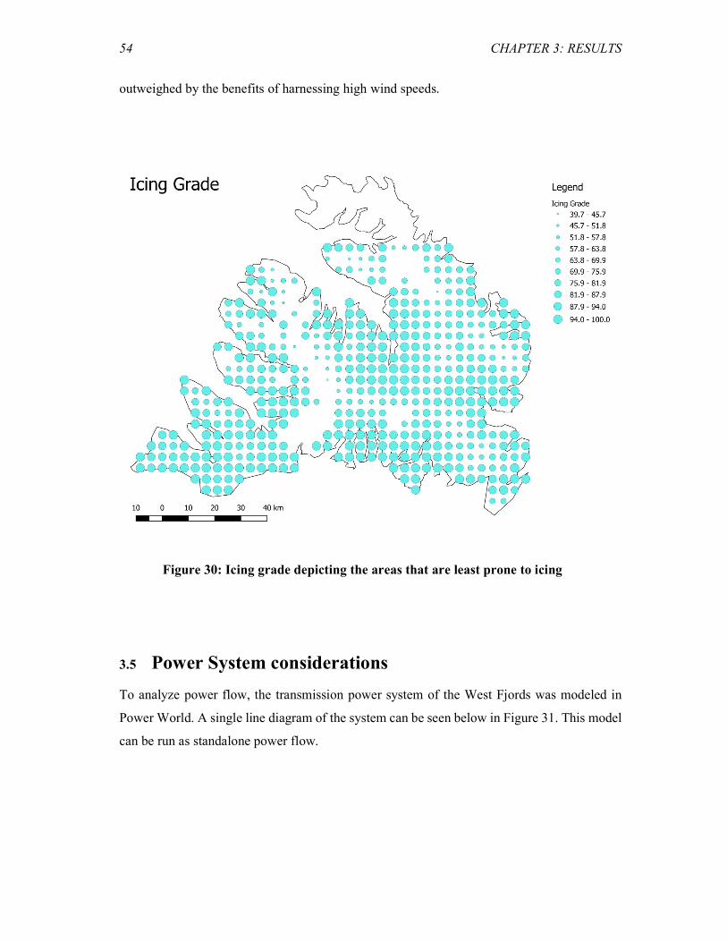
54 CHAPTER 3: RESULTS
outweighed by the benefits of harnessing high wind speeds.
3.5 Power System considerations
To analyze power flow, the transmission power system of the West Fjords was modeled in
Power World. A single line diagram of the system can be seen below in Figure 31. This model
can be run as standalone power flow.
Figure 30: Icing grade depicting the areas that are least prone to icing

3.5 POWER SYSTEM CONSIDERATIONS 55
The thick blue and red lines represent computational buses, the green lines model power lines,
and the arrows represent load [37]. After the base case was modeled in Power World, the base
case was scripted into a MATLAB extension called MATPOWER. This program was used to
automate the power flow analysis process by iteratively conducting analysis at each evaluation
location.
3.5.1 Maximum Generation Input
The first power system evaluation criterium is maximum allowable energy input. The
constraints considered when modeling the implementation of generation to the current West
Fjords grid is discussed in Section 2.4.3.
Below in Figure 32 there is a tendency for high marks in the eastern part of the West Fjords.
A contributing factor to this is that the locations in the East are more likely to be connected to
a substation that transports electricity using power lines with a higher apparent power rating.
Figure 31: Simplified single line diagram depicting the transmission system in the West Fjords

56 CHAPTER 3: RESULTS
3.5.2 Power Loss Evaluation
Anticipated losses are also deduced from the power flow analysis. This section displays
calculated transmission losses when adding power generation at each potential site location.
The previous section determined the maximum amount of power that can be introduced into
the current transmission system at each evaluation site. These values are assumed as the
amount of generation input when calculating losses.
Figure 32: Maximum allowable input grade that depicts amount of generation that can be input at each evaluation location

3.5 POWER SYSTEM CONSIDERATIONS 57
Figure 33: Power losses at all evaluation locations versus distance between site location and nearest substation.
Power loss at each evaluation location is plotted in Figure 33 according to the distance between
the site and the closest transmission substation. The transmission substation connected to each
site is indicated by color. Calculated power losses are between 0.55 MW and 7.7 MW. A
general trend suggesting that the larger the distance between the evaluation site being analyzed
and the nearest substation, the larger the anticipated power losses. This trend is followed by
the sites connected to the GED, KEL, MJO, and GLE substations.
The base case assumes no generation is added at any of the potential sites, and experiences
1.06 MW of power loss. There is one site that has power losses lower than the base case. Future
studies should analyze this location more carefully.
Now that a relationship has been established between power loss and distance to substation,
one of the substations that does not follow this relationship will be analyzed. This is done to
determine whether there are additional factors influencing power losses, and to understand
where fluctuation is occurring.

58 CHAPTER 3: RESULTS
Figure 34 shows the calculated power losses expected to occur between the Ísafjörður
substation and the evaluation sites located nearest to this substation. There are 36 evaluation
sites represented in this figure and in contrast to the previous example, Figure 34 displays an
inconsistent relationship between distance and power losses. Table 3.2 shows that the diesel
generators in Ísafjörður produced the second largest amount of electricity from diesel from the
years 1999 to 2017. Diesel consumption suggests disturbances in the power system, as it is
only used for reserve power generation. Figure 22 shows that there is high energy consumption
in Ísafjörður. The combination of large energy consumption and diesel usage suggests there
are additional factors other than distance contributing to the power losses occurring between
the Ísafjörður substation and the relevant evaluation sites. There is also a chance that the
variation may be attributed to a mathematical anomaly within the MATPOWER algorithm
linked to voltage. Further analysis is suggested for sites connected to the ISA substation.
Once the power losses between each location and the nearest substation is calculated and
assessed each site is graded based on how loss at the location compared to loss at all other
locations as described in 2-17. In Figure 35 the grades are displayed showing that the sites in
Figure 34: Power losses between Ísafjörður and the nearest evaluation sites versus distance

3.5 POWER SYSTEM CONSIDERATIONS 59
the west are rated higher. The score is particularly high in areas near substations, mirroring the
results found in the power flow analysis.
3.5.3 Transmission Cost
Transmission cost was determind based on a study conducted by Landvernd with similar
cables. The cost was provided per meter, and adjusted based on wind turbine lifespan and the
length a cable would need to be in order to connect a site location with the nearest transmission
substation. The site with the lowest transmission cost received the highest grade, and the other
sites were scaled based on the lowest cost. It can be seen in Figure 36 that the locations located
closest to substations received the best grades.
Figure 35: Transmission system power loss grade that depicts the power loss experienced when inputting the max power input at each evaluation location

60 CHAPTER 3: RESULTS
3.6 Cumulative Score
This study set the weighted all input variables equally. The eight criteria were averaged, and
the cumulative outcome can be seen in Figure 37. When weighing all inputs equally, the most
favorable sites are in the South Eastern part of the West Fjords and close to the Mjolka
substation. Though the top five evaluation locations are highlighted, all the sites encompassed
by the black ovals are worth investigating further. At the end of October 2018, it was
announced that EM Orka intends to construct 35 wind turbines after analyzing the
Reykhólahreppur location, which is located in the south western part of the West Fjords [53].
EM Orka conducted a GIS assessment considering wind resource and electrical grid
connection [54]. It is noteworthy that separate, unrelated assessments resulted in similar
location choices. The location EM Orka choose to construct their wind farm is ranked 3rd best
in this study.
Figure 36: Cost grade depicting the cost of building transmission lines between each evaluation location and the nearest transmission substation

3.6 CUMULATIVE SCORE 61
Figure 37: Total cumulative grade depicting the score of each location accounting for all eight evaluation criteria with point circled in black
Now that a visual assessment has been presented, a more traditional presentation of results is
provided in Table 3.3. The coordinates for the top five overall wind energy generation sites are
listed. Though there is value in knowing the specific location (for example when conducting
further analysis), it is more beneficial to present results visually during the comparison stage.
Table 3.3 Coordinates for the top five overall wind generation site locations
Rank Latitude Longitude Grade
1 65.760 -23.2033 55.3
2 65.463 -21.766 54.2
3 65.500 -21.8558 54.1
4 65.760 -23.2033 53.6
5 65.501 -21.766 52.6
1 4
3 2 5

62 CHAPTER 3: RESULTS
The sites located near transmission substations, diesel generators, and far from towns were
ranked highest in the ‘social’ subsection. As is shown in Figure 38 these areas lie mostly in the
central western part of the West Fjords. There are also some highly rated sites south of Flateyri
and near the south eastern part of the boundary layer.
The ranking in the ‘status quo’ subsection does not vary widely as can be seen in Figure 39.
This is because the two criteria in this subsection, icing and power potential have contradicting
evaluations. The area with high icing has a tendency of being associated with high wind speeds.
Wind speed in turn results in higher potential power output. Despite having high wind speeds,
areas prone to icing are not favorable because extreme weather negatively impacts power
generation, negating the benefits of higher wind speeds.
Figure 38: Cumulative social subsection grade in the West Fjords accounting for diesel usage, electricity consumption, and proximity to population
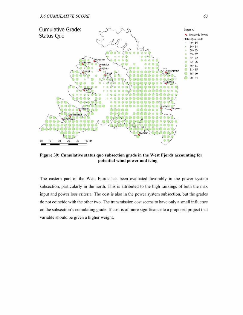
3.6 CUMULATIVE SCORE 63
The eastern part of the West Fjords has been evaluated favorably in the power system
subsection, particularly in the north. This is attributed to the high rankings of both the max
input and power loss criteria. The cost is also in the power system subsection, but the grades
do not coincide with the other two. The transmission cost seems to have only a small influence
on the subsection’s cumulating grade. If cost is of more significance to a proposed project that
variable should be given a higher weight.
Figure 39: Cumulative status quo subsection grade in the West Fjords accounting for potential wind power and icing

64 CHAPTER 3: RESULTS
Figure 40: Cumulative power system subsection grade in the West Fjords considering maximum potential power input, power losses, and transmission
costs
The power system cumulative results are unexpected. Figure 40 suggests that the ideal wind
energy site locations are in the North East. This area in the West Fjords has been proven
inconvenient in Figure 35 and Figure 36 where power losses and costs are high. Despite two
of the three criteria highlighting the downfalls of the area, the maximum generation input
criterion holds the most influence. One may refer to Figure 41 and note that the maximum
generation input points often have a higher-criteria grade accounting for disproportionate
influence.
3.7 Sensitivity Analysis
The previous section illustrates how widely the best location varies based on which criterion
is used for ranking. This study presents a base case scenario in which each variable is weighted
equally. To better understand the influence of the criteria on the final score, a sensitivity
analysis is presented. The sensitivity analysis aims to identify trends relating each criterion’s
raw score (includes units) to the dimensionless cumulative score. Possible raw scores are
derived using normal random distributions created to encompass all expected scenarios for a

3.7 SENSITIVITY ANALYSIS 65
given criterion at one location.
To compare each criterion’s effect on the final grade, each criterion’s raw score is normalized,
set on a scale of 0-100, and plotted together in Figure 41. Each criterion’s elasticity can be
derived from Figure 41. For example, icing, population, and cost are very inelastic, meaning
that a small change in the criteria grade can result in a large change in overall grade. In contrast,
power potential is elastic and changes in the criterion’s score are less impactful to the
cumulative score.
Figure 41 also provides insight into the anticipated normalized grade. The intention of
weighting each c riterion as of the cumulative score is to consider all criteria equally. Figure
41 proves this was not accomplished. The criteria with grades on the right side of the plot carry
more weight than those further left. The normalization was carried out by setting the best score
to 100, and most likely affected the weight discrepancy between criteria. It is suggested that
future studies normalize grades based on the median instead of the top score. To understand
the relationship between where points lie on the x-axis of Figure 41 and the effect on the
cumulative score, consider the example of the power system integration subsection. The three
criteria grades in this subsection are shown in Figure 42 side by side. The transmission cost
(yellow) and transmission system power losses (red) grades rank locations near transmission
substations and the western part of the West Fjords higher. In contrast, the grades for maximum
allowable power (green) input are higher in the eastern part of the West Fjords.
Figure 41: Sensitivity analysis showing the effect of eight criteria on the overall score in one location

66 CHAPTER 3: RESULTS
a. b. c.
Despite two of the three criteria in the power system integration subsection favoring locations
in the west, it can be seen in Figure 43 that the cumulative power system score ranks locations
in the east as better.
How is it that the maximum allowable power input criterion (green) has a greater impact on
the cumulative score than the other two criteria despite the three criteria being weighted
equally? The reasoning is revealed in part b. of Figure 43 where the normalized power system
sensitivity analysis is shown. Note that the most influential criterion -maximum allowable
power input- has an overall higher criteria grade than max power loss and cost. This suggests
that the normalization gave preference to criteria that had higher normalized criteria grade on
average.
a. b.
Figure 42: Power system integration subsection individual criterion grades mapped in the West Fjords
Figure 43: (a) Cumulative grade for the power system integration criteria in the West Fjords (b), and the sensitivity analysis showing the relationship between the normalized scores of the power system integration subsection and overall grade.

3.7 SENSITIVITY ANALYSIS 67
In order to view trends between raw scores and the overall grade each criterion is plotted
separately and further separated into three plots corresponding to the three subsections. The
curves representing the sensitivity analysis for the social considerations are presented in Figure
44.
Diesel usage and power consumption both have positive trends and the population criterion
has a less defined trend. inverse relationship between input and score. This is anticipated
because the evaluation site is less desirable when neighboring a large population; there is a
direct correlation between distance and rank in the population criteria.
Figure 44: Sensitivity analysis showing effect of the social considerations on the overall score
Figure 45: Sensitivity analysis showing effect of the status quo criteria on the overall score
×102 ×103
×103

68 CHAPTER 3: RESULTS
The two curves representing the sensitivity of the variables in the Status quo subsection act as
anticipated (Figure 45). The power potential has a positive slope that can be attributed to the
positive relationship between the amount of power that can be produced at a given site and the
site’s cumulative score. The icing criteria has an inverse relationship, therefore giving
sensitivity a negative slope. It is interesting to see how high the magnitude is in the icing
sensitivity as it is confined between 80 and 90 percent grades.
The power system subsection’s sensitivity analysis can be seen in Figure 46. The maximum
power input is shown to have a positive slope. The higher the amount of power that can be
input into the current power system, the higher the score it receives. This allows for project
growth with minimal infrastructure investment. As expected, both the power loss and the cost
criteria have negative slopes for their sensitivity curve as they are the only dependent
variables in their respective categories and both have an inverse relationship with cumulative
score.
3.8 Summary
The eight variables: diesel use, electricity use, population size, predicted power, icing,
maximum potential generation input, expected power losses, and cost were identified as
important factors for wind farm siting and assigned a score. Each variable was individually
assessed and evaluated. The ideal location for each variable is as follows:
Diesel: 65.7596, -23.203,
Electricity Use: 66.01683, -23.383
Figure 46: Sensitivity analysis showing effect of the power system integration criteria on overall score

3.8 SUMMARY 69
Population: 65.463, -21.317
Predicted Power Potential: 65.907, -22.0364
Icing: 65.538, -22.575
Maximum Potential Power Input: The points east of latitude -22.485
Power Losses: 66.017, -23.652
Transmission Cost: 65.907, -21.317
When all eight criteria are weighted equally the best overall location for constructing a wind
farm was determined to be at coordinates 65.760, -23.203 which is in the western part of the
West Fjords near Mjolka.
70
Chapter 4
4Conclusion
A multi criteria siting assessment was developed by analyzing eight criteria: diesel use,
electricity use, population size, predicted power, icing, maximum potential generation input,
expected power losses, and cost. These topics were assessed in an attempt to expand on
standard siting procedures by addressing often-expressed concerns regarding wind energy
generation. 580 locations spaced four km from one another were reduced to 482 after sites that
did not meet the disqualifying factor requisites were eliminated. The remaining sites were
graded using the eight criteria. Each criterion was individually analyzed and used to assess all
locations. Once all potential sites were given a grade using the criteria separately, all criteria
were combined to create a cumulative score. Based on the cumulative score, the most favorable
wind energy generation sites lie in the South Eastern part of the West Fjords and near Mjolka.
Ultimately, this method is validated considering a separate, unrelated study by EM Orka
announced a wind farm will be constructed near the site ranked third best in this study [51].
4.1 Recommendations
Though this study begins to address reoccurring problems in wind energy generation siting as
a way to improve the state-of-the-art methodology, expanding on the status quo is an ongoing
process. This section will review recommendations for future improvements.
The disqualifying factors in this study currently include natural sites, high terrain slope, and
proximity to population. To expand the scope of applicability, bird migration patterns and
airport locations could also be included as disqualifying factors. This study eliminated sites
within a two km radius of 16 towns in the West Fjords. Though population is considered further
as a grading criterion, it is recommended that the initial buffer around towns be expanded.
Potential sites eliminated due to high slope are currently assessed visually. This can be
improved in future studies by calculating the average gradient over a 4 km by 4 km block and

71
eliminating sites with an average gradient higher than 30%. Because terrain is a significant
siting factor, future studies may also consider adding terrain slope as a grading criterion.
Potential power is evaluated in this study using the average expected power production at each
site as determined by Landsvirkjun using Harmonie. This study recommends producing a
monthly predicted power production curve at each evaluation site. Expanding past the yearly
average can help to better model intermittent generation. This fluctuating power production
can then be input into power flow analysis to simulate the effects of intermittent power
generation on the power system in the West Fjords.
In terms of improving the power system analysis, this study suggests widening the scope
beyond assuming the system operates under steady state conditions. To more accurately model
the power system, dynamic power flow analysis should be conducted and N-1 contingencies
should be analyzed. It is also suggested that a more intensive economic analysis be performed.
An example of how cost can be further analyzed is to determine the infrastructure budget
required to facilitate transportation and installation at different siting locations.
Lastly, the sensitivity analysis in Figure 41 reveals that different criteria bear more weight in
the overall score than others. In the future, the criteria can be normalized to account for this
and give all criteria equal weight in the overall base case scenario.
Addressing reoccurring problems is a way to improve the state-of-the-art methodology.
Including multi-disciplinary assessment criteria such as economic cost, impact on society and
the electrical grid can further advance wind energy generation siting to optimize wind
resources and benefit to the affected population.

72
5 References
[1] P. D.-W. a. T. T. S. Batel, "“Social acceptance of low carbon energy and associated
infrastructures: A critical discussion”," Energy Policy, vol. 58, pp. 1-5, July 2013.
[2] Sigurður Elías Hjaltason and María Guðmundsdóttir, "Energy Statistics in Iceland," Orkustofnun, 2017.
[3] Landsnet, "Afhendingaröryggi og gæði flutningskerfisins," 2017.
[4] National Statistical Institute of Iceland, "Population development in the West Fjords," 2007.
[5] International Energy Agency (IEA), "2018 Global Energy & CO2 Status Report," 2018.
[6] R. K. a. S. M. Tripathy, "Cost and emission additionality of wind energy in power systems, Sustainable Energy, Grids and Networks," Sustainable Energy, Grids and Networks, vol. 17, March 2019.
[7] T. R. H. a. W. T. Pennell, "The Meteorological Aspects of Siting Large Wind Turbines, US Department of Energy," US Department of Energy , Springfield, Virginia, 1981.
[8] J. M. a. A. R. J. F. Manwell, Wind Energy Explained, Wiley, 2009.
[9] a. S. .. J. A. Carta P. Ramírez, "A review of wind speed probability distributions used in wind energy analysis: Case studies in the Canary Islands," Renewable and Sustainable Energy Reviews, vol. 13, no. 5, June 2009.
[10] W. Kenton, "Probability Density Function (PDF)," Investopedia, April 2019. [Online]. Available: https://www.investopedia.com/terms/p/pdf.asp.
[11] A. D. S. A. Akdağ, "A new method to estimate Weibull parameters for wind energy applications, Energy Conversion and Management," INIS, pp. 1761-1766, 2009.
[12] H. Rinne, The Weibull Distribution: A Handbook, CRC Pres, 2008 .
[13] S. J. a. V. Ran, "Optimum siting of wind turbine generators," IEEE Transactions on Energy Conversion, 2001.
[14] "Wind Turbine Speed," Turbine Generator, 2018. [Online]. Available: https://www.turbinegenerator.org/wind/what-is-wind/wind-speed/.
[15] F. K. C. S. a. B. K. C. Eisenhut, "Wind-Turbine Model for System Simulations Near Cut-In Wind Speed," IEEE Transactions on Energy Conversion, vol. 22, no. 2, 2007.
[16] "Wind Turbine Speed," Woodmead Energy Services, 2018. [Online]. Available: https://woodmeadenergyservices.com/renewable-energy/wind-turbine-planning-application/.
[17] M. O. L. Hansen, Aerodynamics of Wind Turbines, Second Edition, Taylor and Francis, 2008.
[18] A. J. Elíasson, "Natural Hazards and The Icelandic Power Transmission Grid," Landsnet Icegrid, 2005.
[19] G. N. P. H. B. a. K. J. N. Nawri, "The Wind Energy Potential of Iceland," Icelandic Meteorological Office, 2013.
[20] Energydata.info, "Global WInd Atlas," Vortex, [Online]. Available: https://globalwindatlas.info/.
[21] Landsvirkjun, "Búrfellslundur," 2018.
[22] J. V. R. M. M. O. a. R. L. D. H. L. Wegley, "Uniform Roughness," in A Siting handbook for Small Wind Energy Conversion systems, U.S. Department of Energy, 1980, p. 8.
[23] K. V. a. R. C. Rolv Erlend Bredesen, "WIND ENERGY PROJECTS IN COLD CLIMATES," IEA WInd, 2017.
[24] Á. J. Elíasson, "Natural Hazards and The Icelandic Power Transmission Grid," Landsnet Icegrid, Reykjavík, 2005.

73
[25] M. Valdimarsdóttir, "Byggð og náttúruvá Viðhorf íbúa á ofanflóðasvæðum til áhættu og öryggis," Háskóli Íslands, Reykjavik , 2000.
[26] T. Jóhannesson, "Ofanflóðastarfsemi: Veðurstofa Íslands 90 ára," Veðurstofa Íslands, 2010.
[27] M. S. a. T. O. Duncan Glover, Power System Analysis and Design, fifth edition, Cengage Learning, 2008.
[28] G. Valdimarsson, "Real-Time Security Assessment for the Icelandic Electrical Power System Phasor Measurements," Reykjavik University, 2016.
[29] "Aflflutningur núna," Landsnet, 2018. [Online]. Available: https://www.landsnet.is/flutningskerfid/kerfisstjornun/aflflutningur-nuna/.
[30] Orkubú Vestfjarða ohf., "ÁRSSKÝRSLA 2017," 2018.
[31] Orkustofnun, "Raforkuspá 2015 – 2050: Orkuspárnefnd," 2015.
[32] Iceland Review, "Questions Over Record Cruise Year in West Fjords," Iceland Review, 17 April 2017. [Online]. Available: https://www.icelandreview.com/news/questions-over-record-cruise-year-west-fjords/.
[33] Fiskvinnslan Íslandssaga, "Íslandssaga," [Online]. Available: https://icelandicsaga.is/.
[34] International Energy Agency, "Global Energy & CO2 Status Report," IEA, 2018.
[35] Lazard, "Lazard's Levelized Cost of Energy Analysis - Version 12.0, pg. 8," 2018.
[36] IRENA, "The Power to Change: Solar and Wind Cost Reduction Potential to 2025," 2016.
[37] The University of Texas at Austin, Energy Institute, "The Full Cost of Electricity (Fce-)," The University of Texas at Austin, 2018.
[38] METSCO, "Comparison of Underground and Overhead Transmission Options in Iceland (132 and 220kV)," METSCO Energy Solutions, commissioned by Landvernd, 2013.
[39] F. M. EFLA, "High Voltage Underground Cables in Iceland: Research Project concerning Options and Cost for 132 kV and 220 kV Underground Cables for Different System- and Ground Conditions Gereral Discussion and Study of Three Different Cases," 2015.
[40] PowerWorld Corporation, "PowerWorld Simulator 18," 2018. [Online]. Available: https://www.powerworld.com/powerworld-simulator-18.
[41] C. E. M.-S. &. O. R. D. Zimmerman, " Free, open-source Electric Power System Simulation and Optimization Tools for MATLAB and Octave," MATPOWER, 2018.
[42] XLPE, "XLPE Land Cable Systems: User’s Guide," ABB, 2018.
[43] W. Tours, "Hornstrandir Nature Reserve," [Online]. Available: http://www.westtours.is/trip-categories/hornstrandir-nature-reserve/.
[44] a. S. .. J. A. Carta P. Ramírez, " A review of wind speed probability distributions used in wind energy analysis: Case studies in the Canary Islands, Renewable and Sustainable Energy Reviews," vol. 13, no. 5, 2009.
[45] Landsvirkjun, "Wind Power Predictions Deduced Using Harmonie," Landsvirkjun.
[46] X. L. a. J. W. Shunlin Liang, "Chapter 2: Geometric Processing and Positioning Techniques," in Advanced Remote Sensing, Elsevier, 2012.
[47] B. H. Hallgrimson, Interviewee, EFLA. [Interview]. 18 September 2018.
[48] Landmælingar Íslands, "Simple Maps," 2018. [Online]. Available: http://www.lmi.is/kort/.
[49] H. O. H. a. P. G. H. Max Halperin, "Recommended Standards for Statistical Symbols and Notation. COPSS Committee on Symbols and Notation," The American Statistician, vol. 19, no. 3, pp. 12-14, 1965.
[50] Visit West Fjords, "Towns and Villages," [Online]. Available: https://www.westfjords.is/en/inspiration/towns.
[51] International Electrotechnical Commission, "IEC 61400-12-1:2017- Wind energy generation systems - Part 12-1: Power performance measurements of electricity producing wind turbines," 2017.
[52] M. Webster, "Definition of mesoscale," [Online]. Available: https://www.merriam-

74
webster.com/dictionary/mesoscale.
[53] RUV, "Kynna vindorkugarð í Reykhólahreppi," [Online]. Available: http://www.ruv.is/frett/kynna-vindorkugard-i-reykholahreppi.
[54] EM Orka, "Garpsdalur Wind Farm," [Online]. Available: https://www.emorka.is/project.
[55] RUV, "Kynna vindorkugarð í Reykhólahreppi," 24 10 2018. [Online]. Available: http://www.ruv.is/frett/kynna-vindorkugard-i-reykholahreppi.
[56] J. Chen, G. Hoversten, K. Key, G. Nordquist and W. Cumming, "Stochastic inversion of magnetotelluric data using a sharp boundary parameterization and application to a geothermal site," Geophysics, pp. E265 - E279, 2012.
[57] R. Bratvold, J. Bickel and H. Lohne, "Value of Information in the Oil and Gas Industry: Past, Present, and Future," Society of Petroleum Engineers Reservoir Evaluation and Engineering, pp. 630 - 638, 2009.
[58] T. Gamble, W. Goubau and J. Clarke, "Magnetotellurics with a remote magnetic reference," Geophysics, pp. 53 - 68, 1979.
[59] R. Karlsdóttir, A. M. Vilhjálmsson, K. Árnason and A. T. Beyene, "Þeistareykir (Theistareykir) Geothermal Area, Northern Iceland: 3D Inversion of MT and TEM Data," ÍSOR - Iceland Geosurvey, Reykjavík, 2012.
[60] X. Yang, "Stochastic Inversion of 3D ERT Data," 1999.
[61] W. Trainor-Guitton and G. Hoversten, "Stochastic inversion for electromagnetic geophysics: practical challenges and improving convergence efficiency," Geophysics, pp. F373 - F386, 2011.
[62] W. Trainor-Guitton, J. Caers and T. Mukerji, "A methodology for Establishing a Data Reliability Measure for Value of Spatial Information Problems," Mathematical Geosciences, pp. 929-949, 2011.
[63] A. Ramirez, J. Nitao, W. Hanley, R. Aines, R. Glaser, S. Sengupta, K. Dyer, T. Hickling and W. Daily, "Stochastic inversion of electrical resistivity changes using a Markov Chain Monte Carlo approach," Journal of Geophysical Research, vol. 110, 2005.
[64] P. D.-W. a. T. T. S. Batel, “Social acceptance of low carbon energy and associated infrastructures: A critical discussion”, Energy Policy,.
[65] Landsvirkjun, Interviewee, [Interview].
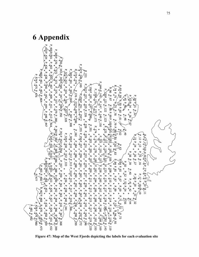
75
6 Appendix
Figure 47: Map of the West Fjords depicting the labels for each evaluation site

76
Table 4.1 Grading breakdown for each evaluation site showing all criteria grades
and cumulative grade
Point Diesel Use
Energy Use Population
Power Potential Icing
Max Power Input
Power Losses Cost Cumulative
P_1 11.9 9.5 38.4 81.0 94.6 48.1 19.1 0.6 37.8 P_2 14.7 8.7 40.3 81.0 93.1 46.2 20.8 3.4 38.5 P_3 13.6 7.9 42.3 75.0 82.5 45.2 21.5 3.1 36.4 P_4 12.7 7.3 44.5 66.0 85.7 43.3 23.5 2.8 35.7 P_5 11.1 6.3 49.3 79.0 90.0 40.4 26.4 2.3 38.1 P_6 10.5 5.9 51.9 93.0 59.5 39.4 27.3 2.1 36.2 P_7 9.9 5.5 54.6 87.0 60.1 100.0 7.1 0.5 40.6 P_8 9.4 5.2 57.4 72.0 78.7 100.0 7.1 0.5 41.3 P_9 9.0 5.0 60.2 63.0 89.8 100.0 7.2 0.5 41.8 P_10 8.6 4.7 63.2 70.0 78.3 100.0 7.2 0.5 41.6 P_11 8.2 4.5 66.1 64.0 97.3 100.0 7.2 0.5 43.5 P_12 17.9 10.8 35.7 84.0 59.7 50.0 17.7 4.5 35.0 P_13 14.6 8.6 39.8 82.0 49.4 46.2 20.8 3.5 33.1 P_14 13.5 7.8 42.2 79.0 53.6 45.2 21.4 3.0 33.2 P_15 12.5 7.1 44.7 76.0 73.9 43.3 23.3 2.7 35.4 P_16 11.6 6.6 47.4 77.0 83.0 41.3 25.4 2.4 36.8 P_17 9.3 5.1 58.6 75.0 72.8 100.0 7.4 0.5 41.1 P_18 8.8 4.8 61.5 68.0 80.6 100.0 7.4 0.5 41.5 P_19 8.4 4.6 64.6 62.0 89.8 100.0 7.4 0.5 42.2 P_20 18.8 10.8 36.8 89.0 98.0 51.0 18.0 4.8 40.9 P_21 21.9 12.7 34.5 90.0 73.1 51.9 17.3 5.1 38.3 P_22 27.2 15.7 32.7 89.0 54.1 0.0 0.0 13.1 29.0 P_23 17.5 10.6 35.4 80.0 72.9 50.0 17.7 4.5 36.1 P_24 15.6 9.3 37.8 80.0 81.0 48.1 19.1 3.8 36.8 P_25 14.2 8.3 40.3 86.0 56.2 46.2 20.6 3.3 34.4 P_26 13.1 7.5 43.0 86.0 60.7 44.2 22.3 2.9 35.0 P_27 12.1 6.8 45.7 86.0 72.3 42.3 24.3 2.6 36.5 P_28 9.5 5.2 57.2 78.0 72.1 100.0 7.6 0.6 41.3 P_29 9.1 5.0 60.2 69.0 77.9 100.0 7.6 0.6 41.2 P_30 8.7 4.7 63.2 69.0 76.8 100.0 7.6 0.6 41.3 P_31 8.3 4.5 66.3 72.0 78.5 100.0 7.6 0.6 42.2 P_32 7.9 4.3 69.5 70.0 86.8 100.0 7.6 0.6 43.3 P_33 20.4 11.7 35.0 79.0 97.1 51.9 17.6 6.0 39.8 P_34 24.1 14.2 32.6 80.0 100.0 51.9 17.8 6.8 40.9 P_35 29.8 17.9 30.8 90.0 52.6 51.9 17.9 7.0 37.2 P_36 41.6 24.7 29.2 76.0 69.3 0.0 0.0 23.9 33.1 P_37 45.5 28.1 27.8 72.0 75.1 0.0 0.0 26.4 34.4 P_38 13.7 7.8 41.6 71.0 90.6 44.2 22.6 3.0 36.8 P_39 12.6 7.1 44.4 81.0 86.8 42.3 24.5 2.6 37.7 P_40 11.0 6.1 50.1 81.0 69.9 100.0 7.7 0.6 40.8 P_41 9.3 5.1 59.0 78.0 70.5 100.0 7.8 0.6 41.3 P_42 8.9 4.8 62.1 77.0 70.6 100.0 7.8 0.6 41.5 P_43 8.5 4.6 65.2 76.0 78.8 100.0 7.8 0.6 42.7

77
P_44 8.1 4.4 68.4 71.0 98.5 100.0 7.8 0.6 44.8 P_45 22.0 12.5 34.3 83.0 74.0 0.0 43.4 7.8 34.6 P_46 26.3 15.5 31.9 74.0 55.3 0.0 0.0 9.7 26.6 P_47 31.7 19.9 29.9 80.0 100.0 0.0 0.0 10.4 34.0 P_48 39.3 27.6 28.2 84.0 55.4 0.0 0.0 11.9 30.8 P_49 29.7 21.3 27.8 57.0 97.8 0.0 0.0 11.0 30.6 P_50 12.1 6.7 46.3 76.0 91.8 41.3 25.2 2.4 37.7 P_51 11.3 6.2 49.2 83.0 82.9 100.0 7.9 0.6 42.6 P_52 10.6 5.8 52.1 90.0 72.7 100.0 8.0 0.6 42.5 P_53 9.5 5.2 58.1 94.0 44.5 100.0 8.0 0.6 40.0 P_54 9.1 4.9 61.2 83.0 73.7 100.0 8.0 0.6 42.6 P_55 8.7 4.7 64.3 78.0 80.8 100.0 8.0 0.6 43.1 P_56 8.3 4.5 67.5 69.0 96.2 100.0 8.0 0.6 44.3 P_57 17.0 9.3 40.2 82.0 83.0 51.9 17.3 5.3 38.3 P_58 19.7 10.8 37.1 77.0 98.6 51.9 17.9 7.1 40.0 P_59 30.3 17.1 31.9 67.0 88.8 0.0 0.0 16.4 31.4 P_60 37.3 22.4 29.9 90.0 63.1 0.0 0.0 20.4 32.9 P_61 42.5 31.1 28.4 85.0 49.9 0.0 0.0 7.7 30.6 P_62 31.2 23.0 28.0 59.0 70.9 0.0 0.0 12.2 28.0 P_63 17.9 10.5 34.8 62.0 99.7 50.0 17.7 4.4 37.1 P_64 12.4 6.8 45.7 77.0 95.4 100.0 8.1 0.6 43.2 P_65 11.6 6.3 48.6 80.0 89.3 100.0 8.1 0.6 43.1 P_66 10.9 5.9 51.5 83.0 87.4 100.0 8.2 0.6 43.4 P_67 10.3 5.5 54.5 95.0 74.8 100.0 8.2 0.7 43.6 P_68 9.7 5.3 57.5 96.0 68.1 100.0 8.3 0.7 43.2 P_69 9.3 5.0 60.5 86.0 76.9 100.0 8.3 0.7 43.3 P_70 8.8 4.8 63.6 80.0 84.7 100.0 8.3 0.7 43.9 P_71 8.4 4.6 66.8 71.0 88.9 100.0 8.3 0.7 43.6 P_72 8.1 4.4 70.0 68.0 96.1 100.0 8.2 0.7 44.4 P_73 7.5 4.1 76.8 72.0 100.0 100.0 8.1 0.6 46.1 P_74 17.4 9.3 40.3 88.0 75.0 51.9 17.4 5.5 38.1 P_75 20.1 10.8 37.4 83.0 86.4 0.0 100.0 7.5 43.1 P_76 24.6 13.2 34.7 72.0 97.7 0.0 0.0 11.7 31.7 P_77 36.0 18.7 32.4 64.0 95.8 0.0 0.0 26.4 34.2 P_78 83.6 39.1 30.6 71.0 88.0 0.0 0.0 100.0 51.5 P_79 41.9 32.2 28.4 80.0 67.5 0.0 0.0 17.8 33.5 P_80 29.1 19.9 28.9 50.0 86.5 0.0 0.0 10.2 28.1 P_81 24.0 15.0 30.5 45.0 94.5 51.9 16.9 7.1 35.6 P_82 18.3 10.3 34.9 64.0 98.0 49.0 18.5 4.3 37.2 P_83 16.4 9.1 37.4 55.0 99.4 47.1 19.9 3.6 36.0 P_84 12.7 6.8 45.5 66.0 99.3 100.0 8.3 0.7 42.4 P_85 11.9 6.3 48.3 77.0 97.3 100.0 8.4 0.7 43.7 P_86 11.1 5.9 51.2 87.0 90.6 100.0 8.4 0.7 44.4 P_87 10.5 5.6 54.1 97.0 82.7 100.0 8.5 0.7 44.9 P_88 9.9 5.3 57.1 98.0 75.4 100.0 8.5 0.7 44.4 P_89 9.4 5.1 60.1 88.0 78.0 100.0 8.6 0.7 43.7 P_90 9.0 4.9 63.2 82.0 83.9 100.0 8.6 0.7 44.0 P_91 8.6 4.7 66.4 77.0 84.2 100.0 8.5 0.7 43.8 P_92 8.2 4.5 69.6 73.0 86.2 100.0 8.5 0.7 43.8 P_93 7.9 4.3 72.9 71.0 76.0 100.0 8.5 0.7 42.7

78
P_94 7.6 4.1 76.3 66.0 100.0 100.0 8.4 0.7 45.4 P_95 7.3 4.0 79.9 70.0 97.2 100.0 8.3 0.7 45.9 P_96 17.4 9.1 40.8 79.0 85.5 51.9 17.3 5.3 38.3 P_97 20.0 10.4 38.0 86.0 68.8 51.9 17.9 7.1 37.5 P_98 29.6 15.4 33.3 73.0 67.6 0.0 0.0 16.4 29.4 P_99 33.0 19.3 30.4 81.0 91.0 0.0 0.0 13.3 33.5 P_100 30.0 18.9 29.7 66.0 81.3 0.0 0.0 9.3 29.4 P_101 26.7 16.1 30.4 44.0 97.6 0.0 33.3 7.6 32.0 P_102 23.4 13.5 31.6 49.0 100.0 51.9 16.6 6.1 36.5 P_103 20.7 11.5 33.4 52.0 99.7 51.0 17.0 4.9 36.3 P_104 18.5 10.0 35.5 64.0 91.0 48.1 19.3 4.0 36.3 P_105 16.7 8.9 37.9 58.0 98.8 46.2 20.8 3.4 36.3 P_106 15.2 8.0 40.3 54.0 100.0 44.2 22.5 3.0 35.9 P_107 12.9 6.8 45.6 68.0 99.6 100.0 8.5 0.7 42.8 P_108 12.1 6.4 48.4 83.0 96.8 100.0 8.6 0.7 44.5 P_109 11.3 6.0 51.2 91.0 89.8 100.0 8.7 0.7 44.8 P_110 10.7 5.7 54.1 97.0 83.5 100.0 8.8 0.7 45.1 P_111 10.1 5.4 57.0 99.0 77.8 100.0 8.8 0.8 44.9 P_112 9.6 5.1 60.0 90.0 81.8 100.0 8.9 0.8 44.5 P_113 9.1 4.9 63.0 85.0 83.9 100.0 8.9 0.8 44.5 P_114 8.7 4.7 66.1 86.0 74.5 100.0 8.8 0.8 43.7 P_115 8.4 4.5 69.3 83.0 70.1 100.0 8.8 0.7 43.1 P_116 8.0 4.2 72.6 74.0 87.6 100.0 8.7 0.7 44.5 P_117 7.7 4.1 76.1 71.0 86.8 100.0 8.6 0.7 44.4 P_118 7.4 3.9 79.7 71.0 100.0 100.0 8.5 0.7 46.4 P_119 7.2 9.9 83.4 0.0 100.0 100.0 8.4 0.7 38.7 P_120 19.5 11.2 38.9 70.0 89.6 51.9 17.6 6.1 38.1 P_121 22.3 12.8 36.5 80.0 91.4 0.0 43.4 7.8 36.8 P_122 25.5 14.2 34.5 83.0 73.6 0.0 0.0 9.7 30.1 P_123 29.1 15.1 32.0 86.0 75.3 0.0 0.0 9.0 30.8 P_124 27.8 14.8 31.4 63.0 83.3 51.9 16.7 6.5 36.9 P_125 25.7 13.5 32.0 57.0 67.6 51.9 16.6 5.9 33.8 P_126 23.3 12.0 33.1 51.0 92.4 51.0 17.1 5.0 35.6 P_127 20.9 10.7 34.7 57.0 94.3 49.0 18.5 4.3 36.2 P_128 18.8 9.5 36.5 67.0 78.0 47.1 20.0 3.7 35.1 P_129 17.0 8.6 38.7 58.0 97.1 45.2 21.7 3.2 36.2 P_130 15.5 7.9 41.0 51.0 100.0 43.3 23.5 2.8 35.6 P_131 14.2 7.3 43.5 58.0 99.9 51.9 20.1 2.3 37.2 P_132 13.1 6.8 46.0 66.0 100.0 100.0 8.8 0.8 42.7 P_133 12.2 6.4 48.7 80.0 96.1 100.0 8.9 0.8 44.1 P_134 11.5 6.0 51.4 94.0 89.2 100.0 9.0 0.8 45.2 P_135 10.8 5.7 54.3 98.0 82.2 100.0 9.1 0.8 45.1 P_136 10.2 5.5 57.2 99.0 76.1 100.0 9.1 0.8 44.7 P_137 9.7 5.2 60.1 93.0 79.0 100.0 9.2 0.8 44.6 P_138 9.3 5.0 63.1 87.0 84.3 100.0 9.2 0.8 44.8 P_139 8.9 4.8 66.2 94.0 65.7 100.0 9.1 0.8 43.7 P_140 8.5 4.6 69.3 85.0 66.5 100.0 9.1 0.8 43.0 P_141 7.8 4.5 76.0 62.0 90.6 100.0 8.9 0.8 43.8 P_142 7.5 4.3 79.7 71.0 100.0 100.0 8.8 0.8 46.5 P_143 7.3 4.1 83.4 0.0 100.0 100.0 8.7 0.7 38.0 P_144 15.4 4.0 45.5 79.0 88.8 51.9 17.3 2.5 38.1
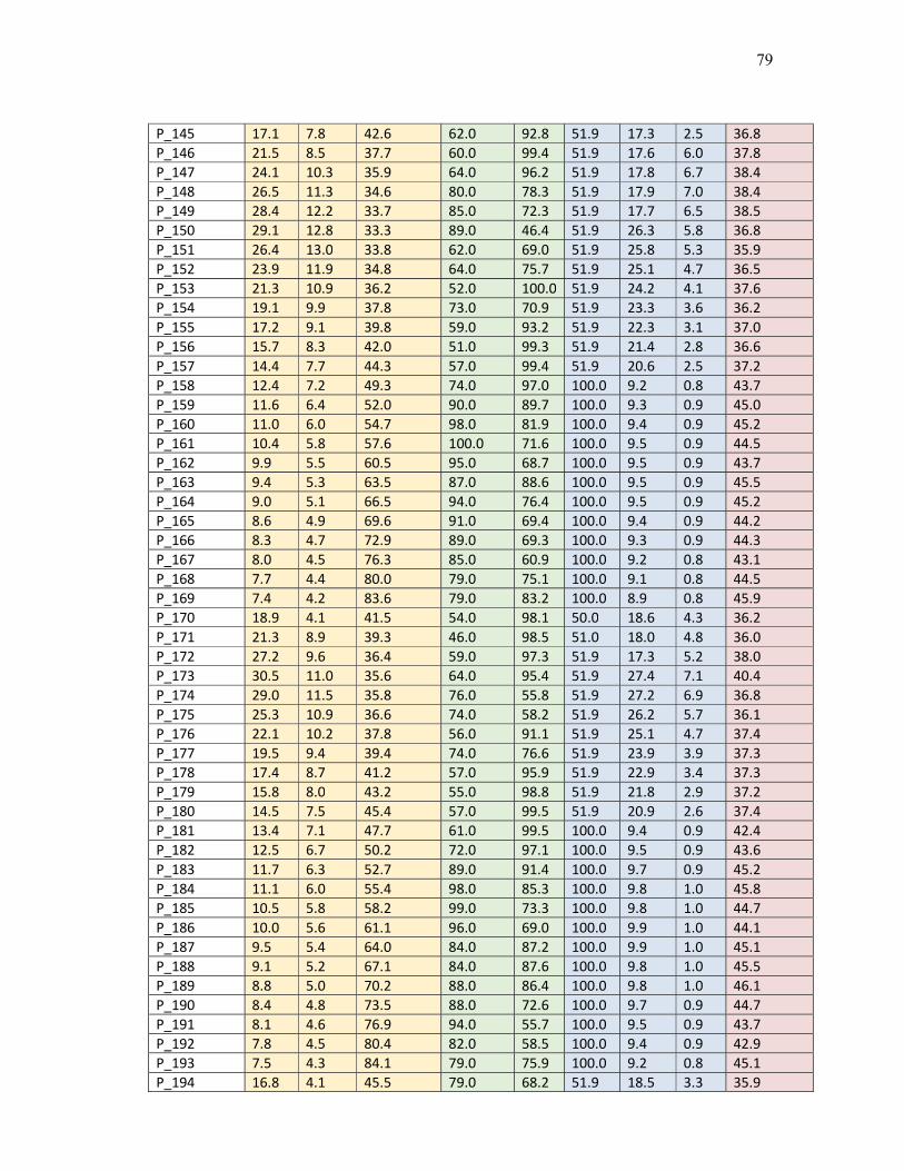
79
P_145 17.1 7.8 42.6 62.0 92.8 51.9 17.3 2.5 36.8 P_146 21.5 8.5 37.7 60.0 99.4 51.9 17.6 6.0 37.8 P_147 24.1 10.3 35.9 64.0 96.2 51.9 17.8 6.7 38.4 P_148 26.5 11.3 34.6 80.0 78.3 51.9 17.9 7.0 38.4 P_149 28.4 12.2 33.7 85.0 72.3 51.9 17.7 6.5 38.5 P_150 29.1 12.8 33.3 89.0 46.4 51.9 26.3 5.8 36.8 P_151 26.4 13.0 33.8 62.0 69.0 51.9 25.8 5.3 35.9 P_152 23.9 11.9 34.8 64.0 75.7 51.9 25.1 4.7 36.5 P_153 21.3 10.9 36.2 52.0 100.0 51.9 24.2 4.1 37.6 P_154 19.1 9.9 37.8 73.0 70.9 51.9 23.3 3.6 36.2 P_155 17.2 9.1 39.8 59.0 93.2 51.9 22.3 3.1 37.0 P_156 15.7 8.3 42.0 51.0 99.3 51.9 21.4 2.8 36.6 P_157 14.4 7.7 44.3 57.0 99.4 51.9 20.6 2.5 37.2 P_158 12.4 7.2 49.3 74.0 97.0 100.0 9.2 0.8 43.7 P_159 11.6 6.4 52.0 90.0 89.7 100.0 9.3 0.9 45.0 P_160 11.0 6.0 54.7 98.0 81.9 100.0 9.4 0.9 45.2 P_161 10.4 5.8 57.6 100.0 71.6 100.0 9.5 0.9 44.5 P_162 9.9 5.5 60.5 95.0 68.7 100.0 9.5 0.9 43.7 P_163 9.4 5.3 63.5 87.0 88.6 100.0 9.5 0.9 45.5 P_164 9.0 5.1 66.5 94.0 76.4 100.0 9.5 0.9 45.2 P_165 8.6 4.9 69.6 91.0 69.4 100.0 9.4 0.9 44.2 P_166 8.3 4.7 72.9 89.0 69.3 100.0 9.3 0.9 44.3 P_167 8.0 4.5 76.3 85.0 60.9 100.0 9.2 0.8 43.1 P_168 7.7 4.4 80.0 79.0 75.1 100.0 9.1 0.8 44.5 P_169 7.4 4.2 83.6 79.0 83.2 100.0 8.9 0.8 45.9 P_170 18.9 4.1 41.5 54.0 98.1 50.0 18.6 4.3 36.2 P_171 21.3 8.9 39.3 46.0 98.5 51.0 18.0 4.8 36.0 P_172 27.2 9.6 36.4 59.0 97.3 51.9 17.3 5.2 38.0 P_173 30.5 11.0 35.6 64.0 95.4 51.9 27.4 7.1 40.4 P_174 29.0 11.5 35.8 76.0 55.8 51.9 27.2 6.9 36.8 P_175 25.3 10.9 36.6 74.0 58.2 51.9 26.2 5.7 36.1 P_176 22.1 10.2 37.8 56.0 91.1 51.9 25.1 4.7 37.4 P_177 19.5 9.4 39.4 74.0 76.6 51.9 23.9 3.9 37.3 P_178 17.4 8.7 41.2 57.0 95.9 51.9 22.9 3.4 37.3 P_179 15.8 8.0 43.2 55.0 98.8 51.9 21.8 2.9 37.2 P_180 14.5 7.5 45.4 57.0 99.5 51.9 20.9 2.6 37.4 P_181 13.4 7.1 47.7 61.0 99.5 100.0 9.4 0.9 42.4 P_182 12.5 6.7 50.2 72.0 97.1 100.0 9.5 0.9 43.6 P_183 11.7 6.3 52.7 89.0 91.4 100.0 9.7 0.9 45.2 P_184 11.1 6.0 55.4 98.0 85.3 100.0 9.8 1.0 45.8 P_185 10.5 5.8 58.2 99.0 73.3 100.0 9.8 1.0 44.7 P_186 10.0 5.6 61.1 96.0 69.0 100.0 9.9 1.0 44.1 P_187 9.5 5.4 64.0 84.0 87.2 100.0 9.9 1.0 45.1 P_188 9.1 5.2 67.1 84.0 87.6 100.0 9.8 1.0 45.5 P_189 8.8 5.0 70.2 88.0 86.4 100.0 9.8 1.0 46.1 P_190 8.4 4.8 73.5 88.0 72.6 100.0 9.7 0.9 44.7 P_191 8.1 4.6 76.9 94.0 55.7 100.0 9.5 0.9 43.7 P_192 7.8 4.5 80.4 82.0 58.5 100.0 9.4 0.9 42.9 P_193 7.5 4.3 84.1 79.0 75.9 100.0 9.2 0.8 45.1 P_194 16.8 4.1 45.5 79.0 68.2 51.9 18.5 3.3 35.9

80
P_195 18.7 8.0 43.2 71.0 71.6 51.9 18.4 3.2 35.8 P_196 21.2 8.6 41.2 57.0 85.2 49.0 19.3 3.9 35.7 P_197 24.5 9.1 39.6 59.0 88.8 50.0 18.5 4.1 36.7 P_198 29.2 9.7 38.4 69.0 81.9 50.0 18.5 4.2 37.6 P_199 36.2 10.3 37.7 65.0 88.0 51.9 28.9 9.8 41.0 P_200 43.9 11.1 37.4 72.0 88.5 51.9 29.9 12.7 43.4 P_201 42.7 11.8 37.4 87.0 60.7 51.9 29.8 12.4 41.7 P_202 27.5 11.6 38.6 80.0 52.3 51.9 27.2 6.9 37.0 P_203 23.0 9.7 39.7 69.0 77.8 51.9 25.8 5.3 37.8 P_204 19.9 8.9 41.1 68.0 90.7 51.9 24.5 4.3 38.7 P_205 17.6 8.3 42.8 55.0 97.9 51.9 23.3 3.6 37.5 P_206 15.9 7.8 44.6 60.0 97.3 51.9 22.2 3.1 37.8 P_207 14.5 7.3 46.7 56.0 99.4 51.9 21.1 2.7 37.5 P_208 13.4 6.9 48.9 64.0 98.2 100.0 9.7 0.9 42.8 P_209 12.6 6.6 51.3 77.0 95.9 100.0 9.9 1.0 44.3 P_210 11.8 6.3 53.7 89.0 91.5 100.0 10.0 1.0 45.4 P_211 11.2 6.1 56.4 95.0 85.7 100.0 10.1 1.0 45.7 P_212 10.6 5.8 59.1 98.0 77.8 100.0 10.2 1.1 45.3 P_213 10.1 5.6 61.9 94.0 76.1 100.0 10.3 1.1 44.9 P_214 9.7 5.4 64.8 84.0 85.1 100.0 10.3 1.1 45.1 P_215 9.3 5.3 67.8 76.0 93.1 100.0 10.2 1.1 45.3 P_216 8.9 5.1 71.0 81.0 92.0 100.0 10.2 1.0 46.1 P_217 8.5 4.9 74.2 80.0 90.1 100.0 10.0 1.0 46.1 P_218 8.2 4.7 77.6 92.0 74.4 100.0 9.9 1.0 46.0 P_219 7.9 4.6 81.1 87.0 68.1 100.0 9.7 0.9 44.9 P_220 7.6 4.4 84.7 79.0 81.2 100.0 9.5 0.9 45.9 P_221 11.6 4.2 58.4 87.0 97.3 51.9 18.4 3.2 41.5 P_222 16.5 6.2 47.2 71.0 96.3 51.9 19.2 3.9 39.0 P_223 18.5 8.0 45.0 78.0 92.3 51.9 19.1 3.8 39.6 P_224 21.1 8.4 43.2 73.0 89.6 47.1 20.9 3.3 38.3 P_225 24.9 8.8 41.7 75.0 88.8 47.1 21.0 3.4 38.8 P_226 31.3 9.3 40.7 80.0 75.9 51.9 28.2 8.3 40.7 P_227 86.1 10.0 39.7 78.0 89.0 51.9 31.9 29.2 52.0 P_228 75.7 14.8 39.7 84.0 75.5 51.9 31.6 25.3 49.8 P_229 29.4 13.8 40.8 90.0 39.7 51.9 27.9 7.8 37.7 P_230 23.5 9.3 41.8 77.0 62.4 51.9 26.2 5.7 37.2 P_231 20.0 8.6 43.0 64.0 90.5 51.9 24.8 4.5 38.4 P_232 17.6 8.0 44.5 60.0 96.2 51.9 23.5 3.7 38.2 P_233 15.8 7.5 46.3 60.0 95.9 51.9 22.3 3.1 37.9 P_234 14.5 7.1 48.2 61.0 97.4 100.0 9.8 1.0 42.4 P_235 13.4 6.8 50.3 64.0 97.6 100.0 10.0 1.0 42.9 P_236 12.6 6.5 52.6 77.0 96.5 100.0 10.2 1.1 44.6 P_237 11.9 6.3 55.0 89.0 91.3 100.0 10.4 1.1 45.6 P_238 11.2 6.1 57.5 94.0 85.9 100.0 10.6 1.2 45.8 P_239 10.7 5.9 60.1 95.0 81.9 100.0 10.7 1.2 45.7 P_240 10.2 5.7 62.9 88.0 88.3 100.0 10.7 1.2 45.9 P_241 9.8 5.6 65.8 82.0 91.1 100.0 10.7 1.2 45.8 P_242 9.4 5.4 68.8 70.0 97.4 100.0 10.7 1.2 45.4 P_243 9.0 5.2 71.9 74.0 94.2 100.0 10.6 1.2 45.8 P_244 8.7 5.0 75.1 65.0 96.7 100.0 10.4 1.1 45.3 P_245 8.3 4.9 78.5 71.0 90.2 100.0 10.2 1.1 45.5

81
P_246 8.0 4.7 82.0 75.0 89.1 100.0 10.0 1.0 46.2 P_247 11.5 4.5 59.9 86.0 89.1 51.9 18.9 3.7 40.7 P_248 12.4 6.2 56.9 80.0 78.0 51.9 19.4 4.1 38.6 P_249 13.5 6.7 54.1 74.0 100.0 51.9 19.7 4.6 40.6 P_250 20.6 7.2 45.3 69.0 99.0 51.9 19.5 4.3 39.6 P_251 24.3 8.6 44.0 59.0 99.2 45.2 22.7 3.0 38.2 P_252 30.8 9.0 43.0 62.0 98.3 51.9 28.2 8.4 41.5 P_253 45.4 9.5 42.4 65.0 100.0 51.9 30.2 14.0 44.8 P_254 100.0 10.8 42.1 72.0 98.7 51.9 32.2 34.8 55.3 P_255 83.9 15.5 42.1 84.0 90.6 51.9 31.9 28.7 53.6 P_256 23.1 14.0 43.9 92.0 56.1 51.9 26.3 5.7 39.1 P_257 19.6 8.2 45.1 82.0 74.9 51.9 24.8 4.5 38.9 P_258 17.3 7.7 46.5 73.0 84.2 51.9 23.5 3.7 38.5 P_259 15.6 7.3 48.1 72.0 88.6 51.9 22.3 3.1 38.6 P_260 14.4 7.0 49.9 73.0 92.7 100.0 10.1 1.0 43.5 P_261 13.4 6.7 51.9 77.0 95.4 100.0 10.4 1.1 44.5 P_262 12.5 6.5 54.0 75.0 95.5 100.0 10.6 1.2 44.4 P_263 11.9 6.3 56.4 87.0 91.9 100.0 10.8 1.2 45.7 P_264 11.3 6.1 58.8 92.0 86.5 100.0 11.0 1.3 45.9 P_265 10.8 6.0 61.4 90.0 86.8 100.0 11.1 1.3 45.9 P_266 10.4 5.8 64.1 75.0 94.0 100.0 11.2 1.4 45.2 P_267 10.0 5.7 67.0 63.0 98.4 100.0 11.2 1.4 44.6 P_268 9.6 5.5 69.9 60.0 98.8 100.0 11.2 1.3 44.5 P_269 9.2 5.4 73.0 58.0 98.3 100.0 11.0 1.3 44.5 P_270 8.8 5.2 76.2 60.0 97.9 100.0 10.8 1.2 45.0 P_271 8.5 5.0 79.5 62.0 97.7 100.0 10.6 1.2 45.6 P_272 8.2 4.8 83.0 67.0 98.0 100.0 10.4 1.1 46.5 P_273 12.3 4.6 58.7 84.0 82.1 51.9 20.0 4.9 39.8 P_274 13.4 6.9 56.0 80.0 74.1 51.9 20.4 5.7 38.5 P_275 14.6 7.5 53.5 71.0 92.4 51.9 20.7 6.3 39.7 P_276 16.0 8.0 51.2 64.0 95.9 51.9 20.8 6.4 39.3 P_277 22.7 8.4 46.4 63.0 99.1 43.3 24.6 2.6 38.7 P_278 27.4 8.7 45.5 63.0 99.1 51.9 27.6 7.4 41.3 P_279 35.1 9.0 44.9 69.0 98.5 51.9 29.1 10.3 43.5 P_280 44.7 9.6 44.6 76.0 98.1 51.9 30.2 14.0 46.1 P_281 43.3 10.3 44.6 89.0 89.6 51.9 30.0 13.5 46.5 P_282 33.4 10.1 44.9 98.0 74.4 51.9 28.8 9.7 43.9 P_283 21.7 9.1 46.2 97.0 73.1 51.9 25.9 5.4 41.3 P_284 18.8 7.8 47.3 93.0 73.3 51.9 24.5 4.3 40.1 P_285 16.8 7.4 48.6 91.0 69.7 51.9 23.3 3.6 39.0 P_286 15.3 7.1 50.1 93.0 62.4 51.9 22.2 3.1 38.1 P_287 14.1 6.8 51.8 93.0 78.0 100.0 10.4 1.1 44.4 P_288 13.2 6.6 53.6 89.0 78.1 100.0 10.7 1.2 44.1 P_289 12.5 6.5 55.7 84.0 76.1 100.0 11.0 1.3 43.4 P_290 11.9 6.3 57.9 90.0 79.0 100.0 11.3 1.4 44.7 P_291 11.4 6.2 60.3 93.0 81.9 100.0 11.5 1.5 45.7 P_292 10.9 6.1 62.8 89.0 87.9 100.0 11.7 1.5 46.3 P_293 10.5 6.0 65.5 78.0 92.0 100.0 11.8 1.6 45.7 P_294 10.1 5.9 68.3 71.0 95.2 100.0 11.8 1.6 45.5 P_295 9.8 5.7 71.2 64.0 97.4 100.0 11.7 1.5 45.2

82
P_296 9.4 5.6 74.2 54.0 99.1 100.0 11.5 1.5 44.4 P_297 9.0 5.4 77.4 59.0 98.1 100.0 11.3 1.4 45.2 P_298 8.6 5.2 80.7 67.0 96.5 100.0 11.0 1.3 46.3 P_299 8.3 5.0 84.1 69.0 98.5 100.0 10.7 1.2 47.1 P_300 12.1 4.7 60.7 76.0 96.5 51.9 20.6 6.0 41.1 P_301 13.3 7.1 58.0 81.0 84.6 51.9 21.2 7.4 40.6 P_302 14.6 8.0 55.6 83.0 73.7 51.9 21.6 8.9 39.7 P_303 15.8 8.9 53.5 76.0 76.4 51.9 21.6 9.1 39.2 P_304 17.0 9.3 51.6 67.0 95.1 51.9 21.3 7.9 40.1 P_305 20.7 9.1 48.9 64.0 99.7 51.9 20.1 5.1 39.9 P_306 23.5 8.5 48.1 70.0 98.3 51.9 26.6 6.0 41.6 P_307 27.0 8.5 47.6 71.0 97.9 51.9 27.6 7.4 42.3 P_308 29.7 8.6 47.3 82.0 94.9 51.9 28.2 8.4 43.9 P_309 19.9 8.7 48.7 94.0 87.2 51.9 25.2 4.8 42.5 P_310 17.7 7.4 49.6 93.0 86.6 51.9 24.0 4.0 41.8 P_311 16.1 7.1 50.8 88.0 89.8 51.9 22.9 3.4 41.3 P_312 14.8 6.9 52.2 91.0 85.9 51.9 21.9 2.9 40.9 P_313 13.8 6.7 53.8 95.0 80.5 100.0 10.7 1.2 45.2 P_314 11.9 6.6 59.6 95.0 80.1 100.0 11.7 1.6 45.8 P_315 11.5 6.3 62.0 95.0 85.8 100.0 12.0 1.7 46.8 P_316 11.1 6.3 64.4 97.0 79.3 100.0 12.2 1.8 46.5 P_317 10.7 6.2 67.0 93.0 75.6 100.0 12.4 1.9 45.9 P_318 10.4 6.2 69.8 76.0 81.2 100.0 12.4 1.9 44.7 P_319 10.0 6.0 72.7 61.0 96.9 100.0 12.3 1.8 45.1 P_320 9.6 5.9 75.7 54.0 98.9 100.0 12.1 1.7 44.7 P_321 12.0 5.6 62.8 75.0 100.0 51.9 21.0 7.0 41.9 P_322 13.3 7.5 60.3 72.0 100.0 51.9 21.8 10.0 42.1 P_323 15.2 9.0 57.9 76.0 85.5 51.9 22.5 14.8 41.6 P_324 16.5 11.3 55.9 80.0 88.8 51.9 22.6 16.1 42.9 P_325 16.7 12.1 54.2 70.0 91.8 51.9 22.1 11.3 41.3 P_326 17.4 10.2 52.8 58.0 99.5 51.9 21.3 7.8 39.9 P_327 20.3 8.9 50.9 66.0 99.2 51.9 25.4 4.9 40.9 P_328 21.9 8.1 50.3 74.0 98.2 51.9 26.1 5.6 42.0 P_329 18.0 7.9 51.2 84.0 94.5 51.9 24.3 4.2 42.0 P_330 16.5 7.0 52.1 79.0 96.3 51.9 23.3 3.6 41.2 P_331 15.2 6.8 53.2 82.0 96.8 51.9 22.4 3.2 41.4 P_332 14.2 6.7 54.4 81.0 97.8 51.9 21.4 2.8 41.3 P_333 13.5 6.6 55.9 84.0 94.0 100.0 11.0 1.3 45.8 P_334 12.3 6.5 59.5 94.0 71.3 100.0 11.8 1.6 44.6 P_335 11.9 6.5 61.5 94.0 90.7 100.0 12.2 1.8 47.3 P_336 11.6 6.5 63.8 91.0 90.7 100.0 12.6 2.0 47.3 P_337 11.4 6.5 66.2 94.0 87.3 100.0 12.9 2.2 47.6 P_338 11.1 6.6 68.8 99.0 68.9 100.0 13.0 2.3 46.2 P_339 10.7 6.6 71.5 84.0 68.3 100.0 13.1 2.3 44.5 P_340 10.3 6.5 74.3 66.0 90.2 100.0 12.9 2.2 45.3 P_341 9.9 6.2 77.3 57.0 99.2 100.0 12.6 2.0 45.5 P_342 9.3 6.0 73.9 80.0 88.9 51.9 18.9 3.6 41.6 P_343 9.9 5.3 70.8 73.0 98.4 51.9 19.6 4.4 41.7 P_344 11.7 5.8 62.7 71.0 96.8 51.9 22.2 12.3 41.8 P_345 13.3 9.8 60.5 62.0 98.7 0.0 0.0 29.8 34.3 P_346 17.6 17.7 58.6 76.0 97.8 0.0 0.0 49.4 39.6

83
P_347 22.4 26.6 57.0 71.0 89.7 51.9 22.5 15.1 44.5 P_348 16.4 11.6 55.7 56.0 99.2 51.9 21.5 8.7 40.1 P_349 16.2 9.0 54.6 67.0 99.2 51.9 20.7 6.1 40.6 P_350 16.9 8.1 53.8 69.0 99.0 51.9 24.2 4.1 40.9 P_351 17.8 7.7 53.3 76.0 99.4 51.9 24.1 4.0 41.8 P_352 17.4 6.9 53.9 75.0 99.5 51.9 23.4 3.6 41.5 P_353 16.3 6.7 54.7 71.0 100.0 51.9 22.6 3.2 40.8 P_354 15.3 6.6 55.7 82.0 99.7 51.9 21.7 2.9 42.0 P_355 14.4 6.5 56.8 77.0 98.9 51.9 20.9 2.6 41.1 P_356 13.7 6.4 58.2 75.0 96.9 100.0 11.2 1.4 45.4 P_357 13.1 6.4 59.8 89.0 88.1 100.0 11.7 1.6 46.2 P_358 12.6 6.5 61.5 89.0 89.4 100.0 12.2 1.8 46.6 P_359 12.2 6.6 63.5 89.0 93.9 100.0 12.7 2.1 47.5 P_360 12.0 6.7 65.7 83.0 95.6 100.0 13.2 2.4 47.3 P_361 11.8 6.9 68.1 91.0 91.8 100.0 13.6 2.7 48.2 P_362 11.7 7.1 70.6 99.0 78.1 100.0 13.8 2.9 47.9 P_363 11.6 7.2 73.3 96.0 69.6 100.0 13.8 2.9 46.8 P_364 11.3 7.1 76.2 74.0 87.1 100.0 13.6 2.7 46.5 P_365 10.8 6.8 79.1 68.0 95.5 100.0 13.2 2.4 47.0 P_366 10.3 6.4 82.2 69.0 84.6 100.0 12.8 2.1 45.9 P_367 9.8 6.0 85.4 72.0 92.5 100.0 12.3 1.8 47.5 P_368 9.3 5.6 88.7 70.0 98.9 100.0 11.8 1.6 48.2 P_369 8.9 5.3 79.2 84.0 98.9 51.9 18.2 3.1 43.7 P_370 8.5 4.8 76.2 82.0 89.7 51.9 18.9 3.6 42.0 P_371 9.0 5.2 73.3 74.0 87.3 51.9 19.6 4.4 40.6 P_372 9.6 5.6 70.5 67.0 99.0 51.9 20.3 5.5 41.2 P_373 10.3 6.3 65.5 72.0 95.8 51.9 22.1 11.3 41.9 P_374 12.6 9.2 63.4 80.0 97.5 0.0 0.0 20.4 35.4 P_375 15.1 13.4 61.6 82.0 93.5 0.0 0.0 24.4 36.2 P_376 16.6 15.3 60.0 83.0 82.2 51.9 22.3 13.3 43.1 P_377 15.1 10.6 58.7 75.0 85.9 51.9 21.4 8.3 40.9 P_378 15.0 8.6 57.7 82.0 91.7 51.9 20.6 6.0 41.7 P_379 15.3 7.7 56.9 85.0 92.4 51.9 23.1 3.5 42.0 P_380 15.8 7.3 56.3 85.0 93.5 51.9 23.5 3.7 42.1 P_381 16.3 7.0 55.9 84.0 97.3 51.9 23.4 3.7 42.4 P_382 16.2 6.6 56.2 73.0 100.0 51.9 23.0 3.4 41.3 P_383 15.6 6.5 57.4 73.0 99.6 51.9 21.8 2.9 41.1 P_384 14.3 6.4 58.3 79.0 99.4 51.9 21.1 2.7 41.6 P_385 13.7 6.3 59.4 71.0 99.0 51.9 20.4 2.4 40.5 P_386 13.1 6.3 60.6 76.0 99.1 100.0 11.5 1.5 46.0 P_387 12.7 6.4 62.1 82.0 98.3 100.0 12.0 1.7 46.9 P_388 12.3 6.5 63.7 85.0 97.9 100.0 12.6 2.0 47.5 P_389 12.1 6.7 65.6 85.0 96.6 100.0 13.2 2.4 47.7 P_390 12.1 7.0 67.7 75.0 99.0 100.0 13.8 2.9 47.2 P_391 12.2 7.4 70.1 88.0 94.1 100.0 14.3 3.5 48.7 P_392 12.4 7.9 72.6 97.0 87.1 100.0 14.7 4.0 49.5 P_393 12.5 8.4 75.3 97.0 76.4 100.0 14.7 4.1 48.5 P_394 12.3 8.3 78.1 85.0 78.8 100.0 14.4 3.6 47.6 P_395 11.6 7.7 81.1 82.0 69.6 100.0 13.8 2.9 46.1 P_396 10.8 7.0 84.1 82.0 81.4 100.0 13.2 2.4 47.6

84
P_397 10.2 6.4 87.3 72.0 93.4 100.0 12.6 2.0 48.0 P_398 9.6 5.9 90.5 70.0 94.4 100.0 12.5 0.9 48.0 P_399 9.1 5.4 93.8 73.0 92.9 100.0 13.6 0.8 48.6 P_400 8.7 5.1 84.7 0.0 99.1 51.9 17.5 2.6 33.7 P_401 7.9 4.4 81.7 81.0 93.7 51.9 18.1 3.0 42.7 P_402 8.3 4.7 78.7 83.0 90.7 51.9 18.7 3.5 42.4 P_403 8.7 5.0 75.9 80.0 90.5 51.9 19.4 4.1 41.9 P_404 9.3 5.4 73.2 79.0 92.8 51.9 20.1 5.1 42.1 P_405 9.9 6.0 70.7 69.0 97.2 51.9 20.8 6.4 41.5 P_406 10.6 6.7 68.5 69.0 100.0 51.9 21.5 8.5 42.1 P_407 11.6 7.8 66.5 74.0 99.1 51.9 22.0 10.9 43.0 P_408 12.6 9.0 64.7 82.0 94.3 51.9 22.1 11.4 43.5 P_409 13.3 9.4 63.2 88.0 81.5 51.9 21.7 9.2 42.3 P_410 13.5 8.6 61.9 82.0 89.2 51.9 21.0 7.0 41.9 P_411 13.6 7.7 60.8 77.0 95.9 51.9 20.3 5.4 41.6 P_412 14.0 7.2 60.0 78.0 95.3 51.9 22.0 3.0 41.4 P_413 14.3 6.8 59.4 81.0 96.1 51.9 22.3 3.1 41.9 P_414 14.6 6.6 59.1 71.0 99.8 51.9 22.5 3.2 41.1 P_415 14.8 6.5 59.6 79.0 99.9 51.9 21.5 2.8 42.0 P_416 13.8 6.2 60.2 78.0 99.7 51.9 21.0 2.6 41.7 P_417 13.4 6.2 61.0 80.0 99.7 51.9 20.4 2.4 41.9 P_418 12.9 6.2 62.0 78.0 100.0 51.9 19.8 2.2 41.6 P_419 12.6 6.2 63.2 80.0 99.7 100.0 11.6 1.5 46.9 P_420 12.3 6.3 64.5 80.0 100.0 100.0 12.2 1.8 47.1 P_421 12.1 6.5 66.0 81.0 98.8 100.0 12.8 2.1 47.4 P_422 12.0 6.8 67.8 75.0 99.0 100.0 13.5 2.6 47.1 P_423 12.2 7.2 69.9 70.0 99.1 100.0 14.3 3.5 47.0 P_424 12.6 8.0 72.2 76.0 98.7 100.0 15.0 4.8 48.4 P_425 13.4 9.2 74.8 93.0 91.6 100.0 15.6 6.5 50.5 P_426 14.7 10.9 77.4 98.0 83.2 100.0 15.7 6.6 50.8 P_427 14.5 11.0 80.2 99.0 72.7 100.0 15.1 4.9 49.7 P_428 12.9 9.2 83.2 91.0 68.6 100.0 14.4 3.6 47.8 P_429 11.5 7.7 86.2 84.0 76.0 100.0 13.6 2.7 47.7 P_430 10.6 6.8 89.3 75.0 86.7 100.0 12.9 2.2 47.9 P_431 9.9 6.1 92.5 78.0 87.2 100.0 13.2 1.0 48.5 P_432 9.3 5.6 95.7 0.0 98.5 100.0 14.4 0.9 40.6 P_433 8.9 5.2 87.2 87.0 99.0 51.9 17.3 2.5 44.9 P_434 7.7 4.3 84.2 85.0 93.2 51.9 17.9 2.9 43.4 P_435 8.0 4.5 81.4 82.0 96.4 51.9 18.4 3.3 43.2 P_436 8.5 4.8 78.7 80.0 98.6 51.9 19.1 3.8 43.2 P_437 8.9 5.2 76.1 79.0 95.3 51.9 19.7 4.5 42.6 P_438 9.4 5.6 73.7 84.0 95.0 51.9 20.3 5.4 43.2 P_439 10.0 6.1 71.6 83.0 95.6 51.9 20.8 6.4 43.2 P_440 10.7 6.7 69.6 84.0 95.5 51.9 21.1 7.2 43.3 P_441 11.3 7.2 67.9 84.0 95.1 51.9 21.1 7.4 43.2 P_442 11.8 7.4 66.4 76.0 95.8 51.9 20.9 6.7 42.1 P_443 12.2 7.2 65.1 79.0 96.9 51.9 20.4 5.7 42.3 P_444 12.5 6.9 64.1 70.0 99.6 51.9 19.8 4.7 41.2 P_445 12.8 6.6 63.3 73.0 99.5 51.9 21.0 2.6 41.4 P_446 13.0 6.4 62.7 81.0 99.1 51.9 21.3 2.7 42.3 P_447 13.3 6.3 62.3 79.0 100.0 51.9 21.4 2.8 42.1

85
P_448 13.4 6.2 67.1 80.0 100.0 100.0 12.3 1.8 47.6 P_449 11.8 6.5 68.5 86.0 97.6 100.0 13.0 2.2 48.2 P_450 11.9 6.8 70.1 83.0 97.0 100.0 13.7 2.8 48.2 P_451 12.2 7.4 72.2 74.0 98.2 100.0 14.6 3.9 47.8 P_452 12.9 8.5 74.5 72.0 99.8 100.0 15.6 6.3 48.7 P_453 14.7 10.8 77.1 86.0 95.4 100.0 16.6 14.1 51.8 P_454 21.2 18.6 79.7 92.0 88.7 100.0 16.7 15.5 54.1 P_455 22.2 20.0 82.5 98.0 75.7 100.0 15.7 6.6 52.6 P_456 14.5 11.0 85.4 96.0 83.3 100.0 14.7 4.1 51.1 P_457 12.1 8.4 88.4 93.0 76.2 100.0 13.8 2.9 49.4 P_458 10.9 7.1 91.4 87.0 78.9 100.0 14.2 1.2 48.8 P_459 10.1 6.4 94.6 77.0 94.2 100.0 13.9 1.1 49.7 P_460 9.6 5.8 76.8 84.0 100.0 51.9 19.6 4.5 44.0 P_461 9.5 5.6 74.7 84.0 99.5 51.9 20.0 5.0 43.8 P_462 10.0 5.9 72.8 87.0 93.4 51.9 20.3 5.4 43.3 P_463 10.4 6.2 71.2 78.0 93.1 51.9 20.3 5.4 42.1 P_464 10.9 6.4 69.7 67.0 99.7 51.9 20.1 5.1 41.3 P_465 11.2 6.4 71.1 79.0 97.5 100.0 13.0 2.2 47.5 P_466 11.7 6.8 72.5 84.0 98.1 100.0 13.7 2.8 48.7 P_467 12.1 7.4 82.2 87.0 96.7 100.0 16.6 14.6 52.1 P_468 21.6 19.2 85.0 90.0 95.6 100.0 15.6 6.6 54.2 P_469 14.6 11.1 87.8 92.0 92.4 100.0 14.7 4.0 52.1 P_470 12.3 8.5 90.7 89.0 89.1 100.0 15.3 1.4 50.8 P_471 11.2 7.3 93.7 78.0 94.8 100.0 15.0 1.3 50.2 P_472 10.4 6.5 96.8 71.0 100.0 100.0 14.7 1.3 50.1 P_473 9.8 6.0 100.0 0.0 100.0 100.0 16.3 1.1 41.6 P_474 9.3 5.5 78.0 85.0 99.2 51.9 19.3 4.1 44.0 P_475 9.4 5.4 76.2 87.0 95.2 51.9 19.5 4.3 43.6 P_476 9.8 5.6 74.5 76.0 97.4 51.9 19.5 4.3 42.4 P_477 10.1 5.7 75.5 83.0 99.8 100.0 13.5 2.6 48.8 P_478 11.8 7.2 93.2 82.0 91.2 100.0 16.3 1.6 50.4 P_479 11.3 7.3 96.2 74.0 94.5 100.0 16.0 1.5 50.1 P_480 10.6 6.6 99.2 77.0 82.4 100.0 15.5 1.4 49.1 P_481 10.1 6.1 95.9 80.0 75.4 100.0 17.5 1.9 48.3 P_482 11.5 7.3 98.8 83.0 72.1 100 17.1 1.8 48.9

86
Figure 48: Cumulative grade combining eight evaluation criteria with an overlay of the locations that experience high wind speeds of 10 m/s or greater

87

88

89

90