HAL Id: halshs-02518234https://halshs.archives-ouvertes.fr/halshs-02518234

Preprint submitted on 25 Mar 2020

HAL is a multi-disciplinary open accessarchive for the deposit and dissemination of sci-entific research documents, whether they are pub-lished or not. The documents may come fromteaching and research institutions in France orabroad, or from public or private research centers.

L’archive ouverte pluridisciplinaire HAL, estdestinée au dépôt et à la diffusion de documentsscientifiques de niveau recherche, publiés ou non,émanant des établissements d’enseignement et derecherche français ou étrangers, des laboratoirespublics ou privés.

Security TransitionsThiemo Fetzer, Pedro Cl Souza, Oliver Vanden Eynde, Austin Wright

To cite this version:Thiemo Fetzer, Pedro Cl Souza, Oliver Vanden Eynde, Austin Wright. Security Transitions. 2020.�halshs-02518234�

WORKING PAPER N° 2020 – 13

Security Transitions

Thiemo Fetzer Pedro CL Souza

Oliver Vanden Eynde Austin L. Wright

JEL Codes: D72, D74, L23 Keywords: Counterinsurgency, Civil Conflict, Public Goods Provision

Security Transitions∗

Thiemo Fetzer† Pedro CL Souza‡ Oliver Vanden Eynde§

Austin L. Wright¶

March 23, 2020

Abstract

How do foreign powers disengage from a conflict? We study the recent large-scale security transition from international troops to local forces in the context ofthe ongoing civil conflict in Afghanistan. We construct a new dataset that com-bines information on this transition process with declassified conflict outcomesand previously unreleased quarterly survey data. Our empirical design leveragesthe staggered roll-out of the transition onset, together with a novel instrumentalvariables approach to estimate the impact of the two-phase security transition. Wefind that the initial security transfer to Afghan forces is marked by a significant,sharp and timely decline in insurgent violence. This effect reverses with the ac-tual physical withdrawal of foreign troops. We argue that this pattern is consistentwith a signaling model, in which the insurgents reduce violence strategically tofacilitate the foreign military withdrawal. Our findings clarify the destabilizingconsequences of withdrawal in one of the costliest conflicts in modern history andyield potentially actionable insights for designing future security transitions.

Keywords: Counterinsurgency, Civil Conflict, Public Goods Provision

JEL Classification: D72, D74, L23

∗We thank Ethan Bueno de Mesquita, Wioletta Dziuda, Anthony Fowler, Hannes Mueller, Christo-pher Price, Jacob Shapiro, and audiences at the Chicago Harris Political Economy, ESOC Annual Con-ference, University of Warwick, IAE Barcelona Workshop on Prediction for Prevention, HiCN confer-ence, CREST Political Economy Workshop, and Labex OSE Aussois Days. Manh Duc Nguyen providedexcellent research assistance. Support from the Pearson Institute for the Study and Resolution of Con-flicts and ANR grant COOPCONFLICT is gratefully acknowledged. We thank Phil Eles, ANQARtechnical lead at NATO, for granting access to the platform and providing technical feedback. Anyerrors remain our own.†Department of Economics, University of Warwick. Email: t.fetzer@warwick.ac.uk.‡Department of Economics, University of Warwick. Email: pedro.souza@warwick.ac.uk.§Paris School of Economics and CNRS. Email: oliver.vanden.eynde@ens.fr.¶Harris School of Public Policy, University of Chicago. Email: austinlw@uchicago.edu.

1 Introduction

Foreign military occupations typically end with a security transition, in which inter-

national forces transfer military and police powers to local allies. Such foreign-to-local

security transitions are difficult to manage (Lake, 2016). This is due to the likely sur-

vival, in one form or another, of anti-government elements that triggered the foreign

military intervention to begin with. Therefore, a successful security transition is cru-

cial for the economic and political development of the local state that emerges in

the wake of military interventions. Yet surprisingly little is known about the conflict

dynamics of countries experiencing a foreign-to-local security transition. Our paper

relies on rich microlevel data to study the impact of the large-scale security transi-

tion that marked the end of Operation Enduring Freedom in Afghanistan—NATO’s

long-running military campaign.

Since 1960, at least 115 foreign military occupations have ended (Collard-Wexler,

2013) (see Figure 1). A substantial percentage of these interventions involved the

withdrawal of troops and redeployment of weaponry to local allies. As Figure 1 re-

veals, security transitions remain an important economic and policy issue as a large

number of military occupations remain active globally. Even though the historical

record is riddled with security transitions, nearly all microlevel empirical research on

counterinsurgency focuses on understanding the economic and political drivers that

explain how military interventions begin and how conflict strategies and warfight-

ing tactics evolve within an ongoing campaign. How foreign campaigns end has been

mostly ignored in this literature (Berman and Matanock, 2015). Empirical work on this

topic is naturally constrained by the lack of consistent conflict data during the transi-

tion period, in particular for unsuccessful transitions. Our paper relies on unique data

sources that were collected continuously during the transition process, which enables

us to address the knowledge gap around exit strategies after foreign interventions.

Conflict patterns during and after security transitions—which mark the end of a

foreign intervention or occupation—are theoretically ambiguous. A security transi-

tion may shift provision of policing and formal military operations from well trained

and equipped foreign fighters to unseasoned local forces using unfamiliar or out-

dated technology. Even if local fighters are capable, they may lack legitimacy, commit

1

unintended harm to civilians, or deliberately discriminate against ethnic rivals, un-

dermining economic welfare and damaging public confidence in the quality and sta-

bility of host nation institutions. Local forces might also transfer weaponry and other

warfighting capital to unregulated paramilitary groups (Dube and Naidu, 2015). Un-

der these conditions, insurgent operations are likely to increase, and their control over

previously contested territory may consolidate. On the other hand, local forces might

actually be more capable of integrating with communities within their operational

zone and extracting information from non-combatants about insurgent operations

(Lyall et al., 2015). Insurgents might also find it more difficult to mobilize support for

attacks on host nation forces as opposed to foreign soldiers. Knowledge of the hu-

man terrain and difficulties motivating violence against conationals or coethnics could

translate to reduced insurgent activity and increased counterinsurgent effectiveness.

Furthermore, insurgents may directly and strategically respond to plans of foreign

forces to withdraw troops by changing their underlying tactics and targets (Bueno de

Mesquita, 2013; Wright, 2016; Vanden Eynde, 2018). Lastly, security transitions may

be poorly coordinated between foreign and local forces, leading to political and tac-

tical disorder and further enhancing tensions and conflict. Importantly, there is no

existing empirical evidence on the relative significance of these different mechanisms

in the context of security transitions.

To study how security transitions from foreign to local forces influence insurgent

activity and counterinsurgent effectiveness, we examine the large-scale transfer of

policing and military power from the International Security Assistance Force (ISAF)

to host nation forces in Afghanistan at the end of Operation Enduring Freedom. Char-

acteristic of other foreign military interventions, the occupation of ISAF displaced the

incumbent regime and assisted in the installation of an ostensibly democratic govern-

ment in 2001. During the occupation, foreign forces coordinated under the auspices

of NATO helped train and equip local police and military forces. Planning for the

transition of security provision from ISAF to Afghan forces began as early as 2010,

and was formally announced in 2011. The transition was staggered, and coordinated

around administrative districts. Over three years, and five transition tranches, all of

Afghanistan’s districts were transferred from ISAF to Afghan control.

2

We estimate the impact of the security transition on conflict dynamics using ex-

ceptionally granular data. Data limitations may be a central reason for why there

have been no prior quantitative studies on the impact of security transitions. We are

uniquely positioned to overcome this obstacle. Since the start of major ISAF opera-

tions, a system to collect comprehensive conflict data from ISAF and host nation forces

was set up to track significant activities, referred to as SIGACTS. These event data are

geotagged and timestamped, and document dozens of different types of insurgent

and security force operations. Access to this database was secured through formal

declassification channels and represents the most complete catalog of conflict activity

during Operation Enduring Freedom currently available (Shaver and Wright, 2016).

We combine this observational data with microlevel survey data collected by NATO

(using local contractors) through the Afghanistan National Quarterly Assessment Re-

search (ANQAR) platform. The primary aim of the survey was to provide and collect

data on perceptions of the security situation from Afghan citizens across the country

in a systematic manner. We have obtained restricted access to the complete survey

records of around 370,000 individual respondents across dozens of quarterly waves

from 2008 to 2016. These surveys include multiple questions measuring respondent’s

perceptions of security conditions, the extent of local security provision and percep-

tions of territorial control. These measures will allow us to validate our findings based

on conflict measures, and to distinguish between potential mechanisms.1

Our empirical analysis sheds light on the two main phases of the security transi-

tion. The first phase is the onset of the transition marked by a sequence of public an-

nouncements providing lists of districts where security responsibility is to be handed

over to local forces from a given date onwards. The second phase is the actual physical

withdrawal and closure of military bases hosting NATO troops. To estimate the effect

of the onset of the security transition, we use a difference-in-difference approach. We

exploit the staggered schedule of transition announcements that occurred across five

tranches. This allows us to pool five difference-in-difference estimators to study the

effect of the onset of the security transition on conflict outcomes, comparing localities

where the Afghan National Security Forces (ANSF) took over security to those where

1Existing work rarely combines observational and survey data on conflicts. Exceptions are Gouldand Klor (2010), and Jaeger et al. (2015), who use survey evidence on the Israeli-Palestinian conflict.

3

ISAF is still in charge, before and after the security transfer. The geographic precision

of our conflict data enables us to employ a high resolution spatial matching design as

an alternative to our district-level analysis. Our results show that the local announce-

ment of the security transition schedule led to a short-term decline in local violence.

This pattern holds both for conflict measures drawn from the SIGACTS database as

well as ANQAR survey instruments measuring security perceptions of the local pop-

ulation. This improvement in security outcomes appears to have gone hand-in-hand

with a substantial upward shift in civilian perceptions of the efficacy of local security

forces.

Our second empirical exercise focuses on the physical withdrawal of NATO troops.

Using a newly constructed data set of individual base closures and handovers, we

employ a novel instrumental variables strategy exploiting operational and logistical

constraints to the organization of the troop withdrawal. This approach helps us to

address concerns about the endogeneity of the decision to close bases in one area

earlier compared to others. Our IV strategy relies on cross-sectional variation in the

travel distance between individual districts and ten major logistical hubs. These ten

hubs were central to the withdrawal as they had military grade airports that could

physically accommodate the heavy cargo airplanes that were used to transport arms

and troops out of the country. Our findings suggest that following the second phase

of the transition—the physical withdrawal of troops and closure of military bases—

violence significantly surged and perceptions of security worsened substantially. We

address potential violations of the exclusion restriction directly by accounting for

the correlation between logistical constraints and other measures of population and

market proximity. While our empirical design allows us to fully control for the direct

effect that the first phase of the security transition had on conflict, we also combine the

analysis from both phases in a single framework. Overall, the pattern that emerges

suggests that the transition onset announcement is associated with an improvement

in the security situation, while the physical withdrawal of NATO troops is marked by

a dramatic worsening of security.

We argue that these two pieces of evidence are consistent with insurgents strategi-

cally drawing down their forces (‘lying low’) until after counterinsurgents sufficiently

4

raised the cost of local re-intervention. We develop a simple model that rationalizes

this logic and treats the initial reduction in violence as a costly signal sent by the Tal-

iban to ISAF. As ISAF cannot directly observe the local capacity of the Taliban relative

to the ANSF, it bases its decision to stick to a fixed withdrawal timeline on observed

levels of violence during the transition period. A high-capacity Taliban can then de-

cides to ‘lie low’ as part of a pooling equilibrium, which facilitates ISAF’s withdrawal,

and increases the ability of the Taliban to inflict violence when the transition is com-

pleted. Official documents of the US Department of Defense interpreted the initial

phases of the transition as a success, which is consistent with the idea that the Tal-

iban effectively understated their true capacity. Public opposition to the war in most

Western troop sending countries may have incentivized insurgents to make the tran-

sition appear successful until it became excessively costly for political and military

leaders to revert back. As such, ISAF’s public commitment to a timeline for a troop

withdrawal—an often criticized tactical decision—may have undermined the success

of the security transition.

Even if we lack a direct test of the ‘lying low’ strategy described above, the most

plausible alternative interpretation of our violence patterns can be investigated di-

rectly. In principle, the reduction in violence during the transfer phase and its rise

after the withdrawal of foreign troops could have been driven by complementarities

between ISAF and the ANSF. Relying on a range of empirical tests, we find no evi-

dence of such complementarities between ISAF and the ANSF. We can also rule out

other plausible alternative explanations. We pay particular attention to SUTVA viola-

tions inherent in designs in which spatial spillovers or displacement effects are possi-

ble. This paper is the first to leverage new econometric techniques to directly tackle

this issue in the context of the conflict literature. Rather than invoking conventional

spatial models that require the researcher to pre-specify the extent to which conflict

processes interact across spatial,2 we leverage the work by de Paula et al. (2019) and

adopt it to the specific issue at hand: learning the pattern of spatial spillovers of

conflict, and then using that information to directly control for the spillovers.

We contribute to several strands of literature in economics and political science.

2For a seminal contribution on the estimation of spatial models with fixed interaction matrix, see?. A review of estimation of network models can be found in ?

5

Prior work on the economics of civil war has largely focused on factors that cause

insurgencies to emerge (Fearon and Laitin, 2003; Collier and Hoeffler, 2004; Miguel

et al., 2004; Nunn and Qian, 2014; Bazzi and Blattman, 2014; Berman et al., 2017),

rather than how insurgents strategically respond to shifts in military power as occu-

pations draw to a close. In most countries, state capacity is central to these dynamics

(Besley and Persson, 2009, 2010; Powell, 2013; Gennaioli and Voth, 2015; Esteban et al.,

2015; Sanchez de la Sierra, 2017).3 In Afghanistan, recent work by Condra et al. (2018)

shows that the Taliban have disrupted core democratic institutions (elections), which

undermines the government’s state building efforts. Our study emphasizes another

key component of Afghanistan’s state building process—the gradual transfer of se-

curity to local forces. Also in line with Condra et al. (2018) we document how the

strategic use of violence by the Taliban may have had an impact on the subsequent

consolidation of political control by government forces. More broadly, our paper fills

an important gap in the literature on interventions in civil wars, by examining the

conflict dynamics of a foreign-to-local security transfer.

A growing number of recent papers study security and development interventions

that occur within conflicts. These studies have produced mixed results. On the one

hand, development projects have been found to reduce conflict in Iraq (Berman et al.,

2011), India (Fetzer, 2014), and Afghanistan (Beath et al., 2013), which could be be-

cause they allow counter-insurgency forces to win “hearts and minds” or because they

raise the opportunity cost of participating in conflict. But, evidence from the Philip-

pines (Crost et al., 2014) and contested areas in Afghanistan (Sexton, 2016) suggests

that development projects could also increase violence, possibly because the insur-

gents try to disrupt these programs. Nunn and Qian (2014) argue that food aid could

even extend the duration of conflicts by funding its participants indirectly. Violence

within conflicts may also respond to warfighting tactics. Dell and Querubin (2016)

show that US bombing runs in Vietnam increased operations of Viet Cong forces, in

line with earlier work by Kocher et al. (2011). A tactical choice in civil wars that is

particularly relevant for our paper is whether to rely on coethnic fighting units. Lyall

3Many papers study the interaction between two groups, often a government and a rebel move-ment, even if real world conflicts involve complex alliances between many actors in a network Koniget al. (2017).

6

(2009) finds that coethnic forces in Chechnya were more effective than entirely foreign

(Russian) forces. However, the deployment of foreign and coethnic forces in Chech-

nya occurred throughout the conflict, and was not linked to an exit strategy. None

of these papers on economic or security interventions in conflict zones examine what

happens when foreign powers try to leave a war.

In parallel to the literature on interventions in ongoing conflicts, a growing num-

ber of papers study post-conflict societies. Existing work has found that development

aid and reconciliation programs can improve social cohesion after war (Fearon et al.,

2009; Cilliers et al., 2016). Voigtlander and Voth (2012) find that denazification poli-

cies implemented by occupying forces in Germany after the World War II had long-

run effects on anti-Semitic attitudes. Related work has shown that the experience of

war veterans can profoundly shape the societies they return to (Jha and Wilkinson,

2012; Vanden Eynde, 2016), and that individual exposure to war violence could in-

crease prosocial behavior (Bellows and Miguel, 2006; Blattman, 2009; Gilligan et al.,

2014; Bauer et al., 2016). This literature has produced rich insights in the legacies of

conflict, but it tends focus on settings in which the conflict has clearly ended. This

could be the case if there is a credible peace agreement. As highlighted by Fearon

(2004), commitment problems preclude durable peace agreements in many civil wars.

Our paper tries to understand these complex environments, in which severe security

threats may outlive foreign interventions and successful exit strategies are crucial for

whether countries can transition to “post-conflict” status.

Lastly, by leveraging the framework developed by de Paula et al. (2019), we bring

a new econometric tool to the conflict literature. Geocoded conflict-event data has

become an extremely valuable resource in conflict research. Yet concerns about spa-

tial spillovers and violations to the SUTVA assumption implicit in the difference-in-

difference estimation strategies so commonly used in the field become more severe as

the spatial aggregation of data becomes more precise. In the literature, spatial depen-

dence is typically modelled through spatial autoregressive processes (see, for exam-

ple, Berman et al., 2017; Mueller et al., 2017; Ferrara and Harari, 2018; McGuirk and

Burke, 2020).4 Yet, as spatio-temporal autoregressive models require the researcher

4Tapsoba (2018, 2019) introduces flexible kernel density estimation that are more general to the

7

to pre-specify the dependence structure (e.g., physical proximity), the correction bun-

dles explicit and implicit assumptions about the decay of autocorrelation. Existing

approaches are insufficient in the presence of autocorrelation driven by factors un-

known to the researcher. This is likely the case when studying conflict dynamics,

where the use of violence may be linked across locations through factors beyond

physical distance.5 We instead use the framework by de Paula et al. (2019) to learn

about the pattern of spillovers from within the data itself.

Our study also yields potentially actionable insights regarding one of the costli-

est conflicts in modern history. Since 2001, the United States alone has invested 1.07

trillion dollars in combat operations, economic assistance, and soldier healthcare di-

rectly related to the war in Afghanistan. The Pentagon estimates that continuing

annual costs of US operations after the security transition are roughly 45 billion dol-

lars; roughly six times Afghanistan’s yearly national budget. The human toll of the

war has also been substantial. As of April 2018, ISAF had lost 3,547 soldiers in com-

bat operations. In addition to these troop fatalities, more than 31,000 civilian deaths

have been documented during the conflict. The security transition marked a turning

point in the conflict, and it has been the subject of fierce political debates at all its

stages: when it was first announced, when it was implemented, and after it had been

completed. The evidence we present demonstrates how the withdrawal of foreign

forces influenced the stability of local political actors and institutions and how future

transitions might be managed more effectively, addressing a significant gap in our

understanding of a topic of immense economic and policy significance.

The paper proceeds as follows. First, we provide background on the security

transition in Afghanistan. Second, we introduce and describe the data used in this

investigation. Third, we review the empirical strategies we employ and, in section

four, we present the main results. Section five discusses the mechanisms that could

drive our findings, providing a simple conceptual framework as well as discussing

the external validity. Section six concludes.

commonly used spatio-temporal autoregressive models used.5For example, Limodio (2019) suggests that financing and capital flows across cities in Pakistan

may be an important driver of conflict between spatially quite disconnected cities. Manacorda andTesei (2019) point to the importance of the internet connectivity in explaining the spatial and temporalspread of anti-government mass mobilizations.

8

2 Context and Data

2.1 Timing of the security transition

The ongoing war in Afghanistan, which started in 2001, saw a large number of NATO

countries participate in ground operations, under the umbrella of International Secu-

rity Assistance Force (ISAF). ISAF’s role, according to UN Security Council Resolution

1386, was explicitly to assist the Afghan Interim Authority in rebuilding government

institutions and providing security. From its inception, the mission was conceived

as a temporary intervention, and the first steps towards a security transition were

taken in November 2009, when then-President Karzai announced the desire to see

a complete transition by the end of 2014. The US subsequently announced that the

transition process would begin in 2011. In July 2010, the Joint Afghan-NATO Inteqal

Board (JANIB) was established to implement the transition process. JANIB selected a

first tranche of districts for which the ANSF took over security, and President Karzai

announced these districts in March 2011. The process was completed in five tranches,

with an official transition ceremony to mark the completion of the transfers at the end

of 2014. These events are depicted on a timeline in Figure 2. The official transfer of

security responsibility is the first phase of the broader transition process, with ISAF base

closures and the ultimate physical withdrawal of ISAF troops as the second phase. The

next subsections discuss these two transition phases in detail.

2.2 Security transfer: assignment to transition tranches

In November 2010, the Joint Afghan NATO Inteqal Board (JANIB) convened for the

first time.6 Under the leadership of Dr. Ashraf Ghani (appointed by President Karzai

as the Chairman of the Afghan Transition Coordination Commission) and co-chaired

by ISAF Commander General Petraeus and NATO representatives, the JANIB con-

firmed the 2011-2014 transition timeline. It emphasized stability and self-sufficiency

as goals of transition. In February 2011, JANIB recommended the geographic areas

assessed as prepared to begin the transition process. Authorization to proceed from

6Inteqal is the Dari and Pashtu word for transition.

9

Stabilization into Transition was decided by JANIB based on the following factors:7

1. The capability of the ANSF to shoulder additional security tasks with less assis-

tance from ISAF;

2. The level of security in the area and the degree to which the local populace was

able to pursue routine daily activities;

3. The development of local governance structures, so that security would not be

undermined as ISAF assistance diminished;

4. Whether the force level and posture of ISAF forces could be readjusted as the

ANSF expanded its capabilities and as threats to security were reduced.

Although these criteria suggest a rules-based approach, the actual assessments

and recommendations of the JANIB board were not made public and remain classi-

fied.8 The final decision on the assignment to transition tranches was taken by the

Afghan cabinet, where political considerations played an important role too, imply-

ing divergence from the intention of following a rules-based approach. For example,

President Karzai is reported to have aimed at an ethnically- and regionally-balanced

first tranche, resulting in the inclusion of districts in the first tranche that were not

recommended.9 It was noted in 2012, that while NATO provided thorough security

assessments “ultimately, the transfer decision lies with President Hamid Karzai and

his principal advisor for transition, Ashraf Ghani. Complex political considerations,

including ethnic balancing, at times influence the transfer decisions, despite ISAFs

advice.”10 Concerns over whether the JANIB board stuck to the initial aspiration set

out in the Lisbon NATO summit of a conditions-based, not calendar-driven process is

7UK Parliament, Defence Committee, “Written Evidence from the Ministry of Defence”, session2012-2013. See also https://tinyurl.com/ya58xbzv.

8In principle, a condition-based tranche assignment could have relied on a quantitative assessment.Any subsequent ranking could be leveraged in a regression discontinuity approach. However, we havebeen able to confirm neither the use of a ranking system nor the algorithm that could have been usedin a quantitative assessment. Perhaps most importantly, the final tranche sequence was assigned bythe Afghan government, not JANIB, and deviated from the board’s assessments in notable cases.

9See the Department of Defense Report, available https://tinyurl.com/ya58xbzv.10Vanda Felbab-Brown, Brookings Institution, ”Afghanistan Field Trip Report VII: The Overall Tran-

sition in Afghanistan”, https://tinyurl.com/y9fzwkba.

10

highly questionable. As the process continued, the assignment of districts to different

transition tranches became more and more opaque.11

While the allocation of districts to transition tranches was subject to discretion,

NATO’s commitment to five tranches between 2011 and 2014 imposed severe con-

straints on the timing of the security transfers. The districts and their assignments to

the ultimate transition tranches are presented in Panel B of Figure 3.12 Our various

difference-in-difference strategies will exploit the temporal variation generated by the

transition process, which we will discuss in detail in Section 3. We present event

study evidence and pre-treatment effects to address concerns about endogeneity in

the tranche assignments.

It is important to highlight that the security transfers marked a real shift in respon-

sibility, but did not represent a complete break. While ISAF troops were transferred

out of lead combat roles, the coalition maintained a supporting and advisory role even

after the transition. These trends are evident in Figure 4. This figure plots the share

of recorded events in the SIGACTS conflict dataset we describe in the next section

that involved coalition and/or Afghan security forces together. Prior to the transition

onset, as ISAF is preparing Afghan forces for the handover of security responsibility,

joint operations increase. This increase captures the fact that Afghan Forces are de-

ployed to the field. Towards the end of the transition, Afghan forces absorbed the vast

majority of all operations on their own. The transition announcement thus marks the

gradual handover of security responsibility to local forces, which typically took be-

tween 3-12 months to complete, during which which NATO gradually shifted into an

oversight and supporting role. The date of the announcement of a tranche and which

districts would participate in each wave was public information. We consider these

security transfers the first phase of the transition process. The second phase of the

transition was the formal withdrawal of troops and the closure of ISAF installation,

which we describe in the next subsection.11Afghan Analyst Network, “Opaque and Dilemma-Ridden: A look back at transition”, https:

//tinyurl.com/ybqnzjxz.12We exclude Nimroz and Daykundi provinces from our main sample, as they did not have a

Provincial Reconstruction Team and hence did not experience a security transition. We also excludeMihtarlam district, as different parts of the district were transitioned at different points in time.

11

2.3 Base closures

Over the course of ISAF’s engagement, up to 140,000 NATO troops operated out of an

estimated 825 physical bases scattered across Afghanistan. The withdrawal of most

NATO forces saw the closure, demolition, or handing over to Afghan Security Forces

of nearly 800 of these bases. The vast majority of these bases were small tactical

positions, such as Observation Posts, or check points, that were hosting—at most—

small troop consignments (SIGAR, 2016). Only a handful of bases still remain in

NATO operation under ISAF’s small scale Resolute Support follow up mission that

currently involves around 15,000 troops and started officially on January 1st, 2015.

Collecting data on base-level deployments from more than 51 troop sending coun-

tries proved a major challenge. Nevertheless, we identified a robust method for mea-

suring and coding base closures by focusing on a set of military facilities that regularly

were mentioned in the Department of Defense’s Periodic Occupational and Environ-

mental Monitoring Summary (POEMS). The POEMS provide information about the

physical environment and environmental hazards of main bases along with a list of

names of smaller bases out of which NATO troops operated.13 Unfortunately, the PO-

EMS does not provide exact location information or exact data when bases ceased to

be used for operations.14 However, we use the list of 338 main base locations extracted

from POEMS and we conduct a systematic search of sources and references for each

base. In particular, we searched video and image hosting platforms for timestamped

video and image footage as many soldiers on deployment shared material on social

media; we further conducted systematic searches of main news sources using the Lex-

isNexis and Factiva news databases, along with standard search engine queries. For

most bases we have several name variations as bases were sometimes named after

fallen soldiers and our list also includes a substantial number of bases that were not13We restrict ourselves to the likely set of larger bases such as Forward Operating Bases (FOBs),

Camps, Combat Outposts (COPs), and bases hosting the Provincial Reconstruction Teams (PRTs).While no clear size ranking exists, Camps tend to be bigger than FOBs, which in turn are largerthan COPs. The PRTs are particularly important as most were operated by multinational forces.

14Currently, the best available deployment data is the Order of Battle (ORBAT) platform. This datafocuses on tracking troop level deployments, which are typically assigned to bases (as opposed totracking base operation explicitly). Relative to the data we have compiled, a substantially smaller setof distinct physical bases with location information (44) are present in ORBAT. We thank Tarek Ghanifor sharing access to the ORBAT platform.

12

exclusively under US command.

For a subset of 170 bases out of 338 main bases we were able to identify the district

in which they are located as well as confirming when the base was either Closed,

Handed over to the Afghan Security Forces, or Retrograded/Demolished using the

aforementioned secondary sources. We cannot confirm whether an individual base

that was handed over to the ANSF saw a subsequent deployment of Afghan forces. It

is also likely that our sample is biased towards including bases that were physically

not demolished but handed-over. Given the lack of spatial accuracy and the potential

measurement error, we aggregate the information to the district level, computing the

date in which the last base was either retrograded or handed over in a district. Lastly,

we also obtained data on the public handover ceremonies that were usually held at

the end of the formal withdrawal process in the provincial capitals. Since our base

closure data does not provide us with a date for all districts in a province, we infer

the physical withdrawal date based on these handover ceremonies, which formally

mark the end of the transition process.

Base transitions and withdrawals tend to happen after the formal transfer of secu-

rity responsibility (i.e. the first phase of the transition). Panel A of Figure 5 presents

the timing of the transition tranche announcement relative to the recorded transition

ceremony or base closure in months. The pattern that emerges is quite evident: base

closures and handovers were happening earliest (lighter shades)—relative to the tran-

sition onset date—in remote areas relative to a few geographic centers. We will argue

and document a host of compelling anecdotal evidence that this pattern is a conse-

quence of the logistic organization of the withdrawal process and not a coincidence

or artifact of dataset construction.

2.4 Exploiting logistic constraints to construct an instrument for the

sequencing of base closures

The physical withdrawal of ISAF troops and material was a significant logistical chal-

lenge, which was impeded by several factors that we exploit to inform the construc-

tion of an instrumental variable to isolate as-if random variation in the sequencing of

13

the physical closure of ISAF bases. First, being landlocked, the closest accessible sea

port was Karachi, Pakistan. From Afghanistan, Karachi can be reached by crossing

the Khyber Pass in the east, or via the Chaman border crossing in the south. Early

into the transition, Pakistan closed the borders for in- and out-bound NATO supplies

for seven months in 2011 and 2012, following an American air strike that accidentally

killed 24 Pakistani troops near the ill-defined border between the two countries in

November 2011. Unreliable access to Pakistan continued and the challenge to navi-

gate the treacherous south as well as the Khyber Pass limited the ability to transport

equipment via the most economical route to Karachi.15

Second, the only alternative land-based route was also constrained. In principle,

the so-called “Northern Distribution Network” gives access to Uzbekistan through

the northern border crossing of Hairatan (Sanderson and Petersen, 2010). From there,

the Soviet-era rail system could be utilized to eventually reach the Black Sea and Eu-

rope. But land transports on this route need to traverse the 3,900-meter-high Salang

Pass, which is vulnerable to avalanches and landslides.16 Further, as a US General

William Fraser highlighted in a Senate hearing, the “existing agreements with Tajik-

istan, Kyrgyzstan, and Kazakhstan allowed equipment that is now in Afghanistan to

pass through their territory as the war draws down—but not any weapons.”17 This

implied that only light armored vehicles with the weapon systems removed could

be transported via the Northern route. This proved a severe problem as the con-

voys needed to be armed to defend themselves against attacks. Further, bureaucratic

hurdles at the border crossing implied significant delays and backlogs, which vastly

limited the use of this route (see e.g. Felbab-Brown, 2012).

Third, transport of equipment, material and personnel for long distances within

Afghanistan is challenging due to the exposure of the convoys to attacks and due to

limitations on the road infrastructure. While being only slightly smaller than Texas—

which has around 501,000 kilometers of roads—Afghanistan has a road network of

15Equipment crawls through Afghanistan to Pakistan, The Tribune Pakistan, https://tinyurl.

com/yaw7cpef.16The Big Retrograde, The Economist, https://tinyurl.com/yapfzsor.17U.S. General Says Closure Of Pakistan Supply Routes Complicates Afghan Pullout, Radio Free

Europe, https://tinyurl.com/ycotacza.

14

only 42,150 kilometers out of which only 12,350 kilometers are paved.18

Fourth, the scale of the logistical task was enormous by any standard. It is es-

timated that the US alone had USD 36 billion worth of equipment in the country.

Roughly 3% of ISAF bases would subsequently remain under NATO control under

the small scale Resolute Support follow up mission.19 The remaining bases needed to

be handed over to the ANSF or be retrograded, which in many cases meant that they

were physically destroyed. For this, heavy machinery like fork-lifts and caterpillar

tractors were needed. Throughout this process, the ongoing security challenge was a

constant concern, resulting in the adoption of special measures to ensure that equip-

ment remaining in Afghanistan could not be turned into weapons.20 It was estimated

that the US needed to move an estimated 90,000 twenty foot shipping containers of

equipment together with 50,000 vehicles. Overall, the dozens of troop-sending coun-

tries participating in ISAF are thought to have moved at least 70,000 vehicles and

120,000 containers (Loven, 2013).

The scale of the withdrawal operations along with the significant logistical chal-

lenges faced by ISAF forces implied that a small set of nodal bases with airfields suited

for heavy duty cargo machines played a crucial role. These nodal bases informed both

the timing and geographic sequencing of the pullout. The key nodes that were used

were Bagram Airfield near Kabul, along with Kandahar Airfield in the south and

Camp John Pratt near Mazar-i-Sharif in the north. These bases served as significant

Retrograde Sort Yards to consolidate the materials. Seven smaller Forward Retrograde

Elements were established to handle smaller cargo planes and to consolidate mate-

rials and equipment from bases within the vicinity.21 The consolidation of materials

around main airhubs was necessary as the transport constraints by land implied that

only heavy duty long-haul transport planes, such as the Boeing C-17 Globemaster,

could economically transport military gear out of Afghanistan. A dedicated route

with up to seven trips a day was established between Kuwait and Afghanistan. From

Bagram Airfield alone, the 455th Expeditionary Aerial Port Squadron lifted out 84,000

18See https://tinyurl.com/ybozco6k and https://tinyurl.com/yrkmrh.19A salute for Afghanistan retrograde efforts, Army Times, https://tinyurl.com/yarnd86s.20Getting Out Of Afghanistan, Fast Company, https://tinyurl.com/y9dxz3au.21These were located at bases near Kabul, Jalalabad Airport, Shindand Airbase in the West, Camp

Dwyer, FOB Shank and Camp Bastion.

15

tons of cargo (or 1,083 fully loaded Boeing C-17 carrying each 77.5 tons) between Jan-

uary and August 2014, as well as 134,000 passengers.22

As indicated, smaller or remote bases were handed over first with materials being

consolidated around larger bases. This is best illustrated using an example. Forward

Operating Base (FOB) Torkham in Momand Dara district of Nangarhar province was

formally handed over to the ANSF on December 18th, 2013. The base was located

right on the border with Pakistan; despite the relative proximity of a transit point to

leave Afghanistan, most of the equipment from FOB Torkham was sent 73 km inland

to Jalalabad Airfield by road and using sling-loaded CH-53 helicopters. From there,

materials were transferred an additional 185 kilometers to the Bagram Airfield north

of Kabul. There, the equipment was finally loaded on to heavy duty C-17 Globemaster

military cargo airplanes flying to Kuwait.23

The above discussion suggests that access to a small subset of NATO air-ready

bases was crucial up until the last stages of the military pullout. As a consequence,

bases were closed from the outside in, consecutively starting with the outlying bases

with difficult or limited access to these central transport hubs. We use this informa-

tion, together with information on the available road network, to construct a variable

capturing the travel distance on the least cost path to one of the ten logistical hubs.

The resulting instrument is presented in Panel B of Figure 5. We will show that our

results are robust to controlling for a host of other distance measures, most impor-

tantly distance to the nearest airport of any type (i.e. including airfields not suited for

military planes or heavy cargo).

2.5 Measuring Conflict Activity and Perceptions

In order to study the evolution of conflict around the transition, we rely on two

novel microlevel datasources that will allow us to combine results from institutionally

tracked conflict data with detailed survey data.

22NATO’s Afghan Drawdown Poses Logistics Challenges, Aviation Week, https://tinyurl.com/ybyaq8gb.

23See https://tinyurl.com/ydhadfd2.

16

2.5.1 Significant Activities Event Data

Afghanistan provides a rich environment for investigating security transitions, and

as we describe below, our study overcomes several critical obstacles that usually limit

the ability to draw meaningful and robust inferences. We rely on newly declassified

microdata collected by ISAF and local national security partners. Throughout the

ongoing conflict, these security forces have tracked insurgent attacks by documenting

the approximate time and precise location of attacks perpetrated against them or

reported to them. This dataset includes more than 200,000 individual observations of

insurgent attacks between 2008 and 2014, each of which is identified by attack type

(e.g., direct fire attack, improvised explosive device). These data were secured by

Shaver and Wright (2016).

Afghan insurgents undertook several primary types of attacks throughout the war

involving direct fire and IEDs as well as other combat activity. Direct fire includes

attacks perpetrated at close range (direct line-of-sight encounters). Individual insur-

gents (often acting in groups) carry out these attacks in a variety of ways. IEDs tend to

be directed against moving targets (e.g., vehicle patrols and convoys) and are typically

placed on or immediately around roadways. Our data also tracks indirect fire combat

events. Indirect fire refers to attacks that include mortars and rockets, which can be

launched from much greater distances, but tend to be far less accurate. Nevertheless,

even when mortars and rockets fail to strike their intended target, they often create

loud explosions that can be heard over relatively large distances.

2.5.2 Afghanistan Nationwide Quarterly Assessment Research Survey Data

Our survey evidence relies on the Afghanistan Nationwide Quarterly Assessment

Research (ANQAR) platform. ANQAR tracks civilian attitudes toward government,

anti-government entities, and coalition partners. Survey responses are collected on

a quarterly basis by a local contractor. Before administering a survey wave, local

elders are contacted to secure permission for enumerators to enter sample villages.24

24Blair et al. (2014) note that ANQAR Wave 13 had high refusal and non-contact rates in severalprovinces. Although NATO did not keep records of participation and non-contact rates before Wave16, we have been given access to data on these rates for survey rounds 16 through 38. We plot theseSupporting Information (see Figure A1). The cooperation rate exceeds 94% in all rounds, with an

17

When enumerators could not access sampled villages, intercept interviews were used

to collected information from residents traveling in neighboring areas (Child, 2016).

Questions vary by survey wave, but the questions most relevant to our investigation

are consistently included. Although early waves have higher non-response rates than

later waves, these rates are consistently lower (5-10%) than comparable nation surveys

in the United States and Europe. We have restricted access to data from 2008 to 2016,

covering roughly 370,000 respondents, through a data-sharing agreement with NATO.

Summary statistics of SIGACT and ANQAR data are presented in Table 1.

2.5.3 Other data sources used

We rely on digital placemats from ISAF archives to link districts to Regional Com-

mands, and we classify districts using a standardized administrative map compiled

by the Empirical Studies of Conflict (ESOC) research group. All events and survey

waves are rectified to match this map. We incorporate information from Afghan Com-

mander’s Emergency Response Program (CERP), which is a military-led scheme for

small-scale development projects. These data were obtained through formal chan-

nels.25 In addition, our empirical analysis will include detailed land cover data, grid

cell population data, as well as measures of elevation and terrain features that we

exploit in our empirical designs.

3 Empirical strategy

Our paper studies the impact of the two main phases of the security transition: (1) the

transfer of control from ISAF to the ANSF and (2) the physical withdrawal of ISAF

troops. We rely on different strategies to estimate these effects, which we detail in

this section. Lastly, we discuss in detail how we leverage new methods from spatial

econometrics allowing us to flexibly control for for conflict displacement.

average of 96%. The refusal rate during this period never exceeds 5% (mean = 3.5%). The non-contactrate similarly ranges from 1.9% to 3.9% (mean = 3%). These are consistent with or better than nationalsurveys conducted in the United States (such as ANES) and other developed countries (BHPS in theUK and HILDA in Australia). These diagnostic trends give us confidence in the overall design andimplementation of the survey.

25We thank Duncan Walker for his collaborative work in processing this data.

18

3.1 Security transfer to ANSF

Our baseline empirical strategy is a difference-in-difference approach, comparing dis-

tricts in which the security transition has been implemented to non-treated districts,

before and after the transition.

yd,r,t = αd + βr,t + γ� ANSFd,t + ηd � t + εd,t (1)

In the equation above, d indicates the district, r the Regional Command (RC) and t

the quarter. ANSFd,t switches on when ANSF takes over from ISAF. At the district

and quarter level our outcome measures yd,r,t come from both, the SIGACTS incident

and ANQAR survey data. While the SIGACTS data contains finer timestamps, the

ANQAR survey data are collected quarterly. In order to maintain consistency, we use

the quarterly frequency for the district-level analysis. We allow each district to follow

a specific linear trend ηd � t, and we allow for regional command specific non-linear

time effects (βr,t). The RC, indexed by r, served as most important organizational

units in ISAF and it is possible that reporting practices differed by regional command,

hence the choice of the time fixed effects.

Our preferred outcome for the SIGACTS data at the district level is the logarithm

of incidents (plus one). This specification allows us to capture changes on the exten-

sive and intensive margin, but is not sensitive to vertical outliers.26 Our estimate of

the coefficient γ captures the causal impact of the security transition as long as con-

flict in districts in different transition tranches where following common trends. As

discussed in the background section, the selection into different transition tranches

was based on a variety of factors, which were not clearly linked to trends in violence.

To validate our estimates, we provide important evidence in support of the common

trends assumption based on event studies around the transition dates and based on

the estimation of pre-treatment effects. We introduce these tests later. As a baseline,

consider Table A1, which shows that several baseline characteristics were not balanced

at the district level. However, more violent districts are not systematically allocated

26Our results are robust to using alternative transformations of the dependent variable. While in thepaper, we focus on district-level data, in appendix B we present an alternative identification strategythat makes use smaller grid-cells and work with binary binary violence outcomes.

19

to later tranches. There are few significant differences between violence levels when

we compare tranches 1 to 2, 3 to 4, and 4 to 5. Only tranche 3 appears to have been

significantly more violent compared to its previous tranche.27 Our basic district-level

panel includes district specific linear time trends to alleviate the concerns associated

with these baseline differences.

3.2 ISAF troop withdrawal

At the end of the transition process, the vast majority of ISAF troops physically left

Afghanistan. While the troop withdrawal was made possible by the transfer of control

to the ANSF, its timing was not mechanically linked to the formal security transfers.

Unlike the transfer process, which was constrained by a fixed schedule in 5 tranches,

the decision to close or hand over individual bases was highly discretionary. Hence,

the identification of the effect of the withdrawal is particularly challenging. We try

to overcome these identification concerns by exploiting the importance of logistical

constraints for the withdrawal process. As described in section 2.4, a small number of

military grade airports acted as crucial logistical hubs during the withdrawal process.

We hypothesize that bases that were furthest removed from these airports saw their

ISAF troops leave first once the transition process started (i.e., after 2011). We use a

a least cost path algorithm (illustrated in Figure 5) to calculate distances from every

district to the nearest military airport, and we use the interaction of this distance

measure with a dummy for the post-2011 period as an instrument for the ISAF troop

withdrawal. The corresponding first stage is:

cd,t = αd + γ� ANSFd,t + λ�Distance to Hubd � Postt + βt � Xd + ηd � t + εd,t (2)

cd,t is a dummy indicator that switches to 1 when the last military base has closed in

the district according to our dataset. This outcome is defined at the district level, and

its construction is described in detail in section 2. We keep the security transfer in this

specification, as it typically precedes the withdrawal. To isolate the effect of distance

27As a robustness check, we present treatment effects by tranche and we confirm that our resultsare not driven by tranches 1 to 2, or 3 to 5.

20

to military airports, our main specifications will control for time-varying effects of the

distance to the nearest airport (of any type) as well as distance to the province border

(i.e., these distance measures enter Xd). A more demanding specification includes

tranche-specific time effects, which fully absorb any level effect of the transition cap-

tured by the variable ANSFd,t, thus relying only on the within-tranche variation to

estimate λ.

In the second stage, we model violence outcomes yd,t with the following specifica-

tion:

yd,t = αd + γ� ANSFd,t + κ � cd,t + βt � Xd + ηd � t + εd,t (3)

For the exclusion restriction to hold, the differential effect of the distance to military

grade airports after 2011 on conflict outcomes can only operate through the with-

drawal of ISAF troops. This assumption could be violated if our distance measure

proxies for, as an example, market integration. The inclusion of time-varying effects

of other market-oriented distances like distance to any type of airport in our vector

of covariates Xd addresses this concern. As the base closure measure is defined at

the district level, this is the most natural unit for us to examine. However, the distant

matched pair (grid) specification can easily be augmented with the (instrumented)

base closure measure wd,t, which we consider as a robustness check.

3.3 Conflict displacement

We now consider a specification that adds displacement effects on the differences-and-

differences (Equation 1) and instrumental-variable specification (Equation 3). One

potential concern is that insurgent activity is likely highly mobile, and the transition

to ANSF might have induced a strategic reallocation to other districts. In this case,

spillovers may affect the identification of transition effects – both at the onset and at

the withdrawal.

We consider a specification with spatial spillover effects to account for possi-

ble transition externalities. In what follows, we focus on the spatial version of the

differences-in-differences specification (1) with spatial controls. The instrumental-

variable version follows with minimal changes. We implement a specification of the

21

form

yi,r,t = αd + βr,t + γANSFi,t + δN

j=1

wi,j � ANSFj,t + ρN

j=1

wi,j � yj,r,t + ηd � t + εd,t

(4)

where wi,j captures the extent to which district j affects i. The spillover effects may

happen in either of two ways. First, the network effect may originate directly from the

transition itself: given a set of weights, the term°N

j=1 wi,j � ANSFj,t is a combination

of the transition onset indicator ANSFj,t across all other districts j P t1, . . . , N; j � iu.

Thus the parameter δ captures the extent to which conflict in district i is affected by

the handover from ISAF to ANSF in other districts. Following Manski (1993), this is

referred to as “exogenous effects.” Second, the term°N

j=1 wi,j � yj,r,t collects the extent

to which conflict in district i is affected by conflict in other districts, and the scalar

ρ measures the intensity though which it spreads. Again following Manski (1993),

this term is referred to as “endogenous effects.” The distinction between endogenous

and exogenous effects is important because only the former generates spatial multi-

plicative effects. Finally, the presence of district-time linear interactions and regional

command-time nonlinear effects control for the correlated effects. We do not place

any distributional assumption on the structure of the error term εd,t.

A few special cases of Equation (4) are of interest. First, if δ = ρ = 0 there are

no spillover effects and the specification above boils down to Equation (1). Second,

setting only ρ = 0 leads to spillover specification with controls for exogenous effects.

We offer both the versions with ρ = 0 and freely estimated without restrictions, such

as typical in models of social interactions (?). It is worth also mentioning that if either

ρ or δ are not equal to zero, than identification of the treatment effects through the

standard differences-in-differences in model (1) might be compromised as untreated

units suffer from spillovers from the treated ones, and the comparison between treated

and control no longer accounts for the treatment (transition) effects (SUTVA violation).

This is particularly relevant as, throughout the exercise, our interest is in evaluating

the robustness of the estimates of γ with respect to alternative formulations of the

spillover effects.

22

The choice of the set of weights wi,j attracts particular prominence in our context

because it reflects the extent to which the insurgents are able to displace across dis-

tricts. This is the case for example, in Mueller et al. (2017), Ferrara and Harari (2018)

and McGuirk and Burke (2020) where wi,j depends on some inverse function of dis-

tance; or in Berman et al. (2017) where it reflects ethnic control of mines in Africa. In

turn, this would translate into specific assumptions on the mechanism that underpins

conflict displacement. This is particularly limiting as it is not ex-ante clear how the in-

surgency displaces in space. In reality, insurgent activity is potentially highly mobile,

and the transition to ANSF might have induced a strategic reallocation of insurgent

activity to districts elsewhere. Furthermore, it would be in their interest to obfuscate

their displacement strategy, so as not to make their movements predictable by the oc-

cupying forces. In such case, the weights can hardly be assumed to be ex-ante known

by the empiricist.

To circumvent this issue, our main specifications leverage on a novel estimation

strategy to recover the weights wi,j along with the parameters γ and δ from within the

data itself. To do so, we apply the method in de Paula et al. (2019) which allows us

to fully and flexibly recover the network of interactions from panel data. The method

provides a high-dimensional technique to deal with a large number of parameters

implicit in estimating the full interaction matrix. Furthermore, the authors show that

wij, i, j P t1, . . . , Nu and the parameters ρ, γ and δ are globally identified under certain

assumptions based on the network asymmetry, and similar to the peers-of-peers iden-

tification strategy (?; ?). We review and expand on the methodology in the Appendix

A.

4 Main Results

The discussion first focuses on the effect of the security transfer to ANSF, and then

estimates the separate impact of the ISAF troop withdrawal, along the lines discussed

in our empirical strategy.

23

4.1 Phase I: Security transfer to ANSF

Table 2 shows the effects of the security transition for important conflict outcomes

captured in our military records—fatal events, direct fire attacks, and IED explosions.

Our baseline difference-in-difference specification at the district level shows that the

intensity of violence dropped sharply when the ANSF became responsible for secu-

rity provision. The estimated decline is around 10% for all outcomes. While the

inclusion of district-specific trends and RC � time fixed effects weakens the results

slightly, the estimated effects remain large and precisely estimated in this demand-

ing specification. To validate our estimates, we introduce a number of event studies,

which are presented in Figure 6. They provide compelling evidence of the common

trends assumption that underlies our difference-in-difference estimates. We see very

flat trends prior to the security transition and marked drops, once security respon-

sibility had been formally handed over to ANSF, which is indicated by the vertical

line in the subfigures. In Figure 7, we present coefficient estimates from our main

specification for a wider set of violence outcomes. These additional outcomes include

fatal events involving security forces, civilians, and insurgents, as well as indirect fire

attacks. Across this broader set of violence measures, we observe consistent drops in

conflict measures after the responsibility for security provision has been transferred

to ANSF.

We present the analysis of the spatial spillovers on Table A3 for the SIGATCs

data.28 In Column (1), we replicate the coefficients from the differences-in-differences

analysis. Columns (2)-(7) initially implement standard spatial spillover regressions

with known and given proximity matrices (e.g., Ferrara and Harari, 2018). More

specifically, we define as two districts as “connected” if they are neighbors, neighbors-

of-neighbors, if they are within neighboring provices, if geodesical distance is smaller

than 250km and 500km, and if the driving distance is smaller than 500km. As mo-

tivated in Subsection 3.3, those specifications are rather restrictive as they impose

very strong assumptions behind the mechanism of displacement. We thus also uti-

lize the data itself to inform about the pattern of spillovers. This is accomplished by28We do not implement a similar version for the ANQAR data because the data is unbalanced.

? document that non-classical measurement errors arise when the network is composed of sampledunits.

24

estimating the weights wi,j, and the results are seen in Columns (8)-(10) for various

specifications. To slightly reduce the dimensionality of the problem, we assume the

districts which are too distant (with driving distance above 500km and 1000km) are

unconnected and thus wi,j = 0. In all cases, we observe that the majority of the point

estimates for the treatment effects are robust to the inclusion of displacement effects.

Table 3 shows results for ANQAR survey responses. The ANQAR data are only

available at the district level and, for consistency, we report results for the most de-

manding specifications at this level. Table 3 includes measures that are systematically

collected across the multitude of different ANQAR survey waves independently from

the SIGACTS data. These results suggest that the shift in security perceptions matches

the changes we observed in the tactical reports. An increased share of respondents

reported security improved in the last 6 months after the ANSF took over security

(column 1). They also perceive that the Taliban had grown weaker since the transi-

tion (column 2), even if this effect is marginally insignificant. Moreover, respondents

were more likely to have seen the Afghan National Army (ANA, i.e. the most im-

portant component of the ANSF) in their village at least once a month (column 3),

and they were more likely to respond that the Afghan forces bring security to their

area (column 4). This suggests that the formal transfer of security responsibility dur-

ing the transition process is clearly perceived as such. The consistency of our results

across data types (military records and individual survey evidence), together with

our demanding empirical designs, gives us confidence in the robustness of this core

finding.29 Yet, as shown in column 5 of Table 3, the security transfer does not ap-

pear to have affected the perceptions of the local population about who is actually in

control of their area. This suggests that the security transfer, while being associated

with improvements in the perceived security situation, seems to have failed at shift-

ing the underlying fundamentals of the conflict. This result foreshadows our findings

regarding the second phase of the security transition.

29In particular for the quality of the SIGACTS data may have been affected by the security transitionitself (despite continuous collection throughout NATO’s withdrawal (as evidenced in Panel A of FigureA2). The consistency across the two data sources is thus reassuring.

25

4.2 Phase II: Withdrawal of ISAF troops

The initial transfer of security to the ANSF was followed by the gradual closure of

ISAF bases. As discussed in section 2.3, the logistical challenges of organizing the

troop withdrawal imposed a certain structure on the military pullout. We instrument

the sequence of base closure with the interaction of the distance to the closest military

airport hub and a dummy for the post-2011 period (see equations 2 and 3). Table 4

presents the first stage results and confirms that our interacted distance measure does

a good job predicting the timing of base closures in a district. This remains true when

we control for time-varying effects of the transition tranche in column (2), as well as

distance to the closest airport of any type (i.e. including non-military airports) and

province borders in column (3).

We take the instrumental variable strategy and contrast our IV estimates with the

naive OLS results in Table 5. The OLS results are presented in Panel A and suggest

that base closures are not associated with any significant changes in conflict outcomes.

As we argued earlier, the OLS estimates could suffer from endogeneity problems, as

the decision to close a base is highly discretionary. In particular, if bases are closed

earlier in districts where violence is decreasing, the OLS coefficient would suffer from

a downward bias, masking any violence-enhancing effect of troop withdrawal. Panel

B of table 5 presents our IV results. When we use our instrument for the base closure,

using our measure of travel distance to the nearest military airport interacted with a

post-2011 dummy, we find positive effects of the base closure dummy on our main

conflict outcomes in columns (1) through (6). In fact, as we highlight by contrasting

the direct effect of the transfer in the previous section with the effect of the base

closures in columns (1), (3), and (5), the increase in violence due to the base closures

completely offsets the reductions in violence due to the security transfer.

This finding is robust to using exclusively within tranche variation, by including

a set of tranche � time fixed effects (in columns 2, 4, and 6). Hence, the uptick in

violence cannot be explained by a general time pattern that is specific to districts be-

longing to an individual tranche. Rather, the increased violence appears to reflect an

effect that is specific to the physical withdrawal of Western troops—after and indepen-

dent from the transfer announcement we studied in the previous section. In Figure 8 we

26

study a broader set of conflict outcomes at the district level. In Table A4 we confirm

those findings and show the estimates are robust to the inclusion of spillover controls.

To what extent do these distinct effects on conflict outcomes map into changes

in the perceived security situation? In Table 6, we present results studying ANQAR

survey response data. In panel A, we estimate both the effect of the security tran-

sition onset, as well as the effect of the (instrumented) physical base closure. The

picture that emerges is consistent with our findings from the SIGACTS conflict data:

while the transition onset is associated with a marked improvement in the perceived

security situation, the physical withdrawal and base closure is associated with a re-

ported worsening of the security situation. In particular, perceptions of the Taliban

having grown weaker strongly reverses, suggesting that the Taliban have, indeed, be-

come stronger since bases were closed. In Panel B, we study the same outcomes, yet,

only exploiting within tranche variation. This precludes the estimation of the secu-

rity transfer to ANSF, as this variable is perfectly collinear with the tranche by time

fixed effects. Our results remain robust, suggesting that the closure of bases is in-

deed associated with a significant worsening of the security situation. Before turning

to a discussion of the underlying mechanism, we highlight the additional robustness

checks that we performed.

4.3 Robustness

In the online appendix, we introduce a range of robustness checks.

Matched distant gridcell pairs. In an attempt to relax the identification assumption

that underlies our main district level difference-in-difference approach, we change

the unit of analysis to 10�10 km gridcells. This is only possible for the SIGACTs

data, as the ANQAR survey data is reported at the district level. In the resulting

high-resolution dataset, we construct pairs of matched gridcells using baseline district

population, elevation and terrain features, road connections, and land cover data. The

gridcell-level outcomes see reductions in violence are that even larger—up to 30%,

although it should be kept in mind that this is at the extensive margin and for the

subsample of matched gridcells. For more details on the matching procedure, see

27

Appendix B. For the summary statistics at the gridcell level, see Table A5. Results

for the gridcell analysis are presented in Table A6, along with event study graphs in

Figure A3.

Tranche-by-tranche effects. We look at heterogeneous effects by tranche in Table A7.

We confirm that the effects are not driven by a single tranche. Even if the magnitudes

differ across tranches, the signs are consistent and significant for key outcomes in

multiple tranches.

Other pre-treatment effects. We study whether the the security transfer to ANSF

has effects prior to the treatment announcement for the broader set of of outcomes in

Figures A4 and A5. Similar to the event studies already presented, the vast majority of

these pretreatment effects are insignificant and small compared to the actual treatment

effects.30

We next turn to the discussion of the underlying mechanisms, presenting a con-

ceptual framework that captures the effects we observe.

5 Mechanisms

Afghanistan’s security transition could affect violence outcomes through a large set

of mechanisms, but the evidence presented so far allows us to rule out a number of

plausible mechanisms.

5.1 Withdrawal of foreign targets

In principle, the transfer of security to the ANSF could reduce violence because the

ability of the Taliban to mobilize was weakened by the ISAF withdrawal. However,

30One exception is the pre-treatment effect for ”Having seen ANA at least monthly” in Figure A5.It is possible that this effect is just due to chance, or that the Afghan army was preparing the transitionby boosting its presence even before the formal transition took place. It is striking though that theimpacts in terms of violence measures and general security perceptions show up only after the formaltransition. Therefore, we think it is implausible that we are merely picking up the effect of increasedANA presence.

28

this explanation cannot account for the increase in violence we observe after the base

closures. Another interpretation of the reduction in local violence following the secu-

rity transfer, is that the ANSF are more effective, for example because it monopolizes

violence better than the multinational ISAF forces,31 or because it coordinates more

effectively with the local population. However, these mechanisms are in themselves

not consistent with the violence-increasing effect of base closures.

5.2 Complementarities during the transition period

Our main results are consistent with the idea that complementarities between ISAF

and the ANSF generate improved security outcomes, to the extent that ISAF base

closures wipe out the gains in security outcomes that accompany the security transfer.

These complementarities could arise because ISAF monitors the ANSF and provides

military support. It could also be that NATO countries targeted aid to smoothen the

transition process. Another possibility is that the initial reduction in violence results

from the impact of the total troop numbers peaking after the onset of the transition

but before the withdrawal of troops. Strictly speaking, this mechanism would not

require any complementarities, but it is interpretationally close in that it suggests

that security force activity was more effective in the transition period thanks to the

combination of ISAF and ANA forces. We look for evidence of “improved security

force efficiency” in the first phase of the transition a through a variety of tests.

In Table 7 we look at survey responses that could reflect complementarities as well

as the construction of small-scale development projects. In column (1), we confirm

that the transition process did not affect reported misbehavior by ANA (as measured

in the ANQAR survey), which is an outcome for which monitoring should have been

31Security provision in large international coalitions can be thought of as the interaction betweena principal and many agents, as in the canonical “Moral Hazard in Teams” framework (Holmstrom,1982). One potential advantage of the security transition in Afghanistan was the reduction in thenumber of agents responsible for providing security in a given region. Because security was jointlyproduced by ISAF forces, composed of dozens of troop contributing nations with various conflictingrules of engagement and authorizations for use of force, and host nation forces, the security transi-tion could have radically reduced institutional frictions in the production of security. A monopoly oncoercive violence has been theorized to play a critical role in statebuilding. See Auerswald and Saide-man (2009) and Auerswald and Saideman (2014) for an excellent in depth discussion of the underlyingagency problems.

29

particularly important. There are also no changes in the perceived importance of

complementarities between ISAF and the ANSF in the first phase of the transition

(column 2, based on ANQAR). Similarly, there is no evidence that aid, in the context

of the US Army’s Commander’s Emergency Response Program (CERP), was targeted

to coincide with the transition process (column 4). In Table 8, we zoom in on tactical

support activities. We hypothesize that improved complementarities between ANSF

and ISAF should change how support activities respond to the violent events that

trigger these interventions. In columns (1) and (2), we see that close air support and

medical evacuations are highly correlated with contemporaneous direct fire attacks.

There evidence that ISAF base closures reduced these support activities, but crucially

there is no evidence that the first phase of security transfer significantly increased

the responsiveness to these “trigger events”. Column (3) shows that the relationship

between IED explosions and IED neutralization activities also did not change signifi-

cantly during the first phase of the transition. Hence, there is no evidence of changes

in war-fighting tactics or behavior after the formal security transfer to Afghan forces

in the first phase of the transition. Therefore, the reduction in violence that we observe

during the transition period is unlikely to have been the result of improved tactical

and logistical support.

It is still possible that an unobserved shock to state capacity occurred just after

each local transition announcement and reversed after foreign withdrawal. One such

shock might be a large shift in the stock of weapons available to Afghan forces, which

were depleted by the time coalition forces exit. Another shock might be coordinated

crackdowns during the transition period. However, socks of this type would have

observable implications for the levels and composition of insurgent attacks. Theoreti-

cal accounts, most importantly Powell (2007) and Bueno de Mesquita (2013), suggest

insurgents should substitute conventional, labor-intensive combat (e.g., direct fire en-

gagements) for guerrilla style attacks (e.g., IEDs) when faced with capacity shocks.

Empirical findings from a variety of contexts yield evidence consistent with such a

tactical shift (in the Colombian context see Wright (2016), for the Naxalite conflict in

India, refer to Vanden Eynde (2018); Hanson et al. (2009) provides evidence for Iraq,

while Wood (2014) studies similar mechanisms in African conflicts). In our setting, we

30

would expect a shock to the Taliban’s capacity to induce a downward shift in direct

fire and an increase in roadside bomb deployment. We find no evidence of such a

composition shift. Instead, conventional and guerrilla attacks each decline during the

first phase of the transition and jointly increase after the actual closure of bases. This

pattern is more consistent with a strategic choice by the Taliban to reduce all types of

violence after the transition, and to step up violence after the troop withdrawal. Such

a strategic choice is the key ingredient of the mechanism we introduce in the next

subsection.

5.3 Lying Low

One compelling mechanism that could account for our findings is a strategic decision

by the Taliban to scale back violence during the transition period. The concern that

the Taliban could lie low during the transition period was often raised in the political

debate surrounding the process. John McCain argued in 2010: “If you tell the enemy that

you’re leaving on a date certain, unequivocally, then that enemy will wait until you leave.”

Hillary Clinton challenged this notion: “They cannot wait us out. They cannot defeat

us. And they cannot escape this choice.” From a theoretical perspective, it is important

to point out that ‘lying low’ does not necessarily imply a strategy that is tied to the

transition schedule. If the Taliban wanted to ‘wait out’ ISAF troops, it could reduce

violence across Afghanistan as soon as the transition process was announced in 2010.

But the local security transfers were particularly important because they created a

period in which the relative capacity of the Taliban and the ANSF was revealed to

ISAF forces. As such, the Taliban had an incentive to understate its capacity in a

manner that was both difficult to detect and confirmed the biases of NATO forces,

i.e. that Afghan security forces were ably trained and capable of delivering security

on their own. We formalize this logic in a simple game in which violence serves as a

signal about the relative capacities of the Taliban and ANSF.

31

5.3.1 A simple model of Lying Low

Our model studies the interaction between a local Taliban group and an ISAF unit as

a signaling game.32 We assume that the capacity of the ANSF versus the Taliban is

θ P t0, 1u, the cost for the Taliban of staging attacks. Importantly, θ cannot be observed

directly by ISAF. In the first period of the game, ISAF maintains its full capacity ρ ¡ 1,

but it has committed not to use any capacity against the Taliban during the transition

period. The Taliban chooses the level of attacks a P t0, 1u according to the objective

function: [a� θa]. If the game would end in the first period, it is clear that the Taliban

would choose a = 1 if θ = 0.

To capture the transition dynamics, we assume that ISAF takes a final decision to

maintain capacity or not at the start of period 2. In the parameters of the model, this

means ISAF can keep ρ ¡ 1 (i.e., the initial level) or to scale down to ρ = 0. Maintain-

ing ρ in period 2 costs c. This cost includes the direct cost of maintaining capacity,

but it also incorporates the large political costs of maintaining military presence.33

The public “commitment” to a particular transition timeline contributed clearly to

this political cost. For example, NATO repeatedly referred to the transition process as

“irreversible” in public briefings34. As in period 1, the insurgents attack according to

their objective function in period 2. We assume that the Taliban does not just engage

with the ANSF in period 2, but also with ISAF, which uses its remaining capacity

ρ. So, the second period objective function is: [a2 � (θ + ρ)a2]. We give the second

period weight ω ¡ 1, as we assume the Taliban puts more weight on the long-term,

post-transition period.

The order of the game can be summarized as follows:

32We do not model the moral hazard dimension of the transition. Coordination between the inter-national coalition and Afghan forces can be interpreted as an example of “indirect control”, as in theframework of Padro i Miquel and Yared (2012). One of the explicit goals of the transition was to incen-tivize the Afghan government and the ANSF to invest in independent counterinsurgency capabilities.President Obama stated this goal as making it “clear to the Afghan government and, more importantly,to the Afghan people that they will ultimately be responsible for their own country.” (President BarackObama, Remarks by the President in Address to the Nation on the Way Forward in Afghanistan andPakistan, 1 December 2009). The moral hazard logic would work against our main findings, in thatthey would give an incentive to the ANSF to lower its effectiveness during the transition period.

33For a discussion of the political costs of maintaining a military presence, see Marinov et al. (2015).34Reuters, “NATO sets ’irreversible’ but risky course to end Afghan war’, 2012, https://tinyurl.

com/y7b6m4q7.

32

1. Nature draws θ P t0, 1u with E(θ) = λ

2. Taliban choose a1 P t0, 1u

3. Taliban receive period 1 pay-off [a1 � θa1], period 1 pay-off for ISAF doesn’t

matter.

4. ISAF observes a1 and chooses ρ2 P t0, ρu

5. Taliban choose a2 P t0, 1u

6. Period 2 pay-offs for Taliban: ω[a2 � (θ + ρ2)a2]

7. Period 2 pay-offs for ISAF: [�a2 � cρ2]

A pooling equilibrium now exists with a1 = 0 and ρ2 = 0 if 1 � λ   cρ   1. In

period 2, a2 = 0 if the Taliban has low capacity relative to the ANSF (θ = 1) and

a2 = 1 if the Taliban has high capacity. The pooling equilibrium is consistent with the

patterns in our data, if the Taliban turns out to be of the high type ex post: violence

levels are low during the initial transition period, ISAF withdraws interpreting low

violence levels as proof of the effectiveness of the ANSF, and violence levels increases

after withdrawal.35

5.3.2 Imperfect information during the transition

Official US Department of Defense (DoD) reports suggest that the transition period

was perceived to be a (qualified) success. In July 2013, while the transition was still

ongoing, the DoD wrote: “During the reporting period, the ANSF has performed effectively

in the field, losing no major bases or district centers to the insurgency and protecting the

majority of the Afghan population. Although challenges remain, the ANSF demonstrated an

35Clearly, there are other equilibria. If cρ   1� λ, then ISAF invests in capacity in period 2 if boththe high and low capacity taliban choose a1 = 0. This means that there is no incentive to ‘lie low’,and a separating equilibrium can arise, with a1 = 1 if (θ = 0) and a1 = 0 if (θ = 1). In period 2,both types inflict no violence, as ISAF has maintained its full capacity. If cρ ¡ 1, ISAF will not investin maintaining capacity, even if it knows that the Taliban has high capacity (θ = 0). Again, a1 = 1 if(θ = 0) and a1 = 0 if (θ = 1), but now the second period will also see violence by the high capacityTaliban (a2 = 1 if θ = 0).

33

increasing level of effectiveness.”36 In April 2014, the DoD expressed continued confi-

dence in the capabilities of the ANSF.37 Interestingly, these reports refer explicitly to

ANQAR survey data as evidence that security provision had improved significantly.

The security transfer was completed by the end of 2014. A large majority of ISAF

bases had been closed at that point. But, in the 2015 fighting season, the conflict takes

a turn. The Taliban were suddenly more active than expected. As one US DoD re-

port noted: ”The Taliban-led insurgency remained determined, maintained or consolidated its

influence in traditional rural strongholds, dominated the information space, and carried out

attacks with an increased frequency compared to a year ago.”38 These official reports, our

microlevel findings, and the aggregate country-wide violence trends are all highly

consistent with strategic disengagement by the Taliban during the initial transition

process. In particular, the optimism expressed in early ISAF reports could have been

the result of effective signaling by the Taliban, who carefully calibrated their use of

force around the transition schedule to manipulate perceptions of ANSF capacity.

5.4 Policy Relevance

This study addresses a topic of substantial economic and policy significance: the

transition of military control to local forces after an international military interven-

tion. Our findings suggest that insurgents acted strategically around the withdrawal,

responding to the two phases differently. Violence decreased after the announcement

of the local transition of security forces, but increased after the physical withdrawal of

troops. We suggest that the Taliban calibrated their violence to manipulate the signals

that ISAF received about the capacity of local security forces as well as the strength

of the insurgency. After the political costs of re-intervention were sufficiently high,

rebels expanded their combat operations. Withdrawal schedules, thus, might endan-

36US DoD, Progress towards Security and Stability in Afghanistan, July 2013, https://tinyurl.com/ya58xbzv.

37US DoD, Progress towards Security and Stability in Afghanistan, April 2014, https://tinyurl.com/yaddxqnu.

38US DoD, Enhancing Security and Stability in Afghanistan, December 2015, https://tinyurl.com/y9jsmdqu.

34

ger post-occupation stability by tying the hands of political and military leaders.39

In this respect, the experience of Afghanistan is not unique. To unpack the policy

relevance of the Afghan security transition, we briefly introduce facts from two his-

torical cases. These other security transitions reflect the potential pitfalls of publicly

announced withdrawal schedules—the 1989 Soviet transfer of power to Afghan forces

and end of US-led operations in Iraq in 2011. Each of these cases reveal similar pat-

terns of insurgent violence declining during the initial phase of the security transition

and surging after the final withdrawal of foreign troops.

Soviet forces first entered Afghanistan in 1979 in an attempt to support communist

government forces. The mission was narrowly defined as a stabilization effort, in-

tended to help the government consolidate control over the outlying provinces (Gom-

pert et al., 2014). The first formal plans for withdrawal were drafted in 1985. In 1988,

the Afghan Geneva Accords were signed, leading to a temporary ceasefire and a pub-

licly announced timetable for Soviet withdrawal in 1989. The subsequent decline in

insurgent activity raised expectations about a successful handover of security. How-

ever, after the withdrawal, mujahideen forces abandoned the ceasefire agreement and

engaged in open attacks on government compounds. By that point in time, the po-

litical costs of another intervention were too great. Three years later, Soviet economic

assistance was withdrawn and the Afghan government was unable to pay salaries,

bribe tribal militias, or manage the economy. During this period of instability, the

Taliban emerged, eventually establishing control over most of the country (with the

exception of some northern provinces) by 1998. Much like the security transition

we study, rebel forces strategically reduced violence levels until after foreign troops

withdrew and the political costs of conducting another intervention were prohibitive

(Smith, 2014). The subsequent political instability, like the current political situation

in Afghanistan, created a window of opportunity for opposition forces to consolidate

territorial control without directly confronting well-equipped Soviet fighters.

The transfer of power following the US-led operations in Iraq also exhibits strong

parallels to the recent Afghan transition. In 2008, the Status of Forces Agreement laid

39Not all interventions end with a formal, staggered withdrawal schedule. The Italian-led interven-tion in Albania (Operation Alba), for example, rapidly transitioned policing operations back to localforces following a national election (Perlmutter, 1998; Dobbins et al., 2008).

35

out the timeline for withdrawal. Starting in July 2009, US troops no longer patrolled in

urban centers. In September 2010, operational control over primary security provision

was handed over to Iraqi troops. During this period, 50,000 US troops remained in

Iraq to support the transition and violence decreased sharply. After the Obama and

Al-Maliki administrations failed to reach a consensus on legal immunity for US forces,

the US prepared for a complete withdrawal by mid-December 2011. The conflict

reemerged during and after this phase of the security transition. Several high profile

attacks targeted the Iraqi parliament, a number of transferred US military bases, as

well as a large-scale insurgent assault on Basra. Following this last phase of the

security transition, sectarian violence flared and, within several years, the Islamic

State (IS) emerged as a major threat to Iraqi security, where they captured the city of

Mosul.

These cases suggest that the patterns of violence we observe in Afghanistan may

reflect a broader dynamic as foreign wars end. The security transition we study offers

us a unique opportunity to conduct an arguably internally valid assessment of how

withdrawals influence conflict dynamics after a foreign occupation. These historical

transitions confirm that the insights of our findings may generalize to other contexts

including the ongoing peace negotiations with the Taliban.

The Trump administration re-entered negotiations with the Taliban in late 2019

after the failed meeting at Camp David scheduled for the week of September 11.

After agreeing to a temporary seven-day ceasefire between combatants, the Taliban

coordinated a drawdown of their forces and significantly reduced attack activity. US

officials, in turn, agreed to the first phase of a peace deal and it was signed Febru-

ary 29, 2020. This first phase includes releasing 5,000 Taliban fighters from Afghan

government prisons and a diplomatic engagement with the elected government of

Ashraf Ghani. The signing ceremony, attended by US Special Representative Zalmay

Khalilzad and Taliban leader Mullah Abdul Ghani Baradar, was touted as a symbolic

victory by the Taliban. Classified intelligence collected since the first phase agree-

ment was signed suggest the Taliban, as with the withdrawal of Soviet forces in 1989

and majority of NATO forces in 2014, are prepared to violate the terms of this peace

36

agreement and overwhelm the Ghani government once US forces withdraw.40 Despite

reassurances from Secretary of Defense Mark Esper that the US would “not hesitate

to nullify the agreement,” President Trump, when asked about the intelligence sug-

gesting the Taliban were planning to overrun the government, put it more bluntly:

“Countries have to take care of themselves... You can only hold someone’s hand for

so long.”41

6 Conclusion

Our findings suggest that the short-run impacts of the security transition appeared

positive and meaningful. Local forces may have been more capable or Taliban forces

were weaker than previously thought. However, these effects reverse themselves dur-

ing the second phase of the transition, the actual withdrawal period. Our evidence is

consistent with a widely documented surge in violence since the end of 2014, when

the formal NATO mission officially concluded.

This article makes several contributions to the economics of conflict literature.

Prior work has largely focused on the economic causes of civil conflict and, during

the course of an insurgency, how government forces can use economic incentives

(typically development aid) to quell violence. What is largely ignored is how foreign

military occupations end and the conditions under which these security transitions

can successfully transfer power to local forces. We also bring together highly detailed

conflict microdata with survey measures that enable us to test how combat activity

changes during a security transition and, perhaps more importantly, explore how

public perceptions and attitudes are influenced by the foreign-to-local handover. This

paper opens up a new set of research questions about the industrial organization of

coalitions at war, and whether transitions resolve the hazards of jointly producing

security through a network of foreign militaries.

Our results also suggest several actionable insights for managing international

military interventions. First, announcing a prolonged timeline for withdrawal may

40See https://tinyurl.com/w9oq42t (March 2020).41See https://tinyurl.com/tfkrmzr (March 2020) and https://tinyurl.com/w9oq42t (March

2020).

37

create opportunities for opposition forces to strategically respond to the intervention.

In particular, insurgents may, as US politicians frequently decried and our evidence

suggests, simply wait out the withdrawal. By conserving their fighting capacity, rebels

may implicitly (or explicitly) manipulate the signals that international organizations

and coalition forces receive about the relative capabilities of local government forces.

Benchmarks may or may not be useful in a context where a rival is “holding their

punches”. This point is made more poignant by numerous US DoD assessments

conducted during the transition, using the same data we employ, that interpreted

the short-run reductions in violence we observe as evidence that local Afghan forces

were prepared for their long-term mission of providing security after the coalition

withdrawal.

Second, local force preparation should be reconsidered. The United States Congress

alone allocated 60.7 billion dollars training and arming the Afghan security forces,

including their national military and police forces. The Special Inspector General

for Afghan Reconstruction (SIGAR) has conducted several high profile investigations

of the US effort to enhance Afghan forces, noting widespread corruption in hiring,

‘ghost’ soldiers, and poor training.42 The recent declassification of the Afghanistan

Papers, a compilation of retrospective interviews conducted by SIGAR, makes this

point even clearer: tens of billions of dollars were siphoned from official projects

to enrich political elites, warlords, and the Taliban. 129 of the roughly 400 inter-

views explicitly mention concerns about the role of corruption in undermining eco-

nomic growth, political stability, and security provision in Afghanistan. Corruption

represents a first-order threat to successful security transitions and sustainable state-

building efforts. The handover of foreign-owned assets (including vehicles, weaponry,

ammunition, basic supplies) was also a notable legal hurdle which may have hindered

the preparation of Afghan forces for long-term security provision. Reevaluating how

local forces receive training and regularly auditing these forces may stabilize future

security transitions.

Finally, future security transitions should maintain stronger data collection efforts

even after international forces have withdrawn. Although our survey data enable us

42See the SIGAR report at https://tinyurl.com/y9jvavfx.

38

to track public perceptions of the transition until 2016, our tactical records effectively

end earlier. The platform used to collect combat operation activity was used less

consistently after the end of the NATO mission. While we are able to estimate the

short- and medium-run consequences of the transition using these military records,

longer-term dynamics cannot be estimated. Data on other vital information, including

Afghan troop levels, also became much less reliable. In general, these data gaps have

made it difficult for NATO to monitor how the resources provided to Afghan forces

are being utilized. To enable more comprehensive audits of local allies, development

and military aid should include more robust data-sharing conditions. How military

interventions end may have profound consequences on economic development and

political stability. It is therefore imperative to maintain data collection, even after

security transitions end, in order to continually inform important economic and policy

decisions.

References

Auerswald, D. P. and S. M. Saideman (2009). NATO at War: Understanding the

Challenges of Caveats in Afghanistan.

Auerswald, D. P. and S. M. Saideman (2014). NATO in Afghanistan: Fighting Together,

Fighting Alone. Princeton University Press.

Bauer, M., C. Blattman, J. Chytilova, J. Henrich, E. Miguel, and T. Mitts (2016). Can

war foster cooperation? Journal of Economic Perspectives 30(3), 249–74.

Bazzi, S. and C. Blattman (2014). Economic shocks and conflict: evidence from com-

modity prices. American Economic Journal: Macroeconomics 6(4), 1–38.

Beath, A., F. Christia, and R. Enikolopov (2013). Winning hearts and minds through

development: Evidence from a field experiment in afghanistan. In APSA 2013 An-

nual Meeting Paper.

Bellows, J. and E. Miguel (2006). War and institutions: New evidence from Sierra

Leone. American Economic Review 96(2), 394–399.

39

Berman, E. and A. M. Matanock (2015). The Empiricists’ Insurgency. Annual Review

of Political Science 18, 443–64.

Berman, E., J. Shapiro, and J. Felter (2011, aug). Can hearts and minds be bought? The

economics of counterinsurgency in Iraq. Journal of Political Economy 119(4), 766–819.

Berman, N., M. Couttenier, D. Rohner, and M. Thoenig (2017). This Mine is Mine!

How Minerals Fuel Conflicts in Africa. American Economic Review 107(6), 1564–1610.

Besley, T. and T. Persson (2009). The origins of state capacity: Property rights, taxation,

and politics. American Economic Review 99(4), 1218–1244.

Besley, T. and T. Persson (2010). State capacity, conflict and development. Economet-

rica 78, 1–34.

Blair, G., K. Imai, and J. Lyall (2014). Comparing and Combining List and Endorse-

ment Experiments: Evidence from Afghanistan. American Journal of Political Sci-

ence 58(4), 1043–1063.

Blattman, C. (2009). From violence to voting: War and political participation in

uganda. American Political Science Review 103(2), 231–247.

Bueno de Mesquita, E. (2013). Rebel tactics. Journal of Political Economy 121(2), 323–357.

Channan, S., K. Collins, , and W. R. Emanuel. (2014). Global mosaics of the standard

MODIS land cover type data. Technical report, University of Maryland and the

Pacific Northwest National Laboratory, College Park, Maryland, USA.

Child, T. B. (2016). We Don’t Need No Education : Reconstruction and Conflict across

Afghanistan. mimeo, 1–75.

Cilliers, J., O. Dube, and B. Siddiqi (2016). Reconciling after civil conflict increases

social capital but decreases individual well-being. Science 352(6287), 787–794.

Collard-Wexler, S. (2013). Understanding Resistance to Foreign Occupation. PhD

Dissertation (Columbia University).

40

Collier, P. and A. Hoeffler (2004). Greed and grievance in civil war. Oxford Economic

Papers 56(563-595).

Condra, L. N., J. D. Long, A. C. Shaver, and A. L. Wright (2018). The logic of insurgent

electoral violence. American Economic Review, Forthcoming.

Crost, B., J. H. Felter, and P. B. Johnston (2014). Aid under fire: Development projects

and civil conflict. American Economic Review 104(6), 1833–1856.

de Paula, A., I. Rasul, and P. Souza (2019). Recovering Social Networks from Panel

Data: Identification, Simulations and an Application. mimeo (February).

Dell, M. and P. Querubin (2016). Nation building through foreign intervention: Ev-

idence from discontinuities in military strategy. Working Paper 22395, National

Bureau of Economic Research.

Dobbins, J., S. Jones, K. Crane, C. Chivvis, A. Radin, S. Larrabee, N. Bensahel, B. Law-

son, and B. Goldsmith (2008). Europe’s Role in Nation-Building: From the Balkans to

the Congo, Chapter 2. Albania, pp. 7–24. RAND Corporation.

Dube, O. and S. Naidu (2015, jan). Bases, Bullets, and Ballots: The Effect of US Military

Aid on Political Conflict in Colombia. The Journal of Politics 77(1), 249–267.

Esteban, J., M. Morelli, and D. Rohner (2015). Strategic mass killings. Journal of Political

Economy 123(5), 1087–1132.

Fearon, J. (2004). Why do some civil wars last so much longer than others? Journal of

Peace Research 41, 275–301.

Fearon, J. and D. Laitin (2003). Ethnicity, insurgency and civil war. American Political

Science Review 97(1), 75–90.

Fearon, J. D., M. Humphreys, and J. M. Weinstein (2009). Can development aid con-

tribute to social cohesion after civil war? evidence from a field experiment in post-

conflict liberia. American Economic Review 99(2), 287–91.

Felbab-Brown, V. (2012). Stuck in the mud: The Logistics of Getting Out of

Afghanistan.

41

Ferrara, E. L. and M. Harari (2018, oct). Conflict, Climate, and Cells: A Disaggregated

Analysis. The Review of Economics and Statistics 100(4), 594–608.

Fetzer, T. (2014). Social Insurance and Conflict: Evidence from India. mimeo.

Gennaioli, N. and H.-J. Voth (2015). State capacity and military conflict. The Review of

Economic Studies 82(4), 1409–1448.

Gilligan, M. J., B. J. Pasquale, and C. Samii (2014). Civil war and social cohesion: Lab-

in-the-field evidence from nepal. American Journal of Political Science 58(3), 604–619.

Gompert, D. C., H. Binnendijk, and B. Lin (2014). The Soviet Invasion of Afghanistan,

1979, pp. 129–138. RAND Corporation.

Gould, E. D. and E. F. Klor (2010, nov). Does Terrorism Work? The Quarterly Journal

of Economics 125(4), 1459–1510.

Hanson, M., R. Iyengar, and J. Monten (2009). Building Peace: The Impact of Recon-

struction Spending on the Labor Market for Insurgents. mimeo.

Holmstrom, B. (1982). Moral Hazard in Teams. Bell Journal of Economics 13(2), 324–340.

Jaeger, D. A., E. F. Klor, S. H. Miaari, and M. D. Paserman (2015, apr). Can Militants

Use Violence to Win Public Support? Evidence from the Second Intifada. Journal of

Conflict Resolution 59(3), 528–549.

Jha, S. and S. Wilkinson (2012). Does combat experience foster organizational skill?

evidence from ethnic cleansing during the partition of south asia. American Political

Science Review 106(4), 883–907.

Kocher, M., T. Pepinsky, and S. Kalyvas (2011). Aerial bombing and counterinsurgency

in the vietnam war. American Journal of Political Science 55(2), 201–218.

Konig, M. D., D. Rohner, M. Thoenig, and F. Zilibotti (2017). Networks in Conflict:

Theory and Evidence From the Great War of Africa. Econometrica 85(4), 1093–1132.

Lake, D. A. (2016). The Statebuilder’s Dilemma: On the Limits of Foreign Intervention.

Ithaca, NY: Cornell University Press.

42

Limodio, N. (2019). Terrorism Financing, Recruitment and Attacks: Evidence from a

Natural Experiment. mimeo.

Loven, F. V. (2013). The Logistical Challenges Confronting the Afghanistan Draw-

down. Technical report, Civil-Military Fusion Centre.

Lyall, J. (2009). Does indiscriminate violence incite insurgent attacks? evidence from

chechnya. Journal of Conflict Resolution 53(3), 331–362.

Lyall, J., Y. Shiraito, and K. Imai (2015). Coethnic Bias and Wartime Informing. Journal

of Politics 77(3), 833–48.

Manacorda, M. and A. Tesei (2019). Liberation Technology: Mobile Phones and Polit-

ical Mobilization in Africa. forthcoming, Econometrica.

Manski, C. F. (1993). Identification of Endogenous Social Effects: The Reflection Prob-

lem. The Review of Economic Studies 60(3), 531.

Marinov, N., W. G. Nomikos, and J. Robbins (2015). Does electoral proximity affect

security policy? The Journal of Politics 77(3), 762–773.

McGuirk, E. and M. Burke (2020). The economic origins of conflict in Africa. forth-

coming, Journal of Political Economy.

Miguel, E., S. Satyanath, and E. Sergenti (2004). Economic shocks and civil conflict:

an instrumental variables approach. Journal of Political Economy 112(4), 725–753.

Mueller, H., D. Rohner, and D. Schonholzer (2017). The peace dividend of distance:

violence as interaction across space. CEPR Discussion Paper, 55.

Nunn, N. and N. Qian (2014). US food aid and civil conflict. American Economic

Review 104(6), 1630–1666.

Padro i Miquel, G. and P. Yared (2012). The political economy of indirect control.

Quarterly Journal of Economics 127(2), 947–1015.

Perlmutter, T. (1998). The politics of proximity: The italian response to the albanian

crisis. The International Migration Review 32(1), 203–222.

43

Powell, R. (2007). Allocating defensive resources with private information about vul-

nerability. American Political Science Review 101(4), 799–809.

Powell, R. (2013). Monopolizing violence and consolidating power. Quarterly Journal

of Economics 128(2), 807–859.

Sanchez de la Sierra, R. (2017). On the origns of the state: Stationary bandits and

taxation in eastern congo. Working paper.

Sanderson, T. M. and A. Petersen (2010). The Northern Distribution Network and

Afghanistan-Geopolitical Challenges and Opportunities. Technical Report January,

Center for Strategic and International Studies, Washington, DC.

Sexton, R. (2016). Aid as a Tool against Insurgency: Evidence from Contested and

Controlled Territory in Afghanistan. American Political Science Review 110(4), 731–

749.

Shaver, A. and A. Wright (2016). Are modern insurgencies predictable? new. evidence

from the afghanistan and iraq wars.

SIGAR (2016). Department of Defense Base Closures and Transfers in Afghanistan.

Technical report, Special Inspector General For Afghanistan Reconstruction, Wash-

ington DC.

Smith, S. (2014). Afghanistan after the occupation: Examining the post-soviet with-

drawal and the najibullah regime it left behind, 1989-1992. Historian 76(2).

Tapsoba, A. (2018). The Cost of Fear : Impact of Violence Risk on Child Health During

Conflict. mimeo, 1–40.

Tapsoba, A. (2019). Measuring Violence Risk in Space and Time using Kernel Density.

mimeo, 1–23.

Vanden Eynde, O. (2016). Military service and human capital accumulation: Evidence

from colonial punjab. Journal of Human Resources 51(4), 1003–1035.

Vanden Eynde, O. (2018). Targets of violence: Evidence from india’s naxalite conflict.

The Economic Journal 128(609), 887–916.

44

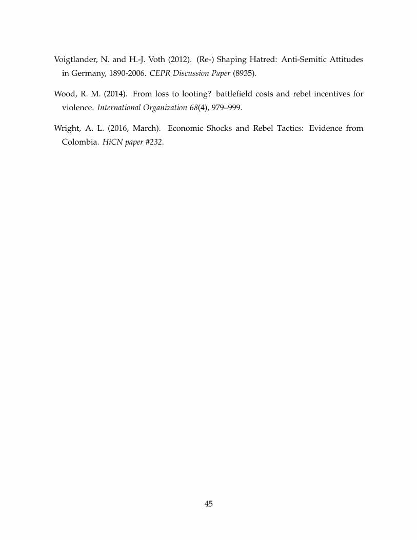
Voigtlander, N. and H.-J. Voth (2012). (Re-) Shaping Hatred: Anti-Semitic Attitudes

in Germany, 1890-2006. CEPR Discussion Paper (8935).

Wood, R. M. (2014). From loss to looting? battlefield costs and rebel incentives for

violence. International Organization 68(4), 979–999.

Wright, A. L. (2016, March). Economic Shocks and Rebel Tactics: Evidence from

Colombia. HiCN paper #232.

45

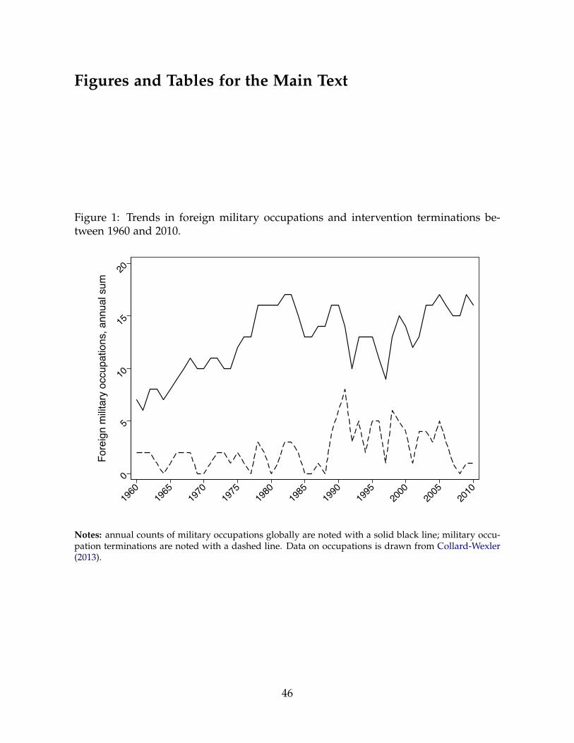
Figures and Tables for the Main Text

Figure 1: Trends in foreign military occupations and intervention terminations be-tween 1960 and 2010.

0

5

10

15

20

Fore

ign

milit

ary

occu

patio

ns, a

nnua

l sum

1960

1965

1970

1975

1980

1985

1990

1995

2000

2005

2010

Notes: annual counts of military occupations globally are noted with a solid black line; military occu-pation terminations are noted with a dashed line. Data on occupations is drawn from Collard-Wexler(2013).

46

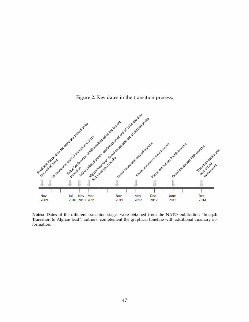
Figure 2: Key dates in the transition process.

Notes: Dates of the different transition stages were obtained from the NATO publication “Inteqal:Transition to Afghan lead”, authors’ complement the graphical timeline with additional auxiliary in-formation.

47

Figure 3: Distribution of conflict intensity and assignment of districts to different phases of the security transfer to theAfghan National Security Forces (ANSF).

Panel A: Conflict intensity Panel B: Assignment of districts to tranches

Notes: Panel A presents the distribution of conflict events in the SIGACTS data across the country. Panel B presents the different assignmentsof districts to the five different transition tranches.

Figure 4: Share of SIGACTS events involving security forces.

Notes: Figure plots the share of events per quarter is calculated using all events (including non-combatactivities) that do include information about security forces involved. Afghan security forces (ANSF)includes all armed forces, including local and border police. Vertical line indicates the quarter of thefirst transition tranche.

49

Figure 5: Timing of base handover relative to district tranche announcement and travel distance to nearest retrogradelogistic hub

Panel A: Last Base Closure date relative to tranche date Panel B: Distance to nearest logistic hub

Notes: Panel A visually presents the variation in the timing of the base handover dates relative to the transition onset announcements. If adistrict is matched with several bases, the date at which the timing that is used is for the base that was last retrograded or handed over. Panel Bpresents visually the least cost shortest path distance between a district centroid to one of the 10 retrograde logistic hubs used in the withdrawaloperation. We assume a unit cost of crossing via paved roads; the cost of crossing via an unpaved road occurs two units of costs per unit ofdistance, while crossing terrain without roads incurs a cost of 10 units. Least cost paths are computed used Dijkstra’s algorithm.

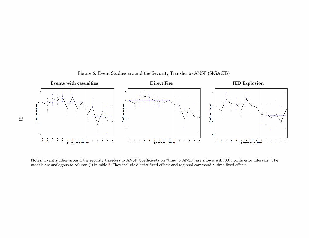
Figure 6: Event Studies around the Security Transfer to ANSF (SIGACTs)

Events with casualties Direct Fire IED Explosion

Notes: Event studies around the security transfers to ANSF. Coefficients on “time to ANSF” are shown with 90% confidence intervals. Themodels are analogous to column (1) in table 2. They include district fixed effects and regional command � time fixed effects.

51

Figure 7: Effect of the Security Transfer to ANSF on Conflict (SIGACTs)

All casualties

Direct Fire

IED Explosion

Insurgent casualties

Security force casualties

Civilian casualties

Indirect Fire

-.2 -.15 -.1 -.05 0

Notes: Coefficients and 90% confidence intervals on“ANSF” in a model that is analogous to column(2) in table 2. They include district fixed effects, regional command � time fixed effects, and district-specific trends. Full results can be found in the online appendix, in table A2.

52

Figure 8: ISAF Base Closure and Conflict (SIGACTs)

All casualties

Direct Fire

IED Explosion

Insurgent casualties

Security force casualties

Civilian casualties

Indirect Fire

-.5 0 .5 1 1.5

Notes: Coefficients and 90% confidence intervals on“ISAF Base Closure” in a model that is analogousto column (2) in table 5. All regressions include district fixed effects, regional command � time fixedeffects, and district-specific trends. The instrument used for ISAF base closure is the interaction of thetravel distance to the nearest military airport and an indicator for the post-2011 period. The IV controlset includes distance to any airport � time fixed effects, and distance to province borders � time fixedeffects. Outcomes are measured as log plus 1. Full results can be found in the online appendix tableA2.

53

Table 1: Summary Statistics

Mean Standard Deviation N(1) (2) (3)

Panel A: District-quarter level, SIGACTS

All casualties 5.048 15.548 10976Direct Fire 9.800 43.122 10976IED Explosion 3.110 10.343 10976ANSF 0.362 0.481 10556ISAF base closure 0.221 0.415 10976

Panel B: District-quarter level, ANQAR

Security improved in village in last 6 months (share) 0.322 0.220 8889Taliban grown weaker in last 6 months (share) 0.433 0.234 8170Seen ANA at least monthly in village (share) 0.685 0.324 8661ANSF brings most security to area (share) 0.507 0.236 8888Anti-government elements in control (versus govt, share) 0.185 0.226 8889

Panel C: District level

Travel distance to nearest military airport (cost units) 18785 10305 392

Notes: Observations at the district-quarter level in Panel A (2008-2014) and B (2008-2016); anddistrict-level level in Panel C.

54

Table 2: Security transfer to ANSF and conflict (SIGACTs)

All fatal Events Direct Fire Attacks IED Explosions(1) (2) (3) (4) (5) (6)

ANSF -0.134*** -0.096*** -0.131*** -0.064* -0.070** -0.076**(0.032) (0.031) (0.036) (0.035) (0.029) (0.029)

Number of Districts 377 377 377 377 377 377District time trend No Yes No Yes No Yes

Notes: Regressions at the district-quarter level, covering the period 2008-2014. Allregressions include location (i.e. district/gridcell) fixed effects and regional com-mand � time fixed effects. The dependent variable is expressed as log plus one.Standard errors clustered at the district level and are presented in parentheses, starsindicate *** p   0.01, ** p   0.05, * p   0.1.

Table 3: Security transfer to ANSF and perception of security (ANQAR)

Security ANSF presence and control

Improved Taliban weaker See ANA Monthly ANSF brings security Taliban control(1) (2) (3) (4) (5)

ANSF 0.027* 0.025 0.031* 0.024* -0.002(0.015) (0.017) (0.018) (0.014) (0.013)

Number of Districts 375 375 375 375 375

RC � Time FE Yes Yes Yes Yes YesDistrict Time Trend Yes Yes Yes Yes Yes

Notes: Regressions at the district-quarter level, covering the period 2008-2016. All regressions include districtfixed effects, regional command � time fixed effects, and district-specific trends. The dependent variables measureshares of respondents at the district level. Standard errors clustered at the district level and are presented inparentheses, stars indicate *** p   0.01, ** p   0.05, * p   0.1.

Table 4: ISAF Base Closure First Stage

ISAF Base Closure(1) (2) (3)

Travel distance to military airport � Post 2011 1.728*** 1.898*** 2.007***(0.237) (0.235) (0.236)

ANSF 0.193*** 0.190***(0.028) (0.029)

Number of Grid Cells

IV control set � time FE No Yes YesTranche � time FE No No Yes

Notes: Regressions at the district-quarter level, covering the period 2008-2016.All regressions include district fixed effects, regional command � time fixedeffects, and district-specific trends. The additional IV control set includes thedistance to any airport and to the province border. The dependent variable isa binary indicator for the last (observed) ISAF base closure at the district level.Standard errors clustered at the district level and are presented in parentheses,stars indicate *** p   0.01, ** p   0.05, * p   0.1.

56

Table 5: ISAF Base Closure and Conflict (SIGACTs)

All Casualty Events Direct Fire Attacks IED Explosions(1) (2) (3) (4) (5) (6)

Panel A: District level – OLS

ISAF base closure 0.002 -0.002 -0.006 0.001 -0.010 -0.010(0.035) (0.037) (0.040) (0.043) (0.029) (0.031)

ANSF -0.101*** -0.056 -0.093***(0.031) (0.036) (0.029)

Number of Districts 377 377 377 377 377 377

Tranche � time FE No Yes No Yes No Yes

Panel B: District level – IV

ISAF base closure 0.656** 0.613** 0.581* 0.506 0.768** 0.734**(0.305) (0.294) (0.324) (0.308) (0.300) (0.284)

ANSF -0.202*** -0.146** -0.213***(0.059) (0.063) (0.061)

Weak IV statistic 48.8 57.9 48.8 57.9 48.8 57.9Number of Districts 377 377 377 377 377 377

Tranche � time FE No Yes No Yes No Yes

Notes: Regressions at the district-quarter level, covering the period 2008-2014. Allregressions include district fixed effects, regional command � time fixed effects, anddistrict-specific trends. The instrument used for ISAF base closure is the interactionof the travel distance to the nearest military airport and an indicator for the post-2011period. The IV control set includes distance to any airport � time fixed effects, anddistance to province borders � time fixed effects. Outcomes are measured as log plus1. Standard errors clustered at the district level and are presented in parentheses,stars indicate *** p   0.01, ** p   0.05, * p   0.1.

57

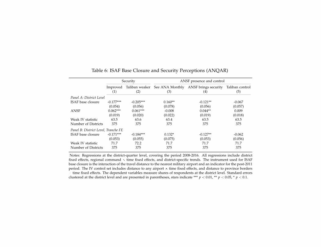
Table 6: ISAF Base Closure and Security Perceptions (ANQAR)

Security ANSF presence and control

Improved Taliban weaker See ANA Monthly ANSF brings security Taliban control(1) (2) (3) (4) (5)

Panel A: District LevelISAF base closure -0.177*** -0.205*** 0.160** -0.121** -0.067

(0.054) (0.056) (0.078) (0.056) (0.057)ANSF 0.062*** 0.061*** -0.008 0.044** 0.009

(0.019) (0.020) (0.022) (0.019) (0.018)Weak IV statistic 63.5 63.6 63.4 63.5 63.5Number of Districts 375 375 375 375 375

Panel B: District Level, Tranche FEISAF base closure -0.171*** -0.184*** 0.132* -0.127** -0.062

(0.053) (0.055) (0.075) (0.053) (0.056)Weak IV statistic 71.7 72.2 71.7 71.7 71.7Number of Districts 375 375 375 375 375

Notes: Regressions at the district-quarter level, covering the period 2008-2016. All regressions include districtfixed effects, regional command � time fixed effects, and district-specific trends. The instrument used for ISAFbase closure is the interaction of the travel distance to the nearest military airport and an indicator for the post-2011period. The IV control set includes distance to any airport � time fixed effects, and distance to province borders� time fixed effects. The dependent variables measure shares of respondents at the district level. Standard errorsclustered at the district level and are presented in parentheses, stars indicate *** p   0.01, ** p   0.05, * p   0.1.

Table 7: Security Force Activity

Improper behavior ANA needs full ANA will most likely defeat CERP spendingby ANA international support insurgents

(1) (2) (3) (4)

ISAF base closure 0.009 0.099** -0.056 -1.392(0.092) (0.048) (0.054) (1.177)

ANSF -0.012 -0.009 0.015 -0.053(0.019) (0.015) (0.016) (0.428)

Weak IV statistic 27.2 63.5 63.5 65.3Number of Districts 360 375 375 377

Notes: Regressions at the district-quarter level, covering the period 2008-2014. All regressions include district fixed effects, regionalcommand � time fixed effects, and district-specific trends. The instrument used for ISAF base closure is the interaction of the traveldistance to the nearest military airport and an indicator for the post-2011 period. The IV control set includes distance to any airport� time fixed effects, and distance to province borders � time fixed effects. The dependent variables in columns (1)-(3) measure theshare of respondents in the ANQAR survey at the district level. Column (4) contains CERP spending, which is subject to a log plus onetransformation. Standard errors clustered at the district level and are presented in parentheses, stars indicate *** p   0.01, ** p   0.05, *p   0.1.

59

Table 8: Military Support

Close air support Medevacs IED Found & Cleared(1) (2) (3)

ISAF base closure -0.017 0.512*** -0.086(0.149) (0.187) (0.219)

ANSF 0.016 0.001 -0.081(0.043) (0.042) (0.058)

ISAF base closure=1 � log(Direct Fire) -0.095 -0.199***(0.076) (0.066)

ANSF=1 � log(Direct Fire) -0.010 -0.017(0.039) (0.034)

log(Direct Fire) 0.116*** 0.104***(0.015) (0.013)

ISAF base closure=1 � log(IED Explosion) -0.318*(0.168)

ANSF=1 � log(IED Explosion) -0.010(0.064)

log(IED Explosion) 0.423***(0.023)

Weak IV statistic 25.8 25.8 25.6Number of Districts 377 377 377

Notes: Regressions at the district-quarter level, covering the period 2008-2014. All regressions include district fixedeffects, regional command � time fixed effects, and district-specific trends. The instrument used for ISAF base closureis the interaction of the travel distance to the nearest military airport and an indicator for the post-2011 period. The IVcontrol set includes distance to any airport � time fixed effects, and distance to province borders � time fixed effects.The dependent variables are measured as log plus one. Standard errors clustered at the district level and are presentedin parentheses, stars indicate *** p   0.01, ** p   0.05, * p   0.1.

60

Appendix to “Security Transitions”

For Online Publication

A Spillover Controls

We write the model above in a more concise notation by collecting the wi,j in a N � N

matrix W. In our case, we have N = 392 districts in Afghanistan.1 Matrix W is

often known as the spatial, neighbouring or adjacency matrix. We also stack the other

elements to write the model

yt = α + βt + ρWyt + γANSFt + δW � ANSFt + η � t + εt (5)

where yt, α, βt, ANSFt and εt are, respectively, the column-vector of outcomes, district

fixed effects, regional command time trends, ANSFd,t treatment indicators and error

term, for all regions and districts at a given point in time. Instead of pre-specifying

W, we opt to recover it from the data. To do so, we apply the method in de Paula et al.

(2019) which allows us to fully and flexibly recover the network matrix W from the

panel data. The method provides a high-dimensional technique to deal with a large

number of parameters. Furthermore, the authors show that W and the parameters ρ,

γ and δ are globally identified. The purpose of this Section is to review and provide

an adaptation of their methodology.

The method in de Paula et al. (2019) postulates that W, ρ, γ and δ are globally

identified under the assumptions that districts have a different number network link-

ages to other districts. More specifically, it relies on the identification assumption that

the main diagonal of W2 is not proportional to a vector of ones. To give a concrete

interpretation to this assumption, note that the elements of the diagonal of W2 are

1We maintain in the sample all districts that is consistently defined in the survey. This slightlyreduces the number of districts from 398 to 392.

1

given by

diag(W2) =

°N

j=1 w1jwj1

� � �°N

j=1 wNjwjN.

The first element of the expression above,

°Nj=1 w1jwj1 captures the extent to which

district 1 affects other districts, which in turn affects district 1 back. So elements of the

diagonal of W2 are interpreted as “self-spillovers”. Thus diag(W2) not proportional to

the vector of ones translates into heterogenous exposure to the “self-spillovers” across

districts.

For the sake of clarity consider the canonical example of peer friendships, and

further assume that W is unweighted (with Wij = 1 if j affects i and zero otherwise).

In this case, the (i, j)-th element of W2 captures the number of times that j reaches i

through intermediary friendships. Its diagonal is simply the number of reciprocated

friendships among the group. The identification assumption means that students

have different number of reciprocated friendships.

The identification assumption in de Paula et al. (2019) is sufficient to the peers-

of-peers identification strategy which makes use of the variation in the composition

of peers-of-peers to identify the endogenous effects. Such type of assumptions which

originate from the network asymmetry have been shown to overcome the “reflection

problem” as first postulated by Manski (1993). In line with de Paula et al. (2019), we

additionally require the following standard regularization conditions: (i) no district

affects itself, and so the main diagonal of W is equal to zero, Wii = 0 for every

i = 1, . . . , N, ruling out a trivial solution to the model; (ii) the row-sums of W are

smaller than one in absolute value,°N

j=1 |Wij| ¤ 1 for every i = 1, . . . , N and |ρ|   1,

ensuring that the system of equations is stationary in the spatial sense and the inverse

of (I � ρWyt) is well defined; (iii) there is one row i such that°N

j=1 Wij = 1, which is a

simple normalization; and, finally, (iv) the spatial effects do not cancel each other out,

ργ + δ � 0. We apply the method on the residualized yt and xt after projecting on the

space generated by the fixed effects.

As de Paula et al. (2019) suggest, we make use of moment conditions given by the

2

orthogonality between ANSFt and the error term to formulate moment conditions

gNT(θ) where the full set of structural parameters is given by θ = (ρ, γ, δ, w12, . . . , wN,N�1).

The first step in the Adaptive Elastic Net GMM is the solution to

θ(p) = (1 + p2/T) � arg minθPRK

$&%gNT(θ)

1gNT(θ) + p1

N

i,j=1,i�j

��wi,j��+ p2

N

i,j=1,i�j

w2i,j

,.-

where K is the number of parameters to be estimated, equal to N(N � 1) + 3, and p1

and p2 are the non-negative penalization terms. The term gNT(θ)1gNT(θ) is the GMM

objective criteria. The first penalization term linearly increases the objective function

for every wi,j estimated as non-zero. As the penalization increases, more elements wi,j

are estimated as zeros. The second term penalizes for the sum of the square of the

links between units. This term has been shown to provide a more stable solution to

the problem.

Finally, it has been shown that the solution to the first step alone would bias the

estimates towards zero. To alleviate this problem, the estimates from the first step are

refined in the adaptive stage,

θ(p) = (1 + p2/T) � arg minθPRK

$&%gNT(θ)

1gNT(θ) + p�1N

i,j=1,i�j

��wi,j��

��wi,j���k + p2

N

i,j=1,i�j

w2i,j

,.-

where typically k = 2.5, and the full set of penalization parameters (p1, p�1 , p2) is

chosen by BIC. See de Paula et al. (2019) for implementation details.

B Distant Gridcell Pair Matching

In an attempt to relax the identification assumption that underlies our main district

level difference-in-difference approach, we change the unit of analysis to 10�10 km

gridcells. The choice of 10 x 10 km gridcells is appealing as this resolution is the

basis of the geo-coordinate standard used by NATO militaries for locating points on

the earth. This is only possible for the SIGACTs data, as the ANQAR survey data

is reported at the district level. In the resulting high-resolution dataset, we construct

pairs of matched gridcells. We rely on purely geographical characteristics of gridcells

3

measured at baseline, such as: grid level population (as of 2008), elevation, terrain

features, distance to nearest asphalt road, distance to nearest road, and distance to

the nearest airport. In addition we use land cover data and construct the share of grid

cells covered by different land cover type across sixteen land cover classes using the

detailed 500m pixel resolution MODIS product (Channan et al., 2014). We proceed

by constructing these matched pairs sequentially sampling without replacement: we

first find matches for grid cells in the first transition waves by sampling from cells in

later waves, only retaining matched pairs that are sufficiently similar with a propen-

sity score difference of less than 0.01.2 Our main estimating sample is chosen such

that matched pairs are at least 200km apart (we call these distant matched pairs).

This strategy allows us to rule out displacement effects, which could affect estimates

relying on close matched pairs.

The estimating specification for the distant matched panel difference-in-differences

is as follows:

yi,p,d,t = αi + βp,t + γ� ANSFd,t + ηd � t + εi,d,t (6)

As before, the level of analysis is gridcell i, that is part of a matched pair p located in

district d, and month t. We include matched-pair specific time fixed effects βp,t. These

are very demanding, as for every matched pair, we allow conflict to be on a different

trajectory common only to the cells that form the matched pair. This zooms in to

any time-varying changes that are specific to the matched-pair and accounts for any

non-linear trends specific to the propensity score. As in earlier specifications, ANSFd,t

switches on when ANSF takes over from ISAF. Since the distant matched pair panel

is very granular (both in terms of time and geography), we use dummy variables as

outcomes capturing the incidence of a conflict event within a given gridcell-month as

a more meaningful measure of conflict activity. The crucial identifying assumption

remains that there are common trends in conflict levels across observationally similar

distant matched grid cells in the different transition phases. Table ?? shows that we

achieve much better balance on conflict characteristics compared to the district level

when resorting to the distant matched pair analysis, yet, some important baseline

2This approach could result in a decay in match quality for later transition rounds, as the set ofavailable grid cells for matching becomes smaller. It turns out that the average estimated propensityscore does not systematically differ between early versus late transition rounds.

4

differences still exist. Importantly, as with the district-level difference-in-difference

strategy, relying on event studies around the transition dates, we will provide strong

evidence in support of the common trends assumption, necessary to enable us to

interpret any estimated effects as causal.

5

Appendix Figures and Tables

Figure A1: Diagnostic statistics about cooperation and participation in the ANQARsurvey waves 16 to 38

0.0

1.0

2.0

3.0

4.0

5R

efus

al R

ate

15 20 25 30 35 40ANQAR Survey Wave (Quarterly)

Respondent Refusal to Take Survey Among Targets

0.0

1.0

2.0

3.0

4.0

5N

on-C

onta

ct R

ate

15 20 25 30 35 40ANQAR Survey Wave (Quarterly)

Contact with Targeted Respondent not Possible

.9.9

2.9

4.9

6.9

81

Coo

pera

tion

Rat

e

15 20 25 30 35 40ANQAR Survey Wave (Quarterly)

Respondent Cooperation with Survey Enumerators

Notes: Figure present data on refusal, non-contact, and overall cooperation in the ANQAR surveywaves 16-38 that were shared with the authors by NATO.

6

Figure A2: Events with casualties reported in SIGACTS over time and NATO troopstrength.

Panel A: Events with casualties Panel B: NATO troop deployments

Notes: The left figure presents the overall number of SIGACTs events with casualties for Afghan- orCoalition forces. The right figure presents average monthly NATO and US troop deployments.

7

Figure A3: Event Studies around the Security Transfer to ANSF (SIGACTs) - Gridcell level

Events with casualties Direct Fire IED Explosion

Notes: Event studies around the security transfers to ANSF. Coefficients on “time to ANSF” are shown with 90% confidence intervals. Themodels are analogous to column (1) in table 2. They include gridcell fixed effects and regional command � time fixed effects. The gridcell levelresults also include match pair � time fixed effects.

8

Figure A4: ISAF Base Closure and Conflict (SIGACTs) - Placebo timing

ANA

ANA

(t+4q

)

All casualtiesDirect Fire

IED ExplosionInsurgent casualties

Security force casualtiesCivilian casualties

Indirect Fire

All casualtiesDirect Fire

IED ExplosionInsurgent casualties

Security force casualtiesCivilian casualties

Indirect Fire

-.3 -.2 -.1 0 .1

ANA

ANA

(t+4q

)

All casualtiesDirect Fire

IED ExplosionInsurgent casualties

Security Force casualtiesCivilian casualties

Indirect Fire

All casualtiesDirect Fire

IED ExplosionInsurgent casualties

Security Force casualtiesCivilian casualties

Indirect Fire

-.02 -.01 0 .01

District Level Gridcell Level

Notes: Coefficients and 90% confidence intervals on“ANSF” and “ANSF (t+4q)”. We add the forwarded treatment indicator (by 4 quarters or12 months) to a model that is analogous to column (1) in table 5 using the distance to the closest military airport interacted with a post 2011dummy as the IV, and including location fixed effects, time fixed � regional command fixed effects, district-specific trends, and tranche � timefixed effects. In the grid cell level model, we also include match pair � time fixed effects. The dependent variable is measured as log plus one.

Figure A5: ISAF Base Closure and Conflict (ANQAR) - Placebo timing

ANA

ANA

(t+4q

)

Security improved in village in last 6 months (share)

Taliban grown weaker in last 6 months (share)

Seen ANA at least monthly in village (share)

ANSF brings most security to area (share)

Anti-government elements in control (versus govt, share)

Security improved in village in last 6 months (share)

Taliban grown weaker in last 6 months (share)

Seen ANA at least monthly in village (share)

ANSF brings most security to area (share)

Anti-government elements in control (versus govt, share)

-.050 .05 .1 .15

District Level

Notes: Coefficients and 90% confidence intervals on“ANSF” and “ANSF (t+4q)”. We add the for-warded treatment indicator (by 4 quarters or 12 months) to a model that is analogous to column (1)in table 5 using the distance to the closest military airport interacted with a post 2011 dummy as anIV, and including location fixed effects, time fixed � regional command fixed effects, district-specifictrends, and tranche � time fixed effects. In the grid cell level model, we also include match pair � timefixed effects. The dependent variable measures the share of respondents.

10

Table A1: Comparison of district level characteristics across different tranche phases

T1 T2 T2-T1 T3 T3-T2 T4 T4-T3 T5 T5-T4

(1) (2) (3) (4) (5) (6) (7) (8) (9)

Is security in your village better than 6 month ago? 0.288 0.291 0.002 0.216 -0.074 *** 0.156 -0.060 *** 0.138 -0.019(0.023) (0.018) (0.024) (0.015) (0.017) (0.024) (0.023) (0.015) (0.022)

All casualties per capita -3.374 -3.410 -0.036 0.467 3.877 ** -2.229 -2.695 * 9.288 11.516(0.728) (1.015) (1.151) (1.014) (1.516) (1.198) (1.536) (1.820) (2.596)

Insurgent casualties per capita -0.945 -1.001 -0.056 -0.356 0.645 * -0.840 -0.484 2.711 3.551(0.189) (0.293) (0.295) (0.279) (0.369) (0.357) (0.391) (0.615) (0.863)

Security force casualties per capita -1.646 -1.604 0.042 0.491 2.094 ** -0.950 -1.441 * 4.637 5.587(0.406) (0.554) (0.619) (0.560) (0.840) (0.666) (0.867) (0.924) (1.338)

Civilian casualties per capita -0.784 -0.806 -0.022 0.332 1.137 *** -0.438 -0.770 ** 1.940 2.378(0.187) (0.215) (0.257) (0.240) (0.355) (0.237) (0.349) (0.381) (0.515)

Direct Fire per capita -6.710 -5.071 1.639 -1.448 3.623 -5.034 -3.587 26.711 31.746(3.654) (4.543) (6.347) (2.865) (5.944) (3.150) (3.547) (6.446) (8.331)

Indirect Fire per capita -3.905 -3.339 0.566 -0.667 2.672 *** 0.348 1.014 14.066 13.719(0.729) (0.851) (0.532) (0.803) (0.790) (1.201) (1.302) (2.815) (3.434)

IED Explosion per capita -3.037 -2.670 0.367 1.549 4.219 *** -0.266 -1.815 6.717 6.983(0.647) (0.899) (0.981) (1.007) (1.471) (1.555) (2.019) (1.542) (2.515)

Nightlights per capita 892.036 637.193 -254.843 316.111 -321.082 -126.970 -443.081 *** -73.006 53.964(336.144) (167.234) (382.774) (84.300) (201.716) (44.089) (108.032) (46.020) (53.553)

Opium Yield [HA] per capita 0.124 0.169 0.045 0.293 0.123 0.372 0.080 0.498 0.126(0.071) (0.088) (0.100) (0.086) (0.107) (0.132) (0.148) (0.145) (0.189)

Notes: Table reports coeffients on tranche dummies and their differences from a district-level regression with quarter fixed effects, covering the period 2008-2014(2008-2016 for the first row, which is based on ANQAR). Standard errors clustered at the district level and are presented in parentheses, stars indicate *** p   0.01,** p   0.05, * p   0.1.

Table A2: Security transfer to ANSF and conflict (SIGACTs) - District level additional outcomes

Insurgent Casualty Events Security Force Casualty Civilian Casualty Indirect FireEvents Events Events Attacks

(1) (2) (3) (4) (5) (6) (7) (8)

Panel A: District cell level – Security TransferANSF -0.096*** -0.064* -0.076** -0.044* -0.066** -0.022 -0.133***

(0.031) (0.035) (0.029) (0.026) (0.028) (0.023) (0.032)Number of Districts 377 377 377 377 377 377 377Mean of DV pre ANADistrict time trend No Yes No Yes No Yes No Yes

Panel B: District level – ISAF Base Closure (IV)ISAF base closure 0.656** 0.581* 0.768** 0.242 0.688** 0.428* 0.033

(0.305) (0.324) (0.300) (0.195) (0.274) (0.227) (0.237)ANSF -0.202*** -0.146** -0.213*** -0.078** -0.186*** -0.089* -0.141***

(0.059) (0.063) (0.061) (0.039) (0.053) (0.045) (0.050)Weak IV statistic 48.8 48.8 48.8 48.8 48.8 48.8 48.8Number of Districts 377 377 377 377 377 377 377Mean of DV pre ANATranche � time FE No Yes No Yes No Yes No Yes

Notes: Regressions at the district-quarter level, covering the period 2008-2014. All regressions include district fixedeffects, regional command � time fixed effects, and district-specific trends. The instrument used for ISAF baseclosure is the interaction of the travel distance to the nearest military airport and an indicator for the post-2011period. The IV control set includes distance to any airport � time fixed effects, and distance to province borders� time fixed effects. Outcomes are measured as log plus 1. Standard errors clustered at the district level and arepresented in parentheses, stars indicate *** p   0.01, ** p   0.05, * p   0.1.

12

Table A3: Security transfer to ANSF and conflict (SIGACTs) - Spillover estimates

(1) (2) (3) (4) (5) (6) (7) (8) (9) (10)

All Fatal Events ANSF transition effect (γ) -0.095*** -0.119*** -0.109*** -0.153*** -0.102*** -0.101*** -0.099*** -0.098*** -0.088*** -0.102***(0.031) (0.033) (0.029) (0.032) (0.026) (0.025) (0.025) (0.025) (0.025) (0.026)

Exogenous effects (δ) 0.041 0.030 0.119** 0.015 0.383 -0.146 -0.447*** -0.554*** 0.039(0.051) (0.063) (0.046) (0.153) (0.389) (0.185) (0.027) (0.026) (.060)

Endogenous effects (ρ) 0.039(0.554)

Direct Fire Attacks ANSF transition effect (γ) -0.066* -0.064** -0.074*** -0.073** -0.065** -0.066** -0.064** -0.019 -0.012 -0.066**(0.035) (0.027) (0.026) (0.034) (0.027) (0.027) (0.027) (0.027) (0.026) (0.028)

Exogenous effects (δ) -0.143 -0.031 0.016 -0.035 0.032 -0.143 -0.477*** -0.615*** 0.004(0.197) (0.056) (0.049) (0.163) (0.415) (0.197) (0.030) (0.028) (0.042)

Endogenous effects (ρ) 0.001(0.226)

IED Explosions ANSF transition effect (γ) -0.074** -0.086*** -0.074*** -0.104*** -0.083*** -0.082*** -0.081*** -0.074*** -0.068*** -0.088***(0.029) (0.029) (0.026) (0.029) (0.023) (0.022) (0.023) (0.022) (0.022) (.027)

Exogenous effects (δ) 0.010 -0.031 0.052 0.056 -0.121 -0.036 -0.482*** -0.576*** 0.002(0.046) (0.056) (0.041) (0.136) (0.346) (0.164) (0.027) (0.026) (.087)

Endogenous effects (ρ) -0.386(0.644)

Number of districts 392 392 392 392 392 392 392 392 392 392

District time trend Yes Yes Yes Yes Yes Yes Yes Yes Yes Yes

Spillover specification - Neighbordist.

Neighbordist.2

Neighborprov.

Dist.  250km

Dist.  500km

Drivingdist.  500km

Flexible,zero

beyond500km

Flexible,zero

beyond1000km

Flexible,zero

beyond1000km

Edges that are supposed to be known - 100% 100% 100% 100% 100% 100% 27.51% 17.35% 17.35%

Notes: Column (1): regressions at the district-quarter level, covering the period 2008-2014, including district and regional command x time fixed effects. Dependent variable is expressedas log plus one. Standard errors clustered at the district level and are presented in parentheses. Columns (2)-(7) are spatial panel regressions with spatial neighboring matrix assumed tobe known and given, respectively, by neighboring districts, neighboring district squared, neighboring provices, geodesical distance smaller than 250km and 500km and driving distancesmaller than 500km. Specifications reported in columns (7)-(10) have estimated and flexible spatial neighboring matrix, following de Paula et al. (2019), where weights between districtswith driving distance beyond 500km and 1000k are assumed to be equal to zero, which corresponds to 27.51% and 17.35% of all weights. Stars indicate *** p   0.01, ** p   0.05, * p   0.1.

Table A4: ISAF Base Closure and Conflict (SIGACTs) - Spillover estimates

(1) (2) (3) (4) (5) (6) (7) (8) (9) (10)

All Fatal Events Base closure (gamma) .765** 1.452*** 1.676*** 0.847** 0.947*** 0.496* 0.771*** 0.501** 0.540** 0.533***(0.336) (0.510) (0.383) (0.337) (0.254) (0.264) (0.220) (0.216) (0.215) (0.179)

Exogenous effects (delta) -0.981 -1.689*** -0.216 -1.657* -4.090 -2.932** 4.262*** 4.701*** 2.713***(0.613) (0.553) (0.420) (0.926) (2.747) (1.352) (0.236) (0.230) (0.281)

Endogenous effects (rho) 0.587***(0.071)

Direct Fire Attacks ANSF transition effect (beta) .787** 0.951** 1.816*** 0.547 1.006*** 0.725*** 0.885*** 0.387* 0.679*** 0.628***(0.397) (0.408) (0.343) (0.359) (0.271) (0.281) (0.235) (0.231) (0.228) (0.191)

Exogenous effects (delta) -0.264 -1.404*** 0.417 -1.467 -1.432 -4.398*** 5.006*** 5.480*** 2.900***(0.590) (0.495) (0.447) (0.987) (2.927) (1.440) (0.276) (0.259) (0.306)

Endogenous effects (rho) 0.697***(0.063)

IED Explosions ANSF transition effect (beta) 1.109*** 1.776*** 1.816*** 1.420*** 1.051*** 0.789*** 1.018*** 0.529*** 0.645*** 0.377**(0.364) (0.456) (0.343) (0.301) (0.227) (0.236) (0.197) (0.195) (0.193) (0.166)

Exogenous effects (delta) -1.008* -1.404*** -0.658* -0.235 -4.275* 0.011 3.966*** 3.858*** 1.474***(0.548) (0.495) (0.375) (0.829) (2.457) (1.210) (0.223) (0.206) (0.292)

Endogenous effects (rho) 0.692***(0.070)

Number of districts 392 392 392 392 392 392 392 392 392 392

Tranche x time FE Yes Yes Yes Yes Yes Yes Yes Yes Yes Yes

Spillover specification - Neighbordist.

Neighbordist.2

Neighborprov.

Dist.  250km

Dist.  500km

Drivingdist.  500km

Flexible,zero

beyond500km

Flexible,zero

beyond1000km

Flexible,zero

beyond1000km

Edges that are supposed to be known - 100% 100% 100% 100% 100% 100% 27.51% 17.35% 17.35%

Notes: Column (1): regressions at the district-quarter level, covering the period 2008-2014, including district and regional command x time fixed effects. Dependent variable is expressedas log plus one. Standard errors clustered at the district level and are presented in parentheses. Columns (2)-(7) are spatial panel regressions with spatial neighboring matrix assumed tobe known and given, respectively, by neighboring districts, neighboring district squared, neighboring provices, geodesical distance smaller than 250km and 500km and driving distancesmaller than 500km. Specifications reported in columns (7)-(10) have estimated and flexible spatial neighboring matrix, following de Paula et al. (2019), where weights between districtswith driving distance beyond 500km and 1000k are assumed to be equal to zero, which corresponds to 27.51% and 17.35% of all weights. Stars indicate *** p   0.01, ** p   0.05, * p   0.1.

Table A5: Summary Statistics at the gridcell level

Mean Standard Deviation N(1) (2) (3)

Gridcell-month level

All casualties 0.122 0.895 450072Direct Fire 0.233 2.325 450072IED Explosion 0.073 0.578 450072Insurgent casualties 0.032 0.313 450072Security Force casualties 0.064 0.538 450072Civilian casualties 0.026 0.239 450072Indirect Fire 0.044 0.471 450072ANSF 0.423 0.494 450072ISAF base closure 0.275 0.447 450072

Notes: Observations at the gridcell-month level (2008-2014).

Table A6: Security transfer to ANSF and conflict (SIGACTs) - Gridcell Level

All fatal Events Direct Fire Attacks IED Explosions(1) (2) (3) (4) (5) (6)

ANSF -0.015*** -0.009* -0.008 -0.001 -0.016*** -0.012***(0.005) (0.005) (0.006) (0.006) (0.005) (0.004)

Number of Grid Cells 1182 1182 1182 1182 1182 1182

District time trend No Yes No Yes No Yes

Notes: Regressions at the gridcell-month level, covering the period 2008-2014. Allregressions include location (i.e. district/gridcell) fixed effects and regional command� time fixed effects. They also includes match pair � time fixed effects. The dependentvariable is expressed as a binary indicator variable. Standard errors clustered at thedistrict level and are presented in parentheses, stars indicate *** p   0.01, ** p   0.05,* p   0.1.

15

Table A7: Main results by tranche

All Casualty Events Direct Fire Attacks IED Explosions(1) (2) (3)

District Level (IV)ISAF base closure 0.678** 0.544* 0.736***

(0.292) (0.302) (0.277)ANSF Tranche 1 -0.486** -0.339 -0.550***

(0.195) (0.230) (0.176)ANSF Tranche 2 -0.129 -0.129 -0.203**

(0.083) (0.090) (0.082)ANSF Tranche 3 -0.096 -0.008 -0.096

(0.064) (0.073) (0.062)ANSF Tranche 4 -0.385*** -0.400*** -0.288***

(0.083) (0.101) (0.092)ANSF Tranche 5 -0.154 -0.033 -0.160

(0.113) (0.136) (0.108)Weak IV statistic 65 65 65Number of Districts 377 377 377

Notes: Regressions at the district-quarter level covering the period 2008-2014. Allregressions include district fixed effects and regional command � time fixed effects,and district-specific trends. Panel B also includes match pair � time fixed effects.The instrument used for ISAF base closure is the interaction of the travel distance tothe nearest military airport and an indicator for the post-2011 period. The IV controlset includes distance to any airport � time fixed effects, and distance to provinceborders � time fixed effects. Outcomes are measured as log plus 1 in Panel A, andas binary indicators in Panel B. Standard errors clustered at the district level andare presented in parentheses, stars indicate *** p   0.01, ** p   0.05, * p   0.1.

16