thin film simulation on a rotating wafer - unileoben.ac.at
TRANSCRIPT

Thin Film SimulationThin Film Simulationon a Rotating Waferon a Rotating Wafer
B. Gschaider, D. Prieling, H. Steiner, P. VitaB. Gschaider, D. Prieling, H. Steiner, P. Vita

TopicsTopics
• MotivationMotivation• Finite Area MethodFinite Area Method• Thin Film ModelThin Film Model• Impinging JetImpinging Jet• Polydual MeshPolydual Mesh• Comparison with 3D SolutionComparison with 3D Solution• ConclusionConclusion• Outlook & DiscussionOutlook & Discussion

Motivation (1)Motivation (1)
• Our industry partner, LAM Research AG, initiated a Our industry partner, LAM Research AG, initiated a project to be able to optimize they product, a spin project to be able to optimize they product, a spin processorprocessor– One-sided single wafer
wet processing– Patented wafer chuck with
floating wafer (N2 cushion)
– Vertically arranged process levels
– Clearly separated chemical lines

• 2D Simulation 2D Simulation (Axial Symmetric)‑(Axial Symmetric)‑– Advantages
• Reasonably small meshes• Short computation times in
order of hours• No additional model
assumptions– Disadvantages
• Allows only central impingement
• Resolve waves only in radial direction
Motivation (2)Motivation (2)
• 3D Simulation3D Simulation– Advantages
• Fine resolution only where required
• No additional model assumptions
– Disadvantages• Huge meshes
– Still cannot fully resolve all physical aspects
• Long computation times in order of weeks/months

Finite Area MethodFinite Area Method
• Specialization of FVM to flows on surfaces films‑Specialization of FVM to flows on surfaces films‑• Implementation by H. Jasak and Z. Tukovic in Implementation by H. Jasak and Z. Tukovic in
OpenFOAM-ext projectOpenFOAM-ext project– Only present in 1.5-dev and 1.6-ext version
• Demonstration solver models the transport Demonstration solver models the transport equation on a prescribed velocity fieldequation on a prescribed velocity field– surfactantFoamsurfactantFoam solver
• Equations are solved on a boundary patch of the Equations are solved on a boundary patch of the volume meshvolume mesh– FV-solution can be used as a source term

Thin Film Model (1)Thin Film Model (1)
• Normal velocity component is negligible compared Normal velocity component is negligible compared to tangential oneto tangential one
• Pressure is constant across the film thicknessPressure is constant across the film thickness• Laminar flowLaminar flow• Film thickness is identical with a velocity Film thickness is identical with a velocity
boundary layerboundary layer• Parabolic velocity profile assumed across the film Parabolic velocity profile assumed across the film
thicknessthickness

Thin Film Model (2)Thin Film Model (2)
• Dependent variablesDependent variables– Film thickness hh– Mean velocity uu

Thin Film Model (3)Thin Film Model (3)
• Continuity EquationContinuity Equation
• Momentum EquationMomentum Equation

Thin Film Model (4)Thin Film Model (4)
• where the pressure is expressed bywhere the pressure is expressed by
• with a surface curvature approximated bywith a surface curvature approximated by
• and shear stress at wafer is described byand shear stress at wafer is described by

Thin Film Model (5)Thin Film Model (5)
• In order to describe the shear stress at the wafer In order to describe the shear stress at the wafer and the differential advection, we introduce a and the differential advection, we introduce a polynomial velocity profile functionpolynomial velocity profile function
• which defines the free surface velocitywhich defines the free surface velocity
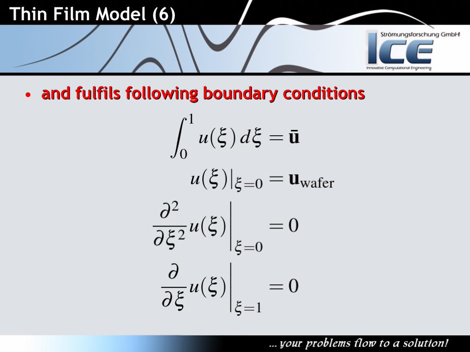
Thin Film Model (6)Thin Film Model (6)
• and fulfils following boundary conditionsand fulfils following boundary conditions

Thin Film Model (7)Thin Film Model (7)
• The boundary conditions imposed on the velocity The boundary conditions imposed on the velocity profile function lead to the following solutionsprofile function lead to the following solutions
Impinging Jet (1)Impinging Jet (1)
• Impingement area is generally not knowImpingement area is generally not know– Impinging jet is moving over the wafer
• Thin film model is not valid in the impingement Thin film model is not valid in the impingement area and its surroundingarea and its surrounding– Solution in the impingement area is known from FVM– Impingement area is “weakly” influenced from “outside”
• Possible impingement implementationsPossible impingement implementations– Remeshing
• Impingement area is represented by a circular boundary condition which moves and the mesh is adapted
– Fixation of solution in faces• Impingement faces are selected and solution is prescribed

Impinging Jet (2)Impinging Jet (2)
• Fixation of solution in the faces Fixation of solution in the faces has significant advantages over has significant advantages over remeshing, however it has its remeshing, however it has its own problemsown problems– “Crown Cap” effect
• Faces in the impingement area are not resolving exact circle
• Face boundaries are not aligned with a circle
– Total mass-flow correction– Inlet velocity profiles
• Velocities varies along the jet edge

Impinging Jet (3)Impinging Jet (3)
• Solution to “Crown Cap” effectSolution to “Crown Cap” effect– Velocity in the outer faces of the fixed area is not only
determined by the location of the face centre, but also by the orientation of the edges that separate them from the free region
• “How much fluid does the next outside face receive?”
• Solution to total mass-flow correctionSolution to total mass-flow correction– Total mass-flow across edges is calculated and the
velocities in the faces are normalized accordingly• Solution to inlet velocity profilesSolution to inlet velocity profiles
– Simple models implemented, real data can be read-in

Impinging Jet: “Crown-Cap” EffectImpinging Jet: “Crown-Cap” Effect
Uncorrected Flow Corrected FlowUncorrected Flow Corrected Flow

Impinging Jet: Inlet Velocity ProfileImpinging Jet: Inlet Velocity Profile

Polydual MeshPolydual Mesh
• Solution is very mesh sensitiveSolution is very mesh sensitive– Mesh neutral to
flow is needed to avoid artefacts
• “flow arms”• “rose petals”
– Polyhedral mesh shown the best results
• polyDualMeshpolyDualMesh utility used to convert a tetrahedral mesh into the polyhedral one

Comparison with 3D SolutionComparison with 3D Solution
• 3D solution 3D solution – Fluent software– 5M cells, 4 CPU cores
used– 1s of process ~ 30days
• 2.5D solution2.5D solution– OpenFOAM software– 36.8k polydual mesh,
single CPU core used– 1s of process ~ 2hours
• CasesCases– Ω = 500rpm, Q = 1.5l– Spinetch-D (ν = 2.87×10⁻⁶) or water (ν = 1×10⁻⁶)– Impingement area
• Reference Case (central impingement; Spinetch-D)• Case 1a (ex-centric case, Δr = 30mm; Spinetch-D)• Case 2b (ex-centric case with dry spot, Δr = 50mm; water)
– No moving inlet was simulated

Reference Case: 500rpm, 1.5lpm,Reference Case: 500rpm, 1.5lpm, Spinetch-D Spinetch-D

Reference Case: 500rpm, 1.5lpm,Reference Case: 500rpm, 1.5lpm, Spinetch-D Spinetch-D
-0,15 -0,10 -0,05 0,00 0,05 0,10 0,150,0000
0,0001
0,0001
0,0002
0,0002
0,0003
0,0003
0,0004
0,0004
0,0005
0,0005
h (xz-Plane through Jet)
OpenFOAM 2.5D Fluent 3D
x [m]
h [m
]

Reference Case: 500rpm, 1.5lpm,Reference Case: 500rpm, 1.5lpm, Spinetch-D Spinetch-D
-0,15 -0,10 -0,05 0,00 0,05 0,10 0,150,0000
0,0001
0,0001
0,0002
0,0002
0,0003
0,0003
0,0004
0,0004
0,0005
0,0005
h (yz-Plane through Jet)
OpenFOAM 2.5D Fluent 3D
y [m]
h [m
]

Reference Case: 500rpm, 1.5lpm,Reference Case: 500rpm, 1.5lpm, Spinetch-D Spinetch-D

Reference Case: 500rpm, 1.5lpm,Reference Case: 500rpm, 1.5lpm, Spinetch-D Spinetch-D
-0,15 -0,10 -0,05 0,00 0,05 0,10 0,150
5
10
15
20
25
30
35
40
45
50
τWafer (xz-Plane through Jet)
OpenFOAM 2.5D Fluent 3D
x [m]
τWaf
er [P
a]

Reference Case: 500rpm, 1.5lpm,Reference Case: 500rpm, 1.5lpm, Spinetch-D Spinetch-D
-0,15 -0,10 -0,05 0,00 0,05 0,10 0,150
10
20
30
40
50
60
τWafer (yz-Plane through Jet)
OpenFOAM 2.5D Fluent 3D
y [m]
τWaf
er [P
a]

Reference Case: 500rpm, 1.5lpm,Reference Case: 500rpm, 1.5lpm, Spinetch-D Spinetch-D

Case 1a: 500rpm, 1.5lpm, Case 1a: 500rpm, 1.5lpm, ΔΔr=30mm,r=30mm, Spinetch-D Spinetch-D

Case 1a: 500rpm, 1.5lpm, Case 1a: 500rpm, 1.5lpm, ΔΔr=30mm,r=30mm, Spinetch-D Spinetch-D
-0,15 -0,10 -0,05 0,00 0,05 0,10 0,150,0000
0,0005
0,0010
0,0015
0,0020
0,0025
h (xz-Plane through Jet)
OpenFOAM 2.5D Fluent 3D
x [m]
h [m
]

Case 1a: 500rpm, 1.5lpm, Case 1a: 500rpm, 1.5lpm, ΔΔr=30mm,r=30mm, Spinetch-D Spinetch-D
-0,15 -0,10 -0,05 0,00 0,05 0,10 0,150,0000
0,0005
0,0010
0,0015
0,0020
0,0025
h (yz-Plane through Jet)
OpenFOAM 2.5D Fluent 3D
y [m]
h [m
]

Case 1a: 500rpm, 1.5lpm, Case 1a: 500rpm, 1.5lpm, ΔΔr=30mm,r=30mm, Spinetch-D Spinetch-D

Case 1a: 500rpm, 1.5lpm, Case 1a: 500rpm, 1.5lpm, ΔΔr=30mm,r=30mm, Spinetch-D Spinetch-D
-0,15 -0,10 -0,05 0,00 0,05 0,10 0,150
10
20
30
40
50
60
τWafer (xz-Plane through Jet)
OpenFOAM 2.5D Fluent 3D
x [m]
τWaf
er [P
a]
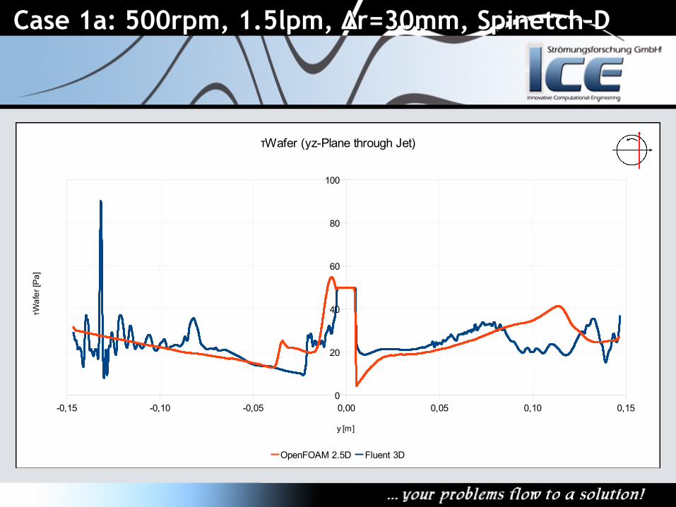
Case 1a: 500rpm, 1.5lpm, Case 1a: 500rpm, 1.5lpm, ΔΔr=30mm,r=30mm, Spinetch-D Spinetch-D
-0,15 -0,10 -0,05 0,00 0,05 0,10 0,150
20
40
60
80
100
τWafer (yz-Plane through Jet)
OpenFOAM 2.5D Fluent 3D
y [m]
τWaf
er [P
a]
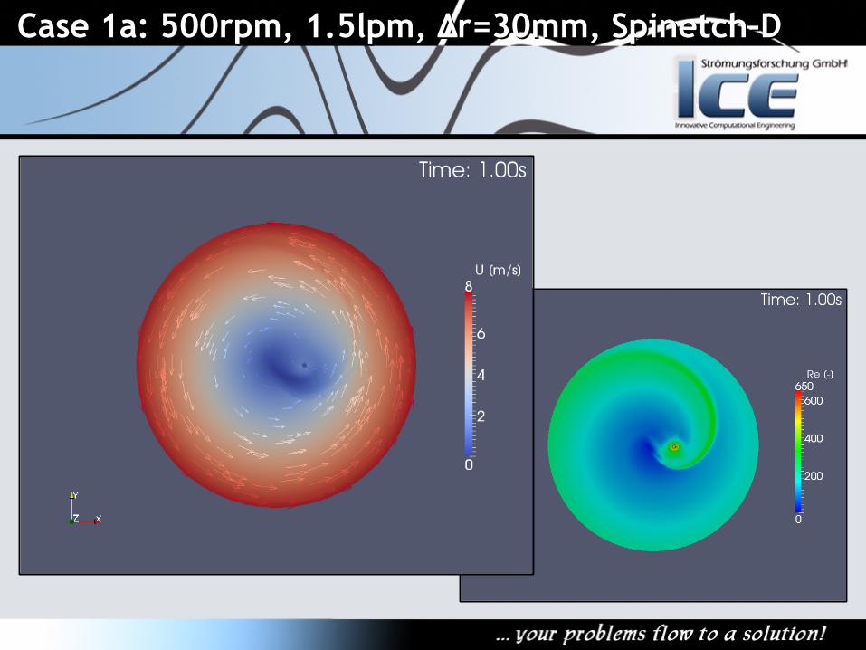
Case 1a: 500rpm, 1.5lpm, Case 1a: 500rpm, 1.5lpm, ΔΔr=30mm,r=30mm, Spinetch-D Spinetch-D

Case 2b: 500rpm, 1.5lpm, Case 2b: 500rpm, 1.5lpm, ΔΔr=50mm,r=50mm, water water

Case 2b: 500rpm, 1.5lpm, Case 2b: 500rpm, 1.5lpm, ΔΔr=50mm,r=50mm, water water
-0,15 -0,10 -0,05 0,00 0,05 0,10 0,150,0000
0,0002
0,0004
0,0006
0,0008
0,0010
0,0012
h (xz-Plane through Jet)
OpenFOAM 2.5D Fluent 3D
x [m]
h [m
]

Case 2b: 500rpm, 1.5lpm, Case 2b: 500rpm, 1.5lpm, ΔΔr=50mm,r=50mm, water water
-0,15 -0,10 -0,05 0,00 0,05 0,10 0,150,0000
0,0002
0,0004
0,0006
0,0008
0,0010
0,0012
h (yz-Plane through Jet)
OpenFOAM 2.5D Fluent 3D
y [m]
h [m
]

Case 2b: 500rpm, 1.5lpm, Case 2b: 500rpm, 1.5lpm, ΔΔr=50mm,r=50mm, water water

Case 2b: 500rpm, 1.5lpm, Case 2b: 500rpm, 1.5lpm, ΔΔr=50mm,r=50mm, water water
-0,15 -0,10 -0,05 0,00 0,05 0,10 0,150
5
10
15
20
25
30
35
40
45
50
τWafer (xz-Plane trough Jet)
OpenFOAM 2.5D Fluent 3D
x [m]
τWaf
er [P
a]

Case 2b: 500rpm, 1.5lpm, Case 2b: 500rpm, 1.5lpm, ΔΔr=50mm,r=50mm, water water
-0,15 -0,10 -0,05 0,00 0,05 0,10 0,150
5
10
15
20
25
30
35
40
45
50
τWafer (yz-Plane through Jet)
OpenFOAM 2.5D Fluent 3D
y [m]
τWaf
er [P
a]

Case 2b: 500rpm, 1.5lpm, Case 2b: 500rpm, 1.5lpm, ΔΔr=50mm,r=50mm, water water

ConclusionConclusion
• 2.5D solution shows a good agreement with 3D 2.5D solution shows a good agreement with 3D solution, while significantly saving on resourcessolution, while significantly saving on resources– Solution in an impingement area has to be prescribed– Zone close to jet, influenced by the impingement, is showing
a reasonable agreement and is still able to capture important effects
• We never promised to be exact there!– Zone outside of the impingement influence is showing a
very good agreement– Shear-stress prediction is good enough
• Important for a chemistry reactions– Smooth solution without fluctuations– Small meshes and significantly shorter simulation times

Outlook & DiscussionOutlook & Discussion
• OutlookOutlook– Dry spot handling– Impingement area
• Prescribing not only dependent variables, but as well the velocity profile function itself
– Velocity profile function• Prediction of the velocity boundary• Hydraulic jump modelling
– Would be great for comparison with experiments!
– Simple etching model• Prediction of the concentration boundary
• DiscussionDiscussion– Thank you for your attention! Questions?