third annual progress report, july 1976 by - pubs.usgs.gov · pdf filethird annual progress...

UNITED STATES DEPARTMENT OF THE INTERIOR

GEOLOGICAL SURVEY

GEOCHEMICAL SURVEY OF THE WESTERN ENERGY REGIONS (formerly Geochemical Survey of the Western Coal Regions)

Third Annual Progress Report, July 1976

By

U.S. Geological Survey Denver, Colorado

Open-file Report 76-729 1976

This report is preliminary and has not been edited or reviewed for conformity with U.S. Geological Survey standards or nomenclature

GEOCHEMICAL SURVEY OF THE WESTERN ENERGY REGIONS (formerly Geochemical Survey of the Western Coal Regions)

July 1976

Third annual progress report descrihing current work In a broad-scaled reconnaissance geochemical study of landscape materials in the major coal-, uranium-, and oil shale-bearing lands of the western United States.

CONTENTS Page

WORK TO DATE......................................................... 1

MOLYBDENUM IN SWEETCLOVER GROWING ON MINE SPOILSJames A. Erdman and Richard J. Ebens............................... 4

Cu/Mo ratios of 2 or less are common in sweetclover growing on both reclaimed and unreclaimed spoil materials in the Northern Great Plains. These ratios compare unfavorably with optimal levels of about 7 or greater in ruminant forage.

MINERALOGY OF FINE-GRAINED ROCKS IN THE FORT UNION FORMATIONTodd K. Hinkley and Richard J. Ebens............................... 10

Clay-rich rocks contain important amounts of quartz and minor amounts of plagioclase, K-feldspar, dolomite, calcite, siderite, and ankerite(?). The clay is predominantly chlorite and kaolinite.

STREAM SEDIMENT CHEMISTRY IN THE NORTHERN GREAT PLAINSJames M. McNeal.................................................... 14

The distribution of selected elements in these sediments is only weakly related to either stream order or size of drainage. Preliminary data suggest that the chemistry of sodium acetate extractions bears no predictable relation to bulk chemistry.

ELEMENTS IN LICHEN NEAR THE DAVE JOHNSTON POWERPLANTLarry P. Gough and James A. Erdman................................. 22

Se, F, and Sr are elevated in lichen samples collected within 3-10 km of the powerplant. Previous work demonstrated elevated levels of Se and Sr in sagebrush near this powerplant.

CHEMISTRY OF POWDER RIVER SEDIMENTSJohn R. Keith, Barbara M. Anderson, James M. McNeal and JosephineG. Boerngen........................................................ 30

Examination of elemental chemistry in four size fractions indicates that in general the geometric means tend to increase and the geo metric deviations decrease with decreasing grain size. An inter mediate size fraction may serve as the best geochemical "monitor" for secular change due to a general lack of large-scale downstream variation in this size fraction.

iii

Page

SOIL AND SAGEBRUSH CHEMISTRY NEAR THE JIM BRIDGER POWERPIANTBarbara M. Anderson and John R. Keith ............................. 37

Element trends were observed outward from this powerplant before it began operation. Such trends in soil likely reflect geologic control but some trends in sagebrush appear to reflect construction site activities.

GEOCHEMISTRY OF GREEN RIVER OIL SHALEWalter E. Dean .................................................... 48

A summary of recent work gives provisional estimates of trace- element abundances in this economic resource.

CHEMISTRY OF NORTHERN GREAT PLAINS SOILSRonald R. Tidball and Ronald C. Severson .......................... 57

Of 36 elements studied in these soils, about half exhibit signi ficant regional patterns but only C, Ca, K, Mn, Rb, and U exhibit more than a fifth of their total observed variation at this scale.

ELEMENTS IN WHEATGRASS, DAVE JOHNSTON MINEJames A. Erdman and Richard J. Ebens .............................. 82

Concentrations of Cd, Co, F, U, and Zn in wheatgrass growing on mine spoils ranged from 140-400 percent higher than in control samples.

GEOCHEMISTRY OF GROUND WATERS IN THE FORT UNION COAL REGIONGerald L. Feder and Lynda G. Saindon .............................. 86

Chemically, these waters are highly variable but only F and gross o> were measured at levels exceeding EPA interim primary drinking water standards.

GEOCHEMISTRY OF THE FORT UNION FORMATIONRichard J. Ebens and James M. McNeal .............................. 94

Preliminary work indicates that outcrops of both sandstone and shale in this formation contain about five times as much Na in Montana and North Dakota as in the southern Powder River Basin. C and Mg likewise are visibly low in outcrops of sandstone of the Southern Powder River Basin.

SOIL CHEMISTRY IN THE PICEANCE CREEK BASINCharles D. Ringrose, Ronald W. Klusman, and Walter E. Dean ........ 101

Surface soil from ridgetops and valley bottoms are chemically similar in this area. Be, Cu, Li, and Zn in soil show marked increases from north to south.

IV

Page

SOIL AND GRASS CHEMISTRY NEAR THE FOUR CORNERS POWERPLANTJon J. Connor, Barbara M. Anderson, John R. Keith, and Josephine G. Boerngen ......................................................

Element trends observed in soil southeast of this powerplant are attributed to substrate differences. Concentrations of many elements in grass increase near the powerplant with Se and F showing the strongest increases.

STREAM SEDIMENT CHEMISTRY IN THE OIL SHALE REGIONJames M. McNeal, Gerald L. Feder, Charles D. Ringrose and Ronald W. Klusman .......................................................

Regional geochemical variation is manifested largely as differ ences among drainages. Variation within drainages appears to exist mostly at scales less than 20 m or scales greater than 1 km.

SPECTROCHEMICAL COMPUTER ANALYSISArthur L. Sutton, Jr. ............................................

112

121

131

Multielement analysis of landscape materials by emission spectro-scopy has been streamlined through the use of an automated,computer-interpreted plate-reading technique.

REFERENCES CITED .................................................... 133

APPENDIX I.

APPENDIX II

APPENDIX III.

APPENDIX IV.

APPENDIX V.

Probable upper limits of element concentration to be expected in some ordinary landscape materials of the Powder River Basin.

Probable upper limits of element concentration to be expected in some ordinary landscape materials of the Northern Great Plains.

Probable upper limits of element concentration to be expected in some ordinary landscape materials of the Oil Shale Region.

Toxicity of selected elements to plants, animals, and man--an outline, by Larry P. Gough and Hansford T. Shacklette.

Chemical elements in vegetation and soils near coal- fired powerplants, Western Energy Regions.

Table 1. Surface and subsurface soil, and sage brush east of Dave Johnston Powerplant, Wyoming.

APPENDIX V. -- Continued.

Table 2, Lichen east and west of Dave Johnston Powerplant,Wyoming.

Table 3. Surface and subsurface soil and sagebrush at Jim Bridger Powerplant, Wyoming.

Table 4. Soil and grass southeast of Four Corners Powerplant, New Mexico.

VI

ILLUSTRATIONS Page

Figure 1. Index map showing location of the major coal basinsin the western United States....................... 2

2. Index map showing stream sediment sampling localitiesin the Northern Great Plains....................... 15

3. Index map showing lichen sampling localities east andwest of the Dave Johnston Powerplant, Wyoming..... 23

4. Regression trends in Parmelia chlorochroa for con centrations of fluorine, selenium, strontium, and ash progressing east from the Dave Johnston Power- plant .............................................. 26

5. Plot of the calcite to quartz X-ray diffraction peak intensity ratios from Parmelia chlorochroa ash against percent ash yield.......................... 28

6. Index map of the Powder River Basin, with samplinglocalities of Powder River stream sediments........ 31

7. Index map showing soil and sagebrush samplinglocalities for four traverses from the Jim Bridger Powerplant......................................... 40

8. Metal trends in ash of sagebrush north of the JimBr idger Powerplant, Wyoming........................ 43

9. Trends in dry weight of sagebrush north of the JimBridger Powerplant, Wyoming........................ 44

10. Trends in ash of sagebrush south and west of the JimBridger Powerplant, Wyoming........................ 45

11. Index map showing location of oil shale samples, distribution of the Green River Formation, and lease tracts C-a, C-b, U-a, and U-b................ 52

12. Concentration ranges and probable average values forminor elements in oil shale........................ 53

13. Computation of the coefficients, a^, for the variancemean ratio, vm................................. 0 ... ^f

14. Dunean f s classes for elements of group A(a)2 and observed ranges of 100-km cell means for each terrain............................................ 65

vtl

ILLUSTRATIONS, continued

PageFigures 15-27. Regional distribution of elements in soils of the

Northern Great Plains:

15. Carbon (total), A-horizon ................. 67

16. Carbon (total), C-horizon ................. 68

17. Magnesium, C-horizon ...................... 69

18. Rubidium, A-horizon ....................... 70

19. Rubidium, C-horizon ....................... 71

20. Sodium, A-horizon ......................... 72

21. Zinc, A-horizon ........................... 73

22. Calcium, C-horizon ........................ 74

23. Potassium, A-horizon ...................... 75

24. Potassium, C-horizon ...................... 76

25. Silicon, A-horizon ........................ 77

26. Thorium, A-horizon ........................ 78

27. Uranium, A-horizon ........................ 79

28. Index map showing locations selected for samplingwell water in the Northern Great Plains ............. 87

29. Index map showing sampling localities of shale and sandstone in the Fort Union Formation in the Northern Great Plains Coal Province ................. 96

30. Regional distribution of Na 2 0 in sandstone and shaleof the Fort Union Formation ......................... 99

31. Regional distribution of carbon (total) and MgO insandstone of the Fort Union Formation ............... 100

32. Index maps showing soil sampling localities in thePiceance Creek Basin, Colorado ...................... 102

Vlll

ILLUSTRATIONS, continued

PageFigures 33-35. Regional element distributions in soils of the

Piceance Creek Basin:

33. Iron and beryllium ........................ 108

34. Copper and lithium ........................ 109

35. Zinc ...................................... 110

36. Index map showing sampling localities of soil and grass southeast of the Four Corners Powerplant, Mexico .............................................. 113

Figures 37-40. Element concentrations in grass as a function of dis tance from the Four Corners Powerplant:

37. Selenium, fluorine, and sulfur ............ 117

38. Ash, and silicon, potassium, andcalcium in ash of grass ................. 118

39. Cobalt, lithium, and sodium in ash ofgrass ................................... 119

40. Molybdenum, nickel, boron, gallium, strontium, and magnesium in ash of grass ................................... 120

41. Index map showing stream sediment sampling localities in the Piceance Creek and Uinta Basins, Colorado and Utah ............................................ 122

42. Methods of total element analysis adopted for rocks,soils, and plants ................................... 132

ix

TABLES

Page Table 1. Copper and molybdenum in sweetclover and pH in spoil

materials from eight coal mines in the Northern Great Plains.................................................. 8

2. Statistical summary of the mineral composition of fine grained rocks cored from the Fort Union Formation, Northern Great Plains Province.......................... 12

3. Geochemical variation in stream sediments of the NorthernGreat Plains............................................ 17

4. Regression statistics for those elements and ash inParmelia chlorochroa found to be related to distancefrom the Dave Johnston Powerplant....................... 25

5. Statistical analysis of partial chemistry of the PowderRiver sediments......................................... 33

6. Percent of total observed logarithmic variance in sage brush and soil constituents accounted for in terms of logarithmic distance from the Jim Bridger Powerplant.... 42

7. Geochemical summary of data from sagebrush around theJim Bridger Powerplant, Wyoming......................... 47

8. Ranges, geometric means, and geometric deviations of con centrations of selected elements in Green River oil shale................................................... 49

9. Variance components expressed as percentages of total variance in samples of two horizons of soils in the Northern Great Plains and variance mean ratios for 100-km cells............................................ 58

10. Geochemical summaries for selected elements in soils ofthe Northern Great Plains............................... 63

11. Statistical analysis of element concentrations in the ash of crested wheatgrass from topsoil borrow areas and from reclaimed spoil areas at the Dave Johnston Mine, southern Powder River Bas in, Wyoming.................... 84

12. Analysis of logarithmic variance for ground waters of theFort Union Formation, North Dakota and Montana.......... 89

TABLES (continued)

Page

Table 13. Geochemical summary of ground water from the Fort UnionFormation, North Dakota and Montana .................... 91

14. Statistical analysis of the chemistry of shale and sand stone of the Fort Union Formation, Northern Great Plains Coal Province .......................................... 98

15. Analysis of variance of surface soil chemistry, PiceanceCreek Basin, Colorado .................................. 104

16. Geochemical summary of surface soil in the Piceance CreekBasin, Colorado ........................................ 106

17. Regression analysis of elements in soil and grass or its ash southeastward of the Four Corners Powerplant, New Mexico ................................................. 115

18. Analysis of variance results, summary statistics, and geochemical baselines for stream sediments of the Piceance Creek and Uinta Basins, Colorado and Utah ..... 124

19. Summary statistics for Asphalt Wash and Cottonwood Wash of Uinta Basin, and Duck Gulch and Ryan Gulch of Piceance Creek Basin ................................... 127

20. Geochemical summary for stream sediments of Roan andBlack Sulfur Creeks, Colorado .......................... 128

XI

******************************** *^ The term "statistically significant" appears often in . ^ scientific literature-tiotably and sometimes confusingly ^ in sampling studies that hold implications for public ^ policy. Understanding its narrow meaning, as an element ^ in the interpretation of degrees of scientific proof, is . ^ essential to grasping the import of a scientific state-

ment bearing on public policy.

**

* * ^ Generally, a sampling result or experimental result is^ deemed "statistically significant" when the calculated ^ probability of its being solely an artifact of chance is ^ below a specified low value. Many scientists disagree on ^ ^ what that low value should be. Customarily, many regard ^ ^ as "statistically significant" a result for which the ^ probability of occurrence as a consequence of pure chance

is less than five percent (the "0.05 probability level"). . ^ This concept is intended to reduce the likelihood that a ^

result may be interpreted as attributable to factors ^ under study when it may be, in fact, the happenstance of ^, a random distribution. ^ ^ (Adapted from the National Academy of Sciences' "News ^* Report," Mid-June, 1976, v. XXVI, no. 8, p. 6) ** ********************************

xii

WORK TO DATE

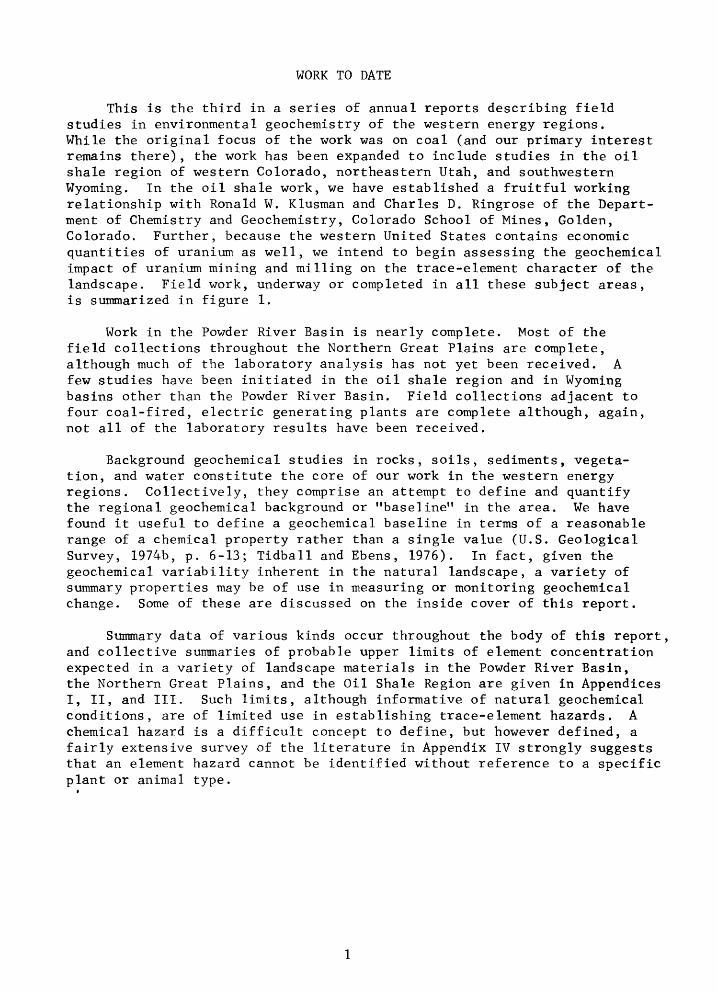
This is the third in a series of annual reports describing field studies in environmental geochemistry of the western energy regions. While the original focus of the work was on coal (and our primary interest remains there), the work has been expanded to include studies in the oil shale region of western Colorado, northeastern Utah, and southwestern Wyoming. In the oil shale work, we have established a fruitful working relationship with Ronald W. Klusman and Charles D. Ringrose of the Depart ment of Chemistry and Geochemistry, Colorado School of Mines, Golden, Colorado. Further, because the western United States contains economic quantities of uranium as well, we intend to begin assessing the geochemical impact of uranium mining and milling on the trace-element character of the landscape. Field work, underway or completed in all these subject areas, is summarized in figure 1.

Work in the Powder River Basin is nearly complete. Most of the field collections throughout the Northern Great Plains are complete, although much of the laboratory analysis has not yet been received. A few studies have been initiated in the oil shale region and in Wyoming basins other than the Powder River Basin. Field collections adjacent to four coal-fired, electric generating plants are complete although, again, not all of the laboratory results have been received.

Background geochemical studies in rocks, soils, sediments, vegeta tion, and water constitute the core of our work in the western energy regions. Collectively, they comprise an attempt to define and quantify the regional geochemical background or "baseline" in the area. We have found it useful to define a geochemical baseline in terms of a reasonable range of a chemical property rather than a single value (U.S. Geological Survey, 1974b, p. 6-13; Tidball and Ebens, 1976). In fact, given the geochemical variability inherent in the natural landscape, a variety of summary properties may be of use in measuring or monitoring geochemical change. Some of these are discussed on the inside cover of this report.

Summary data of various kinds occur throughout the body of this report, and collective summaries of probable upper limits of element concentration expected in a variety of landscape materials in the Powder River Basin, the Northern Great Plains, and the Oil Shale Region are given in Appendices I, II, and III. Such limits, although informative of natural geochemical conditions, are of limited use in establishing trace-element hazards. A chemical hazard is a difficult concept to define, but however defined, a fairly extensive survey of the literature in Appendix IV strongly suggests that an element hazard cannot be identified without reference to a specific plant or animal type.

Fort Union

North Dakota

Figure 1. Location of the major coal basins in the western United States (modified from Trumbull, 1960). Approximate distribution of Green River Formation is cross-hatched.

Figure 1 EXPLANATION

Map unit Material sampled Reference

1. Northern Great

2. Powder River Basin

3. Bighorn, Wind River Basins

4. Oil Shale Region

5. Western United States

o

x

A

A

Sandstone, shaleSoilStream sedimentsGround waterWheat

Sandstone, shaleSoil, soil parent, sagebrush,lichen, grass

Sediments (Powder River)

Soil

Oil shaleSoilStream sediments

Sagebrush (west of line)

Strip-mine spoils, sweetclover,wheatgrassMines: 1. Dave Johnston; 2.Welch; 3. Big Sky: 4. Savage;5. Beulah; 6. Velva; 7. Kincaid;and 8. Utility.

Shale, cored overburden (Cores: 1. Bear Creek; 2. Otter Creek; 3. Dengate; 4. Dunn Center; 5. Estevan.)

Ground water

Vegetation (S, sagebrush; M, mixed feed grains)

Coal-fired powerplants (C, Colstrip; J, Jim Bridger; D, Dave Johnston; F, Four Corners)

Uranium mill

This report, p, 10-13, 94-100This report, p. 57-81This report, p. 14-21This report, p. 86-93This report, Appendix II.

This report, p. 10-13, 94-100 (See U.S. Geol. Survey, 1974, 1975; Connor, Keith, and Anderson, 1976; Tidball and Ebens, 1976.) This report, p. 30-36

(No data as yet)

This report, p. 48-56This report, p. 101-111This report, p. 121-130

(No data as yet)

This report, p. 4-9, 82-85

(See U.S. Geol. Survey, 1975,)

This report, p. 10-13

(See U.S. Geol. Survey, 1974, 1975.)

(No data as yet)

This report, p. 22-29, 37-47, 112-120. (See also U.S. Geol Survey, 1974, 1975; Connor, Keith, and Anderson, 1976)

(No data as yet)

MOLYBDENUM IN SWEETCLOVER GROWING ON MINE SPOILS by James A. Erdman and Richard J. Ebens

Introduction

New environmental regulations governing the strip-mining of coal on federally owned lands in the West contain mining and reclamation performance standards designed to insure that miners leave the land in at least as good condition as they found it (Holden, 1976). The area of the Northern Great Plains within the lignite and subbituminous regions is predominantly rangeland although dryland cropping principally small grain production is also an important agricultural activity. Thus, the intent of these reclamation standards is to assure the rehabilitation of surface-mined lands for agricultural production, providing such areas had been rangeland or cropland before ruining began.

Most assessments of the possible geochemical alteration of surface- mined lands deal with revegetation problems; that is, attempts to provide plant cover as quickly as possible in order to minimize soil erosion. (See, for example, Sandoval and others, 1973; Berg and Vogel, 1973.) Such problems are of immediate and valid concern, but altered physical properties or changes in trace element concentrations that may prove deleterious or harmful to livestock ranging on the reclaimed lands must also be considered. Because of our experience with adverse effects of a clay-mining operation on cattle in Missouri (Ebens and others, 1973), we set out to examine the element composition of coal-mine spoil materials and sweetclover (Melilotus officinalis (L.) Lam. or M. alba Desr.) from eight selected coal mines in the Northern Great Plains. Some preliminary results of that study are given in U.S. Geological Survey (1975, p. 29-35). Whereas the main purpose of this study was to assess the degree of differ ences and similarities for a large suite of elements among the eight mines, our intent here is to describe the potential of sweetclover that grows on spoil materials as a causative agent of molybdenosis in certain livestock.

Coal-mine spoils are geochemically anomalous when compared to naturally occurring surficial materials (Sandoval and others, 1973). Despite the increasing practice of top-soiling contoured spoil banks, we find evidence that these anomalies are being reflected in the element composition of vegetation that grows on this modified substrate. This appears to be the case at least for sweetclover, which is a common and often dominant plant over many of the spoil banks in the Northern Great Plains.

Molybdenosis is a copper-deficiency disease that is well-documented in cattle and sheep; in the latter case, it is called swayback disease of lambs (Alloway, 1973). Generally, excessive amounts of molybdenum in the diet result in a decrease in the physiological availability of copper. Characteristic symptoms in cattle are scouring, weight loss, loss of pig mentation, and in some cases, breeding difficulties. Calves are most susceptible, the effects often being irreversible (Barshad, 1948). Horses are reported to be unaffected.

The total molybdenum in soil where cattle have been known to be affected is not high, ranging from 1.5-10 ppm in the study described by Barshad (1948). In alkaline soils, however, a large percentage of this element may be soluble in water. Barshad (1948) stated, "Growing plants, particularly legumes, are able to absorb amounts of molybdenum harmful to cattle from soils that contain as little as 1.5-5.0 ppm total Mo."

The proportion of copper to molybdenum in the forage is considered to be more critical than the total amount of molybdenum in either the soil or plants. Copper-to-molybdenum ratios of about 5:1 or less in winter herbage from the British Isles have caused swayback in lambs and hypocuprosis in cattle (Alloway, 1973). A copper-to-molybdenum ratio of about 7:1 is apparently optimum for cattle, according to the University of Missouri's veterinary toxicologist, A. A. Case (written communication,1974). Similar ratios were cited by Alloway (1973) for control farms. Clearly, where legumes are a substantial part of the pasturage in molybdic and alkaline soils, certain types of livestock can be severely affected.

Concern over the possible incidence of molybdenum-induced imbalances in animals grazing in regions associated with coal utilization is not new, although more information seems to be available on the effects of fly ash on the content of forage than on the effects of coal-mine spoils (Furr and others, 1975; Gutenmann and others, 1976). The only documented case of molybdenosis in cattle from the western coal regions is the report by Christianson and Jacobson (undated), which describes an area where uraniferous lignite was burned in rotary kilns in order to concentrate the uranium, and the molybdenum in the ash contaminated the surrounding pasturage. The most recent interest in molybdenum-related nutritional problems was expressed by Martens and Beahm (1976) who cautioned, "Molyb denum availability of some fly ashes is sufficiently high that levels in plants grown on fly-ash soil mixtures can be hazardous to grazing animals."

There are reasons for our interest in sweetclover and its molybdenum- accumulating potential other than its abundance and widespread occurrence on the coal-mine spoils that we studied. Legumes are recommended in seed mixes for reclamation because of their nitrogen-fixing capabilities, and sweetclover, in particular, is considered one of the more suitable plant species for spoil bank stabilization. Finally, the forage value of sweetclover rates very high. According to A. A. Case (written communication,1975), "Sweetclover is a wholesome and very nutritious legume, ranking along with other clovers in its nutritional value, perhaps just less than alfalfa, which is considered the 'queen' of legumes for forages and hay purposes." Although under most circumstances, sweetclover is not considered a toxic plant, Case does warn of changes that can occur where it grows in altered environments.

Methods

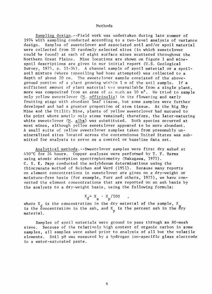
Sampling design.--Field work was undertaken during late summer of 1974 with sampling conducted according to a two-level analysis of variance design. Samples of sweetclover and associated soil and/or spoil material were collected from 10 randomly selected sites (in which sweetclover could be found) at each of eight surface mines scattered throughout the Northern Great Plains. Mine locations are shown on figure 1 and mine- spoil descriptions are given in our initial report (U.S. Geological Survey, 1975, p. 33-34). A channel sample of spoil material or a spoil- soil mixture (where topsoiling had been attempted) was collected to a depth of about 20 cm. The sweetclover sample consisted of the above- ground portion of a plant growing within 1 m of the soil sample. If a sufficient amount of plant material was unavailable from a single plant, more was composited from an area of as much as 10 m 2 . We tried to sample only yellow sweetclover (M. officinalis) in its flowering and early fruiting stage with abundant leaf tissue, but some samples were further developed and had a greater proportion of stem tissue. At the Big Sky Mine and the Utility Mine, plants of yellow sweetclover had matured to the point where mostly only stems remained; therefore, the later-maturing white sweetclover (M. alba) was substituted. Both species occurred at most mines, although yellow sweetclover appeared to be more abundant. A small suite of yellow sweetclover samples taken from presumably un- mineralized sites located across the conterminous United States was sub mitted for analysis to serve as a control or baseline data set.

Analytical methods.--Sweetclover samples were first dry ashed at 450°C for 24 hours. Copper analyses were performed by T. F. Harms using atomic absorption spectrophotometry (Nakagawa, 1975). C. S. E. Papp conducted the molybdenum determinations using the thiocyanate method of Reichen and Ward (1951). Because many reports on element concentrations in sweetclover are given on a dry-weight or moisture-free basis (for example, Furr and others, 1975), we have con verted the element concentrations that are reported on an ash basis by the analysts to a dry-weight basis, using the following formula:

X = X X /100 dapwhere X, is the concentration in the dry material of the sample, Xis the concentration in the ash, and X is the percent ash in the try

.1 P material.

Samples of spoil materials were ground to pass through an 80-mesh sieve. Because of the relatively high content of organic carbon in some samples, all samples were ashed prior to analysis of all but the volatile elements. Soil pH was measured by a hydrogen ion-specific glass electrode in a water-saturated paste.

Results and discussion

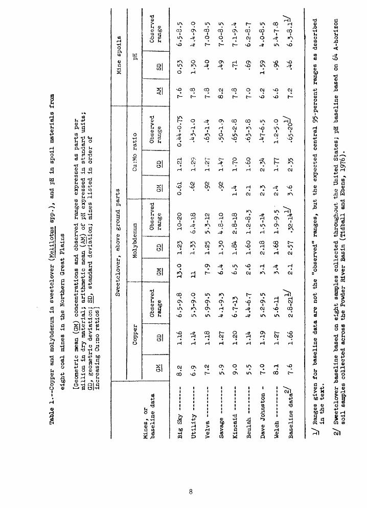
Concentrations of copper and molybdenum were transformed to a logarithmic scale prior to evaluation because their frequency distri butions were more nearly symmetrical on a logarithmic scale than on an arithmetic scale. Under these circumstances, the geometric mean (GM) is the best estimate of the most probable metal concentration. The geometric deviation (GD) is a factor expressing the degree of total variability measured. The expected 95-percent range given for the base line data estimates the range that 95 percent of a suite of randomly collected samples from normal environments should exhibit. Anomalous concentrations are those that lie outside this range. The estimated range of the central 95 percent of the observed distribution has a lower limit equal to GM/(GD) 2 and an upper limit equal to GM-(GD) 2 .

Table 1 lists the summary statistics for copper and molybdenum in sweetclover, and the pH of the spoil material. Because of the importance of the CutMo ratio, we have ranked the mines in increasing value of the ratio. Analysis of variance tests demonstrate significant differences (p<0.05) among the mines for all four variables; but a multiple range test (Duncan, 1955) failed to group the means further, with the exception of molybdenum in sweetclover. Results of the test revealed two distinct groups of sweetclover with respect to its molybdenum content. The Beulah, Dave Johnston, and Welch mines comprised one group with means ranging from 2.6-3.4 ppm Mo in dry material, and the other five mines comprised the other group with means ranging from 6.4-13 ppm.

In comparing the statistics between the mines and the baseline data, it is apparent that the concentrations of copper in sweetclover and the levels of pH in the mine samples and baseline samples are not notably different. However, certain sweetclover samples from several mines show unusually high molybdenum contents and unusually low Cu:Mo ratios. Half of the samples from both the Big Sky and Utility mines had ratios below baseline (the expected 95-percent range). Many spoil samples from all mines are either anomalously high or low in pH.

Even more important, mines having the lowest molybdenum averages in sweetclover are the same mines with decidedly lower pH in the spoil materials. Inasmuch as molybdenum is often much more available to legumes where soils are alkaline (Case, 1974), we computed the correla tion between the concentration of molybdenum in sweetclover and the pH levels in the associated spoil materials. The resulting correlation coefficient--0.46--is significant at the 0.01 probability level, although it does not indicate a particularly strong relationship.

Finally, a test was made of differences in copper and molybdenum concentrations between yellow and white sweetclover based on paired samples collected at each of 12 sites (cf. U.S. Geol. Survey, 1975, p. 31). The two species varied significantly in their molybdenum content at the 0.05 probability level but not in their copper content. White

oo

Table

1.--

Copp

er and mo

lybdenum i

n sveetclover

(Kel

ilot

us spp.), an

d pH

in sp

oil

materials

from

eigh

t coal m

ines in

the

No

rthe

rn Gr

eat

Plai

ns

[Geo

metr

ic me

an (GM) co

ncen

trat

ions

an

d ob

serv

ed ra

nges

ex

pres

sed

as pa

rts

per

million

in dr

y mate

rial

; ar

ithm

etic

mea

n (AM) of

pH

expr

esse

d in st

andard uni

ts;

GD,

geometric

deviat

ion;

SD

, st

anda

rd deviation; mines

list

ed in or

der

of

increasing Cu:iao ra

tios

]

Min

es,

or

bas

elin

e dat

aGM

Big

Sk

y

8.2

TT

H 1

-f-

f-v

-------

A

Q

Vel

va

7.2

VI nnnl

r! -------

Q

O

Beu

lah

5.5

Dav

e Jo

hn

sto

n -

7*0

Wel

ch

8.1

2/

Bas

elin

e d

ata-

^ 7

'6

Obs

erve

d GD

ra

nge

1.16

6-

5-9.

8

1 il

l ^

^-Q

O

X . J

.H

^ .

y

V

1 1

ft

e; Q

_Q

^_L

. .L

O

P

* 7

>

/

X

1.2

7

4.1

-9.3

IO

iO

£.

*7

T "

X.<

£U

O .

(-1

.5

T ik

k

k-A

7

-L . a

.1*

«r . «*

V

J .

{

1.19

5.

2-9.

5

1.27

5*

6-11

1.66

2.8

-2li

/

GM 13-0

11 7-9 6.4

6.5

2.6

3.1 ,

j . *

2.1

GD

1.2

3

1-33

1.2

5

1.3

0

\ ft

liJ_

»^J"

r

1.6

0

2.18

1 68

A w

w

2.5

7

Obs

erve

dra

nge

10-2

0

6.4-

18

5-3-

12

4.8-

10

2Q

T

Q

O-l

O

T

O

Q

1L

.d-O

.J

1.5-

14

1.9-

9-5

^

GM 0.6

1

.62

.92

.92

1.4

2.1 2.3

2.4 3.6

GD

1.2

1

1.2

9

1.2

?

1.4

7

1-70

1.6

0

2.3

4

1-77

2.3

5

Obs

erve

dra

nge

AM

0)1

)1

o

vc

7

A.*

4-*

r W

. (y

(

.O

43-1

0

78

£.1

1

li nr

d

.O3-

1.**

7«

o

cf\

1

r*

Q

oO

U-J

L.y

O

.t;

£.er

rt

O

'i

Q.0

5-2

.0

7*O

^"2

jt

Q

T

/"

\.6

3-3.

0 7.

0

.47-

6.5

6.2

1.2-

5.0

6.6

.65-

20-^

7.

2

Obs

erve

d SD

ra

nge

0.53

6

.5-8

.5

1.3

0

4.4

-9.0

.40

7.0

-8.5

.49

7.0

-8.5

.71

7.1

-9-4

Ao

A p.P

7

. \Jy

\J

£ o

. {

1.5

9

4.0

-8.5

.96

5

-4

-7

-8

M

6-'-

8'li

/

I/ R

anges

given

for

base

line

da

ta a

re no

t th

e "observed" ranges,

but

the

expe

cted

central

95~P

ercent ra

nges

as described

in th

e te

xt.

2/ Sv

eetclover ba

seli

ne b

ased o

n eight

samples

coll

ecte

d th

roug

hout

th

e Un

ited

St

ates;

pH b

asel

ine

based

on 6

4 A-horizon

soil

samples

coll

ecte

d across

the

Povd

er R

iver

Basin

(Tidball an

d Eb

ens,

19

76).

sweetclover contains almost twice as much molybdenum as does yellow sweetclover; their copper contents, on the other hand, are about the same. Similar comparisons by Barshad (1948)--although not based on paired observations also indicated that white sweetclover accumulates more molybdenum than does yellow sweetclover. Despite the significant differences between sweetclover species, the multiple group test (Duncan, 1955) did not separate the Big Sky and Utility mines where we collected white sweetclover from those where we collected yellow sweetclover. Moreover, spoil at most mines that we sampled supported both species.

Conclusions

Molybdenum concentrations in sweetclover growing on coal-mine spoil banks in the Northern Great Plains are probably sufficiently high to in duce metabolic imbalances in cattle and possibly sheep in subclinical, if not acute, levels, assuming the animals were to feed predominantly on this legume. Alloway (1973) considered that a copper to molybdenum ratio less than five may induce swayback in sheep and hypocuprosis in cattle; the ratios of these elements in sweetclover from the mines in this study are considerably below this threshold. A tolerance level for cattle of five ppm molybdenum in dry forage (Webb and Atkinson, 1965) is exceeded by sweetclover at all but the Beulah, Dave Johnston, and Welch mines. In mine areas where molybdenosis may be a potential problem, wholesome pasturage can be established by avoiding molybdenum-accumulat ing plant species, or by minimizing access to the fresh forage which can cause greater injury than properly cured material (Barshad, 1948). Molybdenum-induced copper imbalances in the diet may also be prevented by treating the affected livestock with either copper sulfate or copper glycinate.

It may be difficult, if not impossible, to prevent potentially hazardous geochemical environments in some surface-mining operations. But with the proper management of reclaimed areas, mining need not be precluded.

MINERALOGY OF FINE-GRAINED ROCKS IN THE FORT UNION FORMATION by Todd K. Hinkley and Richard J. Ebens

The rearrangement of rock strata during mining and reclamation commonly exposes originally buried strata to weathering processes which may accelerate chemical release. Shale or mudstone is the most abundant rock type in coal overburden in the Northern Great Plains Coal Province and is most likely to appear as a major constituent of a reclaimed land scape. A knowledge of the mineralogical variability of this rock type may lead to a better understanding of the environmental needs for handling such strata during, or following, strip mining.

The most prominent aspect of mineral variability in these rocks is, of course, reflected as vertical changes among the strata comprising the overburden at any given location. A second and perhaps equally important aspect is the change from place to place over the province of some average mineral property of the overburden column. This second aspect is largely obscured by the magnitude of the first. Nevertheless, the distinctive chemical differences that have been noted in sweetclover substrate among eight strip mines (U.S. Geological Survey, 1975, p. 29-35) suggest that such overburden may vary in its mineralogy in a geographic as well as a stratigraphic sense.

The present report describes an attempt to quantify the magnitude of this geographic variation in these rocks. A suite of fine-grained samples was taken from cores drilled through the overburden sections of strippable coal deposits in rocks of the Fort Union Formation or equiva lents. These samples have been used to estimate the mineralogical variation of the fine-grained rocks over two geographic and one stratigraphic scales: 1) distances greater than 5 km, 2) distances from 0-5 km, and 3) distances across the rock column of less than 100 m (stratigraphic variation).

Sample sites and sampling design

Samples were taken from each of five widely separated sites (>50 km), two in southeastern Montana, two in southwestern North Dakota, and one in southeastern Saskatchewan (fig. 1). At each site, four rock samples were taken from each of two drill holes which were separated by 1-5 km. The samples taken from each core were stratigraphically separated by 0-100 m and consisted of 30 cm of a homogeneous stratum of shale or mudstone. Only three samples were collected from each of the two drill holes at Estevan, Saskatchewan, because of the paucity of fine-grained horizons in these cores. In all, 38 samples were collected. Twelve samples were split and submitted in duplicate to test analytical reliability as distinct from geographical variability, bringing the number of actual analyses to 50.

Cores from three of the five sites (Bear Creek and Otter Creek, Montana, and Dunn Center, North Dakota) were obtained through the

10

Energy Minerals Rehabilitation Inventory and Analysis (EMRIA) program of the U.S. Bureau of Land Management, which program is intended to gather a variety of environmental information at potential coal-mining sites. Cores from Dengate, North Dakota were obtained from C. S. V. Barclay of the Conservation Division, U.S. Geological Survey. Cores from Estevan, Saskatchewan were obtained from the Industrial Minerals Division, Department of Mineral Resources, Saskatchewan.

Analytical methods

Samples were semi-quantitatively analyzed for mineral composition by an X-ray diffraction method similar to that described by Schultz (1964). The rocks were crushed in a jaw crusher and then ground in a vertical Braun pulverizer with ceramic plates set to pass 80 mesh. These were further ground in an agate mortar for three minutes. Final sample preparation and diffractograms were done by D. Gautier, using a slit width continuously variable with 29. The mineral concentrations are summarized in table 2.

Scales of variation

Regional variation.--Three of the mineral constituents (quartz, kaolinite, chlorite) exhibit significant variation at the highest geographic, or regional, level, indicating the existence of truly regional and possibly mappable mineralogical and chemical trends in the Northern Great Plains. These regional differences may be due to broad- scale differences in the environments of deposition, broad-scale hydrologic regimes, or even secular or fossilized weathering effects. In addition, plagioclase, dolomite, and calcite, vary significantly at the regional level when the top level variance is compared with two or more of the lower levels combined (pooled variance). From the small amounts of chemical data available to date in this study, it is clear from a basic comparison of mean abundance values by region that the values for plagio clase (and one of its chemical constituents, Na 2 0) are highest at the same two sites, Dengate, South Dakota and Estevan, Saskatchewan. Similarly, dolomite and MgO are highest at the same site, Otter Creek, Montana.

Local variation.--Essentially no mineralogical variation exists between the paired holes (1-5 km separation) within the individual sites. This indicates that the mineralogy (and presumably chemistry, also) is consistent in overburden over areas approximately the size of a strip mine in this part of the western coal regions. If the geochemical properties at this scale are as uniform as the mineralogical, then chemical character ization of such rocks over areas a few kilometers across becomes a relatively easy matter. For example, detailed analysis in only two or three scattered cores should suffice, and large (and expensive) drilling programs may be mostly wasted effort. Variation among samples taken across the strata (within the cored sections) is large compared to the other components of variation as is expected in layered rocks.

11

Table

2. -Statistical

summary

of th

e mi

nera

l composition

of fine-grained rocks

core

d

from t

he F

t. Union

Formation, No

rthe

rn Gre

at Plains Coal Province

[*,

indi

cate

s si

gnif

ican

ce of

the

variance co

mpon

ent

at th

e 0.05

prob

abil

ity

level;

p,

indicates

significance of a

pooled v

aria

nce]

Mineral

constituent

Total

loglo

variance

Components as

pe

rcen

t of to

tal

variance

Among

site

sBe

twee

n holes

Among

samp

les

Betw

een

anal

ytic

al

duplicates

Summ

ary

stat

isti

cs

Geometric

mean

(per

cent

)

Geometric

deviation

Minimum

Maximum

Quar

tz

Plag

iocl

ase

K-fe

ldsp

ar

Tota

l cl

ay

Kaol

init

e 1

Chlorite

Dolo

mite

Calcite

Side

rite

Mixe

d carbonate

0.0254

.0899

.076

7

.0225

.181

.492

.552

.356

.335

.195

34. 9*

. p

28p 4.8

16.2

58*,

p

56. 9*, p

21. 5p

14. 7p

7.9

0.0

0.0

0.0

0.0

0.0

0.0

0.0

0.0

0.0

0.0

6.4

59.2

57.1

*

15.4

75.8

*

41.9*

42.7

*

55.9

*

41.8

65.1*

93.6*

5.9

14.9

79.7 8

.1 .4

22.6

43.6

27 0.0

25.7 3.51

U65

47.2 5.20

18.5 1.56 .73

.66

.31

1.44

1.99

1.89

1.41

12.2 5.03

5.54

3.95

3.79

2.77

14.0 1

< .25

12 < .25

< .2

5

< .2

5

< .2

5

< .2

5

< .2

5

49.0

10

6

80 80 65 33 10 20 22

Analytical variation.--For several of the minerals determined, major variation occurs at the fourth or analytical level. This repre sents a lack of consistency between analytical duplicates and is due in part to proximity of key mineral peaks on the diffractograins. In general, for the rocks of this study, the minerals which are present in the lowest concentrations (K-feldspar, carbonates) are the ones most affected by analytical variation. They are the most sensitive to chart-reading errors, which yield mineral abundance errors of high fractional magnitude, whereas those present in highest concentrations (clays, quartz) are the least affected.

Mineralogy of the rocks

Quartz, the two carbonate minerals calcite and dolomite, and the two clay minerals kaolinite and chlorite, all vary regionally, and the abundances for each mineral between the high and low sites may be com pared. Judging by the geometric means at individual sites, quartz is at a maximum at Otter Creek, Montana (geometric mean of 31.6%) and a minimum at Dengate, North Dakota (19.1%). Calcite and dolomite have their highest geometric means at Otter Creek, Montana (values of 1.76% and 6.04%, respectively) and lowest geometric means at Dear Creek, Montana (0.35% and 0.39%). Total clay does not vary regionally, but its two main constituents in the mineral scheme of this study, kaolinite and chlorite, show regional variation. The site highest in chlorite, Estevan, Saskatchewan (geometric mean of 52.3%,), is also the one lowest in kaolinite (0.96%). Bear Creek, Montana is both lowest in chlorite (GM of 1.8%) and highest in kaolinite (39.6%). In the absence of evidence for different authigenic processes in the various sites, this observation of an inverse abundance pattern for the two clays in these fine-grained rocks indicates different provenances for the different sites. A regional variation in a clay ratio of this sort may well result in a distinctive distribution of elements held in those clays.

The distribution patterns for siderite and "mixed carbonate" (probably ankerite), the two minor carbonates of the mineral scheme, are too irregular to be considered in the same manner as the other minerals. Both are totally absent from most samples, and "mixed carbonate" is present only at Dengate, North Dakota and Estevan, Saskatchewan.

13

STREAM SEDIMENT CHEMISTRY IN THE NORTHERN GREAT PLAINS by James M. McNeal

One expected geochemical impact of large-scale, coal-based, energy development in the western United States is a change in the mineral and chemical character of the sediment in streams draining strip-mined areas. As with other components of the geochemical landscape, if such expected changes are to be monitored, a regional background or baseline must first be established. A necessary prerequisite to establishing such a baseline in an efficient manner, however, is concrete knowledge of the geographic scale of variation in those sediments. This study was undertaken to pro vide such information using a specific size fraction of stream sediments from the Northern Great Plains. Preliminary results for eight chemical properties are presented here.

There are two objectives of this study. The first was to determine whether or not stream order and size of drainage basin are important parameters in defining different populations of sediments, and the second was to determine the magnitude of the regional geochemical variability of the sediments. To this end, data collected to date were analyzed in two analysis of variance designs.

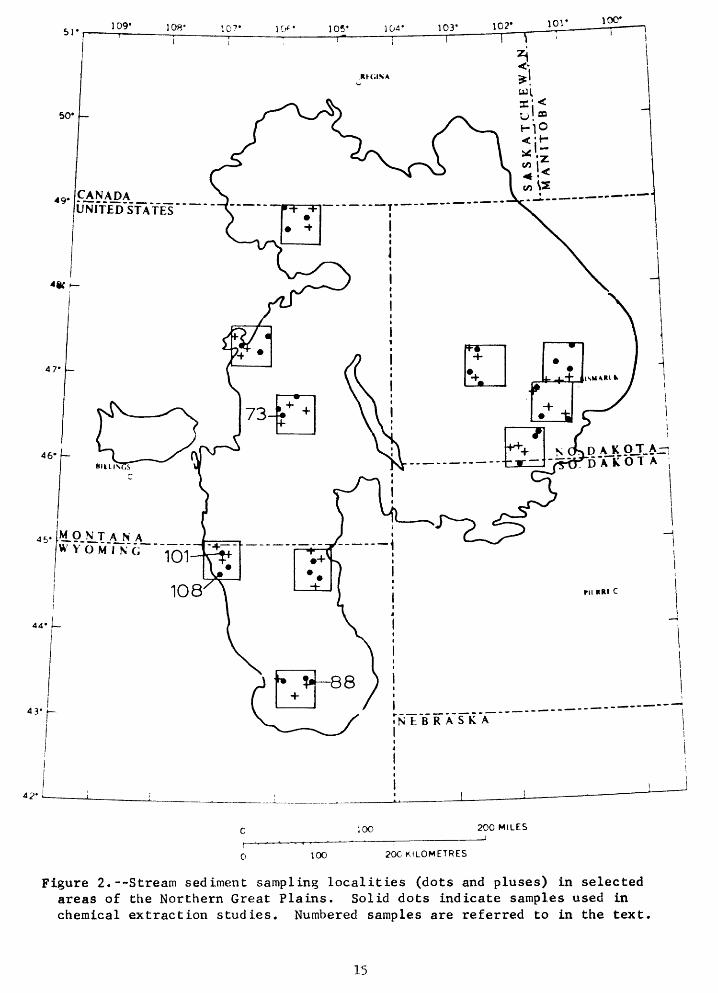
Three target populations were defined: sediments in first, second, and third order streams, as shown on 1/1,000,000 scale topographic maps. A first order stream is an upstream, unbranched stream segment; a second order stream extends downstream from the junction of two first order streams; a third order stream extends downstream from the junction of two second order streams (Strahler, 1969). Streams larger than third order were not studied because they were too few in number. In addition to stream order, the size of the drainage basin above each sample location was measured in order to investigate its relationship to the element con tent of the sediment. Ten randomly selected 50 km2 areas were chosen from a total of 15 in the Northern Great Plains which contained at least two streams of each of the three stream orders of interest. The sample locations and areas are shown in figure 2. Two streams of each of three orders were then randomly selected. Further, one stream of each order was randomly selected and a second sample taken approximately 100 m upstream from the first. In order to reduce the sampling error, all samples were composited from 5-9 grab samples, depending on the size of the stream. All localities were sampled as near to the junction of the target stream and a stream of the next highest order as possible, while at the same time, remaining above the region of influence of the larger stream during flood conditions. In all, 90 stream sediment samples were collected (10 areas, 3 stream orders per area, and 3 samples per order); 20 of these were selected randomly and split into two parts to provide an estimate of analytical error. The resulting 110 samples were placed in a random order, sieved to less than 100 mesh, and submitted for analysis

14

100*

51

50

DAK OJ.A-;D'/TKOT A ;

-1

Pll RKI C

42'

100 200 MILES

100 20C KILOMETRES

Figure 2.--Stream sediment sampling localities (dots and pluses) in selected areas of the Northern Great Plains. Solid dots indicate samples used in chemical extraction studies. Numbered samples are referred to in the text

15

Sample Collection and Preparation

All samples were collected by hand or with a "fox-hole shovel" from wet or "active" portions of the streams (some localities on the smaller streams were dry), being careful to exclude any material that was in contact with the shovel. Approximately 1 to 3 kg of material was collect ed per sample, depending on the proportion of fines available. All samples were placed in cloth bags and, if the cloth bag was oozing water, into polyethelene bags. Sediments in cloth bags were allowed to air-dry. Water was poured from the polyethelene bags as it accumulated. When no further water accumulated, the cloth bag was removed and allowed to dry, as above.

After drying in an oven at approximately 40°C, the material was removed from the bag and disaggregated in a ceramic mortar with a pestle on a drill press. Care was taken to insure that the particle size was not reduced. The material was sieved in a stainless steel sieve and a sieve shaker. The greater than 100 mesh (greater than 150 micron) size fraction was discarded.

The procedures by which the samples were analyzed are given in U.S. Geological Survey (1975), but only results for C-total, Li, Na 2 0, MgO, Rb, Th, U, and Zn are reported here. The analyses were performed by J. Crock, Lorraine Lee, Hugh Mil lard, W. Mountjoy and V. E. Shaw. The drainage area of each sample location was determined by using a polar planimeter.

Results and Discussion

The data from each stream order were analyzed by a nested one-way analysis of variance design in which: (1) differences among the 10 areas (shown in figure 2) constituted the regional effect, (2) differences between the two streams (of each order) within the areas constituted the effects at intermediate geographic scales, (3) differences between samples within each locality constituted the sampling error, and (4) differences between splits constituted the analytical error.

The results in table 3 show that much of the geochemical variance is associated with the between-streams level (within-area level) for each of the eight constituents. Particularly large amounts of the variance of Log MgO, Log Na 2 0 and Log U occur at the between-area level, and except for Log C and Log U, little variation was found at the sampling level. Thus, compositing of samples at a site within a locality sub stantially reduced the variance effects expected at this level.

16

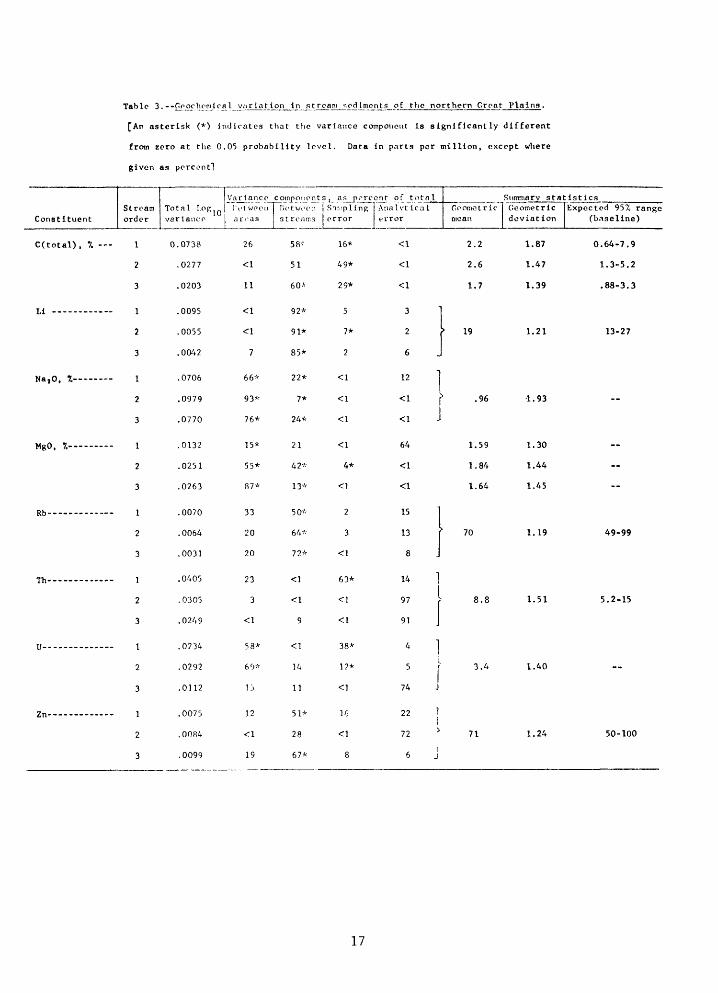
Table 3.--r.pochomlcal variation in stream sediments of the northern Groat Plaina.

[An asterisk (*) Indicates that the variance component Is significantly different

from zero at the 0.05 probability level. Data in parts per million, except where

given as percent!

ConstituentStream order

Total I.o, 10 variance

Variance component s , as percent of totnlIVt woen 1 IlotWi'on nri'as streams

Sir^pling JAnalvtical error error

Summarv statisticsOomotric [ Geometric mean deviation

Expected 957, range (baseline)

C(total), 7.

LI

Na,0, 7.--

MgO, 7.---- --

DKKo -------------

Th- ---- --------

U---

1

2

3

1

2

3

1

2

3

1

2

3

1

2

3

1

2

3

1

2

3

1

2

3

0.0738

.0277

.0203

.0095

.0055

.0042

.0706

.0979

.0770

.0132

.0251

.0263

.0070

.0064

.0031

.0405

.0305

.0249

.0734

.0292

.0112

.0075

.0084

.0099

26

<1

11

<1

7

66*

93*

76*

15*

55*

87*

33

20

20

23

3

58*

69*

}j

12

19

58-- 16*

51 49*

60* 29*

92* 5

91* 7*

85* 2

22* <1

7* <1

24* <1

21 <1

42* 4*

13* <1

50* 2

64* 3

72* <1

^

<1 <1

9 <1

]4 17*

11 <1

51* 16

28 <1

67* 8

<1 2.2 1.87 0.64-7.9

<1 2.6 1.47 1.3-5.2

<1 1.7 1.39 .88-3.3

2 > 19 1.21 13-27

6 J12 !<1 ? .96 -1.93

64 1.59 1.30

<1 1.84 1.44

<1 1.64 1.45

13 r 70 1.19 49-99

8 J

14 ]

97 > 8.8 1.51 5.2-15

91 J

4 15 r 3.4 1.40

74 J

22 ]

72 > 71 1.24 50-100

6 j

17

A second test consisted of a two-way analysis of variance based on the three stream orders by the ten areas. Two samples were selected in each of the 30 (10 areas by 3 orders) cells in the design. The results are summarized by F-ratios as follows:

Constituent Way Log C Log Li Log MgO Log Na 20 Log Rb Log Th Log U Log Zn

Order (3) Area (10)

3.71* 1.10

1.33 1.04

3 . 74* 8.61*

0.70 21.6*

0.41 2 . 84*

0.02.77

1.21 10.76*

1.40 1.74

F-ratios flagged with one asterisk were significantly different from zero at the 0.05 probability level. The results indicate that logarithmic variation for C and MgO is controlled in part by stream order, and they confirm the importance of the broad-scale geographic variation in MgO and Na 20 and U noted in table 3. Interaction in all constituents was found to be nonsignificant at the 0.05 probability level except for Log U (F = 3.12).

Drainage area seems to have little important relation to logarithmic concentration of any of the constituents studied. Only Li, Rb and Zn exhibit statistically significant covariation with size of drainage area (at the 0.05 probability level) and each is negatively correlated (r^-0.45) with only second order drainages. Provisional baselines for those consti tuents with nonsignificant regional variance components are presented in table 3. Baseline as used here is defined by Tidball and Ebens (1976) and is computed as outlined on the inside cover of this report.

Mode of element occurrence

In addition to determining baselines, it is useful to determine the mode of elemental occurrence in the sediments. Such information may be important in assessing the availability of elements to flowing water or to plants. Forty of the 110 samples of <150, L m sediment were chemically leached and each leachate analyzed for Cr, Mn, Ni, Cu, and Zn.

As before, a nested analysis of variance design was used to examine variation at three levels. The three levels are: 1) between 50 km2 areas, 2) within areas, and 3) analytical error. Thirty samples were chosen randomly from the ten areas, three per area. Six samples of these 30 were randomly selected to be analyzed in duplicate to provide an estimate of analytical error. Four additional samples were also examined as they were unusual in one or more aspects of their chemistry, but were not in cluded in the analysis of variance design. All 40 samples were analyzed in a randomized sequence.

18

The following is a list of the chemical extractions in the order performed and the type of sediment material that is expected to be affected. Only the results of the first extraction are complete for the five elements.

1. 1M sodium acetate, pH 5; extracts easily dissolved minerals and readily exchangeable cations from clays, organic materials, and oxide coatings. The procedure consisted of two treatments each of 24 hour duration with a solution to sediment ratio of 3:1.

2. 1M hydroxylamine-hydrochloride, pH 2; extracts poorly crystalline or amorphous Mn oxides. This treatment consisted of two successive aliquots of 20 ml of the solution reacting with the sediment from step 1 for 30 minutes.

3. 30% hydrogen peroxide; extracts most organic materials and sulfide minerals. To the residue of step 2, 5 ml of 30% H 2 0 2 was added. After the reaction ceased the test tubes were placed in a water bath at 65° to 75°C with an additional 5 ml aliquot of H 2 0 2 until all reaction ceased. Samples remained overnight in the water bath at about 40°C. The next morning 10 ml of 1M NaOAc, pH 5, was added and the solution was mixed and separated by decanting after centrifuging.

4. 0.2M ammonium oxalate, pH 3; extracts poorly crystalline or amorphous Fe oxides. To the residues of step 3, 15 ml of the ammonium oxalate solution was added with mixing. The solutions were stored in the dark for 2% to 3 hours. After centrifuging and decanting the solution, an additional 10 ml of reagent was added with mixing. After 1% hours in darkness the sample was centrifuged and the two solutions combined.

5. 50% nitric acid; dissolves remaining well-crystallized Mn and Fe oxides, also minor attack on clays and other minerals. To the residue of step 4, 20 ml of 50% HN0 3 was added with mixing. The mixture was allowed to sit for 4 hours at room temperature with occasional stirring. Solution was removed after centrifuging the mixture.

6. Hydrofluoric, perchloric, and nitric acids; results in total extrac tion. A .50 gm aliquot of untreated sample is placed in a teflon beaker with concentrated HF and 40% HC104 . After heating on a hot plate over night the solution is evaporated to near dryness and the residue dissolved in a diluted solution of HN0 3 .

19

Analysis of variance results are shown here for the chemistry of the 1M sodium acetate leachate along with the summary statistics. All data were logarithmically transformed before statistical analysis:

Extractedelement

CrMnNiCuZn

Total Log 1Qvariance

0.0418.0447.0219.1220.1700

Variance component (%)Betweenareas

24.29.200

44 . 9*

Withinareas

088 . 2*71.066.453.9*

Analyticalvariance

75.82.7

29.033.61.2

Summary statisticsExtracted element

Geometric mean

Geometric deviation

Geometric error

Expected 95% range(baseline)

Cr,Mn,Ni,Cu,Zn,

ppmppmppmppmppm

012

2

.18

.70

.8

.32

.6

11122

.60

.63

.41

.24

.58

1.1.1.1.1.

5108205911

0.11-. 2965-4501.6-5.086-5

---

.0

.0

Components with an asterisk are significantly different from zero (at the 0.05 probability level). Because Zn exhibits a statistically significant difference between areas, the baseline is expected to vary from place to place within the Northern Great Plains. Except for Cr, all elements exhibit a high (>5070 ) proportion of the variance at the within-areas level. The high analytical error in Cr, Cu and Ni is probably due, in part, to the fact that the concentrations are very near the detection limit.

Correlation coefficients were computed between the five extracted constituents and the eight bulk constituents discussed previously. Interestingly, no significant (^=.05) correlations were found between any extractable constituent and any total constituent, including extractable Zn vs. total Zn.

20

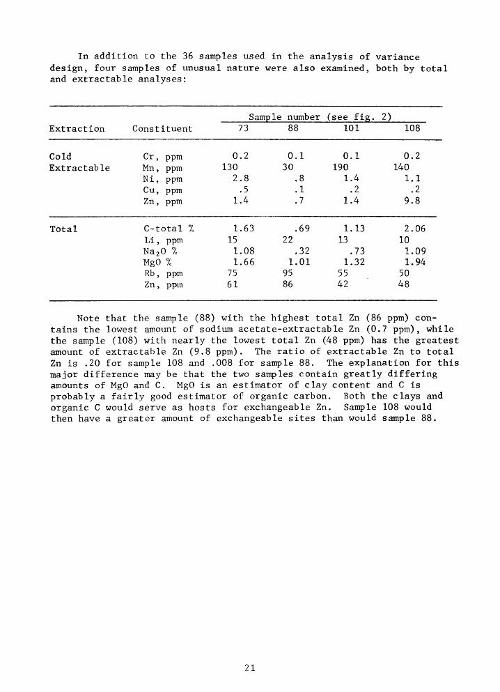
In addition to the 36 samples used in the analysis of variance design, four samples of unusual nature were also examined, both by total and extractable analyses:

Sample number (see fig. 2)Extraction Constituent 73 88 101 108

ColdExtractable

Total

Cr , ppmMn , ppmNi, ppmCu, ppmZn , ppm

C- total 7oLi , ppmNa 2 0 7oMgO %Rb , ppmZn , ppm

0.2130

2.8.5

1.4

1.6315

1.081.66

7561

0.130

.8

.1

.7

.6922

.321.01

9586

0.1190

1.4.2

1.4

1.1313

.731.32

5542

0.2140

1.1.2

9.8

2.0610

1.091.94

5048

Note that the sample (88) with the highest total Zn (86 ppm) con tains the lowest amount of sodium acetate-extractable Zn (0.7 ppm), while the sample (108) with nearly the lowest total Zn (48 ppm) has the greatest amount of extractable Zn (9.8 ppm). The ratio of extractable Zn to total Zn is .20 for sample 108 and .008 for sample 88. The explanation for this major difference may be that the two samples contain greatly differing amounts of MgO and C. MgO is an estimator of clay content and C is probably a fairly good estimator of organic carbon. Both the clays and organic C would serve as hosts for exchangeable Zn. Sample 108 would then have a greater amount of exchangeable sites than would sample 88.

21

ELEMENTS IN LICHEN NEAR THE DAVE JOHNSTON POWERPLANT by Larry P. Gough and James A. Erdman

Introduction

Pacific Power and Light Company's Dave Johnston coal-fired, electric- generating plant is located 8 km east of Glenrock, Wyoming in Converse County near the southern boundary of the Powder River Basin (fig. 3). According to a company brochure, the plant has been in operation since 1958 and burns subbituminous coal in 4 units with a peak capacity of 750,000 KW(e). The mine is located about 15 km northwest of the plant.

Recent studies (Davidson, Natusch, and Wallace, 1974; Lee and others, 1972; Linton and others, 1976) have shown that many potentially toxic trace elements (such as As, Cd, Cr, Ni, Pb, Sb, Se, and Zn) in crease in concentration with decreasing particle size of airborne fly ash. These elements associated with the submicrometer fly-ash fraction, as well as Hg, some Se, Cl, and Br, which are discharged as gases (Klein and others, 1975), pass through conventional particulate control devices and are emitted to the atmosphere. Additional evidence that Hg and Se are emitted as vapors or very fine particles, or both, in. the flue gas, is provided by the mass-balance studies of Kaakinen and others (1975). They speculate that most of the transition elements analyzed form oxides which volatilize at temperatures below 1,500°C (the near-maximum furnace temperature) and therefore escape through the stacks.

Due to the demand for coal-derived energy, operations similar to the mine-mouth facilities at the Dave Johnston Powerplant have been or are being constructed in the Northern Great Plains. This study reports on the usefulness of the foliose soil lichen Parmelia chlorochroa Tuck, as a natural monitor of powerplant element emissions or related contamina tion. Results from using big sagebrush (Artemisia tridentata Nutt.) as a monitor, also at the Dave Johnston plant, were given by Connor, Keith, and Anderson (1976).

Experimental design and data handling methods

Composited samples of P_. chlorochroa were collected at approximate logarithmic intervals along east and west transects from the powerplant (fig. 3). Along the east transect six sites were sampled beginning at 2 km and extending to 64 km. Due to the scarcity of the lichen along the west transect, only three sites were sampled at 2, 4, and 33 km distances. Duplicate samples, taken about 100 m apart and consisting of a composite of many thalli, were collected at each site. Sampling was conducted in September of 1974; however due to the storage of some wet samples, eight were discarded because of decay, and new samples were collected in November, 1974.

All samples were cleaned, dried, and submitted for chemical analyses according to the methods described in U.S. Geological Survey (1975, p. 10- 19). The analyses were performed on either the ashed material by emission spectrography and atomic absorption spectroscopy or on the dried material by techniques described in U.S. Geological Survey (1975, p. 74-78).

22

106°

OO

'-4

5'15

'105°0

0'

DA

VE

JO

HN

S T

ON

P

OW

ER

P

LA

NT

WY

OM

ING

Po

wd

er

Riv

er

Ba

sin

EX

PLA

NA

TIO

N

Sam

plin

g site

--tw

o

Kilo

me

tre

s

ea

st

of

pow

er

pla

nt

Stu

dy

Are

a

GLE

ND

O

RE

SE

RV

OIR

Ki lo

me

tre

s

Figure 3.

--Ma

p of

the

stud

y area showing

lich

en sa

mpli

ng lo

cali

ties

ea

st an

d west of

th

e Da

ve Jo

hnst

on

Powe

rpla

nt,

Wyoming.

Strong evidence exists that a particular element in plant material may be associated with element emissions when that element decreases in its concentration with increasing distance from an emission source (Connor, Keith, and Anderson, 1976). Linear regression analysis was performed to evaluate this relation in lichen. The regressions were based on a least-squares criterion and prediction equations were calcu lated using the form:

1°810 X = ^ + b t log1Q D

where X estimates the concentration of the element, b_ and b are, rexpectively, the intercept and slope of the trend line, and D is the distance from the powerplant.

Where b- was negative (indicating a trend line sloping away from the powerplant) the significance of that slope's deviation from zero (p < 0.05) was estimated using analysis of variance (see, for example, Davis, 1973, p. 192-204). A detailed explanation of this technique when used in point source emission studies is given in Severson and Gough (1976).

Results

Of 71 elements looked for in samples of P. chlorochroa, 35 were detected in at least some of the samples (Appendix V, table 2). Data for 29 of these elements were adequate for the requirements of regression analysis. Data for the other six elements --Ag, Cd, Co, S, Sb, and Si-- were either incomplete or had an unacceptable degree of censoring.

The concentrations of Ca, F, Se, and Sr and ash yield in P_. chloro chroa decrease with increasing distance from the Dave Johnston Powerplant and regression statistics for these elements are presented in table 4. The table shows that the slope of the regression lines for F, Se, and Sr was significantly different from zero (p < 0.01). Coefficients of deter mination for these three elements were relatively large. In the case of F, for example, 56 percent of the total variability observed among samples along this transect is attributed to distance from the powerplant. Severson and Gough (1976) arbitrarily used a coefficient of determination value of 0.50 in identifying the important proportion of the total variance attributable to the independent variable distance. The concentration of Ca in P. chlorochroa may also be related to operations at the powerplant, however, the slope of the regression line was significant only at a probability level of 0.10. Calcium also possessed a low coefficient of determination (table 4).

Ash yield, expressed as a percent of the dry weight of the lichen, showed a significant negative regression slope. This trend, along with the significant trends for F, Se, and Sr, is presented in figure 4. Since Ca, which is the major element in P. chlorochroa and comprises between 12 and 33 percent of the ash was most abundant in those samples

24

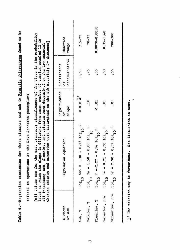
Table 4, Regression st

atis

tics

for

those

elem

ents

an

d as

h in Parmelia

chlorochroa

found

to be

rela

ted

to op

erat

ions at th

e Da

ve Johnston

powerplant

[All va

lues

are

for

the

east tr

anse

ct;

sign

ific

ance

of

the

slop

e is

th

e probability

leve

l at

wh

ich

the

slope

is di

ffer

ent

from

zero;

numb

er of

sa

mple

s eq

uale

d 12

in

al

l instances; ash, fl

uori

ne,

and

sele

nium

wer

e de

term

ined

on

th

e dr

y ma

teri

al

whereas

calcium

and

stro

ntiu

m were determined on the

ash

material;

D^ distance]

Ele

men

t o

r as

h

Ash

, 7.

Cal

cium

, %

Flu

ori

ne,

7.

Sel

eniu

m,

ppra

Str

on

tiu

m,

ppm

Reg

ress

ion

Log

as

h

= 1.3

8

Log

C

a »

1.5

0

10L

ogl(

) F

2.2

2 -

Log

S

e -

0.2

1

Log

S

r »

2.9

0

equati

on

- 0.2

3

log

D

- 0.0

6

log

D 10

0.2

4

Iog

1()

D

-0.3

0

log

D

- 0,3

2

Iog

1()

D

Sig

nif

icance

of

slope

< o.

oil/

.10

<

.01

.01

.01

Coeff

icie

nt

of

dete

rmin

ati

on

0.5

8

.25

.56

.60

.55

Ob

serv

ed

ran

ge 7.5

-22

20-3

3

0.0

020-0

.0050

0.3

5-1

.40

200-7

00

JL/ The

rela

tion

may be fo

rtui

tous

. See

discussion in te

xt.

a a

c o+JE+ C

uc o U

800700600500

400

300

2OOSTRONTIUM

30

20

10ASH

.0060

.0050

g .0040

E .0030 Hc

c .0020 o /o o x

FLUORINE

2.Or

E a a

Co O

64

Distance in KilometersFigure 4.--Regression trends in Parmelia chlorochrqa for concentrations of

fluorine, selenium, strontium, and ash progressing east from the Dave Johnston Powerplant. Slopes are significantly different from zero at the 0.01 probability level.

26

yielding high ash values and because Ca displayed a possible regression trend of importance, it appeared that this element might be responsible for the concurrent ash trend. A product-moment correlation analysis between Ca and ash, however, did not show a strong positive relation. This is evident from Appendix V, table 2, where it can be noted that the samples with the lowest ash values also had some of the highest (31 percent) Ca values.

Silicon, another major constituent of P. chlorochroa comprising between 8 and 18 percent of the ash, was also considered a possible cause of the ash trend. Silicon does not, however, decrease in concen tration with increasing distance. Further, the correlation coefficient for the relation between Si and ash was not significant at the 0.05 probability level.

The intensity of selected calcite and quartz peaks on X-ray diffractograms of the ash of one sample at each sampling site downwind was measured. The ratio of the intensity of the calcite to quartz peaks was plotted against the percent ash of the samples. These data (fig. 5) show that, in general, the amount of calcite in the samples decreases relative to the amount of quartz as ash increases. This trend suggests that, even though the samples were washed, they were contaminated with soil-derived quartz. There is an exception in the sample with the highest ash yield in which very high calcite to quartz ratios were found. This indicates to us that this sample was both very "clean" (free of quartz) and high in Ca.

Variable ash is probably due to both intrinsically high or low Ca and to the relative contamination of the samples. The significant in verse trend observed between ash yield and distance from the powerplant might, therefore, be fortuitous and not related to the powerplant emis sions but to a combination of variable Ca and Si contents and varying degrees of quartz contamination.

Inverse concentration-to-distance trends observed along the west transect were not subjected to regression analysis because of the small number of sample sites. Inspection of these data (Appendix V, table 2) indicates that Ca and Sr may reflect some influence from the operations at the powerplant whereas Se shows a very strong probable relation. Fluorine shows no apparent trend; however, the high values obtained correspond well with the high values observed for close-in samples along the east transect. The ash values show no trend adding support to the probability that the ash trend observed along the east transect is fortuitous.

Of the suspected contaminant elements and ash, only the Se values can be considered to be unusually high in P_. chlorochroa relative to background levels (U.S. Geological Survey, 1975, p. 13), and then only in samples collected within 8 km from the powerplant (fig. 4). Although selenium is noted, in the 1975 report, to be highly variable among samples

27

O

7

o 6 cr

m 5

<U

4N

-H-»

L- O

O 3 \

0)±! u 2o O

0 8 10 12 14 16 18 20 22Percent ash

Figure 5.--Caicite to quartz x-ray diffraction peak intensity ratios from Parmelia chlorochroa ash plotted against percent ash yield.

28

of P. chlorochroa collected from various parts of the basin, the maximum concentration noted in this study (1.20 ppm) is considerably above the observed range of values (0.20-0.70 ppm) for all samples in the 1975 basin-wide study.

It is of interest that in the study by Connor, Keith, and Anderson (1976), also at the Dave Johnston Powerplant, big sagebrush (Artemisia tridentata) samples, like the P. chlorochroa samples, showed significant regression trends for Se and Sr. Big sagebrush also showed significant regression trends for U and V whereas P_. chlorochroa did not. Further, P. chlorochroa showed a trend for F whereas sagebrush did not. These findings lead to the following conclusions: (A) several elements tend to have higher concentrations in vegetation near the powerplant; (B) the most probable source of these accumulated elements is the powerplant; (C) differences in the metabolism, growth form, habitat, and microenviron- ment of different plant species result in differences in their accumulation of elements.

The use of cryptogams, and particularly lichens, as air pollution monitors has received considerable attention over the past decade (see, for example, Ferry, Baddeley, and Hawksworth, 1973). This present study indicates that the widespread terricolous lichen P. chlorochroa has potential use as a monitor of powerplant element emissions in the Northern Great Plains.

29

CHEMISTRY OF POWDER RIVER SEDIMENTSby John R. Keith, Barbara M. Anderson, James M. McNeal

and Josephine G. Boerngen

As part of a general effort to chemically characterize the land scape of the Powder River Basin, samples of Powder River stream sediments were collected in 1973 according to a nested analysis of variance design. The length of the river across the basin was subdivided into six segments, each defined as that length of stream course which occurs in a "supertownship" of Connor, Keith, and Anderson (1976) as shown in figure 6. In each segment, two localities were selected randomly, each locality being about the size of a section (1.6 km on a side). The objective was to reach the river somewhere within each locality and randomly collect two samples of the "active" sediment from a transect across the river bottom. In practice, the transect reached only to the edge of running water, on the side from which the river was approached. The levels in this design reflect geochemical variation 1) between supertownships, 2) between transects within supertownships, 3) between samples within transects, and 4) between analyses of sample splits.

In general, the two samples from each transect were located about 25-100 m apart. Each was collected by shovel, placed in a cloth bag, brought to the laboratory and, if necessary, dried before processing. Each sample was disaggregated and passed through a 2-mm sieve. The <2 mm fraction was further sieved into four size fractions-->200[Lm , 100- 200fj,m. 63-100(im, and <63^m, which are denoted as the A, B, C and D size fractions, respectively. Fifteen of the resulting 96 samples were randomly selected and split into two parts and the entire suite of 111 samples was submitted for analysis in a randomized sequence. The analytical procedures used are described in Miesch (1976). Due to inadequate amounts in some of the size fractions, some chemical constituents could not be determined in all samples. The analysts are J. G. Crock, I. C. Frost, J. Gardner, W. Mountjoy, V. E. Shaw, and J. A. Thomas.

The analysis of variance results are shown in table 5. Except for Na 2 0, Ti, and Zr, which show significant components for three of the four size fractions, the listed constituents show little important large- scale variability. Thus, for many of these properties, provisional base lines may be estimated which should adequately represent a regional background for the length of the river in the basin.

Most broad-scale elemental variation appears in the coarser fraction (A) of these sediments. Thirteen entries in table 5 show such significant variation, including K, Li, Na 2 0, and MgO which may reflect variation in feldspar content or exchangeable ion capacity clay aggregates, or both. Large-scale variation in Ti and Zr in the C and D (finest) fractions as well as in the A fraction probably indicates downstream variation in heavy mineral content. The fraction showing the least broad-scale (down stream) geochemical variability for most elements is the B-fraction,

30

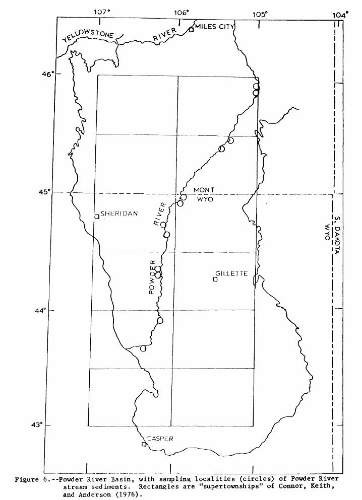
107° 106° 1O5° 104'

43°

Figure 6.--Powder River Basin, with sampling localities (circles) of Powder River stream sediments. Rectangles are "supertownships" of Connor, Keith, and Anderson (1976).

although the environmentally important element Hg does vary significantly at this scale in this fraction. Thus, for a large variety of trace elements (B, Ba, Co, Cu, Li, Nb, Ni, Pb, Rb, Sr, V, Y, Rb, Zn and Zr) the B-fraction of these sediments constitutes the most geochemically uniform stream "monitor".

There is a tendency for the elements to have higher concentrations in the finer fractions. This is best seen in the geometric means in table 5; average concentrations in fraction D are particularly high. This may reflect the fact that the most common constituent, in the larger-grain-size fractions, is quartz which serves to dilute other constituents. Also, there is a tendency for a decrease in variation with decreasing grain size as shown by the geometric deviations in table 5. The combination of increasing concentration and decreasing variance with smaller-grain size indicates that the finer-sized fraction of these sediments is the more easily characterized in a chemical sense. This is so because a smaller variance requires fewer samples for a stable estimate of a mean, and a higher-mean concentration increases chances of detecting the constituent.

Finally, a preliminary 2-way analysis of variance test (supertownships vs. size fractions) suggests that no significant interaction is present except for Ti, Y, Yb and Zr. Again these metals are expected to occur largely in the heavy mineral fraction. This suggests that not only does the heavy mineral component vary significantly along the stream course, but its variation is somewhat dependent on grain size as well.

32

Table 5.--Statlsttc.il analysis of partial chemistry of the Powder River stream sediments

TA, 2 uoi-200-.i fraction; B, 100-200vi fraction; C, 63-100vi; D, <63w fraction; *, statistically significant from zero at the 0.05 probability level. Data arc in parts p«r nillion rxcept where noted as percent; IcAdora ( ) indicate insufficient data ior baseline estimation. Ratio Rives the number of samples

Variance component, per

Total Between onstituent Site L°6io super- Between Betue

fraction variance townships transects snrapl

Total C, ^ A 0.1173 19.6 21.3 47.6

B .0715 30.3 3.8 47.1

C .0154 44.6 2.1 0

D .0105 4.5 0 95.5

Hg A .3827 0 42.0 55.7

B .0688 26.3* 0 60.9

C .0612 0 0 85.6

D .0230 14.2 0 47.6

Li A .0966 28.8* 35.6 27.4

B .0292 21.1 0 51.8

C .0174 8.9 0 45.5

D .0094 13.8 0 1.7

MgO, 1 - -- A .1607 31.2* 37.5 28.2

B .0319 35.4* 0 61.5

C .0073 17.4 29.0 45.1

D .0012 0 5.1 83.4

Na20. % -- A .004.8 58.2* 0 36.8

B .0050 0 49.8 25.2

C .0018 49.7* 17.1 33.2

D .0013 43.3* 0 56.7

Kb A .0161 4.7 40.4 28.3

B .0176 24.2 11.6 39.9

C .0161 36.9* 0 36.5

D .0105 0 0 59.6

Zn A .0538 20.9. 56.9* 10.3

B .0215 6.9 2.6 60.7

C .0103 7.7 0 29.8

D .0066 0 24.6 60.0

cent Summary statistics

Expected 95 percent

en Between Ratio Geometric Geometric Geometric range ea analyses mean deviation error (Baseline)

11,4 23.24 0.77 2.20 1.31 0.16-3.73

18.8 24:24 .54 1.85 1.31 .16-1.85

53.4 24:24 .72 1.33 1.23 .41-1.27

0 24:24 1.22 1.27 < 1.02 .76-1.97

2.3 17:24 .041 4.16 1.24 .002-. 710

12.8 24:24 .019 1.83 1.24

14.4 24:24 .019 1.77 1.24 .006-. 060

38.2 24:24 .030 1.42 1.24 .015-.060

8.2 18:24 12. 2.05 1.23

27.1 24:24 11. 1.48 1.23 5-24

45.6 24:24 12. 1.35 1.23 7-22

84.5 24:24 18. 1.25 1.23 - 12-28

3.2 18:24 .61 2.52 1.18

3.1 24:24 .60 1.51 1.08

8.5 24:24 1.07 1.22 1.06 .72-1.59

11.5 24:24 1.83 1.08 1.03 1.57-2.13

5.0 18:24 .95 1.17 1.04

25.0 24:24 .72 1.18 1.08 .52-1.00

0 24:24 .80 1.10 < 1.01

0 24:24 .84 1.09 < 1.01

26.6 18:24 60. 1.34 1.16 33-108

24.3 24:24 49. 1.36 1.16 26-91

26.6 24:24 53. 1.36 1.16

40.4 24:24 61. 1.27 1.16 38-98

11.9 18:24 46. 1.71 1.20 16-135

29.9 24:24 35. 1.40 1.20 18-69

62.5 24:24 38. 1.26 1.20 24-60

15.4 24:24 67. 1.21 1.08 46-98

33

Table 5.--Statistleal analysis of partial chemistry of the Powder River stream sediments -- Continued.

Constituent Size fraction

Total

variance

Variance component, percent

Between supertownships

Between transects

Between samples

Between analyses

Ratio Geometric mean

Summary statistics

Geometric deviation

Geometric error

Expected 95 percent range (Baseline)

Al, 1

C«, 1

Co

Cr

Cu

A

B

C

D

A

B

C

D

A

B

CD'

D

A

B

C

D

A

B

C

D

A

B

C

D

A

B

C

D

0.0642

.0232

.0331

.0162

.0364

.0192

.0518

.0212

.0205

.0280

.0179

.0255

.0299

,0791

.1025

.0168

.0247

.0500

.0306

.0172

.0117

.1705

.1060

.0587

.0574

1 G £L A. Io5o

.0858

.0250

.1664

< 0.1

< .1

21.4

*>Q 1*/V I**

17.4

7.7

8.6

< .1

< .1

4.3

26.5

34.6*

14.6

5.0

15.6

21.2

< .1

6.3

14.0

1.4

< .1

14.4*

19.4*

7.6

34.5

33.3*

1.7

19.1

< .1

52.7*

< .1

< .1

< .1

42.8

< .1

< .1

34.8

67.9*

24.3

< .1

< .1

< .1

40.5*

< .1

< .1

< .1

30.4

23.6

29.4

29.2

33.2

< .1

14.6

26.4*

3.2

< .1

< .1

< .1

30.5

64.6

41.5

54.4

< .1

< .1

< .1

40.1

< .1

21.8

73.5*

< .1

16.6

< .1

84.4

78.8*

84.3*

10.7

8.7

24.2

48.1

6 0. V

75.7*

71.1

28.4

< .1

90.0*

49.9

97.7*

16.8

35.4

37.1

16.4

O o RJa.o

92.3

91.4

25.2

32.1

49.7

< .1

65.4

Afl Qoo v

54.4

< .1

< .1

15.7

52.6

53.7

45.0

22.8

45. '5

4.9

6.6

10.7

63.5

8.3

31.0

2.3

23:24

24:24

24:24

23:24

13:24

13:24

24:24

24; 24

24:24

24: 24

24: 24

24:24

17:24

24: 24

24: 24

24:24

24:24

24:24

23: 24

24:24

24:24

24: 24

24: 24

24: 24

24:24

24: 24

24:24

24:24

24: 24

.4.88

3.57

4.01

6.12

14

14

32

55

QifiO/U

870

930

1,030

1

2.02

1.13

1.85

3.18

6

4

3

6

26

1 Olo

31

79

1ftio

9

10

34

1.79

1.42

1.52

1.34

1.55

1.38

1.69

1.40

i 30A J '

1.47

1.36

1.44

1.49

1.91

2.09

1.35

1.44

1.67

1.50

1.35

1.28

2.59

2.12

1.75

1.74

2.70

1.96

1.44

2.56

1.27

1.23

1.29

1.13

1.32

1.36

1.65

1.18

1.21

1.31

< 1.02

1.35

1.39

1.61

< 1.02

< 1.02

1.15

1.45

1.34

1.22

1.13

1.90

1 1 Q *>&

1.15

1.20

2.20

1.21

1.22

1.15

1.7-14

2.0-6.2

2.1-7.7

7 ft_9fi. U-.CO

12-17

23-44

31-99

510-1,500

510-1,500

500-1,700

.64-1.6

.84-4.9

.26-4.9

1.0-3.4

1.6-6.1

2.9-12

2.3-7.0

1.9-4.7

3.9-9.2

11-91

28-220

2.5-33

5.5-18

5.3-220

34

Table 5.--Statistical analysis of partial chemistry of the Powder River stream sediments -- Continued.

Constituent Sirs fraction

TotalL°810

variance



Between transects

Between samples

Between analyses

Ratio

Summary statistics

Geometricmoan

Geometric deviation

Geometric error

Expected 95 percentrange

(Baseline)

Pe, % -

f* A __

La

Mn

Nb

Pb

A

B

C

D

A

B

C

D

A

B

C

D

D

A

B

C

D

B

D

A

B

C

D

A

B

C

D

0.0665

.0301

.0151

.0194

.0496

.0248

.0185

.0076

.0172

.0106

.0063

.0146

.0683

.0446

.0198

.0147

.0301

.0247

fiOQO» Uf.O£.

.0241

.1059

.0443

.0257

.0230

.0115

.0101

.0084

.0078

<0.1

< .1

5.2

< .1

20.8*

19.2

12.4

8.7

15.6*

10.0

16.2

< .1

37.2*

< .1

< .1

< .1

11 £* 37.6*

< .1

38.4*

20.7

1 O f*1r32. &*

21.5

25.4

< .1

5 0.0

13.2

7.4

<: .1

57.0*

4.2

< .1

10.6

19.1

< .1

< .1

22.8

?5.9

< .1

< .1

20.4

< .1

29.7

55.2*

17.8

11.3

< .1

< .1

< .1

< .1

< .1

3.3

17.0

60.4*

< .1

< .1

< .1

1.3

70.0

68.9

49.4

27.3

64.7

55.3

68.5*

4.7

41.0

22.2

< .1

19.2

< .1

31.6

82.2*

OQ oJO, £-

24.5

61.6*

< .1

1*7 Q1 1,0

43.9

< .1

< .1

< .1

7.8

< .1

< .1

41.7

25.8

25.9

40.0

*> > QJ/» O

16.1

32.4

< .1

^ ft-> J >

49.0

61.6

79.6

43.7

70.3

13.1

< .1

12.9

75.5

< .1

79.3

49.6

34.6

71.3

83.0

33.9

79.1

92.6

100

24:24

24:24

24:24

24:24

24; 24

24:24

24:24

24:24

24:24

24: 24

24:24

24:24

23:24

24:24

24:24

24: 24

24:24

13: 24

20:24

24:24

24:24

24: 24

24:24

24:24

24: 24

24:24

24:24

7.4; 74

2.88

1.52

1.67

2.58

13

10

10

15

2.90

2.11

2.11

2.68

49

310

220

220

300

6

10

14

13

6

6

13

17

11

11

16

1.81

1.49

1.33

1.38

1.67

1.44

1.37

1.22

1.35

1.27

1.20

1.32

1 Q Q Q->

1.63

1.38

1.32

1.49

1.44

1.47

1.43

2.12

1.62

1.45

1.42

1 0ft ^"

1.26

1.23

1 .? »

1.47

1.22

1.15

1.22

1.34

1.16

1.20

< 1.02

1.25

1.18

1.15

1.28

1.49

1.50

1.12

< 1.01

1.15

1.37

< 1.01

1.37

1.70

1.33

1.37

1.37

1.15

1.23

1.23

1 .91

1.2-7.1

.76-3.0

1.0-2.7

1.6-4.2

5.2-19

6.01-17

10-22

1.5-2.9

1.7-2.6

2.1-3.4

180-520

120-400

130-380

4.2-8.6

10-19

5.2-13

4.0-8.9

9.8-17

8.9-14

9.8-12

35

Table 5.--Statistical analysis of partial chemistry of the Powder River stream sediments -- Continued.

Constituent Sice fraction

Total Log,- variance



Between transects

Between samples

Between analyses

Ratio

Summary statistics

Geometric mean

Geometric deviation

Geometric error

Expected 95 percent range

(Baseline)

0- _______

Ti. %

V .........

y .........

Yb

A

c

D

A

B

D

A

B

D

A

B

C

D

A

C

D

A

B

0

A

B

n

U. .~/ J

.0365

.0294

.0320

.0144

.0124

.0087

.1132

.0351

.0355

.0341

.1383

.0386

.0226

.0268

.0374

O 1 1 1. ZJ-O

.0230

.0501

.0341

.0262

.0350

.0603

.0404

.0231

.1123

_18QO

i J. J

< .1

OQ T*A0« 1*

13.1

1.9

50.4*

6.6

25.2*

< .1

36.6*

1 C. 1 *36.1*

30.9*

< .1

27.2

11.5

40.1*

15.4

21.6

Ifl t.-lrJO, O*

34.4*

12.3

41.8*

48.7

32.3*

1.6

49.6*

n . 7*

i.l/. u

39.6

< .1

44.4

23.5

< .1

< .1

11.7

45.6*

14.4

< .1

15.1

7.6

< .1

< .1

3.7

< .1

< .1

1 O &ly.o

f) f\ f23.6

< .1

< .1

7.9

12.3

< .1

< .1

Q.Q

-HJ . t

39.2

11.4

9.4

3.0

49.6*

48.7

4.3

< .1

49.0*

63.9*

25.7

79.0

18.4

54.9

1 Q 7lu. /

84.6*

27.8

9.5

4.6

68.0

CO OJ.JO. /*

18.6

35.6

50.3

30.2

if, .6*

_~ .0

21.2

59.9

33,1

71.6

< .1

44.6

CO Q_>o.o

54.4

< .1

< .1

oo oZO J

13.4

54.4

33.6

37.5

< .1

50.6

32.3

37.4

19.7

< .1

24.8

1O QI7«O

48.1

20.2

2_n

L->. *t

20:24

24:24

24:24

24:24

24- 24

24:24

24: 24

24:24

24: 24

24:24

24: 24

24:24

24: 24

24; 24

24:24

24:24

24: 24

24:24

24: 24

24:24

24:24

24: 24

24: 24

24:24

24:24

>U- -}U

.*

3

6

1 OA IOU

130

140

180

.090

.10

.17

.32

52

37

54

92

1 QIts

13

19

48

2

2

2

6

61

76

210

«?o

£ . «U

1.55

1.48

1.51

1.32

1.29

1.24

2.17

1.54

1.54

1.53

2.35

1.57

1.41

1.46

1.56

3.04

1.42

1.67

1.53

1.45

1.54

1.76

1.59

1.42

2 1 £..16

7.7?

-«J*

1.22

1 OA« JO

1.27

1.26

< 1.01

1.15

I ftl.01

1.37

< 1.01

< 1.01

1 CQ JO

1.18

1.29

1.24

1.31

< 1.01

1.28

1.34

1.30

1.18

< 1.01

1.33

1.23

1.27

1.41

1 .IS

*. / -J.H

1.4-6.6

92-350

97-170

130-250

.056-. 18

16-85

34-86

50-170

12-31

1.0-3.9

2.3-16

46-130

36

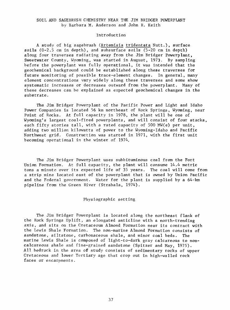
SOIL AND SAGEBRUSH CHEMISTRY NEAR THE JIM BRIDGER POWERPLANT by Barbara M. Anderson and John R. Keith

Introduction

A study of big sagebrush (Artemisia tridentata Nutt.)> surface soils (0-2.5 cm in depth), and subsurface soils (5-20 cm in depth) along four traverses radiating away from the Jim Bridger Powerplant, Sweetwater County, Wyoming, was started in August, 1973. By sampling before the powerplant was fully operational, it was intended that the geochemical background could be established along these traverses for future monitoring of possible trace-element changes. In general, many element concentrations vary widely along these traverses and some show systematic increases or decreases outward from the powerplant. Many of these decreases can be explained as expected geochemical changes in the substrate.

The Jim Bridger Powerplant of the Pacific Power and Light and Idaho Power Companies is located 56 km northeast of Rock Springs, Wyoming, near Point of Rocks. At full capacity in 1978, the plant will be one of Wyoming's largest coal-fired powerplants, and will consist of four stacks, each fifty stories tall, with a rated capacity of 500 MW(e) per unit, adding two million kilowatts of power to the Wyoming-Idaho and Pacific Northwest grid. Construction was started in 1971, with the first unit becoming operational in the winter of 1974,

The Jim Bridger Powerplant uses subbituminous coal from the Fort Union Formation. At full capacity, the plant will consume 14.4 metric tons a minute over its expected life of 35 years. The coal will come from a strip mine located east of the powerplant that is owned by Union Pacific and the Federal government. Water for the plant is supplied by a 64-km pipeline from the Green River (Strabala, 1974).

Physiographic setting

The Jim Bridger Powerplant is located along the northeast flank of the Rock Springs Uplift, an elongated anticline with a north-trending axis, and sits on the Cretaceous Almond Formation near its contract with the Lewis Shale Formation. The non-marine Almond Formation consists of sandstone, siltstone, carbonaceous shale, and minor coal beds. The marine Lewis Shale is composed of light-to-dark gray calcareous to non- calcareous shale and fine-grained sandstone (Spitzer and May, 1975). All bedrock in the area of study consists of sedimentary rocks of upper Cretaceous and lower Tertiary age that crop out in high-walled rock faces or escarpments.

37

The climate of the area is that of a Middle Latitude Steepe (Tre- wartha, 1954), where potential evapotransipiratlon from the soil and vegetation generally exceeds the average annual precipitation. The average temperature of the coldest months is below freezing. The precipitation ranges from 15-38 cm/year, most falling as snow in the winter. Winds are predominantly out of the west and southwest.

The soils of this area are derived primarily from shales and tend to be high in soluble salts and low in nitrogen. The soils, in general, are considered to be warm and dry and lack moisture for plant growth for long periods. The most common soils in the area are classified as Haplargid plus Torriorthents (U.S. Geological Survey, 1970). They are light brown, have a loamy horizon of clay accumulation, are low in organic matter, and are rarely moist for more than three consecutive months. Salorthid soils are also present and are characterized by no horizon or accumulation of clay, but may have accumulations of calcium carbonate, gypsum, or other salts.

The vegetation of the Jim Bridger area is a sagebrush steepe (Kuchler, 1964), consisting of open grassland with dense to open shrub stands. The dominant grass is bluebunch wheatgrass (Agropyron spicatum (Pursh) S. and S.). Growing throughout the area is a number of species of sagebrush, but only the dominant species, big sagebrush (Artemisia. tridentata Nutt.), was chosen for the botanical part of this study.

Methods of sample collection and preparation

All samples of sagebrush and soils were collected in August 1974. Plant samples were collected using stainless steel shears. Each plant sample (approximately 50 g) consisted of stems and leaves from the terminal 15 cm. The samples were stored in quartrsize, refrigerator- freezer boxes. In the laboratory, the unwashed plant tissue was ashed and analyzed for a variety of metals using emission spectrographic, atomic absorption, selective ion electrode, and other techniques described in U.S. Geological Survey (1975, p. 74-78) and Miesch (1976, p. 14). The elements fluorine, total sulfur, arsenic, mercury, and selenium were determined in dry plant material.

The soil samples were collected by first removing coarse surface material and plant or other non-soil debris. At all sites, a surface soil sample (0-2.5 cm depth) and a subsurface soil sample (5-20 cm depth) were collected using a chrome-plated trowel. The samples (approximately 200 g each) were stored in paper soil envelopes and were analyzed by methods described in Miesch (1976).

All plant and soil samples were analyzed in a randomized sequence to reduce possible effects from systematic laboratory error. The samples were prepared and analyzed in laboratories of the U.S. Geological Survey in Denver. Analyses were performed by J. Baker, L. Bradley, W. Gary, C. Freeman, J. Gardner, P. Guest, T. Harms, R. Havens, C. Huffman, Jr., L. Lee, V. Merritt, C. Papp, L. Riley, V. Shaw, G. Shipley, J. Thomas, R. Van Loenen, J. Wahlberg, and T. Yager.

38

Sampling Design

The sampling design consisted of collecting soil and plants at geometrically increasing distances along four traverses radiating north, east, south, and west from the powerplant (fig. 7). At each locality two sites, separated by about 230 m, were chosen. A sample each of big sagebrush, surface soil, and subsurface soil was collected at each site. Five localities were sampled along both the north and south traverses, and six localities were sampled along the east and west traverses. There were a total of 22 sampling localities from which 44 sagebrush samples and 84 soil samples were collected (no soils were collected at site 3E). Analytical results and distances of samples from the powerplant are given in Appendix V, table 3.

Statistical analysis and results

Connor, Keith and Anderson (1976) successfully used a log-linear function of the following form to relate metal concentration in the landscape to distance from the Dave Johnston Powerplant:

Log X = a + b (Log D)

Log X is an estimate of the logarithmic concentration of a chemical constituent at a point and Log D is the logarithm of the distance in kilometers of the point from the powerplant. The coefficient, a, is the estimated logarithmic concentration at 1 km and the coefficient, b, is the estimated slope of the concentration trend away from the powerplant.

Because one effect of element emissions from a powerplant is assumed to be a continual element accumulation in the landscape near the powerplant, the logarithmic model given above should have a negative b coefficient if such accumulation is pronounced enough.

Inasmuch as the work described here was undertaken prior to completion of the Jim Bridger generating plant, it was not expected that geochemical variation related to the logarithm of distance from the powerplant would be found in either soils or sagebrush; that is, b was expected to be near zero. However, a large number of significant relations were found in this study, particularly along the southern traverse (table 6). Thirteen chemical constituents along this traverse significantly increase with distance in both the surface and subsurface soils, including A1 2 0 3 , the most important constituent of clay (Appendix V, table 3). In addition, Si0 2 in the subsurface decreases in a signifi cant way. Clearly, these changes reflect, in large part, lithic changes in bedrock from dominantly shale of Cretaceous age at localities IS, 2S, and 3S to dominantly sandstone of Tertiary age at localities 4S and 5S.

Increases in elemental concentration away from the powerplant were also found to be significant for a number of constituents along the west traverse, although here the dominant effect appears to be noticeably low concentrations in localities 1W and 3W (Appendix V, table 3). The

39

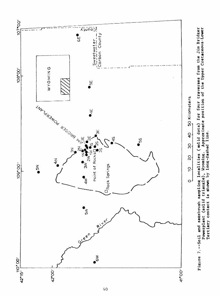
110°

OO

(42*1

5'

42°0

0'

41*0

0'

6W

109°

00

'

,5N

3N

ft 2N

3W

Poin

t o

f R

ocksn

*

3S

'Ro

ck S

prings

^^ J '5

S

108°

OO

' I

107

-00

'

WY

OM

ING

'5E

GE

'

Sw

ee

twa

tej

_

'Carb

on

County

>i

M i c, o'

U!

10

20

30

40

50 K

ilom

ete

rs

Fig

ure

7.-

-Soil

an

d sa

geb

rush

sa

mp

lin

g lo

cali

ties

(soli

d

dots

) fo

r fo

ur

traver

ses

from

th

e Ji

m B

rid

ger

P

ower

pla

nt

(soli

d

tria

ngle

),

Wyo

min

g.

Ap

pro

xim

ate

po

siti

on

o

f th

e U

pp

er

Cre

tace

ou

s-L

ow

er

Ter

tiary

co

nta

ct

is

show

n b

y lo

ng

-da

shed

li

ne.

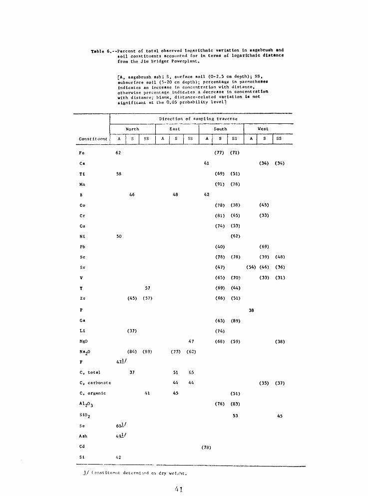
Table 6.--Percent of total observed logarithmic variation In sagebrush and soil constituents accounted for In terms of logarithmic distance from the Jim Brldger Powerplant.

[A, sagebrush ash; S, surface soil (0-2.5 era depth); SS, subsurface soil (5-20 cm depth); percentage In parentheses Indicates an Increase In concentration with distance, otherwise percentage Indicates a decrease In concentration with distance; blank, distance-related variation Is not significant at the 0.05 probability level]

Constituent

Direction

North

A S SS

of sampling traverse

East

A S SS

South

A S SS

West

A S SS

Fe 62

Ca

Tl 58

Mn

B 46

Co

Cr

Cu

Ni 50

Pb

Sc

Sr

V

Y 57

Zr (45) (57)

P

Ga

Li (37)

MgO

Na20 (84) (89)

F 47l/

C, total 37

C, carbonate

C, organic 41

A1 20 3

S10 2

(77)

41

(69)

(91)

48 42

(78)

(81)

(74)

(40)

(78)

(47)

(65)

(69)

(68)

(63)

(74)

47 (68)

(73) (62)

51 65

44 44

45

(76)

(71)

(51)

(78)

(58)

(65)

(53)

(62)

(78)

(70)

(44)

(51)

(89)

(59)

(51)

(83)

53

(34) (34)

(45)

(33)

(69)

(39) (48)

(54) (46) (36)

(33) (31)

38

(38)

(35) (37)

45

Se

Ash

Cd

SI

(78)

42

J./ Constituent determtt^d on dry weight.

41

importance of the major element, Ca, here suggests, again, a geologic control. These two sites are relatively low in Ca (and in the subsurface are relatively high in Si0 2 ) and likely reflect a calcium-poor substrate. The increase in Na 2 0 along the north and east traverses may reflect a relatively high content of Na-Feldspar in the Tertiary rocks at locali ties 4N, 5N, 4E, 5E, and 6E.

Chemical variability in soil along the north and east traverses is less marked than along the south and west traverses. Carbon decreases along both, and Na 2 0 increases along both suggesting, again, parental control of soil composition. In both directions, the parent bedrock changes from carbonaceous shale (relatively high carbon) to arkosic sandstone (relatively high Na 2 0). Controlling features of the trends in subsurface soil along the eastern traverse are the occurrence of high Na 2 0 and A1 2 0 3 , and low MgO, and C (both total and organic) in localities 5E and 6E compared to the other localities. Similarly, total carbon in the surface soil, and yttrium and organic carbon in the subsurface soil of the northern traverse, and B in the surface of the eastern traverse largely reflect the occurrence of exceptionally high concentrations in samples closest to the powerplant (IN and IE). Possibly, such effects reflect construction or mining activities.

Regression analysis of the sagebrush chemistry resulted in many fewer significant relations than were found in the soils, and all but two of twelve trends so defined decrease away from the powerplant (figs. 8, 9 and 10). Of the four traverse directions, the one to the north exhibits the most trends (seven). Three of these trends (Fe, Ti, and F) are visibly controlled by high concentrations in the first locality, IN (Appendix V, table 3), suggesting as mentioned above that they may be reflecting construction or mining activities. In this sense, the three elements can probably be viewed as point-source pollu tants. Construction was heavy on the north side of the Bridger powerplant at the time of sampling, and the resultant suspended dust may have been a source of sagebrush contamination. This conjecture is supported by the higher ash and titantium values at localities close to the powerplant. According to Shacklette C1965), titanium is the most favorable trace metal in plant material for determining the extent of soil contamination. Unless the dust had a special character, it is difficult to account for the elevated fluorine. Nevertheless, its presence is especially interesting because this element seems to be an important pollution suspect in vegetation at "on-line", coal-fired powerplants (this report, figs. 4 and 37).

Variation in Ca and B on the southern Traverse (fig. 10) is also largely controlled by elevated concentrations at the nearest site (IS). In contrast, the increase in Cd southward is strong, even if the first locality is ignored. Also, the trends in P (decreasing) and Sr (increas ing) west of the plant are probably real but, again, lack a ready explanation. The positive slopes seen for Cd and Sr (fig. 10) are interesting because Cd is one of the more environmentally important

42

20O.OOQ,

150,0001

100000+

7OOOCJ

oQ.

3QOOO

20.000-

11S-.VXN

7,000-

(XCXV-

-q 3,oor-

Log Si *= 5.08 - 0.193 Log D

i(r - -0.72)

700-

50C

300-

20>

100-

70-

50-

1.5-

Log Fe - 4.03 - 0.172 Log D (r - -0.79)

Log Ti = 3.19 - 0.238 Log D (r - -0.80

Log Ni = 1 12 - 0.162 Log D (r » -0.78)

25 423 1O

Distance north of powerp^ant

Figure 8.--Metal trends in ash of sagebrush north of the Jim Bridger Power- plant, Wyoming. Open circles indicate concentrations below the limit of analytical detection that are arbitrarily taken as about 0.7 of the limit, Correlation coefficients in parentheses Where three analyses are given at a site, two represent analyses of a single sample.

43

Log ash = A.93 - 0.087(Log D) (r « -0.79)

10 25 42

n o> CT a

IT Dl

oQ-

5CH"Log F = 1.42 - 0.222(Log D)

(r = -0.68)

25 42

.3

.2

.15-

.1 -

.07-

.05-

.03-

.02-

015-

Log Se = -0.530 - 0.481(Log D) (r = -0.83)

1 3 TO 25 42

Distance north of powerpiant (Km)

Figure 9.--Trends in dry weight of sagebrush north of the Jim BridgerPowerpiant, Wyoming. Correlation coefficient in parenthesis Where three analyses are given at a site, two represent analyses of a single sample.

44

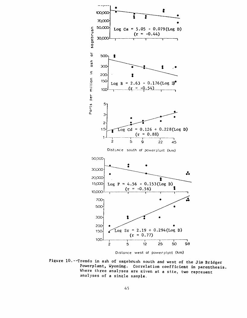
r 50.00CH «n3

g 3O.OOOO)o

Log Ca -=5.05 - 0.079(Log D) (r - -0.44)

5OO-, S

30O-

20O-

150-

inrv

^-t

SLog B = 2.63 -

f ~~~ --^

0.1 76 (Log D)*

o CL

og Cd = 0.126 + 0.228(Log D)(T = 0.88) i

9~T

222 59 22 45

Distance south of powerplant (Km)

50.000-,

3OOOO-

20,000-

15,OOQ

10DOO-

7OO-

5OO-

~r-^Log P = 4.56 - 0.153(Log D)

(r = -0.56) tT I ..,-.- , , -,

* ^^&^-^XX *

30O-

2OO-

T5O-

1OO

Log Sr = 2.19 + 0.294(Log D) (r = 0.77)

12 25 50 98

Distance west of powerplant (Km)

Figure 10.-- Trends in ash of sagebrush south and west of the Jim Bridger Powerplant, Wyoming. Correlation coefficient in parenthesis Where three analyses are given at a site, two represent analyses of a single sample.

45

elements, and Sr in big sagebrush is listed as a suspected pollutant around the Dave Johnston Powerplant (Connor, Keith, and Anderson, 1976). The low concentrations of both of these elements close to the powerplant indicate that if pollution "halos" were to develop in the future around this powerplant, they would not necessarily be exhibited by decreasing trends, at least along these particular traverses.

Metal trends in sagebrush involve a different and more limited suite of elements than do those of the soils, indicating that sagebrush geochemistry varies independently of substrate geochemistry. Moreover, if the sampling localities nearest the powerplant are ignored, six of the sagebrush trends (figs. 8, 9, and 10) would become either nonsignifi cant or strongly reduced. These observations suggest that a provisional estimate of the geochemical background in sagebrush is possible if sum maries are based on all data except that from sites IN, IE, IS, and 1W. Such summaries are given in table 7.

46

Table 7.--Ccochfmlcal summary of data from sagebrush (Artcmlsia

tridcnt.itn) around the Jtm Brldgcr Povcrplnnt, Wyoming

[Data in parts per million, except where noted as percent (%); GM, geometric mean; CD, geometric deviation; CE, E^omctric error; ratio plves the number of samples in which the constituent was determined to the total number of samples analyzed; leaders (--) indicate base line cannot be estimated with given data]

Constituent Ratio GM

As!/ ' 38:41 0.15

F!' 41:41 15

Expected 95 percent range

GD CE (Baseline)

2.46 1.22 0.026-0.87

1.71 1.26 5.7-39

Hgi' 41:41 .019 1.45 1.14 .0094-. 038

S 41:41 .15

Se^ 41:41 .15

Ash, ^y 41:41 6.9

Al, I 41:41 2.2

B 41:41 260

Ba 41:41 310

Ca, I 41:41 9.1

Cd 41:41 2.8

Co 41 : 41 1.8

Cr 41:41 16

Cu 41:41 110

Fe, I 41:41 .68

K, I 41:41 23

Li 41:41 13

Xg, I 41:41 1.5

Mn 41:41 470

y.o 41:41 9.8

j:a, I 41-.41 .21

Ki 32:41 10

P, Z 41:41 2.7

fb 41:41 46

Si, I 41:41 8.6

Sr . 41:41 360

Ti 41:41 910

V 40:41 .77

V 40: 41 26

Zn 41:41 260

Zr 41-.41 59

1.26 1.10 .099-. 23

2.59 1.10 .023-1.0

1.25 1.08 4.6-10

1.62 1.17 .88-5.5

1.43 1.46

1.64 1.17 120-790

1.24 1.04 5.9-14

1.72 1.15 .98-8.0

1.93 1.40 .58-5.6

1.61 1.15 6.4-40

1.42 1.30 69-170

1.64 1.29 .29-1.6

1.33 1.09 13-39

1.59 1.19 5.5-31

1.31 1.33

1.53 1.37 270-830

1.39 1.30 6.6-15

1.83 1.22 .067-. 66

1.64 1.25 4.1-24

1.46 1.15 1.3-5.4

1.53 1.38 26-80

1.63 1.14 3.4-22

1.64 1.21 140-900

1.73 1.48 420-2,000

1.57 1.21 .3'4-1.8

1.85 1.33 8.8-77

1.55 1.10 120-660

1.71 1.30 23-150

\J Determined 0:1 dry weight.

47

GEOCHEMISTRY OF GREEN RIVER OIL SHALE by Walter E. Dean

Introduction

This report brings together a wide variety of selected trace and minor element data on the Green River oil shale in order to examine in a provisional way, the geochemical variability of those bedrock materials likely to be brought to the surface by energy-related activities. Table 8 summarizes data from six sources. General sample locations are shown in figure 11.

Included here are summaries based on unpublished as well as published work. A search was made of the U.S. Geological Survey's Rock Analysis Storage System (RASS) for analyses of oil shale from the Piceance Creek (Colorado), Uinta (Utah), and Green River (Wyoming) Basins. Where possible, only analyses of drill core samples were in cluded in the compilation in order to eliminate possible weathering effects; however, all samples from the Green River Basin were collected from outcrops or roadcuts. The groups of RASS analyses are referenced by the name of the sample submitter, all of whom are Geological Survey personnel. Most of the analyses are of samples from potentially economic oil shale zones in the upper part of the Green River Formation. A few additional trace element data may be found in Stanfield and others (1951) and Smith and Stanfield (1964).

Seven trace elements listed in table 8 are generally considered of particular environmental interest, and geochemical work by the lessees in the prototype oil shale program has focused on analyses for these elements in both oil shale and soil as part of predevelopment baseline environmental assessments. These elements are cadmium, antimony, arsenic, mercury, selenium, fluorine, and boron. Ranges in concentration reported in table 8 for minor and trace elements are shown in figure 12. Also shown in figure 12 are provisional estimates of average concentrations.

The dominant minerals in Green River oil shale are quartz, dolomite, albite, and calcite (usually in that order of abundance) with minor amounts of siderite, analcime, K-feldspar, dawsonite, and nahcolite, all of which may occur locally as major constituents. Therefore, the dominant major elements are silicon (quartz + minor albite, analcime, and K-feld spar), aluminum (albite, dawsonite, and K-feldspar), and sodium (albite, dawsonite, and nahcolite). Iron usually occurs in concentrations between 1.5 and 2 percent, and is present mainly in pyrite, ferroan dolomite, and siderite. Titanium rarely occurs in concentrations greater than 0.2 percent, and minor amounts of phosphorus and sulfur are usually present, mainly in the form of apatite (phosphorus), and organic material and pyrite (sulfur). Desborough and others (1976) examined the mineralogy of oil shale by X-ray diffraction and attempted to relate element abun dances to mineralogical residences. Additional reports on the mineralogy of the Green River oil shale include Smith (1974), Desborough and Pitman (1974), Robb and Smith (1974), Beard and others (1974), Dyni (1974), Desborough (1975), Desborough and Pitman (1975), Desborough (1976).

48

Table 8. Ranges, geometric means

(GM)

and

geometric deviations (GD) of concentrations

of selected elements in

Green River oi

l shale

from the Piceance Creek (Colorado),

Uinta (U

tah)

, an

d Green River (W

yomi

ng)

Basi

ns.

[Data

in parts

per

million, ex

cept

where noted as pe

rcen

t (7

L);

leaders ( )

indicate no da

ta]

Element

Piceance Cr

eek

Basin

Vine

-Dv

ni-

Donnell-

47

-a x

C-a

"En

vir

on

men

tall

y

imp

ort

an

t"

elem

ents

^'^

".g

'

G . M

?G

.D.

Anti

mony

range

G . M

.G

.D.

Ars

enic

ran

^e

G . M

.G

.D.

Mer

cury

ran

ge

G . M

.G

.D.

Sel

eniu

mra

ng

eG

.M.

G.D

.F

luori

ne

range

G . M

.G

.D.

Boro

nra

nge

G.M

.G

.D.

-- -- --

<30-

300

58 1.8

7

_.

__ -- _-

--

<20-5

00

22 3.

00

0.5

4

- 4

.0:

2.4

1 .2

2

JO. 1

0-2

. 8

0.4

9i

1.67

! 0.90-15

! 6-5

0.1

0-1

.50

.44

2.3

^

1.6

4

0.0

5-3

.60.6

01

.91

0.1

0-1

.3

0.32

1.91

75-1

,500

550 1

.64

1 -

516

129 1

.79

i j

<0

.5-0

.7;

o.l

4

<0.6

-1.2

!

(all

but

! 0.7

i

3 <0

.5)

' j<1

-

3 :

0.3

91.

2 i

1.6

5

! j -1

0-12

5 I

7.2

1-6

;

2.1

i

--

i (

25-7

5 i

38

i 37

j

--

1.9

0

! t

iI

!

<0

.02

-1.3

: <

0.1

<

C.0

8-2

.9

--

' --

0.2

2

! i

0.3

5

!1.

73

;<

2 -

10

1 0.0

82.2

j

1.8

21

600-

3,40

0 l,

700

1,30

0

<o.i

-

3 i

i --

1.1

J

!i

:i

;

700-2

,100

! --

1,2

00

1.40

:

;

10-3

00-

.140

41

i2.0

2

i

30

-30

0

<2

0-1

00

86

; 38

i 2

.00

--

20-5

0043

2,6

7Other el

emen

ts

Iron

, %

range

G.M.

G.D.

Magnesium, %

range

G.M.

G.D.

1.2-

2.8

1.9

1.27

0.10

-7.0

2.1

3.55

0.3-

5.0

1.7

1.59

0.30-5.0

2.3

1.88

_.

__ --

.-

_1.

3-2.

71.9

0.7-

5.0

2.1

2,15

jo. 6o-4. 8

to. 70-3.0

1.8

i 1.3

: 1.70

0.7-

7.0

2.6

2.05

0.50-10

3-7

2.60

Tab

le 8

.--R

ange

s,

geom

etri

c m

eans

(G

M)

and

geom

etri

c d

evia

tio

ns

(GD

) of

con

cen

trat

ion

s o

f se

lect

ed e

lem

ents

in

Gre

en R

iver

oil

sh

ale

fro

m t

he

Pic

ean

ce C

reek

(C

olor

ado)

, U

inta

(U

tah

),

and

Gre

en R

iver

(W

yom

ing)

Bas

ins C

onti

nu

ed.

O

Element

Pota

ssiu

m, %

range

G.M.

G.D.

Sodium, %

range

G.M.

G.D.

Titanium, %

range

G . M .

G.D.

Barium

range

G.M"

.G.

D.Cobalt

range

G.M.

G.D.

Chromium

range

G.M.

G.D.

Copper

range

G.M.

G.D.

Gallium

rang

eG.M.

G.D.

Lead ra

nge

G.M.

G.D.

Lithium

range

G.M.

!

Vine^/

1.5-7-0

2.7

1.49

1.0-7.0

2.4

1.54

Pice

ance

Cr

eek

Basin

j j

j Dyni^/

j Do

nnel

l^/

C-a^/

] C

i i

0.30-2

.8 '

1.4

i1.40

<1 . 0-

171 .2

8.02

<0. 030-0. Z 0.02-0.20

0.15

1 .66

0.11

1.57

30-5,0

00

100-

1,00

0600 2,01

<7.o

-30

9-2

1.50

2.0-

35241.

67

<i5-io

o50 1.

68

<7.o-3

013 1.

51

<7. o-

ioo

123.

57

300 1 .6

0 :

<3.0-20

8.3

i1.

67i

7.0-70

i341.

61

7.0-100

33 1.89

<10-70

18 1.83

--

-- __ __ __ __ -- __

Coo

k'6

/

j G

reen

Uin

ta

Bas_

in_j

Riv

er]D

esbo

roug

hj ""

f B

asin

32 39 49 15 2.2

10

850

et

al.

Vin

e-V

ine-

jo. 7

5-2.

2 ri

.5-3

.0

2.0

-7.0

l.o

; 2.

3 i

3.2

l.4i

1.49

!o.7

4-i

.9

'0.7

-3.0

0

.7-3

.01

.3

1.58

1,7

1.

61

0.0

57

0

.07

-0.2

0

0.0

5-0

.50

0.0

2-0

.20

0.1

20.1

61.8

40

.11

1

-57

200-1

,200

;20

0-7

00

300-2

,000

345

^.0

-20

10

20

-70

37

14

2-1

10

! 55

34o

620

1.4

92.0

0

;5.0

-300

i<3

-0-1

5j

13

I 4

.9!

2.8

0

1.8

9

(20-7

0

11

5-5

0i

53

j 33

; i.4

6 1.

5610

-70

34 1.61

:5.0

-10

10-3

07.0

19-5

2 32

35-2

08

i 70

18 1.39

15-3

0

21 1.2

9

115-

100

I 30

1.89

<5.

o-30

14

1.97

<io

-30

13 1.6

2

I Table 8. Ranges, geometric means (GM) and geometric deviations (CD) of concentrations of selected elements in Green River oil shale from the Piceance Creek (Colorado), Uinta (Utah), and Green River (VfyonrLng) Basins Continued.

1tLement

inganeserange

IG.M. G.D. olybdenum

Vine-^/

<30-?00257

2.26

Dyni-^/

20-300174

1.63

range ; <5. 0-3.0 f <5.0-50G.M. 11 16

G.D. 2.11 | 1.82 Nickel j

rangeG.M.

§ G.D. candium rangeG.M.G.D.

Strontium range

G.M.G.D.

ranadium range G.M.'G.D.

^inc range | G.M.Zirconium

range

1 G.M. G.D.

20-60 ;<"5. 0-200391.23

<5.o-i57.51.31

10-2,000

181.66

5.0-2008.82.01

20-720870 300

2.79 1.51

<15-2001251.34

__

<10-20038 1.80

20-200 109

1.53

--

-_

Piceanc

Donnell-2/

__

__

__

-_

e Creek Ba

C-a^

--

sin

C-bV

_-

f

j,i

-11ii

)j

-- .

__ __

Cook^/

34

4.9

11

2.4

69

29

13

9.3

I Uinta Basin

Desborough et al.-Z/

180-300 230

7.0-4020

20-40 28

<5.o-io

1^9-690 560

100-200 130

49-110 81

20-70 49

Vine^/

150-1,500 320

1.84

O.O-205.2 2.03

<3.0-20 22 1.6?

--

150-1,000 380

1.92

20-100 61 l.?o

--

10-150 532.29

Green River Basin

Vine-^/

70-1,000280

1.79

<5.0

3.0-5015 2.29

100-1,000560

2.41

20-150 621.74

--

20-20077 2.23

I I I I I

I/ From unpublished data of James D. Vine (U.S. Geological Survey). Includes 36 samples of core material ~~ in the Piceance Creek Bcsin (sample numbers D114433-D114438; D118018-D118046), 14 samples of core

material in the Uinta Basin (sample numbers D142083-D142085; D142088-D142096; D143400-D143401), and nine samples of outcrop and roadcut material in the Green River Basin (sample numbers D129429-D129430; D129454-D129459; D1296G5).

2/ From unpublished data of John R. Dyni (U.S. Geological Survey). Includes 371 samples of core material (sample numbers D122302.-U122399; D129483-D129495; D130466-D130681). Data for potassium, strontium, and sodium are based on 371 analyses; all other summaries are based on 89 analyses.

3/ From unpublished data of John R. Donnell (U.S. Geological Survey). Includes 183 samples of core ~" material (sample numbers D158971-D159153).

4/ Rio Blanco Oil Shale Project (1975). Two hundred and thirty samples of fresh shale from the C-a lease tract.

J>/ C-b Shale Oil Project (1975). One hundred and forty samples of fresh shale from the C-b lease tract.

£/ Cook (1973). One composited, pyrolized (at 500°C) sample of the Mahogany Bed at the Colony Mine.

_7/ Desborough and others (1976). Ten samples of oil shale from the Piceance Creek and Uinta Basins.

51

1125 111' 110* 109* 108*

4 2 « -----« UTAH

41°-

40°H

39s

-- .4i

SAND WASH BASIN

COLORADO

PICEANCE

CREEK

BASIN

I

Figure 11.--Location of selected sample sites for oil shale, distribution of the Green River Formation, and lease tracts C-a, C-b, U-a, and U-b. Unpublished data of James D. Vine (1), John R. Dyni (2), and John R. Donnell (3), all of the U.S. Geological Survey, shown by symbols.

52

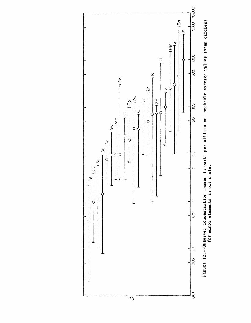
1 I

I I

1 I

I I

I I

Ul u>

I_______I_________________1_______I_________________I_______I__________________I_______I

OOl

0.05

0.1

05

1 5

10

50

100

500

1OOO

5OOO

K3.00O

Figure 12

.--O

bser

ved

concentration

ranges in parts

per

mill

ion

and

prob

able

average

valu

es (o

pen

circ

les)

for

minor

elements in oi

l sh

ale.

Trace elements

The summaries in table 8 and the extant literature suggest the following notes.

Cadmium.--A concentration around 1 ppm would seem to be a reasonable average for Green River oil shale. The mean concentration for raw shale reported by the C-b Shale Oil Project (1975), is less than half of a part per million whereas the mean reported from the C-a tract (table 8) is over 2 ppm. Cadmium probably occurs as a substitute for zinc in minor sulfide minerals.

Antimony.--The values for antimony given in table 8 exhibit a range of <l-6 ppm. The values from the C-a tract and from Cook (1973) may be low, and Desborough and others (1976) suggest that some Sb may be vola tilized during pyrolysis. An expected concentration on the order of 1 ppm antimony might be a reasonable average for raw oil shale.

Arsenic.--The C-a tract values and the single Cook value are low compared to the data of Desborough and others (1976) and the C-b tract. The low concentration (7.2 ppm) reported by Cook (1973) in pyrolized oil shale led Desborough and others (1976) to suspect that perhaps As, like Sb, may be volatilized on pyrolysis, but they could not confirm this. An expected value for arsenic on the order of 35 ppm seems reasonable. Microprobe studies by Desborough and others (1976) indicated that most of the As was present as a substitute for S in pyrite.

Mercury.--The average concentrations for mercury in table 8 all fall within a fairly narrow range, and a value of 0.4 ppm probably represents a reasonable average for oil shale. Cadigan (1970) reported a median concentration of 0.1 ppm Hg in 260 samples from the Uinta and Green River Formations of the northern Colorado Plateau. Donnell's samples included ten each of raw and pyrolized oil shale from the same core intervals. The geometric mean concentrations of Hg in the fresh and spent shale were 3.7 and 3.1 ppm respectively indicating that little Hg is lost on pyrolysis.

Selenium. The means for selenium in oil shale from the C-b tract and from Desborough and others, suggest an average concentration on the order of about 1.5 ppm. Selenium may substitute for sulfur in sulfide minerals, but may also occur as elemental selenium in a number of organic compounds.

Fluorine. Mean concentrations of fluorine in oil shale listed in table 8 range from 550-1,300 ppm; a value of about 1,000 ppm would appear to be a reasonable concentration for fluorine in an average oil shale sample. Microprobe studies by Desborough and others (1976) show that F occurs as 5- to 10-nm grains of fluorite and cryolite disseminated within the shale.

54

Boron.--Mean values for boron listed in table 8 range from 22 to over 100 ppm, and average about 70 ppm. Desborough and others (1976) concluded that boron resides in K-feldspar disseminated throughout the Green River Formation.

Barium.--Table 8 suggests that a concentration on the order of 450 ppm barium is a reasonable average for typical Green River oil shale, although values of several thousand ppm (that is, several tenths of a percent) should not be surprising. The most probable mineral residence of Ba is in barite. Barite is a common diagenetic mineral in marine sediments, especially in organic-rich sediments (Church and Wolgemuth, 1972; Cronan, 1974; Dean and Schreiber, 1976).

Cobalt, Chromium, and Copper.--Suggested concentrations of these three elements in the average Green River oil shale are on the order of 10 ppm for cobalt, 35 ppm for chromium, and 40 ppm for copper. Cook's value of 39 ppm cobalt appears to be too high while his value of 15 ppm for copper appears to be too low. All three of these elements are probably present as substitutes for iron in pyrite (Desborough and others, 1976).

Gallium.--The data in table 8 suggest typical concentration on the order of 10 ppm gallium.

Lead. Most of the data for lead falls within a fairly narrow range and suggests an average concentration in oil shale of about 20 ppm. Lead probably resides in a sulfide phase, either as a separate trace sulfide or substituting for iron in pyrite.

Lithium and zinc.--The only values for lithium and zinc listed in table 8 are those by Desborough and others (1976) and Cook (1973) who give markedly contrasting figures. Desborough's data suggest that average oil shale probably contains less than 100 ppm each, perhaps 75 ppm. Desborough and others (1976) report correlations between lithium and fluorine, calcium, and magnesium, suggesting that lithium is associated with one or more carbonate phases.

Manganese.--Except for Cook's value of 34 ppm, the data on the manganese in oil shale suggest a typical concentration on the order of 250 ppm. According to Desborough and others (1976), the main occurrence of manganese in oil shale is substitution for iron in ferroan dolomite, siderite, and magnesiosiderite.

Molybdenum and Nickel.--Most of the values for molybdenum in oil shale lie between <5 and about 20 ppm, suggesting an average concentra tion of perhaps 10 ppm. Nickel concentrations tend to fall within a fairly narrow range of 15 to 40 ppm, with an average of about 25 ppm. Desborough and others (1976) report general correlations between both Mo and Ni and sulfide-S, suggesting that the dominant residences for both elements are in sulfide phases, probably substituting for iron in pyrite.

55

Scandium.--The limited values for scandium suggest an average value for oil shale of about 8 ppm.

Strontium.--The data for strontium in table 8 range from 10 to 2,000 ppm. The values of Desborough and others (1976) and Dyni were obtained by atomic absorption and probably represent more reliable results than those obtained by semiquantitative optical emission spectrometry (Vine's samples), and an average of about 300 ppm is pro visionally suggested. Most of the Sr in oil shale probably occurs as a substitute for Ca in calcite and dolomite.

Vanadium.--Concentrations of vanadium show considerable variation, and this probably reflects variation in amount of, and concentration of vanadium in, organic material within the Green River Formation. A mean value of about 100 ppm seems reasonable. The value of 29 ppm V in Mahogany zone oil shale from the Piceance Creek Basin reported by Cook (1973) appears low, although this may reflect the fact that his sample was pyrolized prior to analysis.

Zirconium.--Most zirconium concentrations in table 8 fall between 10 and 200 ppm, and an average of about 50 ppm seems reasonable. Again, the value of 9.3 ppm reported by Cook (1973) appears a little low. Desborough and others (1976) suggested that most of the Zr in the Green River Formation probably occurs as zircon.

56

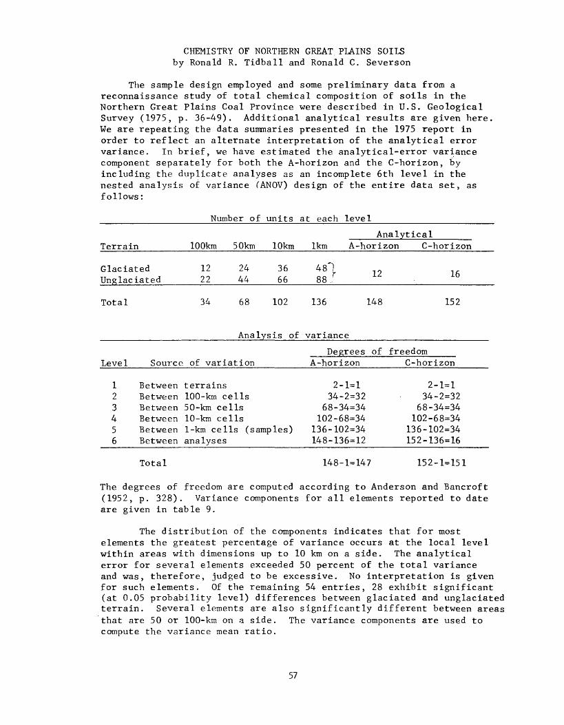
CHEMISTRY OF NORTHERN GREAT PLAINS SOILS by Ronald R. Tidball and Ronald C. Severson

The sample design employed and some preliminary data from a reconnaissance study of total chemical composition of soils in the Northern Great Plains Coal Province were described in U.S. Geological Survey (1975, p. 36-49). Additional analytical results are given here We are repeating the data summaries presented in the 1975 report in order to reflect an alternate interpretation of the analytical error variance. In brief, we have estimated the analytical-error variance component separately for both the A-horizon and the C-horizon, by including the duplicate analyses as an incomplete 6th level in the nested analysis of variance CANOV) design of the entire data set, as follows:

________________Number of units at each level________________________

AnalyticalTerrain

Glaciated Unglaciated

100km

12 22

50km

24 44

10km

36 66

1km

M)

A-horizon

12

C-horizon

16

Total 34 68 102 136 148 152

Analysis of variance

Degrees of freedom_Level

123456

Source of variation

Between terrainsBetween 100-km cellsBetween 50-km cellsBetween 10-km cellsBetween 1-km cells (samples)Between analyses

A-horizon

2-1=134-2=32

68-34=34102-68=34

136-102=34148-136=12

C-horizon

2-1=134-2=32

68-34=34102-68=34

136-102=34152-136=16

Total 148-1=147 152-1=151

The degrees of freedom are computed according to Anderson and Bancroft (1952, p. 328). Variance components for all elements reported to date are given in table 9.

The distribution of the components indicates that for most elements the greatest percentage of variance occurs at the local level within areas with dimensions up to 10 km on a side. The analytical error for several elements exceeded 50 percent of the total variance and was, therefore, judged to be excessive. No interpretation is given for such elements. Of the remaining 54 entries, 28 exhibit significant (at 0.05 probability level) differences between glaciated and unglaciated terrain. Several elements are also significantly different between areas that are 50 or 100-km on a side. The variance components are used to compute the variance mean ratio.

57

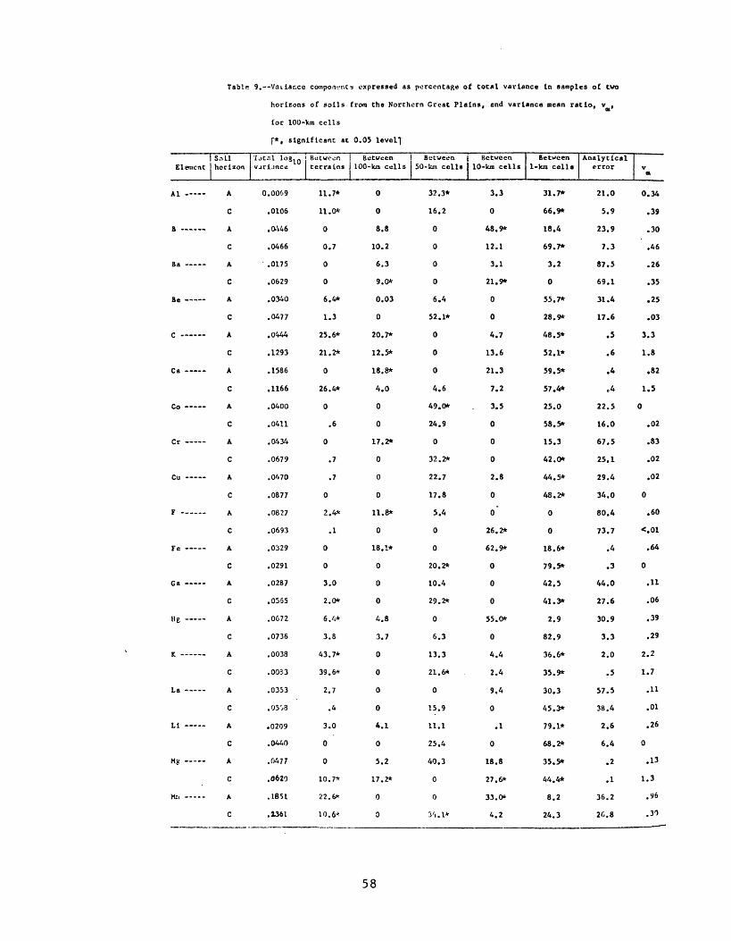
9.--Vai iar.cc components expressed as percentage of total variance In samples of tvo

horizons of soils from the Northern Great Plains, end variance mean ratio, v ,

foe 100-km cells

f*, significant at 0.05 level 1]

ElementSoil horizon

Tot.il logl(J vari.mce

Between terrains

Between 100-kn cells

Between 50-km cells

Between 10-km cells

Between 1-kra cells

Analytical error V

at

Al -

B

Ba

Be

C

Ca

Co

Cr

F

He -

K

La

Li

Mg --

H« -.-

A

C

A

C

A

C

A

C

A

C

A

C

A

C

A

C

A

C

A

C

A

C

A

C

A

C

A

C

A

C

A

C

A

C

A

C

0.0069

.0106

.0446

.0466

.0175

.0629

.0340

.0477

,0444

.1293

1 CQf.* Ooo

.1166

.0400

.0411

.0434

.0679

.0470

.0877

.0827

.0693

.0329

.0291

.0287

.0565

.0672

.0736

.0038

.0033

.0353

.0503

.0209

.0440

.0477

.0«0

.1851

.1361

11.7*

11.0*

0

0.7

0

0

6.4*

1.3

25.6*

21.2*

0

26.4*

0

.6

0

.7

.7

0

2.4*

.1

0

0

3.0

2.0*

6.4*

3.8

43.7*

39.6*

2.7

.4

3.0

0

0

10.7*

22.6*

10.6*

0

0

8.8

10.2

6.3

9.0*

0.03

0

20.7*

12.5*

18.8*

4.0

0

0

17.2*

0

0

0

11.8*

0

1 A 1*lo* 1*

0

0

0

L ft(*. o

3.7

0

0

0

0

4.1

0

5.2

17.2*

0

0

32.3*

16.2

0

0

0

0

6.4

52.1*

0

0

0

4.6

49.0*

24.9

0

32.2*

22.7

17.8

5.4

0

0

20.2*

10.4

29.2*

0

6.3

13.3

21.6*

0

15.9

11.1

25.4

40.3

0

0

V..1*

3.3

0

48.9*

12.1

3.1

21.9*

0

0

4.7

13.6

n 3. J

7.2

3.5

0

0

0

2 ft &

0

0

26.2*

0

0

0

55.0*

0

4.4

2.4

9.4

0

.1

0

18.8

27.6*

33.0*

4.2

31.7*

66.9*

18.4

69.7*

3.2

0

55.7*

28.9*

48.5*

52.1*

59.5*

57.4*

25.0

58.5*

15.3

42.0*

44.5*

48.2*

0

0

79.5*

42.5

41.3*

2.9

82.9

36.6*

35.9*

30.3

45.3*

79.1*

68.2*

35.5*

44.4*

8.2

24.3

21.0

5.9

23.9

7.3

87.5

69.1

31.4

17.6

.5

.6

.4

.4

22.5

16.0

67.5

25.1

29.4

34.0

80.4

73.7

.4

.3

44.0

27.6

30.9

3.3

2.0

.5

57.5

38.4

2.6

6.4

.2

.1

36.2

26.8

0.34

.39

.30

.46

.26

.35

.03

3.3

1.8

82

1.5

0

.02

.02

.02

0

.60

64

0

.11

.06

.39

.29

2.2

1.7

.11

.01

.26

0

.13

1.3

.96

.30

58

Table 9. Variance component* expressed ns percentage of toc*l variance In samples of two

horlrons of sollu from the Northern Great Plains, and variance mean ratio, v ,

for 100-krc cells Continued

Soil Element liorl

«* »

C

Nai/ A

C

C

Mf ____ A

C

f ...... A

C

BK ^ .. A

C

DK A

C

Sc A

C

Sli/ A

C

St A

C

Th A

C.

Til/ ... A

C

U A

C

V ...... A

C

Y ...... A

C

fb A

C

Zni/»- - A

C

Zr A

C

Total log zon variance 10

0.1068

.1860

.0774

.1249

.0510

.0600

.0275

.0519

.0319

.0281

.0396

.0826

.0093

.0186

.0622

.0772

9.531

12.61

.0295

.0372

.0094

\l .0208

.0023

.004 1

.0131

.0288

.0171

.0449

.0369

.0361

.0296

.0347

540.2

413.5

.OSVi

.o;o<,

Between terrains

0.5

0

7.7

1.6

.7

0

0

3.8*

0

0

1.9

.1

25.0*

31.2*

0

2.2

0

6.9*

8.8*

9.3*

17. 7*

13.3*

0

1.3

31.7*

17.7*

7.3*

10.7*

2.2

0

6.4*

1.2

3.3

0

4.6*

0

Between Between 100-iun cell* 50-kra cells

7.8* 11.1

0 32.5*

19.5* 10.1

7.2 0

0 19.1*

0 21.3

11.0* 0

0 20.8

1.1 5.7

0 17.9

0 9.9

0 39.6*

11.1* 0

0 3.3

9.1 0

0 22.9

27.0* 0

9.3 0

2.1 0

6.1 0

5.5 0

0 2.2

11.2 0

0 6.4

10.2* 0

0 10.6

0 3.1

0 17.5*

7.1 0

0 0

0 9.0

0 0

19.0* 0

0 10.7

2.3 0

5.0 4.2

Between Between 10-km cells 1-Vm cells

0 44.4

0 25.7

0 62.2 *

29.2 61.1*

0 24.5

18.8 0

12.3 40.6

0 58.2*

0 0

0 4.9

0 26.6

0 55.4*

29.2* 24.8*

9.4 49.3*

6.9 21.3

0 5.8

7.6 52.0*

7.3 64.7*

37.5* 33.4*

0 75 48*

29.2* 23.5

16.5 17.1

39.9* 32.2*

0 87.4*

18.0 37.6*

11.5 57.9*

12.6 22.1

0 60.6*

0 47.2

30.9* 29.1

0 3.3

26.7* 24.5

13.4 62.4*

0 74.9*

10.0 0

0 22.9

Analytical error

36.2

41.8

.5

.9

55.7

59.9

36.0

17.2

93.2

77.2

61.6

24.9

9.9

6.8

62.2

69.1

13.4

11.8

18.3

8.8

24.1

50.9

16.7

4.9

2.5

2.3

54.9

11.2

43.5

40.1

81.3

47.6

1.9

14.4

76.6

67.9

Vm

.31

0

1.2

.33

.02

0

.46

.12

.04

0

.07

<.01

1.8

1.6

.39

.07

1.4

.74

.40

.73

1.0

.54

.41

.05

2.5

.68

.28

.37

.41

0

.24

.04

1.1

0

.59

2.0

I/ Variance co-r.p-jtt«l on

59

Variance mean ratio

The variance mean ratio, v , of Miesch (1976) provides an index of the relative stability of the estimate of the mean of any given cell size based on the data already collected. In particular we use v to evaluate the feasibility of mapping the regional distribution of elements using means computed for 100-km cells. We require that v equal or exceed a value of 1.0 for such maps. The equation for v rias been modi fied from that of Miesch to account for the staggered, nested design (U.S. Geological Survey, 1975, p. 39), as follows:

v PT + P100

O P + ft P -f. O (P -4- P N

a50 50 a l(T 10 ar r i V

where the subscripted P's are the percentages of total variation in table 1 corresponding to terrains, 100-km cells, 50-km cells, 10-km cells, 1-km cells (samples), and analytical error, respectively. The denominator is the variance of the mean of 100-km cells. The coefficients, a., which represent the average numbers of samples in each level of the design, are developed from the general expression of Leone and others (1968), p. 725),

n 2 + n 2 + - - n 2 a. = 1 2______x1 N 2

where n_ , n,-, and so forth are the numbers of samples within each unit of a level, and N is the total number of samples within the level.

The computations are illustrated in figure 13 for each coefficient in the equation for v (above). The necessity to sum the two lowest variance components (P,+P ) stems from the irregular distribution of the analytical duplicates through the staggered sample design. The inability to treat P as a separate term here results in a slightartificial inflation of the value for v .

m

60

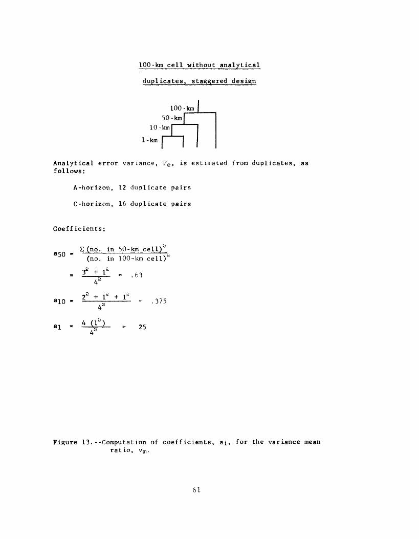
100-km cell without analytical

duplicates, staggered design

100-km 50-km

10-km

1-km

Analytical error variance, P e , is estimated from duplicates, as follows:

A-horizon, 12 duplicate pairs

C-horizon, 16 duplicate pairs

Coefficients:

£ (no. in 50-km cell)'' (no. in 100-km cell) :

_ r « .63

a !0 2 +A2

(1s8 )

.375

25

Figure 13.--Computation of coefficients, ai, for the variance mean ratio, vm .

61

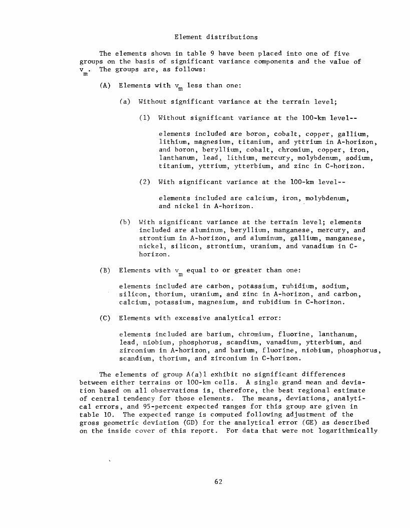
Element distributions

The elements shown in table 9 have been placed into one of five groups on the basis of significant variance components and the value ofv . The groups are, as follows: m

(A) Elements with v less than one:

(a) Without significant variance at the terrain level;

(1) Without significant variance at the 100-km level-

elements included are boron, cobalt, copper, gallium, lithium, magnesium, titanium, and yttrium in A-horizon, and boron, beryllium, cobalt, chromium, copper, iron, lanthanum, lead, lithium, mercury, molybdenum, sodium, titanium, yttrium, ytterbium, and zinc in C-horizon.

(2) With significant variance at the 100-km level-

elements included are calcium, iron, molybdenum, and nickel in A-horizon.

(b) With significant variance at the terrain level; elements included are aluminum, beryllium, manganese, mercury, and strontium in A-horizon, and aluminum, gallium, manganese, nickel, silicon, strontium, uranium, and vanadium in C- horizon.

(B) Elements with v equal to or greater than one:

elements included are carbon, potassium, rubidium, sodium,silicon, thorium, uranium, and zinc in A-horizon, and carbon,calcium, potassium, magnesium, and rubidium in C-horizon.

(C) Elements with excessive analytical error:

elements included are barium, chromium, fluorine, lanthanum, lead, niobium, phosphorus, scandium, vanadium, ytterbium, and zirconium in A-horizon, and barium, fluorine, niobium, phosphorus, scandium, thorium, and zirconium in C-horizon.

The elements of group A(a)l exhibit no significant differences between either terrains or 100-km cells. A single grand mean and devia tion based on all observations is, therefore, the best regional estimate of central tendency for those elements. The means, deviations, analyti cal errors, and 95-percent expected ranges for this group are given in table 10. The expected range is computed following adjustment of the gross geometric deviation (GD) for the analytical error (GE) as described on the inside cover of this report. For data that were not logarithmically

62

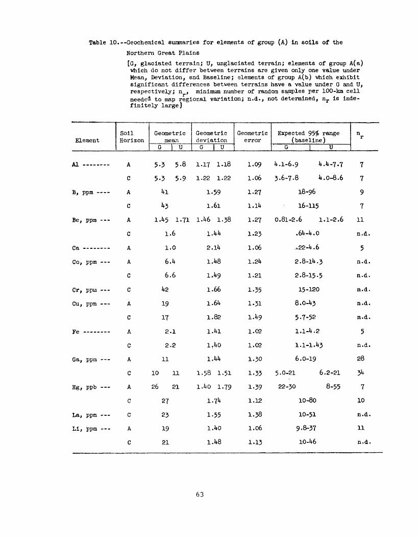
Table 10.--Geochemical summaries for elements of group (A) In soils of the

Northern Great Plains

[G, glaciated terrain; U, unglaciated terrain; elements of group A(a) vhich do not differ between terrains are given only one value under Mean, Deviation, and Baseline; elements of group A(b) which exhibit significant differences between terrains have a value under G and U, respectively; n , minimum number of random samples per 100-km cell needed to map regional variation; n.d., not determined, nr is inde finitely large]

ElementSoil Horizon

Geometric mean

G 1 U

Geometric deviationG | U

Geometric error

Expected 95$ range (baseline)

G | U

n r

A! ____ _ __

B, ppm --

Be, ppm -

fa --------

Co, ppm ---

Cr, ppm ---

Cu, ppm -

Ga, ppm ---

Hg, ppb

La, ppm

Li, ppm -

.

C

A

C

A

C

An.

A

C

C

A

C

Af\

C

A

C

A

C

C

A

C

5 -1 C. & 3 ? «o

5-3 5-9

4l

M

1.45 1.71

1.6

1.0

6.4

6.6

42

19

17

2.1

2.2

11

10 11

26 21

27

23

19

21

I T rr T -| O If 1 . lO

1.22 1.22

1.591.61

1.46 1.38

1.44

2.14

1.48

1.49

1.66

1.64

1.82

1.41

1.40

1.44

1.58 1.51

1.40 1-79

1.74

1-55

1.40

1.48

1.09

1.06

1.27

1.14

1.27

1-23

1 f\£. .Ob

1.24

1.21

1-55

1.31

1.49

1.02

1.02

1.30

1.33

1.39

1.12

1.38

1.06

1.13

4.1-6.9 4.4-7.7

3.6-7.8 4.0-8.6

18-96

16-115

0.81-2.6 1.1-2.6

.64-4.0

22-4 6.»

2.8-14.3

2.8-15-5

15-120

8.0-43

5-7-52

1.1-4.2

1.1-1.43

6.0-19

5.0-21 6.2-21

22-30 8-55

10-80

10-51

9.8-37

10-46

7

7

9

7

11

n.d.

5

n.d.

n.d

n.d

n.d

n.d

5

n.d

28

34

7

10

n.d

11

n.d

63

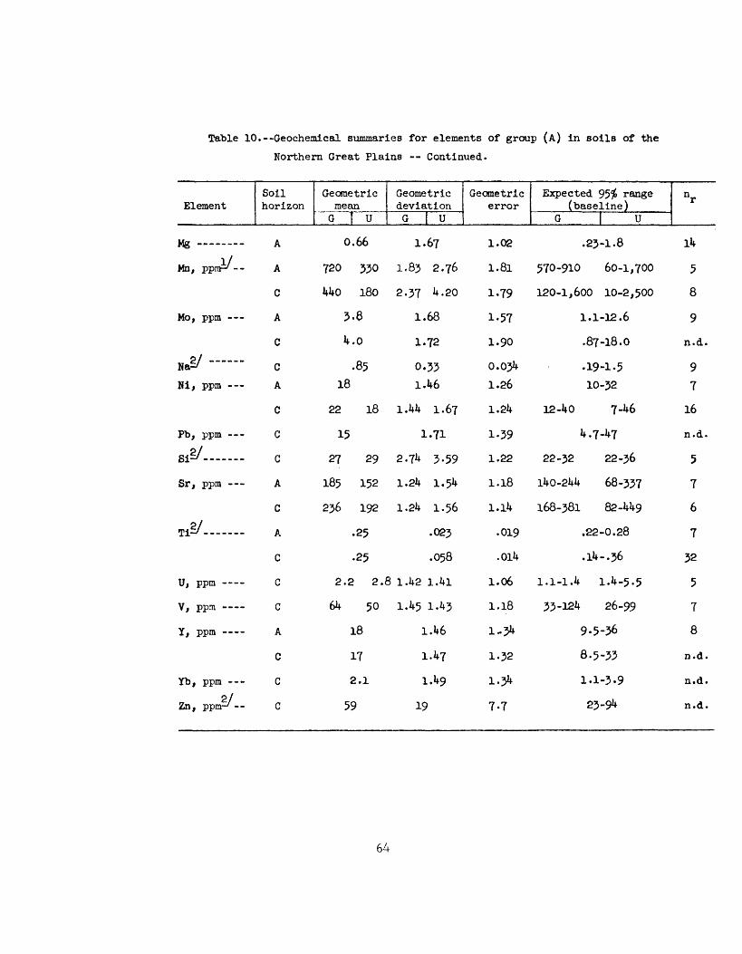
Table 10.--Geochemical summaries for elements of group (A) in soils of the

Northern Great Plains Continued.

ElementSoil horizon

Geometric mean

G I U

Geometric deviationG [ U

Geometric error

Expected 95$ range (baseline)

G | U

nr

Wtt ---

Mn, ppra '--

Mo, ppm

Ni, ppm ---

Pb, ppm

Sig/

Sr, ppm

v&

U, ppm

V, ppm

Y, ppm

Yb, ppm ---

Zn, ppm-/ --

t\.

A

C

A

C

C

A

C

C

A

C

Af\

C

C

C

A

C

C

C

720 330

44o 180

3.3

4.0

.85 18

22 18

15

27 29

185 152

236 192

.25

.25

2.2 2.8

64 50

18

17

2.1

59

A.V(

1.83 2.76

2.37 4.20

1.68

1.72

0.33 1.46

1.44 1.67

1.71

2 74 ^ «?Q* ( H J *J7

1.24 1.54

1.24 1.56

.023

.058

1.42 1.41

1.45 1.43

1.46

1.47

1.49

19

i!a1-79

1.57

1.90

0.034 1.26

1.24

1.391.22

1.18

1.14

.019

.014

1.06

1.18

1-3^

1.32

7-7

570-910 60-1,700

120-1,600 10-2,500

1.1-12.6

.87-18.0

.19-1-5 10-32

12-40 7-46

4.7-47

22-32 22-36

140-244 68-337

168-381 82-449

.22-0.28

.14-.36

1.1-1.4 1.4-5.5

33-124 26-99

9.5-36

8-5-33

1.1-3-9

23-91*

j.t

5

8

9

n.d

9

7

16

n.d

5

7

6

7

32

5

7

8

n.d

n.d

n.d

64

Calcium, A-horizon, percent

.57 2.6

Glaciated

Unglaciated A

1

.42

.18

18

1.8

.85\

.73 1..11 x

1.1

i

2.6\

2.6

Iron, A-horizon, percent

1.7_____________3.5I .i

1.4 3.1

1.3 2,5

Glaciated

Unglaciated f

1.8 2.2 2.5

X________3,5

X

Molybdenum, A-horizon, parts per million

1.9___________________6.8j I1.3___________4.4

I i1.0__________3.8

. ,. . 1.0_________3..6 4.4 Glaciated i b iX

TT . . ... 1.3_________3..9__________6.8Unglaciated ( r^ iX

Nickel, A-horizon, parts per million

1A 25

13________24

11________22 I '

~i . * 15 1.8 24 Glaciated j b r

Unglaciated

X11

Figure 14. Duncan's classes for elements of group A(a)2 and observed ranp.es of 100-km cell means for each terrain.

[X, terrain mean.

65

transformed (where SD is standard deviation and SE is standard error of analysis), the expected 95-percent range is computed as,

AM - 2(SD ) to AM + 2(SD ) n n

Here, AM is the arithmetic mean and SD is computed from the standardn deviation (SD) and the standard error (SE) as follows:

SD = i (SD) 2 - (SE) 2 2 n

The elements of group A(a)2 are shown in figure 14 as the shortest significant ranges (classes) for distinguishing among cell means accord ing to Duncan's multiple range test (Duncan, 1955). The array of cell means for a given element has been grouped into classes, each with the shortest significant range. That is, each class contains means that are not significantly different from each other. In essence, the largest value of the class does not differ from the smallest value. For example, the mean for calcium in the glaciated terrain does not differ from that of unglaciated terrain, but ANOV indicates that the means of 100-km cells within each terrain are significantly different from each other. This suggests that the measure of central tendency is best estimated by the local cell mean. It can be seen in figure 14, however, that significant differences between 100-km cell means do exist in unglaciated terrain for calcium. Therefore, the terrain mean of 1.1 percent is the best estimate for calcium in A-horizon soil in glaciated terrain, and local cell means are better estimates within the unglaciated terrain, but with the constraint that these cell means require additional sampling before they can be viewed as "stable" (because v is less than one). Because maps of these elements would be unstable, the only useful summary based on the data at hand is that for the entire area. Consequently, these elements are summarized in table 10 along with the A(a)l elements.

The elements of group A(b) exhibit a significant difference between terrains but no significant difference between 100-km cells within the terrains. The best estimate of central tendency for these elements is given by separate means, one for glaciated and one for nonglaciated terrain. These means, deviations, analytical errors, and 95-percent expected ranges are also given in table 10.

Elements in group (B) all have v greater than one, which indicates that the means of 100-km cells are minimally stable estimates. The geographic distribution of these cell means is presented in the form of maps in figures 15 to 27.

We have ventured to draw contours on the cell means merely as an aid to quickly visualizing the distributions. We do so with the know ledge of at least two deficiencies--first, the contours are very sub jective and represent only one of several possible patterns; and second, a known gradient is implied for all possible points between adjacent

66

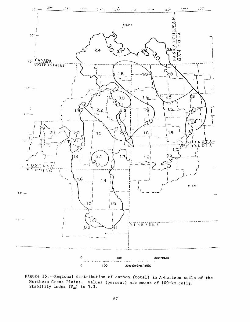
5C"

S . CANADA __ \ I'M TED'ST A'TES ~" ~~' ? ~(~ ~ ~ ~ ~

Vm N_7 A_> A' _" ' " "

)OO 20OMILE5

100

Figure 15.--Regional distribution of carbon (total) in A-horizon soils of the Northern Great Plains. Values (percent) are means of 100-km cells. Stability index (V m) is 3.3.

67

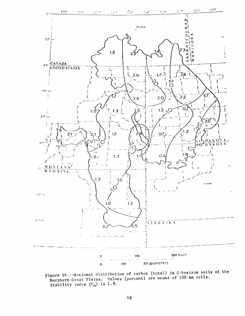
100

100 ZOC

Figure 16.--Regional distribution of carbon (total) in C-horizon soils of the Northern Great Plains. Values (percent) are means of 100-kra cells.

Stability index (Vm ) is 1.8.

68

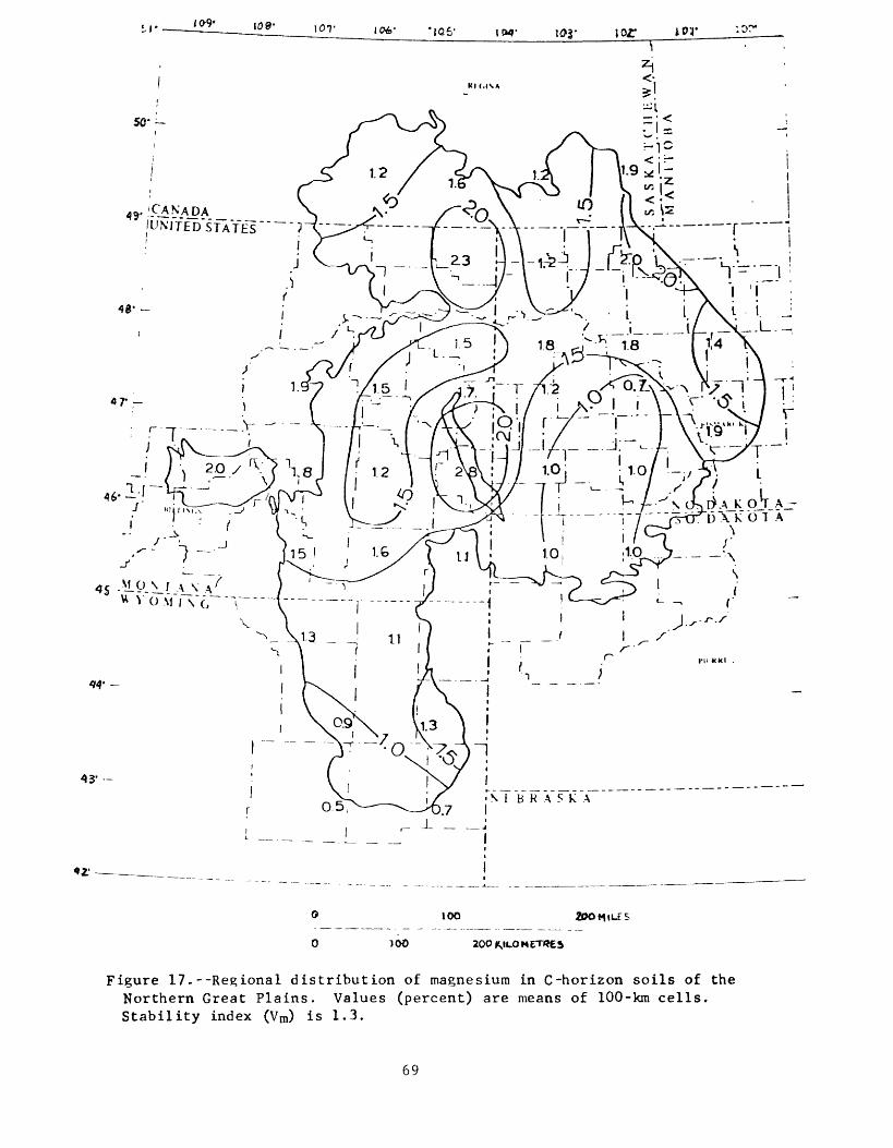
SO"-

>oo 200 MILES

Figure 17.--Regional distribution of magnesium in C-horizon soils of the Northern Great Plains. Values (percent) are means of 100-km cells. Stability index (V m) is 1.3.

69

51' 109' 106 IOT 103' IQ^I ___

5Q' -

49

48

42"

100 200 M \U S

10O

Figure 18.--Regional distribution of rubidium in A-horizon soils of the Northern Great Plains. Values (ppm) are means of 100-km cells. Stability index is 1.8.

70

5J- '09' 108' 107JOO*

50'

49-

48'

47*

A_N A_^ ^ O M I \"G "\

43'

100

10O

Figure 19.--Regional distribution of rubidium in C-horizon soils of the Northern Great Plains. Values (ppra) are means of 100-km cells. Stability index (Vm) is 1.6.

71

sr __L??'__1?8-_ IOT__ wfr\00'

50

49

>A K pjr A^-D\K01A

43*

\00 2OO MttJLi

IOO

Figure 20.--Regional distribution of sodium in A-horizon soils of the Northern Great Plains. Values (percent) are means of 100-km cells. Stability index (Vm) is 1.2.

72

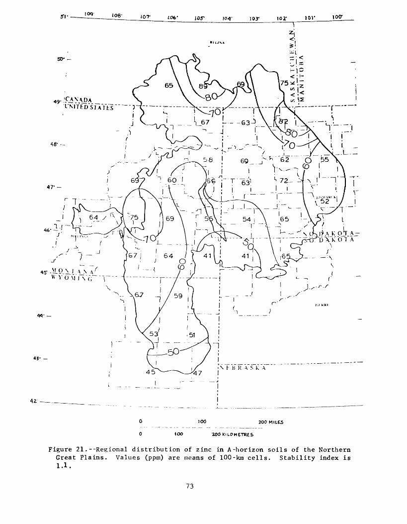
51- - 109 JOB'10T lor

100 200 MILE5

Figure 21.--Regional distribution of zinc in A-horizon soils of the Northern Great Plains. Values (ppm) are means of 100-kra cells. Stability index is 1.1.

73

51*109* 108'

100 200H.LES

100 200 KILOMETRES »",-,»-74

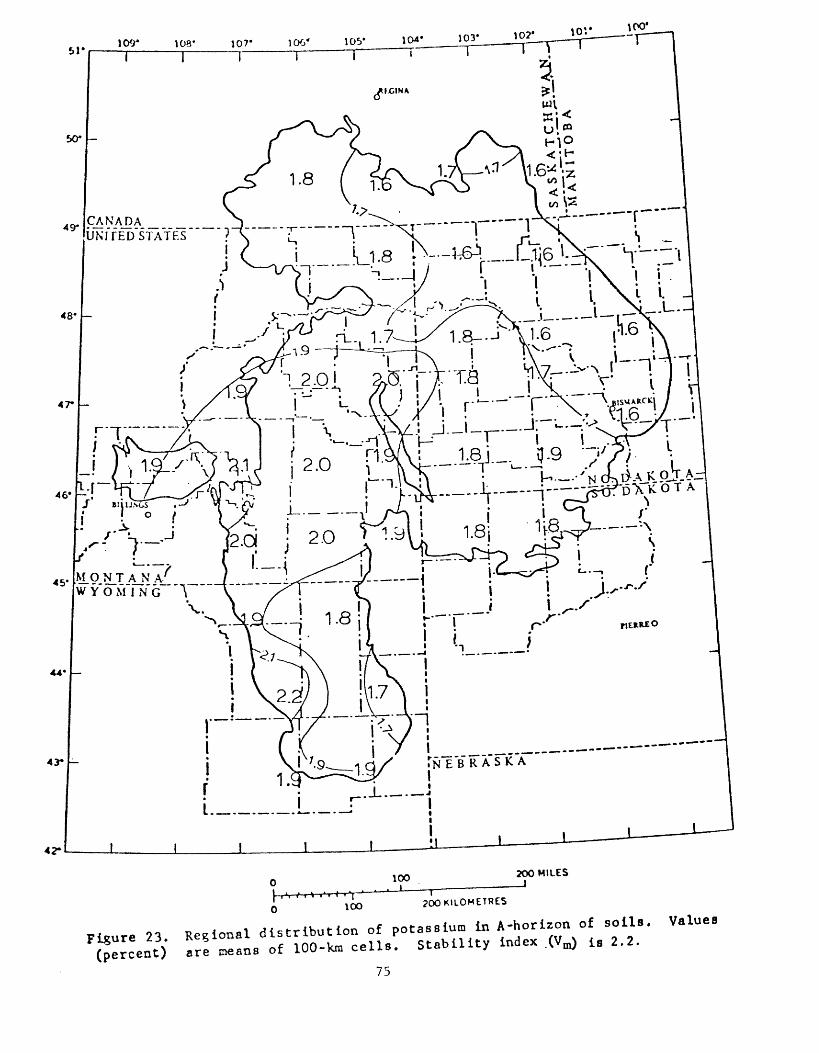
100'

109* 108* 107

45-_ _ _ _ _ ~ ~ "

43-

42-

Sis75

51'100'

50*

y L. 45- M.P N-I A_N A/ _

WYOM'lNG "1

0 20O KILOMETRES

Figure 24. Regional distribution of potassium in C -horizon of soils (percent) are means of 100-ka cells. Stability index (V m) is 1.9.

76

Values

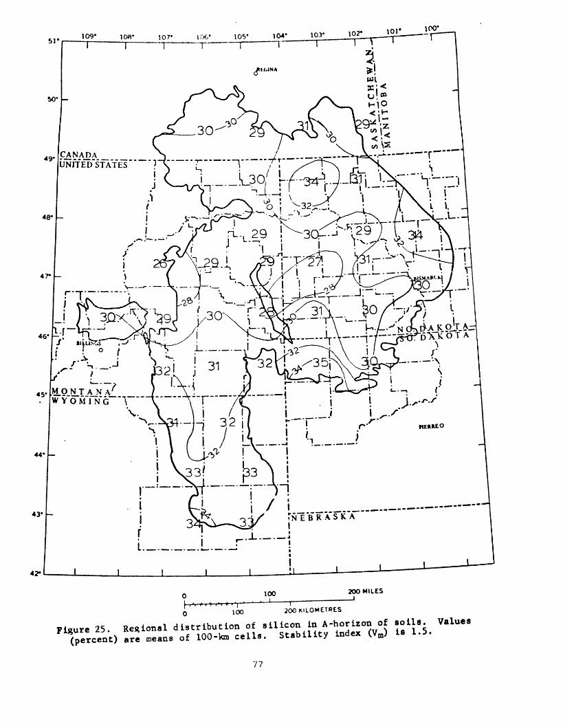
51'109*

100*

108

50-U

49-

48"

45« [*L9 N.T A_N A/WY"OM"IN"G~"^

100

100

j r '200 KILOMETRES

2OO MILES

Fi*ure 25. Regional distribution of silicon in A-horizon of soils. Values ^percent) are means of 100-km cells. Stability index (Vm) is 1.5.

77

\0\* \ (JO-

100*

43*

42*

78

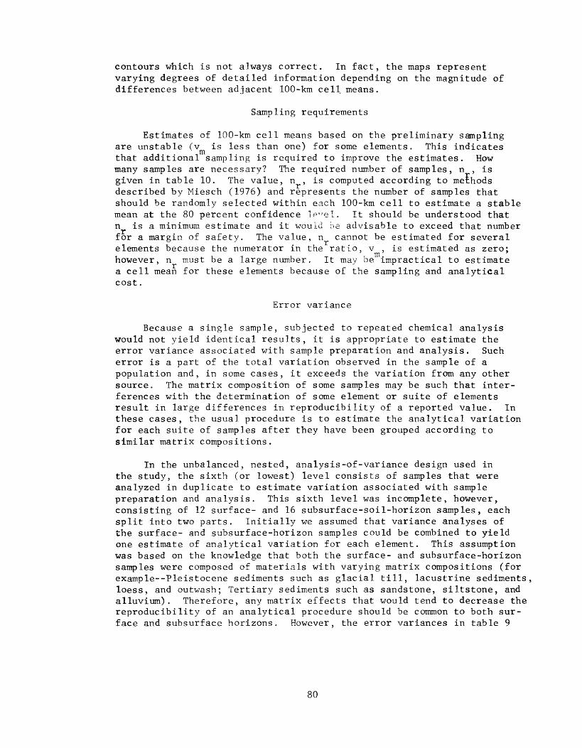
contours which is not always correct. In fact, the maps represent varying degrees of detailed information depending on the magnitude of differences between adjacent 100-km cell means.

Sampling requirements

Estimates of 100-km cell means based on the preliminary sampling are unstable (v is less than one) for some elements. This indicates that additional sampling is required to improve the estimates. How many samples are necessary? The required number of samples, n , is given in table 10. The value, n , is computed according to methods described by Miesch (1976) and represents the number of samples that should be randomly selected within each 100-km cell to estimate a stable mean at the 80 percent confidence ]p^el. It should be understood that n is a minimum estimate and it would be advisable to exceed that number for a margin of safety. The value, n cannot be estimated for several elements because the numerator in the "ratio, v , is estimated as zero; however, n must be a large number. It may be 'impractical to estimate a cell mean for these elements because of the sampling and analytical cost.

Error variance

Because a single sample, subjected to repeated chemical analysis would not yield identical results, it is appropriate to estimate the error variance associated with sample preparation and analysis. Such error is a part of the total variation observed in the sample of a population and, in some cases, it exceeds the variation from any other source. The matrix composition of some samples may be such that inter ferences with the determination of some element or suite of elements result in large differences in reproducibility of a reported value. In these cases, the usual procedure is to estimate the analytical variation for each suite of samples after they have been grouped according to similar matrix compositions.

In the unbalanced, nested, analysis-of-variance design used in the study, the sixth (or lowest) level consists of samples that were analyzed in duplicate to estimate variation associated with sample preparation and analysis. This sixth level was incomplete, however, consisting of 12 surface- and 16 subsurface-soil-horizon samples, each split into two parts. Initially we assumed that variance analyses of the surface- and subsurface-horizon samples could be combined to yield one estimate of analytical variation for each element. This assumption was based on the knowledge that both the surface- and subsurface-horizon samples were composed of materials with varying matrix compositions (for example Pleistocene sediments such as glacial till, lacustrine sediments, loess, and outwash; Tertiary sediments such as sandstone, siltstone, and alluvium). Therefore, any matrix effects that would tend to decrease the reproducibility of an analytical procedure should be common to both sur face and subsurface horizons. However, the error variances in table 9

80

suggest that for many elements, the analytical reproducibility differs widely in the two soil horizons. In fact, the logarithmic variance estimates of analytical error for B, Ba, C, Hg, Li, Na, Th and Zn are significantly different as shown in the following table of F-ratios.

Element

AlBBaBeCCaCoCrCuF

F-ratio

2.423 . 12*2 . 84*1.273.36*1.551.361.722.161.30

Element

FeGaHgKLaLiMgMnMoNa

F-ratio

1.391.248.60*1.631.045.19*2.651.012.013.30*

Element

NbNiPPbRbSScSiSrTh

F-ratio

1.271.111.371.181.382.001.381.161.644.64*

Element

TiUVYYbZnZr

F-ratio

2.112.051.881.101.465.88*1.65

The ratio is computed for each element by dividing the variance of the surface or subsurface horizon, whichever is larger, by the smaller variance. Ratios with an asterisk are significantly different from 1.0 at the 0.05 probability level. Because 29 elements do not show significant differences, it appears that some properties or factors other than matrix composition are affecting the reproducibility of the analytical determinations. If the analytical technique is at fault, then we would expect that a group of elements determined by a single technique should consistently exhibit either significant or nonsignificant variation between horizons. However, the elements that exhibit significant differences between errors in the two horizons were determined by a number of procedures Ccf. U.S. Geological Survey, 1975, fig. 2).

As a general recommendation, the investigator should be aware of the possibility for significant analytical variability between diverse types of materials and should plan to account for it. The degree of anticipated diversity, however, must be balanced against the costs of the additional duplicate analyses that are necessary to derive an adequate estimate of the analytical variation within each type. The final practi cal test is to determine whether the method of estimating the analytical- error variance affects the final interpretation of the overall study.

ELEMENTS IN WHEATGRASS, DAVE JOHNSTON MINE by James A. Erdman and Richard J. Ebens

Crested wheatgrass was sampled on July 24, 1974, at the Dave Johnston mine as an adjunctive study to our main investigation of the compositional variability in sweetclover and spoil materials among surface coal mines of the Northern Great Plains (U.S. Geological Survey, 1975, p. 29-35). This grass dominates the revegetated spoil banks at the Dave Johnston mine, as it does at many of the surface mines that we sampled. According to James Sarvey of the mine staff (oral commun.), the intent is to eventually permit cattle to graze in the mined area; there was evidence even in 1974 that some cattle had already ranged over the reclaimed spoils.

Crested wheatgrass is of considerable value both as a reclamation plant and as a forage herb. It is usr-cl more widely for reseeding purposes than any other grass (Humphrey, 1960). Further, when actively- growing, there are few grasses that are more nutritious to livestock. When dry, however, its forage value is much less.

Methods

Sampling design

Sampling was conducted according to a three-level analysis of variance design. The first level assessed the differences in element composition between wheatgrass growing on spoil materials and wheatgrass growing on comparatively normal soils. The second level estimated the degree of uniformity in the element composition of wheatgrass within these two substrate types. A third level, based on the analyses of splits of each sample, estimated the laboratory precision (reproducibility)

Ten sites were selected randomly from two tracts of reclaimed spoil piles; one sample of crested wheatgrass was collected from each site. We selected two sites from a 47-acre tract that had been seeded in the Fall of 1969 with a seed mixture that included Standard crested wheatgrass, Agropyron desertorum (Fisch.) Schult. The remaining eight samples were collected from sites in a 110-acre tract seeded in the Fall of 1972. The seed mixture in this latter tract included Fairway crested wheatgrass, A.- cristatum (L. ) Gaertn. Both tracts had been covered with topsoil to a depth of 4 to 6 inches (10-15 cm) in preparation for seeding, but the kind of surficial material at the sampling sites varied considerably, ranging from what appeared to be spoil material (mixed overburden and coal) to as much as ten inches (25 cm) of topsoil.

Coir "control" samples were collected from two topsoil borrow areas, one seeded in the Spring of 1972 and totaling 30 acres; the other seeded in the Fall of that year and totaling 70 acres. Both areas were seeded with the Fairway species of wheatgrass. Inasmuch as only about six inches (15 cm) of the surface soil was removed and soils from the Powder River Basin tend not to vary chemically with depth (Tidball and Ebens, 1976), these ten samples seem adequate to provide valid baseline data.

82

Hanson and Churchill (1961, p. 92) described the two species of grass that we sampled as follows: "The Fairway strain of crested wheatgrass (Agropyron cristatum), much used in reseeding rangeland, is smaller, more decumbent, and finer-leaved than the Standard strain." Despite the morphological differences between the two species (or strains) of crested wheatgrass, our analyses indicated no clear element differences between the two.

The grasses we selected were clipped about 15 cm above the ground surface in order to minimize the effects of soil contamination. A composite sample of leaf and culm material was then placed in large cloth bags and taken to the U.S. Geological Survey laboratories in Denver, Colorado. Each sample was pulverized in a Wiley mill and the resulting homogenized material divided into two equal portions. The number of samples for this study was therefore doubled from 20 field samples to 40 laboratory samples. These 40 samples were then randomized before being submitted for chemical analysis. The analytical techniques used are given in U.S. Geological Survey (1975, p. 74-78). Analysts were T. F. Harms, C. S. E. Papp, and W. Gary.

Results and conclusions

We transformed all data to logarithms in order to better approxi mate normal frequency distributions for the element and ash analyses. Geometric means and deviations, therefore, are used as estimates of the most probable concentrations and of the degree of variability, respectively.

Results of the analysis of variance and appropriate summary statistics are given in table 11. Concentrations of six elements were significantly different (p_<0.05) between crested wheatgrass samples taken from the spoil tracts and those taken from the topsoil borrow areas. Concentrations of Cd, Co, F, U, and Zn in samples that grew on spoils ranged from 140 to 400 percent higher than those grown on the borrow areas. Conversely, the P content in samples from the spoil tracts was about two-thirds that in the samples collected from the control areas. The analytical error for Hg, although extremely high when viewed as a percentage of the total variation, simply reflects the uniform concentration of this element in the sample material- ranging from 0.01 to 0.02 ppm. The error for Cd, too, is quite high when viewed as a percentage and reflects a similar compositional uniformity in the data from each area. The non-laboratory variation in Cd appears to reflect solely a "treatment" effect.

Where the detection ratio is less than one, means and variance were estimated by techniques developed by Cohen (1959) and described in mathematical detail for geochemical applications by Miesch (1967). Because the analysis of variance requires a completely numeric data set, we arbitrarily assigned small values equal to 0.7 of the limit of de tection of a. given element to samples whose concentration was too low to be measured.

83

Tab

le 1

1.

S ta

ti:;

11

c_nl

_ analy

sis

of

elem

ent

concentr

ati

ons

in

the

ash

o

f crn

sted w

hea

tgra

ss f

rom

topso

il b

orro

w a

reas

and

fron

recla

im a

"3

00

1!

are^

s^a'

t.'T

lie

Dav

e Jo

hns

ton /

line,

south

ern

Pow

der

itiv

er

iJas

in,

Vftr

omin

g

/Concentr

ati

ons

exp

ress

ed

as

part

s p

er m

illi

on,

exce

pt

for

Ca,

N

a,

K,

P,

S,

Si,

an

d as

h,

whi

ch a

re in

perc

ent;

*,

com

pone

nt

of

var

iance

te

sted

to

be

si

gn

ific

an

t at

the

0.0

5 p

rob

ab

ilit

y le

vel;

ra

tio,

num

ber

of

sam

ple

s in

vhic

h

elcr

.ent

was

dete

cte

d

to to

tal

nurr

.ber

o

f sa

mple

s an

aly

sed

^

oo

To

tal

Ele

men

t lo

gic

or

ash

var

ian

f a-

_

n ('in

'

r* j

r\*7

n

FJ-

/

.024

Hg

l/

.013

S,

tota

l-2/

.02C

Se2

/

.071

Si

.013

U

.216

Zn

.015

A^

DO

"3

Anal

ysi

s of

vari

an

ce

..-,

-,,

-' , r

0 , ;

~ v

. -. p

/

rJ.

X *.

-

. - I

' \.. o:

\-s

Var

iance

B

etw

een

c:v-

.;.lo

3 du

e to

ce

ar

eas

vi^

hin

an

alyti

c?

are

as

err

or

6 <

l 05

,. 5

2 27

* *1

73

1 35

* 13

52

0 30

* 61

* 9

8 <1

18

82

8 -1

96

* U

1 15

83

* 2

1 <1

87

* 13

7 55

* 29

* 16

3 <

i 97

* 3

0 <1

.

91*

9

8 15

65

* 20

5 39

* 5U

* 7

9 59

* 39

* .

2

5 <1

9U

* 6

Sum

mar

y sta

tisti

cs

Topso

il b

orro

w

are

as

il

Rat

io

Geo

met

ric

:nea

n

20

:20

U

.I

20

:20

.8

6

10:2

0

.72

20

:20

4

.5

20

:20

.O

n

20:2

0

18

20

:20

13

15:2

0

.27

20

:20

2

.1

20:2

0

.17

20:2

0

.23

20

:20

20

9:2

0

.25

20:2

0

310

20

:20

6.3

Geo

rret

ric

dev

iati

on

1.1

1

1.9

0

1.7

6

1.17

1.33

1.23

2.02

2.32

1.16

1.29

1.91

1.22

2. il

l

1.20

1.15

Obs

erve

d R

t ra

ri^e

Rec

laim

ed sp

oil

ar

e

itio

G

eom

etri

c

3.6

-5.2

20

:20

3.9

.2-2

2

0:2

0

l.U

<l-

2

15:2

0

1.5

3-6

20

:20

6.2

.01

-. 0

2 2

0:2

0

.011

13-2

1;

20

:20

20

U-3

0 2

0:2

0

22

<.2

-.8

18:2

0

.37

1.8

-2.1

; 2

0:2

0

l.U

.10

-. 2

7 20:2

0

.18

.10 6

0

20:2

0

.27

1U-2

6 2

0:2

0

16

<.!

;-!.

2

19

:20

1

.0

220-

U60

2

0:2

0

14*0

5.3

-8.0

2

0:2

0

6.0

Geo

met

ric

dev

i" t

ion

1.2

1

i.Uo

2.59

1.46

1.29

1.38

1.93

1.67

1.38

1.U

5

1.73

1.33

3.02

1.25

as Ob

serv

ed

2o6-

5.3

.6-2 3-10

.01-.

02

9.8-

30

8-65

.6-2

. U

.09 3

3

.10-.

70

9.U

-26

< .U

-io

300-

580

2.6

-5.3

expre

ssed

as p

erc

en

t of

the

tota

l v

aria

nce

2/A

nal

yee

s d

eter

min

ed

on

dry

m

ate

rial,

not

ash

; th

ere

fore

ex

pre

ssed

on

d

ry-w

eig

ht

basi

s.

Two additional elements of great environmental interest but for which only very limited data are available are Sb and As. Their de tection ratios and ranges in ppm follow: Sb, 0:40, <0.05; As in wheatgrass from the topsoil borrow areas, 1:20, <0.05-0.05, and in wheatgrass from the reclaimed spoil areas, 10:20, <0.05-0.09.

It is clear from these results that a substrate of reclaimed spoil material can affect the trace element chemistry of crested wheatgrass. The next and more difficult step is to assess these changes as they might apply to productive post-mining land use. How will these geochemical alterations affect the nutritional requirements of range plants or of livestock that utilizes the forage?

Possible deficiencies in elements essential to vegetation have attracted a major interest in mine-spoil reclamation efforts. One such essential element is phosphorus. Our analyses of P in crested wheatgrass confirms the conclusions of Sandoval and others (1973) that the available P in spoil materials derived from the Fort Union Formation is generally very low, and is the most pronounced fertility limitation to successful revegetation of reclaimed spoil banks. The fact that wheatgrass is reasonably well-established at the Dave Johnston mine, however, is evidence that these limitations are not insurmountable.

The problem of potentially toxic elements is more intractable. The slight but significant increases in Co and Zn in the spoil-associated wheatgrass may be of little consequence, for most problems associated with these elements have involved deficiency diseases in livestock (Lee, 1975). Significant increases in Cd and F were also noted for those samples that grew on spoil material. There is some indication that acid spoils promote fluoride uptake in plants (National Research Council, Committee on Animal Nutrition, Subcommittee on Fluorosis, 1974), and the pH of the spoils that we sampled (this report, table 1, pH = 6.2 at Dave Johnston mine) is, on the average, considerably lower than the pH of 7.2, typical of the surface horizon of the Powder River Basin soils (U.S. Geological Survey, 1975, p. 27). This may account, at least in part, for the significant F effect. The toxicity of Cd and F to livestock is well known. Chronic fluorosis in grazing animals, recognized as a disease entity in 1931, has been widely encountered throughout the world. However, the F concentrations in all samples of crested wheatgrass from the Dave Johnston mine were well below levels at which normal per formance in livestock may be affected; natural forage normally contains 2 to 20 ppm F on a dry-weight basis (National Research Council, Committee on Animal Nutrition, Subcommittee on Fluorosis, 1974). The Cd concentra tions also appear normal when compared with ranges found in other native plants (Connor and Shacklette, 1975). As for U, we know of no recognized critical levels in forage, either from a radiation or chemical viewpoint.

85

GEOCHEMISTRY OF GROUND WATERS IN THE FORT UNION COAL REGION by Gerald L. Feder and Lynda G. Saindon

Since the last progress report all laboratory analyses for the samples collected in the Fort Union coal region have been completed and statistical analysis of the data has been performed and is presented herein.

Sampling design

Field sampling in the Fort Union coal region was based on a Stage la nested analysis-of-variance sampling plan (Miesch, 1976), according to the model:

log X. .. = M 4- T. -t- S. . 4- E. ..ijk i ij ijk '

where the logarithm of the concentration of a chemical constituent for a given ground-water sample, as reported by the analyst (log X..,), is assumed to deviate from the true logarithmic average for that material (M) by the cumulative effect of three independent sources of variation. T. represents broad scale differences observed between townships within trie Fort Union coal region, S.. represents differences between wells spaced within 5 km of each other, and E.., represents ever-present non- geographic effects, including errors caused by sample collection, shipping procedures, and laboratory methods (analytical errors). These last effects are estimated independently by obtaining duplicate samples at randomly selected wells and analyzing them in random order. Estimates of the variance of the above effects, denoted as S;?,, S^, and S^,, respectively, can be computed using procedures given in Anderson and Bancroft (1972, p. 327), and their sum (S^ y ) represents the total observed logarithmic variance in the study area. The study in the Fort Union coal region is part of a larger study that of ground-water chemistry in all of the western coal region. In this context, the above equation could be ex panded to include a regional effect, S^, which would reflect differences among coal regions in the Rocky Mountain and Northern Great Plains Provinces.

Estimates of S^, have been obtained from samples of wells in each of 19 randomly selected areas (townships) within the study area (see fig. 28). In order to estimate S^, 4 of these areas were randomly chosen, and an additional well within 5 km was sampled.

All samples were collected from geologic formations above the Pierre Shale, including glacial drift, and only wells used for human or livestock water supplies were chosen, regardless of depth. The average well depth is about 30 m.

86

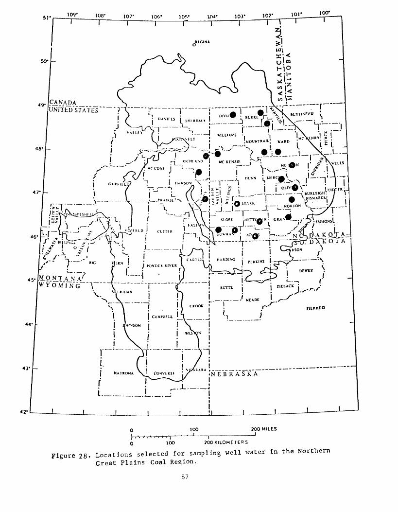
51jor i 00*.

100 2OO MILES_J

0 100 2OOKILOMETERS

Figure 28- Locations selected for sampling well water in the Northern

Great Plains Coal Region.

87

Chemical variability of ground water in the Fort Union coal region

Results of an analysis of variance of data from ground-water samples from the Fort Union coal region indicate that for most of the chemical constituents analyzed, most of the variance is large scale, that is between widely spaced sampling sites within the region (see table 12).

In addition, because of the large values for the variance of most chemical constituents the confidence with which one could predict the chemical composition of a randomly selected well in the region would be poor. Recent work by Thorstenson, Fisher, and Croft (oral commun., 1976) has helped to explain at least part of the high variability of many chemical constituents. In the Fox Hills aquifer of the Fort Union coal region, Thorstenson and colleagues have found that as ground water moves downdip from recharge areas a combination of chemical reactions with the aquifer minerals, sulfate reducing bacteria, and exchange reactions with aquifer clays, gradually change the water from a Ca Mg HC0 3 S04 type that has a pH around 8.0, to a Na HC0 3 water that has a pH above 8.5. Even though ground waters near the recharge areas may contain appreciable Na and HC0 3 , the deeper waters contain much higher Na and HC0 3 concentra tions. Constituent correlation coefficients based on data from the 19 randomly selected wells of this study in general support the process as described by Thorstenson and colleagues. For example, Na, pH, HC0 3 , and total dissolved solids (TDS) tend to increase together, while S0 4 , Ca, Mg tend to decrease in relation to these constituents, as shown in the following table:

Log Na Log HC0 3 Log TDS Log S0 4 Log Ca Log Mg

pH 0.40 0.47 -0.04 -0.43 -0.88 -0.83Log Na .84 .79 .16 .46 -.45Log HC0 3 .51 -.09 -.56 -.53Log TDS .55 <-.01 .01Log S04 .55 .62Log Ca .95

The positive correlation between S04 and TDS is a result of some recharge area ground waters having relatively high TDS with S0 4 as the major anion. Such waters would show an increase in dissolved solids and a reduction in sulfate as the water moved down gradient. In contrast, ground water from recharge areas that starts with relatively low dissolved solids might end up down gradient with a dissolved solid content lower than some recharge area waters. In both cases, however, there is a re duction in sulfate and an increase in dissolved solids downdip.

From the small number of samples collected in this study, it appears that the scale of this process is not regional, or basin wide, but rather is on a scale of less than 100 km. In addition the initial compositions of ground waters in the recharge areas further obscure this process. However, ratios of the various chemical constituents in recharge areas

Table 12. Analysis of logarithmic variance for ground waters of

the Fort Union Formation, North Dakota and Montana.

[An asterisk (*) indicates component is significantly different from zero at the 0.05 probability level; data in milligrams per liter, except where noted as picocuries per liter (pCi/1) or micrograms per liter fogm/1)^

Constituent Total Log-, 0 variance

Ra (pCi/1) 0.242

U fog/1) .979

p (pCi/1 as Sr/Y-90) .097

TDS mg/1 ,066

PH .375-7

Temperature (°C) .011

HC0 3 (mg/1) .039

Br (mg/1) .171

Ca (mg/1) .484

Cl (mg/1) .232

Hardness (Total as CaC0 3 ) mg/1 .546

Mg (mg/1) .715

Mn dig/1) .340

K (mg/1) .095

SAR- .485

Si0 2 (mg/1) .042

Na (mg/1) .192

S04 (mg/1) .504

Zn (tig/1) .578

Al fog/1) .124

Ba fog/1) .171

B fog/1) .168

Li (jig/D -062

Sr fog/1) .160

Fe fog/1) .313

Variance component f%)Between Between Between areas wells samples

41.8 56.6* 1.5

96.5* 2.6 .8

87.6* .0 12.4

82.5* 17.4* <.l

96.8* 3.2 <.l

81.4* 18.6 <.l

82.8* 17.2* <.l

86.7* 4.4 8.8

98.8* 1.2* <. 1

99.0* .5 .4

98.6* 1.2* .1

98.3* 1.3 .3

89.8* 7.8 2.4

85 . 6* 14 . 2* .2

97.9* 2.1 <.l

99.5* .0 .4

90.5* 9.4* .1

81.8* 18.2* <.l

45.7 54.1* .1

44.6 25.8 29.5

85 . 0* 14 .0* .9

64.4 35.1* .5

59.4 32.2 8.4

85.0* 10.4 4.6

75.3 24.0* .7

J_/ Measured in standard units.

2/ Sodium absorption ratio.

89

are generally much less variable than the individual chemical constituents For example, despite high variability of Na content of ground water from recharge areas, the sodium absorption ratio (SAR) in recharge areas is

/ SAR =Na

Ca-fMg

generally less than 5, while in downdip ground waters it reaches values as high as 86. This latter point may have important implications for coal spoil-pile reclamation and irrigation, and indicates the wide range in suitability of ground water for such uses.

As shown in table 13, in addition to large variations in the con centrations of major elements, most trace elements also show wide vari ations. The large variability in the trace-element concentrations of the ground waters is controlled in many instances by the same geochemical processes controlling the concentrations of major chemical constituents. For example, as the sulfate is reduced by sulfate reducing bacteria to H 2 S, the H 2 S in turn precipitates the trace metals, greatly lowering their concentration in the ground water. Waters which have a reducing potential due to production of H 2 S can also control the solubility of uranium.

Despite the large variations in trace element concentrations in the ground waters of this region, only a few samples show trace element concentrations above maximum contaminant levels established by the safe drinking water act (U.S. Environmental Protection Agency, 1975; 1976), as outlined below. Those trace elements involved include fluorine and gross a.

Constituents

AsBaCdCrPbHg

Maximum allowable values

0.05 mg/11.0 mg/1.01 mg/1.05 mg/1.05 mg/1.002 mg/1

Constituents

N03 (as N)SeAgFGross alphaGross beta

Ra226,228

Maximum allowable values

10.0 mg/1.01 mg/1.05 mg/1

1.4-2.4 mg/1*15 pCi/150 pCi/15 pCi/1

*, varies with annual average of the maximum daily air temperature for the locality.

90

Table 13.--Geochemical summary of ground water from the Fort Union Formation,North Dakota and Montana

fData expressed as milligrams per liter except where noted as micromhos centimeter (^mhos/cm) , micrograms per liter (fi gm/l) and picocuries per (pCi/1); detection ratio is number of samples in which constituent was mined to total number of samples analyzed"!

Sp. Cond. (M- mhos /cm)

Diss Solids (180°C mg/1)

PH

Temperature °C

Alkalinity (mg/1)

Al fog/1)

As fog/1)

Ba fog/1)

Be 0*g/l)

HC0 3 (mg/1)

Bi fog/1)

B fog/1)

Br (mg/1)

Cd fog/1)

Ca (mg/1)

Cl (mg/1)

Co fog/1)

Cu fog/1)

Cr fog/1)

F (mg/1)

Ga (jig /I)

Ge (j.g/1)

Hardness (Total as CaC0 3 mg/1)

Hardness (non-carb mg/1)

I (mg/1)

Detection ratio

19/19

19/19

19/19

19/19

19/19

18/19

9/19

19/19

0/19

19/19

0/19

19/19

15/19

2/19

19/19

19/19

0/19

8/19

0/19

19/19

0/19

0/19

19/19

6/19

8/19

Geometric Geometric mean deviation Maximum

1690 1.66 4300

1031 1.92 4140

7.S-7 .64-' 8.89

9.6 1.27 20.4

576 1.60 1070

24 2.36 90

<1 -- 26

50 2.58 520

<7

665 1.63 1160

<14

175 2.72 800

.21 2.87 1.7

<1 « 1

28 4.50 350

15 3.45 170

<14

<1 -- 15

<14

.6 3.19 7.5

<2

<15

126 4.98 1900

<1 « 1600

<.01 -- .78

per liter deter-

Minimum

495

281

6.55

7.1

206

<5

<1

13

--

251

--

23

<.l

<1

1.8

1.8

--

<1

--

.1

--

5

<1

<.01

91

Table 13.--GcocheTnical summary of ground water from the Fort Union Formation,North Dakota and Mont ana- -Continued.

Detection ratio

Fe

Pb

Li

Mg

Mn

Hg

Mo

Ni

K

Be

Si0 2

Ag

Na

IM^

S0 4

Sn

Sr

Ti

V

Zn

Zr

Gross

Gross

Radiuv

Oig/D

(tig/1)(tig/1)(mg/1)

Oig/D

(ng/D

Cig/i)

Cig/D

(mg/1)

Cig/1)

(mg/1)

fog/D

(mg/1)

(mg/1)

fog/D

Cig/1)

fog/D

Ctg/i)

Otg/l)

(ug/D

alpha Ci8/l as u-nat)

beta (pCi/1 as Sr/Y-90)

n 226 (PCi/D

Uranium Ci8/l)

19/19

0/19

19/19

18/19

15/19

4/19

7/19

0/19

19/19

6/19

19/19

0/19

19/19

19/19

19/19

0/19

19/19

1/19

0/19

16/19

0/19

4/19

15/19

16/19

18/19

Geometric mean

427

<14

49

12

31

<.l

<1

<14

4.6

<1

14

<3

219

8.5

128

<18

551

<2

<14

42

<25

<4.2

5.7

.40

.74

Geometric deviation

3.88

1.79

6.73

3.73

--

--

--

1.77

~

1.61

--

2.97

5.08

5.12

2.40

6.58

1.87

3.12

12.5

i

Maximum

5000

--

150

240

470

.1

30

--

34

6

27

760

86

2400

3800

150

1600

49

22

4.2

40

Minimum

70

.>

20

<.l

<1

<.l

<1

--

1.5

<1

6.2

--

23

.7

4.7

--

110

<2

<10

--

<4.2

<2.9

<.l

<.01

I/ Arithmetic mean and standard deviation.

2/ Sodium absorption ratio.

Comparison of use of 0.45-micrometer filter with 0.10-micrometer filter

By convention a 0.45-micrometer filter is normally used to filter water samples in the field. However, Kennedy, Zellweger, and Jones (1974) and U.S. Geological Survey (1972, p. 81) have shown that for some samples a 0.45-micrometer filter allows appreciable fine particulate material to pass through the filter, which may significantly affect the resulting chemical analysis. When the water-quality data obtained in this manner are interpreted as dissolved chemical constituents, large errors may result in the interpretation due to variations in the quantity of particulate material passing through the filter. The above investigators found that using a 0.10-micrometer filter greatly reduced the amount of fine particulate material passing through the filter, and resulted in water-quality data that more accurately defined soluble constituents. The chemical constituents studied also more closely approached their calculated thermodynamic solubilities.

A test was run to determine if using a 0.10-micrometer filter rather than a 0.45-micrometer filter would have a significant effect on analytical results obtained for ground waters from the Fort Union coal region. At each of three random sites where duplicate samples were collected using a 0.45-micrometer filter, a third sample was also collected using a 0.10-micrometer filter. Results of this experiment indicate no recognizable difference between laboratory results obtained for the two 0.45-micrometer filtered samples and the 0.10-micrometer filtered sample. The differences found appear to lie within the limits of analytical precision for each of the chemical constituents analyzed. In addition to the results obtained from comparison of the 0.1 and 0.45- micrometer data, all the other laboratory data show expected low concen trations of insoluble chemical constituents, which indicates insignificant effects on analytical results by particulate matter. The only exception to this conclusion was the measurement of unusually high concentrations of Ti in two closely-spaced wells. These wells will be resampled. We cautiously conclude, therefore, that for most ground-water sampling in the Northern Great Plains Coal Province a 0.45-micrometer filter is sufficient. However, if much fine sediment is encountered in a ground- water sample, or if anomalously high concentrations of relatively insoluble chemical constituents such as aluminum or titanium are obtained, a 0.10-micrometer filter should be used.

93

GEOCHEMISTRY OF THE FORT UNION FORMATION by Richard J. Ebens and James M. McNeal

Introduction

The Northern Great Plains Coal Province includes the lignite deposits in the Northern Great Plains of eastern Montana and western North Dakota and South Dakota as well as the coal deposits in the Powder River Basin of northeastern Wyoming and southeastern Montana. Most of the strippable coal beds in this region are in the Paleocene Fort Union Formation. This formation consists of interbedded siltstone, claystone, and sandstone deposited in a deltaic floodplain-floodbasin environment. Any substitution, even partial, of these overburden rock materials for natural soils in areas of strip mining, may cause sub stantial changes in the chemical composition of the surface environment in these disturbed areas. A knowledge of the geochemistry of potential overburden rock materials may indicate which, if any, of these materials could be substituted for soil with minimal chemical change.

To acquire this knowledge, a suite of shale and sandstone samples was collected from outcrops of the Fort Union Formation throughout the Northern Great Plains Coal Province during the summer of 1975. This initial reconnaissance study was undertaken to assess the magnitude and distribution of chemical variation in these rock units. The purpose of this report is to describe the sampling design and to present some preliminary results of the study.

94

Sampling design and analytical procedures

Samples for this study were collected according to a staggered nested analysis of variance design (Leone and others, 1968). The sampling design, which is outlined below, has five geographic "levels", one stratigraphic "level" and a "level" of laboratory error. Sampling localities are shown in figure 29 and consist of a randomly selected outcrop of the Fort Union Formation within a 5-km cell. At 10 of the 40 localities shown, two samples of each rock type (shale and sandstone) were collected from a stratigraphic section in order to estimate stratigraphic variability. Geographic variability was estimated by nesting 5-km cells within 25-km cells, 25-km cells within 50-km cells, 50-km cells within 100-km cells, and 100-km cells within 200-km cells. Lab oratory error was estimated by splitting 20 of the 60 samples into two parts resulting in a total analytical load of 80.

The two sample groups, shale and sandstone, were each submitted to the laboratories in randomized sequence. Each sample was crushed in a jaw crusher and then ground in a vertical Braun pulverizer with ceramic plates set to pass 100 mesh. T. L. Yager analyzed the samples for total carbon, J. G. Crock analyzed for zinc, and W. Mountjoy analyzed for magnesium, sodium, lithium, and rubidium. Methods used for analyzing for these elements are described in U.S. Geological Survey (1975, p. 71- 73).

ta

200-km

100-km

50-km

25-km

5-km

Strat igraph ic nLevel

123k56't

Number of units Source of variation at each levelBetween 200-kin ceJlsBetween 100-km cellsBetween 50-ton cellsBetween 25-km cellsBetween ^>-kifi cellsStratigraphicLaboratory

6122k361*86080

Degrees of freedom

561212121220

95

.] locr

bO

49

43*

45- .___ o M i N~G

4?-I

1OO 2OO MILES _I

0 100 POO KILOMETRES

Figure 29.--Sampling localities of shale and sandstone of the Fort Union Formation in the Northern Great Plains Coal Province. Large squares are 200 km on a side; intermediate squares, 100 km; and smaller squares, 50 km. Dots indicate sampling localities. Map adapted from U.S. Geological Survey (1974a) and Whitaker and Pearson (1972).

Geochemical variation

Variance components and summary statistics for six elements in shale and sandstone are given in table 14. In shale, most of the variation occurs at local scales (within 25-km cells) except for sodium which has important regional variation. In contrast, four elements (total carbon, sodium, magnesium, and zinc) of the six in sandstone have important regional variation. The regional differences in sandstone are probably related to differences in feldspar and dolomite concentrations However, quantitative mineralogical work (X-ray diffraction work) has not been completed on these sample suites and until completed, we can only speculate as to the cause of these differences.

Geochemical maps

The variance mean ratio, vm , (Miesch, 1976) was calculated to determine the feasibility of mapping those elements that have signifi cant variation among 200-km cells. This ratio, given in table 14, is an index of the stability of a map pattern. A ratio of one or greater indicates that differences among 200-km cells means are stable at the 80-percent confidence level. Maps of sodium in shale and total carbon, sodium and magnesium in sandstone are judged to be stable and appear in figures 30-31.

The exceptionally low values noted for Na 2 0 in both shale and sand stone collected from outcrops in the southeastern Powder River Basin are clearly anomalous compared to Fort Union Formation samples elsewhere, and very likely indicate a general lack of feldspar. Similarly, the low content of MgO in outcrops of sandstone throughout the southern part of the study area (including the Powder River Basin) probably reflects more abundant dolomitic cement in the northern outcrops. The regional distri bution of total carbon in sandstone varies by a factor of about 3.0 (fig. 31) but is a more erratic pattern than are those of Na 2 0 or MgO. The lack of a pattern for total carbon similar to that for MgO indicates that the southern outcrops are more carbonaceous than the northern out crops.

97

Tabl

e 14.

Statistical

analysis of

th

e chemistry

of sh

ale

and

sand

ston

e of

th

e Fort Union

Form

atio

n, Northern Gre

at Pl

ains

Co

al Province

[*,

sign

ific

antl

y gr

eate

r th

an ze

ro at

the

0.05

probability

level]

Cons

titu

ent

Anal

ysis

of

lo

gari

thmi

c variance

Total

L°8

lO

Variance

Perc

ent

of to

tal

vari

ance

Betw

een

200-

kra

cells

Betw

een

100-

kmce

lls

Betw

een

50-kra

cell

s

Betw

een

25 -km

cell

s

Betw

een

5-km

cells

Stra

ti-

grap

hic

Labora

tory

vl/

(200

-km

cell

s)

Summ

ary

statistics

Geometric

mean

Geometric

deviation

Geom

etri

cerror

Expected

95 pe

rcen

trange

(bas

elin

e)Sh

ale

C, total,

7L ~

MgO,

1

Na20,

T. --

----

0.26

99

.0631

.153

8

.162

0

.070

8

.072

6

< 1

< 1 8*

39* 3

< 1

17*

17 8

< 1 19

< 1

2

< 1 2 1

< 1

35

< 1

< 1

< 1 20

< 1

< 1

29

78*

70*

28*

76*

45*

30* 3*

12*

10* 2*

20*

23 2

< 1 2

< 1

< 1

0 0

.8

1.6 .2

0

0.94

31 2.4 .58

110 80

3.31

1.78

2.47

2.53

1.85

1.86

1.77

1.09

< 1.

09

1.14

< 1.

06

< 1.

06

0.11

-77

9.9-97

32-3

76

23-270

Sand

ston

e

C, total,

7. -

-

T

-1

nw _ _ _ _ _

MgO,

T.

-----

Na20, *

.567

9

.018

6

.2482

.1914

.017

8

.046

3

32*

< 1

42*

50*

< 1 24*

21*

< 1 20*

< 1

< 1

< 1

< 1

44*

< 1 22

36*

34*

14 3 18*

< 1

< 1

8*

11

23 1 26*

36* 9

13*

29*

18* 2*

26* 1

9 1

< 1 1 2 23

1.2

0 1.8

1.9

0

.7

1.0

15 1.7 .67

59

43

5.67

1.37

3.15

2.74

1.36

1.64

1.68

1.03

< 1.

12

1.11

1.04

1.27

8.0-

28

32-1

10

I/ Variance mean

ratio

for

200-

km cells.

See

text for

expl

anat

ion.

>00

200

KIL

OM

ETR

ES

San

dst

on

eSh'He

Figu

re 30.--Regional

dist

ribu

tion

of

Na20

in sa

ndst

one

and

shale

of th

e Fo

rt Union Fo

rmat

ion.

Values

are

mean

s (in

percent) of

20

0-km

cel

ls.

vm is

in

dex

of stability.

o o

49.|

CA

NA

DA

_

'l/N

JT

ED

ST

AT

ES

'

'

tOO

2O

O K

ILO

ME

TR

ES

Tota

l ca

rbo

nM

gO2O

O K

ILO

MC

TDC

S

Figu

re 31. Regional di

stri

buti

on of

to

tal

carbon and

MgO

in sa

ndst

one

of the

Fort

Union Fo

rmat

ion.

Va

lues

ar

e means

(in

percent) of 20

0-km

cel

ls.

vm is in

dex

of stability.

SOIL CHEMISTRY IN THE PICEANCE CREEK BASIN by Charles D. Ringrose ', Ronald W. Klusman ', and Walter E. Dean

Introduction

The oil-shale regions of Colorado, Wyoming and Utah hold promise of providing a substantial amount of liquid hydrocarbons within the next decade, and environmental baselines for soil, plant, air, and water quality are needed prior to economic development. An important part of this need is the establishment of trace-element baselines in surficial materials. A knowledge of the variance of trace-element concentrations, in particular, would allow the determination of the soil sampling interval required in order to construct practical geochemical baselines in this and adjacent areas.

The main objective of this study was to establish the extent and magnitude of regional variations in major and trace elements in soils within the Piceance Creek Basin of western Colorado. The sampling design was constructed to test geochemical variability at a number of geographic levels (distances between samples) as well as at one physio graphic level fridge top vs. valley bottom). A secondary goal was to provide a first approximation of natural (baseline) variations in soil composition within the Piceance Creek Basin, and to provide a scale for measuring deviations from the baseline during the course of oil shale production, processing, and land reclamation. R. J. Ebens and R. R. Tidball provided valuable assistance with the sampling design. A. T. Miesch and R. R. Tidball helped with the statistical analyses. We extend special thanks to J. G. Boerngen who did most of the data pro cessing.

Sampling design

The sampling design for the study of soils in the Piceance Creek Basin is a partially unbalanced nested analysis of variance design. The sampling localities are shown diagrammatically in figure 32. The initial sampling design, as used in the field, was balanced. Within each of 36 townships, 2 sections were chosen at random. Within each section, two samples of surface soil were collected 100 meters apart. All four samples within a given township were collected either from ridge tops or valley bottoms. Ridge top and valley bottom sampling alternated according to a checkerboard design. By eliminating one sample from one section in each township, a slightly unbalanced design resulted in a reduction of analytical load of 25 percent. The decision as to which of the two sections in each township would have two samples included in the analytical design, and which would have only one was made by a simple flip-of-the-coin. This technique was also used to decide which of the samples to eliminate in the section chosen for only one sample. A higher geographic level was constructed by grouping all

_/ Department of Chemistry and Geochemistry, Colorado School of Mines, Golden, Colo.

101

39"30

108°30'108*

supertownship

township,

1* 1 .1.' ! ->

----- £--- - -i

p.

1ii

,

1.'

rn > » w .

> Vk 441samples

ridge top valley bottom

Figure 32.--Index map (top) showing location of study area, lease tracts Ca and Cb (stippled), and distribution of the Green River Formation and soil"^? sampling localities. Map (bottom) ,-J showing soil sampling design and ^^^X number of samples at each locality. (^ Piceance Creek Basin, Colorado.

102

samples within four adjacent townships into a "supertownship". From the 108 samples used in this design, 32 were chosen at random to be replicated in analysis. The final design therefore consisted of six levels one physiographic (ridge top vs. valley bottom), four geographic (between supertownships, between townships, between sections, and between samples, and one analytical (32 replicate analyses). All 140 samples (108 separate samples plus 32 replicates) were submitted for analysis in a randomized sequence. Level 1 (the top level) was designed to examine geochemical differences between soils on ridge tops and those in valley bottoms, level 2 was designed to examine geochemical differ ences at geographic scales greater than 19 km (between supertownships), level 3 examines differences at scales from 3 to 19 km (between town ships) , level 4 examines differences at scales from 0.1 to 3 km (between sections), and level 5 examines differences at a scale of 100 m (between samples). Level 6 measures analytical precision and includes errors due to sample inhomogeneity, sample preparation, and analysis.

Chemical analyses

The samples were ground with a ceramic mill to pass a 100-mesh sieve. The major elements Al, Si, Ca, Ti, Fe, and K, and the trace elements Sn, Sb, Ge, As, and Se were analyzed by X-ray fluorescence by J. S. Wahlberg, Nichele Goff, and J. W. Baker. Violet Merritt and Wayne Mountjoy analyzed the samples for Mg, Na, Li, and Rb by atomic absorption spectrometry. Atomic absorption was also used by J. G. Crock and G. 0. Riddle to determine Zn concentrations. Johnnie Gardner and Patricia Guest determined F using the specific fluoride ion electrode method. Mercury was determined by the wet oxidation, flameless atomic absorption method by J. A. Thomas and G. 0. Riddle. Total carbon was determined by combustion by V. E. Shaw. The remaining trace elements (B, Ba, Be, Co, Cr, Cu, Ga, Mn, Mo, Nb, Ni, Pb, Sc, Sr, V, Y, Yb, and Zr) were all determined by plate-reader optical emission spectrometry by Arthur L. Sutton and Richard Lemert. Details of these analytical methods are described in U.S. Geological Survey (1975, p. 69-81, and this report, p.

Results

Logarithmic variance components for 37 elements in soils from Piceance Creek Basin (table 15) shows that most of the geographic variation for most elements occurs between sections (0.1 to 3 km). This conclusion supports analysis of variance results for soils from other areas which indicate that most of the variability in soil com position occurs at local scales (U.S. Geological Survey, 1975, p. 20- 28, 36-49).

Of the 37 elements listed in table 15, 27 have significant variancecomponents at the section level (Al, Ca, Fe, Mg, K, Si, Na, Ti, As, B,Ba, Be, Co, Cr, Cu, Ga, Hg, Li, Mo, Pb, Rb, Sc, Sr, V, Y, Yb, and Zn).

103

Table 15.--Analysis of variance of surface soil chemistry, Piceance Creek Basin, Colorado

[*, indicates component is significantly different from zero at the 0.05 probability level]

ElementAlCaFeMgKSiNaTi

Total-C

AsBBaBeCoCrCuFGaGeKgLiMnMoNbNiPbRbSbScSeSnSrVyYbZnZr

Total Logarithmic

Variance0.0044.1596.0080.0291.0075.0038.0^73.0064.0535

.0914

.0173

.0313

.0264

.0624

.0452

.0821

.0331

.0677

.1378

.1631

.0363

.0476

.0976

.1055

.0694

.1029

.0127

.1867

.0491

.0947

.3488

.0350

.0396

.0330

.0986

.0083

.0359

Variance components as percentage of total variance

Betv/een Ridge Tops

and Valley Bottoms

000020011

0000000300250000001010100012

Between Super-

townships (>19 km)

1828*27*28*7

22*428*14

018*0

24*1217*28*7

10*0

1023*0

111

10662502

1979*8*

31*1

Between TownshiDS (3-19 kin)

015*0300

41*0

26*

000000000

1136*080000000

150

18*000

120

Between Sections (0.1-3 km)

58*48*38*57*80*46*46*54*19

81*57*35*37*33*37*18*1559*031*

58*4

48*172439*77*0

37*00

31*52*42*38*32*28

Between Samples (0-100 m)

14*9216*

22*6*9*

31*

6

I000134*0

274

10*070

36*06

100

25335000

19*2

Analytical Error

100

33115

1038

10

132158395546?24l3262175

883382305511865959652741495^5

66

104

Only 10 elements (Al, K, Si, Na, Ti, F, Li, Ni, Zn and total C) have significant variance components at the sample level (100-meter distance), and only 5 elements (Ca, Na, Hg, Sr, and total C) have significant vari ance components at the township level (3-19 km). More than one-third of the elements listed in table 15 (14 of 37) have significant variability between supertownships (<19 km). These 14 elements include Ca, Fe, Mg, Si, Ti, B, Be, Cr, Cu, Ga, Li, Y, Yb, and Zn. Although soil development and characteristic vegetation on ridge tops visibly differ from that in bottom valleys, we were surprised to find that there were no significant elemental differences between soil samples collected on ridge tops and those collected in valley bottoms. This means that the ridge top and valley bottom samples can be viewed as part of the same population, and they have been considered as such in all subsequent statistical analyses.

The significant variance at the supertownship level for 14 elements indicates that these elements have a regional component of variability in the Piceance Creek Basin, and that a proper baseline for these elements must take this component into account either as a listing of supertown ship means or as a map based on such means. To explore the usefulness of such means, if based on the data in hand, the variance ratio, v, may be used as a starting point. For this study, v is defined (Miesch, 1976) as the ratio of the variance among map units (supertownships here) to the sum of the variances at all levels within a map unit:

tN S 2

v = _Y. = _£_ _

where S 2 , S 2 S 2 , S?, and S^ are the logarithmic variances at the supertownship, township, section, sample, and analytical levels, respectively. Once v has been calculated for each element, it is possible to determine the number of random samples which must be collected within a supertown ship to insure that two supertownships can be distinguished, at a given level of confidence, based on mean values for that element. This effective number of samples has been defined as n by Miesch (1976), and he presents curves at the 80- and 95-percent confidence levels for determining n knowing the value of v. The n values listed in table 16 indicate that from as few as three to more than 30 random samples would have to be collected at random from within each supertownship, depending upon the element of interest, to distinguish between supertownship means, at the 80-percent confidence level. For example, it would require a mean based on iron analyses of only four random samples from each supertownship to distinguish between supertownships based on iron concentrations in soils, but it would require a mean based on ten random samples from each supertownship to distinguish confident supertownships on the basis of vanadium concentrations in soils.

105

Tablo 16. --Ci mtcal siir.mnry of surface soil in the IMccance Crook Basin. Colorads,

TDota expvcs.:cd In parts per million except where noted us percent (".)', N, total number of samples of 1-tO in which eU-nvnl concentration was quantitatively do.tnrrolne.d; v, vat- tance rot to of Mli-scli (see toxt); nr , minimum numlter of randomly selected noil samples with each suportownship required to distinguish aniotiK townships; Er , vaximum acceptable value of the error variance of suprrtowushlp iroana; E , observed error variance of the supertownshlp mratis based on the d:ita in hand; n.d., not determined, nr la indefinitely large]

Observed Element range

Al, X 3.4-7.8

Ca. % .46-9.8

Fe , 1 1.1-2.9

Mg, I .51-2.7

K, I .77-3.2

Na, 1 .18-3.5

T* ¥- ... . 1 **- Ifl

C(total), I- .87-12

As <2.0-21

B 25-102

B« 600-13, OOC

Be .88-4.4

Co 1.2-16

Cr - 12-110

Cu <8. 7-122

F <400-l,600

r_. *~3 3.1Q

Hg - .01-. 22

Li 16-140

Mn 82-1,200

Mo <1. 04-14

Kb <2.2-21

N l <3.4-42

Pb <3.3-56

Rb 40-190

Sb <.l4-4.5

g c __- _ _____ si 1-13

Se <.11-1.2

Sn <. 11-11

S T 61-660

V --- 7.5-120

Y - 4.9-36

Yb - '.23-6. 2

7r. --------- 14-700

Geometric Geometric mean deviation

5.5 1.17

1.9* 2.48

I QJL. 4 <> >

1.0* 1.49

2.3 1.22

26* 1.15

1.4 1.65

9 fl+ 1 91

3.0 1.69

6.4 2.01

61* 1.35

1,400 1.50

2.4 1.46

7.9 1.77

60* 1.63

29* 1.94

490 1.52

1 ft* 1 87

07 o ^7

.041 2.56

34* 1.55

490 1.65

5.3 2.05

6.9 2.11

21 1.83

26 2.09

105 1.29

.90 2.70

6.7 1.66

9 fl 7 A 9

on -1 Qft

280 1.55

56 1.58

15* 1.52

2.1* 2.06

BO* 1.23

?7fj l-SS

N

140

140

140

140

140

140

140

140

140

139

140

140

140

140

140

139

112

139

136

140

140

140

134

127

139

139

140

134

131

126

121

140

140

140

133

140

l&ri

V

0.30

.40

tn

.39

.07

.24

.05

.40

.16

<.01

.23

<.01

.32

.12

.20

.39

.08

.11

<.01

.11

.31

<.01

.12

.01

.11

.07

.06

.02

.05

<.01

.03

.23

nfl

.10

.09

.46

.01

nr

5

4

4

4

12

4

15

4

6

n.d.

5

n.d.

4

7

5

4

11

7

n.d.

7

4

n.d.

7

n.d.

7

12

14

35

15

n.d.

30

5

10

10

3

Er

0.0007

.0285

.0015

.0053

.0006

.0007

.0030

.0011

.0076

n.d.

.0028

n.d.

.0050

AAftQ

.0075

.0148

.0027

.0087

n.d.

.0205

AAflfl

n.d.

.0124

n.d.

ArtflQ

.0080

.0008

.0007

.0031

n.d.

.0097

.0056

.0037

.0038

.0091

.0019

E,

0.0010

.0408

.0014

.0065

.0022

.0008

.0182

.0013

.0144

n.d.

.0039

n.d.

.0046

.0114

.0084

.0109

.0055

.0162

n.d.

.0529

.0080

n.d.

.0214

n.d.

.0129

.0208

.0036

.0243

OAQfl

n.d.

.0507

.0085

AAOft

.006R

.0194

.0018

106

Once values of n have been determined, it is possible to calculate the maximum acceptable error variance (E ) of the means of the mapping units (supertownships) according to the following equation (Miesch, 1976)

_r

Because n was determined at the 80-percent confidence level, the values of E listed in table 16 are also at the 80-percent level. E estimates the maximum permissible error variance in any computation of supertown ship means. If the actual variance of the mean for a supertownship, E , based on the samples currently in hand is less than or equal to E (i.e. E <E ), the samples currently in hand may be used to compute suitably suable estimates of the mean concentrations in each supertownship. If E >E , additional sampling is in order before suitably stable estimates can Be computed. For a balanced, hierarchical design, the observed error variance, E , is computed according to the following equation (Miesch, 1976): S

S 2 S 2 S 2 S 2T-, _ __g_ "r" / "r" _____6 "*" _____[J_______ ) .Cj

s n_ n_ n na n n n_ n n rL.

where n_ , n , n , and ru are the number of selected townships within supertownshlps , the number of sections within townships, the number of samples within sections, and the number of analyses within samples. Because the actual design was unbalanced, the effective n-values at each level are somewhat less than in a completely balanced design. The effective n-values were calculated according to techniques described by Leone, et al. (1968). For this particular design, E was calculated according to the equation

7.71

E values for each of the 37 elements are listed in table 16. The gcondition E <E is satisfied for five elements--Fe, Be, Cu, Li, and

s r. Zn--and maps of these five elements are shown in figures 33-35.

All five distributions show higher concentrations in the southern part of the basin and three--Cu, Li and Zn--exhibit well-defined trends in that direction. Concentrations of soil zinc increase from 68 ppm in the northeastern part of the basin to almost 100 ppm in the southwestern part. Concentrations of Li increase from 25 to 57 ppm in the same direction, and Cu concentrations increase from 18 to 50 ppm. The reason for these strong patterns is not yet clear. The geochemical trends parallel in a rough way those of the regional topography and possibly they are reflecting some altitude-related feature of the landscape.

107

o CO

IRO

NB

ER

YU

.IUM

Figure 33.--Regional

dist

ribu

tion

of

iron

(p

erce

nt)

and

beryllium

(ppm

) in

surface

soils

in

the

Pice

ance

Creek Basin,

Colo

rado

. Values ar

e su

pert

owns

hip

mean

s.

50

LIT

HIU

M

o;C

OPP

ER

O

'

Figure 34

.--R

egio

nal

distribution of co

pper

(ppm)

and

lith

ium

(ppm)

in surface

soils

in th

e Pi

cean

ce Creek B

asin,

Colo

rado

. Values are

supe

rtow

nshi

p means.

Figure 35.--Regional distribution of zinc (ppm) in surface soils in the Piceance Creek Basin, Colorado. Values are supertownship means.

110

A comparison of trace element concentrations in soils from the Piceance Creek Basin (table 16) with concentrations in oil shale (table 8) suggests that oil shale tends to contain substantially higher concentrations of As, Hg, and Se, and slightly higher concentrations of F, Li, and Mo. Barium and zirconium, on the other hand, tend to be sub stantially higher in soils than oil shale. Environmental concerns generally focus more on trace element increases in the landscape rather than decreases as a consequence of surface disruption during mining operations. Our data suggest that any land reclamation in the Piceance Creek Basin using spent shale or overburden, could induce an increase in several of the better known "noxious" trace elements.

Ill

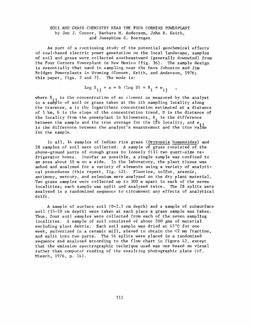
SOIL AND GRASS CHEMISTRY NEAR THE FOUR CORNERS POWERPLANTby Jon J. Connor, Barbara M. Anderson, John R. Keith,

and Josephine G. Boerngen

As part of a continuing study of the potential geochemical effects of coal-based electric power generation on the local landscape, samples of soil and grass were collected southeastward (generally downwind) from the Four Corners Powerplant in New Mexico (fig. 36). The sample design is essentially that used in sampling near the Dave Johnston and Jim Bridger Powerplants in Wyoming (Connor, Keith, and Anderson, 1976; this paper, figs. 3 and 7). The mode is:

Log X = a + b (Log D) + R± + e

where X. . is the concentration of an element as measured by the analyst in a sample of soil or grass taken at the ith sampling locality along the traverse, a is the logarithmic concentration estimated at a distance of 1 km, b is the slope of the concentration trend, D is the distance of the locality from the powerplant in kilometers, R. is the difference between the sample and the true average for the ith locality, and e.. is the difference between the analyst's measurement and the true value for the sample.

In all, 14 samples of Indian rice grass (Oryzopsis hymenoides) and 28 samples of soil were collected. A sample of grass consisted of the above-ground parts of enough grass to loosely fill two quart-size re frigerator boxes. Insofar as possible, a single sample was confined to an area about 10 m on a side. In the laboratory, the plant tissue was ashed and analyzed for a variety of elements using a variety of analyti cal procedures (this report, fig. 42). Fluorine, sulfur, arsenic, antimony, mercury, and selenium were analyzed on the dry plant material. Two grass samples were collected up to 300 m apart in each of the seven localities; each sample was split and analyzed twice. The 28 splits were analyzed in a randomized sequence to circumvent any effects of analytical drift.

A sample of surface soil (0-2.5 cm depth) and a sample of subsurface soil (15-20 cm depth) were taken at each place a grass sample was taken. Thus, four soil samples were collected from each of the seven sampling localities. A sample of soil consisted of about 200 gms of material excluding plant debris. Each soil sample was dried at 45°C for one week, pulverized in a ceramic mill, sieved to obtain the <2 mm fraction, and split into two parts. The 56 splits were placed in a randomized sequence and analyzed according to the flow chart in figure 42, except that the emission spectrographic technique used was one based on visual rather than computer reading of the resulting photographic plate (cf. Miesch, 1976, p. 14).

112

108' 107

38°- - - --38

1O9 108' 107

0L_

10O Km _i

50 Miles

pre-Upper Cretaceous

rocks

UpperCretaceous

rocks

Figure 36.--Sampling localities of soil and grass southeast of the Four Corners Powerplant, New Mexico.

113

The analysts were J. Baker, W. Gary, A. Drenick, A. England, J. Gardner, P. Guest, J. Hamilton, T. Harms, C. Huffman, Jr., R. Havens, L. Lee, V. Merritt, H. Millard, Jr., H. Neiman, C. Papp, J. Thomas, R. Van Loenen, J. Wahlberg and T. Yager,

Results of the search for distance-related geochemical variability are summarized in table 17. Nearly half of the elements measured in grass or its ash (and the ash itself) exhibit statistically significant variation associated with distance. All trends, except silicon, decrease away from the powerplant, as would be expected if chemical pollution is occurring. Fewer trends are seen in the substrate (eight in surface soils and five in the subsurface), and about half exhibit distance-related increases rather than decreases.

A distance-related element increase is unlikely to reflect simple contamination (although it could conceivably reflect a more complicated response to chemical pollution) and, at least in the substrate, such an increase almost certainly reflects a natural variability in the soil parent. The highest concentrations for K 2 0 and Rb in both soil horizons were measured in samples from the two most distant localities (Appendix V, table 4). Both localities are underlain by sandy rocks of Tertiary age which, when compared to the shaly bedrock at the nearer localities, would be expected to show higher K 2 0 and Rb, presumably because of a higher K-feldspar content. Conversely, decreases with distance in soil CaO, MgO, and C largely reflect higher concentrations in the first three localities (Appendix V, table 4), which are underlain by carbonaceous and locally calcareous shale.

The tendency for these soil trends to involve the same major elements in both horizons (K 2 0, CaO, MgO, C) further suggests a parent mineralogical control. In addition, the minor elements Rb and Zn involve both horizons and likewise probably reflect a parent control. Mn and Pb in the surface also show trends but because they increase, rather than decrease with distance, they cannot be viewed as pollutants from the Four Corners Powerplant. Thus, soil chemistry in this area shows no obvious geochemical features that could be attributed to the presence of the powerplant.

Vegetation chemistry, however, points to a large number of suspect elements (figs. 37-40), including, again, a number of major elements-- Ca, K, Mg, and Si. Silicon increases with distance and may reflect a change in soil-dust composition. (The grass was not cleaned prior to analysis.) Ca, Mg, and K all decrease with distance from the powerplant but as all major constituents of living tissue (and, hence, presumably subject to biological mechanisms controlling concentration), these trends are hard to interpret, and none are particularly well developed. The trend in Ca, for example, is largely due to low concentrations in the farthest locality (fig. 38). Conceivably, the trends in Ca and Mg, which parallel similar trends in soil Ca and soil MgO, might be due to soil contamination but K cannot be so explained. The trends in Na and

114

Table 17. Re^reaalon analysis of element* In soil and gra*s or It* a»h southeastward of the Four Corner* Poverplant,

New Mexico

[», Indicates that slope of aetal trend away from power plant Is significantly different at the 0.05 probability level; percentages In p&rentheaeo Indicate a Metal trend which increases away from poverpl&nt; leaders ( ) Indicate so data)

Element or ash

Aluminum

Antimony

Arcanlc

Ash

Boron

Barium

Cadmium

Calcium

Carbon

Chromium

Cobalt

Copper

Fluorine

Gallium

Iron

Lead

Lithium

Magnet lum

Manganese

Mercury

Molybdeeum

Nickel

Phosphorus

Potassium

Rubidium

Scandium

Selenium

Silicon

Sodium

Strontium

Sulfur

Thorium

Tltaniim

Uranium

Vanadium

Ytterbium

Yttrium

Zinc

21 rconl-jin

Total log varisncs 10

0.0343

0.0782-'

.07071'

.0126

.0149

.0156

.0843

.0059

.0245

.0272

.0065

.0474^'

.0290

.0122

.0259

.0124

.0158

.0123

.0170^

.0567

.0385

.0132

'.0214

.0534*'

.0041

.0358

.0352

W

.0268

.0405

.OJ51

.0087

.OOO

Grids

As percent of the total

Regression

8.0

(4.7)

(3.5)

24.9*

47.4*

6.2

(1.3)

22.5*

(<0.1)

33.6*

<0.1

82.2*

18.6*

5.9

(3.6)

65.4*

21.8*

(1.3)

4.1

56.8*

36.2*

(0.8)

16.6*

60.8*

(38.5*)

45.1*

46.3*

46.2*

<0.1

3.9

4.4

7.7

0.5

Analytical

13.8

29.5

S2.9

6.7

29.7

11.0

90.1

28.3

100.0

75.3

100.0

4.5

25.3

38.4

37.8

26.1

35.1

18.6

42.4

43.1

57.1

37.8

17.1

7.8

17.5

11.0

12.7

7.6

33.7

42.5

39. 8

17.3

99.5

Soil.

Total log variance l

0.0044

.0093

.0063

.0448

.1140

.0223

.0158

.0249

.0033

.0083

.0054

.0057

.0485

.0082

.0224

.0279

'.0020

.0028

.0530

.0004

.0032

.0190

.0060

.0106

.0056

.0183

.00^6

.0060

.0035

.05-V4

0-2.5 an depth

As percent of the total

Regression

5.1

10.4^

(4.4)

56.9*

30.7*

< 0.1

0.2

0.5

(3.5)

2.1

(21.7*)

7.2

47.8*

(24.4*)

(0.1)

2.1

(54.3*)

(29.0*)

(2.1)

(8.5)

9.3

4.5

(2.7)

(1.9)

1.7

3.8

(0.3)

(2.3)

24.2*

(3.6)

Analytical

19.2

65.6

93.2

0.6

28.2

58.6

45.6

50.2

96.5

65.3

78.3

5.4

1.1

34.0

62.1

44.7

1.6

12.4

60.4

34.6

2.0

23.3

30.7

5.9

8.1

59.8

33.8

55.0

2.5

06.4

Soil. 15-20 cm depth

Total logjo variance

0.0031

.0093

.0053

.0298

.1181

.0146

.0141

.0234

.0042

.0051

.0078

.0040

.0244

.0132

.0293

.0222

.0015

.0019

.0526

.0003

.0032

.0137

.0064

.0072

.0051

.0114

.0227

.0093

.0001

.0530

Aa percent

Regression

0.2

5.5

(5.1)

57.5*

11.1^

5.4

(0.6)

6.5

(0.2)

0.2

(5.9)

7.0

56.1*

(9.3)

(0.3)

(1.3)

(41.2*)

(15.1*)

4.3

(l.D

8.3

(2.8)

(8.6)

(2.8)

0.4

9.1

1.7

(O.I)

21.6*

1.1

of the total

Analytical

27.5

65.6

94.9

0.9

27.3

89.9

51.2

53.4

78.9

99.8

56.7

7.6

2.3

21.0

47.6

56.3

2.1

18.5

60.8

47.9

2.0

32.5

28.8

8.6

8.9

90.9

9.7

34.0

3.5

98.9

17 Determined on dry material. 115

and S (figs. 37 and 39) are fairly strong, although their interpretation is fraught with the same problems as K, Ca, and Mg since they are also essential elements in plant tissue. Ash weight of grass also decreases away from the powerplant, in a fashion clearly related to the variation in K (r=0.56 for Log Ash vs. Log K in 14 samples, significant at the 0.05 probability level). log Ash is not significantly correlated with Log Ca (r=-0.18), Log Mg (r=-0.35), or Log Si (r=0.39), indicating that soil contamination is probably not an important contributor to plant ash. The underlying cause for these seven trends remains unknown but does not appear to involve, in an important way, simple element contamination from either nature (soil dust) or man (powerplant). Of the remaining 9 suspect elements, the strongest trends in vegetation are in F and Se (fig. 37), both volatile elements and both suspected pollutants at the Dave Johnston Powerplant in Wyoming (Connor, Keith, and Anderson, 1976; this report, fig. 4). Trends for Co, and Sr (figs. 39 and 40) are fairly strong, and these three must be considered as suspect pollutants. Both have been implicated at the Dave Johnston Powerplant (Connor, Keith, and Anderson, 1976; this report, fig. 4). The trends in Mo, Ni, Ga, Li, and B (figs. 39 and 40) largely reflect concentrations in the outer three or outer four localities, which suggests a possible substrate control on concentration.

Thus, geochemical work with three vegetation types (sagebrush, lichen, and grass) and two soil horizons (surface and subsurface) around three powerplants in the Western Coal Regions has demonstrated the complexity of attempts to quantify potential element emissions by use of "natural" monitors (cf. Connor, Keith, and Anderson, 1976; U.S. Geological Survey, 1974b, p. 14-29; U.S. Geological Survey, 1975, p. 50-57; this report, figs. 4, 8-10). Based on examination of distance-related geochemical variability, a large number of elements have been implicated as suspect pollutants. Most soil elements so implicated appear to be better inter preted as reflecting natural geochemical changes in the soil substrate (that is, geologic control), but this explanation seems less satisfactory for the interpretation of distance-related plant chemistry.

The most likely suspect elements at this time are Se, F, and Sr because all exhibit significant distance-related -decreases in vegetation near the operating powerplants. In addition, Se and F are "volatile" elements and might be expected in flue gasses. Contradictorily, Se and F show a similar distance-related variation in vegetation near the Jim Bridger Powerplant before this powerplant was fully operational. Their trends are not as well developed here as at'Dave Johnston and Four Corners (figs. 8 and 9). These mixed results demonstrate that vegetation has greater promise than soil as an element monitor but that considerably more work is required before such monitors can be used with much confidence

116

if) m o t_O)

5OOCH

30OO

1OOO-9OOJ i

1.51

4.01

7.51

15.51

2G.O

00 XX

1 50.75

-f96.0

.C 0)

C 0)

E

3O

2O-

15- Log F (ppm) = 1.733 - 0.331 Log D

1.5

o ^o0

1 4.O

i 7.5

i 15.5 26. 0 50.75 9G.O

<D

C O

0) CL

I/)

O CL

-0.200 - 0.303 Log D

26.O 50.75

00

96.O

Distance from power plant (Km)Figure 37.--Parts per million of selenium, fluorine, and sulfur in dry weight of grass as a function of distance (D) from the Four Corners Powerplant, New Mexico. Cross (x) indicates duplicate analysis of first grass sample in each sampling locality, and circle (o) denotes duplicate analysis of second grass sample in each sampling locality.

117

in inoCD

m o

o O

10.0-1

7.0-

5.O

3.0

2D-

1.5-

1.0-

Log Ca (percent) =- 0.853 - 0.061 Log D

i 1.5

I 4.0 7.5 15.5 26.O 50.75 96.0

in ifiO

CD

15.O

^ 10.0

.C

a 7.0

5.0-

Log K (percent) « 1.159 - 0.100 Log D

1 T 5 45 75 1?5 5O'.75

& 30.0!a t_O) 5 200]

in a

15.0-

b 10.O

Log Si (percent) «- 1.278 + 0.067 Log D

1.5 4.0n I I 7.5 15.5 26.0 50.75 96.0

10.Oiin in a 7.O-Ien c

m

5.O-

3.0

Log ash (percent) » 0.958 - 0.094 Log D

1.5i

4.0 7.5 15.5 26.0 50.75 96.0

Distance from powerplant (km)Figure 38.--Percent ash, and percent silicon, potassium, and calcium in ash, of grass as a function of distance (D) from the Four Corners Powerplant, New Mexico, Cross (x) indicates duplicate analysis of first grass sample in each sampling locality, and circle (o) denotes duplicate analysis of second grass sample in each sampling locality.

118

3000-

2000 Log Na (ppm) - 3.297 - 0.213 Log D

155 2G.O 50.75 96.0

E

oc o

c_<u a

L.a

o_

20.0-

15.0-

10.0-

7.0-

5.0-

3.0-

2.0-

1.5-

1.0-

Log Li (ppm) - 1.126 - 0.151 Log D

oxo xxIT ^- ^-_ ._

xo

Log Co (ppm) - 0.633 - 0.161 Log DO X XO

1.5 4.0 7.5 15.5 26.0 50.75 96.0

Distance from powerplant (km)Figure 39.-- Parts per million of cobalt, lithium, and sodium in ash of grass as

a function of distance (D) from the Four Corners Powerplant, New Mexico. Cross (x) indicates duplicate analysis of first grass sample in each sampling locality, and circle (o) denotes duplicate analysis of second grass sample in each sampling locality.

119

Ports per million element in ash of gross

P.W»« »oDr»

ro-» ro

8 gi g ^8

io

£

8 5

*</ 9 x/ o

Parts per million element in ash of

33"Oo

o o"

Ul

grass

Oru p

I* o

a"O8

Figure 40.--Parts per million of molybdenum, nickel, boron, gallium, strontium, and magnesium in ash of grass as a function of distance (D) from the Four Corners Powerplant, New Mexico. Cross (x) indicates duplicate analysis of first grass sample in each sampling locality, and circle (o) denotes duplicate analysis of second grass sample in each sampling locality. N indicates con centration is below limit of analytical determination.

120

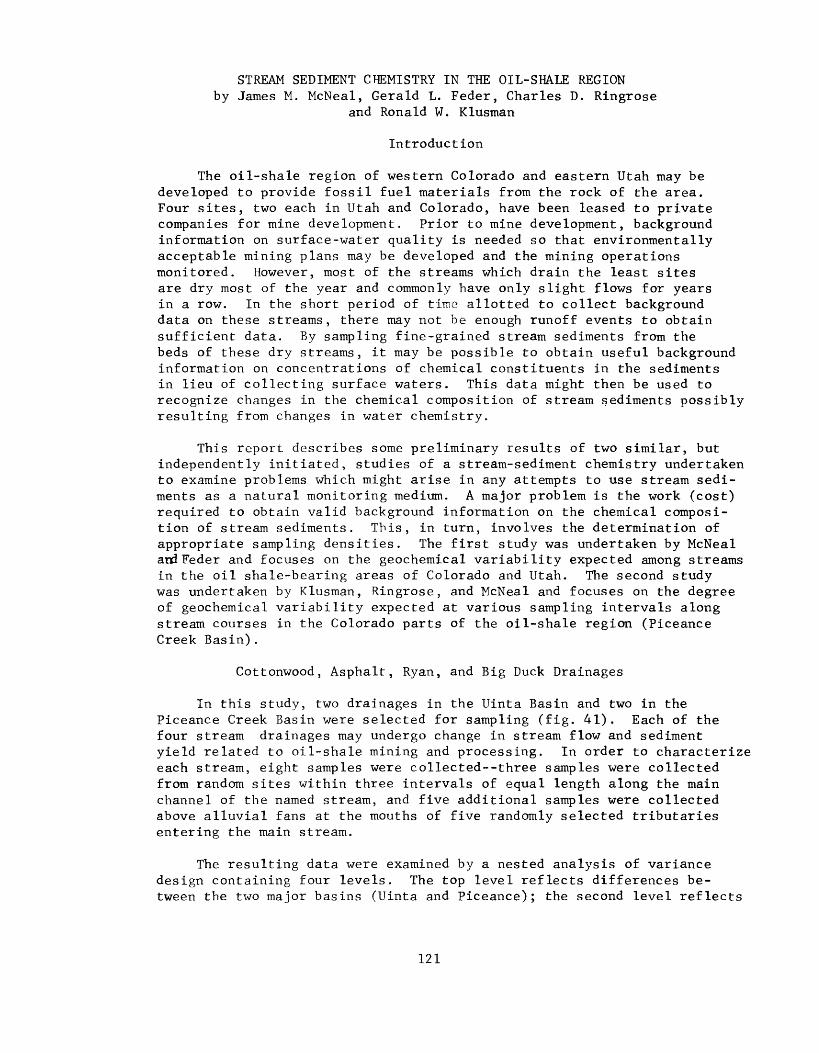
STREAM SEDIMENT CHEMISTRY IN THE OIL-SHALE REGIONby James M. McNeal, Gerald L. Feder, Charles D. Ringrose

and Ronald W. Klusman

Introduction

The oil-shale region of western Colorado and eastern Utah may be developed to provide fossil fuel materials from the rock of the area. Four sites, two each in Utah and Colorado, have been leased to private companies for mine development. Prior to mine development, background information on surface-water quality is needed so that environmentally acceptable mining plans may be developed and the mining operations monitored. However, most of the streams which drain the least sites are dry most of the year and commonly have only slight flows for years in a row. In the short period of time allotted to collect background data on these streams, there may not be enough runoff events to obtain sufficient data. By sampling fine-grained stream sediments from the beds of these dry streams, it may be possible to obtain useful background information on concentrations of chemical constituents in the sediments in lieu of collecting surface waters. This data might then be used to recognize changes in the chemical composition of stream sediments possibly resulting from changes in water chemistry.

This report describes some preliminary results of two similar, but independently initiated, studies of a stream-sediment chemistry undertaken to examine problems which might arise in any attempts to use stream sedi ments as a natural monitoring medium. A major problem is the work (cost) required to obtain valid background information on the chemical composi tion of stream sediments. This, in turn, involves the determination of appropriate sampling densities. The first study was undertaken by McNeal ani Feder and focuses on the geochemical variability expected among streams in the oil shale-bearing areas of Colorado and Utah. The second study was undertaken by Klusman, Ringrose, and McNeal and focuses on the degree of geochemical variability expected at various sampling intervals along stream courses in the Colorado parts of the oil-shale region (Piceance Creek Basin).

Cottonwood, Asphalt, Ryan, and Big Duck Drainages

In this study, two drainages in the Uinta Basin and two in the Piceance Creek Basin were selected for sampling (fig. 41). Each of the four stream drainages may undergo change in stream flow and sediment yield related to oil-shale mining and processing. In order to characterize each stream, eight samples were collected three samples were collected from random sites within three intervals of equal length along the main channel of the named stream, and five additional samples were collected above alluvial fans at the mouths of five randomly selected tributaries entering the main stream.

The resulting data were examined by a nested analysis of variance design containing four levels. The top level reflects differences be tween the two major basins (Uinta and Piceance); the second level reflects

121

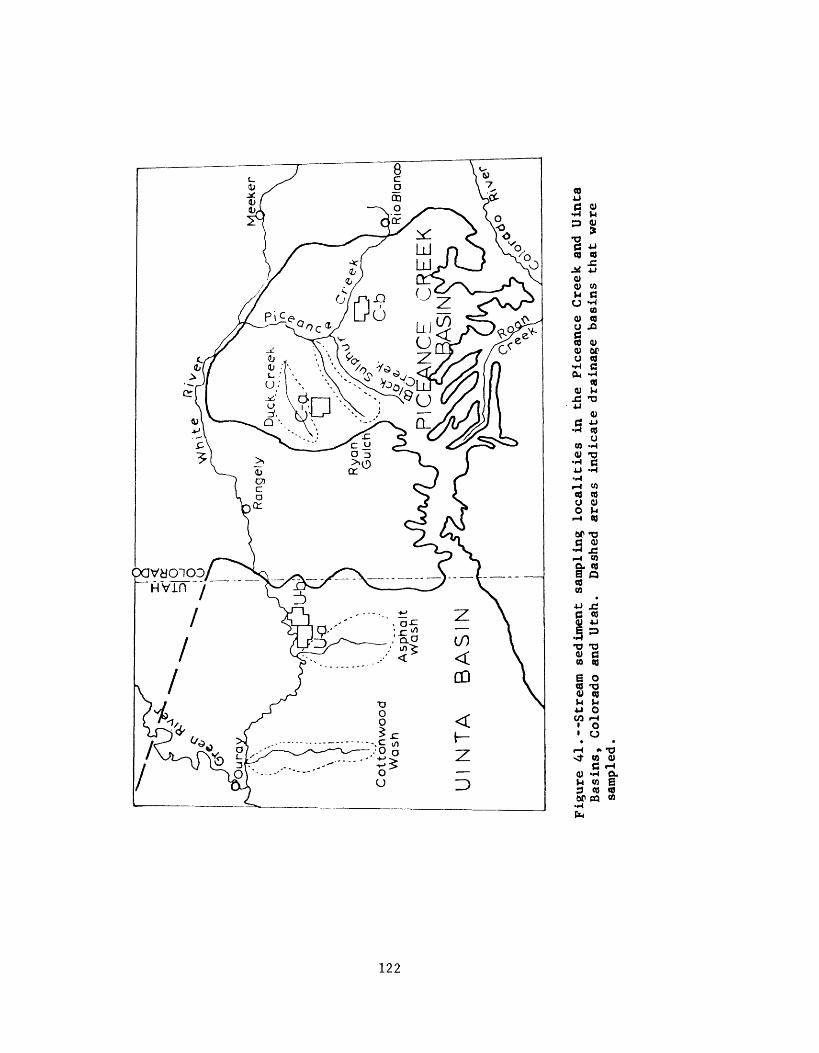
ro

ro

UIN

TA

B

AS

IN

Figure 41

.--S

tream

sedi

ment

sa

mpli

ng localities in

the

Piceance Creek a

nd Uinta

Basins,

Colo

rado

and

Utah.

Dashed areas

indi

cate

dr

aina

ge basins that were

samp

led.

differences among the paired drainages within each basin; the third level reflects differences among the eight samples taken within each of the four drainages, and the lowest level reflects differences among splits of the randomly selected samples.

All samples were collected from dry stream channels in areas where fine sediments had accumulated. At each locality, approximately two kilograms of sediment were composited from material taken at seven to ten sites within 20 meters of each other and at depths of no more than three centimeters. The samples were air dried at 40°C, then sieved through a 150-micron stainless steel screen. The <150-micron sediment was then sent to the laboratory for analysis. All samples, including replicates, were coded and placed in random order prior to analysis. Spectrographic analysis was performed in the U.S. Geological Survey, Water Resources Division laboratories in Denver, Colorado under the supervision of P. R. Barnett. Wet chemical analysis was performed in the U.S. Geological Survey, Water Resources Division laboratories in Salt Lake City, Utah under the supervision of R. L. McAvoy.

The analysis of variance results shown in table 18 indicate that nearly two-thirds of the constituents exhibit significant differences between the four streams. In particular, the fact that Ca, Mg, Sr , and carbonate C each have greater than 70 percent of their total variance associated with the between-stream level implies that it is the presence or absence of carbonate minerals, presumably detritus of the calcareous Green River Formation that causes the main difference between streams. Na, K and Ba also have significant variance components at this level, indicating that the concentration of alkali-feldspar detritus may also vary significantly between streams. Possibly, some of the Na occurs in NaHC0 3 (nahcolite) , or NaAlSi20^-H2 0 (analcime) .

In view of the large number of constituents with significant variance at the between-stream level, it seems reasonable that future stream-sediment work should be concerned with examining differences among streams if an appropriate number of samples (nr ) are randomly collected from each stream to stabilize its mean; nr can be estimated from the variance ratio, v, of Miesch (1976):

v = (P + V /(PT + VD b L A

where P , P , P and P are percentages of variance (from table 18) estimated for the between-basins , between-streams , between-samples , and between-analyses levels, respectively. If interest focuses on differences among streams in one basin rather than both, the numerator becomes reduced to P only. From the variance ratio and figure 2 of Miesch (1976, p. 9), the minimum number of randomly selected sample composites needed from each stream can be found. In general, the number of samples required is inversely related to the size of the variance ratios. The following

123

Table IS. Analysis of v.iriimce results, summary statistics, and gcocheinlcal baselines

for stream aeJlT.cuts of tho Plccanca Creek and Ulnta Basins, Colorado, and

Utah

[Data In parts per million, except where noted aa percent (Z); *, component

significantly different from rero at the 0.05 probability level; leadcra

( -), summary dr.tft given In tabl* 19]

Analysis of logarithmic varlan

Total

variance basins streams strca

Al, I 0.0132 < O.I 2.7 < 0.

As .0906 3.8 < .1 92.

B .0200 < .1 48.1* 2.

Ba .0132 < .1 55.2* 31.

Be .0346 < .1 < .1 71.

C, carbonate, ^ .2509 < .1 86.1* 1.

C, organic, ^ .1634 35.5 38.4* 21.

Ca, I .0626 < .1 79.6* 20.

Co .0146 < .1 35.3* 46.

Cr .0968 < .1 < .1 40.

Cu .0159 5.4 < .1 82.

F .2264 < .1 2.6 53.

Fc, ^ ------ .0269 < .1 31.3* 54.

GQ .0150 < .1 36.0* 25.

K, 1 .0074 < .1 67.8* < .

La .0536 10.7 < .1 79.

LI .0260 < .1 54.0* 39.

Mg, Z ------ .0387 < .1 71.9* < .

Na, 7. ------ .0137 < .1 26.1* 67.

Nb .0162 < .1 52.2* < .

Hi .0860 < .1 < .1 48.

P. % .0045 4.0 3.0 84.

Pb .0237 6.0 29.7* < .

S C .0225 < .1 30.0* 27.

Sr .0383 < .1 71.0* 27.

Tl, \ - - .0300 < .1 5.3 50.

v .0203 < .1 52.7 < .

y -- .0146 10.6 23.6* 23.

7f ...... - <l-\7S »A X. 11 L 4.K

CO

Summary statistics

Analy- Expected 95^ n tlcal Geometric Geometric Geometric range ms error mean deviation error (Baseline)

1 97.3 4.28 1.30 1.30

1* 4.1 6.5 2.00 1.15 1.7-25

6 49.3 1.26

4 13.4 1.10

0 29.0 3.3 1.53 1.26 1.6-6.7

7 12.2 1.50

7* 4.3 1.21

2* .2 1.03

4 18.3 1.13

1 59.9 61 2.05 1.74 25-150

3* 12.3 21 1.34 1.11 12-36

0 44.4 7.8 2.99 2.08 1.5-40

3 14.4 1.15

2 38.8 ' 1.19

1 32.2 1.12

4* 10.0 45 1.70 1.18 16-124

5* 6.5 1.10

1 28.1 1.27

4 21.2 1.10

9-> 6.0 1.07

1 47.3 1.22

1 51.9 48 1.76 1.63 19-120

9*' 8.0 .082 1.17 1.04 .06-. 11

1 64.3 1.33

1 43.9 1.26

4* 1.7 1.06

4 44.3 .030 1.49 1.30 .020-. 050

1 47.3 1.25

f, 42.1 1.20

6 27.7 1.19

7 36.3 245 '2.12 1.57 74-B15

^ i<* L. >!«; i '.-i i IQ <>&-4 f<ri

124

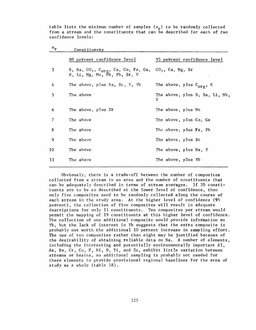
table lists the minimum number of samples (nr ) to be randomly collected from a stream and the constituents that can be described for each of two confidence levels:

n. Constituents

80 percent confidence level

3 B, Ba, C0 3 , Corg , Ca, Co, Fe, Ga, K, Li, Mg, Mn, Nb, Pb, Sr, V

4 The above, plus Na, Sc, Y, Yb

5 The above

6 The above, plus Zr

7 The above

8 The above

9 The above

10 The above

11 The above

95 percent confidence level

C03 , Ca, Mg, Sr

The above, plus CQ , K

The above, plus B, Ba, Li, Nb,V

The above, plus Mn

The above, plus Co, Ga

The above, plus Fe, Pb

The above, plus Sc

The above, plus Na, Y

The above, plus Yb

Obviously, there is a trade-off between the number of composites collected from a stream in an area and the number of constituents that can be adequately described in terms of stream averages. If 20 consti tuents are to be so described at the lower level of confidence, then only five composites need to be randomly collected along the course of each stream in the study area. At the higher level of confidence (95 percent), the collection of five composites will result in adequate descriptions for only 11 constituents. Ten composites per stream would permit the mapping of 19 constituents at this higher level of confidence. The collection of one additional composite would provide information on Yb, but the lack of interest in Yb suggests that the extra composite is probably not worth the additional 10 percent increase in sampling effort. The use of ten composites rather than eight may be justified because of the desirability of obtaining reliable data on Na. A number of elements, including the interesting and potentially environmentally important Al, As, Be, Cr, Cu, F, Ni, P, Ti, and Zn, exhibit little variation between streams or basins, so additional sampling is probably not needed for these elements to provide provisional regional baselines for the area of study as a whole (table 18).

125

The remaining elements are too variable among streams to permit regional baseline estimation, so valid baseline estimation must be undertaken on a stream-by-stream basis. In order to distinguish among streams at the 80 percent confidence level, each stream average must be based on at least four randomly selected composites. Because the eight composites actually collected from each stream drainage are not nested (although they are stratified), it is likely that they may be viewed as fulfilling these sampling requirements. Based on such data, provisional summary estimates are listed in table 19 for the 20 constituents so affected.

Roan and Black Sulfur Creeks

This study is aimed largely at quantifying the major scales of geochemical variability along two selected streams in the Piceance Creek Basin. The sampling design is a six-level, nested analysis of variance design.

The six levels used in this design define components of geochemical variability (1) between streams, (2) between 10-km intervals, (3) between 1-km intervals, (4) between 200-m intervals, (5) between 20-m intervals, and (6) analytical error. The two streams chosen at the top level are Roan Creek, which flows nearly east-west in the southern part of the basin, and Black Sulfur Creek, which flows nearly north-south in the central portion of the basin (fig. 41). The Roan Creek drainage crosses exposures of the lower Uinta Formation, all of the Green River Formation, and the upper Wasatch Formation. Black Sulfur Creek lies mostly in the upper Green River and lower Uinta Formations. Two major sample locations were picked on each stream and separated by 10 km. The design is geo graphically balanced and in each locality, two segments of stream 200 m in length were randomly located about 1 km apart. In each 200-m length, two segments about 20-m long were randomly located, and in each 20-m segment, two sampling sites were randomly located. Ten samples of the 32 collected were randomly selected for duplicate analysis, and all 42 were placed in a random order prior to chemical analysis.

The samples were collected by hand and placed in cloth bags and allowed to air-dry. They were then disaggregated with a mortar and pestle and passed through a 80-mesh sieve. The -80 mesh fraction was retained for analysis. All samples were collected away from the influence of stream banks and were not composited. They were analyzed by John C. Hamilton who used the semiquantitative emission spectrographic technique described in Miesch (1976, p. 14),

The analysis of variance results in table 20 show that little varia tion occurs between the two streams and that most of the variation is associated with scales of 1-10 km and 0-20 m. Thus, most of the variation occurs either at very local scales or at relatively large scales. There is no significant variation occurring at the 20-200 m interval for any of the elements, and only three elements (B, Cu, and Mg) have significant variation at the 200 m - 1 km interval.

126

Table

19. Sueaary statistics fo

r Asphalt

Wash

and

Cottonwood Wash

of U

inta B

asin,

and

Duck Gulch an

d Ry

an Gulch

of Pi

cean

ce Creek Basin

[Data

in parts

per mi

llio

n except where

noted

aa pe

rcen

t

Asphalt

Wash

Expected 95

7.

Constitutnt

Geometric

Geometric

range

ccan

de

viat

ion

(Bas

eline)

3

54.0

1.17

39-74

3a

780

1.18

560-

1,09

0

C, CO,, ^

.93

1.66

.34-2.56

C, or

gani

c, 7

. .80

1.33

.4

5-1.

42

Ca,

Z

4.50

1.38

2.36-8.57

C2 .

7.0

1.20

4.9-10.1

cef

;

1.9

i.26

1.2-

3.0

Ca

17

1.17

12-23

K> i

....

. 2.22

1.04

2.05

-2.4

0

Ll

36

1.32

21-6

3

Mg>

7,

1.17

1.

29

.70-1.95

Mn

51C

1.07

44

5-53

5

Ka,

7.

2.45

1.22

1.65-3.65

\?w

11

i 01

ft A

on

Pb

18

1.16

13-2

4

< .

« M

^

1

£ Q

*) 1

Sr

295

1.30

17

5-50

0

V

91

1.18

65-130

Y_

_____

">O

1 IS

?9_^ft

Yb

2.5

1.32

1.4-

4.4

Cottonwood Was

h

Geometric

mean

38.0

1,08

0

.26

.25

3.11

8.4

2.6

20 1.64

23 .6

5

600 2.

45

14

19

11

420

120 34 3.1

Geometric

deviation

1.40

1.28

1.43

1.84

1.06

1.40

1.60

1.24

1.10

1.18

1.19

1.20

1.11

1.21

1.26

1.28

1.36

1.40

1.27

1.53

Expe

cted

95*

ran{

;e

(Baseline)

19.0-74.0

660-1,770

.13-

. 53

.07-. 85

2.77-3.49

4.3-

16

1.0-

6.7

13-3

1

1.36-1.98

17-3

2

.46-. 92

415-

865

1.99-3.02

10-2

0

5.7-

14

67-18

225-775

61-235

21-5

5

1.3-

7.3

Duck

Creek

Geom

etri

c me

an 34.0

935 1.

95

1.26

7.51

5.9

1.7

15 2.02

38 .9

5

615 1.

83

9.2

13 7.4

440 73

22 2.1

Geom

etri

c de

viat

ion

1.27

1.14

1.44

1.79

1.48

1.20

1.38

1.24

1.08

1.31

1.20

1.16

1.52

1.30

1.23

1.34

1.14

1.13

1.30

1.26

Expected 957.

range

(Baseline)

21.0-55.0

720-1,220

.94-

4.04

.39-4.04

3.43-16.4

4.1-

8.5

.9-3.2

9.8-23

1.73-2.36

22-65

.66-

1.37

455-

830

.79-

4.23

5.4-16

8.6-

20

4.1-

13

340-

570

57-9

3

13-37

1.3-

3.3

Ryan

Gulch

Geometric

mean 53

.0

725

.38

1.31

2.96

8.0

2.4

22 1.98

31 .6

8

480 2.

49

14

19

12

225

120 27 2.9

Geometric

devi

etio

n

1.33

1.20

1.53

1.44

1.15

1.20

1.24

1.34

1.17

1.28

1.27

1.20

1.09

1.15

1.14

1.33

1.29

1.23

1.21

1.15

Expected 951

range

(Bas

elin

e)

30.0-94.0

505-1,040

.16-. 39

.63-

2.72

2.24

-3.9

1

5.6-

12

1.6-

3.7

12-40

1.45

-2.7

1

19-5

1

.42-

1.10

335-

690

2.10

-2.9

6

11-19

15-25

'

6.8-

21

135-

375

:

79-180

18-4

0

2.2-

3.8

Table 20.--Ceochemical summaries for stream sediments of Roan and Black Sulfur Creeks, Colorado .

[Data given In parts per million, except where noted as percent (1); an asterisk (*)

indicates variance component Is significantly different from zero at the 0.05

probability level; leaders ( ), data Insufficient for estimation]

Element

Analysis of logarithmic variance

TotalL0810 variance

Percent of total variance

Between streams 1-10 km 200 m-1 km 20-200 m 0-20 m

Analy tical error

Summary statistics

Geometric mean i'

Geometric deviation '

Geometric error

Expected 95' Range (Baseline) '

Al, 1

8

Ba

Ca, I

Co

Cr

Cu

*e, 1

Ga

K, I

Kg, I

Mn

Ha, 1

Ml

Pb

Se

Sr

Ti, 1

V

T

Tb

Zr

0.0223

.0201

.0168

.0253

.0289

.1048

.0189

.0156

.0106

.0015

.0081

.0193

.0131

.0078

.0137

.0186

.0027

.0450

.0188

.0135

.0195

.0470

25*

< 1

6

< 1

38

58

8

< 1

49*

< 1

3

27

69*

24*

1

17

< 1

11

< I

11

< I

5

3

< I

< 1

68*

29*

21*

53*

58*

8*

< 1

13

12*

< I

5

< 1

60*

12

25*

40*

< 1

< 1

< 1

6

38*

13

< 1

< 1

I

11*

2

< 1

3

35*

5

< 1

14

< 1

< I

5

< I

6

< 1

< 1

< 1

< 1

< 1

4

7

< 1

< 1

< 1

< 1

7

< 1

< 1

< 1

< 1

< 1

< 1

< 1

< 1

< 1

< 1

< 1

< 1

< 1

33

15

23

3

17

11

8

35*

< 1

97*

19

20

6

47*

61*

< 1

< 1

38*

33*

39

45

87*

33

47

54

22

16

9

20

5

37

< I

30

36'25

10

38

23

83

26

21

50

55

8

6,0, 7.6

44

940

5.4

8

56

17

2.2

15, 20

3.1

1.4

260

2.2, 3.0

15, 18

18

8

520

.21

70

22

2

180

1.32, 1.20

1.39

1.35

1.44

1.48

2.11

1.37

- 1.33

1.09, 1.19

1.09

1.23

1.38

1.18, 1.09

1,07, 1.20

1.31

1.37

1.13

1.63

1.37

1.31

1.38

1.65

1.22

1.25

1.25

1.19

1.17

1.25

1.15

1.07

1.16

< 1.01

1.12

1.15

1.14

1.07

1.18

1.16

1.12

1.28

1.16

1.21

1.27

1.15

4.1-8.8,

27-71

630-1,400

2.8-10

3.9-16

13-230

9.6-30

1.3-3.8

, 17-24

2.6-3.7

.99-2.0

160-430

1.8-2.7, *--

, 13-25

12-28

4.6-14

470-570

.091-. 49

40-120

15-32

1.3-3.1

69-470

\f Where two estimates appear, first is for Roan Creek, second for Black Sulfur Creek.

128

The lack of between-stream variability in this study conflicts with the major conclusion of the first study (above), but this apparent con tradiction reflects the choice of streams used in each study. For the oil-shale regions as a whole, the first study clearly indicates that stream drainages can differ; the second study simply shows that of a multitude of possible streams two specific drainages--Roan and Black Sulfur are not geochemically distinct. In fact, the two studies are complementary; the first demonstrates the presence of important between- stream variability, the second defines the important scales of variability within stream drainages. Attempts to map the geochemical variability of the sediments in these two streams can only be directed to variation at scales greater than 1 km. Mapping at shorter scales may increase the sample load and analytical costs an unbearable amount, and mapping at larger scales will drastically reduce the amount of variation that can be mapped. (Mapping based on 10-km stream segments will not show the variation at the 1-10 km scale because all of that variation is estimated to be at scales less than 10 km.) The minimum number of randomly collect ed samples, nr , needed to stabilize the mean concentration can be based on the variance ratio of Miesch (1976):

v . (PB + P

where Pg to P^ are the percentages of variance estimated for the six levels of the design (table 20). The minimum number of samples, nr , required to characterize a 1-km stream segment may be read from graphs in Miesch (1976, p. 9). The number required for a number of elements at two confidence levels is:

nr Constituents

80-percent confidence level 95-percent confidence level

3 Ca, Co, Cr, Cu, Fe, Ga, Mn, Ca, Cr, Na, ScNa, Sc, Ti, V

4 The above, plus Al, Ni The above, plus Co, Cu, Fe, Ga

6 The above, plus Mg The above, plus Mn, V

7 The above, plus Sr, Y The above, plus Ti

8 The above, plus Sr The above

9 The above The above, plus Ni

10 The above The above, plus Al

Thus, it appears that geochemical mapping within a single drainage should use composite samples of at least seven and perhaps as many as ten samples in each 1-km stream segment. This estimate, together with a need for at least ten such composites to map differences among streams (from the previous study) suggests the probable sampling effort required to adequatelymap stream-sediment chemistry over the entire oil-shale region.

129

The occurrence of at least some significant differences between the two streams in this study suggests that geochemical baselines are required for each, at least for those elements judged to be significantly different among streams. For the remaining elements, more stable averages applicable to both streams may be obtained by a "pooled" average based on all the data. The appropriate summaries are given in table 20.

130

SPECTROCHEMICAL COMPUTER ANALYSIS by Arthur L. Sutton, Jr.

In an attempt to insure analytical consistency during analysis of rock, soil, and plant material throughout the lifetime of the geochemical survey of the western energy lands, a system of elemental analysis was established near the outset of the work based on the flowchart in figure 42. Descriptions of all methods except that based on emission spectroscopy were described in U.S. Geological Survey (1975, p. 69-81). Analysis of water samples generally follows procedures described in Miesch (1976, p. 18-22).

The "workhorse" of the system outlined in figure 42 is emission spectroscopy by which some 64 elements are looked for simultaneously down to the parts per million level. Of these, 20 to 25 are commonly detected in most samples of a study, arid another eight may be measured in a small number of the samples. Most of the initial work of this survey (that undertaken largely in the Powder River Basin of Wyoming and Montana) relied on a visual spectrographic technique described in Miesch (1976, p. 14). Since then, a computerized plate-reading procedure has been instituted for all work of a "background" nature in order to gain a faster, more versatile, and for some elements, a more sensitive analysis.

The analytical procedure is described in Dorrzapf (1973). The recording method as published by Helz (1973) has been replaced with a Hewlett Packard 9601-E Data acquisition system. The following is a list of equipment and Software used for the automatic plate-reading:

32,000-word core storage. 2.47-million word cartridge Disc. 12-bit analog-digital converter. 9-track magnetic tape unit. Line printer.

The software is described by Walthal (1974) and has been modified to run on the data acquisition system. The new system will be described in a paper in preparation by Catherine Thomas of the U.S. Geological Survey.

131

ROCKS AND SOILS (Sample ground to pass 100 mesh)X-ray fluorescence

Majors: Al Si Ca S MgFeKP

Ti Mn Cl

Minors: Se Sn Ge As Sb Te Bi

Atomic absorption

MgNa

Sz/

Zn Rb CdiI/

Selective ion electrode

Gasometric

Total C

Neutron activation

U Th

Emission spectrographic

Common:FeMgCaTiMnBBaBeCoCrCuNb

Rare:AgLaMo

NiPbScSrVYZrAlKGaYbZn

CeNdSn

PLANT MATERIAL(Sample ashed (Sample dried at ~ 450°C) at ~ 40°C)

Atomic absorption

Co Na Cd Ca Li K Si Zn

Colorimetric

P

Fluorimetric

U

Emission spectrographic

Atomic absorption

As , Sb Hgl/

Selective ion electrode

F

2, 3-Diamino- naphthalene

Se

Turbidometric

S

Gravimetric

Ash

_!/ Looked for only if Zn >200 ppm. 1J Determined by "flameless" atomic

absorption,,

Figure 42. Methods of total element analysis adopted for rocks, soils, and plants in the geochemical survey of the western energy regions 0

132

REFERENCES CITED

Alloway, B. J., 1973, Copper and molybdenum in swayback pastures: Jour. Agric. Sci., v. 80, p. 521-524.

Anderson, R. L., and Bancroft, T. A., 1952, Statistical theory in research: New York, McGraw-Hill, 399 p.

Barshad, I., 1948, Molybdenum content of pasture plants in relation to toxicity in cattle: Soil Sci., v. 66, p. 187-195.

Beard, T. N., Tait, D. B., and Smith, J. W., 1974, Nahcolite and Dawsoniteresources in the Green River Formation, Piceance Creek Basin, Colorado, rn Murray, D. K., ed.: Energy resources of the Piceance Creek Basin, Colorado, Rocky Mountain Assoc. Geologists Guidebook, 25th Field Conf., p. 101-109.

Berg, W. A., and Vogel, W. 0., 1973, Toxicity of acid coal-mine spoils to plants, p. 57-68, in Hutnik, R., and Davis, G., eds.: Ecology of reclaimed and devasted land, v. 1, World Symposium on Mined Land and Mineral Waters, Proc., New York, Gordon and Breach.

Cadigan, R. A., 1970, Mercury in sedimentary rocks of the Colorado Plateau region, _in Mercury in the Environment: U.S. Geol. Survey Prof. Paper 713, p. 17-18.

Case, A. A., 1974, Toxicity of various chemical agents to sheep: Jour. Amer. Vet. Med. Assoc., v. 164, p. 277-283.

C-b Shale Oil Project, 1975, Quarterly Report No. 3, Section II, B-13, Core and Cuttings - Trace Element Analysis.

Christianson, G. A., and Jacobson, G. A., undated, Report on molybdenosis in farm animals and its relationship to a uraniferous lignite ashing plant: Unpublished report, No. Dak. State Dept. Health, 9 p.

Church, T. M., and Wolgemuth, K., 1972, Marine barite saturation: Earth and Planetary Sci. Letters, v. 15, p. 35-44.

Cohen, A. C., Jr., 1959, Simplified estimators for the normal distribution when samples are singly censored or truncated: Technometrics, v. 1, no. 3, p. 217-237.

Connor, J. J., Keith, J. R., and Anderson, B. M., 1976, Trace-metalvariation in soils and sagebrush in the Powder River Basin, Wyoming and Montana: Jour. Research U.S. Geol. Survey, v. 4, p. 49-59.

133

Connor, J. J., and Shack]ette, H. T., 1975, Background geochemistry of some rocks, soils, plants, and vegetables in the conterminous United States; U.S. Geolo Survey Prof. Paper 574-F.

Cook, E. W., 1973, Elemental abundances in Green River oil shale: Chem 0 Geology, v. 11, p. 321-324.

Cronan, D. S., 1974, Authigenic minerals in deep-sea sediments, in Goldberg, E. Do, ed.: The Sea, v. 5, New York, Wiley-Interscience, p, 491-525 0

Davidson, R 0 L., Natusch, D. F. S., and Wallace, J. R., 1974, Trace elements in fly ash--dependence of concentration on particle size: Environ. Sci. and Technol., v. 8, p. 1107-1113.

Davis, J. Co, 1973, Statistics and data analysis in geology: New York, John Wiley and Sons, Inc., 550 p.

Dean, W. E., and Schreiber, B. c»> 1976, Authigenic barite, Leg 41, Deep-Sea Drilling Project, jln Lancelot, Y., Seibold, E., et a! 0 : Initial Reports of the Deep-Sea Drilling Project, v. 41, Washington, D.C 0 , U.S. Govt. Printing Office (in press) 0

Desborough, G. A., 1975, Authigenic albite and potassium feldspar in theGreen River Formation, Colorado and Wyoming: Am 0 Mineralogist, v. 60, p. 235-239.

____1976, Mineralogy of oil shale in the upper part of the Parachute Creek Member of the Green River Formation in the eastern Uinta Basin, Utah: U.S. Geol. Survey Open-file Rept, 76-381, 27 p.

Desborough, Go A., and Pitman, J. K», 1974, Significance of applied mineralogy to oil shale in the upper part of the Parachute Creek Member of the Green River Formatior, Piceance Creek Basin, Colorado, in Murray, D. K., ed.: Energy Resources of the Piceance Creek Basin, Colo., Rocky Mountain Assoc. Geologists Guidebook, 25th Field Conf., p 0 81-90.

____1975, Interpretation of Fischer assay data for the evaluation of analcime-bearing oil shale in the Green River Formation, Colorado and Utah: U.S. Geol. Survey Opne-file Rept. 75-219, 26 p.

Desborough, G. A., Pitman, J 0 K 0 , and Huffman, C., Jr., 1976, Concentration and mineralogical residence of elements in rich oil shales of the Green River Formation, Piceance Creek Basin, Colorado, and the Uinta Basin, Utah - A preliminary report: Chem. Geology, v a 17, p<> 13-26.

Dorrzapk, A. F., Jr., 1973, Spectrochemical analysis--argon--oxygen d-c arcmethod for silicate rocks: U.S 9 Geol. Survey Jour. Research, v» 1, no» 5, p. 559-562.

134

Duncan, D. B., 1955, Multiple range and multiple F tests: Biometrics, v. 11, no. 4, p. 1-42.

Dyni, J. R., 1974, Stratigraphy and nahcolite resources of the saline facies of the Green River Formation in northwest Colorado, in Murray, D. K., ed.: Energy Resources of the Piceance Creek Basin, Colorado, Rocky Mountain Assoc. Geologists Buidebook, 25th Field Conf., p. 111-122.

Ebens, R. J., Erdman, J. A., Feder, G. L., Case, A. A., and Selby, L. A., 1973, Geochemical anomalies of a claypit area, Callaway County, Missouri, and related metabolic imbalance in beef cattle: U.S. Geol, Survey Prof. Paper 807, 24 p.

Ferry, B. W., Baddeley, M. S., and Hawksworth, D. L., ed., 1973, Air pollution and lichens: Toronto, Univ. of Toronto Press, 389 p.

Furr, K., Stoewsand, G. S., Bache, C. A., and Gutenmann, W. A., 1975, Multi-element residues in tissues of Guinea pigs fed sweetclover grown on fly ash: Archives Environ. Health, v. 30, p. 244-248.

Gutenmann, W. H., Bache, C. A., Youngs, W. D., and Lisk, D. J., 1976, Selenium in fly ash: Science, v. 191, p. 966-967.

Hanson, H. C., and Churchill, E. D., 1961, The plant community: New York, Reinhold Publ. Corp., 218 p.

Helz, A. W. , 1973, Spectrochemical computer analysis instrumentation: U.S. Geol. Survey Jour. Research, v. 1, no. 4, p. 475-482.

Holden, C. H., 1976, Interior releases new standards for surface mining: Science, v. 192, p. 1085.

Humphrey, R. R., 1960, Arizona range grasses, their description, forage value, and management: Ariz. Agric. Exper. Sta. Tech. Bull. 298, 104 p.

Kaakinen, J. W., Jordan, R. M., Lawasani, M. H., and West, R. E., 1975, Trace-element behavior in coal-fired powerplant: Environ. Sci. and Technol., v. 9, p. 862-869.

Kennedy, V. C., Zellweger, G. W., Jones, B. F., 1974, Filter pore-size effects on the analysis of Al, Fe, Mn, and Ti in water: Water Resources Research, v. 10, no. 4, p. 785-790.

135

Klein, D. H e , Andren, A 0 W e , Carter, J, A., Emery, J 0 F a , Feldman, C 9 ,Fulkerson, W 0 , Lyon, W. S., Ogle, J 0C ot Talmi, Y 9 , Van Hook, R 0 ! , and Bolton, N 0 , 1975, Pathways of thirty-seven trace elements through coal-fired power plant: Environ,, Sci. andTechnolo, v 0 9, p» 973-979,,

Krumbein, W 0 C., and Slack, H 0 A., 1956, Statistical analysis of low-level radioactivity of Pennsylvanian black fissile shale in Illinois: Geol» Soc* America Bull., v* 67, p. 739-762,

Kuchler, A, W 0 , 1964, Potential natural vegetation of the conterminous United States: Am. Geog. Soc. Spec«, Pub. 36, map and 116 p. text.

Lee, H. J 0 , 1975, Trace elements in animal production, p» 39-53, in Nicholas, D. J. Do, and Egant, A 0 R 0 , eds.: Trace Elements in Soil-PI ant-Animal Systems, Academic Press, Inc 0 , New York, 417 p.

Lee, Ro E., Goranson, S. S 0 , Enrione, R 0 E«, Morgan, G. B 0 , 1972, National air surveillance cascade impactor network 0 II 0 Size distribution measurements of trace metal components: Environ,, Sci. and Technol 0 , v, 6, p 0 1025-1030.

Leone, F 0 C., Nelson, L 0 S., Johnson, N. L 0 , and Eisenstat, Stan, 1968,Sampling distributions of variance components 2, Empirical studies of unbalanced nested designs: Technometrics, v. 10, no. 4, p. 719-737.

Linton, R 0 W 0 , Loh, A 0 , Natusch, D. F. S., Evans, C 0 A., and Williams, P 0 , 1976, Surface predominance of trace elements in airborne particles: Science, v. 191, p 0 852-854 0

Martens, D. C Q , and Beahm, B 0 R., 1976, Chemical effects of fly ash incor poration into soil on plant growth: Environ,, Chem0 and Cycling Proc., 2nd Mineral Cycling Symposium, Augusta, Ga 0 , abs., p 0 32

Miesch, A. T c , 1967, Methods of computation for estimating geochemical abundances: U 0 S 0 Geol. Survey Prof,, Paper 574-B, 15 p 0

1976, Methods of sampling, laboratory analysis, and statistical reduction of data in a geochemical survey of Missouri, with sections on laboratory methods by P 0 R 0 Earnett, A. J 0 Bartel, J. I. Dinnin, G. L» Feder, T. F. Harms, Claude Huffman, Jr., V. J. Janzer, H. T., Millard, Jr 0 , H. G. Neimau, M 0 W. Skougstad, and J, S 0 Wahlberg: U 0 S 0 Geol. Survey Prof* Paper 954-A, 39 p c

Nakagawa, H 0 M 0 , 1975, Atomic absorption determination of silver, bismuth, cadmium, cobalt, copper, nickel, lead, and zinc in calcium and iron- rich geologic material, in F 0 N. ^ard, ed., New and Defined Methods of trace analysis useful in geochemical exploration; U,S 0 Oeol 0 Survey Bull. 1408, p. 85-96.

136

National Research Council, Committee on Animal Nutrition, Subcommitteeon Fluorosis, 1974, Effects of fluorides in animals: National Acad. of Sci., Washington, D. C., 70 p.

Reichen, L. E., and Ward, F. N., 1951, Field method for the determination of molybdenum in plants: U.S. Geol. Survey Circ. 124, 4 p.

Rio Blanco Oil Shale Project, 1975, Quarterly Report No. 2, Section 1.1. 2.4 - Trace Element Analysis.

Robb, W. A., and Smith, J. W., 1974, Mineral profile of oil shales inColorado core hole no. 1, Piceance Creek Basin, Colorado, in Murray, D. K., ed.: Energy Resources of the Piceance Creek Basin, Colorado, Rocky Mountain Assoc. Geologists Guidebook, 25th Field Conf., p. 91- 100.

Sandoval, F. M., Bond, J. J., Power, J. F., and Willis, W. 0., 1973,Lignite mine spoils in the northern Great Plains characteristics and potential for reclamation: No. Dak. Geol. Survey Education Series 5, p. 1-24.

Schultz, L. G. , 1964, Quantitative interpretation of mineralogical com position from X-ray and chemical data for the Pierre Shale: U.S. Geol. Survey Prof. Paper 391-C, 31 p.

Severson, R. C., and Gough, L. P., 1976, Concentration and distribution of elements in plants and soils as related to phosphate processing, Pocatello, Idaho: Jour. Environ. Quality (in press).

Shacklette, H. T., 1965, Element content of Bryophytes: U.S. Geol. Survey Bull. 1198-D, 21 p.

Smith, J. W. , 1974, Geochemistry of oil-shale genesis in Colorado'sPiceance Creek Basin, in Murray, D. K., ed.: Energy Resources of the Piceance Creek Basin, Colorado, Rocky Mountain Assoc. Geologists Guidebook, 25th Field Conf., p. 71-79.

Smith, J. W., and Stanfield, K. E., 1964, Oil yields and properties of Green River oil shales in Uinta Basin, Utah, in Guidebook to the Geology and Mineral Resources of the Uinta Basin, Intermountain Assoc. Petroleum Geologists, 13th Ann. Field Conf., p. 213-221.

Spitzer, G. L., and May, M., 1975, Baseline monitoring study of the Jim Bridger Powerplant area, Point of Rocks, Wyoming: Ph. D. thesis, Range Management, Univ. of Wyo., Laramie.

Stanfield, K. E., Frost, I. C., McAuley, W. S., and Smith, H. N., 1951, Properties of Colorado oil shale: U.S. Bur. Mines Rept. Invest. 4825, p. 12.

137

Strabala, W., 1974, Monster rises on Wyoming prairie: The Denver Post, Monday, June 17, p. 28.

Strahler, A. N., 1969, Physical geography: New York, John Wiley and Sons, Inc., 733 p.

Tidball, R. R., and Ebens, R. J., 1976, Regional geochemical baselines in soils of the Powder River Basin, Montana-Wyoming: Wyo. Geol. Assoc. Guidebook (in press).

Trewartha, G. T., 1954, An introduction to climate: New York, McGraw- Hill, 3rd ed., 402 p.

Trumbull, James, 1959, Coal fields of the United States, Sheet 1: U.S. Geol. Survey [I960].

U.S. Environmental Protection Agency, 1975, Proposed interim primary drinking water regulations: 40 Code of Federal Regulations, Pt. 141, Federal Register, v. 40, no. 51, March 14, 1975, p. 11,990- 11,998.

_____1976, Interim primary drinking water regulations: 40 Code ofFederal Regulations, Pt. 141, Rederal Register, v. 41, no. 133, July 9, p. 28,402-28,409.

U.S. Geological Survey, 1970, The national atlas of the United States of America: Washington, B.C., 417 p.

_____1972, Environmental geochemistry--Geochemical survey of Missouri,plans and progress for sixth six-month progress report (January- June, 1972): U.S. Geol. Survey Open-file Rept. 86 p.

_____1974a, Stripping coal deposits of the Northern Great Plains, Montana, Wyoming, North Dakota, and South Dakota: U.S. Geol. Survey Misc. Field Studies Map MF-590, 1 sheet.

_____1974b, Geochemical survey of the Western Coal Regions, 1st ann. pro gress report (July, 1974): U.S. Geol. Survey Open-file Rept. 74-250, 38 p.

_____1975, Geochemical survey of the Western Coal Regions, 2nd ann. pro gress report (July, 1975): U.S. Geol. Survey Open-file Rept. 75-436, 132 p.

Webb, J. S., and Atkinson, W. J., 1965, Regional geochemical reconnaissance applied to some agricultural problems in Co. Limerick, Eire: Nature, v. 208, no. 5015, p. 1056-1059.

Walthall, F. G., 1974, Spectrochemical computer analysis--program description: U.S. Geol. Survey Jour. Research, v. 2, no. 1, p. 61-71.

Whitaker, S. H., and Pearson, D. E., 1972, Geological map of Saskatchewan:Saskatchewan Dept. Mineral Resources and Saskatchewan Research Council, 1 sheet.

138

UNITED STATES DEPARTMENT OF THE INTERIOR

U.S. GEOLOGICAL SURVEY Denver, Colorado

APPENDICES TOGEOCHEMICAL SURVEY OF THE WESTERN ENERGY REGIONS

(formerly Geochemlcal Survey of the Western Coal Regions) Third Annual Progress Report, July, 19?6

APPENDIX I.

APPENDIX II.

Probable upper limits of element concentration to be expected in some ordinary landscape materials of the Powder River Basin.

Probable upper limits of element concentration to be expected in some ordinary landscape materials of the Northern Great Plains.

APPENDIX III. Probable upper limits of element concentration to be expected in some ordinary landscape materials of the Oil Shale Region.

APPENDIX IV,

APPENDIX V.

Toxicity of selected elements to plants, animals, and man--an outline, by Larry P. Gough and Hansford T. Shacklette.

Chemical elements in vegetation and soil near coal- fired powerplants, Western Energy Regions.

Table 1. Surface and subsurface soil, and sagebrush east of Dave Johnston Powerplant, Wyoming.

2. Lichen east and west of Dave Johnston Powerplant, Wyoming.

3. Surface and subsurface soil, and sagebrush at Jim Bridger Powerplant, Wyoming.

4. Soil and Grass southeast of Four Corners Powerplant, New Mexico.

Open-file Report ?6-729 1976

This report is preliminary and has not been edited or reviewed for conformity with U.S. Geological Survey standards or nomenclature.

APPENDIX I

Prob

nhlp

iippor li

mits

of

concentration to

he

fx

pect

cd In ordinary landscape

materials

of the

Powd

er River

Basi

n.

[The Units ar

e estimated

as those

abov

e which on

ly ab

out

one

sample In

20

of

a randomly se

lect

ed suite

Is ex

pect

ed to fall

due

tc na

tura

l causes al

one.

Va

lues

expressed

as parts

per

million

exce

pt as

Indicated.

Limi

ts

give

n to two

sign

ific

ant

figu

res

except th

ose

In parentheses, which ar

e given

to on

ly one

significant

figu

re

beca

use

they arc

judg

ed to

be less stable.

Lead

ers

(--) Indicate in

suff

icie

nt da

ta to es

tima

te li

mit]

]

Landscape

Property

f

Shale

(1)

Al.

7. --

----

Ca,

T ----- -

C(tctnn,

7,

5.3

f .............

Ga -

Ge ---

I ...

....

..

Fe.

1 --

.

. --

La

T>L

Ll

80

>«n

Nb ...

....

....

.

Hi ............

I/

01.

iock Sindsfone

Surf

ace

CO

(3)

| (4

)

7.3

(2) 12

910

990

1.7

57

54

2.3

(?)

98

69

16

10

31

30

730 20

18

2.2

30

30

21

25

34

(1)

1.5

830

560

.041

.024

37

24

(3)

Soil

Subs

urfa

ce(5

)

1.8 17

1200

1.9 50 71

13

36 19

2.0 50

36

41

500

.032 29

(6)

| (7

)

7.7

8.2

890

1000

60

4.3

11

2.2

3.0

87

110

18

16

49

90

830

840 26

3.8

5.0

180

26

23

43

44

1.6

4.8

770

810

.053

.061

38

49 <fl

Materlal-

Powd

er River

Sedi

ment

(8) 12

1400

25

4.2

2.6

(80)

11

(50)

(26)

6.1

(20)

(20)

(2)

480

.42

(30) CO

(9)

5.6

1400

16

3.8

1.3

(60)

6.3 26 17

2.7 13

19

(.7)

360

(.05

)

8.1 11

2t!>

(10)

6.9

1500

41 3.0

1.0 75

4.3 16 15

2.5 12

17

.97

350

.046

(19)

8.3

2.5

(11)

(10)

(1500)

1.4 90

5.5

1.8

190

8.6

160 21

3.9

(100

)

21

1.2

(600)

.047 18

16

'33

Plan

t

SaRebruih

Lich

(12)

|

(13)

fl

Ash

en

Cras

s4)

(15)

| (16)

7.6

--

(6)

5.0

1.2*

' (2

)*/

-

1100

710

760

460

400

--

180

25

16

(9)

2.0

(2)

11

--

6.1

(4)

73

39

67

(70)

6.1

5.1

6.5

8.6

(1)

(100)

200

II-1

(50)

-'

(100

)-'

(6)-

'

17

5.5*'

-

2.1

--

1.9

2.2

100

(200

) (4

0)

25

11

16

(40)

3.4

1.0

1.5

1000

910

600

1300

.037-'

.034^

.132

/ (.04)-'

(.01

)-'

15

18

24

28

29

17

14

2.5

--

1.1

(3)

36

= -

3,^

20

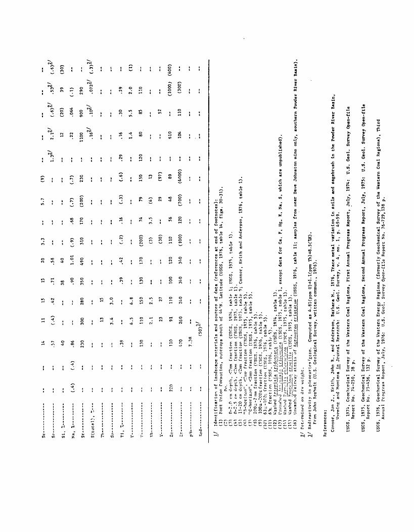
So ---

----

-

si,

r. --

-N

a, I.........

(.4

) (.

4)

SP- -

----

----

Ti.

r.-- --

V

14 .57 40

Q£

230

.39

130

110

470

11 (.4)

300 13

3.4

4.5 11

0

2.1 23 91 26

0

(50

)^

15 .42

9B(1 15

3.0

4.8 150

2.5 27 no 24

0

13

20

3.3

--

5

.7

.71

.58

1A

40

-

--

--

.90

1.0

1

(.9

) .6

8 (.

7)

350

490

310

170

(200

)

.39

.42

(.2)

.16

(.3)

130

170

(200

) 74

79

(3)

3.5

(4)

(30)

--

29

100

120

110

56

48

340

340

(100

) 12

0 (7

00)

(9)

12

(20

) 39

(3

0)

(.7

) --

.2

2 .0

64

(.1)

230

--

1100

90

0 29

0

(.6)

.29

.16

.30

.29

1.4

5.5

2.0

(1

)

150

120

80

85

110

13 (97)

--

--

52

89

--

610

(100

0)

(400

)

(400

0)

--

104

110

(300

)

l_/

Iden

tifi

cati

on of

la

ndsc

ape

mate

rial

s and

sour

ces

of da

ta (references

at end

of fo

otno

tes)

:(1)

Fort Un

ion

Formation, outcrops south

of 44 "N.

Latitude (USGS, 1976,

tabl

e 14,

figs

. 30

-31)

.C>

Po.

(.1)

0-:

.P

cm d

op

tli,

<?

:rni

fr

acti

on

(US

CS

, 1

97

4,

table

1;

U

SGS,

1975,

table

1).

(4}

0-2

.5

en

ilopib

. <2

cim

fr

acti

on

(K

SOS,

1975,

table

1

).(5

) 1

5-2

0

cm

diM

Jth.

<2

nra

fracti

on

(US

CS

, 1

97

3,

table

9;

Connor,

K

eith

an

d A

nd

erso

n,

1976,

table

1).

(r,1

"B

-hcrJ

son

"'.

<?n

w

fracti

on

(I-S

CS

, 1

97

5,

table

5).

(7^

"C-h

ori

zon",

<

2iro

fr

acti

on

(I'S

GS

, 1

97

5,

table

5

).(8

) 200:1

-2 r

un

fracti

on

(I'S

GS

. 1

97

6,

table

5).

(9)

100ii

-:oO

i: f

racti

on

(V

SGS,

1

97

6,

table

5

).(1

0)

63;i

-10C

U fr

acti

on

(VSC

S,

1976,

table

5

).(in

6*

1 fr

acti

on

("S

OS

. 1

076.

table

5).

(12

) W

ashe

d A_

r ten

-i s

1 a

trid

c-n

tata

(I

'SO

S,

1974,

tab

le

1).

(13

) l':

r..-;

!rf!

u-J

.\n .

.-i:,i

s l.i

t

r U

lvnia

t n

(1,'S

CS,

1

97

5,

tab

le

1,

exce

pt

data

fo

r C

a,

F,

Hg,

K

, N

a,

S,

wh

ich

are

u

np

ub

lish

ed

).(I

M

Was

hed

r.i^

\-H

:i

cl-,

1or:

u-hr

na

(t'P

GS

, 1

97

5,

table

1

).(1

5)

Was

hed

?on

tc lo

-.i.-i

pnic

i'li

s (U

SGS,

1975,

tab

le

1).

(16

) li

nv

asli

od

F

airw

ay str

ain

of

Afi

rooyro

n cri

statu

n-

(USG

S,

19

76

, ta

ble

11

; sa

mple

s fr

om

near

Dav

e Jo

hnst

on

min

e only

, so

uth

ern

P

owde

r R

iver

Basi

n).

J2/

Doto

rwin

od

on

drv

v

clp

ht.

3_/

Radio

acti

vit

y

in

pic

ocuri

rs'g

rnm

. C

ompu

ted

as

4.8

1(p

pm

U

)4-l

. l(

ppm

T

h)-^

8.5(

7JC

) .

fro

m

John

Rosh

olt

(U

.S.

Geolo

gic

al

Surv

ey,

wri

tten

com

mun

., 1976).

References:

Connor,

Jon

J.,

Keith, Jo

hn R.

, and

Anderson,

Barbara

M.,

1976,

Trac

e metal variation In

soils

and

sage

brus

h In

the

Powd

er River

Basi

n,

Wyom

inp

and Montana in

Jo

urna

l Re

sear

ch:

U.S. Geol.

Survey,

v. 4, no.

1, p. 49

-59.

USGS

, 197-1, Cc

ochc

ttic

al Survey of

th

e Western Co

al Re

gion

s, Fi

rst

Annual Progress Report,

July,

1974

; U.

S. Ge

ol.

Survey Op

en-f

ile

Repo

rt No

. 74-250,

38 p.

USGS,

1975

, Ge

oche

mica

l Survey of

the Western Co

al Re

gion

s, Second Annual Progress Report,

July

, 1975:

U.S.

Ge

ol.

Surv

ey Open-file

Repo

rt No

. 75-436,

132

p.

USGS

, 1976,

Geoc

hemi

cal

Survey of the Western Energy Regions

(formerly Geochemical Survey of the Western Coal Regions),

Third

Annual frogrc-ss

Repo

rt,

July,

1976:

U.S.

Geol.

Survey Open-flic

Repo

rt No

. 76-729,138 p.

Probable upper limits of concentration to be expected in ordinary landscape

materials of the Northern Great Plaina.

[The limits are estimated as those above which only about one sample in 20 of a randomly collected suite is expected to fall due to natural causes alone. Values expressed as parts per million (milligrams per liter in water) except as indicated. Limits given to two significant figures except those in paren theses, which are given to only one significant figure because they are judged to be less stable. Leaders (--) indicate data insufficient to estimate limit]

Property

Landscape Material-

RockShale Sandstone

(1) (2)

Soil

(3) (4)

Sediment

(5)

Ground water

(6)

Wheat-'

(7)

Al, 7.-

As

Ba

Br-

C(total), 7o 5.3

Ca, 7.

Cd-

Cl-

Cr-

Co-

Fe, 7.

HC0 3 -- --

K, 7. -

Li 80

Mg, 7. -----

Mn ----

Mo ---

Na, 7,-

Ni-- -

Pb --

25

(7)

79

(8)

91

(10) (6) (5)

3.5 (15)

82

11 12

38 35

3.7 3.8

(.05) .066

(2) (2)

33 39 26

1-5 (4) (2)

(1000)(2000)

(1) 1-4

30

30

(2)

-779x10

.91

.024

1.1

(.02)

.012

(4)

.0004

1500

.0012

.12

(.03)

.13

(.1)

(.03)

(.06)

(5)

(1)

(.01)

(.2)

(3)

(.6)

(.1)

300 98 (100) (100) 91

APPENDIX II (continued)

Probable upper limits of concentration to be expected in ordinary landscape

materials of the Northern Great Plains.

Property

Landscape Material-

RockShale'

(1)Sandstone

(2)

Soil

(3) (4)

Sediment

(5)

Ground water (6}

21 Wheat-'

(7)

S04 , %

SI, 7o -- -- (40) (40)

Sr ~ -- (JOG) (400)

Th ------- (10) (10)

rnj cy 1 O 1 s

U - ----- - - (4) (5) (6)

V - -- (100)

Zn 220 -- (100) 87 95r I

Rad-' -- -- -- (50)

In water only

Alkalinity

Dissolved solids (180°C)

Hardness (Total as CaC0 3 )

Temperature, °C

pH (standard units)

Gross B

Specific conductance, micromhos/cm

Sodium absorption ratio

(.2)

4/.0031-

(2.3)

(.05)

(.9)

(1000)

3000

(2000)

14

8.9

3/15-

(4000)

(100)

(2)

--

(.02)

(50)

_!/ Identification of landscape materials and sources of data (references at end of footnotes),(1) Fort Union Formation, outcrop (USGS, 1976, table 14).(2) Do(3) "A~horizon", <2mm fraction (USGS, 1976, table 9, figs. 15-27).(4) "B-horizon", <2mni fraction (USGS, 1976, table 9, figs. 15-27).(5) <150(t fraction (USGS, 1976, table 3).(6) From domestic or livestock wells, average depth 30m (USGS, 1976, table 13).(7) Grains of Triticum aestivum and _T. durum (Shacklettc and others, 1976).

2/ Determined on dry weight. 3/ Radioactivity in picocuries per liter. 4/ As Si0 2 .5_/ Radioactivity in picocuries/gram. Computed as 4.81(ppm U)+l.l(ppm Th)+8.5(7»K) .

From John Rosholt (U.S. Geological Survey, written commun., 1976).

References:

Shacklette, H. T., Erdman, J. A., Harms, T. F., and Papp, C. S. E. , 1976.Trace elements in plant foodstuffs jin Oehme, F. W., ed., Toxicity of HeavyMetals in the Environment: Marcel Dekker, New York (in press).

USGS, 1976, Goochemical Survey of the Western Energy Regions (formerly Geochenu'cal Survey of the Western Coal Regions), Third Annual Progress Report, July, 1976: U.S. Geol. Survey Open-file Report No. 76-729, 138 p.

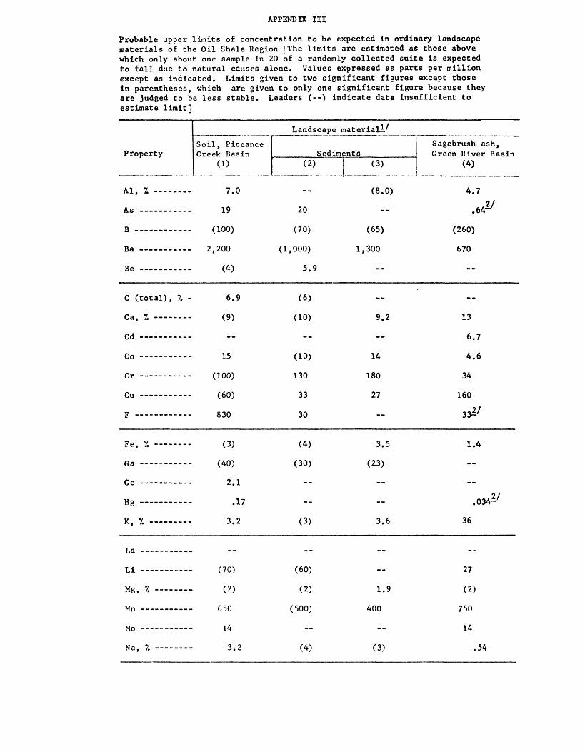
APPENDIX III

Probable upper limits of concentration to be expected in ordinary landscape materials of the Oil Shale Region ("The limits are estimated as those above which only about one sample in 20 of a randomly collected suite is expected to fall due to natural causes alone. Values expressed as parts per million except as indicated. Limits given to two significant figures except those in parentheses, which are given to only one significant figure because they are judged to be less stable. Leaders ( ) indicate data insufficient to estimate limit]

Property

Landscape material^'

Soil, Piceance Creek Basin

(1)Sediments

(2) (3)

Sagebrush ash, Green River Basin

(4)

A c

Ba

n _^

C (total), 7. -

Pa 1 ________

Cd

Co -

F ____________

Fe, 7.

Ga --

Hg --____" o

K v _____

T a

T i _______ __

Me 7 --------ng, /. --------

\*_,

Mo

N.i 7 ________

19

(100)

2,200

(4)

6.9

(9)

15

(100)

(60)

Q 1A

(3)

(40)

2.1

.17

3.2

(70)

(2)

650

14

T 9

on

(70) (65)

(1,000) 1,300

5.9

(6)

(10) 9.2

(10) 14

130 180

33 27

30

(4) 3.5

(30) (23)

/ O \ O £

(60)

(2) 1.9

(500) 400

(L\ C\\

*+ 1

(260)

670

13

6.7

4.6

34

160

332/

1 4x **

034^

36

27

(2)

750

14

s&

APPENDIX III -- Continued

Probable upper limits of concentration to be expected in ordinary landscape materials of the Oil Shale Region

Property

Landscape material!/

Soil, Piceance Creek Basin

(1)Sediments

(2) (3)

Sagebrush ash, Green River Basin

(4)

no ----------

Ni

Y

p V _________r, /.

Pb

S (total), 7. -

o _.

O t

Ti, 7. ------

U

v

\7U

7 ____ ______

48 100 (24) 21

.10 4.8

59 (20^ 26 73

i ar\ __

1.7

.59

an -- -- 072

(30) -- 19

510 (700) 560 770

(.4) .049 .42 .17

1.5

100 (100) 110 64

(20) (40) 30

(6) (4) 2.9

(100) 660 560

410 (400) 390 130

_!/ Identification of landscape materials and sources of data (references at end of footnotes):

(1) Bulk surface soil (U.S. Geol. Survey, 1976, tables 15, 16).(2) <150M- fraction (U.S. Geol. Survey, 1976, tables 18, 19).(3) <150p, fraction (U.S. Gcol. Survey, 1976, table 20).(4) Unwashed Artcmisia trident ata (U.S. Geol. Survey, 1976, table 7).

_?/ Determined on dry weight.

References:

U.S. Geological Survey, 1976, Geochcmicnl Survey of the Western Energy Regions (formerly Geochetnical Survey of the Western Coal Regions), 3rd Ann, Progress Report,(July, 1976): U.S. Geol. Survey Open-file Rept. No. 76-729, 138 p.

APPENDIX IV

TOXICITY OF SELECTED ELEMENTS TO PLANTS, ANIMALS, AND MAN-

AN OUTLINE

By

Larry P. Goue;h and Hansford I. Shacklette

CONTENTS

Page

Introduction.......................... 1

Aluminum.............................. 3

Arsenic............................... U

Boron................................. 6

Bromine............................... 7

Cadmium............................... 8

Chlorine.. ........................... 10

Chromium.............................. 11

Cobalt................................ 12

Copper................................ 13

Fluorine.............................. ll;

Iodine................................ 16

Lead.................................. 1?

Lithium............................... 20

Magnesium............................. 21

Manganese............................. 21

Mercury............................... 22

Molybdenum............................ 2ij.

Nic ke1................................ 2 6

Selenium.............................. 2?

Thallium.............................. 29

Tin................................... 30

Vanadium.............................. 31

Zinc.................................. 33

References cited...................... 35

iii

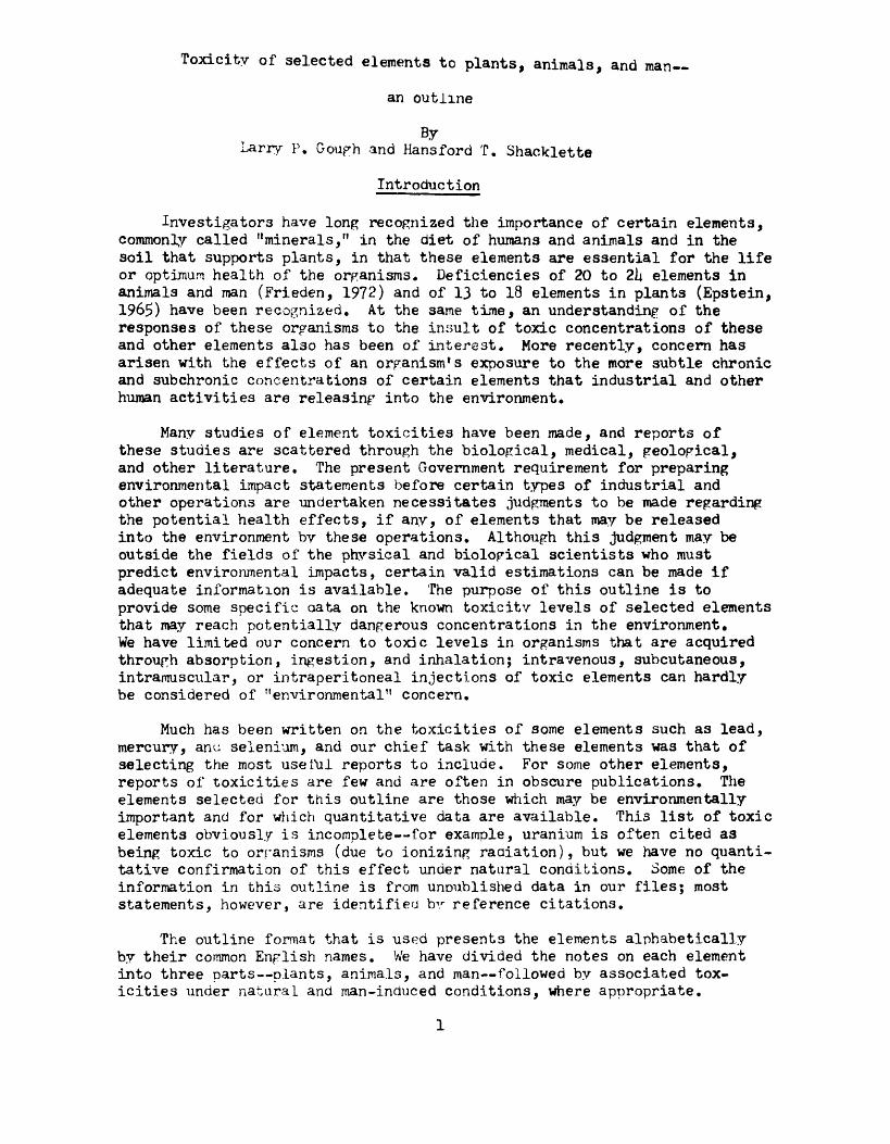
Toxicity of selected elements to plants, animals, and man

an outline

By Larry P. Gough and Hansford T. Shacklette

Introduction

Investigators have long recognized the importance of certain elements, commonly called "minerals," in the diet of humans and animals and in the soil that supports plants, in that these elements are essential for the life or optimum health of the organisms. Deficiencies of 20 to 2h elements in animals and man (Frieden, 1972) and of 13 to 18 elements in plants (Epstein, 196£) have been recognized. At the same time, an understanding of the responses of these organisms to the insult of toxic concentrations of these and other elements also has been of interest. More recently, concern has arisen with the effects of an organism 1 s exposure to the more subtle chronic and subchronic concentrations of certain elements that industrial and other human activities are releasing into the environment.

Many studies of element toxicities have been made, and reports of these studies are scattered through the biological, medical, geological, and other literature, The present Government requirement for preparing environmental impact statements before certain types of industrial and other operations are undertaken necessitates judgments to be made regarding the potential health effects, if any, of elements that may be released into the environment by these operations. Although this judgment may be outside the fields of the physical and biological scientists who must predict environmental impacts, certain valid estimations can be made if adequate information is available. The purpose of this outline is to provide some specific aata on the known boxicity levels of selected elements that may reach potentially dangerous concentrations in the environment, We have limited our concern to toxic levels in organisms that are acquired through absorption, ingestion, and inhalation; intravenous, subcutaneous, intramuscular, or intraperitoneal injections of toxic elements can hardly be considered of "environmental" concern.

Much has been written on the toxicities of some elements such as lead, mercury, am; selenium, and our chief task with these elements was that of selecting the most useful reports to include. For some other elements, reports of toxicities are few and are often in obscure publications. The elements selected for this outline are those which may be environmentally important and for which quantitative data are available. This list of toxic elements obviously is incomplete for example, uranium is often cited as being toxic to organisms (due to ionizing radiation), but we have no quanti tative confirmation of this effect under natural conditions. Some of the information in this outline is from unoublished data in our files; most statements, however, are identified bv reference citations.

The outline format that is used presents the elements alphabetically by their common English names. We have divided the notes on each element into three parts plants, animals, and man followed by associated tox icities under natural and man-induced conditions, where apDropriate.

Concentrations of elements generally are presented as parts per million (ppm), although other methods of expressing concentrations may be quoted. In some instances units such as mg/kg of body weight, umoles/1, ug/m3 , or percent provide a clearer concept for a given example, and converting them to ppm was either impossible or considered to be unnecessary.

It will be noted in this report that many of the elements that are discussed are essential for plants or animals, yet are toxic under certain conditions. The toxicitv of an element depends, first of all, on its chemical form. Kor example, chlorine in the elemental form (a pas) is highly toxic, whereas chlorine compounds mav be harmless, as is sodium chloride (common salt). Conversely, elemental arsenic is not toxic, although many arsenical compounds are highly toxic. Many reports do not specify the chemical form of an element when discussing its toxicity. It can be assumed for most of these reports that, under the soecified natural or experimental conditions, the element existed in an undetermined com pound, and that only the. total concentration of the element was known. In most reports in which the basis for expressing concentrations of an element in plant or animal tissues is not specified, a dry weight basis can be assumed.

The toxicity of a substance is also determined by the aosape that is, the amount (in relation to body weight), ana the frequency and duration of administering the substance to the organism. The duration of specified dosages of toxic elements was not given by Bowen in his 1966 report. In reports that relate toxicity to bodv weight of the experimental animals, "live" or "wet" weight is commonly used. Amounts of an element in relation to body weight are expressed as ingested amounts. The term "LJV " means that the specified dose is lethal to 50 percent of the experimental organisms, Quantities of total diets given are based on a one-day consumption, unless otherwise stated.

To be toxic, an element must be "available" to the plants or animals that is, it must exiyt, in a foriri that can enter tissues of the organism, either in solution (generally aqueous), as a gas, or iuncommonly) as a solid, or it must eiriit ionizing rauiition. i'otaj. amounts of a toxic element in the environment are not relevant to an adequate estimation of the toxicity hazard unless it can be shown that the element exists in, or is likely to assume, an available form under the environmental conditions in which it occurs.

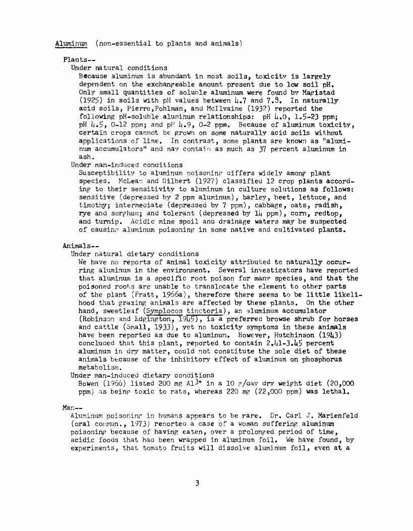
Aluminum (non-essential to plants and animals)

Plants Under natural conditionsBecause aluminum is abundant in most soils, toxicity is largely dependent on the exchangeable amount present due to low soil pH. Only small quantities of soluble aluminum were found by Magistad (192^) in soils with pH values between lu? and 7.3. In naturally- acid soils, Pierre,Pohlman, and Mcllvaine (193?) reported the following pH-soluble aluminum relationships: pH iuQ, 1.5-23 ppm; pH lj.5> 0-12 ppm; and pH Iu9, 0-2 ppm. Because of aluminum toxicity, certain crops cannot be grown on some naturally acid soils without applications of lime. In contrast, some plants are known as "alumi num accumulators" and may contain as much as 37 percent aluminum in ash.

Under man-induced conditionsSusceptibility to aluminum poisoning differs widely among plant species. McLean and Gilbert (192?) classified 12 crop plants accord ing to their sensitivity to aluminum in culture solutions as follows: sensitive (depressed by 2 ppm aluminum), barley, beet, lettuce, and timothy; intermediate (depressed by 7 ppm), cabbage, oats, radish, rye and sorphurn; and tolerant (depressed by Ik ppm), corn, redtop, and turnip. Acidic mine spoil and drainage waters may be suspected of causing aluminum poisoning in some native and cultivated plants.

Animals Under natural dietary conditionsWe have no reports of animal toxicity attributed to naturally occur ring aluminum in the environment. Several investigators have reported that aluminum is a specific root poison for manv species, and that the poisoned roots are unable to translocate the element to other parts of the plant (Pratt, 1966a), therefore there seems to be little likeli hood that grazing animals are affected by these plants. On the other hand, sweetleaf (Symplocos tinctoria), an aluminum accumulator (Robinson and Edgington, 19U5)> is a preferred browse shrub for horses and cattle (Small, 1933), yet no toxicity symptoms in these animals have been reported as due to aluminum. However, Hutchinson (19U3) concluded that this plant, reported to contain 2j.il-3.h5 percent aluminum in dry matter, could not constitute the sole diet of these animals because of the inhibitory effect of aluminum on phosphorus metabolism.

Under man-induced dietary conditionsBowen (1966) listed 200 mg Al3+ in a 10 p/day dry weight diet (20,000 ppm) as beinp toxic to rats, whereas 220 mg (22,000 ppm) was lethal.

Man Aluminum poisoning in humans appears to be rare. Dr. Carl J. Marienfeld (oral coirjnun., 1973) reported a case of a woman suffering aluminum poisoning because of having eaten, over a prolonged period of time, acidic foods that hao been wrapped in aluminum foil. We have found, by experiments, that tomato fruits will dissolve aluminum foil, even at a

temperature of 0°F. Smith (192S) reported that ingestion of 150 mg aluminum per day is without obvious effects on normal humans; 200 mg may, however, Rive rise to mild catharsis, which increases with the dose. Regarding absorption of inhaled airborne aluminum, Hutchinson (19U35 p. 2£2) wrote, "The fact that all investigators have found aluminum in the bile indicates that some of the aluminum present in the faeces, as well as in the urine, has been involved in a metabolic cycle. It is conceivable that this aluminum has in part entered the blood stream through the pulmonary epithelium, but if such a mode of entry were generally important significant negative balances would have been reported wherever balance sheets have been made." A number of observations indicate that high concentrations of aluminum may be toxic to the nervous system (Crapper and others, 1973). These authors analyzed the brains of persons who died with Alzheimer's disease (a disease occurring after the age of UO and producing progressive dementia) and found concentrations of aluminum similar to those in the brains of experimental animals that had been injected with l£0-225 p,g aluminum, as aluminum chloride, and as a result had developed neurological symp toms similar to those of Alzheimer's disease in humans.

Arsenic (non-essential to plants and animals)

Plants Under natural conditions

Although the free element is not considered poisonous, many of its compounds are extremely so (Liebig, 1966). Brooks (1972) stated that the toxicity of this element to plants was severe. The arsenic in normal soils ranges from <1 to 1|0 ppm (Underwood, 1971); within this range, damage to plants is not expected, and the arsenic content of most species is low (<10 ppm, dry weight). Soils in the vicinity of some heavy metal deposits may contain much more arsenic, and douglas- fir (Pseudotsuga menziesii) growing in such soils may contain as much as 8/200 ppm in ash (Warren and others, 1968).

Under man-induced conditionsThe toxicity to plants of certain arsenic compounds, principally sodium arsenite and arsenic trioxide, is so great that these compounds were used as herbicides for many years. Arsenic compounds such as calcium arsenate, lead arsenate, and cupric arsenite (Paris green) formerly were widely used as insecticides. The lonp-berm use of these materials in agricultural practice accounts for most recorded cases of plant toxicities. The toxicity depends on the concentration of soluble, not total, arsenic in soils. Studies of unproductive old orchara soils in the Yakima Valley from which apple trees had been removed revealed 3.U-9.5> ppm of readily soluble arsenic in the top 6 inches of soil. Damage to alfalfa and barley was proportional to the concentration of soluble arsenic; if above 2 ppm, marked damage to the plants occurred (Vandecaveye and others, 1936). Arsenic is introduced into the environment as an air pollutant from burning coal, and from smelters and refineries (Underwood, 1971), but we have no reports of damage to plants from these sources.

Animals Under natural dietary conditions

Examples of toxicity of arsenic to animals under natural conditions are believed to be uncommon. Grimmett (1939) investigated livestock poisoning in a valley of New Zealand and found soils and muds contained as much as 1.9 psrcent arsenic; water from springs, streams, and surface depressions varied from a trace to 13 ppm of arsenic; and pasture grasses contained 2.8 to 6.9 ppm (dry weight) arsenic. He concluded that the danger to stock was not from the arsenic in the forage, but from that in the mud or water which might be ingested.

Under man-induced dietary conditionsThere is probably little danger of arsenic poisoning from feeding plants and plant products to animals. In fact, four organic arsenic compounds (arsenilic acid, lj-nitrophenylarsonic acid, 3-nitro-U- hydroxyphenylarsenic acid, and arsenobenzene) are used as growth stimulants for pigs and poultry (Underwood, 1971). Trivalent com pounds (arsenites) are far more toxic than the pentavalent forms (arsenates). The 96-hour LDgo for mice and rats is 11.2 ppm arsenite in the diet whereas it is 112 ppm for arsenate. Schroeder and Balassa (1966) reported that arsenic deactivates enzymes with thiol groups and acts as an antagonist of iodine and selenium.

Man- Under natural dietary conditionsWater is the most common natural material causing arsenic poisoning. Amounts in excess of 0.05 mg/1 in drinking water constitute grounds for rejection (U.S. Public Health Service, 196l). Wyllie (1937) reported illness and one fatality in a farm family that used water from a deep well having O.).i-10 ppm arsenic (as As203). Large beds of FeAsS occurred about 10 miles from this well. Water from shallow wells near this farm were free of arsenic. Borgono and Greiber (1971) reported that prolonged consumption (12 years) of water high in arsenic (0.8 ppm) produced cutaneous lesions in over 30 percent of the inhabitants of a city in Chile. Foods of plant origin contain so little arsenic that toxicity to humans in unlikely. Seafood of marine origin contains much more arsenic maximum values reported (fresh weight basis) follow: Oysters, 10 ppm; mussels, 120 ppm; prawns, Ilk ppm; and shrimp, 1*2 ppm (Underwood, 1971). This author stated further that the amounts of arsenic ingested daily in the food are greatly influenced by the amounts and pronortions of seafoods included in the diet.

General notes on toxicityElemental arsenic is not toxic (Schroeder and Balassa, 1966), whereas most compounds of this element are highly toxic (Stecher, 1968). Schroeder and Ralassa (1966) reported that mountaineers in Syria and the Alps have been known to consume large quantities of native arsenic ("arsen"), believing that it promotes endurance at high altitudes. The minimum fatal dose of arsenous oxide for man was given as 0.06-0.18 g bv Monier-Williams (1950). This author also stated that the British Royal Commission set maximum limits of

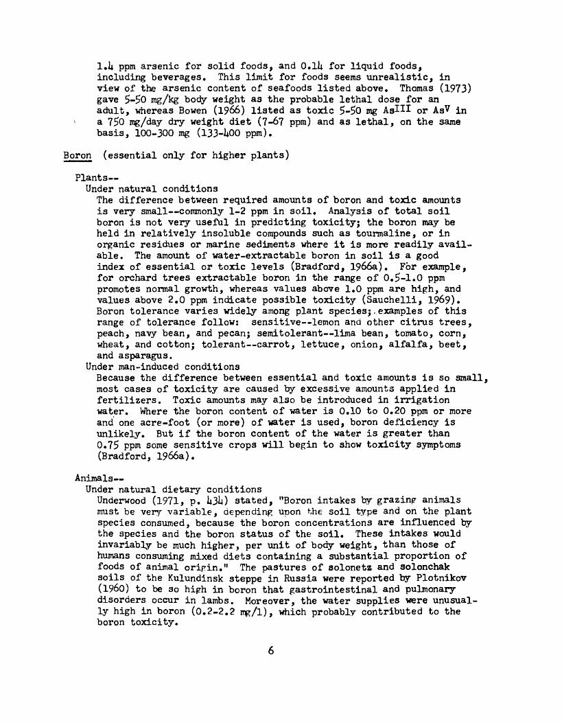
1.1* ppm arsenic for solid foods, and O.ll* for liquid foods, including beverages. This limit for foods seems unrealistic, in view of the arsenic content of seafoods listed above. Thomas (1973) gave 5-50 mg/kg body weight as the probable lethal dose for an adult, whereas Bowen (1966) listed as toxic 5-50 mg As^I or AsV in

\ a 750 ing/day dry weight diet (7-6? ppm) and as lethal, on the same basis, 100-300 mg (133-1*00 ppm).

Boron (essential only for higher plants)


The difference between required amounts of boron and toxic amounts is very small commonly 1-2 ppm in soil. Analysis of total soil boron is not very useful in predicting toxicity; the boron may be held in relatively insoluble compounds such as tourmaline, or in organic residues or marine sediments where it is more readily avail able. The amount of water-extractable boron in soil is a good index of essential or toxic levels (Bradford, 1966a). For example, for orchard trees extractable boron in the range of 0.5-1.0 ppm promotes normal growth, whereas values above 1.0 ppm are high, and values above 2.0 ppm indicate possible toxicity (Sauchelli, 1969). Boron tolerance varies widely among plant species;.examples of this range of tolerance follow: sensitive lemon and other citrus trees, peach, navy bean, and pecan; semitolerant lima bean, tomato, corn, wheat, and cotton; tolerant carrot, lettuce, onion, alfalfa, beet, and asparagus.

Under man-induced conditionsBecause the difference between essential and toxic amounts is so small, most cases of toxicity are caused by excessive amounts applied in fertilizers. Toxic amounts may also be introduced in irrigation water. Where the boron content of water is 0.10 to 0.20 ppm or more and one acre-foot (or more) of water is used, boron deficiency is unlikely. But if the boron content of the water is greater than 0.75 ppm some sensitive crops will begin to show toxicity symptoms (Bradford, 1966a).


Underwood (1971, p. k3k) stated, "Boron intakes by grazing animals must be very variable, depending upon the soil type and on the plant species consumed, because the boron concentrations are influenced by the species and the boron status of the soil. These intakes would invariably be much higher, per unit of body weight, than those of humans consuming mixed diets containing a substantial proportion of foods of animal origin." The pastures of solonetz and solonchak soils of the Kulundinsk steppe in Russia were reported by Plotnikov (I960) to be so high in boron that gastrointestinal and pulmonary disorders occur in lambs. Moreover, the water supplies were unusual ly high in boron (0.2-2.2 mg/1), which probably contributed to the boron toxicity.

Man- Underwood (I9H, p. U3U) stated, "The boron in food, and boron added as sodium borate or boric acid, is rapidly and almost completely absorbed and excretec, largely in the urine. Where high intakes occur either accidentally or from the treatment of large burns with boric acid, similar high absorption and urinary excretion take place, but sufficient boron may be temporarily retained in the tissues, especially in the brain, to produce serious toxic effects." Bowen (19'66) listed as toxic UjOOO mg boron (borate) in a 750 g/day dry weight diet (5,300 ppm).

Bromine (non-essential for plants and animals)


The bromine content (principally as bromides) in normal soil is so low, ranging from 10 to hO ppm, that bromine toxicity has not been a problem in crop production in the past (Martin, 1966a).

Under man-induced conditionsMost cases of bromine toxicity to plants are related to residual bromine in the soil following fumigation with bromine compounds (principally ethylene dibromide and methyl bromide). However, the possibility exists of bromine contamination of soils by motor vehicle and industrial emissions. In land plants bromine normally ranges from trace concentrations to about 260 ppm in the dry tissue. It is especially hi^h in melons, carrot tops, celery tops, and mushrooms. In contrast to land plants, marine plants contain up to about 2,000 ppm (Martin, 19663). Plant species differ greatly in their tolerance to soil bromine; onion is so sensitive that it has been used as a test plant for detecting soil bromide (O'Bannon, 1958). Other sensitive plants include bean, beet, cabbage, celery, citrus, pea, peanut, pepper, potato, spinach, sugar beet, sweet potato, and turnip. The bromine content of dry leaf tissue has been used as an indication of toxicity; for example, leaf bromine concentrations in citrus seedlings of 0.17, 0.33> O.I', 1.3> and 1.8 percent were associated with 12, 22, 31, 57, and 90 percent reduction in growth, respectively (Martin and others, 1956). Concentrations of water- soluble soil bromine were reported to have the following effects: 38-83 ppm, reduced growth of bean and cabbage; 26-53 ppm injured carnation plants; 15 ppm reduced growth of citrus seedlings, and 600 ppm almost killed the plants; and growth of beans was greatly retarded by 300 ppm (summaries given by Martin, 1966a).


Although the bromine content of animal tissues and milk is greatly influenced by the bromine in the feeds, we have no reports of bromine toxicity froim feed sources.

Under man-induced dietary conditionsBowen (1966) listed as lethal to rats 800 mp Br~ in a 10 g/day dry- weight diet (So,000 ppm).

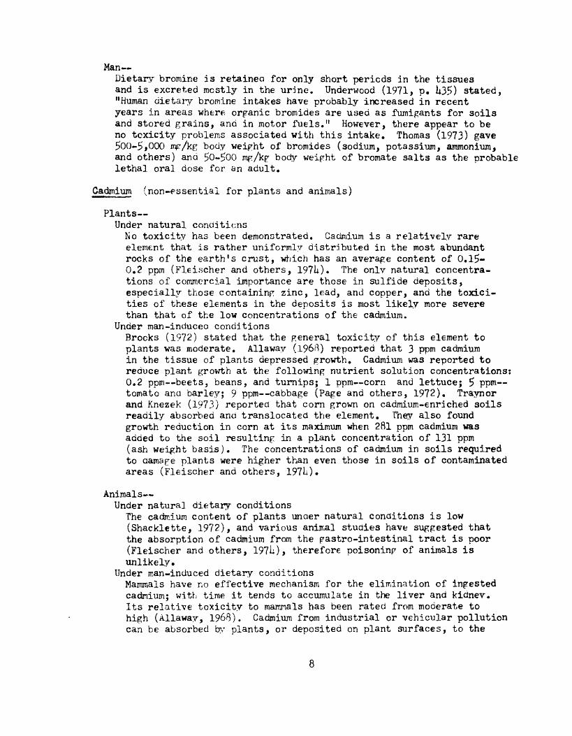
Man- Dietary bromine is retained for only short periods in the tissues and is excreted mostly in the urine. Underwood (1971, p. U35) stated, "Human dietary bromine intakes have probably increased in recent years in areas where organic bromides are used as fumigants for soils and stored grains, and in motor fuels." However, there appear to be no tcxicity problems associated with this intake. Thomas (1973) gave ^00-5,000 mg/kg body weight of bromides (sodium, potassium, ammonium, and others) and 50-500 mg/kg body weight of bromate salts as the probable lethal oral dose for an adult.

Cadmium (non-essential for plants and animals)

Plants Under natural conditionsNo toxicity has been demonstrated. Cadmium is a relatively rare element that is rather uniformly distributed in the most abundant rocks of the earth's crust, which has an average content of O.l£- 0.? ppm (Fleischer and others, 197U). The only natural concentra tions of commercial importance are those in sulfide deposits, especially those containing zinc, lead, and copper, and the toxicities of these elements in the deposits is most likely more severe than that of the low concentrations of the cadmium.

Under man-induced conditionsBrocks (1972) stated that the general toxicity of this element to plants was moderate. Allaway (1968) reported that 3 ppm cadmium in the tissue of plants depressed growth. Cadmium was reported to reduce plant growth at the following nutrient solution concentrations: 0.2 ppm beets, beans, and turnips; 1 ppm corn and lettuce; 5 ppm tomato ana barley; 9 ppm cabbage (Page and others, 1972). Traynor and Knezek (1973) reported that corn grown on cadmium-enriched soils readily absorbed and translocated the element. They also found growth reduction in corn at its maximum when 281 ppm cadmium was added to the soil resulting in a plant concentration of 131 ppm (ash weight basis). The concentrations of cadmium in soils required to damage plants were higher than even those in soils of contaminated areas (Fleischer and others, 1971).


The cadmium content of plants under natural conditions is low (Shacklette, 1972), and various animal studies have suggested that the absorption of cadmium from the gastro-intestinal tract is poor (Fleischer and others, 1971), therefore poisoning of animals is unlikely.

Under man-induced dietary conditionsMammals have no effective mechanism for the elimination of ingested cadmium; with time it tends to accumulate in the liver and kidney. Its relative toxicity to mamnals has been rated from moderate to high (Allaway, 1968). Cadmium from industrial or vehicular pollution can be absorbed by plants, or deposited on plant surfaces, to the

extent that the plants are toxic to animals. For example, Goodman and Roberts (1971) reported grass that was contaminated by industrial pollution contained 9.9 ppn cadmium, whereas control samples of the grass contained only 1 ppm; this contaminated grass caused the death of a horse (but the immediate cause of death was attributed to plumbism). They found contaminated grass to contain as much as IiO ppm cadmium in ash. Cadmium was suspected of killing a horse which contained 80 ppm cadmium in its liver and 1^10 ppm in its kidneys (Lewis, 1972). Thirty to sixty ppm cadmium in the diet of sheep for 191 days was shown to reduce growth and feed intake (Doyle and others, 1972). Forty-five ppm cadmium in the diet of rats for 6 months caused slight toxic symptoms (Underwood, 1971). Bowen (1966) stated that 0.5 mg/day Cd2+ in a total dry weight diet of 10 g (£00 ppm) is toxic to rats, whereas 16 mg/da^ (1,600 ppm) is lethal. A subtoxic level of 5 ppm cadmium in the drinking water of rats, given for 180- 2kQ days, produced systolic hypertension. It has been used as an anthelmintic drug in swine and poultry at concentrations ranging from 30-1,000 ppm in the diet (Stecher, 1968). Cadmium appears to be highly toxic to aquatic organisms at low concentrations, as follows: lethal to the flatworm Polycelis nigra at 2.7 ppm; to sticklebacks at 0.2 ppm; to goldfish at 0.02 ppm; to Daphnia magna at 0.003 ppm (Schroeder and Balassa, 196la).

Man- Under normal environmental conditions

The normal cadmium content of food plants is low, ranging from 0.1 to 1 ppm in dry material (Shacklette, 1972), therefore poisoning from this source is unlikely.

Under the effects of environmental pollution by cadmiumThe first likely instance of cadmium poisoning in man due to general environmental contamination is that of itai-itai disease in the elderly women who lived in the vicinity of a mine in Japan. It was demonstrated that the water, rice, and fish in the endemic area con tained high concentrations of cadmium and other metals, probably due to contamination of the local river by the effluent from a zinc- lead-caamium smelter (Fleischer and others, 197h). Bowen (1966) stated that the normal dietary intake of Cd^, based on a total dry weight diet of 7£0 g/day, is 0.6 (0.8 ppm), whereas 3 mg/day (k ppm) is toxic. A recent study of the environmental impact of cadmium (Fleischer and others, I97h) concluded, "Based on present knowledge, and there are many gaps, there is no solid evidence of a hazard to the general population from cadmium in food, air, or water. Contamination of food and water rather than air would seem to present more of a potential problem. This might not be the case with smoking or excessive occupational exposures."

Chlorine (essential for plants and animals)


The chloride ion is itself toxic if too greatly concentrated, also the common natural chlorine compound, sodium chloride, is toxic through its effect on osmotic pressure within the plant, if too concentrated. Symptoms of excess chloride include burning and firing of leaf tips or margins, bronzing, premature yellowing and abscission of leaves and, less frequently, chlorosis (Eaton, 1966). Within the concentration ranges of sodium chloride tolerated by a species of plant, for each increase in the osmotic pressure of the substrate solution there is an increase in the osmotic pressure of the plant sap; beyond this range s lethal wilting occurs. Under natural conditions, areas inundated by sea water, or strongly in fluenced by sea spray, may accumulate toxic amounts of sodium chloride in the soil. Evaporative salt in closed geographic basins may also reach toxic concentrations. On natural undrained soil in Australia the chloride in leaf petioles of grape (percent, dry matter) related to leaf toxicity symptoms were as follows: 0.81, no toxicity; 1.35> slight burning; 1.55, burning; 2.50, severe burning (Woodham, 1956).

Under man-induced conditionsChloride toxicity may be produced in plants by over-fertiliaing, such as with potassium chloride. Chloride toxicity may also result from irrigation with slightly salty water with insufficient flushing of the soil. Plants range widely in their resistance to toxicity from the halophytes such as asparagus, to highly sensitive species. Experimental stuaies with grapefruit in which the trees were watered with different levels of salt concentration in the water gave the following results (Pearson and others, 1957): 300 ppm salt, relative weight of tops was 100, 0.0? percent (in dry matter) in leaves; 1,300 ppm salt, relative weight of tops was 1*6, 1.28 percent in leaves; and 2,300 ppm salt, relative weight of tops was 38, 1.35 percent in leaves. The two higher concentrations produced defolia tion, dieback, chlorosis, bronzing, and burning.


Forage plants in general are so low in chlorine that salt must be provided to herbivorous animals; therefore, natural chlorine toxicity in these animals is very unlikely.

Under man-induced dietary conditionsOur only report is one given by Bowen (1966) who listed as lethal to rats >900 mg Cl" in a 1C) g/day dry weight diet (90,000 ppm).

Man We have no reports of human toxicity attributed to excessive chlorine in the natural environment, although of course chlorine gas is highly toxic to plants, animals, ana man. Thomas (1973) gave 50-500 mg/kg body weight as the probable lethal dose of chlorate salts for an adult.

10

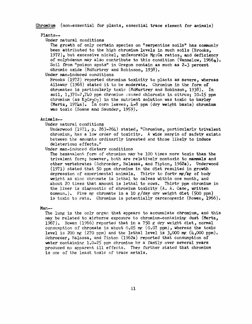
Chromium (non-essential for plants, essential trace element for animals)


The growth of only certain species on "serpentine soils" has commonly been attributed to the high chromium levels in such soils (Brooks, 1972), but excessive nickel, unfavorable Mg:Ca ratios, and deficiency of molybdenum may also contribute to this condition (Vanselow, 1966a)« Soil from "poison spots" in Oregon contain as much as 2-3 percent chromic oxide (McMurtrey and Robinson, 1938).

Under man-induced conditionsBrooks (1972) reported chromium toxicity to plants as severe, whereas Aliaway (1968) stated it to be moderate. Chromium in the form of chromates is particularly toxic (McMurtrey and Robinson, 1938). In soil, 1,370-2,7liO ppm chromium caused chlorosis in citrus; 10-15 ppm chromium (as l^C^Oy) in the nutrient solution was toxic to barley (Mertz, 197ha). In corn leaves, U-8 ppm (dry weight basis) chromium was toxic (Soane and Saunder, 19$9).

Animals Under natural conditions

Underwood (1971, p. 263-26U) stated, "Chromium, particularly trivalent chromium, has a low order of toxicity. A wide margin of safety exists between the amounts ordinarily ingested and those likely to induce deleterious effects."

Under man-induced dietary conditionsThe hexavalent form of chromium may be 100 times more toxic than the trivalent form; however, both are relatively nontoxic to mammals and other vertebrates (Schroeder, Balassa, and Tipton, 1962a). Underwood (1971) stated that $0 ppm chromium in the diet resulted in growth depression of experimental animals. Thirty to forty mg/kg of bocly weight as zinc chromate is lethal to calves within one month, and about 20 times that amount is lethal to cows. Thirty ppm chromium in the liver is diagnostic of chromium toxicity (A. A. Case, written commun.). Five mg chromate in a 10 g/day dry weight diet ($00 ppm) is toxic to rats. Chromium is potentially carcenogenic (Bowen, 1966).

Man- The lung is the only organ that appears to accumulate chromium, and this may be related to airborne exposure to chromium-containing dust (Mertz, 1967). Bowen (1966) reported that in a 7$0 g dry weight diet, normal consumption of chromate is about 0.0$ mg (0.07 ppm), whereas the toxic level is 200 mg (270 ppm) and the lethal level is 3,000 mg (U,000 ppm). Schroeder, Balassa, and Tipton (I962a) reported that consumption of water containing 1.0-2$ ppm chromium by a family over several years produced no apparent ill effects. They further stated that chromium is one of the least toxic of trace metals.

11

Cobalt (essential trace element for blue-green algae and nodule bacteria,non-essential for higher plants although growth and yield increases have been reported; essential trace element for animals)

Plants Under natural conditionsVanselow (l966b >/ reported that cobalt exhibits toxicity to plants when the amounts available to the plant exceed certain low levels, but that a naturally occurring excess of cobalt in soils is im probable and that no instances so far had been noted. Plant species range widely in their content of cobalt, yet show no toxicity symptoms. Some trees have very hiph concentrations in their leaves, as for example, black gum (Nyssa sylvatica) leaves were renorted to contain as much as 10,003 ppm in ash, ana persimmon (Diospyros virginiana) leaves 2,000 ppm; most other species contain much less (Connor, Shacklette, and others, 197!?).

Under experimental conditionsA number of authors (see Vanselow, 1966b) have reported that in solution cultures small amounts of cobalt, sometimes as low as 0.1 ppm, produced adverse or toxic effects on many crop plants. The symptoms of cobalt excess include depressed growth, chlorosis, necrosis, and even death of the plant. The chlorosis is frequently described as resembling that of iron deficiency (Vanselow, 1966b). Sudan grass containing 19-32 ppm (dry weight basis) cobalt showed toxicity symptoms when grown in soils to which 2,000 pounds of cobalt per acre had been added (Fujimoto and Sherman, 1950).


We have no reports of cobalt toxicity attributed to consumption of natural feedstuffs; pasturage deficiency in cobalt is of far greater concern than are potentially toxic concentrations in plants.

Under man-induced dietary conditionsCobalt is relatively non-toxic. Sheep can tolerate large doses of cobalt; 0.35/100 kg/day produced no ill effects (Recker and Smith, 1951). Smith (1^62) listed the following in mp/kg body weight/dav: rats 2.5, non-toxic; dogs 10, non-toxic; sheep 3, non-toxic; and cattle about 1, toxic. Bowen (1966) listed as toxic to rats 0.7 mg Co^* in a 10 g/day dry weight diet (70 ppm).

Man- The edible parts of food plants contain only Si-10 ppm (ash basis) cobalt, therefore toxicitv attributed to this source is very unlikely (Connor, Shacklette, ana others, 1975). As with animals, the toxicity of non-radioactive isotopes of cobalt are of little importance. At a time when cobalt was used in beer in order to preserve the foam, it was suspected of causing the "beer drinkers cardiomyopathy" syndrome. Some evidence (Burch, Williams, and Sullivan, 1973), however, implicates selenium in conjunction with cobalt as being responsible. Rowen (1966) listed as toxic 5 (JO mg Co2* in a 750 g/day dry weight diet (670 ppm).

Copper (essential trace element for plants and animals)


Soil influenced by a high degree of copper mineralization may be toxic to native or cultivated plants. Eraser (1961) reported that large trees were absent, and tree seedlings were killed, in a syngenetic copper deposit in a swamp in New Brunswick, and that muck from this swamp killed cucumber plants to which it was applied. There are many reports in the literature of copper toxicity to plants on or near copper deposits, and the degree of resistance to copper toxicity by different species has been used as a geobotanical method of mineral exploration.

Under man-induced conditionsCopper sulfate (blue vitriol) has been used for over seventy years as an algicide at an achieved concentration of 1 mg/1 (1 ppm) for the upper 0.5 m of water (Mackenthun and Ingrain, 196?). Most copper toxicities in crop plants have been caused by the use of Bordeaux mixture (copper sulfate and lime) as a fungicide. Toxicity to copper in plants is usually manifested bv chlorosis (yellowing) of the foliage, caused by the interference of excessive copper with iron metabolism in the plant. Reuther and Smith (1953) found appreciable chlorosis of citrus seedlings occurring when the total copper of a very sandy soil of pH 5.0 or below exceeded 150 ppm. Westgate (1952) reported copper toxicity in several crops on old vegetable fields having over iiOO ppm total copper in the topsoil as a result of many years of Bordeaux mixture spraying of celery. Copper is added to the environment by industrial pollution and vehicular emissions (Shacklette and Connor, 1973)> but we have no reports of copper toxicity attributed to these sources. Copper deficiencies in agri cultural soils are much more common than copper excesses, and ferti lization with copper, especially on highly organic or very sandy soils, is a common practice.


Dick (195^) reported than when sheep graze on pastures of normal copper content, but low in molybdenum (less than 0.1 ppm), copper accumulates in their livers. This accumulation sometimes results in chronic copper poisoning, followed by death. On the other hand, when pasture or forage contains a normal copper content but high molybdenum (5 ppm or more), a poisoning having many of the clinical symptoms of copper deficiency mav occur. The average (geometric mean) copper content of United States soils was reported as 18 ppm, with a range of <L-300 ppm, and most soil samples contained <3 ppm molybdenun, with high values ranging from 3-7 ppm (Shacklette and others, 1971).

Under man-induced dietary conditionsHemkes and Hartmans (1973) found that sheep feeding on either side, and within 20 m of, high-tension copper power lines became ill and died after consuming dry forage and soil with copper in excess of

13

15 ppm. Sheep appear to be particularly sensitive to copper intoxi cation. Chronic copper poisoning of animals may occur as a conse quence of excessive consumption of copper-containing salt licks or mixtures, or the unwise use of copper-containing drenches. Contami nation of feeds with copper compounds from horticultural or industrial sources is a further cause. In all animals the continued ingestion of copper in excess of requirements leads to some accumulation in the tissues, especially in the liver (Underwood, 1971). Copper toxicity in mammals, compared to other animals, is of little significance because they possess barriers to copper absorption. Schroeder and others (I966b, p. 1028) stated, "Avian and mammalian resistance to copper is 100 to 1,000 times greater than is that of more primitive animals," For aquatic organisms copper is the most toxic common heavy metal; this toxicity, however, is inversely related to the water hardness (principally, calcium content). Bowen (1966) reported that a 20 mg Cu^* (2,000 ppm) ration in a dry weight diet of 10 g/day was lethal to rats.

Man- Under normal environmental conditions

Underwood (1971, p. 106) stated, ?9Continuoui ingestion. of copper from food or water supply at intakes sufficient to induce chronic copper poisoning in man is extremelv unlikely, judging by the amounts required for this purpose in other monogastric species." From a normal intake of 2-5 mg/day (Bowen, 1966) there is normallv main tained a net balance of zero copper.

Under excessive copper intakeExcessive build-up of copper in the liver and central nervous system, caused by a metabolic inability to excrete copper, is the fundamental cause of Wilson's disease (Scheinberg, 1969). Bowen (1966) reported that 250-500 mg Cu2+ (330-670 ppm) in a dry weight diet of 750 g/day is toxic to normal individuals. Soluble copper salts, notably copper sulfate, are strong irritants to the skin and mucous membranes (Stecher, 1968).

Fluorine (non-essential for plants; essential trace element for some higher animals, improves animal teeth and bones)


Toxicity is unusual, but plants growing in acid soils have accumulated toxic levels of fluorine (Allaway, 1968). The amount of fluoride taken up from the soil by plants is usually unrelated to total soil fluorine, but is controlled bv soil type, calcium and phosphorus content of the soil, and soil pH (Brewer, 1966a). Brewer (1966a, p. 182) reported, "With few exceptions, the usual fluoride content of most plant foliage growing in areas removed from possible sources of fluoride air pollution is in the range of 2 to 20 ppm on a dry-weight basis. Notable exceptions include tea leaves, which have been found - - - to contain, on the average, 50 to 90 ppm of fluorine. The highest fluoriae concentrations reported for vegetation, presumably attributable to fluorine absorption from the substrate, include 1,900 ppm in camellia leaves - - - and in excess of 8,000 pprr, in tea leaves

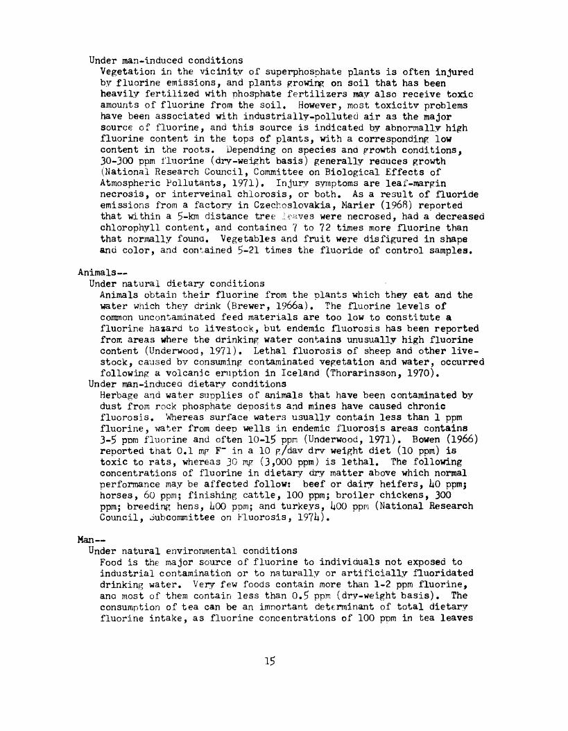
Under man-induced conditionsVegetation in the vicinity of superphosphate plants is often injured by fluorine emissions, and plants growing on soil that has been heavily fertilized with phosphate fertilizers may also receive toxic amounts of fluorine from the soil. However, most toxicitv problems have been associated with industrially-polluted air as the major source of fluorine, and this source is indicated by abnormally high fluorine content in the tops of plants, with a corresponding low content in the roots. Depending on species and growth conditions, 30-300 ppm fluorine (dry-weight basis) generally reduces growth (National Research Council, Committee on Biological Effects of Atmospheric Pollutants, 1971). Injury symptoms are leaf-margin necrosis, or interveinal chlorosis, or both. As a result of fluoride emissions from a factory in Czechoslovakia, Warier (1968) reported that within a 5-km distance tree leaves were necrosed, had a decreased chlorophyll content, and contained 7 to 72 times more fluorine than that normally found. Vegetables and fruit were disfigured in shape and color, and contained 5-21 times the fluoride of control samples.

Animals Under natural dietary conditionsAnimals obtain their fluorine from the plants which they eat and the water which they drink (Brewer, 1966a). The fluorine levels of common uncontaminated feed materials are too low to constitute a fluorine hazard to livestock, but endemic fluorosis has been reported from areas where the drinking water contains unusually high fluorine content (Underwood, 1971). Lethal fluorosis of sheep and other live stock, caused by consuming contaminated vegetation and water, occurred following a volcanic eruption in Iceland (Thorarinsson, 1970).

Under man-induced dietary conditionsHerbage and water supplies of animals that have been contaminated by dust from rock phosphate deposits and mines have caused chronic fluorosis. Whereas surface waters usually contain less than 1 ppm fluorine, water from deep wells in endemic fluorosis areas contains 3-5 pom fluorine and often 10-15 ppm (Underwood, 1971). Bowen (1966) reported that 0.1 mp F~ in a 10 g/dav drv weight diet (10 ppm) is toxic to rats, whereas 30 mg (3,000 ppm) is lethal. The following concentrations of fluorine in dietary dry matter above which normal performance may be affected follow: beef or dairy heifers, kO ppm; horses, 60 ppm; finishing cattle, 100 ppm; broiler chickens, 300 ppm; breeding hens, UOO ppm; and turkeys, IjOO ppn (National Research Council, Subcommittee on Fluorosis, 197^).

Man Under natural environmental conditions

Food is the major source of fluorine to individuals not exposed to industrial contamination or to naturally or artificially fluoridated drinking water. Very few foods contain more than 1-2 ppm fluorine, ana most of them contain less than 0.5 ppm (dry-weight basis). The consumption of tea can be an important determinant of total dietary fluorine intake, as fluorine concentrations of 100 ppm in tea leaves

15

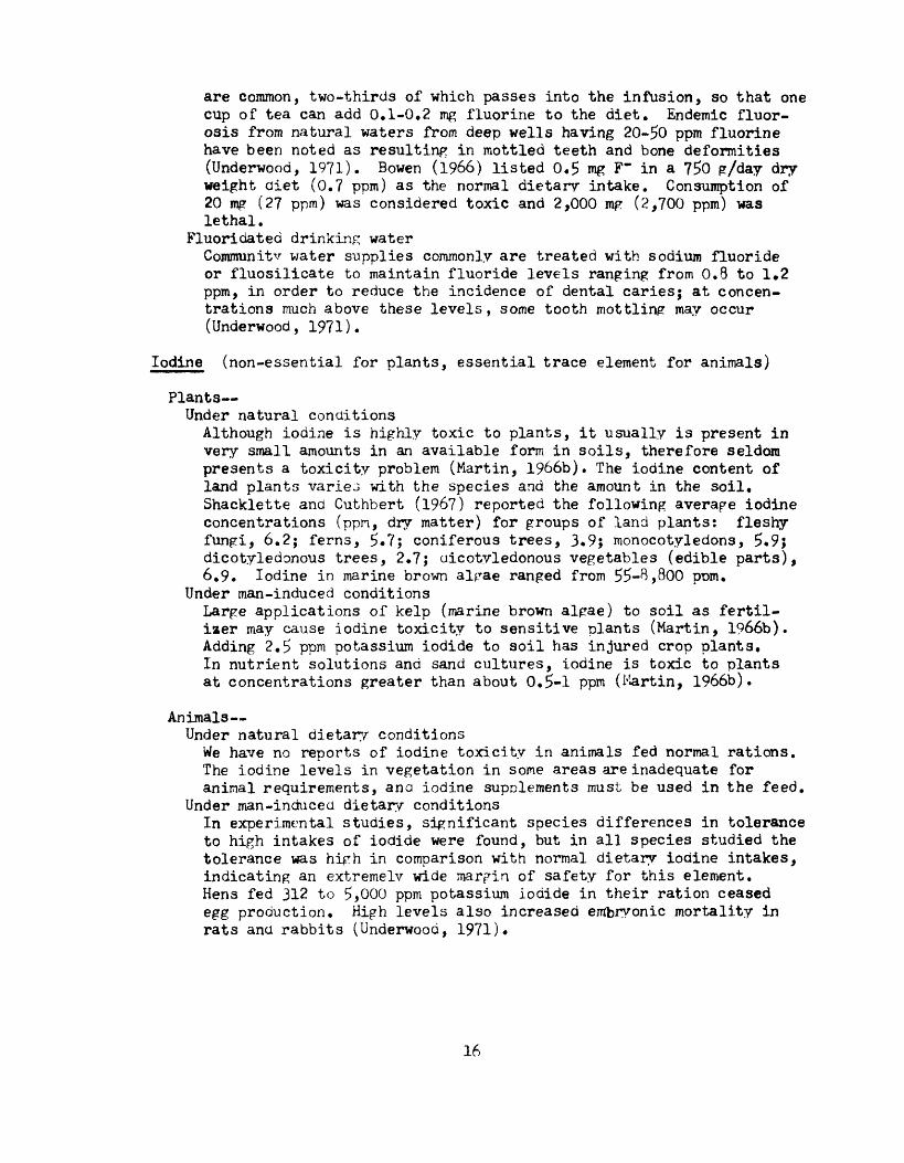
are common, two-thirds of which passes into the infusion, so that one cup of tea can add 0.1-0,2 mg fluorine to the diet. Endemic fluorosis from natural waters from deep wells having 20-50 ppm fluorine have been noted as resulting in mottled teeth and bone deformities (Underwood, 1971). Bowen (1966) listed 0.5 mg F" in a 750 g/day dry weight diet (0.7 ppm) as the normal dietary intake. Consumption of 20 mg (27 ppm) was considered toxic and 2,000 mg (2,700 ppm) was lethal.

Fluoridated drinking waterCommunitv water supplies commonly are treated with sodium fluoride or fluosilicate to maintain fluoride levels ranging from 0.8 to 1.2 ppm, in order to reduce the incidence of dental caries; at concen trations much above these levels, some tooth mottling may occur (Underwood, 1971).

Iodine (non-essential for plants, essential trace element for animals)


Although iodine is highly toxic to plants, it usually is present in very small amounts in an available form in soils, therefore seldom presents a toxicity problem (Martin, 1966b). The iodine content of land plants varies with the species and the amount in the soil. Shacklette and Cuthbert (1967) reported the following average iodine concentrations (ppm, dry matter) for groups of land plants: fleshy fungi, 6.2; ferns, 5.7; coniferous trees, 3.9; monocotyledons, 5.9; dicotyledonous trees, 2,7; dicotyledonous vegetables (edible parts), 6,9. Iodine in marine brown algae ranged from 55-^,800 ppm.

Under man-induced conditionsLarge applications of kelp (marine brown algae) to soil as fertil iser may cause iodine toxicity to sensitive plants (Martin, 1966b). Adding 2.5 ppm potassium iodide to soil has injured crop plants. In nutrient solutions and sand cultures, iodine is toxic to plants at concentrations greater than about 0,5-1 ppm (Martin, 1966b).


We have no reports of iodine toxicity in animals fed normal rations. The iodine levels in vegetation in some areas are inadequate for animal requirements, and iodine supolements must be used in the feed.

Under man-induced dietary conditionsIn experimental studies, significant species differences in tolerance to high intakes of iodide were found, but in all species studied the tolerance was high in comparison with normal dietary iodine intakes, indicating an extremely wide margin of safety for this element. Hens fed 312 to 5,000 ppm potassium iodide in their ration ceased egg production. High levels also increased embryonic mortality in rats and rabbits (Underwood, 1971).

16

Man- Under natural environmental conditions

Prolonged intake of large amounts of iodine by normal individuals markedly reduces thyroidal iodine uptake the antithyroidal or goitrogenic effect. In an area in Japan the consumption of large quantities of iodine in the diet was reported as the cause of endemic goiter ( Underwood, 1971). However, areas of iodine de ficiency, rather than excesses, are bv far more common, and iodine supplements to foods are widely used.

Iodine tolerancesBowen (1966) listed 0.2 mg I- in a 750 g/day dry weight diet (0.3 ppm) as normal, whereas 10,000 mg (13,300 ppm) was toxic. Thomas (1973) gave 5-50 mg/kg body weight as the probable lethal dose of iodine for an adult.

Lead (non-essential for plants and animals)

Plants Under natural conditionsWe can find no reports of definite toxicity symptoms in plants that grew in areas of natural enrichment of lead only. Lead, zinc, and other heavy metals often occur together in mineralized outcrops, therefore it is difficult to associate observed toxicity symptoms in plants at these sites with lead alone. These plants may absorb large amounts of lead without exhibiting toxicity symptoms; concen trations in stems of certain shrubs may be as high as 350 ppm lead in ash of the samples (Shacklette, I960) without producing visible toxicity.

Under man-inauced conditionsElevated levels of lead in plants affected by automotive and industri al contamination have been extensively reported. However, we have no reports that conclusively demonstrate toxicity to the plant of such contamination. Frank toxicity of lead to plants has been shown, insofar as we are informed, onlv by very few laboratory and field experiments. Wieler (1938) added lead salts to acid soils and pro duced injury to oak and birch trees, but not to spruce trees. Prat (1927) studied uptake of lead from lead chloride solutions, and found that broad-bean plants (Viela faba) absorbed all the lead in less than three days, but grew very little as a result . Hooper (1937) found that French beans (Phaseolus sp.) growing in solution cultures were damaged by 30 ppm of lead as the sulfate alone, or in combination with nutrient salts. Plants spraved with leac sulfate solutions were not injured unless sufficient lead residue was left to block the stomates. Wilkins (1957), using lead nitrate as the nitrogen source, grew sheep fescue (Festuca ovina) in solution cultures and reported that root growth was measurably retarded with 10 ppm of lead, markedly reduced by 30 ppm, and stopped at 100 ppm. Miller and Koeppe (1970) showed that 60 ^moles of lead nitrate added to a nutrient solution retarded growth of young corn plants when phosphate was deficient (in young leaves the concentration of lead was 115 pprc in dry weight). At 600 nmoles and greater

17

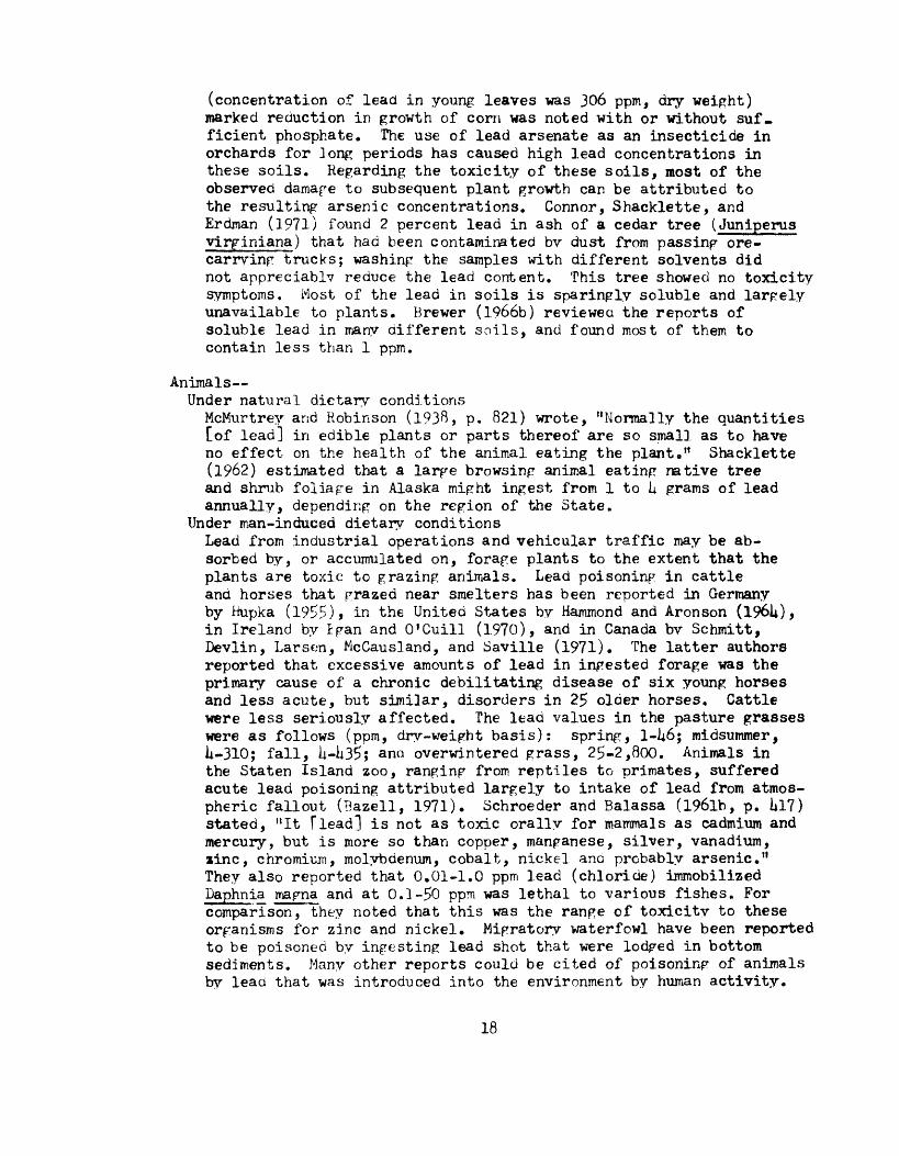
(concentration of lead in young leaves was 306 ppm, dry weight) marked reduction in growth of corn was noted with or without suf ficient phosphate. The use of lead arsenate as an insecticide in orchards for long periods has caused high lead concentrations in these soils. Regarding the toxicity of these soils, most of the observed damage to subsequent plant growth can be attributed to the resulting arsenic concentrations. Connor, Shacklette, and Erdman (1971) found 2 percent lead in ash of a cedar tree (Juniperus virginiana) that had been contaminated bv dust from passing ore- carrying trucks; washing the samples with different solvents did not appreciable reduce the lead content. This tree showed no toxicity symptoms. Most of the lead in soils is sparingly soluble and largely unavailable to plants. Brewer (1966b) reviewea the reports of soluble lead in many different soils, and found most of them to contain less than 1 ppm.

Animals Under natural dietary conditionsMcMurtrey and Robinson (193$, p. 821) wrote, "Normally the quantities [of lead] in edible plants or parts thereof are so small as to have no effect on the health of the animal eating the plant." Shacklette (1962) estimated that a large browsing animal eating native tree and shrub foliage in Alaska might ingest from 1 to U grams of lead annually, depending on the region of the State.

Under man-induced dietary conditionsLead from industrial operations and vehicular traffic may be ab sorbed by, or accumulated on, forage plants to the extent that the plants are toxic to grazing animals. Lead poisoning in cattle and horses that grazed near smelters has been reported in Germany by Hupka (1955)> in the United States by Hammond and Aronson (19610, in Ireland by Igan and O'Cuill (1970), and in Canada bv Schmitt, Devlin, Larswi, McCausland, and Saville (1971). The latter authors reported that excessive amounts of lead in ingested forage was the primary cause of a chronic debilitating disease of six young horses and less acute, but similar, disorders in 25 older horses. Cattle were less seriously affected. The lead values in the pasture grasses were as follows (ppm, dry-weight basis): spring, 1-U6; midsummer, U-310; fall, U-h35; ano overwintered grass, 25-2,800. Animals in the Staten Island zoo, ranging from reptiles to primates, suffered acute lead poisoning attributed largely to intake of lead from atmos pheric fallout (Bazell, 1971). Schroeder and Balassa (196lb, p. 1*17) stated, "It flead] is not as toxic orally for mammals as cadmium and mercury, but is more so than copper, manganese, silver, vanadium, line, chromium, molybdenum, cobalt, nickel anc probably arsenic." They also reported that 0.01-1,0 ppm lead (chloride) immobilized Daphnia magna and at 0.1-50 ppm was lethal to various fishes. For comparison, they noted that this was the range of toxicity to these organisms for zinc and nickel. Migratory waterfowl have been reported to be poisoned by ingesting lead shot that were lodged in bottom sediments. Many other reports could be cited of poisoning of animals by lead that was introduced into the environment by human activity.

18

Man- Under natural environmental conditions

Lead poisoninp from natural sources is very unlikely. Brewer (I966b, p. 2lii) commented, "The extremely low lead content of edible parts of the majority of croos is reassuring, in light of the potential toxicity of lead to aiimals, including man." Schroeder and Balassa (I96lb) reported that poisoning of man has occurred when drinking water with 0.18 to more than 1.0 ppm Pb2+ (0.14-2.5 mg daily, in addition to lead in food) has been consumed over an unspecified period of time. Water should not exceed 0.05 ppm lead (World Health Organi zation, 1963). "Normal" rural air contains about 0.05 ug lead per cubic meter (Patterson, 1965). However, it should be pointed out that very few humans today live in a natural, unpolluted environment.

Lead intakes and toxicitiesThe average daily intake of lead from food and beverages in the United States is now estimated at about 0.30 mg, with only about 10 percent of this being absorbed from the intestinal tract. In addition, some lead is inhaled and absorbed through the respiratory tract; the relative imnortance of this respiratory exposure is a matter about which there is some dispute (Goldsmith and Hexter, 196?). These authors concluded that the absorption of lead from the two sources may be of similar magnitude. In another study (Rabinowitz and others, 1973} in which a healthy man was fed a diet normal in lead content arid labeled with lead-20U it was concluded that about two- thirds of his assimilated lead was dietary in origin and the remain der was inhaled. Studies have generally shown that less than 10 percent of ingested lead is absorbed, whereas 25-50 percent of in haled lead is absorbed (Goldsmith and nexter, 1967). The possible physiological significance of environmental lead was discussed at length by Warren (197k), who listed the sources of lead insult as air, dust, leaded oaint, cigarette tobacco, beer and wine, drinking water, food, fertilizers (particularly, sewage sludge), leaded gasoline, and miscellaneous, which included smelters, vegetables grown over refuse dumps, glazed pottery, plastics, solders, and fillers in alkaline piping. Boweri (1966) reported that the normal consumption of Pb2"1" in a 750 g/day dry weight diet was 0.3-O.ii mg (oUj-0.5 ppm) and that a consumption of 10,000 mg (13,300 ppm) on the same basis may be considered lethal, ochroeder and Balassa (196lb) speculated that poisoning in man would be eventually achieved if 1 or 2 percent of the total bodily content (80 mp) were ingested daily (0.8-1.6 mg). Patterson (1965) noted that a concentration of Pb2+ in the blood of 0.5-0.8 ppm is the threshold for acute lead poisoning.

19

Lithium (non-essential for higher plants and animals, but an essential trace element for some micro-organisms)

Plants Under natural conditionsNaturally-occurring instances of lithium toxicity to plants are not known, except in the case of citrus (Bradford, 1966b), which are very sensitive to small amounts of lithium. However, a report on lithium in the environment (Mertz, 197kb, p. UO) stated, "Crops grown in closed basins in California, Nevada, and Arizona are exposed to toxic levels of lithium," Lithium excesses occur most commonly in soils derived directly from igneous rocks rich in ferromagnesian minerals, and in soils derived from sedimentary deposits rich in clays or micas (Bradford, 1966b) s The lithium concentration in 912 samples of soils from throughout the conterminous United States was reported (Shacklette and others, 1973) as follows: range, 5-136 ppm; arithmetic mean, 2U.7. Bradford (I966b, p. 221) stated, "There is no evidence available to indicate that total lithium in soils is in any way related to plant availability. - - - Plant content of this element is at present the best guide to the lithium status of the soil."

Under man-induced conditionsMany crops are susceptible to injury when lithium is applied to the soil in the form of soluble salts (McMurtrey and Robinson, 193$), and many plants are tolerant of high lithium levels (Mertz, 197iib). Lithium was toxic to citrus when concentrated in soil (as Li^SO^) to 2-5 ppm, and when concentrated in leaves to lljO-220 ppm in dry weight (Alcrich ana others, 1951). Lithium toxicity has also been observed in avocado, celery, corn, olive, and wheat. In contrast, cotton seems to be completely resistant to lithium toxicity, even up to one ton of lithium nitrate per acre. Lithium content in citrus leaves ranpinp from k to liO ppm in dry weight has caused moderate to severe toxic effects (Sauchelli, 1969).

Animals We have no reports of lithium toxicity in animals.

Man- Toxic symptoms that have been reported at the pharmacological dose level in humans include development of goiter and congenital malform ations (Mertz, 197lib). Massive doses of lithium were reported to reduce aggressive behavior in humans and other vertebrates (Lew, 1968). Bowen (1966) pave as the toxic dose in humans 200 mp/day Li* in a 750 g dry weight diet (270 ppm).

20

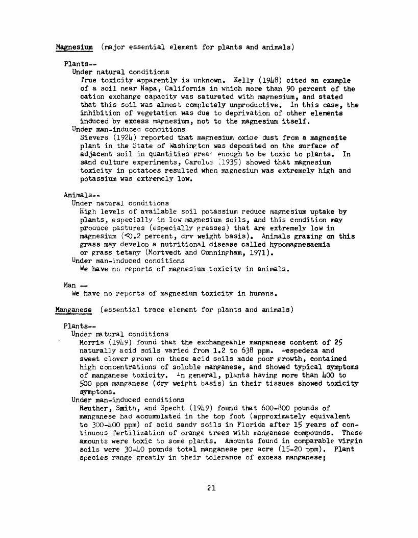
Magnesium (major essential element for plants and animals)


True toxicity apparently is unknown. Kelly (19U8) cited an example of a soil near Napa, California in which more than 90 percent of the cation exchange capacity was saturated with magnesium, and stated that this soil was almost completely unproductive. In this case, the inhibition of vegetation was due to deprivation of other elements induced by excess magnesium, not to the magnesium itself.

Under man-inducea conditionsSievers (192U) reported that magnesium oxide dust from a magnesite plant in the State of Washington was deposited on the surface of adjacent soil in quantities great enough to be toxic to plants. In sand culture experiments, Carolus (1935) showed that magnesium toxicity in potatoes resulted when magnesium was extremely high and potassium was extremely low.

Animals Under natural conditionsHigh levels of available soil potassium reduce magnesium uptake by plants, especially in low magnesium soils, and this condition may produce pastures (especially grasses) that are extremely low in magnesium (<0.2 percent, dry weight basis). Animals grazing on this grass may develop a nutritional disease called hypomagnesaemia or grass tetany (Mortvedt and Cunninpham, 1971).

Under man-induced conditionsWe have no reports of magnesium toxicity in animals.

Man We have no reports of magnesium toxicity in humans.

Manganese (essential trace element for plants and animals)


Morris (I9ii9) found that the exchangeable manganese content of 25 naturally acid soils varied from 1.2 to 638 ppm. -^espedeza and sweet clover grown on these acid soils made poor growth, contained high concentrations of soluble manganese, and showed typical symptoms of manganese toxicity. 1n general, plants having more than UOO to 500 ppm manganese (dry weight basis) in their tissues showed toxicity symptoms.

Under man-induced conditionsReuther, Smith, and Specht (I9ii9) found that 600-800 pounds of manganese had accumulated in the top foot (approximately equivalent to 300-1*00 ppm) of acid sandy soils in Florida after 15 years of con tinuous fertilization of orange trees with manganese compounds. These amounts were toxic to some plants. Amounts found in comparable virgin soils were 30-10 pounds total manganese per acre (15-20 ppm). Plant species range greatly in their tolerance of excess manganese;

21

Fergus (195^) found that kidney beans, a good indicator plant for excess manganese, showed toxicity symptoms when grown on a soil of less than pH 5»0 because of the easily reducible manpanese in the soil, Schroeder, Balassa, and Tipton (1966) reported the following toxic concentrations (ppm) of the divalent manganous ion in water supplied to cultures: yeast, 550; legumes, 1-10j orange and mandarin seedlings, 5; tomatoes, 5-10; soybeans, 10-25; flax, 25-100; and oats, 150-500.

Animals Under natural dietary conditionsCotzias (1962) reported from the literature that spontaneous lactation tetany has been recorded in cows grazing on pastures high in manganese. Further, consumption by animals of large amounts of certain tree foliape, which contains more manganese than do most herbaceous plants (6hacklette ana Severson, 1975)? potentially could be toxic

Under man-induced dietary conditionsThe Mn2+ form has a low order of toxicity to living organisms, especially to vertebrate animals (Schroeder, Balassa, and Tipton, 1966). The hexavalent form is highly toxic but does not occur in nature. The above report listed the following as toxic concentrations (ppm) of Mn2+ in foods: Laphnia magna, 50; flatworms, 700, fresh water fish, 2,h20-3,li50; birds, U,800; chicks, U,800, rats, >2,000; rabbits, 1,250-6,000; pigs, 500-2,000; and lambs, 5,000.

Man- Underwood (1971, p. 202) reported, "Chronic manganese poisoning occurs in miners.working with manganese ores. The manganese enters the lungs as oxide dust from the air and also enters the body via the gastrointestinal tract. The disease is characterized bv a severe psychiatric disorder (locura manpanicaj resembling schizophrenia, followed by a permanently crippling neurological (extrapyramidal) disorder clinically similar to Parkinson's disease." Cotzias (1962) renorted that a particle size of manganic oxide <5u. was responsible for the disorder. Bowen (1966) reported that the normal consumption of Mn2+ in a 750 g/day dry weight diet was 3-10 mg (h-12 ppm).

Mercury (non-essential for plants ana animals)


Mercury in living tissues is believed to be largely organic and primarily methyl mercury. The conversion of inorganic mercury to methyl mercury or dimethyl mercury is accomplished by anaerobic bacteria in the bottom muds of streams. Dimethyl mercury, stable in alkaline solutions, dissociates to ionic methyl mercury at low pH values such as may exist in the anaerobic bottom muds of streams and lakes. Hethyl mercury is soluble in water, and is available for incorporation into the tissues of aquatic organisms, thus can enter

22

the food chain of higher animals and man. Ur the methyl mercury may enter the higher organisms by direct assimilation from the surroundinr medium (Greeson, 1970), Mercury compounds inhibit the growth of bacteria, and have long been used as antiseptics and disinfectants. In contrast, most higher (vascular) plants are remarkably resistant to mercury poisoning, although they may accumulate high concentrations of mercury in their tissues. Shack- lette (1970) reported as much as 3,500 parts per billion (ppb) in dry material of Labrador tea that grew where its roots were above cinnabar mineral deposits, but the plant showed no toxicity symp toms. The geometric mean mercury concentration in 912 samples of soil from throughout the conterminous United States was reported as 71 ppb (Shacklette and others, 1971). Shacklette (1970) stated that the few available reports of mercury analysis of plants sug gest that this metal is not concentrated to a great extent, if at all, in the tissues of most plants that grow in normal soils. Mosses are tolerant of high mercury levels in their substrate (Shacklette, 196$).

Under man-induced conditionsFungicides containing mercury compounds have been widely used on agricultural and horticultural crops. These compounds, if sprayed on plants, may be absorbed by the plants and translocated from one part of the plant to another. Novick (1969) stated that mercury compounds from sprays applied to apple leaves may be translocated to the fruits, and also may be moved from potato leaves to the tubers. In addition, the sprays may produce surficial deposits on the leaves that are not easily removed. The mercury compounds, as applied, have no toxic effects on the plants themselves. Shacklette and Connor (1973) reported 0.5 ppm mercury (drv weight basis) in Spanish moss plants that presumably resulted from airborne industrial pollution, but toxic effects on the plants were not noted. Some greenhouse flowers, notably roses, are sensitive to volatilized elemental mercury, in that very low concentrations in the air cause toxic symptoms (Shacklette, 1970).


We have no reports of toxicitv resulting from animals grazing on normal vegetation; it is likely that the small amounts present in the plants are well within the elimination rates of animals. Wershaw (1970, p. 31) stated, "Natural surface waters contain tolerably small concentrations of mercury except in areas draining mercury deposits."

Under man-induced dietary conditionsThe concentration of mercury in crop plants that was derived from the soil probably is never toxic. However, the mercury compounds applied as fungicides to plant leaves, seeds, and grains may reach levels that are toxic to animals. Bowen (1966) reported that the consumption of 8 ing/day Hg2+ in a total dry weight diet of 10 g (800 ppm) was lethal to rats.

Man Greeson (1970, p. 33) stateo, "Aquatic organisms, as well as man, will concentrate mercury within their bodies - - -, The result - - - is a buildup with time to the extent that the accumulated mercury can become toxic and, eventually, lethal." In Japan about 50 persons out of more than 100 affected died of the "Minamata disease," caused by the consumption of fish and shellfish obtained from a bay that had received large amounts of methyl mercury compounds in the waste effluents from a plastics factory (Kurland and others, I960). Mercury poisoning among citizens of Iraq who consumed bread made from seed wheat that had been treated with methyl mercury was reported by Bakir and others (1973) They stated that the wheat contained 8 ppm mercury, and acute concen trations (resulting in many patient- deaths) were measured at 0.5-0,8 mg Hg/kg body weight. The biolopical half-life of methyl mercury in man is about 70-^0 days. It is readily absorbed by the gastrointestinal tract. Lofroth (1972, p. 66) stated, " - - - clinical methylmercury poisoning in adult people can occur at a mercury level of about UOO np/g in the red blood cells - - - corresponding to a regular daily intake of 0.3 mg mercury as methylmercury, i.e. O.OOh mg/kg body weight." Bowen (1966) reported that the normal daily consumption of Hg2+ was from 0.005-0.02 mg when based on a 750 g dry weight diet (0.007-0.03 ppm). Consumption of 150-300 mg on the same basis (200-UOO ppm) was considered lethal. The U.S. Public Health Service (1961) proposed a tentative upper limit of 5.0 ppb of mercury in drinking water.

Molybdenum (essential trace element for plants and animals)


There are no recorded instances of a field occurrence of molybdenum toxicity to plants (Johnson, 1966), although high levels may be accumu lated in the plants. Dye and O'Harra (1959) reported that among forage plants legumes usually collect more molybdenum than do grasses, and cited a high value of 372 ppm molyboenum (dry weight basis) in a sample of black medic (Medicago lupulina) from a Carson Valley, Nevada ranch, rtarrea and Delavault (1965) stated that many trees and lesser plants growing over commercial, or potentially commercial, molybdenum deposits may of. expected to carry upwaras of 500 ppm molybdenum in their asnes, and that relatively few should be found with less than 250 ppm. Deficiency levels for plants are usually indicated by less than 0.10 ppm in their tissues (Johnson, 1966).

Under man-induced conditionsToxicity in the plant is observed only under extreme experimental conditions; in solution culture experiments using 1,000-2,000 ppm molybdenum, tomato plants developed an intense polden yellow color in their leaves, anc seedlings of cauliflower turned an intense purple (Johnson, 1966).

21*


"Molybdenum toxicity, variously referred to as molybdenosis, teart disease, and peat scours, has been reportec from many parts of the world - - -. In most instances toxic a/noun r.s of molybdenum in forage consumed by ruminants have resulted from naturally occurring excess molybdenum in the soil or irrigation water" (Johnson, 1966, p. 28?) This toxicity in ruminants is a complex matter, involving not only excess molybdenum but also low copper levels and high sulfate-sulfur concentrations in Lht forare. Molybdenosis occurs when the copper in forage is normal (8-10 ppm in dry matter) and the molybdenum is above normal (above 5-6 ppin for cattle or 10-12 ppm for sheep) (Dye and O'Harra, 1959). Molybdenosis in grazing animals has been observed in Nevada and Oregon (K\bcta and others, 1961 and 1967). The amount of molybdenum absorbed by plants is not strongly corre lated with total molybdenum in the soil, because soil pH and other soil properties greatly affect availability to plants, it being more available at high pH values.

Under man-induced dietary conditionsApplying molybdenum fertilizers, or liminp to release previously unavailable molybdenum, mav result in the forage containing amounts of the element that are toxic to animals. Mining activities mav expose deposits having concentrations of molybdenum and other elements that can be considered anomalous in the natural geochemical environment of plants and animals. An area in Missouri was studied (Ebens and others, 1973) where clay mining operations had contaminated adjacent areas to the extent that beef cattle grazing these areas exhibited symptoms of metabolic imbalance thought to be chronic molybdenosis due principally to copper-molybdenum imbalance. Bowen (1966) reported that 5 nig MoO* (molybdate) in a 10 g/day dry weight diet (500 ppm) was toxic and 50 mg (5*000 ppm) was lethal to rats. Due to poor absorption, horses and pigs have low susceptibility to molybdenosis (Underwood, 1971).

Man At normal environmental concentrations of molybdenum, toxicity is of little concern. Underwood (1971, p. 135) stated, "Molybdenum is apparently of so little practical significance in human nutrition, either in health or disease, that few people have been stimulated to undertake studies with this element." The only incidence of molybden osis in humans of which we are aware was reported by Agarwal (1975). He fcund that peasants in India who consumed sorghum as a staple that was grown in alkaline soils high in molybdenum ana fluorine developed a crippling syndrome of knock-knees (genu valgum). No instances of the disease were reported prior to the construction of a large dam that raised the water table in the surrounding district and caused an increase in alkalinity and concurrently the uptake of molybdenum by the sorghum. No specific concentrations of molybdenum in sorghum, soils, or humans were given.

25

Nickel (nor.-essential for plants and animals)

Plants Under natural conditionsMitcheJ1 (iyh5) stated that the normal nickel content of plant material, dry weight basis, ranges from O.]0 to 5 ppf', depending on the species, the part of the plant, maturity, time of sampling, and other factors. Excessive nickel in serpentine soils may be a contributing factor to the restricted growth of plants on these soils, as reported by many investigators, but excessive chromium, unfavorable magnesium-calcium ratios, and deficiency of molybdenum may also limit plant growth (Vanselow, 1966®). The amount of nickel absorbed by plants on serpentine soils ranges wicely among species; Shacklette (1966) reported the following concentrations (ppm in ash) from a site in Alaska: aspen, 10; white birch, 50; and low juniper, 1^0. The soil at this site contained 50-75 ppm nickel, and the oasaltic greenstone on which the soil developed contained 100 ppm nickel. Malyuga (1961j) described apetalous forms of anemone growing over nickel deposits, attributec to toxicity of the nickel,

Unaer man-induced conditionsToxicity to many plants, even at relatively low concentrations, has been noted; ibO ppm (dry weight basis) in tomato plants was toxic, and 150 ppm stopped growth (Sauchelli, 1969). Soane and Saunder (1959) reported 12-2^6 ppm (crv weight basis) in leaves of com, and Ill-Oil ppm ii; leaves of tobacco botn kinds of plants developed toxicity symptoms.

Anijnals Under natural dietary conditions

Mitchell (I9ii5) recorded levels of 0.5-1* ppm (drv weight basis) nickel in pasture herbage; Allaway (1968) reported that toxicity to animals was moderate to low. In view of these relationships, toxicity to grazing animals seems unlikely.

Under man-induced dietary conditionsCompared to many other trace metals, the concentration of nickel in foods is high. There appears, however, to be a mechanism in mammals limiting its intestinal absorption. The toxicity of nickel to mammals is low (ranking with the essential trace elements) exceot in astringent doses. Nickel ^alts irritate the ir.ucosal lining of the gut more than they cause inherent poisoning (Schroeder, Balassa, and Tiptori, 1962b) Underwood (1971) reported that 700 ppm nickel in the diet of chicks depressed growth, 1,600 ppm depressed growth of young mice, arid 1,000 ppm had no apparent, tcxic effect on rats or monkeys. Bowen (I9t>6) gave as toxic to rats a ration of 50 mg Ni^* in 10 g/d of dry weiprit diet (5>000 ppm). He listed the element as potentially carcinogenic.

Man- The toxicity of nickel to humans is low. Workers in nickel rei'ineries have developed "nickel dermatitis" and resDiratory-tract neoDlasia; a direct link between the elemental form and these pathologies, however, has not been made (Schroeder, Balassa, and Pipton, 196?b),

26

Selenium (non-essential for plants, essential trace element for animals)


The occurrence and ecological relationships of selenium-indicating plants has been documented by many investigators. Two groups of native species may be recognized: the primary indicator plants are those found growing only on seleniferous soils and which absorb large amounts of selenium; the second group is composed of those species which are also capable of absorbing selenium in concentrations toxic to animals if growing on seleniferous soils but which may also grow elsewhere. Excess soil selenium may prevent plants not in these two groups from growinp on selenifer-us soils by causing toxicity symp toms to develop. These symptoms are never seen in crop plants grown on naturally seleniferous soils, but in experimental conditions the symptoms in grasses ordinarily are snow-white chlorosis of the leaves, and pink root tissue; symptoms in other plants vanr, but commonly include stunting, yellow chlorosis, and pink leaf veins (Ganje, 1966). Lakin (1972) stated that certain species of Astragalus utilize selenium in an amino acid peculiar to these species, and that they absorb many times as much selenium as do other plants grow ing in the same soil. These plants convert selenium into forms absorbed by other, non-seleniferous, species through foliage decom position and oxidation to inorganic salts or soluble organic com pounds (Ganje, 1966). The plants, both fresh and dried, often have a strong garlicky odor. Byers and Lakin (1939) analyzed about 300 samples of shales, soils, ana plants collected in seleniferous areas of Canada and found the selenium of shales to vary from from 0.3 to 3.0; of soils, from 0.1 to 6 ppm; and of vegetation, from 3 to Ii,190 ppm in dry matter. The organic compounds of selenium in soil are derived from partially decayed seleniferous vegetation. Inorganic selenium exists as the element; as ion selenide; as a substitute in sulfide minerals, particularly pyrites; as selenite, particularly basic ferric selenite; and as selenate, particularly calcium selenate. Basic ferric selenite seems to be the most common in soils, while very little is present in the elemental form. Selenate and organic selenium are the forms most available to plants (Ganje, 1966).

Under man-induced conditionsSoils producing seleniferous vegetation have been found onlv in arid or semiarid regions, at least in the United States, where the mean annual rainfall is less than 20 inches. For crop plants, only the soil content of water-soluble selenium is important, because elemental selenium and selenite are of slight availability to these plants, as was demonstrated by Hurd-Karrer (193U) and others. Corn grown in culture solutions containing 5> ppm of selenite or organic selenium accumulated 200 and 1,000 ppm selenium, respectively. At the 10-ppm level, corn accumulated 300 ppm from the selenite form and more than 1,500 ppm from the organic selenium form (Ganje, 1966). Resistance to selenium toxicity among plant species ranges so widely that a general toxicity level cannot be estimated.


Lakin (1972, p. U9-50) reported, "Acute poisoning of cattle and sheep occurs when herds or bands are being driven from one pasturage to another. Animals, under these conditions, eat forage indiscriminately and many may die overnight. Both seleniferous Astragalus species and alkaloids are probably involved. - - - Subacute poisoning, known locally as blind staggers, loco disease, or pushing disease, has been reported in western United States ana in South Africa. This is probably another instance of the confusion between selenium toxicity and naturally toxic vegetation. The actual cause of these diseases is in debate. Chronic poisoning is caused by daily ingestion of cereals and grasses containing 5 to 20 ppm selenium, - - -Subchronic poisoning has been reported by Brown and de Wet (1962) in South Africa. They suggest - - - that the moderate selenium content of the diets of these animals has weakened them and made them more suscept ible to disease." Byers (1935) suggested k ppm (dry weight basis) of selenium in plants as a tolerance limit for animals that consume them, and considered $ ppm to be potentially danperous. Water con taining 0.5 ppm selenium may also be danperous </)an je, 19o6).

Under man-induced dietary conditionsBecause of the dual role of selenium as a micronutrient and a toxin to animals, the selenium concentrations in feeds can be critical factors in the health of the animals. Underwood (1971, p. 3U6) stated, "A dietary intake of 0.1 ppm [in dry feeds] provides a satisfactory margin of safety against any dietary variables or environmental stresses likely to be encountered by grazing sheep and cattle." Many factors determine the level of selenium in feeds that are toxic to animals, but amounts of 5 pprc (dry weight basis) or more may generally be considered toxic. Underwood (1971, p. 356) stated, "Signs of chronic poisoning are common in rats and dogs given diets containing 5-10 ppm selenium, and, at 20 ppm, there is complete refusal of food and death in a short time. Young pigs fed seleniferous diets con taining 10-15 ppm selenium develop aipns of selenosis within 2 to 3 weeks. Ditti; containing lower levels than these would induce similar effects if fed for a longer period. The minimum toxic levels for grazing stock are more Difficult to determine. They probably lie close to 5 ppm seleni\)jn. kdible herbage in seleniferous areas commonly contain 5-20 ppm selenium." oauchelli (3V69) reported that as little as 1 ppm selenium in the soil permitted the growth of wheat, but when the grain containing 8-10 ppm selenium was fed to rats, it retarued growth and killed them after a few weeks. Selenium may be introduced into the environment through the burning of coal, in phosphate fertilizers, and in selenium-containing insecticides, but the latter source has very little application to toxicity problems at Dresent because the use of these insecticides on food plants is prohibited, except in special circumstances.

Man- Under dietarv conditions in seleniferous regions

Lakin (1972, p. 5?1) wrote, "Soils producing crop plants that are toxic because of selenium are confined to small areas but occur throughout the world. Such soils are confined to semiarid regions or areas of impeded drainage. They contribute no significant hazard to human health and only locally to animal health." The selenium content of certain foods mav reach levels that could affect human health. For example, the selenium content of tuna was reported (Kifer and others, 1969) to average Iu63 ppro (dry weight basis), and to range from 3*U to 6.?. A daily intake of 1 mg selenium in food is probably not harmful to an adult person. Robinson (1936) found that seleniferous wheat may be blended with sufficient selenium-free grain to drop the selenium concentration to the tolerance level. Hadjimarkos (1970) reported that the incidence of dental caries appears to be greater in areas naturally high in selenium. This is particularly true among children who consume small amounts of dietary selenium in addition to the naturally high amounts in the local water. Selenium concentrations of 0.08 ppm in the urine identified those individuals with increased incidence of dental caries. The situation regarding selenium poisoning in man was summarized by Lakin (1972, p. £0) as follows: "Fortunately, the human diet is rarely restricted solely to the products of a highly seleniferous area. Thus, selenium poisoning through the food-plant cycle is rare in the world human population and tends to be restricted to combi nations of highly seleniferous areas whose populations depend largely on local agricultural produce." Chronic selenium poisoning in humans was reported to occur in Mexico by Byers (1937) and in Columbia by Ancizar-Sordo (19^7) and Leonidas and Hernan (1970).

Under the effects of environmental pollution by seleniumSauchelli (1969) reported that the maximum amount of selenium in the whole diet that man can consume without ill effects is believed to be 3 ppm. Bowen (1966) listed as toxic 5 mg SelV (selenite) in a 750 g/day dry weight diet (7 ppm). Pollution-related selenium intoxication is most commonly associated with industrial exposure (Cooper, 1967) because selenium compounds are absorbed through the lungs in dust or fumes, and through the skin. Whether ingested or inhaled, Cooper (1967, p. 186) stated, " - - - there is marked variations between and within animal species in their response to selenium at what may be considered toxic levels."

Thallium (non-essential for plants and animals)


Very few oata are available on the normal concentrations of thallium in vegetation. The following ppm in ash were reported (Shacklette and others, in press) for trees and shrubs of the Rocky Mountain reg ion: subalpine fir needles 2-100, stems 2-70; limber pine needles 2-3, stems 3-^; lodpepole pine needles 2-5, stems 3-7; Engelmann

29

spruce needles 2-30, stems 15; myrtle blueberrv stems and leaves 2-7; phyllodoce stems, 2; and ponderosa pine stems 15. Toxic levels were reported by Zyka (1972) in vegetation of a region in Yugoslavia remarkable for high levels of thallium in the substrate. He found thallium in ash of herbaceous plants to range from 10 ppm in Eryngium to 17,000 ppm in bedstraw (Galium sp.). Toadflax (Linaria sp.) contents ranged from 3,000-3,800 ppm. He also noted zonation of species related to soil concentrations of thallium, which indi cated the degree of toxicity of the element to certain plant species.

Under man-induced conditionsMcMurtrey and Robinson (1938* p. 827) stated, "When artificially applied, it fthallium] is probably taken up by the plant, and as little as 35 ppm in sandy soils has practically prevented the growth of plants." Berg (1925) reporter 0.1 mg thallium in 100 g (I ppm; of spinach and rye samples.


Zyka (1972, p. 91*) reported, regarding the high thallium region of Yugoslavia, "The high thallium contents in the plants explain their toxic effects on cattle." We have no other reports of thallium poisoning resulting from the consumption of vegetation.

Under man-induced dietary conditionsThallium compounds have been widelv used in poisoned bait for rodents and animal predators because of their extremely toxic effects on these animals. When this poisoned bait is scattered on the soil, its effects persist for several years (McMurtrey and Robinson, 1938). Bowen (1966) reported that 7.5 mg T1+ in a 10 g/day dry weight diet (750 ppm) was lethal to rats.

Man Thallium compounds are highly toxic to humans. McMurtrey and Robinson (1938, p. 827) wrote, "Thallium compounds have been used as depila tories with disastrous effects." Thomas (1973) gave 5-50 mg/kg body weight as the probable lethal dose of thallium salts for an adult, whereas Bowen (1966) listed 600 mg/day in a 750 g drv weight diet (800 ppm) as lethal.

Tin (.non-essential for plants and most animals, but recently found essential for rats]

Plants Under natural conditionsMeasurable amounts of tin are but rarely found in native plant species and when found are usually in concentrations of 20-30 ppm in ash (Connor, Shacklette, and others, 1975). Harbaugh (1950) reported 17 ppm tin in ash of oak twigs, and Millman (1957) found 0.36 (dry weight basis) in twigs of birch. Wallihan (1966, p. 1*76) stated, "Unlike lead, tin is generally a biologically innocuous element, as shown by its use for storing and conducting distilled water and in tin-coated food containers. Plants absorb it only to a very

30

slight extent - - -." We have no reports of tin toxicity to plants that are substantiated by data, although Brooks (1972, p. 225) stated, "Toxicity to plants, severe,"

Under man-induced conditionsPrince (I957a, 1957b) reported 2.9li ppm (dry weight basis) tin in corn grains, Duke (1970) reported 0.10 ppm tin in dry material of avocado, and tin was reported in one sample each (ppm in ash) of carrot root (20 ppm), corn grains (30 ppm), and beet root (20 ppm) (Connor, ohacklette, and others, 1975). We have no other reports of tin in food plants. Forty ppm 3n2+ (stannous ion) solution in sand cultures has been reported as not affecting the growth of sugar beets (Schroeder, Balassa, and Tipton, 196ij). Willihan (1966, p. k76) wrote, "There appears to be no substantial evidence that tin is essential or beneficial to plants in any way, and it has not been shown to be detrimental under field conditions."


We have no reports of animal toxicity attributed to naturally occurring tin in the environment.

Under man-induced dietary conditionsSchroeaer, Balassa, and Tipton (1961;) reported from the literature that relatdxely large doses of tin in the diet of laboratory animals are needed to produce toxicity. For cats and rats 30-50 mg/kg body weight, and for dogs 850-1,000 mg/kg, was toxic. They noted that a diet of 1 g every 6-10 days caused death in rabbits after 1 to 2 months. Further, 1,000 ppm tin in a tank of goldfish was fatal after 1.5 hours; at a concentration of 626 ppm, after U«5 hours.

Man Bowen (1966) reported 2,000 mg tin as toxic in a dry weight diet of 750 g/day (2,700 ppm). Schroeder, Balassa, and Tipton (196U) reported from the literature that severe gastrointestinal symptoms in man have resulted from consumption of fruit punch (pH3) that contained 2 g/1 tin. Tin-plated containers for canned foods can be a source of large amounts of tin, particularly for foods that are acidic. However, the double-lacquered metal cans currently in use greatly reduce the tin in canned foods.

Vanadium (non-essential for higher plants and most higher animals,although reported to be beneficial for some; essential trace element for some algae and other micro-organisms, and for chicks)


Pratt (1966) stated that he had found no reports indicating either deficiency or toxicity of vanadium to plants under field conditions. Some food plants may accumulate high levels of vanadium without exhibiting toxicity symptoms, as is shown by the following data (maximum ppm found in ash): snap bean, 700; cabbage, 50; tomato fruits, 30; and asparagus, 20 (Connor, Shacklette, and others, 1975).

31

Under man-induced conditionsVon ^charrer and Schropp (1935) found vanadium to be toxic to germinating seeds, but even more toxic at later stapes of growth. Chiu (19$3) reported that $00 ppm of vanadium oxide in culture solutions produced toxicity in rice seedlings, and that 1,000 ppm killed all the seedlings. Cannon (1^63) conducted plot experiments in a desert environment by adding sodium vanadate to the soil. After a few weeks time, 8)40 pnm of vanadium was found in the soil water solution, and no planted species was able to grow in the plots during the first season. By the second year after a winter of leaching, four species were grown and harvested from the plots which contained lUO to 560 ppm vanadium in solution. The toxicity symptoms exhibited by these plants were extreme dwarfing and chlorosis. Pratt (I966b) suggested that vanadium toxicity <>,ay be indicated bv two or more ppm vanadium (ary weight basis) in the tops of pea or soybean plants. He concluded that concentrations of 0.$ ppm or greater in nutrient solutions are toxic to plants, and that additions of the element to soils have produced toxicity for a variety of crop plants. As soluble vanadium, the following solution concentrations were reported as slightly toxic: by Schroeder, Balassa, ana Tip ton (1963): 10-20 ppm for soybeans, 26 ppm for beets, UO ppm for barley, 20 ppm for wheat, and 22 ppm for oats.

Animals Under normal dietary conditions

We have no reports of toxicity attributed to vanadium in feedstuffs.Under man-induced dietary conditionsVanadium is a relatively non-toxic metal to animals. Schroeder, Balassa, and Tipton (1963) reported that 160 ppm in the diet of rats over an unspecified period of time was lethal due to gastrointestinal irritation. Similar values were given by Bowen (1966), who listed as toxic to rats 0,5 mg V7 (vanadate) in 10 g/day dry weight diet (50 ppm) and l.£ mg (l£0 ppm) as lethal. Underwood (1971) gave the following concentrations and manifestations: >20-25 ppm vanadium in the diet resulted in growth depression in chicks; 2$ ppm was toxic to rats whereas $0 ppm caused diarrhea and mortality. He listed the jallowing relative toxicities for five elements to rats when fed 2;? ppm diets: arsenic <- molybdenum < tellurium < vanadium < selenium.

Man- Vanadium is not a particularly toxic metal to man. Not only is vanadium poorly absorbed bv the gastrointestinal tract but it results in minimal irritation to the lungs when inhaled. Curran and Burch (196?, p. 98) stated, "A specific toxicity from naturally occurring vanadium salts or those contacted in industry would seem to be minimal." Schroeder, Balassa, ana Tipton (1963) fed patients a.$ mg/day as the oxvtartarovanaaate for 16 months with no apparent toxicity. Underwood (1971) reportec that experiments with ammonium vanadyl tartrate given orally to 6 subjects for 6-00 weeks produced no toxic effects other than some cramps and diarrhea at the larger dose levels.

32

Zinc (essential for plants and animals)


Zinc concentrations of O.h3-10.16 percent in New York peat soils were reported by Staker and Gummings (191*2) to be severely toxic to vegetable crops such as spinach, lettuce, and carrots. The effects of the several metals that commonly are associated with zinc in areas of natural enrichment cannot be distinguished with certainty by visual inspection, therefore visible toxicity effects are often attributed to the zinc. Ernst (197U, p. 3) wrote (trans lated): "In nature soils rich in heavy metals are found over ore bodies which crop out at the surface or extend in the near surface one at least up to 30 meters. - - - Because of the diversity of bedrock types the distribution of the quality and quantity of heavy metals in the naturally metal-rich soil is quite variable. - - - At a concentration of at least 0.1 percent all heavy metals have a strongly selective effect on vegetation. As a rule, zinc-rich soils (0.1-10 percent zinc) are distinguished by also having a high content of lead (0.1-3.2 percent), but not of cadmium." Many reports in the literature of zinc toxicity to vegetation in natural environments are based on circumstantial evidence, in that the exact cause of the symptoms was not determined.

Under man-induced conditionsContamination of vegetation with zinc, as, well as with other heavy metals, is common in the vicinity of metal-working industries. For example, Ernst U97li) reported the concentrations in soil (mg/kg, dry soil) with distance from the sources as follows: zinc smelter, at 2^0 m, U,500; at iiOO m, 1,300; ana at it,000 m, 210. Brass foundry, at 2% m, li,520; at iiOO m, 350; at h,000 m, 173, and at 10,000 m, 91. These zinc values contrast with the geometric mean zinc concentration in United States soils of hh ppm (Shacklette and others, 1971). Thorne, Laws, and Wallace (19li2) found that total zinc differentiated zinc-deficient soils from those not de ficient in zinc as well as did Hibbard's extraction procedure, but researchers prefer to judge deficiencies and toxicities on the basis of soluble zinc in soils. The zinc content of plant leaves as indicative of nutritional sufficiency and toxic excesses was summar ized by Chapman (1966) as follows: deficiency levels are character ized by less than 20-25 ppm in dry matter; ample but not excessive levels, 25 to 150 ppm; amounts greater than hOO ppm may indicate zinc excess. However, there is a wide range in content of zinc among plant species; likewise, tolerance to high levels of soil zinc ranges widely. For example, Hobinson, Lakin, and Reichen (I9h7) reported that a good indication of zinc mineral outcrops is the presence of luxuriantly growing ragweed when other vegetation is stunted. At the location that they studied, total zinc in the soil was 12.5 percent.

33

Animals Under normal dietarv conditions

We have no reports of zinc toxicity to animals resulting from the consumption of ordinary feedstuffs. Underwood (1^71, p. 21*2-21*3) stated, "Zinc is relatively nontoxic to birds and mammals and a wide margin of safety exists between normal intakes and those likely to produce deleterious effects. Rats, pigs, poultry, sheep, and cattle exhibit considerable tolerance to high intakes of zinc, the extent of the tolerance depending upon the composition of the basal diet, particularly its content of minerals known to affect zinc absorption and utilization, such as copper, iron, and cadmium."

Under man-induced dietary conditionsZinc compounas are relatively non-toxic to organisms, particularly to mammals, ^ciiroeder and others '196?) reported that a diet for laboratory animals with 0.25 percent (2,500 ppm) zinc salts is apparently non-toxic. The following summary was obtained from Underwood (1971): rats with dietary intake of 2,500 ppm zinc, no discernible effects; 5*000 Dom, severe growth depression, severe anemia; and 10,000 ppm heaw mortality. Weanling pigs with dietary intake of 1,000 ppm zinc, no ill-effects; higher levels, growth depression; and U,000-8,000, high mortality. Lambs with dietary levels of 1,000 to 1,500 ppm zinc, depressed feed consumption, reduced gains, increased mineral consumption. Steers with dietary levels of zinc of 500 ppm or less, no detrimental effects; 900 ppm, reduced gains and lower feed efficiency; and 1,700 ppm caused, in addition, a depraved appetite with excessive salt and mineral con sumption and wood chewing. Bowen (1966) listed 50 mg Zn2+ in a 10 g/day dry weight diet (5,000 ppm) as toxic to rats and 150 mg (15,000 ppm) as lethal.

Man Unlike the aberrant syndromes for most of the essential trace elements, there has been no primary disorder of zinc metabolism described for humans. Underwood (1971) noted that there existed a wide margin of safety between normal zinc intakes and those likelv to produce dele terious effects. Acute zinc poisoning is commonly reported, however, when acidic foods stored in galvanized iron containers have been ingested, ochroeder and others (1967) speculated that cadmium intoxi cation may also be associated with these cases. Thomas (1973) listed as probably lethal to adults 50-500 mg/kg body weight of zinc salts (chloriae, sulfate, acetate, and others).

References cited

Agarwal, A. K., 1975, Crippling cost of India's big dam: New Scientist, v. 30, p. 260-261.

Aldrich, D. LI., Vanselow, A. P., and Bradford, G. R., 195l> Lithium toxicity in citrus: Soil Sci., v. 71, p. 291-295.

Allaway, W. H., 196S, Apronomic controls over the environmental cycling of trace elements, in Norman, A. G., ed., Advances in agronomy, v, 20: New York, Academic Press, p. 2&-27k.

Ancizar-Sor-Jo, Jorpe, 19U7, Occurrence of selenium in soils and plants of Columbia, South 4merica: Soil uei., v. t>3, no. 6, p. U37-h38.

Bakir, F., Damluji, S. F., Amin-Zaki, L., Murtadha, M., Khalidi, A.,Al-Rawi, N. T., Tikriti, S., Dhahir, H. I., Clarkson, T. W., Smith, J. G., and Uoherty, R. A., 1973* Methylmercury poisoning in Iran: Science, v. 181, no. U096, p. 230-21*1.

Bazell, R. J., 1971, Lead poisoning zoo animals maybe the first victims: Science, v. 173> p. 130-131.

Becker, D. £., and Smith, S. E., 1951> The level of cobalt tolerance in yearling sheep: Jour. Animal Sci., v. 10, p. 266-271.

Berg, Rapnar, 1925, Lias Vorkommen seltener Elemente in den Nahrungs- mitteln und rnenschlichen Ausscheidungen: Biochem. Zeitsch., v, 165, P. U61-U62.

Borgono, J. M., and Greiber, R., 1971, Epidemiological study of arsenicism in the city of Antofagasta, in Hemphill, D. D., ed., Trace substances in environmental health: Missouri Univ. Ann. Conf., 5th, Proc. p. 13-21*.

Bowen, H. J. M., 1966, Trace elements in biochemistry: New York, Academic Press, 2kl p.

Bradford, G. R., 19o6a, Boron, chap, k in Chapman, H. D., ed., Diagnostic criteria for plants and soils: Riverside, California Univ., Div. Agricultural Sci., p. 33-61.

_______1966b, Lithium, chap. 17 in Chapman, H. D., ed., Diagnosticcriteria for plants and soils: Riverside, California Univ., Div. Agricultural Sci., p. 21S-22U

Brewer, R. F., 1966a, Fluorine, chap. 12 in Chapman, H. D., ed., Diagnostic criteria for plants and soils: Riverside, California Univ., Div. Agricultural Sci., p. ISO-196.

35

JL?66b, Lead, chap. 16 in Chapman, H, D., ed., Diagnostic criteriafor plants arid soils: Riverside, California Univ., Div. Agricultural Sci., p. 213-217.

Brooks, R. H., 1972, Geobotany and biogeochemistry in mineral exploration: New york, Harper & Row, 290 p.

Brown, J. M. M., and de Wet, P. J., 1962, A preliminary report on the occur rence of selenosis in South Africa and its possible role in the aeti ology of tribulosis (Gleeldikkop), enzootic icterus and some other disease conditions encountered in the Karoo areas: Onderstepoort Jour. Veterinary Res., v. 29, no. 1, p. 111-135.

Burch, R. E., Williams, R. V., and SulMvan, J. F., 1973* Tissue trace metal content of rats fed selenium with and without cobalt, in Hempnill, D. D., ed., Trace substances in environmental health: Missouri Univ. Ann. Conf., 7th, Proc. p. 257-261.

Byers, h. G., 1935, Selenium occurrence in certain soils in the UnitedStates, with a discussion of related topics: U.S. Dept. Agriculture Tech. Bull. UB2,

_______1937, Selenium in Mexico: Indus, and Enp. Chemistry* v. 29,no. 10, p. 1200-1202.

Byers, H. G. , and Lakin, H. W., 1939, Selenium in Canada: Canadian Jour. Res., v. 17, p. 3611-369.

Cannon, H. L., 1963, The biogeochemistry of vanadium: Soil Sci., v. 96, no. 3, p. 196-?0iu

Carolus, R. L., 193S The relation of potassium, calcium, and sodium to magnesium deficiency: American Soc. Hort. Sci. Proc., v. 33> p«

Chapman, H, D., 1966, Zinc, chap. 33 in Chapman, H. D., ed., Diagnostic criteria for plants and soils: Riverside, California Univ., Div. Agricultural Sci., p.

Chiu, T. F., 1953, The effect of vanadium application on paddy rice: Agricultural Res. (formosa), v. U, no, 2, p. U8-59.

Connor, J. J., and Shacklette, H. T., with sections on field studies by Ebens, ti. J., Erdraan, J. A., rdesch, A. T., Tidball, R. R., and Tourtelot, H. A., 1975, Background geochemistry of some rocks, soils, plants, and vegetables in the conterminous United States: U.S. Geol. Survey Prof. Paper 57U-F, p. F1-F168.

Connor, J. J,, Shacklette, H. T., and Erdman, J. A., 1971, Extraordinary trace-element accumulations in roadside cedars near Centerville, Missouri, in Geol. Survey Research, 1971: U.S. Geol. Survey Prof. Paper 750-3, p. B151-B156.

36

Cooper, W. C., 1967, Selenium toxicity in man, in Muth, 0. H., ed., Selenium in biomedicine: Westport, Conn., The Avi Publ. Co., p. 185-199.

Cotzias, G. C., 1962, Manganese, in Comar, C. L. , and Bronner, Felix, eds. , Mineral metabolism, an advanced treatise, sec. 2, pt. B: New York and London, Academic Press, p.

Crapper, D. H., Krishnan, S. 3., ana Dalton, A. J., 1973, Brain aluminum distribution in Alzheimer's disease and experimental neurofibrillary degeneration: Science, v. 180, no. i±085, p.

Curran, C. L., and Burch, R. E., 1967, Biological and health effects of vanadium, in Hemphill, D. D., ed. , Trace substances in environmental health: hissouri Univ. Ann. Conf . , 1st, Proc. p. 96-10iu

Dick, A. T., 1956, Molybdenum in animal nutrition: Soil Sci., v. 81, p. 229-236.

Doyle, J. J., Pfander, W. H., Grebing, S. It,., and Piercer, J. 0., 1972, Effects of dietarv cadmium on growth and tissue levels in sheep, in Hemphill, D. D., ed., Trace substances in environmental health: Missouri Univ. Ann. Conf . , 6th, Proc. p. 181-186.

Duke, J. A., 1970, Ethnobotanical observations on the Choco Indians: Econ. Botany, v. 2[j, no. 3* p» 3^-366.

Dye, W. B., and O'Harra, J. L., 1959, Molybdenosis : Nevada Univ., Max C. Fleischmann Coll. Agriculture, Agricultural Expt. Sta. Bull. 208, 15 p.

Eaton, F. M., 1966, Chlorine, chap. 8 in Chapman, H. D., ed., Diagnostic criteria for plants and soils: Riverside, California Univ., Div. Agricultural Sci., p. 98-135.

Ebens, R. J., Erdman, J. A., Feder, G. L., Case, A. A., and Selby, L. A., 1973 > Geocnemical anomalies of a claypit area, Callaway County, Missouri, and related metabolic imbalance in beef cattle: U.S. Geol. Survey Prof. Paper 807> 21^ p.

Egan, D. A., and O'Cuill, T. , 1970, Cumulative lead poisoning in horses in a mining area contaminated with galena: Veterinary Record, v. 86, p. 726-738.

Epstein, Emarmel, 1965, Mineral metabolism, in Bonner, James, and Varner, J. E. , eds., Plant biochemistry: New York and London, Academic Press, p. l438-ii66.

Ernst, Wilfried, 19714, ochwermetallvepetation der Erde: Stuttgart, Gustav Fischer Verlag, l81i p.

Fergus, I. F., 195k, Manganese toxicity in an acia soil: Queensland Jour. Agricultural Sci., v. 11, p. 15-27.

37

Fleischer, Michael, Sarcfim, A. F., Fassett, b. V.'., Harmond, Paul, Shacklette, H. i1 ., Msbet, I. C. f., and Epstein, Samuel, 1^7ii, Environmental impact of cadmium. A review bv the panel on hazardous trace substances: Environmental Health Perspectives, May, p. 253-323.

Eraser, I). C., 1961, A syrigenetic copper deposit of recent ape: Econ. Geol., v. 56, p. 951-U62.

Frieden, Earl, 1972, The chemical elements of life: Scientific American, v. 227, p. 52-60.

Fujimoto, 0., ana Sherman, 0. D., 1950, Cobalt content of typical soils and plants of the Hawaiian Islands: Agronomy Jour., v. Ii2, p. 57Y-5-U.

Ganje, T. J., l^oo, oelenium, chap. 2{? ±n Gnapma:,, h. ^., ed., Diagnostic criteria for r>1 ^:. r-a and soils: Kiversice, Gaiifor.'ia Uidv., Div. Agricultural 3d., p. 39U-iiOU.

Goldsmith, J. !(., ar.ci -^exter, A. C., 19o7, Resr:iratorv exoosure to lead epidendolotncui ana experimental dose-response relationships: Science, v. 1^8, no. 3797, p. 13?-13iu

Goodman, G. T., arid uoberts, T. M., ly?l, Plants and soils as indicators of metals in the air: Mature, v. 231, no. 5301, p. 287-292.

Greeson, P. £., 1 (//C, Biological factors in the cher.istry of mercury, inU.S. Geological S\irvey, -ercury in the environment: U.S. Geol. Survey Prof. Paper 713, p. 32-3U.

Griinmett, R. E. H., 193V, Arsenical soils of the Waiotapu Vallev Evidence of poisoning of stock at Reporoa: New Zealand Jour. Apriculture, v. 5B, p. 383-391.

Hadjimarkos, L». i'., 197u, Fne role o;' selenium in dental caries, in Hemphill, L. L., ed., Trace substances in environr.-ient-ai health: Missouri Ur.i.v. Ann. Gonl'., Uth, Proc. p. 301-306.

Hammond, P. B., ana Aronson, A. L., 196U, Lead poisoning in cattle and horses in the vicinity of a smelter: New York Acad. Sci. Ann., v. 3, p. 595-611.

Harbaugh, J. «'., 1950, Biogeochemical investigations in the Tri-State district: Econ. Geol., v. a5, p. 5^8-567.

Hemkes, 0. J., ana Hartrnans, J., 1973, Copper content in grass and soil under high-voltage lines in inaustrial and rural areas, in Hemphill, D. B., ed., Trace substances in environmental health: Missouri Univ. Ann. Conf., 7 + h, Proc. p. 175-17B.

Hooper, M. C., 1937, An investigation of the effect of lead on plants: Applied Biology Ann., v. 2ii, p. 690-695.

38

Hupka, E., 1955, Flue dust poisoning near metal smelters: Wien Tieraerztl. Mschr., v. 12, p. 763-775.

Hurd-Karrer, A. M., 193U, Selenium injury to wheat plants and its inhibition by sulfur: Jour. Agricultural Res., v, h9, p. 3ii3-357»

Hutchinson, G. E., 19)i3, The bi©geochemistry of aluminum and of certainrelated elements: Quarterly Review of Biol., v. 18, p. 1-29, 128-153, 2h2-262, and 331-363-

Johnson, C. M., 1966, Molybdenum, chap. 20 in Chapman, H. D., ed., Diagnos tic criteria for plants and soils: Riverside, California Univ., Div. Agricultural Sci., p. 28*-301.

Kelley, W. P., 19i|P, Cation exchange in soils: American Chem. Soc. Monograph ser. 109, New York, Reinhold Publ. Corp., llili p.

Kifer, R. R., Payne, W. L., and Ambrose, M. E., 1969, Selenium content of fish meals II: Feedstuffs, v. Ul, no. 51, p. 2b-25.

Kubota, J., Lazar, V. A., Langan, L. N., and Beeson, K. C., 1961, The relationship of soils to molybdenum toxicity in cattle in Nevada: Soil Sci. Soc. America Proc., v. 25, p. 227-232.

Kubota, J., Lazar, V. A., Simonson, G. H., and Hill, W. W., 1967, The relationship of soils to molybdenum toxicity in grazing animals in Oregon: Soil Sci. Soc. America Proc., v. 31, p. 667-671.

Kurland, L. T., Faro, S. N., and Siedler, H. S., I960, Minamata disease: World Neurologist, v. 1, p. 320-325.

Leonidas, M. C., and Hernan, C. E., 1970, Estudio general de suelos Reconocimiento de areas seleniferas en un sector del valle del rio Guaguaqui, Municipios de Puerto Boyaca (Boyaca) y Yacopi (Cundinamarca): Instituto Geografico "Agustin Codazzi," Direccion Agricola, Columbia Geografica, A?ro 1, v. 1, no. 1, p. 109-191*

kevy* ** » 196R, A practicum for the use of lithium salts in affective psychoses: Jour. American Med. Assoc., v. 206, p. 10lj5-10ij7.

Lewis, T. R., 1972, Fffects of air pollution on livestock and animal products, in Helena Valley, Montana area environmental pollution study: T '.~ Environmental Protection Agency Office of Air Programs Publ. AP-91, p. 113-12)j.

Lakin, H. W., 1972, Selenium accumulation in soils and its absorption by plants and animals, in Cannon, H. L., and Hopps, H. C., eds., Geochemical environmentTn relation to health and disease: Geol. Soc. America Special Paper liiQ, p. ij5-53»

Liebig, G. F., 1966, Arsenic, chap. 2 in Chapman, H. D., ed., Diagnostic criteria for plants and soils: Riverside, California Univ., Div. Agricultural Sci., p. 13-23.

39

Lofroth, G., 1972, The mercury problem a review at midway, in Hemphill, D. D., ed., Trace substances in environmental health: Missouri Univ. Ann. Conf., 6th, Proc. p. 63-70.

McMurtrey, J. E., Jr., and Robinson, W. 0., 1938, Neglected soil con stituents that affect plant and animal development, in U.S. Dept. Agriculture, Soils and men Yearbook of Agriculture T938: U.S. Govt. Printing Office, p. 807-829.

McLean, F. T., and Gilbert, B. E., 1927, The relative aluminum tolerance of crop plants: Soil Sci., v. 2h, p. 163-175

Mackenthun, K. M., and Ingram, W. M., 1967, Biological associated problems in freshwater environments: U.S. Dept. Interior, Federal Water Pollution Control Admin., 287 p.

Magistad, n. c., 1925, The aluminum content of the soil solution and its relation to soil reaction and plant growth: Soil Sci., v. 20, p. 181-225.

Malyuga, D. P., 196h, Biogeochemical methods of prospecting: New York, Consultants Bureau, 205 p.

Marier, J. R., 1968, Fluoride research: Science, v. 159, no. 3822, p.

Martin, J. P., 1966a, Bromine, chap. 5 in Chapman, H. D., ed., Diagnostic criteria for plants and soils: Riverside, California Univ., Div. Agricultural Sci., p. 62-6h.

1966b, Iodine, chap, lii in Chapman, H. D., ed., Diagnosticcriteria for plants and soils: Riverside, California Univ., Div. Agricultural Sci., p. 200-202.

Martin, J. P., Helmkamp, G. K., and Ervin, J. 0., 1956, Effect of bromide from a soil fumigant and from CaBr2 on the growth and chemical composition of citrus plants: Soil Sci. Soc. America Proc., v. 20, p. 209-212.

Mertz, Walter, 1967, The role of chromium in glucose metabolism, in Hemphill, D. P., ed., Trace substances in environmental health: Missouri Univ. Ann. Conf., 1st, Proc. p. 86-95.

_______197ba, Chromium, in Geochemistry and the environment, v. 1: Washington, National Acad. Sci., p. 29-35.

_______197lb, Lithium, in Geochemistry and the environment, v. 1: Washington, National Jcad. Sci., p. 36-b2.

Miller, R. J., and Koeppe, D. E., 1970, Accumulation and physiologicaleffects of lead in corn, in Hemphill, D. D., ed., Trace substances in environmental health: Missouri Univ. Ann. Conf., 6th, Proc. p. 181-193

ho

Millman, A. P., 1957, Biogeochemical investigations in areas of copper-tin mineralization in southwest England: Geochim. Cosmochim. Acta, v. 12, p. 85-93.

Mitchell, H. L., 19U5, Cobalt and nickel in soils and plants: Soil Sci., v. 60, p. 63-70.

Monier-Williams, G. w., 1950, Trace elements in foods: New York, John Wiley and Sons, 511 p.

Morris, H. iJ., 19i*9, The soluble manpanese content of acid soils and itsrelation to the growth and manganese content of sweet clover andlespedeza: Soil Sci. America Proc. (19^8), v. 13, p. 362-371.

Mortvedt, J. J., and Cunningham, H. G., 1971, Production, marketing,and use of other secondary and micronutricnt fertilizers, in Olson, R. A., (editor-ir.-chief), Fertilizer technology and use, 2nd ed.: Madison, Wise., Soil Sci. Soc. America, inc., 611 p.

National Research Council, Committee on Animal Nutrition, Subcommittee on Fluorosis, 1971;, Effects of fluorides in animals: Washington, National Acac. Sci., 70 p.

National Research Council, Committee on Biologic Effects of AtmosphericPollutants, 1971, Fluorides: Washington, National Acad. Sci., 295 p.

Novick, Shelaon, 1969, A new pollution problera: Environment, v. 11, no. k, p. 2-9.

O'bannon, j. H., 1958, Application of emulsifiable dibromochloropropane in irrigation water as a preplanting soil treatment: Plant Disease Kept., v. 1|2, p. 857-860.

Page, A. L., Binghair,, F. T., and Nelson, C., 1972, Cadmium absorptionand growth of various plant species as influenced by solution cadmiumconcentration: Jour, invironmcntal Quality, v. 1, no. 3, p. 288-291.

Patterson, C. C., 1965, Contaminated and natural lead environments of man: Archives Environmental Health, v. 11, p. 3^9-358,

Pearson, C. A., Goss, J. A., and Hayward, H. F., 1957, The influence of salinity and water table on the growth and mineral composition of young grapefruit trees: American Soc. Horticultural Sci., Proc., v. 69, p. 197-203.

Plotnikov, K. I., I960, Role of trace elements in the pathogenesis ofgastro-intestinal and pulmonary disorders of lambs on the Kulundinsk Steppe: Nutritional Abs. Rev., v. 30, p. 1138-1139.

Pierre, W. H., Pohlman, G. G., and Mcllvaine, T. C., 1932, Soluble alumi num studies I. The concentration of aluminum in the displaced soil solution of naturally acid soils: Soil Sci., v. 31, p. 183-207.

hi

Prat, S., 1927, The absorption of lead by plants: American Jour. Botany,v. Ui, p. 633-631*.

Pratt, P. F., 1966a, Aluminum, chap. 1 in Chapman, H. L)., ed., Diagnostic criteria for plants and soils: Riverside, California Univ., Div. Agricultural ^ci., p. 3-12.

_1966b, Vanadium, chap. 32 in Chapman, H. D., ed. , Diagnosticcriteria for plants and soils: Riversice, California Univ., Div. Agricultural Sci., p. 1480-1|83.

Prince, A. L., 1957a, Influence of soil types on the mineral composition of corn tissues, as determined spectrographically: Soil Sci., v. 83, p. 399-ii05.

_______1957b, Trace-element delivering capacity of ten New Jerseysoil types, as measured by spectrographic analyses of soils and mature corn leaves: Soil Sci., v. 8ii, p.

Rabinowitz, M. B., Wetherill, G. W., and Kopple, J. D., 1973, Leadmetabolism in the normal human stable isotope studies: Science, v. 182, no. 10.13, p. 725-727.

Reuther, W., and Smith, P, F,, 1953, Effects of high copper content of sandy soil on growth of citrus seedlings: Soil Sci., v. 75, p. 219-221*.

Reuther, W. , Smith, P. F., and Specht, A. W. , 19li9, A comparison of the mineral composition of Valencia orange leaves from the major pro ducing areas of the United States: Florida State Horticultural Soc. Proc., v. 62, p. 38-1*5.

Robinson, W. 0., 1936, Selenium content of wheat from various parts of the world: Ind. Eng. Chem., v. 28, p. 736-738.

Robinson, W. 0., and Edgington, G., 19i*5, Minor elements in plants, and some accumulator plants: Soil Sci., v. 60, p. 15-28.

Robinson, W. 0., Lakin, H. W. , and Reichen, L. K., 191*7, The zinc contentof plants on the Friedensville zinc slime ponds in relation to bio-geochemical prospecting: Econ. Geol., v. 1*2, p. 572-582.

Sauchelli, Vincent, 1969, Trace elements in agriculture: New York, Van Nostrand Reinholo Co., 2U8 p.

Scharrer, K., and Schropp, W. , 1935, Uber die Wirkung des vanadiums auf Kulturpflanzen: Pflanzenernahr. Dung. Bodenk., v, 37, p. 196-202.

Scheinberg, H., 1969, The essentiality and toxicity of copper in man, in Hemphill, D. D. , ed., Trace substances in environmental health: Missouri Univ. Ann. Conf . , 3rd, Proc. p. 79-82.

Schmitt, Nicholas, Devlin, E. L., Larsen, A. A., McCausland, E. D. andSaville, J. M., 1971, Lead poisoning in horses: Archives Environmental Health, v. ?3, no. 3, p. 185-195.

Schroeder, H. A., and J. J. Balassa, 1961a, Abnormal trace metals in man cadmium: Jour. Chronic Diseases, v. llj, p. 236-258.

196lb, Abnormal trace metals in man lead: Jour. Chronic Diseases, vTTC, p. l4084|25.

1966, Abnormal trace metals in man arsenic: Jour. ChronicDiseases, v. 19, p. 85-106.

Schroeder, H. A., Balassa, J. J., and Tipton, I. H., 1962a, Abnormal trace metals in man chromium: Jour. Chronic Diseases, v. 15, p. 9iil-96iu

________1962b, Abnormal trace metals in man nickel: Jour. ChronicDiseases, v. 15, p. 51-65.

_______1963, Abnormal trace metals in man vanadium: Jour. Chronic Diseases, v. 16, p. 10U-1071.

______196Ii, Abnormal trace metals in man tin: Jour. Chronic Diseases,v. 17, p. U83-502.

_______1966, Essential trace metals in man manganese: Jour. Chronic Diseases, v. 19, p. 5U5-571.

Schroeder, H. A., Nason, A. P., Tipton, I. H., and Balassa, J. J., 1966, Essential trace metals in man copper: Jour. Chronic Diseases, v. 19, p. 1007-1031*.

__ 1967, .Essential trace metals in man zinc. Relation to environmental cadmium: Jour. Chronic Diseases, v. 20, p. 179-210.

Shacklette, H. P., I960, Soil and plant sampling at the Mahoney Creek lead-zinc deposit, Revillagigedo Island, Southeastern Alaska, in Geological Survey Research, Short papers in the geological sciences: U.S. Geol. survey Prof. Paper 500-B, p. B102-B101*.

1962, Biotic implications of Alaskan biogeochemical distributionpatterns: Ecology, v. Ii3, no. 1, p. 138-139.

____1965, Bryophytes associated with mineral deposits and solutions in Alaska: u'.J. Geol. Survey Bull. 1198-C, p. C1-C18.

1966, Phytoecology of a greenstone habitat at Eagle, Alaska:U.S. Geol. Survey Bull. 1198-F, p. F1-F36.

____1970, Mercury content of plants, in U.S. Geological Survey, Mercury in the environment: U.S. Geol. Survey Prof. Paper 713, p« 35-36.

1*3

___1972, Cadmium in plants: U.S. Geol. Survey Bull. 1311*-G, p. Gl-028.

Shacklette, H. T., Boerngen, J. G., Cahill, J. P., and Rahill, R. L., 1973,Lithium in surfioial materials of the conterminous United States andpartial data on cadmium: U.S. Geol. Survey Circ. 673, 8 p.

Shacklette, H. ^.j Boerngen, J. G., and Turner, R. L., 1971, Mercury in the environment surficial materials of the conterminous United States: U.S. Geol. Survey Circ. 6hh, £ p.

Shacklette, H. T., and Connor, J. J., 1973, Airborne chemical elements in Spanish moss: U.S. Geol. Survey Prof. Paper 57l*-E, p. El-Eh6.

Shacklette, H. T., and Cuthbert, M. E., 1967, Iodine content of plantgroups as influenced by variation in rock and soil type: Geol. Soc. America Special Paper 90, p. 31-U6.

Shacklette, H. T., Erdman, J. A., Harms, T. F., and Papp, C. S. E., Trace elements in plant foodstuffs, in Oehme, F. W., ed., Toxicity of heavy metals in the environment: New York, Marcel Dekker, in press .

Shacklette, H. T., Hamilton, J. C., Boerngen, J. G., and Bowles, J. M.,1971, Elemental composition of surficial materials in the conterminous United States: U.S. Geol. Survey Prof. Paper 57U-B, p. D1-D71.

Shacklette, H. T., and Severson, R. C., 197£, Sources and use of fertilizers and other soil amendments for food production an outline: U.S. Geol. Survey open-File Rept. 7^-23, 102 p.

Sievers, F. J., 192ii, Crop injury resulting from magnesium oxide dust: Phytopathology, v. Ik, p. 108-113.

Small, J. K., 1933, Manual of the Southeastern flora: Chapel Hill, The Univ. of North Carolina Press, 15& p.

Smith, E. E., 1928, Aluminum compounds in food: New York, Hoeber, 378 p.

Smith, E. L., 1962, Cobalt, in Comar, C. L. , Bronner, Felix, eds.,Mineral metabolism, an advanced treatise, sec. 2, pt. B: New York and London, Academic Press, p. 3^9-367.

Soane, B. D., and Saunder, D. H., 19^9> Nickel and chromium toxicity ofserpentine soils in southern Rhodesia: Soil Sci., v. 88, p. 322-330.

Staker, E. V., and Curomings, R. W., 19ii2, The influence of zinc on theproductivity of certain New York peat soils: Soil Sci. Soc. America Proc. (19lU), v. 6, p. 207-21U.

Stecher, P. G., (ed.)> 1968, The Merck index, 8th ed., Rahway, New Jersey, Merck and Co., Inc., 1713 p.

Thomas, C. D., (ed.), 1973, Taber's cyclopedic medical dictionary, 12thed.: Philadelphia, F. A. Davis Co., pages not consecutively numbered

Thorarinsson, Sugudur, 1970, The "Hekla Fires" A preliminary report of

the 1970 Mt. Hekla volcanic eruption: Washington, Smithsonian Inst. Center for Short-lived Phenomena, 2 p.

Thorne, D. W. , Laws, Vr . D., and Wallace, A., 19^2, Zinc relationship of some Utah soils: Soil Sci., v. £ii, p. L63-h68.

Traynor, M. F., and Knezek, P. D., 1973, Effects of nickel and cadmium contaminated soils on nutrient composition of corn plants, in Hemphill, f>. D., ed., ^race substances in environmental health: Missouri Univ. Ann. Conf., 7th, Proc . p. 83-87«

Underwood, F,. J., 1971, Trace elements in human and animal nutrition ed . ) : New York and London, Academic Press, 5h3 p»

U.S. Public Health Service, 1961, Drinking water standards, 1961, U.S. Public Health Service: American Water Works Assoc. Jour., v. £3, no. 8, p. 935-91*5.

Vandecaveye, S. C., Horner, G. M., and Keaton, C. M., 1936, Unproductive ness of certain orchard soils as related to lead arsenate spray accumulations: Soil Sci., v. 1*2, p. 203-215.

Vanselow, A. P., 1966a, Nickel, chap. 21 in Chapman, H. D., ed.,Diagnostic criteria for plants and seals : Riverside, California Univ. Div. Agricultural Sci., p. 302-309.

_______ 1966b, Cobalt, chap. 10 in Chapman, H. D., ed., Diagnostic criteria for plants and soilsT~ Riverside, California Univ. Div. Agricultural Sci., p. Ilt2-l58.

Wallihan, E. F., 1966, Tin, chap. 30 in Chapman, H. D., ed., Diagnostic criteria for plants and soils: Eiverside, California Univ. Div. Agricultural Sci., p. U76-!i77.

Warren, H. V., 197ii, Environmental lead a survey of its .possible physio logical significance: Jour. Biosociological Sci., v. 6, p. 223-238

Warren, H. TT . , and Delavault, R. F., 1965, Further studies of the biogeo chemistry of molybdenum: Western Miner, October, 5 p.

Warren, H. ^., Delavault, R. E., and Rarakso, J., 1968, The arsenic content of Douplas fir as a guide to some gold, silver and base metal deposits: Canadian Mining and Metallurgical Bull., July, p. 860-866.

Wershaw, R. L., 1970, Sources and behavior of mercury in surface waters, in U.S. Geological Survey, Mercury in the environment: U.S. Geol. Survey Prof. Paper 713, p. 29-31.

Westgate, P. J., 19^2, Preliminary report on chelated iron for vegetables and ornamentals: Soil Sci. Soc. Florida Proc., v. 12, p. 21-23.

Wieler, A., 1938, The action of lead and zinc compounds on the growth and development of plant cultures t Mitt. Forstwirtsch . u. Forstwiss. (Hanover), v. 9, p. 17^-191.

Wilkins, D. A«, 195>7> A technique for the measurement of lead tolerance in plants? Nature, v. 180, p. 37-38.

Woodham, R. C., 195£, The chloride status of the irrigated Sultana vineand its relation to vine health: Australian Jour. Agricultural Res., v. 7, p. bUj-li?7.

World Health Organization, 19^3, International standards for drinking water: Geneva, World Health Organization, 70 p.

Wyllie, J., 1937, An investigation of the source of arsenic in well water: Canadian Public Health Jour., v. 28, p. 128-135.

Zyka, Vaclav, 1972, Thallium in plants from Alsar: Sbornik Geologickych Ve'd, Tech. Geochem., no. 10, p. 9l-9£»

1*6

APPENDIX V.

CHEMICAL ELEMENTS IN VEGETATION AND SOIL NEAR

COAL-FIRED POWERPLANTS, WESTERN ENERGY REGIONS

Page

Table 1. Surface and subsurface soil, and sagebrush east of Dave Johnston Powerplant, Wyoming.................................. 1

2. Lichen east and west of Dave JohnstonPowerplant, Wyoming...................... 8

3. Surface and subsurface soil, and sagebrushat Jim Bridger Powerplant, Wyoming....... 11

4. Soil and grass southeast of Four CornersPowerplant, New Mexico................... 31

*

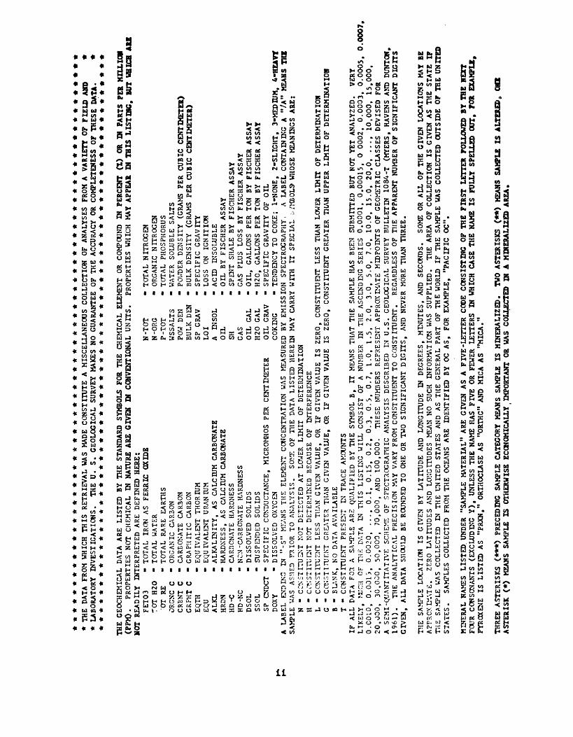
TH

E

DA

TA

FRO

M W

HIC

H

TH

IS

RE

TR

IEV

AL

WA

S M

AD

E C

ON

STIT

UT

E

A

MIS

CE

LL

AN

EO

US

CO

LL

EC

TIO

N

OF

AN

ALY

SES

FRO

M A

V

AR

IET

Y

OF

FIE

LD

A

HD

*

LAB

OR

ATO

RY

IN

VE

ST

IGA

TIO

NS

. T

HE

U.

S.

GE

OL

OG

ICA

L

SUR

VEY

M

AK

ES

NO

GU

AR

AN

TEE

OF

TH

E

AC

CU

RA

CY

O

R

CO

MPL

ET

EN

ESS

O

F T

HE

SE

DA

TA

.*

**

**

**

**

**

**

***

***************************

**

**

**

**

**

**

**

**

**

*

TH

E

CE

OC

HE

MIC

AL

D

ATA

A

RE

LIS

TE

D

BY

T

HE

ST

AN

DA

RD

SY

MB

OLS

FO

R T

HE

C

HE

MIC

AL

EL

EMEN

T O

R CO

MPO

UN

D

IN

PER

CE

NT

(I

) O

R

IN

PAR

TS

PER

M

ILL

ION

(PP

M).

PR

OPE

RT

IES

NO

T C

HEM

ICA

L IN

N

ATU

RE

AR

E

GIV

ES

IN

C

ON

VE

NT

ION

AL

U

NIT

S.

NO

T R

EA

DIL

Y

INT

ER

PRE

TE

D

AR

E D

EFI

NE

D

HE

RE

:F

ET

03

- T

OT

AL

IR

ON

A

S FE

RR

IC

OX

IDE

TO

T

H20

-

TO

TA

L

WA

TER

'OT

R

E -

TO

TA

L

RA

RE

EAR

THS

OR

GN

C

C "

OR

GA

NIC

C

AR

BO

NC

REN

T C

-

CA

RB

ON

ATE

C

AR

BO

NG

RPH

T

C

" G

RA

PH

ITIC

C

AR

BO

NEQ

TH

-

EQ

UIV

AL

EN

T

THO

RIU

MEQ

U

- E

QU

IVA

LE

NT

U

RA

NIU

MA

LK

L

- A

LK

AL

INIT

Y,

AS

CA

LCIU

M

CA

RB

ON

ATE

HR

DS

- H

AR

DN

ESS

, A

S C

ALC

IUM

C

AR

BO

NA

TEH

D-C

-

CA

RH

ON

ATE

H

AR

DN

ESS

HD

-NC

-

NC

N-C

AR

BO

NA

TE

HA

RD

NES

SD

SOL

-

DIS

SOL

VE

D

SOL

IDS

SSO

L

N-T

OT

N-O

RG

P-T

OT

WSS

AL

TS

POW

D

ENB

UL

K D

ENSP

G

RA

VL

OI

A IN

SO

LO

ILSH G

AS

OIL

G

AL

H20

G

AL

OIL

G

RAV

CO

KIN

G

PRO

PER

TIE

S W

HIC

H

MAY

APP

EAR

IN

TH

IS

LIS

T D

IG,

BUT

WH

ICH

AR

E

- TO

TAL

NIT

RO

GE

N-

OR

GA

NIC

N

ITR

OG

EN

- TO

TAL

PHO

SPH

OR

US

- W

ATE

R SO

LUB

LE

SAL

TS

- PO

WD

ER

DE

NSI

TY

(G

RA

MS

PER

C

UB

IC

CE

NT

IME

TE

R)

- B

ULK

D

EN

SIT

Y

(GR

AM

S PE

R

CU

BIC

C

EN

TIM

ET

ER

)-

SP

EC

IFIC

G

RA

VIT

Y-

LO

SS

ON

IGN

ITIO

N-

AC

ID

INSO

LU

BL

E-

OIL

BY

F

ISC

HE

R

ASS

AY

- SP

EN

T

SHA

LE

BY

FI

SCH

ER

A

SSA

Y-

GA

S PL

US

LO

SS

BY

FISC

HE

R

ASS

AY

" O

IL,

GA

LLO

NS

PER

TO

N

BY

FISC

HE

R

ASS

AY

- H

20,

GA

LLO

NS

PER

TO

N

BY

F

ISC

HE

R A

SSA

Y-

SP

EC

IFIC

G

RA

VIT

Y

OF

OIL

- TE

ND

ENC

Y

TO

CO

KE

; 1-

NO

NE

, 2-

SL

IGH

T.

3-M

ED

nJM

. 4-

HE

AV

T

A L

AB

EL

C

ON

TA

ININ

G

A "/

A"

MEA

NS

TH

E

/ME

OL

9 W

HO

SE

MEA

NIN

GS

AR

E:

- SU

SPQ

fDE

D

SOL

IDS

SP

CN

DC

T -

SP

EC

IFIC

C

ON

DU

CTA

NC

E,

MIC

RO

MH

OS

PER

C

EN

TIM

ET

ER

DO

XY

-

DIS

SOL

VE

D

OX

YG

ENA

L

AB

EL

EN

DIN

G

IN

"-S

" M

EAN

S T

HE

EL

EMEN

T C

ON

CEN

TRA

TIO

N

WA

S M

EASU

RED

BY

E

MIS

SIO

N

SPE

CT

RO

GR

APH

Y,

SAM

PLE

WAS

A

SMED

PR

IOR

TO

A

NA

LY

SIS

. SO

>T.

OF

TH

E

DA

TA

LIS

TE

D

HE

RE

IN

MA

Y

CA

RR

Y

WIT

H

IT

SP

EC

IAL

N

" C

ON

STIT

UE

NT

N

OT

DE

TE

CT

ED

A

T LO

WER

L

IMIT

O

F D

ET

ER

MIN

AT

ION

H -

C-T

NST

ITU

rNT

N

OT

DET

ERM

INED

B

ECA

USE

O

F IN

TE

RFE

RE

NC

EL

-

CO

NST

ITU

EN

T

LE

SS

THA

N

GIV

EN

V

AL

UE

, O

R

IF G

IVE

N

VA

LUE

IS

ZE

RO

, C

ON

STIT

UE

NT

L

ESS

TH

AN

LO

WER

L

IMIT

O

F D

ET

ER

MIN

AT

ION

G -

CO

NST

ITU

EN

T

GR

EATE

R

THA

N

GIV

EN

V

AL

UE

, O

R IF

G

IVE

N

VA

LUE

IS

ZE

RO

, C

ON

STIT

UE

NT

G

REA

TER

TH

AN

U

PPE

R

LIM

IT

OF

DE

TE

RM

INA

TIO

NB

- B

LA

NK

, N

O

DA

TA

AV

AIL

AB

LE

T -

CO

NS

Tm

JEN

T

PRE

SEN

T

IN

TRA

CE

AM

OU

NTS

IF

ALL

D

ATA

FO

R

A SA

MPL

E A

RE

QU

AL

IFIE

D

BY

T

HE

SY

MB

OL

B,

IT

MEA

NS

THA

T T

HE

SA

MPL

E H

AS

BEE

N

SUB

MIT

TE

D

BU

T N

OT

YET

A

NA

LY

ZE

D.

VER

Y

LIK

EL

Y,

MJC

H

OF

TH.-

DA

TA

IN

TH

IS

LIS

TIN

G

WIL

L

CO

NSI

ST

OF

A N

UM

BER

IN

TH

E

ASC

EN

DIN

G

SE

RIE

S

0.0

00

1,

0.0

0015.

0 0

00

2,

0.0

00

3,

0.0

00

5,

0.0

00

7,

0.0

010,

0.0

013,

0.0

020,

....

0

.1,

0.1

5,

0.2

, 0

.3,

0.5

, 0

.7,

1.0

, 1.5

, 2

.0,

3.0

, 5.0

, 7

.0,

10.0

, 1

5.0

, 2

0,0

, ..

..

10

,00

0,

15,0

00,

20,0

00,

30

,00

0,

50

,00

0,

70

,00

0,

AN

D

100,0

00.

TH

ESE

N

UM

BER

S R

EPR

ESD

IT

APP

RO

XIM

AT

E

MID

POIN

TS

OF

GEO

MET

RIC

C

LA

SSE

S D

EV

ISE

D

FOR

A

SE

MI-

QU

AN

TIT

AT

IVE

SC

HEM

E O

F SP

EC

TR

OG

RA

PHIC

A

NA

LY

SIS

DE

SCR

IBE

D

IN

U.S

. G

EO

LO

GIC

AL

SU

RV

EY

BU

LL

ET

IN

10

84

-T

(MY

ER

S,

HA

VEN

S A

ND

D

UN

TON

, 1961

).

THE

AN

AL

YT

ICA

L

PR

EC

ISIO

N

MAY

V

AR

Y

FRO

M C

ON

STIT

UE

NT

TO

C

ON

STIT

UE

NT

. R

EGA

RD

LESS

O

F T

HE

A

PPA

RE

NT

N

UM

BER

O

F S

IGN

IFIC

AN

T

DIG

ITS

G

IVE

N,

AL

L

DA

TA

SHO

ULD

B

E R

OU

ND

ED

TO

ON

E O

R

TWO

S

IGN

IFIC

AN

T

DIG

ITS

, A

ND

N

EVER

M

ORE

TH

AN

T

HR

EE

.

THE

SAM

PLE

LO

CA

TIO

N

IS

GIV

EN

B

Y

LA

TIT

UD

E

AN

D

LON

GIT

UD

E IN

D

EG

RE

ES,

M

INU

TE

S,

AN

D

SEC

ON

DS.

SO

ME

OR

A

LL

O

F TH

E G

IVE

N

LO

CA

TIO

NS

MAY

B

E A

PPR

OX

IMA

TE

. ZE

RO

L

AT

ITU

DE

S A

ND

L

ON

GIT

UD

ES

MEA

N

NO

SU

CH

IN

FOR

MA

TIO

N

WA

S S

UP

PL

IED

. T

HE

A

REA

O

F C

OL

LE

CT

ION

IS

G

IVE

N

AS

TH

E

STA

TE

IP

T

HE

SA

MPL

E W

AS

CO

LL

EC

TE

D

IN

TH

E

UN

ITE

D

STA

TE

S A

ND

A

S T

HE

G

ENER

AL

PAR

T

OF

TH

E W

ORL

D

IF

TH

E

SAM

PLE

WA

S C

OL

LE

CT

ED

O

UT

SID

E

OP

TH

E U

NIT

ED

S

TA

TE

S.

SAM

PLES

C

OL

LE

CT

ED

FR

OM

TH

E

OC

EAN

S A

RE

ID

EN

TIF

IED

B

Y

OC

AS

, FO

R

EX

AM

PLE

, "P

AC

IFIC

O

C".

MIN

IRA

L N

AM

ES

LIS

TE

D

UN

DER

"S

AM

PLE

M

AT

ER

IAL

" A

RE

GIV

EN

A

S A

F

IVE

-LE

TT

ER

C

OD

E C

ON

SIST

ING

O

P T

HE

F

IRS

T

LE

TT

ER

FO

LLO

WED

B

Y T

HE

N

EX

T

FOU

R

CO

NSO

NA

NTS

(E

XC

LU

DIN

G Y

).

UN

LE

SS

TH

E

NA

ME

HA

S F

IVE

O

R

FEW

ER

LE

TT

ER

S IN

W

HIC

H

CA

SE

TH

E N

AM

E IS

FU

LLY

SP

EL

LE

D

OU

T,

FOR

E

XA

MPL

E,

PYR

OX

ENE

IS

LIS

TE

D

AS

"PR

XN

,"

OR

THO

CLA

SE

AS

"OR

TH

C"

AN

D

MIC

A

AS

"MIC

A."

TH

RE

E

AS

TE

RIS

KS

(*

**)

PRE

CE

DIN

G

SAM

PLE

CA

TEG

OR

Y

MEA

NS

SAM

PLE

IS

MIN

ER

AL

IZE

D.

TWO

AST

ER

ISK

S (*

*)

MEA

NS

SAM

PLE

IS A

LT

ER

S1.

CSSX

A

ST

ER

ISK

(*

}

MEA

NS

SAM

PLE

IS

OT

HE

RW

ISE

EC

ON

OM

ICA

LLY

IM

POR

TAN

T O

R W

AS

CO

LL

EC

TE

D

IN

A M

INE

RA

LIZ

ED

AR

EA

.

APPE

NDIX

V.

LAB, KO

,

161965

161989

161893

161968

161*95

161956

.U1955

161517

161*50

161*61

1619J3

161902

161357

lAb. KO.

161965

U1

93

9

1 »,

1 9 <b

6

ltl?

95

16 1

5 *

6 16

1955

16

1*17

16

1350

1 6

1 5 *

I

1613

32

161S

57

LA

P.

NO

.

161965

H1939

1 6

1 5 * 3

1 6

1 5 fc

8

161955

161917

161*50

\ 6

1 & 6

1 161*18

U19C2

161957

SAMPLE

K3G1AS1

K3GUS1X

K3G1BS1

K.3G2AS1

K3G3AS1

K3G3BS1

K3G4AS1

K3G4RSI

K3G5AS1

K3G5oSl

K3C6AS1

K3G6BS1

K3G

1AS

1XK

3GIR

S1K

3C2A

S1

K3G43S1

K3C

5HS1

K

3G6A

S1

X3G

6PS1

SAM

PLE

K3G1AS1

K3G1AS1X

X3G1BS1

K3G4AS1

K3G4BS1

K3C5AS1

K3G56-51

K3G6AS1

K3G6BS1

CHEM

ICAL

ELE

MEN

TS

IN V

EGET

ATI

ON

AND

SO

IL N

EAR

CO

AL-

FIR

ED P

OWER

PLAN

TS,

WES

TERN

EN

ERGY

REG

ION

S

Tab

le 1.

Surf

ace

and

sub

surf

ace

soil

, an

d sa

gebr

ush

east

of

Dav

e Jo

hnst

on

Pow

erpi

ant.

W

yom

ing^

BA

PP

M.5

700

700

700

700

700

700

1000 70

050

070

010

00 700

1000

CO

PPM

-S 5 5 5 5 0 N

5 7 7 5 S 5 5 S

LATITUDE

42 42 42 42 42 42 42 42 42 42 42 42 42 BI CU

50 OON

50 OON

50 OON

50 40N

50 40N

49 35*

49

35^J

46 15*

45 15N

16 32N

46

32*J

40 15

N40 15*

PPM

o.i

0.3

O.lL

O.lL

O.lL

0.3

C.I

O.lL

O.lL

O.lL

O.lL

O.lL

0,4-

PPM.S

10 107 5 2

IS 10 10 107 7 5 7

Mill -1

||

! ! *

LONGITUD

105

105

105

105

105

105

105

105

105

105

105

105

105 CRl

F

SURFACE

46 30*

46 30*

46 30

^39 45*

39 45

*42 05

*42 05V

37 57

437 57*

29

07^)

29 07*

11 15*

11 15*

1ST

C%

SURFACE

0.11

0,11

0,03

0,07

O.OO

ti0.39

0.84

0,008

0.01L

0.01L

0.01L

O.OOU

0.01L %

SURFACE

0.04L

0.04

0.04L

0.04L

0.04L

0.05

0.04L

0,04

0.13

0,10

0.04L

0.04L

0.04L

DIST-KM

SOIL EAST

0.8

0.8

0.8

2.6

2.6

6.6

6.6

13.5

13.5

26.4

26,4

53.8

53.8

ORGNC C%

SOIL EAST

1.4

1.6

1.0

1.9

0.08

1.2

1.0

O.OB

1.3

1.2

1.0

0.08

1.3

FE

%-S

SOIL EAST

2.0

2.0

1.5

1.0

0.5

2.0

2.0

2.0

1.0

1.0

1.0

1.0

1.5

AL

l-S

AL203

%

OF DAVE JOHUSTON

7 7 5 5 5 7107 7 5 5 7

10

TOTAL C%

CA

OF DAVE JQHNSTON

1.54

1.68

1,05

1.99

0,61

1.59

1 .84

0,82

1.31

1.18

1,01

0.95

1,33

FE2C3

% GA

OF DA

VE:

JOHN

STON

2.7

;>,7

2.4

1.8

1.2

3.1

3.1

3,2

2.7

2.0

1.7

1.8

1.9

9,5

9.4

8.4

7,8

7.7

11.5

11.7

11.3

9.8

9.1

7.9

12.1

11.3

%-S

0.7

0.7

0.5

0.7

0.3

2.0

5.0

1,5

0,7

0,3

0,5

0,7

1,0

PPfc

-S

15 15 10 10 10 15 15 15 15 10 10 15 15

AS

CAO

GE-

PPM

3.7

3.9

5.3

2.1

2,5

2.4

2.2

3.2

4.9

4.1

3.2

5.5

1.5

%

1.2

41

.25

0,7

61

.14

0.7

53

.34

5.6

41,9

11

,16

0.7

10

,68

1.5

11,3

1

P>M

2,0

1.8

0.6

1.9

0.3

3.3

2,6

1.4

0.4

0,7 1.0

0,7

1."

B P

PM

.S

20 30 200

L0

N30 20

0 I

30 200

L0

N0

N

CL

%

O.l

LO

.lL

O.l

LO

.lL

O.l

L0,

11-

O.l

LO

.lL

O.l

LO

.lL

O.l

L0

.10

.1L

HG

PPM

0,0

20,0

20.0

20.0

20.0

10.0

20.0

10.0

20,0

20,0

20.0

20,0

10.0

1

BE

PP

M.S

O.O

N1

.01.0

O.O

NO

.ON

1.0

1.5

1.0

1.0

0.0(

4O

.ON

i.o

C*

PPM

-S

5010

0 30 20

23 30

30

70 30 20 20 20 30

K20

'

2.1

2.1

2

.0

2.2

2.7

2.5

3.0

2.8

2.6

2.7

2,9

3.4

3.3

APP

END

IX V

. (c

onti

nu

ed)

Tab

le

1.-

-Surf

ace,

and

su

bsu

rfac

e so

il,

and

sag

ebru

sh east

of

Dav

e Jo

hn

sto

n P

ow

erp

lan

t.

Wyo

min

g (c

onti

nued

)

LA

B,

NO

, SA

MPL

E

LA

PP

M-S

L

I PP

M

MG

%-S

M

GU

% M

N P

PM

-S

MNO

*

16

19

65

161989

16

1*

93

1

61

96

9

UU

95

1

61

9S

6

1 6

1 8 5 0

161861

1 6

1 9

1 P.

161*02

161957

1618

9.

1*1*95

: 6 1

? " 6

16li

9S5

161917

161550

161SC2

161S65

161989

16 1

? 5 3

j 61

& 6 e

1 <

! !

9 5

1619

B6

16

19

55

161917

16

1*

50

161561

161916

U1

90

2

16

19

57

K3G1AS1

K3G1AS1X

K3G1BS1

K3G3AS1

K3C1PS1

K3G4AS1

K3G5AS1

K3C5RS1

K3G

6*S

1

K3G1AS1

K3GIAS1X

K 3

C, 4

? 5

1

K3G1AS1

K3G1AS1X

K3G4AS1

K3G4RS1

K3G5AS1

K3G5BS1

K3G6AS1

K3G6RS1

50

30

50

300

N 30

50

30

500. N

30

50

30

P205

0.1L

0.1L

0.1L

0.1L

0. 1L

0.1L

0.1L

0.1L

0,1

0,1L

0.1L

0.1L

C.lL

TH

PPM

7.9

10,0

7.1

10,4

11^2

21.3

15,6

16.2

11,0

e.3

15.6

12,6

LI

PPM

MG

*-S

SUPFACE

20 21 17 117

27 25 17 15 12 109

11

PP PPM-S

SURFACE

20 20 20 20 15 20 20 20 20 20 20 20 20

TI

*«S

SOIL EAST

0,50

0.70

0,50

0,20

0,15

0,70

1.00

0,70

0,30

0,30

0.20

0.30

0,30

TOTAL

s%

SOIL EAST

0.04

0.04L

0.04L

0.04L

0.041

0.04L

0.04L

0.04L

0.04L

0.04L

0.04L

0.04L

0.04L

TI02

%

SURFACE SOIL EAST

0,15

0,20

0.15

0,15

0.10

0,20

^.20

0.20

0,15

0.20

0,15

0,15

0,20

0,42

0.42

0.40

0.28

0,17

0,45

0.38

0,47

0.49

0.40

0,33

0.31

0.35

MGU

OF DAVE 1. 1. 1, 1. 1. 2. 2, 1. 1. 1. 1. 1. 1.

% MN

PPM-S

JOHNSTON

4 4 OL OL OL 0 0 7 3 OL OL 2 1

200

200

150

200

100

300

500

500

300

200

200

150

300

SB

PPM

SC PPM-S

OF DAVE 1 0 0 1 0 0 0 1 0 0 0 0 0

JOHNSTON

.4 .9 .4 t 8

.1 .6 ,9 .2 .5 .7 .P .4 ,6

U PPM

ECU

OF DAVE 2 2 2 2 I 3 3 3 3 7 2 y. 2

JOHNSTON

.6 .4 .7 .2 .8 ,2 .5 .4 .6 , 8

.5 .9 ,8

7 5 5 0 N

0 N

7 710 5 5 0

L5 5 PPM

10 L

10 L

30 30 20 20 30 40 20 20 20 20 30

SCPP

M

0.1

L0.1

L0,1

0.1

L0,1

L0

.1L

0,1

L0.1

L0.1

L0,1

L0

.1L

0,3

0,1

L

V P

PM

.S

70 70 70

50 30 70 70 70 70 30 30 50 50

NA

20

0,0

42

0.0

41

0,0

27

0,0

33

0.0

20

L0

,06

90,0

71

0,0

80

0,0

53

0,0

40

0,0

35

0,0

31

0,0

44

0,8

10,7

90,7

91,2

51

.65

1.3

41

,90

1,8

91,6

81

,18

1,2

02,5

.02,3

0

SIG

2

76 77 79 82 83

70

66

74

78

BO

76

74

Y P

PM

-S

15 20

15

150

U Ib

15

15

20

15

10

20

Ib

NB

PP

M-S

10 0

ti10

0 N

0 N

10 0

N 0

N 0

N10

0 N

0 N

0 N

SNP

Ph

YB

PP

M.5

1.5

2.0

1.5

1.5

1.0

1.5

2.0

2,0

2

.0

1.5

1.5

2.0

1.5

NX

PP

M-5

15 15 10 5 5 15 15 10 157 5 5 7

5R

PP

f.-S

1.6

0,3

0,3

C.1L

0,11

0,5

1.9

0,7

0,4

0,5

0,8

0,6

1.5

200

20C

ISO

200

150

300

500

200

200

ISO

130

200

300 PP

M

58 58 47 28 20 57 45 48 44 36 33 33 33

APP

END

IX

V.

(con

tinued

)

Tab

le

1.-

-Surf

ace

end

subsu

rfac

e so

il,

and

sag

ebru

sh east

o

f D

ave

Johnst

on

Fo

wer

pla

nt.

W

yom

ing

(co

nti

nu

ed)

LA

B.

NO

.

1619

65

H

1S

89

1

61*93

161S

63

1616

95

1

61966

16

19

55

1

61917

161*

50

1

61

*M

urn

s1619

02

1619

57

LAB. NO.

161943

161921

162001

161949

161947

161951

161938

161*46

161&56

161907

1 6

1 9 1 9

161900

161905

1619&7

LAB,

K3.

161943

161S21

162001

161949

U1947

161951

161938

161358

161907

16l8o7

161919

161900

161935

161905

161987

SAMPLE

K3GUS1

K3G1AS1X

K3S1BS1

K3G2AS1

K3G28S1

K3G3AS1

K3G3BS1

K3G4*S1

K3G46.

S1

K3G5*Sl

K3G5PS1

XjG&iSl

K3G6BS1

SAMPLE

K3<"

.t AS2

K3GUS2

K3G2AS2

K3G23S2

K3G3AS2

K3G3AS2X

K3G3&S2

KJG4AS2

K3G4AS2X

K3G4BS2

K3^'i*S2X

.<3G

f>AS

2K3G5SS2

X3G6AS2

K3GMS2X

K3G*BS2

SAMPLE

K3G1AS2

K3G1BS2

K3G2AS2

K3G2BS2

K3G3AS2

K3C3AS2X

K3G3RS2

K3G4AS2

K3G4AS2X

K3G43S2

K3G4BS2X

K3G5AS2

K3G5BS2

K3G6AS2

K3G6AS2X

K3G6HS2

ZB PPM-S

150

150

150

200

100

150

100

200

200

200

150 70

150

LATITUDE

42 42 42 42 42 42 42 42 42 42 42 42 42 42 42 42 BI

50 DON

50 DOS

50 40N

50 40

>V49 35N

49 35N

49 35N

43 15*

48 15

N48 15

*48

15N

46

32*'

46 32

N40 15M

40 l5N

40 15

H

PPM

0,5

0, 1L

O.lL

O.lL

0.1L

0.1L

0.1L

0.1

O.lL

O.lL

O.lL

O.lL

O.lL

O.lL

0.1L

O.lL

SURFACE SOIL EAST OF DAVk* JOKNSTON

LONGITUD

DIST-KM

AL

%*S

AL203

\

105

105

105

105

105

105

105

105

105

105

105

105

105

105

105

105

SUBSURFACE

46 30*

46 30

439

45*

39 45*

42 054

42 054

42 05 rf

37 57

rt37 57*

37 57*

37 57

rf29

07

'J29

07*

11 154

11 15*

It 15*

CRBNT C%

OF

SUBSURFACE

O.OOB

O.OOa

O.OOB

o.oo

fl0.08

0,13

2.18

O.OOB

0.003

O.OOB

o.ooa

O.OOB

O.OOB

O.OOB

0,0GB

0,006

SOIL CAST

0,8

0,8

2.6

2,6

6.6

6,6

6.6

13.5

13.5

13,5

13,5

26,4

26,4

53,8

53,8

53,8

IGNC C%

SOIL EAST

0,08

O.Od

0,08

0.08

1,6

1,1

O.lL

O.OB

O.OB

O.OB

0,08

. O.OB

O.Ofa

O.OB

0,08

O.OB

OF DAVE JOHNSTQN

7 S 7 7 10 107 7 5 7 7 5 7

10 10 10

TOTAL C%

CA

OF DAVE JOHNSTUN

0,88

0,83

'0,7

30,32

1,73

1,21

2,10

0,93

0.94

0,69

0,78

0,52

0,72

0.63

0,61

0,64

8,1

8,1

7.5

8,2

11.1

11,0

11,1

11,5

10,7

11,4

11.7

9,2

9.6

12.9

12,9

13,2

%-S

1,0

0,7

1,0

0,5

2,0

2.0

10,0

0,7

0,7

0.7

0,7

0,3

0,5

1,0

0,7

0,7

AS

PPM

6.0

5,0

2

,3

2,1

3,7

3,5

3

,5

5,6

2

,2

5,9

5,5

4,5

3,7 1.2

1.3

0,9

CA

O

%

1,6

3

1.1

4

1.2

7

0,6

8

2.1

8

2,3

3

11,9

1

1.3

6

1,3

0

l.H

1.0

9

0.6

1

0,6

9

1.5

7

1.4

4

1.3

2

B P

PM

.5

CE

PP

M-S 0

N 0

N 0

N 0

N 0

N 2

00

0 fe

0 N

0 N

0 N

0 N

0 ft

0 N

0 N

0 N

0 N

BA

PP

M-S

20 200 0

50 30 30 20 200

300 0 0 C 0

L N L L L N N N

700

700

1000

700

700

700

1000

500

700

1000

bOO

1SOO

1000

1000

1000

1000

CO

PP

*-S 5 5 0

L0

N7 7 5 5 5 7 5 5 7 5 5 5

BE

PPM

»S

O.O

N0,

CN

0,0

*0,

ON

1,0

1,0 1,0

1,0

1,0 1,0

1,0

O.O

.N1,0

1,5

l.S

1,0

CR

P

PM

-S

30

30

20

20

50

50

30

50

30

50

50

50

30

20

30

SO

APP

END

IX

V.

(conti

nued

)

Tab

le 1. S

urf

ace

and

subsu

rfac

e so

il,

and

sag

ebru

sh east

of

pave

Jo

hnst

on

Pow

erpla

nt

. W

yom

ing

(co

nti

nu

ed)

LA

B.

NO

. SA

MPL

E

CU

P

PM

-S

F %

FE

*-S

F

ET

03

% G

A

PP

M-S

G

E PP

M

161943

161921

162001

161949

161*47

161951

161935

161?46

161958

161507

161567

161919

161500

161535

161905

161967

LAB, KO

,

161943

161921

162001

161949

161947

* 161951

lr>1938

161*46

1 6 1

6 5 8

U1907

161900

161935

1619C5

161931

LA*. HO

.

161943

161921

16200;

161

94'.

161947

161938

161646

161658

161907

161867

161919

161900

161935

161905

I6l9b7

SAMPLE

K3G1AS2

K3G13S2

K3G2AS2

K3G2BS2

K3G3AS2

*3G3^S2X

K3G3BS2

K3G4AS2

K3G4AS2X

K3G4BS2

K3G48S2X

K3G5AS2

K3G5BS2

K3G6AS2

K3G6AJS2X

K3G6BS2

SA-PLE

K3G1AS2

A 3G t SS2

K3G2AS2

K3G2

.^S2

K3G3AS2

K3G3AS2X

K 3

Ci 3 a S 2

K3G4AS2

K3G4i.52X

K3G4P.S2

K3G4BS2X

K3G5AS2

K3G5PS2

K3G6AS2

K3G6AS2X

K3G63S2

SAVPLE

K3G1AS2

K3G 1 rf

S2K3G2AS2

K3G2PS2

K3G3AS2

K3G3AS2X

K 3<"

» 3bs2

K3G4AS2

K3G4AS2X

K3G4BS2

K3G4BS2X

K3G5AS2

K3G5BS2

K3G6AS2

K3G6AS2X

K3G6&&2

CU PPM-S 5 3 5 2

20 15 15 107

10 107 7 5 5 7

LA PPH-S

30 300 0

50 100 050 30 3Q 500

50 50 50 30

NI PPM-S

107 7 5 15 15 10 15 10 15 15 7 7 7 7 7

N N N N

F %

FE

SUBSURFACE

0.04L

0.05

0.04L

0.04L

0.04L

0.04L

0.05

' 0.04L

0.04L

0.04L

0.04L

0.05

0,041

0.04L

0.05

0.04L

LI

PPM

MC

SUBSURFACE

17 16 118

23 22 37 19 16 20 23 17 16 108

11

P205

% PB

SUBSURFACE

0.1L

0.1L

O.lL

0,1L

O.lL

O.lL

,O.lL

o.i

0.1L

0.1L

O.lL

0,11

O.lL

O.lL

O.lL

O.lL

%-S

SOIL EAST

2.0

1.0

1.5

0,7

2.0

3.0

2.0 .5 .5

2.0

2.0 .5 .5 .5 .0 ,5

%-S

SOIL EAST

0.5

0,5

0,3

0,2

0.7

1.0

i.o

0.5

0,5

0,5

0.5

0,5

0.5

0.5

0.3

0.3

PPM-S

SOIL EAST

10 10 20 15 15 30 15 15 20 15 20 IS 20 20 20 20

FET03

% GA PPM-S

OF DAVE JOHNSTON

2.6

2.5

1.9

1,1

3.5

3,8

3.2

3.2

3,2

3,5

3.7

2.6

2.5

l.P

1.8

2.1

10 10 10 10 15 15 20 15 15 15 15 10 15 20 15 15

MGO

% MN PPM-S

OF DAVE JOHNSTON

1,2

1.3

l.OL

l.OL

1.6

1.7

4.2

1,6

1,4

l.l

1,3

1,3

l.OL

1.3

), ,OL

t.2

200

150

200

100

300

300

700

200

200

200

200

200

200

ISO

150

200

SB

PPH

5C PPM-S

OF DAVE JOHNSTON

1.3

0.5

1.9

0.3

0,7

2,4

0.7

1.0

0.5

1.5

0.3

0.6

.1.0

0,9

0.3

0.3

5 5 0 L

0 N

10 107 7 7 7 7 5 5 5 5 7

1.4

1.0

1,9

1.0

1.3

1.1

1.2

0.9

0.5

1.3

0.5

1.3

2.6

0.9

1.1

3.4

MNO

PPM

O.lL

O.lL

O.lL

O.lL

O.lL

0,1

O.lL

0.2

0,1

0,2

0.1L

0.1L

O.lL

O.lL

0.1L

0.1L

HG

PPrt

0,01

0.01

0.01

0.01

0,02

0,01

0.02

0.02

0.01

0.02

0,01

0,01

0.01

0,01

O.U1

O.ul

NA20

%

0,0

43

0.0

28

0.0

30

.0

.02

0L

0.0

64

0.0

65

0.1

43

0,0

50

0.0

42

O.C

47

0.0

47

0.0

30

0.0

34

0.0

32

0.0

24

0.0

39

0.7

30.7

31.4

01.5

51

.30

1,3

81

,26

i.tfo

1.9

81,1

31

,13

0.6

91,0

13,1

33,1

32,7

5

SI02

77 80 75 84 72 69 54 73 69 75 74 75 74 72 72 75

1-5 2 2 3 2 3 2 3 3 3 3 3 2 3 3 3 S

NB PPM-S 0 N

15 0 N

0 N

10 0 N

0 ft

10 0 N

10 10 0 N

0 N

0 N

0 ft

0 N'

SNPPM

0.5

0,4

0.1L

0.1L

0,6

0.3

0.4

4.5

0.4

O.lL

0.4

0.7

1.6

O.lL

2.4

0.4

K20

2.0

2.0

2.4

2.3

2.5

2.5

2.4

2.7

2.8

2.5

2.5

2,5

2,8

3,8

3.7

3.9

ND PPH-S 0 N

0 N

0 B

0 B

0 L

700

B0

N0

N0

N0

N0

B0

N0

N0

N0

N

5R PPM»6

150

100

300

200

300

300

500

200

200

200

200

100

200

300

300

300

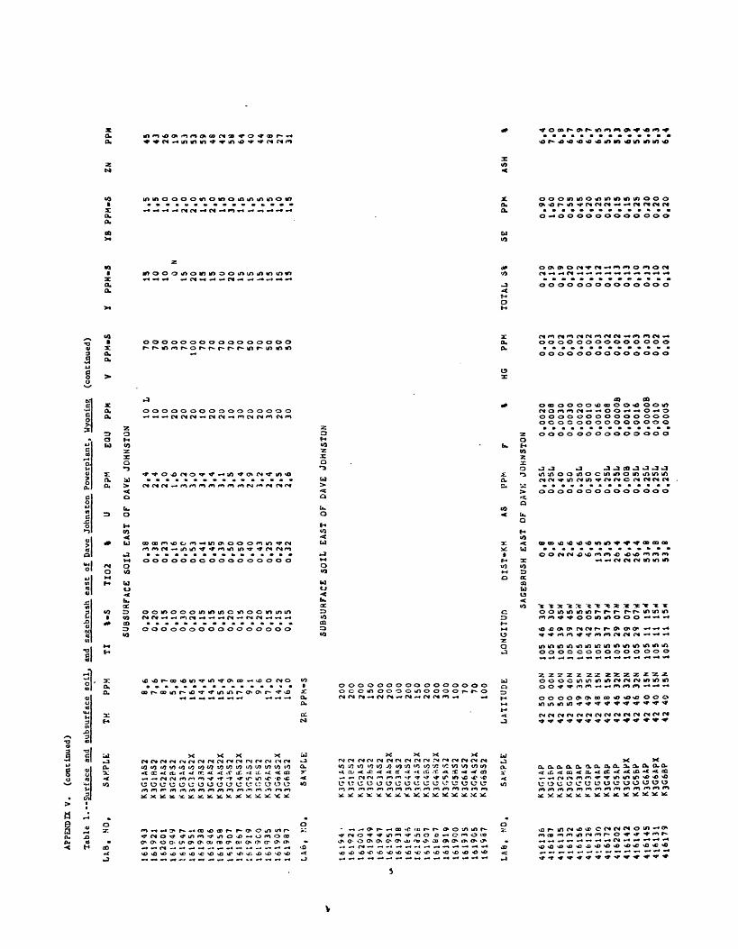
APP

END

IX

V.

(co

nti

nu

ed)

Tab

le

1.

LA

8.

NO

.

161943

161921

162001

161949

161547

161951

161938

161846

161358

1619Q7

161867

161919

1619CO

161935

161905

161987

LAD, NO.

16194 '

161921

16

20

01

1

61

94

9

161947

161951

16

19

38

16

1&46

16

13

55

16

19

07

irfa

ce

and

sub

surf

ace

soil

, an

d sa

geb

rush

east

of

_ D

ave

Joh

nst

on

P

ov

erp

lan

t,

Wyo

min

g;

(co

nti

nu

ed)

TI

%-S

T

I02

I U

PPK

EQ

U

PPM

V

PP

M.S

1619

19

1619

00

1619

35

1619

05

161*

87

LA

6,

MO

.

SAMPLE

K3G1AS2

X3G1BS2

MG2AS2

K3G2?S2

K3G3AS2

K3G3tS2X

K3G33S2

K3G4AS2

K3G4AS2X

K3G4

siS2

K3G4BS2X

K3r,

'jAS

2K3G5PS2

K3G6AS2

K3G6AS2X

K3G6B32

SAMPLE

K3G1AS2

K3G1BS2

K3C-.2AS2

K.3G

2BS2

K3G3AS2

*3G3A*>2X

K3G3aS2

K3G4AS2

MG4A52X

K3G4BS2

K3G4H&2X

K3GS

A.S2

K3G5WS2

K3G6&S2

X3G6AS2X

K3G6SS2

TK

PPM

8.6

7,6

8.7

5.8

17,6

16,5

14,4

14.5

15,4

IS, 9

17,8

9,1

9,6

17.0

14,2

16.0

ZR PPfc-S

200

200

200

150

200

200

100

200

150

200

200

300

100

70 70

100

SAMPLE

LATI

TUDE

%-S

TI02

I U

PPK

EI

SUBSURFACE

0.20

0.20

0.15

0.10

0,30

0,20

0,15

0,15

0.15

0.20

0,15

0.20

0,20

0,15

0.15

0.15

SOIL EAST OF

0.38

0,38

0,23

0.16

0,50

0.53

0.41

0,45

0,39

0,50

0,50

0,40

0,43

0,25

0.24

0,32

DAVE JO

HNS'

2,4

2.4

2.0

1,6

3.2

3.0

3,4

3,4

3,1

3.5

3,4

2.9

3,2

2.4

2.5

2,6

10

L10 10 20 20 20 10 20 20 10 30

20 20 30 20 30

SUB

SUR

FAC

E

SO

IL

EA

ST

OF

DA

VE

JQH

NST

UN

LONGITUn

DIST-KM

AS

PP!«

416136

416187

416135

416132

416156

4lfcl2*

416130

416172

416202

416142

416140

41&145

416131

416179

K3Ct AP

K3G1&P

K.3C2AP

K3G28P

K3G3AP

K3G3PP

K3G4AP

K3G4RP

K3G5AP

K3G5APX

K3G5BP

K3G6AP

K3G6APX

KJG6BP

42 42 42 42 42 42 42 42 42 42 42 42 42 42

50

50 50 50 49 49 48 48 46 46 46 40 40 40

OON

OON

40N

40N

35N

35N

15N

15N

32N

32N

32N

15N

15N

15N

105

105

105

105

105

105

105

105

105

105

105

105

105

105

46 46 39 39 42 42 37 37 29 29 29 11 11 11

30*

30*

45M

45*

05*

05*

57*

57*

07N

07*

07rt

151

15*

15*SAGEBRUSH CAST OF DAVK JOHNSTON

0.8

0.8

2.6

2.6

6.6

6,6

13,5

13.5

26.4

26,4

26,4

53,8

53,8

53.8

0.25L

0.2SL

0.40

0.50

0.25L

0,50

0.40

0.25L

0.25L

o.ooa

0.25L

0.25L

0.25L

0.25L

0.0020

0.0008

0.0030

0.0030

0.0020

0.0010

0.0016

0,0008

O.OOOOB

0,0010

0.0016

O.OOOOB

0,0010

0.0005

70

70

SO

30

70

100 70

70

70

70

70

50

70

50

SO

SO

HG

PPM

0.02

0.03

0,02

0,03

0.02

0.02

0.03

0,02

0,02

0,01

0,03

0,03

0,02

0.01

PPM.S

15

10

100

N 15

20

15

15

10

20

15

15

15

15

15

IS

TO

TA

L

S%

0,2

00,1

90,1

90

,20

0,1

20,1

40,1

20,1

10,1

30,1

30,1

00.1

30,1

00,1

2

YB

PP

M.S

i.5

1

.51,0

1.0

2

,0

2.0

1

,3

2,0

1,9

3,0

1

,5

1,5

1

,5

1,5

1

,0

1,5

SE

PPM

0.9

01.6

00.7

00,5

50,4

50,2

00,2

50,2

50,1

50,1

50.2

50.2

00.2

00.2

0

ASH

PPM

45 43 26 19 53 53 59 48 42 58 64 40 44 28 27 31 6.4

7

.0

6,8

6.7

6.9

6.7

6

.5

5.3

5

,3

6,9

5

,4

5.6

5,3

6.4

APPE.DDC

Table

1.

LAB. NO.

416136

4161&7

416135

416132

416156

416123

416130

4iel72

416202

410142

4!bl40

416145

41*131

410179

Lib, MO.

4*6136

4l6l87

416135

416132

416156

41&128

416130

41&172

416202

416142

416140

416145

416131

416179

LAB. NO.

V.

(continued)

--Surface

and

subs

urfa

ce soil,

SAMPLE

K3G1AP

K3GiBP

K3G2AP

K3G?^P

K3G3*.

?X3G3&P

K3G4A?

K3G4HP

K3(J

5*P

K3f,5i?X

r-'3G5Pp

K3G6AP

<3G6A?X

K3G6P?

SAMPLE

K3G1AP

K3Gln?

K3G2AR

*3G2»P

K3G3tP

*3G3Bp

K3G4AP

K3C43P

K3G5

A.P

K3G5APX

K3G53P

K3G6AP

K-3G6APX

K3G68?

SAMPLE

AC PPM-S

o.otf

0.0*

o.rt*

O.ON

O.ON

0,0*

0,0(4

O.ON

O.CN

1,5

O.ON

O.ON

0,0*

G.Ort

CR PPV.S

30

15

50

70

50

30

30

30

15

15

30

15

20

15

NA/A

%

and

sagebrush

ease of Dav

e Johns ton

Puwerplant.

Wyoming

AL

%-S

3,0

3.0

3.0

5.0

5,0

3,0

3,0

3,0

1,5

1.5

3,0

1.5

3,0

3.0

CU PPM-S

150

150

150

200

150

200

150

ISO

150

150

150

150

100

150

Nl PPM-S

B PPM.S

SAGEBRUSH

EAST

300

300

300

300

300

300

300

300

300

200

200

300

300

300

FG

%-S

SAGEBRUSH EAST

0.7

0,7

0,7

1.5

1,5

0,7

0.7

1,0

0,5

0,3

0,7

0,5

0,7

0.7

P %-S

SAGEBRUSH EAST

416136

416167

416135

41&132

416156

416128

416130

416172

416202

416142

416140

416145

*1&131

416179

K3G1AP

. K3G1SP

K3G2AP

K3G2SP

K3G34P

K3G36P

K3G4AP

K3G4BP

K3G5AP

X3G5APX

K3G53P

K3G6AP

K3G6APX

K3G6BP

0,070

0,065

0.075

0.075

0,l9o

0, 1

10

0,075

0.080

0,075

0.065

0,130

O.OB5

0.03o

0.080

20

10

20

30

15

15

10

15

15

10

20

10

10

15

2,0

2,0

2,0

2.0

1.5

1.5

1.5

3.0

3.0

1.5

1,5

1.5

1.5

2,0

BA PPM.S

CA

OF DAVE JOHNSTON

700

$00

700

1000

1000

lOf'O

700

1000

1500

1500

15CO

SCO

5CO

SCO

GA PPM.S

K/A

OF DAVE JOHNSTON

15

10

15

20

15

15

10

15

10 L

10

15

10 L

10

10 L

i vm **r

%-S

10 G

10

10 G

10 G

10 G

10 G

10

10 G

10 G

10 G

10

10

10 G

10 G %

26

32

28

13

18

26

29

27

36

34

28

28 0 B

26

P/A

PPM

pB PPM-S

OP DAVE JOHNSTON

36000

36COO

36000

36000

24000

24000

24000

36000

36000

36000

24000

46000

24000

36000

150 70

50

50

150 70

150

200

100

100

150

70

150

100

(continued)

CA/A

%

12,0

9,6

12,0

10.0

9,8

10,0

8,4

11.0

10,0

8.4

9,2

11.0

O.OB

12,0

LI/A PPM

16

12

35 24

22 16

16

16

12

10

14 8

10

12

SC PPM-S

IS

10 L

10

15

15

10 L

10 L

0 N

0 N

10 I

10 L

10 L

10 L

10 L

CD/A PPM

3,0

5.9

8.3

6,8

3,1

1,9

3.0

6,8

5.6

6,6

4,8

3,0

2,5

4,0

MG

%-S

1,5

1,5

2,0

2,0

2,0

2,0

1,5

2,0

2.0

1,5

1,5

1,5

1,5

2,0

SI/A PPM

63000

39000

56000

90000

91000

56000

58000

53000

34000 0 B

90000

54000

52000

53900

CO PPM-S

500

1000

300

500

500

500

700

1000

500

500

500

700

700

1000

&* PPM-S

CO/A PPM

10 L

10 L

10 I

10 10 L

10 L

10 L

10 L

10 L

10 L

10 L

10 L

10 L

10 L

'M.S

3 5 3 6 4 2 3 3 2 1 4 0 B

3 2MO PPM.S

10 157

157

157 7 7 7 7 7 7 15

5R PPM-S

0 N

0 N

0 N

0 N

0 tt

0 N

0 N

0 N

0 N

300

N0

N0

t>0

fc

2000

700

1500

1000

700

1500

700

1000

700

700

700

300

500

300

APP

END

IX V

. (c

onti

nu

ed)

LAB.

NO.

416136

416187

416135

416132

41*156

416130

416172

416202

416142

416140

416145

416131

4J6179

SAMPLE

K3GUP

K3GJ3P

K3GJAP

K3G2SP

K3G5AP

K3r,

5ftP

X

K3G6APX

TI

%-S

0,20

Ot 15

0,20

0,30

0,20

0,15

0, 15

0.15

0,07

0,07

0.20

0,07

0,10

0,15

id

sag

ebru

sh

east

of

Dav

e Jo

hnst

on P

ow

erpla

nt.

W

yom

lnz

U/A

PP

M

1.6

1.6

1.6

3.0

2.0

1.2

1.2

1.6

0.8

0.8

1.6

0.4

1.2

1.2

V P

PM

-S

SAGF

BRUS

H EA

ST

' 10

0 70 100

150

100 70 70 70 30 30 70 30 70 SO

Y Pt

>\N

or D

AVS 20 20 20 30 20 20 20 20 20 20 20 20 20 2

0

S Y

8 PP

M

JOH

NST

ON

L L L L L L L Li L L L L

-S 2 0 2 2 2 2 2 2 0 2 2 2 2 2

L L L L L L t N L L t L L

(co

nti

nu

ed)

ZN

/A

PPM

54

05

00

55

05

30

32

040

02

70

41

05

40

48

03

80

42

03

00

28

0

ZR PPM-S

70 70 7010

0100 70 70 70 30 30 70 30 70

100

APP

END

IX V

. CH

EMIC

AL

ELEM

ENTS

IN

VEC

ETJ

Tab

le 2

. --L

ichen

east

an

d w

est

of

Dav

e .

LA

B,

NO

. SA

MPL

E

LA

TIT

UD

E

41

7926

41

7931

4J7

92

4

4p923

447

92

1

417925

41

7937

417S

27

41

7933

417929

41

79

22

417936

4}7

93

0

417935

4S

7932

417934

417928

4«7938

\TIC

N A

ND

S

OU

M£A

K t

John

s co

n P

ow

erpla

nt.

*u

n^~

f

»- -

«. v

n(w

n

Wyo

min

g

LO

NG

ITU

D

DIS

T-K

M

AS

PPM

F

%

LIC

HE

N

EA

ST

OF

DA

VE

JOH

NST

ON

DJ0

2E

01

DJ0

2K

02

DJ0

4E

03

DJ0

4E

04

D

J08E

05

OJ0

8E

06

D

J16E

07

DJ1

6E

08

DJ3

2E

09

D

J32

E1

0

DJ*

4E

U

DJ6

4E

12

DJ0

2«

13

D

J02K

14

DJ0

4K

15

DJ0

4X

16

DJ3

2X

17

O

J32

41

8

42

50

UN

42

5

0

14N

42

5

0

25N

42

50

27N

42

50

O

ON

42

5

0

OO

N

42

SO

21"

42

50

21N

42

49

36

N

42

49

3&N

42

5

0

OO

N

42

50

O

ON

42

50

15

N

42

50

15

N

42

50

15N

42

5

0

15N

42

5

0

4QN

42

50

4QN

105

44

45

4

105

44

45

4

105

43

25W

105

43

25

4

105

40

15*'

105

40

15

4

105

34

34W

1

05

34

3

44

105

21

53

4

105

21

S34

104

59

OO

rt 104

59

0

04 L

ICH

EN

105

47

50

4

105

47

50

4

105

49

18

4

105

49

18

4

106

10

26

4

106

10

26W

2,2

2

,2

4,5

4,5

8,3

8,3

1

6,3

1

6,3

33,0

33,0

6

4,0

6

4,0

WES

T O

F D

AV

E

2.0

2.0

4.0

4.0

33.0

3

3,0

1.2 1,0

1.8

1

,4

1,4 i.o

0.9

0.6

0.8

0

.7

2.0

2.0

JQH

NST

ON

1.6

1

,2

1.6

1

.6

2.0

2

.4

0,0

05

0

0,0

05

0

0,0

04

5

0.0

04

5

0,0

05

0

0.0

04

5

0.0

02

2

0,0

02

0

0.0

02

2

0.0

02

4

0,0

02

4

0,0

03

5

0,0

05

0

0,0

05

0

0,0

05

0

0.0

045

0.0

04

5

0,0

05

0

HG

PPM

0,14

0,10

0,10

0.12

0.10

0,12

0,10

0.10

0,10

0,14

0.09

0,09

0,13

0,10

0.12

0.16

0.12

0,08

TOTAL

LAB, NO,

SAMPLE

ASH

AG PPM.S

AL

%-S

B PPI'.-S

BA PPM-S

CA/A

%

LI:HEN C

AST

OF D

AVE

417926

417931

417924

417523

417921

417925

40937

417927

41753!

41792*

41792'.

417936

417930

417935

417932

417934

417929

417938

DJ02E01

DJ02T02

DJ04E03

OJ04E04

DJ08E05

DJ08E06

DJ16EC7

DJlbEOe

DJ32

F.09

DJ32E10

OJ64E11

DJ64E12

DJ02M13

DJ02W14

DJ04415

DJ04W16

DJ32W17

DJ32418

22,0

21.0

18,0

19.Q

16,0

17.0

7,5

7,8

11.2

11,5

11.0

11,0

16.5

17.0

15.3

15.0

15.5

14.7

O.ON

0.5

0,5

0,7

O.Or

t O.ON

1,0

1,0

i.o

1,0

1.5

0,7

LICHEN

0,5

O.ON

0,7

0,7

0,7

1.0

S 5 7 5 7 7 5 5 3 5 5 7

WEST OF

. 7 5 7 7 7 7

30

30

70 50

50

50

SO 70 50 50150

70

DAVE JUHNSTON

SO

SO

SO

SO

70 70

300

200

700

300

500

500

300

300

200

300

300

300

500

300

300

300

700

500

33 33 24 25 28 26 31 31 28 29 20 24 28 24 30 28 12 16

0,06

0,06

O.OOB

0.04

0,06

0,07

0,06

0,06

0,07

0,06

0,04

0,04

0,06

0,06

0,07

0,07

0.09

0,09

sa

PPM

0,10

0,10

0,15

O.OOB

0,05

0,10

0.05L

0,05

0.05L

0.05

0,05

0,05

0.10

C.10

0.10

0.10

0.10

0,10

SE

3.0

3.0

O.OB

O.OB

3,0

3,0

0,06

12.0

5.5

5,0

4,5

6,5

5,0

3.5

4.5

4.0

5.0

6.0

1 2 0 B

0 B

2 3 0 B

5 5 5 3 2

1,40

1,20

1,20

1.20

0,70

0,70

0.55

0,50

1.00

0.90

0,35

0,40

1,20

1,20

1,00

0,90

0,40

0.35

CD/A PPM

CO/A PPM

CR

70 70 70 70 70 70 70 70 70 70 70 100 70 70 70 70 70 70

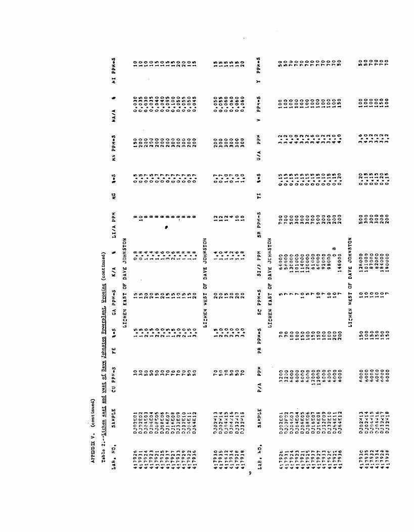
APP

END

IX V

. (c

onti

nued

)

Tab

le

2.-

-Lic

hen

ea

st,

and

vest

o

f D

ave

Joh

nst

on

P

ow

erpla

nt.

W

yom

ing

(co

nti

nu

ed)

LA

B,

NO

. SA

MPL

E

CU

PP

M-S

FE

%

-S

GA

P

PM

-S

K/A

%

LI/

A

PPM

417926

417931

417924

417923

417921

417925

417937

417927

4*7933

417522

417936

417930

417935

DJ02K01

DJ02E02

DJ04E03

DJ04E04

DJ08E06

DJ16E08

DJ32E09

DJ32E10

DJ64E12

4J7934

4i7926

417938

DJ02

>/14

0JO 4X1 5

DJ04/16

DJ32A17

M-S

30 30 50 50 50 30 70 70 70 70 50 50 70 50 70

50 50 70

FE

%-S

GA

LICHEN

1,5

1.5

2.0

1,5

2,0

2.0

1,5

1,5

2.0

2,0

1.5

3,0

LICHEN

1.5

2.0

2.0

2,0

3,0

3,0

PPM-S

EAST OF

15 15 20 20 IS 20 15 15 10 15 15 20

WEST OF

20 20 15 20 20 20

K/A

% 1

DAVE JQHNSTON

0.8

0.8

1.4

1,4

1,6

1,6

3.0

2.6

1.8

l.fl

1.8

1.8

DAVE JOHNSTON

1,4

1.0

1,4

1.2

1.6

1,8

810 8 8 8 B 8 8 .8 8 8 8

12 12 124

10 10

MG

%-S

0.5

0.5

0.7

0,5

0,7

0,7

0.7

0.7

0.7

0,7

0,5

0.7

0,7

0,7

1,0

0,7

1,0

1.0

M.N PPM-S

150

200

200

200

200

200

200

300

200

300

200

200

200

300

300

300

300

300

NA/A 0.030

0,035

0,030

0.035

0.040

0.040

0.095

0.100

0.050

0.055

0.050

0.045

0.050

0.055

0.060

0,000

0.060

0.060

M FPM-S

10 10 10 10 15 10 15 15 20 20 10 15 15 15 15 15 15 20

LAB

4l79

2fc

417931

4'7924

417923

417921

417937

417927

417933

417S2T

41792:

417936

41793C

417935

417932

417934

417923

417938

SAMPLE

OJ02E01

DJ02F02

DJ04E03

DJ04E04

DJ05E05

DJ08E06

DJ16E07

DJ16E08

DJ32F09

DJ32E10

DJ64E11

DJ64E12

DJ02W13

DJ02

*'14

D JO 4 "'15

DJ04W16

DJ32*17

DJ32W18

P/A

PPM

3200

3200

6000

6000

6000

6000

12000

12000

6000

6000

6000

6000

6000

6000

6000

60CO

6000

6000

PB PPM«S

SC PPM-S

SI/?

I'PM

SR PPM-S

LICHEN EAST OF DAVE JCHNSTON

70 70 100

100

150

100

150

150

100

100

200

200

150

100

150

150

150

150

TI

5 7 7 7105 7

107

10 107

64000

51=000

13COOO

1010CO

114000

12COOO

61000

60000

92000

98000 0

B146000

700

700

500

300

300

300

700

500

200

200

200

200

LICHEN WEST OF DAVE JOHNSTON

10 10 10 10 107

126000

101000

87000

82000

184000

160000

500

300

300

300

200

200

0,15

0,15

0.15

0,15

0,15

0.15

0,15

0,15

0,10

0.15

0.15

0,20

0,20

0,15

0,15

0,15

0.20

0,15

U/A

PPM

3,2

3.2

4,0

4,0

3.2

3,2

3.6

4.0

3,2

3.2

4.0

4,0

3,6

4,0

3,2

3,2

3,2

3.2

v PPM-S

100

100

100

100

100

100

100

100

100

100

100

150

100

100

100

100

150

100

50 50 70 70 70 70 70 70 70 70 70 50 50 50

70

70 70 70

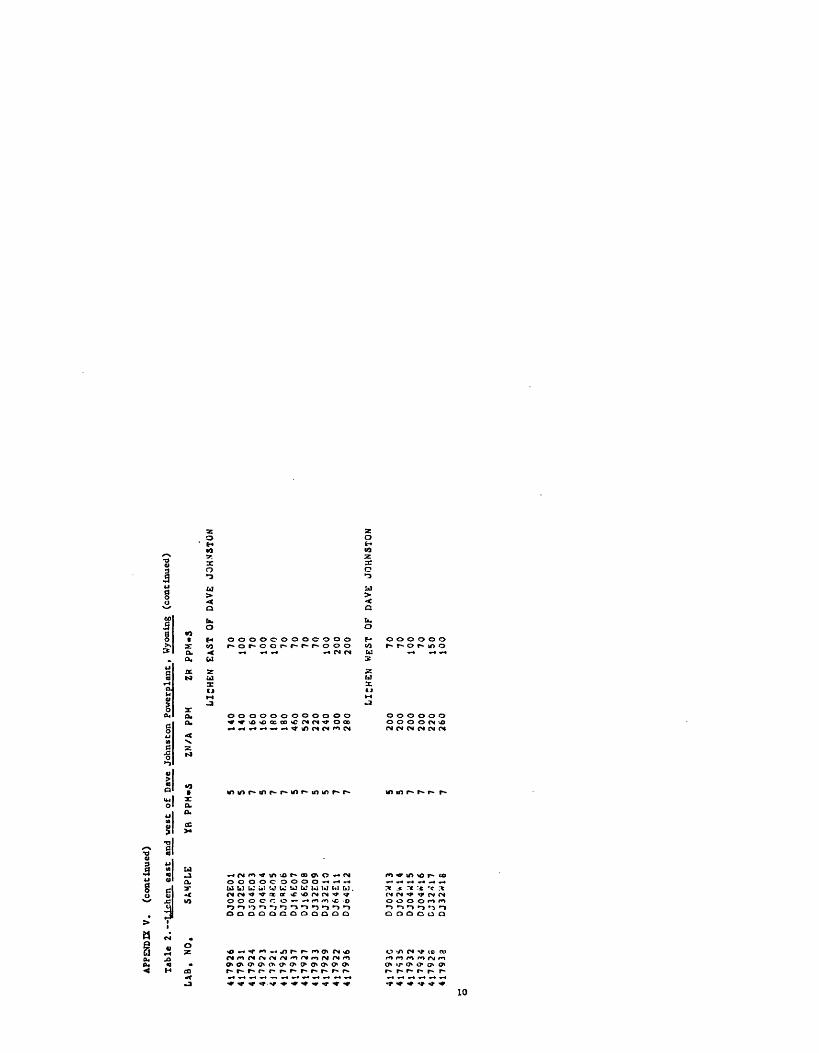
APPE

NDIX

V.

(con

tinu

ed)

Table 2. Lichen ea

st an

d ve

st of

Dave Jo

hns to

g Powerplant,

Wyoming

(continued)

LAB. NO.

SA4PLE

YB PPM-

417926

417931

417924

417923

417921

417937

417927

417933

417929

417922

417936

OJ02E01

DJ02E02

OJ04

F:03

DJ04E04

DJ.T

BCOS

DJ16E07

OJ16E08

DJ32E09

DJ32E10

DJ64£l 1

DJ64E12

41793C

417535

417932

417*34

41792S

417932

DJ02W13

DJ04W15

OJ04«16

CJ32

«'l7

DJ32-1B

I«S

S S 7 5 7 7 5 7 5 5 7 7 S 5 7 7 7 7

ZN/A PPM

ZR

LICHEN

140

140

160

160

180

180

460

520

220

240

300

280

LICHEN

200

200

200

200

220

260

PPM-S

EAST OF DAVE JOH-VSTON

70100 70

100

100 70 70 70 70

100

200

200

WEST OF DAVE JOHNSTON

70 7010

0 70150

100

APP

END

IX V

. CH

EMIC

AL

ELEM

ENTS

IN

VEG

ETA

TIO

N A

ND

SOIL

NEA

R C

OA

L-FI

RED

PO

WER

PLA

NTS

, W

ESTE

RN

ENER

GY

REG

ION

S (c

on

tin

ued

)

Tab

le

3.

LAB,

NO

,

164963

164123

164965

16

49

24

1

64

94

9

164°5

6

1*

49

17

1649U

1

64

^74

16

49

20

16

49

76

16

*9

30

164912

If'5

93

4

-Surf

ace

and

subsu

rfac

e so

il,

and

sag

ebru

sh at

Jim

Bri

dget

Po

wer

pia

nt.

W

yom

ing

SAM

PLE

164Q

67

16497*

1M

964

U 4910

16 * Q 7 2

16*986

164973

164^02

U, 4 c 9 3

!*497e

164977

16-959

164945

16493^

164<V13

164935

164^3?

164971

164908

164922

164^04

K3

H.V

1B

S1

K 3 P

'i *4 p,

1

K3HM5AS1

K 3 H

"- 2

* S

Si

AS

1

C.3«S3AS1

K3eSiA5l

" .V

.: 5

< S 1

K j!

«* )

HS

l

164»97

1649S1

1649QO

LATITUDE

41 41 41 41 41 43 41 41 42 42 41 41 41 41 41 41 41 41 41 41 41 41 41 41 41 4 1

41 41 41 41 41 41 41 41 41 41 41 41 41 41 41 41 41 41 41

44

44.

46 46 49 49 - 7

57 06 06 44 44 44 44 42 42

43 43 48 43 43 43 43 42 42 42 3a 3? 32 32 20 20 '. 4

44 '.4

44 46 46 45 45 45 40 40 40 40

25N

25!v

05N

0«>N

50&

50N

45M

45N

4.7N

47N

25-J

25N

20"

2 OK

14SN

45 M

ISM

15N

40N

4QN

3 ON

3 ON

3 0 N

OOM

OC*

0 V«

4bN

4SN

3 ON

'30*

5511

5.5 N

20N

20^

20^

20k

1 ON

ION

25^

25S

30"

35N'

35N

35N

35N

LONGI.TUD

109

108

108

10B

103

103

10B

10"

100

109

10«

JOB

10*

10*

10*5

10s

109

10*5

107

107

10?

109

1 C

flIDS

10B

10e

IOR

10s

109

103

10P

10»

10"

J 0^

IOR

108

iOR

108

109

1C9

109

109

109

109

109

4646

46 46

48 4H 55

5500 00 45 45 42 42 25 25 Cy 08 34 34 46 4(3

4*5

45 45 45 46 4h 4242 44 44

47 47 50 50 51 54 04 04 22 57 57 57 57

SURFACE

30^

30V

504

50*'

low

10"1

404

40*

25*

25 4 SURFACE

25^

25^

So 4

50*

5* A'

55"'

00"!

oow

00*1

00*

SURFACE

15"

15 d

15^

00-J

OCrt

00"

55V

55V

15*

15V

05-"

05V SURFACE

55«l

55^

oov

QQtl

2S V

25V

20W

2 CM

55>"

05V

OS-*

05^

05*

KMAL

* i AL203

%

SOIL NORTH OF

JI

M ERlDGER

1 1 3 310 10 25 25 42 42

SOIL EAST

2 2 6 6 30 30 54 54 100

100

SOIL SOUTH

2 2 2 5 5 5 9 922 22 45 45

SOIL

WEST

2 2 5 5 12 12 25 25 50 50 98 98 98

7 7 3 3 5 3 7 5 7 7

OF J

IM 10 5 3 3 7 7 7 7 7 7

OF JIM 2 5 2 3 2 2 5 3 3 7 5 7

OF J

IM 3 5 3 5 1 1 5 5 7 7 7 7' T

12 42 5 7 7 10 9 10 9 9

BR1DGER

G 14 5 6 7 9 fe 10 11 10 11

BPIDGER

4 5 5 4 4 4 fr 6 9 fl 8 8

BRIDGER

5 7 5 8 2 2 7 8 to 10 12 11 12

.173

.181

,709

.232

.470

,013

,681

,055

.804

,600

,228

.831

,849

. 1 7

H,9

67,835

,586

,286

.R51

,512

,H56

.645

,930

.881

.592

,fi?

fc.060

.467

.374

,376

.787

,598

,792

,2*0

,653

.2"*

.2*2

.085

.438

,20r>

,730

.3R9

.257

.719

,102

B PP

M

30 50 30 50 30 30 20 30 20 30 70

30

30

30

30

30

30

30 20 20 30 30 30 30 30 20 50

50

20

20

0 L

300

L

BA

PPM

50

07

00

50

03

00

50

05

00

1500

70

07

00

70

0

700

700

300

bOO

7

00

700

700

700

700

700

0 L

300

L30 20 20 50 30 30 70 20 30

700

500

700

500

bOO

500

500

500

500

SOU

700

700

70

07

00

50

05

00

70

05

00

300

700

700

700

15

00

15

00

BE

PP

M

1.5

1

.50

,OL

O.O

LO

.ON

0,0

*1.5

1.5

1.5

1.5

1.5

O.O

LO

.OL

O.O

L1.5

O.O

LO

.OL

1.5

O.C

L1.5

O.O

NO

.ON

0,O

NO

.ON

O.O

NO

.ON

1.5

0,O

LO

.OL

1.5

O.O

NO

.ON

O.O

L

1,5

O.O

L

1.5

O.O

N

O.O

N

0,O

L1.5

1.5

O.O

L1.5 O.OL

O.

OL

C%

0,2

0.2

0

,8

0.8

0.1

0

.5

0.8

0.2

0.7

0

.&

0.4

0.6

0.9

0,6

0,1

C.l

L0.5

0.5

0(

1L0

.1L

0.3

0,2

0,2

0.3

0.3

0.3

C.l

L0

.1L

1.1

1.1

0.1

L0.1

L

0.1

O.I

0,9

0,2

0.1

L0

.1L

2.4

2.3

1.1

1.0

0.8

0

,8

0.7

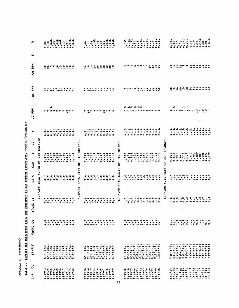
APP

EN

DH

V.

(conti

nued

)

Tab

le 3

. S

urf

ace

and

sub

surf

ace

soil

, an

d sa

geb

rush

at

Jim

Bri

dger

Pow

erpla

nt.

W

yom

ing

(co

nti

nu

ed)

LA

B,

1649*3

164923

164965

164924

164949

16

49

56

16

49

14

164974

164976

16-1

930

1*4

*12

164^3

4

16491.,

16

*53

6

164967

16

49

75

164964

16

4S

99

16

49

46

164972

1 f-

-\ 9

f. 6

164=

*73

16

40

70

16

49

59

164945

16493S

I

6 -i

9 2

9 if 4

<» 1

316

45

351

64

93

9

1*4971

1 ?

4 9 0

3

1*

49

22

16

49

04

164951

SA

MP

LE

K3H

-.1A

S1

K3M

1B

51

K3F-

.H2

AS

1

K3R

K3A

S1

K3

BM

KS

1

K3P

S18S

1

JS4A

S1

X3

PS

5A

S1

K-3

PM

AS

I

K 3

=i *

4 A

S 1

ORGM

C c%

2,9

2

.4

0,4

0.5

1.0

0

.4

C.5

1.1

0.5

1.0

1.7

2.2

1.9

2.1

0

,8

0,9

0

,9

0.7

2

,0

0,7 1,2

0

.3

0.4

0.4

1.8

1.3

2,4 us l.R

1

.00

,8

0.9

0,5

1,7

3

,10

,80

,31.2

0.8

0

,P1.3

1,1

0,3

0,6

TOTAL C% SURFACE

3.C

2.6

1.2

1,3

1.1

0,9

1.3

1,3

1.2

1.6 SURFACE

2,1

2.9

2,8

2,7

0,9

0.9

1.4

1.2

2.0

0,7 SURFACE:

1,5

0,4

0.6

O.T

2.1

1.6

2,4

l.o

2,6

2.9

1,0

. 0.

8 SURFACE

1.0

0.6

2.5

3.3

0.8

0.3

3,6

3.1

1.9

2,3

1.9

1,1

1,3

CA %

CAO

% CL

%

SOIL NORTH OF JIM BKlDGER

0.7

0,7

2.0

3,0

0.5

1.0

3,0

1.0

3.0

3.0

SOIL EAST OF

2,0

' 2.0

3,0

1,5

0.7

0,5

3.0

2.0

0.7

0.5

SOIL SOUTH OF

1.0

0,7

0,7

1,0

1,0

1.0

0.5

0,3

3,0

3,0

0.5

0.5

SOIL rfEST

OF

0,7

0.5

3,0

1,0

0,2

0.1

7,0

5.0

5,0

3.0

5,0

5.0

5.0

1.415

1.318

2,757

3,628

0,879

2.030

4,780

2.107

3.41*>

3,380

JIM BPIDGER

2.348

1.482

4,045

0,547

1.003

0.747

3.020

2.822

0.834

0.6&7

JIK 9FIDGES

1.633

0,835

0,893

1.427

1.388

1,414

0.51&

0.434

4.739

4,«9(*

0.771

0.76«

JI"1 BRIDGED

0.923

2,655

3,909

-3, Os 4

0,273

0.138

8.412

8.561

6,259

6.287

6,205

6,321

6,078

0.1L

O.lL

0.1L

0.1L

0.1L

0.1L

0.1L

O.lL

0.1L

O.lL

O.lL

O.lL

0.1L

0.1L

O.IL

0.1L

0.1L

0.1L

O.lL

0.1L

O.lL

O.lL

O.lL

O.iL

0.1L

0,1L

O.lL

O.lL

0.1L

O.lL

O.lL

O.lL

0.1L

O.iL

0.1L

0.1L

O.IL

0.1L

O.IL

O.lL

0,IL

0.1L

O.IL

P.1L

O.IL

CO

7 7 0 L

S 7 7 710

7 7 730

7 5 7 710 7 7 5 0

L 0

L 0

L 0

L 0

L 0

L 7

. 5 7 7 7 7 5 0

L5 7 0

L0

L7 7

107

10

107

CR

PP

M

70 50 15 70 30 30 7,0

50 50 30 70 30 30 30 30 30 70 70 30 30 7 10

7 15

10

10

30

3o

50

30

30

50 30 15 30 50 15 10 30 50 50 70 70 70

70

CU

PPM

30 20S 7

20

15

10

10

15

10 30 10 10 20 20

30

30

30 20 10

2 3 3 5 3 3 7 730 20 10 15 105

10 157 3 15 15 10 15 30 10 15

0,0

50

,10

0.0

4L

0.0

80.0

4L

0.0

4L

0.1

30

.07

0.0

4L

0.0

4L

0.0

60

,11

0,0

40.0

4L

0,0

50.0

60.0

40

.04

L0

.04

L0

.04

L

0.0

4L

0.0

4L

0.0

4L

0.1

10,0

80.0

4L

0.0

70

.04

L0

,06

0,0

70.0

4L

0,0

41

0,0

«L

0,1

00

.05

0.0

40.0

4L

0.0

4L

o.cs

0,1

0O

.C6

O.C

4L0,0

50,0

50,0

4L

APP

END

IX

V.

(conti

nued

)

Tab

le

3,

LA

B,

KO

,

16

49

63

16

49

23

16

49

65

16

49

24

1

64

94

9

16

49

56

164917

15

49

U

16

49

74

1

64

92

0

16

49

76

1

64

93

0

16

49

12

1649J4

1

64

91

6

16

49

36

16*567

36

49

75

1

64

96

d

16

4*

99

16494*

1649JO

1

6*

97

2J*

4S

86

164973

Surf

ace

and

subsu

rfac

e so

il,

and

sageb

rush

at

Jim

Bri

dger

P

ow

erp

len

t.

Wyo

min

g (c

on

tin

ued

)

16

4^9

3

16

49

70

1 £

;9?,

9

11-4

977

164959

164^4

5

164938

If,'

'12

9

16

49

13

16*935

164=

53"

164971

', 6

4 9

* ?

164922

1*4904

164944

164*97

16

45

51

1

64

90

0

SAMP

LE;

K3

BM

AS

1

K3&

F.1A

51

K3

»»

ei8

Sl

MR

F2A

S1

K3B

S1A

S1

Kjp

sies

i K 3

* s i

* s 1

A 3b

S3A

,:ii

K 3 F

*' 1

A S

1

* ' 3 '

= *

3 A

s 1

K 1

a A

V-<

5 I

K3n,4

HS

l K

3R.»

5AS1

K

s^f.

AS

lK

3H/.6

AS

1

FE

%

2.0

1

,5

1,0

1.0

2

,0

1,5

1,5

1,5

2

,0

1.5

2,0

3.5

1,5

1,5

2,0

2

.0

2,0

3

,C

1,5

1,5

0,3

0.5

0,5

1,0

0,7

0

,7

1,5

1,5

2.0

2,0

1.5

2.0

1,0

0

,7

1.5

1.5

0,3

0,3

1.5

1.5

1,5

!,

5

2,0

2

,0

2.0

GA

PP

M

K %

K20

%

LA

SUR

FAC

E

SO

IL

NO

RTH

O

F JI

M

&R

IDG

ER

15 157

10 10 10 15 15 15 15

SURFACE

-20

10 10 10 15 15 15 10 15 15 SURFACE

7 7 7 7 7 7 7 7 10 15 10 15

SURFACE

10 107

100

L0

L15 10 15 15 15 15 15

3 3 2 3 3 3 3 3 3 3

SOIL EAST

5 3 2 2 3 3 3 3 3 3

SOIL SOUTH

3 3 3 3 2 3 2 2 3 3 3 3

SOIL

WEST

3 3 2 2 0 M

0 M

3

2,693

2,791

1,711

l.S-iO

2,253

2.2C4

3.3H7

2,5<

>fl

2.2C9

2,224

OF Jl

f" BRIDGER

2,663

2.207

1,622

2.3HO

2.442

2,235

2,317

2,354

2,792

3,075

OF JIM BRIDGE*

2,196

2,1«7

2,220

1,803

1.692

1,719

1,56*

1,611

2.0f

,52,021

2,375

2,249

OF JIM BF

<IUG

ER

2,'0

531,675

1,385

1,941

0,417

0,286

1,«23

2,15

.02.110

2,092

2,3(1

2,225

2,325

50 500

L0

L0

L0

L70 0

L700

L

700

L0

L0

L50 50

700

L70 50

0 L

0 L

0 L

0 L

0 N

500

L0

L0

L0

L0

L0

L

0 L

0 L

0 L

0 L

0 L

0 L

0 L

50

500

L70 70 50

MG

%

0.7

0

,7

0,7

0,5

0

,7

0,7

1.5

0,7

0,7

0

.7

0.7

0

.7

0,7

0

.7

0,7

0

,5

1,0

i,

0

0,3

0

.3

0.2

0

,2

0,2

0,3

0,2

0.3

0,3

0,2

0,7

1,0

0

,5

0,7

HG

Q

1,3

81.4

11,2

20

,84

0,8

91

.38

2,3

81,4

11

,62

1,6

4

1,0

3

1,6

7

1,1

8

1,2

0

M2

1

,76

1,7

5

0,b

7

0,6

4

0,1

70,2

2

0,2

0

0,4

0

0,

jR

0,4

3

0,4

3

0,3

d

l.tf

l 1

,78

0,6

b

0 0 0 0 0 0 050 50

070 70 50

L L L L L L L L

0,5

0,2

0,5

0.5

0,1

0,1 2,0

2,0

1.0

0.7

1.0

0,7

1,0

0,6

20,3

31,0

00

,bl

0,1

60,1

03,2

b3.2

22,1

7I,

b8

1,7

61

,66

1,7

5

MN

PPM

30

0

20

0

20

0

150

$0

0

30

0

30

0

30

0

30

0

30

0

30

03

00

50

02

00

30

0300

30

03

00

30

01

50 70 70 70

15

01

00

10

02

00

150

20

03

00

30

03

00

15

01

00

50

03

00 70 50 300

20

05

00

300

50

05

00

50

0

UN

O

0,0

52

0

,05

0

0,0

25

0,0

27

0,0

61

0.0

34

0

,07

2

0.0

5S

0,0

58

0,0

61

0,0

75

0.0

2C

L0,0

93

0.0

20

L0

,06

20,0

40

0,0

b9

0,0

60

0,0

47

0,0

24

0.0

20

L0

.02

0L

0.0

2C

L0

.02

0L

0.0

20

LO

.C20

L0,0

34

0,0

23

0,0

47

0,0

49

0,0

35

0,0

49

0,0

26

0,0

36

0,0

72

0,0

24

0.0

20L

0.0

20L

0,0

53

0,0

51

0,0

76

0,0

63

0,0

74

0,0

75

0,0

71

APP

EKD

EC V

. (c

onti

nued

)

Tab

le 3.-

-Surf

ace

and

subsu

rfac

e so

il,

and

sage

brus

h at

Jim

Bri

dg

er P

ower

iila

at.

Wyo

min

g (c

onti

nued

)

LA

B.

NO

. SA

SPL

E

MO

PPM

M

A20

%

NB

PPM

NO

PP

M

NI

PPM

P

205

%

164563

164923

164924

164949

164956

164517

164914

164974

164920

164976

U4930

164912

164S34

164916

164936

1*4967

1*4964

164&99

1 : 4 9

I :

1545 12

lA-i^c

164973

1-.4

9C2

164993

164970

U.4969

1*4977

164559

164933

l*492r

1649

1s

1645j»

16497'

K3R

MB

S1

K

3BN

2AS

1

1^ 3

r1 \f'

S H

S 1

N3

=:S

lh{>

l K

? H

S <

r» S

1

K3-

VS

4.1S

1

K 3

6 '

1 A

S 1

16^

*22

164*97

164951

16*900

0 L

0 L

0 N

o »

0 L

0 N

3 0 L

0 N

0 L

3 0 L

0 N

0 N'

3 0 L

0 N

0 L

0 L

3 0 N

0 N'

0 N

3 o r,

o N

o «

3 0 W

0 L

3 0 L

0 N

o a

o L

0 L

0 L

3 0 L

3 0 N

0 L

0 L

3 0 N

20

% SURFACE

0.68

0.72

0,93

0.88

0.96

0,92

1.61

1."

1.37

1,40 SURFACE

0,59

0,79

0,42

0.52

1.01

1,10

1.2&

1.23

1,61

1,89 SURFACE

0,77

0,85

0.&3

0,50

0,56

0,55

0.24

0.21

0,64

0.68

1.34

1.26

NB PPM

SOIL NORTH

0 L

100

L0

L0

L0

L0

L0

U0

L0

L

SOIL EAST

lb0

L0

L0

L0

L100

L0

L0

L0

L

SOIL SOUTH

0 L

0 L

0 L

0 L

0 L

0 u

100

L0

L10 0

L0

L

SURFACE SOIL WEST

0.95

1.01

0.39

0,35

0.1S

0.10

0,63

0.67

1.84

1.79

1.81

2.00

1.88

0 L

0 L

0 L

10 0 N

0 L

0 L

0 It

0 L

10 0 L

100

L

N[> PPM

NI

OF JIM BRIOGCK

70 0

L0

N0

N'

0 L

0 N

vo 0 L

700

L

OF JIM SRIDCER

700

L0

N0

L70 70 0

L0

L.

70 0 L

OF JIM BRIDGKR

0 N

0 N

0 L

0 B

o a

0 L

0 N

0 N

0 L

0 L

0 L

0 L

OF J1K BH1DGER

0 H

0 iJ

0 L

0 L

0 «

0 N

0 N

0 N

0 L

0 L

70 0

L0

N

PPM

15 15 7 7 720 30 20 15 15 20 10 10 15 15 15 20 20 15 10 15 0

L5 7 105 15 15 15 15 10 10 157 15 15 150

L

10 15 10 10 157 15

0.147

0.113

0.100L

0.1OOL

0.1UOL

0.100L

0,147

0.100L

0.100L

0.100L

0.100L

0,10

01,

0.100L

0.1GOL

0.100L

0.100L

0.10CL

0.100L

0.100L

0.100L

0.100L

0.100L

0.100L

0, lOOL

0,10

«">L

0.1OOL

0.1OOL

0,1OOL

0,10

01,

0.100L

C.100L

0.100L

0.100L

0.10CL

0.100L

0.100L

0.10CL

0.100L

0, 100L.

O.JOOL

0.100L

O.lOOb

0.100L

0,1 OOL.

0.100L

PB

PPM

15 15 15 15 20 15 15 15 15 15 30 20

15 15 15 15 15 15 15 20 10

15

15

lb 15 15 15 15 20 30 15 20 15 15

15

IS

20 20 2

020 15 15 20

20

TOTA

L S%

0.0

40L

0.0

43

0.0

40

1*

O.M

OL

0.0

40

L0.0

40L

0,0

401

0.0

40

L0.0

40L

0.0

40L

0,0

53

0.0

*O

L0

.04

CL

0.0

40L

0,1

18

0.0

40L

0.0

40L

0.0

40L

0.0

4O

L0

.04

0L

0.0

40

L0.0

40L

0.0

4O

b0.0

40L

0,0

4C

L0.0

4C

L0

.04

0L

0.0

41

0.0

40L

0.0

40L

0.0

40L

0.0

40

L

0.0

47

0.0

40L

0.0

53

0.0

40

L0

.04

0L

C.0

40L

0.04CL

0.040L

0.040L

O.C40L

0.040L

0.040L

0.0401

SC

PPK

157 5 5 7 7 10 10 7 7 0

» 0

L 0

N C

L 0

N 0

N 7 5 7 7 7 7 5 0

L 7 7 0

N 0

N

7 7 7 7 107 10

APPE

NDIX

V.

(con

tinu

ed)

Table

3.

LAB.

K'0.

164963

164923

164565

164924

164949

164556

164917

1649M

164974

164<>20

164976

164930

164912

164934

SAMP

LE

1649

34,

164975

16*964

164899

! f-1

943

U 4 >

! 0

I 6 4 9

; 2

l649n6

164?73

J64902

164995

16497Q

164977

164945

16*929

1^490*

164522

164904

164944

164*97

U4951

164900

Kjrtt'AASl

K3?C*H51

*3f S5HS1

K 3^5*31

KjPSjASl

"3«S3AS1

K"3BS3-«Si

K3f»

54*5

1* 3*

5 -^51

l ASl

K3a»

:4AS

i

SI %

10 G

10 G

10 G

' 10 G

10 G

10 G

10 G

10 G

1 rt

f*1 U u

10 G

10 G

10 G

10 G

10 G

10 G

10 G

10 G

10 G

10 G

10 G

SI02

% SURFACE

68.104

63.839

66,848

79.403

71.654

BO. 056

58,475

74,509

73.558

73.433 SURFACE

65.712

87,336

75,933

85.215

72.146

8b,162

70.751

71.173

74,438

73.829

SR PPM

wwEipiaui. Wyoming

iconr

II

* TIQ2

%

SOIL NORTH OF JIM BHIDGER

150

150

150

150

100 70

1000

300

200

200

SOIL EAST

300

150

ISO

100

150

150

200

200

150

150

SURFACE SOIL SOUTH

10

r,10 G

10 G

10 G

10 G

10 G

10 G

10 G

10 G

10 G

10 G

10 G

10 G

JO G

10 G

10 G

10 G

10 G

10 G

10 G

10 G

10 G

10 G

10 G

10 G

76,307

84.272

90,592

8.1.033

39.153

88.974

86.312

83.fl3f?

70.725

7C.548

84.954

70,357 SURFACE

55,281

78,003

80,3

3ft

79.079

72.979

96,659

64.055

63,691

67.691

66.223

67.910

66,423

67.797

100 70

100

100 70

100

100 70

150

150

150

150

SOIL WEST

150

150

200

200 70 50 200

300

700

500

500

300

700

0,20

0.531

0,20

0,544

0,15

0,264

0.15

0.295

0.15

0,395

0.20

0,389

0.30

0,681

0,20

0,421

0.3°

0.461

0,15

0,489

OF JIM BRIDGES

0,20

0.615

0,15

0,104

3.15

0,373

0.15

0,177

3.15

0.44ft

3.20

0,349

0.20

0,493

°»3°

0,493

0,20

0,428

0.15

0,313

OF JIM BPIDGER

0.07

0.083

0..1

0 0,1

Ofl

'3.07

0.113

0.15

0,157

0.07

0,148

0.10

0,15

>7O.t5

0,333

«>,15

0,336

°.2°

0,476

0,',JO

0,476

0.?.

5 0,331

0,20

0,399

OF JIM bFlDGER

'),15

0.283

O.J5

0,370

0,15

0,318

0 .

' -5

0,313

0,07

0,118

0.07

0,118

O.lb

0,384

0,15

0,392

0.15

0.472

0.15

0,476

0,20

0.446

0.20

0.411

0.-20

0,471

70 70 30 70 50 50 70 50 70

70

150

70 70 70 70 70 70 70 70 70 20 30 30 30 30 30 70 30 70 70 50 70 50 30 50 70 30 30 70 70 70 70 70 70 70

Y PPM

15

20

15

15

15

15

IS

Ib

15

20 30 15 15 15 20 15 15 15 15 15 0 L

10 0 L

U L

0 L

15 15 15 15 20 15 15 IS 10

15

20 0 L

0 L

15 15 15 15 15 15 15

PPM

1.5

1.5

1.5

1.5

1,5

1.5

1.5

1.5

2.0

2.0

2,0

1.5

1,5

1,5

2.0

2.0

1,5

1,5

1,5

2,0

O.OL

1.0

O.OL

1.0

1,0

1.5

1.5

1.5

1.5

2.0

1.5

1.5

0,OL

1,5

2.0

O.OL

1.0

1.5

1.5

1.5

1.5

1.5

1.5

1.5

ZR PPM

150

150

ISO

100

200

300

200

150

300

300

100

150

200

150

150

300

200

ISO

200

100

70100 70

100

70200

300

200

200

200

300

200

150 70

150

200 70

150

150

150

150

150

100

100 70

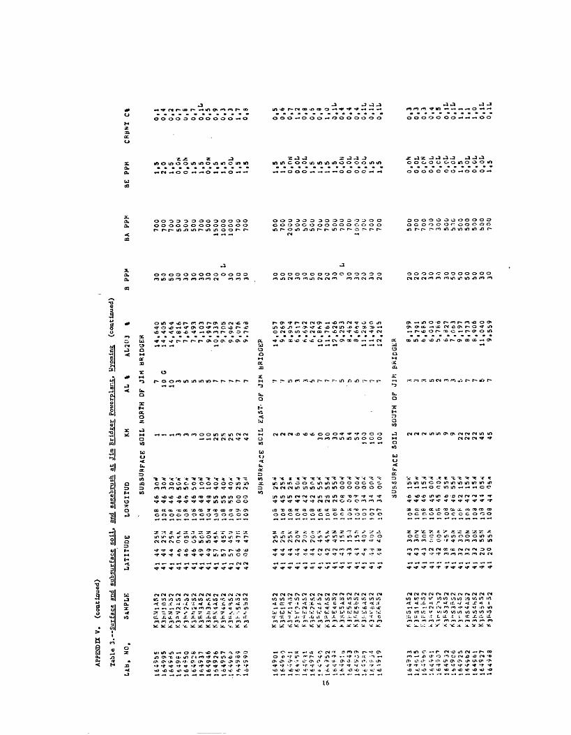
APP

END

IX V

. (c

on

tin

ued

)

Tab

le 3.-

-Surf

ace

atid

su

bsu

rfac

e so

il,

and

sag

ebru

sh at

Jim

Bri

dger

P

ow

erpla

r.t.

W

yom

ing

(co

nti

nu

ed)

uu,

NO.

SAMPLE

LATITUDE

LOMGIT

UD

KM

AL %

AL

2t>3

%

B PPM

16

*9

95

16

4*

50

16492ft

164937

16

49

46

1

54

92

6

16

49

57

.1

*4<*

6,3

J *>

4 9

5 5

164S

9U

1649

Q1

16.4

9,.:)

1 6 '

c> '

1 !

6 *

> S

R 1A

4<V

U

16497ft

I 6 4

? 3

J

1649

In

1649

431

6^0

3

i 6 4

5 s

7If.

4?j4

16

1*

19

164933

lf.4015

1 6

-i v 6 0

: (, 4

v <» i

1649C.1

164532

14.49C6

164525

164562

16*561

lt4S

27

164963

SAMPLE

KJPJJ1AS2

K3hH!OS2

K 3

F- N

j * 5 2

K 3 a S 2 i 5 2

fk'3H%2A52

K3*°'2

i;S2

K3BM3AS2

K 3 h N 3

r- S 2

K3&N4A52

K3HV4KS2

.«' 3 K N 4 S S 2

K3S-'"'5A31

N3r,>.

5bS2

K 3

"*. t'

j A S 2

K3^El RS2

K 3 J

1. 1

*> 5 2

K 3 1

1" ? - S ?

S3*E2AS2

K 3 c K ? p

,s 2

*3~7;i;S2

K 3

F. 4 A S 2

h 3>

-E4t

iS2

H3SS5AS2

KJi-r;5AS2

K3r<E5bS2

*3.!-t6AS2

K3-*t'

f;AS

2*3

er-.

*wS2

LATITUDE

41 41 41 41 41 41 41 4 1

41 41 41 42 42 41 41 41 41 4l 4 1

41 4 1

41 41 41 4 1

41 41 41

44

44 44

Af)

4b46

494?

57

57 57 06

Ofc

44 44 44 44 14

44 <2 42 42 43 43 4 )

Ay

Vd

48

25N

2 S

,'i25*

OSN

05 N

OS'

450"

SON

45k

45fi

45?J

47fi

47M

25N

25'<

25K

20^

2 ON

7 0«

45:»

4SN

45N

15N

15.)

15*1

4Q^

A r; \

4 ON

LO^GITUD

108

loa

1 0" ioa

108

10*J 108

10M

10^

108

101

109

109

105

torf

10P

1 0*

!0«

108

10*

1 OKJOB

1 nt>

ion

1 0^

107

107

107

46

46

46 464o 46

43 4855

55

55 00

CO

4S 45

45 42

42

42

25 2S 25

OR Od 0^ 34 34 34

SUBSURFACE

30*

304

304

50*'

504

504

10W

104

404

40*

404

254

25//

SUBSURFACE

25*'

25*

25*

504

504

504

554

554

55^

004

004

004

00*:

00/1

00/1

SUBSURFACE

*3i;Sl A52

K3CS1*S2

:-'.

iFSj

bS2

* 3

;; *» 2 i S 2

^rS2'ts2

K 3^53 AS2

* 3 " S 3

fc S 2

» 3

' S

-i f> S 2

* 3BS4A32

"3hS4bS2

K3f<S5ftS2

*3K35-52

41 4 1

41 41 41 4 1

41 41 41 41 41 41

43 43

43 52

42 38 38 32 32 32 20 20

30^

3nv

3nf>

00 M

00N

45<*

45M

3 0

'"'30N

3 ON

55M

S5N

1QH

ion

i 08

10B

JOB

10^

1 oB

10H

in?

1 03

108

109

46

46 46 45 45 4b 46

42

42 42 44 44

15".

'15*

1 54

004

004

55*

55r)

154

154

154

05 4

05*

KM

AL %

SOIL NORTH OF JIM

1 1 1 3 3 310 10 25 2S 25 42

42 SOIL

EAST- OF

2 2 2 6 6 630

30 30 545454

JOO

ICO

100

SOIL SOUTH OF

2 2 2 5 S 9 92222 22 45 45

710 G

103 S S 5 5 7 7 7 7 7

JIM 7 '/ !i 1 3 5 7 7 i 5

N U b 7 7 ''

JIM 3 3 ;i 5 2 3 3 c, 7 7 5 7

AL203

%

HRIDGEH

14 14 147 7 7 7 9

109 9 9 9

BRIDGEP 149 H 6 6 6

1C 11 179 R B

11 11 12

&RIDGER 8 5 6 6 b 6 7 9 8 8119

, , , , , , . , , . , , . . , . , , ( . . , , , . . . . , , , . , t , , , , , ,640

405

464

816

f>4.7

491

103

947

339

705

962

076

768

057

269

Qb4

517

692

242

8h9

761

626

253

4b2

664

2nO

4tfO

215

199

791

685

010

7B6

«*27

063

197

773

906

040

559

BA

30

50

50

30

30

30

30

30

20 0

L

30

30

30 20 2020 30 30 30 50

505050 30 30

700

700

700

500

500

SOU

700

500

1500

1000

1000

700

700

30 50 20 30 30 50 20 20 300

L30 30

20 30

20

500

700

20GU

50o

bOG

500

700

700

500

700

700

1000

70U

700

700

500

700

700

voo

300

500

b.i<;

500

500

500

500

700

BE PPM

1,5

2,0

1,5

0,ON

O.O.

N1,5

1.5

O.ON

1,5

1,5

O.OL

1,5

1,5

1,5

1,5

O.ON

O.OL

O.OL

1,5

1,5

1,5

1.5

O.GU

O.OL

O.OL

O.Ob

1,5

1,5

O.ON

O.OL

O.CN

O.OL

O.CL

0,01*

O.OL

1,5

O.OL

O.OL

O.OL

1,5

C%

0,1

0,4

0,2

0,7

0,6

0,7

O.lL

0,5

0.9

0.3

0,3

1,7

0,9

0,5

0,6

0,7

1,2

0,8

0,6

0,8

1,0

O.lL

0.4

0,4

0,4

O.lL

0.1L

0,1L

0,3

0,3

0.3

0,4

0,5

O.lL

O.lL

1,1

1,1

1,0

0.1L

0.1L

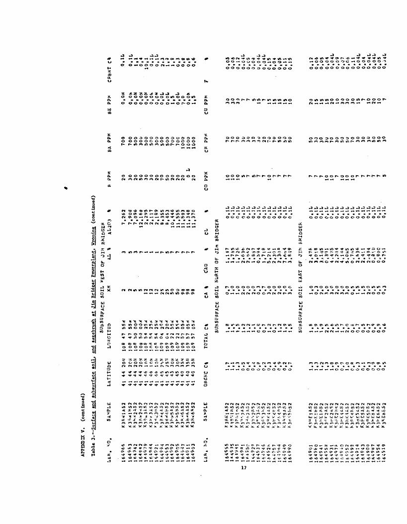
APP

END

IX V

. (c

onti

nued

)

Tab

le 3. S

urf

ace

and,

subau

rfae

e so

il,

and

sageb

rush

at

Jim

Brl

dger

Pow

erpla

nt.

W

yom

ing

(conti

nued

)

16

49

66

1649S

3

164992

16

4^5

3

16

45

92

1

64

90

5

16494;

164911

16

45

03

16

45

S5

1*4535

1 A

4 ?

5 0

16

4S

37

Jf

t 4945

11 4

"5 »

S

1 6

4 9

4 9

164901

16

45

60

164941

16

45

53

16

49

31

J r.

4 9

4 0

1*<

952

16

45

93

16

49

43

16

49

0?

16

49

H7

164954

SAMP

LE

K3FUU52

K3

--O

A5

2

K 3?

. MA

3 2

K 3 f » 5 8 S 2

SIMPLE

K3b

V3^

S2

K 31

- E 2

5* *

2

K3H

K-U

S2

LATI

TUDE

41 41 41 41 41 41 41 41 41 41 41 41 41 41

44 44 44 44 46 46 46 45 45 45 45 40 40 40

20M

20K

20*

20V

ION

ION

lofo

?SN

^5N

30N

30N'

351*!

15W

35N

108

JOB

10e

JOB

10P

1 ftf

l10"

109

109

109

1G9-

109

109

109

47 47 bO 50 54 54 54 04 G-t

22 22 57 57 57

55*

55«

OO"'

OOrf

25W

25*

25W

20«<

20-*

55 *

5S"

05W

05rt

05W

SOIL K

EKM 2 2 5 5

12 12 12 25 25 50 50 98 98 98

ST OF Oi

lAL

'

3 5 3 7 1 1 1 7 5 7 7 7 7 7

AL2P3

%

3 5 3 7 1 1 1 7 5 7 7 7 7 7

7.2

62

7.9

0B

7,0

96

12

.16

62,2

^5

2,1

17

2.1

99

8.3

55

8.4

53

10,4

46

11,5

55

11

.59

31

1.3

48

11

,37

0

ORGN'C

TOTAO C%

CA %

C"AO

CL

SlT

RSl

'BFA

CE

S

OIL

N

OR

TH

OF

Jln

B

RID

GE

R

K3F-

E6AS

2

1,7

1

,1

1.3

0.5

0

,4

0.4 o.e

0.2

0

.3

0.4

0

,9

0.2

0

,7

1.3

1.3

1.2

1.3

1.8

0.9

0.9

1.0

t>l3

0.1

0.3

0,9

0

,9

0.5

1.8

l.S

t.5

1.2

1.2

l.l

0.8

0.7

1.2

0.7

1.2

1.9

1.5

SUBSURFACE

1.8

1.9

1.9

2.5

2.6

1.5

1.7

2,0

0.8

0.7

0.3

0.7

0.9

0.9

0.6

0.7

i.o

1.0

2.0

2.0

2.0

0.3

0.7

3.0

2.0

2.0

7.0

3.0

SOIL

1.0

0.3

2.0

3.0

3.0

2.0

3.0

3.0

0.5

1.5

1.5

2,0

0.5

0.5

0.3

1.1*7

1.785

1,726

2 «63t>

2. 6*2

1.8S7

0 . b94

1.718

5.214

2.301

2.30«

7 1 6

15 4

3.8 19

EAST OF JIM

2,47*

3,018

3, Li 5

0,3'U

4.4V5

2,204

4,144

5.0H5

0..7H5

24636

2,411

2 .434

o a

\ o0

U3()C

0B7

«jl

O.lL

O.lL

O.lL

O.lL

O.lL

O.lL

O.lL

O.lL

O.lL

O.lL

O.lL

O.lL

O.lL

BHIDGER

O.lL

O.lL

0.1L

0.1L

O.lL

O.lL

O.lL

O.lL

O.lL

O.lL

O.lL

O.lL

O.lL

0.1L

0,1L

PPM

20

CO PPH

10 10 10 5 7 5 7 7107 7 7 7 7 7 7

10 107

10 10 107 7 7 7 7 5

BA PPM

700

30 20 50 30 30 20 70 50 20 20 200

L20

700

500

300

500

500

300

$00

500

700

70C

1000

1000

1000

C»

70 70 70 30 30 30 30 20 70 70 50 50 50 50 30 30 30 70 30 50 50 70 30 30 30 50 50 30

BE PPM

CU PPM

30 30 307 7 5

15 7

15

15

IS

15

10 20 15 15 15 20 10 30 30 30 157

10 20 107

O.ON

0,0

*0,

ON

O.O

NO

.ON

O.O

K0,

CN

O.O

L0,O

L1,5

O.O

L7

,0O

.ON

1,5

O.l

L

O.l

L1.1

0,4

10

,1O

.lL

O.l

L2.3

1.5

1.8

0.3

0.8

0.8

0.6

0.05

0.06

0.12

0.04L

0,C5

0.0*

U.04L

0.04L

0,15

0,04

0,05

0.11

0,15

0.12

0,06

0,05

0.04

0.04L

0,09

0,07

0.06

0,11

0.04L

0,04

0.04L

0.041

0,05

O.J4L

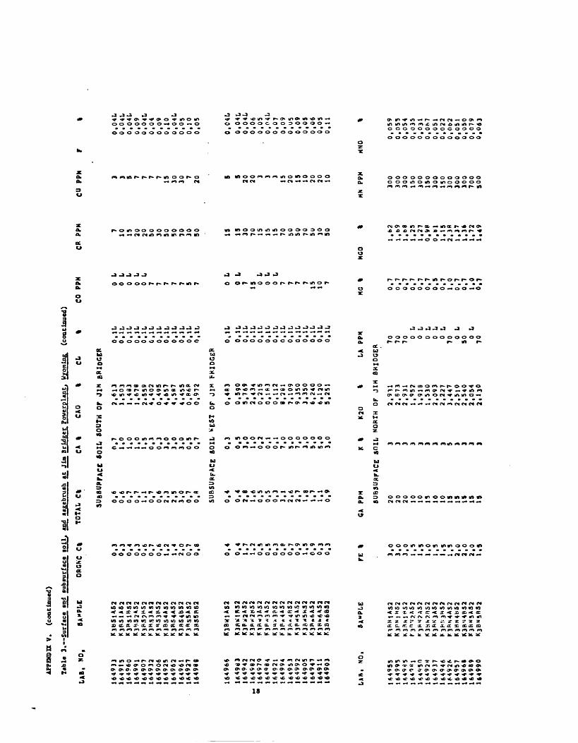
APP

END

IX V

. (c

on

tin

ued

)

Tab

le 3

. S

urf

ace

»nd

mbm

rfac

e lo

ll,

and

ngeb

ruih

at

Jim

Bri

dger

Po

ver

pla

nt.

W

yom

ing

(co

nti

nued

)

LA

B,

NO

. SA

MPL

E O

P.G

NC

C%

TOTA

L C%

C

* %

CAO

t

CL

% CO

PP

MPPM

CU PP

M

SUBSUPFACe

SOUTH OP JI

H

164933

164915

164960

1649

91

16490?

164932

164906

164923

164962

1649

61

164927

164981

164966

U49t)3

164942

*- 164982

» 164971

164484

164921

164994

164953

164992

164905

164947

1649

11

164903

K3PS1AS2

K3HS3AS2

K38S4AS2

K3RS4AS2

K3BS4bS2

K3BS5BS2

K3BW1B32

K3P«4AS2

0,3

0,3

0,4

0.3

0.6

0.7

0.6

1.2

1,4

2.0

0,7

0.8

0.4

0,4

1.7

1.2

0.5

0.3

0.3

o.e

0.7

0.9

1.3

0.9

0.3

0,3

0.6

0.6

0.7

0,7

1,1

0.7

0,6

2.3

2.5

3.0

0.7

0,«

SUBSURFACE

0.4

0.4

2,8

1,6

0,5

0,5

0,3

3,1

2,6

2,7

1.8

1,7

1.1

0,9

0.7

1,0

1,0

1.0

1.5

0.3

0.3

3,0

3.0

3.0

0,5

0.7

SOIL

WEST

0.3

0,5

3,0

1.0

0,2

0.1

0.1

7.0

5.0

7.0

3,0

»,0

5.0

3,0

2.61

31.

503

1.483

1.678

2*539

4,402

0.495

4,65

74.5S7

4,455

0,86*

0,97

2

OF JI

M FHIDGER

0.4A3

0,590

5,769

2,434

0,21

5o,m

0,112

8,26

17,109

9,350

3.35

06,

240

6.120

5,251

0.1L

0.1L

0.1L

0.1L

0.1L

C.1L

0.1L

0.1L

0.1L

0.1L

0.1L

0.1L

OtlL

0.1L

0.1L

O.lL

0.1L

0.1L

0.1L

0.1L

0.1L

0.1L

O.lL

O.lL

O.lL

O.lL

0 L

0 L

0 L

0 L

0 L

7 7 7 7 7 5 7 0 L

0 L

7130

L0

L0

L7 7 7 7

15

10 7

7 10 15 20 20 50 30 50 30 70 30 50 15 15 30 70 15 15 15 70 50 50 70 50 30 50

3 3 S 7 7 7 7 15 30 307 20

S20 203 3 3

15 20 15 10 20 20 10

0.04

L0.04L

0.04

L0,

090.

04L

0,04

0,09

0,10

0,04

L0,

050,10

0,05

O.C4L

0.04L

0.04L

0,06

0,05

0.04

L0,

070,

090,

050,

090,05

0,06

O.OS

0,11

LAB, NO

, SAMPLE

164924

164937

164946

164957

164961

164989

164990

1649

55164995

K3f'NiHS2

K3HS3H52

K3BNJA82

FE I

3.0

3.0

3.0 .5 .5 .0 .3 .3 .3

2.0

2.0

2,0

1.5

GA PPM

K t

K2U

LA PP

M

SUBSURFACE SOIL NORTH OF JI

H BHJOGE«

20

20

20

10

10

13

10

10

13

IS

IS

15

15

2,911

2.67

32,931

1,952

1.916

1.53

02,093

2,227

3,447

2.51

02.540

2,05

42.130

70 70 70 0 L

0 L

0 L

0 L

0 L

70 0 L

50 0 L

70

MG I

0,7

0,7

0,7

0,7

0,7

0,7

0,5

0,7

1,0

0,7

0,7

1.0

0,7

MCO

1,68

1,

25

1.27

O.

VP

0,bl

1,

15

2,3»

1,3'

1,36

1,72

1.49

MN PP

H

300

300

300

150

300

150

300

150

300

300

300

700

500

MNO

0,0

59

0,0

53

0,0

54

0,0

35

0.0

31

0,0

h7

0

,05

1

0,0

22

0.

0t>

2 0,0

51

0,0

50

0,0

79

0,0

63

APP

END

IX V

. (c

onti

nued

)

Tab

le 3

.

a,

NO,

164901

U4S80

164941

1*4959

-Sur

face

an

d su

bsu

rfac

e so

il,

and

sage

brus

h at

Jim

Bri

dg

er

Pow

erpl

ant.

W

yom

ing

(co

nti

nu

ed)

SAMPLE

FE %

164975

164952

164899

16491S

164943

U49C9

J64954

164915

16-1933

164915

16^560

1 6 4 9

<J i

164906

16-1925

164*62

164S27

1649bE

164966

1549

83

16-J

S42

16

4982

164921

164994

16* 95 3

1649*2

1649Q5

164947

164911

164903

K3KF

.1AS

2

K3-

S3A

52

K 3

r< *

i A

S 2

K3&

/I5H

52

K3B

*6A

S2

X3B

-6A

S2

K33

W6E

S2

2,0

1

.5

1.5

1.5

2.0

1.5

2

,0

3.0

2.0

1.0

1

.0

1.5

1

.5

1.5

1.5

0.5

0

.5

C.7

1

.5

1.0

1

.5

1.5

1

.5

2,0

2.6

1.5

2.0

0.7

0,7

1.5

1.5

0.3

0.3

C

.2

2.0

2.0

1

,5

1.5

2

.0

2,0

1

.5

GA.

PPM

SUB

SUR

FAC

E

20 15 15 10 10 10 15 15 20 10 15 10 15 15 15

SUB

SUR

FAC

E

107 7 7 7

10 10 15 15 15 15 15 SUB

SUR

FAC

E

7 10 10 15 0 L

0 L

0 L

15 10 15 15 15 15 15

K %

SO

IL 3 3 3 2 3 2 3 3 3 3 3 2 3 3 3

SO

IL 2 3 3 3 2 2 2 3 3 s 3 3

SOIL 3 3 3 3 0 0 0 3 3 3 3 3 3 3

K20

%

LA

EA

ST

OF

JIM

B

RID

GE

R

2,6

92

2.1

94

2.1

90

1.6

55

1.6

21

1 .4

66

2.7

16

2.7

71

2.3

75

2.1

63

1.9

55

1.9

47

2.3

43

2.7

96

2.3

70

SOU

TH

Or

JIM

B

AD

GE

R

7.0

81

2.2

06

2.3

31

1.7

72

I.h

92

.t.^

04

1.7

09

2.i

61

2.J

.13

2.0

96

2.7

17

2,1

89

WEST

or

JIM &

RIDG

KRJJ

.^85

1!. 3

81l.

^OO

i.m

N C

',335

N (1

.-.0

7N

0 .

?, 1 7

2.1

34

2.1

P«

1.^

37

?.:>o

72

.34

52.

7-25

2 . :;

i s

PPM

500

L0

L0

L50

0 L

50 50 500

L0

L0

L0

L50 50

0 N

0 L

0 L

0 L

0 L

0 L

0 L

SO0

L0

L0

L0

L

0 N

0 N

0 L

0 L

so 0 L

0 L

0 L

0 L

0 L

50 50 50 50

HG

%

0,7

0,7

0.7

1,0

1,0

0,7

0,7

1

,0

0.7

0.5

0.7

0,5

0,3

0,3

0,5

0,2

0,2

0

,2

0.3

0.3

0.3

0,3

1

,0

1.0

1.0

0

.3

0.7

0,2

0.2

0,5

fl

.3

0,1

0

.1

0.1

2.0

1.5

1

.5

0,7

0.7

0,7

0.7

MGO

1,7

81

,34

1.3

11.8

5l.

B*

1.0

1

1,6

5

1.7

3

1.4

7

0.9

2

0.0

3

0.9

5

0.6

6

0,4

1

0.2

2

0,2

2

0.2

6

0.5

6

O.b

3 0.3

9

0,3

8

1.H

7 1,6

2

1.H

3 0.7

0

0.2

5

0,2

81,0

8o.

*o1.3

00,1

30,1

33,1

12

.72

2.2

71

.68

1,8

21

,66

1.5

3

MN

P

PM

200

300

300

1000

1000 30

030

030

030

020

02

00

300

30

020

015

0 70 70 100

150

150

200

150

300

300

300

200

300

150

150

500

300 70 70 SO

300

300

700

500

500

500

500

MNO

0.0

62

0,0

63

0,0

57

0,0

35

0.1

11

0.0

42

0.0

58

0.0

59

0,0

05

0,0

45

0.0

42

0.0

44

0.0

42

0.0

41

0.0

21

0.0

53

0,0

201,

0.0

20L

0.0

20L

0.0

20

L0

.1C

70.0

2C

L0.0

46

O.C

«7O

.P50

0,0

67

0.0

53

0.0

20L

0.0

20L

0,0

84

0.0

44

0.0

20

L0.0

20L

0.0

20L

O.u

SO

0.0

47

0.0

67

0,0

76

0,0

74

0.0

75

0,0

69

APP

END

IX V

. (c

on

tin

ued

)

Tab

le

3.

LA

B.

NO

.

164955

164

99

5

-Surf

ace

and

subsu

rfac

e soil

, an

d sa

geb

rush

at

Jim

Bri

dger

P

ow

erp

lan

t.

Wyo

min

g (c

onti

nu

ed)

SAM

PLE

16

49

al

164

55

0

164

92

5

16

49

37

1

64

S4

6

16

49

26

164

95

7

164

96

6164989

16

49

90

164<

*01

-

»**

??»

o

If 4

973

16

49

40

1649

18

1649

43

16

49

19

1645

33

1649

15

1

6 4

? 6

0 1 6

45^1

16*90

7

1649

32

1649

06

164«2

5

16

4?6

2

164

961

16492

7

Ie4

9&

3

K3

BN

3A

S2

K3B

V5B

S2

K3B

EJA

S2

f3*

-Zln

S2

"

3BK

1SS

2

K3F»

S1 A

S2

K 3^54*52

MO

PPM 3 0

L 3 0

N 0

L 0

L 0

L 0

L 0

L 0

L 0

L 5 0

L

0 L

0 N

7 0 N

0 L

0 L

0 L

0 .N

0

L 0

N 0

N 0

L 3 0

L

0 N

0 N

0 L

7 0 L

0 N

0 L

0 L

0 L

0 L

0 L

20

% NQ

PPM

SUBSURFACE

0,62

0.63

0.60

. 0,96

1,00

0,87

0,99

0,94

1.64

1.62

1.63

1.43

1.45

SUBSURFACE

0,60

').B3

0.81

0.42

0.39

0.35

0,79

0,74

0,90

l.*9

1.71

1.76

1.69

1,75

1.6B

ND PPM

SOIL NORTH OF JIM

0 L

IS 150

L100

L0

L0

L100

L0

L10 10 SOIL E

AST

10 10 0 L

0 ',

C L

100

L0

L10 ,0

L

0 L

0 L

0 L

100

L

SUBSURFACE SOIL SOUTH

O.H2

0.82

0,7'>

0,60

0.53

0.24

0.19

0,61

0.59

0,58

1,3f

t1,25

0 L

0 L

0 L

100

L0

L0

L100

L0

L10 10

700

L700

L0

L0

L0

L0

N

700

L0

L0

H0

L

NI PPM

&RIOGER 10 20 30 15 15 10 Ib 15 30 15 15 15 15

OF JIM BRIDGER

700

L0

L0

L0

L0

L0

L0

!*

700

«0

N0

N0

L0

I.0

L

OF JIM

fv

0 B

0 N

0 N

0 N

0 L

0 L

0 L

0 N

700

L0

L0

L

15 15 15 15 15 10 20 15 15 15 10 10 15 15 15

RlDGER

0 L

. 0

L7

107

10 10 Ib 15 15 10 15

P205

PR

PPM

TO

TA

L

S%

10 20 30 15 15 10 Ib 15 30 15 15 15 15

0,149

O.IOOL

0. 1

001,

O.IOOL

0.100L

0.100L

0.100L

0.100L

0.150

O.IOOL

0.100L

O.IOOL

0.100L

20 30 3U 15 15 15 15 15 15 15 15 20 20

0.040L

0.04CL

0.04CL

0.040L

0.040L

0,04OL

0.040L

0.04

01.

0.04uL

0.040L

0.040L

0.040L

0.040L

0,

100L

O

.IO

OL

0.1

001,

0.1U

OL

0,

lOO

u 0.

100L

O

.IO

OL

0

, 10

0L

0.1

59

0,1

GO

L 0,

100L

0,

lOO

li 0,

100L

O

.IO

OL

P.1

00L

0,

1OO

L

O.I

OO

L

O.I

OO

L

0,1

00

L

O.I

OO

L

C.1

00L

O

.IO

OL

O

.IO

OL

O

.IO

OL

O

.iO

OL

O

.IO

OL

20

3U

20

15

IS

3U

20

20

20

15

15 is 20 30 20 15

15

15

15

15

15

Ib

15

15

15

15

20

0.0

4C

L

U.0

40

L

0.0

40

L

0.0

40L

Q

.04

0L

0.0

54

0,0

46

0.0

-jO

L0

.04

0L

0.0

40

L0

.04

0L

0.0

4C

L0

.04

0L

0.0

4y

L

0.0

40

L

0.0

40

L

0.0

40

L

O.C

40L

0.0

40L

0

.04

0L

0

.04

0L

0

,0/j

OL

0

.04

0L

O

.C40

L

0.0

40

L

SC

PPM

10 10 105 7 7 7 7 7 7 7 7 7

107 7 7 7 7

10 10 105 5 5 7 7 7 0

N0

N0

L0

L0

L5 7 7 7 7 7 7

APP

END

IX 7

. (c

onti

nued

)

Tab

le 3.-

-Surf

ace

and

sub

surf

ace

soil

, an

d sa

gebr

ush

at J

im B

ridget

Pow

erpl

ant.

W

yom

ing

(con

tin

ued

)

LA

B,

NO

. SA

MPL

E «n

pp

w

NA

20

% M

B PP

M

NO

PPM

H

I PP

M

P20

5 %

0.100L

0.100L

164993

154982

1M979

16*984

164921

If, 4994

164553

164992

164905

164947

LAB, NO

,

164955

164995

If 4965

1 64

93J

164950

164928

164937

164946

1649S7

164969

If 4?«9

164990

1649PI

1649M

164955

164931

16<973

1 6 4 S 4 0

lf.4

9.-5

2 164698

164516

164943

164909

16*9«J?

1S4SE4

164919

K3?.

»'2A

S2

K33-5PS2

SAMPLE

K 3

=5 S1

i a 5 j

K3F-E1AS2

K 3 « Ki t S 2

3r'E4A$2

«n ppw

NA20

% MB PPM

0 N

0 N

0 L

3 3 3 0 L

0 L

0 L

0 L

7 0 N

0 L

3

SI %

10 G

10 G

10 G

10 G

10 G

10 G

10 G

10 G

10 G

10 G

10 G

10 G

10 G

10 G

10 G

10 G

10 G

10 G

10 G

10 G

10 G

10 G

10 G

10 G

10 G

10 G

10 G

10 G

SUBSURFACE

1.04

0.98

0.33

0,14

0,12

0,11

0,09

0,73

0,68

1,65

1.97

1.87

2,00

2,02

SIU2

% 5

SUBSURFACE

68.H7

66.036

67,134

B2.4&8

79,927

7P.372

64.226

80.097

66,802

69,294

75.601

M.738

73,468

SUBSURFACE

63,491

73.344

70,912

84,997

72,935

81,712

60,440

64.002

70.466

75,154

71,332

71,544

78.259

76.034

69,131

NO PPM

NX PPM

SOIL WEST OF

JIM

BRID

GER

0 L

0 L

0 L

100

L0

L0

L100

I0

L15 100

L0

L

P PPM

SOIL

ISO

150

150

150

ISO

150

100 70

1000

$00

500

150

200

SOIL

200

150

150

150

150

100

150

150

150

150

150

200

150

150

150

0 B

0 B

0 M

0 L

0 L

0 H

0 N

0 H

0 N

0 N

700

N0

N0

L

TI %

NORTH CF JIM

0.20

0.20

0.20

O.lb

0,15

0,15

O.lb

0.15

0.20

0,20

0.20

0,15

0,20

EAST OF JIM

0,15

C.15

0,20

0.15

0,15

0,15

0-.20

0,20

0,15

0.15

0,15

0.15

0.20

D.15

0.15

7 715 207 7 7

15 15 15 15 150

L15

TI02

%

BKIDGER 0,577

0,5f?5

0,592

0,319

0,316

0.3S5

0,376

0,339

0,701

.0,406

0,410

0,364

0.486

BRIDGE 0,595

0,425

".413

0,340

0,373

0,337

0,463

0,476

0,578

0.334

0.318

0,322

0,391

0,387

0.323

0.100L

0.100L

0.100L

O.iOOL

0.100L

O.IOOL

O.IOOL

O.IOOL

O.IOOL

0.1UOL

O.IOOL

V PPM

100

100

150 50 70 70 70 50 70 70 70 70 70

100 70 70 70 70

50 70 70 70 70 70 70 70 70 70

PB PPM

IS

20

15

20

20

20

15

30

20

Ib

20

30

IS

20

Y PPM

20

20

20

15

15

Ib

15

Ib

15

15

15

15

15 15 15 15 13 15 20 15 15 15 10 15 10 15 15 15

TOTAL 8%

0.040L

0,040

0.040L

0.040L

0.040L

0.04CL

0.040L

0.040L

0.040L

0.040L

0.040L

0.040L

0.040L

O.C40L

YB PPM

1.5

2.0

3.0

1.5

1,5

1,5

1,5

1,3

1.5

1.5

1,5

1.5

1,5

2,0

1.5

1,5

1.5

1.5

2,0

1.5

1,5

2.0

1.0

1.5

1.5

1,5

2,0

1.5

5C PPM 0 L

0 L

5 7 0 N

0 N

0 N

7 7 7 710 7 7

ZR PPM

150

100

100

100

200

150

200

150

150

200

150

200

300

100

150

200

ISO

150

500

100

100

100

100

ISO

100

ISO

150

100

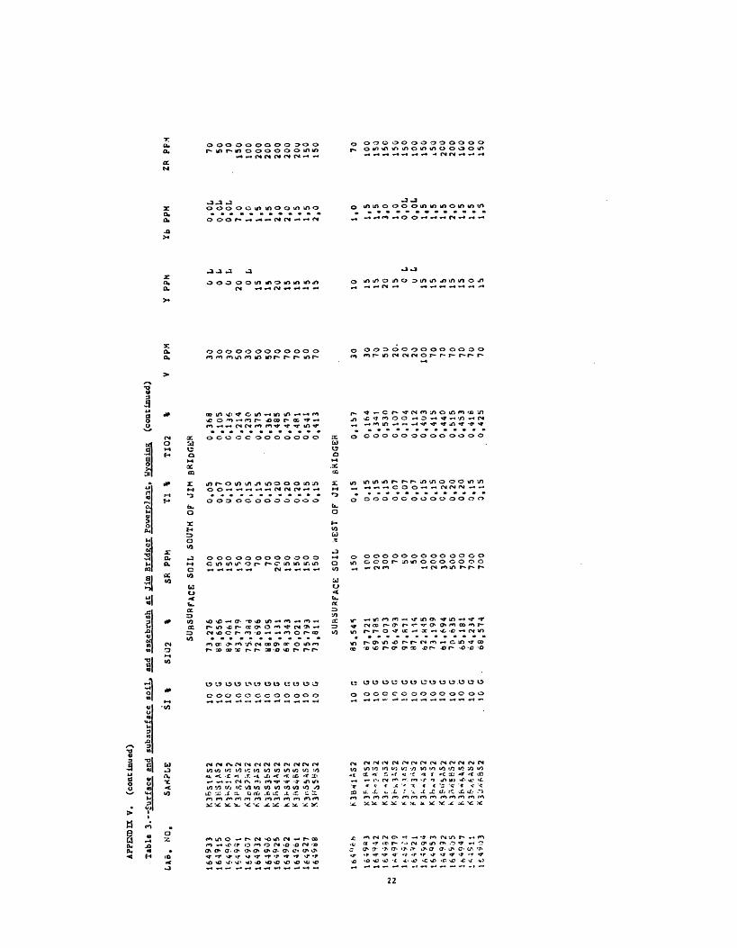
APP

END

IX V

. (c

onti

nued

)

Tab

le

3.-

-Surf

ace

and

sub

surf

ace

soil

, an

d sa

gebr

ush

at

Jim

Bri

dg

et

gow

erpJ

.a.-3

t. W

yom

ing

(conti

nued

)

.,

NO

, SA

MPL

E S

I %

SJU

2 %

SR

PPM

T

l %

TI0

2

% V

PPM

164933

164915

164932

164906

164925

1649

6216

4561

164S

42

M

164*52

^

1*4

97

91 *

4 9

i' 4

164^

211

*49

94

164905

K3&SUS2

K3&S4AS2

X3

^-1*52

K3^

«?A

S2

K3r

*2n

52

K3K

^3«6

2

SI %

SJU2

% SR

PPM

SUBSURFACE SOIL SOUTH

10 G

10 G

10 G

10 G

10 rf

10 G

10 G

10 G

10

C,10

G

10 G

10 G

10

r.10

G

10 G

1.0

G10 G

10 G

10 G

10 G

10 G

10 G

10 G

10 G

10 G

. JO

G

73.276

89,656

89.061

H3.779

7S..3fl,i

72.696

US, 105

69.131

6B.343

70,021

75.793

73,811

SUBSURFACE

85.54S

17.

721

69.785

75.073

96.493

97.R71

H7.114

62.H45

73.199

61.694

70.635

65,181

64,234

68,574

100

150

150

150

100 70 70

200

150

150

150

150

SOIL '.

vEST

150

100

200

300 70 50 50 100

200

300

500

700

700

700

TI %

OF JIM

0,05

Ot07

0,10

0,15

0,15

0,15

0,15

0,20

0,20

0.20

0.15

0.15

OF JIM

0.15

0, 15

0,15

0,15

0,07

0,07

0,07

C.15

0,15

o,2o

0,20

0,20

0.15

D.lS

TI02

%

BRIOOKH 0.368

0,105

C.136

0.214

0.230

0,375

0,361

0.485

0,475

0.4R1

0,541

0.413

BHlDGEH 0,157

0,164

0,3*1

0,530

0,107

0.104

0.112

0,403

0.41S

0,440

0.515

0.453

0.416

0,425

30 30 30 50 30 50 50 70 70 70 50 70 30 30 70 50 20.

20 2010

0 70 70 70 70 70 70

PPM 0 L

0 L

0 L

20 0 L

15 15 20 15 15 15 10 15 15 20 15 0 L

l> L

15 15 15 15 15 10 ib

PPM

1,0

ZR PPM

O.OL

O.OL

O.OL

7.0

1,0

1.5

1.5

2,0

2,0

1.5

1,5

2.0

70 50 70

150

100

200

200

200

200

20U

150

150 70

1,5

1,5

3,0

1,0

O.OL

O.OL

1,5

1,5

1.5

2,0

1.5

1,5

1,5

100

150

150

150

150

100

150

»50

200

200

100

100

150

APP

END

IX

V.

CHEM

ICA

L EL

EMEN

TS

IN

VEG

ETA

TIO

N A

ND

SOIL

NEA

R C

OA

L-FI

RED

PO

WER

PLA

NTS

, W

ESTE

RN

ENER

GY

REG

ION

S (c

on

tin

ued

)

Tab

le

3.-

-Su

rfac

e^ a

nd

subsu

rfac

e so

il,

and

sag

ebru

sh

at

Jim

Bri

dger

Pow

erpla

nt.

W

yom

ing

(co

nti

nu

ed)

LAB. ^o

. sA

^pLt

LA

TITU

DE

LO^GITUD

DIST

KM

AS

P?M

F %

HG

PPM

TOTA

L s%

4ifc

223

416216

41*25*

4J6244

41123*

416237

41*224

4 1 f

t 2 3 0

< 1

> 2 2 5

41*252

tJfPSl

4 1 -

J I \

^

* I * 2 2 3

<s i o

2 4 i

4 } *

> 2 3 1

41*214

» 1 *

> 2 1

»

4 5 *

1 \

2

4 ! f

t * 5

4 l 6

? 4 *

41&232

416220

4)6234

41624^

416255

41-J

240

416221

SAMP

LE

LATI

TUDE

K.^jAP

K3'-

1.' 1 A?X

K3V. 1

r>?

K 3

r, ,\ j A ?

K 3 B * 2

fc ?

Ksn.ij AP

/ 3T'O*P

hj«i MAP

K 3n

-.4b

P*3? '5A?

K3r;;?HP

f- 3

* ' 5 b P X

K 3

J K

1 A P

K 3r*£l APX

K 3

1» K

1 H P

^- ^i^px

K.3'r?-?A3

K 3

.A »: 2

.» r>

r'3'

-. F"^

'»PX

K 3.^.3 if

* 3 " K 3 n ?

K 3 h

?. < A ?

l^-rqAPX

K 3

:, (f

,1 a p

K 3

'. 5 A P

K 3 P

. -: 6

* ?K3

-ir"

fiA5

XK3

.-S6

HPX

K3BS1AP

K 3

r* S

1 rj P

K 3

*- S 2 A ?

Kj^RJAPX

K3?S?3P

K 3

5 3 A P

K 3r>S3Bp

K3ibS4AP

K34S4HP

K3BS5AP

K3BS56P

41.

41 4l 41 41 41 41 41 41 42 42

42

41 41 41 41 41

41 41 41 41 41 41 41 41

41

41 41

41 41

41 i 1 41 41 41 41 41 41 41

44 4444

4S46

4949

57

57060606

4444

444444

44

4439

3942

42 42 43

48 IS

48

434342

42 42 3d 39 32 32 20 20

25V

25K

25N

05"-

05K

5CN

5(VV

45 N

45^

47N

47 N

4?N

2SN

25N

2SN

35\

20^

20N

2 ON

55N

55'4

45M

45N

45N

1 5

'«'40'J

4 Or,

4 ON

30N

30fJ

OON

DOS

OO'J

45N

45^

30^

30N

55N

55^

LO^GITUD

DIST KM

A.'J

PpH

F %

loft

ioa

106

10s

10ft

103

10*

JO*

108

109

109

109

10"

lOfl

j oft

] Oti

1 0<

f\ 0^

1 »K

1 nf

l!.

> *

1 0«

10?

< oa

1 0>

>107

107

107

108

103

1 On

lOR

103

108

108

10P

1'OR

108

108

46 46 46 46 40 4H 49 55 55 00 00 00 45 45 45 45 42 42 42 33 38 2S 25 25 08 34 34 34 46 46 45 45 45 4ft

46 42 42 44 44

SAGEBRUSH

30''

30*'

30*

50*

SO*

io**

10V

40«

40*1

25*

25<<

25* SAGEBRUSH

25*

25 4

75,1

25"

504

50^

Sf'rV

00 W

00"

55>W

55. »

55*'

00-i

(oo

«00*

00^

SAGEBRUSH

15^

IS*'

OOW

00''

oo«v

55^

55^

15*'

15^

05<V

05^

NOrt

TH OF

1 1 1 3 310 10 25 25 42 42 42 EAST OF

2 2 2 2 6 6 612 12 30 30 30 54

100

100

100

SOUTH OF

2 2 5 5 5 9 922 22 45 45

JIM BRIDGEB

o. 0. o. 0. o. o. 0, 0. 0. o. o. 0.

20 25 15 10 25 20 30 20 15 20 25 15

0. 0. 0. 0. o. 0. o. 0, o. 0, o. o.

0032

0045

0024

0016

0012

0009

0020

0016

OOlO

0009

0014

0018

JJH BHIDGER

o. o. o. o. o. o. 0. o. 0. o. o. 0. o. 0. 0. o,

05 07 05L

05 05 05 06 08 25 70 80 15 30 05 07 05L

0, o. 0. 0. 0. o, 0. o. 0. o. 0, 0. 0. 0. o. o.

0008

0014

0014

0016

000*

onoB

OOOh

0014

0018

0040

0045

0010

0020

0014

OC09

0035

JIM BRIDGER

0. 0. 0, 0. o, 0, o. o. o. o, o.

20 20 05L,

05L

20 25 15 15 10 25 35

0. o. o. 0, o. 0. 0, o. 0. o. o.

0020

OOlfi

0014

0020

0012

0014

0012

0006

0010

0012

0022

0,02

0,02

0,01

0.02

0,01

0,02

0.02

0,02

0,01

0,01

0,02

0,02

0.02

0,02

0.02

0,02

0,01

0.01

0,01

0.02

0.02

0.03

0,03

0,02

0.02

0,03

0,03

0.03

0,03

0,03

0.02

0,03

0,02

0.04

0.02

0.01

0.03

0,02

0.02

0,15

0,18

0,16

U.23

0,21

0,21

0.11

0.13

0.12

0,17

0,16

O.lo

0.19

0,22

0. 15

0.19

0,16

0,16

0,13

0,16

0.10

0,15

0,13

C.15

0.18

0.14

0,15

0,18

0,14

0,20

0,13

0,12

0,15

0.21

0,15

0.14

0,25

0,13

0.08

SE

PPM

0.35

0,35

0.45

0.10

0,10

0.06

0.10

0,20

0.08

0,04

0,04

0,04

0,40

0.40

0,50

0.55

0,20

0,20

0.15

0.10

0.20

0,15

0.15

0,15

0.30

0.40

0.35

5,00

0.15

0,15

0,70

0.80

0.20

0.10

0.06

0.08

0,10

0,06

0,10

ASH

7.4

6.9

7.7

7.5

9,7

7,1

7.5

7,2

6.0

5,8

6.0

5.6

7,2

6.9

7.6

6.8

4.7

6,6

5.6

6.2

8.6

8.0

7.7

7.2

11.0

5,0

5.4

6.2

8.6

6,2

6.4

6.0

5.9

8.0

6.6

5,8

8,6

7.3

B.9

TAB

LE

V.

Tab

le

3.

is.

KO

.

4 1 1

2 1

5 «

1 o 2 4 7

-16235

4 1 *

2 1 a

4 !

* 2 2 7

4«c250

410209

41

62

23

41

62

-15

4jo

7l9

41

*2

42

4

1 6

2 1

6 41555?

41

62

-;',

» 1

* 2

0 7

41

*2

3*

4

1 6

2 3

7 4lf

c224

416230

416225

*l<

525l

4J6

22S

4

1*

25

2

41

62

53

4

l 6

2 1

7 416222

4 l

*> 2

4 S

41*231

416214

416213

416212

4 l

6 2

J 3

41^25

4J6

2S

6

41 S

259

(co

nti

nu

ed

)

Surf

ace

and

sub

surf

ace

Boil

,

SA

'-'P

Lt

LA

TIT

UD

E

K3h*l

AP

K

3 c.

' 1

H P

SA

-.P

Lc

K3

HK

2A

P

and

sageb

rush

et

Jim

B

rid

ger

Pow

erp

lan

t.

Wyo

min

g (c

onti

nued)

LO

NG

ITU

n D

IST

KM

A

S PF

M

F %

HG

PPM

TO

TA

L

S%

SAG

EBR

USH

W

EST

OF

JIM

BR

UJG

KK

41 < !

41 41 41 4J 41 4! 43 41 41 41 41

44 44 44 44 46 f. 6

i5 '5 45 <5 >0

'10

40

2C*

20 N

2 ON

20-f'

iION

ION

2SN

?EN

3nlJ

3Ci»

35N

35M

35«

lOfr

lot

10*

10?

1C«

10*

10«

1 09

109

109

109

10?

109

47 47 50 50 54 54 04 04 22 22 57 57 57

55*

55*

00*

00-*'

25*

254

20*

20*

55*

55V

OS A

'

OSrV

05*1

2 2 5 512 12 25 25 50 50 9t3

98 98

AL

%

3.0

3,0

3.0

1

.5

2.0

3.0

3.0

2,0

1.5

1.5

'

2.0

1.5

2.0

3.0

3.0

3

.0

1.0

1

,0

0.7

1

,5

3.0

5,0

5.0

3.0

3.0

1

.5

2.0

3.0

8 PP

M

BA

PP

M

C*

* C

A/A

SA

GE

BR

US

H

NO

RT

H

OF

JIM

B

RlD

GE

R

200

200

200

300

300

300

150

150

300

300

300

200

SAGEBR

300

300

300

300

500

2uO

200

300

200

150

150

500

200

150

soo

500

500

500

300

300

200

300

300

300

300

200

200

300

USH EAST

300

300

300

300

200

150

150

500

500

300

300

300

300

200

300

300

7 7 7 7 7 7 7 7107 7 7

OF JIM E,

«lDG

b'R

10 7 7 7 7 V 7107 5 7

10 7 7 7 7

7,8

7,4

0.0

9.2

10.0

<J,

6

5,4

11.0

12.0

11.0

9.0

8.4

CD

/A

PP

X

3,5

2

,9

2,6

2.3

1

,3

3.3

I.

7 1,9

1

.7

2.6

2

,3

1,9

CE

PP

M 0 N

0 N

U N

0 N

0 N

0 N

50

0

L U

N U

N 0

N 0

N 0

N

SE

PP

M

0..2S

0./!

0 O.Ob

0.05

0.15

0,15

0.35

0, 15

0.70

0.60

0.25

0.25

0,25

0,0016

0,0026

0.0012

0,0010

0,0010

0,0007

0,0020

0,0026

0.0040

0.0045

0.0013

0,0022

0,0020

0,02

0,02

0,02

0.02

0,02

0.02

0,01

0.02

0,02

0.02

0.02

0,C3

0.02

0.00

0.20

0,16

0,15

0,14

0.11

0,17

0,17

0,10

0.12

0,13

0,17

0,16

0.25

0.10

0,50

0,35

0,10

0,10

O.OH

O.oO

0,06

O.OH

0.10

0.20

0.25

CO

PP

M

10

L 10

L

10

L 0

N 10

L

10

L 10

b

10

L 10

L

10

L 10

L

10

L

11.0

10.0

a. 6

8,6

10.0

10.0

10.0

12.0

7.1

5.7

6.0

9.4

9.6

10,0

11,0

8.6

3.5

4,7

3,2

4,6

5,0

3.0

3.3"

4.0

3,0

3,8

3,4

7.2

3,2

3,6

3,6

26,0

0 N

0 N

0 N

0 N

0 N

0 N

0 N

0 N

0 S

500 L

500 L

0 N

0 N

0 N

0 N

0 N

10 b

10 L

10 L

10 L

0 N

0 N

0 N

10 L

10 L

10 b

10 b

10 b

10 L

10 L

10 L

lOL

AS

H

7.3

6.9

6

.2

5,7

6

.66.1

7

,37

,013.0

12.6

6,8

6.8

5.6

CO

/A

PPM

APP

END

IX V

. (c

onti

nued

)

Tab

le

3."

-Surf

ace

and

sub

surf

ace

soil

, an

d sa

geb

rush

at

Jtra

Brt

dger

P

ower

gL;:

nt.

Wyo

min

g (c

onti

nued

)

US

. N

O.

SAM

PLE

A

L %

B PP

M

BA

PPM

C

A

% C

A/A

%

CD

/A

PPM

4]6246

416254

416226

41*232

416234

4i 6249

4 ! 6

2 0 8

416255

416240

416221

K3B51AP

K3rSlbP

K3PS55?

5.0

3.0

2.0

2.0

2,0

3.0

3.0

1.0

2.0

3.C

3.0

SAGEBRUSH SOUTH OF JIM BRlDGER

SOO

SOO

300

200

200

300

300

300

3CO

300

150

500

300

3no

300

300

300

300

150

200

1000

700

10 7 7 7 7 7 7 7 7 7 5

11,0

13.0

8.8

R.6

9.6

fi.fi

8,0

11.0

12.0

9.0

6.4

1.4

1.4

1.9

2,1

2,6

2.3

2.1

2,8

2,3

3.6

2.8

CE PPM 0

N0

N0

N0

N0

N0

N0

N0

N0

N0

N0

N

CO PPM

10 L

10 L

10 L

10 L

10 L

10 L

10 L

10 L

10 L

10 L

10 L

CO

/A

PPM

SAG

EBRU

SH W

EST

OF

JIM

BR

IDG

ER

41*255

416247

416206

4J6241

4 ! & 2

3 S

* 1*

2 11

i t> 2

4 3

4J6227

4<625C

4le209

R, 3 h

> 7 i P

K3S-3A?

X 3

' ' » < A P

< 3 -

> 5 A ?

3.0

3.0

i.

O

1 .5

1.5

1.5

3.0

3.0

5

.0

5.0

3

.0

3.0

3

.0

20

03

00

30

03

00

30

03

00

300

300

20

02

60

30

05

00

200

10

00

1500

150

150

30

05

00

20

0300

1000

50

07

00

70

05

00

7 7 7 7 710

JO 7 7 S

10 7

10

8.8

10.0

9.0

10.0

12.0

12.0

9.2

6.7

6.4

6.6

11.0

10.0

10

.0

2,3

2.6

3.3

4.7

3.3

3

.2

2.4

O

.B

1.2

1.5

2

.6

2.6

3.2

0 N

0 N

0 N

0 H

0 fc

0 N

0 N

0 ft

SCO

L

50

0

L 0

N 0

N 0

N

10

L10

L

10

L0

N1

010 10 10 10 10 10 10

L10

L

LAB.

416223

416245

41

62

42

41621*

416259

41

62

44

416207

41

62

36

416237

416224

4162JC

SAMPLE

K3?M

-j AP

K 33M APX

K 3

1» » 3 B P

K3RMAP

K3HN4BP

30 30

3*

10

15

15

20

20

10

10

15

15

CU PPM

FE %

GA FPM

SAGEBRUSH WORTH OF JIM ERIDGER

K/A

100 70 150 70 70

150

100

100

100

200

150

150

1.0

1.5

1.0

0.7

0.7

0.7

1.0

0.7

0,5

0.5

O.S

0.7

10 10 10 10 10 10 10 10 n JO

10

10

10 G

10 G

10

10

10

10

10

10

10 G

10 G

10 G

10 G

2424 24 26 19 30 16 24 28 28 32 30

LA PPM 0

N 0

N 0

N 0

K 0

I* 0

H 10

0 L

0 N

0 N

0 K

0 N

0 N

LI/A PPM

12 12 12 12 146

14 14 20 10 12 12

MG t

1.5

1,0

1.5

3.0

2,0

2.0

1.0

1.0

1.5

1,5

I. 5

1.5

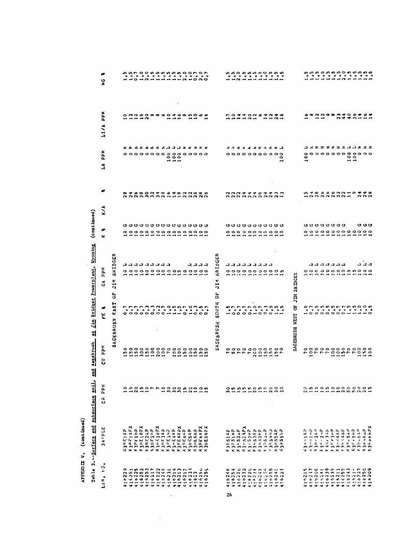
APP

END

IX V

. (c

on

tin

ued

)

Tab

le

3.-

-Su

rface

and

subsu

rfac

e so

il,

and

sageb

rush

at

Jim

Bri

dger

P

ow

erp

lan

t.

Wyo

min

g (c

on

tin

ued

)

K %

K/A

LJS. KO

.

416251

410225

<l6252

416253

4 112 17

416222

4J 624

fi

416231

416214

416213

41621?

4 16 2 3 *

41612

4J62<6

416254

4 1

f- 1 2 6

4 1 * ? 3 4

410/55

4 1 6

2 4 C

41*215

41f247

4 i b 2 0 6

* 1 c

i 4 1

«16239

416235

416

2 11

41*257

t 16243

4i*it'

4i6?27

416250

KjP-

k'lb

P

K3PE4APX

K3BE6&PX

fv 3 r 3

l o P

K 3

H 3

3£

P

*,3rS

5A

P

X3

*r2

A»

t^^rP

K 3

f-» c

b ?

K 3 f

*' fc

D ?

C» PPM

10 15 20 15 10 7 7 10 30

30

30 15 20 10 10 15 30 15 15 15 15 20 15 10 20 30 30

20 15 10 10

15 10 10 20 50 50 20 20 15

CU PPM

FE %

SAGEBRUSH

150

150

150

300

150

100

200

100 70

100

100

150

100

150

150

150 SAGEBRUSH

70 50 70 70 70 2CO

100

150

150

150 70

EAST OF

0.7

0.7

0.7

0.7

0.3

0.3

0.2

0.7

1.0

1.5

1.5

0.7

1.0

0.3

0.5

0.7

SOUTH OF

1.5

0.7

0.7

0.7

0,7

i.o

-0.7

0.3

0.5

1.5

1.5

SAGEBRUSH WE

ST OF JIM

70 100 70 70 70 100

100

150 70 70

100

150

100

1.0

0.7

0.5

0,5

0.5

0.5

0,7

0.7

1.5

1.5

1,0

1 ,0

0.5

GA PPM

JIM BRIDGER

10 L

10 L

10 L

10 L

10 L

10 L

10 L

10 L

10 L

10 15 10 10 k

10 L

10 L

10 L

JIH RRIOGER

10 L

10 L

:o L

10 L

10 L

10 L

1 0 L

10 L

10 L

10 15

BRIDGED 10 .1

0 L

10 L

10 L

10 L

10 L

10 L

10 L

15 J.5

10 L

JO L'

10 L

10 G

10 G

10 G

10 G

10 G

10 G

10 G

10 G

10 G

10 G

10 G

10 G

10 G

10 G

10 G

10 G

10 G

10 G

10 G

10 G

10 G

10 G

10 G

10 G

10

C, 10 G

10 G

10 G

10 G

10 G

10 G

10 G

10 G

10 G

10 G

10

10 10 G

10 G

10 G

28 24 26 26 30 32 34 28 16 14 18 22 22 26 28 26 22 22 22 24 24 24 26 28 24 23 13 15 24 28 26 26 26 22 22 119

24 24 28

LA PPM 0

N0

N0

N0

N0

N0

N0

N0

N100

L100

L100

L0

M0

N0

N0

HQ

N

0 N

0 W

0 N

0

N

0 N

0 N

0 N

0 N

0 N

0 N

100

L

100

L0

N0

N0

N0

N0

N0

N0

N10

0 L

100

L0

N0

N0

N

LI/A PPM

10 12 10

16

20

' 8 6 610

14

168

15

10 6 16 17 10 14 14 20 126

14 12 24 16 168

12 12a 8

23 44 40 26 14 16 14

MG I

1.5

1.5

0.7

1.0

2.0

1.5

1,5

1.5

1,5

1.5

1.5

2.0

1.0

0,7

2.0

0.7

1.5

1.5

2.0

1.5

1.5

1.0

1.5

1.5

1.5

1.5

1.5

1.5

l.b

1,5

1,5

1.5

2,0

1.5

1,5

1.5

1.5

1.5

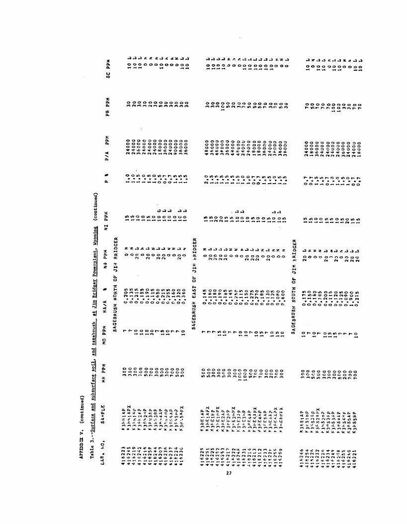
APPE

NDIX

V.

(con

tinu

ed)

Table

3.

LAB. M3,

416223

416245

416219

4J6242

4i62l6

4J625P

416244

416207

416236

416237

41622C

416230

416229

4162M

416225

4ie252

416253

w 41*217

416222

416231

-16214

416213

416212

416259

416246

416254

«lb232

4i6220

416234

4! f 2 4 S

416208

416255

416240

416221

K3FU3AP

K3BE1AP

-Surface

and

subsurface soil,

SAMPLE

MN PPM

300

300

300

700

500

700

300

500

300

700

500

500

500

500

300

300

500

300

3CO

1000

1000

500

700

700

300

200

700

300

300

300

SCO

500

300

300

300

5C'0

200

700

700

K3KS1AP

K3FS5AP

MO PPM

NA/A

%

SAGEBRUSH NORTH OF

7 710 10 10 307

15 107 7

10

C.205

0.135

0.215

0.155

0.190

0.115

0.650

0.215

0.255

0.160

0.320

0.340

SAGEBRUSH EAST OF

7 7 715 10 7 710 107

10 15 7 10 IS 10

0.145

0.160

0.180

0.190

0.185

.0.145

0.260

0.115

0.150

0.275

0.270

0.185

0.130

0.125

0.080

P. 600

SAGEBRUSH

SBUT

H OF

107

107

10 15 157 7 7 10

0.175

0.150

0.130

0,)85

0.200

0.115

0.120

0.125

0.090

1.900

0.215

Nd PPM

JIM BRIDGER

0 N

0 N

:>o L 0 N

20 L

0 N

20 L

20 L

0 N

0 N

20 L

0 N

JIM bfllDGER

0 N

20 L

20 L

20

fc20

L

0 N

0 N

0 N

20 L

20 L

20 L

0 N

20 L

0 N

0 N

0 N

J1K F.

RIDG

ER

20 L

0 N

0 I"

0 N

20 L

D ri

20 L

0 N

20

L,20 L

20 L

NI PPK

15 15 10 10 15 10 10 -L

10 L

10 L

10 10 L

10 L

15 15 20 20 15 15 10 L

10 L

10 15 10 10 15 10 L

10

L

15 15 15 10 10 15 15 10 15 20 15 15

p %

1.0

1.0

1.5

1.0

1.5

1.0

0.5

0.7

0.7

1.5

1.5

1.5

0.7

0.7

1,5

1.5

0.7

1.0

1.0

1.5

1,0

0,7

0,7

P/A

PPM

24000

24000

36000

24000

24000

24000

18000

36000

24000

90000

36000

36000

2.0

1.5

1.5

1.5

1.5

1.5

1.5

1.0

1.0

0.7

0.7

1.5

1.5

1.0

1.5

1.5

48000

36000

46000

36000

36000

4*000

48000

24000

24000

18000

16000

36000

24000

3f>000

36000

36000

24000

18000

36000

24000

24000

24000

24000

36000

24000

24000

13000

PB PPM

30 20 30 30 20 30 50 30 30 30 30 30 30 30 30

100 50 20 30 70 50 50 50 70 30 70 50

30 70 50

70 70 70

100

100 30 30 70 70

SC PPM

SO L

10 L

10 L

0 N

0 N

0 M

10 L

0 N

0 N

0 S

10 L

10 L

10 L

10 L

10 L

10 L

0 N

0 >

0 N

10 L

10 L

10 L

10

L,10

L

10 L

0 N

0 H

0 L

10 L

0 N

10 L

10 L

0 N

10 L

10 L

0 N

0 N

10 L

10 L

APP

END

IX V

. (c

onti

nued

)

Tab

le 3

. S

urf

ace

and

subsu

rfac

e so

il,

and

sag

ebru

sh at

Jim

Brl

dger

P

ov

ero

lan

t.

Wyo

min

g (c

on

tin

ued

)

LA

B.

HO

. S

A-^

PL

t M

h' FP

M

MO

PPM

N

A/A

%

NH

PP

M

Nl

PPM

SAG

EBRU

SH V

EST

OF

JIM

BR

IDG

ER

416215

416247

4 1 6

20'i

41*241

416239

*! 6235

4 1 b 2 * 7

4lc

227

<rl

t>25

0

500

700

3CO

300

7 CO

700

500

300

700

700

3f'0

700

5:>0

7 7157

10 10 15 107 7

15 107

0.325

0.175

0.180

0.190

0.175

0.100

0.250

0.19Q

0.345

0.560

0.450

0.250

0.265

20 200 0 0 0

200

20 200

200

L L N N N N' L N L I N L N

15 15 10 20 10 15 10 15,

I5 15 10 15 10

0.7

1,5

1.0

1.5

1.5

0.7

0.5

0,7

0,5

0,5

1.0

1,0

0,7

P/A

PPM

24000

36000

36000

36QOO

36000

24000

18000

18000

12000

12000

24000

24000

24000

PB PPM

70

50

70 70 50 30 50 30 50 70 70 50 50

5C PPM

10 L

10 L

0 N

0 N

0 *

0 N

10 L

10 L

10 L

10 L

10 L

10 L

10 L

416223

416245

4le2l9

41&242

4 l 6 2 2 4

416230

416229

416251

416225

M6252

41*253

416217

4i»222

4 6 2 4 9

4:6231

415214

416213

4i62l2

416233

4i62

2fl

41*256

*3'v

':f-3

*"-;

K3F.

E4B?

K3BE5AP

SI/A

PPM

120000

120000

lOnOQO

72000

120000

72000

160000

74000

44000

52000

5ROOO

54000

60000

6^000

88000

60000

45000

4«<000

32000

52000

160000

200000

180000

120000

100000

64000

5 o 0 0 0

94000

PPM

PPM

Tl %

U/A

PPM

SAGEBRUSH NORTH OF JI

M' BRlDGER

0 N

0 N

0 fj

0 N

0 H

0 N

0 1*

0 N

0 *

0 *

0 N

0 N

200

200

150

700

300

300

200

300

500

500

500

500

SAGEBRUSH EAST OF

0 N

0 N

0

fi

300

N0

N0

N0

N0

*0

it0

N0

N0

b0

N0

N0

N

300

500

300

500

500

200

200

300

200

150

150

300

500

500

700

1000

0 0 0 0 0 0 0 0 0 0 d 0

JIM

0 0 0 0 0 0 c 0 0 0 0 0 0 0 c 0

.15

.15

.15

.07

.15

.07

.15

.07

.05

.05

.07

.07

BRIOGER

.07

.10

.07

.15

.07

.05

.03

.10

.20

.20

.20

.15

.10

.03

.07

.10

1.2

o.e

1.2

0.4

o.a

o.e

1.2

1.2

0.8

0.4

0.8

0.8

0.4

o.a

0.8

0.8

0,8

0.4

0.4

0.4

0.8

1.2

1,2

0.8

0.4L

0,8

0.8

2.4

PPM

50 50 50 15 20 15 50 20 15 15 20 20 15 30 30 30 15 15 15 L

15 50 70 70 30 50 15 15 30

Y PPM

20 L

20 L

20 I

20 L

20 I

20 L

20 L

20 L

20 b

20 L

20 U

20 U

20 I

20 L

20 L

0 N

20 L

20 L

0 N

20 L

20

Li 20

30 20 t

20 L

20

Li 20

b

20 L

*B PPM

ZN PPM

2 2 2 0 2 2 2 0 2 2 2 0

L L L N L L L N L L L N

0 0 0 0 0 0 0 0 07

00 0 0

N N N N N N ,<l N S L N N

0 N

a L

0 N

2 L

0 N

0 N

0 N

0 N

2 L

2 3 2 L

2 L

0 N

2 L

2 L

0 N

0 N

0 N

0 N

0 N

0 N

700 L

C N

0 »

0 N

0 N

0 N

0 K

0 N

0 N

0 *

APP

EUjE

C V

. (c

on

tin

ued

)

Tab

le 3.-

-Surf

ace

and

sub

surf

ace

soil

, an

d sa

geb

rush

at

Jim

Bri

dger

P

ovet

pla

nt,

W

yom

ing

(conti

nued

)

SI/

A

PPM

416246

416220

416234

41

62

49

.£

16209

41

62

55

4

(62

40

41

*5

06

4

1 1

2 4

1 <

lo"3

*

4t6

23

5

416211

4J*

257

41

62

43

4lf

r2!S

4

«c2

2T

4

! t

2 5

rt

L t B

, HC.

4lb223

41&7.45

416219

416242

41*216

41625*

416J44

4)6207

416236

4! £ 2 3 7

4lt224

416230

Sftv

pt.E

SN PPM

SR PPM

ri %

y/A

PPM

K3PS2H?

l AP

'X 3 n

' ! 1 A P

K3B-

J2AP

K 3 5

.'. 2

* P

K36S3A?

120000

6^000

120000

120000

innooo

100000

1000CO

SPOOO

72000

100000

190000

16*>

000

92000

6?000

bfOOO

54000

51000

920^0

12COfO

24nooo

22^000

Kjt \56PX

92000

70000

ZN/A PPM

330

330

340

165

140

320

IfO

2?5

190

600

440

500

SAGEBRUSH

SOUT

H OF

JIM

B*I

DGER

0 N

0 N

0 N

0 <*

0 N

0 N

0 N

0 N

0 N

0 K

0 I* SA

GEB

RUSH

0 ft

0 N

0 K

0 N

0 N

0 N

0 N

0 M

0 N

0 N

0 ft

0 V

0 N

70

03

00

50

05

00

30

03

00

30

02

00

50

03

00

15

0

WES

T

15

02

00

30

03

00

30

03

00

300

70

05

00

20

07

00

70

07

00

9.1

3o.

to0.0

70,0

70

.07

0.1

00

..1

50.0

50

.07

0.1

50

.20

OF

JIM

BR

IDG

ER

0.1

50

.15

0 , (

. 50,0

70.0

7O

.C7

0.1

00

.15

0.3

0C

-,30

C.C

7C

.20

C.0

7

ZP PPK SAGE

BRUS

H NO

RTH

OF J

IM BP

IOGE

R

70 70 70 5015

0 70 70 70 30 50 30 50

0,8

0

,8

0.8

0

,8

0.8

0.8

0

,8

0,4

0.4

1

.2

1,2

o.a

0.8

1,2

1

.2

0.8

0.4

1,2

0

,8

1.2

0

,8

0,8

0

.5

0.8

V PP

M

50 20 20 20 20 30 30 15 20 70 70 50 30 15 15 20 15 50 50 70 70 30 50 20

V PP

M

20

L 20

L

20

L 20

L,

20

L 20

it

20

L 0

N 20

L

20

L 20 20

L

20

L 0

N 20

L.

20

L 20

L

20

L 20

L

20

20 20

L 20

L

20

L

YB P

PM 2 L

2 L

2 L

2 L

2 L

2 L

2 L

0 N

2 L

2 L

ZN

PPM 0

N0

N0

N0

N0

N0

*0

N0

N0

N0

N0

N

2 L

2 L

0 N

2 L

0 N

0 N

2 L

2 L

2 L

3 2 L

2 L

0 N

0 N

0 N

0

N7

00

L

0

N0

NC

hi0

hC

N0

N0

N

0 K

0 N

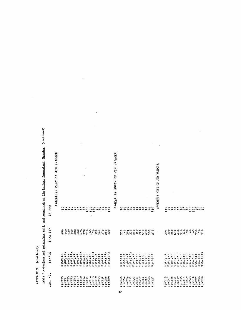
APPE& IX V.

(con

tinu

ed)

Table

^.. Surface

and

subs

urfa

ce soil,

and

sagebrush

at Jim Bri

dger

Povcrplant.

Wyoming

(continued)

LAB. so

, SA

HPLK

ZN/A

PPM

ZP PPH

416225

416251

4J6225

416252

<-6253

4ic2l7

41*222

4lfc24s

« 1* 2 3 1

4i

r»2l

4 416213

41*212

416233

I!*22*

41*256

416259

o 416245

4 1

ft 2 3 4

4lb249

4 l 6

2 C.

8

416255

416221

k 3 1 K 3 A P

*3>-Si Ap

'f3&S2AP

*3rs2AF)

K 3 r

- 5 2 * ?

K 3 b S 4

- ?

K3-S5"?

490

440

420

440

500

600

575

270

210

165

170

320

260

J70

280

320

230

140

205

230

210

350

265

570

430

255

215

SAGEBRUSH CAST OF JIM 8HIDGER

30 50 30 50 20 30 30 70 100

too

150 70

70 30 50 100 SAGEBRUSH SOUTH OF JIM

70 50 70 70 30 70 70 30 70 50 150 SAGE

BRUS

H WE

ST OF JIM

BRIDGER

416239

M*?

J5

4lt,2

ll

4 1 -

2 s

7 41&

243

4-6227

416250

416209

K3P/

J3AP

i*'3^» 3r-P

'. 3 r « 4

»* F-

K 3 6

* 6 B P

200

300

250

530

430

310

140

14S

230

170

210

150 70 70 30 30 30 70 70

150

150 70 50 50

Tab

le 4

.--S

oil

an

d gra

ss

sou

thea

st of

Fou

r C

orne

rs P

ow

erp

lan

t. N

ew M

exic

o

LIB

. N

O.

SAM

PLE

LA

TIT

UD

E

LON

GIT

UD

KM

A

L t-

S

AL

203

%

165954

169973

165943

169955

169532

169934

169939

169942

169930

169977

169935

169972

165974

169952

165945

165965

169976

169971

169968

169970

16S937

16^956

169929

169938

169940

169951

169959

169991

FC1S1A

FC1S1AX

FC1S2A

F:iS2AX

FC251A

FC2S1AX

FC2S2A

FC2S2AX

F:3S1A

FZ3S1AX

FC3S2A

FC3S2AX

FC4S1A

FCAS1AX

FC4S2A

FC4S2AX

F:5S1A

FC5S1AX

FC5S2A

FC5S2AX

FC6S14

KC6S1AX

FC6S2A

FC6S2AX

FC7S1A

FC7S1AX

FC7S2*

FC7S2AX

36 36 36 36 36 36 36 36 36 36 36 36 36 36 36 36 36 36 36 36 36 36 36 36 36 36 36 36

41 41 41 41 40 40 40 40 39 39 39 39 37 37 37 37 33 33 33 33 24 24 24 24 14 14 14 U

OON

OON

OON

OON

42N

42N

42N

42N

25N

25N

25N

2SN

20N

20N

20N

20N

ION

ION

ION

ION

05N

05M

05N

05N

15N

15N

15N

15*

iofl

108

108

108

108

108

108

108

108

108

108

108

108

106

108

108

108

108

108

108

108

108

108

108

107

107

107

107

28 28 28 28 26 26 26 26 24 24 24 24 21 21 21 21 14 14 14 14 02 02 02 02 33 33 33 33

oo*

004

00"'

004

454

454

45*

454

454

45*

454

454

30*

304

304

304

354

354

35*

354

304

30*

304

30*

504

504

504

504

1. 1. 1. 1. 4. 4, 4, 4. 7, 7. 7, 7.15.

15.

15.

15.

26.

26.

26.

26.

50.

50,

50.

50.

96.

96.

96.

96.

50 50 50 50 00 00 00 00 50

50

50 50 50 50

50 5000

00 00 00 75 75 75 75 00 000000

9.0

8.7

9,1

8.5

8.8

9.5

7,5

7.7

9.4

10.1

10

.91

0.9

7.8

7,2

6.6

6.7

8.0

7,5

7.9

7,5

8,4

6.4

10

,410. 5

7,7

6,9

8,4

9.6

15 150

15 15 15 15 15 150 0 15 15 200 0

150 0 0 0 0 0

150 0

15 15

N N H N N N N N N N N N N.

700

700

700

700

700

700

700

700

1000

700

700

1000

700

500

700

1000

1000

1000

1000

700

700

700

1000

700

700

700

700

1000

0 0 0 0 0 0 0 0 0 0 0 I 1 0 0 0 0 0 0 0 0 0 0 0 0 0 1 0

N N N N N N H N N N N N N N ft N N N N N H N N N N

0,5

90.6

10,3

20,4

60,5

60,5

30.4

10,3

30,3

00.3

60.5

60.5

70.2

60.2

5O

.lS

0.0

90.1

30.2

10.2

20.2

50.1

70,0

80.2

20.2

50.1

20.0

20.5

20.6

4

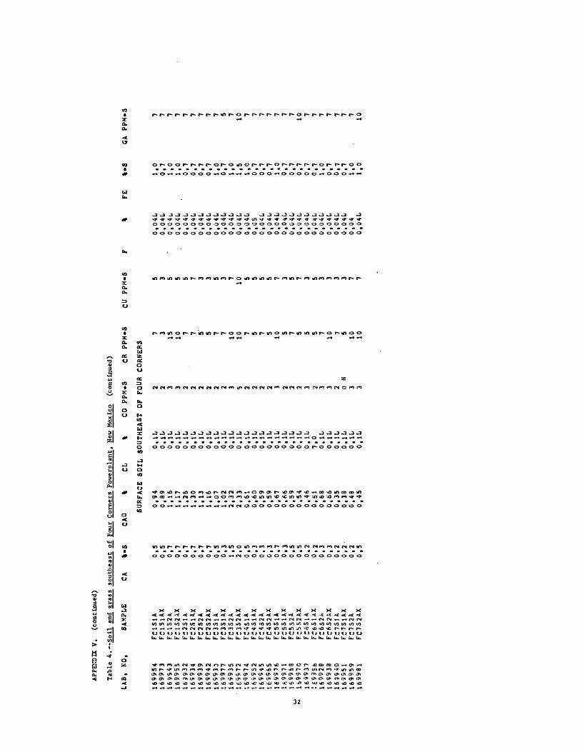
APP

END

IX V

. (c

onti

nued

)

Tab

le A

. S

oil

an

d gra

ss

south

east

of

Fou

r C

orne

rs

Pow

erpl

ant.

N

ew M

exic

o (c

onti

nued

)

CO

PP

M.S

C

R

PPM

-SLAB, NO,

169954

169973

169943

169955

169932

169934

169939

169942

169930

169977

169935

16.9

572

169974

169552

169945

169965

169976

1*9971

169968

169970

169937

:«595b

169928

169933

1639

-10

169951

169959

169981

SAMPLE

FC1S1A

FClSlAX

FC1S2A

FC1S2AX

FC2S1A

FC2S1AX

FC2S2A

FC2S2AX

FC3S1A

FC3S1AX

FC3S2A

FC3S2AX

FC4S1A

FC4S1AX

FC4S2A

FC4S2AX

FC5S1A

FC5S1AX

FC532A

FCSS2AX

FC6S1A

FC6SUX

F:6S2A

FC6S2AX

FC7S1A

FC7S1AX

FC7S2A

FC7S2AX

CA

l-s

0,5

0,5

0,7

0,7

0,7

0,7

0.7

0,7

0,5

0,3

1,5

2,0

0,5

0.3

0,3

0,3

0,7

0,3

0.5

0,5

0,2

0,2

0,3

0,3

0,2

0,2-

0,2

0,5

CAO

% CL

SURFACE SOIL

0,94

0,89

1,16

1,17

1,26

1,30

1,13

1,16

1,07

1,02

2,32

2,33

0.61

0,60

0,59

0,59

0,67

0,66

0,59

0,54

0,46

o.si

0,68

0,66

0,35

0,33

0,48

0,45

t

SOUTH!

0.1L

0.1L

0,1L

0.1L

0.1L

0,11

0.1L

0.1L

0,1L

0.1L

0.1L

0.1L

O.lL

0.1L

0.1L

O.lL

0,1L

0.1L

O.lL

0.1L

0.1L

7,0

0.1L

O.lL

0.1L

O.lL

O.lL

0,1L

7 315

10

7 7 5 5 7 7 10

10 7 5 7 5 10 5 7 S 5 5 7

10 7 5

10

10

CU

PPM

-S 5 3 5 5 5 7 3 3 5 3 710 5 5 5 5 7 3 5 7 3 5 3 3 3 3 7 7

0.0

4L

0.0

4L

0,0

4b

0.0

4L

0.0

4L

0.0

4L

0.0

4L

0.0

4L

0.0

4L

0.0

4L

0.0

4L

0.0

4L

0.0

4L

0,0

50.0

4L

0,0

4b

0.0

4L

0.0

4L

0.0

4L

0.0

4L

0,0

4L

O.C

4L0.0

4L

0,

04L

0.0

4L

0.0

4L

0,0

40.0

4L

FE

%-S

1,0

0

,7

1,0

1

,0

0,7

0,7

0,7

0,7

1

,0

0,7

1

,0

1,5

1,0

0,7

0

,7

0,7

1,0

0,7

0,7

0

,7

0,7

0,7

1,0

0,7

0,7

0,7

1,0

1,0

CA

PPM

-S 7 7 7 7 7 7 7 7 7 5 710 7 7 7 7 7 7 710

7 7 7 7 7 7 7 10

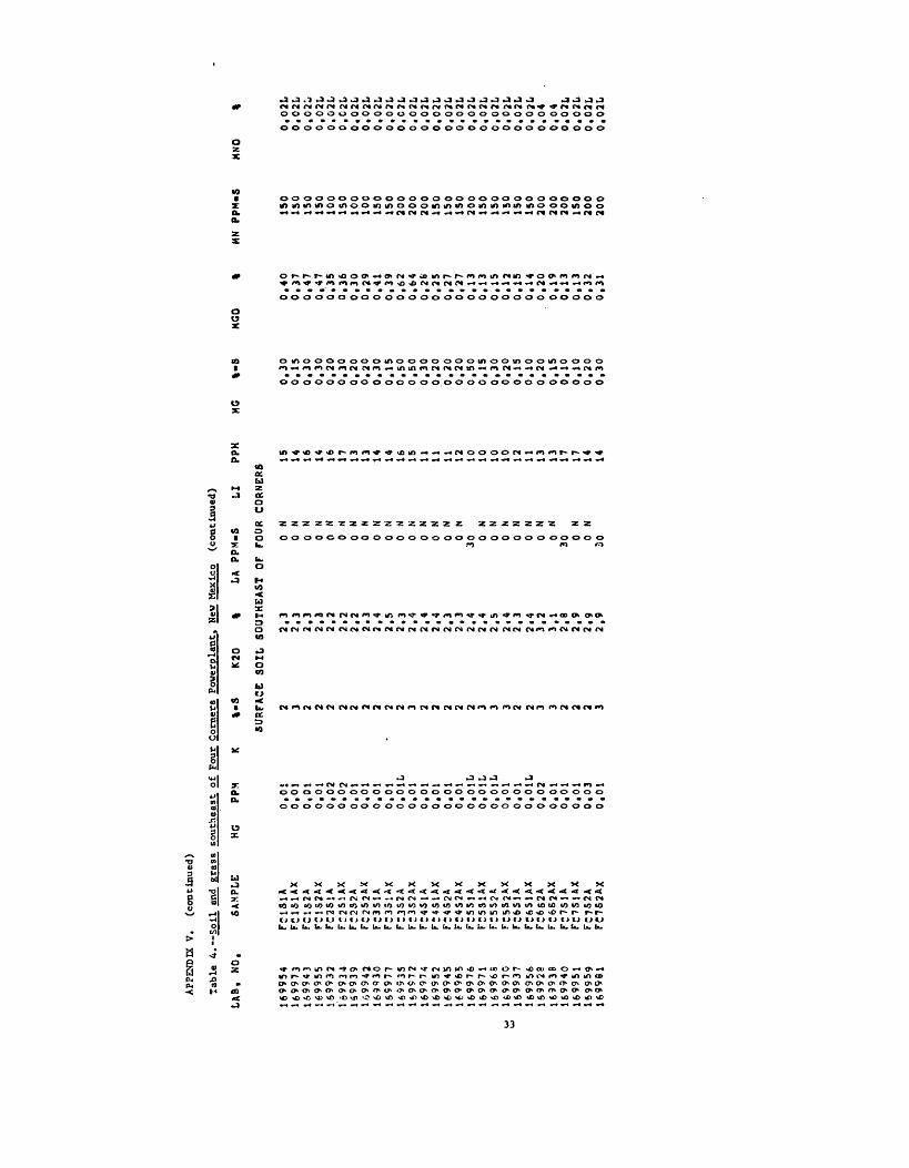
APP

END

IX V

. (c

onti

nued

)

Tab

le 4.

Soil

an

d g

rass

so

uth

east

o

f F

our

Cor

ners

P

ower

plan

t.

New

Mex

ico

(co

nti

nu

ed)

LA

B,

NO

, SA

MPL

E HG

PP

M

K %

-S

K20

%

LA

PPM

-S

LI

PPM

169954

169973

169943

169955

169932

169934

169939

169942

163930

165977

165935

169572

169974

169952

169945

169965

169976

169971

169966

169970

169937

169956

169928

169938

169940

169951

169959

169961

SAMPLE

FC1SU

FC1S1AX

FC152A

FC1S2AX

FC251A

FC2S1AX

FC2S2A

FC2S2AX

FC3S1A

FC3S1AX

FCJS2A

FC3S2AX

FC4S1A

FJ4S1AX

FC4S2A

FC4S2AX

FZ551A

FC531AX

FC5S2A

FC5S2AX

FC6SJA

FC6S1AX

FC6S2A

FC6S2AX

FC7S1A

FC7S1AX

FC7S2A

FC752AX

HG

PPM

0,01

0,01

0,01

o.oi

0,02

o.o2

0,01

0.01

0.01

0,01

0.01L

0.01

0,01

0,01

0.01

0,01

O.OlL

0.01L

O.OlL

0,01

0,01

0.01L

0,02

0,01

0,01

0,01

0,03

0,01

K %-S

K20

SURFACE SOIL

2 3 2 2 2 2 2 2 2 2 2 3 2 2 2 2 2 3 3 3 2 2 3 3 2 2 2 3

t

SOUTI

2,3

2.3

2.3

2,3

2.2

2.2

2.2

2.3

2.4

2.5

2.3

2.4

2.4

2.4

2.3

2.3

2.4

2.4

2.5

2.4

2.3

2.4

3.2

3.1

2.8

2,9

2,9

2,9

MG

0 N

0 N

0 N

0 N

0 N

0 N

0 N

0 N

0 N

0 N

0 N

0 N

0 N

0 N

0 N

0 N

30 0 N

0 N

0 N

0 N

0 N

0 N

0 *»

30 0

N 0

N30

IS

14

16

14 16 17 13 13 14 14 16 15 11 11 11 12 10 10 10 10 12 11 13 13 17 17 14 14

%-S

0,30

0,15

0,30

0,30

0,20

0,30

0,20

0,20

0,30

0,15

0,50

0,50

0,30

0,20

0,20

0,20

0,50

0,15

0,30

0,20

0,15

0,10

0,20

0,15

0,10

0,10

0,20

0,30

MGO

0,40

0,37

0,47

0,47

0.35

0,36

0,30

0.29

0.41

0,39

0,62

0.64

0,26

0,25

0,27

0,27

0,13

0,13

0,15

0,12

0,15

0,14

0,20

0,19

0,13

0,13

0,32

0,31

MN PPM«S

ISO

150

150

ISO

100

150

100

100

150

150

200

200

200

150

150

150

200

ISO

150

150

150

ISO

200

200

200

ISO

200

200

UN

O

0.0

2L

0.0

2L

0.0

2L

0.0

2L

0.0

2L

O.C

2L0

.02

L0

.02

L0

.02

L0

.02

LO

.C2L

0.0

2L

0.0

2L

0.0

2L

0.0

2L

0.0

2L

0,0

2L

0.0

2L

0.0

2L

0.0

2L

0.0

2L

0.0

2L

0.0

40,0

40

.02

L0

,02

10

.02

L0

.02

L

APP

QJD

IX V

. (c

onti

nued

)

Table

4. -Soil an

d grass

southeast

of Four Corn

ers

Pm«.rpl

- ,- , Npw Mnr1rn

CrrmMn,,r^

LAB.

N'o,

169954

169973

169943

169955

169932

16^534

169939

169942

163930

$69977

169935

169972

169974

159952

159945

163965

169976

169971

169968

169970

169937

169956

169928

169938

169940

169951

169959

169981

SAMPLE

FC1S1A

FClSlAX

FC1S2A

FC152AX

FC2S1A

FC2S1AX

FC2S2A

FC2S2AX

FC3S1A

FCJS1AX

FC3S2A

FC3S2AX

FC4S1A

FC451AX

FC432A

FC4S2AX

FC5S1A

FC5S1AX

FC5S2A

FC5S2AX

FC6S1A

FC631AX

FC6S2A

FC6S2AX

FC7S1A

FC7S1AX

FC7S2A

FC7S2AX

NA

%-s

1.0

1.0

1.0

1.0

0.7

1.0

0.7

1,0

1,0

1.0

1.0

1.5

1.0

0.7

0.7

1,0

1,5

i.o

1.5

1.5

1.0

1.0

1.5

l.o

1.0

0.7

1.0

1.0

NA20

%

SURFACE

1.49

1,45

1.44

1.43

1.30

1,30

1 23

, J

1.23

1.60

1.63

1.71

1.80

1,29

1.2&

1.26

1.29

1,30

1,29

1.40

1.33

1,30

1,30

1,66

1.68

1,05

1,09

1.36

1.30

NB P

PM-S

N;

SOIL SOUTHEAST

0 N

0 N

0 N

0 N

0 N

0 N

On N

0 N

Oij N

0 N

0 N

0 N

0 H

0 N

0 N

0 N

0 N

0 N

0 N

0 N

0 N

0 N

0 N

0 N

10 0 N

7 0 N

[ f'Pf.mS

PB PPM-S

Of FOUR

2 2 3 3 2 2 2 2 2 3 3 5 3 2 2 2 5 2 3 2 2 2 2 2 0 N

0 N

3 5

CORNERS

10

10

10

10

10

10 10

10 10

10

10

IS

10

10

10

10

15

10

10

10

10

10

15

10

15

10

15

15

SC PPM-S 0 N

0 N

3 3 0 N

3 0 N

0 N

3 0 N

3 3 2 0 N

0 N

0 H

3 2 2 0 N

0 N

0 N

3 3 3 0 N

3 3

RB

PPM

70 70 80 75 70 70 71 76 76 68 69 70 66 71 79 69 70 68 68 69 80 7910

010

4 86 91 8b 86

5X02

78 80 74 78 76 78 75 76 76 78 71 73 81 82 77 82 84 83 84 80 81 78 75 73 77 81 79 79

SR PPM-S

150

ISO

150

150

150

150

100

100

200

150

300

300

150

100

100

100

200

150

200

200

100

150

150

150

100

100

100

ISO

Table A. Soil

and

gras

s southeast

of Four C

orne

rs Poverplant.

New Mexico

(continued)

LAB. KO.

169954

169973

169943

169955

169532

169934

169939

lf.3542

169930

165977

169935

169972

169974

169952

169945

169965

169376

169971

165968

169970

169937

169956

16992g

169938

169940

169551

169959

169981

SAMPLE

FClSlA

FclSUX

FC1S2A

FC1S2AX

r:2su

FC2S1AX

FC2S2A

FC2S2AX

FC3S1A

FC3SJAX

FC3S2A

F23S2AX

FC4S1A

FC4S1AX

FC4S2A

FC4S2AX

FC5S1A

FC5S1AX

FC5S2A

FC5S2AX

FC6S1A

FS6S1AX

FC6S2A

FC6S2AX

FC7S1A

FC7S1AX

FC7S2A

FC732AX

TH

PPM

6,8

7,1

7.8

6.1

6.2

5.4

5 ,0

5,3

7,3

6.5

7.6

7.7

6.5

4,6

6.6

6.1

4,9

5.7

5.4

5.1

8.1

7.4

7.9

8.7

5.8

6.2

a.4

7.8

Tl

%-S

SURFACE

0.15

0.10

0.15

0.15

0,15

0,15

0.10

0.10

0,10

0.10

0,15

0,15

0.15

0,10

0,10

0.10

0.15

0.10

0.15

0.10

0,15

0,10

0,15

0,15

0.20

0.15

0.20

0.15

T102

% U

SOIL SOUTHEAST

0,28

0.26

0.30

0.30

0.27

0.27

0.20

0.21

0,30

0,30

0,34

0.36

0.24

0.22

0.23

0.23

o.ie

0.17

0.21

0.17

0.29

0.34

0.31

0.30

0.28

0.29

0.42

0.40

PPM

OF FOUR

2.1

2.1

2.1

2.1

2.1

2.4

i.e

1.7

2.2

2.0

2.2

2.1

1.8

1.5

1.7

1.7

i.s

1.4

1.5

1.4

1.7

>.8

1,9

1.7

2.0

2.0

2,7

2.6

V PPM-5

CORNERS

20 15 30 30 20 20 IS 15 20 15 30 30 20 15 20 15 30 10 20 15 15 15 15 15 15 15 30 30

10

10

15

10

10

10

10

10

10

10

15

15

10

10

10

10

IS

10

10

10

15

10

10

10

10

10

15

15

1.0

1,0

1,5

1,5

1.0

1.0

1.0

1,0

1,0

1,0

1,5

1.5

1.0

1,0

1,0

1.0

1,0

i,o

1,0

1.0

1,5

i.o

1.5

1.0

1.0

1.0

1,5

1,5

30 29 30 30 24 25 24 22 29 29 34 35 24 23 24 23 20 19 20 19 22 20 24 25 16 16 31 32

100

200

200

150

150 70

300 50

150

150

300

300

150

100

100

200

200

100

200

ISO

300 70

500

300

300

100

150

200

APP

END

IX V

. (c

ontl

aued

)

Tabl

v* 4

. S

oil

an

d gra

ss

south

east

of

Fou

r C

orne

rs

Pow

erpl

ant.

N

ew M

exic

o (c

onti

nued

)

1699

5016

9975

1699

4416

9947

1699

26165931

1699

*616

9564

169979

169953

1699

6716

9962

1699

2716

5953

1699S7

169949

1659

6016

9933

1699

69169941

1699

63169948

169936

169961

1699

7816

9929

1699

66169980

FC1S1B

FC1S1BX

FC1523

FC1S2BX

FC231B

FC2S1BX

FC2S2B

FC2S2BX

FJ3S1B

FC3S1BX

FC3S21

FC3S23X

FC431B

FC4S1BX

FC4S28

FC4S2BX

FC5S1B

FC5S1BX

FC5S29

F:5S2BX

FC6S1B

F"6SlBx

FC6S2B

FC6S2BX

FS7Si»

FC7S1BX

FC7S2B

FC7S2BX

36 36 36 36 36 36 36 36 36 36 36 36 36 36 36 36 36 36 36 36 36 36 36 36 36 36 36 36

41 41 41 41 40 40 40 40 39 39 39 39 37 37 37 37 33 33 33 33 24 24 24 24 14 14 14 14

OON

OON

OON'

OON

42N

42N

42N'

42N

25M

25N

25N

25N

20N

2 OK

20N

20N

ION

ION

ION

ION

OSN

05N

05N

OSN

15*

1SN

15N

1SN

108

108

108

108

108

108

108

10B

108

108

108

108

108

108

108

108

108

.OR

108

108

108

108

108

108

107

107

107

107

28 28 28 28 26 26 26 26 24 24 24 24 21 21 21 21 14 14 14 14 02 02 02 02 33 33 33 33

004

004

004

004

454

454

454

454

454

454

454

45W

304

304

304

304

354

354

354

354

304

304

304

304

50"

504

504

504

1. 1, 1, 1, 4, 4, 4, 4, 7, 7, 7, 7,15,

15.

15,

15,

26,

26,

26,

26.

50.

50,

50.

50,

96,

96.

96.

96.

50 50 SO 50 00 00 00 00 50 50 50 50 50 50 50 50 00 00 00 00 75 75 75 75 00 00 00 00

9.4

9,6

8

,4

7,9

8

.6

8,4

6.7

6.8

8

.7

7.6

8

.1

7.9

7

.6

6.8

7

.47

.27

.3

7.7

8

.0

8,2

6

,3

7,8

1

0.3

8

.87

.8

6.7

9

.8

9.8

15 0 150 IS 15 15 15 0 15 20 15 15 0 0

150 0 0 0 0 15 0 15 15 0 0 15

N N N N N N N N N N N N

N

700

700

700

700

700

700

700

1000 700

700

700

1000

700

500

700

700

700

700

700

700

1000 700

1000

1000 700

700

700

100.

0

0 0 1 0 0 0 0 0 0 0 0 0 0 0 0 0 0 0 0 0 0 0 0 0 0 0 1 0

N N N N N N N N N N N N N N N N N N N N N N N N ti N

0,5

60,6

60,4

80,3

70,5

50,5

40,2

30,1

90,1

70,1

40,2

10,1

60,2

70,1

20,2

80,3

70,1

50.1

40,2

00,1

70,0

40,0

20,2

00,1

70,4

80,4

10,5

10,4

2

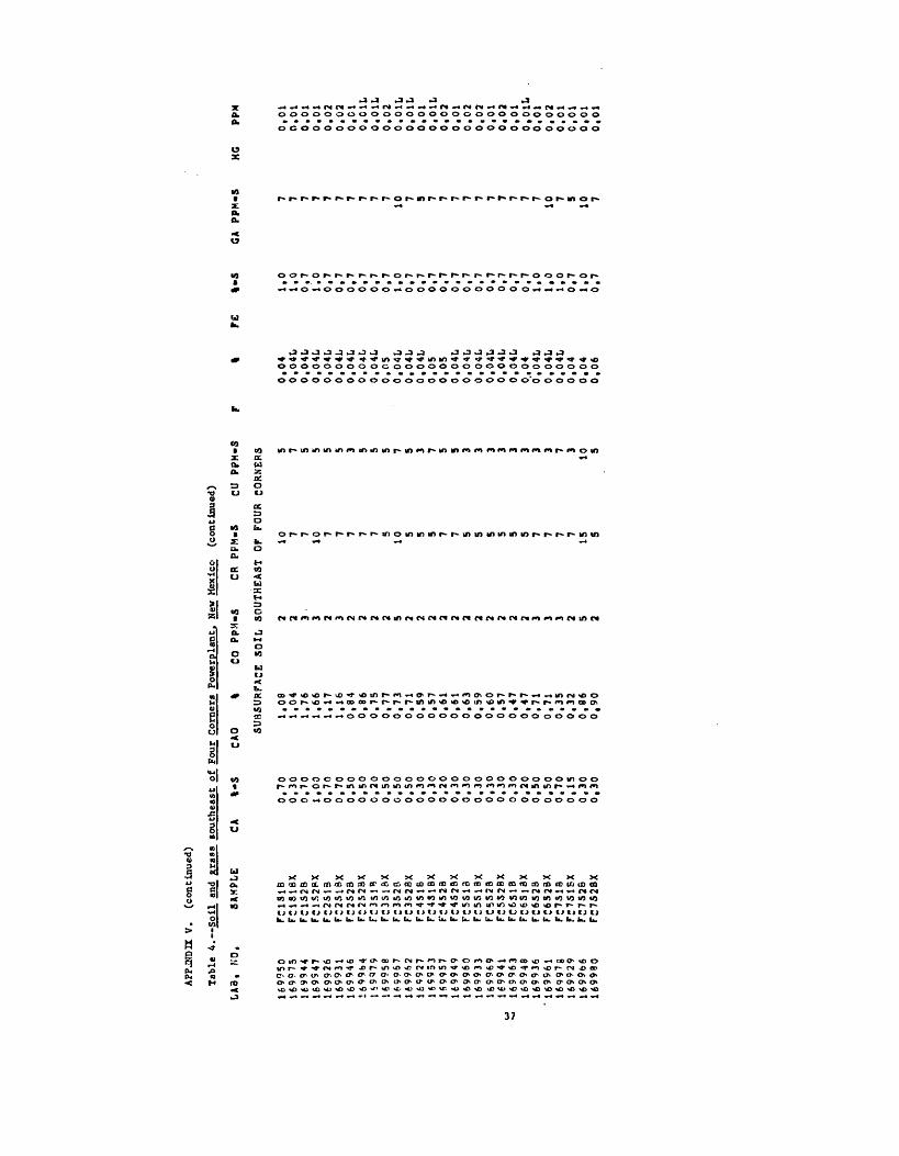
APP

JMD

H V

. (c

onti

nued

)

Tab

le 4

. S

oil

an

d gra

ss

sou

thea

st

of F

our

Cor

ners

P

ower

plan

t.

Nev

Mex

ico

(co

nti

nu

ed)

CR

P

PM

.S

CU

PP

M-S

LAS. NO

,

169950

169975

169944

169947

169926

165931

169946

1699M

IS9979

169958

169967

169962

169927

169953

1S9957

169949

169960

169933

169969

169941

169963

169948

169936

169961

1699?g

169929

169966

169980

SAMPLE

FC1S1B

FC1S1SX

FC1S2B

FC1S2BX

FC2S13

FC2S1BX

FC2S2B

FC2S2BX

FC3S1B

FC3S1BX

FC3S20

FC3S28X

FC4S1B

FC4S1BX

FC4S28

FC4S29X

FC5S13

FC5S1BX

FC5S2B

FC5S2BX

FC6S1B

FC6S18X

FC6S2B

FC632BX

FC7S18

FC7S1SX

FC7S2B

FC7S28X

CA

I-S

0,70

0.30

0.70

1,00

0.70

0,70

0,50

0,50

0,20

0.50

0,50

0.50

0,30

0,30

0.20

0,30

0.30

0.30

0,30

0.30

0.30

0,20

0.50

0,50

0.70

0,15

0,30

0,30

CAO

%

SUBSURFAC

1,08

1.04

1.76

1.66

1.17

1,16

0,84

0,86

0.75

0,77

0,73

0,71

0.59

0,57

0,61

0,61

0,63

0,59

0.60

0.57

0.47

0,47

0.71

0,71

0,35

0.32

0,86

0,90

CO PPM-i

C SOIL SC 2 2 3 3 2 3 2 2 2 2 5 2 2 2 2 2 2 2 2 2 2 2 3 3 3 2 5 2

10 7 7 10 7 7 7 7 7 5

10 5 5 5 7 7 5 S 5 5 5 5 7 7 7 7 15 5

7 310 5

0.0

40

.04

L0

.04

L0.0

4L

0.0

4L

0.0

4L

0.0

4L

0.0

4L

0.0

4L

0.0

50

.04

L0

.04

U0.0

4L

0,0

50,0

50

.04

L0.0

4L

0.0

4L

0.0

4L

0.0

4L

0.0

4L

0,0

40'

,04L

0.0

4L

0.0

4L

0,0

40,0

40.0

6

re

%»s

i.o

1.0

0.7

1

.0

0,7

0.7

0.7

0.7

0.7

0,7

1

.0

0.7

0

.7

0.7

0

.7

0,7

0,7

0

.7

0.7

0

,7

0,7

0.7

1.0

1,0 i.o 0,7

1

.0

0,7

GA

PPM

-S 7 7 7 7 7 7 7 7 7 7 10 7 3 7 7 7 7 7 7 7 7 7 7 10 7 5 10 7

KG

PPM

0,0

10.0

10.0

10.0

10.0

20

,02

0,0

1O

.C1L

0.0

1L

0.0

20

.01

L0

.01

L0,0

10

.01

L0,0

20,0

10

.02

0.0

20,0

10.0

20,0

10

.01

L0.0

10

,02

0.0

10,0

10,0

10,0

1

APP

S.D

IX V

. (c

onti

nued

)

Tab

le 4.-

-Soil

an

d gra

ss

sou

thea

st of

Fou

r C

orne

rs

Pow

erpl

ant.

N

ew M

exic

o (c

on

tin

ued

)

1699SO

169975

169944

169947

169926

169931

169946

169964

169979

165958

169567

169962

169927

169953

169957

169949

169960

169933

169969

169941

e

169963

169948

169936

169961

169973

169929

169966

169980

FCIS

IBFC1S1BX

FC1S2B

FC1S2BX

FC2S13

FC2S18X

FC2S2B

FC2S2BX

FC3S1B

FC3S1BX

FC3S2B

FS3S2BX

FC4S1B

FC4S1BX

FC4S2B

FC4S23X

FCSSlB

FC5MBX

FC5S2B

FC5S2BX

FC6S1B

F:6si&x

FC6S2B

FC6S2BX

FC7S1B

FC7S1BX

FC7S2B

rc7S

2ax

2,3

2,3

2.3

2,3

2,3

2,3

2,3

2.3

2.4

2.4

2.5

2,4

2,3

2

,3

2,3

2.3

2.4

2.3

2.4

2

.3

2.3

2.3

3

.0

3.0

2.8

2.6

2.8

2.9

0 N

0 N

0 N

0 N

0 N

0 N

0 N

0 N

0 N

0 N

30 0

N 0

N 0

N30

0 N

0 N

0 N

0 N

0 N

0 N

0 N

0 N

0 N

0 N

0 N

0 N

0 N

16 15

U

J.3 16 16 11 13 12 13 11 13 11 11 12 11 12 12 11 12 10 11 13 14 10 17 14 14

0.3

00

,20

0.3

00

,30

0,3

00

,20

0,2

00

,20

0,1

50

,20

0,3

00

,20

0,2

00

,20

0,2

00

,20

0,1

50

,15

0,1

50

,15

0,1

00

,10

0,2

00

,20

0,3

00

,07

0,3

00

,20

0,4

70

,45

0,4

30

.42

0,3

70

,36

0.2

70

,28

0.2

60

.26

0,2

70

,27

0,2

50

.25

0,2

70

.28

0,1

90

,18

0,1

80

.17

0.1

50

.14

0.2

10

,22

0,1

40

,15

0.3

40..33

150

200

150

150

150

150

100

150

200

150

200

150

ISO

15

0 15

0 15

0 15

0 10

0 15

0 15

0 15

0 15

0 30

0 30

0 20

0 15

0 30

0 15

0

0.0

2L

0.0

2L

0.0

2L

0.0

2L

0.0

2L

0.0

2L

0.0

2L

0.0

2L

0.0

2L

0.0

2L

0.0

2L

0.0

2L

0.0

2L

0.0

2L

0.0

2L

0.0

2L

0.0

2L

0.0

2L

0.0

2L

0.0

2L

0.0

2L

0.0

2L

0,0

50,0

40.0

2L

0.0

2L

0.0

2L

0.0

2L

1.0

1

.0

«.7

1.0

1

.0

0,7

0,7

1,0

1.0

1.0

1.0

1

.0

0,7

0,7

1,0

0.7

1,0

1.0

1

,0

1,0

1

,0

1,0

1

,0

2,0

1.0

0,7

1.5

1,0

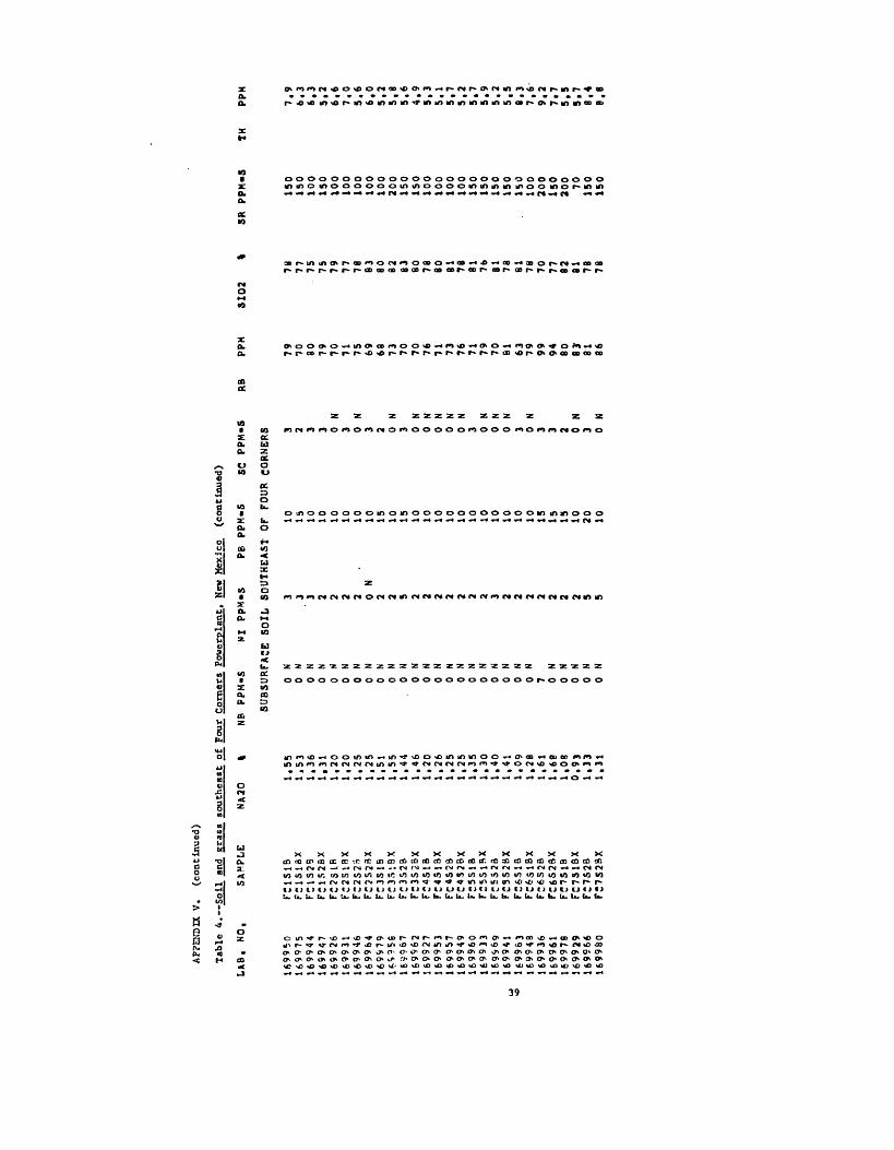
APP

END

IX V

. (c

onti

nued

)

Tab

le 4

. S

oil

an

d gra

ss

sou

theast

o

f F

our

Co

rner

s P

ow

erpla

nt.

N

ev M

exic

o (c

onti

nued

)

LA

B,

NO

, SA

MPL

E

NA

20

% N

B P

PM

-S

NI

PP

M-S

PB

P

PM

-S

SC

PP

M-S

16

99

50

U

9975

169

94

4

16

99

47

1

69

92

6

169

93

1

16

99

46

16

99

64

1

69

97

9

16

99

67

1

69

56

2

16

99

27

1

69

95

3

16

99

57

1

69

94

9

16

99

60

1

69

93

3

16

9*

69

16

99

41

16

99

63

1

69

94

8

16

99

36

16

99

61

16

99

78

1699J9

1

69

96

6

16

99

80

SAMPLE

NA20

%NB PPM-S

f

SUBSURFACE

FC1S1B

FC1S13X

FC1S2B

FC1S2BX

FC2S

I.B

FC2S1BX

T Z 2 S 2 3

FC2S23X

FC3S1B

FC3S1BX

FC3S2B

FC3S2BX

FC4S1B

FC4S1BX

FC4S28

FC432BX

FC5S1B

FC5S1BX

FC552B

FC3S2BX

FC6S1B

FC6S1BX

FC6S2B

FC6S2BX

FC7S1B

FC7S1BX

FC7S2B

FC7S2BX

1 1 1 1 1 1 1 1 1 1 1 1 1 1 1 1 1 1 1 1 1 1 1 1 1 0 1 1

.55

,53

,36

.31

,20

.20

.25

.25

,51

,55

.44

.46

,20

.26

.25

.25

.35

.30

.40

.41

.09

.20

.61

.68

,08

.93

.33

.31

0 0 0 0 0 0 0 0 0 0 0 0 0 0 0 0 0 0 0 0 0 0 7 0 0 0 0 0

N N N N fi N N N N N N N N N N N N N N' N N N N N N N N

il PPM-!

SOIL SI 3 3 3 2 2 2 2 0 2 2 5 2 2 2 2 2 2 2 3 2 2 2 2 2 2 2 5 5

RB

10 15 10 10 10 10 10 10 15 10 15 10 10 10 10 10 10 10 10 10 10 10 15 15 15 10 20 10

3 2 3 3 0 N

3 0 N

3 2 0 N

3 0 N

0 N

0 N

0 N

0 N

3 0 N

0 N

0 N

3 0 N

3 3 2 0 N

3 0 N

PPM

79

70 80

79

70 71

75

69

68

73

70

70

76

71

73

76

7i

79

70

81

63

79

99

94

80

83

81

86

S102

78 77 75

75

79 77 78 83 80

02 83 80 78

80 81 78 81 76 81 78 81 78 70 77 82 81 78 78

5R

PP

M-S

15

01

50

10

01

50

10

01

00

10

01

00

10

02

00

15

01

50

10

0to

o1

00

10

01

50

15

01

50

15

01

50

10

02

00

15

02

00 70

15

01

50

TH

PPM

7.9

6

.3

6.3

5

,2

6,6

7

.0

5.6

6,0

5,2

5,8

5

.6

4.9

5,3

5

.1

5,7

5,2

5.7

5,9

5

.2

5,5

8,3

7,6

9,2

7,7

5

,5

5,7

8,4

8

.8

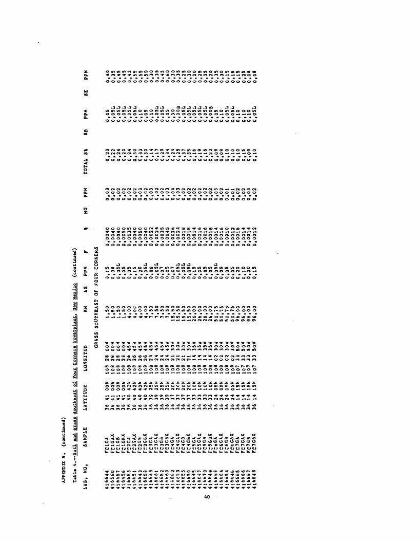
APP

END

IX V

. (c

onti

nued

)

Tab

le 4

. S

oil

an

d gra

ss

south

east

of

F

our

Cor

ners

P

ower

plan

t.

New

Hex

tco

(co

nti

nu

ed)

LA

B,

NO

. SA

MPL

E L

AT

ITU

DE

LQ

NG

ITU

D

KM

AS

PPM

F

%

416644

416560

416&57

416656

416653

416651

416643

416658

416663

416661

4]6652

41*669

41^662

416659

416655

416650

416645

416647

*.

416670

0 416649

. 416668

416664

416654

416646

416665

416666

416667

416648

FCICA

FC1GAX

Fcic

aFC1CBX

F*2GA

FC2GAX

FC2G3

FZ2GBX

FC3G*

FC3GAX

FC3GB

FC3GBX

FC4GA

FC4GAX

FC4GB

FC4GBX

FCSG

ftFC5GAX

FC5GB

FCSGBX

FC6GA

FC6GAX

FC6G3

FC6GBX

FC7GA

FC7GAX

FC7GB

FC7GBX

36 36 36 36 36 36 36 36 36 36 36 36 36 36 36 36 36 36 36 36 36 36 36 36 36 36 36 36

41 41 41 41 40 40 40 40 39 39 39 39 37 37 37 37 33 33 33 33 24 24 24 24 14 14 14 14

OON

OON

OON

OON

42N

42N

42"

42N

25N

25N

25N

25N

2 ON

20N

20N

20N

ION

ION

ION

ION

05N

05N

05N

05N

15N

15N

15N

15N

108

108

108

108

108

108

108

108

108

108

108

108

108

108

108

108

108

108

108

108

108

108

108

108

107

107

107

107

28 28 28 28 26 26

26 26 24 24 24 24 21 21 21 21 14 14 14 14 02 02 02 02 33 33 33 33

00*

00*

00*

OOrf

45rf

454

45*

454

45*

454

45rf

45rf

30*

30*

30*

30*

35*

35rf

3SW

35*

30*

30*

30*

SO*

SOW

50"

SOW

sow

1 1 1 1 4 4 4 4 7 7 7 715 15 IS IS 26 26 26 26 50 50 50

,50

.50

,50

,50

,00

,00

,00

,00

,50

,50

.50

,50

,50

,50

,50

,50

,00

,00

,00

,00

,75

.75

,7b

50,75

96 96 96 96

,00

,00

,00

,00

0,15

O.OB

0.05L

0.05

0.05

0.15

0,20

0.05L

0,06

O.OSL

0,07

0,05

0,07

<),0

5L0.05L

0,05L

0,15

0,05

0,05

0,05

0.05L

0,09

0,05

0,05

0.20

0,10

0,20

0,15

0,0040

0,0040

0.0040

0,0050

0,0035

0,0040

0,0050

0,0040

0,0022

0,0024

0,0035

0.0045

0,0026

0,0024

0.001B

0.001B

0,0014

0,0016

0,0016

0,0018

0,0014

0,0016

0,0010

0,0012

0,0016

0,0014

0,0014

0,0012

0,0

30

.02

0,0

20.0

20

,02

0,0

20

,03

0,0

20,0

30

,02

0,0

20,0

30,0

40,0

30

,02

0,0

20,0

20,0

20,0

20

,02

0,0

30

,02

0,0

10

,01

0,0

20

,02

0,0

30

,02

0,2

30

,22

0,2

40

,20

0.2

40

.30

0.3

30

.30

0.1

40,1

70,2

90,3

40,2

40,2

50,3

70,3

50,1

60,1

90,1

60,2

20,0

90,0

90,1

00,1

00,1

00,1

50,0

90,1

0

0,0

50,

OS

L0

.05

LO

.OSL

0,0

5L

0.0

5L

0,1

00,0

50,1

0O

.OSL

O.O

SL0.0

50,3

0O

.OO

BO

.OSL

O.O

SL0

,05

1,

0.0

5L

0.0

5L

O.O

OB

0,0

5 ,

0,1

0O

.OSL

O.O

SL

0,1

00,1

00,1

0O

.OSL

0,4

00,3

50,4

50,4

50,4

50,5

50,5

50,5

00,3

00,3

50,4

50.6

00,3

00,3

50.2

50,3

00.2

00,2

50.2

50,2

00.3

50.3

00,1

50,1

50

,15

0,2

50

,08

0,0

8

APPENDIX V

. (continued)

Table

A.--Soil and

grass

southeast

of F

our

Corn

ers

Powerplant.

New Mexico

(con

tinu

ed)

LAB, NO.

4JI5

644

41 bobO

41665?

416656

416653

4J6651

416643

416655

416663

416661

416652

416661

4l66( 2

4165-

)416615

41665:

41664 >

416647

416670

41-6

649

4<6t63

416664

416654

416646

416665

4«6666

416667

416648

SAMPLE

FC1GA

FC1GAX

FC1G9

FCIG

SXFC2GA

FC2GAX

FC2G3

FC2GBX

FC3GA

TC3GAX

FC3G3

FC3GSX

FC4GA

FC4GAX

FC4G&

FC4GBX

FC5GA

FC5GAX

FC5G5

FCSG

SXFC6GA

FC6GAX

FC6G3

FC6GBX

FC7GA

FC7GAX

FC7GB

FC7GBX

ASH

%

7,7

6,5

8.5

8,6

9,5

10,0

9,6

8,0

5,9

6,3

12,0

12.0

7.1

6,3

7,7

8,5

5,7

5.8

5,1

5.1

5,7

5.1

4,8

5,2

6,7

6,4

6,3

7.5

AG PPM-S

AL

GRASS SO

I

0,ON

O.ON

O.ON

0.7

O.ON

O.ON

0,ON

O.OM

O.OM

O.OM

O.ON

O.OPJ

O.ON

O.ON

O.ON

O.ON

o.ow

O.ON

. O.ON

O.OM

O.ON

O.ON

0,7

0,ON

O.ON

O.CN

O.Of*

O.ON

%-S

UTHEAi

5.0

5,0

5.0

7,0

2,0

3,0

5,0

5,0

3,0

3.0

5,0

5.0

3,0

5.0

1,5

1.5

3.0

3,0

2.0

2.0

3,0

2,0

5,0

5,0

5.0

5,0

3.0

3,0

B PPM.5

300

200

200

200

200

300

200

300

300

200

200

200

200

200

150

150

i50

150

200

200

200

200

150

150

100

!.00

150

150

BA PPM-S

1500

1500

1500

1500

700

1000

1500

1500

1500

1500

1000

1000

1500

1500

700

700

1500

1500

1000

1000

1500

1500

1500

1500

1000

1000

1000

700

CA

%-S

10 10 G

10

105 7

10 10 G

10 G

10

10

10

10

10

10 10 G

10

10 7 7 107

10

107 7 7 7

CA/A

6,6

7,2

6,8

6,6

5,2

5.2

6,0

8,0

7,2

6,6

5,6

5,6

6,0

5,6

7,6

7,4

6,6

7,2

7,2

6,6

4,8

5,6

6,6

6,6

4.4

5,2

4,4

4,2

CD/A PPM

0,4

0,4L

1.6

1,0

0,4L

1,6

1.0

l.OL

0.4L

0,4

1,0

0,8

0,4

0,4L

1,0

1,0

0,4

0,4L

-0,8

1,8

0.8

0,4

0,4L

1,8

0,4

1,2

1,2

1.0

CO/A PPM

4.2

4,6

3,2

3,8

2,4

3.2

4,2

5,0

3,2

3,8

3,2

1,4

3,2

3.8

3,2

3,2

3,8

2,4

1,4

3,2

1.4

2,8

2,8

2.8

2,8

1,4

1.4

2,4

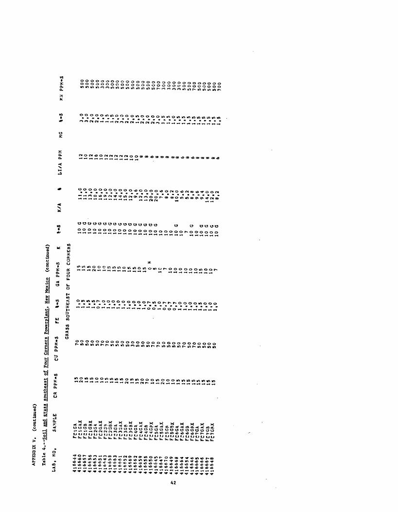
APPSMJDC V.

(continued)

Table

LAB, NO

416644

4:6660

416657

416656

416653

416651

416643

416659

416663

416661

416652

416669

4}6662

4:6659

416655

416650

416645

4J664?

416670

416649

416668

416664

416654

416646

416665

416666

416667

416648

4. Soil

and

gras

s

SAMPLE

FC1GA

FCIGAX

PClGS

FC1G3X

FC2GA

FC2GAX

FC23*

FC2GBX

FC3GA

FC33AX

FC3G9

FC3G3X

FC4GA

FC4GAX

FC4GS

FC4G?X

FC5GA

FC5GAX

F:SGP

FC5G3X

FC6GA

FC6GAX

FC6G3

FC6G8X

FC7GA

FC7GAX

FC7G3

FC7GRX

southeast

o

CR PPK-S

15 20 15 15 10 10 15 15 15 15 20 15 15 20 70 10 15 20 10 10 15 15 15 15 15 15 15 15

Ctf PPM-S GRASS

70 50 50 50

50 70

70 50

50

50 50

30

50 50 50

70

70 50 50

50 50 70

50

70 50 50 50

50

FE

I-S

SOUTHEAST

1,0

1,5

1.5

1.5

0,7

1.0

1,0

1,0

1.0

i.o

1.0

1.0

1.0

1,0

0,7

' 0,5

1,0

0.7

0,7

0,7

1.0

1,0

1.0

1.0

1.5

1.0

1,0

1,0

«... *.wv

Y**VUI. MAUBU7

GA PPM-5

K

OF FOUR CORNERS

15 IS 15 20 10 1()

15 15 15 10 IS 15

10 15 0 N

51C7

10 10 10 10 10

10 15 10 107

%-S

10 G

10 G

10 G

10 G

10 G

10 G

10 G

10 G

10 G

10 G

10 G

10 G

10 G

10 G

10 G

10 G

10 10 10 10 G

10 710 G

10 10 G

10 G

10 G

10 G

K/A

ll.C

11,0

13.0

10,0

16,0

19,0

12.0

14,0

14,0

15,0

12,0

9,6

12,0

13,0

20.0

20,0

7,6

e.o

8,2

10,0

3.6

5.2

8.8

9,6

9,4

14,0

12.0

8.2

LI/A PPM

12 10 12 16 10 12 12 12 12 12 10 108 8 6 a a 8 e e 6 e 6 e 8 e e 6

HG

%-S

3,0

3.0

2,0

2,0

1,0

1,5

1.5

2,0

3,0

2.0

2,0

1,5

2,0

2,0

2,0

3.0

1,5

1.5

1.0

1,5

1,5

1,5

1.5

1.5

1,5

1,5

1,5

1,5

KM PPM-S

500

500

500

500

300

300

500

500

500

500

500

500

500

500

500

700

300

300

300

300

500

500

700

500

500

500

500

700

APP

END

IX V

. (c

onti

nued

)

Tab

le 4.-

-Soil

an

d g

rass

so

uth

east

of

Fou

r C

orne

rs P

ov

erp

lan

t.

New

Mex

ico

(con

tin

ued

)

LA

B.

NO

. SA

MPL

E M

O PP

M-S

N

A/A

%

NX

PpM

-S

P %

«S

P/A

PP

M

416644

416660

4166

5?4*6656

416653

416651

4lb£

4341

6658

4166

634l6f61

4'6652

4166

69416662

416659

4166

5541

6650

4166

4541

6647

416670

416649

4166

68416664

4166

54416646

416665

416666

4166

6741

6648

FCIGA

FCIGAX

FCIG

BFC

IG&X

FC2GA

F-2GAX

FC2G8

FC2G3X

FC3GA

FC3'

GAX

FC3GB

FC3G3X

F-4GA

FC4GAX

FC4GB

FC4GSX

FC5GA

FC5GAX

F:5GB

FC5GBX

FC6GA

FC6GAX

F:6GB

FC6GSX

F^7GA

FC7GAX

FC7GB

FC7GBX

30

30

15

50

20

30

30

20

30

30

20

20

20

IS

30

20

157

10

15

15

15

15 710

150

N7

0.24

0,22

0.15

0,19

0.24

0.17

O.lR

0,15

0.14

0.11

0,12

0.11

0.09

0.11

0.06

0.06

0.06

O.OB

0.

07

0.07

0,15

0.10

0,15

0.15

O.OB

O.OB

O.OB

0,07

30

10

20

15

'

7 10

15 7 10

10

107 7

10

10

157 10 7 0

N7 7 7 7

10

105 5

1.5

1.5

1.5

l.o

1.5

2.0

1.5

2.0

1.5

1.5

1.5

1.5

1.5

2.0

3,0

2,0

1,5

1,5

1.5

2,0

1.5

1.5

1.5

1.5

2.0

2,0

1.5

1.5

6000

6000

6000

6000

9000

12000

9000

9000

6000

9000

9000

9000

9000

9000

1200

012

000

6000

9000

9000

12000

6000

6000

9000

6000

9000

1200

06000

6000

50 50 30 50 20 20 30 30 30 20 20 30 '30

300

N20 50 50 30 50 30 50 30 30 50 30

.50 50

190000

210000

210000

2100

00.

200000

210000

210000 0

B220000

2200

00220000

250000

210000

190000

160000

1700

00250000

260000

240000

250000

270000

260000

250000

250000

280000

230000

260000

300000

700

700

700

700

700

1000 700

700

1000

1000 700

500

500

500

700

700

500

300

300

300

500

500

700

700

300

300

300

200

0,10

0.15

0,10

0.15

0.05

0,07

0.10

0.10

0.10

0.10

0,07

0.10

0.10

0.10

0.03

0.05

0,07

0,07

0.07

0,07

0.10

0,10

0,10

0,07

0.15

0.15

0.15

0,07

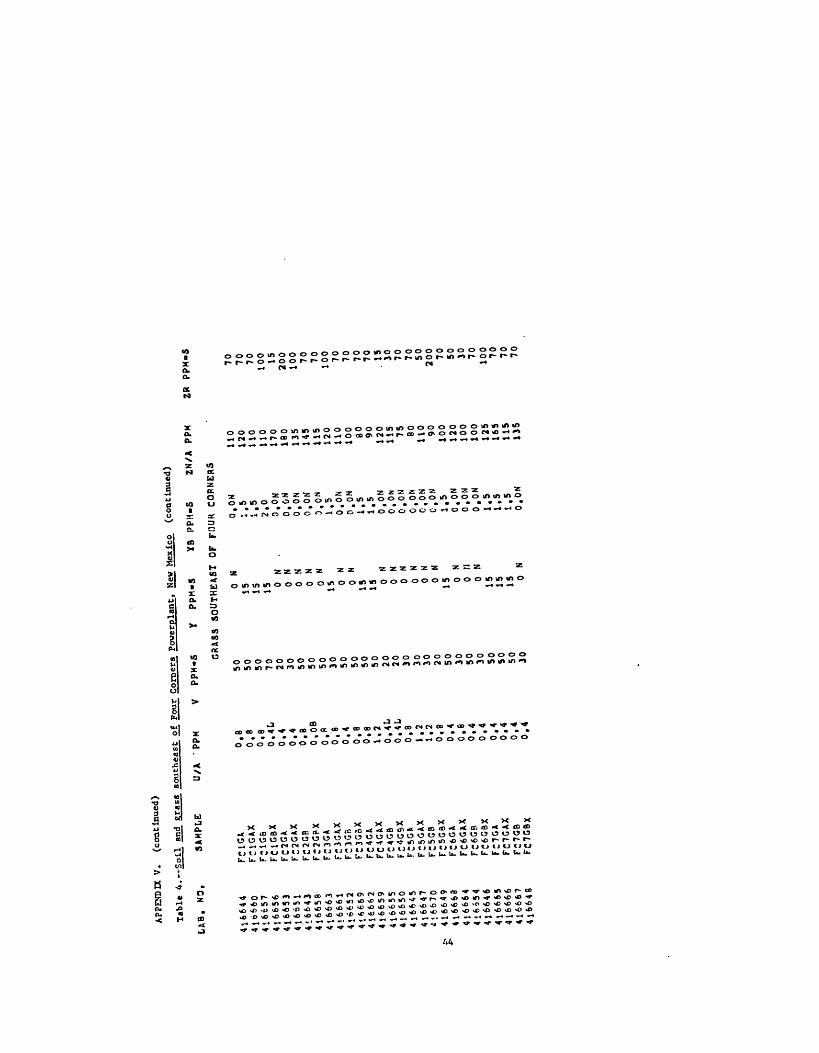
APP

END

IX V

. (c

onti

nued

)so

uth

east

of

Fou

r C

orne

rs,

Po

ver

pla

nt.

N

ew M

extc

o (c

on

tin

ued

)

YB

PPH

«S

ZN

/A

PPM

Table

4. Soil an

a gr

ass.

&;

LAB. NO.

SAMPLE

416644

416660

416657

416656

416653

416651

416643

416658

416663

41666!

416652

416669

416662

416659

416655

416650

416645

416647

4 «6670

416649

416663

416664

416654

416646

416665

416666

416667

416648

FC1GJ,

FC1GAX

FC1GB

FC1GBX

FC2GA

FC2GAX

FC2GB

FC2GPX

FC3GA

FC3GAX

FC3G&

FC3GBX

FC4GA

FC4GAX

FC4GB

FC4G5X

FC5GA

FC5GAX

FC5G3

FC5GBX

FC6GA

FC6GAX

FC6G3

FC6GBX

FC7GA

FC7GAX

FC7GB

FC7GBX

U/A 'PPM

V

O.B

0.8

OQ

. 8

0.4L

0.4

0.4

00

. B

O.OB

O.fl

0,8

0.4

o.e

00 . 8

1.2

0.4L

0.4L

O.B

1.2

1.2

o.e

0.4

0.6

0.4

0.4

0.4

0.4

0,4

0.4

PPM-S

Y

GRASS

50

50

50 70

20

30

50 50

50 30 50 50

50 50

20

20

30

30

30 20

50

30

50

30

50

50

50

30

PPM-S

SOUTHEAST

0 N

15

15 150

N 0

N 0

N0

N 0

N15 0

N0

N 15 150

N 0

N 0

N 0

N 0

N 0

N150

No

n0

N 15

15

150

N

O.ON

i.5

1.5

2.0

O.ON

O.ON

O.ON

O.Of

JD.

ON1.5

O.ON

O.ON

1.5

1.5

O.ON

O.ON

O.ON

O.ON

O.ON

C.ON

1.5

O.ON

O.ON

O.ON

1.5

1.5

1.5

O.OM

110

120

110

110

170

180

135

145

115

120

110

100 80 90 120

115 75 BO

110 90 100

120

100

100

125

165

115

135

ZR

PP

M-S

70 70 70 100 15

20

010

0 70 70 100 70 70 70 70 .

15 30 70 70 50

20

0 70 50 30 70

100 70 70 70

third annual progress report, july 1976 by - pubs.usgs.gov · pdf filethird annual progress...

Documents