thirty-three miniatures: mathematical and algorithmic ...matousek/stml-53-matousek-1.pdf ·...
TRANSCRIPT
Thirty-three Miniatures: Mathematical and Algorithmic Applications of Linear Algebra Jiřì Matoušek This is a preliminary version of the book Thirty-three Miniatures: Mathematical and Algorithmic Applications of Linear Algebra published by the American Mathematical Society (AMS). This preliminary version is made available with the permission of the AMS and may not be changed, edited, or reposted at any other website without explicit written permission from the author and the AMS.
Author's preliminary version made available with permission of the publisher, the American Mathematical Society

1991 Mathematics Subject Classification. 05C50, 68Wxx, 15-01
Author's preliminary version made available with permission of the publisher, the American Mathematical Society

Contents
Introduction vii
Notation 1
Miniature 1. Fibonacci Numbers, Quickly 3
Miniature 2. Fibonacci Numbers, the Formula 5
Miniature 3. The Clubs of Oddtown 7
Miniature 4. Same-Size Intersections 9
Miniature 5. Error-Correcting Codes 11
Miniature 6. Odd Distances 17
Miniature 7. Are These Distances Euclidean? 19
Miniature 8. Packing Complete Bipartite Graphs 23
Miniature 9. Equiangular Lines 27
Miniature 10. Where is the Triangle? 31
Miniature 11. Checking Matrix Multiplication 35
Miniature 12. Tiling a Rectangle by Squares 39
v
Author's preliminary version made available with permission of the publisher, the American Mathematical Society

vi Contents
Miniature 13. Three Petersens Are Not Enough 41
Miniature 14. Petersen, Hoffman–Singleton, and Maybe 57 43
Miniature 15. Only Two Distances 49
Miniature 16. Covering a Cube Minus One Vertex 53
Miniature 17. Medium-Size Intersection Is Hard To Avoid 55
Miniature 18. On the Difficulty of Reducing the Diameter 59
Miniature 19. The End of the Small Coins 65
Miniature 20. Walking in the Yard 69
Miniature 21. Counting Spanning Trees 75
Miniature 22. In How Many Ways Can a Man Tile a Board? 83
Miniature 23. More Bricks—More Walls? 95
Miniature 24. Perfect Matchings and Determinants 105
Miniature 25. Turning a Ladder Over a Finite Field 111
Miniature 26. Counting Compositions 117
Miniature 27. Is It Associative? 123
Miniature 28. The Secret Agent and the Umbrella 129
Miniature 29. Shannon Capacity of the Union: A Tale of Two
Fields 137
Miniature 30. Equilateral Sets 145
Miniature 31. Cutting Cheaply Using Eigenvectors 151
Miniature 32. Rotating the Cube 161
Miniature 33. Set Pairs and Exterior Products 169
Index 177
Author's preliminary version made available with permission of the publisher, the American Mathematical Society
Introduction
Some years ago I started gathering nice applications of linear algebra,
and here is the resulting collection. The applications belong mostly
to the main fields of my mathematical interests—combinatorics, ge-
ometry, and computer science. Most of them are mathematical, in
proving theorems, and some include clever ways of computing things,
i.e., algorithms. The appearance of linear-algebraic methods is often
unexpected.
At some point I started to call the items in the collection “minia-
tures”. Then I decided that in order to qualify for a miniature, a
complete exposition of a result, with background and everything,
shouldn’t exceed four typeset pages (A4 format). This rule is ab-
solutely arbitrary, as rules often are, but it has some rational core—
namely, this extent can usually be covered conveniently in a 90 minute
lecture, the standard length at the universities where I happened to
teach. Then, of course, there are some exceptions to the rule, six-page
miniatures that I just couldn’t bring myself to omit.
The collection could obviously be extended indefinitely, but I
thought thirty three was a nice enough number and a good point
to stop.
The exposition is intended mainly for lecturers (I’ve taught al-
most all of the pieces at various occasions) and also for students
interested in nice mathematical ideas even when they require some
vii
Author's preliminary version made available with permission of the publisher, the American Mathematical Society

viii Introduction
thinking. The material is hopefully class-ready, where all details left
to the reader should indeed be devil-free.
I assume background of basic linear algebra, a bit of familiarity
with polynomials, and some graph-theoretical and geometric termi-
nology. The sections have varying levels of difficulty and generally
I have ordered them from what I personally regard as the most ac-
cessible to the more demanding.
I wanted each section to be essentially self-contained. With a
good undergraduate background you can as well start reading at Sec-
tion 24. This is kind of opposite to a typical mathematical textbook,
where material is developed gradually, and if one wants to make sense
of something on page 123, one usually has to understand the previous
122 pages, or with some luck, suitable 38 pages.
Of course, the anti-textbook structure leads to some boring rep-
etitions and, perhaps more seriously, it puts a limit on the degree of
achievable sophistication. On the other hand, I believe there are ad-
vantages as well: I gave up reading several textbooks well before page
123, after I realized that between the usually short reading sessions
I couldn’t remember the key definitions (people with small children
will know what I’m talking about).
After several sections the reader may spot certain common pat-
terns in the presented proofs, which could be discussed at great
length, but I have decided to leave out any general accounts on linear-
algebraic methods.
Nothing in this text is original, and some of the examples are
rather well known and appear in many publications (including, in few
cases, other books of mine). Several general reference books are listed
below. I’ve also added references to the original sources where I could
find them. However, I’ve kept the historical notes at a minimum and
I’ve put only a limited effort into tracing the origins of the ideas (many
apologies to authors whose work is quoted badly or not at all—I will
be glad to hear about such cases).
I would appreciate to learn about mistakes and suggestions of
how to improve the exposition.
Author's preliminary version made available with permission of the publisher, the American Mathematical Society
Introduction ix
Further reading. An excellent textbook is
L. Babai and P. Frankl, Linear Algebra Methods
in Combinatorics (Preliminary version 2), Depart-
ment of Computer Science, The University of Chi-
cago, 1992.
Unfortunately, it has never been published officially and it can be ob-
tained, with some effort, as lecture notes of the University of Chicago.
It contains several of the topics discussed here, a lot of other material
in a similar spirit, and a very nice exposition of some parts of linear
algebra.
Algebraic graph theory is treated, e.g., in the books
N. Biggs, Algebraic Graph Theory, 2nd edition,
Cambridge Univ. Press, Cambridge, 1993
and
C. Godsil and G. Royle, Algebraic Graph Theory,
Springer, New York, NY, 2001.
Probabilistic algorithms in the spirit of Sections 11 and 24 are well
explained in the book
R. Motwani and P. Raghavan, Randomized Algo-
rithms, Cambridge University Press, Cambridge,
1995.
Acknowledgments. For valuable comments on preliminary versions
of this booklet I would like to thank Otfried Cheong, Esther Ezra,
Nati Linial, Jana Maxova, Helena Nyklova, Yoshio Okamoto, Pavel
Patak, Oleg Pikhurko, and Zuzana Safernova, as well as all other
people whom I may have forgotten to include in this list. Thanks
also to David Wilson for permission to use his picture of a random
lozenge tiling in Miniature 22. Finally, I’m grateful to many people
at the Department of Applied Mathematics of the Charles University
in Prague and at the Institute of Theoretical Computer Science of the
ETH Zurich for excellent working environments.
Author's preliminary version made available with permission of the publisher, the American Mathematical Society

Author's preliminary version made available with permission of the publisher, the American Mathematical Society
Notation
Most of the notation is recalled in each section where it is used. Here
are several general items that may not be completely unified in the
literature.
The integers are denoted by Z, the rationals by Q, the reals by
R, and Fq stands for the q-element finite field.
The transpose of a matrix A is written as AT . The elements
of that matrix are denoted by aij , and similarly for all other Latin
letters. Vectors are typeset in boldface: v,x,y, and so on. If x is a
vector in Kn, where K is some field, xi stands for the ith component,
so x = (x1, x2, . . . , xn).
We write 〈x,y〉 for the standard scalar (or inner) product of vec-
tors x,y ∈ Kn: 〈x,y〉 = x1y + x2y2 + · · · + xnyn. We also interpret
such x,y as n×1 (single-column) matrices, and thus 〈x,y〉 could also
be written as xT y. Further, for x ∈ Rn, ‖x‖ = 〈x,x〉1/2 is the Eu-
clidean norm (length) of the vector x.
Graphs are simple and undirected unless stated otherwise; i.e., a
graph G is regarded as a pair (V,E), where V is the vertex set and
E is the edge set, which is a set of unordered pairs of elements of V .
For a graph G, we sometimes write V (G) for the vertex set and E(G)
for the edge set.
1
Author's preliminary version made available with permission of the publisher, the American Mathematical Society

Author's preliminary version made available with permission of the publisher, the American Mathematical Society

Miniature 1
Fibonacci Numbers,Quickly
The Fibonacci numbers F0, F1, F2, . . . are defined by the relations
F0 = 0, F1 = 1, and Fn+2 = Fn+1 +Fn for n = 0, 1, 2, . . .. Obviously,
Fn can be calculated using roughly n arithmetic operations.
By the following trick we can compute it faster, using only about
logn arithmetic operations. We set up the 2×2 matrix
M :=
(
1 1
1 0
)
.
Then(
Fn+2
Fn+1
)
= M
(
Fn+1
Fn
)
,
and therefore,(
Fn+1
Fn
)
= Mn
(
1
0
)
(we use the associativity of matrix multiplication).
For n = 2k we can compute Mn by repeated squaring, with k
multiplications of 2×2 matrices. For n arbitrary, we write n in binary
as n = 2k1 +2k2 + · · ·+2kt , k1 < k2 < · · · < kt, and then we calculate
the power Mn as Mn = M2k1
M2k2 · · ·M2kt. This needs at most
2kt ≤ 2 log2 n multiplications of 2×2 matrices.
3
Author's preliminary version made available with permission of the publisher, the American Mathematical Society

4 1. Fibonacci Numbers, Quickly
Remarks. A similar trick can be used for any sequence (y0, y1, y2, . . .)
defined by a recurrence yn+k = ak−1yn+k−1 + · · ·+a0yn, where k and
a0, a1, . . . , ak−1 are constants.
If we want to compute the Fibonacci numbers by this method,
we have to be careful, since the Fn grow very fast. From a formula
in Miniature 2 below, one can see that the number of decimal digits
of Fn is of order n. Thus we must use multiple precision arithmetic,
and so the arithmetic operations will be relatively slow.
Sources. This trick is well known but so far I haven’t encounteredany reference to its origin.
Author's preliminary version made available with permission of the publisher, the American Mathematical Society

Miniature 2
Fibonacci Numbers, theFormula
We derive a formula for the nth Fibonacci number Fn. Let us consider
the vector space of all infinite sequences (u0, u1, u2, . . .) of real num-
bers, with coordinate-wise addition and multiplication by real num-
bers. In this space we define a subspace W of all sequences satisfying
the equation un+2 = un+1 +un for all n = 0, 1, . . .. Each choice of the
first two members u0 and u1 uniquely determines a sequence from W,
and therefore, dim(W ) = 2. (In more detail, the two sequences begin-
ning with (0, 1, 1, 2, 3, . . .) and with (1, 0, 1, 1, 2 . . .) constitute a basis
of W.)
Now we find another basis of W : two sequences whose terms are
defined by a simple formula. Here we need an “inspiration”: We
should look for sequences u ∈ W in the form un = τn for a suitable
real number τ .
Finding the right values of τ leads to the quadratic equation τ2 =
τ + 1, which has two distinct roots τ1,2 = (1 ±√
5)/2.
The sequences u := (τ01 , τ
11 , τ
21 , . . .) and v := (τ0
2 , τ12 , τ
22 , . . .) both
belong to W , and it is easy to verify that they are linearly independent
(this can be checked by considering the first two terms). Hence they
form a basis of W .
5
Author's preliminary version made available with permission of the publisher, the American Mathematical Society

6 2. Fibonacci Numbers, the Formula
We express the sequence F := (F0, F1, . . .) of the Fibonacci num-
bers in this basis: F = αu + βv. The coefficients α, β are calculated
by considering the first two terms of the sequences; that is, we need
to solve the linear system ατ01 + βτ0
2 = F0, ατ11 + βτ1
2 = F1.
The resulting formula is
Fn =1√5
[(
1 +√
5
2
)n
−(
1 −√
5
2
)n]
.
It is amazing that this formula full of irrationals yields an integer for
every n.
A similar technique works for other recurrences in the form yn+k =
ak−1yn+k−1 + · · ·+a0yn, but additional complications appear in some
cases. For example, for yn+2 = 2yn+1− yn, one has to find a different
kind of basis, which we won’t do here.
Sources. The above formula for Fn is sometimes called Binet’s
formula, but it was known to Daniel Bernoulli, Euler, and de Moivrein the 18th century before Binet’s work.
A more natural way of deriving the formula is using generating func-tions, but doing this properly and from scratch takes more work.
Author's preliminary version made available with permission of the publisher, the American Mathematical Society
Miniature 3
The Clubs of Oddtown
There are n citizens living in Oddtown. Their main occupation was
forming various clubs, which at some point started threatening the
very survival of the city. In order to limit the number of clubs, the
city council decreed the following innocent-looking rules:
• Each club has to have an odd number of members.
• Every two clubs must have an even number of members in
common.
Theorem. Under these rules, it is impossible to form more clubs
than n, the number of citizens.
Proof. Let us call the citizens 1, 2, . . . , n and the clubs C1, C2, . . . , Cm.
We define an m× n matrix A by
aij =
{
1 if j ∈ Ci, and
0 otherwise.
(Thus clubs correspond to rows and citizens to columns.)
Let us consider the matrix A over the two-element field F2. Clear-
ly, the rank of A is at most n.
Next, we look at the product AAT . This is an m × m matrix
whose entry at position (i, k) equals∑n
j=1 aijakj , and so it counts
the number of citizens in Ci ∩Ck. More precisely, since we now work
over F2, the entry is 1 if |Ci∩Ck| is odd, and it is 0 for |Ci∩Ck| even.
7
Author's preliminary version made available with permission of the publisher, the American Mathematical Society

8 3. The Clubs of Oddtown
Therefore, the rules of the city council imply that AAT = Im,
where Im denotes the identity matrix. So the rank of AAT is at least
m. Since the rank of a matrix product is no larger that the minimum
of the ranks of the factors, we have rank(A) ≥ m as well, and so
m ≤ n. The theorem is proved. �
Sources. This is the opening example in the book of Babai andFrankl cited in the introduction. I am not sure if it appears earlier inthis “pure form”, but certainly it is a special case of other results, suchas the Frankl–Wilson inequality (see Miniature 17).
Author's preliminary version made available with permission of the publisher, the American Mathematical Society

Miniature 4
Same-Size Intersections
The result and proof of this section are similar to those in Miniature 3.
Theorem (Generalized Fisher inequality). If C1, C2, . . . , Cm are dis-
tinct and nonempty subsets of an n-element set such that all the in-
tersections Ci ∩ Cj, i 6= j, have the same size, then n ≥ m.
Proof. Let |Ci ∩ Cj | = t for all i 6= j.
First we need to deal separately with the situation that some Ci,
say C1, has size t. Then t ≥ 1 and C1 is contained in every other
Cj . Thus Ci ∩ Cj = C1 for all i, j ≥ 2, i 6= j. Then the sets Ci \ C1,
i ≥ 2, are all disjoint and nonempty, and so their number is at most
n− |C1| ≤ n− 1. Together with C1 these are at most n sets.
Now we assume that di := |Ci| > t for all i. As in Miniature 3,
we set up the m× n matrix A with
aij =
{
1 if j ∈ Ci, and
0 otherwise.
Now we consider A as a matrix with real entries, and we let B :=
AAT . Then
B =
d1 t t . . . t
t d2 t . . . t...
......
......
t t t . . . dm
,
9
Author's preliminary version made available with permission of the publisher, the American Mathematical Society

10 4. Same-Size Intersections
t ≥ 0, d1, d2, . . . , dm > t. It remains to verify that B is nonsingular;
then we will have m = rank(B) ≤ rank(A) ≤ n and we will be done.
The nonsingularity of B can be checked in a pedestrian way, by
bringing B to a triangular form by a suitably organized Gaussian
elimination.
Here is another way. We will show that B is positive definite;
that is, B is symmetric and xTBx > 0 for all nonzero x ∈ Rm.
We can write B = tJn +D, where Jn is the all 1’s matrix and D
is the diagonal matrix with d1 − t, d2 − t, . . . , dn − t on the diagonal.
Let x be an arbitrary nonzero vector in Rn. Clearly, D is positive
definite, since xTDx =∑n
i=1(di−t)x2i > 0. For Jn, we have xTJnx =
∑ni,j=1 xixj =
(∑n
i=1 xi
)2 ≥ 0, so Jn is positive semidefinite. Finally,
xTBx = xT (tJn + D)x = txTJnx + xTDx > 0, an instance of a
general fact that the sum of a positive definite matrix and a positive
semidefinite one is positive definite.
So B is positive definite. It remains to see (or know) that all
positive definite matrices are nonsingular. Indeed, if Bx = 0, then
xTBx = xT0 = 0, and hence x = 0. �
Sources. A somewhat special case of the inequality comes from
R.A. Fisher, An examination of the different possible solu-
tions of a problem in incomplete blocks, Ann. Eugenics 10
(1940), 52–75.
A linear-algebraic proof of a “uniform” version of Fisher’s inequalityis due to
R.C. Bose, A note on Fisher’s inequality for balanced in-
complete block designs, Ann. Math. Statistics 20,4 (1949),619–620.
The nonuniform version as above was noted in
K.N. Majumdar, On some theorems in combinatorics relat-
ing to incomplete block designs, Ann. Math. Statistics 24
(1953), 377–389
and rediscovered in
J. R. Isbell, An inequality for incidence matrices, Proc. Amer.Math. Soc. 10 (1959), 216–218.
Author's preliminary version made available with permission of the publisher, the American Mathematical Society

Miniature 5
Error-Correcting Codes
We want to transmit (or write and read) some data, say a string v of
0’s and 1’s. The transmission channel is not completely reliable, and
so some errors may occur—some 0’s may be received as 1’s and vice
versa. We assume that the probability of error is small, and that the
probability of k errors in the message is substantially smaller than
the probability of k − 1 or fewer errors.
The main idea of error-correcting codes is to send, instead of the
original message v, a somewhat longer message w. This longer string
w is constructed so that we can correct a small number of errors
incurred in the transmission.
Today error-correcting codes are used in many kinds of devices,
ranging from CD players to spacecrafts, and the construction of error-
correcting codes constitutes an extensive area of research. Here we
introduce the basic definitions and we present an elegant construction
of an error-correcting code based on linear algebra.
Let us consider the following specific problem: We want to send
arbitrary 4-bit strings v of the form abcd, where a, b, c, d ∈ {0, 1}.
We assume that the probability of two or more errors in the trans-
mission is negligible, but a single error occurs with a non-negligible
probability, and we would like to correct it.
11
Author's preliminary version made available with permission of the publisher, the American Mathematical Society

12 5. Error-Correcting Codes
One way of correcting a single error is to triple every bit and
send w = aaabbbcccddd (12 bits). For example, instead of v = 1011,
we send w = 111000111111. If, say, 110000111111 is received at the
other end of the channel, we know that there was an error in the third
bit and the correct string was 111000111111 (unless, of course, there
were two or more errors after all).
That is a rather wasteful way of coding. We will see that one can
correct an error in any single bit using a code that transforms a 4-bit
message into a 7-bit string. So the message is expanded not three
times, but only by 75 %.
Example: The Hamming code. This is probably the first known
non-trivial error-correcting code and it was discovered in the 1950s.
Instead of a given 4-bit string v = abcd, we send the 7-bit string
w = abcdefg, where e := a+ b+ c (addition modulo 2), f := a+ b+d
and g := a+ c+d. For example, for v = 1011, we have w = 1011001.
This encoding also allows us to correct any single-bit error, as we will
prove using linear algebra.
Before we get to that, we introduce some general definitions from
coding theory.
Let S be a finite set, called the alphabet; for example, we can
have S = {0, 1} or S = {a, b, c, d, . . . , z}. We write Sn = {w =
a1a2 . . . an : a1, . . . , an ∈ S} for the set of all possible words of length
n (here a word means any arbitrary finite sequence of letters of the
alphabet).
Definition. A code of length n over an alphabet S is an arbitrary
subset C ⊆ Sn.
For example, for the Hamming code, we have S = {0, 1}, n = 7,
and C is the set of all 7-bit words that can arise by the encoding proce-
dure described above from all the 24 = 16 possible 4-bit words. That
is, C = {0000000, 0001011, 0010101, 0011110, 0100110, 0101101,
0110011, 0111000, 1000111, 1001100, 1010010, 1011001, 1100001,
1101010, 1110100, 1111111}.
Author's preliminary version made available with permission of the publisher, the American Mathematical Society

5. Error-Correcting Codes 13
The essential property of this code is that every two of its words
differ in at least 3 bits. We could check this directly, but labori-
ously, by comparing every pair of words in C. Soon we will prove it
differently and almost effortlessly.
We introduce the following terminology:
• The Hamming distance of two words u,v ∈ Sn is
d(u,v) := |{i : ui 6= vi, i = 1, 2, . . . , n}|,
where ui is the ith letter of the word u. It means that we
can get v by making d(u,v) “errors” in u.
• A code C corrects t errors if for every u ∈ Sn there is at
most one v ∈ C with d(u,v) ≤ t.
• The minimum distance of a code C is defined as d(C) :=
min{d(u,v) : u,v ∈ C,u 6= v}.
It is easy to check that the last two notions are related as follows:
A code C corrects t errors if and only if d(C) ≥ 2t + 1. So for
showing that the Hamming code corrects one error we need to prove
that d(C) ≥ 3.
Encoding and decoding. The above definition of a code may look
strange, since in everyday usage, a “code” refers to a method of en-
coding messages. Indeed, in order to actually use a code C as in the
above definition, we also need an injective mapping c : Σk → C, where
Σ is the alphabet of the original message and k is its length (or the
length of a block used for transmission).
For a given message v ∈ Σk, we compute the code word w =
c(v) ∈ C and we send it. Then, having received a word w′ ∈ Sn,
we find a word w′′ ∈ C minimizing d(w′,w′′), and we calculate v′ =
c−1(w′′) ∈ Σk for this w′′. If at most t errors occurred during the
transmission and C corrects t errors, then w′′ = w, and thus v′ = v.
In other words, we recover the original message.
One of the main problems of coding theory is to find, for given
S, t, and n, a code C of length n over the alphabet S with d(C) ≥ t
and with as many words as possible (since the larger |C|, the more
information can be transmitted).
Author's preliminary version made available with permission of the publisher, the American Mathematical Society

14 5. Error-Correcting Codes
We also need to compare the quality of codes with different
|S|, t, n. Such things are studied by Shannon’s information theory,
which we will not pursue here.
When constructing a code, other aspects besides its size need also
be taken into account, e.g., the speed of encoding and decoding.
Linear codes. Linear codes are codes of a special type, and the
Hamming code is one of them. In this case, the alphabet S is a finite
field (the most important example is S = F2), and thus Sn is a vector
space over S. Every linear subspace of Sn is called a linear code.
Observation. For every linear code C, we have
d(C) = min{d(0,w) : w ∈ C,w 6= 0}.
�
A linear code need not be given as a list of codewords. Linear
algebra offers us two basic ways of specifying a linear subspace. Here
is the first one.
(1) (By a basis.) We can specify C by a generating matrix
G, which is a k×n matrix, k := dim(C), whose rows are
vectors of some basis of C.
A generating matrix is very useful for encoding. When we need
to transmit a vector v ∈ Sk, we send the vector w := vTG ∈ C.
We can always get a generating matrix in the form G = (Ik |A)
by choosing a suitable basis of the subspace C. Then the vector w
agrees with v on the first k coordinates. It means that the encoding
procedure adds n− k extra symbols to the original message. (These
are sometimes called parity check bits; which makes sense for the case
S = F2—each such bit is a linear combination of some of the bits in
the original message, and thus it “checks the parity” of these bits.)
It is important to realize that the transmission channel makes no
distinction between the original message and the parity check bits;
errors can occur anywhere including the parity check bits.
Author's preliminary version made available with permission of the publisher, the American Mathematical Society

5. Error-Correcting Codes 15
The Hamming code is a linear code of length 7 over F2 and with
a generating matrix
G =
1 0 0 0 1 1 1
0 1 0 0 1 1 0
0 0 1 0 1 0 1
0 0 0 1 0 1 1
.
Here is another way of specifying a linear code.
(2) (By linear equations) A linear code C can also be given as
the set of all solutions of a system of linear equation of the
form Pw = 0, where P is called a parity check matrix of
the code C.
This way of presenting C is particularly useful for decoding, as
we will see. If the generating matrix of C is G = (Ik |A), then it is
easy to check that P := (−AT | In−k) is a parity check matrix of C.
Example: The generalized Hamming code. The Hamming code
has a parity check matrix
P =
1 1 1 0 1 0 0
1 1 0 1 0 1 0
1 0 1 1 0 0 1
.
The columns are exactly all possible non-zero vectors from F32. This
construction can be generalized: We choose a parameter ℓ ≥ 2 and
define a generalized Hamming code as the linear code over F2 of
length n := 2ℓ−1 whose parity check matrix P has ℓ rows, n columns
and the columns are all non-zero vectors from Fℓ2.
Proposition. The generalized Hamming code C has d(C) = 3, and
thus it corrects 1 error.
Proof. For showing that d(C) ≥ 3, it suffices to verify that every
nonzero w ∈ C has at least 3 nonzero entries. We thus need that
Pw = 0 holds for no w ∈ Fn2 with one or two 1’s. For w with one 1
it would mean that P has a zero column, and for w with two 1’s we
would get an equality between two columns of P . Thus none of these
possibilities occur. �
Author's preliminary version made available with permission of the publisher, the American Mathematical Society
16 5. Error-Correcting Codes
Let us remark that the (generalized) Hamming code is optimal in
the following sense: There exists no code C ⊆ F2ℓ−12 with d(C) ≥ 3
and with more words than the generalized Hamming code. We leave
the proof as a (nontrivial) exercise.
Decoding a generalized Hamming code. We send a vector w
of the generalized Hamming code and receive w′. If at most one
error has occurred, we have w′ = w, or w′ = w + ei for some i ∈{1, 2, . . . , n}, where ei has 1 at position i and 0’s elsewhere.
Looking at the product Pw′, for w′ = w we have Pw′ = 0, while
for w′ = w + ei we get Pw′ = Pw + Pei = Pei, which is the ith
column of the matrix P . Hence, assuming that there was at most one
error, we can immediately tell whether an error has occurred, and if
it has, we can identify the position of the incorrect letter.
Sources. R.W. Hamming, Error detecting and error correcting
codes, Bell System Tech. J. 29 (1950), 147–160.
As was mentioned above, error-correcting codes form a major areawith numerous textbooks. A good starting point, although not to alltastes, can be
M. Sudan, Coding theory: Tutorial & survey, in Proc. 42ndAnnual Symposium on Foundations of Computer Science(FOCS), 2001, 36–53, http://people.csail.mit.edu/
madhu/papers/focs01-tut.ps.
Author's preliminary version made available with permission of the publisher, the American Mathematical Society

Miniature 6
Odd Distances
Theorem. There are no 4 points in the plane such that the distance
between each pair is an odd integer.
Proof. Let us suppose for contradiction that there exist 4 points with
all the distances odd. We can assume that one of them is 0, and we
call the three remaining ones a,b, c. Then ‖a‖, ‖b‖, ‖c‖, ‖a − b‖,
‖b − c‖, and ‖c − a‖ are odd integers, where ‖x‖ is the Euclidean
length of a vector x.
We observe that if m is an odd integer, then m2 ≡ 1 (mod 8)
(here ≡ denotes congruence; x ≡ y (mod k) means that k divides
x−y). Hence the squares of all the considered distances are congruent
to 1 modulo 8. From the cosine theorem we also have 2〈a,b〉 =
‖a‖2 + ‖b‖2 − ‖a − b‖2 ≡ 1 (mod 8), and the same holds for 2〈a, c〉and 2〈b, c〉. If B is the matrix
〈a,a〉 〈a,b〉 〈a, c〉〈b,a〉 〈b,b〉 〈b, c〉〈c,a〉 〈c,b〉 〈c, c〉
,
then 2B is congruent to the matrix
R :=
2 1 1
1 2 1
1 1 2
17
Author's preliminary version made available with permission of the publisher, the American Mathematical Society
18 6. Odd Distances
modulo 8. Since det(R) = 4, we have det(2B) ≡ 4 (mod 8). (To
see this, we consider the expansion of both determinants according to
the definition, and we note that the corresponding terms for det(2B)
and for det(R) are congruent modulo 8.) Thus det(2B) 6= 0, and so
det(B) 6= 0. Hence, rank(B) = 3.
On the other hand, B = ATA, where
A =
(
a1 b1 c1a2 b2 c2
)
.
We have rank(A) ≤ 2 and, as it is well known, the rank of a product
of matrices is no larger than the minimum of the ranks of the factors.
Thus, rank(B) ≤ 2, and this contradiction concludes the proof. �
Sources. The result is from
R.L. Graham, B. L. Rothschild, and E. G. Straus, Are there
n + 2 points in En with pairwise odd integral distances?,Amer. Math. Monthly 81 (1974), 21–25.
I’ve heard the proof above from Moshe Rosenfeld.
Author's preliminary version made available with permission of the publisher, the American Mathematical Society

Miniature 7
Are These DistancesEuclidean?
Can we find three points p,q, r in the plane whose mutual Euclidean
distances are all 1’s? Of course we can—the vertices of an equilateral
triangle.
Can we find p,q, r with ‖p−q‖ = ‖q− r‖ = 1 and ‖p− r‖ = 3?
No, since the direct path from p to r can’t be longer than the path
via q; these distances violate the triangle inequality, which in the
Euclidean case tells us that
‖p− r‖ ≤ ‖p− q‖ + ‖q − r‖
for every three points p,q, r (in any Euclidean space).
It turns out that the triangle inequality is the only obstacle for
three points: Whenever nonnegative real numbers x, y, z satisfy x ≤y+ z, y ≤ x+ z, and z ≤ x+ y, then there are p,q, r ∈ R2 such that
‖p − q‖ = x, ‖q − r‖ = y, and ‖p − r‖ = z. These are well known
conditions for the existence of a triangle with given side lengths.
What about prescribing distances for four points? We need to
look for points in R3; that is, we ask for a tetrahedron with given side
lengths. Here the triangle inequality is a necessary, but not sufficient
condition. For example, if we require the distances as indicated in
the picture,
19
Author's preliminary version made available with permission of the publisher, the American Mathematical Society

20 7. Are These Distances Euclidean?
p q
rs
2
2
2
2
3
3
then there is no violation of a triangle inequality, yet there are no cor-
responding p,q, r, s ∈ R3. Geometrically, if we construct the triangle
pqr, then the spheres around p,q, r that would have to contain s
have no common intersection:
q
r p
2 2
3
This is a rather ad-hoc argument. Linear algebra provides a very
elegant characterization of the systems of numbers that can appear
as Euclidean distances, using the notion of a positive semidefinite
matrix . The characterization works for any number of points; if there
are n+1 points, we want them to live in Rn. The formulation becomes
more convenient to state if we number the desired points starting
from 0:
Theorem. Let mij, i, j = 0, 1, . . . , n, be nonnegative real numbers
with mij = mji for all i, j and mii = 0 for all i. Then points
p0,p1, . . . ,pn ∈ Rn with ‖pi − pj‖ = mij for all i, j exist if and
Author's preliminary version made available with permission of the publisher, the American Mathematical Society
7. Are These Distances Euclidean? 21
only if the n× n matrix G with
gij =1
2
(
m20i +m2
0j −m2ij
)
is positive semidefinite.
Let us note that the triangle inequality doesn’t appear explicitly
in the theorem—it is hidden in the condition of positive semidefinite-
ness (you may want to check this for the case n = 2).
The proof of the theorem relies on the following characterization
of positive semidefinite matrices.
Fact. An real symmetric n × n matrix A is positive semidefinite if
and only if there exists an n× n real matrix X such that A = XTX.
Reminder of a proof. If A = XTX , then for every x ∈ Rn we have
xTAx = (Xx)T (Xx) = ‖Xx‖2 ≥ 0, and so A is positive semidefinite.
Conversely, every real symmetric square matrix A is diagonal-
izable, i.e., it can be written as A = T−1DT for a nonsingular n×n
matrix T and a diagonal matrix D (with the eigenvalues of A on the
diagonal). Moreover, an inductive proof of this fact even yields T
orthogonal, i.e., such that T−1 = T T and thus A = T TDT . Then
we can set X := RT , where R =√D is the diagonal matrix hav-
ing the square roots of the eigenvalues of A on the diagonal; here we
use the fact that A, being positive semidefinite, has all eigenvalues
nonnegative.
It turns out that one can even require X to be upper triangular,
and in such case one speaks about a Cholesky factorization of A. �
Proof of the theorem. First we check necessity: If p0, . . . ,pn are
given points in Rn and mij := ‖pi − pj‖, then G as in the theorem
is positive semidefinite.
For this, we need the cosine theorem, with tells us that ‖x−y‖2 =
‖x‖2+‖y‖2−2〈x,y〉 for any two vectors x,y ∈ Rn. Thus, if we define
xi := pi−p0, i = 1, 2, . . . , n, we get that 〈xi,xj〉 = 12 (‖xi‖2+‖xj‖2−
‖xi − xj‖2) = gij . So G is the Gram matrix of the vectors xi, we
can write G = XTX , and hence G is positive semidefinite.
Author's preliminary version made available with permission of the publisher, the American Mathematical Society

22 7. Are These Distances Euclidean?
Conversely, if G is positive semidefinite, we can decompose it as
G = XTX for some n × n real matrix X . Then we let pi ∈ Rn be
the ith column of X for i = 1, 2, . . . , n, while p0 := 0. Reversing
the above calculation, we arrive at ‖pi − pj‖ = mij , and the proof is
finished. �
The theorem solves the question for points living in Rn, the
largest dimension one may ever need for n + 1 points. One can also
ask when the desired points can live in Rd with some given d, say
d = 2. An extension of the above argument shows that the answer
is positive if and only if G = XTX for some matrix X of rank at
most d.
Source. I. J. Schoenberg: Remarks to Maurice Frechet’s Arti-
cle “Sur La Definition Axiomatique D’Une Classe D’Espace
Distances Vectoriellement Applicable Sur L’Espace De Hil-
bert”, Ann. Math. 2nd Ser. 36 (1935), 724–732.
Author's preliminary version made available with permission of the publisher, the American Mathematical Society
Miniature 8
Packing CompleteBipartite Graphs
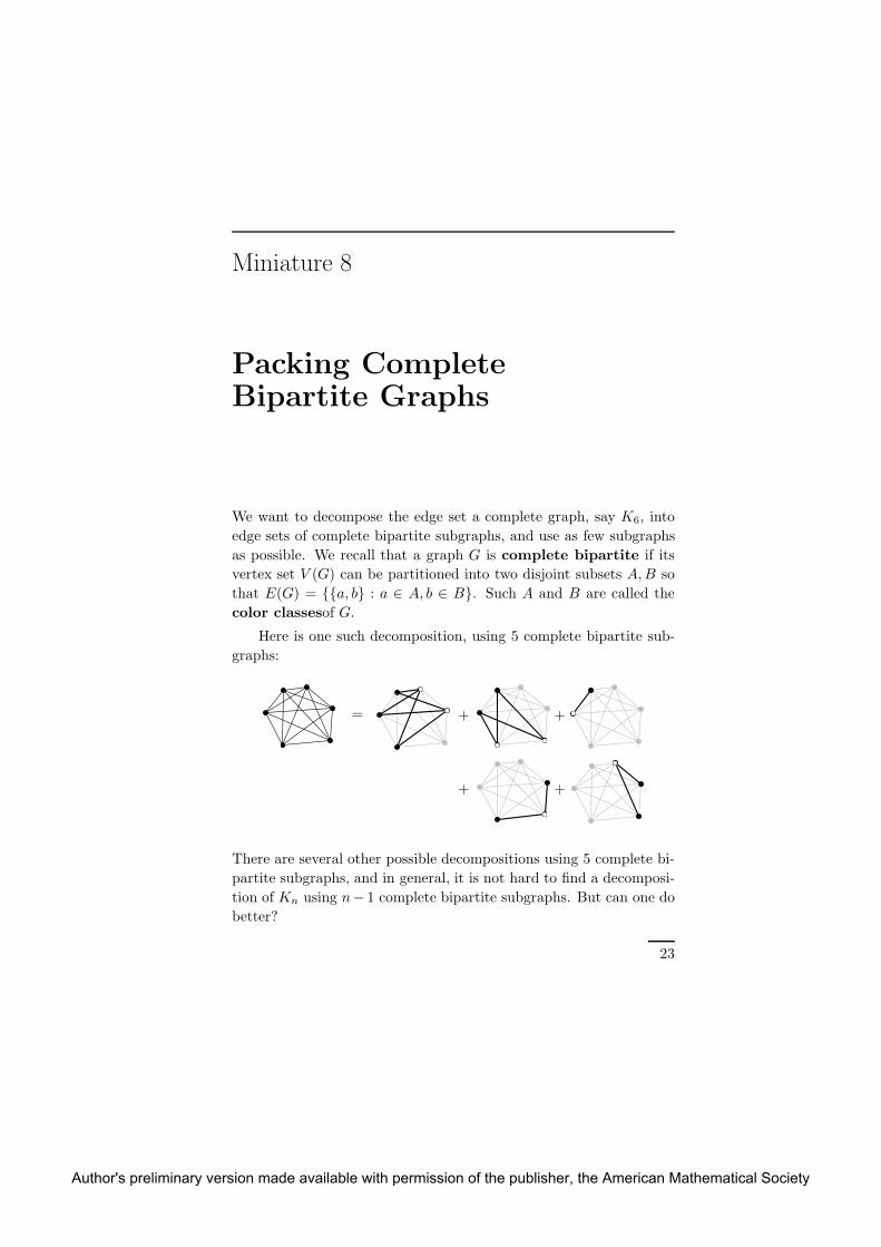
We want to decompose the edge set a complete graph, say K6, into
edge sets of complete bipartite subgraphs, and use as few subgraphs
as possible. We recall that a graph G is complete bipartite if its
vertex set V (G) can be partitioned into two disjoint subsets A,B so
that E(G) = {{a, b} : a ∈ A, b ∈ B}. Such A and B are called the
color classesof G.
Here is one such decomposition, using 5 complete bipartite sub-
graphs:
= + +
+ +
There are several other possible decompositions using 5 complete bi-
partite subgraphs, and in general, it is not hard to find a decomposi-
tion of Kn using n− 1 complete bipartite subgraphs. But can one do
better?
23
Author's preliminary version made available with permission of the publisher, the American Mathematical Society

24 8. Packing Complete Bipartite Graphs
This problem was motivated by a question in telecommunications.
We present a neat linear-algebraic proof of the following:
Theorem. If the set E(Kn), i.e., the set of the edges of a complete
graph on n vertices, is expressed as a disjoint union of edge sets of m
complete bipartite graphs, then m ≥ n− 1.
Proof. Suppose that complete bipartite graphs H1, H2, . . . , Hm dis-
jointly cover all edges of Kn. Let Xk and Yk be the color classes of
Hk. (The set V (Hk) = Xk ∪ Yk is not necessarily all of V (Kn).)
We assign an n × n matrix Ak to each graph Hk. The entry of
Ak in the ith row and jth column is
a(k)ij =
{
1 if i ∈ Xk and j ∈ Yk
0 otherwise.
We claim that each of the matrices Ak has rank 1. This is because
all the nonzero rows of Ak are equal to the same vector, namely, the
vector with 1’s at positions whose indices belong to Yk and with 0’s
elsewhere.
Let us now consider the matrix A = A1 + A2 + · · · + Am. The
rank of a sum of two matrices is never larger than the sum of their
ranks (why?), and thus the rank of A is at most m. It is enough to
prove that this rank is also at least n− 1.
Each edge {i, j} belongs to exactly one of the graphs Hk, and
hence for each i 6= j, we have either aij = 1 and aji = 0, or aij = 0
and aji = 1, where aij is the entry of the matrix A at position (i, j).
We also have aii = 0. From this we get A + AT = Jn − In, where
In is the identity matrix and Jn denotes the n× n matrix having 1’s
everywhere.
For contradiction, let us assume that rank(A) ≤ n− 2. If we add
an extra row consisting of all 1’s to A, the resulting (n+1)×n matrix
still has rank at most n− 1, and hence there exists a nontrivial linear
combination of its columns equal to 0. In other words, there exists a
(column) vector x ∈ Rn, x 6= 0, such that Ax = 0 and∑n
i=1 xi = 0.
Author's preliminary version made available with permission of the publisher, the American Mathematical Society

8. Packing Complete Bipartite Graphs 25
From the last equality we get Jnx = 0. We calculate
xT(
A+AT)
x = xT (Jn − In)x = xT (Jnx) − xT (Inx) =
= 0 − xT x = −n∑
i=1
x2i < 0.
On the other hand, we have
xT(
AT +A)
x =(
xTAT)
x + xT (Ax) = 0Tx + xT 0 = 0,
and this is a contradiction. �
Sources. The result is due to
R. L. Graham and H.O. Pollak, On the addressing problem
for loop switching, Bell System Tech. J. 50 (1971), 2495–2519.
The proof is essentially that of
H. Tverberg, On the decomposition of Kn into complete bi-
partite graphs, J. Graph Theory 6,4 (1982), 493–494.
Author's preliminary version made available with permission of the publisher, the American Mathematical Society

Author's preliminary version made available with permission of the publisher, the American Mathematical Society

Miniature 9
Equiangular Lines
What is the largest number of lines in R3 such that the angle between
every two of them is the same?
Everybody knows that in R3 there cannot be more than three
mutually orthogonal lines, but the situation for angles other than 90
degrees is more complicated. For example, the six longest diagonals
of the regular icosahedron (connecting pairs of opposite vertices) are
equiangular:
27
Author's preliminary version made available with permission of the publisher, the American Mathematical Society

28 9. Equiangular Lines
As we will prove, this is the largest number one can get.
Theorem. The largest number of equiangular lines in R3 is 6, and
in general, there cannot be more that(
d+12
)
equiangular lines in Rd.
Proof. Let us consider a configuration of n lines, where each pair
has the same angle ϑ ∈ (0, π2 ]. Let vi be a unit vector in the direction
of the ith line (we choose one of the two possible orientations of vi
arbitrarily). The condition of equal angles is equivalent to
|〈vi,vj〉| = cosϑ, for all i 6= j.
Let us regard vi as a column vector, or a d×1 matrix. Then vTi vj
is the scalar product 〈vi,vj〉, or more precisely, the 1×1 matrix whose
only entry is 〈vi,vj〉. On the other hand, vivTj is a d×d matrix.
We show that the matrices vivTi , i = 1, 2, . . . , n, are linearly
independent. Since they are the elements of the vector space of all
real symmetric d×d matrices, and the dimension of this space is(
d+12
)
,
we get n ≤(
d+12
)
, just as we wanted.
To check linear independence, we consider a linear combination
n∑
i=1
aivivTi = 0,
where a1, a2, . . . , an are some coefficients. We multiply both sides of
this equality by vTj from the left and by vj from the right. Using the
associativity of matrix multiplication, we obtain
0 =n∑
i=1
aivTj (viv
Ti )vj =
n∑
i=1
ai〈vi,vj〉2 = aj +∑
i6=j
ai cos2 ϑ
for all i, j. In other words, we have deduced that Ma = 0, where
a = (a1, . . . , an) and M = (1 − cos2 ϑ)In + (cos2 ϑ)Jn. Here In is
the unit matrix and Jn is the matrix of all 1’s. It is easy to check
that the matrix M is nonsingular (using cosϑ 6= 1); for example, as
in Miniature 4, we can show that M is positive definide. Therefore,
a = 0, the matrices vivTi are linearly independent, and the theorem
is proved. �
Author's preliminary version made available with permission of the publisher, the American Mathematical Society

9. Equiangular Lines 29
Remark. While the upper bound of this theorem is tight for d = 3,
for some larger values of d it can be improved by other methods. The
best possible value is not known in general. The best known lower
bound (from the year 2000) is 29 (d+ 1)2, holding for all numbers d of
the form 3 · 22t−1 − 1, where t is a natural number.
Sources. The theorem is stated in
P.W.H. Lehmmens and J. J. Seidel, Equiangular lines, J. ofAlgebra 24 (1973), 494–512.
and attributed to Gerzon (private communication). The best upperbound mentioned above is from
D. de Caen, Large equiangular sets of lines in Euclidean
space, Electr. J. Comb. 7 (2000), R55.
Author's preliminary version made available with permission of the publisher, the American Mathematical Society

Author's preliminary version made available with permission of the publisher, the American Mathematical Society

Miniature 10
Where is the Triangle?
Does a given graph contain a triangle, i.e., three vertices u, v, w,
every two of them connected by an edge? This question is not entirely
easy to answer for graphs with many vertices and edges. For example,
where is a triangle in this graph?
An obvious algorithm for finding a triangle inspects every triple
of vertices, and thus it needs roughly n3 operations for an n-vertex
graph (there are(
n3
)
triples to look at, and(
n3
)
is approximately n3/6
for large n). Is there a significantly faster method?
31
Author's preliminary version made available with permission of the publisher, the American Mathematical Society

32 10. Where is the Triangle?
There is, but surprisingly, the only known approach for breaking
the n3 barrier is algebraic, based on fast matrix multiplication.
To explain it, we assume for notational convenience that the ver-
tex set of the given graph G is {1, 2, . . . , n}, and we define the adja-
cency matrix of G as the n×n matrix A with
aij =
{
1 if i 6= j and {i, j} ∈ E(G),
0 otherwise.
The key insight is to understand the square B := A2. By the
definition of matrix multiplication we have bij =∑n
k=1 aikakj , and
aikakj =
{
1 if the vertex k is adjacent to both i and j,
0 otherwise.
So bij counts the number of common neighbors of i and j.
Finding a triangle is equivalent to finding two adjacent vertices
i, j with a common neighbor k. So we look for two indices i, j such
that both aij 6= 0 and bij 6= 0.
To do this, we need to compute the matrix B = A2. If we perform
the matrix multiplication according to the definition, we need about
n3 arithmetic operations and thus we save nothing compared to the
naive method of inspecting all triples of vertices.
However, ingenious algorithms are known that multiply n × n
matrices asymptotically faster. The oldest one, due to Strassen, needs
roughly n2.807 arithmetic operations. It is based on a simple but
very clever trick—if you haven’t seen it, it is worth looking it up
(Wikipedia?).
The exponent of matrix multiplication is defined as the infi-
mum of numbers ω for which there exists an algorithm that multiplies
two square matrices using O(nω) operations. Its value is unknown
(the common belief is that it equals 2); the current best upper bound
is roughly 2.376.
Many computational problems are known where fast matrix mul-
tiplication brings asymptotic speedup. Finding triangles is among the
simplest of them, we will meet and several other, more sophisticated
algorithms of this kind appear later.
Author's preliminary version made available with permission of the publisher, the American Mathematical Society

10. Where is the Triangle? 33
Remarks. The described method for finding triangles is the fastest
known for dense graphs, i.e., graphs that have relatively many edges
compared to the number of vertices. Another nice algorithm, which
we won’t discuss here, can detect a triangle in time O(m2ω/(ω+1)),
where m is the number of edges.
One can try to use similar methods for detecting subgraphs other
than the triangle; there is an extensive literature concerning this prob-
lem. For example, a cycle of length 4 can be detected in time O(n2),
much faster than a triangle!
Sources. A. Itai and M. Rodeh, Finding a minimum circuit
in a graph, SIAM J. Comput., 7,4 (1978), 413–423.
Among the numerous papers dealing with fast detection of a fixedsubgraph in a given graph, we mention
T. Kloks, D. Kratsch, and H. Muller, Finding and counting
small induced subgraphs efficiently, Inform. Process. Lett.74,3–4 (2000), 115–121,
which can be used as a starting point for further explorations of thetopic.
The first “fast” matrix multiplication algorithm is due to
V. Strassen, Gaussian elimination is not optimal, Numer.Math. 13 (1969), 354–356.
The asymptotically fastest known matrix multiplication algorithm isfrom
D. Coppersmith and S. Winograd, Matrix multiplication via
arithmetic progressions, J. Symbolic Computation 9 (1990),251–280.
An interesting new method, which provides similarly fast algorithmsin a different way, appeared in
H. Cohn, R. Kleinberg, B. Szegedy, and C. Umans, Group-
theoretic algorithms for matrix multiplication, in Proc. 46thAnnual IEEE Symposium on Foundations of Computer Sci-ence (FOCS), 2005, 379–388.
Author's preliminary version made available with permission of the publisher, the American Mathematical Society

Author's preliminary version made available with permission of the publisher, the American Mathematical Society

Miniature 11
Checking MatrixMultiplication
Multiplying two n × n matrices is a very important operation. A
straightforward algorithm requires about n3 arithmetic operations,
but as was mentioned in Miniature 10, ingenious algorithms have
been discovered that are asymptotically much faster. The current
record is an O(n2.376) algorithm. However, the constant of propor-
tionality is so astronomically large that the algorithm is interesting
only theoretically. Indeed, matrices for which it would prevail over
the straightforward algorithm can’t fit into any existing or future
computer.
But progress cannot be stopped and soon a software company
may start selling a program called MATRIX WIZARD that, sup-
posedly, multiplies matrices real fast. Since wrong results could be
disastrous for you, you would like to have a simple checking program
appended to MATRIX WIZARD that would always check whether
the resulting matrix C is really the product of the input matrices A
and B.
Of course, a checking program that actually multiplies A and B
and compares the result with C makes little sense, since you do not
know how to multiply matrices as fast as MATRIX WIZARD. But
it turns out that if we allow for some slight probability of error in
35
Author's preliminary version made available with permission of the publisher, the American Mathematical Society

36 11. Checking Matrix Multiplication
the checking, there is a very simple and efficient checker for matrix
multiplication.
We assume that the considered matrices consist of rational num-
bers, although everything works without change for matrices over
any field. The checking algorithm receives n × n matrices A,B,C
as the input. Using a random number generator, it picks a random
n-component vector x of zeros and ones. More precisely, each vec-
tor in {0, 1}n appears with the same probability, equal to 2−n. The
algorithm computes the products Cx (using O(n2) operations) and
ABx (again with O(n2) operations; the right parenthesizing is, of
course, A(Bx)). If the results agree, the algorithm answers YES, and
otherwise, it answers NO.
If C = AB, the algorithm always answers YES, which is correct.
But if C 6= AB, it can answer both YES and NO. We claim that the
wrong answer YES has probability at most 12 , and thus the algorithm
detects a wrong matrix multiplication with probability at least 12 .
Let us set D := C − AB. It suffices to show that if D is any
nonzero n × n matrix and x ∈ {0, 1}n is random, then the vector
y := Dx is zero with probability at most 12 .
Let us fix indices i, j such that dij 6= 0. We will derive that then
the probability of yi = 0 is at most 12 .
We have
yi = di1x1 + di2x2 + · · · + dinxn = dijxj + S,
where
S =∑
k=1,2,...,n
k 6=j
dikxk.
Imagine that we choose the values of the entries of x according to
successive coin tosses and that the toss deciding the value of xj is
made as the last one (since the tosses are independent it doesn’t
matter).
Before this last toss, the quantity S has already been fixed, be-
cause it doesn’t depend on xj . After the last toss, we have xj = 0
with probability 12 and xj = 1 with probability 1
2 . In the first case,
Author's preliminary version made available with permission of the publisher, the American Mathematical Society
11. Checking Matrix Multiplication 37
we have yi = S, while in the second case, yi = S + dij 6= S. There-
fore, yi 6= 0 in at least one of these two cases, and so Dx 6= 0 has
probability at least 12 as claimed.
The described checking algorithm is fast but not very reliable: It
may fail to detect an error with probability as high as 12 . But if we
repeat it, say, fifty times for a single input A,B,C, it fails to detect
an error with probability at most 2−50 < 10−15, and this probability
is totally negligible for practical purposes.
Remark. The idea of probabilistic checking of computations, which
we have presented here in a simple form, turned out to be very fruitful.
The so called PCP theorem from the theory of computational com-
plexity shows that for any effectively solvable computational prob-
lem, it is possible to check the solution probabilistically in a very
short time. A slow personal computer can, in principle, check the
work of the most powerful supercomputers. Furthermore, a surpris-
ing connections of these results to approximation algorithms have
been discovered.
Sources. R. Freivalds, Probabilistic machines can use less
running time, in Information processing 77, IFIP Congr.Ser. 7, North-Holland, Amsterdam, 1977, 839–842.
For introduction to PCP and computational complexity see, e.g.,
O. Goldreich, Computational complexity: A conceptual per-
spective, Cambridge University Press, Cambridge, 2008.
Author's preliminary version made available with permission of the publisher, the American Mathematical Society

Author's preliminary version made available with permission of the publisher, the American Mathematical Society

Miniature 12
Tiling a Rectangle bySquares
Theorem. A rectangle R with side lengths 1 and x, where x is irra-
tional, cannot be “tiled” by finitely many squares (so that the squares
have disjoint interiors and cover all of R).
Proof. For contradiction, let us assume that a tiling exists, consisting
of squares Q1, Q2, . . . , Qn, and let si be the side length of Qi.
We need to consider the set R of all real numbers as a vector
space over the field Q of rationals. This is a rather strange, infinite-
dimensional vector space, but a very useful one.
Let V ⊆ R be the linear subspace generated by the numbers x
and s1, s2, . . . , sn, in other words, the set of all rational linear combi-
nations of these numbers.
We define a linear mapping f : V → R such that f(1) = 1 and
f(x) = −1 (and otherwise arbitrarily). This is possible, because
1 and x are linearly independent over Q. Indeed, there is a basis
(b1, b2, . . . , bk) of V with b1 = 1 and b2 = x, and we can set, e.g.,
f(b1) = 1, f(b2) = −1, f(b3) = · · · = f(bk) = 0, and extend f
linearly on V .
For each rectangle A with edges a and b, where a, b ∈ V , we define
a number v(A) := f(a)f(b).
39
Author's preliminary version made available with permission of the publisher, the American Mathematical Society

40 12. Tiling a Rectangle by Squares
We claim that if the 1 × x reclangle R is tiled by the squares
Q1, Q2, . . . , Qn, then v(R) =∑n
i=1 v(Qi). This leads to a contra-
diction, since v(R) = f(1)f(x) = −1, while v(Qi) = f(si)2 ≥ 0 for
all i.
To check the claim just made, we extend the edges of all squares
Qi of the hypothetical tiling across the whole of R, as is indicated in
the picture:
This partitions R into small rectangles, and using the linearity of f ,
it is easy to see that v(R) equals to the sum of v(B) over all these
small rectangles B. Similarly v(Qi) equals the sum of v(B) over all
the small rectangles lying inside Qi. Thus, v(R) =∑n
i=1 v(Qi). �
Remark. It turns out that a rectangle can be tiled by squares if and
only if the ratio of its sides is rational. Various other theorems about
the impossibility of tilings can be proved by similar methods. For
example, it is impossible to dissect the cube into finitely many convex
pieces that can be rearranged so that they tile a regular tetrahedron.
Sources. The theorem is a special case of a result from
M. Dehn, UberZerlegung von Rechtecken in Rechtecke, Math.Ann. 57,3 (1903), 314–332.
Unfortunately, so far I haven’t found the source of the above proof.Another very beautiful proof follows from a remarkable connection ofsquare tilings to planar electrical networks:
R. L. Brooks, C. A.B. Smith, A.H. Stone, and W.T. Tutte,The dissection of rectangles into squares, Duke Math. J. 7
(1940), 312–340.
Author's preliminary version made available with permission of the publisher, the American Mathematical Society

Miniature 13
Three Petersens AreNot Enough
The famous Petersen graph
has 10 vertices of degree 3. The complete graph K10 has 10 vertices
of degree 9. Yet it is not possible to cover all edges of K10 by three
copies of the Petersen graph.
Theorem. There are no three subgraphs of K10, each isomorphic to
the Petersen graph, that together cover all edges of K10.
The theorem can obviously be proved by an extensive case anal-
ysis. The following elegant proof is a little sample of a part of graph
theory dealing with properties of the eigenvalues of the adjacency
matrix of a graph.
41
Author's preliminary version made available with permission of the publisher, the American Mathematical Society
42 13. Three Petersens Are Not Enough
Proof. We recall that the adjacency matrix of a graph G on the
vertex set {1, 2, . . . , n} is the n×n matrix A with
aij =
{
1 if i 6= j and {i, j} ∈ E(G),
0 otherwise.
It means that the adjacency matrix of the graph K10 is J10 − I10,
where Jn is the n×n matrix of all 1’s and In is the identity matrix.
Let us assume that the edges of K10 are covered by subgraphs
P , Q and R, each of them isomorphic to the Petersen graph. If AP
is the adjacency matrix of P , and similarly for AQ and AR, then
AP +AQ +AR = J10 − I10.
It is easy to check that the adjacency matrices of two isomorphic
graphs have the same set of eigenvalues, and also the same dimensions
of the corresponding eigenspaces.
We can use the Gaussian elimination to calculate that for the
adjacency matrix of Petersen graph, the eigenspace corresponding to
the eigenvalue 1 has dimension 5; i.e., the matrix AP − I10 has a
5-dimensional kernel.
Moreover, this matrix has exactly three 1’s and one −1 in every
column. So if we sum all the equations of the system (AP −I10)x = 0,
we get 2x1+2x2+· · ·+2x10 = 0. In other words, the kernel of AP −I10is contained in the 9-dimensional orthogonal complement of the vector
1 = (1, 1, . . . , 1).
The same is true for the kernel of AQ−I10, and therefore, the two
kernels have a common non-zero vector x. We know that J10x = 0
(since x is orthogonal to 1), and we calculate
ARx = (J10 − I10 −AP −AQ)x
= J10x− I10x − (AP − I10)x − (AQ − I10)x − 2I10x
= 0− x − 0− 0 − 2x = −3x.
It means that −3 must be an eigenvalue of AR, but it is not an
eigenvalue of the adjacency matrix of the Petersen graph—a contra-
diction. �
Source. O.P. Lossers and A. J. Schwenk, Solution of advanced
problem 6434, Am. Math. Monthly 94 (1987), 885–887.
Author's preliminary version made available with permission of the publisher, the American Mathematical Society
Miniature 14
Petersen,Hoffman–Singleton,and Maybe 57
This is a classical piece from the 1960s, reproduced many times, but
still one of the most beautiful applications of graph eigenvalues I’ve
seen. Moreover, the proof nicely illustrates the general flavor of alge-
braic nonexistence proofs for various “highly regular” structures.
Let G be a graph of girth g ≥ 4 and minimum degree r ≥ 3,
where the girth of G is the length of its shortest cycle, and minimum
degree r means that every vertex has at least r neighbors. It is not
obvious that such graphs exist for all r and g, but it is known that
they do.
Let n(r, g) denote the smallest possible number of vertices of such
a G. Determining this quantity, at least approximately, belongs to
the most fascinating problems in graph theory, whose solution would
probably have numerous interesting consequences.
A lower bound. A lower bound for n(r, g) is obtained by a sim-
ple “branching” argument (linear algebra comes later). First let us
assume that g = 2k + 1 is odd.
Let G be a graph of girth g and minimum degree r. Let us fix a
vertex u in G and consider two paths of length k in G starting at u.
43
Author's preliminary version made available with permission of the publisher, the American Mathematical Society

44 14. Petersen, Hoffman–Singleton, and Maybe 57
For some time they may run together, then they branch off, and they
never meet again past the branching point—otherwise, they would
close a cycle of length at most 2k. Thus, G has a subgraph as in the
following picture:
u
r successors
r − 1 successors
(the picture is for r = 4 and k = 2). It is a tree T of height k, with
branching degree r at the root and r − 1 at the other inner vertices.
(In G, we may have additional edges connecting some of the leaves at
the topmost level, and of course, G may have more vertices than T .)
It is easy to count that the number of vertices of T equals
(1) 1 + r + r(r − 1) + r(r − 1)2 + · · · + r(r − 1)k−1,
and this is the promised lower bound for n(r, 2k + 1). For g = 2k
even, a similar but slightly more complicated argument, which we
omit here, yields the lower bound
(2) 1 + r + r(r − 1) + · · · + r(r − 1)k−2 + (r − 1)k−1
for n(r, 2k).
Upper bounds. For large r and g, the state of knowledge about
n(r, g) is unsatisfactory: The best known upper bounds are roughly
the 32 -th power of the lower bounds (1), (2), and so there is uncertainty
already in the exponent.
Still, (1), (2) remain essentially the best known lower bounds
for n(r, g), and a considerable attention has been paid to graphs for
which these bounds are attained, since they are highly regular and
usually have many remarkable properties. For historical reasons they
are called Moore graphs for odd g and generalized polygons1 for
even g.
1In some sources, though, the term Moore graph is used for both the odd-girthand even-girth cases.
Author's preliminary version made available with permission of the publisher, the American Mathematical Society

14. Petersen, Hoffman–Singleton, and Maybe 57 45
Moore graphs. Here we will consider only Moore graphs (for infor-
mation on generalized polygons and the known exact values of n(r, g)
we refer, e.g., to G. Royle’s web page http://people.csse.uwa.edu.
au/gordon/cages/). Explicitly, a Moore graph is a graph of girth
2k+1, minimum degree r, and with 1+r+r(r−1)+ · · ·+r(r−1)k−1
vertices.
To avoid trivial cases we assume r ≥ 3 and k ≥ 2. We also note
that every vertex in a Moore graph must have degree exactly r, for
if there were a vertex of larger degree, we could take it as u in the
lower bound argument and show that the number of vertices is larger
than (1).
The question of whether a Moore graph exists for given k and r
can be cast as a kind of “connecting puzzle.” The vertex set must
coincide with the vertex set of the tree T in the lower-bound argu-
ment, and the additional edges besides those of T may connect only
the leaves of T . Thus, we draw T , add r− 1 “paws” to each leaf, and
then we want to connect the paws by edges so that no cycle shorter
than 2k + 1 arises. The picture illustrates this for girth 2k + 1 = 5
and r = 3:
In this case the puzzle has a solution depicted on the right. The
solution, which can be shown to be unique up to isomorphism, is the
famous Petersen graph, whose more usual picture was shown in
Miniature 13.
The only other known Moore graph has 50 vertices, girth 5, and
degree r = 7. It is obtained by gluing together many copies of the
Petersen graph in a highly symmetric fashion, and it is called the
Hoffman–Singleton graph. Surprisingly, it is known that this very
short list exhausts all Moore graphs, with a single possible exception:
Author's preliminary version made available with permission of the publisher, the American Mathematical Society
46 14. Petersen, Hoffman–Singleton, and Maybe 57
The existence of a Moore graph of girth 5 and degree 57 has been
neither proved nor disproved.
Here we give the proof that Moore graphs of girth 5 can’t have
degree other than 3, 7, 57. The nonexistence of Moore graphs of higher
girth is proved by somewhat similar methods.
Theorem. If a graph G of girth 5 with minimum degree r ≥ 3 and
with n = 1 + r + (r − 1)r = r2 + 1 vertices exists, then r ∈ {3, 7, 57}.
We begin the proof of the theorem by a graph-theoretic argument,
which is a simple consequence of the argument used above for deriving
(1), specialized to k = 2.
Lemma. If G is a graph as in the theorem, then every two non-
adjacent vertices have exactly one common neighbor.
Proof. If u, v are two arbitrary non-adjacent vertices, we let u play
the u in the argument leading to (1). The tree T has height 2 in our
case, and so v is necessarily a leaf of T and there is a unique path of
length 2 connecting it with u. �
Proof of the theorem. We recall the notion of adjacency matrix
A of G, already used in Miniatures 10 and 13. Assuming that the
vertex set of G is {1, 2, . . . , n}, A is the n×n matrix with entries
given by
aij =
{
1 for i 6= j and {i, j} ∈ E(G),
0 otherwise.
The key step in the proof is to consider B := A2. As was already
mentioned in Miniature 10, from the definition of matrix multiplica-
tion one can easily see that for an arbitrary graphG, bij is the number
of vertices k adjacent to both of the vertices i and j. So for i 6= j, bijis the number of common neighbors of i and j, while bii is simply the
degree of i.
Specializing these general facts to a G as in the theorem, we
obtain
(3) bij =
r for i = j,
0 for i 6= j and {i, j} ∈ E(G),
1 for i 6= j and {i, j} 6∈ E(G).
Author's preliminary version made available with permission of the publisher, the American Mathematical Society

14. Petersen, Hoffman–Singleton, and Maybe 57 47
Indeed, the first case states that all degrees are r, the second one that
two adjacent vertices in G have no common neighbor (since G has
girth 5 and thus contains no triangles), and the third case restates
the assertion of the lemma that every two non-adjacent vertices have
exactly one common neighbor.
Next, we rewrite (3) in a matrix form:
(4) A2 = rIn + Jn − In −A,
where In is the identity matrix and Jn is the matrix of all 1’s.
Now we enter the business of graph eigenvalues. The usual open-
ing move in this area is to recall the following from linear algebra: Ev-
ery symmetric real n×nmatrixA has nmutually orthogonal eigenvec-
tors v1,v2, . . . ,vn, and the corresponding eigenvalues λ1, λ2, . . . , λn
are all real (and not necessarily distinct).
If A is the adjacency matrix of a graph with all degrees r, then
A1 = r1, with 1 standing for the vector of all 1’s. Hence r is an
eigenvalue with eigenvector 1, and we can thus assume λ1 = r, v1 = 1.
Then by the orthogonality of the eigenvectors, for all i 6= 1 we have
1Tvi = 0, and thus also Jnvi = 0.
Armed with these facts, let us see what happens if we multiply
(4) by some vi, i 6= 1, from the right. The left-hand side becomes
A2vi = Aλivi = λ2i vi, while the right-hand side yields rvi−vi−λivi.
Both sides are scalar multiples of the nonzero vector vi, and so the
scalar multipliers must be the same, which leads to
λ2i + λi − (r − 1) = 0.
Thus, each λi, i 6= 1 equals one of the roots ρ1, ρ2 of the quadratic
equation λ2 + λ− (r − 1) = 0, which gives
ρ1,2 := (−1 ±√D)/2, with D := 4r − 3.
Hence A has only 3 distinct eigenvalues: r, ρ1, and ρ2. Let us suppose
that ρ1 occurs m1 times among the λi and ρ2 occurs m2 times; since
r occurs once, we have m1 +m2 = n− 1.
The last linear algebra fact we need is that the sum of all eigen-
values of A equals its trace, i.e., the sum of all diagonal elements,
Author's preliminary version made available with permission of the publisher, the American Mathematical Society

48 14. Petersen, Hoffman–Singleton, and Maybe 57
which in our case is 0. Hence
(5) r +m1ρ1 +m2ρ2 = 0.
The rest of the proof is pure calculation plus a simple divisibility
consideration (a bit of number theory if we wanted to sound fancy).
After substituting in (5) for ρ1 and ρ2, multiplying by 2, and using
m1 +m2 = n− 1 = r2 (the last equality is one of the assumptions of
the theorem), we arrive at
(6) (m1 −m2)√D = r2 − 2r.
If D is not a square of a natural number, then√D is irrational, and
(6) can hold only if m1 = m2. But then r2 − 2r = 0, which cannot
happen for r ≥ 3. Therefore, we have D = 4r − 3 = s2 for a natural
number s. Expressing r = (s2 + 3)/4, substituting into (6), and
simplifying leads to
s4 − 2s2 − 16(m1 −m2)s = s(
s3 − 2s− 16(m1 −m2))
= 15.
Hence 15 is a multiple of the positive integer s, and so s ∈ {1, 3, 5, 15},
corresponding to r ∈ {1, 3, 7, 57}. The theorem is proved. �
Source. A. J. Hoffman and R.R. Singleton, On Moore graphs
with diameters 2 and 3, IBM J. Res. Develop. 4 (1960),497–504.
Author's preliminary version made available with permission of the publisher, the American Mathematical Society
Miniature 15
Only Two Distances
What is the largest number of points in the plane such that every
two of them have the same distance? If we have at least three, they
must form the vertices of an equilateral triangle, and there is no way
of adding a fourth point.
How many points in the plane can we have if we allow the dis-
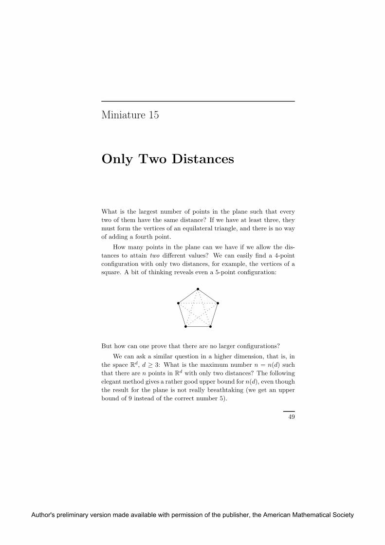
tances to attain two different values? We can easily find a 4-point
configuration with only two distances, for example, the vertices of a
square. A bit of thinking reveals even a 5-point configuration:
But how can one prove that there are no larger configurations?
We can ask a similar question in a higher dimension, that is, in
the space Rd, d ≥ 3: What is the maximum number n = n(d) such
that there are n points in Rd with only two distances? The following
elegant method gives a rather good upper bound for n(d), even though
the result for the plane is not really breathtaking (we get an upper
bound of 9 instead of the correct number 5).
49
Author's preliminary version made available with permission of the publisher, the American Mathematical Society

50 15. Only Two Distances
Theorem. n(d) ≤ 12 (d2 + 5d+ 4).
Proof. Let p1,p2, . . . ,pn be points in Rd. Let ‖pi − pj‖ be the
Euclidean distance of pi from pj . We have
‖pi − pj‖2 = (pi1 − pj1)2 + (pi2 − pj2)2 + · · · + (pid − pjd)2,
where pij is the jth coordinate of the point pi. We suppose that
‖pi − pj‖ ∈ {a, b} for every i 6= j.
With each point pi we associate a carefully chosen function
fi : Rd → R,
defined by
fi(x) :=(
‖x− pi‖2 − a2) (
‖x − pi‖2 − b2)
,
where x = (x1, x2, . . . , xd) ∈ Rd.
The key property of these functions is
(7) fi(pj) =
{
0 for i 6= j,
a2b2 6= 0 for i = j,
which follows immediately from the two-distance assumption.
Let us consider the vector space of all real functions Rd → R, and
the linear subspace V spanned by the functions f1, f2, . . . , fn. First,
we claim that f1, f2, . . . , fn are linearly independent. Let us assume
that a linear combination f = α1f1 + α2f2 + · · · + αnfn equals 0;
i.e., it is the zero function Rd → R. In particular, it is 0 at each pi.
According to (7) we get 0 = f(pi) = αia2b2, and therefore, αi = 0
for every i. Thus dimV = n.
Now we want to find a (preferably small) system G of functions
Rd → R, not necessarily belonging to V , that generates V ; that is,
every f ∈ V is a linear combination of functions in G. Then we will
have the bound |G| ≥ dimV = n.
Each of the fi is a polynomial in the variables x1, x2, . . . , xd of
degree at most 4, and so it is a a linear combination of monomials
in x1, x2, . . . , xd of degree at most 4. It is easy to count that there
are(
d+44
)
such monomials, and this gives a generating system G with
|G| =(
d+44
)
.
Author's preliminary version made available with permission of the publisher, the American Mathematical Society
15. Only Two Distances 51
Next, proceeding more carefully, we will find a still smaller G.
We express ‖x − pi‖2 =∑d
j=1(xj − pij)2 = X −∑dj=1 2xjpij + Pi,
where X :=∑d
j=1 x2j and Pi :=
∑dj=1 p
2ij . Then we have
fi(x) =(
‖x− pi‖2 − a2) (
‖x− pi‖2 − b2)
=
=
(
X −d∑
j=1
2xjpij +Ai
)(
X −d∑
j=1
2xjpij +Bi
)
,
where Ai := Pi − a2 and Bi := Pi − b2. By another rearrangement
we get
fi(x) = X2 − 4Xd∑
j=1
pijxj +
( d∑
j=1
2pijxj
)2
+
+ (Ai +Bi)
(
X −d∑
j=1
2pijxj
)
+AiBi.
From this we can see that each fi is a linear combination of functions
in the following system G:
X2,
xjX, j = 1, 2, . . . , d,
x2j , j = 1, 2, . . . , d,
xixj , 1 ≤ i < j ≤ d,
xj , j = 1, 2, . . . , d, and
1.
(Let us remark that X itself is a linear combination of the x2j .) We
have |G| = 1 + d + d +(
d2
)
+ d + 1 = 12 (d2 + 5d + 4), and so n ≤
12 (d2 + 5d+ 4). The theorem is proved. �
Remark. The upper bound in the theorem can be improved to(
d+22
)
by additional tricks, which we don’t consider here. However, it has the
right order of magnitude, as the following example shows. We start
with the(
d2
)
points in Rd with two coordinates equal to 1 and the
remaining 0. This is a two-distance set, and it lies in the hyperplane∑d
i=1 xi = 2. Thus we can place it into Rd−1 as well, and that gives
a lower bound n(d) ≥(
d+12
)
= 12 (d2 + d).
Author's preliminary version made available with permission of the publisher, the American Mathematical Society
52 15. Only Two Distances
Sources. D.G. Larman, C.A. Rogers, and J. J. Seidel, On
two-distance sets in Euclidean space, Bull. London Math.Soc. 9,3 (1977), 261–267.
According to Babai and Frankl, a similar trick first appears in
T. H. Koornwinder, A note on the absolute bound for sys-
tems of lines, Indag. Math. 38,2 (1976), 152–153.
The improved upper bound of`
d+2
2
´
is due to
A. Blokhuis, A new upper bound for the cardinality of 2-
distance sets in Euclidean space, Ann. Discrete Math. 20
(1984), 65–66.
Author's preliminary version made available with permission of the publisher, the American Mathematical Society
Miniature 16
Covering a Cube MinusOne Vertex
We consider the set {0, 1}d ⊂ Rd of the vertices of the d-dimensional
unit cube, and we want to cover all of these vertices except for one,
say 0 = (0, 0, . . . , 0), by hyperplanes. (We recall that a hyperplane
in Rd is a set of the form {x ∈ Rd : a1x1 + · · · + adxd = b} for some
coefficients a1, . . . , ad, b ∈ R with at least one ai nonzero.)
Of course, we can cover all the vertices using only two hyper-
planes, say {x1 = 0} and {x1 = 1}, but the problem becomes in-
teresting if none of the covering hyperplanes may contain the point
0. What is the smallest possible number of hyperplanes under these
conditions?
One easily finds (at least) two different ways of covering with d
hyperplanes. We can use the hyperplanes {xi = 1}, i = 1, 2, . . . , d, or
the hyperplanes {x1 + x2 + · · · + xd = k}, k = 1, 2, . . . , d. As we will
see, d is the smallest possible number.
Theorem. Let h1, . . . , hm be hyperplanes in Rd not passing through
the origin that cover all points of the set {0, 1}d except for the origin.
Then m ≥ d.
53
Author's preliminary version made available with permission of the publisher, the American Mathematical Society

54 16. Covering a Cube Minus One Vertex
Proof. Let hi be defined by the equation ai1x1+ai2x2+· · ·+aidxd =
b. We consider the following, cleverly chosen, polynomial
f(x1, x2, . . . , xd) =
m∏
i=1
(
1 −d∑
j=1
aijxj
)
−d∏
j=1
(1 − xj).
It is constructed so that f(x) = 0 for all x = (x1, . . . , xn) ∈ {0, 1}n
(to check this, one needs to distinguish the cases x = 0 and x 6= 0,
and to use the assumptions of the theorem).
For contradiction, let us suppose that m < d. Then the degree of
f is d, and the only monomial of degree d with a non-zero coefficient
is x1x2 · · ·xd. It remains to show that this monomial is not a linear
combination of monomials of lower degrees, when we consider these
monomials as real functions on {0, 1}d.
First we observe that on {0, 1}d we have xi = x2i , and therefore,
every polynomial is equivalent to a linear combination of multilinear
monomials xI =∏
i∈I xi, where I ⊆ {1, 2, . . . , d}. So it suffices to
prove that such xI are linearly independent.
Let us consider a linear combination
(8)∑
I⊆{1,2,...,d}αIxI = 0.
Assuming that there is an αI 6= 0, we take a minimum such I, min-
imum in the sense that αJ = 0 for every J ⊂ I. Let us substitute
xi = 1 for i ∈ I and xi = 0 for i 6∈ I into (8). Then we get αI = 0—a
contradiction. �
Source. N. Alon and Z. Furedi, Covering the cube by affine
hyperplanes, European J. Combin. 14,2 (1993), 79–83.
Author's preliminary version made available with permission of the publisher, the American Mathematical Society

Miniature 17
Medium-SizeIntersection Is Hard ToAvoid
An extensive branch of combinatorics, extremal set theory, investi-
gates problems of the following kind: Suppose that F is a system of
subsets of an n-element set, and suppose that certain simply described
configuration of sets doesn’t occur in F . What is the maximum pos-
sible number of sets in F?
Here is a short list of famous examples:
• The Sperner lemma (one of the Sperner lemmas, that is):
If there are no two distinct sets A,B ∈ F with A ⊂ B, then
|F| ≤(
n⌊n/2⌋
)
.
• The Erdos–Ko–Rado “sunflower theorem”: If k ≤n/2, each A ∈ F has exactly k elements, and A ∩ B 6= ∅for every two A,B ∈ F , then |F| ≤
(
n−1k−1
)
.
• The Oddtown theorem from Miniature 3: If each A ∈ F has
an odd number of elements and |A∩B| is even for every two
distinct A,B ∈ F , then |F| ≤ n.
Such a list of theorems could be extended over many pages, and linear
algebra methods constitute one of the main tools for proving them.
55
Author's preliminary version made available with permission of the publisher, the American Mathematical Society

56 17. Medium-Size Intersection Is Hard To Avoid
Here we present a strong and perhaps surprising result of this
kind. It has a beautiful geometric application, which we explain in
Miniature 18 below.
Theorem. Let p be a prime number and let F be a system of (2p−1)-
element subsets of an n-element set X such that no two sets in Fintersect in precisely p − 1 elements. Then the number of sets in Fis at most
|F| ≤(
n
0
)
+
(
n
1
)
+ · · · +
(
n
p− 1
)
.
There are(
n2p−1
)
subsets of an n-element set altogether. The
theorem tells us that if we forbid one single intersection size, namely
p− 1, we can have only much fewer sets. The following is a possible
quantification of “much fewer.”
Corollary. Let F be as in the theorem with n = 4p. Then(
4p2p−1
)
|F| ≥ 1.1n.
Proof of the corollary. First of all,(
nk−1
)
= kn−k
(
nk
)
, and so for
n ≥ 4k we have(
nk−1
)
≤ 13
(
nk
)
. So(
4p
p− 1
)
+
(
4p
p− 2
)
+· · ·+(
4p
0
)
≤(
4p
p
)(
1
3+
1
32+
1
33+· · ·
)
≤ 1
2
(
4p
p
)
.
Then(
4p2p−1
)
|F| ≥ 2 ·(
4p2p−1
)
(
4pp
) = 2 · (3p)(3p− 1) · · · (2p+ 2)
(2p− 1)(2p− 2) · · · (p+ 1)
≥ 2
(
3
2
)p−1
>
(
3
2
)p
> 1.1n.
(There are many other ways of doing this kind of calculation, and
one can use well-known estimates such as (n/k)k ≤(
nk
)
≤ (en/k)k or
Stirling’s formula, but we didn’t want to assume those here.) �
Proof of the theorem. The proof combines tricks we have already
met in Miniatures 15 and 16.
To each set A ∈ F we assign two things:
Author's preliminary version made available with permission of the publisher, the American Mathematical Society
17. Medium-Size Intersection Is Hard To Avoid 57
• A vector cA ∈ {0, 1}n. This is simply the characteris-
tic vector of A, whose ith component is 1 if i ∈ A and 0
otherwise.
• A function fA : {0, 1}n → Fp, given by
fA(x) :=
p−2∏
s=0
(
(
∑
i∈A
xi
)
− s
)
.
All the arithmetic operations in the definition of fA are in the finite
field Fp, i.e., modulo p (and thus 0 and 1 are also treated as elements
of Fp). For example, for p = 3, n = 5, and A = {2, 3} we have
cA = (0, 1, 1, 0, 0) and fA(x) = (x2 + x3)(x2 + x3 − 1).
We consider the set of all functions from {0, 1}d to Fp as a vector
space over Fp in the usual way, and we let VF be the subspace spanned
in it by the functions fA, A ∈ F .
First we check that the fA’s are linearly independent, and hence
dim(VF ) = |F|.We have fA(cB) =
∏p−2s=0(|A ∩B| − s) (mod p), and this product
is nonzero exactly if |A ∩ B| ≡ p − 1 (mod p). For A = B we have
|A ∩ A| = 2p − 1 ≡ p − 1 (mod p), and so fA(cA) 6= 0. For A 6= B
we have |A ∩B| ≤ 2p− 2 and |A ∩B| 6= p− 1 by the “omitted inter-
section” assumption, thus |A∩B| 6≡ p− 1 (mod p), and consequently
fA(cB) = 0.
Now a standard argument shows the independence of the fA: As-
suming∑
A∈F αAfA = 0 for some coefficients αA ∈ Fp, we substitute
cB into the left-hand side. All terms fA(cB) with A 6= B vanish,
and we are left with αBfB(cB) = 0, which yields αB = 0 in view of
fB(cB) 6= 0. Since B was arbitrary, the fA are linearly independent
as claimed.
We proceed to bound dim(VF ) from above. In our concrete ex-
ample above, we had fA(x) = (x2 +x3)(x2 +x3 −1), and multiplying
out the parentheses we get fA(x) = x22 + x2
3 + 2x2x3 − x2 − x3. In
general, each fA is a polynomial in x1, x2, . . . , xn of degree at most
p− 1, and hence it is a linear combination of monomials of the form
xi11 x
i22 · · ·xin
n , i1 + i2 + · · · + in ≤ p− 1.
Author's preliminary version made available with permission of the publisher, the American Mathematical Society

58 17. Medium-Size Intersection Is Hard To Avoid
We can still get rid of the monomials with some exponent ij larger
than 1, because x2j and xj represent the same function {0, 1}n → Fp
(we substitute only 0’s and 1’s for the variables). So it suffices to
count the monomials with ij ∈ {0, 1}, and their number is the same
as the number of all subsets of {1, 2, . . . , n} of size at most p−1. Thus
dim(VF ) ≤(
n0
)
+(
n1
)
+ · · · +(
np−1
)
, and the theorem follows. �
Sources. The theorem is a special case of the Frankl–Wilsoninequality from
P. Frankl and R.M. Wilson, Intersection theorems with geo-
metric consequences, Combinatorica 1,4 (1981), 357–368.
The proof follows
N. Alon, L. Babai, and H. Suzuki, Multilinear polynomials
and Frankl–Ray-Chaudhuri–Wilson type intersection theo-
rems, J. Combin. Theory Ser. A 58,2 (1991), 165–180.
More general “omitted intersection” theorems were proved by differentmethods in
P. Frankl and V. Rodl, Forbidden intersections, Trans.Amer.Math. Soc. 300,1 (1987), 259–286.
Author's preliminary version made available with permission of the publisher, the American Mathematical Society

Miniature 18
On the Difficulty ofReducing the Diameter
Exceptionally in this collection, the next result relies on a theorem
proved earlier, in Miniature 17.
The diameter of a set X ⊆ Rd is defined as
diam(X) := sup{‖x− y‖ : x,y ∈ X},
where ‖x − y‖ stands for the Euclidean distance of x and y. If X
is finite, or more generally, closed and bounded, the supremum is
always attained and we can simply say that the diameter is the largest
distance among two points of X .
The question. The following was asked by Karol Borsuk in 1933:
Can every set X ⊂ Rd of finite diameter be parti-
tioned into d+1 subsets X1, X2, . . . , Xd+1 so that
each Xi has diameter strictly smaller than X?
Let us call a partition of a set X ⊂ Rd into subsetsX1, X2, . . . , Xk
with diam(Xi) < diam(X) for all i a diameter-reducing partition
of X into k parts.
It is easily seen that there are sets in Rd with no diameter-
reducing partition into d parts. For example, let X consist of d + 1
points, every two with distance 1 (in other words, the vertex set of
59
Author's preliminary version made available with permission of the publisher, the American Mathematical Society

60 18. On the Difficulty of Reducing the Diameter
a regular d-dimensional simplex—an explicit construction of such a
set is sketched in Miniature 30). If we partition X into d parts, one
of the parts contains at least two points and thus it has diameter 1,
same as X . Borsuk in his 1933 paper proved, among others, that the
d-dimensional ball has a diameter-reducing partition into d+ 1 parts
(this is easy) but it has none into d parts (this isn’t).
Up until 1993, it was widely believed that every X ⊂ Rd of finite
diameter should have a diameter-reducing partition into d+ 1 parts,
so widely that people started speaking about Borsuk’s conjecture (al-
though Borsuk didn’t express any such belief in his paper).
Borsuk’s question was often reformulated with the additional as-
sumption that X is convex. It is easy to see that involves no loss of
generality, since the diameter of a set is the same as the diameter of
its convex hull.
Several partial results supporting (so-called) Borsuk’s conjecture
were proved over the years. It was proved for arbitrary sets X in
dimensions 2 and 3, for all smooth convex sets in all dimensions (where
smooth, roughly speaking, means “no sharp corners or edges”), and
for some other special classes of convex sets.
The answer. As the reader might have already guessed or known,
Borsuk’s question has eventually been answered negatively. Let us
begin with preliminary considerations, which are not really necessary
for the proof but may be helpful for understanding it.
The first thing to understand is that the additional assumption
of convexity, which seemingly simplifies the problem, happens to be
a smoke-screen: The essence of Borsuk’s question lies in finite sets.
A useful class of finite sets is obtained from finite set systems.
For a system F of subsets of {1, 2, . . . , n} let XF ⊂ Rn be the set of
all characteristic vectors of sets in F : XF := {cA : A ∈ F}, where
the ith component of cA is 1 if i ∈ A and 0 otherwise.
We will translate the result of Miniature 17 into the language of
characteristic vectors and distances. We recall the corollary of the
theorem in that miniature: If p is a prime, n = 4p, and F is a system
of (2p− 1)-element subsets of {1, 2, . . . , n} such that |A ∩B| 6= p− 1
for every A,B ∈ F , then(
n2p−1
)
/|F| ≥ 1.1n.
Author's preliminary version made available with permission of the publisher, the American Mathematical Society

18. On the Difficulty of Reducing the Diameter 61
Let A be the system of all (2p−1)-element subsets of {1, 2, . . . , n}(so |A| =
(
n2p−1
)
). The statement in the previous paragraph implies
the following:
(9)
If we partition the sets in A into fewer than 1.1n
classes, then at least one of the classes contains two
sets with intersection of size exactly p−1.
We observe that since all sets in A have the same size, the Eu-
clidean distance of two characteristic vectors cA, cB ∈ XA is deter-
mined by the size of the intersection |A ∩B|. Indeed, ‖cA − cB‖2 =
|A \ B| + |B \ A| = |A| + |B| − 2|A ∩ B| = 2(2p− 1) − 2|A ∩ B|. In
particular, if |A ∩ B| = p − 1, then ‖cA − cB‖ =√
2p. So whenever
the point set XA is partitioned into fewer than 1.1n subsets, one of
the subsets contains two points cA, cB with distance√
2p.
This already sounds similar to Borsuk’s question: It tells us that
we can’t get rid of the distance√
2p by partitioning XA into fewer
than exponentially many parts. The only problem is that√
2p is not
the diameter of XA but rather some smaller distance. We thus want
to transform XA into another set so that the pairs with distance√
2p
in XA become pairs realizing the diameter of the new set. Such a
transformation is possible, but it raises the dimension: The resulting
point set, which we denote by QA, lies in dimension n2.
This ends the preliminary discussion. We now proceed with a
statement of the result and the actual proof.
Theorem. For every prime p there exists a point set in Rn2
, n = 4p,
that has no diameter-reducing partition into fewer than 1.1n parts.
Consequently, the answer to Borsuk’s question is no.
Proof. First we need to recall the notion of tensor product1 of
vectors x ∈ Rm, y ∈ Rn: It is denoted by x ⊗ y, and it is the vector
in Rmn whose components are all the products xiyj, i = 1, 2, . . . ,m,
j = 1, 2, . . . , n. (Sometimes it is useful to think of x⊗y as the m×n
matrix xyT .)
1In linear algebra, the tensor product is defined more generally, for arbitrary twovector spaces. The definition given here can be regarded as the “standard” tensorproduct.
Author's preliminary version made available with permission of the publisher, the American Mathematical Society

62 18. On the Difficulty of Reducing the Diameter
We will need the following identity involving the scalar product
and the tensor product: For all x,y ∈ Rn,
(10) 〈x ⊗ x,y ⊗ y〉 = 〈x,y〉2,as is very easy to check.
Now we begin with the construction of the point set in the the-
orem. We recall that A consists of all (2p − 1)-element subsets of
{1, 2, . . . , 4p}. For A ∈ A, let uA ∈ {−1, 1}n be the signed charac-
teristic vector of A whose ith component is is +1 if i ∈ A and −1
otherwise. We set qA := uA ⊗ uA ∈ Rn2
, and the point set in the
theorem is QA := {qA : A ∈ A}.
First we verify that for A,B ∈ A with |A ∩B| = s,
(11) 〈uA,uB〉 = 4(s− p+ 1).
This can be checked using the following diagram, for instance:
{1, 2, . . . , 4p}
2p−1−s
AB
4p − 2(2p − 1) + s = s + 2
2p−1−s s
Components in (A \ B) ∪ (B \ A) (gray) contribute −1 to the scalar
product, and the remaining ones (white) contribute +1. Conse-
quently, 〈uA,uB〉 = 0 if and only if |A ∩B| = p− 1.
For the Euclidean distances in QA we have, using (10),
‖qA − qB‖2 = 〈qA,qA〉 + 〈qB ,qB〉 − 2〈qA,qB〉= 〈uA,uA〉2 + 〈uB,uB〉2 − 2〈uA,uB〉2.
Now 〈uA,uA〉2 +〈uB,uB〉2 is a number independent of A and B, and
〈uA,uB〉2 is a nonnegative number that is 0 if and only if |A ∩B| =
p − 1. Thus, the maximum possible distance of qA and qB, equal
to diam(QA), is attained exactly for |A ∩ B| = p− 1. So by (9) QA
Author's preliminary version made available with permission of the publisher, the American Mathematical Society
18. On the Difficulty of Reducing the Diameter 63
has no diameter-reducing partition into fewer than 1.1n parts as the
theorem claims.
Finally, if we choose p sufficiently large so that 1.1n > n2 + 1 and
put d := n2, we have a point set in Rd that has no diameter-reducing
partition into d+ 1 parts. �
What is the smallest dimension d for which Borsuk’s question
has a negative answer? Using only the statement of the theorem
above, we get an upper bound of almost 104. Some improvement can
be achieved by doing the calculations more precisely. At the time of
writing, the best known upper bound is d = 298, whose proof involves
additional ideas. It may still be quite far from the smallest possible
value.
Sources. Borsuk’s problem was stated in
K. Borsuk, Drei Satze uber die n-dimensionale euklidische
Sphare, Fundamenta Mathematicae 20 (1933), 177–190.
The counterexample is from
J. Kahn and G. Kalai, A counterexample to Borsuk’s con-
jecture, Bull. Amer. Math. Soc. 29 (1993), 60–62.
The 298-dimensional counterexample is from
A. Hinrichs and C. Richter, New sets with large Borsuk num-
bers, Disc. Math. 270 (2003), 137–147.
Author's preliminary version made available with permission of the publisher, the American Mathematical Society

Author's preliminary version made available with permission of the publisher, the American Mathematical Society
Miniature 19
The End of the SmallCoins
An internet shop was processing m orders, each of them asking for
various products. Suddenly, all coins with values below 1 Euro were
taken out of circulation, and all prices had to be rounded, up or down,
to whole Euros.
How can the shop round the prices so that the total price of each
order is not affected by much? This rounding problem and similar
questions is studied in discrepancy theory. Here we present a nice
theorem with a linear-algebraic proof.
Theorem. If at most t pieces of each product have been ordered in
total, and if no order asks for more than one piece of each product,
then it is possible to round the prices so that the total price of each
order changes by no more than t Euros.
It is interesting that the bound on the rounding error depends
neither on the total number of orders nor on the number of different
products.
A mathematical formulation of the problem. Let us call the
products 1, 2, . . . , n and let cj be the price of the jth product. We
can assume that each cj ∈ (0, 1) (because only the rounding plays a
role in the problem). No order contains more than one product of each
65
Author's preliminary version made available with permission of the publisher, the American Mathematical Society

66 19. The End of the Small Coins
kind, and so we can represent the ith order as a set Si ⊆ {1, 2, . . . , n},
i = 1, 2, . . . ,m. The theorem now asserts that if no j is in more than
t sets, then there are numbers z1, z2, . . . , zn ∈ {0, 1} such that∣
∣
∣
∣
∑
j∈Si
cj −∑
j∈Si
zj
∣
∣
∣
∣
≤ t, for every i = 1, 2, . . . ,m.
Proof. For every index j ∈ {1, 2, . . . , n} we introduce a real variable
xj ∈ [0, 1], with initial value cj . This variable will change during the
proof and at the end, each xj will have the value 0 or 1, which we
will then use for zj .
In each step, some of the variables xj are already fixed, while the
others are “floating”. At the beginning, all the xj are floating. The
fixed xj have values 0 or 1, and they won’t change any more. The
values of the floating variables are from the interval (0, 1). In each
step, at least one floating variable becomes fixed.
Let us call a set Si dangerous if it contains more than t indices j
for which xj is still floating. The other sets are safe. We will keep
the following condition satisfied:
(12)∑
j∈Si
xj =∑
j∈Si
cj for all dangerous Si.
Let F be a set of indices of all floating variables and let us consider
(12) as a system of linear equations with the floating variables as
unknowns (while the values of the fixed variables are regarded as
constants). This system surely has a solution—the current values
of the floating variables. Since we assume that all floating variables
lie in the interval (0, 1), this solution is an interior point of the |F |-dimensional cube [0, 1]|F |. We need to prove that there is a solution
at the boundary of this cube as well, i.e., such that at least one of the
variables attains value 0 or 1.
The crucial observation is that there are always fewer dangerous
sets than floating variables, since every dangerous set needs more
than t floating variables, while each floating variable contributes to
at most t dangerous sets. Thus, the considered system of equations
has fewer equations than unknowns, and so the solution space has
dimension at least 1. Hence there is a straight line (a one-dimensional
affine subspace) passing through the considered solution such that all
Author's preliminary version made available with permission of the publisher, the American Mathematical Society

19. The End of the Small Coins 67
points of this line are solutions, too. The line intersects the boundary
of the cube at some point y. We use the coordinates of y as the
values of the floating variables in the next step, and all the floating
variables xj for which the corresponding value of y is 0 or 1 become
fixed.
We repeat the described procedure until all variables become
fixed. We claim that if we take the final value of xj for zj , j =
1, 2, . . . , n, then∣
∣
∣
∑
j∈Sicj −
∑
j∈Sizj
∣
∣
∣≤ t for every i = 1, 2, . . . ,m
as we wanted.
To see this, let us consider a set Si. At the moment when it ceased
to be dangerous, we still had∑
j∈Sicj −
∑
j∈Sixj = 0 according to
(12), and Si contained the indices of at most t floating variables. The
value of each of these floating variables has not changed by more than
1 in the rest of the process (it could have been 0.001 and later be fixed
to 1). This finishes the proof. �
Source. J. Beck and T. Fiala, “Integer making” theorems,Discr. Appl. Math 3 (1981), 1–8.
Author's preliminary version made available with permission of the publisher, the American Mathematical Society

Author's preliminary version made available with permission of the publisher, the American Mathematical Society

Miniature 20
Walking in the Yard
A mathematically inclined prison guard forces a prisoner to take a
walk under the following strict instructions. The prisoner receives a
finite set M of vectors, each of length at most 10 m. He must start
the walk in the center of a circular prison yard of radius 20 m, then
move by some vector v1 ∈ M , then by some other vector v2 ∈ M ,
etc., using each vector in M exactly once. The vectors in M sum up
to 0, so the prisoner will again finish in the center. However, he must
not cross the boundary of the yard any time during the walk (if he
does, the guard will start shooting without warning).
the set M a wrong order a correct order
The following theorem shows that a safe walk is possible for every
finite M , and it also works for yards that are d-dimensional balls.
Theorem. Let M be an arbitrary set of n vectors in Rd such that
‖v‖ ≤ 1 for every v ∈ M , where the norm ‖v‖ of v is the usual
69
Author's preliminary version made available with permission of the publisher, the American Mathematical Society

70 20. Walking in the Yard
Euclidean length, and∑
v∈M v = 0. Then it is possible to arrange
all vectors of M into a sequence (v1,v2, . . . ,vn) in such a way that
‖v1 + v2 + · · · + vk‖ ≤ d for every k = 1, 2, . . . , n.
In the example in the picture, the vectors can even be arranged so
that the path lies within a circle of radius 1, but for an arbitrary set of
vectors, radius 1 may be impossible (find an example). For the plane,
the smallest possible radius of the yard is known:√
5/2 ≈ 1.118. For
a general dimension d, the best known lower bound is of order√d. It
is not known whether the theorem can be improved to d-dimensional
spherical yards of radius O(√d ).
The proof below actually yields a more general statement, for an
arbitrary (not necessarily circular) yard: If B ⊂ Rd is a bounded
convex set containing the origin, and M is a set of n vectors with
v ∈ B for every v ∈ M and∑
v∈M v = 0, then there is an ordering
(v1,v2, . . . ,vn) of the vectors fromM such that v1+v2+· · ·+vk ∈ dB
for all k = 1, 2, . . . , n, where dB = {dx : x ∈ B}. In this more general
setting, the constant d cannot be improved. To see this for d = 2, we
take B as an equilateral triangle centered at the origin.
We start the proof with a simple general lemma (which was also
implicitly used in Miniature 19).
Lemma. Let Ax = b be a system of m linear equations in n ≥ m
unknowns, and let us suppose that it has a solution x0 ∈ [0, 1]n. Then
there is a solution x ∈ [0, 1]n in which at least n−m components are
0’s or 1’s.
Proof. We proceed by induction on n − m. For n = m there is
nothing to prove, so let n > m. Then the solution space has dimension
at least 1, and so it contains a line passing through x0. This line
intersects the boundary of the cube [0, 1]n; let y be an intersection
point. Thus, yi ∈ {0, 1} for some index i.
Let us set up a new linear system with n − 1 unknowns that is
obtained from Ax = b by fixing the value of xi to yi. This new system
satisfies the assumption of the lemma (a solution lying in [0, 1]n−1 is
obtained from y by deleting yi), and so, by the inductive assumption,
it has a solution with at least n−m− 1 components equal to 0 or 1.
Author's preliminary version made available with permission of the publisher, the American Mathematical Society

20. Walking in the Yard 71
Together with yi this gives a solution of the original system with n−mor more 0’s and 1’s. �
Proof of the theorem. The rough idea is this: The set M is “very
good” because its vectors sum to 0, and thus the sum has norm 0. We
introduce a weaker notion of a “good” set of vectors. The definition
is chosen so that if K is a good set, then the sum of all of its vectors
has norm at most d. Moreover, and this is the heart of the proof, we
will show that every good set K of k > d vectors has a good subset
of k− 1 vectors. This will allow us to find the desired ordering of the
vectors of M by induction.
Here is the definition: A set K = {w1,w2, . . . ,wk} of k ≥ d
vectors in Rd, each of length at most 1, is called good if there exist
coefficients α1, . . . , αk satisfying
αi ∈ [0, 1], i = 1, 2, . . . , k
α1w1 + α2w2 + · · · + αkwk = 0(13)
α1 + α2 + · · · + αk = k − d.(14)
We note that if the right-hand side of (14) were k instead of k − d,
then all the αi would have to be 1 and thus (13) would simply mean∑k
i=1 wi = 0. But since∑n
i=1 αi is k − d, most of the αi must be
close to 1, but there is some freedom left.
First let us check that if K = {w1,w2, . . . ,wk} is good, then
‖w1 + w2 + · · · + wk‖ ≤ d. Indeed, we have
∥
∥
∥
∥
k∑
i=1
wi
∥
∥
∥
∥
=
∥
∥
∥
∥
k∑
i=1
wi −k∑
i=1
αiwi
∥
∥
∥
∥
≤k∑
i=1
‖(1 − αi)wi‖ =
k∑
i=1
(1 − αi)‖wi‖
≤k∑
i=1
(1 − αi) = d.
Next, we have the crucial claim.
Claim. If K = {w1,w2, . . . ,wk} is a good set of k > d vectors, then
there is some i such that K \ {wi} is a good set of k − 1 vectors.
Author's preliminary version made available with permission of the publisher, the American Mathematical Society

72 20. Walking in the Yard
Proof of the claim. We consider the following system of linear
equations for unknowns x1, . . . , xk:
x1w1 + x2w2 + · · · + xkwk = 0(15)
x1 + x2 + · · · + xk = k − d− 1.(16)
Here (15) is an equality of two d-dimensional vectors and thus it
actually represents d equations. The last equation (16) is like the
condition (14), except that the right-hand side is k − d − 1; this is a
preparation for showing that a suitable subset of k − 1 vectors in K
is good.
The above system has d+1 equations for k unknowns. If α1, . . . , αk
are the coefficients witnessing that K is good, then by setting xi :=k−d−1
k−d αi we obtain a solution of (15),(16) lying in [0, 1]k.
Thus by the lemma there is also a solution x ∈ [0, 1]k with at
least k − d − 1 components equal to 0 or 1. We want to see that at
least one component of x has to be 0. Indeed, if all the k − d − 1
components guaranteed by the lemma happen to be 1, then all of the
remaining d+ 1 components must be 0, since all components add up
to k − d− 1 by (16).
Now it is easy to check that for any index i with xi = 0 the set
K \{wi} is good. Indeed, the remaining components of x can be used
in the role of the αi in the definition of a good set. This proves the
claim.
The proof of the theorem is finished easily by induction. We start
with the set Mn := M , which is obviously good. Using the claim, we
find a vector in Mn whose removal produces a good set. We call
this vector vn, and we let Mn−1 := Mn \ {vn}. Similarly, having
constructed the good set Mk, we find a vector vk ∈ Mk such that
Mk−1 := Mk \ {vk} is good, and so on, all the way down to Md.
We are left with the set Md of d vectors, and we number these
arbitrarily v1, . . . ,vd. For k ≤ d we obviously have ‖v1 + · · ·+vk‖ ≤k ≤ d, and for k > d the norm of the sum of all vectors in Mk is at
most d since Mk is a good set. The theorem is proved. �
Sources. The theorem is sometimes called the Steinitz lemmasince Steinitz gave a first complete proof of a weaker version in 1913,
Author's preliminary version made available with permission of the publisher, the American Mathematical Society
20. Walking in the Yard 73
following an incomplete proof of Levy from 1905. The above proof isfrom
V. S. Grinberg and S.V. Sevastyanov, The value of the Stei-
nitz constant (in Russian), Funk. Anal. Prilozh. 14 (1980),56–57.
For background and several results of a similar nature see
I. Barany, On the power of linear dependencies, in Gy.O.H.Katona, M. Grotschel editors, Building bridges, Springer,Berlin 2008, 31–46.
Author's preliminary version made available with permission of the publisher, the American Mathematical Society

Author's preliminary version made available with permission of the publisher, the American Mathematical Society

Miniature 21
Counting SpanningTrees
A spanning tree of a graph G is a connected subgraph of G that has
the same vertex set as G and contains no cycles. The next picture
shows a 5-vertex graph with one of the possible spanning trees marked
thick.
1
2
3 4
5
What is the number κ(G) of spanning trees of a given graph G? Here
is the answer:
Theorem (Matrix-tree theorem). Let G be a graph on the vertex set
{1, 2, . . . , n}, and let L be the Laplace matrix of G, i.e., the n× n
matrix whose entry ℓij is given by
ℓij :=
deg(i) if i = j,
−1 if {i, j} ∈ E(G),
0 otherwise,
75
Author's preliminary version made available with permission of the publisher, the American Mathematical Society

76 21. Counting Spanning Trees
where deg(i) is the number of neighbors (degree) of the vertex i in G.
Let L− be the (n − 1) × (n − 1) matrix obtained by deleting the last
row and last column of L. Then
κ(G) = det(L−).
For example, for the G in the picture we have
L =
3 −1 −1 0 −1
−1 3 −1 −1 0
−1 −1 4 −1 −1
0 −1 −1 3 −1
−1 0 −1 −1 3
, L− =
3 −1 −1 0
−1 3 −1 −1
−1 −1 4 −1
0 −1 −1 3
,
and det(L−) = 45 (can you check the number of spanning trees di-
rectly?).
I still remember my amazement when I saw the matrix-tree theo-
rem for the first time. I believe it remains one of the most impressive
uses of determinants. It is rather well known, but the forthcoming
proof, hopefully, is not among those presented most often, and more-
over, it resembles the proof of the Gessel–Viennot lemma, which is a
powerful general tool in enumeration.
Proof. We begin with the usual expansion of det(L−) according to
the definition of a determinant as a sum over all permutations of
{1, 2, . . . , n− 1}:
(17) det(L−) =∑
π
sgn(π)
n−1∏
i=1
ℓi,π(i).
Here sgn(π) is the sign of the permutation π, which can be defined
as (−1)t, where t is an integer such that one can obtain π from the
identity permutation by t transpositions.
We now write each diagonal entry ℓii of L− in (17) as a sum of
1’s, e.g., instead of 3 we write (1 + 1 + 1). Then we multiply out the
parentheses, so that each of the products in (17) is further expanded
as a sum of products, where the factors in the products are only
1’s and −1’s. Let us call the resulting sum the superexpansion of
det(L−).
Author's preliminary version made available with permission of the publisher, the American Mathematical Society

21. Counting Spanning Trees 77
Graphically, each nonzero term in the superexpansion is obtained
by selecting one 1 or −1 in each row and in each column of L−. One
of such selections is marked by circling the selected items:
1 + 1 + 1 ©−1 −1 0
−1 1 + 1 + 1 ©−1 −1
©−1 −1 1 + 1 + 1 + 1 −1
0 −1 −1 1 +©1 + 1
.
The sign of such a term is (−1)m sgn(π), where m is the number of
−1’s factors and π is the corresponding permutation. In the example,
m = 3 and π = (2, 3, 1, 4), with sign +1, so the term contributes a −1
to the superexpansion.
Next, we associate a combinatorial object with each term in the
superexpansion. The object is a directed graph (or digraph for short)
on the vertex set {1, 2, . . . , n}, and moreover, each directed edge is
either positive or negative. The rules for creating this signed digraph
are as follows:
• If there is a circled −1 in row i and column j, make a negative
directed edge from i to j.
• If the kth “1” in the diagonal entry ℓii is circled, make a
positive directed edge from i to the kth smallest neighbor of
i in G (the vertices of G are numbered, so we can talk about
the kth smallest neighbor).
For the term shown by the circles above, we thus obtain the following
signed digraph (negative edges are shown black and positive edges
white):
1
2
3
4
5
−−
− +
Let D denote the set of all signed digraphs D obtained in this
way from the terms of the superexpansion. It is easy to see that each
Author's preliminary version made available with permission of the publisher, the American Mathematical Society
78 21. Counting Spanning Trees
D ∈ D comes from exactly one term of the superexpansion. We can
thus talk about sgn(D), meaning the sign of the corresponding term,
and write πD for the associated permutation.
We divide D into three parts as follows:
• T , the D ∈ D with no directed cycle.
• D+, the D ∈ D with sgn(D) = +1 and at least one directed
cycle.
• D−, the D ∈ D with sgn(D) = −1 and at least one directed
cycle.
Here is a plan for the rest of the proof. We will show that the
“acyclic objects” in T all have positive signs and they are in one-to-
one correspondence with the spanning trees of G—thus they count
what we want. Then, by constructing a suitable bijection, we will
prove that |D+| = |D−|—so the “cyclic objects” cancel out. We then
have det(L−) =∑
D∈D sgn(D) = |T | + |D+| − |D−| = |T | and the
theorem follows.
To realize this plan, we first collect several easy properties of the
signed digraphs in D.
(i) If i → j is a directed edge, then {i, j} is an edge of G.
(Clear.)
(ii) Every vertex, with the exception of n, has exactly one out-
going edge, while n has no outgoing edge. (Obvious.)
(iii) All ingoing edges of n are positive. (Clear.)
(iv) No vertex has more than one negative ingoing edge. This is
because two negative ingoing edges j → i and k → i would
mean two circled entries ℓji and ℓki in the ith column.
(v) If a vertex i has a negative ingoing edge, then the outgoing
edge is also negative. Indeed, a negative ingoing edge
j → i means that the off-diagonal entry ℓji is circled, and
hence none of the 1’s in the diagonal entry ℓii may be circled
(which would be the only way of getting a positive outgoing
edge from i).
Claim A. These properties characterize D. That is, if D is a signed
digraph satisfying (i)–(v), then D ∈ D.
Author's preliminary version made available with permission of the publisher, the American Mathematical Society

21. Counting Spanning Trees 79
Proof. Given D, we determine the circled entry in each row i,
1 ≤ i ≤ n− 1, of L−. We look at the single outgoing edge i→ j. If it
is positive, we circle the appropriate 1 in ℓii, and if it is negative, we
circle ℓij . We can’t have two circled entries in a single column, since
they would correspond to the situations excluded in (iv) or (v). �
Next, we use (i)–(v) to describe the structure of D.
Claim B. Each D ∈ D has the following structure (illustrated in the
next picture):
n
(a) The vertex set is partitioned into one or more subsets V1,
V2,. . . ,Vk corresponding to the components of D, with no
edges connecting different Vi. If V1 is the subset containing
the vertex n, then the subgraph on V0 is a tree with all edges
directed towards n. The subgraph on every other Vi contains
a single directed cycle of length at least 2, and a tree (pos-
sibly empty) attached to each vertex of the cycle, with edges
directed towards the cycle.
(b) The edges not belonging to the directed cycles are all positive,
and in each directed cycle either all edges are positive or all
edges are negative.
(c) Conversely, each possible D with this structure and satisfy-
ing (i) above belongs to D.
Sketch of proof. Part (a), describing the structure of the digraph, is
a straightforward consequence of (ii) (a single outgoing edge for every
vertex except for n), and we leave it as an exercise. (If we added a
directed loop to n, then every vertex has exactly one outgoing edge,
Author's preliminary version made available with permission of the publisher, the American Mathematical Society

80 21. Counting Spanning Trees
and we get a so-called functional digraph, for which the structure as
in (a) is well known.)
Concerning (b), if we start at a negative edge and walk on, con-
dition (v) implies that we are going to encounter only negative edges.
We thus can’t reach n, since its incoming edges are positive, and so
at some point we start walking around a negative cycle. Finally, a
negative edge can’t enter such a negative cycle from outside by (iv).
As for (c), if D has the structure as described in (a) and (b), the
conditions (ii)–(iv) are obviously satisfied and Claim A applies. This
proves Claim B. �
The first item in our plan of the proof is now very easy to com-
plete.
Corollary. All D ∈ T have a positive sign and they are in one-to-one
correspondence with the spanning trees of G.
Proof. If D ∈ D has no directed cycles, then D is a tree with posi-
tive edges directed towards the vertex n. Moreover, πD is the identity
permutation since all the circled elements in the term corresponding
to D lie on the diagonal of L−. Thus sgn(D) = +1, and if we forget
the orientations of the edges, we arrive at a spanning tree of D. Con-
versely, given a spanning tree of G, we can orienting its edges towards
n, and we obtain a D ∈ T . �
It remains to deal with the “cyclic objects”. For D ∈ D+ ∪ D−,
let the smallest cycle be the directed cycle that contains the vertex
with the smallest number (among all vertices in cycles). Let D be
obtained from D by changing the signs of all edges in the smallest
cycle.
Obviously D = D, and for D ∈ D we have D ∈ D as well, as
can be seen using Claim B. The following claim then shows that the
mapping sending D to D is a bijection between D+ and D−, which
is all that we need to finish the proof of the theorem.
Claim C. sgn(D) = − sgn(D).
Proof. We have sgn(D) = sgn(πD)(−1)m, where m is the number of
negative edges of D and πD is the associated permutation.
Author's preliminary version made available with permission of the publisher, the American Mathematical Society

21. Counting Spanning Trees 81
Let i1, i2, . . . , is be the vertices of the smallest cycle of D, num-
bered so that the directed edges of the cycle are i1 → i2, i2 → i3,. . . ,
is−1 → is, is → i1.
In one of D and D, the smallest cycle is positive; say in D (if it
is positive in D, the argument is similar). Positive edges correspond
to entries on the diagonal of L−, and thus the ij are fixed points
of the permutation πD, i.e., πD(ij) = ij , j = 1, 2, . . . , s. In D, the
smallest cycle is negative, and so for πD we have πD(i1) = i2,. . . ,
πD(is−1) = is, πD(is) = i1. Otherwise, πD and πD coincide.
So πD has an extra cycle of length s, and thus it can be obtained
from πD by s− 1 transpositions. Hence sgn(πD) = (−1)s−1 sgn(πD),
and
sgn(D) = sgn(πD)(−1)m+s = (−1)s−1 sgn(πD)(−1)m+s = − sgn(D).
Claim C, and thus also the theorem, are proved. �
Sources. The theorem is usually attributed to
G. Kirchhoff, Uber die Auflosung der Gleichungen, auf wel-
che man bei der Untersuchung der linearen Verteilung gal-
vanischer Strome gefuhrt wird, Ann. Phys. Chem. 72
(1847), 497–508,
while
J. J. Sylvester, On the change of systems of independent
variables, Quart. J. Pure Appl. Math. 1 (1857), 42–56
is regarded as the first complete proof.
The above proof mostly follows
A.T. Benjamin and N.T. Cameron, Counting on determi-
nants, Amer. Math. Monthly 112 (2005), 481–492.
Benjamin and Cameron attribute the proof to
S. Chaiken, A Combinatorial proof of the all-minors matrix
tree theorem, SIAM J. Alg. Disc. Methods 3 (1982), 319–329,
but it may not be easy to find it there, since the paper deals with amore general setting.
Author's preliminary version made available with permission of the publisher, the American Mathematical Society

Author's preliminary version made available with permission of the publisher, the American Mathematical Society
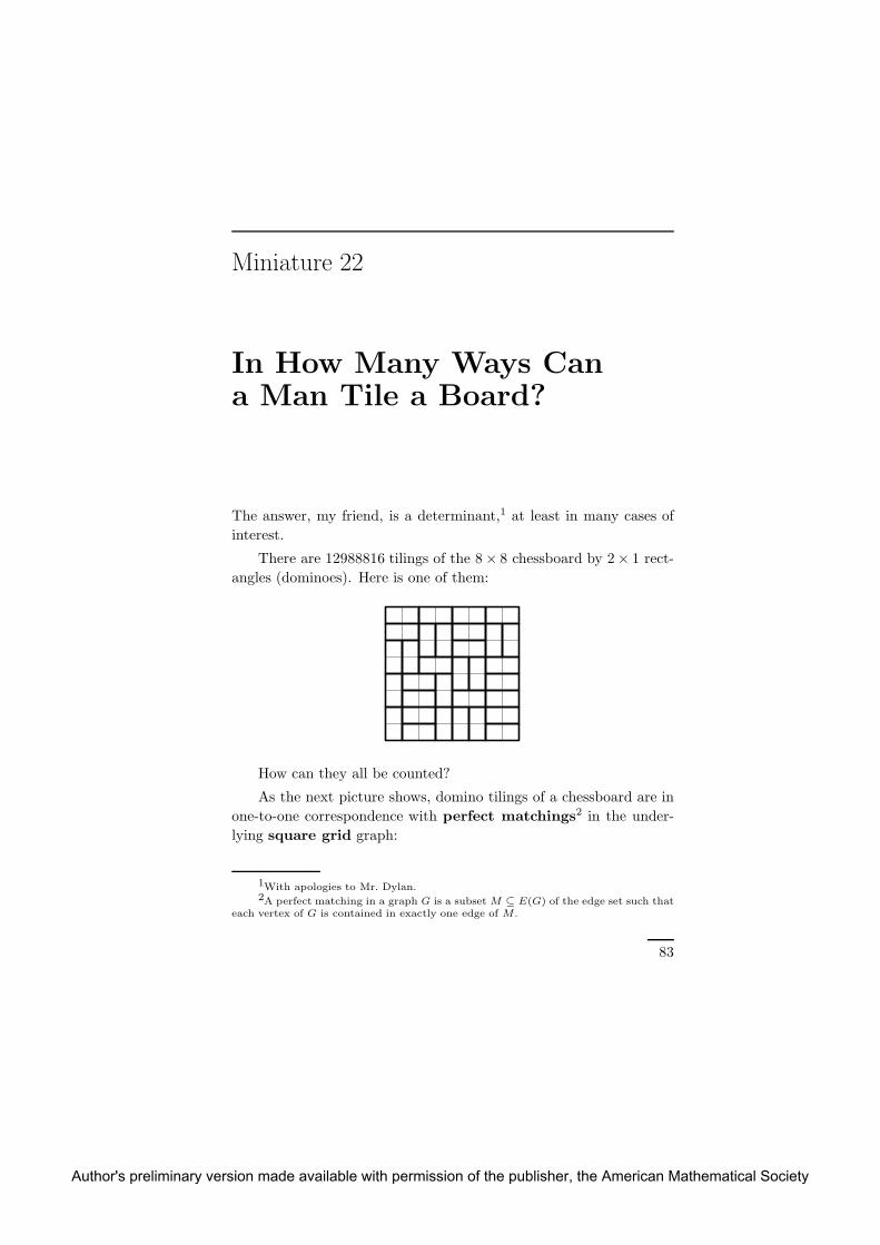
Miniature 22
In How Many Ways Cana Man Tile a Board?
The answer, my friend, is a determinant,1 at least in many cases of
interest.
There are 12988816 tilings of the 8 × 8 chessboard by 2 × 1 rect-
angles (dominoes). Here is one of them:
How can they all be counted?
As the next picture shows, domino tilings of a chessboard are in
one-to-one correspondence with perfect matchings2 in the under-
lying square grid graph:
1With apologies to Mr. Dylan.2A perfect matching in a graph G is a subset M ⊆ E(G) of the edge set such that
each vertex of G is contained in exactly one edge of M .
83
Author's preliminary version made available with permission of the publisher, the American Mathematical Society

84 22. In How Many Ways Can a Man Tile a Board?
Another popular kind of tilings are lozenge tilings (or rhombic
tilings). Here the board is made of equilateral triangles, and the tiles
are the three rhombi obtained by gluing two adjacent triangles:
As the right picture illustrates, these tilings correspond to perfect
matchings in honeycomb graphs.
We will explain how one can express the number of perfect match-
ings in these graphs, and many others, by a determinant. First we
need to introduce some notions.
The bipartite adjacency matrix and Kasteleyn signings. We
recall that a graph G is bipartite if its vertices can be divided into
two classes {u1, u2, . . . , un} and {v1, v2, . . . , vm} so that the edges go
only between the two classes, never within the same class.
We may assume that m = n, i.e., the classes have the same size,
for otherwise, G has no perfect matching.
We define the bipartite adjacency matrix of such G as the
n× n matrix B given by
bij :=
{
1 if {ui, vj} ∈ E(G),
0 otherwise.
Let Sn denote the set of all permutations of the set {1, 2, . . . , n}.
Every perfect matching M in G corresponds to a unique permutation
Author's preliminary version made available with permission of the publisher, the American Mathematical Society
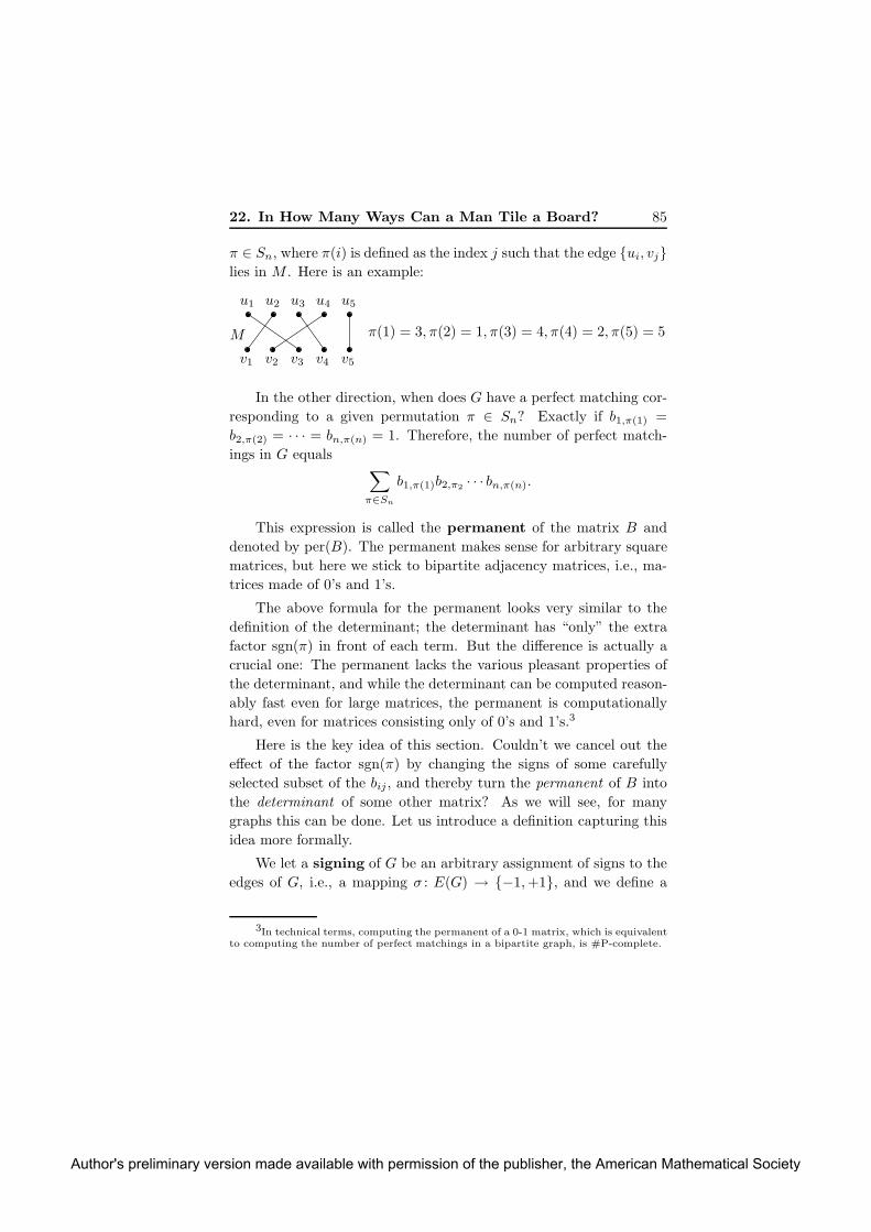
22. In How Many Ways Can a Man Tile a Board? 85
π ∈ Sn, where π(i) is defined as the index j such that the edge {ui, vj}lies in M . Here is an example:
u1 u2 u3 u4 u5
v1 v2 v3 v4 v5
π(1) = 3, π(2) = 1, π(3) = 4, π(4) = 2, π(5) = 5M
In the other direction, when does G have a perfect matching cor-
responding to a given permutation π ∈ Sn? Exactly if b1,π(1) =
b2,π(2) = · · · = bn,π(n) = 1. Therefore, the number of perfect match-
ings in G equals∑
π∈Sn
b1,π(1)b2,π2· · · bn,π(n).
This expression is called the permanent of the matrix B and
denoted by per(B). The permanent makes sense for arbitrary square
matrices, but here we stick to bipartite adjacency matrices, i.e., ma-
trices made of 0’s and 1’s.
The above formula for the permanent looks very similar to the
definition of the determinant; the determinant has “only” the extra
factor sgn(π) in front of each term. But the difference is actually a
crucial one: The permanent lacks the various pleasant properties of
the determinant, and while the determinant can be computed reason-
ably fast even for large matrices, the permanent is computationally
hard, even for matrices consisting only of 0’s and 1’s.3
Here is the key idea of this section. Couldn’t we cancel out the
effect of the factor sgn(π) by changing the signs of some carefully
selected subset of the bij , and thereby turn the permanent of B into
the determinant of some other matrix? As we will see, for many
graphs this can be done. Let us introduce a definition capturing this
idea more formally.
We let a signing of G be an arbitrary assignment of signs to the
edges of G, i.e., a mapping σ : E(G) → {−1,+1}, and we define a
3In technical terms, computing the permanent of a 0-1 matrix, which is equivalentto computing the number of perfect matchings in a bipartite graph, is #P-complete.
Author's preliminary version made available with permission of the publisher, the American Mathematical Society
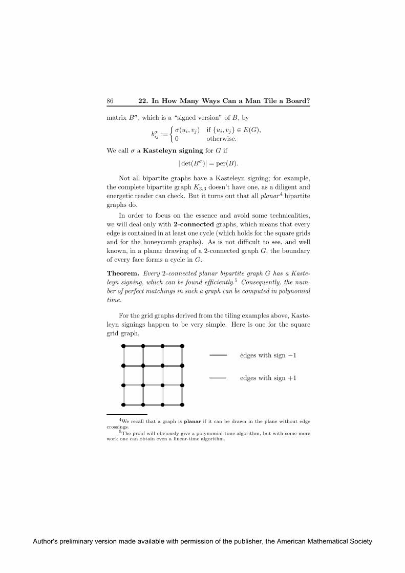
86 22. In How Many Ways Can a Man Tile a Board?
matrix Bσ, which is a “signed version” of B, by
bσij :=
{
σ(ui, vj) if {ui, vj} ∈ E(G),
0 otherwise.
We call σ a Kasteleyn signing for G if
| det(Bσ)| = per(B).
Not all bipartite graphs have a Kasteleyn signing; for example,
the complete bipartite graph K3,3 doesn’t have one, as a diligent and
energetic reader can check. But it turns out that all planar4 bipartite
graphs do.
In order to focus on the essence and avoid some technicalities,
we will deal only with 2-connected graphs, which means that every
edge is contained in at least one cycle (which holds for the square grids
and for the honeycomb graphs). As is not difficult to see, and well
known, in a planar drawing of a 2-connected graph G, the boundary
of every face forms a cycle in G.
Theorem. Every 2-connected planar bipartite graph G has a Kaste-
leyn signing, which can be found efficiently.5 Consequently, the num-
ber of perfect matchings in such a graph can be computed in polynomial
time.
For the grid graphs derived from the tiling examples above, Kaste-
leyn signings happen to be very simple. Here is one for the square
grid graph,
edges with sign −1
edges with sign +1
4We recall that a graph is planar if it can be drawn in the plane without edgecrossings.
5The proof will obviously give a polynomial-time algorithm, but with some morework one can obtain even a linear-time algorithm.
Author's preliminary version made available with permission of the publisher, the American Mathematical Society

22. In How Many Ways Can a Man Tile a Board? 87
and for the hexagonal grid we can even give all edges the sign +1.
Both of these facts will immediately follow from Lemma B below.
The restriction to 2-connected graphs in the theorem can easily be
removed with a little more work. The restriction to bipartite graphs
is also not essential. It makes the presentation slightly simpler, but
an analogous theory can be developed for the non-bipartite case along
similar lines—the interested readers will find this in the literature.
On the other hand, the assumption of planarity is more sub-
stantial: The method certainly breaks down for a general nonplanar
graph, and as was mentioned above, counting the number of perfect
matchings in a general graph is computationally hard. The class of
graphs where this approach works, the so-called Pfaffian graphs, is
somewhat wider than all planar graphs, but not easy to describe, and
most applications deal with planar graphs anyway.
Properly signed cycles. As a first step towards the proof, we give
a sufficient condition for a signing to be Kasteleyn. It may look
mysterious at first sight, but in the proof we will see where it comes
from.
Let C be a cycle in a bipartite graph G. Then C has an even
length, which we write as 2ℓ. Let σ be a signing of G, and let nC be
the number of negative edges (i.e., edges with sign −1) in C. Then
we call C properly signed with respect to σ if nC ≡ ℓ− 1 (mod 2).
In other words, a properly signed cycle of length 4, 8, 12, . . . contains
an odd number of negative edges, while a properly signed cycles of
length 6, 10, 14, . . . contains an even number of negative edges.
Further let us say that a cycle C is evenly placed if the graph
obtained from G by deleting all vertices of C (and the adjacent edges)
has a perfect matching.
Lemma A. Suppose that σ is a signing of a bipartite graph G (no
planarity assumed here) such that every evenly placed cycle in G is
properly signed. Then σ is a Kasteleyn signing for G.
Proof. This is straightforward. Let the signing σ as in the lemma be
fixed, and let M be a perfect matching in G, corresponding to a per-
mutation π. We define the sign of M as the sign of the corresponding
Author's preliminary version made available with permission of the publisher, the American Mathematical Society
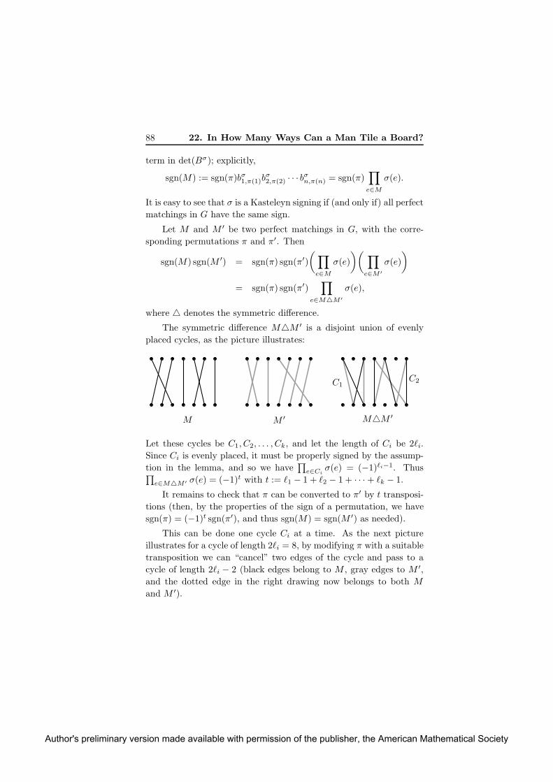
88 22. In How Many Ways Can a Man Tile a Board?
term in det(Bσ); explicitly,
sgn(M) := sgn(π)bσ1,π(1)bσ2,π(2) · · · bσn,π(n) = sgn(π)
∏
e∈M
σ(e).
It is easy to see that σ is a Kasteleyn signing if (and only if) all perfect
matchings in G have the same sign.
Let M and M ′ be two perfect matchings in G, with the corre-
sponding permutations π and π′. Then
sgn(M) sgn(M ′) = sgn(π) sgn(π′)
(
∏
e∈M
σ(e)
)(
∏
e∈M ′
σ(e)
)
= sgn(π) sgn(π′)∏
e∈M△M ′
σ(e),
where △ denotes the symmetric difference.
The symmetric difference M△M ′ is a disjoint union of evenly
placed cycles, as the picture illustrates:
M M′ M△M
′
C1C2
Let these cycles be C1, C2, . . . , Ck, and let the length of Ci be 2ℓi.
Since Ci is evenly placed, it must be properly signed by the assump-
tion in the lemma, and so we have∏
e∈Ciσ(e) = (−1)ℓi−1. Thus
∏
e∈M△M ′ σ(e) = (−1)t with t := ℓ1 − 1 + ℓ2 − 1 + · · · + ℓk − 1.
It remains to check that π can be converted to π′ by t transposi-
tions (then, by the properties of the sign of a permutation, we have
sgn(π) = (−1)t sgn(π′), and thus sgn(M) = sgn(M ′) as needed).
This can be done one cycle Ci at a time. As the next picture
illustrates for a cycle of length 2ℓi = 8, by modifying π with a suitable
transposition we can “cancel” two edges of the cycle and pass to a
cycle of length 2ℓi − 2 (black edges belong to M , gray edges to M ′,and the dotted edge in the right drawing now belongs to both M
and M ′).
Author's preliminary version made available with permission of the publisher, the American Mathematical Society

22. In How Many Ways Can a Man Tile a Board? 89
→
transpose these values in π
Continuing in this way for ℓi − 1 steps, we cancel Ci, and we can
proceed with the next cycle. Lemma A is proved. �
The rest of the proof of the theorem is a simple graph theory.
First we show that for graphs as in the theorem, it is sufficient to
check the condition in Lemma A only for special cycles, namely, face
boundaries. Clearly it is enough to deal with connected graphs.
Lemma B. Let G be a planar bipartite graph that is both connected
and 2-connected, and let us fix a planar drawing of G. If σ is a signing
of G such that the boundary cycle of every inner face in the drawing
is properly signed, then σ is a Kasteleyn signing.
Proof of Lemma B. Let C be an evenly placed cycle in G; we need
to prove that it is properly signed.
Let the length of C be 2ℓ. Let F1, . . . , Fk be the inner faces
enclosed in C in the drawing, and let Ci be the boundary cycle of Fi,
of length 2ℓi. Let H be the subgraph of G obtained by deleting all
vertices and edges drawn outside C; in other words, H is the union
of the Ci.
F1F2
F3F4
F5
F6
C
H
Author's preliminary version made available with permission of the publisher, the American Mathematical Society

90 22. In How Many Ways Can a Man Tile a Board?
We want to see how the parity of ℓ is related to the parities of
the ℓi. To this end, we need to do some counting. The number of
vertices of H is r + 2ℓ, where r is the number of vertices lying in the
interior of C. Every edge of H belongs to exactly two cycles among
C,C1, . . . , Ck, and so the number of edges of H equals ℓ+ℓ1 + · · ·+ℓk.
Finally, the drawing of H has k + 1 faces: F1, . . . , Fk and the outer
one.
Now we apply Euler’s formula, which tells us that for every
drawing of a connected planar graph, the number of vertices plus the
number of faces equals the number of edges plus 2. Thus
(18) r + 2ℓ+ k + 1 = ℓ+ ℓ1 + · · · + ℓk + 2.
Next, we use the assumption that C is evenly placed. Since the
complement of C inG has a perfect matching, the number r of vertices
inside C must be even. Therefore, from (18) we get
(19) ℓ− 1 ≡ ℓ1 + · · · + ℓk − k (mod 2).
Let nC be the number of negative edges in C, and similarly for
nCi. The sum nC + nC1
+ · · · + nCkis even because it counts every
negative edge twice, and so
(20) nC ≡ nC1+ · · · + nCk
(mod 2).
Finally, we have nCi≡ ℓi−1 (mod 2) since the Ci are properly signed.
Combining this with (19) and (20) gives nC ≡ ℓ− 1 (mod 2). Hence
C is properly signed. Lemma B now follows from Lemma A. �
Proof of the theorem. Given a connected, 2-connected, planar, bi-
partite G, we fix some planar drawing, and we want to construct a
signing as in Lemma B, with the boundary of every inner face properly
signed.
First we start deleting edges from G, as the next picture illus-
trates:
Author's preliminary version made available with permission of the publisher, the American Mathematical Society

22. In How Many Ways Can a Man Tile a Board? 91
F1
F2
e1
G1 = G G2
e2
F3
G3
e3
G6
. . .
We set G1 := G, and Gi+1 is obtained from Gi by deleting an edge ei
that separates an inner face Fi from the outer (unbounded) face (in
the current drawing). The procedure finishes with some Gk that has
no such edge. Then the drawing of Gk has only the outer face.
Now we choose the signs of the edges of Gk arbitrarily, and we
extend this to a signing of G by going backwards, choosing the signs
for ek−1, ek−2, . . . , e1 in this order. When we consider ei, it is con-
tained in the boundary of the single inner face Fi in the drawing of
Gi, so we can set σ(ei) so that the boundary of Fi is properly signed.
The theorem is proved. �
From the determinant formula one can obtain, with some effort,
the following amazing formula for the number of domino tilings of an
m×n chessboard:
[
m∏
k=1
n∏
ℓ=1
(
2 cosπk
m+ 1+ 2i cos
πℓ
n+ 1
)
]1/2
,
where i is the imaginary unit. But the determinants can be used not
only for counting, but also for generating a random perfect matching
(chosen uniformly among all possible perfect matchings), and for an-
alyzing its typical properties. Such results are relevant for questions
in theoretical physics.
Here is a quick illustration of an interesting phenomenon for ran-
dom tilings. The next picture shows a random lozenge tiling of a large
hexagon:
Author's preliminary version made available with permission of the publisher, the American Mathematical Society
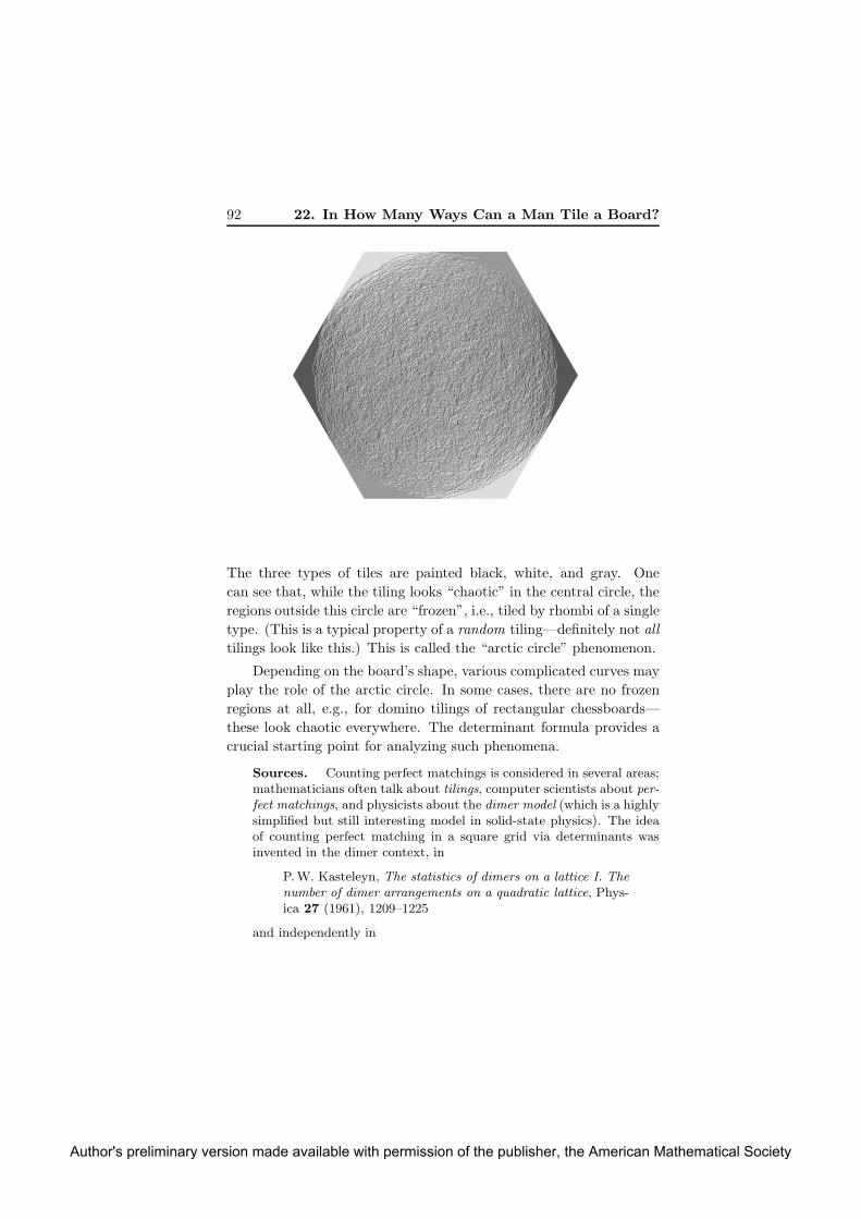
92 22. In How Many Ways Can a Man Tile a Board?
The three types of tiles are painted black, white, and gray. One
can see that, while the tiling looks “chaotic” in the central circle, the
regions outside this circle are “frozen”, i.e., tiled by rhombi of a single
type. (This is a typical property of a random tiling—definitely not all
tilings look like this.) This is called the “arctic circle” phenomenon.
Depending on the board’s shape, various complicated curves may
play the role of the arctic circle. In some cases, there are no frozen
regions at all, e.g., for domino tilings of rectangular chessboards—
these look chaotic everywhere. The determinant formula provides a
crucial starting point for analyzing such phenomena.
Sources. Counting perfect matchings is considered in several areas;mathematicians often talk about tilings, computer scientists about per-
fect matchings, and physicists about the dimer model (which is a highlysimplified but still interesting model in solid-state physics). The ideaof counting perfect matching in a square grid via determinants wasinvented in the dimer context, in
P.W. Kasteleyn, The statistics of dimers on a lattice I. The
number of dimer arrangements on a quadratic lattice, Phys-ica 27 (1961), 1209–1225
and independently in
Author's preliminary version made available with permission of the publisher, the American Mathematical Society

22. In How Many Ways Can a Man Tile a Board? 93
H.N.V. Temperley and M.E. Fisher, Dimer problem in sta-
tistical mechanics—An exact result, Philos. Magazine 6
(1961), 1061–1063.
The material covered in this section is just the beginning of amazingtheories going in several directions. As starting points one can use,e.g.,
R. Kenyon, The planar dimer model with boundary: A sur-
vey, Directions in mathematical quasicrystals, CRM Mono-graph Ser. 13, Amer. Math. Soc., Providence, R.I., 2000,pp. 307–328
(discussing tilings, dimers, the arctic circle, random surfaces, and such)and
R. Thomas, A survey of Pfaffian orientations of graphs, inInternational Congress of Mathematicians. Vol. III, Eur.Math. Soc., Zurich, 2006, pp. 963–984
(with graph-theoretic and algorithmic aspects of Pfaffian graphs).
Author's preliminary version made available with permission of the publisher, the American Mathematical Society

Author's preliminary version made available with permission of the publisher, the American Mathematical Society
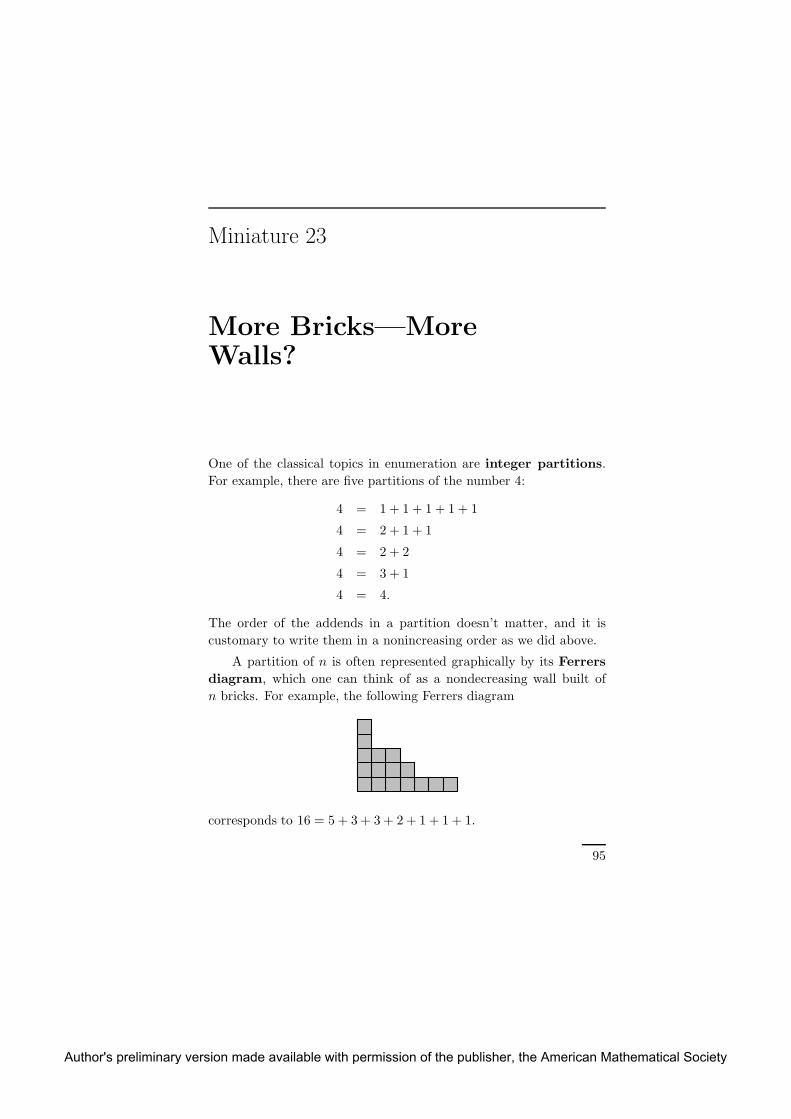
Miniature 23
More Bricks—MoreWalls?
One of the classical topics in enumeration are integer partitions.
For example, there are five partitions of the number 4:
4 = 1 + 1 + 1 + 1 + 1
4 = 2 + 1 + 1
4 = 2 + 2
4 = 3 + 1
4 = 4.
The order of the addends in a partition doesn’t matter, and it is
customary to write them in a nonincreasing order as we did above.
A partition of n is often represented graphically by its Ferrers
diagram, which one can think of as a nondecreasing wall built of
n bricks. For example, the following Ferrers diagram
corresponds to 16 = 5 + 3 + 3 + 2 + 1 + 1 + 1.
95
Author's preliminary version made available with permission of the publisher, the American Mathematical Society
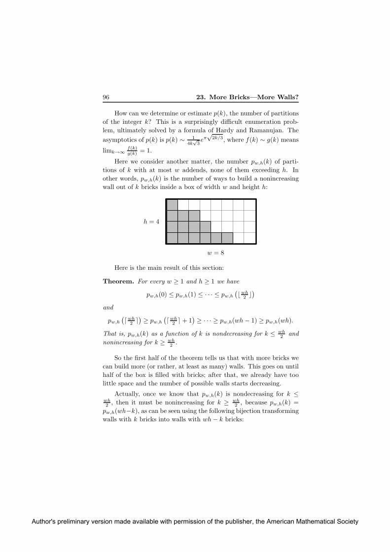
96 23. More Bricks—More Walls?
How can we determine or estimate p(k), the number of partitions
of the integer k? This is a surprisingly difficult enumeration prob-
lem, ultimately solved by a formula of Hardy and Ramanujan. The
asymptotics of p(k) is p(k) ∼ 14k
√3eπ√
2k/3, where f(k) ∼ g(k) means
limk→∞f(k)g(k) = 1.
Here we consider another matter, the number pw,h(k) of parti-
tions of k with at most w addends, none of them exceeding h. In
other words, pw,h(k) is the number of ways to build a nonincreasing
wall out of k bricks inside a box of width w and height h:
w = 8
h = 4
Here is the main result of this section:
Theorem. For every w ≥ 1 and h ≥ 1 we have
pw,h(0) ≤ pw,h(1) ≤ · · · ≤ pw,h
(
⌊wh2 ⌋)
and
pw,h
(
⌈wh2 ⌉)
≥ pw,h
(
⌈wh2 ⌉ + 1
)
≥ · · · ≥ pw,h(wh− 1) ≥ pw,h(wh).
That is, pw,h(k) as a function of k is nondecreasing for k ≤ wh2 and
nonincreasing for k ≥ wh2 .
So the first half of the theorem tells us that with more bricks we
can build more (or rather, at least as many) walls. This goes on until
half of the box is filled with bricks; after that, we already have too
little space and the number of possible walls starts decreasing.
Actually, once we know that pw,h(k) is nondecreasing for k ≤wh2 , then it must be nonincreasing for k ≥ wh
2 , because pw,h(k) =
pw,h(wh−k), as can be seen using the following bijection transforming
walls with k bricks into walls with wh− k bricks:
Author's preliminary version made available with permission of the publisher, the American Mathematical Society

23. More Bricks—More Walls? 97
→
bricks↔nonbricks
→
turn by 180 degrees
The theorem is one of the results that look intuitively obvious
but are surprisingly hard to prove. The great Cayley used this as a
fact requiring no proof in his 1856 memoir, and only about twenty
years later did Sylvester discover the first proof.
One would naturally expect such a combinatorial problem to have
a combinatorial solution, perhaps simply an injective map assigning
to every wall of k bricks a wall of k+1 bricks (for k+1 ≤ wh2 ). But to
my knowledge, nobody has managed to discover a proof of this kind,
and estimating pw,h(k) or expressing it by a formula doesn’t seem to
lead to the goal either.
Earlier proofs of the theorem used relatively heavy mathematical
tools, essentially representations of Lie algebras. The proof shown
here is a result of several simplifications of the original ideas, and it
uses “only” matrix-rank arguments.
Functions, or sequences, that are first nondecreasing and then,
from some point on, nonincreasing, are called unimodal (and so are
functions that begin as nonincreasing and continue as nondecreasing).
There are many important results and conjectures in various areas
of mathematics asserting that certain quantities form an unimodal
sequence, and the proof below contains tools of general applicability.
Preliminary considerations. Let us write n := wh for the area of
the box, and let us fix a numbering of the n squares in the box by
the numbers 1, 2, . . . , n.
To prove the theorem, we will show that pw,h(k) ≤ pw,h(ℓ) for
0 ≤ k < ℓ ≤ n2 .
The first step is to view a wall in the box as an equivalence class.
Namely, we start with an arbitrary set of k bricks filling some k
squares in the box, and then we tidy them up into a nonincreasing
wall:
Author's preliminary version made available with permission of the publisher, the American Mathematical Society

98 23. More Bricks—More Walls?
First we push down the bricks in each column, and then we rearrange
the columns into a nonincreasing order.
Let us call two k-element subsets K,K ′ ⊆ {1, 2, . . . , n}, under-
stood as sets of k squares in the box, wall-equivalent if they lead to
the same nonincreasing wall. This indeed defines an equivalence on
the set K of all k-element subsets of {1, 2, . . . , n}. Let the equivalence
classes be K1,K2, . . . ,Kr, where r := pw,h(k).
Let us phrase the definition of the wall-equivalence differently, in
a way that will be more convenient latter. Let π be a permutation of
the n squares in the box; let us say that π doesn’t break columns
if it corresponds to first permuting the squares in each column arbi-
trarily, and then permuting the columns. It is easily seen that two
subsets K,K ′ ∈ K are wall-equivalent exactly if K ′ = π(K) for some
permutation that doesn’t break columns.1
Next, let L be the set of all ℓ-element subsets of {1, 2, . . . , n},
and let it be divided similarly into s := pw,h(ℓ) classes L1, . . . ,Ls
according to wall-equivalence. The goal is to prove that r ≤ s.
1In a more mature mathematical language, the permutations that don’t breakcolumns form a permutation group acting on K, and the classes of the wall-equivalenceare the orbits of this action. Some things in the sequel could (should?) also be phrasedin the language of actions of permutation groups, but I decided to avoid this terminol-ogy, with the hope of deterring slightly fewer students.
Author's preliminary version made available with permission of the publisher, the American Mathematical Society

23. More Bricks—More Walls? 99
Let us consider the bipartite graph G with vertex set K ∪ L and
with edges corresponding to inclusion; i.e., a k-element set K ∈ Kis connected to an ℓ-element set L ∈ L by an edge if K ⊆ L. A
small-scale illustration with w = 2, h = 3, k = 2, and ℓ = 3 follows:
K1K2
L1 L2
Claim. For every i and j, all L ∈ Lj have the same number dij of
neighbors in Ki.
Proof. Let L,L′ ∈ Lj , and let us fix some permutation π that
doesn’t break columns and such that L′ = π(L). For K ∈ Ki, we
have π(K) ∈ Ki as well (by the alternative description of the wall-
equivalence), and it is easily seen that K 7→ π(K) defines a bijection
between the neighbors of L lying in Ki and the neighbors of L′ lying
in Ki. �
Let us now pass to a more general setting for a while: Let U, V be
disjoint finite sets, let (U1, . . . , Ur, V1, . . . , Vs) be a partition of U ∪Vwith U = U1 ∪ · · · ∪ Ur and V = V1 ∪ · · · ∪ Vs, where the Ui and
Vj are all nonempty, and let G be a bipartite graph on the vertex
set U ∪ V (with all edges going between U and V ). We call the
partition (U1, . . . , Ur, V1, . . . , Vs) V -degree homogeneous w.r.t. G
if the condition as in the claim holds, i.e., all vertices in Vj have the
same number dij of neighbors in Ui, for all i and j. In such case,
we call the matrix D = (dij)ri=1
sj=1 the V -degree matrix of the
partition (with respect to G).
In the setting introduced above, we have a bipartite graph with a
V -degree homogeneous partition, and we would like to conclude that
r, the number of the U -pieces, can’t be smaller than s, the number of
Author's preliminary version made available with permission of the publisher, the American Mathematical Society
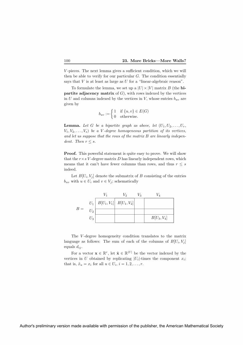
100 23. More Bricks—More Walls?
V -pieces. The next lemma gives a sufficient condition, which we will
then be able to verify for our particular G. The condition essentially
says that V is at least as large as U for a “linear-algebraic reason”.
To formulate the lemma, we set up a |U | × |V | matrix B (the bi-
partite adjacency matrix of G), with rows indexed by the vertices
in U and columns indexed by the vertices in V , whose entries buv are
given by
buv :=
{
1 if {u, v} ∈ E(G)
0 otherwise.
Lemma. Let G be a bipartite graph as above, let (U1, U2, . . . , Ur,
V1, V2, . . . , Vs) be a V -degree homogeneous partition of its vertices,
and let us suppose that the rows of the matrix B are linearly indepen-
dent. Then r ≤ s.
Proof. This powerful statement is quite easy to prove. We will show
that the r×s V -degree matrixD has linearly independent rows, which
means that it can’t have fewer columns than rows, and thus r ≤ s
indeed.
Let B[Ui, Vj ] denote the submatrix of B consisting of the entries
buv with u ∈ Ui and v ∈ Vj ; schematically
B[U1, V1] B[U1, V2]U1
U2
U3B[U3, V4]
V1 V2 V3 V4
B =
The V -degree homogeneity condition translates to the matrix
language as follows: The sum of each of the columns of B[Ui, Vj ]
equals dij .
For a vector x ∈ Rr, let x ∈ R|U| be the vector indexed by the
vertices in U obtained by replicating |Ui|-times the component xi;
that is, xu = xi for all u ∈ Ui, i = 1, 2, . . . , r.
Author's preliminary version made available with permission of the publisher, the American Mathematical Society
23. More Bricks—More Walls? 101
For this x, we consider the product xTB. Its vth component
equals∑
u∈U xubuv =∑r
i=1 xi
∑
u∈Uibuv =
∑ri=1 xidij = (xTD)j .
Hence xTD = 0 implies xTB = 0.
Let us assume for contradiction that the rows of D are linearly
dependent; that is, there is a nonzero x ∈ Rr with xTD = 0. Then
x 6= 0 but, as we’ve just seen, xTB = 0. This contradicts the linear
independence of the rows of B and proves the lemma. �
Proof of the theorem. We return to the particular bipartite graph
G introduced above, with vertex set K ∪ L and with the L-degree
homogeneous partition (K1, . . . ,Kr,L1, . . . ,Ls) according to the wall-
equivalence. For applying the lemma, it remains to show that the rows
of the corresponding matrix B are linearly independent.
This result, known as Gottlieb’s theorem,2 has proved useful
in several other applications as well. Explicitly, it tells us that for
0 ≤ k < ℓ ≤ n2 , the zero-one matrix B with rows indexed by K
(all k-subsets of {1, 2, . . . , n}), columns indexed by L (all ℓ-subsets),
and the nonzero entries corresponding to containment, has linearly
independent rows.
Several proofs are known; here we present one resembling the
proof of the lemma above.
Proof of Gottlieb’s theorem. For contradiction, we assume that
yTB = 0 for some nonzero vector y. The components of y are indexed
by k-element sets; let us fix some K0 ∈ K with yK06= 0.
Next, we partition both K and L into k + 1 classes according to
the size of the intersection with K0 (this partition has nothing to do
with the partition of K and L considered earlier—we just re-use the
same letters):
Ki := {K ∈ K : |K ∩K0| = i}, i = 0, 1, . . . , k
Lj := {L ∈ L : |L ∩K0| = j}, j = 0, 1, . . . , k.
Every Ki and every Lj is nonempty—here we use the assumption k <
ℓ ≤ n2 (if, for example, we had k + ℓ > n, we would get L0 = ∅, since
there wouldn’t be enough room for an ℓ-element L disjoint from K0).
2This is not the only theorem associated with Gottlieb’s name, though.
Author's preliminary version made available with permission of the publisher, the American Mathematical Society
102 23. More Bricks—More Walls?
Here, for a change, we will need that this partition is K-degree
homogeneous (with respect to the same bipartite graph as above, with
edges representing inclusion). That is, every K ∈ Ki has the same
number dij of neighbors in Lj . More explicitly, dij is the number of
ways of extending a k-element set K with |K∩K0| = i to an ℓ-element
L ⊃ K with |L ∩K0| = j; this number is clearly independent of the
specific choice of K. (We could compute dij explicitly, but we don’t
need it.)
By this description, we have dij = 0 for i > j, and thus the
K-degree matrix D is upper triangular. Moreover, dii 6= 0 for all
i = 0, 1, . . . , k, and so D is non-singular.
Using the vector y, we are going to exhibit a nonzero x = (x0,
x1, . . . , xk) with xTD = 0, which will be a contradiction. A suitable
x is obtained by summing the components of y over the classes Ki:
xi :=∑
K∈Ki
yK .
We have x 6= 0, since the class Kk contains only K0, and so xk =
yK06= 0.
For every j we calculate
0 =∑
L∈Lj
(yTB)L =∑
L∈Lj
∑
K∈KyKbKL =
∑
K∈KyK
∑
L∈Lj
bKL
=
k∑
i=0
∑
K∈Ki
yKdij =
k∑
i=0
xidij = (xTD)j .
Hence xTD = 0, and this is the promised contradiction to the non-
singularity of D. Gottlieb’s theorem, as well as our main theorem,
are proved. �
Another example. For readers familiar with the notion of graph
isomorphism, the following might be a rewarding exercise in applying
the method shown above: Prove that if gn(k) stands for the number of
nonisomorphic graphs with n vertices and k edges, then the sequence
gn(0), gn(1), . . . , gn((
n2
)
) is unimodal.
Sources. As was mentioned above, the theorem was implicitlyassumed without proof in
Author's preliminary version made available with permission of the publisher, the American Mathematical Society

23. More Bricks—More Walls? 103
A. Cayley, A second memoir on quantics, Phil. Trans. Roy.Soc. 146 (1856), 101–126.
The word “quantic” in the title means, in today’s terminology, a homo-geneous multivariate polynomial, and Cayley was interested in quanticsthat are invariant under the action of linear transformations. The firstproof of the theorem was obtained in
J. J. Sylvester, Proof of the hitherto undemonstrated fun-
damental theorem of invariants, Philos. Mag. 5 (1878),178–188.
A substantially more elementary proof than the previous ones, phrasedin terms of group representations, was obtained in
R.P. Stanley, Some aspects of groups acting on finite posets,J. Combinatorial Theory Ser. A 32 (1982), 132–161.
Our presentation is based on that of Babai and Frankl in their textbookcited in the introduction.
Gottlieb’s theorem was first proved in
D.H. Gottlieb, A certain class of incidence matrices, Proc.Amer. Math. Soc 17 (1066), 1233–1237.
The proof presented above rephrases an argument from
C. D. Godsil,Tools from linear algebra, Chapter 31 of R. Gra-ham, M. Grotschel, and L. Lovasz, editors, Handbook of
Combinatorics, North-Holland, Amsterdam, 1995, pp. 1705–1748.
For an introduction to integer partitions see
G. Andrews and K. Eriksson, Integer partitions, CambridgeUniversity Press, Cambridge 2004,
(this is a very accessible source), or Wilf’s lecture notes at http://
www.math.upenn.edu/~wilf/PIMS/PIMSLectures.pdf.
Author's preliminary version made available with permission of the publisher, the American Mathematical Society

Author's preliminary version made available with permission of the publisher, the American Mathematical Society

Miniature 24
Perfect Matchings andDeterminants
A matching in a graph G is a set of edges F ⊆ E(G) such that no
vertex of G is incident to more than one edge of F .
A perfect matching is a matching covering all vertices. The reader
may want to find a perfect matching in the graph in the picture.
In Miniature 22, we counted perfect matchings in certain graphs
via determinants. Here we will employ determinants in a simple algo-
rithm for testing whether a given graph has a perfect matching. The
basic approach is similar to the approach to testing matrix multipli-
cation from Miniature 11. We consider only the bipartite case, which
is simpler.
Consider a bipartite graph G. Its vertices are divided into two
classes {u1, u2, . . . , un} and {v1, v2, . . . , vn} and the edges go only
between the two classes, never within one class. Both of the classes
105
Author's preliminary version made available with permission of the publisher, the American Mathematical Society

106 24. Perfect Matchings and Determinants
have the same size, for otherwise, the graph has no perfect matching.
Let m stand for the number of edges of G.
Let Sn be the set of all permutations of the set {1, 2, . . . , n}.
Every perfect matching of G uniquely corresponds to a permutation
π ∈ Sn. We can describe it in the form {{u1, vπ(1)}, {u2, vπ(2)}, . . .,{un, vπ(n)}}.
We express the existence of a perfect matching by a determinant,
but not of an ordinary matrix of numbers, but rather of a matrix
whose entries are variables. We introduce a variable xij for every
edge {ui, vj} ∈ E(G) (so we have m variables altogether), and we
define an n× n matrix A by
aij :=
{
xij if {ui, vj} ∈ E(G),
0 otherwise.
The determinant of A is a polynomial in the m variables xij . By the
definition of a determinant, we get
det(A) =∑
π∈Sn
sgn(π) · a1,π(1)a2,π(2) · · · an,π(n)
=∑
π describes a perfectmatching of G
sgn(π) · x1,π(1)x2,π(2) · · ·xn,π(n).
Lemma. The polynomial det(A) is identically zero if and only if G
has no a perfect matching.
Proof. The formula above the formula makes it clear that if G has
no perfect matching, then det(A) is the zero polynomial.
To show the converse, we fix a permutation π that defines a per-
fect matching, and we substitute for the variables in det(A) as follows:
xi,π(i) := 1 for every i = 1, 2, . . . , n, and all the remaining xij are 0.
We have sgn(π) · x1,π(1)x2,π(2) · · ·xn,π(n) = ±1 for this permutation
π.
For every other permutation σ 6= π there is an i with σ(i) 6= π(i),
thus xi,σ(i) = 0, and therefore, all other terms in the expansion of
det(A) are 0. For this choice of the xij we thus have det(A) = ±1. �
Author's preliminary version made available with permission of the publisher, the American Mathematical Society
24. Perfect Matchings and Determinants 107
Now we would like to test whether the polynomial det(A) is the
zero polynomial. We can’t afford to compute it explicitly as a polyno-
mial, since it has the same number of terms as the number of perfect
matchings of G and that can be exponentially many. But if we substi-
tute any specific numbers for the variables xij , we can easily calculate
the determinant, e.g., by the Gaussian elimination. So we can imag-
ine that det(A) is available to us through a black box, from which we
can obtain the value of the polynomial at any specified point.
For an arbitrary function given by a black box, we can never be
sure that it is identically 0 unless we check its values at all points.
But a polynomial has a wonderful property: Either it equals 0 ev-
erywhere, or almost nowhere. The following theorem expresses this
quantitatively.
Theorem (The Schwartz–Zippel theorem1). Let K be an arbitrary
field, and let S be a finite subset of K. Then for every non-zero
polynomial p(x1, . . . , xm) of degree d in m variables and with coef-
ficients from K, the number of m-tuples (r1, r2, . . . , rm) ∈ Sm with
p(r1, r2, . . . , rm) = 0 is at most d|S|m−1. In other words, if r1, r2,. . . ,
rm ∈ S are chosen independently and uniformly at random, then the
probability of p(r1, r2, . . . , rm) = 0 is at most d|S| .
Before we prove this theorem, we get back to bipartite matchings.
Let us assume that G has a perfect matching and thus det(A) is a non-
zero polynomial. Then the Schwartz–Zippel theorem shows that if we
calculate det(A) for values of the variables xij chosen independently
at random from S := {1, 2, . . . , 2n}, then the probability of getting 0
is at most 12 .
But in order to decide whether the determinant is 0 for a given
substitution, we have to compute it exactly. In such a computation,
we may encounter huge numbers, with about n digits, and then arith-
metic operations would become quite expensive.
It is better to work with a finite field. The simplest way is to
choose a prime number p, 2n ≤ p < 4n (by a theorem from number
theory called Bertrand’s postulate such a number always exists and
1This Schwartz is really spelled with “t”, unlike the one from the Cauchy–Schwarzinequality.
Author's preliminary version made available with permission of the publisher, the American Mathematical Society
108 24. Perfect Matchings and Determinants
it can be found sufficiently quickly) and operate in the finite field Fp
of integers modulo p. Then the arithmetic operations are fast (if we
prepare a table of inverse elements in advance).
Using the Gaussian elimination for computing the determinant,
we get a probabilistic algorithm for testing the existence of a bipartite
matching in a given graph running in O(n3) time. It fails with a
probability at most 12 . As usual, the probability of the failure can be
reduced to 2−k by repeating the algorithm k times.
The determinant can also be computed by the algorithms for fast
matrix multiplication (mentioned in Miniature 10), and in this way
we obtain the asymptotically fastest known algorithm for testing the
existence of a perfect bipartite matching, with running timeO(n2.376).
But we should honestly admit that a deterministic algorithm is
known that always finds a maximum matching in O(n2.5) time. This
algorithm is much faster in practice. Moreover, the algorithm dis-
cussed above can decide whether a perfect matching exists, but it
doesn’t find one (however, there are more complicated variants that
can also find the matching). On the other hand, this algorithm can
be implemented very efficiently on a parallel computeri, and no other
known approach yields comparably fast parallel algorithms.
Proof of the Schwartz–Zippel theorem. We proceed by induc-
tion on m. The univariate case is clear, since there are at most d
roots of p(x1) by a well-known theorem of algebra. (That theorem is
proved by induction on d: If p(α) = 0, then we can divide p(x) by
x− α and reduce the degree.)
Let m > 1. Let us suppose that x1 occurs in at least one term
of p(x1, . . . , xn) with a nonzero coefficient (if not, we rename the
variables). Let us write p(x1, . . . , xm) as a polynomial in x1 with
coefficients being polynomials in x2, . . . , xn:
p(x1, x2, . . . , xm) =
k∑
i=0
xi1pi(x2, . . . , xm),
where k is the maximum exponent of x1 in p(x1, . . . , xn).
We divide the m-tuples (r1, . . . , rm) with p(r1, r2 . . . , rm) = 0 into
two classes. The first class, called R1, are those with pk(r2, . . . , rm) =
Author's preliminary version made available with permission of the publisher, the American Mathematical Society
24. Perfect Matchings and Determinants 109
0. Since the polynomial pk(x2, . . . , xm) is not identically zero and
has degree at most d − k, the number of choices for (r2, . . . , rm) is
at most (d − k)|S|m−2 by the induction hypothesis, and so |R1| ≤(d− k)|S|m−1.
The second class R2 are the remaining m-tuples, that is, those
with p(r1, r2, . . . , rm) = 0 but pk(r2, . . . , rm) 6= 0. Here we count
as follows: r2 through rm can be chosen in at most |S|m−1 ways,
and if r2, . . . , rm are fixed with pk(r2, . . . , rm) 6= 0, then r1 must be
a root of the univariate polynomial q(x1) = p(x1, r2, . . . , rm). This
polynomial has degree (exactly) k, and hence it has at most k roots.
Thus the second class has at most k|S|m−1 m-tuples, which gives
d|S|m−1 altogether, finishing the induction step and the proof of the
Schwartz–Zippel theorem. �
Sources. The idea of the algorithm for testing perfect matchingsvia determinants is from
J. Edmonds, Systems of distinct representatives and linear
algebra, J. Res. Nat. Bur. Standards Sect. B 71B (1967),241–245.
There are numerous papers on algebraic matching algorithms; a recentone is
N. J. A. Harvey, Algebraic Algorithms for Matching and Ma-
troid Problems, Proc. 47th IEEE Symposium on Founda-tions of Computer Science (FOCS), 2006, 531–542.
The Schwartz–Zippel theorem (or lemma) appeared in
J. Schwartz, Fast probabilistic algorithms for verification of
polynomial identities, J. ACM 27 (1980), 701–717
and in
R. Zippel, Probabilistic algorithms for sparse polynomials,Proc. International Symposium on Symbolic and AlgebraicComputation, vol. 72 of LNCS, Springer, Berlin, 1979, 216–226.
Author's preliminary version made available with permission of the publisher, the American Mathematical Society

Author's preliminary version made available with permission of the publisher, the American Mathematical Society
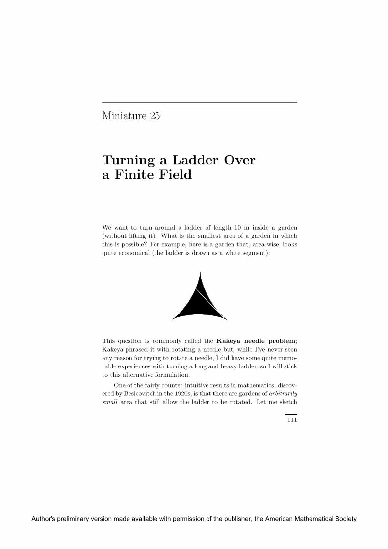
Miniature 25
Turning a Ladder Overa Finite Field
We want to turn around a ladder of length 10 m inside a garden
(without lifting it). What is the smallest area of a garden in which
this is possible? For example, here is a garden that, area-wise, looks
quite economical (the ladder is drawn as a white segment):
This question is commonly called the Kakeya needle problem;
Kakeya phrased it with rotating a needle but, while I’ve never seen
any reason for trying to rotate a needle, I did have some quite memo-
rable experiences with turning a long and heavy ladder, so I will stick
to this alternative formulation.
One of the fairly counter-intuitive results in mathematics, discov-
ered by Besicovitch in the 1920s, is that there are gardens of arbitrarily
small area that still allow the ladder to be rotated. Let me sketch
111
Author's preliminary version made available with permission of the publisher, the American Mathematical Society

112 25. Turning a Ladder Over a Finite Field
the beautiful construction, although it is not directly related to the
topic of this book.
A necessary condition for turning a unit-length ladder inside a set
X is that X contains a unit-length segment of every direction. An X
satisfying this latter, weaker condition is called a Kakeya set; unlike
the ladder problem, this definition has an obvious generalization to
higher dimensions. We begin by constructing a planar Kakeya set of
arbitrarily small area (actually, one can get a zero-measure Kakeya
set with a little more effort).
Let us consider a triangle T of height 1 with base on the x-axis,
and let h ∈ [0, 1). The thinning of T at height h means replacing T
with the two triangles T1 and T2 obtaining by slicing T through the
top vertex and the middle of its base and translating left T2 so that
it exactly overlaps with T1 at height h:
0
h
1T1T2T
More generally, thinning a collection of triangles at height h means
thinning each of them separately, so from k triangles we obtain 2k
triangles.
We will construct a small-area set in the plane that contains seg-
ments of all directions with slope at least 1 in absolute value (more
vertical than horizontal); to get a Kakeya set, we need to add another
copy rotated by 90 degrees.
We choose a sequence (h1, h2, h3, . . .) that is dense in the interval
[0, 1) and contains every member infinitely often, e.g., the sequence
(12 ,
14 ,
24 ,
34 ,
18 ,
28 , . . .). We start with the triangle with top angle 90
degrees, perform thinning at height h1, then at height h2, etc.
Author's preliminary version made available with permission of the publisher, the American Mathematical Society

25. Turning a Ladder Over a Finite Field 113
Let Bi be the union of all the 2i triangles after the ith thinning. We
claim that the area of Bi gets arbitrarily small as i grows. The idea of
the proof is that after k thinnings at height h, the total length of the
intersection of the current collection of triangles with the horizontal
line of height h is at most 2−k times the original length. Then we need
a “continuity” argument, showing that the length is very small not
only at height exactly h, but also in a sufficiently large neighborhood.
We leave the details to an ambitious reader.
How can we use Bi to turn the ladder? We need to enlarge it so
that the ladder can move from one triangle to the next. For that, we
add “translation corridors” of the following kind to Bi:
The dark gray triangles are from Bi, and the lighter gray corridor can
be used to transport the ladder between the two marked positions. If
we’re willing to walk with the ladder far enough, then the translation
tunnels add an arbitrarily small area.
Kakeya’s conjecture. A similar construction produces zero-meas-
ure Kakeya sets in all higher dimensions too. However, a statement
known as Kakeya’s conjecture asserts that they can’t be too small.
Namely, a Kakeya setK in Rn should have Hausdorff dimension n (for
readers not familiar with Hausdorff dimension: roughly speaking, this
means that it is not possible to cover K with sets of small diameter
much more economically than the n-dimensional cube, say).
Author's preliminary version made available with permission of the publisher, the American Mathematical Society

114 25. Turning a Ladder Over a Finite Field
While the Kakeya needle problem has a somewhat recreational
flavor, Kakeya’s conjecture is regarded as a fundamental mathemati-
cal question, mainly in harmonic analysis, and it is related to several
other serious problems. Although many partial results have been
achieved, by the effort of many great mathematicians, the conjecture
still seems far from solution (it has been proved only for n = 2).
Kakeya for finite fields. Recently, however, an analogue of Ka-
keya’s conjecture, with the field R replaced by a finite field F, has
been settled by a short algebraic argument (after previous, weaker
results involving much more complicated mathematics). A set K in
the vector space Fn is a Kakeya set if it contains a “line” in every
possible “direction”; that is, for every nonzero u ∈ Fn there is a ∈ Fn
such that a + tu belongs to K for all t ∈ F.
Theorem (Kakeya’s conjecture for finite fields). Let F be a q-element
field. Then any Kakeya set K in Fn has at least(
q+n−1n
)
elements.
For n fixed and q large,(
q+n−1n
)
behaves roughly like qn/n!, so
a Kakeya set occupies at least about 1n! of the whole space. Hence,
unlike in the real case, a Kakeya set over a finite field occupies a
substantial part of the “n-dimensional volume” of the whole space.
The binomial coefficient enters through the following easy lemma.
Lemma. Let a1,a2, . . . ,aN be points in Fn, where N <(
d+nn
)
. Then
there exists a nonzero polynomial p(x1, x2, . . . , xn) of degree at most
d such that p(ai) = 0 for all i.
Proof. A general polynomial of degree at most d in variables x1, x2,
. . . , xn can be written as p(x) =∑
α1+···+αn≤d cα1,...,αnxα1
1 · · ·xαnn ,
where the sum is over all n-tuples of nonnegative integers (α1, . . . , αn)
summing to at most d, and the cα1,...,αn∈ F are coefficients.
We claim that the number of the n-tuples (α1, . . . , αn) as above is(
d+nn
)
. Indeed, we can think of choosing (α1, . . . , αn) as distributing
d identical balls into n + 1 numbered boxes (the last box is for the
d − α1 − · · · − αn “unused” balls). A simple way of seeing that the
number of distribution is as claimed is to place the d balls in a row,
and then insert n separators among them defining the groups:
Author's preliminary version made available with permission of the publisher, the American Mathematical Society
25. Turning a Ladder Over a Finite Field 115
So among n + d positions for balls and separators we choose the n
positions that will be occupied by separators, and the count follows.
A requirement of the form p(a) = 0 translates to a homogeneous
linear equation with the cα1,...,αnas unknowns. Since N <
(
n+dd
)
,
we have fewer equations than unknowns, and such a homogeneous
system always has a nonzero solution. So there is a polynomial with
at least one nonzero coefficient. �
Proof of the theorem. We proceed by contradiction, assuming
|K| <(
q+n−1n
)
. Then by the lemma, there is a nonzero polynomial p
of degree d ≤ q − 1 vanishing at all points of K.
Let us consider some nonzero u ∈ Fn. Since K is a Kakeya
set, there is a ∈ Fn with a + tu ∈ K for all t ∈ F. Let us define
f(t) := p(a + tu); this is a polynomial in the single variable t of
degree at most d. It vanishes for all the q possible values of t, and
since a univariate polynomial of degree d over a field has at most d
roots, it follows that f(t) is the zero polynomial. In particular, the
coefficient of td in f(t) is 0.
Now let us see what is the meaning of this coefficient in terms of
the original polynomial p: It equals p(u), where p is the homogeneous
part of p, i.e., the polynomial obtained from p by omitting all mono-
mials of degree strictly smaller than d. Clearly, p is also a nonzero
polynomial, for otherwise, the degree of p would be smaller than d.
Hence p(u) = 0, and since u was arbitrary, p is 0 on all of Fn.
But this contradicts the Schwartz–Zippel theorem from Miniature 24,
which implies that a nonzero polynomial of degree d can vanish on at
most dqn−1 ≤ (q− 1)qn < |Fn| points of Fn. The resulting contradic-
tion proves the theorem. �
Sources. Zero-measure Kakeya sets were constructed in
A. Besicovitch, Sur deux questions d’integrabilite des fonc-
tions, J. Soc. Phys. Math. 2 (1919), 105–123.
After hearing about Kakeya’s needle problem, Besicovitch solved it bymodifying his method, in
A. Besicovitch, On Kakeya’s problem and a similar one,Math. Zeitschrift 27 (1928), 312–320.
Author's preliminary version made available with permission of the publisher, the American Mathematical Society

116 25. Turning a Ladder Over a Finite Field
There are several simplifications of Besicovitch’s original construction(e.g., by Perron and by Schoenberg). The above proof of the Kakeyaconjecture for finite fields is from
Z. Dvir, On the size of Kakeya sets in finite fields, J. Amer.Math. Soc. 22 (2009), 1093–1097.
(the above result includes a simple improvement of Dvir’s original lowerbound, noticed independently by Alon and by Tao).
Author's preliminary version made available with permission of the publisher, the American Mathematical Society

Miniature 26
Counting Compositions
We consider the following algorithmic problem: P is a given set of
permutations of the set {1, 2, . . . , n}, and we would like to compute
the cardinality of the set P ◦P := {σ◦τ : σ, τ ∈ P} of all compositions
of pairs of permutations from P .
We recall that a permutation of {1, 2, . . . , n} is a bijective map-
ping σ : {1, 2, . . . , n} → {1, 2, . . . , n}. For instance, with n = 4, we
may have σ(1) = 3, σ(2) = 2, σ(3) = 4, and σ(4) = 1. It is custom-
ary to write a permutation by listing its values in a row; i.e., for our
example, we write σ = (3, 2, 4, 1). In this way, as an array indexed by
{1, 2, . . . , n}, a permutation can also be stored in a computer.
Permutations are composed as mappings: In order to obtain the
composition ρ := σ ◦ τ of two permutations σ and τ , we first apply τ
and then σ, i.e., ρ(i) = σ(τ(i)). For example, for σ as above and τ =
(2, 3, 4, 1), we have σ ◦ τ = (2, 4, 1, 3), while τ ◦σ = (4, 3, 1, 2) 6= σ ◦ τ .
Using the array representation of permutations, the composition can
be computed in O(n) time.
As an aside, we recall that the set of all permutations of {1, . . . , n}equipped with the operation of composition forms a group, called the
symmetric group and denoted by Sn. This is an important object
in group theory, both in itself and also because every finite group can
be represented as a subgroup of some Sn. The problem of computing
117
Author's preliminary version made available with permission of the publisher, the American Mathematical Society

118 26. Counting Compositions
|P ◦ P | efficiently is a natural basic question in computational group
theory.
How large can P ◦ P be? One extreme case is when P forms
a subgroup of Sn, and in particular, σ ◦ τ ∈ P for all σ, τ ∈ P—
then |P ◦ P | = |P |. The other extreme is that the compositions are
all distinct, i.e., σ1 ◦ τ1 6= σ2 ◦ τ2 whenever σ1, σ2, τ1, τ2 ∈ P and
(σ1, τ1) 6= (σ2, τ2)—then |P ◦ P | = |P |2.
A straightforward way of computing |P ◦ P | is to compute the
composition σ ◦ τ for every σ, τ ∈ P , obtaining a list of |P |2 per-
mutations, in O(|P |2n) time. In this list, some permutations may
occur several times. A standard algorithmic approach to counting
the number of distinct permutations on such a list is to sort the
list lexicographically, and then remove multiplicities by a single pass
through the sorted list. With some ingenuity, the sorting can also be
done in O(|P |2n) time; we will not elaborate on the details since our
goal is to discuss another algorithm.
It is not easy to come up with an asymptotically faster algorithm
(to appreciate this, of course, the reader may want to try for a while).
Yet, by combining tools we have already met in some of the previous
miniatures, we can do better, at least if we are willing to tolerate
some (negligibly small) probability of error.
To develop the faster algorithm, we first relate the composi-
tion of permutations to a scalar product of certain vectors. Let
x1, x2, . . . , xn and y1, y2, . . . , yn be variables. For a permutation σ,
we define the vector x(σ) := (xσ(1), xσ(2), . . . , xσ(n)); e.g., for σ =
(3, 2, 4, 1) we have x(σ) = (x3, x2, x4, x1). Similarly we set y(σ) :=
(yσ(1), . . . , yσ(n)).
Next, we recall that τ−1 denotes the inverse of the permuta-
tion τ , i.e., the unique permutation such that τ−1(τ(i)) = i for all i.
For τ = (2, 3, 4, 1) as above, τ−1 = (4, 1, 2, 3).
Now we look at the scalar product
x(σ)T y(τ−1) = xσ(1)yτ−1(1) + · · · + xσ(n)yτ−1(n);
this is a polynomial (of degree 2) in the variables x1, . . . , xn, y1, . . . , yn.
All nonzero coefficients of this polynomial are 1’s; for definiteness, let
Author's preliminary version made available with permission of the publisher, the American Mathematical Society
26. Counting Compositions 119
us interpret them as integers. For our concrete σ and τ we have
x(σ)T y(τ−1) = x3y4 + x2y1 + x4y2 + x1y3.
The polynomial x(σ)T y(τ−1) as above contains exactly one term
with y1, exactly one term with y2, etc. (since τ−1 is a permutation).
What is the term with y1? We can write it as xσ(k)yτ−1(k), where k is
the index with τ−1(k) = 1; that is, k = τ(1). Therefore, the term
with y1 is xσ(τ(1))y1, and similarly, the term with yi is xτ(σ(i))yi. So,
setting ρ := σ ◦ τ , we can rewrite
x(σ)T y(τ−1) =
n∑
i=1
xρ(i)yi.
This shows that the polynomial x(σ)T y(τ−1) encodes the composition
σ ◦ τ , in the following sense:
Observation. Let σ1, σ2, τ1, τ2 be permutations of {1, 2, . . . , n}. Then
x(σ1)T y(τ−11 ) and x(σ2)Ty(τ−1
2 ) are equal (as polynomials) if and
only if σ1 ◦ τ1 = σ2 ◦ τ2. �
Let P = {σ1, σ2, . . . , σm} be a set of permutations as in our orig-
inal problem. Let X be the n ×m matrix whose jth column is the
vector x(σj), j = 1, 2, . . . ,m, and let Y be the n × m matrix with
y(σ−1j ) as the jth column. Then the matrix product XTY has the
polynomial x(σi)Ty(σ−1
j ) at position (i, j). In view of the observation
above, the cardinality of the set P ◦ P equals the number of distinct
entries of XTY .
It may not be clear why this strange-looking reformulation should
be algorithmically any easier than the original problem of computing
|P ◦ P |. However, the Schwartz–Zippel theorem from Miniature 24
and fast matrix multiplication come to our aid.
Let s := 4m4 (later we will see why it is chosen this way), and
let S := {1, 2, . . . , s}. Our algorithm for computing |P ◦ P | is going
to work as follows:
(1) Choose integers a1, a2, . . . , an and b1, b2, . . . , bn at random;
each ai and each bi are chosen from S uniformly at random,
and all of these choices are independent.
(2) Set up a matrix A, obtained from X by substituting the
integer ai for the variable xi, i = 1, 2, . . . , n. Similarly, B is
Author's preliminary version made available with permission of the publisher, the American Mathematical Society

120 26. Counting Compositions
obtained from Y by replacing each yi by bi, i = 1, 2, . . . , n.
Compute the product C := ATB.
(3) Compute the number of distinct entries of C (by sorting),
and output it as the answer.
Lemma. The output of this algorithm is never larger than |P ◦ P |,and with probability at least 1
2 it equals |P ◦ P |.
Proof. If two entries of XTY are equal polynomials, then they also
yield equal entries in ATB, and thus the number of distinct entries
of ATB is never larger than |P ◦ P |.Next, suppose that the entries at positions (i1, j1) and (i2, j2) of
XTY are distinct polynomials. Then their difference is a nonzero
polynomial p of degree 2. The Schwartz–Zippel theorem tells us that
by substituting independent random elements of S for the variables
into p we obtain 0 with probability at most 2/|S| = 1/(2m4).
Hence every two given distinct entries of XTY become equal in
ATB with probability at most 1/(2m4). NowXTY is anm×mmatrix
and thus it definitely cannot have more than m4 pairs of distinct
entries. The probability that any pair of distinct entries of XTY
becomes equal in ATB is no more than m4/(2m4) = 12 . So with
probability at least 12 , the number of distinct entries in ATB and in
XTY are the same, and this proves the lemma. �
The lemma shows that the algorithm works correctly with proba-
bility at least 12 . If we run the algorithm k times and take the largest
of the answers, the probability that we don’t get |P ◦ P | is at most
2−k.
How fast can the algorithm be implemented? For simplicity, let
us consider only the case m = n, i.e., n permutations of n numbers.
We recall that the straightforward algorithm we outlined first needs
time of order n3.
In the randomized algorithm we have just described, the most
time-consuming step is the computation of the matrix product ATB.
For m = n, A and B are square matrices whose entries are integers
no larger than s = 4n4, and as we mentioned in Miniature 10, such
Author's preliminary version made available with permission of the publisher, the American Mathematical Society

26. Counting Compositions 121
matrices can in theory be multiplied in time O(n2.376). This is a
considerable asymptotic gain compared to O(n3).
Source. R. Yuster, Efficient algorithms on sets of permu-
tations, dominance, and real-weighted APSP, Proc. 20thAnnual ACM-SIAM Symposium on Discrete Algorithms,SIAM, 2009, pp. 950–957.
Author's preliminary version made available with permission of the publisher, the American Mathematical Society

Author's preliminary version made available with permission of the publisher, the American Mathematical Society
Miniature 27
Is It Associative?
In mathematics, one often deals with sets equipped with one or sev-
eral binary operations. Familiar examples include groups, fields, and
rings.
Let us now consider a completely arbitrary binary operation
“⊙” on a set X . Formally, “⊙” is an arbitrary mapping X×X → X .
Less formally, every two elements x, y ∈ X are assigned some element
z ∈ X , and this z is denoted by x ⊙ y. Algebraists sometimes study
binary operations at this level of generality; a set X together with a
completely arbitrary binary operation is called a groupoid.
One of the most basic properties of binary operations is associa-
tivity; the operation “⊙” is associative if (x ⊙ y) ⊙ z = x ⊙ (y ⊙ z)
holds for all x, y, z ∈ X . Practically all binary operations in everyday
mathematics are associative; multiplication of the Cayley octonions
is a honorable exception proving the rule. Once a groupoid is proved
to be associative, its social status is immediately upgraded, and it has
the right to be addressed semigroup.
Here we investigate an algorithmic problem, which might be use-
ful to an algebraist studying finite groupoids and semigroups: Is a
given binary operation “⊙” on a finite set X associative?
We assume that X has n elements and that “⊙” is given by a
table with rows and columns indexed by X , where the entry in row x
123
Author's preliminary version made available with permission of the publisher, the American Mathematical Society

124 27. Is It Associative?
and column y stores the element x ⊙ y. For X = {♥,♦,♠,♣}, such
a table may look as follows:
⊙ ♥ ♦ ♠ ♣♥ ♥ ♥ ♥ ♥♦ ♥ ♦ ♠ ♣♠ ♥ ♠ ♥ ♠♣ ♥ ♣ ♥ ♦
Let us call a triple (x, y, z) ∈ X3 associative if (x ⊙ y) ⊙ z =
x⊙(y⊙z) holds, and nonassociative otherwise. An obvious method
of checking associativity of “⊙” is to test each triple (x, y, z) ∈ X3.
For each triple (x, y, z), we need two lookups in the table to find
(x⊙ y)⊙ z and two more lookups to compute x⊙ (y⊙ z). Hence the
running time of this straightforward algorithm is of order n3.
We will present an ingenious algorithm with much better running
time.
Theorem. There is a probabilistic algorithm that accepts a binary
operation “⊙” on an n-element set given by a table, runs for time at
most O(n2), and outputs one of the answers YES or NO. If “⊙” is
associative, then the answer is always YES. If “⊙” is not associative,
then the answer can be either YES or NO, but YES is output with
probability at most 12 .
The probability of an incorrect answer can be made arbitrarily
small by repeating the algorithm sufficiently many times, similar to
the algorithm in Miniature 11.
An obvious randomized algorithm for associativity testing would
be to repeatedly pick a random triple (x, y, z) ∈ X3 and to test its
associativity. But the catch is that the nonassociativity need not
manifest itself on many triples. For example, the operation speci-
fied in the above table has only two nonassociative triples, namely
(♣,♣,♠) and (♣,♠,♣), while there are 43 = 64 triples altogether.
Actually, it is not hard to construct an example of an operation on
an n-element set with a single nonassociative triple for every n ≥ 3.
In such case, even if we test n2 random triples, the chance of detect-
ing nonassociativity is only 1n , very far from the constant 1
2 in the
theorem.
Author's preliminary version made available with permission of the publisher, the American Mathematical Society

27. Is It Associative? 125
The heart of the better algorithm from the theorem is the fol-
lowing mathematical construction. First we fix a suitable field K.
We want it to have at least 6 elements, and it is also convenient to
assume that the addition and multiplication in K can be done in con-
stant time. Thus, we can take the 7-element field for K (with some
care, though, we could also implement the algorithm with K = R or
with many other fields).
We consider the vector space KX , whose vectors are n-tuples of
numbers from K indexed by the elements of X .
We let e : X → KX be the following mapping: For every x ∈ X ,
e(x) is the vector in KX that has 1 at the position corresponding to
x and 0’s elsewhere. Thus e defines a bijective correspondence of X
with the standard basis of KX .
We now come to the key part of the construction: We define a
binary operation “⊡” on KX . Informally, it is a linear extension of
“⊙” to KX . Two arbitrary vectors u,v ∈ KX can be written in the
standard basis as
u =∑
x∈X
αxe(x), v =∑
y∈X
βye(y),
where the coefficients αx and βy are elements of K, uniquely deter-
mined by u and v. To determine u ⊡ v, we first “multiply out” the
parentheses:
u ⊡ v =
(
∑
x∈X
αxe(x)
)
⊡
(
∑
y∈X
βye(y)
)
=∑
x,y∈X
αxβy(e(x) ⊡ e(y)).
Then we replace each e(x) ⊡ e(y) with e(x⊙ y), obtaining
(21) u ⊡ v =∑
x,y∈X
αxβye(x⊙ y).
The right-hand side is a linear combination of basis vectors, thus a
well-defined vector of KX , and we take it as the definition of u ⊡ v.
Of course, one could define “⊡” by stating only (21), but the above
calculation shows how one arrives at this definition starting from the
idea that “⊡” should be a linear extension of “⊙”.
It is easy to check that if “⊙” is associative, then “⊡” is associa-
tive as well (we leave this to the reader). On the other hand, if (a, b, c)
Author's preliminary version made available with permission of the publisher, the American Mathematical Society
126 27. Is It Associative?
is a nonassociative triple for “⊙”, then (e(a), e(b), e(c)) is clearly a
nonassociative triple for “⊡”.
However, the key feature of this construction is that there are
many more nonassociative triples for “⊡”: Even if “⊙” has a single
nonassociative triple, “⊡” has very many, and we are quite likely to
hit one by a random test, as we will see.
Now we are ready to describe the algorithm for associativity test-
ing. Let us fix a 6-element set S ⊂ K.
(1) For every x ∈ X , choose elements αx, βx, γx ∈ S uniformly
at random, all of these choices independent.
(2) Let us set u :=∑
x∈X αxe(x), v :=∑
y∈X βye(y), and w :=∑
z∈X γze(z).
(3) Compute the vectors (u ⊡ v) ⊡ w and u ⊡ (v ⊡ w). If they
are equal, answer YES, and otherwise, answer NO.
Given two arbitrary vectors u,v ∈ KX , the vector u ⊡ v can be
computed, following the definition (21), using O(n2) lookups in the
table of the operation “⊙” and O(n2) operations in the field K. If we
assume that each operation in K takes constant time, it is clear that
the algorithm can be executed in time O(n2).
Since “⊡” is associative for an associative “⊙”, it is also clear
that algorithm always answers YES for an associative operation. For
establishing the theorem, it is now sufficient to prove the following
claim.
Claim. If “⊙” is not associative and u,v,w are chosen randomly as
in the algorithm, then (u ⊡ v) ⊡ w 6= u ⊡ (v ⊡ w) with probability at
least 12 .
Proof. Let us fix a nonassociative triple (a, b, c) ∈ X3. Let us con-
sider the random choice of the αx, βy, γz ∈ S in the algorithm, and
let us imagine that αa, βb, and γc are chosen last, after all of the
other αx, βy, γz have already been fixed. We will actually show that
if we fix all αx, βy, γz, x 6= a, y 6= b, z 6= c to completely arbitrary
values and then choose αa, βb, and γc at random, the probability of
(u ⊡ v) ⊡ w 6= u ⊡ (v ⊡ w) is at least 12 .
Author's preliminary version made available with permission of the publisher, the American Mathematical Society
27. Is It Associative? 127
To this end, we show that with probability at least 12 , these vec-
tors differ in the component indexed by the element r := (a⊙ b) ⊙ c,
i.e., ((u ⊡ v) ⊡ w)r 6= (u ⊡ (v ⊡ w))r . To emphasize that we treat
αa, βb, and γc as (random) variables, while all the other αx, βy, γz
are considered constant, we write f(αa, βb, γc) := ((u ⊡ v) ⊡ w)r,
g(αa, βb, γc) := (u ⊡ (v ⊡ w))r .
Using the definition of “⊡”, we obtain
f(αa, βb, γc) =∑
x,y,z∈X,(x⊙y)⊙z=r
αxβyγz.
Thus, f(αa, βb, γc) is a polynomial in αa, βb, γc of degree at most 3.
Since (a⊙ b)⊙ c = r, the monomial αaβbγc appears with coefficient 1
(and thus the degree equals 3).
Similarly, we have
g(αa, βb, γc) =∑
x,y,z∈X,x⊙(y⊙z)=r
αxβyγz .
But now a ⊙ (b ⊙ c) 6= r since (a, b, c) is a nonassociative triple, and
thus the coefficient of αaβbγc in g(αa, βb, γc) is 0.
Now we can use the services of our reliable ally, the Schwartz–
Zippel theorem from Miniature 24: The difference f(αa, βb, γc) −g(αa, βb, γc) is a nonzero polynomial of degree 3, and so the prob-
ability that substituting independent random elements of S for the
variables αa, βb, γc yields value 0 is at most 3/|S| = 12 . Hence, for
random αa, βb, γc we have f(αa, βb, γc) 6= g(αa, βb, γc) with proba-
bility at least 12 . This finishes the proof the claim and also of the
theorem. �
Source. S. Rajagopalan and L. Schulman, Verification of
Identities, SIAM J. Computing 29,4 (2000), 1155–1163.
Author's preliminary version made available with permission of the publisher, the American Mathematical Society

Author's preliminary version made available with permission of the publisher, the American Mathematical Society

Miniature 28
The Secret Agent andthe Umbrella
A secret government agent in a desert training camp of a terrorist
group has very limited possibilities of sending messages. He has five
scarves: red, beige, green, blue, and purple, and he wears one of them
with his uniform every day. The analysts at the headquarters then
determine the color of his scarf from a satellite photography.
But since the scarves are not really clean, it turned out that
certain pairs of colors can’t be distinguished reliably. The possibilities
of confusion are shown in the next picture:
red green
bluepurple
beige
For example, one cannot reliably tell purple from blue nor from red,
but there is no danger to confuse purple with beige or green.
129
Author's preliminary version made available with permission of the publisher, the American Mathematical Society

130 28. The Secret Agent and the Umbrella
In order to transmit reliably, the agent can, for example, use
only the blue and red scarves, and thereby send one of two possible
messages every day—one bit in the computer science language. He
can communicate one of 2k possible messages in k days.
Among every three scarves there are some two that can be con-
fused, and so it may seem that there is no chance to send more than
one bit per day. But there is a better way! In two successive days,
the agent can send one of five messages, e.g., as follows:
the first day the second day
message 1 red red
message 2 beige green
message 3 green purple
message 4 blue beige
message 5 purple blue
Indeed, there is no chance of mistaking any of these two-day combi-
nations for another, as the reader can easily check. So the agent can
transmit one of 5k/2 =√
5k
possible messages in k days (for k even),
and the efficiency per day has increased from 2 to√
5.
Can the efficiency be increased further using three-day or ten-
day combinations, say? This is a difficult mathematical problem.
The answer is no, and the following masterpiece is the only known
proof.
First we formulate the problem in mathematical terms (and gen-
eralize it). We consider some alphabet S; in our case S consists of
the five possible colors of the scarf. Some pairs of symbols can be
confused (in other words, are interchangeable), and this is expressed
by a graph G = (S,E), where the interchangeable pairs of symbols
of S are connected by edges. For the situation with five scarves, the
graph is drawn in the above picture and it is a cycle of length 5,
i.e., C5.
Let us consider two messages of length k, a message a1a2 · · · ak
and a message b1b2 · · · bk. In the terminology of coding theory, these
are the words of length k over the alphabet S; see Miniature 5. These
messages are interchangeable if and only if ai is interchangeable with
bi (meaning that ai = bi or {ai, bi} ∈ E) for every i = 1, 2, . . . , k.
Author's preliminary version made available with permission of the publisher, the American Mathematical Society
28. The Secret Agent and the Umbrella 131
Let αk(G) be the maximum size of a set of messages of length k
with no interchangeable pair. In particular, α1(G) is the maximum
size of an independent set in G, i.e., a subset of vertices in which
no pair is connected by an edge. This quantity is usually denoted by
α(G). For our example, we have α1(C5) = α(C5) = 2. Our table
proves that α2(C5) ≥ 5, and actually equality holds—the inequality
α2(C5) ≤ 5 is a very special case of the result we are about to prove.
The Shannon capacity of a graph G is defined as follows:
Θ(G) := sup{
αk(G)1/k : k = 1, 2, . . .}
.
It represents the maximum possible efficiency of message transmission
per symbol. For a sufficiently large k, the agent can send one from
approximately Θ(C5)k possible messages in k days, and not more.
We prove the following:
Theorem. Θ(C5) =√
5.
First we observe that αk(G) can be expressed as the maximum
size of an independent set of a suitable graph. The vertex set of
this graph is Sk, meaning that the vertices are all possible messages
(words) of the length k, and two vertices a1a2 · · ·ak and b1b2 · · · bkare connected by an edge if they are interchangeable. We denote this
graph by Gk, and we call it the strong product of k copies of G.
The strong product H ·H ′ of two arbitrary graphs H and H ′ is
defined as follows:
V (H ·H ′) = V (H) × V (H ′),
E(H ·H ′) = {{(u, u′), (v, v′)} : (u = v or {u, v} ∈ E(H))
and at the same time
(u′ = v′ or {u′, v′} ∈ E(H ′))}.For bounding Θ(C5), we thus need to bound above the maximum size
of an independent set in each of the graphs Ck5 .
We are going to establish two general results relating independent
sets in graphs to certain systems of vectors. Let H = (V,E) be an
arbitrary graph. An orthogonal representation of H is a mapping
ρ : V → Rn, for some n, that assigns a unit vector ρ(v) to every vertex
v ∈ V (H) (i.e., ‖ρ(v)‖ = 1), such that the following holds:
Author's preliminary version made available with permission of the publisher, the American Mathematical Society
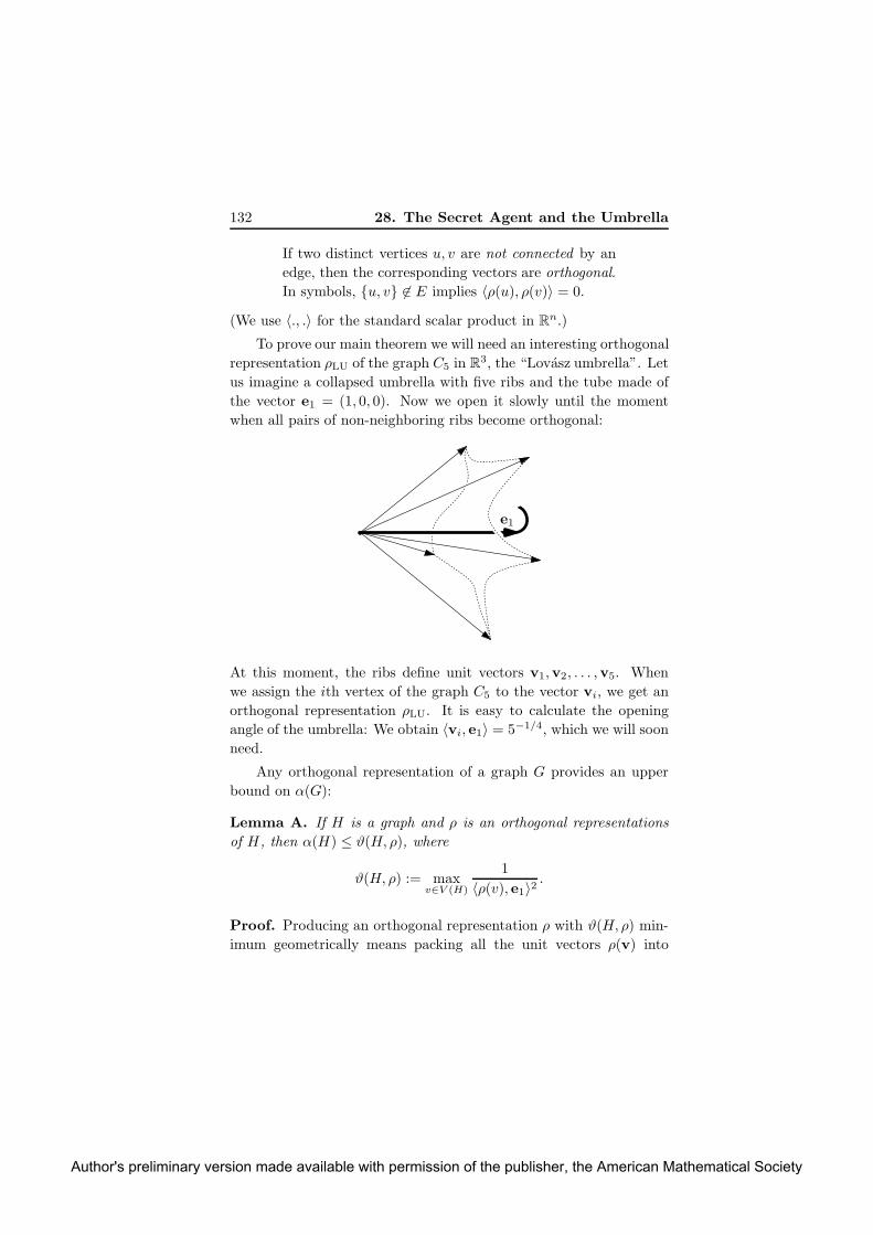
132 28. The Secret Agent and the Umbrella
If two distinct vertices u, v are not connected by an
edge, then the corresponding vectors are orthogonal.
In symbols, {u, v} 6∈ E implies 〈ρ(u), ρ(v)〉 = 0.
(We use 〈., .〉 for the standard scalar product in Rn.)
To prove our main theorem we will need an interesting orthogonal
representation ρLU of the graph C5 in R3, the “Lovasz umbrella”. Let
us imagine a collapsed umbrella with five ribs and the tube made of
the vector e1 = (1, 0, 0). Now we open it slowly until the moment
when all pairs of non-neighboring ribs become orthogonal:
e1
At this moment, the ribs define unit vectors v1,v2, . . . ,v5. When
we assign the ith vertex of the graph C5 to the vector vi, we get an
orthogonal representation ρLU. It is easy to calculate the opening
angle of the umbrella: We obtain 〈vi, e1〉 = 5−1/4, which we will soon
need.
Any orthogonal representation of a graph G provides an upper
bound on α(G):
Lemma A. If H is a graph and ρ is an orthogonal representations
of H, then α(H) ≤ ϑ(H, ρ), where
ϑ(H, ρ) := maxv∈V (H)
1
〈ρ(v), e1〉2.
Proof. Producing an orthogonal representation ρ with ϑ(H, ρ) min-
imum geometrically means packing all the unit vectors ρ(v) into
Author's preliminary version made available with permission of the publisher, the American Mathematical Society

28. The Secret Agent and the Umbrella 133
a spherical cap centered at e1 and having the minimum possible ra-
dius.
The vectors resist such a packing since pairs corresponding to
non-edges must be orthogonal. In particular, the vectors correspond-
ing to an independent set in H form an orthonormal system, and for
such a system the minimum cap radius can be calculated exactly.
For a formal proof we need to know that for an arbitrary orthonor-
mal system of vectors (v1,v2, . . . ,vm) in some Rn and an arbitrary
vector u, we havem∑
i=1
〈vi,u〉2 ≤ ‖u‖2.
Indeed, the given system (v1,v2, . . . ,vm) can be extended to an or-
thonormal basis (v1,v2, . . . ,vn) of Rn, by adding n−m other suitable
vectors (vm+1,vm+2, . . . ,vn). The ith coordinate of u with respect
to this basis is 〈vi,u〉, and we have ‖u‖2 =∑n
i=1〈vi,u〉2 by the
Pythagorean theorem. The required inequality is obtained by omit-
ting the last n−m terms on the right-hand side.
Now if I ⊆ V (H) is an independent set in H , then, as noted
above, (ρ(v) : v ∈ I) forms an orthonormal system, and so∑
v∈I
〈ρ(v), e1〉2 ≤ ‖e1‖2 = 1.
Hence there exists v∈I with 〈ρ(v), e1〉2≤ 1|I| , and thus ϑ(H, ρ) ≥|I|.
�
The lemma together with the Lovasz umbrella gives
α(C5) ≤ ϑ(C5, ρLU) =√
5,
but this is not an earth-shattering result yet, since everyone knows
that α(C5) = 2. We need to complement this with the following
lemma, showing that orthogonal representations behave well with re-
spect to the strong product.
Lemma B. Let H1, H2 be graphs, and let ρi be an orthogonal rep-
resentation of Hi, i = 1, 2. Then there is an orthogonal represen-
tation ρ of the strong product H1 · H2 such that ϑ(H1 · H2, ρ) =
ϑ(H1, ρ1) · ϑ(H2, ρ2).
Author's preliminary version made available with permission of the publisher, the American Mathematical Society
134 28. The Secret Agent and the Umbrella
Applying Lemma B inductively to the strong product of k copies
of C5, we obtain
α(Ck5 ) ≤ ϑ(C5, ρLU)k =
√5
k,
which proves that Θ(C5) ≤√
5 and thus yields the theorem.
Proof of Lemma B. We recall the operation of tensor product,
already used in Miniature 18. The tensor product of two vectors
x ∈ Rm and y ∈ Rn is a vector in Rmn, denoted by x ⊗ y, with
coordinates corresponding to all products xiyj for i = 1, 2, . . . ,m and
j = 1, 2, . . . , n. For example, for x = (x1, x2, x3) and y = (y1, y2), we
have
x⊗ y = (x1y1, x2y1, x3y1, x1y2, x2y2, x3y2) ∈ R6.
We need the following fact, whose routine proof is left to the
reader:
(22) 〈x ⊗ y,x′ ⊗ y′〉 = 〈x,x′〉 · 〈y,y′〉for arbitrary x,x′ ∈ Rm, y,y′ ∈ Rn.
Now we can define an orthogonal representation ρ of the strong
product H1 · H2. The vertices H1 · H2 are pairs (v1, v2), v1 ∈ H1,
v2 ∈ H2. We put
ρ((v1, v2)) := ρ1(v1) ⊗ ρ2(v2).
Using (22) we can easily verify that ρ is an orthogonal representation
of H1 ·H2, and the equality ϑ(H1 ·H2, ρ) = ϑ(H1, ρ1)·ϑ(H2, ρ2) follows
as well. This completes the proof of Lemma B. �
Remarks. The quantity
ϑ(G) = inf{ϑ(G, ρ) : ρ an orthogonal representation of G}is called the Lovasz theta function of the graph G. As we have
seen, it gives an upper bound for α(G), the independence number of
the graph. It is not hard to prove that it also provides a lower bound
on the chromatic number of the complement of the graph G, or
in other words, the minimum number of complete subgraphs needed
to cover G. Computing the independence number or the chromatic
number of a given graph is algorithmically hard (NP-complete), but
Author's preliminary version made available with permission of the publisher, the American Mathematical Society
28. The Secret Agent and the Umbrella 135
surprisingly, ϑ(G) can be computed in polynomial time (more pre-
cisely, approximated with arbitrary required precision). Because of
this and several other remarkable properties, the theta function is
very important.
The Shannon capacity of a graph is a much harder nut.No algo-
rithm at all, polynomial or not, is known for computing or approx-
imating it. And we need not go far for an unsolved case—Θ(C7) is
not known! If the agent had seven scarves, nobody can tell him the
best way of transmitting.
Source. L. Lovasz, On the Shannon capacity of a graph, IEEETrans. Inform. Th. IT-25 (1979), 1–7.
Author's preliminary version made available with permission of the publisher, the American Mathematical Society

Author's preliminary version made available with permission of the publisher, the American Mathematical Society
Miniature 29
Shannon Capacityof the Union:A Tale of Two Fields
Here we continue with the topic of Miniature 28: the Shannon capac-
ity of a graph. However, for convenience, we will repeat the relevant
definitions. Reading the beginning of Miniature 28 may still be useful
for understanding the motivation of the Shannon capacity.
So we first recall that if G is a graph, then α(G) denotes the
maximum possible size of an independent set in G, that is, of a set
I ⊆ V (G) such that no two vertices of I are connected by an edge
in G. The strong product H · H ′ of graphs H and H ′ has vertex
set V (H) × V (H ′), and two vertices in this vertex set, which we can
write as (u, u′) and (v, v′), are connected by an edge if u = v or
{u, v} ∈ E(H), and at the same time, u′ = v′ or {u′, v′} ∈ E(H ′).
The Shannon capacity of a graph G is denoted by Θ(G) and
defined by
Θ(G) := sup{
α(Gk)1/k : k = 1, 2, . . .}
,
where Gk stands for the strong product of k copies of G.
The Shannon capacity is quite important in coding theory and
graph theorists have been studying it with great interest for a long
137
Author's preliminary version made available with permission of the publisher, the American Mathematical Society

138 29. Shannon Capacity of the Union
time, but it remains one of the most mysterious graph parameters.
The aim of this section is to prove a surprising result concerning the
behavior of the Shannon capacity with respect to the operation of
disjoint union of graphs.
Informally, the disjoint union of graphs G and H , denoted by
G + H , is the graph obtained by putting G and H “side by side.”
A formal definition of the disjoint union is easy if the vertex sets
V (G) and V (H) are disjoint; then we can simply set V (G + H) :=
V (G) ∪ V (H) and E(G + H) := E(G) ∪ E(H). However, in general
G and H may happen to have some vertices in common, or their
vertex sets may even coincide. Then we first have to construct an
isomorphic copy H ′ of H such that V (G) ∩ V (H ′) = ∅, and then we
put
V (G+H) := V (G) ∪ V (H ′), E(G+H) := E(G) ∪ E(H ′).
(In this way the graph G+H is defined only up to isomorphism, but
this is just fine for our purposes.)
It is a nice and not entirely trivial exercise, which we don’t even
urge the reader to undertake, to prove that
(23) Θ(G+H) ≥ Θ(G) + Θ(H)
for every two graphs G and H .
In the coding-theoretic interpretation from Miniature 28, Θ(G)
is the number of distinguishable messages “per symbol” that can be
sent using (arbitrarily long) messages composed of symbols from the
alphabet V (G), and similarly for Θ(H). Then the inequality (23) tells
us that if no symbol from the alphabet V (G) can ever be confused
with a symbol from V (H), and if we are allowed to send messages
composed of symbols from V (G) and from V (H), then the number
of distinguishable messages per symbol is at least Θ(G) + Θ(H). The
reader will probably agree that this sounds quite plausible, if not
“intuitively obvious.”
However, it may seem equally plausible, or intuitively obvious,
that (23) should always hold with equality (and this was conjectured
by Shannon). But it has turned out to be false, and this is the result
we have announced above as “surprising.”
Author's preliminary version made available with permission of the publisher, the American Mathematical Society
29. Shannon Capacity of the Union 139
Theorem. There exist graphs G and H such that Θ(G+H) > Θ(G)+
Θ(H).
For the proof, we will introduce two tools: the first will be used
for bounding Θ(G + H) from below, and the second for bounding
Θ(G) and Θ(H) from above. The first tool is the following simple
lemma.
Lemma. Let G be a graph on m vertices, and let G denote the com-
plement of G, i.e., the graph on the vertex set V (G) in which two dis-
tinct vertices u, v are adjacent exactly if they are not adjacent in G.
Then
Θ(G+G) ≥√
2m.
Proof of the lemma. By the definition of the Shannon capacity, it
suffices to find an independent set of size 2m in the strong product
(G+G)2.
Let v1, v2, . . . , vm be the vertices of G and let v′1, v′2, . . . , v
′m be
the vertices of the isomorphic copy of G used in forming the dis-
joint union G + G. We set I := {(v1, v′1), (v2, v
′2), . . . , (vm, v
′m)} ∪
{(v′1, v1), (v′2, v2), . . . , (v′m, vm)}. Then I is independent in (G +G)2:
Indeed, (vi, v′i) is not adjacent to (v′j , vj) since vi and v′j are non-
adjacent in G + G, and (vi, v′i) and (vj , v
′j), i 6= j, are not adjacent
since either vi and vj are not adjacent in G or v′i and v′j are not
adjacent in (the isomorphic copy of) G. The lemma is proved. �
Functional representations. The second tool, which will be used
for bounding Θ(.) from above, is algebraic. Let K be a field (such
as R, Q, or F2), and let G = (V,E) be a graph. A functional
representation F of G over K consists of the following:
• A ground set X (an arbitrary set, not necessarily related to
G or K in any way),
• an element cv ∈ X for every vertex v ∈ V , and
• a function fv : X → K for every vertex v ∈ V .
These objects have to satisfy
(i) fv(cv) 6= 0 for every v ∈ V , and
Author's preliminary version made available with permission of the publisher, the American Mathematical Society

140 29. Shannon Capacity of the Union
(ii) if u, v are distinct and non-adjacent vertices of G, then
fu(cv) = 0. (If u and v are adjacent, then fu(cv) can be
anything.)
We write F = (X, (cv, fv)v∈V ).
The dimension dimF of a functional representation F is the
dimension of the subspace generated by all the functions fv, v ∈ V ,
in the vector space KX of all functions X → K. (As usual, the
functions are added pointwise, (f+g)(x) = f(x)+g(x), and similarly
for multiplication by elements of K.)
Proposition. If G has a functional representation of dimension d
over some field K, then Θ(G) ≤ d.
The proof of this proposition follows immediately from the defi-
nition of the Shannon capacity and the next two claims.
Claim A. If G has a functional representation F = (X, (cv, fv)v∈V )
over some field K, then α(G) ≤ dimF .
Claim B. Suppose that a graph G = (V,E) has a functional rep-
resentation F over some field K and G′ = (V ′, E′) has a func-
tional representation F ′ over the same K. Then the strong product
G · G′ has a functional representation over K of dimension at most
(dimF)(dimF ′).
Proof of Claim A. It suffices to show that whenever I ⊆ V (G) is
an independent set, the functions fv, v ∈ I, are linearly independent.
This is done in a fairly standard way. We suppose that
(24)∑
v∈I
tvfv = 0
for some scalars tv, v ∈ I (the 0 on the right-hand side is the function
assigning 0 to every x ∈ X). We fix u ∈ V and evaluate the left-hand
side of (24) at cu. Since no two distinct u, v ∈ I are connected by an
edge, we have fv(cu) = 0 for v 6= u, and we obtain∑
v∈I αvfv(cu) =
αufu(cu). Since fu(cu) 6= 0, we have tu = 0, and since u was arbitrary,
the fv are linearly independent as claimed. �
Proof of Claim B. We are going to define a functional represen-
tation G of G · G′ in a quite natural way (it can be regarded as
Author's preliminary version made available with permission of the publisher, the American Mathematical Society
29. Shannon Capacity of the Union 141
a “tensor product” of F and F ′). Let F = (X, (cv, fv)v∈V ) and
F ′ = (X ′, (c′v′ , f ′v′)v′∈V ′). The ground set of G is X×X ′. A vertex of
G · G′ has the form (v, v′) ∈ V × V ′, and we complete the definition
of G by setting
c(v,v′) = (cv, c′v′) ∈ X ×X ′ f(v,v′) := fv ⊗ f ′
v′ ,
where fv ⊗ f ′v′ stands for the function X ×X ′ → K defined by fv ⊗
f ′v′(x, x′) := fv(x)f ′
v′ (x′). It is straightforward to check that this Gindeed satisfies the axioms (i) and (ii) of a functional representation
(and we leave it to the reader).
It remains to verify dimG ≤ (dimF)(dimF ′), which is equally
straightforward: If all the fv are linear combinations of some basis
functions b1, . . . , bd, and the f ′v′ are linear combinations of b′1, . . . , b
′d′,
then it is almost obvious that each fv ⊗ f ′v′ is a linear combination of
functions of the form bi ⊗ b′j , i = 1, 2, . . . , d, j = 1, 2, . . . , d′. (It can
be checked that dimG actually equals (dimF)(dimF ′)). �
Proof of the theorem. It remains to exhibit suitable graphs G and
H and apply the tools above. Several constructions are known, and
some of them show that Θ(G+H) can actually be much larger than
Θ(G) + Θ(H). Here, for simplicity, we present only a single very
concrete construction, for which Θ(G+H) is only “somewhat larger”
than Θ(G) + Θ(H).
We let s be an integer parameter; later on we will calculate that
for proving the theorem it suffices to set s = 16. The vertices of G
are all 3-element subsets of the set {1, 2, . . . , s}, and two such vertices
A and B are connected by an edge of G if |A∩B| = 1. (Graphs of this
kind, where the vertices are sets and the edges are defined based on
the cardinality of the intersection, serve as very interesting examples
for many graph-theoretic questions.)
The graph H is the complement G of G.
First of all, G has(
s3
)
vertices, and so Θ(G+G) ≥√
2(
s3
)
by the
lemma.
Now we define suitable functional representations. For G, we use
the field F2, and we let the ground setX be Fs2, so that its elements are
s-component vectors of 0’s and 1’s. For a vertex (3-element set) A ∈
Author's preliminary version made available with permission of the publisher, the American Mathematical Society

142 29. Shannon Capacity of the Union
V (H), we let cA be the characteristic vector of A; that is, (cA)i = 1
for i ∈ A and (cA)i = 0 for i 6∈ A. Finally, the function fA : Fs2 → F2
is given by fA(x) =∑
i∈A xi (addition in F2, i.e., modulo 2).
To see that this is indeed a functional representation of G, we
observe that fA(cB) equals |A∩B| modulo 2. In particular, fA(cA) =
1 6= 0. Now if A 6= B are not adjacent in G, then |A ∩ B| can be 2
or 0, and so fA(cB) = 0 in this case.
The dimension of this functional representation is at most s, since
each fA is a linear combination of the coordinate functions x 7→ xi.
Therefore, Θ(G) ≤ s.
For G we use a very similar functional representation, but over
a different field, say R (or any other field of characteristic distinct
from 2). Namely, we let X ′ := Rs, c′A is again the characteristic
vector of A (interpreted as a real vector this time), and f ′A(x) :=
(∑
i∈A xi
)
− 1. Now f ′A(c′B) = |A ∩ B| − 1, and so f ′
A(c′A) = 2 6=0, while for A 6= B non-adjacent in G we have |A ∩ B| = 1 and
f ′A(c′B) = 0, as needed. The dimension is at most s+ 1 this time (in
addition to the coordinate functions x 7→ xi we also need the constant
function −1 in the basis), and so Θ(G) ≤ s+ 1.
The proof of the theorem is finished by choosing s sufficiently
large so that√
2(
s3
)
> 2s+1. A numerical calculation shows that the
smallest suitable s is 16. Then the graphs G and G have 560 vertices
each. �
Remark. It is interesting to compare the functional representations
treated here with the orthogonal representations discussed in Minia-
ture 28. These notions, and the proofs that they both yield upper
bounds for Θ(G), are basically similar. However, functional represen-
tations can yield only bounds that are integers, and thus they cannot
establish, e.g., that Θ(C5) ≤√
5. On the other hand, orthogonal
representations don’t appear suitable for the proof in the present sec-
tion, since the use of two different fields in it is essential, as we will
illustrate next.
Indeed, reasoning similar to that in the proof of the lemma shows
that α(G ·G) ≥ m for every m-vertex graph G. Thus, if F is a func-
tional representation of G and F ′ is a functional representation of G
Author's preliminary version made available with permission of the publisher, the American Mathematical Society

29. Shannon Capacity of the Union 143
over the same field, we have (dimF)(dimF ′) ≥ m by Claims A and B.
Consequently, dimF +dimF ′ ≥ 2√m (by the inequality between the
arithmetic and geometric means), and thus functional representations
over the same field can never give an upper bound for Θ(G) + Θ(G)
smaller than√
2m, which is what the lemma yields for Θ(G+ G).
Source. N. Alon, The Shannon capacity of a union, Combina-torica 18 (1998), 301–310.
Our presentation achieves a weaker result and is slightly simpler.
Author's preliminary version made available with permission of the publisher, the American Mathematical Society

Author's preliminary version made available with permission of the publisher, the American Mathematical Society

Miniature 30
Equilateral Sets
An equilateral set in Rd is a set of points p1,p2, . . . ,pn such that
all pairs pi,pj of distinct points have the same distance.
Intentionally we haven’t said what distance we mean: This will
play a key role in this section. If one considers the most usual Eu-
clidean distance, then it is not too hard to prove that an equilateral
set in Rd can have d+ 1 points but no more.
As an aside, let us sketch the classical proof that there can’t be
more than d + 1 points; it proceeds in a way very similar to Minia-
ture 6: Let the points be p1 through pn+1, translate them so that
pn+1 = 0, re-scale so that the interpoint distances are 1, and set up
the matrix (the Gram matrix) G with gij = 〈pi,pj〉 (scalar product).
Using the equilaterality condition one calculates that G = 12 (In +Jn),
where In is the identity matrix and Jn is the all 1’s matrix, and thus
rank(G) = n. On the other hand, we have G = PTP , where P is
the d × n matrix with the vector pi as the ith column, and thus
rank(G) ≤ d, which gives n ≤ d.
(And, by the way, how do we prove rigorously that a (d+1)-point
equilateral set is possible? We can take, e.g., the vectors e1, e2, . . . , ed
of the standard basis plus the point (−t,−t, . . . ,−t) for a suitable
t > 0—even if we are too lazy to calculate the right t, it is easy to
prove its existence.)
145
Author's preliminary version made available with permission of the publisher, the American Mathematical Society

146 30. Equilateral Sets
Approximately equilateral sets. We will now relax the condition
that all interpoint distances must be exactly the same: We will require
them to be only approximately the same. With a sufficiently strong
notion of “approximately the same” we will show that the size of
such an approximately equilateral set in Rd is bounded by a constant
multiple of d. The proof relies on a neat linear algebra trick. We will
then use the result in the proof of the main theorem of this section.
Rank Lemma. Let A be a real symmetric n×n matrix, not equal
to the zero matrix. Then
rank(A) ≥(∑n
i=1 aii
)2
∑ni,j=1 a
2ij
.
Proof. Linear algebra teaches us that A as in the lemma has n real
eigenvalues λ1, λ2, . . . , λn. If rank(A) = r, then exactly r of the λi
are nonzero; we may suppose that λi 6= 0 for 1 ≤ i ≤ r, while λi = 0
for i > r.
Let us write down the Cauchy–Schwarz inequality (∑r
i=1 xiyi)2 ≤
(∑r
i=1 x2i )(∑r
i=1 y2i ) for xi = λi, yi = 1; we obtain (
∑ri=1 λi)
2 ≤r∑r
i=1 λ2i . Dividing by
∑ri=1 λ
2i yields the following inequality for
the rank in terms of eigenvalues:
(25) rank(A) ≥(∑n
i=1 λi
)2
∑ni=1 λ
2i
.
(We have extended the summation all the way to n, since λr+1 through
λn are 0’s.)
The last inequality can be converted to the inequality in the Rank
Lemma in three easy steps: First, the sum of all eigenvalues of A
equals the trace of A, i.e.∑n
i=1 λi =∑n
i=1 aii (a standard linear
algebra fact). This takes care of the numerator in (25). Second, the
eigenvalues of A2 are λ21, . . . , λ
2n, as one can recall or immediately
check, and thus∑n
i=1 λ2i = trace(A2). Third, trace(A2) =
∑ni,j=1 a
2ij ,
as one easily calculates. This brings the denominator into the desired
form. �
Author's preliminary version made available with permission of the publisher, the American Mathematical Society
30. Equilateral Sets 147
Corollary (A small perturbation of In has a large rank). Let A be a
symmetric n×n matrix with aii = 1, i = 1, 2, . . . , n, and |aij | ≤ 1/√n
for all i 6= j. Then rank(A) ≥ n2 . �
Proposition (on approximately equilateral sets). Let p1,p2, . . . ,pn∈Rd be points such that for every i 6= j we have
1 − 1√n≤ ‖pi − pj‖2 ≤ 1 +
1√n.
Then n ≤ 2(d + 2). (Note that, for technical convenience, we bound
the squared Euclidean distances.)
Proof. Let A be the n×n matrix with aij = 1 − ‖pi − pj‖2. The
assumptions of the proposition immediately give that A meets the
assumptions of the above corollary, and thus rank(A) ≥ n2 .
It remains to bound rank(A) from above in terms of d. Here we
proceed as in Miniature 15. For i = 1, 2, . . . , n let fi : Rd → R be
the function defined by fi(x) = 1 − ‖x− pi‖2; so the ith row of A is(
fi(p1), fi(p2), . . . , fi(pn))
.
We rewrite fi(x) = 1−‖x‖2−‖pi‖2+2(pi1x1+pi2x2+· · ·+pidxd),
where pik is the kth coordinate of pi. Then it becomes clear that each
fi is a linear combination of the following d+2 functions: the constant
function 1, the function x 7→ ‖x‖2, and the “coordinate functions”
x 7→ xk, k = 1, 2, . . . , d. Hence the vector space generated by the fi
has dimension at most d+2, and so has the column space of A. Thus
rank(A) ≤ d+ 2, and the proposition is proved. �
Other kinds of distance. Equilateral sets become much more puz-
zling if one considers other notions of distance in Rd.
First, as a cautionary tale, let us consider the ℓ∞ (“el infinity”)
distance, where the distance of two points x,y ∈ Rd is defined as
‖x− y‖∞ = max{|xi − yi| : i = 1, 2, . . . , d}. Then the “cube” {0, 1}d
is an equilateral set with as many as 2d points! (Which turns out to
be the largest possible example in Rd with the ℓ∞ distance, but this
is not the story we want to narrate here.)
Author's preliminary version made available with permission of the publisher, the American Mathematical Society

148 30. Equilateral Sets
The distance we really want to focus on here is the ℓ1 distance,
given by
‖x− y‖1 = |x1 − y1| + |x2 − y2| + · · · + |xd − yd|.
Then the following is an example of an equilateral set with 2d points:
{e1,−e1, e2,−e2, . . . , ed,−ed}. A widely believed conjecture states
that this is as many as one can ever get, but until about 2001, no
upper bound better than 2d − 1 (exponential!) was known.
We will present an ingenious proof of a polynomial upper bound,
O(d4). The proof of the current best bound, O(d log d), uses a number
of additional ideas and it is considerably more technical.
Theorem. For every d ≥ 1, no equilateral set in Rd with the ℓ1distance has more than 100d4 points.
The main reason why for the ℓ1 distance one can’t imitate the
proof for the Euclidean case sketched above or something similar
seems to be this: The functions ϕa : R → R, ϕa(x) = |x− a|, a ∈ R,
are all linearly independent—unlike the functions ψa(x) = (x − a)2
that generate a vector space of dimension only 3.
The forthcoming proof has an interesting twist: In order to es-
tablish a bound on exactly equilateral sets for the “unpleasant” ℓ1distance, we use approximately equilateral sets but for the “pleasant”
Euclidean distance. Here is a tool for such a passage.
Lemma (on approximate embedding). For every two natural
numbers d, q there exists a mapping fd,q : [0, 1]d → Rdq such that for
every x,y ∈ [0, 1]d
‖x − y‖1 − 2dq ≤ 1
q ‖fd,q(x) − fd,q(y)‖2 ≤ ‖x− y‖1 + 2dq .
Let us stress that we take squared Euclidean distances in the
target space. If we wanted instead that the ℓ1 distance ‖x − y‖1 be
reasonably close to the Euclidean distance of the images for all x,y,
the task becomes impossible.
Our proof of the lemma is somewhat simple-minded. By more
sophisticated methods one can reduce the dimension of the target
Author's preliminary version made available with permission of the publisher, the American Mathematical Society
30. Equilateral Sets 149
space considerably, and this is also how the d4 bound in the theorem
can be improved.
Proof of the lemma. First we consider the case d = 1. For x ∈[0, 1], f1,q(x) is the q-component zero/one vector starting with a seg-
ment of ⌊qx⌋ ones, followed by q−⌊qx⌋ zeros. Then ‖f1,q(x)−f1,q(y)‖2
is the number of position where one of f1,q(x), f1,q(y) has 1 and the
other 0, and thus it equals∣
∣
∣⌊qx⌋ − ⌊qy⌋∣
∣
∣. This differs from q|x − y|by at most 2, and we are done with the d = 1 case.
For larger d, fd,1(x) is defined as the dq-component vector ob-
tained by concatenating f1,q(x1), f1,q(x2),. . . , f1,q(xd). The error
bound is obvious using the 1-dimensional case. �
Proof of the theorem. For contradiction, let us assume that there
exists an equilateral set in Rd with the ℓ1 distance that has at least
100d4 points. After possibly discarding some points we may assume
that it has exactly n := 100d4 points.
We re-scale the set so that the interpoint distances become 12 ,
and we translate it so that one of the points is (12 ,
12 , . . . ,
12 ). Then
the set is fully contained in [0, 1]d.
We use the lemma on approximate embedding with q := 40d3.
Applying the mapping fd,q to our set, we obtain an n-point set in
Rqd, for which the squared Euclidean distance of every two points
is between q2 − 2d and q
2 + 2d. After re-scaling by√
2/q, we get
an approximately equilateral set with squared Euclidean interpoint
distances between 1 − 4dq and 1 + 4d
q . We have 4dq = 1
10d2 = 1√n
,
and thus the proposition on approximately equilateral sets applies
and shows that n ≤ 2(dq + 2). But this is a contradiction, since
n = 100d4, while 2(dq + 2) = 2(40d4 + 2) < 100d4. The theorem is
proved. �
Source. N. Alon and P. Pudlak, Equilateral sets in lnp , Geo-metric and Functional Analysis 13 (2003), 467–482.
Our presentation via an approximate embedding is slightly different.
Author's preliminary version made available with permission of the publisher, the American Mathematical Society

Author's preliminary version made available with permission of the publisher, the American Mathematical Society

Miniature 31
Cutting Cheaply UsingEigenvectors
In many practical applications we are given a large graph G and we
want to cut off a piece of the vertex set by removing as few edges as
possible. For a large piece we can afford to remove more edges than
for a small one, as the next picture schematically indicates:
We can imagine that removing an edge costs one unit and we want
to cut off some vertices, at most half of all vertices, at the smallest
possible price per vertex.
This problem is closely related to the divide and conquer para-
digm in algorithms design. For example, in areas like computer graph-
ics, computer-aided design, or medical image processing we may have
a two-dimensional surface represented by a triangular mesh:
151
Author's preliminary version made available with permission of the publisher, the American Mathematical Society
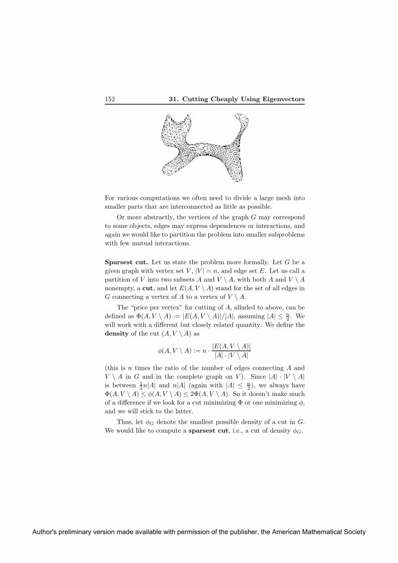
152 31. Cutting Cheaply Using Eigenvectors
For various computations we often need to divide a large mesh into
smaller parts that are interconnected as little as possible.
Or more abstractly, the vertices of the graph G may correspond
to some objects, edges may express dependences or interactions, and
again we would like to partition the problem into smaller subproblems
with few mutual interactions.
Sparsest cut. Let us state the problem more formally. Let G be a
given graph with vertex set V , |V | = n, and edge set E. Let us call a
partition of V into two subsets A and V \A, with both A and V \Anonempty, a cut, and let E(A, V \A) stand for the set of all edges in
G connecting a vertex of A to a vertex of V \A.
The “price per vertex” for cutting of A, alluded to above, can be
defined as Φ(A, V \ A) := |E(A, V \ A)|/|A|, assuming |A| ≤ n2 . We
will work with a different but closely related quantity: We define the
density of the cut (A, V \A) as
φ(A, V \A) := n · |E(A, V \A)||A| · |V \A|
(this is n times the ratio of the number of edges connecting A and
V \ A in G and in the complete graph on V ). Since |A| · |V \ A|is between 1
2n|A| and n|A| (again with |A| ≤ n2 ), we always have
Φ(A, V \A) ≤ φ(A, V \A) ≤ 2Φ(A, V \A). So it doesn’t make much
of a difference if we look for a cut minimizing Φ or one minimizing φ,
and we will stick to the latter.
Thus, let φG denote the smallest possible density of a cut in G.
We would like to compute a sparsest cut, i.e., a cut of density φG.
Author's preliminary version made available with permission of the publisher, the American Mathematical Society

31. Cutting Cheaply Using Eigenvectors 153
This problem is known to be computationally difficult (NP-com-
plete), and various approximation algorithms have been proposed for
it. One of such algorithms, or rather a class of algorithms, called
spectral partitioning, is based on eigenvectors of a certain matrix as-
sociated with the graph. It is widely and successfully used in practice,
and thanks to modern methods for computing eigenvalues, it is also
quite fast even for large graphs.
Before we proceed with formulating the algorithm, a remark is
in order. In some applications, a sparsest cut is not really what we
are interested in—we want a sparse cut that is also approximately
balanced, i.e., it cuts off at least 13 of all vertices (say). To this end,
we can use a sparsest cut algorithm iteratively: We cut off pieces,
possibly small ones, repeatedly until we have accumulated at least13 of all vertices. It can be shown that with a good sparsest cut
algorithm this strategy leads to a good approximately balanced cut.
We will not elaborate on the details, since this would distract us from
the main topic.
Now we can begin with preparations for the algorithm.
The Laplace matrix. For notational convenience let us assume that
the vertices of G are numbered 1, 2, . . . , n. We define the Laplace
matrix L of G (also used in Miniature 21) as the n×n matrix with
entries ℓij given by
ℓij :=
deg(i) if i = j,
−1 if {i, j} ∈ E(G),
0 otherwise,
where deg(i) is the number of neighbors (degree) of i in G.
We will need the following identity: For every x ∈ Rn,
(26) xTLx =∑
{i,j}∈E
(xi − xj)2.
Indeed, we have
xTLx =
n∑
i,j=1
ℓijxixj =
n∑
i=1
deg(i)x2i − 2
∑
{i,j}∈E
xixj ,
the right-hand side simplifies to∑
{i,j}∈E(xi−xj)2, and so (26) holds.
Author's preliminary version made available with permission of the publisher, the American Mathematical Society

154 31. Cutting Cheaply Using Eigenvectors
The right-hand side of (26) is always nonnegative, and thus L is
positive semidefinite. So it has n nonnegative real eigenvalues, which
we write nondecreasing order as µ1 ≤ µ2 ≤ · · · ≤ µn.
Since the row sums of L are all 0, we have L1 = 0 (where 1 is the
vector of all 1’s), and thus µ1 = 0 is an eigenvalue with eigenvector 1.
The key role in the forthcoming algorithm, as well as in many other
graph problems, is played by the second eigenvalue µ2 (sometimes
called the Fiedler value of G).
Spectral partitioning. The algorithm for finding a sparse cut works
as follows.
(1) Given a graph G, compute an eigenvector u belonging to
the second smallest eigenvalue µ2 of the Laplace matrix.
(2) Sort the components of u descendingly. Let π be a permu-
tation such that uπ(1) ≥ uπ(2) ≥ · · · ≥ uπ(n).
(3) Set Ak := {π(1), π(2), . . . , π(k)}. Among the cuts (Ak, V \Ak), k = 1, 2, . . . , n−1, output one with the smallest density.
Theorem. The following hold for every graph G:
(i) φG ≥ µ2.
(ii) The algorithm always finds a cut of density at most 4√dmaxµ2,
where dmax is the maximum vertex degree in G. In particular, φG ≤4√dmaxµ2.
Remarks. This theorem is a fundamental result, whose significance
goes far beyond the spectral partitioning algorithm. For instance, it
is a crucial ingredient in constructions of expander graphs.1
The constant 4 in (ii) can be improved by doing the proof more
carefully. There can be a large gap between the upper bound for φG in
(i) and the lower bound in (ii), but both of the bounds are essentially
tight in general. That is, for some graphs the lower bound is more or
less the truth, while for others the upper bound is attained.
For planar graphs of degree bounded by a constant, such as the
cat mesh depicted above, it is known that µ2 = O( 1n ) (a proof is
1Part (ii) is often called the Cheeger–Alon–Milman inequality, where Cheeger’sinequality is an analogous “continuous” result in the geometry of Riemannianmanifolds.
Author's preliminary version made available with permission of the publisher, the American Mathematical Society

31. Cutting Cheaply Using Eigenvectors 155
beyond the scope of this text), and thus the spectral partitioning
algorithm always finds a cut of density O(n−1/2). This density is
the smallest possible, up to a constant factor, for many planar graphs
(e.g., consider the n×n square grid). Thus, one can say that “spectral
partitioning works” for planar graphs of bounded degree. Similar
results are known for several other graph classes.
Proof of part (i) of the theorem. Let us say that a vector x ∈Rn is nonconstant if it is not a multiple of 1.
For a nonconstant x ∈ Rn let us put
Q(x) := n ·∑
{i,j}∈E(xi − xj)2∑
1≤i<j≤n(xi − xj)2.
First let (A, V \A) be a cut in G and let cA be the characteristic
vector of A (with the ith component 1 for i ∈ A and 0 otherwise).
Then Q(cA) is exactly the density of (A, V \ A), and so φG is the
minimum of Q(x) over all nonconstant vectors x ∈ {0, 1}n.
Next, we will show that µ2 is the minimum of Q(x) over a larger
set of vectors, namely,
(27) µ2 = min{Q(x) : x ∈ Rn nonconstant}
(computer scientists would say that µ2 is a relaxation of φG). This,
of course, implies φG ≥ µ2.
Since Q(x) = Q(x + t1) for all t ∈ R, we can change (27) to
µ2 = min{Q(x) : x ∈ Rn \ {0}, 〈x,1〉 = 0}.
Claim. For x orthogonal to 1, the denominator of Q(x) equals n‖x‖2.
Proof of the claim. The denominator of Q(x) is
the sum of (xi − xj)2 over all edges of the com-
plete graph on {1, 2, . . . , n}, whose Laplace matrix
is nIn−Jn. Then the identity (26) for the Laplace
matrix then tells us that∑
1≤i<j≤n(xi − xj)2 =
xT (nIn − Jn)x = n‖x‖2 since Jnx = 0 by the as-
sumption. �
Author's preliminary version made available with permission of the publisher, the American Mathematical Society

156 31. Cutting Cheaply Using Eigenvectors
Thus, we can further rewrite (27) to
(28) µ2 = min{
xTLx : ‖x‖ = 1, 〈1,x〉 = 0}
.
But this is a (special case of a) standard result in linear algebra,
the variational characterization of eigenvalues (or the Courant–Fisher
theorem). It is also easy to check: We write x in an orthonormal basis
of eigenvectors of L and expand xTLx; we leave this to the reader.
We just remark that the proof also shows that the minimum in (28) is
attained by an eigenvector of L belonging to µ2, which will be useful
in the sequel. This concludes the proof of part (i) of the theorem. �
One of the main steps in the proof of part (ii) is the next lemma.
Lemma. Let Ak = {1, 2, . . . , k}, and let α be a real number such that
each of the cuts (Ak, V \Ak), k = 1, 2, . . . , n, has density at least α.
Let z ∈ Rn be any vector with z1 ≥ z2 ≥ · · · ≥ zn. Then
(29)∑
{i,j}∈E,i<j
(zi − zj) ≥ α
n
∑
1≤i<j≤n
(zi − zj).
Proof. In the left-hand side of (29) we rewrite each zi − zj as (zi −zi+1) + (zi+1 − zi+2) + · · · + (zj−1 − zj). How many times does the
term zk+1−zk occur in the resulting sum? The answer is the number
of edges {i, j} ∈ E such that i ≤ k < j, i.e. |E(Ak, V \Ak)|. Thus
∑
{i,j}∈E,i<j
(zi − zj) =n−1∑
k=1
(zk − zk+1) · |E(Ak, V \Ak)|.
Exactly the same kind of calculation shows that∑
1≤i<j≤n(zi−zj) =∑n−1
k=1 (zk − zk+1)|Ak| · |V \ Ak|. The lemma follows by using the
density assumption |E(Ak, V \Ak)| ≥ αn |Ak| · |V \Ak| for all k. �
Proof of part (ii) of the theorem. To simplify notation, we as-
sume from now on that the vertices of G have been renumbered so
that u1 ≥ u2 ≥ · · · ≥ un, where u is the eigenvector in the algorithm
(then π(i) = i for all i).
Let α be the density of the cut returned by the algorithm; we
want to prove α ≤ 4√dmaxµ2. In the proof of part (i) we showed
Author's preliminary version made available with permission of the publisher, the American Mathematical Society

31. Cutting Cheaply Using Eigenvectors 157
µ2 = Q(u) =(∑
{i,j}∈E(ui − uj)2)
/‖u‖2, and so it suffices to prove
(30) α‖u‖ ≤ 4
(
dmax
∑
{i,j}∈E
(ui − uj)2)1/2
.
We will obtain this inequality from the lemma above with a suit-
able z, z1 ≥ z2 ≥ · · · ≥ zn. Choosing the right z is perhaps the
trickiest part of the proof; it may look like a magic but the calcula-
tions below will show why it makes sense.
First we set v := u − u⌈n/2⌉1. That is, we shift all coordinates
so that vi ≥ 0 for i ≤ n/2 and vi ≤ 0 for i > n/2. For later use, we
record that ‖v‖ ≥ ‖u‖ (because u is orthogonal to 1).
Let us now assume that∑
i:1≤i≤n/2 v2i ≥ ∑
i:n/2<i≤n v2i ; if it is
not the case, we start the whole proof with −u instead of u (which
obviously doesn’t influence the outcome of the algorithm).
Next, we define w by wi := max(vi, 0); thus, w consists of the
first half of v and then 0’s. By the assumption made in the preceding
paragraph we have ‖w‖2 ≥ 12‖v‖2 ≥ 1
2‖u‖2.
Now, finally, we define z by zi := w2i , and we substitute it into
the inequality of the lemma (and swap the sides for convenience):
(31)α
n
∑
1≤i<j≤n
(w2i − w2
j ) ≤∑
{i,j}∈E
(w2i − w2
j )
We will estimate both sides and finally arrive at (30).
First we deal with the right-hand side of (31). Factoring w2i −
w2j = (wi − wj)(wi + wj) and using the Cauchy–Schwarz inequality∑n
i=1 aibi ≤(∑n
i=1 a2i
)1/2(∑ni=1 b
2i
)1/2with ai = wi−wj , bi = wi+wj
yields
∑
{i,j}∈E
(w2i − w2
j ) ≤(
∑
{i,j}∈E
(wi − wj)2)
1
2
(
∑
{i,j}∈E
(wi + wj)2)
1
2
≤(
∑
{i,j}∈E
(vi − vj)2)
1
2
(
∑
{i,j}∈E
2(w2i + w2
j )
)1
2
≤(
∑
{i,j}∈E
(ui − uj)2)
1
2√
2dmax ‖w‖.
Author's preliminary version made available with permission of the publisher, the American Mathematical Society

158 31. Cutting Cheaply Using Eigenvectors
It remains to deal with the left-hand side of (31), which is quite
simple:
∑
1≤i<j≤n
(w2i − w2
j ) ≥∑
1≤i≤n/2
∑
n/2<j≤n
(w2i − w2
j )
=∑
1≤i≤n/2
∑
n/2<j≤n
w2i
≥ n
2‖w‖2 ≥ n
4‖u‖2.
Putting this together with (31) and the previous estimate for its right-
hand side, we arrive at (30) and finish the proof of part (ii) of the
theorem. �
Sources. The continuous analog of the theorem is due to
J. Cheeger, A lower bound for the smallest eigenvalue of
the Laplacian, in Problems in analysis (Papers dedicated toSalomon Bochner, 1969), Princeton Univ. Press, Princeton,NJ, 1970, 195–199.
The discrete version was proved in
N. Alon and V.D. Milman, λ1, isoperimetric inequalities for
graphs, and superconcentrators, J. Combin. Theory Ser. B38,1 (1985), 73–88.
and
N. Alon, Eigenvalues and expanders, Combinatorica 6,2
(1986), 83–96
and independently in
J. Dodziuk, Difference equations, isoperimetric inequality
and transience of certain random walks, Trans. Amer. Math.Soc. 284,2 (1984), 787–794.
A somewhat different version of the proof of part (ii) of the theoremcan be found, e.g., in the wonderful survey
S. Hoory, N. Linial, and A. Wigderson, Expander graphs
and their applications, Bull. Amer. Math. Soc. (N.S.) 43,4
(2006), 439–561.
It is shorter, but to me it looks even slightly more “magical” than theproof above. A still different and interesting approach, regarding the
Author's preliminary version made available with permission of the publisher, the American Mathematical Society

31. Cutting Cheaply Using Eigenvectors 159
proof as an analysis of a certain randomized algorithm, was providedin
L. Trevisan, Max cut and the smallest eigenvalue, preprint,http://arxiv.org/abs/0806.1978, 2008.
The result concerning the second eigenvalue of planar graphs is from
D.A. Spielman and S.-H. Teng, Spectral partitioning works:
planar graphs and finite element meshes, Linear AlgebraAppl. 421,2–3 (2007), 284–305.
A generalization and a new proof was given in
P. Biswal, J. R. Lee, and S. Rao, Eigenvalue bounds, spectral
partitioning, and metrical deformations via flows, in Proc.49th Annual IEEE Symposium on Foundations of ComputerScience, 2008, 751–760.
Approximation algorithms for the sparsest cut form an active researcharea.
Author's preliminary version made available with permission of the publisher, the American Mathematical Society

Author's preliminary version made available with permission of the publisher, the American Mathematical Society

Miniature 32
Rotating the Cube
First we state two beautiful geometric theorems. Since we need them
only for motivation, we will not discuss the proofs, which involve
methods of algebraic topology. Let Sn−1 = {x ∈ Rn : ‖x‖ = 1} stand
for the unit sphere in Rn, where ‖x‖ =√
x21 + x2
2 + · · · + x2n denotes
the Euclidean norm. Thus, for example, S2 is the usual 2-dimensional
unit sphere in the 3-dimensional space.
(T1) For every continuous function f : S2 → R there exist three
mutually orthogonal unit vectors p1,p2,p3 with f(p1) =
f(p2) = f(p3).
(T2) Let α ∈ (0, 2] and let f : Sn−1 → Rn−1 be an arbitrary
continuous mapping. Then there are two points p,q ∈ Sn
whose Euclidean distance is exactly α and such that f(p) =
f(q). In popular terms, at any given moment there are two
places on the Earth’s surface that are exactly 1234 km apart
and have the same temperature and the same barometric
pressure.
Theorem (T2) probably motivated Bronis law Knaster to pose the
following question in 1947:
Knaster’s question. Is it true that for every continuous mapping
f : Sn−1 → Rm, where n− 1 ≥ m ≥ 1, and every set K of n−m+ 1
161
Author's preliminary version made available with permission of the publisher, the American Mathematical Society

162 32. Rotating the Cube
points on Sn−1 there exists a rotation ρ of Rn around the origin such
that all points of the rotated set ρK have the same value of f?
It is easily seen that a positive answer to Knaster’s question for all
m,n would contain both (T1) and (T2) as special cases. In particular,
the second theorem deals exactly with the case m = n−1 of Knaster’s
question.
Somewhat disappointingly, though, the claim in Knaster’s ques-
tion does not hold for all n,m, as was discovered in the 1980s. Actu-
ally, it almost never holds: By now counterexamples are known for
every n and m such that n− 1 > m ≥ 2, and also for m = 1 and all
n sufficiently large.1
Here we discuss a counterexample for the last of these cases,
namely, m = 1 (with some suitable large n). It was found only in
2003, after almost all of the other cases had been settled.
Theorem. There exist an integer n, a continuous function f :Sn−1→R, and an n-point set K ⊂ Sn−1 such that for every rotation ρ of Rn
around 0, the function f attains at least two distinct values on ρK.
The function f in the proof is very simple, namely, f(x) =
‖x‖∞ := max{|x1|, |x2|, . . . , |xn|}. The sophistication is in construct-
ing K and proving the required property.
Some geometric intuition, not really necessary. The maximum
value of f on Sn−1 is obviously 1, attained at the points ±e1, . . . ,±en.
With a little more effort one finds that the minimum of f on Sn−1
equals n−1/2, attained at points of the form (±n−1/2,±n−1/2, . . .,
±n−1/2).
Let us now consider the function f(x) = ‖x‖∞ on all of Rn. Then
the set {x ∈ Rn : ‖x‖∞ = 1} is the surface of the unit cube [−1, 1]n,
and more generally, the level set {x ∈ Rn : ‖x‖∞ = t} is the surface
of the scaled cube [−t, t]n. Thus, if K is a point set on Sn−1, finding
a rotation ρ such that f is constant on ρK can be reformulated as
follows: Find a scaling factor t and a rotation of the scaled cube
1This doesn’t kill the question, though: It remains to understand for which setsK the claim does hold, and this question is very interesting and very far from solved.
Author's preliminary version made available with permission of the publisher, the American Mathematical Society

32. Rotating the Cube 163
[−t, t]n such that all points of K lie on the surface of the rotated and
scaled cube.
In the proof of the theorem, K is chosen as the disjoint union
of two sets K1 and K2. These are constructed in such a way that if
K1 should lie on the surface of a rotated and scaled cube, then the
scaling factor t has to be large (which means, geometrically, that the
points of K1 must be placed far from the corners of the cube), while
for K2 the scaling factor has to be small (the points of K2 must be
close to the corners). Hence it is impossible for both K1 and K2 to
lie on the surface of the same scaled and rotated cube.
Preliminaries. In the theorem we deal with a point set K in the
(n−1)-dimensional unit sphere and with rotated copies ρK. In the
proof it will be more convenient to work with a set K living in the
unit sphere Sd−1 of a suitable lower dimension. Then, instead of
rotations, we consider isometries ϕ : Rd → Rn, that is, linear maps
such that ‖ϕ(x)‖ = ‖x‖ for all x ∈ Rd. If ϕ0 is one such isometry,
then K := ϕ0(K) is a point set in Sn−1, and the sets ϕ(K) for all
other isometries ϕ : Rd → Rn are exactly all rotated copies of K (and
their mirror reflections—but for the purposes of the proof we can
ignore the mirror reflections).
Author's preliminary version made available with permission of the publisher, the American Mathematical Society

164 32. Rotating the Cube
We need one more definition. Let X ⊆ Rn be a set and let δ > 0
be a real number. A set N ⊆ X is called δ-dense in X if for every
x ∈ X there exists y ∈ N such that ‖x− y‖ ≤ δ.
Lemma K1. (i) Let ϕ : Rd → Rn be an isometry. Then there
exists x ∈ Sd−1 such that ‖ϕ(x)‖∞ ≥√
d/n.
(ii) Let, moreover, K1 ⊂ Sd−1 be a 12 -dense set in Sd−1. Then
there exists p ∈ K1 with ‖ϕ(p)‖∞ ≥ 12
√
d/n.
Proof. We begin with part (i). Let A be the matrix of the isometry
ϕ with respect to the standard bases; i.e., the ith column of A is the
vector ϕ(ei) ∈ Rn, i = 1, 2, . . . , d. Since ϕ preserves the Euclidean
norm, the columns of A are unit vectors in Rn, and thus
(32)
n∑
i=1
d∑
j=1
a2ij = d.
Let ai ∈ Rd denote the ith row of A. For x ∈ Rd, the ith
coordinate of ϕ(x) is the scalar product 〈ai,x〉, and thus ‖ϕ(x)‖∞ =
max{|〈ai,x〉| : i = 1, 2, . . . , n}.
Now (32) tells us that∑n
i=1 ‖ai‖2 = d, and thus there is an i0with ‖ai0‖ ≥
√
d/n. Setting x := ai0/‖ai0‖, we have ‖ϕ(x)‖∞ ≥〈ai0 ,x〉 = ‖ai0‖ ≥
√
d/n, which finishes the proof of part (i).
We proceed with part (ii), which is the result that we will actually
use later on. The proof is somewhat more clever than one might
perhaps expect at first sight.
In the setting of (ii), we let M := sup{‖ϕ(x)‖∞ : x ∈ Sd−1}, and
let x0 ∈ Sd−1 be a point where M is attained.2 By part (i) we have
M ≥√
d/n.
Since K1 is 12 -dense, we can choose a point p ∈ K1 with ‖x0 −
p‖ ≤ 12 . If, by chance, p = x0, we are done, and so we may assume
p 6= x0 and let v := (x0 − p)/‖x0 − p‖ ∈ Sd−1 be the unit vector
in direction x0 − p. Then ‖ϕ(v)‖∞ ≤ M by the choice of M , and
thus ‖ϕ(x0 − p)‖∞ ≤ 12M . Then, using the triangle inequality for
2The supremum is attained because Sd−1 is compact. Readers not familiarenough with compactness may as well consider x0 such that ‖ϕ(x0)‖∞ ≥ 0.99M ,say, which clearly exists. Then the constants in the proof need a minor adjustment.
Author's preliminary version made available with permission of the publisher, the American Mathematical Society

32. Rotating the Cube 165
the ‖.‖∞ norm, we have
‖ϕ(p)‖∞ ≥ ‖ϕ(x0)‖∞ −‖ϕ(x0 −p)‖∞ ≥M − 12M = 1
2M ≥ 12
√
n/d.
This proves part (ii). �
Lemma K2. Let K2 be a set of m distinct points of the unit circle
S1 ⊂ R2. If t is a number such that there exists an isometry ϕ : R2 →Rn with ‖ϕ(p)‖∞ = t for all p ∈ K2, then t ≤
√
8/m.
Proof. We begin in the same way as in the proof of Lemma K1, this
time setting d = 2: A is the matrix of ϕ and ai ∈ R2 is its ith row. By
(32) we have∑n
i=1 ‖ai‖2 = 2. We are going to bound the left-hand
side from below in terms of m and t.
Since the ith coordinate of ϕ(p) equals 〈ai,p〉, the condition
‖ϕ(p)‖∞ = t for all p ∈ K2 can be reformulated as follows:
(C1) For every p ∈ K2 there exists an i = i(p) with |〈ai,p〉| = t.
(C2) For all p ∈ K2 and all i we have |〈ai,p〉| ≤ t.
From (C1) we can infer that
(33) if i = i(p) for some p ∈ K2, then ‖ai‖ ≥ t.
Indeed, p is a unit vector, so |〈y,p〉| ≤ ‖y‖ for all y, and thus
|〈ai,p〉| = t implies ‖ai‖ ≥ t.
It remains to show that there are many distinct i with i = i(p)
for some p ∈ K2. To this end, we observe that any given i can serve
as i(p) for at most 4 distinct points p. This can be seen from the
following geometric picture:
〈ai,x〉 = t
x1
x2
〈ai,x〉 = −t
p
Author's preliminary version made available with permission of the publisher, the American Mathematical Society

166 32. Rotating the Cube
The condition i = i(p) means that the point p lies on one of the
lines {x ∈ R2 : 〈ai,x〉 = t} and {x ∈ R2 : 〈ai,x〉 = −t}, and (C2)
implies that all points of K2 lie within the parallel strip between these
two lines. In this situation, the boundary of such a parallel strip can
contain at most 4 points of K2 (actually, at most 2 points provided
that K2 is chosen in a suitably general position).
Consequently, there are at least m/4 distinct vectors of Euclidean
norm at least t among the ai, and so∑n
i=1 ‖ai‖2 ≥ t2m/4. Since we
already know that the left-hand side equals 2, we arrive at the claim
of Lemma K2. �
Two ways of making δ-dense sets. The last missing ingredient
for the proof of the theorem is a way of making a 12 -dense set K1 in
Sd−1, as in Lemma K1(ii), that is not too large. More precisely, it
will be enough to know that for every d ≥ 1 such a K1 exists of size
at most g(d), for an arbitrary function g.
This is a well-known geometric result. One somewhat sloppy but
quick way of proving it starts by observing that the integer grid Zd
is√d-dense in Rd (actually 1
2
√d-dense). If we re-scale it by 1/(4
√d)
and intersect it with the cube [−1, 1]d, we have a 14 -dense set N0 in
that cube, of size at most (8√d+ 1)d. Finally, for every point x ∈ N0
that has distance at most 14 to Sd−1, we choose a point y ∈ Sd−1 at
most 14 apart from x, and we let N ⊂ Sd−1 consist of all these y. It
is easily checked that N is 12 -dense in Sd−1. This yields g(d) of order
dO(d).
Another proof, the standard “textbook” one, uses a greedy algo-
rithm and a volume argument. We place the first point p1 to Sd−1
arbitrarily, and having already chosen p1, . . . ,pi−1, we place pi to
Sd−1 so that it has distance at least 12 from p1, . . . ,pi−1. This pro-
cess finishes as soon as we can no longer place the next point, i.e.,
the resulting set is 12 -dense. To estimate the number m of points pro-
duced in this way, we observe that the balls of radius 14 around the pi
are all disjoint and contained in the ball of radius 54 around 0. Thus,
the total volume of the small balls is at most the volume of the large
ball, and this gives m ≤ 5d, a better estimate than for the grid-based
argument.
Author's preliminary version made available with permission of the publisher, the American Mathematical Society

32. Rotating the Cube 167
Proof of the theorem. We choose an even n ≥ 2g(100), we let K1
be a 12 -dense set in S99 of size at most n
2 , and K2 is a set of n2 points
in S1. We let K := K1 ∪ K2, where K1,K2 ⊂ Sn−1 are isometric
images of K1 and K2, respectively.
Lemma K1(ii) shows that for every rotation ρ there is a point
p ∈ ρK1 with ‖p‖∞ ≥ 12
√
100/n > 4n−1/2. On the other hand,
if ρ is a rotation such that ‖p‖∞ equals the same number t for all
p ∈ ρK2, then t ≤√
16/n = 4n−1/2 by Lemma K2. This proves that
K = K1∪K2 cannot be rotated so that all of its points have the same
‖.‖∞ norm. �
Source. B. S. Kashin and S. J. Szarek, The Knaster problem
and the geometry of high-dimensional cubes, C. R. Acad.Sci. Paris, Ser. I 336 (2003), 931–936.
Author's preliminary version made available with permission of the publisher, the American Mathematical Society

Author's preliminary version made available with permission of the publisher, the American Mathematical Society

Miniature 33
Set Pairs and ExteriorProducts
We prove yet another theorem about intersection properties of sets.
Theorem. Let A1, A2, . . . , An be k-element sets, let B1, B2, . . . , Bn
be ℓ-element sets, and let
(i) Ai ∩Bi = ∅ for all i = 1, 2, . . . , n, while
(ii) Ai ∩Bj 6= ∅ for all i, j with 1 ≤ i < j ≤ n.
Then n ≤(
k+ℓk
)
.
It is easy to understand where(
k+ℓk
)
comes from: Let X :=
{1, 2, . . . , k + ℓ}, let A1, A2, . . . , An be a list of all k-element sub-
sets of X , and let us set Bi := X \ Ai for every i. Then the Ai and
Bi meet the conditions of the theorem and n =(
k+ℓk
)
.
The perhaps surprising thing is that we can’t produce more sets
satisfying (i) and (ii) even if we use a much larger ground set (note
that the theorem doesn’t put any restrictions on the number of el-
ements in the union of the Ai and Bi; it only limits their size and
intersection pattern).
The above theorem and similar ones have been used in the proofs
of numerous interesting results in graph and hypergraph theory, com-
binatorial geometry, and theoretical computer science; one even speaks
169
Author's preliminary version made available with permission of the publisher, the American Mathematical Society

170 33. Set Pairs and Exterior Products
of the set-pair method. We won’t discuss these applications here,
though. The theorem is included mainly because of the proof method,
where we briefly meet a remarkable mathematical object, the exterior
algebra of a vector space.
The theorem is known in the literature as the skew Bollobas
theorem. Bollobas originally proved a weaker (non-skew) version,
where condition (ii) is strengthened to
(ii′) Ai ∩Bj 6= ∅ for all i, j = 1, 2, . . . , n, i 6= j.
That version has a short probabilistic (or, if you prefer, double-
counting) proof. However, for the skew version only linear-algebraic
proofs are known. One of them uses the polynomial method (which
we encountered in various forms in Miniatures 15, 16, 17), and an-
other one, shown next, is a simple instance of a different and powerful
method.
We begin with a simple claim asserting the existence of arbitrarily
many vectors “in general position”.
Claim. For every d ≥1 and every m ≥1 there exist vectors v1,v2, . . . ,
vm ∈ Rd such that every d or fewer among them are linearly inde-
pendent.
Proof. We fix m distinct and nonzero real numbers t1, t2, . . . , tm ar-
bitrarily and set vi := (ti, t2i , . . . , t
di ) (these are points on the so-called
moment curve in Rd).
Since this construction is symmetric, it suffices to check linear
independence of v1,v2, . . . ,vd (we assume m ≥ d, for otherwise, the
result is trivial). So let∑d
j=1 αjvj = 0. This means∑d
j=1 αjtji = 0
for all i, i.e., t1, . . . , td are roots of the polynomial p(x) := αdxd +
αd−1xd−1 + · · ·+α1x. But 0 is another root, so we have d+1 distinct
roots altogether, and since p(x) has degree at most d, it cannot have
d + 1 distinct roots unless it is the zero polynomial. So α1 = α2 =
· · · = αd = 0.
Alternatively, one can prove the linear independence of the vi us-
ing the Vandermonde determinant (usually computed in introductory
courses of linear algebra).
Author's preliminary version made available with permission of the publisher, the American Mathematical Society
33. Set Pairs and Exterior Products 171
Yet another proof follows easily by induction if one believes that
Rd is not the union of finitely many (d − 1)-dimensional linear sub-
spaces. (But proving this rigorously is probably as complicated as
the proof above.) �
On permutations and signs. We recall that the sign of a per-
mutation π : {1, 2, . . . , d} → {1, 2, . . . , d} can be defined as sgn(π) =
(−1)inv(π), where inv(π) = |{(i, j) : 1 ≤ i < j ≤ d and π(i) > π(j)}|is the number of inversions of π.
Let d be a fixed integer and let s = (s1, s2, . . . , sk) be a sequence
of integers from {1, 2, . . . , d}. We analogously define the sign of s as
sgn(s) :=
{
(−1)inv(s) if all terms in s are distinct,
0 otherwise,
where inv(s) = |{(i, j) : 1 ≤ i < j ≤ k and si > sj}|.If we regard a permutation π as the sequence (π(1), . . . , π(d)),
then both definitions of the sign agree, of course.
The exterior algebra of a finite-dimensional vector space. In
1844 Hermann Grassmann, a high-school teacher in Stettin (a city
in Prussia at that time, then in Germany, and nowadays in Poland
spelled Szczecin), published a book proposing a new algebraic foun-
dation for geometry. He developed foundations of linear algebra more
or less as we know it today, and went on to introduce “exterior prod-
uct” of vectors, providing a unified and coordinate-free treatment of
lengths, areas, and volumes. His revolutionary mathematical discov-
eries were not appreciated during his lifetime (he became famous as a
linguist), but later on, they were completed and partially re-developed
by others. They belong among the fundamental concepts of modern
mathematics, with many applications e.g. in differential geometry,
algebraic geometry, and physics.
Here we will build the exterior algebra (also called the Grass-
mann algebra) of a finite-dimensional space in a minimalistic way
(which is not the most conceptual one), checking only the properties
we need for the proof of the above theorem.
Author's preliminary version made available with permission of the publisher, the American Mathematical Society
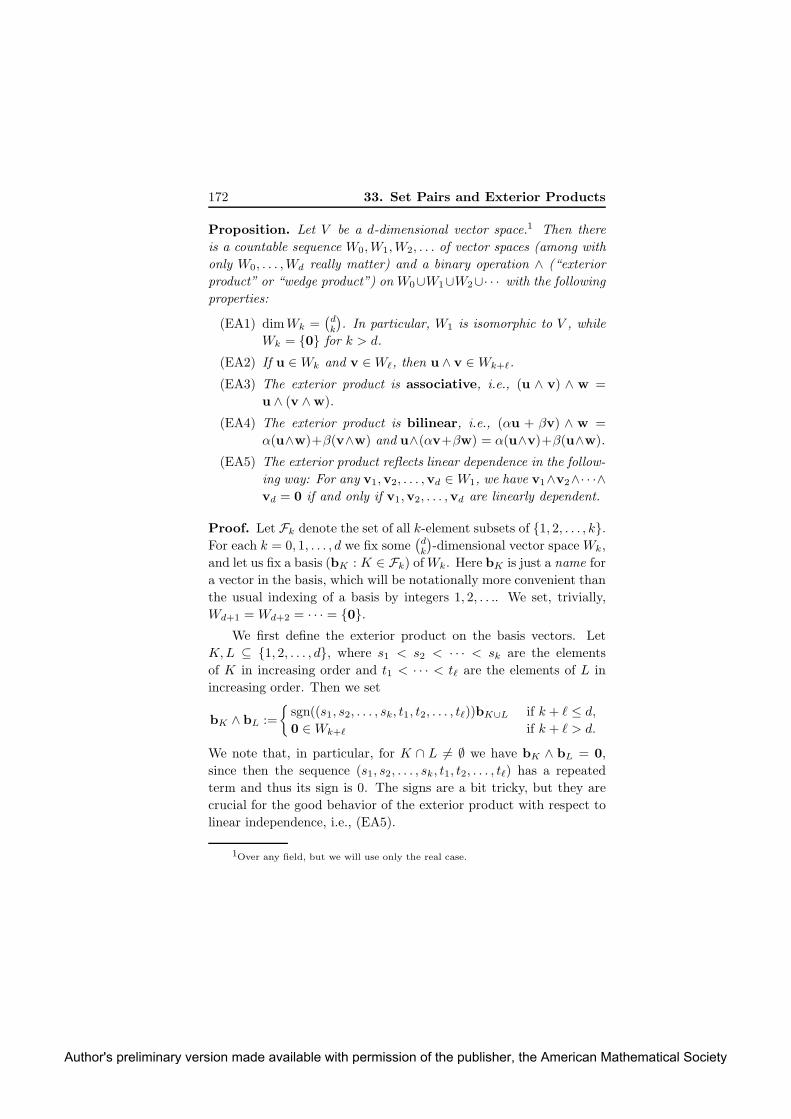
172 33. Set Pairs and Exterior Products
Proposition. Let V be a d-dimensional vector space.1 Then there
is a countable sequence W0,W1,W2, . . . of vector spaces (among with
only W0, . . . ,Wd really matter) and a binary operation ∧ (“exterior
product” or “wedge product”) on W0∪W1∪W2∪· · · with the following
properties:
(EA1) dimWk =(
dk
)
. In particular, W1 is isomorphic to V , while
Wk = {0} for k > d.
(EA2) If u ∈ Wk and v ∈Wℓ, then u ∧ v ∈ Wk+ℓ.
(EA3) The exterior product is associative, i.e., (u ∧ v) ∧ w =
u ∧ (v ∧ w).
(EA4) The exterior product is bilinear, i.e., (αu + βv) ∧ w =
α(u∧w)+β(v∧w) and u∧(αv+βw) = α(u∧v)+β(u∧w).
(EA5) The exterior product reflects linear dependence in the follow-
ing way: For any v1,v2, . . . ,vd ∈ W1, we have v1∧v2∧· · ·∧vd = 0 if and only if v1,v2, . . . ,vd are linearly dependent.
Proof. Let Fk denote the set of all k-element subsets of {1, 2, . . . , k}.
For each k = 0, 1, . . . , d we fix some(
dk
)
-dimensional vector space Wk,
and let us fix a basis (bK : K ∈ Fk) of Wk. Here bK is just a name for
a vector in the basis, which will be notationally more convenient than
the usual indexing of a basis by integers 1, 2, . . .. We set, trivially,
Wd+1 = Wd+2 = · · · = {0}.
We first define the exterior product on the basis vectors. Let
K,L ⊆ {1, 2, . . . , d}, where s1 < s2 < · · · < sk are the elements
of K in increasing order and t1 < · · · < tℓ are the elements of L in
increasing order. Then we set
bK ∧ bL :=
{
sgn((s1, s2, . . . , sk, t1, t2, . . . , tℓ))bK∪L if k + ℓ ≤ d,
0 ∈Wk+ℓ if k + ℓ > d.
We note that, in particular, for K ∩ L 6= ∅ we have bK ∧ bL = 0,
since then the sequence (s1, s2, . . . , sk, t1, t2, . . . , tℓ) has a repeated
term and thus its sign is 0. The signs are a bit tricky, but they are
crucial for the good behavior of the exterior product with respect to
linear independence, i.e., (EA5).
1Over any field, but we will use only the real case.
Author's preliminary version made available with permission of the publisher, the American Mathematical Society

33. Set Pairs and Exterior Products 173
We extend ∧ to all vectors bilinearly: If u ∈ Wk and v ∈ Wℓ,
we write them in the appropriate bases as u =∑
K∈FkαKbK , v =
∑
L∈FℓβLbL, and we put
u ∧ w :=∑
K∈Fk,L∈Fℓ
αKβL(bK ∧ bL).
Now (EA1), (EA2), and (EA4) (bilinearity) are clear.
As for the associativity (EA3), it suffices to check it for basis
vectors, i.e., to verify
(34) (bK ∧ bL) ∧ bM = bK ∧ (bL ∧ bM )
for all K,L,M . The interesting case is when K,L,M are pairwise
disjoint and |K| + |L| + |M | ≤ d. Then, obviously, both sides of (34)
are ±bK∪L∪M , and it suffices to check that the signs match.
To this end, we let s1 < · · · < sk be the elements of K in
increasing order, and similarly for t1 < · · · < tℓ and L and for
z1 < · · · < zm and M . By counting the inversions of the appro-
priate sequences, we find that (bK ∧ bL) ∧ bM = (−1)NbK∪L∪M ,
where N = inv((s1, . . . , sk, t1, . . . , tℓ))+inv((s1, . . . , sk, z1, . . . , zm))+
inv((t1, . . . , tℓ, z1, . . . , zm)), and the right-hand side of (34) comes out
the same.
Next, if K,L,M are not pairwise disjoint or k + ℓ + m > d, it
is easily checked that both sides of (34) are 0 ∈ Wk+ℓ+m. Finally,
having checked (34), it is routine to verify associativity in general—
one just writes out the three participating vectors in the respective
bases, expands both sides using bilinearity, and uses (34).
It remains to prove (EA5), which is the most interesting part
where, finally, the choice of the sign turns from a hassle into a blessing.
Let v1, . . . ,vd ∈ W1 be arbitrary, and let us write them in the
basis b{1}, . . . ,b{d} of W1 as
vi =
d∑
j=1
aijb{j}.
Then, using bilinearity and associativity, we have
v1 ∧ v2 ∧ · · · ∧ vd =
n∑
j1,j2,...,jd=1
a1j1a2j2 · · · adjdbj1 ∧ bj2 ∧ · · · ∧ bjd
.
Author's preliminary version made available with permission of the publisher, the American Mathematical Society

174 33. Set Pairs and Exterior Products
By the definition of the exterior product of basis vectors, all terms on
the right-hand side where some two ji coincide are 0. What remains
is a sum over all d-tuples of distinct ji’s, in other words, over all
permutations of {1, 2, . . . , d}:
v1 ∧ · · · ∧ vd =∑
π
a1π(1)a2π(2) · · · adπ(d)bπ(1) ∧ bπ(2) ∧ · · · ∧ bπ(d).
By considerations very similar to those in checking the associativity,
we find that bπ(1) ∧ bπ(2) ∧ · · · ∧ bπ(d) = sgn(π)b{1,2,...,d}. Then the
last sum transforms into det(A)b{1,2,...,d}, which is 0 exactly if the vi
are linearly dependent. The proposition is proved. �
With just a little more effort, (EA5) can be extended to any
number of vectors; i.e., v1, . . .vn ∈W1 are linearly dependent exactly
if their exterior product is 0 (we won’t need this but not mentioning
it seems inappropriate).
Proof of the theorem. Let d := k + ℓ and let us consider the ex-
terior algebra of Rd as in the proposition, with the vector spaces
W0,W1, . . . and the operation ∧. Let us assume, without loss of gen-
erality, that A1 ∪ · · · ∪ An ∪ B1 ∪ · · · ∪ Bn = {1, 2, . . . ,m} for some
integer m, and let us fix m vectors v1, . . .vm ∈ W1∼= Rd in gen-
eral position according to the claim above (every d or fewer linearly
independent). Note that m may be considerably larger than d.
Let A ⊆ {1, 2, . . . ,m} be an arbitrary subset, and let us write its
elements in increasing order as i1 < i2 < · · · < ir, where r = |A|.Then we define
wA := vi1 ∧ vi2 ∧ · · · ∧ vir.
Thus, wA ∈ Wr.
For A,B ⊆ {1, 2, . . . ,m} with |A| + |B| = d, (EA3) and (EA5)
yield
wA ∧ wB =
{±wA∪B 6= 0 for A ∩B = ∅,0 for A ∩B 6= ∅.
We claim that the n vectors wA1,wA2
, . . . ,wAn∈Wk are linearly
independent. This will prove the theorem, since dim(Wk) =(
dk
)
=(
k+ℓk
)
.
Author's preliminary version made available with permission of the publisher, the American Mathematical Society

33. Set Pairs and Exterior Products 175
So let∑n
i=1 αiwAi= 0. Assuming that, for some j, we already
know that αi = 0 for all i > j (for j = n this is a void assumption),
we show that αj = 0 as well. To this end, we consider the exterior
product
0 ∧ wBj= 0 =
( n∑
i=1
αiwAi
)
∧ wBj
=
n∑
i=1
αi(wAi∧ wBj
) = αj(wAj∧ wBj
),
since wAi∧ wBj
= 0 for i < j (using Ai ∩ Bj 6= ∅), αi = 0 for i > j
by the inductive assumption, and wAi∧ wBi
6= 0 since Ai ∩Bi = ∅.
Thus, αj = 0, and the theorem is proved. �
The geometry of the exterior product at a glance. Some low-
dimensional instances of the exterior product correspond to familiar
concepts. First let d = 2 and let us identify W1 with Rd so that
(b{1},b{2}) corresponds to the standard orthonormal basis (e1, e2).
Then it can be shown that u ∧ v = ±a · e1 ∧ e2, where a is the area
of the parallelogram spanned by u and v.
u
v
In R3, again making a similar identification of W1 with R3, it
turns out that u ∧ v is closely related to the cross product of u and
v (often used in physics), and u ∧ v ∧ w = ±a · e1 ∧ e2 ∧ e3, where
a is the volume of the parallelepiped spanned by u,v, and w. The
latter, of course, is an instance of a general rule; in Rd, the volume of
the parallelepiped spanned by v1, . . . ,vd ∈ Rd is | det(A)|, where A
is the matrix with the vi as columns, and we’ve already verified that
v1 ∧ · · · ∧ vd = det(A) · e1 ∧ · · · ∧ ed.
These are only the first indications that the exterior algebra has
a very rich geometric meaning. Generally, one can think of v1 ∧ · · · ∧vk ∈ Wk as representing, uniquely up to a scalar multiple, the k-
dimensional subspace of Rd spanned by v1, . . . ,vk. However, by far
not all vectors in Wk correspond to k-dimensional subspaces in this
Author's preliminary version made available with permission of the publisher, the American Mathematical Society
176 33. Set Pairs and Exterior Products
way; Wk can be thought of as a “closure” that completes the set of
all k-dimensional subspaces into a vector space.
Sources. Bollobas’ theorem was proved in
B. Bollobas, On generalized graphs, Acta Math. Acad. Sci.Hung. 16 (1965), 447–452.
The first use of exterior algebra in combinatorics is due to Lovasz:
L. Lovasz, Flats in matroids and geometric graphs, in Com-binatorial surveys (Proc. Sixth British Combinatorial Conf.,Royal Holloway Coll., Egham, 1977), Academic Press, Lon-don, 1977, 45–86.
This paper contains a version of the Bollobas theorem for vector sub-spaces, and the proof implies the skew Bollobas theorem easily, butexplicitly that theorem seems to appear first in
P. Frankl, An extremal problem for two families of sets, Eu-ropean J. Combin. 3,2 (1982), 125–127,
where it is proved via symmetric tensor products (while the exteriorproduct can be interpreted as an antisymmetric tensor product). Themethod with exterior products was also discovered independently byKalai and used with great success in the study of convex polytopesand geometrically defined simplicial complexes:
G. Kalai, Intersection patterns of convex sets, Israel J. Math.48 (1984), 161–174.
Applications of the set-pair method are surveyed in two papers of Tuza,among which the second one
Zs. Tuza, Applications of the set-pair method in extremal
problems, II, in Combinatorics, Paul Erdos is eighty, Vol. 2,J. Bolyai Math. Soc., Budapest, 1996, 459–490
has a somewhat wider scope.
Author's preliminary version made available with permission of the publisher, the American Mathematical Society
Index
≡ (congruence), 18
‖ · ‖ (Euclidean norm), 1
‖ · ‖1 (ℓ1 norm), 148
‖ · ‖∞ (ℓ∞ norm), 162
〈·, ·〉 (standard scalar product), 1
AT (transposed matrix), 1
u ∧ v (exterior product), 172
G (graph complement), 139
G · H (strong product), 131
α(G) (independece number), 131
ϑ(G) (Lovasz theta function), 134
Θ(G) (Shannon capacity), 131
adjacency matrix, 32, 42, 46
bipartite, 84, 100
algebra
exterior, 171
Grassmann, 171
algorithm
probabilistic, 35, 36, 108, 119,124
Strassen, 32
alphabet, 12
arctic circle, 92
associativity, 123
Bertrand’s postulate, 107
binary operation, 123
Binet’s formula, 6
bipartite adjacency matrix, 84, 100
bipartite graph, 84, 99, 105
bits, parity check, 14
Borsuk’s conjecture, 60
Borsuk’s question, 59
capacity, Shannon, 131, 137
Cauchy–Schwarz inequality, 146,157
characteristic vector, 57, 60
checking matrix multiplication, 35
checking, probabilistic, 105, 124
Cheeger–Alon–Milman inequality,154
Cholesky factorization, 21
chromatic number, 134
code, 12
error-correcting, 11
generalized Hamming, 15
Hamming, 12
linear, 14
color class, 23
complement (of a graph), 139
complete bipartite graph, 23
congruence, 17
conjecture
Borsuk’s, 60
Kakeya’s, 113
corrects t errors, 13
cosine theorem, 17, 21
covering, 53
177
Author's preliminary version made available with permission of the publisher, the American Mathematical Society
178 Index
of edges of Kn, 41
cube, 53
curve, moment, 170
cut, 152
sparsest, 152cycle
evenly placed, 87
properly signed, 87
decoding, 13
degree, 76minimum, 43
δ-dense set, 164
density, 152
determinant, 18, 75, 83, 105, 174
Vandermonde, 170diagonalizable matrix, 21
diagram, Ferrers, 95
diameter, 59
diameter-reducing partition, 59digraph, 77
functional, 80
dimension, 140
Hausdorff, 113
dimer model, 92directed graph, 77
discrepancy theory, 65
disjoint union (of graphs), 138
distance
Euclidean, 19Hamming, 13
ℓ1, 148
minimum (of a code), 13
odd, 17
only two, 49divide and conquer, 151
E(G), 1
eigenvalue, 146
eigenvalue (of a graph), 41, 43, 47
eigenvector, 153encoding, 13
equiangular lines, 27
equilateral set, 145
Erdos–Ko–Rado theorem, 55
error-correcting code, 11Euclidean distance, 19
Euclidean norm, 1
Euler’s formula, 90
evenly placed cycle, 87
exponent of matrix multiplication,32
exterior algebra, 171
exterior product, 169, 172extremal set theory, 169
Fq, 1
factorization, Cholesky, 21fast matrix multiplication, 32, 35,
108, 119
Ferrers diagram, 95
Fibonacci number, 3, 5
Fiedler value, 154
finite field, 1, 57, 114Fisher inequality, generalized, 9
formula
Binet’s, 6
Euler’s, 90
Frankl–Wilson inequality, 58function, Lovasz theta, 134
functional digraph, 80
functional representation, 139
general position, 170
generalized Fisher inequality, 9
generalized Hamming code, 15
generalized polygon, 44
generating matrix (of a code), 14girth, 43
Gottlieb’s theorem, 101
Gram matrix, 21, 145
graph, 1
bipartite, 84, 99, 105complete bipartite, 23
directed, 77
Hoffman–Singleton, 45
honeycomb, 84
Moore, 44Petersen, 41, 45
Pfaffian, 87
planar, 86
square grid, 83
2-connected, 86
graph isomorphism, 102Grassmann algebra, 171
group
Author's preliminary version made available with permission of the publisher, the American Mathematical Society
Index 179
action, 98symmetric, 84, 117
groupoid, 123
Hamming code, 12Hamming distance, 13Hausdorff dimension, 113Hoffman–Singleton graph, 45honeycomb graph, 84hyperplane, 53
In, 24icosahedron, regular, 27independence number (of a graph),
131independent set, 131inequality
Cauchy–Schwarz, 146, 157Cheeger–Alon–Milman, 154Frankl–Wilson, 58generalized Fisher, 9triangle, 19
integer partition, 95inversion, 171isometry, 163isomorphism, graph, 102
Jn, 24
Kn (complete graph), 24Kakeya needle problem, 111Kakeya set, 112Kakeya’s conjecture, 113Kasteleyn signing, 86Knaster’s question, 161
ℓ1 distance, 148Laplace matrix, 75, 153lemma
rank, 146Sperner, 55Steinitz, 72
linear code, 14Lovasz theta function, 134Lovasz umbrella, 132lozenge tiling, 84
matching, 105perfect, 83, 105
random, 91
matrixadjacency, 32, 42, 46
adjacency, bipartite, 84, 100diagonalizable, 21generating (of a code), 14Gram, 21, 145Laplace, 75, 153multiplication
checking, 35
fast, 32, 35, 108, 119orthogonal, 21parity check, 15positive semidefinite, 20, 154
matrix-tree theorem, 75minimum degree, 43minimum distance (of a code), 13model, dimer, 92
moment curve, 170Moore graphs, 44
norm
Euclidean, 1ℓ1, 148ℓ∞, 162
numberchromatic, 134Fibonacci, 3, 5
odd distances, 17Oddtown, 7operation, binary, 123orthogonal matrix, 21
orthogonal representation, 131
parity check bits, 14parity check matrix, 15
partitiondiameter-reducing, 59integer, 95
partitioning, spectral, 153PCP theorem, 37perfect matching, 83, 105
random, 91
permanent, 85permutation, 117Petersen graph, 41, 45Pfaffian graph, 87planar graph, 86polygon, generalized, 44
Author's preliminary version made available with permission of the publisher, the American Mathematical Society

180 Index
polynomial, 50, 57, 106, 114, 127,170
polynomials, vector space, 50, 54positive definite matrix, 10positive semidefinite matrix, 20,
154postulate, Bertrand’s, 107probabilistic algorithm, 35, 36, 108,
119, 124probabilistic checking, 37, 105, 124problem, Kakeya needle, 111product
exterior, 169, 172standard scalar, 1strong, 131, 137tensor, 61, 134, 141wedge, 172
properly signed cycle, 87
questionBorsuk’s, 59Knaster’s, 161
random perfect matching, 91rank, 7, 10, 24, 97, 145
rank lemma, 146recurrence, 4representation
functional, 139orthogonal, 131
rhombic tiling, 84
Sn, 161Sn, 84, 117scalar product, standard, 1Schwartz–Zippel theorem, 107
application, 115, 119, 127semigroup, 123set
δ-dense, 164equilateral, 145independent, 131Kakeya, 112
set-pair method, 169, 176
Shannon capacity, 131, 137sign (of a permutation), 76, 171signing, Kasteleyn, 86skew Bollobas theorem, 170spanning tree, 75
sparsest cut, 152spectral partitioning, 153Sperner lemma, 55square grid graph, 83Steinitz lemma, 72Strassen algorithm, 32strong product, 131, 137
sunflower theorem, 55symmetric group, 84, 117
tensor product, 61, 134, 141theorem
cosine, 17, 21Erdos–Ko–Rado, 55Gottlieb’s, 101matrix-tree, 75PCP, 37Schwartz–Zippel, 107
application, 115, 119, 127skew Bollobas, 170sunflower, 55
theta function, Lovasz, 134thinning, 112tiling
lozenge, 84of a board, 83of a rectangle, 39rhombic, 84
trace, 47, 146tree, spanning, 75triangle, 31triangle inequality, 192-connected graph, 86
umbrella, Lovasz, 132unimodal, 97
V (G), 1value, Fiedler, 154
Vandermonde determinant, 170vector, characteristic, 57, 60vector space of polynomials, 50, 54
wall-equivalence, 98wedge product, 172word, 12
Author's preliminary version made available with permission of the publisher, the American Mathematical Society