This article can be cited as A. Khalifa and M. Fanni, Position Inverse Kinematics and Robust Internal-loop Compensator-based Control of a New Quadrotor Manipulation System, International Journal of Imaging and Robotics, vol. 16, no. 1, pp. 94-113, 2016. Copyright©2016 by CESER Publications

Position Inverse Kinematics and Robust Internal-loopCompensator-based Control of a New Quadrotor

Manipulation System

Ahmed Khalifa1 and Mohamed Fanni2

1,2Department of Mechatronics and Robotics Engineering,Egypt-Japan University of Science and Technology,

New Borg El-Arab City, Alexandria, Egypt2 On leave from Department of Production Engineering and Mechanical Design

Mansoura University, Mansoura, Egyptahmed.khalifa@ejust.edu.eg, mohamed.fanni@ejust.edu.eg

ABSTRACT

In this paper, the design and the position inverse kinematics analysis of a novel aerialmanipulation system are presented. The proposed system consists of 2-link manipulatorattached to the bottom of a quadrotor. This new system presents a solution for the limita-tions found in the current quadrotor manipulation system. New inverse kinematic analysisare derived such that quadrotor/joint space controller can be designed to track the requiredtask space mission. To study the feasibility of the proposed system, a quadrotor with highenough payload to add the 2-link manipulator is designed and constructed. Experimentalsetup of the system is introduced and the design is verified experimentally. An experi-ment is carried out to estimate the rotors parameters. These parameters are used in thesimulation and controller design of the proposed system in order to make more realisticsetup. System dynamics are derived briefly based on Newton Euler Method. The controllerof the proposed system is designed based on Robust Internal-loop Compensator (RIC)and compared to Fuzzy Model Reference Learning Control (FMRLC) technique which waspreviously designed and tested for the proposed system. These controllers are tested forprovide system stability and trajectory tracking under the effect of picking as well as placinga payload and under the effect of changing the operating region. Simulation framework isimplemented in MATLAB/SIMULINK environment with the real parameters. The simulationresults indicate the feasibility and the efficiency the proposed inverse kinematic analysisand the proposed RIC-based control technique.

Keywords: Aerial Manipulation, Identification, Position Kinematic Analysis, Demining, In-spection, Transportation, Robust Internal-loop Compensator.

2010 Mathematics Subject Classification: 68T40, 70B10.

1 Introduction

Quadrotor is one of the Unmanned Aerial Vehicles (UAVs) which offer possibilities of speedand access to regions that are otherwise inaccessible to ground robotic vehicles. Quadro-tor vehicles possess certain essential characteristics, such as small size and cost, Vertical

Take Off and Landing (VTOL), performing slow precise movements, and impressive maneu-verability, which highlight their potential for use in vital applications. Such applications include;homeland security (e.g. Border patrol and surveillance), and earth sciences (to study cli-mate change, glacier dynamics, and volcanic activity) (Gupte, Mohandas and Conrad, 2012),(Salih, Moghavvemi, Mohamed and Gaeid, 2010), (DiCesare, 2008), (Guo, Wang, Zheng andWang, 2014), and (Kim, Kang and Park, 2010). However, most research on UAVs has typicallybeen limited to monitoring and surveillance applications where the objectives are limited to”look” and ”search” but ”do not touch”. Due to their superior mobility, much interest is givento utilize them for mobile manipulation such as inspection of hard-to-reach structures or trans-portation in remote areas. Previous research on aerial manipulation can be divided into threecategories. The first approach is to install a gripper at the bottom of an UAV to hold a payload.In (Mellinger, Lindsey, Shomin and Kumar, 2011), (Lindsey, Mellinger and Kumar, 2012), and(Willmann, Augugliaro, Cadalbert, D’Andrea, Gramazio and Kohler, 2012), a quadrotor witha gripper is used for transporting blocks and to build structures. The second approach is tosuspend a payload with cables. In (Bisgaard, la Cour-Harbo and Dimon Bendtsen, 2010), anadaptive controller is presented to avoid swing excitation of a payload. In (Michael, Fink andKumar, 2011), specific attitude and position of a payload is achieved using cables connectedto three quadrotors. The other types of research are concerned about interaction with exist-ing structures, as example, for contact inspection. In (Torre, Mengoli, Naldi, Forte, Macchelliand Marconi, 2012) and (Albers, Trautmann, Howard, Nguyen, Frietsch and Sauter, 2010) re-search has been conducted on utilizing a force sensor or a brush as a manipulator. However,the above approaches have limitations for manipulation.For the first category using a gripper, payloads are rigidly connected to the body of an UAV.Accordingly, not only the attitude of the payload is restricted to the attitude of the UAV, butalso the accessible range of the end effector is confined because of the UAV body and blades.In the second type using cables, the movement of the payload cannot be always regulateddirectly because manipulation is achieved using a cable which cannot always drive the motionof the payload as desired. The last cases are applicable to specialized missions such as wallinspection or applying normal force to a surface.To overcome these limitations, one alternative approach is to equip an aerial vehicle with arobotic manipulator that can actively interact with the environment. For example, in (Korpela,Danko and Oh, 2012), a test bed including four-DOF robot arms and a crane emulating anaerial robot is proposed. By combining the mobility of the aerial vehicle with the versatility of arobotic manipulator, the utility of mobile manipulation can be maximized. When employing therobotic manipulator, the dynamics of the robotic manipulator is highly coupled with of the aerialvehicle, which should be carefully considered in the controller design for the aerial vehicle.Also, an aerial robot needs to tolerate the reaction forces from the interactions with the objector external environment. These reaction forces may affect the stability of an aerial vehiclesignificantly.In (Khalifa, Fanni, Ramadan and Abo-Ismail, 2012), we propose a new aerial manipulationsystem that consists of a 2-link manipulator attached to the bottom of a quadrotor. This newsystem presents a solution for the limitations found in the current quadrotor manipulation sys-

tem. It has the capability of manipulating the objects with arbitrary location and orientation(DOF are increased from 4 to 6), the manipulator provides sufficient distance between quadro-tor and object location, and it is considered as the minimum manipulator weight for aerialmanipulation. In (Khalifa, Fanni, Ramadan and Abo-Ismail, 2013), The dynamic model of thissystem is derived taking into account the effect of adding a payload to the manipulator, in ad-dition to, the design of two controllers namely, Direct Fuzzy Logic controller and Fuzzy ModelReference Learning Control applied to this system, are presented. The simulation results in-dicate the outstanding performance of the FMRLC and the feasibility of the proposed robot.This proposed system opens new application area for robotics. Such applications are inspec-tion, maintenance, firefighting, service robot in crowded cities to deliver light stuff such as postmails or quick meals, rescue operation, surveillance, demining, performing tasks in dangerousplaces, or transportation in remote places.In (Orsag, Korpela and Oh, 2013), a quadrotor with light-weight manipulators are tested, al-though the movement of manipulator is not explicitly considered during the design of the PIDcontroller. In (Kim, Choi and Kim, 2013), an aerial manipulation using a quadrotor with a 2 DOFrobotic arm is presented but with different configuration from us. It did not provide a solutionfor the limited DOFs problem of aerial manipulation, in addition to, it did not provide explicitsolution to the inverse kinematics problem.In this paper the point-to-point kinematics analysis (forward and inverse) of the proposed sys-tem is derived. In addition, an experiment to identify rotors parameters is carried out. Moreover,controller design based on RIC is presented and compared on the previously designed FMRLCtechnique.This paper is organized as following. Design of the proposed system is described in section2. Section 3 introduces the system kinematic and dynamic analysis. The rotors parametersexperiment is described in section 4. The proposed control system is presented in section5. In section 6, simulation results using MATLAB/SIMULINK are presented. Finally, the maincontributions are concluded in section 7.

2 Design of the Proposed System

The structure of the proposed system is shown in Fig. 1. The proposed quadrotor manipulationsystem consists mainly from two parts; the quadrotor and the manipulator.

2.1 Quadrotor

The quadrotor components are selected such that it can carry payload equals 500g (larger thanthe total arm weight and the maximum payload). Asctec pelican quadrotor (Asctec PelicanQuadrotor, 2014) is used as the quadrotor platform with the following specification: Autopilotsensor board, GPS receiver, Futuba R/C, X-bee, 11.1 V LiPo battery, 1.6 GHz Intel Atomprocessor board, and wireless LAN access point.

Figure 1: 3D CAD model of the New Quadrotor Manipulation System

2.2 The Two-Link Manipulator

Our target is to design a lightweight manipulator that can carry a payload of 200g and has maxi-mum reach in the range between 22cm to 25cm. The arm components are selected, purchasedand assembled such that the total weight of the arm is 200g and can carry a payload of 200g

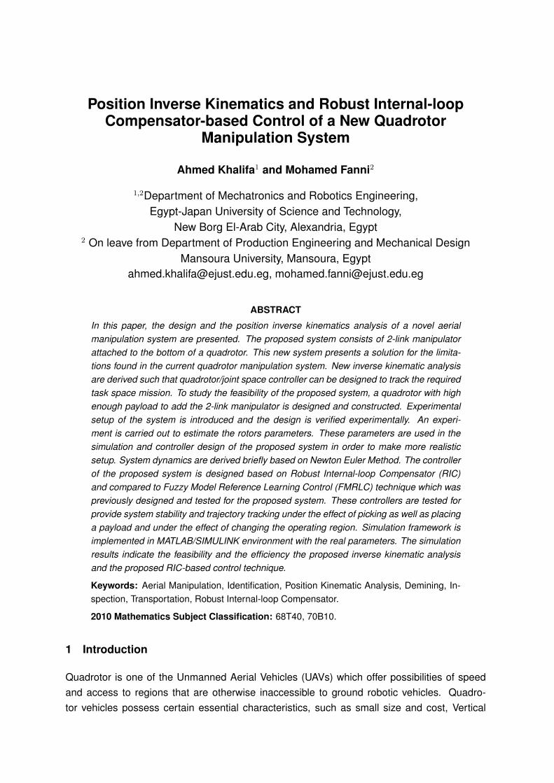
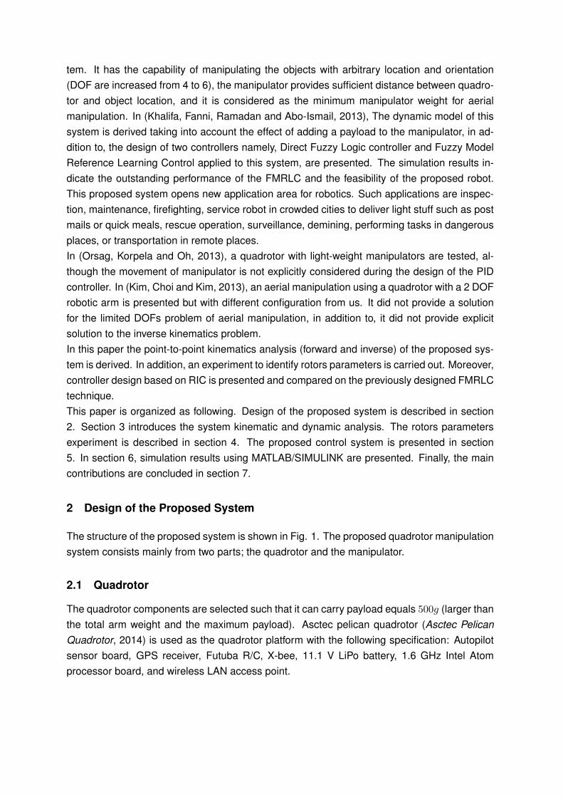
(Robotic Gripper for Robotic Arm, 2014). The arm components are; Three DC motors (HS-422(Max torque = 0.4N.m) for gripper, HS-5485HB (Max torque = 0.7N.m) for joint 1, and HS-422 (Max torque = 0.4N.m) for joint 2), Motor’s Driver (SSC-32) (Interface between the maincontrol unit and the motors), Arduino board (Mega 2560) (Arduino Board, 2014) (Implementmanipulator control algorithm), PS2 R/C (Remote controller to send commands to manipu-lator), and Motor accessories (Aluminum Tubing - 1.50in diameter, Aluminum Multi-PurposeServo Bracket, Aluminum Tubing Connector Hub, and Aluminum Long ”C” Servo Bracket withBall Bearings) (LYNXMOTION, 2014).The safety of this design and structure, with respect to the deflections and stress, is checkedthrough finite element analysis using ANSYS software (see Figs. 2 and 3). From these figures,the maximum deflection is about 0.6 mm which is smaller than the allowable value which equals1mm. In addition, the maximum stress of the structure is 113MPa which is smaller than theyield strength of aluminum alloy which is 270MPa. Also, the bearings and gripper are selectedto carry the load Therefore, this design is safe.

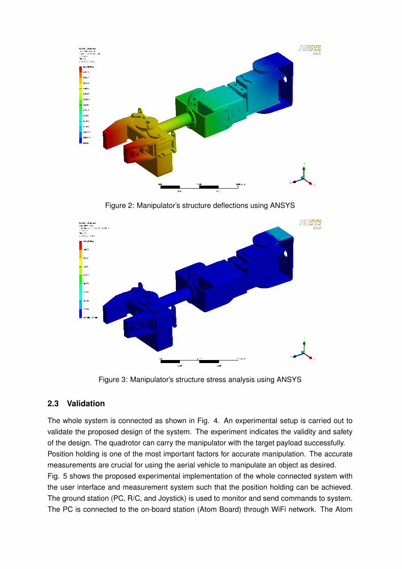
Figure 2: Manipulator’s structure deflections using ANSYS

Figure 3: Manipulator’s structure stress analysis using ANSYS

2.3 Validation

The whole system is connected as shown in Fig. 4. An experimental setup is carried out tovalidate the proposed design of the system. The experiment indicates the validity and safetyof the design. The quadrotor can carry the manipulator with the target payload successfully.Position holding is one of the most important factors for accurate manipulation. The accuratemeasurements are crucial for using the aerial vehicle to manipulate an object as desired.Fig. 5 shows the proposed experimental implementation of the whole connected system withthe user interface and measurement system such that the position holding can be achieved.The ground station (PC, R/C, and Joystick) is used to monitor and send commands to system.The PC is connected to the on-board station (Atom Board) through WiFi network. The Atom

Figure 4: Experimental setup of the proposed system

Figure 5: Aerial manipulation functional block diagram

Board, which runs under Linux platform, is used for control interface among ground PC, ArduinoBoard, and Autopilot Board. In addition, it is used to execute high computation algorithms,which is used for precise position estimation and control, such as VSLAM, Data fusion, andPlanning. Moreover, the proposed architecture of the system enables it to operate in eitherautonomous or tele-operated mode.

3 Kinematics and Dynamics Analysis

Fig. 6 presents a sketch of the Quadrotor-Manipulator System with the relevant frames. Theframes are assumed to satisfy the Denavit-Hartenberg (DH) convention (Leishman, 2000).The manipulator has two revolute joints. The axis of the first revolute joint (z0), that is fixed withrespect to the quadrotor, is parallel to the body x-axis of the quadrotor (see Fig. 6). The axis ofthe second joint (z1) will be parallel to the body y-axis of quadrotor at home (extended) configu-ration. Thus, the pitching and rolling rotation of the end effector is now possible independentlyon the horizontal motion of the quadrotor. Hence, With this new system, the capability of

Figure 6: Schematic of Quadrotor Manipulation System Frames

manipulating objects with arbitrary location and orientation is achieved because the DOF areincreased from 4 to 6.

3.1 Kinematics

The rotational kinematics of the quadrotor is represented through Euler angles. A rigid body iscompletely described by its position and orientation with respect to reference frame E, OI -XY Z, that it is supposed to be earth-fixed and inertial. Let define η1 as

η1 = [X,Y, Z]T (3.1)

the vector of the body position coordinates in the earth-fixed reference frame. The vector η1 isthe corresponding time derivative. If one defines

ν1 = [u, v, w]T (3.2)

as the linear velocity of the origin of the body-fixed frame B, OB-x y z, whose origin iscoincident with the center of mass (CM ), with respect to the origin of the earth-fixed frameexpressed in the body-fixed frame, the following relation between the defined linear velocitiesholds:

ν1 = RBI η1 (3.3)

where RBI is the rotation matrix expressing the transformation from the inertial frame to the

body-fixed frame.Let define η2 as

η2 = [φ, θ, ψ]T (3.4)

the vector of body Euler-angle coordinates in an earth-fixed reference frame. Those are com-monly named roll, pitch and yaw angles and corresponds to the elementary rotation around X,Y and Z in fixed frame. The vector η2 is the corresponding time derivative (expressed in theinertial frame). Let define

ν2 = [p, q, r]T (3.5)

as body-fixed angular velocity. The vector η2 is related to the body-fixed angular velocity by aproper Jacobian matrix:

ν2 = Jvη2 (3.6)

The matrix Jv can be expressed in terms of Euler angles as:

Jv =

1 0 −S(θ)

0 C(φ) C(θ)S(φ)

0 −S(θ) C(θ)C(φ)

(3.7)

where C(α) and S(α) are short notations for cos(α) and sin(α). The rotation RBI matrix needed

to transform the linear velocities, is expressed in terms of Euler angles by the following:

RBI =

C(ψ)C(θ) S(ψ)C(θ) −S(θ)

−S(ψ)C(φ) + S(ψ)S(θ)C(ψ) C(ψ)C(φ) + S(ψ)S(θ)S(φ) C(θ)S(φ)

S(ψ)S(φ) + C(ψ)S(θ)C(φ) −C(ψ)S(φ) + S(ψ)S(θ)C(φ) C(θ)C(φ)

(3.8)

The DH parameters for the 2-Link manipulator are derived and presented in (Khalifa et al.,2012).The position and orientation of the end effector relative to the body-fixed frame is easily ob-tained by multiplying the following homogeneous transformation matrices AB

0 , A01, A

12.

3.1.1 Forward Kinematics

Let define the position and orientation of the end effector expressed in the inertial frame, asηee1 and ηee2 respectively.

ηee1 = [xee, yee, zee]T (3.9)

ηee2 = [φee, θee, ψee]T (3.10)

The forward kinematics problem consists of determining the operational coordinates (ηee1 andηee2) of the end effector, as a function of the quadrotor movements (X, Y , Z, and ψ) as wellas the motion of the manipulator’s joints (θ1 and θ2). This problem is solved by computing thehomogeneous transformation matrix composed of relative translations and rotations.The transformation matrix from the body frame to the inertial frame AI

B which is:

AIB =

X

RIB Y

Z

0 0 0 1

, (3.11)

where RIB is 4x4 matrix. The total transformation matrix that relates the end effector frame to

the inertial frame is T I2 , which is given by:

T I2 = AI

BAB0 A

01A

12 (3.12)

Define the general form for this transformation matrix as a function of end effector variables(ηee1and ηee2), as following:

Tee =

r11 r12 r13 xee

r21 r22 r23 yee

r31 r32 r33 zee

0 0 0 1

(3.13)

Equating (3.12) and (3.13), an expression for the parameters of Tee (rij , xee, yee, and zee;i, j = 1, 2, 3) can be found, from which values of the end effector variables can determined.Euler angles of the end effector (φee, θee and ψee) can be computed from the rotation matrix ofTee as in (Slabaugh, 1999).

3.1.2 Inverse Kinematics

The inverse kinematics problem consists of determining the quadrotor movements (X, Y , Z,and ψ) as well as the motion of the manipulator’s joints (θ1 and θ2) as function of operationalcoordinates (ηee1 and ηee2) of the end effector.The inverse kinematics solution is essential for the robot’s control, since it allows to computethe required quadrotor movements and manipulator joints angles to move the end effector to adesired position and orientation.The rotations of the end effector can be parameterized by using several methods one of them,that is chosen, is the euler angles (Slabaugh, 1999).Equation (3.12) can be expressed, after putting φ = θ = 0, since we apply for point-to-pointcontrol because we target end effector control during picking and placing positions (reset con-figuration), as following:

T I2 =

C(ψ)S(θ2) + C(θ1)C(θ2)S(ψ) C(ψ)C(θ2)− C(θ1)S(ψ)S(θ2) S(ψ)S(θ1) X + L1C(θ1)S(ψ) + L2C(ψ)S(θ2) + L2C(θ1)C(θ2)S(ψ)

S(ψ)S(θ2)− C(ψ)C(θ1)C(θ2) C(θ2)S(ψ) + C(ψ)C(θ1)S(θ2) −C(ψ)S(θ1) Y − L1C(ψ)C(θ1) + L2S(ψ)S(θ2)− L2C(ψ)C(θ1)C(θ2)

−C(θ2)S(θ1) S(θ1)S(θ2) C(θ1) Z − L0 − L1S(θ1)− L2C(θ2)S(θ1)

0 0 0 1

(3.14)

From (3.14) and (3.13), the inverse kinematics of the system can be derived. According to thestructure of (3.14), the inverse orientation is carried out first followed by inverse position. Theinverse orientation has three cases as following:CASE 1:Suppose that not both of r13 , r23 are zero. Then from (3.14), we deduce that sin(θ1) 6= 0 andr33 6= ±1. In the same time, cos(θ1) = r33 and sin(θ1) = ±

√1− r233 and thus,

θ1 = atan2(√

1− r233, r33) (3.15)

orθ1 = atan2(−

√1− r233, r33) (3.16)

If we choose the value for θ1 given by (3.15), then sin(θ1) > 0, and

ψ = atan2(r13,−r23) (3.17)

θ2 = atan2(r32,−r31) (3.18)

If we choose the value for θ1 given by (3.16), then sin(θ1) < 0, and

ψ = atan2(−r13, r23) (3.19)

θ2 = atan2(−r32, r31) (3.20)

Thus, there are two solutions depending on the sign chosen for θ1. If r13 = r23 = 0, then the factthat Tee is orthogonal implies that r33 = ±1.CASE 2:If r13 = r23 = 0 and r33 = 1, then cos(θ1) = 1 and sin(θ1) = 0, so that θ1 = 0. In this case, therotation matrix of (3.14)becomes

RI2 =

S(θ2 + ψ) C(θ2 + ψ) 0

−C(θ2 + ψ) S(θ2 + ψ) 0

0 0 1

(3.21)

Thus the sum θ2 + ψ can be determined as

θ2 + ψ = atan2(r11, r12) (3.22)

We can assume any value for ψ and get θ2. Therefor, there are infinity of solutions.CASE 3:If r13 = r23 = 0 and r33 = -1, then cos(θ1) = -1 and sin(θ1) = 0, so that θ1 = π. In this case, therotation matrix of (3.14) becomes:

RI2 =

S(θ2 − ψ) C(θ2 − ψ) 0

C(θ2 − ψ) −S(θ2 − ψ) 0

0 0 −1

(3.23)

Thus, θ2 − ψ can be determined as

θ2 − ψ = atan2(r11, r12) (3.24)

One can assume any value for ψ and get θ2. Therefor, there are infinity of solutions.In cases 2 and 3, putting ψ = 0 will lead to find θ2.Finally, the inverse position is determined from:

X = xee − (L1C(θ1)S(ψ) + L2C(ψ)S(θ2) + L2C(θ1)C(θ2)S(ψ)) (3.25)

Y = yee − (−L1C(ψ)C(θ1) + L2S(ψ)S(θ2)− L2C(ψ)C(θ1)C(θ2)) (3.26)

Z = zee − (−L0 − L1S(θ1)− L2C(θ2)S(θ1)) (3.27)

3.2 Dynamics

The equations of motion of the proposed robot are derived in details in (Khalifa et al., 2012).Applying Newton Euler algorithm (Tsai, 1999) to the manipulator considering that the link (withlength L0) that is fixed to the quadrotor is the base link, one can get the equations of motion ofthe manipulator as well as the interaction forces and moments between the manipulator andthe quadrotor. The effect of adding a payload to the manipulator will appear in the parametersof its end link, link 2, (e.g. mass, center of gravity, and inertia matrix). Therefore, the payloadwill change the overall system dynamics.The equations of motion of the manipulator are:

M1θ1 = Tm1 +N1 (3.28)

M2θ2 = Tm2 +N2 (3.29)

where, Tm1 and Tm2 are the manipulator actuators’ torques. M1, M2, N1, and N2 are nonlinearterms and they are functions in the system states as described in (Khalifa et al., 2012).The Newton Euler method are used to find the equations of motion of the quadrotor after addingthe forces/moments from the manipulator are:

mX = T (C(ψ)S(θ)C(φ) + S(ψ)S(φ)) + F Im,qx (3.30)

mY = T (S(ψ)S(θ)C(φ)− C(ψ)S(φ)) + F Im,qy (3.31)

mZ = −mg + TC(θ)C(φ) + F Im,qz (3.32)

Ixφ = θφ(Iy − Iz)− IrθΩ + Ta1 +MBm,qφ

(3.33)

Iy θ = ψφ(Iz − Ix) + IrφΩ + Ta2 +MBm,qθ

(3.34)

Izψ = θφ(Ix − Iy) + Ta3 +MBm,qψ

(3.35)

where F Im,qx , F I

m,qy , and F Im,qz are the interaction forces from the manipulator to the quadrotor

in X,Y , and Z directions defined in the inertial frame and MBm,qφ

, MBm,qθ

, and MBm,qψ

are theinteraction moments from the manipulator to the quadrotor around X, Y , and Z directionsdefined in the body frame.The variables in (3.30-3.35) are defined as follows: m is the mass of the quadrotor. Each rotorj has angular velocity Ωj and it produces thrust force Fj and drag moment Mj which are givenby:

Fj = KFjΩ2j (3.36)

Mj = KMjΩ2j (3.37)

where KFj and KMj are the thrust and drag coefficients.T is the total thrust applied to the quadrotor from all four rotors, and is given by:

T =

4∑j=1

(Fj) (3.38)

Ta1 , Ta2 , and Ta3 are the three input moments about the three body axes, and are given as:

Ta1 = d(F4 − F2) (3.39)

Ta2 = d(F3 − F1) (3.40)

Ta3 = −M1 +M2 −M3 +M4 (3.41)

d is the distance between the quadrotor center of mass and rotor rotational axis.

Ω = Ω1 − Ω2 + Ω3 − Ω4 (3.42)

Ir is the rotor inertia. If is the inertia matrix of the vehicle around its body-frame assuming thatthe vehicle is symmetric about x-, y- and z-axis.

4 System Parameters Estimation

In order to test the feasibility of the proposed system, a simulation framework will be built. Thus,there is a need to find the real parameters of the system to make the simulation results morereliable. The identified parameters include the structure and rotor assembly parameters (Kfj

and Kmj ). To calculate the structure parameters, a 3D CAD model is developed using SOLID-WORKS software to calculate the mass moments of inertia and all the missing geometricalparameters. To estimate the rotor assembly parameters, an experimental setup of quadrotoris carried out, see Fig. 7. In this experiment, the rotor is mounted on a 6-DOF torque/forcesensor that is connected to a NI Data Acquisition Card (NI DAC). Then, the DAC is connectedto a PC running SIMULINK program as an interface to read data from DAC. The velocity ofrotor is changed gradually and each time the generated thrust and drag moment is measuredand recorded using SIMULINK program. By using MATLAB Curve Fitting toolbox the gener-ated date are fitted by using (3.36 and 3.37), thus the thrust and moment coefficients can beobtained. The identified parameters are given in Table 1.

5 Controller Design

Quadrotor is an under-actuated system, because it has four inputs (angular velocities of its fourrotors) and six variables to be controlled. By observing the operation of the quadrotor, one canfind that the movement in X- direction is based on the pitch rotation, θ. Also the movementin Y - direction is based on the roll rotation, φ. Therefore, motion along X- and Y -axes will becontrolled through controlling θ and φ.

Figure 7: Experiment to estimate rotor coefficients

Table 1: System Parameters

Par. Value Unit Par. Value Unitm 1 kg L2 85x10−3 m

d 223.5X10−3 m m0 30x10−3 kg

Ix 13.215X10−3 N.m.s2 m1 55x10−3 kg

Iy 12.522X10−3 N.m.s2 m2 112x10−3 kg

Iz 23.527X10−3 N.m.s2 Ir 33.216X10−6 N.m.s2

L0 30x10−3 m L1 70x10−3 m

KF1 1.667x10−5 kg.m.rad2 KF2 1.285x10−5 kg.m.rad2

KF3 1.711x10−5 kg.m.rad2 KF4 1.556x10−5 kg.m.rad2

KM1 3.965x10−7 kg.m2.rad2 KM2 2.847x10−7 kg.m2.rad2

KM3 4.404x10−7 kg.m2.rad2 KM4 3.170x10−7 kg.m2.rad2

Fig. 8 presents a block diagram of the proposed control system. The desired values for theend effector’s position (xeed , yeed and zeed) and orientation (φeed , θeed and ψeed) are convertedto the desired values of the quadrotor (Xd, Yd, Zd and ψd) and joints variables (θ1d and θ2d)through the inverse kinematics that are derived in section 3. Next, these values is applied toa trajectory generation algorithm which will be explained later. After that, the controller blockreceives the desired values and the feedback signals from the system and provides the controlsignals (T , τa1 , τa2 , τa3 , Tm1 and Tm2). The matrix G of the control mixer, in Fig. 8, is used totransform the assigned thrust force and moments of the quadrotor (the control signals) from thecontroller block into assigned angular velocities of the four rotors. This matrix can be derivedfrom (3.38-3.41) and presented as following:

Ω21

Ω22

Ω23

Ω24

=

KF1 KF2 KF3 KF4

0 −dKF2 0 dKF4

−dKF1 0 dKF3 0

−KM1 KM2 −KM3 KM4

−1

︸ ︷︷ ︸G

T

τa1

τa2

τa3

(5.1)

Figure 8: Block Diagram of the Control System

Finally, The actual values of the quadrotor and joints are converted to the actual values of theend effector variables through the forward kinematics which are derived in section 3.The control design criteria are to achieve system stability and zero position error, for the move-ments in X, Y , Z, and ψ directions as well as for joints’ angles θ1 and θ2 and consequently forthe end effector variables (ηee1 and ηee2), under the effect of:

• Picking and placing a payload.

• Changing the operating region of the system.

Noting that in the task space, a position tracking is implemented, and in the joint space, trajec-tory tracking is required.

5.1 Robust Internal-loop Compensator-based Control

Robust control is widely used in robotic system to ensure stability and robustness against exter-nal disturbances, uncertainties, and measurement noise (Hassanein, Anavatti and Ray, 2011).Disturbance Observer (DOb)-based controller design is one of the most popular methods inthe field of motion control. In (Yamada, Komada, Ishida and Hori, 1996), the DOb-based con-troller is designed to realize a nominal system which can control acceleration in order to realizefast and precise servo system, even if servo system has parameter variation and suffers fromdisturbance. In (Kim and Chung, 2003) and (Kim, Choi, Lee and Koh, 2012), the generalizeddisturbance compensation framework, named the robust internal-loop compensator (RIC) isintroduced and an advanced design method of a DOb is proposed based on the RIC. In (Park,Won, Kang, Kim, Lee and Kwon, 2005), the developed quadrotor shows stable flying perfor-mances under the adoption of RIC based disturbance compensation. Although a model isincorrect, RIC method can design a controller by regarding the inaccurate part of the modeland sensor noises as disturbances.We propose a robust internal loop compensator based control as robust controller to get ac-curate positioning of the proposed system. The controller consists of two parts, internal and

Figure 9: RIC Disturbance Compensation Controller

external loop. Internal loop is used as a compensator for canceling disturbances, uncertaintiesand nonlinearities including difference between reference model and real system, and exter-nal loop is designed to meet the specification of the system using the result of internal loopcompensator.The RIC based control algorithm, as shown in Fig. 9, controls the response of the plant P (s)

to follow that of the model plant Pm(s) even though disturbances dex and sensor noise ζ areapplied to the plant (Park et al., 2005). RIC based disturbance compensator can be usedfor position, attitude, and manipulator’s joints control in the same way. For all controllers, thereference plant model are given in the form of:

Pmi(s) =1

τcis2

(5.2)

where ym(s) is the output response of the reference model (nominal plant), and yr(s) is thedesired value of the plant. The value τi (i = x, y, z, φ, θ, ψ, θ1, and θ2), which depends on theplant dynamics, is mass for x, y, z-controller and mass moment of inertia for φ, θ, ψ, θ1, andθ2.The external-loop compensator Cz(s) for altitude (z) control, for instance, are given like PDcontroller as follows:

Cz(s) = kpz + kdzs (5.3)

with the error ez = zr - z as the controller input. where kpz and kdz are P - and D-gain of theexternal-loop compensator, respectively. The output of the external-loop compensator, i.e., thereference input of RIC is given as

urz(s) = Cz(s)ez (5.4)

The output of the reference model is compared to the actual response generating the referenceerror erz = zr - z which is applied to internal controller Kz

RIC(s) that is chosen to be a PID-likecontroller and it is given as follows:

KzRIC(s) = kzp + kzds+ kzi

1

s(5.5)

Thus, the final control signal uz is given as:

uz = ucz + ukz + uexz (5.6)

where ucz and ukz are the control signals from the external and internal controllers respectively,while uexz is an external value equal to the robot weight to compensate system weight (mg).The procedures for obtaining the RIC control input for X, Y , φ, θ, ψ, θ1, and θ2 control are thesame with that for altitude (Z) control except that uexz equal 0. In addition, there is difference inthe design of X and Y controllers. In this control strategy, the desired pitch and roll angles, θdand φd , are not explicitly provided to the controller. Instead, they are continuously calculatedby X and Y controllers in such a way that they stabilize the quadrotor’s attitude. However,there is a need to convert the error and its rate of X and Y that is defined in the inertial frameinto their corresponding values defined in the body frame. This conversion is done using thetransformation matrix, defined in (3.8), assuming small angles (φ and θ) as following:

x = X cos(ψ) + Y sin(ψ) (5.7)

y = X sin(ψ)− Y cos(ψ) (5.8)

6 Simulation Results

Quintic Polynomial trajectories (Leishman, 2000) are used as the reference trajectories for X,Y , Z, ψ, θ1, and θ2. Those types of trajectories have sinusoidal acceleration which is better inorder to avoid vibrational modes. The desired values of end effector position and orientation(Multi-region of operation and point-to-point control) are used to generate the desired trajecto-ries for X, Y , Z, φ, θ and ψ using the inverse kinematics and then the algorithm for generatingthe trajectories.The system equations of motion and the control laws for both FMRLC and RIC techniques aresimulated using MATLAB/SIMULINK program. The design details, simulation results, and pa-rameters of FMRLC can be found in (Khalifa et al., 2013).The controller parameters of the RICcontroller are given in Table 2; we use the methodology for the RIC design given in (Kim andChung, 2002) and the one used to design PID controllers in (Precup and Preitl, 2006). Thoseparameters are tuned to get the required system performance. The two controllers are testedto stabilize and track the desired trajectories under the effect of picking a payload of value 150g at instant 15 s and placing it at instant 65 s. The simulation results of both FMRLC and RICare presented in Fig. 10. These results show that RIC and FMRLC is able to track the de-sired trajectories (with different operating regions) before, during picking, holding, and placingthe payload, in addition to, the RIC results is better than the FMRLC in disturbance rejectioncapability. Furthermore, the generated desired trajectories of θ and φ from RIC are smoothcompared with that from FMRLC which are more oscillatory (see Fig. 10g and Fig. 10h).Moreover, since the RIC is simpler than FMRLC, the computation time for control laws of RICis very small compared to that of FMRLC. Therefore, RIC is recommended to be implementedin experimental work.

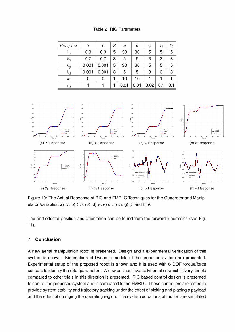
Table 2: RIC Parameters

Par./V al. X Y Z φ θ ψ θ1 θ2

kpi 0.3 0.3 5 30 30 5 5 5kdi 0.7 0.7 3 5 5 3 3 3kip 0.001 0.001 5 30 30 5 5 5kid 0.001 0.001 3 5 5 3 3 3kii 0 0 1 10 10 1 1 1τci 1 1 1 0.01 0.01 0.02 0.1 0.1

0 10 20 30 40 50 60 700

10

20

30

40

50

60

70

Time (s)

X (

m)

DesiredFMRLCRIC

(a) X Response

0 10 20 30 40 50 60 700

10

20

30

40

50

60

70

Time (s)

Y (

m)

DesiredFMRLCRIC

(b) Y Response

0 10 20 30 40 50 60 700

10

20

30

40

50

60

70

Time (s)

Z (

m)

DesiredFMRLCRIC

(c) Z Response

0 10 20 30 40 50 60 70−0.2

0

0.2

0.4

0.6

0.8

1

1.2

1.4

1.6

Time (s)

ψ (

rad)

DesiredFMRLCRIC

(d) ψ Response

0 10 20 30 40 50 60 70−0.2

0

0.2

0.4

0.6

0.8

1

1.2

1.4

1.6

Time (s)

θ 1 (ra

d)

DesiredFMRLCRIC

(e) θ1 Response

0 10 20 30 40 50 60 70−0.1

0

0.1

0.2

0.3

0.4

0.5

0.6

0.7

0.8

Time (s)

θ 2 (ra

d)

DesiredFMRLCRIC

(f) θ2 Response

0 10 20 30 40 50 60 70−0.15

−0.1

−0.05

0

0.05

0.1

Time (s)

φ (r

ad)

Desired−FMRLCFMRLCDesired−RICRIC

(g) φ Response

0 10 20 30 40 50 60 70−0.2

−0.15

−0.1

−0.05

0

0.05

0.1

0.15

0.2

Time (s)

θ (r

ad)

Desired−FMRLCFMRLCDesired−RICRIC

(h) θ Response

Figure 10: The Actual Response of RIC and FMRLC Techniques for the Quadrotor and Manip-ulator Variables: a) X, b) Y , c) Z, d) ψ, e) θ1, f) θ2, g) φ, and h) θ.

The end effector position and orientation can be found from the forward kinematics (see Fig.11).

7 Conclusion

A new aerial manipulation robot is presented. Design and it experimental verification of thissystem is shown. Kinematic and Dynamic models of the proposed system are presented.Experimental setup of the proposed robot is shown and it is used with 6 DOF torque/forcesensors to identify the rotor parameters. A new position inverse kinematics which is very simplecompared to other trials in this direction is presented. RIC based control design is presentedto control the proposed system and is compared to the FMRLC. These controllers are tested toprovide system stability and trajectory tracking under the effect of picking and placing a payloadand the effect of changing the operating region. The system equations of motion are simulated

0 10 20 30 40 50 60 700

10

20

30

40

50

60

70

Time (s)

x ee (

m)

DesiredFMRLCRIC

(a) xee Response

0 10 20 30 40 50 60 700

10

20

30

40

50

60

70

Time (s)

y ee (

m)

DesiredFMRLCRIC

(b) yee Response

0 10 20 30 40 50 60 700

10

20

30

40

50

60

70

Time (s)

z ee (

m)

DesiredFMRLCRIC

(c) zee Response

0 10 20 30 40 50 60 70−0.2

0

0.2

0.4

0.6

0.8

1

1.2

1.4

1.6

1.8

Time (s)

φ ee (

rad)

DesiredFMRLCRIC

(d) φee Response

0 10 20 30 40 50 60 70−0.2

0

0.2

0.4

0.6

0.8

1

1.2

1.4

1.6

Time (s)

θ ee (

rad)

DesiredFMRLCRIC

(e) θee Response

0 10 20 30 40 50 60 70−2

−1.5

−1

−0.5

0

0.5

1

1.5

2

Time (s)

ψee

(ra

d)

DesiredFMRLCRIC

(f) ψee Response

Figure 11: The Actual Response of both RIC and FMRLC Techniques for the End EffectorPosition and Orientation: a) xee, b) yee, c) zee, d) φee, e) θee, and f) ψee.

using MATLAB/SIMULINK based on the system real parameters. Simulation results show thatthe RIC based control is very simple, has low computation time, and has higher disturbancerejection abilities comparing with FMRLC. In addition, these results indicate the feasibility ofthe proposed system. Therefore, the RIC is highly recommended to be implemented in realtime to experimentally control the proposed system.

Acknowledgment

The first author is supported by a scholarship from the Mission Department, Ministry of HigherEducation of the Government of Egypt which is gratefully acknowledged.

References

Albers, A., Trautmann, S., Howard, T., Nguyen, T. A., Frietsch, M. and Sauter, C. 2010. Semi-autonomous flying robot for physical interaction with environment, Robotics Automationand Mechatronics (RAM), 2010 IEEE Conference on, IEEE, pp. 441–446.

Arduino Board 2014. Available at http://store.arduino.cc/product/A000067.

Asctec Pelican Quadrotor 2014. Available at http://www.asctec.de/en/

uav-uas-drone-products/asctec-pelican/.

Bisgaard, M., la Cour-Harbo, A. and Dimon Bendtsen, J. 2010. Adaptive control system forautonomous helicopter slung load operations, Control Engineering Practice 18(7): 800–811.

DiCesare, A. 2008. Design Optimization of a Quad-Rotor Capable of Autonomous Flight, PhDthesis, WORCESTER POLYTECHNIC INSTITUTE.

Guo, J., Wang, Z., Zheng, M. and Wang, Y. 2014. An approach for uav reconnaissance mis-sion planning problem under uncertain environment, International Journal of Imaging andRobotics 14(3): 1–15.

Gupte, S., Mohandas, P. I. T. and Conrad, J. M. 2012. A survey of quadrotor unmanned aerialvehicles, Southeastcon, 2012 Proceedings of IEEE, IEEE, pp. 1–6.

Hassanein, O. I., Anavatti, S. G. and Ray, T. 2011. Robust position control for two-link manip-ulator, International Journal of Artificial Intelligence 7(A11): 347–359.

Khalifa, A., Fanni, M., Ramadan, A. and Abo-Ismail, A. 2012. Modeling and control of a newquadrotor manipulation system, 2012 IEEE/RAS International Conference on InnovativeEngineering Systems, IEEE, pp. 109–114.

Khalifa, A., Fanni, M., Ramadan, A. and Abo-Ismail, A. 2013. Adaptive intelligent controllerdesign for a new quadrotor manipulation system, Systems, Man, and Cybernetics (SMC),2013 IEEE International Conference on, IEEE, pp. 1666–1671.

Kim, B. K. and Chung, W. K. 2002. Performance tuning of robust motion controllers for high-accuracy positioning systems, Mechatronics, IEEE/ASME Transactions on 7(4): 500–514.

Kim, B. K. and Chung, W. K. 2003. Advanced disturbance observer design for mechanicalpositioning systems, Industrial Electronics, IEEE Transactions on 50(6): 1207–1216.

Kim, J., Choi, S. B., Lee, H. and Koh, J. 2012. Design of a robust internal-loop compensator ofclutch positioning systems, Control Applications (CCA), 2012 IEEE International Confer-ence on, IEEE, pp. 1473–1478.

Kim, J., Kang, M.-S. and Park, S. 2010. Accurate modeling and robust hovering control for aquad-rotor vtol aircraft, Selected papers from the 2nd International Symposium on UAVs,Reno, Nevada, USA June 8–10, 2009, Springer, pp. 9–26.

Kim, S., Choi, S. and Kim, H. J. 2013. Aerial manipulation using a quadrotor with a twodof robotic arm, Intelligent Robots and Systems (IROS), 2013 IEEE/RSJ InternationalConference on, IEEE, pp. 4990–4995.

Korpela, C. M., Danko, T. W. and Oh, P. Y. 2012. Mm-uav: Mobile manipulating unmannedaerial vehicle, Journal of Intelligent & Robotic Systems 65(1-4): 93–101.

Leishman, J. 2000. Principles of Helicopter Aerodynamics, Cambridge University Press.

Lindsey, Q., Mellinger, D. and Kumar, V. 2012. Construction with quadrotor teams, AutonomousRobots 33(3): 323–336.

LYNXMOTION 2014. Available at http://www.lynxmotion.com/default.aspx.

Mellinger, D., Lindsey, Q., Shomin, M. and Kumar, V. 2011. Design, modeling, estimation andcontrol for aerial grasping and manipulation, 2011 IEEE/RSJ International Conference onIntelligent Robots and Systems (IROS), IEEE, pp. 2668–2673.

Michael, N., Fink, J. and Kumar, V. 2011. Cooperative manipulation and transportation withaerial robots, Autonomous Robots 30(1): 73–86.

Orsag, M., Korpela, C. and Oh, P. 2013. Modeling and control of mm-uav: Mobile manipulatingunmanned aerial vehicle, Journal of Intelligent & Robotic Systems 69(1-4): 227–240.

Park, S., Won, D., Kang, M., Kim, T., Lee, H. and Kwon, S. 2005. Ric (robust internal-loop com-pensator) based flight control of a quad-rotor type uav, Intelligent Robots and Systems,2005.(IROS 2005). 2005 IEEE/RSJ International Conference on, IEEE, pp. 3542–3547.

Precup, R.-E. and Preitl, S. 2006. Pi and pid controllers tuning for integral-type servo systemsto ensure robust stability and controller robustness, Electrical Engineering 88(2): 149–156.

Robotic Gripper for Robotic Arm 2014. Available at http://robokits.co.in.

Salih, A. L., Moghavvemi, M., Mohamed, H. A. and Gaeid, K. S. 2010. Flight pid controllerdesign for a uav quadrotor, Scientific Research and Essays 5(23): 3660–3667.

Slabaugh, G. G. 1999. Computing euler angles from a rotation matrix, Retrieved on August6: 2000.

Torre, A., Mengoli, D., Naldi, R., Forte, F., Macchelli, A. and Marconi, L. 2012. A prototype ofaerial manipulator, Intelligent Robots and Systems (IROS), 2012 IEEE/RSJ InternationalConference on, IEEE, pp. 2653–2654.

Tsai, L.-W. 1999. Robot analysis: the mechanics of serial and parallel manipulators, Wiley-Interscience.

Willmann, J., Augugliaro, F., Cadalbert, T., D’Andrea, R., Gramazio, F. and Kohler, M. 2012.Aerial robotic construction towards a new field of architectural research, International jour-nal of architectural computing 10(3): 439–460.

Yamada, K., Komada, S., Ishida, M. and Hori, T. 1996. Analysis of servo system realized bydisturbance observer, Advanced Motion Control, 1996. AMC’96-MIE. Proceedings., 19964th International Workshop on, Vol. 1, IEEE, pp. 338–343.