1

Contents Introduction: How to Succeed in Physics Lab page 3 Tutorial 1: Errors and Significant Figures 5 Tutorial 2: Making a Good Graph by Hand 9 Tutorial 3: Computer Software and Sensors 11 Laboratory Exercises Mechanics 1 Position and Velocity 13

2 Acceleration 17 3 Vectors 19 4 Tension Force and Acceleration 23 5 Conservation of Energy 25 6 Collisions and Momentum 27

7 Density; Significant Figures 29

Oscillations 8 Part I: Simple Harmonic Motion 33 Part II: The Simple Pendulum 37 9 The Sonometer 39

Thermodynamics 10 The Mechanical Equivalent of Heat 43 11 Boyle's Law 47 12 Part I: Heat of Fusion of Ice 51 Part II: The Specific Heat of a Metal 53

2

This collection of Laboratory Exercises is the introductory physics laboratory manual used by Hunter College. The original exercises were developed by the Physics Faculty over thirty years ago. A number of revisions have since been made. In particular, major revisions led by Professors Robert A. Marino in 1994 and by Mark Hillery and Y.C. Chen in 2002, introduced several new exercises involving modern electronic and optical equipment and computerized data acquisition systems. We are indebted to the faculty and students who participated in the creation and revision of the manual over the years.

Physics Faculty Hunter College

June,2002 © 1998, 1999, 2002, 2011 by Department of Physics, Hunter College of the City University of New York All rights reserved.

3

INTRODUCTION

How to Succeed in Physics Lab Read the lab manual before coming to class to become familiar with the experiment. Lecture and Lab are NOT in perfect synch, so you may have to give the textbook a look also. You should take responsibility to learn safe operating procedures from the lab instructor. The lab manual is also occasionally a good source of safety tips. With electrical circuits, no power is to be supplied unless OK'd by instructor or lab tech. Report any accidents immediately! You will work with a lab partner to take data, but you are individually responsible for your own data. All subsequent calculations, graphs, etc. are also your own individual responsibility. Original data MUST be in ink. If you change your mind, cross out with a single stroke, and enter new datum nearby. Do not leave the lab room without obtaining the instructor's signature on your original data sheet. Without it, your lab report will not be accepted. No exceptions. The lab has been designed to be a "low pressure" experience. We hope it is an enjoyable one as you take the time to become familiar with new equipment and experiences. Still, you should aim to complete all data-taking, all necessary calculations, reach all conclusions, and at least sketch all graphs before you leave. It's well known (to those who know it well) that once you walk out that door, all work on lab reports will take longer. Besides, most of the grade for the course will come from the lecture part, so spend your time accordingly. Before taking good data, run through the experiment once or twice to see how it goes. It is often good technique to sketch data as you go along, whenever appropriate. The Report: Your Lab Report should be self-contained: It should still make sense to you when you pass it on to your grandchildren. It should include: a) Front page: your original data sheet with your name, partners and date. The original data MUST be in ink. Report not acceptable if original data is in pencil or if data sheet was not signed by your instructor. (So... don't leave lab room without it.) b) Additional pages with data and calculations in neat tabular form. If the original came out messy, you should rewrite your data before continuing with calculations. c) Any graphs. Neatness counts! It's one of the aims of this lab to produce students that know how to produce a decent graph. d) Answers to any Questions

4

e) An Appendix made up of the pages from the lab manual that describes the experiment. Including them relieves you from having to rewrite the essential points of the procedure, description of equipment, etc. Lab reports are due the next time the lab meets. At the beginning of the period! It is department policy to penalize you for lateness in handing in lab reports. This is to discourage you from working on stale data with the lab experience no longer fresh in your mind. A schedule will be announced. Laboratory Grade: The lab instructor will make up a grade 90% based on the average of your lab reports, and 10% on his/her personal evaluation of your performance in the laboratory. This grade is then reported to your lecturer for inclusion in the final course grade (15% weight factor). The list below will give you an idea of the criteria used by your lab instructor in grading your lab report: 1. Quality of measurements. Logical presentation of report contents. 2. Accuracy and correctness of calculations resulting from proper use of data and

completion of calculations. 3. Orderly and logical presentation of data in tabular form, where appropriate. 4. Good-looking graphs, easiness to read, good choice of scales and labels. 5. Comparison with theory. 6. Answers to Questions; Conclusions. 7. Clarity, Neatness, Promptness.

5

TUTORIAL # 1

On Errors and Significant Figures Errors We could distinguish among three different kinds of "errors" in your lab measurements: 1. Mistakes or blunders. We all make these. But with any kind of luck, and some care, we catch them and then repeat the measurement so that these errors can be corrected. 2. Systematic Errors. These are due either to a faulty instrument (a meter stick that shrank or a clock that runs fast) or by an observer with a consistent bias in reading an instrument. These errors affect all of the measurements in the same way, i.e. they make them all too big or too small. For example, if our clock runs fast, all of our measurements of time intervals will be too long. 3. Random Errors. Small accidental errors present in every measurement we make at the limit of the instrument's precision. These errors will sometimes make a measurement too big and sometimes too small. To deal with these we repeat a measurement several times and take the average. The average gives the best estimate of the quantity we are trying to measure, and the spread of the values about the average gives us an estimate of the uncertainty. After blunders are eliminated, the precision of a measurement can be improved by reducing random errors ( by statistical means or by substituting a more precise instrument, i.e., one that yields more significant figures for the same measurement.) Accuracy can be increased by reducing any systematic errors as well as by increasing the precision. Significant Figures, Error, Fractional Error No measurement of a physical quantity can ever be made with infinite accuracy. As an honest experimentalist, you should relay to the reader just how good you think your measurement is. One simple way to relay this information is by the number of significant figures you quote. For example, 3.4 cm says one thing, 3.40 cm tells a different story. The last digit you write down can be your best estimate made between the markings of a scale, but it still represents a willfully reported number, it still is a significant figure. The placement of the decimal point does not change the number of significant figures. For example, 20.8 grams and 0.00208 grams each have three significant figures; each is assumed to be uncertain by at least ±1 in the last figure, i.e., ±1 part in 208. Normally, figuring out how many significant figures are in a stated number gives no problems, except when zeros are involved. For example, is it obvious how many significant figures are expressed in 5500 feet, 250 years, or $1,300,000 ? A good way to tell the reader which is, in fact, the last significant figure is by using scientific notation. For

6

example, 5.50 x 103 feet, 2.5 x 102 years, and 1.300 Megabucks, telegraph that the number of digits in which any confidence can be placed was three, two, and four, respectively. Another way of representing the error is to explicitly indicate it. Suppose that we measure a length, which we find to be 1.520 m, and we believe that this measurement is accurate to within a centimeter. We could then write the result of our measurement as 1.520±0.005 m, which means that our result is between 1.515 m and 1.525 m. In general, if we are measuring a quantity x, we can write the result of a measurement of x as xbest±δx, where xbest is our best estimate of the quantity being measured, and δx, which is a positive number, is the value of the uncertainty in our measurement. We can also use what is called the fractional error. This is just δx /| xbest |. To get the percent error, we just multiply the fractional error by 100. In our example, we have that xbest =1.52 m, δx =0.005 m, the fractional error is 0.0032 and the percent error is 0.32. Note that the fractional error and the percent error have no units. Finding the uncertainty We have been discussing representing the result of a measurement as xbest±δx, but given a set of readings from an instrument, how do we find xbest and δx? We find xbest by taking the average of the readings, so if we have made three measurements of a length, and have found the results 1.26 m, 1.28 m and 1.25 m, we have that xbest = (1.26 m + 1.28 m +1.25 m )/3 = 1.26 m. Finding δx is a bit trickier. First, it cannot be any smaller than the precision of our measuring instrument. If we are using a meter stick to measure a length, and the smallest units marked on the meter stick are millimeters, then the uncertainty in our measurements will be approximately one millimeter (it can actually be a bit less than this, because we can estimate the length to a fraction of a millimeter – this would give us an uncertainty of about 0.3 mm). However, it might be bigger due to random errors. In order to do a detailed analysis of random errors, it is necessary to know a lot more about probability theory and statistics than you do now, so we will just give you the answer. Suppose you have made N measurements and the results are x1, x2, …xN. You first calculate the average value of the measurements, xbest, and then you use it to find what is called the standard error, s, which is given by s = [(x1 - xbest)2+(x2 - xbest)2+…(xN - xbest)2]1/2/[N(N-1)]1/2. The uncertainty, δx, will just be the sum of the uncertainty due to the measuring instrument and the standard error, s. Computations using raw data How do you combine your carefully gathered data with other numbers in an expression? With a little common sense, and a hand calculator, you can verify that the following rules should be followed: Addition and Subtraction: Suppose we want to add two measured lengths, 0.36±0.01 m and 0.48±0.02 m. Why would we want to do this? Each length might be the length of a block, and then the sum would correspond to the length of the object we get when we put the two blocks together. What can we say about the length of the combined blocks? Our best estimate of their

7

combined length is just 0.36 m + 0.48 m = 0.84 m, but we have to worry about the uncertainties too. The longest the combined blocks can be is (0.36 m + 0.01 m)+(0.48 m + 0.02 m) = 0. 87 m, and the shortest they can be is (0.36 m - 0.01 m)+(0.48 m - 0.02 m) = 0. 81 m. We can then write the combined length as 0.84 ± 0.03 m. This gives us the following rule. Suppose that q=x+y, and that x and y are measured quantities, which we represent as xbest±δx and ybest±δy. Then qbest= xbest + ybest and δq=δx+δy. The same rule holds for subtraction, if q = x-y, where x and y are measured quantities, then qbest= xbest - ybest and δq=δx+δy. One conclusion that can be drawn from this is that when adding numbers with different numbers of significant figures, the number with the least number of significant figures determines the number of significant figures in the sum. For example, 3.1 m +1.11 m is 4.2 m, and not 4.21 m. Similarly, 1.11 x 103 m + 3.33 x 104 m is, unfortunately, just 3.44 x 104 m. Note: To see this you have to write it out in ordinary notation (even better: line-up one under the other): 1,110 + 33,300 = 34,410 mathematically but the tens position is not significant in one of the terms, so it cannot be significant in the final sum. The answer is 34,400, or 3.44 x 104. Multiplication and Division: Suppose we have measure the sides of a rectangle and we want to find its area. In particular, we found the length to be 0.240±0.002 m and the width to be 0.120±0.001 m. Our best estimate for the area is just Abest=(0.240 m)(0.120 m) = 0.0288 m2, but what is the uncertainty? The biggest A can be is (0.242 m)(0.121 m)=.0293 m2, and the least it can be is (0.238 m)(0.119 m) =0.0283 m2, so δA=0.005 m2. Can we use this example to come up with a rule? Let us look at the fractional errors. The fractional error for the length is (0.002 m)/(0.240 m)=0.0083, the fractional error for the width is (0.001 m)/(0.120 m)=0.0083, and the fractional error for the area is (0.005 m)/(0.0288 m)=0.172. Notice that the fractional error for the area is approximately the sum of the fractional errors of the length and the width, (0.0083+0.0083=0.0166). This is, in fact, a good general rule, when multiplying the results of two measurements, the fractional error for the product is approximately the sum of the fractional errors of the factors. Let us see why this is true. Suppose that q=xy, where x and y are measured quantities, so x= xbest±δx and y=ybest±δy. We can write q=qbest±δq, where qbest=xbestybest. This means that qbest±δq=(xbest±δx)(ybest±δy)≈ xbest ybest± (xbestδy+ybestδx), where we have assumed that is δxδy small compared to everything else. If we now divide both sides by |qbest| and then subtract qbest/|qbest | from both sides, we get that (δq/|qbest |) =(δx/|xbest |)+(δy/|ybest |). The same rule works if q=x/y, but we won’t show the derivation explicitly. Summarizing, we have that the fractional error of a product of two measured quantities is just the sum of the fractional errors of the factors, and the fractional error of a quotient of two measured quantities is just the sum of the fractional error of the numerator and the fractional error of the denominator.

8

What does this mean in terms of significant figures? Roughly there are as many significant figures in your final answer (product or quotient) as there were in the least precise value you used. For example, 3.481 x 1.75 gets reported as 6.09, not 6.092. Of course, you should only round off the final answer. If a number is used again in another computation, you should not round it off in between, or you may make a small but significant error.

9

TUTORIAL # 2

Making a Good Graph by Hand Start thinking about a nice title. e.g., " The Square of the Period (T2) of a Simple Pendulum vs. its Length (L)" [ A shorter title would have been even better] Keep your axes straight: If you need to plot "A vs B", or "A as a function of B", then A is on the vertical axis and B is on the horizontal axis.

vertical axis = y-axis = the "ordinate" horizontal axis = x-axis = the "abscissa"

The crucial part is choosing the range and scale for each axis. Two examples: a) 0 to 5 sec; 5 graph boxes =1 sec. b) -300 to +200 degrees; 2 boxes =100 degrees The range must be: just large enough to accommodate all your data, yet allow a

readable scale. The scale should be: spread out enough so your data take up most of the graph area,

and labeled so plotting (and reading) is easy. Label the x and y axis with the appropriate magnitudes. These should be round numbers which cover the entire range of values that you will be plotting. A common mistake is to label too many boxes. If you are trying to show that one quantity is proportional to another, or if you are not told otherwise, zero is part of the range and must be located at the Origin. The numbers should be evenly spaced with the same number of boxes between the same increase in numbers including the space from zero to the first non-zero number. Choose an appropriate number of boxes between numbers. It is better to have 5 boxes between numbers than 4 since it is easier to interpolate in the first case than in the second. (Similarly 10 is better than 8, and 2 is better than 3.) Plot the results of your measurements on this graph. Where appropriate, you should include error bars to indicate the uncertainty in your measurements. These error bars are not of arbitrary size but should be of the size of your uncertainty on the scale dictated by the numbers on the axis of your graph. When you draw the line that best fits your data, the line should be a smooth one that need not go through any points. In general, there should be as many points on one side of the line as on the other. If you have done your work properly, the line should pass inside of the error bars for each point. (If it does not, that may be an indication that there is something wrong with the point in question. Perhaps you miss-recorded a measurement, or your estimate of the error was too small, or there was something wrong with the apparatus, or with the technique you applied, etc.) If your graph shows that one quantity is proportional to another, it should be a straight line that starts at the origin and passes through the plotted data with as many points on one side as the other.

10

If you are asked to find the slope of the line, choose two points on the line which are as far apart as possible. This will minimize the error that is introduced in reading the value of those points. The slope is the difference between the vertical values of those points divided by the difference in the horizontal values of those points. A common mistake is to measure the slope of the segment connecting two actual data points: this does not yield the slope of the straight line you fitted to your data! Note: Normally. the slope of your graphs has its own units. e.g., The slope of graph of velocity vs. time has units of (m/s)/(s) = m/s2. Here is a graph so messy, you can surely do better with a little practice:

11

Tutorial #3

Computer Software and Sensors

Many of the experiments you will do this semester use the same computer software. The date will be collected by sensors and fed directly into the computer. The software will plot the data and can be used to further analyze it. To start the software open the Logger Pro program, and then under File, choose Open. You should see a window containing a number of folders. Open the one called Real Time Physics. Open this and you will see another window with folders. Select the folder called Mechanics and open it. There will be yet another window with folders in it, only two this time. Choose the one called Dual Range Force Sensor and open it. You will see one last window, and it contains the experiment files. When you are doing a specific experiment you will be told which of the experiment files to open. As an example, open the one called Distance Graphs. You should see axes for a plot of distance versus time. At the top of the screen you should see a button called Collect. This is what you click on when you want to start collecting data. Also notice a menu called Analyze (it is not activated for this file); you will be using it frequently. It allows you to do things like find the average value of a plotted function, find the area under a curve, read off individual data points from a curve, and fit functions to experimental plots. You will be using two sensors, the motion detector and the force probe. Each has its own personality. The motion detector measures how far an object is in front of it. It will not give good results if the object is closer than 0.5 m. In addition, you need to make sure that the motion detector is seeing the object you want it to see. Usually you want to know the distance of a cart in front of the motion detector, but if there is something in the way or if the motion detector is not pointed properly, it may be seeing something else. If your plots look weird, make sure the motion detector is seeing what you want it to. The tricky thing about the force probe is that you have to calibrate it. To calibrate the force probe you first need to open the file of an experiment that uses it. Then click on Setup and then select Sensors. Choose the Force Sensor and then click on Calibrate, and finally click on Perform Now. You will see a window titled Reading 1. With no force on the force probe type 0 into the white slot in the window, and then click Keep. You will now see a second window that says Reading 2. Now you should attach a known mass to the force probe (it should be hanging from the probe) and then enter the force corresponding to that mass (in other words, the mass times g) in the Reading 2 window. Then click Keep. After you do this you will see one last window, and you should click OK. Your force probe will now be calibrated. Before doing an experimental run, you should click on Zero (it is next to the Collect button). You will have to calibrate the force probe several times during a lab, because the calibration tends to drift.

12

13

Laboratory Exercise #1

Position and Velocity Objectives: To understand the relation between position and velocity, and to understand how to represent each of them graphically. Equipment and supplies: Ultrasonic motion detector, track and cart

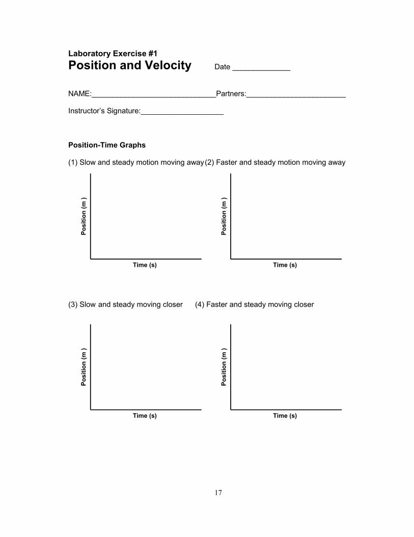
Position-Time Graphs 1. Open the file called Distance Graphs. Starting at about 0.5m from the detector (but

not closer), make a position-time graph by walking away from the detector slowly and steadily. Sketch the resulting graph (1) in the report sheet. Try to sketch only the section that best represents how you were trying to walk.

2. Repeat, but this time walk a little faster. Sketch graph (2). 3. Make a position-time graph by walking toward the detector, slowly and steadily.

Sketch graph (3). 4. Repeat Step 3, but this time walk a little faster. Sketch the graph (4) in the report

sheet.

Note: When you sketch these graphs, it is not crucial to include all the fine details. However, be sure to label and number the axes as they appear on the screen, and provide a title (e.g. Position vs. Time, Walking Away Slowly).

5. Sketch your prediction of the position-time graph on graph (5) produced by the

following: Starting 1.0 m in front of the detector, walk slowly and steadily away from the detector for 5 seconds. Stop for 5 seconds, then walk quickly and steadily toward the detector for 3 seconds.

6. Now test your prediction. Before you do, you need to increase the amount of time

that data will be collected. With the left mouse button, click once on the highest value of the time axis. When it is highlighted, type in the new value (about 15 for this exercise) and press Enter. Sketch the resulting graph on graph (6)

Note: The motion detector measures the distance of the object in front of it. The ultrasound wave spreads out over a 15-degree angle from the transducer. The sensor will not work properly if there are other objects in the vicinity of the track. Thus clear the bench top during the experiment and do not sit too close to the bench. The sensor must be in the upright position. To check the alignment, look into the sensor from the opposite end of the track from about 20 cm above the track. If you can see your eyes from the reflection, the alignment is correct.

14

(Does your result match your prediction? If not, make the necessary adjustments to your prediction and/or your motion until the graphs agree). 7. Now let us see if we can do the reverse, given a graph we want to move to match it. Open the file called Position Match, and you should see a graph on your screen that looks like this.

This plot will stay on the screen, and plots of your data will be superimposed on it. Walk in such a way to make your data look as much like the above plot as possible. Describe what you had to do (how you had to walk) in order to match the above graph.

Velocity-Time Graphs You have done exercises in which velocity changes over time. It would be useful to examine more directly how velocity varies with time for different types of motion. We can do this by generating velocity-time graphs. This is a bit more challenging. Irregularities in the motion show up more prominently on velocity graphs than on position graphs. Remember: you do not have to (and cannot) produce ideal, textbook-like graphs - no measurement is perfect. But at the same time, you are expected to do your best to obtain the best results possible within the limits of precision of the equipment. So be patient, be creative, and make adjustments to your experimental technique – generally you will see improvements. Repeat Steps 1-4, but this time make velocity-time graphs. To do this select the file Velocity Graphs. When you feel comfortable with your execution and with the results, sketch graphs (a) – (d) in the report sheets.

Position and Velocity We now want to study the relation between position and velocity. We want to get some numerical results, so instead of measuring the position and velocity of a moving person, we will measure the position and velocity of a moving cart instead. This will give us better data. Open the file Velocity from Position. You should see two sets of axes on the

15

screen, one for a position-time graph and another for a velocity-time graph. Put the motion detector on the track so that it can be used to take data from the cart. 1. Give the cart a push, and, after the push, start taking data. You will see both a position-time graph and a velocity time graph. By looking at the position-time graph, calculate the slope of the plot. You can do better if you use the Examine feature in the Analyze Menu of the software to read off values of position and time from the graph. Read off several pairs of points (about 5 or 6) and calculate (∆x)/(∆t) for each. Include these values in your lab report, and use them to find the average value of (∆x)/(∆t). 2. By looking at your velocity-time plot, find the average value of the velocity. Again, you can do better by using the Examine feature to read off several points and then find their average value. Do this and be sure to record the values you find. How does the average value of the velocity compare to the slope of the position-time plot. This tells us how to find velocity information from a position-time graph. 3. Suppose we want to find position information from a velocity graph. If an object is moving with a constant velocity, then the distance it travels between two times, t1 and t2, is just the velocity multiplied by (t2-t1). We can see if our graphs confirm this. Choose two times, which we shall call t1 and t2, and find the positions corresponding to them using the position-time graph and the Examine feature. Let us call these positions x1 and x2. Take your average velocity from the previous step and multiply it by (t2-t1). How does this compare to x2-x1? Do this for 3 pairs of points.

Post-Lab Check List

Before you leave the lab, make sure that you have the following data. All of it must appear in your lab report. Position-Time Graphs 1. 4 result graphs from steps 1-4 2. 1 prediction graph and one result graph from steps 5 and 6 3. 1 result graph from step 7 Velocity Graphs 4 result graphs Position and Velocity 1. 1 result graph from step 1 2. 5 sets of data from step 1 – each data set consists of 5 numbers: t1, t2, x1, x2, and (∆x/∆t) – and an average value of (∆x/∆t). 3. At least 5 values for the velocity, and their average value from step 2 3. 3 sets of data from step 3 Note: Your Lab report should include: 1. Front page: your original data sheet with your name, partners and date. Report not

acceptable if original data sheet was not signed by you instructor. (So... don't leave lab room without it.)

16

2. Additional pages with data and calculations in neat tabular form 3. Any graphs (none required for this lab report, however) 4. Answers to any questions 5. An Appendix made up of these pages from the lab manual. This relieves you from

having to rewrite the essential points of the procedure.

17

Laboratory Exercise #1 Position and Velocity Date ______________ NAME:______________________________Partners:________________________ Instructor’s Signature:____________________ Position-Time Graphs (1) Slow and steady motion moving away (2) Faster and steady motion moving away

Time (s)

Posi

tion

(m )

Time (s)

Posi

tion

(m )

(3) Slow and steady moving closer (4) Faster and steady moving closer

Time (s)

Posi

tion

(m )

Time (s)

Posi

tion

(m )

18

(5) Prediction

(6) Final Result

Superimpose the data of your motion displayed on the screen to recreate the following graph.

Describe what you had to do (how you had to walk) in order to match the above graph.

0

0.5

1

0 5 10 15

Posi

tion

(m)

Time(s)

0

0.5

1

0 5 10 15

Posi

tion

(m)

Time(s)

19

Velocity-Time Graphs (a) Slow and steady moving away (b) Faster and steady moving away

Time (s)

Velo

city

(m/s

)

Time (s)

Velo

city

(m/s

)

© Slow and steady moving closer (d) Faster and steady moving closer

Time (s)

Velo

city

(m/s

)

Time (s)

Velo

city

(m/s

)

Position and Velocity Relation Table I Data from the position-time graph Position, x

Time, t txVelocity∆∆

= (slope)

Average velocity =

20

Read five points (with units) from the velocity-time graph, calculate the average value, and compare to the average value of the slope in the position-time graph. Use the position, x1 corresponding velocity, v, at a given time, t1, to predict the position x2 at time t2. Do this for three pairs of points.

Online quiz.

21

LABORATORY EXERCISE #2

Acceleration

Objectives: To study the relation between position, velocity, and acceleration when the acceleration is constant. Equipment: Ultrasonic motion detector, track, cart, mass, pulley, strings, and a 20-gram cylindrical mass. Introduction: Velocity tells us how position changes with time, and acceleration tells us how velocity changes with time. If an object, like a cart, has a constant acceleration, then we can find what the acceleration is by calculating ∆v/∆t, where the velocity of the object changes by an amount ∆v in a time interval ∆t. The relation between acceleration and position is more complicated. In particular, the position of an object with constant acceleration depends not only on the acceleration, a, but on the initial position, v0 and initial position, x0, of the object as well. The exact relation is x(t)=(1/2)at2+v0t+x0 . Velocity and Acceleration Our first task is to understand the relation between velocity and acceleration. We will again use the cart on a track, but this time there will be weight attached to the cart that will make it accelerate. First we will look at the velocity and acceleration of the cart when it is speeding up, and then we will look at them when the cart is slowing down. 1. Set up the cart on the track with the pulley attached to the end of the track. The 20-gram weight is then attached to the cart through a string which is laid over the pulley. 2. Open the file called Speeding Up. On the screen you should see the axes for a position-time graph, a velocity-time graph, and an acceleration-time graph. 3. What you are going to do is to release the cart from rest with the weight lifted to the

height of the pulley, and the motion detector will collect data while the cart is moving. Before you do this, sketch in graphs (1) and (2) a picture of what you think the velocity-time graph and acceleration-time graphs will look like (hint: the weight gives the cart a constant acceleration). Now do it and see how the actual graph and your prediction compare. When you do the experiment, hold on to the cart until you are ready to take the data, and then release it (do not give it a push). Catch the cart as soon as the weight hits the floor and do not let it hit the end stop. Sketch the velocity-time and acceleration-time plots in graphs (3) and (4).

22

4. Use the Examine feature in the Analyze Menu to read off four pairs of points from the velocity-time graph. Calculate (∆v/∆t)=(v2-v1)/(t2-t1) for each pair, and find their average value. Now use the analysis feature to read off four points from the acceleration-time graph. Take the average of the acceleration values. How does your average acceleration compare to the average value of (∆v/∆t)? 5. Repeat what you just did, but with a mass in the cart. Plot the results in graphs (5) and (6) Again find the average value of (∆v/∆t) and the acceleration. Compare them to each other. What was the effect of adding the mass on the acceleration-time graph and on the velocity-time graph? 6. Now we want to try something a bit different. You are now going to start the cart (without a mass ) not too far from the motion sensor with the weight hanging on the string at about 2 cm from the floor. Give the cart a gentle push away from the motion detector. ( Push too hard can result in the weight hitting the pulley and make the analyze difficult.) The cart will move away from the motion detector, turn around and come back. Before you do this, sketch a prediction for the velocity-time and acceleration-time plots in graphs (7) and (8). Pay particular attention to what you think is going to happen to the velocity and the acceleration at the turning point. Now do the experiment and sketch the resulting velocity-time, acceleration-time, and position-time relation in graphs (9) (10) and (11). How do they compare to your predictions? Keep this data displayed on the screen – you are going to need it for the next part. Position, Velocity and Acceleration We now want to understand how position is related to acceleration and velocity when there is a constant acceleration. From class we know that the velocity should be a linear function of time, and the position should be a quadratic function of time. We want to figure out what those functions are for the data in our last run. The coefficients that appear in those functions are related to the acceleration, initial velocity, and the initial position. 1. Choose two points from your velocity-time graph, which should look something like a straight line, using the Examine feature in the Analyze Menu. Use them to find the equation for the line, i.e. if v=At+B, find A and B. You can check your values by using the Linear Fit in the Analyze Menu. ( To avoid the artifacts at the beginning and end of the graph, you may select a portion of the data for linear fit by pointing and dragging the curser over the range of interest.) What physical quantities do A and B represent? Is either one related to your acceleration graph? If so, compare the value you found for A or B to the relevant value on the acceleration graph. 2. Now go to the position-time graph. We want to find an equation for this curve, which should be something like a parabola. This means we should have, x(t)=At2+Bt+C. We want to find the coefficients A, B, and C. We can do this using the Curve Fit feature in the Analyze Menu. Go to it and select quadratic to fit your position-time data. You can then read off the values of A, B, and C. ( To avoid the artifacts at the beginning and end of the graph, you may select a portion of the data for curve fit by pointing and dragging the curser over the range of interest.) What physical quantities do A, B, and C represent? Are any of them related to either your acceleration graph or to your velocity-time graph? If so, compare the values you found here to the values you found from your acceleration

23

and velocity-time graphs.

24

LABORATORY EXERCISE #2 Acceleration Date ______________ NAME:______________________________Partners:________________________ Instructor's Signature:____________________ Velocity and acceleration Predict the velocity-time and acceleration-time relations when the cart is pulled by the weight. (1) (2)

Time (s)

Velo

city

(m/s

)

Time (s)

Acce

lera

tion

(m/s

/s)

Plot the experimental results with empty cart. Make sure to complete the scales of the axes. (3) (4)

Velo

city

( U

nit:

)

Time (Unit: )

Acce

lera

tion

( Uni

t:

)

Time (Unit: )

25

Read off four pairs of points from the velocity-time graph. Calculate (∆v/∆t)=(v2-v1)/(t2-t1) for each pair,

Velocity , v Time, t Slope

tva∆∆

=

Average value= Average of four acceleration values from the acceleration-time graph = How does your average acceleration compare to the average value of (∆v/∆t)? ______________________________________________________________________ Plot the experimental results with a mass in the cart. Make sure to complete the scales of the axes. (5) (6)

Velo

city

( U

nit:

)

Time (Unit: )

Acce

lera

tion

( Uni

t:

)

Time (Unit: )

26

Read off four pairs of points from the velocity-time graph. Calculate (∆v/∆t)=(v2-v1)/(t2-t1) for each pair,

Velocity , v Time, t Slope

tva∆∆

=

Average value= Average of four acceleration values from the acceleration-time graph = What is the effect of adding a mass on the acceleration? Sketch predicted velocity-time and acceleration-time graph for the procedures outlined in step (6). (7) (8)

Time (s)

Velo

city

(m/s

)

Time (s)

Acce

lera

tion

(m/s

/s)

27

Plot the experimental results with empty cart. Make sure to complete the scales of the axes. (9) (10)

(11)

Fit the velocity-time curve with the equation v=At+B and find A and B. What physical quantities do A and B represent? Is either one related to your acceleration graph? If so, compare the value you found for A or B to the relevant value on the acceleration graph.

Fit the position-time curve with x(t)=At2+Bt+C and read off the values of A, B, and C. What physical quantities do A, B, and C represent? Are any of them related to either your acceleration graph or to your velocity-time graph? If so, compare the values you found here to the values you found from your acceleration and velocity-time graphs. Online quiz.

Velo

city

( U

nit:

)

Time (Unit: )

Acce

lera

tion

( Uni

t:

)

Time (Unit: )

Posi

tion

(Uni

t:

)

Time (Unit: )

28

LABORATORY EXERCISE #3 Vectors

Objectives: To learn adding vectors by their components and to compare the calculation with an experiment. Equipment and Supplies Force table, three low-friction pulleys, mass hangers, mass set. Discussion Consider a vector A that lies in a plane. It can be expressed as the sum of two components. The components are usually chosen to be along two perpendicular directions. An example is shown in Figure 1. The vector A can be resolved in to its x- and y-components by drawing two lines perpendicular to the x- and y-axes. Then Ax and Ay are the x and y components of A, respectively. From Figure 1, Ax=A cosθ and Ay =Asinθ

. Figure 1

Consider then the addition of two vectors A and B to give a resultant vector C, as shown in Figure 2.

X

y

θ

Ax

AyA

X

y

θa

A

BC

θc

θb

29

Figure 2 C=A+B (1)

The x and y components of these three vectors satisfy the following relations: Cx = Ax + Bx (2) Cy = Ay + By (3) where Ax=A cosθa (4) Ay =Asinθ a (5) Bx=B cosθb (6) By =B sinθb (7)

The magnitude and angle of C can be determined by: C=( Cx

2+ Cy2)1/2 (8)

θ c= tan -1(Cy / Cx) (9)

In the present experiment, the methods of vector addition is used to study the condition of equilibrium for three forces on a force table. These forces are created by the weights attached to the mass hangers. The diagram of the vectors involved is illustrated shown in Figure 3.

Figure 3 When the sum of three is zero, the knot is at the origin. We have A+B+C = 0 (10) Forces A and B are created by the weights of two known masses. To determine the unknown force C, we can rewrite Equation (10) in the following form:

A

B

C=?

30

C= -(A+B) =(-A) + (-B) (11) Then the method described above can be directly applied to determine C. Procedure A Set up the force table on a level plane. Attached three pulleys on the rim of the round table. B. Hang the following masses on two of the pulleys and clamp the pulleys at the given angles: Force A : 20 g at 0° Force B : 10 g at 270° Place the third pulley (Force C) at 150° with 20 g on the hanger. Add masses to this hanger until the knot is centered at the origin. Due to a small friction in the pulley, you may help the gently tap the strings to help initiate the motion. To correctly calculate the forces, the mass of the hanger (5 g) must also be included in each force. The force in Newtons equals the mass multiplied by 9.8 m/s2. C. Place two pulleys at 0° with 200 g on the hanger and 210° with 250 g on the hanger. By trial and error, find the angle for the third pulley and the mass, which must be suspended from it that will balance the forces. Again, tapping the strings to help Record the angle and mass. Calculations and Conclusions 1. Calculate the magnitudes and the angles of the unknown vectors for the experimental

conditions of A to C. 2. Tabulate the calculated and measured results.

31

LABORATORY EXERCISE #3 Data Sheet: Vector Analysis Date:_____________ NAME:______________________________Partners:________________________ Instructor's signature:____________________ Procedure B

Force A

Force B Force C Experimental

Force C Calculated

A

θa B

θb C θc C θc

Kg

Kg

Kg

Kg

N

N

N

N Newton = 9.8 Kg x m/s2. Don’t forget to include the mass of the hangers into the calculation. Show the calculation of Force C using the space below.

32

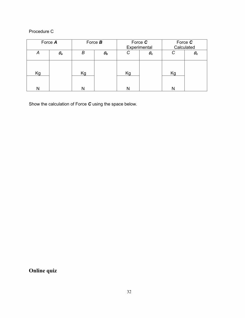
Procedure C

Force A

Force B Force C Experimental

Force C Calculated

A

θa B

θb C θc C θc

Kg

Kg

Kg

Kg

N

N

N

N Show the calculation of Force C using the space below.

Online quiz

33

LABORATORY EXERCISE #4

Tension Force and Motion Objectives: To understand the relation between the total force acting on an object and its acceleration. Equipment: Ultrasonic motion detector, force probe, track, cart, 20 g, 50 g, and 70 g masses, string, pulley wheel, and electronic balance Introduction According to Newton’s Second Law, the acceleration of an object is proportional to the total force acting on the it. In this experiment you will look at a situation in which the force is a tension force. A cart on a track will have a string attached to it, and the string will go over a pulley wheel and have a weight hanging from it. You will study the acceleration of the cart as a function of how much mass is hanging from the string. You have to be careful, though, because if the mass hanging from the string is m, then the tension in the string is not mg once the cart starts to accelerate. Before you come to this lab, you should work out the following problem: A cart of mass M moves on a frictionless track. It is attached to a string, which goes over a pulley wheel, and has a mass m hanging from it, as shown in Fig. 1.

m

M

T

Ta

mg

At t=0 s the cart starts from rest and accelerates. The tension, T, pulls the cart toward the pulley with an acceleration a given by

𝑀𝑀𝑀𝑀 = 𝑇𝑇 (1)

34

The weight m is also accelerating downward with the same acceleration give by

𝑚𝑚𝑀𝑀 = (𝑚𝑚𝑚𝑚 − 𝑇𝑇) (2)

The tension and acceleration can be calculated by solving the simultaneous equations. The results will be useful when you work on the report and online quiz. Procedure: 1. Open the file called Motion and Force. You should see three sets of axes on your screen, one set for a velocity-time graph, another for an acceleration-time graph, and one for a force-time graph. Before doing anything else you need to calibrate the force probe. Your instructor will show you how to do this. If at any point in the experiment your force readings start to look strange, you should go back and calibrate the force probe again. In addition, before each run, you should zero the force probe (your instructor will also show you how to do this). Procedure of sensor calibration

Click the blue-green button called Lab Pro Click Calibrate and CH1 (Channel 1) Click Perform Now Remove the string from the force probe so that the tension on the force probe is zero. Under Reading 1, set the force to 0 N, the click Save, Connect the string with a weight to the force sensor. Set the force value in Newtons. ( If 50g is used, fill in 0.49 N), then click Save Click Ok to close the window. Click the Zero button, Remove the weight to the force sensor and click zero force. Now the sensor has been calibrated.

2. Hold the cart, and attach the string to the hook on the force probe. Run the string over the pulley wheel and hang a 20 g mass from it. While still holding the cart, start the run, and continue holding the cart for 2 s or so. Then let the cart go. You should notice that the value of the force, which is the tension force in the string, changes when you let the cart go. Use the Statistics feature from the Analyze Menu to find the average value of the force both before and after you release the cart. In addition, use it to find the average value of the acceleration after the cart is released. Do this run three times and compute

35

the average value of your results for the tension force and the average value of your results for the acceleration. 3. Repeat step 2, but with 50 g and then with 70 g hanging from the string. Find the

average values of the tension force and the acceleration for each case. 4. Use the electronic balance to find the combined mass, M, of the cart and the force probe. The balance has a maximum range of 500 g. If balance shows “Error”, the cart and the force probe must be weighed separately. 5. Plot (by hand) your force and acceleration data. On the x axis plot the acceleration and on the y axis plot the tension force. You will have three points, one each for hanging masses of 20 g, 50 g, and 70 g. Fit the best straight line you can to your data, and find its slope. To what quantity should the slope correspond (assuming Newton’s Second Law is correct), and can you compare it to any other quantity you have measured? If you can, do so. Does your data support Newton’s Second Law? 6. If you have done the problem at the beginning of the lab, you should have a formula that gives you the tension force in terms of the combined mass of the cart and force probe and the hanging mass. Make a table comparing the calculated values for the tension and the measured values.

Post-Lab Checklist

Before leaving the lab you should have the following data: 1. Three values of acceleration and three values of tension (a value for each of the three runs) from step 2 2. Six values of acceleration and six values of tension from step 3 3. A mass from step 4 4. A graph and a slope from step 5

36

LABORATORY EXERCISE #4 Tension Force and Motion Date ______________ NAME:______________________________Partners:________________________ Instructor's Signature:____________________ Tension Before

Release

Tension After Release

Acceleration After Release

20g

Ave:

Ave: Ave:

50g

Ave:

Ave: Ave:

70g

Ave:

Ave: Ave:

Combined mass of the cart and the force probe =___________________

37

Plot measured tension force vs acceleration. Choose suitable scales and units and mark the axes clearly.

Fit the best straight line you can to your data, and find its slope. Slope=_____________________ To what quantity should the slope correspond (assuming Newton’s Second Law is correct), and can you compare it to any other quantity you have measured? If you can, do so. Does your data support Newton’s Second Law? If you have done the problem at the beginning of the lab, you should have a formula that gives you the tension force in terms of the combined mass of the cart and force probe and the hanging mass. What is the formula for T? When the cart is acceleration, is the tension always smaller than the weight of mass m? Is this consistent with your observation?

Tens

ion

(N)

Acceleration (m/s/s)

38

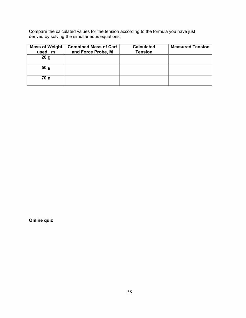
Compare the calculated values for the tension according to the formula you have just derived by solving the simultaneous equations.

Mass of Weight

used, m Combined Mass of Cart

and Force Probe, M Calculated

Tension Measured Tension

20 g

50 g

70 g

Online quiz

39

LABORATORY EXERCISE #5

Conservation of Energy

Objectives: To study when mechanical energy is conserved and when it is not Equipment: Ultrasonic motion detector, cart, track, friction block, electronic balance, meter stick Introduction In this experiment we are going to consider two kinds of energy, kinetic energy and gravitational potential energy, and their sum, which is the total mechanical energy. We are going to apply these concepts to a cart moving down an inclined track. The cart will start from rest, and then accelerate down the track. As it does, it speeds up, and its height above the table decreases. This means that its kinetic energy increases and its potential energy decreases. We want to see if these changes compensate each other so that their sum stays the same. The second part of the experiment is the same as the first, except that a friction block will be attached to the cart. We will again want to see if the mechanical energy is constant. From class you should remember that if an object of mass m is moving with a velocity v, then its kinetic energy is given by (1/2)mv2. An object of mass m, which is a height y above the origin, has a gravitational potential energy given by mgy, where g=9.80 m/s2. If there is no other source of potential energy around (like a spring, for instance), then the total mechanical energy of the mass is just the sum of the two, E=(1/2)mv2+mgy . If there is no friction present, this quantity will be conserved. If there is friction present, the mechanical energy will decrease, and we will have that (work done by friction)=(final mechanical energy)-(initial mechanical energy) . The work done by the friction force, Ff, is just –Ffs, where s is the distance the object moved. Because the work done by the friction force is negative, the above equation implies that the final mechanical energy is less than the initial mechanical energy. Procedure 1. Open the file called Inclined Ramp. Be careful, there are two of these, you want the one closest to the end of the list. You should see two sets of axes. The upper one is for a plot of total mechanical energy versus time, and the lower one is for a plot of the kinetic energy and the potential energy versus time. 2. Measure the length of the track, l, the elevation of the higher end, h, and the mass of the cart, M.

40

3. Go to the Data menu and then to the Modify Column feature. You will need to modify the equation for both the potential and the kinetic energy. In the equation for the kinetic energy replace 1 by the mass of the cart, which you measured. In the equation for the potential energy, replace the 1 by M(h/l). 4. You are going to hold the cart part of the way up the ramp and then let it go. Sketch you predictions for the kinetic energy versus time plot, the potential energy versus time plot, and the total mechanical energy versus time plot. Now do a run and sketch your results. 5. Derive an equation for the kinetic energy of a cart going down an inclined ramp in terms of h, l, g, and M. We want to compare it to an experimental curve. Open the file Kinetic Energy; you should see two sets of axes, one for a velocity versus time plot and another for a kinetic energy versus time plot. Do another experimental run, i.e. hold the cart part way up the ramp and let it go. You can use the Curve Fit feature (fit it with a quadratic function) from the Analyze menu to fit the kinetic energy versus time plot. Compare this to the result you derived. 6. Now attach the friction block to the cart. You are again going to hold the cart part of the way up the ramp and then let it go. Sketch you predictions for the kinetic energy versus time plot, the potential energy versus time plot, and the total mechanical energy versus time plot. Now do a run and sketch your results. 7. Use the fact that the change in the mechanical energy is equal to the work done by friction to find the value of the friction force acting on the cart. This force is due to the friction block. Use the electronic balance to find the mass of the friction block, and then find the coefficient of friction between the friction block and the track. Post-Lab Checklist Before leaving the lab you should have the following data: 1. From step 2 the length of the track, the elevation of the higher end, and the mass of the cart 2. Predicted and actual results for kinetic energy versus time, potential energy versus time and total mechanical energy versus time graphs from step 4 3. An equation for the curve fitted to your kinetic energy versus time data from step 5 4. Predicted and actual results for kinetic energy versus time, potential energy versus time and total mechanical energy versus time graphs from step 6 5. Values of the friction force and coefficient of friction

41

Laboratory Exercise #6

Collisions and Momentum

Objectives: To study the relation between force and change in momentum, and to determine whether momentum is conserved in inelastic collisions Equipment: two carts, two force probes, motion detector, electronic balance, masses Introduction Instead of writing Newton’s Second Law as F=ma, we can also write it as F=∆p/∆t. This means that if a constant force is acting on an object for a time ∆t, then its momentum will change by an amount F∆t. Let us assume that the force starts acting at a time t0. If we plot the force as a function of time, it will be zero until t0, F between t0 and t0+∆t, and then zero again after that. The area under the force versus time plot is just F∆t, which is the change in momentum. If the force is not constant, it is still true that the area under the force versus time plot will be the change of the momentum of the object. When two objects collide in the absence of external forces, Newton’s Third Law guarantees that the total momentum is unchanged. If the two colliding objects are object A and object B, then when they hit, the force exerted by A on B will have the same magnitude as the force that B exerts on A, but its direction will be opposite. This means that the change in momentum of object A will be the opposite of the change in the momentum of object B, so that the sum of their changes in momentum is zero. Therefore, the total momentum before the collision is the same as the total momentum after the collision. In terms of equations, if pA=mAvA is the initial momentum of object A pB=mBvB is the initial momentum of object B, PA=mAVA is the final momentum of object A, and PB=mBVB is the final momentum of object B, then pA+pB=PA+PB . In this lab, we want to verify Newton’s Third Law, show that the change in momentum is equal to the area under the force versus time graph, and study momentum conservation in an inelastic collision. The collision will involve two carts, one initially moving and the other sitting still, that stick together when they hit. This means that if the initially stationary cart is object B, then vB=0 and VA=VB. Procedure 1. You should have two cars with force probes mounted on them. Place them both on the track with the parts sticking out of the force probes facing each other. Open the file Collisions; you should see two sets of axes on the screen, a force versus time plot for each force probe. You are going to push the carts together (gently!) so that that they collide. The force probes will hit each other and measure the forces on each of the carts. Sketch predictions for what the force versus time plots for each cart will look like. Zero all

42

sensors by clicking the button “Zero all sensors” before every measurement. Now do the experiment and sketch the results. 2. Now place a mass in one of the carts and repeat step 1. What do your results tell you about Newton’s Third Law? 3. Now open the file Impulse and Momentum. You should see two sets of axes, one for a velocity-time plot and one for a force time plot. The force probe that will be recorded is the one that goes into channel 2. You are going to start with one cart moving and the other standing still, and then they will collide. The force probe going into channel 2 should be on the car that is initially motionless, and the motion detector would also be recording the motion of this cart. After doing the experiment what you will see is a plot of the force acting on the initially motionless cart and a plot of its velocity. Sketch a prediction for what you think these plots will look like. Zero all sensors. Now do the experiment. Sketch your results. 4. We now want to see if the change in the momentum of the initially motionless cart was equal to the area under the force versus time plot. Use the electronic balance to find the mass of the cart that was initially at rest, and then make use of your velocity-time plot to find change in momentum of this cart due to the collision. This is just the momentum after the collision minus the momentum before the collision. Now use the Integrate feature in the Analyze Menu to find the area under the Force time plot. Compare this area to the change in momentum. Do this again, i.e. collide the carts again and compare the change in momentum to the area under the force-time plot. 5. Inelastic collision: Remove the force probes from the carts making sure not to lose any screws. Find the mass of each cart by using the electronic balance. Open the file Inelastic Collision, and you should see axes for a velocity-time plot on the screen. Notice that on each cart there are velcro pads on one end. You want to have one cart initially moving and one initially at rest so that the two velcro ends are facing each other. This will cause the two carts to stick together when they hit (again, gently!). The motion detector should be on the same side of the track as the initially moving cart. When you start the experiment, the motion detector will see the initially moving cart, and, after the collision, it will see the two carts moving together. You can use the velocity data to find the momentum before and after the collision. Now do the experiment and compare the initial and final momentum. 6. Repeat step 5 except with a mass in one of the carts. Post-Lab Checklist Before leaving the lab you should have the following data: 1. Two predicted and two actual force versus time plots from step 1 2. Two predicted and two actual force versus time plots from step 2 3. One predicted and one actual force-versus time plot, and one predicted and one actual velocity-time plot from step 3 4. Two values of the area under the force-time graph and two values of the change in momentum from step 4

43

5. Values of initial and final momentum from step 5 6. Values of initial and final momentum from step 6

44

LABORATORY EXERCISE #7

Density; Significant Figures Objectives To become familiar with instruments to measure length (meter stick, vernier caliper, micrometer) and to appreciate the difference between accuracy and precision of experimental measurements. Incidentally, to learn the concept of mass density, and practice proper use of significant figures. Equipment and Supplies Metal samples, electronic balance, meter sticks (long and short), vernier caliper, vernier model, micrometer calipers. Discussion The mass density of a body measures the amount of mass per unit volume of that body. Definition: Density of a body = (body's mass)/(body's volume) or D = M / V The density of a substance does not depend on the shape or the particular amount of that substance. For example, the density of a small gold ring and the density of a large gold brick should be the same number, i. e., the density of gold. As part of your density calculations you will need to compute the volume of a regular solid from its linear dimensions. The quality of your volume measurements will thus depend on how precisely you can measure lengths. You will use three progressively more precise instruments: a wooden "meter stick", vernier calipers and a micrometer. Your instructor will demonstrate how to use each one. In each case, you should read the instrument to the smallest division plus one more digit by estimation. So, a meter stick with millimeter markings can be used to estimate a length to the nearest tenth of a millimeter, e.g., 12.4 mm, or 1.24 cm. This estimate by "eye" is often only good to ±2 or 3, as you can verify by repeating the measurement or asking your partner to do the estimating. A vernier is an invention that removes the uncertainty in reading to the nearest tenth between adjacent markings, thus increasing the precision of the final measurement. Your instructor will demonstrate how this is done with the vernier model, prominently displayed in the front of the laboratory room. On Errors and Uncertainty in a measurement:

45

When you work out a math computation, the numbers are usually considered exact, e.g., 1.1 x 1.2 x 1.3 = 1.716. But when a number represents a physical measurement it is never exact because of the limitations of the instrument used, or the way it was employed, etc. It is essential, therefore, that each experimental result be presented in a way that indicates its reliability. A very simple way to do this is by the use of significant figures. (See Tutorial #1, on Significant Figures) As an example, consider how different the following three cases are, even though they refer to exactly the same steel block:

a) 1.1 cm x 1.2 cm x 1.3 cm = 1.7 cm3

b) 1.13 cm x 1.20 cm x 1.29 cm = 1.75 cm3

c) 1.127 cm x 1.195 cm x 1.293 cm = 1.741 cm3 What is different about these three reports, is the precision with which the data was taken. (By the way, all three workers used significant figures correctly.) Now, how accurate are the results? This concept reports on how close the reported answer is to the "accepted answer". What determines accuracy? Examples are the calibration of the measuring instruments or systematic errors on the part of whoever is taking the data. The following somewhat oversimplified table may be useful in thinking about these concepts:

Problem Remedy _______________________________________ Mistakes and blunders Repeat measurements several times to check on

yourself

Systematic errors Use calibrated instruments, use them properly

Random errors Treat data statistically and report on the average magnitude of errors

Procedure A. Estimating the number of kilograms of air contained in this room when it is empty. Estimate the volume of the room by the following procedure. First measure the height, width and length ignoring protruding structural columns. Use the long meter sticks, and make full use of the geometric tiles on the floor (they are very nearly 12" x 12"). The resulting volume yields the mass of the air when multiplied by the density, 1.29 kg/m3. Your answer here should reflect the number of significant figures of your raw data. B. Finding the density of a metal block. First weigh the block carefully with the balance provided. Then, measure the dimensions of the block with three different instruments: B1. Use of meter stick. Lay block on meter stick, measure the position of each edge, estimating to the nearest 0.1 mm. Take several readings on different parts of the

46

specimen. B2. Use of vernier calipers. Examine the calipers. What is the distance corresponding to the smallest markings on this instrument? How many significant figures can be obtained when measuring a length between 1 and 10 cm? Is the "zero" calibrated correctly, or do you need to correct for a misalignment? Take several readings on different parts of the specimen, estimating to 0.01 mm. B3. Use of micrometer calipers. Examine this fine instrument, noting the proper use of the slip clutch to prevent forcing the gears. What is the distance between smallest markings on the shaft? Open the jaws to the 1-mm mark. Rotate the micrometer thimble through two revolutions: record the reading. Rotate by one revolution. Record the reading again. Careful consideration of your data should lead you to understand how the micrometer can be read correctly to 0.001 mm. When you are satisfied that you can use and read this instrument, obtain several readings of each of the three dimensions of the metal block. Note any misalignment of the "zero" and correct your data accordingly. B. Repeat procedure B for a cylindrical metal block, time permitting. Calculations and Conclusions A. Complete and sign the statement in the Data Sheet . B. For each of the three methods in part B, compute the density of the metal block to the appropriate number of significant figures. 1. Are the three results consistent with one another? What criteria did you use to answer the question? 2. For your best value of the density, compute the percent deviation from the accepted value (obtained from your instructor). Note on the "propagation of errors":

The equation for the volume of a rectangular solid is hwlV = Applying our rule for products, that means that the fractional error of the volume is just the sum of the fractional errors of the for the length, width and height. You can use this to find the uncertainty, ∆V, in the volume itself.

2

2

2

2

2

2 )()()(hh

ww

ll

VV ∆

+∆

+∆

=∆

*Just ONE significant figure is appropriate, here.

47

48

LABORATORY EXERCISE # 8

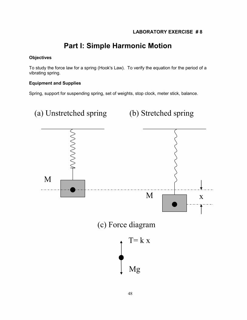
Part I: Simple Harmonic Motion Objectives To study the force law for a spring (Hook's Law). To verify the equation for the period of a vibrating spring. Equipment and Supplies Spring, support for suspending spring, set of weights, stop clock, meter stick, balance.

x

(a) Unstretched spring (b) Stretched spring

(c) Force diagram

M

M

T= k x

Mg

49

Discussion When a stretching force F is applied to a spring, the elongation of the spring x is found to be proportional to F if the elastic limit is not exceeded. The force is a restoring force, i.e., always opposite to the displacement. This empirical law is called Hook's law:

F kx= − where k is called the force constant, or the stiffness of the spring. The general equation of motion for the mass M with acceleration a which is vertically hung from the spring as seen in the figure is

Ma Mg kx= − within the elastic limit. Here, we completely neglect the mass of the spring which in our experiment is much smaller than the mass attached. (1) If the mass M is in an equilibrium state, the equation is reduced to

Mg kx=

since a = 0 . The elongation x of the spring can be measured as a function of the weight hung on it when varying the mass M of the suspended weight F Mg= and a plot of F vs x is a straight line, as illustrated below.

The slope of the straight line is the stiffness k of the spring. In the MKS units it is N m/ . (2) If a mass, M, hung from the end of an elastic spring is pulled down and released, it will oscillate up and down. This is an example of simple harmonic motion. The acceleration a

Forc

e F

(N)

Elongation x (m)

50

must not be neglected since the mass is not in equilibrium. In this case the equation of motion is rewritten as

′′ + =xkM

x g

where ′′ =x a and the displacement at time t is

xg

A t= + −ω

ω δ2 cos( )

where ω =kM

depends on the mass M and the stiffness of the spring. If the time t is

replaced by t+2π ω/ , then the displacement x is unchanged. This means that the displacement has the same value after time T,

TMk

= =2

2πω

π .

This is the period of the oscillation. A is the amplitude of the oscillation and δ is determined by the initial displacement of the mass. Actually, since all parts of the spring also execute simple harmonic motion, the mass of the spring needs to be included in some way. Since not all parts of the spring execute the full motion, it turns out that m', the "effective mass" of the spring is just 1/3 of the full inertial mass, m. So, the parameter M should be the sum of the mass of the hung weight, M0, plus 1/3 of the mass of the spring:

M = M0 + m' = M0 + m/3 where, M0 is the mass of the suspended weight, m is the mass of the spring, and m' is the effective mass of the spring ( m' = m/3). Procedure 1. F vs. x data. Measure the elongation x of the spring as a function of the weight hung on it. Vary the mass of the suspended weight from 200 grams to 800 grams in 100 g steps. Take the position when 200 g is suspended to be zero displacement ( the origin). Do not exceed 800 g. 2. T vs. M data. Hang a mass of 200 grams from the spring and make at least three determinations with a stop clock of the time for 50 complete oscillations of the mass. Use a different initial amplitude in each determination. Repeat with masses of 350, 550 and 700 grams.

51

Calculations and Conclusions A. From the data in Procedure 1, calculate analytically and graphically the force constant of the spring and compare the two values. The analytic calculations involve using Hook’s law for each of your data points. The graphical method involves plotting F vs. x, and measuring the slope of the best straight line through the data points (see the sketch above). B. Plot T2 vs. M, i.e., the square of the period on the vertical axis and the mass of the suspended weight on the horizontal axis. From the graph, calculate the value of the stiffness k. C. Compare the values of k found in A and B. This means, by what percent do they differ? Now, in summary, considering both measurements, what is the precision (expressed as a percent) of your measurement of k ? D. Does the period of simple harmonic motion depend on the amplitude? How well does your data justify your answer ?

52

LABORATORY EXERCISE # 8

Part II: The Simple Pendulum Objective To study how the period of a simple pendulum depends on its length. To measure the acceleration due to gravity in the laboratory room. Equipment and Supplies Metal sphere suspended by a fine string, stop clock, meter stick, vernier calipers. Discussion A simple pendulum is one where all the mass is concentrated at a small "bob". A good approximation is made by using a massive weight held with a light string from a sturdy support. If the motion is restricted to "small angles", the motion is closely simple harmonic. T, the period of the motion, depends only on the length of the string, and the acceleration of gravity. Surprisingly, the period does not depend on the value of the

suspended mass: where, T is the period of oscillation.

L is the distance from the support point to the center of the massive bob, and g is the local acceleration due to gravity.

Procedure 1. T vs. L data. Adjust the pendulum so that L is about 100 cm. Measure L using the meter stick and vernier calipers. Determine the time for 50 oscillations with the amplitude of motion less than 10°. 2. Repeat Procedure 1. using a length approximately 30 cm, and again with L about 60 cm. Calculations and Conclusions A. Plot your data as T2 vs. L. The theory, given by Eq. (1), predicts that your data points should fall on a straight line of slope 2π/g. Thus by measuring the slope of the best straight line fit, you can pull out the value of g in the lab. What is the value of g you obtain, and what is the precision you claim for your measurement ( expressed as a

)1(2gLT π=

53

percent) ? B. You have just finished measuring g, the acceleration due to local gravity. Express your result as in the form wxy ±z %. In exercise #2, several weeks ago, you also measured g, using an entirely different method. For the two results summarize the following information:

a) claimed precision

b) agreement with accepted value Do the two results agree? The key here is the criterion you used to answer the question. Add any further relevant comments.

54

LABORATORY EXERCISE # 9 The Sonometer: Vibrations of a Taut String INTRODUCTION When you pluck a taut fixed string of length L, the resultant vibrations are a superposition of many simpler "standing wave" patterns, depicted below:

Note that, in general, λn = 2L / n, and fn = nf1, meaning that all harmonics are an integer multiple of a fundamental frequency, f1. Also note, that the place on a standing wave where there is no vibration is called a node, and the place where there is maximum amplitude is called an antinode. PURPOSE In this exercise you will excite and study the first few vibrational modes of the taut string. You will use a sonometer, a single-string "musical" instrument. See figure below.

55

EQUIPMENT AND SUPPLIES 1. Sonometer from Pasco Scientific Company. This instrument allows a known tension to be placed on a guitar string whose vibrating length can be varied between movable "bridges." 2. A function generator. It can "drive" an electromagnet with AC current in the lower audio range. Note: The guitar string will be attracted to the AC electromagnet twice each AC cycle, because both the North and South poles are equally good at attracting the steel string. 3. "Detector" coils capable of picking up the AC motion of a steel string. 4. A dual-trace oscilloscope to display both the driving frequency and the detected string vibrational frequency. PROCEDURE A1. Set up the sonometer system. Set the bridges 60 cm apart. Hang a 2 kg mass from the tensioning lever. Adjust the string tensioning knob so the tensioning lever is horizontal. A2. Position the driver coil about 5 cm from one of the bridges and the detector about 35 cm away from the same bridge. A3. Gently pluck the string with a fingertip. The detector coil will pick up an induced voltage which you can see displayed on the oscilloscope. You can excite different waveforms by plucking in different places or with a different technique. Play with this a while. You are seeing a different mix of excited harmonics (another

56

name for the different modes corresponding to different values of n.) Note: If the oscilloscope does not display, adjust the TRIGGERING: all three levers in the upper right corner should be flipped up, and the level knob pulled out (auto mode.) Also, adjust the trace position knobs as necessary. A4. Set the signal generator to produce a sine wave and set the gain of the oscilloscope of channel B to 5 mV/cm. A5. With the function generator amplitude set at about 12 o'clock slowly increase the frequency of the signal to the driver coils, starting from about 5 Hz. (This part will require a gentle hand and some patience.) Listen for an increase in sound from the sonometer and/or an increase in size of the detector signal on the oscilloscope screen. Frequencies that result in maximum string vibrations are the resonant frequencies. Determine the lowest frequency at which resonance occurs. This is the first or fundamental mode (n = 1). Measure this frequency and record it on the data sheet provided. Note: Because of the effect noted in the equipment section, the resonant frequency is twice the driving frequency. Note: For the n = 1 mode, you should actually hear the sonometer hum and produce enough amplitude vibration to clearly see the central antinode and the nodes at the bridges. A6. Continue increasing the frequency to find successive resonant frequencies for each mode - at least five or six. For each resonant mode you find, locate all the nodes, and record the distance between adjacent nodes. There are two ways to locate notes: 1. Use the "detector" provided as follows: Start with the detector as close as you can to the free bridge. Watch the oscilloscope display as you slide the detector slowly along the vibrating string. When you reach a node, the amplitude on the scope will drop to a minimum. (This method breaks down when you get too close to the "driver" and start to

57

pick up its field directly.) 2. Use your fingers. Watch the oscilloscope display as you slide your fleshy fingertips along the vibrating string. Even a light touch will kill the vibrations everywhere except when you touch a node, where there is no vibration to kill, in any case. (Make sure that the detector is not accidentally left under a node, or this won't work.) A7. From your results, determine and record the wavelength of each resonant mode you find. Make use of the fact that the wavelength is twice the distance between adjacent nodes. B1. Repeat the experimental procedure A, for a string length of 50 cm, obtained by moving one or both of the bridges. Compute the average value, and quote the uncertainty of your measurement as a percent.

58

LABORATORY EXERCISE # 10

The Mechanical Equivalent of Heat Objective The purpose of this Laboratory Exercise is to prove the mechanical equivalence of heat and to verify that 1 kcal = 4186 Joules. Equipment and Supplies Commercial apparatus is provided which consists of the following: 1. An aluminum cylinder whose specific heat you know, whose mass you will soon measure, and whose temperature is conveniently sensed by a built-in thermistor. [A thermistor is a resistor whose resistance varies with temperature]. You are provided with a digital ohmmeter and a Table to tell you what temperature corresponds to what resistance. This often requires interpolation. If you are rusty on interpolation, ask your instructor. 2. A hand-crank and digital counter to record the number of revolutions. 3. A nylon rope with a "10 kg" weight at one end. The rope is wrapped a few times around the aluminum cylinder so that tangential frictional forces are set up between rope and aluminum cylinder when you turn the crank. CAUTION: Allowing the 10 kg weight to rise more than a few inches off the floor is dangerous both to student feet and to the delicate one-way digital counter. CAUTION: The Proper Procedure for turning and stopping the crank will be demonstrated by your instructor. It may look simple enough, but in fact it is easy to hurt yourself or damage the equipment. Respect this warning! Discussion Mechanical Work, which for linear motion is simply "force times distance", takes on the following expression for circular motion: W = (Torque) x angle, W = (Tangential force x Radius) x angle, W = F⋅R⋅θ, where θ is in radians. For example, a force of 2.00 N acting for one complete revolution (2π radians) around a circle of radius 1.00 meter does an amount of work given by, W =F⋅R⋅θ= (2.00 N)(1.00 m)(2π radians) = 4π J = 12.6 Joules. The heat energy Q transferred to a body of mass m and heat capacity c, will raise its

59

temperature by an amount ∆T degrees, where Q = mc∆T For example, if the temperature of 0.10 kg of Aluminum (c = 0.220 kcal/kg °C) is seen to rise from 21.5 °C to 38.5°C, we can conclude that an amount of heat Q must have been added to the aluminum, where Q = m c∆T = (0.10 kg)(0.220 kcal/kg°C)(38.5°C - 21.5°C) = 0.38 kcal. Procedure A. Introduction: A1. Familiarize yourself with the apparatus. Find all the parts in the diagram below.

A2. Note how sensitive the thermistor resistance is to the touch of your hot little hands, and how quickly or slowly thermal equilibrium is approached. Now you know the timescale of the response of this equipment. A3. When confident, unscrew the black knob that holds the aluminum cylinder in place and weigh the cylinder. Measure its diameter alone, and the diameter of the cylinder plus rope, when tightly wound. A4. Weigh the "10 kg" mass to 3 significant figures.

60

B. "Quick and Dirty" Run B1. Note the approximate initial temperature of the aluminum cylinder. Look-up what thermistor resistance corresponds to a "target" final temperature about 8 Celsius degrees higher. Your aim is to do enough mechanical work to heat up the aluminum cylinder to the target temperature. B2. Reset the counter. Enter the actual initial temperature in your data sheet and start cranking vigorously! Now you are finally getting "physical" in your physics class! B3. When you get to your target temperature, stop cranking BUT DO NOT LET GO OF THE CRANK. Allow the "10 kg" weight to drift to the floor before slowly returning the crank to its equilibrium position. Do not let go prematurely or the crank will snap back, possibly damaging the plastic clicker and invaluable body parts. Continue to watch the thermistor resistance carefully and enter in your data sheet the lowest value (highest temperature) it drifts to. B4. Record the total number of turns and complete the calculations called for in your data sheet. C. Serious Run Even when done by an expert student, one of the major sources of error in Procedure B is that some of the heat generated will go to heat up the surroundings rather than the aluminum cylinder. To counteract this, in this procedure you will precool the cylinder so that during your run the temperature of the block will be as much below room temperature as above it. Then there should be as much heat gained from the surroundings as lost to them. It is by tricks of this nature that successful experiments are accomplished. C1. Note the temperature of the room. Plan your target initial and final temperatures to be about 8°C below and above room temperature, respectively. C2. Remove the aluminum cylinder and cool it in the ice chest provided. Use plastic baggies, if available, to prevent wetting. You may not need to cool it all the way to 0°C. In any event, the heat from your hands can now be skillfully used to make-up for too much precooling. NOTE: Carefully dry any condensed water from the aluminum cylinder with the tissue paper provided. Do this before re-wrapping the friction rope. Evaporating water could carry away a considerable amount of heat; heat that would otherwise go to warm up the aluminum. Now, re-assemble the apparatus, reset the counter and get ready. Watch the ohmmeter carefully as the thermistor resistance drifts toward your predesignated "target" for the initial temperature. When it gets there, start cranking vigorously. Crank until the temperature reaches approximately one degree short of your designated final temperature. Then crank slowly until you reach your target. Record the actual maximum temperature (minimum resistance) reached. Record the total number of turns. REMEMBER THE SAFE STOPPING PROCEDURE. A MISTAKE CAN RESULT IN

61

YOUR HURTING YOURSELF. C3. Compute the work done, the heat input, and the mechanical equivalent of heat as guided by your data sheet. Compute the percent deviation from the accepted value. D. Consider the possible reasons (mechanisms) why your answer is different from the accepted value. Do you have any suggestions to improve this experiment? Resistance versus Temperature for your thermistor: Res. T Res. T Res. T Res. T (Ω) (°C) (Ω) (°C) (Ω) (°C) (Ω) (°C) 351,020 0 95,447 26 30,976 52 11,625 78 332,640 1 91,126 27 29,756 53 11,223 79 315,320 2 87,022 28 28,590 54 10,837 80 298,990 3 83,124 29 27,475 55 10,467 81 283,600 4 79,422 30 26,409 56 10,110 82 269,080 5 75,903 3 25,390 57 9,767.2 83 255,380 6 72,560 32 24,415 58 9,437.7 84 242,460 7 69,380 33 23,483 59 9,120.8 85 230,260 8 66,356 34 22,590 60 8,816.0 86 218,730 9 63,480 35 21,736 61 8,522.7 87 207,850 10 60,743 36 20,919 62 8,240.6 88 197,560 11 58,138 37 20,136 63 7,969.1 89 187,840 12 55,658 38 19,386 64 7,707.7 90 178,650 13 53,297 39 18,668 65 7,456.2 91 169,950 14 51,048 40 17,980 66 7,214.0 92 161,730 15 48,905 41 17,321 67 6,980.6 93 153,950 16 46,863 42 16,689 68 6,755.9 94 146,580 17 44,917 43 16,083 69 6,539.4 95 139,610 18 43,062 44 15,502 70 6,330.8 96 133,000 19 41,292 45 14,945 71 6,129.8 97 126,740 20 39,605 46 14,410 72 5,936.1 98 120,810 21 37,995 47 13,897 73 5,749.3 99 115,190 22 36,458 48 13,405 74 109,850 23 34,991 49 12,932 75 104,800 24 33,591 50 12,479 76 100,000 25 32,253 51 12,043 77

62

LABORATORY EXERCISE # 11

Boyle's Law Objectives To study how changing the pressure on a gas makes the volume change. To compare your results with those obtained by Bobby Boyle. Equipment and Supplies A sample of air trapped at the bottom of a glass tube by a short column of mercury. A ruler to measure the length of the air column. A barometer somewhere in the room. Discussion According to Robert Boyle, if the temperature of a fixed amount of gas is not allowed to change, the following relationship will hold as the volume, V, and the pressure, P, are changed: P⋅V = a constant number (1) The value of the constant depends on the number of moles of gas, the temperature, and the particular units used to measure Pressure and Volume. Boyle's Law accurately describes the constancy of the pressure-volume product for most common gases at moderate temperatures and pressures. Deviations from this Law may become significant if the pressure is too high or the temperature is too low. These limiting values vary drastically with different gases. For example, hydrogen obeys Boyle's Law at -200°C and 100 atmospheres; sulphur dioxide does not at 20°C and 1 atmosphere. The apparatus for this experiment is elegant in its simplicity. The short mercury column in the glass capillary serves two purposes. First, it serves as a leak-proof piston to isolate your gas sample. Second, it provides additional pressure on the gas sample as the glass tube is inclined. By varying the vertical orientation of the glass tube, you can vary the pressure of the gas sample. To see how this works, note that the absolute pressure of the enclosed air in Figure (1a) is,

P = Patm + ρg (Y1 - Y2) (2) where Patm = atmospheric pressure,

ρ = the density of mercury, 13,000 kg/m3, and Y1 and Y2 = the vertical heights of the ends of the mercury column.

If atmospheric pressure is expressed in centimeters of mercury, call it B cm of Hg, (obtained directly from the mercury barometer at the end of your lab room) then the

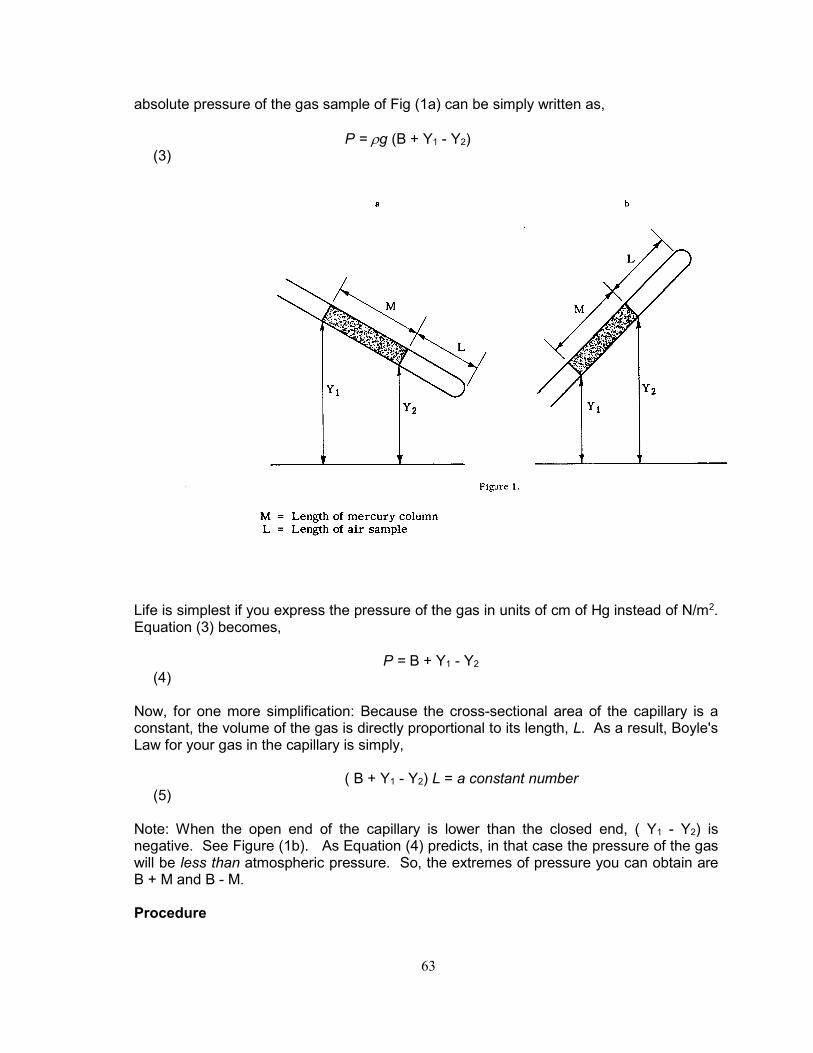
63

absolute pressure of the gas sample of Fig (1a) can be simply written as, P = ρg (B + Y1 - Y2) (3)

Life is simplest if you express the pressure of the gas in units of cm of Hg instead of N/m2. Equation (3) becomes, P = B + Y1 - Y2 (4) Now, for one more simplification: Because the cross-sectional area of the capillary is a constant, the volume of the gas is directly proportional to its length, L. As a result, Boyle's Law for your gas in the capillary is simply, ( B + Y1 - Y2) L = a constant number (5) Note: When the open end of the capillary is lower than the closed end, ( Y1 - Y2) is negative. See Figure (1b). As Equation (4) predicts, in that case the pressure of the gas will be less than atmospheric pressure. So, the extremes of pressure you can obtain are B + M and B - M. Procedure

64

1. Measure atmospheric pressure in cm of Hg using the classroom barometer. Locate the barometer, examine its parts. Adjust the barometer so that the surface of the mercury in the cup at the bottom of the instrument just touches the apex of the ivory cone. This marks the zero point of the barometer scale. Next, align the lower surface of the vernier slide with the top of the mercury column. (Use the top of the meniscus). Record the mercury level in your Data Sheet. Some days the pressure can change measurably during the course of the experiment; take another reading at the end of the lab period and use the average value if you notice a change. 2. Measure the length of the air column as you vary the pressure of the gas. For ten positions of the apparatus, chosen to yield approximately equal increments of pressure, record the length, L, of the air column, and the heights Y1 and Y2. Two of the positions must correspond to the extremes of pressure. Note: The best way to measure L is to measure the positions of the endpoints of the air column, L =X1 - X2. Calculations and Conclusions 1. Plot P vs. L and P⋅L vs. L on a single sheet of graph paper. Calculate the product P⋅L for each value of L you chose, then plot the graphs requested. Suppress the origin of the abscissa so that the range of L observations covers the horizontal scale. Do not suppress the origin of the ordinates, otherwise the experimental errors will be magnified on the graph. Draw a smooth curve through the P vs. L points. Draw the best straight line through the P⋅L vs. L points. Which graph is better suited to judge how well your data follows Boyle's Law? 2. Plot P vs. 1/L. Draw the best straight-line fit through the origin, representing "the theory", i.e., Boyle's Law. How well does your data follow the accepted theory? Comment on possible reasons for disagreement, if there is any in your case.

65

66

LABORATORY EXERCISE # 12

Part I: Heat of Fusion of Ice Objective To determine the heat of fusion of ice by the method of mixtures. Equipment and Supplies Calorimeter, balance, thermometer, ice cubes. Discussion The change of a substance from the solid to the liquid state, called melting or fusion, takes place at a definite temperature characteristic of each substance. During the transition no change in temperature occurs. To bring about this change of state a definite amount of heat must be supplied from the surroundings for each unit mass melted. This quantity of heat is called the (latent) heat of fusion of the substance. Thus the amount of heat required to melt a solid of mass m and heat of fusion Hf without changing its temperature is mHf . This is also the amount of heat given up to the surroundings when the liquid changes to the solid state. In the metric system Hf is measured in calories/gram or kilocalories/kilogram. (Numerically these are the same. ) If two substances at different temperatures are mixed in a container thermally insulated from its surroundings, the final temperature of the mixture will be between the original temperatures. From the principle of the conservation of energy, the heat lost by the warmer substance must equal the heat gained by the colder:

Heat gained by colder body = Heat lost by warmer body To determine the heat of fusion of water by this method of mixtures, a piece of ice at 0° C is dropped into a calorimeter containing warm water. The initial temperature of the water, its final temperature after being cooled by the ice and the masses of the ice, warm water and calorimeter are measured. If the specific heat of the calorimeter is known, the heat of fusion of water may be determined using the fact that the heat absorbed by the ice in melting, plus the heat needed to raise the temperature of the resulting cold water to the final temperature of the mixture equals the heat lost by the warm water and calorimeter:

[ m Hf + m c ∆T ]ICE = [ m' c ∆T '']WARM WATER + [ m" c" ∆T'']CALORIMETER Here, m, m' and m'' are the masses of the ice cube, the warm water and the calorimeter, respectively. Also, c and c'' are the specific heats of water and aluminum. Finally, ∆T is

67

the temperature rise of the ice, while ∆T '' is the temperature fall of the warm water. Procedure 1. Weigh the inner calorimeter vessel and stirrer, fill it approximately two-thirds full of water about five degrees above room temperature and weigh again to determine the mass of the water. Place the calorimeter vessel inside the calorimeter and insert a thermometer to determine the temperature of the water and vessel. 2. Stir the water in the calorimeter well and record its temperature. Dry an ice cube, place it in the water, replace the calorimeter cover and, when the ice has melted, stir the water and record its final temperature. 3. Weigh the calorimeter vessel, stirrer and contents to determine the mass of the ice used. Calculations and Questions A. Calculate from your data the heat of fusion of water. B. Compare the value found in A and the generally accepted value for the heat of fusion of water. C. Why was it desirable to have the initial temperature of the water slightly above the temperature of the room? Note: The data sheet for this experiment and the next are combined into one. You will find it following the next experiment.

68

LABORATORY EXERCISE # 12

Part II: The Specific Heat of a Metal Objective Determine the specific heat of a metal by the method of mixtures. Equipment and Supplies Calorimeter, steam boiler, metal shot, balance, two thermometers, small beaker. Discussion The "specific heat", c, of a substance is the amount of heat required to raise the temperature of a unit mass one degree. If the specific heat is independent of the temperature**, the amount of heat, Q, required to raise the temperature of a substance whose mass is m and whose specific heat is c, from an initial temperature Ti to a final temperature Tf , is,

Q = m c ( Tf - Ti ) = m c ∆T Since the calorie (kilocalorie) is defined as the amount of heat required to raise the temperature of 1 gram (1 kilogram) of water 1° Celsius from 14. 5° to 15. 5°, the specific heat of water is 1 cal/gm °C (1 kilocal/kgm °C). If two substances at different temperatures are mixed in a container thermally insulated from its surroundings, the final temperature of the mixture will be between the original temperatures. From the principle of the conservation of energy, the heat lost by the warmer substance must equal the heat gained by the colder:

Heat gained by colder body = Heat lost by warmer body.

** Specific heats actually vary slightly with temperature. However, for the range of temperatures encountered in this experiment and for the expected precision, this variation may be safely neglected.

69

You will determine the specific heat of a metal by this method of mixtures. A mass of metal pellets at a high temperature is dropped into a calorimeter containing cold water. You will measure the initial temperature of the metal pellets and of the water, the final temperature of the mixture and the masses of the components (metal pellets, water and calorimeter.) If the specific heat of the calorimeter is known or if the calorimeter is made of the metal whose specific heat is being determined, the specific heat of the metal may then be determined by using the fact that the heat lost by the metal must equal the heat gained by the water and the calorimeter. Procedure 1. Heat the water in the boiler. Weigh the boiler cup, fill it approximately two-thirds full of metal pellets (copper or aluminum) and weigh again to determine the mass of the pellets. Place the cup in the boiler and insert a thermometer in contact with the pellets. 2. While the metal pellets are heating, weigh the inner calorimeter vessel and stirrer, fill it approximately two-thirds full of water which is a few degrees below room temperature and weigh again to determine the mass of the water. Place the calorimeter vessel inside the calorimeter and insert a thermometer to determine the temperature of the water and vessel. 3. When the temperature of the metal pellets has become stationary at nearly 100°C, record its temperature and that of the water in the calorimeter. Be sure that the water has been stirred well. Then quickly pour the shot into the water being careful that no water is splashed out. Replace the calorimeter cover, stir well and record the highest temperature to which the water rises. 4. If the calorimeter is not made of the same metal as the shot, obtain from your instructor the specific heat of the calorimeter. ( The calorimeter is made of aluminum.) Calculations and Conclusions A. Calculate from your data the specific heat of the metal used. B. Compare the value found in A with the generally accepted value for the specific heat of the metal used. C. Why was it desirable to have the initial temperature of the water slightly below the temperature of the room?

70

71

LABORATORY EXERCISE #5 Conservation of Energy Date ______________ NAME:______________________________Partners:________________________ Instructor's Signature:____________________ Length of the track, l =_________________________ Elevation of the higher end, h =__________________ Mass of the cart, M =___________________________ Predicted energy-time relation and explain why

Time (s)

Kin

etic

Ene

rgy

Time (s)

Pote

ntia

l Ene

rgy

Time (s)

Mec

hani

cal

Ener

gy

72

Measured energy-time relations

List the equation for the kinetic energy of a cart going down an inclined ramp in terms of h, l, g, and M. Use the Curve Fit feature (fit it with a quadratic function) from the Analyze menu to fit the kinetic energy versus time plot. Compare this to the equation listed above.

Kin

etic

Ene

rgy

(Uni

t:

)

Time (Unit: )

Pote

ntia

l Ene

rgy

(Uni

t:

)

Time (Unit: )

Tota

l Mec

hani

cal E

nerg

y (U

nit:

)

Time (Unit: )

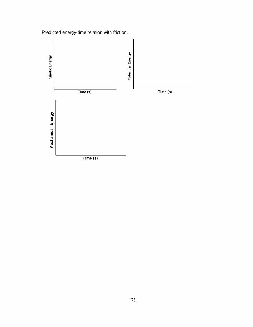
73

Predicted energy-time relation with friction.

Time (s)

Kin

etic

Ene

rgy

Time (s)

Pote

ntia

l Ene

rgy

Time (s)

Mec

hani

cal

Ener

gy

74

Measured energy-time relations with friction.

Use the fact that the change in the mechanical energy is equal to the work done by friction to find the value of the friction force acting on the cart. Use the electronic balance to find the mass of the friction block, and then find the coefficient of friction between the friction block and the track.

Kin

etic

Ene

rgy

(Uni

t:

)

Time (Unit: )

Pote

ntia

l Ene

rgy

(Uni

t:

)

Time (Unit: )

Tota

l Mec

hani

cal E

nerg

y (U

nit:

)

Time (Unit: )

75

Laboratory Exercise #6 Collisions and Momentum Date ______________ NAME:______________________________Partners:________________________ Instructor's Signature:____________________ Sketch predictions for what the force versus time plots for each cart, without a mass will look like during collision.

Time (s)

Forc

e on

Car

t 1

Time (s)

Forc

e on

Car

t 2

Sketch the experimental results for the forces during collision. Choose suitable scales and units and mark the axes clearly.

Forc

e on

Car

t 1 (U

nit:

)

Time (Unit: )

Forc

e on

Car

t 1 (U

nit:

)

Time (Unit: )

76

Sketch predictions what the force versus time plots for each cart with a mass, without a mass will look like during collision.

Time (s)

Forc

e on

Car

t 1

Time (s)

Forc

e on

Car

t 2

Sketch the experimental results for the forces for each cart with a mass during collision. Choose suitable scales and units and mark the axes clearly.

What do your results tell you about Newton’s Third Law? Impulse and Momentum. Sketch a prediction for the velocity and force plots on initially motionless cart.

Forc

e on

Car

t 1 (U

nit:

)

Time (Unit: )

Forc

e on

Car

t 1 (U

nit:

)

Time (Unit: )

77

Time (s)

Velo

city

(m/s

)

Time (s)

Forc

e on

Car

t

Run 1: Sketch the experimental results. Choose suitable scales and units and mark the axes clearly.

Mass of cart and force probe =_______________________ Change in momentum of cart due to collision=___________________________ Area under the force versus time plot =______________________________ Compare this area to the change in momentum. Run 2: Sketch the experimental results of collision with a different velocity.

Velo

city

( U

nit:

)

Time (Unit: )

Forc

e (U

nit:

)

Time (Unit: )

78

Mass of cart=_______________________ Change in momentum of cart due to collision=___________________________ Area under the force versus time plot =______________________________ Compare this area to the change in momentum. Results of inelastic collision of carts without an added mass Mass of cart 1=_________________ Mass of cart 2=__________________

Velo

city

( U

nit:

)

Time (Unit: )

Forc

e (U

nit:

)

Time (Unit: )

Velo

city

( U

nit:

)

Time (Unit: )

79

From the graph, calculate and compare the initial and final momentum Results of inelastic collision of carts with a mass on one of the carts Mass of cart 1 (initially moving) =_________________ Mass of cart 2 (initially motionless) =__________________ Mass=______________________ on which cart?____________

From the graph, calculate and compare the initial and final momentum.

Velo

city

of c

art 1

( Uni

t:

)

Time (Unit: )

80

81

LABORATORY EXERCISE #7

Data Sheet: Density; Significant Figures Date:_________ Name:______________________________ Partners:_________________ Instructor's signature:____________________ A. I have measured the volume of the air in this laboratory room and hereby report that using an assumed density of ____________ kg/m3, I find that the room contained _________ kg of air. How close you come to the "true" answer is how accurate your measurement was. I certify that, should another careful experimentalist attempt to make the same measurement, she (he) will come within* ± ________%, approximately, of my value. Too high a number here, will show you to be a sloppy experimentalist, unable to squeeze the best from the tools available. Too low a number will expose you as a fraud, claiming a precision unwarranted by your instruments and methods of using them. ______ (signed) B. For each of the three methods in part B, compute the density of the metal block to the appropriate number of significant figures. Present data, calculations and answers below. Use additional sheets if necessary.

82

B1. Are the three results consistent with one another? What criteria did you use to answer the question? B2. For your best value of the density, compute the percent deviation from the accepted value (obtained from your instructor).

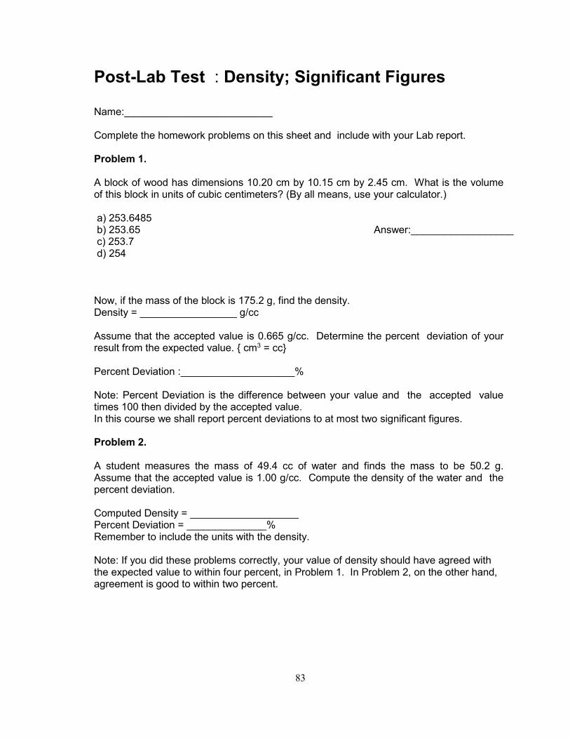
83

Post-Lab Test : Density; Significant Figures Name:__________________________ Complete the homework problems on this sheet and include with your Lab report. Problem 1. A block of wood has dimensions 10.20 cm by 10.15 cm by 2.45 cm. What is the volume of this block in units of cubic centimeters? (By all means, use your calculator.) a) 253.6485 b) 253.65 Answer:__________________ c) 253.7 d) 254 Now, if the mass of the block is 175.2 g, find the density. Density = _________________ g/cc Assume that the accepted value is 0.665 g/cc. Determine the percent deviation of your result from the expected value. cm3 = cc Percent Deviation :____________________% Note: Percent Deviation is the difference between your value and the accepted value times 100 then divided by the accepted value. In this course we shall report percent deviations to at most two significant figures. Problem 2. A student measures the mass of 49.4 cc of water and finds the mass to be 50.2 g. Assume that the accepted value is 1.00 g/cc. Compute the density of the water and the percent deviation. Computed Density = ___________________ Percent Deviation = ______________% Remember to include the units with the density. Note: If you did these problems correctly, your value of density should have agreed with the expected value to within four percent, in Problem 1. In Problem 2, on the other hand, agreement is good to within two percent.

84

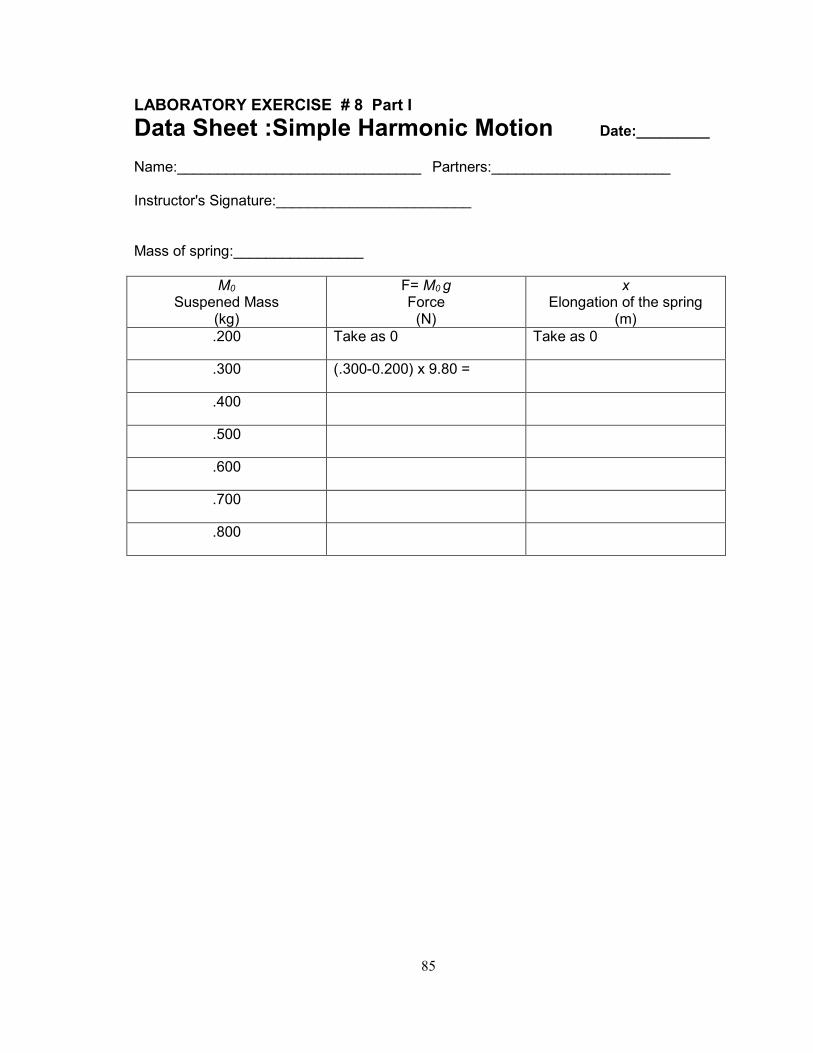
85

LABORATORY EXERCISE # 8 Part I Data Sheet :Simple Harmonic Motion Date:_________ Name:______________________________ Partners:______________________ Instructor's Signature:________________________ Mass of spring:________________

M0

Suspened Mass (kg)

F= M0 g Force

(N)

x Elongation of the spring

(m) .200 Take as 0 Take as 0

.300 (.300-0.200) x 9.80 =

.400

.500

.600

.700

.800

86

Hung mass: 200 g 350 g 550 g 700 g

Time for 50 cycles (sec) amplitude #1

Time for 50 cycles (sec) amplitude #2

Time for 50 cycles (sec) amplitude #3

Average of three above times (sec)

Period, T (sec)

T2 (sec2)

87

LABORATORY EXERCISE # 8 Part II Data Sheet : Simple Pendulum Date ______________ Name:______________________________ Partners:__________________________ Instructor's Signature:___________________________

Nominal length Of pendulum, L

100 cm 60 cm 30 cm

Actual length, L

Time for 50 oscillations

(sec)

Period, T (sec)

T2

(sec2 )

88

89

LABORATORY EXERCISE # 9 Data Sheet :Sonometer Date ______________ Name:______________________________ Partners:_______________________ Instructor's Signature:__________________________ 1. What mathematical relationship holds, for a given value of n, between the length L and the wavelength λ ? Procedure A: String length, L = __________ n = 1 Driver frequency =__________ Actual string frequency f (twice driver frequency) = __________ Distance between nodes =__________ wavelength =1 = ____________ n = 2 Driver frequency =__________ Actual string frequency f2 (twice driver frequency) = __________ Distance between nodes =__________ wavelength =2 = ____________ n = 3 Driver frequency =__________ Actual string frequency f3 (twice driver frequency) = __________ Distance between nodes: __________ __________ Average distance between nodes =__________ wavelength =3 = ____________ n = 4 Driver frequency =__________ Actual string frequency f4 (twice driver frequency) = __________ Distance between nodes: __________ __________ __________ Average distance between nodes =__________ wavelength =4 = ____________

90

n = 5 Driver frequency =__________ Actual string frequency f5 (twice driver frequency) = __________ Distance between nodes: __________ __________ __________ ________ Average distance between nodes =__________ wavelength =5 = ____________ n = 6 Driver frequency =__________ Actual string frequency f6 (twice driver frequency) = __________ Distance between nodes: __________ __________ __________ __________ Average Distance between nodes =__________ wavelength =6 = ____________ n = 7 Driver frequency =__________ Actual string frequency f7 (twice driver frequency) = __________ Distance between nodes: __________ __________ __________ ________ Average distance between nodes =__________ wavelength =7 = ____________ 2a. Plot your values of the resonant frequencies versus n, the mode number. On the same graph, draw the best straight-line fit that goes through the origin. This line is the theoretical result,

fn = n f1 2b. The slope of this best straight-line fit to the data (which passes through the origin) is just the fundamental frequency (f1) abstracted from all of your data, not just your first measurement. How good is the agreement? Procedure B: Use your own data sheet for this part. Take all necessary data, and present data and calculations in neat tabular form. 3. To what extent do your results in Procedure B verify the relationship given in the answer to question 1? 4. For each mode you identified and recorded in the data sheets, compute the wave speed.

91

DATA SHEET : Mechanical Equiv. of Heat Date:_____________ Name:_________________________________ Partners:_____________________ Instructor's Signature:__________________ A. Fixed parameters Specific heat of Aluminum, c = 0.220 kcal/kg°C Mass of Aluminum cylinder, m = ___ Diameter of cylinder, D1=_________ Diameter of cylinder plus rope, D2=_______ Average, Do = ( D1 + D2)/2=_________ Average Radius, R = Do/2=_________ Mass of "10 kg" mass, to 3 significant figures, m=__________kg Weight of "10 kg" mass, to 3 significant figures, F=__________Newtons B. "Quick and Dirty" Run B1. Approximate initial temperature: Thermistor Resistance =_________ Corresponding Temperature = __________ "Target" final temperature: Target Temperature =_________ Thermistor Resistance=__________ B2. Actual starting temperature: Thermistor Resistance =__________ Corresponding Temperature =________ B3. Actual final temp.: Thermistor Resistance =__________ Corresponding Temperature =___________ B4. Number of turns, N =__________ Total angle, θ = 2πN=___________radians B5. Computed total work you did, W = F R θ =___________Joules Computed heat input to Aluminum cylinder, Q = mc∆T = ___________kcal Your computed Mechanical Equivalent of Heat, (ratio of above two results):_______________ What is the percent deviation of your result from the accepted value of 4186 J/kcal? ____________ %

92

C1. Room Temperature today____________°C Target initial temperature____________°C Corresponding Thermistor Resistance__________Ω Target final temperature_____________°C Corresponding Thermistor Resistance____________Ω C2. Actual initial temp.: Thermistor Resistance =__________ Corresponding Temperature = ___________°C Actual final temp: Thermistor Resistance =__________ Corresponding Temperature = ___________°C Number of Turns__________ Total angle, θ = 2π N =____________radians C3. Compute the total work you did against friction: W = FRθ = ___________Joules Compute the amount of heat that must have been transferred to the Aluminum, Q = mc∆T = ____________kcal Compute the Mechanical Equivalent of Heat and the percent deviation: D. Did you do better in Part C than in Part B? If not, what went wrong? Give reasons.

93

LABORATORY EXERCISE # 10 DATA SHEET : Mechanical Equiv. of Heat Date:_____________ Name:_________________________________ Partners:_____________________ Instructor's Signature:__________________ A. Fixed parameters Specific heat of Aluminum, c = 0.220 kcal/kg°C Mass of Aluminum cylinder, m = ___ Diameter of cylinder, D1=_________ Diameter of cylinder plus rope, D2=_______ Average, Do = ( D1 + D2)/2=_________ Average Radius, R = Do/2=_________ Mass of "10 kg" mass, to 3 significant figures, m=__________kg Weight of "10 kg" mass, to 3 significant figures, F=__________Newtons B. "Quick and Dirty" Run B1. Approximate initial temperature: Thermistor Resistance =_________ Corresponding Temperature = __________ "Target" final temperature: Target Temperature =_________ Thermistor Resistance=__________ B2. Actual starting temperature: Thermistor Resistance =__________ Corresponding Temperature =________ B3. Actual final temp.: Thermistor Resistance =__________ Corresponding Temperature =___________ B4. Number of turns, N =__________ Total angle, θ = 2πN=___________radians B5. Computed total work you did, W = F R θ =___________Joules Computed heat input to Aluminum cylinder, Q = mc∆T = ___________kcal Your computed Mechanical Equivalent of Heat, (ratio of above two results):_______________

94

What is the percent deviation of your result from the accepted value of 4186 J/kcal? ____________ % C1. Room Temperature today____________°C Target initial temperature____________°C Corresponding Thermistor Resistance__________Ω Target final temperature_____________°C Corresponding Thermistor Resistance____________Ω C2. Actual initial temp.: Thermistor Resistance =__________ Corresponding Temperature = ___________°C Actual final temp: Thermistor Resistance =__________ Corresponding Temperature = ___________°C Number of Turns__________ Total angle, θ = 2π N =____________radians C3. Compute the total work you did against friction: W = FRθ = ___________Joules Compute the amount of heat that must have been transferred to the Aluminum, Q = mc∆T = ____________kcal Compute the Mechanical Equivalent of Heat and the percent deviation: D. Did you do better in Part C than in Part B? If not, what went wrong? Give reasons.

95

LABORATORY EXERCISE # 11

Boyle's Law: Data Date ______________ NAME:______________________________Partners:________________________ Instructor's Signature:____________________ Boyle's Law

B (Air Pressure, cm of H)

Temperature °C

Trail #! Trail #2 Average

Length of mercury column, M=______________________________ Trial # X1

cm X2 cm

L=∆x cm

Y1 cm

Y2 cm

∆Y= Y1-Y2

P, cm =B+∆Y

P x L cm2

96

LABORATORY EXERCISE # 12 Data Sheet for both calorimetry Labs Date ______________ Name:______________________________Partners:_____________________________ Instrutor's Signature:_________________ Calorimetry (1): Heat of Fusion of Water 1. (a) Mass of calorimeter & stirrer:_________________________________gm

(b) Mass of calorimeter and stirrer 2/3 full of water:__________________gm water is ~5° above room temperature

(c) Mass of water (difference of above two masses): _________________gm

2. (a) Initial temperature of water, calorimeter & stirrer:__________________°C

Here, you added towel-dried ice cubes

(b) Final temperature of water, calorimeter & stirrer and melted ice:______°C

(c) ∆T , temperature change, from the above two temperatures:_________°C

3. (a) Final mass of calorimeter & stirrer, original water plus melted ice:_____°C

(b) Mass of ice cubes line 3(a) minus line 1(b):_____________________gm

Do not empty or add more water! All will be used "as is" for the next exercise ( # 14).

97

98

Calorimetry (2): The Specific Heat of a Metal

4. (a) Initial mass of boiler cup:____________________________________gm

(b) Mass of cup plus metal pellets:_______________________________gm

(c) Mass of metal pellets line 1(a) minus line 1(b):__________________gm

5. (a) Mass of calorimeter & stirrer same as line 1(a) from other side:_____gm

(b) Mass of calorimeter & stirrer and cool water:_____________________gm same as line 3(a) if no water was added or removed

(c) Mass of water line 5(b) minus line 5(a):_______________________gm

6. (a) Temperature of hot metal pellets:______________________________°C

(b) Initial temperature of water and calorimeter & stirrer:_______________°C

(c) Final highest temperature of mixture:___________________________°C

7. (a) Specific heat of calorimeter & stirrer:______________________cal/gm°C

given by instructor, if needed

99