‘Optimal’ Probabilistic & Directional Predictions

of Financial Returns∗

Dimitrios D. Thomakos† and Tao Wang‡

March 10, 2009

Abstract

This paper examines the probability of returns exceeding a threshold, extending earlier work

of Christoffersen and Diebold (2006) on volatility dynamics and sign predictability. We find

that the choice of the threshold matters and that a zero threshold (leading to sign predic-

tions) does not lead to the largest probability response to changes in volatility dynamics.

Under certain conditions there is a threshold that has maximum responsiveness to changes

in volatility dynamics that leads to ‘optimal’ probabilistic predictions. We connect the evo-

lution of volatility to probabilistic predictions and show that the volatility ratio is the crucial

variable in this context. The overall results strengthen the arguments in favor of accurate

volatility measurement and prediction, as volatility dynamics are integrated into the ‘optimal’

threshold. We illustrate our findings using daily and monthly data for the S&P500 index.

Keywords: maximum responsiveness, probabilistic predictions, sign predictions, volatility.

JEL classification: C5, G17

∗We would like to thank the editor Richard Baillie, the associate editor, and an anonymous referee for usefulcomments that improved the presentation of the paper. An earlier version of the paper was presented at theWorkshop Series of the Rimini Center for Economic Analysis, Rimini, Italy. We would like to thank workshopparticipants, and especially John Maheu, for useful comments. All remaining errors are ours.

†Department of Economics, University of Peloponnese, Greece, and Senior Fellow, Rimini Center for EconomicAnalysis, Italy. Email: thomakos@uop.gr

‡Department of Economics, Queens College and the Graduate Center of the City University of New York, USA.Email: tao.wang@qc.cuny.edu

1

1 Introduction

Many studies document that asset return volatilities are predictable.1 One implication of volatil-

ity predictability is that the signs of asset returns are also predictable. Christoffersen and Diebold

(2006) study the link between volatility dependence and sign dependence, when expected returns

are non-zero. Based on a simple sign decomposition, they argue that signs of asset returns are

predictable, given that volatilities are. In addition, since expected returns at high frequencies

are close to zero, sign dependence can be mostly found at intermediate return horizons.

This paper examines the relationship between volatility dependence and probability forecasts

for returns exceeding a threshold value ct+1|t, which nests the work of Christoffersen and Diebold

(2006). Since we make no assumption about expected returns (allowing them to be zero or

non-zero), our approach can deal with different forecasting horizons. The novel part of our

analysis shows that there is an ‘optimal’ value of the threshold for returns, which maximizes the

responsiveness of the probability forecast to changes in volatility dynamics.

We discuss the choice of and implications of the ‘optimal’ threshold value and connect volatil-

ity dynamics to probabilistic predictions in a specific fashion. We find that the ratio of lagged

volatility to current volatility plays an important role and uncover a positive relationship be-

tween the conditional probability forecast for returns exceeding a given value and conditional

asset return volatility. Standard asset pricing models predict a positive equilibrium relationship

between conditional first and second moments (Merton 1973, Ferson and Harvey 1991). A pos-

itive relation is consistent with a deterministic model where volatility dynamics drives return

dynamics or it is consistent with a stochastic model where conditional volatility dynamics drives

conditional mean where both unconditional mean and volatility could be constant. In empirical

studies, however, the relationship is inconclusive. French et al. (1987), Campbell and Hentschel

(1992), and Ghysels et al. (2005) found a positive relationship between return and volatilities

while Campbell (1987), Brandt and Kang (2004) and Lettau and Ludvigson (2005) found a neg-

ative relationship between return and asset return volatilities. Our results suggest that when

conditional volatility increases, the conditional probability for returns exceeding a given value x

would increase. Therefore, when risk increases, it is more likely there will be higher returns but

there is no certainty that high returns would actually occur.

There is also considerable interest on the technical aspect of probabilistic predictions. A

brief list includes Anatolyev and Gospodinov (2008), who consider joint modeling of signs and

absolute returns; Chung and Hong (2006) and Hong and Chung (2003), who consider testing for

directional predictability given a known arbitrary threshold; Taylor (2005) and Engle and Man-1The literature is large and cannot be reviewed here. Earlier references on the importance and predictability

of asset volatility can be found, among others, in Schwert and Seguin (1990) and Hsieh (1991).

2

ganelli (2004), who consider quantile predictions; Fleming et al. (2001), who consider volatility

timing and dynamic portfolio adjustment. Finally, Granger and Pesaran (1999) and Leitch and

Tanner (1991), who claim that directional measures are potentially appropriate in the context

of economic welfare maximization.

The rest of the paper is organized as follows. In section 2 we present the mathematical

framework. Section 3 shows why sign predictions do not maximize response towards volatility

changes, obtaining an explicit expression for the optimal threshold value that maximizes predic-

tive response, and show how volatility evolution is related to probabilistic predictions via the

volatility ratio. In section 4 we discuss the empirical implications of our findings and related

estimation issues. Section 5 illustrates the results using daily returns, monthly returns, and

realized volatilities for the S&P500 index. We offer some concluding remarks in section 6.

2 Model Setup

Let Rt+1 denote a return series with conditional mean µt+1|tdef= E [Rt+1|Ωt] and volatility σ2

t+1|tdef=

Var [Rt+1|Ωt], Ωt being the information set on and before period t. All subsequent analysis is

conditional on Ωt which we omit for clarity of exposition. The (conditional) standardized returns

are defined by:

Zt+1|Ωt ≡ Zt+1def= (Rt+1 − µt+1|t)/σt+1|t (1)

and possible values for standardized returns are denoted by zt+1. In what follows, and as in

Christoffersen and Diebold (2006), we denote the information ratio as Itdef= µt+1|t/σt+1|t.

We assume that the standardized returns Zt+1 consist of independent and identically dis-

tributed (i.i.d.) random variables and denote by F (·) and f(·) the cumulative and probability

density function of the standardized returns. The i.i.d. assumption can be relaxed without much

additional cost but is used here as an approximation. The density function f(·) can exhibit

asymmetries. Our main focus is in making conditional probabilistic predictions about future

returns of the form:

p(ct+1|t)def= P

[Rt+1 > ct+1|t

] ≡ P [Zt+1 > zt+1] = 1− F (zt+1) (2)

where we define zt+1def= (ct+1|t − µt+1|t)/σt+1|t. An immediate relationship obtained is between

ct+1|t and the quantiles of the standardized returns’ distribution. Suppose that p(ct+t|t) = 1−p∗,

for some value p∗ ∈ [0, 1], and note that zt+1 = F−1(p∗) ≡ Q(p∗) and is equal to the p∗ quantile

3

of the distribution. Solving for ct+1|t we obtain that:

ct+1|t = µt+1|t + Q(p∗)σt+1|t (3)

While this looks familiar to the Value-at-Risk (VaR) framework, even though VaR emphasizes

the left tail of the distribution, the situation here is different since neither the probability p∗

(and thus Q(p∗)) nor the threshold value ct+1|t is known. If ct+1|t is zero, this becomes the case

of sign prediction which was discussed by Christoffersen and Diebold (2006).

To motivate the use of a more general threshold value, different from zero, consider the follow-

ing quotations from Christoffersen and Diebold (2006) and Hong and Chung (2003) respectively:

Other explorations may also prove interesting. One example is generation of prob-

ability forecasts for future returns exceeding any given value ct+1|t or percentile α...

and

To sum up, (i) when the market is not efficient (i.e., there exists serial dependence

in conditional mean), the direction of returns with any threshold ct+1|t is generally

predictable using past returns. (ii) When the market is efficient but there exists

serial dependence in such higher order conditional moments as skewness and kurtosis,

the direction of returns with any threshold ct+1|t is also predictable using Ωt. (iii)

When the market is efficient and serial dependence is completely characterized by

volatility clustering, the direction of returns is predictable using Ωt except for threshold

ct+1|t = µ. As long as ct+1|t 6= µ, volatility clustering is a driving force for directional

predictability.

There is clearly an interest in probabilistic predictions beyond the sign of the returns. A

number of interesting questions thus arise: (a) What should be the value of the threshold ct+1|t?

(b) If higher moment dynamics are the source of directional predictability, is there a threshold

that maximizes the response of probabilistic predictions with respect to these moment dynamics?

We attempt to answer these questions in the following sections.

3 ‘Optimal’ Probabilistic Predictions

3.1 Maximizing Predictive Response

Christoffersen and Diebold (2006) analyze sign predictability using the ‘response function’ of the

probability of positive returns. This function is the derivative of the probability in equation (2)

4

with respect to changes in volatility. We generalize this response function to account for changes

in the conditional mean as well as the conditional variance and define the matrix response

function as follows:

R(ct+1|t)def=

∂p(ct+1|t)∂θt+1|t

= −f(zt+1)∂zt+1

∂θt+1|t(4)

where θt+1|tdef= (µt+1|t, σt+1|t)′. This is a (2 × 2) matrix that contains the response of the

probabilistic prediction of future returns changes in the value of the conditional mean and the

volatility. Straightforward calculations give us the two partial derivatives as:

∂p(ct+1|t)∂µt+1|t

=f(zt+1)σt+1|t

> 0 (5)

for changes in the mean;

∂p(ct+1|t)∂σt+1|t

= f(zt+1)zt+1

σt+1|t≡ ∂p(ct+1|t)

∂µt+1|tzt+1 (6)

for changes in the volatility.

Notice that the response of volatility is a function of the response of the mean but not vice

versa and its sign depends on the choice of the threshold value relative to the conditional mean.

If ct+1|t > µt+1|t, the response is greater than zero and vice versa. It is also straightforward to

see how the probabilistic prediction changes as the cut-off value ct+1|t alone changes. We obtain:

∂p(ct+1|t)∂ct+1|t

= −f(zt+1)σt+1|t

< 0 (7)

so that changes in the cut-off value are inversely related to volatility.

The easiest way to explore the effects of the choice of the threshold on the response function

is graphically through examples of distributions for the standardized returns. We consider both

symmetric and asymmetric distributions, to see how the value of the threshold changes based on

the degree of asymmetry of the underlying distribution, and concentrate on volatility dynamics.

[INSERT FIGURE ONE ABOUT HERE]

Figure 1 plots the response function of equation (6) for various values of zt+1 that correspond to

different choices of ct+1|t. We use the standard normal and Student’s t(2) distributions for this

plot. Notice that:

• The response is symmetric around ct+1|t = µt+1|t, nonlinear and a function of the kurtosis

of the underlying density.

5

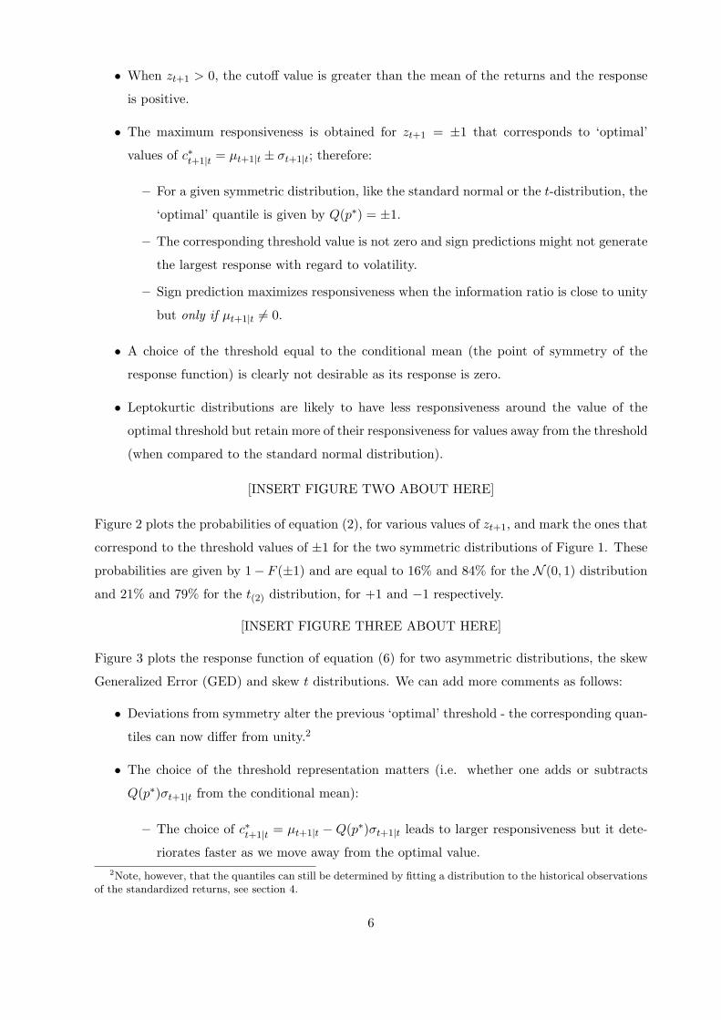
• When zt+1 > 0, the cutoff value is greater than the mean of the returns and the response

is positive.

• The maximum responsiveness is obtained for zt+1 = ±1 that corresponds to ‘optimal’

values of c∗t+1|t = µt+1|t ± σt+1|t; therefore:

– For a given symmetric distribution, like the standard normal or the t-distribution, the

‘optimal’ quantile is given by Q(p∗) = ±1.

– The corresponding threshold value is not zero and sign predictions might not generate

the largest response with regard to volatility.

– Sign prediction maximizes responsiveness when the information ratio is close to unity

but only if µt+1|t 6= 0.

• A choice of the threshold equal to the conditional mean (the point of symmetry of the

response function) is clearly not desirable as its response is zero.

• Leptokurtic distributions are likely to have less responsiveness around the value of the

optimal threshold but retain more of their responsiveness for values away from the threshold

(when compared to the standard normal distribution).

[INSERT FIGURE TWO ABOUT HERE]

Figure 2 plots the probabilities of equation (2), for various values of zt+1, and mark the ones that

correspond to the threshold values of ±1 for the two symmetric distributions of Figure 1. These

probabilities are given by 1− F (±1) and are equal to 16% and 84% for the N (0, 1) distribution

and 21% and 79% for the t(2) distribution, for +1 and −1 respectively.

[INSERT FIGURE THREE ABOUT HERE]

Figure 3 plots the response function of equation (6) for two asymmetric distributions, the skew

Generalized Error (GED) and skew t distributions. We can add more comments as follows:

• Deviations from symmetry alter the previous ‘optimal’ threshold - the corresponding quan-

tiles can now differ from unity.2

• The choice of the threshold representation matters (i.e. whether one adds or subtracts

Q(p∗)σt+1|t from the conditional mean):

– The choice of c∗t+1|t = µt+1|t −Q(p∗)σt+1|t leads to larger responsiveness but it dete-

riorates faster as we move away from the optimal value.2Note, however, that the quantiles can still be determined by fitting a distribution to the historical observations

of the standardized returns, see section 4.

6

– The choice of c∗t+1|t = µt+1|t + Q(p∗)σt+1|t leads to smaller responsiveness but is more

robust to deviation from the optimal value.

• Under an asymmetric distribution it is more likely that sign prediction will maximize

responsiveness when It+1 is close to Q(p∗) but again if µt+1|t 6= 0!

A question that arises is whether the above observations on the ‘optimal predictive response’

of returns on probability dynamics are possibly an artifact of the function chosen to represent

optimality, namely the response function of equation (6). We now illustrate that our findings are

probably independent of the measure used to gauge optimality. To this end, let Yt+1(ct+1|t) ≡Yt+1

def= I(Rt+1 > ct+1|t) be the actual outcome of a probabilistic prediction, a discrete binary

random variable with conditional mean given by p(ct+1|t). We can use a standard measure, such

as the mean squared error, for Yt+1 to examine the effects on the choice of the threshold. The

mean squared error for Yt+1 is given by:

MSE(ct+1|t)def= p(ct+1|t)

[1− p(ct+1|t)

](8)

and is well known that it attains its maximum value when p(ct+1|t) = 0.5, irrespective of the

choice of the density. Therefore, the MSE of directional predictions depends on the choice of

the threshold and, as the next figure illustrates, sign predictions are ‘good performers’ only for a

certain range of values for the information ratio. However, these values may not be empirically

plausible. We illustrate the above in Figure 4 where we plot the MSE (based on the standard

normal density) and mark the MSE values based on the ‘optimal’ threshold as defined before

and on two different values for the information ratio (10% above and below unity).

[INSERT FIGURE FOUR ABOUT HERE]

First, it is clearly futile to perform sign predictions when the conditional mean is zero. However,

even when the conditional mean is not zero, it is only in rare occasions that we will have available

an information ratio high enough to beat the ‘optimal’ threshold in MSE terms. In Figure 4 we

see that making a sign prediction with an information ratio of 1.10 yields a 12.7% decrease in

MSE, compared to the ‘optimal’ threshold; with an information ratio of 0.90 the MSE increase

of a sign prediction, compared to the ‘optimal’ threshold, is 11.4%. What is crucial here is the

plausibility of having information ratios that exceed unity and how often they occur. If most

of the time the information ratio is below unity then making sign predictions is not going to be

very productive. However, even with medium term returns we cannot know when and if we are

going to get high information ratios: such a case is illustrated by our empirical application in

section 5.

7

3.2 Volatility/Threshold Evolution and Probabilistic Response

When we consider c∗t+1|t and make the connection with the generic formula for ct+1|t = µt+1|t +

Q(p∗)σt+1|t we see that the ‘optimal’ threshold value corresponds to a particular quantile of the

standardized returns’ distribution, that is Q(p∗). This distribution is, of course, unknown and it

would have to be fitted from historical observations. Then the probability associated with c∗t+1|t,

namely p(c∗t+1|t), can be computed. However, if the assumption of i.i.d. standardized returns

is valid then this probability would be identical for all time periods and, therefore, not very

interesting from an empirical perspective. What might be more interesting is to see if there is a

connection between the evolution of the ‘optimal’ threshold value and the associated probabilistic

predictions - the optimal threshold is, after all, dynamic. For example, we can think that in a

practical application one will not only be interested in the probability of future returns exceeding

a particular threshold that depends on future volatility, but also one will be interested in the

probability of future returns exceeding the realized threshold that depends on today’s volatility.

To make this specific, define c∗t|tdef= µt|t ± Qσt|t as the realized threshold with Q ≡ Q(p∗)

being estimated from historical observations. The associated probabilistic prediction would then

correspond to:

p(c∗t|t)def= P

[Rt+1 > c∗t|t

]= 1− F (qt+1|t) (9)

where qt+1|tdef=

[−(µt+1|t − µt|t)± Qσt|t

]/σt+1|t is the ratio of current to future volatilities, ad-

justed by the difference between expected and realized returns. How is the above probabilistic

prediction affected by volatility dynamics? Straightforward computations yield the following

responses:

∂p(c∗t|t)

∂σt+1|t= −f(qt+1|t)

(µt+1|t − µt|t)± Qσt|tσ2

t+1|t(10)

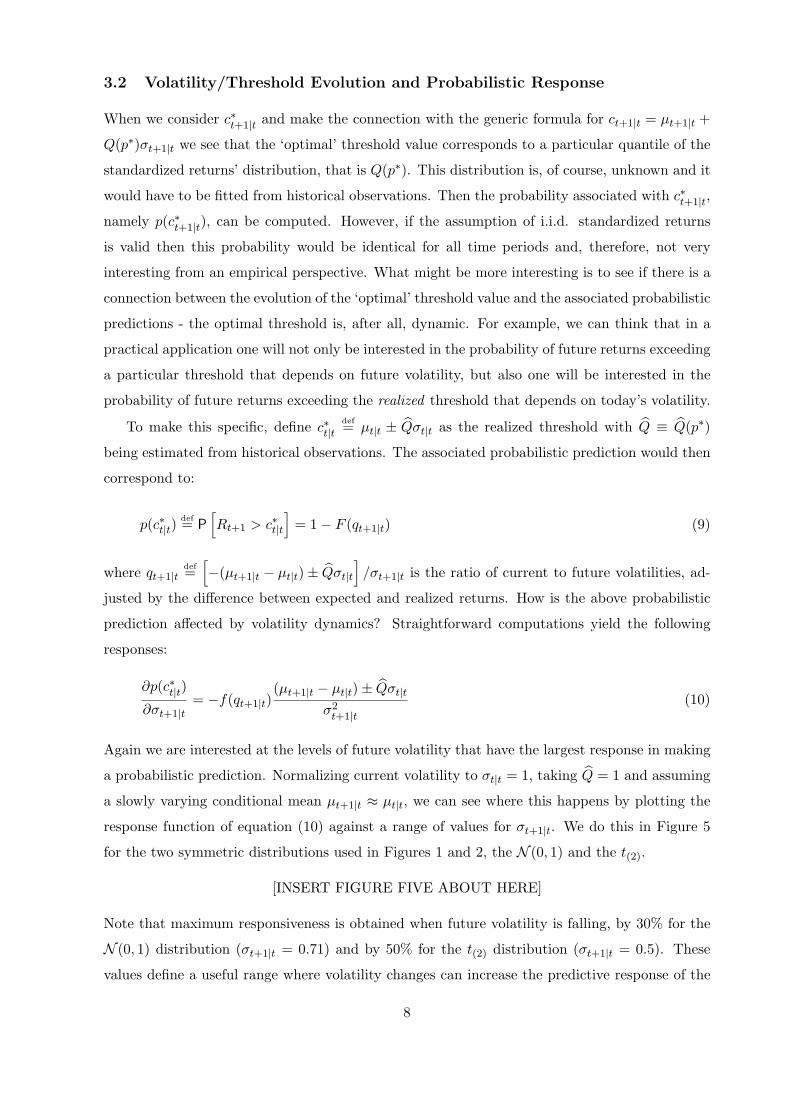
Again we are interested at the levels of future volatility that have the largest response in making

a probabilistic prediction. Normalizing current volatility to σt|t = 1, taking Q = 1 and assuming

a slowly varying conditional mean µt+1|t ≈ µt|t, we can see where this happens by plotting the

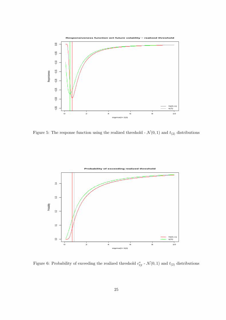
response function of equation (10) against a range of values for σt+1|t. We do this in Figure 5

for the two symmetric distributions used in Figures 1 and 2, the N (0, 1) and the t(2).

[INSERT FIGURE FIVE ABOUT HERE]

Note that maximum responsiveness is obtained when future volatility is falling, by 30% for the

N (0, 1) distribution (σt+1|t = 0.71) and by 50% for the t(2) distribution (σt+1|t = 0.5). These

values define a useful range where volatility changes can increase the predictive response of the

8

probability in equation (9). As volatility rises above or falls below these values the responsiveness

starts decreasing. For example, for the N (0, 1) distribution the maximum responsiveness at

σt+1|t = 0.71 is -0.29 while for σt+1|t = 1 is -0.25 and for σt+1|t = 1.30 is -0.17; we see that there

is a substantial drop in responsiveness as volatility increases by 30%, compared to the case when

volatility decreases by the same percentage.

Figure 6 plots the corresponding probabilities for exceeding the realized threshold based on

equation (9). We can clearly see a ‘risk-return’ trade-off relationship. As volatility increases,

the probability of exceeding the realized threshold increases - for the N (0, 1) distribution the

relevant probabilities for σt+1|t = 0.71, 1, 1.30 are 8%, 16% and 22% respectively. Note that

the probability cannot, by construction, exceed 50%.

[INSERT FIGURE SIX ABOUT HERE]

Finally, we examine the effect that a change in the expected return has on p(c∗t|t). Unlike the

case of future volatility, the sign of the corresponding derivative is unambiguous and positive:

∂p(c∗t|t)

∂µt+1|t=

f(qt+1|t)σt+1|t

(11)

which implies that higher expected returns, which raise c∗t+1|t, will always increase the probability

of exceeding the realized threshold, irrespective of the path of future volatility. Figure 7 plots

the probability of equation (9) against a range of values for µt+1|t. We normalize µt|t = 0 take

Q = 1 and use the N (0, 1) distribution. Each panel in the plot presents the probabilities for a

range of values for µt+1|t from -30% to +30%, for a specific value of σt|t and for three alternative

values for σt+1|t = γσt|t, for γ = 0.7, 1, 1.3. We can see the effect of rising and falling future

volatility with respect to current volatility. Note that now qt+1| = −(µt+1|t−σt|t)/σt+1|t and the

lines for the three probabilities will intersect at the point where µt+1|t = σt|t.

[INSERT FIGURE SEVEN ABOUT HERE]

The main characteristic in all four panels in Figure 7 is that the lines corresponding to higher

future volatility (blue) are always on top of the other two lines (red and green) until the point

where they intersect. Again, higher future volatility is associated with a higher probability for

future returns to exceed the realized threshold. However, once the expected return µt+1|t exceeds

σt|t the probability is inversely related to future volatility - this can be seen clearly in the top

panels of the figure. We can also observe that the higher σt|t is the lower is the probability of

future returns exceeding the realized threshold and volatility dynamics matters less in this case.

This can be seen by comparing the upper left with the lower right panels: in the upper left panel

we have a much larger distance between the lines that correspond to volatility dynamics (blue

9

and green) where volatility either rises or falls with the line where future volatility stays the

same with its realized value; this distance is clearly reduced when we consider the lower right

panel of the figure where current volatility is eight times larger than the current volatility in the

upper left panel.

4 Empirical Implications, Estimation and Prediction

Our previous discussion has a number of interesting empirical implications. It provides us with

a sequential approach for working with probabilistic predictions. Let us assume that we have

a time series of return observations and a corresponding one for volatility (e.g. any realized

volatility measure) and denote them byRt, V

2t

T

t=1respectively. A rough guide for the steps to

be followed is:

1. Test for serial correlation in the returns and fit an appropriate model µt+1|t for the condi-

tional mean - in most cases µt+1|t = µ, the global mean. We assume a constant conditional

mean for simplicity in what follows.

2. Compute the standardized returns Ztdef= (Rt− µ)/Vt and fit an appropriate distribution to

them. Plot the response function of equation (6) to locate the optimal quantile Q.

3. Based on the distributional approximation compute the probability that future returns will

exceed the optimal threshold c∗t+1|t. Note that a forecast of future volatility is not needed

for this: the required probability is given by 1− F (Q); for example, in the N (0, 1) or any

symmetric distribution this will be given by 1−F (±1). This probability can be computed

using the underlying theoretical distribution or using the sample empirical distribution, see

below.

4. Compute the binary variable Ytdef= I(Zt > Q), then use any suitable statistic that can test

for serial dependence (and hence predictability) of the discrete series Yt.

5. For making dynamic directional predictions using the realized threshold c∗t|t compute the

probability 1 − F (qt+1|t) where qt+1|tdef= QVt/Vt+1 for t = 1, . . . , T − 1 for the in-sample

observations. For out-of-sample observations a forecast VT+1|T of volatility is required in

which case the probability will be computed using qT+1|Tdef= QVT /VT+1|T .

4.1 Estimation and Prediction of Probabilities

There are various methods we can estimate the required probabilities, either p(c∗t+1|t) or p(c∗t|t),

including the empirical distribution function of the returns, the empirical distribution function

10

of standardized returns, or a parametric/expansion-based approximation. All these have been

used in previous work by Christoffersen and Diebold (2006) and Christoffersen, et al. (2007).

The key ingredients in the application of these methods are appropriate historical volatility and

volatility forecasts. We assume that these volatility measures are available and concentrate on

methods for the estimation and prediction of probabilities.

The empirical distribution function of the returns FR(r) is nothing more than a sample

proportion of observations less than than a chosen evaluation value r and is defined as:

FR(r) def= T−1T∑

t=1

I(Rt ≤ r) (12)

This is a relatively crude estimator, although it enjoys many optimal properties as an estimator

of the underlying cumulative distribution function F (r). Notice that this estimator does not

use information about historical volatility. In addition, the standard errors for this estimator

are complicated by the possible dependence in the returns.3 A way to introduce both historical

volatility and volatility forecasts and to work in an i.i.d. framework is to consider, as in Christof-

fersen and Diebold (2006), Christoffersen, et al. (2007) and our previous discussion, realized

standardized returns Zt. The standardization is performed using historical volatility while the

chosen evaluation value z can depend on either current or predicted volatility. The relevant

estimator now becomes:

FZ(z) def= T−1T∑

t=1

I(Zt ≤ z) (13)

For the i.i.d. case it is well known that the empirical distribution function is the nonparamet-

ric maximum likelihood estimator of the distribution function and is unbiased, consistent and

asymptotically normally distributed as:

√T

[FZ(z)− F (z)

]∼ N (0, σ2

Z(z)) , T →∞ (14)

where σ2Z(z) def= F (z) [1− F (z)] is the variance of the estimator. An easy improvement in the

above estimator FZ(z) can be made by taking advantage of the possible symmetry of the dis-

tribution of standardized returns. If the distribution of standardized returns is symmetric then

one can use the symmetrized estimator, say FS(z), and have a gain in efficiency with smaller

standard errors. For details see Shuster (1973) and Modarres (2002).

3If the returns are dependent then estimation of the standard errors for bFR(r) would require estimation of the

joint empirical distribution function, say bFk(r, r)def= T−1

TXt=1

I(Rt ≤ r ∧Rt+k ≤ r).

11

Another straightforward way of improving the estimator FZ(z) of the distribution function

is to smooth it, akin to the smoothing that leads from a histogram to a density estimator.

This smoothing can done in a variety of ways, the most popular being kernel methods. A

different approach is based on direct smoothing of the empirical distribution function. This

approach, based on the use of Bernstein polynomials as smoothing coefficients, has a number

of advantages including simplicity of computation and optimal asymptotic properties that hold

both for independent and dependent observations, and its thus preferred here. We provide a brief

description of this smoothed estimator below; for further details see Babu, Canty and Chaubey

(2002).

The application of Bernstein polynomials requires a rescaling of the observations to have

support on the unit interval. Suitable transformations, of the form τ(z) 7→ w, for standardized

returns can be based on either a compact support of the form [a, b] for some constants a < b or

the whole real line (−∞, +∞) and are given by:

τ(z) =z − a

b− a, τ(z) = 0.5 +

1π

tan−1 z (15)

Using either of the above transformations for the observations τ(Zt) 7→ Wt and τ(z) 7→ w and

letting FW (w) def= T−1T∑

t=1

I(Wt ≤ w), the smoothed estimator is given by:

FB(z) ≡ FB(w) def=m∑

k=0

FW (k/m)bk(m,w) , k = 0, . . . ,m (16)

where the weights bk(m,w) are given by the Bernstein polynomials:

bk(m,w) def=

m

k

wk(1− w)m−k (17)

and m is the smoothing coefficient. Note that the estimator FB(z) is a polynomial and thus has

all its derivatives. The choice of m is based on asymptotic considerations (strong consistency and

proximity of the smooth estimator to the empirical distribution function) and can be shown that

obeys the lower bound m ≥ T 2/3 for both independent and dependent observations. However,

Babu, Canty and Chaubey (2002) do not provide explicit expressions for the mean and the

variance of their estimator. It is straightforward to derive them and we do so in the appendix

for the i.i.d. case.

We can also motivate the use of logit-type models in estimation and prediction of the relevant

probabilities. Consider the probability given in equation (9), that of future returns exceeding

12

the realized threshold. For the case we are examining here, where µt+1|t = µ, we can consider

the following expansion around a fixed value (say the optimal value Q = 1):

p(c∗t|t) ≈ 1− f(1)(qt+1|t − 1)− f ′(1)(qt+1|t − 1)2

≈ γ0 + γ1qt+1|t + γ2q2t+1|t

(18)

where γ0def= 1 + f(1) − f ′(1), γ1

def= −1 + 2f ′(1) and γ2def= −f ′(1). For the binary variable

Yt+1def= I(Rt+1 > c∗t|t) we have that E [Yt+1|Ωt] = p(c∗t|t) and therefore one can use a logit-type

model to compute the relevant probability using the volatility ratio and its square as explanatory

variables.

5 Empirical Illustration

This section presents an empirical illustration of the results presented above. We use daily and

monthly data for the S&P500 index. The monthly S&P500 cash index data are from December

1969 to May 2007, for a total of T = 448 observations; the daily S&P500 futures data are from

April 1982 to May 2007, for a total of T = 6, 328 observations.4

For the monthly data we use the realized volatility based on daily squared returns as V 2t

def=m∑

i=1

R2t,i, where Rt,i is the daily return of the ith day in month t. For the daily data we calculate the

realized volatility based on intraday squared returns. We did not use the naive estimator that uses

(all or sparsely sampled) squared returns directly; instead, we use the Zhang, Mykland and Ait-

Sahalia (2005) two time scales estimator. We experimented with both an asymptotically-based

and a finite-sample based choices of the subsamples used with qualitatively identical results.5

See Andersen et al. (2007) for a review of methods on estimation and forecasting with the earlier

realized volatility measures and the literature around the two time scales class of estimators in,

among others, Zhang, Mykland and Ait-Sahalia (2005), Bandi and Russell (2006) and Barndorff-

Nielsen, Hansen, Lunde, and Shephard (2005, 2008, 2009).

We begin by examining the autocorrelations of both daily and monthly returns, standardized

returns, and realized volatilities.6 There is no significant serial correlation in the returns or

standardized returns while the presence of dynamics is evident for the volatility series; the latter

has the standard signs of long memory presence in the autocorrelation funciton, with medium

to low autocorrelation that is present at long lags. This is more pronounced in the daily data.4We excluded the week of the October 19, 1987 stock market crash from the plots and calculations5Our presented results are based on the finite-sample choice. We also experimented with other choices of state-

of-the-art realized volatility estimators with similar to identical results. Further empirical results are available onrequest.

6The data plots and autocorrelation plots for both frequencies are available on request.

13

Table 1 presents some descriptive statistics for the data at both frequencies. For the monthly

data, the returns appear as independent with a non-normal marginal distribution; in the absence

of conditional mean dynamics, we compute standardized returns as Zt = (Rt − µ)/Vt with µ as

the unconditional mean. The standardized returns now appear as uncorrelated but with a normal

marginal distribution, jointly implying independence for the standardized returns.

[INSERT TABLE ONE ABOUT HERE]

For the daily returns we have to be cautious in drawing inferences from the various tests: the

sample size is really large so chances are that all hypotheses will be easily rejected at the con-

ventional levels of significance. For example, the sample skewness for the standardized returns is

0.08 with a standard error of 0.03 resulting in a conventional test value for zero skewness of 2.66

with a p-value of 0.004. Should we reject the hypothesis of zero skewness while we can see both

visually and numerically that its practically zero? Be that as it may, we can still see that the

daily returns are clearly non-normally distributed because of the excess kurtosis. However, the

results from the Ljung-Box tests do not agree with the autocorrelation plots: the null hypothesis

of no serial correlation is strongly rejected while there is no such evidence in the plots.7 To

account for the possibility of some serial correlation present in the daily returns, we fit a MA(1)

model to the returns to remove a part of the potential conditional mean dynamics and use the

residuals to compute the standardized returns. The evidence in favor of a marginal normal dis-

tribution is not as strong now as was in the case of the monthly returns: the Cramer-Von Misses

(CVM) test does reject the null hypothesis of normality (using the asymptotic critical value)

but the tests based on the sample proportions all indicate conformability with an underlying

normal distribution. To further evaluate normality assumption for the standardized returns we

computed a bootstrap8 based p-value for the CVM test which equaled 0.60 thus supporting

the possibility for an underlying marginal normal distribution. Finally, and again to safeguard

against spurious rejections, we repeated the bootstrap approach for the Ljung-Box test for the

standardized returns which resulted in a p-value of 0.91. The joint results from both monthly

and daily data suggest that we could use the quantile values Q = ±1 corresponding to a normal

distribution for the standardized returns.

The probable absence of autocorrelation coupled with underlying normality suggests that

the standardized returns may be i.i.d., more so in the monthly data and less so in the daily

data. While there are more powerful and specialized tests for checking the i.i.d. hypothesis, see

for example Hong and White (2005), here we are interested in testing independence not for the

standardized returns directly but for certain binary sequences that are related to probabilistic7See Lo and MacKinlay (1990) on the evidence and explanations of serial correlations for daily stock returns.8Using the stationary bootstrap of Politis and Romano (1994).

14

predictions. We use a simple test of independence versus a 1st order Markov alternative as

in Christoffersen (1998) based on the binary series Yt = I(Zt > Q) for various values of Q,

specifically: Yt = I(Zt > 0), Yt = I(Zt > 1) and Yt = I(Zt < −1).

[INSERT TABLE TWO ABOUT HERE]

The results in Table 2 are interesting. For the monthly data they show that the only value that

splits the standardized returns’ space into a possibly predictable binary sequence is Q = 1. Note

the absence of symmetry in these results which makes them potentially useful: looking for excess

positive returns is predictable while looking for excess negative returns (with the symmetric

threshold) is not. For the daily data the results are similar for the value of Q = 0, in terms

of the mean percentage of values in either side of zero; they are, however, slightly different for

the values of Q = ±1. We see now a very close match of the mean percentages (16.83% and

16.35%) with the corresponding theoretical one of the standard normal distribution (which is

equal 15.9%); for the monthly data the corresponding mean percentages were higher (19.19%

and 17.41% respectively). However, for the daily data it appears that both sequences, in excess

of ±1, are possibly predictable.

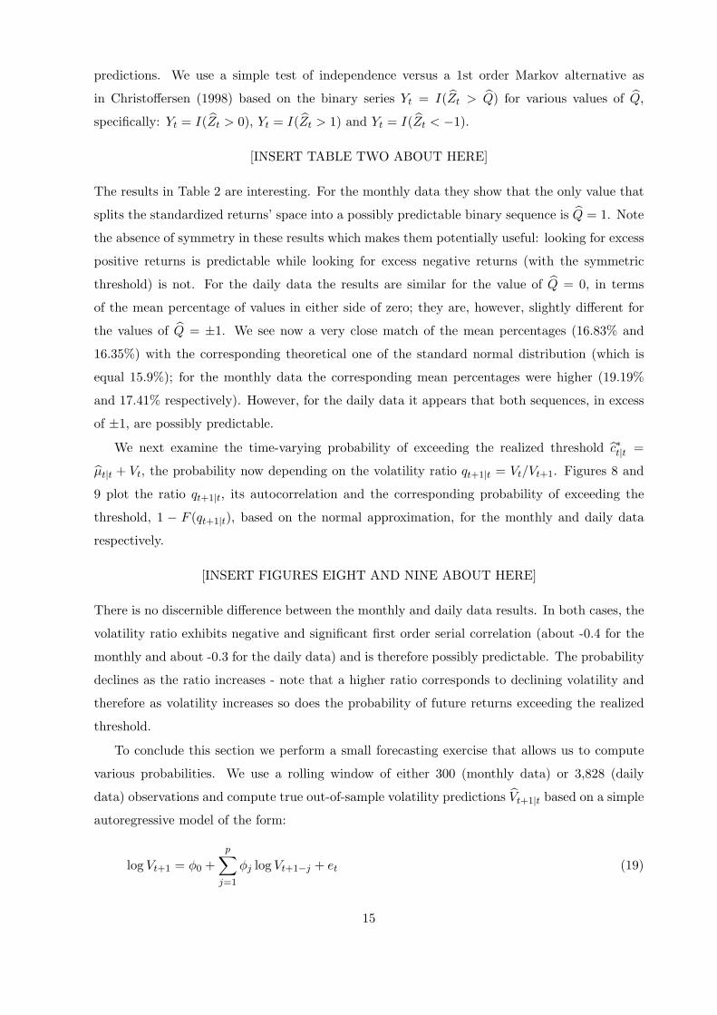
We next examine the time-varying probability of exceeding the realized threshold c∗t|t =

µt|t + Vt, the probability now depending on the volatility ratio qt+1|t = Vt/Vt+1. Figures 8 and

9 plot the ratio qt+1|t, its autocorrelation and the corresponding probability of exceeding the

threshold, 1 − F (qt+1|t), based on the normal approximation, for the monthly and daily data

respectively.

[INSERT FIGURES EIGHT AND NINE ABOUT HERE]

There is no discernible difference between the monthly and daily data results. In both cases, the

volatility ratio exhibits negative and significant first order serial correlation (about -0.4 for the

monthly and about -0.3 for the daily data) and is therefore possibly predictable. The probability

declines as the ratio increases - note that a higher ratio corresponds to declining volatility and

therefore as volatility increases so does the probability of future returns exceeding the realized

threshold.

To conclude this section we perform a small forecasting exercise that allows us to compute

various probabilities. We use a rolling window of either 300 (monthly data) or 3,828 (daily

data) observations and compute true out-of-sample volatility predictions Vt+1|t based on a simple

autoregressive model of the form:

log Vt+1 = φ0 +p∑

j=1

φj log Vt+1−j + et (19)

15

with the order of the autoregression selected by the AIC criterion.9 We use both the actual

and predicted volatility ratios qt+1|t and qt+1|t to compute empirical probabilities of exceeding

the optimal and realized thresholds. We follow the methods presented in the previous section:

we compute probabilities based on the smoothed empirical distribution function using Bernstein

polynomials as in equation (16) and conditional probabilities as in equation (18).

[INSERT FIGURES TEN AND ELEVEN ABOUT HERE]

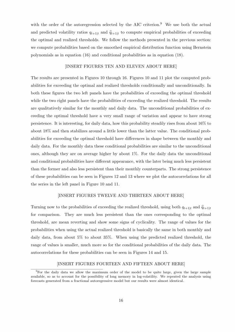
The results are presented in Figures 10 through 16. Figures 10 and 11 plot the computed prob-

abilities for exceeding the optimal and realized thresholds conditionally and unconditionally. In

both these figures the two left panels have the probabilities of exceeding the optimal threshold

while the two right panels have the probabilities of exceeding the realized threshold. The results

are qualitatively similar for the monthly and daily data. The unconditional probabilities of ex-

ceeding the optimal threshold have a very small range of variation and appear to have strong

persistence. It is interesting, for daily data, how this probability steadily rises from about 16% to

about 18% and then stabilizes around a little lower than the latter value. The conditional prob-

abilities for exceeding the optimal threshold have differences in shape between the monthly and

daily data. For the monthly data these conditional probabilities are similar to the unconditional

ones, although they are on average higher by about 1%. For the daily data the unconditional

and conditional probabilities have different appearance, with the later being much less persistent

than the former and also less persistent than their monthly counterparts. The strong persistence

of these probabilities can be seen in Figures 12 and 13 where we plot the autocorrelations for all

the series in the left panel in Figure 10 and 11.

[INSERT FIGURES TWELVE AND THIRTEEN ABOUT HERE]

Turning now to the probabilities of exceeding the realized threshold, using both qt+1|t and qt+1|t

for comparison. They are much less persistent than the ones corresponding to the optimal

threshold, are mean reverting and show some signs of cyclicality. The range of values for the

probabilities when using the actual realized threshold is basically the same in both monthly and

daily data, from about 5% to about 35%. When using the predicted realized threshold, the

range of values is smaller, much more so for the conditional probabilities of the daily data. The

autocorrelations for these probabilities can be seen in Figures 14 and 15.

[INSERT FIGURES FOURTEEN AND FIFTEEN ABOUT HERE]9For the daily data we allow the maximum order of the model to be quite large, given the large sample

available, so as to account for the possibility of long memory in log-volatility. We repeated the analysis usingforecasts generated from a fractional autoregressive model but our results were almost identical.

16

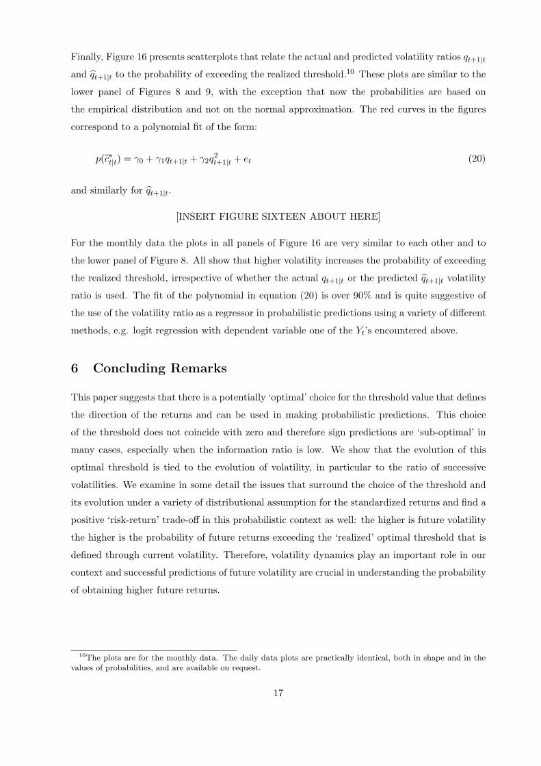
Finally, Figure 16 presents scatterplots that relate the actual and predicted volatility ratios qt+1|t

and qt+1|t to the probability of exceeding the realized threshold.10 These plots are similar to the

lower panel of Figures 8 and 9, with the exception that now the probabilities are based on

the empirical distribution and not on the normal approximation. The red curves in the figures

correspond to a polynomial fit of the form:

p(c∗t|t) = γ0 + γ1qt+1|t + γ2q2t+1|t + et (20)

and similarly for qt+1|t.

[INSERT FIGURE SIXTEEN ABOUT HERE]

For the monthly data the plots in all panels of Figure 16 are very similar to each other and to

the lower panel of Figure 8. All show that higher volatility increases the probability of exceeding

the realized threshold, irrespective of whether the actual qt+1|t or the predicted qt+1|t volatility

ratio is used. The fit of the polynomial in equation (20) is over 90% and is quite suggestive of

the use of the volatility ratio as a regressor in probabilistic predictions using a variety of different

methods, e.g. logit regression with dependent variable one of the Yt’s encountered above.

6 Concluding Remarks

This paper suggests that there is a potentially ‘optimal’ choice for the threshold value that defines

the direction of the returns and can be used in making probabilistic predictions. This choice

of the threshold does not coincide with zero and therefore sign predictions are ‘sub-optimal’ in

many cases, especially when the information ratio is low. We show that the evolution of this

optimal threshold is tied to the evolution of volatility, in particular to the ratio of successive

volatilities. We examine in some detail the issues that surround the choice of the threshold and

its evolution under a variety of distributional assumption for the standardized returns and find a

positive ‘risk-return’ trade-off in this probabilistic context as well: the higher is future volatility

the higher is the probability of future returns exceeding the ‘realized’ optimal threshold that is

defined through current volatility. Therefore, volatility dynamics play an important role in our

context and successful predictions of future volatility are crucial in understanding the probability

of obtaining higher future returns.

10The plots are for the monthly data. The daily data plots are practically identical, both in shape and in thevalues of probabilities, and are available on request.

17

References

1. Anatolyev, A., and N. Gospodinov, 2008, “Modeling financial return dynamics by decom-

position”, Journal of Business and Economic Statistics, forthcoming.

2. Andersen, T.G., T. Bollerslev, F.X. Diebold, 2007, “Parametric and nonparametric volatil-

ity measurement,” L.P. Hansen, Y. Ait-Sahalia, eds. Handbook of Financial Econometrics,

forthcoming, Amsterdam: North-Holland.

3. Babu, G. J., Canty, A. and Chaubey, Y, 2002, “Application of Bernstein polynomials for

smooth estimation of a distribution and density function”, Journal of Statistical Planning

and Inference, vol. 105, pp. 377-392.

4. Bandi, F.M., and J.R. Russell, 2006, “Market microstructure noise, integrated variance

esti- mators, and the accuracy of asymptotic approximations”, Working paper.

5. Barndorff-Nielsen, O.E., P. Hansen, A. Lunde and N. Shephard, 2005, “Regular and mod-

ified kernel-based estimators of integrated variance: the case with independent noise”,

Working paper.

6. Barndorff-Nielsen, O.E., P. Hansen, A. Lunde and N. Shephard, 2008, “Designing realized

kernels to measure ex-post variation of equity prices in the presence of noise”, Econometrica,

vol. 76, pp. 1481-1536.

7. Barndorff-Nielsen, O.E., P. Hansen, A. Lunde and N. Shephard, 2009, “Subsampling real-

ized kernels”, Journal of Econometrics, forthcoming.

8. Brandt, M.W., and Q. Kang, 2004, “On the relationship between the conditional mean

and volatility of stock returns: a latent VAR approach,” Journal of Financial Economics,

vol. 72, pp. 217-57.

9. Campbell, J. 1987, “Stock returns and the term structure,” Journal of Financial Ecoo-

nomics, vol. 18, pp. 373-99.

10. Campbell, J. and L. Hentschel, 1992, “No news is good news: an asymmetric model of

changing volatility in stock returns,” Journal of Financial Economics, vol. 31, pp. 281-

318.

11. Christoffersen, P.F., 1998, “Evaluating Interval Forecasts”, International Economic Review,

vol. 39, pp. 841-862.

12. Christoffersen P.F. and F. X. Diebold, 2006, “Financial asset returns, direction-ofchange

forecasting, and volatility dynamics,” Management Science, vol. 52, pp. 1273-1287.

18

13. Christoffersen, P.F., Diebold, F.X., Mariano, R.S., Tay, A.S. and Tse, Y.K. 2007, “Direction-

of-Change forecasts based on conditional variance, skewness and kurtosis dynamics: Inter-

national evidence”, Journal of Financial Forecasting, vol. 1, pp. 3-24.

14. Chung, J. and Y. Hong, 2006, “Model-Free evaluation of directional predictability in foreign

exchange markets”, Journal of Applied Econometrics, vol. 22, pp. 855-889

15. Engle, R.F. and S. Manganelli, 2004, “CAViaR: Conditional autoregressive value at risk

by regression quantiles”, Journal of Business & Economic Statistics, vol. 22, pp. 367-381.

16. Ferson, W. E., and C. R. Harvey, 1991, “The variation of economic risk premium” Journal

of Political Economy, vol. 99, pp. 385-415.

17. Fleming, J., C. Kirby, B. Ostdiek, 2001, “The economic value of volatility timing,” Journal

of Finance, vol. 56, pp. 329-352.

18. French, K.R., W. Schwert, R.F. Stambaugh, 1987, “Expected stock returns and volatility,”

Journal of Financial Economics, vol. 19, pp. 3-29.

19. Ghysels, E., P. Santa-Clara, R. Valkanov, 2005, “There is a risk-return tradeoff after all,”

Journal of Financial Economics, vol. 76, pp. 509-548.

20. Granger, C.W.J. and H. Pesaran, 1999, “Economic and statistical measures of forecast

accuracy”, Journal of Forecasting, vol. 19, pp. 537 - 560.

21. Hong, Y. and J. Chung, 2003, “Are the directions of stock price changes predictable?

Statistical theory and evidence”, manuscript, Cornell University.

22. Hong, Y.M. and H. White, 2005, “Asymptotic distribution theory for an entropy-based

measure of serial dependence”, Econometrica, vol. 73, pp. 837-902.

23. Hsieh, D.A., 1991, “Chaos and nonlinear dynamics: Application to financial Markets,”

Journal of Finance, vol. 46, pp. 1839-1877

24. Leitch, G. and J.E. Tanner, 1991, “Economic forecast evaluation: profits versus the con-

ventional error measures”, American Economic Review, vol. 81, pp. 580–590.

25. Lettau, M., and S. Ludvigson, 2005, “Measuring and modeling variation in the risk-return

tradeoff,” in Y. Ait-Shalia, L.P. Hansen, eds. Handbook of Financial Econometrics, North-

Holland, Amsterdam, The Netherlands.

26. Lo, A.W., and C. MacKinlay, 1990, “An econometric analysis of nonsynchronous trading”,

Journal of Econometrics, vol. 45, pp. 181-212.

19

27. Merton, R.C. 1973, “An intertemporal capital asset pricing model,” Econometrica, vol. 41,

pp. 867-887.

28. Modarres, R., 2002, “Efficient nonparametric estimation of a distribution function”, Com-

putational Statistics & Data Analysis, vol. 39, pp. 75 - 95.

29. Schwert, G.W., and P.J. Seguin, 1990, “Heteroskedasticity in stock returns,” Journal of

Finance, vol. 45, pp. 1129-1155.

30. Shuster, E.F., 1973, “On the goodness-of-fit problem for continuous symmetric distribu-

tions”, Journal of the American Statistical Association, vol. 68, pp. 713-715.

31. Taylor, J.W. 2005, “Generating volatility forecasts from value at risk estimates” Manage-

ment Science, vol. 51, pp. 712-725.

32. Zhang, L., P.A. Mykland and Y. Ait-Sahalia (2005), “A tale of two time scales: determining

integrated volatility with noisy high frequency data,” Journal of the American Statistical

Association, vol. 100, pp. 1394-1411.

20

Appendix

We give explicit expressions for the mean and variance of the smoothed estimator of the

distribution function given in equation (18). Define F ∗B(w) as:

F ∗B(w) def=

m∑

k=0

F (k/m)bk(m,w) (21)

where F ∗B(w) → F (z) as m → ∞, by the properties of the distribution function and Bernstein

polynomials. Expressing the difference between FB(w) and F ∗B(w) as D∗

B(w), then,

D∗B(w) =

m∑

k=0

DB(k/m)bk(m,w) (22)

where DB(k/m) def=[FW (k/m)− F (k/m)

]. We immediately get that E [D∗

B(w)] = 0 by the unbi-

asedness of the empirical distribution function, and therefore E[DB(k/m)

]= 0. Using the large

sample properties of the empirical distribution function we also get that limm→∞ E[FB(w)

]=

F (z). Thus, the estimator is biased in finite samples but asymptotically unbiased.

To find the variance of the estimator, notice that the variance of DB(k/m) from equa-

tion (14) is given by T−1F (k/m) [1− F (k/m)]. Since we can show that the covariance terms

Cov[DB(k/m), DB(j/m)

]= T−1F (k/m) [1− F (j/m)] for j ≥ k, (Mood, Graybill, and Boes,

1974, ch. 11), we immediately obtain that:

Var [D∗(w)] = T−1∑m

k=0 F (k/m) [1− F (k/m)] b2k(m,w)+

2T−1∑m−1

k=0

∑mj=k+1 F (k/m) [1− F (j/m)] bk(m,w)bj(m,w)

(23)

Finally, although we do not have exact results about the rate of convergence, we should have

that FB(w) is asymptotically normally distributed as:

√TD∗

B(w) ∼ N (0, σ2B(w)) , T →∞ (24)

where σ2B(w) def= TVar [D∗(w)].

21

Table 1. Descriptive Statistics for the S&P500 DataMonthly Data Daily Data

Rt Vt Zt Rt Vt Zt

Observations 448 6328Mean 0.01 0.04 0.05 0.00 9e-3 0.04RMSE 0.04 0.02 1.01 0.01 4e-3 1.04Skewness -0.37 4.08 0.06 -0.36 5.89 0.08(s.e.) 0.12 0.12 0.12 0.03 0.03 0.03Kurtosis 5.04 38.96 2.49 8.92 12.17 3.17(s.e.) 0.23 0.23 0.23 0.06 0.06 0.06CV M -test 0.20 3.24 0.07 11.72 30.38 0.61(p-value) 0.00 0.00 0.27 0.00 0.00 0.00P1-test 1.18 3.73 0.90 6.94 11.22 0.39P2-test 0.31 0.07 0.12 0.56 1.21 0.20P3-test 0.12 0.12 0.02 1.08 0.76 0.17LB-test 15.02 647.60 14.06 53.50 4.1e+4 46.15(p-value) 0.78 0.00 0.83 0.00 0.00 0.00LB2-test 26.88 63.65 38.91 1.6e+03 3.3e+03 80.60(p-value) 0.14 0.00 0.01 0.00 0.00 0.00

Notes:

1. Rt, Vt and bZt denote the returns, realized volatility and standardized returns respectively.

2. Mean, RMSE, Skewness and Kurtosis correspond to the usual sample moments; (s.e.) denotes the standard

error under the assumptions of normality and independence.

3. CV M corresponds to the Cramer-Von Misses statistics for normality. Pi, i = 1, 2 are two statistics based

on the sample proportions of observations defined as Pidef=

√T |bpi − γ| where bpi is the proportion of

observations within i standard deviations from the mean and γ is the theoretical proportion of the standard

normal distribution. Under the hypothesis of normality and independence we should have that P1 < 1.40,

P2 < 0.63 and P3 < 0.16 jointly.

4. LB and LB2 correspond to the Ljung-Box test for autocorrelation applied to the original and the squares

of the series respectively; (p-value) denotes the p-value of the test.

Table 2. Tests of Independence vs. a 1st Order Markov AlternativeMonthly Data Daily DataMean p-value Mean p-value

Zt > 0 51.33% 0.75 51.36% 2e-3Zt > 1 19.19% 0.04 16.83% 0.00Zt < −1 17.41% 0.22 16.35% 0.00

Note: the test is applied to the binary series defined by the inequality in the first column of the table.

22

−4 −2 0 2 4

−0.2

−0.1

0.00.1

0.2

Responsiveness Function wrt Volatility − symmetric distributions

Values of z

Respo

nsiven

ess

−5 −4 −3 −2 −1 0 1 2 3 4 5

N(0,1)

t(2)

Figure 1: Implied threshold values ct+1|t and responsiveness - N (0, 1) and t(2) distributions

−4 −2 0 2 4

0.00.2

0.40.6

0.81.0

Probability as a function of various thresholds − symmetric distibutions

Values of z

Probab

ility

N(0,1)

t(2)

Figure 2: Probability as a function of the threshold - N (0, 1) and t(2) distributions

23

−4 −2 0 2 4

−0.3

−0.2

−0.1

0.00.1

0.2

Responsiveness Function wrt volatility − skewed distributions

Values of z

Respo

nsiven

ess

Skew GED,c* = −0.96,1.08

Skew t,c* = −0.77,0.85

Figure 3: Implied threshold values ct+1|t and responsiveness - Skew GED and t distributions

0.0 0.2 0.4 0.6 0.8 1.0

0.00

0.05

0.10

0.15

0.20

0.25

Mean Squared Error for different thresholds

Probability of exceeding threshold

MSE

’Optimal’ c

c = 0 & Inf. ratio = 1.10

c = 0 & Inf. Ratio = 0.9

Figure 4: The effect of the threshold and information ratio on the MSE - N (0, 1) distribution

24

0 2 4 6 8 10

−0.35

−0.30

−0.25

−0.20

−0.15

−0.10

−0.05

0.00

Responsiveness function wrt future volatility − realized threshold

sigma(t+1|t)

Respo

nsiven

ess

N(0,1)

t(2)

Figure 5: The response function using the realized threshold - N (0, 1) and t(2) distributions

0 2 4 6 8 10

0.00.1

0.20.3

0.4

Probability of exceeding realized threshold

sigma(t+1|t)

Probab

ility

N(0,1)

t(2)

Figure 6: Probability of exceeding the realized threshold c∗t|t - N (0, 1) and t(2) distributions

25

−0.3 −0.2 −0.1 0.0 0.1 0.2 0.3

0.00.2

0.40.6

0.81.0

sigma(t|t) = 0.1

Values of mu(t+1|t)

Probab

ility

sigma(t+1|t)=sigma(t|t)

sigma(t+1|t)=0.7sigma(t|t)

sigma(t+1|t)=1.3sigma(t|t)

−0.3 −0.2 −0.1 0.0 0.1 0.2 0.3

0.00.2

0.40.6

0.81.0

sigma(t|t) = 0.2

Values of mu(t+1|t)

Probab

ility

sigma(t+1|t)=sigma(t|t)

sigma(t+1|t)=0.7sigma(t|t)

sigma(t+1|t)=1.3sigma(t|t)

−0.3 −0.2 −0.1 0.0 0.1 0.2 0.3

0.00.2

0.40.6

0.81.0

sigma(t|t) = 0.5

Values of mu(t+1|t)

Probab

ility

sigma(t+1|t)=sigma(t|t)

sigma(t+1|t)=0.7sigma(t|t)

sigma(t+1|t)=1.3sigma(t|t)

−0.3 −0.2 −0.1 0.0 0.1 0.2 0.3

0.00.2

0.40.6

0.81.0

sigma(t|t) = 0.8

Values of mu(t+1|t)

Probab

ility

sigma(t+1|t)=sigma(t|t)

sigma(t+1|t)=0.7sigma(t|t)

sigma(t+1|t)=1.3sigma(t|t)

Figure 7: Effect of an increase in µt+1|t in the probability of exceeding the realized threshold c∗t|t- N (0, 1) distribution

0 100 200 300 400

0.51.0

1.52.0

2.53.0

Volatility ratio

Index

V(t)/V

(t+1)

0 5 10 15 20

−0.4

0.00.2

0.40.6

0.81.0

Lag

ACF

ACF of volatility ratio

0.5 1.0 1.5 2.0 2.5 3.0

0.00.1

0.20.3

0.4

Probability vs. Volatility Ratio

Volatility Ratio

Probab

ility

Figure 8: Volatility ratio, its autocorrelation function and the probability of exceeding qt+1|t,monthly data

26

0 1000 2000 3000 4000 5000 6000

0.00.5

1.01.5

2.02.5

Volatility ratio

Index

V(t)/V

(t+1)

0 5 10 15 20

−0.2

0.20.4

0.60.8

1.0

Lag

ACF

ACF of volatility ratio

0.0 0.5 1.0 1.5 2.0 2.5

0.00.1

0.20.3

0.4

Probability vs. Volatility Ratio

Volatility Ratio

Probab

ility

Figure 9: Volatility ratio, its autocorrelation function and the probability of exceeding qt+1|t,daily data

0 50 100 150

0.170

0.175

0.180

0.185

0.190

0.195

Probability of exceeding optimal threshold

Index

Probab

ility

0 50 100 150

0.05

0.10

0.15

0.20

0.25

0.30

0.35

Probability of exceeding realized threshold

Index

Probab

ility

actual ratio

forecasted ratio

0 50 100 150

0.17

0.18

0.19

0.20

0.21

C−probability of exceeding optimal threshold

Index

Probab

ility

0 50 100 150

0.05

0.10

0.15

0.20

0.25

0.30

0.35

C−probability of exceeding realized threshold

Index

Probab

ility

actual ratio

forecasted ratio

Figure 10: Predicted probabilities of exceeding optimal and realized thresholds, monthly data

27

0 500 1000 1500 2000 2500

0.160

0.165

0.170

0.175

0.180

Probability of exceeding optimal threshold

Index

Probab

ility

0 500 1000 1500 2000 2500

0.00.1

0.20.3

Probability of exceeding realized threshold

Index

Probab

ility

actual ratio

forecasted ratio

0 500 1000 1500 2000 2500

0.15

0.20

0.25

C−probability of exceeding optimal threshold

Index

Probab

ility

0 500 1000 1500 2000 2500

0.00.1

0.20.3

0.4

C−probability of exceeding realized threshold

IndexPro

bability

actual ratio

forecasted ratio

Figure 11: Predicted probabilities of exceeding optimal and realized thresholds, daily data

0 10 20 30 40 50 60

0.00.2

0.40.6

0.81.0

Lag

ACF

ACF of probability of exceeding optimal threshold

0 10 20 30 40 50 60

0.00.2

0.40.6

0.81.0

Lag

ACF

ACF of conditional probability of exceeding optimal threshold

Figure 12: Autocorrelation of probabilities of exceeding optimal threshold, monthly data

28

0 10 20 30 40 50 60

0.00.2

0.40.6

0.81.0

Lag

ACF

ACF of probability of exceeding optimal threshold

0 10 20 30 40 50 60

0.00.2

0.40.6

0.81.0

Lag

ACF

ACF of conditional probability of exceeding optimal threshold

Figure 13: Autocorrelation of probabilities of exceeding optimal threshold, daily data

0 10 20 30 40 50 60

−0.2

0.20.4

0.60.8

1.0

Lag

ACF

ACF of probability of exceeding actual realized threshold

0 10 20 30 40 50 60

−0.2

0.00.2

0.40.6

0.81.0

Lag

ACF

ACF of probability of exceeding predicted realized threshold

Figure 14: Autocorrelation of probabilities of exceeding realized threshold, monthly data

29

0 10 20 30 40 50 60

−0.2

0.20.4

0.60.8

1.0

Lag

ACF

ACF of probability of exceeding actual realized threshold

0 10 20 30 40 50 60

0.00.2

0.40.6

0.81.0

Lag

ACF

ACF of probability of exceeding predicted realized threshold

Figure 15: Autocorrelation of probabilities of exceeding realized threshold, daily data

0.5 1.0 1.5

0.05

0.10

0.15

0.20

0.25

0.30

0.35

Vol. ratio vs. prob. (actual)

volatility ratio

Probab

ility

0.8 1.0 1.2 1.4 1.6

0.10

0.15

0.20

0.25

Vol. ratio vs. prob. (predicted)

volatility ratio

Probab

ility

0.5 1.0 1.5

0.05

0.10

0.15

0.20

0.25

0.30

0.35

Vol. ratio vs. c−prob. (actual)

volatility ratio

Probab

ility

0.8 1.0 1.2 1.4 1.6

0.05

0.10

0.15

0.20

0.25

Vol. ratio vs. c−prob. (predicted)

volatility ratio

Probab

ility

Figure 16: Probabilities of exceeding realized threshold as functions of the volatility ratio,monthly data

30