thomas asendorf - ams.med.uni-goettingen.de · considering covariates in a non-parametric model is...
TRANSCRIPT
Adjusting for Covariates in Non-ParametricSimultaneous Inference
Master’s Thesis - Institute for Mathematical Stochastic
Thomas Asendorf
First academic advisor: Prof. Dr. Edgar Brunner
Second academic advisor: Prof. Dr. Tatyana Krivobokova
2013


Statutory Declaration
I here with declare that I have completed the presented thesis independently, making use ofthe specified literature and aids only. The thesis in this form or in any other form has notbeen submitted to an examination body and has not been published.
.............................................. ..............................................Date Signature


Acknowledgements
A special thanks goes out to Prof. Brunner and Dr. Konietschke for their patients andguidance throughout the thesis. I also thank Prof. Krivobokova for kindly taking the roleof a second academic advisor.
Thank you Marius for the hours of intense math chat during lunch time and beyond. Ialso thank brave Philipp for taking the courtesy of correcting my writing style. Last butnot least, I thank my beloved Svenja for her unbound support, the best one can wish for.
CONTENTS I
Contents
1 Introduction 11.1 Motivating Covariates . . . . . . . . . . . . . . . . . . . . . . . . . . . . . . . 2
2 Preliminaries 42.1 Basic Notation and Important Definitions . . . . . . . . . . . . . . . . . . . . 42.2 The Non-Parametric Model . . . . . . . . . . . . . . . . . . . . . . . . . . . . 5
2.2.1 The Non-Parametric Model without Covariates . . . . . . . . . . . . . 62.2.2 The Non-Parametric Model with Covariates . . . . . . . . . . . . . . . 7
2.3 Formulation of Hypotheses . . . . . . . . . . . . . . . . . . . . . . . . . . . . 92.3.1 Formulation of Hypotheses without Covariates . . . . . . . . . . . . . 92.3.2 Formulation of Hypotheses with Covariates . . . . . . . . . . . . . . . 10
2.4 Estimation of the Relative Treatment Effects . . . . . . . . . . . . . . . . . . 112.5 Estimation of the Regression Parameters . . . . . . . . . . . . . . . . . . . . . 132.6 Properties of the Adjusted Relative Treatment Effects . . . . . . . . . . . . . 14
3 Simultaneous Inference 163.1 Parametric ANCOVA . . . . . . . . . . . . . . . . . . . . . . . . . . . . . . . 163.2 Parametric Multiple Contrast Test Procedures . . . . . . . . . . . . . . . . . 173.3 Wald-Type Statistic . . . . . . . . . . . . . . . . . . . . . . . . . . . . . . . . 183.4 ANOVA-Type Statistic . . . . . . . . . . . . . . . . . . . . . . . . . . . . . . . 193.5 Multiple Contrast Test Procedures . . . . . . . . . . . . . . . . . . . . . . . . 19
3.5.1 Estimating the Covariance Matrix . . . . . . . . . . . . . . . . . . . . 243.5.2 Derivation of Test Statistics . . . . . . . . . . . . . . . . . . . . . . . . 273.5.3 Small Sample Size Approximation . . . . . . . . . . . . . . . . . . . . 30
3.6 Another Approach . . . . . . . . . . . . . . . . . . . . . . . . . . . . . . . . . 323.7 Multiple Contrast Test Procedures with Unknown Regression Parameters . . 33
4 Simulation Study 344.1 Contrast Matrices . . . . . . . . . . . . . . . . . . . . . . . . . . . . . . . . . 344.2 Type I Error Simulation . . . . . . . . . . . . . . . . . . . . . . . . . . . . . . 35
4.2.1 Multivariate Normal Distribution . . . . . . . . . . . . . . . . . . . . . 354.2.2 Multivariate Log-Normal Distribution . . . . . . . . . . . . . . . . . . 394.2.3 Binomial Distribution . . . . . . . . . . . . . . . . . . . . . . . . . . . 404.2.4 Further Distributions . . . . . . . . . . . . . . . . . . . . . . . . . . . 414.2.5 Comparing Contrast Matrices . . . . . . . . . . . . . . . . . . . . . . . 414.2.6 Unbalanced Design . . . . . . . . . . . . . . . . . . . . . . . . . . . . . 424.2.7 Higher Number of Factor Levels . . . . . . . . . . . . . . . . . . . . . 43
4.3 Power Simulation . . . . . . . . . . . . . . . . . . . . . . . . . . . . . . . . . . 444.3.1 Multivariate Normal Distribution . . . . . . . . . . . . . . . . . . . . . 444.3.2 Multivariate Log-Normal Distribution . . . . . . . . . . . . . . . . . . 454.3.3 Binomial Distribution . . . . . . . . . . . . . . . . . . . . . . . . . . . 464.3.4 Unbalanced Design . . . . . . . . . . . . . . . . . . . . . . . . . . . . . 47
5 Example - The Bogalusa Heart Study 505.1 Descriptive Statistics . . . . . . . . . . . . . . . . . . . . . . . . . . . . . . . . 505.2 Analysis Using R . . . . . . . . . . . . . . . . . . . . . . . . . . . . . . . . . . 515.3 Evaluation of the Results . . . . . . . . . . . . . . . . . . . . . . . . . . . . . 54

CONTENTS II
6 Discussion and Outlook 55
7 Appendix 577.1 Applied Theoretical Results . . . . . . . . . . . . . . . . . . . . . . . . . . . . 577.2 Supplementary Simulation Results . . . . . . . . . . . . . . . . . . . . . . . . 61
7.2.1 Type I Error Simulation . . . . . . . . . . . . . . . . . . . . . . . . . . 617.2.2 Power Simulation . . . . . . . . . . . . . . . . . . . . . . . . . . . . . . 70
7.3 R-Code . . . . . . . . . . . . . . . . . . . . . . . . . . . . . . . . . . . . . . . 73

1 INTRODUCTION 1
1 Introduction
In many fields of research, experiments are conducted to measure differences between sub-ject groups of interest. Experimenters are interested in the behavior of groups of subjectswhich are influenced by a factor and, within a factor, by different factor levels. For exam-ple, in medical statistics dose finding studies aim at finding a medication dose, at which acertain medication is effective, but not harmful. In such a study, subjects are commonlysplit into different groups, a placebo group and several groups of different dosage. Then,the medication is referred to as the factor and the different dosage levels as factor levels.After having allocated the subjects into distinct groups, a relevant parameter of interest ismeasured, the so called dependent variable. This can be a blood parameter from a metricscale, like the C-reactive protein (CRP), or a discrete scale in which the subjects describetheir own well-being, like the visual analogue scale (VAS). Frequently, more information,such as the age of the subjects, is taken to provide for typical descriptive statistics. Theseparameters, which are not relevant for the hypothesis of the experiment, but might havean influence on the dependent variable, are referred to as concomitant variables or covariates.
When trying to verify a difference in the dependent variable between experimental groups,the most common tests are the t-test Student (1908), in the case of only two experimentalgroups, and the analysis of variance (ANOVA), see e.g. Timm (1975) p.359, for inference inmore than two groups. These methods require the dependent variable to follow a normal dis-tribution. Should this not be the case, for example when the dependent variable is collectedon a discrete scale, non-parametric alternatives like Wilcoxon-Mann-Whitney-Test Mannand Whitney (1947), in the case of two experimental groups, and the Kruskal-Wallis-TestKruskal and Wallis (1952), for more than two groups, can be applied to test for differencesin the dependent variable between the experimental groups.
While these procedures are adequate when testing the global hypothesis, i.e. “there isno effect between the experimental groups”, in the case of more than two groups they donot provide the experimental supervisor with an answer to which groups differ. This ques-tion is answered by conducting pairwise-comparisons, comparing all groups or only selectedgroups of interest with each other. To cope with α-inflation, the p-values from the pairwise-comparisons are commonly adjusted using the Bonferroni correction or the less conservativeBonferroni-Holm correction Holm (1979).
In recent years, procedures have been developed which make the testing of the global hy-pothesis and afterward sequential testing obsolete. These new procedures are often referredto as simultaneous test procedures. For a semi-parametric model, like the case of a normaldistributed dependent variable, Hothorn et al. (2008) developed procedures for simultaneousinference, replacing the ANOVA with subsequent p-value correction. In a non-parametricsetting, Konietschke et al. (2012a) provide for simultaneous inference in factorial designs.
When additionally taking into account covariates, other procedures have to be applied forstatistical inference. In place of the ANOVA, the so called analysis of covariance (AN-COVA), an ANOVA model with an additional regression term (3.1) is used instead. Theprocedures developed by Hothorn et al. (2008) allow for simultaneous inference in the AN-COVA and ANOVA model alike. In a non-parametric setting, several works provide forstatistical analysis, among them Quade (1967), Langer (1998) and Siemer (1999). Thesemerely provide for testing of global hypothesis though, making a pairwise-comparisons andsubsequent correction of the p-values necessary when investigating for differences between

1 INTRODUCTION 2
the groups. So far, no simultaneous test procedures for the non-parametric setting exist,which are capable of considering covariates. The aim of this thesis will be to provide for anon-parametric simultaneous test procedure which considers covariates.
1.1 Motivating Covariates
When taking into account covariates in a parametric setting we assume a linear dependencybetween the covariate and the dependent variable (3.1). By taking this dependency intoaccount in the statistical inference we hope to reduce the variance of the error term, givingmore precise testing results and thus a higher power of the test. Figure 1 illustrates howcovariates are supposed to reduce the error term and increase the power of the test statistic.
ANOVA Model
Between
Within
Dependent Variable
Regression Model
Residual
Regression
Dependent VariableCovariate
ANCOVA Model
Residual within
Total Regression
Adjuste
d Tr
eatm
ent
Dependent VariableCovariate
Figure 1: Variance partitioning for the ANOVA model (left), the regression model (center) and theANCOVA model (right), according to Huitema (1980) p.26.
Figure 1 shows how the ANOVA partitions the variance into between and within variance,where the between variance is explained through the factor levels while the within varianceis not. On the other hand, the regression model tries to explain as much of the variance ofthe residual as possible through the regressor, or in this case, through the covariate, leavingthe unexplained variance to the residual. The ANCOVA model combines these two models,and therefore leads to a reduced variation of the error term.
In a non-parametric setting we also aim at reducing the variation of the dependent variableby partially explaining the dependent variable through the covariates, but using the ranksof the observations. More precisely, we assume a linear dependency between the rank of thedependent variable and the rank of the covariate (2.8). Within this setting, we are able toreduce the variance of the dependent variable by adjusting through the covariates.
It is important to understand, that this is the sole purpose of using covariates. Manyexperimenters wish to correct the dependent variable through covariates, especially whenthe covariate is unequally distributed among the factor levels and a correction promises morefavorable results. Huitema (1980) comments on this issue:
“If a non-randomized design other than the biased assignment design [a designwith sufficiently randomized covariates] is employed and the covariate is mea-sured after treatments are administered, the ANOVA on the covariate will be es-sentially uninterpretable because treatment effects and pretreatment differences

1 INTRODUCTION 3
among the populations will be confounded.” (p.190)
In fact, the overwhelming majority of opinions condemns the logic of correcting for covariatesas not consistent and an abusive use of covariates, see Miller and Chapman (2001) for a fulllist of comments out of a broad range of literature. Covariates are not intended to correcta bias caused by bad or unhappy pre-experiment randomization. From this argumentationit immediately follows, that covariates should be chosen to be independent from the factorlevels and equally distributed among the factor levels, otherwise interpretation difficultieswill arise when conducting statistical analyses.
The thesis is structured as follows. In Section 2 we present the basic notation used through-out the thesis, as well as the underlying non-parametric model with and without covariates.We continue by explaining how hypotheses are formed and how they differ between the mod-els presented. Afterwards, estimators are presented which will be used to conduct statisticalanalyses. In Section 3 we then continue by introducing parametric and non-parametric pro-cedures for statistical inference with covariates. Then, the simultaneous test procedure forconsidering covariates in a non-parametric model is derived. In Section 4, the introducedprocedures are compared in an extensive simulation study. Section 5 shows how the newlyderived procedure can be applied on an example, the Bogalusa Heart Study. Section 6concludes the thesis, giving an outlook on possible improvements and discussing the resultsattained. Section 7 contains supplementary material like theoretical results used throughoutthe thesis, as well as supplementary simulation results and programming code.
2 PRELIMINARIES 4
2 Preliminaries
2.1 Basic Notation and Important Definitions
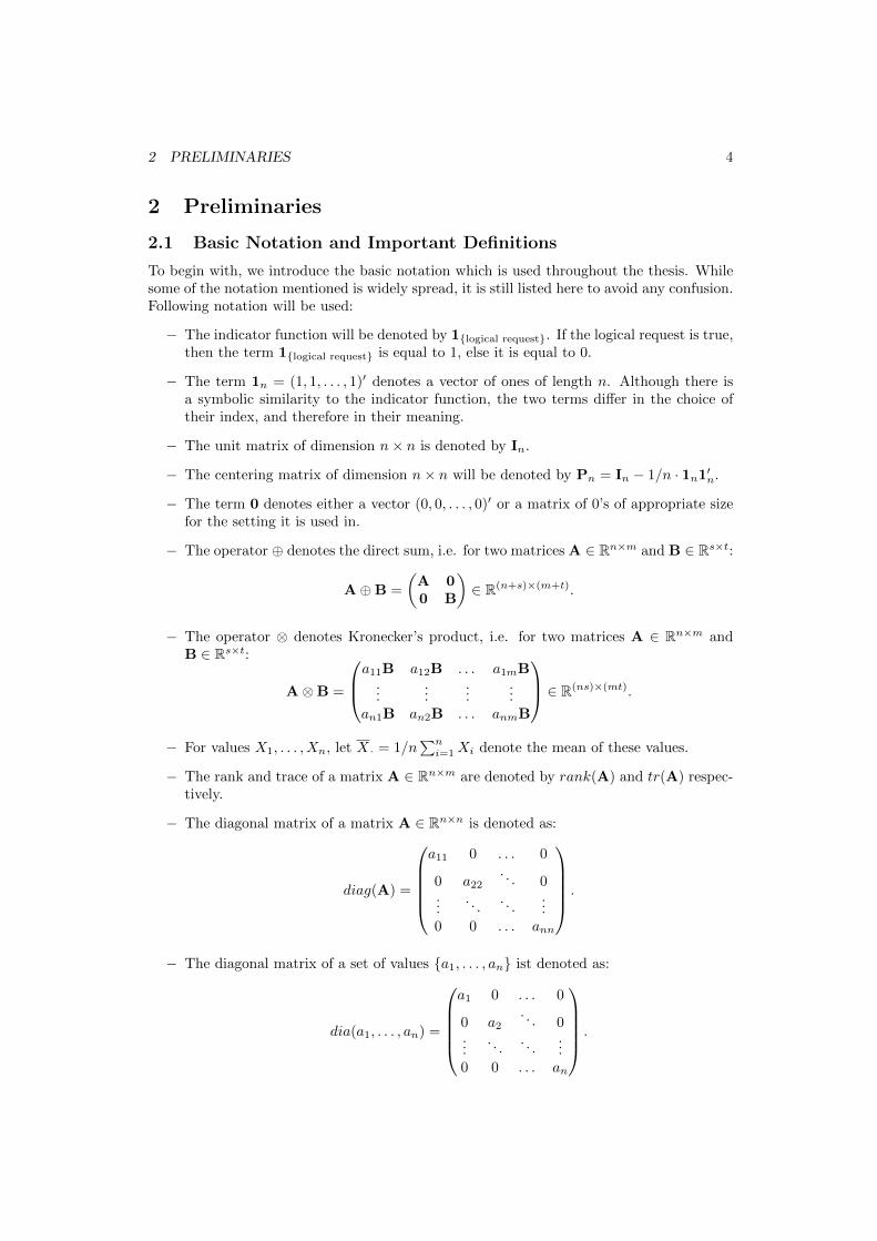
To begin with, we introduce the basic notation which is used throughout the thesis. Whilesome of the notation mentioned is widely spread, it is still listed here to avoid any confusion.Following notation will be used:
− The indicator function will be denoted by 1logical request. If the logical request is true,then the term 1logical request is equal to 1, else it is equal to 0.
− The term 1n = (1, 1, . . . , 1)′ denotes a vector of ones of length n. Although there isa symbolic similarity to the indicator function, the two terms differ in the choice oftheir index, and therefore in their meaning.
− The unit matrix of dimension n× n is denoted by In.
− The centering matrix of dimension n× n will be denoted by Pn = In − 1/n · 1n1′n.
− The term 0 denotes either a vector (0, 0, . . . , 0)′ or a matrix of 0’s of appropriate sizefor the setting it is used in.
− The operator ⊕ denotes the direct sum, i.e. for two matrices A ∈ Rn×m and B ∈ Rs×t:
A⊕B =
(A 00 B
)∈ R(n+s)×(m+t).
− The operator ⊗ denotes Kronecker’s product, i.e. for two matrices A ∈ Rn×m andB ∈ Rs×t:
A⊗B =
a11B a12B . . . a1mB...
......
...an1B an2B . . . anmB
∈ R(ns)×(mt).
− For values X1, . . . , Xn, let X · = 1/n∑ni=1Xi denote the mean of these values.
− The rank and trace of a matrix A ∈ Rn×m are denoted by rank(A) and tr(A) respec-tively.
− The diagonal matrix of a matrix A ∈ Rn×n is denoted as:
diag(A) =
a11 0 . . . 0
0 a22. . . 0
.... . .
. . ....
0 0 . . . ann
.
− The diagonal matrix of a set of values a1, . . . , an ist denoted as:
dia(a1, . . . , an) =
a1 0 . . . 0
0 a2. . . 0
.... . .
. . ....
0 0 . . . an
.

2 PRELIMINARIES 5
Definition 2.1.1 (Convergence types). Let X denote a random variable with distributionfunction F and X1, . . . , Xn denote a sequence of random variables with corresponding dis-tribution functions F1, . . . , Fn. If:
1. For all continuity points of F it holds, that limn→∞
Fn(x) = F (x), then Xn converges
in distribution to X and we write: XnD→ X.
2. For all ε > 0 it holds that limn→∞
P (|Xn − X| ≥ ε) = 0, then Xn converges in
probability to X and we write: XnP→ X.
3. It holds, that P ( limn→∞
Xn = X) = 1, then Xn converges almost surely to X and we
write: Xna.s.→ X.
4. It holds, that limn→∞
E(|Xn − X|r) = 0, then Xn converges to X in the rth mean
and we write: XnLr
→ X.
Almost sure convergence and convergence in the rth mean imply convergence in probability,and convergence in probability implies convergence in distribution. The opposite is generallynot true, see Van der Vaart (1998) p.10.
Definition 2.1.2 (Asymptotic Equivalence). Let (Xn)n∈N and (Yn)n∈N denote two se-
quences of random variables, such that |Xn − Yn|P→ 0 for n → ∞. Then Xn and Yn
are asymptotically equivalent and we write:
Xi.=. Yi.
This relation is particularly useful when one is interested in the asymptotic distribution ofa sequence of random variables. Then, it is sufficient to know the asymptotic distributionof an asymptotically equivalent sequence of random variables.
Definition 2.1.3 (Asymptotic Distribution). Let (Xn)n∈N and (Un)n∈N denote two se-quences of random variables. Further denote F a distribution function and U a random
variable with distribution function F (we write U ∼ F ), such that UnD→ U ∼ F . If
Xn.=. Un we say Xn asymptotically follows the distribution F and write:
Xn.∼. F.
Now that basic notations and definitions have been introduced, we will continue by intro-ducing the non-parametric model, both with and without covariates.
2.2 The Non-Parametric Model
The statistical inference procedures presented in this master’s thesis are supposed to bederived with minimal technical assumptions. Most importantly, we wish to derive statis-tics in a non-parametric environment, meaning we do not assume that the data has anycharacteristic structure or follows a certain distribution. The only assumption we makeon the data provided is that it is at least ordinal. This allows us to examine data notonly from continuous scales, but also from discrete scales. Further, we will be examininga one-factorial design with factor A and factor levels 1, . . . , a, also referred to as groups ofthe factor A. The results presented will technically allow for unequally distributed covari-ates between the groups, which is why we do not assume a completely randomized factorial

2 PRELIMINARIES 6
(CRF) design. However, we strongly advise the user to provide for a CRF design, as unequaldistributions of the covariates among the factor levels will inevitably lead to interpretationdifficulties, see Miller and Chapman (2001). Although we will only present the calculationsfor a one-factorial design, the presented results can certainly be used for more complexfactorial designs.
2.2.1 The Non-Parametric Model without Covariates
Let Xik denote the kth observation in the ith group, k = 1, . . . , ni and i = 1, . . . , a. Thetotal number of observations will be denoted by N =
∑ai=1 ni. Further, let:
Fi(x) = P (Xik < x) +1
2P (Xik = x) (2.1)
denote the normalized version of the distribution function, first mentioned in the context ofnon-parametric models by Levy (1925). It was later used by numerous personalities, amongthem Ruymgaart (1980), Akritas et al. (1997), Munzel (1999) and Gao et al. (2008), forderiving asymptotic results for rank statistics. In the following, we will assume that:
Xiki.i.d.∼ Fi, i = 1, . . . , a, k = 1, . . . , ni.
Thus, Xik and Xst are independent whenever i 6= s or k 6= t. In the non-parametric model,relative treatment effects are defined as:
pi =
∫HdFi, i = 1, . . . , a, (2.2)
where H denotes the mean distribution function, i.e. H(x) =∑ai=1 ωiFi(x) with weights
ωi, fulfilling ωi ≥ 0 for all i = 1, . . . , a and∑ai=1 ωi = 1. We will be using the unweighted
form, i.e. ωi = 1/a, discussed by Brunner and Puri (2001), Gao et al. (2008), opposed tothe weighted form using ωi = ni/N , introduced by Kruskal and Wallis (1952). Unweightedrelative treatment effects have “...the advantage of not being influenced by the allocation ofsample sizes in the data.” Gao et al. (2008) p.2575. More specifically, the hypotheses statedon the relative treatment effects are not influenced by the allocation of sample sizes.
Relative treatment effects are of high importance in the non-parametric model, as theycan be used to uncover differences between factor levels. They can be interpreted in sucha way, that if pi < pj , then the observations from the ith group, i.e. observations from thenormalized version of the distribution function Fi, tend to be smaller than the observationsfrom the jth group. If the relative treatment effect pi < 1/2, then observations from thenormalized distribution function Fi tend to be smaller than observations from the meandistribution function H, while pi > 1/2 indicates that observations from the normalizeddistribution function Fi tend to be larger than observations from the mean distributionfunction H.
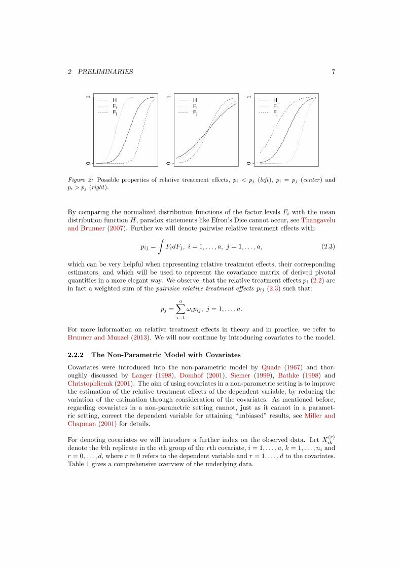
Figure 2 shows different distribution functions and the resulting properties for the relativetreatment effects.
2 PRELIMINARIES 7
01
HFiFj
01
HFiFj
01
HFiFj
Figure 2: Possible properties of relative treatment effects, pi < pj (left), pi = pj (center) andpi > pj (right).
By comparing the normalized distribution functions of the factor levels Fi with the meandistribution function H, paradox statements like Efron’s Dice cannot occur, see Thangaveluand Brunner (2007). Further we will denote pairwise relative treatment effects with:
pij =
∫FidFj , i = 1, . . . , a, j = 1, . . . , a, (2.3)
which can be very helpful when representing relative treatment effects, their correspondingestimators, and which will be used to represent the covariance matrix of derived pivotalquantities in a more elegant way. We observe, that the relative treatment effects pi (2.2) arein fact a weighted sum of the pairwise relative treatment effects pij (2.3) such that:
pj =
a∑i=1
ωipij , j = 1, . . . , a.
For more information on relative treatment effects in theory and in practice, we refer toBrunner and Munzel (2013). We will now continue by introducing covariates to the model.
2.2.2 The Non-Parametric Model with Covariates
Covariates were introduced into the non-parametric model by Quade (1967) and thor-oughly discussed by Langer (1998), Domhof (2001), Siemer (1999), Bathke (1998) andChristophliemk (2001). The aim of using covariates in a non-parametric setting is to improvethe estimation of the relative treatment effects of the dependent variable, by reducing thevariation of the estimation through consideration of the covariates. As mentioned before,regarding covariates in a non-parametric setting cannot, just as it cannot in a paramet-ric setting, correct the dependent variable for attaining “unbiased” results, see Miller andChapman (2001) for details.
For denoting covariates we will introduce a further index on the observed data. Let X(r)ik
denote the kth replicate in the ith group of the rth covariate, i = 1, . . . , a, k = 1, . . . , ni andr = 0, . . . , d, where r = 0 refers to the dependent variable and r = 1, . . . , d to the covariates.Table 1 gives a comprehensive overview of the underlying data.

2 PRELIMINARIES 8
Table 1: The underlying data setting when considering covariates.
Factor level Dep. variable 1st Covariate . . . dth Covariate
1 X(0)11 X
(1)11 . . . X
(d)11
1 X(0)12 X
(1)12 . . . X
(d)12
......
......
...
1 X(0)1n1
X(1)1n1
. . . X(d)1n1
2 X(0)21 X
(1)21 . . . X
(d)21
......
......
...
a X(0)ana X
(1)ana . . . X
(d)ana
Analogously to the non-parametric model without covariates, we denote the normalizedversion of the distribution function by:
F(r)i (x) = P (X
(r)ik < x) +
1
2P (X
(r)ik = x) (2.4)
and assume that:
(X(0)ik , . . . , X
(d)ik )′
i.i.d.∼ Fi, i = 1, . . . , a, k = 1, . . . , ni.
Now X(r)ik and X
(u)st are still independent whenever i 6= s or k 6= t, but may be dependent
over the indizes r and u. The covariates are therefore assumed to be random variables andnot fixed constants. In this setting, the relative treatment effects are defined as:
p(r)i =
∫H(r)dF
(r)i , i = 1, . . . , a, r = 0, . . . d, (2.5)
with the mean distribution function H(r), i.e. H(r)(x) =∑ai=1 ωiF
(r)i (x) and weights ωi,
fulfilling ωi ≥ 0 for all i = 1, . . . , a and∑ai=1 ωi = 1. As in the non-parametric setting
without covariates, when using the unweighted form of H(r) with ωi = 1/a, the relativetreatment effects do not depend on the allocation of the sample size and will therefore befavored over the weighted form using ωi = ni/N . The pairwise relative treatment effects aredenoted by:
p(r)ij =
∫F
(r)i dF
(r)j , i, j = 1, . . . , a, r = 1, . . . , d, (2.6)
which can, just as in the case of no covariates, be used for a more elegant representation of
the relative treatment effects p(r)i . Further we denote:
Y(r)ik = H(r)(X
(r)ik ), i = 1, . . . , a, k = 1, . . . , ni, r = 0, . . . , d, (2.7)
the asymptotic rank transformation of X(r)ik .
This notation will help us introduce a model which considers covariates in a non-parametricsetting. To adjust the dependent variable for covariates, we need some sort of connectionbetween the dependent variable and the covariates. This connection we will be consideringthroughout this thesis is the same as can be found in Langer (1998) and Siemer (1999).

2 PRELIMINARIES 9
The proposed model takes into account covariates by assuming a connection between thecovariates and the dependent variable in the asymptotic rank transformation, of the form:
Y(0)ik =
d∑r=1
γ(r) · Y (r)ik + Y regik , (2.8)
where Y regik is an unobservable random variable and γ(r), for r = 1, . . . , d, are unknown butfixed regression parameters. This type of connection between the dependent variable andthe covariates implies a connection between the relative treatment effects of the dependentvariable and the covariate, described through the adjusted relative treatment effect, which isgiven by:
p∗i = p(0)i −
d∑r=1
γ(r) · p(r)i .
It is important to state, that p∗i is not a relative treatment effect, but behaves similarly, ina sense that differences between factor levels will result in differences between the p∗i . Thiscan already be seen in the fact, that the adjusted relative treatment effect is a weighted sumof relative treatment effects which does not have to be within the interval [0, 1]. The valuep∗i cannot be interpreted in another meaningful manner, therefore solely being useful for thetesting of hypotheses.
2.3 Formulation of Hypotheses
2.3.1 Formulation of Hypotheses without Covariates
In a one-factorial design, the usual parametric approach lies in comparing the groupwisemeans, denoted by µi = E(Xik), i = 1, . . . , a, to discover differences between the factorlevels. Hypotheses are therefore formulated over µ = (µ1, . . . , µa)′. In a non-parametricmodel, hypotheses are often formulated over the marginal distributions of the factor levels,F = (F1, . . . , Fa)′ (2.1) or over relative treatment effects p = (p1, . . . , pa)′ (2.2). To comparethe groupwise means, marginal distributions or relative treatment effects, so called contrastmatrix are used.
Definition 2.3.1 (Contrast matrix). A matrix C ∈ Rq×a is called contrast matrix, whenC 6= 0 and the row sums of C are equal to 0, i.e. C1a = 0.
Using a contrast matrix C, hypotheses in the parametric setting can be formulated byH0 : Cµ = 0. In a non-parametric setting, contrast matrices are also used, but to formulatehypotheses for the marginal distributions of the data, i.e. H0 : CF = 0, or for relativetreatment effects by H0 : Cp = 0. It can easily be seen, that if the marginal distributionsare equal, i.e. if H0 : CF = 0 is true, then the other hypotheses over the groupwise means orthe relative treatment effects also have to be true, see Brunner and Munzel (2013) p.190. Theother direction is generally not true though, see Example 1. Furthermore, the implicationsH0 : Cp = 0 ⇒ H0 : Cµ = 0 and H0 : Cµ = 0 ⇒ H0 : Cp = 0 are generally not true, ascan be seen in Examples 2 and 3.
− Example 1 : Consider two groups, i.e. a=2. Assume that F1 = N(0, 1) and F2 =N(0, 2). Then the groups have unequal marginal distributions, but equal means andequal relative treatment effects.
− Example 2 : Consider two groups and assume that F1 = N(1, 1) and F2 = Exp(1).Then µ1 = µ2, but p1 6= p2.

2 PRELIMINARIES 10
− Example 3 : Again, consider two groups and assume that F1 = N(δ, 1) and F2 =Exp(1). The shift parameter δ can be chosen such that p1 = p2, but in that case,µ1 6= µ2.
When testing hypotheses under consideration of covariates, we find a similar constellation.
2.3.2 Formulation of Hypotheses with Covariates
When considering covariates in a parametric setting, hypotheses are formulated through ad-justed population means, see Section 3.1, denoted by b∗. Hypotheses are therefore formulatedby H0 : Cb∗ = 0. In a non-parametric setting, two possibilities of formulating hypotheseshave been discussed. For developing hypotheses, Langer (1998) pp.26, 40-41 assumes equal
marginal distributions in the covariates, i.e. F(r)1 = · · · = F
(r)a for all r = 1, . . . , d, and states
hypotheses over the marginal distributions of the dependent variable. The developed tests
therefore test the hypothesis H0 : CF(0) = 0, where F(0) = (F(0)1 , . . . , F
(0)a )′. On the other
hand, Siemer (1999) p.25 does not assume equal marginal distributions in the covariates andtherefore develops tests for the hypothesis H0 : Cp∗ = 0, where p∗ = (p∗1, . . . , p
∗a)′. In fact,
both Langer (1998) and Siemer (1999) see in this hypothesis the only reasonable hypothesiswhen confronted with unequal marginal distributions in the covariates. The multiple con-trast test procedures derived in this thesis will also test for the hypothesis H0 : Cp∗ = 0, butbecause we would like to provide for confidence intervals for the adjusted relative treatmenteffects, which can be used for testing hypotheses. This is not possible when formulating thehypothesis over the marginal distributions of the dependent variable. The advantage of al-lowing for unequal marginal distributions in the covariates when formulating the hypothesesover the adjusted treatment effects will be technically allowed, but treated with caution, asinterpretation difficulties will arise when such covariates are used.
The connection between the hypothesis for the parametric setting H0 : Cb∗ = 0 and thehypothesis for the non-parametric setting H0 : Cp∗ = 0 is not as clear as it was in thecase without covariates. The most simple connection between the two hypotheses is given,when the covariates have no influence on the dependent variable. In this special case, theregression parameters of the parametric and the non-parametric model are all equal to 0,and the hypotheses are related to each other as if no covariates were involved. As soonas the covariates have an influence on the dependent variable, it becomes very difficult tocompare these two hypothesis, because the regression parameters for the linear dependencybetween the covariates and the dependent variable calculated in the parametric setting andin the non-parametric setting are very different from each other. The relation between theregression parameters from the non-parametric model and the parametric model though, iscrucial for deriving implications between the two corresponding hypotheses. The only state-ment which can surely be made is that if the covariates have equal marginal distributions,then sufficient differences between the factor levels will subsequently lead to a rejection ofboth hypotheses. For equal marginal distributions of the covariates and if H0 : CF = 0 istrue, then the hypotheses H0 : Cb∗ = 0 and H0 : Cp∗ = 0 are also true, see Langer (1998)p.41. This again shows how important equal marginal distributions of the covariates are forattaining interpretable results.
We will now continue by showing how the adjusted treatment effects can be estimatedand derive test statistics for testing the mentioned hypotheses. Estimating p∗i amounts totwo steps. In the first step, the relative treatment effects of the dependent variable andthe covariates (2.5) are estimated for r = 0, . . . , d and i = 1, . . . , a. In a second step, the
2 PRELIMINARIES 11
unknown regression parameters γ(r) are estimated for r = 1, . . . , d.
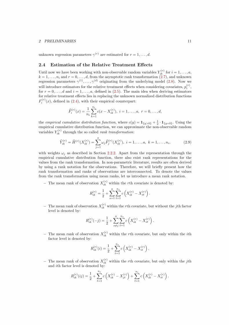
2.4 Estimation of the Relative Treatment Effects
Until now we have been working with non-observable random variables Y(r)ik for i = 1, . . . , a,
k = 1, . . . , ni and r = 0, . . . , d, from the asymptotic rank transformation (2.7), and unknownregression parameters γ(1), . . . , γ(d) originating from the underlying model (2.8). Now we
will introduce estimators for the relative treatment effects when considering covariates, p(r)i ,
for r = 0, . . . , d and i = 1, . . . , a, defined in (2.5). The main idea when deriving estimatorsfor relative treatment effects lies in replacing the unknown normalized distribution functions
F(r)i (x), defined in (2.4), with their empirical counterpart:
F(r)i (x) =
1
ni
ni∑k=1
c(x−X(r)ik ), i = 1, . . . , a, r = 0, . . . , d,
the empirical cumulative distribution function, where c(y) = 1y>0 + 12 · 1y=0. Using the
empirical cumulative distribution function, we can approximate the non-observable random
variables Y(r)ik through the so called rank transformation:
Y(r)ik = H(r)(X
(r)ik ) =
a∑j=1
ωjF(r)j (X
(r)ik ), i = 1, . . . , a, k = 1, . . . , ni, (2.9)
with weights ωj as described in Section 2.2.2. Apart from the representation through theempirical cumulative distribution function, there also exist rank representations for thevalues from the rank transformation. In non-parametric literature, results are often derivedby using a rank notation for the observations. Therefore, we will briefly present how therank transformation and ranks of observations are interconnected. To denote the valuesfrom the rank transformation using mean ranks, let us introduce a mean rank notation.
− The mean rank of observation X(r)ik within the rth covariate is denoted by:
R(r)ik =
1
2+
a∑s=1
ns∑t=1
c(X
(r)ik −X
(r)st
).
− The mean rank of observation X(r)ik within the rth covariate, but without the jth factor
level is denoted by:
R(r)ik (−j) =
1
2+
a∑s6=j
ns∑t=1
c(X
(r)ik −X
(r)st
).
− The mean rank of observation X(r)ik within the rth covariate, but only within the ith
factor level is denoted by:
R(r)ik (i) =
1
2+
ns∑t=1
c(X
(r)ik −X
(r)it
).
− The mean rank of observation X(r)ik within the rth covariate, but only within the jth
and ith factor level is denoted by:
R(r)ik (ij) =
1
2+
nj∑t=1
c(X
(r)ik −X
(r)jt
)+
ni∑t=1
c(X
(r)ik −X
(r)it
).

2 PRELIMINARIES 12
Through this notation of the mean ranks of observations, we attain a mean rank notation
for the rank transformation Y(r)ik , by:
Y(r)ik = ωi
1
ni
(R
(r)ik (i)− 1
2
)+
a∑j 6=i
ωj1
nj
(R
(r)ik −R
(r)ik (−j)
), i = 1, . . . , a, k = 1, . . . , ni.
Using the cumulative distribution function, estimators for the relative treatment effects aregiven by:
p(r)j =
∫H(r)dF
(r)j =
a∑i=1
ωi · p(r)ij , j = 1, . . . , a, r = 0, . . . , d, (2.10)
where p(r)ij =
∫F
(r)i dF
(r)j = 1/nj
∑nj
k=1 F(r)i (X
(r)jk ) is an estimator for the pairwise relative
treatment effects defined in (2.6). It is also possible to notate the estimators for the relativetreatment effects using the mean ranks notation. It holds that:
p(r)j =
a∑i=1
ω(r)i ·
1
ni
(R
(r)
j· (ij)− nj + 1
2
)and p
(r)ij =
1
ni
(R
(r)
j· (ij)− nj + 1
2
).
The estimator p(r)j has been shown to be unbiased and consistent for estimating p
(r)j .
Theorem 2.4.1. Let p(r)j and p
(r)j be as defined in (2.10) and (2.5), respectively. If N →∞
such that N/ni ≤ N0 <∞ for a N0 ∈ N, then:
E(p
(r)j
)= p
(r)j and E
((p
(r)j − p
(r)j )2
)→ 0 for j = 1, . . . , a.
Proof. The theorem can be proven analogously to Proposition 4.7 from Brunner and Munzel(2013) p.180. We will prove the unbiasedness of the estimator, to demonstrate how theadditional index for the covariates is added.
E(p
(r)j
)= E
(∫H(r)dF
(r)j
)= E
(a∑i=1
∫ωiF
(r)i dF
(r)j
)
=
a∑i=1
E
(1
nj
nj∑k=1
ωiF(r)i (X
(r)jk )
)=
a∑i=1
1
nj
nj∑k=1
ωiE(F
(r)i (X
(r)jk ))
=
a∑i=1
1
nj
nj∑k=1
ωiE
(1
ni
ni∑l=1
c(X(r)jk −X
(r)il )
)
=
a∑i=1
1
nj
nj∑k=1
ωi1
ni
ni∑l=1
E(c(X
(r)jk −X
(r)il ))
=
a∑i=1
1
nj
nj∑k=1
ωi
∫F
(r)i dF
(r)j =
a∑i=1
1
nj
nj∑k=1
ωip(r)ij =
a∑i=1
ωip(r)ij = p
(r)j
For further details on the estimation of relative treatment effects, their representation withmean ranks and their properties, as well as the subject of pseudo ranks, we refer to Brunnerand Munzel (2013) and Gao et al. (2008). Now that we have appropriate estimators forthe relative treatment effects, it remains to find estimators for the regression parametersγ(1), . . . , γ(r).

2 PRELIMINARIES 13
2.5 Estimation of the Regression Parameters
The basis for our estimation of the regression parameters is equation (2.8). Using this equa-tion, a natural way of estimating the constants γ(r), for r = 1, . . . , d, would be a linearregression. The only problem with directly performing a linear regression is that, contrarilyto a usual linear regression, no intercept is specifically stated, but instead the intercept ishidden within the terms of the asymptotic rank transformation. Therefore we will performa linear regression on the mean adjusted form of (2.8). Langer (1998) also uses a mean ad-justed form for the estimation of the regression parameters γ(r), but assumes equal marginal
distributions of the covariates, i.e. F(r)i = F (r), i = 1, . . . , a, for all r = 1, . . . , d. The valid-
ity of this assumption and the consequences for the null hypothesis have been thoroughlydiscussed by Langer (1998) pp.40-41. A different approach using an adjusted means regres-sion was given by Siemer (1999), who does not assume equal marginal distributions withinthe covariates. This setting was also shortly discussed by Bathke and Brunner (2003), whogive a different possibility from the estimation proposed by Langer (1998) for adjusting theregression model, to cope with unequal marginal distributions within the covariates. Wewill not assume equal marginal distributions within the covariates and therefore use a meanadjusted regression model as can be found in Bathke and Brunner (2003).
Taking (2.8), we can transfer the model into the mean adjusted form:
Y(0)ik =
d∑r=1
γ(r) · Y (r)ik + Y regik
⇒ Y(0)ik − Y
(0)
i· =
d∑r=1
γ(r) · (Y (r)ik − Y
(r)
i· ) + (Y regik − Y regi· ).
Because Y(r)ik are non-observable random variables, we will approximate the values from the
asymptotic rank transformation with corresponding values from the rank transformation
Y(r)ik defined in (2.9). Having done this, the least squares estimator for γ = (γ(1), . . . , γ(d))′
is given by:γ = (X′X)−1X′y, (2.11)
where X and y denote:
X =
Y
(1)11 − Y
(1)
1· . . . Y(d)11 − Y
(d)
1·
Y(1)12 − Y
(1)
1· . . . Y(d)12 − Y
(d)
1·...
. . ....
Y(1)ana − Y
(1)
a· . . . Y(d)ana − Y
(d)
a·
and y =
Y
(0)11 − Y
(0)
1·
Y(0)12 − Y
(0)
1·...
Y(0)ana − Y
(0)
a·
. (2.12)
In the following, we will further denote the non-empirical counterparts of X and y as X andy, respectively. When introducing the non-parametric model with covariates, we noticedthat the covariates are assumed to be random variables and not fixed values. Therefore,the regressors within X are random variables and we need a conditional assumption on theresiduals, i.e. Y regik − Y regi· , to justify this approach.

2 PRELIMINARIES 14
For a consistent estimation of γ we make the following technical assumptions:
(A1) There exists a number N0 ∈ N such that Nni≤ N0 <∞ for all i = 1, . . . , a.
(A2) E(Y regik − Y regi· | X = x
)= 0 for all i = 1, · · · , a, k = 1, · · · , ni.
(A3) Let λmin be the smallest eigenvalue of the matrix 1NX′X. Then there exists a constant
κ0 such that λmin ≥ κ0 > 0 almost surely for all N ∈ N.
Using these technical assumptions, we are able to prove the consistency of our estimator γfor the regression parameters.
Theorem 2.5.1. Under the assumptions (A1)-(A3) and as N →∞ it holds that:
γP→ γ
Proof. For a detailed proof see Langer (1998) Lemma 4.6-4.7 and Theorem 4.8, as well asSiemer (1999) p.59.
Note that every time γ has to be estimated for one of the upcoming test statistics, theassumptions (A1)-(A3) have to apply. By plugging in the estimator γ = (γ(1), . . . , γ(d))′
for γ, we attain estimators for the adjusted relative treatment effects p∗i given by:
p∗i = p(0)i −
d∑r=1
γ(r)p(r)i , i = 1, . . . , a.
These estimators will be the basis for the upcoming simultaneous inference.
2.6 Properties of the Adjusted Relative Treatment Effects
From the previous section we have attained an estimator for the adjusted relative treatmenteffects, given by:
p∗i = p(0)i −
d∑r=1
γ(r)p(r)i , i = 1, . . . , a, (2.13)
where definition and properties of the estimators for the regression parameters γ(1), . . . , γ(d)
are given in Section 2.5, and definition and properties of the estimators for the relative
treatment effects p(r)i , i = 1, . . . , a and r = 0, . . . , d, are given in Section 2.4.
This estimator, for the adjusted relative treatment effect, can be shown to be asymptot-ically unbiased and consistent.
Lemma 2.6.1. Under the assumption (A1), i.e. N/ni ≤ N0 < ∞ for some N0 ∈ N, andfor N →∞ it holds that:
E(p∗i )→ E(p∗i ) and p∗iP→ p∗i for i = 1, . . . , a (2.14)
Proof. From (2.5.1) and (2.4.1) we know that:
p(r)i
P→ p(r)i and γ(r) P→ γ(r).
2 PRELIMINARIES 15
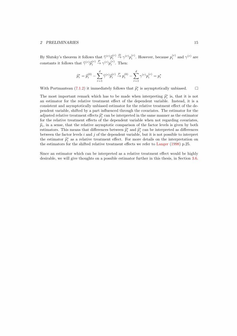
By Slutsky’s theorem it follows that γ(r)p(r)i
D→ γ(r)p(r)i . However, because p
(r)i and γ(r) are
constants it follows that γ(r)p(r)i
P→ γ(r)p(r)i . Then:
p∗i = p(0)i −
d∑r=1
γ(r)p(r)i
P→ p(0)i −
d∑r=1
γ(r)p(r)i = p∗i
With Portmanteau (7.1.2) it immediately follows that p∗i is asymptotically unbiased.
The most important remark which has to be made when interpreting p∗i is, that it is notan estimator for the relative treatment effect of the dependent variable. Instead, it is aconsistent and asymptotically unbiased estimator for the relative treatment effect of the de-pendent variable, shifted by a part influenced through the covariates. The estimator for theadjusted relative treatment effects p∗i can be interpreted in the same manner as the estimatorfor the relative treatment effects of the dependent variable when not regarding covariates,pi, in a sense, that the relative asymptotic comparison of the factor levels is given by bothestimators. This means that differences between p∗i and p∗j can be interpreted as differencesbetween the factor levels i and j of the dependent variable, but it is not possible to interpretthe estimator p∗i as a relative treatment effect. For more details on the interpretation onthe estimators for the shifted relative treatment effects we refer to Langer (1998) p.25.
Since an estimator which can be interpreted as a relative treatment effect would be highlydesirable, we will give thoughts on a possible estimator further in this thesis, in Section 3.6.

3 SIMULTANEOUS INFERENCE 16
3 Simultaneous Inference
In the literature, several procedures for testing with covariates in a non-parametric environ-ment have been developed. Taking an arbitrary contrast matrix C ∈ Rs×a Langer (1998)derives two test statistics for the hypothesis H0 : CF(0) = 0, a Wald-Type statistic and anANOVA-Type statistic. Siemer (1999) then uses this as a basis for developing Wald-Typeand ANOVA-Type test statistics for the hypothesis H0 : Cp∗ = 0, which becomes neces-sary, because unlike Langer (1998), Siemer (1999) does not assume equal distributions ofthe covariates between the groups. Christophliemk (2001) decided to take the test statisticsproposed by Siemer (1999) and improve these using transformation methods on the relativetreatment effects.
In addition to some of the existing test statistics, we would like to develop a further teststatistic based on the work of Konietschke et al. (2012a). This test, for the hypothesisH0 : Cp∗ = 0, will be a multiple contrast test procedure, giving us the ability not only tosay if there is a group effect, but additionally also where this group effect can be observed,without having to perform post-hoc analysis.
Before we do so, we briefly introduce the parametric ANCOVA, the parametric multiplecontrast test procedures and the methods used by Siemer (1999), as these will be comparedto the newly derived multiple contrast test procedure in an extensive simulation study.
3.1 Parametric ANCOVA
The ANCOVA is an extension of the well-known ANOVA, which tests for differences betweenblocks of observations, by a regression parameter. It is well described in Timm (1975),Huitema (1980), Kirk (1982), Seber (1977) and many other works. The described model inTimm (1975) pp.471-474 is given by:
X(0) = M1b︸ ︷︷ ︸ANOVA component
+ M2β︸ ︷︷ ︸Linear regression component
+ ε︸︷︷︸Error term
, (3.1)
where the components of this model are given by:
− The dependent variable X(0) = (X(0)11 , X
(0)12 , · · · , X
(0)ana)′
− The design matrix M1 =a⊕i=1
1ni
− The parameter vector of factor level means b = (µ1, . . . , µa)′
− The regressor matrix M2 =
X
(1)11 · · · X
(d)11
X(1)12 · · · X
(d)12
.... . .
...
X(1)ana · · · X
(d)ana
− The vector of regression parameters β = (β1, · · · , βd)′
− The error term ε = (ε11, ε12, · · · , εana)′ ∼ N(0, σ2 · IN ).

3 SIMULTANEOUS INFERENCE 17
Contrarily to our model assumptions, Timm (1975) states that the covariates need to be fixedand continuous values. While it is possible to cope with random covariates by stating condi-tional assumptions on the residuals, i.e. E (ε|M2 = m2) = 0 and Cov (ε|M2 = m2) = σ2·IN ,we will not do so, to avoid unforeseen consequences for the interpretation of the adjustedpopulation means. Therefore the multiple contrast test procedures will be compared to themodel as explained in Timm (1975), which assumes continuous fixed observed variables ascovariates. The aim of the ANCOVA model described is to test for differences between thelevels of the adjusted population means, given by b∗ = b− (M′
1M1)−1M′1M2β. As long as
the upper assumptions and the conditions that M′1M1 and M′
2M2 are regular are fulfilled,we attain estimators for β, b, the adjusted population means b∗ and σ2 through (3.2), (3.3),(3.4) and (3.5), respectively.
β = (M′2 (IN − JM ) M2)
−1M′
2 (IN − JM ) X(0) with JM = M1(M′1M1)−1M′
1 (3.2)
b = (M′1M1)−1M′
1X(0) (3.3)
b∗ = b− (M′1M1)−1M′
1M2β = (M′1M1)−1M′
1(X(0) −M2β) (3.4)
σ2 =(X(0)′ (IN − JM ) X(0) − β
′M′
2(IN − JM )M2β)/f (3.5)
where f = N − rank(M1)− rank(M2)
Using these estimators, we can attain test statistics for testing the hypothesis H0 : Cb∗ = 0,where C denotes an arbitrary contrast matrix. Timm (1975) p.474 further shows that with:
S = Var[b∗]
= σ2[(M′
1M1)−1
+ (M′1M1)
−1M′
1M2 (M′2(IN − JM )M2)
−1M′
2M1 (M′1M1)
−1]
QT = b∗′C′(CSC′)−Cb∗
Following equation holds:
TT =QT /g
σ2
H0∼ F (g, f), (3.6)
where g = rank(C) and f = N−rank(M1)−rank(M2). The test statistics TT , as one of themost widely spread test statistics for statistical inference with covariates, will be comparedto the multiple contrast test procedure in terms of α-level and power.
3.2 Parametric Multiple Contrast Test Procedures
Additionally to the parametric ANCOVA, multiple contrast test procedures exist for theparametric setting given in (3.1). These procedures allow not only for testing the globalhypothesis H0 : Cb∗ = 0, but also for investigating between which groups differences occur,without having to perform post-hoc tests. A simultaneous test procedure for general linearmodels, and thus for the parametric ANCOVA, was developed by Hothorn et al. (2008).The procedure assumes an underlying semi-parametric model:
M = ((X1, . . . , Xn),θ, τ) ,
with a fixed but unknown parameter θ ∈ Rp and other random (or nuisance) parameters
τ . Further it is required, that if θn is an estimator for θ and Sn an estimator for Cov(θn),then following equation has to hold:
a1/2n (θn − θ)
D→ N(0,Φ),

3 SIMULTANEOUS INFERENCE 18
for some multivariate central limit theorem and some positive non-decreasing sequence
(an)n∈N, such that anSnP→ Φ. Under these assumptions, Hothorn et al. (2008) develop
simultaneous test procedures for the hypothesis H0 : Cθ = 0 through a test statistic:
TH = D−1/2n (θn − θ)
D→ N(0,R), (3.7)
where Dn = diag(CSnC′). Then the components of the test statistic TH are asymptoti-cally N(0, 1) distributed, and a testing procedure is conceived by estimating the unknowncorrelation matrix R and using appropriate critical values from the multivariate normaldistribution, a similar approach as we will follow when deriving the multiple contrast testprocedures in this thesis, derived in Section 3.5. For more information on the technicaldetails of the procedure, we refer to Hothorn et al. (2008).
The implementation developed by Hothorn et al. (2008) is given in statistics program R,with the multcomp package. This package contains a function glht which can be used as awrapper for many functions treating general linear models in R, among them the functionaov, which allows for global inference in the parametric ANCOVA model. Since our upcom-ing simulation study is conducted in R, we will use the function aov for statistical inference,and the wrapper glht to allow for simultaneous inference. The procedure can be applied bycalling following functions in R:
1 ancova<−aov ( X0 ∼ group+X1 , data=datalm )2 result<−g lh t ( ancova , linfct=mcp ( group= ‘ ‘Tukey ’ ’ ) )
where datalm is an appropriate data frame containing the data, X0 refers to the dependentvariable, group refers to a group variable employed as a factor and X1 refers to a covariate.The result from the simultaneous inference will then be compared to the multiple contrasttest procedure for the non-parametric setting, derived in Section 3.5. For more details onthe implementation of the simultaneous test procedures, as well as examples, we refer toHothorn et al. (2008).
3.3 Wald-Type Statistic
One of the methods we will be comparing the multiple contrast test procedures to is the non-parametric approach using a Wald-type statistic proposed, by Siemer (1999). The reasonwe do not compare the Wald-type statistic of Langer (1998) with the multiple contrasttest procedure, is that Langer (1998) tests a different hypothesis, namely H0 : CF(0) = 0opposed to Siemer (1999), who tests for the hypothesis H0 : Cp∗ = 0, the same hypothesiswhich is tested by the multiple contrast test procedure. For this denote:
ΛN = Cov
(√N
(∫H(r)dF(r) −
∫F(r)dH(r)
)r=0,...,d
), (3.8)
where F(r) = (F(r)1 , . . . , F
(r)a )′ and F(r) = (F
(r)1 , . . . , F
(r)a )′. Furthermore denote:
VN = (γ′ ⊗ Ia) ·ΛN · (γ ⊗ Ia). (3.9)
A detailed description on estimating VN can be found in in the upcoming Section 3.5.1. Forthe Wald-type statistic proposed to work properly, following technical assumptions have tohold:

3 SIMULTANEOUS INFERENCE 19
(A1) - (A3) For estimating the regression coefficients.
(A4) The matrix VN → V such that rank(VN ) = rank(V) for all N ≥ N0 ∈ N.
(A5) Let θ(r)N,i, i = 1, . . . , a and r = 1, . . . , d, denote the eigenvalues of ΛN . Then Nθ
(r)N,i → 0
or Nθ(r)N,i →∞ for all i = 1, . . . , a and r = 1, . . . , d.
Under these assumptions, Siemer (1999) pp.54-55 shows that under H0 : Cp∗ = 0 followingequation holds:
QWTS = N p∗′C′(CVNC)−Cp∗.∼. χ2
f, (3.10)
with f = rank(CVN ). For a full proof we refer to Siemer (1999) Theorem 4.20.
3.4 ANOVA-Type Statistic
The following ANOVA-type statistic proposed by Siemer (1999) is supposed to performbetter for smaller sample sizes than the Wald-type statistic. For this we define a matrixK = C′(CC′)−C. Instead of estimating the complete matrix (CVNC)−, the ANOVA-type
statistic only requires the traces of the matrices KVN and KVNKVN to be estimated.Using the so called Box-approximation Box (1954), we are then able to construct a teststatistic for the hypothesis H0 : Cp∗ = 0.
When constructing the ANOVA-type statistic, we first reformulate our hypothesis.
Lemma 3.4.1. Let K = C′(CC′)−C and U denote an arbitrary vector of appropriate size.Then the hypotheses H0 : CU = 0 and H0 : KU = 0 are equivalent.
Proof. For a detailed proof see Langer (1998), Lemma 5.2.
Under the assumptions (A1)-(A5) and additionally:
(A6) For all N there exists a c0 ∈ R such that: tr(KVN ) =a∑i=1
λi ≥ c0 > 0, where λ1, . . . , λa
are the eigenvalues of KVN ,
Siemer (1999) pp.56-59 shows, that under H0 : Cp∗ = 0 following equation holds:
QN = fN p∗′Kp∗
tr(KVN
) .∼. χ2f, (3.11)
with f = tr(KVN )2
tr(KVNKVN ). Both test procedures were implemented in R and will be compared
to the multiple contrast test procedure.
3.5 Multiple Contrast Test Procedures
We will now commence with deriving multiple contrast test procedures (MCTP) for thenon-parametric setting including covariates. Multiple contrast test procedures are simulta-neous test procedures, which allow for simultaneously testing multiple contrasts. As we havealready mentioned in the introduction, the aim of MCTP is to not only provide a testingprocedure for global hypotheses, but additionally make post-hoc tests, such as the Bon-ferroni or Bonferroni-Holm correction, unnecessary, by considering dependencies betweenindividual hypotheses and providing for adjusted p-values of the individual hypotheses.

3 SIMULTANEOUS INFERENCE 20
The main motivation for the MCTP in this thesis comes from Konietschke et al. (2012a),where MCTP for relative treatment effects are derived without covariates. The key inproviding for MCTP lies in deriving asymptotic distribution properties of the estimatorp∗ = (p∗1, . . . , p
∗a)′. More specifically, we will commence by proving that the pivotal quantity√
N(p∗ −p∗) asymptotically follows a multivariate normal distribution with mean vector 0and covariance matrix VN , i.e.:
√N(p∗ − p∗)
.∼. N(0,VN ).
Using this result, we will then derive a simultaneous test procedure. To simplify the calcu-lations in this section, we will calculate asymptotic results by assuming that γ is known.
For a more elegant representation of the upcoming equations, we further set γ(0) = −1.Then it holds, that:
√N(p∗ − p∗) =
√N
p
(0)1 −
d∑r=1
p(r)1 γ(r) − (p
(0)1 −
d∑r=1
p(r)1 γ(r))
...
p(0)a −
d∑r=1
p(r)a γ(r) − (p
(0)a −
d∑r=1
p(r)a γ(r))
(3.12)
=√N
p
(0)1 − p
(0)1
...
p(0)a − p(0)
a
−√N d∑r=1
p
(r)1 − p
(r)1
...
p(r)a − p(r)
a
γ(r)
= −√N
d∑r=0
p
(r)1 − p
(r)1
...
p(r)a − p(r)
a
γ(r).
To continue our calculations we need a result from non-parametric theory.
Theorem 3.5.1 (Asymptotic Equivalence). Let X(r)i1 , . . . , X
(r)ini
be the observations from the
rth covariate, r = 0, . . . , d in the ith group, i = 1, . . . , a. Then, assuming that X(r)ik and X
(r)il
are independent for k 6= l, following equation holds for r = 0, . . . , d:
√N(p
(r)j − p
(r)j
).=.√N
a∑i=1
ωiZ(r)ij , (3.13)
where the unweighted form is given by ωi = 1/a, and:
Z(r)ij =
1
nj
nj∑k=1
F(r)i (X
(r)jk )− 1
ni
ni∑k=1
F(r)j (X
(r)ik ) + 1− 2p
(r)ij .
Proof. By adding an index r to the mean distribution functions, Brunner and Munzel (2013)p.192 prove that:
√N
∫H(r)d
(F
(r)j − F (r)
j
).=.√N
∫H(r)d
(F
(r)j − F (r)
j
)j = 1, . . . , a, r = 0, . . . , d.
3 SIMULTANEOUS INFERENCE 21
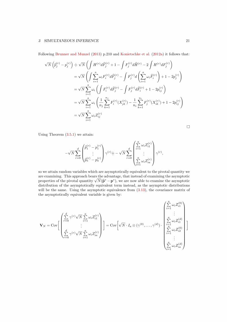
Following Brunner and Munzel (2013) p.210 and Konietschke et al. (2012a) it follows that:
√N(p
(r)j − p
(r)j
).=.√N
(∫H(r)dF
(r)j + 1−
∫F
(r)j dH(r) − 2
∫H(r)dF
(r)j
)=√N
(∫ a∑i=1
ωiF(r)i dF
(r)j −
∫F
(r)j d
(a∑i=1
ωiF(r)i
)+ 1− 2p
(r)j
)
=√N
a∑i=1
ωi
(∫F
(r)i dF
(r)j −
∫F
(r)j dF
(r)i + 1− 2p
(r)ij
)
=√N
a∑i=1
ωi
(1
nj
nj∑k=1
F(r)i (X
(r)jk )− 1
ni
ni∑k=1
F(r)j (X
(r)ik ) + 1− 2p
(r)ij
)
=√N
a∑i=1
ωiZ(r)ij
Using Theorem (3.5.1) we attain:
−√N
d∑r=0
p
(r)1 − p
(r)1
...
p(r)a − p(r)
a
γ(r) .=. −√N
d∑r=0
a∑i=1
ωiZ(r)i1
...a∑i=1
ωiZ(r)ia
γ(r),
so we attain random variables which are asymptotically equivalent to the pivotal quantity weare examining. This approach bears the advantage, that instead of examining the asymptoticproperties of the pivotal quantity
√N(p∗−p∗), we are now able to examine the asymptotic
distribution of the asymptotically equivalent term instead, as the asymptotic distributionswill be the same. Using the asymptotic equivalence from (3.13), the covariance matrix ofthe asymptotically equivalent variable is given by:
VN = Cov
[
d∑r=0
γ(r)√N
a∑i=1
ωiZ(r)i1
...d∑r=0
γ(r)√N
a∑i=1
ωiZ(r)ia
]
= Cov
[√N · Ia ⊗ (γ(0), . . . , γ(d)) ·
a∑i=1
ωiZ(0)i1
...a∑i=1
ωiZ(d)i1
a∑i=1
ωiZ(0)i2
...a∑i=1
ωiZ(d)ia
]

3 SIMULTANEOUS INFERENCE 22
= Cov
[√N · Ia ⊗ (γ(0), . . . , γ(d))︸ ︷︷ ︸
=γ′
· Iad ⊗ (ω1, . . . , ωa)︸ ︷︷ ︸=:W
·
Z(0)11...
Z(0)a1
Z(1)11...
Z(d)a1
Z(0)12...
Z(d)aa
︸ ︷︷ ︸
=:Z
]
= (Ia ⊗ γ′) ·W · Cov[√NZ]︸ ︷︷ ︸
=:ΣN
·W′ · (Ia ⊗ γ′)′. (3.14)
Now the main task for calculating VN lies in calculating Cov(√NZ) = ΣN . For this, let
us compute the pairwise covariances for all possible indizes, Cov(Z
(r)ij , Z
(u)st
). From Section
2.2.2 we remember that X(r)ik and X
(u)jl are independent if i 6= j or if k 6= l, and X
(r)ik
i.i.d.∼ F(r)i
for k = 1, . . . , ni. Using these properties, we attain:
Cov(Z
(r)ij , Z
(u)st
)=Cov
(1
nj
nj∑k=1
F(r)i (X
(r)jk )− 1
ni
ni∑k=1
F(r)j (X
(r)ik ) ,
1
nt
nt∑k=1
F (u)s (X
(u)tk )− 1
ns
ns∑k=1
F(u)t (X
(u)sk )
)
=Cov
(1
nj
nj∑k=1
F(r)i (X
(r)jk ) ,
1
nt
nt∑k=1
F (u)s (X
(u)tk )
)
− Cov
(1
nj
nj∑k=1
F(r)i (X
(r)jk ) ,
1
ns
ns∑k=1
F(u)t (X
(u)sk )
)
− Cov
(1
ni
ni∑k=1
F(r)j (X
(r)ik ) ,
1
nt
nt∑k=1
F (u)s (X
(u)tk )
)
+ Cov
(1
ni
ni∑k=1
F(r)j (X
(r)ik ) ,
1
ns
ns∑k=1
F(u)t (X
(u)sk )
)
=1
nj
nj∑k=1
1
nt
nt∑l=1
Cov(F
(r)i (X
(r)jk ) , F (u)
s (X(u)tl )
)− 1
nj
nj∑k=1
1
ns
ns∑l=1
Cov(F
(r)i (X
(r)jk ) , F
(u)t (X
(u)sl )
)− 1
ni
ni∑k=1
1
nt
nt∑l=1
Cov(F
(r)j (X
(r)ik ) , F (u)
s (X(u)tl )
)+
1
ni
ni∑k=1
1
ns
ns∑l=1
Cov(F
(r)j (X
(r)ik ) , F
(u)t (X
(u)sl )
)︸ ︷︷ ︸
=0 for i 6=s or k 6=l

3 SIMULTANEOUS INFERENCE 23
=1
n2j
nj∑k=1
[Cov
(F
(r)i (X
(r)jk ), F (u)
s (X(u)jk )
)· 1j=t
− Cov(F
(r)i (X
(r)jk ), F
(u)t (X
(u)jk )
)· 1j=s
]− 1
n2i
ni∑k=1
[Cov
(F
(r)j (X
(r)ik ), F (u)
s (X(u)ik )
)· 1i=t
− Cov(F
(r)j (X
(r)ik ), F
(u)t (X
(u)ik )
)· 1i=s
]=
1
nj
[Cov
(F
(r)i (X
(r)j1 ), F (u)
s (X(u)j1 )
)· 1j=t
− Cov(F
(r)i (X
(r)j1 ), F
(u)t (X
(u)j1 )
)· 1j=s
]− 1
ni
[Cov
(F
(r)j (X
(r)i1 ), F (u)
s (X(u)i1 )
)· 1i=t
− Cov(F
(r)j (X
(r)i1 ), F
(u)t (X
(u)i1 )
)︸ ︷︷ ︸
=:θ(r,u)jit
·1i=s]
=1
nj
(θ
(r,u)ijs · 1j=t − θ
(r,u)ijt · 1j=s
)− 1
ni
(θ
(r,u)jis · 1i=t − θ
(r,u)jit · 1i=s
).
Using the upper calculations, all possible index combinations are listed in the following table:
For i = j ∨ t = s : Cov(Z
(r)ij , Z
(u)st
)= 0
For (i 6= j ∧ t 6= s) ∧ (j = t ∧ i = s) : Cov(Z
(r)ij , Z
(u)st
)=
1
njθ
(r,u)ijs +
1
niθ
(r,u)jit
For (i 6= j ∧ t 6= s) ∧ (j = s ∧ i = t) : Cov(Z
(r)ij , Z
(u)st
)= − 1
njθ
(r,u)ijt −
1
niθ
(r,u)jis
For (i 6= j ∧ t 6= s) ∧ (j 6= s, t ∧ i = t) : Cov(Z
(r)ij , Z
(u)st
)= − 1
niθ
(r,u)jis
For (i 6= j ∧ t 6= s) ∧ (j 6= s, t ∧ i = s) : Cov(Z
(r)ij , Z
(u)st
)=
1
niθ
(r,u)jit
For (i 6= j ∧ t 6= s) ∧ (j = t ∧ i 6= s, t) : Cov(Z
(r)ij , Z
(u)st
)=
1
njθ
(r,u)ijs
For (i 6= j ∧ t 6= s) ∧ (j = s ∧ i 6= s, t) : Cov(Z
(r)ij , Z
(u)st
)= − 1
njθ
(r,u)ijt
For (i 6= j ∧ t 6= s) ∧ (j 6= s, t ∧ i 6= s, t) : Cov(Z
(r)ij , Z
(u)st
)= 0.
We have now successfully calculated the covariance matrix ΣN , by calculating the covari-
ances of Z(r)ij and Z
(u)st for all possible index combinations, and therefore the covariance
matrix VN = (Ia ⊗ γ′) ·W ·ΣN ·W′ · (Ia ⊗ γ′)′. It remains to show the asymptotic multi-variate normality of the pivotal quantity
√N(p∗−p∗) and conclude the connection to VN .
This is done in the following theorem.

3 SIMULTANEOUS INFERENCE 24
Theorem 3.5.2. Let VN be as given in the upper calculation. Under the assumptions(A1), i.e. there exists N0 ∈ N such that N
ni≤ N0 <∞ for i = 1, . . . , a, and that VN → V
such that rank(VN ) = rank(V) ≥ 1 for all N ≥ M0 < ∞ is fulfilled, the rank statistic√N(p∗ − p∗) asymptotically follows a multivariate normal distribution with expectation 0
and covariance matrix VN .
Proof. The theorem can be proven analogously to Theorem 2 in Konietschke et al. (2012a).First we take a close look at the covariance matrix VN . Let λi,N , i = 1, . . . , a, denote theeigenvalues of VN where λmin
N = minλN,i|λN,i > 0, i = 1, . . . , a is the smallest eigenvaluelarger than zero. Then, by the assumptions of this theorem, there exists a constant c0 > 0such that λmin
N ≥ c0 for all N ≥ M0. Without loss of generality let λ1,N , . . . , λj,N → 0and λj+1,N , . . . , λa,N ≥ c0. Since VN is a covariance matrix and therefore a symmetricmatrix, by the spectral decomposition theorem there exists an invertible matrix B suchthat BVNB′ = D = D1 ⊕D2 where D1 = dia(λ1,N , . . . , λj,N ) a diagonal matrix with thefirst j eigenvalues and D2 = dia(λj+1,N , . . . , λa,N ) a diagonal matrix with the remaining
eigenvalues. The asymptotic normality of√N(Ia ⊗ γ′)WZ is now established through the
Cramer-Wold device (7.1.9). Let k = (k1, . . . , ka)′ denote an arbitrary vector of constants.Since B is invertible, there exists a vector k such that k′ = kB. From Lindeberg-Feller limittheorem it follows that:
√Nk′(Ia ⊗ γ′)WZ√
Var(√Nk′(Ia ⊗ γ′)WZ)
=Nk′(Ia ⊗ γ′)WZ√
Var(Nk′(Ia ⊗ γ′)WZ)
D→ N(0, 1)
Because:
Var(Nk′(Ia ⊗ γ′)WZ) = N ·Var(√Nk′(Ia ⊗ γ′)WZ) = Nk′VNk
= N k′BVNB′k = N k′(D1 ⊕D2)k ≥ N ·a∑
s=j+1
ksc0 →∞.
Therefore the sum of variances of Nk′(Ia ⊗ γ′)WZ diverges for N → ∞ and Lindeberg’s
condition (7.1.7) is fulfilled, because the random variables Nni· F (r)
i (X(r)jk ) are uniformly
bounded, because N/ni ≤ N0 < ∞. Since it might not be clear how the term Nk′(Ia ⊗γ′)WZ is written as a sum of independent variables, further calculations can be attainedfrom the appendix in Lemma (7.1.11).
Theorem (3.5.2) is a central result for developing the multiple contrast test procedure.Before calculating test statistics however, it remains to find an appropriate estimator for thecovariance matrix VN , or subsequently ΣN , as can be seen through (3.14). An estimatorwill be provided in the next section.
3.5.1 Estimating the Covariance Matrix
Through the upper calculations of the covariance matrix ΣN it becomes obvious that for
estimating ΣN , and thus VN , it is sufficient to estimate the parameters θ(r,u)ijs . Normally,
we would estimate θ(r,u)ijs through:
θ(r,u)ijs =
1
nj − 1
nj∑k=1
(F
(r)i (X
(r)jk )− 1
nj
nj∑l=1
F(r)i (X
(r)jl )
)(F (u)s (X
(u)jk )− 1
nj
nj∑l=1
F (u)s (X
(u)jk )
),

3 SIMULTANEOUS INFERENCE 25
but because the random variables F(r)i (X
(r)jk ) are non-observable random variables, θ
(r,u)ijs is
not a valid estimator for θijs. Therefore, we will replace F(r)i (X
(r)jk ) by F
(r)i (X
(r)jk ), random
variables which are observable and presumably close enough to the non-observable random
variables for a valid estimation. The resulting estimator for θ(r,u)ijs is then given by:
θ(r,u)ijs =
1
nj − 1
nj∑k=1
(F
(r)i (X
(r)jk )− 1
nj
nj∑l=1
F(r)i (X
(r)jl )
).
(F (u)s (X
(u)jk )− 1
nj
nj∑l=1
F (u)s (X
(u)jl )
).
Using the mean rank notation introduced in Section 2.4 enables us to denote the proposed
estimator θ(r,u)ijs using ranks by:
θ(r,u)ijs =
1
nj − 1
nj∑k=1
1
ni
(R
(r)jk (ij)−R(r)
jk (j)−R(r)
j· (ij) +nj + 1
2
)· 1
ns
(R
(u)jk (sj)−R(u)
jk (j)−R(u)
j· (sj) +nj + 1
2
).
With these estimators, we are able to estimate VN consistently. Let the proposed estimator,
replacing θ(r,u)ijs by θ
(r,u)ijs , be denoted by VN , and ΣN the estimator for ΣN accordingly. The
consistency of VN is proven in the following theorem.
Theorem 3.5.3. Under the assumption (A1), i.e. N →∞ such that N/ni ≤ N0 <∞ for
N0 ∈ N and all i = 1, . . . , a, it holds that: VN −VNa.s.→ 0.
Proof. The theorem can be proven analogously to Lemma A.2 and Theorem A.4 fromKonietschke et al. (2012a). The key in proving the consistency of VN lies in proving the
consistency of ΣN . By the strong law of large numbers it holds that θ(r,u)ijs − θ(r,u)
ijsa.s.→ 0
when nj , ns →∞ . Because the number of groups a and number of covariates d is bounded,
it is sufficient to prove the consistency of ΣN componentwise. Therefore, the proof amounts
to showing: |θ(r,u)ijs − θ
(r,u)ijs |
a.s.→ 0. For this denote:
D(r)ijk = F
(r)i (X
(r)jk )− 1
nj
nj∑l=1
F(r)i (X
(r)jl ),
and its empirical counterpart by:
D(r)ijk = F
(r)i (X
(r)jk )− 1
nj
nj∑l=1
F(r)i (X
(r)jl ).
Then it holds that:
|θ(r,u)ijs − θ
(r,u)ijs | =
∣∣∣∣∣ 1
nj − 1
nj∑k=1
D(r)ijkD
(u)sjk − D
(r)ijkD
(u)sjk
∣∣∣∣∣=
∣∣∣∣∣ 1
nj − 1
nj∑k=1
D(r)ijkD
(u)sjk − D
(r)ijkD
(u)sjk ± D
(r)ijkD
(u)sjk
∣∣∣∣∣=
∣∣∣∣∣ 1
nj − 1
nj∑k=1
D(r)ijk(D
(u)sjk − D
(u)sjk)− D(u)
sjk(D(r)ijk − D
(r)ijk)
∣∣∣∣∣

3 SIMULTANEOUS INFERENCE 26
≤ 1
nj − 1
nj∑k=1
∣∣∣D(r)ijk(D
(u)sjk − D
(u)sjk)− D(u)
sjk(D(r)ijk − D
(r)ijk)∣∣∣
≤ 1
nj − 1
nj∑k=1
∣∣∣D(r)ijk
∣∣∣ ∣∣∣D(u)sjk − D
(u)sjk
∣∣∣+∣∣∣D(u)
sjk
∣∣∣ ∣∣∣D(r)ijk − D
(r)ijk
∣∣∣≤ 1
nj − 1
nj∑k=1
∣∣∣D(u)sjk − D
(u)sjk
∣∣∣+1
nj − 1
nj∑k=1
∣∣∣D(r)ijk − D
(r)ijk
∣∣∣≤ njnj − 1
maxk=1,...,nj
∣∣∣D(u)sjk − D
(u)sjk
∣∣∣+nj
nj − 1max
k=1,...,nj
∣∣∣D(r)ijk − D
(r)ijk
∣∣∣ , (3.15)
where we used∣∣∣D(r)
ijk
∣∣∣ ≤ 1 and∣∣∣D(u)
sjk
∣∣∣ ≤ 1. Considering that:
∣∣∣D(r)ijk − D
(r)ijk
∣∣∣ =
∣∣∣∣∣F (r)i (X
(r)jk )− 1
nj
nj∑l=1
F(r)i (X
(r)jl )− F (r)
i (X(r)jk ) +
1
nj
nj∑l=1
F(r)i (X
(r)jl )
∣∣∣∣∣≤∣∣∣F (r)i (X
(r)jk )− F (r)
i (X(r)jk )∣∣∣+
∣∣∣∣∣ 1
nj
nj∑l=1
(F
(r)i (X
(r)jk )− F (r)
i (X(r)jk ))∣∣∣∣∣
≤ 2 · maxk=1,...,nj
∣∣∣F (r)i (X
(r)jk )− F (r)
i (X(r)jk )∣∣∣
and denoting the supremum norm by ‖·‖∞, equation (3.15) yields that:
njnj − 1
maxk=1,...,nj
∣∣∣D(u)sjk − D
(u)sjk
∣∣∣+nj
nj − 1max
k=1,...,nj
∣∣∣D(r)ijk − D
(r)ijk
∣∣∣≤ 2 · njnj − 1
(max
k=1,...,nj
∣∣∣F (u)s (X
(u)jk )− F (u)
s (X(u)jk )
∣∣∣+ maxk=1,...,nj
∣∣∣F (r)i (X
(r)jk )− F (r)
i (X(r)jk )∣∣∣)
≤ 2 · njnj − 1
(∥∥∥F (u)s − F (u)
s
∥∥∥∞
+∥∥∥F (r)
s − F (r)s
∥∥∥∞
)a.s.→ 0,
where we used that 2nj/(nj − 1) → 2 and from the Glivenko-Cantelli theorem (7.1.4) it
follows that∥∥∥F (u)
s − F (u)s
∥∥∥∞
a.s.→ 0. Other index combinations of the θ(r,u)ijs are proven in the
same manner, only with different indexing.
From the upper calculations and the assumption (A1) it follows, that:
VN −VN = (Ia ⊗ γ′) ·W · ΣN ·W′ · (Ia ⊗ γ′)′ − (Ia ⊗ γ′) ·W ·ΣN ·W′ · (Ia ⊗ γ′)′
= (Ia ⊗ γ′) ·W · (ΣN −ΣN )︸ ︷︷ ︸a.s.→ 0
·W′ · (Ia ⊗ γ′)′a.s.→ 0,
which proves the claim. Note, that plugging in the estimator γ for γ as proposed in Section
3.7, will weaken the convergence to VN −VNP→ 0.
The results from this section, Theorem (3.5.2) and Theorem (3.5.3), will now be used toderive the MCTP.

3 SIMULTANEOUS INFERENCE 27
3.5.2 Derivation of Test Statistics
In Theorem (3.5.2) we have shown that:√N(p∗ − p∗)
.∼. N(0,VN ). (3.16)
The main motivation for using MCTP lies in testing hypotheses to uncover differencesbetween factor levels. We will be testing hypotheses using a contrast matrix C ∈ Rq×a(2.3.1) with row vectors c1, . . . , cq, the desired contrasts, i.e. cl = (cl1, . . . , cla)′. Our goalwill be to derive multiple contrast test procedures for the family of hypotheses:
Ωp∗
=Hp∗
0 : c′lp∗ = 0 | l = 1, . . . , q
, (3.17)
by providing compatible simultaneous confidence intervals for the effects δl = c′lp∗. Simul-
taneous confidence intervals are confidence intervals for the effects δl, l = 1, . . . , q, such thatif 0 is not contained within at least one of the confidence intervals, then the global hypothesis,
i.e.⋂ql=1H
p∗
0 : c′lp∗ = 0 or simply H0 : Cp∗ = 0, can be rejected to a pre-specified level
α. In order to do this, we will begin by deriving test statistics for the individual hypotheses
Hp∗
0 : c′lp∗ = 0, for l = 1, . . . , q. We define test statistics for the individual hypotheses by:
Tp∗
l =√Nc′l(p
∗ − p∗)/√vll, (3.18)
where vlm = c′lVNcm. Then by Theorem (3.5.2), Theorem (3.5.3) and Slutsky’s theorem
it follows, that Tp∗
lD−→ N(0, 1) under the null hypothesis H0 : c′lp
∗ = 0. For developingMCTP we will require not only the distribution of an individual test statistic, but moreimportantly the joint distribution of all individual test statistics, i.e. we further need the
covariance structure of the vector of test statistics, T = (Tp∗
1 , . . . , Tp∗
q ). Denote R =Cov(T), and assuming VN is known, with:
Cov(Tp∗
l , Tp∗
m ) = Cov(√Nc′l(p
∗ − p∗)/√vll ,
√Nc′m(p∗ − p∗)/
√vmm)
= Cov
√N a∑i=1
cli(p∗i − p∗i ),
√N
a∑j=1
cmj(p∗j − p∗j )
/√vllvmm
=
a∑i=1
cli
b∑j=1
cmjCov(√
N(p∗i − p∗i ),√N(p∗j − p∗j )
)/√vllvmm
= c′lVNcm/√vllvmm = vlm/
√vllvmm,
we can calculate the covariance matrix of T, Cov(T) = R = (rlm)l,m=1,...,q where rlm =vlm/
√vllvmm. From Theorem (3.5.2), Slutsky’s theorem and the upper calculations, it
follows that:T
.∼. N(0,R). (3.19)
Our goal will be to use this multivariate asymptotic property of the vector of test statis-tics T for conceiving simultaneous test procedures. The idea behind a simultaneous test
procedure is to control the type I error for the global hypothesis⋂ql=1H
p∗
0 : c′lp∗ = 0
by properly adjusting the individual hypotheses from Ωp∗ (3.17). The global hypothesisis rejected, when any adjusted individual hypothesis is rejected. To better understand thenotion of simultaneous test procedures, let us introduce some important terminology fromthis field, before theoretically justifying this testing approach. Most of the terminology onsimultaneous testing, and the ideas represented, can be found in a similar manner in Gabriel(1969) and Konietschke et al. (2012a).
3 SIMULTANEOUS INFERENCE 28
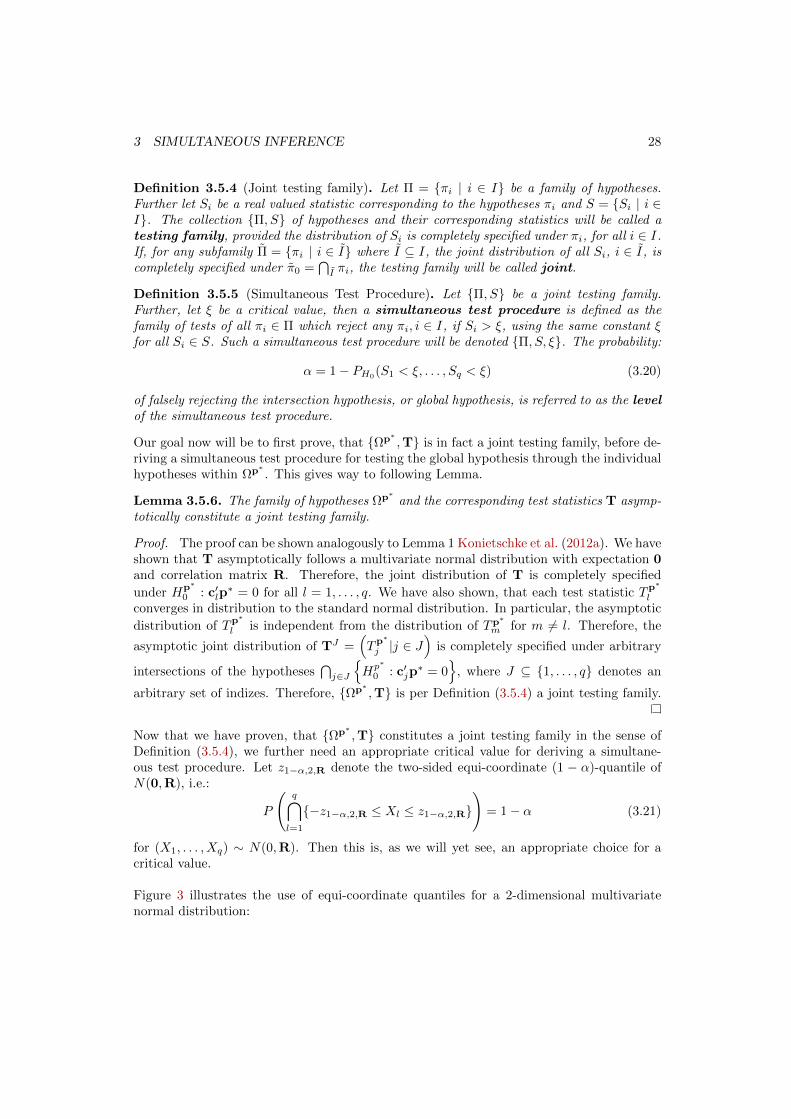
Definition 3.5.4 (Joint testing family). Let Π = πi | i ∈ I be a family of hypotheses.Further let Si be a real valued statistic corresponding to the hypotheses πi and S = Si | i ∈I. The collection Π, S of hypotheses and their corresponding statistics will be called atesting family, provided the distribution of Si is completely specified under πi, for all i ∈ I.If, for any subfamily Π = πi | i ∈ I where I ⊆ I, the joint distribution of all Si, i ∈ I, iscompletely specified under π0 =
⋂I πi, the testing family will be called joint.
Definition 3.5.5 (Simultaneous Test Procedure). Let Π, S be a joint testing family.Further, let ξ be a critical value, then a simultaneous test procedure is defined as thefamily of tests of all πi ∈ Π which reject any πi, i ∈ I, if Si > ξ, using the same constant ξfor all Si ∈ S. Such a simultaneous test procedure will be denoted Π, S, ξ. The probability:
α = 1− PH0(S1 < ξ, . . . , Sq < ξ) (3.20)
of falsely rejecting the intersection hypothesis, or global hypothesis, is referred to as the levelof the simultaneous test procedure.
Our goal now will be to first prove, that Ωp∗ ,T is in fact a joint testing family, before de-riving a simultaneous test procedure for testing the global hypothesis through the individualhypotheses within Ωp∗ . This gives way to following Lemma.
Lemma 3.5.6. The family of hypotheses Ωp∗ and the corresponding test statistics T asymp-totically constitute a joint testing family.
Proof. The proof can be shown analogously to Lemma 1 Konietschke et al. (2012a). We haveshown that T asymptotically follows a multivariate normal distribution with expectation 0and correlation matrix R. Therefore, the joint distribution of T is completely specified
under Hp∗
0 : c′lp∗ = 0 for all l = 1, . . . , q. We have also shown, that each test statistic Tp∗
l
converges in distribution to the standard normal distribution. In particular, the asymptotic
distribution of Tp∗
l is independent from the distribution of Tp∗
m for m 6= l. Therefore, the
asymptotic joint distribution of TJ =(Tp∗
j |j ∈ J)
is completely specified under arbitrary
intersections of the hypotheses⋂j∈J
Hp∗
0 : c′jp∗ = 0
, where J ⊆ 1, . . . , q denotes an
arbitrary set of indizes. Therefore, Ωp∗ ,T is per Definition (3.5.4) a joint testing family.
Now that we have proven, that Ωp∗ ,T constitutes a joint testing family in the sense ofDefinition (3.5.4), we further need an appropriate critical value for deriving a simultane-ous test procedure. Let z1−α,2,R denote the two-sided equi-coordinate (1 − α)-quantile ofN(0,R), i.e.:
P
(q⋂l=1
−z1−α,2,R ≤ Xl ≤ z1−α,2,R
)= 1− α (3.21)
for (X1, . . . , Xq) ∼ N(0,R). Then this is, as we will yet see, an appropriate choice for acritical value.
Figure 3 illustrates the use of equi-coordinate quantiles for a 2-dimensional multivariatenormal distribution:

3 SIMULTANEOUS INFERENCE 29
−3 −2 −1 0 1 2 3
−3
−2
−1
01
23
95%5%
−3 −2 −1 0 1 2 3−
3−
2−
10
12
3
95%5%
Figure 3: Two-sided (left) and one-sided (right) equi-coordinate 95%-quantiles of a 2-dimensionalmultivariate standard normal distribution with correlation ρ = 0.5.
We write z1−α,2,R to emphasize that it is the two-sided equi-coordinate quantile; one-sidedquantiles are written as z1−α,1,R. For further details on equi-coordinate quantiles and theirnumerical computation we refer to Bretz et al. (2001) and Genz and Bretz (2009).
The only problem which remains is that the correlation matrix R is unknown and mustbe estimated. For this, we can use the estimator VN for VN , given in Section 3.5.1.Then by Slutsky’s theorem, an estimator for R is given by R = (rlm)l,m=1,...,q where
rlm = vlm/√vllvmm. Taking the estimator R into consideration instead of the unknown
correlation matrix R, the set Ωp∗ ,T, z1−α,2,R asymptotically constitutes a simultaneoustest procedure, which controls the family wise error rate in the strong sense. This is shownin the next theorem.
Theorem 3.5.7. The simultaneous test procedure Ωp∗ ,T, z1−α,2,R asymptotically controlsthe family wise error rate in the strong sense.
Proof. The theorem can be proven analogously to Theorem 3 from Konietschke et al.(2012a). From Lemma (3.5.6) we know that Ωp∗ ,T asymptotically constitutes a jointtesting family. By construction, the simultaneous test procedure Ωp∗ ,T, z1−α,2,R is co-herent, i.e. a hypothesis is rejected if any hypothesis implied by it is rejected. Then theassumptions of Theorem 7.1.1 are fulfilled. Now we replace R by its consistent estimatorR. Since the map f : Rq×q → R with f(R) = z1−α,2,R is continuous, by the continuous
mapping theorem it follows that f(R) − f(R) = z1−α,2,R − z1−α,2,RP→ 0. Therefore, the
assumptions of Theorem 7.1.1 are asymptotically fulfilled and the probability of rejecting
one or more true hypotheses Hp∗
0 : c′lp∗ = 0 if all hypotheses are true for l = 1, . . . , q is
equal to the α-level of the simultaneous test procedure. Additionally, if not all hypotheses
are true, but Hp∗
0 : c′lp∗ = 0 for l ∈ J ⊆ 1, . . . , q is true, the probability of rejecting at
least one true hypothesis is at most α.
Theorem (3.5.7) justifies a test decision on the global hypothesis⋂ql=1H
p∗
0 : c′lp∗ = 0 by
calculating confidence intervals for the individual hypotheses and performing a simultaneous

3 SIMULTANEOUS INFERENCE 30
test procedure. More precisely, Theorem (3.5.7) allows us to construct confidence intervals
for the individual hypothesis H0 : c′lp∗ by using the test statistics Tp∗
l with a critical valuez1−α,2,R. The simultaneous confidence intervals for a two-sided individual hypotheses aregiven by: [
c′lp∗ − z1−α,2,R
√vll/N ; c′lp
∗ + z1−α,2,R
√vll/N
], l = 1, . . . , q. (3.22)
By the construction of these simultaneous confidence intervals, a test decision for the hy-
pothesis Hp∗
0 : c′lp∗ = 0 can be made, i.e. whenever zero is not contained within the
corresponding confidence interval, the hypothesis is rejected. In such a case, the global hy-
pothesis Hp∗
0 : Cp∗ = 0 would also be rejected, at level α. One-sided testing is also possibleby using the one-sided equi-coordinate quantiles:[
−∞ ; c′lp∗ + z1−α,1,R
√vll/N
]or[c′lp∗ − z1−α,1,R
√vll/N ; ∞
], (3.23)
where the confidence interval on the left corresponds to the hypothesis H0 : c′lp∗ ≥ 0
and the confidence interval on the right to the hypothesis H0 : c′lp∗ ≤ 0. The derived
simultaneous confidence intervals in (3.22) are the heart and soul of the multiple contrasttest procedures and give the possibility not only to decide on the global hypothesis, but moreimportantly to know between which groups a difference occurs, without having to performpost-hoc procedures. Of course, we could have just as well calculated the p-values of the teststatistic T through a multivariate normal distribution (this is done as well in the presentedR-script, Section 7.3), but often confidence intervals give the applicant a better feeling for thesignificance of the result and are therefore required. For example, the European MedicinesAgency’s guideline on clinical evaluation of diagnostic agents states that:
“The impact on diagnostic thinking may be presented numerically; the rate ofcases where diagnostic uncertainty with a new agent has decreased as comparedto pre-test diagnosis should be reported (percentage, and confidence intervals).Positive and negative predictive values may help clinicians modify diagnosticthinking if reasonable thresholds have been reached.”(EMEA 2009, Section 7.3,p.15)
Since the multivariate normal distribution of the test statistic T is only valid asymptotically,it is not clear how good the procedure will perform on finite data. The performance in termsof α-level and power on finite data can be attained from a simulation study in Section 4.In the next section, we will try to approximate the distribution of the test statistic T toimprove the test procedure in terms of α-level and power.
3.5.3 Small Sample Size Approximation
Although the above procedure has been proven to work asymptotically, the convergence tothe multivariate normal distribution tends to be rather slow, especially when confrontedwith small sample sizes or a large number of treatment groups. For this, we propose afurther approach which is supposed to approximate the multivariate distribution of the teststatistics faster, hence being more suited for small sample sizes.
The small sample size approximation we consider is an adaptation of Gao et al. (2008)and Konietschke et al. (2012a) multivariate t-approximation, to which we introduce co-variates. The idea behind this approximation is that instead of taking equi-coordinatequantiles from the multivariate normal distribution, we take equi-coordinate quantiles from

3 SIMULTANEOUS INFERENCE 31
a multivariate t-distribution with ν degrees of freedom, in hopes of improving the si-multaneous confidence intervals (3.22) in terms of coverage probability. The only ques-tion which remains is how many degrees of freedom the multivariate t-distribution shouldhave for a useful approximation. For this, let cl = (cl1, . . . , cla)′, l = 1, . . . , q denotethe lth row of the contrast matrix C, of which hypotheses are formed. Further, de-
note p(r) = (p(r)1 , . . . , p
(r)a )′, its estimator as p(r) = (p
(r)1 , . . . , p
(r)a )′ and a further term
A(r)lik = cli
(H(r)(X
(r)ik )− ωiF (r)
i (X(r)ik ))−∑s6=i clsωiF
(r)s (X
(r)ik ). Then we can calculate a
Satterthwaite approximation for the degrees of freedom by:
√Nc′l(p
∗ − p∗) =√N
a∑i=1
cli(p∗i − p∗i )
=√N
a∑i=1
cli
d∑r=0
γ(r)(p(r)i − p
(r)i )
=
d∑r=0
γ(r)√N
a∑i=1
cli(p(r)i − p
(r)i )
=
d∑r=0
γ(r)√Nc′l(p
(r) − p(r))
.=.
d∑r=0
γ(r)√N
[a∑i=1
1
ni
ni∑k=1
A(r)lik − 2
a∑i=1
clip(r)i
](3.24)
=√N
a∑i=1
1
ni
ni∑k=1
d∑r=0
γ(r)A(r)lik −
√N
d∑r=0
γ(r) · 2a∑i=1
clip(r)i ,
where the asymptotic equivalence in (3.24) is proven in Lemma (7.1.10). Because the terms
A(r)lik and A
(r′)l′i′k′ are independent for k 6= k′ and i 6= i′, we obtain:
Var
[√N
a∑i=1
1
ni
ni∑k=1
d∑r=0
γ(r)A(r)lik
]= N
a∑i=1
1
niVar
[d∑r=0
γ(r)A(r)li1
]
= N
a∑i=1
1
niγ′ Cov
A
(0)li1...
A(d)li1
︸ ︷︷ ︸=:Λli
γ = N
a∑i=1
ηlini,
with ηli = γ′Λliγ. Since the covariance matrices Λli are unknown, they have to be estimated.
Using A(r)lik = cli
(H(r)(X
(r)ik )− ωiF (r)
i (X(r)ik ))−∑s6=i clsωiF
(r)s (X
(r)ik ), an estimator for Λli
is given by:
Λli =
A
(0)li1 . . . A
(d)li1
.... . .
...
A(0)lini
. . . A(d)lini
′
·Pni·
A
(0)li1 . . . A
(d)li1
.... . .
...
A(0)lini
. . . A(d)lini
. (3.25)
This enables us to estimate ηli using ηli = γ′Λliγ. Following Gao et al. (2008), we can
approximate T by a multivariate t-distribution, t(ν,0, R) with ν = max1,minν1, . . . , νq

3 SIMULTANEOUS INFERENCE 32
degrees of freedom, where:
νl =
(a∑i=1
η2li/ni
)2 / a∑i=1
η4li
(n2i (ni − 1))
, l = 1, . . . , q. (3.26)
This approximation will be especially useful for small sample sizes. How good it performs,in comparison to the MCTP using equi-coordinate quantiles from the multivariate normaldistribution can be obtained from the simulation study in Section 4.
3.6 Another Approach
In Section 2.6 we shortly mentioned that estimators for the adjusted relative treatment ef-fects, p∗i , which can be interpreted as relative treatment effects would be desirable. We willnow give some thoughts on a procedure in which such an estimator is seemingly attained,but which has not been proven to be correct. The reason why we present it here and not onlyas an outlook for future works is, that it will be part of the simulation study and thereforeshould be presented before the simulation results are discussed.
The basic idea is to undertake the data a two-step procedure. In a first step, the regressionparameters γ(r), r = 1, . . . , d, are estimated and the data is adjusted by the covariates withinthe rank transformation. For this, we take a look at our underlying model (2.8) and take itfrom there.
The underlying model gave us a presumed connection between the dependent variable andthe covariates in the asymptotic rank transformation by:
Y(0)ik =
d∑r=1
γ(r) · Y (r)ik + Y regik . (3.27)
From here, differences between the factor levels i = 1, . . . , a were tested for, by testing fordifferences between the adjusted relative treatment effects. But instead, we could use theadjusted terms Y regik to estimate the relative treatment effects of the factor levels. Hopesare, that the resulting estimates for the relative treatment effects correspond to the relativetreatment effects of the dependent variable, and are still useful for testing hypotheses. Forthis, we define the adjusted random variables by:
Y regik = Y(0)ik −
d∑r=1
γ(r)Y(r)ik . (3.28)
In a second step, the multiple contrast test procedures are performed on the data Y regik , i =1, . . . , a, k = 1, . . . , ni, as described in Konietschke et al. (2012a), i.e. as if no covariates wereinvolved. Under circumstances yet to be studied, the resulting estimates for the adjustedrelative treatment effects can be seen as estimates for the relative treatment effects of thedependent variable, and test results using the these estimators remain valid. A similarapproach was also discussed by Siemer (1999) p.25, who does not follow it any further,arguing that it is unprovable. Nevertheless, we will take a look as to how good this procedureworks, to validate if it is even worth following.

3 SIMULTANEOUS INFERENCE 33
3.7 Multiple Contrast Test Procedures with Unknown RegressionParameters
Until now, we assumed that γ (2.11), the vector of regression parameters, is known. Inpractice however, the parameter is unknown and has to be estimated. We have shown apossibility of estimating γ in Section 2.5. Further, in Theorem (2.5.1), we have seen that:
γP→ γ
Since γ is an unknown but fixed parameter, using Theorem (2.5.1) and Slutsky’s theorem, theresults presented, especially the main results Theorem (3.5.2), Theorem (3.5.3) and Theorem(3.5.7), remain valid. That is, the MCTP developed in Section 3.5 is still asymptoticallycorrect when plugging in γ for γ.
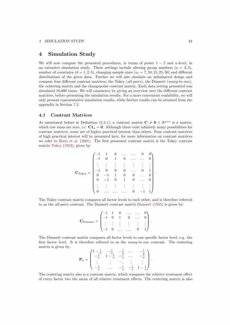
4 SIMULATION STUDY 34
4 Simulation Study
We will now compare the presented procedures, in terms of power 1 − β and α-level, inan extensive simulation study. These settings include altering group numbers (a = 3, 5),number of covariates (d = 1, 2, 5), changing sample sizes (ni = 7, 10, 15, 25, 50) and differentdistributions of the given data. Further we will also simulate an unbalanced design andcompare four different contrast matrices, the Tukey (all-pairs), the Dunnett (many-to-one),the centering matrix and the changepoint contrast matrix. Each data setting presented wassimulated 10,000 times. We will commence by giving an overview over the different contrastmatrices, before presenting the simulation results. For a more convenient readability, we willonly present representative simulation results, while further results can be attained from theappendix in Section 7.2.
4.1 Contrast Matrices
As mentioned before in Definition (2.3.1), a contrast matrix C 6= 0 ∈ Rq×a is a matrix,which row sums are zero, i.e. C1a = 0. Although there exist infinitely many possibilities forcontrast matrices, some are of higher practical interest than others. Four contrast matricesof high practical interest will be presented here, for more information on contrast matriceswe refer to Bretz et al. (2001). The first presented contrast matrix is the Tukey contrastmatrix Tukey (1953), given by:
CTukey =
−1 1 0 . . . . . . 0 0−1 0 1 0 . . . . . . 0...
......
......
......
−1 0 0 0 . . . 0 10 −1 1 0 0 . . . 00 −1 0 1 0 . . . 0...
......
......
......
0 . . . . . . . . . 0 −1 1
.
The Tukey contrast matrix compares all factor levels to each other, and is therefore referredto as the all-pairs contrast. The Dunnett contrast matrix Dunnett (1955) is given by:
CDunnett =
−1 1 0 . . . . . . 0−1 0 1 0 . . . 0...
......
......
...−1 0 . . . . . . 0 1
.
The Dunnett contrast matrix compares all factor levels to one specific factor level, e.g. thefirst factor level. It is therefore referred to as the many-to-one contrast. The centeringmatrix is given by:
Pa =
1− 1
a − 1a − 1
a . . . − 1a
− 1a 1− 1
a − 1a . . . − 1
a...
.... . .
......
− 1a . . . − 1
a − 1a 1− 1
a
.
The centering matrix also is a contrast matrix, which compares the relative treatment effectof every factor two the mean of all relative treatment effects. The centering matrix is also

4 SIMULATION STUDY 35
used for testing global hypotheses in the ANOVA and ANCOVA models, and therefore ofpractical interest. A more complex contrast matrix is the changepoint contrast matrix, orchangepoint comparisons, given by:
CChangepoint =
−1 n2
N2a. . . . . . na−1
N2a
na
N2a
− n1
N12− n2
N12
n3
N3a. . . na−1
N3a
na
N3a
......
. . ....
......
− n1
N1(a−1)− n2
N1(a−1). . . . . . − na−1
N1(a−1)1
.
where Nij =∑jk=i nk. The changepoint contrast matrix compares the relative treatment
effects in such a way, that change points of the relative treatment effects are uncovered.While these contrasts were used for our simulations, we will only present the results attainedusing the Tukey or all-pairs contrast matrix, the reason being, that the other simulatedcontrasts behaved very similarly. Therefore, all simulation results are attained using a Tukeycontrast matrix, unless stated otherwise. Nevertheless, we will compare the performance ofthe test procedures for different contrasts for one selected data setting in Section 4.2.5.
4.2 Type I Error Simulation
Before taking a look at the power 1 − β of the test procedures, we will first simulate theα-level, or type I error of the test procedures. Table 2 gives a comprehensive overview ofthe power 1− β and the α-level.
Table 2: Type I and type II errors of statistical inference.
H0 is not rejected H0 is rejectedH0 is true 1− α α (Type I error, level)H0 is false β (Type II error) 1− β (Power)
The α-level, or type I error, refers to the probability of a test procedure rejecting the nullhypothesis, although the null hypothesis is true. The power on the other hand, refers to thetest procedure rejecting the null hypothesis under alternative. While the nature of statisticalinference makes it inevitable for type I errors to occur, the type I error can be freely chosenwhen testing, provided the corresponding test behaves accordingly. In other words, if thetest user decided to test with a certain α-level, the test should hold this level. The type IIerror on the other hand is harder to control and should tend to 0 as differences in the factorlevels of the data increase. It is desirable for a test to show a steep increase in power asdifferences in factor levels increase.
For the upcoming simulation results, an α-level of 0.05 was chosen. It is therefore preferablefor the compared procedures to have a type I error of exactly 0.05. Should a test show a typeI error less than α, it is referred to as being conservative, because it tends to under rejectthe corresponding hypothesis. If a test shows a type I error higher than α, it is referred toas being liberal, because it tends to over reject the corresponding hypothesis.
4.2.1 Multivariate Normal Distribution
In the first part of the simulation, the covariates are simulated from a multivariate normaldistribution,
(X(1)ik , . . . , X
(d)ik )
i.i.d.∼ N(0,Ψ), i = 1, . . . , a, k = 1, . . . , ni, (4.1)

4 SIMULATION STUDY 36
where Ψ denotes a covariance matrix of compound symmetry structure with parameter ρ:
Ψ = ρ · 1d1′d + (1− ρ) · Id.
The covariates were simulated to be independent, slightly dependent and strongly dependentthrough ρ = 0, ρ = 0.5 and ρ = 0.9, respectively. In the first simulation result presented,the dependent variable follows a standard normal distribution and is not influenced by thecovariates, i.e.:
X(0)ik
i.i.d.∼ N(0, 1), i = 1, . . . , a, k = 1, . . . , ni. (4.2)
Taking into account covariates in this setting cannot improve the test and will, in the worstcase, lead to erroneous results. Table 3 shows the type I error rates of the compared proce-dures.
Table 3: An α-level simulation. Design: balanced with ni = 7, 10, 15, 25, 50 observations. Factorlevels: a = 3. Number of covariates: d = 1, 2, 5. Covariates: multivariate normal distributed (4.1),ρ = 0. Dependent variable: standard normal distributed (4.2).
d ni mctp.n mctp.t 2-step sie.ats sie.wts mctp.nc mctp.par f.par
1 7 0.1389 0.0824 0.0662 0.0913 0.1458 0.0680 0.0515 0.050210 0.1051 0.0723 0.0576 0.0788 0.1100 0.0641 0.0491 0.050615 0.0856 0.0652 0.0544 0.0682 0.0886 0.0587 0.0519 0.051925 0.0689 0.0560 0.0505 0.0579 0.0705 0.0525 0.0458 0.046950 0.0599 0.0557 0.0515 0.0573 0.0623 0.0544 0.0520 0.0537
2 7 0.1575 0.1001 0.0905 0.1166 0.1656 0.0721 0.0502 0.050910 0.1204 0.0816 0.0682 0.0923 0.1250 0.0632 0.0479 0.049015 0.0935 0.0712 0.0632 0.0762 0.0991 0.0588 0.0498 0.049425 0.0783 0.0687 0.0597 0.0699 0.0812 0.0594 0.0539 0.053350 0.0635 0.0571 0.0532 0.0571 0.0629 0.0539 0.0509 0.0500
5 7 0.2613 0.1804 0.1890 0.2246 0.2699 0.0735 0.0564 0.057010 0.1752 0.1272 0.1195 0.1459 0.1776 0.0639 0.0485 0.050815 0.1272 0.1029 0.0928 0.1113 0.1327 0.0649 0.0524 0.053425 0.0872 0.0734 0.0675 0.0800 0.0890 0.0532 0.0484 0.048050 0.0677 0.0620 0.0584 0.0630 0.0684 0.0512 0.0490 0.0486
The multiple contrast test procedure using equi-coordinate quantiles from the multivariatenormal distribution is denoted by mctp.n (Section 3.5), the multiple contrast test procedureusing equi-coordinate quantiles from the multivariate t-distribution is denoted by mctp.t(Section 3.5.3), the 2-step procedure, which remains unproven, is denoted as 2-step (Section3.6), the ANOVA-type statistic (Section 3.4) from Siemer (1999) and the Wald-type statis-tic (Section 3.3) are denoted by sie.ats and sie.wts respectively. Furthermore, the multiplecontrast test procedure not using covariates from Konietschke et al. (2012a), thus only us-ing the dependent variable for statistical inference, is denoted by mctp.nc, the parametricmultiple contrast test procedure is denoted by mctp.par (Section 3.2) and the parametricf-test is denoted by f.par (Section 3.1). Note that the procedure not considering covariatespresented here is the procedure using the multivariate t-approximation from Konietschkeet al. (2012a). While better procedures have been proposed within the same paper, thisprocedure is best compared to the mctp.t derived here.

4 SIMULATION STUDY 37
All procedures show asymptotic properties, performing better for high sample sizes (ni = 50)than for low sample sizes (ni = 7). Of the non-parametric approaches, aside from the 2-stepprocedure, the mctp.t performs best in all displayed settings. However, the mctp.t is veryliberal, especially for a large number of covariates and few observations (d = 5, ni = 7).The type I error is as large as 0.1804, far higher than the targeted 0.05 and unaccept-able for a good statistical inference. For a high number of observations and few covariates(d = 1, ni = 50), the type I error improves to a satisfactory level of 0.0557.
The reason for such a high type I error, especially considering that not using the covariateswould result in a drastically improved type I error (mctp.nc), could lie in the estimation ofthe regression parameters γ(1), . . . , γ(d), d = 1, . . . , r. In this setting, an optimal estimationwould be γ(r) = 0 for all r = 1, . . . , d, as it is in the case of mctp.nc. While the estimationin a parametric setting is adequate, in a non-parametric setting the number of combinationsin the rank transformation is limited, especially for few observations, and the regressionparameters are estimated erroneously, causing the procedure to detect a false coherence be-tween the dependent variable and the covariates, more frequently than in the parametricsetting.
This simulation shows that adding covariates to the model in hopes of attaining signifi-cant results will work, but yields erroneous results. To attain credible results, the samplesize needs to be accordingly high when planning to use covariates. Only then will falselychosen covariates be ignored by the non-parametric procedures.

4 SIMULATION STUDY 38
In the second simulation result presented, covariates are attained from a multivariate normaldistribution as in (4.1). The dependent variable is chosen to be the unweighted sum of thecovariates, plus an additional independent random variable, i.e.:
X(0)ik =
d∑r=1
X(r)ik + Uik where Uik
i.i.d.∼ N(0, 1), i = 1, . . . , a, k = 1, . . . , ni. (4.3)
Thus, in this case the dependent variable is influenced by the covariates and taking intoaccount the covariates should yield better results. Table 4 shows the results for ρ = 0, i.e.for independent covariates.
Table 4: An α-level simulation. Design: balanced with ni = 7, 10, 15, 25, 50 observations. Factorlevels: a = 3. Number of covariates: d = 1, 2, 5. Covariates: multivariate normal distributed (4.1),ρ = 0. Dependent variable: unweighted sum of covariates (4.3).
d ni mctp.n mctp.t 2-step sie.ats sie.wts mctp.nc mctp.par f.par
1 7 0.1024 0.0596 0.0694 0.0734 0.1078 0.0705 0.0506 0.050310 0.0778 0.0501 0.0570 0.0620 0.0810 0.0611 0.0485 0.048315 0.0710 0.0531 0.0606 0.0611 0.0728 0.0599 0.0518 0.051625 0.0606 0.0514 0.0503 0.0521 0.0607 0.0520 0.0472 0.048750 0.0532 0.0486 0.0495 0.0512 0.0550 0.0534 0.0506 0.0517
2 7 0.1125 0.0645 0.0940 0.0870 0.1170 0.0715 0.0581 0.058010 0.0851 0.0555 0.0745 0.0696 0.0887 0.0675 0.0528 0.052215 0.0680 0.0493 0.0617 0.0569 0.0707 0.0586 0.0466 0.046725 0.0627 0.0523 0.0587 0.0588 0.0638 0.0542 0.0532 0.053650 0.0526 0.0475 0.0508 0.0491 0.0532 0.0513 0.0449 0.0449
5 7 0.1548 0.0935 0.1849 0.1290 0.1609 0.0714 0.0516 0.051810 0.1108 0.0754 0.1248 0.0964 0.1142 0.0618 0.0513 0.054415 0.0842 0.0641 0.0948 0.0736 0.0860 0.0586 0.0516 0.052725 0.0701 0.0584 0.0752 0.0662 0.0705 0.0537 0.0489 0.049650 0.0547 0.0500 0.0550 0.0527 0.0545 0.0504 0.0481 0.0490
In this setting, the mctp.t again performs better than the other non-parametric alternativesin almost all parameter combinations displayed. The procedure still performs poorly for ahigh number of covariates and a low number of observations, but not as dramatically as inTable 3. Out of a methodological point of view, taking into account covariates now would bethe correct decision and, as long as the ratio between the number of covariates and samplesizes remains healthy, the α-level of 0.05 is met more often when considering covariates,opposed to not considering covariates.

4 SIMULATION STUDY 39
In a further simulation study, the covariates were generated in the same way as describedin (4.1), with the only difference being, that the dependent variable was chosen to be aweighted sum of the covariates, i.e.:
X(0)ik =
d∑r=1
r
2·X(r)
ik + Uik where Uiki.i.d.∼ N(0, 1), i = 1, . . . , a, k = 1, . . . , ni. (4.4)
The corresponding simulation results can be attained from Table 5.
Table 5: An α-level simulation. Design: balanced with ni = 7, 10, 15, 25, 50 observations. Factorlevels: a = 3. Number of covariates: d = 1, 2, 5. Covariates: multivariate normal distributed (4.1),ρ = 0. Dependent variable: weighted sum of covariates (4.4).
d ni mctp.n mctp.t 2-step sie.ats sie.wts mctp.nc mctp.par f.par
1 7 0.1294 0.0765 0.0724 0.0913 0.1368 0.0733 0.0512 0.052110 0.0967 0.0663 0.0588 0.0737 0.1035 0.0624 0.0483 0.049615 0.0791 0.0594 0.0552 0.0642 0.0822 0.0572 0.0500 0.050925 0.0614 0.0502 0.0461 0.0540 0.0620 0.0498 0.0457 0.045550 0.0584 0.0523 0.0512 0.0547 0.0588 0.0532 0.0496 0.0511
2 7 0.1280 0.0706 0.0992 0.0982 0.1341 0.0716 0.0515 0.052010 0.0885 0.0579 0.0714 0.0688 0.0933 0.0606 0.0487 0.048715 0.0744 0.0563 0.0617 0.0640 0.0772 0.0629 0.0487 0.049025 0.0657 0.0543 0.0591 0.0603 0.0666 0.0540 0.0478 0.049150 0.0567 0.0526 0.0541 0.0548 0.0579 0.0558 0.0530 0.0530
5 7 0.1221 0.0714 0.1888 0.0947 0.1278 0.0686 0.0516 0.051310 0.0808 0.0531 0.1233 0.0709 0.0864 0.0638 0.0514 0.052615 0.0642 0.0459 0.0925 0.0555 0.0665 0.0594 0.0511 0.050825 0.0554 0.0466 0.0732 0.0521 0.0560 0.0556 0.0498 0.050350 0.0498 0.0457 0.0539 0.0471 0.0494 0.0521 0.0479 0.0485
The mctp.t again performs very well compared to the other non-parametric procedures, butnot as well as in the case of unweighted covariates (Table 4). Not taking the covariatesinto account partially promises even better results in terms of α-level. It becomes clearthough, that the 2-step procedure seems to perform good for a low number of covariatesand devastating for small sample sizes and a large number of covariates. As this procedureis unproven, we leave it to the reader to decide on further interpretations. Supplementaryresults can be attained from the appendix in Section 7.2.1.
4.2.2 Multivariate Log-Normal Distribution
After having tested the procedures in different settings involving the multivariate normaldistribution, we will now regard simulation results involving the log-normal distribution.For this, the covariates were generated to be multivariate normally distributed as describedin (4.1). Then, the components of the vector were transformed to:
(exp(X(1)ik ), . . . , exp(X
(d)ik )), i = 1, . . . , a, k = 1, . . . , ni, (4.5)
where exp denotes the exponential function. Thus, the covariates now follow a multivariatelog-normal distribution with parameters 0 and covariance matrix Γ given by:
Γ = (e1(eΨij − 1))i=1,...,d,j=1,...,d.

4 SIMULATION STUDY 40
For the following simulation result, the dependent variable was chosen to be an unweightedsum of the covariates, with a log-normal error term, i.e.:
X(0)ik =
d∑r=1
exp(X(r)ik ) + Uik where Uik
i.i.d.∼ logN(0, 1), i = 1, . . . , a, k = 1, . . . , ni, (4.6)
where logN(0, 1) denotes the distribution function of exp(X), where X denotes a standardnormal random variable. Under these circumstances, neither the dependent variable, northe covariates are normally distributed. Therefore, the assumptions for using the parametricapproaches to considering covariates are no longer fulfilled. Nevertheless, we will comparethese procedures to see how well they perform compared to the non-parametric approaches.Table 6 shows the results for this simulation.
Table 6: An α-level simulation. Design: balanced with ni = 7, 10, 15, 25, 50 observations. Factorlevels: a = 3. Number of covariates: d = 1, 2, 5. Covariates: multivariate log-normal distributed(4.5), ρ = 0. Dependent variable: unweighted sum of covariates (4.6).
d ni mctp.n mctp.t 2-step sie.ats sie.wts mctp.nc mctp.par f.par
1 7 0.1025 0.0550 0.0689 0.0739 0.1096 0.0716 0.0348 0.036910 0.0794 0.0507 0.0572 0.0611 0.0858 0.0627 0.0321 0.034315 0.0723 0.0520 0.0566 0.0605 0.0778 0.0632 0.0369 0.040225 0.0591 0.0479 0.0502 0.0516 0.0604 0.0554 0.0369 0.038150 0.0543 0.0498 0.0505 0.0526 0.0556 0.0518 0.0428 0.0428
2 7 0.1204 0.0675 0.0962 0.0912 0.1277 0.0790 0.0356 0.037110 0.0920 0.0546 0.0718 0.0707 0.0936 0.0587 0.0348 0.037015 0.0736 0.0548 0.0643 0.0614 0.0769 0.0594 0.0364 0.037825 0.0636 0.0532 0.0578 0.0568 0.0685 0.0549 0.0379 0.038950 0.0537 0.0485 0.0531 0.0517 0.0555 0.0531 0.0419 0.0431
5 7 0.1975 0.1256 0.1856 0.1671 0.2055 0.0663 0.0398 0.040710 0.1419 0.0972 0.1275 0.1194 0.1461 0.0624 0.0388 0.038615 0.1048 0.0797 0.0929 0.0922 0.1088 0.0616 0.0386 0.039125 0.0785 0.0661 0.0727 0.0713 0.0794 0.0573 0.0359 0.037250 0.0586 0.0519 0.0543 0.0553 0.0597 0.0514 0.0397 0.0398
As in the simulation results already presented, the mctp.t performs very well. Only forlow sample sizes and a high number of covariates the procedure becomes very liberal, stillperforming better than the non-parametric alternatives. The parametric approaches nowturn out to be slightly conservative, which might be because of the underlying skewness inthe distribution of the data.
4.2.3 Binomial Distribution
One simulation study was conducted using covariates which follow a binomial distributionwith parameters m = 4 and q = 0.5. The dependent variable was chosen to be an unweightedsum of the covariates plus an additional standard normal distributed error term. In otherwords, the covariates were chosen to be:
X(r)ik
i.i.d.∼ Bin(m, q) for i = 1, . . . , a, k = 1, . . . , ni, r = 1, . . . , d, (4.7)

4 SIMULATION STUDY 41
and the dependent variable was calculated as:
X(0)ik =
d∑r=1
X(r)ik + Uik, where Uik
i.i.d.∼ N(0, 1), i = 1, . . . , a, k = 1, . . . , ni. (4.8)
The simulation results are given in Table 7.
Table 7: An α-level simulation. Design: balanced with ni = 7, 10, 15, 25, 50 observations. Factorlevels: a = 3. Number of covariates: d = 1, 2, 5. Covariates: binomial distributed (4.7). Dependentvariable: unweighted sum of covariates (4.8).
d ni mctp.n mctp.t 2-step sie.ats sie.wts mctp.nc mctp.par f.par
1 7 0.1106 0.0606 0.0730 0.0806 0.1180 0.0765 0.0504 0.050110 0.0832 0.0541 0.0587 0.0665 0.0858 0.0648 0.0479 0.048615 0.0680 0.0491 0.0520 0.0572 0.0703 0.0589 0.0475 0.045725 0.0602 0.0504 0.0518 0.0553 0.0638 0.0551 0.0529 0.051750 0.0578 0.0531 0.0518 0.0546 0.0576 0.0566 0.0518 0.0503
2 7 0.1163 0.0646 0.0900 0.0912 0.1202 0.0712 0.0511 0.051010 0.0906 0.0601 0.0760 0.0733 0.0962 0.0694 0.0477 0.048415 0.0758 0.0582 0.0674 0.0654 0.0772 0.0612 0.0519 0.051025 0.0666 0.0539 0.0589 0.0584 0.0663 0.0545 0.0524 0.051150 0.0576 0.0516 0.0546 0.0555 0.0574 0.0542 0.0519 0.0513
5 7 0.1715 0.1046 0.1916 0.1407 0.1762 0.0693 0.0475 0.049410 0.1181 0.0801 0.1261 0.1053 0.1242 0.0637 0.0525 0.050715 0.0834 0.0632 0.0864 0.0757 0.0862 0.0544 0.0493 0.050625 0.0730 0.0609 0.0725 0.0660 0.0723 0.0593 0.0505 0.050550 0.0609 0.0563 0.0580 0.0566 0.0602 0.0524 0.0504 0.0501
As seen in the previous simulation results, the mctp.t performs very well in comparison tothe other non-parametric results, but still very liberal for a high number of covariates and alow sample size. Given the standard normal error term, the parametric approaches performexcellent.
4.2.4 Further Distributions
Apart from the multivariate normal, the multivariate log-normal and the binomial distribu-tion, simulation studies were also conducted for covariates from a Poisson, an exponential,a Bernoulli and a Chi-squared distribution. In these settings, the dependent variable waschosen to be an unweighted sum of the covariates, plus a standard normal error term. Theresults attained are very similar to those of the binomial distribution, and are thereforelisted in the appendix, Section 7.2.1. Other simulation results for the multivariate normaland the multivariate log-normal distributions can also be attained from Section 7.2.1.
4.2.5 Comparing Contrast Matrices
As mentioned before, we would like to compare the contrast matrices, presented at thebeginning of this section, in terms of α-level. For comparing contrast matrices, we chose touse covariates generated from a multivariate normal distribution as in (4.1) with dependency

4 SIMULATION STUDY 42
parameter ρ = 0 and the dependent variable being an unweighted sum of the covariates,plus an additional standard normal error term, as in (4.3). The results for d = 2 covariatescan be attained from Table 8.
Table 8: An α-level simulation. Design: balanced with ni = 7, 10, 15, 25, 50 observations. Factorlevels: a = 3. Number of covariates: d = 2. Covariates: multivariate normal distributed (4.1),ρ = 0. Dependent variable: unweighted sum of covariates (4.3). Contrast matrices (Con): Centering(Cen), Changepoint (Cha), Dunnett (Dun) and Tukey (Tuk).
ni Con mctp.n mctp.t 2-step sie.ats sie.wts mctp.nc mctp.par f.par
7 Cen 0.1023 0.0531 0.0984 0.0792 0.1111 0.0648 0.0494 0.0499Cha 0.0960 0.0543 0.0835 0.0803 0.1122 0.0621 0.0503 0.0503Dun 0.0928 0.0575 0.0817 0.0803 0.1096 0.0642 0.0500 0.0502Tuk 0.1125 0.0645 0.0940 0.0870 0.1170 0.0715 0.0581 0.0580
10 Cen 0.0858 0.0525 0.0805 0.0705 0.0888 0.0611 0.0506 0.0523Cha 0.0762 0.0503 0.0729 0.0678 0.0855 0.0567 0.0489 0.0509Dun 0.0771 0.0509 0.0654 0.0659 0.0878 0.0576 0.0505 0.0502Tuk 0.0851 0.0555 0.0745 0.0696 0.0887 0.0675 0.0528 0.0522
15 Cen 0.0719 0.0513 0.0709 0.0639 0.0731 0.0546 0.0506 0.0505Cha 0.0695 0.0531 0.0650 0.0622 0.0738 0.0570 0.0533 0.0525Dun 0.0672 0.0513 0.0610 0.0588 0.0717 0.0547 0.0515 0.0500Tuk 0.0680 0.0493 0.0617 0.0569 0.0707 0.0586 0.0466 0.0467
25 Cen 0.0616 0.0516 0.0586 0.0541 0.0630 0.0582 0.0497 0.0505Cha 0.0577 0.0495 0.0536 0.0542 0.0612 0.0535 0.0502 0.0503Dun 0.0574 0.0483 0.0537 0.0518 0.0567 0.0499 0.0488 0.0478Tuk 0.0627 0.0523 0.0587 0.0588 0.0638 0.0542 0.0532 0.0536
50 Cen 0.0504 0.0453 0.0496 0.0495 0.0495 0.0491 0.0463 0.0469Cha 0.0541 0.0505 0.0538 0.0548 0.0574 0.0508 0.0518 0.0542Dun 0.0512 0.0480 0.0519 0.0503 0.0544 0.0509 0.0481 0.0490Tuk 0.0526 0.0475 0.0508 0.0491 0.0532 0.0513 0.0449 0.0449
Taking a look at Table 8, it becomes clear that the type of contrast matrix does not makea big difference in terms of α-level, independent from the procedure chosen. Further resultscan be attained from the appendix in Section 7.2.1.
4.2.6 Unbalanced Design
Although most experiments aim at having a balanced design, i.e. an equal number of ob-servations per group, only few experiments actually meet this criterion in the end. Unequalgroup sizes can have many reasons like dropouts, subjects who do not return for an eval-uation, or natural restrictions, like in gene datasets, where certain genes simply occur lessfrequently than others. In statistics, it is therefore very important for a test procedure toallow for unequal sample sizes between the experiment groups, otherwise the test procedureis highly restrictive and can only be applied very seldom.
The derived MCTP (mctp.n, mctp.t) allow for an unbalanced experiment design. In thispart of the simulation study, we would like to examine how good the procedures perform interms of α-level when confronted with an unbalanced design. For this, we will examine two

4 SIMULATION STUDY 43
different degrees of imbalance, a low degree of imbalance with n1 = 10, n2 = 15 and n3 = 20observations in the groups, and a high degree of imbalance with n1 = 10, n2 = 50 andn3 = 100 observations. Further, we examined three different distributions of the data. Herewe only present the results from the multivariate normal distribution, with covariates gen-erated as in (4.1) with dependency parameter ρ = 0 and the dependent variable generatedas in (4.3), an unweighted sum of the covariates with standard normal error term, whichresults are given in Table 9. The results for the other distributions, namely the log-normaland the binomial distribution, can be attained from the appendix in Section 7.2.1.
Table 9: An α-level simulation. Design: unbalanced with n1 = 10, n2 = 15, n3 = 20 (low) andn1 = 10, n2 = 50, n3 = 100 (high) observations. Factor levels: a = 3. Number of covariates: d =1, 2, 5. Covariates: multivariate normal distributed (4.1), ρ = 0. Dependent variable: unweightedsum of covariates (4.3). The degree of imbalance is abbreviated by Imba.
d Imba mctp.n mctp.t 2-step sie.ats sie.wts mctp.nc mctp.par f.par
1 low 0.0733 0.0518 0.0528 0.0624 0.0749 0.0499 0.0576 0.0505high 0.0731 0.0623 0.0423 0.0723 0.0744 0.0478 0.0479 0.0490
2 low 0.0792 0.0547 0.0640 0.0672 0.0802 0.0528 0.0608 0.0531high 0.0776 0.0633 0.0465 0.0713 0.0764 0.0490 0.0470 0.0510
5 low 0.0883 0.0662 0.0872 0.0771 0.0906 0.0495 0.0548 0.0492high 0.0734 0.0625 0.0501 0.0735 0.0732 0.0535 0.0481 0.0502
Comparing the mctp.t in the unbalanced design with the prior balanced designs, the unbal-anced observation numbers do not seem to have a strong effect. It seems though, that anincreasing imbalance between the factor levels results in slightly liberal test decisions. Thisis not true, when taking into account 5 covariates, where the estimation of the regressionparameters seems to profit more from the higher observation numbers, than the imbal-ance does damage. As in the prior simulation results, the mctp.t performs better than thenon-parametric alternatives, but not as good as the parametric procedures. The mctp.parhowever, seems to be more conservative when confronted with a higher imbalance betweenthe factor levels.
4.2.7 Higher Number of Factor Levels
We shortly mentioned that we would also like to compare the performance of the testprocedures when confronted with a higher number of factor levels. Now we would liketo compare the test procedures when confronted with a = 5 factor levels. Due to the highnumerical computation times, we will only present the results for one data setting. Thecovariates were generated to be multivariate normal distributed as in (4.1), with dependencyparameter ρ = 0, and the dependent variable was generated to be an unweighted sum ofcovariates with an additional standard normal error term, as in (4.3). We simulated thecase of d = 2 covariates. Table 10 yields the results of this simulation.

4 SIMULATION STUDY 44
Table 10: An α-level simulation. Design: balanced with ni = 7, 10, 15, 25, 50 observations. Factorlevels: a = 5. Number of covariates: d = 2. Covariates: multivariate normal distributed (4.1),ρ = 0. Dependent variable: unweighted sum of covariates (4.3).
ni mctp.n mctp.t 2-step sie.ats sie.wts mctp.nc mctp.par f.par
7 0.1309 0.0510 0.0857 0.0711 0.1397 0.0852 0.0495 0.048710 0.1024 0.0514 0.0651 0.0629 0.1101 0.0716 0.0517 0.051715 0.0798 0.0514 0.0570 0.0553 0.0828 0.0657 0.0501 0.049525 0.0660 0.0499 0.0525 0.0505 0.0652 0.0599 0.0479 0.051050 0.0585 0.0522 0.0504 0.0509 0.0569 0.0530 0.0480 0.0478
Comparing the results with the results attained when considering a = 3 factor levels, seeTable 4, the mctp.t does not perform worse. In fact, in performs better, which could bebecause the additional observations lead to a better estimation of the regression param-eters γ(1), . . . , γ(d). The sie.ats procedure also performs slightly better, while the sie.wtsprocedure, the mctp.n and mctp.nc perform worse.
4.3 Power Simulation
We will now continue with comparing the power of the simulated procedures. As mentionedin Section 4.2, it is desirable for a procedure to maintain the α-level as long as the nullhypothesis is fulfilled, and then show a steep increase in power under the alternative. Underthe alternative, the best procedure in terms of power is the procedure which power is closestto one.
4.3.1 Multivariate Normal Distribution
In a similar manner as for the type I error simulation, we simulated data from the mul-tivariate normal distribution. Analogously to (4.1), the covariates were generated to bemultivariate normal distributed, slightly dependent with parameter ρ = 0.2. The dependentvariable was chosen do be the sum of covariates, with a standard normal distributed errorterm and a shift term δ on each factor level, i.e.:
X(0)ik =
d∑r=1
X(r)ik + Uik + δ · (i− 1), i = 1, . . . , a, k = 1, . . . , ni, (4.9)
where the shift term δ varied from 0 to 1 in steps of 0.2. All procedures should increase inpower, as δ increases, and thus the differences between the factor levels of the dependentvariable increase. Figure 4 shows selected results from the power simulation. For reasonsof readability, we have chosen to compare only 4 procedures, the newly developed multiplecontrast test procedure considering covariates, mctp.t, the current procedure for copingwith covariates in a non-parametric setting, sie.ats, the parametric alternative to multiplecontrast test procedures, mctp.par, and finally the case of ignoring covariates, mctp.nc.Further comparisons can be attained from the appendix in Section 7.2.2.

4 SIMULATION STUDY 45
0.00 0.25 0.50 0.75 1.00
0.0
0.2
0.4
0.6
0.8
1.0
Deviation (δ)
Pow
er (
1−β)
mctp.tsie.atsmctp.parmctp.ncα−level
0.00 0.25 0.50 0.75 1.000.
00.
20.
40.
60.
81.
0
Deviation (δ)
Pow
er (
1−β)
mctp.tsie.atsmctp.parmctp.ncα−level
Figure 4: Simulation results for the power (1 − β). Design: balanced with ni = 10 and ni = 25observations on the left and right figure, respectively. Factor levels: a = 3. Number of covariates:d = 2. Covariates: multivariate normal distributed (4.1), ρ = 0.2. Dependent variable: unweightedsum of covariates (4.9).
In this power simulation, we have chosen a balanced data set with ni = 10 and ni = 20observations on the left and on the right figure, respectively. Further, d = 2 covariates wereobserved. On both figures it becomes clear, that considering covariates can dramaticallyimprove the power of the test statistic. Compared to the sie.ats procedure, mctp.t does notperform as good, which could be because the sie.ats procedure is slightly liberal. In thissetting, the mctp.par performs better than both non-parametric approaches.
4.3.2 Multivariate Log-Normal Distribution
Similar to the type I error simulation, we also conducted a power simulation using themultivariate log-normal distribution. The covariates were generated in the same manner asin (4.1) and then transformed analogously to (4.5). The dependent variable was then givenas in (4.6), but with an additional shift parameter δ, i.e.:
X(0)ik =
d∑r=1
exp(X(r)ik ) + Uik + δ · (i− 1), i = 1, . . . , a, k = 1, . . . , ni, (4.10)
where Uiki.i.d.∼ logN(0, 1). The simulation results can be attained from Figure 5.

4 SIMULATION STUDY 46
0.00 0.25 0.50 0.75 1.00
0.0
0.2
0.4
0.6
0.8
1.0
Deviation (δ)
Pow
er (
1−β)
mctp.tsie.atsmctp.parmctp.ncα−level
0.00 0.25 0.50 0.75 1.000.
00.
20.
40.
60.
81.
0
Deviation (δ)
Pow
er (
1−β)
mctp.tsie.atsmctp.parmctp.ncα−level
Figure 5: Simulation results for the power (1 − β). Design: balanced with ni = 10 and ni = 25observations on the left and right figure, respectively. Factor levels: a = 3. Number of covari-ates: d = 2. Covariates: multivariate log-normal distributed (4.5), ρ = 0.2. Dependent variable:unweighted sum of covariates (4.10).
As in the case of the multivariate normal distribution, we chose a balanced design withni = 10 and ni = 25 observations per group on the left and on the right figure, respectively.The number of covariates was chosen to be d = 2 and the number of factor levels is givenby a = 3. For ni = 10 observations, the power of the statistics is almost equal, with thesie.ats procedure being slightly liberal. For ni = 25 observations, the non-parametric pro-cedures for considering covariates, sie.ats and mctp.t, perform equally well, but better thanthe parametric alternative mctp.par. As in the case of multivariate normal distributed data,not considering covariates, given this data setting, will lead to a loss in power.
It is important to mention that, while this is a setting in which the non-parametric pro-cedures perform better than the parametric alternatives, this is not always the case whenconsidering the log-normal distribution. As can be seen in the Appendix 7.2.2, raising thenumber of covariates leads to the parametric procedure being better than the non-parametricprocedure.
4.3.3 Binomial Distribution
The final power simulation was conducted using binomial distributed covariates, as done forthe type I error simulation in (4.7), with parameters m = 4 and q = 0.5. The dependentvariable was calculated analogously to (4.8) with an additional shift term δ, ranging from 0to 1 in steps of 0.2, i.e.:
X(0)ik =
d∑r=1
X(r)ik + Uik + δ · (i− 1), i = 1, . . . , a, k = 1, . . . , ni, (4.11)
where Uiki.i.d.∼ N(0, 1). The simulation results can be attained from Figure 6.

4 SIMULATION STUDY 47
0.00 0.25 0.50 0.75 1.00
0.0
0.2
0.4
0.6
0.8
1.0
Deviation (δ)
Pow
er (
1−β)
mctp.tsie.atsmctp.parmctp.ncα−level
0.00 0.25 0.50 0.75 1.000.
00.
20.
40.
60.
81.
0
Deviation (δ)
Pow
er (
1−β)
mctp.tsie.atsmctp.parmctp.ncα−level
Figure 6: Simulation results for the power (1 − β). Design: balanced with ni = 10 and ni = 25observations on the left and right figure, respectively. Factor levels: a = 3. Number of covariates:d = 2. Covariates: binomial distributed (4.7). Dependent variable: unweighted sum of covariates(4.11).
The figures show a similar result as for the multivariate normal distributed data. The para-metric alternative shows the best results in terms of power, while the sie.ats procedure isthe best for non-parametric procedures, which may very well be because it is slightly liberal.The mctp.t still performs adequately.
Concluding the power simulation for balanced designs, we have seen that the slight dif-ferences between the non-parametric procedures, i.e. sie.ats and mctp.t, probably resultfrom the sie.ats procedure being slightly liberal, opposed to the mctp.t. The difference isonly very small and both procedures perform well in terms of power. Comparing the para-metric alternative mctp.par with the mctp.t, we do not have a clearly better procedure, asresults vary according to the data setting. Under the presented data settings, an increasein power was always observed when considering covariates, opposed to ignoring these.
4.3.4 Unbalanced Design
In Section 4.2.6 we examined the performance of the test procedures in terms of α-level,when confronted with an unbalanced design. The aim of this part of the simulation is toverify whether or not the derived procedure mctp.t is still effective in terms of power, whenconfronted with unequal sample sizes. As in the α-level simulation, we chose to comparetwo different degrees of inequality, a slight inequality between the experiment groups, wheresample sizes are n1 = 10, n2 = 15 and n3 = 20, and a grave inequality with sample sizesn1 = 10, n2 = 50 and n3 = 100. Furthermore, we will compare the results for two differentlygenerated datasets. In the first simulation, the underlying data is multivariate normaldistributed as described in (4.9), but with dependency parameter ρ = 0, i.e. independentcovariates, and in the second simulation the data is multivariate log-normal distributed asdescribed in (4.10), again with independent covariates. The results for the first simulationare attained from Figure 7.
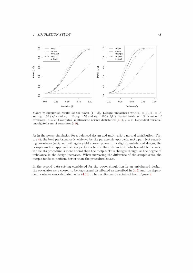
4 SIMULATION STUDY 48
0.00 0.25 0.50 0.75 1.00
0.0
0.2
0.4
0.6
0.8
1.0
Deviation (δ)
Pow
er (
1−β)
mctp.tsie.atsmctp.parmctp.ncα−level
0.00 0.25 0.50 0.75 1.000.
00.
20.
40.
60.
81.
0
Deviation (δ)
Pow
er (
1−β)
mctp.tsie.atsmctp.parmctp.ncα−level
Figure 7: Simulation results for the power (1 − β). Design: unbalanced with n1 = 10, n2 = 15and n3 = 20 (left) and n1 = 10, n2 = 50 and n3 = 100 (right). Factor levels: a = 3. Number ofcovariates: d = 2. Covariates: multivariate normal distributed (4.1), ρ = 0. Dependent variable:unweighted sum of covariates (4.9).
As in the power simulation for a balanced design and multivariate normal distribution (Fig-ure 4), the best performance is achieved by the parametric approach, mctp.par. Not regard-ing covariates (mctp.nc) will again yield a lower power. In a slightly unbalanced design, thenon-parametric approach sie.ats performs better than the mctp.t, which could be becausethe sie.ats procedure is more liberal than the mctp.t. This changes though, as the degree ofunbalance in the design increases. When increasing the difference of the sample sizes, themctp.t tends to perform better than the procedure sie.ats.
In the second data setting considered for the power simulation in an unbalanced design,the covariates were chosen to be log-normal distributed as described in (4.5) and the depen-dent variable was calculated as in (4.10). The results can be attained from Figure 8.

4 SIMULATION STUDY 49
0.00 0.25 0.50 0.75 1.00
0.0
0.2
0.4
0.6
0.8
1.0
Deviation (δ)
Pow
er (
1−β)
mctp.tsie.atsmctp.parmctp.ncα−level
0.00 0.25 0.50 0.75 1.000.
00.
20.
40.
60.
81.
0
Deviation (δ)
Pow
er (
1−β)
mctp.tsie.atsmctp.parmctp.ncα−level
Figure 8: Simulation results for the power (1 − β). Design: unbalanced with n1 = 10, n2 = 15and n3 = 20 (left) and n1 = 10, n2 = 50 and n3 = 100 (right). Factor levels: a = 3. Numberof covariates: d = 2. Covariates: multivariate log-normal distributed (4.5), ρ = 0. Dependentvariable: unweighted sum of covariates (4.10).
For a small imbalance between the factor levels, the mctp.t and the sie.ats procedure donot seem to differ much. The parametric alternative mctp.par on the other hand, shows anincrease in power later than the non-parametric procedures. For a high imbalance betweenthe factor levels, the procedures perform very different from each other. The mctp.t performsbest, with a power always higher than that of the other procedures. The sie.ats proceduredoes not rise as quickly in power, as it did for a low imbalance. The parametric alternative,mcpt.par, again rises in power a little bit later than the non-parametric procedures, this timeending up being better than the sie.ats procedures for δ ≥ 0.5. As in the prior simulations,not considering covariates yields the worst power in both degrees of imbalance.
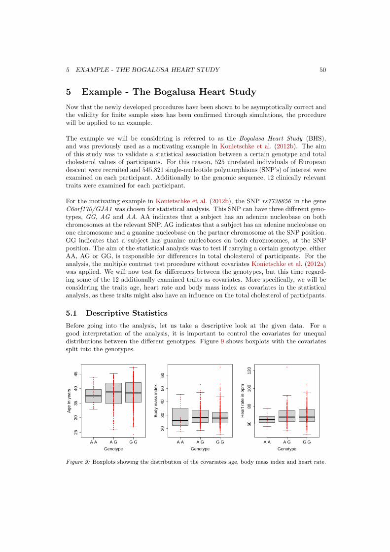
5 EXAMPLE - THE BOGALUSA HEART STUDY 50
5 Example - The Bogalusa Heart Study
Now that the newly developed procedures have been shown to be asymptotically correct andthe validity for finite sample sizes has been confirmed through simulations, the procedurewill be applied to an example.
The example we will be considering is referred to as the Bogalusa Heart Study (BHS),and was previously used as a motivating example in Konietschke et al. (2012b). The aimof this study was to validate a statistical association between a certain genotype and totalcholesterol values of participants. For this reason, 525 unrelated individuals of Europeandescent were recruited and 545,821 single-nucleotide polymorphisms (SNP’s) of interest wereexamined on each participant. Additionally to the genomic sequence, 12 clinically relevanttraits were examined for each participant.
For the motivating example in Konietschke et al. (2012b), the SNP rs7738656 in the geneC6orf170/GJA1 was chosen for statistical analysis. This SNP can have three different geno-types, GG, AG and AA. AA indicates that a subject has an adenine nucleobase on bothchromosomes at the relevant SNP. AG indicates that a subject has an adenine nucleobase onone chromosome and a guanine nucleobase on the partner chromosome at the SNP position.GG indicates that a subject has guanine nucleobases on both chromosomes, at the SNPposition. The aim of the statistical analysis was to test if carrying a certain genotype, eitherAA, AG or GG, is responsible for differences in total cholesterol of participants. For theanalysis, the multiple contrast test procedure without covariates Konietschke et al. (2012a)was applied. We will now test for differences between the genotypes, but this time regard-ing some of the 12 additionally examined traits as covariates. More specifically, we will beconsidering the traits age, heart rate and body mass index as covariates in the statisticalanalysis, as these traits might also have an influence on the total cholesterol of participants.
5.1 Descriptive Statistics
Before going into the analysis, let us take a descriptive look at the given data. For agood interpretation of the analysis, it is important to control the covariates for unequaldistributions between the different genotypes. Figure 9 shows boxplots with the covariatessplit into the genotypes.
A A A G G G
2530
3540
45
Genotype
Age
in y
ears
A A A G G G
2030
4050
60
Genotype
Bod
y m
ass
inde
x
A A A G G G
6080
100
120
Genotype
Hea
rt r
ate
in b
pm
Figure 9: Boxplots showing the distribution of the covariates age, body mass index and heart rate.
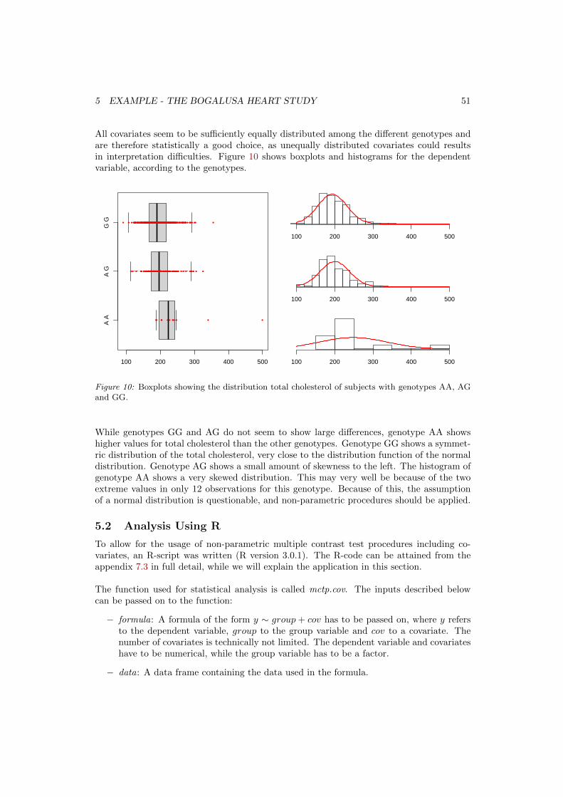
5 EXAMPLE - THE BOGALUSA HEART STUDY 51
All covariates seem to be sufficiently equally distributed among the different genotypes andare therefore statistically a good choice, as unequally distributed covariates could resultsin interpretation difficulties. Figure 10 shows boxplots and histograms for the dependentvariable, according to the genotypes.
A A
A G
G G
100 200 300 400 500
100 200 300 400 500
100 200 300 400 500
100 200 300 400 500
Figure 10: Boxplots showing the distribution total cholesterol of subjects with genotypes AA, AGand GG.
While genotypes GG and AG do not seem to show large differences, genotype AA showshigher values for total cholesterol than the other genotypes. Genotype GG shows a symmet-ric distribution of the total cholesterol, very close to the distribution function of the normaldistribution. Genotype AG shows a small amount of skewness to the left. The histogram ofgenotype AA shows a very skewed distribution. This may very well be because of the twoextreme values in only 12 observations for this genotype. Because of this, the assumptionof a normal distribution is questionable, and non-parametric procedures should be applied.
5.2 Analysis Using R
To allow for the usage of non-parametric multiple contrast test procedures including co-variates, an R-script was written (R version 3.0.1). The R-code can be attained from theappendix 7.3 in full detail, while we will explain the application in this section.
The function used for statistical analysis is called mctp.cov. The inputs described belowcan be passed on to the function:
− formula: A formula of the form y ∼ group + cov has to be passed on, where y refersto the dependent variable, group to the group variable and cov to a covariate. Thenumber of covariates is technically not limited. The dependent variable and covariateshave to be numerical, while the group variable has to be a factor.
− data: A data frame containing the data used in the formula.

5 EXAMPLE - THE BOGALUSA HEART STUDY 52
− type: An argument in which the contrast matrix is passed on. It can be either “Tukey”,“Dunnett”, “Sequen”, “Williams”, “Changepoint”, “AVE”, “McDermott”, “Marcus”,“UmbrellaWilliams” or a contrast matrix, for user defined contrasts. By default, theTukey matrix is chosen as a contrast matrix.
− conf.level : A number between 0 and 1, giving the confidence level to which the globalhypothesis is tested. The default confidence level is set to 0.95 (95%).
− alternative: The alternative to which the test should be performed. It can be either“two.sided”, “less” or “greater”. By default, a two sided alternative is tested.
− asy.method : The asymptotic method to use. It can be either “mult.t” or “normal”,where the multivariate t-approximation is used by default.
− info: A logical parameter giving whether or not to post additional information whencalling the function.
− rounds: The number of digits to which the results should be rounded.
− effect : A parameter indicating whether to use unweighted or weighted relative treat-ment effects. It can be either “unweighted” or “weighted”, where unweighted relativetreatment effects are chosen by default.
The data set given for the Bogalusa Heart Study was transferred into a data frame suitedfor the analysis, with following structure:
Table 11: Outtake of the Bogalusa Heart Study
rs7738656 tc AGE BMI hr
1 AG 209 38.8 42.0 632 GG 190 44.9 34.2 64...
......
......
...525 AG 144 38.0 20.5 71
In genetic models, an allele can either be dominant, additive or recessive. Since it is notknown whether the allele is dominant, recessive or additive, we will test for differencesbetween the genotypes by first assuming that G is a dominant allele, secondly by assumingthat G is an additive allele and finally by assuming that G is a recessive allele, in a multiplecontrast test procedure. A common contrast matrix for this type of testing is the Marcustype contrast matrix, given by:
CMarcus =
−1 n2
n2+n3
n3
n2+n3
−1 0 1− n1
n1+n2− n2
n1+n21
. (5.1)
For testing the hypothesis no global effect, i.e. the total cholesterol is not different amongthe genotypes, or equivalently H0 : Cp∗ = 0, the R-script can be called using followingR-code:
1 test<−mctp . cov ( tc ∼ rs7738656+AGE+BMI+hr , data=BHS ,2 info=T , type=”Marcus” , rounds=6)
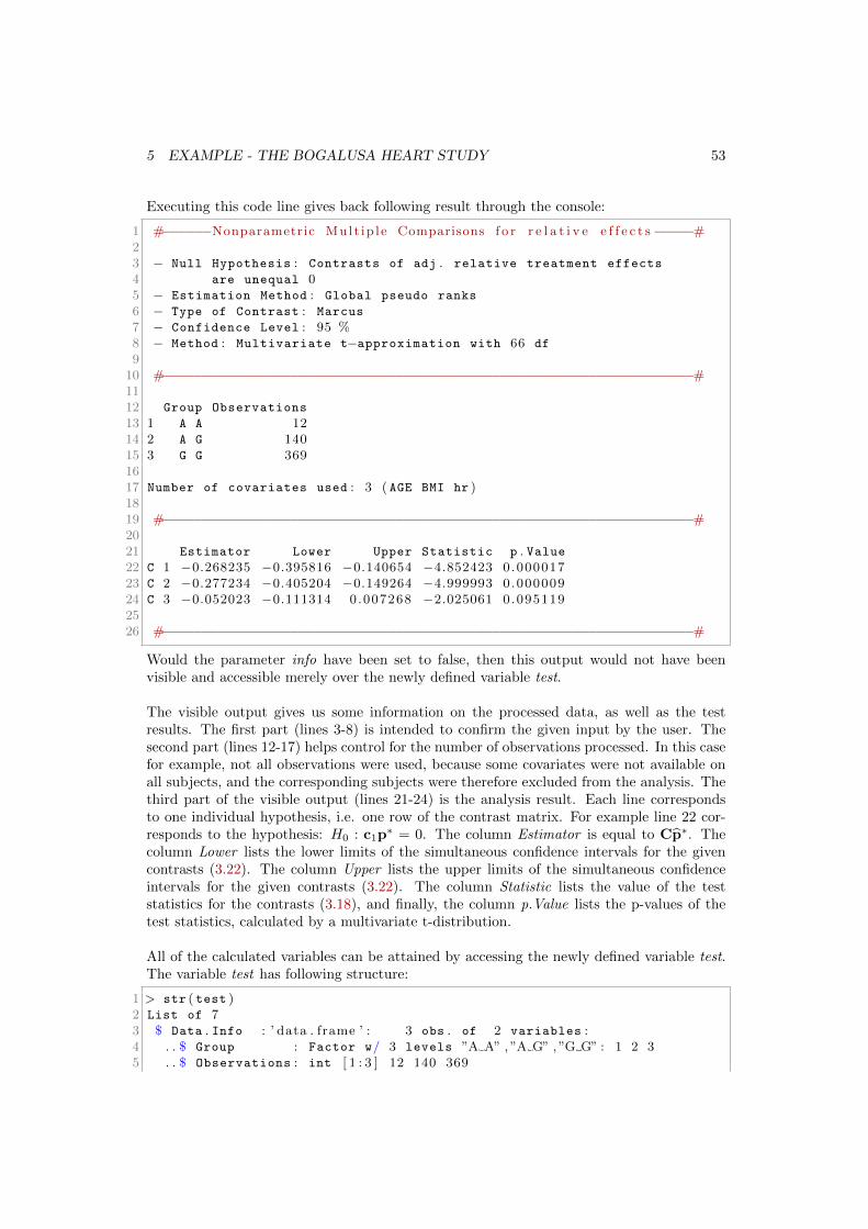
5 EXAMPLE - THE BOGALUSA HEART STUDY 53
Executing this code line gives back following result through the console:
1 #−−−−−−Nonparametric Mult ip l e Comparisons f o r r e l a t i v e e f f e c t s−−−−−#23 − Null Hypothesis : Contrasts of adj . relative treatment effects
4 are unequal 05 − Estimation Method : Global pseudo ranks
6 − Type of Contrast : Marcus
7 − Confidence Level : 95 %8 − Method : Multivariate t−approximation with 66 df
910 #−−−−−−−−−−−−−−−−−−−−−−−−−−−−−−−−−−−−−−−−−−−−−−−−−−−−−−−−−−−−−−−−−−#1112 Group Observations
13 1 A A 1214 2 A G 14015 3 G G 3691617 Number of covariates used : 3 ( AGE BMI hr )1819 #−−−−−−−−−−−−−−−−−−−−−−−−−−−−−−−−−−−−−−−−−−−−−−−−−−−−−−−−−−−−−−−−−−#2021 Estimator Lower Upper Statistic p . Value22 C 1 −0.268235 −0.395816 −0.140654 −4.852423 0.00001723 C 2 −0.277234 −0.405204 −0.149264 −4.999993 0.00000924 C 3 −0.052023 −0.111314 0.007268 −2.025061 0.0951192526 #−−−−−−−−−−−−−−−−−−−−−−−−−−−−−−−−−−−−−−−−−−−−−−−−−−−−−−−−−−−−−−−−−−#
Would the parameter info have been set to false, then this output would not have beenvisible and accessible merely over the newly defined variable test.
The visible output gives us some information on the processed data, as well as the testresults. The first part (lines 3-8) is intended to confirm the given input by the user. Thesecond part (lines 12-17) helps control for the number of observations processed. In this casefor example, not all observations were used, because some covariates were not available onall subjects, and the corresponding subjects were therefore excluded from the analysis. Thethird part of the visible output (lines 21-24) is the analysis result. Each line correspondsto one individual hypothesis, i.e. one row of the contrast matrix. For example line 22 cor-responds to the hypothesis: H0 : c1p
∗ = 0. The column Estimator is equal to Cp∗. Thecolumn Lower lists the lower limits of the simultaneous confidence intervals for the givencontrasts (3.22). The column Upper lists the upper limits of the simultaneous confidenceintervals for the given contrasts (3.22). The column Statistic lists the value of the teststatistics for the contrasts (3.18), and finally, the column p.Value lists the p-values of thetest statistics, calculated by a multivariate t-distribution.
All of the calculated variables can be attained by accessing the newly defined variable test.The variable test has following structure:
1 > str ( test )2 List of 73 $ Data . Info : ’ data . frame ’ : 3 obs . of 2 variables :4 . . $ Group : Factor w/ 3 levels ”A A” , ”A G” , ”G G” : 1 2 35 . . $ Observations : int [ 1 : 3 ] 12 140 369

5 EXAMPLE - THE BOGALUSA HEART STUDY 54
6 $ Contrast : contrMat [ 1 : 3 , 1 : 3 ] −1 −1 −0.0789 0 .275 0 . . .7 . .− a t t r ( ∗ , ”dimnames”)=List of 28 . . . . $ : chr [ 1 : 3 ] ”C 1” ”C 2” ”C 3”9 . . . . $ : chr [ 1 : 3 ] ”A A” ”A G” ”G G”
10 ..− a t t r ( ∗ , ” type ”)= chr ”Marcus”11 ..− a t t r ( ∗ , ” c l a s s ”)= chr [ 1 : 2 ] ”contrMat” ” matrix ”12 $ Analysis : ’ data . frame ’ : 3 obs . of 5 variables :13 . . $ Estimator : num [ 1 : 3 ] −0.268 −0.277 −0.05214 . . $ Lower : num [ 1 : 3 ] −0.396 −0.405 −0.11115 . . $ Upper : num [ 1 : 3 ] −0.14065 −0.14926 0.0072716 . . $ Statistic : num [ 1 : 3 ] −4.85 −5 −2.0317 . . $ p . Value : num [ 1 : 3 ] 1 .71 e−05 9 .30 e−06 9 .51 e−0218 $ gamma : num [ 1 : 4 ] −1 0 .0799 0 .1951 0 .078319 $ formula : Class ’ formula ’ length 3 tc ˜ rs7738656 + AGE + BMI + hr
20 . . . .− a t t r ( ∗ , ” . Environment”)=<environment : R GlobalEnv>21 $ data : ’ data . frame ’ : 525 obs . of 5 variables :22 . . $ rs7738656 : Factor w/ 3 levels ”A A” , ”A G” , ”G G” : 2 3 3 2 3 3 . . .23 . . $ tc : int [ 1 : 5 2 5 ] 209 190 240 219 142 163 197 196 232 233 . . .24 . . $ AGE : num [ 1 : 5 2 5 ] 38 .8 44 .9 43 .2 38 .3 41 .9 . . .25 . . $ BMI : num [ 1 : 5 2 5 ] 42 34 .2 28 .7 31 .3 30 .2 . . .26 . . $ hr : int [ 1 : 5 2 5 ] 63 64 59 53 77 59 71 57 66 65 . . .27 $ Text . Output : List of 528 . . $ null . hyp : chr ” Contrasts o f adj . r e l a t i v e treatment e f f e c t s . . . ”29 . . $ est . method : chr ” Global pseudo ranks ”30 . . $ contr . type : chr ”Marcus”31 . . $ conf . level : num 0 .9532 . . $ method : chr ” Mul t i va r i a t e t−approximation with 66 df ”
from which even more estimates, parameters and variables can be accessed, if necessary.For example, the estimated vector of regression parameters γ can be accessed throughtest$gamma, where the order corresponds to the order in which the covariates were addedthrough the formula.
5.3 Evaluation of the Results
In this particular example, the global hypothesis is rejected to the α-level of 0.05, be-cause at least one p-value was lower than 0.05. Konietschke et al. (2012b) come to thesame result, only that the p-values for all three individual hypothesis are slightly higher,with (0.0058, 0.0043, 0.13) opposed to (0.00002, 0.00001, 0.09512) when considering covari-ates. Considering that the first and the second individual hypothesis were rejected, theexperimenter can now conclude that, under the assumption that the allele G is dominant oradditive, the genotype has an effect on the total cholesterol of the subjects. Subjects withan AA genotype show a significantly higher total cholesterol value, than subjects with anAG or GG genotype.

6 DISCUSSION AND OUTLOOK 55
6 Discussion and Outlook
In this thesis we provided for a multiple contrast test procedure for relative treatment ef-fects in a one-factorial design considering covariates. To improve the performance of thetest procedure a small sample size approximation using the multivariate t-distribution wasintroduced. Additionally, an R-script, which can be used for applications of the procedure,was written and demonstrated.
In an extensive simulation study, the validity of the procedure and the small sample sizeapproximation were verified. The simulation results show, that, in terms of α-level, the de-veloped small sample size approximation is an improvement over using the asymptotic mul-tivariate normal distribution, and an improvement over using the current non-parametricalternatives for considering covariates, developed by Siemer (1999). It still performs poorlythough, especially when the number of covariates is high compared to the number of obser-vations. Simulations showed that to maintain the α-level in a balanced design, there shouldbe at least 10 observations per group for each covariate considered. In terms of power,the developed MCTP can compete with current approaches of considering covariates and,in some cases, performs better than parametric alternatives. The developed small samplesize approximation should therefore be considered when considering covariates in a non-parametric one-factorial design.
Although the small sample size approximation presented is an improvement over the cur-rent non-parametric approaches to considering covariates, it still performs poorly in somedata settings. A possible improvement could be considering a transformation of the rel-ative treatment effects. Christophliemk (2001) presented transformation methods for therelative treatment effects when considering covariates, which could still be weaved into thisprocedure and could yield better results. Another remaining problem is that the resultingestimator for the adjusted relative treatment effects cannot be interpreted as relative treat-ment effects. The 2-step procedure presented here promises to be a possible alternative, butwas not proven to be correct. In fact, it performed poorly in the simulation study, especiallywhen considering a large number of covariates. This could however be, because of a wrongestimation of the degrees of freedom of the multivariate t-distribution which, in the case ofthe 2-step procedure, does not depend on the number of covariates considered. More insighton this procedure could help understand why it performed so poorly and how it could beimproved.
A more elemental point of criticism is the model assumption (2.8) itself. While the assump-tion of a linear connection between the asymptotic rank transformations of the dependentvariable and the covariates is useful for establishing a connection between the two, it is proneto errors. Especially for small sample sizes and a large number of covariates, false coherencesbetween the covariates and the dependent variable are quickly discovered, as the number ofpermutations a data set can show in the rank transformation is limited. Simulations haveshown, that this is a problem which has to be dealt with.
Apart from theoretical improvements, the evaluation program for the user could also beimproved. A question which frequently arises when considering covariates, is whether ornot covariates even influence the dependent variable. Tests for the influence of covariates onthe dependent variable in a non-parametric setting were introduced by Bathke (1998). Aswe have seen in the simulation study, taking into account covariates which do not influencethe dependent variable can lead to a high type I error rate. Testing for effects between the

6 DISCUSSION AND OUTLOOK 56
dependent variable and the covariate, and taking into account only covariates which show asignificant influence on the dependent variable might improve the test procedure. Further-more, the one-sided confidence intervals could be improved by deriving results for upper andlower bounds of the adjusted relative treatment effects. While the relative treatment effectsare easily covered, it is more difficult to provide upper and lower bounds for the regressionparameters.
Concluding we can say, that although there are many points of criticism and research is notyet finished at this point, the derived simultaneous test procedure for considering covari-ates in a non-parametric design is applicable and superior to the established non-parametricalternatives, but still performs poorly in some data settings.

7 APPENDIX 57
7 Appendix
7.1 Applied Theoretical Results
Theorem 7.1.1. The probability that a coherent simultaneous test procedure Π,S, ζ oflevel α rejects at least one true π ∈ Π is α if π0 is true; it is at most α irrespective ofthe truth of π0 provided Π,S is either closed or joint. The probability of rejecting anyparticular true π ∈ Π is no more than the above probability.
Proof. See Gabriel (1969) Theorem 2.
Lemma 7.1.2 (Portmanteau). Let Xn and X be two random vectors. Then it holds that:
XnD→ X ⇔ E(f(Xn))→ E(f(X))
for all continuous and bounded functions f .
Proof. See Van der Vaart (1998) p.6.
Lemma 7.1.3 (Slutsky). Let Xn, X and Y be random vectors or variables. If XnD→ X
and YnP→ c for a constant c, then:
1. Xn + YnD→ X + c
2. XnYnD→ cX
Proof. See Van der Vaart (1998) p.11.
Theorem 7.1.4 (Glivenko-Cantelli Theorem). Let X1, . . . , Xn denote independently andidentically distributed random variables with distribution function F . Further let dn =supx |Fn(x) − F (x)| denote the supremum of the absolute difference between the distribu-
tion function F and the empirical distribution function F . Then:
P(
limn→∞
dn = 0)
= 1 (7.1)
Proof. See Van der Vaart (1998) p.266.
Theorem 7.1.5 (cr-Inequality). Let X and Y denote two random variables. Then:
E [|X + Y |r] ≤ cr · (E[|X|r] + E[|Y |r]) ,
where
cr =
1 , for 0 < r ≤ 1,
2r−1 , for r > 1.
Proof. See Loeve (1977) p.157.
Theorem 7.1.6 (Jensen’s Inequality). Let X denote a random variable with E[X] < ∞and g(·) a convex function. Then:
g(E[X]) ≤ E[g(X)].
Proof. See Loeve (1977) p.161.

7 APPENDIX 58
Theorem 7.1.7 (Lindeberg-Feller). Let X1, . . . , Xni.i.d.∼ F denote random variable with
mean E[Xi] = µi and Var[Xi] = σ2i > 0, i = 1, . . . , n. Further denote C2
n =∑ni=1 σ
2i . Then
for it holds that:
limn→∞
maxi=1,...,n
σiCn
= 0 and1
Cn
n∑i=1
(Xi − µi)D→ U ∼ N(0, 1)
if and only if for all ε > 0 the Lindeberg condition is fulfilled:
limn→∞
1
C2n
n∑i=1
∫|x−µi|>εCn
(x− µi)dFi = 0.
While the Lindeberg condition seems unhandy, it can be verified through Corollary (7.1.8).
Proof. See Gnedenko (1962).
Corollary 7.1.8. Let X1, . . . , Xn be independently distributed and uniformly bounded ran-dom variables. Let Var(Xi) = σ2
i > 0 for i = 1, . . . , n. Then the Lindeberg condition isfulfilled iff
∑ni=1 σ
2i →∞ for n→∞.
Proof. See Gnedenko (1962).
Theorem 7.1.9 (Cramer-Wold Technique). Let Xn = (Xn1, . . . , Xnd)′ and X = (X1, . . . , Xd)
′
denote two d-dimensional random vectors. Then XnD→ X if and only if all linear combi-
nations of Xn converge in distribution against the corresponding linear combinations of X,i.e.:
XnD→ X⇔ t′Xn
D→ t′X ∀t ∈ Rd.
Proof. See Cramer and Wold (1936).
Lemma 7.1.10 (Asymptotic Equivalence). Let C ∈ Rq×a be an arbitrary contrast matrixwith row vectors cl = (cl1, . . . , cla), l = 1, . . . , q. Define:
A(r)lik = cli
(H(r)(X
(r)ik )− ωiF (r)
i (X(r)ik ))−∑s6=i
clsωiF(r)s (X
(r)ik )
Then it holds that:
√Nc′l(p
(r) − p(r)).=.√N
(a∑i=1
1
ni
ni∑k=1
A(r)lik − 2
a∑i=1
clipi
)
Proof. From Brunner and Munzel (2013) p.210 it follows that:
√N(p
(r)i − p
(r)i
).=.√N
[∫H(r)dF
(r)i −
∫F
(r)i dH(r) + 1− 2p
(r)i
]
=√N
1
ni
ni∑k=1
H(r)(X(r)ik )−
a∑j=1
ωj1
nj
nj∑k=1
F(r)i (X
(r)jk ) + 1− 2p
(r)i
=√N
1
ni
ni∑k=1
(H(r)(X
(r)ik )− ωiF (r)
i (X(r)ik ))−
a∑j 6=i
ωj1
nj
nj∑k=1
F(r)i (X
(r)jk ) + 1− 2p
(r)i
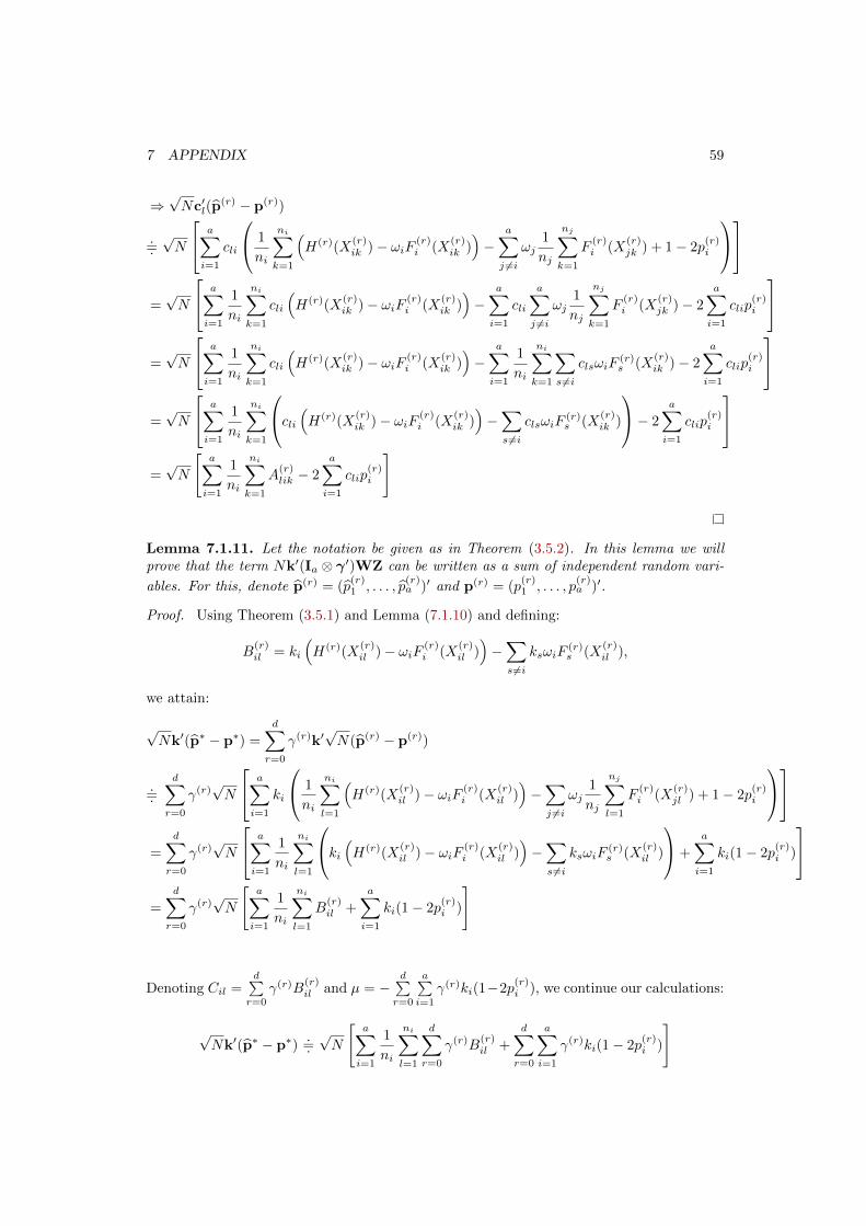
7 APPENDIX 59
⇒√Nc′l(p
(r) − p(r))
.=.√N
a∑i=1
cli
1
ni
ni∑k=1
(H(r)(X
(r)ik )− ωiF (r)
i (X(r)ik ))−
a∑j 6=i
ωj1
nj
nj∑k=1
F(r)i (X
(r)jk ) + 1− 2p
(r)i
=√N
a∑i=1
1
ni
ni∑k=1
cli
(H(r)(X
(r)ik )− ωiF (r)
i (X(r)ik ))−
a∑i=1
cli
a∑j 6=i
ωj1
nj
nj∑k=1
F(r)i (X
(r)jk )− 2
a∑i=1
clip(r)i
=√N
a∑i=1
1
ni
ni∑k=1
cli
(H(r)(X
(r)ik )− ωiF (r)
i (X(r)ik ))−
a∑i=1
1
ni
ni∑k=1
∑s 6=i
clsωiF(r)s (X
(r)ik )− 2
a∑i=1
clip(r)i
=√N
a∑i=1
1
ni
ni∑k=1
cli (H(r)(X(r)ik )− ωiF (r)
i (X(r)ik ))−∑s6=i
clsωiF(r)s (X
(r)ik )
− 2
a∑i=1
clip(r)i
=√N
[a∑i=1
1
ni
ni∑k=1
A(r)lik − 2
a∑i=1
clip(r)i
]
Lemma 7.1.11. Let the notation be given as in Theorem (3.5.2). In this lemma we willprove that the term Nk′(Ia ⊗ γ′)WZ can be written as a sum of independent random vari-
ables. For this, denote p(r) = (p(r)1 , . . . , p
(r)a )′ and p(r) = (p
(r)1 , . . . , p
(r)a )′.
Proof. Using Theorem (3.5.1) and Lemma (7.1.10) and defining:
B(r)il = ki
(H(r)(X
(r)il )− ωiF (r)
i (X(r)il ))−∑s6=i
ksωiF(r)s (X
(r)il ),
we attain:
√Nk′(p∗ − p∗) =
d∑r=0
γ(r)k′√N(p(r) − p(r))
.=.
d∑r=0
γ(r)√N
a∑i=1
ki
1
ni
ni∑l=1
(H(r)(X
(r)il )− ωiF (r)
i (X(r)il ))−∑j 6=i
ωj1
nj
nj∑l=1
F(r)i (X
(r)jl ) + 1− 2p
(r)i
=
d∑r=0
γ(r)√N
a∑i=1
1
ni
ni∑l=1
ki (H(r)(X(r)il )− ωiF (r)
i (X(r)il ))−∑s6=i
ksωiF(r)s (X
(r)il )
+
a∑i=1
ki(1− 2p(r)i )
=
d∑r=0
γ(r)√N
[a∑i=1
1
ni
ni∑l=1
B(r)il +
a∑i=1
ki(1− 2p(r)i )
]
Denoting Cil =d∑r=0
γ(r)B(r)il and µ = −
d∑r=0
a∑i=1
γ(r)ki(1−2p(r)i ), we continue our calculations:
√Nk′(p∗ − p∗)
.=.√N
[a∑i=1
1
ni
ni∑l=1
d∑r=0
γ(r)B(r)il +
d∑r=0
a∑i=1
γ(r)ki(1− 2p(r)i )
]

7 APPENDIX 60
=
a∑i=1
ni∑l=1
√N
niCil − µ
=
a∑i=1
ni∑l=1
(
√N
niCil − µil),
where µil are chosen such that E(Cil) = µil, which implies∑ai=1
∑ni
l=1 µil = µ. By con-
struction, Cil are independent over the indizes i and l. With∑ai=1
∑ni
l=1(NniCil −
√Nµil)
we therefore attain a term which is applicable as the enumerator for the Lindeberg-Fellertheorem (7.1.7).

7 APPENDIX 61
7.2 Supplementary Simulation Results
7.2.1 Type I Error Simulation
Table 12: An α-level simulation. Design: balanced with ni = 7, 10, 15, 25, 50 observations. Factorlevels: a = 3. Number of covariates: d = 1, 2, 5. Covariates: multivariate normal distributed (4.1),ρ = 0.5. Dependent variable: standard normal distributed (4.2).
d ni mctp.n mctp.t 2-step sie.ats sie.wts mctp.nc mctp.par f.par
1 7 0.1353 0.0842 0.0713 0.0973 0.1441 0.0708 0.0529 0.052510 0.1017 0.0725 0.0599 0.0764 0.1070 0.0636 0.0480 0.049615 0.0848 0.0641 0.0529 0.0661 0.0874 0.0583 0.0478 0.047625 0.0719 0.0615 0.0539 0.0631 0.0739 0.0584 0.0505 0.050850 0.0611 0.0565 0.0528 0.0566 0.0622 0.0546 0.0512 0.0507
2 7 0.1625 0.1001 0.0907 0.1186 0.1697 0.0718 0.0504 0.051210 0.1251 0.0883 0.0743 0.0963 0.1310 0.0674 0.0512 0.051615 0.0873 0.0676 0.0584 0.0717 0.0917 0.0536 0.0454 0.045125 0.0798 0.0673 0.0593 0.0681 0.0816 0.0585 0.0504 0.050750 0.0619 0.0569 0.0532 0.0581 0.0626 0.0501 0.0505 0.0509
5 7 0.2579 0.1742 0.1831 0.2150 0.2641 0.0734 0.0490 0.051210 0.1708 0.1265 0.1188 0.1448 0.1772 0.0628 0.0495 0.048515 0.1273 0.1029 0.0919 0.1099 0.1317 0.0620 0.0515 0.050425 0.0856 0.0736 0.0658 0.0784 0.0882 0.0488 0.0457 0.047550 0.0692 0.0645 0.0591 0.0651 0.0690 0.0517 0.0503 0.0510
Table 13: An α-level simulation. Design: balanced with ni = 7, 10, 15, 25, 50 observations. Factorlevels: a = 3. Number of covariates: d = 1, 2, 5. Covariates: multivariate normal distributed (4.1),ρ = 0.9. Dependent variable: standard normal distributed (4.2).
d ni mctp.n mctp.t 2-step sie.ats sie.wts mctp.nc mctp.par f.par
1 7 0.1428 0.0878 0.0724 0.0984 0.1525 0.0752 0.0576 0.055710 0.1029 0.0703 0.0595 0.0768 0.1068 0.0622 0.0475 0.047315 0.0857 0.0662 0.0553 0.0694 0.0886 0.0586 0.0501 0.050525 0.0688 0.0596 0.0528 0.0596 0.0716 0.0553 0.0495 0.049750 0.0627 0.0566 0.0534 0.0584 0.0632 0.0566 0.0516 0.0519
2 7 0.1599 0.0980 0.0854 0.1179 0.1690 0.0697 0.0463 0.048310 0.1211 0.0841 0.0708 0.0939 0.1259 0.0654 0.0531 0.053315 0.0905 0.0679 0.0607 0.0745 0.0922 0.0564 0.0463 0.045725 0.0764 0.0655 0.0580 0.0659 0.0787 0.0557 0.0501 0.048850 0.0655 0.0608 0.0566 0.0601 0.0657 0.0568 0.0524 0.0527
5 7 0.2570 0.1731 0.1830 0.2125 0.2638 0.0709 0.0500 0.050010 0.1710 0.1263 0.1152 0.1446 0.1780 0.0628 0.0469 0.046015 0.1247 0.0991 0.0877 0.1065 0.1254 0.0611 0.0514 0.050625 0.0903 0.0771 0.0677 0.0805 0.0926 0.0566 0.0522 0.053850 0.0706 0.0645 0.0595 0.0642 0.0691 0.0516 0.0500 0.0490
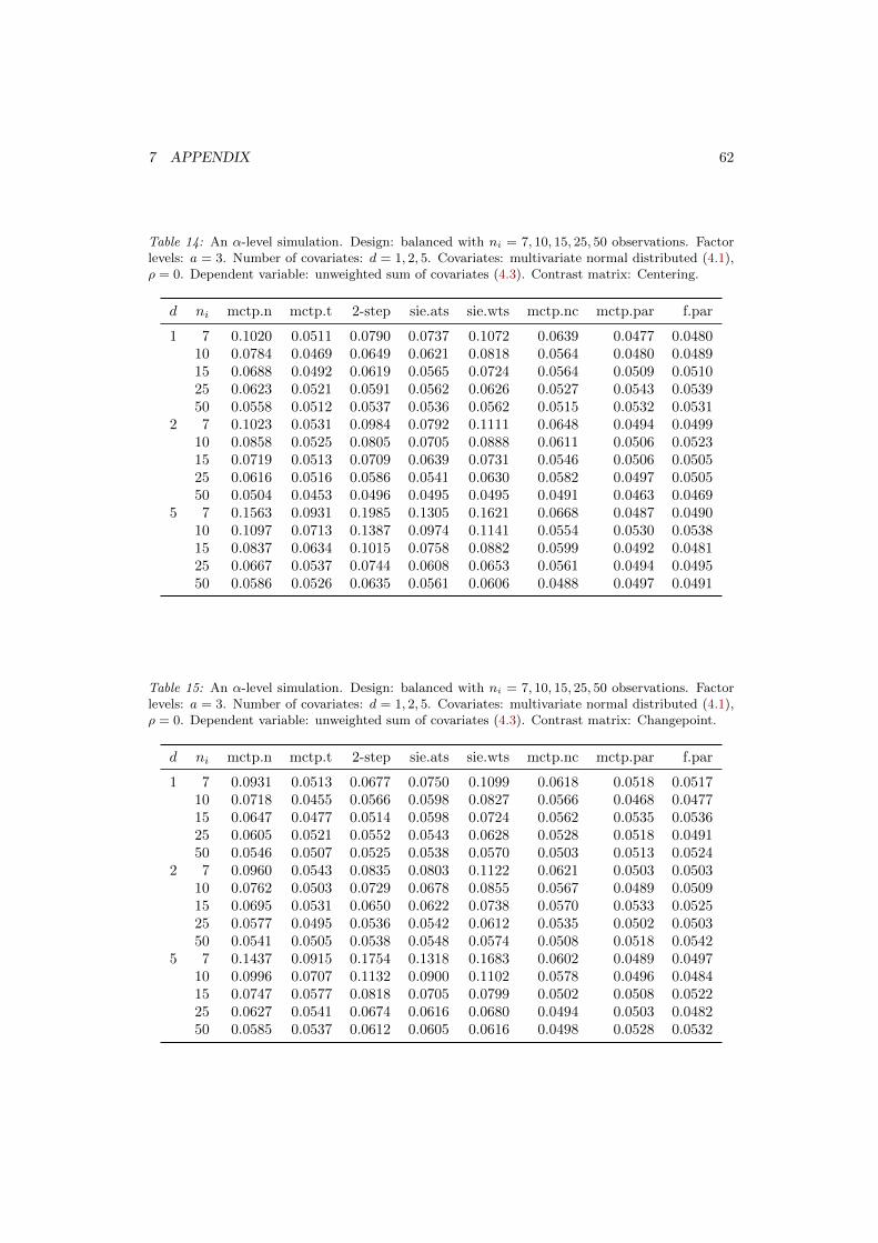
7 APPENDIX 62
Table 14: An α-level simulation. Design: balanced with ni = 7, 10, 15, 25, 50 observations. Factorlevels: a = 3. Number of covariates: d = 1, 2, 5. Covariates: multivariate normal distributed (4.1),ρ = 0. Dependent variable: unweighted sum of covariates (4.3). Contrast matrix: Centering.
d ni mctp.n mctp.t 2-step sie.ats sie.wts mctp.nc mctp.par f.par
1 7 0.1020 0.0511 0.0790 0.0737 0.1072 0.0639 0.0477 0.048010 0.0784 0.0469 0.0649 0.0621 0.0818 0.0564 0.0480 0.048915 0.0688 0.0492 0.0619 0.0565 0.0724 0.0564 0.0509 0.051025 0.0623 0.0521 0.0591 0.0562 0.0626 0.0527 0.0543 0.053950 0.0558 0.0512 0.0537 0.0536 0.0562 0.0515 0.0532 0.0531
2 7 0.1023 0.0531 0.0984 0.0792 0.1111 0.0648 0.0494 0.049910 0.0858 0.0525 0.0805 0.0705 0.0888 0.0611 0.0506 0.052315 0.0719 0.0513 0.0709 0.0639 0.0731 0.0546 0.0506 0.050525 0.0616 0.0516 0.0586 0.0541 0.0630 0.0582 0.0497 0.050550 0.0504 0.0453 0.0496 0.0495 0.0495 0.0491 0.0463 0.0469
5 7 0.1563 0.0931 0.1985 0.1305 0.1621 0.0668 0.0487 0.049010 0.1097 0.0713 0.1387 0.0974 0.1141 0.0554 0.0530 0.053815 0.0837 0.0634 0.1015 0.0758 0.0882 0.0599 0.0492 0.048125 0.0667 0.0537 0.0744 0.0608 0.0653 0.0561 0.0494 0.049550 0.0586 0.0526 0.0635 0.0561 0.0606 0.0488 0.0497 0.0491
Table 15: An α-level simulation. Design: balanced with ni = 7, 10, 15, 25, 50 observations. Factorlevels: a = 3. Number of covariates: d = 1, 2, 5. Covariates: multivariate normal distributed (4.1),ρ = 0. Dependent variable: unweighted sum of covariates (4.3). Contrast matrix: Changepoint.
d ni mctp.n mctp.t 2-step sie.ats sie.wts mctp.nc mctp.par f.par
1 7 0.0931 0.0513 0.0677 0.0750 0.1099 0.0618 0.0518 0.051710 0.0718 0.0455 0.0566 0.0598 0.0827 0.0566 0.0468 0.047715 0.0647 0.0477 0.0514 0.0598 0.0724 0.0562 0.0535 0.053625 0.0605 0.0521 0.0552 0.0543 0.0628 0.0528 0.0518 0.049150 0.0546 0.0507 0.0525 0.0538 0.0570 0.0503 0.0513 0.0524
2 7 0.0960 0.0543 0.0835 0.0803 0.1122 0.0621 0.0503 0.050310 0.0762 0.0503 0.0729 0.0678 0.0855 0.0567 0.0489 0.050915 0.0695 0.0531 0.0650 0.0622 0.0738 0.0570 0.0533 0.052525 0.0577 0.0495 0.0536 0.0542 0.0612 0.0535 0.0502 0.050350 0.0541 0.0505 0.0538 0.0548 0.0574 0.0508 0.0518 0.0542
5 7 0.1437 0.0915 0.1754 0.1318 0.1683 0.0602 0.0489 0.049710 0.0996 0.0707 0.1132 0.0900 0.1102 0.0578 0.0496 0.048415 0.0747 0.0577 0.0818 0.0705 0.0799 0.0502 0.0508 0.052225 0.0627 0.0541 0.0674 0.0616 0.0680 0.0494 0.0503 0.048250 0.0585 0.0537 0.0612 0.0605 0.0616 0.0498 0.0528 0.0532

7 APPENDIX 63
Table 16: An α-level simulation. Design: balanced with ni = 7, 10, 15, 25, 50 observations. Factorlevels: a = 3. Number of covariates: d = 1, 2, 5. Covariates: multivariate normal distributed (4.1),ρ = 0. Dependent variable: unweighted sum of covariates (4.3). Contrast matrix: Dunnett.
d ni mctp.n mctp.t 2-step sie.ats sie.wts mctp.nc mctp.par f.par
1 7 0.0877 0.0538 0.0622 0.0722 0.1067 0.0630 0.0479 0.047710 0.0805 0.0538 0.0576 0.0657 0.0875 0.0638 0.0534 0.055815 0.0650 0.0501 0.0561 0.0577 0.0713 0.0549 0.0491 0.051625 0.0558 0.0482 0.0487 0.0515 0.0575 0.0558 0.0465 0.048450 0.0528 0.0486 0.0494 0.0505 0.0544 0.0494 0.0510 0.0514
2 7 0.0928 0.0575 0.0817 0.0803 0.1096 0.0642 0.0500 0.050210 0.0771 0.0509 0.0654 0.0659 0.0878 0.0576 0.0505 0.050215 0.0672 0.0513 0.0610 0.0588 0.0717 0.0547 0.0515 0.050025 0.0574 0.0483 0.0537 0.0518 0.0567 0.0499 0.0488 0.047850 0.0512 0.0480 0.0519 0.0503 0.0544 0.0509 0.0481 0.0490
5 7 0.1461 0.0941 0.1695 0.1314 0.1652 0.0651 0.0461 0.049010 0.1039 0.0758 0.1166 0.0950 0.1133 0.0587 0.0522 0.051615 0.0797 0.0629 0.0851 0.0736 0.0852 0.0561 0.0487 0.049425 0.0632 0.0554 0.0669 0.0639 0.0693 0.0529 0.0512 0.051250 0.0547 0.0518 0.0554 0.0545 0.0565 0.0518 0.0484 0.0490
Table 17: An α-level simulation. Design: balanced with ni = 7, 10, 15, 25, 50 observations. Factorlevels: a = 3. Number of covariates: d = 1, 2, 5. Covariates: multivariate normal distributed (4.1),ρ = 0.5. Dependent variable: unweighted sum of covariates (4.3).
d ni mctp.n mctp.t 2-step sie.ats sie.wts mctp.nc mctp.par f.par
1 7 0.1428 0.0878 0.0724 0.0984 0.1525 0.0752 0.0576 0.055710 0.1029 0.0703 0.0595 0.0768 0.1068 0.0622 0.0475 0.047315 0.0857 0.0662 0.0553 0.0694 0.0886 0.0586 0.0501 0.050525 0.0688 0.0596 0.0528 0.0596 0.0716 0.0553 0.0495 0.049750 0.0627 0.0566 0.0534 0.0584 0.0632 0.0566 0.0516 0.0519
2 7 0.1599 0.0980 0.0854 0.1179 0.1690 0.0697 0.0463 0.048310 0.1211 0.0841 0.0708 0.0939 0.1259 0.0654 0.0531 0.053315 0.0905 0.0679 0.0607 0.0745 0.0922 0.0564 0.0463 0.045725 0.0764 0.0655 0.0580 0.0659 0.0787 0.0557 0.0501 0.048850 0.0655 0.0608 0.0566 0.0601 0.0657 0.0568 0.0524 0.0527
5 7 0.2570 0.1731 0.1830 0.2125 0.2638 0.0709 0.0500 0.050010 0.1710 0.1263 0.1152 0.1446 0.1780 0.0628 0.0469 0.046015 0.1247 0.0991 0.0877 0.1065 0.1254 0.0611 0.0514 0.050625 0.0903 0.0771 0.0677 0.0805 0.0926 0.0566 0.0522 0.053850 0.0706 0.0645 0.0595 0.0642 0.0691 0.0516 0.0500 0.0490

7 APPENDIX 64
Table 18: An α-level simulation. Design: balanced with ni = 7, 10, 15, 25, 50 observations. Factorlevels: a = 3. Number of covariates: d = 1, 2, 5. Covariates: multivariate normal distributed (4.1),ρ = 0.9. Dependent variable: unweighted sum of covariates (4.3).
d ni mctp.n mctp.t 2-step sie.ats sie.wts mctp.nc mctp.par f.par
1 7 0.1078 0.0587 0.0745 0.0761 0.1130 0.0709 0.0515 0.051810 0.0809 0.0518 0.0574 0.0646 0.0848 0.0621 0.0488 0.050215 0.0681 0.0527 0.0560 0.0587 0.0704 0.0607 0.0512 0.052025 0.0569 0.0451 0.0470 0.0492 0.0572 0.0520 0.0465 0.045950 0.0551 0.0507 0.0534 0.0519 0.0558 0.0523 0.0493 0.0497
2 7 0.1081 0.0594 0.0934 0.0797 0.1132 0.0735 0.0520 0.053410 0.0810 0.0504 0.0726 0.0648 0.0837 0.0595 0.0482 0.048415 0.0690 0.0510 0.0613 0.0574 0.0710 0.0603 0.0495 0.048625 0.0605 0.0505 0.0584 0.0561 0.0610 0.0526 0.0534 0.053150 0.0517 0.0468 0.0525 0.0512 0.0520 0.0544 0.0497 0.0492
5 7 0.1535 0.0908 0.2032 0.1268 0.1580 0.0729 0.0516 0.051210 0.1075 0.0727 0.1330 0.0937 0.1128 0.0639 0.0547 0.054815 0.0765 0.0587 0.0911 0.0675 0.0757 0.0622 0.0505 0.050725 0.0656 0.0555 0.0726 0.0612 0.0665 0.0526 0.0502 0.049250 0.0526 0.0478 0.0556 0.0504 0.0540 0.0524 0.0491 0.0463
Table 19: An α-level simulation. Design: balanced with ni = 7, 10, 15, 25, 50 observations. Factorlevels: a = 3. Number of covariates: d = 1, 2, 5. Covariates: multivariate normal distributed (4.1),ρ = 0.5. Dependent variable: weighted sum of covariates (4.4).
d ni mctp.n mctp.t 2-step sie.ats sie.wts mctp.nc mctp.par f.par
1 7 0.1227 0.0726 0.0701 0.0870 0.1304 0.0725 0.0522 0.051810 0.0969 0.0658 0.0598 0.0752 0.1013 0.0624 0.0495 0.050615 0.0787 0.0601 0.0543 0.0658 0.0819 0.0580 0.0511 0.050425 0.0636 0.0530 0.0493 0.0547 0.0632 0.0544 0.0475 0.046450 0.0597 0.0549 0.0521 0.0568 0.0595 0.0542 0.0531 0.0543
2 7 0.1215 0.0654 0.0996 0.0947 0.1266 0.0763 0.0562 0.055210 0.0829 0.0506 0.0662 0.0670 0.0855 0.0600 0.0460 0.044415 0.0732 0.0539 0.0627 0.0622 0.0738 0.0582 0.0490 0.048125 0.0660 0.0560 0.0597 0.0582 0.0654 0.0538 0.0527 0.051850 0.0565 0.0512 0.0560 0.0532 0.0555 0.0583 0.0502 0.0504
5 7 0.0944 0.0513 0.1928 0.0708 0.1001 0.0684 0.0537 0.053010 0.0578 0.0356 0.1216 0.0474 0.0600 0.0653 0.0518 0.053215 0.0493 0.0339 0.0955 0.0415 0.0490 0.0556 0.0519 0.051525 0.0459 0.0377 0.0784 0.0425 0.0451 0.0584 0.0527 0.051650 0.0422 0.0385 0.0573 0.0407 0.0407 0.0546 0.0494 0.0478

7 APPENDIX 65
Table 20: An α-level simulation. Design: balanced with ni = 7, 10, 15, 25, 50 observations. Factorlevels: a = 3. Number of covariates: d = 1, 2, 5. Covariates: multivariate normal distributed (4.1),ρ = 0.9. Dependent variable: weighted sum of covariates (4.4).
d ni mctp.n mctp.t 2-step sie.ats sie.wts mctp.nc mctp.par f.par
1 7 0.1326 0.0768 0.0739 0.0926 0.1395 0.0742 0.0527 0.052810 0.0957 0.0656 0.0581 0.0745 0.1020 0.0637 0.0498 0.050615 0.0811 0.0623 0.0585 0.0660 0.0841 0.0603 0.0531 0.052125 0.0618 0.0517 0.0486 0.0538 0.0631 0.0518 0.0439 0.043150 0.0596 0.0547 0.0524 0.0554 0.0596 0.0537 0.0527 0.0528
2 7 0.1268 0.0728 0.0981 0.0983 0.1337 0.0773 0.0533 0.053110 0.0895 0.0590 0.0740 0.0726 0.0945 0.0603 0.0469 0.048715 0.0780 0.0575 0.0661 0.0649 0.0793 0.0619 0.0505 0.049125 0.0684 0.0551 0.0596 0.0606 0.0666 0.0575 0.0539 0.053750 0.0527 0.0480 0.0512 0.0499 0.0535 0.0522 0.0467 0.0465
5 7 0.1170 0.0671 0.1875 0.0917 0.1210 0.0733 0.0507 0.049910 0.0785 0.0526 0.1219 0.0645 0.0802 0.0678 0.0525 0.052515 0.0598 0.0463 0.0879 0.0514 0.0618 0.0626 0.0524 0.052225 0.0521 0.0422 0.0683 0.0467 0.0507 0.0543 0.0502 0.049550 0.0485 0.0431 0.0570 0.0457 0.0474 0.0547 0.0462 0.0467
Table 21: An α-level simulation. Design: balanced with ni = 7, 10, 15, 25, 50 observations. Factorlevels: a = 3. Number of covariates: d = 1, 2, 5. Covariates: multivariate log-normal distributed(4.5), ρ = 0.5. Dependent variable: unweighted sum of covariates (4.6).
d ni mctp.n mctp.t 2-step sie.ats sie.wts mctp.nc mctp.par f.par
1 7 0.1042 0.0570 0.0703 0.0736 0.1143 0.0731 0.0343 0.036410 0.0831 0.0519 0.0586 0.0630 0.0871 0.0646 0.0317 0.033315 0.0749 0.0546 0.0617 0.0629 0.0794 0.0622 0.0363 0.037525 0.0617 0.0503 0.0527 0.0544 0.0633 0.0578 0.0351 0.035250 0.0583 0.0527 0.0535 0.0546 0.0590 0.0533 0.0450 0.0466
2 7 0.1049 0.0537 0.0939 0.0784 0.1107 0.0731 0.0355 0.036110 0.0815 0.0497 0.0727 0.0652 0.0868 0.0660 0.0331 0.036415 0.0677 0.0494 0.0624 0.0552 0.0738 0.0596 0.0372 0.040025 0.0597 0.0495 0.0590 0.0565 0.0635 0.0572 0.0395 0.039950 0.0565 0.0510 0.0527 0.0528 0.0590 0.0533 0.0422 0.0439
5 7 0.1514 0.0883 0.1881 0.1270 0.1575 0.0720 0.0375 0.037710 0.1080 0.0683 0.1338 0.0932 0.1154 0.0607 0.0352 0.037015 0.0764 0.0565 0.0926 0.0702 0.0801 0.0594 0.0363 0.038825 0.0658 0.0537 0.0770 0.0613 0.0708 0.0556 0.0399 0.040550 0.0558 0.0508 0.0603 0.0546 0.0591 0.0487 0.0436 0.0441

7 APPENDIX 66
Table 22: An α-level simulation. Design: balanced with ni = 7, 10, 15, 25, 50 observations. Factorlevels: a = 3. Number of covariates: d = 1, 2, 5. Covariates: multivariate log-normal distributed(4.5), ρ = 0.9. Dependent variable: unweighted sum of covariates (4.6).
d ni mctp.n mctp.t 2-step sie.ats sie.wts mctp.nc mctp.par f.par
1 7 0.1074 0.0563 0.0724 0.0746 0.1157 0.0764 0.0336 0.035610 0.0794 0.0524 0.0592 0.0592 0.0850 0.0635 0.0321 0.034915 0.0694 0.0522 0.0550 0.0563 0.0733 0.0621 0.0364 0.037425 0.0579 0.0469 0.0478 0.0507 0.0597 0.0531 0.0350 0.036550 0.0555 0.0515 0.0503 0.0518 0.0553 0.0533 0.0429 0.0434
2 7 0.0937 0.0457 0.0933 0.0766 0.1011 0.0727 0.0354 0.037110 0.0746 0.0443 0.0751 0.0624 0.0809 0.0639 0.0306 0.033015 0.0638 0.0429 0.0618 0.0555 0.0685 0.0530 0.0349 0.036925 0.0598 0.0491 0.0602 0.0556 0.0635 0.0554 0.0386 0.039350 0.0527 0.0482 0.0504 0.0502 0.0564 0.0537 0.0408 0.0411
5 7 0.1357 0.0738 0.1961 0.1129 0.1357 0.0714 0.0376 0.037610 0.0930 0.0563 0.1285 0.0830 0.0975 0.0632 0.0405 0.041515 0.0708 0.0492 0.0970 0.0647 0.0735 0.0603 0.0358 0.037325 0.0551 0.0424 0.0680 0.0533 0.0595 0.0513 0.0397 0.042050 0.0516 0.0452 0.0604 0.0503 0.0572 0.0567 0.0403 0.0407
Table 23: An α-level simulation. Design: balanced with ni = 7, 10, 15, 25, 50 observations. Factorlevels: a = 3. Number of covariates: d = 1, 2, 5. Covariates: Poisson(1) distributed. Dependentvariable: unweighted sum of covariates with standard normal error term.
d ni mctp.n mctp.t 2-step sie.ats sie.wts mctp.nc mctp.par f.par
1 7 0.1118 0.0635 0.0745 0.0788 0.1168 0.0742 0.0536 0.053310 0.0891 0.0562 0.0640 0.0700 0.0919 0.0590 0.0497 0.049315 0.0687 0.0506 0.0519 0.0549 0.0709 0.0547 0.0453 0.045525 0.0637 0.0544 0.0536 0.0598 0.0650 0.0529 0.0527 0.052750 0.0590 0.0537 0.0537 0.0550 0.0588 0.0547 0.0505 0.0503
2 7 0.1194 0.0651 0.0878 0.0922 0.1216 0.0694 0.0488 0.050110 0.0877 0.0554 0.0694 0.0703 0.0885 0.0638 0.0478 0.048215 0.0728 0.0539 0.0602 0.0629 0.0732 0.0586 0.0486 0.047325 0.0618 0.0519 0.0551 0.0548 0.0622 0.0559 0.0488 0.048950 0.0574 0.0526 0.0559 0.0525 0.0553 0.0523 0.0524 0.0517
5 7 0.1882 0.1178 0.1914 0.1599 0.1941 0.0680 0.0512 0.053310 0.1318 0.0886 0.1268 0.1126 0.1352 0.0658 0.0470 0.045915 0.0930 0.0731 0.0955 0.0827 0.0979 0.0581 0.0509 0.050925 0.0725 0.0614 0.0695 0.0659 0.0731 0.0586 0.0519 0.052250 0.0592 0.0544 0.0584 0.0555 0.0593 0.0505 0.0531 0.0519

7 APPENDIX 67
Table 24: An α-level simulation. Design: balanced with ni = 7, 10, 15, 25, 50 observations. Factorlevels: a = 3. Number of covariates: d = 1, 2, 5. Covariates: Exp(1) distributed. Dependentvariable: unweighted sum of covariates with standard normal error term.
d ni mctp.n mctp.t 2-step sie.ats sie.wts mctp.nc mctp.par f.par
1 7 0.1072 0.0575 0.0694 0.0759 0.1135 0.0691 0.0491 0.049210 0.0887 0.0570 0.0604 0.0677 0.0947 0.0630 0.0507 0.050515 0.0693 0.0517 0.0530 0.0582 0.0734 0.0564 0.0492 0.048025 0.0609 0.0516 0.0532 0.0568 0.0628 0.0567 0.0503 0.049050 0.0556 0.0500 0.0490 0.0531 0.0562 0.0524 0.0497 0.0493
2 7 0.1201 0.0648 0.0908 0.0903 0.1272 0.0715 0.0491 0.049110 0.0928 0.0604 0.0711 0.0774 0.0974 0.0649 0.0499 0.050715 0.0767 0.0554 0.0628 0.0635 0.0769 0.0601 0.0495 0.049725 0.0656 0.0562 0.0586 0.0609 0.0673 0.0616 0.0503 0.049350 0.0576 0.0518 0.0542 0.0536 0.0567 0.0577 0.0508 0.0520
5 7 0.1897 0.1161 0.1880 0.1641 0.1940 0.0749 0.0519 0.052110 0.1323 0.0900 0.1221 0.1116 0.1339 0.0633 0.0509 0.050215 0.0972 0.0760 0.0916 0.0893 0.1008 0.0572 0.0487 0.049325 0.0705 0.0578 0.0677 0.0638 0.0700 0.0548 0.0491 0.050150 0.0640 0.0600 0.0616 0.0597 0.0654 0.0514 0.0507 0.0522
Table 25: An α-level simulation. Design: balanced with ni = 7, 10, 15, 25, 50 observations. Factorlevels: a = 3. Number of covariates: d = 1, 2, 5. Covariates: Bernoulli(0.5) distributed. Dependentvariable: unweighted sum of covariates with standard normal error term.
d ni mctp.n mctp.t 2-step sie.ats sie.wts mctp.nc mctp.par f.par
1 7 0.1320 0.0809 0.0727 0.0965 0.1371 0.0750 0.0531 0.052610 0.0981 0.0671 0.0594 0.0753 0.1032 0.0643 0.0476 0.047815 0.0785 0.0611 0.0542 0.0637 0.0811 0.0596 0.0474 0.049525 0.0678 0.0559 0.0542 0.0584 0.0710 0.0541 0.0488 0.049550 0.0573 0.0529 0.0517 0.0535 0.0585 0.0546 0.0495 0.0512
2 7 0.1447 0.0856 0.0933 0.1128 0.1482 0.0701 0.0548 0.053510 0.1061 0.0712 0.0710 0.0832 0.1102 0.0663 0.0470 0.046815 0.0820 0.0636 0.0608 0.0685 0.0853 0.0583 0.0488 0.048225 0.0684 0.0572 0.0552 0.0615 0.0701 0.0564 0.0527 0.051750 0.0571 0.0527 0.0504 0.0548 0.0588 0.0532 0.0518 0.0509
5 7 0.2333 0.1497 0.1887 0.1983 0.2390 0.0699 0.0491 0.049810 0.1491 0.1048 0.1189 0.1308 0.1546 0.0661 0.0514 0.050415 0.1115 0.0874 0.0941 0.0992 0.1171 0.0625 0.0516 0.050025 0.0818 0.0708 0.0685 0.0752 0.0826 0.0581 0.0505 0.048650 0.0659 0.0596 0.0597 0.0639 0.0673 0.0533 0.0523 0.0544
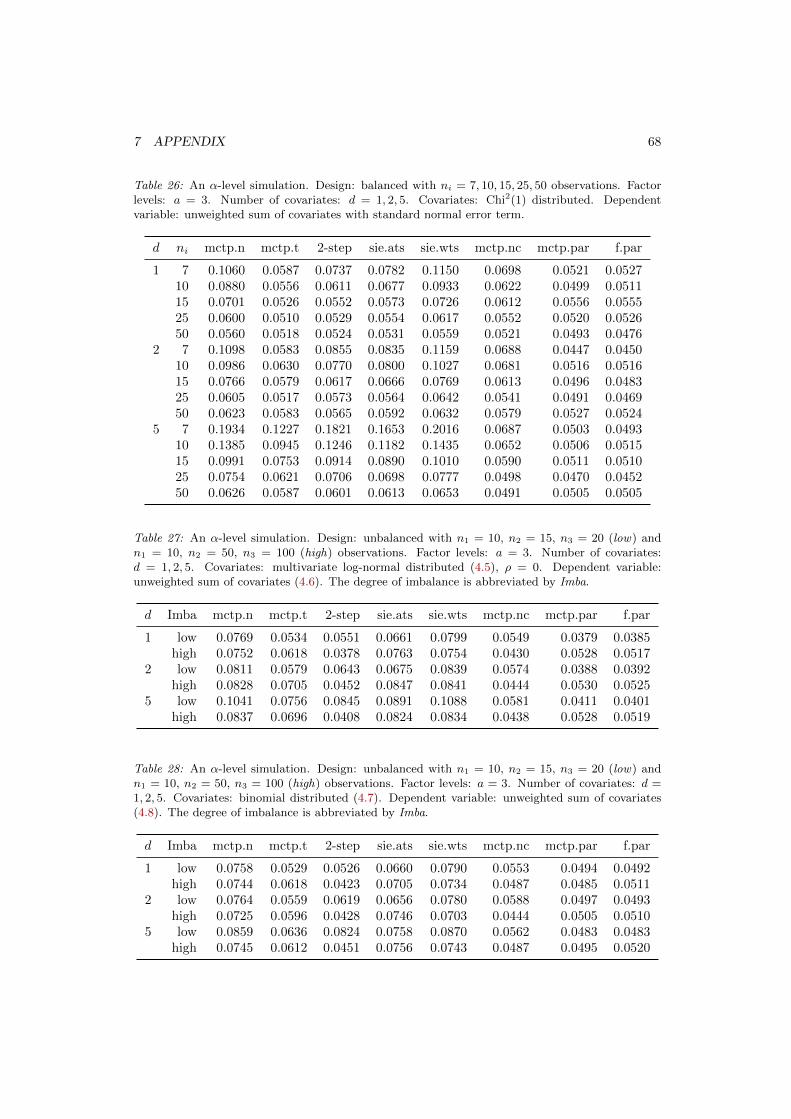
7 APPENDIX 68
Table 26: An α-level simulation. Design: balanced with ni = 7, 10, 15, 25, 50 observations. Factorlevels: a = 3. Number of covariates: d = 1, 2, 5. Covariates: Chi2(1) distributed. Dependentvariable: unweighted sum of covariates with standard normal error term.
d ni mctp.n mctp.t 2-step sie.ats sie.wts mctp.nc mctp.par f.par
1 7 0.1060 0.0587 0.0737 0.0782 0.1150 0.0698 0.0521 0.052710 0.0880 0.0556 0.0611 0.0677 0.0933 0.0622 0.0499 0.051115 0.0701 0.0526 0.0552 0.0573 0.0726 0.0612 0.0556 0.055525 0.0600 0.0510 0.0529 0.0554 0.0617 0.0552 0.0520 0.052650 0.0560 0.0518 0.0524 0.0531 0.0559 0.0521 0.0493 0.0476
2 7 0.1098 0.0583 0.0855 0.0835 0.1159 0.0688 0.0447 0.045010 0.0986 0.0630 0.0770 0.0800 0.1027 0.0681 0.0516 0.051615 0.0766 0.0579 0.0617 0.0666 0.0769 0.0613 0.0496 0.048325 0.0605 0.0517 0.0573 0.0564 0.0642 0.0541 0.0491 0.046950 0.0623 0.0583 0.0565 0.0592 0.0632 0.0579 0.0527 0.0524
5 7 0.1934 0.1227 0.1821 0.1653 0.2016 0.0687 0.0503 0.049310 0.1385 0.0945 0.1246 0.1182 0.1435 0.0652 0.0506 0.051515 0.0991 0.0753 0.0914 0.0890 0.1010 0.0590 0.0511 0.051025 0.0754 0.0621 0.0706 0.0698 0.0777 0.0498 0.0470 0.045250 0.0626 0.0587 0.0601 0.0613 0.0653 0.0491 0.0505 0.0505
Table 27: An α-level simulation. Design: unbalanced with n1 = 10, n2 = 15, n3 = 20 (low) andn1 = 10, n2 = 50, n3 = 100 (high) observations. Factor levels: a = 3. Number of covariates:d = 1, 2, 5. Covariates: multivariate log-normal distributed (4.5), ρ = 0. Dependent variable:unweighted sum of covariates (4.6). The degree of imbalance is abbreviated by Imba.
d Imba mctp.n mctp.t 2-step sie.ats sie.wts mctp.nc mctp.par f.par
1 low 0.0769 0.0534 0.0551 0.0661 0.0799 0.0549 0.0379 0.0385high 0.0752 0.0618 0.0378 0.0763 0.0754 0.0430 0.0528 0.0517
2 low 0.0811 0.0579 0.0643 0.0675 0.0839 0.0574 0.0388 0.0392high 0.0828 0.0705 0.0452 0.0847 0.0841 0.0444 0.0530 0.0525
5 low 0.1041 0.0756 0.0845 0.0891 0.1088 0.0581 0.0411 0.0401high 0.0837 0.0696 0.0408 0.0824 0.0834 0.0438 0.0528 0.0519
Table 28: An α-level simulation. Design: unbalanced with n1 = 10, n2 = 15, n3 = 20 (low) andn1 = 10, n2 = 50, n3 = 100 (high) observations. Factor levels: a = 3. Number of covariates: d =1, 2, 5. Covariates: binomial distributed (4.7). Dependent variable: unweighted sum of covariates(4.8). The degree of imbalance is abbreviated by Imba.
d Imba mctp.n mctp.t 2-step sie.ats sie.wts mctp.nc mctp.par f.par
1 low 0.0758 0.0529 0.0526 0.0660 0.0790 0.0553 0.0494 0.0492high 0.0744 0.0618 0.0423 0.0705 0.0734 0.0487 0.0485 0.0511
2 low 0.0764 0.0559 0.0619 0.0656 0.0780 0.0588 0.0497 0.0493high 0.0725 0.0596 0.0428 0.0746 0.0703 0.0444 0.0505 0.0510
5 low 0.0859 0.0636 0.0824 0.0758 0.0870 0.0562 0.0483 0.0483high 0.0745 0.0612 0.0451 0.0756 0.0743 0.0487 0.0495 0.0520

7 APPENDIX 69

7 APPENDIX 70
7.2.2 Power Simulation
0.00 0.50 1.00
0.0
0.2
0.4
0.6
0.8
1.0
d = 1 n = 7
Deviation (δ)
Pow
er (
1−β)
0.00 0.50 1.00
0.0
0.2
0.4
0.6
0.8
1.0
d = 1 n = 10
Deviation (δ)
Pow
er (
1−β)
0.00 0.50 1.00
0.0
0.2
0.4
0.6
0.8
1.0
d = 1 n = 15
Deviation (δ)P
ower
(1−
β)
0.00 0.50 1.00
0.0
0.2
0.4
0.6
0.8
1.0
d = 1 n = 25
Deviation (δ)
Pow
er (
1−β)
0.00 0.50 1.00
0.0
0.2
0.4
0.6
0.8
1.0
d = 1 n = 50
Deviation (δ)
Pow
er (
1−β)
0.00 0.50 1.00
0.0
0.2
0.4
0.6
0.8
1.0
d = 2 n = 7
Deviation (δ)
Pow
er (
1−β)
0.00 0.50 1.00
0.0
0.2
0.4
0.6
0.8
1.0
d = 2 n = 10
Deviation (δ)
Pow
er (
1−β)
0.00 0.50 1.000.
00.
20.
40.
60.
81.
0
d = 2 n = 15
Deviation (δ)
Pow
er (
1−β)
0.00 0.50 1.00
0.0
0.2
0.4
0.6
0.8
1.0
d = 2 n = 25
Deviation (δ)
Pow
er (
1−β)
0.00 0.50 1.00
0.0
0.2
0.4
0.6
0.8
1.0
d = 2 n = 50
Deviation (δ)
Pow
er (
1−β)
0.00 0.50 1.00
0.0
0.2
0.4
0.6
0.8
1.0
d = 5 n = 7
Deviation (δ)
Pow
er (
1−β)
0.00 0.50 1.00
0.0
0.2
0.4
0.6
0.8
1.0
d = 5 n = 10
Deviation (δ)
Pow
er (
1−β)
0.00 0.50 1.00
0.0
0.2
0.4
0.6
0.8
1.0
d = 5 n = 15
Deviation (δ)
Pow
er (
1−β)
0.00 0.50 1.00
0.0
0.2
0.4
0.6
0.8
1.0
d = 5 n = 25
Deviation (δ)
Pow
er (
1−β)
0.00 0.50 1.00
0.0
0.2
0.4
0.6
0.8
1.0
d = 5 n = 50
Deviation (δ)
Pow
er (
1−β)
mctp.nmctp.t2−stepsie.atssie.wtsmctp.parmctp.ncchisq.parf.parα−level
Figure 11: Simulation results for the power (1 − β). Design: balanced with ni = 7, 10, 15, 25, 50observations. Factor levels: a = 3. Number of covariates: d = 1, 2, 5. Covariates: multivariatenormal distributed (4.1), ρ = 0.2. Dependent variable: unweighted sum of covariates (4.9).

7 APPENDIX 71
0.00 0.50 1.00
0.0
0.2
0.4
0.6
0.8
1.0
d = 1 n = 7
Deviation (δ)
Pow
er (
1−β)
0.00 0.50 1.00
0.0
0.2
0.4
0.6
0.8
1.0
d = 1 n = 10
Deviation (δ)
Pow
er (
1−β)
0.00 0.50 1.00
0.0
0.2
0.4
0.6
0.8
1.0
d = 1 n = 15
Deviation (δ)
Pow
er (
1−β)
0.00 0.50 1.00
0.0
0.2
0.4
0.6
0.8
1.0
d = 1 n = 25
Deviation (δ)
Pow
er (
1−β)
0.00 0.50 1.00
0.0
0.2
0.4
0.6
0.8
1.0
d = 1 n = 50
Deviation (δ)
Pow
er (
1−β)
0.00 0.50 1.00
0.0
0.2
0.4
0.6
0.8
1.0
d = 2 n = 7
Deviation (δ)
Pow
er (
1−β)
0.00 0.50 1.00
0.0
0.2
0.4
0.6
0.8
1.0
d = 2 n = 10
Deviation (δ)
Pow
er (
1−β)
0.00 0.50 1.00
0.0
0.2
0.4
0.6
0.8
1.0
d = 2 n = 15
Deviation (δ)
Pow
er (
1−β)
0.00 0.50 1.00
0.0
0.2
0.4
0.6
0.8
1.0
d = 2 n = 25
Deviation (δ)
Pow
er (
1−β)
0.00 0.50 1.00
0.0
0.2
0.4
0.6
0.8
1.0
d = 2 n = 50
Deviation (δ)
Pow
er (
1−β)
0.00 0.50 1.00
0.0
0.2
0.4
0.6
0.8
1.0
d = 5 n = 7
Deviation (δ)
Pow
er (
1−β)
0.00 0.50 1.00
0.0
0.2
0.4
0.6
0.8
1.0
d = 5 n = 10
Deviation (δ)
Pow
er (
1−β)
0.00 0.50 1.00
0.0
0.2
0.4
0.6
0.8
1.0
d = 5 n = 15
Deviation (δ)
Pow
er (
1−β)
0.00 0.50 1.00
0.0
0.2
0.4
0.6
0.8
1.0
d = 5 n = 25
Deviation (δ)
Pow
er (
1−β)
0.00 0.50 1.00
0.0
0.2
0.4
0.6
0.8
1.0
d = 5 n = 50
Deviation (δ)
Pow
er (
1−β)
mctp.nmctp.t2−stepsie.atssie.wtsmctp.parmctp.ncchisq.parf.parα−level
Figure 12: Simulation results for the power (1 − β). Design: balanced with ni = 7, 10, 15, 25, 50observations. Factor levels: a = 3. Number of covariates: d = 1, 2, 5. Covariates: multivariatelog-normal distributed (4.5), ρ = 0.2. Dependent variable: unweighted sum of covariates (4.10).
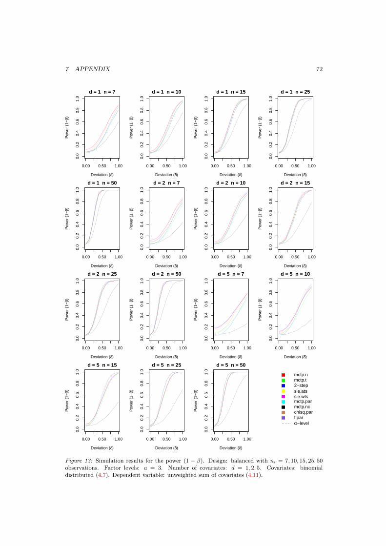
7 APPENDIX 72
0.00 0.50 1.00
0.0
0.2
0.4
0.6
0.8
1.0
d = 1 n = 7
Deviation (δ)
Pow
er (
1−β)
0.00 0.50 1.00
0.0
0.2
0.4
0.6
0.8
1.0
d = 1 n = 10
Deviation (δ)
Pow
er (
1−β)
0.00 0.50 1.00
0.0
0.2
0.4
0.6
0.8
1.0
d = 1 n = 15
Deviation (δ)
Pow
er (
1−β)
0.00 0.50 1.00
0.0
0.2
0.4
0.6
0.8
1.0
d = 1 n = 25
Deviation (δ)
Pow
er (
1−β)
0.00 0.50 1.00
0.0
0.2
0.4
0.6
0.8
1.0
d = 1 n = 50
Deviation (δ)
Pow
er (
1−β)
0.00 0.50 1.00
0.0
0.2
0.4
0.6
0.8
1.0
d = 2 n = 7
Deviation (δ)
Pow
er (
1−β)
0.00 0.50 1.00
0.0
0.2
0.4
0.6
0.8
1.0
d = 2 n = 10
Deviation (δ)
Pow
er (
1−β)
0.00 0.50 1.00
0.0
0.2
0.4
0.6
0.8
1.0
d = 2 n = 15
Deviation (δ)
Pow
er (
1−β)
0.00 0.50 1.00
0.0
0.2
0.4
0.6
0.8
1.0
d = 2 n = 25
Deviation (δ)
Pow
er (
1−β)
0.00 0.50 1.00
0.0
0.2
0.4
0.6
0.8
1.0
d = 2 n = 50
Deviation (δ)
Pow
er (
1−β)
0.00 0.50 1.00
0.0
0.2
0.4
0.6
0.8
1.0
d = 5 n = 7
Deviation (δ)
Pow
er (
1−β)
0.00 0.50 1.00
0.0
0.2
0.4
0.6
0.8
1.0
d = 5 n = 10
Deviation (δ)
Pow
er (
1−β)
0.00 0.50 1.00
0.0
0.2
0.4
0.6
0.8
1.0
d = 5 n = 15
Deviation (δ)
Pow
er (
1−β)
0.00 0.50 1.00
0.0
0.2
0.4
0.6
0.8
1.0
d = 5 n = 25
Deviation (δ)
Pow
er (
1−β)
0.00 0.50 1.00
0.0
0.2
0.4
0.6
0.8
1.0
d = 5 n = 50
Deviation (δ)
Pow
er (
1−β)
mctp.nmctp.t2−stepsie.atssie.wtsmctp.parmctp.ncchisq.parf.parα−level
Figure 13: Simulation results for the power (1 − β). Design: balanced with ni = 7, 10, 15, 25, 50observations. Factor levels: a = 3. Number of covariates: d = 1, 2, 5. Covariates: binomialdistributed (4.7). Dependent variable: unweighted sum of covariates (4.11).

7 APPENDIX 73
7.3 R-Code
In this section we present the R-script written for the user, which was used to evaluatethe example in Section 5. The R-code for the simulations and graphics is not listed in thisthesis. If you are interested in the R-code for the simulations and graphics, please write mean email: [email protected].
1 mctp . cov<−f unc t i on ( formula , data , type=c ( ”Tukey” , ”Dunnett” , ”Sequen” ,2 ” Wil l iams ” , ”Changepoint” , ”AVE” , ”McDermott” , ”Marcus” ,3 ” Umbrel laWil l iams ” ) , conf . level=0.95 , alternative=c ( ”two . s ided ” ,4 ” l e s s ” , ” g r e a t e r ” ) , asy . method=c ( ”mult . t ” , ”normal” ) , info=T , rounds=3,5 effect=c ( ” unweighted ” , ” weighted ” ) )67 input . l i s t<− l i s t ( formula=formula , data=data , type=type [ 1 ] ,8 conf . level=conf . level , alternative=alternative [ 1 ] ,9 asy . method=asy . method [ 1 ] , info=info , rounds=rounds ,
10 effect=effect [ 1 ] )1112 #−−−−−−−−−−−−−−−−−−−−−−−−−−−−−−−−−−−−−−−−−−−−−−−−−−−−−−−−−−−13 #Loading r equ i r ed packages14 #−−−−−−−−−−−−−−−−−−−−−−−−−−−−−−−−−−−−−−−−−−−−−−−−−−−−−−−−−−−15 r e q u i r e ( mvtnorm , quietly=T )16 r e q u i r e ( MASS , quietly=T )17 r e q u i r e ( nparcomp , quietly=T )18 #−−−−−−−−−−−−−−−−−−−−−−−−−−−−−−−−−−−−−−−−−−−−−−−−−−−−−−−−−−−1920 #−−−−−−−−−−−−−−−−−−−−−−−−−−−−−−−−−−−−−−−−−−−−−−−−−−−−−−−−−−−21 #D e f i n i t i o n o f custom f u n c t i o n s22 #−−−−−−−−−−−−−−−−−−−−−−−−−−−−−−−−−−−−−−−−−−−−−−−−−−−−−−−−−−−23 P<−f unc t i on (n )24 diag (1 , abs (n))−1/n25 2627 ’%+%’<−f unc t i on (A , B )28 a . 1<−nrow (A )29 a . 2<−nco l (A )30 b . 1<−nrow (B )31 b . 2<−nco l (B )3233 cbind ( rbind (A , matrix (0 , nco l=a . 2 , nrow=b . 1 ) ) ,34 rbind ( matrix (0 , nco l=b . 2 , nrow=a . 1 ) , B ) )35 3637 tr<−f unc t i on (A )38 sum( diag (A ) )39 40 #−−−−−−−−−−−−−−−−−−−−−−−−−−−−−−−−−−−−−−−−−−−−−−−−−−−−−−−−−−−4142 #−−−−−−−−−−−−−−−−−−−−−−−−−−−−−−−−−−−−−−−−−−−−−−−−−−−−−−−−−−−43 #P o s s i b l e input e r r o r s44 #−−−−−−−−−−−−−−−−−−−−−−−−−−−−−−−−−−−−−−−−−−−−−−−−−−−−−−−−−−−45 i f ( conf . level >=1 | | conf . level <=0)46 stop ( ”The con f idence l e v e l must be between 0 and 1” )47 48 i f ( length ( formula ) !=3)
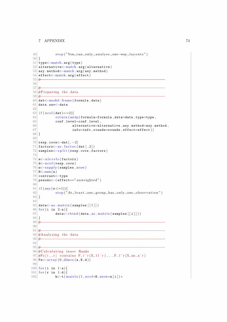
7 APPENDIX 74
49 stop ( ”You can only ana lyse one−way layout s ” )50 51 type<−match . arg ( type )52 alternative<−match . arg ( alternative )53 asy . method<−match . arg ( asy . method )54 effect<−match . arg ( effect )55 #−−−−−−−−−−−−−−−−−−−−−−−−−−−−−−−−−−−−−−−−−−−−−−−−−−−−−−−−−−−5657 #−−−−−−−−−−−−−−−−−−−−−−−−−−−−−−−−−−−−−−−−−−−−−−−−−−−−−−−−−−−58 #Prepar ing the data59 #−−−−−−−−−−−−−−−−−−−−−−−−−−−−−−−−−−−−−−−−−−−−−−−−−−−−−−−−−−−60 dat<−model . frame ( formula , data )61 data . sav<−data6263 i f ( nco l ( dat)==2)64 return ( mctp ( formula=formula , data=data , type=type ,65 conf . level=conf . level ,66 alternative=alternative , asy . method=asy . method ,67 info=info , rounds=rounds , effect=effect ) )68 6970 resp . covs<−dat [ ,−2]71 factorx<−as . f a c t o r ( dat [ , 2 ] )72 samples<−s p l i t ( resp . covs , factorx )7374 a<−n l e v e l s ( factorx )75 d<−nco l ( resp . covs )76 n<−sapply ( samples , nrow )77 N<−sum(n )78 contrast<−type79 pseudo<−( effect==” unweighted ” )8081 i f ( any (n<=1))82 stop ( ”At l e a s t one group has only one obse rvat i on ” )83 8485 data<−as . matrix ( samples [ [ 1 ] ] )86 f o r (i in 2 : a )87 data<−rbind ( data , as . matrix ( samples [ [ i ] ] ) )88 89 #−−−−−−−−−−−−−−−−−−−−−−−−−−−−−−−−−−−−−−−−−−−−−−−−−−−−−−−−−−−9091 #−−−−−−−−−−−−−−−−−−−−−−−−−−−−−−−−−−−−−−−−−−−−−−−−−−−−−−−−−−−92 #Analyzing the data93 #−−−−−−−−−−−−−−−−−−−−−−−−−−−−−−−−−−−−−−−−−−−−−−−−−−−−−−−−−−−9495 #−−−−−−−−−−−−−−−−−−−−−−−−−−−−−−−−−−−−−−−−−−−−−−−−−−−−−−−−−−−96 #Ca l cu l a t ing inner Ranks97 #Fs [ i , , r ] conta in s F i ˆ r (X 11ˆ r ) , . . , F i ˆ r (X an aˆ r )98 Fs<−array (0 , dim=c (a , N , d ) )99
100 f o r (i in 1 : a )101 f o r (r in 1 : d )102 h<−t ( matrix (1 , nco l=N , nrow=n [ i ] ) ∗

7 APPENDIX 75
103 data [ ( sum(n [ 0 : ( i−1) ])+1) : sum(n [ 1 : i ] ) , r ] )104 Fs [ i , , r ]<−rowSums ( ( data [ , r]>h)+1/2∗ ( data [ , r]==h ) ) ∗1/n [ i ]105 106 #−−−−−−−−−−−−−−−−−−−−−−−−−−−−−−−−−−−−−−−−−−−−−−−−−−−−−−−−−−−107 #Estimating the p ’ s108 M . 1<−t ( as . matrix ( rep (1 , n [ 1 ] ) ) /n [ 1 ] )109 f o r (i in 2 : a )110 M . 1<−M.1%+%t ( as . matrix ( rep (1 , n [ i ] ) ) /n [ i ] )111 112113 #p . p a i r s [ i , j , r ] conta in s p i j ˆ r114 p . p a i r s<−array (0 , dim=c (a , a , d ) )115 f o r (i in 1 : a )116 p . p a i r s [ i , , ]<−M . 1 %∗%Fs [ i , , ]117 118119 p . hat<−array (0 , dim=c (a , d ) )120 i f ( pseudo==T )121 f o r (r in 1 : d )122 p . hat [ , r ]<−colMeans (p . p a i r s [ , , r ] )123 124 e l s e 125 f o r (r in 1 : d )126 p . hat [ , r ]<−t (n/N )%∗%p . p a i r s [ , , r ]127 128 129130 #−−−−−−−−−−−−−−−−−−−−−−−−−−−−−−−−−−−−−−−−−−−−−−−−−−−−−−−−−−−131 #Estimating the gamma’ s132 y . hat<−rep (0 , N )133134 #data . r [ j , r ] conta in s Y ik ˆ r where ik are chosen acco rd ing ly135 data . r<−array (0 , dim=c (N , d ) )136137 i f ( pseudo==T )138 f o r (r in 1 : d )139 data . r [ , r ]<−t ( rep (1 /a , a ) ) %∗%Fs [ , , r ]140 141 e l s e 142 f o r (r in 1 : d )143 data . r [ , r ]<−t (n/N )%∗%Fs [ , , r ]144 145 146147 D<−P (n [ 1 ] )148 f o r (i in 2 : a )149 D<−D%+%P (n [ i ] )150 151152 y . hat<−D%∗%data . r [ , 1 ]153154 X . hat<−D%∗%data . r [ ,−1]155 gamma . hat<−s o l v e (t (X . hat )%∗%X . hat )%∗%t (X . hat )%∗%y . hat156 gamma<−c (−1 ,gamma . hat )

7 APPENDIX 76
157158 #−−−−−−−−−−−−−−−−−−−−−−−−−−−−−−−−−−−−−−−−−−−−−−−−−−−−−−−−−−−159 #Estimating p∗160 p . star<−−p . hat%∗%gamma
161 #−−−−−−−−−−−−−−−−−−−−−−−−−−−−−−−−−−−−−−−−−−−−−−−−−−−−−−−−−−−162 #Estimation o f VN163 theta<−f unc t i on (i , j , s , r , u , Fs , n )164 n . j<−c (0 , n )165 1/ (n [ j ]−1)∗ ( Fs [ i , ( sum(n . j [ 1 : j ] ) + 1 ) : sum(n . j [ 1 : ( j+1) ] ) , r ] %∗%166 P (n . j [ j+1])%∗%Fs [ s , ( sum(n . j [ 1 : j ] ) + 1 ) : sum(n . j [ 1 : ( j+1) ] ) , u ] )167 168169 Sigma<−matrix (0 , nco l=aˆ2∗d , nrow=aˆ2∗d )170171 f o r (t in 1 : a )172 f o r (u in 1 : d )173 f o r (s in 1 : a )174 f o r (j in 1 : a )175 f o r (r in 1 : d )176 f o r (i in 1 : a )177 i f (i==j | t==s )178 Sigma [ a∗d∗ (j−1)+a∗ (r−1)+i , a∗d∗ (t−1)+a∗ (u−1)+s ]<−0179 180 i f ( ( i !=j & t !=s ) & (j==t & i==s ) )181 Sigma [ a∗d∗ (j−1)+a∗ (r−1)+i , a∗d∗ (t−1)+a∗ (u−1)+s ]<−1/n [ j ] ∗182 theta (i , j , s , r , u , Fs , n)+1/n [ i ] ∗theta (j , i , t , r , u , Fs , n )183 184 i f ( ( i !=j & t !=s ) & (j==s & i==t ) )185 Sigma [ a∗d∗ (j−1)+a∗ (r−1)+i , a∗d∗ (t−1)+a∗ (u−1)+s ]<−186 −1/n [ j ] ∗theta (i , j , t , r , u , Fs , n)−1/n [ i ] ∗187 theta (j , i , s , r , u , Fs , n )188 189 i f ( ( i !=j & t !=s ) & (j !=s & j !=t & i==t ) )190 Sigma [ a∗d∗ (j−1)+a∗ (r−1)+i , a∗d∗ (t−1)+a∗ (u−1)+s ]<−191 −1/n [ i ] ∗theta (j , i , s , r , u , Fs , n )192 193 i f ( ( i !=j & t !=s ) & (j !=s & j !=t & i==s ) )194 Sigma [ a∗d∗ (j−1)+a∗ (r−1)+i , a∗d∗ (t−1)+a∗ (u−1)+s ]<−195 1/n [ i ] ∗theta (j , i , t , r , u , Fs , n )196 197 i f ( ( i !=j & t !=s ) & (j==t & i !=s & i !=t ) )198 Sigma [ a∗d∗ (j−1)+a∗ (r−1)+i , a∗d∗ (t−1)+a∗ (u−1)+s ]<−199 1/n [ j ] ∗theta (i , j , s , r , u , Fs , n )200 201 i f ( ( i !=j & t !=s ) & (j==s & i !=s & i !=t ) )202 Sigma [ a∗d∗ (j−1)+a∗ (r−1)+i , a∗d∗ (t−1)+a∗ (u−1)+s ]<−203 −1/n [ j ] ∗theta (i , j , t , r , u , Fs , n )204 205 i f ( ( i !=j & t !=s ) & (j !=s & j !=t & i !=s & i !=t ) )206 Sigma [ a∗d∗ (j−1)+a∗ (r−1)+i , a∗d∗ (t−1)+a∗ (u−1)+s ]<−0207 208 209210 i f ( pseudo==T )

7 APPENDIX 77
211 W<−diag (a∗d)%x%t ( rep (1 /a , a ) )212 e l s e 213 W<−diag (a∗d)%x%t (n/N )214 215 VN<−N∗ ( d iag (a)%x%t ( gamma ) ) %∗%W%∗%Sigma%∗%216 t (W )%∗%( diag (a)%x%gamma )217218 #−−−−−−−−−−−−−−−−−−−−−−−−−−−−−−−−−−−−−−−−−−−−−−−−−−−−−−−−−−−219 #Making o f the con t ra s t matrix220221 i f ( i s . matrix ( contrast ) )222 CM<−contrast223 e l s e 224 CM<−contrMat (n , contrast )225 226227 q<−nrow ( CM )228229 #−−−−−−−−−−−−−−−−−−−−−−−−−−−−−−−−−−−−−−−−−−−−−−−−−−−−−−−−−−−230 #MCTP with normal d i s t r i b u t i o n231 i f ( asy . method==”normal” )232233 CV<−CM%∗%VN%∗%t ( CM )234 R . hat<−cov2cor ( CV )235236 switch ( alternative ,237 ”two . s ided ”=238239 q u a n t i l e<−qmvnorm ( conf . level , tail=”both” , corr=R . hat ) $ q u a n t i l e240241 upper . SKI<−CM%∗%p . star+q u a n t i l e ∗ s q r t ( d iag ( CV ) /N )242 lower . SKI<−CM%∗%p . star−q u a n t i l e ∗ s q r t ( d iag ( CV ) /N )243 T . mctp<−( CM%∗%p . star ) / s q r t ( diag ( CV ) /N )244245 mctp . pvalue<−rep (0 , nrow ( CM ) )246 f o r (i in 1 : nrow ( CM ) )247 mctp . pvalue [ i ]<−round(1−pmvnorm ( lower=−abs (T . mctp [ i ] ) ,248 upper=abs (T . mctp [ i ] ) , mean=rep (0 , nrow ( CM ) ) ,249 corr=R . hat ) [ 1 ] , 7 )250 251 ,252 ” l e s s ”=253254 q u a n t i l e<−qmvnorm ( conf . level , tail=” lower . t a i l ” ,255 corr=R . hat ) $ q u a n t i l e256257 upper . SKI<−Inf258 lower . SKI<−CM%∗%p . star−q u a n t i l e ∗ s q r t ( d iag ( CV ) /N )259 T . mctp<−( CM%∗%p . star ) / s q r t ( diag ( CV ) /N )260261 mctp . pvalue<−rep (0 , nrow ( CM ) )262 f o r (i in 1 : nrow ( CM ) )263 mctp . pvalue [ i ]<−round ( pmvnorm ( lower=T . mctp [ i ] ,264 upper=Inf , mean=rep (0 , nrow ( CM ) ) ,

7 APPENDIX 78
265 corr=R . hat ) [ 1 ] , 7 )266 267268 ,269 ” g r e a t e r ”=270271 q u a n t i l e<−qmvnorm ( conf . level , tail=” lower . t a i l ” ,272 corr=R . hat ) $ q u a n t i l e273274 upper . SKI<−CM%∗%p . star+q u a n t i l e ∗ s q r t ( d iag ( CV ) /N )275 lower . SKI<−−Inf276 T . mctp<−( CM%∗%p . star ) / s q r t ( diag ( CV ) /N )277278 mctp . pvalue<−rep (0 , nrow ( CM ) )279 f o r (i in 1 : nrow ( CM ) )280 mctp . pvalue [ i ]<−round ( pmvnorm ( lower=−Inf ,281 upper=T . mctp [ i ] , mean=rep (0 , nrow ( CM ) ) ,282 corr=R . hat ) [ 1 ] , 7 )283 284285 286 )287288 h . mctp<−data . frame ( row . names=row . names ( CM ) , Estimator=CM%∗%p . star ,289 Lower=lower . SKI , Upper=upper . SKI , Statistic=T . mctp ,290 p . Value=mctp . pvalue )291 292293 #−−−−−−−−−−−−−−−−−−−−−−−−−−−−−−−−−−−−−−−−−−−−−−−−−−−−−−−−−−−294 #MCTP with student−t d i s t r i b u t i o n295 i f ( asy . method==”mult . t ” )296297 CV<−CM%∗%VN%∗%t ( CM )298 R . hat<−cov2cor ( CV )299300 eta<−array (0 , dim=c (q , a ) )301 nu<−rep (0 , q )302303 f o r (l in 1 : nrow ( CM ) )304 f o r (i in 1 : a )305 i f ( pseudo==T )306 W<−matrix (1 /a , nco l=d , nrow=a∗n [ i ] )307 e l s e 308 W<−matrix (n/N , nco l=d , nrow=a∗n [ i ] )309 310 h1<−matrix ( as . vec to r ( Fs [ , ( sum(n [ 0 : ( i−1) ])+1) :311 sum(n [ 1 : i ] ) , ] ) , nco l=d , nrow=a∗n [ i ] ) ∗W312 h2<−diag (−1 ,a ) ; h2 [ i , ]<−1 ; h2 [ i , i ]<−0313 A . li<−( d iag (1 , n [ i ])%x%t ( CM [ l , ] ) ) %∗%( diag (1 , n [ i ])%x%h2 )%∗%h1
314 eta [ l , i ]<−t ( gamma )%∗%t (A . li )%∗%P (n [ i ] ) %∗%A . li%∗%gamma
315 316 nu [ l ]<−sum( eta [ l , ] /n )ˆ2 /sum( eta [ l , ] ˆ 2 / (nˆ2∗ (n−1)))317 318
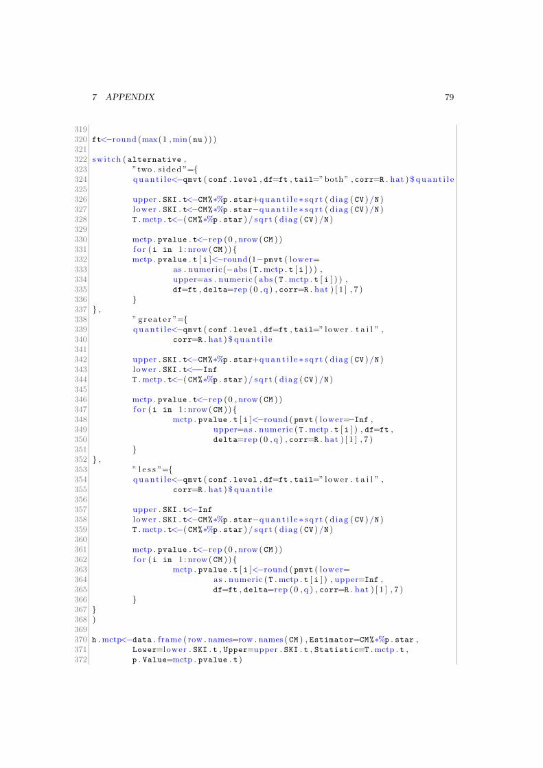
7 APPENDIX 79
319320 ft<−round (max(1 , min ( nu ) ) )321322 switch ( alternative ,323 ”two . s ided ”=324 q u a n t i l e<−qmvt ( conf . level , df=ft , tail=”both” , corr=R . hat ) $ q u a n t i l e325326 upper . SKI . t<−CM%∗%p . star+q u a n t i l e ∗ s q r t ( d iag ( CV ) /N )327 lower . SKI . t<−CM%∗%p . star−q u a n t i l e ∗ s q r t ( d iag ( CV ) /N )328 T . mctp . t<−( CM%∗%p . star ) / s q r t ( diag ( CV ) /N )329330 mctp . pvalue . t<−rep (0 , nrow ( CM ) )331 f o r (i in 1 : nrow ( CM ) )332 mctp . pvalue . t [ i ]<−round(1−pmvt ( lower=333 as . numeric(−abs (T . mctp . t [ i ] ) ) ,334 upper=as . numeric ( abs (T . mctp . t [ i ] ) ) ,335 df=ft , delta=rep (0 , q ) , corr=R . hat ) [ 1 ] , 7 )336 337 ,338 ” g r e a t e r ”=339 q u a n t i l e<−qmvt ( conf . level , df=ft , tail=” lower . t a i l ” ,340 corr=R . hat ) $ q u a n t i l e341342 upper . SKI . t<−CM%∗%p . star+q u a n t i l e ∗ s q r t ( d iag ( CV ) /N )343 lower . SKI . t<−−Inf344 T . mctp . t<−( CM%∗%p . star ) / s q r t ( diag ( CV ) /N )345346 mctp . pvalue . t<−rep (0 , nrow ( CM ) )347 f o r (i in 1 : nrow ( CM ) )348 mctp . pvalue . t [ i ]<−round ( pmvt ( lower=−Inf ,349 upper=as . numeric (T . mctp . t [ i ] ) , df=ft ,350 delta=rep (0 , q ) , corr=R . hat ) [ 1 ] , 7 )351 352 ,353 ” l e s s ”=354 q u a n t i l e<−qmvt ( conf . level , df=ft , tail=” lower . t a i l ” ,355 corr=R . hat ) $ q u a n t i l e356357 upper . SKI . t<−Inf358 lower . SKI . t<−CM%∗%p . star−q u a n t i l e ∗ s q r t ( d iag ( CV ) /N )359 T . mctp . t<−( CM%∗%p . star ) / s q r t ( diag ( CV ) /N )360361 mctp . pvalue . t<−rep (0 , nrow ( CM ) )362 f o r (i in 1 : nrow ( CM ) )363 mctp . pvalue . t [ i ]<−round ( pmvt ( lower=364 as . numeric (T . mctp . t [ i ] ) , upper=Inf ,365 df=ft , delta=rep (0 , q ) , corr=R . hat ) [ 1 ] , 7 )366 367 368 )369370 h . mctp<−data . frame ( row . names=row . names ( CM ) , Estimator=CM%∗%p . star ,371 Lower=lower . SKI . t , Upper=upper . SKI . t , Statistic=T . mctp . t ,372 p . Value=mctp . pvalue . t )

7 APPENDIX 80
373 374375 #−−−−−−−−−−−−−−−−−−−−−−−−−−−−−−−−−−−−−−−−−−−−−−−−−−−−−−−−−−−376 #Writing the ouput377378379 switch ( as . cha rac t e r ( pseudo ) ,380 ”TRUE”=est . method<−” Global pseudo ranks ” ,381 ”FALSE”=est . method<−” Global ranks ”382 )383 switch ( asy . method ,384 ”normal”=asy . t ex t<−” Mul t i va r i a t e normal approximation ” ,385 ”mult . t ”=asy . t ex t<−paste ( ” Mu l t i va r i a t e t−approximation with ” ,386 ft , ” df ” , sep=”” )387 )388 switch ( alternative ,389 ”two . s ided ”=alt . t ex t<−” Contrasts o f adj . r e l a t i v e treatment390 e f f e c t s are unequal 0” ,391 ” l e s s ”=alt . t ex t<−” Contrasts o f adj . r e l a t i v e treatment392 e f f e c t s are l e s s than 0” ,393 ” g r e a t e r ”=alt . t ex t<−” Contrasts o f adj . r e l a t i v e treatment394 e f f e c t s are g r e a t e r than 0”395 )396 group . info<−data . frame ( Group=levels ( factorx ) , Observations=n )397 rownames ( group . info )<−NULL398399 i f ( info==T )400 cat ( ”\n” , ”#−−−−−−−−−−−−−−−−Nonparametric Mult ip l e Comparisons401 f o r r e l a t i v e e f f e c t s −−−−−−−−−−−−−−−#” ,402 ”\n” , ”\n” , ”−” , ” Nul l Hypothes is : ” , alt . text ,403 ”\n” , ”−” , ” Est imation Method : ” , est . method ,404 ”\n” , ”−” , ”Type o f Contrast : ” , type , ”\n” , ”−” ,405 ” Conf idence Leve l : ” , conf . level ∗ 100 , ”%” , ”\n” ,406 ”−” , ”Method : ” , asy . text , ”\n” , ”\n” ,407 ”#−−−−−−−−−−−−−−−−−−−−−−−−−−−−−−−408 −−−−−−−−−−−−−−−−−−−−−−−−−−−−−−−−−−−−−−−−−−−−−−−−−−−−−−−#” ,409 ”\n” , ”\n” )410 p r in t ( group . info )411 cat ( ”\n” , ”Number o f c o v a r i a t e s used : ” )412 cat (d−1,” ( ” , sep=”” )413 cat ( colnames ( dat ) [ 3 : ( d+1)])414 cat ( ” ) ” , ”\n” , sep=”” )415 cat ( ”\n” ,416 ”#−−−−−−−−−−−−−−−−−−−−−−−−−−−−−−−417 −−−−−−−−−−−−−−−−−−−−−−−−−−−−−−−−−−−−−−−−−−−−−−−−−−−−−−−#” ,418 ”\n” , ”\n” )419 p r in t ( round (h . mctp , rounds ) )420 cat ( ”\n” ,421 ”#−−−−−−−−−−−−−−−−−−−−−−−−−−−−−−−422 −−−−−−−−−−−−−−−−−−−−−−−−−−−−−−−−−−−−−−−−−−−−−−−−−−−−−−−#” , )423 cat ( ”\n” , ”\n” )424 return ( l i s t ( Data . Info=group . info , Contrast=CM ,425 Analysis=h . mctp , gamma=gamma , formula=formula , data=data . sav ,426 Text . Output=l i s t ( null . hyp=alt . text ,

7 APPENDIX 81
427 est . method=est . method ,428 contr . type=type , conf . level=conf . level , method=asy . t ex t ) ) )429 e l s e 430 return ( l i s t ( Data . Info=group . info , Contrast=CM , Analysis=h . mctp ,431 gamma=gamma , formula=formula , data=data . sav ,432 Text . Output=l i s t ( null . hyp=alt . text ,433 est . method=est . method ,434 contr . type=type , conf . level=conf . level , method=asy . t ex t ) ) )435 436
REFERENCES 82
References
M. G. Akritas, S. F. Arnold, and E. Brunner. Nonparametric hypothesis and rank statisticsfor unbalanced factorial designs. Journal of the American Statistical Association, 92:258–265, 1997.
A. Bathke. Einfluß von Kovariablen in nichtparametrischen Modellen. Master’s Thesis,Georg-August-University Gottingen, 1998.
Arne Bathke and Edgar Brunner. Recent advances and trends in nonparametric statistics,chapter A Nonparametric Alternative to Analysis of Covariance, pages 109–120. Tba,2003.
G.E.P. Box. Some theorems on quadratic forms applied in the study of analysis of varianceproblems. I. Effect of inequality of variance in the one-way classification. Ann. Math.Stat., 25:290–302, 1954. ISSN 0003-4851. doi: 10.1214/aoms/1177728786.
F. Bretz, A. Genz, and L. A. Hothorn. On the numerical availability of multiple comparisonprocedures. Biometrical Journal, 43(5):645–656, 2001.
E. Brunner and U. Munzel. Nichtparametrische Datenanalyse, 2nd Ed. Springer-Verlag,Heidelberg, 2013.
E. Brunner and M. L. Puri. Nonparametric methods in factorial designs. Statistical Papers,42(1):1–52, 2001.
O. Christophliemk. Die Transformationsmethode im gemischten nichtparametrischen Modellmit Kovariablen. Master’s Thesis, Georg-August-University Gottingen, 2001.
H. Cramer and H. Wold. Some theorems on distribution functions. J. Lond. Math. Soc., 11:290–294, 1936. ISSN 0024-6107; 1469-7750/e. doi: 10.1112/jlms/s1-11.4.290.
S. Domhof. Nichtparametrische relative Effekte. Dissertation, Georg-August-UniversityGottingen, 2001.
C. W. Dunnett. A multiple comparison procedure for comparing several treatments with acontrol. Journal of the American Statistical Association, 50(272):1096–1121, 1955.
K. R. Gabriel. Simultaneous test procedures - some theory of multiple comparisons. Annalsof Mathematical Statistics, 40:224–250, 1969.
X. Gao, M. Alvo, J. Chen, and G. Li. Nonparametric multiple comparison procedures forunbalanced one-way factorial designs. Journal of Statistical Planning and Inference, 138(8):2574–2591, 2008.
A. Genz and F. Bretz. Computation of Multivariate Normal and t Probabilities. Springer-Verlag, New York, 2009.
B. V. Gnedenko. The Theory of Probability. Chelsea Publishing, New York, 2nd edition,1962.
Sture Holm. A simple sequentially rejective multiple test procedure. Scand. J. Stat., 6:65–70, 1979. ISSN 0303-6898; 1467-9469/e.
T. Hothorn, F. Bretz, and P. Westfall. Simultaneous inference in general parametric models.Biometrical Journal, 50(3):346–363, June 2008.

REFERENCES 83
B. Huitema. The analysis of covariance and alternatives. Wiley, New York, 1980.
R. Kirk. Experimental Design:Procedures for the Behavioral Sciences. Brooks/Cole, Cali-fornia, 1982.
F. Konietschke, L. A. Hothorn, and E. Brunner. Rank-based multiple test procedures andsimultaneous confidence intervals. Electronic Journal of Statistics, 6:1–8, 2012a.
F. Konietschke, O. Libiger, and L. Hothorn. Nonparametric evaluation of quantitative traitsin population-based association studies when the genetic model is unknown. PLoS ONE,7(2), February 2012b.
W.H. Kruskal and W.A. Wallis. Use of ranks in one-criterion variance analysis. J. Amer.Stat. Ass., 47:583–621, 1952.
F. Langer. Berucksichtigung von Kovariablen im nichtparametrischen gemischten Modell.Dissertation, Georg-August-University Gottingen, 1998.
M. Loeve. Probability Theory I. Springer Verlag, Berlin, 1977.
P. Levy. Calcul des probabilitees. Gauthiers-Villars, Paris, 1925.
H.B. Mann and D.R. Whitney. On a test of whether one of two random variables is stochas-tically larger then the other. Annals of Mathematical Statistics, 18(2):50–60, June 1947.
G.A. Miller and J.P. Chapman. Misunderstanding analysis of covariance. American Psy-chological Association, 110(1):40–48, 2001.
U. Munzel. Linear rank score statistics when ties are present. Statistics and ProbabilityLetters, 41:389–395, 1999.
Dana Quade. Rank analysis of covariance. Journal of the American Statistical Association,62:1187–1200, 1967.
F.H. Ruymgaart. A unified approach to the asymptotic distribution theory of certainmidrank statistics. Statistique non Parametrique Asymptotique, 118, J.P. Raoult. Lec-ture Notes on Mathematics, 821, 1980.
Lee A. Seber, G. Linear Regression Analysis. Wiley, New Jersey, 1977.
A. Siemer. Die Berucksichtigung von heterogen verteilten Kovariablen in einem nicht-parametrischen Modell. Master’s Thesis, Georg-August-University Gottingen, 1999.
Student. The probable error of a mean. Biometrika, 6(1), 1908.
Karthinathan Thangavelu and Edgar Brunner. Wilcoxon–Mann–Whitney test for stratifiedsamples and Efron’s paradox dice. J. Stat. Plann. Inference, 137(3):720–737, 2007. doi:10.1016/j.jspi.2006.06.005.
Neil H. Timm. Multivariate Analysis with Applications in Education and Psychology.Wadsworth Publishing Company, Inc., 1975. ISBN 0-8185-0096-4.
J. W. Tukey. The problem of multiple comparisons. Unpublished manuscript reprinted in:The Collected Works of John W. Tukey, 8:Chapman and Hall, June 1953.
A.W. Van der Vaart. Asymptotic statistics. Cambridge: Cambridge Univ. Press, 1998. ISBN0-521-49603-9/hbk. doi: 10.1017/CBO9780511802256.