three dials, and a few more: a practical introduction to
TRANSCRIPT

HAL Id: inria-00172407https://hal.inria.fr/inria-00172407
Submitted on 16 Sep 2007
HAL is a multi-disciplinary open accessarchive for the deposit and dissemination of sci-entific research documents, whether they are pub-lished or not. The documents may come fromteaching and research institutions in France orabroad, or from public or private research centers.
L’archive ouverte pluridisciplinaire HAL, estdestinée au dépôt et à la diffusion de documentsscientifiques de niveau recherche, publiés ou non,émanant des établissements d’enseignement et derecherche français ou étrangers, des laboratoirespublics ou privés.
Three dials, and a few more: a practical introduction toaccurate gnomonics
Denis Roegel
To cite this version:Denis Roegel. Three dials, and a few more: a practical introduction to accurate gnomonics. [TechnicalReport] 2007, pp.70. �inria-00172407�

Three dials, and a few more:
a practical introduction to accurate gnomonics
Denis Roegel∗
22 August 2007
Abstract
Sundials provide an interesting application for the METAPOST
graphical programming language, at the intersection of geometry, as-tronomy and time. This article considers three classical sundial draw-ings (normal hours, horizontal coordinates, and Babylonian/Italianhours), shows how to reproduce them accurately, and extends thestudy to related dials, such as those showing the declination, tempo-rary hours, or sidereal time. Analemmatic sundials, related to commonsundials, are also covered.
Contents
1 Introduction 2
2 Programming prerequisites 3
3 Common vertical and horizontal dials 7
3.1 The local sphere and its gnomonic projection . . . . . . . . . . 73.2 Construction with descriptive geometry . . . . . . . . . . . . . 103.3 Horizontal dials . . . . . . . . . . . . . . . . . . . . . . . . . . 19
4 Azimuth and elevation dials 20
4.1 Intersection of a cone with a vertical plane . . . . . . . . . . . 204.2 Construction of the dial . . . . . . . . . . . . . . . . . . . . . 26
∗LORIA & Nancy Université, [email protected].
1

5 Babylonian and Italian hour dials 30
5.1 Principles . . . . . . . . . . . . . . . . . . . . . . . . . . . . . 305.2 Construction of the dial . . . . . . . . . . . . . . . . . . . . . 32
6 Temporary hours sundials 48
6.1 Sunrise angles . . . . . . . . . . . . . . . . . . . . . . . . . . . 516.2 Horizontal projection of temporary hour lines . . . . . . . . . 516.3 Vertical projection of temporary hour lines . . . . . . . . . . . 52
7 Declination sundials 54
8 Sunrise and sunset 56
9 Sidereal time sundials 57
9.1 Drawing a vertical sidereal sundial . . . . . . . . . . . . . . . 589.2 Reading a sidereal sundial . . . . . . . . . . . . . . . . . . . . 62
10 Analemmatic sundials 64
11 Conclusion 67
1 Introduction
Sundials are a fascinating topic where astronomy, geometry and time meetnaturally. A great number of treatises have been written on sundials sincethe middle ages, the most important being perhaps Clavius’ book, publishedin 1581 [3].
Dials were often associated with clocks, and the original dials thatprompted this study were computed around 1572 by the mathematiciansConrad Dasypodius and David Wolkenstein as part of the then new Stras-bourg astronomical clock (1571–1574). They were painted by Tobias Stim-mer in 1572 and finally engraved in 1669 [8, p. 123–125, plates 44–46]. In1912, Paul Werkmeister published a first thorough analysis of these dials,and he provided reproductions of the dials drawn according to the principlesof descriptive geometry [14]. More recently, these dials were described byRohr [10] and Staub [13].
In the following sections, we show how Werkmeister’s drawings can beaccurately reproduced with METAPOST. Our drawings do not only providea new illustration of the use of METAPOST in descriptive geometry (followinga previous study on gears [9]), but they also open the way to more elaboratescientific applications, including in 3-D.
2

Although the initial focus of our work was the construction of three dialsusing descriptive geometry, we have actually departed from that goal, intwo ways. First, although we aimed at reproducing Werkmeister’s drawings,we did not strictly resort to the rules of descriptive geometry. There isindeed a difference between reproducing a descriptive geometry drawing, andreproducing it with descriptive geometry. Instead, we have actually used alltechniques at our hand, including analytical geometry, to produce the resultswe sought.
The second departure from the initial goal concerns the scope of ourstudy. Sundials are a vast topic, and although our focus was on three dials,we thought it was important to cover a number of dials that are related to thethree basic ones. We have however decided to restrict the study to verticaland horizontal dials, and to problems that are purely geometric. In thatframe, drawing a sundial is little more than finding the intersection of twosurfaces, one of which is rotating. Further investigations would consider nonplanar dials (with the general intersection problem being exactly the same),special dials such as bifilar sundials, or dials showing uniform angles, suchas those related to the mean time. The latter problems are more physicalin nature, since they are (partly) related to the uneven motion of the Eartharound the Sun. This explains why analemmas are not considered in thisstudy, although, oddly enough, analemmatic dials are briefly covered.
For the three basic drawings, an approach similar to the one used in aprevious study of descriptive geometry will be used [9]. We will detail theconstruction of the basic drawings, labelling the various points, but we willnot show how the lines are drawn, except in cases where this is not obvious.
2 Programming prerequisites
The next sections deal with different types of sundials, and the drawings areoften made with 3-D constructions that are projected. The main META-POST features, as well as those used for 3-D purposes, are briefly describedhere, and the other interesting features are described when they occur, butthe reader is still assumed to have some basic knowledge of METAPOST
programming, such as can be found in John Hobby’s manual [6] or in The
LATEX Graphics Companion [5].Most of the METAPOST code is rather self-explanatory, in particular
the manipulation of coordinates. An expression such as z5 (or z[5] whichis equivalent), for instance, represents a point in the plane, or a complexnumber (which we denote z5), and it can receive a value or be involved ina computation. Moreover, z5 is actually equal to the pair (x5,y5), so that
3

defining one amounts to defining the other, and vice-versa. Of course, sucha pair may at times be only incompletely defined.
A variable gets a value either through an assignment (:=), or through anequation (=). Equations are very convenient, because they make it possibleto express geometrical relations very naturally. The unknowns may thenappear on either side of the equation. Assignments are usually used whenwe want to give a new value to a variable that already has one.
A very convenient construction is whatever. Although not strictly nec-essary, its use is so practical that it is hard not to use it. It is usuallyused as follows: whatever[A,B] represents an undefined point between A
and B, like .5[A,B] represents the middle between A and B, and more gen-erally a[A,B] is an abreviation for A+a*(B-A). Now, if A, B, C and D arefour points such that AB is not parallel to CD, then, provided the intersec-tion does not result in an overflow, it can be obtained by the mere equationwhatever[A,B]=whatever[C,D]. And in this equation, we stress that thetwo occurrences of whatever do represent different and unnamed variables.whatever is used in this study in several places.
Variables have types, and a number of basic types are available. Thoseof most interest to us are the types numeric (a numerical value, float orinteger), pair (a pair of numerics) and path (a curve).
Curves in the plane are actually Bézier curves, and they are excellentapproximations to the curves of interest to us, provided we use the rightcontrol points. METAPOST can build a Bézier curve going through a list ofpoints, and although this curve is usually not unique, METAPOST choosesthe control points in a way that tries to be best. It is of course possible tohave METAPOST construct a Bézier curve with given control points, but thisis a feature seldom used. So, if we want to build a path p going through z3,z7 and z1, we merely write p=z3..z7..z1.
Arrays of basic types are often used, as sundials are inherentely repeti-tive. The same graphical constructions appear with a number of variants,for instant different declinations, different hour angles, etc.
One noteworthy feature is METAPOST’s ability to build a path as itunrolls a loop. This may seem strange at first, but it is very convenient. So,instead of writing p=z1..z2..z3..z4..z5, for instance, we can write p=z1
for i=2 upto 5: ..z[i] endfor;, which is exactly the same, but moreflexible. We use this construction several times, but, when doing so, we oftenneed to do some caretaking from one value of the loop to the next, and thiscaretaking would disrupt the path construction. So, in order to circumventthis problem, we use a special macro hide which executes its parameters,but has no side-effects in a loop constructing a path. An example showingthe construction of a path, and at the same time the recording of the sums
4

of its x-components, is:
p=z1 for i=2 upto 5: hide(sx:=sx+x[i];) ..z[i] endfor;
Paths are of course used to find intersections, and operations such asrotations or scalings are applied to points or paths.
Eventually, components of a construction are drawn with draw. Thismacro can be used with paths, or mere points, and the pen used for drawingcan be changed. Lines can also be dashed and colored. However, in thisstudy we do not go into the details of drawing, and concentrate primarily onthe constructions. Once the points and paths are defined, drawing is usuallystraightforward.
For the 3-D approach, we manipulate vectors which are numerical triplets.To that effect, we use a synonym of the color type, and we define Xp, Ypand Zp to access the components of a vector:
let vector=color;
let Xp=redpart;
let Yp=greenpart;
let Zp=bluepart;
A few basic vector constants are defined to make some macros friendlier:
vector vo,vi,vj,vk;
vo=(0,0,0);
vi=(1,0,0);
vj=(0,1,0);
vk=(0,0,1);
The coordinate system we use is shown in figure 1: for a vertical sundial,−→vi is perpendicular to the wall, −→vj is parallel to it, and −→vk is vertical, sothat (−→vi ,
−→vj ,−→vk) is a right-handed orthonormal system. The origin of the
coordinates is the tip of the gnomon, except when stated otherwise.Once vectors are available, we can define a number of useful operations
such as the dot product and the vector product:
def dotprod(expr Va,Vb)=
(Xp(Va)*Xp(Vb)+Yp(Va)*Yp(Vb)+Zp(Va)*Zp(Vb))
enddef;
def vecprod(expr Va,Vb)=
(Yp(Va)*Zp(Vb)-Zp(Va)*Yp(Vb),
Zp(Va)*Xp(Vb)-Xp(Va)*Zp(Vb),
Xp(Va)*Yp(Vb)-Yp(Va)*Xp(Vb))
enddef;
5

(−d, 0, 0)z
yx
wall
O
Figure 1: Reference directions. d is the distance between the tip O of thegnomon and the wall.
In order to compute ‖~v‖, we do not use√~v · ~v, because that could lead
to overflows. Instead, we first compute an intermediate vector where theabsolute value of the greatest component is 1. So, we introduce maxv whichreturns the greatest of the absolute values of the components, and this is usedin the macros norm (which returns the norm), and normed (which returns anormed vector):
def maxv(expr V)=
max(abs(Xp(V)),abs(Yp(V)),abs(Zp(V)))
enddef;
def norm(expr V)=
(maxv(V)*sqrt(dotprod(V/maxv(V),V/maxv(V))))
enddef;
def normed(expr V)=
(V/norm(V))
enddef;
Finally, it is also useful to have a means to rotate a given vector−→Va by
a certain angle a around another vector−→Vb , and this is achieved with the
following macro:
vardef rotatearound(expr Va,Vb,a)=
save v;
vector v[];
v0=normed(Vb);
v1=dotprod(Va,v0)*v0; % Va’s part parallel to Vb
6

v2=Va-v1; % Va’s part orthogonal to Vb
v3=vecprod(v0,v2);
v4=v2*cosd(a)+v3*sind(a)+v1;
v4
enddef;
3 Common vertical and horizontal dials
The most common type of dial shows the “hour angle” of the Sun (or merelythe “solar time”) on a vertical plane. Such a dial is depicted at the top offigure 5. The hour angle is the angle between a plane going through theSun and the polar axis on one side, and the meridian plane on the otherside, counted positively towards the West (hence increasing with time) andmeasured in hours, such that 15 degrees equal one hour. Since the hour angleis proportional to time (ignoring small changes such as the slowing down ofthe Earth’s rotation), hours are well defined: the time between noon and1 p.m. is the same as between 1 p.m and 2 p.m., and so on. We will seelater that this is not true for all dials, or, in other words, there are differentnotions of hours where the length of an hour is not constant during the day orduring the year, or when changing locations. In this section, however, thereare exactly 24 hours of the same duration in one day. Such hours are alsocalled “equinoctial hours,” because they can be obtained by taking a twelfthof the length of the day or the night at the equinoxes.
3.1 The local sphere and its gnomonic projection
Figure 2 shows a sundial on a vertical wall, with a style parallel to the axisof the world. The “style” is the mathematical line which is the source of theshadow, and we will sometimes also use “gnomon” for the same meaning.The hour lines are shown from 5 a.m. (true solar time) to 4 p.m.
Throughout this study, the style is assumed to have no thickness. Amore elaborate computation should of course take into account the physicalcharacteristics of the style, as well as the fact that the Sun is not a point,and that solar rays are deviated by refraction. We ignore all these factorshere.
Figure 4 shows the same dial, but makes the wall apparent as well as asphere on which the motion of the Sun is visible.
The sphere is a representation of a local equatorial sphere on which anumber of lines are shown: the horizontal plane H (parallel to the horizon),the equatorial plane Eq (parallel to the equator), the meridian plane M, andthe two tropical planes, positionned like the Cancer (_) and Capricorn (d)
7

A
5
6
7
8 9 10 11 12 1 2
3
4
X
X
A
Figure 2: A vertical dial, with a gnomon AX parallel to the world axis, andwith hour lines from 5 a.m. till 4 p.m. The left figure shows the dial from thefront, and the right figure shows it with a perspective. (The lengths of thelines are not the same in both drawings.) The other line leaving X in theright-hand drawing is an horizontal fixation of the style.
circles, at angles of ±23◦26′ with the equator. The angle between the horizonand the North pole is exactly the latitude ϕ (figure 3).
The Sun rises East and sets West, but always remains between the twotropics. We can assume that on a given day the angular distance between theSun and the equator, namely the declination, is constant. As a consequence,the Sun seems to travel along a parallel to the equator.
If the meridian plane is rotated by multiples of 15◦, it cuts the sphere atlines which are the hour lines, shown in figure 4. When the Sun goes throughthe meridian, it is noon solar time. The hour arc right East of the meridianis reached at 11 a.m., and the arc West of the meridian is reached at 1 p.m.,and so on. These arcs are therefore like the meridians on a terrestrial globe.
This sphere also explains the principles of equatorial sundials. These dialsare usually made of a wide ring along the equator, but only on half of itscircumference, in the direction opposite to the Sun. The axis of the Earth ismaterialized in the form of an arbor, so that the shadow of that arbor reachesthe wide ring. The plane containing the Sun and the arbor corresponds tothe hour line and the ring is marked accordingly with parts of great circlesevery 15◦, exactly the way it is done in figure 4.
Figure 4 also shows how the 10 a.m. line on the wall can be constructed. Aline is drawn from the 10 a.m. Summer point (on the Cancer tropic) throughthe tip of the style, and hits the wall at a point which is then connected to the
8

horizon
Pn
Ps
Eq
_
d
ϕϕ′ ε
ε
x
Figure 3: Position of the polar axis and the tropics. x is the distance betweenthe projection of the center of the Cancer tropic and the center of the equator.
10
Eq
_
d
M Pn
Ps
H
S
C9
10
C
Figure 4: The same vertical sundial, with a local sphere centered on the endof the style. The smaller circle C9 parallel to the meridian shows how theequatorial points can be obtained from evenly-spaced points on the horizon.The righthand picture is an excerpt of the left one showing the projection ofthe 10 a.m. Cancer point. The projection is indicated by a small circle.
9

Figure 5: The three sundials at the South gable of the Strasbourg cathe-dral [2].
intersection of the polar axis with the wall. Since the hour lines of the sphere— the meridians — are generated by the rotation of the meridian plane, andsince the style is parallel to the polar axis, it follows that all points on a samemeridian project on a same line going through the intersection between thestyle and the wall.
3.2 Construction with descriptive geometry
As an example, we consider a graphical construction of a dial drawn for theStrasbourg cathedral. This dial is located on the South wall, but it is notexactly oriented towards the South. In sundial parlance, the dial is referredas a declining one.
The original dial (figure 5, top) has a peculiarity, in that the mark for3 p.m. has no line, and is not engraved in the stone like the other marks,although it was initially the case, according to ancient etchings. Rohr gave a
10

very simple interpretation of that oddity, namely that the dial was certainlyengraved in the Summer of 1669 and an error was made [10, p. 111–112].Indeed, since the Sun cannot reach the 3 p.m. mark during that period of theyear, because of the wall declination, only the marks until 2 p.m. must havebeen engraved. The last one, for 3 p.m., was probably added, with a differentstyle, and no line, in 1872 after it was noticed that there could be a shadowat 3 p.m. In principle, the 4 p.m. mark should also appear, because at theWinter solstice the Sun sets slightly after 4 p.m., and South of the wall.
Such a dial can be constructed with descriptive geometry methods andthis was done by Werkmeister [14] (figure 6). Here, we merely reproduce theresult of the descriptive geometry approach, that is, every line of the originalconstruction is reproduced, but sometimes we may resort to analytical ge-ometry to find certain coordinates. This, of course, could be avoided, but wedecided to present the construction as a mix of different techniques. As anexercise, the reader may rewrite our code in a purely descriptive geometryway. This could be done by defining macros for the various ways rulers andcompasses are used in the pure construction.
Figure 7 shows the result of our construction. The upper part of thedrawing is the vertical projection, whereas the lower part is the horizontalprojection. The horizontal line dividing the two parts is the “ground line.”
The upper part therefore shows the wall, and A is the foot of the gnomon.The gnomon is parallel to the polar axis and appears as the inclined segmentb′A.
On the horizontal projection, the gnomon is the segment Ba and theground line is the projection of the wall. (Ba) is parallel to the meridianline and α is the angle between the wall and East, the so called gnomonicdeclination. This angle and the latitude ϕ are defined as follows:
numeric alpha,phi;
alpha=29+40/60; % angle between the wall and the East
phi=48+35/60; % latitude
These are the values for the Strasbourg cathedral, and they could of coursebe changed. Our purpose, however, is to reproduce drawings that were madefor these particular circumstances, and therefore we will only consider slightchanges to these values. We will also see later that the more elaborate thedrawings, the more sensitive they become to the parameters. Certain curves,for instance, may intersect only in certain cases, and handling properly allthe different cases is a challenge, especially if one wants to automate thepositioning of labels in drawings with ever-changing angles.
We now define a number of points to which lines will be attached. Someof the points are chosen at arbitrary locations, others correspond to certain
11

Figure 6: The original drawing by Werkmeister for the upper dial of theSouth gable [14]. The new drawing is shown in figure 7.
12

A
A′
A
5
6
7
8 9 10 11 121 2
3
4
a
B
α
A′
b′
90◦
ϕ
5
6
7
89
1011
12
1
2
3
4
Figure 7: The construction of the solar time dial with descriptive geometry.See the original drawing in figure 6. Our construction adds the lines for 3 p.m.and 4 p.m. The latter is a possible case overseen in the original construction.
13

A
A′
A
5
6
7
8 9 10 11 121 2
3
4
a
B
α
A′
b′
90◦
ϕ
5
6
7
89
1011
12
1
2
3
4
11 10
2
6
0
3
4
5
7
1
A13
A12
A11 A10
B12
B11
p2
p3
p1131
132
133
134 130 144
155
165
55
65
75
Figure 8: Details of the construction of the solar time dial.
14

geometrical properties. The whole drawing (upper and lower parts) is con-sidered as one drawing in the plane, with 2-dimensional coordinates. We takethe origin at the foot of the gnomon in the horizontal projection. This is thepoint labelled a.
z0=origin; % horizontal projection of gnomon foot
The following variables will be useful later. They show the definition ofthe arrays A, B and p. In METAPOST, arrays are not given a size, and theindexes can have any numeric value, including negative and non integer:
numeric sr,t;
pair A[],B[];
path p[];
Besides α and ϕ, there is a third important parameter, namely the lengthof the gnomon. Although it does not affect the general appearance of thedrawing, it affects its dimensions. However, instead of the length of thegnomon, we actually use its horizontal projection lh, and we express it as amultiple of some predefined unit u:
numeric lh;
lh=5u; % length of the horizontal projection of the gnomon
We can now set other points, and we refer to figure 8 which gives thedetails of all the points: z1 is the tip of the gnomon, z2 the intersection ofthe East-West line going through B with the wall, etc.:
z1-z0=lh*dir(-90-alpha); % z1=gnomon tip (B)
z2=z1+whatever*dir(180-alpha)=z0+whatever*left;
z10-z0=7u*right;z0-z11=12u*right; % ground line
Right now, the foot A of the gnomon in the vertical projection has notyet been drawn. We know that A is somewhere on the vertical line goingthrough b, but we do not know where. The exact position of A depends on α,ϕ and lh. In fact, since the height of the North pole is equal to the latitude,we have lh = l cosϕ, where l is the length of the gnomon. If we have theangle ϕ, the length l can easily be constructed as it is the length of segmentBA′:
z3=z1+whatever*((z0-z1) rotated -phi)
=z0+whatever*((z0-z1) rotated -90); % z3=A’
At the same time, aA′ is equal to the distance aA because the wall isvertical. We can now construct A (point z4):
15

z4-z0=arclength(z0--z3)*up; % z4=gnomon foot
The arc showing how A is obtained from A′ can be drawn using a circlep1 defined as follows, only the part (0, t) of this circle being drawn later:
p1=fullcircle rotated angle(z3-z0)
scaled 2arclength(z0--z4) shifted z0;
t=xpart(p1 intersectiontimes (z0--(z4+u*up))); % used for the arc A’-> A
Next, we consider the equator as it appears in figure 4, and we project itonto the horizontal plane. For that purpose, we must choose a radius sr forthe local sphere:
sr=4.5u; % the exact value is not relevant
z5 is defined towards East:
z5-z1=1.2sr*unitvector(z1-z2); % z5 towards East
and slightly more than half of the projection of the local sphere is defined asp2:
p2=subpath(0,4.5) of fullcircle scaled 2sr rotated (180-alpha) shifted z1;
We define Ai (i = 0, ..., 23) to be equidistant points on the circle withA0 being towards North. We have therefore Ai − z1 = sre
j(π
2−α−i π
12), where
j is the complex number such that j2 = −1. In degrees, and using the factthat z1 − z2 is directed East (hence towards A6), we can easily express thedifference Ai − z1 as follows for i = 5 until 16:
for i=5 upto 16:
A[i]-z1=sr*unitvector(z1-z2) rotated (-(i-6)*15);
endfor;
The closest mathematical expression for the previous equation would beAi − z1 = sre
j arg(z1−z2)e−j(i−6) π
12 .Now, the vertical projection b′ of the tip of the gnomon is easily defined
using B and a’s coordinates:
z6=(x1,y0);
Another dashed line is defined 90 degrees South of A′:
z7-z1=(z3-z1) scaled .8 rotated -90;
16

In order to draw the horizontal projection of the equator, we use a macroparalleltransform defined as follows:
def paralleltransform(expr angleA,d,phi,angleB)=
rotated angleA scaled cosd(d) yscaled cosd(90-phi) rotated angleB
enddef;
Such a transformation appears several times throughout this work, and itis convenient to abreviate it. In the present case, the projected equator is anellipse whose semi-major axis is sr and whose semi-minor axis is sr cos(90−ϕ),and this is exactly what paralleltransform does here, besides rotating theellipse. The second parameter of the macro is not used here, and will onlybe used when projecting smaller circles such as tropics. And like p2, p3 isactually defined as slightly more than half of the ellipse, and it is shifted tobe centered in B (z1). And finally, the ellipse is actually rotated by 180◦−α
so that its origin lies West.
p3=subpath(0,4.5)
of fullcircle scaled 2sr
paralleltransform(0,0,phi,180-alpha)
shifted z1;
The equator is also subdivided and the way this is done is that we considerthe Ai divisions (the first rotation in paralleltransform produces Ai), andthese divisions are scaled along the minor axis of the ellipse; yielding the Bi
divisions. These divisions correspond to the hour angles of the Sun:
for i=5 upto 16:
B[i]-z1=(sr*right) paralleltransform(-(i-6)*15,0,phi,angle(z1-z2));
endfor;
Like above, the previous expression actually corresponds to the followingequation Bi−z1 = (ℜ
(
sre−j(i−6) π
12
)
,ℑ(
sre−j(i−6) π
12
)
sinϕ)ej arg(z1−z2) and theconciseness of the METAPOST code is obvious.
Finally, each of these divisions is used to construct the projection on thevertical dial. This is valid because the whole circle going through the polesand through a certain hour mark Bi is projected on a straight line goingthrough A. We can therefore satisfy ourselves with the projection of the tipof the gnomon when the Sun is located in Bi.
Now, we loop i from 5 to 16, that is from 5 a.m. until 4 p.m. solar time:
for i=5 upto 16:
17

A number of points are defined. z10i, for instance, is the horizontal pro-jection of the shadow when the Sun is at Bi. Figure 8 shows the constructionof z130, for 1 p.m.
z[10i]=whatever[B[i],z1]=whatever[z6,z0];
Next, we compute how much Bi is above the horizontal plane goingthrough B. It is immediate that this is sr sin(90 − ϕ) cos(15(i − 12)), an-gles being expressed in degrees. Hence the vertical projection z10i+2 (forinstance z132) and the intermediate point z10i+1 (for instance z131):
z[10i+1]=(xpart(B[i]),y0);
z[10i+2]-z[10i+1]=sind(90-phi)*cosd(15*(i-12))*sr*up;
Finding the points z10i+3 (for instance z133) is immediate, as the line(z10i+2z10i+3) is the vertical projection of the solar ray. When i 6= 16, thispoint is the shadow of the tip of the gnomon at the equinoxes for the hour i(with the convention that i = 13 corresponds to 1 p.m., and so on), providedwe consider z10i+3 as part of the vertical projection, and provided the Suncasts a shadow at that time. This, however, is not true for i = 16, that is,for 4 p.m. Nevertheless, the construction below will provide the right shadowline for i = 16, for a reason that will be explained shortly. First, the definitionof z10i+3:
z[10i+3]=whatever[z[10i+2],z6]=whatever[z[10i],z[10i]+down];
For 8 a.m. until 2 p.m. we stop the dial lines at the ground line, and thepoints z10i+4 (for instance z134) are used for that purpose:
z[10i+4]=whatever[z4,z[10i+3]]=whatever[z6,z0];
The lines for 3 and 4 p.m., however, stop shorter:
if i>14: % 3 and 4 p.m.
z[10i+5]=whatever[z[10*14+4],z[10*14+4]+up]=whatever[z4,z[10*i+4]];
fi;
Now, we close the loop:
endfor;
Finally, we define the ends for the 5, 6 and 7 a.m. lines, all ending at thevertical of z84:
18

for i=5 upto 7:
z[10i+5]=whatever[z[10*8+4],z[10*8+4]+up]=whatever[z4,z[10*i+4]];
endfor;
When i = 16, that is for 4 p.m., there is actually no shadow at theequinoxes, but what the previous computation produces is the imaginaryshadow for the symmetric hour 4 a.m. This shadow is imaginary, becausethe Sun has not yet risen at 4 a.m. at the equinoxes, but if the Earth weretransparent, there would be a shadow. This shadow is given by the linez4z163, somewhat unintentionally, but still correctly. z164, then, produces theshadow for 4 p.m., because the two shadow lines (for 4 a.m.near the equinoxesand for 4 p.m. near the Winter solstice) are exactly opposite lines.
We have now drawn all the shadow lines, based on the positions of theSun at the equinoxes and of the shadow it casts on the tip of the gnomon.However, the shadow of the tip of the gnomon can be well beyond the wall,in which case only an initial part of the style serves as an index.
More generally, we can also use such a construction to check whether theSun projects a shadow at a certain hour and time of the year. For instance,on figure 25 which shows the normal hour lines in an horizontal projection(not shown in figure 7), one can readily see that the Sun’s shadow shouldbe visible at 3 p.m. at least between September and March, but not at theSummer solstice. We can also observe that the shadow is possible at 4 p.m.(provided nothing obstructs the Sun, of course), but only near the Wintersolstice. At the equinoxes, however, the Sun is already too much North to beable to cast a shadow on the wall. And the same figure 25 also shows thatthe 4 a.m. line is not reached, but could still be useful, since the Sun rises atthe earliest slightly after 4 a.m.
The previous construction is of course somewhat tied to the values of αand ϕ, and different values would entail different constraints for the linesto be drawn. It is up to the reader to adapt the previous definitions, or togeneralize them appropriately.
3.3 Horizontal dials
These dials are constructed in the same way as the vertical dials, but byinverting the two projection planes. In fact, it is easy to see that an horizontaldial for latitude ϕ corresponds to a non-declining vertical dial for a latitude90 − ϕ, but with symmetric hours marks. More precisely, if one wants toproduce an horizontal dial, it suffices to draw a non-declining vertical dialfor the colatitude, and replace the marks h by 24−h: 6 a.m. becomes 6 p.m.,7 a.m. becomes 5 p.m., etc., 11 a.m.becomes 1 p.m., the noon mark remainsthe same, 1 p.m. becomes 11 a.m., and so on.
19

Pn
Sun
M(x, y, z)
Eq
O
δψ
ψ
Figure 9: The cone of angle ψ.
Of course, both horizontal and vertical dials are only special cases of dialson more general surfaces. On planes the hour curves are lines, but on othersurfaces they do appear differently, since the hour curves are obtained by theintersection of planes with the projection surfaces.
4 Azimuth and elevation dials
Azimuth and elevation dials are sundials locating the Sun with respect toits horizontal direction (Azimuth, 0◦ being South, 90◦ West, etc.) as well asvertical direction (elevation, or height, counted from 0 till 90◦), or, in otherwords, with respect to its horizontal coordinates. An example of such a dialwhere the gnomon is horizontal is given at the bottom left corner of figure 5.
These dials contain two sets of lines, one for the azimuth values and onefor the elevation values. The first lines are vertical lines which are obtainedin a very straightforward way. The second lines are hyperbolas obtained asthe intersections of cones with the surface of the wall. We will first considerthese intersections, before poring over the code.
4.1 Intersection of a cone with a vertical plane
We consider the horizontal plane (Oxy), with (Ox) opposite the verticalplane and (Oy) parallel to it. The vertical projection plane is given by theequation x = −d (see figure 1).
4.1.1 Constant declination shadow lines
Let us now consider the constant declination shadow lines. Because of therotation of the Earth, the apparent direction of the Sun describes a conecentered on O = (0, 0, 0), with its axis the polar axis (OPn), and with a coneangle ψ = 90 − δ, where δ is the declination of the Sun (figure 9).
We assume the polar axis given by a point A such that−→OA is a unit vector
directed towards the celestial North pole Pn. We set−→OA = (xA, yA, zA) and
20

we have:
xA = − cosϕ cosα (1)
yA = cosϕ sinα (2)
zA = sinϕ (3)
(Section 9 shows how this vector can easily be computed using a combi-nation of rotations.)
Now, M(x, y, z) belongs to the intersection of the cone and the verticalplane if
−→OA · −−→OM
‖−−→OM‖ · ‖−→OA‖= cosψ (4)
x = −d (5)
It comes:
xxA + yyA + zzA = cosψ√
x2 + y2 + z2 (6)
Squaring each side leads to:
y2y2A + d2x2
A + z2z2A = cos2 ψ(d2 + y2 + z2) + 2yyAxAd+ 2zzAxAd− 2yzyAzA
(7)
This is a second degree equation in z:
z2(z2A − cos2 ψ) + z(2yyAzA − 2zAxAd)
+ y2yA + d2x2A − cos2 ψ(d2 + y2) − 2yyAxAd = 0 (8)
We set:
cA = z2A − cos2 ψ (9)
cB = 2zA(yyA − xAd) (10)
cC = y2y2A + d2x2
A − cos2 ψ(d2 + y2) − 2xAyAdy (11)
and the equation is now
21

cAz2 + cBz + cC = 0 (12)
z can now easily be expressed as a function of y, as shown later in themacro def_declination_line (section 4.2).
In the special case where δ = 0, that is when ψ = 90◦, eq. (6) leads toyyA + zzA = dxA which is the equation of a line.
It can be rewritten:
z =dxA − yyA
zA
= − sinα
tanϕy − d
cosα
tanϕ(13)
If z = 0, we have y sinα = −d cosα, hence y = − d
tanα. The intersection
of that line with the horizon is therefore:
(
− d
tanα, 0
)
.
If y = 0, then z = −d cosα
tanϕ, and we have the point
(
0,−d cosα
tanϕ
)
4.1.2 Constant height shadow lines
The formulas for constant height shadow lines are special cases of the previousformulas, because at the poles declination lines are height lines. So, takingOA = (0, 0, 1), that is x1 = yA = 0 and zA = 1, eq. (8) becomes:
z2(1 − cos2 ψ) − cos2 ψ(d2 + y2) = 0 (14)
that is
z2 sin2 ψ = cos2 ψ(d2 + y2) (15)
and
z = ±√
d2 + y2
tanψ= ± tanh ·
√
d2 + y2 (16)
where h = 90 − ψ.When h > 0, we have actually simply
z = − tanh ·√
d2 + y2 (17)
the other solution being for negative values of the elevation.
22

Figure 10: The original drawing by Werkmeister for the lower left dial of theSouth gable [14]. The new drawing is shown in figure 11.
23
270
270
280
280
290
290
300
300
310
310
320
320
330
340
350
350
0
0
10
10
20
20
30
30
40
50
0◦ 0◦
10◦ 10◦
20◦20◦
30◦30◦
40◦
40◦
50◦
50◦
a′
60◦ 60◦70◦ 70◦
α
270
280
290
300
310
320
330
34035
0
0
10
20
30
40
50
a
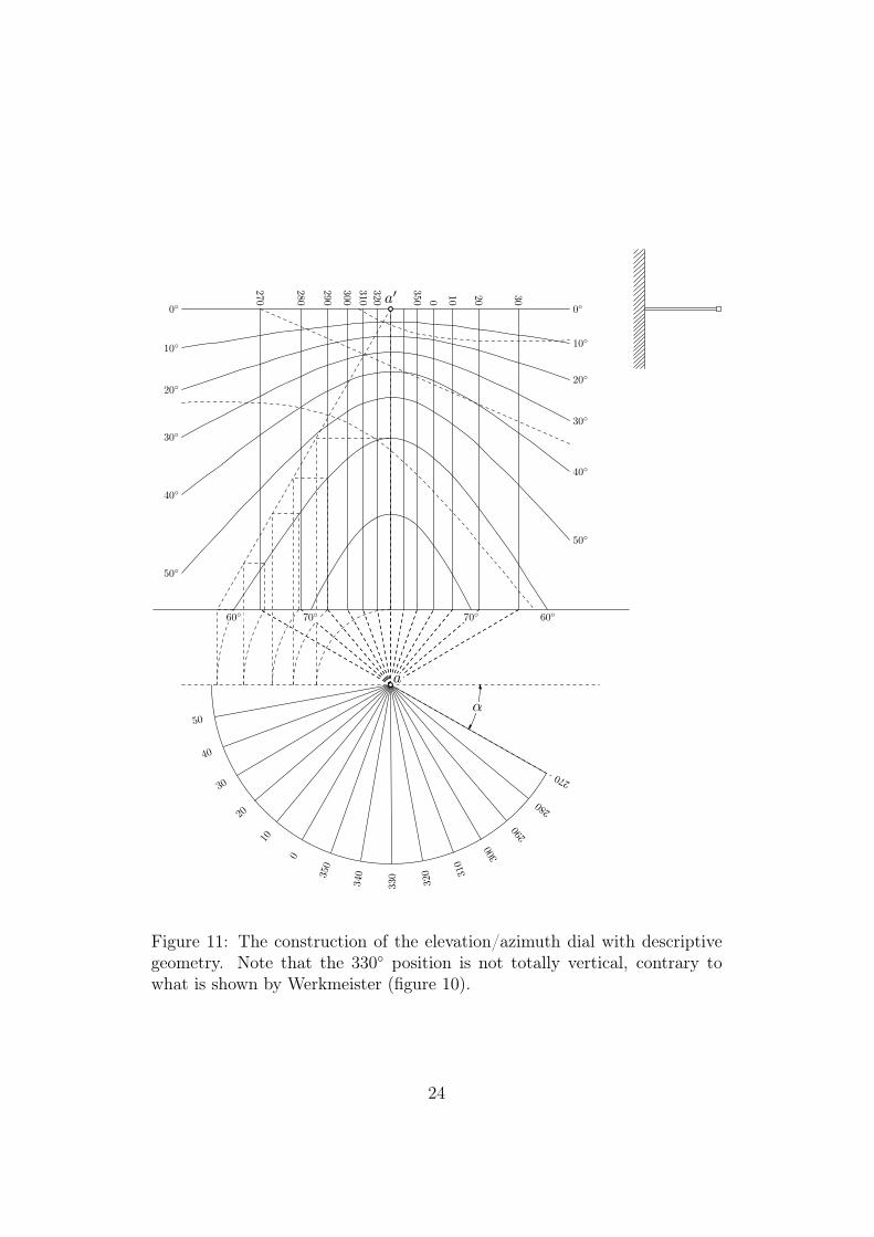
Figure 11: The construction of the elevation/azimuth dial with descriptivegeometry. Note that the 330◦ position is not totally vertical, contrary towhat is shown by Werkmeister (figure 10).
24

270
270
280
280
290
290
300
300
310
310
320
320
330
340
350
350
0
0
10
10
20
20
30
30
40
50
0◦ 0◦
10◦ 10◦
20◦20◦
30◦30◦
40◦
40◦
50◦
50◦
a′
60◦ 60◦70◦ 70◦
α
270
280
290
300
310
320
330
34035
0
0
10
20
30
40
50
a
15 16
18
2
19
20
170
11 12
13 14
1
3
A41
A36
A28
A27
C39
B39
p8
p9p1
p2
p3
p4
p5
p6
p0
Figure 12: Detail of the construction of the elevation/azimuth dial.
25

4.2 Construction of the dial
Figure 11 shows our reproduction of the original drawing by Werkmeister(figure 10). In order to make the construction easier to understand, we haveincluded figure 12 showing the location of the various points.
Like in the first case, the construction starts with definitions of the valuesof the declining angle (or declination) α and the latitude ϕ:
numeric alpha,phi;
alpha=29+40/60;
phi=48+35/60;
We define several variables that will be useful later:
numeric lh,lv,sr,t,nsteps;
numeric xA,yA,zA,psi,cA,cB,cC;
pair A[],B[],C[],D[],E[];
path p[];
The azimuth of the Sun is shown on a circle whose radius is sr.
sr=6u; % circle radius in horizontal projection
This circle is centered at z1 and the foot of the horizontal gnomon is atz0. The gnomon is at right angle with the wall and its length is lh.
z0=origin; % horizontal projection of the foot of the gnomon
lh=2.5u; % length of the gnomon’s horizontal projection
z0-z1=lh*up; % z1=tip of the gnomon in horizontal projection
In the vertical projection, the gnomon a′ is set at a distance lv above theground line. This is of course an arbitrary distance.
lv=10.1u; % dial height
z2-z0=lv*up; % z2=tip of the gnomon in vertical projection
Next, we define the ground line (z11z12) and a line parallel to it and goingthrough the tip of the gnomon:
z0-z11=z12-z0=8u*right; % ground line
z1-z13=z14-z1=7u*right; % parallel to the wall
Point z3 marks the Eastern direction, declining by an angle α:
z3-z1=7u*dir(-alpha); % z3 towards East
26

The horizontal circle is p0, which is here rotated in order to have it starton the left side. (In METAPOST circles are paths, and have a beginning andan end.) t is a numerical value which will be used to show only the part of thecircle until the East. Drawing this part is achieved with draw subpath(0,t)
of p0.
p0=fullcircle rotated -180 scaled 2sr shifted z1;
t=xpart(p0 intersectiontimes (z1--(z1+2sr*dir(-alpha))));
Azimuth positions Ai for angles ranging 270◦ until 410◦ are drawn, every10 degrees. These points enable the construction of the projections. Whenthe Sun has a certain azimuth A, it is actually in a vertical plane, and thisplane projects as a vertical line on the dial. Bi is the projection of Ai on thewall, through the tip of the gnomon, in its horizontal projection. Ci is thevertical projection of Ai, in the horizontal gnomon plane. For instance (seefigure 12) A39 corresponds to an azimuth of 30◦, it is projected as B39 andC39.
for i=27 upto 41:
A[i]-z1=sr*dir(-90-alpha-i*10);
B[i]=whatever[z1,A[i]]=whatever[z0,z0+right];
C[i]=(xpart(B[i]),y2);
endfor;
The horizon is delimited by (z15z16) on the vertical projection:
% horizontal line going through the gnomon foot
z2-z15=7u*right;z16-z2=6u*right;
Next, we construct seven hyperbolas, for the heights 10◦, 20◦, . . . , 70◦.We already have the equation (17) for the hyperbola corresponding to heighth. In our case, this equation becomes
z − y2 = − tanh√
l2h + x2 (18)
or
z = y2 − tanh√
l2h + x2 (19)
In order to draw such a hyperbola, we have x vary between two limits, inour case between x15 and x16. We construct a smooth curve going through thehyperbola points of abscissa x15, x15 + 1
nsteps(x16−x15), x15 + 2
nsteps(x16−x15),
. . . , x16. Each hyperbola is therefore made of nsteps + 1 points.
27

Now,√
l2h + x2 is actually the distance between z1 and the point on theground line with abscissa x, that is, the point of coordinates (x, y0). InMETAPOST, the distance between two points A and B can be obtainedeasily by computing the length of the path A--B with arclength. So,given a point of abscissa (j/nsteps)[x15,x16], the value of
√
l2h + x2 isarclength(((j/nsteps)[x15,x16],y0)--z1). Combining all this and in-troducing the macro hyppoint, with the parameter X being
√
l2h + x2 and bbeing the elevation:
def hyppoint(expr x,X,b)=
(x,y2-X*tan(b))
enddef;
we obtain the following code:
nsteps=20;
for i=1 upto 7:
p[i]=hyppoint(x15,arclength((x15,y0)--z1),i*10)
for j=1 upto nsteps:
..hyppoint((j/nsteps)[x15,x16],
arclength(((j/nsteps)[x15,x16],y0)--z1),i*10)
endfor;
endfor;
We cut the elevation curves for 60◦ and 70◦ so that they don’t extendbelow the ground line. Interestingly, the following code works, and showsthat cutbefore and cutafter do not choose the same intersection:
p6:=p6 cutbefore (z11--z12) cutafter (z11--z12);
p7:=p7 cutbefore (z11--z12) cutafter (z11--z12);
The figure 11 also shows how the elevation curves can be obtained in ageometrical way. The construction is shown for the 60◦ hyperbola. Considerfor instance the hyperbola point at azimuth 290◦. The distance betweenthis point and the upper line (z15z16) is tan 60◦ × l, where l is the distancebetween a and the ground line point with the selected azimuth. This lengthl is transferred onto the line (z13z14) with a circular arc. Then a verticalline is drawn and reaches a line starting at a′ with a slope of 60◦. This is ofcourse also an asymptote to the 60◦ hyperbola. By construction, the pointwhere this inclined line is reached is exactly at a distance tan 60◦ × l fromthe upper line, and the hyperbola point is then immediately obtained as theintersection of two lines, one horizontal from the last intersection, and onevertical for the azimuth. We do not detail all these construction drawings,but merely define the asymptote:
28

% z17 is defined on the ground line as a point through
% which the left asymptote of the 60 degrees hyperbola goes:
z17=whatever[z11,z12]=z2+whatever*dir(-90-30);
We now only have to draw the projection of the equator and the twotropics. First, we have already seen (eq. (13)) that the projection of theequator is a straight line. Two points are readily obtained: z18 on the horizonline, and z19 at the vertical of the gnomon foot. The line is extended to athird point, z20, having abscissa x16:
z18=(-lh/tan(alpha),y2);
z19=(0,y2-lh*cosd(alpha)/tan(phi));
z20=whatever[z18,z19];x20=x16;
Finally, the two tropics, the Cancer and Capricorn parallels, are obtainedby tracing the two hyperbolas. (The name of the tropic is Capricorn, but thesign is Capricornus.) We use the macro def_declination_line that definestwo arrays dec_lineA and dec_lineB, given a pole distance ψ. These twoarrays correspond to the two sought hyperbolas, as these hyperbolas are theintersections of only one cone with the wall. The macro is therefore onlycalled once. It may however be called more than once if other declinationsare desired, for instance those for the entrances in Zodiac signs.
The parameters of this macro are the initial and final values of the ab-scissa, the unit vector VA directed towards the North pole (already seen insection 4.1.1), the distance lh, the cone angle ψ = 90 − 23◦26′ and zorigin,the point corresponding to the vertical projection of the tip of the gnomon.The rest of the code follows equations (9), (10) and (11), and then solves the2nd degree equation. Special care is taken to avoid overflows. The hyperbolasare plotted on 31 points and stored in the arrays given as parameters.
vardef def_declination_line(expr ybegin,yend)
(expr VA,lh,psi,zorigin)(text dec_lineA)(text dec_lineB)=
save xA,yA,zA,Y,cA,cB,cC,Delta;
numeric xA,yA,zA,Y,cA,cB,cC,Delta;
xA=Xp(VA);
yA=Yp(VA);
zA=Zp(VA);
for i=0 upto 30:
Y:=(i/30)[ybegin,yend]; % will vary
cA:=(zA*zA-cosd(psi)*cosd(psi))/100; % z^2 term
cB:=2zA*(-lh*xA+yA*Y)/100;
cC:=(Y/10)*(Y/10)*yA*yA+lh*lh*xA*xA/100
-cosd(psi)*cosd(psi)*((Y/10)*(Y/10)+lh*lh/100)
-2*yA*xA*lh*Y/100;
Delta:=cB*cB-4*cA*cC;
29

if Delta<0:Delta:=0;fi;
dec_lineA[i]:=(Y,ypart(zorigin)+(-cB-sqrt(Delta))/(2cA));
dec_lineB[i]:=(Y,ypart(zorigin)+(-cB+sqrt(Delta))/(2cA));
endfor;
enddef;
Calling the macro def_declination_line is then straightforward, andthe two arrays are D (Cancer) and E (Capricorn). (Vector VA is assumedgiven, but section 9 shows that it can easily be computed.)
% VA is a unit vector for the polar axis
VA=(-cosd(phi)*cosd(alpha),cosd(phi)*sind(alpha),sind(phi));
psi=90-(23+26/60);
def_declination_line(x15,x16)(VA,lh,psi,z2)(D)(E);
Finally, the two projections are obtained as follows, each curve beingappropriately cut:
% projection of Cancer tropic
p8=(D0 for i=1 upto 30:..D[i] endfor) cutafter (z11--z12);
% projection of Capricorn tropic
p9=(E0 for i=1 upto 30:..E[i] endfor) cutbefore (z15--z16);
5 Babylonian and Italian hour dials
5.1 Principles
Normal sundials show equinoctial hours starting at midnight. When the Sunculminates, these dials show 12 p.m.
A millenium ago, midnight, however, was not a clearly defined instant.There was no visible change at midnight, and there was no good reason tostart counting at an instant that was so hard to define. Instead, there are twoother instants which are much better candidates for serving as time origins,namely sunrise and sunset. These choices led to Babylonian (or Babylonic)and Italian (or Italic) hours: Babylonian hours are equinoctial hours countedfrom sunrise, whereas Italian hours are equinoctial hours counted from lastsunset.
As a consequence, the Babylonian hour is 0 at sunrise and the Italianhour is 0 at sunset.
Sundials can be made to show these two types of hours. The dial depictedat the lower right of figure 5 is of that kind.
In order to have a good understanding of the differences between “nor-mal” hours and Babylonian and Italian hours, it is useful to consider the
30

corresponding divisions or curves on the local sphere (figure 13). M is themeridian plane, H the horizon, Pn and Ps are the poles and Eq is the equato-rial plane. The hour angle lines are obtained by rotating the meridian planearound the polar axis by multiples of 15◦. They are shown from 6 a.m. until1 p.m. The figure shows immediately that the Sun rises earlier in Summer(Cancer tropic) than in Winter (Capricorn tropic). It also shows that whenthe Sun is on the equator, it rises at 6 a.m.
Babylonian hour lines B1, B2, etc. appear somewhat parallel to the hori-zon. These lines start on the Cancer tropic at points PB0 (on the horizon),PB1, PB2, . . . , PB23. Similarly they end on the Capricorn tropic at pointsPC 0 (on the horizon), PC 1, PC 2, . . . , PC 23. Obviously these curves aregreat circles and are obtained by rotating the horizon plane around the polaraxis by increments of 15◦.
Italian hour lines are constructed symmetrically, but starting at sunset.They are also great circles obtained by rotating the horizon plane around thepolar axis. Figure 13 shows the Italian hour curve I18, corresponding to 18hours after the last sunset.
These curves are then projected and their projections on a vertical surfaceare of course straight lines.
The construction of the lines for Babylonian and Italian hours is shownby various authors such as Rohr [11, p. 90], but we will confine ourselves toreproducing the drawing made by Werkmeister using descriptive geometry(figure 15). The horizontal and vertical projections of the local sphere areshown in figure 14. The horizontal gnomon is visible on the vertical wall onthe left.
As it was the case for the previous figures, it should be clear that the twoprojections in Werkmeister’s figures are of a different nature. The projectionon the horizontal surface is a mere parallel projection along vertical lines, butthe projection on the vertical surface is actually a central perspective, or agnomonic projection. The lines joining a point in the scene to its projectionalways go through the tip of the gnomon.
The two projections are shown simultaneously in figure 16. The verticalprojection (top) shows the two sets of lines, marked with numbers such as3 for Babylonian hours, and 17 for Italian hours. These hours can be usedto find the length of the day. Indeed, if the Babylonian hour is b and theItalian hour i, during the day the number of hours until the sunset is 24− i,and hence the day length is 24 − i + b; during the night, if we could havethe values of b and i, we would obtain the length of the night by computing24 − b + i. So, during the day, it would actually be more convenient to usethe number of hours until the next sunset. Then adding this number tothe Babylonian hour would give the length of the day. On figure 16, this
31

reasoning can be used to find that the two tropics correspond to about 8 and16 hours of daylight. If we had added declination curves (see section 7), wewould have been able to use them to find the length of the day as a functionof the season.
The horizontal plane (bottom) shows the projection of the equator, aswell as of the Cancer and Capricorn parallels. All Babylonian hour arcswhich are above the horizon are shown in plain lines and are each identifiedby three points: b0a0c0 for hour 0, b1a1c1 for hour 1, etc., where ai, bi and ciare the projections of Ai, Bi and Ci on the horizontal plane. The points ai
lie on the equator and a6 is on the meridian. The starts and ends of the arcsare marked with small unfilled circles.
Only one Italian arc is shown, namely b′18a′18c
′18 for the Italian hour 18.
All these arcs start and end at the filled circles, which in general do notcoincide with the unfilled ones. However, the Italian arc 18 coincides withthe Babylonian arc 6 exactly on the meridian and at the same time on theequator, because the Sun goes through the meridian at the equator (henceat the equinoxes) exactly six hours after sunrise, hence the coincidence withthe Babylonian hour 6, but there are then also exactly six hours until sunset,or 18 hours since last sunset, hence the coincidence with Italian hour 18.More generally, Babylonian hour n coincides with Italian hour n+ 12 at theequator.
On figure 16, the unfilled and filled circles are very close, but this is acoincidence. With a different latitude, these points are closer or further apart.The conditions for their coincidence are easy to compute (see section 5.2.1)and b10 coincides with b′18 (and all others at the same time) when the latitudeis arctan
(
12 tan ε
)
which is about 49.08◦. When this is true, the minimal andmaximal lengths of the days are exactly 8 and 16 hours. The sundials drawnby Werkmeister are made for Strasbourg, located at 48◦35′ N, which is veryclose to this value, hence the coincidence. Unfortunately, this is misleadingfor the understanding of Werkmeister’s drawing, since the casual reader isled to believe that an Italian hour line goes through b10 and c10, which is nottrue in general, and not even exactly the case in Strasbourg.
5.2 Construction of the dial
Figure 16 shows our reproduction of the original drawing by Werkmeister(figure 15). In order to make the construction easier to understand, we haveincluded figure 17 showing the location of the various points.
Like in the previous cases, the construction starts with definitions of thevalues of the declining angle (or declination) α and the latitude ϕ:
32

Eq
_
d
M Pn
Ps
H
S
7
6
B1
B2
B3
B4
I18
PB30
PC 30
PB2
PB1
PB0
PC 0
PC 1
PC 2
~I
~J
~K
Figure 13: The local sphere with Babylonian and Italian hours for ϕ = 48◦35′.Babylonian hours (counted from sunrise) correspond to the curves B0, B1, B2,etc. The corresponding tropic points in space are PB i and PC i. Italian hourcorrespond to the curves I0, I1, etc. The tropic points in space correspondingto Ii are PB24+(24−i) and PC 24+(24−i).
33

Figure 14: The projections of the local sphere on the two planes, with andwithout the sphere.
34

Figure 15: The original drawing by Werkmeister for the lower right dial ofthe South gable [14]. The new drawing is shown in figure 16.
35

11 1213
14
15
1617
18
19
20
12 3 4 5 6 7
8
p′
α
ϕ′
ε
ε
a0
a′
12
a1
a′
13a2
a6
a′
18
b0b′8
b1b′9
b2b′10
b10b′18
c0
c′16
c1
c′17
c2
c′18
p
West
East
South
Figure 16: The simultaneous projections on the two planes for ϕ = 48◦35′.See the original drawing in figure 15 (where filled and unfilled points areidentified). The underlined numbers, such as 3, correspond to Babylonianhours, hours counted from sunrise. On the horizontal projection (bottom),they correspond to unprimed points (for instance b2a2c2 for 2). The overlinednumbers, such as 17, correspond to Italian hours, hours counted from lastsunset. On the horizontal projection, they correspond to primed points (forinstance b′18a
′18c
′18 for 18).
36

11 1213
14
15
1617
18
19
20
12 3 4 5 6 7
8
p′
α
ϕ′
ε
ε
a0
a′
12
a1
a′
13a2
a6
a′
18
b0b′8
b1b′9
b2b′10
b10b′18
c0
c′16
c1
c′17
c2
c′18
p
11 12
13 14
Pd37
Pa−1
Qa
Qb
23 Pd35
Pd34
Pc0 Pc32
2
24
Pc27
Pc26
Pc25
Pc7Pc6
p8
Pa3
Pa8
25
Pe32
Pe31
Pe30 Pe29
Pe28
Pb38 Pb2
Pb37
Pb7
Pb8
p7
Pb31
Pb9
p0
15
16
1722
0
Px 3
p2 p3
p4
1
18
q4
q5
q100
C24
C8
C26
C6
C27
C3
C30
A0A4
A5
A8
A9
A10
A11
B3
B5B7
B31
B30
B29
19
20
21
Figure 17: Details of the simultaneous projections on the two planes forϕ = 48◦35′.
37

numeric alpha,phi;
alpha=29+40/60;
phi=48+35/60;
We then define a number of variables that will be useful later.
numeric phip,eps,lh,lv,sr;
path p[],q[];
pair H[],Px[],Pa[],Pb[],Pc[],Pd[],Pe[],A[],B[],C[],D[],Paa,Pab;
numeric nsteps;
numeric ca,sa,cancer_a,capricorn_a,ta,tb,tc,td;
numeric si;
pair Qa,Qb;
vector IA,JA,KA,MB,MC,I,J,K,M,PB[],PC[];
Next, we define the colatitude and the obliquity of the ecliptic:
phip=90-phi; % colatitude
eps=23+26/60; % obliquity of the ecliptic
Like for the first drawing, we consider the local sphere of radius sr andthis sphere is centered at z1 in the horizontal projection. z0 is located on theground line, above z1 and the length of the gnomon is lh.
sr=7u; % radius of the local sphere
z0=origin; % horizontal projection of the basis of the gnomon
lh=2.5u; % gnomon length
z0-z1=lh*up; % z1=gnomon tip in h. proj.
The vertical projection z2 of the gnomon is located at a distance lv abovez0. This is an arbitrary distance chosen to reproduce faithfully the originaldrawing.
lv=8.7u; % height of the dial
z2-z0=lv*up; % z2=gnomon tip in v. proj.
The horizon, or sunrise-sunset line, is (z11z12), and these points are definedas follows:
z2-z11=9u*right;z12-z2=7u*right;
Next we define points for the ground line, for a parallel to the wall, forthe East-West line, and for the South:
z0-z13=z14-z0=9u*right; % ground line
z15-z1=9u*right; % z1--z15 is parallel to the wall
z1-z17=z16-z1=9u*dir(-alpha); % East-West line
z18-z1=9u*dir(-90-alpha); % South line
38

We now consider the projections of the local sphere and of its variouscircles. First, p0 is the projection of the sphere itself and p1 is that part of p0
which is below the ground line. The rotation we perform on p0 ensures thatthe origin of p1 lies on the ground line, but we have to be careful that thisdoes not interfere with the removal of the end of the circle, hence the slightadjustment to the angle, in order to avoid rounding surprises.
p0=fullcircle scaled 2sr shifted z1;
% p1 is the part of p0 below the ground line
ta=angle((p0 intersectionpoint (z13--z14))-z1);
p1=(p0 rotatedaround(z1,ta+.01)) cutbefore (z13--z14);
The projection of the equator is identical to the one made for the firstdrawing, except that we only draw half of the equator, and cut the partwhich is above the ground line:
p2=(subpath(0,4) of fullcircle scaled 2sr
paralleltransform(0,0,phi,180-alpha) shifted z1)
cutbefore (z13--z14);
The projections of the tropics are similar in shape and orientation to theprojection of the equator, but the original circle has a different radius, andthe center of the tropics do not project on z1. Since the tropics correspondto parallels at latitude ε, their radius is sr cos ε. The second parameter of themacro paralleltransform takes this scaling down into account. The centerof the equator is shifted by sr sin ε cosϕ in the direction 90−α (see figure 3)for the Cancer tropic, and in the direction −90−α for the Capricorn tropic.Like in the first drawing, the two paths have their origins towards the West.Later, this will make it easier to trim the paths.
% The horizontal projections of the parallels are defined as follows:
% upper parallel (Cancer)
p3=fullcircle scaled 2sr paralleltransform(0,eps,phi,180-alpha)
shifted (z1+dir(90-alpha)*sr*sind(eps)*cosd(phi));
% lower parallel (Capricorn)
p4=subpath(0,4)
of fullcircle scaled 2sr
paralleltransform(0,eps,phi,180-alpha)
shifted (z1+dir(-90-alpha)*sr*sind(eps)*cosd(phi));
These two paths will later be adjusted and yield p13 and p14.We now define again equidistant points, like we did for the first drawing.
These points are numbered differently, and the code is slightly different, butequivalent to the code given in the first place. Ai is a point on the projectedequator and A6 is South (whereas it was East in the first drawing) and A0 isEast.
39

for i=-1 upto 11:
% A[i]=hour point on the projected equator
A[i]-z1=(sr*right) rotated (-i*15) yscaled cosd(phip) rotated -alpha;
endfor;
The projection z23 of A0 on the wall is easy to find, because it is on thehorizon line:
z22=whatever[z16,z17]=z0+whatever*left;
z23=(x22,y2); % vertical projection of A0
Like we did in the previous drawing, we draw the projection of the equatorby considering the point z24 which is at the vertical from the gnomon foot(this corresponds to z19 in figure 12 and the computation is identical) and athird point z25 at the vertical of z12 (this corresponds to z20 in figure 12).
z24=(0,y2-lh*cosd(alpha)/tan(phi));
% the vertical projection of the equator is prolonged:
z25=whatever[z23,z24];x25=x12;
Hour points on the equator are straightforward: the intersection of (Aiz1)with the ground line defines Px i and the projection of Ai lies on the equatorprojection and at the vertical of Px i. This projection is Pa i. Figure 17 showssuch a construction for i = 3.
% we draw the hour points from one hour before sunrise (-1)
% to eight hours after sunrise (8)
for i=-1 upto 8:
% Px[i]=h. projection of A[i] on the wall
Px[i]=whatever[A[i],z1]=whatever[z13,z14];
% Pa[i]=v. projection of A[i] on the wall
Pa[i]=whatever[Px[i],Px[i]+up]=whatever[z23,z25];
endfor;
In order to ease the computation related to the parallels, we perform thecomputations in space, using three vectors ~I, ~J and ~K (figure 13). Thiscoordinate system is expressed in a system where ~ı is towards the South, ~towards East and ~k towards the zenith (see figure 1).
% K towards the celestial pole
K=(-cosd(phi)*cosd(alpha),cosd(phi)*sind(alpha),sind(phi));
% I towards South
I=(cosd(alpha)*sind(phi),-sind(alpha)*sind(phi),cosd(phi));
% and J as follows:
J=vecprod(K,I);
40

5.2.1 Intersections between the tropics and the horizon
Now, we need to find the intersections PB0 (sunrise), PB24 (sunset), PC 0
(sunrise) and PB24 (sunset) of the tropics with the horizon. From thesepoints, other hour points will be obtained by rotation, and all these points,when projected, will define the sundial lines for Babylonian and Italian hours.
The calculation is in fact rather straightforward. A parallel at latitude εis given by the parametric equation
−−→PM (θ) =
−→PN + sr cos ε cos θ~I + sr cos ε sin θ ~J (20)
where P is the center of the local sphere, N is the center of the parallel, andθ is the angle between
−−→NM and ~I. We have of course
−→PN = sr sin ε ~K.
What is sought is the intersection of that parallel with the horizontalplane of P . Projecting this equation on the vertical axis, we have:
0 = sr sin ε sinϕ+ sr cos ε cos θ cosϕ (21)
hence
cos θ = − tan ε · tanϕ (22)
From that value, we determine the value of sin θ, which is assumed pos-itive. cos θ and sin θ define θ uniquely on the interval [0, 360[. We callcancer_a the angle corresponding to the (sunrise) intersection of the Cancertropic with the horizon:
ca=-tan(eps)*tan(phi); % cos(a)
sa=sqrt(1-ca*ca); % sin(a)
cancer_a=angle((ca,sa));
A similar calculation could be done for the Capricorn tropic, but thechange of ε into −ε actually leads to an angle 180−cancer_a, when measuredfrom the South.
capricorn_a=180-cancer_a;
The two intersections that we have considered are of course related to theextreme lengths of the days. So, the longest day corresponds to a sunrise atposition PB0 and the length of the day is cancer_a
180× 24 hours. Similarly, the
shortest day corresponds to a sunrise at position PC 0 and the length of theday is capricorn_a
180× 24 hours.
We can now return to the problem of identifying the filled and unfilledpoints in figure 16. It is clear that on the Cancer tropic, these points coincide
41

when the length of the day is an integer number of hours. This condition isalways fulfilled on both tropics at the same time, or not fulfilled at all, formere symmetry reasons. So, when the longest day has ℓ hours, the shortesthas 24 − ℓ hours, and when ℓ is an integer, so is 24 − ℓ.
In figure 16, b10 nearly coincides with b′18. On the Cancer tropic, theformer point is 10 hours after sunrise, whereas the latter corresponds to 6hours before sunset. So, the coincidence will be exact when the length of thelongest day is 16 hours. This occurs when
cancer_a
180× 24 = 16 (23)
hence when cancer_a = 120◦. But cos(cancer_a) = − tan ε tanϕ, andtherefore tan ε tanϕ = 0.5, hence ϕ = arctan
(
12 tan ε
)
.
5.2.2 Projection of the Cancer tropic
We now define the points PB i, for i = 0 until 12, as these are the only valuesof interest in our drawing. These points are obtained by starting at thesunrise, and decrementing the parameter angle by multiples of 15 degrees.In addition, we call the macro project_hv which merely projects a spatialpoint into two points in the plane. This macro is defined as follows. Theprojection on the horizontal plane is simple, since it is a parallel projectionalong a vertical axis. The projection on the vertical plane is slightly morecomplex, because we perform a central projection through the origin.
% project 3-D point Po on Ph (horizontally) and Pv (vertically)
vardef project_hv(expr Po)(text Ph)(text Pv)=
save N;vector N;
% the horizontal projection is:
Ph:=z1+(Yp(Po),-Xp(Po));
% we now project Po on the wall (coordinate x=-lh)
% the result is N
N=whatever[Po,(0,0,0)]=(-lh,whatever,whatever);
Pv:=(whatever,whatever);
% N is now transformed into a 2-D coordinate,
% obtaining the Y-part of Pv:
ypart(Pv)=y2+Zp(N);
% and the following gives a value to the X-part of Pv:
(xpart(Pv),y0)=whatever[Ph,z1];
enddef;
The code defining points PB0, B0, Pb0, PB1, B1, Pb1, etc., is:
% Babylonian hours:
for i=0 upto 12:
42

PB[i]=sr*sind(eps)*K+sr*cosd(eps)*cosd(-i*15+cancer_a)*I
+sr*cosd(eps)*sind(-i*15+cancer_a)*J;
project_hv(PB[i])(B[i])(Pb[i]);
endfor;
Italian hour points are defined similarly, and PB24 is the point at sunset,PB25 the point one hour before sunset, PB26 the point two hours beforesunset, etc. These points are projected on the horizontal and vertical planeslike before.
for i=24 upto 24+16:
% i-24=number of hours until sunset
% 24-(i-24)=48-i=number of hours since sunset
PB[i]=sr*sind(eps)*K+sr*cosd(eps)*cosd((i-24)*15-cancer_a)*I
+sr*cosd(eps)*sind((i-24)*15-cancer_a)*J;
project_hv(PB[i])(B[i])(Pb[i]);
endfor;
The projection of the Cancer tropic can be obtained with an excellentapproximation by joining a number of its points with a smooth curve. Afirst solution merely connects points Pb2 to Pb9, but a close examinationwill show that, in our setting, the curve slightly drifts from its ideal shape incertain places.
p5=Pb2 for i=3 upto 9:..Pb[i] endfor;
A better approximation is obtained by adding two points between eachpair (Pbi,Pbi+1), hence plotting the curve every 20 minutes, solar time. Thefollowing loop has si range over the values 2, 2+ 1
3, 2+ 2
3, 3, 3+ 1
3, . . . , 8+ 2
3,
9, and it constructs a point M on the tropic on the fly, and projects it onPab (which is ignored) and Paa (which is used to construct this new pathp7).
p7=Pb2
for i=0 upto 21: % 21=3*(9-2)
hide(si:=(i/21)[2,9];
M:=sr*sind(eps)*K+sr*cosd(eps)*cosd(-si*15+cancer_a)*I
+sr*cosd(eps)*sind(-si*15+cancer_a)*J;
project_hv(M)(Pab)(Paa);
)
..Paa
endfor;
43

5.2.3 Projection of the Capricorn tropic
The same construction is done for the Capricorn parallel, the only changebeing the use of arrays PC , C and Pc, as well as a different equation for theparallel, stemming from the replacement of ε by −ε.
Hence, the following loop defines points PC i and its projections Ci andPci for the Babylonian hours. PC 0 corresponds to sunrise at the Wintersolstice:
for i=0 upto 12:
PC[i]=-sr*sind(eps)*K+sr*cosd(eps)*cosd(-i*15+capricorn_a)*I
+sr*cosd(eps)*sind(-i*15+capricorn_a)*J;
project_hv(PC[i])(C[i])(Pc[i]);
endfor;
Italian hours on the Capricorn parallel are defined as follows, PC 24 cor-responding to sunset at the Winter solstice:
for i=24 upto 24+13:
% i-24=number of hours until sunset
% 24-(i-24)=48-i=number of hours since sunset
PC[i]=-sr*sind(eps)*K+sr*cosd(eps)*cosd((i-24)*15-capricorn_a)*I
+sr*cosd(eps)*sind((i-24)*15-capricorn_a)*J;
project_hv(PC[i])(C[i])(Pc[i]);
endfor;
Like above, a path p6 is constructed joining the points Pc0 to Pc7 on thevertical projection:
p6=Pc0 for i=1 upto 7:..Pc[i] endfor;
But, like for the Cancer tropic, this path is not perfect, and a much betterapproximation is p8, obtained with additional points every 20 minutes, solartime:
p8=Pc0
for i=0 upto 21:
hide(si:=(i/21)[0,7];
M:=-sr*sind(eps)*K+sr*cosd(eps)*cosd(-si*15+capricorn_a)*I
+sr*cosd(eps)*sind(-si*15+capricorn_a)*J;
project_hv(M)(Pab)(Paa);
)
..Paa
endfor;
44

5.2.4 Trimming the tropics
p3 is the projection of the Cancer parallel, and we remove what is beyondB0, as well as what is above the ground line:
% upper parallel: B0=sunrise
tb=xpart(p3 intersectiontimes (z1--(B0+(B0-z1))));
p13=(subpath(0,tb) of p3) cutbefore (z13--z14); % upper parallel
p4 is the projection of the Capricorn parallel, and we keep only the partbetween C24 and C0:
% lower parallel: C0=sunrise,C24=sunset
tc=xpart(p4 intersectiontimes (z1--(C0+(C0-z1))));
td=xpart(p4 intersectiontimes (z1--(C24+(C24-z1))));
p14=subpath(td,tc) of p4; % lower parallel
5.2.5 Babylonian arcs
We now define twelve arcs for the Babylonian hours 1 to 12. q1, q2, . . . , q12are the horizontal projections of these arcs (see figure 17). q1 is the projectionof B1, q2 is the projection of B2, etc.
In order to draw such an arc, we consider a parametric equation of thearc. For each value of i = 1, . . . , 12, we consider two points: PB i on theCancer tropic and PC i on the Capricorn tropic. These two points correspondto Babylonian hour i. We build three vectors
−→IA,
−→JA and
−→KA, such that−→
IA = PB i
‖PB i‖,−→KA = PB i∧PC i
‖PB i∧PC i‖and
−→JA =
−→KA ∧ −→
IA.Then, a parametric equation of the arc is
−−→PM (θ) = sr cos θ
−→IA + sr sin θ
−→JA (24)
where P is the center of the local sphere and M is a point of the arc withparameter θ.
Using this equation, it is easy to find where the arcs intersect with thehorizontal plane, something which is needed to draw the arcs properly, plainwhen seen, and dashed when not seen.
So, projecting eq. (24) on a vertical axis, equating it to 0, we have:
cos θIz + sin θJz = 0 (25)
where Iz and Jz are the z-components of−→IA and
−→JA.
Hence
tan θ = − Iz
Jz
(26)
45

This yields two values for θ, corresponding to the two intersections withthe horizontal plane. However, we will draw the arcs starting at the Cancertropic and going to the Capricorn tropic, and so we actually need the valueof θ corresponding to that direction. We use here an ad-hoc selection of theright value which is sufficient for our needs, but a better solution should beimplemented for the general case. The path in the horizontal plane is thenconstructed by taking nsteps points between the Cancer tropic position andthe intersection with the horizontal plane: if θh is the angle corresponding tothe horizontal plane, we consider the nsteps + 1 points
sr
−→IA,
sr cos(
1nsteps
θh
)−→IA + sr sin
(
1nsteps
θh
)−→JA,
. . .
sr cos(
insteps
θh
)−→IA + sr sin
(
insteps
θh
)−→JA,
. . .
sr cos(
nsteps−1nsteps
θh
)−→IA + sr sin
(
nsteps−1nsteps
θh
)−→JA,
sr cos (θh)−→IA + sr sin (θh)
−→JA
The horizontal projection of one of these points M is then merely z1 +(My,−Mx), given our reference directions (figure 1). This is all summarizedin the code below, which ends by trimming the arcs either at the Capricorntropic (for Babylonian hours 1 to 7), or at the ground line (for Babylonianhour 12). The other arcs, from 8 to 11 end at the horizon.
nsteps=50;
for i=1 upto 12:
IA:=normed(PB[i]);
KA:=vecprod(normed(PB[i]),normed(PC[i]));
KA:=KA/norm(KA);
JA:=vecprod(KA,IA);
ta:=-Zp(IA)/Zp(JA);
if i>6:
ta:=angle((1,ta));
else:
ta:=180+angle((1,ta));
fi
M:=sr*IA;
q[i]=(z1+(Yp(M),-Xp(M)))
for j=1 upto nsteps:
hide(M:=sr*cosd(ta*(j/nsteps))*IA+sr*sind(ta*(j/nsteps))*JA;)
.. (z1+(Yp(M),-Xp(M)))
endfor;
if i<8:q[i]:=q[i] cutafter p4;fi;
46

if i=12:q[i]:=q[i] cutafter (z13--z14);fi;
endfor;
5.2.6 Italian arcs
Drawing all Italian arcs would be similar, and we only draw one as an ex-ample. This is the arc going through PB30 and PC 30, hence it is the arc forthe time six hours before sunset, or 18 hours after the previous sunset. It istherefore the arc I18. This arc goes through A6, since A6 is six hours beforesunset. The arc which is constructed, q100 and which extends to the horizon,will eventually be cut after p4, the Capricorn tropic.
IA:=PB30/sr;IA:=IA/norm(IA);
JA:=PC30/sr;
KA:=vecprod(IA,JA);KA:=KA/norm(KA);
JA:=vecprod(KA,IA);
M:=sr*IA;
nsteps:=10;
ta:=-Zp(IA)/Zp(JA);
ta:=180+angle((1,ta));
q100=(z1+(Yp(M),-Xp(M)))
for j=1 upto nsteps:
hide(M:=sr*cosd(ta*(j/nsteps))*IA+sr*sind(ta*(j/nsteps))*JA;)
.. (z1+(Yp(M),-Xp(M)))
endfor;
5.2.7 Drawing the vertical projection
Werkmeister’s drawing gave as an example the construction of the verticalprojection of A8. In our case, we merely define Qa as beeing at the vertical ofA8 and on the line connecting the gnomon projection z2 and A8’s projectionPa8:
Qa=whatever[A8,A8+up]=whatever[Pa8,z2];
The remaining definitions are only for various improvements to the draw-ing, such as the positioning of Babylonian hour 8 (position Qb), and pleasingextensions to the Italian lines 16 to 20:
Qb=1.3[Pb8,Pa8]; % position of numeral 8
% distant points on the italic hour lines
Pe32=10[Pc32,Pa4]; % 16 hours since sunset
Pe31=10[Pc31,Pa5]; % 17 hours since sunset
Pe30=10[Pc30,Pa6]; % 18 hours since sunset
Pe29=10[Pc29,Pa7]; % 19 hours since sunset
47

Pe28=10[Pc28,Pa8]; % 20 hours since sunset
% uniformization of distances
for i=28 upto 32:
% Pe[i] is beyond the intersection of italic hour line (48-i)
% with the Babylonian hour line for 8 hours since sunrise:
Pe[i]:=((Pc[i]--Pe[i]) intersectionpoint
((Pb8+(Pb8-Qb))--Qb))+1.5u*unitvector(Pe[i]-Pc[i]);
endfor;
Finally, we define points Pd33 to Pd37, which are the intersections ofItalian hour lines 15, 14, 13, 12, and 11 with the sunrise-sunset line:
for i=33 upto 37:
Pd[i]=whatever[Pa[36-i],Pb[i]]=whatever[z11,z12];
endfor;
6 Temporary hours sundials
Normal, Babylonian and Italian hours are all equinoctial hours, that is, hoursequal to a twenty-fourth part of a day. The only difference between thesetime reckonings is the origin: midnight, sunrise or sunset.
Temporary hours (also called temporal, planetary, or simply unequalhours), instead, do not always have the same length. The day and the nightare each divided in twelve equal hours, and the length of an hour varies withthe season.
In addition to the normal hours, figure 18 shows the temporary hour linestp0 to tp6, tp0 beeing the sunrise line and tp6 being the meridian line. Eachtropic, and each intermediate parallel, is divided in 12 parts between sunriseand sunset, and in 12 parts between sunset and sunrise. Obviously, tp1 andHi (the normal hour curve i) intersect on the equator (at the equinoxes), asthis is when temporary hours are equal to normal hours.
Figure 19 shows the horizontal and vertical projections of the temporaryhour lines. On the vertical projection (top), the temporary hour lines arenot straight lines, albeit get very close (see [4] and [12, p. 295–304]). Whendrawing these curves, one can for instance join the ends by a straight lineand observe that the correct curve does not coincide with the segment. Aconsequence of this observation is the fact that the curves tpi are not partsof great circles.
48

Eq
_
d
M Pn
Ps
H
S
7
6
tp1
tp2
tp3
tp4
tp5
Figure 18: The local sphere with normal and temporary hours.
49

p′
α
p
1
2
34
5
6
7
8
9
1011
1
2 34
5
6 7
8
9
10
11
Figure 19: The simultaneous projections of the temporary hours on the twoplanes. p is the tip of the gnomon in the horizontal projection and p′ in thevertical projection. The Babylonian and Italian hour lines are drawn withdashed lines.
50

6.1 Sunrise angles
In order to define and project the temporary hour lines, it is useful to havea macro returning the hour angle of sunrise and sunset for the various de-clinations of the Sun. We have already seen how to compute these values inthe two extreme cases, for the tropics. The formulæ remain the same:
cos θ = − tan δ tanϕ (27)
sin θ =√
1 − cos2 θ (28)
This is summarized in macro sunrise which takes the declination δ andthe latitude ϕ as parameters, and returns the sought angle:
vardef sunrise(expr dec,phi)=
save sunrise_ca,sunrise_sa,sunrise_a;
sunrise_ca:=-tan(dec)*tan(phi); % cos(a)
sunrise_sa:=sqrt(1-sunrise_ca*sunrise_ca); % sin(a)
sunrise_a:=angle((sunrise_ca,sunrise_sa));
sunrise_a
enddef;
6.2 Horizontal projection of temporary hour lines
We first consider the horizontal projections and construct exactly elevenpaths tph1, tph2, . . . , tph10, and tph11 for the temporary hours 1 to 11 aftersunrise. For each curve, we start at the Cancer tropic (δ = ε) and we endat the Capricorn tropic (δ = −ε), with nsteps − 1 intermediate points. Forevery declination δ, we compute the sunrise angle.
Now, when the sunrise angle is θ, the angle from sunrise to sunset corre-sponds to 2θ, and one temporary hour is equivalent to an angle h = 2θ
12. So,
after having computed the temporary hour (starting at sunrise), we merelysubtract it to the sunrise angle, and from this we compute the actual pointon temporary hour curve i at declination δ. MB is a point on a local sphereof radius 1, on the parallel of declination δ and with the parametric anglecorresponding to temporary hour i. The expression is the same as that usedin equation (20), except that ε is to be replaced by δ and the radius is 1. Fi-nally, when projecting the point on the horizontal plane, we apply the sametransformations as those used in the previous section when projecting theBabylonian and Italian arcs, and we multiply the projections by sr, as thisfactor was omitted in MB . The code also shows how the projected pointsare connected, and computations are done in between, but hidden by hide.
51

And the curves are of course cut above the ground line. This actuallyonly concerns the cases i = 10 and i = 11, but we can remove the partsabove z13--z14 in every case.
nsteps:=10;
path tph[];
for i=1 upto 11:
% we construct and project nsteps points:
tph[i]=
hide(dec:=eps;
sunrise_a:=sunrise(dec,phi);
temp_hour_an:=2*sunrise_a*(i/12);
MB:=sind(dec)*K+cosd(dec)*cosd(sunrise_a-temp_hour_an)*I
+cosd(dec)*sind(sunrise_a-temp_hour_an)*J;)
(z1+(Yp(sr*MB),-Xp(sr*MB)))
for j=1 upto nsteps:
hide(dec:=(j/nsteps)[eps,-eps]; % varies from eps to -eps
sunrise_a:=sunrise(dec,phi);
temp_hour_an:=2*sunrise_a*(i/12);
MB:=sind(dec)*K+cosd(dec)*cosd(sunrise_a-temp_hour_an)*I
+cosd(dec)*sind(sunrise_a-temp_hour_an)*J;)
..(z1+(Yp(sr*MB),-Xp(sr*MB)))
endfor;
draw tph[i] cutbefore (z13--z14);
endfor;
6.3 Vertical projection of temporary hour lines
To a great extent, drawing the vertical projections is similar to drawing thehorizontal projections. The points in space are computed in the same way.The two changes are the variation of the initial declination, and the differentprojection.
In the horizontal projection, the curves were always drawn for declinationsbetween ε and −ε. In the vertical projection, we cannot always do that,because the projected curves end up outside of the page. In order to controlthe drawing, we have introduced the macro Eps which has the initial valueof the declination vary as a function of the temporary hour i:
def Eps(expr i,eps)=
if i=1: .8eps
elseif i=7: .6eps
elseif i=8: .1eps
elseif i=9: -.37eps
elseif i=10: -.7eps
elseif i=11: -.95eps
else:eps
52

fi
enddef;
The result can be seen in figure 19 where temporary hour lines 1, and 7to 11 extend in various ways but stop before reaching the projection of theCancer tropic.
As far as the projection is concerned, we cannot merely project to thewall at right angle. The projection is gnomonic and goes through the tip ofthe gnomon. The point we project is sr ·MB and it is projected on the wallwhich is at distance lh in the negative x-direction. We do therefore introducea macro projV which takes a point V to project, and a position on the x-axis.It finds point Q on the projection plane:
vardef projV(expr V,xw)=
save Q;
vector Q;
Q=whatever[V,vo]=(xw,whatever,whatever);
Q
enddef;
Now, the whole construction is done as follows. The projected point fordeclination δ and hour curve i is named vx , and its coordinates are used toconstruct the projection in the upper part of the drawing:
vector vx;
path tpv[];
for i=1 upto 11:
% we construct and project nsteps points:
tpv[i]=
hide(dec:=Eps(i,eps);
sunrise_a:=sunrise(dec,phi);
temp_hour_an:=2*sunrise_a*(i/12);
MB:=sind(dec)*K+cosd(dec)*cosd(sunrise_a-temp_hour_an)*I
+cosd(dec)*sind(sunrise_a-temp_hour_an)*J;
vx:=projV(sr*MB,-lh);)
(z2+(Yp(vx),Zp(vx)))
for j=1 upto nsteps:
hide(dec:=(j/nsteps)[Eps(i,eps),-eps];
sunrise_a:=sunrise(dec,phi);
temp_hour_an:=2*sunrise_a*(i/12);
MB:=sind(dec)*K+cosd(dec)*cosd(sunrise_a-temp_hour_an)*I
+cosd(dec)*sind(sunrise_a-temp_hour_an)*J;
vx:=projV(sr*MB,-lh);)
..(z2+(Yp(vx),Zp(vx)))
endfor;
draw tpv[i];
endfor;
53

7 Declination sundials
Assuming the declination of the Sun is constant during a day, the shadowof the style describes a hyperbola. There is one hyperbola for each valueof the declination. So far, we have only drawn the extreme hyperbolas,corresponding to the Cancer and Capricorn tropics (figures 11, 16, and 19).If we draw the curves corresponding to other declinations, they can be usedto read the signs of the zodiac. In figure 20, we show the declination linesfor a true longitude of the Sun of 0◦ (start of Aries and Libra), 30◦ (startof Taurus and Virgo), and so on. On the right, and from top to bottom,we show the sign entrances from the Winter solstice to the Summer solstice.On the left, and from bottom to top, we show the sign entrances from theSummer solstice to the Winter solstice.
In section 4.2, we saw how to draw the two extreme declination lines,using the macro def_declination_line. This macro is reused here, but wehave to compute the right cone angles ψ.
The (true) longitude L of the Sun, that is the angle between γ and theSun measured along the ecliptic, is related to its declination δ through
sin δ = sin ε sinL (29)
where ε is the obliquity of the ecliptic.From that, we obtain sin δ, and then δ, assuming δ > 0. And the cone
angle is such that ψ = 90 − δ.The declination lines are then computed for L = 0◦, 30◦, 60◦, and 90◦,
and, at the same time, for the opposite values. For L = 0◦, we obtain ofcourse the projection of the equator, and for L = ±90◦ those of the tropics.Like in section 4.2, we define VA to be the unit vector directed towards theNorth pole.
Finally, the points for the declination line corresponding to longitude 30k(k = 0, 1, 2, 3) are stored in the array dec_line[2k], and those correspondingto longitude −30k (k = 0, 1, 2, 3) are stored in the array dec_line[2k + 1].(The projection of the equator appears twice.) These points are used tobuild the paths dec_path[2k] and dec_path[2k + 1], with the followingmeanings:
54

p′
�
]
f
^
e
_
_
d
d
a
`
b
�
c
meridian
Figure 20: The declination lines for the sign entrances. The dots on theequator line are the hour points, like before. p′ is the gnomon, and thevertical dashed line is the intersection of the meridian plane going throughthe tip of the gnomon with the wall. The arrows show in which order thesigns appear: Aries (�) is followed by Taurus (]), followed by Gemini (^),Cancer (_), Leo (�), Virgo (`), Libra (a), Scorpio (b), Sagittarius (c),Capricornus (d), Aquarius (e) and, finally, Pisces (f).
55

path longitude start ofdec_path0 0◦ and 180◦ Aries (�) and Libra (a)dec_path2 30◦ and 150◦ Taurus (]) and Virgo (`)dec_path4 60◦ and 120◦ Gemini (^) and Leo (�)dec_path6 90◦ Cancer (_)dec_path1 0◦ and 180◦ Aries (�) and Libra (a)dec_path3 210◦ and 330◦ Scorpio (b) and Pisces (f)dec_path5 240◦ and 300◦ Sagittarius (c) and Aquarius (e)dec_path7 270◦ Capricornus (d)
The code is now straightforward:
pair dec_line[][];
path dec_path[];
numeric sdec,cdec;
VA=(-cosd(phi)*cosd(alpha),cosd(phi)*sind(alpha),sind(phi));
for k=0 upto 3:
% we consider the longitudes 0, 30, 60 and 90 deg.
sdec:=sind(eps)*sind(30k);
cdec:=1+-+sdec; % Pythagorean subtraction
psi:=90-angle((cdec,sdec)); % cone angle
def_declination_line(x11-u,x12)(VA,lh,psi,z2)
(dec_line[2k])(dec_line[2k+1]);
% projection of positive declinations
dec_path[2k]=(dec_line[2k][0]
for i=1 upto 30:..dec_line[2k][i] endfor);
% projection of negative declinations
dec_path[2k+1]=(dec_line[2k+1][0]
for i=1 upto 30:..dec_line[2k+1][i] endfor);
draw dec_path[2k];
draw dec_path[2k+1];
endfor
8 Sunrise and sunset
A sundial can easily show certain sunrises and sunsets. However, dependingon the orientation of the wall and the period of the year, sunrise can occurbefore the wall is lit and sunset can occur when the wall is no longer lit.
Notwithstanding, in the cases where the reading is possible, the times forsunrise and sunset can be obtained using the declination lines and the normalhours (figure 21). The intersection(s) of the current declination curve withthe horizon line shows where the Sun is located at sunrise and/or sunset.It is then straightforward to check to which time this corresponds. At the
56

�
]
f
^
e
_
_
d
d
a
`
b
�
c
meridian
A5
6 7 8 9 10 11 12 1 2
3
4
5
78
910
1112
1
2
Figure 21: The declination curves with the normal vertical sundial to readsunrise and sunset. The two extreme curves are the solsticial curves and thestraight line is the equinox line with the hour points. The vertical dashedline is the intersection of the meridian plane going through the tip of thegnomon with the wall.
start of Pisces (f) or Scorpio (b), for instance, the dial shows readily thatsunrise occurs around 7 (solar time), at this location, of course.
9 Sidereal time sundials
A sundial can also show sidereal time. This was apparently first reportedby Hugo Michnik in 1922 [7]. Although Michnik’s work is very detailed,understanding sidereal sundials is straightforward and does not require anycomputation or complex drawing.
The principle is as follows: the sidereal time is the hour angle of the γpoint, and hence, at two different times having the same sidereal time Ts, thepositions of the stars with respect to the Earth are exactly the same. This
57

includes the position of the apparent path of the Sun, the ecliptic (figure 22).Depending on the time of the year, the Sun is somewhere on this path andthe projection of the Sun is a point on the projection of the ecliptic at thismoment. But at a given time, and since the ecliptic is a great circle of thelocal sphere, the projection of the ecliptic is a straight line, and hence toevery value of the sidereal time corresponds a straight line—the projectionof the ecliptic at this time (figure 23).
It can be seen from figure 23 that the solsticial lines are the envelopes ofthe sidereal hour lines. This is of course a consequence of the ecliptic beingtangent to the two tropics (figure 22). Moreover, at noon, the solsticialcurves are met at particular values of the sidereal time: Ts = 6h at theSummer solstice, and Ts = 18h at the Winter solstice, which is obviousfrom figure 22. At the time of the equinoxes, noon corresponds to Ts = 0h(Spring) and Ts = 12h (Fall).
We can of course have vertical or horizontal sidereal sundials, and infact sidereal sundials on any other surface. Michnik gives for instance anhorizontal dial [7, p. 447–448]. In this section, however, we only consider avertical dial.
Once the sidereal time lines have been drawn (one for each value of thesidereal time), the shadow of the tip of the gnomon can be used to readsidereal time.
9.1 Drawing a vertical sidereal sundial
In order to draw a vertical sidereal hour line, we first find the unit vectortowards the North pole of the ecliptic. This vector is a function of the siderealtime, or of the position of γ. But first, we define the celestial North pole.We have already used a vector for that purpose, namely VA, but withoutshowing how it is obtained. Here, we pause to examine how this vector canbe constructed. First, we let uPn be a unit vector towards the North:
vector uPn;
uPn=rotatearound(vj,vk,90-alpha);
% uPn=vj*sind(alpha)-vi*cosd(alpha); % equivalent
Then, Eqa is defined to be a unit vector towards East:
vector Eqa;
Eqa=vecprod(uPn,vk);
% Eqa=vj*cosd(alpha)+vi*sind(alpha); % equivalent
And uPn is rotated by ϕ around the Eastern vector, yielding a unit vectortowards the celestial North:
58
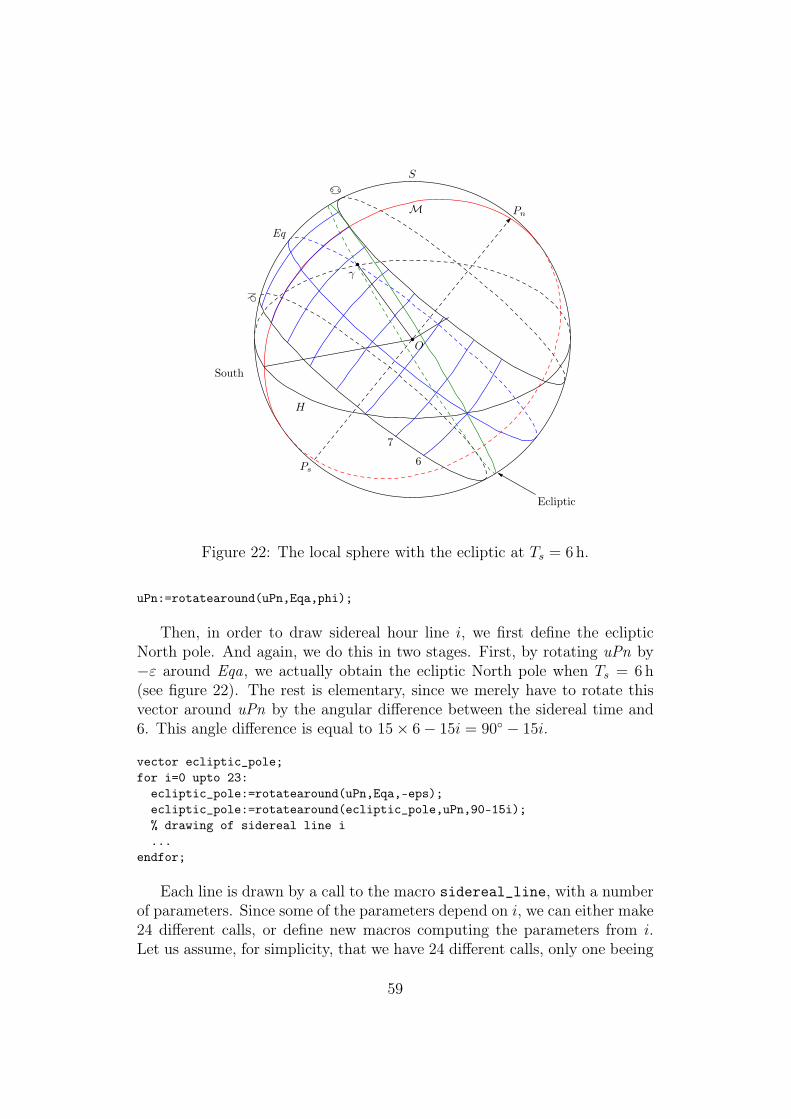
Eq
_
d
M Pn
Ps
H
S
7
6
γ
O
South
Ecliptic
Figure 22: The local sphere with the ecliptic at Ts = 6h.
uPn:=rotatearound(uPn,Eqa,phi);
Then, in order to draw sidereal hour line i, we first define the eclipticNorth pole. And again, we do this in two stages. First, by rotating uPn by−ε around Eqa, we actually obtain the ecliptic North pole when Ts = 6h(see figure 22). The rest is elementary, since we merely have to rotate thisvector around uPn by the angular difference between the sidereal time and6. This angle difference is equal to 15 × 6 − 15i = 90◦ − 15i.
vector ecliptic_pole;
for i=0 upto 23:
ecliptic_pole:=rotatearound(uPn,Eqa,-eps);
ecliptic_pole:=rotatearound(ecliptic_pole,uPn,90-15i);
% drawing of sidereal line i
...
endfor;
Each line is drawn by a call to the macro sidereal_line, with a numberof parameters. Since some of the parameters depend on i, we can either make24 different calls, or define new macros computing the parameters from i.Let us assume, for simplicity, that we have 24 different calls, only one beeing
59

p′
0
011
2
2
3
3
4
4
4
5
5
6
6
7
7
8
9
10
10
11
11
12
12
13
13
14
14
15
15
16
16
17
17
18
1819
1920
20
21
21
22
23
meridian
horizon
Winter to Summer solstice
Summer to Winter solstice
Figure 23: The sidereal time lines on a vertical dial. Plain lines are to be usedfrom Winter solstice to Summer solstice, whereas dashed lines are to be usedfrom Summer solstice to Winter solstice. The part over the horizon is drawnonly for convenience and is of course never reached by the shadow. Thevertical dashed line is the intersection of the meridian plane going throughthe tip of the gnomon with the wall. The lower hyperbola is met at theSummer solstice, whereas the upper one is met at the Winter solstice.
60

chose for a given value of i. The parameters shown here are simplified, butthe three main parameters are the y-range for the lines (the y-axis is parallelto the wall, and directed towards the right, see figure 1), and the pole of theecliptic:
if i=0:sidereal_line(-11u,8u,ecliptic_pole);fi;
...
if i=10:sidereal_line(-7u,6u,ecliptic_pole);fi;
...
if i=23:sidereal_line(-10u,8u,ecliptic_pole);fi;
In order to draw a line, we determine two of its points and connect them.The two points are those for the y-range, named here yA and yB. The twopoints, pa and pb are merely shifted by z2, as this is the origin of the coordi-nates with the macro sidereal_line_point:
vardef sidereal_line(expr ya,yb,pole)=
save pa,pb;
pair pa,pb;
pa=z2+(ya,sidereal_line_point(ya,ecliptic_pole));
pb=z2+(yb,sidereal_line_point(yb,ecliptic_pole));
draw pa--pb;
enddef;
Finally, sidereal_line_point is the function corresponding to the pro-jected ecliptic. It takes two parameters, the value on the y-axis, and theecliptic pole. This function is easy to establish: assuming the pole vectorcomponents to be (Px, Py, Pz), an equation of the ecliptic plane, taking thecenter of the local sphere as the origin, is
xPx + yPy + zPz = 0 (30)
The intersection with the wall is obtained by setting x = −lh, hence:
z =lhPx − yPy
Pz
(31)
which, when translated in METAPOST code, becomes:
def sidereal_line_point(expr y,pole)=
((lh*Xp(pole)-y*Yp(pole))/Zp(pole))
enddef;
61

9.2 Reading a sidereal sundial
9.2.1 The problem of multiple lines
The dials produced with the previous procedure appear very cluttered, be-cause there are two sets of lines, and reading can become difficult. Indeed,except at the time of solstices, and given a position of the Sun on the localsphere, there are actually two possible ways to position the ecliptic, whichmeans that the shadow of the Sun lies on two different lines. Only one mustbe kept.
There is also another problem, namely that near the solstices (upper andlower curves), reading the sidereal time is difficult because there is someuncertainty in the position of the shadow and many lines cross nearby.
The first problem can be avoided by distinguishing the lines in one wayor another, or by drawing two different dials. In figure 23, for instance, thelines are split in two groups: one is drawn in plain lines and is valid from theWinter to the next Summer solstice, the other is drawn in dashed lines andis valid from the Summer to the next Winter solstice. The extremal curvesare valid at the solstices.
9.2.2 Moving through the lines
In order to see how the sidereal time can be read, it is convenient to followthe Sun during its journey through the days, and then through the year. Ifwe start on the first day of Spring, the Sun is located at the γ point and isof course in the equator plane. Hence, the path of its shadow is the equatorline (a/�). On this day, of course, at noon, the Sun as well as γ are inthe meridian plane, and therefore Ts = 0. The shadow is then located at theintersection of the equator line with the meridian line. Two sidereal lines gothrough this point: 0 and 12. The latter is to be discarded for now.
Now after noon, the shadow moves towards the right, and the lines 1,2, etc. are crossed until the shadow does no longer reach the wall (in ourparticular case with α = 29◦40′). The next day, the case is almost the same,but the path followed by the shadow is slightly below the equator. It startsat sunrise, which is slightly before 6 a.m. (solar time), and therefore Ts ≈ 18and it ends at sunset, slightly after 6 p.m., hence Ts ≈ 6. The sidereal timefor noon increases by about 4 minutes every day, and after about two weeksnoon occurs at Ts = 1, then Ts = 2, etc., until Ts = 6 at the Summer solstice.The shadow of the Sun at noon is now at its lowest point, reaching the Cancercurve. For these three months, the sidereal lines that are used are those thatare mostly horizontal.
62

p′
0
011
2
2
3
3
4
4
4
5
5
6
6
7
7
8
9
10
10
11
11
12
12
13
13
14
14
15
15
16
16
17
17
18
1819
1920
20
21
21
22
23
declination lines
meridian
horizon
Winter to Summer solstice
Summer to Winter solstice
Figure 24: The sidereal time lines, together with the declination curves (thindashed lines).
63
9.2.3 A practical approach
A similar reasoning can be applied to follow the shadow from the Summersolstice to the Winter solstice, and so on, but one needs to be very carefulin this reasoning. In fact, it is a lot easier to find out which sidereal lineto use by first computing mentally an approximation of the sidereal time.The sidereal time at noon is approximately the number of half months sincethe beginning of Spring. And the sidereal time n hours after/before noonis approximately n hours more/less than the sidereal time at noon. Theseapproximations are amply sufficient to choose between the two sets of lines.Of course, we need to know the solar time, that might be provided by aconventional sundial.
An example will make this clear. Consider reading the sidereal timearound 10 a.m. on June 30. On this day at noon, the sidereal time is approx-imately Ts = 6.5. At 10 a.m., it must therefore be approximately Ts = 4.5.This means that we need only consider the two lines 4 and 5, and the readingis made a lot simpler. This procedure can be applied even when there is anincertainty of several hours on the solar time, except near the solsticial lines,where the reading is intrinsically difficult.
10 Analemmatic sundials
Analemmatic dials are another kind of sundials, of which there are actuallynumerous varieties [1]. Here, we consider only the commonest type, namelyan horizontal dial with a vertical style.
In this kind of dial, the hours are marked along an ellipse, and the stylemust be positioned according to the period of the year, or, what is equivalent,according to declination of the Sun. Such dials are adequate for places suchas squares, where a person can act as the style.
Although these dials seem strange and mysterious, they are actually verysimple, and do not require any fancy mathematics, contrary to what is oftenseen, for instance in Rohr’s book [11].
Figure 25 shows the construction of the elliptic dial. The dial is actuallythe horizontal projection of the equator circle on a local sphere. It is thereforethe same curve as the equator curve seen in previous construction. On thefigure, this dial is drawn with a thicker line. On the figure, we have alsoput the center of the sphere O where the tip of the gnomon was located inprevious examples. We have also shown the position of the wall, for merereference. The horizontal gnomon or the wall do not play any part here andthey can now be discarded.
64

Figure 25 also shows the horizontal projections of the two tropics (_ andd), as well as the normal hour lines corresponding to the hours of true solartime.
We now consider what happens at a certain time, for instance when thehour angle of the Sun is 22, that is when it is 10 a.m. solar time. At theequinoxes, the Sun is located in S22,0 and the projection of O reaches thelocal sphere at the opposite point Γ22. If we now assume that O is on theground and that a vertical style is put at O, then the shadow of that styleis the line OΓ22. This reasoning is true for every position of the Sun, andtherefore the analemmatic dial clearly works at the equinoxes: the shadow ofa style put at O goes through a point of the dial symmetrical to the directionof the Sun. We can therefore merely translate the numbering of the hours,or swap “a.m.” for “p.m.”
Consider now what happens when it is 10 a.m. at the Summer solstice.The Sun is at S22,ε. The direction of its rays are parallel to S22,εO. What isexpected is that the rays reach the same point Γ22. How can this be achieved?If the style is put at O, the shadow of the Sun will be more towards Γ21 whichwould not be correct. The answer is simple: draw a parallel to (S22,εO) andgoing through Γ22. This line cuts the meridian at G. It is clear that avertical style put at G will cast a shadow which goes through Γ22 at theSummer solstice. If we know where the Sun is, we can now easily find how toposition the style. It is however useful to be able to compute this position.
This is done as follows. In figure 25, we can actually consider that thereare two parallel lines, (S22,εO) and (G′Γ22), and that these lines are in space,G being the horizontal projection of a point G′. Figure 26 shows the planecontaining the polar axis and point Γ22. Beware that this plane is not vertical,except in rare circumstances. The line marked “horizon” is therefore only theintersection of the figure plane with the horizon, not a depiction of the wholehorizon. Point G′ is on the polar axis, slightly beyond the center _c of theCancer tropic, and its position only depends on r and ε, not on the time ofday. We have OG ′ = r tan ε. Now, since the angle between the polar axisand the horizon is exactly the latitude ϕ, it comes that OG = OG ′ cosϕ =r tan ε cosϕ. This is the position of the vertical style at the Summer solstice.
Since we didn’t assign any value to ε, and since we did not even use thefact that it is the obliquity of the ecliptic, we can actually conclude that theresult is valid when ε is replaced by the declination δ of the Sun: the styleshould be put such that OG = r tan δ cosϕ. In this formula, δ is a functionof the day, and r is the semi-major axis of the projected ellipse.
As it appears, the position of the style at the Summer solstice is veryclose—but not identical—to that of the center of the Cancer parallel. Thedistance between O and the projection of _c is r sin ε cosϕ and the distance
65

wall
West
East
South
α
a0
a1a2
a6
O
S22,ε
S22,0
S22,−ε
dc
_cG
Γ22
analemmatic dial
_
d
Figure 25: The construction of the analemmatic sundial.
66

horizonO
Pn
Ps
Eq
G′
S22,ε
S22,−ε
Γ22
_c
r
ε
ε
Figure 26: Position of the style in the analemmatic sundial.
between the two points is r(tan ε − sin ε) cosϕ which of course tends to 0when the declination tends to 0, but a lot faster than either term alone. Thisis easy to prove, using the developments of sin and tan:
sin x = x− x3
3!+ o(x3) (32)
tanx = x+x3
3+ o(x3) (33)
Hence:
r(tan ε− sin ε) cosϕ = r
(
ε3
2+ o(ε3)
)
cosϕ (34)
≈ rε3
2cosϕ (35)
where ε is expressed in radians.
11 Conclusion
Our study has now come to an end, and, taking three particular dials as astarting point, we have covered a wide range of material related to sundials.Dials showing equinoctial hours (normal, Babylonian and Italian) have beenconsidered, as well as dials showing temporary hours. More unusual dialssuch as elevation and azimuth dials, declination dials, sidereal time dials,and analemmatic dials have also been studied.
67

In each case, we have strived to produce accurate drawings and to showhow they were obtained using a high-level drawing language such as META-POST. It should be easy to adapt what we have done to other graphicallanguages, and even to generalize it.
Computations were kept at a minimum, and we have for instance refrainedfrom giving equations for the curves on several dials, because we didn’t needthem. We didn’t give any equation for the Babylonian lines, for instance,and it didn’t prevent us from drawing them accurately.
And although this wasn’t that much the focus of this study, we have alsotried to produce parametric drawings, in such a way that the dials can beadjusted to a different latitude and orientation without difficulty. However, asit can be expected, producing sundials totally automatically is not that easy,because there are also aesthetic requirements. For instance, the labelling offigure 17 is only right for certain values of ϕ and α. Adapting the location ofthe labels, arrows, intermediate points, line lengths, etc. as functions of ϕ,of α, and also of the gnomon dimensions, may prove a real challenge that wehaven’t really tackled. Nevertheless, for “pure” sundials, without labels, andonly simple lines, producing parametric drawings is rather easy, and henceexperimenting different configurations is also possible.
68

References
[1] Margarida Archinard. Les cadrans solaires analemmatiques. Annals of
Science, 62(3):309–346, July 2005.
[2] Henri Bach, Jean-Pierre Rieb, and Robert Wilhelm. Les trois horloges
astronomiques de la cathédrale de Strasbourg. Strasbourg: Éditions Ro-nald Hirlé, 1992.
[3] Christophorus Clavius. Gnomonices libri octo, in quibus non solum
horologiorum solarium, sed aliarum quoquam rerum, quæ ex gnomo-
nis umbra cognosci possunt, descriptiones geometricè demonstrantur.Roma: Franciscus Zanettus, 1581. Several digital versions are availableon internet.
[4] Thomas Stephens Davies. An Inquiry into the Geometrical Character ofthe Hour-Lines upon the Antique Sun-Dials. Transactions of the Royal
Society of Edinburgh, 12:77–122, 1834.
[5] Michel Goossens, Frank Mittelbach, Sebastian Rahtz, Denis Roegel, andHerbert Voß. The LATEX Graphics Companion, Second Edition. Boston:Addison-Wesley, 2008. First printing, July 2007.
[6] John Douglas Hobby. A user’s manual for METAPOST. ComputingScience Technical Report 162, AT&T Bell Laboratories, 1992.
[7] Hugo Michnik. Konstruktion einer siderischen Sonnenuhr. Astronomi-
sche Nachrichten, 216(5184):441–450, 1922.
[8] Günther Oestmann. Die astronomische Uhr des Straßburger Münsters:
Funktion und Bedeutung eines Kosmos-Modells des 16. Jahrhunderts.Berlin: Verlag für Geschichte der Naturwissenschaften und der Technik,2000. Second edition. First edition in 1993.
[9] Denis Roegel. A complex drawing in descriptive geometry. TUGboat,28(2):218–228, 2007.
[10] René Rodolphe Joseph Rohr. Les cadrans solaires anciens d’Alsace.Colmar: Éditions Alsatia, 1971.
[11] René Rodolphe Joseph Rohr. Sundials: History, Theory, and Practice.New York: Dover Publications Inc., 1996.
[12] Denis Savoie. La gnomonique. Paris: Les Belles Lettres, 2001.
69

[13] Hervé Staub. Les horloges silencieuses d’Alsace. Strasbourg: ÉditionsCoprur, 1997.
[14] Paul Werkmeister. Über die Zeitmesser des Strassburger Münsters ins-besondere die Sonnenuhren am Giebel der Südseite. Strassburger Mün-
sterblatt, 6:62–74, 1912.
70