three-dimensional face recognition - technionron/papers/ijcv2005-3dface.pdf · three-dimensional...
TRANSCRIPT
Three-Dimensional Face Recognition ∗
Alexander M. Bronstein, Michael M. Bronstein and Ron KimmelDepartment of Computer ScienceTechnion – Israel Institute of Technology, Haifa 32000, Israel
First version: May 18, 2004; Second version: December 10, 2004.
Abstract.An expression-invariant 3D face recognition approach is presented. Our basic
assumption is that facial expressions can be modelled as isometries of the facialsurface. This allows to construct expression-invariant representations of faces usingthe canonical forms approach. The result is an efficient and accurate face recognitionalgorithm, robust to facial expressions that can distinguish between identical twins(the first two authors). We demonstrate a prototype system based on the proposedalgorithm and compare its performance to classical face recognition methods.
The numerical methods employed by our approach do not require the facialsurface explicitly. The surface gradients field, or the surface metric, are sufficient forconstructing the expression-invariant representation of any given face. It allows usto perform the 3D face recognition task while avoiding the surface reconstructionstage.
Keywords: expression-invariant 3D face recognition, isometry invariant, facial ex-pressions, multidimensional scaling.
1. Introduction
Automatic face recognition has been traditionally associated with thefields of computer vision and pattern recognition. Face recognition isconsidered a natural, non-intimidating, and widely accepted biometricidentification method (Ashbourn, 2002; Ortega-Garcia et al., 2004). Assuch, it has the potential of becoming the leading biometric technology.Unfortunately, it is also one of the most difficult pattern recognitionproblems. So far, all existing solutions provide only partial, and usuallyunsatisfactory, answers to the market needs.
In the context of face recognition, it is common to distinguish be-tween the problem of authentication and that of recognition. In thefirst case, the enrolled individual (probe) claims identity of a personwhose template is stored in the database (gallery). We refer to the dataused for a specific recognition task as a template. The face recognitionalgorithm needs to compare a given face with a given template and
∗ This research was partially supported by Dvorah Fund of the Technion, the BarNir Bergreen Software Technology Center of Excellence and the Technion V.P.R.Fund - E. and J. Bishop Research Fund.
c© 2005 Kluwer Academic Publishers. Printed in the Netherlands.
"IJCV - second review - 3".tex; 13/01/2005; 21:58; p.1
2 Michael M. Bronstein, Alexander M. Bronstein, Ron Kimmel
verify their equivalence. Such a setup (one-to-one matching) can occurwhen biometric technology is used to secure financial transactions, forexample, in an automatic teller machine (ATM). In this case, the useris usually assumed to be collaborative.
The second case is more difficult. Recognition implies that the probesubject should be compared with all the templates stored in the gallerydatabase. The face recognition algorithm should then match a givenface with one of the individuals in the database. Finding a terrorist ina crowd (one-to-many matching) is one such application. Needless tosay, no collaboration can be assumed in this case. At current techno-logical level, one-to-many face recognition with non-collaborative usersis practically unsolvable. That is, if one intentionally wishes not to berecognized, he can always deceive any face recognition technology. Inthe following, we will assume collaborative users.
Even collaborative users in a natural environment present high vari-ability of their faces – due to natural factors beyond our control. Thegreatest difficulty of face recognition, compared to other biometrics,stems from the immense variability of the human face. The facial ap-pearance depends heavily on environmental factors, for example, thelighting conditions, background scene and head pose. It also dependson facial hair, the use of cosmetics, jewelry and piercing. Last but notleast, plastic surgery or long-term processes like aging and weight gaincan have a significant influence on facial appearance.
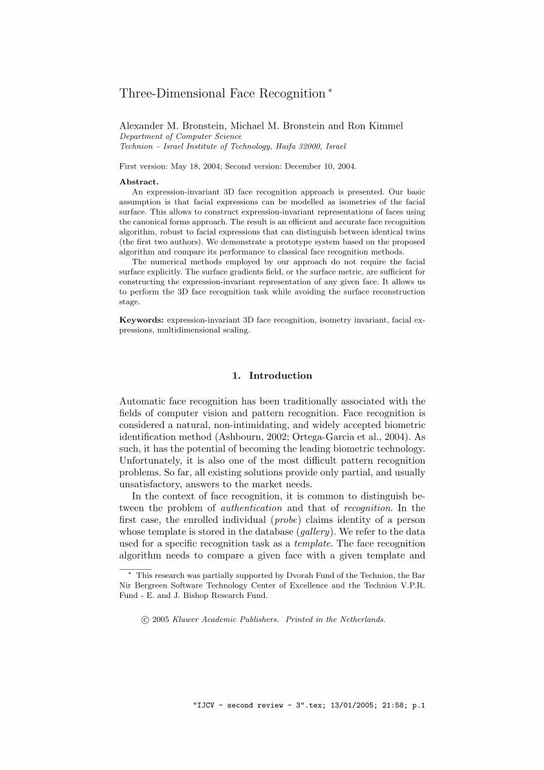
Yet, much of the facial appearance variability is inherent to the faceitself. Even if we hypothetically assume that external factors do notexist, for example, that the facial image is always acquired under thesame illumination, pose, and with the same haircut and make up, still,the variability in a facial image due to facial expressions may be evengreater than a change in the person’s identity (see Figure 1).
Figure 1. Face recognition with varying lighting, head pose, and facialexpression is a non-trivial task.
"IJCV - second review - 3".tex; 13/01/2005; 21:58; p.2
Three-Dimensional Face Recognition 3
1.1. Two-dimensional face recognition: Invariant versusgenerative approaches
Trying to make face recognition algorithms insensitive to illumination,head pose, and other factors mentioned above is one of the main ef-forts of current research in the field. Broadly speaking, there are twoalternatives in approaching this problem. One is to find features thatare not affected by the viewing conditions; we call this the invariantapproach. Early face recognition algorithms advocated the invariantapproach by finding a set of fiducial points such as eyes, nose, mouth,etc. and comparing their geometric relations (feature-based recognition)(Bledsoe, 1966; Kanade, 1973; Goldstein et al., 1971) or comparing theface to a whole facial template (template-based recognition) (Brunelliand Poggio, 1993).
It appears, however, that very few reliable fiducial points can be ex-tracted from a 2D facial image in the presence of pose, illumination, andfacial expression variability. As the result, feature-based algorithms areforced to use a limited set of points, which provide low discriminationability between faces (Cox et al., 1996). Likewise, templates used intemplate matching approaches change due to variation of pose or facialexpression (Brunelli and Poggio, 1993). Using elastic graph matching(Wiskott, 1995; Wiskott et al., 1997) as an attempt to account forthe deformation of templates due to flexibility of the facial surfacehas yielded limited success since the attributed graph is merely a flatrepresentation of a curved 3D object (Ortega-Garcia et al., 2004).
Appearance-based methods that treat facial images as vectors of amultidimensional Euclidean space and use standard dimensionality re-duction techniques to construct a representation of the face (eigenfaces(Turk and Pentland, 1991) and similar approaches (Sirovich and Kirby,1987; Hallinan, 1994; Pentland et al., 1994)), require accurate registra-tion between facial images. The registration problem brings us back toidentifying reliably fiducial points on the facial image independentlyof the viewing conditions and the internal variability due to facialexpressions. As a consequence, appearance-based methods perform wellonly when the probe image is acquired in conditions similar to those ofthe gallery image (Gheorghiades et al., 2001).
The second alternative is to generate synthetic images of the facein new, unseen conditions. Generating facial images with new poseand illumination requires some 3D facial surface as an intermediatestage. It is possible to use a generic 3D head model (Huang et al.,2002), or estimate a rough shape of the facial surface from a set ofobservations (e.g. using photometric stereo (Georghiades et al., 1998;Gheorghiades et al., 2001)) in order to synthesize new facial images and
"IJCV - second review - 3".tex; 13/01/2005; 21:58; p.3
4 Michael M. Bronstein, Alexander M. Bronstein, Ron Kimmel
then apply standard face recognition methods like eigenfaces (Sirovichand Kirby, 1987; Turk and Pentland, 1991) to the synthetic images.Yet, facial expressions appear to be more problematic to synthesize.Approaches modelling facial expressions as warping of the facial imagedo not capture the true geometric changes of the facial surface, andare therefore useful mainly for computer graphics applications. Thatis, the results may look natural, but fail to represent the true natureof the expression.
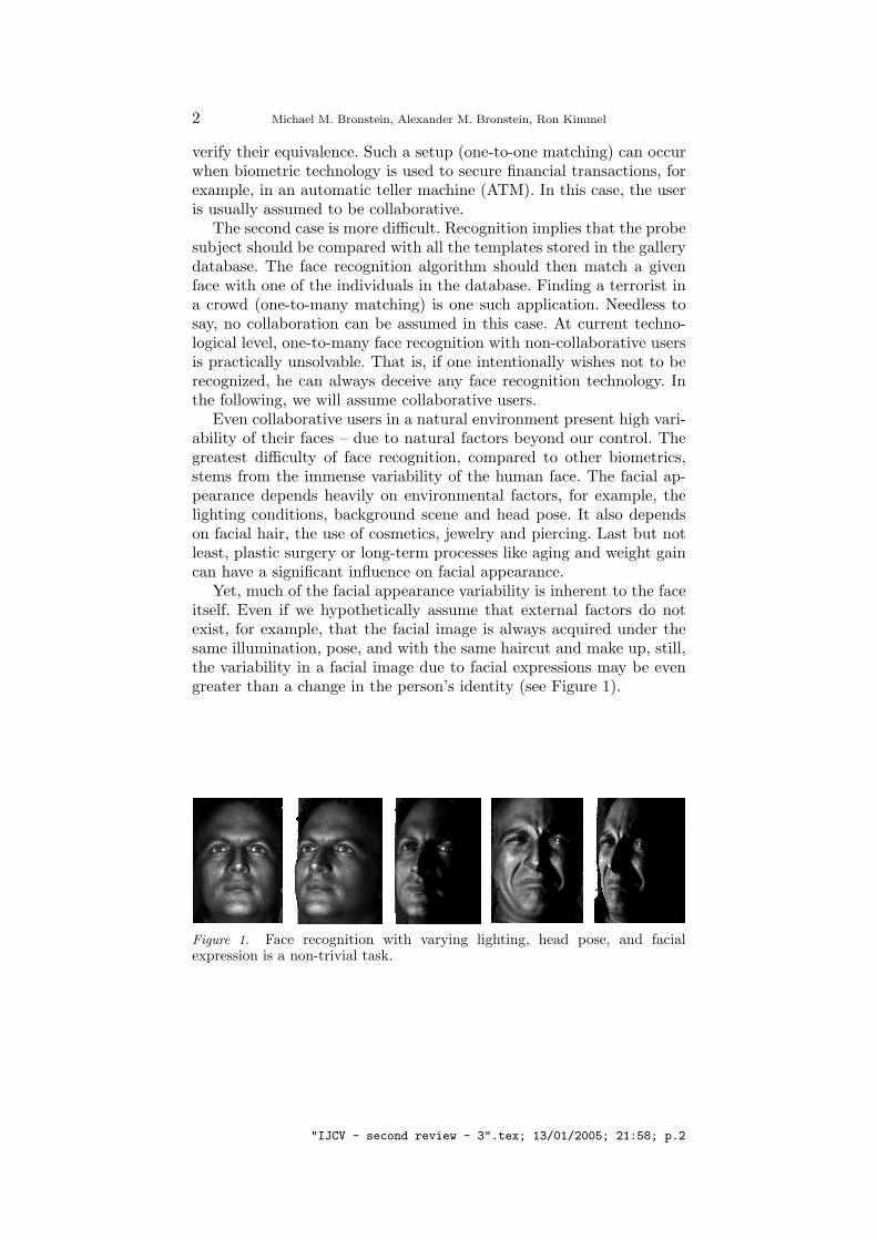
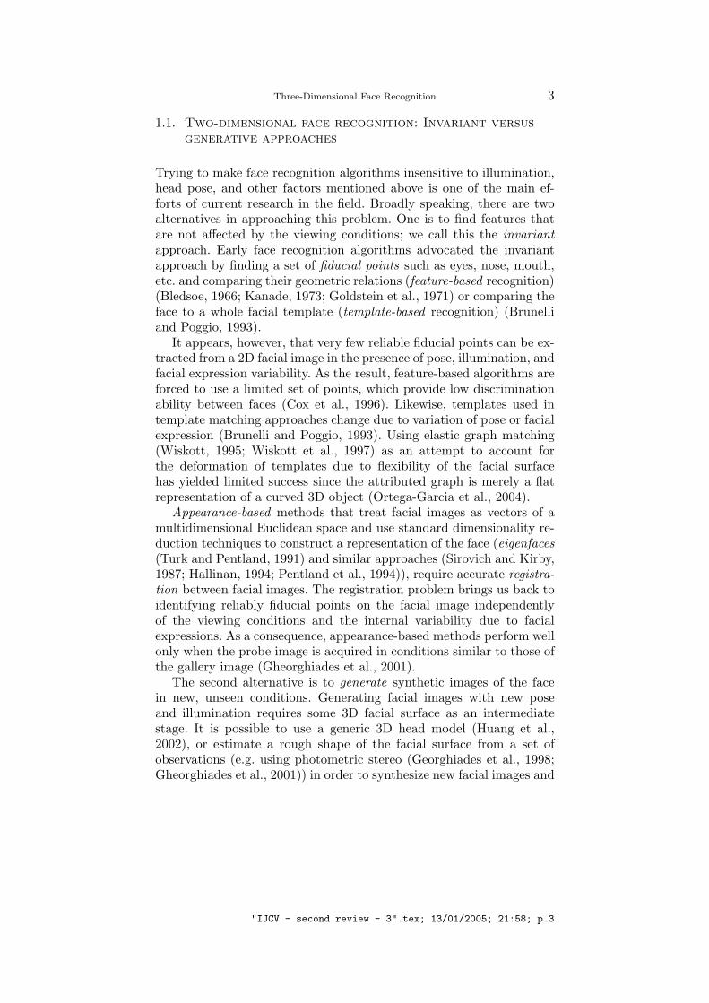
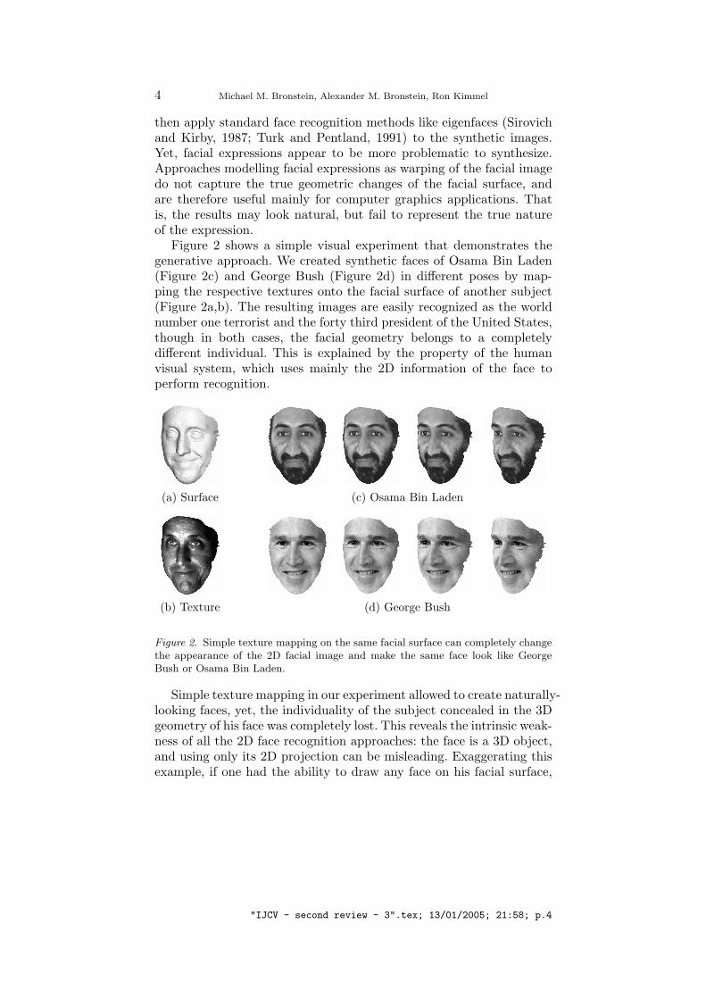
Figure 2 shows a simple visual experiment that demonstrates thegenerative approach. We created synthetic faces of Osama Bin Laden(Figure 2c) and George Bush (Figure 2d) in different poses by map-ping the respective textures onto the facial surface of another subject(Figure 2a,b). The resulting images are easily recognized as the worldnumber one terrorist and the forty third president of the United States,though in both cases, the facial geometry belongs to a completelydifferent individual. This is explained by the property of the humanvisual system, which uses mainly the 2D information of the face toperform recognition.
(a) Surface
(c) Osama Bin Laden
(b) Texture
(d) George Bush
Figure 2. Simple texture mapping on the same facial surface can completely changethe appearance of the 2D facial image and make the same face look like GeorgeBush or Osama Bin Laden.
Simple texture mapping in our experiment allowed to create naturally-looking faces, yet, the individuality of the subject concealed in the 3Dgeometry of his face was completely lost. This reveals the intrinsic weak-ness of all the 2D face recognition approaches: the face is a 3D object,and using only its 2D projection can be misleading. Exaggerating thisexample, if one had the ability to draw any face on his facial surface,
"IJCV - second review - 3".tex; 13/01/2005; 21:58; p.4
Three-Dimensional Face Recognition 5
he could make himself look essentially like any person and deceiveany 2D face recognition method. Practically, even with very modestinstruments, makeup specialists in the theater and movie industry canchange completely the facial appearance of actors.
1.2. Three-dimensional face recognition
Three-dimensional face recognition is a relatively recent trend that insome sense breaks the long-term tradition of mimicking the humanvisual recognition system, like the 2D methods attempt to do. As eval-uations such as the Face Recognition Vendor Test (FRVT) demonstratein an unarguable manner that current state of the art in 2D facerecognition is insufficient for high-demanding biometric applications(Phillips et al., 2003), trying to use 3D information has become anemerging research direction in hope to make face recognition moreaccurate and robust.
Three-dimensional facial geometry represents the internal anatomi-cal structure of the face rather than its external appearance influencedby environmental factors. As the result, unlike the 2D facial image, 3Dfacial surface is insensitive to illumination, head pose (Bowyer et al.,2004), and cosmetics (Mavridis et al., 2001). Moreover, 3D data canbe used to produce invariant measures out of the 2D data (for exam-ple, given the facial surface, the albedo can be estimated from the 2Dreflectance under assumptions of Lambertian reflection).
However, while in 2D face recognition a conventional camera is used,3D face recognition requires a more sophisticated sensor, capable of ac-quiring depth information – usually referred to as depth or range cameraor 3D scanner. The 3D shape of the face is usually acquired togetherwith a 2D intensity image. This is one of the main disadvantages of3D methods compared to 2D ones. Particularly, it prohibits the useof legacy photo databases, like those maintained by police and specialagencies.
Early papers on 3D face recognition revealed the potential hiddenin the 3D information rather than presented working algorithms or ex-tensive tests. In one of the first papers on 3D face recognition, Cartouxet al. (1989) approached the problem by finding the plane of bilateralsymmetry through the facial range image, and either matching theextracted profile of the face, or using the symmetry plane to compensatefor the pose and then matching the whole surface. Similar approachesbased on profiles extracted from 3D face data were also described inthe follow-up papers by Nagamine et al. (1992), Beumier and Acheroy(1988) and Gordon (1997).
"IJCV - second review - 3".tex; 13/01/2005; 21:58; p.5
6 Michael M. Bronstein, Alexander M. Bronstein, Ron Kimmel
Achermann et al. (1997), Hesher et al. (2003), Mavridis et al. (2001),Chang et al. (2003) Tsalakanidou et al. (2003) explored the extension ofconventional dimensionality reduction techniques, like Principal Com-ponent Analysis (PCA), to range images or combination of intensityand range images. Gordon (1992) proposed representing a facial surfaceby a feature vector created from local information such as curvatureand metric. The author noted that the feature vector is similar fordifferent instances of the same face acquired in different conditions,except “variation due to expression” (Gordon, 1992).
Lee and Milios (1990) and Tanaka et al. (1998) proposed performingcurvature-based segmentation of the range image into convex regionsand compute the Extended Gaussian Image (EGI) locally for eachregion. A different local approach based on Gabor filters in 2D andpoint signatures in 3D was presented by Wang et al. (2002).
Finally, many theoretical works including Medioni and Waupotitsch(2003), Achermann and Bunke (2000), as well as some commercialsystems, use rigid surface matching in order to perform 3D face recog-nition. However, facial expressions do change significantly the 3D facialsurface not less than they change the 2D intensity image, hence mod-elling faces as rigid objects is invalid when considering facial expres-sions.
We note that the topic of facial expressions in 3D face recognition isvery scarcely addressed in the literature, which makes difficult to drawany conclusions about the robustness of available algorithms. Many ofthe cited authors mention the problem of facial expressions, yet, noneof them has addressed it explicitly, nor any of the algorithms except inWang et al. (2002) was tested on a database with sufficiently large (ifany) variability of facial expressions.
1.3. The 3DFACE approach
Our approach, hereinafter referred to as 3DFACE, comes to addressexplicitly the problem of facial expressions. It treats the facial surfaceas a deformable object in the context of Riemannian geometry. Ourobservations show that the deformations of the face resulting from facialexpressions can be modelled as isometries (Bronstein et al., 2003b),such that the intrinsic geometric properties of the facial surface areexpression-invariant. Thus, finding an expression-invariant representa-tion of the face is essentially equivalent to finding an isometry-invariantrepresentation of the facial surface.
A computationally-efficient invariant representation of isometric sur-faces can be constructed by isometrically embedding the surface intoa low-dimensional space with convenient geometry. Planar embedding
"IJCV - second review - 3".tex; 13/01/2005; 21:58; p.6
Three-Dimensional Face Recognition 7
appeared to be useful in the analysis of cortical surfaces (Schwartzet al., 1989), and in texture mapping (Zigelman et al., 2002; Grossmanet al., 2002). Embedding into higher dimensional Euclidean spaces, asfirst presented by Elad and Kimmel (2001), was shown to be an efficientway to perform matching of deformable objects. Isometric embeddingis the core of our 3D face recognition system. It consists of measuringthe geodesic distances between points on the facial surface and thenusing multidimensional scaling to perform the embedding. This way,the task of comparing deformable objects like faces is transformed intoa much simpler problem of rigid surface matching, at the expense ofloosing some accuracy, which appears to be insignificant in this case.
An important property of the numerical algorithms implemented inthe 3DFACE system is that we actually do not need the facial surface tobe given explicitly. All the stages of our recognition system, includingpre-processing and computation of geodesic distances can be carriedout given only the metric tensor of the surface. It allows us to use sim-ple and cost-efficient 3D acquisition techniques like photometric stereo.Avoiding explicit surface reconstruction also saves computational timeand reduces the numerical inaccuracies (Bronstein et al., 2004b).
The organization of this paper is the following: Next section startswith modelling faces as Riemannian surfaces. Such a formulation servesas a unifying framework for different procedures described later on. Fa-cial expressions are modelled as isometries of the facial surface. A simpleexperiment justifies this assumption. Section 3 introduces the conceptof multidimensional scaling and its application to isometric embedding.Section 4 describes a prototype 3DFACE system and addresses someimplementation considerations. In Section 5 we show experimental re-sults assessing the performance of our method and comparing it toother 2D and 3D face recognition algorithms. Section 6 concludes thepaper.
2. The geometry of human faces
2.1. A brief introduction into Riemannian geometry
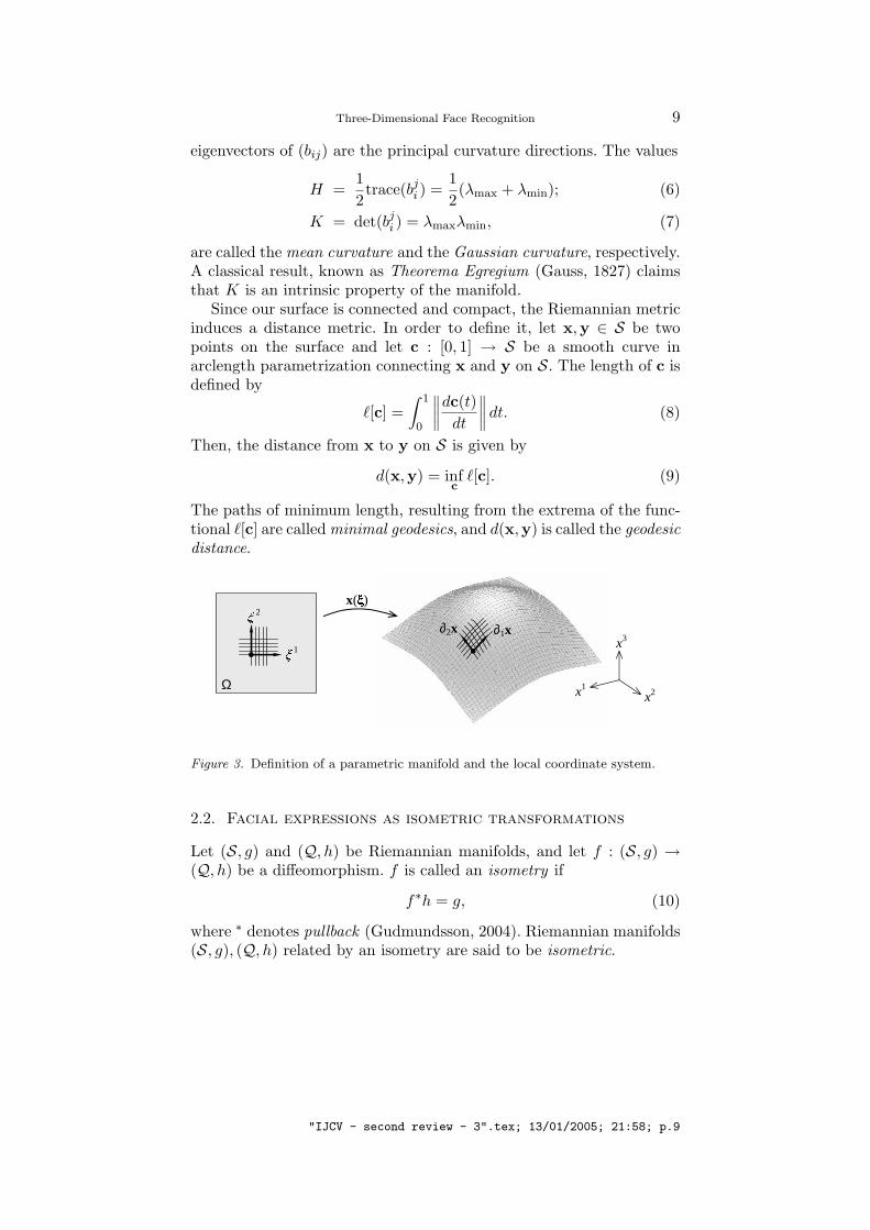
We model a human face as a two-dimensional smooth connected para-metric manifold (surface), denoted by S and represented by a coordi-nate chart from a compact subset Ω ⊂ IR2 to IR3
x(Ω) = (x1(ξ1, ξ2), x2(ξ1, ξ2), x3(ξ1, ξ2)). (1)
We assume that the functions x1, ..., x3 are Cr (with r sufficiently large),and that the vectors ∂ix ≡ ∂
∂ξi x (i = 1, 2) are linearly independent.
"IJCV - second review - 3".tex; 13/01/2005; 21:58; p.7
8 Michael M. Bronstein, Alexander M. Bronstein, Ron Kimmel
We will further assume that the surface can be represented as a graphof a function, e.g. x3 = x3(x1, x2), such that x3 can be referred toas the depth coordinate. Also, for convenience, in the following theparameterization coordinates ξ = (ξ1, ξ2) will be identified with thecoordinates in the image acquired by the camera (see Section 4.1).Similarly, we define the facial albedo as a scalar field ρ : Ω → IR+.
The derivatives ∂ix constitute a local non-orthogonal coordinatesystem on S, and span an affine subspace of IR3 called the tangentspace and denoted by TxS for every x ∈ S. In order to consider the non-Euclidean geometry of the manifold, we introduce a bilinear symmetricnon-degenerate form (tensor) g called the Riemannian metric or thefirst fundamental form. It can be identified with an inner product onTS. The Riemannian metric is an intrinsic characteristic of the mani-fold and allows us to measure local distances on S independently of thecoordinates (Kreyszig, 1991). The pair (S, g) is called a Riemannianmanifold.
In coordinate notation, a distance element on the manifold can beexpressed via the metric tensor gij(x) as
ds2 = gijdξidξj , i, j = 1, 2; (2)
where repeating super- and subscripts are summed over according toEinstein’s summation convention. The metric tensor gij at every pointof a parametric surface can be given explicitly by
gij = ∂ix · ∂jx, i, j = 1, 2. (3)
The unit normal to S at x is a vector orthogonal to the tangentspace TxS and can be written as a cross-product
N(x) =∂1x× ∂2x
‖∂1x× ∂2x‖2. (4)
Another characteristic of the surface called the second fundamentalform, is given in coordinate notation as
bij = −∂ix · ∂jN. (5)
Unlike the metric, the second fundamental form is prescribed by thenormal field N, that is, it has to do with the way the manifold is im-mersed into the ambient space. This distinction plays a crucial role. Themetric is responsible for all properties of the manifold which are calledintrinsic. Propertied expressible in terms of the second fundamentalform are called extrinsic.
The maximum and the minimum eigenvalues λmax, λmin of the ten-sor bj
i = bikgkj are called the principal curvatures. The corresponding
"IJCV - second review - 3".tex; 13/01/2005; 21:58; p.8
Three-Dimensional Face Recognition 9
eigenvectors of (bij) are the principal curvature directions. The values
H =12trace(bj
i ) =12(λmax + λmin); (6)
K = det(bji ) = λmaxλmin, (7)
are called the mean curvature and the Gaussian curvature, respectively.A classical result, known as Theorema Egregium (Gauss, 1827) claimsthat K is an intrinsic property of the manifold.
Since our surface is connected and compact, the Riemannian metricinduces a distance metric. In order to define it, let x,y ∈ S be twopoints on the surface and let c : [0, 1] → S be a smooth curve inarclength parametrization connecting x and y on S. The length of c isdefined by
`[c] =∫ 1
0
∥∥∥∥dc(t)dt
∥∥∥∥ dt. (8)
Then, the distance from x to y on S is given by
d(x,y) = infc
`[c]. (9)
The paths of minimum length, resulting from the extrema of the func-tional `[c] are called minimal geodesics, and d(x,y) is called the geodesicdistance.
t
1
2 ∂1x ∂2x
x( )
Ω x2
x3
x1
Figure 3. Definition of a parametric manifold and the local coordinate system.
2.2. Facial expressions as isometric transformations
Let (S, g) and (Q, h) be Riemannian manifolds, and let f : (S, g) →(Q, h) be a diffeomorphism. f is called an isometry if
f∗h = g, (10)
where ∗ denotes pullback (Gudmundsson, 2004). Riemannian manifolds(S, g), (Q, h) related by an isometry are said to be isometric.
"IJCV - second review - 3".tex; 13/01/2005; 21:58; p.9
10 Michael M. Bronstein, Alexander M. Bronstein, Ron Kimmel
From the point of view of intrinsic geometry, isometric manifolds areindistinguishable. Particularly, in the same way as g induces a distancemetric dS on S, the tensor h induces a distance metric dQ on Q. Thisessentially implies that f preserves the geodesic distance between everypair of points, that is,
dS(x,y) = dQ(f(x), f(y)), ∀x,y ∈ S. (11)
In fact, in our case Equation (11) is an alternative definition of an isom-etry. Furthermore, from Theorema Egregium it stems that isometricsurfaces have equal Gaussian curvature KS(x) = KQ(f(x)).
We apply this isometric model to faces. Facial expressions resultfrom the movement of mimic muscles (Ekman, 1973). We assume thatnatural deformations of the facial surface can be modelled as isometries.In other words, facial expressions give rise to nearly isometric surfaces.This will allow us to construct an expression-invariant representationof the face, based on its intrinsic geometric structure.
It must be understood, of course, that the isometric model is only anapproximation and models natural expressions excepting pathologicalcases. One of such pathologies is the open mouth. The isometric modeltacitly assumes that the topology of the facial surface is preserved,hence, facial expressions are not allowed to introduce arbitrary “holes”in the facial surface. This assumption is valid for most regions of theface except the mouth. Opening the mouth changes the topology of thefacial surface by virtually creating a “hole”. In (Bronstein et al., 2004c)we extend the isometric model to topology-changing expressions. Here,we assume that the mouth is closed in all facial expressions.
2.3. Discrete manifolds
In practice, we work with discrete representation of surfaces, obtainedby taking a finite number of samples on S and measuring the geodesicdistances between them. After sampling, the Riemannian surface be-comes a finite metric space (X,D) with mutual distances described bythe matrix D with elements dij = d(xi, xj).
In (Sethian, 1996) an efficient numerical procedure called the FastMarching Method (FMM), capable of measuring the distances from onesource to N points on a plane in O(N) operations, was introduced (see(Tsitsiklis, 1988) for a related result). The FMM is based on upwindfinite difference approximations for solving the eikonal equation, whichis a differential formulation of a wave propagation equation
‖∇ν(x)‖ = 1. (12)
Here ν : IR2 → IR+ is the distance map from the sources s1, ..., sK ,such that ν(si) = 0 serve as boundary conditions. The distance map
"IJCV - second review - 3".tex; 13/01/2005; 21:58; p.10
Three-Dimensional Face Recognition 11
is constructed by starting from the source point and propagating out-wards. The FMM was extended to triangulated manifolds (FMTD) byKimmel and Sethian (1998).
The classical FMM uses an orthogonal coordinate system (regulargrid). The numerical stencil for an update of a grid point consists ofvertices of a right triangle. In the case of triangulated manifolds, thestencils used by the FMTD algorithm are not necessarily right trian-gles. If a grid point is updated through an obtuse angle, a consistencyproblem may arise. To cope with this problem, Kimmel and Sethianproposed to split obtuse angles by unfolding triangles as a preprocessingstage.
A variation of the FMM for parametric surfaces, presented by Spiraand Kimmel (2003), was adopted here. The main advantage of thismethod is that the computations are performed on a uniform Cartesiangrid in the parametrization plane, and not on the manifold like in theoriginal version of Kimmel and Sethian (1998). The numerical stencilis calculated directly from the local metric value, and therefore, nounfolding is required (see details in (Spira and Kimmel, 2004)). In ourapplication, the advantage of using the PFMM is that the surface is notneeded explicitly in order to measure distances; and the metric givenon the parametrization plane is sufficient (Bronstein et al., 2004b).
2.4. Isometric model validation
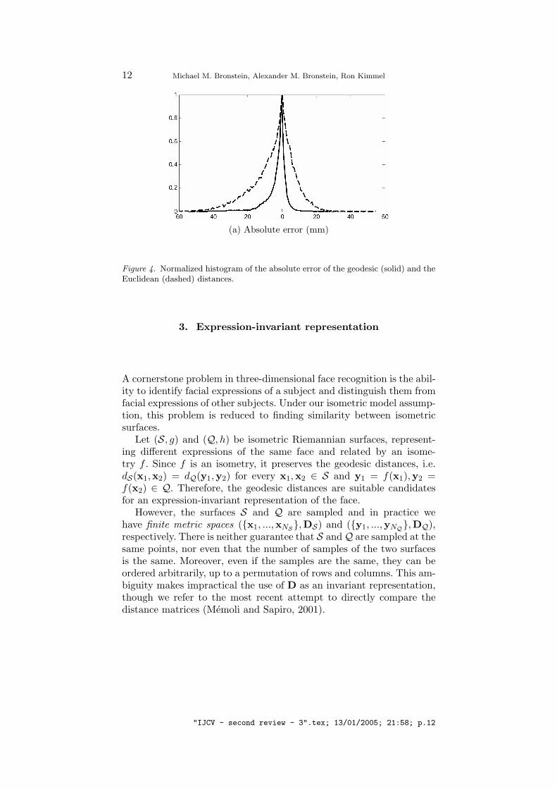
Verifying quantitatively that facial expressions are indeed isometricis possible by tracking a set of feature points on the facial manifoldand measuring how the distances between them change due to facialexpressions. In (Bronstein et al., 2004c) we presented an experimentalvalidation of the isometric model. We placed 133 markers on a face andtracked how the distances between these points change due to facial ex-pressions. Figure 4 shows the distribution of the absolute change of thegeodesic and the Euclidean distances. For more details, see (Bronsteinet al., 2004c).
We conclude from this experiment that the change of the geodesicdistances due to facial expressions is insignificant (which justifies ourmodel), and that it is more than twice smaller than the respectivechange of the Euclidean ones. This implies that the isometric modeldescribes better the nature of facial expressions compared to the rigidone. This observation will be reinforced in Section 5, where we compareour approach to a method that treats facial surfaces as rigid objects.
"IJCV - second review - 3".tex; 13/01/2005; 21:58; p.11
12 Michael M. Bronstein, Alexander M. Bronstein, Ron Kimmel
(a) Absolute error (mm)
Figure 4. Normalized histogram of the absolute error of the geodesic (solid) and theEuclidean (dashed) distances.
3. Expression-invariant representation
A cornerstone problem in three-dimensional face recognition is the abil-ity to identify facial expressions of a subject and distinguish them fromfacial expressions of other subjects. Under our isometric model assump-tion, this problem is reduced to finding similarity between isometricsurfaces.
Let (S, g) and (Q, h) be isometric Riemannian surfaces, represent-ing different expressions of the same face and related by an isome-try f . Since f is an isometry, it preserves the geodesic distances, i.e.dS(x1,x2) = dQ(y1,y2) for every x1,x2 ∈ S and y1 = f(x1),y2 =f(x2) ∈ Q. Therefore, the geodesic distances are suitable candidatesfor an expression-invariant representation of the face.
However, the surfaces S and Q are sampled and in practice wehave finite metric spaces (x1, ...,xNS,DS) and (y1, ...,yNQ,DQ),respectively. There is neither guarantee that S andQ are sampled at thesame points, nor even that the number of samples of the two surfacesis the same. Moreover, even if the samples are the same, they can beordered arbitrarily, up to a permutation of rows and columns. This am-biguity makes impractical the use of D as an invariant representation,though we refer to the most recent attempt to directly compare thedistance matrices (Memoli and Sapiro, 2001).
"IJCV - second review - 3".tex; 13/01/2005; 21:58; p.12
Three-Dimensional Face Recognition 13
3.1. Canonical forms
An alternative proposed by Elad and Kimmel (2001) is to avoid deal-ing explicitly with the matrix of geodesic distances and represent theRiemannian surface as a subset of some convenient m-dimensional man-ifold Mm, such that the original intrinsic geometry is preserved. Wecall such a procedure isometric embedding, and suchMm the embeddingspace.
The embedding allows to get rid of the extrinsic geometry, whichno more exists in the new space. As a consequence, the resulting rep-resentation will be identical for all isometries of the surface. Anotheradvantage is related to the fact that a general Riemannian metric isusually inconvenient to work with. The embedding space, on the otherhand, can be chosen completely to our discretion. Simply saying, theembedding replaces a complicate geometric structure by a convenientone.
In our discrete setting, isometric embedding is a mapping
ϕ : (x1, ...,xN ⊂ S,D) → (x′1, ...,x′N ⊂ Mm,D′) , (13)
between two finite metric spaces, such that d′ij = dij for all i, j =1, ..., N . The symmetric matrices D = (dij) ≡ (d(xi,xj)) and D′ =(d′ij) ≡ (d′(x′i,x
′j)) denote the mutual geodesic distances between the
points in the original and the embedding space, respectively. FollowingElad and Kimmel (2001, 2003), the image of x1, ...,xN under ϕ iscalled the canonical form of (S, g).
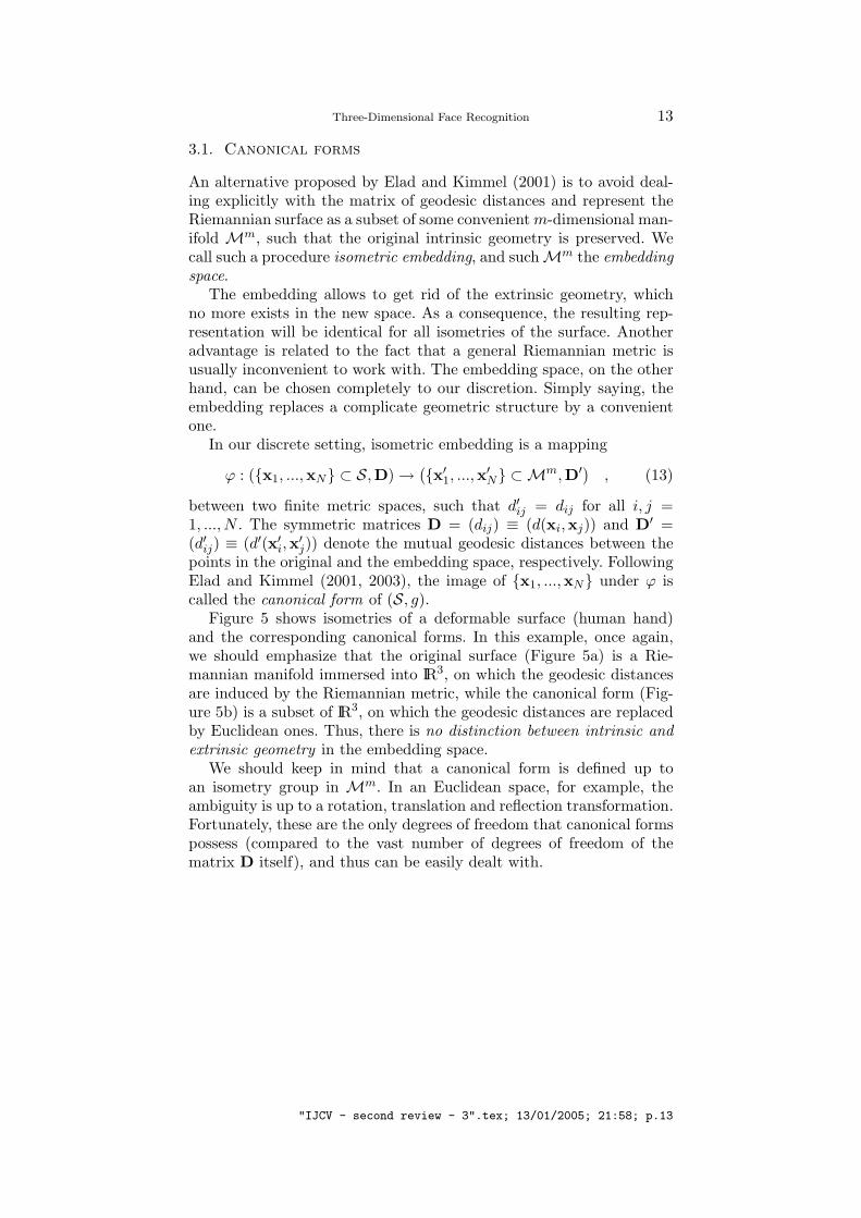
Figure 5 shows isometries of a deformable surface (human hand)and the corresponding canonical forms. In this example, once again,we should emphasize that the original surface (Figure 5a) is a Rie-mannian manifold immersed into IR3, on which the geodesic distancesare induced by the Riemannian metric, while the canonical form (Fig-ure 5b) is a subset of IR3, on which the geodesic distances are replacedby Euclidean ones. Thus, there is no distinction between intrinsic andextrinsic geometry in the embedding space.
We should keep in mind that a canonical form is defined up toan isometry group in Mm. In an Euclidean space, for example, theambiguity is up to a rotation, translation and reflection transformation.Fortunately, these are the only degrees of freedom that canonical formspossess (compared to the vast number of degrees of freedom of thematrix D itself), and thus can be easily dealt with.
"IJCV - second review - 3".tex; 13/01/2005; 21:58; p.13
14 Michael M. Bronstein, Alexander M. Bronstein, Ron Kimmel
(a) Original surfaces
(b) Canonical forms
Figure 5. Illustration of the embedding problem and the canonical forms. (a) Rie-mannian surface (hand) undergoing isometric transformations. Solid line shows thegeodesic distance between two points on the surface, dotted line is the correspondingEuclidean distance in the space where the surface “lives”. (b) After embedding, thehand surfaces become submanifolds of a three-dimensional Euclidean space, and thegeodesic distances become Euclidean ones.
3.2. Embedding error
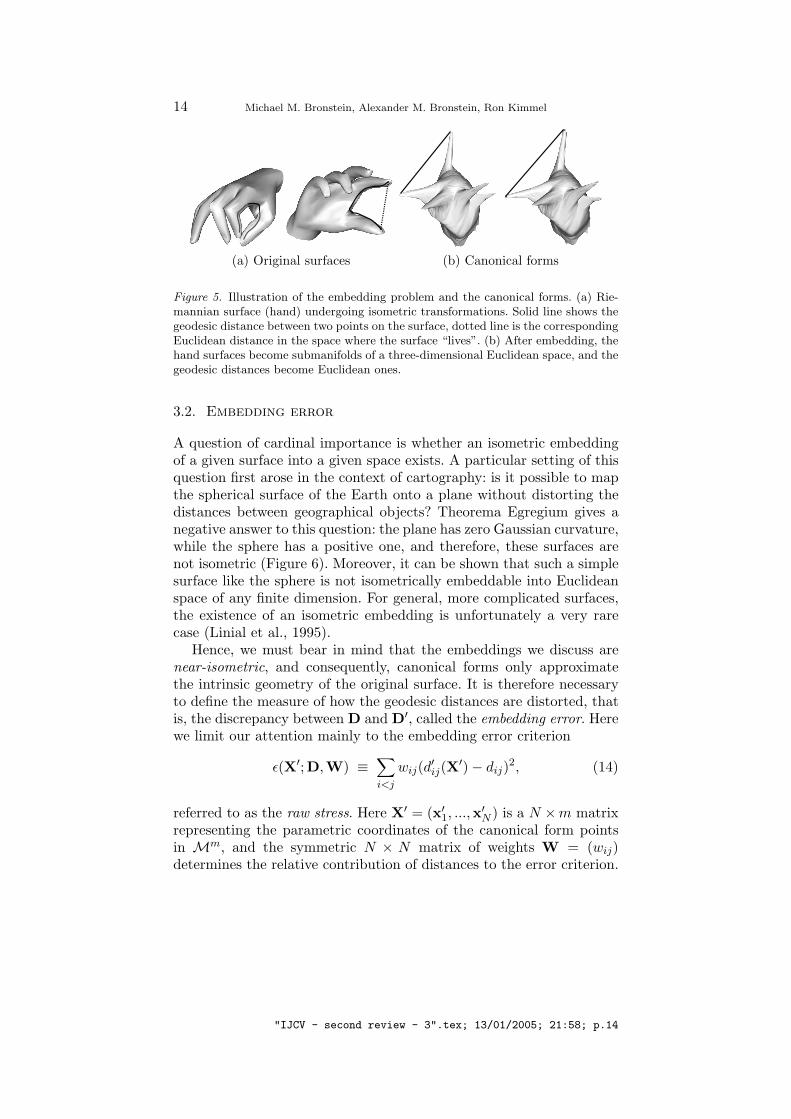
A question of cardinal importance is whether an isometric embeddingof a given surface into a given space exists. A particular setting of thisquestion first arose in the context of cartography: is it possible to mapthe spherical surface of the Earth onto a plane without distorting thedistances between geographical objects? Theorema Egregium gives anegative answer to this question: the plane has zero Gaussian curvature,while the sphere has a positive one, and therefore, these surfaces arenot isometric (Figure 6). Moreover, it can be shown that such a simplesurface like the sphere is not isometrically embeddable into Euclideanspace of any finite dimension. For general, more complicated surfaces,the existence of an isometric embedding is unfortunately a very rarecase (Linial et al., 1995).
Hence, we must bear in mind that the embeddings we discuss arenear-isometric, and consequently, canonical forms only approximatethe intrinsic geometry of the original surface. It is therefore necessaryto define the measure of how the geodesic distances are distorted, thatis, the discrepancy between D and D′, called the embedding error. Herewe limit our attention mainly to the embedding error criterion
ε(X′;D,W) ≡∑
i<j
wij(d′ij(X′)− dij)2, (14)
referred to as the raw stress. Here X′ = (x′1, ...,x′N ) is a N ×m matrixrepresenting the parametric coordinates of the canonical form pointsin Mm, and the symmetric N × N matrix of weights W = (wij)determines the relative contribution of distances to the error criterion.
"IJCV - second review - 3".tex; 13/01/2005; 21:58; p.14
Three-Dimensional Face Recognition 15
(a) Upper hemisphere of the globe
(b) Planar map
Figure 6. The embedding problem arising in cartography: The upper hemisphere ofthe Earth (a) and its planar map (b). The geodesic distances (an example is shownas a white curve) are distorted by such a map.
If some of the distances are missing, the respective weights wij can beset to zero.
A generic name for algorithms that compute the canonical form byminimization of the stress with respect to X′ is multidimensional scaling(MDS). These algorithms differ in the choice of the the embedding errorcriterion and the optimization method used for its minimization (Borgand Groenen, 1997).
3.3. The choice of the embedding space
Another important question is how to choose the embedding space.First, the geometry of the embedding space is important. Popularchoices include spaces with flat (Schwartz et al., 1989; Elad and Kim-mel, 2001; Grossman et al., 2002; Zigelman et al., 2002), spherical (Eladand Kimmel, 2002; Bronstein et al., 2005b) or hyperbolic (Walter andRitter, 2002) geometry. This choice should be dictated by the conve-nience of a specific space (namely, we want the geodesic distances inS ′m to have a simple analytic form) and the resulting embedding error,which, in turn, depends on the embedding error criterion.
Secondly, the dimension m of the embedding space must be chosenin such a way that the codimension of ϕ(S) in Mm is at least 1 (asopposed to dimensionality reduction applications where usually m ¿dim(S)). The reason becomes clear if we think of our manifolds asof function graphs, in our case – functions of two variables z(x, y).Sampling z(x, y) produces a set of points, which when embedded into atwo-dimensional manifold, reflect the sampling pattern rather than the
"IJCV - second review - 3".tex; 13/01/2005; 21:58; p.15
16 Michael M. Bronstein, Alexander M. Bronstein, Ron Kimmel
intrinsic geometry of the surface. On the other hand, when the surface isembedded into IR3 (or a manifold of higher dimension), the samples willlie on some two-dimensional submanifold of IR3 (the continuous limit ofthe canonical form), and increasing the sampling density would resultin a better approximation of the continuous canonical form.
Embedding with codimension zero (e.g. embedding of a surface intoa plane or a two-dimensional sphere S2) is useful when the manifoldis endowed with some additional property, for example, texture. Suchembedding can be thought of as an intrinsic parametrization of themanifold and has been explored in the context of medical visualization(Schwartz et al., 1989), texture mapping (Zigelman et al., 2002) andregistration of facial images (Bronstein et al., 2004a; Bronstein et al.,2005a).
3.4. Least-squares MDS
Minimization of ε(X′) can be performed by first-order, gradient descent-type methods, in which the direction at each step is
X′(k+1) = −∇ε(X′(k)). (15)
The gradient of ε(Ξ′) with respect to Ξ′ is given by
∂
∂x′lkε(X′;D,W) = 2
∑
j 6=k
wkj
(d′kj − dkj)dkj
(x′lk − x′lj ), (16)
and can be written as
∇ε(X′;D,W) = 2UX′ − 2B(X′;D,W)X′, (17)
where U is a matrix with elements
uij =
−wij if i 6= j∑Nj=1 wij if i = j
, (18)
and B is a matrix with elements
bij =
−wijdijd′−1ij (X′) if i 6= j and d′ij(X
′) 6= 00 if i 6= j and d′ij(X
′) = 0−∑
j 6=i bij if i = j. (19)
It was observed by Guttman (1968) that the first-order optimalitycondition, ∇ε(X′) = 0, can be written as X′ = U†B(X′)X′, and thatthe sequence
X′(k+1) = U†B(X′(k))X′(k), (20)
"IJCV - second review - 3".tex; 13/01/2005; 21:58; p.16
Three-Dimensional Face Recognition 17
converges to the local minimum of ε(X′) (here † denotes matrix pseudoin-verse). The algorithm using this multiplicative update is called SMA-COF (De Leeuw, 1977; De Leeuw and Stoop, 1984; Borg and Groe-nen, 1997). It can be shown to be equivalent to weighted gradientdescent with constant step size X′(k+1) = −1
2U†∇ε(X′(k)), and if a
non-weighted stress is used, it is essentially a gradient descent withconstant step size X′(k+1) = − 1
2N∇ε(X′(k)) (Bronstein, 2004).SMACOF is widely used for large-scale MDS problems. Its disadvan-
tage is slow convergence in the proximity of the minimum, which is in-herent to all first-order methods. Second order (Newton-type) methods(Nash, 2000) are usually disadvantageous in large-scale MDS problems.Recently, we showed that the multigrid framework can significantlyimprove the convergence time of the SMACOF algorithm (Bronsteinet al., 2005c)
3.5. Classical scaling
As an alternative to raw stress minimization in Euclidean embedding,it is worthwhile to mention an algebraic algorithm known as classicalscaling (Torgerson, 1952; Gower, 1966), based on theoretical results ofEckart and Young (1936) and Young and Householder (1938). Classicalscaling works with squared geodesic distances, which can be expressedas Hadamard (coordinate-wise) product ∆ = D D, where ∆ = (d2
ij).The matrix ∆ first undergoes double-centering
B∆ = −12J∆J (21)
(here J = I − 1N 11T and I is an N × N identity matrix). Then, the
eigendecomposition B∆ = VΛVT is computed, where V = (v1, ...,vN )is the matrix of eigenvectors of B corresponding to the eigenvaluesλ1 ≥ λ2 ≥ ... ≥ λN .
Let us denote by Λm+ the m×m matrix of first m positive eigenvalues,
by Vm+ the N × m matrix of the corresponding eigenvectors, and by
Λm− the matrix of the remaining N−m eigenvalues. The canonical formcoordinates in the embedding space are given by
X′ = Vm+ (Λm
+ )1/2. (22)
Classical scaling approximates the matrix B∆ by a matrix B∆′ =X′X′T of rank m. It is one of the most efficient MDS algorithms. Inpractical application, since we are usually interested in embedding intoIR3 or IR2, no full eigendecomposition of B∆ is needed – it is enough tofind only the first three or two eigenvectors. In addition, the matrix B∆
is symmetric. This allows us to use efficient algorithms such as Arnoldi
"IJCV - second review - 3".tex; 13/01/2005; 21:58; p.17
18 Michael M. Bronstein, Alexander M. Bronstein, Ron Kimmel
(Arnoldi, 1951), Lanzcos or block-Lanzcos (Golub and van Loan, 1996;Bai et al., 2000) iterations, which find a few largest eigenvectors of asymmetric matrix (Golub and Saunders, 2004).
The major drawback of classical scaling is that the embedding errorcriterion (referred to as strain) that such a procedure minimizes is muchless meaningful in our setting compared to the stress used in LS MDS(Borg and Groenen, 1997).
3.6. Canonical form alignment
In order to resolve the Euclidean isometry ambiguity, the canonicalform has to be aligned. We perform the alignment by first settingto zero the first-order moments (the center of gravity) µ100, µ010, µ001
of the canonical form (here µpqr =∑N
i=1(x′1i )p(x′2i )q(x′3i )r denotes the
pqr-moment). This resolves the translation ambiguity. Next, the mixedsecond-order moments µ110, µ011, µ101 are set to zero and the axes arereordered according to the second order moments magnitude, wherethe projection onto the first axis x′1 realizes the largest variance, andonto the third axis x′3 the smallest variance. This resolves the rotationambiguity. Finally, reflections are applied to each axis xk such that
N∑
i=1
sign(x′ki
)≥ 0, (23)
in order to resolve the reflection ambiguity.
3.7. Stability
An important property that makes the canonical forms practicallyuseful is that the embedding result X′ changes continuously with thechange of D. This guarantees that a small perturbation in the points ofthe surface does not change significantly the canonical form. We showhere stability of canonical forms obtained by LS and classical MDS;while the first (Theorem 1a) is straightforward, the second requiresmore delicate analysis involving matrix perturbation theory.
Theorem 1 (Canonical form stability). .a. A small perturbation of the geodesic distances D results in a smallperturbation of the LS canonical form satisfying the stationary condi-tion X′ = U†B(X′)X′.b. Assume that the matrix B∆ has non-degenerate eigenvalues λ1 <λ2 < ... < λN . Then, a small perturbation of the geodesic distances Dresults in a small perturbation of the classical canonical form.
"IJCV - second review - 3".tex; 13/01/2005; 21:58; p.18
Three-Dimensional Face Recognition 19
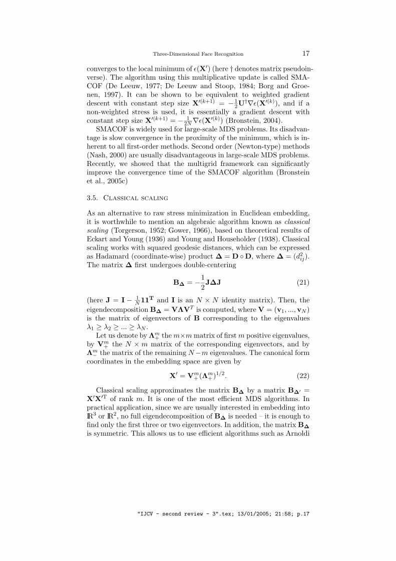
(a) Original surface (b) 3D (c) 2D
Figure 7. Example of embedding into IR3 (b) and into IR2(c).
Remark 1. The assumption of non-degeneracy of the spectrum of B∆
is valid for curved surfaces such as the facial surface.
Proof: See Appendix.
3.8. Canonical forms of facial surfaces
By performing canonization of a facial surface, we create an expression-invariant representation of the face, which can be treated as a rigidobject. We should keep in mind that the embedding error criterionis global, that is, depends on all the geodesic distances. Hence, thecanonical form is influenced by all the samples of the surface. As animplication, it is very important to always crop the same region of theface (though the samples themselves should not necessarily coincide).This is one of the key roles that an appropriate preprocessing plays.
When embedding is performed into IR3, the canonical form can beplotted as a surface. Examples are shown in Figures 7b, 8. Figure 8depicts canonical forms of a subject’s face with different facial expres-sions. It demonstrates that although the facial surface deformations aresubstantial, the deformations of the corresponding canonical forms aremuch smaller.
Embedding of a facial surface into IR2 (Figure 7c) or S2 is a zerocodimension embedding – it produces an intrinsic parametrization ofthe surface. Such embedding can be thought of as “warping” of thefacial texture, yielding a canonical texture (Bronstein et al., 2004a).Canonization in some sense performs a geometry-based registration of2D facial images. That is, in two canonical textures we are able to iden-tify two pixels as belonging to the same point on the 3D facial surface,no matter how the latter is deformed. As the result, 2D appearance-based methods such as eigenfaces can be used to compare canonicaltextures (Bronstein et al., 2004a).
"IJCV - second review - 3".tex; 13/01/2005; 21:58; p.19

20 Michael M. Bronstein, Alexander M. Bronstein, Ron Kimmel
(a) (b) (c) (d) (e)
(f) (g) (h) (i) (j)
Figure 8. Examples of canonical forms (f)-(j) of faces with strong facial expressions(a)-(e).
4. The 3DFACE system
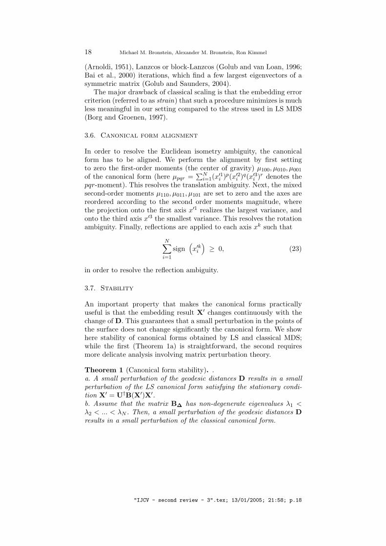
In the Geometric Image Processing laboratory (Department of Com-puter Science, Technion) we designed a prototype 3D face recognitionsystem based on the expression-invariant representation of facial sur-faces. Current 3DFACE system prototype is shown in Figure 9. Itoperates both in one-to-one and one-to-many modes. The 3DFACEsystem runs on a dual AMD Opteron64 workstation under MicrosoftWindows XP. One of the CPUs is dedicated merely to processing andcomputation of the canonical forms; another one handles the graphicaluser interface (GUI) and the visualization.
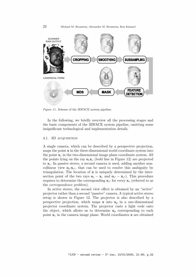
Data processing in the 3DFACE system can be divided into severalstages (Figure 11). First, the subject’s face undergoes a 3D scan, pro-ducing a cloud of points representing the facial surface. The surfaceis then cropped, smoothed and subsampled (subsampling is performedin order to reduce the computational complexity of subsequent stages).Next, a feature detector is applied in order to find a few fiducial points.Next, a geodesic mask is computed around these points. Finally, thefacial surface undergoes canonization using an MDS procedure.
"IJCV - second review - 3".tex; 13/01/2005; 21:58; p.20
Three-Dimensional Face Recognition 21
a
b
c
d
e
Figure 9. The 3DFACE prototype system and its main components: DLP projector(a), digital camera (b), monitor (c), magnetic card reader (d), mounting (e) .
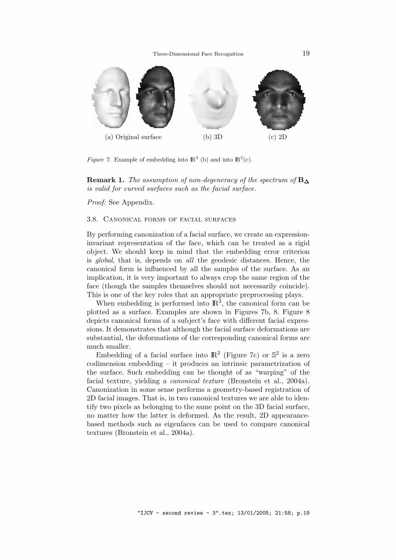
Figure 10. Screenshot from the GUI interface of the 3DFACE system (one-to-manymode), showing successful recognition of one of the authors.
"IJCV - second review - 3".tex; 13/01/2005; 21:58; p.21
22 Michael M. Bronstein, Alexander M. Bronstein, Ron Kimmel
CANONICAL FORM
SCANNER RAW OUTPUT
Figure 11. Scheme of the 3DFACE system pipeline.
In the following, we briefly overview all the processing stages andthe basic components of the 3DFACE system pipeline, omitting someinsignificant technological and implementation details.
4.1. 3D acquisition
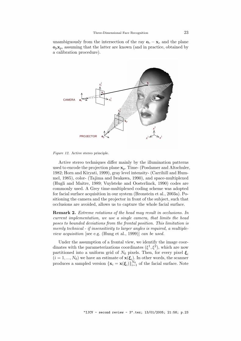
A single camera, which can be described by a perspective projection,maps the point x in the three-dimensional world coordinate system intothe point xc in the two-dimensional image plane coordinate system. Allthe points lying on the ray ocxc (bold line in Figure 12) are projectedto xc. In passive stereo, a second camera is used, adding another non-collinear view oc′xc′ , that can be used to resolve this ambiguity bytriangulation. The location of x is uniquely determined by the inter-section point of the two rays oc − xc and oc′ − xc′). This procedurerequires to determine the corresponding xc′ for every xc (referred to asthe correspondence problem).
In active stereo, the second view effect is obtained by an “active”projector rather than a second “passive” camera. A typical active stereosetup is shown in Figure 12. The projector is also described by aperspective projection, which maps x into xp in a one-dimensionalprojector coordinate system. The projector casts a light code ontothe object, which allows us to determine xp corresponding to eachpoint xc in the camera image plane. World coordinates x are obtained
"IJCV - second review - 3".tex; 13/01/2005; 21:58; p.22
Three-Dimensional Face Recognition 23
unambiguously from the intersection of the ray oc − xc and the planeopxp, assuming that the latter are known (and in practice, obtained bya calibration procedure).
x
xc
xp
x3 x1
x2
x1c
x2c
x1p
oc
op
CAMERA
PROJECTOR
Figure 12. Active stereo principle.
Active stereo techniques differ mainly by the illumination patternsused to encode the projection plane xp. Time- (Posdamer and Altschuler,1982; Horn and Kiryati, 1999), gray level intensity- (Carrihill and Hum-mel, 1985), color- (Tajima and Iwakawa, 1990), and space-multiplexed(Hugli and Maitre, 1989; Vuylsteke and Oosterlinck, 1990) codes arecommonly used. A Grey time-multiplexed coding scheme was adoptedfor facial surface acquisition in our system (Bronstein et al., 2003a). Po-sitioning the camera and the projector in front of the subject, such thatocclusions are avoided, allows us to capture the whole facial surface.
Remark 2. Extreme rotations of the head may result in occlusions. Incurrent implementation, we use a single camera, that limits the headposes to bounded deviations from the frontal position. This limitation ismerely technical - if insensitivity to larger angles is required, a multiple-view acquisition [see e.g. (Hung et al., 1999)] can be used.
Under the assumption of a frontal view, we identify the image coor-dinates with the parameterizations coordinates (ξ1, ξ2), which are nowpartitioned into a uniform grid of N0 pixels. Then, for every pixel ξi
(i = 1, ..., N0) we have an estimate of x(ξi). In other words, the scannerproduces a sampled version xi = x(ξi)N0
i=1 of the facial surface. Note
"IJCV - second review - 3".tex; 13/01/2005; 21:58; p.23
24 Michael M. Bronstein, Alexander M. Bronstein, Ron Kimmel
that though the parameterizations plane is sampled on a regular grid ofpixels, the samples along x1 and x2 are neither necessarily regular noruniform. Specifically, in our implementation, the range data is stored inthree double-precision matrices, each of size 320 × 240, correspondingto the values of x1, x2 and x3 at each pixel. Thereby, the scanner outputis a cloud of N0 = 76.8× 10³ points in 3D.
Reflectance image is also acquired. Assuming Lambertian reflectance,it is possible to estimate the albedo in every pixel (Gheorghiades et al.,2001).
4.2. Cropping
After 3D acquisition, the raw scanner data undergoes several preprocess-ing stages. First, a preliminary cropping is performed, separating thebackground from the facial region and removing problematic pointsin which the reconstruction is inaccurate (the latter usually appearas spikes). A histogram of the depth coordinates is used to roughlyseparate the face from the background. The facial region is definedby a binary 320×240 mask image, whose computation involves severalthresholds: for example, pixels with a high value of the discrete gradientnorm ‖∇x3‖ =
√(∂1x3)2 + (∂2x3)2 are removed as potential spikes.
Morphological operations are then applied to the mask in order toremove non-connected regions and isolate the facial region (which willbe denoted by Ωc) as a single object. Holes inside the facial contour areclosed by interpolation.
4.3. Smoothing
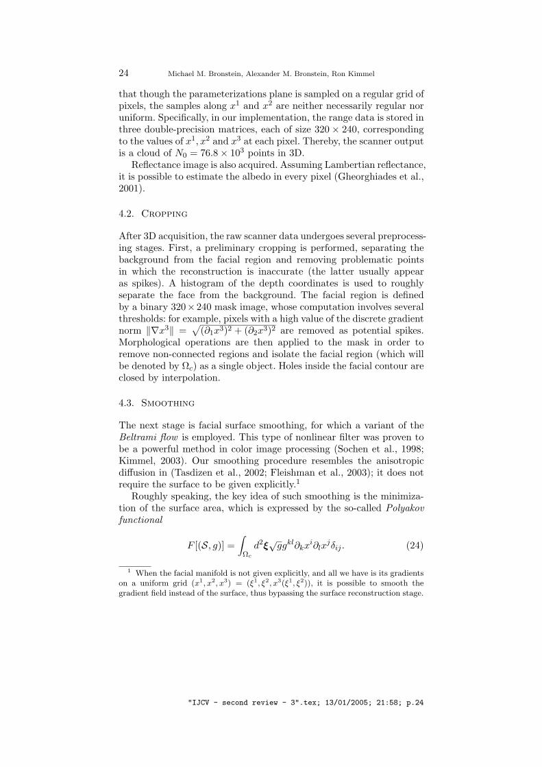
The next stage is facial surface smoothing, for which a variant of theBeltrami flow is employed. This type of nonlinear filter was proven tobe a powerful method in color image processing (Sochen et al., 1998;Kimmel, 2003). Our smoothing procedure resembles the anisotropicdiffusion in (Tasdizen et al., 2002; Fleishman et al., 2003); it does notrequire the surface to be given explicitly.1
Roughly speaking, the key idea of such smoothing is the minimiza-tion of the surface area, which is expressed by the so-called Polyakovfunctional
F [(S, g)] =∫
Ωc
d2ξ√
ggkl∂kxi∂lx
jδij . (24)
1 When the facial manifold is not given explicitly, and all we have is its gradientson a uniform grid (x1, x2, x3) = (ξ1, ξ2, x3(ξ1, ξ2)), it is possible to smooth thegradient field instead of the surface, thus bypassing the surface reconstruction stage.
"IJCV - second review - 3".tex; 13/01/2005; 21:58; p.24
Three-Dimensional Face Recognition 25
(a) Before smoothing
(b) After smoothing
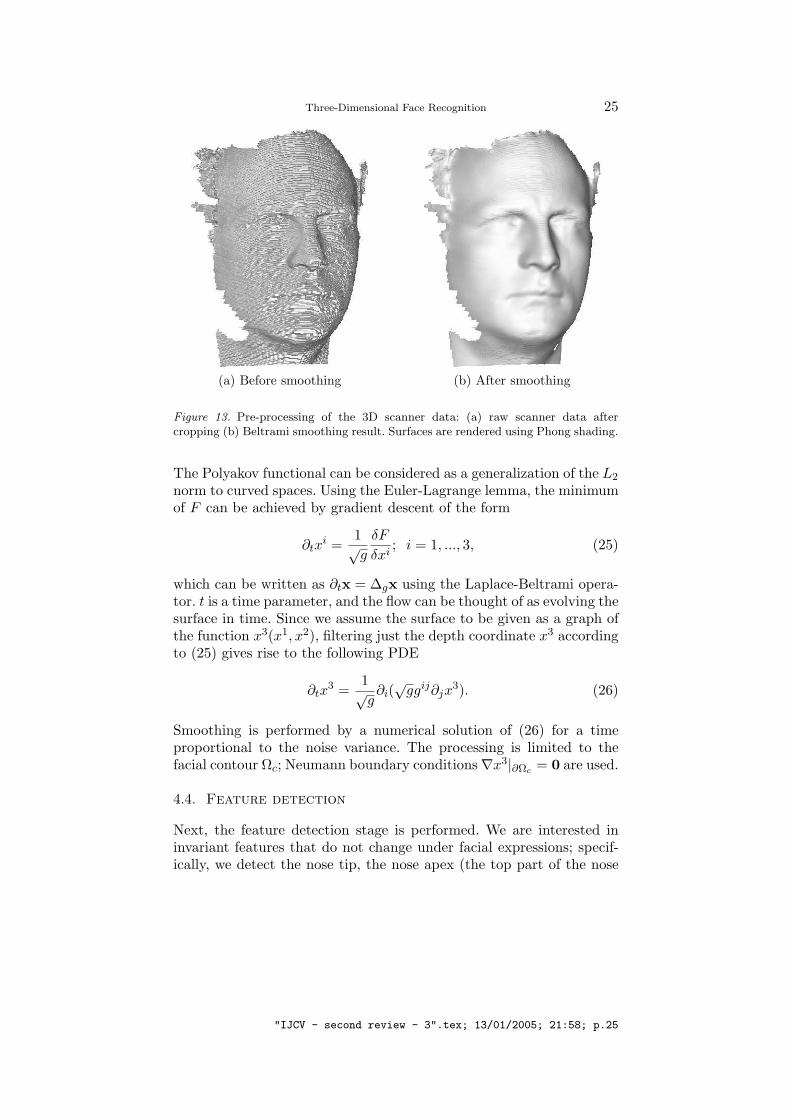
Figure 13. Pre-processing of the 3D scanner data: (a) raw scanner data aftercropping (b) Beltrami smoothing result. Surfaces are rendered using Phong shading.
The Polyakov functional can be considered as a generalization of the L2
norm to curved spaces. Using the Euler-Lagrange lemma, the minimumof F can be achieved by gradient descent of the form
∂txi =
1√g
δF
δxi; i = 1, ..., 3, (25)
which can be written as ∂tx = ∆gx using the Laplace-Beltrami opera-tor. t is a time parameter, and the flow can be thought of as evolving thesurface in time. Since we assume the surface to be given as a graph ofthe function x3(x1, x2), filtering just the depth coordinate x3 accordingto (25) gives rise to the following PDE
∂tx3 =
1√g∂i(√
ggij∂jx3). (26)
Smoothing is performed by a numerical solution of (26) for a timeproportional to the noise variance. The processing is limited to thefacial contour Ωc; Neumann boundary conditions∇x3|∂Ωc = 0 are used.
4.4. Feature detection
Next, the feature detection stage is performed. We are interested ininvariant features that do not change under facial expressions; specif-ically, we detect the nose tip, the nose apex (the top part of the nose
"IJCV - second review - 3".tex; 13/01/2005; 21:58; p.25
26 Michael M. Bronstein, Alexander M. Bronstein, Ron Kimmel
(a) Mean curvature
(b) Gaussian curvature
(c) Candidate points
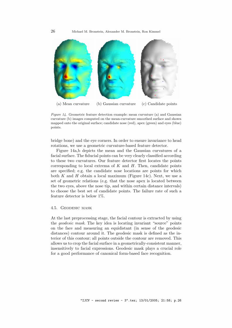
Figure 14. Geometric feature detection example: mean curvature (a) and Gaussiancurvature (b) images computed on the mean-curvature smoothed surface and shownmapped onto the original surface; candidate nose (red), apex (green) and eyes (blue)points.
bridge bone) and the eye corners. In order to ensure invariance to headrotations, we use a geometric curvature-based feature detector.
Figure 14a,b depicts the mean and the Gaussian curvatures of afacial surface. The fiducial points can be very clearly classified accordingto these two curvatures. Our feature detector first locates the pointscorresponding to local extrema of K and H. Then, candidate pointsare specified; e.g. the candidate nose locations are points for whichboth K and H obtain a local maximum (Figure 14c). Next, we use aset of geometric relations (e.g. that the nose apex is located betweenthe two eyes, above the nose tip, and within certain distance intervals)to choose the best set of candidate points. The failure rate of such afeature detector is below 1%.
4.5. Geodesic mask
At the last preprocessing stage, the facial contour is extracted by usingthe geodesic mask. The key idea is locating invariant “source” pointson the face and measuring an equidistant (in sense of the geodesicdistances) contour around it. The geodesic mask is defined as the in-terior of this contour; all points outside the contour are removed. Thisallows us to crop the facial surface in a geometrically-consistent manner,insensitively to facial expressions. Geodesic mask plays a crucial rolefor a good performance of canonical form-based face recognition.
"IJCV - second review - 3".tex; 13/01/2005; 21:58; p.26
Three-Dimensional Face Recognition 27
(a)
(b)
(c)
(d)
(e)
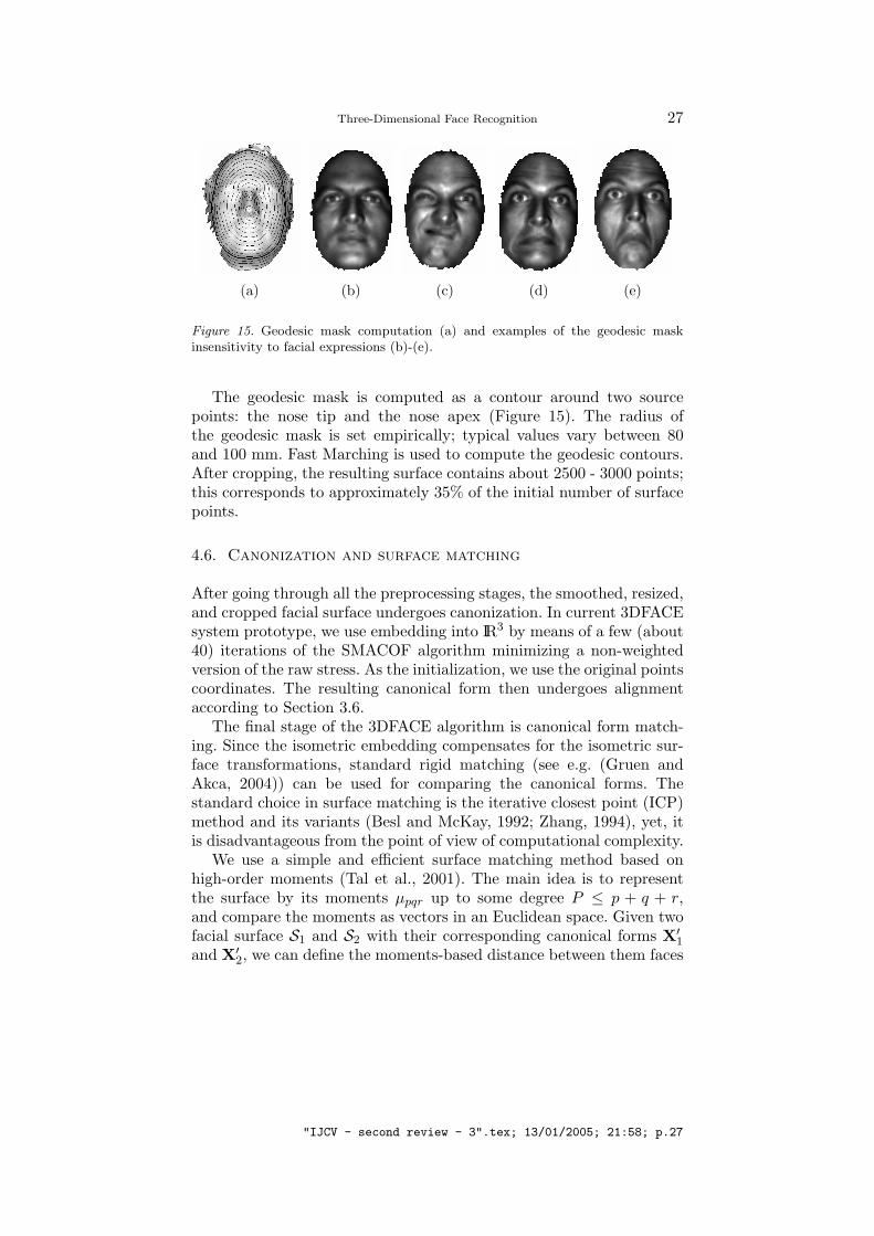
Figure 15. Geodesic mask computation (a) and examples of the geodesic maskinsensitivity to facial expressions (b)-(e).
The geodesic mask is computed as a contour around two sourcepoints: the nose tip and the nose apex (Figure 15). The radius ofthe geodesic mask is set empirically; typical values vary between 80and 100 mm. Fast Marching is used to compute the geodesic contours.After cropping, the resulting surface contains about 2500 - 3000 points;this corresponds to approximately 35% of the initial number of surfacepoints.
4.6. Canonization and surface matching
After going through all the preprocessing stages, the smoothed, resized,and cropped facial surface undergoes canonization. In current 3DFACEsystem prototype, we use embedding into IR3 by means of a few (about40) iterations of the SMACOF algorithm minimizing a non-weightedversion of the raw stress. As the initialization, we use the original pointscoordinates. The resulting canonical form then undergoes alignmentaccording to Section 3.6.
The final stage of the 3DFACE algorithm is canonical form match-ing. Since the isometric embedding compensates for the isometric sur-face transformations, standard rigid matching (see e.g. (Gruen andAkca, 2004)) can be used for comparing the canonical forms. Thestandard choice in surface matching is the iterative closest point (ICP)method and its variants (Besl and McKay, 1992; Zhang, 1994), yet, itis disadvantageous from the point of view of computational complexity.
We use a simple and efficient surface matching method based onhigh-order moments (Tal et al., 2001). The main idea is to representthe surface by its moments µpqr up to some degree P ≤ p + q + r,and compare the moments as vectors in an Euclidean space. Given twofacial surface S1 and S2 with their corresponding canonical forms X′
1
and X′2, we can define the moments-based distance between them faces
"IJCV - second review - 3".tex; 13/01/2005; 21:58; p.27
28 Michael M. Bronstein, Alexander M. Bronstein, Ron Kimmel
asdmom(S1,S2) =
∑
p+q+r≤P
(µpqr(X′
1)− µpqr(X′2)
)2. (27)
In practice, the vectors of moments are those stored in the gallerydatabase and compared to those computed at each enrollment.
4.7. Fusion of 3D and 2D information
In (Bronstein et al., 2003b; Bronstein et al., 2004a) we proposed totreat canonical forms as images, by performing zero-codimension em-bedding into a plane.2 After alignment, both the canonical form andthe flattened albedo are interpolated onto a Cartesian grid, producingtwo images. These images can be compared using standard techniques,such as applying eigendecomposition like in the eigenfaces algorithm.We called the obtained representation eigenforms.
The use of eigenforms has several advantages: First, image compar-ison is simpler than surface comparison, and second, the 2D textureinformation can be incorporated in a natural way. Here, however, wefocus on the 3D geometry, and in the following experiments presentrecognition results based only on the surface geometry, ignoring thetexture.
5. Results
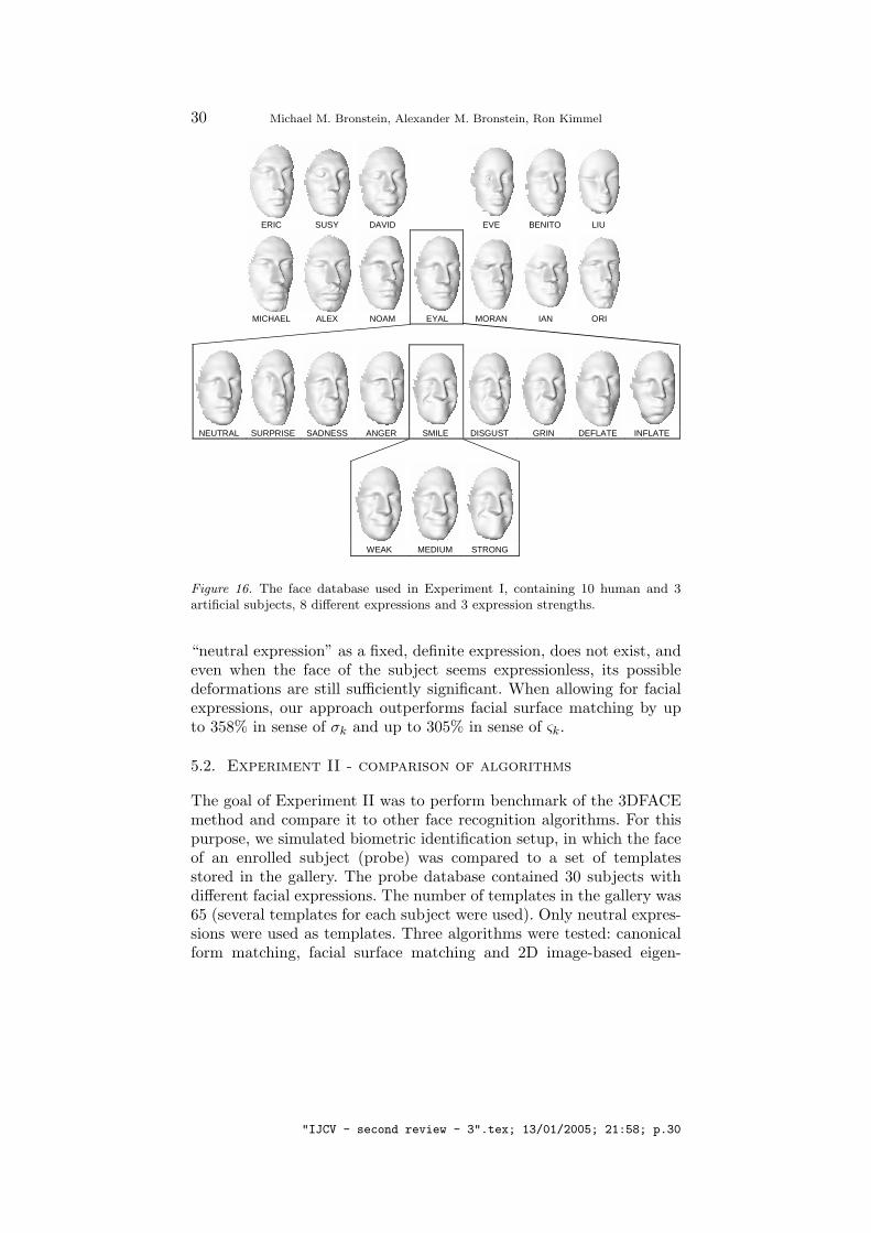
Our experiments were performed on a data set containing 220 faces of30 subjects - 3 artificial (mannequins) and 27 human. Most of the facesappeared in a large number of instances with different facial expres-sions. Facial expressions were classified into 10 groups (smile, anger,etc.) and into 4 strengths (neutral, weak, medium, strong). Neutral ex-pressions are the natural postures of the face, while strong expressionsare extreme postures. Small head rotations (up to about 10 degrees)were allowed. Since the data was acquired in a course of several months,variations in illumination conditions, facial hair, etc. present. SubjectsAlex (blue) and Michael (red) are identical twins, having visually greatsimilarity (see Figure 16).
5.1. Experiment I - Sensitivity to facial expressions
The goal of the first experiment was to demonstrate the differencebetween using original (rigid) facial surfaces and their canonical forms
2 More recently, we studied zero-codimension embedding into S2 (Bronstein et al.,2005a).
"IJCV - second review - 3".tex; 13/01/2005; 21:58; p.28
Three-Dimensional Face Recognition 29
for face recognition under strong facial expressions. Surface matchingbased on moments of degree up to P = 5 (i.e. vectors of dimensionality52), according to (27), was used. In Experiment I, we used a subsetcontaining 10 human and 3 artificial subjects. Each face appeared in anumber of instances (a total of 204 instances), including neutral, weak,medium and strong facial expressions (Figure 16).
Figure 17 visualizes the dissimilarities between faces using classicalscaling. Each face on this plot is represented by a point in IR2. Notethat it is merely a 2D representation of data originally lying in IR52
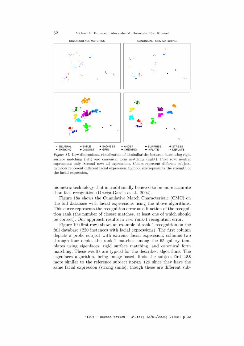
(it captures about 88% of the high-dimensional information). The firstrow depicts the dissimilarities between faces with neutral expressionsonly. The faces of different subjects (marked with different colors)form tight clusters and are easily distinguishable. Canonical surfacematching (left) and rigid surface matching (right) methods produceapproximately the same results.
This idealistic picture breaks down when we allow for facial expres-sions (Figure 17, second row). The clusters corresponding to canonicalsurface matching are much tighter; moreover, we observe that usingoriginal surface matching some clusters (red and blue, dark and lightmagenta, light blue, yellow and green) overlap, which means that a facerecognition algorithm based on rigid surface matching would confusebetween these subjects.
Table I shows the values of the ratio of the maximum inter-clusterto minimum intra-cluster dissimilarity
ςk =maxi,j∈Ck
dmomij
mini/∈Ck,j∈Ckdmom
ij
, (28)
and the ratio of root mean squared (RMS) inter-cluster and intra-cluster dissimilarities
σk =
√√√√2
|Ck|2−|Ck|∑
i,j∈Ck, i>j(dmomij )2
1|Ck|(|C|−|Ck|)
∑i/∈Ck,j∈Ck
(dmomij )2
, (29)
(Ck denotes indexes of k-th subject’s faces, C =⋃
k Ck and dmomij de-
notes the moment-based distance between faces i and j) for rigid andcanonical surface matching. These criteria are convenient being scale-invariant; they measure the tightness of each cluster and its relativedistance from other clusters. Ideally, σk and ςk should tend to zero.
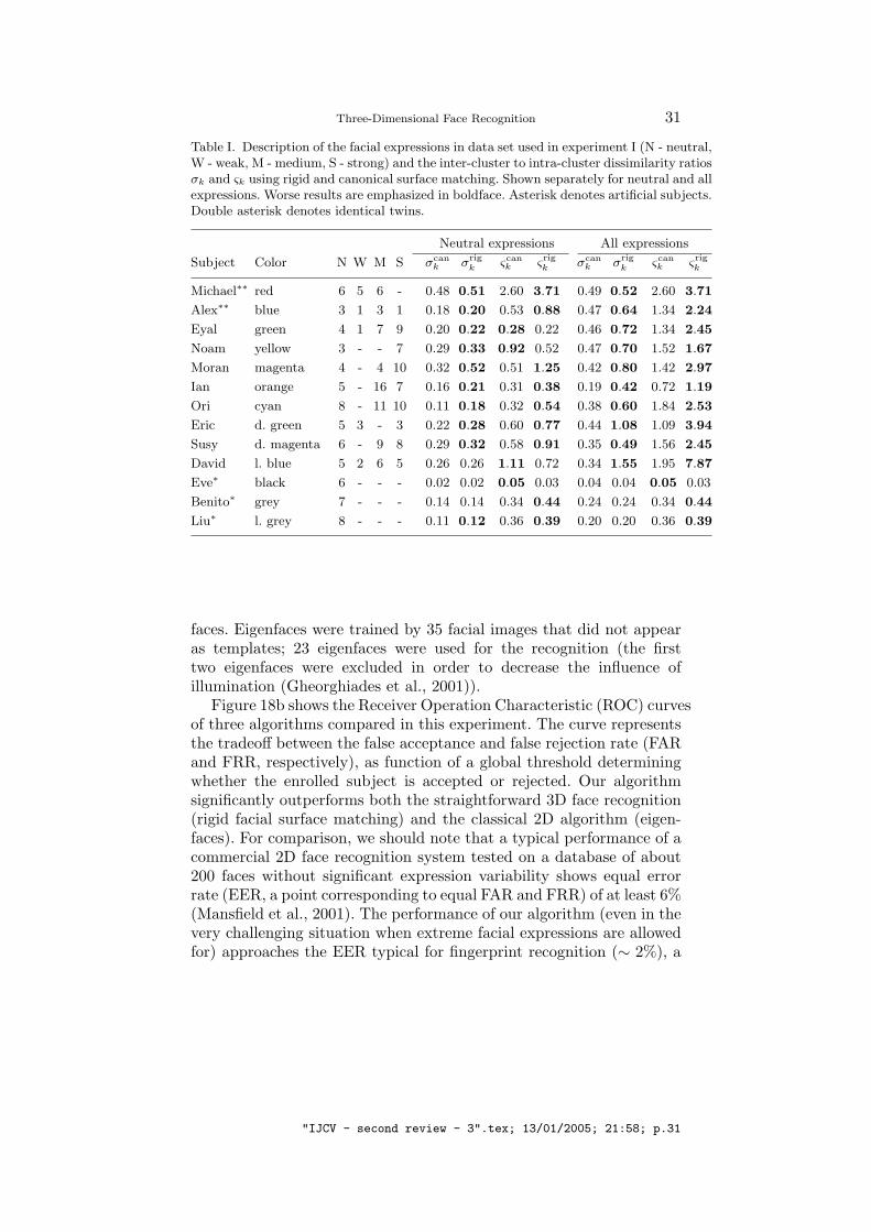
Table I shows the separation quality criterion ςk for rigid and canoni-cal surface matching. When only neutral expressions are used, canonicalform matching slightly outperforms rigid surface matching on mostsubjects. The explanation to the fact that canonical forms are bettereven in case when no large expression variability is present, is that
"IJCV - second review - 3".tex; 13/01/2005; 21:58; p.29
30 Michael M. Bronstein, Alexander M. Bronstein, Ron Kimmel
ERIC SUSY DAVID EVE BENITO LIU
MICHAEL ALEX NOAM EYAL MORAN IAN ORI
NEUTRAL SURPRISE SADNESS ANGER SMILE DISGUST GRIN DEFLATE INFLATE
WEAK MEDIUM STRONG
Figure 16. The face database used in Experiment I, containing 10 human and 3artificial subjects, 8 different expressions and 3 expression strengths.
“neutral expression” as a fixed, definite expression, does not exist, andeven when the face of the subject seems expressionless, its possibledeformations are still sufficiently significant. When allowing for facialexpressions, our approach outperforms facial surface matching by upto 358% in sense of σk and up to 305% in sense of ςk.
5.2. Experiment II - comparison of algorithms
The goal of Experiment II was to perform benchmark of the 3DFACEmethod and compare it to other face recognition algorithms. For thispurpose, we simulated biometric identification setup, in which the faceof an enrolled subject (probe) was compared to a set of templatesstored in the gallery. The probe database contained 30 subjects withdifferent facial expressions. The number of templates in the gallery was65 (several templates for each subject were used). Only neutral expres-sions were used as templates. Three algorithms were tested: canonicalform matching, facial surface matching and 2D image-based eigen-
"IJCV - second review - 3".tex; 13/01/2005; 21:58; p.30
Three-Dimensional Face Recognition 31
Table I. Description of the facial expressions in data set used in experiment I (N - neutral,W - weak, M - medium, S - strong) and the inter-cluster to intra-cluster dissimilarity ratiosσk and ςk using rigid and canonical surface matching. Shown separately for neutral and allexpressions. Worse results are emphasized in boldface. Asterisk denotes artificial subjects.Double asterisk denotes identical twins.
Neutral expressions All expressions
Subject Color N W M S σcank σrig
k ςcank ςrig
k σcank σrig
k ςcank ςrig
k
Michael∗∗ red 6 5 6 - 0.48 0.51 2.60 3.71 0.49 0.52 2.60 3.71
Alex∗∗ blue 3 1 3 1 0.18 0.20 0.53 0.88 0.47 0.64 1.34 2.24
Eyal green 4 1 7 9 0.20 0.22 0.28 0.22 0.46 0.72 1.34 2.45
Noam yellow 3 - - 7 0.29 0.33 0.92 0.52 0.47 0.70 1.52 1.67
Moran magenta 4 - 4 10 0.32 0.52 0.51 1.25 0.42 0.80 1.42 2.97
Ian orange 5 - 16 7 0.16 0.21 0.31 0.38 0.19 0.42 0.72 1.19
Ori cyan 8 - 11 10 0.11 0.18 0.32 0.54 0.38 0.60 1.84 2.53
Eric d. green 5 3 - 3 0.22 0.28 0.60 0.77 0.44 1.08 1.09 3.94
Susy d. magenta 6 - 9 8 0.29 0.32 0.58 0.91 0.35 0.49 1.56 2.45
David l. blue 5 2 6 5 0.26 0.26 1.11 0.72 0.34 1.55 1.95 7.87
Eve∗ black 6 - - - 0.02 0.02 0.05 0.03 0.04 0.04 0.05 0.03
Benito∗ grey 7 - - - 0.14 0.14 0.34 0.44 0.24 0.24 0.34 0.44
Liu∗ l. grey 8 - - - 0.11 0.12 0.36 0.39 0.20 0.20 0.36 0.39
faces. Eigenfaces were trained by 35 facial images that did not appearas templates; 23 eigenfaces were used for the recognition (the firsttwo eigenfaces were excluded in order to decrease the influence ofillumination (Gheorghiades et al., 2001)).
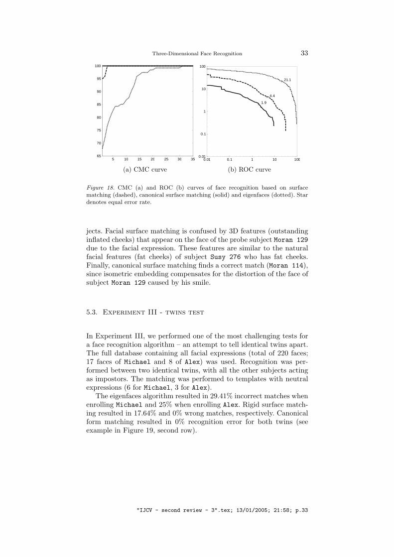
Figure 18b shows the Receiver Operation Characteristic (ROC) curvesof three algorithms compared in this experiment. The curve representsthe tradeoff between the false acceptance and false rejection rate (FARand FRR, respectively), as function of a global threshold determiningwhether the enrolled subject is accepted or rejected. Our algorithmsignificantly outperforms both the straightforward 3D face recognition(rigid facial surface matching) and the classical 2D algorithm (eigen-faces). For comparison, we should note that a typical performance of acommercial 2D face recognition system tested on a database of about200 faces without significant expression variability shows equal errorrate (EER, a point corresponding to equal FAR and FRR) of at least 6%(Mansfield et al., 2001). The performance of our algorithm (even in thevery challenging situation when extreme facial expressions are allowedfor) approaches the EER typical for fingerprint recognition (∼ 2%), a
"IJCV - second review - 3".tex; 13/01/2005; 21:58; p.31
32 Michael M. Bronstein, Alexander M. Bronstein, Ron Kimmel
RIGID SURFACE MATCHING CANONICAL FORM MATCHING
NEUTRAL SMILE SADNESS ANGER SURPRISE STRESS THINKING DISGUST GRIN CHEWING INFLATE DEFLATE
Figure 17. Low-dimensional visualization of dissimilarities between faces using rigidsurface matching (left) and canonical form matching (right). First row: neutralexpressions only. Second row: all expressions. Colors represent different subject.Symbols represent different facial expression. Symbol size represents the strength ofthe facial expression.
biometric technology that is traditionally believed to be more accuratethan face recognition (Ortega-Garcia et al., 2004).
Figure 18a shows the Cumulative Match Characteristic (CMC) onthe full database with facial expressions using the above algorithms.This curve represents the recognition error as a function of the recogni-tion rank (the number of closest matches, at least one of which shouldbe correct). Our approach results in zero rank-1 recognition error.
Figure 19 (first row) shows an example of rank-1 recognition on thefull database (220 instances with facial expressions). The first columndepicts a probe subject with extreme facial expression; columns twothrough four depict the rank-1 matches among the 65 gallery tem-plates using eigenfaces, rigid surface matching, and canonical formmatching. These results are typical for the described algorithms. Theeigenfaces algorithm, being image-based, finds the subject Ori 188more similar to the reference subject Moran 129 since they have thesame facial expression (strong smile), though these are different sub-
"IJCV - second review - 3".tex; 13/01/2005; 21:58; p.32
Three-Dimensional Face Recognition 33
5 10 15 20 25 30 3565
70
75
80
85
90
95
100
(a) CMC curve
0.01 0.1 1 10 1000.01
0.1
1
10
100
1.9
4.4
21.1
(b) ROC curve
Figure 18. CMC (a) and ROC (b) curves of face recognition based on surfacematching (dashed), canonical surface matching (solid) and eigenfaces (dotted). Stardenotes equal error rate.
jects. Facial surface matching is confused by 3D features (outstandinginflated cheeks) that appear on the face of the probe subject Moran 129due to the facial expression. These features are similar to the naturalfacial features (fat cheeks) of subject Susy 276 who has fat cheeks.Finally, canonical surface matching finds a correct match (Moran 114),since isometric embedding compensates for the distortion of the face ofsubject Moran 129 caused by his smile.
5.3. Experiment III - twins test
In Experiment III, we performed one of the most challenging tests fora face recognition algorithm – an attempt to tell identical twins apart.The full database containing all facial expressions (total of 220 faces;17 faces of Michael and 8 of Alex) was used. Recognition was per-formed between two identical twins, with all the other subjects actingas impostors. The matching was performed to templates with neutralexpressions (6 for Michael, 3 for Alex).
The eigenfaces algorithm resulted in 29.41% incorrect matches whenenrolling Michael and 25% when enrolling Alex. Rigid surface match-ing resulted in 17.64% and 0% wrong matches, respectively. Canonicalform matching resulted in 0% recognition error for both twins (seeexample in Figure 19, second row).
"IJCV - second review - 3".tex; 13/01/2005; 21:58; p.33
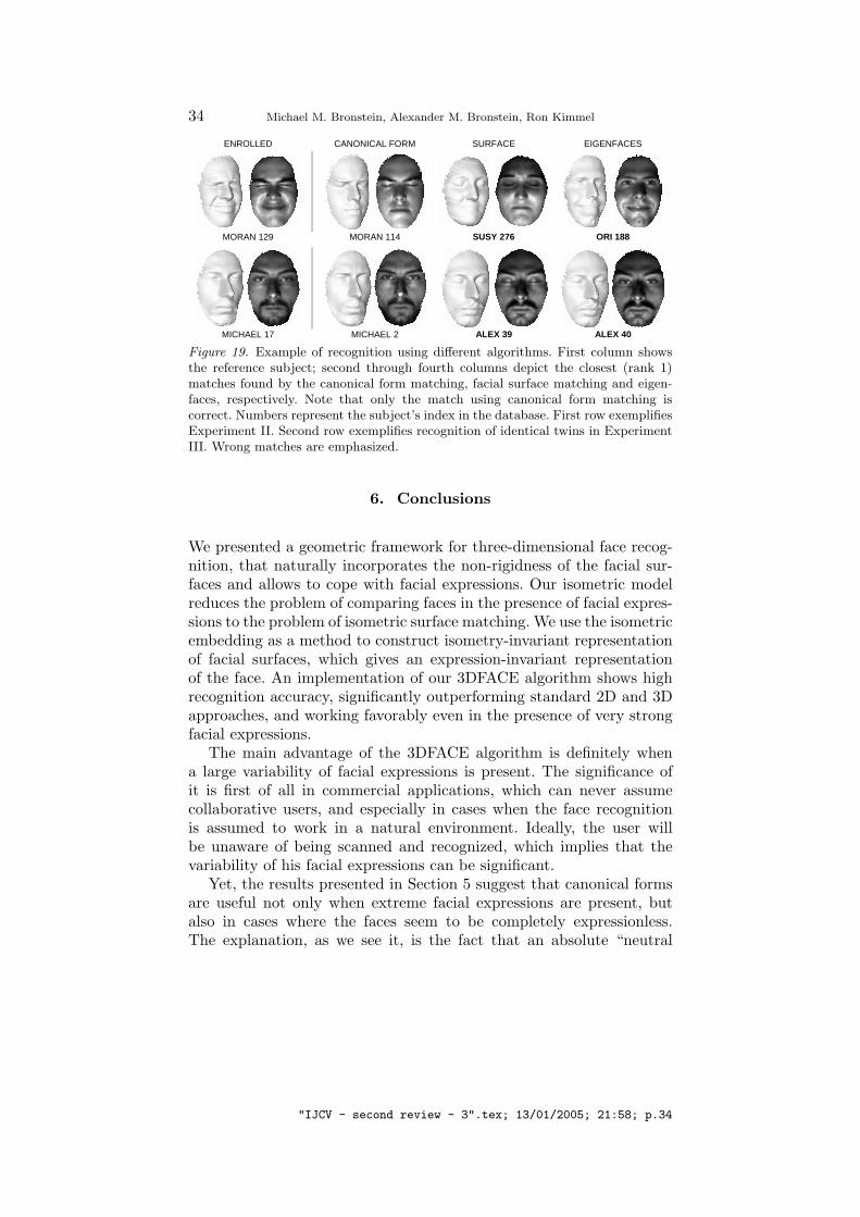
34 Michael M. Bronstein, Alexander M. Bronstein, Ron Kimmel
ENROLLED CANONICAL FORM SURFACE EIGENFACES
MORAN 129 MORAN 114 SUSY 276 ORI 188
MICHAEL 17 MICHAEL 2 ALEX 39 ALEX 40
Figure 19. Example of recognition using different algorithms. First column shows
the reference subject; second through fourth columns depict the closest (rank 1)matches found by the canonical form matching, facial surface matching and eigen-faces, respectively. Note that only the match using canonical form matching iscorrect. Numbers represent the subject’s index in the database. First row exemplifiesExperiment II. Second row exemplifies recognition of identical twins in ExperimentIII. Wrong matches are emphasized.
6. Conclusions
We presented a geometric framework for three-dimensional face recog-nition, that naturally incorporates the non-rigidness of the facial sur-faces and allows to cope with facial expressions. Our isometric modelreduces the problem of comparing faces in the presence of facial expres-sions to the problem of isometric surface matching. We use the isometricembedding as a method to construct isometry-invariant representationof facial surfaces, which gives an expression-invariant representationof the face. An implementation of our 3DFACE algorithm shows highrecognition accuracy, significantly outperforming standard 2D and 3Dapproaches, and working favorably even in the presence of very strongfacial expressions.
The main advantage of the 3DFACE algorithm is definitely whena large variability of facial expressions is present. The significance ofit is first of all in commercial applications, which can never assumecollaborative users, and especially in cases when the face recognitionis assumed to work in a natural environment. Ideally, the user willbe unaware of being scanned and recognized, which implies that thevariability of his facial expressions can be significant.
Yet, the results presented in Section 5 suggest that canonical formsare useful not only when extreme facial expressions are present, butalso in cases where the faces seem to be completely expressionless.The explanation, as we see it, is the fact that an absolute “neutral
"IJCV - second review - 3".tex; 13/01/2005; 21:58; p.34
Three-Dimensional Face Recognition 35
expression” does not exist, such that even when apparently withoutexpressions, the use of canonical forms can still be beneficial.
Besides being insensitive to expressions, canonical forms concealsome other favorable properties. First, the obtained representation isirreversible. Therefore, given the canonical form it is impossible (or atleast very hard) to find the underlying original facial surface. Thus, thecanonical form in some sense “hides” the actual identity of the subjectstored in the gallery. This is significant in commercial systems where thesecurity of the biometric data is an important issue. Secondly, canonicalforms provide an intrinsic parametrization of the facial surface, whichleads to an easy registration of the facial images, and consequently,to an easy fusion of 2D and 3D information. Thirdly, embedding has a“regularization” effect on the facial surface: small local artifacts lead tofluctuation of all geodesic distances. The fluctuations in the canonicalforms are no more local, but rather “spread” among all points of thecanonical form. As a consequence, the canonical forms are less sensitivefor example to acquisition and processing artifacts than the originalsurfaces.
Acknowledgements
We are grateful to David Donoho for pointing us to Ekman’s publi-cations, to Alon Spira for providing his fast marching on parametricmanifolds code; to Michael Elad for helpful discussions; to MichaelSaunders and Gene Golub for advices on efficient eigendecompositionimplementation, to Eyal Gordon for help in data acquisition and to allthe people who agreed to contribute their faces to our 3D face database.
Appendix
Proof of Theorem 1 (Stability of LS canonical forms) .a. For simplicity of the proof, let us assume wij = 1, such that U† =1N J. Consider the stationary condition
X′ = U†B(X′;D)X′ =1N
B(X′;D)X′. (30)
We will write (30) as a nonlinear homogeneous equation in X′ and D:
A(X′;D) = 0. (31)
Now assume that D undergoes a perturbation, such that D = D+ δD,and max |δdij | < ε. The new canonical form will be denoted by X′ =
"IJCV - second review - 3".tex; 13/01/2005; 21:58; p.35
36 Michael M. Bronstein, Alexander M. Bronstein, Ron Kimmel
X′ + δX′. The stationary condition with X′ and D becomes
A(X′ + δX′;D + δD) = 0, (32)
and by the Taylor expansion, neglecting O(ε2) terms and plugging inequation (31), we have
A(X′ + δX′;D + δD) = A(X′;D) +∇X′A(X′;D)δX′ +∇DA(X′;D)δD(33)= ∇X′A(X′;D)δX′ +∇DA(X′;D)δD = 0,
where ∇X′A(X′;D) and ∇DA(X′;D) are four-dimensional tensors de-noting the derivatives of A with respect to X′ and D, respectively.
Let us now write A(X′;D) in coordinate notation:
aji = (A(X′;D))j
i =1N
∑
k
bikx′jk − x′ji . (34)
Plugging in bii = −∑j 6=i bij according to the definition of B, we obtain
aji =
1N
∑
k
bik(x′jk − x′ji )− x′ji . (35)
Differentiating with respect to D and using (19) yields
∂aji
∂di′j′=
1N
∑
k
(x′jk − x′ji )∂bik
∂di′j′(36)
= − 1N
∑
k 6=i
(x′jk − x′ji )δii′δkj′
‖x′i − x′k‖=
− 1N (x′jj′ − x′ji ) δii′
‖x′i−x′j′‖
if k 6= j′
0 otherwise.
The derivatives can be bounded by∣∣∣∣∣
∂aji
∂di′j′
∣∣∣∣∣ ≤1N
maxk 6=l,q
(|x′qk − x′ql |‖x′k − x′l‖2
)=
1N
maxk 6=l
(‖x′k − x′l‖∞‖x′k − x′l‖2
)≡ M1,(37)
and from the regular sampling assumption, it follows that 0 < M1 < ∞.Differentiating with respect to X′ yields
∂aji
∂x′j′
i′=
1N
∑
k
((x′jk − x′ji )
∂bik
∂x′j′
i′+ bik
∂
∂x′j′
i′(x′jk − x′ji )
)− ∂x′ji
∂x′j′
i′(38)
= − 1N
∑
k 6=i
(x′jk − x′ji )δii′dik(x′j
′k − x′j
′i )
‖x′k − x′i‖3− 1
N
∑
k
bikδii′δjj′ +1N
bii′δjj′ − δjj′δii′ .
The derivatives can be bounded by∣∣∣∣∣∂aj
i
∂x′j′
i′
∣∣∣∣∣ ≤ maxk 6=l
‖x′k − x′l‖−1 maxk 6=l
dkl + 2 maxkl
|bkl|+ 1 (39)
≤ maxk 6=l
d′kl
dkl+ 2 max
kl|bkl|+ 1 ≡ M2, (40)
"IJCV - second review - 3".tex; 13/01/2005; 21:58; p.36
Three-Dimensional Face Recognition 37
and since all the quantities are bounded, we have M2 < ∞.Rewriting (34) in coordinate notation and plugging in the bounds
we obtain
0 = aji =
N∑
i′=1
m∑
j′=1
∂aji
∂x′j′
i′δx′j
′i′ +
N∑
i′=1
N∑
j′=1
∂aji
∂di′j′δdi′j′ (41)
≤N∑
i′=1
m∑
j′=1
M1δx′j′i′ +
N∑
i′=1
N∑
j′=1
M2δdi′j′ ,
which leads to a bound on the canonical form perturbation
maxi′j′
|δx′j′i′ | ≤N∑
i′=1
m∑
j′=1
|δx′j′i′ | ≤M2
M1
N∑
i′=1
N∑
j′=1
|δdi′j′ | < M2
M1N2ε (42)
b. Without loss of generality, we assume that the perturbed point is x1,so that d(x1, x1) < ε. Let us denote the perturbed geodesic distancesby dij . By the triangle inequality,
d1j ≤ d(x1, x1) + d(x1,xj) ≤ dij + ε,
whereas, dij for i > 1 remains unchanged.The perturbed geodesic distances matrix D can be written as D =
D + δD, where
δD =
0 ε2 ... εn
ε2...
εN
,
and εi ≤ ε. The perturbed matrix of squared geodesic distances ∆ isgiven by
∆ = ∆ + δ∆ = (D + δD) (D + δD) = ∆ + 2D δD + δD δD.
Neglecting the second-order term δD δD, we obtain δ∆ = 2D δD.The spectral norm of the perturbation of ∆ is∥∥∥∣∣∣∆
∣∣∣∥∥∥2
= ‖|2D δD|‖2 ≤ 2max dij ‖|δD|‖2
= 2 max dij max√
λδDT δDi = 2max dij
√√√√N∑
i=2
ε2i < 2√
Nεmax dij .
"IJCV - second review - 3".tex; 13/01/2005; 21:58; p.37
38 Michael M. Bronstein, Alexander M. Bronstein, Ron Kimmel
The perturbed double-centered matrix B∆ is given by
B∆ = B∆ + δB∆ = −12J(∆ + δ∆)J = B∆ − 1
2Jδ∆J.
Since ‖|J|‖2 = 1, it follows that
‖|δB∆|‖2 ≤ 12‖|δ∆|‖2 <
√Nε max dij .
Eigendecomposition of the perturbed double-centered matrix yieldsB∆ = VΛVT , such that the perturbed canonical form is
X′ = Vm+ (Λm
+ )1/2. (43)
A known result from non-degenerate perturbation theory (Stewartand Sun, 1990) states that
∣∣∣λi − λi
∣∣∣ ≤ ‖|δB∆|‖2 <√
Nεmax dij ,
12
sin 2θ (vi, vi) ≤ ‖|δB∆|‖2
gap(B∆)<
max dij
gap(B∆)
√Nε,
where θ (vi, vi) is the acute angle between the vectors vi and vi, and
gap(B∆) = mini6=j
|λi − λj |, (44)
is the spectral gap of the matrix B∆. The gap(B∆) is non-zero, sincewe assume that B∆ has non-degenerate eigenvalues. Under a smallperturbation, the order of the eigenvalues is preserved, i.e. λ1 ≤ λ2 ≤... ≤ λN ; from Taylor expansion
λ1/2i − λ
1/2i ≈ (λi − λi)
2λi,
and 12 sin 2θ (vi, vi) ≈ θ (vi, vi). Since vi and vi have unit length, it
follows that
‖vi − vi‖2 ≈ sin θ (vi, vi) ≈ θ (vi, vi) <max dij
gap(B∆)
√Nε
Using the triangle inequality and the above relations, the perturba-tion of the canonical form can be bounded by∥∥x′i − x′i
∥∥2 =
∥∥∥λ1/2i vi − λ
1/2i vi
∥∥∥2≤ λ
1/2i ‖vi − vi‖2 +
∣∣∣λ1/2i − λ
1/2i
∣∣∣ ‖vi‖2
≤ λ1/2i ‖vi − vi‖2 +
‖|δB∆|‖2
2λ1/2i
<
(λ
1/2i
gap(B∆)+
1
2λ1/2i
)√Nεmax dij .
"IJCV - second review - 3".tex; 13/01/2005; 21:58; p.38
Three-Dimensional Face Recognition 39
Remark 3. For convenience, we defined our bounds in terms of spec-tral matrix norms. Bounds on other norms can be obtained by usingappropriate norm inequalities.
References
Achermann, B. and H. Bunke: 2000, ‘Classifying range images of human faces withHausdorff distance’. In: Proc. ICPR. pp. 809–813.
Achermann, B., X. Jiang, and H. Bunke: 1997, ‘Face recognition using range images’.In: Int’l Conf. Virtual Systems and Multimedia. pp. 129–136.
Arnoldi, W.: 1951, ‘The Principle of Minimized Iterations in the Solution of theMatrix Eigenvalue Problem’. Quart. Appl. Math. 9, 17–29.
Ashbourn, J.: 2002, Biometrics: advanced identity verification. Springer-Verlag,Berlin Heidelberg New York.
Bai, Z., J. Demmel, J. Dongarra, A. Ruhe, and H. van der Vorst: 2000, Tem-plates for the Solution of Algebraic Eigenvalue Problems: A Practical Guide.Philadelphia: SIAM, third edition. Online: http://www.cs.utk.edu/ don-garra/etemplates/index.html.
Besl, P. J. and N. D. McKay: 1992, ‘A method for registration of 3D shapes’. IEEETrans. PAMI 14, 239–256.
Beumier, C. and M. P. Acheroy: 1988, ‘Automatic face authentication from 3Dsurface’. In: Proc. British Machine Vision Conf. pp. 449–458.
Bledsoe, W. W.: 1966, ‘Man-machine face recognition’. Technical Report PRI 22,Panoramic Research Inc., Palo Alto (CA) USA.
Borg, I. and P. Groenen: 1997, Modern multidimensional scaling - theory andapplications. Springer-Verlag, Berlin Heidelberg New York.
Bowyer, K. W., K. Chang, and P. Flynn: 2004, ‘A survey of 3D and multi-modal3D+2D face recognition’. Dept. of Computer Science and Electrical EngineeringTechnical report, University of Notre Dame.
Bronstein, A. M., M. M. Bronstein, E. Gordon, and R. Kimmel: 2003a, ‘High-resolution structured light range scanner with automatic calibration’. TechnicalReport CIS-2003-06, Dept. of Computer Science, Technion, Israel.
Bronstein, A. M., M. M. Bronstein, E. Gordon, and R. Kimmel: 2004a, ‘Fusion of3D and 2D information in face recognition’. In: Proc. ICIP.
Bronstein, A. M., M. M. Bronstein, and R. Kimmel: 2003b, ‘Expression-invariant3D face recognition’. In: Proc. Audio and Video-based Biometric PersonAuthentication. pp. 62–69.
Bronstein, A. M., M. M. Bronstein, and R. Kimmel: 2005a, ‘Expression-invariantface recognition via spherical embedding’. In: ICIP. submitted.
Bronstein, A. M., M. M. Bronstein, and R. Kimmel: 2005b, ‘On isometric embeddingof facial surfaces into S3’. In: Scale Space. to appear.
Bronstein, A. M., M. M. Bronstein, R. Kimmel, and A. Spira: 2004b, ‘FaceRecognition from Facial Surface Metric’. In: Proc. ECCV. pp. 225–237.
Bronstein, A. M., M. M. Bronstein, R. Kimmel, and I. Yavneh: 2005c, ‘A multigridapproach for multi-dimensional scaling’. In: Multigrid. submitted.
Bronstein, M. M.: 2004, ‘Three-dimensional face recognition’. Master’s thesis,Department of Computer Science, Technion - Israel Institute of Technology.
Bronstein, M. M., A. M. Bronstein, and R. Kimmel: 2004c, ‘Expression-invariantrepresentation of faces’. IEEE Trans. PAMI. submitted.
"IJCV - second review - 3".tex; 13/01/2005; 21:58; p.39
40 Michael M. Bronstein, Alexander M. Bronstein, Ron Kimmel
Brunelli, R. and T. Poggio: 1993, ‘Face recognition: features vs. templates’. IEEETrans. PAMI 15(10), 1042–1053.
Carrihill, B. and R. Hummel: 1985, ‘Experiments with the intensity ratio depthsensor’. Computer Vision, Graphics and Image Processing 32, 337–358.
Cartoux, J. Y., J. T. LaPreste, and M. Richetin: 1989, ‘Face authentication orrecognition by profile extraction from range images’. In: Proc. Workshop onInterpretation of 3D Scenes. pp. 194–199.
Chang, K., K. Bowyer, and P. Flynn: 2003, ‘Face recognition using 2D and 3D facialdata’. In: Proc. Multimodal User Authentication Workshop. pp. 25–32.
Cox, I., J. Ghosn, and P. Yianilos: 1996, ‘Feature-based face recognition usingmixture distance’. In: Proc. CVPR. pp. 209–216.
De Leeuw, J.: 1977, Recent developments in statistics, Chapt. Applications of convexanalysis to multidimensional scaling, pp. 133–145. Amsterdam: North-Holland.
De Leeuw, J. and I. Stoop: 1984, ‘Upper bounds on Kruskal’s stress’. Psychometrika49, 391–402.
Eckart, C. and G. Young: 1936, ‘Approximation of one matrix by another of lowerrank’. Psychometrika 1, 211–218.
Ekman, P.: 1973, Darwin and facial expression; a century of research in review. NewYork: Academic Press.
Elad, A. and R. Kimmel: 2001, ‘Bending invariant representations for surfaces’. In:Proc. CVPR. pp. 168–174.
Elad, A. and R. Kimmel: 2002, Geometric methods in bio-medical image processing,Vol. 2191, Chapt. Spherical flattening of the cortex surface, pp. 77–89. BerlinHeidelberg New York: Springer-Verlag.
Elad, A. and R. Kimmel: 2003, ‘On bending invariant signatures for surfaces’. IEEETrans. PAMI 25(10), 1285–1295.
Fleishman, S., I. Drori, and D. Cohen-Or: 2003, ‘Bilateral Mesh Denoising’. In:Proc. SIGGRAPH. pp. 950–953.
Gauss, C. F.: 1827, ‘Disquisitiones generales circa superficies curva’. Commenta-tiones Societatis RegiæScientiarum Gottingensis Recentiores 6, 99 146.
Georghiades, A. S., P. N. Belhumeur, and D. Kriegman: 1998, ‘Illumination conesfor recognition under variable lighting: faces’. In: Proc. CVPR. pp. 52–58.
Gheorghiades, A. S., P. N. Belhumeur, and D. J. Kriegman: 2001, ‘From few tomany: illumination cone models for face recognition under variable lighting andpose’. IEEE Trans. PAMI 23(6), 643–660.
Goldstein, A., L. Harmon, and A. Lesk: 1971, ‘Identification of human faces’. Proc.IEEE 59(5), 748–760.
Golub, G. H. and M. Saunders: 2004, ‘Personal communication’.Golub, G. H. and C. F. van Loan: 1996, Matrix computations. The John Hopkins
University Press, third edition.Gordon, G.: 1992, ‘Face recognition based on depth and curvature features’. In:
Proc. CVPR. pp. 108–110.Gordon, G.: 1997, ‘Face recognition from frontal and profile views’. In: Proc. Int’l
Workshop on Face and Gesture Recognition. pp. 47–52.Gower, J. C.: 1966, ‘Some distance properties of latent root and vector methods
used in multivariate analysis’. Biometrika 53, 325–338.Grossman, R., N. Kiryati, and R. Kimmel: 2002, ‘Computational surface flattening:
a voxel-based approach’. IEEE Trans. PAMI 24(4), 433–441.Gruen, A. and D. Akca: 2004, ‘Least Squares 3D Surface Matching’. In: Proc. ISPRS
Working Group V/1 Panoramic Photogrammetry Workshop. pp. 19–22.
"IJCV - second review - 3".tex; 13/01/2005; 21:58; p.40
Three-Dimensional Face Recognition 41
Gudmundsson, S.: 2004, ‘An Introduction to Riemanniangeometry (lecture notes)’. Online. Available athttp://www.matematik.lu.se/matematiklu/personal/sigma/Riemann.pdf.
Guttman, L.: 1968, ‘A general nonmetric technique for finding the smallestcoordinate space for a configuration of points’. Psychometrika pp. 469–506.
Hallinan, P.: 1994, ‘A low-dimensional representation of human faces for arbitrarylighting conditions’. In: Proc. CVPR. pp. 995–999.
Hesher, C., A. Srivastava, and G. Erlebacher: 2003, ‘A novel technique for face recog-nition using range images’. In: Int’l Symp. Signal Processing and Its Applications,Vol. 2. pp. 201–204.
Horn, E. and N. Kiryati: 1999, ‘Toward optimal structured light patterns’. Imageand Vision Computing 17(2), 87–97.
Huang, J., V. Blanz, and V. Heisele: 2002, ‘Face recognition using component-basedSVM classification and morphable models’. SVM pp. 334–341.
Hugli, H. and G. Maitre: 1989, ‘Generation and use of color pseudo random sequencesfor coding structured light in active ranging’. In: Proc. Industrial Inspection, Vol.1010. pp. 75–82.
Hung, Y.-P., C.-S. Chen, I.-B. Hsieh, and C.-S. Fuh: 1999, ‘Reconstruction ofcomplete 3D object model from multiview range images’. In: Proc. SPIE Int’lSymposium on Electronic Imaging. pp. 138–145.
Kanade, T.: 1973, ‘Picture processing by computer complex and recognition ofhuman faces’. Technical report, Kyoto University, Dept. of Information Science.
Kimmel, R.: 2003, Numerical geometry of images. Berlin Heidelberg New York:Springer-Verlag.
Kimmel, R. and J. A. Sethian: 1998, ‘Computing geodesic on manifolds’. In: Proc.US National Academy of Science, Vol. 95. pp. 8431–8435.
Kreyszig, E.: 1991, Differential geometry. New York: Dover Publications Inc.Lee, J. C. and E. Milios: 1990, ‘Matching range images of human faces’. In: Proc.
ICCV. pp. 722–726.Linial, N., E. London, and Y. Rabinovich: 1995, ‘The geometry of graphs and some
its algorithmic applications’. Combinatorica 15, 333–344.Mansfield, T., G. Kelly, D. Chandler, and J. Kane: 2001, ‘Biometric product testing
final report’. Technical report, Centre for Mathematics and Scientific Computing,National Physical Laboratory, UK.
Mavridis, N., F. Tsalakanidou, D. Pantazis, S. Malassiotis, and M. G. Strintzis: 2001,‘The HISCORE face recognition application: Affordable desktop face recogni-tion based on a novel 3D camera’. In: Proc. Int’l Conf. Augmented VirtualEnvironments and 3D Imaging. pp. 157–160.
Medioni, G. and R. Waupotitsch: 2003, ‘Face recognition and modeling in 3D’. In:Proc. AMFG. pp. 232–233.
Memoli, F. and G. Sapiro: 2001, ‘Fast computation of weighted distance functionsand geodesics on implicit hyper-surfaces’. Journal of Computational Physics173(2), 730–764.
Nagamine, T., T. Uemura, and I. Masuda: 1992, ‘3D facial image analysis for humanidentification’. In: Proc. ICPR. pp. 324–327.
Nash, S.: 2000, ‘A Multigrid Approach to Discretized Optimization Problems’.Journal of Optimization Methods and Software 14, 99–116.
Ortega-Garcia, J., J. Bigun, D. Reynolds, and J. Gonzalez-Rodriguez: 2004, ‘Au-thentication gets personal with biometrics’. IEEE Signal Processing magazine21(2), 50–62.
"IJCV - second review - 3".tex; 13/01/2005; 21:58; p.41
42 Michael M. Bronstein, Alexander M. Bronstein, Ron Kimmel
Pentland, A., B. Moghaddam, and T. Starner: 1994, ‘View-based and modulareigenspaces for face recognition’. In: Proc. CVPR. pp. 84–91.
Phillips, P. J., P. Grother, R. J. Michaels, D. M. Blackburn, E. Tabassi, and J. Bone:2003, ‘FRVT 2002: overview and summary’. Online. Available at www.frvt.org.
Posdamer, J. L. and M. D. Altschuler: 1982, ‘Surface measurement by spaceencodedprojected beam systems’. Computer Graphics and Image Processing 18(1), 1–17.
Schwartz, E. L., A. Shaw, and E. Wolfson: 1989, ‘A numerical solution to the gen-eralized mapmaker’s problem: flattening nonconvex polyhedral surfaces’. IEEETrans. PAMI 11, 1005–1008.
Sethian, J. A.: 1996, ‘A review of the theory, algorithms, and applications of levelset method for propagating surfaces’. Acta numerica pp. 309–395.
Sirovich, L. and M. Kirby: 1987, ‘Low-dimensional procedure for the characterizationof human faces’. JOSA A 2, 519–524.
Sochen, N., R. Kimmel, and R. Malladi: 1998, ‘A general framework for low levelvision’. IEEE Trans. Image Proc. 7(3), 310–318.
Spira, A. and R. Kimmel: 2003, ‘An efficient solution to the eikonal equation onparametric manifolds’. In: INTERPHASE 2003 meeting.
Spira, A. and R. Kimmel: 2004, ‘An Efficient Solution to the Eikonal Equation onParametric Manifolds’. Interfaces and Free Boundaries 6(3), 315–327.
Stewart, G. W. and J.-G. Sun: 1990, Matrix perturbation theory. Academic Press.Tajima, J. and M. Iwakawa: 1990, ‘3D data acquisition by rainbow range finder’. In:
Proc. Int’l Conf. Pattern Recognition. pp. 309–313.Tal, A., M. Elad, and S. Ar: 2001, ‘Content based retrieval of VRML objects -
an iterative and interactive approach’. In: Proc. Eurographics Workshop onMultimedia.
Tanaka, H. T., M. Ikeda, and H. Chiaki: 1998, ‘Curvature-based face surface recogni-tion using spherical correlation principal directions for curved object recognition’.In: Proc. Int’l Conf. Automated Face and Gesture Recognition. pp. 372–377.
Tasdizen, T., R. Whitaker, P. Burchard, and S. Osher: 2002, ‘Geometric sur-face smoothing via anisotropic diffusion of normals’. In: Proc. IEEE Conf.Visualization. pp. 125–132.
Torgerson, W. S.: 1952, ‘Multidimensional scaling I - Theory and methods’.Psychometrika 17, 401–419.
Tsalakanidou, F., D. Tzocaras, and M. Strintzis: 2003, ‘Use of depth and coloureigenfaces for face recognition’. Pattern Recognition Letters 24, 1427–1435.
Tsitsiklis, J. N.: 1988, ‘Efficient algorithms for globally optimal trajectories’. IEEETrans. Automatic Control 40(9), 1528–1538.
Turk, M. and A. Pentland: 1991, ‘Face recognition using eigenfaces’. In: Proc. CVPR.pp. 586–591.
Vuylsteke, P. and A. Oosterlinck: 1990, ‘Range image acquisition with a singlebinaryencoded light pattern’. IEEE Trans. PAMI 12(2), 148–163.
Walter, J. and H. Ritter: 2002, ‘On Interactive Visualization of High-DimensionalData Using the Hyperbolic Plane’. In: Proc. ACM SIGKDD Int. Conf.Knowledge Discovery and Data Mining. pp. 123–131.
Wang, Y., C. Chua, and Y. Ho: 2002, ‘Facial feature detection and face recognitionfrom 2D and 3D images’. Pattern Recognition Letters 23, 1191–1202.
Wiskott, L.: 1995, Labeled graphs and dynamic link matching for face recognitionand scene analysis, No. 53 in Reihe Physik. Thun - Frankfurt am Main: VerlagHarri Deutsch. PhD thesis.
Wiskott, L., J. Fellous, N. Kruger, and C. von der Malsburg: 1997, ‘Face recognitionby elastic bunch graph matching’. IEEE Trans. PAMI 19(7), 733–742.
"IJCV - second review - 3".tex; 13/01/2005; 21:58; p.42

Three-Dimensional Face Recognition 43
Young, G. and A. S. Householder: 1938, ‘Discussion of a set of point in terms oftheir mutual distances’. Psychometrika 3, 19–22.
Zhang, Z. Y.: 1994, ‘terative point matching for registration of free-form curves andsurfaces’. IJCV 13, 119–152.
Zigelman, G., R. Kimmel, and N. Kiryati: 2002, ‘Texture mapping using surface flat-tening via multi-dimensional scaling’. IEEE Trans. Visualization and computergraphics 9(2), 198–207.
"IJCV - second review - 3".tex; 13/01/2005; 21:58; p.43

"IJCV - second review - 3".tex; 13/01/2005; 21:58; p.44