J . Fluid Mech. (1987), ~ 1 0 1 . 174, p p . 187-208

Printed in Great Britain 187

Three-dimensional instabilities of nonlinear gravity-capillary waves

By JUN ZHANG AND W. K. MELVILLE Massachusetts Institute of Technology, Cambridge, MA 02139, USA

(Received 12 September 1985 and in revised form 28 May 1986)

Linear three-dimensional instabilities of nonlinear two-dimensional uniform gravity- capillary waves are studied using numerical methods. The eigenvalue system for the stability problem is generated using a Galerkin method and differs in detail from techniques used to study the stability of pure gravity waves (McLean 1982) and pure capillary waves (Chen & Saffman 1985). It is found that instabilities develop in the neighbourhood of the linear (triad, quartet and quintet) resonance curves. Further, both sum and difference triad ressonances are unstable for sufficiently steep waves in consequence of which Hasselmann’s (1967) theorem is restricted to weakly nonlinear waves. The appearance of a superharmonic two-dimensional instability and bifurcation to three-dimensional waves are noted.

1. Introduction Considerable progress has been made on the stability of uniform deep-water waves

in the last two decades. For weakly nonlinear gravity waves, perturbation methods have shown that the uniform wavetrain is unstable to modulation (long-wavelength) perturbations (Lighthill 1965; Benjamin & Feir 1967). This is the well-known Benjamin-Feir instability, which results from a quartet resonance. Weakly nonlinear gravity-capillary waves (GCWs), are unstable not only to the above quartet resonance, but also to a (sum) triad resonance. Using perturbation methods, Benney (1976) studied the triad interactions of GCWs in deep water and Djordjevic & Redekopp (1977) considered finite-depth effects. Triad instabilities of weakly non- linear deep-water GCWs have been studied in some quantitative detail by the present authors (Zhang & Melville 1986). That study confirmed Hasselmann’s theorem (Hasselmann 1967) for weakly nonlinear GCWs and provided quantitative predictions for testing the numerical procedures of this paper.

In recent years, a number of innovative numerical schemes for studying the instabilities of finite-amplitude uniform waves have been developed. These schemes are all based on the numerical calculation of waves of finite amplitude. This was first done for gravity waves (Schwartz 1974; Cokelet 1977), and more recently for GCWs (Hogan 1981, 1982). A numerical scheme was developed by Longuet-Higgins (1978a, b ) to investigate the stability of finite-amplitude gravity waves in deep water, but the analysis was confined to two-dimensional perturbations. Instability to three-dimensional perturbations was examined by McLean et al. (1981) and McLean (1982). It was shown that three-dimensional instabilities exist for all wavelengths and are dominant when the wave is sufficiently steep. The same numerical scheme was recently used to investigate the instabilities of pure capillary waves in deep water (Chen & Saffman 1985).

7 FLM 174

188 J . Zhang and W . K. Melville

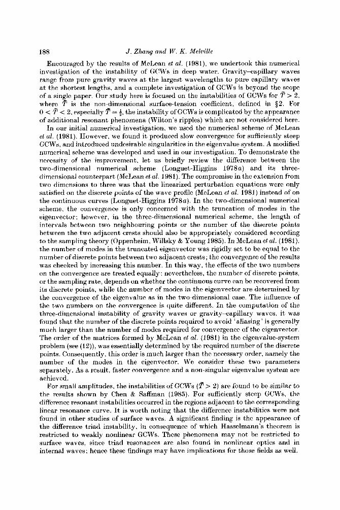
Encouraged by the results of McLean et al. (1981), we undertook this numerical investigation of the instability of GCWs in deep water. Gravity-capillary waves range from pure gravity waves at the largest wavelengths to pure capillary waves a t the shortest lengths, and a complete investigation of GCWs is beyond the scope of a single paper. Our study here is focused on the instabilities of GCWs for p > 2 , where p is the non-dimensional surface-tension coefficient, defined in $2. For 0 < p < 2, especially p = +, the instability of GCWs is complicated by the appearance of additional resonant phenomena (Wilton’s ripples) which are not considered here.

In our initial numerical investigation, we used the numerical scheme of McLean et al. (1981). However, we found it produced slow convergence for sufficiently steep GCWs, and introduced undesirable singularities in the eigenvalue system. A modified numerical scheme was developed and used in our investigation. To demonstrate the necessity of the improvement, let us briefly review the difference between the two-dimensional numerical scheme (Longuet-Higgins 1 9 7 8 ~ ) and its three- dimensional counterpart (McLean et al. 1981). The compromise in the extension from two dimensions to three was that the linearized perturbation equations were only satisfied on the discrete points of the wave profile (McLean et al. 1981) instead of on the continuous curves (Longuet-Higgins 19784. I n the two-dimensional numerical scheme, the convergence is only concerned with the truncation of modes in the eigenvector ; however, in the three-dimensional numerical scheme, the length of intervals between two neighbouring points or the number of the discrete points between the two adjacent crests should also be appropriately considered according to the sampling theory (Oppenheim, Willsky & Young 1985). In McLean et ul. (1981), the number of modes in the truncated eigenvector was rigidly set to be equal to the number of discrete points between two adjacent crests; the convergence of the results was checked by increasing this number. I n this way, the effects of the two numbers on the convergence are treated equally ; nevertheless, the number of discrete points, or the sampling rate, depends on whether the continuous curve can be recovered from its discrete points, while the number of modes in the eigenvector are determined by the convergence of the eigenvalue as in the two-dimensional case. The influence of the two numbers on the convergence is quite different. I n the computation of the three-dimensional instability of gravity waves or gravity-capillary waves, i t was found that the number of the discrete points required t o avoid ‘aliasing’ is generally much larger than the number of modes required for convergence of the eigenvector. The order of the matrices formed by McLean et al. (1981) in the eigenvalue-system problem (see (12)), was essentially determined by the required number of the discrete points. Consequently, this order is much larger than the necessary order, namely the number of the modes in the eigenvector. We consider these two parameters separately. As a result, faster convergence and a non-singular eigenvalue system are achieved.

For small amplitudes, the instabilities of GCWs ( p > 2) are found to be similar to the results shown by Chen & Saffman (1985). For sufficiently steep GCWs, the difference resonant instabilities occurred in the regions adjacent to the corresponding linear resonance curve. It is worth noting that the difference instabilities were not found in other studies of surface waves. A significant finding is the appearance of the difference triad instability, in consequence of which Hasselmann’s theorem is restricted to weakly nonlinear GCWs. These phenomena may not be restricted to surface waves, since triad resonances are also found in nonlinear optics and in internal waves; hence these findings may have implications for those fields as well.

Instabilities of nonlinear gravity-capillary waves 189

2. Formulation The equations governing surface GCWs on an irrotational, inviscid, homogeneous

fluid of infinite depth in a frame moving with the speed c of the unperturbed wave are

vz(b = 0, - o o < z < y , (1)

9 N -cx, Z C - W , (2)

J = “1 + 7 3 ryy - 27,7?/ rzl/ + (1 + 7;) 7,,1(1+ 7: + 7;1-f7 (4) where g, T and p are the gravitational acceleration, surface-tension coefficient and density respectively. The velocity potential is denoted by $(x, y, z, t ) , and ~ ( x , y, t ) is the free-surface displacement. The sum of the principal curvatures of the surface is denoted by J . The wave is assumed to move in the positive x-direction, and the z-axis is positive upwards.

For two-dimensional uniform periodic GCWs, the above equations are independent of time and it is convenient to use the velocity potential $ ( x , z ) and the stream function @(x, z ) as independent variables. Then, following Stokes (1880), the spatial coordinates are given by

( 5 )

5 = -+ 9 x “ ‘ a 2 en$./c sin c n

at the surface @ = 0, and $4- 00 as 2.1 - a. The Fourier coefficients a,, and the phase velocity c, are functions of the non-dimensional surface-tension coefficient p( = k2T/pg) and wave steepness ka, where a is the wave amplitude (half the peak-to-trough height) and k is the wave number. The coefficients an and hence ~ ( x ) may be determined to great accuracy by numerical methods (Hogan 1980).

Following McLean (1982), we consider the stability of two-dimensional steady GCWs subject to arbitrary infinitesimal three-dimensional perturbations. The velocity potential and surface displacement are then given by

(6) 1 7(x, y> t ) = 7 ( 4 + TI (%, y, %

9@3 y, z , t ) = a x , 2) + 9’(x, y, 2, t ) , where, the overbar and prime denote the two-dimensional steady waves and the perturbation respectively.

Substituting (6) into (3) , linearizing the perturbation on the surface of the two-dimensional steady wave, and subtracting the steady solution, we obtain

VqY = 0, -oo < 2 < ?(x), \

& + O , z&-Co ,

9; + 7’ +7,& + $, 9; +7, ?,, 7’+?, ,, 7’ - m 1 + 7:riIl;y + (1 +73-t 7 ; x

rl+7,,r,r‘+,r~+Ts9~-?,,7‘-9: = 0, = 7 ( 4 .

(7) 2 -a- -

--3(1+7,) ~7~,7,7’J = 0, = ~ ( x )

7-2

190 J . Zhang and W . K . Mehille

Without loss of generality, we have set k = 1 and g = 1 . The terms with an overbar may be obtained from the numerical solution of the steady problem by using the Chauchy-Rieman relation.

The three-dimensional perturbation in the moving frame is of the form

m 1 (8)

7’ = exp{i[px+qy]-c~t) X d, exp(inr)+*,

4‘ = exp {i[pz+ qy] - c ~ t ) X

n=-m

m

b , exp (inz) exp {z[(p + n)2 + q2]i} + * n---oo

Where * represents the complex-conjugate. The coefficients b , and d, are to be determined, and v is the frequency of the perturbation relative to the two-dimensional steady, periodic wave. The perturbation wavenumbers p and q are arbitrary real numbers; however, there is a degeneracy in the choice of p . From (8), p may be changed by an arbitrary integer m without modifying the physical eigenfunction ; the only thing that changes is the labelling p + p + m , d,+d,+,, b,+b,+,, - cc < n < 00. A change of the sign of q, is equivalent to the change of direction of the y-axis ; nevertheless the physical eigenfunction remains invariant. Therefore, the instability region of GCWs on the @,q)-plane is symmetric about the p-axis. Furthermore, the physical eigenfunction remains unchanged if the sign of p is changed, for we may keep the physical eigenfunction unchanged by exchanging its complex-conjugate terms and changing the sign of q and -q owing to the symmetry about the p-axis. Based on the above analysis, only positive p and q are considered in this paper.

3. Linear resonant condition

wave has zero amplitude. The eigenvalue is given by Substituting (8) into (7), we may consider the special case in which the unperturbed

~2 = - @ + n ) ( ~ + T ) i f w , , ( 9 4

U, = [ ( p +n)2 + q2]! {I + T[@ + n)2 + q2])4 (9b)

where U, is the positive linear frequency of the eigenfunction with the wavenumbers (p + n, q ) in the stationary coordinates. The f signs in (9a) represent the direction of propagation of the disturbance relative to the unperturbed wave.

As shown in both the pure-gravity-wave and the pure-capillary-wave cases, it is expected that weakly nonlinear GCWs are unstable to disturbances with wavenumber (n, +p, q), (n2 +p, q), whose eigenvalues for zero-amplitude GCWs are equal:

fl&(P, q) = a$*@o, q), (10)

( 1 1 4

w 1 f w 2 = NU,, (1lb)

This equation is equivalent to the linear resonant condition in the stationary coordinates : klfk2 = Nk,,

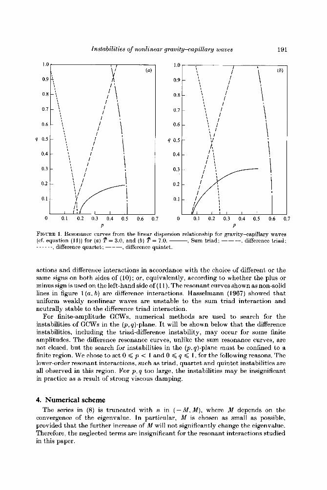
where kj is the direction of propagation of the wave and wi > 0 as given in (9b), and the subscript 0 denotes the unperturbed wave; N = 1 , 2 , 3 refer to triad, quartet and quintet interactions respectively. Figure 1 (a, b) shows the linear resonance curves for triad, quartet, quintet interaction for T = 3.0 and 7.0 respectively.

Following Hasselmann (1967), the instabilities may be classified into sum inter-

Instabilities of nonlinear gruvity-capillary waves 191

1 .o

0.9

0.8

0.7

0.6

4 0.5

0.4

0.3

0.2

0.1

0 0.1 0.2 0.3 0.4 0.5 0.6 0.7

P

1 .o

0.9 -

0.8 -

0.7 -

0.6 -

4 0.5 -

0.4 -

0.3 -

0.2 -

0.1 - I I I

I l l I I

0 0.1 0.2 0.3 0.4 0.5 0.6 0.7 P

FIQURE 1 . Resonance curves from the linear dispersion relationship for gravity-capillary waves (cf. equation (11)) for (a) = 7.0. - , Sum triad : - --, difference triad ; _ _ _ _ _ _ , difference quartet; ---, difference quintet.

= 3.0, and (b)

actions and difference interactions in accordance with the choice of different or the same signs on both sides of (10); or, equivalently, according to whether the plus or minus sign is used on the left-hand side of (1 1 ) . The resonant curves shown as non-solid lines in figure 1 (u, b ) are difference interactions. Hasselmann (1967) showed that uniform weakly nonlinear waves are unstable to the sum triad interaction and neutrally stable to the difference triad interaction.

For finite-amplitude GCWs, numerical methods are used to search for the instabilities of GCWs in the (p, 9)-plane. It will be shown below that the difference instabilities, including the triad-difference instability, may occur for some finite amplitudes. The difference resonance curves, unlike the sum resonance curves, are not closed, but the search for instabilities in the (p,p)-plane must be confined to a finite region. We chose to set 0 < p < 1 and 0 < q < 1 , for the following reasons. The lower-order resonant interactions, such as triad, quartet and quintet instabilities are all observed in this region. For p, q too large, the instabilities may be insignificant in practice as a result of strong viscous damping.

4. Numerical scheme The series in (8) is truncated with n in ( - M , M ) , where M depends on the

convergence of the eigenvalue. I n particular, M is chosen as small as possible, provided that the further increase of M will not significantly change the eigenvalue. Therefore, the neglected terms are insignificant for the resonant interactions studied in this paper.

192 J . Zhang and W. K. Melville

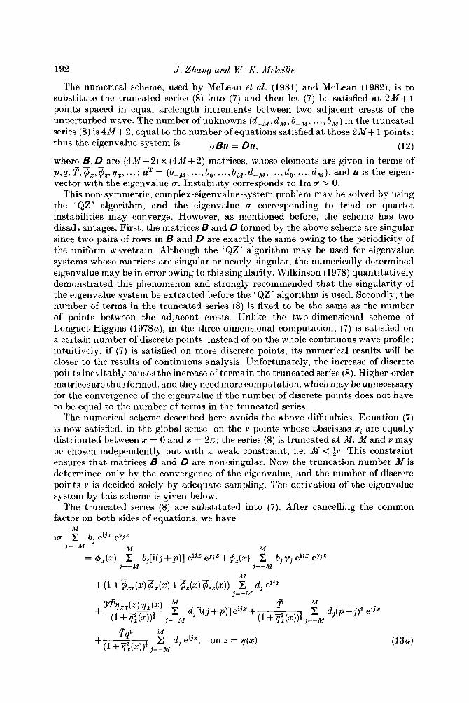
The numerical scheme, used by McLean et al. (1981) and McLean (1982), is to substitute the truncated series (8) into (7) and then let (7) be satisfied at 2M+1 points spaced in equal arclength increments between two adjacent crests of the unperturbed wave. The number of unknowns ( d - M , d,, b-M, . . . , b M ) in the truncated series (8) is 4M+ 2, equal to the number of equations satisfied a t those 2M+ 1 points; thus the eigenvalue system is

where B, D are (4M+2) x (4M+2) matrices, whose elements are given in terms of p , q , T , $z, $ z , 7 j x , . . . ; uT = (kM, . .., b,, . . ., b,, d - M , . . , , d o , .. ., d M ) , and u is the eigen- vector with the eigenvalue IY. Instability corresponds to Im IY > 0.

This non-symmetric, complex-eigenvalue-system problem may be solved by using the 'QZ' algorithm, and the eigenvalue IY corresponding to triad or quartet instabilities may converge. However, as mentioned before, the scheme has two disadvantages. First, the matrices B and D formed by the above scheme are singular since two pairs of rows in B and D are exactly the same owing to the periodicity of the uniform wavetrain. Although the 'QZ' algorithm may be used for eigenvalue systems whose matrices are singular or nearly singular, the numerically determined eigenvalue may be in error owing to this singularity. Wilkinson (1978) quantitatively demonstrated this phenomenon and strongly recommended that the singularity of the eigenvalue system be extracted before the 'QZ' algorithm is used. Secondly, the number of terms in the truncated series (8) is fixed to be the same as the number of points between the adjacent crests. Unlike the two-dimensional scheme of Longuet-Higgins (19784, in the three-dimensional computation, (7) is satisfied on a certain number of discrete points, instead of on the whole continuous wave profile; intuitively, if (7) is satisfied on more discrete points, its numerical results will be closer to the results of continuous analysis. Unfortunately, the increase of discrete points inevitably causes the increase of terms in the truncated series (8). Higher-order matrices are thus formed, and they need more computation, which may be unnecessary for the convergence of the eigenvalue if the number of discrete points does not have to be equal to the number of terms in the truncated series.

The numerical scheme described here avoids the above difficulties. Equation (7) is now satisfied, in the global sense, on the v points whose abscissas xi are equally distributed between x = 0 and x = 2 ~ ; the series (8) is truncated at M. M and v may be chosen independently but with a weak constraint, i.e. M < tv. This constraint ensures that matrices B and D are non-singular. Now the truncation number M is determined only by the convergence of the eigenvalue, and the number of discrete points 11 is decided solely by adequate sampling. The derivation of the eigenvalue system by this scheme is given below.

The truncated series (8) are substituted into (7). After cancelling the common factor on both sides of equations, we have

ig C bj eijx eYjZ

IYBU = Du, (12)

- - -

M

j - - M M M

j - -M j= -M

- = $x(x) x bj[i(j+p)] eijx eYiz+qz(x) x b j y j eifx eYiZ

Instabilities of nonlinear gravity-capillary waves 193

M

ia C dj eijx

M M

j = - M j= -M x I: dj eijz+$z(x) x dj[i@+j)] eijz, on z = ?(x) (13bj

where yj = ( @ + j ) Z + @ ) k (14) Equations (13a, b) are satisfied a t xk = 2nk/v, for k = 0,1, .. ., v- 1, and each equation is multiplied by epiZzk and then added together from k = 0 to k = Y- 1 :

V-1 M ig x bj ei(j-l)xk eYjt(xk)

k-o j - -M

"-1 M

u - 1 M

+ Z- $Jxk) , 2 dj[i(p+j)] ei(j-z)zk, k=O 3--M

where I is integer. Exchanging the order of summation and using the FFT algorithm, we have

M

j--M irr b, &{eYi~(z)}

194 J . Zhang and W. K. Melville

where

Equation (17) defines the discrete Fourier transform (FFT). For a v-point FFT, there are at most v independent discrete-Fourier-transform coefficients. Therefore, we may set 1 = - M, ..., 0, .. ., M, and thus we have 2 x (2M+ 1) independent equations as long as 2M+ 1 < v, which is ensured by the weak constraint M < iv. These inde- pendent equations are satisfied a t all these v discrete points in the global sense; therefore, this new scheme is a Galerkin method, in contrast to the collocation method of McLean (1981). In order to use the FFT algorithm, we set v = 2n , where n is an integer.

These 2 x (2M+ 1) simultaneous equations (16a, b ) may also be written in the matrix form (12), where the coefficients of B and D are the first 2M+1 FFT coefficients of the corresponding functions shown in (16). These functions, as mentioned before, are given by F, p , q and q5x, # z , %jx, . . . , from the numerical solution of the uniform GCWs.

The eigenvalue system formed by the Galerkin method may also be solved by the ‘QZ ’ algorithm. For M = 5, the order of matrices B and D is 4M+ 2 = 22, and it took about 30 CPU seconds to calculate all the eigenvalues and the eigenvectors on a Honeywell Level-68, using double-precision 72-bit arithmetic. For M = 10,20,30, it took about 1.5,10,32 CPU minutes respectively to calculate all the eigenvalues and the eigenvectors. The CPU time increases rapidly with the increase of M. Newton’s method together with the normalization condition for the eigenfunction u*uT = 1 may be used to confirm the results obtained by ‘QZ’ algorithm.

For each ka and given p , v was chosen so that a further increase in the number of points to 2v resulted in a relative error of less than in the transform coefficients of (16). The calculations were repeated with M increasing until the relevant eigenvalue converged, such that an increase in M of 10 led to a relative error in the eigenvalues smaller than with the neglected modes in the corresponding eigenvector no more than times the dominant mode. While searching for the appropriate truncation integer M , the weak constraint M < i i ! should be checked. However, in our numerical computation, is usually much larger than M ; therefore, this constraint is always satisfied.

Our numerical scheme has also been checked against other available numerical and analytical results : the numerical results of McLean (1982) for finite-amplitude gravity waves (5? = 0); the analytic results of Djordjevic & Redekopp (1977), and Zhang & Melville (1986) for quartet and triad resonant interactions in weakly nonlinear GCWs. In our computation of gravity waves, 5? was set to an arbitrarily small number; = The instability at h/h = 0.111, (hh is the ratio of wave height to wave length) was computed, and together with the corresponding results of McLean (1982) are shown in table 1. The comparison between the data clearly shows satisfactory agreement for both the quartet interaction in two-dimensional perturbations (1, = 0.6, q = 0) and the quintet interaction in three-dimensional perturbations ( p = 0.5, q = 1.15). As expected, however, faster convergence may be obtained by the Galerkin method. The relative errors between M = 10 and M = 20

- -

Instabilities of nonlinear gravity-capillary waves 195

Collocation method? Galerkin method$

h lA P 4 M Re u Im u M Re u Im u

0.111 0.60 0.0 10 -0.213688 0.023644 5 -0.215114 0.023096 20 -0.213876 0.022701 15 -0.214709 0.022827 30 -0.213873 0.022703 25 -0.214709 0.022827

- - 10 -0.214711 0.022828 - - 20 -0.214709 0.022827

0.111 0.50 1.15 10 0.000278 0.042674 5 0.000 352 0.040 4 14 20 0.000003 0.041263 15 0.000 00 1 0.040 552 30 0.000000 0.041268 25 0.000000 0.040552

- - 10 0.000002 0.040551 - - 20 0.000 000 0.040 552

t Data for collocation method are from McLean (1982). $ For Galerkin method, !J? = and u = 256.

TABLE 1 . Comparison of the rate of convergence between Galerkin and collocation methods

o.20 t

0.04 1 / 0 0.04 0.08 0.12

1 I I \ I

I I I I I I 1 . I i 0.16 0.20 0.24 0.28 0.32 0.36 0.40

p/2ka

FIGURE 2. Growth rate of two-dimensional instabilities for !J? = 5.0 (weakly nonlinear theory results) - ; for ka = 0.01, - - - - - ; 0.02, - - - - - -; 0.03,

for the Galerkin method are smaller than those between M = 20 and M = 30 for the collocation method.

For GCWs, the quartet instability rates computed by our numerical scheme are also confirmed by the corresponding analytic results derived from the nonlinear Schrodinger equation for T =/= 0 (Djordjevic & Redekopp 1977, equation (2.20)). Figure 2 shows the comparison of the instability rates varying with p(q = 0), for

= 5.0 and ka = 0.01,0.02,0.3. For ka = 0.01, the numerical results agree very well with the analytical results. The difference between the analytical and numerical results increases with increasing nonlinearity. However, i t should be noticed that the non-dimensional quartet instability rate increases with ka for capillary waves while it decreases with ka for gravity waves. This qualitative difference of quartet instability between the weakly nonlinear gravity waves and GCWs is also predicted by the higher-order nonlinear Schrodinger equation (S. J. Hogan 1985, private communication).

196

0.15

0.12

2 ; 0.09 h

Y, 2 0.06 E I

0.03

J . Zhang and W . K . Meloille

-

-

-

-

-

p x 10

0.12 O ' l 5 jl

p x 10

p x 10

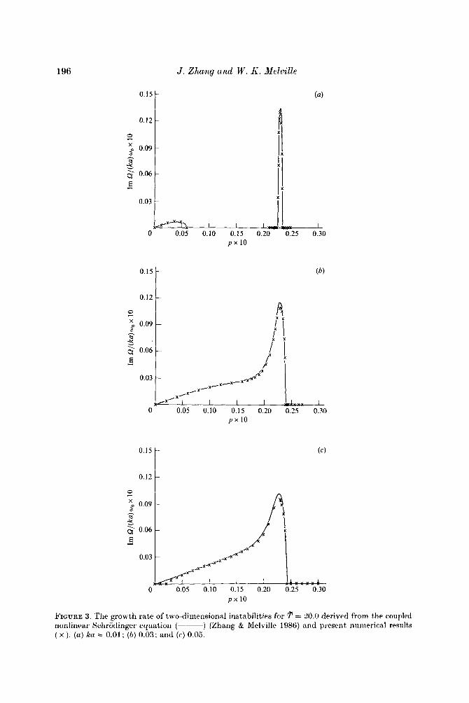
FIGURE 3. The growth rate of two-dimensional instabilities for = 20.0 derived from the coupled nonlinear Schrodinger equation (--) (Zhang & Melville 1986) and present numerical results ( x ). (a ) ka = 0.01 ; ( 6 ) 0.03; and (c) 0.05.

Instabilities of nonlinear grauity-capillary waves 197

Sum triad

Sum quartet

Difference triad

Difference quartet

Difference quintet

Dominant eigenrnodes Linear resonance condition

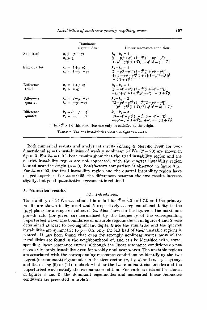
Both numerical results and analytical results (Zhang & Melville 1986) for two- dimensional (q = 0) instabilities of weakly nonlinear GCWs ( p = 20) are shown in figure 3. For La = 0.01, both results show that the triad instability region and the quartet instability region are not connected, with the quartet instability region located near the origin ( p = 0). Satisfactory comparison is observed in figure 3 ( a ) . For ka = 0.03, the triad instability region and the quartet instability region have merged together. For ka = 0.05, the differences between the two results increase slightly, but good quantitative agreement is retained.

5. Numerical results 5.1. Introduction

The stability of GCWs was studied in detail for p = 3.0 and 7.0 and the primary results are shown in figures 4 and 5 respectively as regions of instability in the (p,q)-plane for a range of values of ha. Also shown in the figures is the maximum growth rate (for given k a ) normalized by the frequency of the corresponding unperturbed wave. The boundaries of unstable regions shown in figures 4 and 5 were determined at least to two significant digits. Since the sum triad and the quartet instabilities are symmetric to p = 0.5, only the left half of their unstable regions is plotted. It has been found that even for strongly nonlinear waves most of the instabilities are found in the neighbourhood of, and can be identified with, corre- sponding linear resonance curves, although the linear resonance conditions do not necessarily imply instability even for weakly nonlinear waves. The unstable regions are associated with the corresponding resonance conditions by identifying the two largest (or dominant) eigenmodes in the eigenvector, (n, + p , q ) and (n , -p , - q ) say, and then using (9) or (11) to check whether the two dominant eigenmodes and the unperturbed wave satisfy the resonance condition. For various instabilities shown in figures 4 and 5 , the dominant eigenmodes and associated linear resonance conditions are presented in table 2.

198

1.0

0.9

0.8

0.7

0.6

J . Zhang and W. K. Melville

-

-

-

-

-

0.9

0.8

0.7

0.6

4 0.5 I

-

-

-

-

-

0.3 ):I 0.3 0.4 I

0 0.1 0.2 0.3 0.4 0.5 0.6 0.7 P

0 0.1 0.2 0.3 0.4 0.5 0.6 0.7 P

1.0

0.9

0.8

0.7

0.6

4 0.5

0.4

0.3

0.2

0. I

0 0.1 0.2 0.3 0.4 0.5 0.6 0.7 P

FIGURE 4(a-c). For caption see facing page.

It is useful to introduce some terminology to facilitate the description of the numerical results. Each of the linear resonances can be expressed as a ‘triad’ interaction: a harmonic of the unperturbed wave with two disturbance modes. Thus a pure linear resonance condition is satisfied if only two modes in the eigenvector are non-zero. However, for finite-amplitude or even weakly nonlinear waves, there are always more than two non-zero modes in the eigenvector. We characterized an instability by its corresponding linear resonance if two of the eigenmodes in the

Instabilities of nontinear grurdy-ca.pillury waws 199

1 .o

0.9

0.8

0.7

0.6

4 0.5

0.4

0.3

0.2

0.1

0 0.1 0.2 0.3 0.4 0.5 0.6 0.7 P

1 .o

0.9

0.8

0.7

0.6

4 0.5

0.4

0.3

0.2

0.1

0 0.1 0.2 0.3 0.4 0.5 0.6 0.7 P

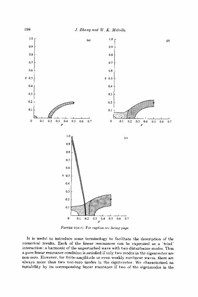
FIGURE 4. Unstable regions of the (p, q)-plane for = 3.0, where m, m, , m, represent sum triad, difference triad, sum quartet, difference quartet and difference quintet respectively. The solid point marks the point of maximum growth rate.

ka (Im V / W ) , , , ~ ~ x lo3

(a ) 0.05 4.88 ( 6 ) 0.15 14.0 ( c ) 0.30 22.6

(el 0.50 30.5 (4 0.40 20.0

eigenvector are much larger than the other modes. For some instabilities, however, the difference between the second largest mode (the smaller dominant mode) and the third largest mode in the eigenvector is not substantial ; we have called it a ‘transition instability’, consistent with the fact that this instability usually happens in the region where two ‘exclusive’ instabilities merge. Two instabilities are said to be exclusive if they share one of the two dominant modes in their eigenvectors, and can not occur coincidentally in the (p , q)-plane. The sum triad instability and sum quartet instability are exclusive for they have one common dominant mode (1 - p , -9) as shown in table 2. Similarly, the difference triad and sum triad, and the difference triad and sum quartet, are also pairs of exclusive instabilities, sharing the common dominant mode ( p , q ) and ( l + p , q ) respectively. Our numerical results did not produce any examples of exclusive instabilities occurring coincidentally in the (p, q)-plane for given P and ha.

Between two merging exclusive instabilities, transition instabilities provide a buffer, where one instability gradually converted to its exclusive counterpart as will be shown in 55.3. The term ‘transition instability ’ is not quantitatively defined and such instabilities are not marked separately in figures 4 and 5.

Two instabilities are said to be ‘overlapping ’ if they may occur at the same value of ( p , q ) . Overlapping instabilities do not share any common dominant mode. As

200 J . Zhang and W . K . Melville

Instability Dominant eigenmodes rates

Instability Im u / w o 1st mode Amplitude? 2nd mode Amplitude

Sum quartet 0.0131 (1 -P, -4) 1 .o ( 1 + P > d 0.85

Difference 0.0043 (-P, - 9 ) 1 .o (2--P, -4) 0.65 quartet

eigenmode is unity. f The amplitude of the dominant modes are normalized such that the larger dominant

TABLE 3. Comparison of quartet instabilities for = 3.0, ka = 0.3, ( p , y) = (0.175,O.lO)

shown in figures 4 and 5, the difference quartet and sum triad instabilities, the difference quintet and sum triad instabilities, the difference quartet and difference triad instabilities, etc. are pairs of overlapping instabilities; they can occur co- incidentally in the ( p , q)-plane for given p and ka.

Stationary disturbances were not specifically studied ; nevertheless some interesting stationary disturbances are observed during our search for instabilities. The existences of stationary disturbances may suggest bifurcations of the unperturbed waves, and will be briefly mentioned in $5.5.

5.2. Development of unstable regions Figure 4(a) ( p = 3.0, ka = 0.05) shows what we found to be a typical instability diagram for ka 1. With the exception of the sum quartet (Benjamin-Feir) instability near the origin of the (p, q)-plane (stable a t the origin), the unstable region lies in the immediate neighbourhood of the sum triad resonance curve with the maximum growth rate occurring at p = 0.5. I n figure 4 ( b ) ( ka = 0.15), the sum triad instability region has grown around its resonance curve, and the sum quartet instability region has expanded but a stable region appears in the immediate neighbourhood of the origin. The two originally disconnected exclusive instability regions (quartet and triad) have merged together, with transition instabilities be- tween them. In figure 4(c) (ka = 0.30), the sum triad instability region has become broader in the q-direction, but is compressed in the p-direction towards p = 0.5 by the sum quartet instability region The difference quartet instability has appeared in the immediate neighbourhood of its linear resonance curve; part of its unstable region overlapping on the sum quartet instability. As shown in table 2 these two instabilities do not have any common dominant eigenmodes. The strength of the overlapping instabilities are quite different; table 3 shows a typical comparison of the instability rates and dominant eigenmodes. I n figure 4(d) (ka = 0.40) the difference quintet instability has appeared in the immediate neighbourhood of its linear resonance curve; part of its unstable region is common to the sum triad instability region. They are overlapping instabilities. The difference quartet instability has expanded slightly along its linear resonance curve. It is now stronger than its overlapping counterpart. Table 4 shows the comparisons of overlapping instabilities. The maximum growth rate is at ( p , q) = (0.50,0.20), still in the sum triad instability region, but is smaller than in figure 4(c) (ka = 0.30). This implies that the sum triad instability is fading. The annular sum quartet instability region has broken into two parts; at larger p i t is still connected to the sum triad instability region, and a t smaller p it is confined near the q-axis. Now it is unstable a t the origin; this implies the existence of a

Instabilities of nonlinear gravity-capillary waves 20 1

Instability Dominant eigenmodes rates

Instability Im u / w o 1st mode Amplitudet 2nd mode Amplitude at ( p , q ) = (0.18,O.lO)

Sum quartet 0.0048 ( 1 + P > d 1 .o ( 1 +P> -9) 0.65

Difference 0.0089 (-P, - 4 ) 1 .o ( 2 - R -9) 0.39 quartet a t ( p , q ) = (0.51,0.20)

Sum triad 0.0199 (1 -P, -9) 1 .o @, 9 ) 0.98

Difference 0.0039 (3-P, -9) 1 .0 (-P, -9 ) 0.926 t Same as in table 3. quintet

TABLE 4. Overlapping instability comparison for = 3.0, ka = 0.4

superharmonic instability, which is discussed in $5.4. In figure 4 ( e ) , the difference triad instability has grown along the neighbourhood of its linear resonance curve, and is connected to the sum quartet instability region ; they are exclusive instabilities. The sum triad instability has disappeared. The previously split sum quartet instability region has recombined into a single region. The strongest instability a t this value of ka is the sum quartet instability a t (p ,q ) = (0.14,O.O): the dominant instability is two-dimensional.

Figure 5 shows the instability diagrams for p = 7.0, for the same range of ka as in figure 4. The development of the unstable regions is generally similar to that for p = 3.0 ; however, a few differences between figures 4 and 5 are evident. I n figure 5 (c) (ka = 0.30), the sum quartet instability has partially appeared in the neighbourhood of the linear sum triad resonance curve. The difference quartet instability overlaps the sum triad instability (cf. figure 4 (c) in which i t overlaps the sum quartet) I n figure 5 ( e ) , the difference quartet instability overlaps the difference triad instability. The difference triad instability region now touches the p-axis, whereas it is separated from p-axis by the sum quartet instability in figure 4(e ) . The strongest instability is the difference triad instability a t (p , q) = (0.21,0.46) ; the dominant instability is three- dimensional. The sum triad instability region has shrunk to a small region centred a t p = 0.5, but does not disappear as in p = 3.0. The difference triad instability occurred in the neighbourhood of the sum triad linear resonance curve, while in figure 4 (e), only a small tip of the difference triad instability region developed on that curve.

5.3. Transition instability Although we do not quantitatively define the transition instability, it is interesting to observe how the instability gradually changes to its exclusive counterpart. Figure 6, which depicts how the amplitudes of the three largest eigenmodes (1-p, -q),(l+p,q),(p,q)varywithpforfixedq, p a n d k a , istypical. Whenp < 0.2, the two dominant modes (1 -p , - q ) , (1 + p , q ) are much larger than the third largest mode ( p , q ) ; therefore, the instability is identified as the sum quartet instability. With the increase of p , the amplitude of the second eigenmode (the smaller dominant mode) gradually decreases as the third mode gradually increases. At p = 0.223, the amplitudes of these two modes are equal. As p increases further, the relative order of the second and third modes are reversed. The dominant modes now are (1 -p, - q) and ( p , q ) , and the instability is recognized as the sum triad instability. I n the vicinity

202 J . Zhang and W. K . Melville

1.0

0.9

0.8

0.7

0.6

4 0.5

0.4

0.9 1 - -

-

-

-

-

-

0.8 1 0.7 1 0.6 1 0.4 0.5 t

0 -0.1 0.2 0.3 0.4 0.5 0.6 0.7 P

1 .o

0.9

0.8

0.7

0.6

4 0.5

0.4

0.3

0.2

0.1

0 0.1 0.2 0.3 0.4 0.5 0.6 0.7 P

0 0.1 0.2 0.3 0.4 0.5 0.6 0.7 P

FIGURE 5(a-c). For caption see facing page.

of p = 0.223, the amplitudes of the second and third modes are almost equal, which is the characteristic of the transition instability.

5.4. Superharmonic instability In sufficiently steep GCWs, our numerical results show superharmonic instabilities at @, q ) = ( 0 , O ) . The threshold of the superharmonic instability is ka = 0.3934 for p = 3.0, and ka = 0.3673 for p = 7.0. For the superharmonic instability, the real part

1 .o

0.9

0.8

0.7

0.6

4 0.5

0.4

0.3

0.2

0.1

Instabilities of nonlinear gravity-capillary u7aves 203

(4 1 .o

0.9

0.8

0.7

0.6

4 0.5

0.4

& 0.3

0.2

0 0.1 0.2 0.3 0.4 0.5 0.6 0.7 P

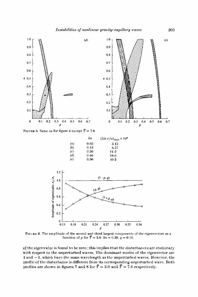
FIGURE 5. Same as for figure 4 except 5? = 7.0

ka

(a ) 0.05 ( b ) 0.15 ( c ) 0.30 (4 0.40 ( e ) 0.50

0.1

1

0 0.1 0.2 0.3 0.4 0.5 0.6 0.7 P

(Im C T / W ) ~ ~ ~ x lo3

3.13 8.57

11.2 18.0 40.3

I I I 1 1 1 1

0.15 0.18 0.21 0.24 0.27 0.30 0.33 0.36 P

FIQURE 6. The amplitude of the second and third largest components of the eigenvectors as a function of p for rf = 3.0, ka = 0.30, q = 0.10.

of the eigenvalue is found to be zero ; this implies that the disturbances are stationary with respect to the unperturbed waves. The dominant modes of the eigenvector are 1 and - 1 , which have the same wavelength as the unperturbed waves. However, the profile of the disturbance is different from its corresponding unperturbed wave. Both profiles are shown in figures 7 and 8 for = 3 .O and = 7 .O respectively.

204

-0.2

J . Zhang arhd W. K. Melville

-

-0.2 -

-0.4 1

0.4 t ka = 0.3934,

-0.4 1 FIGURE 7. (a ) Profiles of unperturbed wave for = 3.0, ka = 0.3934,O.M69,O..C958.

( b ) Corresponding resonant superharmonic perturbations.

-0.2 -

-0.4;-

0.4

0.2

z o 0

-0.2

-0.4

FIGURE 8. (a ) Profiles of unperturbed wave for = 7.0, ka = 0.3673,0.#i18,0.5024. ( b ) Corresponding resonant superharmonic perturbations.

Instabilities of nonlinear gravity-capillary waves

4

3

4 Y ; 2

1

0 1 2 3 4 x / n

2n

0

FIGURE 9(a ,b) . For caption see next page.

205

At the threshold of the superharmonic instability, the profile of the resonant disturbance is symmetric, with a 180' phase shift from the unperturbed waves. With the increase of the wave steepness, the superharmonic instability increases, and the profile of the resonant disturbance becomes more and more asymmetric. The effect of the superharmonic instability is to smooth the back face and steepen the forward face of the unperturbed waves.

206 J . Zhang and W. K. Melville

0.4

0.2

22 0

-0.2

t

- 0.4 c FIGURE 9. Three-dimensional crest-symmetric bifurcation from two-dimensional GCWs for

= 7.0, ka = 0.15, ( p , q ) = (0.5,0.291). (a ) Surface-contour plot. ( b ) Three-dimensional perspective plot, (c) Cut through surface at y = x / q .

9 y x

0 1 2 3 4

X l k

FIGURE lO(a). For caption see facing page.

5.5 Stationary disturbances Two special kinds of stationary disturbances are found in our numerical work. They may suggest different bifurcations of the unperturbed waves.

(i) Three-dimensional stationary disturbance It has been found that the real part of the eigenvalue is always equal to zero for

the sum triad and sum quartet instabilities at p = 0.5 and 0 respectively. Therefore, it is expected that both real and imaginary parts of the eigenvalue are zero at the intersections of the boundary of the corresponding unstable regions and the line p = 0.5 or 0, where the disturbances are three-dimensional, and stationary with respect to the unperturbed wave. For the sum triad instability of pure capillary

Instabilities of nonlinear gravity-capillary waves 207

I 0

0.2 0'4 L 22 0

-0.2

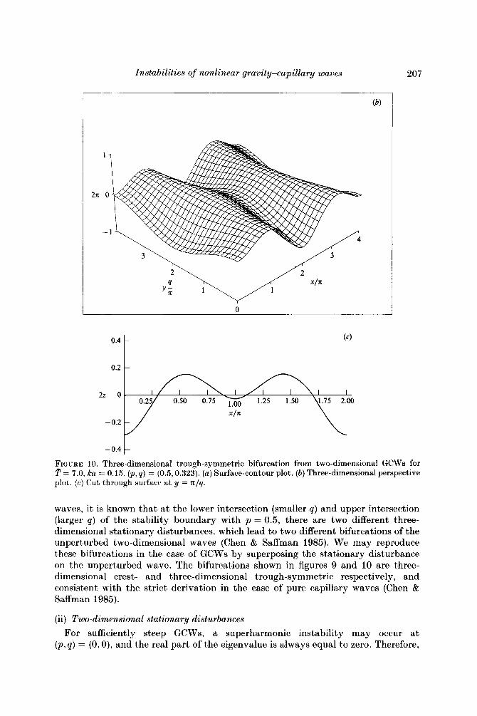
-0.4 t FIQURE 10. Three-dimensional trough-symmetric bifurcation from two-dimensional GCWs for

= 7.0, ka = 0.15, ( p , q ) = (0.5,0.323). (a ) Surface-contour plot. ( b ) Three-dimensional perspective plot. ( c ) Cut through surface at y = x/q.

waves, it is known that a t the lower intersection (smaller q ) and upper intersection (larger q) of the stability boundary with p = 0.5, there are two different three- dimensional stationary disturbances, which lead to two different bifurcations of the unperturbed two-dimensional waves (Chen & Saffman 1985). We may reproduce these bifurcations in the case of GCWs by superposing the stationary disturbance on the unperturbed wave. The bifurcations shown in figures 9 and 10 are three- dimensional crest- and three-dimensional trough-symmetric respectively, and consistent with the strict derivation in the case of pure capillary waves (Chen & Saffman 1985).

(ii) Two-dimensional stationary disturbances

For sufficiently steep GCWs, a superharmonic instability may occur at (p, p) = (0, 0), and the real part of the eigenvalue is always equal to zero. Therefore,

208 J . Zhang and W . K. Melville

a t the threshold of the superharmonic instability both real and imaginary parts of the eigenvalue may be zero, The corresponding stationary disturbance would have the same wavelength as the unperturbed wave, but a different profile. This implies the existence of a two-dimensional bifurcation a t the threshold ; however further careful study is required to prove this conjecture.

We thank Dr John McLean for making available detailed numerical results and Dr John Hogan for comments on an early version of this work. The work was supported by the National Science Foundation through grant MEA 82-1 0649 and OCE-82 14746.

REFERENCES

BENJAMIN, T. B. & FEIR, J. E. 1967 The disintegration of wave trains on deep water. J . Fluid Mech. 27, 417-430.

BENNEY, D. J. 1976 Significant interactions between small and large scale surface waves. Stud. Appl. Math. 55, 93-106.

CHEN, B. & SAFFMAN, P. G. 1985 Three-dimensional stability and bifurcation of capillary and gravity waves on deep water. Stud. Appl. Math. 72, 125-147.

COKELET, E. D. 1977 Steep gravity waves in water of arbitrary uniform depth. Phil. Trans. R . Soc. Lond. A 286, 183-230.

DJORDJEVIC, V. D. & REDEKOPP, L. G. 1977 On two-dimensional packets of capillary-gravity waves. J . Fluid Mech. 79, 703-714.

HASSELMANN, K. 1967 A criterion for nonlinear wave stability. J . Fluid Mech. 30, 737-739. HOGAN, S. J. 1980 Some effects of surface tension on steep water waves. Part 2. J . Fluid Mech.

HOGAN, S. J. 1981 Some effects of surface tension on steep water waves. Par t 3. J . Fluid Mech.

LIGHTHILL, M. J. 1965 Contributions t o the theory of waves in nonlinear dispersive systems. J . Inst. Maths Appls 1 , 296-306.

LONGUET-HIGGINS, M. S. 1978a The instabilities of gravity waves of finite amplitude in deep water. I. Superhamonics. Proc. R . Soc. Lond. A360, 471-488.

LONGUET-HIGGINS, M. S . 1978b The instabilities of gravity waves of finite amplitude in deep water. 11. Subharmonics. Proc. R . Soc. Lond. A 360, 489-505.

MCLEAN, J. W. 1982 Instabilities of finite-amplitude water waves. J . Fluid Mech. 114, 315-330. MCLEAN, J. W., MA, Y. C., MARTIN, D. [J., SAFFMAN, P. G. & YUEN, H. C. 1981 Three-dimensional

OPPENHEIM, A. V. , WILLSKY, A . S. & YOUNG, I . T. 1985 Signal and Systems. Prentice-Hall. SCHWARTZ, L. W. 1974 Computer extension and analytic continuation of Stokes’ expansion for

gravity waves. J . Fluid Mech. 62, 553-578. STOKES, G. G. 1880 S u p p l ~ m e n t t o a paper on the theory of oscillatory waves. Mathematical and

Physical Papers, Vol. 1 , pp. 314-326. Cambridge University Press. WILKINSON, J. H. 1978 Kronecka’s cononical form and the Q Z algorithm. N P L Rep. DNACS

10178. ZHANG, J. & MELVILLE, W . K. 1986 On the stability of weakly-nonlinear gravity-capillary

waves. Wave Motion (in press).

96, 417-445.

110, 381-410.

instability of finite amplitude water waves. Phys. Rev. Lett. 46, 817-820.