three-dimensional simulations of liquid-gas flows …

IV Journeys in Multiphase Flows (JEM 2015)March 23-27, 2015, Campinas, SP, Brazil

Copyright © 2015 by ABCMPaper ID: JEM-2015-0032

THREE-DIMENSIONAL SIMULATIONS OF LIQUID-GAS FLOWS AT THENEAT-PETROBRAS TEST LOOP FOR CALIBRATION OF AN ULTRASONIC

MULTIPHASE FLOW METER

Hugo Alejandro Pineda Perez, Jorge Eduardo Lopez, Nicolas Rios RatkovichUniversidad de los Andes (UNIANDES)Department of Chemical EngineeringBogota, [email protected]@[email protected]

Maurício de Melo Freire Figueiredo, Ricardo Dias Martins de CarvalhoUniversidade Federal de Itajubá (UNIFEI)Instituto de Engenharia MecânicaItajubá, Minas [email protected]@gmail.com

Juliano Scholz SlongoUniversidade Tecnológica Federal do Paraná (UTFPR)Instituto de Engenharia ElectrónicaCuritiba, Paraná[email protected]

Abstract. The present paper describes the CFD numerical simulations of liquid-gas flows in the test rig at NúcleoExperimental de Atalaia (NEAT-PETROBRAS). Results for three flow patterns are presented and discussed: plug flow, slugflow, and stratified wavy flow. In addition, flow pattern transitions were determined based on the CFD results. The simulationresults provided relevant information about the flow patterns as well as the transitions between them. Except for the annularflow, which presents several difficulties for simulation, the flow pattern predictions in the simulations agree with thepredictions made using the Baker flow pattern map. Furthermore, the CFD simulations allowed for reliable, time dependentGVF results, which can be used for direct comparison with the acoustic signals from the multiphase flow meter. The CFDsimulations described herein thus provide the necessary means for calibration of the ultrasonic multiphase flow meter beingdeveloped.

Keywords: CFD numerical simulations, oil-gas flows, NEAT-PETROBRAS, GVF

1. INTRODUCTION

Multiphase flows are very common in the petroleum, chemical, and nuclear industries, oftentimes involving harsh media,strict safety restrictions, access difficulties, long distances, and aggressive surroundings. Accordingly, there is a growinginterest in non-invasive techniques for measurement of the dispersed phase concentration in multiphase flows. The ultrasonictechnique has been receiving increasing attention from researchers and professionals in the oil industry for multiphase flowmetering. This technique is already well established in other fields of application like medicine and flaw detection in solidmaterials. The ultrasonic transducers and the necessary electronics are commercially available at relatively low costs and thesystems are compact and robust. Furthermore, ultrasonic signals are information rich and can penetrate pipe walls and processchambers. Ultrasonic signals can also be used with optically opaque fluids and dense suspensions. The disadvantage of theultrasonic technique is the need for calibration of the ultrasonic signal as a function of the dispersed phase concentration.

The main ultrasonic parameters normally used in process monitoring, measurement, and control are the signal amplitudeand the wave transit time (Bond et al., 2003). These parameters can be measured across the pipe diameter or along any otheracoustic path of interest in the multiphase flow. The distribution and the concentration of the dispersed phases (bubbles, oildroplets, or solid particles) alter these parameters due to transmission, reflection, refraction, and scattering of the ultrasonicbeam so that the received acoustic signals can be calibrated for determination of the hydrodynamic multiphase flowparameters. An initial study to develop the ultrasonic technique for multiphase metering involved correlating acousticattenuation data with GVF for vertical, upward water-gas flows (Tanahashi, 2010). Next, the transit time of the acoustic wave

Pineda Perez et al.Three-Dimensional Simulations of Liquid-Gas Flows at the NEAT-PETROBRAS Test Loop …

was used to determine the velocity of the elongated bubbles and the GVF of horizontal, intermittent water-air flows(Grangeiro, 2010). As a further development, acoustic data and independent GVF measurements were obtained for vertical,upward liquid-gas-solid flows using the mineral oil as the continuous phase (Goncalves, 2013). The previous studies clearlydemonstrated the feasibility of using the ultrasonic technique for multiphase metering; the task at hand then is to take thetechnique from the laboratory environment to the field. In doing so, obtaining ultrasonic data for the real fluids in the oilindustry is the obvious next step.

In this regard, Núcleo Experimental de Atalaia (NEAT-PETROBRAS) provides the proper facilities for accomplishingthis task. However, though acoustic data can be obtained for real flows of the oil industry, the existing facilities currently donot have any independent means of measuring the GVF to correlate the ultrasonic data against. In view of the complexity ofthe facility and the costs and safety regulations involved in carrying out any modification of this kind, for the time beingdetailed numerical simulations of the flows seem a much more feasible solution to obtaining GVF data.

In this context, the proposed paper will present the development of 3D numerical simulations of liquid-gas flows in thepertinent segments of the multiphase loop at NEAT-PETROBRAS. The liquid phase will be dead oil from Sergipe Terra andthe gas phase will come from the Atalaia Gas Station. The gas and oil flow rates at the existing pressure and temperatureconditions will be as determined for obtaining bubbly and fully developed slug flows. Numerical results for the GVF as wellas flow patterns information will then be available for calibrating the prototype of the ultrasonic meter in future experiments.

2. EXPERIMENTAL APPARATUS AND PROCEDURE

2.1 NEAT –PETROBRAS Multiphase Flow Test Loop and the Multiphase Flow Meter Prototype

The facilities at Núcleo Experimental de Atalaia (NEAT-PETROBRAS) are part of Centro de Pesquisas eDesenvolvimento Leopoldo Américo Miguez de Melo, located in Aracaju, Sergipe, Brazil. Of particular interest to thedevelopment of the ultrasonic multiphase flow meter is the well test loop shown in Figure 1. This loop is made of two parts,a permanent circuit and a dedicated one built to suit the needs of the particular equipment under test. The main componentsin the permanent circuit are the oil storage tank, pump, oil and gas flow rate meters, and first and second stage gas separators.The well test set-up has a 38 m3/hr closed-loop liquid flow rate capacity and an 8,000 Nm3/hr open circuit gas flow ratecapacity. The gas supply pressure is 35 kgf/cm2 and pressure reducing valves are used to lower it to the desired operatingpressure; the maximum operating pressure in the test area is 20 kgf/cm2. Pressure and temperature sensors are located closeto the flow meters and pump. The uncertainties in the liquid and gas flow rate are 0.13% and 0.90%, respectively.

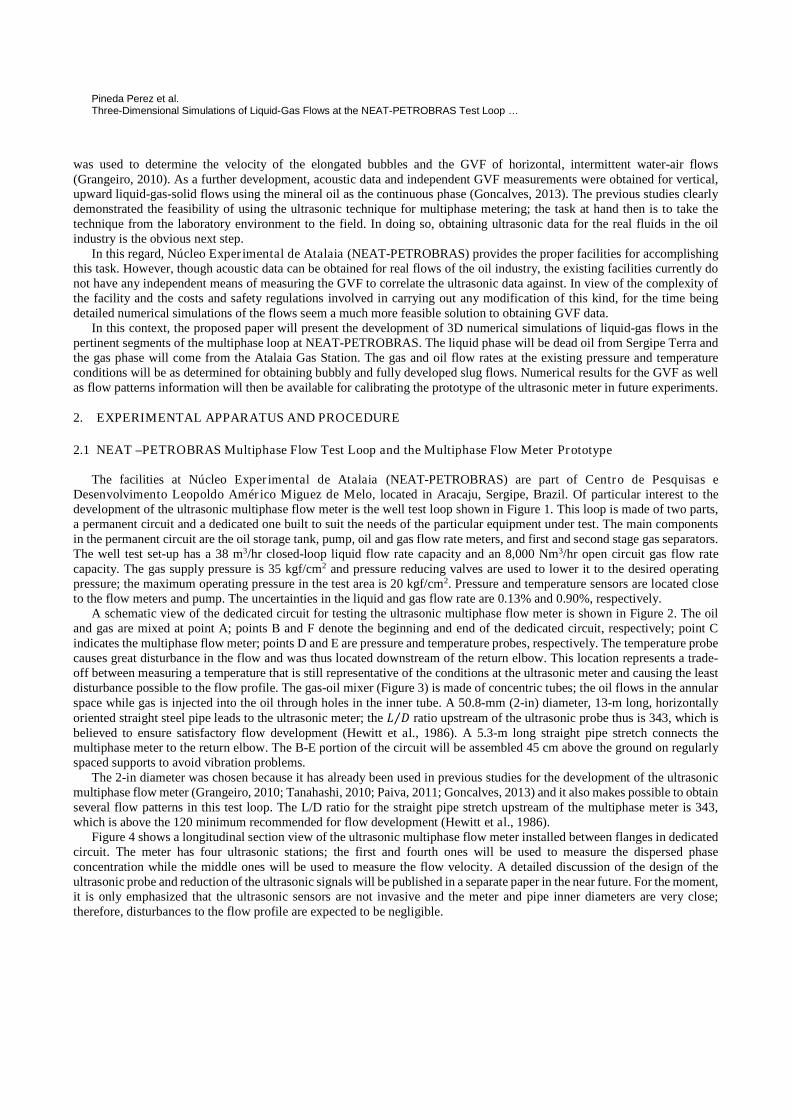
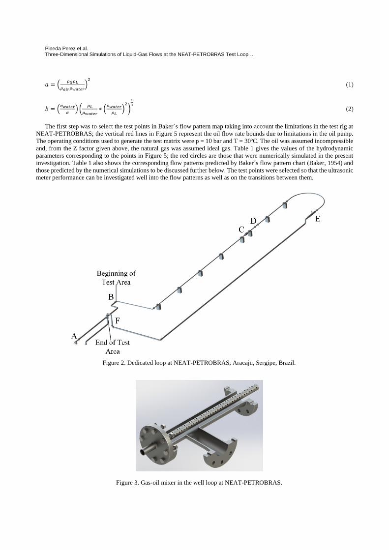
A schematic view of the dedicated circuit for testing the ultrasonic multiphase flow meter is shown in Figure 2. The oiland gas are mixed at point A; points B and F denote the beginning and end of the dedicated circuit, respectively; point Cindicates the multiphase flow meter; points D and E are pressure and temperature probes, respectively. The temperature probecauses great disturbance in the flow and was thus located downstream of the return elbow. This location represents a trade-off between measuring a temperature that is still representative of the conditions at the ultrasonic meter and causing the leastdisturbance possible to the flow profile. The gas-oil mixer (Figure 3) is made of concentric tubes; the oil flows in the annularspace while gas is injected into the oil through holes in the inner tube. A 50.8-mm (2-in) diameter, 13-m long, horizontallyoriented straight steel pipe leads to the ultrasonic meter; the � �⁄ ratio upstream of the ultrasonic probe thus is 343, which isbelieved to ensure satisfactory flow development (Hewitt et al., 1986). A 5.3-m long straight pipe stretch connects themultiphase meter to the return elbow. The B-E portion of the circuit will be assembled 45 cm above the ground on regularlyspaced supports to avoid vibration problems.

The 2-in diameter was chosen because it has already been used in previous studies for the development of the ultrasonicmultiphase flow meter (Grangeiro, 2010; Tanahashi, 2010; Paiva, 2011; Goncalves, 2013) and it also makes possible to obtainseveral flow patterns in this test loop. The L/D ratio for the straight pipe stretch upstream of the multiphase meter is 343,which is above the 120 minimum recommended for flow development (Hewitt et al., 1986).

Figure 4 shows a longitudinal section view of the ultrasonic multiphase flow meter installed between flanges in dedicatedcircuit. The meter has four ultrasonic stations; the first and fourth ones will be used to measure the dispersed phaseconcentration while the middle ones will be used to measure the flow velocity. A detailed discussion of the design of theultrasonic probe and reduction of the ultrasonic signals will be published in a separate paper in the near future. For the moment,it is only emphasized that the ultrasonic sensors are not invasive and the meter and pipe inner diameters are very close;therefore, disturbances to the flow profile are expected to be negligible.

IV Journeys in Multiphase Flows (JEM 2015)

Figure 1. Schematic view of the multiphase flow test loop (Circuito Poço) at NEAT-PETROBRAS.

2.2 Test Fluids

The test fluids for experimentation with the prototype of the ultrasonic multiphase meter will a mixture of dead oils fromGuaricema and Dourado fields and rich natural gas. The oil mixture has API gravity of 38.5, specific gravity of 0.8285, andkinematic viscosity of 45.59 centistokes at 20ºC. The reasons to use this light oil is to reduce the operating pressure of the testloop and to make the results more comparable to those obtained with mineral oil in the laboratory. The rich natural gas issupplied at 35 kgf/cm² and is approximately 78% methane, 13% ethane, 2.6% propane, 2.6% carbon dioxide, 1.3% nitrogen,and less than 3% heavier hydrocarbons. The gas specific gravity is 0.867, dynamic viscosity is 0,010598 cP, and thecompressibility factor Z is 0.99681.

2.3 Experimental procedure

The experimental procedure to be adopted to obtain ultrasonic data for the oil-gas flows at NEAT-PETROBRASdetermined the operating conditions for the numerical simulations presented in this paper. The oil and gas flow rates will beadjusted so that under the pressure and temperature conditions at the ultrasonic test section the flow patterns will be plug flow,slug flow, and annular flow. The test matrix was generated based on Baker´s flow pattern map (Baker, 1954). This map usesmixed dimensionless/dimensional coordinates and correction factors for fluid properties (Figure 5). The expressions for thecorrection factors a and b are given below. Baker´s map is probably one of the most durable, as it is still in use in the oilindustry (Shoham, 2006). The map works well also for oil/gas mixtures with diameters smaller than 50 mm and is expectedto still provide reasonable results for the 54-mm ID pipe in this investigation.


� = ��

� � � � � � � � � ��

(1)

� = ��

��

� �

� � � � � �∗ �

� � � � � �

� ��

�

�

�(2)

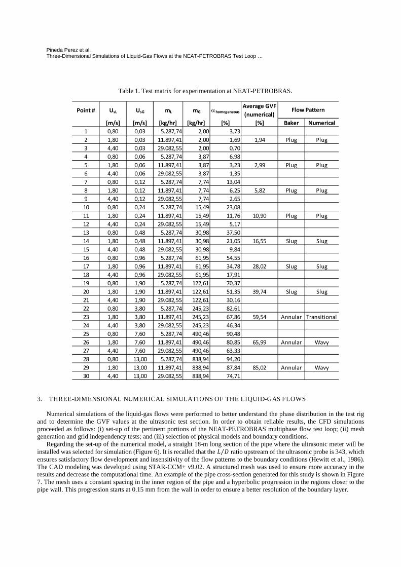
The first step was to select the test points in Baker´s flow pattern map taking into account the limitations in the test rig atNEAT-PETROBRAS; the vertical red lines in Figure 5 represent the oil flow rate bounds due to limitations in the oil pump.The operating conditions used to generate the test matrix were p = 10 bar and T = 30ºC. The oil was assumed incompressibleand, from the Z factor given above, the natural gas was assumed ideal gas. Table 1 gives the values of the hydrodynamicparameters corresponding to the points in Figure 5; the red circles are those that were numerically simulated in the presentinvestigation. Table 1 also shows the corresponding flow patterns predicted by Baker´s flow pattern chart (Baker, 1954) andthose predicted by the numerical simulations to be discussed further below. The test points were selected so that the ultrasonicmeter performance can be investigated well into the flow patterns as well as on the transitions between them.

Figure 2. Dedicated loop at NEAT-PETROBRAS, Aracaju, Sergipe, Brazil.

Figure 3. Gas-oil mixer in the well loop at NEAT-PETROBRAS.


Figure 4. Longitudinal section of the multiphase flow meter to be tested at NEAT-PETROBRAS.

Figure 5. Baker´s flow pattern map and the test matrix for experimentation at NEAT-PETROBRAS. Red circles are thepoints that were numerically simulated.


Table 1. Test matrix for experimentation at NEAT-PETROBRAS.

3. THREE-DIMENSIONAL NUMERICAL SIMULATIONS OF THE LIQUID-GAS FLOWS

Numerical simulations of the liquid-gas flows were performed to better understand the phase distribution in the test rigand to determine the GVF values at the ultrasonic test section. In order to obtain reliable results, the CFD simulationsproceeded as follows: (i) set-up of the pertinent portions of the NEAT-PETROBRAS multiphase flow test loop; (ii) meshgeneration and grid independency tests; and (iii) selection of physical models and boundary conditions.

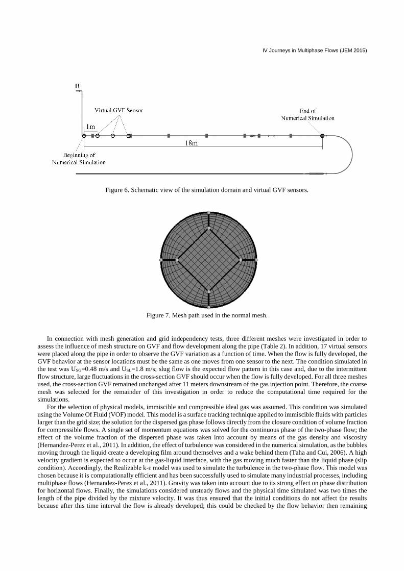
Regarding the set-up of the numerical model, a straight 18-m long section of the pipe where the ultrasonic meter will beinstalled was selected for simulation (Figure 6). It is recalled that the � �⁄ ratio upstream of the ultrasonic probe is 343, whichensures satisfactory flow development and insensitivity of the flow patterns to the boundary conditions (Hewitt et al., 1986).The CAD modeling was developed using STAR-CCM+ v9.02. A structured mesh was used to ensure more accuracy in theresults and decrease the computational time. An example of the pipe cross-section generated for this study is shown in Figure7. The mesh uses a constant spacing in the inner region of the pipe and a hyperbolic progression in the regions closer to thepipe wall. This progression starts at 0.15 mm from the wall in order to ensure a better resolution of the boundary layer.

Point # UsL UsG mL mG ahomogeneousAverage GVF

(numerical)

[m/s] [m/s] [kg/hr] [kg/hr] [%] [%] Baker Numerical

1 0,80 0,03 5.287,74 2,00 3,73

2 1,80 0,03 11.897,41 2,00 1,69 1,94 Plug Plug

3 4,40 0,03 29.082,55 2,00 0,70

4 0,80 0,06 5.287,74 3,87 6,98

5 1,80 0,06 11.897,41 3,87 3,23 2,99 Plug Plug

6 4,40 0,06 29.082,55 3,87 1,35

7 0,80 0,12 5.287,74 7,74 13,04

8 1,80 0,12 11.897,41 7,74 6,25 5,82 Plug Plug

9 4,40 0,12 29.082,55 7,74 2,65

10 0,80 0,24 5.287,74 15,49 23,08

11 1,80 0,24 11.897,41 15,49 11,76 10,90 Plug Plug

12 4,40 0,24 29.082,55 15,49 5,17

13 0,80 0,48 5.287,74 30,98 37,50

14 1,80 0,48 11.897,41 30,98 21,05 16,55 Slug Slug

15 4,40 0,48 29.082,55 30,98 9,84

16 0,80 0,96 5.287,74 61,95 54,55

17 1,80 0,96 11.897,41 61,95 34,78 28,02 Slug Slug

18 4,40 0,96 29.082,55 61,95 17,91

19 0,80 1,90 5.287,74 122,61 70,37

20 1,80 1,90 11.897,41 122,61 51,35 39,74 Slug Slug

21 4,40 1,90 29.082,55 122,61 30,16

22 0,80 3,80 5.287,74 245,23 82,61

23 1,80 3,80 11.897,41 245,23 67,86 59,54 Annular Transitional

24 4,40 3,80 29.082,55 245,23 46,34

25 0,80 7,60 5.287,74 490,46 90,48

26 1,80 7,60 11.897,41 490,46 80,85 65,99 Annular Wavy

27 4,40 7,60 29.082,55 490,46 63,33

28 0,80 13,00 5.287,74 838,94 94,20

29 1,80 13,00 11.897,41 838,94 87,84 85,02 Annular Wavy

30 4,40 13,00 29.082,55 838,94 74,71

Flow Pattern


Figure 6. Schematic view of the simulation domain and virtual GVF sensors.

Figure 7. Mesh path used in the normal mesh.

In connection with mesh generation and grid independency tests, three different meshes were investigated in order toassess the influence of mesh structure on GVF and flow development along the pipe (Table 2). In addition, 17 virtual sensorswere placed along the pipe in order to observe the GVF variation as a function of time. When the flow is fully developed, theGVF behavior at the sensor locations must be the same as one moves from one sensor to the next. The condition simulated inthe test was USG=0.48 m/s and USL=1.8 m/s; slug flow is the expected flow pattern in this case and, due to the intermittentflow structure, large fluctuations in the cross-section GVF should occur when the flow is fully developed. For all three meshesused, the cross-section GVF remained unchanged after 11 meters downstream of the gas injection point. Therefore, the coarsemesh was selected for the remainder of this investigation in order to reduce the computational time required for thesimulations.

For the selection of physical models, immiscible and compressible ideal gas was assumed. This condition was simulatedusing the Volume Of Fluid (VOF) model. This model is a surface tracking technique applied to immiscible fluids with particleslarger than the grid size; the solution for the dispersed gas phase follows directly from the closure condition of volume fractionfor compressible flows. A single set of momentum equations was solved for the continuous phase of the two-phase flow; theeffect of the volume fraction of the dispersed phase was taken into account by means of the gas density and viscosity(Hernandez-Perez et al., 2011). In addition, the effect of turbulence was considered in the numerical simulation, as the bubblesmoving through the liquid create a developing film around themselves and a wake behind them (Taha and Cui, 2006). A highvelocity gradient is expected to occur at the gas-liquid interface, with the gas moving much faster than the liquid phase (slipcondition). Accordingly, the Realizable k-ɛ model was used to simulate the turbulence in the two-phase flow. This model was chosen because it is computationally efficient and has been successfully used to simulate many industrial processes, includingmultiphase flows (Hernandez-Perez et al., 2011). Gravity was taken into account due to its strong effect on phase distributionfor horizontal flows. Finally, the simulations considered unsteady flows and the physical time simulated was two times thelength of the pipe divided by the mixture velocity. It was thus ensured that the initial conditions do not affect the resultsbecause after this time interval the flow is already developed; this could be checked by the flow behavior then remaining


constant as a function of time. The time step in the simulations varied in the 4 x 10-5 to 8 x 10-4 range in order to ensure aCourant number below 0.2 in the entire domain.

The inlet boundary condition was specified as a velocity inlet condition, which requires specifying the velocity and volumefraction of the mixture. In order to reduce the developing length, the liquid and the gas enters through the same boundary butthey are not mixed; the liquid enters through the upper half of the boundary and the gas in the lower half. The velocities foreach phase is specified as twice the corresponding superficial velocities in order to achieve the same volumetric flow. Finally,the separation generates a forced mixing between the fluids. The outlet condition was specified as a pressure outlet condition;a zero gauge pressure (atmospheric pressure) was used. The measurement region, i.e. the location of the ultrasonic probe, is13 m downstream of the inlet condition and 5 m upstream of the outlet condition.

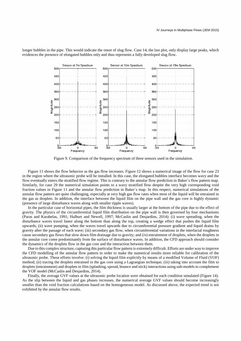
In order to analyze the flow development, a fast Fourier transformation (FFT) of the GVF variations as a function of timewas carried out for the virtual sensors placed every 1 m downstream of the gas injection point. Figure 9 shows the frequencyspectrum of the GVF results at 7, 10, and 13 m of the injection point. It can be observed that while there is a difference in the7 m spectrum, the 10 and 13 m spectra are essentially the same. A double-check was performed by means of cross-correlationsbetween successive GVF sensors using an 80% of the maximum correlation threshold as the flow development criteria; thecross-correlations showed the flow to be fully developed between the 13th and 14th sensors. Therefore, the flow was consideredfully developed 13 m downstream of the gas injection point.

Table 2. Mesh structures and corresponding simulation parameters.

Meshstructure

Number ofelements

Length required for flowdevelopment [m]

Computationaltime required [hr]

Coarse 453,600 11 11.5Normal 1,198,800 11 41.26

Fine 1,801,800 11 48.87

Figure 8. Volume fraction of gas in the inlet boundary condition.

4. RESULTS

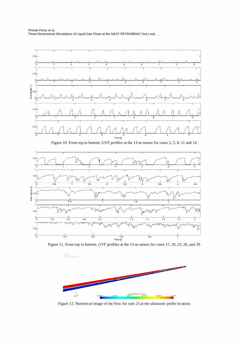
Ten conditions of the test matrix were selected to evaluate the performance of the numerical code developed. Theseconditions correspond to USL=1.8 m/s and are indicated by the red circles in Figure 5. It was then possible to investigate thetransitions from plug to slug flow and from slug flow to annular flow. Figure 10 and Figure 11 show the GVF profile for theten cases simulated at the virtual probe located at 13 m; the flow patterns inferred from the numerical simulations are listedin Table 1 along with the corresponding predictions from Baker´s flow pattern map. The sampling time is different for eachcase because the time required for flow development decreases with increasing mixture velocity. The first two plots in Figure10, cases 2 and 5, exhibit small peaks, which indicates the presence of cap bubbles in the flow. Cases 8 and 11, third andfourth plots, show small peaks as those in cases 2 and 5, but also larger ones, which indicates the presence of bigger and


longer bubbles in the pipe. This would indicate the onset of slug flow. Case 14, the last plot, only display large peaks, whichevidences the presence of elongated bubbles only and thus represents a fully developed slug flow.

Figure 9. Comparison of the frequency spectrum of three sensors used in the simulation.

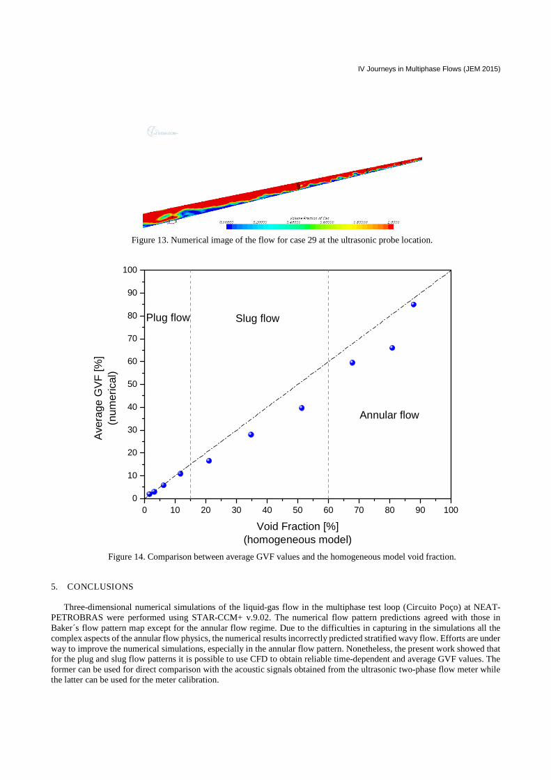
Figure 11 shows the flow behavior as the gas flow increases. Figure 12 shows a numerical image of the flow for case 23in the region where the ultrasonic probe will be installed. In this case, the elongated bubbles interface becomes wavy and theflow eventually enters the stratified flow regime. This is contrary to the annular flow prediction in Baker´s flow pattern map.Similarly, for case 29 the numerical simulation points to a wavy stratified flow despite the very high corresponding voidfraction values in Figure 11 and the annular flow prediction in Baker´s map. In this respect, numerical simulations of theannular flow pattern are quite challenging, especially at very high gas flow rates when most of the liquid will be entrained inthe gas as droplets. In addition, the interface between the liquid film on the pipe wall and the gas core is highly dynamic(presence of large disturbance waves along with smaller ripple waves).

In the particular case of horizontal pipes, the film thickness is usually larger at the bottom of the pipe due to the effect ofgravity. The physics of the circumferential liquid film distribution on the pipe wall is then governed by four mechanisms(Paras and Karabelas, 1991; Hulburt and Newell, 1997; McCaslin and Desjardins, 2014): (i) wave spreading, when thedisturbance waves travel faster along the bottom than along the top, creating a wedge effect that pushes the liquid filmupwards; (ii) wave pumping, when the waves travel upwards due to circumferential pressure gradient and liquid drains bygravity after the passage of each wave; (iii) secondary gas flow, when circumferential variations in the interfacial roughnesscause secondary gas flows that slow down film drainage due to gravity; and (iv) entrainment of droplets, when the droplets inthe annular core come predominantly from the surface of disturbance waves. In addition, the CFD approach should considerthe dynamics of the droplets flow in the gas core and the interaction between them.

Due to this complex structure, capturing this particular flow pattern is extremely difficult. Efforts are under way to improvethe CFD modelling of the annular flow pattern in order to make the numerical results more reliable for calibration of theultrasonic probe. These efforts involve: (i) solving the liquid film explicitly by means of a modified Volume of Fluid (VOF)method; (ii) tracing the droplets entrained in the gas core using a Lagrangian technique; (iii) taking into account the film todroplets (entrainment) and droplets to film (splashing, spread, bounce and stick) interactions using sub-models to complementthe VOF model (McCaslin and Desjardins, 2014).

Finally, the average GVF values at the ultrasonic probe location were obtained for each condition simulated (Figure 14).As the slip between the liquid and gas phases increases, the numerical average GVF values should become increasinglysmaller than the void fraction calculations based on the homogeneous model. As discussed above, the expected trend is notexhibited by the annular flow results.


Figure 10. From top to bottom, GVF profiles at the 13-m sensor for cases 2, 5, 8, 11 and 14.

Figure 11. From top to bottom, GVF profiles at the 13-m sensor for cases 17, 20, 23, 26, and 29.

Figure 12. Numerical image of the flow for case 23 at the ultrasonic probe location.


Figure 13. Numerical image of the flow for case 29 at the ultrasonic probe location.

Figure 14. Comparison between average GVF values and the homogeneous model void fraction.

5. CONCLUSIONS

Three-dimensional numerical simulations of the liquid-gas flow in the multiphase test loop (Circuito Poço) at NEAT-PETROBRAS were performed using STAR-CCM+ v.9.02. The numerical flow pattern predictions agreed with those inBaker´s flow pattern map except for the annular flow regime. Due to the difficulties in capturing in the simulations all thecomplex aspects of the annular flow physics, the numerical results incorrectly predicted stratified wavy flow. Efforts are underway to improve the numerical simulations, especially in the annular flow pattern. Nonetheless, the present work showed thatfor the plug and slug flow patterns it is possible to use CFD to obtain reliable time-dependent and average GVF values. Theformer can be used for direct comparison with the acoustic signals obtained from the ultrasonic two-phase flow meter whilethe latter can be used for the meter calibration.

0 10 20 30 40 50 60 70 80 90 100

0

10

20

30

40

50

60

70

80

90

100

Plug flow Slug flow

Ave

rag

eG

VF

[%]

(nu

me

rica

l)

Void Fraction [%](homogeneous model)

Annular flow


6. REFERENCES

Baker, O., 1954. "Design of Pipelines for Simultaneous Flow of Oil and Gas." Oil & Gas J. 53.Bond, L. J., M. Morra, M. S. Greenwood, J. A. Bamberger and R. A. Pappas, 2003. Ultrasonic Technologies for Advanced

Process Monitoring, Measurement, and Control. 20th IEEE Instrumentation and Measurement Technology.Goncalves, J. L., 2013. Desenvolvimento de uma Técnica Ultrassônica para Medição da Concentração das Fases Dispersas

em Escoamentos Multifásicos Representativos da Indústria de Petróleo e Gás Natural. Doutorado em EngenhariaMecânica Acadêmico, UNIFEI.

Grangeiro, F. A., 2010. Caracterização do Escoamento Intermitente Horizontal Água-Ar através de Ultrassom Auxiliado porFilmagem Ultrarrápida. Mestre em Ciências e Engenharia de Petróleo, UNICAMP.

Hernandez-Perez, V., A. M. and A. B., 2011. "Grid Generation Issues in the CFD Modelling of Two-Phase Flow in a Pipe."The Journal of Computational Multiphase Flows 3(1): 13-26.

Hewitt, G. F., J. M. Delhaye and N. Zuber, Eds., 1986. Multiphase Science and Technology. Springer-Verlag,Hulburt, E. T. and T. A. Newell, 1997. Prediction of the Circumferencial Film Thickness Distribution in Horizontal Annular

Gas-Liquid Flow. Mechanical Engineering Department, University of Illinois.Urbana, IL 61801McCaslin, J. O. and O. Desjardins, 2014. "Numerical Investigation of Gravitational Effects in Horizontal Liquid-Gas Flow."

International Journal of Multiphase Flow 67: 88-105.Paiva, T. A., 2011. Aplicação de Técnicas Ultrassônicas para Análise de Escoamentos Multifásicos Líquido-Sólido e Líquido-

Sólido-Gás. Dissertação de Mestrado, Universidade Federal de Itajubá (UNIFEI).Paras, S. V. and A. J. Karabelas, 1991. "Droplet Entrainment and Deposition in Horizontal Annular Flow." International

Journal of Multiphase Flow 17(4): 455-468.Shoham, O., 2006. Mechanistic Modeling of Gas-Liquid Two-Phase Flow in Pipes. Society of Petroleum Engineers,Taha, T. and Z. F. Cui, 2006. "CFD Modelling of Slug Flow in Vertical Tubes." Chemical Engineering Science 61(2): 676–

687.Tanahashi, E. I., 2010. Desenvolvimento da Técnica de Ultrassom para Medição da Fração de Vazio e Detecção do Padrão

de Escoamentos Água-Ar. Dissertação de Mestrado, Universidade Federal de Itajubá (UNIFEI).

7. RESPONSIBILITY NOTICE

The authors are solely responsible for the printed material included in this paper.

three-dimensional simulations of liquid-gas flows …

Documents