THREE DIMENSIONAL TISSUE CULTURING BASED ON

MAGNETIC CELL LEVITATION

by

James Aman

A senior thesis submitted to the faculty of

William Marsh Rice University

in partial fulfillment of the requirements for the degree of

Bachelor of Science

Department of Physics and Astronomy

William Marsh Rice University

April 2011

ii

Acknowledgements I would like to thank Dr. Killian for his assistance throughout this year. Not only was he always available to offer good advice and a knowledgeable take on various challenges encountered throughout the year but he also afforded me the privilege to work on an interesting and challenging project where I used and developed a wide range of skills. Thanks also go to Dr. Souza for allowing me to use his expensive camera equipment and also for allowing me to work on this project. Thank you also to Carly Filgueira for helping me culture cells and explaining many of the biological aspects of the process. Finally, I'd like to thank Stephanie Padley who worked tirelessly to measure the magnitude of the magnetic fields.

iii

Contents

Chapter 1

Introduction ........................................................................................................................................... 1-5

1.1 Evidence for differentiation ................................................................................................... 1-6

1.2 The single magnet system ...................................................................................................... 1-6

Chapter 2

The Magnetic Field ................................................................................................................................. 2-9

2.1 Finite Element Method Magnetics (FEMM) ........................................................................... 2-9

2.2 B-field results ....................................................................................................................... 2-12

2.3 Verification of 1D B-field measurements with MM-A-32 .................................................... 2-15

Chapter 3

Calculation and Results of the Magnetic Force ................................................................................... 3-17

3.1 MIO nanoparticle hysteresis ................................................................................................ 3-17

3.2 Expected force results .......................................................................................................... 3-17

3.3 Iron levitation results for MM-A-32 and MM-A-20 ............................................................. 3-22

Chapter 4

Cell Levitation and Results ................................................................................................................... 4-25

4.1 Levitation experiments with MM-A-32 and MM-A-20 ........................................................ 4-26

4.2 Complications of magnetic cell levitation ............................................................................ 4-27

Chapter 5

Generalization to a two dimensional magnetic array .......................................................................... 5-29

5.1 D22-N52 and the 96 well plate ............................................................................................ 5-29

5.2 Calculating the perturbed magnetic field ............................................................................ 5-32

5.3 Three dimensional force results .......................................................................................... 5-33

Chapter 6

Conclusions and future work ............................................................................................................... 6-37

Works Cited ................................................................................................................................................. 38

Appendix A

A.1 Defining new materials in FEMM ............................................................................................ 39

iv

1-5

Chapter 1 Introduction

Major advancements in technology, especially nanotechnology, in the past decades has led to a new era in scientific research, where the lines of traditional disciplines have blurred. Chemist are applying material science and engineering expertise to create nano racecars and biologist have achieved single molecule manipulation through application of optical and magnetic fields. Such techniques are common in physics research because they can lead to a high degree of control and predictability. This has led physicists and biologists to work together and tackle traditional problems with novel approaches. The use of nanoparticles in magnetic fields has led to the development of contrast-enhanced magnetic resonance imaging (1) while magnetic fields have been used to create magnetic tweezers capable of controlling single molecules (2). Recently, magnetic iron oxide (MIO) nanoparticles and applied magnetic fields have been used to levitate cells and enable three dimensional cell culturing. Two-dimensional cell culturing techniques have long been the standard in laboratories around the world. The relative ease of plating and incubating cells on the flat bottom of a petri dish has been the foundation of significant biomedical breakthroughs. However, these methods are known to produce cell growth with traits different from those found in vivo (3). This compromises their clinical relevance and motivates the need for innovative laboratory techniques to produce three-dimensional cellular growth environments. Several commercial products have been developed with varying success, which utilize protein-based gels or rotation/agitation-based bio-reactors in attempts to simulate three dimensional environments. Yet, a simple cost effective technique which artificially replicates the three-dimensional environment found in vivo remains an unmet need (3).

The magnetic levitation system developed at Rice University, M.D. Anderson Cancer Center, and n3D Biosciences, Inc. is based on the cellular uptake of a bioinorganic hydrogel composed of a polymer plus magnetic iron oxide and gold nanoparticles. The hydrogel is self assembling, and once mixed with the cells, the MIO nanoparticles are incorporated into the outside structure of the cells. Evidence was found that this system simulates the in vivo environment (4). This is promising since this technique is compatible with any cell type and does not require extensive training to use. Further applications of this technology range from a large number of small scale experiments to tissue or organ engineering, and is limited only by the size of magnetic field that can be created.

This research aims to quantify the forces acting on the cells to achieve a fundamental understanding of the levitation process, and through this investigation create numerical tools that can be used to study new geometries of the magnetic system.

Chapter 2 details the calculation of the magnetic fields produced by permanent magnets of Neodymium Iron-Boride while chapter 3 will discuss the force profiles produced by these magnetic field. Chapter 4 will introduce the experiments done levitating cells and compare predicted results to the real world behavior. The last topic covered in chapter 5 will extend the tools developed with the single magnet case to a two dimensional array of magnets. Finally, the last chapter will present the conclusions and future work to be done on this project.

1-6

1.1 Evidence for In Vivo Similarity

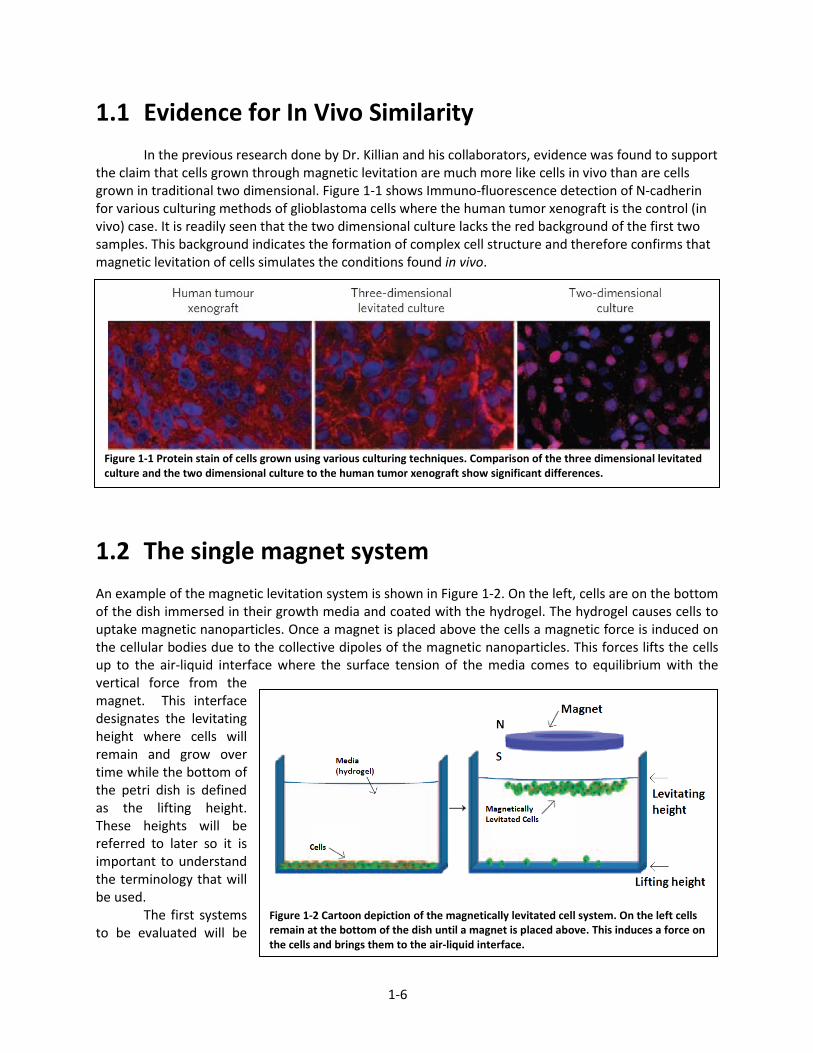
In the previous research done by Dr. Killian and his collaborators, evidence was found to support the claim that cells grown through magnetic levitation are much more like cells in vivo than are cells grown in traditional two dimensional. Figure 1-1 shows Immuno-fluorescence detection of N-cadherin for various culturing methods of glioblastoma cells where the human tumor xenograft is the control (in vivo) case. It is readily seen that the two dimensional culture lacks the red background of the first two samples. This background indicates the formation of complex cell structure and therefore confirms that magnetic levitation of cells simulates the conditions found in vivo.

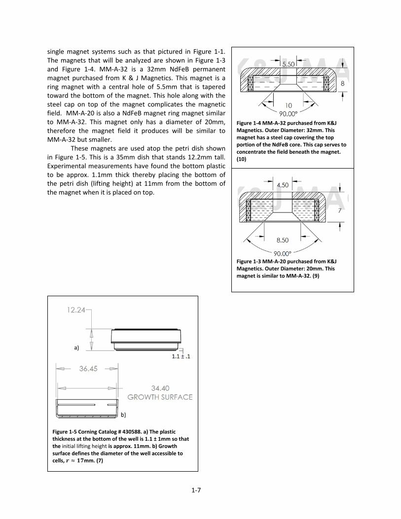
1.2 The single magnet system An example of the magnetic levitation system is shown in Figure 1-2. On the left, cells are on the bottom of the dish immersed in their growth media and coated with the hydrogel. The hydrogel causes cells to uptake magnetic nanoparticles. Once a magnet is placed above the cells a magnetic force is induced on the cellular bodies due to the collective dipoles of the magnetic nanoparticles. This forces lifts the cells up to the air-liquid interface where the surface tension of the media comes to equilibrium with the vertical force from the magnet. This interface designates the levitating height where cells will remain and grow over time while the bottom of the petri dish is defined as the lifting height. These heights will be referred to later so it is important to understand the terminology that will be used. The first systems to be evaluated will be

Figure 1-1 Protein stain of cells grown using various culturing techniques. Comparison of the three dimensional levitated culture and the two dimensional culture to the human tumor xenograft show significant differences.

Figure 1-2 Cartoon depiction of the magnetically levitated cell system. On the left cells remain at the bottom of the dish until a magnet is placed above. This induces a force on the cells and brings them to the air-liquid interface.

1-7

single magnet systems such as that pictured in Figure 1-1. The magnets that will be analyzed are shown in Figure 1-3 and Figure 1-4. MM-A-32 is a 32mm NdFeB permanent magnet purchased from K & J Magnetics. This magnet is a ring magnet with a central hole of 5.5mm that is tapered toward the bottom of the magnet. This hole along with the steel cap on top of the magnet complicates the magnetic field. MM-A-20 is also a NdFeB magnet ring magnet similar to MM-A-32. This magnet only has a diameter of 20mm, therefore the magnet field it produces will be similar to MM-A-32 but smaller. These magnets are used atop the petri dish shown in Figure 1-5. This is a 35mm dish that stands 12.2mm tall. Experimental measurements have found the bottom plastic to be approx. 1.1mm thick thereby placing the bottom of the petri dish (lifting height) at 11mm from the bottom of the magnet when it is placed on top.

Figure 1-5 Corning Catalog # 430588. a) The plastic thickness at the bottom of the well is 1.1 ± 1mm so that the initial lifting height is approx. 11mm. b) Growth surface defines the diameter of the well accessible to cells, mm. (7)

Figure 1-4 MM-A-32 purchased from K&J Magnetics. Outer Diameter: 32mm. This magnet has a steel cap covering the top portion of the NdFeB core. This cap serves to concentrate the field beneath the magnet. (10)

Figure 1-3 MM-A-20 purchased from K&J Magnetics. Outer Diameter: 20mm. This magnet is similar to MM-A-32. (9)

1-8

2-9

Chapter 2 The Magnetic Field

The first step to calculate the force produced on each cell must be to accurately calculate the magnetic field produced by particular permanent magnets. Such magnets may be modeled as a current sheet moving around a fixed geometry but this simple model neglects the effects of varying permeability between materials. The magnetic field is instead calculated using the program Finite Element Method Magnetics (FEMM). Briefly, the advantages of this program are the use of finite element analysis (FEA) to solve for the magnet field, the ability to define custom magnet geometries and materials, and a toolbox, OctaveFEMM that provides compatibility with Matlab and Octave. The following section will explore the use of FEMM to calculate the magnetic fields. Plots of the fields produced by MM-A-20 and MM-A-32 will then be examined and finally an analysis of the expected field measurements will be compared to measurements taken with a gaussmeter.

2.1 Finite Element Method Magnetics (FEMM) As noted above, FEMM utilizes finite element analysis to solve for the magnetic field. FEA is a numerical technique of solving partial differential equations by subdividing a large bounded region into smaller bounded areas. This creates a mesh on which the solution to the partial differential equation is found. Then using linear algebra techniques, separate solutions are pieced together using appropriate boundary conditions to solve for the solution on the entire domain.

When solving magnetostatics problems, such as permanent magnets, FEMM solves for the steady state solution of the magnetic field created by a surface current density, J as shown in Figure 2-1. This method follows easily from Maxwell’s equations and reduces the problem to simply characterizing

the surface current for various materials and applying boundary conditions to solve for the vector potential A. Starting with Maxwell’s equations for magnetostatics:

Eq. 1

= µ J Eq. 2

Eq. 2 is Ampere's law where µ is the permeability of the medium, which may be a function of the magnetic field, . The current density is denoted by J. Applying the Coulomb gauge, = 0, and

appropriate boundary conditions, FEMM solves the elliptical partial differential equation shown in Eq. 3

For the vector potential, . Substituting the definition of the vector potential, = , into Ampere's Law and rearranging gives:

Eq. 3

Figure 2-1 Permanent magnet approximated as a surface current circling a block of ferromagnetic material (6)

2-10

Figure 2-3 FEMM model of MM-A-32. (a) Each object must be completely closed and have a material assigned. (b) Solution mesh used by FEA solver.

Once the solution to A has been found, the magnetic field is calculated from the curl of A.

FEMM is a two-dimensional finite element solver for magnetostatics, electrostatics, heat flow, and current flow problems. Thereby assuming isotropy of the magnet in the phi direction, the full magnetic field can be characterized from a cross section computed by FEMM. Figure 2-2 illustrates the axisymmetric system and outlines field cross sections of constant that are found by FEMM. After finding the spatially dependent magnetic field produced by the permanent magnet the magnetic force produced on the nanoparticles must be calculated. The procedure and results of these force calculations is the subject of chapter 3.

The remainder of this section presents background information for using FEMM and discusses the boundary conditions

utilized in this system. For magnetostatics problems there are seven basic steps to using FEMM. These steps are outlined here with a more detailed overview of each step to follow.

1. Setup problem environment 2. Specify problem definition 3. Model the geometry 4. Define all materials 5. Define objects and their properties 6. Identify and set problem boundaries 7. Solve and load the solution

(Step 1) Analysis of a magnetostatics problem begins by setting up the problem environment. To begin simply create a new environment and select 'Magnetics Problem' from the drop down menu. (Step 2) Next, the problem definition is specified. This option assigns the geometry of the problem, the

Figure 2-2 Theoretical setup of the solution found beneath a single magnet. By assuming rotational symmetry of the magnet FEMM’s solution characterizes the entire magnetic field. This is shown in the figure by B1 = B2 for any Φ.

2-11

unit length in inches or millimeters, and various other options not used in this simulation. (Step 3) The third step is to model the magnet outline. FEMM uses simple points, lines, and arcs to define the geometry of its models. Models must be closed objects with well defined boundaries. Each object must also have a material assigned to it as in Figure 2-3. Otherwise, the solver will fail. One of the advantages FEMM provides is the ability to import AutoCAD DXF files. 3D AutoCAD models are typically available through the manufacturer’s website. Use of the manufacturer’s models minimizes the error between the FEMM model and the magnet since for certain magnets there may be dimensions that cannot be readily measured. (Step 4 & 5) Next, the material of every object in the model must be defined. Unfortunately, FEMM does not include an extensive materials library but does include tools for defining new materials. Details on defining new materials are included in appendix A. Designation of an object's material also assigns variables such as magnetization direction and mesh size. An example of the solution mesh used by the FEA solver is shown in Figure 2-3. Mesh size sets the maximum length of any leg in the triangular solution mesh, which in turn affects the accuracy of the magnetic field solution within the area enclosed by that object's boundaries. Note, the mesh size is inversely related to the computational time required to solve for the magnetic field. (Step 6) The last piece of the model is to establish boundary conditions. Open boundary problems are not solvable by the FEA method directly since it is a domain specific method. Instead open boundaries may be simulated using various techniques including the truncation method, ballooning, asymptotic boundary conditions, and Kelvin mapping (5). Figure 2-4 illustrates the outer boundary of the FEMM model for MM-A-32. For this investigation the asymptotic boundary condition (ABC) is used since it provides the most flexibility and ease of use. Further information about specifying the ABC method may be found below. (Step 7) Finally, after constructing the geometry of the model and defining all of its properties, FEMM creates a mesh of the problem area and solves for the magnetic field. Chen et. al. (5) provides an extensive overview of many common techniques for simulating open boundary problems. Here the focus will be on the derivation and implementation of the asymptotic boundary condition. The ABC condition is derived from general solutions of Laplace's equation in polar coordinates. Since B is only a two-dimensional vector field, then A = A so A is effectively a scalar potential that is required to go to zero as r approaches infinity, or . Therefore, the solution to the magnitude of A can be expressed by .

Where am and αm are the coefficient and phase angle of the nth harmonic, respectively. Similar to the multipole expansion of the vector potential, only the leading harmonic will contribute far from the

Figure 2-4 Full FEMM model for MM-A-32. FEMM assumes A = 0 along r = 0, so only the outer boundary must be specified.

2-12

region of interest. if m = 1 (dipole) is the leading order harmonic then the vector potential is approximated by::

Differentiating with respect to r,

Solving . for a1 and substituting into .

The first order Bayliss - Gunzburger - Turkel (BGT) operator is then given by

requires that thus . This is the form used by the 'mixed' boundary condition in

FEMM with

Where r0 is the outer radius of a circular boundary of the model in meters (regardless of working units set in the problem definition). These coefficients arise from considering higher order BGT operators

where . The asymptotic boundary condition as it is derived here requires a circular

outer boundary removed from the magnet model. To specify the boundary conditions for any model choose Properties from the Menu Bar of

FEMM and add a property. Figure 2-5 depicts the menus that must be completed to specify a Mixed boundary condition..

2.2 B-field results Once FEMM has solved for the magnetic field beneath a particular magnet the OctaveFEMM toolbox is used to read the data into Matlab for analysis. This section will study the vector field as well as contour plots of the magnetic field calculated by FEMM for magnets MM-A-20, MM-A-32. The force felt by the cells will be the primary subject of the next chapter. However, to quantitatively understand the effects of the magnetic field a brief consideration of the minimum force needed to lift the cells follows. Approximating a cell surrounded by MIO

Figure 2-5 FEMM menu for defining the outer boundary. NOTE: FEMM's underlying Lua scripting language parses all input before processing so you may enter c0 as 1/(uo*r). 'uo' is taken to be 4π x 10-7 by FEMM and r must be in meters.

2-13

nanoparticles as a dipole the force produced by the external field is given by Eq. 10. Eq. 10

Where m is the magnetic moment of each cell. In this section the effects of hysteresis are neglected making m constant. However, a full consideration of the hysteresis is presented in the next chapter. Ignoring interactions between nanoparticles and cells the force needed to levitate a cell must satisfy Eq. 11.

Eq. 11

Where Eq. 12

Eq. 13 Given an average cell density g/cm3, the density of water g/cm3, and the volume of a 16µm diameter cell, cm3 then and . This provides a lower limit of needed to lift cells from the bottom of the dish. To illustrate the method of approximating the magnetic force used in this chapter, an example is considered where B = 200 Gauss and ∇B = 50 Gauss/mm. These are experimentally determined measurements found at the bottom of the single well pictured in Figure 1-5 with magnet MM-A-20. Taking the average concentration of magnetic nanoparticles as 70pg/cell (experimentally measured) and the magnetic moment of the bulk nanoparticles as 20emu/g, the cellular magnetic moment is then

.

Where 20 emu/g arises from the response of the nanoparticle hysteresis curve for the given B value. This predicts a lifting force of which is expected to overcome gravity and produce levitation. This example is the same method used in each case shown below. Neglecting the

Figure 2-6 Magnetic vector field produced by MM-A-32, outer radius: 16mm. In the far field it appears a dipole however up close the effects of the ring geometry become pronounced. The unstable equilibrium at the center of the magnet pushes cells to an equilibrium point r > 0.

2-14

dependence of the magnetic moment on the applied field, the B-field gradient is all that changes. Thus the lifting force can be estimated by finding the gradient of the predicted magnetic field at 11mm beneath the magnet, corresponding to the bottom of the single dish, and finding its product with the cellular magnetic moment . This simplified approximation provides a quick check of each magnets levitation ability MM-A-32 Figure 2-6 shows a cross section of the magnetic field for MM-A-32 calculated by FEMM. The area shown is for but considering the axial rotational symmetry of the system, as shown in Figure 2-2, the three dimensional magnetic field can be easily obtained.. As expected the magnetic field lines loop around the magnet and create a vector field pointing to the magnetic material. As previously considered, the force to overcome the influence of gravity at the bottom of a well must satisfy

. From Figure 2-6, Gauss/mm and by Eq. 10, which is significantly more force than needed to levitate cells. General behavior of the magnetic forces can also be predicted using the magnetic vector field shown in Figure 2-6 since force is the gradient of the magnetic field. In the case of MM-A-32, the increase and subsequent decline of |B| along the axis suggests an unstable equilibrium point located beneath the magnet. MM-A-20 The magnetic field of MM-A-20 (Figure 1-3) is given in Figure 2-7. Similar to MM-A-32, the field strength dies off radially and vectors point to the magnetic material of the magnet as expected. At 11mm beneath the magnet the field gradient is approx Gauss/mm which would result in a lifting force of , strong enough to levitate cells.

Figure 2-7 Magnetic vector field produced by MM-A-20, outer radius: 10mm. Due to their comparable geometries this magnet creates a field similar to MM-A-32.

2-15

2.3 Verification of 1D B-field measurements with MM-A-32 The force on a cell due to the external field of the permanent magnet is not easily measureable. Instead, using a gaussmeter the magnetic field from a magnet can be measured and compared to the theoretical calculations. This serves as a preliminary check to determine the accuracy of FEMM's FEA solver and may provide any corrections needed to the computer model. Figure 2-8 details the results of the gaussmeter experiment averaged over several measurements. General behavior of the field is the same between both curves, however, the theoretical data is 10%-15% greater along most of the curve. This suggests that the calculated fields may predict forces slightly larger than what exists. Image a) of Figure 2-8 shows the field along the central axis, r = 0, of the magnet. Interestingly, the field decreases quickly to zero near the magnet. This behavior matches the contours of Figure 2-6 just beneath the center of the magnet and provides further evidence for a radial force pushing away from the center and this unstable equilibrium point of B.

2-16

Figure 2-8 B-field measurements for MM-A-32 using a gaussmeter compared to the theoretical predictions calculated by FEMM. a) Shows the field along the vertical r = 0 line directly beneath the magnet. b,c,d) show measurements along z = 0, -11, and -20 mm respectively. In general the behavior of the real field matches the predicted behavior.

3-17

Chapter 3 Calculation and Results of the Magnetic Force Using the full B-field calculated with FEMM, Matlab is able to determine the spatially dependent force produced per cell from Eq. 10. Unlike the previous force estimates which considered a constant magnetic moment per cell this chapter introduces the magnetization curve of the MIO nanoparticles. This curve is a non linear function of the applied external field, resulting in a spatially dependent magnetic moment for each cell. With this understanding of the calculation method, force profiles for MM-A-32, MM-A-20, and D22-N52 will be examined. Force estimates given in chapter two are then compared to the force predicted considering the effects of the magnetization curve. The last section presents the results of levitation experiments utilizing the levitation apparatus and magnetic iron oxide. This simple system eliminates any interactions present between cells and serves as a simple check of the magnetic forces by comparing predicted and observed equilibrium positions of the nanoparticles.

3.1 MIO nanoparticle magnetization Figure 3-1 shows magnetization of the magnetic nanoparticles as it varies with the applied field. Measurements were recorded at 300 K in a Quantum Design Magnetic Properties Measurement System (QD MPMS; T =1.8-400 K, Hmax = 5.0 T) (4) The maximum field applied is approx. 1.5 Tesla (15,000 Gauss); much greater than the magnetic fields produced by the permanent magnets considered in this project. Thus by fitting the curve shown in Figure 3-1 and interpolating the magnetization due to the external B-field, the magnetic moment per gram of nanoparticles, as a function of applied field, is found. Cells on average contain 70pg/cell of nanoparticles, which allows an estimate of the magnetic moment per cell. Matlab uses this to construct a matrix containing the induced magnetic moment at each spatial point. Then using Eq. 10 the magnetic force is calculated.

3.2 Expected force results This section covers the force per cell calculated for a single magnet. As described previously, MM-A-32 and MM-A-20 were magnets used in the initial testing of the levitation apparatus. Force

Figure 3-1 Magnetization as a function of applied magnetic field at constant temperature (300 K) for the magnetic iron oxide (MIO) nanoparticles. Inset shows magnetic hysteresis. Note: 1T=10,000G

3-18

Distance from

magnet bottom (mm)

Force at r = 0 (pN)

Force at r = 17 (pN)

Initial lifting height -11 60 15

Levitating height -7.5 80 30 Table 1 - Force per cell at selected heights of the single well using

measurements at the lifting height (bottom of the petri dish) will be compared to the estimates given in Chapter 2. The other topic discussed for each magnet will be the equilibrium radial distributions of cells at various media heights,

MM-A-32 This magnet has an outer radius of 16mm and a central hole, 2.75mm in radius. As shown in Figure 3-2, force vectors point to the area beneath the magnet. This suggests cells will follow a spatial distribution that mimics the geometry of the magnet when levitated above a threshold height, . Table 1 shows the predicted forces on each cell at the initial lifting and standard levitation heights. Although, behavior of the cells during levitation depends on |F| as well the direction of F as shown in Figure 3-2. The large discrepancy between the force estimated at the bottom of the single well in chapter 2, , and the calculated value shown in Table 1 demonstrates the importance of considering the nanoparticle magnetization curve. Using the field dependent magnetization curve presented in the previous section and a predicted field value of at

, the magnetic moment is which accounts for the approx 400% discrepancy between the previous estimation and the predicted value.

The threshold height, is the height above which the radial force profile has a zero equilibrium at , implying that cells will form a ring, rather than a concentrated disk on the central axis of the magnet Figure 3-3 presents the contours of radial force beneath the magnet. From this figure the threshold height is

Figure 3-2 Force vector field produced by MM-A-32, outer radius: 16mm. Force calculated using a 0.05mm spatial resolution. MM-A-32 is used in conjunction with the single well dish pictured in Chapter 1. At the initial lifting height of 11mm, Fmag varies from 60pN to 15pN providing adequate force to lift the cells based on the previous assumptions.

3-19

Figure 3-3 Contour lines of the radial force component. This predicts that there will be positive and negative radial forces creating an equilibrium off the central axis above

Figure 3-4 False color plot of the radial force close beneath the magnet. The dotted line shows a polynomial fit to the zero contour shown in Figure 3-3. From the intersection of the levitating height and the polynomial fit the radial equilibrium position of the particles can be determined.

3-20

Distance from magnet bottom (mm)

Force at r = 0 (pN)

Force at r = 17 (pN)

Initial lifting height -11 20 1-2

Levitating height -7.5 70 1-2 Table 2 - Force per cell at selected heights of the single well using MM-A-

. Below this height there are no positive radial forces pushing cells away from the center and cells accumulate in the region beneath the center of the magnet, resulting in a disk of cell growth centered at . At the liquid-air interface the surface tension is in equilibrium with Fz so the distribution of particles is determined solely by Fr. The last section of this chapter will compare observed radial equilibrium positions to predicted equilibrium positions to test the radial force calculations. Figure 3-4 features a polynomial fit to the zero contour shown in Figure 3-3. This curve fit is used to determine the average radial equilibrium point at any specified levitating height greater than the threshold height,

MM-A-20 Similar to MM-A-32, this magnet has an outer diameter of 20mm with a central hole, 4.5mm in diameter. As expected, the force vectors in Figure 3-5 point to the area beneath the magnet suggesting ring like cell growth when above . Table 2 quantifies the forces at specified depths below the magnet. Due to the smaller radius of this magnet the magnetic field, and thereby the force produced, decrease rapidly in the r direction. This results in forces of 1-2 pN at the bottom edge of a well,

. These weak forces may not overcome gravity and could result in incomplete levitation of a sample . Like MM-A-32, the force calculated at the initial lifting height satisfies the levitating condition, Eq. 11, and is greater than the

Figure 3-5 Force vector field produced by MM-A-20, outer radius: 10mm. Force calculated using a 0.05mm spatial resolution. MM-A-20 is used in conjunction with the single well dish pictured in Chapter 1. At the initial lifting height of 11mm, Fmag varies from 20pN to 1-2pN. Since Fmag is of the order of the force needed to lift the cells this may be used to test the force estimates at the bottom of the dish.

3-21

Figure 3-6 Contour lines of the radial force component. This predicts that there will be positive and negative radial forces creating an equilibrium off the central axis above

Figure 3-7 False color plot of the radial force close beneath the magnet. The dotted line shows a polynomial fit to the zero contour shown in Figure 3-6. From the intersection of the levitating height and the polynomial fit the radial equilibrium position of the particles can be determined.

3-22

original force estimate. Figure 3-6 depicts the contours of Fr for MM-A-20. The threshold height to producing ring like cell growth is . Below this height the zero contour follows the axis and there are no positive radial forces. Levitation below the threshold is expected to result in a disk geometry of cell growth beneath the magnet. Figure 3-7 shows a false color plot of the forces in Figure 3-6. Here it is easily seen how the positive radial forces disappear below , creating a large area of almost zero force between Also shown in Figure 3-7 is the polynomial fit to the zero radial contour. Once more, at any specified levitating height greater than the threshold height, the radial distribution of the levitating cells will be determined by the intersection of the levitating height and this curve fit.

3.3 Iron levitation results for MM-A-32 and MM-A-20

This section covers the experiments done levitating Fe2O3 nanoparticles without any cells within the levitation apparatus. This eliminates the added complications of cellular interactions and serves as a check of the equilibrium radial forces produced by each magnet. First, however, the experimental procedure and background information is

covered. The apparatus shown in Figure 3-8 was developed, to observe radial distributions of iron particles without disturbing equilibrium of the system. An optical mount glued beneath the box provides fine control of the level of the system and allows any deviations from normal to be minimized. If the magnet is not parallel to the media during levitation axial symmetry of the system breaks down and particles will concentrate at the point closest to the magnet as pictured in Figure 3-9. This occurs since in the particles frame

of reference . This

causes a force in the direction that pushes particles to cluster together at equal radii. During levitation deviations from parallel are minimized so that the radial force is roughly the same around the axis of the magnet as assumed.

Figure 3-8 Apparatus to monitor cell growth. a) Using a mirror tilted at approximately 45° levitation can be viewed from beneath the magnets allowing observation of the radial equilibrium position b) Actual device, an optical mount beneath the apparatus allows for fine control of the level of the system.

Figure 3-9 Effect of culture plate tilt on particle distribution. (a) Exaggerated schematic of tilted growing environment. The magnetic dipoles will seek to be closest to the source of the external B field when the liquid medium and permanent magnet are not parallel. The equilibrium position of the ring pattern is highly susceptible to this deviation normal which manifests the partial ring as shown in (b)-(c). Distribution of iron particles using MM-A-32 levitated at 5mm. Changing the angle of the magnet with respect to the normal causes the particles to move around a specified radius as shown in (b) and (c).

3-23

Distance from magnet bottom

(mm)

Predicted Observed (±1mm) Radius (mm)

Geometry Radius (mm)

Geometry

5 7 Ring 7.5 Ring

7.5 4.5 Ring 6 Ring 9 0 Disk 0 Disk

Table 3 Predicted and observed radial equilibrium for MM-A-32 using iron in water. Note: A value of radius = 0mm corresponds to a disk centered beneath the center of the magnet as shown in Figure 3-10(c)

Distance from magnet bottom

(mm)

Predicted Observed (±1mm) Radius (mm)

Geometry Radius (mm)

Geometry

4 4 Ring 4.5 Ring 7.5 0 Disk 0 Disk

Table 4 Predicted and observed radial equilibrium for MM-A-20 using iron in water. Note: A value of radius = 0mm corresponds to a disk centered beneath the center of the magnet as shown in Figure 3-11(c)

Results As discussed in previous

sections, the radial equilibrium position is expected occur at the intersection of the zero contour and the levitating height when

. When a disk is expected centered at

Table 3 shows the

expected and observed equilibrium positions for MM-A-32. The intersections of levitating height and the zero contour when

is shown by the blue lines in Figure 3-10(a). At mm, the observed iron radial distribution is given by Figure 3-10(b & c) and for mm a disc is formed, Figure 3-10(c), as expected.

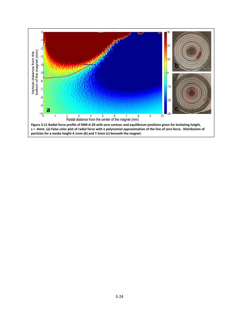
Table 4 and Figure 3-11 show the results of levitating iron using MM-A-20. For mm a ring is expected since

. When levitated at the standard height of 7.5mm, this magnet should produce a disc unlike MM-A-32. Figure 3-11(b & c) confirm the iron particles follow the radial distribution predicted by Figure 3-11(a).

Figure 3-10 Radial force profile of MM-A-32 with zero contour and equilibrium positions given for particular levitating heights, z = -5mm and z = -7.5mm. For various media heights the distribution of Fe2O3 particles is shown in (b)-(d). (a) Positive radial force pushes particles away from the central axis of the magnet while negative forces push inward. Particles are attracted to regions where the force is zero. (b),(c) Distribution of particles at a levitating height of 5 & 7.5mm. At these heights the particles form a ring as expected. (d) Result of levitation at 9mm. A broad disc is formed centered at as expected.

3-24

Figure 3-11 Radial force profile of MM-A-20 with zero contour and equilibrium positions given for levitating height, z = -4mm. (a) False color plot of radial force with a polynomial approximation of the line of zero force. Distribution of particles for a media height 4.1mm (b) and 7.5mm (c) beneath the magnet.

4-25

Chapter 4 Cell Levitation and Results

While chapters 2 & 3 are generally concerned with the theoretical approach to understanding the levitation mechanism, chapter 4 will introduce the experimental application and results of levitating cells for magnets MM-A-32 and MM-A-20. Cells introduce many complicating factors including large drag as a cell moves through the medium and organic interactions as cells grow and mature. These factors, perhaps along with other unidentified effects, cause the cells to react slowly and reach equilibrium only after hours instead of the instantaneous response seen during the iron experiments. This slow evolution creates an opportune environment to monitor cell behavior but also presents experimental complications inherent to biological systems such as maintaining optimal growth temperature while collecting data and preserving sterility of the sample to avoid contamination from outside bacteria. The following sections detail results of these experiments, compare the findings to the theoretical model as well as to similar iron systems, and ends with a brief discussion of problems encountered.

Figure 4-1 Radial cell distributions with a levitating height of 7.5mm below the magnet. Concentric circles are spaced 1mm apart. Approximately 500,000 HEK cells are pictured from beneath the magnet using the apparatus introduced in section 3.3. Cells initially rise to r=10mm beneath the magnet and are slowly pushed toward equilibrium by negative radial forces. The white areas pictured at 23 hours are the result of contamination of the system during growth. These massive particles are not expected to change the forces produced by the magnetic field.

4-26

Magnet Distance from magnet bottom (mm)

Predicted Radius (mm)

MM-A-32 7.5 4.5

9 0 MM-A-20 4 4

7.5 0 Table 5 Expected equilibrium positions at specified heights for MM-A-32 and MM-A-20.

Figure 4-2 Vertical forces beneath MM-A-32. During initial levitation these forces are responsible for bringing the cells to the surface quickly and are much stronger than radial forces (Figure 3-3)

4.1 Levitation experiments with MM-A-32 and MM-A-20

The experiments presented in this section were performed using the single well (Figure 1-5) with human embryonic kidney (HEK) cells grown over a 24 hour period in an incubator. Table 5 specifies the experimental conditions studied for each case.

MM-A-32 Figure 4-1 shows approximately 500,000 cells levitated at 7.5mm beneath the magnet. In the second hour of levitation there is clear movement toward the central axis of the magnet as cells are pushed toward the central axis by negative radial forces. The final picture at 23 hours shows that the cells come to rest near

, in agreement with FEMM's calculations. It should be noted that the white bodies evident in the final picture are the result of contamination during growth. Other interesting behavior can be seen in the early stages of growth as well. During this study and others performed with similar parameters, cells always appear first to surface near . This behavior can be partially attributed to large vertical forces acting on the cells, shown in Figure 4-2. However, vertical forces alone do not predict this reproducible behavior which suggest other interaction forces or dynamics that are not yet understand. MM-A-20 The smaller magnetic field produced by MM-A-20 results in slower movement of cells as shown in Figure 4-4, where cells are levitated 4mm from the bottom of the magnet. The threshold height for this magnet is 5mm so a ring formation is expected and can be seen as cells slowly move toward the central axis. The predicted equilibrium radius is which is not reached within the first 5 hours of growth. However after 23 hours, the cells have collapsed to a single mass which indicates that radial forces continued to push cells toward the center axis. Similar to MM-A-32, cells are brought quickly to the surface by strong vertical forces and pushed slowly toward equilibrium by much weaker radial forces. Repeated levitation experiments under similar conditions to those in Figure 4-3 reveal long strands of cells which stretch across the central area of the magnet in the first hours of levitation. In

4-27

Figure 4-3 these cells have began to collapse to a ring after 5 hours. This example illustrates the unpredictable behavior of these seemingly simple biological systems.

MM-A-20's smaller magnetic field also leads to a higher threshold height which makes characterization of disk like cell growth geometries easier. Figure 4-3 shows the levitation of cells at 7.5mm beneath the magnet. As expected, this configuration produces a well concentrated disk and does so in the first hours of levitation. The calculated radial forces of MM-A-20, shown in Figure 3-7, predicts cells to be no more than 2-3 mm from the center of the magnet and indeed Figure 4-3 shows this to be the case after 3 hours of levitation. Although, cells appear to continue moving inward and after 24 hours most cells have collapsed into a single mass whose shape cannot be explained by magnetic forces. Once again, illustrating the immense complexity present in biological systems

4.2 Complications of magnetic cell levitation As mentioned previously, biological systems introduce complications that are often hard to describe with simple physical models. Experiments with iron powder (Chapter 3) produced consistent results that were easy to interpret. Yet, similar experiments with cells did not show the same reproducibility and often produced results that defied simple explanations. Figure 4-5 shows an anomalous experiment using MM-A-32 with cells levitating 9mm beneath the magnet. Radial forces predict that cells will be

Figure 4-4 Radial distribution of cells levitated 4mm below MM-A-20. Concentric circles are spaced evenly by 1mm. Early growth shows cells stretched across the center of the magnet and subsequent movement by radial forces collapses cells to a single mass after 23 hours.

Figure 4-3 Radial distribution of cells levitated 7.5mm below MM-A-20. Concentric circles are spaced evenly by 1mm. Disk formation is in this system occurs rapidly and again cells are seen to collapse to a single mass after long periods of growth.

4-28

confined within a 6mm radius beneath the center of the magnet. However, after 24 hours of levitation cells appear to have remained nearly static. Other experiments at similar heights showed expected concentration of cells. This anomaly may then indicate something went wrong with the treatment of the cells with nanoparticles or that the cells were unhealthy for some reason.

Such results, as well as the long time required for cells to move to equilibrium suggest that other forces on the order of the magnetic forces are interacting with the levitated cells. From this discussion it is found that biological systems are complex, and more experiments are required to understand all of the factors that contribute to their behavior. But magnetic levitation and careful modeling of the magnetic fields and forces on cells present powerful tools that can be used to enable further study of this system

Figure 4-5 Radial cell distribution of MM-A-32 for a levitating height of 9mm below the magnet. This experiment did not show the expected result of a disk of cells concentrated inside of r=5mm.

5-29

Chapter 5 Generalization to a two dimensional magnetic array

Besides quantifying the magnetic forces produced on each cell from a single magnet, another goal of this research project is to generalize the single magnet results to a two dimensional array of magnets. This chapter will discuss how the magnetic field from D22-N52 (Figure 5-3) is changed due to off axis magnetic interference that results from the proximity of surrounding magnets. Finally, the force profiles created by the perturbed magnetic field will be discussed with the goal of determining the effective range of a single magnetic field in an array and determining which magnetization alignment, parallel or anti parallel, will produce a better levitating environment.

5.1 D22-N52 and the 96 well plate In the initial tests of the levitation apparatus, large scale

magnets and samples were used to prove the viability of this technology. However, by employing the simulation tools developed during this research, a scaled down version of the magnetic system can be analyzed to determine the feasibility of miniaturizing the device. If possible, the production of stable and reproducible magnetic levitation in a 96 well system, shown in Figure 5-2, would mark a significant achievement because this

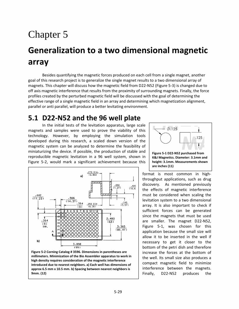
format is most common in high-throughput applications, such as drug discovery. As mentioned previously the effects of magnetic interference must be considered when scaling the levitation system to a two dimensional array. It is also important to check if sufficient forces can be generated since the magnets that must be used are smaller. The magnet D22-N52, Figure 5-1, was chosen for this application because the small size will allow it to be inserted in the well if necessary to get it closer to the bottom of the petri dish and therefore increase the forces at the bottom of the well. Its small size also produces a compact magnetic field to minimize interference between the magnets. Finally, D22-N52 produces the

Figure 5-1 D22-N52 purchased from K&J Magnetics. Diameter: 3.1mm and height: 3.1mm. Measurements shown are inches (11)

Figure 5-2 Corning Catalog # 3596. Dimensions in parentheses are millimeters. Minimization of the Bio Assembler apparatus to work in high density requires consideration of the magnetic interference introduced due to nearest neighbors. a) Each well has dimensions of approx 6.5 mm x 10.5 mm. b) Spacing between nearest neighbors is 9mm. (12)

5-30

strongest magnetic field for a given geometry of all the blends of NdFeB that are commercially available. Figure 5-3 shows the magnetic field and fields lines for D22-N52.

In close proximity, strong nearest neighbor magnets will introduce off axis magnetic interference to the system, D22-N52 has been chosen to minimize this effect when placed in the 96 well array. Figure 5-3 shows the predicted magnetic field which

decreases quickly as a function of the radius from the magnet. This solid cylindrical magnet has a height of 3.175mm and a diameter of 3.175mm, as shown in Figure 5-1. Since D22-N52 is a solid magnet, only disk like geometries can be achieved using this magnet regardless of the levitation height chosen. In chapter 2, when determining the forces produced by MM-A-32 and MM-A-20, it was assumed that the magnet would be placed on top of the petri dish cover, so the distance from the magnet to the dish bottom was fixed for the single well. For D22-N52 and the 96-well geometry, the possibility of modifications to the culture plate must be considered in order to put the magnet wherever the optimal position is. This requirement prompts the search for the distance from magnet bottom to dish bottom and distance from magnet bottom to air-liquid interface that

Figure 5-3 Magnetic vector field produced by D22-N52, outer radius: 3.175mm. This is a solid cylindrical magnet with the vector field pointing to the area directly beneath.

Figure 5-4 Force vector field produced by D22-N52, outer radius: 3.1mm. Force calculated using a 0.02mm spatial resolution. D22-N52 is for use with the 96 well plate pictured in Chapter 1. Due to the small size of the magnet the field produced is compact and decays very quickly.

5-31

Similar to: MM-A-20 MM-A-32

Bottom of well (-11mm)

5.2 4.2

Air-liquid interface (-7.5mm)

3.9 3.8

Height of Media (mm)

1.3 0.4

Amount of media (µL)

55 17

Table 6 - Depth where D22-N52 produces forces similar to MM-A-32 and MM-A-20

produced similar force profiles to those that worked with large magnets and the single well. These results will guide mechanical design of a 96-well geometry . The distances from magnet bottom to various heights where forces are similar to forces found for MM-A-32 and MM-A-20 are shown in Table 6. Also shown are the estimated height of the media and the volume of media needed for each case. Figure 5-6 shows a single well from the 96 plate and explains the relative heights of the system. The measurements in Table 6 make it evident that using D22-N52 in the 96 well plate will require the magnet to be placed close to the cell sample

and the small difference between the distance from magnet to the bottom of the petri dish and the distance from the bottom of the magnet to the air-liquid interface will restrict the amount of media that can be used.

Another limitation of levitating in such narrow wells that must be accounted for is meniscus formation which may cause some cells to travel away from the center and towards the edge of the well. Figure 5-5 shows a vector diagram that illustrates the forces at the meniscus. Migration of the cells up the meniscus will occur if the angle between the magnetic force and the

meniscus (shown by θ) exceeds 90⁰. This effect was

neglected in the single well case since the contact angle of cells at the surface was always less than 90⁰. At this time further investigation is needed to determine if this occurs at any point along the meniscus in the 96 well plate

Before continuing onto the results of the calculations done in the multi well array, various terms must be introduced to aid in the discussion that follows. Figure 5-7 shows the arrangement of the magnets that will be considered. Using this scheme any interior well of the 96 well plate can be modeled when nearest neighbor and next nearest neighbor perturbations dominate. All plots shown for the multi well system will be in the first

Figure 5-6 Schematic of a single well on the 96 plate with a magnet inserted into the well. All distances are relative a) Magnet D22-N52, that can be lowered to any height b) Initial lifting height, difference from the bottom of the magnet and the well bottom. c) Levitating height, difference between bottom of the magnet and the surface-air interface. d) Media volume, amount of media needed to reach the levitating height given by c.

Figure 5-7 Arrangement of the theoretical magnets in a 3x3 array. The central magnet can be considered as any interior well on the 96 well plate.

Figure 5-5 Vector illustration of the forces at the meniscus. Above 90⁰ cells will slide up the meniscus.

5-32

Figure 5-9 Example showing neighboring magnetizations in the 96 well array

quadrant, Q1. This takes advantage of the symmetry along each axis to display the behavior of the entire field. A line along is also shown as a reference for later figures.

The last term to discuss regards the magnetization direction mentioned previously. Parallel or anti parallel refers to the direction of magnetization of each neighboring magnet as shown in Figure 5-9. If parallel all magnets would be aligned the same way. However, If anti parallel the resulting magnetizations would be a checkerboard arrangement.

5.2 Calculating the perturbed magnetic field Calculation of the magnetic force produced by an array of magnets requires the magnetic field

be well defined since the force fields will not merely add linearly. Instead, the magnetic field from surrounding magnets must be summed together to find the resultant B vector field, then applying Eq. 10 the force produced on each cell can be determined in a similar manner to that used previously for the single magnet force profile. Since only like magnets will be used within the array, the contributions of surrounding magnetic fields may be modeled as a perturbation to the original field by other points of the original field. Examination of the magnetic field produced by D22-N52 (Figure 5-3) shows that it decreases rapidly as a function of the distance. Therefore, the dominant perturbations to the magnetic field produced by a single magnet will come from only the nearest and next nearest neighbors..

The 96 well plate has an adjacent well spacing of 9mm which places the next nearest neighbors approx. 13mm from central well in the 3x3 array. Using these parameters the magnetic field at the central well can be easily calculated using Matlab by simply translating the original field and summing the vector components at each point. Figure 5-8 shows a cross section of the perturbed magnetic field in the plane. With the addition of external field components, the axial symmetry of the original magnetic field is destroyed and full characterization of the magnetic field requires specifying r, z, and components.

Figure 5-8 Vector- contour plot showing the magnetic field at . As expected the field lines push away from one another at the midpoint between magnets. This field demonstrates an anti parallel alignment of magnetizations.

5-33

5.3 Three dimensional force results Using the three

dimensional magnetic field shown in the previous section, Matlab is able to calculate the magnetic force produced by D22-N52. In contrast to the earlier cases presented for MM-A-32 and MM-A-20, this system no longer displays axial

symmetry therefore

and a force in the phi direction will result. In general this force is much weaker than the radial forces and cells are still concentrated beneath the center of each magnet. Figure 5-10 shows the force produced in the first quadrant of the 3x3 array and confirms that the behavior is dominated by radial forces. The next behavior that must be analyzed is the effect of parallel vs. anti parallel magnetizations. Figure 5-11 and Figure 5-12 show cross sections of the first quadrant at with parallel and anti parallel magnetizations respectively. In the parallel case the z components of the magnetic field add constructively which creates an unstable equilibrium that will push cells away in all directions.

Figure 5-11 Vector plot of the force profile in a 3x3 array with parallel alignment of neighboring magnetizations at

. The magnetic field vectors show an unstable equilibrium point around 7mm. The point like nature of the equilibrium would cause particles to move in all directions away from this area.

Figure 5-10 Force vector field produced by D22-N52 in the 96 well configuration. This vector field shows how the phi forces are minuscule compared to radial forces which will dominate the cell distribution during levitation.

5-34

Conversely, when the magnetic fields are consider with anti parallel neighbors an unstable equilibrium is created along a line starting near 7mm between the magnets. This is due to the destructive interference of z components of the magnetic fields which decrease in magnitude radially from each magnet. This causes the vertical field components to cancel along a line instead of canceling at a single point when anti parallel. The lines which result from this type of alignment may be beneficial for the magnetic levitation system because they isolate of each well and will provide a more stable magnetic

Figure 5-12 Vector plot of the force profile in a 3x3 array with parallel anti-parallel alignment of neighboring magnetizations at . The magnetic field vectors show an unstable equilibrium line around 7mm. Along this line particles are expected to be push toward the central magnet. This behavior isolates each well from the others.

Figure 5-13 Force vectors in pN per cell at in quadrant 1 of the 3x3 array. Each wells has an approx. 3mm

5-35

environment to grow cells. By varying and taking cross section plots, similar behavior between each magnet is observed. The remainder of this chapter will assume force calculations with an anti parallel magnetization alignment. D22-N52 was chosen for use in the 96 well plate from comparison of its magnetic field and force profile to those of MM-A-32 and MM-A-20. This comparison showed that the lifting height should be approximately 5mm beneath the magnet while the levitating height should be roughly 4mm. Cross sections at of the force beneath the magnet are shown in Figure 5-13 and Figure 5-14. Figure 5-13 shows the cross section at the lifting height of 5mm. Due to the size of each well, cells are confined to a small area around the origin of approx. 3mm. In the region, mm to , the force varies from 10pN to 50pN. This is slightly less than what was expected from the single magnet results but should still allow levitation of cells. At the levitating height of 4mm Figure 5-14 shows the forces have not increased dramatically. Within the area of the well force varies from 30pN to greater than 70pN. This may allow cells to be levitated at slightly higher heights which would increase the stability of the system. However, if the cells get too close to the magnet the vertical force will overcome the surface tension in the media causing cells to emerge and stick to the magnet. Figure 5-15 shows the magnetic forces at 3mm beneath this magnet. From these predictions it may be viable to levitate cells without pulling them from the media but experimental testing must be completed to completely understand the two dimensional magnetic array.

Figure 5-14 Force vectors in pN per cell at in quadrant 1 of the 3x3 array. Each wells has an approx. 3mm

5-36

Figure 5-15 Force vectors in pN per cell at in quadrant 1 of the 3x3 array. Each wells has an approx. 3mm

6-37

Chapter 6 Conclusions and future work

At the time of this writing the code necessary to analyze the magnetic fields of a single magnet and a two dimensional array of magnets is complete. Experimental testing of the single magnet systems with iron particles and cells has shown general agreement between the predicted and observed behavior. However, tests of the 96 well system must be performed to determine the accuracy of the magnetic array solutions. Investigations into the minimum force needed to lift the cells also remain to be completed. It is proposed that such an experiment would proceed by varying the MIO concentration of nanoparticles per cell and thereby varying the force induced by the magnetic field.

The most significant challenge of this project was encountered during the experimental trials with cells, as this required a foray into the methods of research photography and as noted before cells simply did not behave as expected at times. It should be noted, however, that despite the complications encountered along many points in this research significant progress has been made in developing tools that can be passed on to further study this system.

Among the most interesting findings of this project was the determination of how to align neighboring magnets in the 96 well array. This definitive answer is a hallmark of this research project and demonstrates how the application of physical laws can be used to optimize and expand real world systems.

38

Works Cited 1. Applications of magnetic nanoparticles in biomedicine. Pankhurst, Q., et al. 2003, Journal of Physics, D., pp. R167-R181. 2. Single-molecule micromanipulation techniques. Neuman, K.C., Lionnet, T. and Allemand, J.-F. 2007, Annual Review of Materials Research, pp. 33-67. 3. The third dimension bridges the gap between cell culture and live tissue. Pampaloni, F., Reynaud, E. G. and Stelzer, E. H. 2007, Nature Review of Molecular Cell Biology, pp. 839-845. 4. Three-dimensional tissue culture based on magnetic cell levitation. Souza, Glauco, et al. 2010 йил, Nature nanotechnology, pp. 291-296. 5. A review of finite element open boundary techniques for static and quasistatic electromagnetic field problem. Chen, Q. and Konrad, A. 1, s.l. : IEEE, Jan 1997, Transaction on Magnetics, Vol. 33, pp. 663-676. 6. Meeker, David. Finite Element Method Magnetics version 4.2 User's Manual. Dec 26, 2009. p. 147. 7. Corning Incorporated. 35 mm PETRI DISH. Corning, NY : s.n., 2 20, 2007. 8. Campbell, Peter. Basic Permanent Magnetism: The demagnetization curve. Magnetweb. [Online] 2 8, 2008. [Cited: 6 28, 2010.] http://web.archive.org/web/20070802175337/www.magnetweb.com/Sect1C.htm. 9. K&J Magnetics, Inc. Mount magnet style A, MM-A-20. 10. K & J Magnetics, Inc.. Mounting magnet style A, MM-A-32. 11. K&J Magnetics, Inc. Disc/Cylinder magnet, D22. 12. Corning, Inc. 96 well flat bttom corner botch. Acton, MA : s.n., 10 9, 1997.

39

Figure A-3 Sample ideal and intrinsic demagnetization curves. Materials are deemed linear if the demagnetization curves are closer to the ideal curve shown here (8).

Figure A-1 The material definition prompt for FEMM. Users can utilize this function to create or modify materials in FEMM's material library. Boxed properties are those important for magnetostatics.

Appendix A A.1 Defining new materials in FEMM

When defining a new material in FEMM many options are presented to the user. This section will define the characteristics important to magnetostatics problems. Figure A-1 shows the menu a user is presented with to define a new material. After naming the new material the magnetic flux (B) vs. magnetic inductance (H) relationship must be defined. In physics this B-H curve refers to the full hysteresis loop but since permanent magnets only operate in the second quadrant of this loop the industry standard B-H curve refers only to the second quadrant of the full loop and is known as the demagnetization curve. This delineation is important to be aware of because when FEMM refers to a linear B-H relationship it is simply referring to the behavior of the hysteresis loop in the second quadrant. As an example of a linear B-H

relationship in the second quadrant, Figure A-2 shows the B-H curve for NdFeB grade 42 provided by K&J Magnetics. When creating linear materials such as NdFeB grade 42 in FEMM, the characteristics which must be set are the relative permeability in both directions (µr and µz) and the coercivity (Hc). This information is available from the demagnetization curve since the coercivity is the amount of applied field required to reduce the magnetic field produced by the magnet to zero. In other words, since then the coercivity is when the applied field equals the magnetization, ( i.e. ). Although not required by FEMM, another important quantity for permanent magnets is the remanence (Bd). This is the amount of magnetic flux (B) which the magnet produces after it has been magnetized and the magnetizing field reduced back to zero.

40

Figure A-2 Demagnetization curve for NdFeB grade 42[6]. Many manufacturer's typically provide B-H curves similar to this. From this curve a user can determine whether a material is linear or non-linear.

This point occurs where the demagnetization curve crosses the y-axis. By using the x-intercept (coercivity) and y-intercept (remanence) then the slope of the demagnetization curve can be found. This slope is the permeability of the material and since we are assuming isotropic materials the permeability is the same in both directions. Another method of obtaining the coercivity and permeability for linear materials is by using the maximum energy product (BHmax) and the Residual induction (Brmax). The residual induction is simply the maximum remanence point averaged over many samples for that material and the maximum energy product is the point at which the magnetic flux (B) and magnetic inductance (H) are maximized. Figure A-3 shows an ideal and intrinsic demagnetization curve. Since the maximum energy product is the

midpoint of the ideal curve then it can be given by: rearranging this equation the

coercivity can be found in terms of a common manufacturer specification BHmax, this is given by equation 5.

(5)

Since manufacturer's typically quote BHmax in mega- gauss oersteds (MGOe) and FEMM requires the coercivity in Amps per meter (A/m), when applying Eq. 5 the user must follow these conventions. Eq. 5 requires BHmax in MGOe and outputs the coercivity in A/m. Once the coercivity has been calculated Eq. 6 can be used to find the permeability. Eq. 6 simply takes the residual induction (y-intercept) and divides it by the coercivity (x-intercept) with coefficients which ensure the correct units.

(6)

For non-linear materials, access to the manufacturer's demagnetization curves is essential. Figure A-1 shows the option for 'Nonlinear Material Properties' grayed out but when a non-linear material is specified the user may utilize this option to define the demagnetization curve of the new material. FEMM uses a cubic spline method to fit the points and linearly extrapolates from the end of the curve if fields in the model exceed the provided data points.