three essays in development economics joshua gill

THREE ESSAYS IN DEVELOPMENT ECONOMICS

By

Joshua Gill

A DISSERTATION

Submitted to

Michigan State University

in partial fulfillment of the requirements

for the degree of

Agricultural, Food, and Resource Economics – Doctor of Philosophy

2019

ABSTRACT

THREE ESSAYS IN DEVELOPMENT ECONOMICS

By

Joshua Gill

The three essays in this dissertation study how the rural poor in Pakistan make choices and

how better program design can alleviate the constraints they face. The first essay investigates the

participation decision of smallholder paddy farmers in a Warehouse Receipts Financing (WRF)

program which can mitigate their credit and storage constraints, allowing them to increase their

incomes. We a discrete choice experiment approach to study the decision-making process and find

risk aversion and transaction cost erode the benefits for smallholder farmers making it an

unattractive prospect. We find that likelihood of participation can be increased through better

contract design which lower cost of participation and reduce exposure to price uncertainty. These

findings have important implications for the optimal design of warehouse receipt financing

contracts, as well as their general feasibility for marketing to small farmers. It also highlights that

programs aimed to uplift smallholder farmers should not only address constraints of circumstance

(e.g. access) but also internal constraints (e.g. risk aversion).

The second essay aims to alleviate information constraints regrading fertilizer usage as its

indiscriminate and faulty use can affect soil health. Evidence shows that soil quality in Pakistan

has been deteriorating which can be partially explain by poor nutrient management. In this study

we conducted soil tests and provided recommendations on use of organic and inorganic fertilizer.

This study uses an experimental design with two treatment arms and a control group which

received no information and its soil was not tested. The base treatment provided farmers with

information on their soil health and recommended fertilizer use condition on the crops they

cultivate. The second treatment arm complemented this information with a peer comparison which

was used an encouragement mechanism to improve the efficacy of information provided.

The study highlights some important constraints to information dissemination and provides

some evidence on the use of peer comparison as a potential tool to improve efficacy of information

campaigns. We see a statistically significant increase in manure usage and a heterogenous impact

on Urea use but no impact on the overall fertilizer use. We find that farmers they were already

using close to the recommended amount (within 1 bag deviation) increased their urea application

rate. These findings suggest two underlying mechanisms at play. First, it alludes to liquidity

constraints as farmers increased manure use which is cheap and those who could already afford

higher quantities of Urea were able to respond to the recommendation of increasing application

rates. The fact that we do not see impact on DAP further gives credence to this assumption as DAP

is close to 3 times the cost of Urea. Alternatively, it could be that farmers who were away from

the suggested fertilizer amounts did not trust the recommendations.

The third essay studies the dynamics of warehouse receipts financing (WRF) demand by

small scale risk averse farmers in Pakistan. A dynamic model is used to investigate how risk and

time preferences, transaction costs, and uncertainty reduce demand for WRF, and even lead to

non-participation in the program. The model is calibrated and solved for a representative small-

scale farmer that grows paddy. Results show high transaction costs to be a major barrier to

participation. Similarly, expectations about future prices also affect participation which drops to

zero if the subjective probability of prices falling goes beyond 10 percent.

Copyright by

JOSHUA GILL

2019

v

ACKNOWLEDGEMENTS

I am very grateful to Dr. Andrew Dillon for his invaluable support and guidance throughout

my PhD program. His advice was instrumental in helping me frame my research questions, secure

grants, and run my projects as a graduate student. I am especially thankful to Dr. Maria Porter for

agreeing to be my major professor in my last year of PhD and providing the guidance and support

that was needed to finish my dissertation. I also want to thank the other members of my committee,

Dr. Robert Myers, Dr. Vincenzina Caputo, and Dr. Chris Ahlin. Their advice was very helpful in

adding rigor to the analysis. I am also appreciative of other faculty members in AFRE and the

Economics department, particularly those who provided feedback at development seminars.

This dissertation uses data collected with the support of International Food Policy

Research Institute supervised by Dr. David Spielman. I am particularly grateful for his continuous

support and guidance; without him it would have been very difficult to carry out my research. I

would also like to thank Global Center for Food Systems Innovation at Michigan State, Center for

Economic Research in Pakistan, Dr. Asim Ijaz Khawaja and Dr. Farooq Naseer for their support.

I was lucky to be surrounded by great friends during my time at Michigan State University.

I would to thank Marie Steele, Hamza Haider, Mukesh Ray and Awa Sanou for their support.

Sophia, Joey, and Asa were especially helpful in my final year. I am particularly grateful to

Schanzah Khalid for her continuous support during my PhD program, helping me with my research

ideas, grant proposals, job applications, and inspiring me to excel.

Finally, my parents have been a source of constant support and I am grateful to them for

their encouragement. Without their prayers and support, I would not have gotten so far.

vi

TABLE OF CONTENTS

LIST OF TABLES ....................................................................................................................... viii

LIST OF FIGURES ........................................................................................................................ x

Essay 1 : Selling Cheap: Arbitrage in the Basmati Value Chain .................................................... 1

Abstract ........................................................................................................................................... 1

1.1. Introduction .......................................................................................................................... 2

1.2. Background .......................................................................................................................... 4

1.3. Experimental Methods ......................................................................................................... 6

1.3.1. Experiments .................................................................................................................... 6

1.3.2. Treatment Assignments .................................................................................................. 8

1.4. Estimation Procedures ........................................................................................................ 10

1.4.1. Risk Aversion ............................................................................................................... 10

1.4.2. Time preferences .......................................................................................................... 11

1.4.3. Discrete Choice Models ............................................................................................... 12

1.5. Data .................................................................................................................................... 16

1.6. Results ................................................................................................................................ 18

1.6.1. Risk and Time Preferences ........................................................................................... 18

1.6.2. Program Participation ................................................................................................... 19

1.7. Conclusion .......................................................................................................................... 23

APPENDICES .............................................................................................................................. 25

APPENDIX A – DISCRETE CHOICE EXPERIMENT ...................................................... 26

APPENDIX B – RISK AVERSION ..................................................................................... 29

APPENDIX C – TIME PREFERENCES ............................................................................. 34

BIBLIOGRAPHY ......................................................................................................................... 37

Essay 2 : Does peer comparison encourage adoption of best practices among farmers in

Pakistan? ................................................................................................................................ 42

Abstract ......................................................................................................................................... 42

2.1 Introduction ........................................................................................................................ 43

2.2 Conceptual Framework ...................................................................................................... 46

2.3 Experimental Design .......................................................................................................... 48

2.4 Intervention Description ..................................................................................................... 49

2.4.1 Soil Health Cards .......................................................................................................... 49

2.4.2 Mental Accounting and Call Reminders ...................................................................... 51

2.5 Data and Empirical Strategy ............................................................................................... 51

2.6 Estimation Methods ............................................................................................................ 54

2.7 Results ................................................................................................................................ 56

2.7.1 Take-Up ........................................................................................................................ 56

2.7.2 Manure Use .................................................................................................................. 58

2.7.3 Fertilizer Use ................................................................................................................ 59

2.8 Conclusion .......................................................................................................................... 60

vii

APPENDIX ................................................................................................................................... 63

BIBLIOGRAPHY ......................................................................................................................... 68

Essay 3 : A Dynamic Model for Warehouse Receipts Financing Demand in a Developing

Country .................................................................................................................................. 72

Abstract ......................................................................................................................................... 72

3.1. Introduction ........................................................................................................................ 73

3.2. Dynamic Storage Model ..................................................................................................... 76

3.3. Model Parameterization ..................................................................................................... 78

3.4. Results ................................................................................................................................ 83

3.5. Conclusion .......................................................................................................................... 85

APPENDIX ................................................................................................................................... 88

BIBLIOGRAPHY ......................................................................................................................... 95

viii

LIST OF TABLES

Table 1.1: Cost Benefit of WRF ..................................................................................................... 6

Table 1.2: Choice Experiment Attribute and Levels ...................................................................... 8

Table 1.3: Treatment Groups .......................................................................................................... 9

Table 1.4: Balance Table .............................................................................................................. 17

Table 1.5: Risk Aversion and Time Discounting Parameters ....................................................... 18

Table 1.6: MXL-EC Model (Preference Space) ........................................................................... 20

Table 1.7: Actual and Predicted Choices from MXL-EC model (Preference Space) .................. 21

Table 1.8: MXL-EC Model Estimates by Treatments (WTP Space) ........................................... 22

Table 1.9: Risk Aversion Choice List 1 ........................................................................................ 31

Table 1.10: Risk Aversion Choice List 2 ...................................................................................... 33

Table 1.11: Sheet 1 ....................................................................................................................... 34

Table 1.12: Time Discounting Choices ........................................................................................ 36

Table 2.1: Balance Table .............................................................................................................. 53

Table 2.2: Predicted Probabilities of Recalling Receipt of SHC .................................................. 57

Table 2.3: Predicted Probabilities of Trust in SHC ...................................................................... 57

Table 2.4: Tobit Estimates of Manure Applied (maunds/kanal)................................................... 58

Table 2.5: Heterogenous Treatment Effect on Urea ..................................................................... 60

Table 2.6: Balance Table (Restricted Sample for Heterogeneity) ................................................ 64

Table 3.1: Lagrange Results ......................................................................................................... 78

Table 3.2: Time and Risk Parameters ........................................................................................... 79

Table 3.3: Expected Prices (PKR/maund) .................................................................................... 81

Table 3.4: Warehousing Cost (40kg bag) ..................................................................................... 82

ix

Table 3.5: Base Case Parameter Values ....................................................................................... 83

Table 3.6: Simulation Results ....................................................................................................... 84

x

LIST OF FIGURES

Figure 1.1: Sampling strategy ...................................................................................................... 10

Figure 1.2: Switching Distribution ............................................................................................... 11

Figure 1.3: Sample Question (DCE) ............................................................................................. 28

Figure 1.4: Example Game ........................................................................................................... 29

Figure 1.5: Practice Game ............................................................................................................. 30

Figure 1.6: Sample Question (Risk Aversion) .............................................................................. 32

Figure 1.7: Calendar Sheet ............................................................................................................ 35

Figure 2.1: Study Design .............................................................................................................. 49

Figure 2.2: Soil Health Card ......................................................................................................... 66

Figure 3.1: Historical Paddy Prices (PKR/maund) ....................................................................... 80

Figure 3.2: Average Expected Paddy Prices (PKR/maund) ......................................................... 81

Figure 3.3: Storage Sensitivity Analysis ....................................................................................... 85

1

Essay 1 :Selling Cheap: Arbitrage in the Basmati Value Chain

Abstract

Smallholder farmers in developing countries face numerous constraints in both input and

output markets, that reduce their profit-generating potential. Warehouse Receipt Financing (WRF)

has been promoted as an innovative solution that provides access to more remunerative markets

and formal financial institutions. However, participation by smallholder farmers has been low

despite its potential for profit generation. This paper considers the case of a WRF intervention in

Pakistan which saw a similar outcome and aims to identify reasons for low take-up and how better

contract design can improve participation. This study finds that risk aversion as an important factor

for lack of participation. It highlights that smallholder farmers are unwilling to take on the entire

risk of price uncertainty due to intertemporal arbitrage. Results from a choice experiment show

that when smallholder farmers were offered the same WRF product with price certainty that

resulted in a no loss scenario predicted participation increased by 32 percent. This result highlights

that participation of smallholder farmers can be significantly increased by designing WRF

products and contracts that meet the needs of the farmers. These findings have important

implications regarding the demand for WRF and its general feasibility of marketing to smallholder

farmers.

2

1.1. Introduction

In most developing countries agricultural markets are marred with inefficiencies that lead to

a suboptimal equilibrium. Smallholder farmers are affected the most under these conditions as they

suffer both in the input and output markets. They are underserved by financial institutions and

have limited access to downstream buyers, as a result they rely on intermediaries who expropriate

rents. The outcome is a vicious cycle of low investment and low earnings which inhibits their

upward economic mobility. Moreover, a poorly functioning agriculture sector also hinders in

achieving the development goals of poverty reduction and inclusive economic growth as majority

of the poor live in rural areas and derive their livelihood from agriculture.

The desire to break this cycle has motivated numerous interventions (e.g. subsidies,

information, infrastructure) that have provided little benefit to smallholder farmers (Barrett et al.,

2012; Fafchamps and Minten, 2012; Fischer and Qaim, 2014; Jayne et al., 2018; Ricker-Gilbert et

al., 2013; Shiferaw et al., 2011). Warehouse receipts financing (WRF) has lately been promoted

as an innovative solution that can improve incomes of smallholder farmers by alleviating liquidity

and market access constraints (Aggarwal et al., 2018; Basu and Wong, 2015; Burke, 2014;

Omotilewa et al., 2018). However, smallholder farmer participation in these programs has not been

very encouraging (William and Kaserwa, 2015). There is limited work which explores the reasons

for low participation despite it being a profitable prospect (Miranda et al., 2017).

The purpose of this paper is to understand the marketing choices of smallholder rice farmers

in Pakistan under a WRF program.1 This study explores whether potential external and internal

constraints made non-participation a subjectively rational decision. Three main factors are

examined in this study: transaction costs, risk aversion, and impatience. The objective of the paper

1 This program was implemented in 2017 and farmers cultivating less than 10 acres were targeted. However, despite

high interest shown during village meeting, take-up was less than 2 percent among the target population at rollout.

3

is to test how better product and contract design can address these constraints and in doing so,

improve participation and earning possibilities of smallholder farmers. This paper uses a Discrete-

Choice Experiment (DCE), which has been used extensively to study consumer preferences and

has been widely applied in many fields of applied and development economics (Caputo et al.,

2013; Clark et al., 2014; Gibson et al., 2016; Lusk and Briggeman, 2009; Ortega et al., 2011;

Scarpa and Willis, 2010; Tanaka et al., 2014; Ward and Singh, 2015). We collect information on

risk and time preferences through incentivized games using a multiple price list approach.

(Andersen et al., 2008; Ward and Singh, 2015). In addition, respondents were randomly assigned

to one of three different experimental groups offering different hypothetical levels of price

guarantees: Group 1 was guaranteed a high price 3 months after storage; Group 2 was guaranteed

a low price; Group 3 was not given any price guarantees.

This study makes several contributions to the literature on WRF. First, we use a DCE

framework to evaluate whether a market for WRF exists among smallholder farmers, and their

willingness to pay (WTP) for this service. There is very limited and mixed evidence on the benefits

of WRF to smallholder farmers (Aggarwal et al., 2018; Burke, 2014; Miranda et al., 2017; William

and Kaserwa, 2015), and prior studies do not explicitly measure WTP. Information on farmers’

WTP can be very useful in developing appropriate products for smallholder farmers, and in

ascertaining whether such products would be financially feasible for providers. In addition,

internal constraints can act as independent sources of disadvantage and can affect smallholder

farmers’ technology adoption decisions (Duflo et al., 2008; Liu, 2013; Ward and Singh, 2015).

This study contributes to this body of literature by examining the role of risk aversion, time

discounting, and uncertainty on one’s decision to participate in WRF.

4

To our knowledge, only one other study has explicitly accounted for preference-related factors

when evaluating the feasibility of WRF programs (Miranda et al., 2017). The authors highlight the

role of preferences in eroding the profitability of WRF and suggest that WRF is not feasible for

smallholder farmers. We differ from this study by exploring ways to redesign WRF products to

address these issues.

Our results highlight that participation in WRF can be significantly increased if exposure to

price risk can be reduced, and that this factor is more important to farmers than either the cost of

transport or borrowing. Farmers in the price guarantee groups select the WRF option more often

(approximately 30 percent), which suggests that price uncertainty is a major deterrent to

participation. While marginal WTP decreases as interest rates increase, and increases if transport

is provided, farmers in the price guarantee group are willing to pay more for credit in comparison

to those in the other two treatment groups. Farmers who receive a price guarantee also have a lower

willingness to pay for transport compared to those in the other treatment groups. In addition, who

are relatively less risk averse or do no discount future payments are more likely to select WRF.

The remainder of the paper proceeds as follows: Section 1.2 provides background information

on the context of this study of Basmati rice farmers in Pakistan; Section 1.3 outlines the

experimental design; Section 1.4 outlines the estimation strategy; Section 1.5 discusses the data;

Section 1.6 summarizes the results; and Section 1.7 concludes.

1.2. Background

Rice value chain in Pakistan is underdeveloped and smallholder farmers suffer the most in

this environment. There is significant intertemporal and spatial price variation as the output

markets are inefficient and fail to move the product from surplus to shortage periods. Smallholder

farmers suffer more as they lack access to storage and sell their output immediately at harvest

5

when prices are depressed low. In addition, the playing field is also tilted against them in the input

market as they are underserved by formal financial institutions due to their small size and high

poverty incidence. This not only leads to liquidity constraints during the production cycle but also

limits the ability of smallholder farmers to invest in better technology. Taken together, these input

and output constraints severely inhibit the ability of smallholder farmers to take risks, make

necessary investments, and improve their productivity.

WRF has lately been promoted as a viable mechanism to develop the value chain and make it

more inclusive. WRF can improve income of smallholder farmers through three channels. First, it

provides access to storage allowing smallholder farmers to transfer produce from periods of

surplus to shortage. Second, it provides access to formal financial institutions by using stored grain

as collateral. Finally, the warehouse acts as a clearing house where product is graded and

agglomerated thereby improving the bargaining power of smallholder farmers, reducing the

transaction and search costs of doing business.

In 2017 a WRF program was piloted in the district of Hafizabad, Pakistan. The project was

implemented in 50 randomly selected villages with the objective of improving returns for

smallholder farmers through storage, credit, and better market linkages. Approximately, 1500

farmers cultivating under 10 acres registered for the program and gave soft commitments regarding

the quantity they would store in the upcoming harvest. However, once the harvest season

concluded less than 2 percent of the registered farmers had stored paddy at the warehouse. This

outcome was very puzzling as WRF was a profitable prospect and the increase in income was not

trivial as shown in Table 1.1.

6

Table 1.1: Cost Benefit of WRF

Year Harvest Price Post-Harvest Price Net benefit Profit

2016 Rs 1300/40 kg Rs 1900/40 kg Rs 240/40 kg Rs 360/40 kg Rs 10,800/acre

2017 Rs 1550/40 kg Rs 2200/40 kg Rs 240/40 kg Rs 410/40 kg Rs 12,300/acre

Note: This table shows the average prices at harvest and 3 month post-harvest in the project areas. The cost includes

drying charges, storage charges, rent for jute bags, labor, mark-up on loan, and weight-loss due to drying. The profit

figure is calculated using an average yield of 1200 kg per acre. These figures were provided by the warehousing

management company and reflect the prices at which paddy was bought and later sold by them. The cost of storage

was also shared by them based on the actual expenses incurred during the season.

`This paper aims to understand the participation choice of smallholder farmers and test if

alternate designs can improve take-up. The first question we address is whether there is demand

for WRF among smallholder farmers. Risk aversion, time discounting, and transaction costs are

explored as potential factors depressing demand. The choice of these factors is based on literature

which shows smallholder farmers to be price sensitive, reluctant to engage in risk prospects and

value immediate rewards more than future rewards. The second question this study addresses is

can participation be increased through better contract designs. We specifically test how a reduction

in uncertainty on returns can improve participation by farmers. Finally, the paper quantifies the

willingness to pay under different contract designs.

1.3. Experimental Methods

This section illustrates the experimental procedures. Respondents were first exposed to

incentivized games to elicit risk and time preferences and then to DCE questions. The first

subsection explains the games that were played to measure risk and time preferences and the DCE

that was implemented to elicit farmers preferences for WRF. The second subsection describes the

hypothetical price regimes farmers were randomly assigned to before participating in the DCE.

1.3.1. Experiments

This study utilizes risk and time discounting to explain farmer participation choice in WRF.

Risk and time preference have been extensively used to explain a range of choice behavior such

7

as technology adoption, investment, migration, education attainment, and smoking (Ashraf et al.,

2006; Chavas and Holt, 2006; Jensen, 2010; Lawless et al., 2013; McKenzie et al., 2013; Warnick

et al., 2011).

Multiple price list approach was used to elicit risk preferences. Two price lists with 14

questions in each list was used and the respondent had to choose between two lottery options

labelled Option A and Option B. Option A offered a sure small return and Option B offered a

higher expected return but with higher risk. Graphical images were used to help the respondent

understand the probabilities involved under both lotteries.

One price list with 10 questions was used to elicit the discount rate. Respondents were given

a token at the start of the game and informed that they could exchange it for real money based on

the questions in the price list. Each question had two options labelled Option A and Option B

offering different amount of money at different times in the future. Option A was for sooner

smaller payment and Option B was for larger later payment. Picture of a calendar with dates

corresponding to Option A and Option B was used to help the respondents understand the choices

better. These games were incentive compatible, and respondents were informed that at the end of

the game one of their responses will be randomly chosen for actual payment. Experimental

protocols for these games are shown in the Appendix.

In the DCE, respondents were asked to choose between three alternatives; two warehousing

products and an opt-out option. The warehousing products were described by three attributes as

reported in Table 1.2. These three attributes were chosen based on the conversations with farmers.

The cost levels reflect subsidized cost, true cost, and true cost plus a value-added service fee.

Credit up to 70 percent of the value of the stored product was offered to relax liquidity constraints

due to storage. The interest rate levels are reflective of the rate charged by government sponsored

8

agricultural loans, conventional banks, and microfinance banks. Transport is another critical

attribute considered as smallholder farmers do not own a truck and renting can be very costly given

their low volumes. Two levels of this attribute are selected based either paddy is picked from

farmgate or the farmer must arrange for the transportation.

Table 1.2: Choice Experiment Attribute and Levels

Warehouse Receipts Financing

Attributes Description Levels

Cost The cost of storage for a 40 kg bag of paddy. Rs 10 per month Rs 20 per month Rs 40 per month

Interest The depositor has the option to take loan of up to 70% of the value of the product stored at harvest.

No Interest 15 % per annum 30 % per annum

Transport Paddy would be picked from the farmer’s field for storage. Present Absent

An orthogonal optimal design was used for the DCE as a full factorial design would have

resulted in 324 possible choice questions. The questions were generated using Ngene software

which showed that a minimum of 18 choice sets were required to achieve 100 percent D-efficiency.

These questions were further divided into two blocks so that each respondent answered a set of 9

questions. This was done to avoid mental fatigue and loss of interest by the respondent, which can

lead to poor responses. Each choice set had three options; two options of a WRF service and an

opt out option. See appendix A for an example question.

1.3.2. Treatment Assignments

Respondents were randomly assigned to a group with a hypothetical price regime to estimate

its impact on participation choice. Table 1.3 shows the three experimental groups.

9

Table 1.3: Treatment Groups

Groups Treatments Description Price Guarantee

Group 1 Control No Price Guarantee --

Group 2 High Price High Price Guarantee Rs 1800 /40 kg

Group 3 Low Price Low Price Guarantee Rs 1600/40 kg

Respondents in each group were read a script before the start of the DCE informing them

regarding the hypothetical price scenario. Group 1 is the Control and respondents were informed

that the expected price of paddy at harvest is Rs1300/bag and historically paddy prices tend to rise

in the 3 months post-harvest. Hence, if they chose to store and sell later, they could earn a

significantly higher profit. However, they were also informed that profits were not guaranteed as

in any other business and prices can fluctuate unexpectedly. Group 2 is the High Price treatment

and respondents were informed that the expected price of paddy at harvest is Rs1300/bag and

historically paddy prices tend to rise in the 3 months post-harvest. Hence, if they chose to store

and sell later, they could earn a significantly higher profit. However, they were given the guarantee

that the warehouse would purchase at Rs1800/bag 3-month post-harvest irrespective of the market

price. Group 3 is the Low Price treatment and respondents were informed that the expected price

of paddy at harvest is Rs1300/bag and historically paddy prices tend to rise in the 3 months post-

harvest. Hence, if they chose to store and sell later, they could earn a significantly higher profit.

However, they were given the guarantee that the warehouse would purchase at Rs1600/bag 3-

month post-harvest irrespective of the market price. The scripts are given in the appendix.

The sampling frame for this study consisted of 1500 farmers in 50 villages who had earlier

shown interest in the WRF. A subsample of 800 individual was randomly drawn for this study. On

average 16 farmers were picked from each of the 50 villages. Farmers were then randomly assigned

to one of the three experimental groups and then to one of the two DCE blocks. Figure 1.1 outlines

the sampling strategy.

10

Figure 1.1: Sampling strategy

1.4. Estimation Procedures

This section explains the estimation procedure for the preference data collected through the

incentivized games and choice data collected in the DCE.

1.4.1. Risk Aversion

We estimate a Constant Relative Risk Aversion (CRRA) measure in this study and account

for probability weighting (𝛼) when estimating risk aversion (𝛿) (Kahneman and Tversky, 1979).

Consider a game with two potential outcomes X and Y which can occur with the probabilities p

and q, respectively. The value of the prospect can be given by

𝑈(𝑋, 𝑌, 𝑝, 𝑞, 𝛿, 𝛼) = 𝑉(𝑌) + 𝑤(𝑝)[𝑉(𝑋) − 𝑉(𝑌)]𝑓𝑜𝑟𝑋 > 𝑌 (1.1)

where 𝑉(𝑋) = 𝑋𝛿 , 𝑤(𝑝) = 𝑒𝑥𝑝(−(− 𝑙𝑛 𝑝)𝛼) and α and δ are jointly determined. Let us look at

the following example for illustration. If a participant switches from the risk-free option (A) to the

lottery (B) in question number 5 in both game 1 and game 2 then the following problem can be

solved to derive α and δ.

Village 16 Respondents

High Price 5 Respondents

Block1 3 Respondents

Block 2 2 Respondents

Low Price 5 Respondents



Control 6 Respondents



11

200𝛿 > 100𝛿 + 𝑒𝑥𝑝(−(− 𝑙𝑛 0.1)𝛼) (720𝛿 − 100𝛿)

200𝛿 < 100𝛿 + 𝑒𝑥𝑝(−(− 𝑙𝑛 0.1)𝛼) (820𝛿 − 100𝛿)

800𝛿 > 100𝛿 + 𝑒𝑥𝑝(−(− 𝑙𝑛 0.1)𝛼) (1240𝛿 − 100𝛿)

200𝛿 > 100𝛿 + 𝑒𝑥𝑝(−(− 𝑙𝑛 0.1)𝛼) (1300𝛿 − 100𝛿)

Figure 1.2 illustrates the switching points in the two games. As expected, we see a larger proportion

of switches happening later in the games suggesting the that the farmers are risk averse on average.

Figure 1.2: Switching Distribution

1.4.2. Time preferences

We estimate discount rates while controlling for concavity of utility and included a front-end

delay of two weeks in the games. Literature highlights correcting for concavity of utility as

ignoring it results in underestimating the discount factor and overestimating the impatience of the

respondent (Cheung, 2016). Similarly, using a front-end delay is recommended to ensures that the

12

transaction cost of receiving money is consistent across sooner and later payments (Andersen et

al., 2008). Utility in each period can be expressed as

𝑈(𝑡) = 𝐷(𝑡) ∙ 𝑉(𝑋) (1.2)

where utility 𝑉(𝑋) = 𝑋𝛿, the discount function 𝐷(𝑡) =1

(1+𝜌)𝑡 , and the interest rate is 𝜌 .The

respondent will select the sooner payment if the utility from it is higher compared to that in the

future. δ is estimated from the risk game and 𝜌 is estimated from the choices made by respondents

in the time preference game.

1.4.3. Discrete Choice Models

DCE methodology is based on Lancaster theory of consumer demand and McFadden’s

random utility theory (Hensher et al., 2015). The former assumes utility is derived from the

characteristics and properties of the good consumed rather than the good itself (Lancaster, 1966).

The latter assumes individuals to be rational beings who compare alternatives and select the option

that maximize their utility (McFadden, 1974). Formally, let 𝑈𝑛𝑗𝑡 represent the utility that an

individual 𝑛 derives from alternative j at time situation t. The decision maker evaluates all the

alternatives and choses i if and only if 𝑈𝑛𝑖𝑡 > 𝑈𝑛𝑗𝑡 ∀ 𝑗 ≠ 𝑖. However, the utility assigned by the

decision maker is not known to the researcher and is partitioned into an observed and an unknown

stochastic component 𝜖𝑛𝑗𝑡. The functional form of this utility can be written as:

𝑈𝑛𝑗𝑡 = 𝑉𝑛𝑗𝑡 + 𝜖𝑛𝑗𝑡 (1.3)

The most common assumption is that the observed part of the utility is linear in some observed

factors and can be expressed as 𝑉𝑛𝑗𝑡 = 𝑉(𝑥𝑛𝑗𝑡, 𝑧𝑛) where 𝒙𝑛𝑗𝑡 is a vector of product attributes,

𝒛𝑛 is the vector of decision maker’s characteristics, and 𝜖𝑛𝑗𝑡 is assumed to be independent and

identically distributed.

13

We used a mixed logit model with error components (MXL-EC) to analyze the choice data.

Estimation of the model was carried out using a panel data structure which includes individual

level risk aversion and discount rates as behavioral characteristics. MXL-EC was used as it is less

restrictive and allows us to capture both systematic and random taste variations and accounts for

correlations across utilities (Greene and Hensher, 2010). In addition, it also controls for the effects

associated with the opt out option relative to the experimentally designed alternatives (Caputo et

al., 2013; Scarpa et al., 2005, 2007). This utility structure can be expressed as follows:

𝑈𝑛𝑗𝑡 = 𝑉𝑛𝑗𝑡 + 1𝑗(𝜂𝑛𝑡) + 𝜖𝑛𝑗𝑡 (1.4)

where 1𝑗(∙) is an indicator function that takes the value of 1 for experimentally designed

alternatives; and 𝜂𝑛𝑡 is normally distributed with zero mean respondent-specific idiosyncratic error

component associated with the experimentally designed alternative but not with the opt-out option.

The rest of the elements in equation (2) are same as in equation (1). The unconditional probability

of individual n choosing alternative j under MXL-EC is given by:

𝑃𝑛𝑗𝑡 = ∫ ∫ ∏𝑒𝑥𝑝(𝑉𝑛𝑗𝑡 + 1𝑗(𝜂𝑛𝑡)

∑ 𝑒𝑥𝑝(𝑉𝑛𝑗𝑡 + 1𝑗(𝜂𝑛𝑡)𝑗

𝑇

𝑡=1

𝜂𝑛𝛽𝑛

𝑓(𝛽𝑛)𝑓(𝜂𝑛𝑡)𝑑𝛽𝑛𝑑(𝜂𝑛) (1.5)

where 𝑓(𝛽) and 𝑓(𝜂𝑛) are the probability densities over which the coefficients of 𝛽 and 𝜂𝑛vary

in the population.

Three MXL-EC models are estimated, one for each treatment group (Control, High Price,

and Low Price). All models account for random taste variation by allowing the coefficients of

attributes (cost, interest, and transport) to vary in the population following a one-sided triangular

distribution2. Whereas, the OptOut is assumed to be normally distributed as the utility from the

2 One-sided triangular distribution is used as symmetric distributions around zero, example normal can lead to

implausible results, such as a positive coefficient for cost. Under the one-sided triangular distribution, the parameters

in our specification are distributed as 𝛽𝑖 = 𝛽 + 𝛽𝑣𝑖 , 𝑣𝑖~𝑡𝑟𝑖𝑎𝑛𝑔𝑙𝑒[−1,1], where 𝛽𝑖 is distributed between (𝛽, 2𝛽)

with mean 𝛽 and variance 𝛽2 6⁄ .

14

status quo option can both be positive or negative3. The risk variable measures the constant relative

risk aversion (CRRA) and has a positive support. A value of 1 means the individual is risk neutral

while values smaller than 1 imply risk aversion and higher values imply risk loving behavior. The

time variable has a support between zero and 1, it measures the discount factor where zero implies

future income has no value and 1 implies that future income is not discounted at all. These

variables were interacted with the Opt-Out option as we assume that there might be heterogeneity

in farmers’ preferences with respect to selecting the WRF products. The utility function is

expressed as follows for all treatment groups:

𝑈𝑛𝑗𝑡 = 𝑂𝑝𝑡𝑂𝑢𝑡 + 𝛽1𝐶𝑜𝑠𝑡𝑛𝑗𝑡 + 𝛽2𝐿𝑜𝑤_𝐼𝑛𝑡𝑛𝑗𝑡 + 𝛽3𝐻𝑖_𝐼𝑛𝑡𝑛𝑗𝑡 + 𝛽4𝑇𝑟𝑎𝑛𝑠𝑝𝑜𝑟𝑡𝑛𝑗𝑡

+𝛾1(𝑂𝑝𝑡𝑂𝑢𝑡 ∗ 𝑅𝑖𝑠𝑘) + 𝛾2(𝑂𝑝𝑡𝑂𝑢𝑡 ∗ 𝑇𝑖𝑚𝑒) + 1𝑗(𝜂𝑛𝑡) + 휀𝑛𝑗𝑡 (1.6)

where OptOut is an alternative-specific constant representing the opt-out alternative, 𝐶𝑜𝑠𝑡𝑛𝑗𝑡 is a

continuous variable indicating the monthly cost of storage for a bag of paddy; 𝐿𝑜𝑤_𝐼𝑛𝑡 and 𝐻𝑖_𝐼𝑛𝑡

are effects coded variables indicating the per annum interest rate. 𝐿𝑜𝑤_𝐼𝑛𝑡 takes the value of 1 if

the interest rate is 15 percent and 𝐻𝑖_𝐼𝑛𝑡 takes the value 1 if the interest rate is 30 percent. If the

interest rate is zero, then then variables are coded as -1. Transport is also effects coded and takes

the value of 1 if the farmgate pick-up is provided and -1 otherwise.

Predicted probability of selecting an alternative in each choice set was computed using results

from the MXL-EC model. Based on these probabilities a new variable “WRF participation” was

created which takes the value 1 if one of the WRF alternatives was assigned the highest probability

and zero otherwise. A probit model was then estimated with “WRF participation” as the dependent

variable and treatment assignment as independent variables. The specification is given as

𝑌𝑛𝑡 = 𝛿0 + 𝛿1𝐿𝑜𝑤 𝑃𝑟𝑖𝑐𝑒 𝐺𝑢𝑎𝑟𝑎𝑛𝑡𝑒𝑒 + 𝛿2𝐻𝑖𝑔ℎ 𝑃𝑟𝑖𝑐𝑒 𝐺𝑢𝑎𝑟𝑎𝑛𝑡𝑒𝑒 (1.7)

3 The parameter is distributed as 𝑂𝑝𝑡𝑂𝑢𝑡𝑖 = 𝑂𝑝𝑡𝑂𝑢𝑡 + 𝛿𝑧𝑖 + 𝜎𝑣𝑖 , 𝑣𝑖~𝑁[0,1], where (𝑂𝑝𝑡𝑂𝑢𝑡 + 𝛿𝑧𝑖) is the

conditional mean and 𝜎 is the standard deviation.

15

where 𝑌𝑛𝑡 is a binary variable, 𝛿0 is the average participation rate in the control group and 𝛿1and

𝛿2 are the treatment effects on participation relative to the control. In addition to estimating the

impact on predicted choices a probit was also estimated on the actual choices made by the

respondents in the DCE.

Willingness to pay across the three treatment groups was calculated in the WTP space. This

outcome is important in establishing whether WRF has a market among smallholder farmers. WTP

can be obtained by taking a ratio of the attribute and price coefficients. However, these estimators

generally do not have finite moments as the ratios of the coefficients can have infinite variances

under most distributions (Daly et al., 2012). One solution is to fix the coefficient estimate on price

but that inherently assumes that everyone values money similarly. An alternate solution is to

estimate the model in the willingness to pay space as it relaxes the assumption to have a fixed price

coefficient (Scarpa et al., 2008). The coefficients can be directly interpreted as marginal WTP

measures (Scarpa and Willis, 2010) and it is also a more feasible approach when making

comparisons across treatments (Caputo et al., 2017).

An extended utility framework was used by pooling the data and including dummy variables

for treatment assignment which were interacted with the attributes (Bazzani et al., 2017; De-

Magistris et al., 2013; Lin et al., 2019). The data was pooled as high price guarantee vs control,

low price guarantee vs control, and high price guarantee vs low price guarantee. For each of the

experimental groups the utility in willingness to pay space can be specified as

𝑈𝑛𝑗𝑡 = 𝜃𝑛 [−𝐶𝑜𝑠𝑡𝑛𝑗𝑡 + 𝜔𝑛1𝐿𝑜𝑤𝐼𝑛𝑡𝑛𝑗𝑡

+ 𝜔𝑛2𝐻𝑖𝐼𝑛𝑡𝑛𝑗𝑡+ 𝜔𝑛3𝑇𝑟𝑎𝑛𝑠𝑝𝑜𝑟𝑡𝑛𝑗𝑡 + 𝑂𝑝𝑡𝑂𝑢𝑡 +

𝛿1(𝐿𝑜𝑤 𝐼𝑛𝑡𝑛𝑗𝑡 ∗ 𝑇) + 𝛿2(𝐻𝑖 𝐼𝑛𝑡𝑛𝑗𝑡 ∗ 𝑇) + 𝛿3(𝑇𝑟𝑎𝑛𝑠𝑝𝑜𝑟𝑡𝑛𝑗𝑡 ∗ 𝑇) + 1𝑗(𝜂𝑛𝑡)] (1.8)

+휀𝑛𝑗𝑡

where 𝜃𝑛 is a random positive scalar representing the price parameter, 𝜔𝑛𝑖 is the willingness to

pay for each of the attributes which are defined above, 𝛿1, 𝛿2, 𝑎𝑛𝑑 𝛿3 give the respective treatment

16

effects of the experimentally designed attributes. The sign and significance of the 𝛿𝑠 determine

how the willingness to pay for the different attributes varies under different treatments.

1.5. Data

Data for this study comes from two sources: a household level survey conducted in October

2017 and lab in the field experiments implemented in October 2018. Balance among respondents

across socio demographics, farm characteristics, liquidity constraints, and price expectations is

shown in Table 1.4. First three columns show the mean and standard deviation (brackets) of

variables in the three experimental groups. The last three columns show the p-value for differences

in means across the three groups. As shown in the table the variables are balanced across the

treatment groups. Data for variables in panel A, B, and C comes from the household survey while

data for panel D comes from the lab in the field experiments.

The average age of a respondent is 40 years with 7 years of schooling and a household of 5

persons. A farmer cultivates rice on around 7 acres of land and sell 150 maunds of paddy on

average. Around 64 percent of the farmers report that they are liquidity constrained and around 55

percent of them reported that they were able to acquire a loan. Among those who had taken loans,

a large proportion of them were from middleman. The prices reported suggest that on average

farmers expect the price to increase over the 3-month period post-harvest.

17

Table 1.4: Balance Table

Means p-values

Variables C T1 T2 [T1=C] [T2=C] [T1=T2]

A. Socio Demographic

Age (years) 39.27 (0.87)

40.06 (0.95)

39.02 (0.86)

0.718 0.894 0.714

Education (years) 7.05

(0.31) 6.87

(0.36) 7.48

(0.34) 0.898 0.360 0.285

Household Size 4.76

(0.14) 4.70

(0.14) 4.79

(0.15) 0.180 0.868 0.389

Asset Index 0.062 (0.19)

-.026 (0.15)

0.131 (0.16)

0.352 0.976 0.376

B. Farm Characteristics

Area (acres) 6.86

(0.33) 6.63

(0.34) 6.60

(0.33) 0.532 0.442 0.966

Commercial Farmer (0/1)

0.87 (0.03)

0.87 (0.03)

0.90 (0.03)

0.900 0.705 0.628

Quantity Sold (maunds)

146.39 (8.74)

141.25 (9.72)

159.31 (10.08)

0.875 0.204 0.245

Farm Gate Sales (0/1) 0.73

(0.02) 0.73

(0.03) 0.74

(0.03) 0.743 0.678 0.738

C. Credit Constraints

Cash Constrained (0/1)

0.64 (0.05)

0.64 (0.04)

0.62 (0.05)

0.877 0.839 0.998

Borrowing (0/1) 0.57

(0.04) 0.53

(0.04) 0.55

(0.05) 0.446 0.993 0.328

Borrowing from Middleman (0/1)

0.47 (0.02)

0.45 (0.02)

0.47 (0.02)

0.576 0.999 0.763

Borrowing for Ag Inputs (0/1)

0.54 (0.03)

0.52 (0.03)

0.54 (0.03)

0.547 0.765 0.809

18

Table 1.4: (cont’d)

Means p-values

C T1 T2 [T1=C] [T2=C] [T1= T2]

D. Subjective Price Expectations (Rs/40kg)

Min Price at Harvest (Rs/40 kg)

1481.48 (25.82)

1479.19 (28.28)

1496.86 (26.03)

0.909 0.764 0.541

Max Price at Harvest (Rs/40 kg)

1701.14 (30.44)

1681.40 (38.15)

1721.02 (34.82)

0.720 0.756 0.393

Min Price 3-months Post Harvest (Rs/40 kg)

1953.96 (39.20)

1930.78 (38.52)

1933.57 (35.85)

0.671 0.679 0.945

Max Price 3-months Post Harvest (Rs/40 kg)

2221.14 (43.27)

2185.32 (43.90)

2183.18 (49.07)

0.558 0.543 0.968

N 214 203 224

Note: The asset index score is was calculated using PCA and is composed of 23 items, which includes household

items, savings in commodities, and modes of transport.

1.6. Results

The first subsection reports risk aversion and discount factor estimates. The second subsection

reports results from the MXL-EC model, predicted probability of participation calculation, and

WTP outcomes.

1.6.1. Risk and Time Preferences

Table 1.5 shows the estimated constant relative risk aversion (CRRA) and the discount factor.

The average CRRA measure is 0.52 and average discount factor is 0.84. These results imply that

majority of smallholder farmers in our target area are risk averse and compared to a risk neutral

person would require higher returns to participate in WRF. Similarly, the discount factor highlights

that value of income earned in the future is eroded due to discounting. Hence, the return from WRF

would need to compensate for it as well to become an attractive prospect.

Table 1.5: Risk Aversion and Time Discounting Parameters

Mean SD Min Max Median

CRRA 0.51 0.42 0.05 1.5 0.35

Discount Rate 0.84 0.13 0.46 0.99 0.88

19

The table also highlights that there is significant heterogeneity in the risk and time discounting

traits as seen by the large range of the measures. This suggests that the utility derived from

participating would also vary across farmers.

1.6.2. Program Participation

The results show that farmers are price sensitive as higher cost of storage and interest rate

lowers utility and probability of participation. Tables 1.6 reports the MXL-EC estimates which

show coefficient estimates for cost and interest rate to be negative and statistically significant at

the 1 percent level across all treatment groups. This implies that higher cost and interest rates

reduce utility derived from WRF and are associated with a lower probability of participation. The

coefficient for transport is positive and statistically significant at the 1 percent level across all

models. This suggests that farmgate pick up service increases the marginal utility of WRF and

increases the probability of participation.

The result also shows dispersion around the mean of the sample population highlighting

heterogeneity in preferences. The standard deviation (spread) estimates for all elements of the

parameter vector are statistically significant at the 1 percent levels which implies that the

respondents have different individual-specific parameter estimates which might be different from

the mean parameter estimate. Therefore, the utility derived from WRF attributes could also differ

across individuals.

20

Table 1.6: MXL-EC Model (Preference Space)

Variable Pooled Hi Price Low Price Control

Means

Cost -0.13***

(0.01)

-0.14***

(0.01)

-0.11***

(0.01)

-0.14***

(0.01)

Low_Int -0.32***

(0.05)

-0.30***

(0.09)

-0.28***

(0.08)

-0.47***

(0.10)

Hi_Int -1.85***

(0.09)

-1.58***

(0.14)

-1.85***

(0.15)

-2.11***

(0.17)

Transport 1.02***

(0.05)

1.04***

(0.09)

0.91***

(0.08)

1.12***

(0.10)

OptOut 4.78

(4.17)

10.65

(7.94)

-0.10

(5.85)

-1.30

(4.86)

Standard Deviation

Cost -0.13***

(0.01)

0.14***

(0.01)

0.11***

(0.01)

0.14***

(0.01)

Low_Int -0.32***

(0.05)

0.30***

(0.09)

0.28***

(0.08)

0.47***

(0.10)

Hi_Int -1.85***

(0.09)

1.58***

(0.14)

1.85***

(0.15)

2.11***

(0.17)

Transport 1.02***

(0.05)

1.04***

(0.09)

0.91***

(0.08)

1.12***

(0.10)

Opt Out 4.02***

(0.40)

5.34***

(0.66)

5.90***

(0.61)

2.63***

(0.57)

Error Component 4.02***

(0.40)

0.96

(0.99)

0.30

(0.45)

4.31***

(0.48)

Heterogeneity in Mean

OptOut x Risk -4.68**

(1.24)

-6.41**

(2.67)

-3.56**

(1.52)

-2.24**

(1.14)

OptOut x Time -6.21

(4.25)

-14.00*

(7.91)

-1.40

(6.09)

-1.32

(5.12)

AIC 1.067 1.121 1.041 1.028

Sample 641 203 224 214

Observations 5769 1827 2016 1926 Note: The table reports parameter estimates in the preference space. The model was estimated in Nlogit 6 utilizing

500 Halton Draws.

Risk aversion and discounting decrease utility from participation in WRF. However, the effect

is statistically significant and consistent across the treatment groups only for risk aversion. The

coefficient on the interaction terms of opt-out and risk is negative and statistically significant at

the 5 percent level showing that as risk aversion decreases the disutility from not participating in

the WRF program increases, ceteris paribus. Similarly, the coefficient on the interaction term

21

between opt-out and discount rate is negative suggesting that as the discount factor increases

(discounting declines) the disutility from not participating in the WRF program increases, ceteris

paribus. However, this is only statistically significant for the high price guarantee group at the 10

percent level.

A product design which reduces exposure to risk, if financially feasible, could potentially

increase smallholder participation. Table 1.7 reports results from a probit model which estimated

the probability of participation across the three treatment groups. As expected, respondents in the

price guarantees groups have a higher likelihood of selecting the WRF option and the increase is

statistically significant at the 1 percent level as shown by the p-values. Model 2 reports the

predicted probability of selecting the WRF option based on the MXL-EC results which controls

for observable and unobservable preferences. The results are consistent with the actual choice but

of higher magnitude. The probability of selecting the WRF is higher in the price guarantee groups

and the difference between High Price and Low Price group is also statistically significant.

Table 1.7: Actual and Predicted Choices from MXL-EC model (Preference Space)

(1) (2)

Variable Actual Choices Predicted Choices

Control 0.51***

(.03) 0.46***

(.01)

High Price Guarantee 0.67***

(.03) 0.71***

(.01)

Low Price Guarantee 0.68***

(.02) 0.78***

(.01)

Hypothesis Test p-value

H1: Control = High Price 0.001 0.000

H2: Control = Low Price 0.000 0.000

H3: High Price=Low Price 0.743 0.000 Note: Coefficients cannot be compared across different groups due to the scaling factor. Hence, we used the MXL-

EC results to generate individual specific predicted probability of selecting an alternative in each choice set for the

three groups. The probabilities are then pooled across the treatment groups and a Probit model is estimated with village

fixed effects and standard errors were clustered at the village level. The probabilities were calculated using the margins

command in stata. Column 1 reports the estimates on actual choices in the DCE for comparison.

22

WTP space estimates show that WTP is higher for credit in the price guarantee groups and

lower for farmgate pickup. Table 1.8 reports the WTP estimates4 with the corresponding p-values

related to the difference in marginal WTP for interest and transport attributes. Respondents in the

High Price group show a higher WTP for credit compared to the control group. However, the

difference is statistically significant only for the High Int level. WTP for transport on the other

hand is lower in the high price guarantee group and the difference is statistically significant.

Comparison between Low Price and Control groups shows that WTP for credit is higher with a

price guarantee. However, in this case the difference is statistically significant only for the Low

Int level. WTP for transport on the other hand is lower and the difference is statistically significant.

Comparison between the High and Low Price guarantee groups shows WTP for credit is higher

for credit and lower for transport in the high price guarantee. However, the differences are

statistically significant only for Hi Int and transport.

Table 1.8: MXL-EC Model Estimates by Treatments (WTP Space)

Variable Coefficient Standard Error p-value

𝑾𝑻𝑷𝑯𝒊𝒈𝒉_𝑷𝒓𝒊𝒄𝒆 = 𝑾𝑻𝑷𝑪𝒐𝒏𝒕𝒓𝒐𝒍

Low_Int 1.84 1.25 0.140

High Int 3.27*** 1.06 0.002

Transport -2.53*** 0.83 0.002

𝑾𝑻𝑷𝑳𝒐𝒘_𝑷𝒓𝒊𝒄𝒆 = 𝑾𝑻𝑷𝑪𝒐𝒏𝒕𝒓𝒐𝒍

Low Int 2.52** 1.27 0.048

High Int 1.01 1.15 0.380

Transport -3.83*** 0.68 0.000

𝑾𝑻𝑷𝑯𝒊𝒈𝒉 𝑷𝒓𝒊𝒄𝒆 = 𝑾𝑻𝑷𝑳𝒐𝒘 𝑷𝒓𝒊𝒄𝒆

Low Int 0.55 1.59 0.723

High Int 2.98** 1.41 0.035

Transport -2.05* 1.22 0.094

Note: The model was estimated in Nlogit 6 utilizing 500 Halton Draws.

4 The cost variable was divided by 10 and the estimates were multiplied by 10 to calculate WTP. The model was not

estimated with risk and time interactions for two reasons: 1) We are interested in the overall WTP across the three

treatment groups and 2) the models did not converge when these interactions were included.

23

These results show that if there is less uncertainty in returns farmers would be willing to pay

a higher price for credit but would value farmgate pick-up less. These outcomes provide some

evidence that contract designs which reduce exposure to price uncertainty can increase

participation and allow the provider to charge slightly higher prices for WRF.

1.7. Conclusion

Smallholder farmers continue to face numerous constraints which discourage productivity

enhancing investments. WRF has recently be promoted as a viable potential solution to address

financial inclusion and market access constraints of farmers. The introduction of WRF for

smallholder farmers in Hafizabad, Pakistan is a case in point. However, participation by

smallholder farmers was very low despite it being a profitable prospect.

We find that external and internal constraints combined erode the profitability of WRF,

making it a less attractive prospect. Results show that high transaction costs reduce the

attractiveness of WRF as seen by the negative marginal utility on cost and interest rate parameter

estimates. We also see that farmers value transport from the farm gate to the warehouse, a service

which was not offered in the pilot. Risk aversion is another important factor that reduces the

attractiveness of WRF as the program required farmers to take price risks. The experimental

treatment design further validates this conclusion as we see an increase in predicted participation

for WRF under the price guarantee groups. An important finding is that the increase in participation

is also high under the low-price guarantee suggesting that smallholder farmers and they would be

willing to participate as long they are assured that they will not incur a loss.

Since, this study uses stated preference data one can argue that the results suffer from

hypothetical bias. This criticism is fair, but it does not diminish the findings of the study which

highlights that the existing contract only focused on the constraints of circumstance and failed to

24

address the internal constraints of smallholder farmers which made participation an unattractive

prospect. These findings are particularly relevant for Pakistan as the agriculture value chains are

very underdeveloped and WRF has the potential to improve and develop these value chain.

Importantly, the federal government also recognizes this potential of WRF and the state bank of

Pakistan and developed a regulatory framework to operationalize WRF. However, establishing a

warehouse network is an expensive infrastructure endeavor and it is important to understand the

markets appetite while designing WRF products, especially those that would target smallholder

farmers. These results also highlight the need to incorporate the preferences of the target

population while designing programs aimed to improve their welfare.

25

APPENDICES

26

APPENDIX A – DISCRETE CHOICE EXPERIMENT

Now I will present you with some choices regarding a warehousing service. In each of these

questions I will present you with two versions of a warehousing product and a no-purchase option.

The warehousing options vary across the questions in terms of cost of storage, pickup service from

your farm, and future price after 3 months. For each of these questions, we would like to know if

you are interested in either of the warehouse product. You can always choose the not interested

option. If you are interested in the warehousing option, please also share what proportion of your

harvest you would be interested in storing. For example, you will only store 50 out of your 150

bags of paddy.

There are a few things you should keep in mind when making these decisions:

• Assume there are no other options except for the ones we are showing you.

• All the choices are separate so do not try to remember your choices in the previous questions.

In simple words treat each warehouse product option separately.

• Once you have made the choice you cannot go back and change it.

Group 1 Script – High Price Guarantee

Suppose your paddy is ready for harvest and the selling price of paddy is Rs1300 per maund

if you take it to the mandi. Looking at past paddy prices there is a good chance that the price of

paddy will rise in the future and you can earn more if you sell later. A company is offering farmers

like you the option to store your paddy and earn better income by selling later. The company is

guaranteeing to buy the paddy at a premium of Rs1800 after 4 months even if the prices are lower,

so you have a guaranteed higher income.

Credit against the stored paddy is also available if required, for example if you store paddy

worth Rs 100,000 you can get credit of upto Rs70,000 at a service charge. You can sell you paddy

to anyone and anytime once you repay the credit. The sale option is also available at the warehouse.

27

Once the product arrives at the warehouse it will be cleaned, dried, graded, weighed, and bagged

by the staff at the warehouse. After the bagging is complete your bags will be tagged using your

id number and stacked in the warehouse. The warehouse staff will regularly check the paddy to

ensure that the moisture level is controlled and will be responsible for the safety of the product.

The warehouse charges are meant to cover these expenses. The service charge on loans is meant

to cover the cost of employees and travel.

Group 2 Script – No loss Guarantee



paddy will rise in the future and you can earn more if you sell later. A company is offering farmers

like you the option to store your paddy and earn better income by selling later. The company is

guaranteeing to buy the paddy at a premium of Rs1800 after 4 months even if the prices are lower,

so you have a guaranteed higher income.










Group 3 Script – No Price Guarantee

28



paddy will rise in the future and you can earn more if you sell later. However, the company gives

no guarantee about future price.










Figure 1.3: Sample Question (DCE)

Option 1 Option 2 Option 3

29

APPENDIX B – RISK AVERSION

Instructions

This game gives you two options to choose from and the two options are labelled Option A

and Option B like before. Please look at the handout which shows an example of the game.

Figure 1.4: Example Game

If you select Option A you draw a ball from the cylinder on the left and you will get Rs100 if you

pick a blue ball which will be true every time as all balls are blue. If you select Option B then you

draw a ball from the cylinder on the right. You will get Rs 2600 if you pick the green ball and Rs

500 if pick the yellow ball. The chance if picking a green ball is one out of ten. Here again, there

are no correct or incorrect answers. We just want to know what you prefer and would choose. Now

let’s play a practice game so that you understand the game better.

Practice Game

As you see each question had two Options: A and B to earn some candies. These two options

differ in the number of candies you can win depending on your choices. For example, in question

number 1, under Option A, you always draw a blue ball and earn three candies for sure. For the

30

same question, if you choose Option B, you can earn either five candies if you draw green ball or

you earn only 1 candy if you draw the yellow. The number of candies you can earn in Option A

under all the questions remains the same but in Option B, the number of candies you can win with

the green ball increases, but if you get yellow colored ball it remains the same (1 candy), in all the

questions.

Figure 1.5: Practice Game

Let’s suppose that question 1 gets selected for actual payment. If you had chosen option A

you will get 3 candies. Suppose you selected option B for question 1, ask the respondent to pull

out one ball from the bag (which has 9 yellow and 1 green ball), if it is green pay five candies or

Option A Option B

1 = 3 Candies

= 1 Candy

= 5 Candies

2 = 3 Candies

= 1 Candy

= 6 Candies

3 = 3 Candies

= 1 Candy

= 7 Candies

31

if it is yellow, then give one candy. Do you understand the game? If yes, let’s play the real game

now.

Game Instructions

I will ask you to choose between option A and Option B for each of the pairs. The amount of

money you can win in Option A is the same Rs 200. On the other hand, in Option B, you can win

up to Rs 5600 if you draw a green ball (1 out of 10 chances) and you win Rs 500 if you draw the

yellow ball (9 out 10 chances). So, look carefully at the questions as they come, and select your

preferred option. You have the complete freedom to select Option B for any question or not select

Option B at all. Table 1.9 shows the first price list that was used in the risk aversion game.

Table 1.9: Risk Aversion Choice List 1

Option A Option B

No. Rupees you get Rupees if you pick green ball Rupees if you pick yellow ball

1 200 520 100

2 200 560 100

3 200 640 100

4 200 720 100

5 200 820 100

6 200 940 100

7 200 1120 100

8 200 1260 100

9 200 1440 100

10 200 1700 100

11 200 2080 100

12 200 2660 100

13 200 3620 100

14 200 5600 100

32

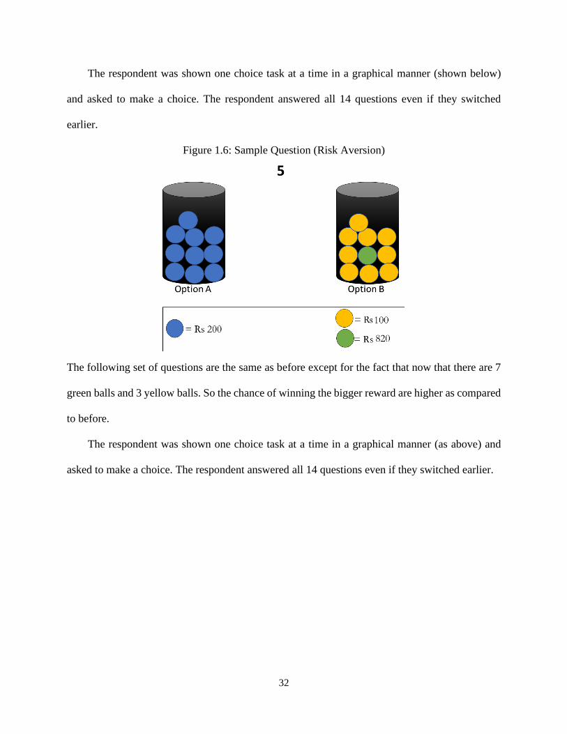
The respondent was shown one choice task at a time in a graphical manner (shown below)

and asked to make a choice. The respondent answered all 14 questions even if they switched

earlier.

Figure 1.6: Sample Question (Risk Aversion)

The following set of questions are the same as before except for the fact that now that there are 7

green balls and 3 yellow balls. So the chance of winning the bigger reward are higher as compared

to before.

The respondent was shown one choice task at a time in a graphical manner (as above) and

asked to make a choice. The respondent answered all 14 questions even if they switched earlier.

33

Table 1.10: Risk Aversion Choice List 2

Option A Option B

No Rupees you get Rupees if you pick green ball Rupees if you pick yellow ball

15 800 1120 100

16 800 1140 100

17 800 1200 100

18 800 1240 100

19 800 1300 100

20 800 1380 100

21 800 1460 100

22 800 1540 100

23 800 1640 100

24 800 1740 100

25 800 1900 100

26 800 2100 100

27 800 2380 100

28 800 2740 100

34

APPENDIX C – TIME PREFERENCES

Instructions

I am giving you a token (hand over a token) and you can exchange this token with me for real

money. I will give you two options labelled Option A and Option B offering different amount of

money at different times in the future. How much money you receive will depend on which option

you choose. Let me give you an example, [hand over the sheet 1 with the example] you will get

Rs1000 in 2 weeks if you select Option A and Rs 1100 in 8 weeks if you select Option B [Show

the calendar to the respondent to make the choice easier to understand]. So you get additional

money for waiting. As you go down the questions, you can see that Option A does not change but

how much you earn in Option B increases. As you can see Option A gives you money in two weeks

and Option B gives you money 2 months later than Option A. We would like to know which option

you prefer for each question. I would like to reiterate that there is no wrong or correct answer. We

just want to know what options you prefer and hope that you would find the games interesting.

Table 1.11: Sheet 1

Task Horizon in Months Option A Option B

1 2 1000 1100

2 2 1000 1200

3 2 1000 1300

35

Figure 1.7: Calendar Sheet

We will now randomly select a question, let’s suppose question 2 in this game is selected for

actual payment. The reward will now be based on your choice – 1000 in two weeks if you selected

Option A or 1200 in 8 weeks if you had selected Option B.

Now let’s play the actual game. The structure of this game is very similar to the practice game.

Option A is for sooner smaller payment and Option B is for larger later payment. The questions

differ in the waiting period and the amount in the later period. Let me remind you again that these

questions are eligible to be selected for a real payment at the end of the survey. Do you have any

questions? If no, then let start the game.

36

Table 1.12: Time Discounting Choices

Task Horizon in Months Earlier Payment Delayed Payment Annual Interest Rate

1 4 500 517 10

2 4 500 525 15

3 4 500 533 20

4 4 500 542 25

5 4 500 550 30

6 4 500 558 35

7 4 500 567 40

8 4 500 575 45

9 4 500 583 50

10 4 500 592 55

37

BIBLIOGRAPHY

38

BIBLIOGRAPHY

Aggarwal, S., Francis, E., and Robinson, J. 2018. Grain today, gain tomorrow: Evidence from a

storage experiment with savings clubs in Kenya, Journal of Development Economics,

Advance Access published 2018: doi:10.1016/j.jdeveco.2018.04.001

Andersen, S., Harrison, G. W., Lau, M. I., and Rutström, E. E. 2008. Eliciting risk and time

preferences, Econometrica, Advance Access published 2008: doi:10.1111/j.1468-

0262.2008.00848.x

Ashraf, N., Karlan, D., and Yin, W. 2006. Tying odysseus to the mast: Evidence from a

commitment savings product in the Philippines, Quarterly Journal of Economics, Advance

Access published 2006: doi:10.1162/qjec.2006.121.2.635

Barrett, C. B., Bachke, M. E., Bellemare, M. F., Michelson, H. C., Narayanan, S., and Walker, T.

F. 2012. Smallholder participation in contract farming: Comparative evidence from five

countries, World Development, Advance Access published 2012:

doi:10.1016/j.worlddev.2011.09.006

Basu, K. and Wong, M. 2015. Evaluating seasonal food storage and credit programs in east

Indonesia, Journal of Development Economics, Advance Access published 2015:

doi:10.1016/j.jdeveco.2015.02.001

Bazzani, C., Caputo, V., Nayga, R. M., and Canavari, M. 2017. TESTING COMMITMENT COST

THEORY IN CHOICE EXPERIMENTS, Economic Inquiry, Advance Access published

2017: doi:10.1111/ecin.12377

Burke, M. 2014. Selling Low and Buying High : An Arbitrage Puzzle in Kenyan Villages, Working

Paper, Advance Access published 2014

Caputo, V., Lusk, J. L., and Nayga, R. M. 2018. Choice experiments are not conducted in a

vacuum: The effects of external price information on choice behavior, Journal of Economic

Behavior and Organization, Advance Access published 2018:

doi:10.1016/j.jebo.2017.11.018

Caputo, V., Nayga, R. M., and Scarpa, R. 2013. Food miles or carbon emissions? Exploring

labelling preference for food transport footprint with a stated choice study, Australian Journal

of Agricultural and Resource Economics, Advance Access published 2013:

doi:10.1111/1467-8489.12014

Caputo, V., Scarpa, R., and Nayga, R. M. 2017. Cue versus independent food attributes: The effect

of adding attributes in choice experiments, European Review of Agricultural Economics,

Advance Access published 2017: doi:10.1093/erae/jbw022

Chavas, J.-P. and Holt, M. T. 2006. Economic Behavior Under Uncertainty: A Joint Analysis of

Risk Preferences and Technology, The Review of Economics and Statistics, Advance Access

39

published 2006: doi:10.2307/2109935

Cheung, S. L. 2016. Recent developments in the experimental elicitation of time preference,

Journal of Behavioral and Experimental Finance

Clark, M. D., Determann, D., Petrou, S., Moro, D., and de Bekker-Grob, E. W. 2014. Discrete

Choice Experiments in Health Economics: A Review of the Literature, PharmacoEconomics

Daly, A., Hess, S., and Train, K. 2012. Assuring finite moments for willingness to pay in random

coefficient models, Transportation, Advance Access published 2012: doi:10.1007/s11116-

011-9331-3

De-Magistris, T., Gracia, A., and Nayga, R. M. 2013. On the use of honesty priming tasks to

mitigate hypothetical bias in choice experiments, American Journal of Agricultural

Economics, Advance Access published 2013: doi:10.1093/ajae/aat052

Duflo, E., Kremer, M., and Robinson, J. 2008. How high are rates of return to fertilizer? Evidence

from field experiments in Kenya, in American Economic Review

Fafchamps, M. and Minten, B. 2012. Impact of SMS-based agricultural information on Indian

farmers, World Bank Economic Review, Advance Access published 2012:

doi:10.1093/wber/lhr056

Fischer, E. and Qaim, M. 2014. Smallholder farmers and collective action: What determines the

intensity of participation?, Journal of Agricultural Economics, Advance Access published

2014: doi:10.1111/1477-9552.12060

Gibson, J. M., Rigby, D., Polya, D. A., and Russell, N. 2016. Discrete Choice Experiments in

Developing Countries: Willingness to Pay Versus Willingness to Work, Environmental and

Resource Economics, Advance Access published 2016: doi:10.1007/s10640-015-9919-8

Greene, W. H. and Hensher, D. A. 2010. Modeling ordered choices: A primer

Hensher, D. A., Rose, J. M., and Greene, W. H. 2015. Applied choice analysis

Jayne, T. S., Mason, N. M., Burke, W. J., and Ariga, J. 2018. Review: Taking stock of Africa’s

second-generation agricultural input subsidy programs, Food Policy

Jensen, R. 2010. The (Perceived) returns to education and the demand for schooling, Quarterly

Journal of Economics, Advance Access published 2010: doi:10.1162/qjec.2010.125.2.515

Kahneman, D. and Tversky, A. 1979. Kahneman & Tversky (1979) - Prospect Theory - An

Analysis Of Decision Under Risk.pdf, Econometrica

Lancaster, K. J. 1966. A new approach to consumer theory., The Journal of Political Economy,

vol. 74, no. 2, 132–57

Lawless, L., Drichoutis, A. C., and Nayga, R. M. 2013. Time preferences and health behaviour: a

40

review, Agricultural and Food Economics

Lin, W., Ortega, D. L., and Caputo, V. 2019. Are Ex-Ante Hypothetical Bias Calibration Methods

Context Dependent? Evidence from Online Food Shoppers in China, Journal of Consumer

Affairs, Advance Access published 2019: doi:10.1111/joca.12202

Liu, E. M. 2013. Time to change what to sow: Risk preferences and technology adoption decisions

of cotton farmers in China, Review of Economics and Statistics, Advance Access published

2013: doi:10.1162/REST_a_00295

Lusk, J. L. and Briggeman, B. C. 2009. Food values, American Journal of Agricultural Economics,

Advance Access published 2009: doi:10.1111/j.1467-8276.2008.01175.x

McFadden, D. 1974. Conditional logit analysis of qualitative choice behaviour, in Frontiers in

econometrics

McKenzie, D., Gibson, J., and Stillman, S. 2013. A land of milk and honey with streets paved with

gold: Do emigrants have over-optimistic expectations about incomes abroad?, Journal of

Development Economics, Advance Access published 2013:

doi:10.1016/j.jdeveco.2012.01.001

Miranda, M. J., Mulangu, F. M., and Kemeze, F. H. 2017. Warehouse Receipt Financing for

Smallholders in Developing Countries: Short on Logic, Long on Imagination.:

Omotilewa, O. J., Ricker-Gilbert, J., Ainembabazi, J. H., and Shively, G. E. 2018. Does improved

storage technology promote modern input use and food security? Evidence from a

randomized trial in Uganda, Journal of Development Economics, Advance Access published

2018: doi:10.1016/j.jdeveco.2018.07.006

Ortega, D. L., Wang, H. H., Wu, L., and Olynk, N. J. 2011. Modeling heterogeneity in consumer

preferences for select food safety attributes in China, Food Policy, Advance Access published

2011: doi:10.1016/j.foodpol.2010.11.030

Ricker-Gilbert, J., Jayne, T., and Shively, G. 2013. Addressing the ‘wicked problem’ of input

subsidy programs in africa, Applied Economic Perspectives and Policy, Advance Access

published 2013: doi:10.1093/aepp/ppt001

Scarpa, R., Campbell, D., and Hutchinson, W. G. 2007. Benefit estimates for landscape

improvements: Sequential Bayesian design and respondents’ rationality in a choice

experiment, Land Economics, Advance Access published 2007: doi:10.3368/le.83.4.617

Scarpa, R., Ferrini, S., and Willis, K. 2005. Performance of Error Component Models for Status-

Quo Effects in Choice Experiments, in Applications of Simulation Methods in Environmental

and Resource Economics

Scarpa, R., Thiene, M., and Train, K. 2008. Utility in willingness to pay space: A tool to address

confounding random scale effects in destination choice to the Alps, American Journal of

Agricultural Economics, Advance Access published 2008: doi:10.1111/j.1467-

41

8276.2008.01155.x

Scarpa, R. and Willis, K. 2010. Willingness-to-pay for renewable energy: Primary and

discretionary choice of British households’ for micro-generation technologies, Energy

Economics, Advance Access published 2010: doi:10.1016/j.eneco.2009.06.004

Shiferaw, B., Hellin, J., and Muricho, G. 2011. Improving market access and agricultural

productivity growth in Africa: What role for producer organizations and collective action

institutions?, Food Security, Advance Access published 2011: doi:10.1007/s12571-011-

0153-0

Tanaka, M., Ida, T., Murakami, K., and Friedman, L. 2014. Consumers’ willingness to pay for

alternative fuel vehicles: A comparative discrete choice analysis between the US and Japan,

Transportation Research Part A: Policy and Practice, Advance Access published 2014:

doi:10.1016/j.tra.2014.10.019

Ward, P. S. and Singh, V. 2015. Using Field Experiments to Elicit Risk and Ambiguity

Preferences: Behavioural Factors and the Adoption of New Agricultural Technologies in

Rural India, Journal of Development Studies, Advance Access published 2015:

doi:10.1080/00220388.2014.989996

Warnick, J. C. E., Escobal, J., and Laszlo, S. C. 2011. Ambiguity aversion and portfolio choice in

small-scale peruvian farming, B.E. Journal of Economic Analysis and Policy, Advance

Access published 2011: doi:10.2202/1935-1682.2331

William, J. G. and Kaserwa, N. 2015. Improving smallholder farmers access to finance through

warehouse receipt system in Tanzania, International Journal of Economics and Financial

Research, Advance Access published 2015

42

Essay 2 :Does peer comparison encourage adoption of best practices among farmers in Pakistan?

Abstract

Poor nutrient management has contributed towards deteriorating soil quality in Pakistan.

Despite years of experience, non-convergence to optimal practices suggests constraints to learning.

Informing farmers about optimal organic and inorganic fertilizer use, given soil and crop type, can

address this challenge. This study takes an experimental approach with treated farmers receiving

this information either with or without a peer comparison, while the control farmers receive no

information. Results show that majority of the soils are in poor health, manure use is very low, and

93 percent of farmers are underusing fertilizers. The intervention increased manure and urea use

in the peer comparison group. However, urea increase was concentrated among farmers that were

applying fertilizers closer to the recommended quantities at the baseline. These findings provide

some evidence on the effectiveness of peer comparisons and highlights the presence of other

constraints in addition to information.

43

2.1 Introduction

Sustainable agricultural systems are essential for addressing poverty and ensuring food

security. The current agricultural systems have significantly degraded the natural resource base,

especially soils, reducing its productive capacity and efficiency of land, making food security and

poverty alleviation an increasingly difficult task to achieve. According to the Global Land

Degradation Assessment (GLADA) land degradation is increasing and almost one-quarter of the

total global land area has undergone it. Estimates show that in 2007 about 1.5 billion people in

some way depended on degraded areas for their livelihoods while in excess of 42 percent of the

world’s very poor population lived on degraded areas (Nachtergaele et al., 2010). Pakistan has also

been severely affected by land degradation due to unsustainable land management practices and

increasing demands on natural resources (Zia et al., 2004). Around 68 million hectares of land

across Pakistan has been affected and the issue has been worsening in the absence of effective

policies (Khan et al., 2012). Several studies have highlighted that land resource degradation due

to nutrient mining is a dominant factor for poor productivity in Pakistan (Ali and Byerlee, 2002;

Khan et al., 2012; Malik et al., 2017; Pingali and Shah, 2001). Since, agriculture continues to be

the prime source of livelihood for the country’s poor and a major contributor to the economy,

growth in this sector is important for achieving economic growth and broader developmental goals.

Improper use of fertilizers is one of the core factors for declining soil health as it leads to

nutrient mining and yield stagnation (Concepcion, 2007). Each soil and crop type has a specific

mineral requirement and under or overuse of fertilizers can cause damage to the productive

capacity of soils (Ahmed and Gautam, 2013; Bumb and Baanante, 1996; Coulter, 2008). Existing

practices in Pakistan have caused the soil organic matter concentration to fall to extremely low

levels reducing its fertility and its ability to efficiently use fertilizers. This is also one of the factors

44

behind decreasing returns to fertilizer application (Ali et al., 2017; Lal, 2014). Field experiments

in Pakistan suggest that use of compost manure along with inorganic fertilizers can significantly

improve soil health and yields (Ibrahim et al., 2008; Sangeetha et al., 2013; Sarwar et al., 2007).

Non convergence to ideal practices despite decades of experience using fertilizer technology

suggests barriers to complete adoption. Two streams dominate this discourse, one argues is that

there is heterogeneity in cost and/or returns and farmers might have possibly internalized the cost

of this resource degradation. Alternatively, there might be informational and behavioral factors

such as perceived risks, learning, and limited attention driving incomplete technology adoption

(Janvry et al., 2016).

This study alleviates the information constraint by providing fertilizer recommendations

based on soil tests which provide an objective means to ascertain fertilizer requirements based on

crop and soil type. This in itself is not a novel idea but the impact of providing customized

information on nutrient management has not been encouraging (Corral et al., 2016; Fishman et al.,

2016). Therefore, this study complements information provision with peer comparison which has

been shown to be a useful, low cost nudge to alter behavior in various contexts such as energy

conservation, residential water use, and charitable giving among other things (Cooter et al., 2008;

Goldstein et al., 2008; Martin and Randal, 2008; Schultz et al., 2007). The paper addresses two

main questions regarding fertilizer application: (1) Does information on soil quality improve

fertilizer use? and (2) Does including peer comparison to information improve fertilizer use?

Moreover, since small farmers face numerous constraints and the intervention only alleviated the

information constraint. The study focuses on heterogenous impacts.

Incomplete adoption of fertilizers is relatively understudied. Most of the existing work on

fertilizer adoption has focused on heterogenous adoption of fertilizer across farmers due to

45

availability, affordability, risk and information (Jack, 2013). While some authors have looked at

differential marginal returns and barriers to learning as potential factors for incomplete adoption

(Duflo et al., 2008; Janvry et al., 2016; Marenya and Barrett, 2009). Recently, a few papers have

evaluated the role of information and knowledge on fertilizer application (Corral et al., 2016;

Fishman et al., 2016). However, the results are mixed where Corral et al. (2016) find an increase

in fertilizer rate but it is not statistically significant. While Fishman et al. (2016) found no impact

of providing the information.

This study adds to this sparse literature by evaluating the impact of information on agricultural

practices such as fertilizer. Results show that 87 percent of the farmers could recall receipt of the

SHC and 75 percent of the reported that they trusted the information on it which is very

encouraging as Fishman et al. (2016) attribute lack of trust as the reason for null effect.

Secondly, the study also contributes to the literature on social comparisons by testing this

nudge in an agricultural setting. A random subset of farmers was also given peer comparisons in

addition to information to induce behavioral change. Results show that manure use increased in

the peer comparison group while there was no change in the information group. These results

validate earlier finding that information provision might not be sufficient to change practices.

Another contribution this paper makes is that it measures the heterogenous impact of

information provision which the earlier two studies did not. We find a statistically significant

increase in urea use among farmers who were given the peer comparison and were applying urea

within one bag of recommended quantity at baseline. These findings provide some evidence that

peer comparisons can be a useful level to alter behavior.

The remainder of this paper is as follows. Section 2 outlines the conceptual framework,

section 3 explains the experimental design, followed by intervention details in section 4, section 5

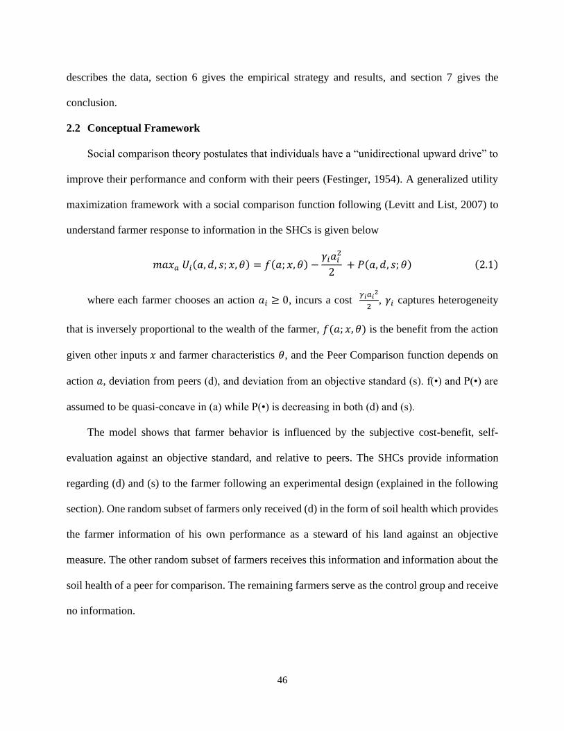
46

describes the data, section 6 gives the empirical strategy and results, and section 7 gives the

conclusion.

2.2 Conceptual Framework

Social comparison theory postulates that individuals have a “unidirectional upward drive” to

improve their performance and conform with their peers (Festinger, 1954). A generalized utility

maximization framework with a social comparison function following (Levitt and List, 2007) to

understand farmer response to information in the SHCs is given below

𝑚𝑎𝑥𝑎 𝑈𝑖(𝑎, 𝑑, 𝑠; 𝑥, 𝜃) = 𝑓(𝑎; 𝑥, 𝜃) −𝛾𝑖𝑎𝑖

2

2 + 𝑃(𝑎, 𝑑, 𝑠; 𝜃) (2.1)

where each farmer chooses an action 𝑎𝑖 ≥ 0, incurs a cost 𝛾𝑖𝑎𝑖

2

2, 𝛾𝑖 captures heterogeneity

that is inversely proportional to the wealth of the farmer, 𝑓(𝑎; 𝑥, 𝜃) is the benefit from the action

given other inputs 𝑥 and farmer characteristics 𝜃, and the Peer Comparison function depends on

action 𝑎, deviation from peers (d), and deviation from an objective standard (s). f(•) and P(•) are

assumed to be quasi-concave in (a) while P(•) is decreasing in both (d) and (s).

The model shows that farmer behavior is influenced by the subjective cost-benefit, self-

evaluation against an objective standard, and relative to peers. The SHCs provide information

regarding (d) and (s) to the farmer following an experimental design (explained in the following

section). One random subset of farmers only received (d) in the form of soil health which provides

the farmer information of his own performance as a steward of his land against an objective

measure. The other random subset of farmers receives this information and information about the

soil health of a peer for comparison. The remaining farmers serve as the control group and receive

no information.

47

The design of our experiment allows us to test the following hypotheses:

Hypothesis 1: SHC informs farmers on their optimal use of fertilizers, and farmers adjust

their fertilizer use accordingly, provided they do not face other binding constraints

The first and most important assumption that this hypothesis rests on is that information is the

only binding constraint. Second, once the information is provided farmers would be able to

understand it. Third, once farmers understand the information, they will trust it and update their

beliefs regarding optimal fertilizer quantities. Fourth, once the farmers update their beliefs they

will act on these changed beliefs. This is strongly linked with the first assumption that information

is the only binding constraint.

If the farmer faces other constraints such as liquidity, water availability, and fertilizer

availability then it will lead to a null result as those constraints are not removed through this

intervention. As we expect farmers in developing countries to face these constraints we will focus

on the heterogeneous impact of this intervention.

Hypothesis 2: Peer Comparison increases the efficacy of information and results in higher

compliance to the fertilizer recommendations.

The second hypothesis rests on the idea that augmenting information with social comparison

will improve compliance to the recommendations. Peer comparison will induce a ‘competitive

behavior’ as it will highlight that others are doing better. Peer comparisons will also raise the

aspirations of the farmers. For example, without information on the soil health of peers, a farmer

could easily assume that they are performing equally as well as everyone else. Social comparison

will inform them that a better outcome is possible, encouraging them to adopt the

recommendations provided on the card.

48

2.3 Experimental Design

The study had three experimental groups (two treatment and a control) shown in figure 2.1.

Randomization was done at the individual level and farmers were randomly assigned to one of the

groups in each of the 90 villages in the study area. Treatment 1 (Information Only) group received

information on soil health score5 and recommendations on manure and fertilizer use based on the

soil and crop type. Treatment 1 provided farmers with an objective feedback on the fertility of

their soil which was also reflective of their ability to manage their land. The aim was to improve

learning and knowledge of the farmer and induce change in practices. Treatment 2 (Peer

Comparison) group received the same information and a nudge in the form a peer comparison.

Farmers in this group were also given information on the best soil health score among their peers.

Treatment 2 was designed learning from earlier studies which had failed to bring change from

information provision. The peer comparison was aimed to stimulate the competitive nature of

farmers by comparing them against a better performing peer. Secondly, it also aimed to encourage

them and raise their aspiration for a better equilibrium.

The intervention was implemented in 90 villages spread across four districts of south Punjab.

A random sample of agricultural households6 in each village was selected for the intervention and

randomly assigned to the treatment and control groups as shown in Fig 2.1.

5 Soil health information was provided as a score out of ten for simplification. A higher number represented better soil

health. This information was also presented graphically so that it was cognitively less demanding. 6 Households engaged in the production of wheat or cotton were selected as these are the main crops. This exercise let

to the identification of approximately 4200 households.

49

Figure 2.1: Study Design

2.4 Intervention Description

Learning in the agricultural setting is a complicated process for many reasons. First, farmers

can choose from numerous inputs and there could potentially be several optimal bundles.

Secondly, there is a significant unobservable component of the underlying production function

which is not completely understood. Third, there are exogenous stochastic shocks to farm output

in the form of weather. Fourth, the production process takes a long time and updating of beliefs

can usually happen once a year. Finally, returns to inputs can be heterogenous conditional on the

underlying resource base. This is particularly true in the case of fertilizer response and land quality.

This intervention provided farmers with objective information on soil health and fertilizer

requirements based on soil testing. In addition, mental accounting and reminders were also used.

Details are provided in the sub-sections below.

2.4.1 Soil Health Cards

Soil samples were collected, tagged, and delivered to the district soil testing laboratories. Soil

samples were not collected from all the farmers but limited to farmers assigned in the treatment

groups only. This was done to avoid an effect on the control group through the soil collection

Farming Households in

the village

ControlInformation Only

(T1)

Peer Comparison

(T2)

50

activity as it could have led them to seek out information on soil testing and fertilizer

recommendations leading to some changes in practices. Once the soil testing was complete the

information was used to create a soil health score. Organic matter content and availability of macro

nutrients (Nitrogen, Phosphorous, and Potassium) was used to assign a soil health score between

0 to 10 points, with 10 being the ideal score. This score was highlighted on the front of the card

along with a labelling of the soil as very poor, poor, medium, and fertile. To make the interpretation

of the score results easier this information was also presented graphically showing the ideal score

and the score of the farmer’s plot next to each other. The peer comparison group also included the

best soil health score of a peer farmer to act as a behavioral nudge.7 The back side of the card had

detailed information on the quantity of fertilizer to be used for kharif crops.

The delivery of the cards started in end of March before the planting of cotton which starts in

the first week of April. Enumerators went through training before the delivery of the card and were

also given a script to follow. The soil script was translated in the local language for the enumerators

and covered the following points:

I. Explain the soil health status to the farmer and help them understand the score given to

them.

II. Inform them that one of the major reasons for poor soil health is the poor nutrient

management by the farmer.

III. Explain to the farmer that their soil health can be improved if they use the correct quantities

and types of fertilizers and use manure to improve the organic content of their soils.

Farmers were also encouraged to call on the toll-free number given on the soil health card if they

had any follow up questions.

7 The best soil health card was chosen to avoid the boomerang effect as seen in other studies where sharing average

scores resulted in better performing subjects gravitating towards the mean. The best performing peer was chosen from

a cluster of villages based on their proximity. The cluster consisted of 6 villages on average.

51

2.4.2 Mental Accounting and Call Reminders

Once the enumerator went through the information on the soil health card, farmer was asked

the amount of land that assigned to cultivation in the upcoming season for cotton. The enumerator

then calculated the fertilizer requirement for the farmers based on the land reported and the results

of the soil health card. The farmers were then asked to plan when they would go to get the fertilizer

for the upcoming season. They were asked to plan the day, time of the day, and the location from

where they would procure the fertilizers. This information was also recorded by the enumerator

and reminder calls were made to the farmers around their planned date of purchase.

2.5 Data and Empirical Strategy

This paper utilizes three waves of data which were collected under the Punjab Economic

Opportunities Program. Two rounds of survey were done preintervention and one post

intervention. The first survey wave was conducted in August 2016 and a random sample of 12,700

households were surveyed in this round across the 90 villages. This dataset was used as the

sampling frame to identify households engaged in farming. The second survey wave was

conducted in February 2018 and is used as the baseline for the study. The intervention was rolled

out in April 2018 (details in the next section) and the post treatment survey was conducted in April

2019.

This study focuses on cotton production as it is the main cash crop in this region, has

significant forward market linkages, and is also a very input intensive. The following regression

approach was used for balance checks on pre-treatment socio-demographic, soil characteristics,

and production variables.

𝑌𝑖𝑗 = 𝛽0 + 𝛽1𝑇𝑖𝑗1 + 𝛽2𝑇𝑖𝑗

2 + 휀𝑖𝑗 (2.2)

52

The left-hand-side variable, 𝑌𝑖𝑗, refers to the value for household i in village j. 𝑇 is a dummy

variable indicating the household’s treatment status, and standard errors were clustered at the

village level. Table 2.1 shows the summary statistics and checks for balance across the treatment

and control groups. The first three columns show the mean of the variables and the last three

columns give the difference in means. Standard errors are reported in parenthesis and the asterisks

show if the differences are statistically significant. Panel A shows household levels variables and

Panel B shows plot characteristics for the largest plot cultivated by the household. Panel C reports

yield and inputs, averaged across all plots managed by the household.

Panel A shows that households were balanced across the experimental groups for non-

business assets, agricultural assets, land ownership and education. The asset indices were

generated using principal component analysis (PCA) and then normalized. The non-business assets

comprised of 34 items such as household furniture, electrical equipment, vehicles, and livestock

while the agricultural asset index comprised of 12 items which included different kinds of

agricultural machinery and equipment. There is imbalance for age of the household head and size

of the households. Household heads are older in the Peer Comparison group (T2) with an average

age of approximately 51 years as compared to 50 years in the other two groups. Similarly, the

household size is larger in the Peer Comparison group (T2). The mean size is approximately 7.1

in T2 and 7 in the other groups. However, as can be seen in the table these differences even though

statistically different are not very different in absolute terms.

53

Table 2.1: Balance Table Control T1 T2 T1 vs C T2 vs C T1 vs T2

Panel A. Household Demographic

Non-Business Asset

Index

0.472 0.447 0.514 -0.057 0.010 -0.066

(1.450) (1.309) (1.564) (0.066) (0.082) (0.078)

Agricultural Asset

Index 0.553 0.564 0.598 0.010 0.065 -0.060

(1.843) (1.687) (1.935) (0.095) (0.106) (0.112)

Land Owned (kanals) 24.398 24.581 22.645 0.656 -1.440 1.625

(54.646) (36.904) (40.620) (2.239) (2.533) (2.219) Education (years) 3.542 3.760 3.507 0.083 -0.169 0.214 (4.141) (4.283) (4.181) (0.233) (0.215) (0.217) Household Head Age

(years)

49.730 49.464 50.989 -0.047 1.283* -1.555* (13.463) (13.375) (13.320) (0.807) (0.725) (0.786) Household Size 6.833 6.945 7.084 0.077 0.255* -0.164 (2.785) (2.886) (2.773) (0.159) (0.151) (0.166)

Panel B. Land Characteristics Suffer Waterlogging 0.183 0.184 0.199 0.001 0.017 -0.015 (0.387) (0.388) (0.400) (0.024) (0.020) (0.017) Suffer Salinity 0.165 0.169 0.172 0.004 0.007 -0.003 (0.371) (0.375) (0.378) (0.023) (0.022) (0.023) Suffer Soil Erosion 0.169 0.134 0.143 -0.035* -0.026 -0.009 (0.375) (0.341) (0.350) (0.020) (0.018) (0.018) Fertility Score (Likert

Scale 1-5)

4.077 4.075 4.086 -0.002 0.009 -0.011 (0.638) (0.626) (0.672) (0.032) (0.035) (0.030) Soil Type: Sandy 0.161 0.139 0.154 -0.022 -0.007 -0.015 (0.368) (0.346) (0.361) (0.018) (0.017) (0.015) Soil Type: Sandy Clay 0.537 0.543 0.559 0.006 0.023 -0.016

(0.499) (0.499) (0.497) (0.027) (0.027) (0.027)

Soil Type: Clay 0.135 0.141 0.128 0.005 -0.007 0.013

(0.342) (0.348) (0.334) (0.017) (0.018) (0.018)

Soil Type: Clay Loam 0.059 0.050 0.062 -0.009 0.002 -0.011

(0.236) (0.219) (0.241) (0.013) (0.012) (0.017)

Soil Type: Loam 0.102 0.122 0.096 0.020 -0.006 0.027

(0.303) (0.328) (0.294) (0.017) (0.015) (0.019)

Access to Tubewell 0.891 0.911 0.896 0.020 0.005 0.015

(0.311) (0.285) (0.305) (0.019) (0.023) (0.016)

Access to Canal 0.740 0.750 0.736 0.010 -0.004 0.015

(0.439) (0.433) (0.441) (0.032) (0.034) (0.020)

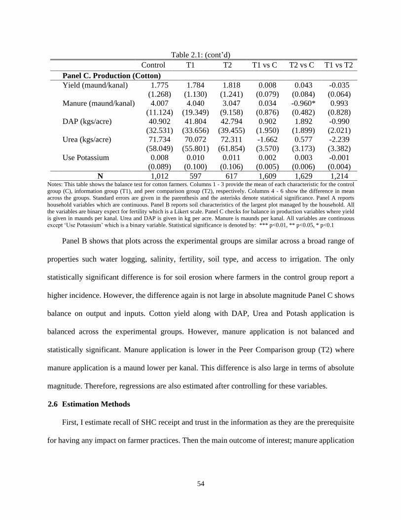
54

Table 2.1: (cont’d) Control T1 T2 T1 vs C T2 vs C T1 vs T2

Panel C. Production (Cotton)

Yield (maund/kanal) 1.775 1.784 1.818 0.008 0.043 -0.035

(1.268) (1.130) (1.241) (0.079) (0.084) (0.064)

Manure (maund/kanal) 4.007 4.040 3.047 0.034 -0.960* 0.993

(11.124) (19.349) (9.158) (0.876) (0.482) (0.828)

DAP (kgs/acre) 40.902 41.804 42.794 0.902 1.892 -0.990

(32.531) (33.656) (39.455) (1.950) (1.899) (2.021)

Urea (kgs/acre) 71.734 70.072 72.311 -1.662 0.577 -2.239

(58.049) (55.801) (61.854) (3.570) (3.173) (3.382)

Use Potassium 0.008 0.010 0.011 0.002 0.003 -0.001

(0.089) (0.100) (0.106) (0.005) (0.006) (0.004)

N 1,012 597 617 1,609 1,629 1,214 Notes: This table shows the balance test for cotton farmers. Columns 1 - 3 provide the mean of each characteristic for the control

group (C), information group (T1), and peer comparison group (T2), respectively. Columns 4 - 6 show the difference in mean

across the groups. Standard errors are given in the parenthesis and the asterisks denote statistical significance. Panel A reports

household variables which are continuous. Panel B reports soil characteristics of the largest plot managed by the household. All

the variables are binary expect for fertility which is a Likert scale. Panel C checks for balance in production variables where yield

is given in maunds per kanal. Urea and DAP is given in kg per acre. Manure is maunds per kanal. All variables are continuous

except ‘Use Potassium’ which is a binary variable. Statistical significance is denoted by: *** p<0.01, ** p<0.05, * p<0.1

Panel B shows that plots across the experimental groups are similar across a broad range of

properties such water logging, salinity, fertility, soil type, and access to irrigation. The only

statistically significant difference is for soil erosion where farmers in the control group report a

higher incidence. However, the difference again is not large in absolute magnitude Panel C shows

balance on output and inputs. Cotton yield along with DAP, Urea and Potash application is

balanced across the experimental groups. However, manure application is not balanced and

statistically significant. Manure application is lower in the Peer Comparison group (T2) where

manure application is a maund lower per kanal. This difference is also large in terms of absolute

magnitude. Therefore, regressions are also estimated after controlling for these variables.

2.6 Estimation Methods

First, I estimate recall of SHC receipt and trust in the information as they are the prerequisite

for having any impact on farmer practices. Then the main outcome of interest; manure application

55

and heterogenous impact on fertilizer application is estimated. The empirical specifications are

explained in the subsections below.

Since the assignment to treatment and control groups was random, we can measure the causal

impact of the two treatment arms on outcomes of interest. The regressions are run at the household

for cotton. First, a simple linear regression model without controlling for any village level fixed

effects or pre-treatment covariates is estimated. Village fixed effects and controls are these

subsequently included in the specifications. ANCOVA is used to improve the power of the study

as it allows us to retain observations with missing values at the baseline. These observations were

assigned a zero value and controlled for through an indicator variable in the regressions. The

improvement in power is significant over the difference-in-differences (DID) estimator as a DID

with equal power to the ANCOVA would require twice the sample size (McKenzie, 2012). The

main specification used to measure the impact is given below.


2+ 𝜑𝑋′𝑖𝑗 + 𝐷𝑖𝑗 + 휀𝑖𝑗 (2.3)

where 𝑌𝑖𝑗 is the outcome variable of individual i in village j at the endline, T1 and T2 are indicator

variables for treatment assignment, 𝑋′𝑖𝑗 is a vector of controls, 𝐷 is an indicator variable if the

information for the household is missing in the baseline, 휀𝑖𝑗 is the error term. 𝛽1 and 𝛽2 are the

coefficients of interest and capture the intent-to-treat (ITT) effect of proving the information.

Farmers in developing countries face numerous constraints, alleviating only one constraint

(information in our case) might not be sufficient to induce behavioral change (Karlan et al., 2014).

Hence, heterogenous impact of the intervention are estimated. The sample is restricted to those

who were underusing fertilizer compared to the recommended quantities, which is 90 percent of

the sample. The deviation from the recommended quantity at baseline is used to generate an

indicator variable which takes the value 1 if the deviation is less than a bag and zero otherwise.

56

Balance was also testing for this restricted sample and the results were same as for the original

sample. The table is shown in the appendix. This indicator is a proxy for liquidity as those already

using higher quantities of fertilizer should not be facing this constraint. The main specification

used is given below


2+𝛿1𝑇𝑖𝑗1 ∗ Dev + 𝛿2𝑇𝑖𝑗

2 ∗ Dev + 𝜑𝑋′𝑖𝑗 + 𝐷𝑖𝑗 + 휀𝑖𝑗 (2.4)

where all the variables are the same except for the interaction term where Dev is the indicator for

deviation from the recommendation at the baseline. I also estimate a Difference in Difference

version of the above specification for robustness.

2.7 Results

This section presents the results of the study. The first subsection reports the take-up of the

SHC followed by the impact of receiving information and peer comparison on our outcomes of

interest – organic and inorganic fertilizer use.

2.7.1 Take-Up

Recall and trust variables provide important information on the receptiveness of the SHCs.

We use these two variables as proxy for the take-up of the information as they are prerequisite to

any change in beliefs or nutrient management practices of farmers in our treatment sample.

Farmers were asked if they can recall receiving a SHC and did they trust the information provided8.

Results show that close to 90 percent of the respondents could recall receiving a SHC and

close to 70 percent stated that they trusted the information on the SHC. logit regressions with

village fixed effects and cluster the standard errors at the village level were performed. Table 2.2

8 Only farmers in the treatment groups were asked these question as we felt that asking this question from the

control group would prime them and lead them to misreporting. Also, based on our knowledge there was no other

intervention happening during this period which delivered SHC to farmers.

57

and 2.3 reports the average probabilities of being able to recall receipt of the card and trusting the

information. the two treatment arms, across the different specifications.

Table 2.2: Predicted Probabilities of Recalling Receipt of SHC

(1) (2) (3)

VARIABLE Received SHC Received SHC Received SHC

Informationa .932*** .879*** .878***

(.012) (.011) (.011)

Peer Comparisonb .918*** .858*** .860***

(.014) (.011) (.010)

Observations 1888 1082 1082

p-value (a vs b) 0.267 0.353 0.393

Village Fixed Effects No Yes Yes

Controls No No Yes Note: This table reports the average probabilities of recalling receipt of SHC based on a logistic regression

(standard errors are reported in parenthesis). The results show that the average probability of recalling receipt

of SHC would be around 90 percent if everyone in the data was given the information or the peer comparison

treatment. This question was only asked from the treatment group who were delivered the card under the

treatment. Including village fixed effects reduces sample as there was no variation in responses within the

village. The sample for this analysis includes everyone who was given the card irrespective of the crop they

grow. Statistical significance is denoted by: *** p<0.01, ** p<0.05, * p<0.1

Table 2.3: Predicted Probabilities of Trust in SHC

(1) (2) (3)

VARIABLE Trust SHC Trust SHC Trust SHC

Informationa .742*** .720*** .720***

(.024) (.009) (.009)

Peer Comparisonb .762*** .742*** .742***

(.021) (.009) (.008)


p-value (a vs b) 0.249 0.236 0.236


Controls No No Yes

Note: This table reports the average probabilities of trust in SHC based on a logistic regression (standard errors

are reported in parenthesis). The results show that the average probability of trusting the information on the

SHC would be around 72 percent if everyone in the data was given the information treatment or the peer

comparison treatment. This question was only asked from the treatment group who were delivered the card

under the treatment. Including village fixed effects reduces sample if there was no variation in responses across

the village. Statistical significance is denoted by: *** p<0.01, ** p<0.05, * p<0.1

58

2.7.2 Manure Use

In this subsection, we test whether farmers change their practice of using manure. This was

one of the primary advices given to farmers as the organic matter in soils was below the ideal

threshold. The dependent variable is the quantity of manure applied in maunds per kanal for cotton.

Tobit model was estimated with the lower bound at zero and no upper bound and the results are

reported in Table 2.4.

Table 2.4: Tobit Estimates of Manure Applied (maunds/kanal)

(1) (2) (3)

VARIABLE Manure (maund/kanal) Manure (maund/kanal) Manure (maund/kanal)

Informationa 4.65** 4.66** 4.79***

(2.03) (2.00) (2.03)

Peer Comparisonb 6.731*** 5.57*** 6.58***

(2.45) (2.34) (2.38)

Manure baseline 0.23* 0.19 0.19

(0.12) (0.12) (0.12)

Missing Dummy -0.67 0.53 0.57

(2.87) (3.45) (3.44)

Constant -19.38*** -17.57*** -9.47

(4.82) (4.07) (8.28)


p-value (a vs b) 0.333 0.367 0.416


Controls No No Yes

Notes: The dependent variable is maunds of manure used in a kanal of land. This table provides the ITT estimates of

the treatments on manure use. Information and peer comparison are binary variables indicating treatment assignment.

Manure baseline is the quantity of manure that was applied at baseline. Control variables include education, household

size, non-business and agricultural asset indices, soil type, agriculture training, soil fertility, access to irrigation,

waterlogging, salinity, erosion, and land ownership. All regressions are estimated using Tobit and the standard errors

are clustered at the village level. Statistical significance is denoted by: *** p<0.01, ** p<0.05, * p<0.1

The results show that manure use increased in both treatment arms and the increase was

statistically significant. The increase in manure application is higher in the peer comparison group

as shown in the table, however, the difference is not statistically significant but substantially large

in absolute terms. This outcome provides some support to the hypothesis that peer comparisons

can act as a good encouragement device and improve the efficacy of information. Since an

59

ANCOVA specification was used, the baseline value of manure use was also included in the

regression along with an indicator variable to control for missing values in the baseline. The results

show that they are not strongly correlated to manure use at endline.

2.7.3 Fertilizer Use

Earlier interventions in India and Mexico which only alleviated the information constraints

on fertilizer use have not been very successful (Corral et al., 2016; Fishman et al., 2016). Lack of

trust and availability of fertilizers were cited as the factors responsible in India and Mexico

respectively. These results validate the finding by Karlan et al. (2014) that smallholder farmers

face many constraints which need to be removed simultaneously to induce behavioral change.

Therefore, this paper focuses on the heterogenous impact as compared to the overall change in

fertilizers as that might be attenuated.

First, I restrict my sample to farmers that were underusing fertilizer (90 percent of the sample).

Then I generate a variable that captures deviation from the recommended quantity at baseline9.

This variable takes the value 1 if the deviation is less than a bag and zero otherwise. Results are

given in table 2.5 which show a statistically significant increase in Urea application for farmers in

the peer comparison group that were underusing by less than 1 bag.

Urea use increased in peer comparison group by 10 kg per acre among farmers that were

within 1 bag deviation compared to those who were further away. The coefficient is statistically

significant at the 10 percent level and consistent across the three specifications. The impact in the

information only group is negligible suggesting the peer comparison was a successful

encouragement design for this sub-sample of farmers.

9 Soils tests were only conducted for treatment groups and exact deviation from mean cannot be calculated for the

control group. I impute values for these observations and use the median recommended quantities at village level.

60

Table 2.5: Heterogenous Treatment Effect on Urea

(1) (2) (3)

VARIABLE Urea (kg/acre) Urea (kg/acre) Urea (kg/acre)

Information ● Deva 2.63 2.20 2.05

(4.51) (4.26) (4.35)

Peer Comparison ● Devb 10.03** 9.22* 9.11*

(4.63) (4.83) (4.88)

Dev -5.48 4.84 5.97

(6.09) (4.21) (4.21)

Information -2.89 -2.89 -2.91

(3.08) (2.62) (2.56)

Peer Comparison -1.35 -0.64 -0.47

(2.84) (2.64) (2.63)

Missing Dummy 18.58*** 2.16 1.45

(6.98) (5.41) (5.43)

Urea baseline 0.18* -0.01 -0.03

(0.09) (0.06) (0.06)

Constant 79.02*** 73.36*** 74.38***

(6.66) (3.65) (10.00)


p-value (a vs b) 0.182 0.198 0.199


Controls No No Yes Notes: This table provides the coefficient estimates for heterogenous treatment effects based on the deviation from

recommended amounts at the baseline. Dev is an indicator variable which takes the value of 1 if deviation was less

than 1 bag and 0 otherwise. The Information ●Dev and Peer Comparison ●Dev are interaction terms which capture

the impact for farmers in the treatment groups that were within a deviation of 1 bag. Urea baseline is the quantity used

at baseline and missing dummy controls for values that were missing in the baseline. Control variables include

education, household size, non-business and agricultural asset indices, soil type, attended agriculture training, soil

fertility, access to canal and tube well, waterlogging, salinity, erosion, and land owned. Standard errors are clustered

at the village level. Statistical significance is denoted by: *** p<0.01, ** p<0.05, * p<0.1

2.8 Conclusion

I find that approximately 90 percent of farmers could recall receiving the SHC and around 72

percent stated that they trusted the information provided on the cards. This suggests that the

intervention was successful in proving improved information to majority of the farmers. Delivery

of SHC led to an increase in manure application in the both treatment groups. The magnitude of

impact was substantially larger in the peer comparison group but not statistically significant. Urea

use also increased among across the two treatment groups, however, in this case the impact was

61

only statistically significant in the peer comparison group among those farmers that were close to

the recommended quantities at the baseline.

The results provide some evidence that peer comparisons can be used in an agricultural setting

to promote more sustainable practices. The results show that the nudge works and leads to impacts

of higher magnitude, however it is not strong enough to have an impact which is statistically

different than the traditional mechanism of information dissemination. The heterogenous impact

on fertilizer use also provides suggestive evidence that other binding constraints might be limiting

use of fertilizers according to recommendations. Farmers who were already using high quantities

of fertilizer might not be facing as stringent liquidity constraint as those very far from it and when

they were given information on correct fertilizer recommendations that could improve their soil

health, they changed their practices. The impact on manure application and the lack of impact on

DAP further supports the financial constraints hypothesis as the cost of DAP is almost twice as

that of Urea whereas manure is usually available at a very low cost. However, an alternative

mechanism could be that those who were operating far from the recommended quantities

discounted the recommendations. This points towards confirmation bias, because if the farmers

felt they were using the correct or near correct quantities they would not accept recommendation

that asks them to change application by more than a bag per acre. However, we cannot identify the

mechanism at play for the heterogenous impact and more research is needed to disentangle the

reasons for low adoption.

The findings of this study have important policy relevance as soils in Pakistan have been

severely affected by land degradation and desertification due to farm practices and environmental

factors. Degrading soils have made increasing agricultural productivity an increasingly difficult

task to achieve. This has important food security implications for Pakistan which is has a

62

burgeoning population and an economy that is heavily dependent on agriculture. This experiment

provides some evidence on the role of information dissemination programs to encourage adoption

of sustainable practices through soil health cards. It also highlights that the impact of such

programs can be intensified through low cost peer comparisons. Finally, the study highlights that

in the presence of other binding constraints (e.g. liquidity, apriori bias) programs that only alleviate

the information constraint would not be enough.

63

APPENDIX

64

APPENDIX

Table 2.6: Balance Table (Restricted Sample for Heterogeneity)

(1)

C

(2)

T1

(3)

T2

(4)

[CvsT1]

(5)

[CvsT2]

(6)

[T1vsT2]

Panel A. Household Demographic p-values

Non-Business Asset Index 0.502

(0.096)

0.495

(0.101)

0.588

(0.109) 0.007 -0.085 -0.093

Agricultural Asset Index 0.592 0.616 0.644 -0.024 -0.052 -0.028

(0.094) (0.100) (0.108)

Land Owned (kanals) 25.259 26.096 23.461

-0.836 1.798 2.634 (2.806) (2.229) (2.297)

Household Head Education 3.593 3.943 3.672 0.349 -0.079 0.270

(0.229) (0.229) (0.245) Household Head Age 49.871 49.588 50.932

0.283 -1.061 -1.344 (0.677) (0.718) (0.789) Household Size 6.892 7.010 7.115

-0.117 -0.222 -0.105 (0.106) (0.142) (0.154)

Panel B. Land Characteristics Suffer Waterlogging 0.177 0.199 0.207

-0.023 -0.030 -0.008

(0.031) (0.038) (0.034) Suffer Salinity 0.169 0.178 0.179

-0.009 -0.010 -0.001

(0.027) (0.032) (0.030) Suffer Soil Erosion 0.154 0.134 0.124

0.020 0.030* 0.010

(0.016) (0.020) (0.019) Fertility (Likert Scale 1-5) 4.078 4.069 4.089

0.009 -0.010 -0.020

(0.027) (0.033) (0.035) Soil Type: Sandy 0.166 0.142 0.156

0.025 0.010 -0.015 (0.022) (0.023) (0.027) Soil Type: Sandy Clay 0.527 0.540 0.559

-0.014 -0.033 -0.019 (0.027) (0.028) (0.031)

Soil Type: Clay 0.139 0.140 0.137 -0.001 0.002 0.002

(0.017) (0.018) (0.019)

Soil Type: Clay Loam 0.054 0.052 0.055 0.002 -0.001 -0.003

(0.009) (0.012) (0.012)

Soil Type: Loam 0.106 0.123 0.090 -0.016 0.016 0.032

(0.013) (0.022) (0.017)

Access to Tubewell 0.882 0.900 0.893 -0.018 -0.010 0.008

(0.028) (0.028) (0.028)

Access to Canal 0.769 0.774 0.753 -0.005 0.016 0.021

(0.045) (0.041) (0.043)

N 883 522 531

65

Table 2.6: (cont’d)

(1)

C

(2)

T1

(3)

T2

(4)

[CvsT1]

(5)

[CvsT2]

(6)

[T1vsT2]

Panel C. Production (Cotton) Difference in Means Yield (maund/kanal) 1.763 1.818 1.846

-0.55 -0.083 -0.028 (0.091) (0.094) (0.096)

Manure (maund/kanal) 4.007 4.040 3.047

-0.034 0.960* 0.993 (0.445) (0.898) (0.461)

DAP (kgs/acre) 43.078 42.793 44.443

0.285 -1.364 -1.649 (1.396) (1.606) (1.814)

Urea (kgs/acre) 76.065 72.490 75.294 3.574 0.771 -2.803

(3.319) (3.228) (3.433) Use Potassium 0.007 0.011 0.011

-0.005 -0.005 0.000 (0.003) (0.004) (0.004)

N 883 522 531 Notes: This table provides a check on the randomization for the full data. Columns 1 - 3 provide the mean (and standard

errors) of each baseline characteristic for the control group (C), information group (T1), and peer comparison group

(T2), respectively. Columns 4 - 6 give difference in means. Statistical significance is denoted by: *** p<0.01, **

p<0.05, * p<0.1

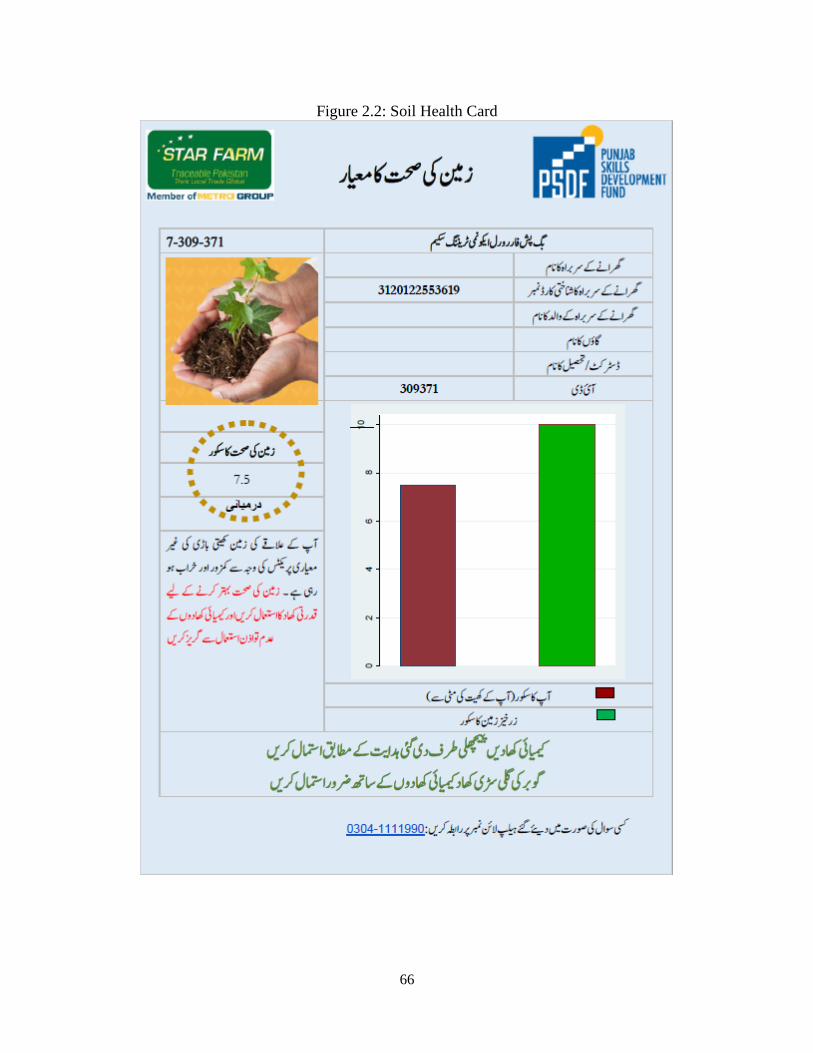
66

Figure 2.2: Soil Health Card

67

Figure 2.2: (cont’d)

68

BIBLIOGRAPHY

69

BIBLIOGRAPHY

Ahmed, S. A. and Gautam, M. 2013. Agriculture and Water Policy : Toward Sustainable Inclusive

Growth

Ali, M., Ahmed, F., Channa, H., and Davies, S. 2017. Chapter 6. Pakistan’s Fertilizer Sector:

Structure, Policies, Performance, and Impacts, in Agriculture and the Rural Economy in

Pakistan

Ali, M. and Byerlee, D. 2002. Productivity Growth and Resource Degradation in Pakistan’s

Punjab: A Decomposition Analysis, Economic Development and Cultural Change, Advance

Access published 2002: doi:10.1086/342759

Bumb, B. L. and Baanante, C. A. 1996. Role of fertilizers in food security and protecting the

environment to 2020, IFPRI Discussion Paper

Concepcion, R. 2007. Sustainable Fertilization Management of Croplands: The Philippines

Scenario.:

Cooter, R. D., Feldman, M., and Feldman, Y. 2008. The misperception of norms: The psychology

of bias and the economics of equilibrium, Review of Law and Economics, Advance Access

published 2008: doi:10.2202/1555-5879.1222

Corral, C., Giné, X., Mahajan, A., and Seira, E. 2016. A Multiple Intervention Approach to

Increasing Technology Adoption with a view towards scaling-up: evidence from Mexico:

Coulter, J. K. 2008. Unwelcome Harvest: Agriculture and Pollution. By G. R. Conway and J. N.

Pretty. London: Earthscan Publications Ltd (1991), pp. 672, £15.00. ISBN 1-85383-036-4.,

Experimental Agriculture, Advance Access published 2008:

doi:10.1017/s0014479700020226

Duflo, E., Kremer, M., and Robinson, J. 2008. How high are rates of return to fertilizer? Evidence

from field experiments in Kenya, in American Economic Review

Fishman, R., Kishore, A., Rothler, Y., Ward, P. S., Jha, S., and Singh, R. K. P. 2016. Can

information help reduce imbalanced application of fertilizers in India?, IFPRI Discussion

Paper, Advance Access published 2016

Goldstein, N. J., Cialdini, R. B., and Griskevicius, V. 2008. A Room with a Viewpoint: Using

Social Norms to Motivate Environmental Conservation in Hotels, Journal of Consumer

Research, Advance Access published 2008: doi:10.1086/586910

Ibrahim, M., Hassan, A. U., Iqbal, M., and Valeem, E. E. 2008. Response of wheat growth and

yield to various levels of compost and organic manure, Pakistan Journal of Botany, Advance

Access published 2008

Jack, B. K. 2013. Constraints on the adoption of agricultural technologies in developing countries.,

Literature review, Agricultural Technology Adoption Initiative, J-PAL (MIT) and CEGA

(UC Berkeley)., Advance Access published 2013

70

Janvry, A. de, Macours, K., and Sadoulet, E. 2016. Learning for adopting: Technology adoption

in developing country agriculture, in Policy briefs from the workshop organised by FERDI

and SPIA on June 1-2, 2016 in Clermont - Ferrand

Karlan, D., Osei, R., Osei-Akoto, I., and Udry, C. 2014. Agricultural decisions after relaxing credit

and risk constraints, Quarterly Journal of Economics, Advance Access published 2014:

doi:10.1093/qje/qju002

Khan, M. A., Ahmad, M., and Hashmi, H. S. 2012. Review of available knowledge on land

degradation in Pakistan

Lal, R. 2014. Societal value of soil carbon, Journal of Soil and Water Conservation, Advance

Access published 2014: doi:10.2489/jswc.69.6.186a

Levitt, S. D. and List, J. A. 2007. What Do Laboratory Experiments Measuring Social Preferences

Reveal About the Real World?, Journal of Economic Perspectives, Advance Access published

2007: doi:10.1257/jep.21.2.153

Malik, S., Shujat, A., Riaz, K., and Whitney, E. 2017. Chapter 2: Agriculture, Land, and

Productivity in Pakistan, in Agriculture and the Rural Economy in Pakistan

Marenya, P. P. and Barrett, C. B. 2009. State-conditional fertilizer yield response on Western

Kenyan Farms, American Journal of Agricultural Economics, Advance Access published

2009: doi:10.1111/j.1467-8276.2009.01313.x

Martin, R. and Randal, J. 2008. How is donation behaviour affected by the donations of others?,

Journal of Economic Behavior and Organization, Advance Access published 2008:

doi:10.1016/j.jebo.2007.08.001

McKenzie, D. 2012. Beyond baseline and follow-up: The case for more T in experiments, Journal

of Development Economics, Advance Access published 2012:

doi:10.1016/j.jdeveco.2012.01.002

Nachtergaele, F. O., Petri, M., Biancalani, R., and Lynden, G. Van. 2010. An Information database

for Land Degradation Assessment at Global Level:, date last accessed at Global Land

Degradation Information System ( GLADIS )

Pingali, P. and Shah, M. 2001. Policy re-directions for sustainable resource use: The rice-wheat

cropping system of the Indo-Gangetic Plains, Journal of Crop Production, Advance Access

published 2001

Sangeetha, S. P., Balakrishnan, A., and Devasenapathy, P. 2013. Influence of Organic Manures on

Yield and Quality of Rice (<i>Oryza sativa</i> L.) and Blackgram

(<i>Vigna mungo</i> L.) in Rice-Blackgram Cropping Sequence, American

Journal of Plant Sciences, Advance Access published 2013: doi:10.4236/ajps.2013.45141

Sarwar, G., Hussain, N., Schmeisky, H., and Muhammad, S. 2007. Use of compost an environment

friendly technology for enhancing rice-wheat production in Pakistan, Pakistan Journal of

Botany, Advance Access published 2007

Schultz, P. W., Nolan, J. M., Cialdini, R. B., Goldstein, N. J., and Griskevicius, V. 2007. The

constructive, destructive, and reconstructive power of social norms: Research article,

71

Psychological Science, Advance Access published 2007: doi:10.1111/j.1467-

9280.2007.01917.x

Zia, M. S., Muhmood, T., Baig, M. B., and Aslam, M. 2004. Land and environmental degradation

and its amelioration for sustainable agriculture in Pakistan., Sci Vision, Advance Access

published 2004

72

Essay 3 :A Dynamic Model for Warehouse Receipts Financing Demand in a Developing Country

Abstract

This paper studies the dynamics of warehouse receipts financing (WRF) demand by small

scale risk averse farmers in Pakistan. A dynamic model is used to investigate how risk and time

preferences, transaction costs, and uncertainty reduce demand for WRF, and even lead to non-

participation in the program. The model is calibrated and solved for a representative small-scale

farmer that grows paddy. Results show high transaction costs to be a major barrier to participation.

Similarly, expectations about future prices also affect participation which drops to zero if the

subjective probability of prices falling goes beyond 10 percent.

73

3.1. Introduction

Warehouse receipts financing (WRF) has been promoted as a potential solution to some of

the fundamental issues that affect agricultural markets in developing countries (Aggarwal, Francis,

& Robinson, 2018; Basu & Wong, 2015; Burke, 2014). WRF essentially provides small farmers

access to storage facilities where their product is weighed, graded, and agglomerated. The storage

organization issues a receipt stating the value of the product stored. This warehouse receipt can be

used as collateral to acquire loans from financial institutions such as banks. WRF gives farmers

bargaining power as they can choose time of sales, provides access to downstream buyers due to

quality control and higher volumes, and most importantly access to formal financial institutions

for loans. The establishment of a mechanism under which warehouse receipts can be traded has

the potential of modernizing the agricultural value chains, improving market practices on quality

control, standardization of product, and promoting exports.

However, the demand for WRF programs has been weak and these services mostly end up

being used by large farmers, traders, and processors (William & Kaserwa, 2015). Several authors

have postulated that poor farming households face multiple constraints which need to be relaxed

simultaneously (Duflo, Kremer, & Robinson, 2011; Karlan et al., 2014). Lack of WRF take up

also suggests that access to a storage or financial institutions are not be the only binding

constraints. Other aspects such as risk aversion, present bias, and uncertainty also play an

important role in the decision making of farmers. Since, WRF has the potential to significantly

improve the agricultural value chains in developing countries it is important to understand under

what conditions small farmers would be willing to participate.

WRF requires farmers to take on the role of speculators who are expecting to make money

off future prices increases. However, in the absence of financial products that can be used to hedge,

74

farmers have to take on the entire risk of price volatility. We have ample evidence that small

farmers are generally risk averse might not invest in options which have risky cash flows (Feder,

Just, & Zilberman, 1985; Liu, 2013; Ward & Singh, 2015). Given the possibility of a downward

price shock it is possible that WRF is not a profitable venture for small farmers under the expected

profit margins. Apart from risk considerations, storage is also a choice between foregoing current

income for future income. This is important for farmers as they earn bulk of their income in lump

sum at harvest and engaging in WRF would mean less cash available in the current period to payoff

outstanding debt, meet current consumption needs, invest in next crop cycle, and plan for

anticipated and unanticipated expenses during the post-harvest period. These factors individually

or collectively can make WRF non-participation a subjectively rational choice, making it important

to understand the conditions under which participation is feasible for a small farmer.

Risk and time preferences introduce dynamic considerations into storage and marketing

choices of small farmers. The main goal of this paper is to explicitly model the dynamics of WRF

in the context of Pakistan. This paper adds to the existing literature on WRF programs, most of

which have taken a reduced form approach to evaluate the benefits of WRF (Aggarwal et al., 2018;

Basu & Wong, 2015; Burke, 2014). Miranda et al. (2017) develop a dynamic model to evaluate

WRF for an average smallholder Ghanaian farmer while and find WRF not to be a viable product

for small farmers. The motivation for this paper is to estimate demand for WRF in Pakistan which

has two agricultural cycles instead of one due to irrigation, most farmers are commercial growers,

and there is a lot interest by the government to establish a WRF system in the country.

This paper employs dynamic programming to solve a two-period model for an agricultural

year. Even though the model is for two period its findings are clear into how risk, time, and

uncertainty undermine the benefits of WRF. The model is simulated for a representative farmer

75

who grows rice as a cash crop on 5 acres of land and has an average harvest of 150 maunds. The

model is calibrated to reflect a small farmer’s risk and time preferences, subjective future

expectations, and credit constraints. Results derived show that farmers will not store using modern

approach of storing in silos due to high cost. However, under the traditional system which is 25

percent cheaper farmers would will store 24 percent of the harvested paddy. Sensitivity analysis

further supports this claim as participation falls to zero if interest rate on loans offered against

stored grain goes beyond 15 percent. This also highlights that liquidity is an important constraint

for farmers who need the cash advance through WRF to participate. Results also show that farmers

will not participate if the subjective probability of prices falling is more than 10 percent. Similarly,

risk aversion also depresses the demand for storage as expected and the quantity stored increases

as the farmer becomes less risk averse. These results highlight that reducing exposure to risk would

also improve demand for WRF. Hence, a product design which reduces the transaction cost of

participation and reduces future price uncertainty can significantly improve participation.

Transaction costs can be decreased by registering farmers and forming small community groups

so that costs can be reduced by economies of scale. Similarly, providing information about past

prices and future expected prices can help the farmers develop price expectation which are closer

to the true distribution. Alternatively, developing financial products through which the warehouse

management companies can hedge their risk to price shocks can reduce uncertainty in future prices

making WRF an investment with less volatile cash flows for warehousing companies, banks, and

the farmers.

The rest of the paper is organized as follows. Section 2 outlines the dynamic model for a

standard WRF product and decision rules are then presented under these scenarios. Derivations

are initially shown for a scenario without liquidity constraint and perfect risk pooling, these

76

constraints are then included in the model and their effect on demand is investigated. Section 3

lays out the specific functional form and explains the data collected to calibrate its parameters for

a representative rice grower in central Punjab. Section 4 discusses the results from the analysis and

shows how delayed payments and a reduction in price uncertainty through price floor can increase

demand. Section 5 gives concluding comments.

3.2. Dynamic Storage Model

Consider a small farmer who has the option of participating in a WRF program, which allows

intertemporal arbitrage and access to more remunerative markets through quality control and

agglomeration of grain. However, intertemporal arbitrage inherently carries the risk of loss if

future prices do not rise sufficiently. Also, it requires a compromise between current income over

future income. Finally, beliefs about future also effect the choice about either selling now or storing

and selling in the future after considering several factors.

I use a stylized model to represent the decision making of the farmer under risk aversion, time

preferences and uncertainty. Risk and time preference play an important role in the decision

making of individuals especially when it involves makes choices which have a time dimension

and uncertainty such as technology adoption, investment, migration, education, and health (Ashraf,

Karlan, & Yin, 2006; Engle Warnick, Escobal, & Laszlo, 2011; Jensen, 2010; Lawless, Drichoutis,

& Nayga, 2013; McKenzie, Gibson, & Stillman, 2013). In any given year there are two time

periods – the paddy harvest period and the wheat production period. In each period utility is a

function of income and the objective of the farmer is to maximize the present value of utility

derived over these two periods. Period one starts with the stock of freshly harvested paddy and

there are no carryovers from the previous period. The farmer decides how much of this paddy to

store and how to sell at the prevailing price. The income generated from sales is then allocated

77

between saving and investment in the wheat crop which yields a return at the end of the second

period. The farmer has a subjective probability regarding price of paddy at the end of period two

(when he liquidates the stock) and believes that the prices will increase with a probability 𝜋𝐺 to

earn him a profit from storage.

The small holder farmer’s formal two period dynamic optimization problem can be expressed

as follows. I closely follow the approach used by Karlan et al. (2014):

max𝑦,𝑧,𝑎

𝑈(𝜋0) + 𝛽 ∑ 𝜇𝑠𝑈(𝜋1𝑠)

𝑠∈𝑆

(3.1)

Before grain is stored it needs to be transported, dried, cleaned, and graded. Once stored the

farmer receives a warehouse receipt which can be used to acquire a loan which is equal to a fraction

of the value of the grain stored. The loan is repaid at the end of period two when the farmer

liquidates the stored grain. Another aspect that the farmer needs to consider is the return from other

investment opportunities such as growing wheat. The resource allocation decision is made subject

to

𝜋0 = 𝑝0(𝑞 − 𝑦 + 𝛾𝑦) − 𝑎 − 𝑧

𝜋1𝑠 = 𝑓(𝑧) + 𝑅𝑎 + y(𝑝1

𝑠 − 𝜏 − 𝑅𝛾𝑝0)

𝑞 ≥ 𝑦 (3.2)

𝑦 ≥ 0

𝑧 ≥ 0

where 𝑈(∙) is an increasing and concave utility function, 𝜋0 is income in period 0, there are two

states good and bad 𝑠 ∈ {𝐺, 𝐵}, 𝜋1𝑠 is income in period 1 for each state, 𝜇𝑠 is probability of each

state, 𝛽 is the discount factor, 𝑞 is the amount of storable commodity in period 1, 𝑦 is quantity

stored, 𝑧 is investment in wheat crop whose price is normalized to one, 𝑎 is the net saving in

financial market, 𝛾 is the advance rate set by the warehousing firm which allows the farmers to

receive credit against the value of the stored grain, 𝑅 is the return on the credit market or the cost

78

of borrowing from the credit market or the WRF, 𝜏 is the per unit cost of storage, and 𝜇𝐵 is the

probability of being in bad state.

Since, the main interest is storage choice under risk and credit constraint. The model is

solved using the Lagrange method under four different market scenarios in which access to credit

and risk pooling is varied.

Table 3.1: Lagrange Results

Scenarios Storage Wheat

Perfect Credit Market and Risk

Pooling

�̅�1 − 𝜏

𝑝0= 𝑅 𝑓′(𝑧) = 𝑅

Incomplete Credit Market and

Perfect Risk Pooling

�̅�1 − 𝜏 − 𝑅𝛾𝑝0

𝑝0( 1 − 𝛾)= 𝑓′(𝑧) 𝑓′(𝑧) > 𝑅

Perfect Credit Market and

Incomplete Risk Pooling 𝑝1

𝐺 =𝑅𝑝0(1 − 𝛾)

𝜏 + 𝑅𝛾𝑝0 [

𝜇𝐵𝑈′(𝜋1𝐵)

𝜇𝐺𝑈′(𝜋1𝐺)

+ 1] 𝑓′(𝑧) = 𝑅

Incomplete Credit Market and

Risk Pooling 𝑝1

𝐺 =𝑓′(𝑧)𝑝0(1 − 𝛾)




+ 1] 𝑓′(𝑧) > 𝑅

3.3. Model Parameterization

In order to provide a sense of the magnitude of the value of the insurance under various market

conditions the model is fully parameterized so that we can solve it numerically. The utility function

is assumed to take the form

𝑈(𝜋) =𝜋𝜎 𝑖𝑓 𝜋 ≥ 0

−(−𝜋𝜎) 𝑖𝑓 𝜋 < 0

where 𝜎 > 0 dictates the curvature of the function and can be thought of as a measure of risk.

The model parameters are calibrated to represent an average smallholder farmer. The average

farmer sell approximately 150 maunds immediately at harvest as the quality of the paddy starts to

deteriorate if it is not dried within a few days. We assume that a farmer would store paddy for 90

days as the prices stabilize at a higher equilibrium by that time. However, small farmers are also

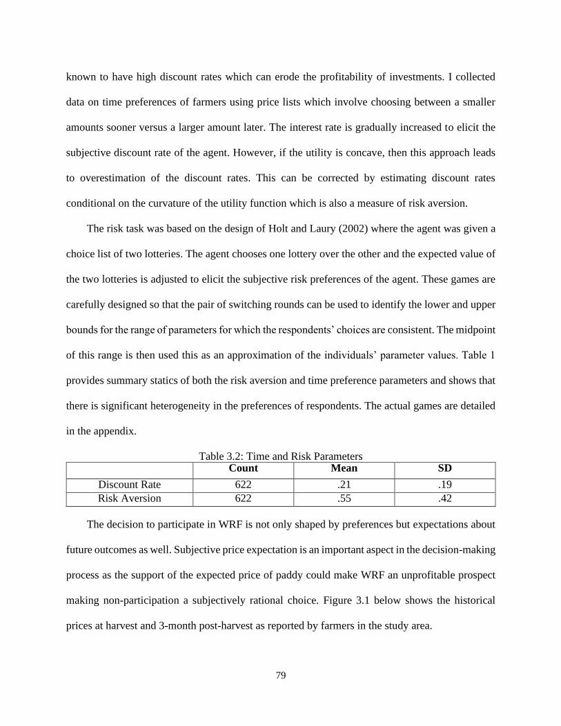
79

known to have high discount rates which can erode the profitability of investments. I collected

data on time preferences of farmers using price lists which involve choosing between a smaller

amounts sooner versus a larger amount later. The interest rate is gradually increased to elicit the

subjective discount rate of the agent. However, if the utility is concave, then this approach leads

to overestimation of the discount rates. This can be corrected by estimating discount rates

conditional on the curvature of the utility function which is also a measure of risk aversion.

The risk task was based on the design of Holt and Laury (2002) where the agent was given a

choice list of two lotteries. The agent chooses one lottery over the other and the expected value of

the two lotteries is adjusted to elicit the subjective risk preferences of the agent. These games are

carefully designed so that the pair of switching rounds can be used to identify the lower and upper

bounds for the range of parameters for which the respondents’ choices are consistent. The midpoint

of this range is then used this as an approximation of the individuals’ parameter values. Table 1

provides summary statics of both the risk aversion and time preference parameters and shows that

there is significant heterogeneity in the preferences of respondents. The actual games are detailed

in the appendix.

Table 3.2: Time and Risk Parameters Count Mean SD

Discount Rate 622 .21 .19

Risk Aversion 622 .55 .42

The decision to participate in WRF is not only shaped by preferences but expectations about

future outcomes as well. Subjective price expectation is an important aspect in the decision-making

process as the support of the expected price of paddy could make WRF an unprofitable prospect

making non-participation a subjectively rational choice. Figure 3.1 below shows the historical

prices at harvest and 3-month post-harvest as reported by farmers in the study area.

80

Figure 3.1: Historical Paddy Prices (PKR/maund)

Since these prices are reported by the farmers, we can consider them as subjective prices based

on which the farmers would form expectations about future prices. The figure also shows that on

average post-harvest prices have been higher in the past three years. However, we also see that

there is an overlap in the harvest and the post-harvest price distributions suggesting that there is a

positive probability that the farmers could receive a lower price in the post-harvest compared to

the price at harvest. Therefore, farmers’ expectations about future prices at harvest and post-

harvest were collected before the rollout of the warehouse receipts financing program. Farmers

were asked to report the maximum and minimum price for the upcoming 2018 harvest and 3-

months post-harvest. Table 3.3 shows the summary statistics of prices reported by farmers.

81

Table 3.3: Expected Prices (PKR/maund) N Mean SD Min Max

Min Harvest 2018 661 1482 272 1100 2100

Max Harvest 2018 661 1702 352 1200 2500

Min Post Harvest 2018 661 1938 378 1200 2800

Max Post Harvest 2018 661 2207 453 1350 3000

On average the farmers expected prices to be between rupees 1500 to 1700 at harvest and

between rupees 1900 to 2200 post-harvest. I use the minimum and maximum expected prices to

calculate averages and the distribution is shown in figure 3.2 which shows an overlap in the price

distributions. This suggests that farmers do assign a positive probability to prices falling in the

future.

Figure 3.2: Average Expected Paddy Prices (PKR/maund)

Another important consideration for participating in the WRF would be the transaction cost.

A small holder will only use WRF if the premium earned from the stored grain adjusted for cost

of warehousing is positive. Data on warehouse charges was obtained from a local warehouse

management company which offered these services to small farmers in the study area. Table 3.4

reports the cost of warehousing which is substantial even when non-pecuniary costs such as

82

arranging for labor and vehicles for transportation are not incorporated. Grading and weighting

charges are assumed to be zero. Loading and dispatch is the labor cost for taking the paddy off the

trucks and then loading them back at sale time. Preclearing is the cost of labor used to feed the

paddy to the dryers. The moisture content needs to be reduced before its stored, mechanical drying

is done by passing the paddy through dryers which dry it and clear it of impurities such as dust and

empty kernels. Under mechanical drying paddy is stored in silos where moisture level is

automatically maintained. In the case of traditional storage paddy is dried in the sun and overturned

several times. Paddy is stored in jute bags and manually monitored to ensure moisture levels are

within acceptable levels. The cost of drying and storage are higher for mechanical drying due to

high energy costs and using off grid sources of electricity due to load shedding. Jute bags are

available on rent from the warehouse or can be bought by the farmer themselves, a jute bag

normally costs around PKR 250 and often short in supply at harvest time. The transport cost

reported in the table is the mean, but cost can double depending on the distance from warehouse

and availability at the time of harvest.

Table 3.4: Warehousing Cost (40kg bag) Cost per bag Mechanical Traditional

Unloading and Dispatch 10 10

Preclearing 15 0

Drying cost 50 24

Storage 90 days 120 60

Jute bag rental 90 days 0 36

Transportation cost to warehouse 15 15

Total Warehousing Cost 210 145

If the farmer stores the paddy, it leads to 6 percent loss of weight under mechanical storage

and a 2.5 percent weight loss under the traditional sun drying method on average. The weight loss

is higher in the mechanical drying as it is more efficient in drying and removing impurities such

as empty kernels, dust, and other debris. The total cost of mechanical drying is approximately

83

PKR60 per maund higher than the traditional drying, and the premium for mechanically dried

paddy can vary between 0 to PKR 200 per maund.

The farmer is issued a warehouse receipts which records the amount of paddy stored and its

value at the time of storage based on its quality. This warehouse receipt can be used to acquire a

loan which needs to be repaid at the time of liquidating the stored grain. The advance rate is fixed

at 70 percent of the value of the crop at the time of storage at an annualized interest rate of 28

percent. Base-case model parameters are set to the values given in Table 3.5.

Table 3.5: Base Case Parameter Values

Symbol Value Description

𝑝0 1550 Price/maund at harvest

𝑝1𝐺 2100 Price/maund 3-month post-harvest in the good state

𝑝1𝐵 1300 Price/maund 3-month post-harvest in the bad state

𝜋𝐵 0.10 Subjective probability of being in the bad state.

𝛽 0.79 Subjective annual discount rate

q 150 Harvest quantity in maunds

ra 0.55 Risk Aversion

𝜏a 145 Per maund storage cost for 90 days

𝛿a 0.025 Weight loss due to drying and cleaning

R 1.14 Annualized interest rate

𝛾 0.70 Advance rate for loan against warehouse receipts

𝛼b 1.25 Return on investment in wheat aWarehousing cost and weight loss are given for traditional drying and cleaning. bReturn on wheat is based off the calculations provided by the agriculture department.

3.4. Results

The model is calibrated for a smallholder farmer and solved under the four market conditions

derived earlier. Under complete credit market the farmer can borrow and solve from the market

under the prevailing interest rate. Future price of paddy is assumed to be known and equal to the

average of the good and bad state. However, to ensure that results are reflective of actual market

outcome and unrealistic amounts are not borrowed, investment in wheat capped at PRK 200,000

84

which is the cost of production for 5 acres of land10. Results show that under these conditions the

farmer would store the entire 150 maunds, borrow PRK 164,000 from the market, and invest PKR

200,000 in wheat production. The model is then solved with incomplete credit market, and to make

this binding the farmer cannot borrow but can save at the prevalent rate. Other conditions are same

where expected future price is known with certainty and the maximum amount that can be invested

in wheat is capped. Results show that the farmer will store the entire 150 maunds again, invest

PKR 55,000 in wheat and not save anything. Next the credit market is assumed to be functional

but there is uncertainty in future paddy prices. Results show that the farmer will store the entire

harvest, borrow lower quantities from the market and invest PKR 200,000 in wheat. Finally, the

model is solved under the final market scenario where there is no credit market or risk pooling.

The results show that the farmer will store 36 maunds of the produce, invest PKR 108,000 in

wheat, and not save any money. A summary of these outcomes is given in table 3.6.

Table 3.6: Simulation Results

Scenarios Paddy Stored

(maunds)

Borrowing

(PKR)

Investment in

Wheat (PKR)

Perfect Credit Market and Risk Pooling 150 164,000 200,000

Incomplete Credit Market and Perfect Risk Pooling 150 0 55,000

Perfect Credit Market and Incomplete Risk Pooling 150 158,000 200,000

Incomplete Credit Market and Risk Pooling 36 0 108,000

I then conduct a sensitivity analysis on how the demand for storage will change under different

interest rates, probability of a bad state, and risk aversion. All of these parameters are changed

individually to identify parameter values at which they become binding. Interest rates are varied

from 7 percent to 20 percent with steps of 1 percent, probability of being in the bad state is varied

from 5 percent to 20 percent, with steps of 1 percent. The subjective risk aversion parameters is

10 I use the production costs for 2018-19 under average conditions in Punjab developed by the local agriculture department

85

varied one standard deviation above and below the mean. Figure 3.3 reports these sensitivity

analysis results under the traditional storage method.

The results show that risk aversion does not impact storage when risk pooling is possible.

When risk pooling is not possible risk aversion decreases quantity stored and as relative risk

aversion decreases the farmer higher proportion of paddy. Similarly, at low interest rates the farmer

would store the entire stock of paddy but as the interest rate increases the quantity of paddy stored

decrease and goes to zero. The subjective probability of bad state also reduces participation, and

farmers under incomplete credit markets are most sensitive this variable.

Figure 3.3: Storage Sensitivity Analysis

3.5. Conclusion

This paper develops a dynamic model of demand for a standard WRF product in the context

of Pakistan in the presence of liquidity constraints, risk aversion, and price uncertainty. This paper

86

adds to the existing literature by analyzing the feasibility of WRF in a context where there are two

complete agricultural cycles. Most of the WRF evaluations and technical reports have been in

contexts where there is primary growing season followed by a dry season in which limited

agricultural activities can be carried out. I solve a two-period model for an agricultural year, and

even though the model is for two period its findings are clear into how preferences and uncertainty

affect the benefits of WRF. The model is calibrated to reflect a small farmer’s preference and

solved under four different market condition. Results show that farmers will store if either the

credit market or insurance market is functioning. However, in a scenario where access to credit is

constrained and risk cannot be pooled demand for storage would fall. I also find that farmers are

sensitive to transaction cost of storage and would not store under the mechanized method as it is

more costly, similarly the demand for storage also falls as interest rates increase. Risk also plays

an important role in the decision to participate. Risk averse farmers have low demand when there

is no risk pooling. Similarly, as the subjective probabilities of the prices falling in the future

increases non-participation becomes the dominant strategy.

These results suggest that transaction costs of warehousing are significant and erode the

profitability of WRF. The farmer is better off selling the paddy at harvest especially under

mechanical storage as the weight loss due to drying and the cost of storage are very high and the

premium over traditional methods is not certain. Participation in the WRF can be increased by

offering lower interest rates on credit and reducing the exposure to risk. One mechanism could be

that collateral management company’s hedge the price risk in paddy against other commodities or

buying futures. However, absence of these market in developing countries make the success of

WRF difficult as it requires the small farmer to bear the entire risk.

87

A limitation of this model is that it assumes disutility from losses to be proportional to the

utility from gains. Prospect theory highlights that this might not be the case as people derive higher

disutility from losses. This might be particularly true in the case of small farmers who might be

highly loss averse as one negative shock could push them into poverty. Hence, the results from

this numerical solution must be viewed an upper bound to the storage demand. Future work can

include loss aversion as an additional parameter to test the feasibility of this program.

Government and international organizations promoting warehouse receipts financing need to

take the transaction and risk factor into account while planning this program. The direct impact of

improving profitability of small farmers through intertemporal arbitrage would be limited unless

access to this program is improved through measure which protect small farmers against large

negative shocks. If we look past the distributional impact of WRF, it has many other benefits such

as it could promote the development of agricultural value chains by making it more efficient and

imposing quality controls and standards. It would also reduce the price volatility of the

commodities, therefore reducing uncertainty and increasing investment.

88

APPENDIX

89

APPENIDX

Preferences over income in the first period and in the various states of the second period with

probability of state and a discount factor are

𝑈(𝜋0) + 𝛽 ∑ 𝜇𝑠𝑈(𝜋1𝑠)

𝑠∈𝑆

(3.3)

where 𝑈(∙) is an increasing and concave utility function, 𝜋0 is income in period 0, there are two

states good and bad 𝑠 ∈ {𝐺, 𝐵}, 𝜋1𝑠 is income in period 1 for each state, 𝜇𝑠 is probability of each

state, and 𝛽 is the discount factor. The farmer maximizes (1) under the following constraints

𝜋0 = 𝑝0(𝑞 − 𝑦 + 𝛾𝑦) − 𝑎 − 𝑧

𝜋1𝑠 = 𝑓(𝑧) + 𝑅𝑎 + y(𝑝1

𝑠 − 𝜏 − 𝑅𝛾𝑝0)

𝑞 is the amount of storable commodity in period 0, 𝑦 is quantity stored, 𝑧 is investment in wheat

crop whose price is normalized to one, 𝑎 is the net saving in financial market (negative if

borrowing and positive if saving), 𝛾 is the advance rate set by the warehousing firm against the

value of the stored grain11, 𝑓(𝑧) is the concave wheat production function, 𝑅 is the return on the

credit market or the cost of borrowing from the WRF, 𝛿 is the weight loss due to storage, and 𝜏 is

the per unit cost of storage. Additional side conditions are imposed so that the farmer cannot store

negative amounts or store more than quantity produced and investment in wheat is nonnegative.

𝑞 ≥ 𝑦

𝑦 ≥ 0, 𝑧 ≥ 0

Since the main interest is in storage choice under risk and credit constraint, storage rules under

these environments are derived. The problem is initially solved under perfect credit and risk

11 For simplicity I assume that the farmer would always take the maximum amount of cash advance through WRF.

90

pooling to arrive at a well-known intertemporal arbitrage optimal decision rule. Credit constraint

and imperfect risk pooling are then introduced into the model, first individually and then together.

Case 1: Perfect credit market and risk pooling.

Under this market condition the farmer does not face liquidity constraints and consumes an average

of the good and bad states due to perfect risk pooling {�̅�1 = 𝑓(𝑧) + 𝑅𝑎 + y(�̅�1 − 𝜏 − 𝑅𝛾𝑝0)}.

This extreme case of perfect insurance later helps us to focus on the implications of a binding

credit constraint when risk plays no role in the decision to allocate resources. The setup of the

problem under Lagrange method is given below.

max𝑦,𝑧,𝑎

𝐿 = 𝑈(𝜋0) + 𝛽𝑈(�̅�1) + 𝜆1(𝑞 − 𝑦) + 𝜆2(𝑝0(𝑞 − 𝑦 + 𝛾𝑦) − 𝑎 − 𝑧) + 𝜌1𝑦 + 𝜌2𝑧

The first order conditions are

𝜕𝐿

𝜕𝑎= −𝑈′(𝜋0) + 𝛽𝑅𝑈′(�̅�1) − 𝜆2 = 0

𝜕𝐿

𝜕𝑧= −𝑈′(𝜋0) + 𝛽𝑓′(𝑧)𝑈′(�̅�1) − 𝜆2 + 𝜌2 = 0

𝜕𝐿

𝜕𝑦= 𝑝0( 𝛾 − 1)𝑈′(𝜋0) + 𝛽(�̅�1 − 𝜏 − 𝑅𝛾𝑝0)𝑈′(�̅�1) − 𝜆1 + 𝜆2𝑝0( 𝛾 − 1) + 𝜌1 = 0

𝜆1(𝑞 − 𝑦) = 0, 𝜆2(𝑝0(𝑞 − 𝑦 + 𝛾𝑦) − 𝑎 − 𝑧) = 0, 𝜌1𝑦 = 0, 𝜌2𝑧 = 0

Using the above results, we can derive the decision rules for the farmer.

Assuming 𝜆1 = 0, 𝜆2 = 0, 𝜌1 = 0, 𝑎𝑛𝑑 𝜌2 = 0.

𝑓′(𝑧) = �̅�1 − 𝜏

𝑝0= 𝑅

With perfect credit markets and risk‐pooling, investment in wheat is independent of resources (q)

and preferences. The investment is only determined by the cost of interest and the return from

investment which depends on the production function and prices. Similarly, the choice of storage

depends on expected price, current price, and the cost of storage. Neither reduction in risk or access

to credit would influences the choices under this scenario.

91

Case 2: Imperfect credit market and perfect risk pooling.

In this case credit market is non functions and binding which essentially adds an additional

constraint 𝑎 ≥ 0. Risk pooling is still available, so the farmer continues to earn the expected

income. The setup of the problem under Lagrange method is given below.

max𝑦,𝑧,𝑎

𝐿 = 𝑈(𝜋0) + 𝛽𝑈(�̅�1) + 𝜆1(𝑞 − 𝑦) + 𝜆2(𝑝0(𝑞 − 𝑦 + 𝛾𝑦) − 𝑎 − 𝑧) + 𝜌1𝑦 + 𝜌2𝑧 + 𝜌3𝑎


𝜕𝐿

𝜕𝑎= −𝑈′(𝜋0) + 𝛽𝑅𝑈′(�̅�1) − 𝜆2 + 𝜌3 = 0

𝜕𝐿

𝜕𝑧= −𝑈′(𝜋0) + 𝛽𝑓′(𝑧)𝑈′(�̅�1) − 𝜆2 + 𝜌2 = 0

𝜕𝐿

𝜕𝑦= 𝑝0( 𝛾 − 1)𝑈′(𝜋0) + 𝛽(�̅�1 − 𝜏 − 𝑅𝛾𝑝0)𝑈′(�̅�1) − 𝜆1 + 𝜆2𝑝0( 𝛾 − 1) + 𝜌1 = 0



Assuming 𝜆1 = 0, 𝜆2 = 0, 𝜌1 = 0, 𝜌2 = 0, 𝑎𝑛𝑑 𝜌3 > 0.

𝑓′(𝑧) > 𝑅

Due to the liquidity constraint, investment in wheat is constrained and lower than under

functioning credit market. The choice of storage now depends on the relative return from wheat.

�̅�1 − 𝜏 − 𝑅𝛾𝑝0

𝑝0( 1 − 𝛾)= 𝑓′(𝑧)

The choice of storage depends on the expected future prices, return in the credit market, advance

rate in WRF, current prices, and return from investment in wheat. Preferences still do not enter the

decision making for either of the investment options.

92

Case 3: Imperfect risk pooling but a perfect capital market.

In this scenario there is no risk pooling, but the capital market is complete, and the farmer can

engage in income smoothing across the two time periods. The setup of the problem under Lagrange

method is given below.

max𝑦,𝑧,𝑎

𝐿 = 𝑈(𝜋0) + 𝛽{𝜇𝐵𝑈(𝜋1𝐵) + 𝜇𝐺𝑈(𝜋1

𝐺)} + 𝜆1(𝑞 − 𝑦) + 𝜆2(𝑝0(𝑞 − 𝑦 + 𝛾𝑦) − 𝑎 − 𝑧)

+ 𝜌1𝑦 + 𝜌2𝑧


𝜕𝐿

𝜕𝑎= −𝑈′(𝜋0) + 𝛽𝑅{𝜇𝐵𝑈′(𝜋1

𝐵) + 𝜇𝐺𝑈′(𝜋1𝐺)} − 𝜆2 = 0

𝜕𝐿

𝜕𝑧= −𝑈′(𝜋0) + 𝛽𝑓′(𝑧){𝜇𝐵𝑈′(𝜋1

𝐵) + 𝜇𝐺𝑈′(𝜋1𝐺)} − 𝜆2 + 𝜌2 = 0

𝜕𝐿

𝜕𝑦= 𝑝0( 𝛾 − 1)𝑈′(𝜋0) − 𝛽(𝜏 + 𝑅𝛾𝑝0){𝜇𝐵𝑈′(𝜋1

𝐵)𝑝1𝐵 + 𝜇𝐺𝑈′(𝜋1

𝐺)𝑝1𝐺} − 𝜆1 + 𝜆2𝑝0( 𝛾 − 1)

+ 𝜌1 = 0



Assuming 𝜆1 = 0, 𝜆2 = 0, 𝜌1 = 0, 𝑎𝑛𝑑 𝜌2 = 0.

𝑓′(𝑧) = 𝑅

The choice of investment in z is independent of resources (q) or preferences and only depends on

the cost of credit and the return from wheat which depends on its production function and prices.

The decision rule for storage is given by

𝑅𝑝0(1 − 𝛾)

𝜏 + 𝑅𝛾𝑝0=

𝜇𝐵𝑈′(𝜋1𝐵)𝑝1

𝐵 + 𝜇𝐺𝑈′(𝜋1𝐺)𝑝1

𝐺

𝜇𝐵𝑈′(𝜋1𝐵) + 𝜇𝐺𝑈′(𝜋1

𝐺)

Assuming 𝑝1𝐵 = 0 for simplicity

93

𝑝1𝐺 =

𝑅𝑝0(1 − 𝛾)




+ 1]

Storage choice is influenced by return in the credit market, advance rate, current prices, cost of

storage, future price in different states and their probabilities, and the preferences of farmers.

Case 4: Imperfect Credit and Risk Pooling

In this scenario there is no access to a credit market or risk pooling. The setup of the problem under

Lagrange method is given below.

max𝑦,𝑧,𝑎

𝐿 = 𝑈(𝜋0) + 𝛽{𝜇𝐵𝑈(𝜋1𝐵) + 𝜇𝐺𝑈(𝜋1

𝐺)} + 𝜆1(𝑞 − 𝑦) + 𝜆2(𝑝0(𝑞 − 𝑦 + 𝛾𝑦) − 𝑎 − 𝑧)

+ 𝜌1𝑦 + 𝜌2𝑧 + 𝜌3𝑎


𝜕𝐿

𝜕𝑎= −𝑈′(𝜋0) + 𝛽𝑅{𝜇𝐵𝑈′(𝜋1

𝐵) + 𝜇𝐺𝑈′(𝜋1𝐺)} − 𝜆2 + 𝜌3 = 0

𝜕𝐿

𝜕𝑧= −𝑈′(𝜋0) + 𝛽𝑓′(𝑧){𝜇𝐵𝑈′(𝜋1

𝐵) + 𝜇𝐺𝑈′(𝜋1𝐺)} − 𝜆2 + 𝜌2 = 0

𝜕𝐿

𝜕𝑦= 𝑝0( 𝛾 − 1)𝑈′(𝜋0) − 𝛽(𝜏 + 𝑅𝛾𝑝0){𝜇𝐵𝑈′(𝜋1

𝐵)𝑝1𝐵 + 𝜇𝐺𝑈′(𝜋1

𝐺)𝑝1𝐺} − 𝜆1 + 𝜆2𝑝0( 𝛾 − 1)

+ 𝜌1 = 0



Assuming 𝜆1 = 0, 𝜆2 = 0, 𝜌1 = 0, 𝜌2 = 0, 𝑎𝑛𝑑 𝜌3 > 0.

𝑓′(𝑧) > 𝑅

Due to the liquidity constraint, investment in wheat is constrained and lower than under

functioning credit market. The choice of storage now depends on the relative return from wheat.

The decision rule is given by

94

𝑓′(𝑧)𝑝0(1 − 𝛾)

𝜏 + 𝑅𝛾𝑝0=

𝜇𝐵𝑈′(𝜋1𝐵)𝑝1

𝐵 + 𝜇𝐺𝑈′(𝜋1𝐺)𝑝1

𝐺

𝜇𝐵𝑈′(𝜋1𝐵) + 𝜇𝐺𝑈′(𝜋1

𝐺)

Assuming 𝑝1𝐵 = 0 for simplicity

𝑝1𝐺 =

𝑓′(𝑧)𝑝0(1 − 𝛾)




+ 1]

95

BIBLIOGRAPHY

96

BIBLIOGRAPHY

Aggarwal, S., Francis, E., & Robinson, J. (2018). Grain today, gain tomorrow: Evidence from a

storage experiment with savings clubs in Kenya. Journal of Development Economics.

https://doi.org/10.1016/j.jdeveco.2018.04.001

Ashraf, N., Karlan, D., & Yin, W. (2006). Tying odysseus to the mast: Evidence from a

commitment savings product in the Philippines. Quarterly Journal of Economics.

https://doi.org/10.1162/qjec.2006.121.2.635

Basu, K., & Wong, M. (2015). Evaluating seasonal food storage and credit programs in east

Indonesia. Journal of Development Economics.

https://doi.org/10.1016/j.jdeveco.2015.02.001

Burke, M. (2014). Selling Low and Buying High : An Arbitrage Puzzle in Kenyan Villages.

Working Paper.

Chavas, J. P., Despins, P. M., & Fortenbery, T. R. (2000). Inventory dynamics under transaction

costs. American Journal of Agricultural Economics. https://doi.org/10.1111/0002-

9092.00023

Duflo, E., Kremer, M., & Robinson, J. (2011). Nudging farmers to use fertilizer: Theory and

experimental evidence from Kenya. American Economic Review.

https://doi.org/10.1257/aer.101.6.2350

Engle Warnick, J. C., Escobal, J., & Laszlo, S. C. (2011). Ambiguity aversion and portfolio choice

in small-scale peruvian farming. B.E. Journal of Economic Analysis and Policy.

https://doi.org/10.2202/1935-1682.2331

Feder, G., Just, R. E., & Zilberman, D. (1985). Adoption of Agricultural Innovations in Developing

Countries: A Survey. Economic Development and Cultural Change.

https://doi.org/10.1086/451461

Jensen, R. (2010). The (Perceived) returns to education and the demand for schooling. Quarterly

Journal of Economics. https://doi.org/10.1162/qjec.2010.125.2.515

Karlan, D., Osei, R., Osei-Akoto, I., & Udry, C. (2014). Agricultural decisions after relaxing credit

and risk constraints. Quarterly Journal of Economics. https://doi.org/10.1093/qje/qju002

Lai, J. Y., Myers, R. J., & Hanson, S. D. (2003). Optimal On-Farm Grain Storage by Risk-Averse

Farmers. Journal of Agricultural and Resource Economics.

Lawless, L., Drichoutis, A. C., & Nayga, R. M. (2013). Time preferences and health behaviour: a

review. Agricultural and Food Economics. https://doi.org/10.1186/2193-7532-1-17

Liu, E. M. (2013). Time to change what to sow: Risk preferences and technology adoption

97

decisions of cotton farmers in China. Review of Economics and Statistics.

https://doi.org/10.1162/REST_a_00295

McKenzie, D., Gibson, J., & Stillman, S. (2013). A land of milk and honey with streets paved with

gold: Do emigrants have over-optimistic expectations about incomes abroad? Journal of

Development Economics. https://doi.org/10.1016/j.jdeveco.2012.01.001

Miranda, M. J., Mulangu, F. M., & Kemeze, F. H. (2017). Warehouse Receipt Financing for

Smallholders in Developing Countries: Short on Logic, Long on Imagination.

Saha, A., & Stroud, J. (2006). A Household Model of On-Farm Storage under Price Risk.

American Journal of Agricultural Economics. https://doi.org/10.2307/1243663

Ward, P. S., & Singh, V. (2015). Using Field Experiments to Elicit Risk and Ambiguity

Preferences: Behavioural Factors and the Adoption of New Agricultural Technologies in

Rural India. Journal of Development Studies. https://doi.org/10.1080/00220388.2014.989996

William, J. G., & Kaserwa, N. (2015). Improving smallholder farmers access to finance through

warehouse receipt system in Tanzania. International Journal of Economics and Financial

Research.

three essays in development economics joshua gill

Documents