three essays on adoption and impact of agricultural ... · three essays on adoption and impact of...

Three Essays on Adoption and Impact of Agricultural Technology in

Bangladesh

Ahsanuzzaman

Dissertation submitted to the faculty of the Virginia Polytechnic Institute and State University in

partial fulfillment of the requirements for the degree of

Doctor of Philosophy

In

Economics, Agriculture and Life Sciences

George W. Norton, Chair

Jeffrey R. Alwang

Bradford F. Mills

Daniel B. Taylor

Edwin G. Rajotte

October 22, 2014

Blacksburg, Virginia

Keywords: Technology Adoption, Survival Analysis, Impact Assessment, Uncertainty, Risk &

Ambiguity Aversion

Three Essays on Adoption and Impact of Agricultural Technology in

Bangladesh

Ahsanuzzaman

ABSTRACT

New agricultural technologies can improve productivity to meet the increased demand for

food that places pressure on agricultural production systems in developing countries. Because

technological innovation is one of major factors shaping agriculture in both developing and

developed countries, it is important to identify factors that help or that hinder the adoption process.

Adoption analysis can assist policy makers in making informed decisions about dissemination of

technologies that are under consideration. It is also important to estimate the impact of a

technology. This dissertation contains three essays that estimate factors affecting integrated pest

management (IPM) adoption and the impact of IPM on sweet gourd farming in Bangladesh.

The first essay estimates factors that affect the timing of IPM adoption in Bangladesh. It

employs duration models, fully parametric and semiparametric, and (i) compares results from

different estimation methods to provide the best model for the data, and (ii) identifies factors that

affect the length of time before Bangladeshi farmers adopt an agricultural technology. The paper

provides two conclusions: 1) even though the non-parametric estimate of the hazard function

indicated a non-monotone model such as log-normal or log-logistic, no differences are found in

the sign and significance of the estimated coefficients between the non-monotone and monotone

models. 2) economic factors do not directly influence the adoption decision but rather factors

related to information diffusion and farmer’s non-economic characteristics such as age and

education. Particularly, farmer’s age and education, membership in an association, training,

distance of the farmer’s house from local and town markets, and farmer’s perception about the use

iii

of IPM affect the length of time to adoption. Farm size is the only variable closely related to

economic factors that is found to be significant and it decreases the length of time to adoption.

The second paper measures Bangladeshi farmers’ attitudes toward risk and ambiguity using

experimental data. In different sessions, the experiment allows farmers to make decisions alone

and communicate with peers in groups of 3 and 6 to see how social exchanges among peers affect

attitudes toward uncertainty. Combining the measured attributes to household survey data, the

paper investigates the factors affecting those attributes as well as the role of risk aversion and

ambiguity aversion in technology choice by farmers who: face uncertainty alone, in a group of 3,

or in a group of 6. It finds that Bangladeshi farmers in the sample are mostly risk and ambiguity

averse. Their risk and ambiguity aversion, moreover, differ when they face the uncertain prospects

alone from when they can communicate with other peer farmers before making decisions. In

addition, farmer’s demographic characteristics affect both risk and ambiguity aversion. Finally,

findings suggest that the roles of risk and ambiguity aversion in technology adoption depend on

which measure of uncertainty behavior is incorporated in the adoption model. While risk aversion

increases the likelihood of technology adoption when farmers face uncertainty alone, only

ambiguity aversion matters and it reduces the likelihood of technology adoption when farmers face

uncertainty in groups of three. Neither risk aversion nor ambiguity aversion matter when farmers

face uncertainty in groups of six.

The third paper presents an impact assessment of integrated pest management on sweet

gourd in Bangladesh. It employs an instrumental variable and marginal treatment effects approach

to estimate the impact of IPM on yield and cost of sweet gourd in Bangladesh. The estimation

methods consider both homogeneous and heterogeneous treatment effects. The paper finds that

IPM adoption has a 7% - 34% yield advantage over traditional pest management practices. Results

iv

regarding the effect of IPM adoption on cost are mixed. IPM adoption alters production costs from

-1.2% cost to +42%, depending on the estimation method employed. However, most of the cost

changes are not statistically significant. Therefore, while we confidently argue that the IPM

adoption provides a yield advantage over non-adoption, we do not find a robust effect regarding a

cost advantage of adoption.

v

To my mother

Asma Ahmad

vi

Acknowledgement

I would like to thank my advisor, Dr. George W. Norton, for guiding me through these past few

years of graduate school. He has not only taught me how to research by providing innumerable

thought provoking comments and suggestions during past few years, but also about different issues

about health and life in general. George’s encouragement and guidance were indispensable to

completion of this dissertation. I would also like to thank Dr. Jeffrey Alwang for being in my

committee and providing comments on my papers that helped immensely. And special thanks to

Dr. Alwang for supporting me during my worst time at Virginia Tech. Thanks to Dr. Dan Taylor,

Bradford Mills, and Dr. Edwin Rajotte for being in my committee and their comments over time.

I would like to thank my friends and family for their support during this process. I have to mention

some of my friends’ names for their unlimited support during the process: Dulal bhai, Todd White,

Debi, and Sanaz for their time to time support. I would like to thank Ehsan and Shishir for their

unconditional support that made things very easy for me in the last couple of months in Blacksburg.

Thanks to Adnan for helping me with my computer whenever I needed it. Thanks to all others,

including my roommates at different times and Bangladeshi community in Blacksburg, who made

me feel Blacksburg home away from home.

Finally, I would like to thank the U.S. Agency for International Development (USAID) for

providing financial support for my research through Agreement No. EPP-A-00-04-00016-00 to

Virginia Tech.

vii

Contents

1 Introduction 1 References………………………………………………………………………………9

2 Essay 1: Duration Analysis of Technology Adoption in Bangladeshi

Agriculture 14

2.1 Introduction ……………………………………………………………………… 14

2.2 Determinants of Adoption of Agricultural Technologies ……………………….. 19

2.3 Conceptual Framework ...………………………………………………………... 21

2.4 Methodology ……………………………………………………………………... 25

2.5 The Data ………………………………………………………………………….. 31

2.6 Estimation Issues and Results ……………………………………………………. 33

2.6.1 Estimation Issues …………………………………………………………... 33

2.6.2 Results ……………………………………………………………………… 40

2.7 Conclusion ……………………………………………………………………….. 54

References…………………………………………………………………………56

3 Essay 2: Social Exchanges, Attitudes toward Uncertainty and

Technology Adoption by Bangladeshi Farmers: Experimental

Evidence 62

3.1 Introduction …………………………………………………………………….. 62

3.2 Literature Review ………………………………………………………………. 65

3.3 Context of the Experiment and the Data ………………………………………... 69

viii

3.4 Eliciting Risk and Ambiguity Preferences: Experimental Design and Procedure 70

3.5 Data Description ………………………………………………………………… 73

3.6 Results ………………………………………………………………………….... 75

3.6.1 Eliciting Risk and Ambiguity Preferences ………………………………… 75

3.6.1.1 Risk Preferences ……………………………………………………… 75

3.6.1.2 Ambiguity Preferences ……………………………………………….. 77

3.6.2 Demographic Characteristics and Attitudes toward Uncertainty...………… 83

3.6.3 Explaining Adoption Decision ……………………………………………... 86

3.7 Conclusion ………………………………………………………………………... 92

References ………………………………………………………………………... 95

3.8 Appendix Tables ………………………………………………………………… 101

4 Essay 3: Ex-post Impact Assessment of Integrated Pest Management

in Bangladesh 104 4.1 Introduction …………………………………………………………………….. 104

4.2 Integrated Pest Management in Bangladesh …………………………………… 106

4.3 Modeling Economic Impacts …………………………………………………... 108

4.4 Estimation Issues ………………………………………………………………. 110

4.5 The Data ………………………………………………………………………... 113

4.6 Results ………………………………………………………………………….. 115

4.7 Conclusion …………………………………………………………………….... 126

References ……………………………………………………………………... 126

4.8 Appendix Tables ………………………………………………………………. 129

ix

List of Figures

1 Introduction


Agriculture

Figure 1: Cumulative Survival Rate for IPM Adoption ..…………………………… 34

Figure 2: District-wise Cumulative Survival Rate for IPM Adoption ……………… 34

Figure 3: Nonparameteric Smoothed Hazard Estimate …………………………….. 39

Figure 4: Weibull Estimate of Hazard with Respect to Different Variables ……….. 52



Evidence

Figure 1: Empirical Distribution of Estimated Risk Aversion Coefficients ……….. 78

Figure 2: Empirical Distribution of Estimated Ambiguity Aversion Coefficients 81


in Bangladesh Figure 1: Kernel Density Estimation of Sweet Gourd Yields of IPM Adopters and

Non-Adopters …………………………………………………………... 116

Figure 2: Kernel Density Estimation of Sweet Gourd Total Costs of IPM

Adopters and Non-Adopters …………………………………………… 116

Figure 3: Yield Marginal Treatment Effect Estimation ………………………….. 120

x

Figure 4: Cost Marginal Treatment Effect Estimation …………………………….123

Figure 5: Yield Marginal Treatment Effect Estimation (Parametric) ……………. 124

Figure 6: Cost Marginal Treatment Effect Estimation (Parametric) …………….. 125

List of Tables

1 Introduction


Agriculture

Table 1: Expected Signs of the Variables in Consideration ………………………… 24

Table 2: Functional Forms for Parametric Models ………………………………….. 28

Table 3: Summary Statistics of the Variables in the Paper ………………………….. 32

Table 4: Regression of Full Model Using Different Distribution …………………… 37

Table 5: Summary of Results of Duration Analysis of IPM Adoption ……………… 42

Table 6: Summary Statistics for Testing the Null Hypothesis that the Coefficients of

Omitted Variables are Jointly Not Different From Zero …………………… 43

Table 7: Estimation of Conditional Probability of IPM Adoption …………………... 50

Table 8: Estimation of the Ancillary Parameter, p, for the Weibull Model …………. 51

Table 9: Estimation Results for IPM Adoption: Heterogeneity Effect Removed ….…54



Evidence

Table 1: Descriptive Statistics of Participants …………………………………...… 74

xi

Table 2: Summary Statistics of the Estimated Risk and Ambiguity

Aversion Coefficients …………………………………………………….. 76

Table 3: Distribution of Constant Relative Risk Aversion Parameters of Bangladeshi

Farmers Versus Other Estimates in the Literature ……………………… 79

Table 4: t-Test for the Equality of the Means of the Estimated Coefficients of

Risk (Ambiguity) Aversion ………………………………………………. 79

Table 5: Summary of Ambiguity Preferences from Certainty Equivalence ………. 79

Table 6: Distribution of Ambiguity Aversion Parameters of Bangladshi Farmers

Versus Other Estimates in the Literature ………………………………… 81

Table 7: Correlation Between Risk and Ambiguity Measures ……………………. 82

Table 8: Regression Analysis for Factors Affecting Risk and Ambiguity Aversion

Of Bangladeshi Farmers When Facing Uncertainty Alone ……………… 84


Of Bangladeshi Farmers When Facing Uncertainty in a Group of 3 ……. 85


Of Bangladeshi Farmers When Facing Uncertainty in a Group of 6 ……. 86

Table 11: Effects of Risk and Ambiguity Aversion on IPM Adoption by Bangladeshi

Farmers: Uncertainty Faced Alone ……………………………………. 88


Farmers: Uncertainty Faced in a Group of 3 ………………………….. 90


Farmers: Uncertainty Faced in a Group of 6 ………………………….. 91

xii

Table A1: The Ten Binary Choice Tasks Used in the Experiments, Patterned After

Holt and Laury (2002) ………………………………………………. 101

Table A2: Certainty Equivalent Procedure for Risk Experiments ………………. 102

Table A3: Certainty Equivalent Procedure for Ambiguous Experiments ……….. 103


in Bangladesh Table 1: Rice and Vegetable IPM Practices in Bangladesh ……………………... 107

Table 2: Descriptive Statistics of Sweet Gourd Farmers by Adoption Type ……. 114

Table 3: Estimation of Yield and Cost ATTs ……………………………………. 119

Table 4: ATT Estimation Using PSM Approach ………………………………... 119

Table 1A: Probit Estimation of the Adoption Equation ………..………………… 129

Table 2A: Full Estimation of Yield ATT: Cobb-Douglas Specification …………. 130

Table 3A: Full Estimation of Yield ATT: Translog Specification ……………….. 131

Table 4A: Full Estimation of Cost ATT: Cobb-Douglas Specification …………... 132

Table 5A: Full Estimation of Cost ATT: Translog Specification ………………… 133

1

Chapter 1

Introduction

Food demand is growing over time due to rapid population growth and in some cases

income growth, placing pressure on agricultural production in developing countries. Use of

improved agricultural technologies can raise productivity to meet this demand. Technological

innovation is one of major factors shaping agriculture, and it, along with institutional changes,

not only shapes and improves the agricultural sector, but reduces poverty, and improves standards of

living through increased productivity (Barrett and Carter, 2010; Bandiera and Rasul, 2006).

One of the factors constraining agricultural production is pests (insects, diseases, weeds,

nematodes and so forth). Integrated pest management (IPM) is one of the approaches that has

been developed to reduce those pests and improve food security. IPM can increase

productivity, reduce the cost of production, and minimize risks (Resosudarmo, 2008). IPM not

only helps provide sustainable food security, it minimizes negative environmental and health

effects of pesticide use. IPM employs a holistic approach to pest management by integrating

biological, cultural, and chemical controls of pests to reduce losses and minimize the use of

pesticides (Greene et al., 1985). A growing body of research has demonstrated that excessive

use of pesticides harms human health and the environment. Regular pesticide use can also

increase pest resistance to pesticides (Mullen et al., 2005; Norton et al., 2005). The benefits of

IPM accrue to individuals through higher yields, lower production costs, and environmental

benefits. The lower costs of production and higher yields at the individual level can be passed

through the market to consumers, thereby increasing total economic surplus. Policymakers need

information on the efficacy of IPM innovations and on the most cost effective means to

2

disseminate IPM technologies. Research and extension personnel can benefit from accurate

information on the impacts of IPM and on alternative means for diffusing IPM practices.

Despite the expected benefits of many agricultural technologies, farmers often adopt them at

a slower pace than might be expected in developing countries (Suri, 2011). Typical factors

linked to adoption are farm size (Feder et al., 1985; Weil, 1970), education (Foster and

Rosenzweig, 1975; Huffman, 2001), tenure arrangements (Newbery, 1975; Bardhan, 1979),

credit constraints (Weil, 1970; Lowdermilk, 1972; Lipton, 1976; Feder and Umali, 1993; Dercon

and Krishnan, 1996), information constraints (Schutjer and Van der Veen, 1977), social

networks and social learning (Foster and Rosenzweig, 1995; Conley and Udry, 2010), and Risk

(Sandmo, 1971; Srinivasan, 1972; Feder, 1980; Feder et al., 1985; Liu, 2013; Ward and Singh,

2013). Literature lists factors that often affect technology adoption, but some are common in

most studies while others require more investigation before they can be considered to be

universal factors affecting technology adoption. While some factors are observable, others are

unobservable such as attitudes toward risk and ambiguity. Individuals’ heterogeneous

preferences toward uncertainty may reflect the technology adoption pattern. Such preferences

affect individuals’ utility functions or their value functions, which in turn may result in

otherwise sub-optimal investment and/or production decisions. Therefore, along with estimating

impacts of a technology, it is interesting to investigate factors affecting technology adoption.

More specifically, it is important to focus on unobservable factors, along with observable ones,

such as attitudes towards risk and ambiguity and their roles in technology adoption.

This dissertation is a collection of three essays that identifies the factors affecting agricultural

technology (IPM) adoption by farmers in Bangladesh using both experimental and non-

3

experimental data. It also estimates the impacts of IPM technologies on yield and cost of sweet

gourd in Bangladesh. The first essay addresses the factors that determine the timing of

adoption of pheromone traps, one of the IPM practices on sweet gourd farming in Bangladesh.

Using data from a survey of 318 farmers, duration models are used to identify factors that

increase or decrease the speed of IPM adoption in Bangladesh. The second essay estimates the

risk and ambiguity preference/aversion parameters for Bangladeshi farmers. These measures of

attitudes toward risk and ambiguity are obtained for when farmers make decisions alone; and

when they make them in groups of 3 or 6. T h e c a l c u l a t e d a t t r i b u t e s a r e t h e n

i n c l u d e d i n a d o p t i o n m o d e l s t o a s s e s s t h e e f f e c t s o f r i s k a n d a m b i g u i t y

a v e r s i o n o n t e c h n o l o g y a d o p t i o n . The third essay uses data for the first essay to

assess impacts of IPM on yield and cost of sweet gourd in Bangladesh

The first paper, entitled “Duration Analysis of Technology Adoption in Bangladeshi

Agriculture” examines the factors that affect the timing of IPM technology adoption. Application

of new agricultural technologies such as chemical and organic fertilizers can raise the

productivity of agricultural farms and increase agricultural growth (Dadi et al., 2004). The slow

and incomplete adoption of new and improved technologies by farmers in developing countries,

despite their contribution to increased productivity, reduced poverty, and improved standards of

living (Barrett and Carter, 2010; Bandiera and Rasul, 2006; Dadi et al. 2004), has been puzzling

to policymakers (Fuglie and Kascak, 2001; Suri, 2011). For example, improved pest

management practices have been slow to be adopted by Bangladeshi farmers even though insects,

pathogens, and weeds are major inhibitors to increased agricultural productivity. As a result,

farmers heavily depend on chemical pesticides, the misuse of which harms human health and

environment (Maumbe and Swinton, 2003) and can lead to pest resistance to pesticides (Norton

4

et al., 2005). Integrated pest management (IPM) is a potentially effective method that makes

use of many non-chemical means to control pests.

There is a large body of literature on estimating the determinants of the adoption of new

technologies. Most of these studies use cross-sectional data to estimate probit-like models for

static analysis of technology choices (Feder et al., 1985; Knudson, 1991; Jansen, 1992; Shields et

al., 1993; Polson and Spencer, 1991; Akinola, 1987; Weir and Knight, 2000 among others).

However, technology adoption is a dynamic process, in which time plays an important role and

the explanatory variables may change during the observation period (Lapple, 2010). Therefore, the

traditional methods employed in a static analysis of technology adoption have limitations in that

inference about the stochastic adoption process may be misleading without considering time in the

analysis of adoption. An alternative approach that is utilized less in the agricultural technology

adoption literature is Duration Analysis. This approach models the time an individual farmer takes

before adoption. Hence, duration analysis includes both the adoption and diffusion components of

the problem (Burton et al. 2003). This paper uses duration models, which model the length of time

to adoption, to investigate the factors which prompt Bangladeshi farmers to adopt integrated pest

management (IPM) as well as to assess the relative importance of these factors in the decision

made. Since duration models focus on the timing of adoption, they have particular advantages in

the study of the take-up of new technologies and they provide better informed policy intervention

in the sector (Burton et. al., 2003).

The paper attempts to explain the time a farmer takes to adopt pheromone traps, one of the

integrated pest management (IPM) practices in sweet gourd farming in Bangladesh. More

specifically, the study estimates the probability that a farmer with a given set of characteristics

5

adopts pheromone traps in a particular year, provided adoption has not yet occurred. While

estimating the probability of adoption, both fully parametric and semi-parametric duration models

are estimated and the models are compared in terms of fit, magnitude, and sign and significance

of the estimated coefficients. This study finds that, even though the non-parametric estimate of the

hazard function indicated a non-monotonic model such as log-normal or log-logistic, estimating a

monotonic model did not perform worse. More importantly, no differences in the sign and

significance of the estimated coefficients in different models were found. A second and perhaps

more informative finding is that it is not the economic factors that influence the farmer’s IPM

adoption decision directly, but the factors related to farmer’s characteristics and information

diffusion. Particularly, farmer’s age, education, membership in an association, training on

vegetable farming, distance of the farmer’s house from local and town markets, and farmer’s

perception about the use of IPM affected the length of time to adoption. Farm size was the only

variable closely related to economic factors that was found to be significant and it decreased the

length of time to adoption.

The second paper, entitled “Social Exchanges, Attitudes toward Uncertainty and Technology

Adoption by Bangladeshi Farmers: Experimental Evidence” m e a s u r es risk and ambiguity

preference/aversion parameters of Bangladeshi farmers and estimates the factors that affect those

attributes. It also attempts to estimate the role of risk/ambiguity aversion, along with other socio-

economic factors, on technology adoption. The literature on technology adoption demonstrates

individual attitudes towards uncertainty are an important factor in technology adoption decisions,

including agricultural technologies (Barham et. al., 2013; Feder et. al., 1985, Alpizar et. al., 2009).

A large body of literature exists that focus on the role of risk attitudes on adoption

6

(Binswanger,1980; Liu, 2007; Srinivasan, 1972; Feder, 1980; Feder et al., 1985; Liu, 2013; Ward

and Singh, 2014; Barham et al., 2013; Alpizar et al., 2011 among others). Another type of

uncertainty that is less studied is ambiguity aversion. Ambiguity aversion implies that an agent

has a preference for a known risk over an unknown risk. The literature also demonstrates the

changes in attitudes toward uncertainty when subjects are allowed to communicate among

themselves before making choices over risky and ambiguous prospects in the experiments

(Alpizar et al., 2011; Engle et al., 2013). Outcome of a new technology or the distribution of its

outcome is unknown to a farmer. Hence, adoption of a new agricultural technology contains an

unknown risk (ambiguity), thereby giving rise to the issue of the role of ambiguity aversion in

technology adoption.

In economics, the unmeasurable uncertainty termed “ambiguity” is traced back to the

Ellsberg paradox (Ellsberg, 1961). An ambiguity aversion implies the agent has preference

towards known risk over unknown risk. An ambiguity-averse agent is expected to not adopt the

new technology. However, whether the attitude towards risks and ambiguity work in the same

direction or not is an empirical question (Barham et al., 2013). The literature of technology

adoption also discusses farmers’ capacity and willingness to coordinate in pursuit of lower

adoption costs. Sometime the behavior of others (mostly peers, neighbors, or people in same

network in different dimensions) determines technology adoption. One reason is that agents

(farmers) learn from others in their network (Bandiera and Rasul, 2006; Basley and Case, 1997).

Another reason is that, because of the economies of scope, the cost and benefit of technology

adoption is potentially a function of how many people adopt it (Dybvig and Spatt, 1986). This

makes technology adoption a public good. Hence, it is interesting to know whether

communication among farmers changes attitudes towards risk or not, and hence toward technology

7

adoption.

This paper exploits data from a risk experiment conducted among farmers in rural Bangladesh

to elicit latent attitudes towards risk and ambiguity. This experiment investigates the following

issues. First, it estimates the risk and ambiguity aversion parameters to find if farmers in

Bangladesh are risk averse and/or ambiguity averse. It also estimates the factors that determine

those attitudes. Second, the study examines if farmers’ attitudes towards uncertainty (risk

aversion, ambiguity aversion) change when they make decisions alone versus when

communicating with peers. The existence of co-ordination nature in technology adoption

(Bandiera and Rasul, 2006; Belsey and Case, 1997) is addressed in this question. Finally, the paper

investigates if risk aversion and/or ambiguity aversion have any role in agricultural technology

adoption among Bangladeshi farmers. The experiment is designed in such a way that each

agent elicits his/her certainty equivalent for both the risky and ambiguous prospects. It

allows us to control for risk attitude to measure ambiguity of each farmer.

Certainty equivalence is calculated as the mid-point between the lowest sure payoff for which

the participant takes the sure cash and the highest sure payoff for which the participant prefers

to play the prospect. Expected utility with power utility, one of the most common specifications

in the literature that has been applied in varieties of fields such as finance, intertemporal choices,

and agricultural economics (Akay et al., 2011), has been used and constant relative risk aversion

(CRRA) coefficients have been reported. Ambiguity attitudes, on the other hand, refer to the

difference between the evaluation of the risky prospect and the ambiguous prospect. The

ambiguity aversion is measured in the most simplified way as the difference between the

subject’s certainty equivalent of the risky prospect and his certainty equivalent of the ambiguous

prospect, normalized by the sum of the two certainty equivalents. This measure ranges from -1

8

(ambiguity loving) to 0 (ambiguity neutrality) to 1 (ambiguity averse). These measured attributes

are then used in the adoption equation to investigate if ambiguity aversion/preference affects


This paper finds that Bangladeshi farmers in the sample are generally risk and ambiguity

averse. However, their risk and ambiguity aversion as well as the distribution of the estimated

coefficients (of both risk and ambiguity aversion) differ when they face uncertain prospects alone

versus when they are able to communicate with other peer farmers before making decisions.

Farmers tend to exhibit preferences toward the two extreme behaviors when faced with uncertainty

in groups of 3 rather than when they face it alone or in groups of 6. While considering the effects

of demographic characteristics on the attitudes, household size increases the likelihood of extreme

risk aversion, but decreases ambiguity aversion which is robust to different measures of risk

aversion. The number of dependents in the household increases ambiguity aversion, and being

married reduces it. Second, and perhaps more importantly, we find that the roles of risk and

ambiguity aversion in technology adoption depends on which measure of uncertainty is

incorporated in the adoption model. When risk and ambiguity preferences that were measured

when subjects faced the uncertainty alone are used in the adoption model, only risk aversion

appears to affect the technology choice. Using those measured attributes when subjects faced

uncertainty in groups of 3, ambiguity aversion reduces technology adoption. The behavioral

variables have no effects on technology choice when those were measured from experiments when

subjects faced uncertainty in groups of 6.

The third paper, entitled “Ex-post Impact Assessment of Integrated Pest Management in

Bangladesh” conducts an ex-post impact assessment of integrated pest management in Bangladesh.

9

Insect pests alone cause annual yield losses of 11-25% for rice, wheat, vegetables, jute, and pulses

in Bangladesh (Ricker-Gilbert, 2005). Rahman (2003a) reports pesticide costs account for about

7.7% of the gross value of output in cotton, 3.6% in vegetables, 2.5% in potato, 1.8% in modern

rice, 1.6% in spices and less than 1% in other cereal and non-cereal crops in Bangladesh. Integrated

pest management (IPM) is a potentially effective method that makes use of many non-chemical

means to control pests, but it has been little-adopted. The national food policy (NFP) 2008-2015

plan of action of Government of Bangladesh (GoB) has listed expansion of integrated pest

management as a priority item. Relatively few studies exist that evaluate impacts of IPM in

Bangladesh (Dasgupta et al., 2004; Rahman, 2003b). Using survey data and various econometric

methodologies, this paper conducts an economic impact assessment of IPM in Bangladesh, with a

focus on sweet gourd.

This paper assesses impacts of IPM adoption on yield and cost of sweet gourd in Bangladesh.

It finds that IPM adoption has a 7% - 34% yield advantage over traditional pest management

practices. Results regarding the effect of IPM adoption on cost are mixed. It finds that IPM

adoption alters production costs from -1.2% cost to +42%, depending on the estimation method

employed. However, most of the estimation methods find cost changes to be statistically non-

significant. Therefore, while we confidently argue that the IPM adoption provides a yield

advantage over non-adoption, we do not find any robust effect regarding a cost advantage of

adoption.

References Akay, A., Martinsson, P., Medhin, H. and Trautmann, T. (2011), ‘Attitudes toward uncertainty

among the poor: an experiment in rural Ethiopia’, Theory and Decision, 73(3): 453-464.

10

Akinola, A.A. (1987), ‘An application of Probit Analysis to the adoption of tractor hiring services

scheme in Nigeria’, Oxford Agrarian Studies, 16, 70-82.

Alpizar, F., Carlsson, F. and Naranjo, M.A. (2011), ‘The effect of ambiguous risk, and

coordination on farmers’ adaptation to climate change – A framed field experiment’, Ecological

Economics 70, 2317 – 2326.

Bandiera, O., and Rasul, I. (2006). ‘Social Networks and Technology Adoption in Northern

Mozambique’, The Economic Journal, 116 (October), 869-102.

Bardhan, P. (1979), ‘Agricultural Development and Land Tenancy in a Peasant Economy: A

Theoretical and Empirical Analysis’, American Journal of Agricultural Economics, 61(1), 48-57.

Barham, B.L., Chavas, J. Fitz, D. Salas, V.R. Schechter, L. (2013), ‘The Roles of Risk and

Ambiguity in Technology Adoption’, Unpublished manuscript, preprint submitted to Elsevier.

Barrett, C.B., and Carter, M.R. (2010). ‘The Power and Pitfalls of Experiments in Development

Economics: Some Non-random Reflections’, Applied Economic Perspectives and Policy, Vol. 32,

No. 4, pp. 515-548.

Besley, T., and Case, A. (1997), ‘Diffusion as a Learning Process: Evidence from HYV Cotton’,

mimeo Princeton University.

Binswanger, H. (1980), ‘Attitudes toward risk: experimental measurement in rural India’,

American Journal of Agricultural Economics 62, 395

Burton, M., Rigby, D. and Young, T. (2003), ‘Modeling the adoption of organic horticulture

technology in the UK using Duration Analysis’, The Australian Journal of Agricultural and

Resource Economics, 47(1): 29-54.

Conley, T., and Udry, C. (2010), ‘Learning about a new technology: Pineapple in Ghana’, The

American Economic Review 100(1), 35-69.

Dadi, L., Burton, M. and Ozanne, A. (2004), ‘Duration Analysis of Technology Adoption in

Ethiopian Agriculture’, Journal of Agricultural Economics, 55(3): 613-631.

Dasgupta, S., Meisner, C. and Wheeler, D. (2004), ‘Is Environmentally-Friendly Agriculture Less

Profitable for Farmers? Evidence on Integrated Pest Management in Bangladesh’, World Bank

Policy Research Working Paper 3417, September 2004.

Dercon, S. and Krishnan, P. (1996), ‘Income Portfolios in Rural Ethiopia and Tanzania: Choices

and Constraints’, The Journal of Development Studies, 32(6), 850-876.

Dybvig, P., and Spatt, C. (1983), ‘Adoption Externalities as Public Goods’, Journal of Public

Economics, 20(2): 231-247.

11

Ellsberg, D. (1961), ‘Risk, Ambiguity and the Savage axioms’, Quarterly Journal of Economics

75, 643.

Engle, J., Engle-Warnick, J. and Laszlo, S. (2013), ‘The Effect of Participating in a Social

Exchange on Risk and Ambiguity Preferences’, Preprint submitted to Elsevier, March 1, 2013.

Feder, G. (1980), ‘Farm Size, Risk Aversion and the Adoption of New Technology under

Uncertainty’, Oxford Economic Papers 32(2), 263.

Feder, G., Just, R.E., and Zilberman, D. (1985), ‘Adoption of Agricultural Innovations in

Developing Countries: A Survey’, Economic Development and Cultural Change’, 33(2): 255-

298.

Feder, G., and Umali, D.L. (1993), ‘The adoption of agricultural innovations: a review’,

Technological Forecasting and Social Change, 43, 215-239.

Foster, A. and Rosenzweig, M. (1975), ‘Learning by Doing and Learning from Others: Human

Capital and Technical Change in Agriculture’, Journal of Political Economy, 103(6): 1176-

1209.

Foster, A., and Rosenweig, M. (1995), ‘Learning by Doing and Learning from Others: Human

Capital and Technological Change in Agriculture’, Journal of Political Economy 103, 1176.

Fuglie, K.O. and Kascak, C.A. (2001), ‘Adoption and diffusion of natural-resource-conserving

agricultural technology’, Review of Agricultural Economics, 23, 386-403.

Greene, C.R., Rajotte, E.G., Norton, G.W., Kramer, R.A., and McPherson, R.M. (1985), ‘Revenue

and Risk Analysis of Soybean Pest Management Options in Virginia’, Journal of Economic

Entemology, 78: 10-18.

Huffman, W. (2001), ‘Human Capital: Education and Agriculture’, In ‘Handbook of Agricultural

Economics’, Gardner, B. and Rausser, G. Eds. Vol. 1, Amsterdam: Elsvier, 1st ed.

Jansen, H.G.P. (1992), ‘Inter-regional variation in the speed of modern cereal cultivars in India’,

Journal of Agricultural Economics, 43, 88-95.

Knudson, M.K. (1991), ‘Incorporating technological change in diffusion model’, American


Lapple, D. (2010), ‘Adoption and Abandonment of Organic Farming: An Empirical Investigation

of the Irish Drystock Sector’, Journal of Agricultural Economics, 61(3), 697-714.

Liu, E. M. (2013), ‘Time to Change What to Sow: Risk Preferences and Technology Adoption of

Cotton Farmers in China’, Review of Economics and Statistics 95(4), 1386-1403.

Lipton, M. (1976), ‘Agricultural Finance and Rural Credit in Poor Countries’, World

Development, 4(7), 543-553.

Lowdermilk, M.K. (1972), ‘Diffusion of Dwarf Wheat Production Technology in Pakistan’s

Punjab’, Ph.D. thesis, Cornell University.

12

Muambe, B.M. and Swinto, S.M. (2003), ‘Hidden costs of pesticide use in Zimbabwe’s

smallholder cotton growers’ Social Science & Medicine, 57, 1559-1571.

Mullen, J.D., Alston, J.M., Sumner, D.A., Kreith, M.T., and Kuminoff, N.V. (2005), ‘The Payoff

to Public Investments in Pest-Management R&D: General Issues and a Case Study Emphasizing

Integrated Pest Management in California', Review of Agricultural Economics, 27(4): 558-573.

Newbery, D. (1975), ‘Tenurial Obstacles to Innovation’, The Journal of Development Studies,

11(4), 263-277.

Norton, G., Heinrichs, E.A., Luther G.C., and Irwin M.E., (2005) (Ed.), Globalizing In-

tegrated Pest Management: A Participatroy Research Process, Blackwell Publishing, IA, USA.

Polson, R.A. and Spencer, S.C. (1991), ‘The technology adoption process in subsistence

agriculture: The case of cassava in southern Nigeria’, Agricultural Systems, 36, 65-78.

Rahman, S. (2003a), ‘Farm-level pesticide use in Bangladesh: determinants and awareness’,

Agriculture, Ecosystems and Environment, 95: 241-252.

Rahman, S. (2003b), ‘Environmental impacts of modern agricultural technology diffusion in

Bangladesh: an analysis of farmers’ perceptions and their determinants’, Journal of Environmental

Management, 68: 183-191.

Resosudarmo, B. P. (2008). ‘The economy-wide impact of Integrated Pest Management in

Indonesia’, ASEAN Economic Bulletin, 25 (3), 316-333.

Ricker-Gilbert, J. (2005), ‘Cost-effectiveness Evaluation of Integrated Pest Management (IPM)

Extension Methods and Programs: The Case of Bangladesh’, Masters Thesis, Department of

Agricultural and Applied Economics, Virginia Tech, Blacksburg, VA, U.S.A.

Sandmo, A. (1971), ‘On the Theory of the Competitive under Price Uncertainty’, American

Economic Review, 61(1), 65-73.

Schtjer, W.A. and Van der veen, M.G. (1977), Economic Constraints on Agricultural Technology

Adoption in Developing Countries, Washington D.C., United State Agency for International

Development.

Shields, M.L.G., Rauniyar, G.P. and j Goode, F.M. (1993), ‘A longitudinal analysis of factors

influencing increased technology adoption in Switzerland, 1985-1991’, The Journal of

Development Areas, 27, 469-483.

Srinivasan, T. (1972), ‘Firm Size and Productivity Implications of Choice Under Uncertainty’,

Sankhya: The Indian Journal of Statistics, Series B, 409-420.

Suri, T. (2011), ‘Selection and Comparative Advantage in Technology Adoption’, Econometrica,

79(1), 159-209.

13

Ward, P. S., and Singh, V. (2013), ‘Risk and Ambiguity Preferences and the Adoption of New

Agricultural Technologies: Evidence from Field Experiments in Rural India’, Unpublished

manuscript, presented at the Applied Economics Association 2013 AAEA & CAES Joint Annual

Meeting, Washington, D.C., August 4-6, 2013.

Weil, P. (1970), Introduction of the Ox Plow in Central Gambia’, In “African Food Production

Systems: Cases and Theory”, McLoughlin, P. ed., Baltimore: Johns Hopkins Press.

Weir, S. and Knight, J. (2000), ‘Education externalities in rural Ethiopia: Evidence from average

and stochastic frontier production functions’, Oxford: Center for the study of African Economies,

mimeo.

14

Chapter 2

Essay 1: Duration Analysis of Technology Adoption in Bangladeshi

Agriculture

2.1 Introduction

One of the most important objectives facing policy makers in developing countries is to

accelerate agricultural growth to improve food security. Application of new agricultural

technologies such as chemical and organic fertilizers, particularly those related to weed and pest

control can raise the productivity of farms and increase agricultural growth (Dadi et al., 2004).

However, in addition to attaining higher growth, it is also crucial to maintain environmental and

health safety standards such as the controlled use of chemical pesticides. Integrated pest

management (IPM) practices are an example of a technology that is gaining popularity in both

developing and developed countries as a means of attaining higher growth while maintaining

important safety standards (Ricker-Gilbert et al. 2008). The slow and incomplete adoption of new

and improved technologies by farmers in developing countries, despite its contribution in increased

productivity, reduced poverty, and improved standards of living (Barrett and Carter, 2010;

Bandiera and Rasul, 2006; Dadi et al. 2004), has been puzzling to policymakers (Fuglie and

Kascak, 2001; Suri, 2011; Tan, 2010). There is a large body of literature on identifying the

determinants of the adoption of new technologies. This stream of literature has focused on

technical factors, organizational factors and environmental factors. Most of these studies used

cross-sectional data to estimate probit-like models for static analysis of technology choices (Feder

et al., 1985; Knudson, 1991; Jansen, 1992; Shields et al., 1993; Polson and Spencer, 1991;

Akinola, 1987; Weir and Knight, 2000 among others). However, technology adoption is a dynamic

process, where time plays an important role and the explanatory variables may change during the

15

observation period (Lapple, 2010). Therefore, the traditional methods employed in a static analysis

of technology adoption have limitations in that inference about the stochastic adoption process

may be misleading without considering time in the analysis of adoption. The current study uses

duration models, which model the length of time to adoption, to investigate the factors which

prompt Bangladeshi farmers to adopt integrated pest management (IPM) as well as to assess the

relative importance of these factors in the decision. Since duration models focus on the timing of

adoption, they have particular advantages in the study of the take-up of new technologies and they

provide information for better policy intervention in the sector (Burton et. al., 2003).

To put the study in context, improved pest management practices have been slow to be adopted

by Bangladeshi farmers even though insects, pathogens, and weeds are major factors inhibiting the

increase of agricultural productivity. Insect pests alone cause annual yield losses of 11-25% for

rice, wheat, vegetables, jute, and pulses in Bangladesh (Ricker-Gilbert, 2008). Farmers depend

heavily on chemical pesticides, but their misuse is harmful both to human health and the

environment (Maumbe and Swinton, 2003; Fernandez-Cornejo, 1997). Furthermore, overusing

pesticides can lead to pest resistance (Norton et al., 2005). Integrated pest management (IPM) is a

potentially effective method that makes use of many non-chemical means to control pests, but it

has been scarcely adopted.

Most studies investigating the use of new agricultural technology have mainly used two

approaches: bivariate adoption analysis at the farm level where adoption is measured at a point in

time, or diffusion studies modelling the cumulative adoption rate at the aggregate level (Feder et

al. 1985; Thirtle and Ruttan 1987; Feder and Umali 1993). However, as the diffusion curve is

simply the aggregate of the individual adoption decisions, the supposed dichotomy between

diffusion as a process and adoption due to individual heterogeneity has been criticized in the

16

literature as being artificial (Mohr, 1982; Burton et al. 2003). Davies (1979) mention two reasons

behind the artificial dichotomy between these two approaches mentioned in literature. First,

adoption studies failed to allow for the timing of the adoption event, and the impact that time-

varying factors may have on it. A second reason mentioned is that it is inevitable that diffusion

studies do not address the issue of why particular firms adopt earlier than others.

There are a few studies that have examined the adoption and diffusion of new agricultural

technologies in Bangladesh. Those studies are limited to determining rates of adoption and

identifying factors that affect adoption decisions at a moment in time, generally through static

analysis based on logit, probit, and Heckman models (Rahman, 2003b; Ricker-Gilbert et al., 2008

for example). The limitation of such studies, as mentioned above, is that they have neglected the

dynamic aspects of adoption, as they have not examined either the speed of adoption over time or

the effect of time-varying variables. Thus, those studies have been able to explain, at a particular

time, why some farmers adopted and others did not, but they were unable to explain why some

adopted sooner and others later (speed of adoption).

An alternative approach that is utilized less in the agricultural technology adoption literature

is Duration Analysis. This approach models the time an individual farmer takes before adoption.

Hence, duration analysis includes both the adoption and diffusion components of the problem

(Burton et al. 2003). There is a large set of literature in labor economics that has used duration

analysis (Mills, 2000 for an example). There are only a few studies that have focused on duration

models to analyze technology adoption in general (examples include Hannan and MacDowell,

1984, 1987; Levin et al. 1987; Nie, 2013) or in agricultural technologies (de Souza Filho, 1997;

Carletto et al. 1999; Hattam and Holloway, 2007; Fugile and Kascak, 2001; Burton et al. 2003;

Dadi et al., 2004; D’Emden et al., 2006; Alcon et al., 2011). The advantage of duration analysis

17

is that both cross-section and time series features are included in the model. For example, variables

such as the firm’s characteristics, the price of the new technology, the output price, environmental

characteristics, characteristics of the farmer such as age, and other potential determinants of the

adoption decision may vary not only from person to person but also over time. In cases where there

are time-varying determinants of adoption such as prices, policy, or age, the conventional

approaches are either miss-specified or would require prohibitively complex statistical techniques

(Burton et al. 2003).

The length of time, or “duration”, a farmer waits before adopting a new technology is expected

to depend on a number of variables. Some of these variables vary with time (such as the age of the

farmer, input and output prices) and some are constant over time (such as sex of the farmer,

geographical location, education level etc.). This paper investigates the potential determinants of

the adoption decision by incorporating a wide range of variables using duration analysis. The paper

attempts to explain the time a farmer takes to adopt pheromone traps, one of the integrated pest

management (IPM) practices in sweet gourd farming in Bangladesh. More specifically, the study

estimates the probability that a farmer with a given set of characteristics adopts pheromone traps

in a particular year, provided adoption has not yet occurred. While estimating the probability of

adoption, both fully parametric and semi-parametric duration models are estimated and the models

in terms of fit, magnitude, and sign and significance of the estimated coefficients are compared.

This study finds that, even though the non-parametric estimate of the hazard function indicated a

non-monotonic model such as log-normal or log-logistic, estimating a monotonic model did not

perform worse. More importantly, no differences in the sign and significance of the estimated

coefficients in different models are found. A second and perhaps more informative finding is that

it was not the economic or the personal characteristics of the farmer that influenced the adoption

18

decision directly, but the factors related to information diffusion such as membership in an

association, training, distance of the farmer’s house from local and town markets, and farmer’s

perception about the use of IPM. Neither the farmer’s personal characteristics nor any of the

economic variables have been found to have a significant influence on the technology adoption

decision.

A farmer having a source of income other than farm and being a member in any

association/groups in village increases the likelihood of early adoption. The distance to a center

point such as a local market increases the time to adoption. Distance variable may be (positively)

related to some cost issues (such as transportation costs), but it also affects (negatively) the ability

to gain information about a new innovation. Because IPM practices are not a capital-intensive

means compared to the traditional pest management practices, increased transportation costs due

to an increase in distance from a center point is not expected to greatly influence IPM use

negatively. As result, it can be argued that the increased time to adoption due to living farther from

a center point is more closely related to obtaining information about the innovation than increased

transportation costs.

One of the services by the extension agencies (such as DAE, IPM club, or any NGOs) is to

train farmers about new farming techniques. A farmer’s participation in training on vegetable

farming decreases the time to adoption. The training sessions provides information about new and

improved agricultural technologies. The information gained from training sessions, if favorable,

creates a positive impression about the new innovations. This is demonstrated in the study. It is

found that when farmers perceive that IPM is good for crops, due to the manner with which little

or no pesticides are used, increases the likelihood of adoption. That is, those farmers who believe

IPM is good for crops adopt earlier than farmers who believe otherwise. Since the farmers’ beliefs

19

about the health benefits of IPM use have not been found to be statistically significant, it cannot

be argued that it is the farmers’ positive beliefs about IPM that affects its adoption. It may be the

case that farmers believe that the less use of pesticides in farming will lead to better sales of the

crops and more profit which in turn motivated the farmer to adopt. However, investigating this

indirect economic factor is beyond the scope of this study. Regardless of the reason, it is safe to

claim that providing information by training and educating farmers about IPM might be an

effective way to increase its adoption.

The rest of the paper is organized as follows. Section 2 provides a brief review of the literature

on the determinants of technology adoption. Section 3 describes the conceptual framework for

making choices based on economic theory while section 4 explains the econometric techniques for

estimation. Section 5 describes the data and section 6 provides the results along with issues related

to estimation. Finally, section 7 concludes the paper.

2.2 Determinants of Adoption of Agricultural Technologies

Empirical studies on technology adoption are based on theoretical models explaining the time

to adoption. Those theoretical models are centered around a wide range of issues from learning

and information acquisition, to prior beliefs regarding profitability of the innovation (Lindner et

al., 1979; Lindner, 1980; Feder and O’Mara, 1982; Jensen, 1982, 1983; Feder and Slade, 1984;

Bhattacharya et al., 1986; and Fischer et al., 1996 among others). The empirical works focus,

predominantly, on the characteristics of the farmer such as human capital assets, farmer’s risk

aversion, the economic potential and risk associated with alternative technologies, and farm assets

which link to factor costs such as capital costs (Feder et al., 1985). However, there are other factors

that deserve attention, particularly in the study of agricultural technologies that require the

20

implementation of effective dissemination strategies. The agent’s motives for economic behavior

cannot be reduced to mere profit maximization since there may be many other causes underlying

every choice such as political, religious, and personal attitudinal factors (Colman, 1994). There are

studies that provide evidence of the importance of attitudinal variables in choices of agricultural

practices (Bultena and Hoiberg, 1983; Beus and Dunlap, 1994; Comer et al., 1999). The most

common motivational factors include producers’ concerns about their family’s health, concerns

about husbandry (e.g., soil degradation, animal welfare), lifestyle choice (ideological,

philosophical, religious), perceptions about the usefulness of the adoption to achieve their

objectives (Pannell et al., 2006), and financial considerations (Padel and Lampkin, 1994a; 1994b).

Focusing on non-economic variables is more important for technologies like IPM due to their

similarity to other organic farming technologies. Upon reviewing the published literature, Rigby

et al., (2001) conclude that past evidence indicates that it is in fact non-economic factors that

motivate organic producers to convert to organic production. Large differences in demographic

characteristics, economic situations, and attitudes have been found between organic and non-

organic producers. Information, particularly in terms of awareness and evaluation of alternative

technologies, and sources of information are regarded as an important factor in adoption process

(Alcon et al., 2011; Burton et al., 2003; Nowak, 1987). Organic farming is a “knowledge-based”

innovation (Padel, 2001), so is a complete package of IPM. As a result, information is important

in the adoption process of this type of technologies. Membership in a relevant association is also

found to be an important factor in adoption decisions as it provides several services that contribute

to the farmer’s business and it provides important education about the technology (Sidibe, 2005).

The farmer’s education appears in the literature to have a positive effect on the adoption decision

(Foltz, 2003; Yaron, 1990) while age does not show any consistent pattern - as the evidence ranges

21

from showing no relationship to showing younger farmers adopt early (Rogers, 2003). If

households are not unitary, as Razzaque and Ahsanuzzaman (2009) find for Bangladesh, the

farmer’s spouse also deserves attention in analyses of decision making regarding technology

adoption. Though there is no or not much discussion in the literature, the role of the spouse’s

education in the choice of technology should be considered. Spousal education is, generally,

expected to have a positive effect on adoption. However, if the spouse is risk averse and aversion

to risk is dominant in decision-making, the sign of the impact may not be conclusive. Farm level

characteristics such as ownership status and farm size are also shown to be important factors in the

adoption process. A farmer farming his/her own land is expected to adopt sooner, as is one who

owns a larger farm (Feder et al., 1985; Feder, 1980).

2.3 Conceptual Framework

The concept of duration analysis in agricultural technology adoption is adapted from that in

the labor economics (see Jenkins, 2005 for an analogous concept used in labor economics). It is

assumed that a farmer has two states: (1) adoption, and (2) non-adoption. The farmer can only be

at a single state at any given time. Hence, the only way to exit the non-adoption state is to adopt

the technology. To adopt the new technology requires that the farmer both has the technology

available, and is able to earn a profit from the adoption (V1) that is greater than that engaged in the

non-adoption (V0) state. For a given farmer, the non-adoption exit (to adoption) hazard rate φ(t)

can be written as the product of the exposure to adoption (availability of innovation) hazard ξ(t)

and technology adoption hazard A(t):

φ(t) = ξ(t) A(t). (1)

22

In making the technology adoption choice, the non-adopter farmer makes the decision based on

the distribution of profit from adoption V1. The optimal decision is to adopt if V1 is greater than

the profit from the existing technology V0, V1>V0. Therefore,

φ(t) = ξ(t)[1 – V(t)] (2)

where V(t) is the cumulative distribution function (cdf) of the profit distribution from adoption.

How the hazard of adoption varies with duration thus depends on two factors: (1) the profit with

the duration of non-adoption, and (2) how the hazard of information about the new technology

varies with duration (there is no expected pattern for this). With the negligible influence via ξ, the

structural model provides strong restrictions on the hazard rate. Hence, a reduced form approach

will be more intrinsic. The hazard rate in reduced form can be written as

φ(t) = φ (X(t,s), t), (3)

where X is a vector of personal characteristics that may vary with non-adoption duration (t) or with

calendar time (s). Some of the factors in X increase hazard duration, while others reduce it with

duration. A mixture of these is reflected in the actual shape of the hazard. This suggests that a

particular shape should not be pre-imposed on the hazard function. The set of variables in the X is

determined by economic theory and this is described below.

Along with other cross-sectional and time-varying characteristics of the farm, the farmer,

and the economic factors, we assume in this study that farmers’ perceptions about IPM and

traditional technologies, like D’emden et al. (2006), contribute to each individual farmer’s

subjective utility of IPM use as time progresses. Other models in the literature have also

emphasized the importance of farmer perceptions on innovation (Lindner et al. 1979; Adesina and

Zinnah, 1993; Fischer et al., 1996). We build on the concept on the farm-household choice model

of Carletto et al. (1999). Conceptually, adoption occurs when the increase of the subjective utility

23

of IPM adoption (𝑈𝑖𝑝𝑚) relative to that of non-IPM pest-management (𝑈𝑛𝑖𝑝𝑚) becomes more

likely. That is, adoption occurs at a point in time when 𝑈𝑖𝑝𝑚 > 𝑈𝑛𝑖𝑝𝑚 such that the change in

utility in the new state is positive. The rational farmer maximizes his/her total household income,

Y,

𝑌 = (𝜋0 + 𝜃0)𝐴0 + (𝜋1 + 𝜃1)𝐴1 + 𝑇 − 𝑐1 (4)

where 𝜋𝑖 + 𝜃𝑖 is the household total income with 𝜋 being the deterministic component. 𝜋

is a function of prices, labor wages, and household characteristics and 𝜃 captures the uncertainty

in states i={0,1} with 0= pre-adoption and 1= post-adoption states, respectively. Ai is the

proportion of land used in the two states; 𝑐1 is the fixed cost of starting the new state; and T is

other sources of income. 𝐸(𝜃0) = 𝐸(𝜃1) = 0, ∑(𝜃0, 𝜃1) = (𝜎02, 𝜎1

2, 𝜌01𝜎0𝜎1) where E is the

expectation operator, and ∑ is the variance-covariance matrix of the risk terms 𝜃0 and 𝜃1

𝐸(𝑌) = 𝜋0𝐴 + (𝜋1 − 𝜋0)𝐴1 + 𝑇 − 𝑐1 (5)

𝑉𝑎𝑟(𝑌) = 𝑉𝑎𝑟(𝐴0𝜃0 + 𝐴1𝜃1) = 𝐴02𝜃0

2 + 𝐴12𝜃1

2 + 2𝐴0𝐴1𝜎0𝜎1𝜌01

Assuming farmers are risk-averse, as found in the experimental study in Chapter 3 of this

dissertation, and the farmer’s preference is represented by a mean-variance utility U for income

with relative risk-aversion ψ the household’s problem is,

𝑀𝑎𝑥𝐴1𝑈 = 𝐸(𝑌) −

1

2ψ𝑉𝑎𝑟(𝑌) (6)

After solving the optimization problem1, for an individual farmer:

φ ( t) = φ (X(t,s), t)=𝑃𝑖𝑝𝑚 = 𝑓(𝑙, 𝑙𝑡, 𝑔, 𝑔𝑡, 𝑒𝑡) (7)

Where 𝑃𝑖𝑝𝑚is the probability of IPM adoption (hazard rate) at time t; l is a vector of cross-sectional

variables that describes the farm characteristics; lt is a vector of time-varying variables describing

1 See Carletto et al. (1999) for details.

24

the change in farm characteristics; g is a vector of cross-sectional variables that describe farmer’s

characteristics; gt is a vector of time-varying variables describing the change in farmer’s

characteristics; et is a vector of time-varying variables describing the change in generic economic

conditions. Following the literature2, the determinants of IPM adoption over time are provided in

Table 1 with the expected signs of the parameters.

Table 1: Expected Signs of the Variables in Consideration

Variables Expected sign Findings in literature

Family size (time-varying) +, but – if extremely risk averse Inconclusive

Farm size +

Age +, - Inconclusive

HH education + +

Spouse’s education +, -

Association membership + +

Distance to center points - -

Extent of the access to the extension

services

+ +

Training (on vegetable farming) + +

Positive perceptions: IPM use is

good for the crops and a healthy way

of farming

+ +

Note: ‘+’, and ‘-‘ signs indicate the relationship between the likelihood of adoption at time t and the corresponding variable is

positive, and negative, respectively. Expected signs are the direction of the relationship expected using economic theory.

‘Inconclusive’ indicates that the relationship between the likelihood of adoption at time t and the corresponding variables have

been found to be both positive, negative, and no relation in the literature providing no clear exact direction.

The goal of this paper is to investigate the factors influencing the “time to adoption” (waiting

time of the household before adoption which is referred to as “the adoption spell” in the duration

2 The determinants that are discussed in the literature are in section 2.2.

25

literature) in outcomes where the household chose to adopt. Therefore, the more precise

specification, based on the theoretical framework is

ta = f(age of HHH, education of HHH, education of spouse of HHH, number of

dependent in the HH, farmsize, land ownership, livestock, distance to center points such as

local market and town market, HHH’s membership in an association (dummy), farmer’s

perception about: IPM use is good for the crop quality (dummy)).

The dependent variable ta is the time to adoption (adoption spell, ta). It is defined as the period of

time (in years) the household took from the initial exposure to the possibility of adoption of the

pheromone trap to the actual time when the household started using the particular IPM practice.

2.4 Methodology

The use of duration analysis is extensive in biometrics for analyzing epidemiological problems

and is also utilized in engineering for failure testing of components that resulted in the use of terms

such as ‘hazard rate’ and ‘survival time’. The first use of duration analysis in a social science

setting is thought to be the Lancaster (1972) study that investigated the factors influencing spells

of unemployment. It has recently become common in agricultural economics literature (Carletto

et al. 1999, Carletto et al. 2010; Mead and Islam, 2003; Fuglie and Kascak, 2001; Burton et al.

2003; Dadi et al. 2004; D’Emden et al. 2005). The variable of interest in this approach is the

length of time until a specific event occurs or until a measurement is taken (Greene, 2008). In the

current analysis, the objective is to estimate the probability that a farmer has adopted IPM at time

t, provided that the farmer had not adopted it prior to that time.

26

Let T be a non-negative continuous3 random variable that represents the length of the spell

(the duration of the survival time). Its cdf is F(t) and f(t) is the probability distribution function.

The key components in the duration analysis are the implementation of hazard and survivor

functions which are used to analyze decisions over time. A one-to-one relationship between all

functions exists since they are based on the F(t) and the f(t). The statistical foundation is as follows.

The F(t) is given by:

Pr(𝑇 ≤ 𝑡) = 𝐹(𝑡) (8)

The survival function S(t) provides the probability of the spell is at least of length t, implying the

probability of surviving beyond time t. Therefore, the S(t) is expressed as:

𝑆(𝑡) = 1 − 𝐹(𝑡) = Pr(𝑇 > 𝑡) (9)

S(t)=1 at t=0 and monotonically decreases as t goes to infinity. When T is a continuous variable,

its probability density function is

𝑓(𝑡) = 𝐹′(𝑡) = −𝑆′(𝑡) , 𝑡 ≥ 0. (10)

The hazard function gives the instantaneous rate of failure at t, provided that the individual

(farmer) has survived (not adopted) until time t, i.e.,

ℎ(𝑡) = lim∆→0

𝑃(𝑡≤𝑡<𝑡+∆𝑡|𝑇≥𝑡)

∆𝑡 , 𝑡 ≥ 0. (11)

A clearly defined relationship between S(t) and h(t) is presented by the formula

ℎ(𝑡) =𝑓(𝑡)

𝑆(𝑡)=

−𝑑𝑙𝑜𝑔 𝑆(𝑡)

𝑑𝑡 , (12)

3 Even though most social science data are not continuous, many models are developed assuming the variables to

be continuous random and there are applications in the literature where this assumption is reasonable (Jenkins,

2005). As Heckman and Singer (1984) argue that ‘…two arguments in favor of continuous time models: (1) In most

economic models there is no natural time unit within which agents make their decisions and take their actions. Often

it is more natural and analytically convenient to characterize the agent’s decision and action process as operating in

continuous time. (2) Even if there were natural decision periods, there is no reason to suspect that they correspond to

the annual or quarterly data that is typically available to empirical analysts, or that the discrete periods are

synchronized across individuals.’

27

𝑆(𝑡) = 𝑒𝑥𝑝 [− ∫ ℎ(𝑢)𝑑𝑢𝑡

0

] = exp(−𝐻(𝑡)) , 𝑡 ≥ 0 , (13)

Where H(t) = ∫ ℎ(𝑢)𝑑𝑢𝑡

0 is called the cumulative hazard function, that can be obtained from the

survival function since H(t)= - log S(t). As a result, the probability density function of T from (12)

and (13) can be re-written as

𝑓(𝑡) = ℎ(𝑡) 𝑒𝑥𝑝 [− ∫ ℎ(𝑢)𝑑𝑢𝑡

0] , 𝑡 ≥ 0. (14)

The three functions, f(t), h(t), and S(t) are mathematically equivalent specifications of the

distributions of the survival time T. By knowing any one of them, the other two can be deduced.

As a result, duration models estimate one of these functions as the basis for statistical analysis.

When comparing the survival progress of two groups, the survival function is the most useful. The

hazard function, on the other hand, is useful to describe the risk (likelihood) of failure (adoption)

at any time point.

The hazard function ranges from 0, which implies that there is no risk of failure, to infinity,

implying certainty of failure at that time (Cleves et al., 2008). The underlying data-generating

process determines the shape of the hazard function. Since non-parametric models do not assume

any generating process, it is important to specify a functional form, (semi)parametrically, prior to

estimation. Table 2 reports several possible parametric distributions that will be used in this paper.

Theoretical and empirical evidence is used as the basis for the choice of the specific model

(Allison, 1984; Läpple, 2010). An alternative approach to choosing the model is to estimate

different models and evaluate the fit of the models using criterion such as Akaike information

criterion (AIC) and/or Bayesian information criterion (BIC)4 (Läpple, 2010). Combining the

4 AIC= -2(log-likelihood) + 2(c + p + 1), where c is the number of model covariates and p is the number of model-

specific ancillary parameters listed in Table 2. BIC= -2(log-likelihood) + ln(N)(c + p + 1), where N is the number of

observations. AIC uses a constant, 2, weight to c, whereas BIC uses ln(N). Since there are issues in determining N

for BIC, use of AIC is better to avoid them.

28

aforementioned approaches with an analysis of properties, some models can easily be ruled out for

estimation. For example, the exponential model in duration model is termed as the baseline model

as it, unlike other models, involves the estimation of a single parameter. It has a constant hazard

rate (Table 2), which is independent of time and hence is called memoryless (Kalbfleisch and

Prentice, 2002), that rarely fits the data well (Läpple, 2010). The hazard in the Weibull model, of

which the exponential model is a special case when p = 1, varies monotonically as the duration

proceeds5.

Table 2: Functional Forms for Parametric Models

Distribution Hazard function h(t) Survivor function

S(t)

Ancillary

parameters

Exponential λ Exp( - λt)

Weibull λptp-1 Exp( - λtp) p

Gompertz exp {𝜆𝑗𝛾−1(𝛾𝑡𝑗 − 1)} λ Exp( 𝛾t) 𝛾

Log-logistic 𝛾𝑝(𝛾𝑡)𝑝−1

[1 + (𝛾𝑡)]𝑝

1

[1 + (𝛾𝑡)]𝑝

𝛾

Log-normal

1 − Φ {log(𝑡𝑗) − 𝜇𝑗

𝜎}

𝜎

Note: λ = exp(β’X) and γ = exp( - β’X)

See Cameron and Trivedi (2003) for a detail discussion.

5 In the Weibull model, hazard rises monotonically with time when p>1 and monotonically decreases with time

when p <1.

29

The most popular specification of the duration models is the proportional hazard (PH)

model that is suitable in cases of exponential, Weibull, and Gompertz distributions (Lapple, 2010;

Addison and Portugal, 1998; Jenkins, 2005 among others). In the PH specification, covariates are

related multiplicatively with the baseline hazard6 and the hazards are independent of time:

h(t|X,β) = h0(t) φ(X,β) (15)

where h0(t) is the baseline hazard and depends only on time, t, and φ(X,β) is the hazard that depends

on covariates determined by economic theory, and β is the vector of parameters to be estimated.

Equation (15) can be estimated using two approaches: semi-parametric and fully parametric. The

Cox PH specification estimates (15) without any parametric specification of the baseline hazard,

h0(t), while the alternative PH model, which uses any of the distributions in Table 2, specifies the

baseline hazard function. The specification of the scale parameter, λ=exp(X β)= φ(X,β), that is

shown in Table 2 is widely used to estimate the Exponential, Weibull, and Gompertz models as

no assumptions/restrictions are made on β’ to get a positive hazard (Kalbfleisch and Prentice,

2002). The sign of the parameter of the model, or the magnitude of the hazard ratio (greater than

or less than unity) implies the direction of the effect and each parameter summarizes the

proportional effect on the hazard of absolute changes in the corresponding covariates (Jenkins,

2005). Moreover, this effect is independent of survival time. An alternative approach to specifying

the duration model, utilized less in economics, is to estimate the accelerate failure time (AFT).

Exponential, Weibull, log-normal, log-logistic, and Gamma models are considered for AFT

estimation. While PH type assumes a non-linear relationship between the (latent) survival time T

and individual farmer’s characteristics X, the AFT type assumes a (log-) linear one:

6 Baseline hazard is explained as the hazard rate when the estimated hazard is evaluated at all the covariates X = 0;

but it depends on t.

30

ln(T) = β*X + z (16)

where z= σɛ and σ is rescaled from the shape parameter of the Weibull distribution with σ=1/p,

and ɛ has a specific distribution from the above mentioned distribution family. The estimated

coefficients are easier to explain in cases of AFT than of PH. Under the AFT model, the direct

effects of the explanatory variables on the survival time, as opposed to the effects on the relative

hazard, are measured. They explain the direct relationship between survival probabilities and the

set of covariates. The effect of the covariates is to accelerate/decelerate time by a factor of exp(-

β*X). Thus the parameters in this specification relate proportionate change in survival time to a

unit change in a given regressor, ceteris paribus. The vector of covariates, X, is constant in the

simplest case, but in more complicated cases, it may vary over time. In these more complex cases,

time is split following the change in the variables. Within each of these time intervals, however,

the variables are assumed to remain constant (Lapple, 2010).

Estimation of the parametric models in duration analysis follows the maximum likelihood

procedure, although the estimation is complicated because of right censoring. Let ci be a censoring

indicator where ci equals 0 if censored (spell not ended or not adopted at the time of the survey)

and 1 if otherwise. Assuming we have independently distributed data over individuals i, the log-

likelihood function is

ln 𝐿 (𝜃) = ∑ 𝑐𝑖 ln 𝑓(𝑡𝑖|𝜃) + ∑(1 − 𝑐𝑖) ln 𝑆(𝑡𝑖|𝜃) (17)

𝑛

𝑖=1

𝑛

𝑖=1

where 𝜃 is the parameter to be estimated (Greene, 2008). The first part in the likelihood function,

f(ti), provides the likelihood of the of the completed spells for farmers i =1,2,…,n. The calculated

survivor function in the second part, S(ti), at the censored time ti and with appropriate covariates

provides the likelihoods for censored farmer i.

31

2.5 The Data

Data from a survey of 318 farmers in four districts of Bangladesh - Jessore and Magura in the

south-west, Comilla in the east, and Bogra in the north- are used for the study. Two to three

upazilas (local government unit, smaller than district) in each district are part of the survey. Hence,

318 randomly selected household heads, who were the primary decision makers with regards to

agriculture7, were interviewed. Because of the analysis type – duration analysis – we need to be

cautious regarding the effective sample size. It is important to note that Jessore and some parts of

Magura are the regions in the sample where farmers were first exposed to IPM. The rest of the

sample began to be exposed to IPM later. Therefore, even though 318 households are surveyed, 4

observations are lost due to ending the spell on the same year it started. Our final analysis contains

314 households. Farmers have been asked a broad range of questions that include demographics,

individual farm characteristics, costs of production, where they obtain technical information

(department of agricultural extension (DAE), family, friends, NGOs etc.), and what their

perceptions are about IPM use.

Table 3 provides the definition and summary statistics of all the variables included in the paper.

The farmer’s (HH heads) in the study are, on average, 39 years old, has 6 years of own education

and 5 years of spouse’s education, with 26 percent of them having off farm sources of income.

The average household has 3.49 dependents per working person in the family that ranges from 1

to 118. Thirty six percent of the farmers have renter status. Fifty four percent of the farmers are

7 In the survey, the household heads have not been targeted, instead those have been targeted who make the decisions

about agriculture in the household. But it turns out that most of them are household heads. This may provide another

insight that household decision making over adoption follows a unitary model (Bandiera and Rasul, 2006). It should

not be, however, taken for granted as households are unitary without a formal investigation as Razzaque and

Ahsanuzzaman (2009) find that rural households in Bangladesh are not unitary. 8 Disaggregating more, average size of household was 5.54 with the range of 2-14, and average working persons per

household was 1.93 with maximum of 6 working persons in a household. The average dependent (Family size - # of

working persons in the family) was 3.61 with the range 0-10.

32

Table 3: Summary Statistics of the Variables in the Paper.

Variable

Mean

(Whole

sample,

n=314)

Mean

(IPM

users, n=

149 )

Mean

(Non-IPM

users, n=

165 )

Age 39.30 36.32*** 42***

Off farm income (1=Yes; 0 otherwise) 0.26 0.28 0.25

HH head's education (years) 6.13 6.50 5.80

Spouse's education (years) 4.97 4.70 5.21

Labor Constraint (Dependent/Working person) 3.49 3.31 3.64

Rental status (1=Renter; 0 otherwise) 0.36 0.40 0.32

Association membership (1=yes; 0 otherwise) 0.54 0.67*** 0.42***

Executive member (1=yes; 0 otherwise) 0.11 0.15** 0.07**

Total farm size (Acres) 1.80 2.10** 1.52**

Value of Cattle (Taka) 51697 58579** 45482**

Total household accessories (Taka) 234684 285267 189006

Membership in an MFO (1=Yes; 0 otherwise) 0.32 0.36*** 0.28***

Distance from local market (km) 1.17 0.95*** 1.38***

Distance from town market (km) 7.18 6.88 7.45

Farmer had training on vegetable farming (1=Yes; 0

otherwise)

0.46 0.59*** 0.33***

Whether farmer believes IPM use improves crops by not

touching pesticides (1=Yes; 0=otherwise)

0.51

0.73***

0.30***

Whether farmer believes IPM use is healthy way of farming

(1=Yes; 0=otherwise)

0.49

0.69***

0.30***

Dummy for the first year (Year 2003=1, 0 otherwise) 0.24 0.29* 0.20*

Jessore dummy 0.25 0.29* 0.21*

Magura dummy 0.24 0.20 0.28

Comilla dummy 0.26 0.28 0.24

Bogra dummy 0.25 0.23 0.27

Note: ***, **, and * indicate statistically significant at 1%, 5%, and 10% level respectively in the t-test of equality

of means of the corresponding variables in two IPM adoption status. No asterisk indicates the means of the

corresponding variables are not statistically different in two adoption status.

a member of some association such as a bazaar committee, school/madrasah committee, etc., while

only 11% of them are on an executive board. The average farm size for farmers of all types of

crops is 1.80 acres. The average farmer own approximately 51,700 Bangladeshi Taka (BDT) worth

of livestock (this includes cows, goats, buffalos, chickens, and ducks) and 2, 35000 BDT worth of

general household accessories such as furniture, radio, TV, refrigerator, bicycle, motorcycle etc.

33

The average of the receiving extension service index, measured as the sum of level of farmer’s

frequency of communications to 10 different sources of information where communication to each

source has points from 0-49, is 8.69. Thirty two percent of the farmers are a member of a

microfinance organization (MFOs). Farmers live 1.17 kilometers (kms) from the local markets, on

average, and 7 kms from the town market. Forty six percent of the farmers has some training on

vegetable farming, and 51% farmers, on average, believe that IPM use improves crop quality as

the crops get in touch with no or less chemical pesticides. Twenty five percent of the farmers in

the analysis are from Jessore and Bogra each, 26% are from Comilla, and 24% are from Magura

district.

Adopting farmers are, on average, younger (6 years), with small difference in off-farm source

of income, in own and spousal education than non-adopter farmers. Adopter farmers have bigger

farms on average, more livestock, live farther from the local markets than non-adopters. On

average, adopters have more memberships of any form in any of the village associations than non-

adopters, and have positive perceptions about the IPM use than non-adopters.

2.6 Estimation Issues and Results

2.6.1 Estimation Issues

Before presenting the final estimation results, the appropriate types of duration models are first

determined. It is common practice to investigate the duration data before estimating any parametric

models using a non-parametric technique (Burton et al., 2004). The non-parametric technique

makes no assumptions about the underlying distribution of survival time and provides graphic and

9 Farmers were asked to mention the frequency of getting information from 10 different sources ranging from

extension agents’ visits to farmers’ field days, to listening/watching agricultural programs in radio/TV. Each source

was assigned 0-4 points depending on the frequency, thereby generating an index that ranges from 0 to 40.

34

numeric summaries of the survival times of all individuals in the sample. Such investigations

provide insight into the appropriate functional form of the parametric models as well as the

specification of more complicated models (Kiefer, 1998). In technology adoption studies, non-

parametric analysis may help with depicting and visualizing the speed of adoption of a certain

technology. The non-parametric technique is also useful in depicting the speed of adoption for

different sub-populations in the sample and in comparing them visually. This also provides helpful

information about the homogeneity of behavior of the sub-populations. The homogeneity of

subgroups is important for statistical reasons, as those groups are stacked in a dataset for estimation

(Spanos, 2011). As is the case for most of the studies using duration analysis, we have used the

Kaplan-Meier method to summarize the farmer’s durations of not adopting IPM in sweet gourd

cultivation. Figure 1 provides the Kaplan-Meier estimates of the survival functions for the whole

sample, and Figure 2 provides the district-wise Kaplan-Meier estimates of the survival functions.

The horizontal axis in Figures 1 and 2 is the analysis time that starts from the year when IPM was

first introduced (2003) to the year for which the data has been collected (2011). At time t=2003,

0.0

00

.25

0.5

00

.75

1.0

0

Ka

pla

n-M

eie

r S

urv

ival E

stim

ate

2002 2004 2006 2008 2010 2012analysis time

Bogra Comilla

Jessore Magura

Figure 2: District-wise Cumulative Survival Rate for IPM Adoption

0.0

00

.25

0.5

00

.75

1.0

0

Ka

pla

n-M

eie

r S

urv

ival E

stim

ate

2003 20052004 20072006 2008 2009 2010 2011

Analysis Time

Figure 1: Cumulative Survival Rate for IPM Adoption

35

the function takes a value of 1 since no farmer has yet adopted. Figure 1 demonstrates that the

speed of adoption is slow in the first three years because farmers in the other two districts have not

yet been exposed to IPM. However, when all of them are in the exposure state, a radical change in

the speed of adoption occurs only in 2006, and the pace slows down in later years. When looking

at the survival function for each district separately, the adoption speed for farmers in Jessore is

similar in the first three years. The adoption speed experiences both periods of increase and

decrease in the last few years of the time period. In the case of Magura, adoption is slow in the

first year, then increases abruptly in the next two years, and becomes stable afterwards. The speed

of adoption for both Bogra and Comilla proceeds at a persistent rate until the last year. The survival

functions for all four districts do not appear similar, which is confirmed by both the Wilcoxon test

(Chi squared (3)=171.26, p-val=0.000) and the log-rank test (Chi squared(3)=173.03, p-

val=0.000), as both tests reject the null hypothesis that the survivor functions of all four districts

are equal. The regional dummies in the parametric models should capture the regional

heterogeneity. The median survival times are approximately the same for Jessore and Bogra (3.5

years) which are a little higher than that of Magura farmers (3.25). The median adoption time is

the least for Comilla at 2.5 years.

Parametric models for IPM adoption have been estimated using the maximum likelihood

procedure. There are two types of parametric modeling for duration analysis: proportional hazard

(PH), and accelerated failure time (AFT), in which the former estimates the hazard (ratio) and the

latter estimates the direct effects of covariates on the log of time to failure (adoption). The duration

analysis literature in economics predominantly uses the PH approach. However, we estimate the

conditional probability of the IPM adoption using both approaches. Our analysis includes the most

popular Cox PH model, and alternative PH model. The latter assumes any of the distributions in

36

Table 2 and is determined from the model search. The paper also includes the AFT approach to

check the robustness of the findings. Therefore, the first stage is to choose the appropriate

distributional assumption for both types of (semi)parametric models.

Post estimation tests can assure the validity of certain distributional assumptions

underlying the estimation of the parametric models. However, certain non-parametric techniques

can be applied before estimation to check the usability of specific distributional assumptions. From

Table 2, it is evident that the hazard is constant for the exponential distribution. The Weibull and

Gompertz distributions, on the other hand, are suitable for modeling data with monotonic hazard

rates that either increase or decrease exponentially with time. Therefore, when choosing between

exponential and Weibull or Gompertz model, non-parametric estimation of the hazard function

provides a guideline. For example, if the non-parametric estimation of the hazard function is

constant over the survival time/analysis time, it is suggested that an exponential regression be used.

If the estimated hazard function, on the other hand, is increasing or decreasing

monotonically over the survival time, use of the Weibull or Gompertz distribution is suggested in

order to consider the parametric regression. As shown in the figure 3, the non-parametric hazard

function does not provide any indication of a straight line. As a result, it hints that the distribution

is either a Weibull or Gompertz process (Qi, 2009) or it is in the log-normal/log-logistic group.

Before ruling out any possible data generating process, we run the general model, which includes

all possible explanatory variables, using exponential, Weibull, and the Gompertz model for the PH

approach, and the log-normal and log-logistic model for the AFT approach. We then test whether

the ancillary parameters for the hazard rate of the sample are constant or monotone. We then use

information from those regressions to choose the appropriate distribution for the final models. In

this way, we check the validity of the findings of the non-parametric approach and this helps us to

37

Table 4: Regression of Full Model Using Different Distribution

Variables\Distribution Exponential Weibull Gompertz Lognormal Loglogistic

Age -*** -*** -*** +*** +***

HH head's education (years) NS -** -* +** +**

Spouse's education (years) NS NS -* NS NS

Off farm income (1=Yes; 0 otherwise) NS NS NS NS NS

Labor Constraint (Dependent/Working

person) NS NS

NS NS NS

Rental status (1=Renter; 0 otherwise) NS NS NS NS NS

Association membership (1=yes; 0

otherwise) +*** +***

+*** -*** -***

Executive member (1=yes; 0

otherwise) NS NS

NS

NS NS

Total farm size (Acres) NS NS NS -** -*

Value of livestocks (Taka) NS NS NS NS NS

Total household asset (Taka) NS NS NS NS NS

Membership in an MFO (1=Yes; 0

otherwise) NS NS

NS

NS NS

Distance from local market (km) -** -*** -*** +** +***

Distance from town market (km) -* -** -** NS +*

Farmer had training on vegetable

farming (1=Yes; 0 otherwise) +*** +***

+*** -*** -***

Whether farmer believes IPM use is

good for crop by not touching

pesticides (1=Yes; 0=otherwise)

+* +**

+** -* -*

Whether the farmer believes IPM use

is a healthy way of farming (1=Yes; 0

otherwise) NS NS

NS NS NS

Jessore dummy NS NS NS NS NS

Comilla dummy +* +** +** NS NS

Bogra dummy +* +** +** NS -*

Constant -*** -*** -*** +*** +***

Dummy for Year=2003 NS NS NS NS NS

Ancillary P=2.22 γ=0.428 σ=0.63 γ=0. 355

Kappa

Log likelihood -268.67 -221.68 -231.87 -222.21 -221.50

AIC 58334 491.35 511.175 492.41 491

BIC 669.57 581.34 601.73 582.40 580.98 Notes: + and – with asterisk indicate whether the relationships are positive or negative; ***, **, and * indicate

significance levels at 1%, 5%, and 10% levels, respectively; NS denotes that the variables have been included in the

model but are not significant; P=1 in Weibull model and γ=0 in Gompertz model indicate the constant hazard over

the analysis time; Exponential, Weibull, and Gompertz distribution have been used to estimate proportional hazard,

and log-normal and log-logistic distributions have been used for estimating accelerated failure time. Positive sign for

proportional hazard indicates an increasing hazard, i.e., adopts earlier, and positive sign for the accelerated failure

time estimation indicates an increased wait time, i.e., delays adoption with the corresponding variable.

38

identify the appropriate parametric model. Table 4 presents a summary of the regressions for all

the models. Ancillary parameters in the Weibull and Gompertz models are tested and it is found

that the hazard rates are not constant as the null hypotheses that p=1 in the Weibull and 𝛾=0 in the

Gompertz are rejected at the five percent level. Estimated log-likelihood as well as the information

criterion such Akaike information criterion (AIC) and the Schwartz information criterion (BIC)

are used to choose models in the model search. Log-likelihood as well as both AIC and BIC in

Table 4 suggest that exponential models perform poorly compared to the other models. Moreover,

when the coefficients of all variables in the model are set equal to zero, model as a whole is not

found to be statistically significant. As a result, we assume a monotonic hazard rate and choose

between the Weibull and Gompertz models. Both log-likelihood and information criterion suggest

the most common model, the Weibull regression, to estimate the PH type model. The Weibull

model has a higher log-likelihood value and a lower AIC and BIC than those found in the

Gompertz model.

Accelerated failure time (AFT) models the failure time, regressing log of failure time, or

the length of the spell on the covariates under consideration based on theory as well as empirical

studies. Among available models for the AFT type analysis are exponential, Weibull, log-normal,

and log-logistic. The log-logistic or log-normal distribution in the AFT approach is most

commonly used. Figure 3 suggests a single modal distribution and therefore log-logistic and log-

normal models have been compared. Both the log-likelihood and information criterion in Table 4

demonstrate that the log-normal model performs better than the log-logistic, though not greatly.

When statistics such as the log-likelihood, AIC, and BIC are similar between two models, the

modeler must decide which one to use based on other characteristics of those two models. Because

the log-likelihood, AIC, and BIC are very similar for the log-normal and log-logistic models, these

39

results as well as the significance of the coefficients are used when searching for the specific

models to use. The log-logistic model performs better than the log-normal model in the search for

specific model. Therefore, log-logistic distribution is used to estimate the parametric form of the

AFT type model.

Figure 3: Nonparametric Smoothed Hazard Estimate

The second stage of modeling is to find the most parsimonious model that includes the

relevant variables. As a part of finding the parsimonious model, a general-to-specific approach is

used. To find the final specification, a possible set of regressions, based on empirical adoption

studies, are estimated for the Cox PH and Weibull model for the PH approach and log-logistic

regression for the AFT approach. The AIC and BIC penalize, as opposed to the log-likelihood, the

inclusion of an extra regressor in the model. Therefore, while an extra covariate can increase the

0

.05

.1.1

5.2

Ha

za

rd f

un

ctio

n

2003 2006 2008 2010 2012Analysis Time

95% CI Smoothed hazard function

40

log-likelihood, it can reduce the AIC and/or BIC. Therefore, although the best model is the one

with the maximum log-likelihood value, the preferred one is with the least AIC or the BIC. In this

process, some of the β parameters associated with the explanatory variables have been found to be

consistently insignificant. Therefore, variables with less than unity t-ratios are omitted and the

resulting preferred model is re-estimated. The process is continued until the most parsimonious

model is found, at which point dropping any non-significant variable increases/does not decrease

AIC/BIC and does not change significance or the sign of any coefficient from the previous stage.

2.6.2 Results

Table 5 summarizes the conditional probability for ending spell for all models estimated, including

the general model that included all the explanatory variables. A likelihood ratio test has been

conducted for each model to verify whether the coefficients on the omitted variables are jointly

zero or not. The null hypothesis is not rejected for any model, implying that dropping variables

with less than unity t-ratio is statistically justified (Table 6). Table 7 lists the estimation results

from the preferred models for IPM adoption. Likelihood ratio tests for preferred models are

significant at the 1% level, indicating that the explanatory variables taken together jointly influence

the conditional probability of adopting IPM. The shape parameter, p, in Table 7 is 2.22 which,

being greater than unity, indicates the positive duration dependence. That is, the probability of

IPM adoption increases with time. Estimates of the median time of adoption are found to be 6.56

years (Table 7), which is 3.56 years after all individuals are under observation. Table 5 exhibits

consistent results from various models. In particular, labor constraint (number of dependents per

working person) in the household, land ownership status, being an executive member in any of the

associations in the village, farm size, total value of household accessories, and the membership in

41

the microfinance organizations do not appear to have influence the adoption decisions, as they are

not present in any model or, if present, not significant. A number of explanations for these results

may be provided. For example, non-influence of both farm size and land ownership status may be

due to the fact that average farm size is small in Bangladesh and there is no significant difference

in the value of household accessories between two groups. As a result, both value of household

accessories, farm size, and land ownership status are not important.

There are some variables, on the other hand, that are consistently statistically significant in

all models. Those variables are farmer’s age, education, membership in a village association,

distance variables, farmer’s training on vegetable farming, and farmer’s perception about IPM use.

The signs of all significant variables are as expected except farmer’s education. Significance of

these variables indicate that it is not the economic factors that are important for adoption decisions.

Hazard ratios are reported for the PH models and the standard coefficients are reported for the

AFT approach. A hazard ratio greater (less) than one denotes that the variable has a positive

(negative) impact on the likelihood of the spell ending, that is on adoption. A unity hazard ratio

implies no impact of the variable on adoption. A positive (negative) coefficient in the AFT implies

an acceleration (deceleration) in the time to end spell (adoption). That is, a positive (negative) sign

implies a delay (faster) in adoption.

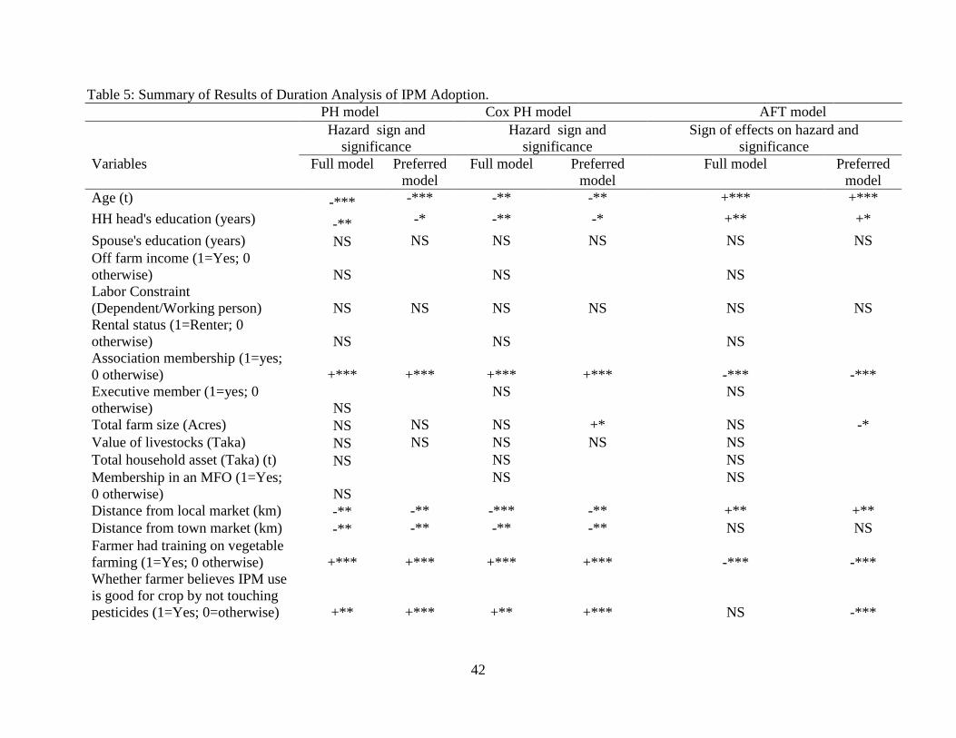
42

Table 5: Summary of Results of Duration Analysis of IPM Adoption.

PH model Cox PH model AFT model

Hazard sign and

significance

Hazard sign and

significance

Sign of effects on hazard and

significance

Variables Full model Preferred

model

Full model Preferred

model

Full model Preferred

model

Age (t) -*** -*** -** -** +*** +***

HH head's education (years) -** -* -** -* +** +*

Spouse's education (years) NS NS NS NS NS NS

Off farm income (1=Yes; 0

otherwise) NS

NS

NS

Labor Constraint

(Dependent/Working person) NS

NS

NS

NS

NS

NS

Rental status (1=Renter; 0

otherwise) NS

NS

NS

Association membership (1=yes;

0 otherwise) +***

+***

+***

+***

-***

-***

Executive member (1=yes; 0

otherwise) NS

NS NS

Total farm size (Acres) NS NS NS +* NS -*

Value of livestocks (Taka) NS NS NS NS NS

Total household asset (Taka) (t) NS NS NS

Membership in an MFO (1=Yes;

0 otherwise) NS

NS NS

Distance from local market (km) -** -** -*** -** +** +**

Distance from town market (km) -** -** -** -** NS NS

Farmer had training on vegetable

farming (1=Yes; 0 otherwise) +***

+***

+***

+***

-***

-***

Whether farmer believes IPM use

is good for crop by not touching

pesticides (1=Yes; 0=otherwise) +**

+***

+**

+***

NS

-***

43

Whether the farmer believes IPM

use is a healthy way of farming

(1=Yes; 0 otherwise) NS

NS

NS

Jessore dummy -*** -*** +** +** NS NS

Comilla dummy +* +** +* +* NS NS

Bogra dummy +** +** +** +** NS -*

Constant -*** -*** +*** +***

Dummy for Year=2003 +*** +***

Log-likelihood -221.68 -223.80 -758.80 -760.94 -221.65 -223.86

Restricted LL -289.36 -289.36 -287.14 -287.14

DF 22 15 21 14 21 14

χ2 135.37 309.13 10703 133.09 118.74 110.89

1% critical value 40.29 30.58 38.93 29.14 38.93 29.14

Note: + and – with asterisk indicate whether the relationships are positive or negative

***, **, and * indicate significance levels at 1%, 5%, and 10% levels, respectively;

NS denotes that the variables have been included in the model but are not significant.

Table 6: Summary Statistics for Testing the Null Hypothesis that the Coefficients of Omitted Variables are Jointly not

Different from Zero. Statistics Weibull Model Cox PH Model AFT Model

Log-likelihood -223.80 (-221.68)a -760.94 (-758.80) -223.86 (-221.65)

Number of restrictionsb 7 7 7

Calculated χ2 4.25 4.28 4.44

1% critical value 18.48 18.48 18.48

Decision: Null hypothesis not rejected not rejected not rejected a: Figures in parentheses indicate the log-likelihood for the model with all variables present. b: The number of restrictions equals the number of

variables omitted. The test statistic is defined as -2(l0 – l1), where L0 and L1 are the values of the log-likelihood functions for the restricted and

unrestricted models, respectively. The null hypothesis is not rejected at the indicated level if the calculated χ2 is less than the critical value of the χ2

.

Table 5 cont. Table 5 cont.

44

Farmer’s age has hazard ratios less than unity which are statistically significant at 5% level.

It means that a younger farmer is more likely to adopt IPM earlier than his older peer farmer. A

less than unity coefficient of the farmer’s education implies a negative impact on adoption. The

result may be unexpected, but it is not uncommon in the literature. Burton et al., (2003) find

further/higher education to have a negative, though marginally non-significant, impact on the

hazard. There may be other explanations for this finding. Figure 4 provides plots of the estimated

hazard function over time for different values of significant variables in the Weibull model. A

static regression might suggest that the higher education, the lower the likelihood of adoption at

any time. Similarly, a static model might suggest that the older the farmer, the less likely he is to

adopt IPM at any time. However, the plots of estimated hazard due to different levels of farmer’s

age and education suggest that though its impacts are negative, they are smaller as the level of

education increases and age increases. The effect of farmer’s education on hazard (risk) of failure

(adoption) is prominent after the 8th grade, after which the hazard becomes less over time. That is,

even though the the coefficient of education appears to affect IPM adoption negatively, it is the

less educated farmers who are more likely to adopt than their more educated peers.

None of the personal or economic characteristics of the farmer appear to significantly affect

the probability of ending the period of non-adoption. Instead, significant variables are those that

are related to information diffusion. In particular, being a member in a village association increases

the hazard compared to non-members. A hazard ratio of more than 2 of association membership

indicates that a member farmer is more than 100 percent more likely to adopt IPM at time t than a

non-member. The plot of the estimated hazard for membership status in Figure 4 indicates that the

gap widens as the exposure to IPM time increases. This implies the effect of membership differs

45

over time. As the exposure time passes, the association member farmer becomes more likely to

adopt. From the AFT model, a member farmer adopted 4% earlier than a non-member farmer.

The literature on agricultural technology adoption often recognizes the distance of the

farmer’s house from certain important places, such as local market or a bigger town market, as

important factors affecting adoption (Dadi et al., 2004). In particular, studies that evaluate impacts

of specific technologies include those distance variables as instruments in the two stage least

squares approach to remedy endogeneity issues. It is expected that distance has a negative impact

on the decision to adopt. Following the literature, two distance variables are included in the

analysis: distance to local market, and distance to a bigger town market. The evidence regarding

the importance of the distance variables in the adoption decision is reasonably strong, with the

relevant coefficients being negative (hazard <1) and statistically significant at 1% level in all three

models. This is also consistent with the expectation and findings in the literature (Dadi et al.,

2004). A one kilometer increase in distance from the local market, holding all other variables

constant, reduces the estimated hazard of IPM adoption to 72-74% of its starting value. That is,

the farther the farmer lives away from a center point such as a local market or a town market, the

more time it takes for him to adopt IPM. Signs of distance variables in the AFT model appear

positive, which indicates the farther the farmer lives from the local market or town market, the

more time she take to adopt. Considering the magnitude and significance of the coefficients in all

three models, local market has more influence on adoption than the town market. The plot of

hazard for distance variables in figure 4 show that the increase in hazard decreases as the distance

increases. However, a notable point from the figure is that the effects of first two miles from a

village market are stronger than farther distance as the change in increase in hazards are shown to

be less after those thresholds. From the AFT model, a farmer living a mile farther from the local

46

market increases his time to adopt, other variables held constant, by 16.2 percent on average.

Distance variables may be (positively) related to some cost issues (such as transportation costs),

but they also affect (negatively) the ability to gain information about a new innovation. Because

IPM is not a capital-intensive technique compared to traditional pest management practices,

increased transportation costs due to an increase in distance from a center point is not expected to

greatly influence IPM use negatively. As a result, it can be argued that the increased time to

adoption due to living farther from a center point is more closely related to obtaining information

about the innovation than increased transportation costs.

Training farmers about agricultural technologies is one of the activities of the DAE and

other agencies involved in agricultural extension services. Hence, a farmer’s participation in any

training program is expected to impact on the use of new and improved technologies positively.

Regardless of the model, the coefficient of a dummy variable indicating whether the farmer has

received any training on vegetable farming is found to be significant at the 1% level. The hazard

approximately doubles (increases by 98-109% (depending on the model)) if a farmer has any

training on vegetable farming compared to not having any, ceteris paribus. From the AFT model,

the farmer’s time to adopt IPM decreases by almost 39 percent compared to a farmer not having

any training. A Farmer’s perception about IPM use is found to significantly affect IPM adoption

choice. If a farmer believes that the use of IPM is good for the crop, as it requires fewer chemical

pesticides, he has a 2.56 times higher hazard rate than a farmer who does not believe so. The AFT

model reveals that a farmer believing that IPM use is good for the crop decreases the log of time

to failure (time to adopt) by 0.37. That is, positive beliefs about IPM decreases the waiting time to

IPM adoption by 37%. Moreover, the plots of the estimated hazard in figure 4 indicate that the

farmer with a training and a positive perception shows much higher likelihood of adoption as the

47

time passes than his peer farmer without a training on vegetable farming and having a negative

perception about the IPM. It can be claimed that providing information by training and educating

farmers about IPM might be an effective way to increase its adoption. Farmers in Bogra and

Comilla adopted earlier, on average, than those in Magura, while farmers in Jessore have mixed

results depending on the model. The estimate of the regional hazard rate is consistent with the

analysis based on the Kaplan-Meier survival curve mentioned before.

We have explained the coefficients of variables that have been found significant in all

models. Now we consider the variables that are significant in at least one of the models. Holding

all variables equal to zero for a hypothetical farmer, the constant in the AFT model is 1.38 which,

in turn, tells us that the hypothetical farmer’s time to adopt IPM increases by 138%. The two

hazard models (Weibull and Cox-PH) show that farmer living farther from the town decreases the

hazard by 4 percent. The AFT model shows that a farmer having an extra acre of farmland, which

is the only economic variable that is significant, decelerate the time to adopt IPM by 5 percent

approximately, which is also similar to result in the Cox PH model. That is, a bigger farmer in

terms of farm size appears to adopt earlier than a smaller farmer. There is a non-economic

implication of the farm-size variable. Even though this is directly related to an economic factor,

having a bigger size farm more likely indicates that the farmer has better connection with persons

related to farming and hence will obtain information about innovation from more and sometime

better sources. As a result, significance of the farm size enhances the importance of information

dissemination in explaining speed of adoption. It has been assumed for the above results that the

shape of the Weibull distribution is same for all covariates. To investigate whether suspicious

variables such as different locations, membership status, and training status show different shape

parameters, ancillary parameter, p, for each of those variables in the Weibull regression is

48

estimated. No substantial differences in estimated coefficients are found, both in terms of

magnitude, sign, and significance, from those mentioned in Table 7. Table 8 presents the estimated

ancillary parameters for each of the categories. It shows that even though the shape parameter, p,

is not exactly the same for each category of each variable, none of them changes the direction of

the effect of the variable on hazard.

The above results have been obtained assuming that the functional forms are correct and

individual farmers in the sample, after controlling observable differences through including

explanatory variables, are homogenous. However, heterogeneity may arise due to two reasons:

misspecification of the functional forms or the presence of unobserved differences among

individual farmers. Ignoring the heterogeneity, if present, may lead to incorrect inferences

regarding duration dependence and the effects of regressors (Kiefer, 1998). A frailty model can be

used to check the presence of such heterogeneity. A frailty model is a generalization of a survival

regression model in which, in addition to the observed regressors, a latent multiplicative effect on

the hazard function is allowed. The effect of the unobserved heterogeneity, or frailty, is not directly

estimated from data. Instead, the assumed mean and variance of the frailty, θ, with unity mean and

finite variance are estimated. If frailty is greater than unity for any specific heterogeneous group,

subjects in the group experience increased hazard (risk) of failure (adoption) and are said to be

more frail than their cohorts (Gutierrez, 2002).

Proportional hazard model has difficulty handling left truncated data. The hazard ratios, with

gamma or inverse Gaussian distributed frailty, decay over time in favor of the frailty effect. Thus,

the hazard ratio in the PH model is actually the hazard ratio only for t=0. The degree of decay

depends on θ. For this reason, many researchers prefer fitting frailty models in the AFT metric

because the interpretation of regression coefficients is unchanged by the frailty – the factors in

49

question serve to either accelerate or decelerate the survival experience (Gutierrez, 2002). As a

result, only the AFT model is employed for the estimation of the conditional probability with

heterogeneity removed. A gamma distribution of frailty has been used since in a large class of

survival models the distribution of heterogeneity among survivors converges to the gamma

distribution (Abbrign and Van Den Berg, 2007). Table 9 reports the AFT estimation with the

heterogeneity effect removed. The model in Table 9 does not perform worse compared to previous

models in terms of AIC, BIC and log-likelihood as they are very close. The null hypothesis that

there was no heterogeneity effect is failed to reject at any conventional level, implying the absence

of unobserved heterogeneity among individual farmers in the sample. Fortunately, there is no

change in the sign of the estimated coefficients from those reported in Table 7. The coefficients in

Table 7 are over-estimated for most variables.

50

Table 7: Estimation of Conditional Probability of IPM Adoption

PH Model (Weibull) Cox PH Model AFT Model

(Loglogistic)

Variables Haz. Ratio Std.

Err.

Haz.

Ratio

Std.

Err.

Coef. Std. Err.

Age 0.975*** 0.008 0.996** 0.002 0.015*** 0.004

HH head's education (years) 0.942* 0.030 0.950* 0.027 0.030* 0.016

Spouse's education (years) 0.960 0.026 0.965 0.024 0.018 0.014

Labor Constraint

(Dependent/Working

person)

0.933

0.054

0.936

0.050

0.035

0.029

Association membership

(1=yes; 0 otherwise)

2.271***

0.446

2.079***

0.369

-0.400***

0.101

Farm size (Acre) 1.065 0.050 1.066* 0.039 -0.048* 0.026

Value of livestocks (Taka) 1.000 0.000 1.000 0.000 -6.5E-07 0.000

Distance from local market

(km)

0.724** 0.100 0.739** 0.091 0.162** 0.070

Distance from town market

(km)

0.958** 0.019 0.963** 0.017 0.015 0.009

Farmer had training on

vegetable farming (1=Yes;

0 otherwise)

2.091***

0.357

1.987***

0.310

-0.391***

0.091

Farmer believes IPM use is

good for crops (1=Yes;

0=otherwise)

2.556***

0.581

2.523***

0.518

-0.369***

0.112

Jessore dummy 7.6E-

06***

0.000 1.716** 0.459 -0.086 0.149

Comilla dummy 1.764** 0.504 1.642* 0.431 -0.205 0.146

Bogra dummy 1.943** 0.561 1.873*** 0.483 -0.265* 0.145

Constant 0.022*** 0.014 1.384*** 0.271

Dummy for year = 2003 155928*** 168951

Ancillary p=2.22 0.153 γ =0.358 0.024

Log likelihood -223.8 -760.94 -223.86

AIC 481.6 1549.88 479.73

BIC 545.34 1602.37 539.72

Median time 6.56 years

N 314

Note: For the Cox PH model, Breslow method for ties has been used. Robust Standard errors have been reported.

***, **, and * indicate statistically significant at 1%, 5%, and 1% levels respectively.

51

Table 8: Estimation of the Ancillary Parameter, p, for the Weibull Model

Variables Coeff. Std. Err ln (𝑝)̂ �̂�

Association Membership Status2:

Association member -0.273 0.141 0.724 2.062

Not a member 0.997 0.128 0.997 2.711

Training status3:

Has training on vegetable

farming -0.457 0.134 1.921 3.034

Constant 1.11 0.114 1.11 3.034

Perception (Good for crops)4

Perceive good 0.318 0.147 0.883 2.420

Do not perceive good 0.566 0.128 0.566 1.761

Geographical location1:

Magura -0.695 0.203 0.791 2.206

Jessore -01.062 0.195 0.424 1.53

Comilla 1.487 0.169 1.487 4.422

Bogra -0.552 0.248 0.934 2.545

Note: ln (𝑝)̂ is the fitted ancillary parameter, p, regressing p on the corresponding dummy variables in the

table. �̂�=Exp( ln (𝑝)̂) that provides the hazard for the corresponding category. 1. While estimating the

ancillary parameters, Comilla has been used as the reference category. Therefore, constant is regarded as

the coefficient of Comilla and the corresponding other statistics. 2. Non-membership is the base category.

3. Those who did not have a training is the reference category. 4. Farmers not perceiving good about IPM is

the reference category.

52

Figure 4: Weibull Estimate of Hazard with Respect to Different Variables

0.1

.2

.3

.4

.5

Haza

rd fu

nctio

n

0 2 4 6 8Analysis time

age=18 age=20

age=25 age=30

age=40

Hazard at different age

0.1

.2

.3

.4

.5

Haza

rd fu

nctio

n0 2 4 6 8

Analysis time

edu=0 edu=5

edu=8 edu=10

edu=12 edu=15

Hazard at different level of education

53

0.1

.2.3

.4.5

Haza

rd fu

nctio

n


org_mem=1 org_mem=0

Hazard at membership status

0.1

.2

.3

.4

Haza

rd fu

nctio

n0 2 4 6 8

Analysis time

v_ba=0.5 v_ba=1

v_ba=1.5 v_ba=2

v_ba=3

Hazard at different distance from local market0

.1

.2

.3

.4

.5

Haza

rd fu

nctio

n


veg_tr=1 veg_tr=0

Hazard at training status

0.1

.2

.3

.4

.5

Haza

rd fu

nctio

n

0 2 4 6 8analysis time

Good for crop=1 Good for crop=0

Hazard at different perception about IPM

54

Table 9: Estimation Results for IPM Adoption: Heterogeneity Effect Removed

AFT Model (Log-logistic)

Variables Coef. Std. Err.

Age 0.013*** 0.003

HH head's education (years) 0.032** 0.013

Spouse's education (years) 0.009 0.013

Labor Constraint (Dependent/Working person) 0.019 0.028

Association membership (1=yes; 0 otherwise) -0.332*** 0.093

Farm size (Acre) -0.051*** 0.019

Value of livestocks (Taka) -5.7E-07 6.9E-07

Distance from local market (km) 0.157*** 0.056

Distance from town market (km) 0.009 0.009

Farmer had training on vegetable farming (1=Yes; 0

otherwise)

-0.344*** 0.083

Farmer believes IPM use is good for crops (1=Yes;

0=otherwise)

-0.334*** 0.093

Jessore dummy -0.215 0.295

Comilla dummy 0.476 0.381

Bogra dummy 0.359 0.365

Constant 1.027*** 0.343

γ (Ancillary parameter) 0.309 0.032

θ (heterogeneity capturing parameter) 0.505 0.472

Log likelihood -224.18

LR test for θ =0 χ2=0.000 p-val=1.00

Frailty Distribution Gamma

AIC 482.35

BIC 546.08

Note: θ is the estimated frailty effect to capture heterogeneity effect, if any. γ is the ancillary parameter for the log-

logistic distribution.

2.7 Conclusion

Despite the significant contribution of technology innovations to increased productivity,

reduced poverty, and improved standards of living, policy makers are still puzzled by the fact that

these technologies are often adopted in a slow and incomplete manner by farmers in many

developing countries. Numerous studies have focused on identifying the determinants of adoption

of new technologies, including technical, organizational, and environmental factors. However,

those studies use cross-section data to estimate probit-like models and these models fail to capture

55

the farmer’s time before adoption. As a result, the studies are inadequate in correctly describing

and explaining the dynamic process of technology adoption. In this paper, duration models are

used to capture the dynamic aspects of the IPM technology adoption process in Bangladesh. Using

survey data from Bangladesh, Cox PH, Weibull PH, and AFT models have been estimated. Both

parametric and semi-parametric models are applied to estimate the conditional probability of IPM

adoption, in which the full parametric models include the Weibull PH model and the log-logistic

AFT model, and the Cox PH model is the semi-parametric model.

The main conclusion of this study is that it is not the economic or personal characteristics of

the farmer that are important influences in the timing of the adoption decision but factors related

to information diffusion and perception about IPM use and unobserved heterogeneous behaviors,

such as attitudes toward risk and ambiguity.

Having a larger farm and being a member in any association in the village increases the

likelihood of early adoption. Distance to a center point such as a local market increases the time

to adoption. Distance variable may be (positively) related to some cost issues (such as

transportation costs), but they also affect (negatively) the ability to gain information about a new

innovation. Because IPM is not capital-intensive compared to traditional pest management

practices, increased transportation costs due to an increase in distance from a center point is not

expected to greatly influence IPM use negatively. As result, it can be argued that the increased

time to adoption due to living farther from a center point is more closely related to obtaining

information about the innovation than increased transportation costs. One of the primary services

offered by extension agencies (such as DAE, IPM club, or any NGOs) is to train farmers. Farmer’s

participation in a training session on vegetable farming decreases the time to adoption. If farmers

believe that IPM use is good for crops, due to the manner with which little or no pesticides are

56

used, this increases the likelihood of adoption. That is, those farmers who believe IPM is good for

crops adopt earlier than farmers who believe otherwise. Therefore, it can be claimed that providing

information by training and educating farmers about IPM is an effective way to increase its

adoption. If speedy adoption is desired, then policy should encourage more training about the new

innovation. This training will not only teach farmers about the technologies but also will affect the

subjective probability of the effectiveness of the innovation and thereby influence its use. More

effective dissemination should lead to a higher speed of adoption.

References

Abbring, J.H. and Van Den Berg, G.J. (2007), ‘The unobserved heterogeneity distribution in

duration analysis’, Biometrika, 94(1), 87-99.

Addison, J.T. and Portugal, P. (1998), ‘Some specification issues in unemployment duration

analysis’, Labor Economics, 5, 53-66.

Adesina, A. and Zinnah, M. (1993), ‘Technology characteristics, farmers’ perceptions and

adoption decisions: a Tobit model application in Sierra Leon’, Agricultural Economics, 9, 297-

311.

Akinola, A.A. (1987), ‘An application of Probit Analysis to the adoption of tractor hiring services

scheme in Nigeria’, Oxford Agrarian Studies, 16, 70-82.

Alcon, F., de Miguel, M.D. and Burton, M. (2011), ‘Duration analysis of adoption of drip irrigation

technology in southeastern Spain’, Technological Forecasting & Social Change, 78, 991-1001.

Allison, P. (1984), Event History Analysis, Regression for Longitudinal Event Data, Series:

Quantitative Applications in the Social Sciences (London, UK: SAGE University Paper, 1984).





No. 4, pp. 515-548.

57

Beus, E.B. and Dunlap, R.E. (1994), ‘Agricultural paradigms and the practice of agriculture’,

Rural Sociology, 59, 620-635.

Bhattacharya, S.K., Chaterjee, K., and Samuelson, L. (1986), ‘Sequential of research and the

adoption of innovations’, Oxford Economic Paper, 38, 219-243.

Bultena, G.L. and Hoiberg, E.O. (1983), ‘Factors affecting Farmers’ adoption of conservation

tillage’, Journal of Soil and Water Conservation, 4, 281-284.

Burton, M., Rigby, D. and Young, T. (2003), ‘Modelling the adoption of organic horticultural

technology in the UK using Duration Analysis’, The Australian Journal of Agricultural and

Resource Economics, 47(1), 29-54.

Cameron, A.C. and Trivedi, P.K. (2005), Microeconometrics: Methods and Applications,

Cambridge University Press, New York, U.S.A.

Carletto, C., de Janvry, A. and Sadoulet, E. (1999), ‘Sustainability in the diffusion of innovations:

smallholder nontraditional agro-exports in Guatemala’, Economic Development and Cultural

Change, 47, 345-369.

Carletto, C., Kirk, A., Winters, P.C. and Davis, B. (2010), ‘Globalization and Smallholders: The

Adoption, Diffusion, and Welfare Impact of Non-traditional Export Crops in Guatemala’, World

Development, 38, 814-827.

Cleves, M., Gutierrez, R., Gould, W. and Marchenko, Y. (2008), An Introduction to Survival

Analysis Using Stata, 2nd edn. (Texas, USA: Stata press).

Colman, D. (1994), ‘Ethics and externality: agricultural stewardship and other behaviour’, Journal

of Agricultural Economics, 45, 299-311.

Comer, S., Ekanem, E., Muhammed, S., Singh, S. and Tegegue, F. (1999), ‘Sustainable and

conventional farmers: a comparison of socio-economic characteristics, attitudes and beliefs’,

Journal of Sustainable Agriculture, 15, 29-45.

D’Emden, F.H., Llewellyn, R.S. and Burton, M.P. (2006), ‘Adoption of conservation tillage in

Australian cropping regions: An application of duration analysis’, Technological Forecasting &

Social Change, 73, 630-646.

Dadi, L., Burton, M. and Ozanne, A. (2004), ‘Duration Analysis of Technological Adoption in

Ethiopian Agriculture’, Journal of Agricultural Economics, 55(3), 613-631.

Davies, S. (1979), The Diffusion of Process Innovation, Cambridge University Press, Cambridge.

de Souza Filho, H.M. (1997), The Adoption of Sustainable Agricultural Technologies: A Case

Study in the State of Espirito Santo, Brazil, Ashgate Publishing, Aldershot, U.K.

58

D’emden, F.H., Llewellyn, R.S. and Burton, M.P. (2006), ‘Adoption of conservation tillage in

Australian cropping regions: An application of duration analysis’, Technological Forecasting &

Social Change, 73, 630-647.

Feder, G. (1980), ‘Farm size, risk aversion and the adoption of new technology under uncertainty’,

Oxford Economic Papers, 32, 263-283.

Feder, G., Just, R. and Zilberman, D. (1985), ‘Adoption of agricultural innovations in developing

countries: a survey’, Economic Development and Cultural Change, 33, 255-298.

Feder, G., and O’Mara, G.T. (1982), ‘On information and innovation diffusion: a Bayesian

approach’, American Journal of Agricultural Economics, 64, 145-147.

Feder, G., and Slade, R. (1984), ‘The acquisition of information and the adoption of new

technology’, American Journal of Agricultural Economics, 66, 312-320.

Feder, G., and Umali, D.L. (1993), ‘The adoption of agricultural innovations: a review’,

Technological Forecasting and Social Change, 43, 215-239.

Fernandez-Cornejo, J. (1997), ‘Environmental and Economic Consequences of Technology

Adoption: IPM in Viticulture’, Agricultural Economics, 18, 145-155.

Fischer, A.J., Arnold, A.J. and Gibbs, M. (1996), ‘Information and the speed of innovation

adoption’, American Journal of Agricultural Economics, 78, 1073-1081.

Foltz, J.D. (2003), ‘The economics of water-conserving technology adoption in Tunisia: an

empirical estimation of farmer technology choice’, Economic Development and Cultural Change,

51(2), 359-373.

Fuglie, K.O. and Kascak, C.A. (2001), ‘Adoption and diffusion of natural-resource-conserving

agricultural technology’, Review of Agricultural Economics, 23, 386-403.

Greene, W. Econometric Analysis, 6th edn. (New Jersey, USA: Prentice Hall, 2008).

Gutierrez, R.G. (2002), ‘Parametric frailty and shared frailty survival models’, The Stata Journal,

2(1), 22-44.

Hannan, T.H. and MacDowell, J.M. (1984), ‘The determinants of technology adoption: The case

of banking firm’, Rand Journal of Economics, 15, 328-335.

Hannan, T.H. and MacDowell, J.M. (1987), ‘Rival precedence and dynamics of technology

adoption: an empirical analysis’, Economica, 54, 155-171.

Hattam, C. and Holloway, G. (2007), ‘Bayes Estimate of Time to Organic Certification’,

Conference paper presented at the Agricultural Economics Society’s 81st Annual Conference,

University of Reading, UK.

59

Heckman, J.J. and Singer, B. (1984), ‘Econometric Duration Analysis’, Journal of Econometrics,

24, 63-132.

Jansen, H.G.P. (1992), ‘Inter-regional variation in the speed of modern cereal cultivars in India’,


Jenkins, S. Survival Analysis, Unpublished manuscript, (Clochester, UK: Institute for Social and

Economic Research, University of Essex, 2005. Available at:

https://www.iser.essex.ac.uk/files/teaching/stephenj/ec968/pdfs/ec968lnotesv6.pdf; last accessed

August, 19, 2014).

Jensen, R. (1982), ‘Adoption and diffusion of an innovation of uncertain profitability’, Journal of

Economic Theory, 27, 182-193.

Jensen, R. (1983), ‘Innovation, Adoption and Diffusion When There Are Competing Innovations’,

Journal of Economic Theory, 29, 161-171.

Kalbfleisch, J. and Prentice, R. The Statistical Analysis of Failure Time Data, 2nd edn. (New

Jersey, USA: Wiley-Interscience, 2002).

Kiefer, N.M. (1998), ‘Economic Duration Data and Hazard Functions’, Journal of Economic

Literature, 26, 646-679.

Knudson, M.K. (1991), ‘Incorporating technological change in diffusion model’, American


Lancaster, T. (1972), ‘A Stochastic Model for the Duration of a Strike,’ Journal of Royal Statistical

Society, Series A-135(2).

Lapple, D. (2010), ‘Adoption and Abandonment of Organic Farming: An Empirical Investigation

of the Irish Drystock Sector’, Journal of Agricultural Economics, 61(3), 697-714.

Levin, S.G., Levin, S.L. and Meisel, J.B. (1987), ‘A dynamic analysis of the adoption of a new

technology: the case of optical scanners’, Review of Economics and Statistics, 86, 12-17.

Lindner, R.K., Fischer, A. and Pardey, P. (1979), ‘The time to adoption’, Economics Letters, 2,

187-190.

Lindner, R.K. (1980), ‘Farm size and the time lag to adoption of a scale neutral innovation’,

mimeographed, University of Adelaide, Adelaide, Australia.

Mead, N. and Islam, T (2003), ‘Modelling the dependence between the times to international

adoption of two related technologies’, Technological Forecasting & Social Change, 70(8), 759-

778.

https://www.iser.essex.ac.uk/files/teaching/stephenj/ec968/pdfs/ec968lnotesv6.pdf

60

Mills, B. F. (2000), ‘Job Search, Employment Density, and the Rate of Exit of Unemployment in

Nonmetropolitan Labor Markets’, Southern Rural Sociology, 16: 148-174.

Mohr, L. 1982, Explaining Organizational Behavior, Jossey-Bass, San Francisco, USA.

Muambe, B.M. and Swinto, S.M. (2003), ‘Hidden costs of pesticide use in Zimbabwe’s

smallholder cotton growers’ Social Science & Medicine, 57, 1559-1571.

Nie, X. (2013), ‘Information Technology Adoption Based on Survival Analysis’, International

Journal of Digital Content Technology and its Applications (JDCTA) 7(6), 628-635.

Norton, G., Heinrichs, E.A., Luther, G.C. and Irwin, M.E. (2005) (Ed.), Globalizing Integrated

Pest Management: A Participatory Research Process, Blackwell Publishing, IA, U.S.A.

Nowak, P.J. (1987), ‘The adoption and conservation technologies: economic and diffusion

explanations’, Rural Sociology, 42, 208-220.

Padel, S. (2001), ‘Conversion to organic farming: A typical example of the diffusion of an

innovation’, Sociol. Ruralis, 4(1), 40-61.

Padel, S. and Lampkin, N.H. (1994a), ‘Conversion to organic farming: An overview’, Pp. 295-313

in N. Lampkin and S. Padel eds, The Economics of organic farming: An international perspective

(Wallingford: cab International)

Padel, S. and Lampkin, N.H. (1994b), ‘Farm-level performance of organic farming systems: An

overview’, Pp. 210-219 in N. Lampkin and S. Padel eds, The Economics of organic farming: An

international perspective (Wallingford: cab International)

Pannell, D.J., Marshall, G.R., Barr, N., Curtis, A., Vanclay, F. and Wilkinson, R. (2006),

‘Understanding and promoting adoption of conservation practices by rural landholders’,

Australian Journal of Experimental Economics, 46, 1407-1424.

Polson, R.A. and Spencer, S.C. (1991), ‘The technology adoption process in subsistence

agriculture: The case of cassava in southern Nigeria’, Agricultural Systems, 36, 65-78.

Qi, J., (2009), Comparison of Proportional Hazards and Accelerated Failure Time Models,

Master’s Thesis, Department of Mathematics and Statistics, University of Saskatchewan,

Saskatoon, Saskatchewan, Canada.




Razzaque, M. and Ahsanuzzaman (2009), Intrahousehold Resource Allocation and Women’s

Bargaining Power: New Evidence from Bangladesh’, Working paper:

http://papers.ssrn.com/sol3/papers.cfm?abstractid=1550559 Last accessed on November 5, 2014.

http://papers.ssrn.com/sol3/papers.cfm?abstractid=1550559

61

Ricker-Gilbert, J., Norton, G.W., Alwang, J., Miah, M. and Feder, G. (2008), ‘Cost-Effectiveness

of Alternative Integrated Pest Management Extension Methods: An Example from Bangladesh’,

Review of Agricultural Economics, 30, 252-269.

Rigby, D., Young, T. and Burton, M. (2001), ‘The development of and prospects for organic

farming in the UK’, Food Policy, 26, 599-613.

Rogers, E.M. (2003), Diffusion of Innovations, V ed New York.

Shields, M.L.G., Rauniyar, G.P. and j Goode, F.M. (1993), ‘A longitudinal analysis of factors

influencing increased technology adoption in Switzerland, 1985-1991’, The Journal of

Development Areas, 27, 469-483.

Sidibe’ (2005), ‘Farm-level adoption of soil and water conservation technique in Northern Burkina

Faso’, Agricultural Water Management, 71(3), 211-224.

Spanos, A. (2011), ‘Revisiting the Statistical Foundations of Panel Data Modeling’, Unpublished

manuscript, Department of Economics, Virginia Tech, Blacksburg, VA, USA.

Thirtle, C.G. and Ruttan, V.W. 1987, The Role of Demand and Supply in the Generation and

Diffusion of Technical Change, Harwood Academic Publishers GmbH, Chur, Switzerland.

Weir, S. and Knight, J. (2000), ‘Education externalities in rural Ethiopia: Evidence from average

and stochastic frontier production functions’, Oxford: Center for the study of African Economies,

mimeo.

Yaron, D.D. (1990), ‘Influence of quality and scarcity of inputs on the adoption of modern

irrigation technologies’, Western Journal of Agricultural Economics, 12(2), 224-233.

62

Chapter 3

Essay 2: Social Exchanges, Attitudes toward Uncertainty and Technology

Adoption by Bangladeshi Farmers: Experimental Evidence

3.1 Introduction

The literature on technology adoption demonstrates that individuals’ attitudes toward

uncertainty are an important factor in technology adoption decisions, including agricultural

technologies. Risk aversion is among the important factors determining technology adoption

(Srinivasan, 1972; Feder, 1980; Feder et al., 1985; Liu, 2013; Ward and Singh, 2014; Barham et.

al., 2013; Alpizar et. al., 2011). Another type of uncertainty that is less studied is ambiguity

aversion. Ambiguity aversion implies that an agent has a preference for a known risk over an

unknown risk. The literature also demonstrates the changes in attitudes toward uncertainty when

subjects are allowed to communicate among themselves before making choices over risky and

ambiguous prospects in the experiments (Alpizar et al., 2011; Engle et al., 2013). The outcome of

a new technology, whether good or bad, or the distribution of its outcome is unknown to the agent.

The benefits or the distribution of benefits of the status quo, the existing practices, may contain a

risk component but the risk is known to the agent from the past. Hence, adoption of a new

agricultural technology contains an unknown risk (ambiguity), thereby giving rise to the issue of

the role of ambiguity aversion in technology adoption. The current study measures the coefficients

of risk and ambiguity aversion of Bangladeshi farmers using data from a series of experiments. In

order to investigate whether attitudes change due to communications, subjects were allowed to

communicate in groups of 3 and 6 before making choices over uncertain prospects. Combining the

measured attributes from the experimental data with a survey data, the study estimates a discrete

63

choice model of technology adoption in order to investigate the effects of attitudes toward

uncertainty (risk aversion and ambiguity aversion) on technology adoption in different situations:

facing uncertainty alone, in groups of 3, and 6.

It is expected that an ambiguity-averse agent will not adopt a new technology as readily as

an ambiguity neutral agent. However, it remains unclear whether the attitudes toward risk and

ambiguity work in the indicated direction (Barham et al., 2013). Empirical questions regarding

risk and ambiguity have important policy implications. In the case of risk-aversion, policy makers

have focused to date on helping to improve ex-post risk coping mechanisms such as farmers’

access to formal credit and insurance markets. On the other hand, in the case of ambiguity aversion,

policy makers can help via ex-ante mechanisms to reduce farmers’ uncertainty or perceived

uncertainty through education, agricultural research, technical assistance or agricultural extension

services (Engle-Warnick et al., 2011). Therefore, because of the different policy prescriptions for

the two cases, it is important to know the relative importance of the two behavioral effects in order

to guide policies toward eliminating any negative effects of uncertainty on the rural poor. The

literature also discusses farmers’ capacity and willingness to coordinate in pursuit of lower

adoption costs. Sometimes, the behavior of others (mostly peers, neighbors, or people in the same

network in different dimensions) influences own decisions (Jackson, 2014) including technology

adoption decision for two reasons. First, agents (farmers) learn from observing decisions and

experiences of others or communicating with others in their network (Banerjee, 1992; Bandiera

and Rasul, 2006; Conley and Udry, 2010; Besley and Case, 1997; Engle et al. 2013; Jackson,

2014), namely social learning (Munshi, 2008). Second, because of economies of scope, the costs

and benefits of technology adoption are potentially a function of how many people adopt it

64

(Dybvig and Spatt, 1986). Therefore, it is important to examine whether communication among

farmers changes attitudes toward uncertainty and hence technology adoption.

Like most experiments measuring risk and ambiguity, this study is a version of the

Ellsberg’s two-color urn experiment. The study investigates two broad issues. First, it attempts to

measure the risk preferences of Bangladeshi farmers to test the degree to which they are risk and/or

ambiguity averse. By allowing communication among subjects in different size groups of 3 and 6

in the experiments, the paper also investigates whether farmers’ attitudes remain the same when

they face uncertainty alone versus in a group, as well as whether group size matters with respect

to attitudes toward uncertainty. The existence of coordination in social exchanges and its effect on

farmers’ attitudes (Bandiera and Rasul, 2006; Besley and Case, 1997; Engle et al. 2013) is

addressed in the latter part. The study also attempts to identify, through regression analysis,

whether demographic characteristics have any effects on attitudes toward uncertainty.

This study addresses a second issue - whether farmers’ measured attributes have any effect

on adoption of integrated pest management (IPM) practices in Bangladesh. The main focus,

however, is given on the effect of ambiguity aversion on technology choice. The study finds that

Bangladeshi farmers in the sample are generally risk and ambiguity averse. However, their risk

and ambiguity aversion as well as the distribution of the measured attributes (of both risk and

ambiguity aversion) differ when they face uncertain prospects alone versus when they are able to

communicate with other peer farmers before making decisions. Farmers exhibit preferences

toward the two extreme behaviors when faced with uncertainty in groups of 3 rather than when

they face it alone or in groups of 6. While considering the effects of demographic characteristics

on the attitudes, household size increases the likelihood of extreme risk aversion, but decreases

ambiguity aversion which is robust to different measures of risk aversion. The number of

65

dependents in the household increases ambiguity aversion, and being married reduces it. Second,

and perhaps more importantly, the study finds that the roles of risk and ambiguity aversion in

technology adoption depends on which measure of uncertainty is incorporated in the adoption

model. When risk and ambiguity preferences that were measured when subjects faced the

uncertainty alone are used in the adoption model, only risk aversion appeared to affect the

technology choice. Using those measured parameters when subjects faced uncertainty in groups

of 3, ambiguity aversion reduced technology adoption. The behavioral variables have no effects

on technology choice when those were measured from experiments when subjects faced

uncertainty in groups of 6.

The rest of the paper is organized as follows. Section 2 presents a review of the literature

measuring risk preferences in developing countries. Section 3 provides the context of the study

and the data. Section 4 discusses the experimental design, while 5 discusses the results. Section 6

presents conclusions and directions for further research.

3.2 Literature Review

Studies on technology adoption mostly center on a wide range of issues such as farm size

(Feder et al., 1985; Weil, 1970), land tenurial arrangements (Bardhan, 1979; Feder, 1980);

education (Foster and Rosenweig, 1996; Huffman, 2001; Foltz, 2003), social stature such as

membership in associations (Sidibe, 2005; Ben Yishay and Mobarak, 2014), information

constraints (Fischer and Lindner, 1980; Schutjer and Van der Veen, 1977; Burton et al., 2003;

Alcon et al., 2011), credit constraints (Weil, 1970; Lowdermilk, 1972; Lipton, 1976; Feder and

Umali, 1993), Social learning and social networks (Foster and Rosenweig, 1995; Conley and Udry,

2010; Bandiera and Rasul, 2006; Duflo et al., 2008), and risk (Srinivasan, 1972; Feder, 1980;

66

Feder et al., 1985; Liu, 2013; Ward and Singh, 2014). Feder et al., (1985) in their survey of

technology adoption literature mentioned risk aversion as one of the major factors hindering the

adoption of new technologies.

Sandmo (1971), Srinivasan (1972), and Feder (1980) are among the early studies taking risk

preferences into consideration in the analysis of technology choices in theoretical settings.

Excluding risk preferences in an empirical study potentially produces bias in the estimated effects

of other determinants. As a remedial measure of this bias, it has been challenge to measure the risk

preferences and incorporate that measured risk into the analysis of technology adoption.

Binswanger (1980, 1981) was among the first experimental researchers to measure risk aversion

of farmers in developing countries. Studies in the literature focusing on risk preferences differ in

methods for data collection and include analyses based on experimental lotteries as well as the

analysis of production decisions based on data collected from household surveys. Among studies

in experimental lotteries, some have been based on hypothetical lotteries (Hill, 2009; de Brauw

and Eozenou, 2014), some on real lotteries (Miayata, 2003; Wik et. al, 2004; Liu, 2013; Yesuf and

Bluffstone, 2009; Tanaka et al. 2010; Harrison et al. 2010), and some on the both (Binswanger,

1981; Holt and Lary, 2002; Mosley and Verschoor, 2005). Moreover, the conceptual framework

found in the literature on characterizing risk preferences varies from expected utility theory (EUT)

to prospect theory (PT).

There are variations in experimental designs in the studies in order to measure attitudes toward

uncertainty. The designs vary from lotteries holding outcome probabilities constant and varying

payouts (Binswanger, 1980, 1981; Miayata, 2003; Barr, 2003; Wik et al., 2004) to a multiple price

list (MPL) approach where probabilities vary holding payouts constant (Holt and Laury, 2002;

Eckel et al., 2002; Harrison et al., 2005; Harbaugh et al., 2002). In the MPL approach, participants

67

are shown certain lottery pairs at once (i.e., on a sheet or computer screen, similar to Table A1 in

the appendix, and are asked to mark their preferences (lottery A or lottery B) in each row.

Though less common, studies to investigate attitudes toward ambiguity have been conducted

using predominantly undergraduate student populations in developed countries. Experimental

studies of attitudes toward ambiguity in farming societies in developing countries have begun but

as of yet, few conclusions have been drawn. Among the few experimental studies of ambiguity

attitudes of farming societies are Henrich and McElreath (2002), Akay et al., (2012), Ward and

Singh (2014), and Engle-Warnick et al. (2011). Another strand of literature on measuring the

attitudes toward uncertainty includes the presence of social exchanges in the experiments. The idea

behind allowance of social exchanges among subjects is that agents coordinate among themselves

in real world before making any decision. By doing so, they attempt to reduce any ambiguity as

well as cost that is related to gathering information (Alpizar et al., 2011). Furthermore, social

learning occurs while communicating with other agents (Munshi, 2008) that plays an important

role in participatory development and contains the potential to build on and enhance social capital

(Labonne and Chase, 2011; Engle et al. 2013).

Using a framed field experiment, Alpizar et al. (2011) estimated the risk and ambiguity

preferences for coffee farmers in the Tarrazu region of Costa Rica. The region was heavily affected

by tropical storm Alma in early 2008. Since this type of storm is new to the region, they related it

to ambiguity and attempt to investigate the role of ambiguity aversion on the choice of adaptation

due to climate change, i.e., this type of storm. Furthermore, they allowed subjects to communicate

in some rounds to make the decision in order to explore the role of communication and

opportunities for cost reduction due to economies of scope arising from full coordination on the

decision to adapt or not to adapt to climate change. In an experimental study, Engle et al., (2013)

68

examined the effect of participating in a social exchange on risk and ambiguity preferences. They

conducted experiments in which participants made choices to reveal both their risk and ambiguity

preferences. The subjects then participated in a social exchange of information, an unstructured

online chat with other participants, and were again asked to make choices that reveal their risk and

ambiguity preferences. The social exchange that is a way of social learning provided the basis for

measuring the effects of social exchange on risk and ambiguity preferences. A separate group of

subjects, the control group, viewed but did not participate in a past chat before they made their

choices that revealed their risk and ambiguity preferences. They compared the latter two rounds

of the experiments to measure the effects of participation in a social exchange on subjects’ attitudes

toward uncertainty. A limitation to their study, however, is that the set-up of social exchange in

their experiments was online which is different from a face-to-face social exchange. This is more

important when we consider the decision-making and social learning of farming societies in

developing countries where virtual communication is not so common. Therefore, their study may

not be generalizable to different groups of subjects.

Regardless of the conceptual framework (EUT vs. PT) and experimental approach, most

studies found subjects in developing countries to be risk and ambiguity averse (Binswanger, 1980,

1981; Henrich and McElreath, 2002; Akay et al., 2011; Alpizar et al., 2011; Engle et al., 2013;

Ward and Singh, 2014 among others.). Even though the communication among subjects reduced

risk aversion (Engle et al. 2013), so far it has not reduced the ambiguity aversion (Alpizar et al.

2011; Engle et al. 2013). One reason for not improving the clarification about the ambiguous

situation may be the form of communication such as online in Engle et al. (2013) or the reliability

of the information provider in the period of communication. In that case, ambiguous situation may

be improved by providing better information. More importantly, the information should be

69

transferred by individuals who are well endowed with skills and reliable to the agents on the

receiving end.

The literature on attitudes toward uncertainty is not limited to measuring the risk aversion and

ambiguity aversion coefficients. Recent studies relate those measured behaviors to actual

behaviors of technology adoption empirically (Engle-Warnick et al. 2007; Ward and Singh, 2013;

Alpizar et al., 2011). The literature on the effects of estimated attitudes variables on technology

choices appeared to have mixed results. While considering the role of the opportunity for cost

reduction, Alpizar et a.l., (2011) found that the pursuit of cost reductions significantly increased

the degree of adaptation. When communication was allowed, farmers were able to coordinate more

frequently in pursuit of the reduced adaptation costs. However, when no financial motives were

allowed, communication was found to be irrelevant to the farmer’s private decision. Engle-

Warnick et al., (2007) found that it is not risk aversion that influenced the choice of diversity

among varieties of crops by Peruvian farmers but the ambiguity aversion that was influential.

Coupling measured coefficients of risk, loss, and ambiguity aversion with a discrete choice model

of technology adoption, Ward and Singh (2014) found that while ambiguity aversion was not

stronger influential to choose a new innovation, risk and loss aversion increased the likelihood of

switching to new, risk-reducing variety.

3.3 Context of the Experiment and the Data

Integrated pest management (IPM) is a way to combat pests while reducing the use of chemical

inputs. It is growing in importance globally, especially in more developed countries, as a way to

combat agricultural pests (Norton et al., 2005). With the support of the USAID-IPM Innovation

Lab (IL), a randomized controlled trial (RCT) was begun in summer 2013 in four districts (Jessore,

70

Magura, Barisal, and Jhalokathi) of Bangladesh in order to measure the impact of an agricultural

technology information dissemination strategy on IPM adoption. First, a baseline household

survey of 832 households was conducted. In order to elicit the farmers’ risk attitudes, we asked

300 farmers in Jessore and Magura districts to participate in a behavioral field experiment. Farmers

in Jessore and Magura were selected due to more availability of IPM practices in the region,

compared to the other two districts, which is important for the second part of the study. Because

those farmers were already in an RCT, it helped us to exploit socio-economic and pest-

management practices data collected in the survey for further analysis. They were reached by the

local extension workers and were given the option to participate or not. Of 300 farmers, 115

farmers in 15 villages in two districts: 48 farmers from 6 villages in Jessore and 67 farmers from

9 villages in Magura agreed to participate. 11 farmers were dropped after the experiment due to

not completing the sessions. Using this pool of subjects in the behavioral experiment provides an

additional opportunity to conduct a similar experiment with the same subjects in the following

season to examine the dynamics of a farmers’ attitudes toward uncertainty over time, and to

compare their behavior based on different theories: expected utility theory and prospect theory.

3.4 Eliciting Risk and Ambiguity Preferences: Experimental Design and Procedure

The literature on risk elicitation procedures tend to follow either the pioneering work of

Binswanger (1980) or that of Holt and Laury (2002). The differences between the two have been

discussed in the previous section. Our instrument, presented in table A2-A3 in appendix, is

different from the one employed by those authors. We follow the approach employed by Akay et

al. (2012), Capon (2009), and Ross et al.,(2012) by asking respondents to directly compare certain

amounts and lotteries. The design of the experiment is similar to a multiple price list (MPL),

71

following Barham et al., (2013) and Akay et al., (2012), which is a slightly modified version of

the original MPL of Holt and Laury (2002). This approach makes the subjects reveal certainty

equivalents (CE) for the lotteries. CE is the sure payment such that the subject is indifferent

between receiving the prospect or the sure amount. The elicited CEs can be used to compare risk

preferences across respondents as well as to measure the coefficients of relative risk aversion.

Furthermore, following Alpizar et al., (2011), Engle et al (2013), we conduct the same exercise

with subject groups of 3 as well as subject groups of 6 to investigate the behavioral pattern when

the subject is alone versus being with peer farmers.

The experiment is designed in a way that the participant’s certainty equivalents for both

the risky and ambiguous prospects are elicited. There are two uncertain prospects: a risky prospect

and an ambiguous prospect. The risky prospect allows the participant to bet on the color of a ball

drawn from a bag with 5 white and 5 yellow balls,10 a 50% chance to win the prize (see table A2).

The ambiguous prospect, on the other hand, allows participants to bet on the color of a ball drawn

from a bag containing 10 balls. The proportion of colors in the ambiguous bag is unknown, thus

each ball can be either white or yellow and hence the probability of winning is unknown to the

subject (see table A3). The participant can win Bangladeshi Taka (BDT) 400 by predicting the

color correctly11. A choice list is used to elicit each participant’s certainty equivalence for the

above-mentioned two prospects.

Participants were provided 21 choices between a certain payoff and the risky prospect

with the certain payoff increasing in 20 BDT increments from 0 BDT to 400 BDT. For small

10 This may be very simple game, but it is reasonable to get their behavior elicited provided that the farmer group has

little to no formal education. With sophisticated lotteries, it might be difficult for farmers to understand the situation

and hence to elicit their true attitude. 11 The daily wage for an unskilled labor in this region is BDT 250-400 depending on the season.

72

certain payments, it is expected that most participants would prefer to play the lottery. However,

when the certain payoff is large, it is expected that participants will opt to take the payment instead

of playing the lottery. Given this, participants’ risk preferences are revealed as they switch at some

point from playing a lottery to the sure thing. Following Eggert and Lokina (2007), and Akay et

al., (2012), the CE for each participant in each game has been calculated as the midpoint between

the lowest certain payoffs for which the participant chooses the sure thing and the highest certain

payment for which (s)he chooses to play lottery.

The literature on measuring risk aversion mostly assumes a constant relative risk aversion

(CRRA) utility function for the agents, 𝑢(𝑥) = 𝑥1−𝛾 where 𝛾 is the coefficient of the relative

risk aversion. The ambiguity aversion can be estimated using the elicited certainty equivalent for

both the risk and ambiguous situations (Akay et al., 2012).

𝐴𝑚𝑏𝑖𝑔𝑢𝑖𝑡𝑦 𝑎𝑣𝑒𝑟𝑠𝑖𝑜𝑛 (𝜃) =𝐶𝐸𝑅−𝐶𝐸𝐴

𝐶𝐸𝑅+𝐶𝐸𝐴 (1)

where CER = Certainty equivalent amount of money for the risky prospect, and CEA = Certainty

equivalent amount of money for the ambiguous prospect. This measure ranges from -1 (ambiguity

loving) to 0 (ambiguity neutrality) to 1 (ambiguity averse). Similar to Engle et al., (2013), our

experimental design provides the scope for measuring the ambiguity aversion based on switchover

points of both risky and ambiguous lotteries. The relative location of the switch-over point in the

ambiguity instrument compared with the switch-over point in the risk instrument reveals the

subject’s ambiguity preferences.

In our study, we make sure that the participants do not communicate with other

participants about their choices to be made. After the first round of each risk and ambiguity

experiment is finished, we let participants form groups of 3 people and ask them to consider their

group members as neighbors, friends etc. if they are not already. We then conduct the same

73

experiments again, but this time participants are allowed to discuss with group members their

decisions of whether to take the sure pay out or bet on the draw for each of 21 choices. We also

tell them that even though they discuss the choices with their group members, each of the

participants in the same group can make their own choices separately where the choices of each

participant in the group may be same as or different from the choices of the other participants. In

fact, we encourage each person to make their own decision after discussion. This approach is

similar to the approach of Alpizar et al., (2013) and Engle et al., (2013). It helps us investigate if

there is any effect of communication with neighbors or peer farmers on attitudes toward risk and

ambiguity. Finally, we let them form groups of 6 members and conduct the same experiments we

did in the second round. This new round allows us to investigate the effect of group size in

assessing risky and ambiguous situations. Therefore, each farmer faces 126 choices in a total of

three rounds. At the end, we randomly choose 20 farmers for payment. For each chosen farmer,

we pick a round randomly for payment. If anyone of those farmers selected chose the sure payout

in the selected round, we gave him/her that amount. Otherwise, he received the amount based on

the result of the bet. In this way, we provided a monetary incentive to participants to elicit their

attitudes toward uncertain situations.

3.5 Data Description

Table 1 provides the descriptive statistics of the participants in the experiments. The average

participant is 40 years old with 5 years of own and spouse’s education, and with 2.30 self-assessed

health condition (medium health) in a scale of 1-5 (1 being very good, 5 being very bad). Twenty

nine percent of participants do not have any formal education, with another 65% having 1-10 years.

Eighty nine percent of subjects are married with an average household size of 5.28, and own 2.38

74

Table 1: Descriptive Statistics of the Participants

Variable Mean St. Dev Min Max

Age 39.7 11.84 18 75

Health Status 2.30 1.01 1 5

Occupation (1= Agriculture, 0=Other) 0.83 0.38 0 1

Education (Years of schooling)

1-5 Years

6-8 Years

9-10 Years

11-12 Years

>12 Years

4.78

0.28

0.18

0.19

0.03

0.03

4.83

0.45

0.39

0.40

0.17

0.17

0

15

Spouse’s Education (Years of schooling)

1-5 Years

6-8 Years

9-10 Years

11-12 Years

>12 Years

4.69

0.22

0.24

0.20

0.02

0

4.69

0.42

0.43

0.40

0.13

0

12

Family Size

Male

Female

5.28

2.82

2.45

1.99

1.22

1.30

1

1

0

10

6

6

Marital status 0.89 0.31 0 1

Food affordable for consumption from household

income (Months)

10.66 2.53 0 12

Electricity (1=If connected, 0 otherwise) 0.59 0.49 0 1

Membership of any Micro-finance institution

(1=member, 0 otherwise

0.375 0.49 0 1

Land owned for farming (acres) 2.38 3.17 0 18.40

Membership in any village organization (1=member, 0

otherwise)

0.23 0.42 0 1

IPM user (1=uses any of IPM practices; 0 otherwise) 0.423 0.496 0 1

Extension Agent’s visit (1=Yes, at least once, 0

otherwise)

0.846 0.363 0 1

Sample size 104

acres of land for farming. Participants were asked how many months in a year they usually have

food sufficient for their consumption. On average, participants lacked food for more than a month

and less than two months per year. Fifty nine percent of participants have electricity in their houses.

38 percent are members of a micro-credit organization such as BRAC, Grameen, etc., and 23

percent are members of a village association such as a bazaar committee, school committee etc.

An extension agent visited at least once in the last cropping season for 85 percent of the

75

participants. Forty two percent of the subjects use at least one IPM practice in their pest-

management.

3.6 Results

3.6.1 Eliciting Risk and Ambiguity Preferences

3.6.1.1 Risk Preferences

Table 2 (upper part) presents the summary statistics of the measured coefficients of constant

relative risk aversion (CRRA) in all three circumstances. In all cases, the table shows that the

farmers, on average, are risk averse. The risk preferences, however, change with the presence and

absence of communication with other farmers and with the size of the group. When making choices

alone, farmers are, on average, more risk averse (mean 𝛾=0.59) than when they repeat the same

exercise after discussions with two other peer farmers (mean 𝛾=0.31). Farmers’ risk aversion,

however, is at its highest when he has five other peer farmers with whom to discuss their choices

(mean 𝛾=0.67). The average degree of risk aversion is similar to that reported in Tanaka et al.

(2010) and Liu (2013) when farmers face uncertainty alone. The median risk aversion coefficient

of 1.05 also shows that farmers are highly risk averse, and this degree of risk aversion is much

higher than the median of Ethiopian farmers (0.73) in Akay et. al., (2012). Figure 1 plots the kernel

density estimates of the relative risk aversion coefficient, 𝛾. It shows that the distribution of the

coefficient of risk aversion is roughly bimodal: one with a density corresponding to low risk

aversion, 𝛾, (or more risk loving) segment, and another density corresponding to the high risk

aversion segment. While subjects in a group of 3 have lower risk aversion, as mentioned before, it

is also evident from figure 1 that in the same situation farmers may also be less prone to make

extreme choices as the modal points lie below those of two other cases. In this situation (group of

76

3), farmers are more prone to be risk neutral as the distribution line lies above the other two cases

at X=0. Farmers in groups of six tend to show more risk aversion than when deciding alone or in

groups of three. However, they are also more risk loving, on average, than when

Table 2: Summary Statistics of the Estimated Risk and Ambiguity Aversion Coefficients

Coefficient* Median Mean St. dev. Min Max

Risk

Risk Aversion (1) 1.05 0.592 1.26 -1.99 1.66

Risk Aversion (3) 1.05 0.319 1.39 -1.99 1.66

Risk Aversion (6) 1.05 0.67 1.29 -1.99 1.66

Ambiguity

Ambiguity Aversion (1) 0.013 0.187 0.457 -0.95 0.95

Ambiguity Aversion (3) 0 0.131 0.436 -0.95 0.95

Ambiguity Aversion (6) 0 0.168 0.406 -0.95 0.95

* Numbers in parentheses indicate the number people in the group, including the

participant.

deciding in groups of three. The figure indicates that farmers tend toward extreme decisions more

when they face uncertainty either alone or when communicating with a larger group. Moreover,

their attitudes tend less toward extreme choices when they communicate in a group of three.

Figure 1 suggests that there are differences in attitudes (how they view or feel about risk)

when faced with uncertainty in groups of different sizes (alone, 3, or 6). There may be some

factors, such as how the characteristics of each farmer in a group are different, that

increase/decrease the probability that some groups will fall into an extremely risk averse sub-

group. Studying this phenomenon is, however, beyond of the scope of this paper and may be an

avenue for future research. Table 3 presents the results of the distribution of estimated risk aversion

coefficients and compares them with those in the literature. The table shows that Bangladeshi

farmers are mostly risk averse in all situations: whether they face the uncertainty alone or in a

group of different sizes. Compared to other findings in the literature, risk preferences of

Bangladeshi farmers are similar, when facing the uncertainty in a group of 3, to those of Ethiopian

77

farmers. Bangladeshi farmers are, however, more highly risk averse than Ethiopian farmers when

decided alone and in groups of 6, though when considering risk aversion in general (mildly risk

averse, risk averse, and highly risk averse), both pool of subjects exhibit similar pattern of risk

preferences: they are mostly risk averse. Bangladeshi farmers, like Ethiopian farmers in Akay et

al., (2012), are more highly risk averse than students in Dutch and U.S. universities. Since we have

used the same experiment in three separate situations, we now pose the question of whether

farmers’ attitudes toward risk are the same, on average, when they face scenarios alone versus in

groups of different sizes. We conduct a t-test of equality of means of the estimated parameters of

CRRA in all scenarios that are presented in table 4 (upper panel). Table 4 indicates that farmers’

CRRA coefficients, on average, are statistically different when they decide alone versus in groups

of three and decide in groups of three versus in groups of six farmers. The means, however, are

not statistically different when they decide alone versus in a group of six farmers. It implies that,

as shown in figure 1, mean risk aversion when deciding in groups of 3 is different from other two

scenarios.

3.6.1.2 Ambiguity Preferences

There exists a vast stream of ambiguity aversion literature testing Ellsberg’s (1961) thought

experiment, mostly in laboratory settings in developed countries (such as Becker and Brownson,

1964; MacCrimmon and Larsson, 1979; Bowen and Zi-lei, 1994) . However, studies on field

experiments measuring ambiguity preferences in developing countries is not so common (Engle-

Warnick et al., 2007; Alpizar et al., 2011, Akay et al., 2012; Ross et al., 2012 are among recent

studies). The reasoning behind Ellsberg paradox is that if a subject prefers, at any given prize, an

uncertain amount over a certain amount when the probability is known, the subject is also expected

78

to prefer the uncertain amount over a certain amount over the same given prize when probability

is unknown. This implies that the agent prefers known uncertainty (risk) over unknown uncertainty

(ambiguity).

Figure 1: Empirical Distribution of Estimated Risk Aversion Coefficients

Regarding the design of the experiment, since the sequence of the certain prospects are the same

in both the cases where probabilities are known and unknown, we merely compare the certainty

equivalent amount of money between two games to elicit each subject’s ambiguity preference.

Table 2 (lower panel) reports the summary statistics of the measured ambiguity preference

parameter, 𝜃. It shows that farmers, on average, are ambiguity neutral or averse, as their means lie

in between 0.1 and 0.2, and medians are greater than or equal to 0. While testing the equality of

means of different measures of ambiguity preferences, farmers on average do not show statistically

different ambiguity attitudes in different circumstances (Table 4, lower panel). Table 5 provides

the summary statistics of ambiguity preferences from certainty equivalence. It shows that farmers

tend to be more ambiguity averse when facing the ambiguous situation alone than in groups. As

0.2

.4.6

.8

-2 -1 0 1 2x

Deciding alone

Communicating with 2 other farmers

Communicating with 5 other farmers

79

Table 3: Distribution of Constant Relative Risk Aversion Parameters of Bangladeshi

Farmers Versus Other Estimates in the Literature

Risk

neutral/loving

Mildly risk

averse

Risk averse Highly

risk averse

𝛾 ≤ 0.15 (%)

0.15 ≤ 𝛾 ≤0.41 (%)

0.41 ≤ 𝛾 ≤0.68 (%)

𝛾 > 0.68 (%)

Dutch students (n=79)a 19 35 44 1

U.S. students (n=93)b 19 19 23 39

Bangladeshi farmers (n=104 )* 19 11 1 69

Bangladeshi farmers (n=104) ¥ 28 11 1 60

Bangladeshi farmers (n=104)† 21 4 1 74

Ethiopian farmers (n=92)c 22 11 10 58 * When each farmer decided alone

¥ when farmers decided in a group of 3 members

†when farmers decided in a group of 6 members

a Trautmann et al. (2011)

b Holt and Laury (2002, p. 1649, Table 3, last column). Identical tasks in Ethiopia and the Netherlands. A slightly

different task has been used for U.S. student by Holt and Laury, with all choice options involving only non-

degenerated gambles

c Akay et. al., (2012)

Table 4: t-Test for the Equality of the Means of the Estimated Coefficients of Risk

(Ambiguity) Aversion

Equality t-test (p-values)

CRRA Parameters

Risk Aversion (1)=Risk Aversion (3) 2.143 (0.034)

Risk Aversion (1) = Risk Aversion (6) -0.529 (0.598)

Risk Aversion (3) = Risk Aversion (6) -2.78 (0.007)

Ambiguity Preference Parameters

Ambiguity Aversion (1) = Ambiguity Aversion (3) 1.058 (0.293)

Ambiguity Aversion (1) = Ambiguity Aversion (6) 0.340 (0.735)

Ambiguity Aversion (3) = Ambiguity Aversion (6) -0.633 (0.528)

Table 5: Summary of Ambiguity Preferences from Certainty Equivalence

Deciding alone (%) Group of 3 (%) Group of 6 (%)

Ambiguity aversea 52 40 41

Ambiguity neutralb 27 46 41

Ambiguity lovingc 21 14 18

a: 𝜃 >0 ; b: 𝜃=0; c: 𝜃<0

they join in a group to face an ambiguous situation, they tend to be less ambiguity averse and more

ambiguity neutral. Figure 2 provides visual support for Table 5.

80

Figure 2 exhibits the empirical distribution of the estimated parameters for ambiguity aversion

in all three scenarios. It shows that farmers’ responses to ambiguous situations tend to be bimodal,

dominated by the ambiguity neutrality if farmers face the situation alone. Their attitudes, on the

other hand, tend to be multimodal dominated by the ambiguity neutrality when they made choices

in groups of 3. When farmers face the ambiguous situations in groups (of 3, or 6) they tend to react

in line with the similar uncertain situation when probability was known to them. This may provide

a policy implication that ambiguous situations may not be completely inflexible if farmers have

any source of information such as peer farmers who can provide them with better information to

reduce the ambiguity. This information can be attained by providing more and better training to

farmers so that farmers are more aware of the new technology and therefore become more likely

to adopt. Table 6 presents the estimated ambiguity aversion coefficients for Bangladeshi farmers

and those in the literature where similar procedures have been used. The table shows that

Bangladeshi farmers generally are ambiguity neutral or ambiguity averse. Bangladeshi farmers are

more ambiguity neutral and less ambiguity averse, in all three scenarios, than Dutch students and

Ethiopian farmers. A common feature among all three studies is that elicitation method is the same:

certainty equivalence with gains and existence of real incentives to earn money. As we did for the

estimated risk aversion parameters, the second part of table 4 provides a t-test of the equality for

the means of the estimated ambiguity preference parameters in different groups. It shows that

statistically there are no differences in the means of the estimated ambiguity preference parameters

in all groups: farmers face uncertainty alone, in group of three, and group of six farmers.

81

Figure 2: Empirical Distribution of Estimated Ambiguity Aversion Coefficients

Table 6: Distribution of Ambiguity Aversion Parameters of Bangladeshi Farmers Versus

Other Estimates in Literature

Ambiguity

seeking

(%)

Ambiguity

neutral (%)

Ambiguity

averse (%)

Elicitation Method

𝜃 < −0.4 (%)

−0.4 ≤ 𝜃 ≤0.3 (%)

𝜃 > 0.3 (%)

Dutch students (n=79)a 15 43 42 CE, gains, real

incentives

British students (n=72)b 39 n.a. 61 Choice, gains,

hypothetical

Business owners (n=130)c 56 n.a. 44 Choice, losses,

hypothetical

Dutch students (n=39)d 3 46 51 WTP, gains,

hypothetical

Bangladeshi farmers

(n=104 )*

8 63 29 CE, gains, real

incentives

Bangladeshi farmers

(n=104)**


incentives

Bangladeshi farmers

(n=104)†


incentives

Ethiopian farmers (n=92)e 20 24 57 CE, gains, real

incentives * When each farmer decided alone

** when farmers decided in a group of 3 members

† when farmers decided in a group of 6 members

a Trautmann et al. (2011)

b Roca et al., (2006)

c Chesson and Viscusi (2003)

d Kreen and Gerritsen (1999)

e Akay et. al., (2012)

01

23

-1 -.5 0 .5 1x

When deciding alone

Group of 3

Group of 6

Empirical distribution of ambiguity aversion parameter

82

Table 7: Correlation Between Risk and Ambiguity Measures

Risk (1) Risk (3) Risk (6) Ambiguity(1) Ambiguity (3) Ambiguity (6)

Risk (1)

1

Risk (3) 0.525

(0.000)

1

Risk (6) 0.302

(0.02)

0.544

(0.000)

1

Ambiguity (1) 0.375

(0.000)

0.010

(0.918)

-0.008

(0.936)

1

Ambiguity (3) 0.052

(0.603) 0.377

(0.000)

-0.003

(0.978) 0.258

(0.08)

1

Ambiguity (6) 0.034

(0.729)

0.055

(0.580) 0.363

(0.000)

0.097

(0.315)

-0.006

(0.951)

1

Note: Numbers in parentheses are p-values.

Finding different CRRA parameters and ambiguity preference parameters for different

experimental set ups raises an issue of whether the way uncertainty is faced, and hence risk and

ambiguity preferences are measured, matters for how we classify respondents’ behavior. We

estimate the correlation between different CRRA parameters and ambiguity parameters using

Spearman correlation coefficients. Table 7 provides the results where the first line in each cell is

the correlation coefficient and the numbers in parentheses are p-values. It shows that the

correlations across different scenarios are positive and high. More importantly, they are also

statistically significant. The correlation between risk aversion and ambiguity aversion parameters

is also positive, high, and statistically significant, corresponding to each of the categories: risk and

ambiguity when facing alone, in a group of three, and in a group of six. The correlations between

risk parameters and ambiguity parameters, in corresponding groups, are higher (lowest is 0.36)

than those in Ross et al., (2012) (highest is 0.21).

83

3.6.2 Demographic Characteristics and Attitudes toward Uncertainty

One of the primary goals of this paper is to determine the factors affecting attitudes toward

risk and ambiguity, and the effects of those risk and ambiguity aversion coefficients on adoption

of IPM practices by Bangladeshi farmers. For the first question, we estimate the following simple

linear regression

𝑈𝑖 = 𝛼 + 𝑋𝛽 + 휀𝑖 (2)

where 𝑈𝑖 is farmer i’s attitudes toward uncertainty, both in risky and ambiguous situations, X is

the set of the farmer’s characteristics including age, household size etc., and 휀𝑖 is an idiosyncratic

error term. Eq. (2) will be used to determine factors affecting attitudes toward uncertainty for both

risky and ambiguous situations.

We have used the socio-economic data collected as part of a field experiment to investigate

if the subjects’ socio-economic characteristics have any effects on their attitudes toward

uncertainty. The socio-economic variables include personal information and family background

such as age, education, marital status, whether the farmer’s occupation is agriculture or not,

household size, number of dependent persons in the household, total land owned for farming, and

geographical location. Respondents during the baseline survey of the field experiment were asked

about the food sufficiency for consumption given their income. In other words, they were asked

how many months in a year, recalling last two years’ experiences, they could feed their family

with their income. The respondents in the experiment were asked to rate their health status from 1

to 5 where 1 implies the very good health and 5 implies very poor health condition.

Following Akay et al. (2012), we avoid the dependence on the expected utility assumptions

for risk attitudes by using the pure certainty equivalence multiplied by – 1 as an index of risk

84

Table 8: Regression Analysis for Factors Affecting Risk and Ambiguity Aversion of

Bangladeshi Farmers When Facing the Uncertainty Alone.

Explanatory variables Risk aversion

(Tobit)*

Extreme risk

aversion

(Probit)*

Ambiguity

aversion (OLS)*

Age -1.017 (0.568) 0.005 (0.316) .003 (0.497)

Education (years) 2.7 (0.553) -.018 (0.130) .013 (0.228)

Occupation (1=Agriculture, 0 otherwise) 19.04 (0.705) -.222 (0.116) -.25 (0.052)

Health status -4.66 (0.800) -.043 (0.387) .043 (0.301)

Household size -1.33 (0.955) .128 (0.034) -.113 (0.041)

Number of dependent in the household -18.10(0.502) -.087 (0.214) .114 (0.071)

Food sufficiency (months) 12.33 (0.098) .011 (0.566) -.026 (0.161)

Total farm land owned -0.014 (0.830) 5e-04 (0.766) -1.13e-4(0.300)

Jessore (1=Jessore; 0=Magura) -74.13 (0.054) -.127 (0.211) .065 (0.518)

Marital status (1=Married; 0 Otherwise) 36.44 (609) -0.033 (0.867) -0.059 (0.769)

Constant -245.70 (0.098) .61 (0.106)

Number of observations 104 104 104

* Numbers in parentheses are p-values. Robust standard errors for OLS have been used.

aversion.12 Since a sizable fraction of participants (35 out of 104) revealed the two extremes,

highest possible and lowest possible, certainty equivalence, we control for censoring of our

measures. Thus we use a Tobit model for our analysis of risk attitudes. We also include a Probit

regression with a dummy variable that assumes the value of 1 if the certainty equivalence is

censored at 1, and 0 otherwise to test whether socio-economic variables can explain the presence

of extreme risk attitudes. Because there is no censoring for ambiguity attitude, we simply use OLS

for explaining ambiguity attitude and estimate the equation (2). Explanatory variables are the same

for all cases. The only difference is that the dependent variable is censored for tobit regression,

dichotomous for the probit regression, and continuous for the OLS regression. Table 8 presents

the regression results for measured attributes when farmers face uncertainty alone. The results of

the similar analysis for risk and ambiguity aversion when farmers face uncertainty in groups of

different sizes, 3 and 6, are presented in tables 9 and 10, respectively. A positive parameter implies

12 The higher the certainty equivalent, the lower the risk aversion.

85

increasing risk or ambiguity aversion, or increasing likelihood to reveal extreme level of risk

aversion respectively. For the probit model, marginal effects are reported.

The regression results suggest that when facing uncertainty alone, having more months of

sufficient food for family increases risk aversion which is not robust to all measures of risk

aversion (Tables 9 and 10). It may be difficult to explain this result as it differs from the general

perception that wealthier individuals are more risk prone (Henrich and McElreath, 2002) and

having more food sufficiency implies higher income. Since we do not have the total income/wealth

data for the household, we cannot generalize the effect of food sufficiency (month) on risk

aversion. We find that household size increases likelihood of extreme risk aversion, but decreases

ambiguity aversion which is robust to different measures of risk aversion (Tables 9 and 10). While

Table 9: Regression analysis of Factors Affecting Risk and Ambiguity Aversion of

Bangladeshi Farmers When Facing Uncertainty in a Group of 3

Risk aversion

(Tobit)

Extreme risk aversion

(Probit)

Ambiguity

aversion (OLS)

Explanatory variables Coef.

p-

value

Marginal

effect

p-

value Coeff.

p-

value

Age 0.560 0.787 0.000 0.961

4.8E-

04 0.904

Education -2.877 0.582 -0.002 0.879 -0.001 0.903

Occupation (1=if agriculture; 0

Otherwise) -6.508 0.912 -0.116 0.401 -0.141 0.321

Health status 34.022 0.121 0.067 0.192 0.024 0.619

Household size 15.762 0.565 0.116 0.066 -0.109 0.047

Number of dependent in the

household -26.438 0.411 -0.120 0.105 0.104 0.108

Food sufficiency (month) 15.219 0.080 0.015 0.477 -0.011 0.477

Farm land owned (decimals) 0.053 0.486 0.000 0.884 0.000 0.552

Marital status (1=Married; 0

Otherwise)

126.09

8 0.127 0.231 0.203 -0.111 0.435

Jessore (1=Jessore; 0=Magura) -37.550 0.396 -0.048 0.646 0.137 0.149

Constant -509.59 0.004 0.545 0.160

86

Table 10: Regression Analysis of Factors Affecting Risk and Ambiguity Aversion of

Bangladeshi Farmers When Facing Uncertainty in a Group of 6

Risk aversion

(Tobit)

Extreme risk aversion

(Probit)

Ambiguity

aversion (OLS)

Explanatory variables Coef.

p-

value

Marginal

effect

p-

value Coeff.

p-

value

Age 0.840 0.646 -0.010 0.047 -0.004 0.301

Education -3.698 0.423 -0.010 0.413 0.004 0.651

Occupation (1=if agriculture; 0

Otherwise) 90.125 0.083 -0.022 0.868 0.030 0.757

Health status 13.415 0.475 -0.005 0.922 0.069 0.081

Household size -25.258 0.274 -0.005 0.926 -0.112 0.006

Number of dependent in the

household 36.012 0.184 -0.002 0.981 0.102 0.029

Food sufficiency (month) 7.318 0.338 -0.007 0.728 0.002 0.918

Farm land owned (decimals) 0.046 0.525 0.001 0.011

8.4E-

05 0.714

Marital status (1=Married; 0

Otherwise) -17.235 0.817 0.150 0.363 0.113 0.470

Jessore (1=Jessore; 0=Magura) -15.926 0.683 -0.024 0.813 0.007 0.931

Constant -

418.965 0.007 0.195 0.520

the number of dependents in the household increases the ambiguity aversion, being married

reduces it. When farmers in groups of six are allowed to exchange information among themselves,

having agriculture as the only occupation increases risk aversion, poor health increases ambiguity

aversion.

3.6.3 Explaining Adoption Decisions

The second of the two broad issues of this paper is to investigate whether there is a separate role

for behavioral preferences and, in particular, ambiguity preferences in explaining the adoption of

innovations, IPM. We use a probit model to explain the role of attitudes toward uncertainty on

87

IPM adoption13. The traditional adoption equation is used to identify factors that affect different

types of agricultural technologies. The following equation represents the adoption behavior

𝐷𝑖 = 𝛿 + 𝑍𝛾 + 𝑈𝜆 + 휀𝑖 (3)

where D is an indicator variable (1 if adopts certain technology, say IPM, 0 if not), Z is the set of

all other regressors including demographic variables, and U is the vector of attitudes toward

uncertainty (risk and ambiguity parameters). The focus of eq. (3) is the coefficient of U, 𝜆. If all

or some of the vector 𝜆 is statistically significant, risk and/or ambiguity aversion affect agricultural

technology practices.

Since we have used a subset of a bigger random survey data, we do not have full

information about the adoption rate and other variables in the whole survey. Therefore, in this part

we focus solely on the two variables: risk aversion and ambiguity aversion coefficients. Besides

these two, the explanatory variables include several other correlates of adoption identified in the

literature14 for which we have information collected through the household survey that we

conducted for the field experiment: age, education, occupation, labor constraint, food sufficiency,

total land owned for farming, total farm size, membership in any organization, MFI membership,

marital status, extension agent’s visits, geographical locations, the farmer’s district, distance of the

household from different important locations such as bazaar, highway, agricultural extension

office and, another IPM farm. Similar to Ross et al., (2012), there are two concerns with our data.

The first is that our data is cross-sectional and have been collected after the adoption, raising the

concern that any ex-post measurement of explanatory variables could be affected by the adoption

13 Farmers were asked if they used any of IPM practices in the last season. If any farmer confirmed that (s)he used

any of the IPM practices was regarded as an IPM adopter. However, it was found that all adopters used only

pheromone traps, one of IPM practices. 14 See, for example, Binswanger (1978), Feder et al., (1980), Akinola (1987), Polson and Spencer (1991), Nkonya,

Schroeder, and Norman (1997), Bultena and Hoiberg (1983), Gould, Saupe, and Klemme (1989), Duraisanny

(2002), Liu (2013).

88

decision, therefore being endogenous (Besley and Case, 1993). Our explanatory variables,

however, are unlikely to suffer from this problem as they are time-invariant in the short time

period. Hence, those covariates are unlikely to be affected by the IPM adoption decision. A second

is that, given the correlation between risk and ambiguity preferences, multicollinearity may be a

statistical problem in equation (3). We circumvent this issue by estimating a separate probit model

with each of the risk and ambiguity preference variables separately. Hence, three regressions will

be used where both the risk and ambiguity aversion coefficients are present in one specification.

The other two specifications include either risk aversion or ambiguity aversion coefficients only.


Farmers: Uncertainty Faced Alone.

Explanatory variables Only Risk

aversion

Only ambiguity

aversion

Both are present

Age -0.001 (0.837) -0.002 (0.749) -0.001 (0.846)

Education (years) 0.013 (0.361) 0.011 (0.450) 0.013 (0.355)

Occupation (1=Agriculture, 0 otherwise) 0.117 (0.427) 0.122 (0.417) 0.113 (0.448)

Health status -0.002 (0.959) -0.004 (0.948) -0.002 (0.966)

Labor constraint 0.594 (0.149) 0.562 (0.163) 0.588 (0.154)

Food sufficiency (months) -0.012 (0.642) -0.019 (0.445) -0.012 (0.640)

Total land owned 0.001 (0.097) 0.001 (0.097) 0.001 (0.109)

Farm size -0.001 (0.071) -0.001 (0.071) -0.001 (0.076)

Distance from:

Bazaar 0.076 (0.080) 0.083 (0.060) 0.076 (0.080)

Highway 0.04 (0.301) 0.032 (0.406) 0.040 (0.296)

Another IPM farm -0.133 (0.599) -0.106 (0.548) -0.135 (0.607)

Agricultural Extension Office 0.021 (0.349) 0.017 (0.414) 0.021 (0.350)

Membership (1=If a member of any

organization; 0 otherwise)

-0.024 (0.857) -0.024 (0.857) -0.022 (0.877)

MFI (1=If a member of any MFI such as

BRAC, Grameen etc.; 0 otherwise)

0.106 (0.379) 0.084 (0.476) 0.108 (0.374)

Married 0.110 (0.623) 0.109 (0.618) 0.011 (0.621)

Extension Agent’s visit (1=if any agent

visited; 0 otherwise)

-0.23 (0.149) -0.254 (0.104) -0.227 (0.148)

Risk aversion 0.100 (0.035) 0.103 (0.043)

Ambiguity aversion 0.081 (0.518) -0.021 (0.877)

Jessore (1=Jessore; 0=Magura) -0.056 (0.659) -0.004 (0.971) -0.056 (0.657)

* Numbers in parentheses are p-values.

89

The estimates of the adoption equation that includes estimated behavioral variables when

subjects faced the uncertainty alone are presented in table 11. The corresponding estimates when

subjects faced uncertainty in groups of 3 and 6 are presented in Tables 12 and 13, respectively.

We are mostly interested in the relative importance of risky and ambiguity aversion in the adoption

of IPM practices. The estimates are not precisely estimated at the usual levels of significance of

5%. Our results suggest that, when farmers face the uncertainty alone, only risk aversion matters

for technology adoption. A risk averse farmer is more likely to adopt IPM, which is robust to the

specifications in table 9. One of the primary concerns of this paper is to investigate whether attitude

toward risk and ambiguous situations differ when subjects face the uncertainty alone versus when

they are allowed to communicate with other peer farmers in groups of 3 and 6. As differences in

attitudes occur in different situations, the question is raised that which of the farmers’ behaviors

should be considered in estimating the role of these behavioral variables on technology adoption.

The results show that, focusing on the behavioral variables, though ambiguity aversion did not

matter for technology adoption in case of facing uncertainty alone, it did while facing it in a group

of 3. Similar to Ross et al. (2012), ambiguity aversion reduces the likelihood of IPM adoption

when farmers are allowed to communicate with two other peer farmers about making decisions.

Measuring the importance of ambiguity in our study extends beyond the results of previous

attempts in literature (Engle-Warnick et al. 2007; Alpizar et al. 2011; Ross et al. 2012) as we

demonstrate that the roles of risk and ambiguity preferences on the probability of technology

adoption depend on what circumstances we provide farmers in the experiments: face alone or in a

group of peers.

90


Farmers: Uncertainty Faced in a Group of 3

Only risk aversion Only ambiguity

aversion

Both risk and

ambiguity aversion

Explanatory variables Margina

l effect

p-values Margina

l effect

p-values Marginal

effect

p-values

Age -0.001 0.784 -0.002 0.759 -0.001 0.798

Education (years) 0.012 0.401 0.010 0.494 0.009 0.537

Occupation (1=

Agriculture; 0

Otherwise)

0.106 0.479 0.074 0.632 0.051 0.744

Health Status .0004 0.995 -0.004 0.949 0.012 0.836

Labor constraint 0.539 0.178 0.516 0.196 0.557 0.170

Food sufficiency

(months)

-0.019 0.437 -0.023 0.363 -0.017 0.492

Farm land owned

(decimals)

0.001 0.110 4.8E-04 0.252 4.7E-04 0.270

Farm size -0.001 0.076 -0.001 0.136 -4.9E-04 0.182

Distance from:

Bazaar 0.082 0.062 0.099 0.032 0.099 0.038

Highway 0.033 0.387 0.029 0.438 0.031 0.412

Another IPM farm -0.110 0.575 -0.199 0.548 -0.269 0.428

Agricultural

Extension Office

0.017 0.434 0.021 0.322 0.024 0.279

Membership (1=If

member in any

organization; 0

Otherwise)

-0.016 0.905 -0.016 0.903 -0.014 0.914

MFI (1=If member in

any MFI such as

BRAC, Grameen,

etc.; 0 Otherwise)

0.092 0.448 0.070 0.560 0.106 0.391

Married 0.117 0.592 0.108 0.630 0.135 0.549

Extension agent's

visit (1=if any

extension agent

visited; 0 Otherwise)

-0.256 0.099 -0.335 0.039 -0.334 0.040

Risk aversion 0.005 0.892 0.055 0.213

Ambiguity aversion -0.352 0.012 -0.419 0.005

Jessore -0.003 0.981 0.048 0.712 0.033 0.796

91


Farmers: Uncertainty Faced in a Group of 6

Only risk aversion Only ambiguity

aversion

Both risk and

ambiguity aversion

Explanatory variables Margina

l effect

p-values Margina

l effect

p-values Marginal

effect

p-values

Age -0.002 0.780 -0.001 0.841 -0.001 0.817

Education (years) 0.011 0.437 0.013 0.381 0.012 0.422

Occupation (1=

Agriculture; 0

Otherwise)

0.130 0.383 0.111 0.455 0.128 0.391

Health Status -.0005 0.993 -0.012 0.838 -0.008 0.894

Labor constraint 0.498 0.216 0.585 0.151 0.542 0.188

Food sufficiency

(months)

-0.019 0.439 -0.023 0.351 -0.021 0.393

Farm land owned

(decimals)

0.001 0.105 0.001 0.105 0.001 0.103

Farm size -0.001 0.089 -0.001 0.075 -0.001 0.087

Distance from:

Bazaar 0.086 0.057 0.077 0.072 0.082 0.069

Highway 0.038 0.320 0.041 0.296 0.042 0.278

Another IPM farm -0.151 0.626 -0.173 0.592 -0.200 0.567

Agricultural

Extension Office

0.018 0.386 0.016 0.448 0.018 0.402

Membership (1=If

member in any

organization; 0

Otherwise)

-0.019 0.890 -0.009 0.948 -0.012 0.929

MFI (1=If member in

any MFI such as

BRAC, Grameen,

etc.; 0 Otherwise)

0.104 0.381 0.100 0.398 0.109 0.363

Married 0.102 0.640 0.105 0.628 0.098 0.653

Extension agent's

visit (1=if any

extension agent

visited; 0 Otherwise)

-0.247 0.112 -0.265 0.089 -0.255 0.103

Risk aversion 0.047 0.286 0.037 0.429

Ambiguity aversion 0.133 0.356 0.089 0.566

Jessore -0.011 0.927 -0.017 0.894 -0.021 0.868

92

3.7 Conclusions

Despite the importance and benefits of innovation, adoption of many new technologies in

developing countries has been slow and incomplete. There has been a vast literature on identifying

factors affecting technology adoption. Along with a number of market and non-market constraints,

the effect of risk aversion is the behavioral determinant of this decision that has the dominant role

in the discussion. Given that the level and distribution of outcomes from an innovation are

unknown to the adopters in the early stages, it has an ambiguous nature (Ellsberg, 1961). However,

little attention has been paid to measuring ambiguity aversion of poor people in developing

countries or to finding the role of ambiguity aversion in technology adoption. Risk experiments in

previous studies that measured the coefficients of risk aversion as well as ambiguity aversion have

been designed such that individuals face the risky and/or ambiguous situations alone. Individuals

in the real world, especially farmers in developing countries, are likely to obtain information from

peer farmers before making any decision regarding a new innovation. Peer farmers or farmers’

networks also matter for technology choices (Bandiera and Rasul, 2006). Hence, experiments that

allow farmers to communicate among themselves provide a new avenue of research that is linked

to the real world.

In this paper we address two broad issues. The first is the size of the risk and ambiguity

aversion coefficients of Bangladeshi rural farmers. It also investigates whether the attitudes toward

uncertainty (risk and ambiguity) differ when farmers face the uncertainty alone versus when they

are allowed to communicate with peer farmers in groups of 3 and 6. In addition, the study attempts

to find whether farmers’ demographic characteristics affect their attitudes toward uncertainty.

Another issue is whether farmers’ aversion to ambiguity is important in explaining adoption

decisions of IPM practices. Along with our experimental data, we have exploited a subset of a

93

unique household survey dataset to explore these issues. The household survey collected

information on Bangladeshi farmers’ technology choices and socioeconomic characteristics.

We provide two conclusions. First, Bangladeshi farmers in our sample are risk and

ambiguity averse. Levels and distributions of their risk and ambiguity aversion differ when they

face an uncertain circumstance alone rather than when they communicate with other peer farmers

before making decisions in uncertain situations. A farmer’s demographic characteristics affect

his/her attitudes toward uncertainty differently depending on which measure of attitudes toward

uncertainty are used. Household size, however, affects a farmer’s attitudes toward uncertainty in

all cases. Second, and perhaps more importantly, our findings suggest that the roles of risk and

ambiguity aversion on technology adoption depend on which measure of uncertainty behavior is

incorporated in the adoption model. While risk aversion increases the likelihood of technology

adoption when farmers face uncertainty alone, neither risk aversion nor ambiguity aversion matter

when farmers face uncertainty in groups of six. When farmers face uncertainty in groups of 3,

however, only ambiguity aversion matters for technology adoption it reduces the likelihood of


Since farmers in the real world face uncertain circumstances together, that leads them to

communicate before making decisions. It is not unreasonable to believe that attitudes toward

uncertainty revealed when they face uncertainty in a group are more appropriate than those when

they face it alone. Our findings have potential policy implications. The vast majority of literature

suggests that risk-aversion, without considering ambiguity aversion, is a possible root-cause for

slow and incomplete technology adoption in developing countries. As a result, the literature

suggests that money-back guarantees (Sunding and Zilberman, 2001) and crop insurance (Liu,

2013) are one of the means that potentially hedge against production risk as well as reduce the fear

94

of loss associated with a new technology. Our findings suggest that Bangladeshi farmers are

ambiguity averse. Moreover, when both calculated risk and ambiguity aversion parameters when

farmers are allowed to communicate in a group of 3 are included in the adoption equation,

ambiguity aversion reduces the likelihood of IPM adoption. It implies that a policy should be

directed to ensure farmers’ more and better access to information about the performance of the

new innovation. This can be attained by better training, with dissemination methods that allows

farmers to evaluate subjective probability of new innovations more accurately.

Unlike most experimental studies in developing countries, our field experiment findings

are related to tangible decisions in the real world. There has been a long standing debate on the

external validity of game experiments. Subjects in our study are decision makers, unlike

experiments conducted in laboratory settings which hypothesize how risk and ambiguity might

dictate decision-making. Similar to Ross et al., (2012), the results of our study suggest that game

experiments, depending on the set-up of the experiment, can predict real decisions that strengthen

their validity.

We designed the experiments in such a way that participants elicit their risk and ambiguity

preferences across the domain of gains. When we designed our experiment, we assumed that

expected utility theory (EUT) holds. Prospect theory (PT) (Kahneman and Tversky, 1979)

describes a “reflection effect” in which a decision-maker exhibits risk-aversion in the domain of

gains and is relatively risk-seeking in the domain of loss and can be used to predict the behavior

of inexperienced individuals (List, 2003).15 Hence, potential future research might investigate the

importance of risk and ambiguity preferences on a farmer’s technology adoption decision using

experiments focused on prospect theory that considers preferences over both gains and losses.

15 Chakravarty and Roy (2009) observed this reflection effect under ambiguity, with differing attitudes over gains

and losses.

95

References

Akay, A., Martinsson, P. Mdhin, H. and Trautmann, S. T. (2012), ‘Attitudes toward uncertainty

among the poor: an experiment in rural Ethiopia’, Theory Dec. 73, 453-464.

Akinola, A. (1987), ‘An application of Probit analysis to the adoption of tractor hiring service

scheme in Nigeria’, Oxford Development Studies 16, 70-82

Alpizar, F., Carlsson, F. and Naranjo, M.A. (2011), ‘The effect of ambiguous risk, and

coordination on farmers’ adaptation to climate change – A framed field experiment’,

Ecological Economics 70, 2317 – 2326.

Anderson, J., Dillon, J. and Haraker, J. (1977), ‘Agricultural decision analysis’, Iowa, USA.

Anscombe, F.J., and Aumann, R. J. (1963), ‘A Definition of Subjective Probability’, The

Annals of Mathematical Statistics 34(1), 199-205.

Bandiera, O., and Rasul, I. (2006), ‘Social Networks and Technology Adoption in Northern

Mozambique’, The Economic Journal 116(514), 869-902.

Banerjee, A.V. (1992), ‘A simple model of herd behavior’, Quarterly Journal of Economics

117, 797-817.

Bard, S. and Barry, P. (2000), ‘Developing a scale for assessing risk attitudes of agricultural

decision makers’, Management Review 3, 9-25.

Bardhan, P. (1979), ‘Agricultural Development and Land Tenancy in a Peasant Economy: A

Theoretical and Empirical Analysis’, American Journal of Agricultural Economics, 61(1), 48-

57.

Barham, B.L., Chavas, J. Fitz, D. Salas, V.R. Schechter, L. (2013), ‘The Roles of Risk and

Ambiguity in Technology Adoption’, Unpublished manuscript, preprint submitted to Elsevier.

Barr, A., and Packard, T.G. (2005), ‘Seeking solutions to vulnerability in old age: Preferences,

constraints, and alternatives for coverage under Peru’s pension system’, The Center for the

Study of African Economies Working Paper Series, BEPress, at

http://www.bepress.com/case/paper239.

Becker, S., and Brownson, F. (1964), ‘What price ambiguity? On the role of ambiguity on

decision-making’, Journal of Political Economy 72, 65-73.

Besley, T., and Case, A. (1993), ‘Modeling technology adoption in developing countries’, The

American Economic Review 83

http://www.bepress.com/case/paper239

96

Besley, T., and Case, A. (1997), ‘Diffusion as a Learning Process: Evidence from HYV

Cotton’, mimeo Princeton University.

Binswanger, H. (1981), ‘Attitudes toward risk: theoretical implications of an experiment in

rural India’, The Economic Journal 91(364), 867-890.

Binswanger, H. (1980), ‘Attitudes toward risk: experimental measurement in rural India’,

American Journal of Agricultural Economics 62, 395

Binswanger, H. (1978), ‘The economics of tractors in South Asia: An analytical review’,

Agricultural Development Council.

Bowen, J., and Zi-lei, Q. (1994), ‘Robust Tolerance for Ambiguity’, Organizational behavior

and human decision process 57, 155.

Bultena, G., and Hoiberg, E. (1983), ‘Factors affecting farmers’ adoption of conservation

tillage’, Journal of Soil and Water Conservation 38, 281.

Capon, T. (2009), ‘An experimental study of risk, ambiguity and market behavior’,

Unpublished PhD dissertation, Griffith University, Australia.

Cardenas, C.J. and Carpenter, J. (2010), ‘Risk Attitudes and Well-being in Latin America’,

IZA Discussion Paper No. 5279, IZA, Germany.

Chakravarty, S., and Roy, J. (2009), ‘Recursive expected utility and the separation of attitudes

towards risk and ambiguity: an experimental study’, Theory and Decision 66, 199.

Conley, T., and Udry, C. (2010), ‘Learning about a new technology: Pineapple in Ghana’, The

American Economic Review 100(1), 35-69.

Dave, C., Eckel, C. Johnson, C. and Rojas, C. (2010), ‘Eliciting risk preferences: When is

simple better?’, Journal of Risk and Uncertainty 41(3), 219-243.

de Brauw, A., and Eozenou, P. (2011), ‘Measuring Risk Attitudes among Mozambican

Farmers’, HarvestPlus Working Paper No. 6

Duraisanny, P. (2002), ‘Changes in returns to education in India, 1983-94: by gender, age-

cohort and location’, Economics of Education Review 21, 609.

Dybvig, P., and Spatt, C. (1983), ‘Adoption Externalities as Public Goods’, Journal of Public

Economics, 20(2): 231-247.

Eckel, C., Johnson, C. and Montmarquette, C. (2002), ‘Will the working poor invest in human

capital? A laboratory experiment’, Social Research and Demonstration Corporation working

paper.

97

Eggert, H., and Lokina, R. (2007), ‘Small-scale fisherman and risk preferences’, Marine

Resource Economics 22, 49.

Ellsberg, D. (1961), ‘Risk, Ambiguity and the Savage axioms’, Quarterly Journal of

Economics 75, 643.

Engle-Warnick, J., Escobal, J. and Laszlo, S. (2007), ‘Ambiguity aversion as a predictor of

technology choice: Experimental evidence from Peru’, Unpublished, CIRANO Working

Papers, Montreal, Canada.

Engle-Warnick, J., Escobal, J. and Laszlo, S. (2011), ‘Ambiguity Aversion and Portfolio

Choice in Small-Scale Peruvian Farming’ B.E. Journal Economic Analysis and Policy 11(1):

Article 68.

Engle, J., Engle-Warnick, J. and Laszlo, S. (2013), ‘The Effect of Participating in a Social

Exchange on Risk and Ambiguity Preferences’, Preprint submitted to Elsevier, March 1, 2013.

Feder, G. (1980), ‘Farm Size, Risk Aversion and the Adoption of New Technology under

Uncertainty’, Oxford Economic Papers 32(2), 263.

Feder, G. (1979), ‘Pesticides, information, and pest management under uncertainty’, American

Journal of Agricultural Economics 61, 97.

Feder, G., Just, R. and Zilberman, D. (1985), ‘Adoption of agricultural innovations in

developing countries: a survey’, Economic Development and Cultural Change 33, 255.

Fletschner, D., Anderson, C.L. and Cullen, A. (2010), ‘Are Women as Likely to Take Risks

and Compete? Behavioral Findings from Central Vietnam’, Journal of Development Studies

46(8), 1459-1479.

Foster, A., and Rosenweig, M. (1995), ‘Learning by Doing and Learning from Others: Human

Capital and Technological Change in Agriculture’, Journal of Political Economy 103, 1176.

Foster, A. and Rosenweig, M. (1996), ‘Technical Change and Human Capital Returns and

Investments: Evidence from the Green Revolution’, American Economic Review 84(6), 931-

953.

Gould, B., Saupe, W. and Klemme, R. (1989), ‘Conservation tillage: the role of farm and

operator characteristics and the perception of soil erosion’, Land Economics 65, 167.

Halevy, Y. (2007), ‘Ellsberg revisited: An experimental study’, Econometrica 75, 503-536.

Harbaugh, W., Krause, K. and Vestrlund (2002), ‘Risk attitudes of children and adults: Choices

over small and large probability gains and losses’, Experimental Economics 5, 53-84.

98

Harrison, G.W., Humphrey, S.J. and Verschoor, A. (2010), ‘Choice under uncertainty in

developing countries: Evidence from Ethiopia, India and Uganda’, The Economic Journal

120(543), 80-104.

Harrison, G., Lau, M.I. Rutstrom, E.E. and Sullivan, M. (2005), ‘Eliciting risk and time

preferences using field experiments: Some methodological issues’, Research in Experimental

Economics 10, 125-218.

Henrich, J., and McElreath, R. (2002), ‘Are peasants risk-averse decision makers?’, Current

Anthropology 43, 172-181.

Hill, R.V. (2009), ‘Using Stated Preferences and Beliefs to Identify the Impact of Risk on Poor

Households’, The Journal of Development Studies 45(2), 151-171.

Holt, C., and Laury, S. (2002), ‘Risk aversion and incentive effects’, American Economic

Review 92, 164-1655.

Humphrey, S.J., and Verschoor, A. (2004a), ‘Decision-making under risk among small farmers

in East Uganda’, Journal of African Economies 13(1), 44-101.

Humphrey, S.J., and Verschoor, A. (2004b), ‘The probability weighing function: experimental

evidence from Uganda, India, and Ethiopia’, Economic Letters 84, 419-425.

Jackson, M.O. (2014), ‘Networks in the Understanding of Economic Behaviors’, Journal of

Economic Perspectives, 28(4), 3-22.

Kahneman, D., and Tversky, A. (1979), ‘Prospect Theory: An Analysis of Choice Under Risk’,

Econometrica 47, 263-291.

Kastens, T., and Featherstone, A. (1996), ‘Feedforward backpropagation neural networks in

prediction of farmer risk preferences’, American Journal of Agricultural Economics 78, 400-

415.

List, J. (2003), ‘Does Market Experience Eliminate Market Anomalies?’, Quarterly Journal of

Economics 118, 41-71.

Liu, E. M. (2013), ‘Time to Change What to Sow: Risk Preferences and Technology Adoption

of Cotton Farmers in China’, Review of Economics and Statistics 95(4), 1386-1403.

Mas-Colell, A., Whinston, M. D. and Green, J. (1995), Microeconomic Theory, New York,

Oxford, OXFORD UNIVERSITY PRESS.

Miyata, S. (2003), ‘Household’s risk attitudes in Indonesian villages’, Applied Economics

35(5), 573-583.

99

Mosley, P., and Verschoor, A. (2005), ‘Risk Attitudes and the ‘Vicious Circle of Poverty’’,

European Journal of Development Research 17(1), 59-88.

Munshi, K. (2004), ‘Social Learning in a heterogenous population: technology diffusion in the

Indian Green Revolution’, Journal of Development Economics 73, 185-213.

Neumann, J.V., and Morgenstern, O. (1994), The Theory of Games and Economic Behavior,

Princeton: NJ: Princeton University Press.

Nkonya, E., Schroeder, T. and Norman, D. (1997), ‘Factors affecting adoption of improved

maize seed and fertiliser in northern Tanzania’, Journal of Agricultural Economics 48, 1-12.

Norton, G., Heinrich, E.A. Luther, G.C. and Irwin M.E. (2005) (Ed.), Globalizing Integrated

Pest Management: A Participatory Research Process, Blackwell Publishing, IA, USA.

Patrick, G., and Ullerich, S. (1996), ‘Information sources and risk attitudes of large-scale

farmers, farm managers, and agricultural bankers’, Agribusiness 12, 461-471.

Polson, R., and Spencer, D. (1991), ‘The technology adoption process in subsistence

agriculture: The case of cassava in Southwestern Nigeria’, Agricultural Systems 36, 65-78.

Ricker-Gilbert, J. (2005),‘Cost Effectiveness Evaluation of Integrated Pest Management (IPM)

Extension Methods and Programs: The Case of Bangladesh’, Master’s Thesis, Agricultural and

Applied Economics, Virginia Teach, Blacksburg, VA.

Ricker-Gilbert, J., Norton, G.W. Alwang, J. Miah, M. and Feder, G. (2008), Cost Effectiveness

of Alternative Integrated Pest Management Extension Methods: An Example from

Bangladesh, Review of Agricultural Economics 30(2).

Ross, N., Santos, P. and Capon, T. (2012), ‘Risk, ambiguity and the adoption of new

technologies: experimental evidence from a developing country’, Unpublished manuscript,

Selected paper prepared for presentation at the International Association of Agricultural

Economists (IAAE) Triennial Conference, Foz do Iguau, Brazil.

Savage, L. (1954), The Foundation of Statistics, New York, Wiley.

Sunding, D., and Zilberman, D. (2001), Chapter 4 ‘The agricultural innovation process:

Research and technology adoption in a changing agricultural sector’, in Bruce, L. and Gordon,

C. eds. ‘Handbook of Agricultural Economics, 207-261: Elsevier.

Tanaka, T., Camerer, C.F. and Nguyen, Q. (2010), ‘Risk and time preferences: Linking

experimental and household survey data from Vietnam’, American Economic Review 100(1),

557-571.

Ward, P. S., and Singh, V. (2013), ‘Risk and Ambiguity Preferences and the Adoption of New

Agricultural Technologies: Evidence from Field Experiments in Rural India’, Unpublished

100

manuscript, presented at the Applied Economics Association 2013 AAEA & CAES Joint

Annual Meeting, Washington, D.C., August 4-6, 2013.

Wik, M., Kebede, T.A. Bergland, O. and Holden, S.T. (2004), ‘On the measurement of risk

aversion from experimental data’, Applied Economics 36, 2443-2451.

Yesuf, M., and Bluffstone, R.A. (2009), ‘Poverty, Risk Aversion, and Path Dependence in

Low-Income Countries: Experimental Evidence from Ethiopia’, American Journal of

Agricultural Economics 91(4), 1022-1037.

http://www.mof.gov.bd/en/budget/1213/ber/en/chapter−7en.pdf accessedat3:50pm,1/13/2013

Bangladesh Economic Review, 2011, Ch.7.

http://www.mof.gov.bd/en/budget/1213/ber/en/chapter−7en.pdf

101

3.8 Appendix

Table A1. The Ten Binary Choice Tasks Used in the Experiments, Patterned After Holt and

Laury (2002)

Order in which tasks were shown

Forward

Order

Revised

Forward

Order

Reverse

Order

Lottery A – “Safe” choicea Lottery B – “Risky” choicea

1 $1.11 with p=0, $0.67 with

p=1.0

$1.78 with p=0, $0.22 with

p=1.0

1 2 10 $1.11 with p=0.1, $0.67 with

p=0.9

$1.78 with p=0.1, $0.22 with

p=0.9

2 3 9 $1.11 with p=0.2, $0.67 with

p=0.8

$1.78 with p=0.2, $0.22 with

p=0.8

3 4 8 $1.11 with p=0.3, $0.67 with

p=0.7

$1.78 with p=0.3, $0.22 with

p=0.7

4 5 7 $1.11 with p=0.4, $0.67 with

p=0.6

$1.78 with p=0.4, $0.22 with

p=0.6

5 6 6 $1.11 with p=0.5, $0.67 with

p=0.5

$1.78 with p=0.5, $0.22 with

p=0.5

6 7 5 $1.11 with p=0.6, $0.67 with

p=0.4

$1.78 with p=0.6, $0.22 with

p=0.4

7 8 4 $1.11 with p=0.7, $0.67 with

p=0.3

$1.78 with p=0.7, $0.22 with

p=0.3

8 9 3 $1.11 with p=0.8, $0.67 with

p=0.2

$1.78 with p=0.8, $0.22 with

p=0.2

9 10 2 $1.11 with p=0.9, $0.67 with

p=0.1

$1.78 with p=0.9, $0.22 with

p=0.1

10 (11)d 1 $1.11 with p=1.0, $0.67 with

p=0

$1.78 with p=1.0, $0.22 with

p=0

Notes: aWinnings were not cash; participants won “1-prize” notes and selected from prizes worth

approximately Rs. 10 (US$0.22). bThe interpretation choose Lottery A in all rows above and

continues choosing Lottery B in all subsequent games. As discussed in the text, this interval is

more difficult to who switch multiple times. cA participant who chooses Lottery B in this row has

misunderstood the task, since it involves no uncertainty and the prize were not presented with this

task in “revised forward” order. It is labeled as Task 11 because all task were standardized to his

order for analysis.

102

Table A2: Certainty Equivalent Procedure Risk Experiments

Turn Option one: Urn

(P(Payoffs))

Option two:

Certain

Payments

BDT

Switch-point

from 1 to 2

CE at

Switch-point

BDT

1 0.5(0),0.5(400) 0 - 0

2 0.5(0),0.5(400) 20 1 to 2 10

3 0.5(0),0.5(400) 40 2 to 3 30

4 0.5(0),0.5(400) 60 3 to 4 50

5 0.5(0),0.5(400) 80 4 to 5 70

6 0.5(0),0.5(400) 100 5 to 6 90

7 0.5(0),0.5(400) 120 6 to 7 110

8 0.5(0),0.5(400) 140 7 to 8 130

9 0.5(0),0.5(400) 160 8 to 9 150

10 0.5(0),0.5(400) 180 9 to 10 170

11 0.5(0),0.5(400) 200 10 to 11 190

12 0.5(0),0.5(400) 220 11 to 12 210

13 0.5(0),0.5(400) 240 12 to 13 230

14 0.5(0),0.5(400) 260 13 to 14 250

15 0.5(0),0.5(400) 280 14 to 15 270

19 0.5(0),0.5(400) 300 15 to 16 290

17 0.5(0),0.5(400) 320 16 to 17 310

18 0.5(0),0.5(400) 340 17 to 18 330

19 0.5(0),0.5(400) 360 18 to 19 350

20 0.5(0),0.5(400) 380 19 to 20 370

21 0.5(0),0.5(400) 400 20 to 21 390

* 0.5 is the probability of winning the lottery.

103

Table A3: Certainty Equivalent Procedure for Ambiguous Experiments

Turn Option one:

Urn

(P(Payoffs))

Option two:

Certain

Payments

BDT

Switch-point

from 1 to 2

CE at

Switch-point

BDT

1 ?(0),?(400) 0 - 0

2 ?(0),?(400) 20 1 to 2 10

3 ?(0),?(400) 40 2 to 3 30

4 ?(0),?(400) 60 3 to 4 50

5 ?(0),?(400) 80 4 to 5 70

6 ?(0),?(400) 100 5 to 6 90

7 ?(0),?(400) 120 6 to 7 110

8 ?(0),?(400) 140 7 to 8 130

9 ?(0),?(400) 160 8 to 9 150

10 ?(0),?(400) 180 9 to 10 170

11 ?(0),?(400) 200 10 to 11 190

12 ?(0),?(400) 220 11 to 12 210

13 ?(0),?(400) 240 12 to 13 230

14 ?(0),?(400) 260 13 to 14 250

15 ?(0),?(400) 280 14 to 15 270

19 ?(0),?(400) 300 15 to 16 290

17 ?(0),?(400) 320 16 to 17 310

18 ?(0),?(400) 340 17 to 18 330

19 ?(0),?(400) 360 18 to 19 350

20 ?(0),?(400) 380 19 to 20 370

21 ?(0),?(400) 400 20 to 21 390

Note:? Implies that probabilities are unknown.

104

Chapter 4

Essay 3: Ex-post Impact Assessment of Integrated Pest Management

in Bangladesh

4.1 Introduction

Technological innovation is regarded as one of major factors shaping agriculture in developing

and developed countries (Sunding and Zilberman, 2001, Ricker-Gilbert, 2005)16. It not only

improves productivity, but reduces poverty and improves standards of living (Barrett and Carter,

2010; Bandiera and Rasul, 2006). Improved pest management practices have been slow to be

adopted by Bangladeshi farmers even though insects, pathogens, and weeds are major inhibitors

to increasing agricultural productivity. Insect pests alone cause annual yield losses of 11-25% for

rice, wheat, vegetables, jute, and pulses in Bangladesh (Ricker-Gilbert, 2005). Rahman (2003a)

reports pesticide costs account for about 7.7% of the gross value of output in cotton, 3.6% in

vegetables, 2.5% in potato, 1.8% in modern rice, 1.6% in spices and less than 1% in other cereal

and non-cereal crops in Bangladesh. Integrated pest management (IPM) is a potentially effective

method that makes use of many non-chemical means to control pests, but it has been little-adopted.

The national food policy (NFP) 2008-2015 plan of action of Government of Bangladesh (GoB)

has listed expansion of IPM as a priority item. There exists relatively few studies evaluating

impacts of IPM in Bangladesh (Dasgupta et al., 2004; Rahman, 2003b are among others). Using

various econometric methodologies, this paper conducts an economic impact assessment of IPM

in Bangladesh.

16 Sunding and Zilbernan (2001) pointed out that in last 100 years, employment in the U.S. agricultural sector declined

from 9.5 million (26% of total labor force) at the beginning of 1920s to only 3.3 million (2.6% of labor force) at the

end of the century (1995) whereas agricultural production, at the same time, increased by 3.3 times. This improvement

in agricultural productivity is due to technological innovations.

105

It is important to evaluate public programs not only because money is spent on them, but

because programs must be assessed in relation to other important functions of government and

other institutions. Impact evaluation can provide information so that policymakers can make

informed decisions regarding policy options that maximize social benefits. Credible impact

evaluations, moreover, can be regarded as global public goods in the sense that they can be used

as reliable guidance for international organizations, governments, donors, and nongovernmental

organizations (NGOs) beyond national borders (Duflo and Kremer, 2008).The main objective of

an impact evaluation is to determine the difference in an outcome of interest, such as profitability,

due to the intervention. It measures not only the effects of the intervention on beneficiaries and the

output generated by them, but also the proportion of the change that is attributable to the project

intervention (Bellamy, 2000). The evaluator seeks to find the latter in the evaluation.

This paper assesses impacts of IPM adoption on yield and cost of sweet gourd in Bangladesh.

Using survey data, the paper employs various econometric methods to estimate effects of IPM

adoption on yield and cost. It finds that IPM adoption has a 7% to 34% yield advantage over

traditional pest management practices. Results regarding the effect of IPM adoption on cost are

mixed. It finds that IPM adoption alters production costs from -1.2% to +42%, depending on the

estimation method employed. However, most of the estimation methods find cost changes to be

statistically insignificant. Therefore, while we confidently argue that the IPM adoption provides a

yield advantage over non-adoption, we do not find a robust effect with respect to cost savings.

106

This paper is organized as follows: section 2 provides information about IPM use in

Bangladesh; section 3 sheds light on modeling of economic impacts while section 4 discusses

estimation issues. Section 5 describes the data, and results are presented in section 6. Finally,

section 7 concludes the paper.

4.2 Integrated Pest Management in Bangladesh

Bangladesh is a developing country situated in the most populated region of the world, South

Asia. Her per capita GDP, at 2011-12 prices, is $772 (Board of Investment, GoB) using the

exchange rate method with a poverty rate of nearly 40%. Agriculture plays an important role in

the Bangladesh economy. In fiscal year (July 1-June 30) 2010-11, the agricultural contribution to

GDP was 19.95% (Bangladesh Economic Review, 2011). The economy is performing well with

nearly a 6% average annual growth rate over the last decade. Though the growth in the agricultural

sector is less than the total economic growth rate, and its contribution to the overall economy has

decreased, it is still one of the major sources of employment in the country. Even though the

agricultural export share has increased, quality and safety standards in agricultural production have

not increased at the same rate, particularly for horticultural production (Ricker-Gilbert et. al,

2008).

Pests such as insects, pathogens, and weeds cause a substantial yield loss for many crops in

Bangladesh. The Bangladesh Ministry of Agriculture (2002) reports that insect pests alone cause

estimated yield losses of 16% for rice, 11% for wheat, 25% for vegetables, 15% for jute and 25%

for pulse crops. Hence, pesticides are widely used by Bangladeshi farmers to manage crop pests.

Pesticides were fully subsidized by the government in the early 1970s, partly in the mid to late

107

Table 1: Rice and Vegetable IPM Practices in Bangladesha

Simple Practices Intermediate Practices Complex Practices

1. Resistance varieties

2. Resistance varieties of

vegetables

3. Sweeping pests off

rice with hand nets

4. Placing branches for

birds to perch in rice

fields

5. Hand-picking insects

of cabbage

1. Hand weeding cabbage

2. Clipping infected rice

leaves

3. Sun solarization in rice

beds

4. Sun solarization in

vegetable beds

5. Sawdust burning in

vegetable beds

6. Spreading poultry refuse

on vegetable seedbeds

7. Placing pheromone traps in

gourd fields

8. Spreading mustard oilcake

on vegetable seedbeds

9. Reducing spraying in rice

10. Utilizing trichoderma

enhanced compost

1. Grafting eggplants

2. Using beneficial

insects in rice

3. Using beneficial

insects in vegetables

a This table has been adapted from Ricker-Gilbert et. al., (2008).

1970s, and not subsidized by the end of 1970s. The use of pesticides, however, was found to be

harmful over time with overuse and misuse due to inadequate labeling and lack of farmer’s

knowledge about the pesticides. Harmful effects of using pesticides include negative externalities

for the environment, human health, and farmer’s insecticide intoxication after spraying (Ricker-

Gilbert, 2005). Extensive dependence on agricultural chemicals can strengthen pest resistance

against pesticides, further worsening the situation (Norton et al., 2005). Integrated pest

management (IPM) is a way to combat pests while reducing the use of chemical inputs. It is

growing in importance globally, especially in more developed countries, to combat agricultural

pests (Norton et al., 2005). Table 1 lists different types of IPM practices that are applied in Rice

and vegetables in Bangladesh.

108

There are several institutions that are involved in IPM programs in Bangladesh.

Government organizations such as the Department of Agricultural Extension (DAE) and the

Bangladesh Agricultural Research Institute (BARI), development partners such as the USAID-

funded IPM Collaborative Research Support Project (IPM CRSP), international centers such as

the International Rice Research Institute (IRRI) and the World Vegetable Center, and NGOs such

as CARE and the Mennonite Central Committee (MCC). These institutions play an important role

in conducting research, development, and diffusion related to IPM, employing combinations of

methods to assist farmers in Bangladesh.

One of the goals of the IPM-CRSP project is to intervene in such a way that it leads to

higher and more secure incomes to farmers. These incomes can be attained through different

mechanisms such as input cost savings, high yields, reduced pest risk, and greater long-term

environmental sustainability. Another goal is to improve food security of both producers and

consumers. Timing of measurement and the possibility of attributing the effects to the projects

should be considered when determining the impact.

4.3 Modeling Economic Impacts

It is assumed that the farmer has two states: adoption of IPM (T=1) and non-adoption

(T=0) to generate the expected profit:

E(πT) = PYT - CT (1)

Where YT and CT are the yield and costs of sweet gourd production with IPM adoption status T, P

is the sweet gourd market price. A farmer adopts IPM with the following condition:

𝑇 = {1, 𝑖𝑓 𝐸(𝜋1) > 𝐸(𝜋0)

0, 𝑖𝑓 𝐸(𝜋1) ≤ 𝐸(𝜋0) (2)

109

Specifying an appropriate production function (such as Cobb-Douglas) with the potential

outcomes at the two states: adoption and non-adoption (Suri, 2011 for example), the yield function

in logarithmic form is specified as:

𝑦1 = 𝛼1 + 𝜃 + 𝑋𝛽1 + 𝑢𝑦1 for T = 0 and (3a)

𝑦0 = 𝛼0 + 𝑋𝛽0 + 𝑢𝑦0 for T = 0 (3b)

where X is the vector of inputs with corresponding coefficients 𝛽𝑇, 𝜃 is farm specific yield gain

with adoption, and 𝑢𝑦𝑇 represents the unobservable factors. The production function can also be

expressed as y=Ty1+ (1-T) y0 or in terms of the generalized Roy model:

y=α0+T (α1- α0) + Tθ +Xβ0+TX(β1- β0)+u (4)

where u=Tu1y+(1-T)uy

0. Equation (4) specifies the yield gain due to IPM adoption and is

represented by the coefficient θ. The error term u incorporates the possible unobserved

heterogeneity.

The analogous cost advantages of the adopting the technology can be estimated using a

cost function approach and is specified as:

CT= γT+φT+PδT+uTC (5)

where CT is the cost of producing sweet gourd at two adoption states, P is the vector of input prices

and other factors such as farm size, sweet gourd output, and uTC represents the unobservable

factors. Equation (5) can also be expressed as C=TC1+(1-T)C0 and in terms of the generalized Roy

model:

C=γ0+T(γ1- γ0) + Tφ+Pδ0+TP(δ - δ0)+uC (6)

where uC=Tu1C+(1-T)u0

C. The coefficient φ in equation (6) is the farm specific cost increase (or

decrease) (percent) due to adoption. The generalized Roy model specification for yield in equation

(4) and for cost in equation (6) are used for yield and cost effect estimation.

110

4.4 Estimation Issues

The treatment effect of a given program in a “non-experimental” set-up, where the treatment

variable T (taking the value 1 if treated and 0 otherwise) is expected to affect a specific target

variable y such as yield and cost. In this set-up, farmer i’s treatment effect (TE) is defined as:

TEi = y1i – y0i (7)

where y1i is the outcome of farmer i when treated and y0i is the outcome when not treated.

Identifying TEi is not possible in a non-experimental set-up since a farmer is at a single state at

any point in time: adopted or not adopted. Therefore, only one component in the TEi is observable

at a point in time for a farmer i causing a missing observation problem in estimating equation (1)

(Holland, 1986) that is crucial in recovering reliably causal effect (Rubin, 1974; 1977). Hence, a

potential outcome model that links together the binary indicator, observable and unobservable

outcomes, is the basis of most treatment effect analyses (Rubin, 1974). The average treatment

effects (ATE), the difference between average outcomes of treated and non-treated, is written as

E(y1 – y0) = E(y1|T=1) - E(y0|T=0) = E(y1 – y0|T=1)+[E(y0|T=1) – E(y1|T=0)] (8)

The ATE in equation (8) consists of two components: average treatment effects on the treated

(ATT) and the selection bias. Due to non-random assignment of treatment, the selection bias

occurs in non-experimental studies. If the selection is on observables, available econometric

techniques can estimate the treatment effects by controlling the set of observable factors (X) into

estimation. However, if the selection is on unobservable variables, the estimation of treatment

effects demand more sophisticated econometric methods to estimate bias-corrected treatment

effects.

111

Identification of treatment effects and selection bias correction for observational data can

be made using different econometric techniques. The most common methods are the instrumental

variable (IV) technique (Minten and Barrett, 2008; Suri, 2011 among others), and propensity score

matching (PSM) (Mendola, 2007). The assumption underlying PSM that all determinants of

selection into treatment are understood and observed. This assumption can easily be violated due

to unobserved heterogeneity that affects adoption such as farmer’s risk attitudes, motivation etc.

resulting in biased estimates. As a result, it is not easy to justify the use of PSM over the IV

approach. However, both IV and PSM and other techniques can be used for robustness checks of

the estimates. The IV approach assumes a causal-effect relationship between treatment

participation and outcomes. It assumes that instruments affect participation but not the outcomes

which are subject to testing. Even though it may not be the case that the set of IVs explain the

participation fully, a reasonable set of IVs can minimize the endogeneity concern. Other technique

that can be used to solve the selection bias problem is a control function (CF) approach in which

estimation of the selection-corrected treatment effects using a two-step procedure is

straightforward with normality assumptions (Suri, 2011; Petrin and Train, 2010). The first stage

in the CF approach is a probit that describes the IPM adoption decision, from which the selection

correction terms are computed and used as controls in the second stage yield or cost functions

(Petrin and Train, 2010). If the conditional mean independence (CMI) assumption is violated the

CF approach produces biased results. Therefore, employing an IV approach can be used as a

viables alternative to estimate bias-corrected treatment effect. There are different IV estimation

methods. One is direct 2SLS, in which in the first stage an OLS is run to estimate the probability

of adoption and the predicted probability is used in the second stage as an exogenous predictor. A

second is probit 2SLS in which a probit model is applied to estimate adoption probability initially,

112

then OLS of adoption on a vector of ones, all exogenous explanatory variables and the predicted

probability in the selection equation, and finally the outcome equation is estimated using the fitted

value from the last step as an instrument. A probit OLS is run in which the outcome equation is

estimated using the fitted values from probit model in the probit 2SLS as instruments. Since probit

OLS is less efficient than probit 2SLS, and for consistency it requires that the probit model is

correctly specified, probit 2SLS is recommended over probit OLS.

The effect of a treatment in a population may vary with both observable and unobservable

characteristics of farmers. Simple OLS or 2SLS estimates of treatment effects produces biased

results if the impact of adoption varies in correlation with unobserved characteristics (Brave and

Walstrum, 2014; Carneiro et al., 2011; Doyle, 2007; Brinch et al., 2012). Therefore, it is important

to consider the possible yield and cost differences at the farm level due to unobserved

characteristics (i.e., farmer’s risk attitudes, managerial capability). Recent literature addresses such

heterogeneity using approaches that include quantile IV regression (Chernozhukov and Hansen,

2005) and local average treatment effect (LATE) estimation (Imbens and Angrist, 1994). A more

recent approach to consider unobserved heterogeneity in treatment effect estimation is the

marginal treatment effects (MTEs) (Heckman et al., 2006). MTEs estimate treatment effects across

the estimated propensity scores. Integrating the estimated MTEs out the observable factors reveals

the average treatment effects of the whole sample as well as those on the treated and non-treated.

While the use of the MTEs to estimate the treatment effects may be common in labor economics

its use is limited in agricultural technology (Suri, 2011).

To account for farmers’ self-selection into treatment, IV techniques are used to estimate

the yield and cost ATTs. We employ CF approach and three approaches of IV techniques: direct

113

2SLS, probit OLS, and probit 2SLS to compare the findings. Both homogenous and heterogenous

treatment effects have been considered in all of the above four cases. Generalized method of

moment (GMM) (Hansen, 1982) is also employed to estimate equations (4) and (6) to allow for

arbitrary heteroscedasticity.

Since the traditional techniques such as IV and PSM cannot account for household level

heterogeneity, marginal treatment effects (MTEs) have been estimated for both yield and cost

ATTs. The MTEs is estimated using a local instrumental variable (LIV) approach proposed in

Heckman et al., (2006). Both semiparametric and parametric approaches have been used to

estimate household specific MTEs. ATT is derived after integrating MTEs out the observed

factors. Finally, Propensity score matching approach was used to check the robustness of findings

from the above mentioned approaches.

4.5 The Data

Data from a farm-household survey in Bangladesh conducted in 2012 are used for the study.

Four districts are covered in the survey: Jessore and Magura in the south-west, Comilla in the east,

and Bogra in the north Two-three upazilas (local government unit, smaller than district) in each

district are part of the survey. A total of 317 randomly selected household heads, who are the

primary decision makers with regards to agriculture17, were interviewed. Farmers were asked a

broad range of questions that include demographics, individual farm characteristics, costs of

production, yields, the sources of technical information (department of agricultural extension

17 In the survey, the household heads were not targeted, instead those were targeted who make the decisions about

agriculture in the household. But it turned out that most, if not all, of them are household heads. This may provide

another insight that household decision making over adoption follows a unitary model (Bandiera and Rasul, 2006). It

should not be, however, taken for granted as households are unitary without a formal investigation as in another study

by Razzaque and Ahsanuzzaman (2009) found that rural households in Bangladesh were not unitary.

114

Table 2: Descriptive Statistics of Sweet Gourd Farmers by Adoption Type1

Adopters

(n=152)

No-adopters

(n=165)

Whole sample

(n=317)

HH age

40.71

(12.5) 42 (12.31) 41.38 (12.4)

HH education (years) 6.52 (4.05) 5.8 (3.8) 6.15 (3.93)

HH marital status (%)

.888

(.316) .939 (.24) .914 (.296)

HH size 5.50 (2.01) 5.56 (1.99) 5.53 (2.00)

Sweet gourd farm size (acre) .441 (.543) .425 (.45) .433 ( .496)

Total cultivation area (acre) 2.78 (2.09) 2.55 (1.84) 2.66 (1.97)

Total landholding (acre) 2.11 (2.63) 1.52 (1.79) 1.80 (2.25)

Total Household asset (Thousand BDT)2 282 (676) 189 (399) 233 (551)

Total labor days 18 (12.71) 16.92 (9.55) 17.69 (11.18)

Total fertilizer cost (BDT)

1194

(1351) 973 (991) 1079 (1181)

Oxen power day in BDT

3180

(1865) 3170 (1983) 3175 ( 1924)

Total other capital inputs (BDT)

2695

(2704) 2222 (2232) 2449 (2477)

Total yield (tons) 8.99 (5.93) 7.93 (5.69) 8.43 (5.82)

Distance of the house from local market

(km) .927 (.788) 1.379 (1.014) 1.162 (.938)

Distance of the house from bigger town

market (km)

6.90 (5.64) 7.44 (5.628) 7.18 (5.63)

Awareness index (0-40) 9.83 (7.44) 7.61 (5.66) 8.68 (6.66)

Off farm income (dummy) .719 (.451) .752 (.433) .736 (.442)

Association membership status (%)

.664

(.473) .418 (.495) .536 (.499)

Number of farmers from:

Jessore 44 34 78

Magura 32 46 78

Comilla 41 40 81

Bogra 35 45 80 1. Numbers in parentheses are standard deviations. 2. Computed as the sum of the self-reported values of all household

assets and measured in Bangladesh Taka (BDT). As of June 30, 2012 the exchange rate was 1 USD=81.80 BDT

(Source: Bangladesh Bank website).

(DAE), family, friends, and NGOs.), and perceptions about IPM use. Information such as costs,

yield, are labor used were collected as recall data from the previous cropping season.

Table 2 provides the definition and summary statistics for the variables under consideration.

Among 317 households, 152 are adopters and 165 are non-adopters. The adopter-farmers are a

115

year younger, have a higher level of schooling, are less likely to be married, have a smaller

household size, and have a bigger sweet gourd farm size, total cultivation area of all crops, and

total landholding, on average, than farmers who have not adopted. Fewer farmers who adopted

pheromone traps are married. They live nearer to local and bigger markets, and have more

connections to sources of information for farming (awareness). Adopting farmers have more

landholdings, and more household assets than non-adopters. Higher yields are recorded for

adopting farmers than for non-adopters. Figure 1 presents the kernel density estimation of yields

with IPM adoption status and Figure 2 is the kernel density estimation of costs with IPM adoption

status.

4.6 Results

Production and cost functions are used to estimate the treatment effects of productivity and

costs, respectively. The explanatory variables in the production side are inputs per acre (labor days,

cost of ox plowing land, fertilizer costs, and costs of all other capital inputs, all in logarithmic

form), human capital inputs such as age, education (both own and spouse), marital status, training,

other variables such as values of household accessories as a proxy for household asset, family size,

farm size and the regional dummies.

Instrumental variable techniques are employed due to endogeneity of the adoption

decision (Suri, 2011). The instruments affect the adoption but not the outcome (productivity or

cost). That is, the instruments affect outcome through their impacts on adoption. The potential IVs

used in the ATT estimation are: distance to the nearest local market, bigger town market, a dummy

116

Figure 1: Kernel Density Estimation of Sweet Gourd Yields of IPM Adopters and

Non-adopters

Figure 2: Kernel Density Estimation of Total Costs of IPM Adopters and Non-

adopters

0

.05

.1

Ker

nel d

ensi

ty

0 10 20 30 40Yield/acre (ton)

Adopters Non-adopters

0

.01

.02

.03

Ker

nel d

ensi

ty

0 20 40 60 80 100Cost (Thousand BDT)/acre

Adopters Non-adopters

117

of the farmer’s membership status in any association, a dummy of the farmer’s membership in any

microfinance organization, a dummy of the farmer’s off farm source of income, farmer’s

perceptions about IPM use, an index (0-40)18 of farmer’s frequency of connectedness to different

sources of agricultural information such as extension agent, and farmer field days. The IVs

included reflect accessibility of information about the innovation, better and more reliable sources

of information about IPM, and extension services. The accessibility captured by the IVs range

from village level (distance from local market) to a broader level – district level (distance from

town market). Inclusion of these IVs are based on discussions in the literature (Suri, 2011 for an

example). Since access to market might affect input use due to transportation costs, it may be

argued that the access variables might have a direct effect on yield and costs. However, a well-

specified production function controlling for the levels of inputs reflects effects on yield and costs

only through the effects of access variables on adoption. More importantly, since IPM is less

capital intensive compared to the traditional practices, it is unlikely that access variables have

direct effects on yield and costs. The distance variables, moreover, would not appear in a

production function where the function is specified under the circumstance of randomized

controlled trials where treatments are randomly assigned. As a result, exclusion of such variables

in a production function where IPM adoption is treated as endogenous should be acceptable.

A cobb-Douglas production is used to estimate yield ATT using control function (OLS),

direct 2SLS, probit OLS, probit 2SLS, and GMM approaches. Heterogeneity has been taken care

of in an alternative estimation in which overall ATT is estimated using household MTEs. Table 3

18 Farmers were asked to mention the frequency of getting information from 10 different sources ranging from

extension agents’ visits to farmers’ field days, to listening/watching agricultural programs in radio/TV. Each source

was assigned 0-4 points depending on the frequency, thereby generating an index that ranges from 0 to 40.

118

(upper panel) presents the yield ATT. Full estimation results are in Table 2A and 3A for Cob-

Douglas and translog specification, respectively. Yield ATT is estimated to be between 7% - 34%

depending on the model. The estimated yield ATT is found to be in the 17%-34% range using a

flexible translog functional form. Regardless of the procedure and the functional form, the upper

bound in the estimated yield ATT is found to be 34%.

Estimated MTEs can be used to find the existence as well as the direction of selection.

MTE tells us how much higher or lower a farmer’s yield or cost is expected to be given a small

increase in propensity score (Brave and Walstrum, 2014). The presence of instrumental variables

in the treatment equation implies that the reason farmers with similar observable characteristics

that are included in the treatment equation were induced to adopt IPM is unrelated to unobservable

characteristics such as motivational skills, managerial skills, attitudes toward uncertainty. MTE is

decreasing in propensity score if farmers with higher unobserved characteristics are more likely to

adopt IPM and their yield or cost is higher. Semiparametric estimation of yield MTEs are provided

in Figure 3. The estimated MTEs are highest among low-medium propensity scores for both Cobb-

Douglas (Figure 3a) and translog functional forms (Figure 3b) and it tends to decrease with higher

propensity scores (propensity score>.6 approximately). Parametric MTEs for both functional

forms are shown in Figure 5, which show a similar pattern. This pattern reflects that the marginal

yield gain to IPM adoption is increasing in the propensity of IPM adoption. It indicates that farmers

who are more likely to observe higher yield gains are more conservative and hence are less likely

to adopt IPM – a negative selection as found in Suri (2011).

119

Table 3: Estimation of Yield and Cost ATTs

Control

function (OLS)

Direct 2SLS Probit OLS Probit 2SLS MTE based GMM

Yield Cobb-

Douglas

.176 (.066)***

.18 (.065)***

.341 (.142)**

.31 (.136)**

.293 (.134)**

.28 (.139)**

.294 (.134)**

.321 (.180)*

.07 (.3)

.257 (.123)**

.174 (.059)***

Translog .173 (.064)***

.19 (.064)***

.342 (.139)**

.304 (.132)**

.268 (.131)**

.262 (.134)*

.27 (.13)**

.254 (.158)

.186 (.267)

.27 (.18)

.178 (.057)***

Cost Cobb-

Douglas

.037 (.044)

.038 (.042)

.216 (.099)**

.161 (.096)*

.184 (.091)**

.176 (.092)*

.190 (.097)*

.221 (.158)

.357(.188)*

.114 (.092)

.029 (.041)

Translog .004 (.043)

.003 (.043)

.216 (.109)**

.154 (.11)

.153 (.092)*

.147 (.095)

.163 (.101)

.211 (.181)

.418 (.198)**

.114 (.082)

-.012 (.04)

Note: Except for the MTE based estimation, first row in each cell represents the ATTs with homogeneity and the second row

with heterogeneity considered. For MTE based estimation, the first row in each cell reports results from semiparametric LIV

estimation, and the second row is the results from parametric MTE estimation. Numbers in parentheses are the standard errors

of the estimated ATTs. Robust standard errors have been reported for control function OLS, Direct 2SLS, Probit 2SLS.

Bootstrapped standard errors (500 replications) are reported for MTE based estimation. ***, **, and * indicate statistically

significant at 1%, 5%, and 10% level respectively.

Table 4: ATT Estimation Using PSM Approach

Matching algorithm ATT

Yield Stratified matching .167 (.09)*

Nearest neighborhood matching .222 (.107)**

Radius matching .143 (.08)*

Kernel matching .123 (.077)

Cost Stratified matching -.05 (.082)

Nearest neighborhood matching .035 (.093)

Radius matching -.063 (.074)

Kernel matching -.083 (.081)

Notes: Numbers in parentheses are bootstrapped (500 replications) standard errors; ***, **, * indicate statistically significant at 1%,

5%, and 10% respectively.

120

Figure 3: Yield Marginal Treatment Effect Estimation1

(a) (b)

1 Solid black line is the estimated MTE; the gray lines are 95% confidence interval (CI) obtained via bootstrapping. MTE and

CI are reported for the common support of the propensity score for both treated and untreated groups obtained from the first

stage of the estimation.

-6-4

-20

24

Yie

ld M

TE

(C

obb

-Do

ug

las)

0 .2 .4 .6 .8Propensity score

MTE

95% norm CI

Estimated Marginal Treatment Effects

-6-4

-20

24

Yie

ld M

TE

(T

ran

slo

g)


MTE

95% norm CI


121

A similar procedure was followed to estimate cost ATT. Explanatory variables included in

the cost function are input prices (labor, fertilizer, plowing, irrigation), sweet gourd yield per acre,

farm size, farmer and household characteristics such as age, education, marital status, household

size, household assets, training dummy, and region dummies. The same set of IVs are included in

the cost effect estimation.

The lower panel of Table 3 reports the cost ATT estimation using different methods. Full

estimation are provided in Table 4A and 5A for Cobb-Douglas and Translog specification,

respectively. Cobb-Douglas estimates of cost ATT range from 3% to 36%, indicating that IPM

adoption increases costs instead of decreasing them. The results with a more flexible translog

functional form show the range from -1.2% to 42% depending on the estimation method. Cost

ATT provides mixed results. The estimated cost ATT varies not only in magnitude over the

estimation methodologies, its significance also deteriorates with the more sophisticated and

improved estimation methodologies. Non-significance of the estimated cost ATT for the translog

functional form using most of the estimation techniques indicates there may be functional form

issues or use of inappropriate IVs may lead to such results. Increased cost due to adoption can be

attributed to the use of other inputs such as fertilizers more than non-adopters (Dasgupta et al.,

2004)

Estimated MTEs , as mentioned above, provide guidelines about the selection issues.

Moreover, if the functional form is correct or appropriatae IVs are used, the estimated MTE is

expected to show a similar pattern if estimated using different methods (see Brave and Walstrum,

2014 for example used to show in STATA simulation). Plots of semiparametric estimation MTEs

122

are shown in Figure 4. Cost MTEs estimated using Cobb-Douglas (4a) and translog (4b) functions

show similar patterns. MTEs are volatile in the medium to low propensity score (propensity score

<.6), but there is a clear indication of rising MTEs with higher propensity scores. This result

indicates that farmers who are to produce with lower cost are more likely to adopt IPM – a negative

selection. A plot of the MTEs using a parametric method are shown in Figure 6 and show the

opposite pattern. Different patterns of MTEs from differing estimation methodologies may

indicate the validity of the functional form or IVs that led to an unexpected estimation of cost ATT.

Propensity score matching was used to check the robustness of findings discussed above.

First, propensity scores were obtained using a probit model where the explanatory variables were

farmers characteristics such as age, education, marital status, training dummy, household

characteristics such as family size, total household assets, regional dummies, and the IVs. No

differences in the distribution of the explanatory variables was found between the treated and

untreated groups in the balancing tests. The matching techniques used were stratified matching,

nearest neighborhood matching, radius matching, and kernel matching.

Table 4 (upper panel) reports the yield ATT estimates using the PSM approach. The yield

ATTs are estimated in the range 12%-22% and all are significant at the 10% level except for those

from kernel matching. The magnitudes of the estimated yield ATTs with different matching

techniques are close to those found in regression estimates. The cost ATT was also estimated using

a PSM approach. The estimated cost ATTs with different matching algorithm was found to be in

-8% - +3.5%, and none of them were found to be statistically significant.

123

Figure 4: Cost Marginal Treatment Effect Estimation1

(a) (b)




-20

24

68

Cost M

TE

(C

ob

b-D

ou

gla

s)


MTE

95% norm CI


-20

24

6

Co

st

MT

E (

Tra

nslo

g)


MTE

95% norm CI


124

Figure 5: Yield Marginal Treatment Effect Estimation (Parametric)1

(a) (b)




-.5

0.5

1

Yie

ld M

TE

(C

obb

-Do

ug

las)

0 .2 .4 .6 .8 1Propensity score

MTE ATT = .26

95% norm CI


-1-.

50

.51

1.5

Yie

ld M

TE

(T

ran

slo

g)


MTE ATT = .27

95% norm CI


125

Figure 6: Cost Marginal Treatment Effect Estimation (Parametric)1

(a) (b)




-1-.

50

.51

Co

st

MT

E (

Co

bb

-Do

ug

las)


MTE ATT = .11

95% norm CI


-1-.

50

.51

Co

st

MT

E (

Tran

slo

g)


MTE ATT = .06

95% norm CI


126

4.7 Conclusion

Assessing impacts and identifying factors affecting adoption of the new innovations on

projects such as the IPM CRSP are essential. Quantitative analysis can be used for this purpose.

This study finds that IPM adoption has a 7% - 34% yield advantage over traditional pest

management practices. Results regarding the effect of IPM adoption on cost were mixed. IPM

adoption affected costs from -1.2% to +42%, depending on the estimation method employed.

However, most of the estimation methods find the cost effect to be statistically non-significant.

Therefore, while we can conclude that IPM adoption in Bangladesh has a yield advantage over

non-adoption, but not a cost advantage.

References



Bangladesh Economic Review (2011), Ch. 7, Link:

http://www.mof.gov.bd/en/budget/12_13/ber/en/chapter-7_en.pdf Last accessed at 3:50pm,

1/13/2013.

Bangladesh Bank, the Central Bank of Bangladesh. Website: http://www.bangladesh-bank.org/



No. 4, pp. 515-548.

Bellamy, M., (2000), Approaches to impact evaluation (assessment) in agriculture information

management: selective reviews of the issues, the relevant literature and some illustrative case

studies, CTA working document number 8021.

Board of Investment, Government of Bangladesh, Link: http://boi.gov.bd/about-

bangladesh/bangladesh-at-a-glance Last accessed at 3:45pm, 1/13/2013.

Brave, S. and Walstrum, T. (2014), ‘Estimating marginal treatment effects using parametric and

semiparametric methods’, The Stata Journal, 14(1), 191-217.

http://www.mof.gov.bd/en/budget/12_13/ber/en/chapter-7_en.pdf

http://www.bangladesh-bank.org/

http://boi.gov.bd/about-bangladesh/bangladesh-at-a-glance

http://boi.gov.bd/about-bangladesh/bangladesh-at-a-glance

127

Brinch, C.N., Bratsberg, B. and Raaum, O. (2012), ‘The effects of an upper secondary education

reform on the attainment of immigrant youth,’ Education Economics, 20(5), 447-473.

Carneiro, P., Heckman, J.J. and Vytlacil, E. (2011), ‘Estimating marginal returns to education’,

American Economic Review, 101, 2754-2781.

Chernozhukov, V. and Hansen, C. (2005), ‘An IV Model of Quantile Treatment Effects’,

Econometrica, 73(1), 245-261.

Dasgupta, S., Meisner, C. and Wheeler, D. (2004), ‘Is Environmentally-Friendly Agriculture Less

Profitable for Farmers? Evidence on Integrated Pest Management in Bangladesh’, World Bank

Policy Research Working Paper 3417, September 2004.

Doyle, J.J. (2007), ‘Child Protection and Child Outcomes: Measuring the Effects of Foster Care’,

American Economic Review, 97(5), 1583-1610.

Duflo, E. and Kremer, M. (2008), ‘Use of Randomization in the Evaluation of Development

Effectiveness’ in Pitman, G.K, Feinstein, O.N. and Ingram, G.K. eds., Evaluating Development

Effectiveness, World Bank Series on Evaluation and Development, Ch. 10, Vol. 7.

Hansen, L.P. (1982), ‘Large Sample Properties of Generalized Method of Moments Estimators’,

Econometrica, 50(4), 1029-1054.

Heckman, J.J., Urzua, S. and Vytlacil, E. (2006), ‘Understanding instrumental variables in models

with essential heterogeneity,’ The Review of Economics and Statistics, 88(3), 389-432.

Holland, P. (1986), ‘Statistics and Causal Inference (with discussion)’, Journal of the American

Statistical Association, 81, 945-970.

Imbens, G.W. and Angrist, J.D. (1994), ‘Identification and Estimation of Local Average Treatment

Effects’, Econometrica, 62(2), 467-475.

Mendola, M. (2007), ‘Agricultural technology adoption and poverty reduction: A propensity score

matching analysis for rural Bangladesh’, Food Policy, 32, 372-393.

Minten, B. and Barrett, C.B.B (2008), ‘Agricultural Technolgy, Productivity, and Poverty in

Madagascar’, World Development, 36(5).

Norton, G., Heinrichs, E.A., Luther, G.C. and Irwin, M.E. (2005) (Ed.), Globalizing Integrated

Pest Management: A Participatory Research Process, Blackwell Publishing, IA, U.S.A.

Petrin, A. and Train, K. (2010), ‘A Control Function Approach to Endogeneity in Consumer

Choice Models’, Journal of Marketing Research, XLVII, 3-13.

Rahman, S. (2003a), ‘Farm-level pesticide use in Bangladesh: determinants and awareness’,

Agriculture, Ecosystems and Environment, 95: 241-252.

128




Razzaque, M. and Ahsanuzzaman (2009), Intrahousehold Resource Allocation and Women’s

Bargaining Power: New Evidence from Bangladesh’, Working paper:

http://papers.ssrn.com/sol3/papers.cfm?abstractid=1550559 Last accessed on November 5, 2014.

Ricker-Gilbert, J. (2005), ‘Cost-effectiveness Evaluation of Integrated Pest Management (IPM)

Extension Methods and Programs: The Case of Bangladesh’, Masters Thesis, Department of

Agricultural and Applied Economics, Virginia Tech, Blacksburg, VA, U.S.A.

Ricker-Gilbert, J., Norton, G.W., Alwang, J., Miah, M. and Feder, G. (2008), ‘Cost-Effectiveness

of Alternative Integrated Pest Management Extension Methods: An Example from Bangladesh’,

Review of Agricultural Economics, 30, 252-269.

Rubin, D. (1974), ‘Estimating Causal Effects of Treatments in Randomized and Non-randomized

Studies’, Journal of Educational Psychology, 66, 688-701.

Rubin, D. (1977), ‘Assignment to Treatment Group on the Basis of a Covariate’, Journal of

Educational Statistics, 2(1), 1-26.

Sunding, D. and Zilberman, D. (2001), ‘The Agricultural Innovation Process: Research and

Technology Adoption in a Changing Agricultural Sector’, Handbook of Agricultural Economics,

B.L. Garndner and G.C. Rausser, eds., Elsvier, Amsterdam, 207-261.

Suri, T. (2011), ‘Selection and Comparative Advantage in Technology Adoption’, Econometrica,

79(1), 159-209.

National Food Policy Plan of Action (2008-2015) prepared by the Food Planning and Monitoring

Unit (FPMU), Ministry of Food and Disaster Management, Government of Bangladesh, Dhaka,

Bangladesh, 5 August 2008.

http://papers.ssrn.com/sol3/papers.cfm?abstractid=1550559

129

4.8 Appendix

Table 1A: Probit Estimation of the Adoption Equation

(n=317)

Dependent variable: IPM adoption

dummy

Marginal

Effect

Std.

Err.

p-val

Age -0.007 0.018 0.720

Age squared 0.000 0.000 0.643

Marital status (1=Married; 0 otherwise)* -0.253 0.132 0.079

Off farm source of income* 0.037 0.074 0.614

Years of education -0.016 0.010 0.102

Association membership* 0.185 0.066 0.006

Family size -0.005 0.017 0.765

Farm size 0.039 0.073 0.597

Awareness index (0-40) 0.007 0.006 0.238

Total value of Household accessories 0.000 0.000 0.778

MFO membership dummy* -0.036 0.074 0.630

Distance from local market (km) -0.128 0.040 0.001

Distance from city market (km) -0.011 0.006 0.057

Perception about IPM use:

Good for crop* 0.252 0.100 0.015

Good for health* 0.182 0.102 0.079

Training dummy 0.219 0.065 0.001

Jessore dummy 0.213 0.094 0.028

Comilla dummy 0.112 0.099 0.262

Bogra dummy 0.139 0.095 0.148

Observed probability 0.479

Predicted probability (at the mean of X) 0.468

LR chi2(19)=106.26 Prob>chi2= 0.000

130

Table 2A: Full Estimation of Yield ATT: Cobb-Douglas Specification

(Dependent variable yield per acre; n=317)

Coef. Std. Err. p-val

IPM adoption 0.294 0.134 0.029

Ln(L) 0.277 0.082 0.001

Ln(F) 0.034 0.024 0.170

Ln(K) 0.085 0.080 0.289

Ln(O) 0.071 0.044 0.105

Age 0.027 0.016 0.102

Age squared

-2.4E-04

1.8E-04

0.175


Family size 0.001 0.015 0.963

Farm size (Acre) -0.080 0.084 0.340

Total value of household accessories

(BDT)

1.4E-08

3.8E-08

0.711

Marital status (dummy) -0.068 0.133 0.609

Tranining (dummy) -0.114 0.072 0.116

Jessore dummy -0.046 0.097 0.637

Comilla dummy 0.582 0.128 0.000

Bogra dummy 0.379 0.110 0.001

F statistics (p-val) 13.49 (0.000)

Overidentification (p-val) 7.674 (.466)

Note: L= Labor day/acre; F = Fertilizer cost (BDT/acre); K = Other inputs including

capital (BDT/acre); O = Plowing cost (BDT/acre) representing oxen power. For input O 1

has been added to avoid zero values.

131

Table 3A: Full Estimation of Yield ATT: Translog Specification

(Dependent variable yield per acre; n=317)

Coef.

Std. Err.

p-val

IPM 0.269 0.130 0.040

Ln(L) 1.767 1.360 0.195

Ln(F) -0.148 0.309 0.633

Ln(K) 0.046 1.211 0.970

Ln(O) 0.951 0.816 0.245

Ln(L) × Ln(L) -0.023 0.090 0.795

Ln(L) ×Ln(F) -0.063 0.053 0.236

Ln(L) ×Ln(K) -0.070 0.144 0.628

Ln(L) ×Ln(O) -0.034 0.120 0.778

Ln(F) ×Ln(F) 0.031 0.014 0.034

Ln(F) ×Ln(K) -0.022 0.051 0.670

Ln(F) ×Ln(O) 0.023 0.031 0.454

Ln(K) ×Ln(K) 0.088 0.066 0.185

Ln(K) ×Ln(O) -0.136 0.108 0.207

Ln(O) ×Ln(O) 0.024 0.011 0.022

Age 0.026 0.016 0.111

Age squared -2.4E-04 1.8E-04 0.185


Family size -0.001 0.015 0.962

Farm size 0.091 0.085 0.287

Total value of household assets

(BDT)

9.2E-09

3.2E-08

0.771

Marital status dummy -0.076 0.135 0.575

Training dummy -0.040 0.071 0.574

Jessore dummy -0.035 0.100 0.729

Comilla dummy 0.491 0.134 0.000

Bogra dummy 0.371 0.109 0.001

Constant -7.575 5.704 0.185

F statistics (p-val)

12.85

(0.000)

Overidentification (p-val)

11.06

(.198)

Note: L= Labor day/acre; F = Fertilizer cost (BDT/acre); K = Other inputs including

capital (BDT/acre); O = Plowing cost (BDT/acre) representing oxen power. For input O 1

has been added to avoid zero values.

132

Table 4A: Full Estimation of Cost ATT: Cobb-Douglas Specification

(Dependent variable cost per acre; n=317)

Coef. St. Err. p-val

IPM 0.190 0.097 0.051

Ln(PO) -0.001 0.046 0.980

Ln(PI) -0.036 0.025 0.143

Ln(PF) 0.419 0.089 0.000

Ln(PL) 0.574 0.118 0.000

Ln(y) 0.284 0.055 0.000

Age 0.002 0.011 0.849

Age squared -3.2E-05 1.2E-04 0.799

years of education -0.009 0.006 0.134

Family size 0.008 0.011 0.488

Farm size -0.584 0.086 0.000

Total value of household

accessories 5.4E-08

2.0E-08

0.007

Marital status (dummy) -0.040 0.095 0.670

Training dummy -0.025 0.050 0.623

Jessore dummy 0.179 0.075 0.017

Comilla dummy -0.480 0.077 0.000

Bogra dummy -0.285 0.072 0.000

Constant 5.893 0.749 0.000

F statistics (p-val)

22.07

(.000)

Overidentification (p-val)

9.98

(.266)

Note: P indicates the vector of price BDT/acre with the corresponding

inputs in the subscript: O=plowing; I = irrigation; F=Fertilizer;

L=Labor/day.

133

Table 5A: Full Estimation of Cost ATT: Translog Specification

(Dependent variable cost per acre; n=317)

Coef. Std. Err. p-val

IPM 0.164 0.101 0.107

Ln(Po) 0.570 0.858 0.507

Ln(PI) -0.938 0.761 0.218

Ln(PF) 0.198 1.880 0.916

Ln(PL) -5.405 4.619 0.243

Ln(PO)×Ln(PO) -0.043 0.035 0.225

Ln(PO) ×Ln(PI) 0.054 0.044 0.216

Ln(PO) ×Ln(PF) -0.085 0.102 0.405

Ln(PO) ×Ln(PL) -0.032 0.149 0.831

Ln(PI) ×Ln(PI) 0.026 0.017 0.136

Ln(PI) ×Ln(PF) 0.016 0.102 0.876

Ln(PI) ×Ln(PL) 0.064 0.118 0.586

Ln(PF) ×Ln(PF) 0.152 0.079 0.057

Ln(PF) ×Ln(PL) -0.009 0.317 0.978

Ln(PL) ×Ln(PL) 0.539 0.427 0.207

Ln(y) 0.292 0.056 0.000

Age 0.005 0.011 0.621

Age squared -6.9E-05 1.2E-04 0.561


Family size 0.006 0.012 0.609

Farm size -0.583 0.088 0.000

Total value of household asset 5.2E-08 2.1E-08 0.015

Marital status dummy -0.050 0.091 0.584

Training dummy -0.012 0.054 0.828

Jessore dummy 0.194 0.077 0.012

Comilla dummy -0.447 0.082 0.000

Bogra dummy -0.242 0.077 0.002

Constant 22.722 12.819 0.077

F statistics (p-val) 18.99 (.000)

Overidentification (p-val) 10.04 (.262)

Note: P indicates the vector of price BDT/acre with the corresponding

inputs in the subscript: O=plowing; I = irrigation; F=Fertilizer;

L=Labor/day.

three essays on adoption and impact of agricultural ... · three essays on adoption and impact of...

Documents