three phase transmission line fault analysis by using …
TRANSCRIPT
THREE PHASE TRANSMISSION LINE
FAULT ANALYSIS BY USING MATLAB
A Thesis submitted in partial fulfillment of the requirements for the Award
of Degree of
Bachelor of Science in Electrical and Electronic Engineering
Submitted By
Name: Md. Azizul Hakim
ID: 153-33-2983
Supervised by
DR. MD. SHAMSUL ALAM
Professor & Dean
Department of Electrical and Electronic Engineering
Faculty of Engineering
Daffodil International University
DEPARTMENT OF ELECTRICAL AND ELECTRONIC ENGINEERING
FACULTY OF ENGINEERING
DAFFODIL INTERNATIONAL UNIVERSITY
December 2018

© Daffodil International University ii
Dedicated To
Our Parents & Honorable Teacher

© Daffodil International University iii
Certification
This is to certify that this thesis entitled “THREE PHASE TRANSMISSION LINE
FAULT ANALYSIS BY USING MATLAB” is done by the following students under my
direct supervision and this work has been carried out by them in the laboratories of the
Department of Electrical and Electronic Engineering under the Faculty of Engineering of
Daffodil International University in partial fulfillment of the requirements for the degree of
Bachelor of Science in Electrical and Electronic Engineering. The presentation of the work
was held on September 2018.
Signature of the candidates
_________________________
Name: Md. Azizul Hakim
ID: 153-33-2983
Supervised by
For
________________________
DR. MD. SHAMSUL ALAM
Professor & Dean
Department of EEE
Faculty of Engineering
Daffodil International University

© Daffodil International University iv
DECLARATION
The thesis entitled “THREE PHASE TRANSMISSION LINE FAULT ANALYSIS BY
USING MATLAB SIMULATION” submitted by Name: Md. Azizul Hakim, ID No: 153-
33-2983, Session: Fall 2015 has been accepted as satisfactory in partial fulfillment of the
requirements for the degree of Bachelor of Science in Electrical and Electronic
Engineering on December 2018.
BOARD OF EXAMINERS
____________________________
Dr. Engr. Chairman
Professor
Department of EEE, DIU
____________________________
Dr. Engr. Internal Member
Professor
Department of EEE, DIU
____________________________
Dr. Engr. Internal Member
Professor
Department of EEE, DIU

© Daffodil International University v
CONTENTS
List of Figures VII
List of Tables VIII
List of Abbreviations IX
Acknowledgment X
Abstract XI
Chapter 1: Introduction 1-3
1.1 Introduction 1
1.2 Problem of the System 2
1.3 Objectives of the Thesis 2
1.4 Project Planning 3
1.5 Benefits Of A Short Circuit Analysis 3
1.6 Report Outline 3
Chapter 2: Literature Review
4-5
2.1 Introduction 4
2.2 Method of Analysis 5
2.2.1 Review of Fault 5
Chapter 3: Types of Transmission Line Fault 6-10
3.1 Introduction 6
3.2 Symmetrical Fault 6
3.2.1 Three-Phase Fault 7
3.2.2 Three-Phase Faults with Ground Fault 7
3.3 Unsymmetrical Fault 8
3.3.1 Single Line to Ground 8
3.3.2 Line to Line 9

© Daffodil International University vi
3.3.3 Double Line to Ground 10
3.3.4 Line to Line With other Line to Ground 10
Chapter 4:
Fault Calculation
11-20
4.1 Introduction 11
4.2 Fortescue’s Theory 11
4.3 Fault Analysis in Power Systems 11
4.3.1 Three-Phase Fault 12
4.3.2 Single Line-to-Ground Fault 15
4.3.3 Line-to-Line Fault 18
4.3.4 Double Line-to-Ground Fault 20
Chapter 5: Matlab Simulation 24-32
5.1 Introduction 24
5.2 Model Of The Power System Parameter List 24
5.2.1 AC Voltage Source Simulink Block 24
5.2.2 Distributed Transmission Line Simulink Block 25
5.2.3 Relay Simulink Block 26
5.2.4 Three-Phase Fault Simulink Block 27
5.2.5 Parallel RLC Load Simulink Block 28
5.2.6 Scope Simulink Block 29
5.2.7 Powergui Simulink Block 30
5.3 Methodology 31
5.3.1 Circuit Model for Three Phase Faults in Power System
Network without Transformer 31
5.3.2 Circuit Model for Three Phase Faults in Power System
Network without Transformer with Transformer 32
Chapter 6: MATLAB Simulation Result & Discussion 35-40
6.1 Three Phase to Ground Fault 35
6.2 Line –Line –ground fault 36
6.3 L-G FAULT 37
6.4 Three Phase to Ground Fault 38

© Daffodil International University vii
6.5 Line-Line-Ground Fault 39
6.6 L-G FAUL 41
6.7 Working Flow Chart 42
Chapter 7: Conclusions 43
7.1 Conclusion 43
7.2 Limitations of the Work 43
References 44
© Daffodil International University viii
LIST OF FIGURES
Figure # Figure Caption Page #
1.1 Transmission line fault 7
3.1 Three-phase faults 8
3.2 Three-phase faults with ground fault 8
3.3 Single line to ground 9
3.4 Sequence network of line to ground fault 9
3.5 Line to line 10
3.6 Line to line circuit 10
3.7 Double line to ground 12
3.8 Line to line with other line to ground 13
4.1 General representation of a balanced three-phase fault 15
4.2 Sequence network diagram of a balanced three-phase fault 16
4.3 General representation of a single line-to-ground fault. 18
4.4 Sequence network diagram of a single line-to-ground fault. 18
4.5 Sequence network diagram of a line-to-line fault. 20
4.6 Sequence network diagram of a single line-to-ground fault. 20
4.7 General representation of a double line-to-ground fault. 25
5.1 AC voltage source Simulink block 26
5.2 Distributed transmission line Simulink block 27
5.3 Relay Simulink block 27
5.4 Three-Phase Fault Simulink block 28
5.5 Parallel RLC Load Simulink block 29
5.6 Scope Simulink Block 30
5.7 Powergui Simulink Block 32
5.8 Transmission Line Fault without Transformer 33
5.9 Transmission Line Fault with Transformer 35
© Daffodil International University ix
6.1 three phase fault current & voltage waveform 36
6.2 Line –Line –ground fault Matlab current & voltage Waveform
from scope
37
6.3 L-G fault Matlab current & voltage Waveform 38
6.4 Three phase to ground fault 39
6.5 Line-Line-ground Fault 39
6.6 L-G Fault 40
© Daffodil International University x
LIST OF TABLES
Table # Table Caption Page #
Table 5.1 Parameters of the Power System 18

© Daffodil International University xi
ACKNOWLEDGEMENT
First of all, I am ever grateful to The Almighty ALLAH, who has blessed and guided me so
that we are able to accomplish this thesis as a partial fulfillment of the requirement for the
degree of BACHELOR OF SCIENCE IN ELECTRICAL AND ELECTRONIC
ENGINEERING, Daffodil International University, Dhaka-1207.
I fell grateful to and wish my profound indebtedness to my Supervisor Dr. M. Shamsul
Alam, Professor and Dean, Department of EEE, Daffodil International University, Dhaka.
Deep knowledge & keen interest of my supervisor has worked as an influencer to carry out
thesis. His endless patience, scholarly guidance, continual encouragement, constant and
energetic supervision, constructive criticism, valuable advice, reading many inferior draft and
correcting them at all stage have made it possible to complete this thesis.
I also express thanks to NUSRAT CHOWDHURY, Lecturer, Department of EEE, for her
support though out the work.
Finally, I will be must acknowledge with due respect the constant support and patients of our
parents.

© Daffodil International University xii
ABSTRACT
Power system fault analysis is a process which determines the bus voltages and line currents
during the occurrence of various types of faults. Faults on power systems can be divided into
three-phase balanced faults and unbalanced faults. Three types of unbalanced fault
occurrence on power system transmission lines are single line to ground faults, line to line
faults, and double line to ground faults. Fault studies are used to select and set the proper
protective devices and switchgears. The determination of the bus voltages and line currents is
very important in the fault analysis of power system. The process consists of various methods
of mathematical calculation which is difficult to perform by hand. The calculation can be
easily done by computer which is generated by a Simulink developed using MATLAB.
However, in the conventional short circuit study there arises an error while doing Y-bus to Z-
bus inversion for a big bus system. To minimize the error, this paper provides a solution
which is solved through “MATLAB SIMULINK”.
© Daffodil International University 1
CHAPTER 1
1.1 Introduction
When different types of fault occurs in power system then in the process of
transmission line fault analysis, determination of bus voltage and the rms line current
are possible. While consulting with the power system the terms bus voltage and rms
current of line are very important. In case of three phase power system mainly two
faults occurs, three phase balance fault and unbalance fault on transmission line of
power system, such as line to ground fault, double line to ground fault and double line
fault. The transmission line fault analysis helps to select and develop a better for
protection purpose. For the protection of transmission line we place the circuit
breakers and its rating is depends on triple line fault.
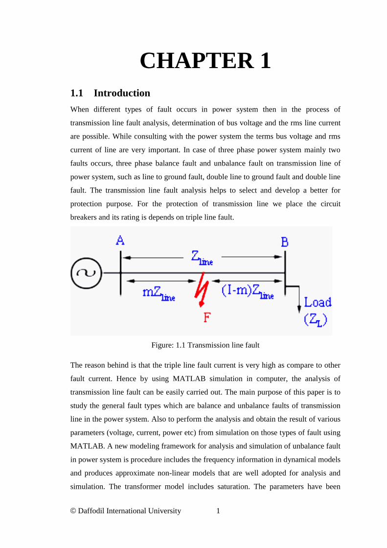
Figure: 1.1 Transmission line fault
The reason behind is that the triple line fault current is very high as compare to other
fault current. Hence by using MATLAB simulation in computer, the analysis of
transmission line fault can be easily carried out. The main purpose of this paper is to
study the general fault types which are balance and unbalance faults of transmission
line in the power system. Also to perform the analysis and obtain the result of various
parameters (voltage, current, power etc) from simulation on those types of fault using
MATLAB. A new modeling framework for analysis and simulation of unbalance fault
in power system is procedure includes the frequency information in dynamical models
and produces approximate non-linear models that are well adopted for analysis and
simulation. The transformer model includes saturation. The parameters have been
© Daffodil International University 2
obtained from practical or experimental measurements. From the study it is seen that
sags can produce transformer saturation when voltage recovers. This leads to produce
an inrush current that is similar to inrush current produced during the transformer
energizing. The study point out that the voltage recovery instant can take only discrete
value, since the fault-clearing is produced in case of natural current zeroes. The
instant of voltage recovery corresponds to the instant of fault clearing. For phase to
phase fault and single phase fault, a single point-on-wave of voltage recovery can be
defined. On the other hand for two-phase- to-ground and three-phase fault, the
recovery takes place in two or three steps. In petrochemical industry, the grounding
and ground fault protection are very important factors. For that first it is important to
have the proper system grounding for the particular system application, and along
with this it is equally important to have the proper protection against the ground-fault.
1.2 Problem of the System
Transmission line protection is an important issue in power system reason behind it is
85-87% fault occur in transmission line. Fault detection & classification is an
important step to safeguard power system. an automated analysis approach which can
automatically characterized fault and subsequent relay operation is required is fault
detection play an important role in damaging equipment due to short circuit and fast
detection of fault In any line conduces to quick isolation of faulty line from service
and hence protecting it prom harmful effect of fault is required. So, the proposed
system is required to act fast to the fault condition.
1.3 Objectives of the Thesis
The objective of this project is to study the common fault type which is balance fault
of the transmission line in the power system. Secondly is to perform the analysis and
obtain the results from simulation on those types of fault using MATLAB. Lastly is to
develop a toolbox for power system fault analysis for educational and training
purposes.
1. To fault detection in three phase transmission line.
2. To fault classification in three phase transmission line.
3. To fault location in three phase transmission line.
© Daffodil International University 3
4. To best fault calculation method to be implemented for calculation.
5. To Calculation of three phase transmission line fault current & voltage.
1.4 Project/Thesis planning
Task performed
i. Feasibility study
ii. Planning of the research method to be adopted.
In this period of time, project/thesis planning was done by the researcher & the
feasibility study about the topic and the methodology to be used was performed.
Planning for primary and secondary research method which will be adopted was done
in this period of time again for this purpose various book, E-book, library resource
was used by the researcher.
1.5 Benefits of a Short Circuit Analysis
Performing a Short Circuit Study provides the following benefits:
Reduces the risk a facility could face and help avoid catastrophic losses.
Increases the safety and reliability of the power system and related equipment.
Evaluates the application of protective devices and equipment.
Identifies problem areas in the system.
Identifies recommended solutions to existing problems.
1.6 Report Outline
Chapter 1: Introduction
Chapter 2: Literature Review
Chapter 3: Types of Transmission Line Fault
Chapter 4: Fault Calculation
Chapter 5: MATLAB Simulation
Chapter 6: MATLAB Simulation Result & Discussion
Chapter 7: Calculation

© Daffodil International University 4
CHAPTER 2
Literature Review
2.1 Introduction
Electric power is generated, transmitted and distributed by large interconnected power
systems. Any power system can be analyzed by calculating the system voltages and
currents under normal & abnormal scenarios.
The fault currents caused by short circuits may be several orders of magnitude larger
than the normal operating currents and are determined by the system impedance
between the generator voltages and the fault, under the worst scenario if the fault
persists, it may lead to long-term power loss, blackouts and permanently damage to
the equipment. To prevent such an undesirable situation, the temporary isolation of
the fault from the whole system it is necessary as soon as possible. This is
accomplished by the protective relaying system.
To complete this task successfully, fault analysis has to be conducted in every
location assuming several fault conditions. The goal is to determine the optimum
protection scheme by determining the fault currents & voltages. In reality, power
system can consist of thousands of buses which complicate the task of calculating
these parameters without the use of computer software’s such as Matlab. In 1956,
L.W. Comber and D. G. Lewis proposed the first fault analysis program.
Many exiting texts offer an extensive analysis in fault studies and calculation. Two
worth mentioning are Analysis of Faulted Power System by Paul Anderson and
Electrical Power Transmission System Engineering Analysis and Design by Turan
Gonen. In addition to offer a very illustrative and clear analysis in the fault studies,
they also offer an impressive guideline for the power systems analysis understanding
in general.

© Daffodil International University 5
2.2 Method of Analysis
In order to analyze any unbalanced power system, C.L. Fortescue introduced a
method called symmetrical components in 1918 to solve such system using a balanced
representation. This method is considered the base of all traditional fault analysis
approaches of solving unbalanced power systems. The theory suggests that any
unbalanced system can be represented by a number of balanced systems equal to the
number of its phasors. The balanced systems representations are called symmetrical
components.
2.3 Review of Fault
In an electric power system, a fault is unusual electric current. A short circuit is also
considered as a fault in which current bypasses the normal load. An open-circuit fault
occurs if a circuit is interrupted by some failure. In three-phase systems, a fault may
involve one or more phases and ground, or may occur only between phases. In a
"ground fault" or "earth fault", charge flows into the earth. The prospective short
circuit current of a fault can be calculated for power systems. In power systems,
protective devices detect fault conditions and operate circuit breakers and other
devices to limit the loss of service due to a failure.

© Daffodil International University 6
CHAPTER 3
Types of Transmission Line Fault
3.1 Introduction As discuss above in three-phase transmission line of power system mainly two types
of fault occurs, balance fault which is also called symmetrical fault and unbalance
fault called as unsymmetrical fault. But this paper only deals with the unsymmetrical
fault which mainly occurs between two or three conductors of the three-phase system
or some time in between conductor and ground. Contingent on this the unsymmetrical
faults can be characterized into fundamental three sorts:-
Single Line to Ground fault.
Double Line fault.
Double Line to Ground fault.
The frequency of occurrence of the single line to ground fault is more in the three
phase system followed by the L-L fault, 2L-G fault and three phase fault. During
electrical storms these types of fault are occurs which may results to insulator
flashover and ultimately affect the power system. To study and analyze the
unsymmetrical fault in MATLAB there is a need of develop a network of positive,
negative and zero sequence. In this paper us analysis positive, negative and zero
sequence voltage and current of buses at different fault situation. In addition to this
we analyze the active and reactive power and rms bus current and voltage of the
system at various fault condition.
3.2 Symmetrical Fault
A symmetric or balanced fault affects each of the three phases equally. In
transmission line faults, roughly 5% are symmetric. This is in contrast to an
asymmetrical fault, where the three phases are not affected equally.
There are two kinds of symmetrical fault
three-phase faults
three-phase faults with ground fault
© Daffodil International University 7
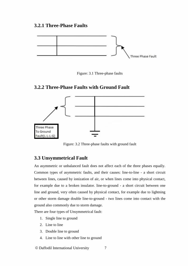
3.2.1 Three-Phase Faults
Figure: 3.1 Three-phase faults
3.2.2 Three-Phase Faults with Ground Fault
Figure: 3.2 Three-phase faults with ground fault
3.3 Unsymmetrical Fault
An asymmetric or unbalanced fault does not affect each of the three phases equally.
Common types of asymmetric faults, and their causes: line-to-line - a short circuit
between lines, caused by ionization of air, or when lines come into physical contact,
for example due to a broken insulator. line-to-ground - a short circuit between one
line and ground, very often caused by physical contact, for example due to lightning
or other storm damage double line-to-ground - two lines come into contact with the
ground also commonly due to storm damage.
There are four types of Unsymmetrical fault:
1. Single line to ground
2. Line to line
3. Double line to ground
4. Line to line with other line to ground
© Daffodil International University 8
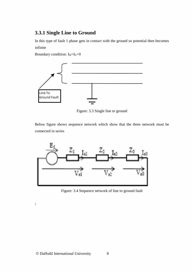
3.3.1 Single Line to Ground
In this type of fault 1 phase gets in contact with the ground so potential then becomes
infinite
Boundary condition: Ifb=Ifc=0
Figure: 3.3 Single line to ground
Below figure shows sequence network which show that the three network must be
connected in series
Figure: 3.4 Sequence network of line to ground fault
\
© Daffodil International University 9
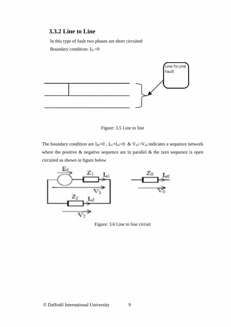
3.3.2 Line to Line
In this type of fault two phases are short circuited
Boundary condition: Ifa =0
Figure: 3.5 Line to line
The boundary condition are Ia0=0 , Ia1+Ia2=0 & Va1=Va2 indicates a sequence network
where the positive & negative sequence are in parallel & the zero sequence is open
circuited as shown in figure below
Figure: 3.6 Line to line circuit
© Daffodil International University 10
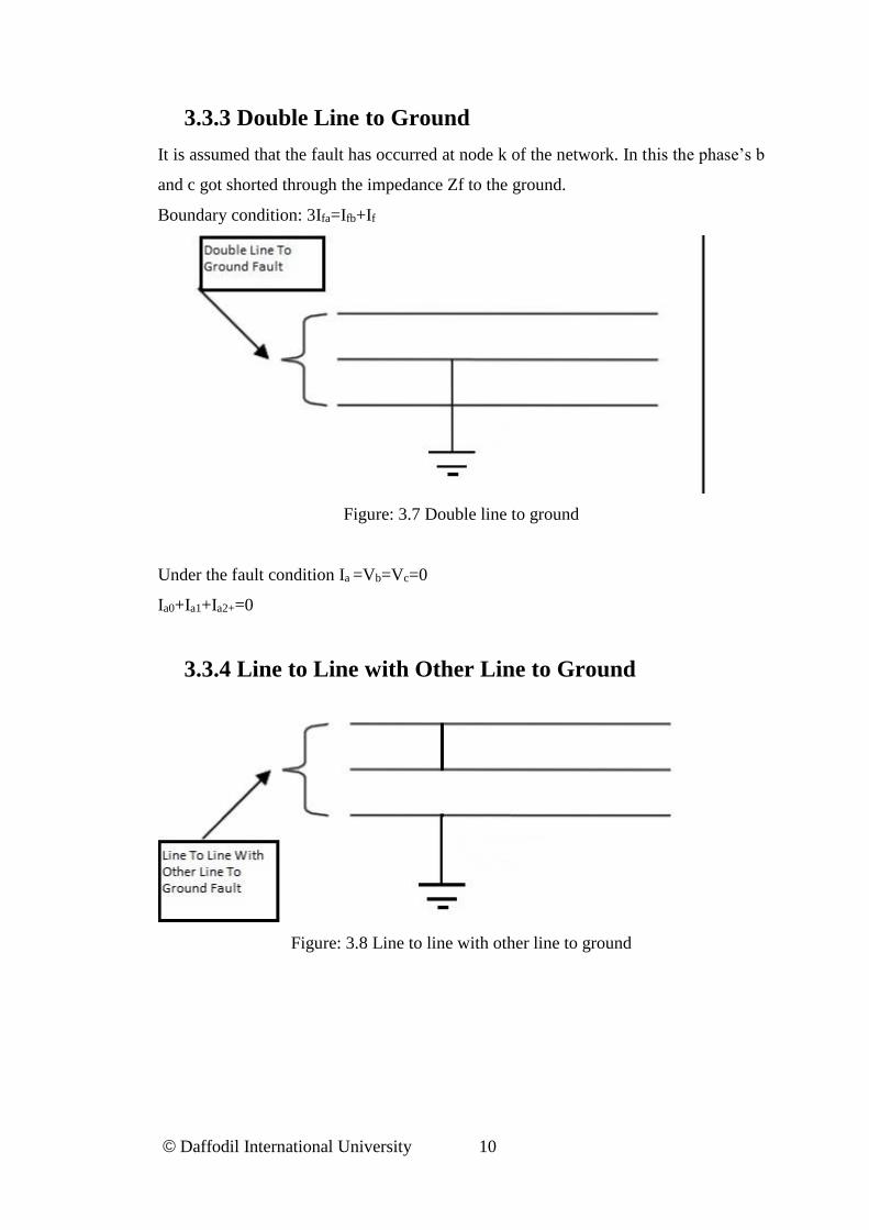
3.3.3 Double Line to Ground
It is assumed that the fault has occurred at node k of the network. In this the phase’s b
and c got shorted through the impedance Zf to the ground.
Boundary condition: 3Ifa=Ifb+If
Figure: 3.7 Double line to ground
Under the fault condition Ia =Vb=Vc=0
Ia0+Ia1+Ia2+=0
3.3.4 Line to Line with Other Line to Ground
Figure: 3.8 Line to line with other line to ground
© Daffodil International University 11
CHAPTER 4
Fault Calculation
4.1 Introduction
This chapter describes the mathematical model that is used in the analysis of faulted
power systems and the assumptions that are used in this project/thesis analysis.
4.2 Fortescue’s Theory
A three-phase balanced fault can be defined as a short circuit with fault impedance
called Zf between the ground and each phase. The short circuit will be called a solid
fault when Zf is equal to zero. This type of fault is considered the most sever short
circuit which can affect any electrical system. Fortunately, it is rarely taking place in
reality. Fortescue segregated asymmetrical three-phase voltages and currents into
three sets of symmetrical components in 1918.
Analyzing any symmetrical fault can be achieved using impedance matrix method or
Thevenin’s method. Fortescue’s theorem suggests that any unbalanced fault can be
solved into three independent symmetrical components which differ in the phase
sequence. These components consist of a positive sequence, negative sequence and a
zero sequence.
4.3 Fault Analysis in Power Systems
In general, a fault is any event, unbalanced situation or any asymmetrical situation
that interferes with the normal current flow in a power system and forces voltages and
currents to differ from each other. It is important to distinguish between series and
shunt faults in order to make an accurate fault analysis of an asymmetrical three-phase
system. When the fault is caused by an unbalance in the line impedance and does not
involve a ground, or any type of inter-connection between phase conductors it is
known as a series fault. On the other hand, when the fault occurs and there is an inter-
© Daffodil International University 12
connection between phase-conductors or between conductor and ground and/or
neutral it is known as a shunt fault.
Statistically, series faults do not occur as often as shunt faults does. Because of this
fact only the shunt faults are explained here in detail since the emphasis in this project
is on analysis of a power system under shunt faults.
4.3.1 Three-Phase Fault
By definition a three-phase fault is a symmetrical fault. Even though it is the least
frequent fault, it is the most dangerous. Some of the characteristics of a three-phase
fault are a very large fault current and usually a voltage level equals to zero at the site
where the fault takes place.
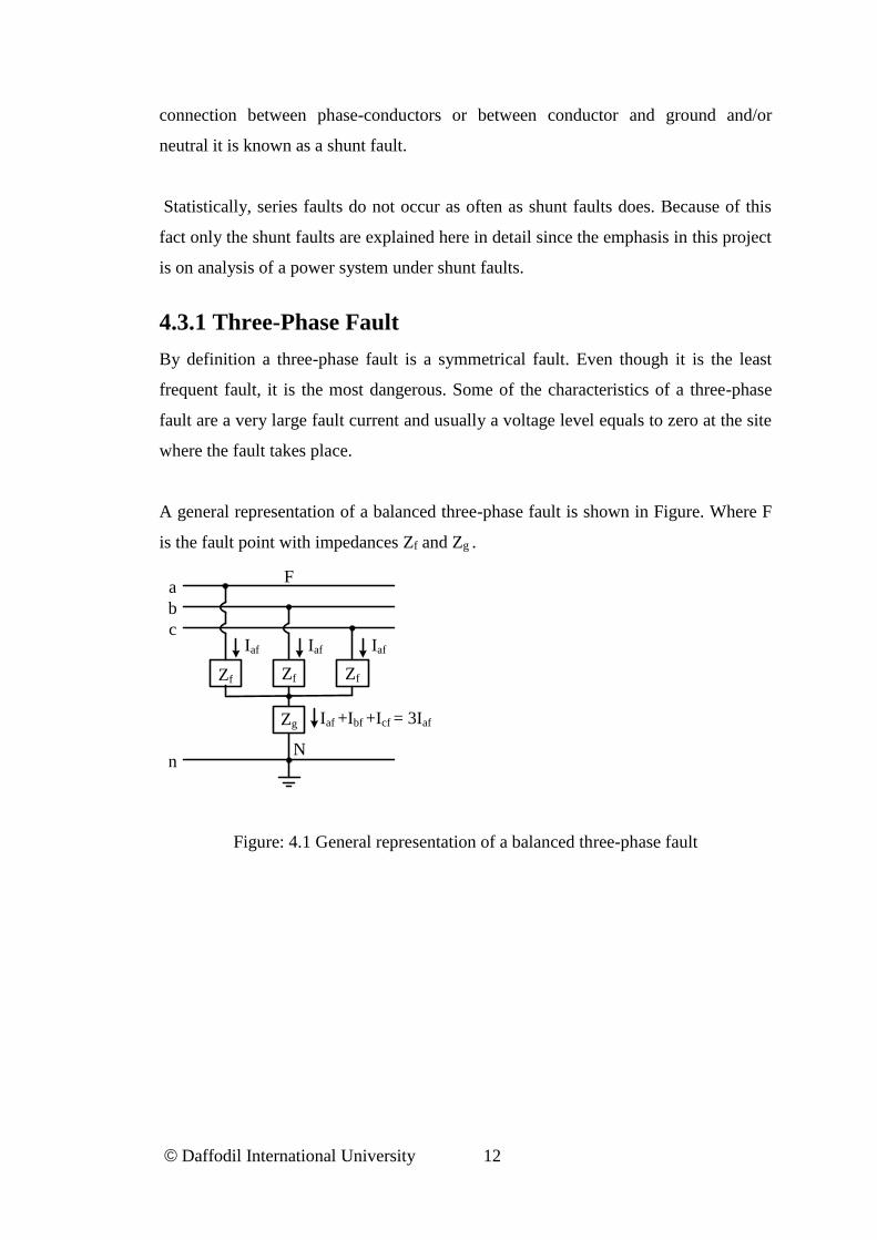
A general representation of a balanced three-phase fault is shown in Figure. Where F
is the fault point with impedances Zf and Zg .
a
c
b
F
Iaf Iaf Iaf
n
Zf Zf
Zg Iaf +Ibf +Icf = 3Iaf
N
Zf
Figure: 4.1 General representation of a balanced three-phase fault
© Daffodil International University 13
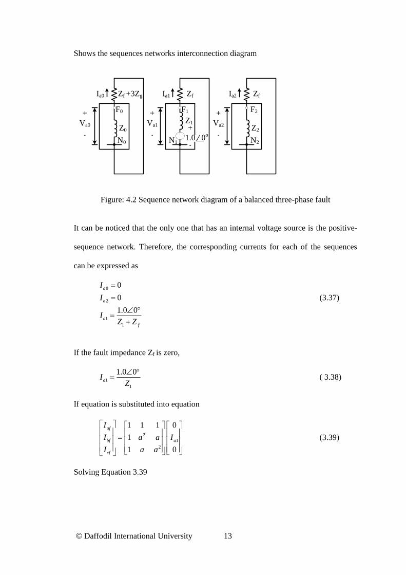
Shows the sequences networks interconnection diagram
Zf +3Zg
F0
Z0
N0
+
Va0
-
Ia0 Zf
F1
Z1
N1
+
Va1
-
Ia1 Zf
F2
Z2
N2
+
Va2
-
Ia2
+
1.0 0o
-
Figure: 4.2 Sequence network diagram of a balanced three-phase fault
It can be noticed that the only one that has an internal voltage source is the positive-
sequence network. Therefore, the corresponding currents for each of the sequences
can be expressed as
0
2
1
1
0
0
1.0 0
a
a
a
f
I
I
IZ Z
(3.37)
If the fault impedance Zf is zero,
1
1
1.0 0aI
Z
( 3.38)
If equation is substituted into equation
2
1
2
1 1 1 0
1
1 0
af
bf a
cf
I
I a a I
I a a
(3.39)
Solving Equation 3.39
© Daffodil International University 14
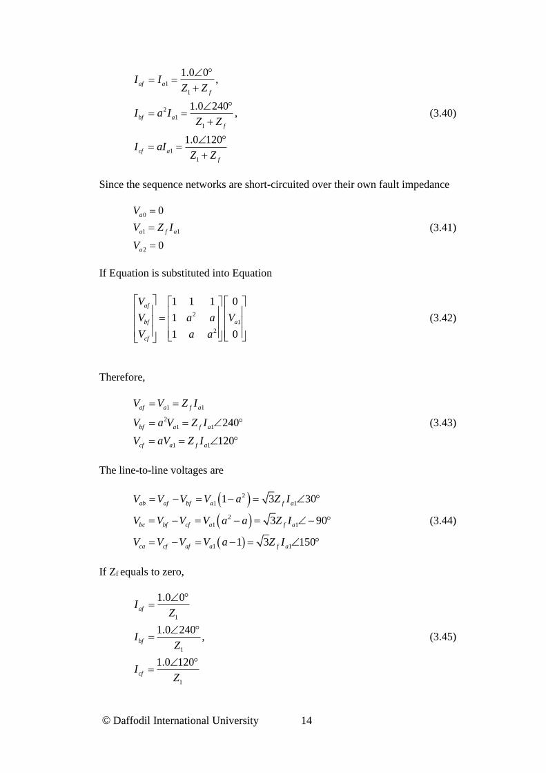
1
1
2
1
1
1
1
1.0 0,
1.0 240,
1.0 120
af a
f
bf a
f
cf a
f
I IZ Z
I a IZ Z
I aIZ Z
(3.40)
Since the sequence networks are short-circuited over their own fault impedance
0
1 1
2
0
0
a
a f a
a
V
V Z I
V
(3.41)
If Equation is substituted into Equation
2
1
2
1 1 1 0
1
1 0
af
bf a
cf
V
V a a V
V a a
(3.42)
Therefore,
1 1
2
1 1
1 1
240
120
af a f a
bf a f a
cf a f a
V V Z I
V a V Z I
V aV Z I
(3.43)
The line-to-line voltages are
2
1 1
2
1 1
1 1
1 3 30
3 90
1 3 150
ab af bf a f a
bc bf cf a f a
ca cf af a f a
V V V V a Z I
V V V V a a Z I
V V V V a Z I
(3.44)
If Zf equals to zero,
1
1
1
1.0 0
1.0 240,
1.0 120
af
bf
cf
IZ
IZ
IZ
(3.45)

© Daffodil International University 15
The phase voltages becomes,
0
0
0
af
bf
cf
V
V
V
(3.46)
And the line voltages,
0
1
2
0
0
0
a
a
a
V
V
V
(3.47)
4.3.2 Single Line-to-Ground Fault
The single line-to-ground fault is usually referred as “short circuit” fault and occurs
when one conductor falls to ground or makes contact with the neutral wire. The
general representation of a single line-to-ground fault is shown in Figure. Where F is
the fault point with impedances Zf. the sequences network diagram. Phase a is usually
assumed to be the faulted phase, this is for simplicity in the fault analysis calculations.
a
c
b
+
Vaf
-
F
Iaf Ibf = 0 Icf = 0
n
Zf
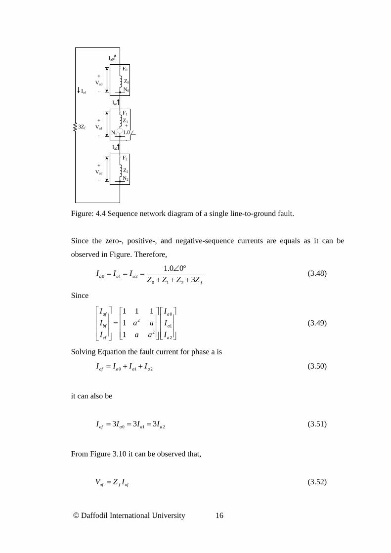
Figure: 4.3 General representation of a single line-to-ground fault.
© Daffodil International University 16
F0
Z0
N0
+
Va0
-
Ia0
F1
Z1
N1
+
Va1
-
Ia1
+
1.0
-
F2
Z2
N2
+
Va2
-
Ia2
3Zf
Iaf
Figure: 4.4 Sequence network diagram of a single line-to-ground fault.
Since the zero-, positive-, and negative-sequence currents are equals as it can be
observed in Figure. Therefore,
0 1 2
0 1 2
1.0 0
3a a a
f
I I IZ Z Z Z
(3.48)
Since
0
2
1
2
2
1 1 1
1
1
af a
bf a
cf a
I I
I a a I
I a a I
(3.49)
Solving Equation the fault current for phase a is
0 1 2af a a aI I I I (3.50)
it can also be
0 1 23 3 3af a a aI I I I (3.51)
From Figure 3.10 it can be observed that,
af f afV Z I (3.52)
© Daffodil International University 17
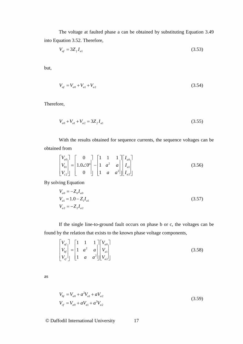
The voltage at faulted phase a can be obtained by substituting Equation 3.49
into Equation 3.52. Therefore,
13af f aV Z I (3.53)
but,
0 1 2af a a aV V V V (3.54)
Therefore,
0 1 2 13a a a f aV V V Z I (3.55)
With the results obtained for sequence currents, the sequence voltages can be
obtained from
0 0
2
1 1
2
22
0 1 1 1
1.0 0 1
0 1
a a
b a
ac
V I
V a a I
a a IV
(3.56)
By solving Equation
0 0 0
1 1 1
2 2 2
1.0
a a
a a
a a
V Z I
V Z I
V Z I
(3.57)
If the single line-to-ground fault occurs on phase b or c, the voltages can be
found by the relation that exists to the known phase voltage components,
0
2
1
2
2
1 1 1
1
1
af a
bf a
cf a
V V
V a a V
V a a V
(3.58)
as
2
0 1 2
2
0 1 2
bf a a a
cf a a a
V V a V aV
V V aV a V
(3.59)
© Daffodil International University 18
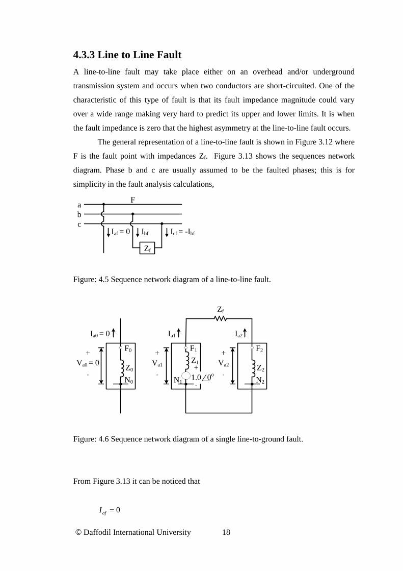
4.3.3 Line to Line Fault
A line-to-line fault may take place either on an overhead and/or underground
transmission system and occurs when two conductors are short-circuited. One of the
characteristic of this type of fault is that its fault impedance magnitude could vary
over a wide range making very hard to predict its upper and lower limits. It is when
the fault impedance is zero that the highest asymmetry at the line-to-line fault occurs.
The general representation of a line-to-line fault is shown in Figure 3.12 where
F is the fault point with impedances Zf. Figure 3.13 shows the sequences network
diagram. Phase b and c are usually assumed to be the faulted phases; this is for
simplicity in the fault analysis calculations,
a
c
b
F
Iaf = 0 Ibf Icf = -Ibf
Zf
Figure: 4.5 Sequence network diagram of a line-to-line fault.
F0
Z0
N0
+
Va0 = 0
-
Ia0 = 0
Zf
F1
Z1
N1
+
Va1
-
Ia1
F2
Z2
N2
+
Va2
-
Ia2
+
1.0 0o
-
Figure: 4.6 Sequence network diagram of a single line-to-ground fault.
From Figure 3.13 it can be noticed that
0afI
© Daffodil International University 19
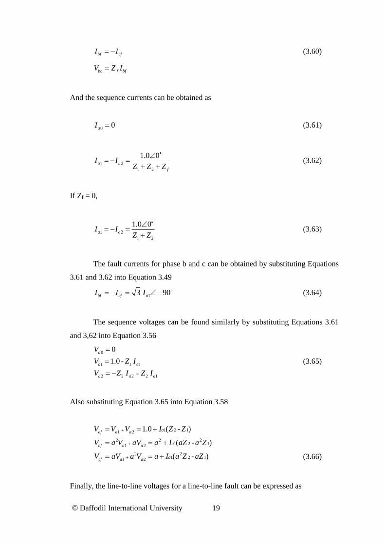
bf cfI I (3.60)
bc f bfV Z I
And the sequence currents can be obtained as
0 0aI (3.61)
1 2
1 2
1.0 0a a
f
I IZ Z Z
(3.62)
If Zf = 0,
1 2
1 2
1.0 0a aI I
Z Z
(3.63)
The fault currents for phase b and c can be obtained by substituting Equations
3.61 and 3.62 into Equation 3.49
13 90bf cf aI I I (3.64)
The sequence voltages can be found similarly by substituting Equations 3.61
and 3,62 into Equation 3.56
0
1 1 1
2 2 2 2 1
0
1.0 -
a
a a
a a a
V
V Z I
V Z I Z I
(3.65)
Also substituting Equation 3.65 into Equation 3.58
1 2 11 2
2 2 21 2 11 2
2 21 2 11 2
1.0 ( - )
( - )
( - )
aaf a a
abf a a
acf a a
V V V I Z Z
V a V aV a I aZ a Z
V aV a V a I a Z aZ
(3.66)
Finally, the line-to-line voltages for a line-to-line fault can be expressed as

© Daffodil International University 20
ab af bf
bc bf cf
ca cf af
V V V
V V V
V V V
(3.67)
4.3.4 Double Line to Ground Fault
A double line-to-ground fault represents a serious event that causes a
significant asymmetry in a three-phase symmetrical system and it may spread into a
three-phase fault when not clear in appropriate time. The major problem when
analyzing this type of fault is the assumption of the fault impedance Zf , and the value
of the impedance towards the ground Zg. [3]
The general representation of a double line-to-ground fault is shown in Figure
3.14 where F is the fault point with impedances Zf and the impedance from line to
ground Zg . Figure 3.15 shows the sequences network diagram. Phase b and c are
assumed to be the faulted phases, this is for simplicity in the fault analysis
calculations. [1]
a
c
b
F
Iaf = 0 Ibf Icf
n
Zf Zf
Zg Ibf +Icf
N
Figure: 4.7 General representation of a double line-to-ground fault.
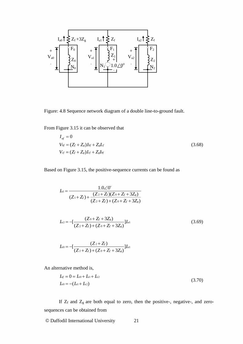
© Daffodil International University 21
Zf +3Zg
F0
Z0
N0
+
Va0
-
Ia0 Zf
F1
Z1
N1
+
Va1
-
Ia1 Zf
F2
Z2
N2
+
Va2
-
Ia2
+
1.0 0o
-
Figure: 4.8 Sequence network diagram of a double line-to-ground fault.
From Figure 3.15 it can be observed that
0
( )
( )
af
bf f g bf g cf
cf f g cf g bf
I
V Z Z I Z I
V Z Z I Z I
(3.68)
Based on Figure 3.15, the positive-sequence currents can be found as
12 0
1
2 0
1.0 0
( )( 3 )( )
( ) ( 3 )
af f g
f
f f g
IZ Z Z Z Z
Z ZZ Z Z Z Z
02 1
2 0
( 3 )[ ]( ) ( 3 )
f ga a
f f g
Z Z ZI I
Z Z Z Z Z
(3.69)
20 1
2 0
( )[ ]( ) ( 3 )
fa a
f f g
Z ZI I
Z Z Z Z Z
An alternative method is,
0 1 2
0 1 2
0
( )
af a a a
a a a
I I I I
I I I
(3.70)
If Zf and Zg are both equal to zero, then the positive-, negative-, and zero-
sequences can be obtained from
© Daffodil International University 22
12 0
1
2 0
1.0 0
( )( )( )
( )
aIZ Z
ZZ Z
02 1
2 0
( )[ ]( )
a aZ
I IZ Z
(3.71)
20 1
2 0
( )[ ]( )
a aZ
I IZ Z
From Figure 3.14 the current for phase a is
0afI (3.72)
Now, substituting Equations 3.71 into Equation 3.49 to obtain phase b and c
fault currents
2
0 1 2
2
0 1 2
bf a a a
cf a a a
I I a I aI
I I aI a I
(3.73)
The total fault current flowing into the neutral is
03n a bf cfI I I I (3.74)
And the sequences voltages can be obtained by using Equation 3.51
0 0 0
1 1 1
2 2 2
1.0
a a
a a
a a
V Z I
V Z I
V Z I
(3.75)
The phase voltages are equal to
0 1 2
2
0 1 2
2
0 1 2
af a a a
bf a a a
cf a a a
V V V V
V V a V aV
V V aV a V
(3.76)
© Daffodil International University 23
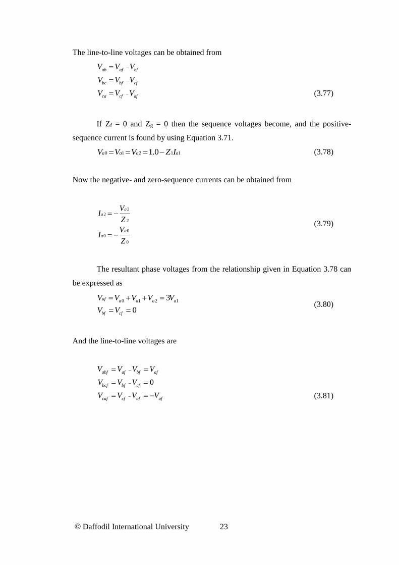
The line-to-line voltages can be obtained from
ab af bf
bc bf cf
ca cf af
V V V
V V V
V V V
(3.77)
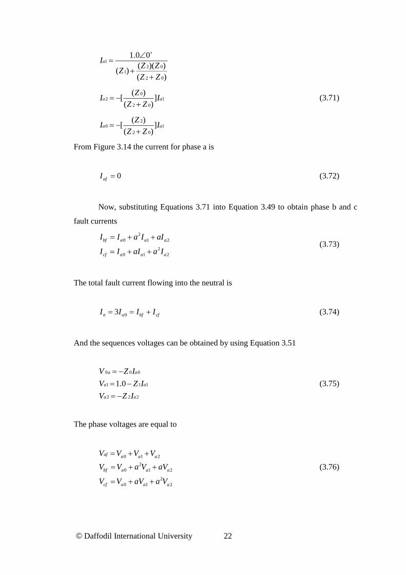
If Zf = 0 and Zg = 0 then the sequence voltages become, and the positive-
sequence current is found by using Equation 3.71.
0 1 2 1 11.0a a a aV V V Z I (3.78)
Now the negative- and zero-sequence currents can be obtained from
22
2
00
0
aa
aa
VI
Z
VI
Z
(3.79)
The resultant phase voltages from the relationship given in Equation 3.78 can
be expressed as
0 1 2 13
0
af a a a a
bf cf
V V V V V
V V
(3.80)
And the line-to-line voltages are
0
abf af bf af
bcf bf cf
caf cf af af
V V V V
V V V
V V V V
(3.81)
© Daffodil International University 24
CHAPTER 5
MATLAB simulation
5.1 Introduction
The name MATLAB views for Matrix Laboratory. MATLAB was written originally
to deliver easy access to matrix software developed by the (Linear method package &
Eigen method package projects).MATLAB is a great performance language for
technical calculating.it integrates calculation, visualization & programing
environment where problem & solution are expressed in familiar mathematical
representation. MATLAB has several advantages to conventional computer language
example (C, FORTRAN) for solving technical problem.
5.2 Model Of The Power System Parameter List
1. AC voltage source Simulink block.
2. Distributed transmission line Simulink block.
3. Relay Simulink block.
4. Three-Phase Fault Simulink block.
5. Parallel RLC Load Simulink block.
6. Scope Simulink Block.
7. Powergui Simulink Block.

© Daffodil International University 25
5.2.1 AC Voltage Source Simulink Block
AC voltage source model in Simulink was presented by three-phase ideal
sinusoidal voltage source with amplitude of 11000 volts and frequency are 50Hz with
three phases lagging respectively other by 120 degrees.
Figure: 5.1 AC voltage source simulink block
5.2.2 Distributed Transmission Line Simulink Block
The Three-Phase PI Section Line blocks implements a balanced three-phase
transmission line model with parameters lumped in a PI section. Contrary to the
Distributed Parameter Line model where the resistance, inductance, and capacitance
are uniformly distributed alongside the line, the Three-Phase PI Section Line block
lumps the line parameters in a single PI section as shown in the figure below.

© Daffodil International University 26
Figure: 5.2 Distributed transmission line simulink block
5.2.3 Relay Simulink Block
The Relay block allows the output to the switch between two specified values. When
the relay is on, it remains on up to the input drops below the value of the Switch off
point parameter. When the relay is off, it remains off until the input exceeds the value
of the Switch on point parameter. The block accepts one input and generates one
output. The Switch on point value must be greater than or equal to the Switch off
point. Specifying a Switch on point value greater than the Switch off point value
models hysteresis, whereas specifying equal values models a switch with a threshold
at that value.
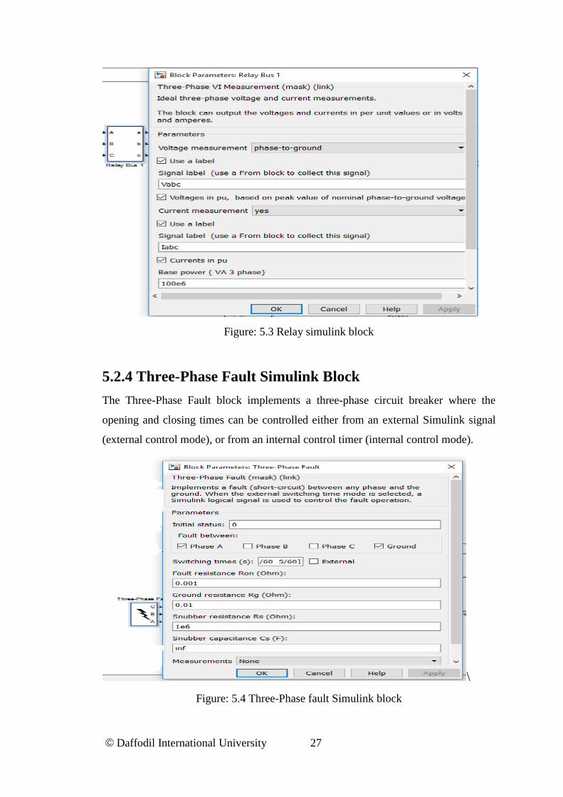
© Daffodil International University 27
Figure: 5.3 Relay simulink block
5.2.4 Three-Phase Fault Simulink Block
The Three-Phase Fault block implements a three-phase circuit breaker where the
opening and closing times can be controlled either from an external Simulink signal
(external control mode), or from an internal control timer (internal control mode).
\
Figure: 5.4 Three-Phase fault Simulink block
© Daffodil International University 28
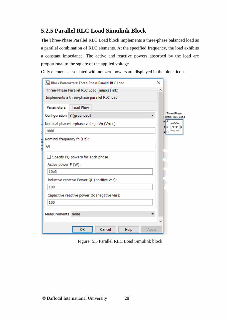
5.2.5 Parallel RLC Load Simulink Block
The Three-Phase Parallel RLC Load block implements a three-phase balanced load as
a parallel combination of RLC elements. At the specified frequency, the load exhibits
a constant impedance. The active and reactive powers absorbed by the load are
proportional to the square of the applied voltage.
Only elements associated with nonzero powers are displayed in the block icon.
Figure: 5.5 Parallel RLC Load Simulink block
© Daffodil International University 29
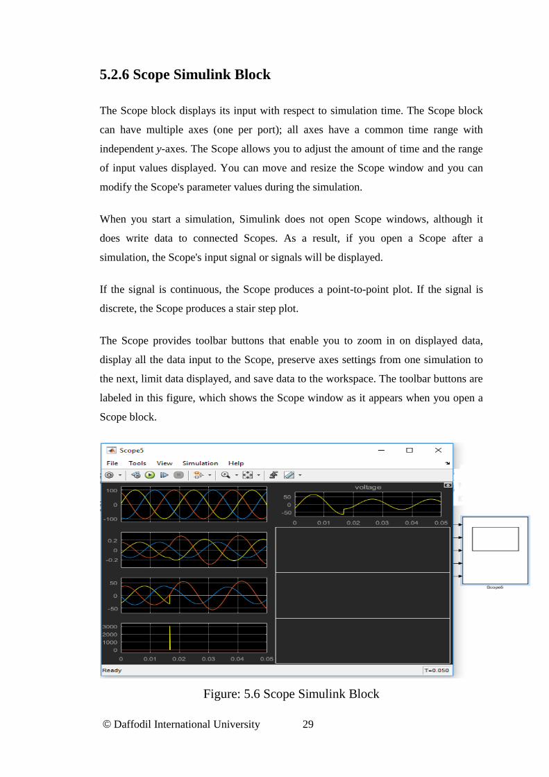
5.2.6 Scope Simulink Block
The Scope block displays its input with respect to simulation time. The Scope block
can have multiple axes (one per port); all axes have a common time range with
independent y-axes. The Scope allows you to adjust the amount of time and the range
of input values displayed. You can move and resize the Scope window and you can
modify the Scope's parameter values during the simulation.
When you start a simulation, Simulink does not open Scope windows, although it
does write data to connected Scopes. As a result, if you open a Scope after a
simulation, the Scope's input signal or signals will be displayed.
If the signal is continuous, the Scope produces a point-to-point plot. If the signal is
discrete, the Scope produces a stair step plot.
The Scope provides toolbar buttons that enable you to zoom in on displayed data,
display all the data input to the Scope, preserve axes settings from one simulation to
the next, limit data displayed, and save data to the workspace. The toolbar buttons are
labeled in this figure, which shows the Scope window as it appears when you open a
Scope block.
Figure: 5.6 Scope Simulink Block
© Daffodil International University 30
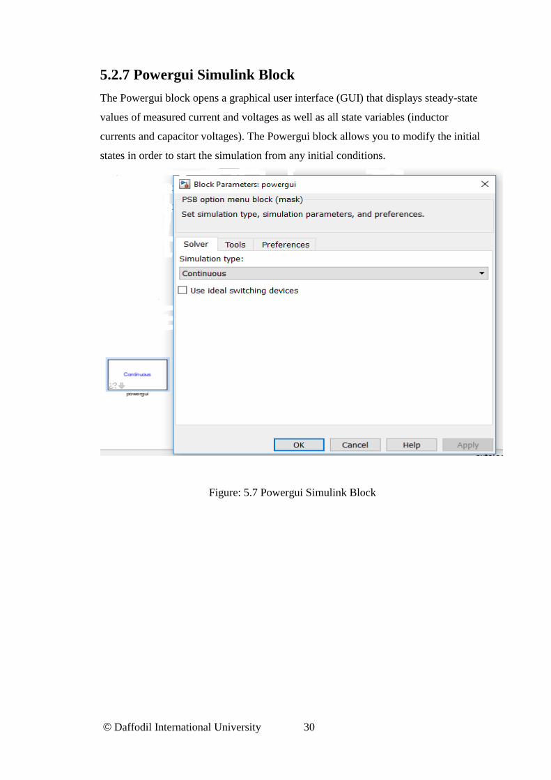
5.2.7 Powergui Simulink Block
The Powergui block opens a graphical user interface (GUI) that displays steady-state
values of measured current and voltages as well as all state variables (inductor
currents and capacitor voltages). The Powergui block allows you to modify the initial
states in order to start the simulation from any initial conditions.
Figure: 5.7 Powergui Simulink Block
© Daffodil International University 31
5.3 METHODOLOGY
MATLAB (matrix laboratory) is a multi-paradigm numerical computing environment
and fourth-generation programming language developed by MathWorks, MATLAB
allows matrix manipulations, plotting of functions and data, implementation of
algorithms, certain of user interfaces and interfacing with programs written in other
languages. Although MATLAB is intended primarily for numerical computing an
optional tool box uses the MuPAD symbolic computing capabilities. An additional
package, simulink, adds graphical multi-domain simulation and model- based design
for dynamic and embedded system. MATLAB users come from various backgrounds
of engineering, science and economics. MATLAB is widely used in academic and
research institutions as well as industrial enterprises. Also MATLAB gives an
attractive environment with hundreds of reliable and accurate built-in functions.
MATLAB family work together with Simulink software to model electrical,
mechanical and control systems. In order to study and analyze the transmission line
fault following circuit arrangement are connected to the parameters values
Generator 11kV 3 phase AC voltage source
Load 10KW Active, 100KVar Reactive
Transmission line Length=300km, R= 0.01273 Ohm/km,
L= 0.9337e-3 H/km, C= 12.74e-9 F/km
Figure: 5.1 Parameters of the power system
5.3.1 Circuit Model for Three Phase Faults in Power System
Network without Transformer
The implementation deals with the model made in MATLAB using the Sim Power
Systems Tool, the GUI. Through this advanced data simulation model fault analysis
of any power system network can be simulated with ease and its fault analysis can be
carried out.
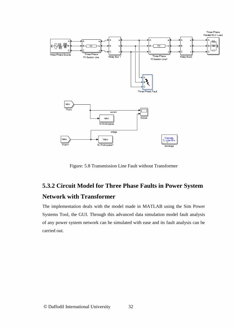
© Daffodil International University 32
Figure: 5.8 Transmission Line Fault without Transformer
5.3.2 Circuit Model for Three Phase Faults in Power System
Network with Transformer
The implementation deals with the model made in MATLAB using the Sim Power
Systems Tool, the GUI. Through this advanced data simulation model fault analysis
of any power system network can be simulated with ease and its fault analysis can be
carried out.
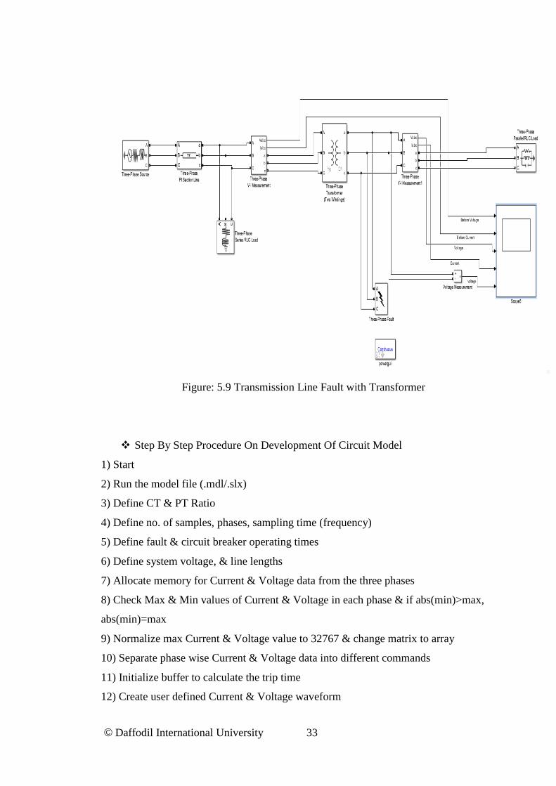
© Daffodil International University 33
Figure: 5.9 Transmission Line Fault with Transformer
Step By Step Procedure On Development Of Circuit Model
1) Start
2) Run the model file (.mdl/.slx)
3) Define CT & PT Ratio
4) Define no. of samples, phases, sampling time (frequency)
5) Define fault & circuit breaker operating times
6) Define system voltage, & line lengths
7) Allocate memory for Current & Voltage data from the three phases
8) Check Max & Min values of Current & Voltage in each phase & if abs(min)>max,
abs(min)=max
9) Normalize max Current & Voltage value to 32767 & change matrix to array
10) Separate phase wise Current & Voltage data into different commands
11) Initialize buffer to calculate the trip time
12) Create user defined Current & Voltage waveform
© Daffodil International University 34
13) Run Test & get the trip status & trip time of the relay
14) Save the generated plots
15) Generate report by creating another server for Excel & passing data from
MATLAB to Excel
16) Convert the file into a pdf & save the report
17) End

© Daffodil International University 35
CHAPTER 6
MATLAB Simulation Result &
Discussion
Following are the graph obtained from scope of different type of fault.
6.1 Three Phase To Ground Fault
Now simulation and modeling on three phases to ground fault occurs their three
phases is short to the ground. When the magnitude of the faults current line are higher
than the normal input current and the voltage are change on the magnitude is zero and
the fault the impedance is not necessary zero and output waveform shows the
gradually rise of current where three phases to ground fault occur on transmission
line.
Figure: 6.1 three phase fault current & voltage waveform
© Daffodil International University 36
In this actual case, the Distribution system model is runs for a Three Phase to Ground
Fault. The simulation is done for 0.05 sec, so that the waveforms can be seen more
clearly. The sampling frequency is taken to be 50 Hz. The system voltage is taken as
11 kV and the line length is taken as 300 kms, with fault occurring at 150 kms. Fault
is started at 0.3 secs. These parameters have been kept constant for other test cases as
well. Indicates the current and voltage waveforms for the given specifications. Upon
injecting these signals to the relay it has been seen that the relay trips after 45 ms and
the status of its coil is shown in the simulated results. As this is a self-reset relay, the
trip status comes back to 0 upon clearing the fault, but for a manual reset relay, it
stays 1 till the reset button is pressed manually. The proposed matlab model can be
ran standalone or on the GUI to view the plots.
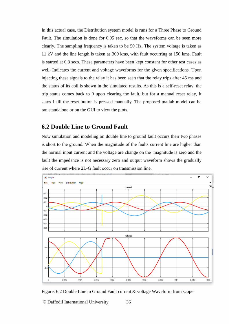
6.2 Double Line to Ground Fault
Now simulation and modeling on double line to ground fault occurs their two phases
is short to the ground. When the magnitude of the faults current line are higher than
the normal input current and the voltage are change on the magnitude is zero and the
fault the impedance is not necessary zero and output waveform shows the gradually
rise of current where 2L-G fault occur on transmission line.
Figure: 6.2 Double Line to Ground Fault current & voltage Waveform from scope
© Daffodil International University 37
In this actual case, the Distribution system model is runs for a line-line and ground
Fault. The simulation is done for 0.05 sec, so that the waveforms can be seen more
clearly. The sampling frequency is taken to be 50 Hz. The system voltage is taken as
11 kV and the line length is taken as 300 kms, with fault occurring at 150 kms. Fault
is started at 0.3 secs. There are indicates the current and voltage waveforms for the
given specifications. Upon injecting these signals to the relay it has been seen that the
relay trips after 45 ms and the status of its coil is shown in the simulated results. As
this is a self-reset relay, the trip status comes back to 0 upon clearing the fault, but for
a manual reset relay, it stays 1 till the reset button is pressed manually. The proposed
matlab model can be ran standalone or on the GUI to view the plots.
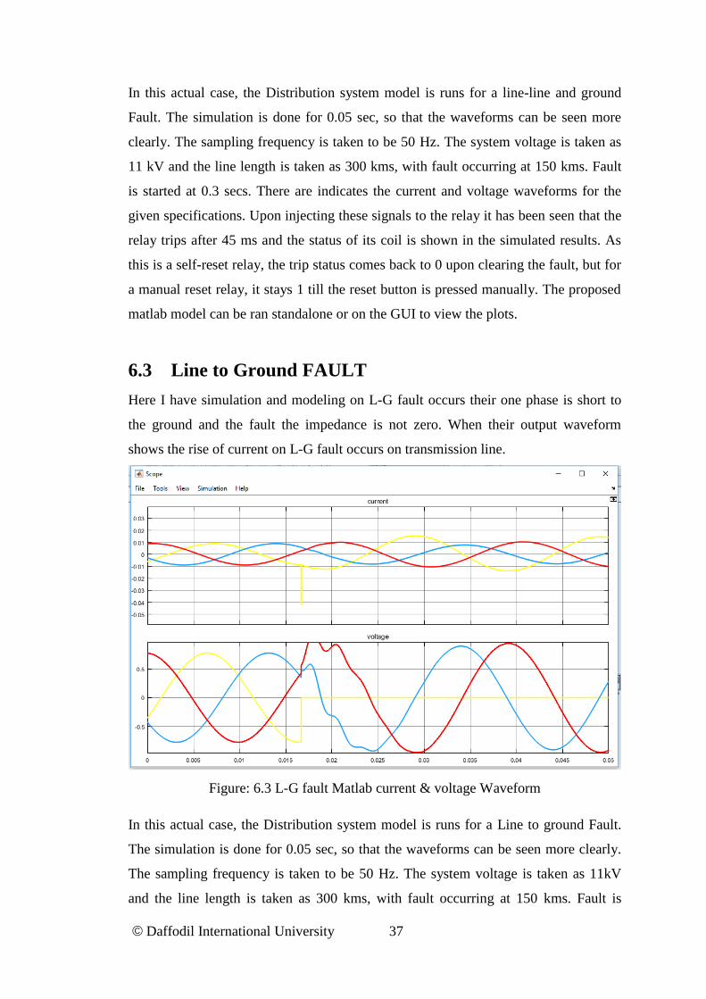
6.3 Line to Ground FAULT
Here I have simulation and modeling on L-G fault occurs their one phase is short to
the ground and the fault the impedance is not zero. When their output waveform
shows the rise of current on L-G fault occurs on transmission line.
Figure: 6.3 L-G fault Matlab current & voltage Waveform
In this actual case, the Distribution system model is runs for a Line to ground Fault.
The simulation is done for 0.05 sec, so that the waveforms can be seen more clearly.
The sampling frequency is taken to be 50 Hz. The system voltage is taken as 11kV
and the line length is taken as 300 kms, with fault occurring at 150 kms. Fault is
© Daffodil International University 38
started at 0.3. These parameters have been kept constant for other test cases as well.
There are indicates the current and voltage waveforms for the given specifications.
Upon injecting these signals to the relay it has been seen that the relay trips after 45
ms and the status of its coil is shown in the simulated results. As this is a self-reset
relay, the trip status comes back to 0 upon clearing the fault, but for a manual reset
relay, it stays 1 till the reset button is pressed manually. The proposed matlab model
can be ran standalone or on the GUI to view the plots.
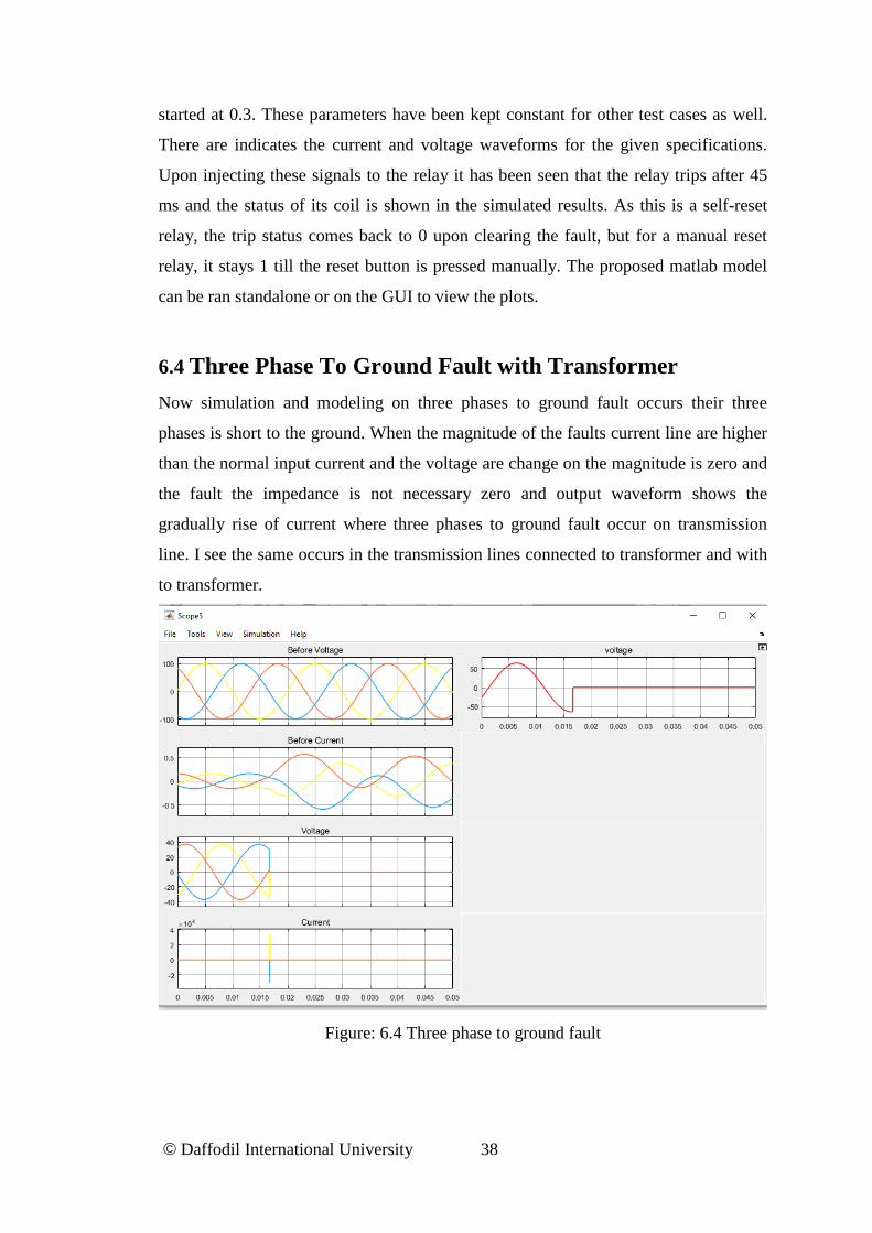
6.4 Three Phase To Ground Fault with Transformer
Now simulation and modeling on three phases to ground fault occurs their three
phases is short to the ground. When the magnitude of the faults current line are higher
than the normal input current and the voltage are change on the magnitude is zero and
the fault the impedance is not necessary zero and output waveform shows the
gradually rise of current where three phases to ground fault occur on transmission
line. I see the same occurs in the transmission lines connected to transformer and with
to transformer.
Figure: 6.4 Three phase to ground fault

© Daffodil International University 39
In this actual case, the Distribution system model is runs for a three phase to ground
fault. The simulation is done for 0.05 sec, so that the waveforms can be seen more
clearly. The sampling frequency is taken to be 50 Hz. The system voltage is taken as
11kV and the line length is taken as 300 kms, with fault occurring at 150 kms. Fault is
started at 0.3. These parameters have been kept constant for other test cases as well.
There are indicates the current and voltage waveforms for the given specifications.
Upon injecting these signals to the relay it has been seen that the relay trips after 45
ms and the status of its coil is shown in the simulated results. As this is a self-reset
relay, the trip status comes back to 0 upon clearing the fault, but for a manual reset
relay, it stays 1 till the reset button is pressed manually. The proposed matlab model
can be ran standalone or on the GUI to view the plots.
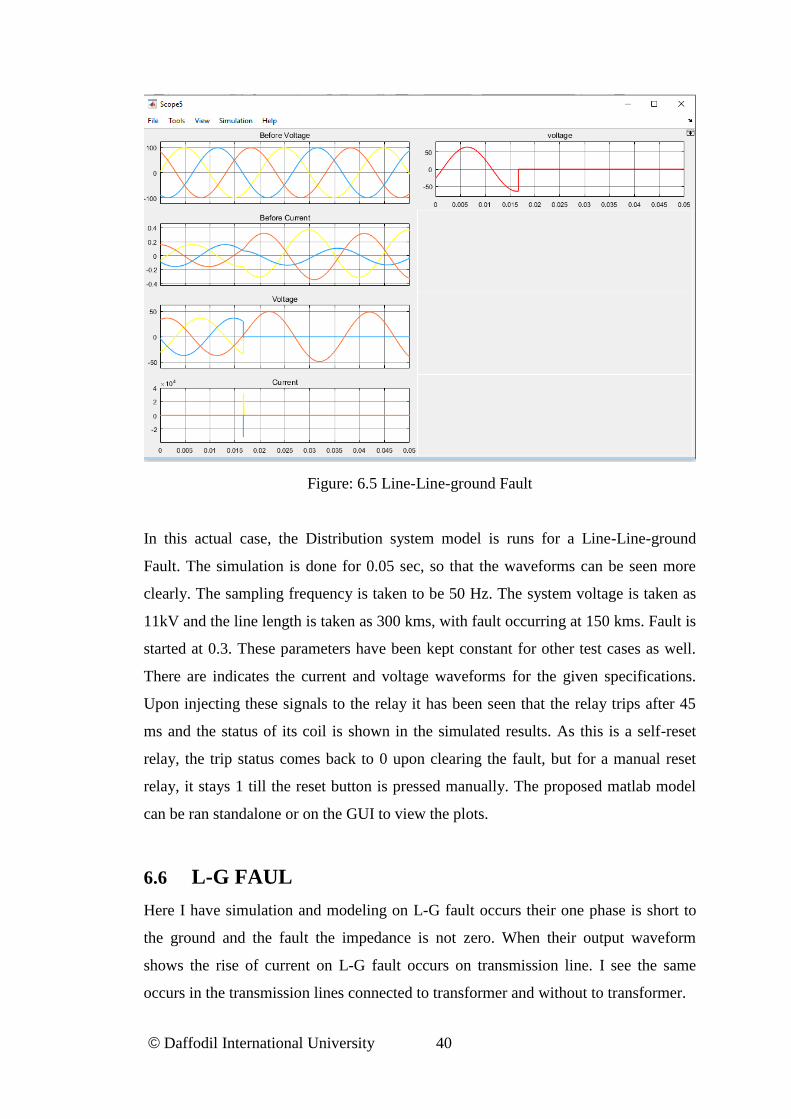
6.5 Double Line To Ground Fault
Now simulation and modeling on double line to ground fault occurs their two phases
is short to the ground. When the magnitude of the faults current line are higher than
the normal input current and the voltage are not change on magnitude and the fault the
impedance is not necessary zero and output waveform shows the gradually rise of
current where 2L-G fault occur on transmission line. I see the same occurs in the
transmission lines connected to transformer and with to transformer.
© Daffodil International University 40
Figure: 6.5 Line-Line-ground Fault
In this actual case, the Distribution system model is runs for a Line-Line-ground
Fault. The simulation is done for 0.05 sec, so that the waveforms can be seen more
clearly. The sampling frequency is taken to be 50 Hz. The system voltage is taken as
11kV and the line length is taken as 300 kms, with fault occurring at 150 kms. Fault is
started at 0.3. These parameters have been kept constant for other test cases as well.
There are indicates the current and voltage waveforms for the given specifications.
Upon injecting these signals to the relay it has been seen that the relay trips after 45
ms and the status of its coil is shown in the simulated results. As this is a self-reset
relay, the trip status comes back to 0 upon clearing the fault, but for a manual reset
relay, it stays 1 till the reset button is pressed manually. The proposed matlab model
can be ran standalone or on the GUI to view the plots.
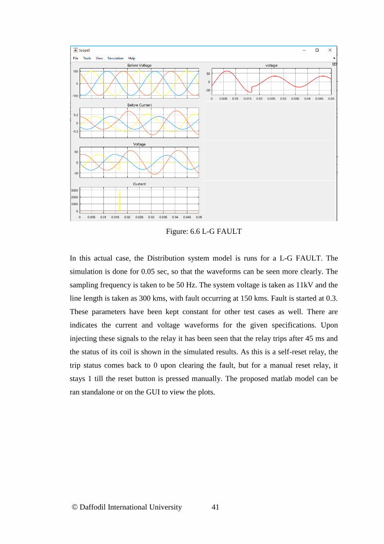
6.6 L-G FAUL
Here I have simulation and modeling on L-G fault occurs their one phase is short to
the ground and the fault the impedance is not zero. When their output waveform
shows the rise of current on L-G fault occurs on transmission line. I see the same
occurs in the transmission lines connected to transformer and without to transformer.
© Daffodil International University 41
Figure: 6.6 L-G FAULT
In this actual case, the Distribution system model is runs for a L-G FAULT. The
simulation is done for 0.05 sec, so that the waveforms can be seen more clearly. The
sampling frequency is taken to be 50 Hz. The system voltage is taken as 11kV and the
line length is taken as 300 kms, with fault occurring at 150 kms. Fault is started at 0.3.
These parameters have been kept constant for other test cases as well. There are
indicates the current and voltage waveforms for the given specifications. Upon
injecting these signals to the relay it has been seen that the relay trips after 45 ms and
the status of its coil is shown in the simulated results. As this is a self-reset relay, the
trip status comes back to 0 upon clearing the fault, but for a manual reset relay, it
stays 1 till the reset button is pressed manually. The proposed matlab model can be
ran standalone or on the GUI to view the plots.

© Daffodil International University 42
6.7 Working Flow Chart
© Daffodil International University 43
CHAPTER 7
Conclusions
7.1 Conclusion
The simulation and analysis of three phase fault to achieve results of the transmission
line parameter is convenient by using MATLAB software. In this paper simulation of
three phase transmission line fault analysis system is proposed. Single Line to Ground
fault, Double Line fault etc in transmission line is also simulated. This system opens
the way to redesign the bus system of the power system according to its results. The
proposed work can able to implement for a larger power systems geographically
apart.
7.2 Limitations of the Work
Mention few limitations or challenges faced in my work. In this thesis, i have faced
few problems as like as.
© Daffodil International University 44
References [1] https://pdfs.semanticscholar.org/38cc/69cafa8ab82af0ec02e00287df050e991428.pdf
[2] http://www.iaeme.com/MasterAdmin/UploadFolder/IJEET_07_02_006/IJEET_07_02_006.pdf
[3] https://www.scribd.com/document/312799120/Review-Paper-On-Three-Phase-fault-analysis
[4]http://www.academia.edu/11389028/TRANSMISSION_LINE_FAULT_ANALYSIS_BY_USING_
MATLAB_SIMULATION
[5] https://www.ijraset.com/fileserve.php?FID=5903
[6]https://www.google.com/search?q=Future+Outlook+for+Fault+Classification+Methods&oq=Future
+Outlook+for+Fault+Classification+Methods&aqs=chrome..69i57.1164j0j7&sourceid=chrome&ie=U
TF-8
[7]http://eie.uonbi.ac.ke/sites/default/files/cae/engineering/eie/ELECTRICAL%20POWER%20SYSTE
M%20FAULT%20ANALYSIS.pdf
[8] https://www.sciencedirect.com/topics/engineering/three-phase-fault
[9] https://www.scribd.com/document/338409031/Symmetrical-Three-Phase-Fault
[10] https://en.wikipedia.org/wiki/Fault_(power_engineering)