three-way contingency tables - mark · pdf filedeviant 1 1 3 8 1 3 three-way contingency...

Three-way Contingency Tables

Statistics 149

Spring 2006

Copyright ©2006 by Mark E. Irwin

Three-way Contingency Tables

Example: Classroom Behaviour (Everitt, 1977, page 67)

97 students were classified on three factors

• X: Teacher’s rating of classroom behaviour (behaviour) - non deviantor deviant

• Y : Risk index based on home conditions (risk) - not at risk or at risk

• Z: Adversity of school conditions (adversity) - low, medium, or high

Adversity Low Medium High

Risk Not at Risk At Risk Not at Risk At Risk Not at Risk At Risk

Non Deviant 16 7 15 34 5 3

Deviant 1 1 3 8 1 3

Three-way Contingency Tables 1

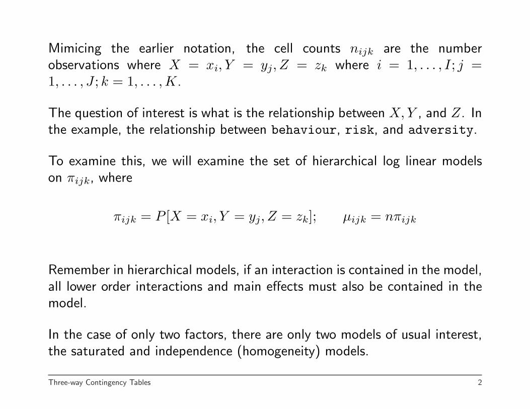
Mimicing the earlier notation, the cell counts nijk are the numberobservations where X = xi, Y = yj, Z = zk where i = 1, . . . , I; j =1, . . . , J ; k = 1, . . . , K.

The question of interest is what is the relationship between X, Y , and Z. Inthe example, the relationship between behaviour, risk, and adversity.

To examine this, we will examine the set of hierarchical log linear modelson πijk, where

πijk = P [X = xi, Y = yj, Z = zk]; µijk = nπijk

Remember in hierarchical models, if an interaction is contained in the model,all lower order interactions and main effects must also be contained in themodel.

In the case of only two factors, there are only two models of usual interest,the saturated and independence (homogeneity) models.


When there are three or more factors, the classes of models in much moreinteresting.

In what follows, one notation that is used to describe a model is based onthe highest order interactions in the model such that all terms in the modelare implied. For example

(XY, XZ)

describes the model with the XY and XZ interactions, and the X, Y ,and Z main effects. This notation relates to compact forms for writing themodels in R. This model in R could be written as

n ~ X*Y + X*Z


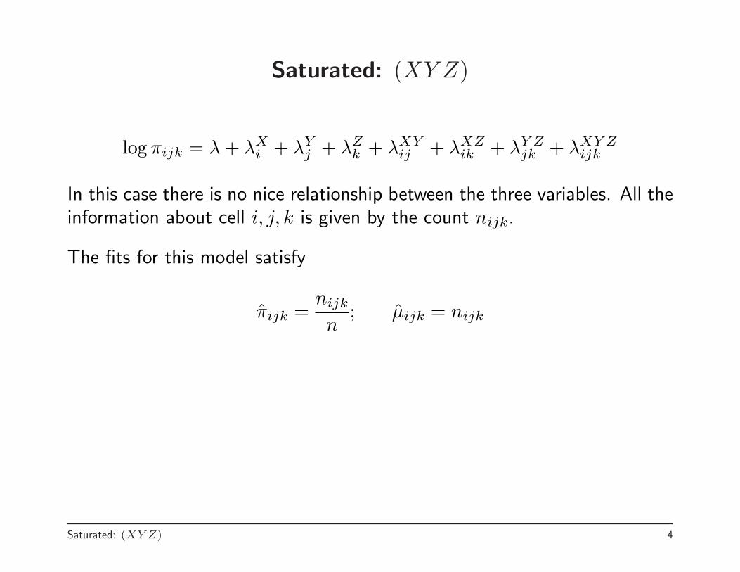
Saturated: (XY Z)

log πijk = λ + λXi + λY

j + λZk + λXY

ij + λXZik + λY Z

jk + λXY Zijk

In this case there is no nice relationship between the three variables. All theinformation about cell i, j, k is given by the count nijk.

The fits for this model satisfy

π̂ijk =nijk

n; µ̂ijk = nijk

Saturated: (XY Z) 4

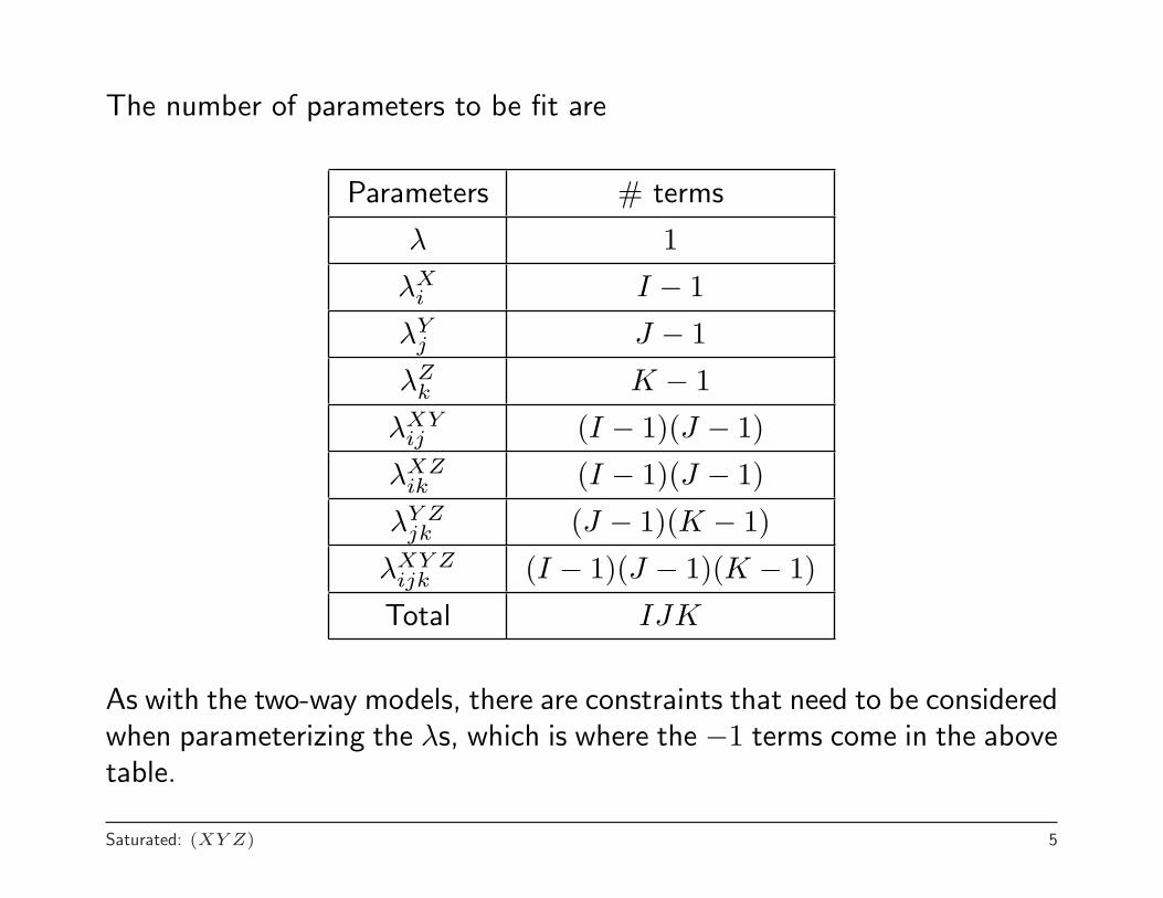
The number of parameters to be fit are

Parameters # terms

λ 1

λXi I − 1

λYj J − 1

λZk K − 1

λXYij (I − 1)(J − 1)

λXZik (I − 1)(J − 1)

λY Zjk (J − 1)(K − 1)

λXY Zijk (I − 1)(J − 1)(K − 1)

Total IJK

As with the two-way models, there are constraints that need to be consideredwhen parameterizing the λs, which is where the −1 terms come in the abovetable.

Saturated: (XY Z) 5

As the total number of parameters in the model = the number of cells inthe table, the degrees of freedom for this model is 0.

All the other models to be considered are subsets of this model wheredifferent combinations of the λs are set to 0.

Saturated: (XY Z) 6

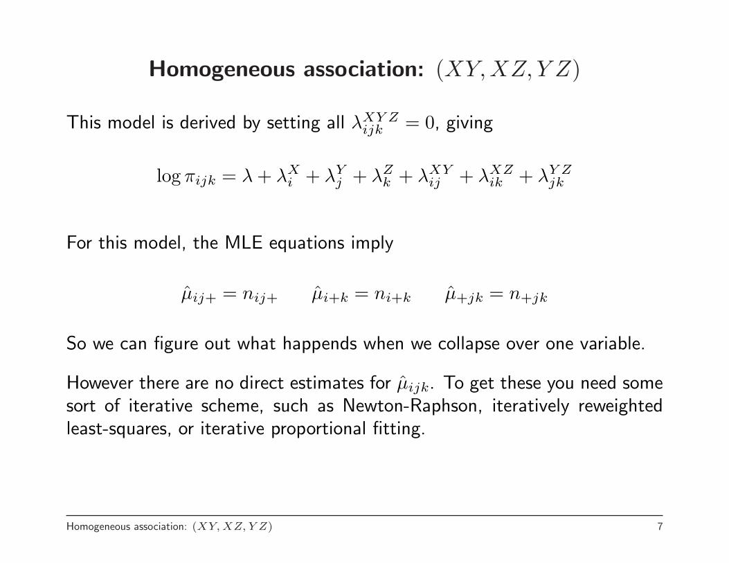
Homogeneous association: (XY,XZ, Y Z)

This model is derived by setting all λXY Zijk = 0, giving


j + λZk + λXY

ij + λXZik + λY Z

jk

For this model, the MLE equations imply

µ̂ij+ = nij+ µ̂i+k = ni+k µ̂+jk = n+jk

So we can figure out what happends when we collapse over one variable.

However there are no direct estimates for µ̂ijk. To get these you need somesort of iterative scheme, such as Newton-Raphson, iteratively reweightedleast-squares, or iterative proportional fitting.

Homogeneous association: (XY, XZ, Y Z) 7

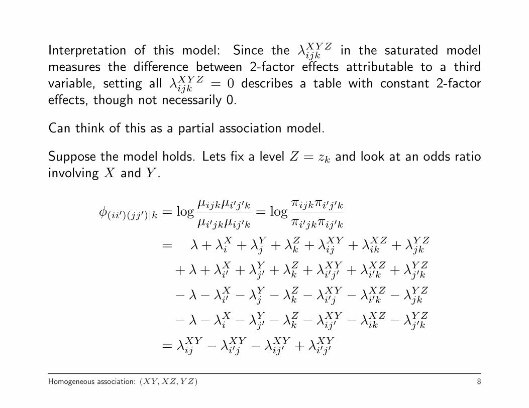
Interpretation of this model: Since the λXY Zijk in the saturated model

measures the difference between 2-factor effects attributable to a thirdvariable, setting all λXY Z

ijk = 0 describes a table with constant 2-factoreffects, though not necessarily 0.

Can think of this as a partial association model.

Suppose the model holds. Lets fix a level Z = zk and look at an odds ratioinvolving X and Y .

φ(ii′)(jj′)|k = logµijkµi′j′kµi′jkµij′k

= logπijkπi′j′kπi′jkπij′k

= λ + λXi + λY

j + λZk + λXY

ij + λXZik + λY Z

jk

+ λ + λXi′ + λY

j′ + λZk + λXY

i′j′ + λXZi′k + λY Z

j′k

− λ− λXi′ − λY

j − λZk − λXY

i′j − λXZi′k − λY Z

jk

− λ− λXi − λY

j′ − λZk − λXY

ij′ − λXZik − λY Z

j′k

= λXYij − λXY

i′j − λXYij′ + λXY

i′j′


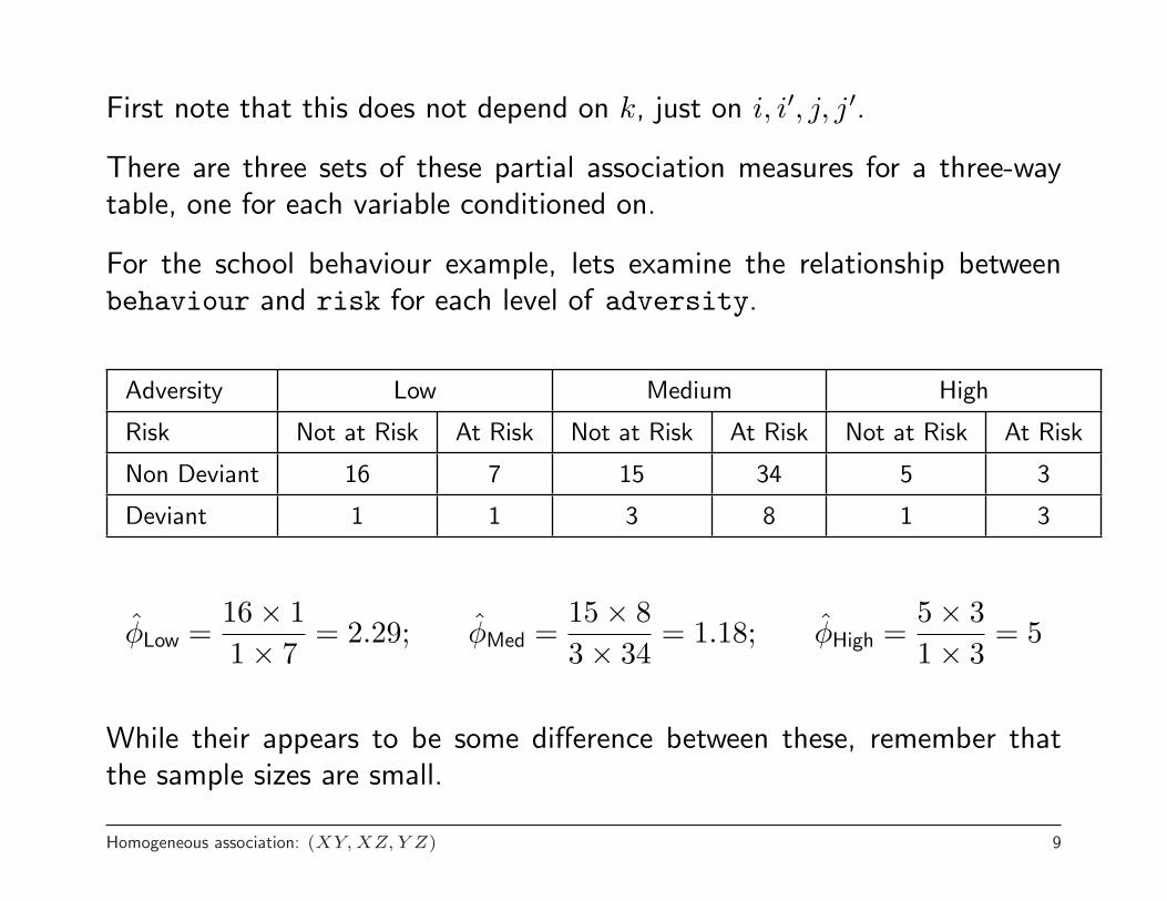
First note that this does not depend on k, just on i, i′, j, j′.

There are three sets of these partial association measures for a three-waytable, one for each variable conditioned on.

For the school behaviour example, lets examine the relationship betweenbehaviour and risk for each level of adversity.


Risk Not at Risk At Risk Not at Risk At Risk Not at Risk At Risk

Non Deviant 16 7 15 34 5 3

Deviant 1 1 3 8 1 3

φ̂Low =16× 11× 7

= 2.29; φ̂Med =15× 83× 34

= 1.18; φ̂High =5× 31× 3

= 5

While their appears to be some difference between these, remember thatthe sample sizes are small.



φ̂ 0.83 0.16 1.61

SE(φ̂) 1.24 0.70 1.19

For this model df = (I−1)(J−1)(K−1), which happens to be the numberof λs set to zero in the saturated log linear model.


Conditional independence: (XY,XZ), (XY, Y Z), or(XZ, Y Z)

There are three different models of this form, which can be derived bydropping the three-factor interactions and one set of two-factor interactions.

One of the possible forms (for the model (XY, Y Z)) is


j + λZk + λXY

ij + λY Zjk

in this case the λXY Zijk s and the λXZ

ik s are all set to zero.

The degrees of freedom for this model is (I − 1)(K− 1)J . Again this is thenumber of λs set to zero.

Models of this form correspond to conditional independence of the variables.For the example (XY, Y Z), X and Z are conditionally independent giventhe level of Y .

Conditional independence: (XY, XZ), (XY, Y Z), or (XZ, Y Z) 11

It can be shown that

P [X = xi, Z = zk|Y = yj] = P [X = xi|Y = yj]P [Z = zk|Y = yj]

for each level of Y under this model.

One way of thinking of this, if you look at the J different I × K tablesyou get by fixing the level of Y and classifying by X and Z, each of themexhibits independence.

So one consequence of this is that

P [X = xi, Y = yj, Z = zk] = P [X = xi|Y = yj]P [Z = zk|Y = yj]P [Y = yj]

(actually showing that this relationship holds proves the conditionalindependence assumption)

So given the labeling of X, Y , and Z, (XY, Y Z) corresponds to behaviourbeing independent of adversity given the risk status of the child.


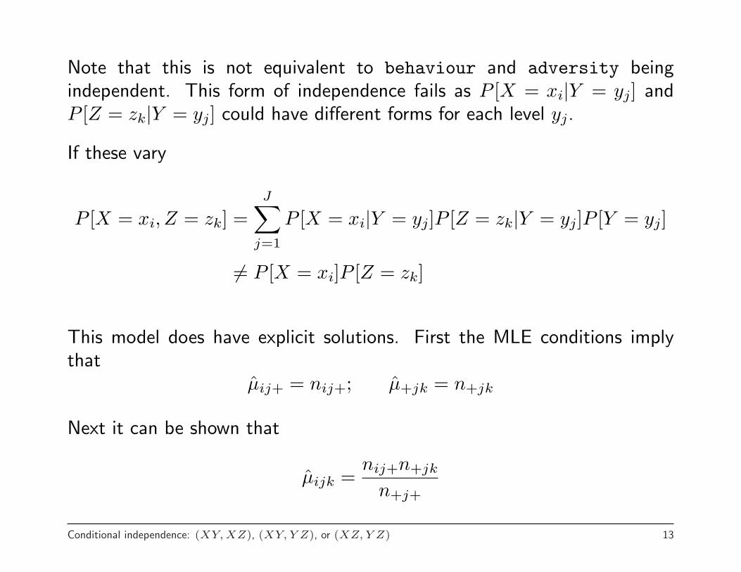
Note that this is not equivalent to behaviour and adversity beingindependent. This form of independence fails as P [X = xi|Y = yj] andP [Z = zk|Y = yj] could have different forms for each level yj.

If these vary

P [X = xi, Z = zk] =J∑

j=1

P [X = xi|Y = yj]P [Z = zk|Y = yj]P [Y = yj]

6= P [X = xi]P [Z = zk]

This model does have explicit solutions. First the MLE conditions implythat

µ̂ij+ = nij+; µ̂+jk = n+jk

Next it can be shown that

µ̂ijk =nij+n+jk

n+j+


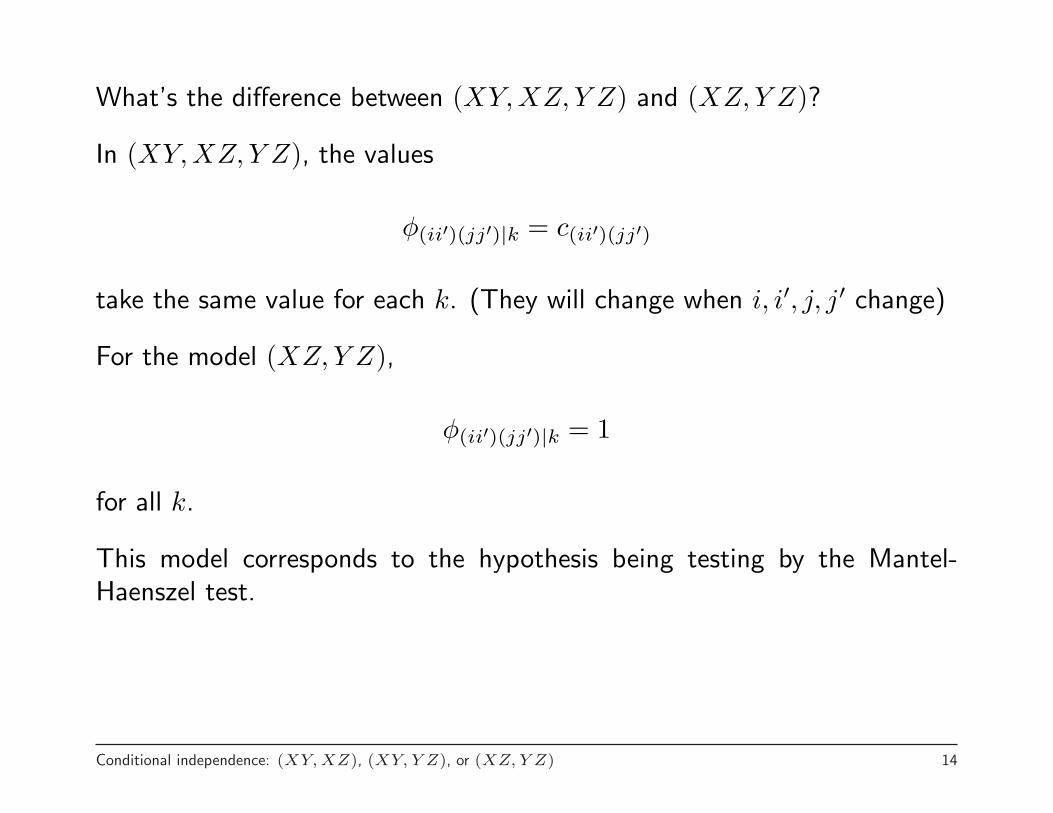
What’s the difference between (XY,XZ, Y Z) and (XZ, Y Z)?

In (XY,XZ, Y Z), the values

φ(ii′)(jj′)|k = c(ii′)(jj′)

take the same value for each k. (They will change when i, i′, j, j′ change)

For the model (XZ, Y Z),

φ(ii′)(jj′)|k = 1

for all k.

This model corresponds to the hypothesis being testing by the Mantel-Haenszel test.


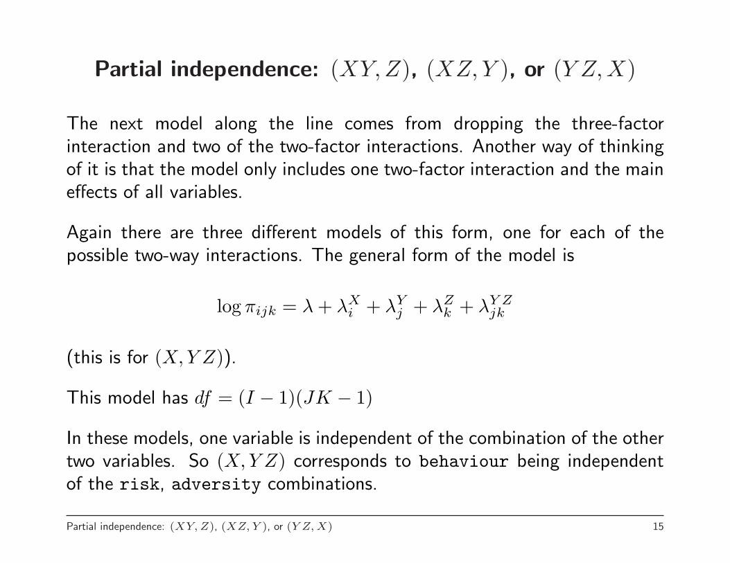
Partial independence: (XY,Z), (XZ, Y ), or (Y Z,X)

The next model along the line comes from dropping the three-factorinteraction and two of the two-factor interactions. Another way of thinkingof it is that the model only includes one two-factor interaction and the maineffects of all variables.

Again there are three different models of this form, one for each of thepossible two-way interactions. The general form of the model is


j + λZk + λY Z

jk

(this is for (X, Y Z)).

This model has df = (I − 1)(JK − 1)

In these models, one variable is independent of the combination of the othertwo variables. So (X,Y Z) corresponds to behaviour being independentof the risk, adversity combinations.

Partial independence: (XY, Z), (XZ, Y ), or (Y Z, X) 15

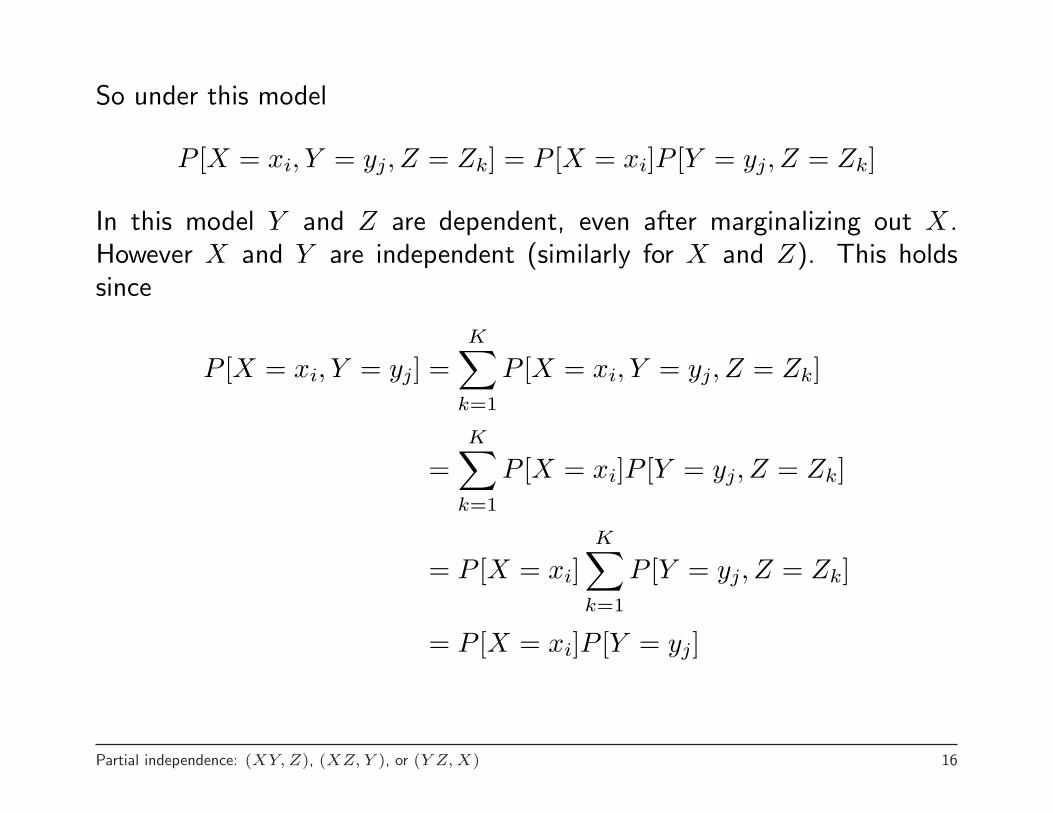
So under this model

P [X = xi, Y = yj, Z = Zk] = P [X = xi]P [Y = yj, Z = Zk]

In this model Y and Z are dependent, even after marginalizing out X.However X and Y are independent (similarly for X and Z). This holdssince

P [X = xi, Y = yj] =K∑

k=1

P [X = xi, Y = yj, Z = Zk]

=K∑

k=1

P [X = xi]P [Y = yj, Z = Zk]

= P [X = xi]K∑

k=1

P [Y = yj, Z = Zk]

= P [X = xi]P [Y = yj]


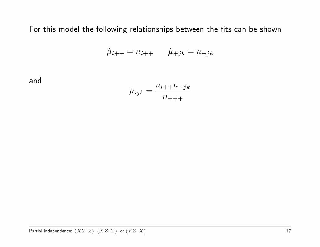
For this model the following relationships between the fits can be shown

µ̂i++ = ni++ µ̂+jk = n+jk

andµ̂ijk =

ni++n+jk

n+++


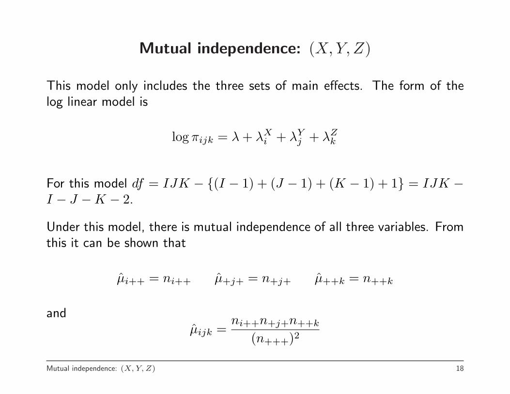
Mutual independence: (X,Y, Z)

This model only includes the three sets of main effects. The form of thelog linear model is


j + λZk

For this model df = IJK − {(I − 1) + (J − 1) + (K − 1) + 1} = IJK −I − J −K − 2.

Under this model, there is mutual independence of all three variables. Fromthis it can be shown that

µ̂i++ = ni++ µ̂+j+ = n+j+ µ̂++k = n++k

andµ̂ijk =

ni++n+j+n++k

(n+++)2

Mutual independence: (X, Y, Z) 18

Since all three variables are mutually independent, it follows that any pairmust be as well.

Mutual independence: (X, Y, Z) 19

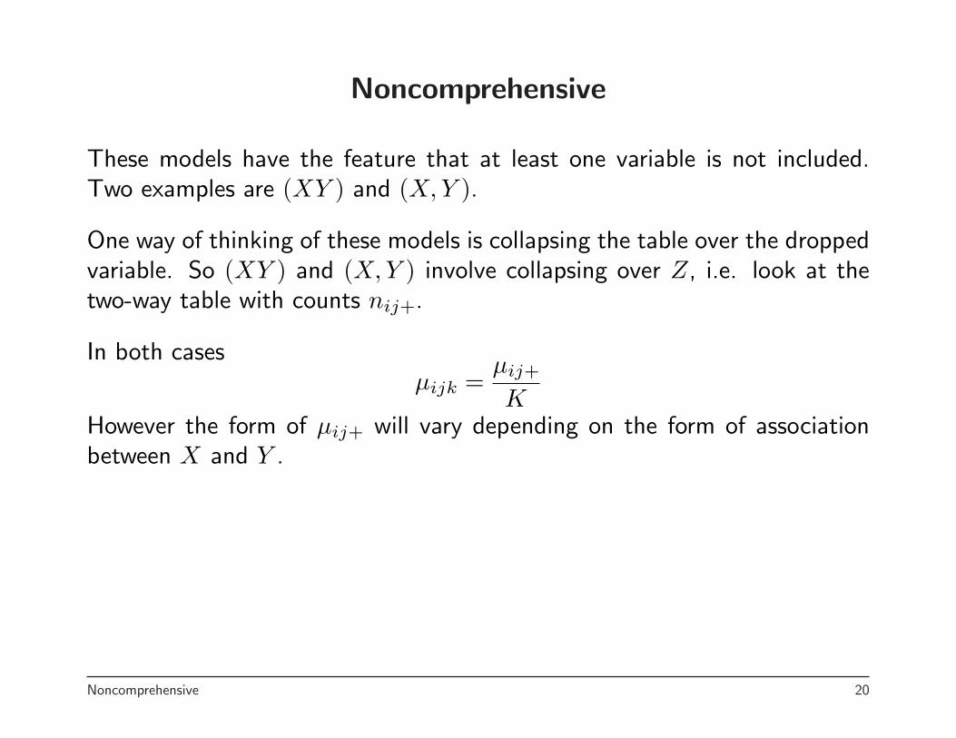
Noncomprehensive

These models have the feature that at least one variable is not included.Two examples are (XY ) and (X, Y ).

One way of thinking of these models is collapsing the table over the droppedvariable. So (XY ) and (X, Y ) involve collapsing over Z, i.e. look at thetwo-way table with counts nij+.

In both casesµijk =

µij+

KHowever the form of µij+ will vary depending on the form of associationbetween X and Y .

Noncomprehensive 20

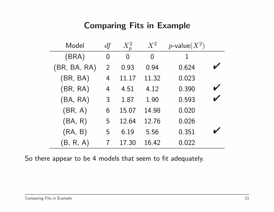
Comparing Fits in Example

Model df X2p X2 p-value(X2)

(BRA) 0 0 0 1

(BR, BA, RA) 2 0.93 0.94 0.624 "(BR, BA) 4 11.17 11.32 0.023

(BR, RA) 4 4.51 4.12 0.390 "(BA, RA) 3 1.87 1.90 0.593 "(BR, A) 6 15.07 14.98 0.020

(BA, R) 5 12.64 12.76 0.026

(RA, B) 5 6.19 5.56 0.351 "(B, R, A) 7 17.30 16.42 0.022

So there appear to be 4 models that seem to fit adequately.

Comparing Fits in Example 21

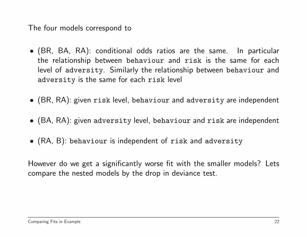
The four models correspond to

• (BR, BA, RA): conditional odds ratios are the same. In particularthe relationship between behaviour and risk is the same for eachlevel of adversity. Similarly the relationship between behaviour andadversity is the same for each risk level

• (BR, RA): given risk level, behaviour and adversity are independent

• (BA, RA): given adversity level, behaviour and risk are independent

• (RA, B): behaviour is independent of risk and adversity

However do we get a significantly worse fit with the smaller models? Letscompare the nested models by the drop in deviance test.


> anova(behave.xy.xz.yz, behave.xy.yz, test=’Chisq’)Analysis of Deviance Table

Model 1: n ~ (behaviour + risk + adversity)^2Model 2: n ~ behaviour * risk + risk * adversityResid. Df Resid. Dev Df Deviance P(>|Chi|)

1 2 0.94282 4 4.1180 -2 -3.1752 0.2044

> anova(behave.xy.xz.yz, behave.xz.yz, test=’Chisq’)Analysis of Deviance Table

Model 1: n ~ (behaviour + risk + adversity)^2Model 2: n ~ behaviour * adversity + risk * adversityResid. Df Resid. Dev Df Deviance P(>|Chi|)

1 2 0.942852 3 1.90396 -1 -0.96112 0.32691

These two tests imply we don’t need all three interactions


> anova(behave.xy.xz.yz, behave.yz.x, test=’Chisq’)Analysis of Deviance Table

Model 1: n ~ (behaviour + risk + adversity)^2Model 2: n ~ risk * adversity + behaviourResid. Df Resid. Dev Df Deviance P(>|Chi|)

1 2 0.94282 5 5.5603 -3 -4.6175 0.2020

> anova(behave.xy.yz, behave.yz.x, test=’Chisq’)Analysis of Deviance Table

Model 1: n ~ behaviour * risk + risk * adversityModel 2: n ~ risk * adversity + behaviourResid. Df Resid. Dev Df Deviance P(>|Chi|)

1 4 4.11802 5 5.5603 -1 -1.4423 0.2298


> anova(behave.xz.yz, behave.yz.x, test=’Chisq’)Analysis of Deviance Table

Model 1: n ~ behaviour * adversity + risk * adversityModel 2: n ~ risk * adversity + behaviourResid. Df Resid. Dev Df Deviance P(>|Chi|)

1 3 1.90402 5 5.5603 -2 -3.6563 0.1607

These three tests imply that the partial independence seems reasonable.

The reason for doing the model comparisons here in addition to the goodnessof fit tests is that drop in deviance tests tend to give better informationabout the significance of fits.

It is possible to have two nested models, both with insignficant goodnessof fit tests, but the drop in deviance test suggest that the smaller model isnot adequate for describing the situation.


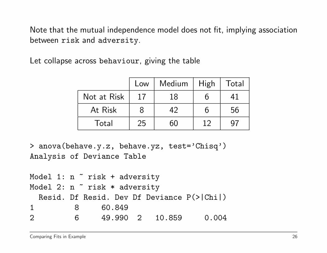
Note that the mutual independence model does not fit, implying associationbetween risk and adversity.

Let collapse across behaviour, giving the table

Low Medium High Total

Not at Risk 17 18 6 41

At Risk 8 42 6 56

Total 25 60 12 97

> anova(behave.y.z, behave.yz, test=’Chisq’)Analysis of Deviance Table

Model 1: n ~ risk + adversityModel 2: n ~ risk * adversityResid. Df Resid. Dev Df Deviance P(>|Chi|)

1 8 60.8492 6 49.990 2 10.859 0.004


This implies that there is an association between risk and adversity.

Note that the test done above is equivalent to the test

> anova(behave.x.y.z, behave.yz.x, test=’Chisq’)Analysis of Deviance Table

Model 1: n ~ behaviour + risk + adversityModel 2: n ~ risk * adversity + behaviourResid. Df Resid. Dev Df Deviance P(>|Chi|)

1 7 16.41922 5 5.5603 2 10.8589 0.0044

This is an example showing that it ok to collapse across a variable that isindependent of the rest.


Describing Independence Relationships Graphically

There is an approach to describing the independence relationships in amodel based on graph theory. The set of hierarchical log linear modelsfor describing contingency tables are examples of graphical models, whoseprobability structure can be described by a graph.

The idea is that the factors in a model are used to give the nodes of a graphand interaction terms in the model give the edges.

Consider the model (XY, Y Z). This can bedescribed by the graph,

Describing Independence Relationships Graphically 28

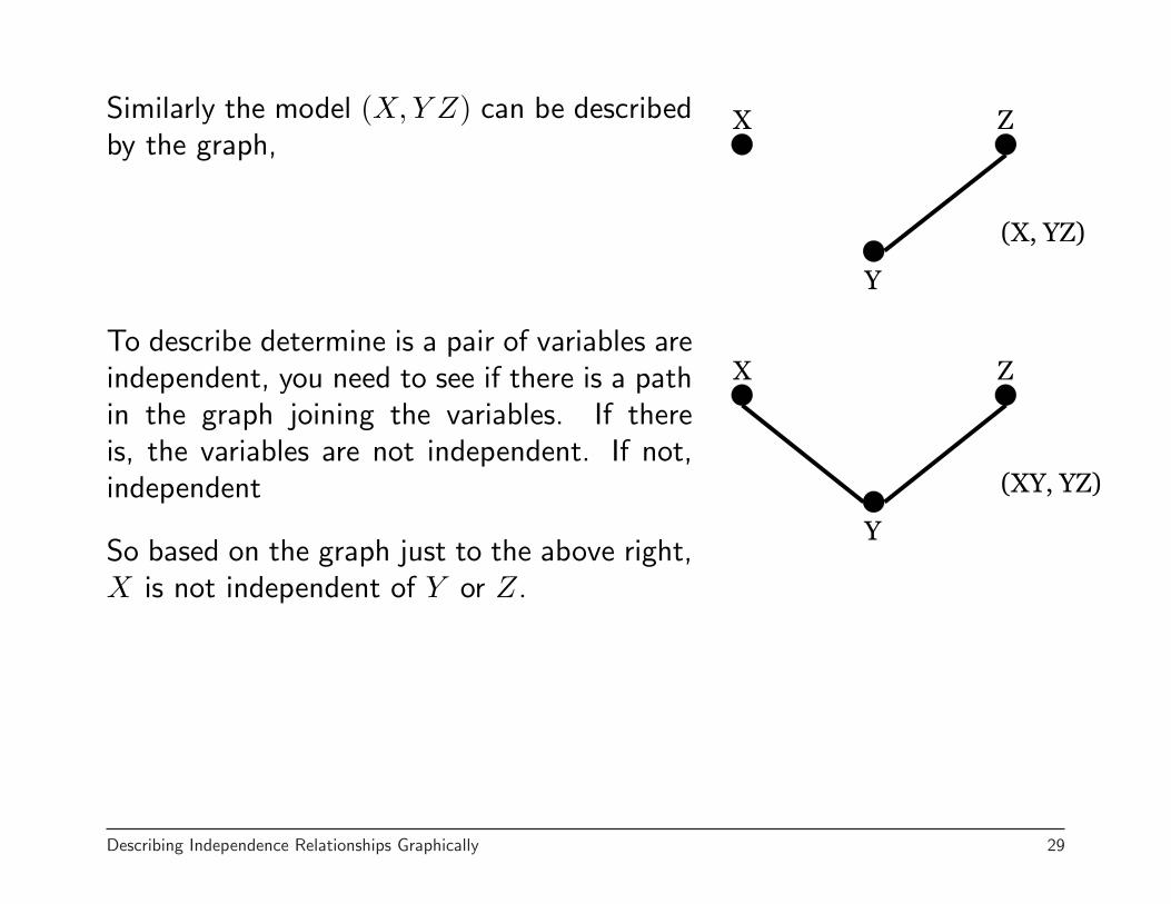
Similarly the model (X,Y Z) can be describedby the graph,

To describe determine is a pair of variables areindependent, you need to see if there is a pathin the graph joining the variables. If thereis, the variables are not independent. If not,independent

So based on the graph just to the above right,X is not independent of Y or Z.


However for this model, we can see that X isindependent of Y and Z, but that Y and Zare associated.

Conditional independence is examined by looking to see if a set of nodesseparate two other nodes (or two other sets of nodes).

In this graph, the nodes for X and Zare separated by the nodes Y and W .So this graph corresponds to X andZ being conditionally independent,given Y and W .

However X is not conditionallyindependent of Z given only Y sinceI can go from X to Z without havingto go through the conditioning set.


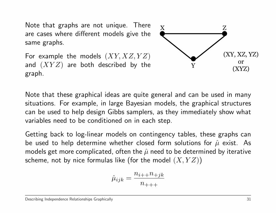
Note that graphs are not unique. Thereare cases where different models give thesame graphs.

For example the models (XY,XZ, Y Z)and (XY Z) are both described by thegraph.

Note that these graphical ideas are quite general and can be used in manysituations. For example, in large Bayesian models, the graphical structurescan be used to help design Gibbs samplers, as they immediately show whatvariables need to be conditioned on in each step.

Getting back to log-linear models on contingency tables, these graphs canbe used to help determine whether closed form solutions for µ̂ exist. Asmodels get more complicated, often the µ̂ need to be determined by iterativescheme, not by nice formulas like (for the model (X,Y Z))

µ̂ijk =ni++n+jk

n+++


three-way contingency tables - mark · pdf filedeviant 1 1 3 8 1 3 three-way contingency...

Documents