threshold signals
TRANSCRIPT
CHAPTER 1
I INTRODUCTION
The fundamental process in the reception of electromagnetic signalsis to make perceptible to the human observer certain features of theincoming electromagnetic radiation. Since perception is the acquisitionof information, these features may be called “intelligence” or “informa-tion.” The electromagnetic wave may contain this information in manyways; the particular method used to abstract it and make it perceptibledepends upon the structure of the original radiation.
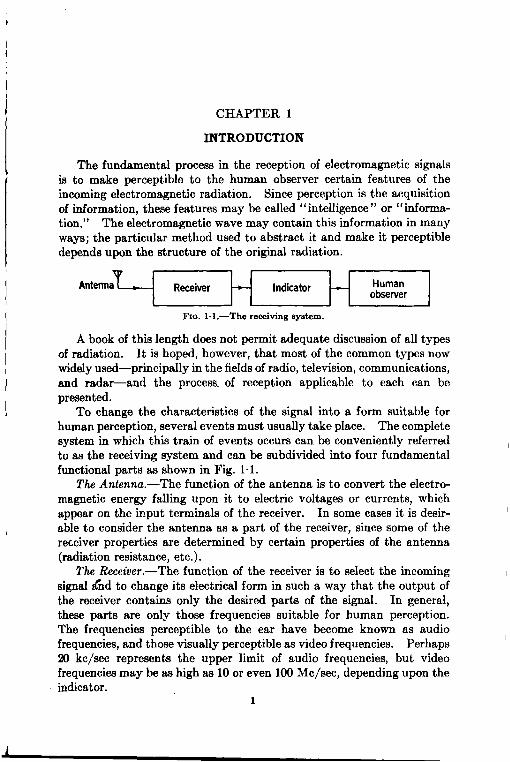
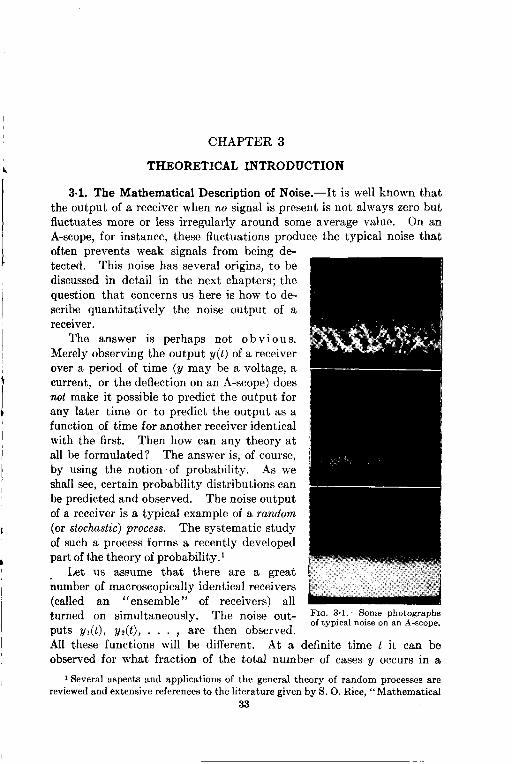
Antenna - Indicator — Humanobserver
FIG. l.l.—The receiving system.
A book of this length does not permit adequate discussion of all typesof radiation. It is hoped, however, that most of the common types nowwidely used—principally in the fields of radio, television, communications,and radar—and the process. of reception applicable to each can bepresented.
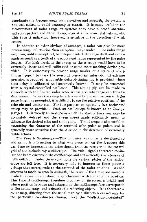
b To change the characteristics of the signal into a form suitable forhuman perception, several events must usually take place. The completesystem in which this train of events occurs can be conveniently referredto as the receiving system and can be subdivided into four fundamentalfunctional parts aa shown in Fig. 1-1.
The Antennu.-The function of the antenna is to convert the electro-magnetic energy falling upon it to electric voltages or currents, whichappear on the input terminals of the receiver. In some cases it is desir-able to consider the antenna as a part of the receiver, since some of thereceiver properties are determined by certain properties of the antenna(radiation resistance, etc.).
The Receiver.—The function of the receiver is to select the incomingsignal rfindto change its electrical form in such a way that the output ofthe receiver contains only the desired parts of the signal. In general,these parts are only those frequencies suitable for human perception.The frequencies perceptible to the ear have become known as audiofrequencies, and those visually perceptible as video frequencies. Perhaps20 kc/see represents the upper limit of audio frequencies, but videofrequencies may be as high as 10 or even 100 Me/see, depending upon theindicator.
1
J
I
2 INTRODUCTION
In addition to frequency selection and frequency changing, thereceiver must also provide amplification. The incoming radiation isordinarily feeble and must be greatly amplified in order to actuate theindicator. The total required power amplification in the receiver may forsome applications be as high as 1015. Noise and interference limitationsprevent its being made as high as one pleases.
The main purpose of this book is to discuss these fundamentallimitations and to determine the effect of the various parameters in thereceiving system on the detectability of signals.
The incoming signal may be of several types. It therefore followsthat the characteristics of the receiver itself must be specialized and aredetermined by the type of information required from the incoming signal.Because of the general complexity of receivers, furthermore, there areusually several types which perform essentially the same function butwhich may differ in their limitations. The various receiver types aremost conveniently discussed in conjunction with the kinds of signal forwhich they are designed.
The Indicator.-The output of the receiver consists of voltages orcurrents containing those desired frequencies in the sigi~althat are suitablefor human perception. The function of the indicator is to convert thesevoltages or currents into audio sound waves or perhaps light patternsthat the human observer can perceive. Common forms of indicators arethe loudspeaker for radio reception and the cathode-ray oscilloscope forthe reception of video signals. There are obviously many ways in whichthis indication can be presented to the observer. Several alternativemethods of indication are mentioned in Sec. 2.6.
The Human Observer.—Human perception of certain signal propertiesdepends not only on what is presented to the observer on the indicatorbut also on what use he makes of that information. Perception sensitiv-ity will therefore depend on characteristics of the human observer thatare not always flexible. The ear, eye, and brain are subject to certainlimitations that in many cases restrict the assimilation of useful informa-tion. The signal information may, for example, be spread out over atime so long that the human observer cannot integrate the information.His memory is limited; hence he can effectively use information onlywithin a limited time. The human observer must therefore be consideredas part of the receiving system. It is even sometimes convenient toexpres%human limitations in terms of certain indicator or receiver param-eters. In the example just mentioned the human memory time can berelated to an equivalent time constant or bandwidth in the receiver.Similarly, properties of the ear, such as its bandwidth or frequencysensitivity, will be similar to the electrical properties of equivalent filtersin the receiver. .
I CHAPTER 2
I TYPES OF SIGNALS AND METHODS FOR THEIR RECEPTION\
[CONTINUOUS-WAVE SIGNALS
2.1. Unmodulated Continuous-wave Signal.-The simplest form ofsignal is the so-called unmodulated continuous wave. Thic io the namegiven an electromagnetic wave in which the magnitude of the alternatingelectric field strength is constant in time; for example,
I & = &oCos zr(fot + so). (1)
I Both 80 and the frequency f, are constant. The constant CXOdefines theI sero of the time scale, so that
1 & = .SOC0527rao at time t = O.
The characteristics of a c-w signal are therefore constant amplitude, con-stant frequency, and particular phase at t = O. These conditions cannot
~
be met by any known electromagnetic radiation, since in such a case 80must have existed throughout all time. Likewise, if &O is not constant,there will be more than a single frequency associated with the wave.This will be shown in Sec. 2.2. Therefore there is no such thing as amonochromatic c-w signal. If 80 is only slowly varying with time, how-ever, &will be very nearly monochromatic in frequency. It is convenientto refer to &O as the signal-carrier amplitude. The carrier frequency isessentially monochromatic or, more specifically, will contain a frequencyband small with respect to the lowest desired audio or video frequency.
The information that can be abstracted from this c-w carrier is verymeager. One can only inquire, does the carrier exist or not? And to
r obtain the answer even to this question may take a long time. Toimprove the rate at which information can be transmitted, some param-eter of the original c-w signal is varied with time or modulated. In theusual modulation of a c-w carrier, either a variation of the amplitude(amplitude modulation), a variation of the frequency (frequency modula-tion), or a variation of the phase off, (phase modulation) may be made.These will be discussed in the next section. The modulating frequenciesare, for convenience, those which ultimately become the indicator fre-quencies, that is, audio or video frequencies, since the human observermost easily abstracts information from them.
The modulating function may be represented by F(t). For audio3
4 TYPES OF SIGNALS AND THEIR RECEPTION [SEC.2.1
movulations one wishes to make F(t) correspond to the instantaneouspressure of the modulating sound wave. Since this pressure is normally1 atm in the absence of sound, it is necessary that F(t) be a constantdifferent from zero in the absence of modulation. The sound pressuremay vary upward or downward with audio modulation. For a singleaudio tone, therefore, F(t) may be represented by
1 + c Cos 2T(pt + B),
where ~ < 1.For a complex audio sound, F(t) may be represented
1+2
C. cm 27(PJ + /3.),,n
where the values of the c’s are such that F(t) never becomes negative.If the original sound wave is feeble, the fluctuating part of F(t) may beamplified but must not be made so great that F(t) becomes negative. IThis amplification is always desirable in practice, since one wishes tomake the part of F(t) that contains the intelligence as large as possiblewith respect to the constant part or carrier that contains essentially noinformation. For a single audio tone where
F(t) = 1 + c COS%@ + ~), (2)
it is convenient to refer to e as the fractional modulation or to 100~ as themodulation percentage.
If the modulating wave is to represent some other desired character-istic, such as light intensity for television transmission, a constant carrieramplitude may not be necessary. Unlike the sound-wave case, wherewithin the wave itself the pressure can be less than that with no sound,the light intensities reproduced by currents in a photoelectric cell arenever less than those produced with no light. In other words, it is nevernecessary to modulate downward from the zero intensity case. ThusF(t) can represent directly the light-intensity values when the photo-electric cell is scanned over the televised scene. A carrier is no longerrequired to ensure that the complete modulating function be positive.In this case the terms “fractional modulation” and “modulation per-centage” are meaningless. The function F(t) can be made as large asone pleases by amplification, until the peak values exceed that whichcan be supplied in transmission.
LThis restriction is necessary because, az will be shown later in the text, devicesdesigned for reproducing F(t) actually give the absolute value of F(t); therefore, in orderto reproduce F(t) without distortion, its sign must never reverse.
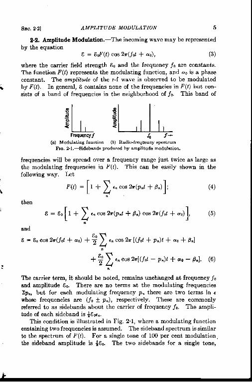
SEC. 2.2] AMPLITUDE MODULATION 5
2.2. Amplitude Modulation.-The incoming wave maybe representedby the equation
& = &#(t) Cos %r(jot + so), (3)
where the carrier field strength 80 and the frequency jo are constants.The function F(t) represents the modulating function, and aO is a phaseconstant. The amplitude of the r-f wave is observed to be modulated
k by F(t). In general, & contains none of the frequencies in F(t)but con-sists of a band of frequencies in the neighborhood of fo. ‘Ms band of
L_ LllLFrequency & f-
(a) Modulating function (b) Radio-frequencyspectrumFm. 2.1.-Sklebands producedby amplitudemodulation.
frequencies will be spread over a frequency range just twice as large asthe modulating frequencies in F(t). This can be easily shown in thefollowing way. Let
[z,F(t) = 1 +1
% WE ~(p.t + (3.) ;n
(4)
[z&=&ol+1
6. Cos %r(p.t + p.) Cos 2T(f0t + ~o) , (5)
nand
& = &, Cos *(jot + ao) + ; zC. COS% [(jOt + Pn)t + ~0 + 8.1
n
+$ zc. COS%[(jot – p.)t + a, – /%]. (6)
: n
The carrier term, it should be noted, remains unchanged at frequency joand amplitude &o. There are no terms at the modulating frequencieszpn, but for each modulating frequency p. there are two terms in ●
whose frequencies are (jo f pJ, respective y. These are commonlyreferred to as sidebands about the carrier of frequency jo. The ampli-tude of each sideband is i&ti..
This condition is illustrated in Fig. 2“1, where a modulating functioncontaining two frequencies is assumed. The sideband spectrum is similarto the spectrum of F(t). For a single tone of 100 per cent modulation,the sideband amplitude is ~&O. The two sidebands for a single tone,
6 TYPES OF SIGNALS’ AND THEIR RECEPTION [SEC.2.2
therefore, for any fractional modulation c contain a total power equal to{2/2 times the carrier power.
A common example of the a-m wave is that used in ordinary broadcastradio transmission. In this case F(t) is simply the audio or speech wave.The input to the receiver from the antenna is essentially an electricvoltage t% that is linearly proportional to the radio-wave field strength &.The function of the receiver is to reproduce the modulating audio functionF(t) from the input voltage sti. The reproduction can be accomplished
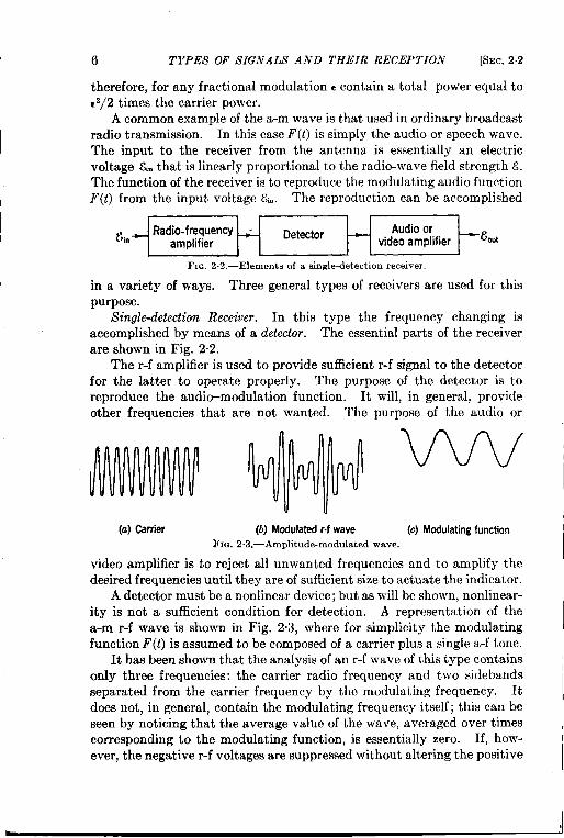
I!;in* Radio-frequency< Detector Audioor—amplifier videoamplifier —-Gout
FIG. 2.2.—Elementsof a single-detectionreceiver.I
in a variety of ways. Three general types of receivers are used for thispurpose.
Singledetection Receiwer.—In this type the frequency changing isaccomplished by means of a detector. The essential parts of the receiverare shown in Fig. 2“2.
The r-f amplifier is used to provide sufficient r-f signal to the detectorfor the latter to operate properly. The purpose of the detector is toreproduce the audio-modulation function. It will, in general, provideother frequencies that are not wanted. The purpose of the audio or
(a) Carrier (b) Modulatedr-fwave (c) ModulatingfunctionFm. 2.3.—Amplitude-modulatedwave.
video amplifier is to reject all unwanted frequencies and to amplify thedesired frequencies until they are of sufficient size to actuate the indicator.
A detector must be a nonlinear device; but as will be shown, nonlinear-ity is not a sufficient condition for detection. A representation of thea-m r-f wave is shown in Fig. 2.3, where for simplicity the modulatingfunction F(t) is assumed to be composed of a carrier plus a single a-f tone.
It has been shown that the analysis of an r-f wave of this type containsonly three frequencies: the carrier radio frequency and two sidebandsseparated from the carrier frequency by the modulating frequency. Itdoes not, in general, contain the modulating frequent y itself; this can beseen by noticing that the average value of the wave, averaged over timescorresponding to the modulating function, is essentially zero. If, how-ever, the negative r-f voltages are suppressed without altering the positive
I
SEC.2-2] AMPLITUDE MODULATION 7
voltages, then the average value of the wave will vary according to themodulating function, and detection will occur. Detection will therefore
result from a nonlinear device that amplifies negative voltages differentlyfrom positive voltages. If the input and output voltages of this non-linear device are represented by the general power series
$&t . zgn&?., (7)
n
detection takes place only because of the presence of the even terms;thatis, n =2,4,”””. The odd terms do not contribute to detection,since for these terms negative or positive input voltages produce negativeor positive output voltages, respectively. Thus a pure cubic-lawnonlinear device will not be a detector.
Perhaps the simplest detector is the s~called squardaw device inwhich the output voltage is proportional to the square of the inputvoltage;
.% = ge. (8)
As shown previously, ~ and F(t) may “be generally represented by theequations
& = &oF(t) Cos 2m(.fot+ so), (9)
[zF(t) = 1 +
16. Cos 21r(p=t+ l%) , (lo)
nso that
& = gwvt) c@J22djot + a,), (11)or
[z 1[2 1 + Cos 4r(f0t + a,)&t= g&; 1+ c. Cos zr(pnt + /%) 2 1
7 (12)
nfrom which
“=g’’[1+2z’nc0s%(pn’+~n)n
+ n CnqCos 2T(pnt + /9.) Cos %(pIt + /%)1n 1
[ 1I + COSzWd + ao) . (13)2
The frequencies present in 8~, are, therefore, zero (d-c term), p., 2Pfl,p. + pl, p“ – pl, 2j0, 2.fo f p., 2f0 f 2p., 2j0 + (p. + pi), and2f0 + (p. – pJ. The only terms of interest are the p. terms and,incidentally, the terms 2p~, pm+ PI, and p. — pt. These four general
8 TYPES OF SIGNALS AND THEIR RECEPTION [SEC.2.2
terms (apart from the d-c term) are the only ones that will fall in the passband of the audio or video amplifier. They have amplitude functions atthe output of the square-law detector given by g&~c.,g&~(c~/4), g&3(c.cJ4),and g&~(c~ct/4), respectively. Of these four terms the first is the desiredone, the second represents second harmonic distortion, and the third andfourth represent cross-modulation products. In general, detectionproduces cross-modulation terms and harmonic distortion, but it will benoticed in the preceding example that the amplitudes of these undesiredterms relative to the desired one are usually quite small. If the coeffi-cients are small (small modulation percentage), these terms may beneglected in comparison with the desired p. terms.
In principle the a-m wave can be detected without producing dis-tortions in the modulating function even when the fractional modulationis high. This is accomplished by means of the so-called linear detector,which passes or amplifies all voltages of one polarity linearly but shows nooutput at all for input voltages of the opposite polarity. The averageoutput voltage is therefore linearly proportional to the envelope of ther-f wave, which, of course, is related to the modulating function F(t)itself. The envelope of the modulated wave is not strictly F(t) butrepresents F(t) only if a sufficient carrier exists to ensure that F(t) isalways a positive function. The envelope, in general, represents theabsolute value of F(t). The significance of this will be brought out moreclearly in later chapters, but this fact ultimately leads to possibilities ofcross modulation even with the envelope detector.
Even though this linear, or envelope, detector reproduces F(t) prop-erly, its characteristic curve is extremely nonlinear at zero voltage. Atthis point the curvature is infinite. Practical detectors are limited inthk curvature; therefore the region of small voltages is not similar to thatof an ideal linear detector. For this reason practical linear detectorsalways operate at high voltage levels and must therefore be preceded byconsiderable r-f amplification. Examples of such detectors are diodedetectors, infinite-impedance triodes, and high-level anode-bend detectors.
Because of limited curvature in characteristics, low-level detectorsare almost invariably square law; examples are crystal detectors, low-level diodes, etc. If desired, high-level detectors can be made squarelaw, but ordinarily linear detectors are preferred.
Few receivers in common use are of the simple type shown in Fig. 2.3.The difficulties with the singl~detection receiver are usually associatedwith the r-f amplification. The r-f amplifier must generally be tunedto the desired r-f signal and have considerable over-all gain. It is usuallydifficult to construct a tuned r-f amplifier of several stages with txoDerstability, selectivity, and tuning range. In widespread ~se is areceiver, the superheterodyne, that overcomes these difficulties.
t;pi of
●
SEC.2.2] AMPLITUDE MODULATION 9
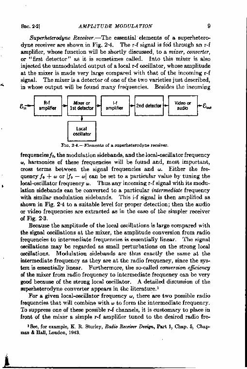
Superhetemd~ Receiver.—The essential elements of a superhetero-dyne receiver are shown in Fig. 2“4. The r-f signal is fdd through an r-famplifier, whose function will be shortly discussed, to a mixer, converter,or “first detector” as it is sometimes called. Into this mixer is alsoinjected the unmodulated output of a local r-f oscillator, whose amplitudeat the mixer is made very large compared with that of the incoming r-fsignal. The mixer is a detector of one of the two varieties just described,
4 in whose output will be found many frequencies. Besides the incoming
&i~ ‘-f Mixeror l-f * 2nddetector+ Videooramphfier + 1stdetector+ amplifwr audio -8 w
A
ILocaloscillatorI
I I~G. 2.4.—Elementsof a superheterodynereceiver,
frequencies jo, the modulation sidebands, and the local-oscillator frequencyu, harmonics of these frequencies will be found and, most important,cross terms between the signal frequencies and u. Either the fre-quency fO + u or Ijo – COIcan be set to a particular value by tuning the
* local-oscillator frequency ~. Thus any incoming r-f signal with its modu-lation sidebands can be converted to a particular intermediate frequencywith similar modulation sidebands. This i-f signal is then amplified asshown in Fig. 2“4 to a suitable level for proper detection; then the audioor video frequencies are extracted as in the case of the simpler receiverof Fig. 2.3.
Because the amplitude of the local oscillations is large compared withthe signal oscillations at the mixer, the amplitude conversion from radiofrequencies to intermediate frequencies is essentially linear. The signaloscillations may be regarded as small perturbations on the strong localoscillations. Modulation sidebands are thus exactlv the same at theintermediate frequency as they are at the radio frequency, since the sys-tem is essentially linear. Furthermore, the so-called conversion ejicienqof the mixer from radio frequency to intermediate frequency can be verygood because of the strong local oscillator. A detailed discussion of thesuperheterodyne converter appears in the literature. 1
For a given local-oscillator frequency u, there are two possible radiofrequencies that will combine with w to form the intermediate frermenc~.To ~uppress one of these possible r-f channels, it is customary to place infront of the mixer a simple r-f amplifier tuned to the desired radio fr~
1&e, for example,K. R. Sturley,Radio Rec&er DeaigrJ, Part 1, Chap. 5, Chap-man& Hall, London, 1943.
10 TYPES OF SIGNALS AND THEIR RECEPTION [SEC.2.2
quency (see Fig. 2.4). This process is called radio-frequency preelection.
For some applications, however, this precaution is not essential.The principal advantages of a superheterodyne receiver over the
simple type shown in Fig. 2’3 are the following:
1. Since most of the gain may be situated in the fixed i-f amplifier,the selectivity and gain of the receiver are essentially independentof the radio frequency. .
2. The tuning control (essentially by the local-oscillator frequency)is much simpler than for a gang-tuned series of r-f amplifiers.
3. For the reception of very-high-frequency waves, high receivergain is much easier to obtain at the relatively low intermediatefrequency.
It is possible to extend the treatment to receiver systems that containseveral mixers. Each process of heterodyne detection or conversion, thatis, one involving the mixing of r-f signal with a local oscillator, will yielda new i-f signal whose amplitude function is linearly proportional to theamplitude function of the original r-f signal. Many superheterodynereceivers have been built involving two heterodyne detectors. The r-fsignal is first converted by means of the first local oscillator to a relativelyhigh first intermediate frequency, which is later converted to a secondlower intermediate frequency by a second fixed-tuned lo~al oscillatorbefore final detection takes place. The advantages claimed for thedouble-superheterodyne receiver are twofold. (1) The first intermediatefrequency can be made high with the result that the r-f preelection (pre-ceding the first mixing) becomes much more effective. (2) The highover-all gain in the receiver can be divided between the two intermediatefrequencies; hence at no time is it necessary to construct an amplifier atone frequency of extreme over-all gain. This process minimizes thedanger of feedback and instability in the amplifier. The principal dis-advantage of the double-heterodyne receiver is, of course, its relativecomplexity.
No matter how many heterodyne detectors tire used in a receiver,however, the over-all conversion from r-f voltage to final i-f voltage islinear; if the pass band of the receiver is great enough, the signal amplifica-tion will be independent of the modulating frequency. In other words,if the original r-f signal voltage at the input of the receiver is representedby
&h = &oF(t) Cos 27r(jd + so), (14)
where, as before, F(t)is the modulating function and ~0 is the radio fre-quency, the voltage in the last i-f amplifier will be given by the expressiori
&i-fa &~.fF(t)COS%(hd + T), (15)
SEC.2-2] AMPLITUDE MODULATION 11
where ho is the last intermediate frequency and Y is a phase constantdetermined by aO and the phases of the local oscillators. Because of thiscompletely linear relationship, all problems encountered in a superhetero-dyne receiver can usually be treated in terms of the i-f amplifier and somesimple conversion quantity representative of the mixer itself. Forexample, in problems of noise this quantity, as will be shown in Chap. 5,has to do essentially with the conversion
* eficiency of the mixer and the noise fig- ~-f
s
R-f Audioure of the i-f amplifier. input oscillator output
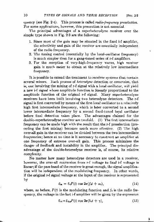
Superregenerative Receiver.-A super-regenerative receiver is one in which the Oscuaa.process of great amplification and theprocess of detection are accomplished
switch
within one vacuum tube. The mainFIG. 2.5.—Elements of a super-
regenerative receiver.purpose, therefore, is to provide a high-gain sensitive receiver by the use of a minimum number of tubes. Thechief drawbacks of such a receiver are (1) the dificulty of making andmaintaining proper adjustment and (2) nonlinear reproduction ordistortion.
The method by which high gain and detection are accomplished isshown in its essential form in Fig. 2.5. The r-f input is connected to atube whose circuits are tuned to the desired signal frequency. AnIoscillation control switch is used to put this tube into an oscillating condi-tion. As soon as this switch makes a connection. the condition foroscillation is established, but the oscillations themselves are not created.They begin to build up, however, from the initial voltage found at theoscillator input (signal voltage in general) and if allowed to proceed wouldbuild up to a steady value determined by the power-output capabilitiesof the oscillator tube. If the gain of the oscillator is constant during thebuildup (which implies linear amplification), the oscillation buildup willfollow a rising exponential curve that will eventually flatten off at thesaturation output value.
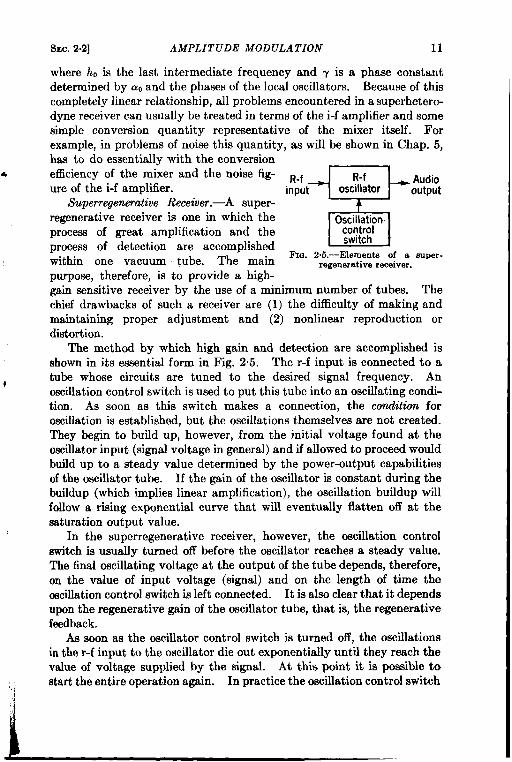
In the superregenerative receiver, however, the oscillation controlswitch is usually turned off before the oscillator reaches a steady value.The final oscillating voltage at the output of the tube depends, therefore,on the value of input voltage (signal) and on the length of time theoscillation control switch is left connected. It is also clear that it dependsupon the regenerative gain of the oscillator tube, that is, the regenerativefeedback.
As soon as the oscillator control switch is turned off, the oscillationsin the r-f input to the oscillator die out exponentially until they reach thevalue of voltage supplied by the signal. At this point it is possible tostart the entire operation again. In practice the oscillation control switch{,;
‘/
12 TYPES OF SIGNALS AND THEIR RECEPTION ~Ec, 2.2
is turned on and off successively at a high rate called the “quench”or “interruption” frequency. The control switch is in actual practice aquench oscillator that controls the feedback in the r-f oscillator. Thequenching rate must be high, since the sampling of the signal voltageat the start of oscillation buildup must be rapid compared with themodulation frequency. The input and output voltages in the super-regenerative r-f oscillator are shown diagrammatically in Fig. 2“6.
Inputvoltage
FIG. 2.6.—Input and output voltages in a superregenerativereceiver.
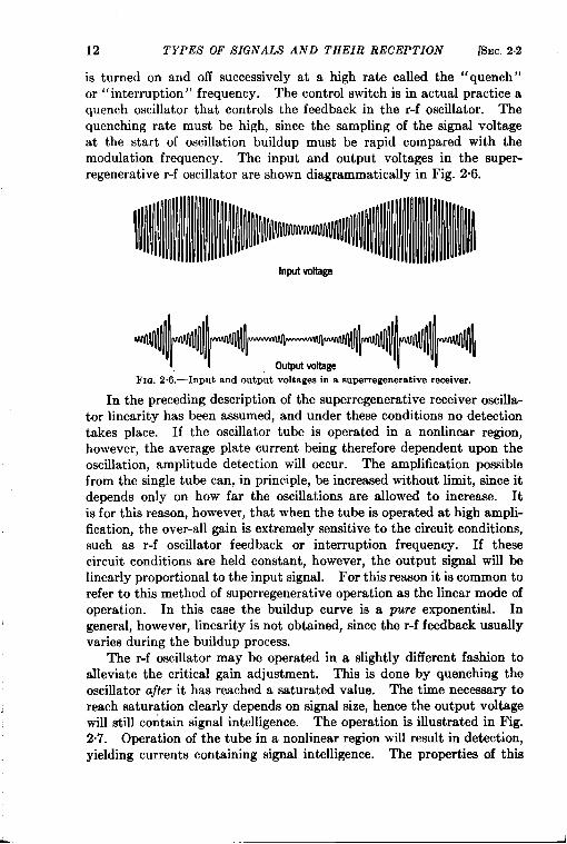
In the preceding description of the superregenerative receiver oscilla-tor linearity has been assumed, and under these conditions no detectiontakes place. If the oscillator tube is operated in a nonlinear region,however, the average plate current being therefore dependent upon theoscillation, amplitude detection will occur. The amplification possiblefrom the single tube can, in principle, be increased without limit, since itdepends only on how far the oscillations are allowed to increase. Itis for this reason, however, that when the tube is operated at high ampli-fication, the over-all gain is extremely sensitive to the circuit conditions,such as r-f oscillator feedback or interruption frequency. If thesecircuit conditions are held constant, however, the output signal will belinearly proportional to the input signal. For this reason it is common torefer to this method of superregenerative operation as the linear mode ofoperation. In this case the buildup curve is a pure exponential. Ingeneral, however, linearity is not obtained, since the r-f feedback usuallyvaries during the buildup process.
The r-f oscillator may be operated in a slightly different fashion toalleviate the critical gain adjustment. This is done by quenching theoscillator ajter it has reached a saturated value. The time necessary toreach saturation clearly depends on signal size, hence the output voltagewill still contain signal intelligence. The operation is illustrated in Fig.2.7. Operation of the tube in a nonlinear region will result in detection,yielding currents containing signal intelligence. The properties of this
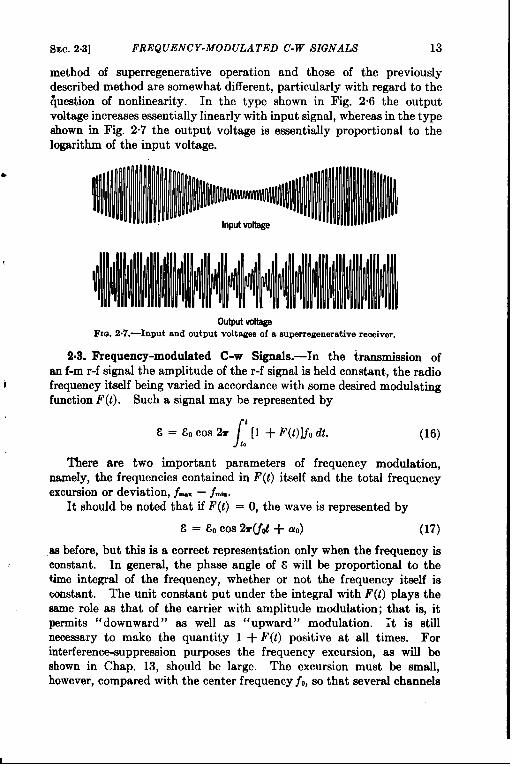
SEC. 2.3] FREQUENCY-MODULATED C-W SIGNALS 13
method of superregenerative operation and those of the previouslydescribed method are somewhat different, particularly with regard to the~uestion of nonlinearity. In the type shown in Fig. 26 the outputvoltage increases essentially linearly with input simal, whereas in the tv~show; in Fig. 2“7 the output vol~age is e~nti~ly ‘proportionallogarithm of the input voltage.
2.3.
OutplliVoltageFIG.2.7.—Input and ontput voltages of a superregenerativereceiver.
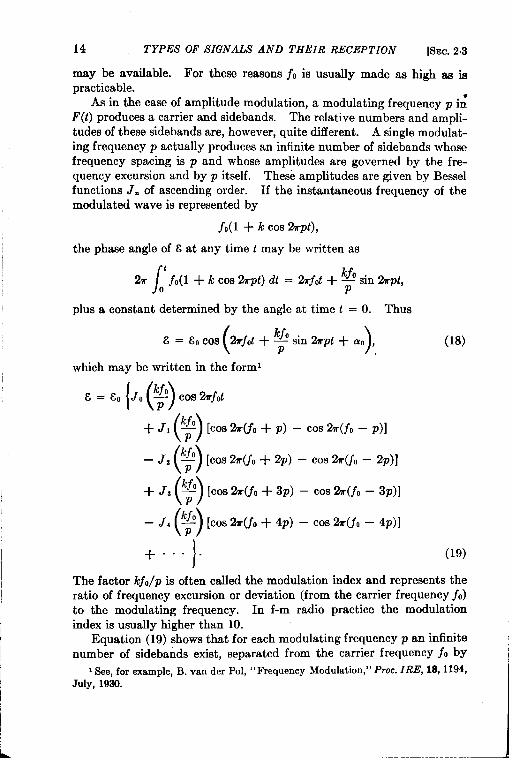
Frequency-modulated C-w Signals.-In the transmission ofan f-m r-f signal the amplitude of the r-f signal is held constant. the radio
I frequency it-mlf being varied in accordance-with some desired modulatingfunction F(t). Such a signal may be represented by
/& = &, Cos > ‘[1 + F(t)]j, dt. (16)
f,
There are two important parameters of frequency modulation,namely, the frequencies contained in F(t) itself and the total frequencyexcursion or deviation, f- — f~.
It should be noted that if F(t) = O, the wave is represented by
& = E, Cos >(.fd + a,) (17)
as before, but this is a correct representation only when the frequency isconstant. In general, the phase angle of 8 will be proportional to thetime integral of the frequency, whether or not the frequency itself isconstant. The unit constant put under the integral with F(t) plays thesame role as that of the carrier with amplitude modulation; that is, itpermits “downward” as well as “upward” modulation. ;t is stillnecessary to make the quantity 1 + F(t) positive at all times. Forinterference-suppression purposes the frequency excursion, aa will beshown in Chap. 13, should be large. The excursion must be small,however, compared with the center frequency f,, so that several channels
I,,
14 TYPES OF SIGNALS AND THEIR RECEPTION [SEC.2.3
may be available. For these reasons jO is usually made as high as ispracticable.
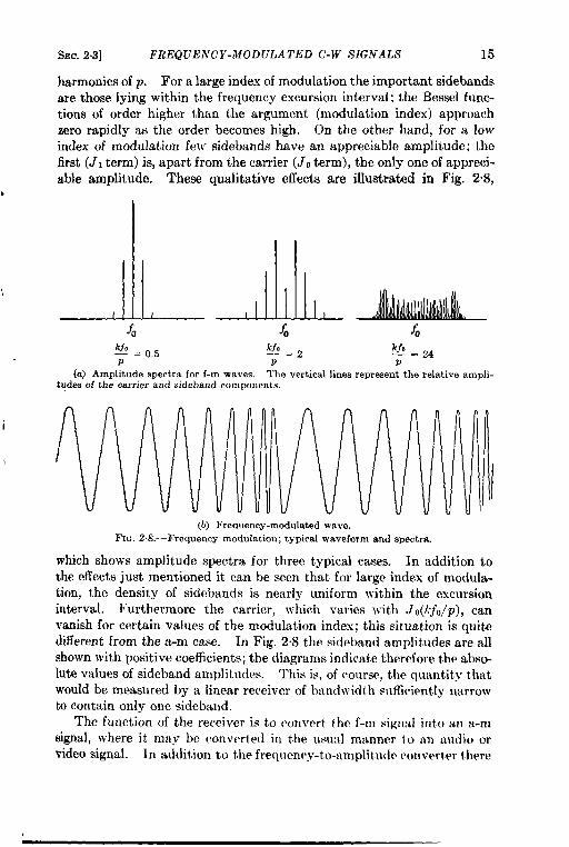
As in the case of amplitude modulation, a modulating frequency p i;F(t) produces a carrier and sidebands. The relative numbers and ampli-tudes of these sidebands are, however, quite different. A single modulat-ing frequency p actually produces an infinite number of sidebands whosefrequency spacing is p and whose amplitudes are governed by the fre-quency excursion and by p itself. These amplitudes are given by Besselfunctions J. of ascending order. If the instantaneous frequency of themodulated wave is represented by
jo(l + k cm %t),
the phase angle of .Sat any time tmay be written as
27r/
~ fo(l + k cos Z@) dt = 27rjot + ~ sin %@,
plus a constant determined by the angle at time t = O. Thus
(
kjo
)& = &o cos >jd + ~ sin 2rpt + aO , (18)
which may be written in the forml
{(),kfo& = 8, Jo ~ COS %rjot
()+ J, : [Cos27r(fo + p) – Cos %Lfo – p)]
()– J, ~ [COS fh(j, + Zp) – COS %(fo – Zp)]
()p [ 0s 2T(jo + 3p) – Cos %(fo – 3p)]+J, !f! ~
()– J, $ [COSti(jO + 4p) – cos ~(j, – 4p)]
+1
. . . . (19)
The factor lcjo/p is often called the modulation index and represents theratio of frequency excursion or deviation (from the carrier frequency fo)to the modulating frequency. In f-m radio practice the modulationindex is usually higher than 10.
Equation (19) shows that for each modulating frequency p an infinitenumber of sidebands exist, separated from the carrier frequency fo by
I See, for example,B. van der Pol, “Frequency Modulation,” ~roc. ~W la, 11%July, 1930.
b
‘1
i
SEC.23] FREQUENCY-MODULATED C-W SIGNALS 15
harmonics of p. For a large index of modulation the important sidebandsare those lying within the frequency excursion interval; the Bessel func-tions of order higher than the argument (modulation index) approachzero rapidly as the order becomes high. On the other hand, for a lowindex of modulation few sidebands have an appreciable amplitude; thefirst (J, term) is, apart from the carrier (JOterm), the only one of appreci-able amplitude. These qualitative effects are illustrated in Fig. 2%,
kfo ~—=P
(a) Amplitude spectra for f-m waves. The vertical lines representthe relative ampli-tudes of the carrier and sidebandcomponents,
(b) Frequency-modulatedwave.~IG. 2.8.—Frequencymodulation; typical waveform and spectra,
which shows amplitude spectra for three typical cases. In addition tothe effects just mentioned it can be seen that for large index of modula-tion, the density of sidebands is nearly uniform within the excursioninterval. Furthermore the carrier, which varies wit h Jo(k.fo/p), canvanish for certain values of the modulation index; this situation is quitedifferent from the a-m case. In Fig. 2.8 the sideband amplitudes are allshown with positive coefficients; the diagrams indicate therefore the absmlute values of sideband amplitudes. This is, of course, the quantity thatwould be measured by a linear receiver of bandwidth sufficiently marrowto contain only one sideband.
The function of the receiver is to convert the f-m signal into m a-m
signal, where it may be converted in the usual manner to an audio orvideo signal. In addition to the frequenry-to-amplitude converter there
I
16 TYPES OF SIGNALS AND THEIR RECEPTION [SEC.23
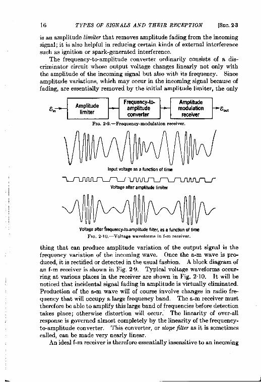
is an amplitude limiter that removes amplitude fading from the incomingsignal; it is also helpful in reducing certain kinds of external interferencesuch as ignition or spark-generated interference.
The frequency-to-amplitude converter ordinarily consists of a dis-criminator circuit whose output voltage changes linearly not only withthe amplitude of the incoming signal but also with its frequency. Sinceamplitude variations, which may occur in the incoming signal because offading, are essentially removed by the initial amplitude limiter, the only
AmplitudeFrequency-b Amplitude
8in- - -limiter
amplitude modulation -V3Mconverter receiver
~G. 2.9.—Frequeney-m0dulationreeeiver.
Inputvoltageas a functionof time
Voltageafter amplitude limiter
Voltageafterfrequency-to-amplitudefilter, as a funtiton of time
FIG. 2.10.—Voltage waveforms in f-m receiver.
thing that can produce amplitude variation of the output signal is thefrequency variation of the incoming wave. Once the a-m wave is pro-duced, it is rectified or detected in the usual fashion. A block diagram ofan f-m receiver is shown in Fig. 2“9. Typical voltage waveforms occur-ring at various places in the receiver are shown in Fig. 2.10. It will benoticed that incidental signal fading in amplitude is virtually eliminated.Production of the a-m wave will of course involve changes in radio fr~quency that will occupy a large frequency band. The a-m receiver musttherefore be able to amplify this large band of frequencies before detectiontakes place; otherwise distortion will occur: The linearity of over-allresponse is governed almost completely by the linearity of the frequency-to-amplitude converter. This converter, or slope filter as it is sometimescalled, can be made very nearly linear.
An ideal f-m receiver is therefore essentially insensitive to an incoming
SEC. 2.4] PHASE-MODULA TED C-W SIGNALS 17
a-m signal. Likewise an a-m receiver is insensitive to an f-m wave, exceptwhere the bandwidth of the a-m receiver is smaller than the frequencyexcursion of the f-m signal. In this case, because of the slope of theresponse curve, the frequency function is converted to an amplitudefunction, usually in a nonlinear fashion, and the receiver will not beinsensitive to the f-m signal.
2.4. Phase-modulated C-w Signals. —Phase modulation is in onesense merely a type of frequency modulation. The total phase angle of&is made to vary in accordance with the modulating wave F(t). A p-mwave can therefore be represented by
8 = .5, Cos 27r~ot+ a, + ml’(f)], (20)
where m is a constant representing the change in phase angle accompany-ing a unit change in F(t). If F(t) is expressible in a Fourier series,
F(t) =2
an cos 27rpnt, (21)
n
comparable p-m and f-m representations can be written
[& = 80 cos 27r(fot+ ao) + m
z 1an cos 2rp.t ,
nphase modulation; (22)
[ 2 1& = 80 cos 2r(fot + 80) + /c.fO ~ sin 2mp.t ,
nfrequency modulation. (23)
These expressions are similar, but they differ in one important respect.The coefficients of the pmterms are independent of p. for phase modula-tion but are inversely proportional to p. for frequency modulation.Phase modulation may therefore be converted to frequency modulationby placing in the modulator a filter whose gain is inversely proportionalto frequency. Similarly, frequency modulation may be converted tophase modulation by placing in its modulator a filter whose gain is pro-portional to the modulating frequency. Thus the essential differencebetween frequency and phase modulation lies in the characteristic of the fil-ter in the modulator. The relative advantage of one system over the otherdepends on the modulating function F(t) and on the frequent y spectrumof undesired interference. In actual practice it is customary to useneither pure phase modulation nor pure frequency modulation. Thelower audio frequencies are usually frequency modulated, and the higherfrequencies are phase modulated. Appropriate. filters in the receiverstraighten out the frequent y characteristic.
I
18 TYPES OF’ SIGNALS AND THEIR RECEPTION [SEC.2.5
PULSED SIGNALS
2.5. Infinite Pulse Trains.-Systems have been developed in whichthe reception of a series or train of r-f pulses is of primary interest. Thefields of radar and pulsed communication utilize such pulse trains. Inprinciple the pulsed function could be amplitude, frequency, or phase,and methods for reception would follow lines suggested in the precedingsections. Because of the great use made of amplitude pulsing, however,and the insignificant use made at present of frequency or phase pulsing,
Frequency— Frequenq——
(a) Amplitude spectrum (b) Power spectrumFIG. 2.1I.—Frequency spectrumof infinite pulsetrain.
this book will treat only the case of amplitude pulsing. The phase rela-tions of the amplitude pulses may be important, of course, and this rela-tionship will be considered where necessary, but the essential feature isone of amplitude pulsing.
The amplitude pulses, it is assumed, are repeated at a rate denotedhere by the pulse repetition frequency, or PRF. If the pulse train isinfinite in extent, the frequency spectrum can be computed by conven-tional methods in Fourier analysis. Denote the pulse train by F(t); then
In this expression, f, denotes the PRF, and, the pulse length. A Fourierdevelopment of Eq. (24) shows that
‘(t) =sin~f.(f,,+:j=coszflf,~) (25)n-l
or.
F(t) =z
‘2 ‘23”’0) * [sin %r(fO+ n,f,)t + sin $k(fo - flff)d, (~)n-o
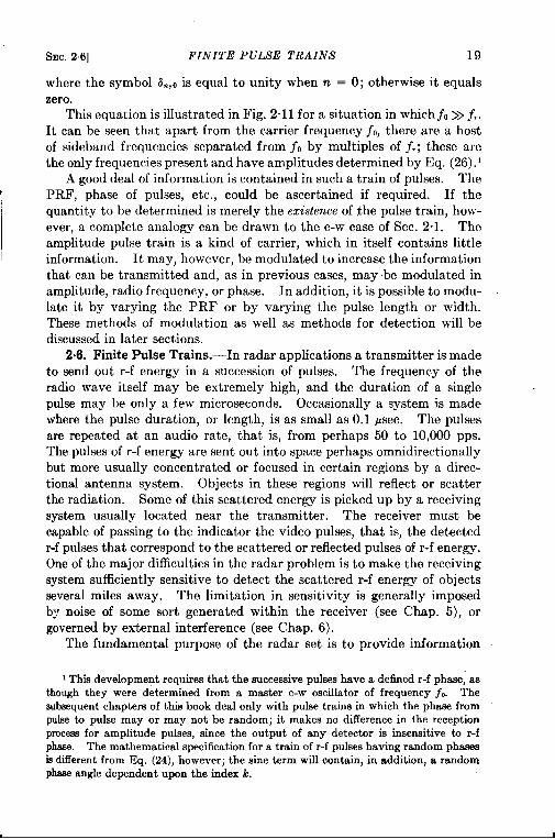
SEC.2.6] FINITE PULSE TRAINS 19
I
t
where the symbol ~.,0 is equal to unity when n = O; otherwise it equalszero.
This equation is illustrated in Fig. 2“11 for a situation in which fO>> f,.It can be seen that apart from the carrier frequency ~0, there are a hostof sideband frequencies separated from jo by multiples of f,; these arethe only frequencies present and have amplitudes determined by Eq. (26).’
A good deal of information is contained in such a train of pulses. ThePRF, phase of pulses, etc., could be ascertained if required. If thequantity to be determined is merely the existence of the pulse train, how=ever, a complete analogy can be drawn to the c-w case of Sec. 2“1. Theamplitude pulse train is a kind of carrier, which in itself contains littleinformation. It may, however, be modulated to increase the informationthat can be transmitted and, as in previous cases, maybe modulated inamplitude, radio frequency, or phase. In addition, it is possible to modu-late it by varying the PRF or by varying the pulse length or width.These methods of modulation as well as methods for detection will bediscussed in later sections.
2.6. Finite Pulse Trains.-In radar applications a transmitter is madeto send out r-f energy in a succession of pulses. The frequency of theradio wave itself may be extremely high, and the duration of a singlepulse may be only a few microseconds. Occasionally a system is madewhere the pulse duration, or length, is as small as 0.1 ~sec. The pulsesare repeated at an audio rate, that is, from perhaps 50 to 10,000 pps.The pulses of r-f energy are sent out into space perhaps omnidirectionallybut more usually concentrated or focused in certain regions by a direc-tional antenna system. Objects in these regions will reflect or scatterthe radiation. Some of this scattered energy is picked up by a receivingsystem usually located near the transmitter. The receiver must becapable of passing to the indicator the video pulses, that is, the detectedr-f pulses that correspond to the scattered or reflected pulses of r-f energy.One of the major difficulties in the radar problem is to make the receivingsystem sufficient y sensitive to detect the scattered r-f energy of objectsseveral miles away. The limitation in sensitivity is generally imposedby noise of some sort generated within the receiver (see Chap. 5), orgoverned by external interference (see Chap. 6).
The fundamental purpose of the radar set is to provide information
I This development requires that the successive pulses have a defined r-f phase, asthough they were determined from a master c-w oscillator of frequency j,. Thesubsequentchapters of this book deal only with pulse trains in which the phase frompalm to pulse may or may not be random; it makes no difference in the receptionprocessfor amplitude pulses, since the output of any detector is insensitive to r-fphsse. The mathematical specification for a train of r-f pulses having random phasesisdifferent from Eq. (24), however; the sine term will contain, in addition, a randomphseeangle dependent upon the index k.
1
20 TYPES OF SIGNALS AND THEIR RECEPTION [SEC.2.6
that permits the human observer to locate objects of particular interest.With a directional antenna system the azimuth and elevation of searchare known; and by the system of pulses, the range of or distance to areflecting object can be found. This range is measured by the time differ-ence between the transmitted pulse and the received echo pulse. Sincethe angular location of the reflecting object requires a directional radiator,a general search of the entire region requires some sort of scanning. Thescanning or searching motion of the antenna system is usually reproducedin some form within the indicator, so that easy correlation of the presenceof a particular echo with a particular azimuth or elevation can be made bythe observer. Because of the scanning action, the return signal reflectedfrom an object consists of a finite train of r-f pulses. This train of pulsesis, of course, repeated at the next scan.
The scanning can be accomplished in many ways, and the pulse videoinformation at the output of the receiver can be presented on the indicatorin many ways. The method of scanning is dictated by both the functionof the radar set and mechanical considerations for moving the antennaassembly.’ The method of indication is usually one that makes the radarinformation most intelligible to the observer. Some of the more commonindicators used are listed below for reference.
The Type A or Linear Time-base Oscilloscope .—This indicator con-sists of a cathode-ray oscilloscope in which the video signals from thereceiver are impressed upon the vertical deflection plates and a linear saw-tooth sweep voltage is applied to the horizontal deflection plates. Thishorizontal sweep is usually started by the initial impulse from the radartransmitter and is made to move across the oscilloscope at a rate con-venient for radar range measurements. The next transmitted impulsestarts the Sweep over again. Thus, near-by objects that scatter the r-fenergy will cause a visual vertical deflection, or “pip” (also called“blip” ), near the starting edge of the sweep; a reflecting object at adistance will produce a pip at a horizontal position corresponding to therange of the object. Thus the linear time base provides a range measurement of objects scattering the r-f pulses. The amplitude of the videodeflection, or pip, is a measure of the effective scattering cross section ofthe object in question. It is also a function of the range of the object,because of geometrical factors, and a function of the over-all sensitivityof the radar set. The type A oscilloscope thus essentially providesinformation about the range of an object and some information as to its“radar” size. It does not give azimuth or elevation information, butthis can always be obtained from separate dials geared to represent theantenna coordinates. Because of the time necessary for the observer to
‘ See Radar Scanners and Radurnes, Vol. 26, Radiation Laboratory Series.z See CathodeRay Tube Displays, Vol. 22, Radiation Laboratory Series.
I
I
SEC.2.6] FINITE PULSE TRAINS 21
coordinate the A-scope range with elevation and azimuth? the system isnot well suited to rapid scanning or search. It is most useful in themeasurement of radar range on systems that have a broad antenna-
1 radiation pattern and eithe~ do not scan at all or scan relatively slowly.
I
I
I
I
I
This type of indication, however, is sensitive in the detection of weakechoes.
In addition to other obvious advantages, a radar can give far moreprecise range information than anoptical range finder. The radar rangeerror can, unlike the optical, be independent of the range itself and can bemade assmallasa tenth of the equivalent range represented by the pulselength. For high precision the sweep on the A-scope would have to beextremely linear and well calibrated or some other marking device pro-vided. It is customary to provide range marks, or a series of sharptiming “pips,” to mark the sweep at convenient intervals. If extremeprecision is required, a movable delayed-timing pip is provided whosetime delay is calibrated and accurately known. It may be generatedfrom a crystal-controlled oscillator. This timing pip can be made tocoincide with the desired radar echo, whose accurate range can thus bedetermined. Where the sweep length is very long in comparison with thepulse length as presented, it is difficult to see the relative positions of theecho pip and timing pip. For this purpose an especially fast horizontalsweep may be provided. Such an oscilloscope is known as an R-scope(range). It is merely an A-scope in which the start of the sweep may beaccurately delayed and the sweep speed made sufficiently great todelineate the desired echo and timing pip. The R-scope is also useful inexamining the character of the returned echo pulse or pulses and isgenerally more sensitive than the A-scope in the detection of extremelyfeeble echoes.
The Type B Oscilloscope.—This indicator was initially developed toadd azimuth information to what was presented on the A-scope; thiswas done by impressing the video signals from the receiver on the controlgrid of the cathode-ray oscilloscope. The video signals therefore modu-late the beam current in the oscilloscope and consequently the intensity oflight output. Under these conditions the vertical plates of the oscillo-scope are left free. It is necessary only to impress on these plates avoltage that corresponds to the azimuth of the radar antenna. As theantenna is made to scan in azimuth, the trace of the time-base sweep ismade to move up and down in synchronism with the antenna position.This type B oscilloscope therefore produces on its screen a bright spotwhose position in range and azimuth on the oscilloscope face correspondsto the actual range and azimuth of a reflecting object. It is therefore aradar map, differing from the usual map by a distortion caused only bythe particular coordinates chosen. Like the “deflection-modulated”
22 TYPES OF SIGNALS AND THEIR RECEPTION [SEC.2.6
type A oscilloscopes, “ intensity-modulated” oscilloscopes such as type Bare very sensitive in the detection of weak echoes; but the intensity-modulated osulloscopes are much better adapted for scanning systems.Because it is convenient to view the oscilloscope face like a map, ant]because the radar-scanning frequencies are generally I)elow the flickerfrequency for the human eye, it is customary to use for the screen of thecathode-ray tube a special material whose light output decays relativelyslowly with time.
The Plan-position Indicator, or PPI.—This is the name given anintensity-modulated oscilloscope in which the time-base sweep is made tostart at the center of the tube and move radially outward. The azimuthof this radial sweep on the oscilloscope is made to correspond to theazimuth of the radar antenna. This type of sweep is usually provided bya magnetic deflection yoke placed around the neck of the cathode-raytube. As the antenna is scanned in azimuth, the magnetic yoke issynchronously rotated about the axis of the tube. This synchronizationis easily accomplished by driving the yoke by a synchro motor or someother remote mechanical synchro-transmission device. Thus the PPIprovides a map of all radar echoes, where the map scale factor is merelythe ratio of twice the velocity of the radio wave to the sweep speed.Because of the ease with which a true map can be interpreted, the PPIis an ideal indicator for use with radar sets searching continuously inazimuth. Intensity-modulated range marks are generally provided forcalibration purposes. They appear as concentric brightened rings atregularly spaced radial intervals.
The Range-height, or RH, Indicator. -h’either the type B oscilloscopenor the PPI can present elevation information, and for radar sets whosefunction is height-finding some other indicator is desirable. Withoutrecourse to a three-dimensional intensity-modulated indicator, whichhas not yet been devised, the presentation of elevation informationrequires the omission of either azimuth or range information. If theazimuth information is suppressed, an indicator presenting range andheight, or RH oscilloscope, can be provided. The radar antenna is madeto nod or oscillate in elevation angle. The angle of the deflection yokein an oscilloscope of the PPI variety is made to follow the antenna eleva-tion angle in such a way thht the indicator presents a true radar map of aparticular vertical section of space. Thus the RH indicator will presenttrue range and height of radar targets, neglecting, of course, the curvatureof the earth’s surface. The range and height scales can, if necessary,be expanded or contracted to provide convenient values.
The Type C Indicator.—If the range information is suppressed, anindicator presenting azimuth and elevation information, or type Cindicator, can be provided. Because the range information is suppressed,the indicator will show a bright spot on its screen at an elevation and
SEC. 2.6] FINITE PULSE TRAINS 23
azimuth wherea radar-reflecting object exists at any range. This is theradar presentation which most closely approximates a visual pictureof the surroundings. It is probably one of the least useful radar pres-entations, however, since it does not utilize the one parameter, that is,range, given best by the radar set. There are usually a tremendousnumber of radar-reflecting objects at any prescribed azimuth and eleva-tion, and it is useful to select preferentially particular ones for presenta-tionofthe type Cindicator. Thisselecting ismadepossible byavariablerange “gate,” or ‘(strobe, ” which sensitizes the indicator only for echoesoccurring within a defined range interval. The gate may be set at anyrange, and its length adjusted to correspond to any required rangeinterval. Gating not only is useful for type C indicators but is oftenwidely used where the video impulse from a single target is to be selectedand used to control other circuits, perhaps even the coordinates of theradar antenna itself. The type C indicator is less sensitive to the detec-tion of weak echoes than the PPI or type A or B oscilloscopes.
Aural Perception.—The presence of the video pulses at the output ofthe receiver may be indicated aurally to the human observer, One wayof accomplishing this is to put the video signals into an audio loudspeaker,then listen for the audio tone produced by the PRF. When this methodof detection is used, all radar range information is lost unless the incomingsignals are gated in order to pass to the loudspeaker only those signalswhich occur within a desired range interval. This aural detection of thePRF component is surprisingly sensitive and very useful in recognizingsignals from a particular radar set, since the PRF’s of various installationsmay differ markedly. The ear appears to be very sensitive to changes inpitch or tone.
Meter Detection.—By still another method of perception, the auralsignals are rectified and impressed on an ordinary d-c meter and thepresence of a signal determined by the meter deflection. If this methodis adopted, both radar range information and information about the PRFare lost but, as in the case of aural detection, the video signals may begated. It might be argued that meter and aural detection methods areequivalent, but this equivalence is not easy to show. The use of therectifier or detector in producing the meter deflection gives rise to possiblecross modulation. This will be discussed in Chap. 9.
Types of Receivers Used.—The function of the radar receiver is toprovide pulsed video signals from the incoming series of r-f pulses. Inprinciple the three types of receivers mentioned in Sec. 2.2 may be used,but some remarks on the usefulness of each type can be made. Thesimple single-detection receiver is useful principally where the receiver isto be made sensitive to a large r-f band. In this case no r-f amplificationis used; detection is accomplished at low level and is thus necessarilysquare law. Because of the low detection sensitivity of the square-law
24 TYPES OF SIGNALS AND THEIR RECEPTION [SEC.27
detector, most of the signal energy is lost, the remainder being forced tocompete with noise produced after detection. For this reason this typeof receiver is not so sensitive as the superheterodyne for weak signals,perhaps by a factor of 104 in power. However, the r-f bandwidth can bemade several hundred megacycles per second in extent.
The superheterodyne receiver is almost universally used in radar appli-cations, because it has better sensitivity than the single-detection receiverand better stability than the superregenerative receiver. At the veryhigh frequencies the r-f amplification, because of its limitations anddifficulties, is not customarily used, but the r-f signal is usually imme-diately converted into an i-f signal. The i-f amplifier therefore has arelatively great voltage gain, perhaps as much as 10G,weak signals being,as a result, made suitably large for linear detection or rectification. Thisamplification must be of such a nature that it has a satisfactory responseto the desired pulses. From Fig. 2.11 it can be seen that most of theenergy in the pulses is concentrated in a band of frequencies roughlyequal to the reciprocal of the pulse length. Therefore the r-f and i-fbandwidths must each be of the order of magnitude of the reciprocal ofpulse length. Since the pulse lengths in use vary from 10–7 to 10–s see,the bandwidths must be of the order of 105 to 107 CPS. This is the chiefdifference between receivers made for radar pulses and those made forradio transmission, the latter being designed to pass only audio frequencies.
Some superregenerative receivers have been constructed for pulsereception. The quench frequency must be high compared with the recip-rocal of the pulse length to make sampling sufficiently frequent. Forpulse lengths of less than 1 psec, this has been found difficult to do.Furthermore the criticalness of adjustment has greatly restricted theusefulness of such receivers. Nevertheless, certain of their properties,such as high gain over satisfactory bandwidths, necessitate taking theminto consideration.
In all these methods of reception the main object of perception is tobecome aware of the existence of the incoming r-f signal. The questionis not one involving the detailed analysis of the signal characteristics butsimply whether or not the signal exists. As pointed out in Sec. 2.5, it is
often useful to consider the detection of a series of pulses that are modu-lated in some manner at a slow rate. The information one wishes toabstract from this type of signal is the relatively slow modulation functionappearing in the pulse train, in much the same way that one wishes toabstract the modulating function from an a-m or f-m c-w signal.
2.7. Amplitude-modulated Pulse Trains.-There are two reasonswhy it is useful to consider the perception of the modulation function of amodulated pulse train. First of all, the echoes obtained in radar recep-tion are indeed modulated by changes in the characteristics of the targetunder surveillance, The effective scattering cross section of the target
SEC.2.7] AMPLITUDE-MOD ULATED PULSE TRAINS 25
may vary with time because of changes in the target aspect or position;it may also vary in a way characteristic of the particular target itself.For example, propeller rotation on an aircraft will give rise to aperiodicchange in its effective radar scattering cross section. Information con-cerning the modulation of received pulsed echo trains may therefore behelpful inderiving information concerning the nature of the target. Asanother example, one can see that the phase of the returned radar echodepends upon the total path length taken up by the radio wave and there-fore changes markedly with target movement. By a phase-detectionscheme a modulating function that depends on target speed can thus bederived. The phase changes brought about by target movement can beconveniently measured by one of two general methods. The coherent-pulse system mixes the incoming echoes with a strong local c-w generatorwhose phase is reset to the phase of the transmitted pulse each time it isproduced. The resulting echo amplitude will be constant from pulse topulse unless the target in question moves during this time interval by anamount that is appreciable with respect to the wavelength of the r-fsignal. As the target moves, the echo will be seen to beat up and downwith a frequency given by the Doppler shift. By analyzing the phasemodulation of the return pulses, therefore, information concerning radialtarget speed can be derived.
A second method of phase detection is possible. Instead of utilizingthe local source of phased c-w oscillations, the echo from the movingtarget is mixed with other strong echoes from fixed targets. Again beatsin the echo amplitude are obtained in the same way as for the coherent-pulse system. The presence of these beats depends, however, upon thepresence of local fixed echoes at the same range as the target. Since thiscondition is not under the observer’s control, the system has a limitedarea of usefulness. It is, however, much simpler than the coherent-pulsesystem.
One of the main uses for modulated pulse trains, however, lies in theirapplication to specialized communication systems. Such systems havethe advantage of highly directional propagation characteristics and ahigh degree of security. In these systems a continuous succession ofpulses modulated at speech frequencies is sent out. As pointed out inSec. 2.5, the modulation itself may be applied to the pulses in several dif-ferent ways. Amplitude modulation will be discussed in this section,and other types of modulation in Sec. 2.8.
The amplitudes of the continuously recurring pulses are assumed tovary in accordance with the modulating function. If the modulatingfunction is one that can take on both positive and negative values withrespect to its normal or quiescent value, there must be provided, as inprevious examples, a carrier term large enough to prevent the entireamplitude function from reversing sign. The function of the receiver
A
26 TYPES OF SIGNALS AND THEIR RECEPTION [SEC.2.7
is to obtain the modulation function from the relatively complicatedtrain of incoming pulses. The first step in the chain of events is thedetection of the r-f signal to provide video pulses, just as in the case ofnormal radar echo detection. Since distortion of the modulating func-tion is undesirable, linear detection is greatly preferred; and for the sakeof sensitivity, a superheterodyne receiver should be used. The ampli-tudes of the video pulses are still S1OW-1Ymodulated by the modulatingfunction. The possibility of gating the pulses at this point makes thistype of communication system much more secure than the ordinary a-mc-w signal. The proper video pulses can be selected by a gate whosePRF is the same as that of the desired signal and whose timing is madeto coincide with the pulses either by a special timing pulse or by auto-matic locking voltages derived from the incoming pulses themselves.The sensitivity of the receiver to weak signals in noise is affected by gatingand by the gate length itself. This point will be discussed in Chap. 10.
The spectrum of the pulses can be derived in a straightforward fashion.Let us represent the modulating wave F(t) by the function
F(t) = 1 + Esin 27rp(t + 8), (27)
where e is the fractional modulation and p is the modulating frequency.This function is now to represent the amplitude of the pulse train, whichhas a PRF denoted here by ~, and pulse lengths indicated by,. For thesake of simplicity it is supposed that the pulse amplitude at the start ofthe pulse will assume the value of F(t) and that the pulse amplitude ismaintained constant throughout each pulse. That is, the signal functionwill be given by
F.(t) =z ()
F ; A,(t), (28)r
k
where
( O otherwise.
The Fourier development of F,(t) becomes
.
+: 2[2 sin 7dTf,
7r 1 c0s2+’-@1=1
~ sin m(ljr + p) sin [2m(lj, + p)t – np + 2rp6]+lfr+p
1~ sin m(tj, – p) sin [%(lj, – p)t + m,p – 2Tpti] . (29)
+ljr–p
%C. 2.7] AMPLITUDE-MODULATED PULSE TRAINS 27
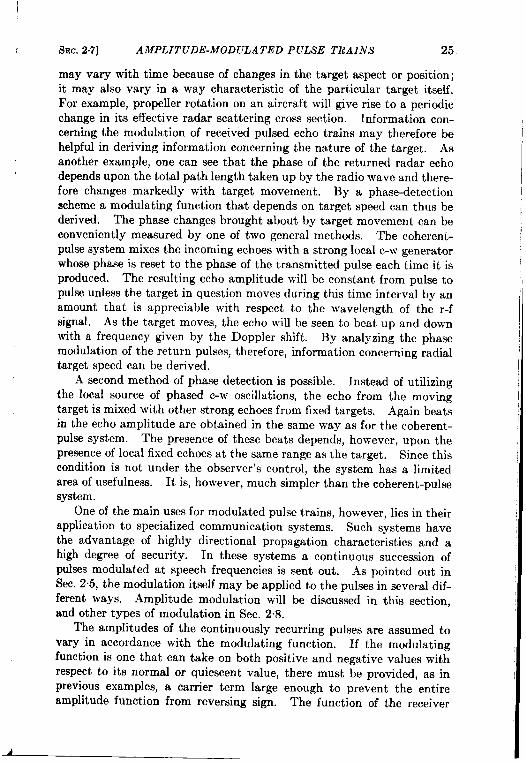
It can be seen that, in general, many frequencies are present in F.(t),
namely, all the harmonics of the PRF f, and cross terms between theseharmonics and the modulating frequency p. The amplitude of any termof frequency j is modified by the familiar (sin m.f) /mj because of thepulse length T. A convenient chart for reading off all frequencies presentis shown in Fig. 2“12. Output frequencies are given on the abscissa scalefor any input modulating frequency chosen on the ordinate scale. The
OutputfrequenciesFIG. 2-12.—Outputfrequenciesfor a given modulatingfrequency.
output frequencies present are those which appear at the intersections ofa horizontal line, whose ordinate is the modulating frequency p, with thearray of diagonal lines and vertical lines shown in the diagram. Anexample is shown by the dotted line drawn for p = j,/4; the output fre-quencies are shown to be 2?lf, and z (2.., f f./4).
The diagram shown in Fig. 2.12 is not suitable for indicating the inten-sities of the various components. A simple rule to remember is toconsider that all intersections with diagonal lines yield amplitudes whichare c times those of the vertical lines.modified according to the individual
‘Furthermore, all in~ersections arepulse spectrum (sin mj)/mf and
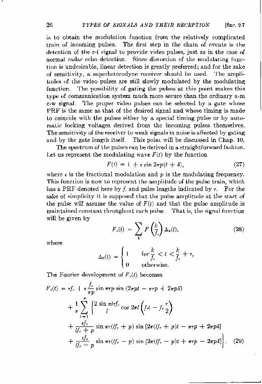
28 TYPES OF SIGNALS AND THEIR RECEPTION [SEC.2.7
therefore fall off with increasing frequency. A typical spectrum is shownin Fig. 2.13, where f,~ = 0.2 and p = f,/4 as shown in Fig. 2“12. Thefrequencies shown with dotted lines are those caused by the modulationitself.
It would be possible to put the video pulses directly into a loud-speaker and derive sound that contains the modulating function (seeFig. 2.13). It would also contain many undesired and extremely annoy-ing frequencies. These undesired frequencies are all higher than themodulating frequencies provided p < f,/2 and can thus be filtered outbefore going into the loudspeaker itself. Generally, the desired audiocomponent must be greatly amplified because of its small energy content.
FIG. 2.13.—V1deospectrumof modulatedpulsetrain.
The filtering and audio amplification may be greatly helped by theso-called “boxcar” generator, or demodulator. This device consists ofan electrical circuit that clamps the potential of a storage element, such asa capacitor, to the video pulse amplitude each time the pulse is received.At all times between, the pulses the storage element maintains the poten-tial of the preceding pulse and is altered only when a new video pulse isproduced whose amplitude differs from that of the previous one. Thename “boxcar generator” is derived from the flat steplike segments of thevoltage wave.
The output of the boxcar generator is given by Eq. (29) (by putting7 = l/f,) and can also be obtained from Fig. 2.13. It can be seen thatnone of the lf, terms remain except the d-c term. The output frequencypresent at the modulating frequency p is also incidentally much amplifiedbecause of the increased pulse length. The output voltage, however,still does contain at reduced amplitude the cross-modulation terms.Nevertheless, the main body of interfering audio frequencies has beenremoved, and therefore the problem of additional filtering is greatlysimplified. The boxcar generator can be used only on gated systems,
SEC.27] AMPLI TUDE-MODULA TED PULSE TRAINS 29
unfortunately, or at least on systems from which an accurately timedclamping pulse is available.
If cross-modulation terms in the output must be avoided, the highestmodulation frequency must be substantially less than one-half of thePRF f,. If a filter is used to separate the output frequencies, it will havea cutoff or attenuation curve that is not infinitely sharp; therefore themaximum value of p must be further restricted. If p is limited to j,/3,then one octave exists for the filter to achieve its cutoff value. This isconsidered to be an acceptable value. It will be noticed that this restric-tion will apply to all of the pulsed communication schemes, since it followsdirectly from the effect of sampling the signal voltage at discrete times.
Before proceeding to other forms of modulation, the part played byvarious detection processes should be considered. The first detectionprocess (actually the so-called “second detection” in a superheterodynereceiver) reduces the r-f voltage to a video voltage. This provides ameasure of the intensity of the r-f wave without regard to its exact r-fstructure. This video voltage still varies at a fairly high rate and maycontain modulation intelligence. An additional detection process, that is,boxcars with audio filtering, will bring out the modulation frequencies.Still another, or fourth, detection can be provided. This one measuresthe average intensity of these audio voltages; that is, it measures thefractional modulation c. Thus the detection process is one that princi-pally provides a measure of the average intensity of a function. Becauseof this averaging process, the frequencies present in successive detectionsbecome progressively lower.
One more point regarding the demodulated signal should be noted.The video output is a measure of the signal size and can therefore be usedas a signal-actuated control voltage. It is sometimes convenient to usethk voltage to control the gain of the receiver. Thk control must clearlybe made of such a sign that an increase in video signal will reduce thereceiver gain; otherwise the system will be regenerative. With thisdegenerative system, the receiver gain tends to maintain the averageoutput signal constant in size regardless of input signal size. The actionof this type of automatic gain control, or AGC, will be described inChap. 11.
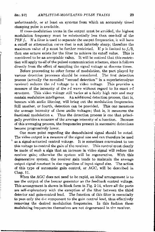
When the AGC does not need to be rapid, an ideal arrangement is touse the output of the boxcar generator as the feedback control voltage.This arrangement is shown in block form in Fig. 2.14, where all the partsare self-explanatory with the exception of the filter between the thirddetector and gain-control lead. The function of this filter is essentiallyto pass only the d-c component to the gain control lead, thus effectivelyremoving the desired modulation frequencies. In this fashion thesemodulating frequencies themselves are not degenerated in th o receiver.
30 TYPES OF SIGNALS AND THEIR RECEPTION [SEC.2.8
If the filter passes the modulating frequencies, they will be degeneratedand greatly reduced in amplitude at the receiver output. They are not,in general, completely degenerated because of the finite change in outputsignal required to cause a change in receiver gain. For some applicationsthis finite degeneration is not serious, since audio amplification willrestore the amplitude of the modulation signal. In addition, because ofthe rapid feedback, the speed of AGC is greatly increased. The filter,however, must considerably attenuate the PRF, or oscillation willdevelop because of the cross terms of Fig. 2.12.
Receiver r-f and .%condSingle
Eh — - + selector Thirdi-f amplifier detector detector Ewt
gate
JIGain-control lead l=] II low-pass I
filter
FIa. 2.14.—Audio-modulationreceiver with automaticgain control.
2.8. Other Types of Modulation. Pulse-length or Pulse-m.dth Modula-
tion.—In this case the modulation is accomplished by variations in pulselength. The PRF and the pulse amplitude are held constant. Recep-tion consists of detecting the r-f pulses, then converting the length varia-tions to amplitude variations. As pointed out in Sec. 2.7, the PRF mustbe at least three times that of the highest modulating frequency, and alow-pass filter must be used to exclude undesired cross terms.
The conversion from pulse length to amplitude is most easily accom-plished by passing the signal through a filter of limited pass band.Through such a filter, if its bandwidth is considerably less than the recipro-cal of the maximum pulse length, the output response will have an ampli-tude proportional to the product of input pulse length and amplitude.This operation can be accomplished in the r-f and i-f sections of thereceiver before detection takes place. It is most convenient, however,to limitthe incoming signals (usually done most easily after detection)before converting the pulses to amplitude-modulated signals. Thelimiter plays the same role as the limiter for f-m radio (see Sec. 2.3);that is, it eliminates amplitude variations in received signals producedby fading and reduces interference of a type in which peak voltages arevery high. The bandwidth of the receiver in front of the limiter shouldbe adequate to pass the shortest pulse properly. From Fig. 2.11 it canbe seen that the bandwidth should exceed the reciprocal of the shortestpulse length.
In addition to peak limiting, it is usually desirable to provide a lowerlimit below which no output signal occurs. If the input signals fall belowsome defined minimum level, noise or interference in the receiver renders
SEC. 2.8] OTHER TYPES OF MODULATION 31
them useless. Therefore a lower limit, which excludes thk noise, isbeneficial. The presence of both a lower and upper limiter constitutesa “slicer,” so named because the output voltage is proportional to theinput voltage only within a narrow voltage range or slice. The slicedoutput of the length-modulated pulses will consist of a series of relatively“clean” constant-amplitude length-modulated pulses suitable for imme-diate conversion to a-m pulses.
As in the case of a-m pulses, gating can be employed within the limitsof pulse lengths used. A gate length as long as the longest pulse mustbe used; this would appear to favor slightly the use of a-m pulses whereaccurate gating of a size equal to the pulse length at all times is possible.
Frequency OTPhase Modulation.—In this type of modulation one canthink first of an ordinary f-m or p-m continuous wave as described inSees 2.3 and 2“4. The pulses merely select short segments out of thisr-f wave; they therefore bear defined frequent y and/or phase changesdetermined by the original modulation. The process of reception con-sists of limiting the pulses, then passing them through a frequency-to-amplitude slope filter. From this point they are handled like a-m pulses.The pulse frequencies spread out over a band about equal in width to thereciprocal of the pulse length. Therefore the frequency deviation shouldbe made large compared with this band of frequencies. In the truepulsed case, it is not really essential that the phase of the r-f signal whichis being frequency modulated be accurately defined at the start of eachpulse, since the frequency-t~amplitude converter is itself insensitive tophase. Unlike the case of f-m continuous waves, the starting phase ofeach pulse may be made random because of the dead time between pulses;no difficulties are caused thereby with f-m pulses, but phase-modulationschemes are, of course, upset. Likewise schemes can be considered inwhich the phase is modulated without changing the center frequencyduring each pulse. ‘Such modulation is again made possible by the dis-continuity between pulses; either frequency or phase can be arbitrarilyyset. For the detection of the phase modulation, a scheme similar to thatdiscussed in Sec. 2.6 can be used. One may use a coherent local c-wsource whose frequency is that of the pulses and whose phase is in quad-rature with the pulse phase in the absence of a modulating signal, that is,carrier present only. As can be seen, variations in pulse phase caused bymodulation, for small phase changes, will cause amplitude changessubstantially proportional to these phase changes. These a-m pulsesare then handled in the usual manner.
Modulation of PRF.—In this scheme the variable that is modulatedis the PRF itself. The maximum range of variation is kept smaller thanone octave to prevent harmonics of the lowest PRF from interfering withthe highest frequency. As in the other sampling schemes the average
32 TYPES OF SIGNALS AND THEIR RECEPTION [%c. 2.8
PRF must be about three times as high as the highest desired modulatingfrequency. Detection of the pulses is made in the usual way. The audiooutput is obtained by putting the video signals into a filter designed topass only the audio frequencies. It should be remembered that sincethe incoming signal amplitude is constant, limiting and slicing can beemployed; but because of the variable PRF, gating is impossible.
Other Schemes.—Other schemes of modulation are possible, andmethods for their reception are obvious. Among these may be mentioneda double-pulse scheme in which the spacing between the two pulses ismodulated. Clearly, this scheme is similar to pulse-length modulation.Again frequency or phase differences between the two pulses can be usedif desired.
CHAPTER 3
THEORETICAL INTRODUCTION
3.1. The Mathematical Description of Noise.—It is well known thatthe output of a receiver when no signal is present is not always zero butfluctuates more or less irregularly around some average value. On anA-scope, for instance, these fluctuations produce the typical noise thatoften prevents weak signals from being de-tected. This noise has several origins, to bediscussed in detail in the next chapters; thequestion that concerns us here is how to de-scribe quantitatively the noise output of areceiver.
The answer is perhaps not obvious.Merely observing the output y(t) of a receiverover a period of time (y may be a voltage, acurrent, or the deflection on an A-scope) doesnot make it possible to predict the output forany later time or to predict the output as afunction of time for another receiver identicalwith the first. Then how can any theory atall be formulated? The answer is, of course,by using the notion of probability. As weshall see, certain probability distributions canbe predicted and observed. The noise outputof a receiver is a typical example of a random(or stochastic) process. The systematic studyof such a process forms a recently developedpart of the theory of probabilityy. 1. Let us assume that there are a greatnumber of microscopically identical receivers(called an “ensemble” of receivers) allturned on simultaneously. The noise out-puts Y,(t), YZ(~), . . . , are then observed.All these functions will be different. At a definite time t it can beobserved for what fraction of the total number of cases y occurs in a
ISeveral aspects and applications of the general theory of random processes arereviewed and extensive references to the literature given by S. O. R]ce, “ Mathematical
33
r—
34 THEORETICAL INTRODUCTION [f3EC. 3.1
given interval between y and y + Ay. This fraction will depend on yand t and will be proportional to Ay when Ay is small. It is writtenW ,(y,t) dy and called the jirst probability distribution. Next can be con-sidered all the pairs of values of y occurring at two given times t1and t2.The fraction of the total number of pairs in which y occurs in the range
(Y1, Y1 + @ at ~1 and in the range (YZ, YZ+ AYJ at b is writtenWZ(Y1, t1; W, tz) dyI dyz and is called the second probability distribution.We can continue in this manner, determining all the triples of values ofy at three given times to arrive at the third probabilityy distribution, etc.
The objection immediately occurs that observations of the noiseoutputs on an ensemble of receivers can never be made. Such observa-tions are not necessary, however, when the noise output is stationary.This means that the influence of the transients (because of the switchingon of the receivers) has died down and that all tubes have warmed upproperly with the result that the receiver is in a stationary state. If one
observation is then made of the noise output y(t) of the receiver for a verylong time, all the information desired will be received. The record canbe cut in pieces of length e (where e is long compared with all “periods”occurring in the process), and the different pieces can then be consideredas the different records of an ensemble of observations from which thedifferent probability distributions can be determined. Furthermore,these distributions now become somewhat simpler. The first one, forinstance, will be independent of t;the second one will depend only onthe time difference tz– t1,etc.; hence the stationary noise output will bedescribed by the series of functions:
W,(y) dy = probability of finding y between y andy + dy;
W&I, YZ,t) dyl dyz = joint probability of finding a pair ofvalues of y in the ranges (Y1, yl + dyl)and (Y2, y2 + dy2), which are a timeinterval tapart from each other;
Analysis of Random Noise,” Bell System T..hn. J., 23, 282 (1944); 26, 46 (1945);
S. Chandrasekhar, “Stochastic Problems in Physics and Astronomy,” Rev. Mod.Phys., 15, No. 1, 1 (1943); Ming Chen Wang and G. E. Uhlenbeck, “On the Theory ofthe Brownian Motion I I,” Rev. Mod. Phys., 17,322 (1945). Discussion in this chapterwill be restricted to the minimum requirements for the understanding of noiseproblemsin radio receivers. It may be well to point out, however, that these problems formonly a small part of the general theory of random processes. Other application ofthe theory are made in many branches of physics (as, for instance, in the theory ofBrownian motion and the theory of other fluctuation phenomena), in hydrodynamics(especially in the theory of turbulence), in the theory of the errors in gunnery andbombing, in economics (especially in the theory of time series), etc. Another applica-tion, the m-called “random walk” problem, will be treated in Chap. 6.
S~c, 3.2] AVERAGE VALUES 35
lv3(u1jv2Jv3,~1,~2)@I dy2 dy3 = jOht probability of finding a triple ofvalues of y in the ranges dy,, dy~, dy3,
where dyl and dyz are the time interval LIapart and dy, and dy~ the time intervaltz apart, etc.
It should be emphasized that these probability distributions representeverything that can be found out about the random process, and one
> may therefore say that the random process is dejned by these distribu-
tions. Of course, the functions W. arc not arbitrary and unrelated toeach other; they must fulfill the three obvious conditions:
W. z O, because the Wnareprobability densities,
Ili~n(yl, (1; y,, (2 . . Y., L) must be a symmetric function in the set of
variablesyl, tl; y?, /2, . . . , Ynj k, since W. is a joint probability, andWk(yl, tl; “ , yk, h)
1I
= J‘“ “ Jdy+“ “ ‘ ‘yn’’’’n(yl;’l;“ “ ‘‘n’”)‘1)I since each function W. must imply all the previous W~ with k < n.
The set of functions W= form therefore a kind of hierarchy; they describesuccessively the random process in more and more detail. A complete
theory of the random m-ocess should make it possible to derive the general~ distribution function W. from an analysis of the origins of the random
process. For the noise produced in or ~assing through Iinear networkst this can actually be done (see Sec. 3.6). However, the investigations
here will usually be restricted to the first two probability distributions.3.2. Average Values.-From the first probability distribution W,(y,t)
Ithe average value of y can be found.
Q=
/
dy yW, (y,t). (2)
(leady, this average value will in general depend on the time t. It canI he determined by averaging, at the time t, the noise outputs y,(t),
Y2(t), . . of the ensemble of receivers mentioned in Sec. 3.1. It willI be spoken of, therefore, as the ensemble average and indicated by a bar.
It must be distinguished from the time average, defined and denoted by
(3)
This will be independent of the time, of course, but will, in general, differfor the various functions y,(t), y,(~), . of the ensemble. We can stillaverage over the ensemble; then the same result will be obtained as the
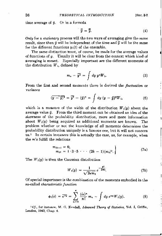
36 THEORETICAL INTRODUCTION [SEC.3.2
time average of ~. Orin a formula
z=? (4)
Only for a stationary process will the two ways of averaging give the sameresult, since then v will be independent of the time and ~ will be the samefor the different functions y,(t) of the ensemble.
The same distinction must, of course, be made for the average valuesof functions of y. Usually it will be clear from the context which kind ofaveraging is meant. Especially important are the different moments ofthe distribution W,, defined by
From thevariance
mn=~= Jdy ymwl. (5]
fi.rat and second moments there is derived the fluctuation or
/(Y – ‘o’ = 7 – (?3’ = dY (Y – ti)’wl, (6)
which is a measure of the width of the distribution W 1(Y) about theaverage value j. From the third moment can be obtained an idea of theskewness of the probability distribution, more and more informationabout W 1(y) being acquired as additional moments are known. Theproblem whether or not the knowledge of all moments determines theprobability distribution uniquely is a famous one, but it will not concernus.’ In certain instances this is actually the case, as, for example, whenthe m’s fulfill the relations
m’sk+l = (),m2k=l .3.5..- (2k – I)(m,)k. I
The W l(y) is then the Gaussian distribution
——W,(y) = *2 e ‘:’.
(7a)
(7b)
Of special importance is the combination of the moments embodied in theso-called characteristic junction
zm(is)”@l(s) =z= . _ mn =
/dy e~””W,(y).n! (8)
?l=o
I
I
1Cf., for instance, M. G. Kendall, Advanced Theory of Statistics, Vol. 1, Griffin,London, 1943,Chap. 4.
;EC.3.2] AVERAGE VALUES 37
rhe significance of the characteristic function lies especially in the follow-,ng two theorems:
1. The characteristic function determines uniquely the probabilitydistribution. In fact, from the Fourier integral theorem it follows’that
(9)
2. If the characteristic functions of two independent random variablesy and z are r#I(.s)and x(s), then the characteristic function of thedistribution of the sum y + z is given by the product ~(s) . ~(s).’
Let us now turn to the second distribution function WZ(yl, t,;VZ,tz).
The most important average value derived from it is
iziz= H dy, dyz YW2WZ(Y1, t,; Y2, tz). (lo)
In general, this will be a function of t, and t,. Letting 12 = t, + 7, wecan perform an additional time average over tl and then obtain a functionof ‘r
+;R(r) = Iim ~
/
—dtl ~(t,, tl + T) = ~z. (11)
0+. –;
The same function R(,) is obtained, of course, by taking the ensembleaverage of
dt, u(t,)y(t, + r). (12)
For a stationary process Eqs. (10) and (12) give the same result. Thefunction R(T) gives a measure for the correlation between successivevalues of y and is therefore called the correlation function. When y(t J
and y(t2) are independent of each other,
W,(y~, t,; y2, t2) = J’Vl(Yi,~J “ ~1(Y2,~2)
and—ylyz = gl “ .!72.
10ne might think that Eqs. (8) and (9) answer the previously mentioned questionof momente in the affirmative. In fact, it can be proved in this way that Eq. (7b)follows from Eq. (7a). The general mathematical problem, however, is to find theconditions that the m. have to fulfill so that .$1(s) exists and has a Fourier transformthat is always positive.
2For a proof and also many mamples and references, cf. Kendall, 10C.tint. For thestrict mathematical discussionof the notion of characteristic function, see H, Cramer,Random Variables andProbability Distributions, Cambridge, London, 1937.
38 THEORETICAL INTRODUCTION
For noise (without signal), this situation will occurinterval tz — tl = T is sufficiently large. For T = O, it
It is sometimes convenient to work with the functionl
~(,) = (Y1–fi)(Y2 -v),
(Y – 02
which will be called the normalized correlation function.
[SEC.3.2
when the timeis obvious that
(13)
We may notesome
1.2.3.4.
properties of P(T):
p(o) = 1.p(r) s p(o).For noise without signal p(r) -+ O as T + w.If P(T) = O for T z TO,thenz
()~ s p(o) Cos*1)Pn
where n is an integer.As already mentioned in Sec. 3“1, W2 (yl, t,; y,, tz) gives more informa-
tion about the random process than the first probability distributionW,(y,t). In fact, WI follows from JV2,since one has
w,(y,,tl) = [ dyz W2(W1, t,; y,, tz) (14)J
and
Wz(yz,tz) =
/dyl W2(Y1, tl; Y’, t’),
which is a special case of the general Eq. (1). It is sometimes impor-tant to introduce instead of W2 the conditional probability distributionP2(Y,,tl lY,,L2), which gives the probabilityy of finding y between VZ and
y, + dyz at time t’,given that y = y, at time tl. Of course,
W’(y,, tl; yz, tz) = w1(Y1,t1)~2(Y1) t11Y2,t2), (15)
and P’ must fulfill the relations
/dfh P,(y,,t, ]y2,t2) = 1,
\ I
(16)
dy, W,(y,,t,)Pz(y,, t,lwz,~,) = Wl(?h,h),
I This function is written for a stationary process, with which we shall be concerned most often.
2For the proof, cj. R. P. Boas and M. Kac, “ Inequalities for Fourier Transforms ofPositive Functions,” Duke Math. J., 12, 189 (1945).
SEC. 3.3] THE CORRELATION FUNCTION AND THE SI’EC1’R L’.ll 39
\v”hichfollow from Eq. (14). From Pz may bc obtained conditionalauerage values, as, for instance,
F2° =/
4J2 l/2P2(?ht11v2,t2),
which is the average value of y at tzwhen one knows that y = yl at timet,.For a stationary process, P, and, therefore, @l also will depend only
Lont2—tl=T.
The notion of the characteristic function for W* can also be general-
ized by forming
@Z(Sl,SJ = et(n,v,+~,u,)=//
dy, dyz e’fs’v’+”~’JW2(y1,y2). (17aj
We again have analogous theorems; in particular WZ is found from & by
w2(Y1,?/2) = *2H
ds, ds, ei(jlv,+s,u,) I$2(s1,s2). (17b)
3.3. The Relation between the Correlation Function and the Spec -trum.-Of special significance for the applications to signal detectabilityis the notion of the spectruml of a random process. Let us suppose thata function y(t) is observed for a long time e. Assuming that y(t) = Ooutside the time interval e, the resulting function can be developed in aFourier integral,
I
/
+.y(t) = dj A (j)ezrij’, (18)
—.
where if A*(f) denotes the complex conjugate, A(~) = A*( —f), sincey(t) is real. It is well known (Parseval theorem) that
/
+-
/--
+;
/
+-yz(t) dt = ~ y2(t) dt = df ]A(f)]z.
—.2
—m
Using the fact that 1A(f) \2 is an even function of j and going to the limite + co, this equation can be written as
where
G(f) = lim ~ \A(f)[*e+.
(19)
(20)
I Cf. Rice, Bell System Tech. J., 23, 310 (1944); Wang and UMenbeck, Rev. Med.Phys., 17, 326 (1945); further references are given in these papers.
40 THEORETICAL INTRODUCTION [SEC.3.3
and will be called the spectral de?lsity or the power spectrum of the func-tion y(t).
Let us consider next the average value,
By introducing the Fourier expansion [Eq. (18)] and using the Fourierintegral theorem, it is easily shown that
—----w.~(t)y(t +,) = df G(j) COS2@,o
(21a)
from which it follows by inversion that
(21b)
All this holds for any function y(t). Let us assume, now, that we havea random process and that y(t) is a member of the ensemble of functions
Y1(O, !42(0, . - . , mentioned in Sec. 3.1. Each of these functions canbe developed in a Fourier integral, and the corresponding G(f) can be
averaged over the ensemble. The resulting G(j) will be called the spectraldensity or the power spectrum of the random process. From Eqs. (21a)and (21b) it follows that the correlation function l?(r) and this spectrumare each other’s Fourier cosine transform, or
This is the relation referred to in the title of this section.The following additional remarks may be helpful.1. Equation (19) can also be averaged over the ensemble, which gives
(23)
2. For a stationary process the averaging over the ensemble can beomitted, since each member y;(t) will lead to the same spectraldensity G(j).
3. The spectral density G(j) may contain singular peaks of the well-known Dirac 6-function type. This certainly occurs, for instance,
t%C.3.31 THE CORRELATION FVNC1’ION AND 7’Hll SI’A’L’I’RUM 41
when ~ is not zero or, in electrical language, when there is a d-cterm. Then
G(j) = 2(~)26(f) + G,(f), (24)
where 6(f) is the Dirac &function.14. For pure noise the peak at f = O, corresponding to the d-c term
will usually be the only peak, so that Gl (j) will be a regular func-tion, representing the really continuous spectrum. From Eqs. (19)and (24) it is apparent that the area under this continuous spectrumis equal to the fluctuation or variance of y(t). In this case it issometimes convenient to introduce the normalized power spectrum
s(j) = al(f)
/,- (ifG,(j);
it becomes apparent that S(f) and the normalized correlation func-tion p(7) of Sec. 3.2 are each other’s Fourier cosine transform.
5. The relations [Eqs. (21a) and (21b)] are perfectly general. Theyhold, for example, when
y(t) = A + B sin 2T(fot + a).
We then have
t ~ = At + ~BZ,
&/(t)y(t + T) = A* + +B2 COS27TfLIT,
and from Eq. (21b) it follows that.
G(f) = 2A2c$(f) + iB2J(f – ~o),
where the following relations have been made use of:
(25)
The spectrum therefore consists, as it should, of the two frequenciesf = Oand j = j,, corresponding to the power in the d-c term A 2andthe power *B2 in the a-c term.
6. When there are noise and a signal, the spectral density G(f) willconsist (in addition to the d-c term) of a continuous spectrum and anumber of peaks at the discrete frequencies f, of the signal. The
. 1This function has the following properties: 3(z) = Ofor z # Oand 6(x) = m for
\+.
z = O in such a way that the integral, 5(z) dx = 1; t(z) = ~( –z) so that—.
/
.a(z) dz = }.
Q
7.
THEORETICAL INTRODUCTION
magnitudes of the peaks—or better, the area
[SEC.3.4
under the peaks—correspond to the power spectrum of” the signal.When a stationary random process with spectral density G,(j)Passes through a linear device that is described by an impedancefunction Z(f),’ then the output will again bea stationary randomprocess and the spectral density will be
Go(j) = [Z(f) 12Gi(f). (26) ~
3.4. Examples of Spectra.—The importance of the relation in Eqs.(21 ) or (22) between the correlation function and the spectrum lies in thefact that itisoften easier tocalculatethe R(7) or p(~) by means of Eqs.(10) and (ll)thanto calculate the spectrum directly. To elucidate therelations in Eqs. (22), consider, for example, the case wherel
p(T) = e–~’.
Then
when
s(f) = 4B(3’ + (2rrj)“
~(r) = ~–azr?,
24; -“+.S(j) =~e
(27)
(28)
When p(,) is a monotonically decreasing function of T, S(j) is also amonotonic decreasing function of f. The function S(f) will becomeflatter and flatter as p(7) becomes narrower. If p(~) drops to zero in avery short time A, then h’(f) will be essentially constant upto avery highfrequency of the order of magnitude 1/A. We call this a white spectrum.The limiting case—where S(j) = constant for all f—would correspondto no correlation at all between successive values of y; hence for all t,
W’(yl, t,; y,, t’) = wl(!/l,fl)T’V1( g/2,t2),
and we have what is called a purely random process. This is, of course, ani Idealization that in actual cases can only be approximated.
When S’(j) has a maximum at some high frequency fO and is sym-metrical around the maximum, so that
s(f) = F(f – j,),F(x) = F’(-z),
then
/
.p(T) = Cos 27rjoT. dz ~(z) COS21rxT, (29)
—.
1In these examples the normalized correlation function p(~) is used and the result-ing spectrum is therefore also normalized; P(0) is always unity, and consequently the
/total ~rea of the spectrum is ~MS(j) df = 1.
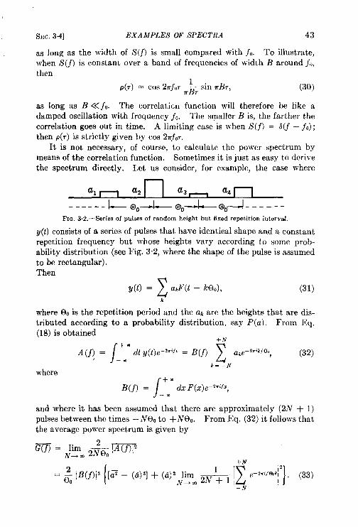
SEC. 3.4] EXAMPLES OF SPECTRA 43
as long as the width of S(f) is small compared with fo. To illustrate,when S(j) is constant over a band of frequencies of width B aroundjO,then
1.p(?) = cm 2rfo7 .— sm 7rB7,
7rBT(30)
as long as B <<.fo. The correlation function will therefore be like adamped oscillation with frequency f,. The smaller B is, the farther thecorrelation goes out in time. A limiting case is when S(f) = ~(f – fo);then p(r) is strictly given by cos 2mfw,
It is not necessary, of course, to calculate the power spectrum bymeans of the correlation function. Sometimes it is just as easy to derivethe spectrum directly. I,et us consider, for example, the case where
al - a2 a3 a4
------ l.w-@o--L- @o-L-@ti-l ------FIG. 3.2.—Seriesof pukes of randomheight but fixed repetition interval.
y(t) consists of a series of pulses that have identical shape and a constantrepetition frequency but whose heights vary according to some prob-abilityy dist ribut ion (see Fig. 3.2, where the shape of the pulse is assumedto be rectangular).Then
y(t) =2
akF(t – keo),k
(31)
where f30 is the repetition period and the ak are the heights that are dis-tributed according to a probability distribution, say P(a). From Eq.(18) is obtained
/
+N
A(j~ = ‘“ o?ty(t)e-’”’j’ = B(j)z
ake–2.ikf Ek7 (32)
—.k=– N
where
B(j) = /_+aM dx F(x)e-2m’~Z,
and where it has been assumed that there are approximately (2N + I)pulses between the times - N&to +N610. From Eq. (32) it follows thatthe average power spectrum is given by
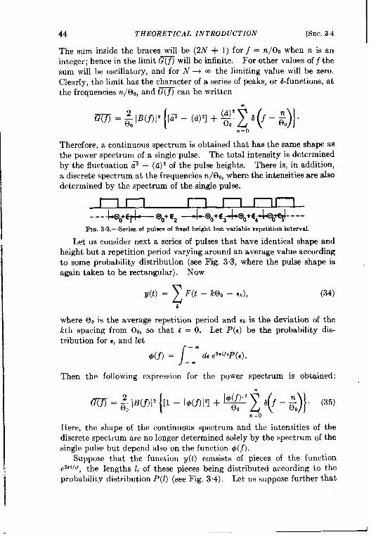
44 THEORETICAL INTRODUCTION [SEC.3.4
The sum inside the braces will be (2N + 1) forj = n/130 when n is aninteger; hence in the limit G(f) will be infinite. For other values off thesum will be oscillatory, and for Ns M the limiting value will be zero.Clearly, the limit has the character of a series of peaks, or &functions, atthe frequencies n/eo, and G(f) can be written
Therefore, a continuous spectrum is obtained that has the same shape asthe power spectrum of a single pulse. The total intensity is determinedby the fluctuation a= – (a) 2 of the pulse heights. There is, in addition,a discrete spectrum at the frequencies n/(30, where the intensities are alSOdetermined by the spectrum of the single pulse.
[ I I 1 I II 1
.--4@o+qL--@o+E2 4@o+&k@o+E4#q -----
FIci. 3.3.—Seriesof pulsesof tied height but variable repetition interval.
Let us consider next a series of pulses that have identical shape and
height but a repetition period varying around an average value according
to some probability y distribution (see Fig. 3.3, where the pulse shape is ,
again taken to be rectangular). Now
y(t) =2
F(t – keo – C,), (34)
k
where E). is the average repetition period and m is the deviation of thekth spacing from eo, so that i = O. Let P(c) be the probabilityy dis-tribution for ●, and let
r+.
d(f) = )_”md~e’ri’’p(~).
Then
Here,
the following expression
(m = &(fll’ [1 –
for the power spectrum is obtained:
–D(f-a}” ’35)I@(f)\’] + ‘@&()” m
.=IJ
the shape of the continuous spectrum and the intensities of thediscrete spectrum are no longer determined solely by the spectrum of thesingle pulse but depend also on the function I#I(j).
Suppose that the function y(t) consists of pieces of the functionezrifo’, the lengths li of these pieces being distributed according to theprobability distribution P(l) (see Fig. 3.4). Let us suppose further that
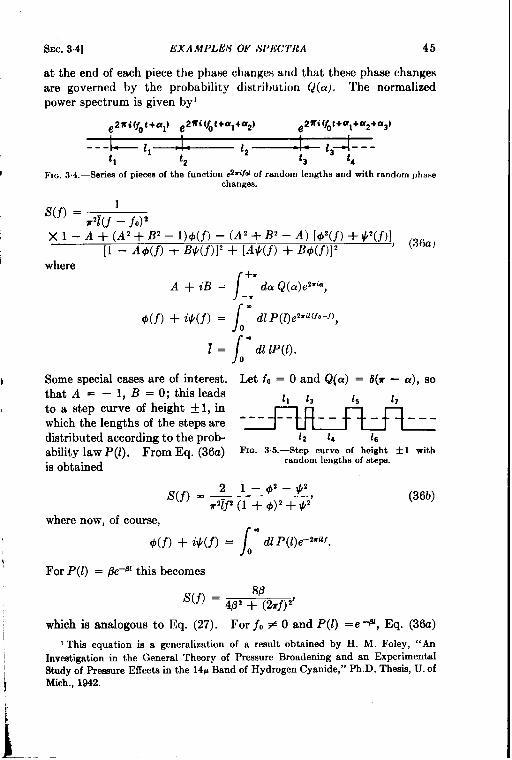
SEC. 3.4] EXAMPLES OF tY1’lW7’ItA 45
at the end of each piece the phase changes and that these phase changesare governed by the probability distribution Q(a). Tbe normalizedpower spectrum is given by’
~zxi(fot+q ~2fi~(~t+a1+u2) ~2fii(~t+u1+a2+a3),
I--- k 11 1. 12 - 13_ L--tl t2 t3 t4
FIO. 3.4.—Series of piecesof the function ~tif~ of randomlengthsand with randomphasechanges.
s(j) = 1A(j –jo)z
xl–z4+(A’ +B’-l)IW)–( A’+B’–A)[W)+W)], ~36a)
[1 – Ad(j) + BW)I’ + [M(j) + BW)]’
i=/
mdl 1P(1).o
Some special cases are of interest. Let fo = Oand Q(a) = IS(T- a), so
that A = – 1, B = O; this leads 11 la 15 1,to a step curve of height +1, inwhich the lengths of the steps aredistributed according to the prob- 1~ 1, 1~
ability law P(l). From Eq. (36a) FIG. 3.5.—Step curve of height * 1 withrandomlengthsof atepu.
is obtained
(36b)
where now, of course,
1#1(~)+ W(j) = Jo” dl P(l)e-2’U/.
For P(l) = f?e-dtthis becomes
which is analogous to Eq. (27). For f, # O and P(l) = e ~, Eq. (30a)
I This equation is a generalization of a result obtained by H. M. Foley, “An
Investigation in the General Theory of Prezsure Broadening and an ExperimentalStudy of pressure Effects in the 14PBand of Hydrogen Cyanide,” Ph.D. Thesis, U. ofMich., 1942.
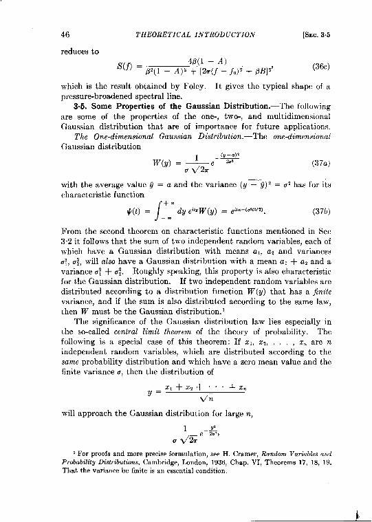
46 THEORETICAL INTRODUCTION [SEC.3.5
reduces to
s(f) =46(1 –.4)
,8’(1 – A)’ + [27r(f – f,)’ + BB]”(36c)
which is the result obtained by Foley. It gives the typical shape of apressure-broadened spectral line.
3.6. Some Properties of the Gaussian Distribution.-The followingare some of the properties of the one-, two-, and multidimensionalGaussian distribution that are of importance for future applications.
The One-dimensional Gaussian Distribution .-The onedimensional
Gaussian distribution
(37a)
with the average value J = a and the variance (y — j) z = U2has for itscharacteristic function
\
+-*(t)= @ ei’v~(y)= @a-&YzW2J. (376)
—.
From the second theorem on characteristic functions mentioned in Sec3.2 it follows that the sum of two independent random variables, each ofwhich have a Gaussian distribution with means al, az and variancesa;, u;, will also have a Gaussian distribution with a mean a, + a, and avariance u? + u;. Roughly speaking, this property is also characteristicfor the Gaussian distribution. If two independent random variables aredistributed according to a distribution function W(y) that has a finite
variance, and if the sum is also distributed according to the same law,then W must be the Gaussian distribution. 1
The significance of the Gaussian distribution law lies especially inthe so-called central limit theorem of the theory of probability. Thefollowing is a special case of this theorem: If xl, Zz, , z. are nindependent random variables, which are distributed according to thesame probability distribution and which have a zero mean value and thefinite variance u, then the distribution of
will approach the Gaussian distribution for large n,
I For proofs and more precise formulation, see H. Cramer, Random Variables and
Probability Distributions, Cambridge, London, 1936, Chap, VI, Theorems 17, 18, 19.That the variance be finite is an essential condition.
SEC. 3.5] SOME PROPERTIES OF THE GAUSSIAN DISTRIBUTION 47
whatever the original distribution functionl of the xi. This independenceof the original distribution function is the surprising feature of thetheorem. Of course, how the Gaussian distribution law is approachedwill depend on further features of the distribution function of the z;. Itcan be shown, 2 for instance, that asymptotically
ah.(_llJ
w(y) = — P ~3 e-*+... ,e 2.,———6 <n dy’ )
(38)
where p = ~ and where the further terms in the development containhigher powers of n-~ and, also, the higher moments of the distributionfunction of the xi. Usually the Gaussian distribution already becomes avery good approximation once n is greater than 10.
The n-dimenw”onal Gaussian Distribution. —This can be written
15B*WW1 1 ‘%kJz~
W(y,, y’z, “ “ “ , —YJ = (2=)./2 q e Y (39)
where we have already assumed, for simplicity, that the y,’s are measuredfrom their mean value, so that ~ = O. The matrix B is a symmetricand positive definite matrix; the meaning of the elements l?~l and of theconstant b is connected with the quadratic averages
b“===/ “+”-Iy’yw(y“““‘n)dyl““ “‘y’-’40)—.It can be shown that B~l is the cofactor of the element b~l in the matrixb whereas b is the determinant of the matrix b. To do this, let us firstshow that t,he characteristic function of the n-dimensional Gaussiandistribution is given by
—M i bh!hti
#(t, . . - tn) = e ‘“=’ (41)
For this we must calculate the integral
*J ‘“”’/dt““-dt’f$t’~(’l“““ ‘“)—.
1For a proof and more precise formulation, see ibid., p. 52. The condition that~ = Ois, of course, no restriction, since that z can always be measured from its meanvalue. For the connection with the random-walk problem, see Sec. 3.6.
zThis is a special case of Theorem 25 in ibid., p. 81. For a formal proof seeAC. 3.6.
48 THEORETICAL INTRODUCTION [SEC.3.5
Introduce instead of the tk new variables Uk by means of
.h —— u, — Y-,=’1
By using the well-known theorem
.
2bT,B,j = 6ijb,
r-lwe find
‘Ztk+bk’t’”=-:zbk’u’u’+z?yk k,l k,l k,l
Thus the integral becomes
– ‘AJB’’V”Y‘“””\du,“““‘Une-’’;u(:)”e —.By transforming the quadratic form 2 bklukut to principal axes the lastintegral is shown to be (27r)“’zb–~fi, so that we really get the Gaussiandistribution [Eq. (39)].
It remains to be shown that the b~~are really the quadratic averagesG. The simplest way is to use the characteristic function. In fact,if F(yl . . . y.) is a polynomial in yl . . . y., it follows from the Fourierintegral theorem that
F’(?A “ “ “ ‘n)=1‘“m”Idy-“‘dvfi(y]““““’)W(Y1“““Yn)
);; *(t, “ “ “ L)1,,=,,- . -,.-,. (42)
Therefore,
Jx–}4 buitii
— azykyl= –-e u
)= b,[.
f,= . . +.=0
SEC. 3.5] SOME PROPERTIES OF THE GAUSSIAN DISTRIBUTION
This result could also have been proved directly by calculating
49
theintegral in Eq. (40). Since the matrix b/b is the inverse of the mat~x B,it follows that b wi!l also be a symmetric and positive definite matrix.
As a special case of Eq. (39), let us consider the two-dimensional
Gaussian distribution. The matrix b is usually written
b= K 7} = [: T}’
calling ~ = U2,y; = rz, @ = PUT;p is the correlation coefficient. Thisgives
Bll = 72; BIZ = –PUT; Bzz = Uz; b = u%’(1 – P2),
so that the distribution can be written
w’(?/l,w) =1
[
1exp —
21ruTv’” ( )1~+$2* “2(1 – pz) U2
(43)
The general theorems mentioned in connection with the one-dimen-sional Gaussian distribution can also be generalized to the n-dimensionalcase. First of all one has again a central limit theorem. Interpretingyl . . . y. as the n components of a vector Y, and providing Yl, Y~, . . . ,Y. are N independent random vectors, which are distributed accordingto the same probability distribution and which have a zero mean valueand finite quadratic averages, then according to this theorem, the distri-bution of
~= Y,+ Y,+. ””+YN
+Y
will for large N approach the C,aussian distribution, regardless of theoriginal distribution functionl of the Y{. There is, furthermore, thetheorem that when YI and Yz are two independent random vectors, eachof which has a Gaussian distribution, the sum Y1 + Yz will also have aGaussian distribution. This stability property is, with certain restrictions,again typical of the Gaussian distribution.
Another aspect of the stability of the Gaussian distribution isexpressed by the following theorem (needed in Sec. 3“7). Suppose thevariables zl, x2, . . . , X. are distributed according to
Let YI, Y2, . “ “ , y, (s s n) be s linear combinations of the xi’s,
1Cf. ibid., Chap. 10, Theorem 20u.
50 THEORETICAL INTRODUCTION [SEC.3.6
n
yk = z(ZkiG, k=l,2, ..”, s,;G1
where the ski’s are constants. The y~’s will then be distributed accordingto an s-dimensional Gaussian distribution of the form in Eq. (39) (with nreplaced by s) and with
.
bkl = ykyl =-2
a~ialia~.;Z1
(45)
To prove this, there may be used the integral representation of theDirac &function
/
+.6(z – z’) = & _ ~ al et’(’-ti), (46)
which allows one to write for the distribution function P(v1 . . . y,) ofthe yi the expression
P(y, “ . 0 ‘s)‘/‘“m”b “ “ “ ‘znw(zl“““ ‘n)—.
‘fi’(y’-$aki’’)=&aul-:un/“+”””[k=l ~=1 —cc
Interchanging the integrations over the x, ~vith those over the t~,integrations over the z~ can easily be carried out, obtaining
the
P(y, . . . ‘s)‘&d ‘“””/d’l“““d’~$”k—.where the bkl’S are given by Eq. (45). Or, in other words, the character-istic function of P(YI y,) is exp ( — $ ~b~t~t~),which is nothing butEq. (41). Therefore P must be a Gaussian distribution of the form inEq. (39).
3.6. The Random-walk Problem. —Consider a point that can moveon a straight line with successive steps, either to the right or to the left.The steps will not be of equal size, but there is a basic probability @(x) dzthat the point will make a step of length between z and z + dx. What
SEC. 3.6] THE RANDOM-WALK PROBLEM 51
is the probability t$n(z)dz that aftern steps the displacement of the point
lies between z and z + dz?This is the famous random-walk problem formulated for the one-
dimensions.1 case. Clearly it is intimately connected with the centralIimittheorem of theprobability theory, sincez = z, +x,+ . . . +x.,when the w’s are the successive displacements of the point. But theproblem occurs in many branches of physics; and especially for the two-dimensional case, the problem can be interpreted as the problem of thecomposition of n isoperiodic vibrations with given probability distribu-tion for the amplitudes and for the phases. 1 The problem occurs in thisform, for instance, when one investigates the return of a radar signalfrom a cloud. The different water drops produce scattered waves, each
having different amplitude and phase. What we want to known is the
probability for a certain amplitude and phase of the resultant of all these
scattered waves. The problem is of fundamental importance and merits
a brief solution here. For the detailed application to the problem of the
radar ret urn from a number of independent scatterers (clouds, “window,”
etc.), see Chap. 6.
Since the successive steps are independent of each other, o.(z) will
fulfill the equation’
/
+.
@n(z) = _ ~ 4.-1(2 – X)4(Z) dz, (47)
with ~l(z) = o(z). The solution of this equation follows immediatelyfrom the convolution theorem of the Fourier transform. Let ~n(u)be the Fourier transform of on(z); then we obtain from Eq. (47),
~.(u) = *.-l(u) #(u),
with #,(u) = 4(u). Therefore #fi(u) = [Y(u)]”, and
/
+.r#%(z) = : _ du e’”z[v(u)]”,
.(48a)
LThis was the formulation of J, W. S. Rayleigh, Scientific Papers, Cambridge,London, 1899-1920, Vol. I, p. 491; Vol. IV, p. 370, who first gave a solution of theproblem for large n. For a complete discussionof the problem and for further refer-ences, cf. S, Chandrasekhar, “Stochastic Problems in Physics and Astronomy, ” Rev.Mod. Ph~s,, 15, No. 1, 1 (1943).
2The variables z and rJcan have all values between - m and + M. Of course,
/+.
_ ~ A(Z) dz = 1,
sinceO(Z) is a probability density. From Eq. (47) it follows that
/
+._ ~ +.(v) dv =
/_+~M+.-,(z) dz,
so that the total probability remains 1, as it should.
I
I
52
with
[&tc. 3.6THEORETICAL INTRODUCTION
/
+-+(u) = dx @(x) e-’UZ. (48b)
—.
Todiscuss the behavior forlargen and, especially, toseetheconnec-tion with the central-limit theorem, let
Xl+xz”””+z.
‘=5= {n ; ‘=%
and assume that -
\
+-$= m$(z) dx = O.
—.
Developing Eq. (48b) in powers of v one obtains
Therefore,
calling ;* = UZand ~3 = p. This is Eq. (38); for large n, O(y) becomestherefore the Gaussian distribution and the error is of order n–~ when thethkd momentl p # O.
For the km-dimensional problem the treatment is similar. Oneobtains, for the probability that after n steps the point lies in the regiondx dy, the general expression
+.
Wdx,y) = &,H du dv e’cUz+wvJ[~(u,v)]N,—.
where+-
*(U,V) =//
dz dy e-{it”*W#Jw(x,~), (49)—.
1Note that the error is of order 1/n when +(z) is an even function of Z. It is alsoeasy to carry the development one step further; the next term in the parentheses is
[1 (7 – w);, +W$qEn
SEC.3-V THE GAUSSIAN RANDOM PROCESS b3
and W(Z,V) = Wl(X,g) is the probability density for one S~P. Themost important case for the applications to be discussed in Chap. 6 is theone in which W(Z,Y) is isotropic, so that one can write> introducing polarcoordinates,
W(X,7J) dx dy = + f(r) dr d+.
By a calculation similar to that in the one-dimensional problem, it canbe shown that for large N,
~N(’Jy’=l’+a[--’l(% +$)+” ””)w’-w’(50)
where
/
.
/
.~2 = drj(r)rz ~= dr f(r)r4,
o 0
and 10 = I@. Except’ for z, y>> liI (where W. is small anyway),W. can be replaced by the isotropix tw~dimensional Gaussiandistribution
~ .*W(Z,y) = ~, e J (51)
with an error of the order I/N. For I = X2 + yz this leads to thedistribution
~(~) dl = ~ e-:,10
(52a)
from which followsI = I,, (1 – 10)’ = Ii. (52ZI)
This is sometimes called the Rayleigh distribution.3.7. The Gaussian Random Process.—Noise problems in radio
receivers, at least up to the detector stage where nonlinear elements beginto enter, involve a special type of random process (the Gaussian randomprocess), for which a complete theory can be given. These processes arecharacterized by the fact that all the basic distribution functions W*,
mentioned in Sec. 3.1, are Gaussian distributions. This fact could betaken as the defining property of the process. But since, as we shall see,the spectrum essentially determines everything, it is, from the physicalpoint of view, more natural to start with the Fourier development of theGaussian random function y(t).
Consider again, as in Sec. 33, the stationary random function y(t)over a long time interval E). In contrast to what was done’ in Sec. 3.3,
1This is of course a special case of the central limit theorem for two dimensions.2Where y(t) was taken zero outside the time interval E),and the rexaultingfunction
54 THEORETICAL INTRODUCTION [SEC.3.7
let us assume now that y(t) is repeated periodically with the period e sothat y(t) can be developed in a Fourier series
y(t) =z
(ak cos %jkt + & sin 27r~d), (53)
k=l
where j~ = lc/e. There is no constant term, since we shall assume that
the average value of y(t) is zero, an assumption that does not constitute arestriction, of course. The different members of the ensemble of func-tions yi (t) will have clifferent Fourier coefficients a~, bt. These coeff-icients are therefore random variables, and we shall assume that they areall independent of each other and have Gaussian distribution with averagevalues zero and with variances which may depend on the order k butwhich are the same for the. a’s and the Vs. Or, in fyrmula,
Zii=iz=o,—.akal = bkbl = O?bkl ; a~l = O. I
(54)
The probability that the ak and bz are in certain ranges da~, dbl can beexpressed as follows:
. ~~,+&,——W(al, az, . “ . ; bl, bt, “ “ “ )=~&, e ZCJZ2. (55)
k=l
The variances u; are connected with the spectral density or power spec-truml G(j); in fact,
since
y’(t) =–E 2
[;; cos’27rfkt + ~ sin’2mfkt] = IJi
‘iw ‘J3mG(f)df=”’ kk
(56)
(57)
whene-+~. This is identical with Eq. (12) or (23).It follows from these assumptions that the basic distributions of Sec.
3.1 are all Gaussian. The method is best explained by considering a fewexamples.
was developed in a Fourier integral. Of course, both methods are artifices to obtainconvergent expressions, Afterward one goes to the limit e ~ m; the two methodswill then give the same results,and 0 will drop out of all the final formulas.
1The bar is omitted since y(t) was assumedto be stationary.
Sl!c. 3.7] THE G:l[rSSI.4.V R.4.VDOM PROCESS 55
The Distribution Of yat Fi.xcd t.—According to ~q. (53), yis, foragivent, a~il~[’arf~lnc’tionof tlleb:~sic ran(iom >’:~riablesak, bl. From thetheorem proved in Sec. 35 (see page M) we know that the probabilitydistribution will be Gaussian with a variance given by k~q. (57) and amean value zero. ‘Me time t has disappeared; this is as it should be,since WI(Y) must be independent of t becuuse the process is stationary.
The Joint~istrzbution ofy(t,) and y(t~).—Since y(t,) and y(tJ areboth linear funrtions of m, b,, one \villobtain, xccording to the theorem ofSec. 3.5, a two-dimensional Gaussian distriblltion; y’(t,) and y2(tJ areagain given by l<:q. (57), and
Ye?/ =H
FI cos2Tf/, /, cos %rff,t?+ ij sin 2mj~tlsin 27r~ktzk )
E /..—u: (’0s 2n-fJf, — (?) = dj G(f) fOS 2Tf, = p(7)u2. (58)
oA
The correlation depends therefore only on ~ = ~z – t,, as it should, since
the process is stationary. Tl~c distribution function (cj”. lZq. (43)] is
1
[
1ll”2(y1jy2,T) = exp —
2X.2 41 – p’ 12U’(1 – ~?)@? + Y? – %?41Y2)
(59)
The qwmtitv P(T) is the normalized correlation function, and Eq. (58)expresses again the connection \\-iththe normalized spectrum,
S’(f) = $G(f) = G(,f)
[,“ djG(f)”
The Joint DisLrilmtion qf y(t,). y(tJ, and y(t,) .—We can go on in themanner just described. lVe can consider the third distribution functionlV,(Y1, tl; Y2, t’; Y,, t,), which Trill be a three-dimensional Gaussian dis-tribution depending only on & – tland t~ – t2. And from the theoremof Sec. 3.5 it follo!rs clearly that a[l the distributions W. will be Gaussianand will depend only on U2and p(T).
Distribution Functions of the Lkioatives of y.—In the same way therecan also be derived distribution functions in which the derivativesy’(t), y“(t), . . . appear. Since y’((), y“(t), . . are also linear func-tions of the random varia~)les a~, bl, it is clear that their distributionfuncticns will also be (;aussian, and ~vefind, for instance, that
(60)
56 THEORETICAL INTRODUCTION [SEC.38
etc. Wecanalso consider joint distributions of g(t) and its derivatives,as, for example, the distribution of yandy’ at a fixed t. This will beatwo-dimensional Gaussian distribution, which is especially simple, how-ever, since y and y’ at a given t are not correlated. One gets, namely,
k
It should still be pointed out that sometimes the distribution functions‘ derived in this way will have no meaning, since some of the integrals
over the spectrum are divergent. For instance, when P(7) = e–~’ sothat G(f)al/[62 + (2m~)’] [see Eq. (27)], the distribution functions inwhich the velocity y’(t) appears will have no meaning, since [see Eq.(60)] ~ will not exist. In this case one may call the process nondifleren-tiable. The degree of differentiability will be characteristic for the processand will depend on the behavior of G(f) for large f.
Finally, a few words should be said about the justification of theassumptions, embodied in Eq. (5.5), made in the beginning of this section.In the actual problems of the signal threshold in radio receivers the con-venient fiction is always allowed that the signal, before it enters thereceiver, is accompanied by a certain amount of noise. This will becalled the primary noise and can be shown to be Gaussian, with a spec-trum that is constant up to a very high frequent y, so that for all practicalpurposes one can consider it a white spectrum (see Sec. 3.4). It cantherefore be said that the pm”mary noise is a purely random, Gaussianprocess. The proof of this statement must come from the analysis ofthe origins of the primary noise. In Chap. 4 this analysis will be givenin deta~l for a few cases like thermal noise and shot noise. It is clear,however, that when this primary noise goes through a linear device (as,for instance, an i-f amplifier), which is characterized by an impedancefunction Z(i), the output will again be Gaussian noise with a spectraldensity DIZ(iu) [2,when D is the constant spectral density of the primarynoise source. In the next section we shall see what happens whenGaussian noise passes through a nonlinear device.
3.8. Spectrum after a Nonlinear Device. Method of North.—Let ussuppose we have an s-dimensional Gaussian process yl(~), yz(t), . ,y,(t), so that all the probability distributions are known, and let ussuppose that
z = F(yl, yz, “ “ “ , YS). (61)
Tt is clear that in principle one can also find all the probability distribu-tions for the random process z(t). For instance, WI(Z) dz would followfrom wI(Y, . . . y,) dyl . . . dy. by integrating over the y‘s with thesondition that the function F(Y1 . . . y,) must lie between z and z + dz.
SEC. 3.8] SPECTRUM AFTER A NONLINEAR DEVICE 5’7
It is also clear that only when the function F’ is linear will the resultingprocess z(t) again be Gaussian. In all other cases one obtains a non-Gaussian process. The great difficulty thenis in finding out what happens when such F (y)
non-Gaussian noise passes through a linear 1network like, for instance, a filter. This isthe reason why the main concentration has rbeen on the calculation of the spectral den-w“ty,since this will give at least some idea ofthe possible response of such a linear net-work. D. O. North’ has pointed out that T
thespectral density can recalculated by first “G” 3&#’&P~&iccalculating the correlation function,
for
-=/”””/dY, dY, F(Y,)F(Y2)W2(Y,, Yz, h – LJ, (62)
where YI is an abbreviation of yl(tJ, yz(tl), . . . , y,(tJ. From thecorrelation function the spectrum can be obtained by means of the
Fm. 3.7.—Effect of clipping on noise; large FIG.3%.-Effect of clippingon noise;smallbandwidth. bandwidth.
general formula of Sec. 3.3. Most calculations of spectra have been madeby this method, which we shall call the method of North. The followingexamples serve to illustrate the method.
Spectrum of Strongly Clipped Noise.2—Suppose that y(t) is a one-dimensional Gaussian process and that F(y) = 1 for y >0 and = – 1 fory <0 (see Fig. 3“6). The effect this has on the random function y(t) is
shown in Figs. 3“7 and 3.8; z(t) will be a step curve between + 1 and – 1,which is more or less irregular depending on whether y(t) is more or lesssinusoidal. To find the spectrum of z(t) we must calculate the correlationfunction [Eq. (62)]
1See for reference S. O. Rice, “ Mathematical Analysis of Random N“oise,” BellSyskm Techn. J., 26, 45 (1945).
z The spectrum of strongly and pnrtially clipped noise has been investigated indetailby J. H. van Vleck, “The Spectrum of Clipped Noise,” RRL Report51,JUIY 21,
1943. One special case will be discussedhere; some further results will be given inSSC.12,5.
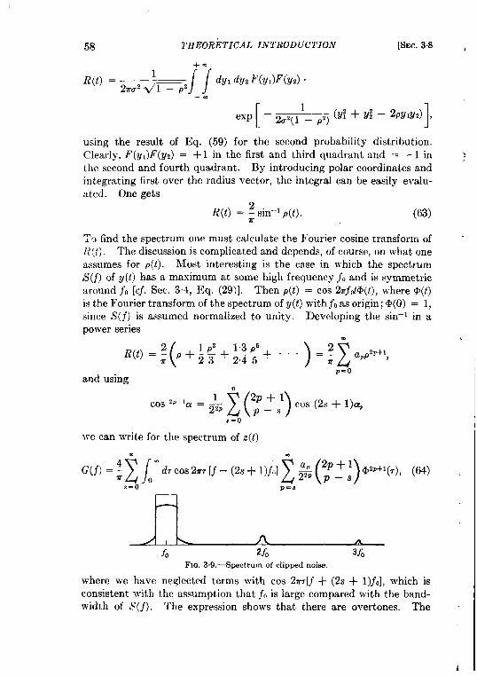
58 THEORETICAL INTRODUCTION [SEC.38
+.1
R(t) = —//
dy, d.y, F(y,)F(y,) .27ru’til – pz
—.
[exp —
12r2(11_p,)(Yf +!/: –2P!J1!/2) ,
using the result of Eq. (59) for the second probability distribution.Clearly, F(v,)F(YJ = +1 in the first and third quadrant and = –linthe second and fourth quadrant. By introducing polar coordinates andintegrating first over the radius vector, the integral can be easily evalu-:Ltcd. One gets
R(t) =~sin-l p(t). (63)
To find the spectrum one must calculate the Fourier cosine transform ofR(t). The discussion is complicated and depends, of course, on what oneassumes for p(t). Most interesting is the case in which the spectrumS(f) of y(t) has a maximum at some high frequency jO and is symmetricaround jo [cf. Sec. 3.4, Eq. (29)]. Then p(t) = cos 2mj0@(t), where ~(t)is the Fourier transform of the spectrum of y(t) with ja as origin; @(O) = 1,since S(j) is assumed normalized to unity. Developing the sin–l in apower series
( )22“R(t)=: P+; $+;4: +””” ‘- 2P+1app ,T
p=oand using
we can write for the spectrum of z(t)
.
G(j) = ; N md, COSk [j – (%+ l)jo]o 24?9’’+1(’),’64)
S=o p-8
—
1 1 \ A A
fo 2f. 3f.
Fm. 3.9.—Spectrumof clipped noise.
where we have neglected terms with cos 27r7[j + (2s + 1)fo], which isconsistent with the assumption that f~ is large compared with the band-width of S(j). The expression shows that there are overtones. The
II
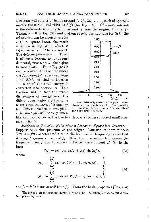
(
)
i
I
SEC.3.8] SPECTIi UM AFTER A NONLINEAR DEVICE 59
spectrum will consist of bands around jo, 2~0,3~0, . . . , each of approxi-mately the same bandwidth as b’(j) (see Fig. 3“9). Of special interestis the deformation of the band around jo from the original form S(j).Taking s = O in Eq. (64) and making special assumptions for S(f), thecalculation can be carried out; for 1,)0S(f), a square band, the result r
-----1
is shown in Fig. 3.10, which is I o,~ . I s(f)
taken from Van Vleck’s report. I /
The deformation is small. ThereI Owl-I
is, of course, less energy in the fun- 6.70
damental, since we have the higher 0.60 -
harmonics also. From Eq. (64) it 0.50-
can be proved that the area under 0.40the fundamental is reduced from 0.30-1 to 8/r2, so that a fraction1 – 8/r2 of the total energy is 0.20-
converted into harmonics. This 0,10-
fraction and in fact the wholedistribution of energy over the -2.0 -1.0 0=$ 1.0 2.0
dMerent harmonics are the same(f-JJ—
FIG, 3.10,—Spectrum of clipped noise;as for a square wave of frequency shape of the fundamental. The quantity~0, This conclusion is also Plau- the noisebefore clipping.V – /a) is in Units of the half bandwidthof
sible, since y(t) will be very muchlike a sinusoidal curve, the bandwidth of S(~) being supposed small com-pared with j,.
Spectrum of Gaussian Noise after a Linear or Square-law Ddector.-
Suppose that the spectrum of the original Gaussian random processV(t) is again concentrated around the high carrier frequency fo and thatit is again symmetric around .fO. It is often convenient to measure thefrequency from jO and to write the Fourier development of V(t)in the
form
l’(t) = x(t) cos 2rr~,t+ y(t) sin 2TjOt, (65)
where+.
x(t) =
z
(ak cos 27rfkt + b, sin 2TfJ,
—m+.
I
(66)
y(t) =z
(–a, sin 27r~,t +- b, cos 27rjkf),
-.
and .f~ = k/e is measuredl from f~. From the basic properties @qs. (54)
1The lower limit ln the sarnssho~llri,of course,be —k~, whcn~~ = ko/~, bllt it maybe replaced by – cc.
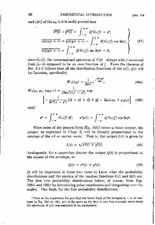
!
60 THEORETICAL INTRODUCTION
and (56)] of the ak, hit is easily proved that
[SEC. 3.8
/~ =v~= ‘“djG,(f) = .2,
—.
\
+-Z(t)fc(t +7) = ~ = df Gv(j) COS2~f~,
I
(67)—.
\
+-Z(t)y(t +7) = dfG,(f)sin2rj~ = O,
—.
since GV(f ), the unnormalized spectrum of V(t+always with j measuredfrom fa—k supposed to be an even function off. From the theorem ofSec. 35 it follows that all the distribution functions of the x(t), ~(t) willbe Gaussian, specifically,
=Z+vz—
WI(W) = &2e “ , (68a)
“(z” “; “y’; ‘) = (2TC’)’;l – p’) ‘Xp
\
+-
/
+.& = G,(f) df; Utp(r) = df Gv(f) COS2ufT.
—. -.
When noise of the general form [Eq. (65)] enters a linear detector, theoutput, as explained in Chap. 2, will be linearly proportional to theenvelope of the r-f or carrier wave. That is, the output L(t) is given by
L(t) = <1’(t) + y’(t). (69)
Analogously, for a square-law detector the output Q(t) is proportional tothe square of the envelope, or
Q(t) = z’(t) + y’(t). (70)
It will be important in these two caws to know what the probabilitydistributions and the spectra of the random functions L(t) and Q(t) are.The first two probability distributions follow, of course, from Eqs.(68a) and (68b) by introducing polar coordinates and integrating overt heangles. One finds, for the first probability distributions,
1Note in the expression for p(r) that the lower limit of the integrrd is — m in con-trast to 13q.(22) or (58); p(r) is the same as the ~(r) in our first example, since therethe spectrum of y(t) was assumed to be normalized.
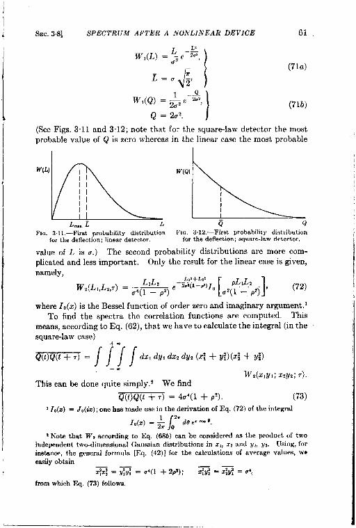
SEC. 3.8] SPECTRUM AFTER A NONLINEAR DEVICE 61
Q.—WI(Q) = &,e 2“’,
Q = 20’. 1
(71a)
(71b)
(See Figs. 3.11 and 3“12; note that for the square-law detector the mostprobable value of Q is zero whereas in the linear case the most probable
FIG. 3.1l.—First probability distribution FIG. 3.12.—First probability distributionfor the deflection; linear detector. for the deflection; square-lawdetector.
value of L is u.) The second probability distributions are more com-plicated and less important. Only the result for the linear case is given,namely,
W,(L1,L2,7) = ~,(:’:’pz) e-=)’L4H91’ ’72)
where 10(z) is the Bessel function of order zero and imaginary argument. 1To find the spectra the correlation functions are computed. This
means, according to Eq. (62), that we have to calculate the integral (in thesquarelaw case)
‘(C)Q(’+’) = /11/dz, dy, dz, dy, (z? + g?) (z: + @
-.W,(x,yl; Z,y,; T).
This can be done quite simply.2 We find
Q(t)Q(t +7) = 4U4(1 + p’). (73)
1~Kz) = JO(iZ);one has madeusein the derivationof M. (72) of the integral
\
2r10(2) = ; ~ de e“ - ‘.
1h’ote that IV* according to Eq, (68b) can be considered as the product of twoindependent two-dimensional Gauseian distributions in ZL, zz and vI, W. Using, fOriaztance, the general formula [Eq, (42)] for the calculations of average values, w~ezzily obtain
72.7~ = ~ = u~(l +2p1); z,y2 — Zld = e’.
from which Eq. (73) follows.
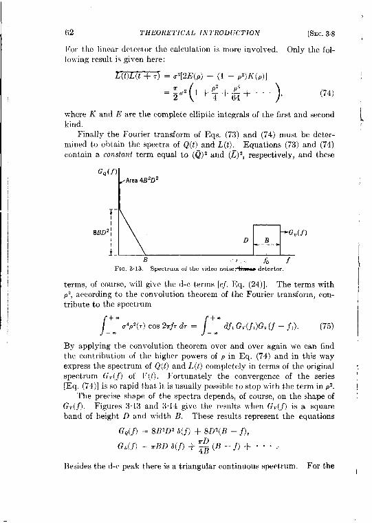
,,
62 THEORETICAL INTRODUCTION [SEC.38 ,
For the linear detector the calculation is more involved. Only the fol-lo~ving result is given here:
L(L)L(L +7) =u’[2E(p) – (1 –p’)K(p)] I
(
2 4— E ~z—
2 )1+%+++””” ‘(74) i
where K and E are the complete elliptic integrals of the first and second ~kind. /
Finally the Fourier transform of Eqs. (73) and (74) must be deter-mined to obtain the spectra of Q(t) and L(t), Equations (73) and (74)contain a constant term equal to (~) 2 and (~)z, respectively, and these
GQ(f)
LArea 4B2D2
B .-/, f, f~lG. 3,13.—Spectrumof the videonoise- detector.
terms, of course, will give the d-c terms [cf. Eq. (24)]. The terms withP2, ac~ording to the convolution theorem of the Fourier transform, con-tribute to the spectrum
/
+.U4P2(T)COS27r~7d7 =
!+ m dj, GdjJGv(f – fI). (75)
—. —.
By applying the convolution theorem over and over again we can findthe contribution of the higher powers of p in Eq. (74) and in this wayexpress the spectrum of Q(t) and L(t) completely in terms of the original !spectrum Gv(.f) of V(t). Fortunately the convergence of the series[Eq. (74)] is so rapid that it is usually possible to stop with the term in p’. !
The precise shape of the spectra depends, of course, on the shape of ~G.(f). Figures 3.13 and 3.14 give the results when G,(f) is a squareband of height D and width B. These results represent the equations
G.(f) = 8B2D2 ~(j) + 8D2(B – j),
G.(f) = TBD b(j) + ‘~ (B – j) + 0. . .
Besides the d-c peak there is a triangular continuous spectrum. For the ,
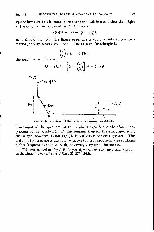
I
SEC. 38] SPECTR(rM AFTER A NONLINEAR DEVICE 63
square-law case this is exact; note that the width is B and that the heightat the origin is proportional to B; the area is
as it should be. For the linear case, the triangle is only an approxi-mation, though a very good one. The area of the triangle is
()~ BD = 0.39uZ;
the true area is, of course,
‘- ‘z)’=[2-01”2=043”’
GL(f)
I:~ / + G. (f )
D ~—-. *
B!$.. ~~ -- Jo f
FIG.3.14.—Spectrumof the videonoise:~ detector.
The height of the spectrum at the origin is (7r/4)D and therefore inde-pendent of the bandwidth’ B; this remains true for the exact spectrum;the height, however, is not (T/4)D but about 6 per cent greater. Thewidth of the triangle is again B, whereas the true spectrum also containshigher frequencies than B, with, however, very small intensities.
1This was pointed out by J, R. Ragazzini, “The ‘Effect of Fluctuation Voltageon the Linear Detector,” Pm.. I. R. E., 30, 277 (1942).
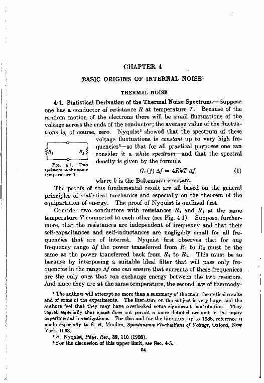
CHAPTER 4
BASIC ORIGINS OF INTERNAL NOISE’
THERMAL NOISE
4.1. Statistical Derivation of the Thermal Noise Spectrurn.--Supposeone has a conductor of resistance R at temperature T. Because of therandom motion of the electrons there will be small fluctuations of thevoltage across the ends of the conductor; the average value of the fluctua-tions is, of course, zero. Nyquist z showed that the spectrum of these
voltage fluctuations is ccnshnt up h very high fr~
a ‘Uencies”
3—s0 that for all practical purposes one can
consider It a white spectrum-and that the spectral~1~ ~,l,_TWO density is given by the formula
resistorsatthesametemperatureT.
G,,(f) Af = 4RlcT A~, (1)
where k is the Boltzxnann constant.The proofs of this fundamental result are all based on the genera~
principles of statistical mechanics and especially on the theorem of theequipartition of energy. The proof of Nyquist is outlined first.
Consider two conductors with resistances RI and Rz at the sametemperature T connected to each other (see Fig. 4.1). Suppose, further-more, that the resistances are independent of frequency and that theirself-capacitances and self-inductances are negligibly small for all fr~quencies that are of interest. Nyquist first observes that for anyfrequency range Aj the power transferred from R1 to R% must be thesame as the Dower transfemed back from RZ to RI. This must be sobecause by interposing a suitable ideal filter that will pass only fre-quencies in the range A.f one can ensure that currents of these frequenicesare the only ones that can exchange energy between the two resistors.And since they are at the same temperature, the second law of thermody-
1The authorswill attemptno morethana summaryof the maintheoreticalrwultaand of come of the experiments. The literatureon the subject k very large,and theauthoce feel that they may have overlooked some significantcontribution. Theyresret ~mciaW that spce dom not Pefit a mom detafledaccount of the manyexperimentalinvestigation. For thiz and for the literatureup to 193s, referenceismade especially to E. B. Moullin, SponiuneouaFltiwat&m.Y of Voltage,Oxford, N(wYork, 1938.
~H. Nyquiet,Ph~u. %., M, 110 (192S).~For the discumionof this upper limit, seeSee. 4%.
64
{
WC. -;11 8TA TISTICAL DERIVATION OF THE SPECTh! .?7M 65
namics (which is, of course, a consequence of statistical mechanics)requires that, on the average, no energy is transferred from the one resistorto the other. Now the spontaneous voltage fluctuations across each ofthe two resistors may be represented by the electromotive forces EI andE,, whose average values are zero and whose spectral densities G,,(j)and G~,(.f) are still unknown functions off. It follows then from simplecircuit theory that the average power transferred from RI to R2 in thefrequency range Af is given by
and the average power transferred back from R2 to R, is
(2a)
(2b)
Since these must be equal, one obtains
G~,(.f)Rz = G.,(f) ‘l. (3)
In particular, if RI = R*, it is clear that the spectral density of the fluctu-ating voltage must be a universal function of the resistance, temperature,and frequency and that it must be independent of the nature of the tworesistors and of the mechanism of the conduction of electricity throughthem.
To find the universal function, Nyquist imagines that the interchangeof energy between the two conductors 1takes place by means of a losslesstransmission line of characteristic impedance R, so that both resistors arematched. There is then no reflection at either end of the line; all poweremitted by one resistor is absorbed by the other, and vice versa. Whenequilibrium has been established there will be present in the line electro-magnetic energy of an amountz
:kTAf
m the frequency range Aj. Here L is the length of the line and v theveIocity of propagation of the waves. This expression follows from thefact that there are (2L/v) Af modes of vibration in the range Aj and thateach mode, according to the equipartition law, has the energy kT (namely,~kT electric and ~kT magnetic energy). The energy density in therange A~ is therefore (2kT/v) Aj; half of this is carried by waves going tothe right, and the energy that flows into the resistor on the right per
] Now supposed to have the sameresistance R.~This is the one-dimensional form of the well-known Rayleigh-Jeans law of radic
tion theory.
L
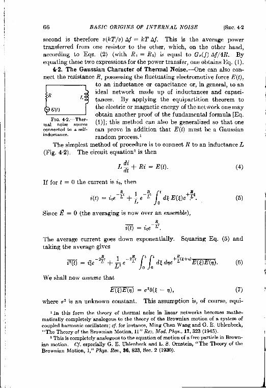
I
66 BASIC ORIGINS OF INTERNAL NOISE [SEC.4.2
second is therefore v(kZ’/v) A.f = kT A~. This is the average powertransferred from one resistor to the other, which, on the other hand,according to Eqs. (2) (with RI = Rz) is equal to GE(f) Af/4R. Byequating these two expressions for the power transfer, one obtains Eq. (1).
4.2. The Gaussian Character of Thermal Noise.—One can also con-nect the resistance R, possessing the fluctuating electromotive force E(t),
D
to an inductance or capacitance or, in general, to an
Rideal network made up of inductances and capaci-
L tances. By applying the equipartition theorem to
~ E(t) the electric or magnetic energy of the network one mayobtain another proof of the fundamental formula [Eq.
‘l~O~~~”–,~&~ (l)]; this method can also be generalized so that onemidconnectedto a self- can prove in addition that E(t) must be a Gaussianinductance.
random process. 1
The simplest method of procedure is to connect R to an inductance L(Fig. 42). The circuit equation’ is then
L: + Rz’ = E(t). (4)
If for t = O the current is i,, then
R!
/
1 -;t ti(t) = iOe–Z + – e
Ld~ E(~)e+&.
o
Since ~ = O (the averaging is now over an ensemble),R–~1
~) = ioe .
(5)
The average current goes down exponentially. Squaring Eq. (5) andtaking the average gives
We shall now assume that
E(t)E(q) = La(t – Tl), (7)
where az is an unknown constant. This assumption is, of course, equi-
1In this form the theory of thermal noise in linear networks becomes mathe-matically completely ‘analogous to the theory of the Brownian motion of a system ofcoupled harmonic oscillators; cf. for instance, Ming Chen Wang and G. E. Ublenbeck,“The Theory of the Brownian Motion, II” Re~. Mod. Phys., 17,323 (1945).
z This is completely analogousto the equation of motion of a free particle in Brown-ian motion, Cf. especially G. E. Uhlenbeck and L. S. Ornstein, “The Theory of theBrownian Motion, I,” Phys. Rev., 36, 823, Sec. 2 (1930).
SEC. 4.2] THE GAUSSIAN CHARACTER OF THERMAL NOISE 67
h
valent to the assumption that the spectral density of E(t) is constant; infact, one can see that
\
.G.(j) = 4 d, COS27f.E(t)E(t + ,) = 2u’.
o(8)
If, in Eq. (6), we let L + q = v, ~ – q = w, the double integral becomes
A’-T’L’’U’;T.”‘w”’’(w)‘d’-’-%’)so that
m ‘&+(’’ -&)’-%t(9)
This equation shows that ~ starts from a value i; and for t ~ cc reachesthe constant value u2/2RL. On the other hand it is known from theequipartition theorem that in the equilibrium state
Therefore u’ must be 2RlcT; or according to Eq. (8), G.(f) = 4RlcT.Equation (9) shows in detail, then, how the equipartition value is reached.
Of course, one could have reached the conclusion U2= 2RkT more~ directly by observing that as a consequence of Eq. (4) the spectralw
densitv of the current is
“(~)= {R !%:;fL12”(1OU)
With Eq. (8), this yields
/
m
/
m;2 = dj G,( j) = 2u’
df u’(lOb)
O R’ + 4r2~L’ = 2RL’o
and Cz is again determined by the equipartition theorem. It should bepointed out that in this derivation the constancy of the spectral densityGE(j) is assumed, whereas in Nyquist’s proof of Sec. 4.1 it is derived.With our method, however, we can now go a step further. In theequilibrium state we know not only that L? = k T but also that the firstprobability distribution W(i) for the current must be the Maxwell-Boltzmann distribution
J–
L~,w(i) = ~
——
2orkT ‘ 2kT”(11)
This is equivalent [see Eq. (3.7a)] to
~m=()
~Tk=l’.3.5...(2~_l) (~)k.
68 BASIC ORIGINS OF INTERNAL NOISE [SEC.42
The higher moments of z(t)can be calculated from Eq. (5). If the fore-going requirements are to be fulfilled as t -+ cc, it is necessary and suffi-cient’ that E(t) fulfill, besides Eq. (7), the relations
E(t,)E(t,) . “ “ E(t2,+1j = O; (12a)
~) = zE(t~)E(tj) _Eel “ “ . , (12b)
(all Pairs)
i where the sum has to be taken over all the different ways in which onecan divide the 2k time p0ink3 tl, tz, . . . , t2k, into ~ Pairs.
It clearly follows from Eqs. (7) and (12) that E(t) is a Gaussian ran-dom process with the constant spectral density 2V2. First, from Eq.(12a) it follows that the average values of all the odd powers of the Fouriercoefficients of E(t) in the time interval e,
/
2eak=6 o
dt Cos ‘21rfktE(t),/
b,=: oe dt sin 2uj@(t),
are zero. Furthermore, from Eq. (12b)
~=(w ‘“[d”“““““’cos%fkt’“““cos%jk””o
E(tJ “ . . E(h)
1“
E(t,)E(t,)
=1.3.5”. . (2n - l)(~)”,
since there are 1 .3 . . . (2n – 1) ways in which one can divide the 2ntime points h “ “ . t2n into n pairs. The distribution function for thea~ is therefore Gaussian, and analogously one can show that the bl’s
have a Gaussian distribution and that the diflerent ak’s and bl’s areindependent of each other; hence the complete distribution functionW(al, at, . . . ; bl, bz, . . . ) is given by Eq. (355), with
This last fact follows from Eq. (7) and is equivalent to the statement thatthe spectral density is 2U2A.f.
~See G. E. Uhlenbeck and L. S. Omzteio, op. cd., Note 1,for details of the proof.
1
I
I
(
I
-
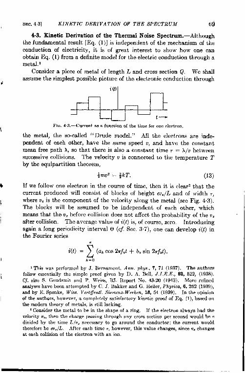
SEC.43] KINETIC DERIVATION OF THE SPECTRUM 69
4.3. Kinetic Derivation of the Thermal Noise Spectrum.-Althoughthe fundamental result [Eq. (1)] is independent of the mechanism of theconduction of electricity, it is of great interest to show how one canobtain Eq. (1) from a definite model for the electric conduction through ametal. 1
Consider a piece of metal of length L and cross section Q. We shallassume the simplest possible picture of the electronic conduction through
*Fm. 4.3.—Currentas a functionof the timefor oneelectron.
the metal, the s~called ‘‘ Drude model. ” All the electrons are inde.pendent of each other, have the same speed v, and have the constantmean free path A, so that there is also a constant time ~ = A/v betweensuccessive collisions. The velocity v is connected to the temperature Tby the equipartition theorem,
@v2 = $jkT. (13)
If we follow one electron in the course of time, then it is clear’ that thecurrent produced will consist of blocks of height ev./L and of width r,where VZis the component of the velocity along the metal (see Fig. 4.3).The blocks will be assumed to be independent of each other, whichmeans that the v, before collision does not affect the probability of the v=after collision. The average value of i(f) is, of course, zero. Introducingagain a long periodicit y interval e (cf. Sec. 3.7), one can develop i(t) inthe Fourier series
.
i(t)=z
(a, cos 2~j,t + b, sin 27rjJ).
k=O
1This was performed by J. Bernamont, Ann, phys., 7, 71 (1937). The authorsfollow essentially the simple proof given by D. A. Bell, J. I. E. E., 82, 522, (1938).Cj. also S. Goudsmit and P. Weiss, RL Report No. 43-20 (1943). More refinedanalyseshave been attempted by C. J, Bakker and G. Heller, Physicu, 6, 262 (1939),and by E. Spenke, Wiss. Vero~entl. Siemens-JVerken,18, 54 (1939). In the opiniondf the authors, however, a completely satisfactory kinetic proof of Eq. (1), based onthe modern theory of metals, is still 1acking.
zConsider the metal to be in the shape of a ring. If the electron always had thevelocity uZ,then the charge passing through any cross eection per second would be edivided by the time L/o. neceseary to go around the conductor; the current wouldtherefore be cu./L. After each time r, however, this value changes, since o=changesat each collision of the electron with an ion.
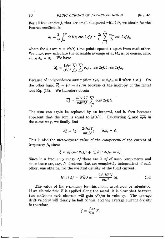
70 BASIC ORIGINS OF INTERNAL NOISE [SEC.43
For all frequencies jk that are small compared with 1/7, we obtain for theFourier coefficients
.
/
2’3
z
eu=,a~=—e.
dt i(t) Cos %.f,t = ; ~ Cos %rf,ti,i=l
where the t~’sare n = (e/r) time points spaced r apart from each other.We must now calculate the ensemble average of a; (~k is, of course, zero,since fiW= O). We have
–n&?2T2 —z=92L2V.,V., COS%fkt, COS%fktj.
i]
Because of independence assumption X = fi=,titj= O when i # j. On
the other hand T, = ~v2 = kT/m because of the isotropy of the metal
and Eq. (13). We therefore obtain
~ _ 4e2r2k T zCOS2%fkti.ak — m0~L2
i
The sum can again be replaced by am integral, and it then becomes
apparent that the sum is equal to ~(9/r). Calculating ~ and a~b~inthe same way, we finally find
7—7 2e2rkTak—bk. —; &=o.m0L2
This is also the mean-square value of the component of the current offrequency jk, since
Since in a frequency range Af there are 9 Af of such components andsince there are, say, N electrons that are completely independent of eachother, one obtains, for the spectral density of the total current,
Gi(j) Aj = N~@ Af = 2~N Af. (14)
The value of the resistance for this model must now be calculated.If an electric field F is applied along the metal, it is clear that betweentwo collisions each electron will gain eF7/m in velocity. The averagedrift velocity will clearly be half of this, and the average current densityis therefore
j=~fi’,
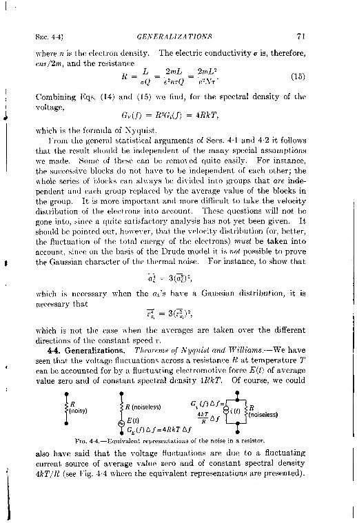
I
IJ
SEC.44] G’EIV17RALIZA TION,~ 71
where n is the electron density. The electric conductivity u is, therefore,e?Lr/2m, and the resistance
l{=$=;$ 2=$;. (15)
Combining Eqs. (14) and (15) w-e find, for the spectral density of thevoltage,
G.(j) = R’G,(j) = 4RkT,
which is the formula of Xyquist.From the g,cnerd statistical arguments of Sees. 41 and 4.2 it follows
that the result should be independent of the many special assumptionswe made. Some of these can be removed quite easily. For instance,the successive block do not have to be independent of each other; thewhole series of blocks can always be divided into groups that are inde-pendent and each group replaced by the average value of the blocks inthe group. It is more important and more difficult to take the velocitydistribution of the electrons into account. These questions will not begone into, since a quite satisfactory analysis has not yet been given. Itshould be pointod out, ho\veT’er,that the velocity distribution (or, better,the fluctuation of the total energy of the electrons) must be taken intoaccount, since on the basis of the Drude model it is not possible to prove
$ the Gaussian character of the thermal noise.
which is necessary when the a~’s have a
1,U1 Illaballue, IJu Mlu}}
Gaussian distribution,
‘-- ‘--’---- ‘- ------ that
it is
which is not the case when the averages are taken over the differentdirections of the constant speed r.
44. Generalizations. Theorems of Nyquist and ~1’illiams.-we haveseen that the voltage fluctuations across a resistance R at temperature T
dcan be accounted for by a fluctuating electromotive force E(t) of averagevalue zero and of constant spectral density 4Rk T. Of course, we could
[l
(~oisy) R (noiseless)
0
G, (j) Af=
E(t) 4+Af i ‘t) ~oiseless)
GE(f)bf=4RkTAfFIG. 4.4,—Equivalent representationsof the noise in a resistor.
also have said that the voltage fluctuations are due to a fluctuating
current source of average value zero and of constant spectral density;
I
4kT/R (see Fig. 44 where the equivalent representations are presented).
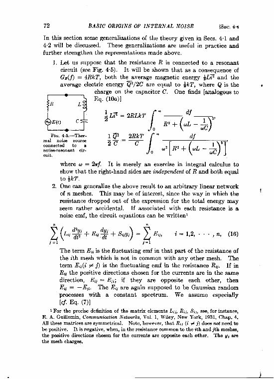
72 BASIC ORIGINS OF INTERNAL NOISE [SEC.d4
Inthksection some generalizations of thetheory given in Sees. 4.1 and4.2 will be discussed. These generalizations are useful in practice andfurther strengthen the representations made above.
1. Let us suppose that the resistance R k connected to a resonantcircuit (see Fig. 4“5). It will be shown that as a consequence ofG,(fl = 4RkT, both the average magnetic energy ~b= and theaverage electric energy ~/2C are equal to ik T, where Q is the
charge on the capacitor C. One finds [analogous to
~-jEq”~l~=2RLkT~mR2+,~_4Y
FIG. 4.5.—Ther-mal noise aourcsconnected to assrise-resonantcir-
:~=%~rnu,[R2+{L-A)s]
cuit.
2.
where o = %J It is merely an exercise in integral calculus toshow that the right-hand sides are independent of R and both equalto ~lcT.One can generalize the above result to an arbitrary linear networkof n meshes. This may be of interest, since the way in which theresistance dropped out of the expression for the total energy mayseem rather accidental. If associated with each resistance is anoise emf, the circuit equations can be written 1
n n
x )2Lii ~ + Rii ~ + Siiyj = Eii, i=l,2, . . ..n. (16)
j=l j=l
The term Eii k the fluctuating emf in that part of the resistance ofthe ith mesh which is not in common with any other mesh. Theterm Eij(i # j~ k the fluctuating emf in the resistance Rii. If inRii the positive directions chosen for the currents are in the samedirection, Eii = Eii; if they are opposite each other, thenEii = – Eii. The Eii are again supposed to be Gaussian randomprocesses with a constant spectrum. We assume especially[Cf. Eq. (7)]
1For the precisedefinitionof the matrix elementsL;i, R; i, S; ~, see, for instance,E. A. Guillemin, Cornmunicdon Networks, Vol. 1, Wiley, New York, 1931, Chap. 4.Alf these matrices are symmetrical. Note, however, that Rii (i #j] does rwtneed tobe positive. It is negative, when, in the resistance common h the ith and jth meshes,the positive directions chosen for the currents are opposite each other. The VI arethe mesh charges.
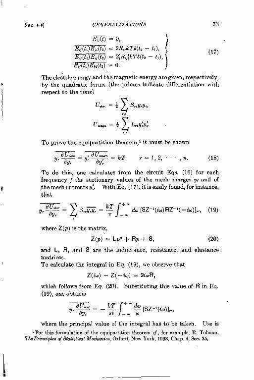
SEC. 4.4] GENERALIZATIONS 73
EJlj=o,
E;j(.fl)EjL(t*) ‘2RijkT’b(t2-tl)l
E,, (t,)lli;(t,) = 21R*,lkz’Nt2– h), [
(17)
The electric energy and the magnetic energy are given, respectively,by the quadratic forms (the primes indicate differentiation withrespect to the time)
Toprove theequipartition theorem,l it must be shown
aude. _ ,au_ ~T
Y, ~ – Yr ~y;— ., T=l,2, . . ..n. (18)
To do this, one calculates from the circuit Eqs. (16) for eachfrequency jthe stationary values of the mesh charges w and of
t themeshcurrentsy~. With Eq. (17), itiseasily found, forinstance,that
a Uehc z /+.yr~= s..=. = ~ dw[SZ-’(ti)RZ-’& o)],,,,, (19)
—.a
where Z(p) is the matrix,
Z(p) = Lp2+Rp+S, (20)
and L, R, and S are the inductance, resistance, and elastancematrices.Tocalculate theintegralin Eq. (19), we observe that
Z(kr) –Z(–iW) =2iaR,
which follows from Eq. (20). Substituting this value of R in Eq.(19), one obtains
_T5U2Z_~ ‘mdu‘r r3y, \
; [Sz-’(iu)].,,l-a —.
where the principal value of the integral has to be taken. Use is
1For this formulation of the equipartition theorem cj., for example, R. Tolman,Tlw Prim-plea of Statistical Mechanics, Oxford, New York, 1938,Chap. 4, Sec. 35,
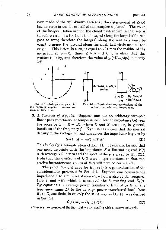
74 BASIC ORIGINS OF INTERNAL NOISE [SEC.4.4
now made of the well-known fact that the determinant of Z(h)has no zeros in the lower half of the complex a-plane.’ The valueof the integral, taken around the closed path shown in Fig. 4.6, istherefore zero. In the limit the integral along the large half circlegoes to zero; therefore the integral along the real axis must beequal to minus the integral along the small half circle around theorigin. This latter, in turn, is equal to mi times the residue of theintegrand at CJ= O. Since Z–I (0) = S–1, it is clear that thisresidue is unity, and therefore the value of y,(d U~../dy,) is merely
kT.
~lxx
FIG. 4.6.—Integrationpath inthe complexw-plane;crossesarezerosof Det [Z(iu)].
1
3.
toA A
z(f) .R(f) +jx(f) z(f)=(noisy) R(.f)+jX(f)
(noiseless)
E(f) GE(f)A@B B 4R(fikTAf
FIG. 4.7.—Equivalent representationsof thenoisein an arbitrary impedance.
A Theorem of Nyquist. Suppose one has an arbitrary two-polelinear passive network at temperature T; let the impedance betweenthe poles be Z = R + jX, where R and X are now, in general,
functions of the frequency j. N’yquist has shown that the spectral
density of the voltage fluctuations across the impedance is given by
G,(f) Af = 4R(j)kT Af. (21)
This is clearly a generalization of Eq. (1). It can also be said thatone must associate with the impedance Z a fluctuating emf E(t)with average value zero and the spectral density given by Eq. (21).Note that the spectrum of E(t) is no longer constant, so that suc-cessive instantaneous values of E(L) will now be correlated.
The proof Nyquist gave for Eq. (21) is a generalization of theconsiderations presented in Sec. 4.1. Suppose one connects theimpedance Z to a pure resistance Rlj which is also at the tempera-ture T and with which is associated the fluctuating emf E,(t).By equating the average power transferred from Z to RI in thefrequency range Af to the average power transferred back fromR, to Z, one finds, in exactly the same way as Eq. (3) was derivedin Sec. 4.1,
GE(f)RI = Ga(f)R(f). (22)
This is an expression of the fact that we are dealing with a passive network,
-
SEC.44] GENERALIZATIONS
Since it is known that G.,(j) = 4RJT,Eq. (21).
75
one immediately obtains
4, A Theorem of Williams. It must, of course, be possible to deriveEq. (21) by associating with each of the constant resistances afluctuating emf having the constant spectrum of Eq. (I) [just as inthe general circuit equations (16) ], and then calculating the com-bined effect of all these fluctuating emf’s on the voltage across thetwo poles of the network. This proof was given by Williams.’It is of special value, because one can also predict what will happenwhen the different resistances are no longer at the same temperature.
In this “more general case it seems quite plausible still to associatewith each constant resistance Ri a fluctuating emf Ei(t)of average valuezero and of spectral density 4Rik T~, where Ti is the temperature of theresistante. In essence, this was first proposed by Ornstein’ in hisstudies of how cooling the resistance influences the sensitivity of gal-vanometers. The first complete experimental confirmation of thisassumption 3 was first given by F. C. Williams, however.
Let Zi(j) be the transfer impedance between the resistance Ri (tem-perature T~) and the two poles A and B of the network. This meansthat a sinusoidal emf E of frequency $ in series with R~ will produce acurrent E/Zi in a link short-circuiting .4 and B. Williams shows thatthe spectral density of the voltage fluctuations across AB is given by
zRiTiG,(f) Af = 4121% A~ —
, 12,1’(23a)
and that the real part of the impedance Z is given by
(23b)
Clearly, when all the temperatures T, are the same, then Eq. (23a) reducesto Nyquist’s result [Eq. (21)].
Finally it should be pointed out that in this way one can also see thatalthough the spectrum of the voltage across A B is no longer constant,the voltage [or the emf E(t) in Fig. 4.7] is still a GausSan random process.The reason for this is that the different fluctuating emf’s E,(t) in the
1F. C. Williams,J. I, E. E., 81, 751 (1937).2L. S. Ornstein,Z. Physik, 41, 848 (1927); L. S. Ornstein,H. C, Burger,J. Taylor,
and W. Clarkaon, Proc. Roy. Sot., 115, 391 (1927).
3One must call it an assumption, because no general statistical proof for thisextensionof the original picture can be given. However, the kinetic proof makes theassumptionvery plausible.
b
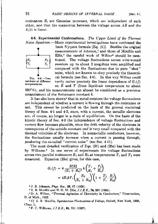
76 BASIC ORIGINS OF INTERNAL NOISE [SEC.4:.
resistances Ri are Gaussian processes, which are independent of eachother, and that the connection between the voltage across A B and theE~(t) is linear.
4.6. Experimental Confirmations. The Upper Limit of the There,
Noise Spectrum. —Many experimental investigations have confirmed the
I
basic Nyquist formula [Eq. (l)]. Besides the originalmeasurements of Johnson, 1 and those of Moullin and
I 1 Ellis, 2 the careful work of Wilbur3 should be men-
WR, R2 tioned. The voltage fluctuations across wire-woundT, T2 resistors up to about 2 megohms were amplified and
compared with the fluctuations due to pure “shot”noise, which are known to obey precisely the theoreti-
Fm. 4.8.—Two cal formula (see Sec. 4.6). In this way Wilbur couldresistorsat different verify rather precisely the linear dependence of G,(f)temperatures.
on R and T (from liquid-air temperature to about380”K), and his measurements can almost be considered as a precisionmeasurement of the Boltzmann constant k.
It has also been shown4 that in metal resistors the voltage fluctuationsare independent of whether a current is flowing through the resistance ornot. This cannot be predicted on the basis of the general statisticaltheory of Sees. 4.1 and 4.2, since, with a current, the metallic electronsare, of course, no longer in a state of equilibrium. On the basis of thekinetic theory of Sec. 4.3 the independence of voltage fluctuations andcurrent flow becomes plausible, since the drift velocity of the electrons inconsequence of the outside constant emf is very small compared with thethermal velocities of the electrons. In nonmetallic conductors, however,the fluctuations usually increase when a current is passing through,producing the so-called “current noise” (see Sec. 4.11).
The most detailed verification of Eqs. (21) and (23a) has been madeby Williams. 6 In one series of experiments the voltage fluctuationsacross two parallel resistances RI and R~ at temperatures TI and Tz weremeasured. Equation (23a) gives, for this case,
“R;%+aW~) = 4 (R, + R,),
‘4R1’T1(R*z)2(1+$”Z)1J. B. Johnson, Ph~s. Rev,, 32, 97 (1928).~E. B. Moullinand H. D, M. Ellis,J. Z.E. E., ’74, 331 (1934).
.’ D. A. Wilbur, “Thermal Agitation of Electricity in Conductors,” Dissertation,U. of Mich., 1932.
4Cj. E. B, Moullin, Spontaneous Fluctuations oj Voltage, Oxford, New York, 1933,Chap. L
6F. C. Williams, J. I, E, E,, 81, 751 (1937).
SEC.45] EXPERIMENTAL CONFIRMATIONS 77
The temperature Tz was varied from 20° to 470°C, while RI remained atroom temperature. The linear dependence of G,(j) on T2/T, and the
absolute value of G.(f) Were well established.
In a second series a capacitance and an inductance were introduced inthe two branches (see Fig. 4.9). In this case Eq. (23a) becomes
Again the temperature T, could be varied and the measurements couldbe made at three different frequencies j. The results again confirmed thetheory.
Finally, R,, Rz, and L were kept at room tempera-ture, and the voltage fluctuations across AB were meas-ured as a function of the temperature of the condenser.The value of G,(j) did not change, confirming the
picture that the fluctuating emf’s must be associated
I
.
\
only with the resistances.
Thk section is concluded with a discussion of theupper limit oj the thermal noise spectrum. It is clearthat the Nyquist formula must break down at somehigh frequency jO and that Gv(j) must then go to
zero. Otherwise (in the argument of Sec. 4“1) the
TA
Qc L
R, R2T1 T2
BFm. 4.9.—Two
impedancesat dif-ferenttemperatures.
total power transferred from one resistance to the other would be infinite.Various statements have been made in the literature about the value offo; they lead to several questions and difficulties, to be discussed briefly.
1. Nyquist pointed out that in his derivation (see Sec. 4.1) for veryhigh frequencies one should replace the equipartition value lcT forthe energy of each of the modes of the transmission line by thePlanck formula
hjehl/k T — 1 “
This would lead to
G,(j) Aj = 4R eh,,,~j_ ~ Aj. (24)
The spectrum would, therefore, vanish at a frequency of the orderof
jo=y =241 x1010T Cps, (25)
~nd the total voltage fluctuation across the resistance R would be
p=/
~2Rl#T2
“ djGv(j) = ~h o0
78 BASIC ORIGINS OF INTERNAL NOISE [~EC.45
On the other hand, from the kinetic proof given in Sec. 4.3, thenoise spectrum must be expected to drop to zero at a frequency ofthe order of
jo =:=; = 1013to 1014 Cps, (26)
and this has been corroborated by Bakker and Heller. 1 Bothlimits [Eqs. (25) and (26)] are, of course, much too high to be of anypractical significance. However, the question still remains:Which is the correct limit? The essential difference between Eqs.(25) and (26) is that Eq. (25) is universal whereas Eq. (26) would,in principle, give different limits for different metals.
2. One might think that the transmission line (or waveguide) proofof Nyquist shows that the limit must be universal, since otherwisethere would be a conflict with thermodynamics. The authorsbelieve thk is not so. Essential in Nyquist’s proof is the assumption that the conductors have a constant resistance, independent offrequency. At high frequencies this will certainly no longer betrue, and the dependence on frequency will be different for differentconduct ors. The proof of Sec. 4.1 breaks down at very highfrequencies because the conductors will no longer match the line,so that reflections will have to be taken into account.
3. The general argument of Nyquist leading to Eq. (21) makes it veryplausible that one always will find
G,(j) = 4R(j)lcT. (27)
It seems, however, that the function R(!) will usually not bedetermined by the nature of the resistor [a supposition that wouldlead to the limit expressed by Eq. (26)] but by the shape of theresistor, since this will determine its self-capacitance and self-inductance. Only when these are completely negligible will thelimit given by Eq. (26) begin to play a rble.
4. It is clear that at these high frequencies it is no longer permissibleto consider only networks with lumped constants. The generalstatistical theory should be generalized, using the Maxwell equa-tions, to an arbitrary system of bodies in equilibrium with theradiation field. Such an investigation would clarify the precisemeaning of Eq. (27) and would then presumably also determine thefunction R(j). It would also be of interest to see if a more generalkinetic investigation would justify Eq. (27).
5. A difficulty of Eq. (27) is that with a frequency-dependent resist-ance, the proofs of the equipartition theorem given in Sees. 4.2 and
1Ph@u, 6, 262 (1939).
SEC. 4.6] DEli!IVA TION OF THE SCHOTTK Y FORMULA 79
4.4 break down. This difficulty is, however, only apparent, sincethe impedance of the conductor must now necessarily also have acomplex part. Thus in the simple case of Sec. 4.2 (Fig. 4.2) themagnetic energy of the circuit will not be ~L;~, for the resistance Ralso will carry some magnetic and electric energy. That we shallagain arrive at the equipartition law can be shown only by themore general statistical investigation mentioned above.
NOISE DUE TO DISCRETENESS OF ‘THE ELECTRONIC CHARGE
4.6. Derivation of the Schottky Formula.-Let us consider a tempera-ture-limited diode connected to a resistance R.Because of discreteness of the electronic charge,the number of electrons emitted in equal timeintervals will fluctuate around an average value.As a result of this fluctuating current the voltage
u
R
across the resistance will fluctuate too, and thesefluctuations can be amplified and measured.This is the well known shot e~ect, first predictedand treated theoretically by Schottky. Heshowed that the spectral density of the current
FIG. 410,-Diode con-nectedto resistorR.
is constant up to frequencies of the order of the
reciprocal of the transit time and that the spectral density (for the tem-
perature-limited case) is given by the formula
G,(j) Af = 2eI Aj, (28)
where e is the electronic charge and 1 is the average current.Since the electrons may be taken as independent in the temperature-
Iimited case, it is clear that the current through the resistance will consist
f (t-t;)of a series of short pulses, each pulse cor-
k ,,=~,-k,, 29,
responding to the passage of an electron
from cathode to anode. The current
will therefore have the form
ti ti+r Time-
F1o. 4.1I.—Current pulse corre-i
spending to the passage of one where the ti’s are the random and in-electron. dependent emission times of the suc-cessive electrons, and where j(t) is almost like a Dirac ~-function (sincethe transit time 7 is very short) with area equal to the electronic charge e(see Fig. 4.1 1).’ Introducing a long periodicity interval f3, l(t) – ~ canbe developed in the Fourier series
1The statistical properties of sums of the type in Eq, (29) have often been investi-
1
80 BASIC ORIGINS OF INTERNAL NOISE
.
I(t) – ~ =z
(a, cos %j,t + b, sin %j,t).
k=O
For frequencies jk large compared with J/r, we obtainN
/
2’3ak=–
e.dt [I(f) – fl c!OS%jkt = ~
zCos 2rjA,
i-l
[SEC.4.-6
(30)’
where N is the total number of electrons passing from cathode to anodein the time 9; N may be considered constant. The averaging has to hdone over the random time points ~, for which a uniform distribution lawis assumed. It is clear that
Xk=-i=O,Cos kkcos %jkt; = sln %jkfi sln % kh = ~b,
cos %jk~ sin %jktj = O;therefore
~k=~k=o,
4e’ -AN = 2%%;a~.~k=@ z a~k = 0,
where n = N/e is the average number of electrons passing per second,The average current ~ is therefore en, and we can write, for the meansquare value of the component of the current of frequency jk,
Since in the frequency range Aj there are e Aj of such components,multiplication by this number yields the results given in Eq. (2$).
To prove that I(t)is a Gaussian random process requires a ratherdetailed investigation. It is clear that the mean values of all the oddpowers of ak and h vanish. Furthermore,
os@=G COS‘hfkti COS%fktj COS%fkti COS%fk&a
=ii;iF(zcos’~fktiY -’z(cos’~fk’”alli alli
+zc0s4%fk’1=@Y(: N’-:N+:N)811i
gated. Cj. S. O. Rice, “ Mathematical Analysis of Random Noise,” Bell System Tezhw.J., 23, 282 (1944), Part I; see also for further references, For the most completeand exact treatment see H. Hurwitz and M. Kac, “Statistical Analysis of CertQirTypes of Random Functions,” Arm. Math. Sfuti@., 16, 173 (1944).
SIX 46] DERIVATION OF THE SCHOTTK Y FORMULA 81
Since N can be chosen arbitrarily large, one might be inclined to concludethat the terms linear in N can be neglected; this would lead to
()2e2N 2
T;=3—ez
= 3 (~) ‘.
In the same way the mean values of all the even powers of a~ could becalculated; and keeping only the highest power of N, we should get
*= 1 .3.5 . . (2m – 1) (E;)’”,
which is characteristic for the Gaussian distribution. The next question
is whether or not the different Fourier coefficients are independent of each
other. Here one gets into trouble. It can be shown that the coefficients
al, az, ..., a, can be considered as independent (in the limit N ~ cc)if, and only if, s/N approaches zero as N approaches infinity. If we letonly @ approach infinity (keeping n = N/@ fixed), we shall have inde-pendence only providings is small compared with (1. Thus independenceof coefficients is obtained solely over narrow portions of the frequencyrange. To get a Gaussian process, where all the Fourier coefficients areindependent, not only must N approach infinity (which can always beachieved by taking @ large enough) but so must n also. The essential
condition for the Gaussian nature of the shot noise is that the averagenumber of electrons passing per second be very large. This conclusionis confirmed by an analysis of the distribution of I(t) itself. Assuming,as before, that the time points t, are distributed uniformly over the time;.nterval e, we obtain
Strictly speaking, we should still average over all possible values of Naccording to the Poisson distribution 1
with ~ = ne, where n is the average number of electrons passing persecond. We then get
/
+-~=n d~ f($). (31)
—m1WhenN is large,?V(N)can be approximatedby a Gaussiandistributionaround~
andw-itha varianceequalto ~; hencefor large ~ the variation of N may be neglected.The formulas become simpler, however, by taking the variation of N into account.
I
82 BASIC ORIGINS OF INTERNAL NOF,’$E [SEC.46
In the same way we get
‘/+-
72=: _e, [.l:m”dtj(t)l’
~tfi(t) + N(N – 1)
.
/
+.=n
—. “f(’)+ n2[J:.-d’f(’)l”
and it follows that
I(1 – 1)2 = n ‘m d~fi(~). (32)
—m
To find the distribution of 1 – ~ it is best to calculate the characteristicfunction
for which we obtain
[~(u) = exp – iun
Thk is still exact. For large n we may develop the exponent in powers ofu, leading to
*(U) ‘exp[-nu’/-+m”fi(i)l’l’(33b)
consequently (for large n) the distribution of 1 — ~ will be Gaussian withthe variance given by Eq. (32). By a calculation similar to that. given
in See. 3.6, it can be shown that the error will be
E
I A of the order of magnitude of l/n~+.
RExperimentally, the Schottky formula [Eq.
(28)] has been verified many times. In thec original experiments of Hull and Williamsl the
L current of a temperatur~limited diode was
B passed through a lightly damped resonant cir-cuit, End the fluctuation of the voltage between
FIG.4.12.—Diodeconnectedto resonantcircuit. the poles A and B was measured (see Fig. 4.12).
To calculate this fluctuation from Eq. (28), thediode must be considered as a fluctuating current source. The sDectraldensity of the voltage is therefore, in general,
G“(j) = [Z(ja) 12G,(j) = 2e~lZ(@) [‘,
when Z is the impedance between the poles A and B.
2eIGv(j) = ~,u,
R2 + L2c#
‘R’+(L”-lV’
(34)
We therefore get
1A. W. Hull and N. H. Williams, “Determination of Elementary Charge E fromMeasurements of Shot-effect,” Phys. Rev., 26, 147 (1925).
1
SEC.4.7] SPACE CHARGE DEPRESSION OF THE SHOT NOISE 83
which gives for the fluctuation of the voltage
In subsequent experiments by Williams and collaborators the current ofthe diode was passed through a resistance R (see Fig. 4.10), and thevoltage fluctuations, whose spectral density for this case is simply 2eZR2,were measured by a highly selective amplifier. The best results areprobably those obtained by Williams and Huxford. 1 They can beconsidered as almost precisionmeasurements of the electronic 11 l,at-~l
charge e.4.7. Space Charge Depression
of the Shot Noise.—When thecurrent through the diode is nottemperature limited, the electrons Aceas~ to be independent, and the Retarding~ Space-charge ~ Temperature
Schottky formula [Eq. (28)] breaksfield region ~ limited region \ limited region
down. Many experimental and ~lG. 4.13.—Current-v0ltage relation for adiode.
theoretical investigations havebeen devoted to the question of how the Schottky formula should be mod-ified. One can say that this problem has now, except for the h-f region(see Sec. 4.8), been solved. The theory is complicated, however; only ashort account of the main results will be attempted here.
It is necessary to recall, first, the well-known theory for the current-voltage characteristic of a diode. 3 For a given temperature of thecathode and for a given geometry, the characteristic has three distinctregions (see Fig. 413). When the voltage of the anode is sufficientlynegative, the potential distribution between cathode and anode will be amonotonic decreasing function; the electrons will therefore always be ina retarding field. The current is extremely small and is produced onlyby those electrons which are emitted with such high velocities that theycan overcome the retarding field and reach the anode. All other electronswill return to the cathode. As a result of the Maxwell distribution in
1N. H. Williams and W. S. Huxford, “Determination of the Charge of PositiveThermions from Nfeasurements of Shot Effect,” Phys. F&.,, 33,773 (1929).
2Cf. E. B. Moullin, Spontaneous F[uctuati”ons of Vottage, Chaps. 3 and 4, Oxford,New York, 1938. The theory was developed independently by D. O. North, “ Fluc-tuations in Space-charge-limited Currents at filodcrately High Frequencies, Part II,Diodes and N-egative-grid Triodes, ” Ii’(’A Rev., 4, 441 (1940); W. Schottky and E.Spenke, Wiss. VerO~erztl. Sie,nens-W”erken, 16 (Xo. 2), 1, 19 (1937); A. J, ltack,“Effect of Space Charge and Transit Time on the Shot Noise in Diodes, ” Bell Syste,nTechn. J., 17, 592 (1938).
i Cf., for example, I. Langmuir, Phys. Reo., 21, 419 (1923).
i
54 BASIC ORIGINS OF INTERNAL NOISE [SEC.4.7
velocity, the relation between the current and voltage in the retarded-field region is given by
I = Zm,e’vlk’. (35)
When the voltage of the anode increases the space-charge-limited regionis reached; here there is a minimum in the potential distribution betweencathode and anode. Therefore part of the field is retarding and partaccelerating. The relation between 1 and V k in this case complicatedand cannot be presented in a closed form. Increasing the anode voltageshifts the minimum toward the cathode. For high enough voltage theminimum will finally disappear, leaving only an accelerating field; one isthen in the temperature-limited region. In this case the current isconstant and equal to the saturation current I-t.
The Schottky formula [Eq. (28)] is valid only in the temperature-
1 I0
I 1 0FIG. 4.14.—Equiva-
lent circuit for a diodeconnectedto a noiselessresistorR.
limited region; then the density of the voltagefluctuations across an external resistance R (seeFig. 4.10) is consequently given bjj
G,(f) Aj = 2eI~,R2 Af. (36)
For the other regions of the characteristic, the firstquestion that has to be considered is the partplayed by the differential resistance p = dV/dZ ofthe diode. It seems plausible and can also be
strictly justified that the diode must always be considered as a fluctuatingcurrent source impressed on the resistances p and R in parallel (see Fig.4.14). Equation (36) is therefore generalized as follows:
‘( )Rp 2
G,(j) Aj = 2e1r” R7P Aj, (37)
where r is a dimensionless quantity, which may still depend on thecurrent 1. For dimensional reasons, r must have the form
()epI‘“Fro ’
(38)
where T. is the cathode temperature. The resistance p is, of course, alsoa function of 1, which can be determined from the characteristic. In thetemperature-limited region p = cc, r = 1, and 1 = I-, so that Eq. (37)goes over into Eq. (36). Moullin’ has shown experimentally that Eq.(37) gives the correct dependence on the resistance R. The point of viewthat the diode may always be considered as a fluctuating current source
I E. B. Moullin, “ Mezaurement of Shot Voltage Used to Deduce the Magnitude of‘Secondary Thermionic Emiesion.” Pmt. Rw. SW., 147, 109 (1934).
I
I
A
SEC.4.7] SPACE CHARGE DEPRESSION OF THE SHOT NOISE 85
has also been confirmed by a series of interesting experiments by Williams.’Williams took into account the thermal noise of the resistance R, whichhe represented by a fluctuating emf E(t) in series with the resistance R.For the voltage fluctuations across All (see Fig. 4.15), we find
()G,(j) =&p 2a~(.f) + (R $ ~), a~(j)
‘(R?;(
2
)2eII’2 + ~ , (39)
using Eq. (37) and the Nyquist formula; T is the temperature of theresistance R. The dependence on R and on 02’ was checked in detail. I 1 A
There remains the problem of calculating thefunction I’. The procedure may be roughly ex-
U
% E(t)
plained as follows: Just as in the temperature- I(t)p
limited case, it can be assumed here that the Relectrons emitted by the cathode emerge inde-pendent of each other and completely random in D
time. The average number vemitted per second Fm. 4.15.—Equivalent
determines 1-,. Let us suppose that in a time to, ~Oi,Y,e,i~to,~,circuitfor a diodeconnected
At, which is short compared with the periodI/j, more electrons than the average number v At are emitted by the cath-ode, and let the excess be An. Because of the exis~enze of a potential mini-mum, the number of electrons delivered at the anode in a time of the orderof the transit time 7 (which is also supposed to be small compared with 1/j)will not exceed the average number by the same amount An. The excesswill be less, because the An electrons will have somewhat lowered thepotential minimum and will have thus prevented other electrons fromreaching the anode. In the same way when fewer electrons than theaverage number v At are emitted by the cathode, the raising of thepotential minimum will diminish this defect at the anode. The fluctua-~ions will consequently be cut down, and one must therefore expect rto be less than unity.
For the precise calculation the velocity distribution of the emittedelectrons should of course be taken into account, since the effect on the.potential minimum will depend strongly on the velocity of the group ofelectrons under consideration. Furthermore, one must distinguishbetween the rej2ectedelectrons (or electrons of Class a), which have insuffi-cient energy to cross the potential minimum, and the transm ittcd clcrtrons
(or electrons of Class ~), which are the only ones contributing to the
1F. C. Williams, “ FluctuationVoltagein Diodes and in hlnlti-k-t rode valves, ”J. I. E. E., 79, 349 (1936). Cf. also Moullin, op. cd., p. 74.
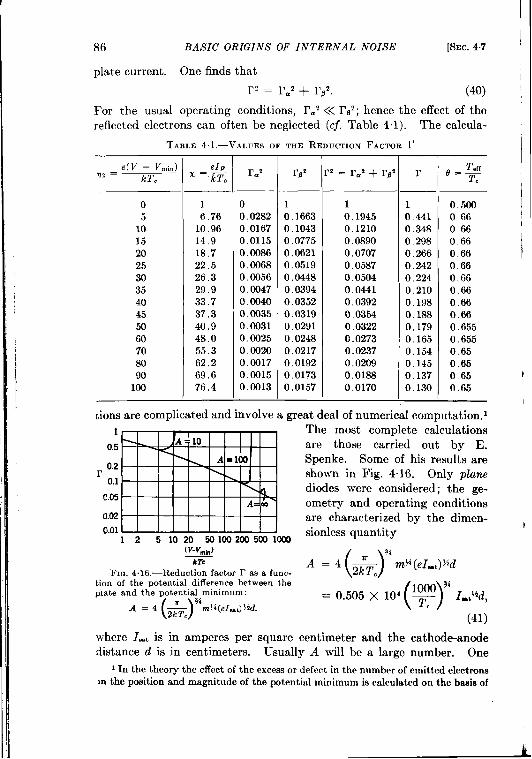
I86 BASIC ORIGINS OF INTERNAL NOISE [SEC.4.7 t
plate current. One finds that Irz = r.a + rB2. (40) \
For the usual operating conditions, r.2 << r02; hence the effect of the ‘reflected electrons can often be neglected (cf. Table 4.1). The calcula-
TABLE4.1.—VALUESOFTHEREDUCTIONFACTORr
e(V — Vmi.)712= IcT.
o5 ~
10152025303540455060708090
100
eIp~=z
16.76
10.9614.918.722.526.329.933.737.340.948.055.362.269.676.4
1r=2
0’
0.0282 10.01670,01150.00860.00680.00560.00470.00400,00350.00310.00250.00200.00170.00150.0013
10.16630.10430.07750,06210.05190.04480.03940.03520.03190.02910,02480.02170.01920.01730.0157
,2 = rat + rpz
10.19450.12100.0890
0.07070.05870.05040.04410.03920.03540,03220.02730.02370.02090,01880,0170
r
10.4410.3480.2980.2660.2420.2240.2100.1980.1880,1790.1650,15401450.1370.130
I
0.5000 660.660.660.660.660.660.660.660.660.6550.6550.650.650.65 1
0,65I
Lionsare complicated and involve a great deal of numerical computation. I1
0.5
0.2r
0.1C.05
0.020.01
12 5 1020 501IN2W5W1OW(V-vm,n)
kTcFm. 4. 16.—Reductionfactor r as a func-
t.im of the potential difference between theplate and the potential minimum:
A = 4 * ‘m!%u%() c
The most complete calculationsare those carried out by E.Spenke. Some of his results areshown in Fig. 4.16. Only planediodes were considered; the ge-ometry and operating conditionsare characterized by the dimen-sionless quantity
(41)
where I=, is in amperes per square centimeter and the cathode-anodedistance d is in centimeters. Usually A will be a large number. One
1In the theorythe effectof the excessor defect in the numberof emittedelectronsm the positionand magnitudeof the potentialminimumis calculatedon the baaisof
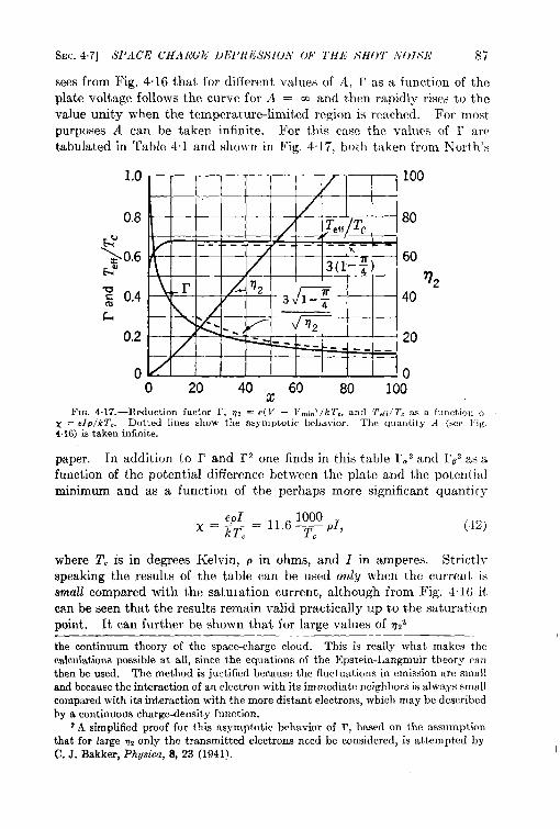
SEC. 4.7] SPACE CHA IIGIi DI$PRILSSIOA1 (IF THE SHOT iVOI<Vl$ 87
sees from Fig. 4.16 that for different values of A, r as a function of theplate voltage follows the curve for A = cc and then rapidly rises to the
value unit y when the temperature-limited region is reached. For mostrmr~oses A can be taken infinite. For this case the val~ws of r are. .tabulated in Table 4.1 and shown in Fig. 4.17, both taken from R’orth’s
1,0
0.8
~0,6fiw
: 0.4
L
0,2
0
/-100
1
/ ‘ ,?’w jTc 80I--- -. .- ,-. ,-- -- -- --
/
3(1:;)— 60
\ 1-r - T23= 40 “
/ ‘m’ — —#
- ~ --- 20. . -- -- --
. 00 20 40 ~ 60 80 100
FIG.4.17.—Reductionfactor r, 7j2 = e(V – V~~.)/kT,, mcf T.ff/T, as a funrtioll o~ = elp/k T.. Dotted lines show the asymptoticbehavior. The quantityA (see I’ig.4.16) is taken infinite.
paper. In addition to r and r2 one finds in this table r.2 and rpz as afunction of the potential difference between the plate and the potentialminimum and as a function of the perhaps more significant quanti[y
1000~=g=ll.6T PI,G ,
(12)
where T. is in degrees Kelvin, p in ohms, and I in amperes. Strictlyspeaking the results of the table can be used only when the current issmall compared with the satin ation current, although from Fig. 4.16 itcm be seen that the results remain valid practically up to the saturationpoint. It can further be shown that for large values of Vzz
the continuum theory of the space-charge cloud. This is really what makes thecalculations possible at all, since the equations of the Epstein-Langmuir theory ranthen be used. The method is juctified because the fluctuations in emission are smal!sad becausethe interaction of an electron with its immediate neighbors is always smallcomparedwith its interaction with the more distant electrons, which may be describedby a continuous charge-density function.
zA simplified proof for this asymptotic behavior of T, based on the assumptionthat for large m only the transmitted electrons need be considered, is attempted byC. J. Bakker, Phyti.a, 8, 23 (1941).
88 BASIC ORIGINS OF INTERNAL NOISE [SEC.4.7
(43)
These asymptotic formulas can be given an interesting interpretationin terms of a pseudothermal voltage fluctuation across the diode resist-ance p. Equations (37) and (39) for the voltage fluctuations across aresistance R may be interpreted in terms of a-fluctuating emf El(t) inseries with the resistance p if one assumes that the spectral density ofEl(t) is given by
GE,(j) Aj = 2eIrzp2 Aj. (44a)
Comparing this with the Nyquist formula, an “effective” temperatureT.. can be introduced by means of the equation,
G.,(j) Aj = 41cT.,P Aj, (44b)
and~_T.,_ eIPr~=~XT2
T. 21cT, 2 “(45)
The temperature T.= will of course depend on the current; from Eq. (43)
()it follows that, for large X, rz = 6 1 — ~ /x; hence
()L9=~=3 1–: =0.644.c
(46)
It is surprising that for smaller currents 0 remains near this value (seeTable 4.1); hence for all practical purposes one can consoler thediode in thespace-charge region as a resistance p at a temperature that is about tw+thirds
of the cathode temperature.
This result breaks down, of course, in the temperature-limited region,where one has the normal shot effect. It also breaks down in theretarded-field region. In this region there is no potential minimum;hence it must be expected that rz = 1. On the other hand from thecurrent-voltage relation, [Eq. (35)] it follows that
dV kTC,‘= Z=Z’
hence x = ePI/kT. = 1. From Eq. (45) it follows therefore that in theretarded-field region
Tes = ~TC. (47)
This simple result, which has been checked experimentally by Pearson
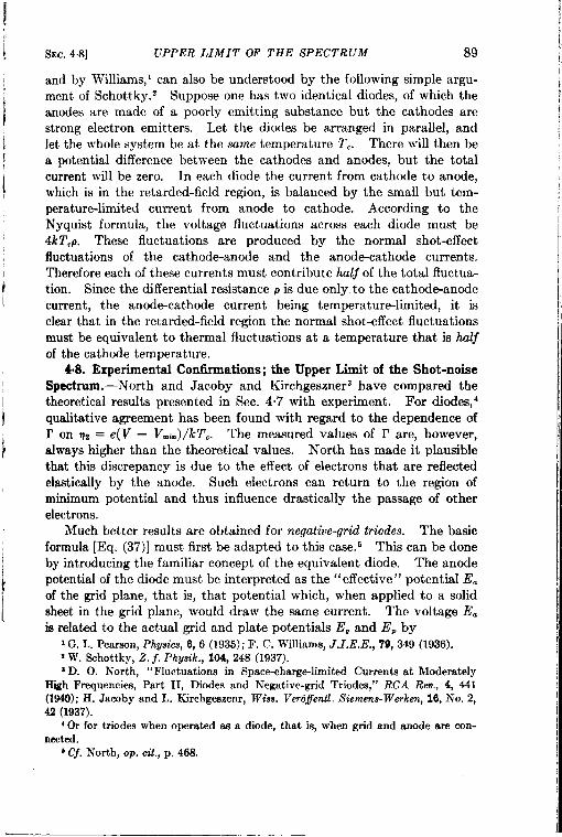
I
}
SEC.4.8] UPPER LIMIT OF THE SPECTRUM 89
and by Williams, 1 can also be understood by the following simple argu-ment of Schottky.2 Suppose one has two identical diodes, of which theanodes are made of a poorly emitting substance but the cathodes arestrong electron emitters. Let the diodes be arranged in parallel, andlet the whole system be at the same temperature 2’.. There will then bea potential difference between the cathodes and anodes, but the totalcurrent will be zero. In each diode the current from cathode to anode,which is in the retarded-field region, is balanced by the small but tem-perature-limited current from anode to cathode. According to theNyquist formula, the voltage fluctuations across each diode must be4kTCP. These fluctuations are produced by the normal shot-effectfluctuations of the cathode-anode and the anod~cathode currents.Therefore each of these currents must contribute hulj of the total fluctua-tion. Since the differential resistance p k due only,to the cathod+anodecurrent, the anode-cathode current being temperature-limited, it isclear that in the retarded-field region the normal shot-effect fluctuationsmust be equivalent to thermal fluctuations at a temperature that is hulfof the cathode temperature.
4.8. Experimental Conti.rrnations; the Upper Limit of the Shot-noiseSpectrum.-North and Jacoby and Kirchgeszner3 have compared thetheoretical results presented in Sec. 4.7 with experiment. For diodes, 4qualitative agreement has been found with regard to the dependence of1’ on V2 = e(V – V.ti)/kT.. The measured values of r are, however,always higher than the theoretical values. North has made it plausiblethat this discrepancy is due to the effect of electrons that are reflectedelastically by the anode. Such electrons can return to the region ofminimum potential and thus influence drastically the passage of otherelectrons.
Much better results are obtained for negative-grid triodes. The basicformula [Eq. (37)] must first be adapted to this case. s This can be doneby introducing the familiar concept of the equivalent diode. The anodepotential of the diode must be interpreted as the “effective” potential E“of the grid plane, that is, that potential which, when applied to a solidsheet in the grid plane, would draw the same current. The voltage Eais related to the actual grid and plate potentials Ea and E= by
1G. L. Pearson, Physic+ 6, 6 (1935); F. C. Williams, J.I.E.E., 79, 349 (1936).~ W. Schottky, Z. $. Phyw”k., 104, 248 (1937).* D. O. North, “Fluctuations in Space-charge-limited Currents at Moderately
High Frequencies, Part II, Diodes and Negative-grid Triodes,” RCA Rw., 4, 441(1940); H. Jacoby and L. Kirchgeszenr, Wiss. Vwoflentl. A’i.men*Wa-ken, 16, No. 2,42 (1937).
~Or for triodes when operated as a diode, that is, when grid and anode are con-nected.
t Cf. North, op. ant.,p. 46S.
90 BASIC ORIGINS OF INTERNAL NOISE [SEC.4%
‘a‘“(E,+:EJ (48)
\rllere u and p (the amplification factor) can, in principle, be calculated
from the geometry of the tube. The factor u lies between 0.5 and 1 and
usually is nearly 1. The plate current is a function of E., and hence theconductance of the equivalent diode is given by
(49)
when g~ is the mutual conductance of the triode. Using Eqs. (44a),(45), and (49), one obtains for the voltage fluctuations across a resistanceR in the plate circuit the formula
()2
G,(f) Aj = ; kT,gm ~~R Aj, (50)
which replaces Eq. (37); TPis the plate resistance, which is related to g~and P by the well-known relation
PTP= ‘“
9m(51)
Equation (50), with 8 = 0.66, has been thoroughly confirmed.’In all results obtained so far the frequency j is supposed to be small
compared with the reciprocal of the transit time 7 of the electrons. Allthe spectral densities are then independent of the frequency. It is clearthat this will cease to be valid when the frequency becomes comparablewith 1/,. In the te?npeTatuTe-iimited case it is easy to see what willhappen. In the Fourier analyses of the series of random current pulses(see Fig. 411) the shape of the pulses must now be taken into account.Taking the shape, for the sake of simplicity, as a rectangular block ofheight ev/d and width r = d/o, one gets, instead of Eq. (30),
As a result, the spectral density of the current fluctuations becomes
()sin 7rf7 2
G,(f) Aj = 2eI — Aj,7rjT
(52)
Irhich, of course, goes over into the Schott ky formula [Eq. (28)] when
‘ Cf. ibid. Since the effect of the electrons in the grid-plate space on the space-c},arge reduction factor r~ (or on the effective temperature L9T.of the cathOde-gridregion), has beenneglected,Eq, (t50)can be expected to hold only for high-ptubes.
SEC.4.9] PARTITION NOISE Q1
j<< l/T. For higher frequencies GJf) is always less than the Schottkyvalue; and for j>> 1/r, G1(j) goes to zero. Spenke’ has refined this roughcalculation by taking into account the velocity distribution of the emittedelectrons and the acceleration of the electrons between cathode and anode.Instead of Eq. (52), one then gets a completely monotonic decreasingfunction of j.
In the space-charge-limited region the problem is much more difficult.Rackz has given an analysis in which only the effect of the transmittedelectrons was taken into account. He obtained for the spectral densitythe expression
()G.(j) Af = 12 1 – : kTcPS(@ A~,
where
S(@) =~(2+82– 2cosd–2dsin 6’)
(53a)
(53b)
and o = %rfr is the transit angle. Equation (5%) is supposed to be arefinement of Eq. (44a) with the value given in Eq. (46) for the effective
temperature of the cathode. 3 The function S(8) is a monotonic decreas-ing function of 0, starting from unity for small 8 and going to zero forlarge 0. The space-charge reduction of the fluctuations would thereforepersist at high frequencies. It is doubtful, however, if this result iscorrect. Spenke4 has shown that in the retarded-field region, values for1’1can be obtained which are much larger than unity when the frequencyis of the order of magnitude of 2/7. The reason for this increase is thatthe rejZectedelectrons then begin to contribute strongly to the fluctua-tions. It seems probable therefore that at high frequencies the effect of
the reflected electrons cannot be neglected, and it may be that rz riseswith increasing frequency and goes through a maximum before going to
sero for very high values of j. Further theoretical investigationsand experimental information, which we do not now have, are requiredwith regard to this question.
4.9. Partition Noise.—In tubes that have more than one collectingelectrode (tetrodes or pentodes) the random nature of the partition of thetotal current over the different electrodes provides an additional cause of
fluctuations in current. The mean currents to the anode and to the
screen grid are determined essentially by the ratio of the free area of
7 Spenke, Wiss. Verafentl. Siemens- Werkenj 16, No. 3, 127 (1937).U.~A. J. Rack, “ Effect of Space Charge and Transit Time on the Shot Noise in
Diodes,” Bell System Te.hn. J., 17, 592 (1938).8 The p in Eq, (53) is the diode resistance at tow frequency and is therefore inde-
pendent off.i Op. cit., 17, No. 3, 85 (1938).
92 BASIC ORIGINS OF INTERNAL NOISE [SEC.4.9
the grid to its total area; the discrete nature of the electronic charge wiligive rise to fluctuations around these mean values.
Let us consider first the temperature-limited case. Since the electronsare completely independent of each other, and since the capture of anelectron by the grid is a matter of pure chance, the times of arrival of theelectrons at the anode will still be entirely random, just as for the diodein the temperature-limited case. The sole effect of the screen grid willbe to diminish the average anode current. The density of the anode-current fluctuations will therefore be given by the Schottky formula
G,.(f) Af = 2eIa Af, (54)
Where I. is the average anode current.Let us imagine, on the other hand, the case where the electrons would
be emitted by the cathode with absolute regularity in time, the timeintervals between successive electrons being constant as a result. In adiode there would then be no mu-rent fluctuations at all; in other words,the shot fluctuations would have been completely suppressed. ForFLmulticollector tube, however, the random nature of the capture ofelectrons by the grid would produce random gaps in the regular series ofcurrent pulses arriving at the anode; hence, there would again be somefluctuations in the current. What the spectrum will be is easily seen.Developing the anode current in a Fourier series in the usual fashion,
we obtain
The time points tiare now supposed to be spaced regularly with theconstant interval A. The random variables are the charges ei, which canhave only two values, namely, e and zero with the probabilities p andl–p. Therefore,
t?i=pt? — ‘-e,~j = t?iej = pzez,
;: = pe2,and we get
a; = —2 n ~i COS2Ufkti COS2Xj~14
ii
‘[ ($ )= ~, p’e’ cm 27rfdi 2 + p(l – p)ez Zcos’zkfk
I!
I
93SEC.4.10] TRANSIT-TIME EFFECTS IN TRIODES
or, again replacing the sums by integrals,
~~ = ~A p(l – p)ez.
Since A represents the spacing between successive electrons, it is clearthat e/A is the sum of the average anode and grid current and that
pe 1 – p)c—. 10 ( A = 1.,.A
We can therefore write~ _ 2e IJ.,
‘k – G 1= + 1,,”
The same result is found for ~; and since 1/(3 = Aj, we get for the spectraldensity of the anode current
G,.(j) Aj = 2e —I:PIg, ‘j”
(55)
Comparing Eqs. (54) and (55), it can be seen that the completesuppression of the shot-effect fluctuation before the partition of thecurrent reduces the fluctuations in the anode current by the factor
~,,/(~. + ~,,). In the actual case when the initial current is space-chargelimited, the shot-effect fluctuations are only partially suppressed; hencethe fluctuations in the anode current must be expected to lie between thevalues given by Eqs. (54) and (55). A more precise analysisl shows thatin the general case
G,a(~) Aj = 2eIa ~f ~ ;z~ Aj, (56)Llg
where 1’2 is the space-charge reduction factor that was discussed in Sec.4“7. For I’z = 1 (no space-charge suppression, temperature-limitedcase) Eq. (56) becomes Eq. (54), whereas for 172= O (complete space-charge suppression) Eq. (56) becomes Eq. (55).
In exactly the same way, we find, for the spectral density of the screen-~“d current,
~“ + ‘21’” Aj.G,,,(j) Af = 2eIw ~a + I,, (57)
Northz tested Eqs. (56) and (57) and found excellent agreement withexperiment.
401O. Tramsit-time Effects in Triodes and MulticoUector Tubes;Induced Grid Noise .—Equations (56) and (57) of Sec. 4.9, for the spectral
I Cf. D. O. North, “ Fluctuationsin Space-chargdmited Currentsat ModeratelyHighFrequencies,”RCA Rev., 6,244 (1940).
2L@& Cf”t.
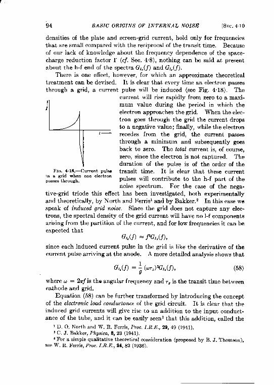
94 BASIC ORIGINS OF INTERNAL NOISE [SEC.410
densities of the plate and screen-grid current, hold only for frequenciesthat are small compared with the reciprocal of the transit time. Becauseof our lack of knowledge about the frequency dependence of the space-charge reduction factor r (cf. Sec. 4.8), nothing can be said at presentabout the h-f end of thespectra G,a(j) and G,.(j).
There is one effect, however, for which an approximate theoreticaltreatment can bedeviled. It is clear that every time an electron passesthrough a grid, a current pulse will be induced (see Fig. 4.18). The
(1
Fm. 4.18.—Current pulsein a grid when one electronpassesthrough.
current will rise rapidly from zero to a maxi-mum value during the period in which theelectron approaches the grid. When the elec-tron goes through the grid the current dropsto a negative value; finally, while the electronrecedes from the grid, the current passesthrough a minimum and subsequently goesback to zero. The total current is, of course,zero, since the electron is not captured. Theduration of the pulse is of the order of thetransit time. It is clear that these currentpulses will contribute to the h-f part of thenoise spectrum. For the case of the nega-
tive-grid triode this effect has been investigated, both experimentallyand theoretically, by North and Ferrisl and by Bakker. Z In this case wespeak of induced grid noise. Since the grid does not capture any elec-trons, the spectral density of the grid current will have no l-f componentsarising from the partition of the current, and for low frequencies it can beexpected that
G~,(j) = ~G~a(j),
since each induced current pulse in the grid is like the derivative of thecurrent pulse arriving at the anode. A more detailed analysis shows that
G,.(j) = : (W7,)2GIa(j), (58)
where a = 27r~is the angular frequency and TOis the transit time betweencathode and grid.
Equation (58) can be further transformed by introducing the conceptof the electronic load conductance of the grid circuit. It is clear that theinduced grid currents will give rise to an addition to the input conduct-ance of the tube, and it can be easily seen3 that this addition, called the
1D. O. North and W. R. Ferris,F%oc.Z.R. E., 29, 49 (1941).2 C. J. Bakker, Ph~m”ca,8, 23 (1941).3For a simple qualitative theoretical consideration (proposed by B. J. Thomson),
see W. R. Ferris, Proc. I. R. E., 24, 82 (1936),
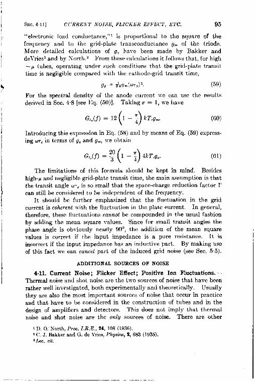
1“
I
1
41’
I1
SEC. 4.11] CURttEN1’ NOISE, FLICKER EFFECT, ETC. 95
“electronic load conductance,”’ is proportional to the square of thefrequency and to the grid-plate transconductance g~ of the triode.More detailed calculations of go have been made by Bakker anddeVries’ and by North. 3 From these calculations it follows that, for high–A tubes, operating under such conditions that the grid-plate transittime is negligible compared with the cathode-grid transit time,
(59)
For the spectral density of the anode current we can use the resultsderived in Sec. 4“8 [see Eq. (50)1. Taking u = 1, we have
()Gr.n(f) = 12 1 – ~ kTcgnv (60)
Introducing this expression in Eq. (58) and by means of Eq. (59) express-ing mu in terms of g,,and g~, we obtain
(61)
The limitations of this formula should be kept in mind. Besideshigh-~ and negligible grid-plate transit time, the main assumption is thatthe transit angle u-q is so small that the space-charge reduction factor IIcan still be considered to be independent of the frequency.
It should be further emphasized that the fluctuation in the gridcurrent is coherent with the fluctuation in the plate current. In general,therefore, these fluctuations cannot be compounded in the usual fashionby adding the mean square values. Since for small transit angles thephase angle is obviously nearly 90°, the addition of the mean squarevalues is correct if the input impedance is a pure resistance. It isincorrect if the input impedance has an inductive part. By making useof this fact we can cancel part of the induced grid noise (see Sec. 5.5).
ADDITIONAL SOURCES OF NOISE
4.11. Current Noise; Flicker Effect; Positive Ion Fluctuations.—Thermal noise and shot noise are the two sources of noise that have beenrather well investigated, both experimentally and theoretically. Usuallythey are also the most important sources of noise that occur in practiceand that have to be considered in the construction of tubes and in thedesign of amplifiers and detectors. This does not imp] y that thermalnoise and shot noise are the only sources of noise. There are other
1D. O.”North, Proc. Z.R. E., 24, 108 (1936).; C. J. Bakker and G. de Vries, Physicu, 2, 683 (1935).$Lot. d.
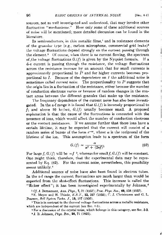
96 BASIC ORIGINS OF INTERNAL NOISE [SW 411
sources, not so well investigated and understood, that may involve otherfluctuation “ mechanisms. ” Here only some of these additional sourcesof noise will be mentioned; more detailed discussion can be found in theliterature.
In semiconductors, in thin metallic films, 1 and in resistance elementsof the granular type (e.g., carbon microphone, commercial grid leaks)2the voltage fluctuations depend strongly on the current passing throughthe element. 3 Of course, when there is no current flowing, the spectrumof,the voltage fluctuations G.(.f) is given by the Nyquist formula. If ad-c current is passing through the resistance, the voltage fluctuationsacross the resistance increase by an amount that for small currents isapproximately proportional to 12 and for higher currents becomes pro-portional to 1. Because of the dependence on 1 the additional noise issometimes called current noise. The proportionality to 12 suggests thatthe origin lies in a fluctuation of the resistance, either because the numberof conduction electrons varies or because of random changes in the con-tact areas between the different granules that make up the resistance.
The frequency dependence of the current noise has also been investi-gated. In the a-f range it is found that G.(j) is inversely proportional toj; and above 10 kc/see, G.(j) usually becomes small. A proposedexplanation is that the cause of the fluctuations is connected with thepresence of ions, which would affect the number of conduction electronsor the contact resistances. If we assume further that these ions have acertain lifetime, it may be expected that the current will consist of arandom series of bursts of the form e–ai, where a is the reciprocal of thelifetime of the ion. This assumption leads to a spectrum of the form
G.(f) = aaz + (2mj)2
(62)
For large j, G.(j) will be =j-’, whereas for small j, G.(j) will be constant.one might think, therefore, that the experimental data may be repre-sented by Eq. (62). For the current noise, nevertheless, this possibilityyseems unlikely. 4
Additional sources of noise have also been found in electron tubes.In the a-f range the current fluctuations are much larger than would beexpected from the shot-effect fluctuations. This increase is called the“flicker effect”” , it has been investigated experimentally by Johnson, s
1Cf. J. Bemamont, Ann. Phys,, 7, 71 (1937); Proc. Phgs. Sot., 49, 138 (1937).2 E. Meyer and H. Thiede, E. N. T., 12, 237 (1935); C. J. Christensen and G. L.
Pearson, Bell Syskrn Te.hn. J., 15, 197 (1936).3 This is in contrast to the thermal voltage fluctuations acrossa metallic resistance,
which are indcpcndcnt of the current (see Sec. 4.5).~For a discussionof the crystal noise, which belongs in this category, see $ec. 5.3.bJ. B. Johnson, Phys. Rsu., 26, 71 (1925).
I
I
Ii
SEC.4.11] CURRENT NOISE, FLICKER EFfi ECT, ETC. 97
who found that the increase is proportional to the square of the averagecurrent and that it is strongly frequency-dependent. For frequenciesabove 5 kc/see, the flicker effect disappears. A theory proposed bySchottkyl attributes the ilicker effect to random changes in the emissivityof the cathode produced by the presence of foreign atoms on the surface.Let us suppose that one foreign atom causes an additional current cI,where 1 is the average current and c a constant; let the average number offoreign atoms per square centimeter of the surface be N and the lifetimeof a foreign atom be I/a. Then the spectrum of the current fluctuationsis given by the formula
G,(f) Aj = 2eI Af + 4Nc21Z a? + y%f)z ‘j(63)
The second term represents the flicker effect and is in qualitative agree-ment with the observations of Johnson. The order of magnitudeof the flicker effect is usually expressed in terms of an apparent electroniccharge. For low frequencies apparent charges of the order 100e arecommon. For oxide-coated filaments the flicker effect is much morepronounced than for pure tungsten filaments, again in accord with theideas of Schottky.
At higher frequencies (100 to 1000 kc/see) increases of the currentfluctuations have been observed when the tube is operated in the space-charge-limited region.z These increases (the apparent electronic chargecan be of the order 10e) are caused by the presence of positive ions trappedin the potential minimum. The slow motion of these ions releasesrandom bursts of electrons. The positive ions are produced by evapora-tion from the cathode or by collision ionization of the residual gas atomsin the tube. This positive-ion effect disappears if the plate voltage israised, and the current becomes temperature limited. The frequencydependence of the effect has not been investigated.
1W. Schottky, Phys. Rev., 28, 74 (1926).2H. N. Kozanowski and N. H. Williams, Phys. Rev., 36, 1314 (1930). For a
theoretical development and more recent experiments, see B. J. Thompson and D. O.North, RCA Rev., 5,371 (1941).
i
CHAPTER 5
RECEIVER NOISE
6.1. Introduction. Separation of Noise Contributions.—The noisevoltage appearing at the output terminals of a receiver actually arisesfrom many sources. Some noise is generated by the antenna itself,which, as we shall see in Sec. 5.2, is due to incoming electromagneticdisturbances. In addition to this antenna noise there are several sourcesof noise within the receiver; chief among these noise contributions are the(crystal) converter noise, the local-oscillator noise, and the noise gener-ated within the i-f amplifier. Here it need be noted only that these noisecontributions are essentially independent. This fact assures that in alinear system the total noise power is the sum of the powers of the indi-vidual noise contributions. Furthermore this independence makes itpossible to break the receiver into hypothetical pieces in each of which thedetailed behaviors of signal and noise are studied, with a view towardultimately synthesizing the over-all signal and noise contributions.Friis’ has presented a method by which this analysis can be effected.The following analysis utilizes extensively the methods of Friis, withmodifications devised by Roberts. 2
The superheterodyn~ converter is essentially linear (see Sec. 2.2), andthe i-f amplifier stages (at least at low level) are linear; let us thus assumethat the over-all superheterodyne receiver consists of a series of linearnetworks; each of these networks is characterized by an input and outputimpedance and a gain that will shortly be defined. These three param-eters are generally complex and depend upon frequency. It is notessential that the input and output signal frequencies be identical; it isnecessary only that the network be linear, i.e., that the output signalvoltage be linearly related to the input signal voltage.
Each of these linear networks serves to amplify (or to attenuate) thesignal as well as any noise produced either in the device generating thesignal or in preceding networks. In addition to this, the network ingeneral adds some extra noise; this extra noise is the only quantity thatprevents the network (or over-all receiver) from being ‘‘ theoreticallyideal. ” The attempt will be made therefore to specify the characteristics
1H. T. Friis, “ NoiseFiguresof Radio Receivers,” Proc. I. 7?.E., 33, 458 (1945).2S. Roberts, “Same considerations GoverningNoise Measurementson Crystal
Lfixcrs,” Pro.. Z,R. E., 35, 257 (1947).
98
t.
SEC.5.1] INTRODUCTION 99
of the over-all receiver in terms of this ideal receiver; this specification, tobe definite, must assume certain properties of the input-signal generatingdevice. [Since the properties of the antenna depend upon externalradiation, which may be quite different under different conditions (seeSec. 5.2), it is customary to measure the properties of a receiver by meansof a signal generator connected to its input terminals.] This signalgenerator is any device which can be represented, according to Tht%enin’stheorem, as a constant voltage source e, in series with an impedanceR. -t- jxo.
Available Power.-The available power from the signal generator or alinear network is simply the maximum power that can be taken from thenetwork by a suitably adjusted load. In the case of the signal generatormentioned previously the available signal power So is
s, = -$.0
(1)
In addition to the available signal power from the generator, there is anoise fluctuation voltage due to R~. The open-circuit mean-square noisevoltage from the generator within a narrow frequency interval dj (seeSec. 3.1) is
G,(f) df = 41cTR, dj, (2)
where k is Boltzmann’s constant and T is the temperature of R., Thequantity Gv is the power spectrum expressed in mean-square volts perunit frequency interval. Therefore, the available noise power dN, fromthe signal generator is
Gv:~ ‘j = ~T dj,dNg = — (3)9
which does not depend upon the generator impedance but does dependupon the temperature of the generator resistance and the bandwidth dj.To standardize the performance of the generator it is necessary to choosesome standard temperature !!’o; it is customary to choose To as 292°K,since this is a reasonable approximation to the ambient temperature atwhich measurements are made, and since for this value of temperaturethere is obtained the simple relation
kTo = ~
40volt,
e(4)
where e represents the electronic charge.The Gain oj a Network.—The power gain G of a network will be defined
here as the ratio of available output signal power to the available inputsignal power delivered either by the signal generator or by a precedingnetwork. C)n the basis of this definition the gain is seen to depend upon
-—
100 RECEIVER NOISE [SEC.51
the impedance of the generator but not upon the impedance of the load.It does not represent the actual power gain unless suitable matching loss-less networks preinserted between thegenerator and load. The over-allgain of a series of cascaded networks is the product of the gain factors ofthe individual networks.
The actual measured output power of the network is not necessarilythe available output power. The quantity with which we are ultimatelyconcerned, however, is the ratio of signal to noise power, i.e., the ratioof gain to noise power. The ratio of measured output power to availableoutput power when the network is connected to a mismatched load will beidentical for both signal and noise; hence only available gain need bedealt with in the analysis that follows.
Noise Figure.—As the noise and signal proceed from the signalgenerator through the various networks, the ratio of noise power tosignal power increases. The reason for this increase is the extra noisecontributions from the networks themselves. Let us consider the ratioof output noise to signal power (available) dN~/&, where the outputnoise power dN~ is measured in a frequency band df centered at the signalfrequency. Thk quantity is larger than the corresponding quantity atthe signal generator by a factor 1’, which is called the noise figure of thenetwork.
(5)
In this definition of noise figure the two signal frequencies can be different,but the noise at each point must be measured in a narrow band of givenwidth df centered at the signal frequency. Furthermore, it is assumedthat there is a one-to-one correspondence between input and outputfrequencies. This last assumption is not generally fulfilled in a super-heterodyne converter; but if the image response is suppressed by pre-election or by other means (see Sec. 2.2), Eq. (5) is valid. If the imageresponse is not suppressed, extra noise will be found in the output of thenetwork. Therefore, presupposing good converter design, it will beassumed (in those cases where it matters) that the image response isproperly suppressed.
The expression for the noise figure F may be written in a slightlydifferent way. The increase of F over unity is explained by extra outputnoise dikf. generated within the network.
or
dNo _ GkTo df dM. kT, dfA’. – GSQ +aqg=F so ‘
(6)
F–1= ‘M” .GkTo df
(7)
SEC. 5.1] INTRODUCTION 101
Integrated Noise Figure.—The noise figure is in general, as just defined,aiunctionof frequency. It is useful, however, tospeak of the integratednoise figure Fi of a network which represents the increase of the ratio oftoti noise to signal power by the network.
From Eq. (5) we may write
dNO = FG dNO = FGkT, df (8)and
N. =/
“ FGkT, dj. (9)o
The noise that would have appeared at the output from an ideal network
is/
“ (X-TO dj; hence we may writeo
I “ FGkT, djF,=om
IGkT, dj
o
If the bandwidth of the network Aj is defined as
/Af=& o“ G df,
(lo)
(11)
where G- is the maximum of the gain vs. frequency characteristic, ~vemay write
F, = ‘0GmkT, Af”
(12)
Cascaded Networks. —When two networks in series follow the signalgenerator, an expression for the over-all noise figure of the combinationmay be derived in terms of the noise figures of each section.
The over-all output noise power dNo,, within a narrow band df cen-tered at the signal frequency is made up of two parts. The first part isthe output noise from the first section dN. amplified by the second net-
. .work according to Its gam Gz, and the second part is the cxt,ra noisecontributed by the second section. This second contribution can bederived from Eq. (7). We may write
dN.,, = dNo,G, + (F, – l)G,kTo df (13)or
F,KAG,kTo df = F,G,G,kTo dj + (F, – l)C,kTO df, (14)
where F12 is the over-all noise figure. From Eq. (14),
F,–1F,2=F, +--G, ~ (15)
102
Thus the over-all noisefigures of the individual
RECEIVER NOISE
figure can be expressed
[SEC.~1
in terms of the noisenet works. This expression is especially useful
in deriving the noise figure of the first network by measuring Fj, Flz, andG,; this procedure is currently used in connection with crystal converters(see Sec. 5.3).
One can proceed from two to three networks byconsidering the firsttwonetworks asasingle network andthenapplying Eq. (15).
F,–1F123 =F12+=
.F1+F~+F~- (16)
If one proceeds in this way the over-all noise figure of n sections will be
It can be seen (and a little reflection makes it obvious) that after anyhigh-gain network the over-all noise figure is not markedly influenced byadditional networks even though their individual noise figures are rela-tively high. Thus in the superheterodyne receiver one need be concernedonly with the r-f amplifier, the converter-which in the microwave fieldgenerally has a gain less than unity—and with the first stage or two of thei-f amplifier.
An expression analogous to Eq. (17) can be derived for the over-all 1integrated noise figure of cascaded networks, but only if the bandwidthof the final network is narrow compared with the bandwidth of anypreceding section.
By analogy with Eq. (10) the following equation may be written:
Since the bandwidth of the nth section is assumed narrow compared withthat of any preceding network, the only quantities in Eq. (18) that depend ‘upon the frequency are F. and G.. From Eqs. (10), (11), (17), and (18),we may write
Fin – 1—— (19)
G,G, . . G,,_,
The form of this equation is similar to that of Eq. (17); it should be noted,ho~rever, that for the intermediate net,\vorksthe noise figures themselves ~are used instead of the corresponding integrated noise figures.
(-.. I
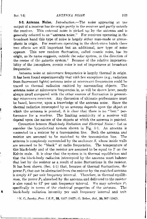
SEC. 52] ANTENNA NOISE
5.2. Antenna Noise. Introduct~on.—The
103
noise appearing at the. .output of a receiver has its origin partly in the receiver and partly outside
the receiver. This external noise is picked up by the antenna and is
generally referred to as “ antenna noise.” For receivers operating in the
broadcast band this type of noise is largely either man-made or atmos-
pheric in origin. For receivers operating in the short-wave bands these
two effects are still important but an additional, new type of noise
appears. This new random fluctuation, called cosmic noise, has its
origin, as its name suggests, outside the solar system, in the direction of
the center of the galactic system. 1 Because of the relative impenetra-
bility of the ionosphere, cosmic noise is not of importance at broadcast
frequencies.
Antenna noise at microwave frequencies is largely thermal in origin.
It has been found experimental y that with few exceptions (e.g., radiation
from fluorescent lights) antenna noise at microwave frequencies could be
traced to thermal radiation emitted by surrounding objects. The
antenna noise at microwave frequencies is, as will be showm later, nearly
always small compared with the other sources of fluctuation in present-
day microwave receivers. Any discussion of ultimate performance must
be based, however, upon a knowledge of the antenna noise. Since the
thermal radiation intercepted by an antenna depends upon the object at
which the ant enna is pointed, it is clear that there is no “best” per-
formance for a receiver. The limiting sensitivity of a receiver will
depend upon the nature of the objects at which the antenna is pointed.
Connection between Blo&body Radiation and Electrical Noise .—Let usconsider the hypothetical system shown in Fig. 5.1. An antenna isconnected to a resistor by a transmission line. Both the antenna andresistor are assumed to be matched to the transmission line. Theantenna is completely surrounded by the enclosure S, whose inside wallsare assumed to be “black” at radio frequencies. The temperature ofthis black-body and of the resistor are assumed to be equal to T on theKelvin scale. It is clear that the system is in thermal equilibrium andthat the black-body radiation intercepted by the antenna must balancethat lost by the resistor as a result of noise fluctuations in the resistor.It has been shown (Sec. 4.1) that, because of thermal fluctuations, thepower PI that can be abstracted from the resistor by the matched antenna
is simply k 2’ per unit frequent y interval. Therefore, in thermal equilib-rium, the power Pz absorbed by the antenna and delivered to the resistoris ako equal to kT per unit frequency interval. We may calculate P,specifically in terms of the electrical properties of the antenna. Theblack-body radiation intensity per unit frequency interval and unit
IK. G. Jansky,Proc. Z.R.E., 25, 1517(1937); G. Reber, ibid., 30, 367 (1942).
1 —— ——-
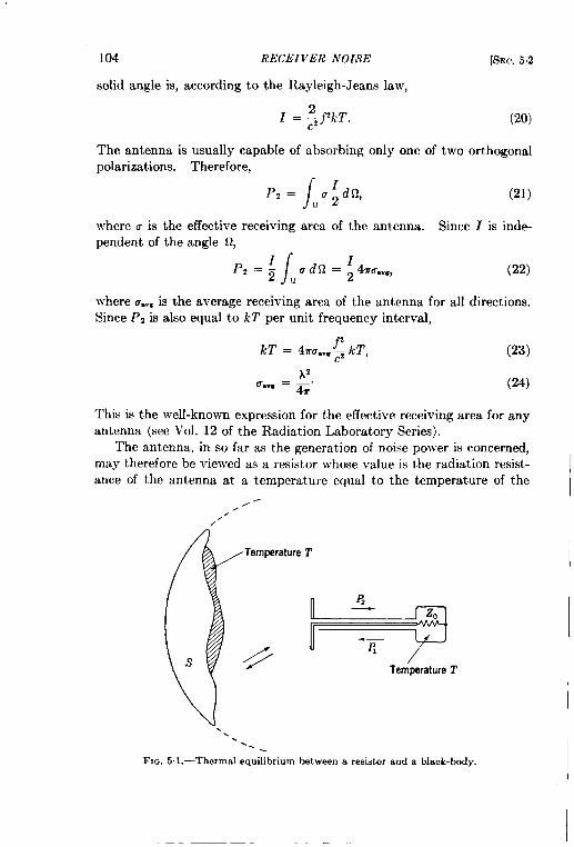
104 RECEIVER NOISE
solid angle is, according to the Rayleigh-Jeans law,
[SEC.5.2
(20)
The antenna is usually capable of absorbing only one of two orthogonalpolarizations. Therefore,
P, =/
zu–dq
.2(21)
where u is the effective receiving area of the antenna. Since I is inde-pendent of the angle Q,
(22)
where u..g is the average receiving area of the antenna for all directions.Since P2 is also equal to kT per unit frequency interval,
kT = 4XU..=$ kT,
AZ“V’ = G“
(23)
(24)
This is the well-known expression for the effective receiving area for anyantenna (see Vol. 12 of the Radiation Laboratory Series).
The antenna, in so far as the generation of noise power is concerned,may therefore be viewed as a resistor whose value is the radiation resist-ance of the antenna at a temperature equal to the temperature of the
.’..“
G‘wZ.
~
Temperature 2’
‘\‘..
FI~.5.1.—Thermalequilibriumbetweena resistoranda black-body,
SEC.5.2] ANTENNA NOISE 105
antenna’s surroundings. If the surroundings of the antenna are not allat the same temperature, an average temperature may be defined. Thisaverage temperature will be called the antenna temperature and may bedefined as the temperature which a black-bed y (see Fig. 5.1) must havein order to duplicate the antenna noise.
Antennu Temperature of Sky.—Since the antenna temperature of ahighly directive microwave antenna depends upon the direction in whichthe antenna is pointed, the antenna temperature must be investigatedunder a variety of conditions. First let us consider the temperature of
[
Top of
+
Black body
atmosphere temperature T.-— —-
1>
-_--—- — -- ——--- —T
—-———Fra~ional “. Air temperature 2’
{
,7---- _,------.,.
ahr~on :? Antenna temperature=7T
[
‘),
-----+-–---:-iii-ii }]
“mospheric !–.1/ “ra~’Jna’temperature T absorption 7
I z+ T(l-7)=T
(a) (b)(z=7T)
FIG.5.2.—Atmosphericabsorptionas a sourceof thermalradiation,
a highly directive antenna pointed at the zenith. An experimentalinvestigation has shown that with the exception of the sun and moon,radiation from astronomical bodies is negligibly small at wavelengths ofthe order of 1 cm. In particular, stellar radiation has been foundexperimentally to contribute less than 20”C to the antenna temperaturefor wavelengths of approximately 1 cm, and it can be easily calculated tocontribute less than 10-80C. Thus it seems plausible that thermalradiation external to the solar system is completely negligible as a causeof antenna noise at microwave frequencies; hence it is necessary toexamine the earth’s atmosphere for sources of thermal radiation.
The atmosphere cannot radiate unless it absorbs at microwave fre-quencies. Figure 5.2a and b illustrates how the antenna temperature canbe calculated in the case of a partially absorbing atmosphere. In Fig.5t2b the earth’s atmosphere is surrounded by an imaginary black-bodyat the same temperature as the atmosphere. The radiation x arising inthe atmosphere must just compensate for the partial absorption of theblack-body radiation in the atmosphere. This fact leads to the result
for the antenna temperature, where ~ is the fractional absorption of theatmosphere. Because of absorption in water vapor, the antenna tem-
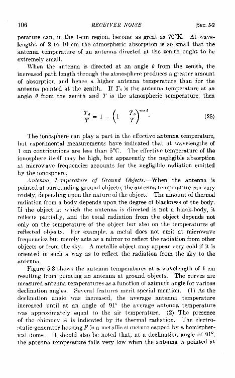
106 RECEIVER NOISE [SEC.5.2
perature can, in the l-cm region, become as great as 70”K. At wave-lengths of 2 to 10 cm the atmospheric absorption is so small that theantenna temperature of an antenna directed at the zenith ought to beextremely small.
W-hen the antenna is directed at an angle 0 from the zenith, theincreased path length through theatmosphere produces a greater amountof absorption and hence a higher antenna temperature than for theantenna pointed at the zenith. If To is the antenna temperature at anangle 0 from the zenith and T is the atmospheric temperature, then
(26)
The ionosphere can play a part in the effective antenna temperature,but experimental measurements have indicated that at wavelengths of1 cm contributions are less than 5°C. The effective temperature of theionosphere itself may be high, but apparently the negligible absorptiontit microwa~-e frequencies accounts for the negligible radiation emittedby the ionosphere.
Antenna Temperature of Ground Objects.—When the antenna ispointed at surrounding ground objects, the antenna temperature can vary\Yidely,depending upon the nature of the object. The amount of thermalradiation from a body depends upon the degree of blackness of the body.If the object at which the antenna is directed is not a black-body, itreflects partially, and the total radiation from the object depends notonly on the temperature of the object but also on the temperatures ofreflected objects. For example, a metal does not emit at microwavefrequencies but merely acts as a mirror to reflect the radiation from otherobjects or from the sky. A metallic object may appear very cold if it isoriented in such a ~vay as to reflect the radiation from the sky to theantenna.
Figure 53 shows the antenna temperatures at a wavelength of 1 cmresulting from pointing an antenna at ground objects. The curves aremeasured antenna temperatures as a function of azimuth angle for variousdeclination angles. Se~-eral features merit special mention. (1) As thedeclination angle was increased, the average antenna temperatureincreased until at an angle of 91° the a~.erage antenna temperature~vas approximately equal to the air temperature. (2) The presenceof the chimney A is indicated by its thermal radiation. The electro-static-generator housing F is a metallic structure capped by a hemispher-ical dome. It should also be noted that, at a declination angle of 91°,the antenna temperature falls very low when the antenna is pointed at
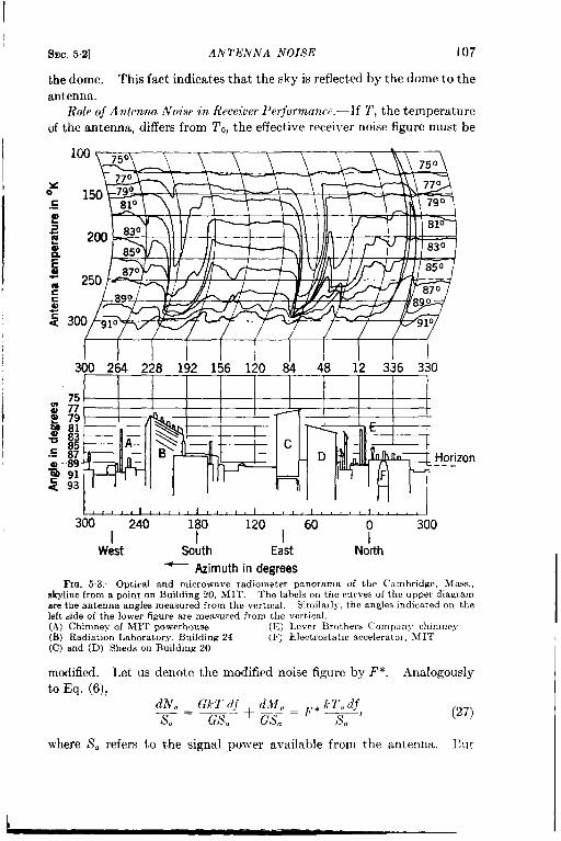
t
1
I
t
I
SEC.5.2] ANTENNA NOISE 107
the dome. This fact indicates that the sky is reflected by the dome to theantenna.
Role of Antcnnu Noise in Receiver Perjormancr.—l f T, the temperatureof the antenna, differs from To, the effective receiver noise figure must be
zos.-0La~8~.scc0E<
300 264 228 192 156 120 84 48 12 336 330
75: 77E 79~ 81:~~ --89 Horizon——_g 91< 93
1 I I ) I I t300 240 180 120
I I I60 0 300
IWest South East North
- Azimuth in degreesFIG.53.-OpticaI and microwaveradiometerpanoramaof the Cambridge,Mass.,
skylinefroma pointon Building20, MIT. The labelson the curvesof the upperdiagramarethe antennaanglesmeasuredfrom the vert]cal. Similarly,the anglesindicatedon theleft sideof the lower figure are measuredfrom the vert]cal,(A) Chimneyof MIT powerhouse (E) Lever Brothers Company chimney(B) RadiationLaboratory, Building 24 (F) Electrostatic accelerator,MIT(C) and (D) Shedson Building 20
modified. Let us denote the modified noise figure by F*. Analogouslyto Eq. (6),
(27)
where Sa refers to the signal power available from the antenna. Rut
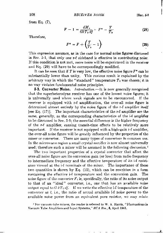
108 RECEIVER NOISE
from Eq. (7),
Therefore,
()T‘*=F+ E–l”
[SEC.5.3
(28)
(29)
This expression assumes, as in the case for normal noise figures discussedin Sec. 5.1, that only one r-f sideband is effective in cent ribut ing noise,If this condition is not met, more noise will be experienced in the receiverand Eq. (29) will have to be correspondingly modified.
It can be seen that if T is very low, the effective noise figure F* can besubstantially lower than unity. This curious result is explained by thearbitrary way in which the “standard” temperature TO was chosen; it inno way violates fundamental noise principles.
5.3. Converter Noise. Introduction.—It is now generally recognizedthat the superhetercdyne receiver has one of the lowest noise figures; itis universally used where weak signals are to be encountered. If thereceiver is equipped with r-f amplification, the over-all noise figure isdetermined almost entirely by the noise figure of the r-f amplifier itself[see Eq. (17)]. The important characteristics of the r-f amplifier are thesame, generally, as the corresponding characteristics of the i-f amplifierto be discussed in Sec. 5.5; the essential difference is the higher frequencyof the r-f amplifier, causing transit-time effects to be relatively moreimportant. If the receiver is not equipped with a high-gain r-f amplifier,the over-all noise figure will be greatly influenced by the properties of themixer or converter. There are many types of converters in common use.In the microwave region a small crystal rectifier is now almost universallyused; therefore such a mixer will be assumed in the following discussion. 1
The two important properties of a crystal converter that affect theover-all noise figure are its conversion gain (or loss) from radio frequencyto intermediate frequency and the effective temperature of its i-f resist-ance viewed at the i-f terminals of the mixer. The importance of thesetwo quantities is shown by Eq. (15), which can be rewritten in a formcontaining the effective i-f temperature and the conversion gain. Thenoise figure of the converter F1 is, specifically, the ratio of its noise outputto that of an “ideal” convert er, i.e., one that has an available noiseoutput equal to GlkTO dj. If we write the effective i-f temperature of theconverter as t, i.e., the ratio of actual available i-f noise power to theavailable noise power from an equivalent pure resistor, we may relate
II
1For vacuum-tube mixers, the reader is referred h W, A. Harris, “Fluctuations inVacuum Tube Amplifiers and Input Systems,” RCA Reu., 5, April 1941.
I SEC.5.3] CONVh’RYh’R NOISE
Fl, Gl, and tin the following way:
and so, from Eq. (15),t+ F2–1.
F,2 = ~1I
109
(30)
(31)
‘This equation shows how the crystal i-f temperature and gain influence1 the over-all receiver noise figure. In most cases G, is actually less than
unity; i.e., the conversion gain is really a loss. Since G, is a factor thatinfluences FIZ in inverse fashion, it has been customary to express I@.(31) logarithmically:
10 log10FIZ = 10 loglci (t + F2 – 1) – 10 loglo Gl, (32)
where ( —10 loglo GJ is the conversion loss of the crystal expressed indecibels and (10 log10 FJ is the over-all noise figure also expressed indecibels. Thus an over-all noise figure of 3.01 db really means an over-alf noise figure F,, of 2; likewise a conversion 10SSof 6.02 db really means avalue for GI of +. The advantage of this loose way of expressing con-version loss and noise figures is that a change in loss of n db results in achange in over-all noise figure of just n db.
I Crystal mixers in common use show an effective i-f temperature tranging between 1.0 and very large numbers; the conversion loss isusually between 5 and 10 db. Since the i-f noise figure F, can usually bemade less than 2 (see Sec. 5.5), the crystal characteristics play anextremely important part in the over-all noise figure. In the followingdiscussion there will be given the important experimental observations,together with a brief explanation of current theories of crystal per-formance. For a complete treatment of this field the reader is referredto Vol. 15 of the Radiation Laboratory Series.
Experimental Observations.—A crystal rectifier consists of a smallsemiconducting block, such as germanium or silicon, embedded in asuitable case. On one exposed surface of the semiconductor a contact ismade with a fine, pointed, metallic wire. The whole assembly is a two-terminal device, which acts much like a diode rectifier.
1. When crystal rectifiers are unexcited by direct or alternatingcurrent, the noise power available from them is just that given bythe Nyquist formula, i.e., kT d.f. This is an experimental resultand is in accord with the requirements of thermodynamics.
2. A crystal excited by either direct or alternating current puts outmore noise in general than an equivalent resistor. This does notviolate the laws of thermodynamics, since the system is not in
II:,I
110 RECEIVER NOISE [SEC. 5.3
thermodynamic equilibrium. In a superheterodyne mixer orconverter the quantity of interest is the effective i-f noise tem-perature t when the crystal is excited by local-oscillator power ofthe order of 1 mw. The corresponding rectified current rangesfrom 0.5 to 1.5 ma. It is found experimentally that t has values inthe range from 1.0 to 3.0. In no authentic cases have values lessthan 1.0 been measured, although such values cannot be excludedon the basis of current theories. Values of t < 1.0 have beenobtained with d-c excitation, however. For burned-out crystalst may become very large (10 to 20).
3. Miller et at.’ have measured the noise temperature of crystals(excited either by d-c or microwave currents) for frequenciesbetween 30 cps and 1 Me/see. They find that at low frequencies thenoise temperature is inversely proportional to the frequency; thisphenomenon appears to be independent of the means of excitation.The fact that this law holds down to a frequency of 30 cps indicatesthat the mechanism responsible has a very long time constant.In many ways this effect is like the “ flicker” effect in thermionictubes (see Sec. 4.11).
At the moderately high frequencies especially useful in i-famplifiers, the noise temperature is essentially independent offrequency. It has been found, however, that there is a closecorrelation between audio noise temperatures and 30 Me/seenoise temperatures; this suggests that the same mechanism may beresponsible in both frequent y regions.
4. The noise temperature ( – 1) is approximately proportional torectified current up to 2 or 3 ma. At higher currents the curvedeparts from linearity, in the direction of smaller t.
5. The noise temperature and conversion loss of a crystal rectifier isa function of the termination of the two noise sidebands generatedby the crystal. These sidebands, for an intermediate frequency $and local oscillator frequency fo, occur at .fO+ f. R. Beringerzhas shown that the conversion loss and noise temperature t go inopposite directions with image sideband tuning. However, thechanges in loss are much greater than those of t; hence for minimumnoise figure the sideband should be tuned for minimum loss.
6. With local-oscillator excitation the noise temperature is influencedby d-c bias; it changes very little for bias in the forward directionbut may increase by a considerable amount for even a small back
1p, H. lfillrr, hf. N, I,ewis, L. I. Schiff, and D. E. Stephens, “Noise Spectrum ofSilicon Rectifiers, ” NDRC 14-256,U, of Pa., ilfar, 20, 1944; P. H. Miller and hf. H,(lrreublat, “ Crystal Audio Noise,” NDRC 14-387,U. of Pa,, Jan. 5, 1945.
2Private communication.
SEC. 53] CON VERTIIR .VOISE 111
bias (self-bias). I?or example, aback bias of 0.1 volt maycausetto incrcasc by more than unity. This effect is especially marked inthose crystals ~vhich are alrcfidy somewhat noisy at zero bias.
7. A. l,awxon d al.l have mctisllrcd tas afurwtio nofthetemperatureof the rectifier. Changes in t ~vwc observed, but they ~vere asIikcly to have one sign as the other.
8. In addition to the influence of termination impedances at signal
freql[ency and image frequency, it has been observed that termina-
tion impedances at harmonics of these frequencies contribute
materially to noise temperature and conl’ersion loss. Since these
termination impedances depend critically upon the particular
circuit in ~vhich the crystal rectifier is placed, it follows that the
two properties of the crystal rectifier with which we are concerned
will also depend on the particular mixer circuit.
Theoretical Ideas. —Weisskopf’ has examined the problem of crystalnoise and has suggested three sources of noise: (1) thermal noise of the
spreading (scmicomluctor) resistance, (2) shot noise caused by electronsflying over the barrier, und (3) ‘‘ fluctuat ion” noise caused by motion ofcharges on the contact surface. The effective noise temperature can beeasily calculated if “ fluctuation” noise is assumed negligible; the result is
(33)
where r is the spreading resistance, R is the dynamic resistance of thebarrier, T is the physical temperature of the semiconductor, and 1 is thesum (arithmetic) of the electron currents from metal to semiconductorand from semiconductor to metal, since both of these currents are equallyeffective in producing shot noise. For a voltage V such that IVI > kT/e,1 ean be taken to be the actual direct current through the rectifier;howe~”er, for V = O and T = To, I becomes equal to e/2kT&.
R. XT.Smith3 has measured the noise temperature with d-c excitationas a function of voltage and, comparing his result with Eq. (33), hasfound that the measured temperature generally exceeds the predictedtemperature, although in a fe}~ inst anccs the observed noise was lessthan predicted. In at least three instances observed noise temperatures
I .4. W’.Lzwwn, P. H. lfillrr, and D. E. Stcphcms,“ IToisc in Silicon Rectifiers atLow Tcmprratllres, ” NDRC 14-189,L-. of Pa., Oct. 1, 1%!3.
2V. F, N-cisskopf, “On the Theory oi’ Noise in Conductors, Semiconductors andCrystal Rcrtifkrs,” NDILC 14-133,Jlay 12, 1943.
s ((Cryst:ll ~oi~e as a Function of D-c Bias,“ XDRC 14-167,Purdue U., June 25,1943.
112 RECEIVER NOISE [SEC.54
were less than unity at a for~vard bias of 0.1 volt. In each of theseinstances 13q. (33) correctly predicted the observed value.
It should be emphasized that Eq. (33) is}-slid only ford-c excitation;no useful formula for crystal noise with a-c excitation has yet beenderived.
observed noise in excess of the thermal and shot noises just mentionedhas never been satisfactorily explained. Most of the mechanisms thathave been suggested have not led to useful expressions, nor have theyproperly predicted the frequency dependence of audio noise. It islikely that most of this excess noise is caused by surface contamination ofthe contact; if this is true, it is not difficult to see why a quantitativeformula is not yet available.
5.4. Imcal-oscillator Noise. Introduction.—In the preceding sectionthe conversion gain and temperature of a crystal mixer was seen to dependupon many factors. Nevertheless one important source of noise appear-ing in the mixer was not mentioned for the reason that this noise has itsorigin not in the mixer but in the local oscillator. Furthermore, it ispossible, by methods to be described, virtually to eliminate this local-oscillator noise. Even so, it is still important to understand the originof local-oscillator noise.
The mixer has been considered as a (nonlinear) network upon whichis impressed the r-f signal and the local-oscillator voltage and from whichthe i-f signal is taken. The local-oscillator voltage is generally assumedto be a pure sinusoid; but as we shall see, this assumption may not bevalid. In fact the r-f terminals of the mixer may contain, besides thesignal and local-oscillator sinusoid, r-f noise voltages generated within thelocal oscillator itself. These noise voltages, to be sure, are very smallcompared with the c-w local-oscillator voltage, but they may easilyexceed a small signal voltage. It is clear that the only local-oscillatornoise with which we shall be concerned is the noise appearing at the signalfrequency and at the image frequency; these two noise sidebands,separated from the local-oscillator frequency -fOby approximately theintermediate frequency j, are the only noise frequencies that will contrib-ute to the mixer i-f noise temperature.
In conventional oscillators, noise is generated in the r-f resonantcircuit principally because of shot and partition noise in the anode circuit;the spectral density in the resonant element simply follows the resonantresponse curve. In more complicated oscillators, such as the reflexvariety, however, the spectral density is not so simple. Since this type ofoscillator is of great importance in the microwa~e field, a brief accountof its noise characteristics }vill be gi~~en.1
1For a completediscussion,seeVol. 7 of the RadiationLaboratorySeries.
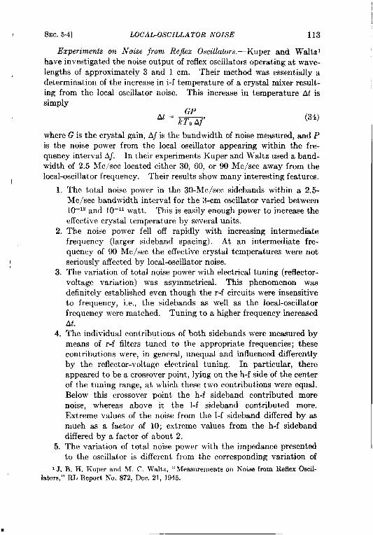
SEC.5.4] LOCAL-OSCILLATOR NOISE 113
Experiments on Noise from Refix Oscillators. —Kuper and Waltz’have investigated the noise output of reflex oscillators operating at wave-lengths of approximately 3 and 1 cm. ‘Their method was essentially adetermination of the increase in i-f temperature of a crystal mixer result-ing from the local oscillator noise. This increase in temperature At issimply. .
GP‘t = kT, Aj’
(34)
where G is the crystal gain, Aj is the bandwidth of noise measured, and Pis the noise power from the local oscillator appearing within the fre-quency interval Aj. In their experiments Kuper and Waltz used a band-width of 2.5 Me/see located either 30, 60, or 90 Me/see away from thelocal-oscillator frequency. Their results show many interesting features.
1.
2.
3.
4.
5.
1J.
The total noise power in the 30-Mc/sec sidebands within a 2.5-Mc/sec bandwidth interval for the 3-cm oscillator varied between10–” and 10-” watt. This is easily enough power to increase theeffective crystal temperature by several units.The noise power fell off rapidly with increasing intermediatefrequency (larger sideband spacing). At an intermediate fre-quency of 90 Me/see the effective crystal temperatures were notseriously affected by local-oscillator noise.The variation of total noise power with electrical tuning (reflector-voltage variation) was asymmetrical. This phenomenon wasdefinitely established even though the r-f circuits were insensitiveto frequent y, i.e., the sidebands as well as the local-oscillatorfrequency were matched. Tuning to a higher frequency increasedAt.The individual contributions of both sidebands were measured bymeans of r-f filters tuned to the appropriate frequencies; thesecontributions were, in general, unequal and influenced differentlyby the reflector-voltage electrical tuning. In particular, thereappeared to be a crossover point, lying on the h-f side of the centerof the tuning range, at which these two contributions were equal..Below this crossover point the h-f sideband contributed morenoise, whereas above it the l-f sideband contributed more.Extreme values of the noise from the l-f sideband differed by asmuch as a factor of 10; extreme values from the h-f sidebanddiffered by a factor of about 2.The variation of total noise power with the impedance presentedto the oscillator is different from the corresponding variation of
B. H. Kuper and M. C. Waltz, “ Measurementson Noise from Reflex Oscil-lators,” RL Report No. 872, Dec. 21, 1945,
114 RECEIVER NOISE [SEC.54
c-w power. In general, the ratio of noise to c-w power increase~with admittance; hence for a given c-w- power the noise can beminimized by presenting a low admittance to the oscillator.
Theoretical Ideas. —Pierce’ has presented a theory of reflex-oscillatornoise that includes the effects from (1) shot and partition noise in theelectron beam coupled out through the cavity, (2) amplitude modulationof the oscillator by i-f noise components in the beam, and (3) frequencymodulation of the oscillator at i-f rates caused by fluctuations in the phaseof returning electrons. Kuper and 1$’altz’ have found experimentallythat with adequate bypassing of theoscillator leads the last twomecha-nisms are relatil-ely unimportant. Knipp3 has extended Pierce’s calcu-lations in two important directions: (1) Reconsiders the noise producedby the mixing of various electron-beam noise components ~rith harmonicsof the oscillator current; (2) he takes into account the coherence, i.e.,phase relationship, of the returning current with the incident current.This coherence causes a marked difference in individual sideband contri-bution and also an asymmetry in noise output as a function of electricaltuning,
In its final form Knipp’s theory appears to account correctly for allthe important experimental facts discovered by Kuper and Waltz, notonly as to functional form but also as to magnitude.
Suppression of Local-oscillator iVoise.--Mthough the local oscillatorhas for a long time been knovm to be an important source of receivernoise, it has also been recognized that this noise can be relatively easilyremoved or suppressed. The most straightf orw-ard may of accomplishingits elimination is by means of a tuned r-f filter inserted betm-cen the mixerand local oscillator. If this filter is tuned to the local-oscillator frequencyand has a band)vidth small compared with the intermediate frequencyitself, the noise sidebands with which \ve are concerned ~vill not betransmitted through the filter to the mixer. For some oscillators ~vemayconsider the resonant property of the oscillator cavity itself to constitutesuch a filter; this is the usual reason why oscillator noise is relativelyunimportant for very high intermediate frequencies. In any case,however, it is al~vays possible to add a new filter in the local-oscillatorcoupling that is sufficiently narrow (high-Q) to suppress local-oscillatornoise. The only flaw in this procedure is the necessity for continuallytuning the filter to the oscillator frequency; this disadvantage can be
1J. A. Pierce, “ X-oise Calculations for RCfICX oscillators, ” BTL Report ~f \I-44-140-4,,Jan.29, 1944.
2Kuper and Waltz, 10C.cit.3J. K. Knipp, “ Theory of Noise from the Reflex Oscillator,” RL Report 873,
Jan. 10, 1946.
SEC.5.5] INTERMEDIATE-FREQUENCY NOISE 115
overcome if a so-called “magic T” mixer is used, described in detail inVol. 16 of the Radiation Laboratory Series. This form of mixer con-stitutes a sort of r-f bridge circuit in which the local-oscillator and signalvoltages are applied to two crystal rectifiers. The connection is so made,however, that the r-f signal voltages applied to each of two crystals are inphase, the local-oscillator voltage being out-of-phase; therefore the crossproducts of the two voltage pairs (i.e., the i-f signals) are out of phasewith respect to each other. The i-f connection is made in such a waythat in-phase i-f contributions from the two crystals are canceled, andtherefore only out-of-phase contributions (namely, i-f signals) are ampli-fied. The principal local-oscillator contribution to the i-f noise comesfrom beats between the local-oscillator carrier and those components ofits noise which are separated from it by the intermediate frequency.,Since the intermediate frequency is small compared with the carrierfrequency, the phase relationship between a noise component and thelocal-oscillator carrier at one crystal is virtually the same as that at theother crystal, even though the carrier itself is m radians out of phase.Therefore the i-f noise outputs from the local oscillator are in phase withrespect to each other and cancel, whereas, as stated, the signal outputsadd.
It is clear that there are other equally satisfactory ways of arrangingthe bridge so that LO noise is canceled and signal components properlyhandled. The fundamental reason why it is possible to suppress local-oscillator noise without at the same time suppressing desired signals isthat the sources are different; this fact makes it possible to build circuitsthat discriminate in favor of the desired signals (see also Sec. 56).
5.5. Intermediate-frequency Noise. Introduction.—In a super-
heterodyne receiver the output voltage from the mixer is connected to
the input terminals of an i-f amplifier. We have seen from Eq. (17) thatif the gain of the first i-f stage is large, the over-all i-f noise figure dependsonly on the first stage itself; furthermore we have seen from Eq. (31)that if we use a crystal converter whose temperature is low (t = 1), theover-all receiver noise figure is approximately proportional to the noisefigure of the i-f amplifier. Therefore the i-f amplifier noise is a veryimportant matter. A great deaf of effort has been expended in designingamplifiers with low noise figures.
Tubes used in i-f amplifiers have generally been of two kinds, pent odesand triodes. A pentode would appear to be more satisfactory since theplate-t o-grid feedback (Miller effect ) is so low; triodes, however, ifproperly used lead to lower noise figures because of the absence of parti-tion noise. Circuits that have been found useful for triodes are of twokinds.
I116 itECEIVER NOISE [SEC.5.5
1. The grounded-grid triode, which does not need to be neutralized(out-of-phase feedback introduced that nullifies the output-to-input capacitance) but it can be used only where the relativelyhigh input conductance can be tolerated. This input conductanceis, in fact, simply the mutual conductance g- of the triode.
2. Thegroutied<athode triode(the conventional arrangement) wouldbe very desirable because of its high input resistance; unfortu-nately, however, if the voltage gain of the tube is high, thenecessary neutralization is extremely critical. Forthis reason thistype of triode connection has been virtually abandoned.
Nevertheless a very ingenious circuit arrangement has been suggestedthat completely eliminates this difficulty. In this new circuit a grounded-cathode triode is immediately followed by a grounded-grid triode. If thetriodes are alike, the voltage gain of the first triode is unity (its load con-ductance is essentially g~); and since its current flows directly to the anodeof the second triode (none is captured by the grid of the second triode),the over-all mutual conductance of the two tubes is just g~. Wallmanhas shown that the noise contribution of the second triode is negligible;hence the over-all noise figure is essentially that of the grounded-cathodetriode. Neutralization of the first triode is extremely easy, however,since its voltage gain is only unity; failure to neutralize at all results in noinstability and in only a slight increase in noise figure.
Representation of Noise Generators.—It has been shown in Chap. 4that the fundamental sources of i-f noise contributing to anode noise in atriode are (1) thermal noise in the signal generator, (2) thermal noise incircuit elements (such as transformer losses, tube glass losses, etc.), (3)shot noise in the anode, and (4) induced grid noise. For a pent ode afifth source of noise was mentioned, namely, partition noise caused byrandom current collection by the screen grid. In determining the noisefigure of the i-f stage in terms of these noise contributions it is mostconvenient to introduce a hypothetical circuit whose over-all gain andnoise out put is in every way just the same as that of the actual i-f circuit.Such an equivalent circuit is shown in Fig. 5.4, in which it is assumed thata completely noiseless tube of the same mutual conductance as that of theactual tube is preceded by particular resistor elements. These resistorelements are so chosen that their noise contributions correspond to thevarious noise contributions in the actual tube. The noise in the gridcircuit will be properly represented by the three load conductance g,g[, g, shown in Fig. 5“4; these symbols represent the conductance of thesignal generator (applied directly to the grid), the conductance caused by
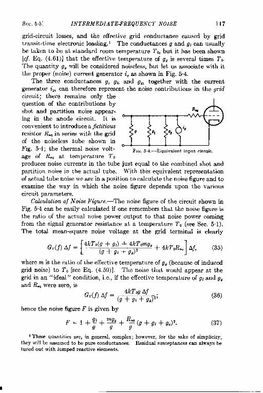
SEC.5.5] INTERMEDIATE-FREQUENCY NOISE 117
grid-circuit losses, and the effective grid conductance caused by gridtransit-time electronic loading. 1 The conductance g and gl can usuallybe taken to be at standard room temperature 1’o, but it has been shown[cf. Eq. (4.61)] that the effective temperature of g, is several times 2’..The quantity g. will be considered noiseless, but let us associate with itthe proper (noise) current generator i, as shown in Fig. 5.4.
The three conductance g, gl, and g,, together with the currentgenerator i,, can therefore represent the noise contributions in the grid
circuit; there remains ordy thequestion of the contributions byshot and partition noise appear- R_
ing in the anode circuit. It iso
convenient to int reduce a fictitiousresistor R.q in series with the gridof the noiseless tube shown inFig. 5.4; the thermal noise volt- FIG.5.4,—Equivalent input circuit.age of R,q at temperature TOproduces noise currents in the tube just equal to the combined shot andpartition noise in the actual tube. With this equivalent representationof actual tube noise we are in a position to calculate the noise figure and toexamine the way in which the noise figure depends upon the variouscircuit parameters.
Calculation of Noise Figure.—The noise figure of the circuit shown inFig. 54 can be easily calculated if one remembers that the noise figure isthe ratio of the actual noise power output to that noise power comingfrom the signal generator resistance at a temperature T, (see Sec. 5.1).The total mean-square noise voltage at the grid terminal is clearly
G,(f) Af =[
4kT0(g + gt) + 4kTtimg,(g + 92 + 9.)2 1
+ 4kToR.a Af, (35)
where m is the ratio of the effective temperature of go (because of inducedgrid noise) to 2’0 [see Eq. (4.59)]. The noise that would appear at thegrid in an “ideal” condition, i.e., if the effective temperature of gl and gaand R~ were zero. is
4kT,g AfG,(f) Af = (g + 91 + 9,)2;
hence the noise figure F is given by
F=l+f+~+ ~(g+gl+go)2.
(36)
(37)
1These quantities are, in general, complex; however, for the sake of simplicity,they will be assumedto be pure conductance. Residual susceptancescan nlways betuned out with lumped reactive elements.
118 RECEIVER NOISE [SEC.5.5
The first constant (unity) comes from the thermal noise in the signalgenerator itself; the remaining three terms, representing “excess” noise,come from circuit losses (usually small), induced grid noise, and shot (andpartition) noise, respectively. Equation (37) can be written in a slightlydifferent way:
.F– 1 = [g, +mgO+R.q(g, +g,)’]: +2Re.(g~+ g,) +R.cQ. (38)
This expression shows that asa function of signal-generator conductanceg, the noise figure (minus unity) has one independent term, one hyper-bolic term, and one linear term. It is clear that (for small F) there is anoptimum signal-generator conductance; for this value of conductance thefirst and third contributions are equal.
(39)
It is clear from Eq. (38) that a measurement of F as a function of g permitsevaluation of all the quantities involved, namely, R ~q, g~, g~, and m.J. L. Lawson and R. R. Nelson’ have used this method with partialsuccess. The quantity R.q can be obtained with good accuracy, but theother quantities cannot usually be determined with adequate precision.If circuit losses are small, gl can be neglected; this fact helps somewhat inthe determination of m and g,. It is usually more satisfactory, however,to determine g. by direct measurement.
In practice, gl can usually be neglected. Furthermore, the contri-bution from the constant term in Eq. (38) is ordinarily negligible. L’nderthese conditions the optimum noise figure (– 1) depends linearly on thesquare root of the grid electronic loading conductance g, [see Eq. (40)].We saw in Sec. 4.10, however, that the electronic loading conductance is(for small transit angles) directly proportional to the square of thefrequency; therefore it would be expected that
F.,, = 1 + kj, (41)
where k is a function characteristic of the particular i-f tube. Thisrelationship has been roughly verified by J, L. Lawson and R. R. Nelson,using a triode-connected 6AK5. They measured the noise figures at6, 30, and 60 Me/see and found values of 1.06, 1.3, and 1.7, respectively,for F.D,.
Role of I-f Input Coupling Transformer.—It seldom happens that asignal generator (or the i-f terminals of a converter) has the optimum
I Unpublished.
I
[
SEC,55] INTERMEDIATE-FREQUENCY NOISE
conductance given by Eq. (39); a transformer is generally
119
used, therefore,to change the effective generator impedance to the most suitable value.If the transforming network is lossless, we may simply view g as the trans-formed generator impedance. Losses in the transformer must be lumpedwith gl; if this is done, the preceding development is valid and noisefigures are easily calculated. It is obvious that the optimum (foroptimum noise figure) transformed generator impedance is not generallyequal to its load; i.e., impedance matching is not generally desirable.
In spite of the fact that the input coupling transformer is used for‘proper impedance transfer, it sometimes happens that, because of theinput shunt capacitance of the tube, the circuit bandwidth is insufficientfor the intended use. In this case a compromise between bandwidthand noise figure must be made; this compromise, however, is not usuallyserious. For instance, in the example just mentioned, i.e., triode-.connected 6AK5, the optimum noise figure occurs when the circuit band-~ridth is approximateely 0.25 the center (intermediatee) frequency. Alarger band!vidth would hardly be useful in view of the difficult problemof adequately separating i-f and video voltage at the second detector.
Experimental Measurement of Noise Figures.—The noise figure of areceiver can be measured in many ~vays; however, the straightforwardmethods involving a direct comparison of the total equivalent noise powerwith a minute c-w signal power involve the difficult task of knowingaccurately the power of the extremely minute signal. This task becomesespecially difficult at high frequencies, where good attenuators aredifficult to construct. There is a method of measuring noise figureswhich does not involve c-w signals and attenuators; it consists essentiallyof a comparison of ‘‘ normal” noise (generator at temperature TO) withthe noise occurring when the generator is artificially changed to a newtemperature. This change in temperature is most easily effected byimpressing diode shot noise (temperature-limited) on the generatorresistance. 1 Let us consider the case where a measurement is made of thed-c diode current I that just doubles the original receiver noise.
The original receiver (available) noise power is simply F (the noisefigure) times the noise contribution arising in the generator resistanceitself [see Eq. (5)], which is now to be set equal to the contribution ofnoise from the test diode operating into the generator resistance R.. Theavailable shot noise power W, (per unit frequency interval) will be givenby the Schottky formula [Eq. (4.28)], together with the generatorresistance RQ:
W, = ~ Af, (42)
I E. J, Schremp showed (in December 1942) the validity of measuring noise figuresby meansof diodes.
120 RECEIVER NOISE [SEC.5.5
which must be set equal to the original receiver noise power, i.e., F’kZ’OA~.Therefore,
F = “J2kT0
(43)
which, if TO is set equal to the “standard” figure of 29201<, reduces to thesimple expression
F = 201R,, (44)
where Z is that d-c diode current in amperes which just doubles the outputnoise and ROis the generator resistance in ohms. In this fashion the noise
figure is easily and accurately measured without recourse to long-range
attenuators and complicated methods of accurate power measurements.
The only precaution that must be taken is to ensure that the only source
of noise from the diode is the one given by the Schottky formula; this
appears to be the case when a temperature-limited tungsten or thoriated-
tungsten cathode is used in a diode of good geometry. Diodes having
oxide cathodes have proved to be somewhat unreliable, for what precise
reason is not yet known.
Another (and less accurate) method of measuring noise figures is
physically to change the temperature of the generator resistance R, andto plot the over-all noise power as a function of temperature. Thethermal noise from R, should be linearly proportional to the temperature,whereas the excess noise contributing to (1’ – 1) [see Eq. (7)] is inde-pendent of the temperature. The zero-temperature (extrapolated) noiseis the excess noise power, which can be divided by the thermal noise attemperature TO to yield the quantity (F – 1). An experimental plotshowing noise power as a function of temperature is reproduced in Fig. 5.5.The data were taken by R. R. Nelson and J. L. Lawson at an intermediatefrequency of 6 Me/see using a triode-connected 6AK5 at approximatelyopt imum generator resistance [see Eq. (39)]. The noise figure determinedby the plot is 1.o7, which substantially agrees with the value of 1.06determined by a diode measurement.
PentOde vs. Triode Ampli@rs.—We have seen [Eq. (40)] that the bestnoise figure available depends upon several factors that are functions ofthe particular tube used. We may ask how these quantities differ in atriode and pentode; indeed, we may ask how the optimum noise figuredepends upon operating a given tube as a pentode or as a triode. With agiven tube the only quantity appearing in Eq. (40) that differs withpentode and triode connection is Rw; the equivalent noise resistance isalways higher in a pentode because of screen-grid partition noise. It iseasy to calculate R- for a triode. We have seen from Eq. (4.50) that theshot-noise voltage fluctuation in the plate is exactly equivalent to a
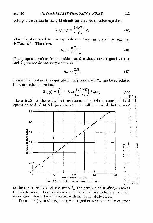
SEC. 5.5] INTERMEDIATE-FREQUENCY NOISE 121
voltage fluctuation in the grid circuit (of a noiseless tube) equal to
(45)
which is also equal to the equivalent voltage generated by R-, i.e.,4kTOR_ Af. Therefore,
~ =~”~1m —.
u TOg~(46)
If appropriate values for an oxide-coated cathode are assigned to O, a,and T., we obtain the simple formula
2.5R,. = ~. (47)
In a similar fashion the equivalent noise resistance R.q can be calculatedfor a pentode connection,
(Rq(p) = 1 + 8.7u —)
19 ~ R..(t),g~ T.
(48)
4’1where R-(L) is the equivalent resistance of a triode-connected tub~ ~operating with identical space current. It will be noticed that becaus{ j
12
1.0
z= 0.8 /
i~ 0,6.-2%.-5~ 0.4 (
0.2
00 100 200 WI WI
Absolute temperature m ‘K
I’1~.5.5,—Relativenoisepoweroutput,
of the screen-grid collector current l@, the pentode noise always exceeds
the triode noise. For this reason amplifiers that are to have a very lownoise figure should be constructed with an input triode stage.
Equations (47) and (48) are given, together with a number of other
122 RECEIVER NOISE [SEC.5.6
useful relations, by Harris.l He has verified them experimentally in alarge number of cases.
Suppression of Induced Grid Noise.—It has been assumed hitherto inthe discussion that the various sources of noise that have been consideredare independent. This asmmption, however, is not valid; the same
electrons that produce fluctuations in anode current (shot noise) inducenoise currents in the grid. It ~~asshown in Sec. 410 from the form of thecurrent pulses produced by a given electron at the grid and anode thatthet~~'o noise contributions aresubstantially in quadrature, provided theeffective load attached to the grid is resistive. In this case the noisepowers from the two sources can be added as though they were inde-pendent. If the grid load is reactive, however, the grid-current pulsewill produce a grid-voltage change having components in phase or out ofphase with the anode-current pulse. It is natural to ask whether or notthis circumstance can be used to cancel out part of the shot noise withpart of the grid noise. From an analysis of the phases involved, thiscancellation might be expected to occur when the grid reactance iscapacitive or, in other words, when the resonant frequency of the gridcircuit is lower than the intermediate frequency chosen for measurement.Experiments by R. R. Nelson and J. L. Lawson have shown that at 30Me/see, the noise figure of a triode-connected 6AK5, measured with afairly high-resistance generator (making induced grid noise evident)is best when the grid circuit is tuned to a somewhat lower frequencythan the noise measurement frequency. This observation corroboratesthe cancellation picture. Unfortunately these experiments were dis-continued before it was ascertained how much cancellation could beeffected.
In a similar manner simple analysis indicated that reactive feedbackfrom anode to grid could accomplish the same type of result. It wasexpected that inductive feedback would accomplish some cancellation;this was experimentally verified by R. R. Nelson and J. L. Lawson.However, more experimental evidence is needed to establish the degree towhich these noise contributions can be canceled.
5.6. Noise CanceUation Schemes.—We have seen in two cases, i.e.,local-oscillator noise and induced grid noise, how noise normally presentin a receiver can be reduced or eliminated by circuit ingenuity withoutat the same time proportionally reducing the desired signal. It is ofgreat importance to learn when noise cancellation is possible and whenimpossible.
The elimination of local-oscillator noise appears to be possible only
1W. A. Harris, “Fluctuations in Vacuum Tube Amplifiers and Input Systems, ”RCA Rev,, 6,4, April 1941.
SEC. 56] NOISE CANCELLATION SCHEMES 123
because one can operate on the local-oscillator noise energy independentlyof the signal energy. In other words, the source of noise does not causeit to appear initially on the same two terminals as the signal. Likewise,in the case of induced grid noise, the noise behavior at grid and anode(from the same source) is substantially different from the signalcontribution.
It seems, on the other hand, that cancellation is not possible if theextra noise is generated at the same terminals as is the signal. In thiscase any noise cancellation scheme should also and to the same degreecancel the signal. This consideration will apply, therefore, to signal-circuit losses, tryst al-mixer losses, etc. For these effects, the only hopefor lower noise lies in improved methods of construction, lowertemperatures, etc.
I
CHAPTER 6
EXTERNAL NOISE SOURCES; CLUTTER
6.1. Origin and Description of “Clutter.’’—The term “clutter” isused to describe signals reflected from such objects as rain, “window” or{(chaff,~~l vegetation, and the surface of the sea. The inclusion of clutterin a discussion of noise is justified by the similarity, though superficial,between the appearance of clutter on an A-scope and that of noise on anextended A-scope and by the close similarity of their mathematicaltreatment. The chief difference between clutter and noise is that whereasthere is correlation in clutter received during a number of consecutivepulses, noise is completely independent from pulse to pulse.
The mathematical description of clutter is based on the assumptionthat it is caused by reflections from a large number of independent andindependent y moving scatterers, (e.g., strips of window, raindrops).With this model statistical predictions can be made of the power receiv.wfas a function I(r) of rangez when the pulse travels through rain or window,etc. These considerations have led to predictions concerning the appear-ance of individual traces on the A-scope. 3 Furthermore, the power I(t)returned from a region at fixed range can be considered as a randomfunction of time. This function is actually observed only for a discreteset of values of the time variable, that is, once for each pulse. Experi-mentally the function I(t) is obtained from these discrete observations byinterpolation using a “boxcar” device (cf. Sec. 2.7) and a low-pass filter.With the commonly used PRF’s the function I(t) thus obtained issufficiently well represented for comparison with the theoreticalpredictions.
Both I(r) and I(t) are random functions. Even if the average numberand cross section of the scatterers do not depend on range, I(r) fluctuatesbecause the phase relations between the scatterers contributing to thereturn are different in different regions of space.
Fluctuations in l(t) occur because the phase relations of one assembly
1Thesetermshave been used to describea largecollectionof thin metallicstrips,used as a jamming device.
aExperimentally,the function of range is obtained as a function of time on amicrosecondscalewith range = c/2 X time.
3A. J. F, Siegert, “On the Appearanceof the A-scope When a Pulse Travelsthrougha HomogeneousDktributionof Scatterers,” RL ReportNo. 466,Nov. 9, 1943.
124
SEC.6.2] THE FIR5’T TWO PROBABILITY DISTRIBUTIONS 125
of scatterers change with time because of the random motion of thescatterers. The changes of intensity arising from the statistical fluctua-tions of the number of scatterers can be neglected, since they are smallcompared with the fluctuations due to changing relative phases when theaverage number of scatterers contributing to the clutter is large. Clutteris therefore considered as the return from N scatterers where N is merelythe average number of scatterers and not a random variable.’ Ther-f signal received from the kth individual scatterer is denoted by
where JOis the carrier frequency.The signal intensity xi + y: depends on the field strength at the
scatterer and on the distance from the scatterer to the receiver. Thetotal power received is given by I(t) = X2(t) + Y2(t), where X = ZXA.,and Y = Zy,. The phase tan-’(~k/~~) depends mainly on thedistancefrom the scatterer to the receiver. The z~ and y~ may be functions oftime for the following reasons: (1) The field strength at the point wherethe scatterer is located may change, for example, if the scatterer movesout of the illuminated area; (2). the scatterer may change its cross section(“chaff,” sea return); and (3) the distance between transmitter andscatterer may change. The first cause will be disregarded, since thenumber of scatterers entering and leaving the beam is usually small duringa continuous series of observations (several thousand pulses). Thesecond cause will also be neglected, since the rotating motion of the“chaff” is slow and does not affect the phase. In sea return, too little isknown about the scatterers to make reasonable assumptions for thepurposes of calculation. The third cause has been studied extensivelyas far as phase changes go. Intensity changes brought about by changesof distance are so small and so slow that they can be neglected.
Besides assuming N to be large, it will be essential to assume that theamplitudes received from the scatterers are independent of mch other.This assumption will be discussed in more detail along with the deriva-tions of the first two probability distributions lT’,(1) and lJ’,(I,,Z,,().
6.2. Derivation of tie First Two Probability Distributions.-l’o obtainthe first probability distribution WI(I), the distribution lJ’,s(X, }“) is firstcalculated for the components
1For distances r from the transmitter that arc large compared \vith the ptllsrlength,
()N=n ~e’;I
where n is the average number of scnttcrcrs pm unit volumr, d the lw:l])l wi{ith, r tIwpulseduration, md c the velocity of light.
I
126 EXTERNAL NOISE SOURCES; CLUTTER [SEC.62
N N
x= zXk, zY= y,
k=l k=l
of thetotal field received from N scatterers, assuming a given probabilitydistribution w(z~,y~) for the field received from the kth scatterer. Theassumption of one distribution for all scatterers can be justified, even ifthere are several classes of scatterers, e.g., raindrops of various sizes.It is assumed further that the return amplitudes from different scatterersare independent, that is, that the probability of receiving x~, yk from thekth scatterer and zt, yt from the lth scatterer is given by the expression
This assumption is justified if the N scatterers represent a sample con-taining large numbers of scatterers of each class. 1
It is clear that under these assumptions the problem of findingW N(X, Y) is nothing but the two-dimentiomd ratiom-walk problem,treated in Sec. 36. With the additional assumption that W(xjy) isisotropic, and hence
,W(XJJ) dx dy = ; j(T) dr d@,
we obtain, within an error of the order of magnitude 1/N, the Rayleighdistribution
WI(Z) dI = ~e-~, (1)
where IO = N~ is the average power returned by the N scatterers.To derive the joint probabilityy of obtaining return signals of power
I(t,) = 1, and I(h) = 12 a time t= h – tI apart, the probabilityW(XI, Y,,x,, Y,) is again first derived for the components of the totalfield received from all N scatterers at the times tl and ta. It is assumedthat the return signals from all N scatterers are received simultaneouslyat both instances of time. As long as 1, and In are observed at the samerange and without turning the antenna, this assumption is justified,since the number of scatterers drifting into and out of the region fromwhich the signals are received during the time t is small compared with N.
The probability of receiving amplitudes x~k),y~~)at time t, and z~k),y~~)at time tl from the kth scatterer is denoted by 7(zf~J,y~~);x~~),y~~)).2The scatterers have been assumed to be independent; that is, the proba-
1If there were, for instance,only a few scatterersof large cross section amongmanyof smallcrosssection,theknowledgethat thereturnsignalfromthelcthscattereris large would diminish the probability of observing a large signal from anotherscatterer.
2The probabilityy w(z~~),y~~))used above is relatedh this functionby
rd$;k’,Yi’)) = ~fr(z$’), Y;’); zj’) Y;”) dz$’ dyz!’).
I
1
SEC. 6.2] THE FIRST TWO PROBABILITY DISTRIBUTIONS 127
bilit y of receiving the field Xjk),y~kl;x~k),yzw from the kth scatterer and(2) ~$, ~2~!)) VI , (Ofrom the lth scatterer is assumed to be 7(@), ~i~);Xjk),vi~))
T(xy], yf) ; zf~, yy) .The fact that a ~vhole cloud of chaff, for instance, may be carried by
the wind so that the average velocity of the particles is the same does notcontradict the assumption of independence.
The probabilityy for the initial phase +, = tan-l (y,/x,) is assumed to beindependent of @,. The unconditional probability for d, = tan-’ (y,/z,)is also assumed independent of ~j, whereas the conditional probabilityfor o!, with given ~1, depends on @ = ~z – @l. The averages xl, y,, z,,
———
~ are therefore all equal to zero.Assuming that u, the velocity component of the scatterers parallel
to the line of sight, does not change during a time t, which in the experi-ments is less than about llK see, we have @ = (4m/k)ut.
The absolute value of the field received at tz,TZ= v’- isassumedl to be the same as the value for tl, rl = -.
Under these assumptions the joint probability for the amplitudes maybe found by the method explained in Sec. 3.6 or by Chandrasekhar;2 andomitting terms vanishing for N ~ m, we obtain J
W,(x,, Y,, x,, Y,, t) =
[
&/// ~,,d[,dq2q2ew WI(I + Ylm + X2t2 + Y2T2) – ~ (xltl + Wm + $2<2 + V2q2)2
1(2)
with
(X1.51 + y,ql + z2t2 + V2712)2
‘////h, dyI dZ2 dyz (~1~1 + Vlql + zzgz + ?/2q2)2
T(z,,y,,z2,y2) (3)
1For window, these assumptions mean that changes of return power and phasecausedby rotation of the strips during the time G – t, have been neglected. Accord-ing to the expressionsderived by F. Bloch, M, Hamermesh, and M. Philips (“ ReturnCross Sections from Random Oriented Resonant Half-wave Length Chaff ,“ RRLReport 411-TM-127, June 19, 1944), the phase of the returned field is actually inde-pendent of the orientation of the strip. Since the time intervals over which theexperiments extend are small compared with the rotation time of window strips,neglect of the intensity changes brought about by changes of orientation during thetime t is justified. The dependence of return power on the initial orientation is takencareof in the probability distribution, of course.
1S. Cbandrasekhar, “Stochastic Problems in Physics and Astronomy,” Rsrr. Mod.Phys. 15, 1-89 (January 1943).
~For further details of the derivation see A. J. F. Siegert, “On tbe Fluctuations inSignalsReturned by Many Independent Scatterers,” RL Re~rt No. 465, Nov. 12,1943, The fact that assumptions made in this report are more special than thoseabove does not affect the expression for W2.
>
128 EXTERNAL NOISE SOURCES; CLUTTER [Si%c. G.2 ,
where
r(xljyl,zj,yz) dxl dyl dxz dyz = w(rl,u) drl ~ d@(r? – ri)2T2 drz’~ (4)
Awith u = — (42 — @l). The ranges of the variables are
47rt
O S r1,r2 g ~, —msl$~+ai, Osq$, s%r,
In the foregoing expression, w(r,,u) dr, du is the probability that a 1
scatterer returns a field between r~ and r1 + drl, and its velocity com- ;
~j~nent away from the transmitter lies between u and u + du.Straightforward calculation leads to the expression
+ YI(–XZ sin ~ + Y2 cos ~)])~, (5)
with10 = Nfi,
‘= l“r’~r~-”m~(’~)~~
ge’’=$k*r’dr1/-”mw’r1u)’4”i”Adu,u, ‘
%
where g is real and positive.For the distribution of intensities ZI = X; + Y?, I, = X; + Y; we
obtain
where g is given by
and JO is the Bessel function of zero order. It is noteworthy that g cannot ibecome negative and that only g appears in the final result; the phaseangle # has dropped out.
The relation between W, and W, is easily verified:
/mdl, W,(~,,~,,t) = w,(~,).
o
For the average product there is obtainedr. r.
SEC.6.2] THE FIRST TWO PROBABILITY DISTRIBUTIONS 129
which, for t = O, leads to the result ~ = 2Z~derived above, since g(0) = 1.The result for ~ can be used to determine g’ experimentally fromobserved values of I(t), since1
1,12 – If9’=z2_ z:’ (9)
The following special cases, though not realized experimentally, mayi’ give some insight into the qualitative behavior of the correlation function
gz(t), especially into its dependence upon the velocity distribution of thescattering centers. If it is assumed that all scatterers return a field ofthe same absolute value r, = p, that all directions of motion are equallyprobable, and that the speed distribution is q(u) do, Eq. (7) yields
/
. Hsin 47rvt
A—— q(v) dv
o()
4vt “
T
(10)
+ If all horizontal directions are equally probable, if the speed distributionis again q(v) dv, and if the radar cross section of a strip is not correlatedwith its direction of motion, we obtain
g=+ll”q(”)dord+e(’”’’’’);l-;l1/.
( )147rvt. q(v) dv JO ~ . (lOa)o
If in addition all particles move with the same speed vO,we get
101g=J04~d. (lOb)
i Correlation between r, and u could occur, for example, if the stripsglided through the air in a direction perpendicular to their long axes,since rl depends on the orientation of the strip. The correct formula forthis dependence leads to a rather involved integral. It can be seen
I qualitatively, however, what will happen if the above hypothesis iscorrect: The particles moving in the line of sight contribute most, and the1picture is essentially equivalent to two clouds, one moving away fromand one moving toward the transmitter, with velocity distributions
! centered about ~ vO. If an equal number of particles move in bothdirections, we may write w(u) = ~~(u – vO)+ j(u + 00)] and we obtain
130 EXTERNAL .VOISE SOURCES; CLUTTER [SEC.63
/
.9=; _ [f(u – Vo) + f(u + v~)]e(’’’’k)’”du.
=; (e(4Ti/A).o+ e-(4=i/h)!o m) J f(U)e(Am~lk)uLdv ,—.
/
4Tvot mg=cos — f(v)e’~l(O dv
A(11)
—m
The normalized spectrum F(w) of 1 – Io is obtained from the Wiener-Kintchine relation
F(u) = :\
.g’ COSat dt.
o
It should be noted that for all values of u,
F((AI)s F(o), (12)
since g’(t) is always positive. This inequality does not exclude thepossibilityy of F’(u) having maxima as long as these maxima are not largerthan F(O). The spectrum can also be expressed by means of W(T,U) asfollows :
since g2 is an even function. Substituting for g we find
/
.F(u)=: _m
()du S(U)S u + ~ , (13)
where
s(u) = $\
.r2 dr W(r,U) (14)
o
and
7= \--.duk”drw”u)u)
Thus S(u) du is that fraction of the received power that is returned byscatterers whose velocity component away from the transmitter liesbetween u – (du/2) and u + (du/2).
6.3. The Probability Distributions When a Constant Signal Is Present.Although the theory developed up to this point adequately describesthe clutter caused by window and rain, it has to be modified forvegetation. Here there is usually a constant signal returned frommotionless objects such as rocks. tree trunks, and cliffs together with theclutter from moving objects such as ieaves and branches. This dis-
tinction is, of course, somewhat dependent on wmd velocity, and the typeof return received from the same wooded slope has been observed to var.v
I
I
I
L
f?iEc.63] CONSTANT SIGNAL DISTRIE UTION 131
from a nearly steady signal on a windless day to clutter with smallconstant signal on a stormy day.
In the presence of a constant return, the voltage in the r-f or i-f stageis given by X, cos W + Y. sin W = (X + S) cos W + Y sin W, where Scos W is the fixed signal, X cos W + Y sin W the random signal, and Xand Y are Gaussian random functions as described above. The proba-bility distribution for the total amplitudes at a chosen time is, therefore,given by the expression
where 10 is the average power of the clutter, 10 = X2 + Y2. By intro-ducing polar coordinates X, = I, cos +, Y, = I, sin $ and integratingover the polar angle O, we obtain, for the probability distribution of thepower 1, = X: + Y:,
d18 -~
‘1(1*)‘z’= z e ‘0(2’%3”The average power is given by
(15)
IS=(X+S)’ +Y’=I+2XS+JW= 10 + s’, (16)
since 1 = O.The joint probabilityy distribution for the total amplitudes X.1, Y.1,
X.2, Y.j observed at two instances t,and h = t, + t is given by theexpression
WJX,I, Y.l; X,2, Y,2; i) dX,l dXa2 =dX,, dY,, dX,, dY.2 exp
7rPo(l — gz)
{(X*,–S)’+ Y:, +(X*, –S)2+ Y:z –2g[(x*,–s)(x,, –s)+Y81Y821 ,—
10(1 – Q2) }(17)
where g is the correlation function of the clutter amplitudes defined inthe preceding section. The joint probability for the power 1.1 = I,(t,),1,2 = I,(tJ has not been obtained in closed form. The average product
IJ.Z can be found, however, without explicit integrations in the followingmanner: We have
m, = (1, + 2XS’ + S’)(I2 + 2X,S + s’)——
= (1 + 92)1; + 2S(XJ, + XJJ + 210s’ + 2gIos’ + s’,
since ~ = O, X1X1 = gIO/2. Since the clutter is symmetrical in time:
we have XJZ = ~. We write
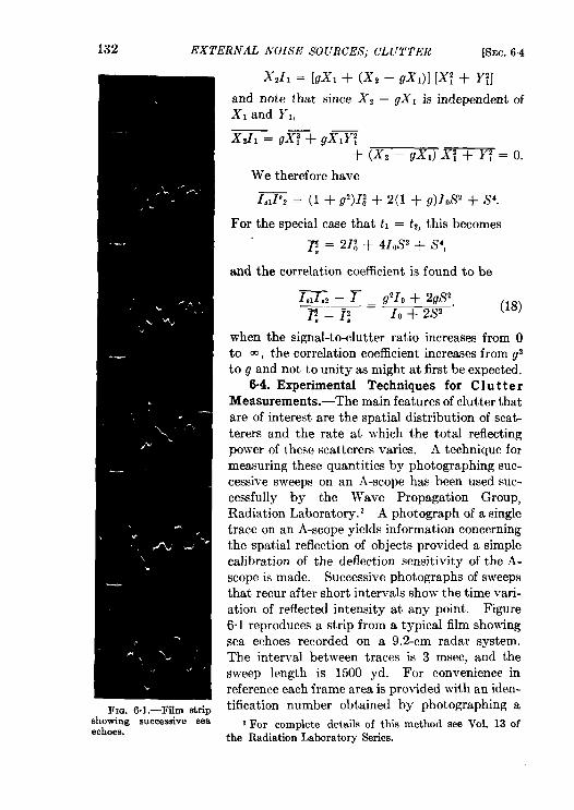
132 EXTERNAL NOISE SOURCES; CL UTTh’R [SEC.64
X*I, = [gx, + (x, – gx,)] [x; + Y;]
and note that since X2 – gXl is independent ofX, and Y,,
We therefore have
1.1P, = (1 + g’)I; + 2(1 + g)IOs’ + s’.
For the special case that h = LZ,this becomes
~ = 213 + 410S” + s’,
and the correlation coefficient is found to be
when the signal-to-clutter ratio increases from Oto cc, the correlation coefficient increases from g’to g and not to unity as might at first be expected.
6.4. Experimental Techniques for C 1ut t e rMeasurements.—The main features of clutter thatare of interest are the spatial distribution of scat-terers and the rate at which the total reflectingpower of these scatterers varies. A technique formeasuring these quantities by photographing suc-cessive sweeps on an A-scope has been used suc-cessfully by the Wave Propagation Group,Radiation Laboratory. 1 A photograph of a singletrace on an A-scope yields information concerningthe spatial reflection of objects provided a simplecalibration of the deflection sensitivity of the A-scope is made. Successive photographs of sweepsthat recur after short intervals show the time vari-ation of reflected intensity at any point. Figure6.1 reproduces a strip from a typical film showingsea echoes recorded on a 9.2-cm radar system.The interval between traces is 3 msec, and thesweep length is 1500 yd. For convenience inreference each frame area is provided with an iden-tification number obtained by photographing a
1For complete details of this method see Vol. 13 ofthe RadiationLaboratorySeries.
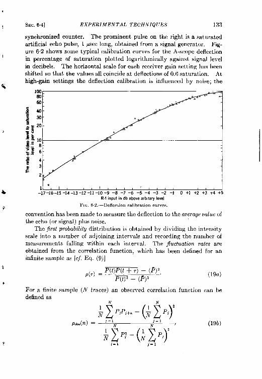
SEC. 6.4] EXPERIMENTAL TL’CHNIQIJES 133
synchronized counter. The prominent pulse on the right isasaturatcdartificial echo pulse, 1 ~sec long, obtained from a signal generator. Fig.
ure 6.2 shows some typical calibration curves for the A-scope deflectionin percentage of saturation plotted logarithmically against signal levelin decibels. Thehorizontal scale foreach receiver gain scttinghasi}eenshifted so that the values all coincident deflections of 0.6saturaticm. Athigh-gain settings the deflection calibration is influenced by noise; the
1 “, I I , , I , I-17–16–15-14 –13–12-11–10-9 -8 –7 -6 –5 –4 –3 -2 -1 0 +1 +2 +3 +4 +5
R-f input in db abovearbitary level
FIG.6,2.—Detlectioncalibrationcurves.
convention has been made to measure the deflection to the average value ofthe echo (or signal) plus noise.
The first probability distribution is obtained by dividing the intensityscale into a number of adjoining intervals and recording the number ofmeasurements falling within each interval. The fluctuation rates areobtained from the correlation function, which has been defined for aninfinite sampleas [qf. Eq. (9)]
P(t)P(t+ ,) – (P) 2p(T) = _
P(t)’ – (P)’ “(19a)
For a finite sample (N traces) an observed correlation function can be
(19b)
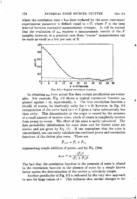
134 EXTERNAL NOISE SOURCES; CLUTTER [SEC. 64
where the correlation time ~ has been replaced by the more convenient
experimental parameter n defined equal to 7/2’, where 2’ is the time
interval between successive measurements (sweeps). It will be noticec!
that the evaluation of p... requires n measurements outside of the Nsamples; however, in a practical case these “excess” measurements canbe made as small as a few per cent of N.
1.0r 1
----------------------o I I I I
O 4 8 12 16 20 24 28 32 36 40T inmillissconds
FIG. 6.3.—Typical correlation function.
In obtaining p.b, from actual film data certain peculiarities are notice-able. For example, Fig. 6.3 shows a typical correlation function P.~
plotted against r or, equivalently, n. The true correlation function pb
should, of course, be identically unity for r = O; however, in Fig. 6.3extrapolation of the curve back to7 = O gives a value substantially lessthan unity. This discontinuity at the origin is caused by the presenceof a small amount of receiver noise, which of course is completely randomfrom sweep to sweep. The effect of thenoise is easily calculated. Thefirst probability distributions for noise alone and for clutter alone aresimilar and are given by Eq. (l). If one remembers that the noise isuncorrelated, one can easily calculate the combined power and correlationfunctions of the clutter plus noise. These are
~C~. = ~, + ~N,
representing simple addition of power, and by Eq. (19a)
(Pc)’P.+. = P. ~PC + ~N)~
The fact tha~ the correlation function in the presence of noise is relatedto the correlation function in the absence of noise by a simple knownfactor makes the determination of the correct p. extremely simple.
Another peculiarity of Fig. 6.3 is indicated by the very slow approachto zero for large values of r. This indicates slow secular changes in the
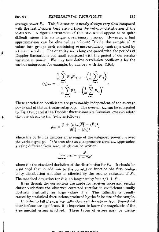
SEC, 64] EXPERIMENTAL TECHNIQUES 135
average power P.. This fluctuation is nearly always very slow comparedwith the fast Doppler beat arising from the velocity distribution of thescatterers. A rigorous treatment of this case would appear to be quitedifficult, since it is no longer a stationary process. However, a firstapproximation can be obtained as follows: Divide the sample of Nvalues into groups each containing m measurements, each separatd by
Ja time interval r. The quantity m, is long compared with the periods ofDoppler fluctuations but small compared with the period of the secularvariation in power. We may now define correlation coefficients for thevarious subgroups; for example, by analogy with Eq. (19a),
m1—
m z P“P’+’-($”Y(~]).b, = ‘=1 ~ i=l
m
+ Zp”-(:2P”J,=1 ,=1
These correlation coefficients are presumably independent of the averagepower and of the particular subgroup. The over-all PO,.can be computedby Eq. ( 19b); and if the Doppler fluctuations are Gaussian, one can relate
& the OVer-all p.,. tO the (/)~).b.as fOllOWS:
[1 + (pj).b,]~ – (F,)’p.,. = 7
2~ – (PO)2
where the curly line denotes an average of the subgroup power . jOoverthe various groups. It is seen that as pi approaches zero, p~~ approachesa value different from zero, which can be written
I
where 6 is the standard deviation of the distribution for Po. It should bementioned that in addition to the correlation function the first proba-bility distribution will also be affected by the secular variation of PO.
The standard deviation for P is no longer unity but ~~.Even though the corrections are made for receiver noise and secular
clutter variations the observed corrected correlation coefficients usuallyfluctuate erratically for large values of 7. This difficulty is usuallycaused by statistical fluctuations produced by the finite size of the sample.
In order to tell if experimentally observed deviations from theoreticaldistributions are significant, it is important to know the magnitude of theexperimental errors involved. Three types of errors may be distin-
136 EXTERNAL NOISE SOURCES; CLUTTER [SEC.64
Wished: the fluctuations due to the finite size of the sample, the errors inreading the film, and the errors in calibration.
The fluctuations in the number of measurements falling within agiven intensity range are distributed according to the well-known Poisson
distribution. The rms fractional deviation is l/v’~, where n is theexpectation value of the number of measurements, providing n is small
horrnalized sigrial power P/P.
FIG.6.4.—ExperimentaIandtheoreticalfirstprobabilitydistributions(for chaff).
compared with the size of the sample N. It must be remembered thatthis assumes independent trials. Normally there is correlation betweensuccessive measurements, and n must be replaced by n’, the number ofindependent measurements.
Errors in the reading of the film may be either systematic or random.It is difficult to estimate a systematic error. However, a known sourceof random error is usually present. Depending upon the computer andthe nature of the trace, there is an error in measuring the deflection,ranging from 0.05 cm to several millimeters, but usually around 1 mm.Consider now an interval equal to the minimum measurable difference,centered about the deflection corresponding to the boundary betweentwo deflection groups. Of the pulses falling in this interval zone, some,
Sm. 6.5] EXPERIMENTAL RESULTS 137
by chance, will be assigned to one group and some to the other. Thermsfluctuation of the number in a group, due to such an “uncertainty zone”
at one boundary, is given by $ -v’% where m is the total number ofmeasurements falling in the uncertainty zone. 1 Note that m includes allmeasurements falling in the interval, since all trials are independent.
6.5. Experimental Results. Chafl.-Since chaff, or “window,” is
h composed of a large number of randomly moving dipoles, it is ideal touse for comparing experiment with theory. Figure 6“4 compares atypical experimental first probability distribution, taken at a wavelengthof 9 cm, with the theoretical exponential curve. The histogram repre-sents the analysis of 1000 pulses, and the straight line corresponding tothe theoretical clmve uses the value of the measured average intensity ofthe sample analyzed. The deviations between the two plots are randomand do not indicate any significant differences.
TABLE6.1.—DEWATIONSBETWEENTHEOEETIC.ALANDEXPERIMENTALFIMT PROB-
Interval ofPF,
b(1)
o -0.340.34-0.680.68-1. O11.01-1.351.35-1.691.6%2.032,03-2.362,36-2.702.7(F3.383.384.05
1 4.05-5.405.4CP8.43
ABILITY DISTRIBUTIONS
Chaff k = 9.2 cm 10QOpulsesI
No. of pulses in intervalExpected
Difference rms due toExperimen-
tally
(2)
27520514313679473221351494
Theoretically I linite sample
(3) (4) (5)1 1
292 – 17 14206 –1 13146 –3 11103 +33 972 +7 854 –7 737 –5 626 –5 531 +4 516 –2 412 +3 34 0 2
Fluctuationn No. border
error
(6)
344333222111
Table 6.1 compares the magnitude of the deviations in each intervalwith the expected rms fluctuations due to the finite size of the sample and“border error” as discussed in Sec. 6.4. In Column 5 it has been assumed
that all the measured pulses are independent of each other. Since there
is actually considerable correlation between neighboring pulses, the
I The reasoning employed is as follows: It is equally likely that a measurement willb assigned to eit~er group. The average number going ~ any
[ Therms fluctuationin this numberis <?n/2(1 – +) = ; v%.
L-- —
one group is m/2.
138 EX7’ERNAL NOISE SOURCES; CL UTTER [SEC.6.5
figures in Column 5 represent minimum values. The “border error”calculation assumes that differences in the pulse height of less than 1 mmwere not measurable, which is likewise a minimum figure. It is seen thatthe actual deviations are, with one exception, well inside the expectedstatistical fluctuations. Equally good results have been obtained in allmeasurements of chaff cut for A = 10 cm and observed on k = 9.2 andk = 3.2 cm. The first probability distribution of the echo on 515Me/see of chaff cut for the “ Wurzburg” band (k = 50 c~l) has been ,4
measured at Radio Research Laboratory and good agreement was likewiseobtained with theory. L
v in CPS
FIG.6.5.—Frequency spectra for chaff,
The shapes of the frequency spectra of the fluctuations of chaff echohave always been found to be roughly similar, resembling error curvescentered at the origin. The widths of the spectra, however, are quitevariable even at one wavelength. For example, Fig. 6.5 shows the spectrafor the echo of chaff cut for X = 10 cm, as measured on h = 9.2 cm onfour occasions. It is significant that the widest spectrum D was obtainedwith gusty winds up to 25 mph while wind speed was 10 mph or less forthe other cases. The width of the spectrum depends upon the relativevelocity of the chaff dipoles, i.e., the so-called “horizontal dispersalrate, ” and it is to be expected that this rate depends on the speed andgustiness of the wind.
The narrowest spectrum, Curve A, was obtained with chaff of thesame electrical properties as used for the other curves but with slightlydifferent mechanical and aerodynamical properties. In addition the
1G. P Kuiper, “A Study of Chaff Echoes at 515 MC,’) RRL Report 411-73,December 1943.
SEC.6.5] EXPERIMENTAL RESULTS 139
chaff was dispensed from a slow-moving blimp instead of into the rela-tively turbulent slip stream of an airplane.
It is not believed that there is any significant dependence of thespectrum on the “age” of the chaff, i.e., the length of time between theinitial drop and the measurement. The ages for the four curves A, B, C,D of Fig. 6.5 are 3 rein, 20 see, 6 rein, and 10 rein, respectively.
If the fluctuation arises solely from the Doppler beats of the movingchaff dipoles, then it is seen from Sec. 6.2 that the correlation function isa function of the quantity v/h, that is, the dispersal velocity divided by
0.8 -
0.6 -:z
0.4 -
0.2 -
0 ,0 20 40 60 80 lCQ 120 140 160 180 200
VAin cm-cps
Fm. 6.6.—Spectrumof chaff for 2 wavelengths.
the wavelength. Hence the width of the frequency spectrum of thefluctuation should be proportional to the radar wavelength for the samevelocity distribution. More exactly, if simultaneous measurements of thefrequency spectra are made on several wavelengths, the curves shouldcoincide when plotted as functions of the product of the fluctuationfrequency and radar wavelength. Accordingly in Fig. 6.6 the experi-mental frequency spectra for chaff measured simultaneously on X = 3.2and 9.2 cm is plotted against the product of frequency and radar wave-length. The small discrepancy between the two curves is well withinexperimental error.
The frequency spectrum of chaff has also been measured at 515Me/see’, and the maximum frequency present to an appreciable extentwas found to be 4 cps on horizontal polarization. When “scaled” toh = 9 mm this value roughly corresponds to Curve A of Fig. 6.5. Con-sidering that the chaff size was different, the wavelength dependenceis at least qualitatively verified. (The frequency of fluctuation on
-- .-— ——.——-..
140 EXTERNAL NOISE SOURCES; CLUTTER [SEC.65
vertical polarization was found to be somewhat slower, with a maximumof 3 cps, whereas all the microwave measurements were made with hori-zontal polarization. )
Mention must also be made of some results obtained in England onthe frequency of fluctuation that are not in agreement with the aboveconclusions. 1 Pulse-to-pulse photographs of chaff echoes were madeon212and 3000 Me/see. A statistical analysis was not carried out, but itis stated that there was qualitative evidence of fluctuation frequenciesin the range 10 to 25 cps on both frequencies.
If the spectrum and velocity distribution have Gaussian shapes, someinformation about average speeds can be easily obtained. Let i bedefined such that one-half of the scatterers have relative velocities in thedirection of the radar set that lie between – J and + Z. Then it is easilyshown that
o = o.2xj>4, (20)
where x is the wavelength and j}fi is the frequency at which the powerfrequency spectrum is down to one-half of its original value. Applyingthis formula to the curves of Fig. 6.5 (although they are not exactlyGaussian in shape) values of u are obtained ranging between 0.6 and 2.oft/sec. These results are of the same order of magnitude as the hori-zontal dispersal rate as actually measured from motion pictures of chaffdipoles.
Precipitation. Echo.—The scatterers responsible for precipitationechoes are undoubtedly either raindrops or water particles in solid form.One would therefore expect that the conditions for treating the targetas an assembly of random scatterers are well satisfied. Figure 6.7 showsa typical experimental first probability distribution as obtained from theanal ysis of 1000 pulses at A = 3.2 cm of the echo from a shower. Thedeviations of the histogram from the theoretical curve (plotted as astraight line on this scale) are random. An analysis of the deviations,similar to that made for chaff echo, shows that they are within theexpected statistical fluctuations.
Unfortunately, only a small amount of data is available on the fre-quency spectrum of the fluctuations of precipitation echo. Three filmswere measured on k = 9.2 cm, and one on A = 3.2 cm, all for the echofrom shower or thunderstorms. The rate fluctuation appears to beseveral times that for chaff. Figure 6.8 is a plot of the power frequencyspectrum for the three cases measured on 9.2 cm. The shapes of thespectra are roughly Gaussian except one case, where there is a pronouncedtail above 80 cps. It is doubtful, however, if this tail is _significant.
1~~Final Report on ADRDE Window Trials,” ADRDE Report No. 2W, Awd1944.
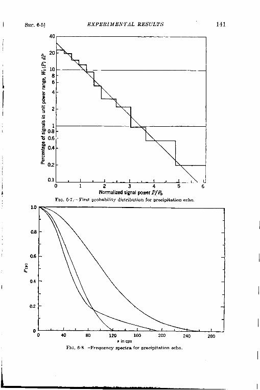
I EXPERIMENTAL RESULTS
1
1
II
,
(
i
)
I
1
40
20
1086
4
2
0.1
\
I I , I f I , 1’
1 2 3 4 5 6Normalizd signal power 4’/Po
FIG.6.7,—First probability distributionfor precipitationecho.
1.0
0.8 -
0.6 -
z<
0.4 -
0.2
00 40 80 120 160 2C0 240 280
v in cm
FIG.6.8 –FrequencyBpect.rafor precipitationecho,
142 EXTERNAL NOISE SOURCES; CLUTTER [SEC.65
The widths of the three spectra, given by j}$, differ by as much asafactor of2. hinthecase ofchaff itistherefore notpossible tospeakofthe fluctuation frequency spectrum, but one must expect to find thespectrum depending on the particular storm, probably varying evenwithin the storm region and changing with time. Additional evidenceforthis variability is furnished byan attempted experiment on the wave-Iength dependence of the fluctuation. Two films were taken of the echofrom arain shower on X = 9.2 and3.2 cm, respectively, separated byatime interval of a few minutes and a range interval of a few thousandyards. The fluctuation spectra, instead of being inversely proportionalto wavelength, were practically identical both in shape and width. Itis concluded that the rate of fluctuations can change by a factor of 3 evenover short intervals of time and space.
An average figure for the speeds of the drops relative to each othermay be obtained from Eq. (20), but one must use greater caution than forchaff because of possible deviations from a Gaussian spectrum. Figure6.7 yields values of v between 3 and 5 ft/sec. These relative velocitiesshould be connected with the turbulence existing in the regions of pre-cipitation, and in this light the values seem low. It must be remembered,however, that the turbulence in a storm is mostly vertical and thefluctuation depends on the horizontal velocities. Furthermore thevelocity distribution is quite broad and extends far beyond V.
Sea Echo.—A striking feature of the radar echo from sea is the pres-ence-of a secular variation to a much more marked degree than in thecase of chaff or precipitation echoes. However, if a time interval ischosen in which the “average” intensity is sensibly constant, then thefirst probability distribution agrees with the theoretical exponentialCuwe.
The power frequency spectrum of the fluctuations of sea echo is againroughly Gaussian in shape and about the same width as the spectra forchaff. The range of widths encountered appears to be much smaller;values of ~%between 25 and 35 cps occur for k = 9.2 cm. No dependenceof the spectrum on pulse length has been found. A comparison of thefluctuation spectra at two wavelengths show that the value of f}~ isapproximately inversely proportional to wavelength. This indicatesthat these fast fluctuations are probably caused by moving randomscatterers. From the value of ~}t it appears that the median relativevelocity u is of the order of 1 or 2 ft/sec.
Ground Clutter.—The previously discussed targets could all be closelyapproximated by assemblies of random, independent, moving scatterers.Targets responsible for ground clutter also include such assemblies, con-sisting of leaves, branches, etc., that move in the wind. However, inaddition there are scatterers with fixed phases, for example, tree trunks,
II
I
SEC. 64$] CLASSIFICATION OF I.VTERFERENCE 143
rocks, etc. Thetotal echo isthesum of theechoes from both classes oftargets.
Se}-eral first probability distributions for ground clutter have beenmeasured. They are found toagreewith Eq. (15) if suitable values areinserted for the reflected power from the fixed and moving scatterersrespectively. Ata\vavelength of9.2cm aheavily \vooded hill subjectedto gusty winds of 50 mph shows almost no fixed contribution, while asparsely vegetated rocky terrain shows almost no random contribution.One would expect the ratio of fixed to random power to increase withwavelength; this has been qualitatively confirmed by experiment.
The shape of the spectrum appears to be roughly similar to those ofthe chaff or sea echo, although the differences from the Gaussian shapeare somewhat more pronounced. The widths of the spectra, however,are smaller by an order of magnitude than those of the other clutterechoes. These widths naturally increase with wind speed and in additiondepend to some extent on the terrain. They also appear to be essentiallyproportional to frequency. Representative values of j}j for a wavelengthof 10 cm are from 1 to 5 cps. This indicates very small relative velocitiesof the moving scatterers.
6.6. Classification of Interference.-Examples of electronic inter-ference are legion. A common one is the static in radio reception. Tounderstand the principles involved in the perception of signals in inter-ference it is well to know the various types of electronic interference thatmay be encountered. Electronic interference reduces the desired signalvisibility, either because of saturation within the receiver or because ofunavoidable mixing of the interference with the desired signal. In themixing process the identity of the signal will be destroyed if the elec-tronic interference is sufficiently strong. In general, the interference ismore serious when its characteristics correspond to those of the desiredsignal. This correspondence may consist of similarities in either powerspectra or time distributions. Likewise, methods for reducing the dele-terious effects of interference are based upon the differences between thedesired signal and the interference. If the interference spectrum issimilar to that of the desired signal, then, in general, the differences intime dependence are utilized. If, however, the time dependence issimilar to that of the signal, it is often feasible to take advantage ofdifferences in the spectra in finding suitable filters for the separation of thedesired signal from the interference. These matters will be discussedin detail in Chap. 12.
It is important to note, however, that the power spectrum of theinterference is not by itself an adequate criterion of its behavior. Onecan appreciate this fact by observing that the spectrum of thermal noise,such as was discussed in Chap. 4, is uniform throughout the frequency
~–-. .-.
144 EXTERNAL NOISE SOURCES; CLUTTER [SEC.67
scale. The spectrum of a single, discrete, extremely short pulse is alsouniform and continuous throughout the frequency scale. The timedependence of the thermal noise and the discrete pulse are entirelydifferent, however, and it is obvious how one can utilize this difference todistinguish the two phenomena. True, if one uses the term “spectrum”in its exact sense, that is, including the phase factors between the variousfrequency components, then the spectrum will be an exact description ofthe phenomenon. It is usually customary, however, to speak of the“spectrum “ in terms of the power per unit jrequenzy interval. Thisneglects the phase factors, and therefore the spectrum is not a completedescription of the phenomenon.
As was stated above, the electronic interference may mix with andcover up the desired signal. It is important to note, however, that thesignal may be lost through still another mechanism. The interference, ifsufficiently large, can cause the receiver to operate in such a region that itis essentially saturated. Under these conditions the signal will be sup-pressed just because the receiver no longer responds to incremental inputvoltages. A more complete discussion of the saturation characteristics ofthe receiver will be found in Chap. 12.
Interference may be variously classified, of course. For the purposesof this book electronic interference can be conveniently put into only twogeneral categories. The first category comprises the simple forms ofinterference; the second, the complex forms. Of the simple forms ofinterference only two varieties will be discussed: c-w interference andpulsed interference, that is, interference caused by a succession. of shortr-f pulses similar to the radar pulses discussed in Chap. 2. There areobviously many types of complex interference, but only four gereralvarieties will be trested here. Three of these are forms of noise-modu-lated r-f power, and the fourth variety is a series of “randomized”pulses, that is, pulses that occur at random time intervals. It is hopedthat other types of interference can be understood by interpolation,superposition, and extension.
6.7. Simple Types of Interference. Continuous-wave InteTjerence.—Continuous-wave r-f energy has a spectrum that is essentially mono-chromatic. Its characteristics are similar to those of the c-w signaldescribed in Chap. 2, for example, a constant-amplitude r-f wave.
One reason for the deleterious effect of c-w r-f interference is that itmixes with the signal in random phase. This arbitrary phase relationshipbetween the interference and the signal causes the signal contribution inthe receiver to vary randomly in time. In addition to this phenomenonthe c-w interference may possibly saturate the receiver in such a waythat the response of the receiver to incremental signals is essentially zero.
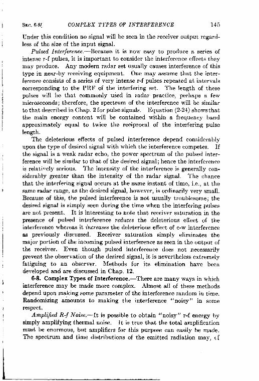
SEC. 6.8] COMPLEX TYPES OF INTERFERENCE 145
Under this condition no signal will be seen in the receiver output regard-less of the size of the input signal.
Pulsed Interference.—Because it is now easy to produce a series ofintense r-f pulses, it is important to consider the interference effects theymay produce. Any modern radar set usually causes interference of thistype in near-by receiving equipment. One may assume that the inter-ference consists of a series of very intense r-f pulses repeated at intervalscorresponding to the PRF of the interfering set. The length of thesepulses will be that commonly used in radar practice, perhaps a fewmicroseconds; therefore, the spectrum of the interference will be similarto that described in Chap. 2 for pulse signals. Equation (2.24) shows thatthe main energy content will be contained within a frequency bandapproximately equal to twice the reciprocal of the interfering pulselength.
The deleterious effects of pulsed interference depend considerablyupon the type of desired signal with which the interference competes. Ifthe signal is a weak radar echo, the power spectrum of the pulsed inter-ference will be similar to that of the desired signal; hence the interferenceis relati!~ely serious. The intensity of the interference is generally con-siderably greater than the intensity of the radar signal. The chancethat the interfering signal occursat the same instant of time, i.e., at thesame radar range, as the desired signal, however, is ordinarily very small.Because of this, the pulsed interference is not usually troublesome; thedesired signal is simply seen during the time when the interfering pulsesare not present. It is interesting to note that receiver saturation in thepresence of pulsed interference reduces the deleterious effect of theinterference whereas it increases the deleterious effect of c-w interferenceas previously discussed. Receiver saturation simply eliminates themajor portion of the incoming pulsed interference as seen in the output ofthe receiver. Even though pulsed interference does not necessarilyprevent the observation of the desired signal, it is nevertheless extremelyfatiguing to an observer. Methods for its elimination have beendeveloped and are discussed in Chap. 12.
6s8. Complex Types of Interference.-There are many ways in whichinterference may be made more complex. Almost all of these methodsdepend upon making some parameter of the interference random in time.Randomizing amounts to making the interference “noisy” in somerespect.
Amplijied R-j Noise.—It is possible to obtain “noisy” r-f energy bysimply amplifying thermal noise. It is true that the total amplificationmust be enormous, but amplifiers for this purpose can easily be made.The spectrum and time distributions of the emitted radiation may, cf
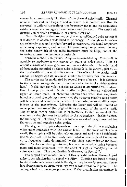
146 EXTERNAL NOISE SOURCES; CLUTTER [SEC.68
course, be almost exactly like those of the thermal noise itself. Thermalnoise is discussed in Chaps. 4 and 5, where it is pointed out that itsspectrum is uniform throughout the frequency range and no correlationexists between the voltages at one instant and the next. The amplitudedistribution of the r-f voltage is, of course, Gaussian.
The difficulties in the production of such amplified r-f noise appear ifit is desired to obtain a wide band of r-f energy. Although such devicesare relatively easy and straightforward to construct, wideband amplifiersare clumsy, expensive, and consist of a great many components. Wherethe noise bandwidth of the radio frequency must be large, one of thefollowing alternative methods is desirable.
Continuous-wave Interference Amplitude-modulated by Noise.—It ispossible to modulate a c-w carrier by audio or video noise. The r-foutput consists of a strong carrier and noise sidebands. The total bandof frequencies occupied by these noise sidebands is, in general, just twicethe bandwidth of the modulating noise. The effect of the carrier itselfcannot be neglected; its action is similar to ordinary c-w interference.
The carrier can be modulated by several types of noise. It is commonto use a noise voltage derived from thermal noise in the video systemitself. In this case the video noise has a Gaussian amplitude distribution.One of the properties of this distribution is that it has no well-definedupper or lower limit. It therefore follows that when this amplitudefunction is used to modulate the carrier, the upper or positive noise peakswill be limited at some point because of the finite power-handling capa-bilities of the transmitter. Likewise the lower end will be limited atsome point because of the original finite strength of the carrier itself.The original carrier amplitude is customarily located at one-half themaximum value that can be supplied by the transmitter. In this fashion,the limiting, or “clipping,” as it is sometimes called, is symmetrical forthe positive and negative noise peaks.
The degree of clipping depends on the amplitude of the modulatingvideo noise compared with the carrier level. If the noise amplitude issmall, the clipping will be relatively unimportant and the r-f sidebandsdue to the noise will be uniformly distributed on each side of the carrierup to frequency limits determined by the video bandwidth of the noiseitself. As the modulating noise amplitude is increased, clipping becomesmore and more important, with the effect of slightly modifying the r-fnoise spectrum. This modification is discussed in Sec. 12.7.
The clipped noise in interference of this type differs from the unclippednoise in its relationship to signal visibility. Clipping produces a ceilingto the interference, above which the signal may be easily seen and there-fore always increases signal visibility for the same total noise power. Theceiling effect will be more pronounced if the modulation percentage is
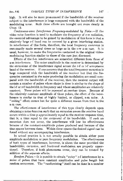
SEC. 6.8] COMPLEX TYPES OF INTERFERENCE 147
high. It will also be more pronounced if the bandwidth of the receiversubject to the interference is large compared with the bandwidth of themodulating noise. Both these effects are brought out more clearly inChap. 12.
Continuous-wave Interference Frequency-modulated by Noise.—If thevideo noise function is used to modulate the frequency of c-w radiation,the essential advantage to be gained by modulation of this form is that arelatively large r-f band can be covered by a given interfering station.In interference of this form, therefore, the total frequency excursion iscustomarily made several times as large as in the c-w a-m case. It isusual, however, to make the frequencies contained in the original video-modulating function similar to those of the case just discussed.
Effects of the f-m interference are somewhat different from those ofa-m interference. Thenoise amplitude inthereceiver is determinedlythe excursions of the interference signal across the r-f or i-f acceptanceband of the receiver. If one assumes that the total frequency excursion islarge compared with the bandwidth of the receiver but that the fre-quencies contained in the noise producing the modulation are small com-
pared with the bandwidth of the receiver, then the receiver output willcontain a number of pulses whose shape in time is similar to the shape ofthe i-f or r-f bandwidth in frequency and whose amplitudes are relativelyconstant. These pulses will be repeated at random times. Because ofthe relatively constant amplitude of these pulses, the effect of the inter-ference is similar to that of highly limited, or clipped, a-m noise. A“ceiling” effect occurs but for quite a different reason from that in thea-m case.
The effectiveness of interference of this type clearly depends uponobtaining a noise function such that an excursion across the receiver bandoccurs within a time p approximately equal to the receiver response time,that is, a time equal to the reciprocal of its bandwidth. If such anexcursion does not occur, the interference will lose its effectivenessbecause of the constant-amplitude pulses produced and because of thetime spaces between them. Within these spaces the desired signal can befound without any accompanying interference.
In actual practice it is not usually possible to obtain either pureamplitude modulation or pure frequency modulation. The effectivenessof both types of interference, however, is about the same provided thebandwidths, excursion, and fractional modulation are properly appor-tioned. Thereforej if both phenomena occur, they can be treated byaddition of the separate effects.
Random Pulses.—It is possible to obtain “noisy” r-f interference by aseries of pulses that have constant amplitudes and pulse length butrandom occurrence. The “randomizing “ itself can be done in a number
148 EXTERNAL NOISE SOURCES; CLUTTER [SEC.68
of ways. One possibility is to produce the pulses from the impulsesgenerated by the disintegrations of a radioactive source. If the averagespacing between these pulses is long, interference of this type willclearly have exactly the effect of the simple pulsed interference discussedin Sec. 6.7. If the average spacing between the pulses becomes of theorder of magnitude of the reciprocal of the receiver bandwidth, however,the output of the receiver will contain a series of superimposed pulsesinwhich the degree of overlapping is random. The output of the receiver,therefore, contains random amplitude fluctuations, or noise, and thisnoise interferes with signal visibility in a way similar to that describedfor thermal noise. Only the two extreme spacing conditions can usuallybe treated adequately: (1) when the spacing between pulses is very largeand (2) when the average spacing bet ween pulses becomes very short.Chapter 12 treats these questions in detail.
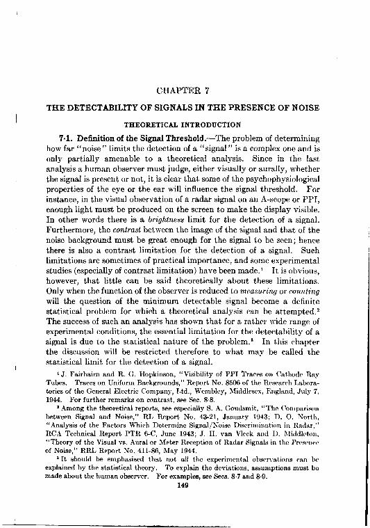
CHAPTER 7
THE DETECTABILITY OF SIGNALS IN THE PRESENCE OF NOISE
THEORETICAL INTRODUCTION
7.1. Definition of the Signal Threshold.—The problem of determininghow far “noise” limits the detection of a “signal” is a complex one and isonly partially amenable to a theoretical analysis. Since in the lastanalysis a human observer must judge, either visually or aurally, whetherthe signal is present or not, it is clear that some of the psychophysiologicalproperties of the eye or the ear will influence the signal threshold. Forinstance, in the visual observation of a radar signal on an A-scope or PPI,enough light must be produced on the screen to make the display visible.In other words there is a brightness limit for the detection of a signal.Furthermore, the contrast between the image of the signal and that of thenoise background must be great enough for the signal to be seen; hencethere is also a contrast limitation for the detection of a signal. Suchlimitations are sometimes of practical importance, and some experimentalstudies (especially of contrast limitation) have been made. 1 It is obvious,however, that little can be said theoretically about these limitations.Only when the function of the observer is reduced to measuring or couxtingwill the question of the minimum detectable signal become a definitestatistical problem for which a theoretical analysis can be attempted.zThe success of such an analysis has shown that for a rather wide range ofexperimental conditions, the essential limitation for the detectability of asignal is due to the statistical nature of the problem. 3 In this chapterthe discussion will be restricted therefore to what may be called thestatistical limit for the detection of a signal.
1J. Fairbairn and R. G. Hopkinson, “Visibility of PPI Traces on C’atboclc RayTubes. Traces on Uniform Backgrounds,” Report No. 8506of the Research Latmra-tories of the General Electric Company, Ltd., Wembley, Middlesex, England, July 7,1944. For further remarks on contrast, see Sec. 8.8.
z Among tbe theoretical reports, see especially S. A. Goudsmit, “ Tbc Comparisonbetween Signal and Noise, ” RL Report No. 43-21, January 1943; D. O. North,“Analysis of the Factors Which Determine Signal/Noise Discrimination in Radar, ”RCA Technical Report PTR 6-C, June 1943; J. H. van Vlcck and D. h1iddleton,“Theory of the Visual vs. Aural or kfeter Reception of Radar Signals in the Presen{,cof Noise, ” RRL Report No. 411-86, May 1944.
3It should be emphasized that not all the expcrimr.ntal ohservntions can beexplained by the statistical theory. To explain the deviations, assumptions must bomade about the human observer. For examples, see Sees. 8.7 and 8$.
149

150 THE DETECTABILITY OF SIGNALS IN NOISE [SEC.7.1
The first question that arises is how to define the minimum detectablesignal, or the signal threshold; here it is important to emphasize that onecan speak of a minimum detectable signal only (1) when the number ofobservations is limited or (2) when the time of observation is limited.,, The simple case of the detection of a small cur-
1
k-rent by means of a sensitive galvanometers may
E help explain this. Because of thermal agita-.-IJ tion the mirror of the galvanometers will have~n to an unavoidable Brownian motion around its
Time_ equilibrium position. It might seem, there-FIG. 7.1.—Brownian motion fore, that when a current or si&al (introduced
of a galvanometersmirror.at t = to; see Fig. 7.1) produces a deflection
small compared with the mean “jitter” of the mirror, such a currentcould not be detected. This is true, however, only when the number ofobservations is limited. When there is unlimited time, the average posi-tion and therefore also a change of the average position of the mirror canbe determined as accurately as desired.
Strictly speaking, therefore, the noise or the thermal motion does notlimit the detectability of a signal. 1 It is only when there is a limited
observation time that for small signals one can make a guess or a bet as towhether the signal is present or not, and there is then a definite probabilitythat the guess is right. Of course, for increasing signal strength thisprobability will rapidly increase and approach unity. A plot of theprobabilityy of success vs. signal strength will be referred to as the bettingcurve. The minimum detectable signal can then be defined as that signalstrength for which the probability of guessing right is, let us say, 90 percent; this means that, on the average, the guess will have proved right innine out of ten cases. The minimum detectable signal defined in this
manner will decrease when the observation time increases and, in principle,
will approach zero when this time goes to infinity. It is not necessary,
of course, that the time of observation be actually the time during which
the human observer looks at or listens to the simal and remembers theresults of his observations. It is often possible to let the detecting systemperform automatically a great number of observations and present asuitable average to the human observer. North’ calls this ‘‘ integrationof the signal before detection, “ in contrast to the effect of the humanobservation time, which he calls “integration after detection. ”a It is
1Excluded here are all systematicvariations (for instance, of the zero position ofthe galvanometers), which in practice will always put a limit on the detectability of asignal.
aLot. cit.3 Similarly a distinction will be made between the integration time of the detecting
system and the observation time, which is the human integration time.
SEC. 72] PROBAIIILIT1’ DISTRIBl~TIO.VS .4,VD ,qPIICTR,t 151
advisable to make this distinction because only the human observation,and not the recording apparatus, is influenced by physiological andpsychological factors that often defy a strict theoretical analysis. Inprinciple, however, the humtin element can always be reduced to ameasuring or a counting, and then the distinction between the integrationand the observation time ~vill disappear.
The idea that the determination of the minimum detectable signal isessentially a game of chance (Ivhen only a finite time is available) iscleally recognized in the experiments carried out at the RadiationLaboratory by ,J.L. Lawson and co;vorkers. In these experiments, ~vhichwill be discussed in detail in Chap. 8, aradar signal could be produced and shown E
Ifi
100 ––––––or–--–- -“j~
on a A-scope at six different positions. ~sThe noise was usually visible all the time. ~ ~Every 3 see, let us say, the position of the m ~ ‘“ ~ .signal was changed in a random fashion, ‘s- ml”
Signalstrengih — -and the observer had to guess Ivhere the ~1~.7.2. —Scher, ~atic betting curve.
signal was. The number of successes(above the number of pure chance successes) was recorded, and in thisway by varying the signal strength, there ~vas obtained a betting curve(see Fig, 7.2) from which the signa! threshold P., could be defined.’
A careful study has been made of the dependence of P,, on all kinds ofparameters (for an enumeration, see Sec. 8.4), and in (’hap, 8 the experi-mental results will be discussed in detail. For the development of thetheory it is first necessary to obtain some information about the prol]-ability distributions and about the spectrum of the output of a super-heterodyne receiver when both signal and noise are present.
7.2. Probability Distributions and Spectra.—In Sec. 3.8 there wasdiscussed the problem of finding the probability distributions and thespectra of Gaussian noise after it has gone through a linear or square-lawdetector. In this section the results of Sec. 3.8 ~vill be extended to thecase where a signal is also present. 2 The whole analysis will start fromthe i-f stage of the receiver. The convenient fiction will be used that
1It would be best to agree on a definite pcrccntagc (say 90 pm cent) and dcfinr 1’~,,(1as the signal strength for which this percentage is reached. Hovrcvcr, it is of trn momconvenient to define Ps graphically, as indicated in Fig. 72 (see also Sec. %3).
2Only an outline of the calculations will be presented. The problcm has bcrndiscussedoften, and several methods have been used. IIcrc the method of .Northwill be used, which was explained in Sec. 3.8, For the so-called “direct method”and further references, see S. 0, Rim, BPI1System Z’echn.J., 25, 45 (1945), I’art IV,and also W. R, Bennett, J. Acoust. Sot. Ant., 15, 164 (1944). Cf. also the report ofJ. H. van Vleck and D. illiddleton, “Theory of the Visual vs. Aural or Met~r I{ccep-tion of Radar Signals in the Presence of Noise, ” RRL Report No, 411-86, hfay 1944,J. Applied Phys., 11, 940 (1946),
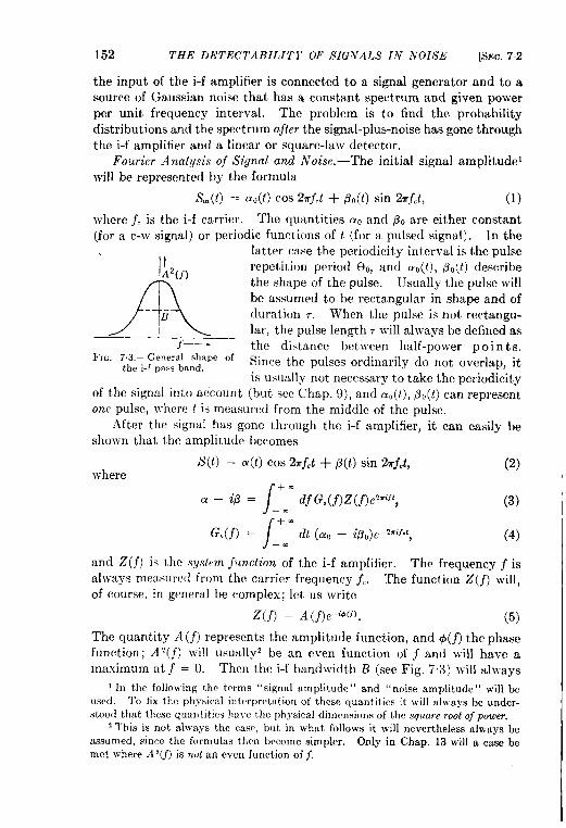
152 THE DE T?%CTA131LIT1’ OF SIGNALS IN NOISE [SEC.72
the input of the i-f amplifier is connected to a signal generator and to asource of Gaussian noise that has a constant spectrum and given powerper unit frequency interval. The problem is to find the probabilitydistributions and the spectrum ajter the signal-plus-noise has gone throughthe i-f amplifier and a linear or square-law detector.
Fourier Analysis of Signal and Noise.—The initial signal amplitudewill be represented by the formula
L%(t) = m(t) cos 2TfCt+ @,(t) sin 27r~ct, (1)
where ~, is the i-f carrier. The quantities a, and ~o are either constant(for a c-w signal) or periodic functions of t (for a pulsed signal). In the
latter case the periodicity interval is the pulse.
A
l%”)repetition period (3., and aO(t), ~O(t) describethe shape of the pulse. Usually the pulse willbe assumed to be rectangular in shape and of
B duration ,. When the pulse is not rectangu-lar, the pulse length 7 will always be defined as
f— the distance between half-power p o i n ts.FIG. 7,3.—General shape of Since the pulses ordinarily do not overlap, it
the i-f pa~sband.is usually not necessary to take the pcriodicity
of the signal into account (but see Chap. 9), and so(t), @o(t) can represent
one pulse, where ~ is measured from the middle of the pulse.
After the signal hfis gone through the i-f amplifier, it can easily be
shown that the amplitude becomes
S(t) = a(t) cos 2mf,t + p(t) sin 27rjCt, (2)where
/
+.~—~~= d~G,(j)Z(~)eZ~;~~, (3)
—.
/G,(f) = ‘m dt (aO – ipO)e-2mif”, (4)
—.
and Z(f) is the sy,strrn junction of the i-f amplifier. The frequency f isalways measured from the carrier frequency j.. The function Z(f) will,of course, in general be complex; let us write
Z(f) = A (j)e<$cj). (5)
The quantity A(j) represents the amplitude function, and @(f) the phasefunction; A ‘(f) v7ill Usuallyz be an even function of f and will have amaximum at ~ = O. Then the i-f bandwidth B (see Fig. 7,3) will always
1In the foilow’ing the terms “signal amplitude” and “noise amplitude 1)will beused. To fix the physical interpretation of these quantities it will always be under.stood that these quantities have tlLcphysical climmsions of the square root of power.
2This is not always the case, but in what follows it will nevertheless always beassumed, since the formulas then become simpler. Only in Chap. 13 will a case bemet where ii ‘(f) is not an cyen function of j,
SEC.7.2] PROBABILITY DISTRIBUTIO]VS A ,VD ISPECTR.1 153
mean the distance between half-power points, that is, points lvhemA’(f) is half of the value at ~ = O.
Let us now consider the noise amplitude. We may assume it to lmperiodic }vith a period G that is very long compared ~vith all perio(lsoccurring in the system and that afterward we shall let approach infinity.Initially the noise amplitude can be developed in a Fourier series
.
N,. (t) =z
(m, cos 27rjkJ + b,., sin 27rj_A4), (G)kg-o
where f~, = k’/8. The quantities a~, and b~, are random variables, andit will be assumed, as in Sec. 3.7, that
—1. a~, = ~t = 0,
—— u’ —ak”alr= b~,bl, = — &l,; ak,bl, = O.
)
(i)
9
2. The a~, and b,, are Gaussianly distributed. The quantity a’ inEq. (7) is a constant with the physical dimension of energy; in fact,
U2 = kTF, (8)
where k is the Boltzmann constant, T the absolute (room) tem-perature, and F the over-all noise figure of the receiver (seeChap. 5).
After the noise amplitude [Eq. (6)] has gone through the i-f amplifier,the amplitude becomes
N(t) = ‘s A~,[a;,,COS (2~fLd – ~~,) + bti,sin (2mfd – @k’)],
y
Since AH will be a maximum for f~, = f., it is convenient again to meas-ure the frequencies from the carrier frequency f, as zero point by putting
j, = f., – f.
The sum of signal and noise amplitude can then be written in the form[cf. Eq. (2)]
S(t) + N(t) = X(t) cos 2rf, t + Y(t) sin 2rf,f,, (9)where
L.!—
x(t) = a(t) +z
Ak[a, cos (2rf,t – o,) + b, sin (2rf,t – Ok)],
k=–.)
+.
Y(t) = B(t) +
2
fik[ – ak sin (2~fktk=–.
-This amplitude is then applied to the
1(lo)
– @k) + bk cos (Zm.fkt – o~)l.
second detector.
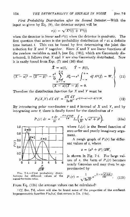
154 l’HE DETECTABILITY Y OF SIGNALS IN NOISE [SEC.7.2
First Probability Distribution after the Second Detector.-With theinput as given by Eq. (9), the detector output will be
r(t)= dx*(t) + Y*(t)
when the detector is linear and rz(t) when the detector is quodratic. Thefirst question that arises is the probability distribution of r at a definitetime instant t. This can be found by first determining the joint dis-tribution for X and Y together. Since X and Y are linear functions ofthe random variables a~ and bl [see Eq. (10)I, which are Gaussianly dis-tributed, it follows that X and Y are also Gaussianly distributed. Nowit is easily found from Eqs. (7) and (10) that
x = a(t), F = p(t), \
(x–a)’=(Y– p)’=: 1x“+”2/::‘fA’(’)=‘] ’11)k=–-
(x - a)(Y – f?) = o.
Therefore the distribution function for X and Y must be
dX dYPI(X, Y) dx dy = ~ ~-[(x-u)2+(Y-8) 21/lw, (12)
By introducing polar coordinates r and O instead of X and Y, and byintegrating over 6, there is finally found for the distribution of r
(13a)
1.0
0.8
0.2
00123456
.
FIG. 7.4.—First probabJity distri-butions for different values of thesignal-to-noiseratio.
where IO(Z) is the Bessel function ofzero order and purely imaginary argu-ment.
A rough graph of Pi(r) for differ-ent values of z, where
z = (CZZ+ &)/2w,
is shown in Fig. 74. For large val-ues of z, the form of PI(T) becomesnearly Gaussian and may then be ap-proximated by
1 _(r–%GTF)S
“(r) = <-We 2W “ (13b)
From Eq. (13b) the average values can be calculated’
1Cf. Sec. 7.6, wherewill also be found some of the propertiesof the confluenthypergeometricfunctionF(a,b;z) that occurs in Ea. (14a).
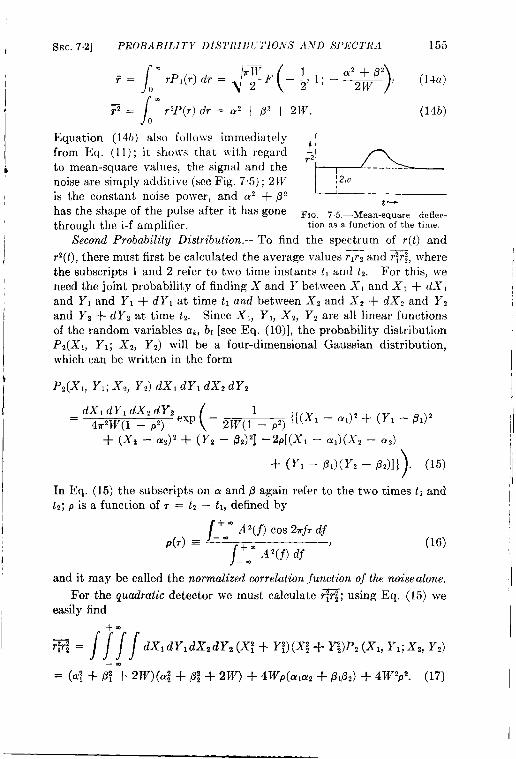
1
I
SEC. 7.2] PROBABILITY DISTRIB1 ‘I’IOA’S AND SPECTRA 155
\
.
d- (7rl[’ 1~= ~z + LV
)rPl(r)dr= -YF —211; —~ , (14a)
II
/
.~z = r2F’(r)dr = az + @ + 2W. (14b)
o
Equation (14b) also follows immediately
“k
from Eq. (11); it shows that lVith regard ~to mean-square values, the signal and thenoise are simply additive (see Fig. 75); 2Wis the constant noise power, and az + @z t-has the shape of the pulse after it has gone FIG. 75.-Mean-square deflec-through the i-f amplifier. tion as a function of the time.
Second Probability Distribution.—To find the spectrum of r(t) andp(t), there must first be calculated the average values rlrz and ~, where
the subscripts 1 and 2 refer to two time instants t,and b For this, weneed the joint probability of finding X and Y between Xl and Xl + dXland YI and YI + dYl at time tland between X2 and Xa + dXa and Yzand Yz + dYz at time t2. Since Xl, Y,, X2, Yz are all linear functionsof the random variables a~, bl [see Eq. (10)], the probability distributionPZ(XI, Y,; X2, Yz) will be a four-dimensional Gaussian distribution,which can be written in the form
PZ(X,, Y,; X,, Yz) dX, dY, dXZ dYz
_ dX, dY, dXz dYZ
(
1—47r2w(l – pz) ‘Xp – 2W(1 – p’) {[(xl – %)2+ (y, – p,)’
+ (x2 – a’)’ + (Y2 – @2)2] –2P[(X1 – %)(x, – a2)
)+ (Y, – @,)(Y, – /32)]) (15)
In Eq. (15) the subscripts on”a and @ again refer to the two times t,andtz; p is a function of r = t’– t,,defined by
(16)
and it may be called the normalized correlation junction of the noise alone.
For the quadratic detector we must calculate r%; using Eq. (15) weeasily find
--
156 THE DETECTABILITY OF SIGNALS IN NOISE [SEC,72
For the linear detector we have to find the average value ~% Thiscannot be calculated exactly; however, for most purposes it is sufficientto find an approximate value by developing Eq. (15) in powers of p[from Eq. (16) we see that p s 1] up to p’.’ The successive terms canthen be integrated and we find
+.—rlr2 =
////
‘dX, dY, dX,dY, <(X;+ Y;) (X:+ ~)P2(X1, Yl; X2, Y2)
—.
= 11(1)1,(1) +,+ {[I,(X) – C2,1,(1)][I,(X) – a,I,(l)]
+ [I,(Y) – @,I,(l)][I,(Y) – @,I,(l)]] +*2 ([1,(X’) – 2a,11(x)
+(a; –w)I,(l)][I,(x’) –2a,I,(x) +(a:–w)I,(l)]+[z, (Y’) –2p,I,(Y)
+ (i% – ~)~l(l)l[~z(y’) – 2B2Z2(Y) + (B; – W) I,(l)] + 2[Z,(XY)+ aJ3,11(l) – a,l,(X) – 19,1,(Y)][1,(XY) + a2J?z12(l) – a,lz(X)
– /32~2(Y)ll, (18)where Z(O) is defined by the integral
In particular, we find (X = r cos 0, Y = r sin @
,(,) =g+;d;-z),%l=ww’’-z):$:;l=~@[wF(-:Jl;-’)+~(a’-”2)F:-;’’)lJlJ
,(xY) =:&xPF(-~,3; -z),
with z = (az + fI’9/2W. The subscripts 1 and 2 on the 1’s in Eq. (18)indicate that the a and o involved should have the corresponding sub-scripts (for some of the integrals involved, see Sec. 7.6). The result is
1When there is no signal, ~~ can be computed exactly in terms of the completeelliptic integrals E(p) and K(p), as was mentioned in Sec. 3.8:
r; = w[2E(p) – (1 – p2)K(p)]Uw.—
2 ( )l+~’ +$+... .
This shows that at least in this case the series development in powers of p convergesrapidly.
d
SEC.72] PROBABILITY DISTRI13UTI0,VS AND SPECTRA 157
still so complicated that for the further discussion, it is convenient toconsider separately thecaseswhemz << 1 and z>> 1. Using the develop-mentsfor theconflucnt hypergeometric functions~ (see Seq. 7.6) ~~ethenfind forsrnali signal-to-noise ratios
— ‘mrl’r~ == —~2}V[(a? +6? +4w)(a~ +6! +4W) +4wp(a1a2+P@2)
+41 V2p2], (20a)
which haspractically thesameformas~q. (17), the latter being the exactexpression for the quadratic detector; and for large signal-to-noise ratios
Determination of the Spectrum—Example .—The average values ~and =, as given by Eqs. (17) and (18) are still functions of the tlro timeinstants tl and b; or with r = h — tl,they may be considered functions oft*and T. To obtain the spectrum we must still average over t,.’ Fromthe resulting functions R~(7) and l?.(~) we then find the spectrum G(f) bythe relation
/G(f) = 4 “ R(,) COS27r~7d,. (21)
o
An example will demonstrate this procedure. Instead of a pulsed signal,let us take an a-m c-w signal
s(t) = (s + so Cos 27rf0t)Cos 27rjct. (22)
The pass band of the i-f amplifier will be taken to be rectangular ofwidth B; hence
{
=1 for Ifl < *B,z(f) (23)
=0 for [f{ > +B.
We then obtain [see Eqs. (3) and (11)]
a(t) ==s + so Cos 2irf0t, p(t) = o, W = U2B. (24)
Substituting these values in Eq. (17) and averaging over tl, we obtain
1Cf. SeC, 3.3. The signal and noise together form a nonstationaryrandom process;and in order to obtain the correlation function, we have to perform both an ensembleand a time average. At this point we should remember that the signal functionsa(t) and L?(t)are periodic functions of t.
--
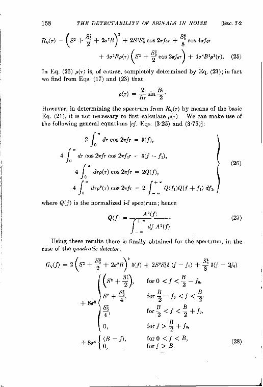
158 THE DETECTABILITY Y OF SIGNA1.S IN NOISE [SEC.72
( )I&(,) = W + : + 2U’B 2 + 2s’.!~ cm 27r.foT + : Cos 47rjo7
( )+ 4u’Ilp(T) S’ + : cm 27rjoT + 4u4B’p’(T). (25)
In Eq. (25) P(T) is, of course, completely determined by Eq. (23); in factwe find from Eqs. (17) and (23) that
2 B,P(T) = ~~ sin ~.
However, in determining the spectrum from h?~(,) by means of the basicEq. (21), it is not necessary to first calculate P(7). We can make use ofthe following general equations [cj. Eqs. (3.25) and (3.75)]:
/
*2 dr COS%fr
o
/
.4 dr COS2~fT COS27rf,7
0
/
.4 d,p(,) COS%rf,
o
/
*4 d,pz(,) Cos 27rf,
o
= a(f),
= b(f – f,),
/ (26)
= 2Q(f),
\
+-=2 Q(fJQ(f + jJ dfl, I—.
where Q(j) is the normalized i-f spectrum; hence
Q(f) = + j’(j) .
/_ ~ df A2(f)
Using these results there is finally obtained forcase of the quadratic detectoT,
(Gc(j) = 2 LS2+ : + 2u’B)
2
a(j)
1
+ ~a, (B – j),o,
+ 2s’s36 (j –
(27)
the spectrum, in the
f,) + : a(f – 2jo)
for O<j<~–fO,
for~–jo<j<~,
for~<j<~+fO,
for f>~+fO,
for O< f<B,for j > B.
(28)
—
SEC. 7.2] PROBABILITY DIS1’RIBUTIONS AND SPECTRA 159
This result is shown in Fig. 7.6 and can be understood in simple terms.The spectrum consists of four parts:
OD-Ccomponent
PO ~~Signal peaks
\ . Continuous spectrum
GQ (f) spectrum due tocross modulation
of signal and noise
~ & 24 ;-~ ; ;+& B
f—F1~. 76.-3 pectrum of a modulatedc-wsignalplusnoiseafterasquare-lawseconddetector.
1.
2.
3.
4.
Direct-current term, shown by the peak at j = O. Both the signaland the noise contribute to this term. The signal part is simplythe square of the mean signal power; the noise part is 4aiB2 or4W2, which, according to Eq. (14 b), is just (~) z for noise alone;finally there is a cross term, which represents the average value ofthe beats between the signal and the noise.Signal pealc.s. They are self-evident; that with the single modu-lating frequency fo we get two peaks (at ~0 and 2j0) is, of course, aconsequence of the fact that we have a quadratic detector.Continuous spectrum due 10 cross modulation of signal and noise.The beats between the three discrete frequencies j,, j. i .fo, whichare contained in the signal before the second detector, with all thenoise frequencies in the band B will lead clearly to a continuousspectrum, which consists of three blocks between the frequencies(O, B/2), [0, (B/2) – ~iI], [0, (B/2) + j,]. It is also easily seenthat the height of the first block will be proportional to flzd,whereas for the other two it will be proportional to ~S&r2. Addingthe three blocks leads, then, to the complete continuous spectrumas shown in Fig. 7.6.continuous spectrum of noise alone. This spectrum is caused bythe beats between any two noise frequencies. Since the number ofpairs of noise components with a certain frequency difference willdecrease as the difference increases, it is clear that the spectrum willdecrease with increasing j, and for a rectangular i-f pass bandit is easy to see that the triangle will be as shown in Fig. 7.6 (cf.also Sec. 3“8).
160 THE DETECTABILITY OF SIGNALS IN NOISE [Sm. 72
For the linear detector there are some important differences in thespectrum. To understand these it is best to consider separately thecases of a small and a large signal.
Using the formula of 13q. (20a), substituting Eq. (24) and averagingover t 1, We obtain for small n“gnal-to-noise ratios
ItL(T) = ~&K )
s’ + : + 4U’B 2 + 2s%S; Cos 2mjoT
1+ ~ cos 47rfOT+ 4U4BZP2 (29a)
The term that is proportional to p may be neglected, since the continuousspectrum due to the cross modulation of signal and noise will no~v benegligible compared with the pure noise spectrum. Equation (29a) leads
to the spectrum
Ks’ + : + 4U’B)2
G.(j) = ~E 8(f) + 2s’s3a(f – j,)
1+: J(j–2fo) + 8.’(B – j) , 0< j < B. (29b)
This result is similar to the case of the quadratic detector; it should benoted especially that, although the detector is linear, we still get thedouble frequency 2j, in the discrete spectrum. The continuous spectrumis still triangular in this approximation, but the height of the triangle(which for the quadratic detector was 8U4B) is now (7r/4)u’ and, thereforeindependent of the bandwidth.
Starting from I?q. (w~”’and now neglecting the term proportional to
P2, we obtain for large signal-~o-noise ratios
R,(r) = S2 + ~ cos 27rj0T + U2BP, (30a)
12U2, for O<~<~,G,(f) = (30b)SW(f) + $ Mf – fo) + o
for f > ~.
Now one gets only a signal peak at j~ and the continuous spectrum con-sists of one block between f = O and j = B/2.
Genmal Discussion of theSpectrum. -In the general case the resultswill be similar. One always starts from 13q. (17) or (18). The signalfunction az + /32 must be developed in a Fourier series, and we mustaverage over the time tl. Thependent of p will give terms ofto the d-c part and the signal
parts in Ilqs. (17) and (18) that are inde-the form C, cos 2~f,.r, and these will leadpeaks in the spectrum, Of course, for a 1
I
t SEC. 73] DETECTABILITY CRITERIA 161
pulsed signal with repetition period e, the peaks will be spaced l/eapart. Thepartsin Eqs. (17) and (18) that areproportional to plead to
/ the continuous cross-modulation spectra, whereas those which areproportional to P2 lead to the pure noise spectra. The shapes of thesespectra will, in general, not besosimpleas in Fig. 7“6; the noise spectrum,for instance, will betriangular only forarectangular i-f pass band. It
4remains true, however, that for a quadratic detector the initial value ofthe noise spectrum is proportional to B and the area is proportional to B2,
~ whereas for a linear detector the initial value is independent of B and thearea is proportional to 1?.
7.3. Detectability Criteria. The De$ection Criterion.-Let us returnnow to the problem of determining the signal threshold. Most of thetheoretical analysis available at present is based on a more or less plausi-
) ble, but in principle arbitrary, choice of a detectability criterion. Forinstance, let us consider again the simple example of measuring a smallcurrent with a galvanometers (see Fig. 7.1) and suppose that only onemeasurement can be made of the deflection r. The average value of thedeflection will be a little different when the current (or signal) is present,and it is plausible to assume that in one measurement the current is justdetectable if the shift of the average value is of the same order of magni-tude as the standard deviation of r (whether with or without current
+ makes little difference, since the currents to be detected are small). Orin a formula
(31a)
where the subscripts S and N refer to signal and noise and where k is aconstant that is of the order of magnitude of 1 if only one observation ismade. The criterion [Eq. (3 la)] will be called the “deflection criterion.”It can also be used for the visual detection of one radar signal pulse on anA-scope in the presence of noise; in this way the dependence of the signal
\ threshold on parameters like pulse length, i-f and video bandwidths canbe satisfactorily explained. A detailed discussion will be found in Chap.8 (especially Sees. 8.6 and 8“7); here only the following more general+observations are made.
1. The detectability criterion [Eq. (31a)] might be generalized to
3s+N – 3N = ~[7?/– (TJ2P’ ‘
(31b)
where j(r) is some function of the deflection still at our disposal.By choosing the proper function j(r) we can try to make the signalthreshold as small as possible. Or by choosing a function j(r)
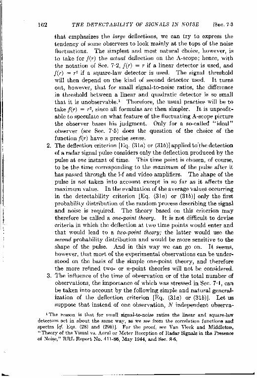
162 THE DETECTABILITY OF SIGNALS IN NOISE [SEC.73
that emphasizes the large deflections, we can try to express thetendency of some observers to look mainly at the tops of the noisefluctuations. The simplest and most natural choice, however, is
to take for j(r) the actual deflection on the A-scope; hence, withthe notation of Sec. 7“2, j(r) = r if a linear detector is used, andf(r) = r’ if a square-law detector is used. The signal thresholdwill then depend on the kind of second detector used. It turnsout, however, that for small signal-t o-noise rat ios, the differencein threshold between a linear and quadratic detector is so smallthat it is unobservable. 1 Therefore, the usual practice will be totake j(r) = rz, since all formulas are then simpler. It is unprofit-able to speculate on what feature of the fluctuating A-scope picturethe observer bases his judgment. Only for a so-called “ideal”observer (see Sec. 7“5) does the question of the choice of thefunction f(r) have a precise sense.
2. The deflection criterion [Eq. (31a) or (31b)] applied tothe detectionof a radar signal pulse considers only the deflection produced by thepulse at one instant of time. This time point is chosen, of course,to be the time corresponding to the maximum of the pulse after ithas passed through the i-f and video amplifiers. The shape of thepulse is not taken into account except in so far as it affects themaximum value. In the evaluation of the average values occurringin the detectability criterion [Eq. (31a) or (31 b)] only the firstprobability distribution of the random process describing the signaland noise is required. The theory based on this criterion maytherefore be called a one-point theory. It is not difficult to devisecriteria in which the deflection at two time points would enter andthat would lead to a two-point theory; the latter would use thesecond probability distribution and would be more sensitive to theshape of the pulse. And in this way we can go on. It seems,however, that most of the experimental observations can be under-stood on the basis of the simple one-point theory, and thereforethe more refined two- or n-point theories will not be considered.
3. The influence of the time of observation or of the total number ofobservations, the importance of which was stressed in Sec. 7.1, canbe taken into account by the following simple and natural general-ization of the deflection criterion [Eq. (31a) or (31b)]. Let ussuppose that instead of one observation, ii independent observa-
1The reason is that for small signal-to-noise ratios the linear and square-lawdetectors act in about the same way, as we see from the correlation functions andspectra [cj. Eqs. (28) and (29b)]. For the proof, see Van Vleck and Middleton,“Theory of the Visual vs. Aural or Meter Reception of Radar Slgnale in the Presenceof Noise,” RRL Report No. 411-86, May 1944,and Sec. 8.6.
L
1
SEC. 7.3] DETECTABILITY CRITERIA
tionsl are made with the signal and N observationssignal.
163
without the
It seems natural, then, to use in the detectability criterion, not thedeflection ~ or ~(T), but the average value
N~=;
sj(r,), (32)
icl
where T1,rz, . . . , r.v are theN observations of the deflection. We shalltherefore assume that the signal is just detectable if the shift of theaverage value of y due to the signal is of the same order of magnitude asthestandard deviation of ywhenonly noise is present. 0rinaformula2
fis+N – GN
[ii$ – (jN)’]}’
= k. (33)
Now it follows easily from Eq. (32) that, if the Ti’S are independent,
g=f, ~ = ~ [NT + N(N – 1)(]) 21.
Hence,~S~N– ~N = fS+N – 3N,
d – (Ii.)’ = *[R – (.G)’1.)
(34)
The shift of the average value is, therefore, the same as before, whereasthe fluctuation decreases and goes to zero for N - m. The signal willtherefore be the more easily detectable the larger N is. Substituting Eq.(34) into Eq. (33) we obtain
f.,. – ~.v k
[E – (3N)’1)* = W@(35)
This equation is the generalization of the deflection criterion [Eq. (31 b)]for the case of N observations. (For further discussion and for the com-parison with experiment, see Sees. 8.8 and 8.9.)
The Power Criterion. -In connection with other methods of observinga radar signal it is sometimes simpler to use a different type of detect-abllit y criterion. Let us consider, for instance, the so-called “aural
I In the example of the measurementof a small current with a galvanometers,“independent” means that the time intervals between the observationsmust belargecomparedwith the correlationtime. For radarsignalpulsesthis independenceis always assured, since the repetition period is always large compared with thecorrelationtime of the noise.
sThe subscript h’ (for “noise”) should not be confused with N the number ofobservations.
164 THE DETECTABILITY OF SIGNALS IN NOISE [SEC. 73
method” of detection. In Sec. 7.2 it was mentioned that the spectrumof the output of the video amplifier consists of a continuous part and a
series of discrete “signal” peaks. These discrete frequencies represent
the power spectrum of the periodic series of signal pulses and are therefore
spaced l/eo apart if eO is the pulse repetition period. By using a filter
with a bandwidth that is small compared with l/eo, one of the discrete
frequencies (for instance, the fundamental frequency l/eO) can be iso-
lated, and we can try to listen to the output of the filter with an earphone.
This is the aural method of detection. It is clear that the power in the
signal peak has to compete with the power in the section of the continuous
noise spectrum that is cut out by the filter. Therefore it is natural to
assume that the signal peak is detectable if its power P.s is of the sameorder of magnitude as the power PN in the segment of the continuous noiseband. Or in a formula
P,F.
= k’, (36)
where k’ is of the order of unity. This criterion will be called the powercriterion.
On the basis of the power criterion [Eq. (36)], Van Vleck and Middle-tonl have analyzed the aural and also the meter method of detection. Ashort account of their work will be given in Chap. 9. The main point tobe emphasized here is that the analysis of these methods of detectiongives essentially the same result for the signal threshold. By the word“essentially” is meant that in the different methods, the dependence ofthe signal threshold on the parameters of the signal, such as pulse length,PRF’, and total number of ~ulses, will be the same. They can still differ.,numerically, which may sometimes be significant, but the differencecannot be made so large as one pleases by changing some parameter of thesignal. This fact will be discussed in detail in Chap. 9; the main dis-tinction between the different methods is fundamentally a difference ofthe ratio of integration time to observation time. or in other words, welet the detecting system do more or less integration before the humanobservation begins.
Of course, ~he different methods of detection are equivalent only ifeach method is pushed to the limit of its capacity. In practice this willalmost never be done, and therefore the different methods will usuallygive different signal thresholds. Furthermore, in actual practice it willmake a lot of difference at which point the human observation begins andwhether it is visual or aural.
‘ Lot. cit. In the meter method ~f detection the output of the filter that selects thesignal peak is rectified and recorded by some kind of meter. The change of theaverage value of the meter deflection when the signal is present provides the methodfor detecting the signal.
?
1 SEC. 7.4] BEST METHOD FOR DETECTING A RADAR SIGNAL 165
The power criterion [Eq. (36)] is also used in the analysis of the noiselimitation in communication systems. The following distinction can bemade between a detection and a communication system. In a detection
1,system only the presence or absence of a signal has to be determined;therefore a c-w signal or a series of constant pulses can be used. Ina communication system more than just a yes-or-no answer is required,and some sort of modulation must therefore be applied to the c-w signal
& or to the series of pulses. The frequencies and amplitudes of thismodulation of the signal are the quantities to be detected. These willappear as a discrete line spectrum superposed on the spectrum of thenoise and the unmodulated signal. For a sinusoidal modulation therewill be only one such peak, and the detectability of this peak will dependon the ratio of its power to the continuous noise power with which it has
● to compete. The power criterion [Eq. (36)] is again applicable, and thetheory is therefore similar to the theory for the aural method of detectinga radar signal. There is one important difference, however. The mainresult of the theory now will not be the determination of the minimumdetectable signal power, but the dependence of the minimum detectablemodulation ~ti on the ratio z of the unmodulated signal power to thenoise power. It is clear that ~mi.will be a monotonic decreasing functionof z, and it can be shown that for large z, c~ti = 1/z, whereas for small z,
+ cfi = l/z2. Explicit expressions for ,~,. as a function of z will be derivedin Chap. 10 for some pulse modulation schemes and in Chap. 13 for the
P well-known a-m and f-m communication systems.7.4. What Is the Best Method for Detecting a Radar Signal.-In the
previous section we mentioned that the visual and the aural methods ofdetection are essentially equivalent if each method is pushed to the limitof its capacity. The question arises whether or not with these methodsof detection an absolute limit has been reached. In this section we shallshow that this is not the case, so that there is still room for an essentialimprovement of the present detection methods.
t Suppose that one has a train of signal pulses which persists over atime 8. Let the repetition period again be 00, so that there are alto-gether N = O/eO pulses. Now it can be shown that under the best
i possible circumstances an average signal power ~~m can be detected, givenby the formula
P.. = —JR,0’. (37]
Here k is a numerical factor of order of magnitude 1, and U2is the averagenoise energy before the i-f amplifier. This noise energy is due to manycauses but can always be considered as thermal noise with an effective
r temperature T *, so that U2= lcT*, where k is the Boltzmann constant.
166 THE DETECTABILITY OF SIGNALS IN NOISE [SEC. 74
For the derivation of Eq. (37) we refer to Sec. 8“6 (visual observationmethod) and Sec. 9“6 (aural and meter detection methods). Here weonly want to point out that Eq. (37) follows from the fact that the detect-ability of the signal depends for small signal strengths on the square of the
signal amplitude. With the deflection criterion [Eq. (31b)], for instance,
the detectability of the signal depends on the shift of the average value
of some function j(r) of the deflection r, which is caused by the signal.
From the probability distribution of the deflection [Eq. (13)] it follows
immediately that for small signals the shift of f(r) will be proportional to
S’2 if S is the signal amplitude. As a consequence one obtains from the
deflection criterion for the signal threshold an equation of the form
s, const.~.x, (38)
where the constant is of the order of unity and depends slightly on thetype of second detector and on the shapes of the pulse and i-f pass band;“W is the noise power after the i-f amplifier. Since ~~ti m S2./130,w c BU2, N = O/E), and since for best performance B, must be of orderunit y, 1 Eq. (37) follows immediately from Eq. (38).
From Eq, (37) follows that the minimum detectable energy of thewhole train of signal pulses is given by
(39)
Clearly Eti is usually much larger than .2 = k T*, since N is usually alarge number. It seems unlikely that this is the best one can do. Thedetection system may be considered as an energy-measuring device,which has itself an uncertain y in energy of the order k T*. The detectionof the whole train of signal pulses can now be considered as one observa-tion of the energy E, and one must expect that the detection can be donewith almost certainty as soon as E is a few times kT*. This gives a limit
for E that is much lower than Eq. (3) and in the authors’ opinion theabsolute limit which one may ever hope to reach.
The reason why with the present detection systems this absolutelimit has not been reached can be traced to the fact that the presentmethods do not measure the total energy of the noise and of the series ofpulses. To the authors’ knowledge only one system of detection has sofar been proposed that really measures the received energy. Emslie2has shown how this can be done in principle by letting the signal beatwith a continuous wave, which is introduced into the receiver at the same
.
1 Cf. Sec. 8.6.~ A. G. Emslie, “Coherent Integration, ” RL Report No. 103-5,May 16, 1944.
SEC. 7.5] THEORY OF THE IDEAL OBSERVER 167
time as the signal pulses and which has always the same phase relationwith the successive signal pulses.1 If the amplitude of the coherentcontinuous wave is large compared with the rms noise amplitude, then theprobability distribution of the deflection r will be Gaussian [13q. (13b)]with a variance 2W and with an average value
~ = (~z + (72 + 2SC Cos @)}$, (40)*
where C is the amplitude of the coherent continuous wave and @ theconstant phase angle between the continuous wave and the signal. Ofcourse, C >> S, and therefore it is clear that the shift of the average valuewhich is caused by the signal is porportional to the signal amplitude. In
fact, from Eq. (40) follows
t FS+N— F,v= s Cos@ (41)
In contrast to Eq. (38) we now obtain from the deflection criterion for thesignal threshold the equation
s CosC#l const.~m = ~. (42)
Clearly, if the phase angle @ can be kept constant and equal to zero, Eq.
4(6) leads to a minimum detectable energy of the pulse train that is of theorder kT *.
7.6. Theory of the Ideal Observer.—The theoretical analysis based onthe detectability criteria discussed in Sec. 7.3 leads to a formula for thesignal threshold that contains a numerical factor k of order of magnitudeunity which has to be found from experiment. The reason for thisindeterminacy is, of course, that the minimum detectable signal is notdefined strictly on the basis of a “ betting curve. ” It seems desirable
therefore to try to formulate a more fundamental theory, which will
remove the ambiguity of the choice of detectability criterion and which
will explain the betting curve and in this way determine the value of the,.
numerical constant k.Referring again to our galvanometers example (Sec. 7.1), suppose that
we know the probability distribution of the deflection r both when the
current is present and when there is noise alone. Suppose, furthermore,
that we do not know whether there is a current present or not and that
we have to decide this question on the basis of N observations. The
question then arises how to make use of these observations in the best
possible way, so that the conclusion we draw from these observations,
namely, whether the current is present or not, will have the best chance
I For further details about the coherent continuous wave, which forms an essmtid+ feature of the so-called MTI system, cj. Chap. 12,
~——--- . . . . . . ..

168 THE DETECTABILITY OF SIGNALS IN NOISE [SEC. 75
to be right. We shall say that the ideal observer always makes use of theobservations in this way, and we shall speak of the ideal observer criterion.
Of course, even the ideal observer can make only a bet, but it is the bestpossible bet that can be made. The betting curve for the ideal observerwill be completely determined by the probability distributions for thedeflection r, so that the numerical value of the constant k can be deter-
mined. To illustrate this we shall now consider a few examples. 1
. The “Off-on” Experiment. +uppose that in a long series of trials asignal of given strength is presented to the observer on the average duringhalf of the time. The observer does not know for any given trial whetherthe signal is present or not, and he has to decide this on the basis of Nobservations, which he is allowed to make during each trial. We shallassume that the time intervals between the observations are long enoughto make the N observations of the deflection r,, rt, . . . , r~ independentof each other. The problem is to find the criterion that in the long runwill lead to the smallest number of errors.
Let P(o,r) and F’(s,r) be the probabilityy distributions for a deflectionr without and with the signal. The functions P(o,r) and P(s,r-) aresupposed to be known. The set of N observations r,, r~, . . . , r~ duringone trial may be represented by one point in a N-dimensional ‘‘ observa-tion space. ” Since the observations are independent, the probability offinding a definite set rl, T2, . . . , r,~ is given by
P(o,r1)P(o,r2) “ “ “ F’(o,r~) (43a)or
P(s,rl)P(s,r2) “ . - P(s,r~), (43b)
depending on whether the signal is off or on. A detectability criterion isa division of the N-dimensional observation space in two regions, whichmay be called the off-region and the on-region. If the point representingthe N observations in one trial falls in the off-region, the observer willdecide that no signal is present; whereas if the point falls in the on-region,he will make the opposite decision. Clearly the probability for obtainingthe right answer is given by
‘l(S)‘W “ “ “b “““‘rNp(sJT1)““~‘(srN)(on)
‘/“““Jar,--“‘rNp(OT1)““~‘(orN)]’44)(OK)
t
1It should be pointed out that the ideal observer theory is practically identicalwith the Ncyman-Pearson theory of the best criterion for testing a statistical hypoth-esis, Cj., for instance, J, h’eyman, “ Basic Ideas and Theory of Testing StatisticalHypotheses, ” J. Roy. Stat. ,$’oc.,106, 292 (1942).
SEC.7.5] THEORY OF THE IDEAL OBSERVER 169
where the symbols-( on) and (off) under the integral signs mean that theintegrations are to be taken over the on- and off- region. The factor ~ is
the a priori probability, which represents the fact that the observer knowsthat in half of the total number of trials the signal is present. The idealobserver will choose the off- and on-regions in such a way that the prob-ability WI is a maximum. Writing Eq. (44) in the form:
One sees that since the common factor ~ P(o,r~) is positive lVl will be ak
maximum if in the on–region ~ P(s,rJ/P(o,rJ > 1 and in the off-region
~ P(S,Ti)/P(O,~i) <1. Or in other words, for the ideal observer criterion
tie surface in the observation space, which divides the off-region fromthe on-region, is given by the equation
N
11P(s,r,) = ~
P(O,’r,) “(46)
i=l
Introducing the functions,
Q(sy)=/~Jll ‘(s’’’)’”’’[’- l’”g~%wizl‘(s,)=/‘~/F1 1‘(OI’’)’’’’[’-ilO%%l’’47)
o k=l i=l
4where IS(Z)is again the Dirac ~-function, the probabilityy of success for theideal observer can be written in the form
um
Jo
w,, -=(s) = ; o dy Q(s,v) + 1dy R(s,y) . (48)—.
We shall postpone the further evaluations of this expression until we haveconsidered some other examples. Clearly
!+Q
/
+.
dy Q(s,y) = dy R(s,y) = 1,—. —.
1
(49)
Q(o,Y) = R(o,?J),
I
170 THE DETECTABILITY OF SIGNALS IN NOISE [SEC. 75
For s = O, W,, ~.(s) is therefore equal to ~ as it should be. For s ~ m,Q(s,y) will be different from zero only for large positive y, where as R(s,y)will only have appreciable values for large negative values of y. Fors ~ cc the integrals in Eq. (6) can therefore be extended to the completerange from — m to + m ; and because of Eq. (49) WI ~.,(s) will thenbecome 1.
The ‘‘ Two-positions” Experiment .—Suppose that in a long series oftrials a signal of given strength is presented to the observer on either oftwo positions with equal a priori probabilityy. 1 For any given trial theobserver does not know in which position the signal is, and he has todecide this on the basis of the observations that he is allowed to makeduring each trial. Call the two positions a and b, and suppose that theobserver makes N observations of the deflection at each position. Adetectability criterion is a division of the 2N-dimensional observationspace in an (a)- and (b)-region. If the point representing the 2N observa-tions r-al, Tmz,. . . , raN, ~bl, rb2, . . . , ~bN falls in the (a)-region, theobserver will decide that the signal was in the position a; whereas if thepoint falls in the @)-region, he will decide in favor of position b. Since:dl observations are supposed to be independent, it can easily be seen thatihe probability for obtaining the right answer is given by
. N
~z(s’) =;/ ~ ~ ~ /r-l~(o~Jp(oJ~Jo K=l
Np(S,Tai)
/rl P(o,Tai)for region (a)
<
;X1x drak drkk (50)
\fi ;(s,~bi)
(o,rb,)for region (b)
i=l
The ideal observer will choose the (a)- and (b)-regions in such a way thatW, is a maximum. From Eq. (8) it follows that this can be done bytaking
A’ N
11P(s,rai) =
nP(s,r,i)
P(O,T=;) P(o,rbJi=l i-l
as the equation of the surface, which divides the (a)- from the (b)-region,and the probability of success for the ideal observer can then be written
I This means of coursethat in the average the signal appears an equal number of itimes on either of the two positiom,
SEC. 75] THEORY OF THE IDEAL OBSERVER 171)
where the functions Q and R are defined by Eq. (47). For s = O,R(o,y) = Q(o,Y); putting
/fl= “ dyl R(s,Y1),
oEq. (51) becomes
/
1w,, -(0) = d~~=~
ot
as it should. For s -+ m the upper limit y in Eq. (9) can be replaced byI
+ m, and because of Eq. (49) it is clear that for s ~ cc, Wa,~.,(s)approaches unity.
The “m-positions” Experiment .—If the signal can appear on any oneof m positions with equal a priori probability, an easy generalization ofthe reasoning for the two-positions experiment leads to the equation
for the probability of success for the ideal observer. It can be easily
seen that for s + m, W~, m. approaches unity; whereas for s + o,w m,mar~ l/m, which is the a priori probability for finding the signal onany one of the m positions.
Calculation of the Betting Curve.—For the further evaluation of the+ functions W~, ~.=(s), which represent the betting curves for the ideal
observer in the different experiments, the functions R(s,y) and Q(s,y)) must first be calculated. According to Eq. (13) one has’
,2 +.y——
()7-8
P(.s,T) = + e 2W 10 ~ ,
.—P(0,7-) = ~ e 2’;. I (53)
With these functions it does not seem feasible to calculate 0 and R fromEq. (47) exactly. However, since we are mainly interested in the part of
i- the betting curve for which the signal is small compared with noise, wecan rmt
1 ()10” $ .l+g. .er,sz,~w%
ThereforeN N
x
P(S,T;) ~ _ NS2 + S2y=10gP(0,7,) 2W 4W2–2
~:. (54)i=l i=l
1JSn= az + ~~. The time chosen must correspond, of course, to the maximum ofthe deformed pulse. The shape of the pulse is not taken into account, l?quation(52) refers to the one-point ideal observer theory (sec. 7.3).
I
172 THE DETECTABILITY OF SIGNALS IN NOISE [SEC.75
Calling
~=zw+xNf32 y,
Eq. (47) can be written
Q(@q=@/ ~‘/fip(sr)d,k~fi(q)dq=q: Jfip(.),k)dTk’(Q
o Ic=l iz=l
= Q(o,q) d,.
In this approximation the ideal observer bases his judgment therefore onthe distribution functions of the mean-square values of the N deflectionsr,, ?“2, .
integrals in
from which
TN with and without the signal. Using Eqs. (53) the
(55) can be calculated exactly, and one obtains
N-“-($)(”-’’’2’4%(5,,Q(w) = ~ e
(-)Nq ‘-’ N -$R(q) =(N! l)! 2W me , I
follows
/q= “ d, Q(s,q) = S2 + 2w,
o
\ 1
(57)
(@’=:o- dq (q – q) ’Q(s,q) = ~ (S2 + W).
If N is sufficiently large, Q(s,q) can be replaced by a Gaussian distributionwith the mean value and variance given by Eq. (57), and the integralsinvolved in the expressions (48), (51), and (52) for the betting curves inthe different experiments can then be expressedfunction
/Erf (z) = ~ z dt e-”.
du o
The final results are (z = S’/2W):1. Off-on experiment:
“-(z)‘V+E%W2. Two-positions experiment:
[ ( )]VTW,,=(z) = ~ , 1 + Erf —‘L ,22, ”
in terms of the error
(58a)
(58b)
SEC. 7.6] MATHEMATICAL APPENDIX 173
3. m-positions experiment:
These expressions may be compared with the experimental bettingcurves. In these curves the quantity plotted against the signal strengthis usually not W~, _ but
Pm(z) =A (mw”)m’ - ‘)”
(59)
Clearly Pm(z) will be zero for z = O and approach unity for z + m.Defining the minimum detectable signal as the signal strength for the90 per cent point on the betting curve Pm(z), it is clear from Eqs. (58) that
(-)S, cm .
“0 = 2W ,0 = @v(60)
The signal threshold is therefore inversely proportional to the square rootof the number of observations. The constant cmincreases slightly withthe number of positions. Since each point on the betting curve decreasesin the same way with increasing N, it is clear that the width of the bettingcurve which can be measured by the ratio of the z values correspondingto the 90 and the 10 per cent point will be independent of the number ofobservations. The width depends on the number of positions; it decreasesif m increases, or in other words the betting curve becomes steeper if thenumber of positions increases. For a more detailed comparison with theexperimental betting curves, compare Sec. 8“9. It should be emphasizedthat Eqs. (58) and their consequences hold only if the two approximations(a, z <<1, even at the 90 per cent point of the betting curve, and b, N
sufficiently large, so that the Gaussian distribution can be used) are valid.
Especially the WN-law expressed by Eq. (60) depends essentially on theGaussian approximation. For the tw~positions experiment we havemade a detailed investigation of the errors cauyxl by the two approxi-mations. For N greater than 20 we found that the error in the signalthreshold (defined by the 90 per cent point on the betting curve) isprobably less than 10 per cent, so that under usual circumstances theerror will be inappreciable.
7.6. Mathematical Appendix. -We shall collect here a number ofmathematical results, which are needed in different places throughoutthe book.
The integrals occurring in Sec. 7“2 can all be performed by means ofthe general formula
/
2W
dtl cos nOe-° C- e = 2r( – I)”I”(a), (61)o
174 THE DETECTABILITY OF SIGNALS IN NOISE [SEC. 76
\
.
d t~–ll.(at)e–@”o
_ ‘(+(%)e2,4p*F(—2p~r(V + 1) )
~+1, u+l; –4$. (62)
Here I.(z) is the Bessel function of purely imaginary argument, andF(a, b; z) is the conlluent hypergeometric function, 1 which is defined by
F(a, b;z)=l+~z+a(a + 1) Z2 a(a + l)(a + 2) Zs
b(b+l)~+ b(b+l)(b+2) ~+””””(63)
The asymptotic series for F(a, b; Z) for large negatioe values of z is
F(a, b; z) = ~(~(~)a) (-2)-’[1 - ‘(U -:+ 1,
+a(a+l)(a–b+l)(a–b +2) +-..22
1(61)
IOften needed are the relations
e–zF(a, b; z) = F(b – a, b; –z), (65)
~F(a, b;z) =~F(a+ l,b+ l;z), (66)
I and the recurrence relations
ZFI,l = bFl, O — bFO,O,
aFl,l = (a — b)FO,l + bFO,O,
abFl, O = b(a + z)FO,O — z(b — a) FO,l,
t
.1
(67)aFl,O = (z + 2a — b)FO,O+ (b — a) F–1,0,
(b – a)zF,,l = b(.z + b – l)FO,, + b(l – b)FO,-1,
where the symbol F~,t is an abbreviation defined by
F~,l = F(a + k, b + l;z).
If a is a negative integer, F(a, b; z) reduces to a polynomial in z. If both aand b are positive integers, F(~, b; z) can be expressed in exponentialfunctions and polynomials in z. If a is a half integer and b is an integer,I’(a, b; z) can be expressed in Bessel functions I.(z) and exponentialfunctions of z. Since in the literature the results are often expressed inthis way, we shall give here a list of some of these identities:
1Tbe usualnotationk ,F, (a, b; z). For the integral (62) see C,.N. Watson, Theoryof Bessel Functions, Cambridge University Press, 1944,p. 394.
,—-—— —
175SEC.7.6] MATHEMATICAL APPENDIX
F(;,,;_z) =e-iIo@
I F(;!2; -.) =e-i[Io(;)+Il(;)]!
F(;,l; -z) =,-:[(, -.)@+I, @],
)F(;,2; -z) =e-i[Io(;) -l,(;)],
F(-;!l; -.) =e-i[(l+z,Io(;) +zI,(;)],
F(-;Jl;-2)=e-i[(; z,+2z+,)Io(;)+(; z2+;z),,(;)].
Tables of I’(a, b; z) for half-integer values of a and integer values of b canbe found in the Report of the British Association for the Advancement ofScience, 1927.
CHAPTER 8
PULSE TWINS IN INTERNAL NOISE
This chapter will present experimental and theoretical results dealingwith the determination of threshold power for a signal consisting of atrain of pulses. A superheterodyne receiver will be assumed in which thenoise is of the variety discussed in Chaps. 4 and 5; for threshold signals inexternal noise the reader is referred to Chaps. 11 and 12. Furthermore,in the interests of simplicity, only the results obtained in using a deflec-tion-modulated, or type A, oscilloscope will be considered here. Theintensity-modulated display is discussed in Chap. 9.
8.1. Standards for the Measurement of Signal Power.—The compari-son between signal and noise power is most conveniently drawn in the i-fanplifier after the restriction in i-f bandwidth is made. At this point, thesignal-to-noise power ratio is affected by both the i-f bandwidth and thenoise figure of the receiver; therefore, both these quantities must beaccurately known in order to calculate the input power ratio. Thiscalculation, however, is very simple. As pointed out in Sec. 5.1 thenoise power P.v in the receiver at any point is given by the relation
where G is the total power gain of the receiver up to the point in question,F, is the noise figure of the receiver expressed for a particular temperatureT, and k is Boltzmann’s constant. Although G is a function of thefrequency, a mid-frequency value will suffice here. To be absolutelycorrect, the bandwidth Aj must be measured in a particular way; it is,in fact, calculated from the relation
Af =\
“ A; dj,o
(2)
where A~ is the amplitude response of the receiver at a particular fre-qllency j, normalized to unity at midband. Equation (2) is introducedbecause the various noise components in the receiver are independent,hence add in power or in the squares of the amplitude functions. Thisassumes (nearly always validly) that the original noise is uniformly dis-tributed throughout the frequency range.
The measurement of bandwidth by means of Eq. (2) is tedious andusually difficult. It is much more convenient to measure the bandwidth
176
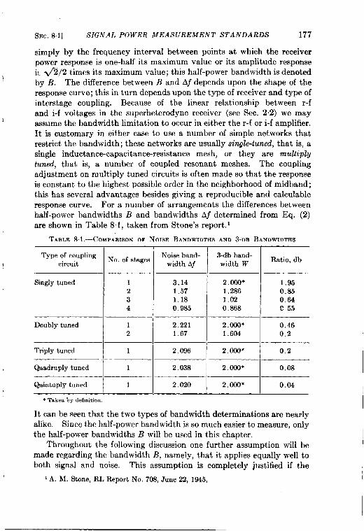
SEC. 81] SIGNAL POWER MEASUREMENT STANDARDS 177
simply by the frequency interval between points at which the receiverpower response is one-half its maximum value or its amplitude responsei: @/2 times its maximum value; this half-power bandwidth is denoted
Iby B. Thedifference between B and Af depends upon the shape of theresponse curve; this in turn depends upon the type of receiver and type ofinterstage coupling. Because of the linear relationship between r-fand i-f voitages in the superheterodyne receiver (see Sec. 2.2) we may
kassume the bandwidth limitation tooccur ineitherthe r-f or i-f amplifier.It is customary in either case touse a number of simple networks thatrestrict the bandwidth; these networks are usually single-tuned, that is, asingle inductance-capacitance-resistance mesh, or they are multiply
tuned, that is, a number of coupled resonant meshes. The couplingadjustment on multiply tuned circuits is often made so that the responseis constant to the highest possible order in the neighborhood of midband;this has several advantages besides giving a reproducible and calculableresponse curve. For a number of arrangements the differences betweenhalf-power bandwidths B and bandwidths Aj determined from Eq. (2)are shown in Table 8.1, taken from Stone’s report. 1
TABLE 8. 1.—COMPARISONOF NOISE 13ANDWIDTHSAND 3-DB BANDWIDTHS
Type of couplingt circuit
Singly tuned
Doubly tuned
Triply tuned
Quadruply tuned
Quintuply tuned
No. of stages
12
34
12
1
1
1
A’oise band-width Af
3.141.571,18
0.985
2.2211.67
2.096
2.038
2.020
3db band-width W
2.000*1.2861,020.868
2.000*1.604
2.000*
2.000*
2.000*
Ratio, db
1.950.8.50.64c 55
0.460.2
0.2
0.08
0.04
● Takenby definition.
It can be seen that the two types of bandwidth determinations are nearlyaliice. Since the half-power bandwidth is so much easier to measure, onlythe half-power bandwidths B will be used in this chapter.
Throughout the following discussion one further assumption will bemade regarding the bandwidth B, namely, that it applies equally well toboth signal and noise. This assumption is completely justified if the
IA. M. Stone,RL Report No, 708, June 22, 1945,
178 PULSE 1’RAINS IN INTERNAL NOISE [SEC.8.1
filter that 1s substantially responsible for B jollows the source of noise.This condition prevails in nearly all microwave receivers and in nearly allwell-designed receivers employing r-f amplification. For receivers inwhich this is not true, i.e., where the signal bandwidth is less than thenoise bandwidth, a reduction in noise, without an accompanying loss insignal response, can be brought about by the use of a final i-f filter. Forbest results this final filter should be made to restrict the noise bandwidthto the same value as the signal bandwidth.
If we now measure the signal-to-noise power at some point in thereceiver, we can calculate the input noise power by means of Eq. (1),noting first that the gain G is the ratio of signal power Ps in the receiverto the available input signal power Psti. Thus,
P.. = :: FJcT Aj; (3)
and as before, Aj can be replaced by the approximate half-powerbandwidth B.
The advantage in using Eq. (3) to calculate input signal power isconsiderable. The noise figure is measurable by methods that do notinvolve large amounts of attenuation; one of these methods, which isquite accurate, simply compares receiver noise with noise of known powergenerated by a diode (see Chap. 5). The measurement of receiver band-width is straightforward; the comparison of signal and noise power is alsousually straightforward, although certain precautions may be necessary.These precautions will be discussed when a complete experimental systemfor determining threshold signals is presented. The input power canthus be measured with good accuracy even though it is in the neighbor-hood of 10-’5 watt; this measurement would be difficult to make directlyby means of a signal generator and a long-range calibrated attenuator.Furthermore, the ratio P,s/P.v, together with the bandwidth, determinesthe signal perceptibility. Two receivers having the same bandwidth andsame shape response curves but different noise figures will have differentsignal threshold powers measured at their input terminals but, in thethreshold condition, will show the same values of P./P,v. Therefore, in
order that results may be universally applicable to all receivers, it is
desirable to express threshold signals in terms of noise power in the
receiver after the bandwidth restriction has occurred.
Up to this point a method has been outlined whereby the threshold
signal power may be computed from the receiver noise figure, bandwidth,
and a universal parameter, which is, in fact, the signal-to-noise power
ratio. It has been tacitly assumed that the signal is a train of pulses,
which is finite in length because of the limited time in which an observa-tion must be made or because of scanning limitations. Scanning has
I
,’
1’I
k
! SEC. 8.2] A SYSTEM FOR EXPERIMENTAL PURPOSES 179
been discussed in Chap. 2 and is of special importance when the intensity-modulated display is used. It has not yet been stated, however, howthe signal power can be measured or, more important, how it can becompared with receiver noise power. Furthermore, it has not yet beenpointed out how the signal power can be adjusted to correspond to thethreshold condition. These questions will be answered in the followingsections.
8.2. A (Synthetic) System for Experimental Purposes.-Since it willbe useful in the discussion of experimental results to be presented in thefollowing sections, a block diagram of a (synthetic) system is shown inFig. 8.1. This system has been used at one time or another by Stone’and Ashby, Meij er, Stone, Sydoriak, and Lawsonz to investigate thefactors involved in signal discernibility for an A-scope display. It con-tains a pulse generator and synchronization circuit so that a series ofpulses of controllable length, spacing, and number can be produced andthe pulse power can be accurately compared with receiver noise power.In addition, the receiver, though a conventional superheterodyne, isarranged so that the i-f bandwidth is variable (in steps) over a widerange. A description of the various components and their functionsfOllows.
The production of a series of r-f pulses having all the characteristicsof a mathematically perfect series of pulses is a goal yet to be achieved.Usually the emitted r-f energy has frequency modulation associated withit, and the pulse shape is not rectangular. Furthermore, it is usuallyfound that the r-f pulse power is affected by the duty ratio or fraction oftime during which the oscillator is energized, even though the voltages ofthe oscillator power supply are held constant. This effect is usually dueto internal heating of the oscillator elements; variations in average heatcause variations in electrode spacing with consequent change in oscillatorefficiency. The difficulty of frequency modulation mentioned above canbe solved by taking extreme care with the shape of the modulator pulseused to excite the oscillator; the difficulty regarding the duty ratio was
I
solved in the system shown in Fig. 8.1 by actually maintaining the dutyratio of the oscillator itself constant. This condition is achievedessentially by operating the signal generator at the highest PRF that isto be used and by operating the A-scope sweep at an equal or lowerrepetition frequency. Thus the information presented on the A-scoperecurs at any desired sweep repetition frequency, or SRF; at the sametime it is certain that the pulse power from the signal generator is inde-pendent of the SRF. The variation in duty ratio brought about by achange in pulse length, however, still exists in this system; hence for each
I 1A, M. Stone, RL Report No. 708, June 22, 1945.z Unpublished.
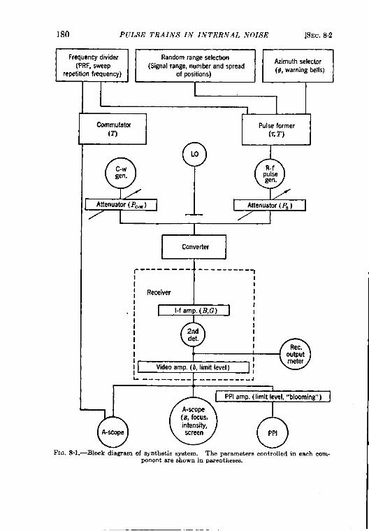
180 PULSE TRAINS IN lNTERNAL NOISE [SEC. 82
c1Frequency divider Random range selection
(PRF, sweep (Signal range, number and spread
Q
Azimuth selector
repetition frequency) of positions)(0, warning bells)
Commutator Pulse former
(n (t T)I I
I
%
c-wgen.
Attenuator (Pc.w ) rLO
AR-fpulsegen,
Attenuator(P )
I
I
(
I I
I Converter I
r
T
------- ------- --- 1I II I
I II
ii I1 II
1I
/ Video amp. (b, limit level ) II IL ________ _________J
I I
7!)A-scope
FIQ. 8.1 .—Block diagram
@~’PPI amp. ( limit level, “blooming”)
of synthetic system. The parameterscontrolled in each com-ponent are shownin parentheses.
SEC. 8.2] A SYSTEM FOR EXPERIMENTAL PURPOSES 181
pulse length a calibration between pulse power and receiver noise powermust be made. The independent control of the PRF and SRF has the
additional advantage that for some experiments it is useful to operate
the A-scope sweep more often than the signal pulse. In this way the
pulse may appear on every other, every fourth, etc., sweep. This formof operation is useful in determining one of the effects of mixing the videosignals of two or more systems. More will be said about this point later.There is therefore found in the top left-hand corner of Fig. 8.1 a syn-chronization unit that produces timing pulses determining both the PRFand SRF; these frequencies must be harmonically related to fulfill thefunctions described above. For convenience, the unit actually built fortests contains a 100-kc/sec crystal oscillator to provide initial stablepulses. A series of frequencydividing stages is then used to halve eachsuccessive frequency. The resulting unit has available output triggerpulses with repetition frequencies from about 1 cps up to 100 kc/see;all these frequencies are harmonically related and can be used inde-pendently to form the PRF and the SRF.
It has been noted that the signal is to consist of a finite train of pulses;the length of the train is determined by various factors, often chieflyconnected with scanning. As we shall see in the following sections, thelength of the pulse train, which will be called the signal presentationtime e, has a profound influence on signal threshold power; therefore, forexperimental purposes it must be controllable over a considerable rangeof values. To prevent the oscillator duty ratio from being affected by 0the following scheme was devised. The signal position, or range, on theA-scope is adjusted so that the signal normally does not appear; i.e., it isdisplaced outside the limits of the A-scope sweep. During the interval othe signal range is changed to bring it into the visible region on theA-scope. This procedure does not affect the duty ratio yet presents thesignal on the A-scope only during the desired interval. The apparentsignal range is, of course, fixed by the time delay between the timingpulse operating the A-scope sweep and the timing pulse operating thesignal generator. The device controlling the signal presentation time isshown in the upper right-hand corner of Fig. 8.1. In addition to con-trolling this parameter it also functions, if desired, to provide a warningsignal to the observer just prior to the signal presentation interval O.Since the function of this unit is to set the length of a train of pulses,accomplished in a scanning system by azimuth selection caused by therotating antenna beam width, the unit is labeled ‘f azimuth select or.”Indeed, for experiments with the PPI, to be discussed in Chap. 9, itbecomes an actual azimuth selector.
In addition to presenting the signal on the A-scope for an interval dit is desirable to present it at one of a number of defined range positions,
182 PULSE TRAINS IN INTERNAL NOISE [SEC. 8.2
This is a necessary part of the method by which threshold signals aredetermined. It has been pointed out in Chap. 7 that a theoretical“betting” curve exists; there is also an experimental betting curve withsimilar characteristics. To determine this experimental betting curve ithas been found most desirable to obtain correlation results between theobserver’s estimate of signal range and the actual signal range. So thatthe observer may be unaware of the actual signal position, it is necessaryfor the signal to occur at one of several designated range positions. Thechosen position must be independent of previous selections and must beselected by chance. More will be said about this procedure below, butit is pertinent to remark here that a synchronization unit is necessary toperform this random range selection and that control of the number andspacing of the positions is also required. This unit is shown in schematicnotation at the top of Fig. 8.1.
One other synchronization unit shown near the top left -hand cornerof Fig. 8.1 needs explanation. It has been found that, when very smallvalues of o are used, the total number of A-scope sweeps of noise, withwhich the signal competes, extends beyond the interval 0. To test thispoint a commutator was used that allows the A-scope to be triggered onlyduring the given interval o; under these conditions the signal presentationtime is still O, and only during this interval is anything shown on theA-scope. The significance of this commutator will be discussed insubsequent sections.
The receiver used in the system of Fig. 8.1 is a conventional microwavesuperheterodyne using a crystal converter. To the r-f input terminals ofthis converter are coupled the output of the local oscillator, the pulsedsignal generator, and a c-w r-f generator, which is used in the comparisonof pulsed signal and noise power by a method to be described below. TheCLWgenerator and pulsed signal generator have associated with themrespective attenuators in their output lines. These attenuators, of thewaveguide-beyond-cutoff variety, have extremely good relative accuracy,but the absolute values of the attenuation are not easily measurable:Both the signal and c-w generators are well shielded; this precaution isessential in making any measurements at levels approaching receivernoise. The part of the receiver following the converter is of the greatestimportance in the experimental work; it is here that there are many param-eters to adjust in the determination of optimum design. Some of thereceiver parameters that may be expected to have an effect on signalthreshold power are
1. I-f bandwidth.2. Shape of i-f bandwidth.3. Type of second detector,4. Video bandwidth.
SEC. 82] A SYS7’Iifi~ FOR EXPERIMENTAL PURPOSES 183
5. Shape of video bancflvidth.6. Video nonlinearity such us that caused by saturation or limiting.Presumably only the most important of these variables were, for
simplicity’s sake, investigated. It ~vas expected that the shapes of i-fand video band~ridths would not greatly affect threshold signals, providedtheshapes ~verethose characterized byproperly adjusted filters. There-fore, in the receiver shown in block-diagram form in Fig. 81, the i-f andvideo bandwidths weredeterrnined by filters of types that are commonlyused but are intermediate in complexity between the simple single-tunedcircuit and the highly complicated multiply tuned circuits. The i-fbandwidth is determined essentially by a single double-tuned stage,’whereas the video bandwidth is determined by a single shunt-peakedsection. In addition to fixing these parameters a type of second detectorwas chosen and not thereafter varied. It is of the linear, or envelope,
type, which in receivers is almost universally used to the exclusion ofother types. Occasionally a parabolic, orsquare-law, detector is found;however, there is now some evidence that the type of second detector hasonly a slight effect on the signal threshold power. This will be broughtout in Sec. 8.7. Therefore, in summary, the receiver consists of a con-verter, an i-f amplifier \vhose gain and bandwidth are controllable, a
linear second detector with an output meter to record the average videolevel, and a video amplifier ~vhose bandwidth and limit level are con-trollable. The output line of the video amplifier is connected directlyto the A-scope or, for intensity-modulated measurements, through anadditional limiting stage to the PPI. The additional limiting stage isdesirable so that the A-scope and PPI can be operated at different limitlevels.
The description of the (synthetic) system is now complete exceptthat the method by which the signal power is compared with noise powerhas not yet been explained. It might be thought that the signal powercould be measured relative to noise by the contribution each makes in theoutput of the second detector, account being taken of the signal dutyratio. This is not the usual case; where the duty ratio is small, thecontribution of a signal compared with that of the noise is unnoticeable.As the signal is increased in size to produce a measurable contribution,the signal pulses in the i-f amplifier become large enough to saturate theamplifier, thereby invalidating any measurement of the power. Toovercome this diflicult y the system shown in Fig. 8“1 was devised; thepulsed signal is first compared in power with a c-w generator, which, inturn, is compared with receiver noise. This latter comparison is easilymade because the duty ratio of the c-w generator is unity. The pro-
1A. hf. Stone and J. L. Lawson, “ Theory and Design of Double-tuned Circuits,”ElectronicInd., April 1946,p. 62.
184 PULSE TRAINS IN INTERNAL NOISE [SEC.82
cedure is to adjust the receiver gain so that the second-detector output Imeter reads some fiducial value due to receiver noise only. The c-wgenerator attenuator is next adjusted so that the output meter increasesits reading to @ times the fiducial reading. At this point the power inthe i-f amplifier, produced by the c-w generator, is just equal to the noisepower in the i-f amplifier. The factor’ W comes about because of thelinear detector; a doubling of input power results in a change in outputamplitude of <2. This procedure is valid only when there is a really I
linear second detector; this point can be checked experimentally bycalibration against the attenuator associated with the c-w generator. Tomake the determination valid, receiver noise is made negligible by reduc-ing the gain of the i-f amplifier.
The method by which the c-w generator power is made equal toreceiver noise power has just been outlined, but the way in which the c-w tpower is compared with the signal power has not yet been mentioned. ~This comparison can be made by the following procedure. With thereceiver gain reduced to the point that noise is negligible the signal isadjusted to an easily measurable amplitude on the A-scope. The c-wgenerator power (tu~ed to the mid-frequency of the signal) is thenincreased S1OW1y until a flutter or ‘‘ beating” effect in the signal isobserved. This phenomenon is due to the addition of signal and c-wvoltages in random phase from pulse to pulse. When the c-w and pulse bvoltages are in phase, the resulting video signals “ beat” up to themaximum value; when they are out of phase, the video signals beat downto their lowest value. As the c-w power is increased, the signal on theA-scope is observed to beat lower and lower until it just beats down to ‘‘the baseline. The c-w power that just produces this effect is easily repro-ducible, since the visual extension of the baseline can be estimated withgreat accuracy. A c-w power greater than this critical value causes the
signal to beat below the baseline. This statement may seem surprising
at first, but it must be remembered that the baseline does not represent
zero video voltage but actually represents the steady rectified voltageproduced by the c-w generator. Let us, therefore, examine the condi-tions under which the signal “ beats” just to the baseline; this is clearly a
iI Strictly speaking, this factor is not entirely correct because of the difference in
the probability distributions of the amplitudes of noise and c-w signal. The outputof the linear detector records the average rectified amplitude, which is proportional tothe square root of power only for voltages that have similar amplitude distributions.The @ factor would apply strictly only to the case where rms voltages are recorded;therefore a correction factor should be applied that comes in because of the differencebetween rms and average voltages. For noise, this factor has been evaluated; toequalize c-w and noise power the fiducial reading of the output meter should beincreased by a factor of 1.45with the addition of c-w power instead of by the stated“factor of 42.
$EC. 83] DETERMINATION OF THRESHOLD SETTING 185
condition in which the difference between signal and c-w voltage duringthe pulse is just equal to the c-w voltage represented by the A-scope base-line. This observation leads to the obvious conclusion that the signalpulse voltage is just twice the c-w voltage or that the signal power is justfour times the c-w power. This condition, incidentally, is independentof the detector linearity; it requires only that the detector response beindependent of i-f signal phase. The procedure, therefore, affords a
high-precision method by which the signal power can be compared withthe c-w generator power. In the use of the beating technique one impor-tant precaution must be observed, however. The i-f and video amplifiermust have adequate bandwidth, enough properly to delineate the signal;otherwise the transient effect at the beginning and end of the signal
arising from inevitable phase changes in the i-f voltage will cause a false
reading. This effect is unimportant as soon as the i-f bandwidth is larger
than about twice the reciprocal of the pulse length; the video bandwidth
should likewise be correspondingly large. Therefore, in the comparison
reading between signal and c-w voltages only the wide-band i-f amplifier
connection should be used.
8.3. The Determination of Threshold-signal Setting.-A system hasbeen described in which, once the attenuator setting is chosen for athreshold signal, the signal power can be measured in convenient units.This process is straightforward and requires no further refinements.However, the procedure by which the threshold signal is established is onein which considerable latitude exists; each investigator has usually seen
fit to use a new procedure that generally has yielded slightly different
results. Apparently the process first used was to ask a number of
observers to estimate the minimum detectable signal; the threshold signalwas then assumed to be the average of their answers. It was found thatthe individual estimates differed by large factors, indeed so large that itwas nearly impossible to obtain reliable averages. Furthermore, a givenobserver would usually change his estimate considerably from day to day,depending on such factors as A-scope trace intensity, focus conditions,and his own state of mind. His estimate of minimum detectable signalwauld also be greatly affected by such factors as his previous training andby the degree of certainty that was required of his answer. Becauseof this sort of difficulty a method was sought that did not depend on theobserver’s opinion. The type of answer required of the observer and theconsistency with which his determinations were found to be repeated at asubsequent date indicate that the procedure outlined here constitutessuch an objective method. Furthermore, different observers, whenproperly trained, all obtain virtually the same results. The method isessentially one in which the observers’ answers are correlated with somedesired parameter of the signal. Tn the case of the A-scope such a param-
186 PULSE TRAINS IN INTERNAL NOISE [SEC. 8.3 I
Ieter is the range position of the signal; in the case of the PPI azimuth Iposition could also be used. In the former case the signal is made toappear at one of several definite range positions, and the observer isasked to guess the correct position. His guesses are then correlated withtheactual known positions inorder to find out whether or not the signalis perceptible. This procedure minimizes the judgment required fromthe observer; he is not required to judge whether or not the signal isvisible but only which of several given positions is most likely to contain i
the signal. Since this type of correlations statistical in nature, a num-ber of observations must be made; in order that each guess be independentof preceding observations, the range position of the signal must be ran-domly selected. It is expected theoretically, and found experimentally,that the signal threshold power depends upon the number and spacing ofthese range positions. A large number of positions increases the thresholdpower slightly; a small number of positions complicates the analysis Ibecause of chance lucky guesses. For most of the experiments to bedescribed in the next two sections six positions have been used; where theeffect of number of positions is studied, however, this restriction obviouslydoes not apply.
It is found experimentally that there is a “twilight” region where thesignal can be detected only part of the time. The fraction of time inwhich the signal is seen can be obtained ~om the correlation betweenguessed position and actual position as outlined above; this fractionincreases continuously with increasing signal. The result is analogous to I
the “betting” curve of the theoretically ideal observer described inChap. 7 and indeed appears to differ from it in only two respects; viz.,the actual observer appears to require a slightly higher value of signalpower than the ideal observer, and the betting curve seems to have a
different width (where the width is defined by the relative signal powerchange from 10 to 90 per cent correlation). The width of the twilightrsgion is usually smaller than that of the ideal observer, although ifconditions of severe video limiting are experienced, the experimental 1twilight zone becomes very large. These two general observations arenot at all surprising. For example, the first amounts to saying that ahuman observer is not so efficient as the theoretically ideal observer. The ‘second observation is expected when due allowance is made for the effectsof contrast limitation in the human observer and for saturation effectsin the video system. These points will be considered in later sections.
A typical experimental betting curve is shown in Fig. 8.2 in which thecorrelation fraction, after the theoretical number of chance lucky guessesis subtracted, is plotted against relative signal power. The signal poweris expressed in decibels relative to the noise power in the receiver with a1.O-Mc/sec i-f bandwidth; and as can be seen, the conditions .in the ‘
L
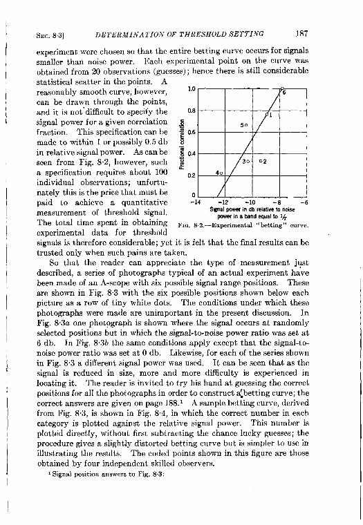
I
ISEC.8.3] DIITERMINA TION OF THRESHOLD SETTING 187
experiment were chosen so that the entire betting curve occurs for signalssmaller than noise power. Each experimental point on the curve wasobtained from 20 observations (guesses); hence there is still considerablestatistical scatter in the points. Areasonably smooth curve, however,can be drawn through the points,and it is not”diffimdt to specify thesignal power for a given correlationfraction. This specification can bemade to within 1 or possibly 0.5 dbin relative signal power. As can beseen from Fig. 8.2, however, sucha specification requires about 100individual observations; unfortu-nately this is the price that must bepaid to achieve a quantitativemeasurement of threshold signal.The total time spent in obtainingexperimental data for threshold
1.0
0.8
0.2
0-14 -12 -lo -8 -6
Sk@ powarindbrelativeto noisepowarina bandequalto %
FIG. S2.-Experimental “ betting” curve.
signals is therefore considerable; yet it is felt that the final results can betrusted only when such pains are taken.
So that the reader can appreciate the type of measurement jqstdescribed, a series of photographs typical of an actual experiment havebeen made of an A-scope with six possible signal range positions. Theseare shown in Fig. 8.3 with the six possible positions shown below eachpicture as a row of tiny white dots. The conditions under which thesephotographs were made are unimportant in the present discussion. InFig. 83a one photograph is shown where the signal occurs at randomlyselected positions but in which the signal-to-noise power ratio was set at6 db. In Fig. 8.3b the same conditions apply except that the signal-to-noise power ratio was set at O db. Likewise, for each of the series shownin Fig. 8.3 a different signal power was used. It can be seen that as thesignal is reduced in size, more and more difficulty is experienced inlocating it. The reader is invited to try his hand at guessing the correctpositions for all the photographs in order to construct ajbetting curve; thecorrect answers are given on page 188.1 A sample betting curve, derivedfrom Fig. 8.3, is shown in Fig. 8.4, in which the correct number in eachcategory is plotted against the relative signal power. This number isplotted directly, without first subtracting the chance lucky guesses; theprocedure gives a slightly distorted betting curve but is simpler to use inillustrating the results. The coded points shown in this figure are thoseobtained by four independent skilled observers.
1Signalpositionanswersto Fig. 8.3:
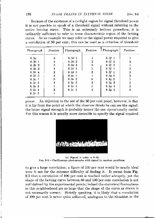
188 PULSE TEAINS IN INTERNAL NOISE [SEX. 8.3
Because of the existence of a twilight region for signal threshold powerit is not possible to speak of a threshold signal without referring to theentire betting curve. This is an extremely tedious procedure; it isordinarily sufficient to refer to some characteristic region of the bettingcurve. As an example we may refer to the signal power required to givea correlation of 50 per cent; this can be used as a criterion of threshold
Photograph
8.3a8.3b 18.3b 28,3b 38.3b 48.3b 58.3c 18.3c 28.3c 38.3c 48.3c 5
Position
64512454131
Photograph
8.3d 18.3d 28.3d 38.3d 48.3d 58.3e 18.3e 28.3. 38.3e 48.3. 5
Position
43653162
:
Photograph
8.3j 183j28.3j 38.3j 48.3j 58.3g 18.3g 28.3g 38.3g 48.3g 5
Position
1452335226
power. An objection to the use of the 50 per cent point, however, is thatit is far from the point at which the observer thinks he can see the signal;the latter signal strength is probably nearer the one operationally useful.For this reason it is usually more desirable to specify the signal required
(a) Signal = noise + 6 dbFIm S.3.—Oscil1oscopephotographswith signalin random positions.
to give a large correlation; a figure of 100 per cent would be nearly idealwere it not for the extreme difficulty of finding it. It seems from Fig.82 that a correlation of 100 per cent is reached rather abruptly, yet theshape of the betting curve between 80 and 100 per cent correlation is notwell defined by the experimental points; indeed the statistical fluctuationsin this neighborhood are so large that the shape of the curve as drawn isnot necessarily correct. Strictly speaking, it is likely that a correlationof 100 per cent is never quite achieved, analogous to the situation in the
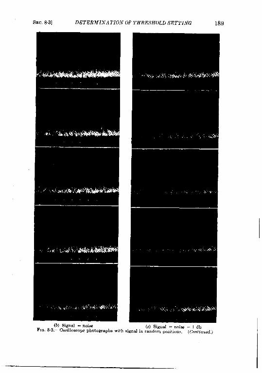
SEC. 8.3] DETERM 1.V.4 TION OF THRESHOLD SETTING 189
(c) Signal =noise – ldbsign~in randOmpositions. (Continued.)
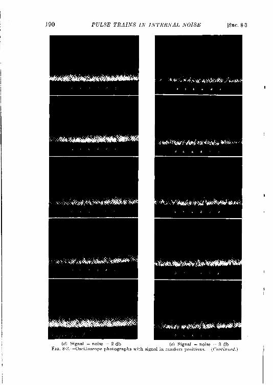
J
i
190 PULSE TRAINS IN I NTERNAL NOISE [SEC.8
1
I
;h ,(e) Signal =noise – 3db
nalin random positions. (Continued.) ;
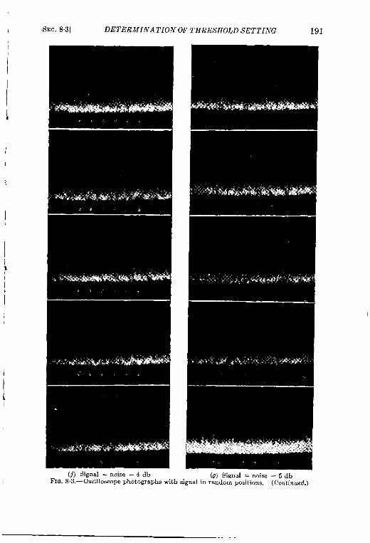
I
I
!i
I
SEC.8.3] DETERMINATION
(n Signal =noise -4dbFIG. 8.3.—Oscilloscopephotographswitl
“OF THRESHOLD SETTING 19 1
(g) Signal =noise -5dblsignal in random position.. (Continued.)
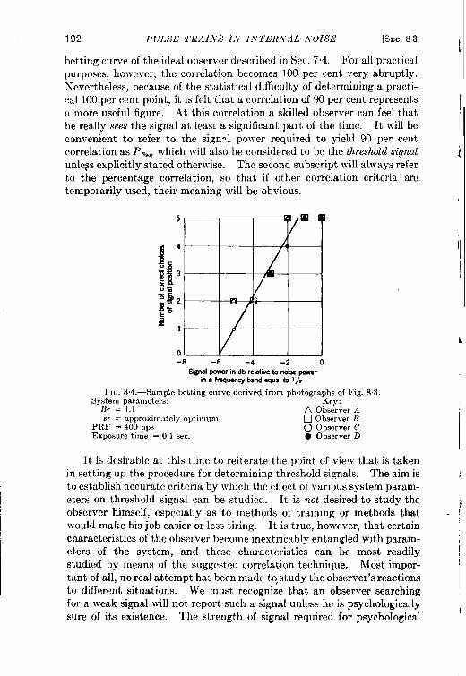
192 PULSE TRAINS IN I,VTERiVAL ,VOISE [SEC. 83 I~betting cur~'eof theideal observer described in Sec. 7"4. Forall practicalpurposes, however, the correlation becomes 100 per cent very abruptly.I$evertheless, because of the statistical difficulty of determining apracti- :eallOOper cent point, itisfelt that acorrelation of Wper cent representsa more useful figure. At this correlation askilled observer can feel that ‘he really sees the signal at least a significant part of the time. It will beconvenient to refer to the sigmd power required to yield 90 per centcorrelation as PSOO,which will also be considered to be the threshold signal iunleps explicitly stated otherwise. The second subscript will always referto the percentage correlation, so that if other correlation criteria aretemporarily used, their meaning will be obvious.
5 m IE1-1
~ 4
;f,
g=0.Y2 m Ii,. .f~
z1 -
0.-8 -6 -4 -2
Signalpowarindbrelativetonoisepowerina frequencybandaqualto l/T
l:IG. 8.4.—Samplebettingcurvederivedfromphotographsof Fig. 8.3.“tiystem parameters: Key:
B7 = 1.1 A Observer Am = :Lpproxirnatelyoptimum ❑ ObserverB
PIW = 400 pps O ObserverCExposuretime = 0.1 sec. ● Observer D
It is desirable at this time to reiterate the point of view that is takenin setting up the procedure for determining threshold signals. The aim is ;to establish accurate criteria by which the effect of various system param-eters on threshold signal can be studied. It is not desired to study the .!observer himself, especially as to methods of training or methods thatwould make his job easier or less tiring. It is true, however, that certaincharacteristics of the observer become inextricably entangled with param- (eters of the system, and these characteristics can be most readily
studied by means of the suggested correlation technique. Most impor-
tant of all, no real attempt has been made to,study the observer’s reactionsto different situations. We must recognize that an observer searchingfor a weak signal will not report such a signal unless he is psychologicallysure of its existence. The strength of signal required for psychological
!
t
SEC. 8.4] SYSTEM PARAMETERS AND SCALING 193
certainty depends upon many factors. Some of them are (1) the impor-tance of correctly reporting the signal, (2) the number of mistakes thathave been previously made, (3) the observer’s state of alertness, (4)previous amount and type of training and practice, etc. These factorsare extremely important in any operational situation; however, they arenot pertinent to a discussion of the system parameters that affect thresholdsignals.
8.4. System Parameters and Scaling.-Let us list the various systemparameters that are expected to have an effect on signal threshold power.It is not intended to be a complete list, but it probably contains most ofthe important quantities that pertain to a relatively straightforwardreceiving system containing an A-scope indicator. For more complicatedsystems, such as the MTI system described in Sec. 11.5, it is obvious thatadditional parameters will be introduced. In Table 8.2 there is listedbeside some of the parameters a symbol that will represent that param-eter. The variables are listed in groups, each group generally beingassociated with some part of the receiving system.
The scanning variable is of special importance in the discussion ofintensity-modulated indicators presented in Chap. 9. For the A-scope,however, matters will be simplified by neglecting the shaping of thepulse train resulting from the antenna beam pattern. The pulse trainwill be assumed to be of constant amplitude but of length o as is listed inItem 5 of Table 8.2.
A blind investigation of the effect of each variable for various condi-tions of all the other parameters would assume prodigious proportionsindeed, but a rough estimate of the number of observations required tocomplete the problem can be made. Assuming that each parameter is tobe set to each of five values and that a single determination for thresholdsignal requires about 100 observations (see Fig. 8“2), we arrive at theastonishing result that about 1016 observations need to be made. Thisfact is convincing evidence that every effort must be made to simplifythe problem and to investigate only those parameters which are expectedto have a relatively pronounced effect on threshold signals. Thissimplification will be carried on to a large extent, and the justification forsuch simplification is indicated below. The numbers preceding thefollowing paragraphs correspond to items in Table 8.2.
1. The pulse power P~ is, in fact, the dependent variable that we wishto find. It is affected, of course, by the definition of thresholdsignal made in the preceding section as well as by all the othersystem parameters.
3. The pulse shape is relatively unimportant. Almost all pulses incommon use have a rectangular shape; for this reason other shapeswill not be considered.
,
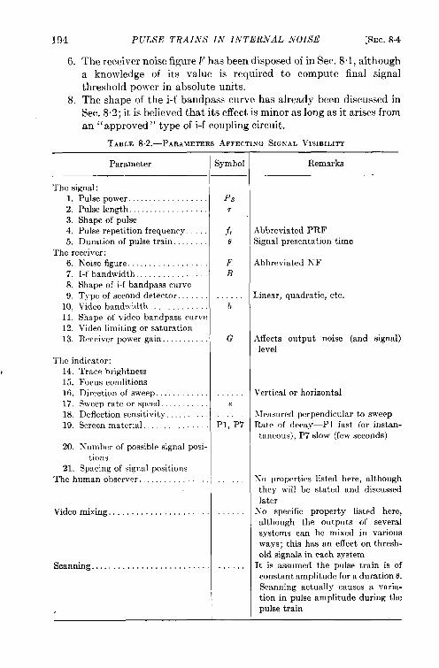
194
6.
8.
PULSE TRAINS IN INTERNAL NOISE [SEC. 8.4
The receiver noise figure F has been disposed of in Sec. 8“1, althougha knowledge of its value is required to compute final signalthreshold power in absolute units.The shape of the i-f bandpass curve has already been discussed inSec. 8.2; it is believed that its effect is minor as long as it arises froman ‘‘ approved” type of i-f coupling circuit.
TABLE82.-PARAMETERS.4FFECTINGSIGNALVISIBILITY
Parameter
The signal:l. Pulse pOwer. . . . . . . . . . . . . . . .2. Pulse length . . . . . . . . . . . . . . . . .3. Shape of pulse4, Pulse repetition frequency.5. Duration of pulse train.
The receiver:6.iYoisc figure. . . . . . . . . . . . . . . .7. I-f bandwidth . . . . . . . . . . . . . . .8. Shape of i-f bandpass curve9. Type of second detector.
10, Video band\vidth11. Shape of video bandpass curv(12. Video limiting or saturation13. Receiver po}ver gain.
The indicator:, 14, Trace brightness
15. Focus conditions16. Direction of sweep.17. Sweep rate or speed18. Deflection sensitivity.19. Screen material . . . . . . . . . . . . . .
20. Number of possible signal positions
21. Spacing of signal positionsThe human observer . . . . . . . . . . . . .
Video mixing . . . . . . . . . . . . . . . . .
Scanning. . . . . . . . . . . . . . . . . . . . . . . .
$ymbol
PsT
.fr!3
FB
b
G
s
Pl; ‘P7
. . .
Remarks
Abbreviated PRFSignal presentation time
Abbreviated A-F
Linear, quadratic, etc.
Affects output noise (and signal)level
Vertical or horizontal
Jfeasured perpendicular to sweepRate of decay-P 1 fast (or instan-taneous), P7 slow (few seconds)
No properties listed here, althoughthey will be stated and discussedlater
X’O specific property listed here,although the outputs of severalsystems can be mixed in variousways; this has an effect on thresh-old signals in each system
It is assumed the pulse train is ofconstant amplitude for a duration 0.Scanning actually ca.usesa varia-tion in pulse amplitude during thepulse train
I
I
SEC. 8.4] SYSTEM PARAMETERS AND SCALING 195
9. The type of second detector also has been mentioned in Sec. 8.2;only thelinear detector wasexperirnentally investigated, althoughin this chapter the quadratic detector is considered from thetheoretical point of view. If the signal is smaller than noisepower—a condition generally experienced in threshold determina-tions—the linear and quadratic detectors are very nearly alike insignal perception sensitivity.
11. Analogous to the case of the i-f bandpass curve shape, it isI expected that the shape of video bandpass curve has little effect
on threshold signals. To be explicit, the shape of the videobandpass curve will be assumed to be that of a single shunt-peaked stage. This means a power-response law proportionalto 1/(1 + j4), where j is the frequency.
Of the remaining quantities it is possible to combine terms 6, 12, 13,and 18 into two useful and suitable variables. The noise figure (6),receiver gain (13), and video limiting voltage (12) essentially fix thefraction of the video noise distribution that is lost in the limiting process.It is therefore more useful to express the limit level directly in terms ofthe average noise voltage (before limiting); this ratio will be denoted bythe symbol L.
Limiting is important only when a substantial fraction of the noiseprobability distribution is affected. Such limiting needs to be introducedonly when an intensity-modulated display, such as the PPI, is used; it isnecessary to prevent defocusing of the beam spot on the tube face forlarge noise fluctuations. For this reason the discussion of limiting willbe deferred until the next chapter, which deals with results obtained fromintensity-modulated display systems.
The noise figure (6), receiver gain (13), and A-scope deflection sensi-tivity (18) fix the average ampiitude of noise as seen on the A-scope. Itis more convenient to refer directly to this parameter than to the combina-tion of system characteristics from which it is derived.
Let us consider a particular set of conditions where we examine indetail the geometrical picture on the face of the A-scope. This geo-metrical picture is composed of a number of overlaid traces; each tracefor the purpose of visual inspection may be considered “laid onto” thescreen instantaneously. There is a certain noise fluctuation in each tracewhose spatial appearance is influenced by the receiver bandwidths B andb, by the average noise deflection, and by the A-scope sweep speed s.
The actual appearance of the signal may be regarded as caused by pulselength ~, the receiver bandwidths B and b, and the signal-to-noise powerratio. Now let us consider the effect of an increase in pulse length by afactors and inquire if there are similar changes that can be made in otherparameters so that the geometrical picture on the A-scope may be leftessentially unchanged.
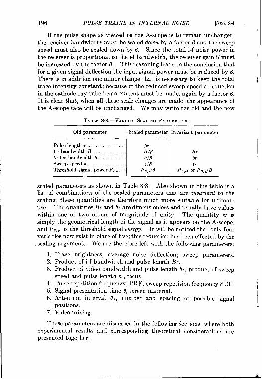
196 PULSE TRAINS IN INTERNAL NOISE [SEC. 84
If the pulse shape as viewed on the A-scope is to remain unchanged,the receiver bandwidths must be scaled down by a factor P and the sweepspeed must also be scaled down by ~. Since the total i-f noise power inthe receiver is proportional to the i-f bandwidth, the receiver gain G mustbe increased by the factor P. This reasoning leads to the conclusion thatfor a given signal deflection the input signal power must be reduced by p.There is in addition one minor change that is necessary to keep the totaltrace intensity constant; because of the reduced sweep speed a reductionin the cathode-ray-tube beam current must be made, again by a factor p.It is clear that, when all these scale changes are made, the appearance ofthe A-scope face will be unchanged. We may write the old and the new
TABLE 83.-VArUOUS SCALING PAItAMETErtS
Old parameter I Scaled parameter lInvariant parameter
Pulse length r . . . . . . . . . . . . . . . . ~.
I-f bandwidth B . . . . . . . . . . . . . . B/~
Vldeobandwidth b. . . . . . . . . . . b/fl
Sweep speed s. . . . . . . . . . . . . . . . s/6Threshold signal power P,s,O. ps,o/B
scaled parameters as shown in Table 8“3. Also shown in this table is alist of combinations of the scaled parameters that are invariant to thescaling; these quantities are therefore much more suit able for ultimateuse. The quantities B~ and b7 are dimensionless and usually have valueswithin one or two orders of magnitude of unity. The quantity sr issimply the geometrical length of the signal as it appears on the A-scope,and PS,Oris the threshold signal energy. It will be noticed that only fourvariables now exist in place of five; this reduction has been effected by thescaling argument. We are therefore left with the following parameters:
I
1.2.3.
4.5.6.
7.
Trace brightness, average noise deflection; sweep parameters.Product of i-f bandwidth and pulse length B,.Product of video bandwidth and pulse length br, product of sweepspeed and pulse length sr, focus.Pulse repetition frequency, PRF; sweep repetition frequency SRF. ~Signal presentation time d, screen material.Attention interval 8*, number and spacing of possible signalpositions. .Video mixing.
These parameters are discussed in the following sections, where bothexperimental results and corresponding theoretical considerations arepresented together.
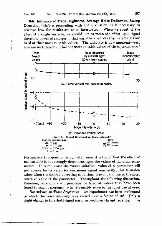
SEC.8.5] INFLUENCE OF TRACE BRIGHTNESS, ETC. 197
8.5. Muence of Trace Brightness, Average Noise Deflection, SweepDirection.-Before proceeding with the discussion, it is necessary todescribe how the results are to be interpreted. When we speak of theeffect of a single variable, we should like to mean the effect upon signalthreshold power of changes in that variable when all other parameters arefixed at their most suitable values. The difficulty is now apparent—justhow are we to know a priori the most suitable values of these parameters?
Trace Trace obscured Tracebarely by &l-watt light uncomfortablyvisible 30 cm from screen bright
o
nu A,~ -lfJ
uz (@ Same vertical and horizontal scales
30~
~ -4~,~mal \> \.-% -6 \za ‘A-.
------ ---
--
-8‘-A
-40 (est.) -30 -20 -lo 0 io 20 30Trace intensity in db
(b) Expanded vertical scaleFm. 8.6.—SignalthresholdUS.trace intensity.
System parameters: Key:B, = 1.2 A PI screenm = 1.7mm O P7 screen
PRF = 3200PPS6’=3sec
Fortunately this question is not vital, since it is found that the effect ofone ,variable is not strongly dependent upon the values of the other para-meters. In some cases the “most suitable” value of a parameter willnot always be its value for maximum signal sensitivity; this situationarises when the desired operating conditions prevent the use of the mostsensitive value of the parameter. Throughout the following discussion,therefore, parameters will generally be fixed at values that have beenfound through experience to be reasonably close to the most useful ones.
Dependence on Trace Brightnas.—An experiment has been performedin which the trace intensity was varied over a factor of 10°. Only aslight change in threshold signal was observed over the entire range. The
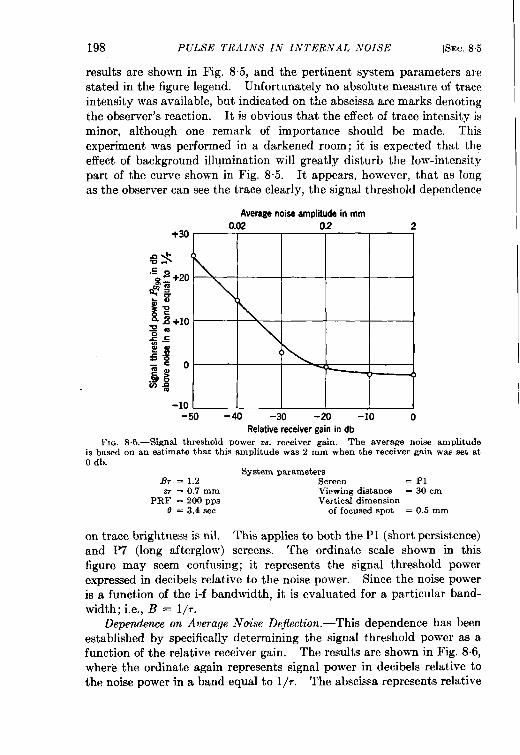
198 PULSE TRAINS IN INTERNAL
results are shown in Fig. 8“5, and the pertinent
~TolfJE @EC. 8.5
system parameters are
stated inthe figure legend. Unfortuna~elyno absolute measure of traceintensity was available, but indicated on the abscissa are marks denotingtheobserver’s reaction. Itisobvious that the effect oftrace intensity isminor, although one remark of importance should be made. Thisexperiment was performed in a darkened room; it is expected that theeffect of background illumination will greatly disturb the low-intensitypart of the curve shown in Fig. 8.5. It appears, however, that as longas the observer can see the trace clearly, the signal threshold dependence
Averagenoise ampliiude in mm
0.02 0.2 2+30 ~
gs (
co“-* ~ +20
%m:La!
t~
Ii +10~m~ .E2!$== ()
j; o Y L.2 ~ ()
m
-10.-50 -40 -30 -20 -lo 0
Relative receiver gain in db
FIG. S.6.—Signal threshold power VS.receiver gain. The average noise amplitudeis based on an estimate that this amplitude was 2 mm when the receiver gain was set atOdb.
System parametersBT = 1.2 Screen = P1m = 0.7 mm Viewing distance = 30 cm
PRF = 200PPS Vertical dimension0 = 3.4 sec of focusedspot = 0.5 mm
on trace brightness is nil. This applies to both the PI (short persistence)
and P7 (long afterglow) screens. The ordinate scale shown in this
figure may seem confusing; it represents the signal threshold power
expressed in decibels relative to the noise power. Since the noise power
is a function of the i-f bandwidth, it is evaluated for a particular band-
width; i.e., B = 1/7.Dependence on Average Noise Deflection. -This dependence has been
established by specifically determining the signal threshold power as afunction of the relative receiver gain. The results are shown in Fig. 8.6,where the ordinate again represents signal power in decibels relative tothe noise power in a band equal to 1/r. The abscissa represents relative
SEC.86] DEPENDENCE ON B, 199
receiver gain in decibels above an arbitrary level. For a relative receivergain of O db, the estimated average noise deflection on the A-scope is 2mm; since the second detector is linear, the average noise deflection forother gain settings can be calculated; this is shown on the top abscissascale.
The pertinent system parameters for this experiment are indicatedin the figure legend. As long as the average noise deflection exceedsabout 0.5 mm, the signal threshold power is independent of the averagedeflection. As the noise deflection becomes smaller, the signal thresholdpower rises; for very small deflections the signal threshold power isinversely proportional to the receiver gain. This is the result expectedif we assume that in this region a given video signal deflection is required,independent of noise power. This assumption is certainly reasonable inview of the negligible amplitude of noise.
Dependence on Direction oj Sweep.—It has been reported in variousplaces that the direction of the A-scope sweep influences the thresholdsignal; one of these reports indicated a difference of as much as 4 db inthreshold signal. The experiment has been repeated by Sydoriak, Ashby,and Lawsonl using the six-position correlation method of evaluation.‘The results show that the vertical sweep requires a signal substantiallythe same as that for the horizontal s~veep. The observers felt, however,that the longer experience obtained in viewing the horizontal trace hadcreated greater psychological difficulty in viewing signals on the verticaltrace. Lack of adequate training on the vertical sweep can easily cause adifference of several decibels in the threshold signal. We may now beassured, however, that there is no fundamental difference in signal per-ception on A-scopes that have different trace directions.
8.6. Dependence on the Product of I-f Bandwidth and Pulse Length.—It is illuminating to look somewhat ahead and discuss qualitatively somefeatures that are to be expected as a result of limitation of i-f and videobandwidths. The effect of i-f bandwidth limitation is somewhat differentfrom the effect of video bandwidth limitation; this fact may seem sur-prising in view of the linear relationship between the modulation voltageof the i-f carrier and the video voltage. .4s has often been remarked,however, the linear detector records only the absolute value of the i-fenvelope function; hence, with receiver noise that contains no carrier,cross-modulation terms develop. Video noise, then, even in a lineardetector, is caused by the interaction of i-f noise components. Thespectrum differs from the i-f noise spectrum. Hence the effect of reduc-tion of video bandwidth differs from that of reduction of i-f bandwidth.The highest important video frequency produced by the second detectoris numerically equal to the i-f bandwidth B, since this highest frequency
1Unpublished.
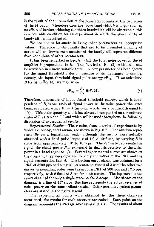
200 PULSE TRAINS IN INTERNAL NOISE [SEC.8.6
is the result of the interaction of the noise components at the two edgesof the i-f band. Therefore once the video bandwidth b is larger than B,
no effect of further widening the video bandw-idth will be observable; thisis a desirable condition for an experiment in which the effect of the i-fbandwidth is investigated.
We are not so fortunate in fixing other parameters at appropriatevalues. Therefore in the results that are to be presented a family ofcurves will be shown; each member of the family will represent differentfixed conditions of other parameters.
It has been remarked in Sec. 8.1 that the total noise power in the i-famplifier is proportional to B. This fact led to Eq. (3), which will nowbe rewritten in a more suitable form. A new parameter has been chosenfor the signal threshold criterion because of its invariance to scaling,namely, the input threshold signal pulse energy 7Psti. If we substituteB for Aj in Eq. (3), we may write
(4)
Therefore, a measure of input signal threshold energy, which is inde-pendent of B, is the ratio of signal power to the noise power, the latterbeing evaluated where Br = 1 (in other words, for a bandwidth equal to1/7). This is the quantity which has already been plotted on the ordinatescales of Figs. 8“5 and 8.6 and which will be used throughout the foUowingdiscussion of experimental results.
Experimental Results.-The results, from a series of experiments bySydoriak, Ashby, and Lawson, are shown in Fig. 8.7. The abscissa repre-sents Br on a logarithmic scale, although the results were actuallyobtained with a fixed pulse length 7 of 1.0 X 10–e see, by varying B insteps from approximately 106 to 107 cps. The ordinate represents thesignal threshold power Ps,a expressed in decibels relative to the noisepower in a band equal to 1/7. Several experimental curves are shown onthe diagram; they were obtained for different values of the PRF and thesignal present ation time e. The bottom curve shown was obtained for aPRF of 3200 pps and a signal presentation time 0 of 3 sec; the other twocurves in ascending order were taken for a PRF of 200 pps and 12.5 pps,respectively, with o fixed at 3 sec for both curves. The top curve is theresult obtained for only a single trace on the A-scope. Also shown on thediagram is a line of 45° slope; this line represents the actual receiver i-fnoise power on the same ordinate scale. Other pertinent system param-eters are stated in the figure legend.
The experimental points were obtained by the three observersmentioned; the results for each observer are coded. Each point on thediagram represents the average over several trials. The results of about
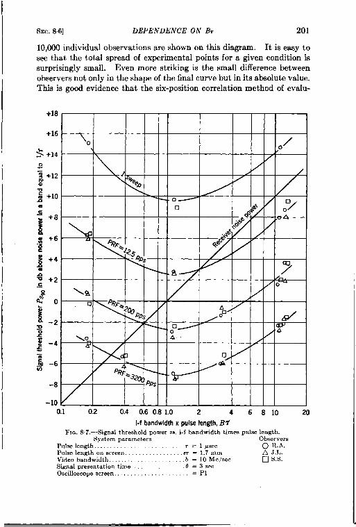
Sig
nal
thre
sho
ldp
ow
erf~
m
0
ind
bab
ove
no
ise
po
wer
Ina
ban
deq
ual
tol/r
+ W+ m
+ 02
1I
I I II I I 1 I
03
202 PULSE TRAINS IN INTERNAL NOISE [SEC.86
sting threshold signals used in these experiments removes the necessity ofnearly all psychological judgment on the part of the observer.
The general form of the curve seems to be relatively unaffected by thedifferent values of PRF and d, but its absolute value is considerablyaltered. The significance of this will be brought out later. For themoment it is sufficient to note that the curve has a broad, flat minimumin the neighborhood of B~ = 1.2. For values of Br much larger thanthis, the curve approaches asymptotically a line that is parallel to thereceiver-noise curve. On the other hand, for very small values of B, theexperimental curve appears to approach a line whose slope is —1, showingthat in this region the signal threshold power is inversely proportionalto Br.
1
.-0.1 1.0 10.0
l-f bandwidthx pulse length B 7FIG. S.S.—Signal thresholdpower VS.i-f bandwidthtimes pulselength.
System parametersPulse repetition frequency. . . . . . PRF=200ppsSignal presentationtime . . . . . . . . . . . . t7=3secPulse length on screen.......,,,,,. . . . . . . . . . . . . . . . ..05 mmr=O.O5mm
It seems wise at this time to interject one word of caution in the
interpretation of these results. The video bandwidth itself was madesufficiently wide so as not to suppress video frequencies produced by thesecond detector. The higher video frequencies, however, are notnecessarily perceived by the observer with the same ease as the lowerfrequencies. This effect, which will be discussed at length in Sec. 8.7,depends on the resolution of the eye and, far more important, on whatspatial separation of events as depicted on the A-scope face are mosteasily seen. Because of the spatial selection of the human eye and brain
the observer may be considered as a type of frequency jilter; the connectionbetween the frequency and the space function is made by means of theA-scope sweep. In this regard the observer may unwittingly limit theeffective video bandwidth. This is indeed the case for the experimentsdepicted in Fig. 8.7. For the moment, therefore, it will be assumed thatthe results are valid only for the value of m shown; i.e., sr = 1.7 mm. Toshow how the curve looks for a widely different value of ST the signalthreshold power was measured as a function of Eh when the pulse lengthon the oscilloscope w was set at 0.05 mm. The result is shown in Fig.8.8, where all parameters other than m are the same-as those for the curve
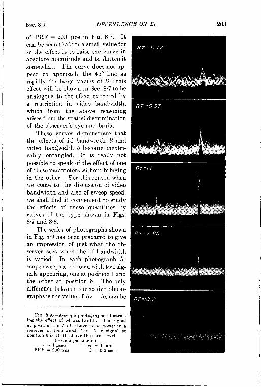
,
SEC. 86] DEPENDENCE ON Br 203
of PRF = 200 pps in Fig. 8.7. Itcan be seen that for a small value forSTthe effect is to raise the curve inabsolute magnitude and to flatten itsomewhat. The curve does not ap-
pear to approach the 45° line as
rapidly for large values of Br; this
effect will be shown in Sec. 8.7tobe
analogous to the effect expected by
a restriction in video bandwidth,
which from the above reasoning
arises from the spatial discrimination
of the observer’s eye and brain.
These curves demonstrate that
the effects of i-f bandwidth 1? and
video bandwidth b become inextri-cably entangled. It is really notpossible to speak of the effect of oneof these parameters without bringingin the other. For this reason whenwe come to the discussion of videobandwidth and also of sweep speed,we shall find it convenient to studythe effects of these quantities bycurves of the type shown in Figs.8.7 and 8.8.
The series of photographs shownin Fig. 8.9 has been prepared to givean impression of just what the ob-server sees when the i-f bandwidthis varied. In each photograph A-scope sweeps are shown with two sig-nals appearing, one at position 1 andthe other at position 6. The onlydifference between successive photo-graphs is the value of B~. As can be
FIG. 8.9.—A-scopephotographsillustrat-ing the effect of i-f bandwidth. The signalat position 1 is 5 dh above noise power in areceiver of handwidth I/r. The signal atposition6 is 11db above the samelevel.
System parameters, = 1#see sr=lmm
PRF = 200PPS .6 = 0.2 sec
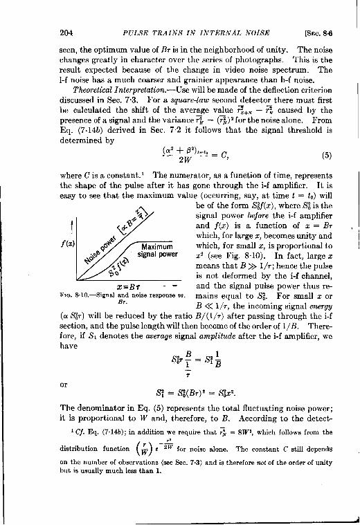
204 PULSE TRAINS IN INTERNAL NOISE [SEC.8.6
seen, the optimum value of Br is in the neighborhood of unity. The noisechanges greatly in character over the series of photographs. This is theresult expect ed because of the change in video noise spectrum. Thel-f noise has a much coarser and grainier appearance than h-f noise.
Theoretical ZnteTpretation. —Use will be made of the deflection criterion
discussed in Sec. 7.3. For a souare-law second detector there must first.be calculated the shift of the aver~ge value ~+. – ~ caused by thepresence of a signal and the variance PN– (~~)2for the noise alone. FromEq. (7.14b) derived in Sec. 7.2 it follows that the signal threshold isdetermined by
(5)
where C is a constant. 1 The numerator, as a function of time, representsthe shape of the pulse after it has gone through the i-f amplifier. It iseasy to see that the maximum value (occurring, say, at time t = to)will
be of the form S~(Z), where Si is the$>
k
~< signal power before the i-f amplifier
! Y%and f(z) is a function of z = B7
f(z)~( which, for large x, becomes unity and
~j~Q Maximum which, for small z, is proportional to
+~%signal power X2 (see Fig. 8-10). In fact, large z
@means that B >> l/r; hence the pulse
$2 is not deformed by the i-f channel,
x=Br — and the signal pulse power thus re-Fm. 8.10.—Signsl and noise responssOU.
Br.mains equal to Si. For small z orB << 1/,, the incoming signal energy
(a Sir) will be reduced by the ratio B/(l/,) after passing through the i-fsection, and the pulse length will then become of the order of I/B. There-fore, if S1 denotes the average signal amplitude after the i-f amplifier, wehave
—T
ors; = s~(BT)’ = A!-&’.
The denominator in Eq. (5) represents the total fluctuating noise power;it is proportional to W and, therefore, to B. According to the detect-
1Cf. Eq. (7.14b); in addition we require that ~~ = 8w~, which follows from the
(),,——
distribution function+
e zw for ~oi~e alone. The constant f7 still depends
on the number of observations (see SeC. 7.3) and is therefore not of the order of unitybut is usually much less than 1.
SEC. 8.6] DEPENDENCE ON B, 205
ability criterion, the maximum signal power after the i-f narrowing mustbea certain fraction of the fluctuating noise power for the signal to bedetected. This condition leads therefore toaformula for the minimumdetectable signal energy’ of the form
‘~’ = ConSt”f%’ (6)
where the constant has the dimension of energy and is proportional tokT. The function z/f(x) isproportional tozforlargez and is propor-tional to l/z for small z; hence it must have a minimum for some inter-mediate value of x; this minimum value will turn out to be of the order of
fum y.For a linear second detector and for weak signals, we obtain,2 instead
of Eq. (5),
(7)
The signal threshold is therefore slightly higher than for a square-lawdetector, but the difference is only about 0.2 db, which is hardlyobservable.
The exact fwm of the function f(z) in Eq. (6) will depend, of course,on the shape of the pulse and on the shape of the i-f pass band. Usingthe notation of Sec. 7“2, we can easily derive’ from Eq. (5)
q /+mrijfl(j,z(j,d-to ‘
2U1/_+m”p(j),2(if ‘=c(8)
I The threshold signal power Ps, used earlier in this chapter, is the same as $,.Siice with the deflection criterion, the signal threshold is not defined in relation to abetting curve, the percentage of the number of successesis not specified; it wouldaffect only the value of the constant in Eq. (6).
2Using Eq. (7.14a), we get for the shift of the average value of r caused by thesignal
—.TS+N — rN =
for small values of z = (a’
q+;+-’]=%+ E?’)/2W. For the variance of r for noise alone we obtain
Equation (7) then follows from the deflection criterion [Eqs. (7.31)].
aSiice the shape of the pulse before the i-f amplifier is symmetrical around themid-point, i%(t) = O can be put in ~q. (7.1). In Fq. (8) there has alsObeen intro-duced
aO(O = sO~(O.
The quantity S: /2 is therefore the initial pulse power !n watts: G(j) is the Fouriertransform of the initial pulse shape F(t).
206 PUL,S.? TRAINJS IN IN TERNAI. NO[,SI{ [Sm. 8.6
This result will be written in terms of the minimum detwtable amm~~e
signal pourer P~i.l [instead of minimum detectable signal energy as in II;II.
(6)]; since
/
~=g +“
(IO –.F2(t) dt,
where ea is again the pulse repetition period, it follows from ILq. (8) that
/‘Q dtF2(t) ~+rn W1.Z(j)122U2C -.
P.=K—.
U(9)+mdj G( jjZ( j)ezr’l’o 2
—. *
To make the dependence on the bandwidth B and pulse length 7 mm-cevident [in order to get the result in a form analogous to Eq. (6)] wc write
()F(t) = F, ; ,()
z(j) = z, ~ ~ (lo)
The functions F,(z) and Zl(u), respectively, characterize, therefore, theshape of the pulse and of the i-f pass band. It is easy to show then thatEq. (9) can be written in the form ..
(11)
where
/
+.q= Iz,(u)[’du,
/~ = ‘m F;(z) dz,
—a —.
1/+- 2
j(z) = X2 G,(ux)Zl(u)e’”’UrO du ,—.
z=Br ) 0=$
Let us now consider a few examples. 21. Gaussian pulse and Gaussian i-f pass band. Theta
Fl(.z) = e–a’”, Zl(u) = e–~’’’”.
1 Usually the pulse shape is rectangular; hence ~~ti = S~r/130= Ps./~o; see alsofootnote on p. 205.
zAll these examples are somewhat academic, since for all of them the systemfunction Z(j) cannot be strictly realized. For all of them the shape of the deformedpulse will be symmetric around the maximum value, which occurs for h = O.
f The numerical values of the constants a and a, depend on the way one definesthe pulse length and the i-f bandwidth. Defining them as the length and width atthe half-power points gives a = a, = 1.18.
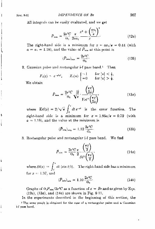
SEC. 84] DEPEIVDENCE ON Br 207
All integrals can be easily evaluated, and we get
(12a)
The right-hand side is a minimum for z = aa,/r = 0.44 (with
a = al = 1.18), and the value of ~~a at this point is
(F.,. ),”,. = ~.
2. Gaussian pulse and rectangular i-f pass band. 1 Then
Fl(z) = e–”’”, I21(?4) :;for [u[ < +,for Iul > +.
We obtain
()‘TX
–$~=2u’c 2 %
mmefl ;“
()J3rf’ ‘~
(12b)
(13a)
\
zwhere Erf(z) = 2/ti~ dt e–” is the error function. The
oright-hand side is a minimum for z = 1.95a/r = 0.72 (witha = 1,18), and the value at the minimum is
(Pm.) .,. = 1.12 ~.
3. Rectangular pulse and rectangular i-f pass
()
rrx2Lr2crr 7
F,,,,. = ~ Q—- Y
()Si’ ‘~
r,
(13b)
band. We find
(14a)
where Si(z) =1“
dt (sin t/t). The right-hand side has a minimum
for z = 1.37, an~l
(F.ir.)~,n = 1.10 ~. (14b)
Graphs of %Pti/2u2C as a function of z = Brand as given by Eqs.(12a), (13a), and (14a) are shown in Fig. 8.11.
In the experiments described in the beginning of this section, the
] The same result is obtained for the case of a rectangular pulse and a Gaussiani-f passband.
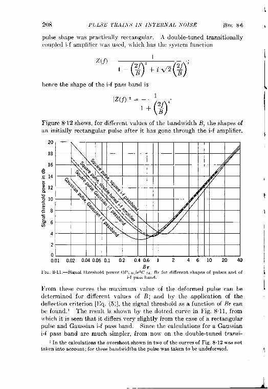
208 PC’LS’E TRAI.V,Y I.V INTERNAL NOISE [SEC 86
pulse shape was practically rectangular. A double-tuned transitionally
r{Nlplcd i-f amplifier }VJSwscd, \rhich has the systcm function
z(f) =
‘-(:)%:);hence the shape of the i-f pass band is
\z(f)l’ = 1()1+ g’”
Figure 8.12 shows, for different values of the bandwidth 1?, the shapes ofan initially rectangular pulse after it has gone through the i-f amplifier.
0.01 002 0.040.06 0.1 0.2 0,40.6 1 2 4 6 10 20 40Br
1’IG.8.11.—Signalthresholdpower OP,,,in/aZCm. BT for different shapesof pulsesand ofi-f pws hand.
k’rom these curves the maximum value of the deformed pulse can bedctcrmincd for different values of B; and by the application of thedeflection criterion [f3q. (5)], the signal threshold as a function of B7 canhe found. 1 The result is showm by the dotted curve in Fig. 8.11, fromIvhich it is seen that it differs very slightly from the case of a rectangularpulse and Gaussian i-f pass band. Since the calculations for a Gaussiani-f pass band are much simpler, from now on the double-tuned transi-
1In the calculations the overshoot shown in two of the curves of Fig. 8.12 was nottaken into account; for these bandwidths the pulse was taken to be undeformed.
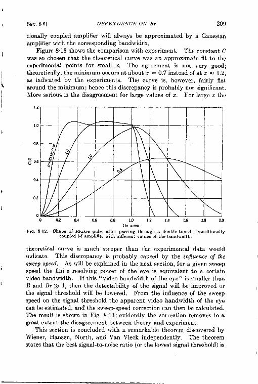
h
t SEC.8.6] DEPENDENCE ON Br 209
tionally coupled amplifier will always be approximated by a Gaussianamplifier with the corresponding bandwidth.
1Figure 813showst hecomparisonw ithexperiment. The constant C
was so chosen that the theoretical curve was an approximate fit to theexperimental points for small x. The agreement is not very good;
Itheoretically, the minimum occurs at about x = 0.7 instead of at z = 1.2,
ias indicated by the experiments. The curve is, however, fairly flataround the minimum; hence this discrepancyy is probably not significant.More serious is the disagreement for large values of z. For large z the
II 12
1.0 r \/ ‘ — .
0.8 I8
~
~ 0.6
0.4
02
00 0.2 0,4 0.6 0.8 1.0 1.2 1.4 1.6 1.8
tin psec2.0
FIG. S.12.—Shape of square pulse after passing through a double-tuned,transitionalycoupledi-f amplifierwith different values of the bandwidth.
theoretical curve is much steeper than the experimental data wouldindicate. This discrepancy is probably caused by the injluence of the
sweep speed. As will be explained in the next section, for a given sweep1 speed the finite resolving power of the eye is equivalent to a certain
video bandwidth. If this ‘‘ video bandwidth of the eye” is smaller thani B and B,>> 1, then the detectabilityy of the signal will be improved or
the signal threshold will be lowered. From the influence of the sweepspeed on the signal threshold the apparent video bandwidth of the eyecan be estimated, and the sweep-speed correction can then be calculatd.The result is shown in Fig. 8.13; evidently the correction removes to agreat extent the disagreement between theory and experiment.
This section is concluded with a remarkable theorem discovered byWiener, Hansen, North, and Van Vleck independently. The theoremstates that the best signal-t~noise ratio (or the lowest signal thrmhold) is
.— --— —
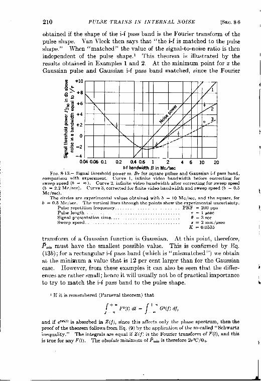
210 PULSE TRAINS IIV I,VTERNAL NOISE ~SEC,8.6
obtained if the shape of the i-f pass band is the Fourier transform of thepulse shape. Van Vleck then says that “the i-f is matched to the pulseshape. ” When “matched” the value of the signal-to-noise ratio is thenindependent of the pulse shape. 1 This theorem is illustrated by theresults obtained in Examples 1 and 2. At the minimum point for x theGaussian pulse and Gaussian i-f pass band matched, since the Fourier
E..+’orT-l-r I III 1
~o \ / fly .,c .s /58 \~ “$ -2
% -40.040.06 0.1 0.2 0.40.6 1 2 461020
l-f bandwidthB in Me/see
FIG. 8.13.—SignalthresholdpowerVS.BT for squarepulsesandGaussiani-f passband,comparisonwith experiment. Curve 1, infinite video bandwidth before correcting forsweepspeed (b = M), Curve 2, infinitevideobandwidthaftercorrectingforsweepspeed(b = 2.2 Me/see). curve 3, correctedfor finite video bandwidthandsweepspeed (b = 0,5Me/see).
The circles are experimentalvalues obtained with b = 10 Mc /see,and the square,forb = 0.5 Me/see. The vertical linesthroughthe pointsshowthe experimentaluncertainty.
Pulse repetition frequency. . . . . . . ,, PRF=200ppsPulse length . . . . . . . . . . . . . . . . . 7 = 1 psecSignal presentationtime. . . . . . . . . . . . t?=3secSweep speed................,., s = 2 mrn/psec
K = 0.0535
transform of a Gaussian function is Gaussian. At this point, therefore,~.h must have the smallest possible value. This is confirmed by Eq.(13b); for a rectangular i-f pass band (which is “mismatched”) we obtainat the minimum a value that is 12 per cent larger than for the Gaussiancase. However, from these examp~es it can al~o be seen that the differ- i
ences are rather small; hence it will usually not be of practical importanceto try to match the i-f pass band to the pulse shape. i
1If it is remembered (Parzeval theorem) that
;_+@MF’(O al = ~_+~” G’(j) df,
and if ezri~~is absorbed in Z(j), since this ailects only the phase spectrum, then theproof of the theorem follows from Eq. (9) by the application of the so-called ‘‘ Schwartzinequality. ” The integrals are equal if Z(j) is the Fourier transform of F(t), and thisis true for any F(t). The absolute minimum of ~ti is therefore 2a’C/f3,.
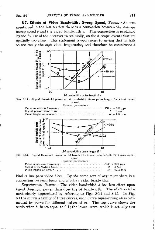
I SEC.87] EFFECTS OF VIDEO BAND WIDTH 211
8.7. Effects of Video Bandwidth; Sweep Speed, Focus. -As wasmentioned in the last section there is a connection between the A-scopesweep speed s and the video bandwidth b. This connection is explainedby the failure of the observer to see easily, on the A-scope, events that arespatialIy too close. This statement is equivalent to saying that he failsto see easily the high video frequencies, and therefore he constitutes a
b
FIQ.
FIG.
10
5
0
-50.1 1 10
l-f bandwidthx pulselengthB T
S 14.—Signrd threshold power w. i-f bandwidth times pulse length for a fastspeed.
System parametersPulse repetition frequency. . . . PRF=200PPsSignalpresentationtime. . . . . . ,. .,,., . . . . e = :3secPulse length on screen. . . . . . . . . . m = l,6mm
~<log“s>gs~=.gg+5=5e-~fig~,;.;
*EO0.1 1 10
l-f bandwidthx pulselengthB7S.15,—Signalthresholdpower VS.i-f bandwidthtimes pulse length for a SIO,V
speed,System parameters
Pulse repetitmn frequency, .,, .PRF=200PPsSignalpresentationtime. . . . . . . . . . . . @=3secPulse length on screen..,... .w = 0.05mm
sweep
sweep
kind of low-pass video filter. By the same sort of argument there is aconnection between focus and effective video bandwidth.
Experimental Results.—The video bandwidth b has less effect uponsignal threshold power than does the i-f bandwidth. The effect can bemost clearly appreciated by referring to Figs. 8.14 and 8.15. In Fig.8.14 is shown a family of three curves, each curve representing an experi-mental 1% curve for different values of b7. The top curve shows theresult when ZWis set equal to O.1; the lower curve, which is actually two
—.- —----
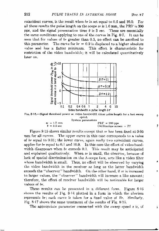
I
212 PULSE TRA INS IN INTERNAL NOISE [SEC.87
coincident curves, is the result when b? is set equal to 0.5 and 10.0. Forall these results the pulse length on the scope STis 1.6 mm, the PRF is 200pps, and the signal presentation time o is 3 sec. These are essentiallythe same conditions applying to one of the curves in Fig. 8.7. It can beseen that for values of br greater than 0.5, no effect can be ascribed to
this parameter. The curve for b, = 0.2 is displaced to a higher absolutevalue and has a flatter minimum. This effect is characteristic forrestriction of the video bandwidth; it will be calculated quantitativelylater on.
1. -
0.1 0.2 0.40.6 1 2 4610Video bandwidth x pulse length b?
Fm. 8.16,—Signalthreshold power w. video bandwidth times pulse length for a fast sweepspeed.
System parameters~ = 1.7mm PRF = 200PPS
O = 3,5 sec Oscilloscopescreen s p7
Figure 8.15 shows similar results except that sr has been fixed at O.OEi
mm for all curves. The upper curve in this case corresponds to a value
of br equal to 0.01; the lower curve, again really two coincident curves,applies for br equal to 0.1 and 10.0. In this case the effect of video band-width disappears when b7 exceeds 0.1. This result may be anticipatedand explained qualitatively. When sr is small, the observer, because oflack of spatial discrimination on the A-scope face, acts like a video filterwhose bandwidth is small. Thus, no effect will be observed by varying i
the video bandwidth in the receiver as long as the latter bandwidthexceeds the ‘‘ observer” bandwidth. On the other hand, if sr is increased *
to larger values, the “ observer” bandwidth will increase a like amount;therefore, the effect of receiver bandwidth will be noticeable for largervalues of br.
These results can be presented in a different form. Figure 8.16shows the results of Fig. 8.14 plotted in a form in which the abscissarepresents br; each curve is taken for a fixed value of B?. Similarly,Fig. 8.17 shows the same treatment of the results of Fig. 8.15.
The appropriate parameter connected with the sweep speed s is, of i
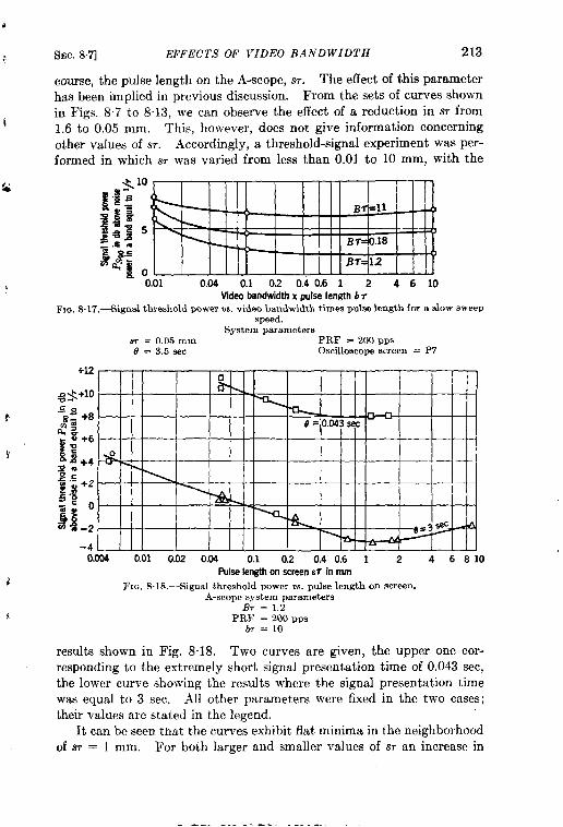
d
SEC.8.7] EFFECTS OF VIDEO BANDWIDTH 213;
course, the pulse length on the A-scope, W. The effect of this parameter
has been implied in previous discussion. From the sets of curves shownin Figs. 8.7 to 8.13, we can observe the effect of a reduction in sr from
11,6 to 0.05 mm. This, however, does not give information concerning
other values of .s7. Accordingly, a threshold-signal experiment was per-
formed in which ST was varied from less than 0.01 to 10 mm, with the
~,g$’”
i$%:Z5-v52_.51u
“% {01 ,M “,1 ,2 ,4,6, ,4610
Videobandwidthx ~ulse length br
FIG.8.17.—Signalthresholdpowerw. video bandwidthtimes pulselength for a slow sweepspeed.
System parametersST = 0.05mm PRF = 200ppSo = 3.5 WC OscillOscOpescreen = P7
0.004 0.01 0.02 0.04 0.1 0.2 0.4 0.6 1 2 4 6810Pulselengthon screen.s7in mm~
FIG. S.18.—Signalthresholdpower m. pulselength on screen.A-scope system parameters
$Br = 1.2
PRJ? = 200ppslw=lo
results shown in Fig. 8.18. Two curves are given, the upper one cor-responding to the extremely short signal presentation time of 0.043 see,the lower curve showing the results where the signal presentation timewas equal to 3 sec. All other parameters were fixed in the two cases;their values are stated in the legend.
It can be seen that the curves exhibit flat minima in the neighborhoodof m = 1 mm. For both larger and smaller values of STan increase in
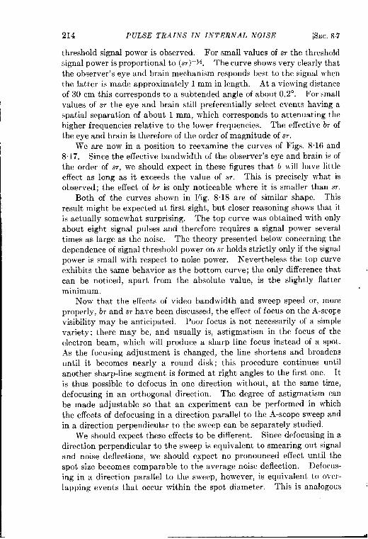
214 PULSE TRAINS IN INTERNAL NOISE [SEC.8.7
threshold signal power is observed. For small values of w the thresholdsignal power is proportional to (s7)–~4. The curve shows very clearly thatthe observer’s eye and brain mechanism responds best to the signal ~rhenthe latter is made approximately 1 mm in length. At a viewing distanceof 30 cm this corresponds to a subtended angle of about 0.2°. For smallvalues of sr the eye and brain still preferentially select events having aspatial separation of about 1 mm, which corresponds to attenuating thehigher frequencies relative to the lower frequencies. The effective bT ofthe eye and brain is therefore of the order of magnitude of s,.
We are now in a position to reexamine the curves of Figs. 8.16 and8.17. Since the effective bandwidth of the observer’s eye and brain is ofthe order of ST, we should expect in these figures that b will have littleeffect as long as it exceeds the value of sT. This is precisely what isobserved; the effect of b~ is only noticeable where it is smaller than ST.
Both of the curves shown in Fig. 8.18 are of similar shape. Thisresult might be expected at first sight, but closer reasoning shows that itis actually somewhat surprising. The top curve was obtained with onlyabout eight signal pulses and therefore requires a signal power severaltimes as large as the noise. The theory presented below concerning thedependence of signal threshold power on S, holds strictly only if the signalpower is small with respect to noise power. Nevertheless the top curveexhibits the same behavior as the bottom curve; the only difference thatcan be noticed, apart from the absolute value, is the slightly flatterminimum.
Now that the effects of video bandwidth and sweep speed or, moreproperly, br and SThave been discussed, the effect of focus on the A-scoFevisibility may be anticipated. Poor focus is not necessarily of a simplevariety; there may be, and usually is, astigmatism in the focus of theelectron beam, which will produce a sharp line focus instead of a spot.As the focusing adjustment is changed, the line shortens and broadensuntil it becomes nearly a round disk; this procedure continues untilanother sharp-line segment is formed at right angles to the first one. Itis thus possible to defocus in one direction without, at the same time,defocusing in an orthogonal direction. The degree. of astigmatism canbe made adjustable so that an experiment can be performed in whichthe effects of defocusing in a direction parallel to the A-scope sweep andin a direction perpendicular to the sweep can be separately studied.
We should expect these effects to be different. Since defocusing in adirection perpendicular to the sweep is equivalent to smearing out signaland noise deflections, we should expect no pronounced effect until thespot size becomes comparable to the average noise deflection. Defocus-ing in a direction parallel to the sweep, however, is equivalent to over-lapping events that occur within the spot diameter. This is analogous
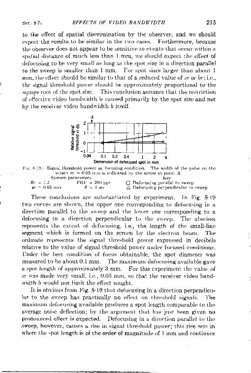
SEC.87] EFFECTS OF VIDEO BA,VDWIDTH 215
to the effect of spatial discrimination by the observer, and we shouldexpect the results to be similar in the two cases. Furthermore, becausetheobserver does not appear to besensitivet oe vents that occur ~rithinaspatial distance of much less than 1 mm, ]ve should expect the effect ofdefocusing to be very small as long as the spot size in a direction parallelto the sweep is smaller than 1 mm. For spot sizes larger than about 1mm, the effect should be similar to that of a reduced value of STor b7; i.e.,the signal threshold power should be approximately proportional to thesqufi:e root of the spot size. This conclusion as.wlmes that the restrictionof effective video bandwidth is caused primarily by the spot size and notby the receiver video bandwidth b itself.
A
.-g 2-+
.3s ~--0 ~ “.: z — Fg~o -n~ \
.X5-1 1
0,04 0.1 0.2 0.4 124Demension ofdefocusedSpotinmm
E’IG81 !).- Signal threshold power vs. focusingcondition, The width of the pulseOILtl!cwreell ST = 0,05mIII is indicated hy-the arrow at ~o]nt A.
System paraznet.ws KeyB, = 1.2 PRF = ?00 pps O Deiorusing parallel to sweep
7 m = 0.05111111 8 = :3SC<, A Defocusingperpendicularto sweep
These conclusions are substantiated by experiment. In Fig. 819I two curves are sbovm, the upper one corrcsponcfiryq to defocusing in a
direction parallel to the s~~eep and the lower one corresponding to adefocusing in a direction perpendicular to the sweep, The abscissarepresents the extent of defocusing, i.e., the length of the small-linesegment which is formed on the screen by the electron beam. Theordinate represents the signal threshold power expressed in decibelsrelative to the value of signal threshold power under focused conditions.Under the best condition of focus obtainable, the spot diameter ~vasmeasured to be about 0.1 mm. The maximum defocusing available gavea spot length of approximately 3 mm. For this experiment the value ofSTwas made very small, i.e., 0.05 mm, so that the receiver video band-width b would not limit the effect sought,
It is obviom from Fig. 8.19 that defocusing in a direction perpendicu-lar to the sJvcep has practically no effect on threshold signals. Themaximum defocusing available produces a spot length comparable to theaverage noise deflection; by the arg~lrnent that has just been given nopronounced effect is expected. Defocusing in a direction parallel to thesweep, however, causes a rise in signal threshold power; this rise sets inwhere the spot length is of the order of magnit~lde of 1 mm and continues
— —— .—.
216 PULSE TRAINS IN INTERNAL NOISE [SEC.8.7
to rise with increasing defocusing. This situation is analogous to theeffect of ST shown in Fig. 8“18. In that case the dependence of signalthreshold power on the reciprocal of the square root of S, was reachedonly for values of STthat were very much smaller than 1 mm.
Theoretical Interpretation.—If the video bandwidth is small comparedwith the i-f bandwidth, then instead of Eq. (6) there will be obtained forthe minimum detectable signal energy an equation of the form
N(x,Y),S& = const. ~(z,y) (15)
where z = Br and g = br. The function N(x,y) is the fluctuating noisepower, and ~H(z,y) is the maximum value of the pulse after it has beendeformed by the. i-f and video amplifiers. The qualitative behavior ofthese functions can easily be discussed. The function N is the squareroot of the area of the continuous noise spectrum I of r2. In Sec. 3.8 wesaw that for a squardaw detector, the ordinate of the continuous spec-trum at the origin is proportional to B. Therefore if the video bandwidth
is much smaller than the i-f bandwidth (b << B), then the area will beproportional to bB whereas, if b>> B, the area will be proportional to B2.Therefore the function N(z,y) will have the’ asymptotic behavior
N(x,y) a (4% for y <<x,x for y>> z. )
(16)
The function H(z,y) has the same asymptotic behavior as the functionf(x) in Eq. (6) for any fixed value of y and reduces, of course, exactly tothe function j(c) if y>> x. Therefore, for fixed y, IIcm’ for z <<1 andH = constant (independent of x) for z>> 1. On the other hand, it iseasily seen that for fixed x, Hay for y <<1. Consequently, for fixedy, Pfi (or L$$) will be proportional to l/x for z <<1 and proportional to
V for x>> 1; hence a minimum value will always exist. The region
~here ~tia ~ occurs when x>> y. Of course, when y itself is large,Pa will be proportional to x in the region 1 <<z <<y, since in this casethe video bandwidth will have practically no influence and the results ofthe previous section will hold.
The dependence of ~ti on y for fixed x is more complicated. If
z <<1, from the asymptotic behavior of N and H we find that ~tial/fifor y <<x and ~fi = constant (independent of y) for y>> x. Thequantity ~ti will therefore be a monotonically decreasing function of y;
1By definition, N~ = ~~ — (~)z. According to the deflection criterion [Eq.(7. la)] with j = rz (square-law detector). For noise alone the spectrum consists ofthe d-c term and the continuous part. From the general formula of Sec. 3.3 it followsthat the area of the continuous spectrum is just the variance of r~.
SEC. 8.7] EFFECTS OF VIDEO BA .VD WIDTH 217
or in other words, if z = 1% <<1, then the narrowing of the video willalways increase the signal threshold. This is no longer the case if x>> 1.
Since ~,.,~al/~ for y <<1 and ~~~a W for 1 <<y <<x, there will be a
minimum for an intermediate value of y. Therefore, if Br >> 1, thenthe narro~ving of the video will at first give an improvement, continuinguntil ~mimreaches a minimum value. Further narrowing of the video willthen again increase the signal threshold. If z decreases, then the mini-mum of ~tim as a function of y becomes less pronounced, and it disappearsforz = 1.
For a square-law detector it is not difficult to find an exact expressionfor the minimum detectable average signal power ~~~. We find that
21J’C[ /_+mmd F’(t)] [ /_+mmd ]Ztid(j)l’ /_+m- d.fl IZ(A)I’IZ(.H1)l’]%
= eo
/+ m df &d(j)e2TtJ’0
I+ “ dj, G(f,)G*(j, – j) Z(j,)Z*(f, – j) “
—. —m(17)
The notation is the same as in Sec. 8.6; Zvid(j) is the system function of thevideo amplifier; to is the time at which the deformed pulse is a maximum:Zvid(f) = Ztd ( – f), from which it can easily be shown that the denomina-tor of Eq. (17) is real. To put Eq. (17) in the same form as Eq. (15) wemust introduce, as in Sec. 86, the shape functional
()F(t) = r, ~ ; ()z(j) = z, j ; ()Zvid(f) =21, vi. ~ .T
Then we can write
~ = 2U2C N(z,y)m,. — y H(xjy)’00
/
+.
/
+.
1( )12
NZ(z,y) = Z~ _ ~ dv IZ., ,,d(~)[’ (:UIZI(U)[2Z1 ‘u — $ ,—:,
/
+.
/
+.H(z,y) = XV dv Z,, ~id(v)e2WW7) du G,(uz)G:(tix – Vy)
—. —.
()Z,(u)z: ‘a – ; v 1
(18)
As the first example let us consider the case where the pulse shape and
I The video handwirlth b will always be defined as the width between zero frequencyand the upper half-power point.
-——. ------ . . .
218 PULSE TRAINS IN INTERNAL NOISE [SEC,87
the shapes of the i-f and video pass band are all Gaussian. Then
~,v,
Fl(z) = e–”’”, Zl(u) = e–”’”’, ZI, .i. (!J) = e 4, (19a)
with a = 1.18. All the integrations can be carried out, and we obtain
v(”)‘W+wi’ I‘(z’)‘(92[[’+G)’][’+w+a)-” “9’)J7rl~= -–.
2a
JVe can easily verify the qualitative behavior of ~~~ as a function of xand y, discussed in the beginning of this section. For fixed y, ~mj as afunction of z, always has a minimum. For y - ~ we again obtain theresult of the previous section [Eq. (12a)]. Of special interest is thedependence of ~~i. on y for fixed x. Putting @~~/dy = O, we see thatat the minimum,
(20)
This shows that for rx/az > 1, ~min, as a function of y, has a minimum,~vhich, as a function of z, is given by Eq. (20). For rx/a2 < 1, Eq. (20)requires an imaginary value for y~, which means that the minimum hasdisappeared. If rz/a’ = 1, one is just at the minimum point of thefunction j(z) [see Eq. (12a)], and the i-f pass band is just the Fouriertransform of the pulse. This is in accordance with the general theorem
of J-an Tleck and lIiddletonj 1 which states that if the i-f pass band
is matched to the pulse shape, then any kind of video filter will increase
the signal threshold.The proof of this theorem follows from Eq. (17). At the “match
point” G(f) = Z“(j). Putting
!+=
v’(f) = dj, Iz(j,)l’lz(f – fl)l’,
)
(21)X(f) = Z~.~f)e’”’{’”V(f),
~re sce that
(22)
To find what video system function Z.,.(j) \vill give the lowest signal
1J. H. Van Vleck and D. ilfiddlcton, J, Applied Phys., 11, 940 (1946).
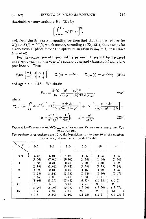
SEC. 8.7] EFFECTS OF VIDEO BAND WIDTH 219
threshold, we may multiply Eq. (22) by
[/
+-
1djv’(f)‘,—.and, from the Schwartz inequality, we then find that the best choice forX(j) is X(f) = V(j), which means, according to Eq. (21), that except fora nonessential phase factor the optimum solution is .%d = 1, or no videoJilterat all.
For the comparison of theory with experiment there will be discussedas a second example the case of a square pulse and Gaussian i-f and videopass bands. Then
{
=1, 121< *;~l(z) =0, [Zl > +; }
Zl(u) = e–”””; 21, vid(~) = e–%”’”’; (Zh)
and again a = 1.18. We obtain
2U’C (d + 4? J’)J$ 1Pm,. = —
630 (2XZYZ + 4Y4)M m’(23b)
where
(23c)
TAZLE 8.4.—VALUES OF (e/u2C)P~i~ FORIhFFERENT VALUES OF z AND v [CF. Em(23b) AND (23c)]
The numbers irr parentheses are 10 X the logarithms to the base 10 of the numbersimmediately above, i.e~ a “decibel” value.
\Y
z
0,2
1
2
5
11
15
0.1
6.38(8.04)3.88
(5. 89)4.52
(6. 55)6.45
(8.10)934(9 70)10,7
(10.3)
0.5
5,01(7. 00)2.34
(3. 69)2,84
(4.53)4.32
(6. 36)6.40
(806)7.39
(8, 69)
1,0
4,95(6. 94)2.33
(3, 68)3.27
(5. 14)5.53
(7,43)8,39
(9.24)9.55
(9. 80)
5.0
4,95(6. 94)2.39(3. 79)4,15(6. 18)9.60
(9.82)17.2
(12 36)22.8
(13.58)
10
4.95(6. 94)2.39(3. 79)4.22
(6. 26)10.3
(10.13)20,9(13.20)26.3
(14.2)
co
4 95(6.94)2.39
(3. 79)4.23(6.27)10,5
(10.2)23.3
(13,67)31.8
(15.02)
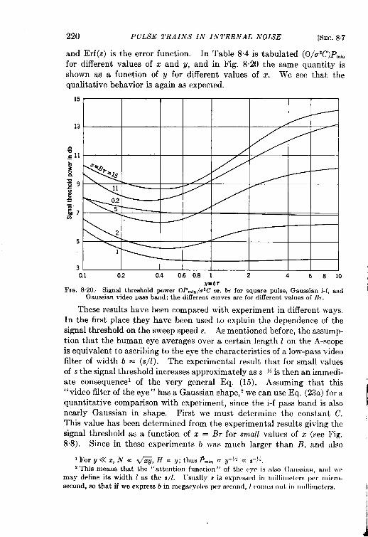
220 PULSE TRAINS IN INTERNAL NOISE [SEC.87
and Erf(z) is the error function. In Table 8-4 is tabulated (f3/u2C)PtiDfor different values of x and y, and in Fig. 8.20 the same quantity isshown as a function of ~ for different values of x. We see that thequalitative behavior is again as expemed.
15 1
13
5
310,1 0.2 0.4 0.6 0.8 1 2 4 6 8 10
u=bTFm. 8.20.—Signalthreshold power13Pmti/LT*Cm. br for squarepulse,Gaussiani-f, and
Gaussianvideopassband;the differentcurvesarefor differentvaluesof BT.
These results have been compared with experiment in different ~vays.In the first place they have been used to explain the dependence of thesignal threshold on the sweep speed s. As mentioned before, the assump-tion that the human eye averages over a certain length 1 on the A-scopeis equivalent to ascribing to the eye the characteristics of a low-pass videofilter of width b = (s/1). The experimental result that for small valuesof s the signal threshold increases approximately as s–~~is then an immedi-ate consequence of the very general Eq. (15). Assuming that this“video filter of the eye” has a Gaussian shape,’ we can use Eq. (23a) for aquantitative comparison with experiment, since the i-f pass band is alsonearly Gaussian in shape. First we must determine the constant C.This value has been determined from the experimental results giving thesignal threshold as a function of z = 11~for small values of z (see Fig.8.8). Since in these experiments b was much larger th:m B, and also
lFory<<z, N= &,Hmg;tht]sP~in my —>1= ~—)~,
2This means that the “attention function” of tbc cyr is nlso C,:lllssi:m,and \vrmay define its width 1 as the s/1. tlslmlly s is cxpresswlill nlillitnctcrs per n)irro-second, so that if we express b in mrgacyrlrs pm scrond, I CO]))(Wm]i in )Ilillimct.ws. i
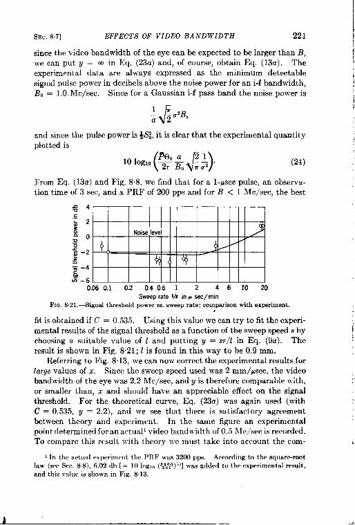
SEC.8.7] EFFECTS OF VIDEO BAND WIDTH 221
since the video bandwidth of the eye can be expected to be larger than B,we can put y = ~ in Eq. (23a) and, of course, obtain Eq. (13a). Theexperimental data are always expressed as the minimum detectablesignal pulse pow-er in decibels above the noise power for an i-f bandwidth,BO = 1.0. Me/see. Since for a Gaussian i-f pass band the noise power is
and since the pulse power is ~i3~,it is clear that the experimental quantityplotted is
10 IOg’”e:J$)”(24)
From Eq. (13cz) and Fig. 8“8, we find that for a l-psec pulse, an observa-tion time of 3 see, and a PRF of 200 pps and for B < 1 Me/see, the best
0.06 0.1 0.2 0.40.6 1 2 4 6 10 20SweeprateW inp sec/min
FIG. 8.21.—Signalthresholdpower m. swssprate; comparisonwith experiment.,
fit is obtained if C = 0.535. Using this value we can try to fit the experi-mental results of the signal threshold as a function of the sweep speeds bychoosing a suitable value of 1 and putting g = sr/1 in Eq. (9a). Theresult is shown in Fig. 8.21; 1 is found in this way to be 0.9 mm.
Referring to Fig. 8.13, we can now correct the experimental results forlarge values of z. Since the sweep speed used was 2 mm/psec, the videobandwidth of the eye was 2.2 Me/see, and g is therefore comparable with,or smaller than, z and should have an appreciable effect on the signalthreshold. For the theoretical curve, Eq. (23a) was again used (withC = 0.535, y = 2.2), and we see that there is satisfactory agreementbetween theory and experiment. In the same figure an experimentalpoint determined for an actual’ video bandwidth of 0.5 illc/sec is recorded.To compare this result with theory we must, take into account the com-
I In the act,~lalrxperimrnt the PRF wae 3200 pps, According to the square-rootlaw (SW= &=c. 8.8), 6.02 dh [ = 10 log,, (+~OoQ)>U]was added to the experimental rwndt,and this vtlae is shown in Fig. 8.13.
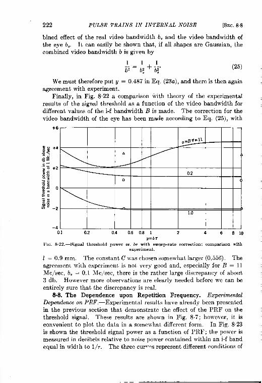
,.,,”,
Sig
nalth
resh
oldc
owerm
db
abov
en
oise
ma
band
wid
thof
1M
c/s
ee
A+
0&
a+ m
,..,..
IQ K)
10
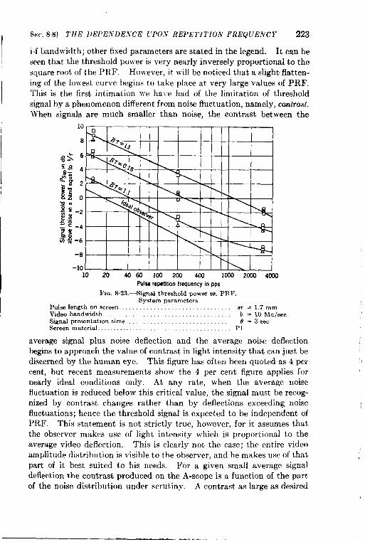
I
SW, 8.8] THE I)h’PE,VDE.VCE L’PO.V REPET[l’[ON FREQUENCY 223
i-f bandwidth; other fixed parameters are stated in the legend. It can beseen that the threshold power is very nearly inversely proportional to thesquare root of the PRF. However, it will be noticed that a slight flatten-ing of the lowest curve begins to take place at very large values of PRF.This is the first intimation we hare had of the limitation of threshold
signal by a phenomenon cliff erent from noise fluctuation, namely, contrast.
When signals are much smaller than noise, the contrast between the
6
-8 I I 1 I I I I w I I 1I 1
-lo~10204060 lm 200 400 1003 2c00 4000
Pulse repetition frequency in pps
FIG. 8.23,—Signalthresholdpower m. PRF.System parameters
Pulselength on screen. . . . . . . . . ,,. sr=l.7mmVideo bandwidth. . . . . . . . .,, ...,, b = 10 Mcjsec.Signalpresentationtime. b’=3secScreenmaterial. . . . . . . . . . . . . . ..” :.:::::::..:..:::P1
average signal plus noise deflection and the average noise deflectionbegins to approach the value of contrast in light intensity that can just bediscerned by the human eye. This figure has often been quoted as 4 percent, but recent measurements show the 4 per cent figure applies fornearly ideal conditions only. At any rate, when the average noisefluctuation is reduced below this critical value, the signal must be recog-nized by contrast changes rather than by deflections exceeding noisefluctuations; hence the threshold signal is expected to be independent ofPRF. This statement is not strictly true, however, for it assumes thatthe observer makes use of light intensity which is proportional to tbeaverage video deflection. This is clearly not the case; the entire videoamplitude distribution is visible to the observer, and he makes use of thatpart of it best suited to his needs. For a given small average signaldeflection the contrast produced on the A-scope is a function of the partof the noise distribution under scrutiny, A contrast as large as desired
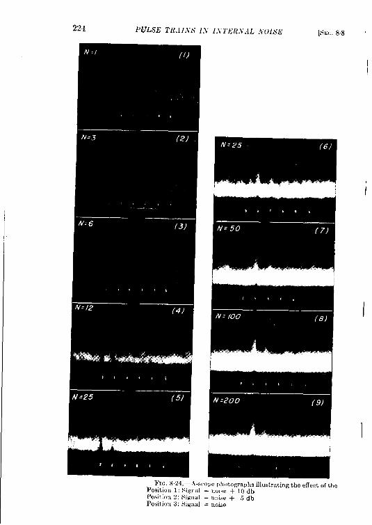
224 PULSE TILiI.VS I.h- 1.V TlilLV.lL iVt)[SE
I
I
I
I?IG.8.24.—A-s.ope photographsillustratingthe effect of thePosition 1: Sig],:d = noi.c + 10dbPosition 2: Si~r,aI = noiw + 5 dbPositiou 3: Signal = nOise
4
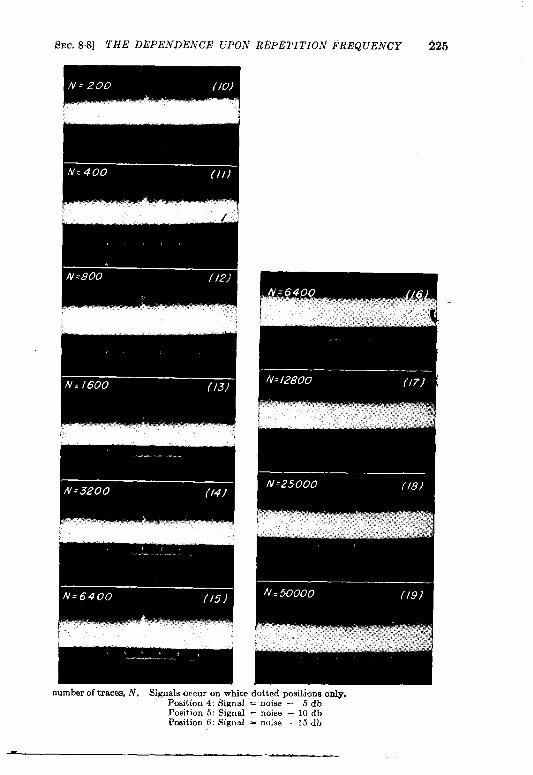
SEC.8.8] THE DEPENDENCE UPO;V REPE1’ITION FREQUENCY 225
m.##
m.,08
~. .-., ..,.. .
,
numberof traces,N. Signalsoccur on whitePosition 4: SignalPosition 5: SignalPosition 6: Signal
: dotted positionsonly.= noise — .5db= noise - 10db= noise — 15db
--—
226 PULSE TRA I,V,9 I.V I.VTER.VA L .VOISE [SEC. 8%
can be obtained by looking high enough in the distribution. Theessential price that is paid in this procedure is the small fraction of timethat the video voltage is observed high in the distribution. Ho\vever, if~veare ~villing to ~rait long enough and have as many signal slreeps as aredesired, enough observations could be made in the high part of the dis-tribution so that a proper statistical reading could be made. In this~vay, even with limited contrast discernibility, the observer should beable to see as small a signal as he pleases if enough signal sweeps are pre-sented to him. However, the dependence of signal threshold power ontotal signal sweeps will not follow the same law; it can be shown thatwhen limited by contrast the signal threshold power changes only slightlywith tremendous changes in the number of signal sweeps. We shouldexpect the transition between the two regions of different behavior tooccur for a signal whose video deflection is a few per cent of the averagenoise deflection, i.e., one whose i-f power is a few per cent of the i-f noisepower. This expectation is substantiated by experiment; when therelative signal-to-noise power in the i-f amplifier approaches —10 or —15db, the contrast limitation becomes easily apparent.
In order to demonstrate this effect and to give the reader a clearpicture of the various processes involved, a series of photographs weretaken of the A-scope. These photographs (Fig. 8.24) differ from eachother only in the number of sweeps that are recorded. In each photo-graph six signal positions are indicated along the base line by small whitedots, but for this series of photographs the signal does not occur randomlYon one of the six signal positions. Signals on the first position alwayshave a power 10 db relative to noise power in an i-f band of width equalto l/~. Similarly signals appearing on positions 2 to 6 have powers of+5, O, – 5, – 10, and – 15 db relati~-e to the same noise power. In eachphotograph two signals occur on adjacent positions, so chosen thatgenerally one signal is easily visible while the other one is not. As the\veakersignal becomes more visible, through a change in the total numberof sweeps, the stronger signal is reduced in intensity to the appropriateYalue and moved to the appropriate signal position. The various systemparameters that apply to these photographs are stated in the figurelegend.
The first photograph shows a single A-scope trace, i.e., N, = 1 withsignals occurring in positions 1 and 2. The stronger first signal is visiblewith some difficulty, while the second signal is probably below thethreshold value. As the number of sweeps is increased in the succeedingphotographs, smaller and smaller signals become discernible; a reductionof threshold signal power of about 5 db is possible for every increase inNs by a factor of 10. This procedure continues until the signal reaches apower of – 10 db relative to noise.
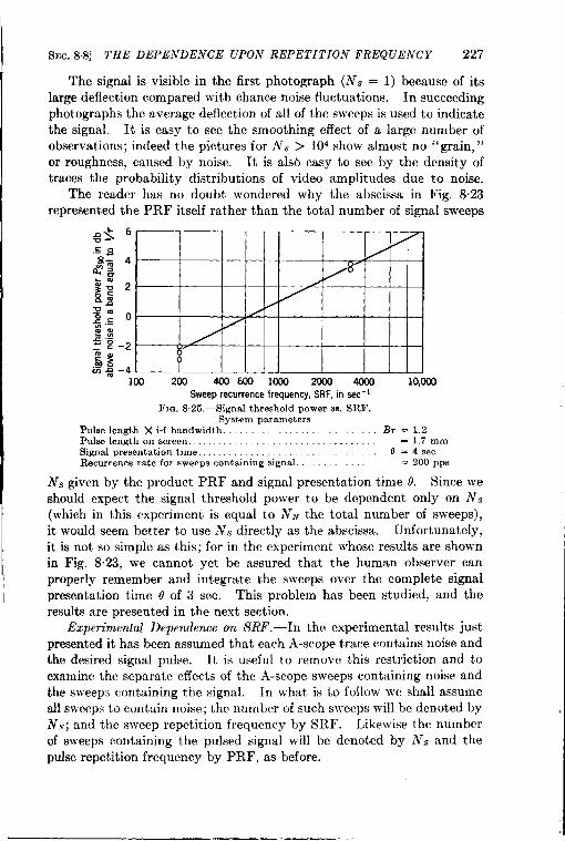
SEC.8.8] THE DEPENDENCE UPON REPETITION FREQUENCY 227
The signal is visible in the first photograph (N. = 1) because of itslarge deflection compared with chance noise fluctuations. In succeedingphotographs theaverage deflection of all of thesweeps isused to indicatethe signal. It is easy to see the smoothing effect of a large number ofobservations; indeed the pictures for Ns > 104 show almost no “grain,”or roughness, caused by noise. It is also easy to see by the density oftraces the probability distributions of video amplitudes due to noise.
The reader has no doubt wondered why the abscissa in Fig. 8.23represented the PRF itself rather than the total number of signal sweeps
,.100 20U 4OO6OO1OOO2WO4OOO 10,OOO
Sweeprecurrencefrequency,SRF,insec-1FIG. 8.25.—SignaIthresholdpoweros. SRF.
System parametersPulse length Xi-f bandwidth. . . . . . . .. Br=l.2Pulse length onscreem . . . . . = 1.7mm8ignalpresentati0n time..... tJ=4secRecurrencerate for sweepscontainingsignal. = 200pps
N. given by the product PRF and signal presentation time 0. Since weshould expect the signal threshold power to be dependent only on N8(which in this experiment is equal to N~ the total number of sweeps),it would seem better to use Ns directlv as the abscissa. Unfortunately,it is not so simple as this; for in the experiment whose results are shownin Fig. 8.23, we cannot yet be assured that the human observer canproperly remember and integrate the sweeps over the complete signalpresentation time o of 3 sec. This problem has been studied, and theresults are presented in the next section.
Experimental Dependence on SRF.—In the experimental results justpresented it has been assumed that each A-scope trace contains noise andthe desired signal pulse. It is useful to remove this restriction and toexamine the separate effects of the A-scope sweeps containing noise andthe sweep, containing the signal. In what is to follow we shall assumeall sweeps to contain noise; the number of such sweeps will be denoted byN~; and the sweep repetition frequency by SRF. Likewise the numberof sweeps containing the pulsed signal will be denoted by Ns and thepulse repetition frequency by PRF, as before.
—.— .-
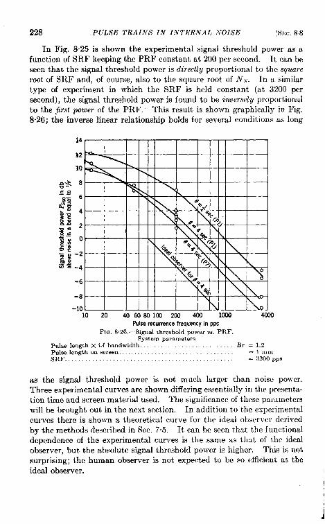
228 PULSE TRAINS IN INTERNAL NOISI{ [SEC. 8.8
In Fig. 8.25 is shown the experimental signal threshold power as afunction of SRF keeping the PRF constant at 200 per second. It can beseen that the signal threshold power is directly proportional to the squareroot of SRF and, of course, also to the square root of N~. In a similartype of experiment in which the SRF is held constant (at 3200 persecond), the signal threshold power is found to be inversely proportionalto the first power of the PRF. This result is shown graphically in Fig.8’26; the inverse linear relationship holds for several conditions as long
14
12
10
8
6
2 I I I 1 I u \
n hk%u
3Z.4
-6
-8 -
-1010 20 406OSO1OO 200 m low WM
Pulserecurrencefrequencyin pps
FIQ. S.26.—Signalthresholdpower VS.PRF.System parameters
Pulse length Xi-f bandwidth. . . . . . . . . . . . . . . . . . . . .. B7 =1.2Pulse length on screen. . . . . . . . . . =ImmSERF. . . . . . . . . . . . . . . . . . . . . . . . . . . . = 3200Pps
as the signal threshold power is not much larger than noise power.
Three experimental curves are shown differing essentially in the presenta-
tion time and screen material used. The significance of these parameters
will be brought out in the next section. In addition to the experimental
curves there is shown a theoretical curve for the ideal observer derived
by the methods described in Sec. 7.5. It can be seen that the functional
dependence of the experimental curves is the same as that of the ideal
observer, but the absolute signal threshold power is higher. This is not
surprising; the human observer is not expected to be so efficient as the
ideal observer.
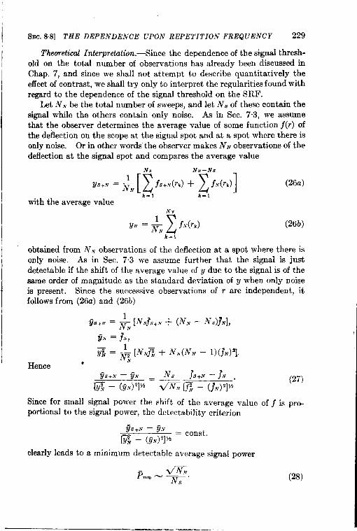
SEC. 8.8] THE DEPENDENCE UPON REPETITION FREQUENCY 229
Theoretical Interpretitwn.-Since thedependence of thesignal thresh-old on the total number of observations has already been discussed inChap. 7, and since we shall not attempt to describe quantitatively theeffect of contrast, we shall try only to interpret the regularities found withregard to the dependence of the signal threshold on the SRF.
Let N. be the total number of sweeps, and let Ns of these contain thesignal while the others contain only noise. As in Sec. 7.3, we assumethat the observer determines the average value of some function j(r) ofthe deflection on the scope at the signal spot and at a spot where there isonly noise, Or in other words the observer makes NN observations of thedeflection at the signal spot and compares the average value
N, N,v-Ns
1“+” = T. [z
fS+N(rk) +2
fN(d
k=l k=lwith the average value
NV1
‘“ = TN zfN(rk)
k=l
(26a)
(26b)
obtained from NN observations of the deflection at a spot where there isonly noise. As in Sec. 7.3 we assume further that the signal is justdetectable if the shift of the average value of y due to the signal is of thesame order of magnitude as the standard deviation of y when only noiseis present. Since the successive observations of T are independent, itfollows from (26a) and (26b)
VS.. = ~, [Ns.i’s+N+ (NN – N.s)]N1,
~. = 3N,
fi = & [NN~ + NN(NN – 1)(]N)7N
Hence 0N, ~s,N - j’.~s+N — fl~ _
[~ – (?iN)2]W fi [~ – (].)’]%”(27)
Since for small signal power the shift of the average value of f is pro-portional to the signal power, the detectability criterion
clearly leads to a minimum detectable average signal power
V“aPm.-—.
N, (28)
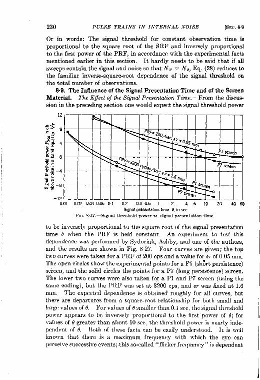
230 PULSE TRAINS IN INTERNAL NOISE [SEC.89
Or in words: The signal threshold for constant observation time isproportional to the square root of the SRF and inversely proportionalto the first power of the PRF, in accordance with the experimental factsmentioned earlier in this section. It hardly needs to be said that if allsweeps contain the signal and noise so that i?N = Ns, Eq. (28) reduces tothe familiar inverse-square-root dependence of the signal threshold onthe total number of observations.
8.9. The Infiuence of the Signal Presentation Time and of the ScreenMaterial. The Effect of the Signal Presentation Time. —From the discus-sion in the preceding section one would expect the signal threshold power
Signalpresentationtime, .9, in sec
FIG. S27.-Signal thresholdpower w. signalpresentationtime,
to be inversely proportional to the square root of the signal presentationtime @ when the PRF is held constant. An experiment to test thisdependence was performed by Sydoriak, Ashby, and one of the authors,and the results are shown in Fig. 8.27. Four curves are given; the toptwo curves were taken for a PRF of 200 cps and a value for STof 0.05 mm.The open circles show the experimental points for a PI (sh~rt persistence)screen, and the solid circles the points for a P7 (long persistence) screen.The lower two curves were also taken for a PI and P7 screen (using thesame coding), but the PRF was set at 3200 cps, and STwas fixed at 1.6mm. The expected dependence is obtained roughly for all curves, butthere are departures from a square-root relationship for both small andlarge values of 0. For values of 0 smaller than 0.1 see, the signal thresholdpower appears to be inversely proportional to the first power of 0; forvalues of o greater than about 10 see, the threshold power is nearly inde-pendent of 0. Both of these facts can be easily understood. It is wellknown that there is a maximum frequency with which the eye canperceive successive events; this so-called “flicker frequency” is dependent
SEC, 89] THE INFLUENCE OF THE SIG,VAL PRILSENTATIO.V TIME 231
on many factors but usually lies between 10 and 60 cps. It thereforefollows that if the slveeps are being continuously presented on the A-scope,the total number of cff’ective noise s\~eeps\rill nmrcr bc smalle: thun thatgiven by the produrt of the I>RF and tlic minimum rcsol{ition time of theeye. Under conditions Jvhere e is very short, therefore, It-eshoul(l expectNN to be constant and from Eq. (28) the signal threshold polver to beinversely proportional to the first power of JV.$, The transition betweenthe regions of different dependence is expected to occur where 6 is of theorder of the reciprocal of the flicker frequency, i.e., somelvhat less than0.1 sec. This result is precisely what is obseryed in Fig. 8.27.
It is clear that the human observer will not be able to integrateproperly what he sees over a very long time. If we assume him to havea finite “memory” time, ~ve should expect the threshold signal to benearly independent of @ ~rhen 0 exceeds the memory time. This followsbecause the total number of effecti}’e signal and noise sweeps, i.e., thoseoccurring ~vithin the memory interval, is independent of 8. From aninspection of Fig, 8.27 it can be seen that the effective memory timeappears to be perhaps 10 sec. It is not surprising that there is not asudden transition region for the effect; one ~vould indeed be astonished ifthe human memory time ~vere characterized by sharply defined limits.
Nevertheless, the human memory time appears to be long enough sothat only slight help is noticeable in using the P7 screen, whose longpersistence acts to integrate noise and signal over a relatively long period.It has heen found by Sydoriak, Ashby, and one of the authors that train-ing an observer appears primarily to lengthen his memory time.Untrained observers may find the 1’7 screen much more sensitive than thePI, although, as training proceeds, the scoring on the P1 screen improvesto nearly that measured on the P7 screen.
It may seem surprising that in the curves for the P7 screen at smallvalues of t?,a rapid departure from the P1 results does not occur. If theP7 screen integrates all sweeps over an interval of a few seconds, it wouldbe expected to yield a signal threshold power inversely proportional tothe first power of @ for values of o less than this integration interval.This was not observed; it is believed to be caused by the existence of theshort-persistence initial “ flash” on the P7 screen. For small values of ethis flash causes the P7 to act very much like the PI screen.
It is possible to check the assumption that was made concerning theminimum resolution time of the eye and brain. It was stated that forvery small values of d, the total number of effective noise sweeps wasindependent of 8 because of this minimum resolution time. However, itis possible to conduct the experiment so that only the sweeps containingthe signal (and noise) are presented on the A-scope. This can be done bythe commutator shown near the upper left-hand corner of Fig. 8.1.
232 PULSE TRAINS IN INTERNAL NOISE [SEC.8.10
For this type of experiment the signal threshold power would be expectwlto be inversely proportional to the square root of I?,even for the smallestvalues of 0. This is just what is experimentally observed.
The Ej7ect o.i the Screen Material.—Evidence has just been presentedthat shows the effect on threshold signal of the use of different A-scopescreen materials. The chief characteristic of the screen with which weare concerned is the time required for the light to decay after excitation.Screen materials are now available that show widely different life times;the PI screen is the most commonly used short-lived material, and the P7the most widely used long-lived material. The decay of light from thesescreens is not exponential; it follows more closely a law given by thereciprocal of the time. In the P7 screen an appreciable amount of lightcan be observed several seconds after excitation, while in the P 1 screen noappreciable light remains after perhaps 0.1 sec.
In any case the persistence of the screen may be thought of as an aidin the integration of multiple sweeps, a process that has just been dis-cussed. The degree to which this integration aids in detecting a signaldepends upon how effective the observer memory time is. It has beenshown in Fig. 8.27 that for a trained observer the signal threshold poweris only slightly influenced by the added effect of screen integration. Thegreatest influence, of course, is felt where the signal presentation time islong; where the latter parameter is a few seconds, the P7 screen showsperhaps a 2-db lower signal threshold power than does the P1 screen.
It is the importance of the observer memory time that led to theearly disappointment in the use of long-persistence screens. It was atfirst believed that a substantial reduction in threshold signal would beobserved because of the screen integration. We now know that suchintegration will not be effective in reducing the threshold signal powerunless the screen life time exceeds by a substantial factor the observermemory time. Even so, a better method is a photographic process.Information can be stored on a photographic film over as long a period oftime as is necessary. This procedure is easily demonstrated by observa-tion of the photographs of Fig. 8.24. However, the usefulness of suchphotographic storage is greatly limited by the contrast requirements ofthe observer, already discussed, and the extremely long time inevitablyrequired for signal detection. Furthermore scanning requirements andtarget motion reduce its utility.
8.10. The Dependence upon the Number and Spacing of PossibleSignal Positions and upon the Attention Interval. The Dependence uponthe Number and Spacing ojPossible Signal Positions.—It was categoricallystated in Sec. 8.3 that the signal threshold power increases with the numberof possible signal positions. The phenomenon is shown graphically inFig. 8.28 where the ordinate represents the signal threshold power in
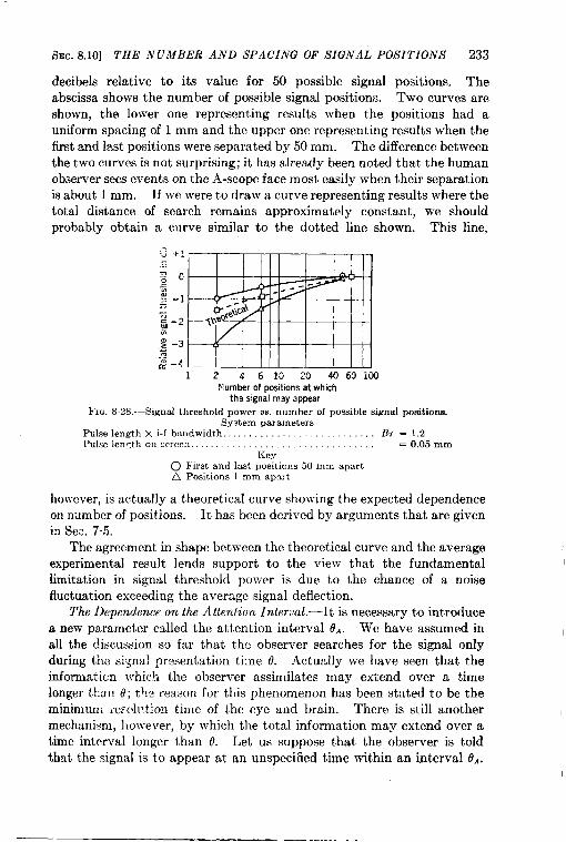
SEC. 8.10] THE N UMBER AND SFIACING OF SIGNAL POSITIONS 233
decibels relative to its value for 50 possible signal positions. Theabscissa shows the number of possible signal positions. Two curves areshown, the lower one representing results when the positions had auniform spacing of 1 mm and the upper one representing results when thefist and last positions were separated by 50 mm. The difference betweenthe two curves is not surprising; it has already been noted that the humanobserver sees events on the A-scope face most easily when their separationis about 1 mm. If we were to draw a curve representing results where thetotal distance of search remains approximately constant, we shouldprobably obtain a curve similar to the dotted line shown. This line,
.d +1c-.
~c%w -157,~-zG,: -3%. .; —4
12 461020 40 60 1(KI}!umber of positions at which
ths signal may appear
FIG. S,2S.-–Signaltbrcsholdpower VS.numberof possiblesignalpositions.System parameters
Pulse length Xi-f bmLdwidth. . . . . . . . . B7 =1.2Pulsclc:lzth cll.crccx . . . . . . ,. = 0.05mm
KeyO First and last positions50 mm apartA Positions 1 mm apart
hotrcver, is actually a theoretical curve sho~ving the expected dependenceon number of positions. It has been derived by arguments that are givenin Se:. 7.5.
The agreement in shape between the theoretical curve and the averageexperimental result lends support to the view that the fundamentallimitation in signal threshold power is due to the chance of a noisefluctuation exceeding the average signal deflection.
The Dependence on the Attention Inter~al.—It is necessary to introducea new parameter called the attention interval d~. We have assumed inall the discussion so far that tho observer searches for the signal onlyduring tile siSnal presentation time O. .4ctually we have seen that theinformation which the observer assimilates may extend over a timelonger tlxu~ 0; the reason for this phenomenon has been stated to be theminimum ms{l~l.tion time of the eye and brain. There is still anothermechanism, holvever, by which the total information may extend over atime interval longer than f?. Let us suppose that the observer is toldthat the signal is to appear at an unspecified time within an titerval 8A.
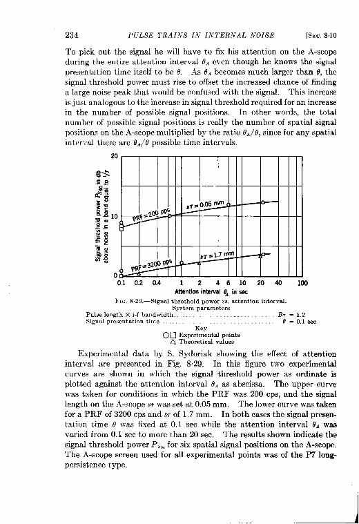
234 PULSE TRAINS [N I,V1’ERNAL NOISE [SEC. 8.10
To pick out the signal he will have to fix his attention on the A-scopeduring the entire attention interval tiAeven though he knows the signalpresentation time itself to be 0. As 8. becomes much larger than 0, thesignal threshold power must rise to offset the increased chance of findinga large noise peak that would be confused with the signal. This increaseis just analogous to the increase in signal threshold required for an increasein the number of possible signal positions. In other words, the totalnumber of possible signal positions is really the number of spatial signalpositions on the A-scope multiplied by ~he ratio d.4/d, since for any spatialInter-,’al there are 19*/dpossible time intervals.
{1 0.2 0.4 1 2 4610 20 40 100Attention interval ~ in sac
l’1~. S.29.—Signal thresholdpower OS.attention interval.System parameters
Pulse length Xi-f bandwidth..,.. .%= 1,2Signalprcsentatio ntim e..,.. e = 0,1 Sec
Keyon Experimentalpoints
A Theoretical values
llxperimental data by S. Sydoriak showing the effect of attention
interval are presented in Fig. 8.29. In this figure two experimental
curves are shown in which the signal threshold power as ordinate is
plotted against the attention interval 0. as abscissa. The upper curve
was taken for conditions in which the PRF was 200 cps, and the signal
length on the A-scope STwas set at 0.05 mm. The lower curve was taken
for a PRF of 3200 cps and s, of 1.7 mm. In both cases the signal presen.
tation time 6 was fixed at 0.1 sec while the attention interval (?A was
varied from 0.1 sec to more than 20 sec. The results shown indicate the
signal threshold power I’s,, for six spatial signal positions on the A-scope.
The A-scope screen used for all experimental points was of the P7 long-
persistence type.
SEC.8.10] THE NUMBER AND SPACING OF SIG.VAL POSITIONS 235
Three types of coded points are indicated on the diagram; two of theseare experimental points, and the third represents theoretical results to bediscussed below. The open circles show the experimental points obtainedwhen the attention interval was defined to the observer by ringing a bellat its beginning and end. It was soon appreciated that for small valuesof attention interval the reactiontime of the observer would causehis attention to be spread over atime interval not necessarily iden-tical with the interval selected forthe appearance of the signal.This defect was remedied by trig-gering the A-scope trace only dur-ing the desired attention interval,thereby giving the observer infor-mation during the specified timeonly. This procedure yielded theexperimental points indicated bysquares. To show how the ex-perimental curves agree withsimple theoretical considerations,three theoretical points, shown bytriangles, are indicated on thelower curve. These have beenderived from calculations made byM. C. Wang following a sugges-tion of E. M. Purcell. Using theprobability distributions derivedin Sec. 7“5, she has, calculated theprobability w that a given possi-ble signal position will display alarger deflection due to noise thanthe position actually occupied by
124816 s26~Numberof observations,N
FIG. 8.30.—Signal power w. number ofobservations N for various values of w. Thesymbol w represents the probability that anoise deflection exceeds the deflection of sig-nal plus noise.
the signal itself. The probability w
depends on the number of pulses N and on the signal strength. Theresults of these calculations are shown in Table 2.1 of Vol. 1 of thisseriesl and are reproduced in Fig. 8“30, where for various values of w thesignal strength is plotted against the number of observations, N.
For a given criterion of threshold signal one must require the prob-ability w to be inversely proportional to the total effective number ofsignal positions. For the system parameters of Fig. 8.29 and with thethreshold power adjusted at one point in order to take into account the
1Ridenour, Radar System Engineering, Vol. 1, Radiation Laboratory Series, p. 39.
————.
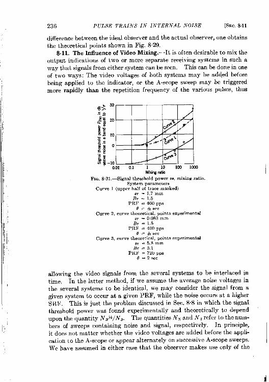
,,
,,
236 PULSE TRAINS IN INTERNAL NOISE [SEC. 8.11
difference between the ideal observer and the actual observer, one obtainsthe theoretical points shown in Fig. 8.29.
8.11. The Influence of Video Mixing.-It is often desirable to mix theoutput indications of two or more separate receiving systems in such away that signals from either system can be seen. This can be done in oneof two ways: The video voltages of both systems may be added beforebeing applied to the indicator, or the A-scope sweep may be triggeredmore rapidly than the repetition frequency of the various pulses, thus
h?.og> c,E ~
$j ~.
?E~zX2 ~~S.g .~$% og .5
$i-1:, ,_ ,~,
Mkhg ratk!
Fm. 8.31.%ignal thresholdpower m. mixing ratio.System parameters
Curve 1 (upper half of trace masked)m = 1.7mm
BT = 1.5PRF = 400ppS
t?=*secCurve 2, curve theoretical, points experimental
m = 0.083mmB, = 1.5
PRF = 400 ppS.9=&sec
Curve 3, curve theoretical, points experimentalST = 5.8 mm
BT = 5.1PRF = 720ppS
8=28ec
allowing the video signals from the several systems to be interlaced intime. In the latter method, if we assume the average noise voltages inthe several systems to be identical, we may consider the signal from agiven system to occur at a given PRF, while the noise occurs at a higherSRF. This is just the problem dkcussed in Sec. 8“8 in which the signalthreshold power was found experimentally and theoretically to dependupon the quantity N.#/N,. The quantities N. and Ns refer to the num-bers of sweeps containing noise and signal, respectively. In principle,it does not matter whether the video voltages are added before the appli-cation to the A-scope or appear alternately on successive A-scope sweeps.We have assumed in either case that the observer makes use only of the
SEC. 8.11] THE INFLIJENCli’ OF VIDEO bfIXING 237
average video deflections; therefore the two procedures should yieldsimilar results.
Let us now consider the more general case of the mixture of two videosystems (which we shall label Channel .4 and Channel B) in which theaverage noise power in the two channels may be unequal. If the noisein Channel B is much larger than that in Channel A, the threshold signalmeasured in Channel A will have to be greatly increased to overcome thegreatly increased noise background. On the other hand, the thresholdsignal measured in Channel B will be hardly affected by the slight increasein its noise due to Channel A. It is convenient to introduce a new para-meter, which we may call the mixing ratio. The mixing ratio is assumedto be unity when the video noise levels in the two channels are equal.Let us assume for the sake of simplicity that in this condition the i-fpower gains GAand G, for Channels A and B, respectively, are also equal.
Under general conditions the mixing ratio MA for Channel A will then be
given by the ratio G~/G~, while the mixing ratio MB for Channel B is theinverse, GA/GB. We may ask how the signal threshold power dependsupon these mixing ratios.
In Fig. 831 is plotted the experimental results for a two-channelmixing experiment. The system parameters are indicated in the legend.The signal threshold power is shown on the ordinate scale, while themixing ratio is indicated (logarithmically) on the abscissa. Three curvesare shown for different system parameters. Curves 2 and 3 have beencomputed using the deflect ion criterion of Sec. 7.3 in which the constantk has been adjusted to fit the experiments for very small mixing ratios.The open circles are experimental points taken by S. G. Sydoriak andseem to agree satisfactorily with the curves. However, the experimentalsquare points that were made with the upper half of the A-scope tracemasked lie about 5 db below the theoretical curve. This has been tracedto a peculiar method by which the observer recognizes the signal. Forlarge mixing ratios the signal in Channel A has practically no noiseassociated with it, therefore displaces the entire noise distribution ofChannel B by a fixed amount. Hence, just at the baseline the signalcreates a small open “hole” within which no noise fl~ctuations can beobserved. This small hole is clearly discernible if STis large enough andthe observer is no longer forced to average the entire noise deflection.The “mouse under the rug,” however, will not be apparent if STbecomessmaller than the spot size on the A-scope as is the case in Curve 2 of Fig.8.31. The “mouse under the rug” effect is not apparent in Curve 3perhaps because of the excessive value of ST.
CHAPTER9
PULSE TRAINS IN INTERNAL NOISE; OTHER METHODS OFPRESENTATION
In Chap. 8 an account was given of the factors that influence thresholdsignals which are displayed on an A-scope. It has been mentioned inChap. 2 that other forms of presentation are in wide use; indeed, for radarthe intensity-modulated display, such as the PPI or B-scope, is at presentmore widely used than any other display. For some applications thedetection of pulse trains by aural means is highly desirable, since by thismeans the observer’s eyes are free for other essential tasks. In thischapter an attempt is made to treat very briefly some of these displaysystems. They have not, however, been so intensively investigated asthe A-scope from the point of view of signal visibility, and in some caseseven the experimental observations are not completely understood.
INTENSITY-MODULATED DISPLAY (PPI)
9.1. Similarities to the A-scope.—In Sec. 2.6 a brief description wasgiven of the various commonly used intensity-modulated displays. Inall cases the signal causes the trace on a cathode-ray tube to brighten; theposition and direction of the trace is made to display appropriate coordi-nates of the antenna. In the ordinary PPI (plan-position indicator), thecathode-ray trace is caused to sweep radially outward from the center ofthe tube; range is indicated by the distance along a radius from the tubecent er. The sweep is oriented at an angle corresponding to the azimuthalangle of the antenna. In this fashion the face of the tube displays echosignals from reflect ing objects as bright spots; the positions of these spotson the tube face correspond to the actual positions of those objects withrespect to the antenna. It is this mapping feature of the PPI which hasmade it one of the most widely used display systems. The PPI willtherefore be treated in all the following discussions on intensity-modulateddisplays; the results are, with minor changes, expected to hold for otherintensity-modulated presentations, such as the B-scope (which displaysthe range-azimuth data in Cartesian coordinates).
The PPI differs from the A-scope in at least two ways. (1) To preventdefocusing of the cathode-ray spot by large signals, the strength of thevideo signal must be limited before application to the oscilloscope terminals. In practice one finds that this limiting action must occur even
238
A
SEC. 91] SIMILARITIES TO THE .4-SCOPE 239
for some of the normal noise distribution and, if carried too far, canprofoundly affect threshold signals. This fact ~vill be brought out inSec. 9.3. (2) '~hemanner in\vhich the PPIisused nearly al~vays bringsin a more or less complicated scartrtzrzgfactor. In the use of the A-scope,discussed in Chap. 8, it was assumed that the signal pulse train was ofuniform amplitude for a time o called the signal presentation time;however, as pointed out in Sec. 2.6, in the PPI the signal consists of afinite~pulse train (because of thenarrow antenna bear nscanningoverthetarget), which isrepeated from scan to scan. Wemay already anticipatefrom the A-scope results that this repetition feature may influence thresh-old signals through some form of integration; the extent of this influenceclearly must depend upon the memory time of the integrating device.These effects will be discussed in Sec. 9.2.
In addition to these new features of the PPI, there is an importantfeature that applies to both the PPI and the A-scope. In radar searchproblems one is seldom interested in the detection of stationary objectsproducing steady echoes. An echo from an airplane, for example, con-tinually fluctuates at rates that are generally functions of the nature ofthe aircraft, flying conditions, and the wavelength of the radar system.It is clear that the specification of threshold power for a fluctuating signalis more difficult than for a steady one. Some remarks and observationson this subject are given in Sec. 9.5.
In spite of the new features introduced by the PPI, much that hasbeen learned about the A-scope still applies. Most important, the basicideas that were developed for an understanding of the A-scope can becarried over to the PPI. This feature has eliminated a great deal ofexperimental labor.
The Influence of I-j Bandwidth. -As in the case of the A-scope (seeSec. 8.6), an important parameter is the product of i-f bandwidth B andthe signal pulse duration ~. A detailed experimental study of the effectof E%has not yet been made; preliminary work by R. R. Meijer and S. G.Sydoriak,’ however, has shown the same general behavior with the PPIas with the A-scope (see Fig. 8.7). There appears to be an optimumvalue of B7, above which the threshold signal power rises approximatelyproportional to the bandwidth and below which it rises approximatelyinversely proportional to the bandwidth. The reasons for this behaviorare the same as in the A-scope case. The essential difference betweenthe PPI and the A-scope curves, as indicated by the preliminary data, isthat the PPI curve is somewhat flatter and the minimum is shifted tosomewhat higher values of %. Neither of these characteristics is cer-tain; they should be verified by further experiments made under a widevariety of conditions.
] L’npublkhed.
~ —— .— ~.._. _ _
240 PULSE TRAINS IN INTERNAL NOISE [SEC. 9.1
The Injluenze of Video Bandwidth and Sweep Speed. -It has been
found that the effects of the video bandwidth and of the sweep speed are
interdependent, just as they were in the A-scope case (see Sec. 8-7).
The effect of sweep speed is, in fact, equivalent to a kind of video-band-width limitation; the connection between the two is made through thecharacteristics of the eye (and brain). In the A-scope case, experimentshowed that the eye was able to see signals most easily when the pulselength on the oscilloscope face STwas approximately 1 mm. Experimentson the PPI have shown exactly the same behavior; an experimental curvetaken by C. M. Allred and A. Gardner is shown in Fig. 9.1. Signal
@+4(L
zj3+2 ‘ \
Sg o \ A5=$ \ _ ,
3@ -;IJ4 0.060.1 0.2
~ ‘
0.4 0.6 1 2 4610.= .Pulselengthon screerie? in mm
FIG. 9.l.—Signal threshold M a function of puke length on the screen.System parameters
B, = 1.2 ream width = 6.o”PRF = 320 pp8 Scanning time = 10 see/rev
threshold power interrns of receiver noise power is plotted (logarithmically)as ordinate, and the pulse length on the tube face w is shown as absc~sa.The behavior of the threshold power is just the same as for the A-scope(e.g., cj. Fig. 8.18). The conditions under which Allred and Gardnertook the data were approximately as follows. The signal was made toappear at one of six random range positions at a defined azimuth (knownto the observer). The antenna beam width @ was constant at 6°, andthe scanning frequency was constant at 6 rpm. The ordinates shown inFig. 9.1 are PS,O, i.e., the signal power at 90 per cent correlation on the“betting” curve (see Chap. 8). During these experiments virtually nolimiting of video voltages was present.
While no detailed data on the influence of video bandwidth b (or moreproperly the quantity br) are yet available to the author’s knowledge,there is no information that indicates a markedly different dependence onthis parameter for the PPI and A-scope. It is entirely possible, however,that in the presence of severe limiting, different results will be obtained;the limiter serves as a highly nonlinear element that distorts both ampli-tude distributions and power spectra. Nevertheless, in the usual caseit is believed that the A-scope results will apply fairly well to the PPI.
There is, in addition to the connection between video bandwidth andsweep speed, a connection between video bandwidth and fecus. Thisfact was recognized in the A-scope case by the observation that defocusing
I
SEC. 92] THE lNFLUE.VCE OF SCANNING 241
in a direction parallel to the sweep was not serious so long as the spot sizedid not exceed 1 mm (see Sec. 8.7); this fact was in accord with the sweep-speed effect; for as long as the eye (and brain) partially neglects eventswith a spatial separation of less than 1 mm, defocusing of this order ofmagnitude was expected to have small effect. This same phenomenonhas been observed by R. Rollefson and J. L. Lawsonl on the PPI,Defocusing parallel to the sweep was not detrimental unless the spotexceeded 1 mm; defocusing in a direction perpendicular to the sweep hadno effect until the spot size exceeded the spatial size of the signal causedby the antenna beam angle O.
9s2. The Influence of Scanning. -It is through the process of scanningthat various time factors are introduced which correspond to the(A-scope) signal presentation time d. It is clear that because of thescanning frequency and the antenna beam width @ an effective signalpresentation time 0 exists for each scan. The pulse train may or may notbe repeated on subsequent scans, depending upon the conditions ofoperation. Scanning, therefore, involves time factors that are expectedto influence threshold signal power because of memory, or integration,effects. The main parameters with which we are concerned are (1)scanning frequency, (2) antenna beam angle O, (3) PRF. The signalpresentation time t9 can be obtained from (1) and (2). A completeireatment of integration effects, which will not be possible here, wouldalso include extra noise svieeps (see Sec. 8,8), screen material (see Sec.8.9), the number of possible signal positions (see Sec. 8.10), and the totallength of time the signal has existed. No experimental informationexists on extra noise sweeps, however. The screen material in a PPIis so universally P7 (long persistence) that data on other screen materialsare scarce. The signal will also be assumed to exist either for one scanor for an infinite number of scans. Finally, in most of the experimentsthat will be mentioned, only six signal positions (in range) were availableand those at a defined azimuth (known to the observer). This corre-sponds to the conditions most used in the A-scope experiments (see Chap.8) but does not necessarily represent the condition most often encounteredwith a PPI in actual radar use. Preliminary experiments have shownthat in accordance with the theoretical arguments of Sec. 8.10, an increasein the number of possible signal positions brings about a rise in thresholdsignal power. This is a relatively important consideration in a high-resolution PPI used for search purposes, where the number of possiblesignal positions (all ranges and all azimuths) can easily exceed 106.
The Effect of Beam Angle &.—We may anticipate the effect expected
by a change in the value of the antenna beam angle from the results of
Sec. 8.9. If the scanning frequency is constant, a change in @ is tanta-
1Unpublished data.
—
242 PULSE TRAINS IN INTERNAL NOISE [SEC. 92
mount to a change in signal presentation time 0 as long as the signalappears ononlyone scan, i.e., single-scan operation. For a constant PRF,one would therefore expect the threshold signal power to vary as ~~,and hence as 1#-~~;this result is expected only if integration or memoryexists over the entire interval 8 and if there is no inherent difference inthreshold power caused by the difference in geometrical shape of signalon the oscilloscope face.
0.01 0.05 0.1 0.5 1 5 10Signalpresentationtime Omsec
I0,45 4.5 45 450
Beamangle+ IndegreesFIG. 9.2.—Signal threshold as a function of the presentation time for constant rpm.
System parametersPulse length r = 1 psec
BT = 1.1s. = ().75 mm
Scanning time = 8 see/revPRF = S00 ppS
An experimental curve showing the effect of @ is reproduced in Fig.
9.2. The ordinate represents the signal threshold power (at 90 per cent
correlation) PS,O; the abscissa represents the antenna beam angle @plotted logarithmically. Also shown on the abscissa scale is the signalpresentation time d, which in this experiment is simply proportional to ~.The data ~rere taken for beam angles from 0.18° to 360°, correspondingto 0’s of 0.004 and 8 see, respectively; the PRF was held constant at 800pps and the scanning frequency was constant at 7.5 rpm. As can beseen, over most of the range the threshold power is proportional to ~–~~in accord with expectation; however, deviations exist at both ends of therange. For very large beam angles ( > 45°) it is lmderstandable thatsignals are less efficiently seen, since one cannot simultaneously view the
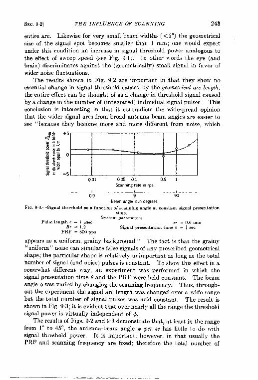
SEC.9.2] THE INFLUENCE OF SCANNING 243
entire arc. Likewise for very small beam widths ( < 1°) the geometricalsize of the signal spot becomes smaller than 1 mm; one would expectunder this condition an increase in signal threshold POwer analogous tothe effect of sweep speed (see Fig. 91). In other words the eye (andbrain) discriminates against the (geometrically) small signal in favor ofwider noise fluctuations.
The results shown in Fig. 9.2 are important in that they show noessential change in signal threshold caused by the geometrical arc length;
the entire effect can be thought of as a change in threshold signal causedby a change in the number of (integrated) individual signal pulses. Thisconclusion is interesting in that it contradicts the widespread opinionthat the wider signal arcs from broad antenna beam angles are easier tosee “because they become more and more different from noise, which
+5
o 4)
-50.01 0.05 0.1 0.5 1
Scanmng rate in rps
! I I
0.9 9 90Beamangle@indegrees
FIG, 9.3.—Signal threshold as a function of scanning angle at ccnmtsnt sigmd presentationtime.
System parametersPulse length r = 1 usec s, = 0.6 mm
BT = 1.2 Signal presentation time 0 = * secp RF = S00 ppS
appears as a uniform, grainy background. ” The fact is that the grainy“uniform” noise can simulate false signals of any prescribed geometricalshape; the particular shape is relatively unimportant as long as the totalnumber of signal (and noise) pulses is constant. To show this effect in asomewhat different way, an experiment was performed in which thesignal presentation time d and the PRF were held constant. The beamangle @ was varied by changing the scanning frequency. Thus, through-out the experiment the signal arc length was changed over a wide rangebut the total number of signal pulses was held constant. The result isshown in Fig. 9.3; it is evident that over nearly all the range the thresholdsignal power is virtually independent of ~.
The results of Figs. 9.2 and 9.3 demonstrate that, at least in the rangefrom 1° to 45°, the antenna-beam angle @ per se has little to do withsignal threshold power. It is important, however, in that usually thePRF and scanning frequency are fixed; therefore the total number of
—
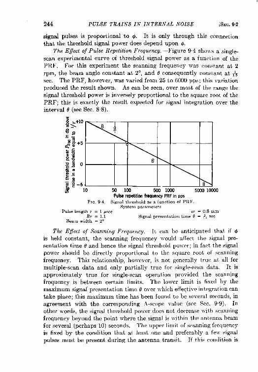
244 PULSE TRAINS IN INTERNAL NOISE [SEC.9.2
signal pulses is proportional to 4. It is only through this connection
that the threshold signal power does depend upon +.The Effect of Pulse Repetzt~on Frequency .-Figure 9“4 shows a single-
scan experimental curve of threshold signal power as a function of thePRF. For this experiment the scanning frequency was constant at 2rpm, the beam angle constant at 2°, and e consequently constant at ~sec. The PRF, however, was varied from 25 to 6000 pps; this variationproduced the result shown. As can be seen, over most of the range thesignal threshold power is inversely proportional to the square root of thePRF; this is exactly the result expected for signal integration over theinterval O (see Sec. 8“8).
FIG. 9.4.—Signal threshold aS a function of PRF.System parameters
Pulse length r = 1 *see sr = 0.S mmBT = 1.1 Signal presentation time @ = +3 sec
Beam width = 2°
The Effect of Scanning Frequency.—It can be anticipated that if ~
is held constant, the scanning frequency would affect the signal pre-sentation time 0 and hence the signal threshold po]rer; in fact the signalpower should be directly proportional to the square root of scanningfrequency. Thi~ relationship, however, is not generally true at all formultiple-scan data and only partially true for single-scan data. It isapproximately true for single-scan operation provided the scanningfrequency is between certain limits. The lower limit is fixed by themaximum signal presentation time o over which effegtive integration cantake place; this maximum time has been found to be several seconds, inagreement with the corresponding A-scope value (see Sec. 9.9). Inother words, the signal threshold pom-er does not decrease with scanningfrequency beyond the point where the signal is within the antenna beamfor several (perhaps 10) seconds. The upper limit of scanning frequencyis fixed by the condition that at least one and preferably a few signalpulses must be present during the antenna transit. If this condition is
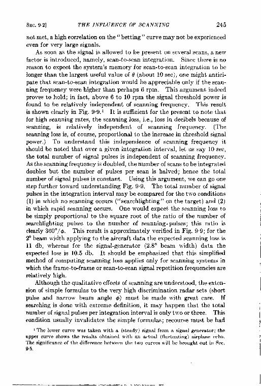
SEC. 92] THE INFLUENCE OF SCANNING 245
not met, a high correlation on the” betting” curve may not be experiencedeven for very large signals.
As soon as the signal is allowed to be present on several scans, a newfactor is introduced, namely, scan-to-scan integration. Since there is noreason to expect the system’s memory for scan-to-scan integration to belonger than the largest useful value of o (about 10 see), one might antici-pate that scan-to-scan integration would be appreciable only if the scan-ning frequency were higher than perhaps 6 rpm. This argument indeedproves to hold; in fact, above 6 to 10 rpm the signal threshold power isfound to be relatively independent of scanning frequency. This resultis shown clearly in Fig. 9.9.1 It is sufficient for the present to note thatfor high scanning rates, the scanning loss, i.e., loss in decibels because ofseaming, is relatively independent of scanning frequency. (Thescanning loss is, of course, proportional to the increase in threshold signalpower.) To understand this independence of scanning frequency itshould be noted that over a given integration interval, let us say 10 see,the total number of signal pulses is independent of scanning frequency.As the scanning frequency is doubled, the number of scans to be integrateddoubles but the number of pulses per scan is halved; hence the totalnumber of signal pulses is constant. Using this argument, we can go onestep further toward understanding Fig. 9.9. The total number of signalpulses in the integration interval maybe compared for the two conditions(1) in which no scanning occurs (“searchlighting” on the target) and (2)in which rapid scanning occurs. One would expect the scanning loss tobe simply proportional to the square root of the ratio of the number ofsearchlight ing pulses to the number of scanning. pulses; this ratio isclearly 3600/$. This result is approximately verified in Fig. 9.9; for the2° beam width applying to the aircraft data the expected scanning loss is11 db, whereas for the signal-generator (2.8° beam width) data theexpected loss is 10.5 db. It should be emphasized that this simplifiedmethod of computing scanning loss applies only for scanning systems inwhich the frame-to-frame or scan-to-scan signal repetition frequencies arerelatively high.
Although the qualitative effects of scanning are understood, the exten-sion of simple formulas to the very high discrimination radar sets (shortpulse and narrow beam angle O) must be made with great care. Ifsearching is done with extreme definition, it may happen that the totalnumber of signal pulses per integration interval is only two or three. Thiscondition usually invalidates the simple formulas; recourse must be had
1The lower curve was taken with a (steady) signal from a signal generator; theupper curve shows the results obtained with an actu[d (fluctuating) airplane echo.The significance of the difference bctwm-n the two curves will be brought out in Sec.9.5.
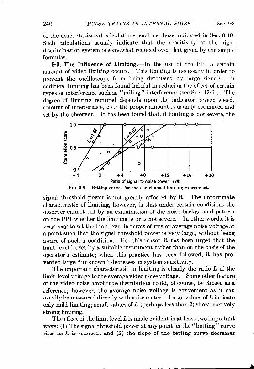
246 PULSE TRAINS IN INTERNAL NOISE [SEC. 93
to the exact statistical calculations, such as those indicated in Sec. 810.Such calculations usually indicate that the sensitivity of the high-discrimination system is somewhat reduced over that given by the simpleformulas.
9.3. The Influence of Limiting. -In the usc of the 1’1’1 a certainamount of video limiting occurs. This limiting is necessary in order toprevent the oscilloscope from being defocused by large signals. Inaddition, limiting has been found helpful in reducing the effect of certaintypes of interference such as ‘‘ railing “ interference (see Sec. 12.6). Thedegree of limiting required depends upon the indicator, sweep speed,amount of interference, etc.; the proper amount is usually estimated aridset by the observer. It has been found that, if limiting is not severe, the
1.0~g ~%m v.5 0.5 /;
G o0-4 0 +4 +8 +12 +16 +20
Ratio of signal to noise power in db
FICT.9.5.—Betting curves for the one-channel limiting experim ?nt.
signal threshold power is not greatly affected by it. The unfortunatecharacteristic of limiting, however, is that under certain conditions theobserver cannot tell by an examination of the noise background patternon the PPI whether the limiting is or is not severe. In other words, it isvery easy to set the limit level in terms of rms or average noise voltage ata point such that the signal threshold power is very large, without beingaware of such a condition. For this reason it has been urged that thelimit level be set by a suitable instrument rather than on the basis of theoperator’s estimate; when this practice has been followed, it has prevented large “unknown” decreases in system sensitivity.
The important characteristic in limiting is clearly the ratio L of thelimit-level voltage to the average video noise voltage. Some other featureof the video noise amplitude distribution could, of course, be chosen as areference; however, the average noise volt age is convenient as it canusually be measured directly with a d-c meter. Large values of L indicateonly mild limiting; small values of L (perhaps less than 2) show relativelystrong limiting.
The effect of the limit level L k made evident in at least two important
ways: (1) The signal threshold power at any point on the” betting” curve
rises as L is reduced: and (2) the slope of the betting curve decreases
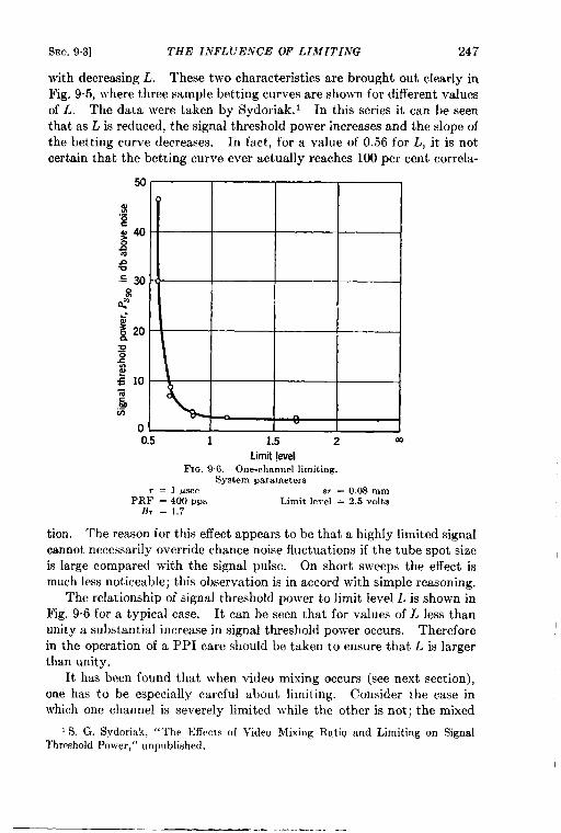
SEC. 9.3] THE INFLUENCE OF LIMITING 247
with decreasing L. These two characteristics are brought out clearly in
Fig. 9.5, where three sample betting curves are shown for different values
of L. The data were taken by Sydoriak. 1 In this series it can be seen
that as L is reduced, the signal threshold power increases and the slope of
the betting curve decreases. In fact, for a value of 0.56 for L, it is not
certain that the betting curve ever actually reaches 100 per cent correla-
limit levelFIG. 9.6. —One.channel limiting.
System parameters~=]~ec 8r = 0.0S mm
PRF = 400 ppS Limit level = 2,5 voltsB, = 1,7
tion. The reason for this effect appears to be that a highly limited signalcannot necessarily override chance noise fluctuations if the tube spot sizeis large compared with the signal pulse. On short sweeps the effect ismuch less noticeable; this observation is in accord with simple reasoning.
The relationship of signal threshold power to limit level L k shown inFig. 9.6 for a typical case. It can be seen that for values of L less thanunity a substantial increase in signal threshold power occurs. Thereforein the operation of a PPI care should be taken to ensure that L is larger
than unity.
It has been found that when video mixing occurs (see next section),
one has to be especially careful about limiting. Consider the case in
which one channel is severely limited \vhile the other is not; the mixed
1S. G. Sydoriak, “The Effects of Video Mixing Ratio and Limiting on Signal‘rhrmhold Power,” unpublished.
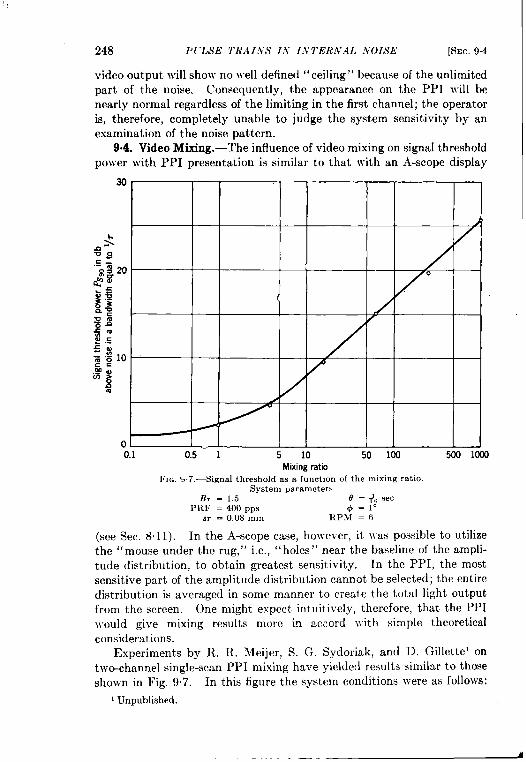
248 1’( “LSE TliAIhrS I,V I,V1’ERNAL NOISE [SEC,9.4
video output will show no ~velldefined “ceiling” because of the unlimitedpart of the noise. Consequently, the appearance on the PPI will benearly normal regardless of the limiting in the first channel; the operatoris, therefore, completely unable to judge the system sensitivityy by anexamination of the noise pattern.
904. Video Mixing.-The influence of video mixing on signal thresholdpower with PPI presentation is similar to that with an A-scope display
T1
I
-1-I
I
0.5Mixing ratio
FIG. >.7.—Signal threshold as a function of the mixing ratio.System parameters
B, = 1.5 0 = +6 SecPRF = 400 ppS .$=l.
w = 0.0S mm RP,M = 6
(see Sec. 8“11). In the A-scope case, hmvever, it VM possible to utilizethe “mouse under the rug, ” i.e., “holes” near the baseline of the ampli-tude distribution, to obtain greatest sensitivity. In the PPI, the mostsensitive part of the amplitude distribution cannot be selected; the entiredistribution is averaged in some manner to create the total li~ht outputfrom the screen. (he might expect intuitively, therefore, that the PPIwould give mixing results more in accord ~vith simple theoreticalconsiderations.
Experiments by R. R. Meijer, S. G. Sydoriak, and D. Gillette’ ontwo-channel single-scan PPI mixing have yielded results similar to thoseshown in Fig. 9.7. In this figure the system conditions were as follows:
1Unpublished,
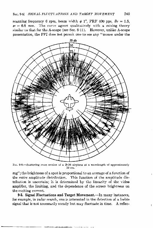
SEC. 95] SIGNAL FL.VCTtIA TIONS AND TARGET MOVEMENT 249
scanning frequency 6 rpm, beam width @ 10, PRF 400 pps, B7 = 1.5,SY= 0.8 mm. The curve agrees qualitatively with a mixing theorysimilar to that for the A-scope (see Sec. 8.11). However, unlike A-scopepresentation, the PPI does not permit one to see any “mouse under the
35 clb
FIG. 9+3.—Scattering cross section of a B-26 airplane at a wavelength of approximately10cm.
rug”; the brightness of a spot is proportional to an average of a function ofthe entire amplitude distribution. This function of the amplitude dis-tribution is uncertain; it is determined by the linearity of the videoamplifier, the limiting, and the dependence of the screen brightness on
the exciting current.9.5. Signal Fluctuations and Target Movement.—In many instances,
for example, in radar search, one is interested in the detection of a feeblesignal that is not necessarily steady but may fluctuate in time. A reflec-
lm.
250 PIJLSE TRAINS I.V I.VTERNAL NOISE [SEC. 9.5
tion patternl from a B-26 airplane is shown in Fig. 9.8 to help the reader
appreciate the magnitude of such fluctuations. This pattern wasobtained on a special automatic recording device that plotted the relativeback-reflected signal strength (at a wavelength of approximately 10 cm)as a radial deflection on the diagram. A B-26 airplane was placed on theground and slowly rotated in azimuth with respect to the incident (andreflect ed) radiation; the azimuthal coordinate of the airplane was auto-matically recorded on the diagram in Fig. 9.8. Care was taken toilluminate the airplane uniformly without appreciable reflection from theground. Although it is true that the finished plot does not representcorrectly the reflection pattern of a B-26 in flight (because of differentaspect, etc. ), it does show clearly the type of detailed structure and theextent to which the reflection intensity varies at different azimuthsettings. The concentric marker circles shown on the diagram representrelative reflected signal power expressed in decibels. It is easy to see thatthe total range in reflected intensities exceeds 35 db, or more than afactor of 3000 in power, and that the change in intensity with evenminute changes in azimuth angle can be fairly large. It follows that theecho from an airplane in flight (which necessarily changes azimuth moreor less constantly) fluctuates over wide limits; the amplitude of thesefluctuations is shown by Fig. 9.8, and the frequency of fluctuation isdetermined primarily by radar wavelength and flying conditions. Inaddition to the fluctuation caused by the gross movement of the airplanethere are rapid contributions caused by the rotating propellers, 2which canyield frequencies up to 1000 or 2000 cps.
In dealing with fluctuating signals care must be exercised in carryingover the results obtained with a steady signal. We have seen that undersome conditions, e.g., severe limiting, the slope of the betting curve canbe greatly altered; it is obvious that, if the signal fluctuates over a wideamplitude, the conclusions arrived at with the steady signal ought to bedisregarded. With respect to scanning loss, one can see qualitativelywhat to expect. Over a long time interval (such as would be obtained“ searchlighting”) the chance of utilizing a large fluctuation peak isrelatively great, whereas for a single-scan measurement with a narrowbeam and hence a small signal presentation time 0, the chance of findinga high signal fluctuation is relatively smaller. Therefore one wouldexpect a greater scanning loss with fluctuating signals, e.g., airplaneechoes, than with a steady signal. An experimental confirmation of thisreasoning is shown in Fig. 9.9, where the scanning loss in decibels is shown
1This pattern was taken by R. }1. Ashby, F. W. }fartin, and J. L. Lawson. Seetheir “ Modulation of Radar Signals from Airplanes,” RL Report Ifo. 914, Mar. 28,1946.
2Ibid.
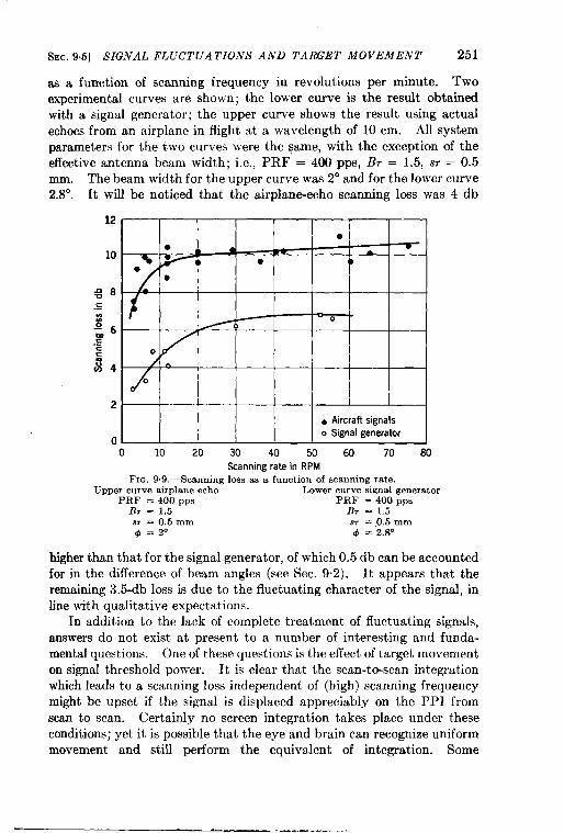
SEC. 9.5] SIGNAL FLUCTUATIONS AND TARGET MOVEMENT 251
as a function of scanning frequency in revolutions per minute. Twoexperimental curves are shown; the lower curve is the result obtainedwith a signal generator; the upper curve shows the result using actualechoes from an airplane in flight at a wavelength of 10 cm. All systemparameters for the two curves were the same, with the exception of theeffective antenna beam width; i.e., PRF = 400 pps, B7 = 1.5, ST = 0.5mm. The beam width for the upper curve was 2° and for the lower curve2.8°. It wifl be noticed that the airplane-echo scanning loss was 4 db
12
10
2
0
●
●
●
0
. Aircraft signals
o Signal generator
o 10 20 30 40 50 60 70 80Scanning rate in RPM
FIG. 9.9.—Scanning loss M a function of scanning rate.Upper curve airplane echo Lower curve signal generator
PRF = 400 pp9 PRF = 400 ppSB, = 1.5 B, = 1.587 = 0,5 mm 87 = .0.5 mm,+ =2. + = 2.8”
higher than that for the signal generator, of which 0.5 db can be accountedfor in the difference of beam angles (see Sec. 9.2). It appears that theremaining 3.5-db loss is due to the fluctuating character of the signal, inline with qualitative expectations.
In addition to the lack of complete treatment of fluctuating signals,answers do not exist at present to a number of interesting and funda-mental questions. One of these questions is the effect of target movementon signal threshold power. It is clear that the scan-to-scan integrationwhich leads to a scanning loss independent of (high) scanning frequencymight be upset if the signal is displaced appreciably on the PPI fromscan to scan. Certainly no screen integration takes place under theseconditions; yet it is possible that the eye and brain can recognize uniformmovement and still perform the equivalent of integration. Some
————.——
252 PULSE TRAINS IN INTERNAL NOISE [SEC.9.6
preliminary experiments on this point by V. Josephson have shown a
dependence of signal threshold power on target velocity, but these
experiments are not sufficiently complete to show the precise mechanism
involved. On the other hand it is a common experience with radar
observers that a moving signal-generator pulse is apparently as easy to
recognize as a fixed signal. More experimental information is required sto understand this problem.
AIJIUL AND METER METHODS OF DETECTION
9.6. Theoretical Results for the Signal Threshold.—The aural andmeter methods of detection of a radar signal have been described alreadyin Sec. 2.6, and a rather complete theoretical discussion of the signalthreshold has been given by Van Vleck and Middleton. 1 Only a shortaccount of the theoretical results will be presented, since no systematicexperimental investigations have been made with which the theory canbe compared.
In the aural method of detection the observer listens to the audio toneproduced by the PRF of the signal. In terms of the spectrum of thesignal and noise (cj. Sec. 7.2) the audio tone is represented by the signalpeak at the frequency 1/90 if G is the pulse repetition period. Since E)Ois always much larger than the pulse length ~, the power of the signal peakwill be the same as the power of the d-c component, that is, the averagevalue of the power distribution in the pulse train after it has beendeformed by the i-f amplifier and rectified by the second detector.before the i-f amplifier, the pulse is represented by
()s(t) = &F : Cos27rjct,
then it can be easily shown (cf. Sec. 7.2) that the average value ofdeformed and rectified pulse train is given by
where
Sgr4+-
()1
2
eo -.dx G(z)Z, ~ ,
/
+-G(z) = dy F(y)e–2”~vs
—.
If,
the
(1)
and Zl(f/B) is the system function of the i-f amplifier, which has thebandwidth B. A quadratic second detector has been assumed.
The qualitative behavior of the function
(2)
1J. H. Van Week and D.Aural and Meter Reception ofPhys., 11, 940 (1946).
Middleton, “ Theoretical Comparison of the Visual,Pulsed Signals in the Presence of Noise, ” J. Applied
SEC. 9.61 THEORETICAL RESULTS FOR THE SIGNAL THRESHOLD 253
can be seen as follows. For small values of B, the i-f amplifier lengthensthe pulse from ~ to 1/B and diminishes the signal amplitude from S0 toS@7. The average pulse power is therefore in this case of the order
On the other hand for B,>> 1 the pulse will not be deformed by the i-famplifier, so that the average power will be S~T/GO. Therefore thefunction h(B,) approaches unity for B,>> 1 and is proportional to B, forsmall values of Br.
The power of the signal peak has to compete with the noise power in anarrow range of frequency A around the audio tone 1/90. Since 1/F)Oisso small, one may take the initial value of the continuous noise spectrum,which for a square-law detector is proportional to the bandwidth B.
Hence in the notation of Sec. 7.2, the square of the noise power in thefrequency range A is [cf. Eq. (7.28)]’
&#BA. (3)
According to the power criterion (cf. Sec. 7.3) the minimum detectablesignal power is determined by putting the ratio of the signal power to thenoise power equal to a constant. Thus one obtains
‘- ‘(2).1.=’”2$% (4)
At this point it is good to remember that in the aural method ofdetection one usually gates or strobes the incoming signals. In this waya considerable improvement of the signal threshold can be achieved,since it is clear that the gat ing will not change the power of the audio tonewhereas the noise power will be reduced. In fact it can be seen that if 1is the length of time that the gate stays open, the signal threshold isreduced by the gating factor (1/130)~s. A simple formal proof of this state-ment runs as follows. With gating, the noise amplitude after the i-famplifier can be represented by
N(t) = j(t) [X(t) cos 2rr~Ct+ Y(t) sin 27rj<t],
where ~(t) is a function that is unity when the gate is open and zerootherwise. Assuming a square-law detector, the video output will be
r-z(t) = jyt)(x’ + Y’) = j’(t)?-:(t).
To find the spectrum we calculate first the correlation function
/R(T) = r-’(t)r’(t + 1) = 4w’p’(T) & ~e”dtjqt)jqt + 7), (5)
1 Thk is for a rectangular i-f pass band of width 1?.
254 PULSE TRAI,VS I.V I.V TERiVAL NOISE [SEC. 97
where we have made use of the fact that for a square-law detector andwithout gate the correlation function of noise alone is equal to 4W2P2(7)(cf. Sec. 73). No}v if 1>> l/B, then for all values of r for which p(7)is different from zero, the integral in (5) is very nearly equal to 1. Thegating therefore reduces the correlation function by the factor l/@.Consequently, the square of the noise power in the frequency range A willbe reduced by the same factor; and since the power of the signal peak hasnot changed, the signal threshold will be lowered by the factor (1/eO)$4.
In the meter method of detection the aural signal is rectified andimpressed on an ordinary d-c meter. The deflection of the meterdetermines the presence of a signal. In terms of the spectrum the situa-tion is clearly similar to the case of the visual detection of a c-w signal.The audio filter takes the place of the i-f pass band and the meter isanalogous to a low-pass video filter. Further investigation is necessary,however, to show that for the rectification of the audio signal and noisethe formula of Sec. 7.2 can be used again. The difficulty lies in the factthat the audio noise is not Gaussian, since it originates from the rectifica-tion of the original Gaussian noise passed by the i-f amplifier. In general,therefore, tile different frequency components of the audio noise are notindependent of each other, nor are their amplitudes distributed accordingto a Gaussian distribution. However, it can be shown that, if the widthA of the audio filter is small compared with B, then the noise passed by theaudio filter is again approximately Gaussian. 1 In this case, therefore, theequations of Sec. 7.2 can be used again. Using again the power criterionit is then easily shown that for the meter method of detection
(6)
where Am is the width of the low-pass filter, which is characteristic for thed-c met er, and km is a constant of the order of magnitude unity.
9.7. The Equivalence with the Visual Method of Detection. —In Sec.
8.7 it has been shown that for the visual method of detection the minimum
detectable signal energy is given by an expression of the form
, N(z,y)(soT)mk,= u c ~(z,y)) (7)
where x = BT, y = br, and C is a constant, which still depends on thetime of observation. The function N(x,y) is the fluctuating noise power,and S~H(Z,y) is the maximum value of the pulse after it has been deformed
I Cf. M. Kac and A. J. F. Siegert, “On the Theory of Noise in Radio Receiverswith Square Law Detectors,” J. Applied Phys., 18, 383 (1947). In this paper adetailed study is made of the probability distribution of the output of the audio filterfor different values of the ratio A/B.
SEC, 9.7] EQUIVALENCE WITH VISUAL METHOD OF DETECTION 255
by the i-f and video amplifiers. For an explicit expression of the func-tions H and N see Eq. (818); here we will need only the qualitativedependence of s~r on the i-f and video bandwidths. As has been shownin the beginning of the theoretical part of Sec. 8.7, S~Twill be an absoluteminimum if z = 1% is of order unity and if y >> x. The ratio N/H isthen of order unity. Suppose, furthermore, that the train of pulses hasthe length O, so that it contains 6’/00 pulses. Every time a pulse is pre-sented, a visual observation can be made; and if the observer can integrateall the observations, then, as has been shown in Sees. 73 and 7,5, theconstant C will be inversely proportional to the square root of the totalnumber of observations, so that
(8)
where km is a constant of the order of magnitude unity. In the caseBT == 1 the visual method can therefore detect, at best, the average signaIpower Pmi. given by
(w)
Let us compare this result with Eq. (4), which gives the minimum detect-able average signal po~ver for the audio method of detection. Since forB, = 1, h(B7) is of order unity, one would get from Eq. (4)
(9b)
which is usually much larger than the value given by Eq. (9a). However,as already mentioned in Sec. 9.6 a considerable improvement can beachieved by gating or strobing the incoming signal. The improvementfactor is (1/(3,) ~~if 1is the length of time that the gate stays open. Clearlyit is best to take 1 = ~ in order to admit the maximum amount of signalpower and the minimum amount of noise. For a pulse train of length othe signal peak will have a width of the order 1/0. The best value forthe width A of the audio filter will therefore also be of the order 1/0.Taking in Eq. (9b) A = I/@ and multiplying Eq. (9b) by the best gatingfactor (r/f30)~ lead to an equation of exactly the same form as Eq. (9a),which shows that in the case Br = 1 the visual and aural method ofdetection are equivalent.
The same conclusion is reached for the case 1?, <<1. With the visualmethod of detection it is best to take the video bandwidth b much largerthan B. Since for y>> x and x<< 1, N = x and H = x’ (see Sec. 8“7),
256 PULSE TRAINS IN
one obtains from Eqs. (7) and (8)
~~,. = k.u’
INTERNAL NOISE [SEC. 9.7
11
<~. r,”(lea)
An equation of the same form is obtained for the aural method from Eq.(4). Since for B~<<l, h(B7) = Br, Eq. (4) becomes (with A = 1/8)
P.,. = k<u2~—d% &“
(lOb)
Since the pulse is now strongly deformed, so that the pulse length hasbecome of the order I/B, the gate length 1 should now be taken equal toI/B. Multiplying Eq. (lOb) with the best gating factor (1/BeO) ~~oneobtains an equation of the same. form as Eq. (lOa).
Finally consider the case B,>> 1. With the visual method of obser-vation an improvement can now be obtained by narrowing the videoband~~iclth b to a value of the order 1/,. Since for x>> 1 and y = 1,N/H is of order z>:, one obtains from Eqs. (7) and (8)
P.,. = km~’ -& v%. (11)
An equation of the same form is obtained for the aural method from Eq.(4), since for B~ >>1, h(l?r) = 1, A = 1/8 and the best gating factor is(r/e,) ~+.
Also for the meter method one reaches the same conclusions, sinceobviously the best choice for the meter bandwidth Amis also 1/0, just asthe bandwidth A of the audio filter. This choice makes Eqs. (4) and (6)of exactly the same form, so that the arguments given for the auralmethod are also applicable to the meter method of detection.
CHAPTER 10
MODULATED PULSE TRAINS
This chapter treats the problem of the modulated pulse train. As ispointed out in Sees. 2.7 and 2.8, many types of modulation are possible,namelY, a-m pulses, f-m pulses, width-modulated pulses, etc. Thesemethods differ somewhat in detail, but the general solutions are similar.A detailed discussion of the a-m pulse train will therefore serve as asuitable example for other types of modulated pulse trains. To bespecific, let us consider the case where the amplitude modulation consistsof propeller modulation on the radar echo pulses returned from an air-craft. Before examining the effect of the propeller modulation itself(see Sec. 10.4), however, the behavior of the receiving system in responseto a single modulating tone or frequency must first be discussed in detail(see Sees. 10.1 and 10.2).
10.1. The Receiving System. The Rectivcr.-As is pointed out inSec. 2:7, the receiver is usually of a superheterodyne type with a linearsecond detect or, with a linear third detector (or “boxcar” generator),and with some form of AGC. A block diagram of such a receiver isshown in Fig. 2. 1%~~To be definite, let us assume the demodulated audiosignal to be the voltage output of the third detector, or boxcar generator,and the AGC feedback to be derived from the average value of the audiosignal. This average value is, of course, obtained from several cycles ofthe modulation, and it can be assured if the low-pass filter in the linebetween the third detector and the gain-control connection has an h-fcutoff much lower than the lowest desired audio frequency.
The third detector will be assumed to be a boxcar generator of the typedescribed in Sec. 2.7. In the formation of boxcars the potential of somestorage element, such as a capacitor, is made to assume the voltage ofvideo signal at the instant of the latter’s occurrence. The storage elementis then disconnected from the video system and remains so until thearrival of the next video signal. In this fashion, flat steplike segmentsoccur in the boxcar output voltage waveform, whose amplitudes aregoverned by the desired signal. As is pointed out in Sec. 2.7, theadvantage of the boxcar output over other forms of audio demodulationis that it furnishes a large audio amplification plus a type of filter actionthat completely suppresses the PRF and all its harmonics.
There are several methods that make the storage element assume the257
,.
258 MODULATED PULSE TRAINS [SEC. 10.1
potential of the signal. In order that only thedesired signal be made toactuate the storage element, a selection circuit is needed to sensitize theboxcar generator at the desired instant. This selection circuit may con-sist of an accurately timed irnpul sethatis made to coincide in time withthe desired radar echo and allows the boxcar circuit to be activated bythedesired video signal. Thus theerrors intiming that can be toleratedin this form of selection circuit are obviously less than the radar pulseduration, i.e., usually less than 1 psec. Since this precision is difficulttoobtain, it iscustomary toprovide a time gate, or strobe (see Sec. 2.6),which sensitizes the video section only during a defined range interval.This range interval may be several times the pulse length; hence it ismuch easier to set the gate on the desired echo than in the case of theaccurately timed impulse already described. The gate length G has adirect bearing on signal detectability, as will be shown in the next section.
Within the time interval allowed by the gate, it is possible that besidesthe desired echo, both receiver noise and perhaps other undesired signalsor interference will appear. The signal-modulation perceptibility in theboxcar output depends upon how the boxcars are formed from the gatedvideo signals. Two methods of formation are customarily considered.In the first method the boxcar height is proportional to the a.veroge video
signal within the gate, and in the second method the height is propor-
tional to the peak video signal in the gate. Since the signal-modulation
detectability depends upon the method of boxcar formation, it vvill be
convenient to distinguish them. If the boxcars are formed from the
average video signal, they will be referred to as “ average value” boxcars;and if they are formed from the peak-video-signal model, they will bedenoted by “ peak value” boxcars. It is clear that peak-value boxcarstend to accentuate the effects of the larger video signals within the gate;and since the largest signal is usually the desired echo, the peak-valueboxcar circuits are usually desirable.
The AGC is indispensable to keep the average value of the third-detector output signal constant. This is done to reduce the effects ofsignal fading. In the absence of input-signal fading the AGC isessentially inoperative and can therefore be neglected in the followingdiscussion. As will be shown in the next section, the properties of thesystem depend, however, upon the ratio of carrier signal power to noisepower; therefore, as a function of this parameter, the magnitude of theoutput voltage of the audio system will depend upon whether the AGC isused or not. If the AGC is used, the average value of the third-detectorvolt age output is constant; if not, the over-all gain of the receiver isconstant. With this in mind, a little thought will show that in both casesthe average value of the boxcar-generator output is independent. of thePRF. This characteristic makes such a type of audio demodulator ideal
SEC 10.1] THE RECEIVING SYSTEM 259
for deriving AGC voltages in a system with a variable PRF. It is prob-ably the only type of demodulator that has this desirable feature.
There are certain practical difficulties in the construction of a high-quality boxcar generator, chiefly the provision of a storage element thathas a small leakage of charge between pulses and can be rapidly chargedor discharged during the desired video pulse. The circuit developed byH. L. Johnson and J. L. Lawson’ produces exceptionally high-qualityboxcars. They are flat to within a few per cent for time intervals as longas 1 see, yet they can be actuated by a video signal as short as 0.03 ~sec.This is accomplished in two steps: (1) The video signals are “stretched”into pulses perhaps 20 ~sec long by a special diode circuit; (2) then the“stretched” pulses actuate the condenser storage element. In this waythe storage-element leakage can be minimized because the maximumcharging current is kept low. The entire circuit is shown in Fig. 10.1.It is designed to accept positive video input signals not greater than 5volts in amplitude and will deliver audio boxcars of approximately 20volts for such video signals. It also requires an input trigger from theradar set occurring at times corresponding to the transmitted radar pulse.
The video signals are put on the grid of Vi,. The three tubes VI,,VW and V16constitute a wide-band video amplifier that serves to producea negative video signal of about 60 volts in the 300-ohm plate resistor ofV16. The plate of V16 is direct-coded to the cathode of the specialdiode V~q, whose plate is, in turn, run at a bias voltage of about +150
volts. This diode was chosen for its large conductivity and its small
interelectrode capacitance. Unless V,7 is made to conduct, the diodeVI, will not conduct even for the large video signals produced by ~16.
However, when the gating pulse, whose generation is discussed below, isproduced in the plate circuit of VIT, the negative video signals will causethe diode to conduct until its plate assumes the most negative valuereached by the video signals in the gate interval. This value of voltagewill be maintained until a positive pulse in the grid of V20 returns theplate voltage of V19 to its original value. The plate voltage of Vlgtherefore amounts to a stretched video pulse. The cathode follower Viireproduces the stretched pulse (perhaps 20 psec long), and during thistime the storage condenser in the cathode of V.2Zis made to assume thissame potential. This is done by the action of a positive pulse on the gridsof V22 and V2S produced by VM just at the end of the gate itself. Thepositive pulse on V22and VZScauses one or both of these tubes to conductso that the cathode of VZZassumes the voltage of the stretched pulse onthe cathode of Vjl. The cessation of this “clamping” pulse produced by
1See R, M. Ashby, F. W. \fartin, and J. L. Lawson, ‘‘ hfodulation of Radar Signalsfrom Airplanes,” RL Report No. 914, Mar. 28, 1946.
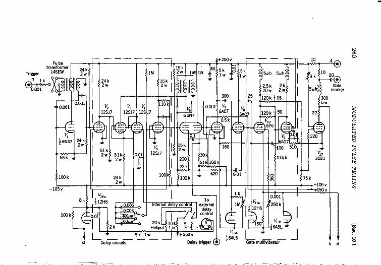
—— ——— —.=
,.,,
‘‘‘-y250;”Pulse
$
transformer
Trigger 145EW ;4;
&
@
1O.OQ10.001
t
II
I
P::
22
------
220
v3;;1
V2 V312SJ7 12SJ7 12s 7
,nl!
$
‘1:. :-- .: _: ------ --- --- --------- ------
II
I 5*I( V5 1:‘w 51k 0.01 12SJ7 .
I‘w
2. ,-.”
a’a--
W.,.,..“,
~ }UXIk 62
J‘5 k
_—— _ ,,
I II I&L—
(
,,
‘! 41
250k
-1
,.. , .
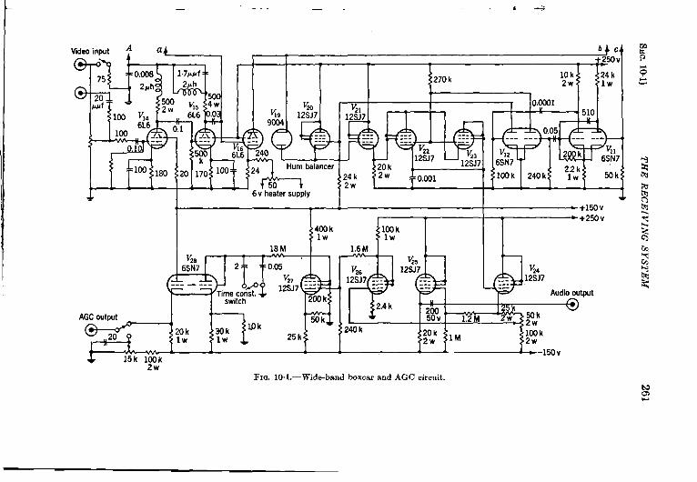
—
2!!1.6M
v12:7 ~::
-..
2,4 k
+150V &
F
+250v ?
~
%~
V24 Y--- 12SJ7------ s
Audiooutout
400k#
llfiklW
18 MV28 %5 -
6SN7 12SJ7
I “ I2W @
AGCoutput 50 v 1.2 M ?Wk240 k lCOk
2W
2WFICL10.1.—Wide-band boxcar and AGC circuit.
Ma
262 MODULATED PULSE TRAINS [SEC. 101
V,, disconnects the storage condenser until the next pulse is produced.The cathode potential of VZ*, and hence of the cathode follower Vzl,therefore, is the audio boxcar voltage desired. For convenience, themajor portion of the d-c voltage is removed by the connection to Vjs,whose out put voltage is essential y the desired boxcar audio component.The tubes V26, V2T,and V28,serve as a direct-coupled amplifier from whichthe AGC voltage may be derived. The low-pass filter in this AGC linkis placed in the grid circuit of V2E;its frequency limit can be made higheror lower than the modulation frecmencies as desired.
The production of the delayed gate and associated timing pulses isaccomplished by the tubes VI to Vlo and their associated circuits. Forany trigger pulse from the radar set that operates the blocking oscillatorVl, a standard trigger pulse of uniform shape appears on the grid of V2.The tubes Vz, V,, V,, and V, forma high-precision delay circuit operatingthe blocking oscillator V6, which, in turn, produces the delayed trigger.The amount of delay is controlled by the delay-control potentiometerthat adjusts the potential on the grid of V,. An idea of the precisionavailable in the delay time may be obtained by noting that for a delaytime of 2000 psec a flutter, or variation in delay, of less than O.I psec isordinarily experienced. The delayed trigger operates the tubes in the
monostable-state multivibrator, or “ flip-flop” circuit, VT and V8, whichproduces a small additional delay in time before operating another flip-flop circuit, composed of Vg and V1O, producing the gating pulse. Thissmall delay is helpful in observing the gate or gated signals on an externalR-scope (see Sec. 2“6) operated from the delayed trigger itself. Thegate-generating circuit whose output is connected to the power tube V17
is shunt-peaked for adequate transient response and can generate asatisfactory gate. The gate length is adjustable from 0.1 to approxi-mately 50 ~sec. The trailing edge of this gate actuates the flip-flopcircuit VII that generates the relatively long clamping pulse as describedabove. The trailing edge of the clamping pulse, in turn, generates ashort pulse in Viz, which causes the stretched pulse, produced by thediode V,,, to terminate.
Several precautions have been taken to prevent hum voltages fromappearing in the audio output. A “hum balancer” is shown in thecathode of Vlf,, and all hum-sensitive tubes are operated with d-c filamentvoltages. These tubes are V2, Vs, Vi, Vs, V18, V21, V22, V2S, V24, VZ,,,
~26, and V27and are for the most part pentodes operated as triodes. Bythese methods the hum appearing in the audio output has been reducedto a value less than 10 mv peak to peak.
The storage element, as can be seen, is a O.OO1-P~ condenser in the
cathode circuit of Vjj. To reduce the leakage from this condenser to asatisfactory value, it is necessary to operate the filaments of the tllbes
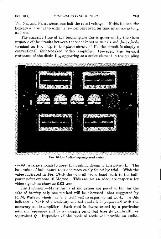
SEC. 10.1] THE RECEIVING SYSTEM 263
V,,, v23j ad VZ4 at about one-half the rated voltage. If this is done, theboxcars will be flat to within a few per cent even for time intervals as longas 1 sec.
The charging time of the boxcar generator is governed by the videoresponse of the circuits between the video input terminals and the cathodeterminal on V,O. Up to the plate circuit of VIG the circuit is simply aconventional shunt-peaked video amplifier. However, the forwardresistance of the diode Vlgj appearing as a series element in the coupling
FIG. 10.2.—Audio-frequency reed meter.
circuit, is large enough to upset the peaking design of this network. Thebest value of inductance to use is most easily found by trial. With thevalue indicated in Fig. 10. lb the over-all video bandwidth to the half-power point exceeds 10 Me/see. This ensures an adequate response forvideo signals as short as 0.03 psec.
The Indicator. -Many forms of indication are possible, but for thesake of brevity only one method will be discussed—that suggested byR. M. Walker, which has lent itself well to experimental work. In thisindicator a bank of electrically excited reeds is incorporated with thenecessary audio amplifier. Each reed is characterized by a particularresonant frequency and by a damping term that fixes its bandwidth, orequivalent Q. Inspection of the bank of reeds will provide an audio-
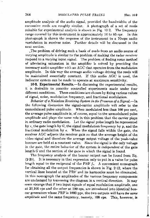
264 MOD L’LATED PULSE TRAINS [SEC.10.2
amplitude analysis of the audio signal, provided the bandwidths of thesuccessive reeds are roughly similar. A photograph of a set of reedssuitable for experimental analysis is shown in Fig. 10.2. The frequencyrange covered by this instrument is approximately 16 to85 cps. In thisphotograph is shown the response of the instrument to a 70-cps audiomodulation in receiver noise. Further details will be discussed in thenext section.
,The problem of driving such a bank of reeds from an audio source ofvarying amplitude is similar to the problem of making the radar receiverrespond to a varying input signal. The problem of finding some methodof alleviating saturation in the amplifier is solved by providing thenecessary audio amplifier with an AGC that operates from the rnodukctiorzamplitude. In this way the average audio voltage driving the reeds willbe “maintained essentially constant. If this audio AGC is used, theindicator system can be made to operate at maximum sensitivity.
10.2. Experimental Results.-In discussing the experimental results,it is desirable to consider controlled experiments made under fourdifferent conditions. These conditions are chosen by fixing various valuesof signal, noise, modulation frequency, and fractional modulation.
Behavior oj a Noiseless Receiving System in the Presence oj a Signal.—Inthe following discussion the signal-carrier amplitude will refer to theunmodulated pulse amplitude. When modulated less than 100 per cent,the average pulse amplitude is, of course, equal to the unmodulated pulseamplitude and plays the same role in this problem that the carrier playsin ordinary radio modulation. Let the signal pulse length be representedby r, the gate length by G, the signal modulation frequency by p, and thefractional modulation by c. When the signal falls within the gate, thereceiver AGC adjusts the receiver gain so that the average height of thevideo signal and therefore the average output voltage of the peak-valueboxcars are held at a constant value. Since the signal is the only voltagein the gate, the entire behavior of the system is independent of the gatelength G and the section of the gate in which the signal is found.
The frequency analysis of the boxcar output can be found from Eq.(2.29). It is necessary in that expression only to put in a value for pulselength equal to the reciprocal of the PRF j,. A convenient nomographfor obtaining all the output frequencies is shown in Fig. 2.12, where thevertical lines located at the PRF and its harmonics must be eliminated.In this nomograph the amplitudes of the various frequency componentsare unchanged by traversing the diagram in a vertical direction. It mayseem strange that if two input signals of equal modulation amplitude, one
at 20,100 cps and the other at 100 cps, are introduced into identical box-car generators whose PRF is 1000 pps, the two outputs will have the same
amplitude and the same frequency, name] y, 100 cps. This, however, is
I
I
SEC. 10.2] EXPERIMENTAL RESULTS 265
the case; and if the boxcar-generator output voltages are analyzed underthe two conditions, they will be found to be identical.
For a linear receiving system there are at least two interestingphenomena regarding the boxcar output worthy of discussion.
1.
2.
If the injected wave consists of several modulation frequencies, theoutput frequencies are represented in the diagram in Fig. 2.12 bythe intersections of the lines at the modulation frequencies with thearray of 45° lines. There are no cross terms due to “beats”between the input modulation frequencies. In other words, effectsproduced on the output by input modulating frequencies can bethought of as only the sum of the individual effects of the individualmodulating frequencies. This is one very cogent reason why alinear receiving system is desirable.If the input wave consists of a modulation term that is itselfmodulated at a slow rate (c can be thought of as a very slow sinu-soidal variable), the slow modulation frequency itself will not appearin the output. Only sidebands will appear in the output fre-quencies, separated from the main frequencies by the frequency ofthe slow modulation. Here again the input frequencies are p andp + u, where u is the modulation frequency of c. The outputfrequencies are on y those given by the independent action of thesethree input frequencies, and u itself will not appear in the output.
These remarks apply when the input modulating function has adefinite time phase. They do not apply when the injected wave is, forexample, receiver noise. This case will be discussed below.
In practice the receiving system is not quite linear, and cross termsmay be detected. The greatest nonlinearity appearing in the receivingsystem just described is in the audio amplifier, whose harmonic genera-tion, however, is very low. The entire receiving system can be madesufficiently linear to reduce the effects of harmonic generation to negligiblevalues.
Behavior of the Receiving System in the Presence of Receiver Noise
Alune.-In the absence of a signal the audio output voltage appears to bea function of both the gate length G and the PRF ~,. Experiments havebeen performed varying both of these parameters, and results are depictedin Figs. 10.3 and 10.4.
The dependence of audio noise on the gate length G is shown in Fig.10,3. An experiment was performed in which the average value of audionoise voltage in a frequency range of approximately 10 to 40 cps wasmeasured as a function of the gate length G. A receiver whose i-f band-width was 2 Me/see was used. The experimental results are plotted i~
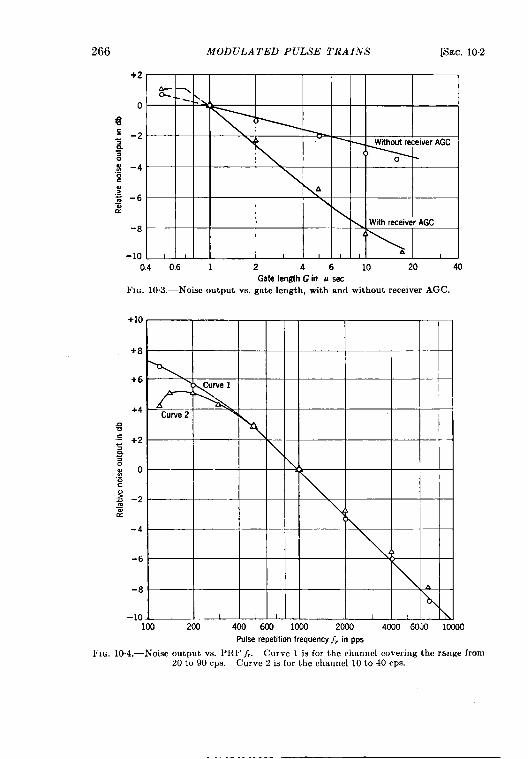
266 MODULATED PULSE TRAINS [SEC. 10.2
+2
ogc3
2s \ ‘ WithoutreceiverAGC~
.$ -4?% A.-= -6~ \
‘8\ Withreceiver AGC
Lb
-10. [ 1 I , 1 1 ! A 1
0.4 0,6 1 2 46 10 20 40Gate lengthGin u sac
FIG. 103. -Noiseoutput vs. gate length, with and without receiver AGC.
+10
+8
+6>
+4
+2
0
-2
-4
-6
-8
lm 200 400 600 1000 2000 4000 6CPulse repetition frequency fr in pps
410 1( no
FIG. 10.4.—Noiseoutput vs. PfW f,. Curve 1 is for the channelcovering the range from20t090cps. Curve 2isfor the channel10t040cps.
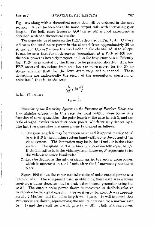
SEC. 10.2] EXPERIMENTAL RESULTS 267
I
Fig. 10.3 along with a theoretical curve that will be deduced in the nextsection. It can be seen that the noise output falls with increasing gatelength. For both cases (receiver AGC on or off) a good agreement isobtained with the theoretical results.
The dependence of noise on the PRF is depicted in Fig. 10.4. Curve 1indicates the total noise power in the channel from approximately 20 to90 cps, and Curve 2 shows the total noise in the channel of 10 to 40 cps.It can be seen that for both curves (normalized at a PRF of 400 pps)the noise power is inversely proportional to the frequency at a sufficientlyhigh PRF, as predicted by the theory to be presented shortly. At a lowPRF observed deviations from this law are more severe for the 20- to90-cps channel than for the lower-frequency audio channel. Thesedeviations are undoubtedly the result of the nonuniform spectrum ofnoise itself, that is, to the term
in Eq. (7), where
Behavior of the Receiving System in the Presence of Receiver Noise andUnmodulated Signuls.-In this case the total output noise power is afunction of three quantities: the pulse length r, the gate length G, and theratio of signal carrier to receiver noise power, which we may denote by z.The last two quantities are more precisely defined as follows:
1. The gate ength G may be written as n, and is approximately equalto n/B if B is the limiting system bandwidth up to the output of thevideo system. This limitation may be in the i-f unit or in the videosystem. The quantity B is ordinarily approximately equal to 1/,.If the limitation is in the video system, however, B represents twicethe video-frequency bandwidth.
2. Let z be defined as the ratio of signal carrier to receiver noise power,which is measured in the i-f unit after the i-f narrowing has takenplace.
Figure 10.5 shows the experimental results of noise output power as afunction of z. The equipment used in obtaining these data was a linearreceiver, a linear detector, and a peak-value boxcar generator using theAGC. The output noise power shown is measured in decibels relativeto its value for no signal carrier. The receiver i-f bandwidth was approxi-mately 2 Mc/secj and the pulse length was 1 ‘Usec. It will be noted thattwo curves are shown, representing the results obtained for a narrow gate(n = 1) and the result for a wide gate (n = 10). Both of these curves
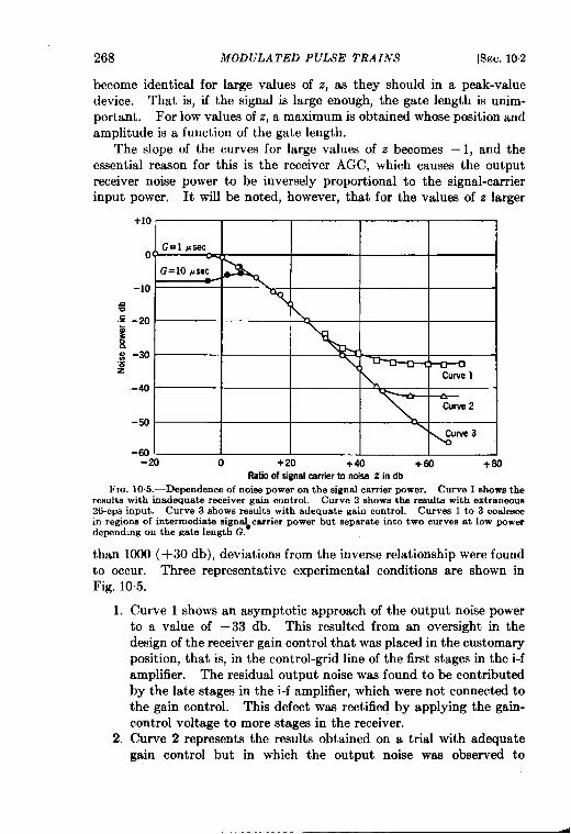
268 MODULATED PULSE TRAINS [SEC.102
become identical for large values of z, as they should in a peak-valuedevice. That is, if the signal is large enough, the gate length is unim-portant. For low values of z, a maximum is obtained whose position andamplitude is a function of the gate length.
The slope of the curves for large values of z becomes – 1, and theessential reason for this is the receiver AGC, which causes the outputreceiver noise power to be inversely proportional to the signal-carrierinput power. It will be noted, however, that for the values of z larger
+10.
G=1O psec
-log
.: -20
E$ -~.-Z
Cuwe 1-40 -
curve2-50
\ ~tva a
-60-20 0 +20 +40 +60 +30
Ratioof signalcarrierto noise Z in dbFIG. 10.5.—Dependenee of noiea power on the signal carrier power. Curve 1 shows the
results with inadequate receiver gain control. Curve 2 shows the reeulta with extraneousM-cps input. Curve 3 chows results with adequate gain control. Curves 1 to 3 coalescein regiom of intermediate sign~carrier power but separate into two curves at low powerdepending on the gate length G.
than 1000 (+30 db), deviations from the inverse relationship were foundto occur. Three representative experimental conditions are shown inFig. 10.5.
1.
2.
Curve 1 shows an asymptotic approach of the output noise powerto a value of – 33 db. This resulted from an oversight in thedesign of the receiver gain control that was placed in the customaryposition, that is, in the control-grid line of the first stages in the i-famplifier. The residual output noise was found to be contributedby the late stages in the i-f amplifier, which were not connected tothe gain control. This defect waa rectifiecj by applying the gain-control voltage to more stages in the receiver.Curve 2 represents the results obtained on a trial with adequategain control but in which the output noise waa observed to
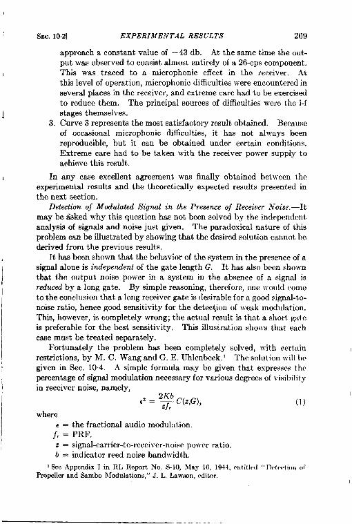
,
I SEC. 10.2] EXPERIMENTAL RESULTS 269
3.
approach a constant value of – 43 db. At the same time the out-put was observed to consist almost entirely of a 26-cps component.This was traced to a microphonics effect in the receiver. Atthis level of operation, microphonics difficulties were encountered inseveral places in the receiver, and extreme care had to be exercisedto reduce them. The principal sources of difficulties were the i-fstages themselves.Curve 3 represents the most satisfactory result obtained. Becauseof occasional microphonics difficulties, it has not always beenreproducible, but it can be obtained under certain conditions.Extreme care had to be taken with the receiver power supply toachieve this result.
J In any case excellent agreement was finally obtained between theexperimental results and the theoretically expected results presented inthe next section.
Detection of Modulated Signal in the Presence of Receiver ~m”se.—lt
may be asked why this question has not been solved by the independentanalysis of signals and noise just given. The paradoxical nature of thisproblem can be illustrated by showing that the desired solution cannot bederived from the previous results.
It has been shown that the behavior of the system in the presence of a
1 signal alone is independent of the gate length G. It has also been shown
ithat the output noise power in a system in the absence of a signal isreduced by a long gate. By simple reasoning, therefore, one would come
I to the conclusion that a long receiver gate is desirable for a good signal-to-noise ratio, hence good sensitivityy for the detection of weak modulation.This, however, is completely wrong; the actual result is that a short gateis preferable for the best sensitivity. This illustration shows that each
I case must be treated separately.
! Fortunate y the problem has been completely solved, with ccrt ;iinrestrictions, by M. C. Wang and G. E. Uhlenbeck. I The solution ~~illbegiven in Sec. 10.4. A simple formula may be given that expresses the
ipercentage of signal modulation necessary for various degrees of visibilityin receiver noise, namely,
/~, _ 21<b— ~ C(Z,G), (1)
where~ = the fractional audio modulation.
j. = PRF.
I z = signal-carrier-to-receiver-noise po}ver ratio.b = indicator reed noise bandlvidt,h.
1See Appendix I in RL Report No. S-10, hfny 16, 1944,cntitlrd “ Drtrrtion O:Propeller and Sambo Modulations,” J. L. Lawson, editor.
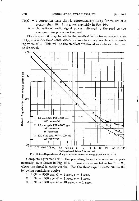
I
I
1
I
I
I
I
270
C(Z,G) =
K=
MODULATED PULSE TRAINS [SEC. 102
a correction term that is approximately unity for values of zgreater than 10. Itisgiven explicitly in Sec. 10.4.the ratio of audio signal power delivered to the reed to theaverage noise power on the reed.
The constant K may be set to the smallest value for consistent visi-bility, and under these conditions the above formula gives the correspond-ing value of c. This will be the smallest fractional modulation that canbe detected.
+60
n-0,= +40$zSi%.=cg&i +20..:~u~,ymzN.g o2
-200.01 0.02 0.040.060.1 0,2 0,40.6 1 2 461020 40 60 100
Fractional modulation 6 in per cent
FIG. 10.6.—Dependenceof signal carrierpower on modulation for K = 20,
Complete agreement with the preceding formula is obtained experi-mentally, as is shown in Fig. 10.6. These curves are taken for K = 20,where the signal is easily visible. For the three experimental curves thefollowing conditions apply:
1. PRF = 5000 cps, G = 1 psec, r = 1 psec.2. PRF = 1000 cps, G = 1 psec, r = 1 psec.3. PRF = 1000 cps, G = 10 psec, r = 1 psec.
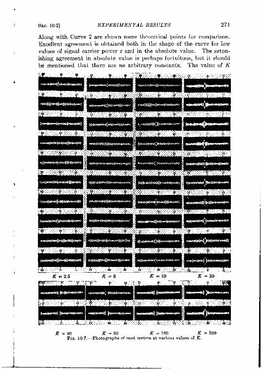
#
I
SEC. 10.2] EXPERIMENTAL RESULTS 271
Along with Curve 2 are shown some theoretical points for comparison.Excellent agreement is obtained both in the shape of the curve for lowvalues of signal carrier po-l~er z and in the absolute value. The aston-ishing agreement in absolute value is perhaps fortuitous, but it shouldbe mentioned that there are no arbitrary constants. The value of K
K =2.5 K=6 K=1O K=20
,. 3s ; z-. ..~
K=40 K=80 K =160 K =32oFm. 10,7.—Photographsof reed meters at various values of K.
I
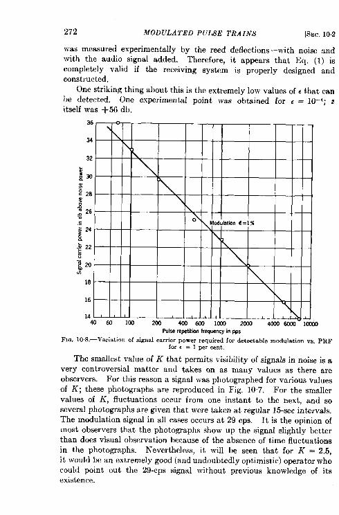
272 MODULATED PULSE TRAINS [SEC.102
was measured experimentally by the reed deflections-with noise :mdwith the audio signal added. Therefore, it appears that Eq. (1) iscompletely valid if the receiving system is properly designed andconstructed.
One striking thing about this is the extremely low values of c that canbe detected. One experimental point was obtained for ~ = 10–4; zitself was +56 db.
40 64 lcs) 200 400 m 10MI 2000 4CC0 m 1(XOJPulserepetitionfrequency in pps
FIG. 10. S.—Variation of signal carrier power required for detectable modulation ve. PRFfor e = 1 per cent.
The smallest value of ~that permits visibility of signals innoise isa
very controversial matter and takes on as many values as there are
observers. For this reason a signal was photographed for various values
of K; these photographs are reproduced in Fig. 10.7. For the smallervalues of K, fluctuations occur from one instant to the next, and soseveral photographs are given that were taken at regular 15-sec intervals.The modulation signal in all cases occursat 29 cps. Itis the opinion ofmost observers that the photographs show up the signal slightly betterthan does visual observation because of the absence of time fluctuationsin the photographs. Nevertheless, it will be seen that for K = 2.5,it would be an extremely good (and undoubtedly optimistic) operator whocould point out the 29-cps signal without previous knowledge of itsexistence.
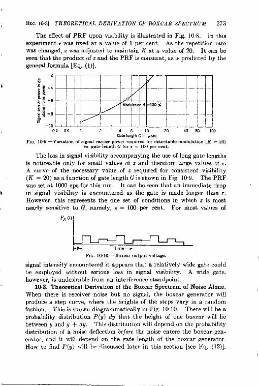
SEC. 10.3] THEORETICAL DERIVATION OF BOXCAR SPECTRUM& 273
The effect of PRF upon visibility is illustrated in Fig. 10”8. In thisexperiment t was fixed at a value of 1 per cent. As the repetition ratewas changed, z was adjusted to maintain K at a value of 20. It can be
)seen that the product of z and the PRF is constant, as is predicted by thegeneral formula [Eq. (l)].
-2-
-4 / d
-6 / ./
-8
1-10 L 1 I ,, 1 ! 1 , 1
@.4 0.6 1 2 4610 20 40601C0Gate Icngth Gin # wc
FIG. 10.9.—Variationof signalcarrierpowerrequiredfor detectablemodulation(K =vs. gatelengthG for 6 = 100 per cent.
20)
The loss in signal visibility accompanying the use of long gate lengthsis noticeable only for small values of z and therefore large values of C.A curve of the necessary value of z required for consistent visibility(K = 20) as a function of gate length G is shown in Fig. 10.9. The PRFwas set at 1000 cps for this run. It can be seen that an immediate drop
$ in signal visibility is encountered as the gate is made longer than T.
However, this represents the one set of conditions in which z is mostI nearly sensitive to G, namely, c = 100 per cent. For most values of
‘“(t)+Time ——
FIG. 10. 10.—Boxcar output voltage.
signal intensity encountered it appears that a relatively wide gate couldbe employed without serious loss in signal visibility. A wide gate,however, is undesirable from an interference standpoint.
1003. Theoretical Derivation of the Boxcar Spectrum of Noise Alone.When there is receiver noise but no signal, the boxcar generator willproduce a step curve, where the heights of the steps vary in a randomfashion. This is shown diagrammatically in Fig. 10.10. There will be aprobability distribution P(y) dy that the height of one boxcar will liebetween y and y + dy. This distribution will depend on the probabilitydktribution of a noise deflection before the noise enters the boxcar gen-erator, and it will depend on the gate length of the boxcar generator.How to find P(y) will b- discussed later in this section lsee Eq. (12)].

274 MODULATED PULSE TRAINS [SEC. 103
If it is known, the spectrum of the boxcar output can be computed accord-ing to the methods explained in Chap. 3. In fact in Sec. 34 the problemof finding the spectrum of a series of pulses of random height but fixedrepetition interval has been considered, and the results obtained therecan be immediately adapted to find the boxcar spectrum. In Sec. 34it was shown that for a series of pulses of the form
F~(t) =z
y~F(t – M&), (2)k
where the~kare the random heights and whereF(t) represents the shapeof a single pulse of unit height, the spectrum is given by the expression
wherer+.
B(j) = / dx F(z)e–zmiJ’ (4)J–.
is the Fourier transform of the pulse shape. For the boxcar spectrum,
{
– E)o +(3,
F(t) = 1 for~<t<~,
o otherwise,
so that
i
(5)
(6)
Since B(j) is zero for j = n/G, the ~-functions in Eq. (3) will not con-tribute for n # O and can therefore be omitted. Only for n = O willthere be a contribution; this represents the d-c term of the spectrum.The final result for the average power spectrum can therefore be writtenin the form
I2 sinz @30 —
G.(j) = ~POT1
[?42– (u)’] + g ?(j) . (7)
This result can be described by saying that besides the d-c term (~) 2, the
spectrum is the same as that of a single boxcar but that its intensity is
determined by the fluctuation of the boxcar heights [~ – (~) 2].
To proceed further more must be known about the probability dis-
tribution P(y) of the boxcar heights. If a Jinear second detecto~ is used,i
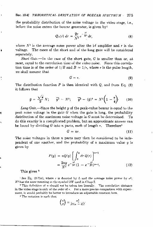
, SEC. 10.3] THEORETICAL DERIVATION OF BOXCAR SPECTRUM 275
the probability distribution of the noise voltage in the video stage, i.e.,before the noise enters the boxcar generator, is given by’
(8)
where N2 is the average noise power after the i-f amplifier and r is theD voltage. The cases of the short and of the long gate will be considered
separately.Short Gate.—In the case of the short gate, G is smaller than or, at
most, equal to the correlation time of the video noise. Since this correla-tion time is of the order of l/B and B = I/r, where ~ is the pulse length,we shall assume that
G=T. (9)
The distribution function P is then identical with Q, and from 13q. (8)it follows that
Long Gate.-Since the height y of the peak-value boxcar is equal to the
1 peak noise voltage in the gate G when the gate is long, the probabilitydistribution of the maximum noise voltage in G must be determined. To
i. do this exactly is a complicated problem, but an approximate answer canbe found by dividing G into n parts, each of length r. Therefore’
G = n,. (11)
The noise voltages in these n parts may then be considered to be inde-pendent of one another, and the probability of a maximum value y isgiven by
‘(y) ‘nQ(dP’r4n-’2ny -X 1P
——~
e ~2 (1 — e ‘~*).-l. (12)
This gives 3
1See Eq. (3.71a), where r is denoted by L and the average noise power by U2;N~ has the samemeaning as the symbol 2W used in Chap 7.
z This definition of n should not be taken too literally. The correlation distancein the video stage is only of the orderof 7, For a more precise comparison with experi-ment, it would probablv be better to introduce an adjustable constant here.
3The notation is such that
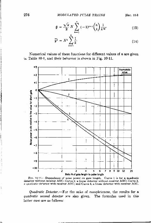
276 MODULATED P171i3E TRAINS [SEC. 10.3
‘=$+’’+’(M’ (13)k=l
n
z
~EN~ ~. (14)k=l
‘1
Numerical values of these functions for different values of n are givenhi Table 10.1, and their behavior is shown in Fig. 10-11.
+3
+2
+1
-8
-9
-10
1 1 w-
—, I I 1 I 1 ! 1 1
I 1 I I I I 1 I I 1 I1 2 3 456 789101215
Ration of gate length to pulse length
FIG. 101 l.—Dependence of noise power on gate length. Curve 1 is for a quadraticdetector without receiver AGC; Curve 2, a linear detector without receiver AGC; Curve 3,~ quadratic de+ector with receiver AGC; and Curve 4, a linear detector with receiver AGC.
Qu.aolrcdti Detector.-For the sake of completeness, the results for aquadratic second detector a-e also given. The formulas used in thislatter case are as follows:
,!
i SEC. 103] THEORETICAL DERIVATION OF BOXCAR SPECTRUM 277
n
zg=N2 !.k’ 7 =’N’&-’)’+’(2)i “6)
k-ln
z
~_(@2=N4 1~2 “
t-l(17)
The dependence of the spectrum G.(j) on the gate length G can becomputed in the following way: When no AGC is used, one determines~ – (J)’ as a function of n (or of G); with AGC, the (~)z is always brought,.
TABLE 10.1 .—DEPENDENCE OF CERTAIN FUNCTIONS ON n FOR A LINEAR AND FOE A
I
$
1z 2
3468
1115
11.291.46
1.571.721.82
1.922.02
b
n
1
123468
1115
j_N,
11.501.832.082.452.72
3.02
3.32
QUADRATIC DETECTOR
Linear Detector
p – (J)2 ~ – (~)1
.j?()
N, 1–:()
(Zi)’ : – 1~,
Value Db Value Db
1 1 0 1 01.5 0,875 –0.57 0.524 –2.811.83 0,786 –1.04 0.370 –4.322.08 0.726 –1.40 0.296 –5.282.45 0.651 –1.86 0.223 –6.522.72 0.600 –2.21 0.183 –7.373.02 0.553 –2.58 0.150 –8.243.32 0.512 –2.90 0.124 –9,05
Quadratic Detector
——11.752.362,883.754,455,346.29
l–11.251.361.421.491,531,561.58
. —0 1
+0. 97 0.556+1.34 0.405+1.53 0.32+1.73 0.248+1.84 0,207+1,92 0.170+1.96 0.144
Db
o–2.56
–3,93–4,84–6.06
–6.84–7.70
–8.42
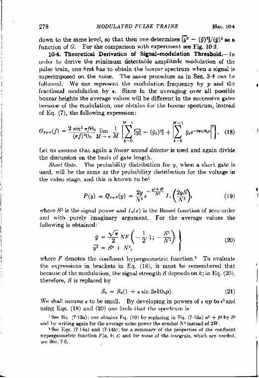
278 MODULATED PULSE TRAINS [SEC. 10.4
down to the same level, so that then one determines [~ – (~)Z]/@’ as afunction of G. For the comparison with experiment see Fig. 10.3.
1004. Theoretical Derivation of Signal-modulation Threshold.-Inorder to derive the minimum detectable amplitude modulation of thepulse train, one first has to obtain the boxcar spectrum when a signal issuperimposed on the noise. The same procedure as in Sec. 3.4 can kefollowed. We can represent the modulation frequency by p and the (fractional modulation by e. Since in the averaging over all possibleboxcar heights the average values will be different in the successive gatesbecause of the modulation, one obtains for the boxcar spectrum, insteadof Eq. (7), the following expression:
M–1 M–1G8+N(j) = 2 sin’ njOO ljrn ~
{z E2
——[n – (!h)’1 + q~e–2mi10&
(rj)%o M+. M 1}. (18)
k=O k=O
Let us assume that again a linear second detector is used and again dividethe discussion on the basis of gate length.
Short Gate.—The probability distribution for y, when a short gate isused, will be the same as the probability distribution for the voltage inthe video stage, and this is known to be’
2y -v
()
2ysF’(y) = Q.+.(y) = ~j e IQ=@’
1
(19)
where Sz is the signal power and 10(z) is the Bessel function of zero orderand with purely imaginary argument. For the average values thefollowing is obtained:
(20)
where F denotes the confluent hypergeometric function. 2 To evaluatethe expressions in brackets in Eq. (18), it must be remembered that ibecause of the modulation, the signal strength S depends on k; in Eq. (20),therefore, S is replaced by
Sk = SO(1 + 6 sin %k&P). (21)
We shall assume c to be small. By developing in powers of c up to # andusing Eqs. (18) and (20) one finds that the spectrum is
1See Eq. (7.13a); one obtains Eq. (19) by replacing in Eq. (7.13a) az + L+by S,and by writing again for the average noise power the symbol N2 instead of 2W,
2See Eqs. (7.14a) and (7.14b); for a summary of the properties of the confluenthypergeometric function F(a, b; z) and for some of the h-teg~als, which are needed, ,see Sec. 7.6.
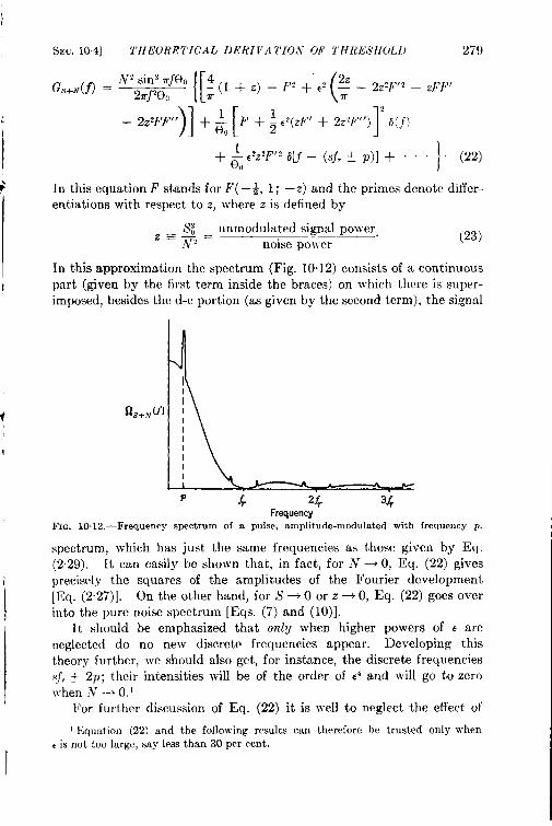
f
1
i
SEC. 104] THEO RE7’ICAL DERI?’ATIOiV OF THRESHOLD ~~(J
G.+.(f) =W2sin’7rfE)0
2Tf ‘e, {[ (~(l+z)– F’+’e’ :– z22Ff2 – #~f
lr
– 2Z2FF”)1 [ 1+&F + ~ C2(ZF’ + 22’F”) 2 b(j)
In this equation F stands for F( –~, 1; —z) and the primes denote differ-entiations with respect to .z, where z is defined by
~=~ unmodulated signal power.N, = noise power
(23)
In this approximation the spectrum (Fig. 10.12] consists of a continuouspart (given by the first term inside the braces) on ~vhich there is super-imposed, besides the d-c portion (as given by the second term), the signal
Frequenzy10. 12.—Frequency spectrum of a pulse, amplitude-modulated with frequency p.
spectrum, which has just the same frequencies as those given by %.
(2.29). It can easily be shown that, in fact, for N ~ O, Eq. (22) givesprecisely the squares of the amplitudes of the Fourier development[Eq. (2.27)]. On the other hand, for S ~ O or z -O, Eq. (22) goes overinto the pure noise spectrum [Eqs. (7) and (10)].
It should be emphasized that only when higher powers of c areneglected do no new discrete frequencies appear. Developing thistheory further, we should also get, for instance, the discrete frequenciess,(r~ 2P; their intensities will be of the order of C4and will go to zerowhen .V -+ 0.1
For further discussion of Eq. (22) it is well to neglect the effect of
I Equation (22) and the following results can therefore be trusted only when
e is not too large, say less than 30 per cent.
I
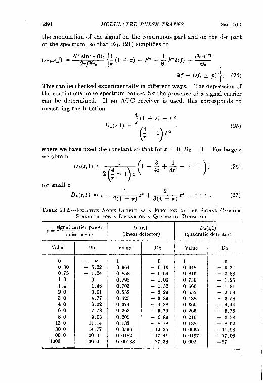
280 MODULATED PULSE TRAINS [SEC. 104
the modulation of the signal’ on the continuous part and on the d-c partof the spectrum, so that Eq. (21) simplifies to
This can be checked experimentally in different ways. The depression ofthe continuous noise spectrum caused by the presence of a signal carriercan be determined. If an AGC receiver is used, this corresponds tomeasuring the function
!(l+Z)– F’
l).(z)]) = r 4
()’
(25)— _l~2T
where we have fixed the constant su that for z = O, DL = 1. For large zwe obtain
DL(Z,l) =1
(
31
())
l–~+~–””” ; (26)2:–12
for small z
D.(z,l) = 1 – 2(4 l_ ~, Z2 +2
3(4–7r)z3 -””””(27)
TABLM 1O.2.—RELATWE INOISE OUTPUT AS A FUNCTION OF THE SIGNAL CARRIERSTRENGTH FOR A LINEAR OR A QUADRATIC DETECTOR
signal carrier powerz=
noise power—
Value
o0.300.751.01.42.03.04.06.08.0
13.030.0
100.01000
Db
—
– 5~2– 1.24
01.463.014,776.027.789.03
11,1414,7720.030.0
DL(Z,l)(linear detector)
Value I DbI
10.9640.8580.7950.7030.5530,4250.3740.2630,2050.1330.05960.01820.00183
0
- 0.16- 0.66
- 1.00- 1.52- 2.29
- 3.36- 4.28
- 5.79– 6.89
– 8.78–12,25–17.41–27.38
DQ(z,l)(quadraticdetector)
Value
10.9480.8160.7500.6600.5550.4380.3600,2660,2100.1380.06350.01970.002
Db
o- 0.24- 0.88- 1.25– 1.81– 2.56- 3.58– 4.44– 5.76– 6.78– 8.62–11.98–17.06–27
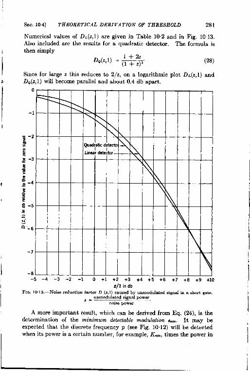
I
I
i~
i
1
)
1
I
i
SEC.10.4] THEORETICAL DERIVATION OF THRESHOLD 281
Numerical values of D.(z,l) are given in Table 10.2 and in Fig. 10.13.Also included are the results for a quadratic detector. The formula isthen simply
DQ(Z,l) = *. (28)
Since for large z this reduces to 2/2, on a logarithmic plot D.(z,l) andD~(z, 1) will become parallel and about 0.4 db apart.
o
-1
FI
-7
-8 k
-
\
Qua
Lint
—.-5 -4 -3 -2 -1 O +1 +2 +3 +4 +5 +6 +7
L
+9 +10z/1 h db
F1& 10.13.—Noise reduction factor D (z, 1) caused by unmodulated signal in a short gate.unmodulated signal power
z=noise power
A more important result, which can be derived from Eq. (24), is thedetermination of the minimum detectable modulatim h. It may beexpected that the discrete frequency p (see Fig. 10.12) will be detectedwhen its power is a certain number, for example, Kti, times the power in
I
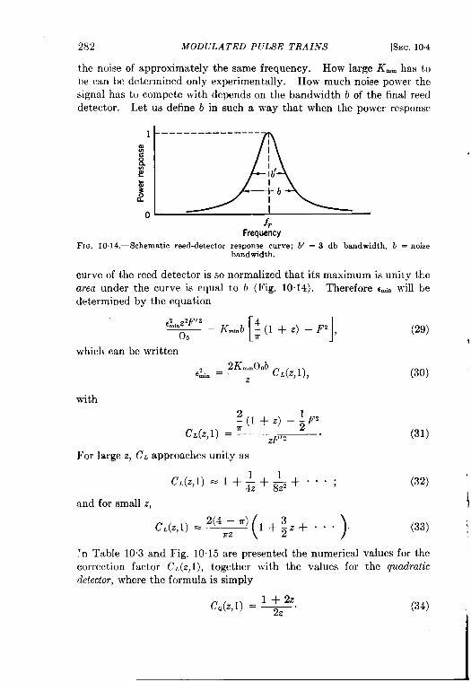
282 MODULATED PULSE TRAINS [SEC. 104
the noise of approximately the same frequency. How large K~,mhas tohe can be determined only experimentally. How much noise power thesignal has to compete with depends on the bandwidth b of the final reeddetector. Let us define b in such a way that when the power response
1 - -----—-—--—.——al!40ng
&3
2
0 rJr
Frequency
FIG. 10. 14.—Schematic reed-detector response curve; b’ = 3 db bandwidth, b = noisebandwidth.
curve of the reed detector is so normalized that its maximum is unity thearea under the curve is equal to b (Fig. 1014). Therefore (~ti will bedetermined by the equation
&Dz2F’2eo [ 1=Kmir,b ~(l+z)– F’,
T(29)
iwhich can be written
2Km.@,bC:in = CL(Z,l),
z
with
+.)+CL(Z,l) = T ZF)2
For large z, c. approaches unity as
CL(Z,l)11
=l+~+~z+”””;
and for small z,
2(4 – m)C.(Z, 1) = -—y
( )l+; Z+... .
(30)
(31)
!n Table 10.3 and Fig. 10.15 are presented the numerical values for the
correction fact or CL (z, 1), together with the values for the quadratic
detector, where the formula is simply
1+2ZCQ(Z,I) = ~. (34)
I
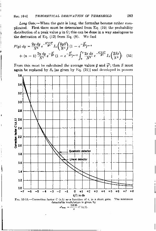
SEC. 10.4] THEORETICAL DERIVATION OF THRESHOLD 283
Long Gate.—When the gate is long, the formulas become rather com-plicated. First there must be determined from Eq. (19) the probabilitydistribution of a peak value y in G; this can be done in a way analogous tothe derivation of Eq. (12) from Eq. (8). We find
()2ydye-U~I0 ~ I _ ~’
P(Y) dy = ~ ~ ( _ e W)?a-1
/
=%+,gl2y dy e–;, (l _ e–~:).–z ~ ~
+(n–1)~()
2SZ‘2xdze–~10 _ .N, (35)
From this must be calculated the average values ~ and ~; then S mustagain be replaced by i% [as given by Eq. (21)] and developed in powers
3.6
3.4
32
3.0 1
2.8
s 2.6w- \
G 2A
i
I
2.2
2.0\ ‘
— . Quadratidetector1.6
\ I- Lineardetsctor
1.6 \
1.4 ~
12 \ \\ : .
Lo-7 -6 -5 -4 -3 -2 -1 0 +1 +2 +3 +4 +5 +6 +7 +8
Z/l in dbFm. 10. 15.—Correction factor C (z, 1) as a function of z, in a short gate. The minimum
detectable modulation is given by2K6h— c (2,1).#mh = ~
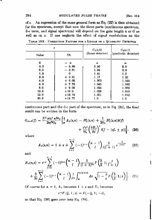
284 MODULA TED PULSE TRAINS [SEC. 10.4
of C. An expression of the same general form as Eq. (22) is then obtainedfor the spectrum, except that now the three parts (continuous spectrum,d-c term, and signal spectrum) will depend on the gate length n cr G aswell as on z. If one neglects the effect of signal modulation on the
TARLE1O.3.—CORRECTIONFACTORSFORA LINEARORA QUADRATICDETECTOR
z
Value
o0.20.51.02.04.06.08.0
10.012.030,0
Db
-m
– 6.99– 3,01
0+ 3.01+ 6.02+ 7.78+ 9.03+10.0+10.79+14.77
CL(Z,l)
(linear detector)
3:61.941.411,171.073
1.0451.0341.0261.0211.0
CQ(Z,l)
~uadratic detector)
3:2.01.51.251,1251,0s3
1.0631.0501.042
1.0
continuous part and the d-c part of the spectrum, as in Eq. (24), the finalresult can be written in the form 1
() )+ ‘+ ~ ‘ b[j – (s.fr ~ p)] , (36)
wheren—l
‘L(z)”)=‘+z+z(-’y+’h‘)&)’-&z’37)1=1
andn—l
‘L(nJz) ‘e-z2(-1)’+’ril) (,:l)~Fcl’&,)1=0
n—1
+:z(-l)l+’r~l)Jr(’+l)dzRF(:’’”)l‘3”)1=1Of course for n = 1, A. becomes 1 + z and B,. becomes
1 1“ —z),‘–zF (;, 1; Z) = F(— TJ ‘
so that Eq. (36) goes over into Eq. (24).
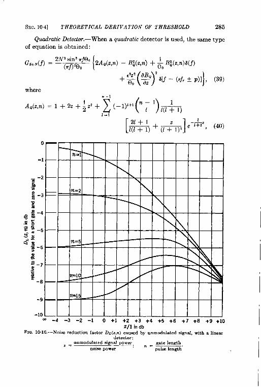
SEC.10.4] THEORETICAL DERIVATION OF THRESHOLD 285
@adratic Detector. -When a quadratic detector is used, the same typeof equation is obtained:
G.+.(f) ={
z~;:;:e;fe” 2AQ(z,rz) –B;(z,n) +& B:(z,n)&(j)
+~(g)’lf –(sjr+p)l}, (39)
where
‘0(2”) =1 +zz+iz’+%+’t~ ‘)&)1=1
[
21+1 11——z
1(1+1)+(1:1)2 e ‘+1 , (40)
i6&.6
%.=~f! k‘:‘‘;‘“““‘‘‘
=10-8
n=l-9
-10C9 -4 -3 -2 -1 0 +1 +2 +3 +4 +5 +6 +7 +8 +9 +10
2/1 h dbFm. 10.16.—Noise reduction factor l)~(z,n) caused by unmodulated signal, with a linear
unmodulated signal powerz= gate length
noise power n = pulse length’
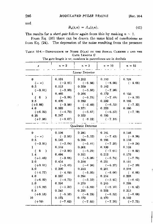
286 Modulated PULSE TRAINS [SEC. 10-4
and11~(.z,n) = A=(z,n). (41)
'rheresults forasbrt gate follo}v again from this bymakingn = 1.From Eq. (36) there can be drawn the same kind of conclusions as
from Eq. (24). The depression of the noise resulting from the presence
TARLE1O.4.—DEFENDENCEOFNOKSED(z,n) ONTHESIGNALCARRIERz AND THEGATE LENGTH G
The gate length is n,; numbers in parentheses are in decibels
z I ~=zI *=5!
n=lo I n=15
Linear Detector
o0,:–4
(–3.01)1
(o)2.5(+3 98)4.0
(+6.02)6.25
(+7.96)
oO,g–m)
(-3.01)1
(o)1,4
(+1.46)2.0
(+3.01)3,0
(+4.77)4,0
(+6.02)5.0
(+6.99)6.5
lo (+8.13)
(+W
0.524(–2.81)
0.513(–2.90)
0.495
(–3.06)0.409
(–3.88)0.332
(-4.79)
0,247(–6.07)
0.252(–5.98)
0,259(-5.86)
0.266(–5,75)
0,282(–5.49)
0.271(–5.67)
0.223(-6.52)
Quadratic Detector
0.556(–2.55)
0.545(–2.64)
0,518
(–2.86)0.494
(-3,06)0.454
(-3.43)0.390
(-4,09)
0,337(–4,73)
0.294(–5.32)
0.245
(–6.10)0.173
(–7.62)
0.281(–5.52)
0.288(–5.41)
0.301(–5.22)
0.311(–5.08)
0,318(–4.98)
0.313(–5.05)
0,294(–5.32)
0.270(-5.69)
0,235(–6.29)
0.172(–7.65)
0.159(–8.00)
0.162(–7.90)
0.179(–7.48)
0.222(–6.55)
0,223(–6.52)
0.195(–7.10)
0,181(–7.43)
0,186(–7.30)
0.199(–7.01)
0.212(–6,74)
0.231(–6.37)
0.251(–6,00)
0.254(–5.95)
0.245(–6.10)
0.223(–6.52)
0.170(–7,70)
0.124
(–9.05)
0.135
(–8.70)0.185
(–7.32)0.195
(–7.10)
0.146(–8.36)
0.150(–8.24)
O.158(–8.02)
0.170(–7.70)
0.191(–7.20)
0.216(–6.66)
0.228(-6.42)
0,228(–6.42)
0.215(–6.68)
0.169(-7.73)
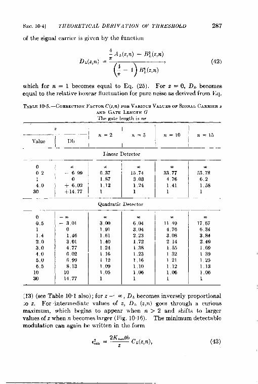
sm. 104] THEORETICAL
of the signal carrier is given
D~(z,n)
DERI VA 7’ION W THRESHOLD 287
by the function
~ AL(z,n) – B~(z,n)T—— /. \ > (42)
N4— – 1 B; (Z,?z)7r
which for n = 1 becomes equal to Eq. (25). For z = O, DL becomesequal to the relative boxcar fluctuation for pure noise as derived from Eq.
TARLE 1O.5.—CORRECTION FACTOR C(z,n) FOR VARIOUS VALUES OF SIGNAL CARRIER zAND ~,ATE LENGTH GThe gate length is nr
z
I 1
fi=~ ~=5 n=lo ~=1~Value Db
Linear Detector
o ~_@lm ~0.2 – 6,99 6 37 1.5.741 0 1.87 3.034.0 + 6.02 1.12 1.24
30 +14.77 1 1
Quadratic Detector
o0.5 : ;.01 3’301 0 1.911.4 1.46 1.612.0 3.01 1.403.0 4.77 1.244.0 6.02 1,165.0 6.99 1.126.5 8,13 1.09
10 10 1.0530 14.77 1
E
6,04
3.042.231,721.381.231.161.101.061
33 ,;74.76
1.41
53 .~86.21.58
—
11:94.763.082.141.551 321,211.121.061
m
17.676.343.842.491,691 391.251.131.061
(13) (see Table 10.1 also) ;forz–’ ~, DLbecomes inversely proportional;O z. Forintermediate values of z, D. (z,n) goes through a curiousmaximum, which begins to appear when n > 2 and shifts to largervalues ofzwhen nbecomes largm-(~ig. 10.16). Theminimum detectablemodulation can again be written in the form
2Kn,,n0b~~n = — C.(z,rt),z
(43)
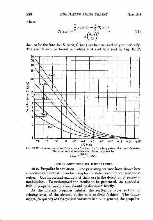
288
where
MODULATED PULSE TRAINS [SEC. 10.5
~A.(z,rz) –2 1 B~(z,n)
CL(z)n) = m
()
aB~ 2(44)
z—az
Just as for the function D.(z,n), C.(z,n) can be discussed only numerically.The results can be found in Tables 10”4 and 10”5 and in Fig. 10.17.
60
m40
30
20
Gi
10
8
654
3
2
1’‘6 ‘4 -2 0 +2 +4 +6 +8 +10 +12 +14 +1
zll indbFIG. 10. 17.—Correction factor CL(z,n) as a fu”ct ion of z for a long gate and a linear detector.
The minimumdetectable modulationis given by2K0b‘C=(Z,~).&h = ~
OTHER METHODS OF MODULATION
10.5. Propeller Modulation.-The preceding sections have shown howa receiver and indicator can be made for the detection of modulated radarpulses. One important example of their use is the detection of propellermodulation. To understand the results to be presented, the character-istic of propeller modulation should be discussed briefly.
As the aircraft propeller rotates, the scattering cross section, orechoing area, of the aircraft varies in a cyclical fashion. The funda-mental frequency of this cyclical variation is not, in general, the propeller-
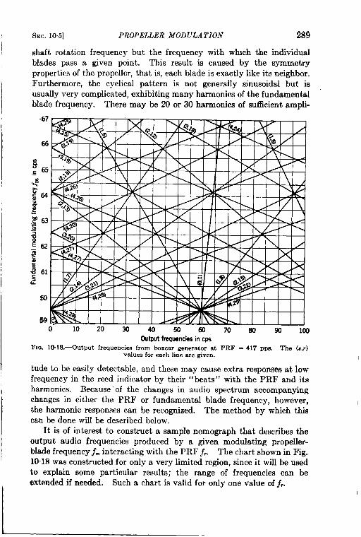
I
I
SEC. 10.5] PROPELLER MODULATION 289
shaft rotation frequency but the frequency with wbmh the indhidualblades pass a given point. Thk result is caused by the symmetryproperties of the propeller, that is, each blade is exactly like its neighbor.Furthermore, the cyclical pattern is not generally sinusoidal but isusually very complicated, exhibiting many harmonics of the fundamentalblade frequency. There may be 20 or 30 harmonics of sufficient ampli-
I [ I [ I I I [J
59 Q
Output frequencies in cps
FIG. 10.18.—Output frequencies from boxcar generator at PRF = 417 pps. The (a,r)values for each line are given.
tude to be easily detectable, and these may cause extra responses at lowfrequency in the reed indicator by their “ beats” with the PRF and itsharmonics. Because’ of the changes in audio spectrum accompanyingchanges in either the PRF or fundamental blade frequency, however,the harmonic responses can be recognized. The method by which thiscan be done will be described below.
It is of interest to construct a sample nomograph that describes theoutput audio frequencies produced by a given modulating propeller-blade frequency f~ interacting with the PRF j,. The chart shown in Fig.10.18 was constructed for only a very limited region, since it will be usedto explain some particular results; the rang; of” frequencies can beextended if needed. Such a chart is valid for only one value of $,.
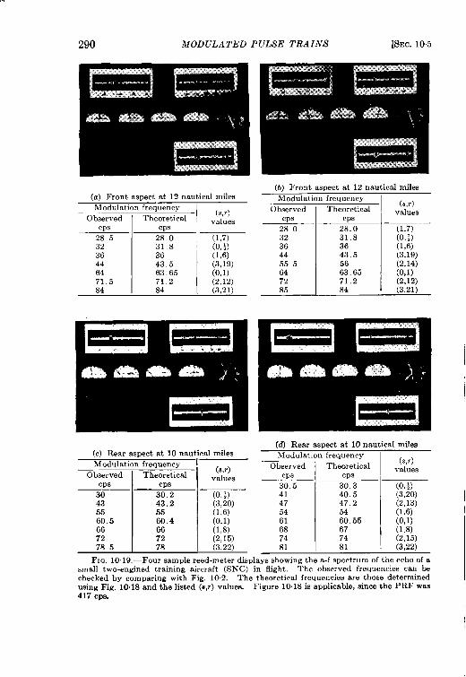
290 MODULATED PULSE TRAINS [SEC. 10.5
(a) Front aspect at 12na~Modulation frequenry
Observed I TheoreticalCps Cps
28 5 28.032 31.836 3644 43.564 63.6571.5 71 284 84
[cal miles
(s,.)values
(1,7)(o,+)(1,6)(3,19)(0,1)(2,12)(3,21)
(b) Front aspect at 12nauticalmiles.Modulationfrequency
Observed Theoretical(s,,)
valuesCps Cps28.0 I 28.0 (1,7)32 31.8 (o,+)36 36 (1,6)44 43.5 (3,19)55.5 56 (2,14)64 63.65 (0!1)
(c) Rear aspect at 10 nautical milesModulation frequency I
Observed Theoretical(8,,)
valuesCps Cps
30 30.2 (o,+)43 43.2 (3,20)55 55 (1,6)60.5 60.4 (0,1)66 66 (1,8)72 72 (2,15)78 5 78 (3,22)
(dl Rear amect at 10nauticalmiles>lod”lation frequency
Observed Theoretical(.,r)
valuesCps cps
30 5 30.3 (o,+)41 40.5 (3,20)47 47.2 (2,13)54 54 (1,6)61 60.55 (0,1)68 67 (1,8)74 74 (2,15)81 81 (3,22)
FIG, 10.19, —Foursample reed-meter displays showing the a-f spectrum of theecho ofasmall two-engined training aircraft (SNC) in flight, The observed frequencies can bechecked by comparing with Fig. 10.2. The theoretical frequencies are those determinedusing Fig. 10.18 and the listed (u,r) values. Figure 10.18 inapplicable, since the PRF was417 Cps.
SEC. 10.5] PROPELLER
In Fig. 10.18, ~r is 417 cps, the
MOD ULA TION 291
abscissa represents the output audio
frequencies from O to 100 cps, and the ordinate, the values of j; between
59 and 67 cps. The output frequencies are obtained by the intersections
of a horizontal line whose ordinate is the desired blade frequency with the
array of oblique lines shown. Each such line is characterized by two
indices s and r. These indices define the harmonics of the PRF, which
interacts with the rth harmonic of ~n to produce the particular a-f com-
ponent represented by the intersection. This nomograph is similar to
the one shown in Fig. 2.12, where output frequencies for a single modu-
lating frequency are given.
In Fig. 10.18 it can be seen that for a given fractional change in the
blade frequency the high harmonics of f- and the PRF produce audio
components that change frequency with relative rapidity. It is because
of this fact that these components can be properly identified. Further-
more a given a-f spectrum can be “fitted” to a chart similar to that shown
in Fig. 10.18, and a very precise value for f~ can be obtained. This
procedure, of course, assumes a known value for the PRF.
Results of actual flight trials with an SNC type aircraft are shown in
Fig. 10.19. These photographs show the responses obtained on a vibrat-
ing reed assembly similar to that shown in Fig. 10.2 except for the absence
of the lowest-frequency reed meter.
A host of responses is obtained. The conditions for these tests are
those for which the nomograph of Fig. 10.18 was constructed, namely, a
PRF of 417 cps and a blade frequency of approximately 64 cps. Since
the photographs are not very clear, a table is presented under each picture
that lists the observed audio frequencies together with the “fitted”
theoretical frequencies and the indices (.s,r) that are assumed to be
responsible for the indication. It will be noticed that a small 32-cps
response is listed for the indices (O,+). This response is caused by a
slight asymmetry in the two-bladed SNC propeller, which produces a
term at the shaft rotation frequency, that is, one-half the blade frequency.
It will also be noticed that responses of appreciable magnitude are
observed from the twenty-first harmonic of the blade frequency.
Furthermore, many of the high-harmonic responses are stronger than
that due to the fundamental itself.
These strong harmonic responses are not at all surprising when one
examines the radar intensity pattern resulting from propeller rotation,
obtained for a fixed aspect of the aircraft. Such a pattern is shown in
llg. 10.20, where the ordinate represents the amplitude of returned echo
and the abscissa represents time. The time required for 90° of shaft
rotation of the four-blade propeller of the B-26 medium bomber used in
this test is the time between the successive prominent minima. This
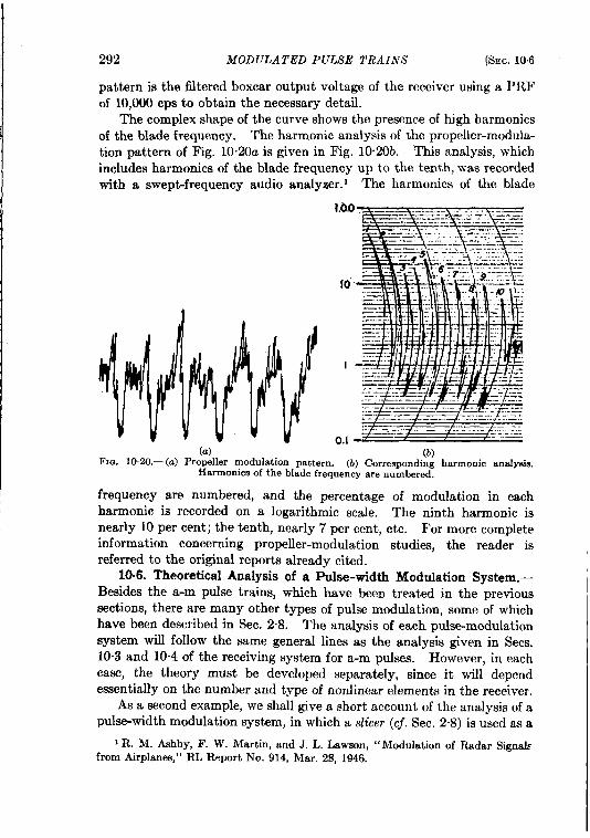
292 MODULATED PULSE TRAINS [SEC. 10.6
pattern is the fltered boxcar output voltage of the receiver using a PRF
of 10,000 cps to obtain the necessary detail.
The complex shape of the curve shows the presence of high harmonics
of the blade frequency. The harmonic analysis of the propeller-modula-
tion pattern of Fig. 10.20a is given in Fig. 10”20b. This analysis, which
includes harmonics of the blade frequency up to the tenth, was recorded
with a swept-frequency audio analyzer. 1 The harmonics of the blade
(a) (b)Fm. 1O.2O.—(IZ) Propeller modkdation pattern. (b) Corresponding harmonic analysia.
Harmonics of the blade frequency are numbered.
frequency are numbered, and the percentage of modulation in each
harmonic is recorded on a logarithmic scale. The ninth harmonic is
nearly 10 per cent; the tenth, nearly 7 per cent, etc. For more complete
information concerning propeller-modulation studies, the reader is
referred to the original reports already cited.
10.6. Theoretical Analysis of a Pulse-width Modulation System.—
Besides the a-m pulse trains, which have been treated in the previous
sections, there are many other types of pulse modulation, some of which
have been described in Sec. 2“8. The analysis of each puke-modulation
system will follow the same general lines as the analysis given in $ecs.
10.3 and 10.4 of the receiving system for a-m pulses. However, in each
case, the theory must be developed separately, since it will depend
essentially on the number and type of nonlinear elements in the receiver.
As a second example, we shall give a short account of the analysis of a
pulse-width modulation system, in which a slicer (cf. Sec. 2.8) is used as a
I R. M. Aahby, F. W. Martin, and J. L. Lawson, ‘( Modulation of Radar SignaLefrom Airplanes,” RL Report No. 914, Mar. 28, 1946.
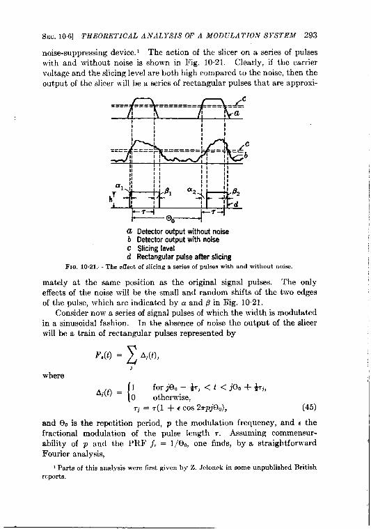
SEC. 106] THEORETICAL ANALYSIS OF A MODULATION SYSTEM 293
noise-suppressing device. 1 The action of the slicer on a series of pulses
with and without noise is shown in Fig. 10”21. Clearly, if the carrier
voltage and the slicing level are both high compared to the noise, then the
output of the slicer will be a series of rectangular pulses that are approxi-
i 18
ii
II
U Detector output without noise
b Detector output with noiseC Slicing level
d Rectangular pulse after slicingFIO. 10.21.—The effect of slicing a seriesof pulseswith and without noise.
mately at the same position as the original signal pulses. The only
effects of the noise will be the small and random shifts of the two edges
of the pulse, which are indicated by a and @ in Rig. 1021.
Consider now a series of signal pulses of which the width is modulated
in a sinusoidal fashion. In the absence of noise the output of the slicer
will be a train of rectangular pulses represented by
where
F,(t) =z
Aj(t),
1
[
for jeo – ~,i < t < jeo + *i,Aj(t) = ~
otherwise,
‘i = ~(1 + c cos 27rpjeO), (45)
and (30 is the repetition period, p the modulation frequency, and e the
fractional modulation of the pulse length ~. Assuming commensur-
ability of p and the PRF j, = 1/E)O, one finds, by a straightforward
Fourier analysis,
,1
I Parts of this analysis were first given by Z. Jclonrk in some unpublished Britishreports.
I
294 MODULATED PULSE TRAINS [SEC. 10.6
m.
22F,(t) =: —— I2– 6,.2– d,, J,[7rT,(lp+kf,)]
2 2 lp +kf,k=ol=o
[61,evenSin7r7(@ + kjr) + i&,oddcoS~~ (1P + kj,)]cos2r(lp + kj,)t
+Jz[7rT6(2p –k.f,)]
lp – kf,[a~,....sinn(~p — kf,) + i&, oddcos7U(lP — k.f,)]
cos27r(1p – kf,)~), (46)
where Jl(z) is the Bessel function of order 1; the symbol J1,e.- is defined by
(1 for 1even,
at, .. .. = ~for 1 odd,
and 81,~d = 1 – 131,,.~. All the harmonics of f, and p and their com-
bination frequencies are therefore present in the spectrum of the signal.
When noise is present, the edges of the jth pulse are shifted by the
random amounts a, and /3j. By an analysis similar to the analysis usedin Examples 3 and 4 of Sec. 3.4, the power spectrum of signal and noisecan be written in the form
N
G,+..(j) = & 27Z;N9[z(W – la,l’) +o l&@-i’’e{21 ’47)j-o j-o
where
In order to obtain the ensemble averages 6, and ~ the probability dis-tribution of the a, and /3, must be found. In Eq. (47), the assumptionhas been made that the a’s and P’S of different pulses and, therefore, thedifferent a,’s are independent of each other. This, of course, will alwaysbe the case, since eo is always large compared witlf l/B if B is the i-fbandwidth. For simplicity, we shall assume in addition that the a’s and~’s of one pulse are independent of each other. This implies that B >>1,so that the original signal pulse is only slightly deformed by the i-famplifier.
The probability distribution F’(a) da follows immediately from theprobability distribution of signal plus noise [cf. Eq. (7.13)]:
s,+,,W(r) dr = ~ e
()
rSrdr –TIO _W
(49)
by putfiing r = h, S = h + cdgd,, dr = da tgO,, where h is the slicing leveland tgill is the slope of the signal pulse after the i-f amplifier and at theheight h. Replacing Eq. (49) with the Gaussian approximation[cf Eq. (713a)], which is allowed, since S’2>> 2W, one finds
da ~-~P(a) da = —
~;(50)
SEC. 10.6] THEORETICAL ANALYSIS OF A MODULATION SYSTEM 295
where u: = W/tg’0,. In the same way one finds for ~ a Gaussian dis-tribution with the variance u; = lL’/tg29Z.
The average values indicated in Eq. (47) can now be evaluated. Theresults are
Substitution of these results in the first sum in Eq. (47) leads to thecontinuous part of the power spectrum. We will neglect in this part, aswe did in Sec. 10.4, the effect of the modulation of the signal. Thecontinuous spectrum becomes therefore
&o (m – M’) = Z+. (2 – ,-4r’/’cL’ – .-4.%, %22). (52)
The substitution of Eq. (51) in the second sum of Eq. (47) leads to thediscrete spectrum due to the signal. Using the expression (45) for ,j anddeveloping in powers of c up to e2, one obtains for the discrete spectrum,when p < f,/2,
.
~& [e-4”’J’ul’ + e–4r,jW-2 cos 2rj7e-2”z’’c~’’+””)] ~ L$(j- Sfr)
,=0
.=’O(53)
If there is no noise, u: = u; = O, and Eq. (53) goes over into the powerspectrum of the signal alone, which, provided the same powers of c arekept, agrees with the power spectrum that follows from Eq. (46).
According to the power criterion (cj. Sec. 7.3), the detectability of themodulation ~ depends on the ratio of the power of the signal peak at thefrequency p to the power of the continuous noise spectrum with which thesignal has to compete. Suppose that a narrow audio filter of width b isused; it follows from Eq. (53) that the power of the signal peak at thefrequency p is
whereas it follows from Eq. (52) that the power of the continuous noisespectrum is
296 MODULATED PULSE TRAINS’ [SEC. 10.6
The minimum detectable modulation is therefore given by
41cb 2 – exp ( –47r2p2u~) – exp ( –47r2p2u~)CL. = —
7r2T2p2j, exp ( —47r2p2a~) + exp ( —47r2p2u~) + 2 COB27rpr exp[– 27r’p’(LT; + ‘@]j (54a)
where k is a constant, which has to be determined experimentally, just asin Sec. 10.2.
For further discussion we shall assume that the i-f amplifier (band-width 1?) deforms the pulses in a symmetrical fashion, so that ul = az = u.Assume further that pu and even p. are much smaller than unity. ThenEq. (54a) reduces to
(54b)
For a Gaussian pulse and a Gaussian i-f pass band, uz and r can be calcu-lated exactly, and Eq. (54b) becomes
(55a)
where SOis the pulse amplitude before the i-f amplifier, h is the height ofthe slicing level, and z = S~/2W. For the case of a square pulse and aGaussian i-f pass band, one obtains in the same way
1.78b 1c~.Ek——
f, 2X’~–z[ 1–( 2WSO)]!, (55b)
where z = Bro is the product of the i-f bandwidth and the original pulselength. In both Eqs. (55a) and (55b) z is assumed to be large comparedwith unity. For a Gaussian pulse ~= is independent of x, whereas fora square pulse CL goes to zero when x - cc. This difference can easilybe understood. The influence of the noise decreases for increasing slopeof the pulse at the slicing level. For a square pulse the slope increasesindefinitely when z ~ ~ ; whereas for the Gaussian pulse the slope will,of course, remain finite.
—
CHAPTER 11
THRESHOLD PULSED SIGNALS
INTRODUCTION
IN CLUTTER
11.1. Comparison between Clutter and Noise.—In many ways noiseand “clutter” are similar. In the following pages are discussed some ofthe similarities as well as the differences bet}veen them. The similaritieshave given rise to the argument that both types of interference havesimilar effects, but this conclusion is not a valid one.
The frequency spectrum of receiver noise is essentially uniform at theinput of the i-f amplifier; the frequency spectrum of the clutter is influ-enced by the transmitted pulse itself. For practical purposes all fre-quencies in the neighborhood of the transmitter frequency are, on theaverage, equally reflected by clutter. Hence the long-time-averagepower spectrum of the clutter will be just that of the transmitted pulse,that is, usually a(sinz z/z’) spectrum, where z is the frequency deviationfrom the center radio frequency. Thus noise and clutter would beexpected to behave differently with respect, for example, to a variationin receiver bandwidth.
The amplitude probability distributions of clutter and noise at thereceiver second detector differ only with respect to a multiplicative con-stant. This property comes about because both phenomena are random;they are produced by the random interaction of many small processes.The average values of the amplitudes at the second detector of noise andclutter behave differently, however. In noise the average value isconstant in time, but for clutter it varies in time, i.e., radar range, notonly with geometrical factors but also with the different scatteringproperties of the illuminated medium. This varying average amplitudeof clutter causes much difficulty since, without special circuits, saturationin the receiver \vill not be avoided in regions of strong clutter return.For receiver noise, however, a setting of the receiver gain control can befound where saturation by receiver noise can be easily avoided. Inaddition to the total variation in clutter amplitude, possibly requiringsome form of receiver AGC for satisfactory operation, the rate at whichthis clutter-amplitude variation occurs, i.e., as the range changes, will beimportant. This rate of change will determine the speed with which theAGC must act to be effective.
One other important property of clutter is the rate at which the clutter297
298 THRESHOLD PCLSED SIGaY.4LS IV C’LI’TYER [SEC. 112
configuration changes in time. If the radar return from a single trans-mitted pulse is examined, a complicated time pattern will be obtained thatcontains all frequencies up to very high ones, a pattern that is similar.except for spectrum differences, to receiver noise. This pattern, orconfiguration, \vill remain essentially unchanged, however, if a secondpulse is used shortly afterward. The configuration is therefore relativelystable in time, perhaps for as long as a second, although its shape may becomplicated. The reason for this stability is that the returned signaldepends on the physical positions of the reflecting objects. Changes inrelative position and therefore in the signal amplitude occur compara-tively slowly. The consequences of this fact v-ill be discussed morefully in Sees. 11.9 and 11.10, where it ~villbe shown how this phenomenoncan be used to reduce the effects of clutter.
11.2. Threshold Signal in the Absence of Saturation. -In the absenceof saturation, problems connected with the perception of signals in clutterare similar to signal-perception problems in noise. Even though clutteris relatively stable, the configurational changes are usually sufficientlyrapid to be visually somewhat similar to normal noise fluctuations.Clutter has a somewhat coarser and more grainy appearance than ordi-nary noise, however. h“evertheless, as with receiver noise, the desiredsignal must be of the order of magnitude of the average clutter (plusnoise) power to be recognizable. These remarks apply exclusively toclutter in which the configurational changes are relatively rapid, forexample, sea return and rainstorm echoes. They do not apply, however,to ground return, where the clutter configuration is virtually stable. Inthe case of ground clutter, a satisfactory criterion for signal perceptionis all but impossible. A small desired target may produce an echo largeenough to be clearly seen, but it will not, in general, be recognized as thedesired target because of confusion with other similar echoes in theneighborhood. Consideration of ground clutter will for this reason bereserved for Sec. 11.9, where it will be shown that the desired signal mayba~re properties differing from those of clutter, for example, velocityproperties.
The problem posed by the perception of a desired signal in fluctuatingclutter, for example, rainstorm clutter, is complicated by several factors.First, unlike the case for receiver noise, the average amplitude of clutterreturn depends not only upon transmitted pulse power but upon thetotal volume of rainstorm illuminated at any given instant by the pulse.in other words, at any given instant the receiver input is collecting from aregion of rainstorm reflectors power that is as large as the packet of r-fenergy sent out by the transmitter in one-half the pulse length. There-fore an increase in transmitted pulse length by a factor of a produces ancz-fo!d increase in the scattering cross section for the clutter. For the
SEC. 11.2] THE ABSE,VCB OF SA T(JRA TION 299
perception in clutter of a desired discrete target, one whose cross sectionor echoing area is independent of the pulse length, short pulses should }JCused. This argument makes it clear that the signal threshold power inclutter should be directly proportional to the pulse length, provided, ofcourse, that the receiver i-f bandwidth is as wide as or wider than optimumfor the pulse length (see Chap. 8) and that the intensity of clutter issufficient to override all receiver noise.
This reasoning was confirmed by an experiment in which the outputpulse of a signal generator was introduced into the r-f receiving section of aradar system. The power of the pulse was known and variable, and itsphase adjustable so that it could be made to coincide with the radarechoes of a local rainstorm. When the lengths of the radar pulse and ofthe signal generator pulse were changed from 5 to 0.05 see, the observedthreshold signal was 18 db less as compared with the theoretical 20-dbdifference. This proportionality betmeen pulse length and signal thres-hold in clutter can also be qualitatively confirmed by studying the effectof antenna beamwidth on the perception of discrete targets in clutter.one would expect that the cross section of clutter extended in threedimensions would be proportional to the antenna-beam solid angle, sincethe illuminated part of the clutter is proportional to it. For clutter on aplane surface, such as sea return, the clutter cross section is proportionalto the width of the antenna beam. No exact quantitative information isavailable on this point, but it is a well-known fact that narrow-beam,high-discrimination radar sets are much less affected by extended clutterthan are radar sets having an equivalent wavelength but a broad antenna-beam pattern. One of the complicating features in the quantitativedetermination of the effect of the beamwidth is the difficulty of securingclutter that is essentially uniform over the large areas likely to be illumi-nated by a broad radar beam. Furthermore, when the discrimination ofthe radar set is very high, that is, when it has very narrow beamwidth andsmall pulse length, the clutter itself is no longer uniform but generallybreaks up into a number of distinct reflecting volumes. This character-istic is particularly true of sea clutter, where the discrimination of the setmay be made high enough to resolve individual reflecting sea waves.When this happens, the experimental determination of the minimumdetectable signal is difficult, not because of insufficient signal amplitudeor clutter fluctuation but because of confusion with other clutter peaksthat appear to be discrete. Nevertheless, for the perception of a discretesignal in clutter, high-discrimination radar sets have proved much moreuseful than low-discrimination sets.
One point should be emphasized: As long as there is sufficient radarpower for the clutter echoes to be much stronger than receiver noise, thesignal threshold power in clutter is independent of transmitted power but
300 THRESHOLD PULSED SIGNALS IAT CL[JTTER [Sl:c. 112
I)aries directly with pulse length. This situation is markedly different
from the problem of signal threshold in receiver noise (see Chap. 8).
For a given pulse length, the effect on signal threshold power inclutter of the various receiver parameters, such as i-f bandwidth, videobandwidth, presentation sweep speed, etc., could be investigated. Thesevariables would be found to have a somewhat different effect from that
observed in the presence of receiver noise because, as was shown in thepreceding section, the spectrum of clutter, as viewed in the i-f amplifier,differs from that of receiver noise. For the same returned power theclutter spectrum is, in fact, the same as that of the desired discrete echo,except that all components of the spectrum of clutter are, in general,independent or noncoherent; for the discrete echo, the various com-ponents are coherently related. Since the spectra of the signal andclutter are the same, it might be argued that changes of i-f or video band-widths would have no effect on the signal threshold power. Because ofthe difference in coherence, however, this is not true. For very narrowi-f bandwidths, it is the amplitude of the signal response and the power ofthe clutter response that will be proportional to bandwidth. Thissituation is analogous to that for receiver noise; obviously, therefore, thesignal threshold power will vary inversely with the i-f bandwidth in thisregion. For wide i-f bandwidths the situation is different, however.
The responses to both clutter and signal approach asymptotic values,
and the signal threshold power becomes independent of i-f bandwidth.Thus there is no optimum i-f bandwidth, although a receiver is usuallyrequired whose bandwidth is nearly optimum for noise, since both typesof interference are usually encountered. N’o good experimental informa-tion is available on this point, however, although rough experiments haveshown that the argument is probably correct.
As for noise, video bandwidth has a less pronounced effect than i-fbandwidth on signal threshold in clutter. For receiver noise at optimumi-f bandwidth the signal threshold power is increased when the video passband is narrowed from either the high side (low-pass filter) or the low side(high-pass filter or differentiator). This characteristic is not necessarily
true of clutter. Because of the difference in coherence between signal
and clutter, a low-pass video filter increases the threshold signal. The
video clutter components are essentially independent; hence for smallvideo bandwidths the average amplitude of clutter response is propor-tional to the square root of video bandwidth, whereas the amplitude ofsignal response is directly proportional to the video bandwidth. Incontrast to this situation, Middleton and Sutrol have shown that when a
1D. Middleton and P. J. Sutro, ~,~aly~i~ of a Possible A/J System Against
Window,” RRL Report No. 411-128,Dec. 9, 1944.
I
I
.
\I
)
1
1
I
1
I
I
L-
SEC. 11.2] THE ABSENCE OF SA YURA TION 301
high-pass filter is employed, an improvement in signal perception is to be
expected, especially when the i-f bandwidth is increased. The reason
for this improvement may be seen by considering the action of a high-pass
filter or diiferentiator. l?rom a wide-band i-f amplifier a pulse from the
desired discrete signal will have relatively steep edges. These sharp
transient voltages will be passed through the differentiator and will
therefore act much like shortened pulses. For each signal pulse, two
shortened pulses will be manufactured, one positive in sign and the other
negative. Were it not for the extra negative pulse, which contributes a
factor of 2 to clutter fluctuations, the signal threshold would be just the
same after differentiation as for the case in which a short transmitted
pulse is used. If sufficiently rapid differentiation is provided, therefore,
a net improvement in signal perception will occur. It should be empha-
sized, however, that a greater improvement could be obtained by using a
short transmitted pulse, since this would avoid the extra negative pulse
produced by the differentiator.
Attempts to prove experimentally the desirable effect of the differ-
entiator have usually been disappointing, partly because of the unavoid-
able low-pass filter characteristics of the human eye and brain pointedout in Sec. 8“7 and partly because of the lack of contrast between highly
differentiated signals. The low-pass characteristics of the eye appear to
override the action of any differentiator and therefore reduce the effec-tiveness of the latter. This is true, of course, only where the presentation
sweep speed is slow enough to make the “eye bandwidth” important.
This condition, however, is universally met in any presentation that is
being used for long-range search, the one function for wh~ch the avoidance
of clutter is so important. These difficulties will be clearly evident from
the results presented in Sec. 11“8.
One important point should be noted regarding the effect of a low-pass
filter. It might be argued that because of the low-pass effect of the
human eye and brain, an additional low-pass filter located in the videosystem should not be serious. This argument is true if there is no non-
linearity between the two falters-a condition that rarely exists.
Although the screen of the cathode-ray tube used for intensity-modulated
presentation is nonlinear, nonlinearity of this type is not usually of
importance. The most troublesome effect of a narrow video system
results from the video-limiting action necessary for intensity-modulated
displays. The average value of clutter (d-c term) causes limiting and
consequent loss of all signals long before clutter jluctuatians are large
enough to mask a desired echo. This situation is also true of receiver
noise, but here a blocking condenser can eliminate the d-c term. The
variable value of the d-c term makes this solution impossible for clutter.
A tierentiator can be us=ed, however, to remove the d-c term and its
I
.,
302 THRESHOLD PULSED SIGNALS IN CLUTTER [SEC. 113
sidebands, which fluctuate at a low frequency; this explains why radar
operators usually report an improvement in operation when they use a
video-differentiating circuit.
It should now be clear that the use of fast sweeps or expanded-range
oscilloscopes such as the R-scope (see Sec. 2.6) will improve signal per-
ception in clutter. This device, enabling the eye to perceive more of the
fine signal detail, i.e., the higher video frequencies, will constitute a video
filter with a higher h-f cutoff. Experiments have qualitatively con-
firmed this.
No good data have been gathered showing the effects of signal-
presentation time and over-all system integration on signal threshold
power in clutter. It seems reasonabl~, however, to suppose that the
effects are similar to those for receiver noise (see Chap. 8); qualitative
observation is in agreement with this supposition.
11.3. Threshold Signals in the Presence of Saturation. —Signal
perception in clutter is greatly reduced if saturation exists in the receiver.
In the presence of saturation the response of the receiver to incremental
input signals is essentially zero. Saturation is most likely to occur in thevideo system as a result of limiting; but as was pointed out in the pre-ceding section, its occurrence can be largely avoided by using a high-passfilter or differentiator between the second detector and video system.Even with such a device, however, saturation may still occur inthe i-famplifier itself. The i-f amplifier tubes may be driven into an overloadregion by the clutter signal. An obvious (but in practice inadequate)palliative is the use of larger tubes; the customary device used to alleviatethis overload effect is an AGC, which regulates the gain of the receiver inaccordance with the total voltage appearing in the output of the seconddetector. The possibility of sudden changes in clutter amplitude makesit imperative that this AGC have a rapid action, but its action must notbe so rapid that it causes serious distortion of discrete echoes. This
form of gain control has been referred to as instantaneous automatic gain
control, or IAGC, to distinguish it from the more conventional .kGC
operated from a third detector and having a relatively slow response (see
Sec. 2.7). NIore will be said about practical circuits and optimum adjust-
ment for the IAGC in the next section.
The major cause of m“gnal loss in clutter is saturation in either the video
or i-f amplijier and not any of the causes mentioned in the precedingsection. Saturation is in many ways extremely unsatisfactory, sincevirtually no quantitative information can be given on its effects. Theconditions for saturation in either the i-f amplifier or video system varyenormously from one receiver design to the next; they depend upon manvfactors beyondand stability.
the scope of this discussion, such as tube characteristicsAbout all that can be said is that once saturation occurs,
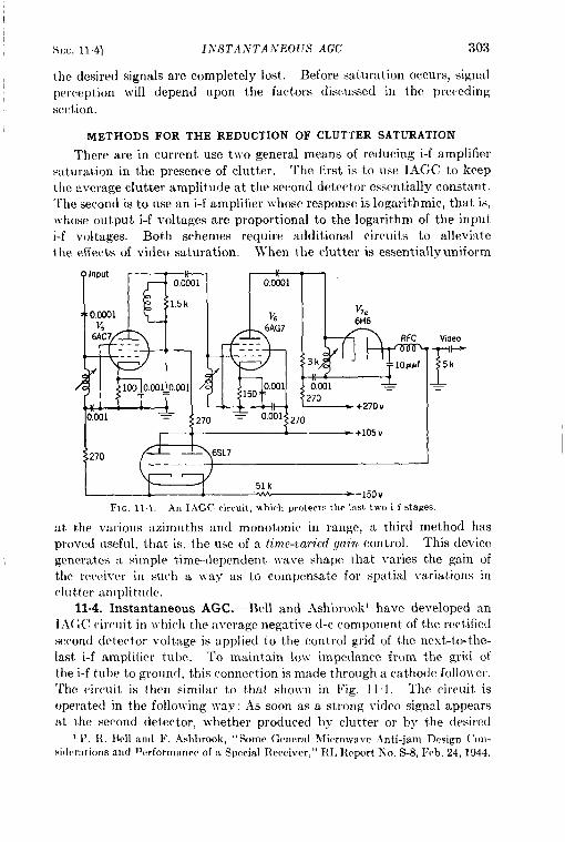
SKC,114]
the desiredperception
INSTA.VTANEOUS AGC 303
signals are completely lost. Before saturation occurs, signal
will depend upon the factors discussed in the preceding
scctjion.
METHODS FOR THE REDUCTION OF CLUTTER SATURATION
There are in current use tlvo general means of reducing i-f amplifiersiituration in the presence of clutter. The first is to use IAGC to keepthe e,verage clutter amplitude at the second detector essential y constant.‘he second is to use an i-f amplifier whose response is logarithmic, that is,Irhose output i-f voltages are proportional to the logarithm of the inputi-f voltages. Both schemes require additional circuits to alleviatethe effects of video saturation. IVhen the clutter is essentially uniform
r“’”’rFFJ=l F-1-l.---1 I ~ 6AG7 I I w!“
—
P-+0.001 —k270d27~+270: ‘
FIG.11 l.-An lAGC circuit,uhirh protectsthelasttwoi-f stages.
at t}le ~zu.iolw azimuths an{l monotonic in range, a third method hasproved useflll, that is, the use of a time-varied gain control. This devicegenerates a simple time-dependent \i-ave shape that varies the gain ofthe receiver in such a ~vay as to compensate for spatial variations inc]uttcr arnplit{ldc.
11.4. Instantaneous AGC.—I3ell and Ashbrook’ have developed an1,i( ;C rircllit in ]rhicll the ~verage negative d-c component of the rectifiedsecon(i detector voltage is applied to the control grid of the next-to-the-last i-f ampli(ier tulle. To maintain low impedance from the grid ofthe i-f tube to ground, this connection is made through a cathode follower.The f,irc,uit is then similar to that shoum in Fig, 11.1. The circuit isoperated in the follolving way: As soon as a strong video signal appearsat the second detector, ~vhether produced by clutter or by the desired
1P. 1{. IIrll and F. .Ishbrook, “ Some General ~~icrowave ..4nti-jamDesign Con-siflemtions and W.rformmcr of a Special Receiver, ” RI, Rrport h-o. S-8, Feb. 24, 1944.
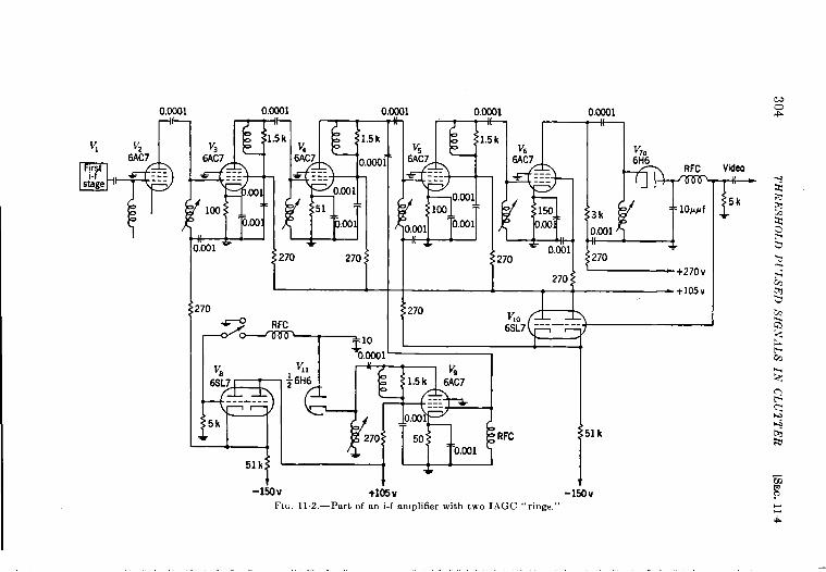
0.0C411
$+~V2
6AC7
D
rst -..l-f ---
stege - ‘--
V36AC7
=(-:
0.0001 O.yl 0.0031
~l&l~
1.5 k~
1.5 kv~
1.5k
6AC7 0.000] 6AC7--- ------ ------ ---
.XJ1
‘b
O.CO10.001
100 51 lW.00 .00 O.ml 0.001
.001 -
kVB6SL7
-------
5k
I $270
I
0.0301
‘n
ii
v~6AC7
---------
{150.00
O.olt?70
270
=
V,. -6SL7 r
---—-
V,,
~~ ~~ ,~
~$ 6H6 1.5 k 6AC7
------
@301---
270 50 RFC
0.001
t-lM v +165v .
F1o. 11.2,—Part of an i-f amplifierwithtwo IAGC “ rings,”
V,a6H6
lk= lo#/Jf
0.0014( 4;270—+270v
-+105V
il k
v
Video
[-5k
... .“. . ,... ,,. ,,, . .,,
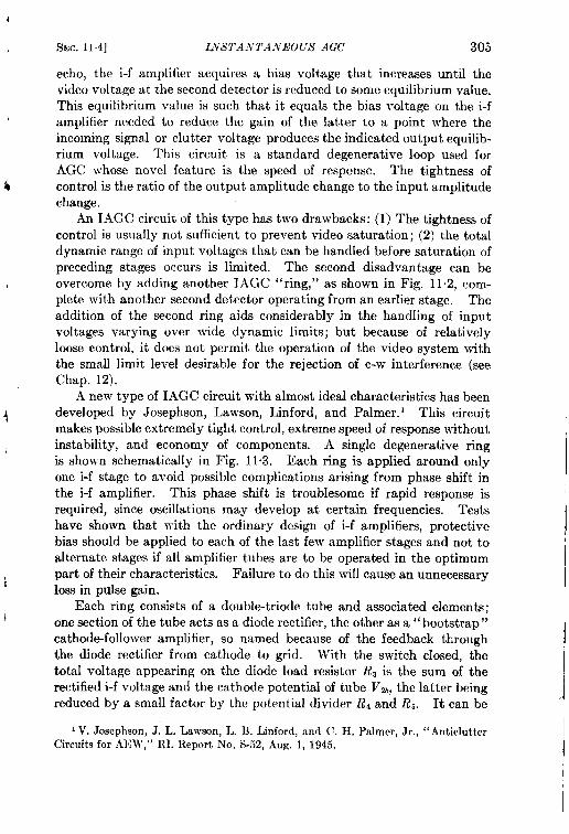
4
(SEC. 11.4] LNSTA A~TTANEOUS AGC 305
echo, the i-f amplifier acquires a bias voltage that increases until thevideo voltage at the second detector is reduced to some equilibrium value.This equilibrium value is such that it equals the bias voltage on the i-famplifier needed to reduce the gain of the latter to a point where theincoming signal or clutter voltage produces the indicated output equilib-rium voltage. This circuit is a standard degenerative loop used forAGC whose novel feature is the speed of respcnse. The tightness of
4 control is the ratio of the output amplitude change to the input amplitudechange.
An IAGC circuit of this type has two drawbacks: (1) The tightness ofcontrol is usually not sufficient to prevent video saturation; (2) the totaldynamic range of input voltages that can be handled before saturation ofpreceding stages occurs is limited. The second disadvantage can beovercome by adding another IAGC “ring,” as shown in Fig. 11.2, com-plete with another second detector operating from an earlier stage. Theaddition of the second ring aids considerably in the handling of inputvoltages varying over wide dynamic limits; but because of relativelyloose control, it does not permit the operation of the video system withthe small limit level desirable for the rejection of c-w interference (seeChap. 12).
A new type of IAGC circuit with almost ideal characteristics has been
4 developed by Josephson, Lawson, Linford, and Palmer. I This circuitmakes possible extremely tight control, extreme speed of response withoutinstability, and economy of components. A single degenerative ringis shown schematicallyy in Fig. 11.3. Each ring is applied around onlyone i-f stage to avoid possible complications arising from phase shift inthe i-f amplifier. This phase shift is troublesome if rapid response isrequired, since oscillations may develop at certain frequencies. Testshave shown that with the ordinary design of i-f amplifiers, protectivebias should be applied to each of the last few amplifier stages and not toalternate stages if all amplifier tubes are to be operated in the optimumpart of their characteristics. Failure to do this will cause an unnecessary
i loss in pulse gain.Each ring consists of a double-triode tube and associated elements;
I one section of the tube acts as a diode rectifier, the other as a” bootstrap”cathode-follower amplifier, so named because of the feedback tlmoughthe diode rectifier from cathode to grid. With the switch closed, thetotal voltage appearing on the diode load resistor R3 is the sum of therectified i-f voltage and the cathode potential of tube V%, the latter beingreduced by a small factor by the potential divider Rq and R~. It can be
I V. Josephson, J. L. Lawson, L. B. Linford, and C. H. palmer, Jr., “AnticlutterCircuits for .ki?W,” RI, Report No. S-52, Aug. 1, 1945.
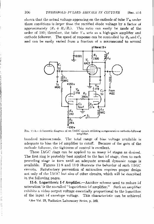
306 THRESHOLD P1’LSED SIGNALS I.V CLUTTER [SEC. 115
shown that the actual voltage appearing on the cathode of tube V2~underthese conditions is larger than the rectified diode voltage by a factor ofapproximately (R4 + R5/RJ. This ratio can easily be made of theorder of 100; therefore, the tube Val, acts as a high-gain amplifier andcathode follower. The speed of response can be controlled by R, and CSand can be easily varied from a fraction of a microsecond to several
J
Iti:c
FIG. 11.3---S Lt.ematic diagramof an IAGC circuitutilizingaregenerativecathode-followeramplifier.
hundred microseconds. The total range of bias voltage available is
adequate to bias the i-f amplifier to cutoff. Because of the gain of the
cathode follower, the tightness of control is excellent.
These lAGC rings can be applied to as many i-f stages as desired.
The first ring is probably best applied to the last i-f stage, then to each
preceding stage in turn until an adequate over-all dynamic range is
available. Figures 11.8 and 119 illustrate the behavior of such IAGC
circuits. Satisfactory prevention of saturation requires proper design
not only of the lAC.C but also of other circuits, which will be described
in the following pages.
11.5. Logarithmic I-f Amplhier.-Another scheme used to reduce i-f
saturat ionl is the so-called “logarithmic i-f amplifier. ” Such an amplifier
exhibits a video output voltage essentially proportional to the logarithm.
of the input i-f envelope voltage. This characteristic can be achieved
1See Vol, 23, Radiation Laboratory Series,p. 583,
SEC. 11.5] LOGARITHMIC I-F AMPLIFIER 307
in at least two ways. L. Belleville has built this type of amplifier by
connecting separate diode second detectors (envelope detectors) to each
i-f stage, then adding linearly the resulting separate video signals. For
small i-f voltages the last i-f stage will make almost the sole contribution
to the video signal, and the video response will be essentially proportional
to the input voltage; this condition will persist until the i-f voltage
becomes large enough to saturate this last stage. For larger inputA, voltages the last i-f stage will contribute nothing to the output, but the
next-to-the-last i-f stage will make a contribution up to input voltagesfor which it saturates, etc. This procedure can, if desired, be continuedfor all i-f stages in the receiver. The final result will be a receiver whosevideo output voltage is approximately proportional to the logarithm ofthe input voltage; the approximation to the smooth logarithmic curveconsists of a number of straight lines (representing linear response) ofvarying slope (the slope depending on the over-all gain up to the particu-lar contributing detector). For such a receiver the video response isalways finite for incremental changes in input voltage; hence saturationin the sense described in the preceding section is not possible.
R. A. McConnell has suggested another method of constructing sucha logarithmic receiver. This one also depends upon successive satura-tions in the i-f stages to secure a logarithmic over-all response, but thevoltage addition for successive stages is made in the i-f amplifier ratherthan in the detector or video sections. Only two additional points mustbe noted in connection with a receiver of this type: (1) The i-f voltagesfrom stage to stage are usually in phase opposition; and in adding i-fvoltages in appropriate phase, reversal must therefore be made in all odd-numbered stages; (2) i-f buffering must generally be used to preventfeedback from the output to an antecedent part of the i-f amplifier.Both conditions are easy to bring about, and some satisfactory loga-rithmic receivers have been constructed in this way.
In the two types of receivers discussed the logarithmic characteristicextends over a limited region of input voltages. Up to voltages thatbegin to saturate the last i-f stage, the response is essentially linear.From this point up to voltages that saturate all stages the response isessentially logarithmic, and above this point the dynamic gain is zero.Therefore these receivers are most commonly referred to as linear-logarithmic receivers. The crossover point between a linear and loga-rithmic characteristic is determined by the saturation of the last i-f stage;in terms of the input voltage the crossover point can be adjusted to anydesired value by an appropriate setting of the over-all gain of the receiver.
Unfortunately, adequate trials of a logarithmic receiver for use in
clutter have not yet been made. Although such receivers have, qualita-
tively, shown promise, results comparable to those shown in Figs. 11.11 to
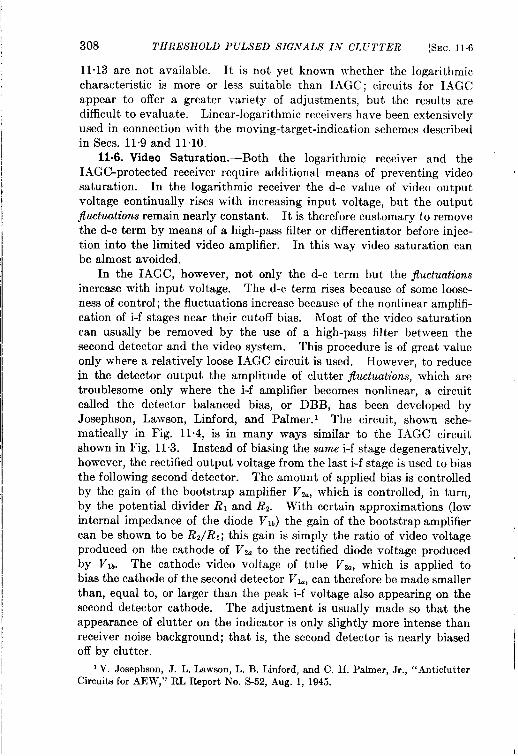
308 THRESHOLD PULSED SIGNALS IN CLUTTER [SEC. 116
11.13 are not available. It is not yet know-n whether the logarithmic
characteristic is more or less suitable than IAGC; circuits for IAGC
appear to offer a greater variety of adjustments, but the results are
difficult to evaluate. Linear-logarithmic receivers have been extensivelyused in connection with the moving-target-indication schemes describedin Sees. 11.9 and 11.10,
11.6. Video Saturation. -Both the logarithmic receiver and theIAGC-protected receiver require additional means of preventing videosaturation. In the logarithmic receiver the d-c value of video outputvoltage continually rises with increasing input voltage, but the outputjlu.ctuations remain nearly constant, It is therefore customary to removethe d-c term by means of a high-pass filter or differentiator before injec-tion into the limited video amplifier. In this way video saturation canbe almost avoided.
In the IAGC, however, not only the d-c term but the fluctuations
increase with input voltage. The d-c term rises because of some loose-ness of control; the fluctuations increase because of the nonlinear amplifi-cation of i-f stages near their cutoff bias. Most of the video saturationcan usually be removed by the use of a high-pass filter bet~veen thesecond detector and the video system. This procedure is of great valueonly where a relatively loose IAGC circuit is used. However, to reducein the detector output the amplitude of clutter juctuations, which aretroublesome only where the i-f amplifier becomes nonlinear, a circuitcalled the detector balanced bias, or DBB, has been developed byJosephson, Lawson, Linford, and Palmer. 1 The circuit, shown sche-matically in Fig. 11.4, is in many ways similar to the IAGC circuitshown in Fig. 11.3. Instead of biasing the same i-f stage degeneratively,however, the rectified output voltage from the last i-f stage is used to biasthe following second detector. The amount of applied bias is controlledby the gain of the bootstrap amplifier Vi., which is controlled, in turn,by the potential divider RI and Rz. With certain approximations (lowinternal impedance of the diode V15) the gain of the bootstrap amplifiercan be shown to be RZ/Rl; this gain is simply the ratio of video voltageproduced on the cathode of V2= to the rectified diode voltage producedby Vlb. The cathode video voltage of tube Vza, which is applied tobias the cathode of the second detector VI., can therefore be made smallerthan, equal to, or larger than the peak i-f voltage also appearing on thesecond detector cathode. The adjustment is usually made so that theappearance of clutter on the indicator is only slightly more intense thanreceiver noise background; that is, the second detector is nearly biasedoff by clutter.
1V. Josephson, J. L. Lawson, L. B. Llnford, and C. H. Palmer, Jr., ‘‘ Anti clutterCircuits for AE W,” RL Report No. S-52, Aug. 1, 1945.
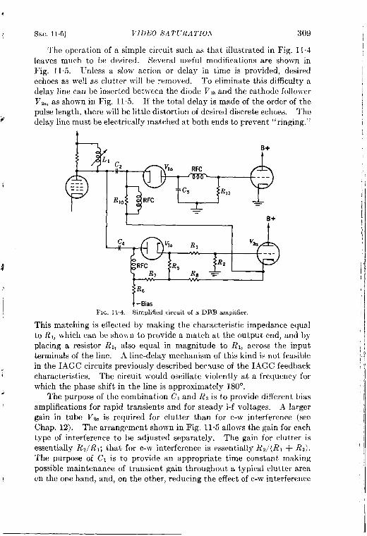
SEC. 11.6] VIDEO SA TVRA TIO.i- 309
The operation of a simple circuit such as that illustrated in Fig. 11.4leaves much to be desired. Several useful modifications are shown in
Fig. 11.5. Unless a slow action or delay in time is provided, desired
echoes as well as clutter will be removed. To eliminate this difficulty a
delay line can be inserted between the diode V1~ and the cathode follower
Vzc, as shown in Fig, 11.5. If the total delay is made of the order of the
pulse length, there will be little distortion of desired discrete echoes. The,!P delay line must be electrically matched at both ends to Frevent ‘‘ ringing. ”
.4
\
B+
C*
R 10 RFC
J_—
=
B+
w+-Bias
FIG. 11 .4.—Simplified circuit of a DBB amplifier.
This matching is effected by making the characteristic impedance equalto R,, which can be shown to provide a match at the output end, and byplacing a resistor Rs, also equal in magnitude to RI, across the input
terminals of the line. A line-delay mechanism of this kind is not feasiblein the IAGC circuits previously described becwse of the IAGC feedback
4 characteristics. The circuit would oscillate violently at a frequency forwhich the phase shift in the line is approximately 180°.
J The purpose of the combination Cl and RS is to provide different bias
amplifications for rapid transients and for steady i-f voltages. A larger
gain in tube Vza is required for clutter than for c-w interference (seeChap. 12). The arrangement shown in Fig. 11.5 allows the gain for eachtype of interference to be adjusted separately. The gain for clutter isessentially R~/R,; that for c-w interference is essential y R2/ (R, + R~).The purpose of Cl is to provide an appropriate time constant makingpossible maintenance of transient gain throughout a typical clutter area
I on the one hand, and, on the other, reducing the effect of c-w interference
[r
I
‘
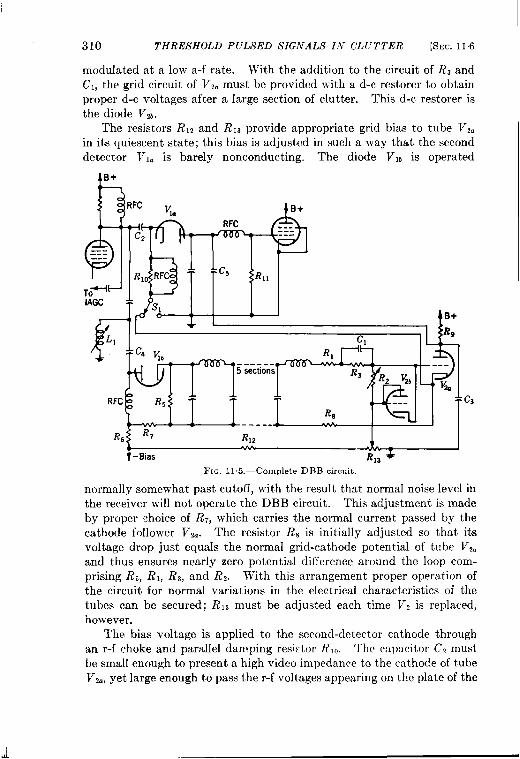
310 THRESHOLD PULSED SIGNALS IiV CL LrTTER [SEC. ] 16
modulated at a low a-f rate. With the addition to the circuit of R, andCl, the grid circuit of Vz. must be provided with a d-c restorer to obtainproper d-c voltages after a large section of clutter. This d-c restorer isthe diode Vz~.
The resistors RIZ and R,S provide appropriate grid bias to tube Vzain its quiescent state; this bias is adjusted in such a way that the seconddetector V,c is barely nonconducting. The diode Vl~ is operated
AI(:=‘:6B+
RFC ~la B+
RFC ---
c~------
---------
R,. RFc~
Rl,
#
IAGC
d?
s~
L, c.
RI ‘ -3----- ---sections R3
R2 VaVti
T q : +1---
R8----- + - T
FIG, 115.-Complete DBB circuit.
normally somewhat past cutoff, with the result that normal noise level inthereceiver will not operate the DBB circuit. This adjustment is madebyproper choice of R,, which carries the normal current passed by thecathode follower V,a. The resistor R, is initially adjusted so that itsvoltage drop just equals the normal grid-cathode potential of tube V~aand thus ensures nearly zero potential difference around the loop com-prising R,, R,, R,, and R,. With this arrangement proper operation ofthe circuit for normal variations in the electrical characteristics of thetubes can be secured; R,, must be adjusted each time V2 is replaced,however.
The bias voltage is applied to the second-detector cathode throughan r-f choke and parallel damping resistor Rio. The capacitor C~ must
be small enough to present a high video impedance to the c~thoc!e of tube
v,., yet large enough to pass the r-f voltages appearing on the plate of the
SEC. 11.7] THE TIM E-1’.41iIEl> GAIN CONTROL 311
last i-f tube directly to the cathode of the second detector. For the
same reasons CA must be of a compromise size. The inductance LI tunesthe i-f circuit to the appropriate value.
Onemore circuit detail should be noted. JVhenrelatively sharp videovoltages are applied to the cathode of the second detector, some effect ofthese voltages is ordinarily seen in the detector output load resistance R1l.This effect is produced by the small interelectrode capacitance of thesecond detector VI=) which, together with Rll, acts as a high-pass filteror differentiator for the biasing video voltages. This differentiatoraction can be nullified by the neutralizing arrangement shown. Avoltage of sign opposite to that of the biasing voltage is obtained from theplate of Vta through the plate load resistor Rg and is applied to RI]through a small capacitor (7,. As a result, the effect of the biasing
voltage appearing through the interelectrode capacitance CP~ of VI. is
approximately neutralized if the product of Rg and L’5 is made equal tcthe product of R, and Cpk. The capacitor C~ k necessary to make t}ic
pl~io-rccovcry characteristic of the cathode follower V!- similar in formto its cathode-recovery charmtcristic. This sknilarity is achieved if Cd i?made approximately equal to (C2 + C4)R6/R9.
The final circuit shown in rig. 11.5 can be made to perform very well.In response to pulsed signals it behaves much like a “line” differentiator,that is, one that preserves satisfactorily the shape of the leading edge ofthe pulse. Areas of clutter can be made nearly invisible on an intensity-modulated display, such as the PPI (see Sec. 2.6), by proper adjustment ofR,, that is, the gain of the biasing amplifier. Interfering C-Wsignals canbe handled smoothly even ~~ithout a subsequent video high-pass filter,provided R, is appropriate. The circuit possesses two important features
not available in the simpler video high-pass filter-the adjustable gain
of the biasing amplifier and the delay time of the line. Both features
should be helpful in final operation; therefore, the circuit is in principlemore satisfactory than a simple high-pass filter. This superiority is notoften easily demonstrated, as evidenced in Figs. 11.11 to 11“13, but thecircuit has been found helpful under many conditions.
11s7. The Time-varied Gain Control.—The time-varied gain, TVG,control is used to vary the gain of a receiver as a function of the time afterthe transmitted radar pulse. It is sometimes called a “sensitivity-timecontrol,” STC, or a “temporal gain control.” The desired gain patternis ordinarily accomplished by generating a voltage wave of a prescribedform, initiated by each transmitted pulse. This voltage wave is appliedto the i-f amplifier gain control lead, and it thus varies the receiver gainwith time according to the shape of the applied voltage wave. If thisvoltage wave is propcrl y shaped to conform with the clutter pattern,receiver saturation may be avoided. The essential difficulty with this
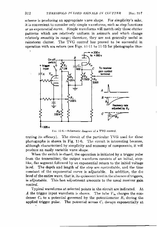
312 THRESHOLD I’1’LSEL) SIGNALS 1A’ CL L:TTER [SEC. 117
scheme is producing an appropriate ~rave shape. For simplicity’s sake,it is convenient to consider only simple waveforms, such as step functionsoranexponential curve. Simple waveforms will match ordy those clutterpatterns which are relatively uniform in azimuth and which changerelatively smoothly in range; therefore, they are not generally useful inrainstorm clutter. The TVG control has proved to be successful inoperation with sea return (see Figs. 1111 to 11”13 for photographs illus-
On-offswitch r
+t.@gef & :input
!~
+
R6 ~100k’
<
+200Vto +W3v
B—---
-/
RIlook
1
To receiver
gain controlterminal
R,imo
‘=adjuatsdby R2
l’1~. 11.6.—Schematic diagram of a TVG control.
trating its eficacy). The circuit of the particular TVG used for thesephotographs is shown in Fig. 11.6. The circuit is interesting because,although characterized by simplicity and economy of components, it willproduce an easily variable wave shape.
When the switch is closed, the operation is initiated by a trigger pulsefrom the transmitter; the output waveform consists of an initial, step-Iike, flat segment followed by an exponential return to the initial voltagele {cl. The depth and length of the step are controllable, and the timeconstant of the exponential curve is adjustable. In addition, the d-clevel of the entire wave, that is, its quiescent Ievcl in the absence of triggers,is adjustable. This last adjustment amounts to the usual receiver gaincontrol.
Typical waveforms at selected points in the circuit are indicated. AtA the trigger input waveform is shovm. The tube V1. charges the con-denser C, to a potential governed by the potentiometer R, during theapplied trigger pulse. The potential across C, decays exponentially at
SEC. 11.8] REDUCTION OF CLUTTER BY CIRCUITS 313
the rate determined by the time constant RZC,. Thus the waveform atB is similar to that depicted in Fig. 11.6, v-here the initial height of the
exponential function is controlled by the potentiometer R,. This wave-form would ordinarily be faithfully reproduced at point C because of thecathode follower Vl~, but the presence of. R~ prevents the cathode fromfollowing the grid potential during a part of the voltage wave. Asufficiently large negative voltage swing on the grid of tube Vti willproduce only a limited negative swing in its cathode; this swing is, infact, the product of R, and the normal quiescent current flowing throughthe tube V,~. Thus a flat section to the output wave will occur when theinput voltage drops to a critical value. The depth of the flat section iscontrolled by Ri, and its length by RI (and, of course, R2). The d-c levelof the output wave is controlled by Rd. One other circuit peculiarityshould be noted: the potential divider Rs and Re. This divider is used tofix the quiescent grid bias on Vlb at such a value that the cathode of ?“Ibis at ground potential; in this way the interaction between the controlsRS and R4 is eliminated.
The fotrr parameters of the waveform, namely, the d-c level, depth ofstep, recovery time constant, and length of step, are therefore adjustableby means of the four controls Rd, R,, R,, and R,, respectively. If adjust-ment is made in this order, little difficulty is experienced in arriving atfinal settings; this procedure usually requires only two or three successiveapproximations.
1108. Efficiency of Cucuits Used for Reduction of Clutter Saturation.Results are now available that show graphically the improvementobtained by the use of IAGC, DBB, and a high-pass video filter of thesimple IW-type. To obtain beneficial results, however, these circuitsmust be designed with particular values of time constants and operatingpotentials.
The following general conclusions may be derived from results pre-sented in Figs. 11.7 to 11.13:
1. The time constant of a simple high-pass filter is not critical; a valueequal to the reciprocal of the pulse length appears satisfactory.
2. The time constant (product of Rz and C8) of the IAGC circuitshown in Fig. 11.3 should be much larger than the radar pulselength; a value of approximately 50 ~sec has been found desirable.Probably more important than the pulse length in determining thistime constant is the rapidity with which the average value ofclutter (or other) echoes changes in time.
3. Proper operation of the DBB circuit in clutter is obtained with atransient gain probably from three to four times as high as thed-c gain. This adjustment is best made in actual trials.
314 THRESHOLD PULSED SIGNALS I,V CL LTTTER [SEC.11.8
4. For sea return the TVG is helpful; it is possibly more satisfactory
than any other single circuit.
5. The beneficial effects of various circuits are usually additive.
Experience has shown the use of lAGC to be advisable when
either DBB or a high-pass filter is employed. The combined
results are superior to the results of either circuit alone. It has
not been found helpful, however, to use both DBB and a high-pass
filter. The TVG is always helpful in sea return; it may greatly
reduce the load the other circuits must carry. Its adjustment
requires considerable skill, however, and its use for actual field
operation may therefore he viewed with some misgivings.
These conclusions were de;ived from data obtained in trialsin whichan airborne radar set ~vas used for the study of the effect of sea return.The radar set employed a beam pattern whose main lobe measuredapproximately 8° vertically and 3° horizontally. The wavelength wasapproximately 10 cm, and the pulse length approximately 2 psec.Enough sensitivity was available to obtain clutter from sea return outto ranges often in excess of 100 miles. The intensity of sea return wasusually sufficient to cause video saturation out to ranges of 40 miles,provided no special circuits were employed. Typical PP1 photographstaken at an elevation of 7000 ft are shown in Figs. 11.7a, 11.9a, 11.10a,and 11.lla. The concentric circles are described by electrical rangemarks separated by time intervals each representing 10 miles. As canbe seen, the total area represented in the photographs exceeds 3 X 10⁴square miles, yet it impossible toobtain strong echoes inmost of this area.These pictures were taken in the region of Boston, lfass.; the patternof Cape Cod, Martha’s Vineyard, and A“antucket can easily be seen.The central portion of the photograph, however, is for the most part auniform white region within which it is not possible to see any detail.‘1’his is the region where video saturation has taken place for both seaclutter and land return, as well as for such desired discrete targets withinthe clutter as ship echoes. In this region even such prominent featuresas the shore line between Massachusetts and the ocean immediately tothe east cannot be recognized.
The improvement effected by the use of a simple high-pass filter isshown in Fig. 11.7b, c, and d. Each photograph was obtained using adifferent time constant in the filter. The white portion in the centerextending out to the 20-mile range mark is an unfortunate addition to thephotographs; it is caused by a marker introduced for reasons not pertinentto this discussion. It can be seen, however, that some improvement ismade possible by the use of the high-pass filter; the region of completesaturation is smaller than that in the normal case (see Fig. 11”7a). The
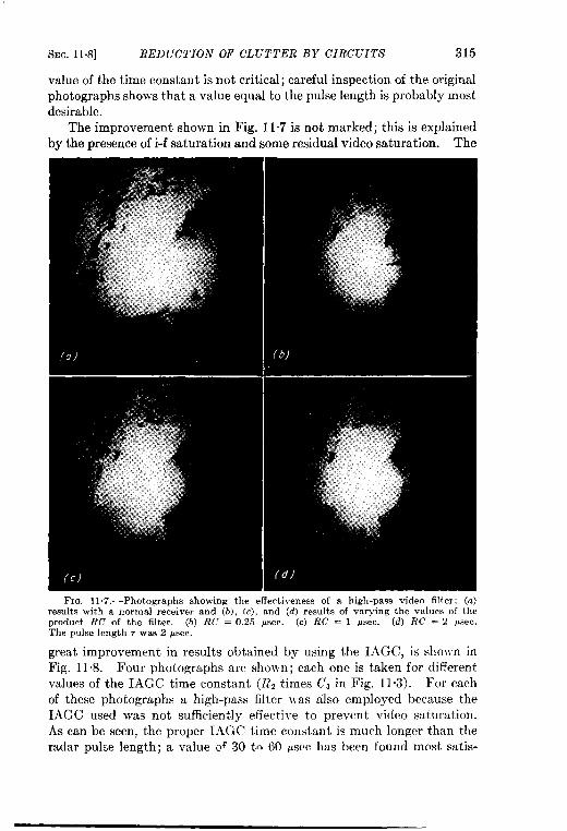
SEC. 11 +3] RED UCTION OF CLUTTER BY CIRCUITS 315
value of the time constant is not critical; careful inspection of the originalphotographs shows that a value equal to the pulse length is probably most
desirable.
The improvement shown in Fig. 11.7 is not marked; this is explained
by the presence of i-f saturation and some residual video saturation. The
FIG, 11.7,—Photographs showing the effectiveness of a high-pass video filter: (a)results with a normal receiver and (b), (c), and (d) results of varying the values of theproduct RC’ of the filter, (b) RC = 0,25 psec. (c) RC = 1 #sec. (d) RC = 2 p.ec.The pulse length 7 was 2 ~sec.
great improvement in results obtained by using the IAGC, is showm in
Fig. 11.8. Four photographs are shown; each one is taken for different
values of the IAGC time constant (RZ times Cs in Fig. 11 .3). For each
of these photographs a high-pass filter was also employed because the
IAGC used was not sufficiently effective to prevent video saturation.
As can be seen, the proper IAGC time constant is much longer than the
radar pulse length; a value of 30 to 60 psec has been found most satis-

316 THRESHOLD PULSED S’IGNALS IN CLUTTER [Sm. 11.8
factory. A single photograph illustrating the use of lACC alone is
shown in Fig. 11.9b; for this photograph a time constant of 60 pscc was
used in the lAGC circuit. Considerable video saturation still remains,
and the result obtained by the combined use of the IAGC and the high-
pass filter is far superior to that obtained by the use of either circuit alone.
I
FIG. 11.8.-Photographs shoting theeffectiveness of the I.4GCcircuit with ahigh-p~video filter. They show the effect of varying the time constant of the lAGC circuit.(a) RIC~ = 0.20 #sec. (b) R,(’, = 1.2 we., (c) R, C’, = 6 psec. (d) R,C, = 60 ySW,
comparewithFigs. 11.ia or 11.9afor normaloperation.
The operation of the DBB circuit is illustrated in Fig. 11.10. Thethree photographs (Fig. 11.10b, c, andd) weretakenw ithdif’ferentv aluesof transient gain. As can be seen, the use of too much gpin result sina“reversal” of the land areas. Too little gain fails to effect the desiredimprovement. When the proper gain is used, the land areas are exilyrecognized, yet sea clutter is kept below strong saturation. For these
I
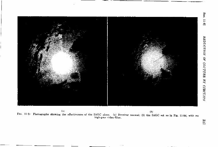
SE
C.
11.8
]R
ED
UC
TIO
NO
FC
LU
TT
ER
BY
CIR
CU
ITS
317
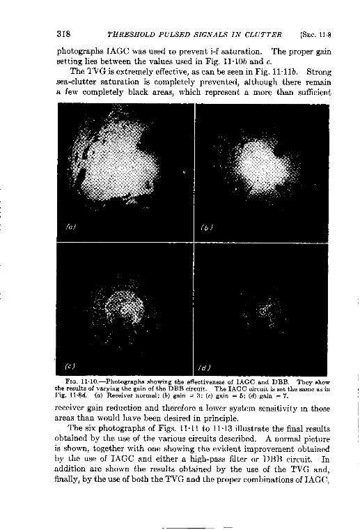
318 THRESHOLD PIJLSED SIGNALS IN CLUTTER [SEC.11.8
photographs IAGC was used to prevent i-f saturation. The proper gainsetting lies between the vaJues used in Fig, 11. 10b and c.
The TVG is extremely effective, as can be seen in Fig. 11.1 lb. Strongsea-clutter saturation is completely prevented, although there remaina few completely black areas, which represent a more than sufficient
FIG. 11. 10.—Photographs showing the effectiveness of IAGC and DBB. They showthe results of varying the gain of the DBB circuit. The IAGC circuit is set the sameM inFig. ll@d. (a) Receiver normal; (b) gain = 3; (c) gain = 5; (d) gain = 7.
receiver gain reduction and therefore a lower system sensitivity m those
areas than would have been desired in principle.
The six photographs of Figs. 11.11 to 11-13 illustrate the final results
obtained by the use of the various circuits described. A normal pictureis shown, together with one showing the evident improvement obtainedby the use of IAGC and either a high-pass filter or DBB circuit. Inaddition are shown the results obtained by the use of the TVG and,finally, by the use of both the TVG and the proper combinations of IAGC,
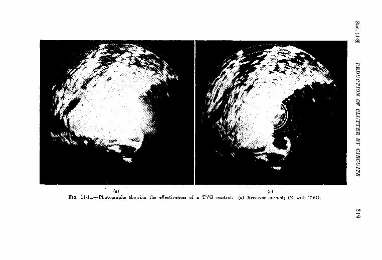
SEC.
11+3]R
ED
UC
TIO
NO
FC
LU
TT
ER
BY
CIR
CU
ITS
319
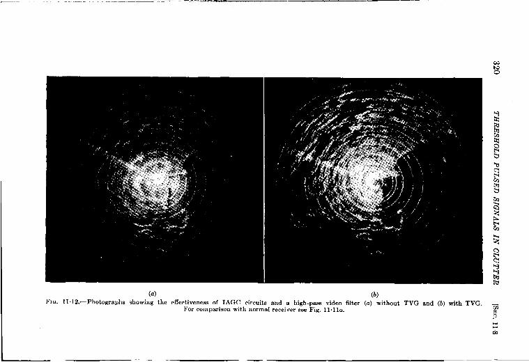
320T
HR
ES
HO
LD
PU
LS
ED
SIG
NA
LS
INC
LU
TT
ER
[SE
C.
118II
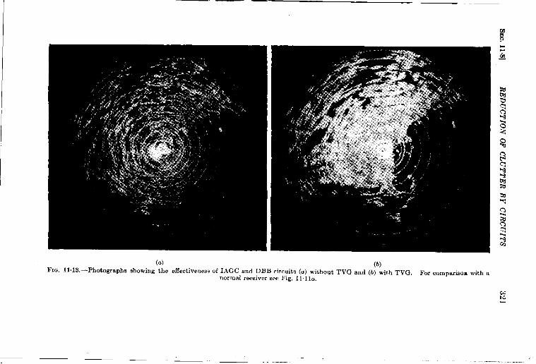
—.. —— —
(a) (b)FIG. 11.13.—Photographs showing the effectiveness of IAGC and DBB circuits (a) without TVG and (b) with TVG, For comparison with a
normal receiver see Fig. 1l.lla.
. ,’
322 THRESHOLD PULSED SIGNALS IN CLUTTER [SEC. 118
high-pass filter, and DBB. It is evident that the use of either combina-tion of three circuits as shown in Figs. 11~12b and 11 .13b gives the bestresults; sea return is nearly invisible, yet many ship echoes can be clearlyseen.
It should be clearly understood that only some of these circuits will beeffective for other forms of clutter. The dramatic improvement effectedby the use of TVG as shown in Fig. 11“11 readily suggests that this circuitalone would suffice for all practical needs, but this assumption does notobtain in cases of clutter originating in storm areas. The complicatedspatial pattern of such storm areas makes TVG useless, and reliance musttherefore be placed on the other circuits. Figure 11.14 shows howeffective appropriate circuits can be. Figure 11. 14b shows a PPI whoseradius represents approximately 20 miles. The faint concentric circlesare range marks separated by intervals representing 5 nautical miles.The strong circle at a range of 8 miles is an artificial echo from a testsignal generator injected directly into the receiver. Since this signal isnot collected by the antenna, it has no dependence on azimuth; hence itappears on the PPI as a circle. The echoes seen in the photograph are,for the most part, produced by objects on the ground. The ground returnis confined mainly within a radius of 10 miles because the radar set waslocated at an elevation of about 100 ft. Some discrete ground targets arestill noticeable out to the edges of the PPI, however. In the photographare also shown the echoes from some storm areas; they are recognized bythe extended nature of the returned pattern and the undefined, fuzzyedges characteristic of such clutter. These clutter areas are noticeablein the left-hand and in the lower right-hand sectors of the photograph.There is also a clutter area at the lowest part of the signal generator circlesufficiently intense to obliterate the signal generator echo in this region,as well as many discrete land echoes.
The improvement afforded by the use of proper IAGC and DBB cir-cuits is shown in Fig. 11.14a. The clutter f~om the storm areas ispractically removed, and the underlying discrete ground echoes can beseen. Furthermore. the signal from the test generator can be seen in itsentirety, with the exception of three or four small breaks; these are due tothe small recovery time of the IAGC, operated by an intense precedingland echo. These breaks do not represent poor performance of the L4GCcircuit; they occur in regions for which the test signal was already invisiblein the original photograph. Ordinarily no desired signals are lost whenthe clutter circuits are used properly and in the proper combination;Fig. 11.14 bears out this statement. Furthermore, the improvement inoperation resulting from the use of clutter circuits is substantial, providedthe circuits are properly designed.
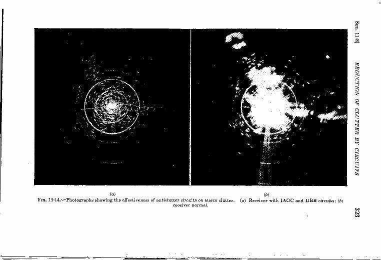
(a) (b)
FIQ. 11.14.—Photographs showing the effactiveness of anti clutter circuits on storm clutter. (a) Receiver with L4GC and DBB circuits; (b)receiver normal.
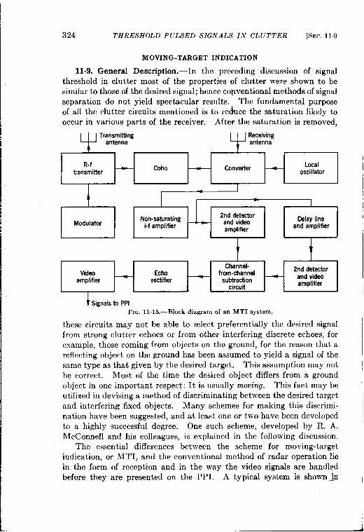
324 THRESHOLD PULSED SIGNALS IN CLUTTER [SEC. 11.9
MOVING-TARGET INDICATION
11.9. General Description. -In the preceding discussion of signalthreshold in clutter most of the properties of clutter were shown to besimilar to those of the desired signal; hence conventional methods of signalseparation do not yield spectacular results. The fundamental purposeof all the clutter circuits mentioned is to re~ce the saturation likely tooccur in various parts of the receiver. After the saturation is removed,
R-f — Coho — Converter ~ Localciansmitter oscillator
r 1I I I4 I
F, F~-l ak;,e!‘
Channel-7
Vidao Echo from-channel2nd detector
amplifier—
rectifier—
subtradlon— and vidao
circuitamplifier
Ii Signals to PPI
Fx~. 11.15.—Block diagram of an MTI system.
these circuits may not be able to select preferentially the desired signalfrom strong clutter echoes or from other interfering discrete echoes, forexample, those coming from objects on the ground, for the reason that areflecting object on the ground has been assumed to yield a signal of thesame type as that given by the desired target. This assumption may notbe correct. Most of the time the desired object differs from a groundobject in one important respect: It is usually moving. This fact may beutilized in devising a method of discriminating between the desired targetand interfering fixed objects. Many schemes for making this discrimi-nation have been suggested, and at least one or two have been developedto a highly successful degree. One such scheme, developed by R. A.McConnell and his colleagues, is explained in the following discussion.
The essential differences between the scheme for moving-targetindication, or M TI, and the conventional method of radar operation liein the form of reception and in the way the video signals are handledbefore they are presented on the PPI. A typical system is shown jm
I
I
SEC. 11.9] QENERAL DESCRIPTION
block form in Fig. 11015. The transmitted mdse
325
is produced in theconventional way by the action of a pulse-forming modulator on the r-ftransmitter. The received echo signal is injected into the superhetero-dyne converter along with the local oscillator, but in addition there isinjected the output of a coherent r-f oscillator, or “ coho. ” This oscillatoris restarted at each pulse with a phase defined by the transmitted r-f pulseand delivers into the receiver a constant r-f voltage larger than anydesired echo voltage. Therefore the signal voltage from the desiredecho, added to the coherent-oscillator voltage, will produce a change inr-f voltage; either an increase or a decrease will result, depending upon therelative phases of the echo and the coho. This scheme is therefore one inwhich the output voltage in the i-f amplifier not only is a function of echoamplitude but is dependent on the phase of the echo return relative to thecoho and hence relative to the main transmitted pulse. Since the totalecho phase relative to the transmitted pulse is dependent only on thedistance from transmitter to reflecting target and is, in fact, a measure ofthis distance in terms of the r-f wavelength, phase variations will occuronly by radial target movement. One wavelength change in radialdistance will result in a 47r change in r-f phase of the echo and hence,because of the local oscillator and converter, in a % change in i-f phaserelative to the i-f coho voltage.
The i-f amplifier that follows the superheterodyne converter is of anonsaturating variety, protected either by IAGC or by linear-logarithmicconstruction. The i-f amplifier output is split into two channels; one ofthese channels produces a conventional video signal, and the otherproduces an exact replica of this signal except that it is delayed in time.The delay in time is made to correspond precisely with the intervalbetween the initiation of successive transmitted pulses, that is, thereciprocal of the PRF. In this way two video outputs, obtained fromsuccessive transmitted pulses, are available. These two video channelsare then put into a circuit that takes their di~erence. In the output lineof this channel-from-channel subtraction circuit will appear only signalswhose phases have changed appreciably in the time between pulses.Echoes from fixed objects will have a fixed phase and amplitude frompulse to pulse; hence they will give identical video signals in the twochannels and therefore be completely canceled out in the subtractioncircuit. The complete system up to the output of the subtraction circuittherefore represents a scheme by which echoes from moving targets aremade visible and echoes from fixed targets are completely removed.The moving target, to be visible, must move an appreciable fraction ofa wavelength in the time between successive pulses.
If the cancellation is to be effective, the two video channels must haveexactly equal signal amplitudes and shapes; this can be effected if the i-f
326 THRESHOLD PULSED SIGNALS IN CLUTTER [SEC. 119
bandwidth at the input of each second detector is the same and if theover-all gain through the delay line and post-delay amplifiers is properlyset. These conditions are not especially difficult to obtain. The delayline itself has usually assumed the form of a liquid transmission mediumin which supersonic waves are propagated. Quartz crystals are generallyused to convert electric energy into sound energy and vice versa. Theover-all attenuation of such a delay line depends upon the bandwidthdesired and for the usual case is of the order of magnitude of 60 db. Thusthe amplifier following the delay line must have an over-all gain in excessof 60 db with adequate bandwidth and negligible noise. Such anamplifier is, however, easy to construct and adjust.
Another scheme devised to obtain delayed video signals uses acathode-ray storage tube. It has not, however, been so highly developedas the one using a supersonic delay line. In this system the video signalsare stored on a suitable cathode-ray-tube scrccn and are later taken offagain for purposes of comparison. This system has generally sufferedby comparison with the supersonic line for two reasons: (1) The signaldefinition is usually not so satisfactory because of the finite area of theelectron beam and possibly the “graininess” of the storage surface; (2)the time over which adequate storage can be maintained is limited becauseof charge leakage in the screen material. It appears, however, that theselimitations are not too serious; already storage tubes that show adequatelength of storage time have been built.
The output from the subtraction circuit invariably contains signals ofboth polarities depending upon the change in phase of the signal frompulse to pulse. It is customary to convert these signals into signals of onepolarity by means of an echo rectifier. The operation with an intensity-modulated display, such as the PPI, is thus made considerably moresatisfactory. A video amplifier between the echo rectifier and the PPI,as shown in Fig. 11“15, is used to bring the signals to a satisfactory valuefor easy visibility.
The construction of an actual system similar to that shown in Fig.11.15 has shown up certain difficulties that have necessitated minorchanges. To ensure an adequate coho, whose r-f voltage is larger thanthat produced by the largest desired echo, enough i-f voltage from thecoho and local oscillator must be produced to overload even a carefullydesigned i-f amplifier. It has therefole become customary to inject thecoho as an i-j voltage directly into the second detector input, as shown inFig. 11-16. In this case the coho is an i-~ oscillator, which is started atthe time of the transmitted pulse but is locked in phase to the i-f pulseproduced by the conversion of the r-f transmitted pulse. This scheme,like the one shown in Fig. 11.15, is sensitive to the phase of the echo, butthe coho voltage itself never goes through the i-f amplifier and cannot
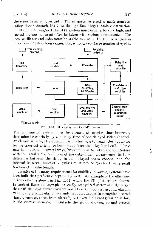
SEC. 119] GE.Vh’RAL J9ES’CRIH’ION 327
therefole cause i-f overload. The i-f amplifier itself is made nonsatu-
rating either through IACIC or through linear-logarithmic construction.
Stability throughout the MT1 system must usually be very high, and
special precautions must often be taken with various components. The
local oscillator and coho must be stable to a small fraction of a cycle in
phase, even at very long ranges, that is, for a very large number of cycles.
YTransmitting
antenna
?
Receiving
antenna
I r
R-f Local
1
—
?= :!E
Delay line
transmitter oscillatorConverter and
amplifier
Non- 2nd detectorModulator Coho saturating and video
i-f amplifier amplifier
I 1 1
t
Video 2rid detectorChannel-from-
Echoand video channel
amplifier rectifieramplifier
subtraction
circuit
Signals to PPI
I~IG. 11.16. Illock diagraln of an h!TI system.
T]lc transmitted pulses must be formed at precise time intervals,determined essentially I)y the delay time of the delayed video channel.An elegant scheme, attempted in \arious forms, is to trigger the modulatorfor the transmitter from pulses derived from the delay line itself. Thesemay be obtained in several Jvaysj but care must be taken not to interferewith the usual video operation of the delay line. In any case the timedifference between the delay in the delayed video channel and theinterval bet!vcen transmitted pulses must not be greater than a smallfraction of a pulse length.
In spite of the many requirements for stability, however, systems havebeen built that perform exceptionally ]J-ell. .4n example of the efficiencyof the device is Shelf-n in Fig. 11’17, ~~here the PP1 pictures are shown.In each of these photographs an easily recognized sector slightly largerthan 90° displays normal system operation and normal ground clutter.Within the ground clutter not only is it impossible to recognize desiredsignals, such as those from aircraft, but even land configuration is lostin the intense saturation. outside the sector showing normal system
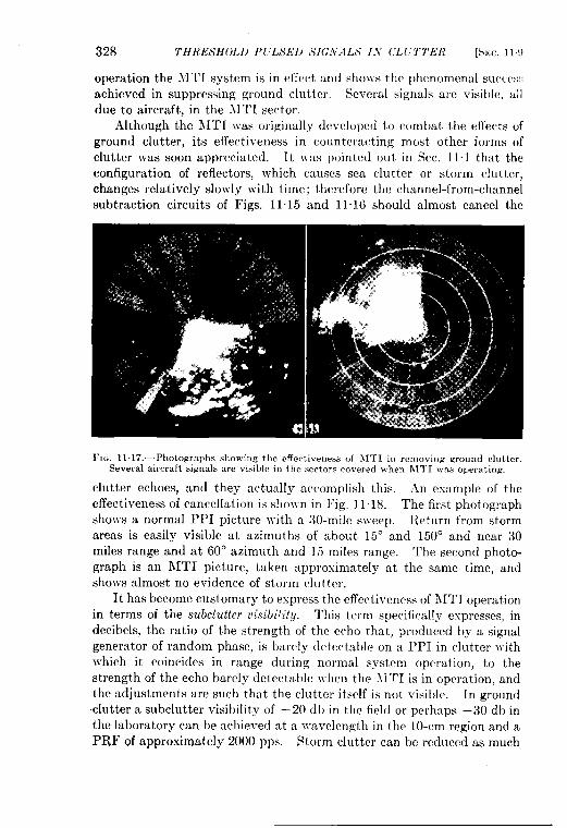
328 THRESHOLD I’[”LSED SIGNALS I.V CL(iTTEIi [SEC. 11{)
r.operation the ill 1 I s.vstem is in effect tincf shows the phenomenal SUCCU::;achieved in suppressing ground clutter, Several signals are visible, alldue to aircraft, in the 31TI sector.
Although the lITI ;vas originally cfeveloped tocwmbat the effects ofground clutter, its effectiveness in counteracting most other forms ofclutter was soon appreciated. It was pointed out in Sec. 11.1 that theconfiguration of reflectors, which causes sea clutter or storm clutter,changes relatively slowly with time; therefore the channel-from-channelsubtraction circuits of Figs. 11.15 and 11.16 should almost cancel the
l~[u. 11.17.—Photographs showing the effectiveness of LIT1 iu removing ground clutter.Several aircraft signals are visible in the sectors covered when NITI was operating.
clutter echoes, and they actually accomplish this. An example of theeffectiveness of cancellation is sholvn in Fig. 11.18. The first photographshows a normal PPI picture ~vith a 30-mile sweep. Return from stormareas is easily visible at azimuths of about 15° and 150° and near 30miles range and at 60° azimuth and 15 miles range. The second photo-graph is an LITI picture, taken approximately at the same time, andsho~vs almost no evidence of storm clutter.
It has become customary to express the effectiveness of LITI operation
in terms of the subc[utter visihi[ity, This term specifically expresses, indecibels, the ratio of the strength of the echo that, produced by a signalgenerator of random phase, is barely detectable on a PPI in clutter withwhich it coincides in range during normal system operation, to thestrength of the echo barely detectable ~vhen the 3 ITI is in opwation, andthe adjustments are such that the clutter itself is not visible. In groundclutter a subclutter visibility of —20 db in the field or perhaps —30 db in
the laboratory can be achieved at a wavelength in the 10-cm region and a
PRF of approximately 2000 pps. Storm clutter can be reduced as much
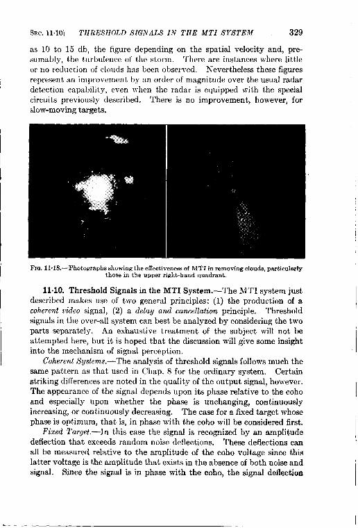
SEC. 11.10] THRESHOLD SIGNALS IN THE A4TI SYSTEM 329
as 10 to 15 db, the figure depending on the spatial velocity and, pre-sumably, the turbulence of the storm. There are instances where littleor no reduction of clouds has been observed. Nevertheless these figuresrepresent an improvement by an order of magnitude over the usual radardetection capability, even ~~hen the radar is equipped with the specialcircuits previously described. There is no improvement, however, forslow-moving targets.
FIG. 11. 18.—Photographs showing the effectiveness of MTI in removing clouds, particularlythose in the upper right-hand quadrant.
11.10. Threshold Signals in the MTI System.—The MTI system justdescribed makes use of two general principles: (1) the production of acoherent video signal, (2) a delay and cancellation principle. Threshold
signals in the over-all system can best be analyzed by considering the two
parts separately. An exhaustive treatment of the subject will not be
attempted here, but it is hoped that the discussion will give some insight
into the mechanism of signal perception.
Coherent S’ystems.-The analysis of threshold signals follows much thesame pattern as that used in Chap. 8 for the ordinary system. Certainstriking differences are noted in the quality of the output signal, however.The appearance of the signal depends upon its phase relative to the cohoand especially upon whether the phase is unchanging, continuouslyincreasing, or continuously decreasing. The case for a fixed target whosephase is optimum, that is, in phase with the coho will be considered first.
Fixed Target.—In this case the signal is recognized by an amplitudedeflection that exceeds random noise deflections. These deflections canall be measured relative to the amplitude of the coho voltage since thislatter voltage is the amplitude that exists in the absence of both noise andsignal. Since the signal is in phase with the coho, the signal deflection
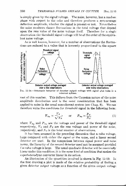
330 THRESHOLD PULSED SIG.VALS IN CLiYTTER [SEC. 1110
is simply given by the signal voltage. The noise, however, has a randomphase with respect to the coho and therefore produces a zero-averagedeflection amplitude, whether the signal is present or not. Neverthelessthe noise produces chance fluctuations in the total voltage that dependupon the rms value of the noise voltage itself. Therefore for a singleobservation the threshold signal voltage will be of the order of the equiva-lent noise voltage.
As is well known, however, for a number of observations the fluctua-tions are reduced to a value that is inversely proportional to the square
Detector output voltageaveragedover a faw observations
Thresholdsignal 44
1
voltage oII
~~
Noisej!
fluctuation / \voltage I
1II
I/’!
Detector output voltage averaged
over many Obsewations
FIG. 11. 19.—Schematic bebavior of detector oqtput voltage with signal plus noise in acoherent sy%tem.
root of this number. This follows from the Gaussian nature of the noiseamplitude distribution and is the same consideration that has beenapplied to noise in the usual noncoherent system (see Chap. 8). We cantherefore write the conditions for threshold signal in the following form:
(1)
where Vs,O and Ps,O are the voltage and power of the threshold signalrespectively, V~ and P~ are the rms voltage and power of the noise,respectively, and .VS is the total number of observations.
It has been assumed in the preceding discussion that a coho voltage,I~rge compared with either the signal or the noise, and a linear second(!etector are used. In the comparison between signal power and noise
power, the linearity of the second detector need not be assumed providedt~lecoho voltage is large. The usual quadratic detector will be essentiallyIiaear under this condition; it is the same kind of condition that makes the,s.~perheterodyne converter linear in its action.
An illustration of the quantities involved is shown in Fig. 11.19. Inthe first drawing a plot is made of the relative probability of finding agiven detector output voltage as a function of the given output voltage
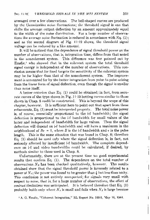
SEC. 11.10] THRESHOLD SIGNALS IN 1’HE MTI SYSTEM 331
averaged over a few observations. The bell-shaped curves are producedby the Gaussianlike noise fluctuations; the threshold signal is one thatshifts the average output deflection by an amount approximately equalto the width of the noise distribution. For a large number of observa-tions the average noise fluctuation is reduced in accordance with Eq. (1);and as the second diagram of Fig. 11.19 shows, the threshold signalvoltage can be reduced by a like amount.
It will be noticed that the dependence of signal threshold power on thenumber of observations, that is, integration time, differs from that notedin the noncoherent system. This difference was first pointed out byEmslie,’ who showed that in the coherent system the total thresholdsignal energy is independent of the number of observations. This con-clusion means that for fixed targets the sensitivity of the coherent systemmay be far higher than that of the noncoherent system. The improve-ment is accounted for by the better integration from pulse to pulse arisingfrom the linear form of signal deflection, even though the signal is smallerthan noise itself.
A better criterion than Eq. (1) could be obtained; in fact, from accu-rate curves of the type shown in Fig. 11”19 betting curves similar to thoseshown in Chap. 8 could be constructed. This is beyond the scope of thischapter, however. It is sufficient hereto point out that apart from theserefinements, Eq. (1) must be interpreted properly. The total noise poweris, of course, essentially proportional to the i-f bandwidth; the signaldeflection is proportional to the i-f bandwidth for small values of thelatter and independent of bandwidth for large values. Thus the signaldeflection will depend on i-f bandwidth and will have a maximum in theneighborhood of Br = 1, where B is the i-f bandwidth and r is the pulselength. This is the same situation that was found in Chap. 8; thereforeEq. (1) should be used only where the signal deflection is, in fact, notseriously affected by insufficient i-f bandwidth. The complete depend-ence on i-f and video bandwidths could be calculated, if desired, bymethods similar to those used in Chap. 8.
Unfortunately, there are at the present time no good experimentalresults that confirm Eq. (1). The dependence on the total number ofobservations N~ has been checked qualitatively, however. The resultsobtained show that the signal threshold power is inversely related to apower of N.; the power was found to be greater than ~ but less than unity.This conclusion is not entirely unexpected; for signals very small withrespect to noise, that is, for a large number of observations, the effect ofcontrast limitations was anticipated. It is believed therefore that Eq. (1)probably holds only where N. is small and fails when Ns is large because
I A. G. Emslie, (‘Coherent Integration,” RL Report No. 103-5, May 16, 1944.
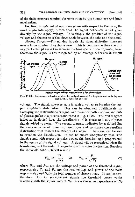
332 THRESHOLD PULSED SIGNALS IN CLUTTER [SEC. 11.10 ~
of the finite contrast required for perception by the human eye and brainmechanism.
For fixed targets not at optimum phase with respect to the coho, thesame arguments apply, except that the signal deflection is not givendirectly by the signal voltage. It is simply the product of the signalvoltage and the cosine of the phase angle between the coho and the signal.
Moving Targets.—For moving targets the signal deflection averagedover a large number of cycles is zero. This is because the time spent in ‘any particular phase is the same as the time spent in the opposite phase;therefore the signal is not recognized by an average deflection in output
FIG. 11.20.—Schematicbehavior of detector output voltage for in-phaseand out-of-phasesignalsin a coherentsystem.
voltage. The signal, however, acts in such a way as to broaden the out-put amplitude distribution. This can be observed qualitatively byaveraging the distributions of signal and noise for both in-phase and out-of-phase signals; this process is indicated in Fig. 11.20. The first diagramindicates in dotted lines the distribution of in-phase and ou~of-phasesignals added to noise. The second diagram indicates by a dotted linethe average value of these two conditions and compares the resultingdktribution with that in the absence of a signal. The signal can be seento broaden the distribution. It can be shown analytically that withsignals small with respect to noise power, this broadening is proportionalto the square of the signal voltage. A signal will be recognized when thebroadening is of the order of magnitude of the noise fluctuation; thereforethe threshold condition will occur if
(2)
where V~,O and Ps,O are the voltage and power of the threshold signal,respectively; VM and PN are the rms voltage and power of the noise
respectively; and Nfl is the total number of observations. It can be seen,
therefore, that for noncoherent signals the threshold power varies
inversely with the square root of NS; this is the same dependence on N8
I
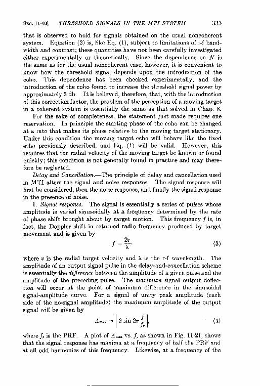
SEC. 11.10] THRESHOLD SIGNALS IN THE MTI SYSTEM 333
that is observed to hold for signals obtained on the usual noncoherentsystem. Equation (2) is, like Eq. (l), subject to limitations of i-f band-width and contrast; these quantities have not been carefully investigatedeither experimental y or theoretically. Since the dependence on N ist!~e same as for the usual noncoherent case, however, it is convenient toknow how the threshold signal depends upon the introduction of thecoho. This dependence has been checked experimentally, and theintroduction of the coho found to increase the threshold signal power byapproximately 3 db. It is believed, therefore, that, with the introductionof this correction factor, the problem of the perception of a moving targetin a coherent system is essentially the same as that solved in Chap. 8.
For the sake of completeness, the statement just made requires onereservation. In principle the starting phase of the coho can be changedat a rate that makes its phase relative to the moving target stationary.Under this condition the moving target echo will behave like the fixedecho previously described, and Eq. (1) will be valid. However, thisrequires that the radial velocity of the moving target be known or foundquickly; this condition is not generally found in practice and may there-fore be neglected.
Delay and Cancellation.-The principle of delay and cancellation usedin MTI alters the signal and noise responses. The signal response willfirst be considered, then the noise response, and finally the signal responsein the cn-esence of noise.
1. Signal response. The signal is essential] y a series of pulses whoseamplitude is varied sinusoidally at a frequency determined by the rateof phase shift brought about by target motion. This frequency $ is, infact, the Doppler shift in returned radio frequency produced by targetmovement and is given by
f=:, (3)
where u is the radial target velocity and k is the r-f wavelength. Theamplitude of an output signal pulse in the delay-and-cancellation schemeis essentially the difference between the amplitude of a given pulse and theamplitude of the preceding pulse. The maximum signal output deflec-tion will occur at the point of maximum difference in the sinusoidalsignal-amplitude curve. For a signal of unity peak amplitude (eachside of the no-signal amplitude) the maximum amplitude of the outputsignal will be given by
A_ = 2 sin 21r–;’
(4)
where jr is the PRF. A plot of Au vs. j, as shown in Fig. 11.21, showsthat the signal response has maxima at a frequency of half the PRF andat all odd harmonics of this frequency. Likewise, at a frequency of the
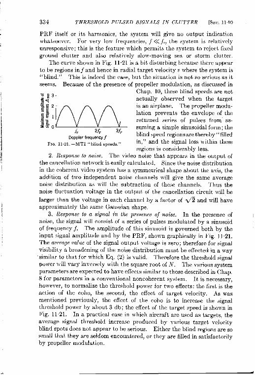
334 THRESHOLD PULSED SIGNALS IN CLUTTER [SEC. 1110
PRF itself or its harmonics, the system will give no output indicationwhatsoever. For very low frequencies, ~<< ~., the system is relativelyunresponsive; this is the feature which permits the system to reject fixedground clutter and also relatively slow-moving sea or storm clutter.
‘l’he curve shown in Fig. 11.21 is a bit disturbing because there appearto be regions in f and hence in radial target velocity v where the system is“blind.” This is indeed the case, but the situation is not so serious as itseems. Because of the presence of propeller modulation, as discussed in
z~3 Chap. 10, these blind speeds are not
+< [ actually observed when the target
I!iwis an airplane. The propeller modu-
lation prevents the envelope of the
returned series of pulses from as-
1- 2fr 3.$suming a simple sinusoidal form; the
Doppler frequency fblind speed regions are thereby” filled
FIG. 11.21 .—MTI “ blind speeds. ” in, ” and the signal loss within theseregions is considerably less.
2. Response to noise. The video noise that appears in the output ofthe cancellation network is easily calculated. Since the noise distributionin the coherent video system has a symmetrical shape about the axis, theaddition of two independent noise channels will give the same averagenoise distribution as will the subtraction of these channels. Thus thenoise fluctuation voltage in the output of the cancellation circuit will be
larger than the voltage in each channel by a factor of ~ and will haveapproximate y the same Gaussian shape.
3. Response to a signal in the presence of noise. In the presence ofnoise, the signal will consist of a series of pulses modulated by a sinusoidof frequency j. The amplitude of this sinusoid is governed both by theinput signal amplitude and by the PRF, shown graphically in Fig. 11.21.The auerage value of the signal output voltage is zero; therefore for signalvisibility a broadening of the noise distribution must be effected in a way
“similar to that for which Eq. (2) is valid. Therefore the threshold signalpower will vary inversely with the square root of N. The various systemparameters are expected to have effects similar to those described in Chap.8 for parameters in a conventional noncoherent system. It is necessary,however, to normalize the threshold power for two effects: the first is theaction of the coho, the second, the effect of target velocity. As wasmentioned previously, the effect of the coho is to increase the signalthreshold power by about 3 db; the effect of the target speed is shown inFig. 11.21. In a practical case in which aircraft are used as targets, theaverage signal threshold increase produced by various target velocityblind spots does not appear to be serious. Either the blind regions are sosmall that they are seldom encountered, or they are filled in satisfactorilyby propeller modulation.
CHAPTER 12
THRESHOLD SIGNALS IN ELECTRONIC INTERFERENCE
.% is pointed out in Sees, 6,6 to 6.8, the different varieties of electronic
interference can be roughly classified as simple and complex. In each of
these categories the effects of the particular interference and the methods
for its alleviation depend upon the detailed structure of the interference.
This chapter will treat the question of pulsd-signal threshold pojver for
three types of interference: (1) unmodultited c-w interference, (2) noise-
modulated C-W interference, and (3) pulsed interference. Pulsed inter-
ference may be of either the simple or the complex variety discussed in
Sees. 67 and 6.8; cases of both varieties are presented together, sincemethods for their alleviation are similar, In all cases treated it isassumed that the interference has been allowed to reach the i-f terminalsof the receiver; that is, no r-f measures ha\~ebeen taken to minimizeinterference.
THRESHOLD SIGNALS INUNMODULATED CONTINUOUS-WAVE INTERFERENCE
12.1. Effect of C-w Interference.-A description of the c-w inter-ference itself is almost unnecessary; it consists essentially of a constant-amplitude, constant-frequency voltage, which ~ve assume exists at theinput terminals of the i-f amplifier. The signal pulses and equivalentnoise also appear on these terminals, however. Our problem is to considerthe interaction effects of all three voltages in an attempt to evaluate thethreshold signal. Because many receiver and indicator characteristicsare involved that do not lend themselves to easy analysis and measure-ment, the task is a difficult one. Wherever possible, however, quantita-tive results ~vill be given.
Interaction of 6-w Interference u,ith Signal.—Let us assume, forsimplicity’s sake, that the C-TVvoltage is large compared with the pulsevoltage. The signal will cause a change in the output voltage of thesecond detector. As the pulse and the c-w interference may occur \vithany relative phase and with any difference in frequency, the video signalwill consist of a small element of length proportional to 7 (the pulseduration); this element has an amplitude that cliffers from the videovoltage (produced by the interference) by an amount proportional to thepulse voltage, The video frequency during this element is the differencebetween the pulse and c-w frequencies, The situation is shown in Fig.
335
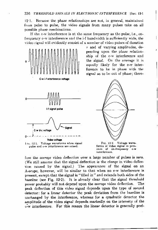
336 THRESHOLD SIGNALS IN ELECTRONIC INTERFERENCE [&C, 121
12.1. Because the phase relationships are not, in general, maintained
from pulse to pulse, the video signals from many pulses take on allpossible phase combinations.
If the c-w interference is at the same frequency as the pulse, i.e., in-frequency c-w interference and the i-f bandwidth is sufficiently wide, thevideo rignal will evidently consist of a number of video pulses of duration
o-
C-w i-f interference voltage
l-f signal pulse
A
o__J_________________Video voltage
1 LG. 12.1.—Voltage waveforms when signalpulse and c-w interference are mixed.
r and of varying amplitudes, de-pending upon the phase relation-
I
shi~ of the c-w interference andthe” signal. On the average it isequally likely for the c-w inter-ference to be in phase with thesignal as to be out of phase; there-
FIC. 12.2.—Voltage wave-forms of video signal in pres-ence of on-frequency c-winterference.
fore the average video deflection over a large number of pulses is zero.(We still assume that the signal deflection is the change in video deflec-tion caused by the signal.) The appearance of the signal on anA-scope, however, will be similar to that when no c-w interference ispresent, except that the signal is “filled in” and extends both sides of thebaseline (see Fig. 12.2). It is already clear that the signal thresholdpower probably will not depend upon the average video deflection. Thepeak deflection of this video signal depends upon the type of seconddetector: for a linear detector the peak deviation from the baseline isunchanged by the interference, whereas for a quadratic detector theamplitude of the video signal depends markedly. on the intensity of thec~w interference. For this reaaon the linear detector is generally pref-
1
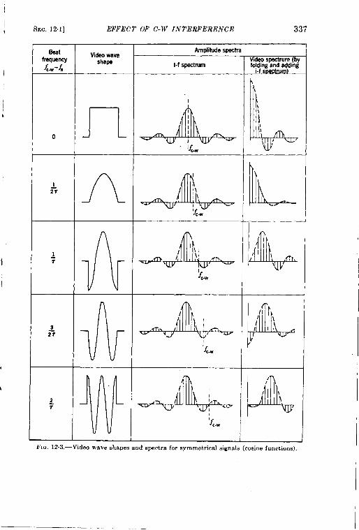
SEC. 121] EFFEcT OF C-W INTERFERENCE 337
I
I
FIO. 12.3.—Video wave shapes and spectra for symmetrical signals (cosine functions).
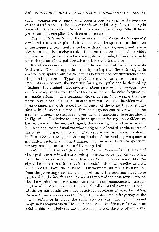
338 THRESHOLD SIG.VALS IN ELECTRONIC INTERFERENCE [SEC. 12.1
erable; comparison of signal amplitudes is possible even in the presenceof the interference. (These statements are valid only if overloading isavoided in the receiver. Prevention of overload is a very difficult task,yet it can be accomplished with some success.)
The amplitude spectrum of the video signal in the case of on-frequencyc-w interference is simple. It is the same as the spectrum of the pulsein the absence of c-w interference but with a different over-all multiplica-tive constant. For a single pulse it is clear that the shape of the videopulse is unchanged by the interference; its amplitude, however, dependsupon the phase of the pulse relative to the c-w interference.
For off-frequency c-w interference the spectrum of the video signalsis altered. One can appreciate this by noting that the video signal isderived principally from the beat tones between the c-w interference andthe puls~ freq~en~ies. Typical spectra for several cases are shovm in Fig.12.3. As can be seen, the spectrum for a given pulse can be derived by“folding” the original pu!se spectrum about an axis that represents thec-w’ frequency; in this way the beat tones, which are the video frequencies,are made evident. The diagrams show-n in Fig. 12.3 assume that thephase in each case is adjusted in such a ~~-ayas to make the video ~vave-form symmetrical with respect to the center of the pulse, that is, it con-sists only of cosine functions. Similar diagrams can be drawn for theantisymmetrical waveforms representing sine functions; these are shownin Fig. 12.4. To derive the amplitude spectrum for any phase differencebetween c-w interference and signal, the video signal must be separatedinto sine and cosine functions ~rhose origins are located at the center ofthe pulse. The spectrum of each of these functions is obtained as shownin F@. 12.3 and 12.4, and the amplitudes of the resulting componentsare added vectorially at right angles. In this way the video spectrumfor any specific case can be rapidly computed.
Intmaction of C-U1 Inter fcrcncr unl~l Receiver ,Voise.—As in the case ofthe signal, the c-v.- interference voltage is assumed to be large compared~vith the receiver noise. In such a situation the video noise, like thesignal, becomes two-sided, that is, it “ beats” below the baseline as oftenas it appears above the baseline. Furthermore, as might be surmisedfrom the preceding discussion, the spectrum of the resulting video noiseis altered by the interference; it consists simply of the beat tones betweenthe i-f c-w-interference component and the i-f noise components. Assum-ing the i-f noise components to be equally distributed over the i-f band-width, we can obtain the video amplitude spectrum of noise by foldingthe amplitude response curve of the i-f amplifier at the frequency of thec-w interference in much the same way as was done for the signalfrequency components in Figs. 12”3 and 12-4. In this case, how-ever, norelationship exists bet\veen the noise components of the two folded halves;
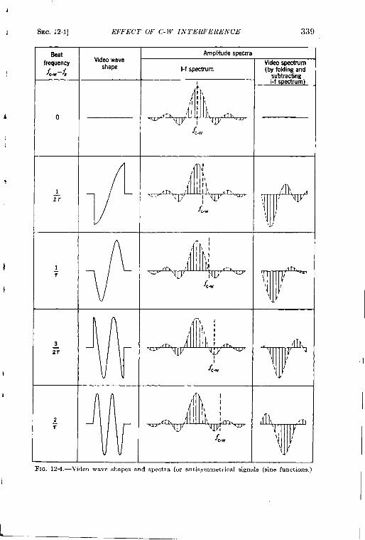
SEC. i21] EFFECT OF C-W INTERFERENCE 339
Beat Amplitude spectra
frequencyVidso wave
Video spectrum
f=w-~shape l-f spectrum (by folding and
subtracthgi-f spectrum)
L,, : \
, ~ \
o T>. / I ! 41.,
f’
Ju
c-w
I/l ‘LTF’l}l’” ‘;’’u’T’Jr ~ ‘%
/
/!\
1 ;! ,
Tr \ ‘, ;
! t! ,
, + ,L,,,J - ;L ;: ‘:
‘ ti L’;( ““J:”w” r
‘ % ‘{’”)’ ““’’’’~;~’” w
IG. l!2.4.-Video wave shapes and spectra for antisytnmetricd signals (sine functions. )
I
I
1
340 THRESHOLD SIGNALS IN ELECTRONIC INTERFERENCE [SEC. 12.1
therefore the resulting spectrum is obtained by adding these halves inquadrature, i.e., vectorially at right angles.
The amplitude of the video-noise fluctuations is increased by theaddition of the interference; for a linear detector this increase is approxi-mately equal to @ and is independent of the amplitude of interferencefor large values of interference. For a quadratic detector, however, theincrease depends on the intensity of interference; for this reason the lineardetector is generally preferred, especially when video overloading isconsidered (see Sec. 12.4).
From what has already been said it can be inferred that the introduc-tion of interference in a system with a linear detector will not appreciablyimpair the signal response, nor will it increase the noise amplitude bymore than the factor {2. This inference is, of course, justified only ifthe video bandwidth is sufficient to pass the signal video frequencies andif the interaction effects between signal and noise are essentiallyunchanged by the interference. The effect of inadequate video band-width will be discussed in Sec. 12“4; it is su5cient for the moment to notethat if the video bandwidth is as large as the full i-f bandwidth, adequatesignal response can be assured.
The interaction effects between signal and noise in the presence ofc-w interference can be investigated theoretically. This effort, however,is probably not yet justified, since the ultimate criterion for signal visi-bility is not yet established. It has already been remarked that thiscriterion can no longer be obtained from the average deflection, becausethe average deflection for both signal and noise is zero. It is probablymore realistic to choose the average absolute value of deflection for acriterion. Nevertheless, no matter what criterion is chosen, one stilldoes not know how to take into account the fluctuating character of thesignal. Thus experimental results are probably most reliable and useful.
Experiments performed by H. Johnson, and J. L. Lawson,l and byStone* demonstrate conclusively that if overloading is avoided, the signalthreshold power increases approximately 3 to 4 db because of on fr~quency c-w interference. This threshold increase is independent of theintensity of the interference, provided the interference is strong comparedwith signal and/or noise power. It must not be inferred from theseexperiments, however, that this relatively small increase in signalthreshold power is all that is usually found. In actual fact the majoreffects ordinarily encountered are caused by overloading phenomena ineither the video or i-f sections of the receiver. These will be discussedlater.
1Unpublished, but see RL Report No. 910, Mar. 22, 1946.2A. M. Stone, “Synthetic Radar Echoes in the Presence of Jamming,” RL Report
;o. 70S, June 22, 1945.
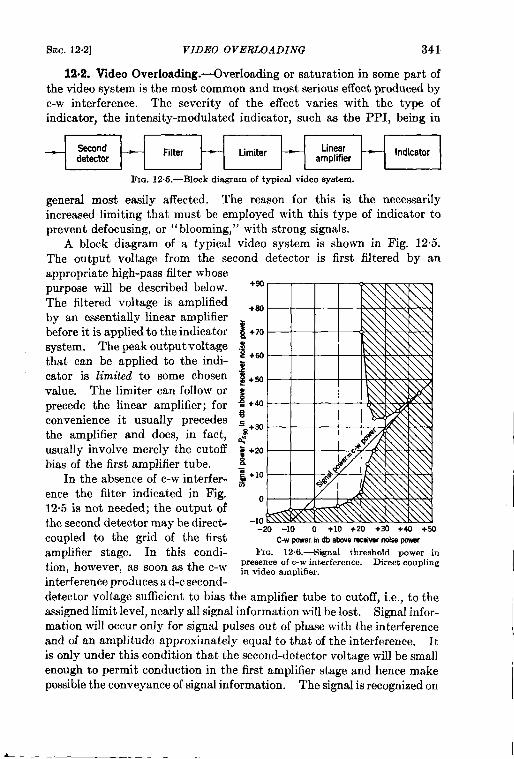
SEC. 12.2] VIDEO OVERLOADING 341
12.2. Video Overloading.-Overloading or saturation in some part ofthe video system is the most common and most serious effect produced byc-w interference. The severity of the effect varies with the type ofindicator, the intensity-modulated indicator, such as the PPI, being in
— Second — Filter — Limiter — Linear —detector
Indicatoramplifier
L
Fm. 12.5.—Blockdiagram of typical video eyatem.
general most easily affected. The reason for this is the necessarily
increased limiting that must be employed with this type of indicator to
prevent defocusing, or “blooming,” with strong signals.
A block diagram of a typical video system is shown in Fig. 12”5.The output voltage from the second detector is first filtered by anappropriate high-pass filter whosepurpose will be described below.The filtered voltage is amplifiedby an essentially linear amplifierbefore it is applied to the indicatorsystem. The peak output voltagethat can be applied to the indi-cator is limited to some chosenvalue. The limiter can follow orprecede the linear amplifier; forconvenience it usually precedesthe amplifier and does, in fact,usually involve merely the cutoffbias of the first amplifier tube.
In the absence of c-w interfer-ence the filter indicated in Fig.12.5 is not needed; the output ofthe second detector may be direc~coupled to the grid of the firstamplifier stage. In this condi-tion, however, as soon as the c-winterference produces ad-c second-
C-w power.in db above receiver noise power
Fm. 12.6.—Signal threshold power inpresenceof c-w interference. Direct couplingin video amplifier.
detector voltage sufficient to bias the amplifier tube to cutoff, i.e., to theassigned limit level, nearly all signal information will be lost. Signal infor-mation will occur only for signal pulses out of phase with the interferenceand of an amplitude approximately equal to that of the interference. It
is only under this condition that the second-detector voltage will be smallenough to permit conduction in the first amplifier stage and hence makepossible the conveyance of signal information. The signal is recognized on
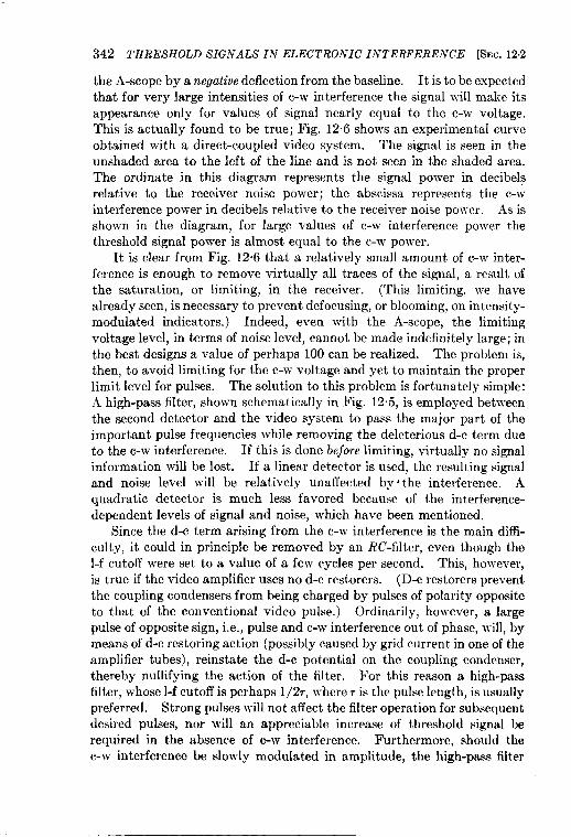
342 THRESHOLD SIGNALS IN ELECTRONIC INTERFERENCE [SEC. 12.2
the A-scope by a negative deflection from the baseline. It is to be expectedthat for very large intensities of c-w interference the signal will make itsappearance only for values of signal nearly equal to the c-w voltage.This is actually found to be true; Fig. 12.6 shows an experimental curveobtained with a direct-coupled video system. The signal is seen in theunshaded area to the left of the line and is not seen in the shaded area.The ordinate in this diagram represents the signal power in decibelsrelative to the receiver noise power; the abscissa represents the c-winterference power in decibels relative to the receiver noise power. .ks isshown in the diagram, for large values of c-w interference power thethreshold signal power is almost equal to the c-w power.
It is clear from Fig. 12.6 that a relatively small amount of c-w inter-ference is enough to remove virtually all traces of the signal, a result ofthe saturation, or limiting, in the receiver. (This limiting, we havealready seen, is necessary to prevent defocusing, or blooming, on intensity-modulated indicators. ) Indeed, even with the A-scope, the limitingvoltage level, in terms of noise level, cannot be made indefinite y large; inthe best designs a value of perhaps 100 can be realized. The problem is,then, to avoid limiting for the C-Wvoltage and yet to maintain the properlimit level for pulses. The solution to this problem is fortunately simple:A high-pass filter, shown schematically in Fig. 125, is employed betweenthe second detector and the video system to pass the major part of theimportant pulse frequencies while removing the deleterious d-c term dueto the c-w interference. If this is done before limiting, virtually no signalinformation will be lost. If a linear detector is used, the resulting signaland noise level will be relatively unaffected by’ the interference. Aquadratic detector is much less favored because of the interference-dependent levels of signal and noise, which have been mentioned.
Since the d-c term arising from the c-w interference is the main diffi-culty, it could in principle be removed by an FW-filter, even though thel-f cutoff were set to a value of a few cycles per second. This, however,is true if the video amplifier uses no d-c restorers. (D-c restorers preventthe coupling condensers from being charged by pulses of polarity oppositeto that of the conventional video pulse. ) Ordinarily, however, a largepulse of opposite sign, i.e., pulse and c-w interference out of phase, will, bymeans of d-c restoring action (possibly caused by grid current in one of theamplifier tubes), reinstate the d-c potential on the coupling condenser,thereby nullifying the action of the filter. For this reason a high-passfilter, whose l-f cutoff is perhaps 1/27, where r is the pulse length, is usuallypreferred. Strong pulses will not affect the filter operation for subsequentdesired pulses, nor will an appreciable increase of threshold signal berequired in the absence of c-w interference. Furthermore, should thec-w interference be slowly modulated in amplitude, the high-pa.sssfilter
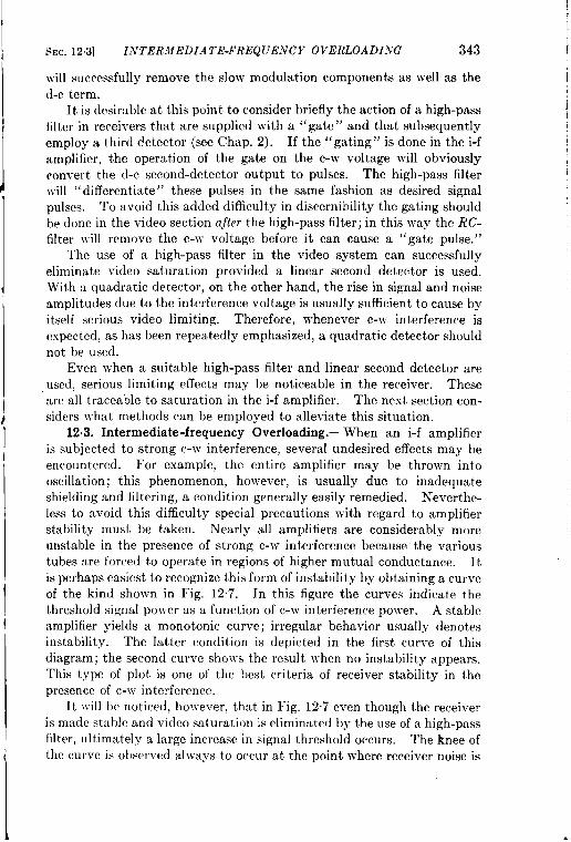
1
i
i
I
SEC. 12.3] INTERMEDIATE-FREQUENCY OVERLOADZ.VG
will successfully remove the slow modulation components ascl-c term.
343
well as the
It is desirable at this point to consider briefly the action of a high-passfilter in receivers that aresupplied witha “gate” and that subsequentlyemploys third detector (see Chap. 2). If the “gating” is done in the i-famplifier, the operation of the gate on the c-w voltage will obviouslyconvert the d-c second-detector output to pulses. The high-pass filter~vill “differentiate” these pulses in the same fashion as desired signalpulses. Toavoid this added difficulty indiscernibility thegating shouldbe done in the video section qfter the high-pass filter; in this way the RC-filter will remove the c-w voltage before it can cause a “gate pulse. ”
The use of a high-pass filter in the video system can successfullyeliminate video saturation provided a linear second detector is used.With a quadratic detector, onthe other hand, therise insignal and noiseamplitudes due to the interference voltage is usually sufficient to cause byitself serious video limiting. Therefore, whenever c-w interference isexpected, as has been repeatedly emphasized, aquadratic detector shouldnot be used.
Even when a suitable high-pass filter and linear second detector areused, serious limiting effects may be noticeable in the receiver. Theseare all traceable to saturation in the i-f amplifier. The next section con-siders what methods can be employed to alleviate this situation.
12.3. Intermediate-frequency Overloading.—When an i-f amplifieris subjected to strong c-w interference, several undesired effects may beencountered. For example, the entire amplifier may be thrown intooscillation; this phenomenon, however, is usually due to inadequateshielding and filtering, a condition generally easily remedied. Neverthe-less to avoid this difficulty special precautions with regard to amplifierstability must be taken. Nearly all amplifiers are considerably moreunstable in the presence of strong c-w interference because the varioustubes are forced to operate in regions of higher mutual conductance. Itis perhaps easiest to recognize this form of instability by obtaining a curveof the kind shown in Fig. 12.7. In this figure the curves indicate thethreshold signal power asa function of c-w interference power. A stableamplifier yields a monotonic curve; irregular behavior usually denotesinstability. The latter condition is depicted in the first curve of thisdiagram; the second curve shows the result when no instability appears.This type of plot is onc of the best criteria of receiver stability in thepresence of c-w interference.
It will bc noticed, however, that in Fig. 12.7 even though the receiveris made stable and video saturation is eliminated by the use of a high-passfilter, ultimately alargeincrease insignal threshold occurs. The knee ofthe curve is observed always to occur at the point where receiver noise is
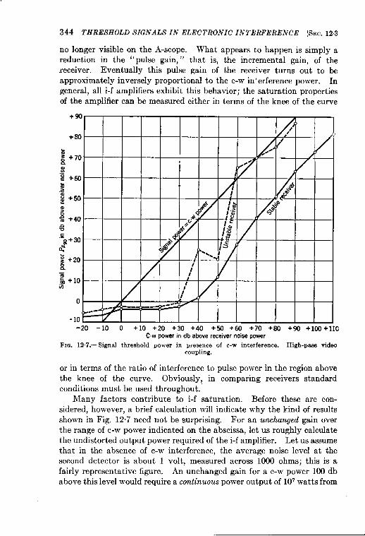
344 THRESHOLD SIGNALS IN ELECTRONIC IN TERFERENC!E [SEC. 12.3
no longer visible on the A-scope. What appears to happen is simply areduction in the “pulse gain, ” that is, the incremental gain, of thereceiver. Eventually this pulse gain of the receiver turns out to beapproximate y inversely proportional to the c-w in’ erference power. Ingeneral, all i-f amplifiers exhibit this behavior; the saturation propertiesof the amplifier can be measured either in terms of the knee of the curve
-20 -10 0 +10 +20 +30 +40 +50 +60 +70 +S0 +90 +IW+l ICC.wpowerin db above receiver noise power
Fm. 12.7.—Signal threshold power in presence of c-w interference. High-paas videmcoupling.
or in terms of the ratio of interference to pulse power in the region abovethe knee of the curve. Obviouslyz in comparing receivers standardconditions must be used throughout.
Many factors contribute to i-f saturation. Before these are con-sidered, however, a brief calculation will indicate why the kind of resultsshown in Fig. 12.7 need not be surprising. For an unchanged gain overthe range of c-w power indicated on the abscissa, let us roughly calculatethe undistorted output power required of the i-f amplifier. Let us assumethat in the absence of c-w interference, the average noise level at thesecond detector is about 1 volt, measured across 1000 ohms; this is afairly representative figure. An unchanged gain for a c-w power 100 dbabove this level would require a continuous power output of 107watts from
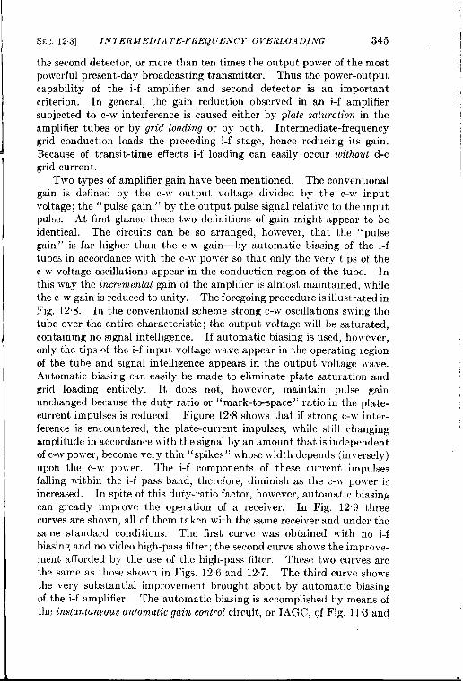
the second detector, or more than ten times the output power of the mostpowerful present-day broadcasting transmitter. Thus the power-outputcapability of the i-f amplifier and second detector is an importantcriterion. In general, the gain reduction observed in an i-f amplifiersubjected to c-w interference is caused either by plate saturation in theamplifier tubes or by grid loading or by both. Intermediate-frequencygrid conduction loads the preceding i-f stage, hence reducing its gain.
A Because of transit-time effects i-f loading can easily occur withou~ d-cgrid current.
Two types of amplifier gain have been mentioned. The conventionalgain is defined by the c-w output voltage divided by the c-w inputvoltage; the “pulse gain, ” by the output pulse signal relative to the inputpulse. At first glance these two definitions of gain might appear to beidentical. The circuits can be so arranged, however, that the “ pulsegain” is far higher than the c-w gain—by automatic biasing of the i-ftubes in accordance with the c-w power so that only the very tips of thec-w voltage oscillations appear in the conduction region of the tube. Inthis way the incremental gain of the amplifier is almost maintained, whilethe c-w gain is reduced to unity. The foregoing procedure is illustrated inFig. 12.8. In the conventional scheme strong c-w oscillations swing the
J
tube over the entire characteristic; the output voltage will be saturated,containing no signal intelligence. If automatic biasing is used, however,only the tips of the i-f input voltage wave appear in the operating regionof the tube and signal intelligence appears in the output voltage wave.Automatic biasing can easily be made to eliminate plate saturation andgrid loading entirely. It does not, however, maintain pulse gain
unchanged because the duty ratio or “mark-to-space” ratio in the plate-current impulses is reduced. Figure 12”8 shows that if strong c-~v inter-ference is encountered, the plate-current impulses, while still changingamplitude in accordance with the signal by an amount that is independentof c-w power, become very thin “ spikes” whose width depends (inversely)upon the c-w power. The i-f components of these current impulsesfalling within tbe i-f pass band, therefore, diminish as the c-w power i:increased. In spite of this duty-ratio factor, however, automatic biasingcan greatly improve the operation of a receiver. In Fig. 12.9 threecurves are shown, all of them taken with the same receiver and under thesame standard conditions. The first curve was obtained with no i-fbiasing and no video high-pass filter; the second curve shows the improve-ment afforded by the use of the high-pass filter. These two curves arethe same as those shown in Figs, 12.6 and 12.7. The third curve showsthe very substantial improvement brought about by automatic biasingof the i-f amplifier. The automatic biasing is accomplished by means ofthe instantaneous automatic gain control circuit, or IAGC, of Fig. 113 and
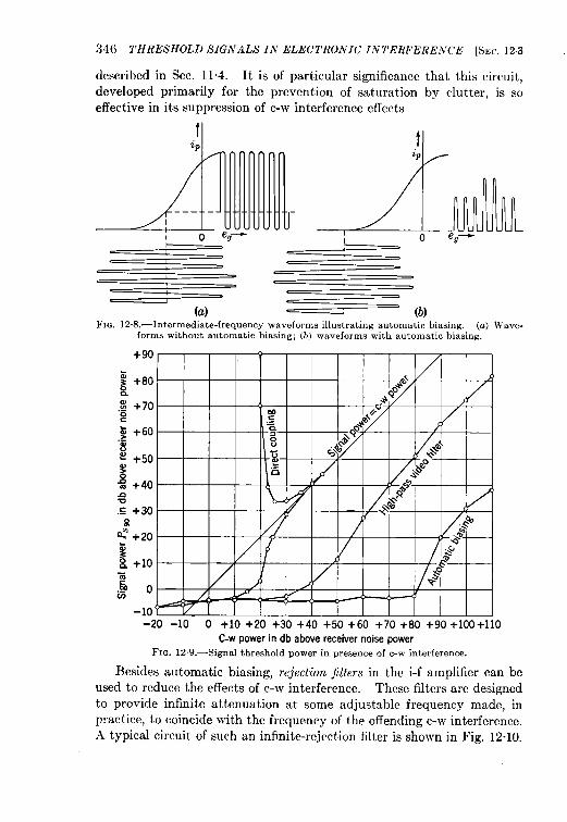
346 THRESHOLD SIGNALS IN ELECTRONIC INTEIWERE.vCli ~~~C.12.3
described in Sec. 11.4. It is of particular significance that this circuit,
developed primarily for the prevention of saturation by clutter, is so
effective in its suppression of c-w interference effects
(a)
II
111-= (b)
FIG. 12.8. —Intermediate-f requency waveforms illustrating automatic biasing. (a) Wavef-orms without automatic biasing; (b) waveforms with automatic biasing.
C-w power in db above receiver noise power
FIG. 12.9.—Signa1 threshold power in presence of c-w interference,
Besides automatic biasing, rejection jilters in the i-f amplifier can beused to reduce the effects of c-w interference. These filters are designedto provide infinite attenuation at some adjustable frequency made, inpractice, to coincide with the frequency of the offending c-w interference.A typical circuit of such an infinite-rejection filter is sho~~n in Fig. 12.10.
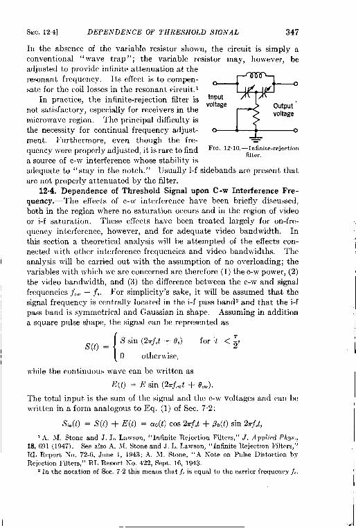
SEC. 124] DEPENDENCE OF THRESHOLD SIGNAL 347
In the absence of the variable resistor shown, the circuit is simply aconventional “wave trap”; the variable resistor mav, ho}vever. beadjusted to provide infinite attenuation at theresonant frequency. Its effect is to compen-
sate for the coil losses in the resonant circuit.1In practice, the infinite-rejection filter is
not satisfactory, especially for receiversin themicrowave region. The principal difficulty is
the necessity for continual frequency adjust-ment. Furthermore, even though the fre-quency were properly adjusted, it is rare to finda source of c-w interference whose stability is
“,
EInput
voltage output ‘
voltage
+
FIG, 12.10,—Infinite-rejectionfilter,
adequate to “stay in the notch. ” Usually l-f sidebands are present thatare not properly attenuated by the filter.
12.4. Dependence of Threshold Signal upon C-w Interference Fre-quency.—The effects of c-w interference have been briefly discussed,both in the region where no saturation occurs and in the region of videoor i-f saturation. These effects have been treated largely for on-fre-quency interference, however, and for adequate video bandwidth. Inthis section a theoretical analysis will be attempted of the effects con-nected with other interference frequencies and video bandwidths. Theanalysis will be carried out with the assumption of no overloading; thevariables with which we are concerned are therefore (1) the c-w power, (2)the video bandwidth, and (3) the difference between the c-w and signalfrequencies jf,w – ~,. For simplicity’s sake, it will be assumed that thesignal frequent y is centrally located in the i-f pass band2 and that the i-fpass band is symmetrical and Gaussian in shape. Assuming in additiona square pulse shape, the signal can be represented as
s(t) = {S sin (27r~,t + 0,) for Itl < ~~
[O otherwise,
while the continuous wave can be ~vritten as
E(t) = E sin (27rjCUt+ Oa).
The total input is tbe sum of the signal and tbe c-wwritten in a form analogous to Eq. (1) of Sec. 7.2:
voltages and can be
s,.(t) = S(t) + E(t) = aO(t) cos 27rf8t+ Po(t)sin2dsL
1A. LI. Stone and J. L. Lawson, “ Infinite Rejection Filters,” J. Applied Phys.,18, 691 (1947). See also .4. NI. Stone and J. L. Lawson, “ Infinite Rejection Filters,”RL Report No. 72-6, June 1, 1943; A. hf. Stone, ,1.4 ~T~te on Pulse Distortion bY
Rejection Filters)’] RL Report No. 422, Sept. 16, 1943,z In the notation of Sec. 72 this means that f. is equal to the carrier frequency f..
348 THRESfiOLD SIGNALS IN ELECTRONIC INTERFEREN(!E [S... 124
where
[
E sin [27r(f.~ – .f.)t + oti] + S sin 0, for It[ < ~)c-lo(t) =
E sin [27r(.fCW– $,)t + O.W] otherwise,
{
E COS[27r(fcw– fs)t + o.w] + ~ cOs d. for Itl < ~,Al(t)=
E COS[27r(j,~ – ~,)t + L] otherwise.
If we assume further that the i-f bandwidth B is much larger than 1/7, sothat the pulse will be practically not deformed, we obtain for the outputof the i-f amplifier
where
a(t)=
S..,(t) = a(t) cos 21rf.t+ ,f3(t)sin 27rf,t,
[ 1az(.fcw– .fS)2 sin [27r(jCwE exp – ~, – f,)t + O,w]
(E exp
E exp
E exp
+ S sin 6. for ltl < ~
_ az(jc~l)— s 1~”sin [27r(jw – j,).!+ O.W]B’
otherwise
B; j.)’_ az(.fcw1
(’0s [2iT(jcw— j,)t + 0..]
+ s Cos f?, for Itl < ~
—1
~a(f’~j; ~s)z Cos [27r(jcw – js)t + O,w]
otherwise
(la)
(lb)
and a = 1.18.As in the previous sections of this chapter, for the case of actual
interest, the original c-w power is much larger than either t!~e signal or the
noise power. As~uming a ~inear second detector, the detector output of
the c-w plus signal plus noise will be a nearly Gaussian distribution of the
form given by Eq. (7” 13a) and with an average value
1[az(f.w — fJ 2E exp – ~, 1~=(a2 +@z))! = + s Cos [27r(fcw– j,)t + PI for Itl< ~7 (2)
E exp[
_ az(jti — j.)zB,
1
otherwise,
where q = oti — d. and where terms proportional to S2 have beenneglected. One sees from Eq. (1) that the average value of the detector
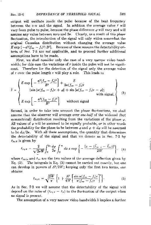
SEC. 12.41 DEPENDENCE OF THRESHOLD SIGN.4L 349
output will oscillate inside the pulse because of the beat frequencybetween the c-w and the signal. In addition the average value T willvary from pulse to pulse, because the phase difference pwill vary and willassume any value between zero and 2ir. Clearly, as a result of this phasefluctuation, the introduction of the signal will only widen somewhat theoriginal Gaussian distribution without changing the average valueE exp [ – az(f~ – j,)2/B2]. Because of these reasons the detectability cri-teria of Sec. 7.3 are not applicable, and to proceed further additionalassumptions have to be made.
First, we shall consider only the case of a very narrow video band-width; for this case the variations of r inside the pulse will not he signifi-cant. Therefore for the detection of the signal only the average valueof r over the pulse length r will play a role. This leads to
I [ 1az(fm—fa)z+E exp – ~z
s%r(fm – .f.)r
;= {Sin [T(.fu – fs)T + P] + sin [T(f.. – fa)~ – 9]}with signal, (3)
[
a’(~cw — ~8)2E exp – ~2 1 without signal
Second, in order to take into account the phase fluctuations, we shallassume that the observer will average over one-half of the widened (hutsymmetrical) distribution resulting from the variations of the phase ~.AU values of p will be assumed to be equally probable, or in other wordsthe probability for the phase to be between P and P + dp will be asmmecfto be dp/2r. With all these assumptions, the quantity that determinesthe detectability of the signal and that we denote as in Sec. 7,3 by~s+~ is given by
where ?U+, and ?.. are the two values of the average deflection given hyEq. (3). The integrals in Eq. (3) cannot be carried out exactly, hut onccan develop in powers of S2/2 W; keeping on]y the first two terms, oneobtains
(5)
As in Sec. 73 we will assume that the detectability of the signal willdepend on the ratio of (~~+.~– 7N) to the fluctuation of the output ~vhenno signal is present.
The assumption of a very narrow video bandwidth b implies a further
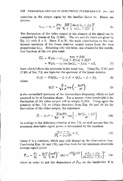
350 THRESHOLD SIGNALS IN ELECTRONIC IN7’ERFERE)V(:IJ’ ~SFx,. 12.4
reduction in the output signal by the familiar factor fJ7. Hence oneobtains
–RS267 2W sin r(f 1__w’:;,y2.‘8+”–‘“=4W rr (6)
The fluctuation of the video output in the absence of the signal can }mcomputed by means of Eq. (7.20 b). The a’s and P’S there are given hyEq. (1) with S = O. Since E >> W, the main contribution to the (,(Jn-
tinuous spectrum of the linear detector output comes from the term
proportional to p. Retaining only this term, one obtains for the correla-tion function of the c-w plus noise
ala” + /31/32m = wp(t2 – tl)
[(~? + B;)(~; + 1%)1~= Wp(h – tl) cm [2T(jm – .f.)(t’– h)], (7)
from which follows the spectrum in the usual way. Using Eq. (7.21 ) and(7.26) of Sec. 7.2, one finds for the spectrum of the linear detector
G.(f) = W[Q(f.. – f, + f) + Q(.fcw – f. – f)], (8)where
(9)
is the normalized spectrum of the intermediate frequency, which we hadassumed to be of Gaussian shape. For a narrow video bandwidth b thefluctuation of the video output will be simply G,(0)b. Using again thenotation of Sec. 7“3, we obtain therefore, from Eqs. (8) and (9) for thefluctuation of the video output, the expression
‘- “N)’=t%exp[-2a2(’cE’-f’)21(lo)
In analogy to the deflection criterion of Sec. 7“3, we shall assume that theminimum detectable signal power is determined by the equation
Fs+.v — F.N = c,[T – (T,v)’pi
(11)
where C is a constant, which may still depend on the observation time.Combining Eqs. (6) and (10), one then finds for the minimum detectableaverage signal power
where in order to put the dependence of ~mi.on the bandwidth B in
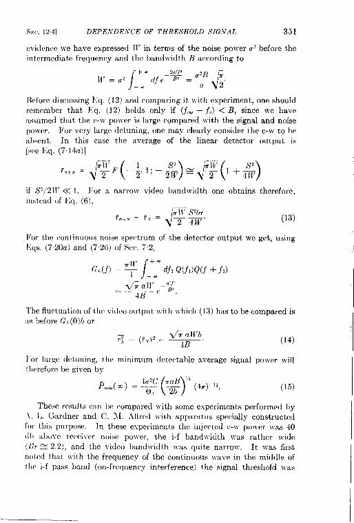
SEC, 124] DEPE,VDEXCE OF THRESHOLD SIGNAL 351
evidence we have expressed TVin terms of the noise po~ver U2before theintermediate frequency and the bandwidth B according to
Before discussing I~q. (12) and comparing it \viLhexperiment, one shouldremember that Eq. (12) holds only if (jw – j,) < 1?, since w-e haveassumed that the c-w power is large compared with the signal and noisepower. For very large detuning, one may clearly consider the c-w to heabsent. In this case the average of the linear detector output is[See I’:q. (7.14a)]
if Sz/2W << 1. For a narrow video bandwidth one obtains therefore.instwd of Ikq. (6),
J-m}~’i$2bT7S+,V — ~.v = — —.
2 41}’
For the continuous noise spectrum of the detectorIkls. (720a) and (7.2(i) of Ser. 72,
(13)
out put we get, using
‘/+.
c,,(f) = ~+ ~fl Q(.fl)fiw + fl)_ + a;.” .g—
413 e “
The fluctuation of the vi(lco output ,vit,h ~vhich (13) has to be compared is:1s before C,, (0)b or
(14)
I’or large detuning, the minimum detectable average signal power will1Iwrefore be given by
(15)
These results can be compared }.itb some experiments performed by.1, I,. Gardner and C. 11. Allred \rith apparatus specially constructedfor this purpose. In these experiments the injected c-lr poiver v-as 40([1) above receiver noise pol~er, the i-f band)vidth was rather wide(B, ~ 2.2), and the video bandlridth v-as quite narro,v. It was firstnoted that ]rith the frequency of the continuous wave in the middle ofIIw i-f pass bond (on-frequency interference) the signal threshold \vas
,,
I
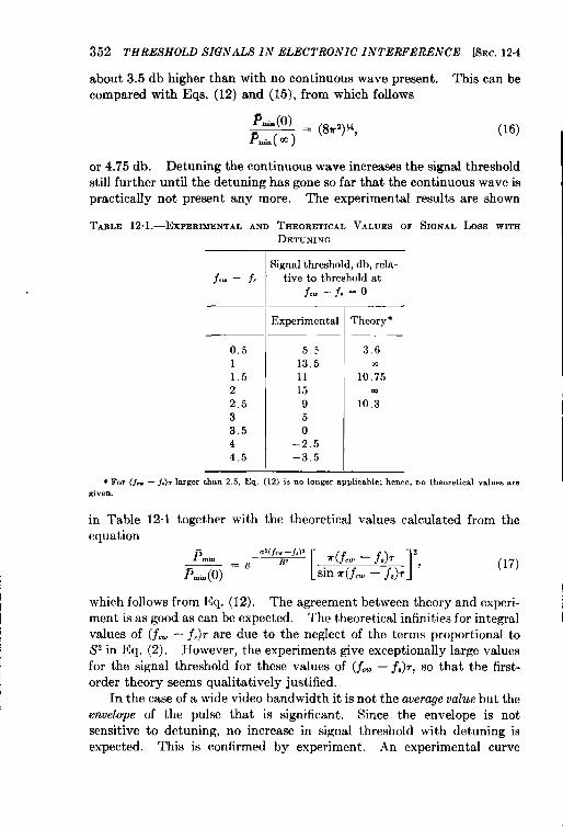
352 THREA’HOLD SIGNALS IN ELECTRONIC INTERFERENCE ISEC. 12.4
about 3.5 cib higher than With no continuous wave present. This can becompared with Eqs. (12) and (15), from which follows
(16)
or 4.75 db. Detuning the continuous wave increases the signal thresholdstill further until the detuning has gone so far that the continuous wave ispractically not present any more. The experimental results are shown
TABLE12.1.—EXPERIMENTALANDTHEORETICALV.ALUESOF SIGNAL Loss WITHDETUNING
i.. - f.
0,511.5
22.5
3
3,544.5
$ignal threshold, db, rela-tive to threshold at
f.w–f. =o
Experimental
55
13.51115950
–2,5–3.5
Theory*
3.6m
10.75
10.;
* For (f,- —f.)r larger than 2.5, Eq. (12) is no longer applicable; hence, no theoretical values megiven.
in Table 12.1 together with the theoretical values calculated from the
equation
Pm. -a-
[ 1~(jcw—j’J72FJmti(o)= e
(17)sin r(~ti — j,)7 ‘
which follows from Eq. (12). The agreement between theory and experi-ment is as good as can be expected. The theoretical infinities for integralvalues of (j- – f,), are due to the neglect of the terms proportional toS’ in Eq. (2). However, the experiments give exceptional y large valuesfor the signal threshold for these values of (f~ – ~.)r, so that the first-order theory seems qualitatively justified.
In the case of a wide video bandwidth it is not the average value but theenvelope of the pulse that is significant. Since the envelope is notsensitive to detuning, no increase in signal threshold with detuning isexpected. This is confirmed by experiment. An experimental curve
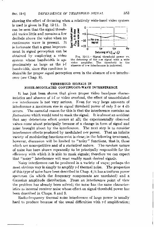
SEC. 12.4] DEPENDENCE OF THRESHOLD SIGNAL 353
showing the effect of detuning when a relatively wide-band video systemis used~s given in Fig. 12”11~ Itcan be seen that the signal thresh-old varies little and remains a fewdecibels above the value when nocontinuous wave is present. Itis fortunate that a great improve-ment in signal perception can beobtained by employing a videosystem whose bandwidth is ap-proximately as large as the i-fband\vidth. since this condition is
Detuning of (&-/J
FIG. 12.11 .—Signal threshold power vs.the detuning of the c-w signal with a widevideo amplifier. The threshold in theabsence of c-w interference is indicated.
desirable for proper signal perception even in the absence of c-w interfer-ence (see Chap. 8).
THRESHOLD SIGNALS INNOISE-MODULATED CONTINUOUS-WAVEl~TERFl%RENCE
It has just been shown that given proper video bandpass charac-teristics and absence of i-f or video overload, the effect of unmodulatedc-w interference is not very serious. Even for very large amounts ofinterference a maximum rise in signal threshold power of only 3 or 4 dboccurs. The essential reason for this is that the interference contains no
jiuc~uations which would tend to mask the signal. It is almost an accident
that any deleterious effect occurs at all; the experimentally observedvalues come about principally because of a change in form of signal andnoise brought about by the interference. The next step is to considerinterference effects produced by modulated c-w power. That an infinitevariety of modulating functions exist is clear; in the following treatment,however, discussion will be limited to “noisy” functions, that is, thosewhich are nonrepetitive and of a statistical nature. The random natureof noise has been shown repeatedly to be principally responsible for theefficiency with which it is able to mask signals; therefore we can expectthat “noisy” interference will most readily mask desired signals.
h’oisy interference can be produced in a variety of ways; perhaps themost obvious way is simply to amplify r-f thermal noise. The propertiesof this type of noise have been described in Chap. 4; it has a uniform powerspectrum (in which the frequency components are unrelated) and aGaussian amplitude distribution. From an interference point of viewthe problem has already been solved; the noise has the same character-istics as internal receiver noise whose effect on signal threshold power hasbeen described in Chaps. 8 and 9.
Radio-frequency thermal noise interference of large power is usuallyhard to produce because of the usual difficulties with r-f amplification;
354 THRESHOLD SIGIV.4LS I.V ELECTRO.VIC I-VTERFERENCE [SEC. 12.5
consequently, it is generally expedient to modulate an r-f c-w carrier withan appropriate video noise function. This modulation can be applied tothe carrier amplitude, frequency, or phase. Frequent y and phasemodulation are shown in Chap. 2 to be similar; one can proceed fromfrequency to phase modulation and vice versa by the use of appropriatefilters. We may therefore consider amplitude and jrequency modulation
as the two fundamental operations. Although it is quite possible toconsider in detail the effects of each type of modulation, only the a-mcase will be presented in the following discussion.
12.5. Continuous-wave Interference Amplitude Modulated by Noise.Let us assume for simplicity that the video-voltage noise function pro-duces corresponding changes in the r-f amplitude within the limitations ofthe r-f amplifier. Ideally these limitations are felt in two ways: (1) Ther-f amplifier has a minimum power output (zero) that the modulatingfunction must not try to cross, and (2) the r-f amplifier has a definite peakoutput-power capability. These limitations mean that any of the noisefunctions which we are likely to consider will not be immediately appli-cable to modulation; these functions must first be passed through limitersto prevent overdriving the r-f amplifier on large noise peaks and to preventcutoff of the r-f amplifier on large negative peaks. This limiting actionmay, of course, be provided by the r-f amplifier itself; however, in com-
puting the spectrum and amplitude distribution of r-f noise it is conven-ient to think first of limiting the video noise function, then of applyingpurely linear amplitude modulation to the r-f carrier.
The problem confronting us, then, is essentially the c-w interferencecase discussed in Sees. 12”1 through 12”4, except that in addition to thec-w carrier we now must consider the r-f noise sidebands. The propertiesof these noise sidebands depend upon the properties of the video noisefunction as well as on the degree of limiting, or “clipping.” That thisproblem is complex is proved by the complicated effects of even theunmodulated c-w carrier. Consideration of the general case will not beattempted. Discussion will be limited to the behavior of the systemunder the following set of conditions:
1. The receiver is fitted with an adequate i-f filter and has an adequatevideo bandwidth.
2. The noise modulating function is to be video thermal noise withGaussian amplitude distribution and bandwidth defined by b..This bandwidth is ordinarily determined by the video amplifiercharacteristics.
3. The limiting, or clipping, is symmetrical about the average value ofthe Gaussian noise function. This implies that the r-f amplitudeis modulated about a value equal to one-half the peak value.
SEC, 12,5] NOISE-MODULATED C-W I.VTERFERENCE 355
With these restrictions in mind we are in a position to discuss qualita-tively the effects to be expected. The signal threshold power will dependessentially on three factors: (1) the amount of receiver noise present, (2)the r-f interference carrier, and (3) the spectrum and amplitude of theinterference noise. The first two factors have already been discussedin Chaps. 8 and 9 and in Sees. 12”1 through 12.4; let us therefore considerthe interference noise itself.
We shall be concerned with two properties of the interference-noisesidebands: (1) the power spectrum that incidentally will give the totalsideband power relative to the carrier power and (2) the quality of thenoise, which must be measured in terms of the efficiency with which it is
able to mask a desired signal. The first property has been calculated
by Van Vleck.’ He has assumed symmetrical limiting, or clipping, of
the video noise function. If one defines the fractional modulation result-
ing from the noise as m, where m is the ratio of rms video noise voltagebefore limiting to the limiting level itself, then Van Vleek has shown that
clipping has little noticeable effect on the spectrum for values of m less
than unity. Furthermore, the total noise sideband power in terms of
the carrier power is given simply by ~mz again for values of m less than
unity. For values of m greater than unity the spectrum is modified
appreciably by the clipping, and the total noise sideband power is not a
simple function of m. Where m becomes infinite, a condition Van Vleck
describes as “super clipping,” he has shown that the total sideband power
is just equal to the carrier power. Representative spectra and amplitude
distributions for m = 1 are shown in Fig. 12”12. In this diagram the
video noise function is assumed to have a uniform spectrum out to the
bandwidth limit b..
In what is to follow the region of particular interest is that for whichthe fractional modulation m is less than unity. Therefore we can easilycalculate the total noise sideband power and its spectrum from the modu-lating video bandwidth bn and the fractional modulation m. Theproblem might appear at this point to be nearly solved; this would betrue if one knew precisely how efficiently the clipped interference noise(compared with unclipped noise) masks the desired signal. Unfor-tunately this property of the interference noise is not easily susceptibleto calculation. Figure 12.12 makes it clear that the noise-amplitudedistribution is profoundly altered by the clipping. The apparent “ceil-ing” produced by the limiting action provides a more or less definiteamplitude baseline over which a relatively small signal can be noticed.Therefore the ceiling produces a qualitative change in the noise that may
1J. H. Van Vleck, “ The Spectrum of Clipped Noise,” RRL Report No. 411-51,July 21, 1943.
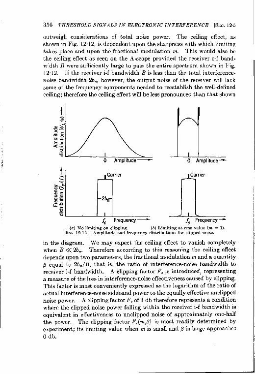
I
356 THRESHOLD SIGNALS IN ELECTRONIC INTERFERENCE
outweigh considerations of total noise power. The ceiling
[SEC. 125
effect, asshown in Fig. 12”12, is dependent upon the sharpness with wh~ch limitingtakes place and upon the fractional modulation m. This would also bethe ceiling effect as seen on the A-scope provided the receiver r-f band-w~dth B were sufficiently large to pass the entire spectrum shown in Fig.]2.12. If thereceiver i-f bandwidth l?islessthanthe total interference-noise bandwidth 2b., however, the output noise of the receiver ~vill lacksome of the frequency components needed to reestablish the well-definedceiling; therefore the ceiling effect will be less pronounced than that shown
Carrier
L~ Frequency+
(a) No limiting on clipping. (b) Limiting at rms value (m = 1).FIQ, 12. 12.—Amplitude and frequency distributions for clipped noise.
in the diagram. We may expect the ceiling effect to vanish completely
when B <<2b~. Therefore according to this reasoning the ceiling effectdepends upon two parameters, the fractional modulation m and a quantity~ equal to 2b~/B, that is, the ratio of interference-noise bandwidth toreceiver i-f bandwidth. A clipping factor F. is introduced, representinga measure of the loss in interference-noise effectiveness caused by clipping.This factor is most conveniently expressed as the logarithm of the ratio ofactual interference-noise sideband power to the equally effective unclippednoise power. A clipping factor F. of 3 db therefore represents a conditionwhere the clipped noise power falling within the receiver i-f bandwidth isequivalent in effectiveness to unclipped noise of approximate y one-halfthe power. The clipping factor F,(m,@ is most readily determined byexperiment; its limiting value when m is small and B is large approx!lcsO db.
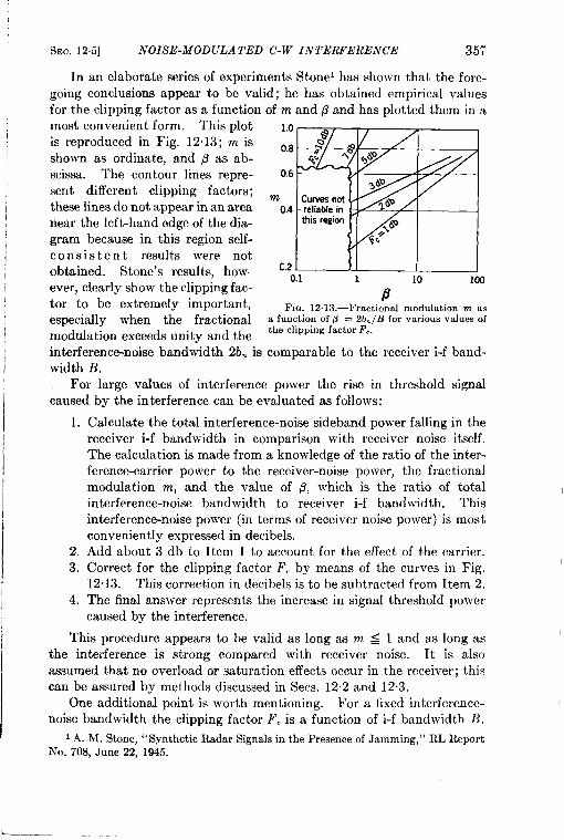
1
I
)
1
,
I
!!
1
SEC. 125] NOISE-MODULATED C-W INTERFERENcE 35:
In anelaborate series of experiments Stonel has shown that the fore-
going conclusions appear to be valid; he has obtained empirical valuesfor the clipping factor as a function of m and @ and has plotted them in a
most convenient form. This plotis reproduced in Fig. 12.13; m isshown as ordinate, and ,8 as ab-scissa. The contour lines repre-
sent different clipping factors;these lines do not appear in an areanear the left-hand edge of the dia-gram because in this region self-
consistent results were notobtained. Stone’s results, however, clearly show the clipping fac-tor to be extremely important,especially when the fractionalmodulation exceeds unity and the
1.0
0.8
0.6
m0.4
C.2o
~
Curvaanotreliable inthis region
1 10 100
FIG. 12.13.—Fracti0nal modulation m asa function of (3 = 2b*jB for various values ofthe clipping factor F..
interference-noise bandwidth 2bn is comparable to the receiver i-f band-width B.
For large values of interference power the rise in threshold signalcaused by the interference can be evaluated as follows:
1.
2.
3.
4.
Calculate the total interference-noise sideband power falling in the
receiver i-f bandwidth in comparison with receiver noise itself.
The calculation is made from a knowledge of the ratio of the inter-
ference-carrier power to the receiver-noise power, the fractional
modulation m, and the value of B, which is the ratio of total
interference-noise bandwidth to receiver i-f bandwidth. This
interference-noise power (in terms of receiver noise power) is most
conveniently expressed in decibels.
Add about 3 db to Item 1 to account for the effect of the carrier.
Correct for the clipping factor F, by means of the curves in Fig.12.13. This correction in decibels is to be subtracted from Item 2.The final answer represents the increase in signal threshold powercaused by the interference.
This procedure appears to be valid as long as m ~ 1 and as long asthe interference is strong compared with receiver noise. It is alsoassumed that no overload or saturation effects occur in the receiver; thiscan be assured by methods discussed in Sees. 12.2 and 12.3.
One additional point is worth mentioning. For a fixed interference-noise bandwidth the clipping factor F. is a function of i-f bandwidth B.
1A. M. Stone, “ Synthetic Radar Signals in the Presence of Jamming, ” RL Reporth’o. 708, June 22, 1945.
L_
358 THRESHOLD SIGVALS I.~ ELECTRONIC Z.VTERII’EREA’G’E [SEC.127
Therefore, in measuring threshold signals as a function of B, in a way
similar to that shown in 1 ig. 87, the smallest threshold signal energy willbe found at a value of B, somewhat I igher than the value determined for
receiver noise. A. 31. Stoncq has found the, t under certain conditions theoptimum value of B~ could be shifted by L factor of as much as 3 or 4.
It does not appear, howc”,er, that this situation should alter the design
of receivers, for the wider bandwidth generally gives a greater opportunity
for off-frequency interference.
THRESHOLD SIGNALS IN PULSED INTERFERENCE
12.6. Description of Pulsed Interference. -In the first two parts of
this chapter an attempt was made to analyze the deleterious effects of
c-w interference even though modulated in amplitude by a complicated
noise function. Other forms of electronic interference exist, one of themost common of which may be termed puked interference. Here, the
interfering wave may conskt of a train of r-f pulses whose repetition fre-
quency may or may not be constant and whose radio frequency and pulse
length may or may not correspond to that of the desired signal. In
radar reception, pulsed interference ~vill very likely arise from other
near-by radar sets operating on nearly the same radio frequency. Suchinterference will appear on the radar A-scope as a series of intensesaturated signals, which usually differ from genuine echo signa!s in theirnonsynchronized positions and in their relatively great intensities.Because of the resulting fencelike appearance on the A-scope, the inter-ference is usually known as “railing” interference. Several interferingradar units produce several sets of interspersed railings whose relativepositions continually change. A discussion of railing interference andmethods of suppressing its effect is given in Sec. 12.7.
Because of the relatively large peak powers that can be produced \vithpulse techniques the possibility of producing damaging interference bythis means should be considered. It can be shown that no power is‘‘ wasted” in a carrier and that a “ noisy” function can be produced byrandom variations in the interval between successive pulses. The condi-tions determining threshold signal power for this situation are discussedin Sec. 12.8.
12.7. Railing Interference. -In railing interference one must considernot only the effect of the main interfering pulse but also the trailinginterference echoes produced by near-by reflecting objects. Theseechoes, though very weak in comparison with the main interference pulse,may still be large enough to exceed a desired signal. In practice thesetrailing echoes can be detected for perhaps 100 ~sec after the main pulse.
1 Ibid.
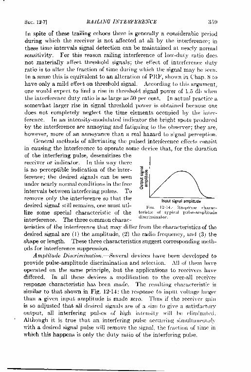
Sm. 12.7] RAILING INTERFERENCE 3!;9
In spite of these trailing echoes there is generally a considerable periodduring which the receiver is not affected at all by the interference; inthese time intervals signal detection can be maintained at nearly normalsensitivity. For this reason railing interference of low-duty ratio doesnot materially affect threshold signals; the effect of interference dutyratio is to alter the fraction of time during which the signal may be seen.In a sense this is equivalent to an alteration of PRF, shown in Chap. 8 tohave only a mild effect on threshold signal. According to this argument,one would expect to find a rise in threshold signal pow-er of 1.5 db whenthe interference duty ratio is as large as 50 per cent. In actual practice asomewhat larger rise in signal threshold po]ver is obtained because onedoes not completely neglect the time elements occupied by the ifiter-ference. In an intensity-modulated indicator the bright spots producedby the interference are annoying and fatiguing to the observer; they are,however, more of an annoyance than a real hazard to s~gnal perception.
General methods of alleviating the pulsed interference effects consistin causing the interference to operate some device that, for the durationof the interfering pulse, desensitizes thereceiver or indicator. In this way thereis no perceptible indication of the inter- E%ference; the desired signals can be seen E Sunder nearly normal conditions in the free SE$mintervals between interfering pLdses. Toremove only the interference so that the h
lnPUt signal amplitude
desired signal still remains, one must uti- Fro, 1214. ltcsputlsc r},ar:sc-lize some special characteristic of the teristic of t.vpicul pulse-amplitude
interference. The three common charac- ‘iscrirni’’ator”
teristics of the interference that may differ from the characteristics of the
desired signal are (1) the amplitude, (2) the radio frequency, and (3) the
shape or length. These three characteristics suggest corresponding meth-
ods for interference suppression.
Amplitude Discrimination .—Several devices have been developed toprovide pulse-amplitude discrimination and selection. All of them ha~,eoperated on the same principle, but the applications to receivers havediffered. In all these devices a modification to the over-all recei~-erresponse characteristic has been made. The resulting characteristic issimilar to that shown in Fig. 12.14: the response to input voltage Iargelthan a given input amplitude is made zero. ‘1’hus if the receiver gainis so adjusted that all desired signals are of a size to give a satisfactoryoutput, all interfering pulses of high in tcnsitj, ~~ill hc elirninat etl.
\Although it is true that an interfering pulse occulring simultuneollsly
with a desired signal pulse will remove the signal, the frartion of time in
which this happens is only the duty ratio of the interfering pulse.
,,
360 THRESHOLD SIGNALS IN ELECTRONIC INTERFERENCE [SEC. 12.7
The response characteristic shown in Fig. 12-14 can be produced in anumber of ways. The normal video output of the receiver can be“swamped” by a video signal of opposite polarity, which at low signallevel is made inoperative by an appropriate bias voltage. This swampingaction can, if desired, be accomplished directly in the output of thesecond detector; in this case it is derived from a biased second detectorof opposite polarity. Perhaps the simplest technique, however, is touse a video signal derived from one of the i-f stages to bias the grid of thefollowing i-f stage; in thk instance a strong input signal will bias the i-fstage to cutoff, and no output voltage will occur.
The principal difficulties with any of these schemes are of two kinds.(1) The desired signals actually have a large range in amplitude, and theamplitude-selection “slot” must therefore be made extremely wide.Under these conditions satisfactory removal of railing interference is notusually possible. (2) As was mentioned previously, railing interferenceconsists of an intense leading pulse followed by a train of reflection echoeslasting for a number of microseconds. These trailing pulses, usually ofmuch longer duration than the original interfering pulse, are nearlyalways of the same general size as the desired signal pulse and cannottherefore be removed by this procedure. These two difficulties can be
overcome by a slightly different form of interference suppressor developedby Lawson. This suppressor, designed to combat railing interference,was required to remove completely the railing pulse together with itstrailing echoes, without removing any desired (radar) pulse.
To remove the railing pulse and echoes, a “blanking gate” of con-trollable length was supplied; this gate was initiated by the interferingsignal and could then be made long enough to remove the trailing echoesas well as the interfering pulse. To make sure desired radar pulses werenot removed, a new system was devised. It is clearly desirable totrigger the gate from video signals in which the interfering pulses areenhanced by comparison with the desired signals. This enhancementcan be assured by receiving the interfering pulses on a separate non-directional antenna. The scheme offers no improvement if the inter-ference comes from the same direction as the desired signal; otherwisethe improvement is proportional to the directional gain of the receivingantenna used for signal reception (radar antenna).
In spite of the separate nondkectional antenna and interferencereceiver the main transmitted radar pulse and close radar echoes will bestrong enough to trigger the blanking gate unless a gate “ deadener” isapplied. This deadener can take the form of a multivibrator triggeredfrom the main radar pulse, preventing operation of the blanking gate fora certain time after the transmitted radar pulse. This time can, ofcourse, be controlled by the multivibrator time constant and can beadjusted so that the interference suppressor removes no radar echoes.
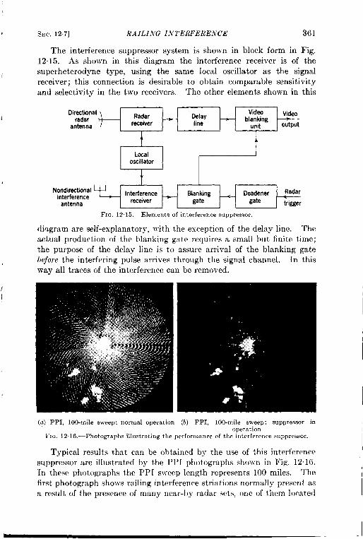
SEC. 127] RAILI.VG 1.V7’ERFERE.VCE 361
The interference suppressor system is shown in block form in Fig.12.15. As showm in this diagram the interference receiver is of thesuperheterodyne type, using the same local oscillator as the signalreceiver; this connection is desirable to obtain comparable sensitivityand selectivity in the two receivers. The other elements shown in this
Directional— Delay Video Video
radarantenna line
blankingunit output
tI,
Localoscillator
t
Nondirectionalinterference
Interference
- ‘ate “m
Blanking
antennareceiver
FIG. 12 15,—Elements of interference suppressor.
dingram are self-explanatory, with the exception of the delay line. The
actual production of the blanking gate requires a small but finite time;
the purpose of the delay line is to assure arrival of the blanking gate
before the interfering pulse arrives through the signal channel. In this
way all traces of the interference can be removed.
/I
(a) PPI, 100-mile sweep; normal operation (b) PPI, 100-mile sweep; suppressor inoperation
l:l~. 1216.-Photographs illustrating the performance of the interference suppressor.
Typical results that can be obtained by the use of this interferencesuppressor are illustrated by the PP1 photographs shown in Fig. 12“16.In these photographs the PPI sweep length represents 100 miles. Thefirst photograph sho~vs railing interference striations normally present asa result of the presence of many near-l)y radar sds, one of them l(wate(l
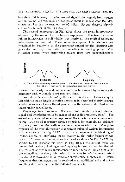
I
362 THRESHOLD SIG.VALS IiV ELECTRONIC IiVTERFERENCE [SEC. 127
less than 100 ft away. Radar ground signals, i.e., signals from targets
on the ground, are visible out to ranges of about 20 miles; some thunder-
storm patches can be seen out to 90 miles. Several discrete aircraft
echoes can be seen at various ranges.
The second photograph in Fig. 12.16 shows the great improvement
obtained by the use of the interference suppressor. It is true that some
railing interference is still visible, but nearly all the original annoying
interference is removed. These remaining s~ots of interference are
explained
generator
situation
$1c0~
c%
by inactivity of the suppressor ~au~ed by the blanking-gate
recovery time after a
occurs when interfering
AA1> v \
Frequency —
(a) Unmodified frequency discriminator
preceding inte~fering pulse. - Thispulses from two nonsynchronous
gc0~
1%kFrequency—
(b) Modified frequency discriminatorFlu. 12.17 .—l:requency discrimination response curves.
transmitters nearly coincide in time and can be avoided by using a gate
generator with extremely short recovery time.
No radar echoes need be lost by the use of this device. Echoes may kelost with the pulse-length-selection devices to be described shortly becausea radar echo has a length that depends upon the nature and extent of thetarget under surveillance.
Frequency Discrimination.—We can discriminate between desiredsignal and interfering pulse by means of the radio frequency itself. Theeasiest way is to enhance the response of the interference receiver shownin Fig. 12.15 to off-frequency signals by using, for example, an ordinaryfrequency discriminator with subsequent pulse rectification. The pulseresponse of the over-all receiver to incoming pulses of various frequencieswill be as shown in Fig, 12.17a. In this arrangement no blanking of(radar) echoes or interfering pulses exactly at the radar frequency willoccur. If, however, the response is altered as shown in Fig. 12.17b, byadding to the response indicated in Fig. 12.17a the output from theunmodified receiver, blanking of on-frequency interference can be effected.‘he ratio of on-frequency interference to radar echo will be as high as inthe unmodified receiver; this ratio will increase for off-frequency inter-ference, thus providing more complete interference suppression. Hencefrequency discrimination may be received as an additional aid and not asan alternative scheme to amplitude discrimination.
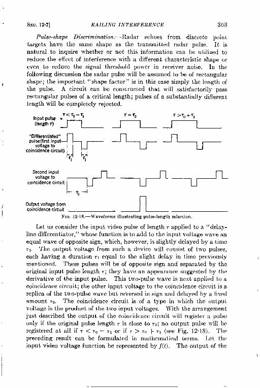
SEC. 12.7] RAILI.VG INTERFERENCE 363
Pulse-shape Discrimination. —Radar echoes from discrete pointtargets have the same shape as the transmitted radar pulse. It isnatural to inquire whether or not this information can be utilized toreduce the effect of interference with a different characteristic shape or
even to reduce the signal threshold power in receiver noise. In thefollowing discussion theradar pulse will reassumed to be of rectangular
1 shape; the important “shape factor” is in this case simply the length ofthe pulse. A circuit can be constructed that will satisfactorily passrectangular pulses of a critical length; pulses of a substantially differentlength will be completely rejected.
I
I
!- ~oi
Out@ voltage from
coincidence circuit
FIG. 12, lS.—Waveforms illustrating pulse-length selection,
Let us consider the input video pulse of length r applied to a “ delay-line clifferentiator,” whose function is to add to the input voltage wave anequal wave of opposite sign, which, however, is slightly delayed by a timerl. The output voltage from such a device will consist of two pulses,each having a duration rl equal to the slight delay in time previouslymentioned. These pulses will be of opposite sign and separated by theoriginal input pulse length r; they have an appearance suggested by thederivative of the input pulse. This two-pulse ~vave is next applied to acoincidence circuit; the other input voltage to the coincidence circuit is areplica of the two-pulse wave but reversed in sign and delayed by a fixedamount ,.. The coincidence circuit is of a type in which the outputvoltage is the product of the two input voltages. With the arrangementjust described the output of the coincidence circuit will register a pulseonly if the original pulse length ~ is close to TO;no output pulse will bcregistered at all if r < TO– ~1 or if ~ > TO+ 71 (see Fig. 12.18). Thepreceding result can be formulated in mathematical terms. Let theinput video VOItage function bc! represented by f(t). The output of the
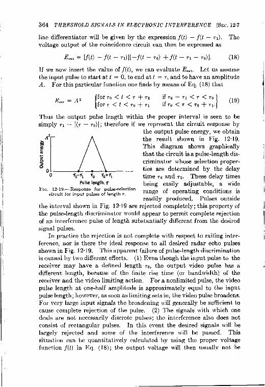
364 THRESHOLD SIGi~ALS IN ELECTRONIC INTERFERENCE [SEC. 127
Iinedifferentiator will begiven bytheexpression j(t) –j(t –r,). Thevoltage output of the coincidence circuit can then be expressed as
E.., = [j(t) – j(t – ~,)][–j(t – To) + j(t – -r, – .,)]. (18)
If we now insert the value of j(t), we can evaluate E..,. Let us assumethe input pulse to start at t = O, to end at t = T,and to have an amplitude
A. For this particular function one finds by means of Eq. (18) that
E.., = A z[
forro<t<r+Tl ifTO—71<r<T0for~<t<70+~l if70<~<~O+~l. I
(19)
Thus the output pulse length within the proper interval is seen to besimply 71 — I(~ — TO)I; therefore if we represent the circuit response by
the output pulse energy, we obtain
(m ‘heresultshOwninFig’12”1’
This diagram shows graphicallythat the circuit is a pulse-length dis-criminator whose selection proper-ties are determined by the delay
o To-1 TO 70+ 1 time ,, and ,1. These delay timesPulse length, ~ being easily adjustable, ~ wide
FIG. 12.19.—Responsefor pulse-selectioncircuitfor inputpulsesof lengthr. range of operating conditions is
readily produced. Pulses outsidethe interval shown in Fig. 12”19 are rejected completely; this property ofthe pulse-length discriminator would appear to permit complete rejectionof an interference pulse of length substantially different from the desiredsignal mdses.
In practice the rejection is not complete with respect to railing inter-ference, nor is there the ideal response to all desired radar echo pulsesshown in Fig. 12.19. This apparent failure of pulse-length discriminationis caused by two different effects. (1) Even though the input pulse to thereceiver may have a defined length To, the output video pulse has adifferent length, because of the finite rise time (or bandwidth) of thereceiver and the video limiting action. For a nonlimited pulse, the videopulse length at one-half ampfitude is approximate y equal to’ the inputpulse length; however, as soon as limiting sets in, the video pulse broadens.For very large input signals the broadening will generally be sufficient tocause complete rejection of the pulse. (2) The signals with which onedeals are not necessarily discrete pulses; the interference also does notconsist of rectangular pulses. In this event the desired signals will belargely rejected and some of the interference will be passed. ‘f’hissituation can be quantitatively calculated by using the proper voltagefunction f(t)in 17q. (18); the output voltage will then usually not, he
SEC. 128] RANDOMLY SPACED INTERFERENCE PULSES 365
zero for arbitrary interference voltage functions. Nevertheless, in spite
of these difficulties, a pulse-length discriminator built by Ashby and
Neher’ has proved to be of the same order of effectiveness as the amplitude
discriminator of I?ig. 12.18. In this particular pulse-length discriminator
the relatively narrow pulses from the coincidence unit were subsequently
lengthened somewhat to permit easy visibility; and to avoid the pulse-
broadening produced by limiting, a wide-band i-f amplifier was used.
The type of pulse-length discriminator just described is only one of
many forms of shape-discriminators that can be considered; nevertheless
it serves to illustrate the general effect expected. One can shape the
signal pulse in special ways; for example, a series of pulses is often gener-
ated with a fixed sequence of lengths and intervals. A suitable pulse-
shape discriminator can be made by using various appropriate delay
lines; this type of discriminator is usually called a decoder; that is, it
serves to decode the relatively complicated signal message. For any of
these decoders the response can be calculated for any input voltage
function by methods similar to that by which Eq. (18) was derived.
At the beginning of the discussion on pulse-shape discrimination an
interesting question was raised regarding the possibility of reducing
signal threshold power in receiver noise by the use of pulse-shape dis-
criininat ion. At first sight it would appear that pulse-length discrimina-
tion would permit one preferentially to select desired signals from noise
(which itself has no defined “length “). Unfortunately this does not
seem to be the case, at least in the region where signals are not larger
than noise itself. The reason is that when pulsed signals and noise
become mixed, the mixture distorts the signal shape. This distortion isso severe that the pulse-length discrimination is of little value. In anactual experiment by R. M. Ashby and J. L. Lawson the signal thresholdpower measured on an A-scope was not perceptibly changed by the useof a pulse-length discriminator. This result might be different if theinitial conditions were such as to cause the threshold signal to be con-siderably larger than noise, but this case was not investigatedexperimentally.
12.8. Randomly Spaced Interference Pulses.-In Sec. 12.7, a discus-sion was undertaken of railing interference, characterized chiefly byintense pulses of relatively low duty ratio. To combat the effects of thisinterference some form of discrimination between interference and desiredsignal is used to desensitize the indicator during periods of interference.The free time between interference pulses is then used for signal observa-tion. None of the interference-suppression methods proposed are suit-
I R. M. Ashby and 1,. Neher, i1pulse Lengths Selector and MultiP1e pulse
Decoder.” RI, Rmmrt No. 917, Mar. 21, 1946.
366 THRESHOLD SIGNALS IN ELECTRONIC’ INTERFERENCE [SEC. 12.8
able when the duty ratio of the interference becomes high and where thetime interval between successive interference pulses becomes comparableto the signal pulse length (strictly, the reciprocal of the i-f bandwidth).In the limit where the interference pulse interval is extremely smallcompared with the reciprocal of i-f bandwidth, the interference is-handledby the receiver just like c-w interference; in such circumstances methodsfor c-w interference suppression are often found helpful (see Sees. 12.1 to
12.4).
If the interference pulses are randomly spaced in time, one mightexpect a relatively large rise in signal threshold power because of the“noisy” appearance. This is only partially true. If the average pulsespacing is large compared with the reciprocal of the i-f bandwidth, manyfree intervals are available for signal detection. This form of inter-ference is like railing interference and can be handled accordingly. Ifthe average interference-pulse spacing is small compared with the recipro-cal of i-f bandwidth, however, the output of the receiver will show ampli-tude noise fluctuations. This noise depends among other things uponthe function that determines the interferenc~pulse spacing; whateverthis function is, one finds the greatest similarity to nonlimited noise ifthe reciprocal of i-f bandwidth is extremely large compared with theaverage pulse spacing. For this condition the interference energy isspread over a relatively great band; the fraction falling within the receiverbandwidth is relatively small. Hence the interference is not generallyso effective as some other forms of noisy interference.
CHAPTER 13
THRESHOLD MODULATIONS FOR AMPLITUDE-MODULATEDi AND FREQUENCY-MODULATED CONTINUOUS-WAVE SYSTEMS
13.1. Introduction.-In this chapter we shall discuss the problem ofdetermining the minimum detectable modulation for a-m and f-m c-wsystems. The problem has been investigated by Crosbyl both experi-mentally and theoretically for the case that the carrier power is largecompared to the noise power. Our main purpose is to extend thetheoretical results of Crosby and to show how the application of thegeneral methods of Chap. 7 lead to a unified treatment of the problem.For a description of the main parts of the receiver we refer to Chap. 2.For amplitude modulation only the superheterodyne receiver will beconsidered, whereas for frequency modulation only the case of completeamplitude limitation will be discussed in detail.
The modulation will be assumed to be sinusoidal, so that for amplitudemodulation the signal will be represented by4
s.(t) = SO(I + 6 Cos 21rpt) Cos 2W-J, (1)
where SOis the carrier amplitude, j, the carrier frequency, p the modula-t ion frequency, and c the fractional modulation (cf. Sec. 2.1). Thespectrum consists of the carrier and the two sidebands of amplitude cSO/2.
For frequency modulation (cf. Sec. 2“3) the signal is represented by
( )S,(t) = SOcos 2mfJ + $ sin 2@ . (2)
The modulation index cf./p will be assumed to be large, so that of the\
sidebands (frequencies j, + np) only those which lie within the frequencyexcursion interval have appreciable intensity. The half width of the i-f
, amplifier will be assumed to be larger than the frequency excursion ~.f.,so that the i-f amplification of the signal will not give rise to any appreci-able deformation of the signal.
The main ~roblem is to find the minimum detectable fractionalmodulation ~~inwhen the signal is disturbed by the presence of noise. Todetermine ~~,. the power criterion will be used just as in Sec. 10”4. In thepower spectrum of signal plus noise there will appear a signal peak at the
I M. G. Crosby, “Frequency Modulation Noise Characteristics,” Proc. I. R. E., 25,472 (1937).
367
,
368 J1ODULA TIONS FOR CON TINUO[’S-WA VE SYS1’I?MS [SEC. 13.2
frequency p and with power z # superposed on a continuous backgroundof noise. The signal peak will be just detectable if its power is of thesame order of magnitude as the power of a segment of the continuousnoise spectrum around the frequency p. The application of this powerm-iterion ~villlead to t.,ti expressed as a function of system parameters andof the ratio z of the unmodulated signal power to the noise power (cj. Sec.7.3). The establishment of this function constitutes the main result ofthe theory.
13.2. The Minimum Detectable Amplitude Modulation.-For ampli-tude modulation all the necessary formulas have been derived already inSec. 7.2. Only the case of the linear detector will be considered. Thestarting point is then Eq. (7.18), in which one has to substitute
al = SO(1 + f Cos 27rpt), p, = o,~2 = SO(I + 6 Cos 2?rp(t + T)), p, = o.
The first term of llq. (7.18) is developed in powers of c. Keeping onlyterms up to C2,one obtains after averaging over the time t
1,(1)12(2) = ~+ [F’ + C’ZF(F’ + 2ZF”) + 2,’Z’F” Cos 27rpT + . . . ],
\rhere z = JS’~/2W, F = F(—~, 1; —z), and the primes denote differ-entiations with respect to z.
In the further terms of Eq. (7.18), which are proportional to p(,) andP:(r), the modulation of the signal can be neglected. Using the recurrence
relations for the hypergeometric function F (cf. Sec. 7.6), one obtainsfinally for the correlation function of signal plus noise
‘(”)‘%’2(-*1’-z)+$’’2(i+z)c@+~F2(:’2+’)+~’2(”{F2(+’1’-Z)+[4J-’)
-F(~2’-z)121‘3)in which the contribution w ~z in the d-c term has still been neglected.
With the help of the general formula [Eq. (7.26)1 the audio spectrum
of signal and noise can be deduced immediately from Eq. (3). The result
is clear; the first two terms give the d-c peak and the signal peak at the
frequency p; the third and fourth term give the continuous noise back-
ground. It is easy to show that for W ~ O or z ~ m (3) goes over into
R(r)( )
—Si l+; cos2Tpt ,z-) m
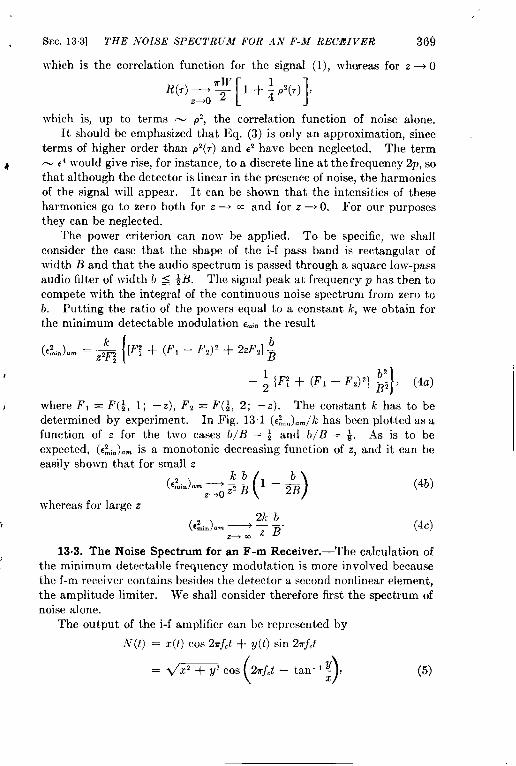
SEC, 133] THE .VOISE SPECTRijJf FOR AN F-M RECEIVER 369
which is the correlation function for the signal (l), whereas for z + O
‘(’)=57’‘~p’(’)l’which is, up to terms - ‘Z, the correlation function of noise alone.
It should be emphasized that Eq. (3) is only an approximation, sinceterms of higher order than p2(7) and C2have been neglected. The term
4 = C4would give rise, for instance, to a discrete line at the frequency 2p, sothat although the detector is linear in the presence of noise, the harmonicsof the signal will appear. It can be shown that the intensities of theseharmonics go to zero both for z ~ ~ and for z ~ O. For our purposesthey can be neglected.
The power criterion can now be applied. To be specific, we shallconsider the case that the shape of the i-f pass band is rectangular ofwidth B and that the audio spectrum is passed through a square low-passaudio filter of width b s ~B. The signal peak at frequency p has then tocompete with the integral of the continuous noise spectrum from zero tob. Putting the ratio of the powers equal to a constant k, we obtain forthe minimum detectable modulation ~~,. the result
(~ [F; + (F, – F,)’ + 2ZF,] ;(~%,)ml = z,~i
1 where F, = F(+, 1; ‘Z), F2 == F(*, 2; —Z). The constant k has to bedetermined by experiment. In Fig. 13.1 (,~,.)a~/k has been plotted as afunction of z for the two cases b/B = ~ and b/B = +. As is to beexpected, (Cli.)amis a monotonic decreasing function of z, and it can beeasily shown that for small z
(“i.’am=~:(’ -*)(4b)
whereas for large z
f (,:in)am —+ M!.2!+. 2B
(4C)
13.3. The Noise Spectrum for an F-m Receiver.—The calculation ofthe minimum detectable frequency modulation is more involved becausethe f-m receiver contains besides the detector a second nonlinear element,the amplitude limiter. We shall consider therefore first the spectrum ofnoise alone.I The output of the i-f amplifier can be represented by
N(t) = x(t) cos 2m~Ct+ y(t) sin 27rf,t
( )= ~xz + y’ cos 2rjCt – tan-’ ~ , (5)
370 MODULATIONS FOR CON7’INUOIJS- WA VE SYSTEMS [SEC. 13.3
lIX
10
1
% 0.1.WE
0.01
0.001
mom
I
I
\
\\
\,
\
\
\
\
\ .4
‘*!I-.
2 4 6 8z
‘-_
.\\
FIG. 13. 1.—Minimum detectable modulation as a function of z for a-m and f-m syatema andfor different values of tbe deviation ratio n = B/2b.
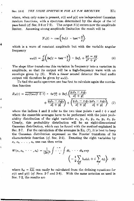
SEC. 13.3] THE A’OISE SPECTRUM FOR AN F-M RECEIVER 371
where, when only noise is present, z(t) and y(t) are independent Gaussianrandom functions, with a spectrum determined by the shape of the i-fpass band (cj. Sec. 3.8 or 7“2). The output N(t) enters now the amplitudelimiter. Assuming strong amplitude limitation the result will be
( )N1(t) = cos Zrjct – tan–l ~ ,
4which is a wave of constant amplitude but with the variable angularfrequency
(UN(t)=~%jct — tan–l–)y=2mfc+$+y2“— a,
z(6)
The slope filter transforms thk variation in frequency into a variation inamplitude, so that its output will be a high-frequency wave with anenvelope given by (6). With a linear second detector the final audiooutput will therefore be given by u~(t).
To find the audio spectrum one has first to calculate again the correla-tion function
4 +y’:G%)+Rii7‘7)$
where the indices 1 and 2 refer to the two time points t and t + r andwhere the ensemble averages have to be performed with the joint prob-ability distribution of the eight variables xl, YI, iI, YI, ZZ, Y2, iz, ~z.
Clearly, this probability distribution will be an eightdimensional
Gaussian distribution, which can be found with the method explained in
Sec. 3.7. For the calculation of the averages in Eq. (7), it is best to keep
the Gaussian distribution expre~ed as the Fourier transform of its
3 characteristic function (cj. Sec. 3.5). Denoting the eight variables by
2,,22, ..., zs, one can then write
//
+-Jv(zl,zz, . . .,28) =*8 . . . dt, . . . dt8 exp
—.
(-~zbkz’k’’+izz$)’ ‘8)k,l i
where bk~ = ~ can easily be calculated from the defining equations forz(t)and y(t) (cj. Sees. 3.7 and 3.8). With the same notation as used inSec. 7.2, the results are
372 MODULATIONS FOR CONTIN7JOUS- WA VE SYSTEMS [%c. 13.3
(!})
Clearly, the average values in the second and the third term of Eq. (7)are zero, since the functions, which have to be averaged, are odd. Tocalculate the fourth term of Eq. (7), the following 16-fold integral has tobe evaluated:
T&J‘“”/dzl“““‘z8d’1““““8z1m’3z5m’7—.‘Xp(-izbk’’+iz“0)
k,l j
The integral over the variables Z1 . . . zS, which will be performed first,can be written as the product of two fourfold integrals of similar form.The first one is
–4rr%a(tJLY(t4)//
‘1—— — e’<zl’l+zJ’jdz, dz, (11)z; + z;
—.
using the integral representation
/
+- .J(t) = & _ dz eitz
.
of the Dirac ~-function. The integrals over z, and ZZcan be performed byintroducing polar coordinates ZI = r cm 0, Z2 = r sin 0 and by using Eq.(761 ) for the integral over O,and
I
1
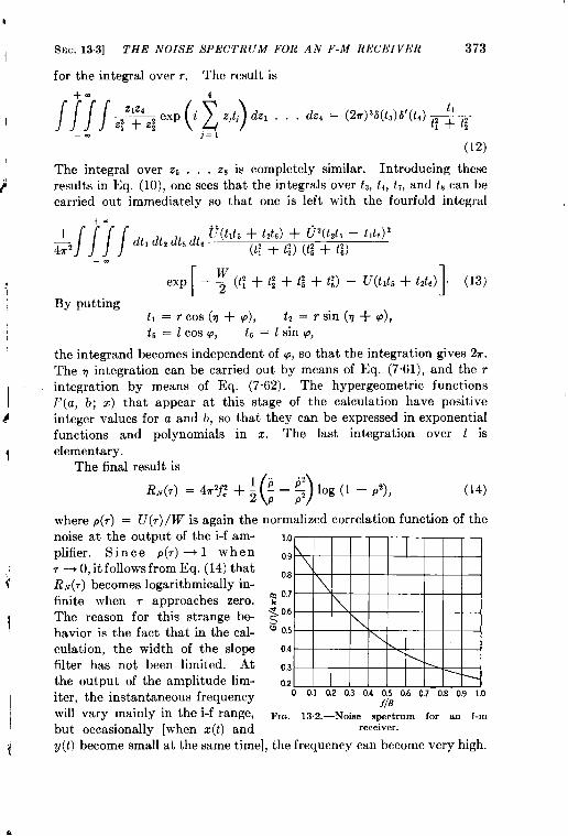
SEC. 13.3] THE NOISE SPECTRIJM FOIL AN F-M RECEIVER 373
fortheintegral overr. The result is
+- 4
////
Zlzd
(z )exp i z)tj dzl . . . dz, = (2r)’6(@’(t,)-tl ---
2; + z; t; + t;—. ;=l
(12)
The integral over Z6 . . . za is completely similar. Introducing theseresults in Eq. (10), one sees that the integrals over h, ti, h, and k can hecarried out immediately so that one is left with the fourfold integral
+-1
////
dtldt, dt, dt, ti(tlt, +t,t,) + v’(t2t5 – tltti)’
G, (t; + W (t; + t;)—.
[
exp — 1g(t;+t;+L%+to–U(tlt, +tzt,) . (13)
By puttingt, =Tcos(q+ q), t2 =rsin(q+ q),tr! = lcos$o, L, = 1 sin q,
the integrand becomes independent of q, so that the integration gives 2m.The q integration can be carried out by means of Eq. (7.61), and the rintegration by means of Eq. (7.62). The hypergeometric function~
~(a, b; z) that appear at this stage of the calculation have positiveinteger values for a and b, so that they can be expressed in exponentialfunctions and polynomials in z. The last integration over 1 is
elementary.The final result is
()RN(T) = 47r’fl + ; : – $ log (1 – P’), (14)
where p(r) = U(7)/W is again the normalized correlation function of thenoise at the output of the i-f am-plifier. Since P(7) ~ 1 when7 ~ (), it follows from Eq. (14) thatli~(,) becomes logarithmically in-finite when r approaches zero.The reason for this strange behavior is the fact that in the cal-culation, the width of the slopefilter has not been limited. Atthe output of the amplitude lim-iter, the instantaneous frequencywill vary mainly in the i-f range,but occasionally [when z(t)and
1.0
0.9
0.8
~ 0.7
~ 0.6>
Q 0.5
0.4
0.3
0.20 0.1 0,2 0,3 0.4 0.5 0.6 0,7 0.8 0.9 10
f/B
Fm. 13.2.—Noise spectrum for an f-mreceiver.
y(t) become small at the same time], the frequency can become very high.
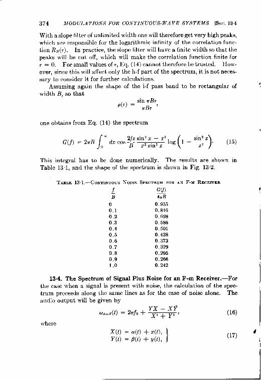
374 MODULATIONS FOR CONTINUOUS- WAVE SYSTEMS [SW. 134
With a slope filter of unlimited width one will therefore get very high peaks,
which are responsible for the logarithmic infinity of the correlation func-tion RN(T). In practice, the slope filter will have a finite width so that thepeaks will be cut off, which will make the correlation function finite for7=0. For small values of,, Eq. (14) cannot therefore be trusted. How-ever, since this will affect only the h-f part of the spectrum, it is not necess-ary to consider it for further calculations.
Assuming again the shape of the i-f pass band to be rectangular of ‘width B, so that
sin 7ri?7p(r) = ~,
one obtains from Eq. (14) the spectrum
/
.C(j) = 27rB
~z Cos xx sin2 x – X2
o B X2 sinz x 10g(l -% ’15)
This integral has to be done numerically. The results are shownTable 13.1, and the shape of the spectrum is shown in Fig. 13”2.
TASLE 13.1.—CONTINUOUS NOISE SPECTRUM FOR AN F-M RECEIVER
J G(f)
B 4TB
o0.10.20.3
0.40.50.60.70.80.91.0
0,9550,816
0.6980.5860,5010,428
0.3730.3290.2950.266
0.242
in
13.4. The Spectrum of Signal Plus Noise for an F-m Receiver.—Forthe case when a signal is present with noise, the calculation of the spec-trum proceeds along the same lines as for the case of noise alone. Theaud~o output will be given by
Yx – XF@s+N(t) = 2m~0 + X2 + Y2 J (16)
where
x(t) = a(t) + z(t),Y(t) = f?(t) + y(t), }
(17) ‘
SEC. 134] THE SPECTRL’M OF SIG,VAL PL~’S NOISE 375
and
a(’)‘soc0s($sin2@)( )1cf.
~(t) = –SO sin ; sm 27rpt
(18)
Here the assumption of a wide i-f pass band has been made, so that thesignal is not deformed by the i-f amplifier and is still represented by Eq.(2) or by
S~(t) = a(t) cos 27rfJ + p(t) sin 27rfrt,
where a(t) and ~(t) are given by Eq. (18).
For the correlation function R.+., (T), one obtains an expression analo-gous to Eq. (7) except that s(t) and y(t) must be replaced by X(t) andY(t); and in addition to the ensemble average, a time average over theinitial time t has to be performed.
The ensemble averages of the second and third terms in the expressionfor l?.+~(,) will not be zero as they were in the case of noise alone. Sincethe joint probability distribution of X(t), Y(t), X(t) and Y(t) is given by
w(x, Y,X, Y) = —[
(x – a)’ + (Y – (3)’~.,;~ ‘=P - 2W
(1 – a)’+ (i – j)’—_2V 11
where V and W have the same meaning as in Eq. (9), it is easily foundthat
(19)
It is clear that the time average of this expression is zero, and therefore,the second and third terms will not contribute to the final result forR,+~(7).
There remains the calculation of the term
Y,xl – X,YI Y,X* – X*Y*x; + Y; X;+Y; ‘
(20)
which is analogous to the fourth term in Eq. (7). The ensemble averagecan be carried out in the same way as in the previous section. Theprobability distribution of Xl, Yl, ~1, YI, Xz, Yz, ~z, Y~ can again befound by the method explained in Sec. 3.7, and the result is similar toEq. (8) except that in the integral the z, have to be replaced by Z, – u,,
376 MODULA TIO,VS FOR CON TIN (’OUS- WA VE SYSTEMS [SEC. 13.4
~vhere the Zj’s denote the eight variables Xl, Yl, Xl, Yl, X2, Y2, ~z, Yz,
and the uI, u2, . . , U8’Sstand for al, PI, til, 61, a~, 82, &Z,~z, respectively.The integrals over Z,, Z,, . , Z, and eve; t,, t,,t,,and t,can be per-formed in exactly the same way as in the case of noise alone, The remain-ing fourfold integral (over tl, tz, t5,and t~) is more complicated than Eq.(13). It is found to be
—.
Since an exact evaluation of this integral does not seem feasible, a fewapmwximations will be made at this stage. It is clear that the first termbetween the braces is proportional to C2and will give rise to the signalpeak in the spectrum of signal plus noise. Therefore, in this term weneglect the U(7) and obtain
+.1 m ..
(it,dt2dts dtti&,82t2t5 + p~tizt,tfi — Ciiciztztc — pJ3~t,t5
h’ (t; + f;)(t: + t:)—.
This integral can be written as a linear combination of products of doubleintegrals. 13ach double integral is of the same form as the one occurringin I~Jq.(11) and can therefore be evaluated easily. Thus, it is found thatthe fourfold integral (22) is equal to
The remaining terms between the braces in 13q. (21) will give rise to thecontinuous noise spectrum. In these terms, therefore, we shall neglectthe modulation of the signal and put
al = a’ = SO, &=/32 =&= ff2=jl= jz=o.
SEC. 13.4] THE SPECTRUM OF SIGNAL PLUS NOISE 377
These terms then reduce to the integral
Substituting in (24),
t, = Rsin 6’COS(q + p), tz = R sin Osin (q + q),ts= R COS8 COSq, tE = R COS6 Sin V,
one sees that the integrations over q and R can he carried out by meansof Eqs. (7.61) and (7.62). The remaining two variables 6 and q are thentransformed into
z = sin 219cos ~, y = sin 26 sin q.
The integration over y is elementary, but the final integration over z canbe reduced only to the integral logarithm Ei(u), defined as
Iu
Ei(u) = : dz,—.
where for positive u, the principle value of the integral has to be taken.The final result for the integral (24) can be written as
R,(7) + R,(7) + ~3(7),
where
‘1(’) ‘$[’ -’-’($+:-’)4)1’ (25a)
.2
R47) = $2
[ =+2’-’(%+:-’)”’(%’)1_ 2e-” (25b)
[
“2 l&Pe-*p _ ‘–:R3(7)=$ ~_p
($+:- N%:)] ‘25’)and z = S~/2W.
The average over the time t affects only Eq. (23). With all theseapproximations, the correlation function for signal plus noise becomes
R,+~(,) = 47r’j: + 27r2c2fi (1 – e-z)z cos 2mPT + ~l(T) + R2(~) + R3(7)(26)
with R,, R2, R3 given by (25). Equation (26) is the analogue of Eq. (3)for the case of frequency modulation. Since for small u
Ei(u)=log u+c+ u+;;+”””,
378 MODULATIONS FOR CONTINUOUS-WA VE SYSTEMS [SEC. 13.4
it is easy to show that for z -0, 2?S+~(r) goes over into RN(T) as given byEq. (14). For large u
( )Ei(u )=: 1+:+:2+””” J
from which it follows that for large z
Rl(T)~– ~:+(p’ +&2+.... (27)
whereas Rz(r) and ~~(~) go to zero for z + cc as exp ( —z) and exp(– 2: ~(1 + p)), respectively, so that they will be negligible comparedwith RI(7) The first two terms in (26) become, of course, for z - cc thecorrelat ion function for the signal alone.
The spectrum Gs+&f) follows from (26) by a numerical integration.Again we have assumed a rectangular i-f pass band of width ~ and havecalculated the spectrum for z = 1.5 and for z = 10. The results arepresected in Tables 13.2 and 13.3 and are shown in Figs. 13.3 and 13.4.
TABLE13.2.—PARTIALSPECTRAANDTOTALCONTINUOUSSPECTRUMOFSIGNALPLUShTOISE FOR Z = 1.5
fB
—
o0.20.30.40,60.8
0.8.51.0
–0.001
0.1080.2360.4050.0810.0370.015
–0.083
–0,001–0,051–o. 106–0.149
0.0210.1300.1660.291
G~ I GS+A4f )4TB 4rB
0.1360,1250.1130.092
0.014–0,071–0,089
0.1340.1820.2430.3480.1160.0960.092
–0.132 0.076
T.ABLE 13.3.—PARTIAL SPECTRA OF SIGNAL PLUS NOISE FOR z = 10
0
0.1
0.20.30.40.5
0.60,70.80.91.0
GI(,f)4mB
o
0.00330,01320.02940.05200.0809 0.0023
0.00270.00280.0025
0.0017
0.0004
G,(f)~ x 103
–0.0013
–0.0034
–0,0078
–0.0112
–0.0108
–0.0070
G,(f)~ x 10’
0.0151
0.0146
0.0138
0.0109
0.0078
0.0043
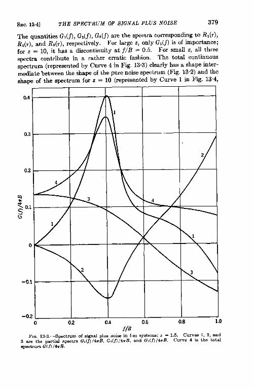
SEC. 13.4] THE SPECTRUM OF SIGNAL PLUS NOISE 379
The quantities Gl(fi, G2(f), Gs(j) are the spctra corresponding to Rl(~),R*(7), and R~(7), respectively. For large z, only Gl(j) is of importance;for z = 10, it has a discontkuity at f/B = 0.5. For small Z, all threespectra contribute in a rather erratic fashion. The total continuousspectrum (represented by Curve 4 in Fig. 13.3) clearly hasa shape inter-medmtebetween the shape of thepure noise spectrum (Fig. 13.2) and theshape of the spectrum for z = 10 (represented by Curve 1 in Fig. 13.4,
I I i I I
0.4
-0.1
-.- u.< I I 1 1 I
o 0.2 0.4 0.6f/B
0.8I,0
FI~. 13.3.—Spectrum of signal Plus noise in f-m systems: z = 1.5. Curves 1, 2, and3 are the partial spectra G1(f)/4TBi G2(fl/4~B, and G~(f)/A~B. curve 4 is the ‘OtalBpectrum G( fl /4uB.
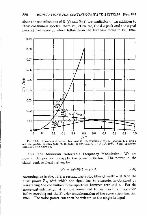
1
1’
380 MOD ULA TIONS FOR CONTINUOUS-WAVE SYSTEMS [SEC. 13.5
since the contributions of Gz ~j) and Gj (f) are negligible). In addition to
these continuous spectra, there are, of course, the d-c peak and the signalpeak at frequency p, which follow from the first two terms in Eq. (26).
0.09
0.08
0,07
0.06
~ 13J35
<~Q 0.04
\#=a
0.03
0s-)2
0.01
0 0.1 0.2. 0.3 0,4 0.5 0.6 0.7 0.8 0.9 1.0f/B
FIG. 13.4.—Spectrum of signal plus noise in f-m systems, z = 10. Curves 1, 2, and 3are the partial spectra G,(f) /4TB, Gz(\) X 103/4mB, G3U) X 103/4n-B. TOtal spectrumcoincides with Curve 1.
13.5. The Minimum Detectable Frequency Modulation. -We arenow in the position to apply the power criterion. The power in thesignal peak is clearly given by
P. = 2r2c2fl(l – e–Z)2. (28)
Assuming, as in Sec. 13.2, a rectangular audio filter of width b s B/2, thenoise power PN, with which the signal has to compete, is obtained byintegrating the continuous noise spectrum between zero and b. For thenumerical calculation, it is more convenient to perform this integrationbefore carrying out the Fourier transformation of the correlation function(26). The noise power can then be written as the single integral
L,
SEC. 13.51 MINIMUM DETECTABLE FREQUENCY MODULATION 381
\
. sin ~
H
“2 I+pe-&P. = 2TB2 dz —n —
o z g2 l–p -=.+’ )
+%’’-’’’+’2’’[’4+”) -E’(9-E’(W1)J(29)
where p(x) = sin z/z and the dots denote differentiations with respect tox. The symbol n = B/2b; in the paper by Crosby, this is referred to asthe deviation ratio.
In order to make a fair comparison between the a-m and the f-msystems, it is better to replace c in Eq. (28) by
(30)
Putting the ratio of P. to PN equal to a constant k, it is then found that
(31a)
TABLE 13.4.—MINIMuM DEmCTABLE MODULATIONFOR A-M AND F-M SYSTEMSFOBDIFFERENT VALUES OF z = ~/2W AND OF n = B/2b
&
z-r
A-m, n = 1 F-m, n = 1 A-m, n = 4 F-m, n = 4
+0 3/8z’ 1/1 .2Z’ 15/128z* l/3.62zS0.1 37.5 83.4 11.7 27.60.2 13.5 20.8 3.89 6.90.3 6.96 9.71 1.97 2.831.5 0.769 0.433 0.199 0.0723.0 0.352 0.124 0.090 0.0118.0 0.125 . . . . . . . 0.031
10 0.10 0.033 0.025 0.00052dw 1/2 1/3z I/& l/192z
which must be compared with Eq. (4). The noise power PN has beencalculated numerically for n = 1 and n = 4 and for different values of z.The corresponding results for (&)J~ are presented in Table 13”4, wherethe values of (&J~~ computed from Eq. (4) are also recorded, and bothare shown in Fig. 13.1. It is clear that for large z, the f-m system isbetter than the a-m system. The factor is 3n2, which can be seen asfollows: For large z, l?,(,) and Its(,) can be neglected in Eq. (26), whereasthe first term in the asymptotic series (27) can be used for l?,(r). This
i
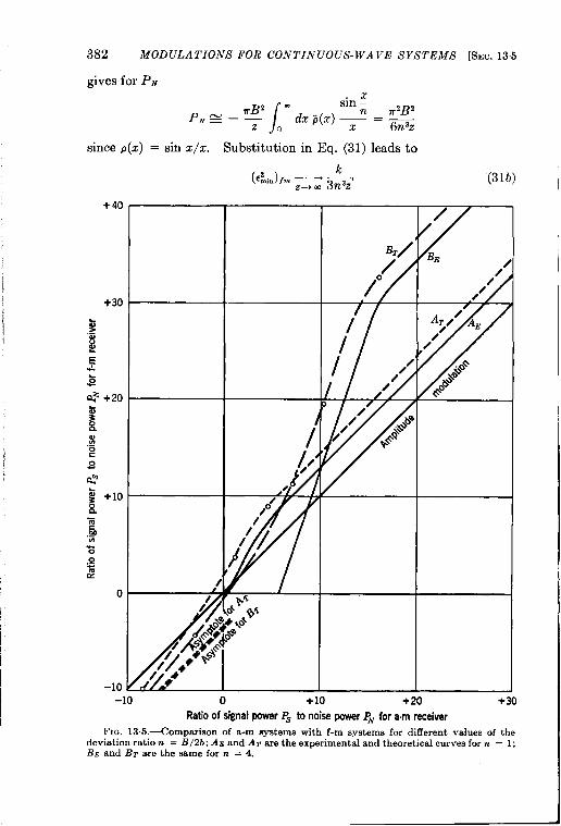
382 MOD ULA TIONS FOR CONTINUOUS-WA Vll SYSTEMS [SEC. 13.5
gives for PA.
/
. sin zP. E–=:
r2B2dx p(X) —n = m
o x
since p(z) = sin x/x. Substitution in Eq. (31) leads to
+40
+30E
.:2 I
(31b)
-lo 0 +10 +20 +30
Ratio of signal power P~ to noise power PN for a.m receiver
FIG. 13.5.—Compariscm of a-m systems with f-m systems for different values of thedeviation ratio n = B/2b; AE and A.r are the experimental and theoretical curves for n = 1;BE and BT are the same for n = 4.
SEC. 13.5] MINIMUM DETECTABLE FREQUENCY MOD ULA TION 383
which has to be compared with Eq. (4c). This shows that for large z,the f-m system is better by the factor 3n2 or by 4.76 db for n = 1 and by16.8 db for n = 4. This is in agreement with the theoretical results ofCrosby.
For small z, the correlation function RN(,) for noise alone can be usedin the calculation of P.v. Since PA will now be only a function of n,it follows from Eq. (3 la) that (~~i.)j~ will become inversely proportionalto z*. The proportionality factor, however, has to be calculated numer-ical~y for the different values of n. Thus, it is found that for z ~ O
which has to be compared with Eq. (4b). For small z, therefore, the a-msystem is better than the f-m system by the factor 2.22 (or 3.46 db) forn = 1 and by the factor 2.36 (or 3.73 db) for n = 4.
TABLE135.-S1GNAkTWNOISERATIOFORF-M AND A-M SYSTEMS FOR DIFFERENTVALUES OF z
z
+*
1031.50.3
+0
Deviation ratio n = 1
Abscissaa-m system
4.541,14
–8.43
Ordinatef-m system
4.76dbabove a-m
“9:083.64
–9.873.46 db
below a-m
Deviation ratio n = 4
Abscicaaa-m system
. . . . . .
15. !3210.457.02
- 2.94., .,..
Ordinatef-m system
16.8dbabove a-m
32.619,611,4
– 4.51
3.72 dbbelow a-m
The results are preeented in another way in Fig. 13.5 (based on Table13.5), where the ratio of the signal power ‘P, to~he noise power P~ forfrequency modulation is plotted against the same ratio for amplitudemodulation. Both abscissa and ordinate are expressed in decibels.The unmodulated signal-t~noise ratio z is (in Fig. 13.5) simply a param-eter. It is clear that the a-m system gives a 45° line. The two dottedcurves, marked A = and B=, are the theoretical curves for the f-m systemfor n = 1 and n = 4. The two solid curves, marked A z and B,, repre-sent the experimental results found by Crosby. 1
1‘‘ Frequency Modulation Noise Characteristics, ” Pmt. IRE, 26, 803 (1937),
Fig. 10.

. ... . . .=
Index
A
Amplitude modulation, s13minimum detectable, 368-369
Amplitude pulsing, 18Antenna, 1Antenna noise, 103-108Antenna temperature, 105Aehby, R. M., 292Attention interval, 233Aural detection, methods of, 252-256Aural perception, 23Average values, 35-39
conditional, 39(See also Ensemble average; Time
average)
B
Bakker, C. J., 69, 94Bandwidth, 176
i-f (see I-f bandwidth)Bell, D. A., 69Bennett, W. R., 151Bernamont, J.j 69, 96Betting curve, 150, 182
calculation of, 171width of, 173
Blind speed, 334Bloch, F., 127Boxcar gene;ator, 28Boxcar spectrum, theoretical derivation
of, 273–278Boxcars, 257
average value, 258peak value, 2.58
c
Carrier, 5, 14Central limit theorem, 46Chaff, 124, 137
6rst probability distribution for, 137frequency spectra for, 138
Chandraeekhar, S., 34, 127Characteristic function, 36Christensen, C. J., 96Clipping factor, 356Clutter, 297-298
exrmimentaltechniquesfor. 132–137gr&nd, 142origin and description of,
Coherent systems, 329Conversion, 10Conversion efficiency, 9Converter, 9Converter noise, 10*1 12Correlation function, 37
normalized, 38Cramer, H., 37Crosby, M. G., 367Cross-modulation, 8Crystal mixers, 109
124-125
Gw interference, 144, 335-340amplitude-modulated by noise, 146frequency-modulated by noise, 147
nOiee-modulated, 353-358Gw signals, 3-17
frequency-modulated, 13-17phaeemodulated, 17
D
Deflection criterion, 161Detectability criteria, 161-165
deflection criteria, 161power criterion, 163
Detection, aural, methods of, 252-256heterodyne, 10meter (see Meter detection)
Detector, 6square-law, 8
E
Electronic interference, 336-366Ellis, H. D. M., 76Emslie, A. G., 166heembl~ #Wmge, 36
385
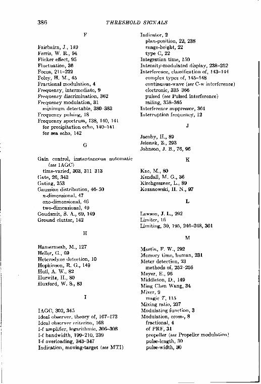
386
F
Fairbairn,J., 149Ferris,W. R., 94Flickereffect,95Fluctuation,36Focus, 211-222Foley, H. M., 45Fractional modulation, 4Frequency, intermediate, 9
THRESHOLD SIGNALS
Indicator, 2plan-position, 22, 238range-height, 22
Frequency discrimination, 362Frequency modulation, 31
minimum detectable, 38&383Frequency pulsing, 18Frequency spectrum, 138, 140, 141
for precipitation echo, 14&141for sea echo, 142
G
Gain control, instantaneous automatic(se. IAGC)
time-varied, 303, 31 1–313Gate, 26, 343Gating, 253Gaussian distribution, 4&50
ndimensional, 47onedimensional, 46two-dimensional, 49
Goudsmit, S. A., 69, 149Ground clutter, 142
H
Hamermesh, M., 127Heller, G,, 69Heterodyne detection, 10Hopkinson, R. G., 149Hull, A. W., 82Hurwitz, H., 80Huxford, W. S., 83
I
IAGC, 31)2, 345Ideal observer, theory of, 167-173Ideal observer criterion, 168I-f amplifier, logarithmic, 30&308I-f bandwidth, 19%210, 239I-f overloading, 343-347Indication, moving-target (see MTI)
type C, 22
Integration time, 150Intensity-modulated display, 238-252Interference, classification of, 143-144
complex types of, 14.$148continuous-wave (see C-w interference)electronic, 33$366pulsed (see Pulsed interference)railing, 35%365
Interference suppressor, 361Interruption frequency, 12
J
Jacoby, H., 89Jelonek, Z., 293Johnson, J. B., 76, 96
K
Kac, M., 80Kendall, M. G., 36Kirchgeszner, L., 89Kozanowski, H. N., 97
L
Lawson, J. L., 292Limiter, 16Limiting, 30, 195, 246-248, 301
M
Martin, F. W., 292Memory time, human, 231Meter detection, 23
methods of, 252–256Meyer, E., 96Middleton, D., 149Ming Chen Wang, 34Mixer, 9
magic T, 115Mixing ratio, 237Modulating function, 3Modulation, cross-, 8
fractional, 4of PRF, 31propeller (see Propeller modulation)pulse-length, 30pulse-width, 30
INDEX 387
I
Modulation index, 14Modulation percentage, 4Mordk, E. B., 64, 76MTI, 324-334
N
Noise, 19, 56amplified r-f, 145antenna, 103-108converter, 108-112cosmic, 103current, 95-97due to discreteness of electronic charge
(see Shot noise)external, 124Fourier analysis of, 152induced grid, 9&95, 122intermediate-f requency, 1~5-122local-oscillator, 112-115mathematical description of, 33–35partition, 91–93primary, 56receiver, 9*1 23thermal, 64
Noise cancellation, 122–123Noise deflection, average, 197-199Noise figure, 100
integrated, 101Noise-modulated continuous-wave inter-
ference, 353–358North, D. O,, 56, 83, 94, 149Nyquist, H., 64, 71, 74
0
Observation time, 150Observer, human, 2Ornstein, L. S., 66, 75Oscillator, local, 9Oscilloscope, linear time-base, 20
type A, 20type B, 21
Overloading, intermediate-frequency,343-347
P
Parameters, system, 193–196Pearson, G. L., 89, 96Phase modulation, 31Phase pulsing, 18Philips, M., 127
Pip, 20Power, available, 99Power criterion, 163Power gain, 99Precipitation echo, 140
first probability distribution for, 140-141
frequency spectra for, 140-141PRF, 18, 244
modulation of, 31Probability distribution, 151-161
conditional, 38first, 34, 137, 140, 141second, 34after second detector, 154
Propeller modulation, 2!3%292, 334Pulse repetition frequency (see PRF)Pulse-shape discrimination, 363Pulse trains, modulated, 257-296
receiving system of, 257–264experimental results in, 264-273indicator for, 263
Pulse-width modulation, 292-296Pulsed interference, 145, 35%366Pulsed signals, 18-32
amplitude pulsing, 18frequency pulsing, 18phase pulsing, 18
Q
Quench frequency, 12
R
Rack, A. J., 83Radio-frequency preelection, 1Ragazzini, J. R., 63Railing interference, 358-365Random process, 33
Gaussian, 53-56purely, 42
Random-walk problem, 50-53two-dimensional, 126
Range marks, 21Rayleigh, J. W. S,, 51Rayleigh distribution, 53Receiver, 1
single-detection, 6superregenerative, 11
Receiver noise, 9%123Receiving area, effective, 104
388 THRESHOLD SIGNALS
Receiv~ system, 1of modulakd pulse trains (see Pulse
trains, modulated, receiving sye-tem of)
Rejection falters, 346Repetition frequency, 222-230
(See alxo PRF)Rice, S. O., 33, 151
s
Saturation, 302Scanning, 24), 241-246scanning factor, 239scanning frequency, 244%hottky, W., 79, 83screen material, 230-232Sea echo, 142
frequency spectrum for, 142Search lighting, 245Shot effect, 79Shot noise, 79
space charge depression of, %89Sidebands, 5, 14Siegert, A. J. F., 124S@d, continuous-wave (see C-w signaIs)
Fourier analysis of, 152minimum detectable, 150
Signal fluctuations, 249-252Signal-modulation threshold, thcxmetical
derivation of, 278-233Signal power, 176-179Signal presentation time, 23&232
human memory time, 231Signal threshold, definition of, 14%151Signals, pulsed (see Pulsed signals)Slope filter, 16Spectrum, 5, 3%42, 151-161
determination of, 157frequency (see Frequency spectrum)of Gaussian noise, 59noise, for f-m receiver, 369-374after nordinear device, 5&63
Spectrum, normalized power, 41power, 40of signal plus noise for f-m receiver,
37&380of strongly clipped noise, 57thermal noise, 64–66, 69-71white, 42
Spenke, E., 69, 83Strobing, 253Subclutter visibility, 328Superheterodyne, 8Sweep direction, 197-199Sweep speed, 209, 211-222, 240System parameters, 193-196
T
Target movement, 24%252Thiede, H., !!6Threshold signal, 185, 192Time average, 35Trace brightneea, 197-199
uUhlenbeck, G. E., 34
v
Van Vleck, J. H., 57, 149Video bandwidth, 211-222, 240Video mixing, 236-237, 243-249
mixing ratio, 237Video overloading, 341-343
w
Weiss, P., 69Wilbur, D. A., 76Williams, F. C., 71, 75, 85Williams, N. H., 82, 83, 97Window, 124
-. 1