thunnus alalunga thunnus alalunga
TRANSCRIPT

AN ABSTRACT OF THE THESIS OF
A. Jason Phillips for the degree of Master of Science in Oceanography presented on November 16, 2011 Title: Long Term Albacore (Thunnus alalunga) Spatio-temporal Association with Environmental Variability in the Northeastern Pacific. Abstract approved: _____________________________________________________________________
Lorenzo Ciannelli
This study investigated long-term (1961-2008) changes in albacore (Thunnus
alalunga) abundance and distribution in relation to local environmental and large-scale
climate indices in the Northeastern Pacific using time series and spatial analyses. Prior to the
time series analysis, a wavelet analysis was conducted to examine nonrandom patterns of
cyclical variability which revealed that monthly and annual time scales had the highest non-
random variability. Thus, the time series analysis was done at these two scales using non-
linear generalized additive models (GAMs) and threshold GAMs. At the monthly scale, sea
surface temperature (SST) was found to be the variable with the strongest (positive)
association to albacore catch per unit effort (CPUE). This association was likely driven by the
seasonal migrations of juvenile albacore into and out of the U.S. coastal waters. At the yearly
time scale over large geographical areas, the SST association broke down, and the scalar wind
speed cubed (an indicator of mixed layer depth) at a five year lag became the dominant
variable. The scalar wind speed cubed index explained 65% of the variability and was highly
significant, even after adjusting for multiple tests (Bonferroni corrected P-value<0.001). These
results suggest that a deeper mixed layer in the Northeastern Pacific may provide favorable

foraging habitat for juvenile (mostly age 3) albacore, resulting in successful growth, spawning,
and recruitment into the fishery in later years. This mixed layer depth association could help
managers and stock assessment groups in their efforts to integrate environmental factors into
the estimate of albacore population size.
The spatial/spatio-temporal analyses involved modeling the CPUE with four
competing GAM formulations, each representative of a different hypotheses for albacore
distribution: 1) spatial, 2) spatial and environmental (SST, PDO, and MEI), 3) spatially
variant, and 4) nonstationary, as indicated by the North Pacific regime shift of 1977. Results
indicate that SST had a predominantly positive but spatially-variable effect on albacore CPUE,
while the PDO had a negative overall effect. Specifically, CPUE was found to increase with
increased SST, particularly off of Oregon and Washington. These results imply that if ocean
temperatures continue to increase, west coast communities reliant on commercial albacore
fisheries are likely to be negatively impacted in the southern areas but positively benefited in
the northern areas, where current albacore landings are highest.

© Copyright by A. Jason Phillips November 16, 2011 All Rights Reserved
Long Term Albacore (Thunnus alalunga) Spatio-temporal Association with
Environmental Variability in the Northeastern Pacific.
by A. Jason Phillips
A THESIS
submitted to
Oregon State University
in partial fulfillment of the requirements for the
degree of
Master of Science
Presented November 16, 2011 Commencement June 2012

Master of Science thesis of A. Jason Phillips presented on November 16, 2011. APPROVED: _____________________________________________________________________ Major Professor, representing Oceanography _____________________________________________________________________ Dean of the College of Earth, Ocean and Atmospheric Sciences _____________________________________________________________________ Dean of the Graduate School I understand that my thesis will become part of the permanent collection of Oregon State University libraries. My signature below authorizes release of my thesis to any reader upon request. _____________________________________________________________________
A. Jason Phillips, Author

ACKNOWLEDGEMENTS
I would like to thank to my committee: Drs. Lorenzo Ciannelli, Bill Pearcy, and Ric
Brodeur for their knowledge, commitment, interest in this work and their efforts to help me
develop as a scientist. Lorenzo thank you for teaching me R, especially GAMs. Learning to
write scripts has forever changed how I analyze data. I hope we can work together in the
future. Ric thanks for paving the way, giving me a chance to work in this field and to grow as
an oceanographer. Bill, thanks for helping me see the big picture when I got bogged down in
the details. Your knowledge of tuna and pretty much anything else in the northeastern Pacific
Ocean is amazing. Thanks Dr. David Myrold for serving as my graduate rep, and taking time
out of your schedule to help me. I would like to thank Oregon Sea Grant for funding this
project, and people at the SWFSC, especially John Childers for sharing the albacore data and
answering questions. I would like to thank JoyDeLee Marrow and other organizers of the
60th tuna conference for giving me a scholarship so that I could attend the meeting. Thanks to
the many people who have helped me with ideas, edits, and statistical analysis Julia Jones,
Dudley Chelton, Peter Gaube, Alix Gitelman, Jeffery Leirness, Ted Strub, Roberto Venegas,
Mike Laurs, Steve Teo, Tom Wainwright, David Pierce, Bobby Ireland, Caren Barcelo, Mac
Barr, Mary Hunsicker, Dongwaha Sohn, Cathleen Vestfals, Paul Lang, Steven Highland, and
many others. Bobby, you were instrumental to me becoming proficient in R, it would have
been very difficult without you around to help. Thanks Lori Heartline and Robert Allan, you
two were always available if I needed to get in touch, and always very helpful.
I would also like to thank my grandparents Nana and Papa for all the support and help.
My life would have turned out very different without your influence. Holley Lantz, you are
the best mother-in-law someone could ask for. Finally thanks to my wife Katie, I definitely
could have not done this without your input, edits, love, and support.

TABLE OF CONTENTS
Page
Chapter 1: Literature review of North Pacific Albacore (Thunnus alalunga). .............. 1
1.1 Introduction to the dominant world tuna fisheries. ................................................ 1
1.2 Pacific Ocean tuna stocks ...................................................................................... 3
1.3 North Pacific albacore background information .................................................... 5
1.3.1 North Pacific albacore biology........................................................................ 5
1.3.2 North Pacific albacore migration and stock structure ..................................... 6
1.3.3 North Pacific albacore fisheries, gear types, and stock status......................... 8
1.3.4 A Brief history of the U.S. Pacific coast fishery ........................................... 10
1.4 Albacore relationships to environmental variability ............................................ 11
1.5 Large scale studies of tuna fisheries in relation to environmental variability. .... 15
1.6 Study objectives and thesis structure ..................................................................... 18
Chapter 2: Temporal effects of climate and regional scale variability on the abundance of albacore in the Northeast Pacific ................................................................. 20
2.1 Abstract ................................................................................................................ 20
2.2 Introduction .......................................................................................................... 22
2.2 Methods ............................................................................................................... 24
2.2.1 Fisheries data ................................................................................................. 24
2.2.2 Environmental data/indices ........................................................................... 25
2.2.3 Wavelet analysis ........................................................................................... 29
2.2.4 Monthly GAM analysis ................................................................................. 33
TABLE OF CONTENTS (Continued)
Page
2.2.5 Yearly GAMs analysis .................................................................................. 36
2.2.6 Yearly age composition analysis ................................................................... 37
2.2.7 Yearly SST threshold GAMs analysis .......................................................... 37
2.3 Results .................................................................................................................. 39
2.3.1 Wavelet analysis ........................................................................................... 39
2.3.2 Monthly GAMs analyses ........................................................................ 41
2.3.3 Yearly aggregated data ............................................................................ 43
2.3.4 Yearly GAMs analysis ............................................................................ 44
2.3.5 Yearly Age composition ......................................................................... 46
2.3.6 Yearly SST threshold GAMs analysis .................................................... 47
2.4 Discussion ............................................................................................................ 49
2.4.1 Wavelet analyses ........................................................................................... 49
2.4.2 Monthly GAM analyses ............................................................................... 50
2.4.3 Yearly Scale ................................................................................................. 52
2.4.4 Research/Management implications and recommendations ......................... 58
Chapter 3: Spatio-temporal associations between albacore CPUE and large-scale environmental variables in the Northeastern pacific. ....................................... 82
3.1 Abstract ................................................................................................................ 82
3.2 Introduction .......................................................................................................... 83
3.3 Material & Methods ............................................................................................. 85
3.3.1 Data ............................................................................................................... 85
3.3.2 Monthly CPUE and SST trends by latitude with MEI .................................. 85
TABLE OF CONTENTS (Continued)
Page
3.3.3 Yearly state-space analysis ........................................................................... 86
3.4 Results .................................................................................................................. 90
3.4.1. Monthly CPUE and SST trends by latitude with MEI ................................. 90
3.4.2 Yearly spatio-temporal analysis .................................................................... 91
3.5 Discussion ............................................................................................................ 93
5 Bibliography ............................................................................................................ 108

LIST OF FIGURES
Figure Page
1. North Pacific albacore catch per unit effort (fish per boat day) yearly average, Catch yearly sums, and Effort yearly sum from 1961-2008 .................................................. 19
2. The U.S. coastal North Pacific albacore fishing study area ..................................... 66
4. Haar wavelet variance output for the North Pacific albacore catch per unit effort (fish per boat day) averaged by month and day from 1961-2008 ................................ 67
3. Box plots of the monthly average CPUE (Fish per boat day) ................................. 68
5. Entire region covariate partial effects on monthly averaged CPUE multiple variable generalized additive model (GAM) with missing CPUE months were converted to 0 CPUE (method one) ..................................................................................................... 69
6. Northern subregion covariate partial effects on monthly averaged CPUE multiple variable generalized additive model (GAM) with missing CPUE months were converted to 0 CPUE (method one) ............................................................................. 70
7. Southren subregion covariate partial effects on monthly averaged CPUE multiple variable generalized additive model (GAM) with missing CPUE months were converted to 0 CPUE (method one) ............................................................................. 71
8. Entire region covariate partial effects on monthly averaged CPUE multiple variable generalized additive model (GAM) reduced to months from July to October (method two) .............................................................................................................................. 72
9. Northern subregion covariate partial effects on monthly averaged CPUE multiple variable generalized additive model (GAM) reduced to months from July to October (method two) ................................................................................................................ 73
10. Southern subregion covariate partial effects on monthly averaged CPUE multiple variable generalized additive model (GAM) reduced to months from July to October (method two) ................................................................................................................ 74
11. Entire region covariate partial effects on yearly averaged CPUE multiple variable generalized additive model (GAM) 1961-2008 ........................................................... 75
12. Northern subregion covariate partial effects on yearly averaged CPUE multiple variable generalized additive model (GAM) 1961-2008 ............................................. 76
LIST OF FIGURES (Continued)
Figure Page
13. Southern subregion covariate partial effects on yearly averaged CPUE multiple variable generalized additive model (GAM) 1961-2008 ............................................. 77
14. Yearly averaged age class structure of North Pacific albacore by catch per unit effort (fish per boat day) from 1961-2004 ................................................................... 78
15. Entire region effect of scalar wind speed cubed lagged 5 years on yearly averaged age-3 CPUE generalized additive model (GAM) 1961-2008 ...................................... 79
16. Linear slope fits of threshold years as determined by threshold generalized additive models for CPUE~SST ................................................................................................ 80
17. Linear fits of yearly (1961-2008) catch vs effort for northern and southern subregions .................................................................................................................... 81
18. Study for spatio-temporal analysis ......................................................................... 97
19. Monthly Sea Surface Temperature vs. CPUE by 1 degree latitude bins from 1961-1984 .............................................................................................................................. 98
20. Monthly Sea Surface Temperature vs. CPUE by 1 degree latitude bins from 1985-2008 .............................................................................................................................. 99
21. Box plots of the 1° latitude monthly averaged log(CPUE+1) (fish per boat day) (1961-2008) by 1°C bins ............................................................................................ 100
22. Effect of position yearly averaged log-transformed albacore catch per unit effort (CPUE) (1961-2008) .................................................................................................. 101
23. Partial effects of (A) position, (B) sea surface temperature (SST), and (C) Pacific Decadal Oscillation (PDO) on yearly averaged log-transformed albacore CPUE (1961-2008) .......................................................................................................................... 102
24. Partial effects of (A) position, (B) sea surface temperature (SST), and (C) Pacific Decadal Oscillation (PDO) on yearly averaged log-transformed albacore CPUE (1961-2008) .......................................................................................................................... 103
25. Partial effects of (A) position overlaid with local sea surface temperature (SST), and (B) Pacific Decadal Oscillation (PDO) on yearly averaged log-transformed albacore CPUE (1961-2008) ...................................................................................... 104
LIST OF FIGURES (Continued)
Figure Page
26. Partial effects of (A) position (1961-2008) overlaid with local sea surface temperature (SST) (1961-1976), (B) SST from (1977-2008), and (C) Pacific Decadal Oscillation (PDO) on yearly averaged log-transformed albacore CPUE (1961-2008) .................................................................................................................................... 105
27. Partial effects of (A) position overlaid with local effects of (PDO), and (B) sea surface temperature (SST) on yearly averaged log-transformed albacore CPUE (1961-2008) .......................................................................................................................... 106
28. Real commercial ex-vessel revenues (2009$) of the albacore fishery in California, Oregon, and Washington, 1981-2009 ........................................................................ 107
LIST OF TABLES
Table Page
1. Signficant (P-value <0.05) Pearson correlations between complete significant (95% confidence spectrum) pairs of variance spectrum between regional CPUE and environmental indices .................................................................................................. 61
2. Method one (null CPUE months converted to 0) monthly averaged (ln(CPUE)~s(Enviromental index)) GAM index model selections sumarized by top 20 ranked models for the entire region and subregions .................................................... 62
3. Method two (July-October) monthly averaged (ln(CPUE)~s(Enviromental index)) GAM index model selections sumarized by top 20 ranked models for the entire region and subregions .............................................................................................................. 63
4. Yearly averaged (CPUE~s(Enviromental index)) GAM index models selections sumarized by the top 20 ranked models for the entire region and subregions ............. 64
5. Pearson correlations between pairs of age 3 and one year lagged age 4 albacore CPUE. Entire region is the U.S. costal troll albacore fishery from 130° E to the U.S. coast, and the subregions are split about 40º N ............................................................ 65

LIST OF APPENDICES
Appendix Page
A. ACRONYMS AND ABBREVIATIONS ....................................................... 120
B. ENVIRONMENTAL INDICES ...................................................................... 121
C. HARR WAVELET .......................................................................................... 124
D. CPUE AND SST TIME SERIES .................................................................... 125
E. DAILY CATCH PER UNIT EFFORT ........................................................... 126
F. WAVELET VARIANCE FOR ENVIRONMENTAL INDICES ................... 132
G. AUTOCORRELATION OF ALBACORE TIME SERIES ............................ 136

1
CHAPTER 1: LITERATURE REVIEW OF NORTH PACIFIC ALBACORE (THUNNUS ALALUNGA).
1.1 Introduction to the dominant world tuna fisheries.
Albacore (Thunnus alalunga) belong to the family Scombridae, which includes
approximately 50 mostly pelagic and commercially exploited species such as tunas,
mackerels, and bonitos (Collette and Nauen 1983). Scombrids have been exploited for
thousands of years, and in the Mediterranean Sea, harvesting dates back to 7000 BC
(Fromentin and Powers 2005). Most tuna are highly migratory, and historically were only
available to the seasonal artisanal fisheries using small vessels (Miyake et al. 2004). In the
early 20th century, however, technological advances (e.g., gas powered engines replaced sails,
availability of inexpensive ice, increased vessel size, and the development of canneries)
coupled with local depletion of coastal aggregations and a greater demand for fish resulted in
the expansion of tuna fisheries to fishing grounds further offshore and multiple days away
from home ports (Miyake 2005; Love 2006).
Distant offshore tuna fisheries expanded over several decades and by the mid 20th
century increasing demand for tuna resulted in the industrialization of tuna fisheries (Miyake
et al. 2004). Several multinational tuna commissions and organizations were subsequently
founded to manage and conserve tuna species in the Pacific, Atlantic, and Indian oceans,
including the Inter-American Tropical Tuna Commission (IATTC) in 1950, the International
Commission for the Conservation of Atlantic Tunas (ICCAT) in 1966, and the Indian Ocean
Tuna Commission (IOTC) in 1982 (Miyake et al. 2004). The cumulative world landings of
tunas have increased from 400,000 metric tons in 1950 to over 4,000,000 metric tons in 1999,
with the bulk of the increase in the Pacific Ocean (Miyake et al. 2004).

2It is believed that many tunas evolved from inshore tropical fish, as some of the more
primitive scombrids remain tropical near shore fishes (Sharp and Pirages 1978; Sund et al.
1981). The more evolved tunas adapted in ways that allowed them to extend their range
horizontally into cooler temperate waters (albacore and bluefin tuna) and/or vertically into
deeper cold waters (e.g. bigeye tuna) (Sharp and Pirages 1978). Therefore, the dominant tuna
species can be divided into tropical (bigeye tuna, yellowfin tuna, and skipjack tuna) and
temperate (bluefin tuna, and albacore) tuna groups (Sharp and Pirages 1978; Collette et al.
2001; Miyake et al. 2004). Sharp and Pirages (1978) concluded that as tuna species adapted to
colder water, they progressively internalized red muscle tissue, allowing them to maintain
tropical red muscle temperatures. Sund et al. (1981) summarized the early life history studies
of Pacific tunas and concluded that warm tropical water is an early life history requirement of
temperate tuna species. This early life history requirement supports Sharp and Pirages (1978)
tuna evolutionary hypothesis based primarily on red muscle internalization. This also explains
why the temperate tuna species have still spawning grounds that are in subtropical warmer
waters.
For the past 50 years seven species have dominated world tuna fisheries (listed in
decreasing order of catch): skipjack tuna (Katsuwonus pelamis), yellowfin tuna (Thunnus
albacares), bigeye tuna (Thunnus obesus), albacore (Thunnus alalunga), Atlantic bluefin tuna
(Thunnus thynnus) combined with Pacific bluefin tuna (Thunnus orientalis), and Southern
bluefin tuna (Thunnus maccoyii) (Miyake et al. 2004; Carocci et al. 2005). With the exception
of skipjack tuna, all the species belong to the genus Thunnus. There are nine species in the
genus Thunnus all of which are commercially exploited, highlighting the commercial
importance of this taxonomic group. Many are in fact considered overfished (Worm et al.
2005; Sibert et al. 2006). Most of the dominant species have circumglobal distributions
3(distributed around the world within a range of latitudes), and de Leiva and Majkowski (2004)
detail the status of twenty-three distinct stocks made up of the seven dominant species. The
stock status is uncertain for several fisheries due to a lack of reliable abundance information,
but approximately half of the tuna stocks had their peak catches before the turn of the 21st
century. These peaks were followed by rapid declines, suggesting that many world tuna stocks
are overfished. The temperate tuna are longer lived and have lower fecundity then tropical
tunas making them more susceptible to overfishing with increased fishing effort (de Leiva and
Majkowski 2005). However, in recent years floating aggregation devices (FADs) have come
into widespread in tropical regions, and could result in overfishing of large schooling tropical
tuna stocks (Fonteneau et al. 2000). Many of the temperate stocks appear to be already
overfished or fully exploited, especially bluefin tuna (de Leiva and Majkowski 2005).
1.2 Pacific Ocean tuna stocks
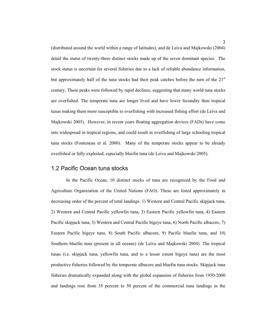
In the Pacific Ocean, 10 distinct stocks of tuna are recognized by the Food and
Agriculture Organization of the United Nations (FAO). These are listed approximately in
decreasing order of the percent of total landings: 1) Western and Central Pacific skipjack tuna,
2) Western and Central Pacific yellowfin tuna, 3) Eastern Pacific yellowfin tuna, 4) Eastern
Pacific skipjack tuna, 5) Western and Central Pacific bigeye tuna, 6) North Pacific albacore, 7)
Eastern Pacific bigeye tuna, 8) South Pacific albacore, 9) Pacific bluefin tuna, and 10)
Southern bluefin tuna (present in all oceans) (de Leiva and Majkowski 2004). The tropical
tunas (i.e. skipjack tuna, yellowfin tuna, and to a lesser extent bigeye tuna) are the most
productive fisheries followed by the temperate albacore and bluefin tuna stocks. Skipjack tuna
fisheries dramatically expanded along with the global expansion of fisheries from 1950-2000
and landings rose from 35 percent to 50 percent of the commercial tuna landings in the

4Pacific. Skipjack is currently third most harvested commercial species in the whole world. The
yellowfin tuna fishery has also expanded, but remains stable at 30 percent of the total tuna
landings. Bigeye tuna fisheries have increased to about 10 percent. Total albacore landings
have not changed significantly since about 1950, resulting in a decrease in percent
composition from about 20 percent to less than 10 percent. Though catches have been highly
variable, Pacific bluefin tuna landings have steadily decreased over the last half century.
Finally, the world catches of Southern bluefin tuna peaked several decades ago and have since
declined to about 20 percent of historical levels (Miyake et al. 2004).
Most tunas in the Pacific Ocean share a similar range from about 40° N to 40° S, but
tend to be restricted to specific geographical and vertical depth strata (Sund et al. 1981;
Collette and Nauen 1983; Sibert et al. 2009 and many others). In the northern latitudes,
juveniles of the North Pacific albacore stock have the most northern population distribution of
the Pacific tunas and they mostly occupy surface waters above the thermocline (Sund et al.
1981; Miyake et al. 2004; Ellis 2008; Laurs and Powers 2010; Childers et al. 2011). The South
Pacific albacore stock ranges from about 40° S to 5° S. Juveniles of the South Pacific
albacore stock are found at the higher southern latitudes, and both stocks of Pacific albacore
reside at lower latitudes (25° S to 25° N) as they mature and spend more time at depth
(Clemens 1961; Sund et al. 1981). The Pacific albacore stocks are separated by warm
equatorial waters where they are essentially absent between 5° S to 10° N (Sund et al. 1981;
Miyake et al. 2004). It appears there is little to no genetic exchange between North and South
Pacific albacore stocks (Sund et al. 1981; Takagi et al. 2007). Pacific bluefin tuna have been
documented as far north as 57° N in the western Pacific and have a similar life history and
geographic range as North Pacific albacore in the western Pacific, but they concentrate in
lower latitudes in the Eastern Pacific (Sund et al. 1981; Marcinek et al. 2001; Miyake et al.

52004). Similar to albacore, juvenile bluefin tuna spend the majority of their time in surface
waters and increase their depth range with age (Sund et al. 1981; Marcinek et al. 2001). The
circumglobal stock of South Pacific bluefin tuna have the most southerly latitudinal
distribution of the Pacific tunas with highest concentrations from 25° S to 50° S. Yellowfin
tuna stocks are the most tropical of the tuna species, followed by skipjack tuna. Yellowfin tuna
and skipjack tuna are primarily found in surface waters above the thermocline (Sund et al.
1981; Marcinek et al. 2001). Collette et al. (2001) placed bigeye tuna in an intermediate
position between the tropical and temperate species, as they range in latitude between the
temperate and tropical tunas and are tolerant of colder waters, spending a significant amount
of time at depth within the tropics.
1.3 North Pacific albacore background information
1.3.1 North Pacific albacore biology
The temperate tunas are the most evolutionally advanced scombrids, and are highly
adapted for long migrations and excursions into temperate waters (Collette 1978). Kishinouye
(1923) first described the countercurrent heat exchange system in tunas that prevents heat loss
through gills (Collette 1978). This unique physiological adaptation allows albacore and other
tunas to maintain high internal temperatures in cold water; internal temperatures 15° C
warmer than ambient waters have been reported (Morrison et al. 1978). Albacore also have
other adaptations to maintain heat, such as specialized internal red muscles surrounded by
white muscle resulting in a passive dissipation of heat from the core body, large heart, large
blood volume, high concentrations of mitochondria within the red muscle tissue, large
complex gill structures, and a ram ventilation method of respiration (Collette 1978;
Hochachka et al. 1978; Roberts 1978; Sharp and Piarages 1978). Essentially, albacore use an
6efficient and highly aerobic metabolism to generate heat in the red muscle tissue while
minimizing heat loss. Albacore have evolutionary advances for swimming fast such as a
fusiform body, bony finlets along caudal peduncle, a rigid high aspect ratio crescent-shaped
tail, foldable dorsal and anal fins with grooves, and rigid pectoral fins. The pectoral fins also
help provide lift as albacore have no swim bladder and are negatively buoyant (Collette 1978).
Albacore physiology is adapted for reduced drag and efficient and powerful swimming at high
speeds, with one exception. They must swim with their mouth open using ram gill ventilation
which increases drag, in order to deliver required high oxygen levels to the muscular system.
Albacore have many other unique physiological and morphological adaptations (e.g., rapid
digestion) to aid in long migrations in order to take advantage of highly abundant seasonal
food sources (Sharp and Pirages 1978).
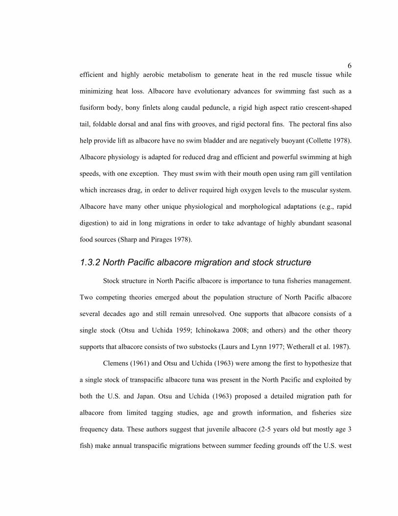
1.3.2 North Pacific albacore migration and stock structure
Stock structure in North Pacific albacore is importance to tuna fisheries management.
Two competing theories emerged about the population structure of North Pacific albacore
several decades ago and still remain unresolved. One supports that albacore consists of a
single stock (Otsu and Uchida 1959; Ichinokawa 2008; and others) and the other theory
supports that albacore consists of two substocks (Laurs and Lynn 1977; Wetherall et al. 1987).
Clemens (1961) and Otsu and Uchida (1963) were among the first to hypothesize that
a single stock of transpacific albacore tuna was present in the North Pacific and exploited by
both the U.S. and Japan. Otsu and Uchida (1963) proposed a detailed migration path for
albacore from limited tagging studies, age and growth information, and fisheries size
frequency data. These authors suggest that juvenile albacore (2-5 years old but mostly age 3
fish) make annual transpacific migrations between summer feeding grounds off the U.S. west

7coast and the western Pacific off of Japan. Additional tagging studies and fisheries data have
revealed that at least a portion of juvenile albacore (approximately age 2-5) make transpacific
migrations and become less migratory with age (Laurs and Lynn 1977; Laurs 1979; Sund et al.
1981). As the albacore become reproductively active (age 5 +), they cease transpacific
migrations, and move south into subtropical waters in the western Pacific during the summer
to spawn (Otsu and Uchida 1963). Little is known about the distribution of juvenile albacore
before they enter the fishery, but young albacore (age 1) have been found to occupy the
Japanese coastal waters and are occasionally captured in the U.S. coastal fisheries (Nakamura
1969). Spawning is believed to occur in warm waters over 24° C centered at about 20° N,
primarily in the western Pacific in the summer months; however, there is also evidence of
winter spawning off of Mexico in some years (Otsu and Uchida 1959; Sund et al. 1981;
Wetherall et al. 1987).
In contrast to the single stock hypothesis Laurs and Lynn (1977) concluded that there
are two subpopulations of the North Pacific albacore stocks which diverge at approximately
40° N. They based this theory on U.S. tagging studies, back-calculated spawn dates (Wetherall
et al. 1987), length frequency information, and albacore commercial landings data.
Additionally, based on limited data analysis of artificial radioactive isotopes (Zinc-65,
Maganese-54, and Cobalt-60) in albacore liver tissue, albacore did not appear to mix between
northern and southern subregions within a given year (Pearcy and Osterberg 1968;Kygier and
Pearcy 1977). One subgroup is thought to be more southerly distributed, to be larger-bodied,
to undertake shorter migrations, and to spawn in the eastern Pacific during winter. The second
subgroup is believed to be a smaller-bodied, more transient, northern group that spawns during
the summer in the western Pacific. In more recent years, researchers have found conflicting
evidence on the nature of the North Pacific albacore stock structure and so the issue still

8remains unresolved (reviewed by Barr 2009). For example, Ichinokawa et al. (2008) modeled
tagging data from Japan and the U.S. studies (1971–1986), and concluded that North Pacific
albacore followed a migratory pattern similar to the one outlined in Otsu and Uchida (1963).
Barr (2009) found that two subgroups of albacore in the North Pacific were present based on
long-term U.S. west coast landings data, but was unable to determine if the subgroups
represented distinct stocks. Childers et al. (2011) found that 20 archival-tagged North Pacific
albacore exhibited five seasonal migratory patterns with a broad range of behaviors ranging
from overwintering off of Baja to a transpacific migration over the winter. Presently, North
Pacific albacore are managed as a single stock (Crone et al. 2006).
1.3.3 North Pacific albacore fisheries, gear types, and stock status
North Pacific albacore account for almost half of all albacore landings worldwide
(Laurs 2010). They are harvested by several countries, but Japan and the U.S. have landed
over 90 percent of the fish captured since the 1950s (Childers and Aalbers 2006). Pelagic
longline, pole-and-line (bait boat), and troll are the three main gear types used to harvest
albacore in the North Pacific.
The pelagic longline fisheries target older fish and occur primarily in the western and
central Pacific and account for 37.5 percent of the North Pacific albacore catch. The pole-and-
line fisheries targeting juvenile albacore occur in the eastern and western Pacific and account
for about 37 percent of total catch; however, juveniles are mainly captured in the eastern
Pacific. A troll fishery dominated by the U.S. and Canada occurs in the Northeastern Pacific
and accounts for about 20 percent of all landings (Laurs 2011). The U.S. North Pacific
albacore troll fishery make up about 15 percent of all North Pacific landings (Childers and

9Betcher 2010), and 6 percent of the world albacore landings. The U.S. west coast ex-vessel
revenue averaged $15.3 million from 1981 to 2007 (PFMC 2008).
The most recent North Pacific albacore stock assessment suggests that the fishery is
being harvested at sustainable levels (Crone et al. 2006). However, others suggest that the
fishery is approaching capacity or may be slightly overfished (de Leiva and Majkowski 2005;
Stocker 2005; Laurs 2010). Albacore is one of the last open access (i.e., no limit on the
number of participants) fisheries remaining off the west coast of North America and anyone
can purchase a permit. The fishery has an established control date of March 9, 2000. This date
is a qualifying criteria to limit participation into the fishery should it become limited (Laurs
2010). For example, if a vessel entered the fishery in June of 2000, and the fishery then
became limited access, they would be excluded from the fishery. However, if the same vessel
began fishing in January of 2000, they would be permitted to continue.
The closely related Atlantic bluefin tuna, which have been heavily overfished and
likely have underreported landings, provides a cautionary example of what can happen once a
multinational fishery becomes depleted (Fromentin and Powers 2005). A combination of
factors have resulted North Pacific albacore being less economically profitable than other tuna
species, which might explain why albacore stocks have not yet declined like the closely
related bluefin tuna species and some stocks of tropical tunas. Albacore have a shorter life
span than bluefin tuna (Collettet and Nauen 1983), lack of easy-to-catch large aggregations
like some of the tropical tunas (Dempster and Taquet 2004), and lower commercial value than
most other tuna (Majkowski 2005). However, North Pacific albacore still have longer life
spans compared to the tropical tunas, and lower fecundity, making them more susceptible to
overfishing if effort increases. In recent years several important commercial fisheries (many
groundfish species and salmonids) have restricted access or closures in the Northeastern
10Pacific due to their declining status (Berkeley et al. 2004; PFMC 2006; Ireland 2011). It is
possible that this reduction could leave vessels that participated in multiple fisheries little
choice but to increase albacore fishing effort and albacore catch in the eastern Pacific. In fact,
fishing effort at latitudes greater than 40° N increased to an all time high in 2006-2007 (Fig.
1).
1.3.4 A Brief history of the U.S. Pacific coast fishery
In the North Pacific, active commercial fisheries for juvenile albacore have persisted
for over a century. Prior to 1904, North Pacific albacore were considered a “trash” or nuisance
fish (Clemens 1961). This may have been partially due to the difficulties of transporting a
fresh product to market as gas powered boats were not widely used and ice was not readily
accessible, making it difficult to get fresh product to market (Love 2006). Subsequently, in
1903, Halfhill a plant packing operator in San Pedro California, initiated canning and
marketing tuna following a crash in the sardine fishery. This prompted, in part, the beginning
of the U.S. west coast tuna fishing industry (Clemens 1961). By 1915 most boats were gas
powered and about 20 million pounds were landed annually. However, at that point most of
the boats were still small, and the fishery was mostly near shore off southern California. In
1926 the landings dropped to 2.5 million pounds, and for the next seven years (1928-1934) the
fishery was almost a complete failure with landings averaging just over 230,000 pounds a
year. The worst year on record was 1933 when less than 500 pounds were landed in California
waters (Clemens and Craig 1965). It has been suggested that overfishing lead to a local
depletion which resulted in the crash in the late 1920s (Brock 1943). However, the near failure
may have been environmentally driven by high sea surface temperature (SST) and/or ENSO
events, which resulted in a more northern distribution of the albacore (Clemens and Craig

111965). The low coastal catches of albacore in the late 1920s prompted the construction of
larger boats and a geographic expansion of the fleet that switched to skipjack tuna and
yellowfin tuna (Clemens and Craig 1965). In August 1936, albacore were landed in large
enough numbers to start a commercial fishery in Oregon (Clemens and Craig 1965; Brock
1943). A commercial fishery began in Washington in 1937, British Columbia in 1939, and
Alaska reported it’s first commercial landings in 1940 (Clemens and Craig 1965).
Among the U.S. coastal albacore fisheries, the pole-and-line fishery has been sporadic
while the troll fishery has remained somewhat constant over several decades with a few
exceptions (Barr 2009; Laurs 2010). For example, in the mid 1980s, global market economics
resulted in the closure of many California canneries, and at the same time Mexico excluded
bait boats from its waters (Love 2006; Laurs 2010). The commercial albacore landings in the
Southern California region were greatly reduced at this time and have not yet recovered.
Northeastern Pacific albacore catch data has been recorded since at least 1904, when
about 150,000 pounds of albacore were landed (Wilcox 1907). Clemens (1961) constructed
Catch-Per-Unit-Effort CPUE (fish per boat month) from California landings from 1930 to
1960. Logbooks of albacore catch information began on a volunteer basis in 1954 (Laurs et al.
1975). In the mid 20th century standardized CPUE (fish per boat day) and geographical catch
location came into widespread use (Childers and Betcher 2010).
1.4 Albacore relationships to environmental variability
Tuna are believed to be sensitive to ocean temperature. Commercial fishermen and
researchers have long acknowledged that juvenile North Pacific albacore are most abundant in
waters with SST ranging from 15–19.5° C (Clemens 1961; Flittner 1963; Laurs et al. 1977;
Childers et al. 2011). By the mid 1900s North Pacific albacore fishermen had coined the term
12“tuna waters” to represent pelagic waters with SST at or above 14.4° C (58° F) as potential
fishing grounds for albacore (Alverson 1961). Lab experiments indicate that false albacore
(Euthynnus affinis) are able to perceive temperature changes as small as 0.15° C (Steffel et al.
1976). Also, Boyce et al. (2008) found evidence that ambient temperature can be used to
predict global tuna species richness from 190 published studies on ambient water temperature
modeled to predict global richness patterns for 18 species of tuna and billfish. Most recently
Childers et al. (2011) found North Pacific archival tagged albacore occupied an average SST
of 17.6 ± 0.9° C with a range in SST from 11.9-22.3° C. Including vertical movements, the
tagged albacore experienced water temperature ranges from 3.3-22.7° C (Childers et al. 2011).
Although albacore can occupy a wide range of temperatures for short periods of time, the
tagged fish preferred temperatures around 17.5° C.
In addition to SST, other oceanic features such as sea color (indicative of
phytoplankton biomass and species distribution), frontal regions, chlorophyll hotspots such as
the Transition Zone Chlorophyll Front, and areas of abundant prey have also been found to be
important factors related to albacore abundance at relatively fine spatial or temporal scales
(Alverson 1961; Clemens 1961; Pearcy and Mueller 1970; Laurs and Lynn 1977; Laurs et al.
1984; Zainuddin et al. 2008; Glasser 2010; Childers et al. 2011 and others). Juvenile albacore
in the northern part of the U.S. coastal waters spend the majority of their time in warmer
surface waters, making short day-long excursions into colder water (Childers et al. 2011). The
most likely explanation for this behavior is that albacore take advantage of the rich
heterogeneous environment in the Northeastern Pacific, making short vertical dives into colder
water to forage (Childers et al. 2011). Interestingly, Childers et al. (2011) also showed that
albacore change behavior in areas with deeper mixed layers and lower productivity, spending
more time at depth during the day.
13There is historical evidence that albacore availability to the coastal fisheries was
regulated by environmental variability in the late 1920s and again in the late 1930s. The near
failure of the albacore fishery off of California in the late 1920s has been primarily attributed
to local depletion, while the larger commercial landings during the late 1930s have been
attributed to the development of larger vessels capable of longer trips (Brock 1943; Love
2006). Scarce albacore catch in California waters may have led to the development and
expansion of a northern fishery off Oregon and Washington. However, environmental
variability likely played an important role, and the fishery failure may have been due to fewer
fish in the area, in addition to or rather than local depletion (Clemens 1961).
Prior to the poor catches starting in 1926, total California albacore landings (1916-
1925) averaged 17.4 million pounds yearly, which was a much lower average than after the
fishery was industrialized, when California yearly (1948–1961) catches averaged 37 million
pounds. The albacore fishery from 1916–1925 was composed of about 300 small vessels
equipped for day trips (Clemens 1961). Given that many albacore were likely offshore beyond
the reach of a limited coastal fleet in the earlier years, and that the fishery rebounds in later
years, environmental variability offers a better explanation for the near failure, as opposed to
fishery depletion. Specifically, the low catches of 1926, an El Niño year, coincided with the
highest Pacific Decadal Oscillation index (PDO) on record since the albacore fishery started in
1904. The PDO was in a cool phase from 1900-1924 before transitioning to the warm phase
which lasted from 1925-1946. Additionally, in August 1926 two salmon troll vessels captured
albacore near shore off of southern Oregon – this was the first documented record of albacore
north of California. Other evidence to suggest that 1926 was anomalous due to a warm event
typical of El Niño’s was the fact that other more southerly fish such as ocean sunfish (Mola
mola) were also encountered near shore in Oregon waters (Hubbs and Schultz 1926). In 1926,

14the fleet off of Oregon was not well equipped to fish for albacore. Salmon trolling fishermen
did not know that the name of the species they had captured was albacore until later identified
by scientists (Hubbs and Schultz 1926). Clemens (1961) pointed out that albacore responded
quickly to increased temperature occurring north of Point Conception in 1926, but were slow
to respond to cooling temperatures in later years.
It was not until August 1936 that albacore were landed in large enough numbers to
start a commercial fishery outside of California (Brock 1943; Clemens and Craig 1965). Again
this coincided with an highly positive PDO value, but in contrast to the warm event of 1926, a
commercial fleet capable of catching tuna farther offshore was in place. Thus, significant
numbers of albacore were landed off of Oregon and Washington from 1936–1940 ranging
from 11,000 pounds to over 14,000,000 pounds. In 1938 and 1940, the Oregon and
Washington landings combined were about 10,000,000 pounds more than the California
landings. Again this occurred during a warm phase of the PDO, when the index was higher
than in 1926. The fleet had dramatically changed between 1926 and 1936 making comparisons
between decades qualitative, as the commercial landings were not adjusted for effort. Still, the
start of the albacore fishery in Oregon and Washington corresponded to the warmest phase of
the PDO since inception of the fisheries at the beginning of the 1900s. Albacore catches taken
north San Francisco decreased steadily until the mid 1950s and rebounded again afterwards
which was found to correspond with tree growth and showed a link of albacore with large
scale atmospheric flow patterns (Clark et al. 1975). From the mid 1980’s to present, almost all
of the fishing effort for albacore has shifted north of 40° N roughly coinciding with warm
phases of the PDO. However, the more recent northern shift in effort has been primarily
attributed to economic stress in that canneries moved out of the U.S. due to global market
competition between 1982-1984 (Love et al. 2006).
151.5 Large scale studies of tuna fisheries in relation to environmental variability.
Studies that analyze large-scale changes in marine fish population in relation to
environmental variability have become more common in recent years. This is, in part, due to
the fact that accurate record keeping of many stocks has been in place long enough now to
allow time series analysis on the order of decades. Additionally, technological advances such
as remote sensing, faster computers, and more advanced statistical programs available to a
wide pool of users have allowed researchers to investigate more complex research questions.
Fish population response to changes in the marine environment over time is a common
research topic.
In recent years many authors have investigated time series of tuna landings data
spanning several decades (Beamish et al. 1999; Ravier and Formentin 2001; Perry et al. 2005
and others). Most commercial tuna data sets started around the mid 20th century and for the
most part contemporary studies are limited to data collected from 1960 to present (e.g. Chen et
al. 2005; Corbineau et al. 2008 and many others). In an extreme example, Ravier and
Fromentin (2001) studied four centuries (1550-1950) of eastern Atlantic and Mediterranean
bluefin tuna landing records, and concluded that bluefin tuna population oscillated on cycles
of 120-100, 20, and 1 year scales. Many of the large-scale studies also document strong
relationships between tunas and SST or other surface related indices. Andrade (2003) found a
strong relationship between Atlantic skipjack and seasonal temperatures. Lu et al. (2001)
analyzed decades of yellowfin tuna and bigeye tuna catches in relation to ENSO and
concluded that both species responded to changes in SST and ENSO events. Lehodey et al.
(2003) modeled several decades of Pacific tuna catches and found increased recruitment for
tropical tunas in the presence of El Niño events and decreased recruitment for albacore.

16Dufour et al (2010) investigated several decades of North Atlantic albacore and Atlantic
bluefin tuna arrival time to summer feeding ground and found that they arrive eight days
(albacore) and 14 days (bluefin tuna) earlier than several decades ago. Boyce et al. (2008)
conducted a meta-analysis on 18 species of tuna in relation to temperature and found evidence
of SST temperature tolerances that could be used to predict species richness on a global scale.
However, not all studies found tuna distribution related to environmental variability. Anda-
Montanex et al. (2004) investigated yellowfin tuna catch in response to anomalously high/low
SST during El Niño and La Niña events in the eastern tropical Pacific, finding weak evidence
of SST related to local CPUE, and speculated that primary productivity was more important
than temperature in regulating catch.
Large scale and long term albacore studies have revealed that all albacore stocks may
be influenced by SST features and other indices at the population scale. Lu et al. (1998) found
an eight year lagged ENSO was associated with poor adult South Pacific albacore catch and
attributed the reduced catch to poor recruitment during ENSO events. Lehodey et al. (2003)
also determined that El Niño events decreased recruitment for Pacific albacore. Chen et al.
(2005) found that SST explained almost all of the variability (partial R2=34%) of Indian
Ocean juvenile albacore concentrations with a stepwise discriminant analysis that also
included surface salinity (partial R2=4%), and chlorophyll (partial R2=1.5%). Sagarminaga and
Arrizabalaga (2010), using generalized additive models (GAMs), found North Atlantic
juvenile albacore had a close spatio-temporal relationship with SST between 16–18° C over a
twenty-year span. Glasser et al. (2011) investigated the autocorrelation of the North Pacific
U.S. coastal fisheries data, and concluded that North Pacific albacore CPUE is primarily
driven by a few key variables, such as SST, chlorophyll a, and prey availability. Barr (2009)
found some evidence of fishery shifts related to El Niño events, although the pattern was not

17consistent. Despite evidence that North Pacific albacore populations respond to long-term
large-scale surface oceanographic features there is a research gap in the understanding of
major variations in distribution of albacore catches related to large-scale changes in the ocean
environment. A better understanding albacore distributions under different ocean conditions
will likely provide useful information to help manage the fishery.
181.6 STUDY OBJECTIVES AND THESIS STRUCTURE
The overarching goal of this thesis is to improve our knowledge base and management
strategies of North Pacific albacore by elucidating the associations between long-term and
large-scale juvenile albacore abundance and environmental variability. Specifically, my
objectives are to: 1) determine on what time scales albacore population abundance varies, 2)
explore temporal albacore CPUE at the scale determined in objective 1, in relation to regional
and large-scale environmental variability, and 3) study long-term spatial dynamics in relation
to climate and regional indices indicative of the thermal regime in the subtropical and
temperate waters in the north Pacific. In other words, the second chapter addresses the
frequency at which albacore populations oscillate, and then investigates relationships with
environmental variability at the most variable scales. The third chapter explores the spatial
distribution of albacore over time.

19
0
50
100
150
Yearly albacore Catch Per Unit Effort CPUE (number of fish per boat day) averages from 1961-2008
Entire region
North regionSouth region
CP
UE
(n
o. o
f fi
sh
pe
r b
oa
t d
ay
)
1961 1963 1965 1967 1969 1971 1973 1975 1977 1979 1981 1983 1985 1987 1989 1991 1993 1995 1997 1999 2001 2003 2005 2007
Yearly sums of albacore catch (no. of fish) from 1961-2008
Entire regionNorth regionSouth region
Ca
tch
(1
00
,00
0's
of
alb
ac
ore
)
0
2
4
6
8
10
12
1961 1963 1965 1967 1969 1971 1973 1975 1977 1979 1981 1983 1985 1987 1989 1991 1993 1995 1997 1999 2001 2003 2005 2007
2000
4000
6000
8000
Yearly sum of albacore fishing effort (no. of boat days) from 1961-2008
Entire regionNorth regionSouth region
Fis
hin
g e
ffo
rt (
no
. of
bo
at
da
ys
)
1961 1963 1965 1967 1969 1971 1973 1975 1977 1979 1981 1983 1985 1987 1989 1991 1993 1995 1997 1999 2001 2003 2005 2007 Figure 1. North Pacific albacore catch per unit effort (fish per boat day) yearly average, Catch yearly sums, and Effort yearly sum from 1961-2008. Entire region is 130° E to the U.S. coast, North region is >40° N within the study area, and south region is <40° N within the study area.
20CHAPTER 2: TEMPORAL EFFECTS OF CLIMATE AND REGIONAL SCALE VARIABILITY ON THE ABUNDANCE OF ALBACORE IN THE NORTHEAST PACIFIC
2.1 Abstract
This work examined the juvenile commercial troll fishery of the North Pacific
albacore (Thunnus alalunga) stock in relation to 10 environmental indices indicative of the
thermal regime of the subtropical and temperate waters in the North Pacific, within the U.S.
coastal fishery grounds (130º W to the U.S. coast). Two subregions, split about 40 º N, were
considered because the stock status of North Pacific albacore is not fully resolved. Daily and
monthly frequency analyses (Harr wavelet transform) were conducted on the catch-per-unit-
effort (CPUE) of the coastal albacore fishery logbook data from 1961-2008 U.S. to determine
at which time scales the CPUE data should be aggregated and to determine if the CPUE and
environmental variables cycled on the same scales.
Variability in albacore abundance was found to be significantly different than a
random pattern around the monthly scale and peaked near the yearly scale, before it dropped
off. A correlation analysis indicated moderate to strong relationships between the CPUE and
environmental indices, particularly with regional indices derived from the International
Comprehensive Ocean-Atmosphere Data Set (ICOADS). The results from the wavelet
analysis guided me to conduct a time series analysis at the monthly and yearly time scales.
For the monthly and yearly analyses, non-linear generalized additive models (GAMs)
were used and ranked by generalized cross validation (GCV). At the monthly scale, sea
surface temperature (SST) was found to be the variable with the strongest (positive)
association to albacore CPUE. This association appears to be driven by the seasonal
migrations of juvenile albacore into and out of the U.S. coastal waters, which is well known

21and has been documented in many studies. However, once months with little to no catch were
removed from the monthly time series, very little association was found between CPUE and
SST or any other tested indices. This indicated that monthly albacore CPUEs are highly
variable within the fishing season and do not appear to be related to the environmental indices
tested at the monthly temporal sub/region spatial scales.
At the yearly time scale, the positive SST association breaks down, and the scalar
wind cubed (an indicator of mixed layer depth) with a five year lag became the dominant
variable with a positive association to CPUE. The five year lagged scalar wind speed cubed
index explained 65% of the variability in catch for the entire region. This association remains
significant after correcting for multiple models using a Bonferroni corrected P-value=0.00001.
Biologically, it is possible that the scalar wind speed cubed provides favorable habitat for age
three albacore, priming them to have a successful recruitment event when they mature at age
5, which results in a strong returning juvenile age 3 year class.
This newly found mixed depth association may be useful to fishery managers.
Specifically, the results from this analysis could help managers and stock assessment scientists
in their efforts to integrate environmental factors into the estimate of albacore population size.

22
2.2 Introduction
Albacore (Thunnus alalunga) is an economically important temperate tuna species
with circumglobal distributions and several genetically distinct stocks occurring in the
Atlantic, Indian and Pacific oceans (Miyake et al. 2004). In the Pacific Ocean, two stocks
split approximately at the equator are presently recognized, and this work investigates
juveniles (2-5 years old) of the North Pacific albacore stock. Juvenile North Pacific albacore
occur through much of the temperate waters of the North Pacific and undergo zonal feeding
migrations across the entire basin. Sea surface temperature (SST), oceanic features such as
sea color, the warm side of fronts, chlorophyll hotspots, the transition zone, and areas of
abundant prey have been found to be important indicators of albacore abundance at relatively
fine temporal scales (Alverson 1961; Clemens 1961; Pearcy and Mueller 1970; Laurs and
Lynn 1977; Laurs et al. 1984; Zainuddin et al. 2008; Glasser 2010; Childers et al. 2011).
Many researchers have found that tuna are influenced by large-scale climate indices,
(see 1.5). Barr (2009) found some evidence that juvenile troll fishery shifts in response to El
Niño events. However, a lack of knowledge exists about North Pacific albacore abundances
in relation to environmental variability at large spatial and temporal scales. Thus, the focus of
this chapter was to determine associations between albacore abundance and environmental
variability at large spatial scales over a time span of approximately 50 years. Specifically,
wavelets, Generalized Additive Models (GAMs), and threshold GAMs (tGAMs) were used to
explore U.S. coastal (130° W to the U.S. coast) albacore troll fishery catch-per-unit-effort
(CPUE) associations with 10 environmental indices indicative of the thermal regime of the
subtropical and temperate waters. Additionally, because the stock status of North Pacific
albacore is not fully resolved, two subregions were also tested.

23In working with time series data a major issue is deciding on what scale to aggregate
the data at (Levin 1992). Time series data inherently has variability on several scales. For
example SST in the North Pacific oscillates at daily, seasonally, interannually 2-7 year (El
Niño), and interdecadally 20-30 year (PDO) cycles (Mantua et al. 1997; Wolter and Timlin
1998). Often researchers select a few common, but somewhat arbitrary time periods (e.g.
weekly) to investigate. This simplistic approach can work with shorter time series, but as high-
resolution time series become longer, selecting an appropriate time period to aggregate the
data becomes more problematic. A great deal of time can be invested exploring multiple
temporal scales, especially when many potential explanatory variables with lags are involved.
Studying process at different time scales should be thought of as investigating different
research questions, because associations can change with scale and patterns that emerge at one
scale can reverse or degrade at another. The worst case situation that can occur is when a
reversal in direction of an association changes from data in several groups being combined,
also known as Simpson’s Paradox (Blyth 1972). To avoid these potential pitfalls, in
examining potential effects of environmental variables on albacore CPUE, it was necessary to
determine at what temporal scales non-random albacore variance was the highest. This was
accomplished by performing a wavelet analysis on the entire time series of daily catches of
albacore tuna in our study region.
24
2.2 Methods
2.2.1 Fisheries data
Commercial North Pacific albacore logbook data were provided by the National
Oceanic and Atmospheric Administration (NOAA) Southwest Fisheries Science Center
(SWFSC) in a text format and used to create a Microsoft Access database. The main data set
included records from both the troll and bait (also referred to as the pole-and-line or live-bait)
fisheries. The grain1 size provided by the SWFSC was one degree resolution for catch
(number of fish) and effort (boat day) by day. The extent of this data set is 110°W westward to
166°E and 23° N to 57° N from a time period spanning from 1961-2008. This catch and effort
data was used to calculate CPUE (catch per unit effort in units of number of fish/boat day)
over several scales. For example, yearly CPUE for a specific region was calculated by
averaging all of the daily CPUE cells for one year within a defined geographical region (Fig.
2).
The geographical range of this study was restricted to the U.S. West Coast albacore
fishery (Fig. 2). This coastal fishery area is defined as eastward of 130° W to the U.S and
north of 20° N, referred hereafter as the entire region. This region is slightly larger than the
U.S. West Coast Exclusive Economic Zone (EEZ), and represents the summer feeding
grounds of juvenile North Pacific albacore. Previous work has established this area to
represent the majority (99%) of the recorded U.S. catches, and determined that 130oW was a
breakpoint between nearshore and offshore albacore regions (Laurs and Lynn 1977; Powers et
al. 2007; Barr 2009; Laurs and Powers 2010). Subregions were simultaneously analyzed at
1 Grain is the resolution of the set of observations, or the smallest distance (in time and space) between adjacent pairs of observations.
25the latitudinal split north and south of 40° N within the entire region, because of the possibility
that two albacore subpopulations split approximately along the 40° N line (Barr 2009; Laurs
and Powers 2010), hereafter referred as the northern and southern subregions (Fig. 2).
This study further restricted the albacore logbook catch to the troll fishery by
excluding the bait fishery data for the following reasons: 1) the CPUE standardization between
the bait and troll fisheries was problematic because of a lack of spatio-temporal overlap, 2) the
bait fishery had a discontinuous time series which was likely influenced by the U.S. bait fish
exclusion from Mexican waters in the late 1980’s (Laurs and Powers 2010), and 3) the troll
fishery composed the vast majority (>85%) of the dataset (Barr 2009).
Catch size composition, based on standard length (SL) measurements, was also
obtained from the SWFSC database for bait boat and troll fisheries over the time span of
1961-2004. Size composition was summarized in two large geographic areas split along the
40° N latitude and east of 130° W longitude at a monthly time scale. Finer scale data were
available for the entire time series; it was reported, however, to have an error rate of
approximately 50% (J. Childers, NOAA Fisheries, SWFSC, Fisheries Resources Division,
8604 La Jolla Shores Drive, La Jolla, California 92037 pers. comm., 2008). Higher resolution
one degree daily size composition data for the time span of 1990-2000 was available, but not
used because this study focused on analyzing longer time spans.
2.2.2 Environmental data/indices
To explore potential sources of variability in albacore abundance related to the
environment, five regional environmental variables and five large scale climate indices were
selected. Albacore are a surface pelagic species with warm water preferences, therefore the
environmental variables selected were related to thermal and surface features (Clemens 1961;

26Flittner 1963; Laurs et al. 1984). Satellite data was considered for the time series analysis, but
was not used primarily because the albacore data predate the introduction of ocean observation
satellites and several decades of early logbook data would also have to be excluded.
The five regional scale environmental variables were obtained from the International
Comprehensive Ocean-Atmosphere Data Set (ICOADS), provided through the
NOAA/OAR/ESRL PSD (Boulder, Colorado, USA), website (http://www.esrl.noaa.gov/psd/).
The ICOADS data set is derived from surface marine observational records from ships, buoys,
and other platform types. ICOADS has surface marine data spanning the past three centuries,
monthly summary products for 2° latitude by 2° longitude areas going back to 1800, and 1°
latitude by 1° longitude monthly products since 1960 (http://www.icoads.noaa.gov). The
ICOADS 1° degree monthly products were chosen because they had the smallest grain and
greatest overlapping extent with albacore logbook data. The five regional ICODAS variables
include monthly means of: (1) sea surface temperature (SST), (2) scalar wind speed cubed, (3)
U wind stress (eastward direction), (4) V wind stress (northward direction), and (5) sea surface
pressure (P) from January 1961 to December 2008. SST was selected because it has long been
known as an important factor to albacore on a fine scale (Laurs 1984; Barr 2009). The scalar
wind speed cubed was selected as a proxy for wind driven mixed layer depth, because
turbulent mixing produced by wind varies approximately as the cube of wind speed,
independent of latitude (Niiler 1977; Bakun and Parrish 1982; Husby and Nelson 1982;
Dasklaov 1999). Negative southward V wind stress is known to be a primary driving
mechanism for upwelling along the U.S. west coast (Allen 1980; Samuelson et al. 2002). The
directional wind stress components were chosen as potential indicators of upwelling or
directional wind-driven currents. Sea surface pressure was selected because it is influenced by
temperature and El Niño events (Trenberth and Caron 2000; Schwing et al. 2002).
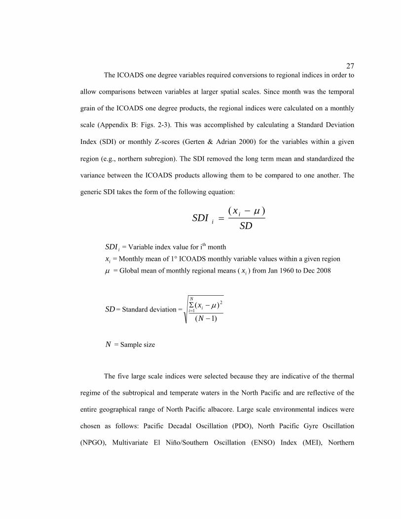
27The ICOADS one degree variables required conversions to regional indices in order to
allow comparisons between variables at larger spatial scales. Since month was the temporal
grain of the ICOADS one degree products, the regional indices were calculated on a monthly
scale (Appendix B: Figs. 2-3). This was accomplished by calculating a Standard Deviation
Index (SDI) or monthly Z-scores (Gerten & Adrian 2000) for the variables within a given
region (e.g., northern subregion). The SDI removed the long term mean and standardized the
variance between the ICOADS products allowing them to be compared to one another. The
generic SDI takes the form of the following equation:
SD
xSDI i
i
)(
iSDI = Variable index value for ith month
ix = Monthly mean of 1° ICOADS monthly variable values within a given region
= Global mean of monthly regional means ( ix ) from Jan 1960 to Dec 2008
SD = Standard deviation =)1(
)( 2
1
N
xi
N
i
N = Sample size
The five large scale indices were selected because they are indicative of the thermal
regime of the subtropical and temperate waters in the North Pacific and are reflective of the
entire geographical range of North Pacific albacore. Large scale environmental indices were
chosen as follows: Pacific Decadal Oscillation (PDO), North Pacific Gyre Oscillation
(NPGO), Multivariate El Niño/Southern Oscillation (ENSO) Index (MEI), Northern

28Oscillation Index (NOI), and Southern Oscillation Index (SOI) by month from Jan. 1961 to
Dec. 2008 (Appendix B: Fig. 1).
The ENSO is the most important ocean-atmospheric cycle over the tropical Pacific
Ocean, operating on a 2-7 year time span (Wolter and Timlin 1998; Hanley et al. 2003).
ENSO events have been related to regional extremes in weather (Ropelewski and Halpert
1996), and to changes in albacore and other fish populations (Ahrens 1994; Bakun and Broad
2003). There are many indices that attempt to capture ENSO events, and it is still debated
within the scientific community which index best defines ENSO events (Hanley et al. 2003).
Although most ENSO indices are highly correlated to each other, they vary in subtle ways.
Several ENSO indices were investigated to see if one, or any, better related to albacore
population changes. One of the most commonly used ENSO indices is the SOI, which is
derived from pressure differences between Darwin and Tahiti (Ropelewski and Jones 1987).
The SOI was obtained from the National Marine Fisheries Service Pacific Fisheries
Environmental Lab (PFEL, http://www.pfeg.noaa.gov). As an alternative to the SOI the MEI
was chosen. The MEI is the first principal component of the six main observed variables (P,
U and V surface wind components, SST, surface air temperature, and total cloud fraction) over
the tropical Pacific (Wolter and Timlin 1993; 1998; available from
www.esrl.noaa.gov/psd/people/klaus.wolter/MEI/). The NOI is similar to the SOI but based
on the differences in P anomalies between the northeast Pacific (NEP) and near Darwin,
Australia (Schwing 2002).
The PDO is a lower frequency atmospheric pattern believed to oscillate on a span of
20 to 30 years (Zhang et al. 1997; Mantua et al. 1997). The PDO is derived as the principle
component of monthly SST anomalies in the North Pacific Ocean, poleward of 20° N with
records starting January 1900 (Zhang et al. 1997). The version of PDO used in this study was
29updated to include May 2009 (http://jisao.washington.edu/pdo) with monthly mean global
average SST anomalies removed to separate the PDO variability from any "global warming"
signal. The PDO was selected because of the potential low frequency influences in albacore
abundance (Bakun and Broad 2003).
The NPGO is an index of the second principle component of sea surface height
variability in the Northeast Pacific Ocean (Di Lorenzo et al. 2008; accessed from
http://www.o3d.org/npgo/index.html). The NPGO is significantly correlated with long-term
fluctuations of salinity, nutrients, and chlorophyll-a in the Northeastern Pacific Ocean. Di
Lorenzo et al. (2008) provided evidence that fluctuations in the NPGO are driven by regional
and basin-scale variations in wind-driven upwelling and horizontal advection, and indicated
that the NPGO can be used as indicator of upwelling strength and bottom-up forcing in the
Northeastern Pacific Ocean. The NPGO has also been found to be more sensitive to influence
subarctic water than the PDO (Lavaniegos 2009).
2.2.3 Wavelet analysis
Several methods are available to detect relevant scales of variability such as
correlogram, Discrete Fourier Transform, evolutive spectral, and wavelet analysis. Wavelet
analysis was selected over other methods because it is robust to non-stationary data at
different frequencies (Daubechies 1990; Torrence and Compo 1998). Wavelet analysis was
conducted on the entire region, northern subregion, southern subregion, and all environmental
variables to allow inspection between the CPUE and potential environmental variables.
Additionally, a frequency analysis requirement is regularly spaced data and no missing values,
therefore in this study, null albacore CPUE values were interpreted as 0 to create a regularly-
spaced time series (see discussion section 2.4.2).
30One of the major criticisms to wavelet transforms is that an infinite number of
wavelets can be tested arbitrarily (Torrence and Campo 1998). To avoid this pitfall of testing
many wavelet functions the recommendations of Torrence and Campo (1998) to select a
specific analyzing wavelet appropriate for the CPUE time series were followed. The Harr
wavelet (Appendix C: Fig. 1) was selected because the CPUE time series abruptly started and
stopped with each fishing season and because the Harr wavelet has been found to be an
effective replacement for the Fourier transform (Torrence and Campo 1998; Chan and Fu
1999). The Fourier transform was not used, because the CPUE time series violated the non-
stationary assumptions required for such analysis, being that the CPUE time series was non-
stationary and discontinuous.
The time series of the environmental indices had trigonometric pattern, in contrast to
the box like CPUE, potentially resulting in the HARR wavelet being a mismatch function for
the environmental indices. So, two common trigonometric wavelet functions (Mexican hat and
Sine) were explored for the environmental indices and CPUE. The Mexican hat and Sine
functions both had similar results to the Harr wavelet in terms of scale spectrum for the
albacore CPUE and indices, further justifying the use of the Harr wavelet for the entire study.
The main difference in the wavelets was the position-scale and power spectra (see below) – a
feature that goes beyond the objective of this study.
The software Pattern Analysis, Spatial Statistics, and Geographic Exegesis
(PASSaGE) version 2.0.10.18 was used for all wavelet analyses (Rosenberg and Anderson
2011). The wavelet transform taken from Bradshaw and Spies (1992) is:

31
a
xxgxf
axaW ki
n
iik
1
)(1
),(
)( ixf = data function (time series)
n = length of the time series
)(a
xg = analyzing wavelet
ix = distance along the time series
kx = centering location of the analyzing wavelet
a = scale of the wavelet
All wavelet functions must meet the following criteria; 1) an integral of zero, 2)
symmetry about an axis, and 3) localization in time and frequency space. The Harr wavelet
function used in this study is (modified from Rosenberg and Anderson 2011):
otherwisea
xif
a
xif
a
xg
0
1)(01
0)(11
)(
The one dimensional (time series) wavelet function can be thought of as taking the
Harr wavelet (or any other wavelet function) at a fixed scale and sliding it along a time series.
The Harr wavelet is essentially correlated to segments of the time series as it is moved along
the length of the time series. If the segment of the time series and wavelet are similar, a
positive value is given, if they are similar but of opposite sign, a negative value is given, and if
they are not related, a zero value is given. The wavelet is then scaled up a unit and slid over
the time series again. This process is repeated many times resulting in relationship values
between the wavelet and data across the time series at multiple scales. This process represents
a decomposition of a one dimension time series into two-dimensional position-scale space

32(Torrence and Compo 1998). The position axis is the location along the time series (e.g.
strength of the PDO at any point in time series), and the scale axis is the wavelet variance by
scale (e.g. variability of PDO at different temporal cycles).
The two dimensional wavelet position scale plane, also called the wavelet power, is
often complicated and difficult to interpret (Bradshaw and Spies 1992). However, the wavelet
power can have variance calculated along both axes. This study focused on only wavelet
variance by scale in order to select likely time periods in which albacore CPUE fluctuations
were non-random. The wavelet variance by scale is an average of the wavelet coefficient
squared at every point along the time series, for a fixed scale (Bradshaw and Spies 1992).
k
n
kk xaW
nxaV ,
1),(
1
2
With the wavelet variance it is also possible to calculate confidence intervals,
otherwise known as a confidence spectrum, with a one-tailed randomization test (Torrence and
Compo 1998). Confidence spectra (CS) at the 95% level for the scale variances were
calculated by taking 100 randomizations of the scale variance. The CS is essentially a Monte
Carlo test, and scales with high variance above the CS are considered to be significant. Thus,
by inspecting the wavelet variance by scale, any peak values above the 95% CS level are
likely correspond to temporal cycles.
First, Harr wavelets were conducted on daily average CPUE to determine if there was
systematic variability at relatively fine scales (days to weeks), and the analyzing wavelet was
restricted in scale from one day to 1% (~1/2 a year) of the albacore CPUE time series (Fig. 3
right three plots). The results of that analysis indicate that almost all of the variability at the
sub-monthly scale was random. Thus the CPUE data was averaged by month, and then

33analyzing wavelets were conducted on the monthly averaged data to a maximum scale of 50%
of the albacore time series. Some information may have been lost during the averaging process
(see 4.2), but more likely the noise was reduced. Finally, spearmen correlations were made
between the significant (95% C.S.) pairs of monthly scale spectra for the albacore CPUE and
environmental indices.
2.2.4 Monthly GAM analysis
Wavelet results (see section 3.1.1) indicated sub-yearly variance was systematic
starting approximately at the monthly scale, therefore a monthly-averaged time series analysis
was conducted. Relationships between monthly averaged CPUE (fish/boat day) for the entire
region and subregions were compared against each of the 10 environmental indices using
generalized additive models (GAMs) with the mgcv package in R (v2.10.1) software (Wood
2006). In recent years GAMs have become commonly used to investigate relationships
between marine fishes and environmental variables (e.g. Ciannelli et al. 2004; Doyle et al
2009; Mugo et al. 2010). GAMs are non-linear regression models that fit curved splines
between nodes. Models are penalized for increased curvature or increased nodes and ranked
based on the minimum generalized cross validation (GCV) scores (Wood 2006). The GCV
measures the predictive error of the model and as such is used as a ranking criterion similar to
the Akaike Information Criterion (AIC), which is often used in selecting linear models.
Monthly averaged CPUE was calculated by taking the daily CPUE in each one degree
cell and averaging over the sub/region wide scales for the time span of one month. The
monthly averaged time series was discontinuous, because often no efforts and therefore
catches were reported during the winter months. Two approaches were taken to correct for the
months without CPUE values. In the first approach missing CPUE months were converted to
340, with the assumption that missing values during winter months justifiably represented 0
CPUE. This justification was based on the fact that little effort has been made from
December-May in over 50 years (Fig. 4). It was assumed that if albacore were present in
significant numbers such that at least a few vessels within the fleet would have been fishing. It
is acknowledged that some albacore were probably present, but for all practical reasons the
missing CPUE values during winter months represented 0 CPUE at a population scale. The
second approach was to remove months with missing data and only analyze months with a
complete time series. The months July-October met this criterion, and also represented 92% of
the total catch for the entire region. The second approach yielded poor results as indicated by
low adjusted (R2<0.12) for all single variable models, and multiple variable models also
performed weakly (R2<0.31). Therefore I focused on describing the results from the first
approach in the rest of this chapter.
Due to a lack of prior knowledge about how the 10 indices related to North Pacific
albacore CPUE (response), an exploratory approach was used to determine top potential
variables for a multiple regression. Environmental index lags of up to 6 months were tested.
This approach resulted in 14 different models for each index, considering both methods, and a
total of 140 single variable models for each region. The individual models were checked for
common statistical violations with the gam.check2 function. The zero-replaced approach
required normalization ln(CPUE + 1), but the reduced July-October monthly CPUE approach
was approximately normally distributed and did not require a transformation. The resulting
single variable GAMs were ranked by the GCV from lowest (best fit) to highest for each
monthly approach. In addition to GCV, adjusted R2, deviance explained, P-values, and
2 gam.check is a function in the R mgcv package which takes a model and produces four residual plots being; diagnostics for residuals. a Normal Q-Q plot, residuals vs. linear predictors, a histogram of residuals, response vs. fitted values.
35Bonferroni corrected P-values for the top 20 models for the entire region and subregions were
reported.
GAM models can overfit data, resulting in spurious relationships between predictor
and response variables in very long and autocorrelated time series. In an effort to prevent this
type of error an inspection of the relative wiggliness of the estimated model fit was visually
performed. If two or more distinct peaks were detected in the predicted fit spline, the model
or covariate was considered overfit. This was corrected by reducing the number of knots in
the spline to 4.
The top 20 models ranked with the lowest predictive errors, as indicated by GCVs, for
the entire region and subregions were considered as covariates in backward elimination,
stepwise multiple variable GAM. An initial model was chosen that allowed each index of the
top 20 models to appear once in the full multiple variable model. For example, if the entire
region SST lagged 0 and lagged 5 months both appeared in the top 20 single variable models,
only the one with the lowest GCV was allowed in a multiple variable model. A full model
with all the potential covariates was tested and ranked by GCV score. Next, the covariate with
the highest P-value was dropped and a model with one less term was tested in the backward
elimination stepwise process. This process was repeated, until GCV scores started to increase.
Covariates with P-values over 0.05 were allowed if the GCV of the model was lower with the
covariate included (Wood 2006). If the environmental indices were related to each other and
showed collinearity, a correlation between the covariates, the P-values were likely to be
inflated (Zurr et al. 2010). Thus, the final multiple variable models were tested for
collinearity, and if a strong correlation (R>0.5) was found, the variable with the highest P-
value was dropped. Final multiple variable model residuals were also tested for
autocorrelation with the built-in acf and pacf functions in R.
36
2.2.5 Yearly GAMs analysis
Based on the wavelet results (see section 3.1.1) a non-random CPUE variance peaked
near the year interval and indicated a yearly analysis would also be an appropriate time scale
to investigate. The yearly averaged CPUE was calculated by taking the daily CPUE in each
one degree cell and averaged over the time span of a year (see Barr (2009) for more details).
Similar to the monthly CPUE analysis, a lack of prior knowledge of the 10 indices in
relation to North Pacific albacore CPUE led me to take an exploratory approach to determine
top potential variables for a multiple regression. However, because the environmental
variables were averaged over a twelve month time period many more options were available.
For example, summer SST could be more influential on yearly albacore availability to the U.S.
west coast fishery than winter SST conditions. So, for each of the 10 potential explanatory
variables, six within-year possible averages were allowed: total yearly averages, the four
seasons (e.g. spring was an average of March-May), and the three months with the highest
albacore CPUE (July-September). Lags up to 5 years were also considered. This approach
resulted in 36 (e.g., spring average SST at a two year lag) different models for each index and
a total of 360 models for each region. The resulting single variable GAMs were ranked by the
GCV from lowest to highest. In addition to GCV, adjusted R2, deviance explained, P-values,
and Bonferroni-corrected P-values for the top 20 models in region were reported.
A backward elimination, stepwise multiple variable GAM, following the same
methods outlined in section 2.2.4 was tested on the yearly 20 best-fit models for each
sub/region. Individual and multiple variable model residuals were tested for autocorrelation
with the default autocorrelation function (acf) and partial autocorrelation function (pacf) in R.

37If autocorrelation was detected it was reported, but no efforts were made to correct
autocorrelated models.
2.2.6 Yearly age composition analysis
Albacore length data, described in section 2.1.1, was converted to age class using the
length-age relationship from Suda et al. (1966) found in the U.S. Pacific albacore logbook data
(http://www.swr.noaa.gov/hms/alblog10.pdf). The monthly length data was compared to the
monthly CPUE for the entire region and North/South subregions. June through October had
available CPUE data for most of the time series, but unfortunately length data were
inconsistently collected. Months were excluded when length data was missing from >50% of
the years in which any fishing effort occurred. Additionally, months were excluded if they had
little or no fishing effort. Ultimately, July, August, and September were the only months that
met these selection criteria. The yearly age class abundance was calculated by taking the
monthly CPUE and multiplying it by the percentage of each calculated age class. Next, July,
August, and September were averaged together to calculate a yearly age class for the entire
time series. The dominant age classes were then correlated for the entire region and both
subregions. Finally a targeted GAM analysis was conducted on the dominant year class for
the entire region, using the best fit index determined in the yearly analysis.
2.2.7 Yearly SST threshold GAMs analysis
Visual inspection of yearly CPUE and yearly SST indices revealed what appeared to
be long temporal spans that correlate well initially and then diverge. These spans
approximately correspond to PDO regime shifts during late 1970’s and 1990’s, suggesting
non-stationarity in the time series (Appendix D: Fig. 1). If threshold shifts occurred during the
time series then any association between SST and CPUE would likely be lost in a single
38variable model that spanned the entire time series. Thus, as an alternative to the yearly GAM
analysis, temporal Threshold Generalized Additive Models (tGAMs) were applied to the
entire region and subregions to test for a threshold in relation to SST, using the R package
mgcv. Only SST was tested since it is known to be important to albacore distribution at small
scales. In this instance the tGAM tested for thresholds at different time periods and fit
individual models before and after the threshold year. The models at each potential threshold
year were ranked by GCV and the model with the lowest GCV was selected as the threshold
year. If significant thresholds were determined linear models were fit to the time periods
before and after the thresholds to inspect relationships before and after the time series. For a
more detailed description of the tGAMs, see Ciannelli et al. (2004).
39
2.3 Results
2.3.1 Wavelet analysis
The entire region and subregions have a similar wavelet variance by scale, hereafter
called the scale spectrum. Specifically, the daily Harr wavelets show scale spectrum at cycles
less than 30 days to have the most variance, but that variance was near or below the 95%
confidence spectrum (C.S., Fig. 3). This indicates that CPUE is not significantly different than
random variability at scales below 1 month. In all regions, scale spectra showed significantly
increasing variance, at time scales from approximately 30 days to the end of the scale
spectrum tested (170 days) for the daily CPUE. A noted difference between the regions was
that the entire region and northern subregion were approximately twice as variable as the
southern subregion as indicated by the y-axis in Fig. 3. Harr wavelet variances by scale to 1%
(~0.5 years) of the daily averaged Pacific albacore CPUE (fish per boat day) for the entire
study area and both subregions are also presented in the right three plots of Figure 3.
Since submonthly CPUE was essentially random, the daily CPUE was averaged to the
monthly scale and the wavelet analysis was repeated. Similar to the results from the daily
wavelets, the entire region and subregions have comparable scale spectra, and the southern
subregion had approximately half the variance on the y-axis (Fig. 3). The monthly averaged
CPUE Harr wavelets scale spectra had the highest, non-random (95% C.S.), variability for the
time periods of 0.25-1.2 years, peaking at 0.58 years. The peak at 0.58 years indicates that
systematic variability in albacore CPUE cycled strongest approximately every 6 months. This
roughly corresponds with the yearly cycle of the fishery, which is visually apparent in the
plots of the daily CPUE and shows seasonal availability of albacore to the fishery (Appendix
E: Figs. 1-6). However, less obvious was high variance significance (95% C.S.) at shorter
40scale spectrum, indicating that within-year variability required investigation. Monthly wavelet
scale spectrum was mostly non-significant from approximately 1.5 to 11 years. However,
marginally significant peaks did occur at 34 months in entire region and southern subregion,
but not the northern subregion (Fig. 3). Beyond 11 years, a significant low-frequency variance
was present in the remainder of the monthly wavelet scale spectrum.
Monthly Harr wavelet scale spectrum, to 50% (24 years) of the albacore time series
1961-2008, for the MEI, PDO, NPGO, NOI, and SOI indices are shown in Appendix F and
Fig. 1). The scale spectrum of the monthly MEI showed significant variability starting about
one year and peaking at 2 years, and then tapering off after that but remaining significant
across the scale spectra. The PDO showed low signal significant variance across the scale
spectra with no distinct peaks. The NPGO showed significant variability beyond one year
peaking at approximately 8 years before it slowly decreased across the time series. The NOI
and SOI had patterns that were closely matched in that they both had significant scale
spectrum beyond a year that slowly decayed. Additionally, the variability of the NOI and SOI
were approximately one order of magnitude higher than the other three large scale variables.
Monthly Harr wavelets scale spectrum to cycles up to 50% (24 years) of the albacore
time series 1961-2008, for the regional SST, scalar wind cubed, sea surface pressure, U wind
stress, and V wind stress indices at the entire region scale are presented in Appendix F: Fig. 2.
Additionally, Appendix F: Figs. 3-4 show the results of the monthly Harr wavelet scale
spectra for the northern and southern subregion local indices.
The differences of scale spectra between subregional and entire region indices are
minor and scale spectrum are described for all regions unless specified. All the regional
indices have peak variance near the yearly scale, which becomes non-significant at
approximately 1.5 years. In terms of peak variability SST was the highest of the regional
41indices at (0.8). The SST, Pressure, and V wind stress had low frequency variance beyond 1.5
years which was mostly non-significant for the remainder of the scale spectra. The U wind
stress had significant low frequency variance beyond 2.5 years and the low frequency variance
peak near 12 years (143 months). The scalar wind speed cubed of the entire and southern
subregion becomes significant after nine years and gradually increase to the 50% scale, while
that of the Northern subregion remains low and non-significant. Overall the regional indices
scale spectra appeared to match better with the CPUE than the large scale indices. However,
the low frequency patterns of the regional indices were difficult to interpret, and a further
correlation analysis between the scale spectra of the CPUE and indices was needed.
Results of the Spearmen correlations made between the significant (95% C.S.) pairs of
scale spectra for the albacore CPUE and environmental indices are shown in Table 1. The
paired correlations were greater than r=0.5 for all of the indices except the NPGO, indicating
that the CPUE and environmental indices had moderate to strong correlation of cyclic variance
across scales. Additionally, the regional scale indices tended to correlate more strongly
(most r > 0.97) in any given region with the CPUE across-scale spectra than the large-scale
indices. A visual inspection of the scale spectrum show that usually CPUE most closely
matched with the regional indices near the yearly scale, while the large scale indices matched
better at time periods beyond 10 years (Fig.4 and Appendix F).
2.3.2 Monthly GAMs analyses
Results of the single variable GAMs analysis in which null CPUE months were
treated as 0 indicated SST to be the most important single variable for the entire region and
both subregions at the monthly scale (Table 2), as indicated by the low GCV score and high
variance explained (58-77%). The SST had a strong non-linear positive relationship with the
42CPUE. The other regional indices had lower GCV scores and higher ranks than the large scale
indices, with the exception of NOI. All of the top-ranking single-variable models appear to be
significant, even after Bonferonni corrections for family-wise errors.
The GCV scores of the multiple regression models were slightly improved over the
single variable SST models. The final models were:
Entire region: Ln(CPUE+1)~s(SST0)+ s(Uwind3)+ s(Scalar0) +s(NOI6) GCV=0.92 adj.R2=0.73
Northern subregion: Ln(CPUE+1)~s(SST0)+s(NOI6) GCV=0.80 adj. R2=0.78
Southern subregion: Ln(CPUE+1)~s(SST5)+s(Uwind3)+s(NOI6) GCV=1.08 adj. R2=0.63
All of the covariates in the multiple variable models had highly significant smoothing
terms (P-values <0.05) (Figs. 5-7). Fitted GAM diagnostic output of gam.check, the
multiple variable model residuals showed a negative trend versus linear predictions in all cases
and the series were significantly autocorrelated at one and twelve month lags. This suggested
that the underlying mechanisms of temporal variability were not adequately explained.
Based strictly on GCV criteria the multiple variable models should be selected for
statistical analysis over the single variable models. However, operationally the SST is
associated with most of the variability (≥90%) explained in the multiple variable models and
could be considered alone in predicting models. Also, a point of clarification needs to be
made in regard to the trend of SST at different lags for the sub/region. Specifically, the non-
lagged SST showed a positive trend for the entire and northern subregion, while the five
month-lagged SST showed a negative trend in the southern region (Figs. 5A, 6A, and 7A).
43The difference in trends between the lagged and non-lagged SST is due to SST and CPUE
being in phase at lag 0 and being out of phase at a five month lag. The trend between SST and
CPUE is almost identical between the areas if the SST lag is same.
Results of the method two (reduced data set) single variable GAM analyses (Table 3)
performed poorly based on greatly reduced adjusted R2 in comparison to the first method
Table 2. All of the models had adjusted R2 values which accounted for no more than 12% of
the variability, and although all of the models had significant P-values, many of the P-values
became non-significant after Bonferonni corrections.
The multiple variable stepwise backward selection analysis GCV scores and fits
improved over the single variable monthly averaged method two models (Figs. 8-10). Fitted
GAM diagnostic output of gam.check showed no major violations, but the series were
significantly autocorrelated at one and twelve month lags.
Entire region: CPUE~s(SST5)+ s(PDO0)+s(Uwind3) GCV=745.88 adj. R2=0.20
Northern subregion: CPUE~s(PDO3)+s(SST0) GCV=1344.00 adj. R2=0.16
Southern subregion: CPUE~s(Uwind3)+ s(MEI4)+s(Scalar0)+s(NPGO0) GCV=700.07 adj. R2=0.28
2.3.3 Yearly aggregated data
Yearly aggregated catch, effort, and CPUE data for the entire region and subregions
show contrasting trends between the catch/effort and CPUE (Fig. 1). The northern subregion
yearly CPUE was on average 80 (fish/boat day), while the southern subregion CPUE average
was almost half as much at 43 (fish/boat day). The two regions had similar CPUE oscillations
44in the early part of the time series 1961-1980 which had a moderate positive linear relationship
with an R=0.79. After 1980, the divergence between the northern and southern CPUE
increased driving the correlation between the northern and southern subregions down to
R=0.55 for the entire time series.
The yearly effort and catch sums show a different pattern than the CPUE. Based on
visual inspection from 1961 to the mid 1980’s total catch and effort in both subregions were
out of phase with each other in cycles of multiple years (~3-7 yr) until the mid 1980’s (Fig. 1).
Then in the mid 1980’s both catch and effort dramatically dropped off in the southern region.
With the exception of 1999, both catch and effort have remained low in the southern
subregion. In the northern subregion, both effort and catch have dramatically increased since
the late 1990’s.
2.3.4 Yearly GAMs analysis
The single variable GAMs analysis on the yearly averaged CPUE indicated that the
five-year lag of the scalar wind speed cubed was the most important single variable for the
entire region (Table 4), showing the lowest GCV and highest R2 (65%). Additionally,
variations of the scalar wind cubed appeared in over half of the top single-variable GAMs for
the entire region. In the northern subregion, spring sea surface pressure lagged at two years
had the lowest GCV and a near-linear positive slope (adj. R2=0.42), followed by yearly
average of scalar wind speed cubed at a five year lag. Summer PDO at a three year lag was
found to be the best fit (adj. R2=0.34) single variable, followed by the yearly average of scalar
cubed lagged two years. All the top single variable models were found to be significant below
the 0.05 P-value. However, after Bonferonni corrections for family-wise errors, scalar cubed
for the entire region at a five year lag was the only significant variable. Diagnostics
45(gam.check) of the scalar wind speed cubed model at a five year lag show no obvious
assumption violations (Appendix G: Fig. 1).
The GCV scores of the multiple regression models were slightly improved over the
single variable models. Final models were:
Entire region: CPUE ~ s(Yr. Avg. Scalar5)+ s(Winter NPGO1)+ s(Fall PDO3) GCV=282.37 adj. R2=0.70
Northern subregion: CPUE~ s(Spring Pressure2)+s(Yr. avg. Scalar5)+s(Yr. avg PDO3)+ s(SOI0) GCV=396.93 adj. R2=0.74
Southern subregion: CPUE~s(Summer PDO3)+ s(Yr. Avg. Scalar2)+s(Fall Vwind2)+s(Yr. avg. Uwind2) GCV=167.17 adj. R2=0.7
A final inspection for collinearity was made between covariates in the multiple
variable models. If any of the terms had moderately strong Spearman correlations (R>0.5),
the term with the highest P-value was dropped. All terms in the entire region and Northern
subregions had R<0.5. Only two covariates in the Southern subregion were found to have
R>0.5, being the Scalar wind speed and V-wind stress lagged 2 years (R= -0.68). Because
these variables were highly correlated, we opted to drop one of the terms. The Scalar wind
speed had a higher P-value, and was dropped from the Southern subregion multiple variable
model, resulting in 3% reduction in adjusted R2, and a 5% increase in GCV.
All yearly multiple variable models had smoothing terms in the full models which
were significant at the 0.05 P-value (Figs. 11-13), with the exception of the two year lagged
scalar wind cubed in the southern subregion (P=0.057). By further visual inspection of the
significant terms (Figs. 11-13) it appears only the SOI in the northern subregion was overfitted
(Fig. 12D), while the other variables have near-linear relationships. For example the PDO at
three year lags had a linear negative association with CPUE in all the yearly multiple variable
46models. The association between CPUE and scalar wind speed cubed appears to be non-
significant in years with low to normal wind speeds, and after wind speed becomes
anomalously linear, positive association occurred (Figs. 11-12).
The three-term multiple variable model of the entire region had a lower GCV and a
slightly improved fit (GCV 282, adj rsq=.070) than the five year lagged scalar wind speed
cubed single variable model (GCV 314, adj rsq=0.65). Based strictly on GCV criteria the
multiple variable model should be selected for statistical analysis. However, operationally the
scalar wind speed cubed is associated with most of the variability (>90%) explained in the
multiple variable model and could be considered alone in predictive models.
Data was significantly temporally autocorrelated to 4 years in the entire study area
(Appendix G: Figs. 2). Autocorrelation investigation of residuals from top 20 region wide
models revealed that only scalar wind speed cubed lagged at 5 years removed all the
significant autocorrelation from the residuals (Appendix G: Figs. 3). The removal of all
significant autocorrelation provides some evidence that the scalar wind speed cubed may be
driving changes in albacore CPUE.
2.3.5 Yearly Age composition
The results of the reconstructed yearly age class structure of the albacore time series
(1961-2004) for the entire region and subregions are presented in Figure 14. In some time
periods length data were not available or did not meet the criteria set for inclusion (see section
2.2.6), and thus gaps were present in all regions studied from 1992-1995. Additionally, the
Southern region did not meet the criteria prior to 1973 and from 1992-1996. Within the
available years, age-three fish dominated the catch in almost all years followed by age-four

47fish in all regions. Notable exceptions were that four year old fish dominated in the southern
subregion in 1979 and 1980 and all regions during 1999. Correlations between the 3 year olds
and one-year lagged 4 year old fish had R = 0.69 (95% C.I. from 0.48 to 0.83 and P= <.0001)
for the entire region, R = 0.27 (95% C.I. from -0.04 to 0.54 and P=0.09) for the northern
subregion, and R = 0.38 (95% C.I. from -0.02 to 0.67 and P=0.06) for the southern
subregion. Thus the relationship between 3 and 4 year old fish appears to be moderately
strong at the region-wide scale, but non-significant at the sub regional scale. However, any
interpretation of this data should be made with caution, because of several potential biases (see
2.4.3).
When including all age classes, the entire region yearly-averaged scalar wind speed
cubed lagged five years had the lowest GCV and had the strongest association (adj. R2=0.65)
In order to examine if model improvements could be made, the calculated CPUE’s of the
dominant age class (age 3 fish) were tested in a GAM against the scalar wind speed cubed
lagged five years. The scalar wind effect on the age-3 albacore (Fig. 15) was similar to the
model when all age groups were combined (Fig. 11A). However, the age 3 fish fit was
reduced (adj. R2=0.43) in comparison to all age classes combined.
2.3.6 Yearly SST threshold GAMs analysis
The GCV profiles of the SST tGAMs all selected unique threshold years for the entire
region and subregions (Fig. 16). Best-fit models had threshold years during 1997-1998 for the
entire region, 1975-1976 for the northern subregion, and 1974-1975 for the southern
subregion. In all cases two near-linear fits were found before and after the threshold years.
Thus, linear models were applied to the time spans before and after the determined threshold
year (Fig. 16).

48For the entire region the SST tGAM had an adjusted R2 of 0.33. This model had a
lower adjusted R2 than many of the other single variable models in Table 4. However, this was
a specific analysis only looking at non-lagged SST. The most similar model to the SST tGAM
was the yearly averaged non-lagged SST model which had corresponding adjusted R2 of 0.02
(P-value=0.14), indicating that the tGAM was an improvement, if the intent is to explain
albacore CPUE variability in relation to SST. For the time span prior to the threshold year of
1997, SST had a weak R2 of 0.11, significant (p-value=0.05) negative association with the
SST index, whereas after 1997, the association trended positive but was non-significant (p-
value=0.18) as indicated by the linear regressions (Fig. 16 A-C).
Both the northern and southern subregions SST tGAMs also had increased adjusted
R2 over similar non-lagged single variable SST models. The northern subregion SST tGAM
had an adjusted R2 of 0.33 in contrast to the equivalent SST GAM model which had an
adjusted R2 of <0.01 (P-value >0.05). The southern subregion tGAM had an adjusted R2 of
0.38 and had a higher adjusted R2 than any of the single variable models from the southern
subregion in Table 4. For the time span prior to the threshold year of 1975, SST in the
northern subregion had a moderate R2 of 50%, significant (p=0.003) positive association with
the SST index, and after 1975 no trend was detected (p=0.68) as indicated by the linear
regressions (Fig. 16 E and F). The slope for the southern subregion prior to the threshold year
of 1974, had a weak non-significant (p=0.45) trend in SST, and after 1974 the association had
a weak negative trend R2 of 0.09, which was non-significant (p=0.09) (Fig. 16 H and I).
49
2.4 Discussion
2.4.1 Wavelet analyses
The CPUE wavelets of the entire region and two subregions are nearly identical in
terms of scale, with significant scale spectrum correlations >0.99 (Fig. 3). The peak variance
near the yearly scale is an order of magnitude higher than the low-frequency signal occurring
beyond 12 years. This indicates that the majority of the variability is occurring at a yearly
cycle.
The strong correlations in Table 1, between wavelet scale spectrum of CPUE and
regional indices (Fig. 3 and Appendix F: Figs. 1-4), indicated that the CPUE was more closely
matched with the regional indices than the large scale indices. This is somewhat surprising
because the regional indices are constructed from a complete time series, with smooth
gradients between months while the CPUE time series abruptly starts/stops, and it is fairly
discontinuous.
Laurs and Powers (2010) suggested that large-scale indices need to be investigated for
North Pacific albacore. They highlighted the work of Hallett et al. (2004) who using sheep as
an example species concluded that large-scale indices, such as the North Atlantic Oscillation,
can be important predictors of density-dependent processes in populations. Lehodey et al.
(2003) found evidence that El Niño conditions negatively affected albacore recruitment in the
South Pacific and others (Lu et al. 1998; Andrade 2003; Chen et al. 2005; Barr 2009; Dufour
et al. 2010; Sagarminaga and Arrizabalaga 2010) have found albacore fluctuated in response
to larger scale environmental variables and SST. However, Goñi and Arrizabalaga (2005)

50studying the Atlantic albacore, found regional monthly averaged sea surface agitation and
insolation3 (both related to mixed layer depth) to be the only variables with significant
negative relationships to albacore CPUE within season.
The CPUE cycles are nonsignificant and appear to be noisy, from about 2-11 years,
with an exception around 36 months. This marginally-significant low signal variability every
three years may roughly correspond to the MEI events. Beyond 11 years, a low significant
signal is spread across the rest of the scale spectrum. This lower frequency variability may be
a signal from the PDO because the scale spectrum of the PDO matches well with the CPUE
beyond 11 years, and the monthly PDO values are weakly (-0.21 entire region, 0.22 northern
subregion, and -0.18 southern subregion) correlated with the CPUE. However, interpretation
at longer time cycles is problematic because of edge effects, also called the “cone of
influence”, occurring when the wavelets increase in scale in relation to the length of the time
series (Torrence and Campo 1998). For example, the PDO only experiences a few low
frequency cycles over the 48 year time period, and it is difficult to determine if it had an effect
on CPUE beyond 11 years.
2.4.2 Monthly GAM analyses
The monthly GAM analysis, which treated missing data CUPE months as zeros,
appears to have captured seasonal variability, and SST is likely the best potential explanatory
variable in all regions. It has been well documented that albacore migrate seasonally in and
out of the U.S. coastal fishery (Brock 1943; Clemens1961; Otsu and Uchida 1962; Laurs and
Lynn. 1977 and others), so it is not surprising to find this relationship at the monthly scale of
3 The amount of solar radiation energy received on a given surface area in a given time.
51analysis. In fact, the SST signal can represent a proxy for seasonality, and therefore it is more
of an innate adaptation of tuna rather than a plastic environmental response.
It should also be noted that the monthly averaged albacore time series was highly
autocorrelated, oscillating between positive and negative values out several lags roughly at a
yearly cycle (Appendix G: Fig. 4), and the residuals of SST (and multiple variable) models
removed some, but not all, of the autocorrelation (See Appendix G: Fig. 5 for an example). So,
although the SST appears to have a strong association with the CPUE at the monthly scale, it
appears to be missing some of the underlying variability. Large scale indices such as the PDO
do not appear to detect this variability at the monthly scale nor remove the remaining
autocorrelation.
As an ad hoc test, I included an analysis with months as a factor to see if
improvements could be made to the SST index after accounting for seasonality. I found that
the month factor alone explained more variability (adj. R2=0.76) than the SST index (adj.
R2=0.67). The models with a month factor in addition to SST removed the SST trend making
the P-value of SST non-significant. This basically confirmed that the SST index and month
factor were modeling the same thing. Once a month factor is included in the model, SST is no
longer significant.
In the alternative analysis, when the months in which fishing effort seldom occurred
were removed, all the indices performed poorly. So, after seasonality is removed (via dropping
the null months), the monthly analysis was very poor at associating albacore CPUE with
environmental indices. The lack of relationships, after months in which albacore are not
captured get removed, is another indication that method one was simply detecting seasonal
variability of albacore migrating in and out of the U.S. coastal fishery.

522.4.3 Yearly Scale
The yearly averaged catch data showed a different pattern than the CPUE between the
subregions (Fig. 1). Examining the catch alone is troubling if not alarming, because if two
substocks are recognized, it appears as though the southern substock crashed during the late
1980s or was unavailable. However, reviewing catch data alone can often be misleading
because several factors unrelated to fish abundance (e.g., economic demand) can result in
dramatic changes in catch and effort (Beverton and Holt 1957; Maunder and Punt 2004). The
dramatic drop in effort in the southern subregion in the 1980’s is likely explained by
economics. Between 1982-1984 almost 2,000 fishermen and 6,000 other positions related to
the albacore fishery were lost because canneries moved outside the U.S. and into the global
market (Love et al. 2006).
The two subregions show a marked difference with a higher catchability in the
northern subregion, as indicated by the higher slope of effort vs catch in this region (Figure
17). This difference in catchability may be due to 1) behavioral changes related to albacore
size, distributions, and/or environmental variability and/or 2) fewer fish in the southern
subregion. Of the potential explanations behavioral changes are the most likely cause of
different catchablity. Childers et al. (2011) showed that tagged albacore were spending more
time at depth as mixed layer and SST increased. As SST and the mixed layer depth increases
in lower latitudes, albacore spend more time at depth in the southern region, and therefore they
are less vulnerable to fishing effort. Goñi and Arrizabalaga (2005) found regional monthly
averaged insolation which decreases as latitude increases to be negatively associated with
North Atlantic albacore CPUE, and attributed this association to a deeper distribution of
albacore prey and thus the foraging albacore. Additionally, fish tend to be larger in the
53southern subregion (Barr 2009). Larger fish can make longer forages into deeper water below
the thermocline, making them less susceptible to surface fisheries. Alternatively, there may be
fewer fish in the southern subregion, and if the CPUEs were averaged over a large area, this
could result in an apparent decrease in catchability.
Crone (1992) showed the albacore fishery throughout the west coast has fluctuated
over the last 100 years primarily due to economics. The California albacore recreational
fishery has had several years of high catch since the late 1980’s (Crone 1992), highlighting
that fish are still present in the area even if commercial vessels do not take them. It appears
that many of the differences in catch are primarily due to effects unrelated to fish abundance,
which underscore the importance of standardizing the catch by the effort. However,
calculating CPUE may not account for fleet dynamics such as changes in fishing power, which
tends to increase over time (Branch et al. 2006). Technological advances such as G.P.S and
satellite technology becoming available to fishermen in the past several decades, may have
some effects on the CPUE over the 48 year time series, but no effort was made to correct for it
in this analysis, and perhaps it introduced some bias. Additionally, no effort was made to
correct for vessel size, but Kleiber and Perrin (1991) concluded that standardizing for vessel
size had negligible effect on the CPUE.
Previous studies have found SST, PDO, and/or other variables related to surface
temperature anomalies to be strongly and positively associated with albacore CPUE at lag 0.
For example, albacore are known to prefer specific surface features related to SST (Laur and
Lynn 1977; Childers et al. 2011). Thus, my finding weak (adj rsq<0.1) and/or non-signficant
(P>0.05) associations between tuna CPUE and SST, MEI, and PDO was somewhat
unexpected. It was not until several yearly lags were included in the analysis, typically 3, that
54an association was found between CPUE and temperature related indices, and those
associations were mostly negative (Table 4 and Figs. 11-13).
I found that the region wide scalar wind speed cubed lagged 5 years was the highest
ranked variable associated with tuna CPUE. The scalar wind speed cubed is correlated to
mixed layer depth (Niiler 1977; Bakun and Parrish 1982; Husby and Nelson 1982). Results
indicate that this variable has a linear positive effect when wind speeds are positive, and little
to no relationship when wind speeds are below average (Figs. 11A, 12B, 13C, and 15). This
can be explained by a dynamic change which occurs as wind speed increases; at low wind
speeds the scalar cubed has little effect on the mixed layer depth because it is dominated by
laminar flow, but as wind speed increases it eventually becomes turbulent, thereby deepens the
mixed layer. Biologically, a deeper mixed layer could provide favorable foraging habitat for
the dominant age class (age 3) of albacore, resulting in faster growth over the summer. If the
three-year old fish are more successful at foraging, they can grow faster over the summer
resulting in larger bodied juveniles capable of making deeper and longer dives to forage below
the thermocline, and would probably be less susceptible to surface fisheries. Therefore, a
deeper mixed layer in the summer feeding grounds could prime age 3 albacore for a successful
recruitment event when they mature around age 5, resulting in a strong returning age 3 year
class five years after a high wind event. Additionally more 4 year old fish would be expected
six years later as that year class should be strong. This sort of priming of juveniles which
produce more offspring has been found with other species such as Cod and yellowfin tuna
(Yamanaka 1989; Marshall et al. 1999). Yamanaka found recruitment and growth for the
juvenile yellowfin in the Southern Philippines appears to be enhanced with the onset of the
monsoonal winds (Yamanaka 1989).
55Alternatively, it is possible that during years with strong winds fishermen are
prevented from going to sea and/or have reduced fishing power resulting in more juvenile
survival to reproductive age. Another possibility is that high winds could result in increased
upwelling and fewer fish captured within the study area. However, neither of these scenarios
seems likely because if CPUE was reduced within the study area during strong winds one
would have expected a negative association between CPUE and scalar wind at lag 0 or a
positive relationship in subsequent years, which was not found.
Another possible reason to explain the association between the scalar wind speed
cubed and albacore abundance 5 years later involves a relationship between wind and quality
of spawning grounds approximately two years after the wind event. Specifically, strong wind
events in the Northeastern Pacific can generate long-lived anticyclonic eddies that propagate
westward and move equatorward due to the anticyclonic spin. Chelton et. al. (2011) tracked
long lived (>1 year) eddies and found anticyclonic ones which were propagated in the
Northeastern Pacific and terminated in western Pacific ~20º N. Although most nutrients
would be depleted shortly after eddy formation, long-lived eddies could possibly provide a
mechanism for larval retention a year or more later.
The age class analysis had many potential biases and could have poorly represented
the age structure. In general, a low percentage of fish lengths were recorded at any given time
(e.g. from 1988-2008 ~0.5% of albacore captured were measured), and those lengths may
have not been reflective of the overall population. There were several gaps in the age class
time series, due to a lack of length data (Fig. 14). Another issue was that October was
removed from the yearly age composition calculations. October is an important month in
terms of catch and CPUE (Fig. 4), but was missing length information for almost 50% of the
time series (19 of the 37 CPUE years). Brock (1943) found fewer but larger fish captured in

56October off of Astoria, Oregon, in 1939 and 1940 than in previous months, and Clemens
(1965) showed a similar trend in most years from 1951 to 1961. Finally, the growth rates are
likely different between the northern and southern subregions (Laurs and Weatherall 1981;
Barr 2009), and probably between years so there may be a bias with applying a single length-
age table for both regions.
Despite the potential errors in the length data, there were some interesting findings
between age classes in relation the scalar wind speed cubed in the yearly age class analysis. A
moderate to strong correlation between the age-3 fish and the returning age-4 fish at the
region-wide level was found. That apparent relationship breaks down at the subregional scale.
I correlated combinations of age three fish with lagged age 4 fish for the different region
combinations in addition to the three correlations presented in section 2.3.5 (Table 5). Based
on the correlations in Table 5, it the best predictor of age-3 albacore returning as 4 years old is
at the region wide scale. However, a moderate correlation was also found between region wide
age-3 fish and southern returning age 4 fish, which was not found between the entire region
and northern subregion. Thus, although speculative, it is possible that three year old fish off
the U.S. coast preferentially return as four year olds in the southern regions. The 26 tagged
returns from Childers et al. (2011), which were released from 31-46 N, showed a similar trend
in that the 21 fish ≥66 cm SL (~ age 3.5 and older) were all recovered south of 34° N, and 4 of
the 5 fish ≤66 cm were recovered north of 45° N, regardless of time at sea or release location.
If this is true, it would point towards a single stock of albacore.
The scalar wind speed cubed model for the age 3 fish class matched well with the
model for all age classes mixed, and GAM fit was almost identical between the mixed age
class model (Fig. 11A) and the calculated age 3 model (Fig. 15). The similarities between
mixed and single age models suggest that age-3 fish are driving the mixed age class model. If
57the age-3 fish population fluctuations were driving the association between CPUE and the
scalar wind an increase in R2 would have been expected. However, the adjusted R2 was 0.43
for the age-3 model and reduced in comparison to GAM of the mixed age classes. This
reduction in adjusted R2 could be explained by a smaller data set, (age-3 fish had a reduced
data set by 6 years) and/or because the lack of length data introduced errors in calculating the
age classes and subsequent analyses. However, given the large number of biases, the
constructed age classes for the entire time series should be used with caution.
The association between CPUE and SST at shorter time frames was found to be
strong, and it was unexpected that a strong association between CPUE and SST was not found
at longer time frames. From a visual inspection of the CPUE and SST, it appears that the
CPUE in relation to SST features may have been non-stationary, roughly corresponding with
phase shifts in the PDO (Appendix D). Others have found apparent non-stationary
relationships between SST related indices and juvenile albacore at large scales. For example,
Barr (2009) found some years in which the fishery shifted south during La Niña years and an
extension of the season during some El Niño years, but a clear pattern did not emerge.
Chen et al. (2005) found that SST explained most of the variability in juvenile
albacore concentration in the Indian Ocean, and Sagarminaga and Arrizabalaga (2010) found a
close spatio-temporal relationship between North Atlantic albacore and SST. A possible
reason why no association between CPUE and SST was detected at the yearly scale in
sub/regional models is because the GAM analysis may have failed to adequately model non-
stationary effects (Ciannelli et al. 2004). Therefore, I explored the possibility of non-
stationary effects, specifically looking at temporal thresholds that may have skewed the
relationship between CPUE and SST without considering of lags. It is possible that other lags
may have yielded more interesting results, but a thorough exploration of tGAMs was beyond
58the scope of this project. Threshold years were found in the subregions, roughly corresponding
to the PDO regime shift to warm phase during the late 1970s. For the entire region, 1999 was
detected as a threshold year, which also corresponded to a shift in the PDO to cool phase for
about four years. This finding is of interest because Lehodey et al. (2003) determined South
Pacific albacore roughly fluctuated with the PDO. The SST tGAM models were an
improvement over comparable stationary SST models, which suggest that non-stationary was
an issue with temperature related indices.
The response of the CPUE was positive and significant in the north and negative, but
not significant in the south prior to the mid 1970s. After the mid 1970s, the trend remained
positive but was non-significant in the northern subregion and it remained negative becoming
marginally significant in the southern subregion. Although evidence is weak due to high p-
values, the tGAM analysis suggests that the southern fish may be moving north in warmer
years, or that the southern substock becomes less available to the sampling gear in warmer
years after roughly accounting for the PDO shift during the mid 1970s. The lack of
significance may be due SST and CPUE being averaged over a large area, and local variability
probably played a role.
2.4.4 Research/Management implications and recommendations
Currently North Pacific albacore are managed as a single stock, but the stock status is
unresolved and two substocks may be present (Barr 2009). Ichinokawa et. al (2008) combined
tagging studies from Japan and the U.S. between 1971-1986, and concluded albacore roughly
followed the migratory path of Otsu and Uchida (1963). However, Laurs and Lynn (1977)
59using U.S. coastal data suggested a different migratory pathway. Barr (2009) found some
evidence of two subgroups of albacore, but could not conclude if those subgroups represented
genetically distinct stocks. Childers et al. (2011) demonstrated albacore use a wide variety of
migratory strategies, but the sample size was small.
This study found inconclusive evidence for stock structure, and continued research to
resolve this issue should be a high priority. The associations between environmental indices
and CPUE in both subregions often responded in a similar fashion, but not always. In general
the region wide models had the strongest associations with the selected environmental
variables. The strong region wide associations were not evidence for or against two sub-
stocks, because even if two substocks are present, they may still respond to the same
environmental cues.
Analysis at region-wide yearly scale is recommended for future studies, as it was
found to be the most promising time scale in this study, in attempting to associate albacore
abundance with environmental variability. The monthly analysis was only able to detect
seasonal migrations of albacore into and out of the study area, which has been known for
many decades. Surprisingly, SST and indices indicative of the thermal regime were not found
to be good predictors of albacore abundance at the yearly scale scales, but non-stationarity
appears to have been an issue as indicted by the tGAM analysis. After the SST model was
corrected for non-stationary it performed better, and perhaps it can be used for within season
predictions. However, local variation in SST still needs to be accounted for. The scalar wind
speed cubed appears to be the best predictor for albacore CPUE over long term (5 years), and
may prove useful for forecasting. An age class analysis indicated age-3 fish were driving the
models, and the scalar wind still appears to be a good predictor of albacore CPUE despite
many bias in the age class analysis.

60 Mixed layer depth appears to be important to albacore, and future studies and stock
assessments could include a large scale mixed layer depth indices in forecasting scenarios. If
the mixed layer depth association is determined to be one of the driving variables for albacore
abundance, the scalar wind speed cubed index calculated from the ICOADS in this study
appears to be a good approximation for it.
Results from this study can have several management implications. For example, an
indication that mixed layer depth may be useful to forecast albacore abundance. Future
research should attempt to gain a better understanding of the role of mixed layer depth, as few
studies have investigate tuna abundance in relation to mixed layer depth. In the Northeastern
Pacific, the mixed layer depth is primarily driven by SST and the wind speed cubed. It is
possible that the scalar wind effect is related to favorable foraging habitat of age three fish, but
it could also be related to the availability to the fishery, thermocline strength, or other
unknown factors. If albacore are primed by a deep mixed layer in the Northeastern Pacific,
growth rates over the summer should increase. Tagging studies examining growth rates over
the summer could help, and it may be possible to review the within-season growth rates from
previously conducted tagging studies (e.g., Laurs 1979). The abundance and distribution of
age 5 and 5+ albacore in the central and western Pacific could be investigated to determine if
scalar wind speed has an effect at a two year lag.

61
Environmental Index Entire region Northern subregion Southern subregionMEI 0.598 0.847 0.550PDO 0.694 0.690 0.688SOI 0.859 0.957 0.849NOI 0.892 0.931 0.849
NPGO -0.191 -0.146 -0.231SST 0.977 0.908 0.986
Scalar cubed 0.973 0.995 0.831U-wind 0.773 0.782 0.898V-wind 0.999 0.980 0.994
Pressure 0.998 0.994 0.996
Table 1. Signficant (P-value <0.05) Pearson correlations between complete significant (95% confidence spectrum) pairs of variance spectrum between regional CPUE and environmental indices : SST= sea surface temperature, Scalar cubed= scalar wind speed cubed, U-wind= U-wind stress, V-wind=V-wind stress, Pressure=sea level pressure, MEI= Multivariate ENSO Index, PDO=Pacific Decadal Oscillation, NOI=Northern Oscillation Index, SOI=Southern Oscillation Index, and NPGO=North Pacific Gyre Oscillation.
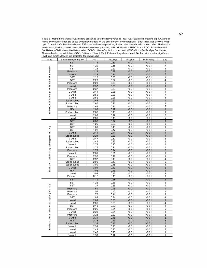
62
Area Enviromental variable GCV Adj. Rsq P-value B. P-value LagSST 1.11 0.67 <0.01 <0.01 0SST 1.20 0.65 <0.01 <0.01 6SST 1.28 0.62 <0.01 <0.01 5
Pressure 2.13 0.37 <0.01 <0.01 0V-wind 2.23 0.34 <0.01 <0.01 2
SST 2.26 0.33 <0.01 <0.01 1SST 2.28 0.32 <0.01 <0.01 4
Pressure 2.29 0.33 <0.01 <0.01 6U-wind 2.37 0.30 <0.01 <0.01 3
Pressure 2.37 0.30 <0.01 <0.01 1U-wind 2.44 0.28 <0.01 <0.01 4V-wind 2.50 0.26 <0.01 <0.01 1V-wind 2.52 0.26 <0.01 <0.01 3
Scalar cubed 2.63 0.22 <0.01 <0.01 0Scalar cubed 2.66 0.21 <0.01 <0.01 1
Pressure 2.68 0.21 <0.01 <0.01 5NOI 2.82 0.17 <0.01 <0.01 6
Scalar cubed 2.82 0.16 <0.01 <0.01 6U-wind 2.82 0.17 <0.01 <0.01 2U-wind 2.86 0.16 <0.01 <0.01 5
SST 0.83 0.77 <0.01 <0.01 0SST 1.25 0.66 <0.01 <0.01 6SST 1.89 0.48 <0.01 <0.01 1SST 1.92 0.47 <0.01 <0.01 5
V-wind 2.14 0.41 <0.01 <0.01 1Scalar cubed 2.24 0.38 <0.01 <0.01 1
V-wind 2.47 0.32 <0.01 <0.01 2Scalar cubed 2.49 0.32 <0.01 <0.01 2
V-wind 2.71 0.25 <0.01 <0.01 0Scalar cubed 2.77 0.24 <0.01 <0.01 0
Pressure 2.79 0.24 <0.01 <0.01 2V-wind 2.89 0.21 <0.01 <0.01 6
Pressure 2.96 0.19 <0.01 <0.01 1SST 2.97 0.18 <0.01 <0.01 4
Scalar cubed 2.99 0.18 <0.01 <0.01 6Scalar cubed 3.00 0.18 <0.01 <0.01 3
U-wind 3.04 0.17 <0.01 <0.01 2NOI 3.05 0.16 <0.01 <0.01 6
U-wind 3.08 0.16 <0.01 <0.01 3Pressure 3.12 0.15 <0.01 <0.01 6
SST 1.19 0.58 <0.01 <0.01 5SST 1.26 0.56 <0.01 <0.01 6SST 1.27 0.55 <0.01 <0.01 0
Pressure 1.54 0.46 <0.01 <0.01 0Pressure 1.57 0.45 <0.01 <0.01 1Pressure 1.70 0.41 <0.01 <0.01 6
SST 1.89 0.34 <0.01 <0.01 4U-wind 2.01 0.30 <0.01 <0.01 3U-wind 2.06 0.28 <0.01 <0.01 4
SST 2.18 0.23 <0.01 <0.01 1Pressure 2.25 0.21 <0.01 <0.01 5U-wind 2.25 0.21 <0.01 <0.01 2
Pressure 2.28 0.20 <0.01 <0.01 2V-wind 2.34 0.18 <0.01 <0.01 2
NOI 2.38 0.17 <0.01 <0.01 6Scalar cubed 2.39 0.16 <0.01 <0.01 0
V-wind 2.39 0.16 <0.01 <0.01 3U-wind 2.44 0.15 <0.01 <0.01 5U-wind 2.48 0.13 <0.01 <0.01 1V-wind 2.52 0.12 <0.01 <0.01 1
So
uth
ern
Cos
tal f
ish
ery
sub
regi
on
(<4
0° N
)
Table 2. Method one (null CPUE months converted to 0) monthly averaged (ln(CPUE)~s(Enviromental index)) GAM index model selections sumarized by top 20 ranked models for the entire region and subregions. Each index was allowed to lag up to 6 months. Varibles tested were: SST= sea surface temperature, Scalar cubed= scalar wind speed cubed,U-wind= U-wind stress, V-wind=V-wind stress, Pressuer=sea level pressure, MEI= Multivariate ENSO Index, PDO=Pacific Decadal Oscillation,NOI=Northern Oscillation Index, SOI=Southern Oscillation Index, and NPGO=North Pacific Gyre Oscillation. Genearalized cross validation (GCV), Estimated fit (Adj. Rsq), Estimated signifance level, Bonferroni corrected signifiance level, and months lagged are indicated for each model.
En
tire
Co
stal
fis
hery
(1
30°
E to
the
U.S
. co
ast
)N
ort
hern
Co
sta
l fis
hery
sub
reg
ion
(>
40°
N )
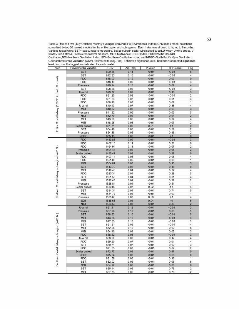
63
Area Enviromental variable GCV Adj. Rsq P-value B. P-value Lag
SST 809.55 0.11 <0.01 <0.01 5SST 812.83 0.10 <0.01 <0.01 4PDO 818.03 0.12 <0.01 0.09 0PDO 818.13 0.09 <0.01 <0.01 3
Pressure 820.94 0.10 <0.01 0.09 4SST 828.68 0.08 <0.01 <0.01 3
U-wind 829.77 0.09 <0.01 0.16 3PDO 831.25 0.08 <0.01 <0.01 2PDO 831.83 0.07 <0.01 0.01 4PDO 838.40 0.07 <0.01 0.02 1
U-wind 840.43 0.07 <0.01 0.36 4MEI 840.67 0.06 <0.01 0.03 3
Pressure 841.32 0.06 <0.01 0.03 5NOI 842.70 0.06 <0.01 0.04 2MEI 843.29 0.06 <0.01 0.04 4MEI 848.25 0.06 <0.01 0.07 2
Scalar cubed 851.71 0.06 0.01 >1 0SST 854.49 0.05 <0.01 0.59 2
Pressure 854.85 0.05 <0.01 0.16 2NPGO 855.13 0.05 <0.01 >1 0PDO 1453.86 0.09 <0.01 <0.01 3PDO 1462.16 0.11 <0.01 0.21 0PDO 1464.91 0.11 <0.01 0.07 2
Pressure 1494.41 0.06 <0.01 0.05 2Scalar cubed 1495.47 0.08 <0.01 0.87 0
PDO 1497.11 0.06 <0.01 0.06 4PDO 1501.08 0.06 <0.01 0.08 1MEI 1504.87 0.05 <0.01 0.10 3SST 1513.73 0.05 <0.01 0.18 0MEI 1519.48 0.04 <0.01 0.27 4PDO 1520.34 0.04 <0.01 0.29 5SST 1521.56 0.04 <0.01 0.31 4MEI 1522.46 0.04 <0.01 0.39 2
Pressure 1528.81 0.04 <0.01 0.51 1Scalar cubed 1530.89 0.07 0.02 >1 4
SST 1534.34 0.04 <0.01 0.74 5MEI 1534.77 0.04 <0.01 0.99 1
Pressure 1535.68 0.07 0.03 >1 4SOI 1535.68 0.04 0.04 >1 6NOI 1536.59 0.03 <0.01 0.86 2
U-wind 831.11 0.12 <0.01 <0.01 3Pressure 837.96 0.12 <0.01 0.03 5
SST 838.63 0.10 <0.01 <0.01 5MEI 843.58 0.10 <0.01 <0.01 4MEI 847.85 0.10 <0.01 <0.01 5SST 851.31 0.09 <0.01 <0.01 4MEI 852.08 0.10 <0.01 0.02 6MEI 854.40 0.09 <0.01 0.02 3PDO 858.52 0.08 <0.01 <0.01 3
U-wind 868.90 0.08 <0.01 0.17 4PDO 869.20 0.07 <0.01 0.01 4SST 869.71 0.07 <0.01 0.02 3PDO 871.05 0.07 <0.01 0.02 2
Scalar cubed 872.77 0.09 <0.01 0.47 0NPGO 875.54 0.08 <0.01 0.66 0PDO 881.58 0.06 <0.01 0.16 1SST 882.02 0.06 <0.01 0.06 6SOI 884.27 0.06 <0.01 0.08 6SST 885.44 0.06 <0.01 0.78 2MEI 887.73 0.05 <0.01 0.79 2
En
tire
Co
stal
fis
hery
(1
30°
E to
the
U.S
. co
ast
)N
ort
hern
Co
sta
l fis
hery
sub
reg
ion
(>
40°
N )
So
uth
ern
Cos
tal f
ish
ery
sub
regi
on
(<4
0° N
)
Table 3. Method two (July-October) monthly averaged (ln(CPUE)~s(Enviromental index)) GAM index model selections sumarized by top 20 ranked models for the entire region and subregions. Each index was allowed to lag up to 6 months. Varibles tested were: SST= sea surface temperature, Scalar cubed= scalar wind speed cubed,U-wind= U-wind stress, V-wind=V-wind stress, Pressuer=sea level pressure, MEI= Multivariate ENSO Index, PDO=Pacific Decadal Oscillation,NOI=Northern Oscillation Index, SOI=Southern Oscillation Index, and NPGO=North Pacific Gyre Oscillation. Genearalized cross validation (GCV), Estimated fit (Adj. Rsq), Estimated signifance level, Bonferroni corrected signifiance level, and months lagged are indicated for each model.
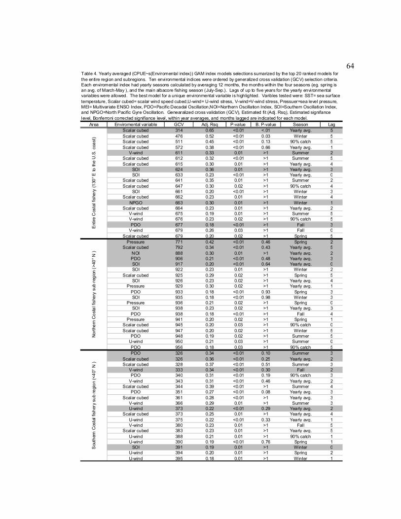
64
Area Enviromental variable GCV Adj. Rsq P-value B. P-value Season LagScalar cubed 314 0.65 <0.01 <.01 Yearly avg. 5Scalar cubed 476 0.52 <0.01 0.03 Winter 5Scalar cubed 511 0.45 <0.01 0.13 90% catch 5Scalar cubed 572 0.38 <0.01 0.66 Yearly avg. 1
V-wind 611 0.33 0.01 >1 Summer 2Scalar cubed 612 0.32 <0.01 >1 Summer 5Scalar cubed 615 0.30 0.01 >1 Yearly avg. 4
SOI 624 0.36 0.01 >1 Yearly avg. 3SOI 633 0.23 <0.01 >1 Yearly avg. 0
Scalar cubed 641 0.35 0.01 >1 Summer 2Scalar cubed 647 0.30 0.02 >1 90% catch 4
SOI 661 0.20 <0.01 >1 Winter 3Scalar cubed 662 0.23 0.01 >1 Winter 4
NPGO 663 0.30 0.01 >1 Winter 1Scalar cubed 664 0.23 0.01 >1 Yearly avg. 2
V-wind 675 0.19 0.01 >1 Summer 5V-wind 676 0.23 0.02 >1 90% catch 5PDO 677 0.18 <0.01 >1 Fall 3
V-wind 679 0.26 0.03 >1 Fall 0Scalar cubed 679 0.20 0.02 >1 Spring 5
Pressure 771 0.42 <0.01 0.46 Spring 2Scalar cubed 792 0.34 <0.01 0.43 Yearly avg. 5
NOI 888 0.30 0.01 >1 Yearly avg. 2PDO 906 0.21 <0.01 0.48 Yearly avg. 3SOI 917 0.20 <0.01 0.64 Yearly avg. 0SOI 922 0.23 0.01 >1 Winter 2
Scalar cubed 925 0.29 0.02 >1 Spring 5SOI 926 0.23 0.02 >1 Yearly avg. 4
Pressure 929 0.30 0.02 >1 Yearly avg. 1PDO 933 0.18 <0.01 0.93 Spring 3SOI 935 0.18 <0.01 0.98 Winter 3
Pressure 936 0.21 0.02 >1 Spring 0SOI 938 0.23 0.02 >1 Yearly avg. 3
PDO 938 0.18 <0.01 >1 Fall 4Pressure 941 0.20 0.02 >1 Spring 1
Scalar cubed 945 0.20 0.03 >1 90% catch 0Scalar cubed 947 0.20 0.02 >1 Winter 5
PDO 948 0.19 0.02 >1 Summer 5U-wind 950 0.21 0.03 >1 Summer 0PDO 956 0.18 0.03 >1 90% catch 5PDO 326 0.34 <0.01 0.10 Summer 3
Scalar cubed 326 0.36 <0.01 0.25 Yearly avg. 2Scalar cubed 328 0.37 <0.01 0.51 Summer 3
V-wind 333 0.34 <0.01 0.30 Fall 2PDO 340 0.31 <0.01 0.19 90% catch 3
V-wind 343 0.31 <0.01 0.46 Yearly avg. 2Scalar cubed 344 0.39 <0.01 >1 Summer 4
PDO 351 0.27 <0.01 0.08 Yearly avg. 3Scalar cubed 361 0.28 <0.01 >1 Yearly avg. 3
V-wind 366 0.29 0.01 >1 Summer 3U-wind 373 0.22 <0.01 0.29 Yearly avg. 2
Scalar cubed 373 0.25 0.01 >1 Yearly avg. 4U-wind 375 0.22 <0.01 0.33 Yearly avg. 1V-wind 380 0.23 0.01 >1 Fall 5
Scalar cubed 383 0.23 0.01 >1 Yearly avg. 5U-wind 388 0.21 0.01 >1 90% catch 1U-wind 390 0.19 <0.01 0.76 Spring 1
SOI 391 0.19 0.01 >1 Winter 0U-wind 394 0.20 0.01 >1 Spring 2U-wind 395 0.18 0.01 >1 Winter 1
Ent
ire C
osta
l fis
hery
(1
30°
E to
the
U.S
. co
ast
)N
ort
hern
Co
sta
l fis
hery
sub
reg
ion
(>
40°
N )
Sou
ther
n C
osta
l fis
her
y su
b re
gio
n (<
40°
N )
Table 4. Yearly averaged (CPUE~s(Enviromental index)) GAM index models selections sumarized by the top 20 ranked models for the entire region and subregions. Ten environmental indices were ordered by generalized cross validation (GCV) selection criteria. Each enviromental index had yearly seasons calculated by averaging 12 months, the months within the four seasons (eg. spring is an avg. of March-May ), and the main albacore fishing season (July-Sep.). Lags of up to five years for the yearly environmental variables were allowed. The best model for a unique environmental variable is highlighted. Varibles tested were: SST= sea surface temperature, Scalar cubed= scalar wind speed cubed,U-wind= U-wind stress, V-wind=V-wind stress, Pressuer=sea level pressure, MEI= Multivariate ENSO Index, PDO=Pacific Decadal Oscillation,NOI=Northern Oscillation Index, SOI=Southern Oscillation Index, and NPGO=North Pacific Gyre Oscillation. Genearalized cross validation (GCV), Estimated fit (Adj. Rsq), Estimated signifance level, Bonferroni corrected signifiance level, within year averages, and months lagged are indicated for each model.
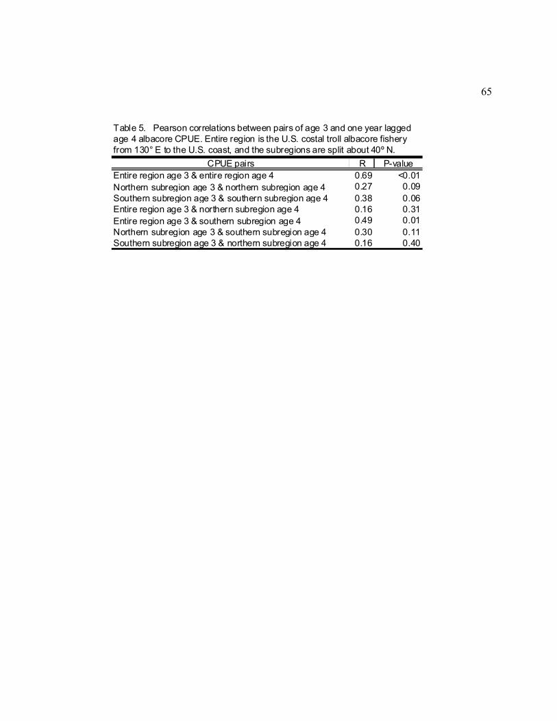
65
CPUE pairs R P-valueEntire region age 3 & entire region age 4 0.69 <0.01Northern subregion age 3 & northern subregion age 4 0.27 0.09Southern subregion age 3 & southern subregion age 4 0.38 0.06Entire region age 3 & northern subregion age 4 0.16 0.31Entire region age 3 & southern subregion age 4 0.49 0.01Northern subregion age 3 & southern subregion age 4 0.30 0.11Southern subregion age 3 & northern subregion age 4 0.16 0.40
Table 5. Pearson correlations between pairs of age 3 and one year lagged age 4 albacore CPUE. Entire region is the U.S. costal troll albacore fishery from 130° E to the U.S. coast, and the subregions are split about 40º N.
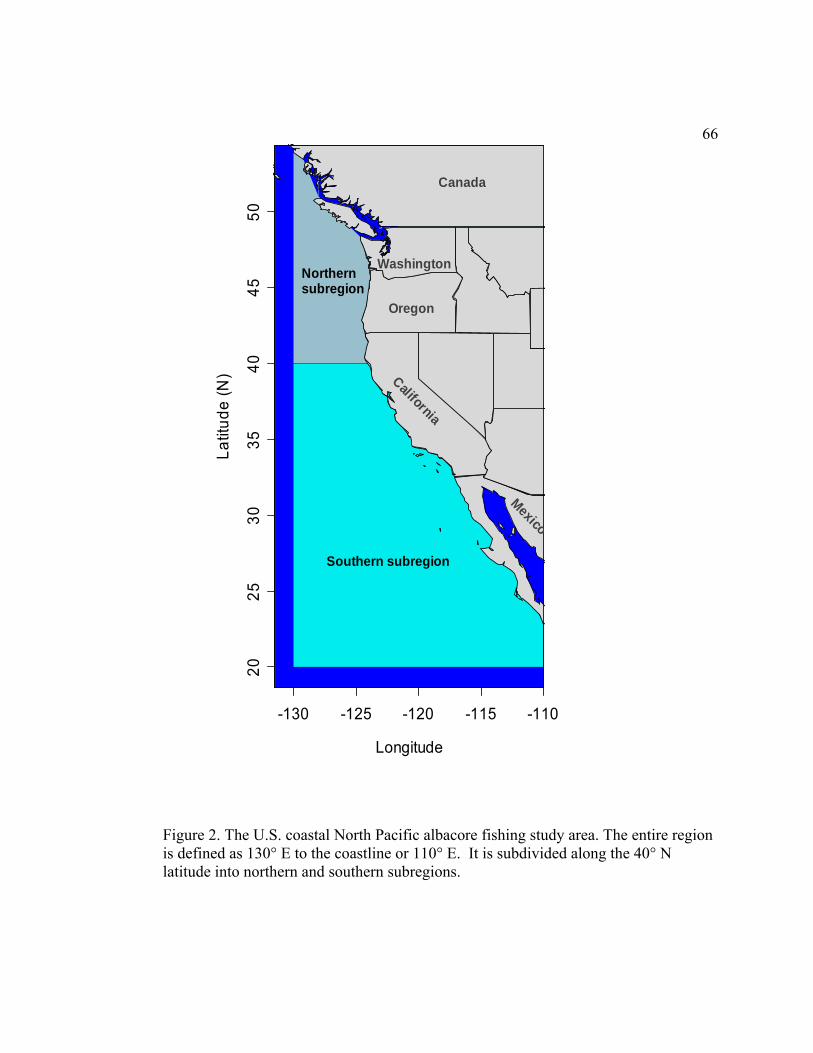
66
-130 -125 -120 -115 -110
20
25
30
35
40
45
50
Longitude
La
titu
de
(N
)
Washington
Oregon
California
Canada
Mexico
Northernsubregion
Southern subregion
Figure 2. The U.S. coastal North Pacific albacore fishing study area. The entire region is defined as 130° E to the coastline or 110° E. It is subdivided along the 40° N latitude into northern and southern subregions.
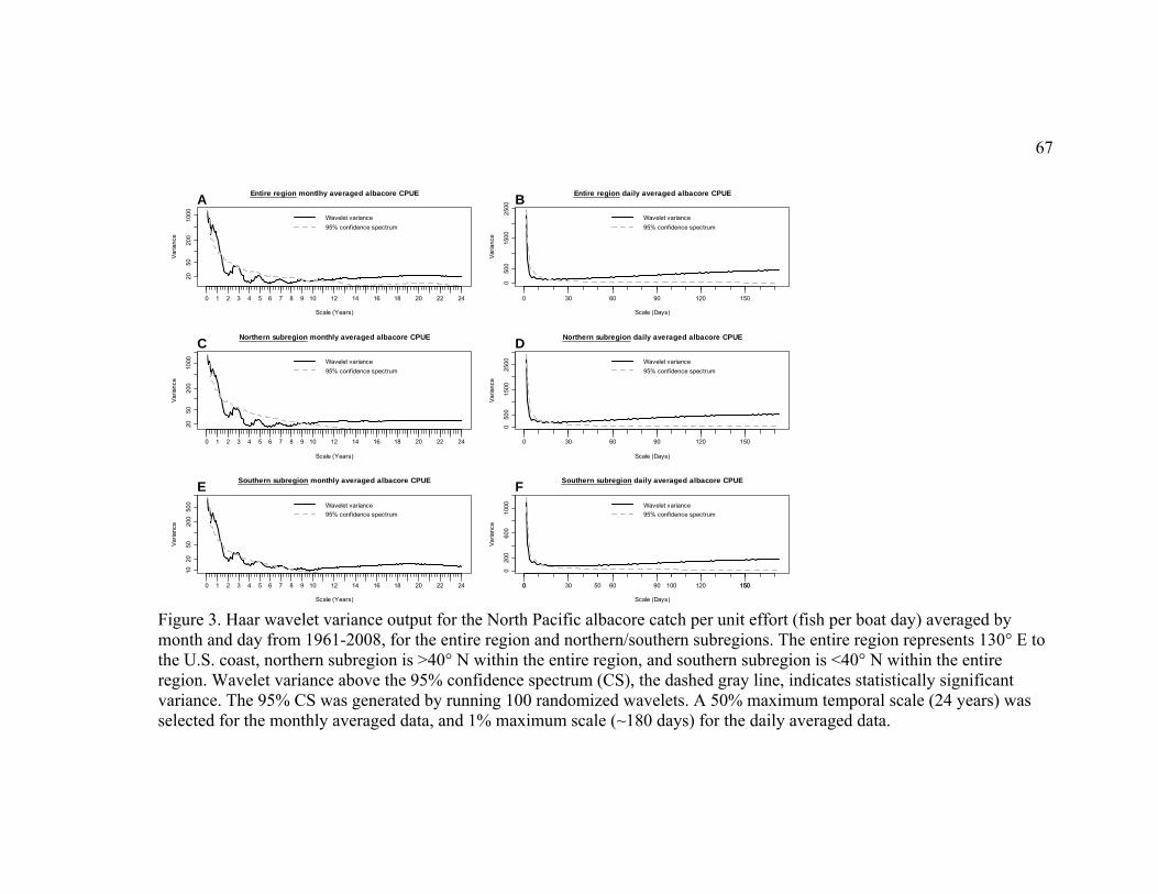
67
2050
200
1000
Entire region montlhy averaged albacore CPUE
Scale (Years)
Var
ianc
e
0 1 2 3 4 5 6 7 8 9 10 12 14 16 18 20 22 24
Wavelet variance
95% confidence spectrum
A
050
015
0025
00
Entire region daily averaged albacore CPUE
Scale (Days)
Var
ianc
e
0 30 60 90 120 150
Wavelet variance
95% confidence spectrum
B20
5020
010
00
Northern subregion monthly averaged albacore CPUE
Scale (Years)
Var
ianc
e
0 1 2 3 4 5 6 7 8 9 10 12 14 16 18 20 22 24
Wavelet variance
95% confidence spectrum
C
050
015
0025
00
Northern subregion daily averaged albacore CPUE
Scale (Days)
Var
ianc
e
0 30 60 90 120 150
Wavelet variance
95% confidence spectrum
D
1020
5020
050
0
Southern subregion monthly averaged albacore CPUE
Scale (Years)
Var
ianc
e
0 1 2 3 4 5 6 7 8 9 10 12 14 16 18 20 22 24
Wavelet variance
95% confidence spectrum
E
0 50 100 150
020
060
010
00
Southern subregion daily averaged albacore CPUE
Scale (Days)
Var
ianc
e
0 30 60 90 120 150
Wavelet variance
95% confidence spectrum
F
Figure 3. Haar wavelet variance output for the North Pacific albacore catch per unit effort (fish per boat day) averaged by month and day from 1961-2008, for the entire region and northern/southern subregions. The entire region represents 130° E to the U.S. coast, northern subregion is >40° N within the entire region, and southern subregion is <40° N within the entire region. Wavelet variance above the 95% confidence spectrum (CS), the dashed gray line, indicates statistically significant variance. The 95% CS was generated by running 100 randomized wavelets. A 50% maximum temporal scale (24 years) was selected for the monthly averaged data, and 1% maximum scale (~180 days) for the daily averaged data.
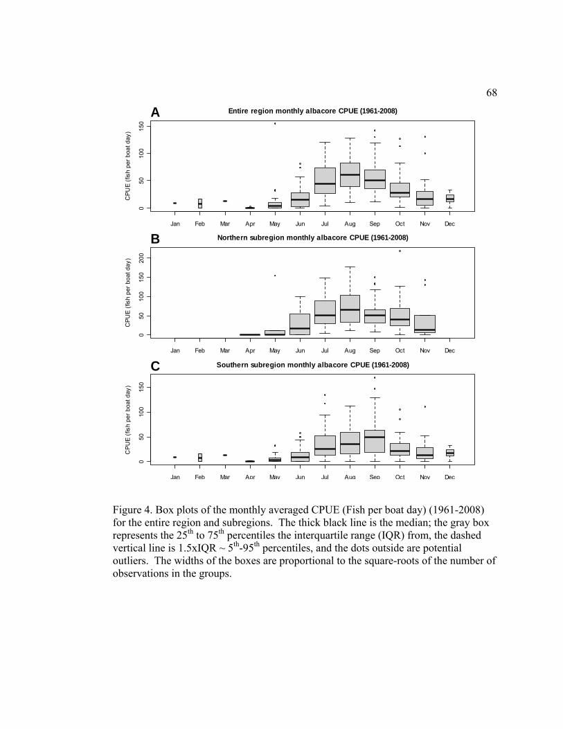
68
050
100
150
Entire region monthly albacore CPUE (1961-2008)
CP
UE
(fis
h pe
r bo
at d
ay)
Jan Feb Mar Apr May Jun Jul Aug Sep Oct Nov Dec
A
050
100
150
200
Northern subregion monthly albacore CPUE (1961-2008)
CP
UE
(fis
h pe
r bo
at d
ay)
Jan Feb Mar Apr May Jun Jul Aug Sep Oct Nov Dec
B
050
100
150
Southern subregion monthly albacore CPUE (1961-2008)
CP
UE
(fis
h pe
r bo
at d
ay)
Jan Feb Mar Apr May Jun Jul Aug Sep Oct Nov Dec
C
Figure 4. Box plots of the monthly averaged CPUE (Fish per boat day) (1961-2008) for the entire region and subregions. The thick black line is the median; the gray box represents the 25th to 75th percentiles the interquartile range (IQR) from, the dashed vertical line is 1.5xIQR ~ 5th-95th percentiles, and the dots outside are potential outliers. The widths of the boxes are proportional to the square-roots of the number of observations in the groups.

69
-1 0 1 2
-2-1
01
2
Sea Surface Temperature anomalies (lagged 0 mo.)
A
-3 -2 -1 0 1 2 3
-2-1
01
2
U w ind stress anomalies, eastw ard direction (lagged 3 mo.)
B
Eff
ec
t o
n lo
g-t
ran
sfo
rme
d m
on
thly
av
era
ge
d a
lba
co
re C
PU
E
-2 -1 0 1 2 3 4
-2-1
01
2
Scalar w ind speed cubbed anomalies (lagged 0 mo.)
C
-10 -5 0 5
-2-1
01
2
NOI index (lagged 6 mo.)
D
Figure 5. Entire region covariate partial effects on monthly averaged CPUE multiple variable generalized additive model (GAM) with missing CPUE months were converted to 0 CPUE (method one). The model with the lowest generalized cross validation was selected from a stepwise backward selection process, which initially included six terms from the entire region in Table 2. Shaded areas are 95% confidence intervals, and tick marks on the x-axis indicate sampling intensity.

70
-1 0 1 2
-2-1
01
23
Sea Surface Temperature anomalies (lagged 0 mo.)
A
-10 -5 0 5
-2-1
01
23
NOI index (lagged 3 mo.)
B
Eff
ec
t o
n lo
g-t
ran
sfo
rme
d m
on
thly
av
era
ge
d a
lba
co
re C
PU
E
Figure 6. Northern subregion covariate partial effects on monthly averaged CPUE multiple variable generalized additive model (GAM) with missing CPUE months were converted to 0 CPUE (method one). The model with the lowest generalized cross validation was selected from a stepwise backward selection process, which initially included six terms from the northern subregion in Table 2. Shaded areas are 95% confidence intervals, and tick marks on the x-axis indicate sampling intensity.

71
-1 0 1 2
-2-1
01
2
Sea Surface Temperature anonalies (lagged 5 mo.)
A
-4 -2 0 2 4
-2-1
01
2
U w ind stress anonalies, eastw ard direction (lagged 3 mo.)
B
Eff
ec
t o
n lo
g-t
ran
sfo
rme
d m
on
thly
av
era
ge
d a
lba
co
re C
PU
E
-2 -1 0 1 2 3 4 5
-2-1
01
2
Scalar w ind speed cubbed anonalies (lagged 0 mo.)
C
Figure 7. Southern subregion covariate partial effects on monthly averaged CPUE multiple variable generalized additive model (GAM) with missing CPUE months were converted to 0 CPUE (method one). The model with the lowest generalized cross validation was selected from a stepwise backward selection process, which initially included six terms from the northern subregion in Table 2. Shaded areas are 95% confidence intervals, and tick marks on the x-axis indicate sampling intensity.

72
-1.5 -1.0 -0.5 0.0
-40
-20
020
Sea Surface Temperature anomalies (lagged 5 mo.)
A
-2 -1 0 1 2 3
-40
-20
020
PDO index (lagged 0 mo.)
B
Eff
ec
t o
n m
on
thly
av
era
ge
d (
Ju
ly-O
cto
be
r) a
lba
co
re C
PU
E
-2 -1 0 1 2
-40
-20
020
U w ind stress anomalies, eastw ard direction (lagged 3 mo.)
C
Figure 8. Entire region covariate partial effects on monthly averaged CPUE multiple variable generalized additive model (GAM) reduced to months from July to October (method two). The model with the lowest generalized cross validation was selected from a stepwise backward selection process, which initially included eight terms from the entire region in Table 3. Shaded areas are 95% confidence intervals, and tick marks on the x-axis indicate sampling intensity.
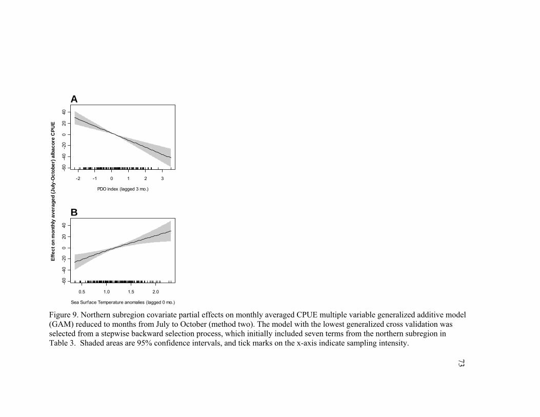
73
-2 -1 0 1 2 3
-60
-40
-20
020
40
PDO index (lagged 3 mo.)
A
0.5 1.0 1.5 2.0
-60
-40
-20
020
40
Sea Surface Temperature anomalies (lagged 0 mo.)
B
Eff
ec
t o
n m
on
thly
av
era
ge
d (
Ju
ly-O
cto
be
r) a
lba
co
re C
PU
E
Figure 9. Northern subregion covariate partial effects on monthly averaged CPUE multiple variable generalized additive model (GAM) reduced to months from July to October (method two). The model with the lowest generalized cross validation was selected from a stepwise backward selection process, which initially included seven terms from the northern subregion in Table 3. Shaded areas are 95% confidence intervals, and tick marks on the x-axis indicate sampling intensity.
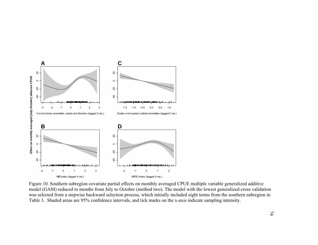
74
-3 -2 -1 0 1 2 3
-40
-20
020
U w ind stress anomalies, eastw ard direction (lagged 3 mo.)
A
-2 -1 0 1 2 3
-40
-20
020
MEI index (lagged 4 mo.)
B
Eff
ec
t o
n m
on
thly
av
era
ge
d (
Ju
ly-O
cto
be
r) a
lba
co
re C
PU
E
-1.5 -1.0 -0.5 0.0 0.5 1.0
-40
-20
020
Scalar w ind speed cubbed anomalies (lagged 0 mo.)
C
-2 -1 0 1 2
-40
-20
020
NPGO index (lagged 0 mo.)
D
Figure 10. Southern subregion covariate partial effects on monthly averaged CPUE multiple variable generalized additive model (GAM) reduced to months from July to October (method two). The model with the lowest generalized cross validation was selected from a stepwise backward selection process, which initially included eight terms from the southern subregion in Table 3. Shaded areas are 95% confidence intervals, and tick marks on the x-axis indicate sampling intensity.

75
-0.5 0.0 0.5 1.0
-20
020
4060
80
Yr avg. scalar w ind speed cubbed anomalies (lagged 5 yr.)
A
-2 -1 0 1 2
-20
020
4060
80
Winter NPGO index (lagged 2 yr.)
B
Eff
ect
on y
earl
y a
vera
ged a
lbaco
re C
PU
E
-2 -1 0 1
-20
020
4060
80
Fall PDO index (lagged 3 yr.)
C
Figure 11. Entire region covariate partial effects on yearly averaged CPUE multiple variable generalized additive model (GAM) 1961-2008. The model with the lowest generalized cross validation was selected from a stepwise backward selection process, which initially included five terms from the entire region in Table 4. Shaded areas are 95% confidence intervals, and tick marks on the x-axis indicate sampling intensity.
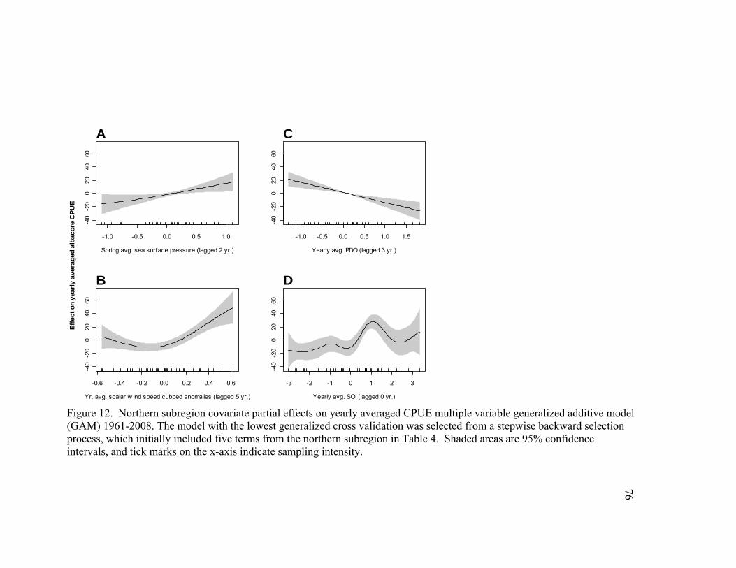
76
-1.0 -0.5 0.0 0.5 1.0
-40
-20
020
4060
Spring avg. sea surface pressure (lagged 2 yr.)
A
-0.6 -0.4 -0.2 0.0 0.2 0.4 0.6
-40
-20
020
4060
Yr. avg. scalar w ind speed cubbed anomalies (lagged 5 yr.)
B
Eff
ect
on y
earl
y a
vera
ged a
lbaco
re C
PU
E
-1.0 -0.5 0.0 0.5 1.0 1.5
-40
-20
020
4060
Yearly avg. PDO (lagged 3 yr.)
C
-3 -2 -1 0 1 2 3
-40
-20
020
4060
Yearly avg. SOI (lagged 0 yr.)
D
Figure 12. Northern subregion covariate partial effects on yearly averaged CPUE multiple variable generalized additive model (GAM) 1961-2008. The model with the lowest generalized cross validation was selected from a stepwise backward selection process, which initially included five terms from the northern subregion in Table 4. Shaded areas are 95% confidence intervals, and tick marks on the x-axis indicate sampling intensity.

77
-1 0 1 2
-20
020
40
Summer avg. PDO index (lagged 3 yr.)
A
-0.5 0.0 0.5 1.0
-20
020
40
Yr. avg. scalar w ind speed cubbed anomalies (lagged 2 yr.)
B
Eff
ect
on y
earl
y a
vera
ged a
lbaco
re C
PU
E
-0.5 0.0 0.5 1.0
-20
020
40
V w ind stress anomalies, northw ard direction (lagged 2 yr.)
C
-1.5 -1.0 -0.5 0.0 0.5 1.0
-20
020
40
U w ind stress anomalies, eastw ard direction (lagged 2 yr.)
D
Figure 13. Southern subregion covariate partial effects on yearly averaged CPUE multiple variable generalized additive model (GAM) 1961-2008. The model with the lowest generalized cross validation was selected from a stepwise backward selection process, which initially included five terms from the southern subregion in Table 4. Shaded areas are 95% confidence intervals, and tick marks on the x-axis indicate sampling intensity.
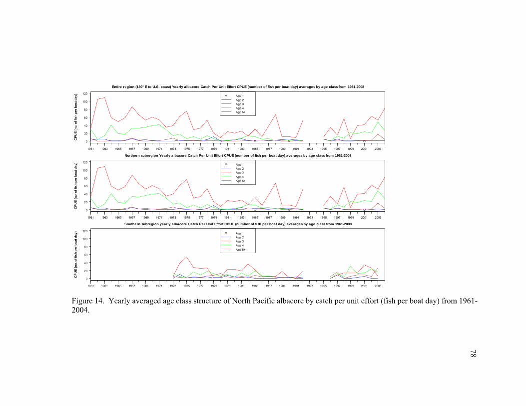
78
0
20
40
60
80
100
120
Entire region (130° E to U.S. coast) Yearly albacore Catch Per Unit Effort CPUE (number of fish per boat day) averages by age class from 1961-2008
Age 1
Age 2Age 3Age 4Age 5+
CP
UE
(n
o. o
f fi
sh
pe
r b
oa
t d
ay
)
1961 1963 1965 1967 1969 1971 1973 1975 1977 1979 1981 1983 1985 1987 1989 1991 1993 1995 1997 1999 2001 2003
0
20
40
60
80
100
120
Northern subregion Yearly albacore Catch Per Unit Effort CPUE (number of fish per boat day) averages by age class from 1961-2008
Age 1Age 2Age 3
Age 4Age 5+
CP
UE
(n
o. o
f fi
sh
pe
r b
oa
t d
ay
)
1961 1963 1965 1967 1969 1971 1973 1975 1977 1979 1981 1983 1985 1987 1989 1991 1993 1995 1997 1999 2001 2003
0
20
40
60
80
100
120
Southern subregion yearly albacore Catch Per Unit Effort CPUE (number of fish per boat day) averages by age class from 1961-2008
Age 1Age 2Age 3Age 4
Age 5+
CP
UE
(n
o. o
f fi
sh
pe
r b
oa
t d
ay
)
1961 1963 1965 1967 1969 1971 1973 1975 1977 1979 1981 1983 1985 1987 1989 1991 1993 1995 1997 1999 2001 2003 Figure 14. Yearly averaged age class structure of North Pacific albacore by catch per unit effort (fish per boat day) from 1961-2004.

79
-0.5 0.0 0.5 1.0
-20
010
2030
4050
Scalar w ind speed cubbed anomalies (lagged 5 yr.)
AE
ffe
ct on y
earl
y a
ve
rage
d a
ge-3
alb
ac
ore
CP
UE
Figure 15. Entire region effect of scalar wind speed cubed lagged 5 years on yearly averaged age-3 CPUE generalized additive model (GAM) 1961-2008. Shaded areas are 95% confidence intervals, and tick marks on the x-axis indicate sampling intensity.GAM plot of yearly averaged entire region age-3 albacore CPUE vs. 5 year lagged scalar wind speed cubed.
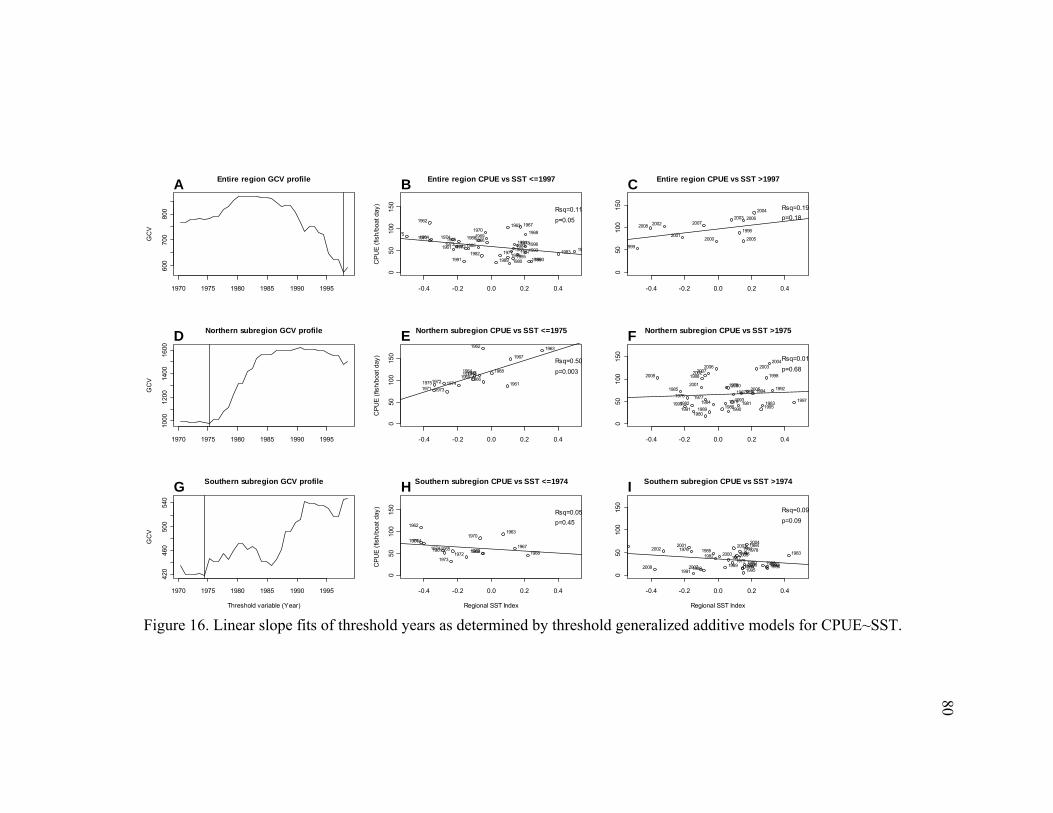
80
1970 1975 1980 1985 1990 1995
600
700
800
Entire region GCV profile
GC
V
A
-0.4 -0.2 0.0 0.2 0.4
050
100
150
Entire region CPUE vs SST <=1997
CP
UE
(fis
h/bo
at d
ay)
1963 1967
1968
1977
1978
19791980
1981 19831984
1986
1987
1989 1990
1993
1994
1995
1996191961
1962
1964 1965 19661969
1970
1971
19721973
197475
1976
1982
1985
1988
1991
Rsq=0.11
p=0.05
B
-0.4 -0.2 0.0 0.2 0.4
050
100
150
Entire region CPUE vs SST >1997
1998
2003
2004
2005
2006
999
20002001
2002 20072008
Rsq=0.19
p=0.18
C
1970 1975 1980 1985 1990 1995
1000
1200
1400
1600
Northern subregion GCV profile
GC
V
D
-0.4 -0.2 0.0 0.2 0.4
050
100
150
Northern subregion CPUE vs SST <=1975
CP
UE
(fis
h/bo
at d
ay)
1961
1963
1967
1968
1962
1964196519661969
1970
1971
1972
197319741975
E
Rsq=0.50
p=0.003
-0.4 -0.2 0.0 0.2 0.4
050
100
150
Northern subregion CPUE vs SST >1975F
1978
1979 1981 19831986
1987
1990
1992
1993
1994
1995
1996
1997
1998
2000
20032004
20051976 1977
1980
1982 1984
1985
1988
198919911999
2001
20022006
20072008
Rsq=0.01
p=0.68
1970 1975 1980 1985 1990 1995
420
460
500
540
Southern subregion GCV profile
Threshold variable (Year)
GC
V
G
-0.4 -0.2 0.0 0.2 0.4
050
100
150
Southern subregion CPUE vs SST <=1974
Regional SST Index
CP
UE
(fis
h/bo
at d
ay)
1963
19671968
1961
1962
1964
1965 19661969
19701971
19721973
1974
H
Rsq=0.05
p=0.45
-0.4 -0.2 0.0 0.2 0.4
050
100
150
Southern subregion CPUE vs SST >1974
Regional SST Index
I
1977
1978
1979 1980
19811983
1984
198619871989 1990199319941995
1996
19982000
20032004
2005
2006
19761982
1985
19881991
20012002
20072008
Rsq=0.09
p=0.09
Figure 16. Linear slope fits of threshold years as determined by threshold generalized additive models for CPUE~SST.

81
0 2000 4000 6000 8000
Total number of boat days per year
1961
1962
1963
1964
1965
1966
1967
1968 1969
1970
1971
1972
1973
1974
1975
1976
1977
1978
1979
1980
1981198219831984
1985
1986
1987
1988
198919901991
1992
1993
1994
1995
19961997
1998 1999
2000
20012002
2003
2004 2005
2006 2007
2008
Northern subregionSouthern subregion
Catc
h (100,0
00's
of a
lbaco
re)
0
2
4
6
8
10
12
1961
196
1963
1964
1965
196619671968
1969
1970
1971
1972
1973
19741975
1976
1977
1978
1979
1980
1981
1982
1983
1984
1985
19861987198819891990199119921993199419951996
19971998
1999
20002001
2002200320042005200620072008
Figure 17. Linear fits of yearly (1961-2008) catch vs effort for northern and southern subregions.

82CHAPTER 3: SPATIO-TEMPORAL ASSOCIATIONS BETWEEN ALBACORE CPUE AND LARGE-SCALE ENVIRONMENTAL VARIABLES IN THE NORTHEASTERN PACIFIC.
3.1 Abstract
The purpose of this study is to analyze the spatial distribution of juvenile North
Pacific albacore in relation to local environmental variability and large scale indices of climate
variability. Specifically, changes in local sea surface temperature (SST) obtained from the
International Comprehensive Ocean-Atmosphere Data Set (ICOADS), the Pacific Decadal
Oscillation (PDO), and the Multivariate El Niño/Southern Oscillation Index (MEI) were
correlated to 48 years of albacore troll catch per unit effort (CPUE) at 1° latitude/longitude
cells. Visual inspection of distribution patterns indicated that albacore CPUE positively
respond to SST, but showed inconsistent patterns in relation to MEI. To statistically validate
these patterns, generalized additive models (GAM) were used to investigate albacore spatial
temporal distributions in relation to SST, MEI, and PDO. Model terms were included to
account for nonstationary and spatially variable effects of the targeted variables on albacore
CPUE. Results indicate that albacore CPUE rates increased with SST both before and after
the threshold year of 1977, but geographically contracted to the north after 1977. SST had a
predominantly positive but spatially-variable effect on albacore CPUE, while the PDO had an
overall negative effect. Specifically, CPUE was found to increase with increased SST,
particularly off of Oregon and Washington, and it appears that albacore shift north and
shoreward as PDO and SST increase. These results imply that if ocean temperatures continue
to increase, west coast communities reliant on commercial albacore fisheries are likely to be
negatively impacted in the southern areas but positively benefited in the northern areas, where
current albacore landings are highest.
833.2 Introduction
North Pacific albacore (Thunnus alalunga) is an economically important temperate
tuna species distributed across the North Pacific (Sund et al. 1981; Miyake et al. 2004; Ellis
2008; Laurs and Powers 2010; Childers et al. 2011). Juvenile albacore are primarily
epipelagic, spending most of their time above the thermocline. They are known to have
specific sea surface temperature (SST) preferences ranging from 15–19.5° C, and centered
around 17.5° C (Clemens 1961; Flittner 1963; Laurs et al. 1977; Childers et al. 2011). This
preference has been well documented at relatively fine scales, as well as at larger scales over
longer time periods. An unexpected result of the time series analysis in Chapter 2 was that
weak associations were found between climate indices indicative of the thermal regime of the
subtropical and temperate waters in the North Pacific and albacore CPUE within a year (see
Section 2.4.3). The apparent weak association at large geographical scales may be explained
by local distributional changes of albacore in response to local environmental variability.
To date the large scale distribution preferences of the North Pacific albacore are
poorly known (Barr 2009; Laurs 2010). However, several studies and anecdotal evidence
indicate that this species exhibits large distributional shift in response to changes in local
environmental variability (Laurs et al. 1977; Barr 2009; Childers et al. 2011). Climate-related
forcing appears to indirectly and nonlinearly affect the distribution of several tuna species, and
may influence juvenile North Pacific albacore. West coast North Pacific albacore is an
important fishery with ex-vessel revenue averaged over 21 million annually (inflation
accounted for) between 1981 and 2009 (PFMC 2010). However, albacore landings are highly
variable in total numbers and geographically from year to year. Thus, the economies of local
84communities along the west coast which are based on the harvesting of albacore are likely to
be impacted in response to climatic changes.
Most studies that have looked at spatial dynamics of albacore and other tuna
distributions have found them sensitive to ocean surface features and climate regime shifts.
Sagarminga and Arrizabalaga (2010) found a close spatio-temporal relationship with a
preferred SST window (16-18º C) and seasonal progression of the juvenile northeastern
Atlantic albacore fishery. Dufour et al. (2010) found juvenile north Atlantic albacore mean
catch trended northward in latitude over time, and Atlantic albacore catches were positively
related to 17º C SST. Dufour et al. (2010) also determined that mean CPUE distributions of
Atlantic albacore changed after the North Atlantic regime shift. Surface features such as SST
were found to be important predictors of the spatial distribution of CPUE in the Indian Ocean
(Chen et al. 2005). Skipjack in the southwestern Atlantic were found to show a North South
displacement of CPUE which was strongly associated with seasonal variation of SST
(Andrade 2003). The Spatio-temporal distribution of Pacific yellowfin and bigeye were found
to be positively associated with higher SST during both El Niño and La Niña years (Lu et al.
2001). This survey indicates that SST, large scale environmental indices, and climatic regime
shifts appear to be important to albacore and other tuna species in several oceans. This chapter
investigates the spatio-temporal distribution of juvenile (2-5 years old) North Pacific albacore
off of the U.S. west coast in relation to ocean thermal conditions such as sea surface
temperature (SST), with consideration of two large scale indices (MEI and PDO) and the
North Pacific regime shift of 1977.
85
3.3 Material & Methods
3.3.1 Data
Commercial North Pacific albacore logbook data were provided by the National
Oceanic and Atmospheric Administration (NOAA) Southwest Fisheries Science Center
(SWFSC). From 1961 to 2008, monthly catch-per-unit-effort (CPUE) was calculated at 1° x
1° spatial resolution (cells hereafter) for troll-caught juvenile albacore in the U.S. coastal
fishery. The U.S. coastal fishery (study area hereafter) is defined as the area from 130° W to
the U.S. coastline and north of 20° N, described in Section 2.2.
To explore albacore spatial distributions in relation with SST and temperature-related
anomalies the following variables were obtained at the monthly scale: 1) SST from the
International Comprehensive Ocean-Atmosphere Data Set (ICOADS) at 1° x 1° resolution, 2)
the Pacific Decadal Oscillation (PDO) (http://jisao.washington.edu ), and 3) the multivariate
El Niño/ Southern Oscillation Index (MEI)
(www.esrl.noaa.gov/psd/people/klaus.wolter/MEI). (see Section 2.2.2 for a detailed
explanation of the variables used.)
3.3.2 Monthly CPUE and SST trends by latitude with MEI
The monthly analysis was primarily descriptive and aimed at visually characterizing
latitudinal patterns of seasonal and interannual distribution in relation to SST. Monthly
albacore CPUEs by one degree latitude bins were calculated by dividing the monthly sum of
daily catch by the monthly sum of daily effort in each 1° latitude bin within the study area.
Average SST (° C) was calculated by averaging the ICOADS monthly SST cells in Figure 18
for each 1° degree latitude bin. SST was plotted by month with the CPUE overlaid to show
86trends in latitudinal-temporal shifts of CPUE. The MEI index was also added to the CPUE
SST time series but as a single line.
The monthly latitudinal-temporal CPUE and SST was binned by 1º C increments and
plotted for the entire time series in order to determine how albacore CPUE might relate to
local SST. A Tukey’s honest significance test was conducted to determine if any of the CPUE
means in the 1º C bins were significantly different from one another (Ramsey and Schafer
2002).
3.3.3 Yearly state-space analysis
Generalized additive models (GAMs) were used to investigate albacore spatial
temporal distributions in relation to SST, MEI, and PDO, using the mgcv package in R
(v2.10.1) software (Wood 2006). I tested for the effects of geography and environmental
variability on the distribution of albacore CPUE. Furthermore, I included terms to account for
nonstationary and spatially variable effects of the targeted variables on albacore CPUE.
Specifically, CPUE was modeled with four competing formulations: 1) spatial, 2) spatial and
environmental, 3) spatially variant, and 4) nonstationary. The spatial GAM model assumes
that albacore distribution along the studied region is only affected by geography, and that
CPUE variations are due to interannual changes of albacore stock size. The spatial and
environmental formulation included environmental covariates (SST, PDO, and MEI), in
addition to the spatial term, and assumed that all the environmental covariates are
independently and therefore additively affecting albacore CPUE. The spatially variant
formulation allowed the environmental covariate to smoothly change in relation to the
geographical location and tested for the spatially variable effects of SST (Ciannelli et al. 2007;
Bacheler et al. 2009; Bartolino et al 2011).
87Nonstationarity was investigated because in 1976-1977 a regime shift occurred in
North Pacific. The regime shift has been well documented by rapid physical and biological
changes which occurred over a short time period, and persisted for decades in the North
Pacific ecosystem (Pearcy and Schoener 1987; Ebbesmeyer et al., 1991; Miller et al., 1994;
McGowan et al. 2003). This climate shift brought changes that resulted in warmer surface
temperatures, declines in species populations, changes in species community structure, and/or
northward species range shifts over large scales across trophic levels (Pearcy and Schoener
1987; McGowan et al. 2003). Additionally, the albacore time series analysis in Chapter 2
detected threshold changes in the mid 1970’s. Thus, the nonstationary formulation, as
expansion of model 3, was used to address nonstationary effects coinciding with the 1977
regime shift.
Models selection was based on Generalized Cross Validation (GCV) and Akaike
Information Criterion (AIC). The GCV is a measure of the prediction error, and lower GCV
scores indicated a lower prediction error. The AIC is a measure of the relative goodness of fit
between competing models, and whichever model has the lowest AIC performed the best.
The AIC is a way to compare competing models, and is not a test of how well a model
performed (Burnham and Anderson 2002). Additionally, the analysis was restricted to cells
with six or more years of CPUE observations, roughly 10% of the years which had spatial
data. This restriction was applied to prevent cells with relatively few years of observations
from being overly influential.
The spatial formulation is:
1) ),(y,1),(y, e),(s=x
),(y,x = ln(CPUE + 1) at ( , ) in y.

88( , ) = given location by longitude and latitude degrees within the study area
y = given year from 1961-2008
1s = 2-dimensional smoothing function (thin plate regression spline, Wood 2004) e = normally distributed random error term with constant variance and a mean of 0
The spatial and environmental formulation included a spatial term and assumed
spatially invariant and additive environmental effects. I also tested to determine if the addition
of a large scale climate index improved the model type 2. Therefore, MEI or PDO which
capture low frequency environmental variability were included additively. However, both
MEI and PDO were not allowed in the same model to avoid collinearity, as they were highly
correlated (R=0.69). This resulted in three spatial and environmental models. Namely,
2a) ),(y,1),(),(y, e),(s][SSTg=x 1
2b) ),(y,1),(),(),(y, e),(s][PDOg+][SSTg=x 21
2c) ),(y,1),(),(),(y, e),(s][MEIg+][SSTg=x 21
ig = 1-dimensional smoothing function (thin plate regression spline, Wood 2004)
The spatially variant formulation was an expansion of the highest ranked model type
2, in which the environmental effect was made spatially variable by assuming a variable
coefficient formulation. Variable coefficient GAM allows the coefficients to smoothly change
in relation to geographical position (Bacheler et al. 2009, 2010; Bartolino et al. 2011;
Ciannelli et al. in prep). The SST was made into a spatially variable coefficient to account
for local variability between SST and CPUE (at the one degree cell level). The PDO was
treated as a fully additive variable, because it is a large scale index and not spatially variable.
3) ),(y,),(1),(),(y, eSST),(s+),(s][PDOg=x 21

89
Finally, the nonstationary was an expansion of type 3 which had a spatial term,
assumed spatially-variable effects of SST, and additive effects of PDO. Additionally, model
type 4 further assumed nonstationary effects in the relationship between SST and CPUE as an
abrupt change coinciding with the regime shift of 1977. The threshold year of 1977 is
supported by the time series threshold analysis in Chapter 2 which indicated that the albacore
CPUE time series is non-stationary, specifically near the PDO regime shift of 1977.
4)
23
12
1
ThSST),(s
ThSST),(s+
e),(s][PDOg=x
),(
),(
),(y,1),(),(y,
1Th = 1 if <1977 else 0
2Th = 1 if ≥1977 else 0

90
3.4 Results
3.4.1. Monthly CPUE and SST trends by latitude with MEI
Latitudinal temporal mapping of monthly averaged CPUE overlaid with SST cells
revealed several spatial trends (Figs. 19 and 20). The most apparent pattern was a positive
correlation between SST and albacore CPUEs. For approximately half of the years in the time
series, the fishery began in June to the south and as the season progressed, there was a
poleward shift in latitude of the fishery with increasing CPUE rates. However, this pattern is
not observed for the entire duration of the time series. Some years (e.g., 1970) showed an
equatorward shift of the fishery. The mean positive albacore CPUE (zero catches removed)
occurred in SST cells of 15.5° C (±1.69 SD), range 9.8-22.7 ° C, and 75% of the positive
CPUE occurred in cells with SST ranging from 14.4 to 16.5° C. When zero catch is included
in the CPUE, which was normalized and binned into 1° C intervals, a similar trend to the
positive only CPUE was found (Fig. 21). The highest CPUEs (zero catch included) occurred
in cells with SST between 15-17° C, but it was not statistically significant from any the cells
above 15° as indicated by a Tukey’s honest significant difference test.
MEI values shown in Figs. 19 and 20 display no clear visual trends in relation to
latitudinal CPUE over the entire time series. During some positive MEI episodes (e.g., 1965,
1972 and 1994) the fishery shifted north and began later (July) than in the previous year.
However, other positive MEI episodes (e.g., 1963, 1983, 1991, 1997, and 1998) show no
distributional shift from the previous year’s fishery. Inconsistent patterns were also found
between the CPUE and negative MEI. For example, southern distributional shifts occurred in
some years with negative MEI (e.g., 1964, 1970 and 1999) while other negative MEI episodes
(e.g., 2008) did not show a marked change from the previous year.
91The highest CPUEs occurred in cells with SST between 15-17° C, but it was not
statistically significant from any the cells above 15° as indicated by a Tukey’s honest
significant difference test.
3.4.2 Yearly spatio-temporal analysis
After removing cells with fewer than 6 years of albacore CPUE, 4561 samples
remained out of the 4704 initial observations. The yearly averaged cells of CPUE ranged from
0 to 1093 fish per boat day with a mean CPUE of 50. The best-fit model identified from the
four competing formulations was the 4) nonstationary (Table 6 and Fig. 26), as indicated by
adjusted R2, GCV, and AIC scores. Formulation performance decreased with all other models
as follows: 3) spatially variant, 2) spatial and environmental, and 1) spatial. Model 2b),
which included SST and PDO, was determined to be the best spatial and environmental model
as indicated by minimized GCV and AIC scores (Table 6 and Fig. 25). The covariates in all of
the formulations were highly significant (P-values <0.01) (Table 6).
Based on the 1) spatial formulation, the highest densities of albacore CPUEs occurred
off of central Oregon at approximately 45º N, and a secondary density peak occurred off of
central California near 35º N (Fig. 22). However, once the environmental variability was
modeled, a secondary peak was no longer evident in the spatial distribution, and only a single
core concentration remained, centered off of central Oregon (Figs. 22-25), with one exception.
Model 3) spatially variant shows two core concentrations of CPUE. One off of central Oregon
and central California (Fig. 25). However, in model 3) the core density in the south is
negatively associated with the local effects SST and positively in the north, as indicated by the

92estimated local effects in Figure 23. Thus, Figure 23 is showing a similar trend to the other
formulations which included environmental variability.
The 4) nonstationary formulation shows that albacore CPUE was highest off of
central Oregon at approximately 45º N 126º W (Fig. 26 A). The effect of the PDO was
negative (Fig. 26 C), as was the case in other models tested, which included a PDO term (Figs.
23 C, 25 B, and 27). The significant local SST effects located within the core concentration of
CPUEs were positive in time periods before and after the North Pacific regime shift as
indicated by the positive estimated slopes in Figure 26 A and B. Positive effects observed off
of southern California, and the negative effect observed after the regime shift are dubious,
because average CPUE in those areas tend to be very low. In the time period before the 1977
regime shift, the variable effects of SST were found outside the core area parallel with the
California coastline, and after the regime shift the variable effects of SST were contracted
northward. In addition to contracting geographically, the overall effect of SST on CPUE was
less influential after 1977, as indicated by a 67 percent reduction in absolute magnitude (Fig
25A &B).
As an add hoc analysis, SST and PDO were switched from model type three, SST was
invariant and PDO was forced to be spatially variant (Fig. 27). Although PDO is not truly
spatially variant, it is found to have stronger negative relationships in southern core CPUE
areas, as indicated by the larger blue bubbles (Fig. 27).
93
3.5 Discussion
My results suggest that Albacore CPUE have contracted northward after the 1977
North Pacific regime shift, and that increasing SST resulted in northward and coastal
movement of albacore (Figs. 20,21 & 25). Dufour et al. (2010) concluded that juvenile
Atlantic albacore were able to respond rapidly to regime shifts, and this appears to have
occurred with North Pacific albacore as well. The PDO switched to a warm phase after 1977,
and it appears that the warm phase of the PDO and higher SST are both related to each other.
However, they may be unrelated because they influence the albacore at different spatial scales.
Other studies have found North Pacific Albacore rapidly respond to changes in local SST (e.g.
Laurs and Lynn 1977), but this is one of the first studies to find juvenile North Pacific
Albacore appear to be influenced by large scale climate variability during summer residency
off of the West coast of North America.
CPUE trends by latitude and the nonstationary model, which outperformed all other
models, support the hypothesis that North Pacific albacore distributions are locally influenced
by changes in SST over large spatial scales (Figs. 20, 21, and 25). The local SST effects in the
nonstationary model were approximately proportional to the effects of the spatial position,
which indicates albacore response to SST is density independent. This apparent preference for
SST can most likely be explained by albacore trying to locally occupy areas with an optimal
temperature. Childers et al. (2011) found that tagged albacore spent most of their time in
waters with approximately 17.5º C. In this study the latitudinal-temporal pattern of albacore
CPUE occurred in cells with temperatures >15° C (Figs. 19-21). The average temperature
albacore appear to occupy in the present study is more variable than what Childers et al. 2011
found, but falls within the range (15°-19.5° C) of temperatures other studies have found

94(Clemens 1961; Flittner 1963; Laurs et al. 1977). It may be that some of the cells used to
calculate SST, especially early and late in the season, were cooler and albacore were captured
more offshore (see Barr 2009 Appendix C), and/or that the albacore are able to find their
preferred temperatures within the averaged 1 degree cells.
Surprisingly, the PDO and MEI showed a negative trend region wide, while the SST
shows a positive relationship (Figs. 23 C and 24 C). The negative trend found with PDO and
MEI can perhaps be explained by the reduction of the southern peak in CPUE found in the
spatially explicit model (Fig. 22). Essentially, when the PDO or MEI are included as
covariates they account for a majority of the CPUE in the southern area, and dramatically
reduce core concentrations of CPUE centered at approximately at 35° N, 122° W. Because
the PDO and MEI use the same values in every cell for a given month, they were unable to
account for local variability in the way that SST did.
A contentious issue that has been unresolved for several decades is if one or two-core
subpopulations of albacore are present, split about 40º N off the U.S. west coast (Otsu and
Uchida 1959; Barr 2009; Laurs 2011). This study provides no conclusive evidence on
albacore population structure. Visual inspections of the latitudinal-temporal plots show no
obvious split in distribution about 40° N, but rather in most years, the core concentrations of
CPUE appear to follow SST (Fig. 21-22). Andrade (2003) found a similar relationship
between skipjack CPUE and SST, where the skipjack appeared to migrate north and south
following preferred SST. When the yearly averages are mapped spatially (Fig. 22), two core
concentrations of high CPUE are apparent (Barr 2009). However, when environmental
variability is incorporated, it appears that albacore distributions shift north and shoreward in
response to SST (Figs. 23A and 26A). This gives an appearance one stock is present, but I
95cannot rule out that two substocks are present. For example two-stocks could be differentially
affected by environmental variability or a recruitment related mechanism.
Predictions made in 2007 by the Intergovernmental Panel on Climate Change (IPCC)
indicate that SST is expected to continue to increase over the next century (IPCC 2007).
Climate change may result in a northern shift in distribution of juvenile North Pacific
albacore, as indicated by this study. This scenario could have scoio-ecological impacts on
fishing communities. Several west coast fisheries, such as salmon, have closed or been
restricted in the last decade (Berkeley et al. 2004; PFMC 2006), and this may have increased
the commercial importance of albacore. If SST continues to increase and albacore
distributions continue to move north they may have reduced availability for harvest. For
example, California ex-vessel revenue has declined from an average of $9.7 to $4.4
million/year between 1981-1994 and 1995-2009 (PFMC 2006) (Fig. 28). Additionally, the
average ex-vessel revenue has been less than $2 million/year from 2005-2009. In contrast
Oregon ex-vessel revenue has increased from $4 to 8.6 million/year between 1981-1994 and
1995-2009. Washington has also had ex-vessel revenue increases from $3.3 to 12.2
million/year during the same time spans. Economics conditions (e.g., California canneries
closures) probably influenced changes in revenue, but a changing marine climate may have
also been a factor. Regardless of stock structure, this study implies that if ocean temperatures
continue to increase, west coast communities reliant on commercial albacore fisheries are
likely to be negatively impacted in the southern areas but positively benefited in the northern
areas, where current albacore landings are highest.
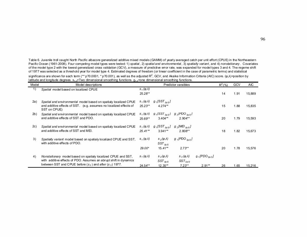
96
Model Model descriptions R2 (%) GCV AIC1) s1 (φ,λ)
25.28** 14 1.91 15,889
2a) s1 (φ,λ) g 1 [SST (φ,λ) ]
25.23** 4.274** 15 1.88 15,835
2b) s1 (φ,λ) g 1 [SST (φ,λ) ] g 2 [PDO (φ,λ) ]
25.69** 3.404** 2.904** 20 1.79 15,593
2c) s1 (φ,λ) g 1 [SST (φ,λ) ] g 2 [MEI (φ,λ) ]
25.41** 3.941** 2.808** 18 1.82 15,673
3) s1 (φ,λ) s 2(φ,λ) g 1 [PDO (φ,λ) ]
SST (φ,λ)
29.00* 15.41** 2.73** 20 1.78 15,576
4) s1 (φ,λ) s 2(φ,λ) s 3 (φ,λ) g 1 [PDO (φ,λ)]
SST (φ,λ) SST(φ,λ)
24.54** 12.35** 7.23** 2.91** 26 1.65 15,216
Table 6. Juvenile troll caught North Pacific albacore generalized additive mixed models (GAMM) of yearly averaged catch per unit effort (CPUE) in the Northeastern Pacific Ocean (1961-2008). Four competing model types were tested: 1) spatial , 2) spatial and environmental , 3) spatially variant , and 4) nonstationary . Covariates of the model type 2 with the lowest generalized cross validation (GCV), a measure of predictive error rate, was expanded for model types 3 and 4. The regeme shift of 1977 was selected as a threshold year for model type 4. Estimated degrees of freedom (or linear coefficient in the case of parametric terms) and statistical
significance are shown for each term (** p?0.0001, * p?0.001), as well as the adjusted R2, GCV, and Akaike Information Criteria (AIC) score. (φ,λ)=position by latitude and longitude degrees. s1-3=Two dimensional smoothing functions. g1-2=one dimensional smoothing functions.
Predictor varaibles
Nonstationary model based on spatialy localized CPUE and SST, with additive effects of PDO. Assumes an abrupt shift in dynamics between SST and CPUE before (s2 ) and after (s 3 ) 1977.
Spatial model based on localized CPUE
Spatial and environmental model based on spatialy localized CPUE and additive effects of SST. (e.g. assumes no localized effects of SST on CPUE)
Spatial and environmental model based on spatialy localized CPUE and additive effects of SST and PDO.
Spatial and environmental model based on spatialy localized CPUE and additive effects of SST and MEI.
Spatially variant model based on spatialy localized CPUE and SST, with additive effects of PDO.

97
-130 -125 -120 -115 -110
20
25
30
35
40
45
50
Longitude
Latit
ude (N
)
Washington
Oregon
California
Canada
Mexico
Figure 18. Study region for spatio-temporal analysis. The black squares represent the 1° x 1° cells used to calculate the mean monthly SST and roughly represent the areas with the highest long term CPUE for each 1° latitude band. The dard blue line is the 200 m isotherm.

98
-2-10123
+ MEI - MEI
25
30
35
40
45
50
Latit
ude
1961 1962 1963 1964 1965 1966 1967 1968
-2-10123
25
30
35
40
45
50
Latit
ude
1969 1970 1971 1972 1973 1974 1975 1976
-2-10123
25
30
35
40
45
50
Latit
ude
1977 1978 1979 1980 1981 1982 1983 1984
0
140
280
410
550
CPUE
SST °C
10
15
20
25
Figure 19. Monthly Sea Surface Temperature vs. CPUE by 1 degree latitude bins from 1961-1984. Multivariate El Niño/Southern Oscillation Index (MEI) values are also plotted with positive values shaded in red and negative values shaded in blue.

99
-2-10123
+ MEI - MEI
25
30
35
40
45
50
Latit
ude
1985 1986 1987 1988 1989 1990 1991 1992
-2-10123
25
30
35
40
45
50
Latit
ude
1993 1994 1995 1996 1997 1998 1999 2000
25
30
35
40
45
50
Latit
ude
2001 2002 2003 2004 2005 2006 2007 2008
0
140
280
410
550
CPUE
SST °C
10
15
20
25
Figure 20. Monthly Sea Surface Temperature vs. CPUE by 1 degree latitude bands from 1985-2008. Multivariate El Niño/Southern Oscillation Index (MEI) values are also plotted with positive values shaded in red and negative values shaded in blue.
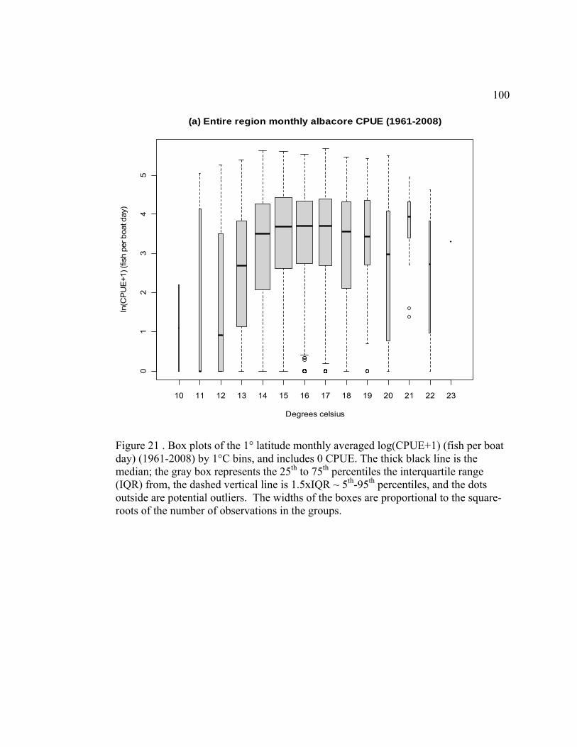
100
10 11 12 13 14 15 16 17 18 19 20 21 22 23
01
23
45
(a) Entire region monthly albacore CPUE (1961-2008)
Degrees celsius
ln(C
PU
E+1) (fis
h p
er boat d
ay)
Figure 21 . Box plots of the 1° latitude monthly averaged log(CPUE+1) (fish per boat day) (1961-2008) by 1°C bins, and includes 0 CPUE. The thick black line is the median; the gray box represents the 25th to 75th percentiles the interquartile range (IQR) from, the dashed vertical line is 1.5xIQR ~ 5th-95th percentiles, and the dots outside are potential outliers. The widths of the boxes are proportional to the square-roots of the number of observations in the groups.
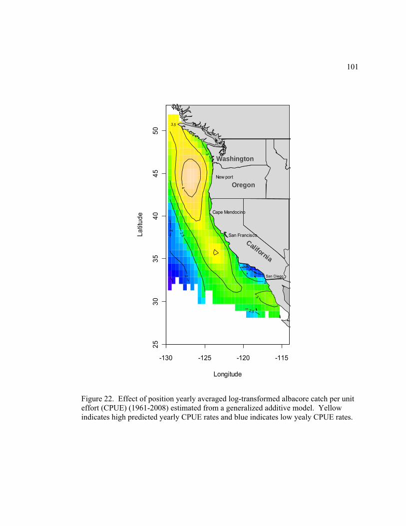
101
-130 -125 -120 -115
25
30
35
40
45
50
Longitude
La
titu
de
2
2
2
2.5
2.5
2.5
3
3
3
3.5
4
Washington
Oregon
California
New port
Cape Mendocino
San Francisco
San Diego
Figure 22. Effect of position yearly averaged log-transformed albacore catch per unit effort (CPUE) (1961-2008) estimated from a generalized additive model. Yellow indicates high predicted yearly CPUE rates and blue indicates low yealy CPUE rates.
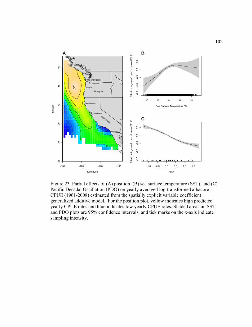
102
-130 -125 -120 -115
2530
3540
4550
Longitude
Latit
ude
1.5
2
2
2.5
2.5
2.5
3
3.5
3.5
4
4.5
Washington
Oregon
California
Newport
Cape Mendocino
San Francisco
San Diego
A
10 12 14 16 18
-1.5
-1.0
-0.5
0.0
0.5
Sea Surface Temperature °C
Eff
ect
on lo
g-tr
ansf
orm
ed a
lbac
ore
CP
UE
B
-1.0 -0.5 0.0 0.5 1.0 1.5
-1.5
-1.0
-0.5
0.0
0.5
PDO
Eff
ect
on lo
g-tr
ansf
orm
ed a
lbac
ore
CP
UE
C
Figure 23. Partial effects of (A) position, (B) sea surface temperature (SST), and (C) Pacific Decadal Oscillation (PDO) on yearly averaged log-transformed albacore CPUE (1961-2008) estimated from the spatially explicit variable coefficient generalized additive model. For the position plot, yellow indicates high predicted yearly CPUE rates and blue indicates low yearly CPUE rates. Shaded areas on SST and PDO plots are 95% confidence intervals, and tick marks on the x-axis indicate sampling intensity.

103
-130 -125 -120 -115
2530
3540
4550
Longitude
Latit
ude
2
2
2
2.5
2.5
3
3
3
3
3.5
3.5
4
Washington
Oregon
California
Newport
Cape Mendocino
San Francisco
San Diego
A
Washington
Oregon
California
Newport
Cape Mendocino
San Francisco
San Diego
A
10 12 14 16 18
-1.0
-0.5
0.0
0.5
1.0
Sea Surface Temperature °C
Eff
ect
on lo
g-tr
ansf
orm
ed a
lbac
ore
CP
UE
B
-1.5 -1.0 -0.5 0.0 0.5 1.0 1.5
-1.0
-0.5
0.0
0.5
1.0
MEI
Eff
ect
on lo
g-tr
ansf
orm
ed a
lbac
ore
CP
UE
C
Figure 24. Partial effects of (A) position, (B) sea surface temperature (SST), and (C) Multivariate El Niño/Southern Oscillation Index (MEI) on yearly averaged log-transformed albacore CPUE (1961-2008) estimated from the spatially explicit variable coefficient generalized additive model. For the position plot, yellow indicates high predicted yearly CPUE rates and blue indicates low yearly CPUE rates. Shaded areas on SST and PDO plots are 95% confidence intervals, and tick marks on the x-axis indicate sampling intensity.
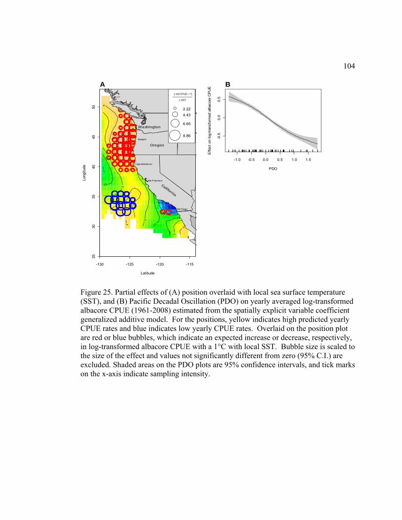
104
-130 -125 -120 -115
2530
3540
4550
Latitude
Long
itude
1
1.5
2
2
2.5
2.5
2.5
3
3
3
3.5
3.5
3.5
4
4
4
4.5
Washington
Oregon
California
Newport
Cape Mendocino
San Francisco
San Diego
2.22
4.43
6.65
8.86
lnCPUE 1
SST
A
-1.0 -0.5 0.0 0.5 1.0 1.5
-0.5
0.0
0.5
PDO
Eff
ect
on lo
g-tr
ansf
orm
ed a
lbac
ore
CP
UE
B
Figure 25. Partial effects of (A) position overlaid with local sea surface temperature (SST), and (B) Pacific Decadal Oscillation (PDO) on yearly averaged log-transformed albacore CPUE (1961-2008) estimated from the spatially explicit variable coefficient generalized additive model. For the positions, yellow indicates high predicted yearly CPUE rates and blue indicates low yearly CPUE rates. Overlaid on the position plot are red or blue bubbles, which indicate an expected increase or decrease, respectively, in log-transformed albacore CPUE with a 1°C with local SST. Bubble size is scaled to the size of the effect and values not significantly different from zero (95% C.I.) are excluded. Shaded areas on the PDO plots are 95% confidence intervals, and tick marks on the x-axis indicate sampling intensity.

105
-130 -125 -120 -115
2530
3540
4550
Latitude
Long
itude
1 1.5
2
2.5
2.5
3
3
3.5
4
Washington
Oregon
California
Newport
Cape Mendocino
San Francisco
San Diego
1.7
3.4
5.1
6.8
lnCPUE 1
SST
A 1961-1976
-130 -125 -120 -115
2530
3540
4550
Latitude
Long
itude
1 1.5
2
2.5
2.5
3
3
3.5
4
Washington
Oregon
California
Newport
Cape Mendocino
San Francisco
San Diego
1.48
2.95
4.43
5.9
lnCPUE 1
SST
B 1977-2008
-1.0 -0.5 0.0 0.5 1.0 1.5
-0.6
-0.4
-0.2
0.0
0.2
PDO
Effe
ct o
n lo
g-tr
ansf
orm
ed a
lbac
ore
CP
UE C
Figure 26. Partial effects of (A) position (1961-2008) overlaid with local sea surface temperature (SST) (1961-1976), (B) SST from (1977-2008), and (C) Pacific Decadal Oscillation (PDO) on yearly averaged log-transformed albacore CPUE (1961-2008) estimated from the threshold spatially explicit variable coefficient generalized additive model. For the positions, yellow indicates high predicted yearly CPUE rates and blue indicates low yearly CPUE rates. Overlaid on the position plot are red or blue bubbles, which indicate an expected increase or decrease, respectively, in log-transformed albacore CPUE with a 1°C with local SST. Bubble size is scaled to the size of the effect and effects not significantly different from zero (95% C.I.) are excluded. Shaded areas on the PDO plots are 95% confidence intervals, and tick marks on the x-axis indicate sampling intensity.

106
-130 -125 -120 -115
2530
3540
4550
Latitude
Long
itude
1.5
1.5
2 2
2 2
2.5
3
3.5
3.5
4
4.5
Washington
Oregon
California
Newport
Cape Mendocino
San Francisco
San Diego
0.46
0.93
1.39
1.85
lnCPUE 1
PDO
A
10 12 14 16 18
-1.5
-0.5
0.0
0.5
1.0
1.5
SST
Eff
ect
on lo
g-tr
ansf
orm
ed a
lbac
ore
CP
UE
B
Figure 27. Partial effects of (A) position overlaid with local effects of (PDO), and (B) sea surface temperature (SST) on yearly averaged log-transformed albacore CPUE (1961-2008) estimated from the spatially explicit variable coefficient generalized additive model. For the positions, yellow indicates high predicted yearly CPUE rates and blue indicates low yearly CPUE rates. Overlaid on the position plot are red or blue bubbles, which indicate an expected increase or decrease, respectively, in local log-transformed albacore CPUE with a 1°C with PDO. Bubble size is scaled to the size of the effect and effects not significantly different from zero (95% C.I.) are excluded. Shaded areas on the PDO plots are 95% confidence intervals, and tick marks on the x-axis indicate sampling intensity.
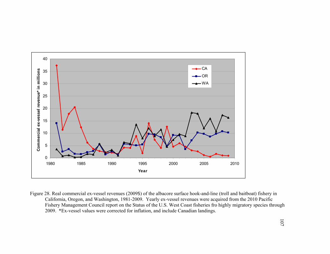
107
Figure 28. Real commercial ex-vessel revenues (2009$) of the albacore surface hook-and-line (troll and baitboat) fishery in California, Oregon, and Washington, 1981-2009. Yearly ex-vessel revenues were acquired from the 2010 Pacific Fishery Management Council report on the Status of the U.S. West Coast fisheries fro highly migratory species through 2009. *Ex-vessel values were corrected for inflation, and include Canadian landings.
0
5
10
15
20
25
30
35
40
1980 1985 1990 1995 2000 2005 2010
Year
Co
mm
erci
al e
x-ve
ssel
rev
enu
e* i
n m
illi
on
s CA
OR
WA
1085 BIBLIOGRAPHY
Ahrens, C. D., 1994. Meteorology Today: An Introduction to Weather, Climate, and the Environment. 5th ed. West Publishing, 591 pp.
Alverson, D. L. 1961. Ocean temperature and relation to Albacore Tuna (Thunnus germo) distribuicion in waters off the coast of Oregon, Washigton and Britist Columbia. J. Fish. Res. BD. Canada 18(6): 1145-1152.
Anda-Montañez, J.A.D., Amador-Buenrostro, A., Martínez-Aguilar, S., Muhlia-Almazán, A., 2004. Spatial analysis of yellowfin tuna (Thunnus albacares) catch rate and its relation to El Niño and La Niña events in the eastern tropical Pacific. Deep-Sea Res., Part 2, Top. Stud. Oceanogr. 51, 575–58.
Andrade, H. A. 2003. The relationship between the skipjack tuna (Katsuwonus pelamis) fishery and seasonal temperature variability in the southwestern Atlantic. Fisheries Oceanography 12 (1): 10-18.
Bacheler, N.M., Ciannelli, L., Bailey, K. M., and Duffy-Anderson, J.T.. 2010. Spatial and temporal patterns of walleye pollock (Theragra chalcogramma) spawning in the eastern Bering Sea inferred from egg and larval distributions. Fish. Oceanogr. 19:2. 107-120.
Bacheler ,N. M., Bailey, K. M., Ciannelli, L., Bartolino, V., & Chan, K.S. 2009. Density-dependent, landscape, and climate effects of spawning distribution of walley pollock Theragra chalcogramma. Mar. Ecol. Progr. Ser. 391, 1-12.
Bakun, A., and Broad., K. 2003. Environmental ‘loopholes’ and fish population dynamics: comparative pattern recognition with focus on El Niño effects in the Pacific. Fisheries Oceanography 12:458-473.
Bakun, A., and Parrish, R.H., 1982. Turbulence, transport, and pelagic fish in the California and Peru Current systems. CalCOFI Rep., 23: 99-1 12.
Barr, M., 2009. Are there two subgroups of Albacore, Thunnus alalunga, in the North Pacific? Evidence from variability in seasonal migration and size composition for two subgroups in the Coastal Fishery of North America. MS. Thesis, Oregon State University, Corvallis. Oregon. p. 132.
Bartolino, V., Ciannelli, L., Bacheler, N.M., & Chan, K.S. (2011). Ontogeny and sex disentangle density-dependent and density-independent spatiotemporal dynamics of a marine fish population. Ecology, 92, 189–200.
109Beamish, R. J., Noakes, D. J., McFarlane, G. A., Klyashtorin, L., Ivanov, V. V., &
Kurashov, V. (1999). The regime concept and natural trends in the production of Pacific salmon. Canadian Journal of Fisheries and Aquatic Science, 56, 516–526.
Berkeley, S. A., M.A., Hixon, R.J., Larson, and M.S., Love. 2004. Fisheries Sustainability via Protection of Age Structure and Spatial Distribution of Fish Populations. Fisheries, 29: 8, 23-32.
Beverton, R.J.H., Holt, S.J., 1957. On the Dynamics of Exploited Fish Populations. HMSO, London. 533 pp.
Blyth, C.R., 1972. On Simpson's paradox and the sure-thing principle, J. Am. Stat. Assoc. 67 364-366.
Boyce, D.G., Tittensor, D.P. & Worm, B. 2008. Effects of temperature on global patterns of tuna and billfish richness. Mar. Ecol. Prog. Ser., 355, 267–276.
Bradshaw, G.A. and T.A. Spies. 1992. Characterizing canopy gap structure in forests using wavelet analysis. Journal of Ecology 80:205-215.
Brock, V.E. 1943. Contributions to the biology of albacore (Germo alalunga) of the Oregon Coast and other parts of the Pacific. Stanford Ichthy. Bulletin 2: 199-248.
Burnham, K.P., and Anderson, D.R. 2002. Model selection and multimodel inference: a practical information-theoretic approach. Springer, New York, USA. 488 pp.
Carocci, F., Crispoldi, A., de Leiva, J.I., Majkowski, J. (2005). Tuna Catch Data in FAO’s Fisheries Global Information System (FIGIS), In: Proceedings of the Second Meeting of the Technical Advisory Committee of the FAO Project on the Management of tuna fishing capacity: conservation and socio-economics,15-18 March 2004. Madrid (Spain). FAO Fisheries Proceedings No. 2. p. 51-57.
Chan, K., and W. Fu.1999. Efficient Time Series Matching by Wavelets. Proceedings of the 15th International Conference on Data Engineering.
Chelton, D. B., Schlax M. G., and Samelson, R. M. (2011) Global observations of nonlinear mesoscale eddies. Prog. Oceanogr., 91, 167-216.
Chen, I.C., Lee, P.F., Tzeng, W.N., 2005. Distribution of albacore (Thunnus alalunga) in the Indian Ocean and its relation to environmental factors. Fisheries Oceanography 14, 71–80.

110Childers, J., and Aalbers, S. 2006. Summary of the 2005 U.S. North and South Pacific
Albacore Troll Fisheries. Southwest Fisheries Science Center Administrative Report No. LJ-06–06, National Marine Fisheries Service, La Jolla, California.
Childers, J., Snyder, S. and Kohin, S., 2011. Migration and behavior of juvenile North Pacific albacore (Thunnus alalunga). Fisheries Oceanography, 20: 157–173. doi: 10.1111/j.1365-2419.2011.00575.x.
Ciannelli, L., Bartolino, V., and Chan, K., (in prep). Nonadditive and nonstationray properties in the spatial distribution of a large marine fish population.
Ciannelli, L., Chan, K.S., Bailey, K.M., Stenseth, N.C., 2004. Nonadditive effects of the environment on the survival of a large marine fish population. Ecol 085 (12): 3418-3427.
Ciannelli L, Bailey K, Chan KS, Stenseth NC (2007) Phenological and geographical patterns of walleye pollock spawning in the Gulf of Alaska. Can J Aquat Fish Sci 64:713-722.
Clark, N.E., Blasing, T.J., Fritts, H.C. 1975. Influence of interannual climatic fluctuations on biological systems. Nature 256: 302-305.
Clemens, H.B. 1961. The migration, age, and growth of Pacific albacore (Thunnus germo), 1951-1958. California Department of Fish and Game, Fish Bulletin 115: 128.
Clemens, H.B., and W.L. Craig. 1965. An analysis of California’s albacore fishery. Calif. Fish Game, Fish Bull. 128 p.
Collette, B.B. 1978. Activity of albacore serum complement reflects its thermoregulatory capacity. In The physiological ecology of tunas (G.D. Sharp and A.E. Dizon, eds.), p. 7-39. Academic Press Inc.
Collette, B. B., and Nauen, C. E. 1983. Scombrids of the world. An annotated and illustrated catalogue of tuna, mackerels, bonitos and related species known to date. FAO Fisheries Synopsis No. 125, 2: 137 p.
Collette, B.B., Reeb, C., Block, B.A., 2001. Systematics of the tunas and mackerels (Scombridae). In: Block, B.A., Stevens, E.D. (Eds.), Tuna: Physiology, Ecology, and Evolution. In: Fish Physiology Series, vol. 19. Academic Press, San Diego, pp. 1–33.
111Corbineau, A., Rouyer, T., Cazelles, B., Fromentin, J.-M., Fonteneau, A. and Menard,
F., 2008. Time series analysis of tuna and swordfish catches and climate variability in the Indian Ocean (1968-2003). Aquatic Living Resources, 21, 277-285.
Crone P.R., 1992. Albacore. In California’s living marine resources: a status report. Leet, W.S., Dewees, C.M., Klingbeil, R. & Johnson, E.J. (eds). State of California Resources Agency and Fish and Game, Sacramento, California. p. 317-321.
Crone, P.R., R.J. Conser, and J.D. McDaniel. 2006. Population analysis of North Pacific albacore based on an age structured assessment program (ASAP) model. Collective Volumes of Scientific Papers of the ICCAT, 59 (3): 890-907.
Daskalov, G. 1999. Relating fish recruitment to stock and physical environment in the Black Sea using generalized additive models. Fisheries Research 41:1-23.
de Leiva, J.I., Majkowski, J., 2005. Status of the tuna stocks of the world. In: Proceedings of the Second Meeting of the Technical Advisory Committee of the FAO Project on the Management of tuna fishing capacity: conservation and socio-economics,15-18 March 2004. Madrid (Spain). FAO Fisheries Proceedings. No. 2. p. 58-114.
Di Lorenzo E., Schneider N., Cobb K. M., Chhak, K, Franks P. J. S., Miller A. J., McWilliams J. C., Bograd S. J., Arango H., Curchister E., Powell T. M. and P. Rivere, 2008: North Pacific Gyre Oscillation links ocean climate and ecosystem change. Geophys. Res. Lett., 35, L08607, doi:10.1029/2007GL032838.
Dufour, F., Arrizabalaga, H., Irigoien, X. and Santiago, J. 2010. Climate impacts on albacore and bluefin tuna migrations phenology and spatial distributions. Progress In Oceanography Volume 86, Issues 1-2: 283-290.
Ebbesmeyer, C.C., Cayan, D.R., McLain, D.R., Nichols, F.H., Peterson, D.H., Redmond, K.T., 1991. 1976 step in Pacific climate: forty environmental changes between 1968–1975 and 1977–1984. In: Betancourt, J.L., Sharp, V.L. (Eds.), Proceedings of the Seventh Annual Pacific Climate (PACLIM) Workshop, April 1990. California Department of Water Resources Technical Report 26, pp. 120–141.
Ellis, R. 2008. Tuna: a love story. Alfred A. Knopf, New York. 22-23, 208-211.
112Flittner, G.A. 1963. Review of the 1962 seasonal movement of albacore tuna off the
Pacific coast of the United States. Commercial Fisheries Review 25(4): 7-13.
Fonteneau A., Pallares P. and Pianet R. (2000) A worldwide review of purse seine fisheries on FADs. In: Le Gall J.-Y., Cayre P. and Taquet M. (eds), Peche thoniere et dispositifs de concentration de poisons. Ed. IFREMER, Actes Colloq. 28, 15-34.
Fromentin, J.-M. and Powers, J. E. (2005), Atlantic bluefin tuna: population dynamics, ecology, fisheries and management. Fish and Fisheries, 6: 281–306. doi: 10.1111/j.1467-2979.2005.00197.x.
Gerten, D. and Adrian, R. (2000) Climate-driven changes in spring plankton dynamics and the sensitivity of shallow polymictic lakes to the North Atlantic Oscillation. Limnol. Oceanogr. 45, 1058–1066.
Glaser, S.M., 2010. Interdecadal variability in predator–prey interactions of juvenile North Pacific albacore in the California Current System. Mar. Ecol. Progr. Ser. 414:209–221.
Glaser, S. M., 2011. Do albacore exert top-down pressure on northern anchovy? Estimating anchovy mortality as a result of predation by juvenile north pacific albacore in the California current system. Fisheries Oceanography, 20: 242–257. doi: 10.1111/j.1365-2419.2011.00582.x.
Glaser, S. M., Ye, H., Maunder, M., MacCall, A., Fogarty, M., Sugihara, G. 2011. Detecting and forecasting complex nonlinear dynamics in spatially structured catch-per-unit-effort time series for North Pacific albacore (Thunnus alalunga). Canadian Journal of Fisheries and Aquatic Sciences, V 68, No. 3, pp. 400-412.
Goñi, N., and Arrizabalaga, H., 2005. Analysis of juvenile North Atlantic albacore (Thunnus alalunga) catch per unit effort by surface gears in relation to environmental variables. ICES Journal of Marine Science, 62:1475-1482.
Hallett, T.B., Coulson, T., Pilkington, J.G., Clutton-Brock, T.H., Pemberton, J.M. & Grenfell, B. (2004) Why large-scale climate indices seem to predict ecological processes better than local weather. Nature, 430, 71–75.
Hanley, D. E., M. A. Bourassa, J. J. O’Brien, S. R. Smith, and E. R. Spade, 2003: A quantitative evaluation of ENSO indices. J. Climate, 16, 1249–1258.
Hochachka P. W., W.C. Hulbert, and Guppy M. 1978. The tuna power plant and furnace. In The physiological ecology of tunas (G.D. Sharp and A.E. Dizon, eds.), p. 153-174. Academic Press Inc.

113Huang, N.E. and Shen, Z. and Long, S.R. and Wu, M.C. and Shih, H.H. and Zhang, Q.
and Yen, N.-C. and Tung, C.C. and Liu, H.H (1998). The empirical mode decomposition and the Hilbert spectrum for nonlinear and non-stationary time series analysis. Proc. R. Soc. Lond. A, 454:903-995.
Husby, D.M. and Nelson, C.S. (1982) Turbulence and verticalstability in the California Current. CalcOFI Rep. 23: 113–129.
IPCC, 2007: Climate Change 2007: Synthesis Report. Contribution of Working Groups I, II and III to the Fourth Assessment Report of the Intergovernmental Panel on Climate Change [Core Writing Team, Pachauri, R.K and Reisinger, A. (eds.)]. IPCC, Geneva, Switzerland, 104 pp.
Ireland, R., 2011. The distribution and aggregation of Chinook salmon stocks on the Oregon Shelf as indicated by the commercial catch and genetics. MS. Thesis, Oregon State University, Corvallis. Oregon. p. 114.
Kishinouye E (1923) Contributions to the comparative study of the so-called scombroid fishes. J Coll. Agric. Imper. Univ. Tokyo 8(3), 293-475.
Kleiber, P. and C. Perin. 1991. Catch-per-effort and stock status in the U.S. North Pacific albacore fishery: reappraisal of both. Fishery Bulletin, US 89: 379-386.
Krygier, E.E., and Pearcy, W.G. 1977. The source of cobalt-60 and migrations of albacore off the west coast of North America. Fish. Bull., 75, 867-870.
Laurs, R.M., C. Hooker, L. Hreha, and R. Lincoln. 1975. A Uniform U.S. West Coast Logbook for Albacore, Thunnus alalunga (Bonnaterre), and Coastwide Albacore Fishery Data System. Marine Fisheries Review, Vol. 31, No. 11:14-21.
Laurs, R.M. 1979. Results from North Pacific albacore tagging studies. South West Fisheries Science Center (SWFSC) Administration Report No. LJ-79-17.
Laurs, R.M., Fielder, P.C. and Montgomery, D.R. 1984. Albacore tuna catch distributions relative to environmental features observed from satellites. Deep-Sea Research 31: 1085-1099.
Laurs, R. M. and Lynn., R.J. 1977. Seasonal migration of North Pacfic albacore, Thunnus alalunga, into North American coastal waters: Distribution, relative abundance, and association with transition zone waters. Fisheries Bulletin, U.S. 75: 795.

114Laurs, R.M., Powers, J.E. 2010. North Pacific Albacore ‘White Paper’ Possible
Management Options for the U.S. West Coast Albacore Fishery. U.S. Department of Commerce, NOAA National Marine Fisheries Service, Long Beach, California. p. 51.
Lavaniegos, B.E. 2009. Influence of a multiyear event of low salinity on the zooplankton from Mexican eco–regions of the California Current. Progr. Oceanogr. 83: 369–37.
Lehodey , P., F. Chai , and J. Hampton (2003): Modeling climate-related variability of tuna populations from a coupled ocean-biogeochemical-populations dynamics model. Fisheries Oceanography. (12)45: 483-494.
Love, M. S. 2006. Subsistence, commercial, and recreational fisheries. In: The ecology of marine fishes: California and adjacent waters. University of California Press, Los Angeles. pp. 567-594.
Levin, S. A. 1992. The problem of pattern and scale in ecology. Ecology 73 (6): 1943-1967.
Lu, H.-J., Lee, K.-T. and Liao, C.H., 1998. On the relationship between El Niño/southern oscillation and South Pacific albacore. Fish. Res. 39, pp. 1–7.
Lu, H.J., Lee, K.T., Lin, H.L., Liao, C.H. 2001. Spatio-temporal distribution of yellowfin tuna (Thunnus albacares) and bigeye tuna (Thunnus obesus) in the tropical Pacific Ocean in relation to large-scale temperature fluctuation during ENSO episodes. Fish Sci 67:1046–105.
Mantua, N.J. and S.R. Hare, Y. Zhang, J.M. Wallace, and R.C. Francis, 1997. A Pacific interdecadal climate oscillation with impacts on salmon production. Bulletin of the American Meteorological Society, 78, pp. 1069-1079.
Marcinek, D.J., Blackwell, S.B., Dewar, H., Freund, E.V., Farwell, C., Dau, D., Seitz, A.C. and Block, B.A. 2001. Depth and muscle temperature of Pacific bluefin tuna examined with acoustic and pop-up satellite tags. Mar. Biol. 138:869-885.
Marshall, C. T., Yaragina, N. A., Lambert, Y. & Kjesbu, O. S. 1999. Total lipid energy as a proxy for total egg production by fish stocks. Nature 402, 288–29
Maunder, M.N., and Punt, A.E. 2004. Standardizing catch and effort data: a review of recent approaches. Fish. Res. 70: 141–159.
McGowan, J.A., Bogard, S.J., Lynn, R.J, Miller, A.J. 2003. Long term variability in the southern California Current system. Deep-Sea Res II 50:2567–2582.
115Miller, A.J., Cayan, D.R., Barnett, T.P., Graham, N.E., Oberhuber, J.M., 1994. The
1976–77 climate shift of the Pacific Ocean. Oceanography 7, 21–26.
Miyake, P.M. 2005. A brief history of the tuna fisheries of the world. In: Proceedings of the Second Meeting of the Technical Advisory Committee of the FAO Project on the Management of tuna fishing capacity: conservation and socio-economics,15-18 March 2004. Madrid (Spain). FAO Fisheries Proceedings. No. 2. p. 23-50.
Miyake, M.P., Miyabe, N., and Nakono, H., 2004. Historical trends of tuna catches in the world. FAO Fisheries Technical Paper Rome FAO 467, 1–74.
Morrison, D.C., R.M. Laurs, and R.J. Ulevitch. 1978. Activity of albacore serum complement reflects its thermoregulatory capacity. In The physiological ecology of tunas (G.D. Sharp and A.E. Dizon, eds.), p. 141-150. Academic Press Inc.
Niiler, P. P., 1977. One-dimensional models of the upper ocean. Modelling and Prediction of the Upper Layers of the Ocean, E. B. Kraus, Ed., Pergamon Press, 143–172.
Otsu, T. and R.N. Uchida. 1959. Sexual maturity and spawning of albacore in the Pacific Ocean. Fishery Bulletin 148 (59): 287-305.
Otsu, T. and R.N. Uchida. 1962. Model of the migration of albacore in the North Pacific Ocean. Fishery Bulletin 63 (1): 33- 44.
Pearcy, W.G., and Osterberg., C.L. 1968. Zinc-65 and Maganese-54 in Albacore Thunnus alalunga from the west coast of North America. Limnology and Oceanography 8: 490-498.
Pearcy, W.G. and Mueller., J.L. 1970. Upwelling, Columbia River plume and albacore tuna. 6th Remote Sensing Environment. Ann Arbor, Michigan. P. 1101-1113.
Pearcy, W. G., and Schoener., A. 1987. Changes in the marine biota coincident with the 1982-1983 El nino in the northeastern subartic Pacific Ocean. J. Geophys. Res., 92(C13), 14,417–14,428, doi:10.1029/JC092iC13p14417.
PFMC, 2006. Preseason report III: analysis of council adopted management measures for 2006 ocean salmon fisheries. . Pacific Fishery Management Council. Portland, Oregon, USA.

116PFMC (Pacific Fishery Management Council). (2008). Status of the U.S. West Coast
fisheries fro highly migratory species through 2007. Pacific Fishery Management Council. Portland, Oregon, USA.
PFMC (Pacific Fishery Management Council). (2010). Status of the U.S. West Coast fisheries fro highly migratory species through 2009. Pacific Fishery Management Council. Portland, Oregon, USA.
Powers, J., M. Laurs, and A. Hough. 2007. Public certification report for AAFA North Pacific albacore pole & line and troll/jig fishery. Moody Marine LTD. Produced for the Marine Stewardship Council.
Ramsey, F. & Schafer, D. (2002). The Statistical Sleuth: A Course in Methods of Data Analysis, 2nd edn. Duxbury Press, Belmont, CA.
Ravier, C., and Fromentin, J.M. 2001. Long-term fluctuations in the Eastern Atlantic and Mediterranean bluefin tuna population. ICES Journal of Marine Science 58, 1299-1317.
Roberts, J.L. 1978 Ram ventilation and respiration in fish. In The physiological ecology of tunas (G.D. Sharp and A.E. Dizon, eds.), p. 83-88. Academic Press Inc.
Ropelewski, C. F., and P. D. Jones, 1987: An extension of the Tahiti–Darwin Southern Oscillation Index. Mon. Wea. Rev., 115, 2161–2165.
Ropelewski, C.F., Halpert, M.S., 1996. Quantifying Southern Oscillation-precipitation relationships. J. Climate 9, 1043-1059.
Rosenberg, M. S., and Anderson, C. D. 2011. PASSaGE: Pattern Analysis, Spatial Statistics and Geographic Exegesis. Version 2. Methods in Ecology and Evolution, 2: no. doi: 10.1111/j.2041-210X.2010.00081.
Samelson, R. M., Barbour, P., Barth, J., Bielli, S., Boyd, T., Chelton, D., Kosro, P., Levine, M., Skyllingstad, E., and Wilczak, J. 2002. Wind stress forcing of the Oregon coastal ocean during the 1999 upwelling season. J. Geophys. Res., 107, doi: 10.1029/20001JC000900
Sagarminaga, Y., and Arrizabalaga, H., 2010. Spatio-temporal distribution of albacore (Thunnus alalunga) Catches in the northeastern Atlantic: relationship with the thermal environment. Fish. Oceanogr., 19, 121-134.
117Schaefer, M.B. 1967. Fishery dynamics and present status of the yellowfin tuna
population of the eastern Pacific Ocean. Bull. Inter-Am. Trop. Tuna Comm. 12: 87–136
Schwing, F. B., Murphree, T., Green, P. M., 2002. The Northern Oscillation Index (NOI): a new climate index for the northeast Pacific. Prog. Oceanogr. 53:115-139.
Sharp G.D., and Piarages, S., 1978. The distribution of red and white swimming muscles, their biochemistry, and the biochemical phylogeny of selected scombrids fishes. In The physiological ecology of tunas (G.D. Sharp and A.E. Dizon, eds.), Academic Press Inc. p. 41-81.
Sibert, J., Hampton, J., Kleiber, P., Maunder, M. 2006. Biomass, size, and trophic status of top predators in the Pacific Ocean. Science 314, 1773–1776.
Stocker, M. (Ed.). 2005. Report of the Nineteenth North Pacific Albacore Workshop. Nineteenth North Pacific Albacore Workshop, Nanaimo, B.C., Canada, November 25- December 2, 2004. Fisheries and Oceans Canada, Pacific Biological Station, Nanaimo, B.C. 127 p.
Suda, A. 1966. Catch variations in the North Pacific albacore VI. The speculation about influence of fisheries on the catch and abundance of the albacore in the north-west Pacific by use of some simplified mathematical models (continued paper - I). Rep. Nankai Reg. Fish. Res. Lab. 24:1-14.
Sund PN, Blackburn M, Williams F (1981) Tunas and their environment in the Pacific Ocean: a review. Oceanogr mar Biol A Rev 19:443-512.
Takagi, M., S. Chow, and N. Taniguchi. 2007. Preliminary study of albacore (Thunnus alalunga) stock differentiation inferred from microsatellite DNA analysis. US Fishery Bulletin 99(4):697-701.
Torrence, C., and G. Compo, 1998. A practical guide to wavelet analysis, Bull. Am. Meteorol. Soc., 79, 61-78.
Wetherall, J.A., R.M. Laurs, R.N. Nishimoto, and M.Y. Yong. 1987. Growth variation and stock structure in North Pacific albacore. Working Paper prepared for the 10th North Pacific Albacore Workshop. Shimizu, Shizuoka, Japan. August 11-13, 1987.
Wilcox, W.A. (1907). The commercial fisheries of the Pacific coast states in 1904. Burea of fisheries document no. 612, 74pp.

118Wolter, K., and M.S. Timlin, 1993: Monitoring ENSO in COADS with a seasonally
adjusted principal component index. Proc. of the 17th Climate Diagnostics Workshop, Norman, OK, NOAA/NMC/CAC, NSSL, Oklahoma Clim. Survey, CIMMS and the School of Meteor., Univ. of Oklahoma, 52-57.
Wolter, K., and M. S. Timlin, 1998: Measuring the strength of ENSO events - how does 1997/98 rank? Weather, 53, 315-324.
Clemens 1961; Flittner 1963; Laurs et al. 1977; Childers et al. 2011
Wood, S.M. 2006. Generalized Additive Models, An Introduciton with R. London: Chapman and Hall, 392 pp.
Worm, B., Sandow, M., Oschlies, A., Lotze, H.K. and Myers, R.A. 2005. Global patterns of predator diversity in the open oceans. Science, 309, 1365–1369.
Yamanaka, K.L.,1989. Age, growth, and spawning of yellowfin tuna (Thunnus albacares) Bonnaterre 1788, in the southern Philippines. M. Sc. Thesis. University of British Columbia, Vancouver, B.C
Zainuddin M., Saitoh K., Saitoh S. 2008. Albacore (Thunnus alalunga) fishing ground in relation to oceanographic conditions in the western North Pacific Ocean using remotely sensed satellite data. Fish Oceanogr 17:61–73
Zhang, Y., J.M. Wallace, D.S. Battisti, 1997: ENSO-like interdecadal variability: 1900-93. J. Climate, 10, 1004-1020.
Zuur, A.F., Ieno, E.N., Elphick, C.S. 2010. A protocol for data exploration to avoid common statistical problems. Methods Ecol Evol 1: 3–14.

119
APPENDICES

120
Appendix A. ACRONYMS AND ABBREVIATIONS
AIC Akaike Information Criterion CPUE Catch-Per-Unit-Effort CS Confidence Spectrum EEZ Exclusive Economic Zone ENSO El Niño/La Niña-Southern Oscillation FADs Floating aggregation devices FAO Food and Agriculture Organization of the United Nations GAM/s Generalized Additive Model/s GCV Generalized Cross Validation CV Cross Validation IATTC Inter-American Tropical Tuna Commission ICCAT International Commission for the Conservation of Atlantic Tunas ICOADS International Comprehensive Ocean-Atmosphere Data Set IOTC Indian Ocean Tuna Commission MEI Multivariate El Niño/Southern Oscillation Index NOAA National Oceanic and Atmospheric Administration NOI Northern Oscillation Index NPGO North Pacific Gyre Oscillation P Sea Surface Pressure PDO Pacific Decadal Oscillation SDI Standard Deviation Index SL Standard Length SOI Southern Oscillation Index SST Sea Surface Temperature SWFSC Southwest Fisheries Science Center tGAM Threshold Generalized Additive Model

121
Appendix B. ENVIRONMENTAL INDICES
-2
-1
0
1
2
3
(a) Monthly series for PDO & MEI
An
om
aly
de
pa
rture
1961 1963 1965 1967 1969 1971 1973 1975 1977 1979 1981 1983 1985 1987 1989 1991 1993 1995 1997 1999 2001 2003 2005 2007
MEI
PDO
-3
-2
-1
0
1
2
3
(b) Monthly series for NPGO
Ano
ma
ly d
ep
art
ure
1961 1963 1965 1967 1969 1971 1973 1975 1977 1979 1981 1983 1985 1987 1989 1991 1993 1995 1997 1999 2001 2003 2005 2007
NPGO
-10
-5
0
5
(c) Monthly series for NOI & SOI
An
om
aly
dep
art
ure
1961 1963 1965 1967 1969 1971 1973 1975 1977 1979 1981 1983 1985 1987 1989 1991 1993 1995 1997 1999 2001 2003 2005 2007
NOISOI
App. B Figure 1. Pacific Decadal Oscillation (PDO), Multivariate ENSO Index (MEI), North Pacific Gyre Oscillation (NPGO), Southern Oscillation Index (SOI), and Northern Oscillation Index (NOI) indices.
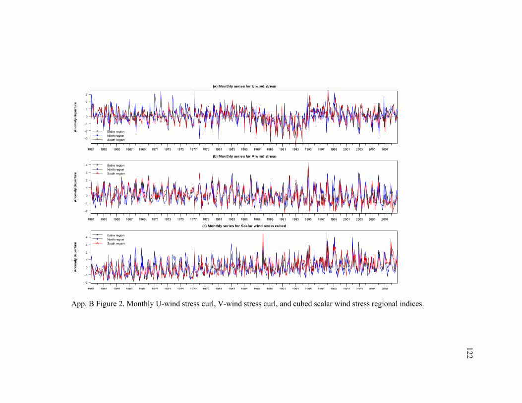
122
-3
-2
-1
0
1
2
3
(a) Monthly series for U wind stress
Ano
maly
depa
rture
1961 1963 1965 1967 1969 1971 1973 1975 1977 1979 1981 1983 1985 1987 1989 1991 1993 1995 1997 1999 2001 2003 2005 2007
Entire regionNorth regionSouth region
-2
-1
0
1
2
3
4
(b) Monthly series for V wind stress
Anom
aly
depart
ure
1961 1963 1965 1967 1969 1971 1973 1975 1977 1979 1981 1983 1985 1987 1989 1991 1993 1995 1997 1999 2001 2003 2005 2007
Entire regionNorth regionSouth region
-2
-1
0
1
2
3
4
(c) Monthly series for Scalar wind stress cubed
Anom
aly
depart
ure
1961 1963 1965 1967 1969 1971 1973 1975 1977 1979 1981 1983 1985 1987 1989 1991 1993 1995 1997 1999 2001 2003 2005 2007
Entire regionNorth regionSouth region
App. B Figure 2. Monthly U-wind stress curl, V-wind stress curl, and cubed scalar wind stress regional indices.
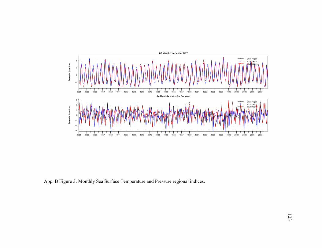
123
-1
0
1
2
(a) Monthly series for SST
Ano
maly
depa
rture
1961 1963 1965 1967 1969 1971 1973 1975 1977 1979 1981 1983 1985 1987 1989 1991 1993 1995 1997 1999 2001 2003 2005 2007
Entire region
North regionSouth region
-3
-2
-1
0
1
2
3
(b) Monthly series for Pressure
Anom
aly
depart
ure
1961 1963 1965 1967 1969 1971 1973 1975 1977 1979 1981 1983 1985 1987 1989 1991 1993 1995 1997 1999 2001 2003 2005 2007
Entire regionNorth regionSouth region
App. B Figure 3. Monthly Sea Surface Temperature and Pressure regional indices.

124Appendix C. HARR WAVELET
-1.5
-1
-0.5
0
0.5
1
1.5
-3 -2 -1 0 1 2 3
x/a
g(x
/a)
App. C. Figure 1. Harr analyzing wavelet g(x/a) which is localized around x/a.

125
Appendix D. CPUE AND SST TIME SERIES
(a) Entire region yearly albacore Catch Per Unit Effort CPUE (number of fish per boat day) and regional SST averages from 1961-2008
Entire regionSST anomaly
-0.4
-0.2
0.0
0.2
0.4
0.6
SS
T A
no
maly
depa
rture
1961 1963 1965 1967 1969 1971 1973 1975 1977 1979 1981 1983 1985 1987 1989 1991 1993 1995 1997 1999 2001 2003 2005 2007
20
40
60
80
100
120
CP
UE
(fi
sh/b
oat da
y)
(b) Northern subregion yearly albacore Catch Per Unit Effort CPUE (number of fish per boat day) and regional SST averages from 1961-2008
Entire region
SST anomaly
-0.2
0.0
0.2
0.4
SS
T A
nom
aly
de
part
ure
1961 1963 1965 1967 1969 1971 1973 1975 1977 1979 1981 1983 1985 1987 1989 1991 1993 1995 1997 1999 2001 2003 2005 2007
50
100
150
CP
UE
(fish/b
oat
day)
(c) Southern subregion yearly albacore Catch Per Unit Effort CPUE (number of fish per boat day) and regional SST averages from 1961-2008
Entire region
SST anomaly
-0.4
-0.2
0.0
0.2
0.4
0.6
SS
T A
nom
aly
depart
ure
1961 1963 1965 1967 1969 1971 1973 1975 1977 1979 1981 1983 1985 1987 1989 1991 1993 1995 1997 1999 2001 2003 2005 2007
0
20
40
60
80
100
CP
UE
(fis
h/b
oat day
)
App. D. Figure 1. Yearly Sea Surface Temperature indices and CPUE time series. black line=Entire region CPUE, blue line= Northern subregion CPUE, Red line=Southern subregion CPUE, and gray line = corresponding regional SST anomaly.

126
APPENDIX E. DAILY CATCH PER UNIT EFFORT
0
50
100
150
200
250
300
Daily time series for albacore CPUE (fish/boat day) 130° E to U.S. coast from 1961-1984
1961-1968
CP
UE
(fis
h/bo
at d
ay)
1962
1964
1966
1968
0
50
100
150
200
250
300
1969-1976
CP
UE
(fis
h/bo
at d
ay)
1970
1972
1974
1976
0
50
100
150
200
250
300
1977-1984
CP
UE
(fis
h/bo
at d
ay)
1978
1980
1982
1984
App. E. Figure 1. North Pacific albacore catch per unit effort (fish per boat day) by day from 1961-1984. Region is 130° E to the U.S. coast.

127
0
50
100
150
200
250
300
Daily time series for albacore CPUE (fish/boat day) 130° E to U.S. coast from 1985-2008
1985-1992
CP
UE
(fis
h/bo
at d
ay)
1986
1988
1990
1992
0
50
100
150
200
250
300
1993-2000
CP
UE
(fis
h/bo
at d
ay)
1994
1996
1998
2000
0
50
100
150
200
250
300
2001-2008
CP
UE
(fis
h/bo
at d
ay)
2002
2004
2006
2008
App. E Figure 2. North Pacific albacore catch per unit effort (fish per boat day) by day from 1985-2008. Region is 130° E to the U.S. coast.
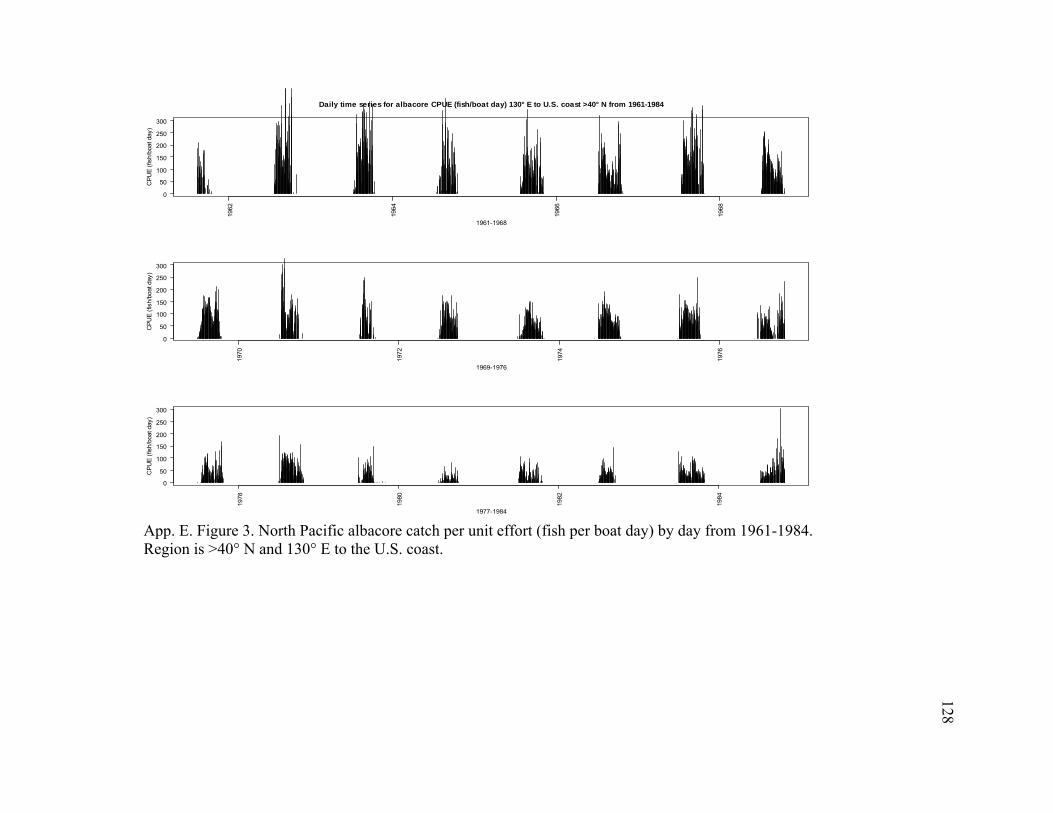
128
0
50
100
150
200
250
300
Daily time series for albacore CPUE (fish/boat day) 130° E to U.S. coast >40° N from 1961-1984
1961-1968
CP
UE
(fis
h/bo
at d
ay)
1962
1964
1966
1968
0
50
100
150
200
250
300
1969-1976
CP
UE
(fis
h/bo
at d
ay)
1970
1972
1974
1976
0
50
100
150
200
250
300
1977-1984
CP
UE
(fis
h/bo
at d
ay)
1978
1980
1982
1984
App. E. Figure 3. North Pacific albacore catch per unit effort (fish per boat day) by day from 1961-1984. Region is >40° N and 130° E to the U.S. coast.

129
0
50
100
150
200
250
300
Daily time series for albacore CPUE (fish/boat day) 130° E to U.S. coast >40° N from 1985-2008
1985-1992
CP
UE
(fis
h/bo
at d
ay)
1986
1988
1990
1992
0
50
100
150
200
250
300
1993-2000
CP
UE
(fis
h/bo
at d
ay)
1994
1996
1998
2000
0
50
100
150
200
250
300
2001-2008
CP
UE
(fis
h/bo
at d
ay)
2002
2004
2006
2008
App. E. Figure 4. North Pacific albacore catch per unit effort (fish per boat day) by day from 1985-2008. Region is >40° N and 130° E to the U.S. coast.

130
0
50
100
150
200
250
300
Daily time series for albacore CPUE (fish/boat day) 130° E to U.S. coast <40° N from 1961-1984
1961-1968
CP
UE
(fis
h/bo
at d
ay)
1962
1964
1966
1968
0
50
100
150
200
250
300
1969-1976
CP
UE
(fis
h/bo
at d
ay)
1970
1972
1974
1976
0
50
100
150
200
250
300
1977-1984
CP
UE
(fis
h/bo
at d
ay)
1978
1980
1982
1984
App. E. Figure 5. North Pacific albacore catch per unit effort (fish per boat day) by day from 1961-1984. Region is <40° N and 130° E to the U.S. coast.
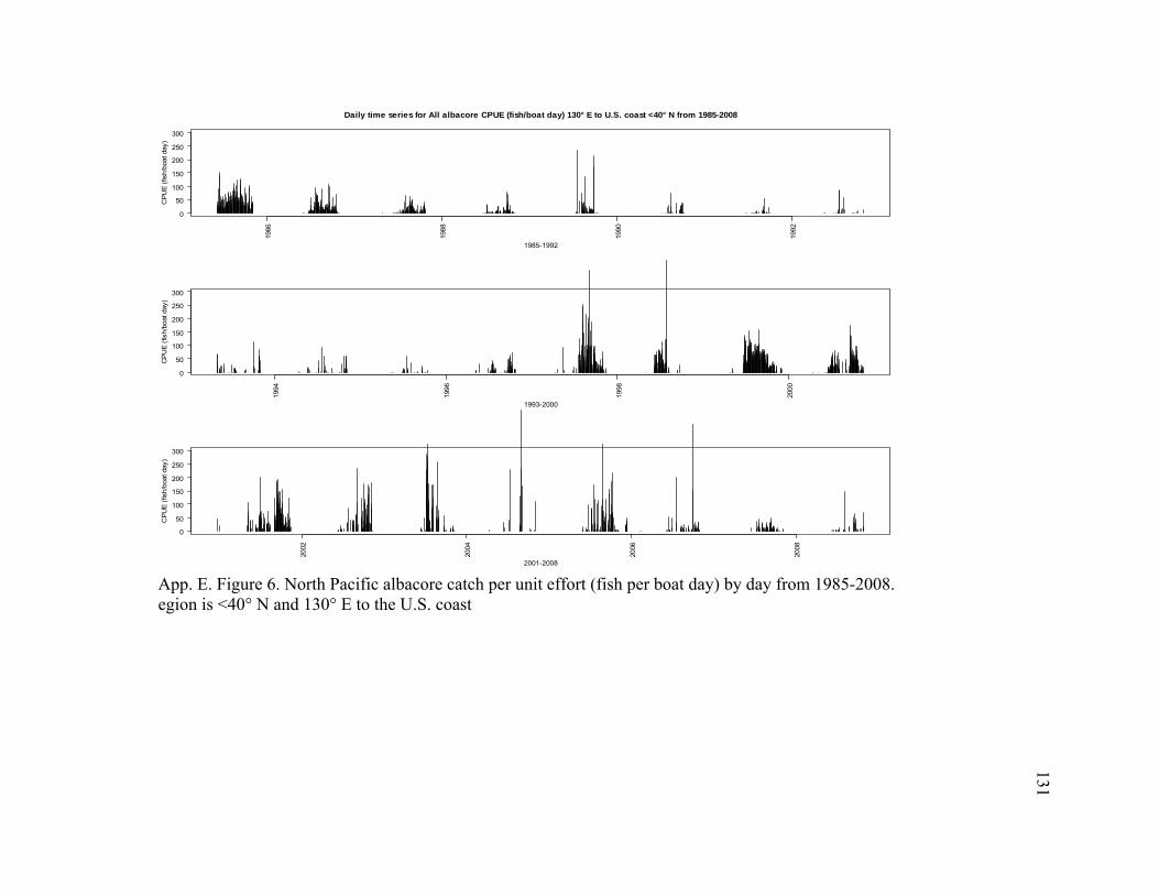
131
0
50
100
150
200
250
300
Daily time series for All albacore CPUE (fish/boat day) 130° E to U.S. coast <40° N from 1985-2008
1985-1992
CP
UE
(fis
h/bo
at d
ay)
1986
1988
1990
1992
0
50
100
150
200
250
300
1993-2000
CP
UE
(fis
h/bo
at d
ay)
1994
1996
1998
2000
0
50
100
150
200
250
300
2001-2008
CP
UE
(fis
h/bo
at d
ay)
2002
2004
2006
2008
App. E. Figure 6. North Pacific albacore catch per unit effort (fish per boat day) by day from 1985-2008. egion is <40° N and 130° E to the U.S. coast
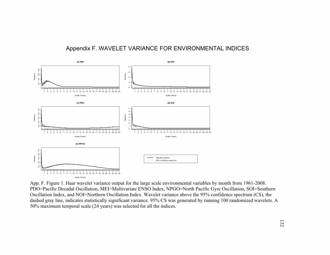
132Appendix F. WAVELET VARIANCE FOR ENVIRONMENTAL INDICES
0.2
0.4
0.6
0.8
(a) MEI
Scale (Years)
Var
ianc
e
1 2 3 4 5 6 7 8 9 10 11 12 13 14 15 16 17 18 19 20 21 22 23 24
02
46
8
(b) NOI
Scale (Years)
Var
ianc
e
1 2 3 4 5 6 7 8 9 10 11 12 13 14 15 16 17 18 19 20 21 22 23 24
0.2
0.4
0.6
0.8
1.0
(c) PDO
Scale (Years)
Var
ianc
e
1 2 3 4 5 6 7 8 9 10 11 12 13 14 15 16 17 18 19 20 21 22 23 24
01
23
45
67
(d) SOI
Scale (Years)
Var
ianc
e
1 2 3 4 5 6 7 8 9 10 11 12 13 14 15 16 17 18 19 20 21 22 23 24
0.2
0.4
0.6
0.8
1.0
(e) NPGO
Scale (Years)
Var
ianc
e
1 2 3 4 5 6 7 8 9 10 11 12 13 14 15 16 17 18 19 20 21 22 23 24
Wavelet variance
95% confidence spectrum
App. F. Figure 1. Haar wavelet variance output for the large scale environmental variables by month from 1961-2008. PDO=Pacific Decadal Oscillation, MEI=Multivariate ENSO Index, NPGO=North Pacific Gyre Oscillation, SOI=Southern Oscillation Index, and NOI=Northern Oscillation Index. Wavelet variance above the 95% confidence spectrum (CS), the dashed gray line, indicates statistically significant variance. 95% CS was generated by running 100 randomized wavelets. A 50% maximum temporal scale (24 years) was selected for all the indices.
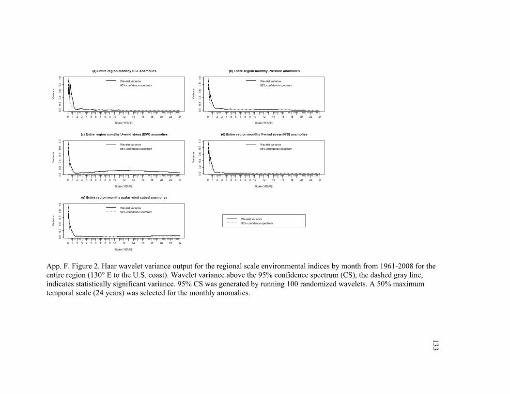
133
0.0
0.2
0.4
0.6
0.8
1.0
(a) Entire region montlhy SST anamolies
Scale (YEARS)
Var
ianc
e
0 1 2 3 4 5 6 7 8 9 10 12 14 16 18 20 22 24
Wavelet variance
95% confidence spectrum
0.0
0.2
0.4
0.6
0.8
1.0
(b) Entire region montlhy Pressure anamolies
Scale (YEARS)
Var
ianc
e
0 1 2 3 4 5 6 7 8 9 10 12 14 16 18 20 22 24
Wavelet variance
95% confidence spectrum
0.0
0.2
0.4
0.6
0.8
1.0
(c) Entire region montlhy U-wind stress (E/W) anamolies
Scale (YEARS)
Var
ianc
e
0 1 2 3 4 5 6 7 8 9 10 12 14 16 18 20 22 24
Wavelet variance
95% confidence spectrum
0.0
0.2
0.4
0.6
0.8
1.0
(d) Entire region montlhy V-wind stress (N/S) anamolies
Scale (YEARS)
Var
ianc
e
0 1 2 3 4 5 6 7 8 9 10 12 14 16 18 20 22 24
Wavelet variance
95% confidence spectrum
0.0
0.2
0.4
0.6
0.8
1.0
(e) Entire region montlhy scalar wind cubed anamolies
Scale (YEARS)
Var
ianc
e
0 1 2 3 4 5 6 7 8 9 10 12 14 16 18 20 22 24
Wavelet variance
95% confidence spectrum
Wavelet variance
95% confidence spectrum
App. F. Figure 2. Haar wavelet variance output for the regional scale environmental indices by month from 1961-2008 for the entire region (130° E to the U.S. coast). Wavelet variance above the 95% confidence spectrum (CS), the dashed gray line, indicates statistically significant variance. 95% CS was generated by running 100 randomized wavelets. A 50% maximum temporal scale (24 years) was selected for the monthly anomalies.

134
0.0
0.2
0.4
0.6
0.8
1.0
(a) North region montlhy SST anamolies
Scale (YEARS)
Var
ianc
e
0 1 2 3 4 5 6 7 8 9 10 12 14 16 18 20 22 24
Wavelet variance
95% confidence spectrum
0.0
0.2
0.4
0.6
0.8
1.0
(b) North region montlhy Pressure anamolies
Scale (YEARS)
Var
ianc
e
0 1 2 3 4 5 6 7 8 9 10 12 14 16 18 20 22 24
Wavelet variance
95% confidence spectrum
0.0
0.2
0.4
0.6
0.8
1.0
(c) North region montlhy U-wind stress (E/W) anamolies
Scale (YEARS)
Var
ianc
e
0 1 2 3 4 5 6 7 8 9 10 12 14 16 18 20 22 24
Wavelet variance
95% confidence spectrum
0.0
0.2
0.4
0.6
0.8
1.0
(d) North region montlhy V-wind stress (N/S) anamolies
Scale (YEARS)
Var
ianc
e
0 1 2 3 4 5 6 7 8 9 10 12 14 16 18 20 22 24
Wavelet variance
95% confidence spectrum
0.0
0.2
0.4
0.6
0.8
1.0
(e) North region montlhy scalar wind cubed anamolies
Scale (YEARS)
Var
ianc
e
0 1 2 3 4 5 6 7 8 9 10 12 14 16 18 20 22 24
Wavelet variance
95% confidence spectrum
Wavelet variance
95% confidence spectrum
App. F. Figure 3. Haar wavelet variance output for the regional scale environmental indices by month from 1961-2008 for the northern subregion of the study area (130° E to the U.S. coast & >40° N). U-wind stress curl, V-wind stress curl, cubed scalar wind stress, Sea Surface Temperature (SST), and pressure regional monthly anomalies. Wavelet variance above the 95% confidence spectrum (CS), the dashed gray line, indicates statistically significant variance. 95% CS was generated by running 100 randomized wavelets. A 50% maximum temporal scale (24 years) was selected for the monthly anomalies.
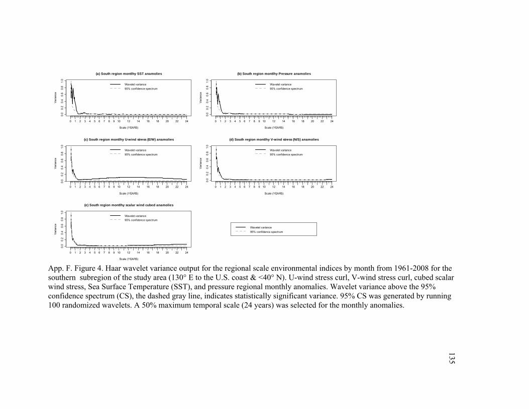
135
0.0
0.2
0.4
0.6
0.8
1.0
(a) South region montlhy SST anamolies
Scale (YEARS)
Var
ianc
e
0 1 2 3 4 5 6 7 8 9 10 12 14 16 18 20 22 24
Wavelet variance
95% confidence spectrum
0.0
0.2
0.4
0.6
0.8
1.0
(b) South region montlhy Pressure anamolies
Scale (YEARS)
Var
ianc
e
0 1 2 3 4 5 6 7 8 9 10 12 14 16 18 20 22 24
Wavelet variance
95% confidence spectrum
0.0
0.2
0.4
0.6
0.8
1.0
(c) South region montlhy U-wind stress (E/W) anamolies
Scale (YEARS)
Var
ianc
e
0 1 2 3 4 5 6 7 8 9 10 12 14 16 18 20 22 24
Wavelet variance
95% confidence spectrum
0.0
0.2
0.4
0.6
0.8
1.0
(d) South region montlhy V-wind stress (N/S) anamolies
Scale (YEARS)
Var
ianc
e
0 1 2 3 4 5 6 7 8 9 10 12 14 16 18 20 22 24
Wavelet variance
95% confidence spectrum
0.0
0.2
0.4
0.6
0.8
1.0
(e) South region montlhy scalar wind cubed anamolies
Scale (YEARS)
Var
ianc
e
0 1 2 3 4 5 6 7 8 9 10 12 14 16 18 20 22 24
Wavelet variance
95% confidence spectrum
Wavelet variance
95% confidence spectrum
App. F. Figure 4. Haar wavelet variance output for the regional scale environmental indices by month from 1961-2008 for the southern subregion of the study area (130° E to the U.S. coast & <40° N). U-wind stress curl, V-wind stress curl, cubed scalar wind stress, Sea Surface Temperature (SST), and pressure regional monthly anomalies. Wavelet variance above the 95% confidence spectrum (CS), the dashed gray line, indicates statistically significant variance. 95% CS was generated by running 100 randomized wavelets. A 50% maximum temporal scale (24 years) was selected for the monthly anomalies.

136
Appendix G. STATISTICAL DIAGNOSTICS OF ALBACORE TIME SERIES
-2 -1 0 1 2
-30
-10
010
2030
Normal Q-Q Plot
Theoretical Quantiles
Sam
ple
Qua
ntile
s
40 60 80 100 120-3
0-1
00
1020
30
Resids vs. linear pred.
linear predictor
resi
dual
s
Histogram of residuals
Residuals
Fre
quen
cy
-40 -20 0 20 40
02
46
810
12
40 60 80 100 120
2040
6080
100
Response vs. Fitted Values
Fitted Values
Res
pons
e
App. G. Figure 1. gam.check output of residuals from North Pacific albacore Yearly catch per unit effort (fish per boat day) from 1966-2008 modeled by yearly averaged Scalar wind speed cubed at a five year lag. Region is 130° E to the U.S. coast.
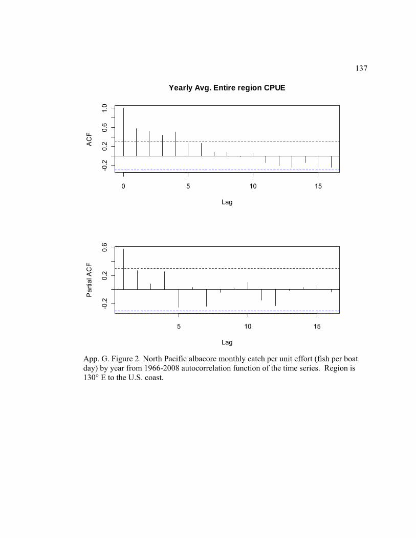
137
0 5 10 15
-0.2
0.2
0.6
1.0
Lag
AC
FYearly Avg. Entire region CPUE
5 10 15
-0.2
0.2
0.6
Lag
Pa
rtia
l AC
F
App. G. Figure 2. North Pacific albacore monthly catch per unit effort (fish per boat day) by year from 1966-2008 autocorrelation function of the time series. Region is 130° E to the U.S. coast.

138
0 5 10 15
-0.2
0.2
0.6
1.0
Lag
AC
FCPUEall~s(Scalar lagged 5 yrs.)
5 10 15
-0.3
-0.1
0.1
0.3
Lag
Pa
rtia
l AC
F
App. G. Figure 3. Autocorrelation of residuals from North Pacific albacore Yearly catch per unit effort (fish per boat day) from 1966-2008 modeled by yearly averaged Scalar wind speed cubed at a five year lag. Region is 130° E to the U.S. coast.
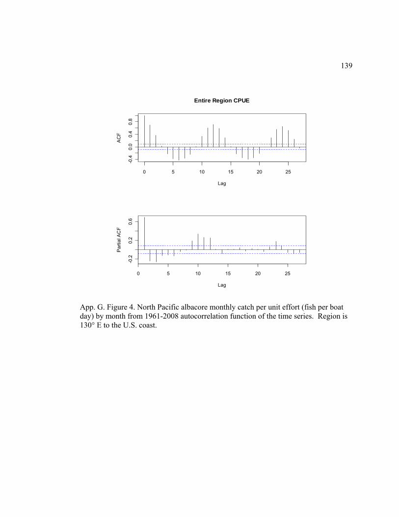
139
0 5 10 15 20 25
-0.4
0.0
0.4
0.8
Lag
AC
F
Entire Region CPUE
0 5 10 15 20 25
-0.2
0.2
0.6
Lag
Pa
rtia
l AC
F
App. G. Figure 4. North Pacific albacore monthly catch per unit effort (fish per boat day) by month from 1961-2008 autocorrelation function of the time series. Region is 130° E to the U.S. coast.

140
0 5 10 15 20 25
0.0
0.4
0.8
Lag
AC
Flog(CPUEall+1)~s(SSTall)
0 5 10 15 20 25
-0.1
0.1
0.3
Lag
Pa
rtia
l AC
F
App. G. Figure 5. Autocorrelation of residuals from North Pacific albacore monthly catch per unit effort (fish per boat day) from 1961-2008 modeled by sea surface temperature. Region is 130° E to the U.S. coast.