tiago, j., gambaruto, a. m., & sequeira, a. (2014 ... ·...

$: Tiago, J., Gambaruto, A. M., & Sequeira, A. (2014 ... · \MMNP_Tiago_Gambaruto_Sequeira_accep" | 2014/5/27 | 0:33 | page 3 | #3 i i i i i i i i Jorge Tiago, Alberto Gambaruto, Adelia$
Tiago, J., Gambaruto, A. M., & Sequeira, A. (2014). Patient-specific bloodflow simulations: setting Dirichlet boundary conditions for minimal errorwith respect to measured data. Mathematical Modelling of NaturalPhenomena, 9(6). https://doi.org/10.1051/mmnp/20149608

Peer reviewed version

Link to published version (if available):10.1051/mmnp/20149608

Link to publication record in Explore Bristol ResearchPDF-document

This is the author accepted manuscript (AAM). The final published version (version of record) is available onlinevia EDP Sciences at http://www.mmnp-journal.org/articles/mmnp/abs/2014/06/mmnp201496p98/mmnp201496p98.html. Please refer to any applicableterms of use of the publisher.

University of Bristol - Explore Bristol ResearchGeneral rights

This document is made available in accordance with publisher policies. Please cite only the publishedversion using the reference above. Full terms of use are available:http://www.bristol.ac.uk/pure/about/ebr-terms

https://doi.org/10.1051/mmnp/20149608

https://research-information.bristol.ac.uk/en/publications/patientspecific-blood-flow-simulations(742736fb-b955-4c77-8182-8c82228cd632).html

https://research-information.bristol.ac.uk/en/publications/patientspecific-blood-flow-simulations(742736fb-b955-4c77-8182-8c82228cd632).html

“MMNP˙Tiago˙Gambaruto˙Sequeira˙accep” — 2014/5/27 — 0:33 — page 2 — #2ii

ii

ii

ii

Jorge Tiago, Alberto Gambaruto, Adelia Sequeira Patient-specific blood flow simulations

not only in the formulation of the mathematical equations, but also in the setup definition of the prob-lem which includes setting coefficients and boundary conditions. In this work we specifically consideruncertainty associated to numerical simulations of patient-specific blood flow, however the methodologycan naturally be extended to other flow problems.

Another important technological development of the last few years has been in medical devices, in-cluding medical imaging. Patient-specific studies using non-invasive clinical imaging data, that can beacquired as part of current medical protocols, have become routine in the research community. Suchnumerical simulations have played a part in further understanding many cardiovascular diseases due tothe accurate and high resolution computed solution. It has enabled researchers to probe, query and ob-serve complex and coupled phenomena based on the mathematical models. The validation of numericalsimulations of patient-specific studies largely remains an open problem as there is no means for accuratebenchmarking for a given clinically acquired dataset. Hence, while the complexity of problems beingmodeled has increased with greater sophistication in the mathematical description, used to build a morerealistic behavior of human physiology, the possibility of feasibly bracketing errors, due to model or setupuncertainty, has grown more difficult and unattainable.

The imaging data, from which patient-specific studies are built upon, are acquired from non-invasive(or minimally-invasive) medical imaging, such as magnetic resonance imaging (MRI) or computed tomog-raphy (CT), with or without contrast. To some extent, also Doppler ultrasound can be used, though itis generally of lower resolution. These data sets contain errors typically in the form of noise and limitedresolution, and a multitude of artifacts and signal degradation can occur (cf. [1, 28, 37]). Sophisticatedimage processing may be used to reconstruct a 3-dimensional computational model. It has been seenhowever, that a substantially different choice in the image processing method will give different results.The reconstructed geometry hence varies, with no way of knowing what is the ground truth.

Several studies ([4, 14, 17, 25]) have looked at variability in the reconstructed geometry definition andreported differences in physiologically relevant measures associated to disease (typically the wall shearstress and derived measures). In a similar fashion, there is uncertainty regarding which rheological modelfor blood to choose [16,23], appropriate inflow/outflow boundary conditions to set [26,30] and parametersfor the structural models describing the vessel lumen and surrounding tissue [24, 27, 35]. Uncertaintiescan be mitigated by sampling the parameter space, estimating therefore error bounds. While this isunfeasible for a general problem, due to high computational costs, a subset of relevant measures can beinvestigated in order to obtain credible results and correlations to disease descriptors [14]. Such selectivesampling of the parameter space often requires human intervention and remains subjective. A preferredapproach would be to have an automatic method to obtain the unique solution that minimizes an errorcost function, based on some extra observations obtained from clinical imaging data. Such solution canhelp setting the parameters for the numerical simulations.

We take this as our starting point and motivation for the current work. The simulation methodologypresented in this paper assures the minimization of error in the solution, that can be associated to anyform of uncertainty in translating the clinical data to a computational domain and setup. The approachis suitable for patient-specific studies and needs two forms of data: i) a stack of medical images (e.g. CTor MRI) from which to reconstruct an approximate computational domain; ii) and a few cross-sectionalvelocity contours, that can be obtained from phase-contrast magnetic resonance imaging (PC-MRI), whichcan be corrupted due to noise or limited resolution. Once we assume this, a misfit between the measuredvelocity data and the computed solution is minimized. This implies a control of the velocity values atthe boundary of the approximated computational domain. Optimal control techniques in cardiovascularmodeling have been used recently in the frame of Data Assimilation (DA) (cf. [7, 8, 19]). Althoughour approach allows the velocity profile reconstruction (the subject of DA), we are mainly interested inreducing the uncertainty associated to the reconstructed domain.

The work presented in this paper outlines the methodology with application to 2-dimensional problems,with more realistic 3-dimensional cases as scope for future work. For each case, a ground truth solution is

2


ii

ii

ii


generated in order to compare and evaluate the minimal error solution obtained from an optimal controlmethodology. The cases studied are presented in order of increasing complexity.

The control parameters are the velocity Dirichlet conditions that describe both the truncated domaininflow sections and the geometry wall. The outflows are given by a traction-free (Neumann) conditionand are not a parameter in the optimal control, but remain a solution of the Navier-Stokes equations. Aninitial guess solution for the optimal control problem is arbitrary, and given here as an average velocityflow field, however, other easily available options including a uniform zero-velocity field and the solutionof the flow field in the approximate computational domain, can also be tested.

The organization of the paper reads as follows. In Section 2 we briefly recall the mathematical modelscommonly used to model blood flow in the vascular system and we introduce the boundary controlproblem that we will use as a tool to reconstruct the blood profile in the approximated geometries. Next,in Section 3, we describe the numerical approach to solve the optimal control problem. Finally, we presentin Section 4 the numerical results obtained for different idealized geometries.

2. Mathematical model and control problem

2.1. Mathematical model for blood flow

In this section we assume that Ω represents the fluid domain, which corresponds to the lumen of theartery, as shown in Figure 1. The boundary of Ω consists of the artery interior wall, represented by Γwall,and two artificial boundaries Γin and Γout to truncate the domain from the whole system. We also callΓin the inlet which corresponds to the proximal section, where the average mean flow is negative withrespect to the section outward-pointing normal direction. As to Γout, we also call it the outlet whichcorresponds to the distal section, where the average mean flow is positive with respect to the sectionoutward-pointing normal direction.

From the linear momentum and mass conservation equations we can derive the blood flow model. Forour purposes we assume blood to be an isothermal, viscous and incompressible fluid. Hence we obtainthe equations

ρ(∂u

∂t+ (u · ∇)u

)− div τ +∇p = f in Ω

div u = 0 in Ω(2.1)

where the stress tensor τ is given by the constitutive equation

τ = 2µDu, where Du =∇u +∇uT

2.

The dynamic viscosity µ can be considered either as constant or as shear rate dependent. In fact, bloodmay present a shear-thinning behavior which can only be accurately represented using a non-Newtonian

Figure 1. Representation of the domain Ω

3


ii

ii

ii


model in which the viscosity is no longer a constant; see for instance [31]. Since here our main focus is therecovery of accurate boundary conditions and the vessel wall, to simplify, we assume that the viscosity isconstant and blood is modeled as a Newtonian fluid by the well known Navier-Stokes equations.

In order to close system (2.1) and obtain a well posed model, we fix the velocity to be zero at Γwalland we impose the so-called homogeneous Neumann boundary conditions

(−pI + 2µDu) · n = 0 on Γout.

Here n represents the exterior unit normal vector to the surface and I the identity matrix. Finally, we fixa velocity profile at the inlet Γin. The right hand side of the balance of the momentum is only composedby the constant gravity force, which can be considered as part of the pressure p by a suitable change ofvariables. Therefore, for simplicity, we can consider it to be f = 0. Furthermore, we will only deal withthe stationary model, neglecting therefore the time dependence. For more details on the mathematicalmodeling of blood flow we refer to [29].

2.2. The optimal control problem

As mentioned in the Introduction, there is an inherent uncertainty when performing patient-specificnumerical simulations. In order to obtain some indicative measure of error bounds, one approach consistsin sampling the uncertainty parameter space to carry out the study. When dealing with the uncertaintyassociated to the geometry reconstruction, the parameter space can be prohibitively large. Here wepropose a less computationally intensive approach based on an optimal control problem.

The inlet velocity profile at the artificial boundary condition Γin, and the location of the no-slipboundary condition that defines the reconstructed wall Γwall, are often indicated as key measures thatpropagate to the solution of equation (2.1). This is especially relevant when considering fluid mechanicsmeasures with physiological interest, such as the wall shear stress [13, 15]. A good criterion to set thecorrect Dirichlet boundary conditions is therefore imperative.

In order to perform a comparison of different boundary conditions we must accept that some data ofthe true solution itself is available (even if corrupted by noise). Here we assume to know the velocityprofile on some sections of the lumen, possibly obtained very close to the boundary wall. We take Ωobsto represent the union of such observed sections, and ud the known velocity data on these sections. Letus denote by Ω the reconstructed domain, obtained from medical images, which lies close to the truedomain Ω0. Let us represent the boundary for which we want to calibrate the velocity profile by Γc. Inpractice this boundary may consist in part or whole of Γwall and/or the inlet Γin. This allows for a greatflexibility in the method.

We can now choose the uncertain velocity profiles as the solution of the optimal control problem

minc∈A

J(c) = α1

∫Ωobs

|u− ud|2 dx+ α2

∫Γc

|∇sc|2 ds (2.2)

subject to

−div τ + ρ(u · ∇)u +∇p = 0 in Ω

div u = 0 in Ω,

u = 0 on Γwall \ Γc

u = c on Γc

(−pI + 2µDu) · n = 0 on Γout.

(2.3)

The variable c stands for the control vector function, consisting in the unknown velocity profiles atthe different parts of Γc. The term α2 weighting the tangential gradient ∇sc is a regularization term(see [21]). In practice, we can also choose c to have lower dimension than the velocity vector through

4


ii

ii

ii


a parametrization. Such parametrization could, for example, be a polynomial function, hence a spatialcorrelation of the point values of Γc. We will give more details in Section 4. The admissible set A refers tothe admissible function space for the control function plus other bound type constraints for the control.While the minimization of the first term in (2.2) clearly leads to an approximation of the computedvelocity to the data, the second term is no less important. Besides the contribution of this term to amore regular solution, it suffices to ensure the uniqueness of solution for the optimal control problemassociated to the linearization of (2.3). Also, at the discrete level, it avoids the presence of spuriousminimum [3,20]. The weights α1, α2 should be positive and balanced in such a way that priority shouldbe given to minimizing the difference rather than obtaining a zero gradient of the control function.

With regards to the well-posedness of the control problem (2.2)-(2.3), it is not clear yet, with such ageneral setting, if it is possible to prove the existence of solution. The main issue is the arbitrariness ofthe sections composing Ωobs. This question was treated for similar problems, in [9–11], but for the caseΩobs = Ω which cannot be applied to our case. We do not treat this important issue here, rather wevalidate this approach with several numerical experiments.

3. Discretization and numerical approach

The solution of problem (2.2)-(2.3) can be obtained numerically. To this purpose we adopt a directapproach also known as the Discretize then Optimize (DO) approach, consisting in two stages. First theoptimal control problem is discretized, then the resulting non-linear mathematical programming problemis solved. To this end, we begin by writing the steady weak formulation of the state equation.

3.1. Galerkin formulation and discretization

Let us consider the classical variational formulation of problem (2.3): Find u ∈ V0 and p ∈ Q0 such that∫Ω

τ : ∇v +∫Ω

(ρ(u · ∇)u) · v −∫Ω

p div v = 0∫Ω

q div u = 0(3.1)

for all v ∈ V and q ∈ Q.The function spaces V and Q depend on the Hilbert spaces V0 and Q0 where u and p are defined.

However the test functions should verify v = 0 on Γin∪Γwall. An example for those spaces is V0 = H1(Ω)and Q0 = L2(Ω). For more details see for instance [18]. We then consider the finite dimensional subspacesVh ⊂ V and Qh ⊂ Q with h > 0, dim(Vh) = Nu, dim(Qh) = Np and take the finite dimensionalapproximations

uh =

Nu∑j=1

ujφj ∈ Vh, ph =

Np∑k=1

pkψk ∈ Qh (3.2)

with φj ∈ Vh and ψk ∈ Qh. Again we refer to [18] for the choice of such spaces. In this work we adoptthe finite element method and typical spaces Vh and Qh corresponding to the Taylor-Hood elements(P2-P1).

Let us now replace both u, p by their finite dimensional approximations in (3.1). Also we replace thecorresponding test functions by φi, i = 1...Nu and ψi, i = 1...Np. Starting with the convective term, weobtain the vector ∫

Ω

ρ Nu∑j=1

ujφj · ∇

Nu∑k=1

ukφk · φi

, i = 1...Nu

that can be written as

N(U)U =

Nu∑j=1

uj

Nu∑k=1

uk

∫Ω

(ρφj · ∇)φk · φi

i=1...Nu

5


ii

ii

ii


where U = (u1, ..., uNu)T and

(N(U))i,j =

Nu∑k=1

uk

∫Ω

(ρφj · ∇)φk · φi .

As for the term corresponding to the viscous stress tensor τ , we obtainNu∑k=1

uk

∫Ω

2µDφk : ∇φi

i=1...Nu

= SU .

Similary, we discretize the pressure term as BTP , with P = (p1, ..., pNp)T , and we obtain the discreteversion of system (3.1), given by

SU + N(U)U + BTP = 0BU = 0 .

(3.3)

The cost function (2.2) can also be discretized using the same approximation spaces. Let us fix(φi)i=1...No

to be the basis functions associated to the nodes in Ωobs. Similarly, let (φi)i=1...Ncbe the

basis functions associated to Γc and set the approximated control function as

ch =

Nc∑j=1

cjφj .

We can now replace the functions in (2.2) by their approximations

uh, ch and uhd=

N0∑i=1

udiφi

obtaining

α1

∫Ωobs

⟨No∑i

(ui − udi)φi,No∑j

(uj − udj)φj

⟩dx+ α2

∫Γc

⟨Nc∑i=1

ci∇sφi,Nc∑j=1

cj∇sφj

⟩ds

=

No∑i

(ui − udi)No∑j

(uj − udi)∫Ωobs

α1 〈φi, φj〉 dx+

Nc∑i=1

ci

Nc∑j=1

cj

∫Γc

α2 〈∇sφi,∇sφj〉 ds

= (U − Ud)TM(U − Ud) + CTWC

=⟨(U − Ud)T , (U − Ud)

⟩M

+⟨CT , C

⟩W

= ‖U − Ud‖2Nu+ ‖C‖2Nc

(3.4)

where the matrices M and W have dimension Nu ×Nu and Nc ×Nc, respectively, and Ud ∈ RNu is anextension of (udi)i=1...No . Both M and Ud have zero components for the positions associated to elementsoutside of Ωobs. The norm ‖ · ‖Nu

, is the norm induced by the inner product < ·, · >M and ‖ · ‖Ncthe

norm obtained from < ·, · >W.Taking into account (3.3) and (3.4), the discrete version of the control problem (2.2)-(2.3) becomes

minC∈A

J(U(C), C) = ‖U − Ud‖2Nu+ ‖C‖2Nc

(3.5)

subject to S(U , C) + N(U , C) (U , C) +BTP = 0B(U , C) = 0

(3.6)

6


ii

ii

ii


where we assumed U = (U , C) with U representing the non-controlled velocity coefficients and A repre-sents the admissible set for the coefficients of C.

If we assume that A can be described using inequality constraints and take F (C) = J(U(C), C), thenproblem (3.5)-(3.6) can be written as

minC

F (C) (3.7)

H(C) ≥ 0 (3.8)

which is a non-linear mathematical programming problem.

3.2. Resolution of the non-linear optimization problem

When using the Discretize then Optimize approach, the main issue is the resolution of the non-linearmathematical programming problem (3.7)-(3.8). To do this, we adopt the Sequential Quadratic Pro-gramming (SQP) approach. It consists in two main stages. In the first one we need to approximatethe non-linear problem by a quadratic programming problem (QP). This is done by linearizing the con-straints (3.8), around a fixed estimate for the control, and by obtaining a second order approximation tothe modified Lagrangian associated to (3.7)-(3.8). The second stage consists in solving (QP) to obtaina descent direction for the non-linear problem and to use it, to obtain the next approximate solution,after applying a line search method. Such solution satisfies the linearized constraints, and converges toa solution satisfying the nonlinear constraints and the first-order optimality conditions for the nonlinearproblem, up to certain given feasibility and optimality tolerances, respectively.

We now describe the algorithm for the used SQP approach, which corresponds to the SNOPT imple-mentation. The interested reader is referred to [22] for further details.

First let us assume that the solution C of (3.7)-(3.8) verifies the KKT optimality conditions

DH(C)Tλ = DF (C)

H(C)Tλ = 0

H(C) ≥ 0λ ≥ 0

where DF and DH are the gradients of F and H, respectively, and λ is the vector of the Lagrangemultipliers.

We can then summarize the algorithm as follows:

1. Fix Ck as an admissible estimate for the minimizer, and λk as the corresponding vector of multipliers;2. Determine Hk, the Hessian (or a quasi-Newton approximation) of the modified Lagrangian

L(C,Ck, λk) = F (C)− λTk [H(Ck)− Ck −DH(Ck)(C − Ck)];

3. Solve the Linear Quadratic problem

minCQ(C,Ck, λk) = F (Ck) +DFT (Ck)(C − Ck)− 1

2(C − Ck)THk(C − Ck)

Ck +DH(Ck)(C − Ck) ≥ 0 (3.9)

to obtain the optimal (Ck, λk, sk), where sk is the vector of the slack variables associated to the linearconstraints in (3.9);

4. Find αk+1 ∈ (0, 1] so that the merit function

Mγ(C, λ, s) = F (C) + λT (H(C)− s) +1

2

m∑i=1

γi(Hi(C)− si)2

7


ii

ii

ii


decreases along the line

d(α) = (Ck, λk, sk) + α[(Ck, λk, sk)− (Ck, λk, sk)],

where si i = 1...m are the components of s and γ is a vector of penalty parameters (see [22] for detailson how to choose γ). Then set (Ck+1, λk+1, sk+1) = d(αk+1);

5. Check if the optimality tolerance is satisfied. If not, go to step one and repeat.

Remark 3.1. It is important to remark that during the procedure outlined above, every time thatF (C) = J(U(C), C) is evaluated, the vector U must be found by solving the discretized Navier-Stokesequations given by system (3.6), where C corresponds to the discretized velocity profile on Γc. This canbe done by a Newton type method together with a suitable linear solver.

4. Numerical experiments

In this section we present the numerical results of the procedure introduced above. To this end weconsidered several 2-dimensional idealized geometries representing longitudinal sections of blood vessels.Before presenting the results, a summary of the procedure is detailed in order to emphasize the analogy todata obtained from a practical clinical setting, and provide a step-by-step explanation of how the resultswere obtained and how they should be analyzed:

i) Fix a domain Ωo and generate a solution which will be considered the reference true solution.At the inlet of the vessel, we considered a characteristic radius of R = 0.31 cm. For the blood model(2.1) we considered ρ = 1050 kg/m3, µ = 0.0036Pa · s. All the solutions, taken as reference solutions,were generated by solving the blood model using a parabolic inlet profile corresponding to a flow rateof Q = 1.95 cm3s−1. This results in Re ≈ 117. These parameters were used in [2] where Newtonianand non-Newtonian effects were compared for blood flow. As to the boundary walls and the outlet,we used no-slip and Neumann conditions, respectively, as described in Section 2.3.

ii) Record the solution at Ωobs ⊂ Ωo into a data vector ud.It is likely that this data will include noise. We simulate this situation in one example (see Section 4.3).Phase-contrast magnetic resonance imaging, that can provide velocity measurements of blood flow inarteries non-invasively, is prone to noise and limited resolution.

iii) Consider an approximated geometry Ω as the reconstruction of Ω0, and rename Ωobs ∩Ω as Ωobs.In current practices of performing patient-specific computational hemodynamics, the reconstructedgeometry from medical images, obtained by careful image processing and segmentation techniques,would, in general, give more reliable approximations than the extreme cases that we analyze here. Theapproximation Ω may not necessarily include nor be included in Ω0. We give an idealized example forthis case (see Section 4.4).

iv) Choose the boundaries to control, the corresponding control variables and its constraints.This step depends on each situation. In particular, the a priori knowledge of some features aboutthe solution may help to define Γc, c and A. For instance, if we can assume that the velocity atthe controlled boundary follows a certain known profile P (x, y), then we can reduce the dimensionof the control variable to a set of control parameters. This is the case when we are trying to adjustthe velocity vector at the inlet where it is assumed to be a parabolic profile P (y). In this case, thecontrol variable reduces to parameter c adjusting the maximum velocity. In this case the correspondingintegral term in (2.2) vanishes.

v) Solve problem (2.2)-(2.3) numerically.We discretize the optimal control problem to obtain a problem of the type (3.7)-(3.8). This was doneusing the finite element discretization implemented in Comsol Multiphysics ([5]), based on the P2-P1 elements. The values of the parameters α1 and α2 can be obtained by different techniques. Apossibility could be the discrepancy principle, which could be computationally expensive when appliedto problem (2.2-2.3). Here we took α1 = 106 and α2 = 10−3 based on the experiments made in [19],

8


ii

ii

ii


for similar approaches. We then use the SQP approach as described in Section 3.2. For that we usedthe SNOPT implementation ([22]), with feasibility and optimality tolerances both equal to 10−6. Asto the computation of F (C) = J(U(C), C), we used the damped Newton method ([12]) together withthe direct linear solver PARDISO ([32]).

vi) Analysis of the results.In the regions where the cross sections of Ω0 are fully contained in Ω we expect to see areas of smallvelocity magnitude reproducing the no-slip conditions on Ω0. Beyond that, in Ω \ Ω0, the velocityprofile does not have any relevant physical meaning. As for the regions where the cross sections of Ω0

lie outside of Ω, we should expect the velocity profile to coincide, up to certain error, with the profileat the corresponding regions of Ω0.

4.1. Wavy channel

Our first example consists in a simple case where we can test some features of our procedure. Let usconsider the geometry represented on the left of the top row of Figure 2. It represents a channel withperturbed boundary, with the inlet Γin at the left vertical boundary and the outlet Γout at the rightvertical boundary. The wavy vessel walls that delineate the top and bottom of the domain, representa non-trivial idealization of a 2D section of an artery. We denote it as Γwall. As mentioned above, wegenerate a solution with a parabolic profile on Γin corresponding to a flow rate of Q = 1.95 cm3s−1. Thestreamlines and axial component of the velocity for this solution are represented on the left hand side ofthe second row. We take this to be our true solution, and the channel as our true domain Ω0. We assumea rough reconstruction of Ω0 and obtain Ω, the domain represented on the right hand side of the toprow. The true solution is only known by the velocity profile ud over the blue lines represented in bothdomains in the top row of the figure. These sections correspond therefore to the observed domain Ωobs.We also assume that the flow rate at the inlet boundary is known. Our first goal consists in adjusting thevelocity profiles on Γwall, and on the inlet, so that the corresponding solution minimizes the differencewith ud over Ωobs. We note that, since the observations were taken close to the wall of Ω0, and seeingthat Ω is larger than Ω0, it is likely that the velocity vectors in Ω should have small magnitude valuesover the regions corresponding to the wall of Ω0.

In this case, Γc = Γc0 ∪ Γc1 ∪ Γc2 where Γc0 = Γin, Γc1 denotes the top wall of the vessel, and Γc2the bottom one. In order to simplify the control variable c0, associated to Γin, we assume that the inletvelocity profile fits the expression

u =

(Pc0(y)

0

)=

uav c0 + 1

c0

[1−

( |y −R|R

)c0]0

.

Keeping the average velocity uav fixed ensures that the flow rate Q is preserved on the inlet boundary,with length L = 2R, for any positive parameter c0. We remark that the shape of the profile varies froma piecewise linear non-smooth profile, when c0 = 1, to an almost flat profile, when c0 = 9. For moredetails see [34]. The velocity profile at Γc0 is then fully determined by the control parameter c0 ∈ [1, 9],and consequently, the part of the regularization term in (4), associated to Γc0 , is meaningless. As for thecontrol variables c1 and c2, we fix them to represent the velocity vector at the corresponding boundaries.Therefore, the regularization term can be decomposed into∫

Γc1

|∇sc1|2 ds+

∫Γc2

|∇sc2|2 ds . (4.1)

We also use a simple constant extrapolation of ud to constrain the wall controls on the outlet. Theseconstraints will restrict the admissible set A to a smaller, yet reasonable, set of solutions.

As initial guess, we consider the solution generated by solving the model with c0 = 1 and the controlfunctions c1 and c2 equal to an extrapolation of ud. This solution is represented on the right hand sideof the second row of Figure 2.

9


ii

ii

ii


True geometry and observation sections Approximated geometry

True solution Initial guess

True solution extrapolated Controlled solution

Zero contour for true solution extrapolated Zero contour of controlled solution

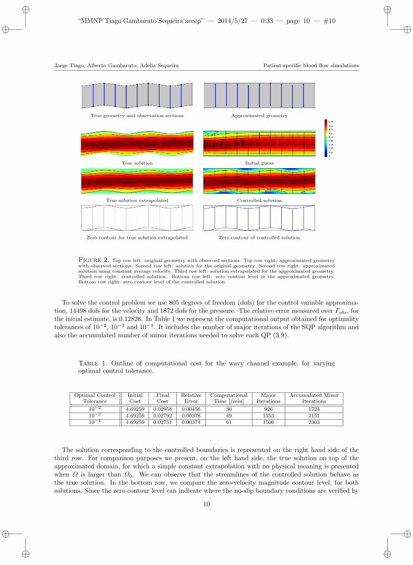
Figure 2. Top row left: original geometry with observed sections. Top row right: approximated geometrywith observed sections. Second row left: solution for the original geometry. Second row right: approximatedsolution using constant average velocity. Third row left: solution extrapolated for the approximated geometry.Third row right: controlled solution. Bottom row left: zero contour level in the approximated geometry.Bottom row right: zero contour level of the controlled solution.

To solve the control problem we use 805 degrees of freedom (dofs) for the control variable approxima-tion, 14498 dofs for the velocity and 1872 dofs for the pressure. The relative error measured over Γobs, forthe initial estimate, is 0.12826. In Table 1 we represent the computational output obtained for optimalitytolerances of 10−2, 10−3 and 10−4. It includes the number of major iterations of the SQP algorithm andalso the accumulated number of minor iterations needed to solve each QP (3.9).

Table 1. Outline of computational cost for the wavy channel example, for varyingoptimal control tolerance.

Optimal Control Initial Final Relative Computational Major Accumulated MinorTolerance Cost Cost Error Time [/min] Iterations Iterations

10−2 4.69259 0.02958 0.00456 30 926 172410−3 4.69259 0.02792 0.00378 49 1353 215110−4 4.69259 0.02751 0.00374 61 1506 2303

The solution corresponding to the controlled boundaries is represented on the right hand side of thethird row. For comparison purposes we present, on the left hand side, the true solution on top of theapproximated domain, for which a simple constant extrapolation with no physical meaning is presentedwhen Ω is larger than Ω0. We can observe that the streamlines of the controlled solution behave asthe true solution. In the bottom row, we compare the zero-velocity magnitude contour level, for bothsolutions. Since the zero contour level can indicate where the no-slip boundary conditions are verified by

10


ii

ii

ii


the true solution, we can see that the controlled solution gives a way to recover the location of the wallboundary for the original domain Ω0.

4.2. Wavy channel - non-uniform sampling

9 equidistant sections 4 equidistant sections

7 sections more concentrated at the beginning 7 sections concentrated only at the beginning

6 sections concentrated only at the end 7 short sections concentrated only at the end

Figure 3. Effect of number and distribution of observed sections Ωobs. The sections and location of theno-slip contour (i.e. where the velocity is zero) are shown. The true solution is presented in Figure 2.

The observations set Ωobs plays an important role. In fact, as we will see next, the number anddistribution of the sections where ud is taken have a large impact on the accuracy of the recoveredsolution. In Figure 3 we present the results obtained for different Ωobs.

We take, as a reference for comparison, the solution using nine observation sections, that has beenpreviously computed as described above. As a measure of accuracy we focus on recovering the wavy wallgeometry, hence the zero-velocity iso-contour that is the no-slip boundary, which is a sensitive measure andis used to evidentiate an important feature of the desired solution. On reducing the number of observationsections to four, a loss of accuracy is noticeable. By adding a higher concentration upstream, the accuracyis improved both in the region of increased number observations and downstream of it. Taking this ideafurther we test only sampling the upstream portion of the section very finely, however we notice that thewhile locally the solution has increased accuracy, elsewhere in the domain the solution is very poor. Infact, the control acted to minimize the misfit at the beginning of the channel while remaining flat closerto the outlet. This effect is independent of the region and similar results are obtained when the highersampling is located towards the outlet. Finally we test the effect of shorter sections and note that thisdoes not necessarily imply less accuracy.

We learn from these numerical experiments that it is important to sample the domain uniformly.Increased spatial sampling can only improve the solution locally, and likely also in the regional neigh-borhood. A partial set of samples, such as shorter observation cross-sections, does not directly imply areduced accuracy.

4.3. Wavy channel - noisy observations

Our next example investigates how the solution of the control problem can be affected by the presence ofnoise in the data ud. Noise is added to the velocity profiles, and this corrupted data is taken as our initialΩobs. We use two intensity Gaussian white noise samples generated such that 99.7 percent (hence 3σ) ofthe values lie on the (normalized) intervals uav× [−0.1, 0.1] and uav× [−0.2, 0.2], respectively. Dependingon the imaging modality, forms of noise will typically be Poisson or Gaussian, however artifacts may also

11


ii

ii

ii


Controlled solution without noise

Controlled solution with 10% of noise

Controlled solution with 20% of noise

Controlled solution vs Original Data at middle section

Initial section with 10% of noise Initial section with 20% of noise

Final section with 10% of noise Final section with 20% of noise

Figure 4. Top left: comparison of the recovered zero contour levels for the case without noise on ud andwith 10 and 20 percent, respectively. Top right: axial component of the velocity for the true and controlledsolutions on a section at the centre of the channel. Middle: comparison of the original solution with thecontrolled one in a section close to the inlet. Bottom: comparison of the original solution with the controlledone in a section close to the outlet.

be present and typically attributed to temporal variations. Gaussian noise is used here to represent anunbiased degradation of the measured data. Since the physical problem is modeled by the Navier-Stokesequations, which results in a smooth solution at low Reynolds numbers, it is expected that other similarforms of local random perturbations will yield comparable results. However, noise or artifacts with largespatial correlation or bias may affect the solution more than the Gaussian noise used here.

In Table 2 we show the relative errors obtained with 84614 dofs for the velocity vector and 2750 for thecontrol variable. The noisy data, when measured over Ωobs, adds a relative error to the original solutionof 4% in the first case, and 8% in the second one. Even though, the controlled solution approximates theoriginal data with a relative error smaller than 1.3% and 1.7%, respectively.

12


ii

ii

ii


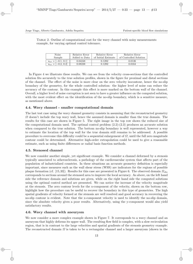
Table 2. Outline of computational cost for the wavy channel with noisy measurementsexample, for varying optimal control tolerance.

Noise Relative Error Relative Error Relative ErrorSample Added to Data of Initial Estimate of Controlled Solution

uav × [−0.1, 0.1] 0.04248 0.1292 0.0126uav × [−0.2, 0.2] 0.08238 0.1292 0.0164

In Figure 4 we illustrate these results. We can see from the velocity cross-sections that the controlledsolution fits accurately to the true solution profiles, shown in the figure for proximal and distal sectionsof the channel. The effect of the noise is more clear on the zero velocity isocontour, hence the no-slipboundary of the geometry, for the whole controlled solution: the higher level of noise can reduce theaccuracy of the contour. In this example this effect is more marked on the bottom wall of the channel.Overall, a higher level of noise corruption is not seen to have a greater influence on the computed solution,with the most evident effect on the identification of the no-slip boundary, which is a sensitive measure,as mentioned above.

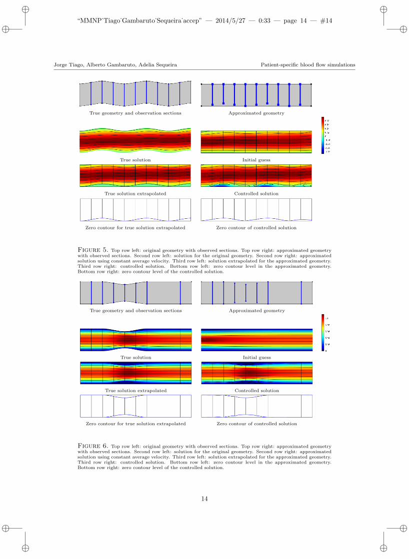
4.4. Wavy channel - smaller computational domain

The last test case using the wavy channel geometry consists in assuming that the reconstructed geometryΩ doesn’t include the top wavy wall, hence the assumed domain is smaller than the true domain. Theresults for this case are shown in Figure 5. The right image in the top row shows the reduced size ofthe computational domain used. The optimal control problem (2.2)-(2.3) produces an accurate solutionwhen compared to the true solution. The bottom no-slip boundary is well represented, however a wayto estimate the location of the top wall for the true domain still remains to be addressed. A possibleprocedure to overcome this difficulty could be a sequential enlargement of Ω, until the full zero magnitudecontour could be determined. Alternative high-order extrapolation could be used to give a reasonableestimate, such as using finite differences or radial basis function methods.

4.5. Stenosed channel

We now consider another simple, yet significant example. We consider a channel deformed by a stenosistypically associated to atherosclerosis, a pathology of the cardiovascular system that affects part of thepopulation of industrialized countries. In these situations an accurate geometry definition is especiallyimportant, since measures such as the wall shear stress (WSS) are indicators for the regions of possibleplaque formation (cf. [15,33]). Results for this case are presented in Figure 6. The observed domain Ωobscorresponds to sections around the stenosed area to improve the local accuracy. As above, on the left handside the reference domain and solutions are given, while on the right hand side the computed solutionsusing the optimal control method are presented. We can notice the increase of the velocity magnitudeat the stenosis. The zero contour levels for the x-component of the velocity, shown on the bottom row,highlight how the procedure can be useful to recover the boundary in this type of geometries. The highspatial gradients of velocity formed at the stenosis are well resolved and good accuracy in recovering theno-slip contour is evident. Note that the x-component velocity is used to identify the no-slip domain,since the absolute velocity gives a poor results. Alternatively, using the y-component would also yieldsatisfactory results.

4.6. Wavy channel with aneurysm

We now consider a more complex example shown in Figure 7. It corresponds to a wavy channel and ananeurysm that highly deforms its upper wall. The resulting flow field is complex, with a slow recirculationregion, that is in contrast to the large velocities and spatial gradients of the stenosis geometry example.The reconstructed domain Ω is taken to be a rectangular channel and a larger aneurysm (shown in the

13


ii

ii

ii












14


ii

ii

ii





Figure 7. Top row left: original geometry with observed sections. Top row right: approximated geometrywith observed sections. Second row left: solution for the original geometry. Second row right: approximatedsolution using constant average velocity. Note that the lines in magenta represent the zero contour of thex-component of the velocity. Third row left: solution extrapolated for the approximated geometry. Third rowright: controlled solution. Bottom row left: zero contour level in the approximated geometry. Bottom rowright: zero contour level of the controlled solution.

left column on the second row, where the true solution is overlapped). Besides the streamlines we alsorepresent, in magenta, the zero contour for the x-component of the velocity. It corresponds to the no-slipboundary condition, and in the interior of the aneurysm it indicates the location of the reversing flow.The observation sections Ωobs (shown by the black vertical lines) are concentrated within the aneurysmarea, due to the big geometry change, the reversed flow and the low magnitude velocity. We also includeother sections, covering the full length of the channel, a need that was detailed in Section 4.2. We notethat the control function c1 also describes the velocity vector at the aneurysm wall, which is included inthe upper boundary Γc1 .

The optimal solution recovers the behavior of the true solution, in terms of the streamlines and also forthe zero contour of the velocity x-component. We note that the no-slip boundary is accurately recovered,however the definition of the proximal region of the aneurysm neck performs worse due to the limitedresolution in distinguishing the geometry wall and the reversed flow boundaries. As noted in Section 4.2,the use of extra observations in this region would yield more precise results.

4.7. A realistic geometry - saccular aneurysm

Finally, we apply our procedure to adjust a reconstructed geometry obtained from a 2D longitudinalsection of a saccular aneurysm, inspired from the work of [36] and generated using interpolating splines,as shown in Figure 8. The computational domain involves a single inflow section (on the left) and two

15


ii

ii

ii


outflow sections (upper and lower). The problem set here is to concentrate on the shape and flow withinthe aneurysm, since this is clinically the most important feature. The reconstructed geometry Ω matchesΩ0 on all boundaries except on the aneurysm dome, where it is inflated. The blue vertical lines representthe observed sections Ωobs which are concentrated solely in the aneurysm. To recover the flow field inthe aneurysm and the no-slip boundary of the dome, we will control a portion of the dome boundary, ashighlighted in the bottom-right image, and also the inlet boundary Γin in a similar way to the exampleof Section 4.1.

True geometry Approximated geometry oversizing the aneurysm

Approximated geometry with observed sections Controlled boundary

Figure 8. Top row left: original geometry. Top row right: approximated geometry. Bottom row left:observation sections Ωobs. Bottom row right: the boundary to be controlled.

The resulting solutions are presented in Figure 9. As above, we use the x-component of the velocityand the streamlines to describe the flow and the no-slip boundary. In this example, the magnitude doesnot reach zero but rather an approximate value 2 × 10−5 which we use to estimate the location of theno-slip boundary in that area.

Similar to the results in Section 4.6, improvement in the accuracy can be obtained with more obser-vation data, especially near the wall. In fact, in the regions close to the controlled boundary, where thevelocity magnitude is very small and there are no observations, the no-slip boundary is not reproducedaccurately. This can be seen in Figure 10, where we represent the detail of the streamlines and themagnitude contour for the true solution (left), initial guess (center) and controlled solution (right). Wenote that the cost function given by equation (2.2) penalizes the misfit of velocities, however if these aresmall as in a slow recirculating region of an aneurysm, this term has a smaller weight. A normalizedmisfit cost function could improve the accuracy of the solution.

16


ii

ii

ii




Figure 9. Top row left: solution for the original geometry. Top row right: approximated solution usingconstant average velocity. Bottom row left: solution extrapolated for the approximated geometry. Bottom rowright: velocity zero contour of the controlled solution.

Zero contour for the true solution extrapolated Zero contour for the initial guess Zero contour of the controlled solution

Figure 10. Left: streamlines and zero-magnitude velocity for original solution. Center: streamlines forinitial guess. Right: streamlines and zero-magnitude velocity for controlled solution.

5. Conclusions and remarks

We have presented an automatic procedure to minimize the difference between measured observationsand solutions to numerical simulations. With emphasis on patient-specific computational hemodynamics,this tool has been used to correct approximate boundary conditions at the inflow and the definition ofthe no-slip boundary. In practice, the method is used to minimize the uncertainty that arises due to: i)the correct choice of the boundary conditions at the artificial truncation of the computational domain,ii) the definition of the geometry caused by noisy and limited resolution medical image data.

17


ii

ii

ii


The measured observations used in the cost minimization are velocity data, that can be obtained fromnon-invasive phase contrast MRI. These observations should adequately cover the computational domain.They also suffer from artifacts, noise and limited resolution, however the procedure outlined in this workis shown by means of example cases, to be robust to such noise. A strength of the method is that it isautomatic as it does not require any supervision, and guarantees minimal error solution.

The procedure has been validated with various 2D models through numerical tests. Particular attentionto the accuracy of the solution has been devoted to the recovery of the true domain’s no-slip boundaries.These are sensitive measures of interest since many diseases have been correlated to the wall shear stress.The test cases have included a stenosis geometry with high values of velocity and velocity gradients, andaneurysm geometries, that contain regions of flow separation and flow recirculation. The simulationshave been performed for steady state which is often sufficient for practical clinical studies. The proposedmethod can be extended to the time dependent case, however the computational cost will be greatlyincreased. Current simulation time requires about 30 min to obtain a relative error smaller than 0.46%,with 800 dofs for the control variable and 14500 dofs for the velocity vector.

At the current stage of the work, there is no criteria for an automatic choice for the location of theobservations in the true domain, that can greatly impact on the quality of the obtained results. This isa subject of observability and controllability theory, that was not treated here. This important point,together with exploring other cost functionals to be minimized and an extension to the 3-dimensionalcase, should be covered in future work.

The proposed method has shown, through the set of numerical test cases, to be useful as an unsuper-vised method to choose flow boundary conditions and identify a more accurate definition of the geometryno-slip walls. The tools presented can be used to address current concerns in correct numerical simulationdefinition setup.

Acknowledgements. This work was partially supported by FCT (Portugal) through the Research Center CEMAT-IST, the grant SFRH/BPD/66638/2009, and the project EXCL/MAT-NAN/0114/2012. The second authorgratefully acknowledges support from project MatComPhys under the European Research Executive AgencyFP7-PEOPLE-2011-IEF framework.

References

[1] F.E. Boas, D. Fleischmann. CT artifacts: causes and reduction techniques. Imaging in Medicine, 4 (2012), 229-240.

[2] T. Bodnar, A. Sequeira and M. Prosi. On the shear-thinning effects of blood flow under various flow rates. AppliedMathematics and Computation, Elsevier, 217 (2011), 5055-5067.

[3] J. Burkardt, M. Gunzburger, J. Peterson. Insensitivite Functionals, Inconsistent Gradients, Spurious Minima andRegularized Funcionals in Flow Optimization Problems. International Journal of Computational Fluid Dynamics, 16(2002), 171-185.

[4] Cebral JR, Castro MA, Appanaboyina S, Putman CM, Millan D, Frangi AF. Efficient pipeline for image-based patient-specific analysis of cerebral aneurism hemodynamics: technique and sensitivity. IEEE Transactions on Medical Imaging,344 (2005), 457-467.

[5] COMSOL Multiphysics, Users Guide, COMSOL 4.3, 2012.

[6] Optimization Module, Users Guide, COMSOL 4.3, 2012.

[7] M. D’ Elia, M. Perego, A. Veneziani. A Variational Data Assimilation Procedure for the Incompressible Navier-StokesEquations in Hemodynamics. Journal of Scientific Computing, 53 (2011).

[8] M. D’ Elia, A. Veneziani. A Data Assimilation technique for including noisy measurements of the velocity field intoNavier-Stokes simulations. Proceedings of V European Conference on Computational Fluid Dynamics, ECCOMAS,June (2010).

[9] J.C. De Los Reyes, K. Kunisch. A semi-smooth Newton method for control constrained boundary optimal control ofthe Navier-Stokes equations. Nonlinear Anal., 62 (2005), No. 7, 1289-1316.

[10] J.C. De Los Reyes, K. Kunisch. Optimal control of partial differential equations with affine control constraints. ControlCybernet., 38 (2009), No. 4, 1217-1249.

[11] J.C. De Los Reyes, Yousept, Irwin. Regularized state-constraint boundary Optimal control of the Navier-Stokes equa-tions., J-Math. Anal. Appl., 356 (2009), No. 1, 257-279.

18


ii

ii

ii


[12] P. Deuflhard. A Modified Newton Method for the Solution of Ill-conditioned Systems of Nonlinear Equations withApplication to Multiple Shooting. Numer. Math., 22 (1974) 289-315.

[13] L. Formaggia, J.F. Gerbeau, F. Nobile, A. Quarteroni. Numerical treatment of defective boundary conditions for theNavier-Stokes equations. SIAM J. Numer. Anal., 40 (2002) 376-401.

[14] A.M. Gambaruto, D.J. Doorly, T. Yamaguchi. Wall shear stress and near-wall convective transport: Comparisonswith vascular remodelling in a peripheral graft anastomosis. Journal of Computational Physics, 229 (2010), No. 14,5339-5356.

[15] A. Garambuto, J. Janela, A. Moura and A. Sequeira. Sensitivity of hemodynamics in a patient specific cerebralaneurysm to vascular geometry and blood rheology. Mathematical Biosciences and Engineering, 8 (2011), No. 2, 409-423.

[16] A. Gambaruto, J. Janela, A. Moura, A. Sequeira. Shear-thinning effects of hemodynamics in patient-specific cerebralaneurysms. Mathematical Biosciences and Engineering, 10 (2013), No. 3, 649-665.

[17] A.M. Gambaruto, J. Peiro, D.J. Doorly, A.G. Radaelli. Reconstruction of shape and its effect on flow in arterialconduits. International Journal for Numerical Methods in Fluids, 57 (2008), No. 5, 495-517.

[18] V. Girault, P.A. Raviart. Finite Element Methods for Navier-Stokes Equations, Theory and Algorithms, Number 5 inSpringer Series in Computational Mathematics. Springer-Verlag, Berlin, 1986.

[19] T. Guerra, J. Tiago, A. Sequeira, Optimal control in blood flow simulations. International Journal of Non-LinearMechanics, Available online (2014), doi:10.1016/j.ijnonlinmec.2014.04.005.

[20] M. Gunzburger, Adjoint Equation-Based Methods for Control Problems in Incompressible, Viscous Flows. Flow, Tur-bulence and Combustion, 65 (2000), No. 3, 249-272.

[21] M. Gunzburger, L.S. Hou, T.P. Svobodny, Analysis and finite element approximation of optimal control problemsfor the stationary Navier-Stokes equations with Dirichlet controls. RAIRO - Modelisation mathemathique et analysenumerique, 25 (1991), No. 6, 711-748.

[22] P. Gill, W. Murray, M.A. Saunders. SNOPT: An SQP Algoritm for Large-Scale Constrained Optimization. Society forIndustrial and Applied Mathematics, SIAM REVIEW, 47 (2005) No. I, 99-131.

[23] B.M. Johnston, P.R. Johnston , S. Corney, D. Kilpatrick. Non-Newtonian blood flow in human right coronary arteries:transient simulations. Journal of Biomechanics, 39 (2006), No. 6, 1116-1128.

[24] M. Kroon , G.A. Holzapfel. Estimation of the distributions of anisotropic, elastic properties and wall stresses ofsaccular cerebral aneurysms by inverse analysis. Proc. R. Soc. A, 464 (2008), 807-825.

[25] K.L. Lee, D.J. Doorly, D.N. Firmin. Numerical simulations of phase contrast velocity mapping of complex flows in ananatomically realistic bypass graft geometry. Medical Physics, 7 (2006), 2621-2631.

[26] J.G. Myers, J.A. Moore, M. Ojha, K.W. Johnston, C.R. Ethier. Factors Influencing Blood Flow Patterns in the HumanRight Coronary Artery. Annals of Biomedical Engineering, 29 (2001), No. 2, 109-120.

[27] R.W. Ogden, G. Saccomandi, I. Sgura. Fitting hyperelastic models to experimental data. Computational Mechanics,34 (2004), N0. 6, 484-502.

[28] E. Pusey, R.B. Lufkin, R.K. Brown, M.A. Solomon, D.D. Stark, R.W. Tarr, W.N. Hanafee. Magnetic resonance imagingartifacts: mechanism and clinical significance. Radiographics, 6 (1986), No. 5, 891-911.

[29] A. Quarteroni, L. Formaggia. Mathematical Modelling and Numerical Simulation of the Cardiovascular System, Mod-elling of living Systems. Handbook of Numerical Analysis Series. Elsevier, Amsterdam, 2002.

[30] S. Ramalho, A. Moura, A.M. Gambaruto, A. Sequeira. Sensitivity to outflow boundary conditions and level of geometrydescription for a cerebral aneurysm. International Journal for Numerical Methods in Biomedical Engineering, 28 (2012),No. 6-7, 697-713.

[31] A.M. Robertson, A. Sequeira, M.V. Kameneva. Hemorheology. Hemodynamical Flows. Modeling, Analysis and Simu-lation. Oberwolfach Seminars. Birkhauser Verlag, Basel, 37 (2008), 63-120.

[32] O. Schenk, K. Gartner, W. Fichtner, A. Stricker. PARDISO: A High-Performance Serial and Parallel Sparse LinearSolver in Semiconductor Device Simulation, Journal of Future Generation Computers Systems, 18 (2001), 69-78.

[33] T. Silva, A. Sequeira, R. Santos, J. Tiago. Mathematical Modeling of Atherosclerotic Plaque Formation Coupledwith a Non-Newtonian Model of Blood Flow. Conference Papers in Mathematics, vol. 2013, Article ID 405914, 2013.doi:10.1155/2013/405914.

[34] N.P. Smith, A.J. Pullan, P.J. Hunter. An anatomically based model of coronary blood flow and myocardial mechanics.SIAM J. Appl. Math., 62 (2002), 990-1018.

[35] P. Tricerri. Mathematical and Numerical Modeling of Healthy and Unhealthy Cerebral Arterial Tissue. Ecole Poly-technique Federale de Lausanne. Ph.D. thesis, 2014.

[36] Y. Wei, S. Cotin, J. Dequidt, C. Duriez, J. Allard, E. Kerrien. A (Near) Real-Time Simulation Method of AneurysmCoil Embolization http://dx.doi.org/10.5772/48635, INTECH, 2012.

[37] C. Westbrook, C.K. Roth, J. Talbot. MRI in Practice. Wiley-Blackwell, 2011.

19

tiago, j., gambaruto, a. m., & sequeira, a. (2014 ... ·...

Documents