tic verifica tion of - university of pennsylvaniaalur/thesis91.pdf · tic verifica tion of realtime...
TRANSCRIPT
TECHNIQUES FOR AUTOMATIC VERIFICATION OF
REAL�TIME SYSTEMS
a dissertation
submitted to the department of computer science
and the committee on graduate studies
of stanford university
in partial fulfillment of the requirements
for the degree of
doctor of philosophy
By
Rajeev Alur
August ����

c� Copyright ���� by Rajeev Alur
All Rights Reserved
ii

I certify that I have read this dissertation and that in my
opinion it is fully adequate� in scope and in quality� as a
dissertation for the degree of Doctor of Philosophy�
David Dill�Principal Advisor�
I certify that I have read this dissertation and that in my
opinion it is fully adequate� in scope and in quality� as a
dissertation for the degree of Doctor of Philosophy�
Zohar Manna�Coadvisor�
I certify that I have read this dissertation and that in my
opinion it is fully adequate� in scope and in quality� as a
dissertation for the degree of Doctor of Philosophy�
Moshe Vardi
Approved for the University Committee on Graduate Studies�
Dean of Graduate Studies
iii

Abstract
This thesis proposes formalmethods for specication and automatic verication of �nite�
state real�time systems� The traditional formalisms for reasoning about programs abstract
away from quantitative time and� consequently� are inadequate for reasoning about real
time systems� We extend the methods based on automata and temporal logics to allow
them to model timing delays and to verify realtime requirements�
We introduce timed automata to model the behavior of realtime systems over time�
Our denition provides a simple� and yet powerful� way to annotate statetransition graphs
with timing constraints using nitely many realvalued clocks � A timed automaton accepts
timed words � strings in which a realvalued time of occurrence is associated with each
symbol� We study timed automata from the perspective of formal language theory� we
consider closure properties� decision problems� and subclasses�
We present two conservative extensions of the existing temporal logics to allow them
to specify timing properties� The metric interval temporal logic �MITL� uses lineartime
semantics� and its syntax allows temporal operators to be subscripted with intervals re
stricting their scope in time� The timed computation tree logic �TCTL� uses branchingtime
semantics� and its syntax provides access to time through a novel kind of time quantier�
In the proposed verication method� a nitestate system is modeled as a composition
of timed automata� and the correctness is specied either as a deterministic timed automa
ton� or as a formula of MITL or TCTL� In each case we develop an algorithm for model
checking � The distinguishing feature of our work is the use of the set of reals to model time�
we argue that the denseness of the time domain is crucial for modeling eventdriven asyn
chronous systems� The thesis also claries the relationship between di erent models and
logics for realtime� and answers some basic questions regarding complexity� decidability�
and expressiveness�
iv

Acknowledgments
First of all I thank my advisors� David Dill and Zohar Manna� for o ering me technical�
nancial� and moral support during the last four years� My reading committee comprised of
David� Zohar� and Moshe Vardi� and I consider myself fortunate that I had access to valuable
guidance from all three of them� I am also thankful to them for their critical reading
of the draft� Zohar introduced me to temporal logics� and directed me to the relatively
unexplored area of realtime logics� He also made possible an extremely productive visit to
the Weizmann Institute in Israel� Much of the research reported in this thesis is inspired by
my discussions with David about his ideas on coupling automata with timing constraints�
Moshe is one of the leading proponents of the automatatheoretic approach to verication�
and his expertise on the subject has been very useful to me�
It has been a great pleasure for me to work closely with Tom Henzinger� We learned to
do research together� we solved many problems together� it would be futile to pinpoint his
innumerable contributions towards my work� Special thanks also go to my other colleagues�
Costas Courcoubetis and Tomas Feder� Costas�s unbounded enthusiasm to attack new
problems has been a source of inspiration to me� The decision procedure for MITL builds
upon some insightful observations made by Tomas�
I have had the opportunity to discuss my research with many scientists at Stanford� at
IBM Almaden Research Center� and at various conferences and seminars� I thank all of
them for being helpful and encouraging� I am particularly grateful to Joe Halpern� Dinesh
Katiyar� John Mitchell� Amir Pnueli� Howard WongToi� and Mihalis Yannakakis�
My allegiance to computer science is mainly due to the excellent education I received
at the Indian Institute of Technology at Kanpur� and I am thankful to the faculty on
its Computer Science Department� Also this thesis would not exist without the love and
support of my family� especially� my parents� I would also like to use this opportunity to
thank all my friends on Stanford campus� because of them my stay here has been very
enjoyable and memorable�
v

Contents
Abstract iv
Acknowledgments v
� Introduction �
��� Motivation � � � � � � � � � � � � � � � � � � � � � � � � � � � � � � � � � � � � �
��� Background� formalisms for qualitative reasoning � � � � � � � � � � � � � � � �
����� Temporal logics � � � � � � � � � � � � � � � � � � � � � � � � � � � � � � �
����� Automatatheoretic approach � � � � � � � � � � � � � � � � � � � � � � �
����� Other approaches � � � � � � � � � � � � � � � � � � � � � � � � � � � � � �
��� Overview � � � � � � � � � � � � � � � � � � � � � � � � � � � � � � � � � � � � � �
����� Verication methodology � � � � � � � � � � � � � � � � � � � � � � � � �
����� Contributions � � � � � � � � � � � � � � � � � � � � � � � � � � � � � � � �
��� Related research � � � � � � � � � � � � � � � � � � � � � � � � � � � � � � � � � ��
����� Modeling realtime systems � � � � � � � � � � � � � � � � � � � � � � � ��
����� Specication languages � � � � � � � � � � � � � � � � � � � � � � � � � � ��
����� Verication � � � � � � � � � � � � � � � � � � � � � � � � � � � � � � � � ��
��� Organization of the thesis � � � � � � � � � � � � � � � � � � � � � � � � � � � � ��
� Adding Time to Semantics ��
��� Trace semantics � � � � � � � � � � � � � � � � � � � � � � � � � � � � � � � � � � ��
��� Timed traces � � � � � � � � � � � � � � � � � � � � � � � � � � � � � � � � � � � ��
����� Adding timing to traces � � � � � � � � � � � � � � � � � � � � � � � � � ��
����� Discretetime model � � � � � � � � � � � � � � � � � � � � � � � � � � � ��
����� Densetime model � � � � � � � � � � � � � � � � � � � � � � � � � � � � ��
vi

����� Fictitiousclock model � � � � � � � � � � � � � � � � � � � � � � � � � � ��
��� A case for the densetime Model � � � � � � � � � � � � � � � � � � � � � � � � ��
����� Correctness � � � � � � � � � � � � � � � � � � � � � � � � � � � � � � � � ��
����� Expressiveness � � � � � � � � � � � � � � � � � � � � � � � � � � � � � � ��
����� Compositionality � � � � � � � � � � � � � � � � � � � � � � � � � � � � � ��
����� Complexity � � � � � � � � � � � � � � � � � � � � � � � � � � � � � � � � ��
� Automata�Theoretic Approach ��
��� �automata � � � � � � � � � � � � � � � � � � � � � � � � � � � � � � � � � � � � ��
��� Timed automata � � � � � � � � � � � � � � � � � � � � � � � � � � � � � � � � � ��
����� Timed languages � � � � � � � � � � � � � � � � � � � � � � � � � � � � � ��
����� Transition tables with timing constraints � � � � � � � � � � � � � � � ��
����� Clock constraints and clock interpretations � � � � � � � � � � � � � � ��
����� Timed transition tables � � � � � � � � � � � � � � � � � � � � � � � � � ��
����� Timed regular languages � � � � � � � � � � � � � � � � � � � � � � � � � ��
����� Properties of timed regular languages � � � � � � � � � � � � � � � � � ��
����� Timed Muller automata � � � � � � � � � � � � � � � � � � � � � � � � � ��
��� Checking emptiness � � � � � � � � � � � � � � � � � � � � � � � � � � � � � � � � ��
����� Restriction to integer constants � � � � � � � � � � � � � � � � � � � � � ��
����� Clock regions � � � � � � � � � � � � � � � � � � � � � � � � � � � � � � � ��
����� The region automaton � � � � � � � � � � � � � � � � � � � � � � � � � � ��
����� The untiming construction � � � � � � � � � � � � � � � � � � � � � � � ��
����� Complexity of checking emptiness � � � � � � � � � � � � � � � � � � � ��
��� Intractable problems � � � � � � � � � � � � � � � � � � � � � � � � � � � � � � � ��
����� A ���complete problem � � � � � � � � � � � � � � � � � � � � � � � � � ��
����� Undecidability of the universality problem � � � � � � � � � � � � � � � ��
����� Inclusion and equivalence � � � � � � � � � � � � � � � � � � � � � � � � ��
����� Nonclosure under complement � � � � � � � � � � � � � � � � � � � � � ��
��� Deterministic timed automata � � � � � � � � � � � � � � � � � � � � � � � � � � ��
����� Denition � � � � � � � � � � � � � � � � � � � � � � � � � � � � � � � � � ��
����� Closure properties � � � � � � � � � � � � � � � � � � � � � � � � � � � � ��
����� Decision problems � � � � � � � � � � � � � � � � � � � � � � � � � � � � ��
����� Expressiveness � � � � � � � � � � � � � � � � � � � � � � � � � � � � � � ��
vii

��� Variants of timed automata � � � � � � � � � � � � � � � � � � � � � � � � � � � ��
����� Clock constraints � � � � � � � � � � � � � � � � � � � � � � � � � � � � � ��
����� Timed automata with �transitions � � � � � � � � � � � � � � � � � � � ��
��� Verication � � � � � � � � � � � � � � � � � � � � � � � � � � � � � � � � � � � � ��
����� �automata and verication � � � � � � � � � � � � � � � � � � � � � � � ��
����� Verication using timed automata � � � � � � � � � � � � � � � � � � � ��
����� Verication example � � � � � � � � � � � � � � � � � � � � � � � � � � � ��
����� Implementation � � � � � � � � � � � � � � � � � � � � � � � � � � � � � � ��
� Linear Temporal Logic �
��� Propositional temporal logic� PTL � � � � � � � � � � � � � � � � � � � � � � � ��
��� Metric interval temporal logic � � � � � � � � � � � � � � � � � � � � � � � � � � ��
����� Intervals � � � � � � � � � � � � � � � � � � � � � � � � � � � � � � � � � � ��
����� Timed state sequences � � � � � � � � � � � � � � � � � � � � � � � � � � ��
����� Syntax and semantics of MITL � � � � � � � � � � � � � � � � � � � � � ��
����� Dened operators � � � � � � � � � � � � � � � � � � � � � � � � � � � � � ��
����� Rening the models � � � � � � � � � � � � � � � � � � � � � � � � � � � ��
����� Real versus rational time � � � � � � � � � � � � � � � � � � � � � � � � ���
����� Allowing rational constants � � � � � � � � � � � � � � � � � � � � � � � ���
����� Avoiding undecidability � � � � � � � � � � � � � � � � � � � � � � � � � ���
��� Interval automata � � � � � � � � � � � � � � � � � � � � � � � � � � � � � � � � � ���
��� Deciding MITL � � � � � � � � � � � � � � � � � � � � � � � � � � � � � � � � � � ���
����� Restricting the problem � � � � � � � � � � � � � � � � � � � � � � � � � ���
����� Intuition for the algorithm � � � � � � � � � � � � � � � � � � � � � � � � ���
����� Witnessing intervals � � � � � � � � � � � � � � � � � � � � � � � � � � � ���
����� Type� and type� formulas � � � � � � � � � � � � � � � � � � � � � � � ���
����� Type� and type� formulas � � � � � � � � � � � � � � � � � � � � � � � ���
����� Constructing the interval automaton � � � � � � � � � � � � � � � � � � ���
����� Complexity of MITL � � � � � � � � � � � � � � � � � � � � � � � � � � � ���
��� Verication using MITL � � � � � � � � � � � � � � � � � � � � � � � � � � � � � ���
��� Expressiveness � � � � � � � � � � � � � � � � � � � � � � � � � � � � � � � � � � ���
����� Comparison with ctitiousclock logics � � � � � � � � � � � � � � � � � ���
����� Comparison with interval automata � � � � � � � � � � � � � � � � � � ���
viii

Branching�Time Logic ���
��� Computation tree logic � � � � � � � � � � � � � � � � � � � � � � � � � � � � � � ���
��� The logic TCTL � � � � � � � � � � � � � � � � � � � � � � � � � � � � � � � � � ���
����� Syntax � � � � � � � � � � � � � � � � � � � � � � � � � � � � � � � � � � � ���
����� Semantics � � � � � � � � � � � � � � � � � � � � � � � � � � � � � � � � � ���
����� On the choice of syntax � � � � � � � � � � � � � � � � � � � � � � � � � ���
����� Undecidability � � � � � � � � � � � � � � � � � � � � � � � � � � � � � � ���
����� Interval automata as TCTLstructures � � � � � � � � � � � � � � � � � ���
��� Model checking � � � � � � � � � � � � � � � � � � � � � � � � � � � � � � � � � � ���
����� Introducing formula clocks � � � � � � � � � � � � � � � � � � � � � � � ���
����� Clock regions � � � � � � � � � � � � � � � � � � � � � � � � � � � � � � � ���
����� The region graph � � � � � � � � � � � � � � � � � � � � � � � � � � � � � ���
����� Labeling algorithm � � � � � � � � � � � � � � � � � � � � � � � � � � � � ���
����� Complexity of the algorithm � � � � � � � � � � � � � � � � � � � � � � ���
����� Complexity of modelchecking � � � � � � � � � � � � � � � � � � � � � � ���
����� TCTL with fairness � � � � � � � � � � � � � � � � � � � � � � � � � � � ���
� Concluding Remarks ���
Bibliography ��
ix

Chapter �
Introduction
��� Motivation
With the increasing use of computers in safetycritical applications there is a pressing need
for designing more reliable systems� As a result� developing formal methods for the design
and analysis of concurrent systems has been an active area of computer science research� The
conventional approach to testing the correctness of a system involves simulation on some
test cases� This method is quite inadequate for developing bugfree complex concurrent
systems� One approach to assure correctness is to employ automatic veri�cation methods�
A verication formalism comprises of
�� A formal semantics which assigns mathematical meanings to system components and
correctness criteria�
�� A language for describing the essential aspects of the system components� and con
structs for combining them�
�� A specication language for expressing the correctness requirements�
�� A verication algorithmto check if the correctness criteria are fullled in every possible
execution of the system�
In this thesis we provide formalisms for automatic verication of �nite�state real�time sys�
tems �
The class of systems to which our methods are applicable includes asynchronous circuits�
communication protocols� and controllers �such as a �ight controller� or a controller for a
�

CHAPTER �� INTRODUCTION �
manufacturing plant�� The essential characteristics of such systems are�
� Finite�state� The system can be in one of the nitely many discrete states� If we focus
only on the control aspect of the system� ignoring the computational aspect� then this
is an useful abstraction in many cases� Statetransitions are triggered by events which
are instantaneous�
� Reactive� The system constantly interacts with the environment reacting to stimuli�
So we are interested in the ongoing behavior over time� This is quite unlike the tra
ditional �transformational� view of the programs where the functional relationship
between the input state and the output state denes the meaning of a program� The
system comprises of a collection of components operating concurrently and commu
nicating with each other�
� Real�time� The correctness of the system depends on the actual magnitudes of the
timing delays of the components� This is obviously the case when the system needs
to meet hard realtime deadlines� the system needs to respond to a stimulus within
a certain xed time bound� Also there are cases when the logical correctness of the
system depends on the lengths of various delays�
Realtime systems are used in safetycritical applications such as controllers for nuclear
plants� Failures in such systems can be very expensive and even lifethreatening� Because
of the intricacies of the timing relationships� realtime systems are quite hard to model�
specify� and design� Consequently� there is a great demand for formal methods applicable
to realtime systems�
��� Background� formalisms for qualitative reasoning
Several di erent formalisms have been proposed to reason about reactive systems� These
include Petri nets� process algebras� temporal logics� automatatheoretic techniques� and
partialorder models�
These methodologies abstract from time� retaining the information about the causality
and�or the temporal order of occurrence of observable events� Even though there is no gen
eral agreement about what is the right semantics of concurrency� some of these techniques
have provided the foundations for building veriers for hardware and communication proto
cols� and some have suggested structured disciplines for writing concurrent programs� We

CHAPTER �� INTRODUCTION �
will brie�y review these approaches� the methods for automatic verication of nitestate
systems are of main interest to us�
����� Temporal logics
The use of temporal logic as a formalism for specifying the behavior of a reactive system over
time was rst proposed by Pnueli in ���� �Pnu���� The subject has been extensively studied
since then �BMP��� MP��� EC��� OL��� Lam��� MW��� BKP��� CES��� Pnu��� MP���
Lam���� Temporal logic is a modal logic with modalities such as � meaning �eventually��
and � meaning �always� �see �Eme��� for an overview�� Temporal logics provide a succinct
and natural way of expressing the desired temporal requirements� Two types of temporal
logics have been proposed� linear�time and branching�time�
In the lineartime framework� a system is viewed as a set of computations� where each
computation is a sequence of systemstates recording all the transitions over the course
of time� A linear temporal logic formula is interpreted over such state sequences �Pnu���
OL���� The branchingtime logics� on the other hand� are interpreted over tree models
�BMP��� EC��� EL���� The system is viewed as a nitelybranching tree� the paths in the
tree correspond to the possible executions of the system�
In the traditional approach to verication of concurrent programs� the correctness of the
program is expressed by a formula in rstorder temporal logic� The verication problem
reduces to proving a theorem in a deductive system� For example� Manna and Pnueli
�MP��� have developed the model of fair transition systems to describe the implementation�
and give a proof system to verify temporal logic specications� Though the technique is
quite general� constructing a proof needs to be done manually and requires a great deal of
understanding of the program� The only extent of automation one can hope for is to have
the proof checked by a machine and possibly to have some limited heuristics in nding the
proof�
Model checking provides a di erent approach to checking properties of nitestate sys
tems �CES��� LP��� EL��� BCD���� GW���� In this approach� the global statetransition
graph is viewed as a nite Kripke structure �with fairness requirements� if necessary�� The
specication of the system is given as a formula of a propositional temporal logic� The
modelchecking algorithm then decides whether the system meets the specication in all
possible scenarios� For the lineartime case� the complexity of modelchecking is linear in
the size of the statetransition graph and exponential in the size of the specication� and in

CHAPTER �� INTRODUCTION �
the branchingtime case� it is linear both in the size of the statetransition graph and the
length of the temporal logic specication� Various aspects of the modelchecking problem
for the logic CTL �EC��� have been studied� This approach has been successfully applied to
verify circuits and protocols� and to nd bugs in previouslypublished� nontrivial protocols
and circuits �CES��� BCDM����
The modelchecking approach to program verication is probably the most exciting
advance in the theory of program correctness in recent years� It has been extended to
probabilistic systems �Var��� PZ��� CY���� to realtime systems �EMSS��� AH��� ACD���
Lew��� HLP���� and to probabilistic realtime systems �HJ��� ACD��a� ACD��b��
The main di�culty in using modelchecking approach is the state�explosion problem� the
size of the global statetransition graph grows exponentially with the number of components
in the system� This problem has received great attention recently� and di erent ways to
cope with the problem have been proposed �BCD���� God��� GW����
����� Automata�theoretic approach
A related approach to verication of nitestate systems uses �automata �WVS��� Var����
The computation of a reactive program is viewed as an innite word over the alphabet
of events �or states�� This gives rise to an intimate connection between reasoning about
reactive systems and the formal language theory� A system is modeled as an automaton
generating innite sequences which correspond to the possible computations of the system�
The automata over innite words were rst studied by B�uchi in relation to the theory
S�S� the second order monadic theory of natural numbers with successor �B�uc���� B�uchi
automata and their variants have been studied in great detail since then �Cho��� Mul���
McN���� leading to a beautiful theory of �regular languages �see �Tho��� for an overview��
In the automatatheoretic framework� a system is modeled as a composition of sev
eral automata� The implementation automaton I is the product of these automata� and
acts as a generator � The specication is given as another automaton S which acts as
an acceptor � Alternatively� from a linear temporal logic specication� one can construct
an automaton which accepts all the computations that satisfy the given formula� The
implementation is correct i every behavior generated by I is accepted by S� Thus the
verication problem reduces to the language inclusion problem� Consequently the known
e ective constructions for intersection� complementation� and test for emptiness can be used

CHAPTER �� INTRODUCTION �
as a basis for automatic verication� Checking for language inclusion involves complement
ing the specication automaton which can be expensive� particularly for nondeterministic
automata �SVW��� Saf���� Alternative ways which use simulation relations have been pro
posed �DHW����
Another advantage of automata specications is the possibility of hierarchical verica
tion� Since both implementation and specication are automata� there is no real distinction
between them� they can be viewed as descriptions of the system at di erent levels of detail�
Consequently verication can be carried out by starting with a highlevel model and apply
ing successive renements� The system COSPAN developed at Bell Laboratories is based
on the automata based selection�resolution model �AKS���� and has been used successfully
to verify some of the commercially used protocols �HK����
Apart from the automatic verication approach� other automata based techniques also
have been proposed� Lynch et� al� have dened inputoutput automata as a model of com
putation in asynchronous distributed networks� and have developed methods to construct
modular correctness proofs of distributed algorithms �LT���� Alpern and Schneider show
how to derive proof obligations from B�uchi automata specications� and give proof rules for
checking these obligations against a concurrent program �AS����
����� Other approaches
Petri nets provide a succinct and elegant way to model concurrency and causal dependencies
in reactive systems �Pet���� An extensive literature exists on the topic� and the formalism
has been widely used in the specication� modeling and performance evaluation of systems�
Reachability analysis on Petri nets can be used to detect if something �bad� will ever
happen�
Milner introduced CCS �Calculus of Communicating Systems� as a model for concurrent
systems �Mil���� CCS views the system computation as a nitelybranching tree� The
calculus provides operators such as nondeterministic choice� parallel composition� and hiding
to build complex terms from simpler ones� with an associated array of algebraic laws� The
verication methodology based on CCS denes an equivalence relation on CCS terms� and
the verication problem is to decide whether or not the specication term is equivalent to
the implementation term� Various notions of observational equivalences and preorders have
been proposed and studied�

CHAPTER �� INTRODUCTION �
Another popular formalism for concurrency is Hoare�s theory of Communicating Sequen
tial Processes �Hoa��� Hoa���� CSP provides a small� and yet powerful� set of constructs
for writing concurrent programs� and laws for reasoning with them� In one of the possible
models for CSP� each process is modeled as a collection of sequences called traces � where a
trace records the order of events that may be observed when the process runs�
��� Overview
The thesis extends the nitestate verication techniques based on automata and temporal
logics to realtime systems� The techniques discussed in the previous section abstract away
from quantitative time and� hence� are unsuitable for modeling and specifying realtime
systems� We develop realtime extensions of automata which can model timing delays
between system transitions� and realtime extensions of temporal logics which can specify
hard realtime requirements�
����� Veri�cation methodology
Formal semantics
The standard notion of a computation models only the sequencing of events or state
transitions� In the eventbased model of automata� we introduce realtime by assigning
a realvalued time to every event occurrence� Similarly� we incorporate realtime in the
model of state sequences by associating an interval of the real number line with every state�
The feature that distinguishes our work from most of the earlier work on formalisms for
realtime reasoning is the use of a dense domain for choosing the time values�
We consider both lineartime and branchingtime logic specications� In the lineartime
world� the system is modeled as a set of �dense� linear executions� In the branchingtime
world� the system is viewed as a tree over such executions� however� because of the innitely
many choices for the time of the next transition� the tree is no longer nitely branching�
Modeling the system
To augment the statetransition graph of a system with its timing constraints� we propose
the formalism of timed automata� Our denition is inspired by the model introduced by Dill
�Dil���� A timed automaton is a nite statetransition graph with a nite set of realvalued

CHAPTER �� INTRODUCTION �
clocks � The clocks can be reset to � �independently of each other� with the statetransitions
of the system� and keep track of the time elapsed since the last reset� To express the timing
delays of the system� we associate with the transitions� or alternatively with the states�
constraints that compare clock values with constants� With this mechanism we can model
timing properties such as �the channel delivers every message within � to � time units of
its receipt��
Timed automata can model several interesting aspects of realtime systems� qualitative
features such as liveness� fairness� and nondeterminism� and quantitative features such
as periodicity� bounded response� and timing delays� The model of timed automata is
compositional � and we provide an algorithm to construct the global automaton from the
automata describing the behaviors of di erent components�
Speci�cation languages
As in the qualitative case� a timed automaton denes a formal language� and thus� when
viewed as an acceptor� provides a specication formalism� We propose that deterministic
timed automata� coupled with Muller acceptance conditions� be used as a specication
language�
We also consider realtime extensions of temporal logics� In the lineartime case� we
dene the logic metric interval temporal logic �MITL� by extending the linear temporal
logic PTL� In MITL� the temporal modalities are subscripted with time intervals restricting
their scope in time� For instance� ������ means �throughout the interval ��� ���� With this
extension one can express a bounded response requirement that �every pstate is followed
by some qstate within � time units�� by the formula
� � p � ���� q ��
In the branchingtime case we dene the logic timed computation tree logic �TCTL�
by extending the �qualitative� branchingtime logic CTL� The syntax of TCTL expresses
timing requirements by using variables ranging over the time domain of reals along with a
novel form of quantication� In this logic� the above bounded response property is written
��x� � p � ��y� �q � y � x �� ��
The time quantier �x�� binds the associated variable x to the �current� time�
We address complexity and expressiveness issues relating to these three specication
languages�
CHAPTER �� INTRODUCTION �
Veri�cation
In a typical verication problem the system behavior is described as a timed automaton
I presented as a composition of several smaller automata� The desired requirement S is
specied in one of the following forms�
� Deterministic timed Muller automaton
� Formula of the lineartime logic MITL
� Formula of the branchingtime logic TCTL
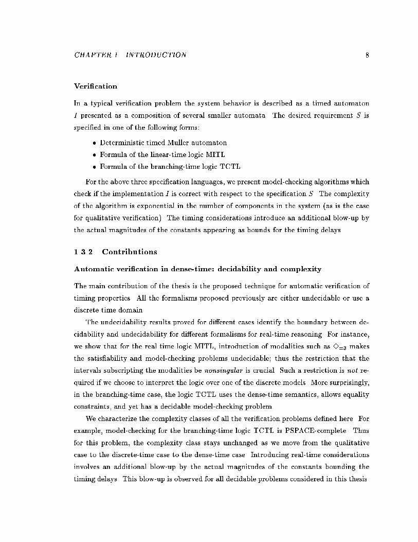
For the above three specication languages� we present modelchecking algorithmswhich
check if the implementation I is correct with respect to the specication S� The complexity
of the algorithm is exponential in the number of components in the system �as is the case
for qualitative verication�� The timing considerations introduce an additional blowup by
the actual magnitudes of the constants appearing as bounds for the timing delays�
����� Contributions
Automatic veri�cation in dense�time decidability and complexity
The main contribution of the thesis is the proposed technique for automatic verication of
timing properties� All the formalisms proposed previously are either undecidable or use a
discrete time domain�
The undecidability results proved for di erent cases identify the boundary between de
cidability and undecidability for di erent formalisms for realtime reasoning� For instance�
we show that for the realtime logic MITL� introduction of modalities such as �� makes
the satisability and modelchecking problems undecidable� thus the restriction that the
intervals subscripting the modalities be nonsingular is crucial� Such a restriction is not re
quired if we choose to interpret the logic over one of the discrete models� More surprisingly�
in the branchingtime case� the logic TCTL uses the densetime semantics� allows equality
constraints� and yet has a decidable modelchecking problem�
We characterize the complexity classes of all the verication problems dened here� For
example� modelchecking for the branchingtime logic TCTL is PSPACEcomplete� Thus
for this problem� the complexity class stays unchanged as we move from the qualitative
case to the discretetime case to the densetime case� Introducing realtime considerations
involves an additional blowup by the actual magnitudes of the constants bounding the
timing delays� This blowup is observed for all decidable problems considered in this thesis�

CHAPTER �� INTRODUCTION �
Timed automata and theory of timed languages
Timed automata provide a simple� and yet powerful� way of annotating statetransition
graphs with timing constraints� Judging by the response we have received so far� we feel
hopeful that it will provide the �canonical� model for nitestate realtime systems�
We study timed automata from the perspective of formal language theory� A timed
language comprises of innite words over a nite alphabet� in which each symbol has a real
valued time of occurrence� Timed automata dene timed regular languages � We consider
closure properties and decision problems for timed automata� The class of nondeterministic
automata is closed under union� intersection� but not under complement� For these au
tomata testing emptiness is PSPACEcomplete� but checking for universality is undecidable
� !��hard� On the other hand� the deterministic automata are closed under complement
also� and problems such as universality and language inclusion are solvable in PSPACE� We
have focused on the application of this theory for verication problems� but the theory may
hold interest of its own�
Models for real�time
Several realtime extensions of existing formalisms have been proposed previously� but the
issue of choosing the �right� model for introducing time in semantics has not been addressed
before� We precisely characterize three di erent models� dense�time� discrete�time and
�ctitious�clock �
The simplest of all these models is the discretetime model� time is assumed to be
isomorphic with the set of natural numbers� Thus events are assumed to happen syn
chronously with the ticks of a global clock� This assumption is relaxed in the �ctitious�clock
approach� Here time is viewed as a global state variable that ranges over the domain of
natural numbers� and is incremented by one with every tick transition of a global� asyn
chronous� ctitious� discrete clock� The timing delay between two events is measured by
counting the number of ticks between them� Finally� there is the possibility of choosing
the real line itself to model time� The occurrence times for events are real numbers in this
model� and consequently it is the most realistic model for asynchronous systems�
We compare these models� and study how the choice of a model a ects the complexity
of di erent decision problems� The model of our choice is the densetime model� in Chapter
� we make a case for our preference�

CHAPTER �� INTRODUCTION ��
��� Related research
The problem of formal methods to deal with the realtime aspect explicitly has received
relatively little attention in the past� However� over the last couple of years there has been
an explosion on the number of papers on this subject� and several realtime logics and real
time algebras have been proposed� In this section we provide an overview of some this work�
the proceedings of a recent REX workshop on the topic �Real Time� Theory in Practice�
will provide an excellent starting point for anybody who wishes to explore the wide range
of research that is under way �dR����
����� Modeling real�time systems
The idea of introducing realtime into qualitative models of behavior by associating a time
of occurrence with every event or statetransition is fairly standard� and is used in most of
the approaches considered here�
Timed automata
Our denition of timed automata is a modied version of the formalism of timed automata
introduced by Dill �Dil���� In the original denition� the automaton has a nite set of
timers � There are two special events associated with every timer� set and expire� A timer
is activated by the set event to an arbitrary value between specied bounds� All the timers
count down at the same rate� and the expire event corresponding to a timer gets red
when its value becomes �� To express a constraint on the delay between two events e� and
e�� a timer with appropriate bounds is set along with e�� and the event e� is required to
be synchronized with the expiration of the timer� In our formalism� the automaton has
a nite set of clocks which count up showing the elapsed time since the last reset� The
clocks can be reset to � along with the statetransitions� and timing delays are expressed by
annotating the transitions with constraints comparing clock values with constant bounds�
Apart from some technical conveniences in developing the emptiness algorithm and proving
its correctness� the reformulation allows a simple syntactic characterization of determinism
for timed automata�
A model similar to Dill�s was independently proposed and studied by Lewis �Lew����
He denes state�diagrams � and gives a way of translating a circuit description to a state
diagram� A statediagram is a nitestate machine where every edge is annotated with a
CHAPTER �� INTRODUCTION ��
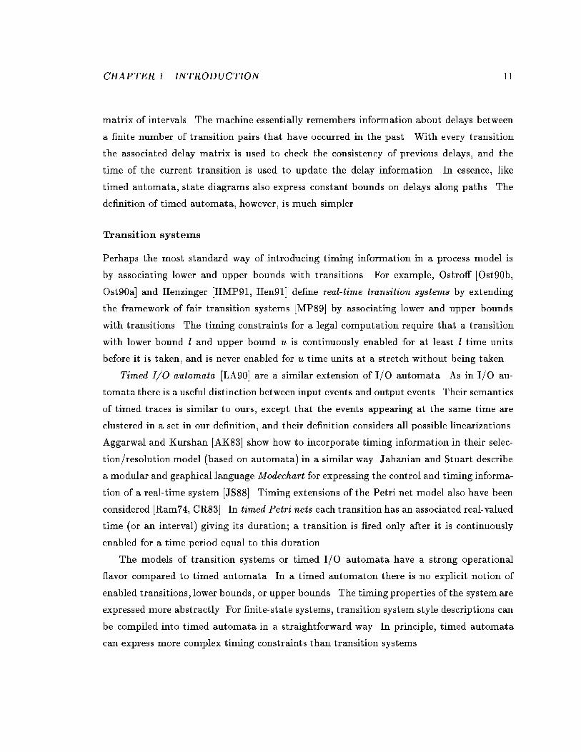
matrix of intervals� The machine essentially remembers information about delays between
a nite number of transition pairs that have occurred in the past� With every transition
the associated delay matrix is used to check the consistency of previous delays� and the
time of the current transition is used to update the delay information� In essence� like
timed automata� state diagrams also express constant bounds on delays along paths� The
denition of timed automata� however� is much simpler�
Transition systems
Perhaps the most standard way of introducing timing information in a process model is
by associating lower and upper bounds with transitions� For example� Ostro �Ost��b�
Ost��a� and Henzinger �HMP��� Hen��� dene real�time transition systems by extending
the framework of fair transition systems �MP��� by associating lower and upper bounds
with transitions� The timing constraints for a legal computation require that a transition
with lower bound l and upper bound u is continuously enabled for at least l time units
before it is taken� and is never enabled for u time units at a stretch without being taken�
Timed I�O automata �LA��� are a similar extension of I�O automata� As in I�O au
tomata there is a useful distinction between input events and output events� Their semantics
of timed traces is similar to ours� except that the events appearing at the same time are
clustered in a set in our denition� and their denition considers all possible linearizations�
Aggarwal and Kurshan �AK��� show how to incorporate timing information in their selec
tion�resolution model �based on automata� in a similar way� Jahanian and Stuart describe
a modular and graphical languageModechart for expressing the control and timing informa
tion of a realtime system �JS���� Timing extensions of the Petri net model also have been
considered �Ram��� CR���� In timed Petri nets each transition has an associated realvalued
time �or an interval� giving its duration� a transition is red only after it is continuously
enabled for a time period equal to this duration�
The models of transition systems or timed I�O automata have a strong operational
�avor compared to timed automata� In a timed automaton there is no explicit notion of
enabled transitions� lower bounds� or upper bounds� The timing properties of the system are
expressed more abstractly� For nitestate systems� transition system style descriptions can
be compiled into timed automata in a straightforward way� In principle� timed automata
can express more complex timing constraints than transition systems�

CHAPTER �� INTRODUCTION ��
Process algebras
The standard way to introduce realtime in algebraic models is to add some form of a
�delay� construct to the calculus �Mil��� RR��� Zwa��� MT��� NRSV��� Wan��� BB����
The following discussion should provide a �avor of these constructs� Reed and Roscoe
�RR��� extend CSP to timed CSP by introducing an additional WAIT construct� The
construct �WAIT t� models the process that terminates successfully after t time units� The
semantics is dened in terms of the timed stability model which uses a dense domain� In
this model� with every event its time of occurrence is recorded� along with the earliest time
at which the process can engage in the next action� A similar approach is Zwarico�s model
of timed acceptances �Zwa���� The semantics uses discretetime� and is an extension of the
acceptance model for CSP� after every event all the possible choices the process may execute
are also recorded�
Milner�s SCCS �Mil��� is a calculus in the style of CCS� It makes the assumption of strong
synchrony � all processes execute in lockstep� performing one event with each passing unit
of time� Sifakis et� al� have dened ATP � an algebra for timed processes �NRSV��� based
on the ctitiousclock model� The vocabulary of actions contains a distinguished element
corresponding to the tick of a global clock� The syntax of the calculus does not allow
explicit references to this tick event� but has a binary unitdelay operator� For two terms t�
and t�� this operator gives a process that behaves as t� if started before the next tick � and
behaves as t� otherwise� Another timed process algebra is TCCS �Wan���� The syntax of
CCS is extended with a delay construct� ���t��P� represents a process that waits for t time
units and then behaves like P � The set of actions contains a special timeout action� and an
action ��t� for every real value t�
In the untimed case� a few constructs of process algebras are rich enough to model
complex aspects of concurrent systems� However� this does not seem to be the case for the
timing properties� None of the above calculi seem to be able to model all the features such
as lower and upper bounds� timeouts� and periodicity�
����� Speci�cation languages
As far as we know� there has been no other attempt to use automata to specify correctness
of realtime systems� However� a large number of realtime extensions of temporal logics
have been proposed�

CHAPTER �� INTRODUCTION ��
Dense�time
The earliest proposal for specifying realtime requirements is found in a paper by Bernstein
and Harter �BH���� They dene an extension of PTL by introducing operators such as
��n�� �� meaning that �every �state is followed by a �state within n time units�� The
paper gives some examples of specications and proofs�
Koymans �KVdR��� Koy��� denes metric temporal logic as a specication language
for timecritical systems� The logic allows temporal modalities for �� to write down
realtime requirements� The logic has a very rich and powerful syntax� and the denition
of the semantics makes very weak assumptions about the time domain� His thesis gives
specications for many interesting problems�
In �Lew���� Lewis considers a realtime branchingtime logic� The syntax is an extension
of CTL with interval subscripts on temporal operators� The logic is interpreted over state
diagrams � his abstraction for nitestate systems�
In �AH��� we showed that the densetime semantics leads to undecidability of the sat
isability problem in the presence of operators such ��� Later in �AFH��� we found a
decidable subset � the logic MITL which disallows singular interval subscripts� Thus� of
all the temporal logics interpreted over dense models� only MITL is decidable�
Fictitious�clock
One approach to specifying realtime requirements using temporal logic is to employ rst
order temporal logic where one of the state variables denotes the value of the global clock�
The logic RTTL of Ostro �Ost��b� uses this approach� It is based on the ctitiousclock
semantics� The syntax uses a dynamic state variable T to denote the current time� and static
variables over the time domain to express timing constraints� For example� the property
that �every pstate is followed by some qstate within time ��� is expressed by the formula
�� � p � T " x � � � � q � T � x � ���
The logic is undecidable even if we restrict to nitestate systems� Consequently� several
di erent decidable fragments of RTTL have been identied�
In �AH��� we dened the logic TPTL� For decidability� TPTL requires that the timing
constraints be of a very simple form� involving only comparisons and addition by constant
values� Secondly� it achieves elementary complexity through a novel form of time quantier
�x� � which captures the current time� The notation also provides abstraction from explicit

CHAPTER �� INTRODUCTION ��
references to the time variable� The syntax for TCTL used in this thesis is based upon this
TPTL notation�
Another decidable fragment of RTTL is the logic MTL �AH���� MTL uses Koyman�s
notation of subscripted temporal operators� and is interpreted over ctitiousclock models�
Unlike TPTL� MTL also allows past operators such as �� meaning �sometime within the
past � time units��
The logic XCTL introduced by Pnueli and Harel �PH��� Har��� is also a restricted
fragment of RTTL� and is decidable� Unlike all the formalisms we consider� XCTL allows
the addition primitive� however it allows only one form of quantication� and consequently�
the logic is not closed under negation�
For a detailed comparison of the above logics see �AH��� or �Hen����
Discrete�time
As an example of a realtime logic with discretetime semantics consider the branchingtime
logic RTCTL of �EMSS���� In this logic one can write formulas such as ���� p� meaning
some pstate is reachable within time �� Since each transition takes unit time� the realtime
operators are merely abbreviations for sequences of next operators of CTL� The paper gives
complexity results on satisability and modelchecking for RTCTL�
Mok and his group have done extensive work on specifying realtime systems� The logic
RTL is an eventbased logic which allows stating relationships between occurrence times of
di erent events �JM��� JM���� The specication style of RTL is quite di erent from the
conventional temporal logics� For instance� the RTL formula
�i� � #�b� i� � �#a� i �� �
states the property that �the ith occurrence of the b event is within � time units of the
ith occurrence of the a event� for all choices of i�� Theoretically� it is an extension of
Presburger arithmetic with an uninterpreted unary function symbol corresponding to every
event symbol� RTL is undecidable� there seems to be no natural decidable fragment�
����� Veri�cation
Dill �Dil��� gives an algorithm to check qualitative temporal properties of nitestate sys
tems� The essential construction involves checking consistency of timing constraints of a

CHAPTER �� INTRODUCTION ��
timed automaton with timers� The untiming construction for timed automata presented in
this thesis has a better worstcase running time�
Lewis also gives an algorithm to check consistency of timing information for a system
modeled by his state diagrams� In �Lew���� he gives an algorithm to check properties written
in a branchingtime logic that is a fragment of TCTL� The algorithm is quite di erent from
ours� and makes the assumption of progressiveness � in a bounded interval of time only
a bounded number of events happen �note that this is not the same as the discretetime
assumption�� Also the worstcase complexity of our algorithm is better�
Lynch and Attiya �LA��� provide a formal basis for comparing two descriptions� not nec
essarily nitestate� presented as timed I�O automata and show how to use it for reasoning
about timing properties of protocols�
Ostro �Ost��b� extends the proof system for temporal logic to handle RTTL formu
las� He also gives algorithms for checking a restricted class of RTTL specications against
systems modeled using realtime transition systems �Ost��a��
Henzinger�s thesis �Hen��� studies several aspects of the verication problem based on
ctitiousclock temporal logics� The modelchecking algorithms for the nitestate case are
reported in �AH��� AH��� HLP���� He also gives axiomatization for MTL �Hen���� and
proof rules for checking certain types of realtime specications such as bounded response
and bounded invariance �HMP���� With its integration in the existing proof systems for
temporal logic� it provides a general system for reasoning about realtime programs�
The algebraic approaches �Zwa��� RR��� Wan��� NRSV��� provide an array of operators
and laws for reasoning with them� The verication is dened using the notions of process
containment and process equivalence� In the context of timed Petri nets �Ram��� CR���
analysis techniques for solving specic performancerelated problems have been considered
for subclasses� Verication methods based on time Petri nets have been considered in
�BD��� YKT���� Aggarwal and Kurshan �AK��� using their timing extension of the selec
tion�resolution model� show how to compute elapsed time between di erent events� and
argue that the timing information helps to reduce the number of reachable states�
In the context of RTL� Jahanian and Mok �JM��� show how to do safety analysis of
timing properties� In �JS��� the semantics for Modecharts is dened using RTLformulas�
thus reducing the verication problem to proving a theorem in RTL� For RTL specications
of a specic form algorithms for modelchecking have been developed�
CHAPTER �� INTRODUCTION ��
�� Organization of the thesis
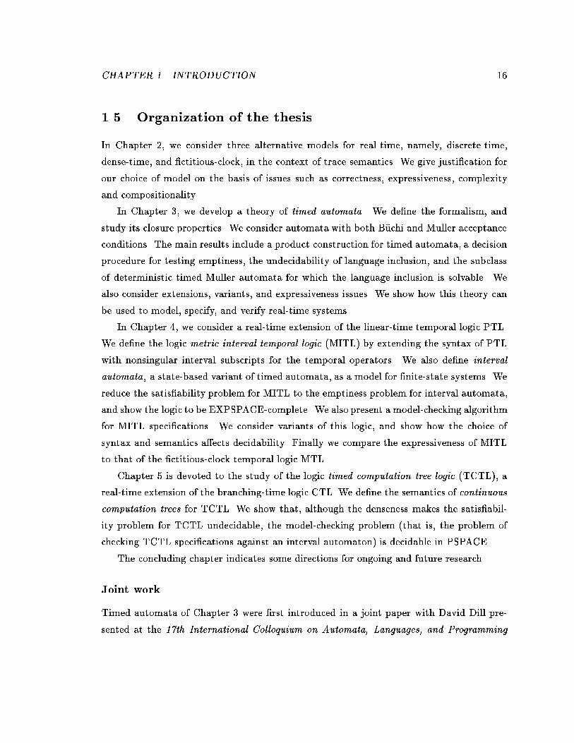
In Chapter �� we consider three alternative models for realtime� namely� discretetime�
densetime� and ctitiousclock� in the context of trace semantics� We give justication for
our choice of model on the basis of issues such as correctness� expressiveness� complexity
and compositionality�
In Chapter �� we develop a theory of timed automata� We dene the formalism� and
study its closure properties� We consider automata with both B�uchi and Muller acceptance
conditions� The main results include a product construction for timed automata� a decision
procedure for testing emptiness� the undecidability of language inclusion� and the subclass
of deterministic timed Muller automata for which the language inclusion is solvable� We
also consider extensions� variants� and expressiveness issues� We show how this theory can
be used to model� specify� and verify realtime systems�
In Chapter �� we consider a realtime extension of the lineartime temporal logic PTL�
We dene the logic metric interval temporal logic �MITL� by extending the syntax of PTL
with nonsingular interval subscripts for the temporal operators� We also dene interval
automata� a statebased variant of timed automata� as a model for nitestate systems� We
reduce the satisability problem for MITL to the emptiness problem for interval automata�
and show the logic to be EXPSPACEcomplete� We also present a modelchecking algorithm
for MITL specications� We consider variants of this logic� and show how the choice of
syntax and semantics a ects decidability� Finally we compare the expressiveness of MITL
to that of the ctitiousclock temporal logic MTL�
Chapter � is devoted to the study of the logic timed computation tree logic �TCTL�� a
realtime extension of the branchingtime logic CTL� We dene the semantics of continuous
computation trees for TCTL� We show that� although the denseness makes the satisabil
ity problem for TCTL undecidable� the modelchecking problem �that is� the problem of
checking TCTL specications against an interval automaton� is decidable in PSPACE�
The concluding chapter indicates some directions for ongoing and future research�
Joint work
Timed automata of Chapter � were rst introduced in a joint paper with David Dill pre
sented at the ��th International Colloquium on Automata� Languages� and Programming

CHAPTER �� INTRODUCTION ��
in June ���� �AD���� The results of Chapter � appear in a joint paper with Thomas Hen
zinger and Tomas Feder �AFH��� presented at the Tenth ACM Symposium on Principles of
Distributed Computing in August ���� �AFH���� Chapter � generalizes the denition and
the results appearing in a joint paper with Costas Courcoubetis and David Dill at the Fifth
IEEE Symposium on Logic in Computer Science in June ���� �ACD����

Chapter �
Adding Time to Semantics
In this chapter we dene three di erent ways of introducing time in linear trace semantics
for concurrent processes� We compare these models� and justify our preference for the
densetime model�
��� Trace semantics
In trace semantics� we associate a set of observable events with each process� and model
the process by the set of all its traces � A trace is a �linear� sequence of events that may
be observed when the process runs� For example� an event may denote an assignment of
a value to a variable� or pressing a button on the control panel� or arrival of a message�
All events are assumed to occur instantaneously� Actions with duration are modeled using
events marking the beginning and the end of the action� Hoare originally proposed such a
model for CSP �Hoa���� In our model� we allow several events to happen simultaneously�
Also we consider only innite sequences� which model nonterminating interaction of reactive
systems with their environments� This is no serious limitation� a nite sequence representing
a terminating behavior can be extended to an innite sequence using a su�x comprising of
innite repetition of a dummy event�
Formally� given a set A of events� a trace � " ���� � � � is an innite word over P��A�
� the set of nonempty subsets of A� An untimed process is a pair �A�X� comprising of the
set A of its observable events and the set X of its possible traces�
Example ��� Consider a channel P connecting two components� Let a represent the
arrival of a message at one end of P � and let b stand for the delivery of the message at the
��

CHAPTER �� ADDING TIME TO SEMANTICS ��
other end of the channel� The channel cannot receive a new message until the previous one
has reached the other end� Consequently the two events a and b alternate� Assuming that
the messages keep arriving� the only possible trace is
�P � fag � fbg � fag � fbg � � � � �
Often we will denote the singleton set fag by the symbol a� The process P is represented
by �fa� bg� �ab��� ��
Various operations can be dened on processes� these are useful for describing complex
systems using the simpler ones� We will consider only the most important of these opera
tions� namely� parallel composition� The parallel composition of a set of processes describes
the joint behavior of all the processes running concurrently� In our framework� processes
synchronize via common events� and concurrency is modeled by all possible interleavings of
the causally independent events�
The parallel composition operator can be conveniently dened using the projection op
eration� The projection of � P��A�� onto B A �written �dB� is formed by intersecting
each event set in � with B and deleting all the empty sets from the sequence� For instance�
in Example ��� �P dfag is the trace a�� Notice that the projection operation may result in
a nite sequence� but we will consider the projection of a trace � onto B only when �i �B
is nonempty for innitely many i�
For a set of processes fPi " �Ai� Xi� j i " �� �� � � �ng� their parallel composition ki Pi is
a process with the event set �iAi and the trace set
f� P���iAi�� j �i �dAi Xig�
Thus � is a trace of ki Pi i �dAi is a trace of Pi for each i " �� � � �n� When there are
no common events the above denition corresponds to the unconstrained interleavings of
all the traces� On the other hand� if all event sets are identical then the trace set of the
composition process is simply the settheoretic intersection of all the component trace sets�
Example ��� Consider another channel Q connected to the channel P of Example ����
The event of message arrival for Q is same as the event b� Let c denote the delivery of the
message at the other end of Q� The process Q is given by �fb� cg� �bc����
�We will use the notation of ��regular expressions freely� The expression e� stands for a �nite repetition
of e� and the expression e� stands for an in�nite repetition of e�
CHAPTER �� ADDING TIME TO SEMANTICS ��
When P and Q are composed we require them to synchronize on the common event b�
and between every pair of b�s we allow the possibility of the event a happening before the
event c� the event c happening before a� and both occurring simultaneously� Thus �P k Q �
has the event set fa� b� cg� and has an innite number of traces� An example trace is
fag � fbg � fcg � fag � fbg � fa� cg � fbg � fag � fcg � fbg � � � �
In this framework� the verication question is presented as an inclusion problem� Both
the implementation and the specication are given as untimed processes� The implementa
tion process is typically a composition of several smaller component processes� We say that
an implementation �A�XI� is correct with respect to a specication �A�XS� i XI XS �
Example ��� Consider the channels of Example ���� The implementation process is �P k
Q �� The specication is given as the process S " �fa� b� cg� �abc���� Thus the specication
requires the message to reach the other end of Q before the next message arrives at P �
In this case� �P k Q� does not meet the specication S� for it has too many other traces�
specically� the trace ab�acb���
��� Timed traces
In this section we explore di erent possible denitions for introducing time in trace seman
tics�
����� Adding timing to traces
An untimed process models the sequencing of events but not the actual times at which the
events occur� Thus the description of the channel in Example ��� gives only the sequencing
of the events a and b� and not the delays between them� Timing can be added to a trace by
coupling it with a sequence of time values� We assume that these values are chosen from a
domain TIME with linear order �� Di erent choices for TIME will lead to di erent ways of
modeling the behavior� The examples in this subsection will use the set of natural numbers
as TIME�
A time sequence � " ���� � � � is an innite sequence of time values �i TIME with
�i �� satisfying the following constraints�

CHAPTER �� ADDING TIME TO SEMANTICS ��
� Monotonicity� � increases strictly monotonically� that is� �i �i�� for all i ��
� Progress� For all t TIME � there is some i � such that t �i�
A timed trace over a set of events A is a pair ��� �� where � is a trace over A� and � is a
time sequence�
In a timed trace ��� ��� each �i gives the time at which the events in �i occur� In
particular� �� gives the time of the rst observable event� we always assume �� �� and
dene �� " �� Sometimes we will represent the timed trace ��� �� by the innite sequence
���� ��� � ���� ��� � ��� �� � � � �
Observe that the progress condition implies that only a nite number of events can
happen in a bounded interval of time� In particular� it rules out convergent time sequences
such as ���� ���� ���� � � � representing the possibility that the system participates in innitely
many events before time ��
A timed process is a pair �A�L� where A is a nite set of events� and L is a set of timed
traces over A�
Example ��� Consider the channel P of Example ��� again� Assume that the rst message
arrives at time �� and the subsequent messages arrive at xed intervals of length � time
units� Furthermore� it takes � time unit for every message to traverse the channel� The
process has a single timed trace
�P " �a� �� � �b� �� � �a� �� � �b� �� � � � �
and it is represented as a timed process PT " �fa� bg� f�Pg��
The operations on untimed processes are extended in the obvious way to timed processes�
To get the projection of ��� �� onto B A� we rst intersect each event set in � with B
and then delete all the empty sets along with the associated time values� The denition
of parallel composition remains unchanged� except that it uses the projection for timed
traces� Thus in parallel composition of two processes� we require that both the processes
should participate in the common events at the same time� This rules out the possibility
of interleaving� parallel composition of two timed traces is either a single timed trace or is
empty�

CHAPTER �� ADDING TIME TO SEMANTICS ��
Example �� As in Example ��� consider another channel Q connected to P � For Q� as
before� the only possible trace is �Q " �bc��� In addition� the timing specication of Q
says that the time taken by a message for traversing the channel� that is� the delay between
b and the following c� is always � unit� The timed process QT has innitely many timed
traces� and it is given by
� fb� cg� f��bc��� �� j �i� ���i � ��i�� " ��g ��
The description of �PT k QT � is obtained by composing �P with each timed trace of QT �
However only one timed trace of QT is consistent with the timing of b events in �P � The
resulting process has the event set fa� b� cg� and a unique timed trace
�a� �� � �b� �� � �c� �� � �a� �� � �b� �� � �c� �� � � � �
The time values associated with the events can be discarded by the Untime operation�
For a timed process P " �A�L�� Untime��A�L�� is the untimed process with the event set
A and the trace set consisting of traces � such that ��� �� L for some time sequence � �
Note that
Untime�P� k P�� Untime�P�� k Untime�P���
However� as Example ��� shows� the two sides are not necessarily equal� In other words� the
timing information retained in the timed traces constrains the set of possible traces when
two processes are composed�
Example ��� Consider the channels of Example ���� Observe that Untime�PT � " P and
Untime�QT � " Q� As seen before� �PT k QT � has a unique trace �abc��� On the other hand�
�P k Q � has innitely many traces� between every pair of b events all possible orderings of
an event a and an event c are admissible�
The verication problem is again posed as an inclusion problem� Now the implementa
tion is given as a composition of several timed processes� and the specication is also given
as a timed process�
Example ��� Consider the verication problem of Example ��� again� If we model the
implementation as the timed process �PT k QT � then it meets the specication S� The

CHAPTER �� ADDING TIME TO SEMANTICS ��
specication S is now a timed process �fa� b� cg� f��abc��� ��g�� Observe that� though the
specication S constrains only the sequencing of events� the correctness of �PT k QT � with
respect to S crucially depends on the timing constraints of the two channels� Consider
another specication S� which requires� in addition to S� the timing delay between every
event a and the next following c to be at most �� The implementation meets S� also�
����� Discrete�time model
In Section ������ while dening timed traces� we did not commit to choosing a specic time
domain� Di erent choices for TIME give us di erent models of realtime�
Choosing TIME to be the set of natural numbers� N� gives us the discrete�time model�
In this model events can happen only at the integer time values� This describes the behavior
of synchronous systems� where all components are driven by a common global clock� The
duration between the successive clock ticks is chosen as the time unit� The discretetime
model is the traditional model for synchronous hardware� The processes considered in
Example ��� use this model�
The advantage of this model is its simplicity� In fact� timed traces are not even necessary
to model the behavior� A timed trace ��� �� over a set of events A may be viewed as an
innite sequence �� over �A� for all i �� let ��i be �j if �j " i� and let ��i be � if for all j �
�j �" i� Thus the ith element of �� gives the events happening at time i� For instance� the
timed trace
�fag� �� � �fbg� �� � �fa� bg� �� � �b� �� � � � �
is represented by the sequence
fag � fbg � � � fa� bg � � � �
Thus a timed process can be modeled as a set of traces over �A� the empty set of events
corresponds to the passage of time� The parallel composition operator can be dened
directly within this framework by modifying the denition of the projection operation on
traces� the projection of a trace � over �A onto B A is formed by simply intersecting
each event set in � with B �that is� empty sets are not deleted��
No substantially new techniques are needed to analyze the timing behavior in this model�
the techniques used in the verication of untimed processes can be modied in a straight
forward way�

CHAPTER �� ADDING TIME TO SEMANTICS ��
����� Dense�time model
Choosing TIME to be the set of real numbers� R� gives the dense�time model� In this
model� we assume that events happen at arbitrary points in time over the realline� and
with each event we associate its realvalued time of occurrence� As it turns out� with regards
to complexity and expressiveness issues� the crucial aspect of the underlying domain is its
denseness � the property that between every two time values there is a third one� and not
its continuity� we may replace R by some other dense linear order� say� the set of rational
numbers� Q�
The densetime model is a natural model for asynchronous systems� It allows events to
happen arbitrarily close to each other� that is� there is no lower bound on the separation
between events� This is a desirable feature for representing two causally independent events
in an asynchronous system� While dening the semantics of a system� no assumptions
regarding the speed of the environment need to be made�
Example ��� Let us consider the channels P and Q of Example ��� again� We keep the
timing specication of the channel P the same� For channel Q assume that the delay
between the event b and the following c is some real value between � and �� The timed
process QT is now given by
� fb� cg� f��Q� �� j �i� ���i�� � ��i ��i�� ��g ��
The composition process �PT k QT � has uncountably many timed traces� An example trace
is
�a� �� � �b� �� � �c� ���� � �a� �� � �b� �� � �c� ����� � � � �
����� Fictitious�clock model
In this section we consider an alternative way to introduce time in traces� We assume that
there is an external� discrete clock ticking at a xed rate� asynchronously with the other
components in the system� Time is viewed as a discrete counter� and is incremented by
one with every tick of this ctitious clock� With each event we associate� instead of its
exact �real� time of occurrence� the value of this counter� Thus events happening between
consecutive ticks have the timestamp� and only the ordering of their times of occurrences
is known�

CHAPTER �� ADDING TIME TO SEMANTICS ��
We formalize this model using observation traces � An observation trace over a set
of events A consists of a trace � over A and an innite sequence � " ����� � � � over N
satisfying the progress constraint and the weak monotonicity constraint that �i � �i�� for
all i �� Thus an observation trace is similar to a timed trace for the discretetime model�
but instead of requiring the time sequence to be strictly increasing we simply require it to
be nondecreasing� If �i equals �i��� it means that the events in the �i ��th set happen
after the events in the ith set� but before the next clock tick� Also �� may be � indicating
that the rst event happens before the rst clock tick� An alternative way to dene the
ctitiousclock semantics would be to use the model of untimed processes with a special
tick event common to all processes� Thus a timed process with an event set A is modeled
as an untimed process with the event set A � ftickg�
Example �� Consider the channel P with alternating events a and b� In addition we know
that an observer with a clock ticking at xed intervals observes at most � tick between every
event a and the successive b� and precisely � ticks between every pair of successive a�s� The
timed process PT is given by
�fa� bg� f��ab��� �� j �i� ���i � ��i�� �� � ���i�� " ��i�� ��g��
An example observation trace is
�a� �� � �b� �� � �a� �� � �b� �� � �a� �� � � � �
The process can be represented using tick events also� For instance� the above trace can be
represented by the trace a� b� tick� tick� a� tick � b� tick� a � � �
The projection operation is dened for observation traces as in the case of timed traces�
Also the denition of the parallel composition operator is unchanged� Thus when composing
two observation traces of two processes� we require synchronization on every successive clock
tick in addition to the common events� As in the qualitative model� we get all possible
interleavings of the events in the two traces between every pair of successive clock ticks�
Consequently� the result of composing two behaviors is not unique as in the discretetime
or the densetime model� but is more constrained than the qualitative model because of the
additional synchronization of ticks�

CHAPTER �� ADDING TIME TO SEMANTICS ��
Example ���� Consider another channel Q as in our previous examples� The timing
specication of Q requires precisely � tick between every event b and the next c� An
example observation trace of QT is
�b� �� � �c� �� � �b� �� � �c� �� � � � �
Composing this trace with the observation trace of PT shown in Example ��� allows arbi
trary ordering of the events a and c at time �� For instance� the composition contains the
trace
�a� �� � �b� �� � �c� �� � �a� �� � �b� �� � �a� �� � �c� �� � � � �
In this case Untime�PT k QT � equals �P k Q ��
The ctitiousclock model can be considered as a generalization of the discretetime
model where successive event sets can have the same time� This model allows arbitrarily
many transitions between the successive tick events� and hence� unlike the discretetime
model� makes no assumptions regarding the speed of the environment� On the other hand� it
can be viewed as an approximation to the densetime model where the time value associated
with each event set is truncated� The observation traces only record the observations of
the actual behaviors with respect to a discrete clock� Since time is considered discrete�
the verication algorithms based on this model are simpler compared to those based on the
densetime model� The techniques used in the verication of nitestate �untimed� processes
can be adopted to develop verication methods for this model�
However since only incomplete timing information is retained it cannot model the timing
delays of a system accurately� The timing delay between two events is measured by counting
the number of ticks between them� When we require that there be k ticks between two
transitions� we can only infer that the delay between them is larger than k�� time units and
smaller than k � time units� Consequently� it is impossible to state precisely certain simple
requirements on the delays such as �the delay between two transitions equals � seconds��
This leads to some unintuitive properties in the model� For instance� consider the property�
if a precedes b� and c happens � time unit later than a� and d happens � unit
later than b� then c precedes d�
This is a valid property of timed traces in the discretetime or the densetime models� but it
is not a valid property of observation traces in the ctitiousclock model� The observation

CHAPTER �� ADDING TIME TO SEMANTICS ��
trace
�a� �� � �b� �� � �d� �� � �c� �� � � � �
satises all the conditions in the antecedent� but violates the precedence requirement of the
consequent�
��� A case for the dense�time Model
Several researchers have used either the discretetime or the ctitiousclock model saying
that it is good enough for all practical purposes provided the unit for time �the rate at
which the clock ticks� is small enough� However� this argument has not been supported by
any precise mathematical claims� Below we make an attempt to give di erent justications
to our preference for the densetime model over the other two�
����� Correctness
For eventdriven asynchronous systems the densetime model gives di erent results com
pared to the other models� We discuss this issue in context of a reachability problem for
asynchronous circuits with bounded inertial delays� The network model we use and some
of the examples are borrowed from �BS����
A network N consists of singleoutput gates connected by wires �� �� � � �m� Each gate
can be identied by its unique output wire� Wires are assumed to have no delays� however
each gate is assumed to have a bounded delay� the delay of a gate j can be an arbitrary
real value in the interval �l�j�� u�j��� Thus l�j� gives the lower bound for the delay� and
u�j� gives the upper bound� All the bounds are nonnegative integers� Wires are assumed
to have only binary states� and the changes are assumed to be instantaneous� A state s of
the circuit is an mtuple over f�� �g giving the values of all the wires� the jth component
s�j� represents the value of the wire j� The value assigned to the output wire of a gate by
a state may not be consistent with the values assigned to its input wires� For a state s and
a gate j� let out�s� j� denote the required value of the wire j according to the values of the
input wires to gate j in state s and the functional laws for the gate j� For instance� if a
state s assigns the value � to the input wire of an inverter gate j� then out�s� j� is �� If s�j�
di ers from out�s� j� then the gate j is unstable in state s�
A state sn is reachable from a state s� i there exists a sequence of the form
s�A�����
s�A�����
� � � � � � sn��An���n
sn
CHAPTER �� ADDING TIME TO SEMANTICS ��
1
x
y1
y2
y3
[1,3]
[1,2]
[1,3]
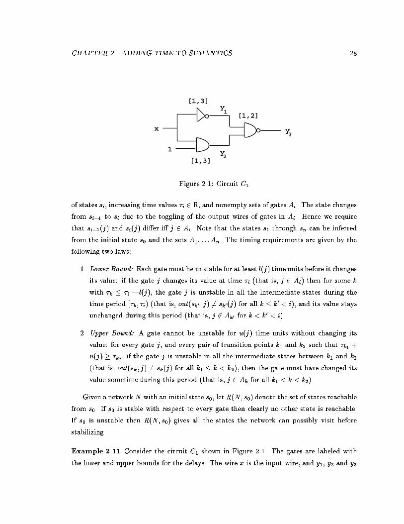
Figure ���� Circuit C�
of states si� increasing time values �i R� and nonempty sets of gates Ai� The state changes
from si�� to si due to the toggling of the output wires of gates in Ai� Hence we require
that si���j� and si�j� di er i j Ai� Note that the states s� through sn can be inferred
from the initial state s� and the sets A�� � � �An� The timing requirements are given by the
following two laws�
�� Lower Bound� Each gate must be unstable for at least l�j� time units before it changes
its value� if the gate j changes its value at time �i �that is� j Ai� then for some k
with �k � �i � l�j�� the gate j is unstable in all the intermediate states during the
time period ��k� �i� �that is� out�sk� � j� �" sk��j� for all k � k� i�� and its value stays
unchanged during this period �that is� j � Ak� for k k� i��
�� Upper Bound� A gate cannot be unstable for u�j� time units without changing its
value� for every gate j� and every pair of transition points k� and k� such that �k�
u�j� �k� � if the gate j is unstable in all the intermediate states between k� and k�
�that is� out�sk � j� �" sk�j� for all k� � k k��� then the gate must have changed its
value sometime during this period �that is� j Ak for all k� k k���
Given a networkN with an initial state s�� letR�N� s�� denote the set of states reachable
from s�� If s� is stable with respect to every gate then clearly no other state is reachable�
If s� is unstable then R�N� s�� gives all the states the network can possibly visit before
stabilizing�
Example ���� Consider the circuit C� shown in Figure ���� The gates are labeled with
the lower and upper bounds for the delays� The wire x is the input wire� and y�� y� and y

CHAPTER �� ADDING TIME TO SEMANTICS ��
give the wires corresponding to the three gates� The wire y� is the output of the inverter
gate� y� is the output of the ANDgate� and y is the output of the NANDgate� Consider
the stable state with x " � and y " ������ Now suppose the input changes to x " �� The
stable state is y " ������ However� before this state is reached the gates can change their
values in di erent orders� A possible behavior of the circuit is shown below �only the values
for y�� y�� and y are listed��
�����fy�g�����
�����fy�g�����
�����fy�g����
�����fy�g�����
�����
In the above behavior� the outputs of the ANDgate and the NANDgate change before
the output of the inverter changes� The inverter responds with a delay ���� the ANDgate
responds with a delay ���� The NANDgate responds with a delay of ��� when the wire y�
changes� and with a delay of ��� when the wire y� changes�
Another possible behavior is when the inverter changes its output before the ANDgate
toggles� giving the state ������ which then changes to the stable state ������
The set of reachable states is given by
R�C�� �x " �� y " ����� " f������ ������ ������ ������ ������ �����g�
In the densetime model� the transition times can be arbitrary real numbers� Clearly� an
analysis based on this model can compute the set R�N� s�� correctly� Note that if we require
all the transition times to be rationals� the set of reachable states will remain unchanged�
The question is whether this set can be computed by other models� if we choose a su�ciently
fast clock�
Consider the discretetime model with a clock ticking at xed intervals of length ���k�
time units� With the assumption that gates can change values only with the ticks of the
clock� this model requires the delays for all gates and the transition times to be multiples of
���k�� Let Rd�N� s�� k� denote the set of reachable states based on this discretetime model�
It is clear that Rd�N� s�� k� Rd�N� s�� k �� R�N� s�� for all k �� From the examples
given in �BS��� it follows that for all k �� there exists a network N with an initial state
s� such that Rd�N� s�� k� �" R�N� s��� Example ���� shows that R
d�N� s�� �� �" R�N� s���
Example ���� �from BS���

CHAPTER �� ADDING TIME TO SEMANTICS ��
y2
y3
y1
y4
y5
y6
7y
8y
x
[1,2]
[1,2]
[1][1]
[1]
[1]
[1]
[1,2]
Figure ���� Circuit C�
Consider the circuit C� of Figure ���� The gates �� �� and � are exclusive�or �XOR�
gates� The gates labeled with ��� have delay precisely equal to � time unit�
Initially the cicuit is in the stable state x " �� and y " ��������� Now consider the
behavior of the circuit when the input x changes to �� First observe that a state in which
the output y of the ORgate toggles is reachable if we choose the delays for the inverters
�� �� and � to be �� ���� and � time units� respectively� In this case the XORgates � and
� are unstable only for an interval of length ���� and hence do not change their outputs�
On the other hand� the XORgate � is unstable for � time unit� and hence� y� changes its
value� Consequently� the gate � is unstable for � time unit� and the wire y� toggles� This
propagates to the ORgate� and y toggles�
On the other hand� if we require the delays for the inverters to be discrete values� either
� or �� it follows that the XORgate � is unstable for � time unit i at least one of the XOR
gates � or � is unstable for � time unit� This means that the gate �� and consequently the OR
gate �� are never unstable� Thus in every reachable state in Rd�C�� �x " �� y " ���������� ��
the value of y is ��
Thus the reachability analysis based on the discretetime model will not be able to detect
some reachable states if k is xed a priori � Notice that for the circuit C� of Example ����
a discretetime analysis using a time granularity of ��� time units detects all the transient
states� In general� for each network N there is some k for which Rd�N� s�� k� " R�N� s���

CHAPTER �� ADDING TIME TO SEMANTICS ��
Because of this� one may argue that discretetime model is good enough� provided that the
time unit is not xed in advance� But this approach has its own problems� Firstly� this
appropriate value of the granularity k is not obvious� and as far as we know nobody has
proposed an algorithm to nd this value� Indeed� the algorithm is likely to be as complex
as the algorithms for the densetime analysis presented in this thesis� Secondly� increasing
the granularity adversely a ects the complexity of the verication algorithms� Thirdly�
for properties more complex than reachability� in particular those involving innite traces�
such a result does not hold� In Section ��� we show that such a result does not hold for
timed automata� We give an example of a timed automaton whose trace set is empty if the
transition times are required to be multiples of ���k�� irrespective of the choice of k� but is
nonempty with the densetime semantics�
Now consider the ctitiousclock model with a clock ticking at the rate of ���k� time
units� Now the transition times are multiples of ���k� as in the discretetime model� but the
sequence of time values is required to be only nondecreasing� The lower bound requirement
says that once a gate becomes unstable there need to be at least l�j� ticks before it can
change its state� and the upper bound requirement says that there cannot be more than u�j�
ticks with some gate staying unstable� The actual lower bound on the delay is �l�j�� ��k��
and the upper bound is �u�j� ��k�� Let Rf�N� s�� k� denote the set of reachable states using
the analysis based on this model� It can be shown that Rf �N� s�� k �� � Rf �N� s�� k� �
R�N� s�� for all k �� To see the second containment� observe that truncating all the
transition times from a real behavior gives a behavior permitted by the ctitiousclock
model� However� since the delays are modeled only imprecisely� the ctitiousclock model
admits some extra behaviors also� The following example shows that there are networks for
which Rf �N� s�� k� di ers from R�N� s�� for all k ��
Example ���� Consider the circuit C of Figure ��� with two inverter gates each of delay
�� Suppose initially x " � and y " ����� Now if the input x changes to � then in the
densetime model both the outputs y� and y� will change to � at time �� and hence�
R�C� �x " �� y " ���� " f����� ����g�
On the other hand� in the ctitiousclock model with k " �� the following is an admissible
timed state sequence�
����fy�g���
����fy�g���
�����
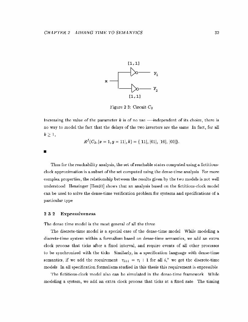
CHAPTER �� ADDING TIME TO SEMANTICS ��
y1
y2
[1,1]
[1,1]
x
Figure ���� Circuit C
Increasing the value of the parameter k is of no use � independent of its choice� there is
no way to model the fact that the delays of the two inverters are the same� In fact� for all
k ��
Rf�C� �x " �� y " ���� k� " f����� ����� ����� ����g�
Thus for the reachability analysis� the set of reachable states computed using a ctitious
clock approximation is a subset of the set computed using the densetime analysis� For more
complex properties� the relationship between the results given by the two models is not well
understood� Henzinger �Hen��� shows that an analysis based on the ctitiousclock model
can be used to solve the densetime verication problem for systems and specications of a
particular type�
����� Expressiveness
The densetime model is the most general of all the three�
The discretetime model is a special case of the densetime model� While modeling a
discretetime system within a formalism based on densetime semantics� we add an extra
clock process that ticks after a xed interval� and require events of all other processes
to be synchronized with the ticks� Similarly� in a specication language with densetime
semantics� if we add the requirement ��i�� " �i � for all i�� we get the discretetime
models� In all specication formalisms studied in this thesis this requirement is expressible�
The ctitiousclock model also can be simulated in the densetime framework� While
modeling a system� we add an extra clock process that ticks at a xed rate� The timing

CHAPTER �� ADDING TIME TO SEMANTICS ��
constraints of the system are modied so that they count ticks instead of the elapsed time�
The same trick can be applied to the specication languages also� In Section ��� we show
that the realtime logic MITL� which uses a densetime semantics and disallows the use
of equality constraints� is more expressive than the realtime logic MTL which uses the
ctitiousclock model� irrespective of the choice of the separation between the successive
clock ticks�
����� Compositionality
The main problem in dening semantics with the discrete models is that the semantics
cannot be dened without xing the time unit� but a reasonable choice for the time unit
depends upon the timing constraints of all the components and the property to be veried�
Consequently� a component cannot be given its own semantics independently of the other
components� Furthermore� the semantic denition depends on the specication also� This
is because� as Example ���� illustrates� the semantics of timed traces does not have enough
information to rene the time unit� The example uses the discretetime model� but the
ctitiousclock model has the same problem�
Example ���� Consider a process P with two events a and b which alternate� The timing
specication says that the delay between a and the following b is � second� Consider the
discretetime semantics for P with time unit equal to � second� P is represented by the set
T �P ��
Consider another process Q with the same alternating events a and b� Its timing speci
cation says that the delay between every occurrence of a and the following b is � second�
and furthermore� the delay between b and the following a is at least � second� The process
Q is modeled as a set of timed traces T �Q�� It is clear that T �P � " T �Q�� Thus within
trace semantics both P and Q have same properties� This is acceptable as long as the time
unit is � second�
Now suppose we introduce a third process R with time unit ��� second� In order to
compose P and R� one needs to change the semantics of P to re�ect the change of time
unit� Let T ��P � denote the semantics for P with this new time unit� If ��� �� is a timed
trace in T �P � then ��� ��� is a timed trace in T ��P �� All such timed traces require the event
a to happen at even time values� but T ��P � has additional timed traces like
�a� �� � �b� �� � �a� �� � �b� �� � � � �

CHAPTER �� ADDING TIME TO SEMANTICS ��
Thus T ��P � cannot be obtained from T �P �� one needs to refer to the original description of
P to dene T ��P ��
Also now T ��Q� is di erent from T ��P �� above timed trace belongs only to T ��P �� Thus
P and Q are no longer equivalent� This shows that properties need to be reproved when
the time unit is rened�
The above example shows that in the discrete models one can reason about a system
only after the descriptions of all the components and all the properties to be veried are
known�
For compositional reasoning� we should be able to dene the semantics of a component
and prove its properties without knowing the details of the other parts of the system� Shift
ing to densetime semantics o ers a natural and mathematically clean way to this e ect� In
this model� the composition operator can be dened on timed processes describing di erent
components in a straightforward way� Also the properties proved for one component hold
independently of the speeds of the others�
����� Complexity
Since the densetime model admits the possibility of an unbounded number of events in
an interval of nite time length� some problems related to the verication of nitestate
systems turn out to be� unlike the other models� undecidable� For example� the language
inclusion problem for timed automata is undecidable� if we had chosen one of the discrete
models� the problem would have been solvable� However� this problem does not turn out
to be fatal� The thesis shows that checking properties of nitestate realtime systems is
possible for several reasonably powerful specication languages based on the densetime
model� With the availability of these positive results� we hope that more researchers will
explore the densetime model further�
For the problems that are decidable� the complexity is almost the same for all the three
models� As an example� let us consider the followingmodelchecking problem� The system I
is described as a composition of several components� each with its delay properties� The cor
rectness specication S is given as a formula of a realtime extension of the branchingtime
logic CTL� The problem of testing whether I satises S is PSPACEcomplete irrespective
of the choice of the model� In fact� even for the qualitative case which ignores all the timing
constraints� the complexity is PSPACE in the descriptions of the component processes of

CHAPTER �� ADDING TIME TO SEMANTICS ��
I �though polynomial in S�� The factors contributing to the exponential complexity of the
modelchecking algorithm are di erent in each case� In all cases� the running time is pro
portional to the product of the number of states in individual components� and the length
of the specication formula� When we add realtime� that is� when we account for the
delay properties of the components and allow time bounds in the formula� the complexity
blows up by a factor of the product of all the constants bounding the delays� This factor
is independent of the time model we use� In the case of densetime� we need to introduce
one clock per each component to model independent simultaneously active delays� and as a
result� the complexity blows up by an additional factor proportional to the factorial of the
number of clocks� In the discrete models� all delays are measured with respect to only one
clock� and hence this factor does not appear� On the other hand� in these models� one may
be forced to choose a smaller time unit to get correct results� This increases the magnitudes
of all the constants blowing up the complexity of the verication algorithm�

Chapter �
Automata�Theoretic Approach
In this chapter we develop a theory of timed automata� and show how it can be used for
formal verication�
��� ��automata
In this section we will brie�y review the relevant aspects of the theory of ��regular languages�
The more familiar denition of a formal language is as a set of nite words over some
given alphabet �see� for example� �HU����� As opposed to this� an �language consists of
innite words� Thus an �language over an alphabet � is a subset of �� � the set of
all innite words over �� �automata provide a nite representation for certain types of
�languages� An �automaton is essentially the same as a nondeterministic nitestate
automaton� but with the acceptance condition modied suitably so as to handle innite
input words� Various types of �automata have been studied in the literature �B�uc���
McN��� Cho��� Tho���� We will mainly consider two types of �automata� B�uchi automata
and Muller automata�
A transition table A is a tuple h�� S� S��Ei� where � is an input alphabet� S is a nite
set of automaton states� S� S is a set of start states� and E S� S�� is a set of edges�
The automaton starts in an initial state� and if hs� s�� ai E then the automaton can change
its state from s to s� reading the input symbol a�
For � ��� we say that
r � s����� s�
���� s����� � � �
��

CHAPTER �� AUTOMATA�THEORETIC APPROACH ��
a
a
a,b
0S 1S
Figure ���� B�uchi automaton accepting �a b��a�
is a run of A over �� provided s� S�� and hsi��� si� �ii E for all i �� For such a run�
the set inf �r� consists of the states s S such that s " si for innitely many i ��
Di erent types of �automata are dened by adding an acceptance condition to the
denition of the transition tables� A B�uchi automaton A is a transition table h�� S� S��Ei
with an additional set F S of accepting states� A run r of A over a word � �� is an
accepting run i inf �r� � F �" �� In other words� a run r is accepting i some state from
the set F repeats innitely often along r� The language L�A� accepted by A consists of the
words � �� such that A has an accepting run over ��
Example ��� Consider the �state automaton of Figure ��� over the alphabet fa� bg� The
state s� is the start state and s� is the accepting state� Every accepting run of the automaton
has the form
r � s����� s�
���� � � ��n�� s�
a�� s�
a�� s�
a�� � � �
The automaton accepts all words with only a nite number of b�s� that is� the language
L� " �a b��a� �
An �language is called ��regular i it is accepted by some B�uchi automaton� Thus the
language L� of Example ��� is an �regular language�
The class of �regular languages is closed under all the Boolean operations� Language
intersection is implemented by a product construction for B�uchi automata �Cho��� WVS����
There are known constructions for complementing B�uchi automata �SVW��� Saf����
When B�uchi automata are used for modeling nitestate concurrent processes� the veri
cation problem reduces to that of language inclusion� The inclusion problem for �regular
languages is decidable� To test whether the language of one automaton is contained in the
other� we check for emptiness of the intersection of the rst automaton with the complement

CHAPTER �� AUTOMATA�THEORETIC APPROACH ��
a
a
b
b
0S 1S
Figure ���� Deterministic Muller automaton accepting �a b��a�
of the second� Testing for emptiness is easy� we only need to search for a cycle that is reach
able from a start state and includes at least one accepting state� In general� complementing
a B�uchi automaton involves an exponential blowup in the number of states� and the lan
guage inclusion problem is known to be PSPACEcomplete �SVW���� However� checking
whether the language of one automaton is contained in the language of a deterministic
automaton can be done in polynomial time �Kur����
A transition table A " h�� S� S��Ei is deterministic i �i� there is a single start state�
that is� jS�j " �� and �ii� the number of alabeled edges starting at s is at most one for
all states s S and for all symbols a �� Thus� for a deterministic transition table� the
current state and the next input symbol determine the next state uniquely� Consequently�
a deterministic automaton has at most one run over a given word� Unlike the automata
on nite words� the class of languages accepted by deterministic B�uchi automata is strictly
smaller than the class of �regular languages� For instance� there is no deterministic B�uchi
automaton which accepts the language L� of Example ���� Muller automata �dened below�
avoid this problem at the cost of a more powerful acceptance condition�
A Muller automaton A is a transition table h�� S� S��Ei with an acceptance family F
�S� A run r of A over a word � �� is an accepting run i inf �r� F � That is� a run r is
accepting i the set of states repeating innitely often along r equals some set in F � The
language accepted by A is dened as in case of B�uchi automata�
The class of languages accepted by Muller automata is the same as that accepted by
B�uchi automata� and� more importantly� also equals that accepted by deterministic Muller
automata�
Example ��� The deterministic Muller automaton of Figure ��� accepts the language L�
consisting of all words over fa� bg with only a nite number of b�s� The Muller acceptance
CHAPTER �� AUTOMATA�THEORETIC APPROACH ��
family is ffs�gg� Thus every accepting run can visit the state s� only nitely often�
Thus deterministic Muller automata form a strong candidate for representing �regular
languages� they are as expressive as their nondeterministic counterpart� and they can be
complemented in polynomial time� Algorithms for constructing the intersection of two
Muller automata and for checking the language inclusion are known �CDK����
��� Timed automata
In this section we dene timed words by coupling a realvalued time with each symbol in
a word� Then we augment the denition of �automata so that they accept timed words�
and use them to develop a theory of timed regular languages analogous to the theory of
�regular languages�
����� Timed languages
Recall the denition of timed traces in Section ������ We dene timed words so that a timed
trace over the event set A is a timed word over the alphabet P��A�� As in the case of the
densetime model� the set of nonnegative real numbers� R� is chosen as the time domain� A
word � is coupled with a time sequence � as dened below�
De�nition ��� A time sequence � " ���� � � � is an innite sequence of time values �i R
with �i �� satisfying the following constraints�
�� Monotonicity� � increases strictly monotonically� that is� �i �i�� for all i ��
�� Progress� For every t R� there is some i � such that �i t�
A timed word over an alphabet � is a pair ��� �� where � " ���� � � � is an innite word
over � and � is a time sequence� A timed language over � is a set of timed words over ��
If a timed word ��� �� is viewed as an input to an automaton� it presents the symbol
�i at time �i� If each symbol �i is interpreted to denote an event occurrence then the
corresponding component �i is interpreted as the time of occurrence of �i� Let us consider
some examples of timed languages�

CHAPTER �� AUTOMATA�THEORETIC APPROACH ��
Example ��� Let the alphabet be fa� bg� Dene a timed language L� to consist of all
timed words ��� �� such that there is no b after time ���� Thus the language L� is given by
L� " f��� �� j �i� ���i ���� � ��i " a��g�
Another example is the language L� consisting of timed words in which a and b alternate�
and the time di erence between the successive pairs of a and b keeps increasing� L� is given
as
L� " f��ab��� �� j �i� ����i � ��i��� ���i�� � ��i����g�
The languagetheoretic operations such as intersection� union� complementation are de
ned for timed languages as usual� In addition we dene the Untime operation which
discards the time values associated with the symbols� that is� it considers the projection of
a timed trace ��� �� on the rst component�
De�nition �� For a timed language L over �� Untime�L� is the �language consisting of
� �� such that ��� �� L for some time sequence � �
For instance� referring to Example ���� Untime�L�� is the �language �a b��a�� and
Untime�L�� consists of a single word �ab���
����� Transition tables with timing constraints
Now we extend transition tables to timed transition tables so that they can read timed
words� When an automaton makes a statetransition� the choice of the next state depends
upon the input symbol read� In case of a timed transition table� we want this choice to
depend also upon the time of the input symbol relative to the times of the previously
read symbols� For this purpose� we associate a nite set of �realvalued� clocks with each
transition table� A clock can be set to zero simultaneously with any transition� At any
instant� the reading of a clock equals the time elapsed since the last time it was reset� With
each transition we associate a clock constraint� and require that the transition may be taken
only if the current values of the clocks satisfy this constraint� Before we dene the timed
transition tables formally� let us consider some examples�

CHAPTER �� AUTOMATA�THEORETIC APPROACH ��
a, x:=0
b, (x<2)?
0S 1S
Figure ���� Example of a timed transition table
Example ��� Consider the timed transition table of Figure ���� The start state is s��
There is a single clock x� An annotation of the form x �" � on an edge corresponds to the
action of resetting the clock x when the edge is traversed� Similarly an annotation of the
form �x ��$ on an edge gives the clock constraint associated with the edge�
The automaton starts in state s�� and moves to state s� reading the input symbol a�
The clock x gets set to � along with this transition� While in state s�� the value of the clock
x shows the time elapsed since the occurrence of the last a symbol� The transition from
state s� to s� is enabled only if this value is less than �� The whole cycle repeats when the
automaton moves back to state s�� Thus the timing constraint expressed by this transition
table is that the delay between a and the following b is always less than �� more formally�
the language is
f��ab��� �� j �i� ���i ��i�� ��g�
Thus to constrain the delay between two transitions e� and e�� we require a particular
clock to be reset on e�� and associate an appropriate clock constraint with e�� Note that
clocks can be set asynchronously of each other� This means that di erent clocks can be
restarted at di erent times� and there is no lower bound on the di erence between their
readings� Having multiple clocks allows multiple concurrent delays� as in the next example�
Example ��� The timed transition table of Figure ��� uses two clocks x and y� and accepts
the language
L " f��abcd��� �� j �j� ����j� ��j�� �� � ���j�� ��j�� ���g�
The automaton loops between the states s�� s�� s� and s� The clock x gets set to � each
time it moves from s� to s� reading a� The check �x ��$ associated with the ctransition

CHAPTER �� AUTOMATA�THEORETIC APPROACH ��
a b c
(x<1)?
d, (y>2)?
x:=0 y:=00S 1S 2S 3S
Figure ���� Timed transition table with � clocks
from s� to s ensures that c happens within time � of the preceding a� A similar mechanism
of resetting another independent clock y while reading b and checking its value while reading
d� ensures that the delay between b and the following d is always greater than ��
Notice that in the above example� to constrain the delay between a and c and between
b and d the automaton does not put any bounds on the time di erence between a and the
following b� or c and the following d� This is an important advantage of having access to
multiple clocks which can be set independently of each other� The above language L is the
intersection of the two languages L� and L
� dened as
L� " f��abcd��� �� j �j� ���j� ��j�� ��g�
L� " f��abcd��� �� j �j� ���j�� ��j�� ��g�
Each of the languages L� and L�
can be expressed by an automaton which uses just one
clock� however to express their intersection we need two clocks�
We remark that the clocks of the automaton do not correspond to the local clocks of
di erent components in a distributed system� All the clocks increase at the uniform rate
counting time with respect to a xed global time frame� They are ctitious clocks invented
to express the timing properties of the system� Alternatively� we can view the automaton
to be equipped with a nite number of stopwatches which can be started and checked
independently of one another� but all stopwatches refer to the same clock�
����� Clock constraints and clock interpretations
To dene timed automata formally� we need to say what type of clock constraints are
allowed on the edges� The simplest form of a constraint compares a clock value with a time
CHAPTER �� AUTOMATA�THEORETIC APPROACH ��
constant� We allow only the Boolean combinations of such simple constraints� Any value
from Q� the set of nonnegative rationals� can be used as a time constant� Later we will show
that allowing more complex constraints� such as those involving addition of clock values�
leads to undecidability�
De�nition ��� For a set X of clocks� the set %�X� of clock constraints is dened induc
tively by
�" x � c j c � x j � j � � ��
where x is a clock in X and c is a constant in Q�
Observe that constraints such as true� �x " c�� x ��� �� can be dened as abbreviations�
A clock interpretation � for a set X of clocks assigns a real value to each clock� that is�
it is a mapping from X to R� We say that a clock interpretation � for X satises a clock
constraint over X i evaluates to true using the values given by ��
For t R� � t denotes the clock interpretation which maps every clock x to the value
��x� t� and the clock interpretation t � � assigns to each clock x the value t � ��x�� For
Y X � �Y �� t�� denotes the clock interpretation for X which assigns t to each x Y � and
agrees with � over the rest of the clocks�
����� Timed transition tables
Now we give the precise denition of timed transition tables�
De�nition �� A timed transition table is a tuple h�� S� S��C�Ei� where
� � is a nite alphabet�
� S is a nite set of states�
� S� S is a set of start states�
� C is a nite set of clocks� and
� E S� S��� �C � %�C� gives the set of transitions� An edge hs� s�� a� �� i
represents a transition from state s to state s� on input symbol a� The set
� C gives the clocks to be reset with this transition� and is a clock
constraint over C�
CHAPTER �� AUTOMATA�THEORETIC APPROACH ��
Given a timed word ��� ��� the timed transition table A starts in one of its start states at
time � with all its clocks initialized to �� As time advances the values of all clocks change�
re�ecting the elapsed time� At time �i� A changes state from s to s� using some transition of
the form hs� s�� �i� �� i reading the input �i� if the current values of clocks satisfy � With
this transition the clocks in � are reset to �� and thus start counting time with respect to
it� This behavior is captured by dening runs of timed transition tables� A run records
the state and the values of all the clocks at the transition points� For a time sequence
� " ���� � � � we dene �� " ��
De�nition ���� A run r� denoted by �s� ��� of a timed transition table h�� S� S��C�Ei over
a timed word ��� �� is an innite sequence of the form
r � hs�� ��i������
hs�� ��i������
hs�� ��i������
� � �
with si S and �i �C � R�� for all i �� satisfying the following requirements�
� Initiation� s� S�� and ���x� " � for all x C�
� Consecution� for all i �� there is an edge in E of the form hsi��� si� �i� �i� ii such
that ��i�� �i � �i��� satises i and �i equals ��i �� ����i�� �i � �i����
The set inf �r� consists of s S such that s " si for innitely many i ��
Example ���� Consider the timed transition table of Example ���� Consider a timed word
�a� �� � �b� ���� � �c� ���� � �d� �� � � � �
Below we give the initial segment of the run� A clock interpretation is represented by listing
the values �x� y��
hs�� ��� ��ia���
hs�� ��� ��ib�����
hs�� ����� ��ic����
hs� ����� ����id���
hs�� ��� ����i � � �
Along a run r " �s� �� over ��� ��� the values of the clocks at time t between �i and
�i�� are given by the interpretation ��i t� �i�� When the transition from state si to si��
occurs� we use the value ��i �i����i� to check the clock constraint� however� at time �i���
the value of a clock that gets reset is dened to be ��
Note that a transition table A " h�� S� S��Ei can be considered to be a timed transition
table A�� We choose the set of clocks to be the empty set� and replace every edge hs� s�� ai
by hs� s�� a� �� truei� The runs of A� are in an obvious correspondence with the runs of A�

CHAPTER �� AUTOMATA�THEORETIC APPROACH ��
����� Timed regular languages
We can couple acceptance criteria with timed transition tables� and use them to dene
timed languages�
De�nition ���� A timed B�uchi automaton �in short TBA� is a tuple h�� S� S��C�E�Fi�
where h�� S� S��C�Ei is a timed transition table� and F S is a set of accepting states�
A run r " �s� �� of a TBA over a timed word ��� �� is called an accepting run i
inf �r�� F �" ��
For a TBA A� the language L�A� of timed words it accepts is dened to be the set
f��� �� j A has an accepting run over ��� ��g�
In analogy with the class of languages accepted by B�uchi automata� we call the class of
timed languages accepted by TBAs timed regular languages�
De�nition ���� A timed language L is a timed regular language i L " L�A� for some
TBA A�
Example ���� The language L of Example ��� is a timed regular language� The timed
transition table of Figure ��� is coupled with the acceptance set consisting of all the states�
For every �regular language L over �� the timed language f��� �� j � Lg is regular�
A typical example of a nonregular timed language is the language L� of Example ���� It
requires that the time di erence between the successive pairs of a and b form an increasing
sequence�
Another nonregular language is f�a�� �� j �i� ��i " �i�g�
The automaton of Example ���� combines the B�uchi acceptance condition with the
timing constraints to specify an interesting convergent response property�
Example ��� The automaton of Figure ��� accepts the timed language Lcrt over the
alphabet fa� bg�
Lcrt " f��ab��� �� j �i� �j i� ���j ��j�� ��g�
The start state is s�� the accepting state is s�� and there is a single clock x� The
automaton starts in state s�� and loops between the states s� and s� for a while� Then�
nondeterministically� it moves to state s� setting its clock x to �� While in the loop between

CHAPTER �� AUTOMATA�THEORETIC APPROACH ��
b
a
b,(x<2)?
a, x:=0
a, x:=01S 0S 2
S 3S
Figure ���� Timed B�uchi automaton accepting Lcrt
a,b,(x<3)?
a,(x=3)?,x:=0
S0
Figure ���� Timed automaton specifying periodic behavior
the states s� and s� the automaton resets its clock while reading a� and ensures that the
next b is within � time units� Interpreting the symbol b as a response to a request denoted
by the symbol a� the automaton models a system with a convergent response time� the
response time is �eventually� always less than � time units�
The next example shows that timed automata can specify periodic behavior also�
Example ���� The automaton of Figure ��� accepts the following language over the al
phabet fa� bg�
f��� �� j �i� �j� ��j " �i � �j " a�g
The automaton has a single state s�� and a single clock x� The clock gets reset at regular
intervals of period � time units� The automaton requires that whenever the clock equals �
there is an a symbol� Thus it expresses the property that a happens at all time values that
are multiples of ��

CHAPTER �� AUTOMATA�THEORETIC APPROACH ��
���� Properties of timed regular languages
The next theorem considers some closure properties of timed regular languages�
Theorem ���� The class of timed regular languages is closed under �nite� union and
intersection�
Proof� Consider TBAs Ai " h�� Si� Si� �Ci�Ei�Fii� i " �� �� � � �n� Assume without loss
of generality that the clock sets Ci are disjoint� We construct TBAs accepting the union
and intersection of L�Ai��
Since TBAs are nondeterministic the case of union is easy� The required TBA is simply
the disjoint union of all the automata�
Intersection can be implemented by a trivial modication of the standard product con
struction for B�uchi automata �Cho���� The set of clocks for the product automaton A is
�iCi� The states of A are of the form hs�� � � �sn� ki� where each si Si� and � � k � n� The
ith component of the tuple keeps track of the state of Ai� and the last component is used
as a counter for cycling through the accepting conditions of all the individual automata�
Initially the counter value is �� and it is incremented from k to �k �� �modulo n� i the
current state of the kth automaton is an accepting state� Note that we choose the value of
n mod n to be n�
The initial states of A are of the form hs�� � � �sn� �i where each si is a start state of Ai�
A transition of A is obtained by coupling the transitions of the individual automata having
the same label� Let fhsi� s�i� a� �i� ii Ei j i " �� � � �ng be a set of transitions with the same
label a� Corresponding to this set� there is a joint transition of A out of each state of the
form hs�� � � �sn� ki labeled with a� The new state is hs��� � � �s
�n� ji with j " �k �� mod n if
sk Fk� and j " k otherwise� The set of clocks to be reset with this transition is �i�i� and
the associated clock constraint is �i i�
The counter value cycles through the whole range �� � � �n innitely often i the accepting
conditions of all the automata are met� Consequently� we dene the accepting set for A to
consist of states of the form hs�� � � �sn� ni� where sn Fn�
In the above product construction� the number of states of the resulting automaton is
n �!ijSij� The number of clocks is �ijCij� and the size of the edge set is n �!ijEij� Note that
jEj includes the length of the clock constraints assuming binary encoding for the constants�
Observe that even for the timed regular languages arbitrarily many symbols can occur
in a nite interval of time� Furthermore� the symbols can be arbitrarily close to each other�
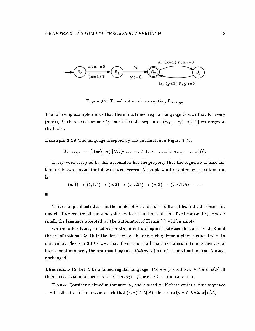
CHAPTER �� AUTOMATA�THEORETIC APPROACH ��
b
(x=1)?
a,x:=0
y:=0
a,(x=1)?,x:=0
b,(y<1)?,y:=0
S0 S1 S2 S3
Figure ���� Timed automaton accepting Lconverge
The following example shows that there is a timed regular language L such that for every
��� �� L� there exists some � � such that the sequence f��i�� � �i� j i �g converges to
the limit ��
Example ���� The language accepted by the automaton in Figure ��� is
Lconverge " f��ab��� �� j �i� ���i�� " i � ���i � ��i�� ��i�� � ��i����g�
Every word accepted by this automaton has the property that the sequence of time dif
ferences between a and the following b converges� A sample word accepted by the automaton
is
�a� �� � �b� ���� � �a� �� � �b� ����� � �a� �� � �b� ������ � � � �
This example illustrates that the model of reals is indeed di erent from the discretetime
model� If we require all the time values �i to be multiples of some xed constant �� however
small� the language accepted by the automaton of Figure ��� will be empty�
On the other hand� timed automata do not distinguish between the set of reals R and
the set of rationals Q� Only the denseness of the underlying domain plays a crucial role� In
particular� Theorem ���� shows that if we require all the time values in time sequences to
be rational numbers� the untimed language Untime�L�A�� of a timed automaton A stays
unchanged�
Theorem ��� Let L be a timed regular language� For every word �� � Untime�L� i
there exists a time sequence � such that �i Q for all i �� and ��� �� L�
Proof� Consider a timed automaton A� and a word �� If there exists a time sequence
� with all rational time values such that ��� �� L�A�� then clearly� � Untime�L�A���

CHAPTER �� AUTOMATA�THEORETIC APPROACH ��
a,(x<5)? a,(x<2)?
b,x:=0 c,x:=0
1S 0S
2S
Figure ���� Timed Muller automaton
Now suppose for an arbitrary time sequence � � ��� �� L�A�� Let � Q be such that
every constant appearing in the clock constraints of A is an integral multiple of �� Let
� �� " �� and �� " �� If �i " �j n� for some � � j i and n N� then choose � �i " � �j n��
Otherwise choose � �i Q such that for all � � j i� for all n N� ��i � �j� n� i
�� �i � � �j� n�� Note that because of the denseness of Q such a choice of � �i is always
possible�
Consider an accepting run r " �s� �� of A over ��� ��� Because of the construction of
� �� if a clock x is reset at the ith transition point� then its possible values at the jth
transition point along the two time sequences� namely� ��j � �i� and ���j � � �i�� satisfy the
same set of clock constraints� Consequently it is possible to construct an accepting run
r� " �s� ��� over ��� � �� which follows the same sequence of edges as r� In particular� choose
� �� " ��� and if the ith transition along r is according to the edge hsi��� si� �i� �i� ii� then
set ��i " ��i �� �����i�� � �i � � �i���� Consequently� A accepts ��� � ���
���� Timed Muller automata
We can dene timed automata with Muller acceptance conditions also�
De�nition ���� A timed Muller automaton �TMA� is a tuple h�� S� S��C�E�Fi� where
h�� S� S��C�Ei is a timed transition table� and F �S species an acceptance family�
A run r " �s� �� of the automaton over a timed word ��� �� is an accepting run i
inf �r� F �
For a TMA A� the language L�A� of timed words it accepts is dened to be the set
f��� �� j A has an accepting run over ��� ��g�

CHAPTER �� AUTOMATA�THEORETIC APPROACH ��
Example ���� Consider the automaton of Figure ��� over the alphabet fa� b� cg� The
start state is s�� and the Muller acceptance family consists of a single set fs�� s�g� So any
accepting run should loop between states s� and s� only nitely many times� and between
states s� and s� innitely many times� Every word ��� �� accepted by the automaton
satises� ��� � �a�b c����ac��� and ��� for all i �� the di erence ���i�� � ��i��� is less
than � if the ��i�th symbol is c� and less than � otherwise�
Recall that B�uchi automata and Muller automata have the same expressive power� The
following theorem states that the same holds true for TBAs and TMAs� Thus the class
of timed languages accepted by TMAs is the same as the class of timed regular languages�
The proof of the following theorem closely follows the standard argument that an �regular
language is accepted by a B�uchi automaton i it is accepted by some Muller automaton�
Theorem ���� A timed language is accepted by some timed B�uchi automaton i it is
accepted by some timed Muller automaton�
Proof� Let A " h�� S� S��C�E�Fi be a TBA� Consider the TMA A� with the same timed
transition table as that of A� and with the acceptance family F " fS� S � S� � F �" �g� It
is easy to check that L�A� " L�A��� This proves the �only if� part of the claim�
In the other direction� given a TMA� we can construct a TBA accepting the same
language using the simulation of Muller acceptance condition by B�uchi automata� Let
A be a TMA given as h�� S� S��C�E�Fi� First note that L�A� " �F�FL�AF� where
AF " h�� S� S��C�E� fFgi� so it su�ces to construct� for each acceptance set F� a TBA
A�F which accepts the language L�AF�� Assume F " fs�� � � �skg� The automaton A
�F uses
nondeterminism to guess when the set F is entered forever� and then uses a counter to make
sure that every state in F is visited innitely often� States of A�F are of the form hs� ii�
where s S and i f�� �� � � �kg� The set of initial states is S� � f�g� The automaton
simulates the transitions of A� and at some point nondeterministically sets the second com
ponent to �� For every transition hs� s�� a� �� i of A� the automaton A�F has a transition
hhs� �i� hs�� �i� a� �� i� and� in addition� if s� F it also has a transition hhs� �i� hs�� �i� a� �� i�
While the second component is nonzero� the automaton is required to stay within the
set F� For every Atransition hs� s�� a� �� i with both s and s� in F� for each � � i � k� there
is an A�Ftransition hhs� ii� hs
�� ji� a� �� i where j " �i �� mod k� if s equals si� else j " i�
The only accepting state is hsk � ki�

CHAPTER �� AUTOMATA�THEORETIC APPROACH ��
��� Checking emptiness
In this section we develop an algorithm for checking the emptiness of the language of a
timed automaton� The existence of an innite accepting path in the underlying transition
table is clearly a necessary condition for the language of an automaton to be nonempty�
However� the timing constraints of the automaton rule out certain additional behaviors�
We will show that a B�uchi automaton can be constructed that accepts exactly the set of
untimed words that are consistent with the timed words accepted by a timed automaton�
����� Restriction to integer constants
Recall that our denition of timed automata allows clock constraints which involve com
parisons with rational constants� The following lemma shows that� for checking emptiness�
we can restrict ourselves to timed automata whose clock constraints involve only integer
constants� For a timed sequence � and t R� let t � � denote the timed sequence obtained
by multiplying all �i by t�
Lemma ���� Consider a timed transition table A� a timed word ��� ��� and t R� �s� �� is
a run of A over ��� �� i �s� t��� is a run of At over ��� t���� where At is the timed transition
table obtained by replacing each constant d in each clock constraint labeling the edges of
A by t � d�
Proof� The lemma can be proved easily from the denitions using induction�
Thus there is an isomorphism between the runs of A and the runs of At� If we choose t
to be the least common multiple of all the constants appearing in the clock constraints of A�
then the clock constraints for At use only integer constants� In this translation� the values
of the individual constants grow with the product of the denominators of all the original
constants� We assume binary encoding for the constants� Let us denote the length of the
clock constraints of A by j �A�j� It is easy to prove that j �At�j is bounded by j �A�j��
Observe that this result depends crucially on the fact that we encode constants in binary
notation� if we use unary encoding then j �At�j can be exponential in j �A�j�
Observe that L�A� is empty i L�At� is empty� Hence� to decide the emptiness of L�A�
we consider At� Also Untime�L�A�� equals Untime�L�At��� In the remainder of the section
we assume that the clock constraints use only integer constants�
CHAPTER �� AUTOMATA�THEORETIC APPROACH ��
����� Clock regions
At every point in time the future behavior of a timed transition table is determined by its
state and the values of all its clocks� This motivates the following denition�
De�nition ���� For a timed transition table h�� S� S��C�Ei� an extended state is a pair
hs� �i where s S and � is a clock interpretation for C�
Since the number of such extended states is innite �in fact� uncountable�� we cannot
possibly build an automaton whose states are the extended states of A� But if two extended
states with the same Astate agree on the integral parts of all clock values� and also on
the ordering of the fractional parts of all clock values� then the runs starting from the
two extended states are very similar� The integral parts of the clock values are needed
to determine whether or not a particular clock constraint is met� whereas the ordering of
the fractional parts is needed to decide which clock will change its integral part rst� For
example� if two clocks x and y are between � and � in an extended state� then a transition
with clock constraint �x " �� can be followed by a transition with clock constraint �y " ���
depending on whether or not the current clock values satisfy �x y��
The integral parts of clock values can get arbitrarily large� But if a clock x is never
compared with a constant greater than c� then its actual value� once it exceeds c� is of no
consequence in deciding the allowed paths�
Now we formalize this notion� For any t R� fract�t� denotes the fractional part of t�
and btc denotes the integral part of t� that is� t " btc fract�t�� We assume that every
clock in C appears in some clock constraint�
De�nition ��� Let A " h�� S� S��C�Ei be a timed transition table� For each x C� let cx
be the largest integer c such that �x � c� or �c � x� is a subformula of some clock constraint
appearing in E�
The equivalence relation � is dened over the set of all clock interpretations for C� ����
i all the following conditions hold�
�� For all x C� either b��x�c and b���x�c are the same� or both ��x� and ���x� are
greater than cx�
�� For all x� y C with ��x� � cx and ��y� � cy � fract���x�� � fract���y�� i
fract����x�� � fract����y���

CHAPTER �� AUTOMATA�THEORETIC APPROACH ��
�
���
��
� � �
�
y
x
� Corner points� e�g� �������
�� Open line segments� e�g� �� x " y ��
� Open regions� e�g� �� x y ��
Figure ���� Clock regions
�� For all x C with ��x� � cx� fract���x�� " � i fract����x�� " ��
A clock region for A is an equivalence class of clock interpretations induced by ��
We will use ��� to denote the clock region to which � belongs� Each region can be
uniquely characterized by a �nite� set of clock constraints it satises� For example� consider
a clock interpretation � over two clocks with ��x� " ��� and ��y� " ���� Every clock
interpretation in ��� satises the constraint �� x y ��� and we will represent this
region by �� x y ��� The nature of the equivalence classes can be best understood
through an example�
Example ���� Consider a timed transition table with two clocks x and y with cx " � and
cy " �� The clock regions are shown in Figure ����
Note that there are only a nite number of regions� Also note that for a clock constraint
� if ���� then � satises i �� satises � We say that a clock region � satises a clock
constraint i every � � satises � Each region can be represented by specifying
��� for every clock x� one clock constraint from the set
fx " c j c " �� �� � � �cxg � fc� � x c j c " �� � � �cxg � fx cxg�
��� for every pair of clocks x and y such that c� � x c and d � � y d
appear in ��� for some c� d� whether fract�x� is less than� equal to� or greater
than fract�y��
By counting the number of possible combinations of equations of the above form� we get
the upper bound in the following lemma�

CHAPTER �� AUTOMATA�THEORETIC APPROACH ��
Lemma ���� The number of clock regions is bounded by �jCj& � �jCj �!x�C��cx ����
Henceforth� we assume that the number of regions is O��j �A�j�� remember that �A�
stands for the length of the clock constraints of A assuming binary encoding� Note that if
we increase �A� without increasing the number of clocks or the size of the largest constants
the clocks are compared with� then the number of regions does not grow with j �A�j� Also
observe that a region can be represented in space linear in j �A�j�
����� The region automaton
The rst step in the decision procedure for checking emptiness is to construct a transition
table whose paths mimic the runs of A in a certain way� We will denote the desired transition
table by R�A�� the region automaton of A� A state of R�A� records the state of the timed
transition table A� and the equivalence class of the current values of the clocks� It is of
the form hs� �i with s S and � being a clock region� The intended interpretation is that
whenever the extended state of A is hs� �i� the state ofR�A� is hs� ���i� The region automaton
starts in some state hs�� ����i where s� is a start state of A� and the clock interpretation ��
assigns � to every clock� The transition relation of R�A� is dened so that the intended
simulation is obeyed� It has an edge from hs� �i to hs�� ��i labeled with a i A in state s
with the clock values � � can make a transition reading a to the extended state hs�� ��i
for some �� ���
The edge relation can be conveniently dened using a time�successor relation over the
clock regions� The timesuccessors of a clock region � are all the clock regions that will be
visited by a clock interpretation � � as time progresses�
De�nition ���� A clock region �� is a timesuccessor of a clock region � i for each � ��
there exists a positive t R such that � t ���
Example ��� Consider the clock regions shown in Figure ��� again� The timesuccessors
of a region � are the regions that can be reached by moving along a line drawn from some
point in � in the diagonally upwards direction �parallel to the line x " y�� For example�
the region ��� x ��� �� y x � ��� has� other than itself� the following regions as
timesuccessors� ��x " ��� �� y ���� ��x ��� �� y ���� ��x ��� �y " ��� and
��x ��� �y ����

CHAPTER �� AUTOMATA�THEORETIC APPROACH ��
Now let us see how to construct all the timesuccessors of a clock region� Recall that a
clock region � is specied by giving ��� for every clock x� a constraint of the form �x " c�
or �c� � x c� or �x cx�� and ��� for every pair x and y such that �c � � x c�
and �d� � y d� appear in ���� the ordering relationship between fract�x� and fract�y��
To compute all the timesuccessors of � we proceed as follows� First observe that the
timesuccessor relation is a transitive relation� We consider di erent cases�
First suppose that � satises the constraint �x cx� for every clock x� The only
timesuccessor of � is itself� This is the case for the region ��x ��� �y ��� in Figure ����
Now suppose that the set C� consisting of clocks x such that � satises the constraint
�x " c� for some c � cx� is nonempty� In this case� as time progresses the fractional
parts of the clocks in C� become nonzero� and the clock region changes immediately� The
timesuccessors of � are same as the timesuccessors of the clock region � specied as below�
��� For x C�� if � satises �x " cx� then � satises �x cx�� otherwise if �
satises �x " c� then � satises �c x c ��� For x � C�� the constraint
in � is the same as that in ��
��� For clocks x and y such that �c� � x c� and �d� � y d� appear in
���� the ordering relationship in � between their fractional parts is same as
in ��
For instance� in Figure ���� the timesuccessors of ��x " ��� �� y ��� are same as the
timesuccessors of �� x y ���
If both the above cases do not apply� then let C� be the set of clocks x with maximal
fractional part� that is� for all y C� fract�y� � fract�x� is a constraint of �� In this case� as
time progresses� the clocks in C� assume integer values� Let � be the clock region specied
by
��� For x C�� if � satises �c�� x c� then � satises �x " c�� For x � C��
the constraint in � is same as that in ��
��� For clocks x and y such that �c� � x c� and �d� � y d� appear in
���� the ordering relationship in � between their fractional parts is same as
in ��
In this case� the timesuccessors of � include �� �� and all the timesuccessors of �� For
instance� in Figure ���� timesuccessors of �� x y �� include itself� ��� x ��� �y "
���� and all the timesuccessors of ��� x ��� �y " ����

CHAPTER �� AUTOMATA�THEORETIC APPROACH ��
Now we are ready to dene the region automaton�
De�nition ���� For a timed transition table A " h�� S� S��C�Ei� the corresponding region
automaton R�A� is a transition table over the alphabet ��
� The states of R�A� are of the form hs� �i where s S and � is a clock region�
� The initial states are of the form hs�� ����i where s� S� and ���x� " � for all x C�
� R�A� has an edge hhs� �i� hs�� ��i� ai i there is an edge hs� s�� a� �� i E and a region
��� such that ��� ��� is a timesuccessor of �� ��� ��� satises � and ��� �� " �� �� ������
Example ���� Consider the timed automaton A� shown in Figure ����� The alphabet
is fa� b� c� dg� Every state of the automaton is an accepting state� The corresponding
region automaton R�A�� is also shown� Only the regions reachable from the initial region
hs�� �x " y " ��i are shown� Note that cx " � and cy " �� The timing constraints of
the automaton ensure that the transition from s� to s is never taken� The only reachable
region with state component s� satises the constraints �y " �� x ��� and this region has
no outgoing edges� Thus the region automaton helps us in concluding that no transitions
can follow a btransition�
From the bound on the number of regions� it follows that the number of states in R�A�
is O�jSj � �j �A�j�� An inspection of the denition of the timesuccessor relation shows that
every region has at most �x�C� �cx � � successor regions� The region automaton has at
most one edge out of hs� �i for every edge out of s and every timesuccessor of �� It follows
that the number of edges in R�A� is O�jEj ��j �A�j�� Note that computing the timesuccessor
relation is easy� and can be done in time linear in the length of the representation of the
region� Constructing the edge relation for the region automaton is also relatively easy� in
addition to computing the timesuccessors� we also need to determine whether the clock
constraint labeling a particular Atransition is satised by a clock region� The region graph
can be constructed in time O��jSj jEj� � �j �A�j��
Now we proceed to establish a correspondence between the runs of A and the runs of
R�A��

CHAPTER �� AUTOMATA�THEORETIC APPROACH ��
0 1
2
a3
y:=0
b,(y=1)? c,(x<1)?
d,(x>1)?c,(x<1)?
S S
S
S
a,(y<1)?,y:=0
0S
x=y=0
3S
0<y<x<13S
0<y<1<x3S
1=y<x3S
x>1,y>1
2S
1=y<x1S
0=y<x<1
1S
y=0,x=11S
y=0,x>1
aa
a
b
b
b
dd
d
dd
c a a aa
d
d
d
Figure ����� Automaton A� and its region automaton

CHAPTER �� AUTOMATA�THEORETIC APPROACH ��
De�nition ���� For a run r " �s� �� of A of the form
r � hs�� ��i������
hs�� ��i������
hs�� ��i������
� � �
dene its projection �r� " �s� ���� to be the sequence
�r� � hs�� ����i���� hs�� ����i
���� hs�� ����i���� � � �
From the denition of the edge relation for R�A�� it follows that �r� is a run of R�A� over
�� Since time progresses without bound along r� every clock x C is either reset innitely
often� or from a certain time onwards it increases without bound� Hence� for all x C�
for innitely many i �� ��i� satises ��x " �� � �x cx��� This prompts the following
denition�
De�nition ���� A run r " �s� �� of the region automaton R�A� of the form
r � hs�� ��i���� hs�� ��i
���� hs�� ��i���� � � �
is progressive i for each clock x C� there are innitely many i � such that �i satises
��x " �� � �x cx���
Thus for a run r of A over ��� ��� �r� is a progressive run of R�A� over �� From
Lemma ���� it follows that progressive runs of R�A� precisely correspond to the projected
runs of A� Before we prove the lemma let us consider the region automaton of Example ����
again�
Example ���� Consider the region automaton R�A�� of Figure ����� Every run r of R�A��
has a su�x of one of the following three forms� �i� the automaton loops between the
regions hs�� �y " � x ��i and hs� �� y x ��i� �ii� the automaton stays in the
region hs� �� y � x�i using the selfloop� or �iii� the automaton stays in the region
hs� �x �� y ��i�
Only the case �iii� corresponds to the progressive runs� For runs of type �i�� even though
y gets reset innitely often� the value of x is always less than �� For runs of type �ii�� even
though the value of x is not bounded� the clock y is reset only nitely often� and yet� its
value is bounded� Thus every progressive run of A� corresponds to a run of R�A�� of type
�iii��

CHAPTER �� AUTOMATA�THEORETIC APPROACH ��
Lemma ��� If r is a progressive run of R�A� over � then there exists a time sequence �
and a run r� of A over ��� �� such that r equals �r���
Proof� Consider a progressive run r " �s� �� of R�A� over �� We construct the run
r� and the time sequence � step by step� As usual� r� starts with hs�� ��i� Now suppose
that the extended state of A is hsi� �ii at time �i with �i �i� There is an edge in R�A�
from hsi� �ii to hsi��� �i��i labeled with �i��� From the denition of the region automaton
it follows that there is an edge hsi� si��� �i��� �i��� i��i E and a timesuccessor ��i�� of
�i such that ��i�� satises i�� and �i�� " ��i�� �� ����i��� From the denition of time
successor� there exists a time �i�� such that ��i �i�� � �i� ��i��� Now it is clear the
next transition of A can be at time �i�� to an extended state hsi��� �i��i with �i�� �i���
Using this construction repeatedly we get a run r� " �s� �� over ��� �� with �r�� " r�
The only problem with the above construction is that � may not satisfy the progress
condition� Suppose that � is a converging sequence� We use the fact that r is a progressive
run to construct another time sequence � � satisfying the progress requirement and show
that the automaton can follow the same sequence of transitions as r� but at times � �i �
Let C� be the set of clocks reset innitely often along r� Since � is a converging sequence�
after a certain position onwards� every clock in C� gets reset before it reaches the value ��
Since r is progressive� every clock x not in C�� after a certain position onwards� never gets
reset� and continuously satises x cx� This ensures that there exists j � such that ���
after the jth transition point each clock x � C� continuously satises �x cx�� and each
clock x C� continuously satises �x ��� and ��� for each k j� ��k� �j� is less than ����
Let j k� k�� � � � be an innite sequence of integers such that each clock x in C�
is reset at least once between the kith and ki��th transition points along r� Now we
construct another sequence r�� " �s� ��� with the sequence of transition times � � as follows�
The sequence of transitions along r�� is same as that along r�� If i � fk�� k� � � �g then we
require the �i ��th transition to happen after a delay of ��i����i�� otherwise we require the
delay to be ���� Observe that along r�� the delay between the kith and ki��th transition
points is less than �� Consequently� in spite of the additional delays� the value of every
clock in C� remains less than � after the jth transition point� So the truth of all the clock
constraints and the clock regions at the transition points remain unchanged �as compared
to r��� From this we conclude that r�� satises the consecution requirement� and is a run of
A� Furthermore� �r��� " �r�� " r�

CHAPTER �� AUTOMATA�THEORETIC APPROACH ��
Since � � has innitely many jumps each of duration ���� it satises the progress require
ment� Hence r�� is the run required by the lemma�
����� The untiming construction
For a timed automaton A� its region automaton can be used to recognize Untime�L�A���
The following theorem is stated for TBAs� but it also holds for TMAs�
Theorem ���� Given a TBA A " h�� S� S��C�E�Fi� there exists a B�uchi automaton over
� which accepts Untime�L�A���
Proof� We construct a B�uchi automaton A� as follows� Its transition table is R�A�� the
region automaton corresponding to the timed transition table h�� S� S��C�Ei� The accepting
set of A� is F� " fhs� �i j s Fg�
If r is an accepting run of A over ��� ��� then �r� is a progressive and accepting run of
A� over �� The converse follows from Lemma ����� Given a progressive run r of A� over ��
the lemma gives a time sequence � and a run r� of A over ��� �� such that r equals �r��� If
r is an accepting run� so is r�� It follows that � Untime�L�A�� i A� has a progressive�
accepting run over it�
For x C� let Fx " fhs� �i j � j" ��x " �� � �x cx��g� Recall that a run of A� is
progressive i some state from each Fx repeats innitely often� It is straightforward to
construct another B�uchi automaton A�� such that A� has a progressive and accepting run
over � i A�� has an accepting run over ��
The automaton A�� is the desired automaton� L�A��� equals Untime�L�A���
Example ���� Let us consider the region automaton R�A�� of Figure ���� again� Since all
states of A� are accepting� from the description of the progressive runs in Example ���� it
follows that the transition table R�A�� can be changed to a B�uchi automaton by choosing
the accepting set to consist of a single region hs� �x �� y ��i� Consequently
Untime�L�A��� " L�R�A��� " ac �ac�� d��
Theorem ���� says that the timing information in a timed automaton is �regular� in
character� its consistency can be checked by a nitestate automaton� An equivalent for
mulation of the theorem is

CHAPTER �� AUTOMATA�THEORETIC APPROACH ��
If a timed language L is timed regular then Untime�L� is ��regular
Furthermore� to check whether the language of a given TBA is empty� we can check for
the emptiness of the language of the corresponding B�uchi automaton constructed by the
proof of Theorem ����� The next theorem follows�
Theorem ���� Given a timed B�uchi automaton A " h�� S� S��C�E�Fi the emptiness of
L�A� can be checked in time O��jSj jEj� � �j �A�j��
Proof� Let A� be the B�uchi automaton constructed as outlined in the proof of The
orem ����� Recall that in Section ����� we had shown that the number of states in A� is
O�jSj � �j �A�j�� the number of edges is O�jEj � �j �A�j��
The language L�A� is nonempty i there is a cycle C in A� such that C is accessible from
some start state of A� and C contains at least one state each from the set F� and each of
the sets Fx� This can be checked in time linear in the size of A� �SVW���� The complexity
bound of the theorem follows�
Recall that if we start with an automaton A whose clock constraints involve rational
constants� we need to apply the above decision procedure on At for the least common
denominator t of all the rational constants �see Section ������� This involves a blowup in
the size of the clock constraints� we have �At� " O� �A����
The above method can be used even if we change the acceptance condition for timed
automata� In particular� given a timed Muller automaton A we can e ectively construct
a Muller �or� B�uchi� automaton which accepts Untime�L�A��� and use it to check for the
emptiness of L�A��
����� Complexity of checking emptiness
The complexity of the algorithm for deciding emptiness of a TBA is exponential in the
number of clocks and the length of the constants in the timing constraints� This blow
up in complexity seems unavoidable� we reduce the acceptance problem for linear bounded
automata� a known PSPACEcomplete problem �HU���� to the emptiness question for TBAs
to prove the PSPACE lower bound for the emptiness problem� We also show the problem
to be PSPACEcomplete by arguing that the algorithm of Section ����� can be implemented
in polynomial space�

CHAPTER �� AUTOMATA�THEORETIC APPROACH ��
Theorem ��� The problem of deciding the emptiness of the language of a given timed
automaton A� is PSPACEcomplete�
Proof� �PSPACEmembership� First we show that the problem is in PSPACE� Since
the number of states of the region automaton is exponential in the number of clocks of A�
we cannot construct the entire transition table� We give a nondeterministic version of the
algorithm which uses only polynomial space� the trick involved is fairly standard�
Let l be the length of the representation of A� As observed earlier� each state of the region
automaton can be represented in space O�l�� and all its successors in the region automaton
can be generated easily� Recall that the language L�A� is nonempty i the region automaton
has a cycle that is accessible from some start state and meets all the acceptance criteria�
The procedure nondeterministically guesses an initial region v�� another region vn� and a
path
v� � � � � � vn � vn�� � � � � � vm " vn�
The path is guessed vertex by vertex� at each step checking that the newly guessed state
is connected by an edge from the previous one� In addition� the procedure checks that the
cycle vn � � � � � vm satises all the acceptance criteria� If L�A� is nonempty then this
nondeterministic algorithm succeeds� The algorithm only uses space O�l�� hence check
ing nonemptiness of L�A� requires nondeterministic polynomial space� It follows that the
emptiness can be checked in PSPACE from Savitch�s theorem�
�PSPACEhardness� The question of deciding whether a given linear bounded automaton
accepts a given input string is PSPACEcomplete �HU���� A linear bounded automatonM
is a nondeterministic Turing machine whose tape head cannot go beyond the end of the
input markers� We construct a TBA A such that its language is nonempty i the machine
M halts on a given input�
Let ' be the tape alphabet of M and let Q be its states� Let � " ' � �' � Q�� and
let a�� a�� � � �ak denote the elements of �� A conguration of M in which the tape reads
���� � � � �n� and the machine is in state q reading the ith tape symbol� is represented by
the string ��� � � ��n over � such that �j " �j if j �" i and �i " h�i� qi�
The acceptance corresponds to a special state qf � after which the conguration stays
unchanged� The alphabet of A includes �� and in addition� has a symbol a�� A computation
of M is encoded by the word
���a� � � � ��na��
��a� � � ��
�na� � � � �
j�a� � � � �
jna� � � �
CHAPTER �� AUTOMATA�THEORETIC APPROACH ��
such that �j� � � ��jn encodes the jth conguration according to the above scheme� The
time sequence associated with this word also encodes the computation� we require the time
di erence between successive a��s to be k �� and if �ji " al then we require its time to be
l greater than the time of the previous a�� The encoding in the time sequence is used to
enforce the consecution requirement�
We want to construct A which accepts precisely the timed words encoding the halting
computations of M according to the above scheme� We only sketch the construction� A
uses �n � clocks� The clock x is reset with each a�� While reading a� we require �x " k ��
to hold� and while reading ai we require �x " i� to hold� These conditions ensure that the
encoding in the time sequence is consistent with the word� For each tape cell i� we have
two clocks xi and yi� The clock xi is reset with �ji � for odd values of j� and the clock
yi is reset with �ji � for even values of j� Assume that the automaton has read the rst j
congurations� with j odd� The value of the clock xi represents the ith cell of the jth
conguration� Consequently� the possible choices for the values of �j��i are determined by
examining the values of xi��� xi and xi�� according to the transition rules for M � While
reading the �j ��th conguration� the yclocks get set to appropriate values� these values
are examined while reading the �j ��th conguration� This ensures proper consecution of
congurations� Proper initialization and halting can be enforced in a straightforward way�
The size of A is polynomial in n and the size of M �
Note that the source of this complexity is not the choice of R to model time� The
PSPACEhardness result can be proved if we leave the syntax of timed automata unchanged�
but use the discrete domain N to model time� Also this complexity is insensitive to the
encoding of the constants� the problem is PSPACEcomplete even if we encode all constants
in unary�
��� Intractable problems
In this section we show the universality problem for timed automata to be undecidable�
The universality problem is to decide whether the language of a given automaton over
� comprises of all the timed words over �� Specically� we show that the problem is
!��hard by reducing a !
��hard problem of �counter machines� The class !�
� consists of
highly undecidable problems� including some nonarithmetical sets �for an exposition of the
analytical hierarchy consult� for instance� �Rog����� Note that the universality problem

CHAPTER �� AUTOMATA�THEORETIC APPROACH ��
is same as deciding emptiness of the complement of the language of the automaton� The
undecidability of this problem has several implications such as nonclosure under complement
and undecidability of testing for language inclusion�
����� A ����complete problem
A nondeterministic ��counter machine M consists of two counters C and D� and a sequence
of n instructions� Each instruction may increment or decrement one of the counters� or
jump� conditionally upon one of the counters being zero� After the execution of a nonjump
instruction� M proceeds nondeterministically to one of the two specied instructions�
We represent a conguration of M by a triple hi� c� di� where � � i � n� c �� and
d � give the values of the location counter and the two counters C and D� respectively�
The consecution relation on congurations is dened in the obvious way� A computation of
M is an innite sequence of related congurations� starting with the initial conguration
h�� �� �i� It is called recurring i it contains innitely many congurations in which the
location counter has the value ��
The problem of deciding whether a nondeterministic Turing machine has� over the empty
tape� a computation in which the starting state is visited innitely often� is known to be
���complete �HPS���� Along the same lines we obtain the following result�
Lemma ���� The problem of deciding whether a given nondeterministic �counter machine
has a recurring computation� is ���hard�
Proof� Every ���formula is equivalent to a �
��formula � of the form
�f� �f��� " � � �x� g�f�x�� f�x �����
for a recursive predicate g �HPS���� For any such � we can construct a nondeterministic
�counter machine M that has a recurring computation i � is true�
Let M start by computing f��� " �� and proceed� indenitely� by nondeterministically
guessing the next value of f � At each stage� M checks whether f�x� and f�x �� satisfy
g� and if �and only if� so� it jumps to instruction �� Such an M exists� because �counter
machines can� being universal� compute the recursive predicate g� It executes the instruction
� innitely often i a function f with the desired properties exists�

CHAPTER �� AUTOMATA�THEORETIC APPROACH ��
����� Undecidability of the universality problem
Now we proceed to encode the computations of �counter machines using timed automata�
and use the encoding to prove the undecidability result�
Theorem ���� Given a timed automaton over an alphabet � the problem of deciding
whether it accepts all timed words over � is !��hard�
Proof� We encode the computations of a given �counter machine M with n instruc
tions using timed words over the alphabet fb�� � � � bn� a�� a�g� A conguration hi� c� di is
represented by the sequence biac�a
d�� We encode a computation by concatenating the se
quences representing the individual congurations� We use the time sequence associated
with � to express that the successive congurations are related as per the requirements
of the program instructions� We require that the subsequence of � corresponding to the
time interval �j� j �� encodes the jth conguration of the computation� Note that the
denseness of the underlying time domain allows the counter values to get arbitrarily large�
To express that the number of a� �or a�� symbols in two intervals encoding the successive
congurations is the same �or that the number is one less or one greater� we require that
every a� in the rst interval has a matching a� at distance � and vice versa�
Dene a timed language Lundec as follows� ��� �� is in Lundec i
� � " bi�ac�� a
d�� bi�a
c�� a
d�� � � � such that hi�� c�� d�i� hi�� c�� d�i � � � is a recurring computation
of M �
� For all j �� the time of bij is j�
� For all j ��
� if cj�� " cj then for every a� at time t in the interval �j� j �� there is an a� at
time t ��
� if cj�� " cj � then for every a� at time t in the interval �j �� j �� except
the last one� there is an a� at time t � ��
� if cj�� " cj � � then for every a� at time t in the interval �j� j �� except the
last one� there is an a� at time t ��
Similar requirements hold for a��s�

CHAPTER �� AUTOMATA�THEORETIC APPROACH ��
Clearly� Lundec is nonempty i M has a recurring computation� We will construct a timed
automaton Aundec which accepts the complement of Lundec � Hence Aundec accepts every
timed word i M does not have a recurring computation� The theorem follows from
Lemma �����
The desired automaton Aundec is a disjunction of several TBAs�
Let A� be the TBA which accepts ��� �� i for some integer j �� either there is no b
symbol at time j� or the subsequence of � in the time interval �j� j �� is not of the form
a��a��� It is easy to construct such a timed automaton�
The subsequence of a timed word ��� �� in Lundec should encode the initial conguration
over the interval ��� ��� Let Ainit be the TBA which requires that the subsequence of
� corresponding to the interval ��� �� is not b�� it accepts the language f��� �� j ��� �"
b�� � ��� �" �� � ��� ��g�
For each instruction � � i � n we construct a TBA Ai� Ai accepts ��� �� i the timed
word has bi at some time t� and the conguration corresponding to the subsequence in
�t �� t �� does not follow from the conguration corresponding to the subsequence in
�t� t �� by executing the instruction i� We give the construction for a sample instruction�
say� �increment the counter D and jump nondeterministically to instruction � or ��� The
automaton Ai is the disjunction of the following six TBAs A�i � � � �A
�i�
Let A�i be the automaton which accepts ��� �� i for some j �� �j " bi� and at time
�j � there is neither b nor b�� It is easy to construct this automaton�
Let A�i be the following TBA�
bi 1a
x:=0
,x:=0
x<1?
1a ,x=1?
0S
1S 2S x 1= ?
In this gure� an edge without a label means that the transition can be taken on every
input symbol� While in state s�� the automaton cannot accept a symbol a� if the condition
�x " �� holds� Thus A�i accepts ��� �� i there is some bi at time t followed by an a� at
time t� �t �� such that there is no matching a� at time �t� ���
Similarly we can construct A�i which accepts ��� �� i there is some bi at time t� and
for some t� �t �� there is no a� at time t� but there is an a� at time �t
� ��� The

CHAPTER �� AUTOMATA�THEORETIC APPROACH ��
complements of A�i and A
�i together ensure proper matching of a��s�
Along similar lines we ensure proper matching of a� symbols� Let Ai be the automaton
which requires that for some bi at time t� there is an a� at some t� �t �� with no match at
�t� ��� Let Ai be the automaton which says that for some bi at time t there are two a��s
in �t �� t �� without matches in �t� t ��� Let A�i be the automaton which requires that
for some bi at time t the last a� in the interval �t �� t �� has a matching a� in �t� t ���
Now consider a word ��� �� such that there is bi at some time t such that the encoding of
a��s in the intervals �t� t �� and �t �� t �� do not match according to the desired scheme�
Let the number of a��s in �t� t �� and in �t �� t �� be k and l respectively� If k l then
the word is accepted by Ai � If k " l� then either there is no match for some a� in �t� t ���
or every a� in �t� t �� has a match in �t �� t ��� In the former case the word is accepted
by Ai � and in the latter case it is accepted by A
�i� If k l the word is accepted by A
i �
The requirement that the computation be not recurring translates to the requirement
that b� appears only nitely many times in �� Let Arecur be the B�uchi automaton which
expresses this constraint�
Putting all the pieces together we claim that the language of the disjunction of A�� Ainit �
Arecur � and each of Ai� is the complement of Lundec �
This result is not unusual for systems for reasoning about dense realtime� Later we
will show the undecidability of certain realtime logics with dense semantics� Obviously� the
universality problem for TMAs is also undecidable� We have not been able to show that the
universality problem is !��complete� an interesting problem is to locate its exact position
in the analytical hierarchy� In the following subsections we consider various implications of
the above undecidability result�
����� Inclusion and equivalence
Recall that the language inclusion problem for B�uchi automata can be solved in PSPACE�
However� it follows from Theorem ���� that there is no decision procedure to check whether
the language of one TBA is a subset of the other� This result is an obstacle in using
timed automata as a specication language for automatic verication of nitestate real
time systems�
Corollary ���� Given two TBAs A� and A� over an alphabet �� the problem of checking
L�A�� L�A�� is !��hard�

CHAPTER �� AUTOMATA�THEORETIC APPROACH ��
Proof� We reduce the universality problem for a given timed automaton A over � to
the language inclusion problem� Let Auniv be an automaton which accepts every timed
word over �� The automaton A is universal i L�Auniv � L�A��
Now we consider the problem of testing equivalence of two automata� A natural de
nition for equivalence of two automata uses equality of the languages accepted by the two�
However alternative denitions exist� We will explore one such notion�
De�nition ���� For timed B�uchi automataA� andA� over an alphabet �� dene A���A�
i L�A�� " L�A��� Dene A� ��A� i for all timed automata A over �� L�A�� L�A��
is empty precisely when L�A� � L�A�� is empty�
For a class of automata closed under complement the above two denitions of equivalence
coincide� However� these two equivalence relations di er for the class of timed regular
languages because of the nonclosure under complement �to be proved shortly�� In fact�
the second notion is a weaker notion� A���A� implies A���A�� but not vice versa�
The motivation behind the second denition is that two automata �modeling two nite
state systems� should be considered di erent only when a third automaton �modeling the
observer or the environment� composed with them gives di erent behaviors� in one case
the composite language is empty� and in the other case there is a possible joint execution�
The proof of Theorem ���� can be used to show undecidability of this equivalence also�
Note that the problems of deciding the two types of equivalences lie at di erent levels of
the hierarchy of undecidable problems�
Theorem ���� For timed B�uchi automata A� and A� over an alphabet ��
�� The problem of deciding whether A� ��A� is !��hard�
�� The problem of deciding whether A� ��A� is complete for the cor�e� class�
Proof� The language of a given TBA A is universal i A��Auniv � Hence the !��
hardness of the universality problem implies !��hardness of the rst type of equivalence�
Now we show that the problem of deciding nonequivalence� by the second denition� is
recursively enumerable� If the two automata are inequivalent then there exists an automaton
A over � such that only one of L�A� � L�A�� and L�A� � L�A�� is empty� Consider the
following procedure P � P enumerates all the TBAs over � one by one� For each TBA A�

CHAPTER �� AUTOMATA�THEORETIC APPROACH ��
it checks for the emptiness of L�A��L�A�� and the emptiness of L�A��L�A��� If P ever
nds di erent answers in the two cases� it halts saying that A� and A� are not equivalent�
Finally we prove that the problem of deciding the second type of equivalence is unsolv
able� We use the encoding scheme used in the proof of Theorem ����� The only di erence
is that we use the halting problem of a deterministic �counter machine M instead of the
recurring computations of a nondeterministic machine� Recall that the halting problem for
deterministic �counter machines is undecidable� Assume that the nth instruction is the
halting instruction� We obtain A�undec by replacing the disjunct Arecur by an automaton
which accepts ��� �� i bn does not appear in �� The complement of L�A�undec� consists of
the timed words encoding the halting computation�
We claim that Auniv ��A�undec i the machine M does not halt� If M does not halt
then A�undec accepts all timed words� and hence� its language is the same as that of Auniv � If
M halts� then we can construct a timed automaton Ahalt which accepts a particular timed
word encoding the halting computation ofM � IfM halts in k steps� then Ahalt uses k clocks
to ensure proper matching of the counter values in successive congurations� The details
are very similar to the PSPACEhardness proof of Theorem ����� L�Ahalt � � L�Auniv � is
nonempty whereas L�Ahalt��L�A�undec� is empty� and thus Auniv and A
�undec are inequivalent
in this case� This completes the proof�
����� Nonclosure under complement
The !��hardness of the inclusion problem implies that the class of TBAs is not closed under
complement�
Corollary ��� The class of timed regular languages is not closed under complementation�
Proof� Given TBAs A� and A� over an alphabet �� L�A�� L�A�� i the intersec
tion of L�A�� and the complement of L�A�� is empty� Assume that TBAs are closed under
complement� Consequently� L�A�� � L�A�� i there is a TBA A such that L�A���L�A�
is nonempty� but L�A�� � L�A� is empty� That is� L�A�� � L�A�� i A� and A� are
inequivalent according to ��� From Theorem ���� it follows that the complement of the in
clusion problem is recursively enumerable� This contradicts the !��hardness of the inclusion
problem�
The following example provides some insight regarding the nonclosure under comple
mentation�
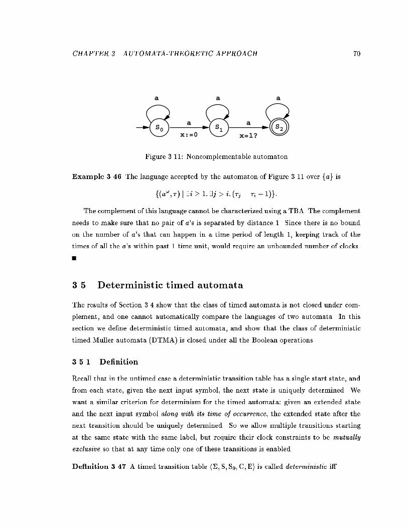
CHAPTER �� AUTOMATA�THEORETIC APPROACH ��
a a a
a a
x=1?x:=00S 1S 2S
Figure ����� Noncomplementable automaton
Example ���� The language accepted by the automaton of Figure ���� over fag is
f�a�� �� j �i �� �j i� ��j " �i ��g�
The complement of this language cannot be characterized using a TBA� The complement
needs to make sure that no pair of a�s is separated by distance �� Since there is no bound
on the number of a�s that can happen in a time period of length �� keeping track of the
times of all the a�s within past � time unit� would require an unbounded number of clocks�
�� Deterministic timed automata
The results of Section ��� show that the class of timed automata is not closed under com
plement� and one cannot automatically compare the languages of two automata� In this
section we dene deterministic timed automata� and show that the class of deterministic
timed Muller automata �DTMA� is closed under all the Boolean operations�
����� De�nition
Recall that in the untimed case a deterministic transition table has a single start state� and
from each state� given the next input symbol� the next state is uniquely determined� We
want a similar criterion for determinism for the timed automata� given an extended state
and the next input symbol along with its time of occurrence� the extended state after the
next transition should be uniquely determined� So we allow multiple transitions starting
at the same state with the same label� but require their clock constraints to be mutually
exclusive so that at any time only one of these transitions is enabled�
De�nition ���� A timed transition table h�� S� S��C�Ei is called deterministic i

CHAPTER �� AUTOMATA�THEORETIC APPROACH ��
b,(x>2)?
b,(x<2)?-
a,x:=0
a,x:=0
a,x:=0
1S
0S
3S2S
Figure ����� Deterministic timed Muller automaton
�� it has only one start state� jS�j " �� and
�� for all s S� for all a �� for every pair of edges of the form hs��� a��� �i and
hs��� a��� �i� the clock constraints � and � are mutually exclusive �i�e�� � � � is
unsatisable��
A timed automaton is deterministic i its timed transition table is deterministic�
Note that in absence of clocks the above denition matches with the denition of deter
minism for transition tables� Thus every deterministic transition table is also a deterministic
timed transition table� Let us consider an example of a DTMA�
Example ���� The DTMA of Figure ���� accepts the language Lcrt of Example ����
Lcrt " f��ab��� �� j �i� �j i� ���j�� � ��j�� ��g
The Muller acceptance family is given by ffs�� sgg� The state s� has two mutually
exclusive outgoing transitions on b� The acceptance condition requires that the transition
with the clock constraint �x �� is taken only nitely often�
Deterministic timed automata can be easily complemented because of the following
property�
Lemma ��� A deterministic timed transition table has at most one run over a given
timed word�

CHAPTER �� AUTOMATA�THEORETIC APPROACH ��
Proof� Consider a deterministic timed transition table A� and a timed word ��� ���
The run starts at time � with the extended state hs�� ��i where s� is the unique start state�
Suppose the extended state of A at time �j�� is hs� �i� and the run has been constructed
up to �j � �� steps� By the deterministic property of A� at time �j there is at most one
transition hs� s�� �j� � �i such that the clock interpretation at time �j � � �j � �j��� satises
� If such a transition does not exist then A has no run over ��� ��� Otherwise� this choice
of transition uniquely extends the run to the jth step� and determines the extended state
at time �j � The lemma follows by induction�
����� Closure properties
Now we consider the closure properties for deterministic timed automata� Like deterministic
Muller automata� DTMAs are also closed under all Boolean operations�
Theorem ��� The class of timed languages accepted by deterministic timed Muller au
tomata is closed under union� intersection� and complementation�
Proof� We dene a transformation on DTMAs to make the proofs easier� for every
DTMA A " h�� S� s��C�E�Fi we construct another DTMA A� by completing A as follows�
First we add a dummy state q to the automaton� From each state s� for each symbol a�
we add an alabeled edge from s to q� The clock constraint for this edge is the negation of
the disjunction of the clock constraints of all the alabeled edges starting at s� We leave
the acceptance condition unchanged� This construction preserves determinism as well as
the set of accepted timed words� The new automaton A� has the property that for each
state s and each input symbol a� the disjunction of the clock constraints of the alabeled
edges starting at s is a valid formula� Observe that A� has precisely one run over any timed
word� We call such an automaton complete� In the remainder of the proof we assume each
DTMA to be complete�
Let Ai " h�� Si� s�i�Ci�Ei�Fii� for i " �� �� be two complete DTMAs with disjoint sets
of clocks� First we construct a timed transition table A using a product construction� The
set of states of A is S� � S�� Its start state is hs�� � s��i� The set of clocks is C� � C��
The transitions of A are dened by coupling the transitions of the two automata having
the same label� Corresponding to an A�transition hs�� t�� a� ��� �i and an A�transition
hs�� t�� a� ��� �i� A has a transition hhs�� s�i� ht�� t�i� a� �� � ��� � � �i� It is easy to check
that A is also deterministic� A has a unique run over each ��� ��� and this run can be
CHAPTER �� AUTOMATA�THEORETIC APPROACH ��
obtained by putting together the unique runs of Ai over ��� ���
Let F� consist of the sets F S� � S� such that the projection of F onto the rst
component is an accepting set of A�� that is�
F� " fF S� � S� j fs S� j �s� S�� hs� s
�i Fg F�g�
Hence a run r of A is an accepting run for A� i inf �r� F�� Similarly dene F� to
consist of the sets F such that fs� j �s S�� hs� s�i Fg is in F�� Now coupling A with the
Muller acceptance family F��F� gives a DTMA accepting L�A���L�A��� whereas using
the acceptance family F� � F� gives a DTMA accepting L�A�� � L�A���
Finally consider complementation� Let A be a complete DTMA h�� S� s��C�E�Fi� A
has exactly one run over a given timed word� Hence� ��� �� is in the complement of L�A� i
the run of A over it does not meet the acceptance criterion of A� The complement language
is� therefore� accepted by a DTMA which has the same underlying timed transition table
as A� but its acceptance condition is given by �S �F �
Now let us consider the closure properties of DTBAs� Recall that deterministic B�uchi
automata �DBA� are not closed under complement� The property that �there are innitely
many a�s� is speciable by a DBA� however� the complement property� �there are only
nitely many a�s� cannot be expressed by a DBA� Consequently we do not expect the class
of DTBAs to be closed under complementation� However� since every DTBA is also a
DTMA� the complement of a DTBAlanguage is accepted by a DTMA� The next theorem
states the closure properties�
Theorem ��� The class of timed languages accepted by DTBAs is closed under union
and intersection� but not closed under complement� The complement of a DTBA language
is accepted by some DTMA�
Proof� For the case of union� we construct the product transition table as in case of
DTMAs �see proof of Theorem ������ The accepting set is fhs� s�i j s F� � s� F�g�
A careful inspection of the product construction for TBAs �see proof of Theorem �����
shows that it preserves determinism� The closure under intersection for DTBAs follows�
The nonclosure of deterministic B�uchi automata under complement leads to the non
closure for DTBAs under complement� The language f��� �� j � �b�a��g is speciable by
a DBA� Its complement language f��� �� j � �a b��b�g is not speciable by a DTBA�

CHAPTER �� AUTOMATA�THEORETIC APPROACH ��
This claim follows from Lemma ���� �to be proved shortly�� and the fact that the language
�a b��b� is not speciable by a DBA�
Let A " h�� S� s��C�E�Fi be a complete deterministic automaton� ��� �� is in the com
plement of L�A� i the �unique� run of A over it does not meet the acceptance criterion of
A� The complement language is� therefore� accepted by a DTMA with the same underlying
timed transition table as A� and the acceptance family �S�F�
����� Decision problems
In this section we examine the complexity of the emptiness problem and the language
inclusion problem for deterministic timed automata�
The emptiness of a timed automaton does not depend on the symbols labeling its edges�
Consequently� checking emptiness of deterministic automata is no simpler� it is PSPACE
complete�
Since deterministic automata can be complemented� checking for language inclusion is
decidable� In fact� while checking L�A�� L�A��� only A� need be deterministic� A� can
be nondeterministic� The problem can be solved in PSPACE�
Theorem ��� For a timed automaton A� and a deterministic timed automaton A�� the
problem of deciding whether L�A�� is contained in L�A�� is PSPACEcomplete�
Proof� PSPACEhardness follows� even when A� is deterministic� from the fact that
checking for the emptiness of the language of a deterministic timed automaton is PSPACE
hard� Let Aempty be a deterministic automaton which accepts the empty language� Now
for a deterministic time automaton A� L�A� is empty i L�A� L�Aempty ��
Observe that L�A�� L�A�� i the intersection of L�A�� with the complement of
L�A�� is empty� Recall that complementing the language of a deterministic automaton cor
responds to complementing the acceptance condition� First we construct a timed transition
table A from the timed transition tables of A� and A� using the product construction
�see proof of Theorem ������ The size of A is proportional to the product of the sizes
of Ai� Then we construct the region automaton R�A�� L�A�� � L�A�� i R�A� has a
cycle which is accessible from its start state� meets the progressiveness requirement� the
acceptance criterion for A�� and the complement of the acceptance criterion for A�� The
existence of such a cycle can be checked in space polynomial in the size of A� as in the proof
of PSPACEsolvability of emptiness �Theorem ������
CHAPTER �� AUTOMATA�THEORETIC APPROACH ��
����� Expressiveness
In this section we compare the expressive power of the various types of timed automata�
Every DTBA can be expressed as a DTMA simply by rewriting its acceptance condi
tion� However the converse does not hold� First observe that every �regular language is
expressible as a DMA� and hence as a DTMA� On the other hand� since deterministic B�uchi
automata are strictly less expressive than deterministic Muller automata� certain �regular
languages are not speciable by DBAs� The next lemma shows that such languages cannot
be expressed using DTBAs either� It follows that DTBAs are strictly less expressive than
DTMAs� In fact� DTMAs are closed under complement� whereas DTBAs are not�
Lemma ��� For an �language L� the timed language f��� �� j � Lg is accepted by
some DTBA i L is accepted by some DBA�
Proof� Clearly if L is accepted by a DBA� then f��� �� j � Lg is accepted by the
same automaton considered as a timed automaton�
Now suppose that the language f��� �� j � Lg is accepted by some DTBA A� We
construct another DTBA A� such that L�A�� " f��� �� j �� L� � �i� ��i " i�g� A� requires
time to increase by � at each transition� The automaton A� can be obtained from A by
introducing an extra clock x� We add the conjunct x " � to the clock constraint of every
edge in A and require it to be reset on every edge� A� is also deterministic�
The next step is the untiming construction for A�� Observe that Untime�L�A��� " L�
While constructing R�A�� we need to consider only those clock regions which have all clocks
with zero fractional parts� Since the time increase at every step is predetermined� and A�
is deterministic� it follows that R�A�� is a deterministic transition table� We need not
check the progressiveness condition also� It follows that the automaton constructed by the
untiming procedure is a DBA accepting L�
From the above discussion one may conjecture that a DTMA language L is a DTBA
language if Untime�L� is a DBA language� To answer this let us consider the convergent
response property Lcrt speciable using a DTMA �see Example ������ This language in
volves a combination of liveness and timing� We conjecture that no DTBA can specify this
property�
Along the lines of the above proof we can also show that for an �language L� the timed
language f��� �� j � Lg is accepted by some DTMA �or TMA� or TBA� i L is accepted
by some DMA �or MA� or BA� respectively��

CHAPTER �� AUTOMATA�THEORETIC APPROACH ��
Class of timed languages Operations closed under
TMA " TBA union� intersection�
DTMA union� intersection� complement�
DTBA union� intersection
Figure ����� Classes of timed automata
Class of �languages Operations closed under
MA " BA " DMA union� intersection� complement�
DBA union� intersection
Figure ����� Classes of �automata
Since DTMAs are closed under complement� whereas TMAs are not� it follows that the
class of languages accepted by DTMAs is strictly smaller than that accepted by TMAs� In
particular� the language of Example ����� ��some pair of a�s is distance � apart�� is not
representable as a DTMA� it relies on nondeterminism in a crucial way�
We summarize the discussion on various types of automata in the table of Figure ����
which shows the inclusions between various classes and the closure properties of various
classes� Compare this with the corresponding results for the various classes of �automata
shown in Figure �����
�� Variants of timed automata
In this section we consider some of the ways to modify our denition of timed automata and
indicate how these decisions a ect the expressiveness and complexity of di erent problems�
���� Clock constraints
Recall that our denition of the clock constraints allows Boolean combinations of atomic
formulas which compare clock values with �rational� constants� With this vocabulary� timed

CHAPTER �� AUTOMATA�THEORETIC APPROACH ��
�
���
��
��
� � �
�
y
x
� Corner points� e�g� �������
�� Open line segments� e�g� �� x " y ��
�� Open regions� e�g� �� x y ��
Figure ����� Clock regions for extended clock constraints
automata can express only constant bounds on the delays between transitions� We consider
two extensions� one allows comparisons between two clock values� and the other allows clock
values to be added�
Comparing two clocks
First we extend the denition of clock constraints to allow subformulas involving two clocks
such as �x � y c�� In particular� in Denition ��� of the set %�X� of clock constraints� we
allow� as atomic constraints� the conditions �x � y c� and �x c � y�� for x� y X and
c Q� Thus the allowed clock constraints are quantierfree formulas using the primitives
of comparison ��� and addition by rational constants � c��
The untiming construction can handle this extension very easily� We need to rene the
equivalence relation on clock interpretations� Now� in addition to the previous conditions�
we require that two equivalent clock interpretations agree on all the subformulas appearing
in the clock constraints� Instead of giving the details we only consider the regions in
Example ���� again�
Example ��� As before the timed transition table has two clocks x and y with cx " �
and cy " �� Suppose the formula �x � y �� appears as a clock constraint labeling one
of the edges� and this is the only condition involving both the clocks� The clock regions
are shown in Figure ����� Comparing it to the clock regions in Figure ��� notice that the
region ��x ��� �y ��� is split into three regions according to the relationship between x
and �y ���
The region graph is constructed as before� The complexity of the algorithm for testing
emptiness remains the same�

CHAPTER �� AUTOMATA�THEORETIC APPROACH ��
This extension of clock constraints does not add to the expressiveness of timed automata�
We can get rid of the constraints of the form �x � y c� or �x c � y� in a systematic
fashion� For instance� consider the constraint �x � y ��� First we tag each state of the
automaton with the truth value of this constraint� In the initial states� the constraint is
true� Now consider an edge e from state s to s�� If x gets reset along e� then �x � y ��
must be true in s�� If only y gets reset along e� then we add one of the conjuncts �x � ��
and �x �� to the clock constraint of e depending on whether �x � y �� is true or false
in s�� If none of the clocks x and y are reset along e� then the tag of s� must be the same
as that of s� Once all the states are tagged in the above manner� we can simplify the clock
constraint of every edge e by replacing the formula �x � y �� by true or false depending
upon the tag of the source state of e�
Introducing the addition primitive
Next we allow the primitive of addition in the clock constraints� Now we can write clock
constraints such as �x y � x� y�� which allow the automaton to compare various delays�
This greatly increases the expressiveness of the formalism� The language of the automaton
in the following example is not timed regular�
Example �� Consider the automaton of Figure ���� with the alphabet fa� b� cg� It ex
presses the property that the symbols a� b� and c alternate� and the delay between b and c
is always twice the delay between the last pair of a and b� The language is dened by
f��abc��� �� j �j� ���j � �j��� " ���j�� � �j����g�
Intuitively� the constraints involving addition are too powerful and cannot be imple
mented by nitestate systems� Even if we constrain all events to occur at integer time
values �i�e�� discretetime model�� to check that the delay between rst two symbols is same
as the delay between the next two symbols� an automaton would need an unbounded mem
ory� Thus with nite resources� an automaton can compare delays with constants� but
cannot remember delays� In fact� we can show that introducing addition in the syntax of
clock constraints makes the emptiness problem for timed automata undecidable�

CHAPTER �� AUTOMATA�THEORETIC APPROACH ��
2x=3y
c
b,y:=0a,x:=0
1S
2S0S
Figure ����� Automaton with clock constraints using
Theorem ��� Allowing the addition primitive in the syntax of clock constraints makes
the emptiness problem for timed automata !��hard�
Proof� As in the proof of Theorem ���� we reduce the problem of recurring computa
tions of nondeterministic �counter machines to the emptiness problem for time automata
using the primitive � The alphabet is fa� b�� � � � bng� We say that a timed word ��� �� en
codes a computation hi�� c�� d�i� hi�� c�� d�i � � � of the �counter machine i � " bi�abi�abi� � � �
with ��j � ��j�� " cj � and ��j�� � ��j " dj for all j �� Thus the delay between b and the
following a encodes the value of the counter C� and the delay between a and the following b
encodes the value of D� We construct a timed automaton which accepts precisely the timed
words encoding the recurring computations of the machine� The primitive of is used to
express a consecution requirement such as the value of the counter C remains unchanged�
The details of the proof are quite straightforward�
���� Timed automata with ��transitions
The denition of nondeterministic nitestate automata sometimes allows the automaton
to make transitions without consuming any input �see� for instance� �HU����� We can allow
such silent transitions for timed automata also� Thus now we allow the edges to be labeled
with ��
Before we dene these automata precisely� let us consider an example�
Example ��� The automaton of Figure ���� accepts a timed word over fag i there is
some a at time t with no a at time t �� The language is given by
f�a�� �� j �i� �j� ��j �" �i ��g�

CHAPTER �� AUTOMATA�THEORETIC APPROACH ��
a a a
a
x=1?x:=00S 1S 2S
Figure ����� Timed automaton with �transitions
If we view the automaton of Figure ���� as accepting timed words over the alphabet
fa� �g� no new denitions are required� However� we want to eliminate ��s from the timed
words accepted by the automaton� Consequently we need to account for the possibility that
there may be only nitely many visible transitions along the run� This calls for changing
the denition of the timed languages to allow timed words of nite length also� In fact� it is
useful to develop the entire theory of timed languages allowing both nite and innite words�
We avoided this for the sake of simplicity of presentation� redening all the constructions
to handle such languages poses no extra problems�
De�nition ��� The pair ��� �� is a nite timed word over � i � is a nite sequence over
�� and � is nite sequence over positive real numbers such that
� both � and � are of the same length�
� � satises monotonicity� for each i j� j� ��i� ��i ���
A mixed timed language over � consists of both innite and nite timed words over ��
The Boolean operations are dened on mixed timed languages the usual way� In addition
we can dene a projection operation also� The result of projecting a timed word ��� ��� nite
or innite� over �� onto a subset �� of �� is obtained by deleting from � the symbols not in
��� and discarding the associated times from the time sequence�
De�nition �� Let ��� �� be a nite or innite timed word over �� and let �� �� Let
� " i�� i�� � � � be the �nite or innite� increasing sequence of integers such that j � i
�j �� for all j � j� j�
CHAPTER �� AUTOMATA�THEORETIC APPROACH ��
The projection of ��� �� on ��� denoted by ��� ��d��� is the �nite or innite� timed word
���� � �� with j��j " j� �j " j�j� such that ��j " �ij and ��j " �ij for all j � j�j�
For a mixed timed language L over �� the projection is dened by
Ld�� " f��� ��d�� j ��� �� Lg�
Observe that from an innite timed word we may get a nite one using projection� For
instance� after projecting the timed word
�a� �� � �b� ���� � �b� �� � �a� �� � �a� �� � �a� �� � � � �
onto fbg we get the nite timed word �b� �����b� ���
The timed automata with �transitions accept mixed timed languages�
De�nition ���� An �TBA over � is a timed B�uchi automaton A over the alphabet ��f�g�
The mixed timed language accepted by A is dened to be the projection onto � of the
language of innite timed words over � � f�g accepted by A�
If an �TBA has no cycles consisting entirely of �labeled edges then its language has
only innite words� Observe that in an �TBA� putting a selfloop with the �label �and no
resets or clock constraints� on a nonaccepting state does not change its language�
Similarly we can dene �TMAs� Along the lines of Theorem ���� we can show that
�TMAs and �TBAs accept the same class of mixed timed languages� This is the class of
mixed timed regular languages � The next theorem considers the closure properties for this
class�
Theorem ���� The class of mixed timed languages accepted by �TBAs is closed under
union� intersection� and projection�
Proof� The case of union is obvious�
Closure under intersection can be shown by modifying the product construction for
TBAs �see proof of Theorem ������ As before� while constructing the intersection of �
TBAs Ai� i " �� � � � �n� the product automaton has states of the form hs�� � � �sn� ki� where
each si is a state of Ai and k is the counter handling the acceptance criteria� For a ��
all the alabeled transitions of the product automaton are obtained as before by coupling

CHAPTER �� AUTOMATA�THEORETIC APPROACH ��
alabeled transitions of the individual automata� However not all the component automata
need to participate in the �labeled transitions� Let J be some subset of f�� � � � �ng� and let
fhsi� s�i� �� �i� ii Ei j i Jg be a set of transitions� Then the product automaton A has
an �transition out of hs�� � � �sn� ki to hs��� � � �s�n� k
�i with s�i " si if i � J � The new counter
value k� is �k �� mod n if sk Fk and k J � otherwise k� equals k�
Given an �TBA A over �� to project its language onto ��� we simply change every edge
label not in �� to ��
It should be obvious that testing for emptiness is no harder for �TBAs� and the problem
is PSPACEcomplete� The lower bound of !��hardness for checking universality of TBAs
applies to �TBAs also� Also like TBAs� these automata are not closed under complement�
In the untimed case� it is known that allowing �transitions does not add to the expressive
power of the automata� The same question can be asked for timed automata also� namely�
given an �TBA A does there always exist a TBA that accepts all the innite timed words
in L�A�$ We conjecture that this indeed is the case� however� we do not have a construction
to eliminate �transitions from a given timed automaton�
��� Veri�cation
In this section we discuss how to use the theory of timed automata to prove correctness
of nitestate realtime systems� We start with an overview of the application of B�uchi
automata to verify untimed processes �VW��� Var����
���� ��automata and veri�cation
We review verication in the untimed case to set a base for the extension to the timed
case� Recall� from Section ���� that an untimed process is a pair �A�X�� where A is the
set of its observable events and X is the set of its possible traces� Observe that L is an
�language over the alphabet P��A�� If it is a regular language it can be represented by a
B�uchi automaton�
We model a nitestate �untimed� process P with event set A using a B�uchi automaton
AP over the alphabet P��A�� The states of the automaton correspond to the internal states
of the process� The automaton AP has a transition hs� s�� ai� with a A� if the process can
change its state from s to s� participating in the events from a� The acceptance conditions

CHAPTER �� AUTOMATA�THEORETIC APPROACH ��
of the automaton correspond to the fairness constraints on the process� The automaton
AP accepts �or generates� precisely the traces of P � that is� the process P is given by
�A�L�AP��� Such a process P is called an ��regular process �
The user describes a system consisting of various components by specifying each indi
vidual component as a B�uchi automaton� In particular� consider a system I comprising of
n components� where each component is modeled as an �regular process Pi " �Ai� L�Ai���
The implementation process is �ki Pi�� We can automatically construct the automaton for
I using the construction for language intersection for B�uchi automata� Since the event sets
of various components may be di erent� before we apply the product construction� we need
to make the alphabets of various automata identical� Let A " �iAi� From each Ai� we con
struct an automatonA�i over the alphabet P
��A� such that L�A�i� " f� P��A�� j �dAi
L�Ai�g� Now the desired automaton AI is the product of the automata A�i� The details of
the construction will be given only for the timed case�
The specication is given as an �regular language S over P��A�� The implementation
meets the specication i L�AI� S� The property S can presented as a B�uchi automaton
AS � In this case� the verication problem reduces to checking emptiness of L�AI��L�AS�c�
The verication problem is PSPACEcomplete� The size of AI is exponential in the
description of its individual components� If AS is nondeterministic� taking the comple
ment involves an exponential blowup� and thus the complexity of verication problem is
exponential in the size of the specication also� However� if AS is deterministic� then the
complexity is only polynomial in the size of the specication� Specications can be written
as formulas of linear temporal logic PTL also� If the formula � of PTL gives the speci
cation� we construct a B�uchi automaton A�� which accepts all traces that do not satisfy
�� The next step is checking for the emptiness of L�AI� � L�A���� This method is also
exponential in the size of the formula�
Even if the size of the specication and the sizes of the automata for the individual
components are small� the number of components in most systems of interest is large� and
in the above method the complexity is exponential in this number� Thus the product
automaton AI has prohibitively large number of states� and this limits the applicability of
this approach� Alternative methods which avoid enumeration of all the states in AI have
been proposed� and shown to be applicable to verication of some moderately sized systems
�BCD���� GW����

CHAPTER �� AUTOMATA�THEORETIC APPROACH ��
���� Veri�cation using timed automata
Recall the denition of a timed process from Section ������ We use the densetime model
with TIME " R� Thus� a timed process is a pair �A�L� where A is a nite set of events�
and L is a timed language over P��A�� A timed regular process is the one for which the set
L is a timed regular language� and can be represented by a timed automaton�
Finitestate systems are modeled by TBAs� The underlying transition table gives the
statetransition graph of the system� We have already seen how the clocks can be used
to represent the timing delays of various physical components� As before� the acceptance
conditions correspond to the fairness conditions� Notice that the progress requirement
imposes certain fairness requirements implicitly� Thus� with a nitestate process P � we
associate a TBA AP such that L�AP� consists of precisely the timed traces of P �
Typically� an implementation is described as a composition of several components� Each
component should be modeled as a timed regular process Pi " �Ai� L�Ai��� The rst step
in the verication process is to construct a TBA AI which represents the composite process
�ki Pi�� To implement this� rst we need to make the alphabets of various automata identical�
and then take the intersection� Combining the two steps� however� reduces the size of the
implementation automaton�
Theorem ���� Given timed processes Pi " �Ai� L�Ai��� i " �� � � �n� represented by timed
automata Ai� there is a TBA A over the alphabet P���iAi� which represents the timed
process �ki Pi��
Proof� The construction is very similar to the one for Theorem ����� The main dif
ference is that for a joint transition of the product automaton� the event sets labeling the
transitions of the individual automata need not be the same� In fact� for an event set a such
that a �Ai " �� the ith automaton does not participate at all in a transition labeled with
a� In addition to checking the acceptance criteria of all the automata� we need to ensure
that every automaton participates in innitely many transitions along an accepting run of
A� This calls for some modications in the strategy for the counter update�
The states of the product automaton A are of the form hs�� � � �sn� ki� where si Si� and
� � k � �n ��� Initially the counter value is �� and it is incremented from k to �k ��
when Ak participates in a transition to one of its accepting states� When the counter reaches
�n �� it is reset to �� A state is an accepting state i the counter value is �n ��� Now
we dene the transitions of A labeled with an event set a �iAi� Let J " fi j Ai � a �" �g�

CHAPTER �� AUTOMATA�THEORETIC APPROACH ��
Consider a family of transitions fhsi� s�i� a � Ai� �i� ii Ei j i Jg� Corresponding to
this family� there is a joint transition of A labeled with a out of each state of the form
hs�� � � �sn� ki� The new state is hs��� � � �s�n� ji� where� for i � J � s�i " si� If k " �n �� then
j " �� Otherwise if k J and s�k Fk then j " �k �� else j " k� The set of clocks to be
reset is �i�J�i� and the clock constraint is �i�J i�
The number of states in AI is ��n �� �!ijSij�� The number of clocks for AI is �ijCij�
and for all clocks x� the value of cx� the largest constant it gets compared with� remains the
same�
The specication of the system is given as another timed regular language S over the
alphabet P��A�� The system is correct i L�AI� � S� If S is given as a TBA� then in
general� it is undecidable to test for correctness� However� if S is given as a DTMA AS �
then we can solve this as outlined in Section ������
Putting together all the pieces� we conclude�
Theorem ���� Given timed regular processes Pi " �Ai� L�Ai��� i " �� � � �n� modeled
by timed automata Ai� and a specication as a deterministic timed automaton AS � the
inclusion of the trace set of �ki Pi� in L�AS� can be checked in PSPACE�
The verication algorithm checks for a cycle with several desired properties in the region
graph of the product of all the automata� The number of states in the product automaton
is O�jAS j �!ijAij�� The number of clock regions for the product is exponential in the total
number of clocks and linear in product of all the constants� Thus the number of vertices in
this region graph is O�jAS j �!ijAij � �j �AS�j��ij �Ai�j��
There are mainly three sources of exponential blowup�
�� The complexity is proportional to the number of states in the global timed automaton
describing the implementation �ki Pi�� This is exponential in the number of compo
nents�
�� The complexity is proportional to the product of the constants cx� the largest constant
x is compared with� over all the clocks x involved�
�� The complexity is proportional to the number of permutations over the set of all
clocks�

CHAPTER �� AUTOMATA�THEORETIC APPROACH ��
in
out
approach
exit
(x>2)?
id T
(x>5)?
x:=00S 1S
2S3S
Figure ����� TRAIN
The rst factor is present in the simplest of verication problems� even in the untimed
case� Since the number of components is typically large� this exponential factor has been a
major obstacle in implementing modelchecking algorithms�
The second factor is typical of any formalism to reason about quantitative time� The
blowup by actual constants is observed even for simpler� discrete models� Note that if the
bounds on the delays of di erent components are relatively prime then this factor leads to
a major blowup in the complexity�
Lastly� in constructing the regions� we need to account for all the possible orderings of
the fractional parts of di erent clocks� and this is the source of the third factor� We remark
that switching to a simpler� say discretetime� model will avoid this blowup in complexity�
However since the total number of clocks is linear in the number of independent components�
this blowup is same as contributed by the rst factor� namely� exponential in the number
of components�
���� Veri�cation example
We consider an example of a gate controller at a railroad crossing� The system is composed
of three components� TRAIN� GATE and CONTROLLER�
The automaton modeling the train is shown in Figure ����� The event set is fapproach�
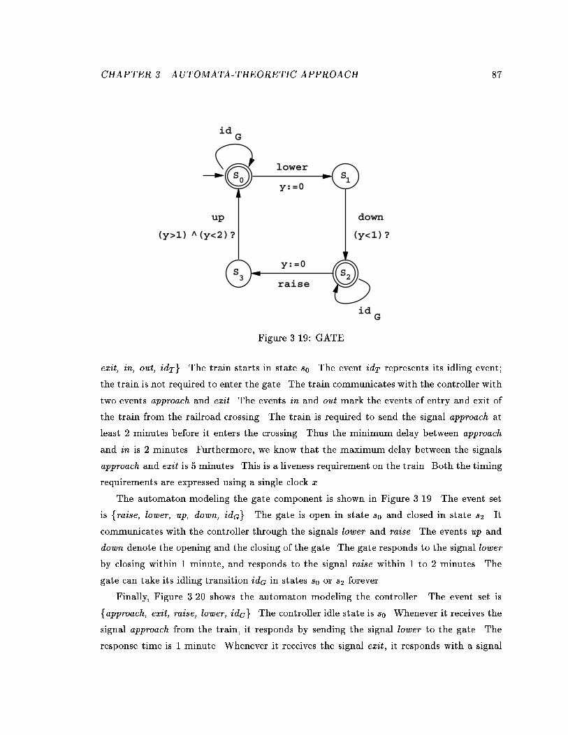
CHAPTER �� AUTOMATA�THEORETIC APPROACH ��
idG
idG
lower
raise
downup
(y<1)?(y>1) >(y<2)?
y:=0
y:=0
3S
0S 1S
2S
Figure ����� GATE
exit� in� out� idTg� The train starts in state s�� The event idT represents its idling event�
the train is not required to enter the gate� The train communicates with the controller with
two events approach and exit � The events in and out mark the events of entry and exit of
the train from the railroad crossing� The train is required to send the signal approach at
least � minutes before it enters the crossing� Thus the minimum delay between approach
and in is � minutes� Furthermore� we know that the maximum delay between the signals
approach and exit is � minutes� This is a liveness requirement on the train� Both the timing
requirements are expressed using a single clock x�
The automaton modeling the gate component is shown in Figure ����� The event set
is fraise� lower� up� down� idGg� The gate is open in state s� and closed in state s�� It
communicates with the controller through the signals lower and raise� The events up and
down denote the opening and the closing of the gate� The gate responds to the signal lower
by closing within � minute� and responds to the signal raise within � to � minutes� The
gate can take its idling transition idG in states s� or s� forever�
Finally� Figure ���� shows the automaton modeling the controller� The event set is
fapproach� exit� raise� lower� idCg� The controller idle state is s�� Whenever it receives the
signal approach from the train� it responds by sending the signal lower to the gate� The
response time is � minute� Whenever it receives the signal exit � it responds with a signal

CHAPTER �� AUTOMATA�THEORETIC APPROACH ��
idC
approach
lower
exit
raise
(z=1)?(z<1)?
z:=0
z:=0
0S 1S
2S3S
Figure ����� CONTROLLER
raise to the gate within � minute�
The entire system is then
� TRAIN k GATE k CONTROLLER ��
The event set is the union of the event sets of all the three components� In this example� all
the automata are particularly simple� they are deterministic� and do not have any fairness
constraints �every run is an accepting run�� The timed automaton AI specifying the entire
system is obtained by composing the above three automata�
The correctness requirements for the system are the following�
�� Safety� Whenever the train is inside the gate� the gate should be closed�
�� Real�time Liveness� The gate is never closed at a stretch for more than �� minutes�
The specication refers to only the events in� out� up� down� The safety property is
specied by the automaton of Figure ����� An edge label in stands for any event set
containing in� and an edge label �in� � out� means any event set not containing out � but
containing in� The automaton disallows in before down� and up before out � All the states
are accepting states�
The realtime liveness property is specied by the timed automaton of Figure ����� The
automaton requires that every down be followed by up within �� minutes�
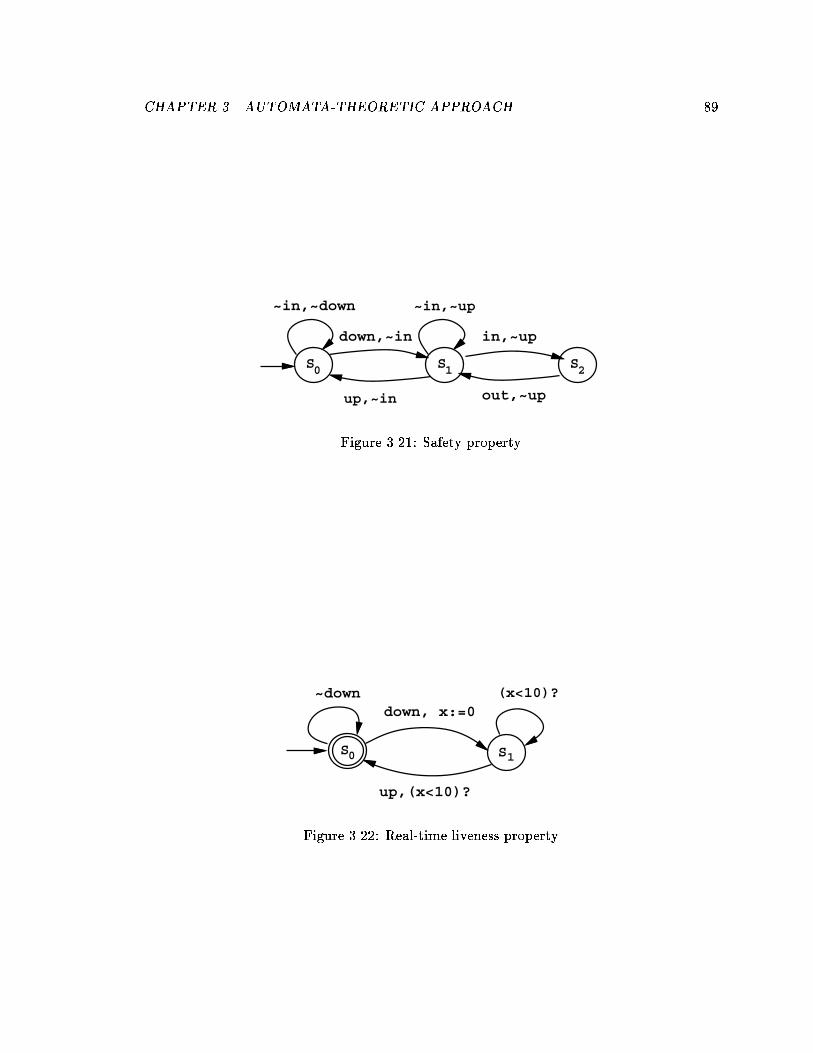
CHAPTER �� AUTOMATA�THEORETIC APPROACH ��
out,~up
in,~updown,~in
~in,~down
up,~in
~in,~up
0S 1S 2S
Figure ����� Safety property
~down
up,(x<10)?
(x<10)?
1S0S
down, x:=0
Figure ����� Realtime liveness property

CHAPTER �� AUTOMATA�THEORETIC APPROACH ��
Note that the automaton is deterministic� and hence can be complemented� Further
more� observe that the acceptance condition is not necessary� we can include state s� also
in the acceptance set� This is because the progress of time ensures that the selfloop on
state s� with the clock constraint �x ��� cannot be taken indenitely� and the automaton
will eventually visit state s��
The correctness of AI against the two specications can be checked separately as out
lined in Section ���� Observe that though the safety property is purely a qualitative property�
it does not hold if we discard the timing requirements�
���� Implementation
We have implemented the verication algorithm in LISP� We brie�y discuss some aspects
of the implementation�
The input to the program consists of a list of timed B�uchi automata A� through An�
The automaton A� is the specication automaton� and is required to be deterministic� The
implementation automaton is the product of the automata A�� � � �An� The output of the
program is �yes� or �no� depending on whether or not the language of the implementation
automaton is contained in that of the specication automaton�
Recall that the verication procedure involves three steps� ��� constructing the product
automaton A from the automata A�� � � �An� ��� constructing the region automaton R�A��
and ��� searching for a cycle meeting all the desired acceptance requirements� Step ��� can
be implemented by nding all the strongly connected components of R�A�� and testing each
component for the desired properties� Because of the constraints on the available memory
space� the above three steps cannot be carried out separately� In the implemented procedure�
neither the product automaton nor the region automaton is constructed explicitly� and all
the three steps are performed simultaneously�
Each vertex is represented by a list
�s�� � � �sn� �x�� x�� � � ��� ��y�� n��� �y�� n��� � � ��� ��z��� m
���� �z
��� m
���� � � ��� ��z
��� m
���� � � ��� � � ��
Each si gives the state of the automaton Ai� and the remaining components represent the
clock region� In the region corresponding to the above vertex the value of each clock yi
equals ni� The value of each clock xi is greater than its maximum value of interest� that
is� cxi� The value of each clock zij is between mi
j and mij � such that �i� the fractional
parts of zij and zik are the same� and �ii� the fractional part of z
ij is less than that of z
i��k �

CHAPTER �� AUTOMATA�THEORETIC APPROACH ��
Given such a representation� all its successors in the region automaton are obtained in a
straightforward way by examining the transitions starting at each of the states si�s�
The procedure performs a depth rst search starting from the initial vertex of the region
automaton� Whenever a new vertex is visited� it is assigned its own depth rst number
�DFN�� The search for strongly connected components uses Tarjan�s algorithm �Tar����
The global data structures include
�� a hashtable mapping vertex representations to their respective DFNs�
�� an array mapping DFNs to the representations of the corresponding vertices�
�� an array storing the DFN of the parent for each vertex�
�� an array which gives for every vertex the least vertex that can be reached using forward
edges and at most one back edge�
�� a stack storing the strongly connected component currently being explored� and
�� an array giving the number of already explored edges from each vertex�
Observe that we do not store the edges of the region automaton� Consequently� the program
needs to generate all the edges starting from a vertex� not only the rst time the vertex is
visited� but every time the depth rst search backtracks to it�
Whenever a strongly connected component is found� the procedure checks if it contains
an accepting state of each of the automataA�� � � �An and contains no accepting state of A�
and meets the progress requirement� If so� the programhalts saying that the implementation
does not meet the specication� Otherwise when the depth rst search terminates� the
program halts saying that the implementation meets the specication�
The example of railroad crossing of Section ����� was given as an input to our program�
The region automaton has about ���� vertices and about ����� edges� The program ter
minated giving the correct answer �yes� �the running time was approximately � minutes
on DEC station ������ Thus the program can handle small examples� The stateexplosion
problem prevents its application to bigger systems� In future� we intend to try out some
heuristics to improve its e�ciency�
Chapter �
Linear Temporal Logic
In this chapter we study realtime extensions of linear temporal logics as specication for
malisms for realtime systems� We introduce the specication language MITL� and study its
complexity and expressiveness� We dene interval automata� a variant of timed automata�
to model nitestate systems� and develop an algorithm for model checking�
��� Propositional temporal logic� PTL
In this section we will brie�y review the denition and the complexity results about PTL�
PTL is a modal logic interpreted over innite state sequences� The modal operator �
is interpreted as �henceforth�� and its dual � is interpreted as �eventually�� We consider
the logic with the next operator � and the until operator U �
We assume that we are given a set of atomic propositions AP� The formulas � of PTL
are built from the atomic propositions using logical connectives and temporal operators as
dened below�
� �" p j �� j �� � �� j � � j �� U ���
Intuitively� a formula�� holds at some state i � holds in the next state� �� U �� holds
at some state i �� holds at some later state and �� holds at all intermediate states� We
will use �� as an abbreviation for true U �� and �� for �����
The semantics of PTL is dened with respect to state sequences� A state sequence�
denoted by �� is an innite sequence ��� ��� � � � of states� where each state �i is a subset of
AP� Thus each state assigns truth values to all the atomic propositions� p is true in state
�i i p �i�
��

CHAPTER �� LINEAR TEMPORAL LOGIC ��
Now we formally dene the semantics of PTL� For a state sequence � " ��� ��� � � � let
�j denote its su�x �j � �j��� � � � The satisfaction relation � j" � �that is� � is a model of ��
is dened inductively below�
� j" p i p ��
� j" �� i � �j" �
� j" �� � �� i � j" �� and � j" ��
� j"�� i �� j" �
� j" �� U �� i �j j" �� for some j �� and �k j" �� for all � � k j�
The formula � is satis�able i some state sequence is a model of ��
The set of models of a formula � can be viewed as a property of state sequences specied
by �� let L��� denote the set of state sequences � such that � j" �� PTLformulas can specify
several interesting properties such as termination� fairness� mutual exclusion� guaranteed
response� precedence �OL��� Pnu��� MP���� A typical response property that �every pstate
is followed by some qstate�� is specied by the following PTLformula�
� � p � �q ��
There is a tableaubased decision procedure for testing satisability of PTLformulas
�BMP���� the problem is known to be PSPACEcomplete �SC����
In one approach to verication using PTL� nitestate systems are modeled as nite
Kripke structures� A Kripke structure is given asM " �S� S�� ��E�� where S is a nite set
of states� S� S is a set of initial states� � � S� �AP gives an assignment of truth values to
propositions in each state� and E is a binary relation over S giving the possible transitions�
The innite paths throughM give the set L�M� of state sequences generated byM� This
set consists of state sequences ���s��� ��s�� � � �� such that s� S�� and hsi� si��i E for
all i �� A system modeled as a Kripke structureM satises the PTLspecication � i
every state sequence generated by the system satises the formula �� that is� M j" � i
L�M� L��� ��
The modelchecking problem is to decide whether a Kripke structureM satises a PTL
formula �� The modelchecking algorithm rst constructs a tableauM�� which generates
precisely the models of ��� and then uses the product construction to check if the inter
section of L�M� and L�M��� is empty �LP��� VW���� The complexity of the algorithm
�Be warned that the notation M j� � is somewhat nonstandard in logic� M is not a single model for the
PTL�formula �� but represents a set of models for ��

CHAPTER �� LINEAR TEMPORAL LOGIC ��
is exponential in the size of the PTLspecication� and linear in the size of the Kripke
structure� The problem is PSPACEcomplete�
Notice the similarity between the verication of �untimed� processes using �automata
of Chapter � and using temporal logic� A process is modeled as a set of traces in Chapter ��
whereas now a process is modeled as a set of state sequences� The basic di erence is only
in the notion of what is observable� In trace semantics� only the events are observable�
and thus we focus only on the transition points without any reference to the state of the
system between the transition points� In semantics of state sequences� the emphasis is on
the state of the system� and the observable aspect of the state is modeled using a set of
propositions� Thus in one case a system is an �language over the alphabet P��A�� where
A is the set of events� and in the other case it is an �language over the alphabet �AP� The
two approaches are very similar� the only reason we are using both of them is that it is
conventional and technically convenient to develop automata theory using an eventbased
model� and temporal logics using a statebased model�
In Chapter � we used �automata to model nitestate systems� now we use Kripke
structures� Kripke structures are similar to transition tables� in transition tables edges
are labeled with alphabet symbols� whereas in Kripke structures states are labeled with
propositions� The language L�M�� for a Kripke structureM� is an �regular language� As
in case of transition tables� we can couple Kripke structures with acceptance conditions�
There is a close connection between B�uchi automata and PTL� For every PTLformula
�� the language L��� is an �regular language over the alphabet �AP� and hence� can be
recognized by a B�uchi automaton� On the other hand� PTL does not have the full expressive
power of �regular languages� it needs to be extended with rightlinear grammar operators
or automata connectives to attain the full expressive power of B�uchi automata �Wol����
Along the same lines� for modeling and verifying timed processes we will shift from the
semantics of timed traces to that of timed state sequences � Accordingly we will modify the
denition of timed automata so that they generate timed state sequences�
��� Metric interval temporal logic
To reason about quantitative time requirements we need to add time explicitly in the syntax
and semantics of PTL� To dene the syntax and semantics we use intervals of the real line�

CHAPTER �� LINEAR TEMPORAL LOGIC ��
����� Intervals
An interval is a convex subset of nonnegative real numbers R� Intervals may be open� half
open� or closed� bounded or unbounded� Each interval is of one of the following forms�
�a� b�� �a� b�� �a���� �a� b�� �a� b�� �a���� where a � b� a� b R� For an interval of the above
form� a is its left endpoint� and b is its right endpoint� The left endpoint of I is denoted
by l�I� and the right endpoint� for bounded I � is denoted by r�I��
An interval I is singular i it is of the form �a� a�� that is� I is closed and l�I� " r�I��
Two intervals I and I � are called adjacent i
�� the right endpoint of I is the same as the left endpoint of I �� and
�� either I is right open and I � is left closed� or I is right closed and I � is left open�
For instance� the intervals ��� �� and ��� ���� are adjacent�
We will freely use intuitive pseudoarithmetic expressions to denote intervals� For exam
ple� the expressions such as � b and a denote the intervals ��� b� and �a���� respectively�
and the expression I denotes the interval ft j �t� I� �t t��g� The expression I t� for
t R� denotes the interval ft� t j t� Ig� Similarly� I � t and t�I stand for the intervals
ft� � t j t� I and t� tg and ft�t� j t� Ig� respectively�
����� Timed state sequences
Let AP be a set of atomic propositions� We assume that� at any point in time� the global
state of a �nitestate� system can be modeled by an interpretation �or truthvalue assign
ment� for AP� We therefore identify states s with subsets of AP� that is� s j" p i p s
�for p AP��
We add time to state sequences by associating an interval with each state� this gives us
timed state sequences � If the interval associated with state s is I � then the state at each
time t I is s� We require that the intervals associated with the consecutive states in a
state sequence be adjacent�
De�nition ��� A state sequence � " ������ � � � is an innite sequence of states� each state
�i is a subset of AP�
An interval sequence I " I�I�I� � � � is an innite sequence of intervals that partitions R
such that

CHAPTER �� LINEAR TEMPORAL LOGIC ��
�i� �adjacency � the intervals Ii and Ii�� are adjacent for all i �� and
�ii� �progress � every time value t R belongs to some interval Ii�
A timed state sequence � " ��� I� is a pair consisting of a state sequence � and an
interval sequence I�
Sometimes we will denote a timed state sequence � " ��� I� by the innite sequence of
pairs of states and intervals�
���� I�� � ���� I�� � ���� I�� � � � �
A timed state sequence � " ��� I� can be viewed as a map �� from the time domain R
to the states �AP �let ���t� " �i if t Ii�� Thus a timed state sequence provides complete
information about the global state of a system at each time instant� Timed state sequences
obey the �nite�variability condition� between any two points in time there are only nitely
many state changes� This assumption is adequate for modeling discrete systems�
Given a timed state sequence ��� I�� the ith transition point� denoted by ti� is dened
to be the left endpoint of the interval Ii� that is� ti " l�Ii�� Note that the state at time ti
is �i�� if Ii is leftopen� and is �i if Ii is leftclosed�
Our denition allows transient states� which occur only at isolated points in time� If Ii
is a singular interval �ti� ti�� then the state at time ti is �i� but the state just before ti is
�i��� and the state just after ti is �i��� Observe that in such a case neither �i�� nor �i��
can be transient� because the interval Ii�� must be rightopen and the interval Ii�� must
be leftopen� The transient states are useful for modeling the truth of propositions that are
true only at the transition points�
We dene the sux of a timed state sequence at every t R below�
De�nition ��� For a timed state sequence � " ��� I�� and time t Ij � the su�x �t is
dened to be the timed state sequence
��j� Ij � t� � ��j��� Ij�� � t� � ��j��� Ij�� � t� � � � �
The su�x operator has been dened such that ��t���t�� " ���t t�� for all t� R� In
particular �� " ��
Another useful operation is the renement operation�

CHAPTER �� LINEAR TEMPORAL LOGIC ��
De�nition ��� A re�nement of a timed state sequence � " ��� I� is a timed state sequence
obtained by replacing each pair ��i� Ii� by a nite sequence
��i� I�i � � ��i� I
�i � � � � ���i� I
nii �
such that ���j�niIji " Ii� and I
ji and I
j��i are adjacent for � � j ni�
Observe that if �� is a renement of � then the associated maps �� and ��� are identical�
����� Syntax and semantics of MITL
We introduce an extension of linear temporal logic�metric interval temporal logic �orMITL��
that is interpreted over timed state sequences� A fairly standard way of introducing real
time in the syntax is to replace the unrestricted temporal operators of PTL by their time
bounded versions� Thus we introduce operators such as ������ meaning �eventually within
� to � time units� �EMSS��� AH��� Koy����
As before let AP be a set of atomic propositions� The formulas of MITL are built from
propositions by boolean connectives and timebounded versions of the until operator U � The
until operator may be subscripted with any nonsingular interval with integer endpoints�
De�nition ��� The formulas of MITL are inductively dened as follows�
� �" p j �� j �� � �� j �� UI ��
where p AP� and I is a nonsingular interval with integer endpoints�
Notice that we require the endpoints of intervals subscripting MITLoperators to be
integers� We will later show that all our results easily extend to the case when rational
endpoints are allowed� the restriction to integer endpoints is mainly to simplify the pre
sentation� The formulas of MITL are interpreted over timed state sequences� which provide
an interpretation for the atomic propositions at each time instant� Informally �� UI �� holds
at time t in a timed state sequence i there is a later time instant t� I t such that ��
holds at time t� and �� holds throughout �t� t��� The formal denition follows�
De�nition �� For an MITLformula �� and a timed state sequence � " ��� I�� the satis
faction relation � j" � is dened inductively as follows�

CHAPTER �� LINEAR TEMPORAL LOGIC ��
� j" p i p ���
� j" �� i � �j" ��
� j" ��� � ��� i � j" �� and � j" ���
� j" �� UI �� i for some t I � �t j" ��� and �t�j" �� for all t� ��� t��
For an MITLformula �� the set L��� consists of timed state sequences � such that � j" ��
An MITLformula � is called satis�able i L��� is nonempty�
Note that MITL has no next�time operator �� because with the dense time domain
there is no unique next time� Also observe that the until operator is strict in its rst
argument� for �� UI �� to hold in the current state �� need not hold now�
����� De�ned operators
Now let us introduce some standard abbreviations for additional temporal operators� The
dened operators �I� �constrained eventually� and �I� �constrained always� stand for
trueUI � and ��I��� respectively� It follows that the formula �I� �or �I�� holds at time
t R of a timed state sequence i � holds at all times �at some time� respectively� within
the interval t I �
We usually suppress the interval ����� as a subscript� Thus the MITLoperators ��
�� and U coincide with the conventional unconstrained strict eventually� strict always� and
strict until operators of temporal logic� This is because the until operator of MITL is
implicitly strict in its rst argument� The corresponding nonstrict operators are denable
in MITL� For instance�
�� � ��� � �� U ���
corresponds to the conventional unconstrained nonstrict until operator �� U ��� Note that�
on the other hand� the MITLoperator UI cannot be dened in terms of an until operator
that is not strict in its rst argument� this is why we have chosen the strict versions of
temporal operators to be primitive�
Example ��� In MITL� we can specify that a particular proposition always holds only
instantaneously� The following formula states that the proposition p is true in innitely
many transient states and nowhere else�
p � ����p � ��p�U p��

CHAPTER �� LINEAR TEMPORAL LOGIC ��
Such formulas can be used to distinguish events from state constraints� Such a property
cannot be expressed if the untiloperator is dened to be nonstrict in its left argument�
We also dene a constrained unless operator as the dual of the until operator�
�� IU�� stands for �������UI �������
It follows that the formula �� IU�� holds in a timed state sequence i either �� is true
throughout the interval I � or there is a time instant t � such that �� is true at time t and
�� holds at all instants t� � t within the interval I �
Let us consider a few examples of MITL properties now� Observe that all the qualitative
temporal properties speciable in PTL are already denable in MITL�
Example ��� A typical bounded response property that �every pstate is followed by some
qstate within time ��� is expressed by the MITLformula
�� p � ����� q ��
Example ��� We consider a time�out property now� Suppose p is some state constraint�
and q is the timeout event� The property we want to specify is that whenever p ceases to
hold� either within next � time units it becomes true again� or at time � the timeout event
q happens� This property is specied by the formula�
���� �p � �������p� � ��������q � �����q ���
More examples of specifying interesting systems using realtime temporal logics can be
found in �Koy��� and �Ost��b��
����� Re�ning the models
In this section� we present some results that will be useful in developing the decision pro
cedure for MITL�
Observe that the logic MITL is insensitive to stuttering � For a timed state sequence
� " ��� I�� and an MITLformula �� the satisfaction relation � j" � depends on the map ���
and not on the particular choice of the interval sequence I � This follows trivially from the
semantic denition� In particular� the next lemma holds�
CHAPTER �� LINEAR TEMPORAL LOGIC ���
Lemma �� If a timed state sequence �� is a renement of a timed state sequence � then
for every MITLformula �� � j" � i �� j" ��
Hence� if for a timed state sequence � " ��� I�� the state does not change after the jth
transition point� that is� �i " �j for all i j� then we represent � by the nite sequence
���� I�� � ���� I�� � � � � � ��j��� Ij��� � ��j ��i�jIi��
Also the satisfaction relation has another nice property� the truth value of a given
MITLformula does not change more than � times over �� Thus the models satisfy the
nitevariability property� not only with respect to the truth of atomic propositions� but
also with respect to more complex MITL properties�
De�nition ���� For an MITLformula �� a timed state sequence � " ��� I� is called ��ne
i for all i �� for all subformulas � of �� for all t� t� Ii� �t j" � i �t
�j" ��
Thus in a �ne timed state sequence ��� I� the truth of all the subformulas of � stays
invariant over every interval of I� The following lemma states that every timed state se
quence can be rened into a �ne timed state sequence� It follows that a formula � is
satisable i it has some �ne model�
Lemma ���� Let � be an MITLformula and � be a timed state sequence� There exists a
�ne timed state sequence �� which renes ��
Proof� The proof is by induction on the structure of the formula� For an atomic
proposition p� take �p to be the same as �� For a negated formula ��� take ��� to be the
same as ���
In case of the conjunction �� � ��� the sequence ��� �� is constructed by rening the
sequence ��� � Let I�� " J�J� � � �We split each interval Ji into a nite sequence J�i � � � �Jnii
so that each Jji is fully contained in some interval of I�� �
Now let us consider the case � " �� UI ��� First we construct the renement ��� ���
Let I�� �� " J�J� � � �We construct a renement I� " J ��J�� � � � of I�� �� such that whenever
t and t� are in the same interval J �i � then both t l�I� and t� l�I� belong to the same
interval Jk for some k i� and� if I is bounded� both t r�I� and t� r�I� belong to the
same interval Jl for some l k� It is clear that such a sequence can be constructed by a
nite splitting of each interval Ji� Furthermore� it is easy to check that �t j" � i �t
�j" �
whenever t and t� are in the same interval J �i �

CHAPTER �� LINEAR TEMPORAL LOGIC ���
���� Real versus rational time
While timed state sequences are dened by choosing the set of �nonnegative� reals to model
time� for interpreting formulas of MITL� the crucial property of the time domain R is not
its continuity� but only its denseness� Choosing some other dense linear order to dene
semantics leaves the complexity and expressiveness results unchanged� In particular� we
show that replacing the time domain R with the set of nonnegative rational numbers� Q�
when dening the semantics of MITL does not change the satisability �and validity� of
any MITLformula�
De�nition ���� A timed state sequence ��� I� is called rational i the endpoints of all
intervals in I are rational�
Let � be an MITLformula� and let � be a rational timed state sequence� � Qsatises
� i � j" �� where the satisfaction relation j" �Denition ���� is redened so that all time
quantiers range over Q only�
A formula � is called Qsatisable i � Qsatises � for some rational timed state se
quence ��
We show that this new notion of satisability is the same as the old one� In other
words� MITLformulas cannot distinguish the time domain R from the time domain Q�
This equivalence of real and rational models follows from the following two lemmas�
Lemma ���� Let � be an MITLformula and � a rational �ne timed state sequence�
Then � Qsatises � i � satises ��
Proof� We use induction on the structure of �� Let us consider only the interesting
case� that � has the form �� UI ���
Suppose � " ��� I� is rational� and �ne timed state sequence� Suppose � Qsatises
�� that is� �t Qsatises �� for some rational t I � and �t�Qsatises �� for all rationals
� t� t� By the induction hypothesis� we may conclude that �t j" �� and �t�j" �� for all
rationals � t� t� Hence� to show that � j" �� UI ��� it su�ces to show that �t�� j" �� for
all reals � t�� t� Consider an arbitrary real � t�� t� and assume that t�� Ii� If Ii
is singular then� since � is rational� t�� must be rational� Otherwise� Ii is nonsingular� and
there is also a rational t� Ii with � t� t� We know that �t�j" �� and� since � is �ne�
it follows that �t��j" ���

CHAPTER �� LINEAR TEMPORAL LOGIC ���
The second direction� that every rational �ne model of � Qsatises �� follows by a
similar argument�
Lemma ���� Let � " ��� I� and �� " ��� I�� be two timed state sequences such that for all
t R� if t " ti m for some left endpoint ti of an interval Ii in I and some m N� then
t Ij i t I �j � For all MITLformulas � j" � i �� j" ��
Proof� The proof is by induction on the structure of �� The only interesting case is
� " �� UI ��� Suppose � j" �� UI ��� Let t Ii be such that �t j" �� and �t��j" �� for all
� t�� t� We can nd t� I �i such that for all t�� R� if t�� " t m for some m N�
then t�� Ij i t�� I �j � The integer part of t
� should be the same as that of t� and for all i�
fract�t� � fract�ti� i fract�t�� � fract�t�i�� Now by applying the induction hypothesis to �t
and ��t�� we get that ��t
�j" ��� By a similar argument� we can show that for all � t�� t��
��t��j" ��� and hence� �
� j" �� UI ���
Lemma ���� classies timed state sequences into equivalence classes such that the mem
bers of a class cannot be distinguished by formulas of MITL� It implies� in particular� the
following theorem�
Theorem ��� A formula � of MITL is Qsatisable i it is satisable�
Proof� Suppose that � is Qsatisable in a rational model �� By Lemmas ��� and �����
there is a rational �ne renement of � that Qsatises �� By Lemma ����� this renement
is a �real� model of ��
The proof of the second direction uses Lemma ����� Consider a �real� model � " ��� I�
of �� We construct another timed state sequence �� " ��� I�� as follows� We adjust the
interval boundaries in I so that no interval is adjusted across integers� and the ordering of
the fractional parts of all interval boundaries is not altered� The denseness of Q allows us to
adjust all boundaries to be rational numbers� In particular� for all i �� the interval I �i is
leftopen i Ii is leftopen� and I�i is rightopen i Ii is rightopen� Let ft
�i ��� �� j i �g be
a sequence of rational numbers such that for every pair i� j� t�i � t�j i fract�ti� � fract�tj��
Set the left endpoint of I �i to be the integral part of ti plus t�i� The timed state sequences
� and �� satisfy the requirements of Lemma ����� and hence �� j" �� By Lemma ��� and
Lemma ���� the �renement of �� Qsatises ��

CHAPTER �� LINEAR TEMPORAL LOGIC ���
���� Allowing rational constants
While dening the syntax of MITL we required the boundaries of the intervals subscripting
the until operator to be integers� We can relax this condition� and allow intervals with
rational endpoints� For example� we can allow formulas such as ����������p� which says that
p holds over the interval ����� �����
All our results can be easily adopted to accommodate this extension� This is because of
the following obvious property of the models of MITL�
Lemma ���� Let � be a formula of MITL possibly with arbitrary rational constants� and
let � " ��� I� be a timed state sequence� For c Q� let �c denote the formula � obtained by
replacing every interval subscript I by c�I � similarly� let �c denote the timed state sequence
obtained from � by replacing every interval Ii in I by c�Ii� � j" � i �c j" �c�
The lemma can be proved by a straightforward induction on the structure of �� Conse
quently� there is an isomorphism between the models of � and the models of �c�
In particular� to test the satisability of � with rational constants� we test the formula
�c for satisability� where c is the least common multiple of all the constants appearing in
�� Note that �c has only integer constants� and the size of �c is bounded by j�j��
����� Avoiding undecidability
In MITL� we cannot write formulas such as
��p � ��� q��
since intervals such as ��� �� are not allowed as subscripts� We will show that there is� in
fact� no MITLformula that expresses this condition� and that the restriction of MITL to
nonsingular intervals is essential for decidability� Note that some forms of equality are
expressible in MITL� we dene ����U�t � as an abbreviation for
�����t���� � �����t���
Thus the stronger condition that �for every pstate the next following qstate is after exactly
� time units��
��p � ��q�U�� q��
is expressible in MITL�

CHAPTER �� LINEAR TEMPORAL LOGIC ���
We show that allowing singular intervals as subscripts for the temporal operators makes
MITL undecidable� The denseness of the underlying time domain allows us to encode
Turing machine computations� Notice that the undecidability result depends on the choice
of densetime semantics� the problem is decidable for the discrete models �AH���� The proof
of the next theorem is similar to the proof of Theorem �����
Theorem ���� If singular intervals are allowed as subscripts for temporal operators in the
syntax of MITL then the satisability problem is ���complete�
Proof� ����hardness�� Recall that the problem of deciding whether a nondeterministic
�counter machine has a recurring computation is ���hard �Lemma ������ We construct a
formula � such that � is satisable i the given machine has a recurring computation�
Let A be a �counter machine with counters C and D� and n program instructions� As
before� a conguration of the machine is represented by a triple hi� c� di� where i gives the
instruction to be executed next and c� d give the contents of the counters� A computation
of the machine is an innite sequence of triples starting at h�� �� �i�
We encode the computations of A in the logic using the propositions pC � pD� and
p�� � � �pn� First we require that all propositions are true only in singular intervals of a
timed state sequence� The following MITLformula species this constraint for the propo
sition pC �
����pC � ��pC�U pC��
Let us say that a timed state sequence � encodes a conguration hi� c� di over the interval
�a� b�� a b� i following hold�
�� The proposition pC holds at exactly c time instants in the interval �a� b� along ��
�� The proposition pD holds at exactly d time instants in the interval �a� b� along ��
�� Each proposition pj � j �" i� is false everywhere in the interval �a� b� along ��
�� The proposition pi is true over �a� a� and false during the interval �a� b� along ��
We construct a formula � such that � j" � i there exists a computation fhij � cj� dji � j �g
of A such that � encodes the jth conguration over the interval �j� j �� for all j ��
The nature of the initial conguration is expressed by the formula�
p� � �������p� � ��������pC � �pD ��
��i�n
�pi ��

CHAPTER �� LINEAR TEMPORAL LOGIC ���
To relate one conguration to the next� we establish a onetoone correspondence be
tween the states separated by distance �� The formula � has one conjunct for each program
instruction� For instance� if the second instruction is to increment D �and goto instruction
��� � has the following conjunct�
���
�����p� �
�BBB���� p � �������p � ����������i�n�i�� �pi� �
������ copy�pC� �
copy�pD�U����pD � ��� pD � copy�pD�U p�
�CCCA
�
We have used the abbreviation copy�p� for �p � ��� p�� The rst conjunct requires the
propositions representing the instruction counter change according to the desired scheme�
The second conjunct makes sure that the number of pC states is the same in the next
conguration as in the current one� The third conjunct holds at time t� i the number of
pDstates in the interval �t �� t �� is precisely one greater than the corresponding number
for the interval �t� t ���
The recurrence requirement is expressed by the conjunct �� p�� It follows that the
satisability question for the extended logic is ���hard�
����containment�� Let � be a formula of MITL possibly using singular interval subscripts
also� First observe that Theorem ���� holds even in presence of singular interval subscripts�
Hence if � has a model� then it has a model with rational interval endpoints� Now the
satisability of � can be phrased as a ���sentence� asserting that some timed state sequence
with rational transition times is a model of �� It is routine to encode a rational model by a
set of natural numbers� and to express the satisfaction relation in rstorder arithmetic�
Another possible extension of the syntax is to permit time bounds for both arguments
of the until operator� The intended semantics of ��� I �UI ��� is that it holds in a timed
state sequence � provided �� holds at some time instant t I and �� holds throughout
��� t� � I �� However such an extension leads to undecidability� A close inspection of the
proof of Theorem ���� shows that the only operator using the equality subscript is ����
The formula ���� can be replaced by false��U�� ��
��� Interval automata
In this section we dene interval automata as a model for nitestate realtime systems�
Just as Kripke structures are the nite models for PTLspecications� interval automata
CHAPTER �� LINEAR TEMPORAL LOGIC ���
will be the nite models for MITLspecications�
Interval automata are similar to timed transition tables� The main di erence is that
in a timed transition table� the transitions are labeled with events and clock constraints�
whereas in a timed states are labeled with atomic propositions and clock constraints� With
this modication interval automata now generate timed state sequences� instead of timed
traces�
A interval automaton operates with nite control � a nite set of states and a nite set
of realvalued clocks� All clocks proceed at the same rate and measure the amount of time
that has elapsed since they were started �or reset�� Each transition of the automaton may
reset some of the clocks� and each state of the automaton puts certain constraints on the
values of the atomic propositions as well as on the values of the clocks� the control of the
automaton can reside in a particular state only if the values of the propositions and clocks
satisfy the corresponding constraints�
Recall that for a set X of clocks� %�X� denotes the set of allowed clock constraints�
Each clock constraint is a Boolean combination of atomic conditions which compare clock
values with constants�
De�nition ���� A interval automaton is a tupleM " hS� S�� ��C�(�Ei� where
� S is a nite set of states�
� S� S is a set of initial states�
� � � S� �AP is a labeling function assigning to each state the set of atomic propositions
true in that state�
� C is a nite set of clocks�
� ( � S � %�C� is a labeling function assigning to each state the clock constraint that
should hold in that state�
� E S�S��C is a set of edges� An edge hs� s�� �i� also denoted as s��� s�� represents
a transition from state s to state s�� and � gives the set of clocks to be reset with this
transition�

CHAPTER �� LINEAR TEMPORAL LOGIC ���
The runs of an interval automaton dene timed state sequences� At any time instant
during a run� the conguration of the system is completely determined by the state in which
the control resides and the values of all clocks� The values of all clocks are given by a clock
interpretation �� which is a map from C to R� for any clock x C� the value of x under the
interpretation � is ��x� R�
Assume that� at time t R� the interval automaton is in state s and the clock values are
given by the clock interpretation �� Suppose the state of the automaton remains unchanged
during the time interval I with l�I� " t� All clocks proceed at the same rate as time elapses�
at any time t� I the value of any clock x is ��x� t� � t� so the clock interpretation is
� t� � t� During all this time the value of the clock interpretation satises the clock
constraint that is associated with s� that is� �� t� � t� j" (�s�� Now suppose that the
automaton changes its state at time r�I� " t�� via the transition s��� s�� This state change
happens in one of the possible two ways� If I is rightclosed� then the state at time t�� is
still s� otherwise the state at time t�� is s�� The clocks in � get reset to � at time t��� Let
� �� be the clock interpretation �� �� ���� t�� � t�� which gives the valuation for the clocks
at the beginning of the next interval� The clock interpretation at the transition time t���
however� depends on whether the state at time t�� is s or s�� If I is rightclosed� then the
clock interpretation at time t�� is �� t��� t� and should satisfy (�s�� If I is rightopen then
the clock values at the transition point are given by ���� and should satisfy (�s��� The state
s� stays unchanged over some interval adjacent to I � and the same cycle repeats�
Let '�M� denote �C �� R�� the set of clock interpretations for the clocks of M� The
behavior of the system is formally dened below�
De�nition ��� A run r of an interval automaton M " hS� S�� ��C�(�Ei is an innite
sequence
r � ����
�s�� I���������s�� I��
�������s�� I��
������
� � �
of states si S� intervals Ii� clock sets �i C� and clock interpretations �i '�M�
satisfying the following constraints�
� Initiality� s� S��
� Consecution�
� the sequence I " I�I�I� � � � forms an interval sequence�
� for all i � either hsi� si��� �ii E or si�� " si with �i " ��

CHAPTER �� LINEAR TEMPORAL LOGIC ���
� �i�� " ��i�� �� ����i r�Ii�� l�Ii�� for all i ��
� Timing� for all t Ii� the clock interpretation �i t� l�Ii�� denoted by �r�t�� satises
(�si��
Note that� according to this denition� the clocks may start at any real values that
satisfy the clock constraints of an initial state� Requiring the initial values of all the clocks
to be � would complicate the presentation of the modelchecking algorithm for MITL �to be
presented in Section ����� A run r gives a map �r from R to '�M� giving the clock values
at every instant of time�
Note that the above denition assumes that there are implicit selfloops on every state
of the automaton� that is� introducing an edge s��� s does not change the set of runs of
the interval automaton�
We can associate timed state sequences with the runs� and use them to interpret MITL
formulas�
De�nition ���� The timed state sequence �r associated with a run r is
�r � ���s��� I�� � ���s��� I�� � ���s��� I�� � ���s�� I� � � � �
L�M� denotes the set of all timed state sequences �r that correspond to the runs of the
interval automaton M�
An interval automaton M satises an MITLspecication � i L�M� L����
We say that M generates �or accepts� the timed state sequences in L�M�� The set
L�M� gives the set of all possible behaviors of the realtime system modeled by M�
Observe that the above denition allows transient or instantaneous states along a run�
This corresponds to conditions �such as propositions denoting occurrence of events� that
hold only during statetransitions� Such states can be forced along a run by associating
clock constraints involving equality with the state� Also there is no commitment to dening
the state at the point of transition� we only require that the clock interpretation consistent
with this choice should satisfy the corresponding clock constraint�
Let us consider some examples�

CHAPTER �� LINEAR TEMPORAL LOGIC ���
p
S0
S1
S2
S3
p
pp
x=0 x=3
x<3
x<3
x:=0
x:=0
Figure ���� Interval automatonM�
Example ���� The interval automatonM� of Figure ��� has four states s� to s� a single
clock x� and a single proposition p�
The automaton starts in state s� with the clock x set to � and the proposition p true�
During the time interval ��� �� the automaton loops between states s� and s�� and thus� the
proposition p may have any value� At time � the automaton moves to state s to check that
p holds� The clock is reset at this point� and the whole cycle repeats� ThusM� requires p
to hold at all time values that are integer multiples of �� A prex of a possible run of the
automaton is shown below� Since there is a single clock� the clock interpretation is given
by a real value�
����s�� ��� ���
�����s�� ��� �����
������
�s�� ����� �������s� ��� ���
fxg����s�� ��� ��� � � �
The set of timed state sequences generated byM� is
L�M�� " f� j �n N� p �����n�g�
Example ���� Consider the interval automaton M�� shown in Figure ��� with seven
states� s� to s�� and uses two clocks� x and y�
The automaton starts in the initial state s� with the clock y initialized to �� At time
�� the automaton moves to state s�� and simply loops there� The proposition p denotes an
external event which is true only at instantaneous points t �� in time �and no more than

CHAPTER �� LINEAR TEMPORAL LOGIC ���
y>40-
x:=0
p ,q
2<x<5y<40
-
p ,qy<40
x=0
p, q
y=0
p q,y<40x<2
p q,
y<40
p q,
S0 S1 S2 S3 S4 S5
y<40p q,
x=5
S6
Figure ���� Interval automatonM�
once every � time units�� namely� whenever M� is in state s�� The automaton responds
to p by resetting the clock x� and then it requires that the proposition q holds over the
interval t ��� ��� Thus the automatonM� models a system which responds� until time ���
to the event p by setting q to true for the interval ��� �� following p� A possible timed state
sequence generated byM� is
��� ��� ����� �fpg� ���� ����� ��� ���� ����� �fqg� ���� ����� ��� ���� ����� �fqg� ��������
The interval automaton satises the MITLformula
�������� p � ������q � � ���� q�
Checking emptiness
The emptiness problem for interval automata is to decide whether L�M� is empty for a
given automaton M� This problem can be solved using the same techniques that we used to
solve the emptiness problem for timed automata in Section ���� Also the modelchecking
algorithm for TCTL �to be dened in Chapter �� can be used to check for the emptiness of
an interval automaton� It follows that the problem can be solved in PSPACE� specically�
in time O��jSj jEj� � �j�j�� where j(j denotes the length of clock constraints�

CHAPTER �� LINEAR TEMPORAL LOGIC ���
The proof of PSPACEhardness of the emptiness problem for timed automata �see The
orem ����� is easily modied to show PSPACEhardness for interval automata also� The
next theorem follows�
Theorem ���� Given an interval automaton M� the problem of deciding whether L�M�
is empty� is PSPACEcomplete�
Composing interval automata
To describe any realtime system it is useful to describe individual components separately
and then combine the di erent descriptions� We discussed this operation� called parallel
composition� in context of timed automata� Interval automata describing behaviors of
di erent components can be put together in a similar way� The next theorem gives the
construction for composing interval automata�
Theorem ���� Given interval automata Mi " hSi� S�i� �i�Ci� �i�Eii� � � i � �� there
exists an interval automatonM such that L�M� " L�M�� � L�M���
Proof� We assume that the clock sets Ci are disjoint� The states of M are of the
form hs�� s�i� where s� is a state ofM� and s� is a state ofM� such that both s� and s�
agree on the assignment of truth values to propositions� that is� ���s�� " ���s��� The clock
constraint for hs�� s�i is the conjunction of the clock constraints for s� and s�� For any pair
of transitions s����� s�� and s�
���� s�� inM� andM�� respectively� the product automaton
has three transitions� hs�� s�i������� hs��� s
��i� hs�� s�i
���� hs��� s�i� and hs�� s�i���� hs�� s
��i�
Thus the transitions ofM simulate the joint behavior of the two component automata�
Introducing fairness
In verifying concurrent systems� we are generally interested only in correctness along the fair
computation paths �LPS���� For example� in a system with two processes� we may wish to
consider only those computation sequences in which each process executes innitely often�
For a Kripke structureM " �S� S�� ��E�� a standard way to introduce fairness requirements
uses a fairness family F �S� A path �s�� s�� � � �� is fair with respect to F i for each F F �
si F for innitely many i �� Note that the fairness constraints for Kripke structures
are similar to the acceptance conditions for �automata� In the automata framework� the
fairness requirement of the above form has been called generalized B�uchi condition� We
introduce fairness in interval automata in a similar way�

CHAPTER �� LINEAR TEMPORAL LOGIC ���
De�nition ��� An interval automaton with fairness is an automaton hS� S�� ��C�(�Ei
with a fairness family F �S�
A run r of the form
r � ����
�s�� I��������
�s�� I��������
�s�� I��������
� � �
is called F fair i for every F F � for innitely many i �� si F�
For an interval automatonM with a fairness family F � the set L�M� of timed state
sequences generated by M consists of all timed state sequences �r corresponding to the
Ffair runs r of M�
The algorithm to check emptiness of L�M� can be generalized to handle fairness con
straints in a straightforward way� Similarly� the product construction for interval automata
is easily extended to handle fairness constraints�
��� Deciding MITL
We solve the satisability problem for MITL by reducing it to the emptiness problem for
interval automata� Our main result is that� given an MITLformula �� we can construct an
interval automatonM� such that the runs ofM� that meet certain fairness requirements
correspond precisely to the timed state sequences that satisfy ��
����� Restricting the problem
To simplify the exposition of the decision procedure� we restrict the satisability question
for MITL to formulas and models of a specic form and show that this can be done without
loss of generality�
De�nition ���� An MITLformula � is said to be in normal form i it is built from
atomic propositions and negated atomic propositions using conjunctions� disjunctions� and
temporal subformulas � of the following six types�
�� �� UI �� with bounded I and l�I� ��
�� �� IU�� with bounded I and l�I� ��
�� �I �� with I " ��� n� or I " ��� n��

CHAPTER �� LINEAR TEMPORAL LOGIC ���
�� �I �� with I " ��� n� or I " ��� n��
�� �� U ���
�� ����
Next we give a series of transformations that allow us to rewrite any formula � into
an equivalent formula �� in normal form� Thus we restrict ourselves to test the satisa
bility of MITLformulas each of whose temporal subformulas are� according to the above
classication� of one of six types� type�� to type���
First� we require that no interval in � contains �� This can be achieved by applying the
following equivalence�
�� UI �� � ��� � ��UI������ ���
provided that � I �
Secondly� we require that the only unbounded intervals in � are of the form ������ This
can be achieved by applying the following two equivalences�
�� U�n��� �� � ����n ��� � �� U ���
�� U�n��� �� � ����n��� � ����n ��� � ��� � �� U ����
provided that n ��
Thirdly� we require that only the eventually and the always operators are constrained
with bounded intervals I such that l�I� " �� This can be achieved by applying the following
equivalence�
��UI �� � �I �� � �� U ��
provided that l�I� " ��
Finally� we push all negations in � to the inside and use the following equivalence to
eliminate each subformula of the form �� U���
�� U�� � � �� � ��U ��� � ����
It is easy to check that the resulting formula is in normal form�
It may appear that these rewritings blow up the size of the formula �� but observe that
the number of distinct subformulas of �� is only linear in the length of �� This is because

CHAPTER �� LINEAR TEMPORAL LOGIC ���
at each step of rewriting� only a constant number of new subformulas are created� In fact�
if the formula is represented as a directed acyclic graph� thus avoiding the duplication of
shared subformulas� then the size of the formula blows up only by a constant factor� The
next lemma follows�
Lemma ���� For every MITLformula � there exists an equivalent formula �� in normal
form such that
� the largest �integer� constant appearing as an interval endpoint in �� is the same as
the largest constant appearing in �� and
� if j�j is the number of atomic propositions� Boolean connectives� and temporal oper
ators in �� then the number of distinct syntactic subformulas of �� is O�j�j��
Proof� For each step of rewriting� we can show that if a formula � is rewritten to
�� then the number of syntactic subformulas in �� is bounded by a constant multiple of
the number of subformulas in � by induction on the automaton of �� Also note that the
rewriting steps do not introduce any new constants�
Henceforth we assume that the MITLformulas under consideration are in normal form�
Let K N be such that K � � is the largest constant appearing as an interval endpoint in
the formula � to be checked�
To check the satisability of an MITLformula �� by Lemmas ��� and ���� we can conne
ourselves to the question if � has a �ne model� Therefore we consider� throughout this
section� only �ne timed state sequences � " ��� I�� It follows that� if � is a subformula of
�� we may write �i j" � for ��t j" � for all t Ii�� In addition� we assume that all intervals
in I are either singular or open� This is su�cient� because any model of � can be brought
into this form by splitting all nonsingular closed intervals� for instance� the interval �a� b�
can be split into the two intervals �a� a� and �a� b��
Let us introduce a new atomic proposition psing such that �i j" psing i the ith interval
Ii of � " ��� I� is singular� Hence the proposition psing holds exactly in every other interval�
For a timed state sequence � that satises these conditions� Then�
� � j" �� UI �� i for some i with Ii � I �" �� ��� both �i j" �� and �i j" �� � psing �
and ��� �j j" �� for all � j i� and ��� �� j" �� � psing �

CHAPTER �� LINEAR TEMPORAL LOGIC ���
� � j" �� IU�� i �� j" �� if I��I �" �� and either ��� �� j" ����psing � or ��� �i j" ��
for some i � and �j j" �� for all � j � i with Ij � I �" �� or ��� �j j" �� for all
j � with Ij � I �" ��
The di erent types of temporal subformulas of � are handled di erently by our algo
rithm� The simplest case is that of type� and type� formulas� they are treated essentially
in the same way in which tableau decision procedures for linear temporal logic handle un
constrained temporal operators� The most interesting case is that of type� and type�
formulas� We concentrate rst on this case� The case of type� and type� formulas will be
considered later�
����� Intuition for the algorithm
Consider the MITLformula
������ �p � ����� q��
Let us assume� for simplicity� that both p and q are true only in singular intervals and let
us try to build an interval automaton that accepts precisely the models of this formula�
Whenever the automaton visits a pstate� it needs to make sure that within � to � time
units a qstate is visited� This can be done by setting a clock x to � when the pstate is
visited� and demanding that some qstate with the clock constraint � � x � � is visited
later� This strategy requires a clock per visit to a pstate within the interval ��� ��� However�
the number of such visits is potentially unbounded and� hence� any automaton with a xed
number of clocks cannot reset a new clock for every visit� That is why this simple strategy
cannot be made to work�
An alternative approach is to guess the times for future qstates in advance� The au
tomaton nondeterministically guesses two time values t� and t� within the interval ��� ���
this is done by resetting a clock x at time t� and another clock y at time t�� The guess is
that the last qstate within the interval ��� �� is at time t� �� and that the �rst qstate
within the interval ��� �� is at time t� �� If the guesses are correct� then the formula����� q
holds during the intervals ��� t�� and �t�� ��� and does not hold during the interval �t�� t���
Consequently� the automaton requires that every pstate within the interval ��� �� lies either
within ��� t�� or within �t�� ��� It also needs to make sure that the guesses are right� that is�
whenever either x " � or y " �� the automaton must be in a qstate� This strategy requires
only two clocks for the interval ��� �� of length �� irrespective of the number of pstates

CHAPTER �� LINEAR TEMPORAL LOGIC ���
within ��� ���
We say that the guessed times t� � and t� � witness the formula ����� q throughout
the intervals ��� t�� and �t�� ��� respectively� In general� the witnesses need not be singular
intervals� they can be open intervals� To see this� let us relax the assumption that q
holds only in the singular intervals� Let � t� t�� � be such that q is true during
I� " �t� �� t�� �� and false during �t
�� �� ��� and let � t� t�� � be such that q is false
during ��� t� �� and true over I� " �t� �� t�� ��� Thus I� is the last qinterval within ��� ���
and I� is the rst qinterval within ��� ��� The formula ����� q holds during the intervals
��� t��� and �t�� ��� and does not hold during the interval �t��� t��� To check the formula� the
automaton nondeterministically guesses four time values t�� t��� t�� and t
��� It requires that
no pstate lies within �t��� t��� and also it needs to ensure that the guesses are right� In
this case we say that the intervals I� and I� witness the formula ����� q throughout the
intervals ��� t��� and �t�� ��� respectively� Notice that we could not have chosen a particular
time instant from I� as a witness for ��� t���� if I� were rightclosed we could have chosen its
right endpoint as the witness�
In the following we develop an algorithm based on this idea of guessing� in advance�
time intervals that witness temporal formulas and� later� checking the correctness of these
guesses� The crucial fact that makes this strategy work� with a nite number of clocks� is
that the same interval may serve as a witness for many points in time� We warn the reader
that the details of this algorithm are quite tedious compared to the other parts of the thesis�
����� Witnessing intervals
De�nition ���� The interval I � is a witnessing interval for the MITLformula �� UI ��
under �t� for a timed state sequence � and t R� i I �� �t I� �" � and �t j" �� UJ�t �� for
every nonempty interval J I ��
The interval I � is a witnessing interval for the MITLformula �� IU�� under �t i t I
I � and �t j" �� I ��tU���
Observe that if I � witnesses �� UI �� under �t� then �� holds throughout �t� r�I ���� and
�� holds throughout the interval I�� Witnessing intervals are dened such that the following
property holds�
Lemma ��� Let � be an MITLformula of the form ��UI �� or �� IU��� let � be a timed
state sequence and t R� There is a witnessing interval for � under �t i �t j" ��

CHAPTER �� LINEAR TEMPORAL LOGIC ���
Proof� If �t j" � for the formula � " �� UI ��� then �t�j" �� for some t
� t I and
the singular interval �t�� t�� witnesses � under �t� If �t j" � for the formula � " �� IU���
then the interval t I witnesses � under �t�
The other direction of the lemma follows from the semantic clauses for the until and
unless operators�
Now we show that the same interval may serve as a witnessing interval for a temporal
formula under �innitely� many su�xes of a timed state sequence�
Example ���� Consider the timed state sequence � over two propositions p and q�
�fpg� ��� ����� � �fp� qg� ����� ����� � �fpg� ���������
Thus along � the proposition p is always true� but the proposition q is true only during the
interval Iq " ����� ����� The interval Iq witnesses the formula pU����� q under �t for every
t ��� ����� On the other hand� the interval ����� �� witnesses the formula ������ ��q� under
�t for every t ����� ���
Lemma ���� Let � be the type� formula �� UI ��� For every timed state sequence ��
there are two bounded� open or closed� intervals I � and I �� such that� for every t ��� ���
the formula � is satised by �t i either I � or I �� witnesses � under �t� Furthermore�
r�Ii� � r�I� � for i " �� ��
Proof� Let � " ��� I� be a �ne timed state sequence with only singular and open
intervals� including the singular interval �r�I� �� r�I� �� �split intervals if necessary�� We
choose two witnessing intervals I � and I �� as follows�
� Let )� be the maximal i � such that Ii�I �" �� both �i j" �� and �i j" ���psing � and
�k j" �� for all � � k i with Ik � I �" �� If no such i exists� let I � " �� otherwise� let
I � " I���
� Let ) be the minimal j � such that Ij��I �� �" �� both �j j" �� and �j j" ���psing �
and �k j" �� for all � � k j with Ik � �I � I �� �" �� If no such j exists� let I �� " ��
otherwise� let I �� " I� �
Consider � � t �� Assume �t satises �� Clearly �t�j" �� for all t� I � If I � exists
and I � � �t I� �" � then I � witnesses � under �t� Otherwise� let t� �t I� be such that

CHAPTER �� LINEAR TEMPORAL LOGIC ���
�t�j" �� and �
t�� j" �� for all t�� �t� t��� In this case I �� exists� if t� Ik then ) � k� Hence
I� � �t I� �" �� and I �� witnesses � under �t�
In the case of type� formulas� a single witness per unit interval su�ces to reduce the
problem to type ��
Lemma ���� Let � be the type� formula �� IU��� For every timed state sequence ��
there is a bounded interval I � such that� for every t ��� ��� the formula � is satised
by �t i either �t satises the type� formula ���������I��� or I� witnesses � under �t�
Furthermore� r�I �� � r�I� ��
Proof� Let � " ��� I� be a �ne timed state sequence with only singular and open
intervals� including the singular interval In " �r�I� �� r�I� ��� We choose witnessing
interval I � as follows�
� Let )� be the minimal i � such that Ii � I �" � and either
�� �k j" �� for all k i with Ik � I �" �� or
�� there is some i � j � n such that �j j" �� � �� and �k j" �� for all i � k j�
� Given )�� let ) be the maximal )� � j � n such that either �k j" �� for all )� � k � j� or
�k j" �� � �� for some )� � k � j� Note that if )� exists� then so does ) � in particular� if
)� exists because of clause �� then ) " n�
If no appropriate )� exists� let I � " �� otherwise� let I � be the union of all Ik for )� � k � ) �
Assume that � � t �� then �t satises � i either ��� �i j" �� for all i with Ii��t I� �"
�� or ��� �i j" �� � �� for some i with Ii � �t I� �" � and �j j" �� for all j i with
Ij � �t I� �" �� or ��� �t�j" �� for some t t� t I � In either of the rst two cases� I �
witnesses � under �t� the third case is equivalent to �t satisfying the formula���������I����
If I � witnesses � under �t� then �t j" � by Lemma �����
����� Type�� and type�� formulas
Now we can be more precise about how we will construct the interval automatonM� that
accepts exactly the models of �� To check the truth of type� and type� subformulas of ��
the automaton guesses corresponding witnessing intervals� The boundaries of a witnessing
interval are marked by clocks� a clock interval is a bounded interval that is dened by

CHAPTER �� LINEAR TEMPORAL LOGIC ���
its type �e�g�� leftclosed and rightopen� and a pair of clocks� Given a time t and a clock
interpretation �� the clock interval C " �x� y�� for two clocks x and y� stands for the closed
witnessing interval �t K � ��x�� t K � ��y��� the clock interval C " �x� y� stands for the
corresponding halfopen interval� etc� �recall that K � � is the largest constant appearing
in the formula�� We write K � C for the interval fK � ��x�� K � ��y�g� for any type of
clock interval C " fx� yg�
For simplicity� let us consider a type� subformula � of the form �I ��� The automaton
resets� nondeterministically� any of its clocks at any time� When guessing a witnessing
interval I �� it writes the prediction that �the clock interval C " fx� yg witnesses the formula
�� into its memory� If the clock x was reset at time t�� and y was reset at time t� t��
then the witnessing interval guessed is I � " ft� K� t� Kg� To check the the truth of
the temporal formula � at time t t�� the automaton needs to verify that its guess I� is
indeed a witness� The condition I � � �t I� �" � translates to verifying the clock constraint
�K � C� � I �" �� It remains to be checked that �� is satised throughout the witnessing
interval I �� that is� the automaton needs to verify that �� holds at all states with the clock
constraint � �K � C��
The Lemmas ���� and ���� are the key to constructing an automaton that needs only
�nitely many clocks� For the type� formula �� UI ��� at most � witnessing intervals need
to be guessed per interval of unit length� Furthermore� the fact that the right endpoint of
a witnessing interval is bounded allows the automaton to reuse every clock after a period of
length r�I� �� Thus we need� at any point in time� at most �r�I� � active clock intervals�
that is� clock intervals that stand for a guess of a witnessing interval and� therefore� have
to be veried later� Similarly� to check a type� formula �� IU��� we need� at any point in
time� no more than r�I� � active clock intervals� Consequently� �K clocks su�ce to check
any type� subformula of �� and �K clocks su�ce for any type� subformula of ��
����� Type�� and type�� formulas
Now let us move to formulas of the form �I �� and �I �
� with I " ��� n� or I " ��� n��
Checking the truth of such a formula is much easier and can be done using a single clock�
Consider the type� formula � " �I ��� Whenever the automaton needs to check that
� holds� say at time t� it starts a clock x and writes the corresponding proof obligation
into its memory � to verify that �� holds at some later state with the clock constraint
x I � The obligation is discharged as soon as an appropriate ��state is found� If the

CHAPTER �� LINEAR TEMPORAL LOGIC ���
automaton encounters another �state in the meantime� at time t� t before the obligation
is discharged� it does not need to check the truth of � separately for this state� This is
because if there is a ��state after time t� within the interval t I � then both �t j" �I ��
and �t�j" �I �
�� Once the proof obligation is discharged� the clock x can be used again�
Thus one clock su�ces to check the formula � as often as necessary�
The described strategy works for checking the truth of � at singular intervals� There
is� however� a subtle problem with this method when the truth of � during open intervals
needs to be checked� as is illustrated by the following example� Consider the timed state
sequence
�fg� ��� ��� � �fg� ��� ��� � �fpg� �������
it satises the formula ������ p at all times t ��� ��� To check the truth of ������ p during
the open interval ��� ��� the automaton starts a clock x upon entry� at time �� However�
the proof obligation that p holds at some later state with the clock constraint x ��� ��
can never be veried� On the other hand� if the automaton were to check� instead� the
truth of the formula ����� p during the interval ��� ��� then our strategy works and the
corresponding proof obligation can be veried� because there is a pstate while x ��� ��
holds� Furthermore� observe that the validity of ����� p throughout the open interval ��� ��
implies that ������ p is also true throughout ��� ���
In general� the following lemma holds�
Lemma ���� Let � and )� be the type� MITLformulas �I �� and �I�fr�I�g�
�� respec
tively� For every timed state sequence � " ��� I� and open interval Ii in I � �i j" � i
�i j" )��
Proof� First note that� for all t �� if � is satised by �t� then )� is also satised by
�t� This is because I I � fr�I�g�
Now consider an open interval Ii and assume that �i j" )�� If I is rightclosed� then
� " )�� So suppose that I is rightopen� and let t Ii� Since Ii is open� there exists some
t� Ii with t� t� Since �t
�j" )�� there exists some j i such that Ij��t
� �I�fr�I�g�� �" �
and �j j" ��� It follows that Ij � �t I� �" � and� hence� that �t j" ��
Consequently� to check the truth of a type� formula � during an open interval� it su�ces
to check the truth of the weaker formula )�� Accordingly� the automaton we construct writes
only the proof obligation that corresponds to checking )� into its memory�

CHAPTER �� LINEAR TEMPORAL LOGIC ���
For checking a type� formula of the form � " �I ��� the situation is symmetric� The
automaton uses also a single clock x to check this formula� Whenever the formula � needs
to be veried� say at time t� the automaton starts the clock x with the proof obligation
that as long as the clock constraint x I holds� so does ��� The obligation is discharged as
soon as x I � If the automaton encounters another �state within the interval t I � say
at time t�� it simply resets the clock x� and thus overwrites the previous proof obligation�
This strategy is justied by the observation that if �� holds throughout the interval �t� t��
and �t�j" �I ��� then also �t j" �I ��� Once the proof obligation is discharged� the clock x
can be reused to check � again whenever necessary�
As in the case of type� formulas� we need to be more careful when checking � during
open intervals� For the type� formula � " �I ��� let )� be the formula �I�fr�I�g��� From
Lemma ���� and duality� it follows that for every timed state sequence � " ��� I�� if Ii is
open� then �i j" � i �i j" )�� Hence to check the truth of � during an open interval�
it su�ces again to check the truth of the weaker formula )�� Accordingly� only a proof
obligation for )� is set up� This is because the corresponding clock x is started at time r�Ii��
and for � to hold during the open interval Ii� �� need not hold at time r�Ii� r�I�� even if
I is rightclosed�
���� Constructing the interval automaton
Now let us dene the interval automatonM� formally� For each temporal subformula of �
of type�� the automatonM� has �K pairs of clocks� These clocks always appear in pairs�
to form clock intervals� From any pair of clocks x and y� four di erent clock intervals can be
formed� �x� y�� �x� y�� �x� y�� and �x� y�� From Lemma ���� for checking type� formulas we
need only open or closed witnessing intervals� Thus associated with each type� subformula
� of � we have �K clock intervals� they are denoted by C������ � �C�K���� For each type�
subformula of � the automatonusesK clock pairs giving �K clock intervals� For subformulas
� of types � and �� the automaton needs one clock x per formula�
In addition to these clocks� we use the clock xsing to enforce that the runs ofM� have
alternate singular and open intervals�
Closure set
For the given MITLformula �� we dene its closure set Closure��� to consist of the following
items�

CHAPTER �� LINEAR TEMPORAL LOGIC ���
�� All subformulas of �� for each type� subformula �� IU�� of �� the type� formula
���������I���� for each type� subformula � " �I �� of �� the type� formula )� "
�I�fr�I�g��� and for each type� subformula � " �I �
� of �� the type� formula
)� " �I�fr�I�g���
�� For each type� or type� formula � in the closure set� the clock intervals C����
through C�K���� and for each type� and type� formula � in the closure set� the
clock x�
�� For each clock interval C " Cj��� in the closure set� where � is �� UI �� or �� IU���
all clock constraints of the form � �K�C�� � � �K�C�� � " �K�C�� �K�C� " ��
I �K � C�� and �K � C�� I �" �� and for each clock x in the closure set� where �
is �I �� or �I �
�� the clock constraints x I and x I �
We write � � �K � C� short for f�g � �K � C�� It should be clear that all of these
conditions are indeed clock constraints� For instance� the condition � � �K � �x� y��
stands for the clock constraint x � K � y K� the condition � " �K� �x� y�� is never
satised�
�� The clock constraint xsing " ��
Note that the number of subformulas of � is O�j�j� and the number of clocks is O�K�
for each subformula of �� Hence the size of the closure set Closure��� is O�j�j�K��
The states of the desired automaton M� will be subsets of Closure���� We need to
consider only those subsets of Closure��� that satisfy certain local consistency constraints�
Whenever the automaton is in state s� the formulas in s indicate which subformulas of �
are true� Accordingly� a state s Closure��� is initial i both � and xsing " � are in s� and
for each state s the propositional constraints ��s� are dened such that p ��s� i p s
for all atomic propositions p AP�
The clock constraints (�s� are the conjunction of all clock constraints in s� The clock
intervals in s indicate which clock intervals are currently active and represent witnessing
intervals for type� and type� formulas� the clocks in s indicate which clocks are currently
active and represent proof obligations for type� and type� formulas�
The transitions of M� are all triples s��� s� that satisfy certain global consistency
criteria� Both the local and the global consistency conditions are dened in the following

CHAPTER �� LINEAR TEMPORAL LOGIC ���
catalog� For every state s Closure��� and every transition s��� s� with source state s�
Logical consistency
� For each atomic proposition p AP� precisely one of p and �p is in s�
� If the formula �� � �� is in s� then both �� and �� are in s�
� If the formula �� � �� is in s� then either �� or �� is in s�
These conditions ensure that no state contains subformulas of � that are mutually incon
sistent�
Timing consistency
� s contains at most one of the clock constraints � �K�C�� � � �K�C�� � " �K�C��
and �K � C� " � for each clock interval C� Furthermore� no two clock intervals in s
share clocks� for instance� s does not contain both the clock intervals �x� y� and �x� y��
� s contains at most one of the clock constraints x I and x I for each type� or
type� formula ��
� If s contains xsing " �� then xsing � �� If s does not contain xsing " �� then xsing �
and s� contains xsing " ��
These conditions guarantee that no state contains clock constraints that are mutually in
consistent� We say that a state s is singular i it contains xsing " �� otherwise s is open�
The last clause of the above conditions ensures that singular and open states alternate along
any run�
Type�� formulas
Consider a type� formula � " �� UI �� in the closure set�
Firstly� if � is in s� then there is some clock interval C " Cj��� such that
� �K � C�� I �" � is in s� and
� either C is in s� or s is singular and C is in s� and the clocks associated with C are
not in ��

CHAPTER �� LINEAR TEMPORAL LOGIC ���
The rst condition checks that the interval K�C is an appropriate candidate for witnessing
the formula �� The second condition activates the clock interval C to represent a witnessing
interval for �� Note that if s is singular� the corresponding clock interval is activated only
in the following open interval� This is because� to check that the interval �K�C� is indeed
a witness� no conditions are required of the current singular state�
Secondly� if some clock interval C " Cj��� is in s� then
� if either � " �K � C� or � � �K � C� is in s� then �� is in s� and
� if either � �K � C� or � � �K � C� is in s� then �� is in s� and
� the clocks associated with C are not in � and either C or �K � C� " � is in s��
The rst two conditions verify that the active clock interval C represents indeed a witness
for the formula �� The nal condition keeps the clock interval C active as long as necessary�
To prove the correctness of the construction of M�� we show that along every run r
of M�� if the state at time t contains the formula � then �tr satises �� The proof is by
induction on the automaton of �� Let us consider the case when � is a type� formula�
Suppose that the above conditions are satised along a run r and the formula � is in a state
s at time t� Consider the clock interval C " Cj��� satisfying the consistency requirements�
We show that the interval I � " �t K � C� is a witnessing interval for � under �tr� The
constraint �K � C� � I �" � is satised� and hence I � � �t I� �" � holds� If s is an
open state then s contains C or if s is singular then its successor contains C� Note that
until the condition �K � C� " � becomes true marking the end of I �� all the intermediate
states contain C� and the clocks associated with C do not get reset� and hence continue
to denote the same witness I �� In all states s� at time instants t t� I � the constraint
� �K � C� holds� by consistency conditions s� contains ��� and hence by induction
hypothesis� �t�
r j" ��� Similarly all states s� at time instants t� I � contain the constraint
� � �K � C� or � " �K � C�� and hence� the formula ��� Furthermore� if t� �" r�I ��
then � � �K � C� holds� and the state contains the formula �� also� Hence� by induction
hypothesis� for all t� I �� �t�
r j" ��� and if t� �" r�I �� then �t
�
r j" ��� Thus I� satises all
criteria to be a witness for � at time t� By Lemma ����� it follows that �tr j" ��
Conversely� if �t j" �� then there is a run r that satises all conditions� This is because�
by Lemma ����� the automaton can� at time t� either share an already activated clock
interval Cj��� or has enough clocks to activate an unused clock interval Cj���� If C is the
CHAPTER �� LINEAR TEMPORAL LOGIC ���
activated clock interval and K � C stands for the guessed witness� then it follows� from
denitions� that all the consistency criteria are met� The rst state in which �K � C� " �
holds� the automaton discards the clock interval C from the state�
Type�� formulas
Consider a type� formula � " �� IU�� in the closure set�
Firstly� if � is in s� then either
� ���������I��� is in s � or
� there is some clock interval C " Cj��� such that
� I �K � C� is in s� and
� either C is in s� or s is singular and C is in s� and the clocks associated with C
are not in ��
If ���������I��� holds then so does �� The second clause corresponds to guessing a witness�
The rst condition checks that the interval K�C is an appropriate candidate for witnessing
the formula �� The second condition activates this clock interval C�
Secondly� if some clock interval C " Cj��� is in s� then
� if either � " �K � C� or � � �K � C� is in s� then �� is in s� and
� either �� is in s� or the clocks associated with C are not � and either C or �K�C� " �
is in s��
These conditions ensure that the active clock interval C represents indeed a witness for the
formula � and that it is kept active as long as necessary�
Soundness and completeness of these conditions follow by the Lemmas ���� and �����
Type�� formulas
Consider a type� formula � " �I �� in the closure set�
Firstly� if � is in s� then either
� s is singular and x s�� or
� s is open and I is rightopen and )� is in s� or

CHAPTER �� LINEAR TEMPORAL LOGIC ���
� s is open and I is rightclosed and x is in s�
These conditions activate a clock to represent a proof obligation� Lemma ���� justies the
decision to start a clock corresponding to the weaker formula )� when s is open�
Secondly� if x is in s� then
� x I is in s� and
� either �� is in s� or x is in s� and x � ��
These conditions verify the proof obligation that is represented by the clock x and keep it
active as long as necessary�
Type�� formulas
Consider a type� formula � " �I �� in the closure set�
Firstly� if � is in s� then either
� s is singular and x s� and x �� or
� s is open and I is rightclosed and )� is in s� or
� s is open and I is rightopen and x s and x s� and x ��
These conditions activate a clock to represent a proof obligation� and reset it� as was justied
in the previous subsection� Recall that if s is open then instead of checking � the automaton
checks )��
Secondly� if x is in s then
� �� is in s� and
� either x or x I is in s��
The rst condition veries the proof obligation that is represented by the clock x� and the
second condition keeps it active as long as necessary�
Type� formulas
Consider a subformula � " �� U �� of type �� Whenever � is in s� then either
� s is singular and � s�� or

CHAPTER �� LINEAR TEMPORAL LOGIC ���
� s is open and �� is in s� and either �� is in s or �� is in s� or both �� and � are in s
��
These conditions ensure that unconstrained until formulas are propagated correctly �re
member that singular and open intervals alternate�� However� these conditions admit the
possibility that a run consists of states containing � and �� without ever visiting a ��state�
Additional fairness constraints are needed to ensure that whenever a run r contains a state
s with the type� formula � then some later state s� along the run contains ��� For each
type� formula � " �� U �� in the closure set� we dene�
F " fs Closure��� j �� s or � � sg�
It is straightforward to show that for the runs r that are fair with respect to F� if a state
s at time t contains the formula � then �tr j" ��
Type�� formulas
Consider a subformula � " ��� of type �� Whenever � is in s� then either
� s is singular and � s�� or
� s is open and �� s and both �� and � are in s��
These conditions guarantee that unconstrained always formulas are propagated forever�
This concludes the denition of the interval automatonM�� The runs ofM� are dened
as before� The fairness requirements on the timed state sequences are given by the family
F� consisting of the sets F for every type� formula � in the closure set�
The following main lemma states the correctness of our construction by relating the
accepting runs ofM� to the models of ��
Lemma ���� The set L��� of the models of an MITLformula � equals the set L�M�� of
timed state sequences generated byM��
Proof� It can be shown� by induction on the automaton of �� that given a F�fair run
r ofM�� if a formula � in Closure��� is in a state s in r at time t R� then �tr j" �� We
have outlined the crucial arguments for the six interesting cases of temporal subformulas
above�
Conversely� given a �ne model � of � with alternating singular and open intervals� we
can construct a F�fair run r ofM� such that � " �r� The Lemmas ���� and ���� instruct
us how to use the available limited number of clocks to mark witnessing intervals�

CHAPTER �� LINEAR TEMPORAL LOGIC ���
This result yields algorithms for checking the satisability and validity of the given
MITLformula �� To check satisability� we rst construct the interval automatonM�� and
then we use the algorithm that checks whether L�M�� is nonempty to test if � has a model�
Similarly� � is valid i L�M��� is empty�
���� Complexity of MITL
We conclude this section by showing that our decision procedure for MITL is in EXPSPACE�
and that this is optimal� because the decision problem for MITL is EXPSPACEcomplete�
First we show the lower bound of EXPSPACEhardness by encoding computations
of exponentialspace bounded Turing machines� The proof is similar to the proof of the
EXPSPACEhardness of the realtime logic MTL �AH����
Lemma ��� The satisability problem for MITL is EXPSPACEhard�
Proof� Consider a �deterministic� �nspacebounded Turing machineM � for each input
X of length n� we construct an MITLformula �X of length O�n � log n� that is satisable
i M accepts X � The EXPSPACE lower bound follows by a standard complexitytheoretic
argument�
Thus it su�ces to show� given X � how to construct a su�ciently succinct formula �X
that describes the �unique� computation ofM on X � as an innite sequence of propositions�
and requires it to be accepting�
First we require that propositions change their values only at the integer time points�
This requirement is imposed by introducing a special proposition clock � and adding the
conjunct
�clock " clock � ���� clock � ��������clock� � ����� clock ��
In every timed state sequence satisfying �clock the proposition clock is true during the
interval �j� j� and false during the interval �j� j �� for all j N�
For every proposition p to be used in the formula� we add the requirement
��� � �p � pU clock� � ���p� � ��p�U clock� ��
This conjunct ensures that p can change its value only at the integer time values� With
these restrictions we assume that every state stays unchanged for precisely one time unit�
We use a proposition pi and a proposition qj for every tape symbol i and state j of M �
respectively� In particular� p� and q� correspond to the special tape symbol �blank� and

CHAPTER �� LINEAR TEMPORAL LOGIC ���
the initial state of M � Let
)pi " pi ��i� ��i
�pi� ���qj �
ri�j " pi � qj ��i� ��i
�pi� ��j� ��j
�qj� �
s "��pi� �
��qj �
We represent congurations ofM by )pstate sequences of length �n� which are separated
by sstates� the position of the readwrite head is marked by an rstate� The computation
of M on X is completely determined by the following two conditions�
�i� it starts with the initial conguration� and
�ii� every conguration follows from the previous one by a move of M �
The computation is accepting i � furthermore�
�iii� it contains the accepting state F �
These conditions can be expressed in MITL� The initialization constraints are expressed by
the formula
�init " � s � ������ rX��� ��
��i�n
��i�i��� )pXi� ��n����n��� )p� ��
The rst conjunct says that the rst state is an sstate� the second conjunct says that the
head is at the beginning of the tape readingX�� the next conjunct sets up the input symbols
in positions � through n� and the last conjunct says that the rest of the tape is blank�
The consecution requirement is expressed by the formula
�move "
�BBB�
��clock � s � ���n����n��� s ��
VP�Q�R�
�� clock � P � ������Q � �����R �
���n����n�� fM �P�Q�R�
�A
�CCCA
The rst conjunct requires sstates separated by length �n �� and the second conjunct
relates the successive congurations� Note that the kth state in the new conguration
can be determined from the the �k � ��th� kth� and �k ��th states of the previous
conguration� P � Q� and R represent three consecutive tape symbols� and each range over
the propositions )pi� ri�j� and s� fM �P�Q�R� refers to the transition function of M � For

CHAPTER �� LINEAR TEMPORAL LOGIC ���
instance� ifM writes� in state j on input i�� the symbol k onto the tape� moves to the right�
and enters state j�� then fM �)pi� ri��j � )pi��� " )pk and fM �ri��j � )pi��� )pi���� " ri���j�
The acceptance requirement corresponds to eventually visiting the state F � it is given
by the formula �accept " � qF �
We take �X to consist of these three additional conjuncts �init � �move � and �accept � The
lengths of �init � �move � and �accept are O�n � log n�� O�n�� and O���� respectively �recall that
constants are represented in binary�� thus implying the desired O�n � log n�bound for �X �
Now we show that the time complexity of our algorithm is doubly exponential in the
length of the constants in �� and singly exponential in the number of logical and temporal
operators in �� Furthermore� the algorithm also implies an upper bound of EXPSPACE for
deciding MITL�
Theorem ���� The decision problem for testing satisability of MITLformulas is com
plete for EXPSPACE� In particular� the proposed algorithmchecks satisability of an MITL
formula � in time O��j�j�K�logK�� where K � � is the largest constant appearing in ��
Proof� Given a formula � the rst step of the algorithm rewrites it to a normal form
��� By Lemma ����� the number of subformulas of �� is O�j�j�� Let K � � be the largest
constant appearing in �� then the size of the closure set Closure���� is O�j�j�K�� Hence the
number of states inM� is O��j�j�K�� The number of clocks inM� is O�j�j�K�� Furthermore�
for every clock x the largest constant that x is compared with in a clock constraint ofM� is
bounded by K� Recall that the complexity of the emptiness test for an interval automaton
is exponential in its number of clocks� and is proportional to the size of its statetransition
graph and product of the timing constants for all the clocks �see Section ����� Consequently�
the algorithm testing emptiness ofM� runs in time O�Kj�j�K��
We have already proved EXPSPACEhardness� For containment in EXPSPACE note
that the description of M� can be given in space polynomial in j�j �K� that is� in space
exponential in the length of �� assuming binary encoding of all interval endpoints� The
emptiness problem for an interval automatonM is PSPACE complete �see Theorem ������
It follows that the validity of � can be decided in space polynomial in j�j �K� that is� in
EXPSPACE�

CHAPTER �� LINEAR TEMPORAL LOGIC ���
�� Veri�cation using MITL
Model checking is a powerful and wellestablished technique for automatic verication of
nitestate systems� it compares a temporallogic specication of a system against a state
transition description of the system�
In the qualitative case� the system is modeled by its statetransition graph� also known
as Kripke structure� and the specication may be presented as a formula of the propositional
linear temporal logic PTL �LP���� Using our results about MITL� we can present a real
time verication procedure that checks MITLspecications against descriptions given as
interval automata�
We model a realtime system by an interval automatonM and give the specication as
a formula � of MITL� Hence the model checking problem is to decide whether or not all
the timed state sequences generated by the structureM satisfy the specication ��
L�M�� L���
Notice the similarity between this approach to verication and the one in Chapter�� Apart
from changing the specication language from automata to logic� we have shifted from the
eventbased semantics of timed traces to the statebased semantics of timed state sequences�
Our construction for testing the satisability of MITLformulas can be used to develop an
algorithm for model checking� The rst step is to construct an interval automatonM�� such
that its runs precisely capture the models of the negated formula ��� L�M��� " L�����
The model checking question can then be reformulated as follows�
L�M� L��� i L�M�� L�M��� " ��
The next step in the model checking algorithm is to construct an interval automatonM�
that is the product ofM and M�� �see Section ����� a timed state sequence is generated
byM� i it is generated by bothM andM���
Hence we have reduced the model checking problem to the emptiness question for interval
automata� M j" � i L�M�� is empty� The size ofM� is polynomial in the sizes ofM and
M��� Consequently� the description ofM� is exponential in the length of �� and polynomial
in the length of the description of M� Since the emptiness for interval automata can be
solved in PSPACE� it follows that the model checking problem can be solved in EXPSPACE�
As for all linear temporal logics� the model checking question for MITL is no simpler
than the satisability question� it is also EXPSPACEhard� The following theorem follows�

CHAPTER �� LINEAR TEMPORAL LOGIC ���
Theorem ���� The problem of checking whether an interval automaton M satises an
MITLformula � is EXPSPACEcomplete�
Proof� We have already outlined how to solve the modelchecking problem in EX
PSPACE�
To prove EXPSPACEhardness we reduce the satisability question for MITL to model
checking question� An MITLformula � is unsatisable i the universal interval automaton�
which generates all possible timed state sequences� satises ��� Thus EXPSPACEhardness
of satisability implies EXPSPACEhardness of model checking�
The time complexity of the model checking algorithm is polynomial in the qualitative
part of the system description� exponential in the qualitative part of the MITLspecication�
exponential in the timing part of the system description� and doubly exponential in the
timing part of the specication� Compared to this the model checking algorithm for PTL
�LP��� is polynomial in the size of the Kripke structure and exponential in the size of the
specication�
Thus moving to real�time gives an additional exponential blowup� This blowup seems�
however� unavoidable for formalisms for quantitative reasoning about time� It occurs even
in the discretetime case �EMSS��� AH��� AH����
�� Expressiveness
Every formula � of MITL species a realtime property � the set of models of �� The
expressive power of a formalism is measured by the realtime properties that can be specied
in it� First we compare the expressive power of MITL to that of MTL� a realtime logic
based on the ctitiousclock model� Then we compare the expressive power of MITL to
that of interval automata�
���� Comparison with �ctitious�clock logics
We compare the expressive power of MITL to the use of a ctitious clock and MTL� which
admits singular intervals as time bounds on temporal operators� More precisely� we show
that the densetime model without equality �MITL� is more expressive than any ctitious
clock model with equality �MTL��

CHAPTER �� LINEAR TEMPORAL LOGIC ���
The logic MTL
First let us dene the syntax and semantics of the logic MTL� metric temporal logic� The
syntax of MTL is the same as that of MITL� however� it also admits singular intervals as
subscripts�
As before let AP be a set of atomic propositions� The formulas of MTL are built from
propositions by Boolean connectives and timebounded versions of the until operator U �
De�nition ���� The formulas of MTL are inductively dened as follows�
� �" p j �� j �� � �� j �� UI ��
where p AP� and I is an interval with integer endpoints�
The semantics of MITL uses the ctitiousclock model of Section ������ Thus time is
viewed as a discrete counter� which is updated with every tick of the global clock� The
formulas of MTL are interpreted over observation sequences�
De�nition ��� An observation sequence is a pair � " ��� T�� where � " ���� � � � is an
innite sequence of states �i �AP� and T " T�T� � � � is an innite sequence of corresponding
time stamps Ti N satisfying
� the initiality condition that T� " ��
� the weak monotonicity condition that Ti � Ti�� for all i �� and
� the progress condition that� for all n N� there is some i � such that Ti n�
We will denote the observation sequence � " ��� T� by an innite sequence
���� T�� � ���� T�� � ���� T�� � ��� T� � � � �
of observations� Each observation consists of a state �i �AP and a time stamp Ti N�
For an observation sequence � and i N� the observation sequence �i is the su�x of � that
begins with the observation �si� Ti��
For an observation sequence � and an MTLformula �� the satisfaction relation � j" �
is dened as usual by induction on the structure of ��

CHAPTER �� LINEAR TEMPORAL LOGIC ���
De�nition ���� For an MTLformula �� and an observation sequence � " ��� T�� the
satisfaction relation � j" � is dened inductively as follows�
� j" p i p ���
� j" �� i � �j" ��
� j" �� � �� i � j" �� and � j" ���
� j" �� UI �� i �i j" �� for some i � with Ti I � and �j j" �� for all � j i�
An MTLformula is called satisable i � j" � for some observation sequence ��
Note that the until operator is strict in its left argument� Also MTL has no next�state
operator� this restriction makes MTLformulas insensitive to stuttering�
The tableaubased decision procedure for PTL can be extended to get a decision proce
dure for checking satisability of MTLformulas� In particular� given an MTLformula � we
can construct a Kripke structureM� with fairness constraints that characterizes the satis
fying models of �� Details of the decision procedure� and comparison of the expressiveness
of MTL with other ctitiousclock logics can be found in �AH���� Here we only state the
result on complexity of MTL�
Theorem ���� The decision problem to test satisability of a given MTLformula � is
EXPSPACEcomplete� Specically� there is an algorithm that checks satisability of a
given MTLformula � in time exponential in O�j�j�K�� where K � � is the largest constant
appearing in ��
De�ning real�time properties using MTL
We need to formalize which realtime properties can be specied in MTL� To this end�
let us consider how to extract an observation sequence from a timed state sequence � that
describes the actual behavior of a realtime system� Observations are made with respect to
a digital clock� the observation at time t records the state ���t� and the reading of the clock
at time t �recall that �� is a map from R to states induced by ��� Clearly the observations
depend on how fast the clock ticks� and at what time the clock is started� This motivates
the next denition�
De�nition ���� A digital clock D " ��� �� is a pair consisting of the distance � R
between two successive clock ticks and the time � R of the rst clock tick� that is�
� � � �� At time t R the clock D shows the integer value tD " d�t� ����e�

CHAPTER �� LINEAR TEMPORAL LOGIC ���
The clock D is called rational i both � and � are rational numbers�
The clock D starts at time � with the reading �D " �� The reading of the clock during
the interval ��� �� is �� and during the interval �� n�� � �n ���� its reading is �n ��
for all n N�
Now we can dene the observed behavior of a timed state sequence � with respect to a
given clockD� The observation of � at time t consists of the state ���t� and the clock reading
tD� As time increases� the Dobservation stays the same until either the clock tick changes
the value of tD� or the state changes along �� Consequently� all possible Dobservations
along � can be described by an �sequence�
De�nition ���� For a clock D� and a timed state sequence � " ��� I�� the Dobservation
of � at time t is Ot " ����t�� tD��
The Dobserved behavior of � is the observation sequence
�D � Ot� � Ot� � Ot� � � � � �
for time values ti R such that for all i �� ��� ti ti��� and ��� for all t �ti� ti���� Ot
equals either Oti or Oti�� �
Note that above properties dene �D uniquely modulo stuttering �i�e�� duplication of
neighboring observations�� Furthermore� the state component of �D is the state component
of � �modulo stuttering��
Example ���� Consider the timed state sequence � �
�s�� ��� ���� �s�� ��� ���� �s�� ��� ������ �s� ���������
Then the digital clock ��� ���� observes the observation sequence ���������
�s�� �� � �s�� �� � �s�� �� � �s�� �� � �s� �� � �s� �� � �s� �� � � � �
Using the above notion of observations we can associate realtime properties with every
MTLformula for every choice of the digital clock�
De�nition ��� For a given digital clock D� a formula � of MTL species a realtime
property LD��� � the set of timed state sequences � such that �D j" ��

CHAPTER �� LINEAR TEMPORAL LOGIC ���
Comparing MITL with MTL
Now we can be specic about the sense in which the densetime model is� even without
equality� more expressive than the ctitiousclock model� for any choice of digital clock�
Theorem ���� �a� For every MTLformula � and every rational clock D� the realtime
property LD��� equals L��� for some MITLformula � �using intervals with rational end
points�� �b� There is an MITLformula � such that the realtime property L��� does not
equal LD��� for all MTLformulas � and all choices of digital clock D�
Proof� �a� Given a rational clock D " ��� �� and a formula � of MTL� we construct
an MITLformula that species the realtime property LD���� We assume that � contains
only intervals of the form ��� ��� ��� ��� �m�n� for � � m � n� and �m��� for m �� It is
trivial to convert any MTLformula into this form� for instance� the MTLformula ��� � is
equivalent to the formula ���� ����� ��������
We model the ticks of the digital clock D by a new proposition r that holds only in
transient states at time instants �� n���
�D � �� �r � �� r � ��� �r � ��r�U�� r��
Let �� be the MITLformula that results from � by replacing every occurrence of a subfor
mula �� UI �� with
�r � ��� � �r�U�� ��
if I is ��� ��� with
�r � ��� � �r�U�� ��� � �� U����� �r � �� � �� U�������
if I is ��� ��� with
�� U��l�I������r�I��� �r � �� � �� U���� ���
if I is bounded and l�I� �� and with
�� U��l�I����� �r � �� � �� U ���
if I is unbounded and l�I� �� It is not hard to show that �D j" � i � j" ��D � ��� for
every timed state sequence ��
For example� consider the MTLformula
��� �p � ��� q��

CHAPTER �� LINEAR TEMPORAL LOGIC ���
and the digital clock D " ��� ��� This formula species the property that �for every pstate
there is a qstate separated from p by exactly ve integer times�� and is equivalent to the
MITLformula
������ � ��� �p � ������ �r � ����� q���
�b� From the tableau decision procedure for MTL �AH���� it follows that if a formula
� of MTL is satisable� then it has a model �D such that any two state changes in � are
separated by at least some minimum time gap �which depends on D and the size of ��� In
fact� for any digital clock D one can always construct timed state sequences in LD��� that
become periodic after some point in time� We show that this is not the case for MITL�
Let us construct a satisable MITLformula � for which every model � " ��� I� contains
arbitrarily close state changes� that is� for every real � �� there is some i � such that
�i�� �" �i and �i �" �i�� and ti���ti �� The set of models of � can clearly not be specied
in MTL� for any choice of digital clock D�
The formula � uses three propositions p� q� and r� First� it requires at most one of these
three propositions to be true at any state� In addition� it has the following three conjuncts�
The rst condition�
r � ��� �r � ��r�U�� r��
places transient rstates at precisely the even integers� The second condition�
��� ��p � q� � ��� r��
ensures that p and q can only hold in the second half of the intervals of length � separating
consecutive rstates� The third condition�
��� p � ��� �p � ��� q� � ��� �q � ����� p��
implies that there is a pstate� and later a qstate� between every pair of consecutive rstates�
and thus between every odd integer and the subsequent even integer�
Moreover� from any model of � we can extract an innite sequence of alternating p and
q states� with the qstate following a pstate guaranteed by the condition p � ��� q� and
the pstate following a qstate by the condition q � ����� p� The times that are associated
with the states in this sequence� taken modulo �� form a strictly increasing innite sequence
of reals contained in the interval ��� ��� Since this time sequence is bounded above� there
must be arbitrarily close pairs of a pstate followed by a qstate� It follows that � has no
eventually periodic models�

CHAPTER �� LINEAR TEMPORAL LOGIC ���
On the other hand� the MITLformula � is satisable� a model for � can be readily con
structed by introducing� in addition to the transient rstates at all even integers� transient
pstates at time �n� ���n� and transient qstates at time �n� ���n� for each integer n ��
Thus even though MITL disallows singular interval subscripts� it is more expressive than
the ctitiousclock logics allowing the use of equality irrespective of the rate of the clock�
Recall that MITL with equality is undecidable �Theorem ������ We have shown two ways
of achieving decidability� MITL puts a syntactic restriction disallowing subscripts such as
��� ��� on the other hand� MTL weakens the expressiveness through a semantic abstraction
that� at every state change only a discrete approximation to the realtime may be recorded�
���� Comparison with interval automata
An interval automaton M generates the set of timed state sequences L�M�� Thus it pro
vides an alternative to MITL for specifying realtime properties� Now we compare the two
formalisms with respect to expressiveness�
The decision procedure for MITL constructs� for a given formula �� an interval automa
ton M� with fairness conditions such that L��� " L�M��� Thus interval automata with
fairness conditions are at least as expressive as MITL� A close inspection of the construc
tion shows that fairness conditions are needed to handle unconstrained eventualities only�
In particular� for an MITLformula �� if its equivalent normal form �� does not contain any
type� subformulas �� U ��� then there exists an interval automatonM� generating L����
Thus no fairness conditions are needed to handle until operators subscripted with bounded
intervals�
However� the formalism of interval automata has strictly greater expressive power com
pared to MITL� We consider some examples to illustrate this point�
Example ���� Assume AP " fp� qg� Consider the following property of timed state se
quences�
L " f� j �t R� �p ���t� � q ���t ���g�
The property L asserts there is a pstate at some time instant t followed by a qstate at
time t �� This property can easily be expressed as an interval automaton with fairness
conditions� It cannot be specied using MITL� Note that it can be expressed in the extension

CHAPTER �� LINEAR TEMPORAL LOGIC ���
of MITL that allows singular intervals as subscripts�
��� � p � ��� q ��
Example ���� shows that the interval automata can express some forms of equality
constraints not expressible by MITL� In addition� there are certain �qualitative� properties
that can be expressed using Kripke structures� but not by linear temporal logics� This also
makes MITL less expressive than interval automata�
Example ���� Assume AP " fp� qg� Furthermore� assume that both propositions are true
only during singular intervals� Such a requirement is expressible using both formalisms� Now
a timed state state sequence � is specied by a state sequence � " ���� � � � and an innite
sequence I " t�t� � � � of time values� Consider the property that �the proposition p holds
in every state �i with even i�� This is a property of state sequences� and does not restrict
the possible choices for I� It is known that PTL cannot specify this property �Wol���� It
follows that MITL cannot specify this property either� even if we allow the use of singular
intervals� It is straightforward to specify the property using interval automata� No fairness
constraints are required�
The next theorem follows�
Theorem ��� �a� For every MITLformula � there exists an interval automatonM with
fairness constraints such thatM generates L���� �b� For every MITLformula � such that
its normal form �� has no unconstrained until operators� there exists an interval automaton
M that generates L���� �c� There exists an interval automatonM such that L�M� is not
speciable by any MITLformula� even if we allow singular intervals and intervals with
rational endpoints�
Note that the realtime properties denable by MITL are closed under complement�
since the logic has the negation operator� On the other hand� interval automata are not
closed under complement� For instance� the complement of the property considered in
Example ���� is not speciable using interval automata� In general� the negative results for
timed automata in Section ��� can be shown for timed structures also� In particular� the
language inclusion problem for interval automata is undecidable�

Chapter �
Branching�Time Logic
This chapter is based on branchingtime semantics of reactive systems� Until now� we have
been using lineartime semantics where a system is modeled by a set of linear sequences� In
contrast� in the branchingtime framework� the system is viewed as a single tree� and the
paths in the tree correspond to the possible executions �Mil��� BMP��� EC���� In general�
the branchingtime semantics is ner than the lineartime semantics� that is� there are ex
amples where the branchingtime semantics distinguishes two systems which the lineartime
semantics considers to be the same �see� for instance� �Mil����� Amongst the researchers
there is no consensus on the choice between the two approaches� Having presented veri
cation methods based on the lineartime approach� now we proceed to show how realtime
can be added to the branchingtime framework� We dene a realtime extension of the
branchingtime logic CTL� and develop an algorithm for checking whether a nitestate
system modeled by an interval automaton satises its specication in this language�
�� Computation tree logic
Computation tree logic �CTL� was introduced by Emerson and Clarke �EC��� as a speci
cation language for nitestate systems� Let us brie�y review its syntax and semantics�
Similarly to the lineartime temporal logic PTL� the logic CTL has atomic propositions�
logical connectives� and temporal operators� However� as CTLformulas are interpreted over
nitelybranching trees� each temporal operator of CTL has two types� �existential� and
�universal�� For instance� �� means �in all states along some path�� and �� means �in all
states along all paths�� Let AP be a set of atomic propositions� The formulas of CTL are
���

CHAPTER �� BRANCHING�TIME LOGIC ���
inductively dened as follows�
� �" p j �� j �� � �� j � � �� j ��� U �� j ��� U ��
where p AP� and ��� �� are CTLformulas�
Intuitively � � � means that there is an immediate successor state� reachable by exe
cuting one step� in which � holds� ��� U �� means that for some computation path� there
exists an initial prex of the path such that �� holds at the last state of the prex and ��
holds at all the intermediate states� ��� U �� means that for every computation path the
above property holds�
Formally� the semantics of CTL is dened with respect to a Kripke structure M "
hS� sinit � ��Ei� where S is a countable set of states� sinit S is an initial state� � � S � �AP
gives an assignment of truth values to propositions in each state� and E is a binary relation
over S giving the possible transitions� A path is an innite sequence of states �s�� s� � � �� S�
such that hsi� si��i E for all i �� Given a CTLformula � and a state s S� the
satisfaction relation �M� s� j" � �meaning � is true in M at s� is dened inductively as
follows �since the structure is xed� we abbreviate �M� s� j" � to s j" ���
s j" p i p ��s��
s j" �� i s �j" ��
s j" �� � �� i s j" �� and s j" ���
s j" �� � i s� j" �� for some state s� such that hs� s�i E�
s j" ��� U �� i for some path �s�� s�� � � �� with s " s�� for some i �� si j" ��
and sj j" �� for � � j i�
s j" ��� U �� i for every path �s�� s�� � � �� with s " s�� for some i �� si j" ��
and sj j" �� for � � j i�
The Kripke structureM satises � i �M� sinit� j" ��
Some of the commonly used abbreviations are� ��� for � true U �� ��� for � true U ��
��� for ������ and ��� for ������
CTL can express several interesting properties of reactive systems� The formula ��p
says that the property p is an invariant of the system� The formula ��p says that p is
inevitable� every possible computation path will have some pstate� The formula �� �� p
says that in every reachable state p potentially holds� that is� it is always possible to get to
some pstate� Incidentally� this property cannot be expressed using a lineartime logic such

CHAPTER �� BRANCHING�TIME LOGIC ���
as PTL� that means there is no PTLformula � such that a Kripke structure M satises
� i M satises the CTLformula �� �� p� We remind the reader that a Kripke structure
gives a set of models for a PTLformula �� andM j" � i all the models generated byM
satisfy �� Properties such as fairness are expressible in PTL� but not in CTL� Consider the
PTLformula
�fair " �� p � � q�
The formula holds in a Kripke structure M i all paths throughM with innitely many
pstates also have some qstate� There is no CTLformula � such thatM j" � i M j" �fair
�EH����
A typical response property that �every pstate is always followed by a qstate�� is
specied by the following CTLformula�
��� p � ��q ��
A CTLformula � is called satis�able i there is a Kripke structureM such thatM j" ��
CTL has the �nite�model property � if a CTLformula is satisable� then it is satisable in a
structure with a nite set of states �in fact� in a structure of size exponential in the size of the
formula�� Consequently� the satisability question for CTL is decidable� It has been shown
that the decision problem is complete for deterministic singlyexponentialtime �EXPTIME
complete�� However� the modelchecking problem is in PTIME � given a CTLformula ��
and a nite Kripke structureM " hS� sinit � ��Ei there is an algorithm for deciding whether
or notM satises � with time complexity O�j�j��jSj jEj�� �CES����
Finitestate concurrent systems can be modeled as nite Kripke structures� Given a
system modeled as a Kripke structure and the specication as a CTLformula� the model
checking algorithm can be used to decide whether or not the implementation satises the
specication �see �CES��� BCDM��� for examples of CTL based verication��
Since CTL cannot express correctness along fair paths� Clarke et�al� have dened CTLF
by changing the semantics of CTL �CES���� The syntax of CTLF is same as that of CTL�
however� the formulas are interpreted over Kripke structures with fairness constraints�
A Kripke structure M now has an additional component F �S� Recall that a path
�s�� s�� � � �� is called F�fair if for each F F � there are innitely many i such that si F�
Given a CTLFformula �� we change the meaning of �M� s� j" � so that the pathquantiers
range only over Ffair paths� The modelchecking algorithm for CTL can be modied to
handle this extension of CTL at a cost of a factor of jFj�

CHAPTER �� BRANCHING�TIME LOGIC ���
�� The logic TCTL
To reason about quantitative time requirements� we add time explicitly to the syntax and
semantics of CTL� As before� we choose the dense�time model� and dene the logic timed
computation tree logic or TCTL�
����� Syntax
Recall that one way to introduce realtime in the syntax of a temporal logic is to allow
bounds on the temporal operators restricting their scope in time� The logic MITL uses
such a notation of bounded temporal operators� The syntax of CTL can be extended in a
similar way� For example� we can write ���� p to say that along some computation path p
becomes true within � time units� However� alternative notations have been proposed� and
to dene TCTL we use a more powerful notation�
In �AH���� we dene a lineartime logic TPTL using a di erent syntax for writing real
time specications� In this logic the bounded response property that �every pstate is
followed by some qstate within � time units�� is written as
�x� � p � �y� �q � y � x ����
The time quanti�er �x�� binds the associated variable x to the �current� time� x� ��x� holds
at time t i ��t� does� Read the above formula as �in every state with time x� if p holds
then there is a later qstate with time y such that �y � x �� holds�� Thus in the formula
�y� �� the time variable y is bound to the time of the state at which � is �eventually� true�
We adopt a notation similar to TPTL to dene the syntax of TCTL� The syntax uses
the time quantiers which allow references to the times of states� and admits the addition
of timing constraints� that is� atomic formulas that relate the times of di erent states�
As timing constraints� we permit comparisons of clock values� possibly with addition of
constants� The formulas of TCTL are built from propositions and timing constraints by
connectives� CTL temporal operators� and time quantiers� As time constants we want to
use the set of rational numbers� but for the sake of simplicity we dene the syntax using
only the integer constants� The changes necessary to handle rational constants should be
obvious to the reader�
Let AP be a set of propositions� V be a set of variables� and N be the set of constants
f�� �� �� � � �g denoting the natural numbers�

CHAPTER �� BRANCHING�TIME LOGIC ���
De�nition �� The formulas � of TPTL are inductively dened as follows�
� �" p j �x c� � �y d� j �� j �� � �� j ��� U �� j ��� U �� j x� �
for c� d N� p AP� and x� y V �
����� Semantics
To dene the semantics of TCTL we choose the set of nonnegative reals R to model time�
Recall that an interpretation for MITLformulas provides an assignment for atomic proposi
tions at each time instant of R� Similarly� to dene the semantics of TCTL we rst generalize
the notion of a computation path from an �sequence of states to a map from R to states�
De�nition �� Let S be a set of states and � be a function from S to �AP labeling each
state with atomic propositions� A computation over S is a map � from R to S satisfying the
�nite�variability condition�
there exists an interval sequence I�I�I� � � � such that whenever two time values
t and t� belong to the same interval Ii� ����t�� equals ����t����
The nitevariability condition says that the map � �� from R to �AP changes its value at
atmost � number of points� This rules out arbitrary variation of truth values of propositions
along a computation� For instance� a map along which p is true at all rational time values
and false at all irrational time values is not a legal computation� Notice that we have not
required that the map � change its value only � number of times� In fact� in the models
for TCTLformulas extracted from interval automata� a state will also encode the clock
values� and thus the state set S will be an uncountable set� and �� by itself� will not meet
the nitevariability constraint�
A structure for a branchingtime logic should specify a set of labeled states and should
associate a computation tree with each state� In discrete time� a structure can be described
by associating a set of �next� states with each state� In dense time� there is always a third
state between every pair of states on a path� so another characterization of trees is needed�
A dense tree can be considered to be a set of �dense� computations describing the paths
in the tree� However� not every such collection of computations describes a reasonable tree�
so some additional properties are needed� To give the denition in detail� let us dene some
notation�

CHAPTER �� BRANCHING�TIME LOGIC ���
De�nition �� Let S be a labeled set� � be a computation over S� and let t R�
The pre�x of � up to time t� denoted by �t� is a map from ��� t� to S obtained by
restricting the domain of �� The sux of � at time t� denoted by �t� is a computation
dened by �t�t�� " ��t t�� for every t� R�
If �� is some map from ��� t� to S� then its concatenation with �� denoted by �� ��� is
dened by�
for t� R� ��� ����t�� "
��
���t�� if t� t
��t� � t� otherwise
Now we are ready dene the notion of a TCTLstructure�
De�nition �� A TCTLstructure is a tuple T " hS� sinit � �� fi� where
� S is a set of states�
� sinit S is an initial state�
� � � S � �AP is a labeling function which assigns to each state the set of atomic
propositions true in that state�
� f is a collection of computations over S satisfying the following closure properties�
�� Sux closure� for all � f and t R� �t f �
�� Fusion closure� for all �� �� f and t R� if ��t� " ����� then �t ��� f �
The second condition says that the behavior of the system does not depend on the past
and only on the current state� If a state s appears along a computation at time t� the
set of all possible computations can be obtained by concatenating the prex up to time t
with all the computations in f starting at the state s� This requirement ensures that the
reachability relation over S induced by f is transitive�
We dene below what it means for a TCTLformula to be true in a state of a TCTL
structure�
De�nition � For a TCTLstructure T " hS� sinit � �� fi� a state s S� an environment
E mapping V to R� a time value t R and a TCTLformula �� the satisfaction relation
�T � s� t� j"E � is dened inductively as follows�

CHAPTER �� BRANCHING�TIME LOGIC ���
�s� t� j"E p i p ��s��
�s� t� j"E �x c� � �y d� i E�x� c � E�y� d�
�s� t� j"E �� i �s� t� �j"E ��
�s� t� j"E �� � �� i �s� t� j"E �� and �s� t� j"E ���
�s� t� j"E x� � i �s� t� j"�x��tE ��
�s� t� j"E ��� U �� i for some � f with ���� " s� for some t� �� ���t��� t
t�� j"E �� and ���t���� t t��� j"E �� for all � � t�� t��
�s� t� j"E ��� U �� i for every � f with ���� " s� for some t� �� ���t��� t
t�� j"E �� and ���t���� t t��� j"E �� for all � � t�� t��
A TCTLstructure T satises a TCTLformula �� written T j" �� i �T � sinit � �� j"�V ��� ��
A TCTLformula � is called satis�able i there is a TCTLstructure T such that T j" ��
In the above denition of �s� t� j"E �� the environment E gives the valuation of all the
free variables of �� The time value t gives the current time� and is used to bind the variable
x while evaluating �x� ��� Consider� for instance� the formula
� " x� � �y� y � x � � p�U �z� z � x �� � q��
Applying the denition of the satisfaction relation gives
�s� t� j"E � i for some � f with ���� " s� for some t� �� ���t��� t t�� j"�x��tE
�z� z � x ��� q� and ���t���� t t��� j"�x ��tE �y� y � x ��p� for all � � t�� t��
Unfolding the denition further gives
�s� t� j" � i for some � f with ���� " s� for some t� �� q ����t��� and
�t t� � t ��� and for all � � t�� t�� either �t t�� � t �� or p ����t�����
Thus the formula states the property that along some computation path� q holds at time
t� � ��� and the proposition p holds over the interval ��� t���
Note that every TCTLformula is equivalent to its closure� in which all free variables
are bound by a prex of time quantiers�
����� On the choice of syntax
In TCTL additional temporal operators such as ��� ��� ��� and �� are dened using
the �until� operators as in case of CTL� Furthermore� for writing timing constraints the

CHAPTER �� BRANCHING�TIME LOGIC ���
abbreviations such as "� � � are dened using the logical connectives and �� We will
also use expressions such as x ��� ��� Note that TCTL has no next�time operator ��
because if time is dense then� by denition� there is no unique next time�
A typical bounded response property that �every pstate is followed by some qstate
within � time units�� is written in TCTL as
�� x� � p � �� y� �q � y x �� ��
A few comments regarding the use of the notation of the time quantier �x�� are in order�
The variables in TCTL range over the time domain R� however� unlike the conventional
rstorder logics� the quantier �x�� is neither existential nor universal� It is its own dual�
observe the following TCTL equivalence�
��x� �� � x� �����
This quantier has been called �halforder� in �Hen����
An alternative to using the temporal quantiers is to adopt the notation of rstorder
temporal logics such as RTTL �Ost��b� or XCTL �HLP��� which use a dynamic variable T
denoting the current time along with the explicit quantication over the time domain� For
instance� the above bounded response property is written as
�� �x� � �p � T " x� � �� �q � T x �� ��
In this formula� the variable x is a static variable ranging over the time domain R� and T
is a dynamic variable representing the current time� We have shown that this rstorder
notation leads to a nonelementary blowup in the decision procedure� for a more detailed
comparison of the two notations see �AH����
In TCTL temporal operators subscripted with time intervals are dened as abbrevia
tions� We dene ��� I �UI �� as an abbreviation for
x� � �y� �y I � x � ����U �z� ��� � z I x���
The intervals I and I � have integer endpoints� but they may be bounded or unbounded�
singular or nonsingular� closed or open or semiclosed� Recall that in the syntax of MITL
singular intervals are disallowed� and so are interval subscripts in both arguments of U � Such
a restriction is not needed for the decidability of the modelchecking problem for TCTL�

CHAPTER �� BRANCHING�TIME LOGIC ���
Consequently� the response property that �every pstate is followed by some qstate at time
��� is expressible in TCTL� we may write
��� p � ������ q ��
The abbreviation ��� I �UI �� is similarly dened� Notice that� unlike MITL� the until
operator of TCTL is nonstrict in its both arguments� The corresponding strict versions can
be dened as abbreviations� For instance� �x� x � � ���U �� holds of a computation �
i for some t �� �� holds at time t and �� holds at all times � t� t�
In TCTL all CTL properties can be specied with time bounds� For instance� now we
can write ��������� It says that �� holds at least once during the time interval ��� �� along
some computation path�� Similarly ���� p means that �p is an invariant until time ���
�� ��� p says that �from every reachable state� some pstate is reachable within time ���
For lineartime temporal logics with discrete semantics� the notation of temporal quanti
ers is equally expressive as the notation of subscripted temporal operators �AH���� though
it can express certain properties more succinctly� However with the densetime semantics�
this notation seems to be strictly more expressive than the notation of subscripted operators�
For example� consider the formula�
��x� �p � �� �q � ��z� �r� z x ����
It says that �there exists a computation with a pstate followed by a qstate� followed by
an rstate� which is within � time units from the pstate�� The notation of subscripted
operators allows us to relate only the adjacent temporal contexts� and we conjecture that
this property cannot be expressed by subscripted CTL operators�
����� Undecidability
The denseness of the underlying time domain allows us to encode Turing machine com
putations in TCTLformulas� Consequently� unlike other logics with similar syntax but
discretetime semantics� the satisability question for TCTL is undecidable � ���hard�
The proof of the next theorem is similar to the proof of undecidability of MITL with sin
gular intervals �Theorem ������
Theorem �� The satisability question for TCTL is ���hard�
Proof� We reduce the recurrence problem for nondeterministic �counter machines
to TCTLsatisability� The encoding of a conguration hi� c� di by an interval �a� b� of

CHAPTER �� BRANCHING�TIME LOGIC ���
a computation � is as in the proof of Theorem ����� For example� we require that the
proposition pC holds at exactly c time instants in the interval �a� b� along ��
We construct a TCTLformula � such that �T � s� �� j"�V ��� � i there exists a computa
tion fhij � cj� dji � j �g of the �counter machine A such that every computation � starting
at s encodes the jth conguration over the interval �j� j �� for all j ��
The initiation� consecution� and recurrence requirements are expressed as in the proof of
Theorem ����� we replace each temporal operator by its universal version� For instance� if
the second instruction is to increment D �and proceed to instruction ��� � has the following
conjunct�
����
�������p� �
�BBBBB�
���� p � ��������p�
������� ����i�n�i�� �pi� �
������� copy�pC� �
� copy�pD�U����pD � ���� pD � � copy�pD�U p�
�CCCCCA
�
The abbreviation copy�p� stands for the conjunction
�p � ���� p� � ��p � ���� �p��
The conjunct ���� p� expresses the recurrence requirement� If � is the formula con
structed this way then � is satisable i A has a recurring computation� Consequently�
TCTLsatisability is ���hard�
����� Interval automata as TCTL�structures
We dened interval automata to model nitestate realtime systems in Section ���� We
will interpret TCTLformulas over interval automata� For technical reasons� we need to
modify the denition of interval automata slightly� so we dene timed structures � The
timed structures di er from the interval automata in two aspects� Firstly� to associate a
unique computation tree with a given timed structure we assume that timed structures
have a single initial state denoted by sinit � Secondly� we need to consider runs that start at
arbitrary states� and hence� we do not impose the initiality requirement on the runs� The
denition of a timed structure and its runs is given below�
De�nition �� A timed structure is a tupleM " hS� sinit � ��C� ��Ei� where S is a nite set
of states� sinit S is an initial state� � � S � �AP is an assignment of atomic propositions

CHAPTER �� BRANCHING�TIME LOGIC ���
to states� C is a nite set of clocks� ( � S � %�C� is an assignment of clock constraints to
states� and E S� S� �C is a set of edges�
A run r of a timed structureM starting in state s� is an innite sequence
r � ����
�s�� I��������
�s�� I��������
�s�� I��������
� � �
of states si S� intervals Ii� clock sets �i C� and clock interpretations �i '�M�
satisfying the following constraints�
� Consecution�
� the sequence I�I�I� � � � forms an interval sequence�
� for all i � either hsi� si��� �ii E or si�� " si with �i " ��
� �i�� " ��i�� �� ����i r�Ii�� l�Ii�� for all i ��
� Timing� for all t Ii� the clock interpretation at time t� �r�t� " �i t� l�Ii�� satises
(�si��
Observe that the future behavior of the system is fully determined by its current state
and the current clock interpretation� This motivates the following denition�
De�nition �� For a timed structureM " hS� sinit � ��C� ��Ei� an extended state is a pair
hs� �i where s S and � is a clock interpretation over C such that � j" (�s��
Given an extended state we can evaluate TCTLformulas by considering all the runs
starting at it� Hence to obtain a TCTLstructure TM from a timed structure M we take
all the extended states of M as the states of TM� The initial state of TM is hsinit � �C �� ��i�
Runs of M give maps from R to extended states of M� that is� a computation over the states
of TM�
De�nition � Consider a run r of M of the form
r � ����
�s�� I��������
�s�� I��������
�s�� I��������
� � �
The computation �r associated with the run r is a map from R to S�'�M� dened by�
for each t Ij � �r�t� " hsj � �r�t�i with �r�t� " �j t� l�Ij��

CHAPTER �� BRANCHING�TIME LOGIC ���
Notice that if two time instants t and t� belong to the same time interval Ii along a run
r then ���r�t�� " ���r�t���� It follows that �r satises the nitevariability constraint� Fur
thermore� the following lemma also holds� it can be proved by a straightforward application
of the denitions�
Lemma ��� For a timed structure M the collection of all the computations correspond
ing to the runs of M satises both the su�x closure and fusion closure requirements of
Denition ����
Now we can formally associate a TCTLstructure with M and use it to interpret TCTL
formulas�
De�nition ��� Given a timed structure M� the corresponding TCTLstructure is TM "
hS � '�M�� hsinit � �C �� ��i� ��� fMi� where the labeling function is dened by ���hs� �i� "
��s�� and fM consists of precisely the computations corresponding to all the runs of M�
For a TCTLformula ��M j" � precisely when TM j" �� A TCTLformula � is called
�nitely satis�able i there exists a timed structure M such thatM j" ��
Theorem ���� shows that the nitesatisability question is also undecidable� For the
conventional temporal logics such CTL or PTL� the algorithm for constructing nite mod
els is used for automatic synthesis of a synchronization skeleton meeting the constraints
specied by the temporal logic specication �EC��� MW���� The undecidability of the
nitesatisability question for TCTL implies that this approach cannot be used for auto
matic synthesis from TCTLspecications� Later� we will show that the set of satisable
TCTLformulas di ers from the set of nitelysatisable TCTLformulas� that is� unlike
CTL the two notions of satisability are di erent for TCTL�
Theorem ��� The set of nitelysatisable TCTLformulas is not recursive�
Proof� We reduce the halting problem for �counter machines to the nitesatisability
question�
While proving the undecidability of TCTLsatisability �see proof of Theorem ����� we
encoded the computations of a given �counter machine A using a formula �� Let us assume
that A is deterministic and its halting corresponds to the location counter taking a specic
value� say n� Let � be the conjunction of � and the halting requirement �� pn�
If A does not halt� then � is not satisable� and hence� not nitely satisable�

CHAPTER �� BRANCHING�TIME LOGIC ���
If A halts� then � is satisable� Suppose A stops after m steps� Clearly both the
counters never exceed m� Hence according to our encoding scheme the truth assignment
need not change more than �m times during an interval of unit length� Consequently we can
construct a nite prex of stateinterval pairs � " �s�� I���s�� I�� � � ��sk� Ik� such that the
transition times �the boundaries of Ijs� are multiples of ����m� and � encodes the halting
computation of A� It is straightforward to construct a nite timed structure that has a
single run which starts with the prex �� Consequently � is nitely satisable�
Thus� � is nitely satisable i A halts� The theorem follows�
�� Model checking
In this section we develop an algorithm for deciding whether a nitestate realtime system
presented as a timed structure M meets its specication given as a TCTLformula �� We
will also study the complexity of the modelchecking problem� Throughout this section we
will assume M and � are xed�
����� Introducing formula clocks
A state of the TCTLstructure TM is a pair hs� �i where � is a clock interpretation� Let
� be a subformula of �� Recall that the satisfaction relation is dened as �hs� �i� t� j"E ��
Thus to evaluate the truth of a formula� in addition to the state and the clock values� one
also needs the current time t and the environment E giving values for the free variables in
�� It is convenient to reformulate the semantic denition by introducing a clock for each
variable appearing in ��
De�nition ��� Let C� be the set of variables appearing in �� let C� be C � C�� The
timed structureM� is dened to be the tuple hS� sinit � ��C��(�Ei�
An extended state of M� is a pair hs� �i where s S and � is a clock interpretation
over C�� The runs ofM� give computations which are maps from R to its extended states�
Note that the extra clocks introduced are not reset along the runs ofM�� they only record
the elapsed time and are used to interpret the variables in ��
Consider a clock interpretation � forM�� The time assignment for the clocks of M is
interpreted as before� In addition� � also gives an assignment from C� to R� This is viewed
as an interpretation for the variables in �� the intended meaning is that at time t� for each
CHAPTER �� BRANCHING�TIME LOGIC ���
variable x� ��x� should equal t � E�x�� Now given an extended state hs� �i� the formula �
can be interpreted� the clock interpretation � contains the information about t and E � We
redene the semantics as follows�
De�nition ��� For an extended state hs� �i ofM�� and a subformula � of �� the satis
faction relation hs� �i j" � is dened inductively as follows�
hs� �i j" p i p ��s��
hs� �i j" �x c� � �y d� i ��x� d ��y� c�
hs� �i j" �� i hs� �i �j" ��
hs� �i j" �� � �� i hs� �i j" �� and hs� �i j" ���
hs� �i j" x� � i �s� �x �� ���� j" ��
hs� �i j" ��� U �� i for some run r ofM� starting at hs� �i� �r�t� j" �� for some
t �� and �r�t�� j" �� for all � � t� t�
hs� �i j" ��� U �� i for every run r of M� starting at hs� �i� �r�t� j" �� for
some t �� and �r�t�� j" �� for all � � t� t�
The advantage of using the revised denition is that environments give static interpreta
tions to variables� whereas the clock interpretations for variables integrate conveniently with
the clock interpretations of the timed structure� The following lemma states the equivalence
of the two semantic denitions�
Lemma �� Consider a subformula � of �� and t R� Let E be an environment and ��
be a clock interpretation for C� such that ���x� " t � E�x� for all variables x C�� Then
�hs� �i� t� j"E � i hs� � ���i j" ��
Proof� The proof is by a straightforward induction on the structure of �� Observe that
�E�x� c � E�y� d� i �t � E�x� d t � E�y� c��
It follows that to check the truth of � with respect to M� it su�ces to check whether
the initial extended state hsinit � �C� �� ��i satises ��
����� Clock regions
The task of the modelchecking algorithm is to evaluate the truth of a formula in the initial
extended state� To this end the algorithm needs to evaluate the truth of all the subformulas

CHAPTER �� BRANCHING�TIME LOGIC ���
in all the extended states� There are innitely many �in fact� uncountable� extended states�
but� not all of these extended states are distinguishable by our logic� If two extended states
corresponding to the same state agree on the integral parts of all clock values� and also on
the ordering of the fractional parts of all clock values� then the computation trees rooted
at these two extended states cannot be distinguished by TCTLformulas� We dene an
equivalence relation over the set of all clock interpretations as in Section ����� and show
that TCTLformulas cannot distinguish between equivalent clock interpretations�
De�nition ��� For x C� let cx denote the largest constant d such that x � d is a
subformula of some clock constraint appearing in E� For x C�� let cx denote the largest
constant d such that �x c � y d� or �x d � y c� is a subformula of ��
Given clock interpretations � and �� over C�� dene ���� i all of the following conditions
are met�
�� For each x C�� either b��x�c and b���x�c are the same� or both ��x� and ���x� are
greater than cx�
�� For every x� y C� such that ��x� � cx and ��y� � cy� fract���x�� � fract���y�� i
fract����x�� � fract����y���
�� For each x C� such that ��x� � cx� fract���x�� " � i fract����x�� " ��
�� For a subformula �x c � y d� of �� ���x� d ��y� c� i ����x� d ���y� c��
A clock region is an equivalence class of clock interpretations induced by ��
An end region is a clock region satisfying x cx for all x C�� A boundary region is a
clock region satisfying x " c for some x C� and for some c � cx�
Example ��� Consider a system with C� " fx� yg with cx " � and cy " �� For a clock
interpretation � with ��x� " ��� and ��y� " ���� the clock region ��� consists of all clock
interpretations satisfying �� x y �� �see Section ����� for greater details��
The clock region �� y x " �� is a boundary region� The end region is given by
��x ��� �y ���� If x and y are clocks corresponding to � and x � y is a subformula of ��
then this end region is split into two end regions� �� x � y� and ��� y x�� �� x���
As a corollary to the modelchecking algorithm it will follow that
For two extended states hs� �i and hs� ��i of M�� if ���� then for every subfor�
mula � of �� hs� �i j" � i� hs� ��i j" �

CHAPTER �� BRANCHING�TIME LOGIC ���
����� The region graph
The rst step in the modelchecking algorithm is to construct a region graph similar to the
one in Section ������
De�nition ��� A region is a pair hs� �i� where s S� and � is a clock region satisfying
(�s��
We want to label the regions with all the subformulas of � such that hs� ���i is labeled
with � i hs� �i j" ��
Suppose we want to determine whether hs� ���i should be labeled with ��� U ��� We
try to nd a run starting at hs� �i such that the associated path satises �� U ��� As time
progresses� the extended state of the system changes� but the truth of the subformulas ��
and �� changes only when it moves to a new region� Hence� instead of the desired run
we search for a nite sequence of regions starting at hs� ���i such that each region can be
reached from the previous one either by a statetransition of M or by increase in the values
of clocks� Furthermore� for the desired sequence� �� should be true over its last region� and
�� should be true over all the intermediate regions�
The edge relation over the regions captures two di erent types of events� ��� transitions
in M� and ��� moving into a new clock region because of the passage of time� We dene a
time�successor function over clock regions to capture the second type of transitions�
De�nition �� Let � and � be distinct clock regions� succ��� " � i for each � ��
there exists a positive t R such that � t �� and for all t� t� � t� � � ��
Successor is dened for every clock region except the end region�
Example ��� Let us consider an example with two clocks x and y with cx " � and
cy " �� The clock regions are shown in Figure ���� Note that the regions which lie on either
horizontal or vertical lines are boundary regions�
The successor of a clock region � is the class to be hit rst by a line drawn from some
point in � in the diagonally upwards direction� For example� the successor of the clock
region �x " �� y " �� is the clock region ��� x ��� �y " x � ���� The successor of
�� y x �� is the clock region �� y x " ���

CHAPTER �� BRANCHING�TIME LOGIC ���
�
���
��
� � �
�
y
x
Figure ���� Clock regions
Notice that the denition of successor here is somewhat di erent from the one used while
checking emptiness of timed automata �see Section ������� Consider a system with one clock
x with cx " �� In case of timed automata� the region �� x �� has two timesuccessors�
the region �x " �� and the region �x ��� On the other hand� by the above denition� the
successor of �� x �� is �x " ��� and the successor of �x " �� is �x ��� This is because for
TCTL modelchecking all the regions appearing along the path are of importance� Consider
a transition from state s to state s� with the clock constraint �x ��� The single transition
from hs� �x ��i to hs�� �x ��i in case of the region automaton for timed automata� now
needs to be modeled by a sequence of transitions� hs� �x ��i to hs� �x " ��i to hs� �x ��i
to hs�� �x ��i�
We can represent each clock region as in Section ����� by recording �i� for every clock x
a single constraint of the form x " c� or x �c� c ��� or x cx� and �ii� the ordering of the
fractional parts of all the clocks� The timesuccessor of every clock region can be computed
�in time linear in the number of clocks� as in Section ������ Let us dene the region graph�
De�nition ��� The region graph R�M� �� is dened to be the graph hV�� E�i� The vertex
set V� is the set of all regions� The edge set E� consists of two types of edges�
�� Edges representing the passage of time� every vertex hs� �i has an edge to hs� succ���i�
�� Edges representing the transitions of M�
� Consider a vertex hs� �i� where � is not a boundary region� For every edge
s��� s�� it has an edge to each of the vertices hs�� �� �� ���i� hs�� succ��� �� ����i�
and hs�� �� �� ��succ���i�
� Consider a vertex hs� �i� where � is a boundary region� For every edge s��� s��
it has an edge to the vertex hs�� succ��� �� ����i�

CHAPTER �� BRANCHING�TIME LOGIC ���
In the above denition� the edges are dened only if the target is a legal region� For
example� in the rst clause there is an implicit assumption that hs� succ���i is a region� that
is� � is not an endregion� and succ��� satises (�s�� The second clause considers di erent
cases� and can be best understood through an example�
Example ��� Consider a system with two clocks x and y� Assume that there is an edge
from s to s� which resets x� Also assume that (�s� and (�s�� are always true�
Suppose the current region is v " �s� ���� ����� The rst clause gives an edge to �s� ���� ���
This corresponds to the case when the transition to state s� does not happen before the
clock y reaches ��
Next consider the edges representing the transition from s to s� assuming that the tran
sition happens before the equivalence class changes� From v there is an edge to �s�� �� �����
this corresponds to the case when the state at the transition point is s�� that is� current
interval is rightopen� and the value of x at the transition point is �� The prex of such a
run looks like
���������
�s� ��� �����fxg��������
�s�� �������� � � �
The vertex v also has an edge to �s�� ����� ������ this corresponds to the case when the current
interval is rightclosed� and hence the region �s�� �� ���� does not appear along the run� only
its successor appears� This case is shown in the following prex�
���������
�s� ��� �����fxg��������
�s�� �������� � � �
Now let us consider the case when the transition from s to s� happens exactly when the
clock region changes� In this case v has an edge to �s�� �� �� corresponding to the case that
the current interval is rightopen� If the current interval is rightclosed then a region change
precedes the statechange�
Finally let us consider the edges from the boundary region �s� ���� ��� The system can
stay in this region only instantaneously� The rst clause gives an edge to �s� ���� ����� For the
edges representing the statetransitions of M� the only relevant case is if the state changes
before the region �s� ���� ���� appears on the run� Since the current interval has to be right
closed� there is only one case to be considered� and the region has an edge to �s�� ���� �����
There is a simple correspondence between the runs of M and innite paths through
R�M� ��� To formalize this correspondence� we dene the notion of a re�ned run as follows�

CHAPTER �� BRANCHING�TIME LOGIC ���
De�nition ��� Let r be a run of the timed structureM��
r � ����
�s�� I��������
�s�� I��������
�s�� I��������
� � �
It is called a re�ned run i whenever two time instants t and t� are in the same interval
Ij � the clock interpretations at time t and t� are equivalent� that is� �r�t���r�t
���
Thus along a rened run all the clock interpretations in the same interval belong to the
same clock region� The next lemma asserts that from any given run we can obtain a rened
run by splitting each interval�
Lemma ��� For every run r ofM� there exists a rened run r� such that the computations
�r and �r� associated with them are the same�
Proof� Consider a run r of the form
r � ����
�s�� I��������
�s�� I��������
�s�� I��������
� � �
To obtain the corresponding rened run� we split each interval Ij into a nite sequence of
adjacent intervals� Given �j � let t�� � � � tk� each ti Ij � be the sequence of time values at
which the clock region changes as time increases� The region does not change during the
intervals �ti� ti���� and during Ij� " ft Ij j t t�g� and during Ij� " ft Ij j t tng�
The successive regions along this chain are related by the successor function� We replace
the element �sj � Ij� by the sqeuence
�sj � Ij������j�t�
�sj � �t�� t�������j�t�
�sj � �t�� t�������j�t�
� � ��sj � �tn� tn������j�tn
�sj � Ij��
For example� let �j " ����� ����� and Ij " ��� ����� Then the desired sequence of transition
times is ���� ���� ���� and the sequence of intervals is
��� ���� � ����� ���� � ����� ���� � ����� ���� � ����� ���� � ����� ���� � ����� ����
Check that if t and t� belong to the same interval in the above sequence then �j t� � and
�j t� � � are equivalent�
Consequently� while interpreting TCTLformulas at an extended state of M� one can
restrict attention only to the rened runs starting at that state�
Observe that a rened run can be characterized by an �sequence of regions�
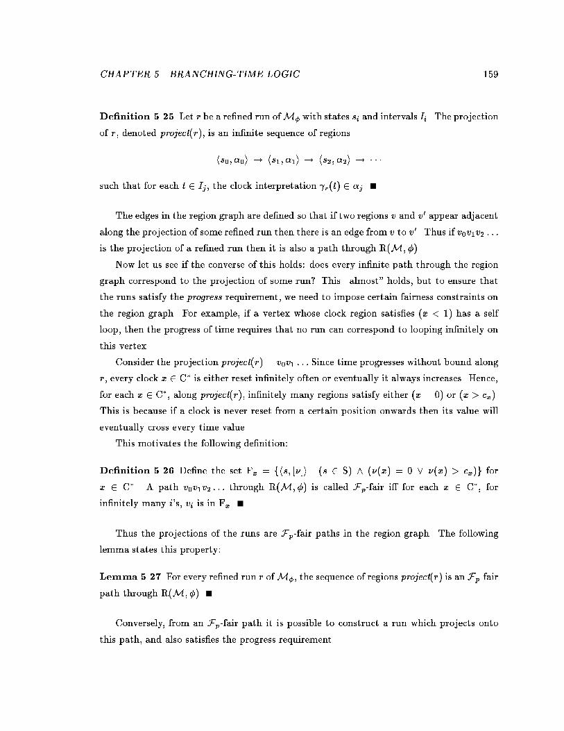
CHAPTER �� BRANCHING�TIME LOGIC ���
De�nition �� Let r be a rened run ofM� with states si and intervals Ii� The projection
of r� denoted project�r�� is an innite sequence of regions
hs�� ��i � hs�� ��i � hs�� ��i � � � �
such that for each t Ij � the clock interpretation �r�t� �j �
The edges in the region graph are dened so that if two regions v and v� appear adjacent
along the projection of some rened run then there is an edge from v to v�� Thus if v�v�v� � � �
is the projection of a rened run then it is also a path through R�M� ���
Now let us see if the converse of this holds� does every innite path through the region
graph correspond to the projection of some run$ This �almost� holds� but to ensure that
the runs satisfy the progress requirement� we need to impose certain fairness constraints on
the region graph� For example� if a vertex whose clock region satises �x �� has a self
loop� then the progress of time requires that no run can correspond to looping innitely on
this vertex�
Consider the projection project�r� " v�v� � � � Since time progresses without bound along
r� every clock x C� is either reset innitely often or eventually it always increases� Hence�
for each x C�� along project�r�� innitely many regions satisfy either �x " �� or �x cx��
This is because if a clock is never reset from a certain position onwards then its value will
eventually cross every time value�
This motivates the following denition�
De�nition ��� Dene the set Fx " fhs� ���i j �s S� � ���x� " � � ��x� cx�g for
x C�� A path v�v�v� � � � through R�M� �� is called Fpfair i for each x C�� for
innitely many i�s� vi is in Fx�
Thus the projections of the runs are Fpfair paths in the region graph� The following
lemma states this property�
Lemma ��� For every rened run r ofM�� the sequence of regions project�r� is an Fpfair
path through R�M� ���
Conversely� from an Fpfair path it is possible to construct a run which projects onto
this path� and also satises the progress requirement�

CHAPTER �� BRANCHING�TIME LOGIC ���
Lemma ��� For every Fpfair path � through R�M� ��� there exists a rened run r of
M� such that � equals project�r��
Proof� Consider an innite path � " v�v� � � � through R�M� �� with vi " hsi� �ii�
Choose some �� ��� The interval I� is leftclosed and l�I�� " �� Now we construct the
desired �rened� run r inductively� Assume �i and the left boundary for Ii is chosen� We
show how to choose the rightboundary of Ii and the clock interpretation �i��� Repeating
this process denes the desired run r�
First consider the case when �i is a boundary region� In this case Ii is a singular interval�
that is� set r�Ii� " l�Ii�� and Ii is rightclosed� If �i�� " succ��i� then �i�� " �� and
�i�� " �i� Otherwise� the edge from vi to vi�� corresponds to a Mtransition si�i���� si���
choose �i�� " ��i�� �� ���i�
Now consider the case when �i is not a boundary region� If �i is not the endregion
then there is some positive �i such that �i �i succ��i�� and �i � �i for all � ��� �i��
That is� the clock interpretation �i changes its equivalence class after �i time elapses� There
are several cases to consider�
��� Suppose the edge from vi to vi�� indicates passage of time� that is� si�� " si and
�i�� " succ��i�� In this case� Ii is rightopen� Choose r�Ii� " l�Ii� �i� �i�� " �i �i� and
�i�� " ��
��� This case corresponds to a statetransition si�i���� si�� happening before the current
clock region changes� We can choose the length of Ii in this case� If �i is the endregion
let � " � else � " �i��� Choose r�Ii� " l�Ii� �� and �i�� " ��i�� �� ����i ���� If
�i�� " ���i�� �� ���i� then Ii is rightopen� and if �i�� " succ����i�� �� ���i�� then Ii is
rightclosed�
��� Let us consider the case when the state change occurs after time �i according the
Medge si�i���� si��� The current interval Ii is rightopen� Choose r�Ii� " l�Ii� �i� and
�i�� " ��i�� �� ����i �i��
It is easy to check that the run r satises the consecution and timing requirements� Also
� equals project�r�� Furthermore� since � is Fpfair� r satises the progress requirement�
Suppose r does not meet the progress requirement� The run contains innitely many tran
sitions corresponding to the edges in M� From the above construction it follows that the
sequence of values �i converges to �� This implies that there exists j � such that for all
i j the regions �i satisfy �d x d �� for some clock x and some integer d cx� This
implies that � is not fair with respect to Fx�

CHAPTER �� BRANCHING�TIME LOGIC ���
From the above two lemmas it follows that the behavior of the timed structureM� can
be analyzed by examining the Fpfair paths in the region graph� Notice that by introducing
the fairness requirements� we are essentially treating the region graph as a Kripke structure
for CTLF with the fairness family given by Fp " fFx � x C�g�
����� Labeling algorithm
We label the regions with subformulas of � starting from the subformulas of length �� then
of length �� and so on� We introduce a special proposition pb� and label a region v " hs� �i
with pb i � is a boundary region�
Let � be a subformula of �� Assume that all the regions are already labeled with each
subformula of �� Let v " hs� ���i be a region�
� If � is an atomic proposition� label v with � i � ��s��
� If � is the timing constraint �x c � y d�� then label v with � i ��x� d ��y� c�
� If � is ���� then label v with � i v is not labeled with ���
� If � is the conjunction �� � ��� then label v with � i v is labeled with both �� and
���
� If � is x� ��� then label v with � i the region hs� �x �� ���i is labeled with ���
� If � is the temporal subformula ���U �� ����U ��� respectively�� then label v with
� i some �every� respectively� Fpfair path through R�M� �� starting at v has a
prex v�� v�� � � �vn such that each vi� � � i n� is labeled with ��� and vn is labeled
with �� and with either �� or pb�
The last condition can be tested using conventional modelchecking algorithms for CTLF
�CES���� The following lemma states the correctness of the above labeling procedure�
Lemma �� Let � be a subformula of �� The above labeling algorithm labels hs� ���i with
� i hs� �i j" ��
Proof� We assume that the CTL labeling algorithm works correctly� The proof is by
induction on the structure of �� For satisfaction of TCTLformulas� we use Denition �����

CHAPTER �� BRANCHING�TIME LOGIC ���
The cases � AP� � " �x c � y d�� � " ���� � " �� � ��� and � " x� �� follow
trivially from denitions� We prove that hs� �i j" � i the algorithm labels hs� ���i with ��
where � " ��� U ��� The other case � " ��� U �� is similar�
First assume that the algorithm labels hs� ���i with �� Hence there exists an Fpfair path
� with prex v�v� � � �vn such that vn is labeled with �� and each vi� � � i n� is labeled
with ��� Let vi " hsi� �ii� By Lemma ���� there exists a rened run r with states si and
intervals Ii such that project�r� " �� Consider some t In� We know that �r�t� �n� Since
vn is labeled with �� it follows from the induction hypothesis that �r�t� j" ��� Consider
t� t� and let t� Ij � If j n then vj is labeled with ��� If j " n� the clocks at two
distinct time values� t and t�� belong to the same clock region �n� and hence� �n cannot be
a boundary region� So even in this case� the vertex vj is labeled with ��� Now we can use
the induction hypothesis to conclude that �r�t�� j" ��� Hence� hs� �i satises ��
Now let us assume that hs� �i j" �� Hence there exists a run starting at hs� �i that
satises �� U ��� By Lemma ���� there exists a rened run r with states si and intervals Ii�
satisfying �� U ��� Suppose �r�t� j" ��� and �r�t�� j" �� for some t In and for all t
� t�
By Lemma ���� the projection v�v� � � � of r is an Fpfair path in R�M� ��� Let vi " hsi� �ii�
We know that �r�t� �n� Hence� by the induction hypothesis� the algorithm labels vn with
��� For each � � i n� there is some t� in Ii with t� t� and �r�t
�� j" ��� Again� by similar
reasoning� each vi should be labeled with ��� Also if �n is not a boundary region then there
is some t� In with t� t� and hence in this case� vn also should be labeled with ��� Thus
the region graph has a path of the desired form� and hence� hs� ���i gets labeled with ��
This gives a decision procedure for modelchecking�
Given a timed structure M and a TCTL�formula �� �rst construct the region
graph R�M� �� Then label all the regions with the subformulas of � using the la�
beling procedure The structureM satis�es the speci�cation � i� hsinit � �C� �� ��i
is labeled with �
����� Complexity of the algorithm
Using the ideas discussed above� one can implement an algorithm for modelchecking which
runs in time linear in the qualitative part� and exponential in the timing part of the input�
As in Lemma ���� of Section ������ we can show that the the number of clock regions
of �C� �� R� induced by � is bounded by �jC�j& ��jC�j �!x�C��� �cx ���� Thus the number

CHAPTER �� BRANCHING�TIME LOGIC ���
of regions is O��j����j�j��M�j�� it is exponential in j(���j� the length of the atomic timing
formulas in �� and also exponential in j(�M�j� the length of the clock constraints �we
assume binary encoding for the constants��
Now from the denition of the region graph� it follows that jV�j " O�jSj��j����j�j��M�j��
The rst clause in the denition of E� contributes at most one edge for every vertex� and
the second clause contributes at most three edges for every edge in E and a clock region of
�C� �� R�� Hence� jE�j " O��jSj jEj���j����j�j��M�j��
Thus the size of the region graph is exponential in the length of timing constraints of the
given timed structure and the formula� but linear in the size of the statetransition graph�
Theorem ��� Given a timed structure M and a TCTLformula �� there is a decision pro
cedure for checking whether or notM j" � which runs in timeO�j�j��jSj jEj���j����j�j��M�j��
Proof� First construct the region graph R�M� �� " hV�� E�i� The successor class of
any class can be computed in time O�jC�j�� Hence� R�M� �� can be constructed in time
O�jV�j jE�j�� Then run the labeling algorithm on the subformulas of �� The number
of fairness constraints is jC�j� The vertices of R�M� �� can be marked with a formula �
in time O��jV�j jE�j� � jC�j�� assuming they are already marked with the subformulas of
�� using the labeling algorithm for CTLF �CES���� So the labeling algorithm takes time
O�j�j�jC�j��jV�j jE�j��� The complexity bound follows from the bounds on jV�j and jE�j�
Since we have shown that the modelchecking problem is decidable� we can also charac
terize the complexity class of deciding nite satisability of TCTLformulas�
Corollary ��� The problem of deciding whether a given TCTLformula is nitely satis
able� is complete for the class of recursivelyenumerable problems ���complete��
Proof� The set of timed structures is enumerable� For any given timed structure M
one can nd whether or not M satises the given TCTLformula� Consequently� the set
of nitelysatisable TCTLformulas is recursively enumerable� Undecidability was proved
earlier in Theorem �����
Note that since the set of satisable TCTLformulas is not recursively enumerable� there
must be some formulas which are satisable but not nitely satisable� Thus TCTL does
not have the nitemodel property�
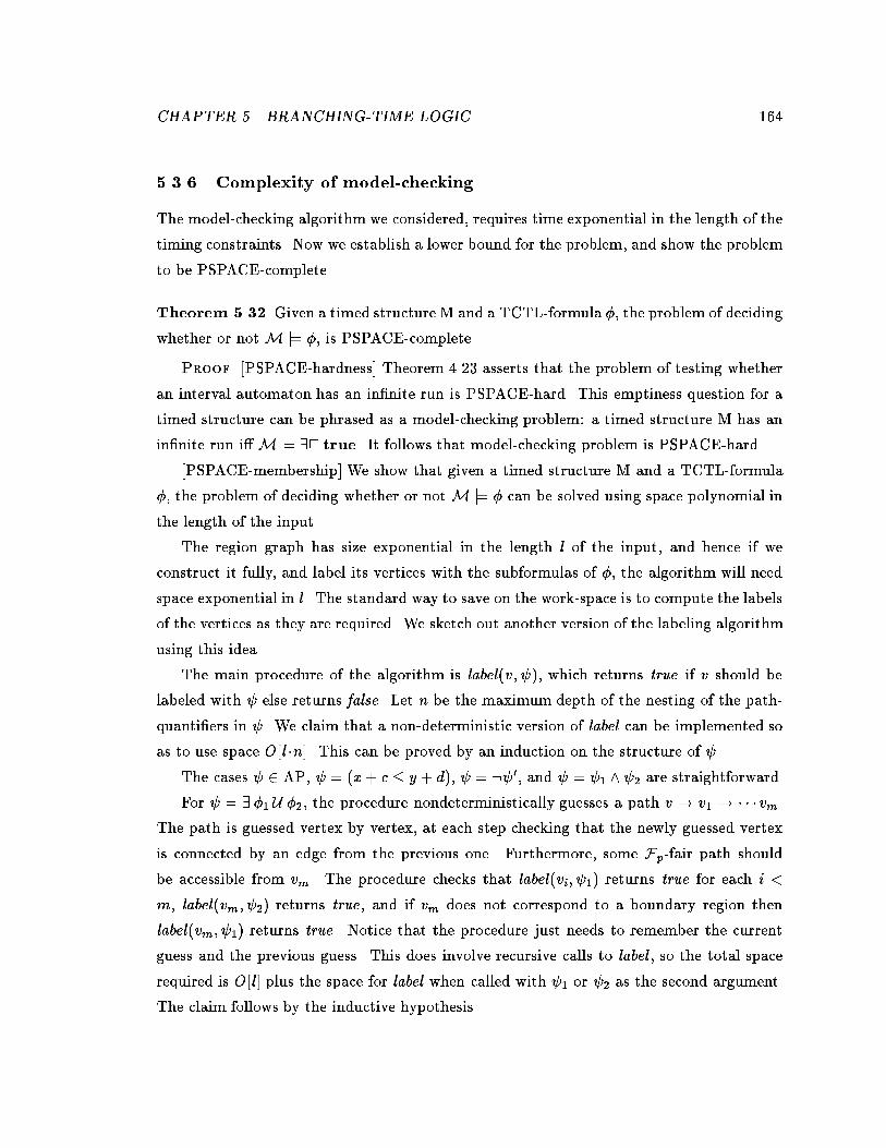
CHAPTER �� BRANCHING�TIME LOGIC ���
���� Complexity of model�checking
The modelchecking algorithm we considered� requires time exponential in the length of the
timing constraints� Now we establish a lower bound for the problem� and show the problem
to be PSPACEcomplete�
Theorem ��� Given a timed structure M and a TCTLformula �� the problem of deciding
whether or notM j" �� is PSPACEcomplete�
Proof� �PSPACEhardness� Theorem ���� asserts that the problem of testing whether
an interval automaton has an innite run is PSPACEhard� This emptiness question for a
timed structure can be phrased as a modelchecking problem� a timed structure M has an
innite run i M j" �� true� It follows that modelchecking problem is PSPACEhard�
�PSPACEmembership� We show that given a timed structure M and a TCTLformula
�� the problem of deciding whether or notM j" � can be solved using space polynomial in
the length of the input�
The region graph has size exponential in the length l of the input� and hence if we
construct it fully� and label its vertices with the subformulas of �� the algorithm will need
space exponential in l� The standard way to save on the workspace is to compute the labels
of the vertices as they are required� We sketch out another version of the labeling algorithm
using this idea�
The main procedure of the algorithm is label�v� ��� which returns true if v should be
labeled with � else returns false� Let n be the maximum depth of the nesting of the path
quantiers in �� We claim that a nondeterministic version of label can be implemented so
as to use space O�l�n�� This can be proved by an induction on the structure of ��
The cases � AP� � " �x c � y d�� � " ���� and � " �� � �� are straightforward�
For � " ��� U ��� the procedure nondeterministically guesses a path v � v� � � � �vm�
The path is guessed vertex by vertex� at each step checking that the newly guessed vertex
is connected by an edge from the previous one� Furthermore� some Fpfair path should
be accessible from vm� The procedure checks that label�vi� ��� returns true for each i
m� label�vm� ��� returns true� and if vm does not correspond to a boundary region then
label�vm� ��� returns true� Notice that the procedure just needs to remember the current
guess and the previous guess� This does involve recursive calls to label � so the total space
required is O�l� plus the space for label when called with �� or �� as the second argument�
The claim follows by the inductive hypothesis�

CHAPTER �� BRANCHING�TIME LOGIC ���
Now consider the case � " ��� U ��� First observe that the negation of � can be written
using only existential pathquantiers�
��� U �� � �� ������U ���� � ���� � ����� �
The procedure label is called recursively on each subformula of the above translation� Note
that the rewriting does not increase the depth of the nesting of path quantiers� The case
� " ���� is handled similarly to the previous case�
By Savitch�s theorem the deterministic version can be implemented in space O�l��j�j���
���� TCTL with fairness
The modelchecking algorithm can be modied to handle timed structures with fairness in
a straightforward way� Recall that a timed structure M with fairness has an associated
fairness family F � A run r of M is Ffair i for every F F � innitely many states of r
are in F� For the TCTLstructure TM associated with such a timed structure� the set of
computations fM consists only of those computations that correspond to the Ffair runs
of M�
The region graph R�M� �� is constructed as before� We only change the denition of
fair paths through the region graph� A path v�v�v� � � �� with vi " hsi� �ii for all i �� in
the region graph is called Ffair i for every F F � for innitely many i �� si F� Now
while labeling a vertex with ��� U �� or ��� U ��� we consider only those paths that are
both Fpfair and Ffair� The algorithm for CTLF is used to compute the labels�

Chapter �
Concluding Remarks
Summary
We have presented a theory for modeling� specifying� and verifying nitestate realtime
systems� The focus of the thesis has been on decidability� complexity� and expressiveness
issues� It shows that automated reasoning is plausible only if we restrict timing constraints
to those comparing delays with constants� With this restriction� the simplifying assumption
of discreteness is not required for checking correctness� we can use the more appealing
densetime model� The thesis also shows that the additional cost of introducing realtime
in nitestate reasoning is a factor proportional to the magnitudes of the constants bounding
the delays�
We have considered three di erent styles of specications� The automatatheoretic ap
proach uses an eventbased model� and regards the verication problem as an inclusion
problem between two descriptions of the system� In the temporal logic based approach� the
process is modeled by an automaton generating timed state sequences� The logic MITL
uses a lineartime semantics� whereas the logic TCTL uses a branchingtime semantics� All
three formalisms can express most of the interesting properties of realtime systems� but
di er from each other in expressiveness� We have outlined an algorithm for verication in
each case�
Towards �e�cient� veri�cation
We have tested toy examples of circuits and tra�c controllers using our implementation of
one of the verication algorithms� However� all algorithms presented in the thesis are of
���

CHAPTER � CONCLUDING REMARKS ���
exponential time complexity� and we have not suggested ways to cope with the PSPACE
hardness of verication problems� Now that we have a reasonable theory for realtime
reasoning� and we understand the basic complexity issues related to automated reasoning
about timing constraints� we should proceed to nd ways to do verication more e�ciently�
Search for heuristics to cope with the stateexplosion problem has been an active area of
research in automatic verication� Recently heuristics to implementmodelchecking without
explicitly enumerating all the states have been proposed� For instance� �BCD���� proposes
the use of binary decision diagrams to represent large state sets symbolically� Godefroid
has proposed a scheme to avoid the stateexplosion due to the modeling of concurrency by
interleaving �God��� GW���� Whether our methods can be applied in practice to verify
complex systems� largely depends on the success of such attempts� We feel hopeful that the
techniques designed for the qualitative case can be generalized to handle timing constraints
also�
Apart from an e�cient implementation of the verication algorithms� the other impor
tant aspect is to provide tools to specify complex systems� Timed automata is a fairly
lowlevel representation� and automatic translations from more structured representations
such as process algebras� timed Petri nets� or highlevel realtime programming languages�
should exist� Recently� Sifakis et�al� have shown how to translate a term of the realtime
process algebra ATP to a timed automaton �NSY����
Probabilistic veri�cation
One promising direction of extending the work reported here is to incorporate probabilistic
information in the process model� This is particularly relevant for systems that control and
interact with physical processes� The computational models used in the theory of stochastic
processes are physically realistic� but formal methods for verication of stochastic realtime
systems have not been studied much�
In the simplest type of probabilistic modelchecking� the statetransition graph is con
verted into a nitestate Markov chain by placing probabilities on the transitions �Var���
PZ��� VW��� CY���� If the specication is presented as a formula of PTL or as a B�uchi
automaton� then the verication problem is to decide whether the sample paths of the
Markov chain satisfy the specication property with probability �� For CTL specications�
the semantics is redened so that the path quantiers in the logic� which previously meant
�for all paths� and �there exists a path�� are reinterpreted to mean �with probability one�
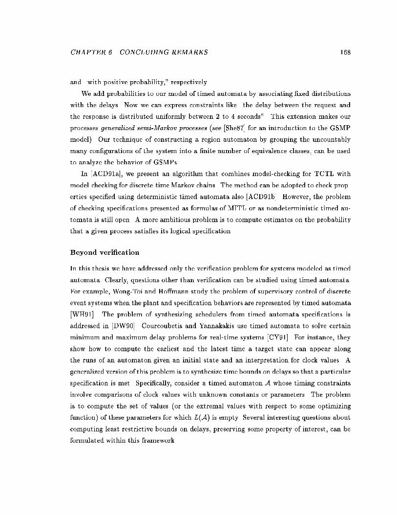
CHAPTER � CONCLUDING REMARKS ���
and �with positive probability�� respectively�
We add probabilities to our model of timed automata by associating xed distributions
with the delays� Now we can express constraints like �the delay between the request and
the response is distributed uniformly between � to � seconds�� This extension makes our
processes generalized semi�Markov processes �see �She��� for an introduction to the GSMP
model�� Our technique of constructing a region automaton by grouping the uncountably
many congurations of the system into a nite number of equivalence classes� can be used
to analyze the behavior of GSMPs�
In �ACD��a�� we present an algorithm that combines modelchecking for TCTL with
modelchecking for discretetime Markov chains� The method can be adopted to check prop
erties specied using deterministic timed automata also �ACD��b�� However� the problem
of checking specications presented as formulas of MITL or as nondeterministic timed au
tomata is still open� A more ambitious problem is to compute estimates on the probability
that a given process satises its logical specication�
Beyond veri�cation
In this thesis we have addressed only the verication problem for systems modeled as timed
automata� Clearly� questions other than verication can be studied using timed automata�
For example� WongToi and Ho mann study the problem of supervisory control of discrete
event systems when the plant and specication behaviors are represented by timed automata
�WH���� The problem of synthesizing schedulers from timed automata specications is
addressed in �DW���� Courcoubetis and Yannakakis use timed automata to solve certain
minimum and maximum delay problems for realtime systems �CY���� For instance� they
show how to compute the earliest and the latest time a target state can appear along
the runs of an automaton given an initial state and an interpretation for clock values� A
generalized version of this problem is to synthesize time bounds on delays so that a particular
specication is met� Specically� consider a timed automaton A whose timing constraints
involve comparisons of clock values with unknown constants or parameters� The problem
is to compute the set of values �or the extremal values with respect to some optimizing
function� of these parameters for which L�A� is empty� Several interesting questions about
computing least restrictive bounds on delays� preserving some property of interest� can be
formulated within this framework�

Bibliography
�ACD��� Rajeev Alur� Costas Courcoubetis� and David Dill� Modelchecking for realtime
systems� In Proceedings of the Fifth IEEE Symposium on Logic in Computer
Science� pages ���*���� �����
�ACD��a� Rajeev Alur� Costas Courcoubetis� and David Dill� Modelchecking for proba
bilistic realtime systems� In Automata� Languages and Programming� Proceed�
ings of the ��th ICALP� Lecture Notes in Computer Science ���� �����
�ACD��b� Rajeev Alur� Costas Courcoubetis� and David Dill� Verifying automata spec
ications of probabilistic realtime systems� In Proccedings of REX workshop
�Real�time� theory in practice�� �����
�AD��� Rajeev Alur and David Dill� Automata for modeling realtime systems� In Au�
tomata� Languages and Programming� Proceedings of the ��th ICALP� Lecture
Notes in Computer Science ���� pages ���*���� SpringerVerlag� �����
�AFH��� Rajeev Alur� Tom+as Feder� and Thomas Henzinger� The benets of relaxing
punctuality� In Proceedings of the Tenth ACM Symposium on Principles of
Distributed Computing� pages ���*���� �����
�AH��� Rajeev Alur and Thomas Henzinger� A really temporal logic� In Proceedings of
the ��th IEEE Symposium on Foundations of Computer Science� pages ���*����
�����
�AH��� Rajeev Alur and Thomas Henzinger� Realtime logics� complexity and expres
siveness� In Proceedings of the Fifth IEEE Symposium on Logic in Computer
Science� pages ���*���� �����
���

BIBLIOGRAPHY ���
�AK��� S� Aggarwal and R�P� Kurshan� Modeling elapsed time in protocol specica
tion� In H� Rudin and C�H� West� editors� Protocol Speci�cation� Testing� and
Veri�cation� volume III� pages ��*��� �����
�AKS��� S� Aggarwal� R�P� Kurshan� and K� Sabnani� A calculus for protocol specica
tion and validation� In H� Rudin and C�H� West� editors� Protocol Speci�cation�
Testing� and Veri�cation� volume III� pages ��*��� �����
�AS��� Bowen Alpern and Fred Schneider� Verifying temporal properties without using
temporal logic� ACM Transactions on Programming Languages and Systems�
���������*���� �����
�BB��� J�C�M� Baeten and J�A� Bergstra� Realtime process algebra� Formal Aspects
of Computing� ��������*���� �����
�BCD���� J�R� Burch� E�M� Clarke� D�L� Dill� L�J� Hwang� and K� L� McMillan� Symbolic
model checking� ���� states and beyond� In Proceedings of the Fifth IEEE
Symposium on Logic in Computer Science� pages ���*���� �����
�BCDM��� Michael Browne� Edmund Clarke� David Dill� and Bud Mishra� Automatic
verication of sequential circuits using temporal logic� IEEE Transactions on
Computers� C�����������*����� �����
�BD��� B� Berthomieu and M� Diaz� Modeling and verication of timedependent sys
tems using time Petri nets� IEEE Transactions on Software Engineering� SE
���������*���� �����
�BH��� Arthur Bernstein and Paul Harter� Proving realtime properties of programs
with temporal logic� In Proceedings of the Eighth ACM Symposium on Operating
System Principles� �����
�BKP��� Howard Barringer� Ruard Kuiper� and Amir Pnueli� A really abstract concur
rent model and its temporal logic� In Proceedings of the ��th ACM Symposium
on Principles of Programming Languages� pages ���*���� �����
�BMP��� Mordechai BenAri� Zohar Manna� and Amir Pnueli� The temporal logic of
branching time� In Proceedings of the Eighth ACM Symposium on Principles of
Programming Languages� �����

BIBLIOGRAPHY ���
�BS��� J�A� Brzozowski and C�J�H� Seger� Advances in asynchronous circuit theory�
Part II� Bounded inertial delay models� MOS circuits� design techniques� �����
�B�uc��� Richard B�uchi� On a decision method in restricted secondorder arithmetic� In
Proceedings of the International Congress on Logic� Methodology� and Philoso�
phy of Science ����� pages �*��� Stanford University Press� �����
�CDK��� E�M� Clarke� I�A� Draghicescu� and R�P� Kurshan� A unied approach for show
ing language containment and equivalence between various types of �automata�
Technical report� Carnegie Mellon University� �����
�CES��� Edmund Clarke� E� Allen Emerson� and A� Prasad Sistla� Automatic verica
tion of nitestate concurrent systems using temporallogic specications� ACM
Transactions on Programming Languages and Systems� ��������*���� �����
�Cho��� Yaacov Choueka� Theories of automata on �tapes� a simplied approach�
Journal of Computer and System Sciences� �����*���� �����
�CR��� J�E� Coolahan and N� Roussopoulos� Timing requirements for timedriven sys
tems using augmented Petrinets� IEEE Transactions on Software Engineering�
SE��������*���� �����
�CY��� Costas Courcoubetis and Mihalis Yannakakis� Verifying temporal properties of
nitestate probabilistic programs� In Proceedings of the ��th IEEE Symposium
on Foundations of Computer Science� pages ���*���� �����
�CY��� Costas Courcoubetis and Mihalis Yannakakis� Minimum and maximum de
lay problems in realtime systems� In Proceedings of the Third Workshop on
Computer�Aided Veri�cation� Aalborg University� Denmark� �����
�DHW��� David Dill� Alan Hu� and Howard WongToi� Checking for language inclusion
using simulation relations� In Proceedings of the Third Workshop on Computer�
aided Veri�cation� Aalborg University� Denmark� �����
�Dil��� David Dill� Timing assumptions and verication of nitestate concurrent sys
tems� In J� Sifakis� editor� Automatic Veri�cation Methods for Finite State
Systems� Lecture Notes in Computer Science ���� Springer*Verlag� �����

BIBLIOGRAPHY ���
�dR��� WillemPaul de Roever� editor� Real Time� Theory in Practice� Lecture Notes
in Computer Science� SpringerVerlag� ����� To appear�
�DW��� David Dill and Howard WongToi� Synthesizing processes and schedulers from
temporal specications� In Proceedings of the Second Workshop on Computer�
Aided Veri�cation� Rutgers University� �����
�EC��� E� Allen Emerson and Edmund M� Clarke� Using branchingtime temporal logic
to synthesize synchronization skeletons� Science of Computer Programming�
�����*���� �����
�EH��� E� Allen Emerson and Joseph Halpern� Decision procedures and expressive
ness in the temporal logic of branching time� In Proceedings of the �th ACM
Symposium on Principles of Programming Languages� pages ���*���� �����
�EL��� E�A� Emerson and C�L� Lei� Modalities for modelchecking� Branching time
logic strikes back� In Proceedings of the ��th ACM Symposium on Principles of
Programming Languages� pages ��*��� �����
�Eme��� E� Allen Emerson� Temporal and modal logic� In J� van Leeuwen� editor�
Handbook of Theoretical Computer Science� volume B� pages ���*����� Elsevier
Science Publishers� �����
�EMSS��� E� Allen Emerson� Aloysius Mok� A� Prasad Sistla� and Jai Srinivasan� Quanti
tative temporal reasoning� Presented at the First Workshop on Computeraided
Verication� Grenoble� France� �����
�God��� Patrice Godefroid� Using partial orders to improve automatic verication meth
ods� In Proceedings of the Second Workshop on Computer�Aided Veri�cation�
Rutgers University� �����
�GW��� Patrice Godefroid and Pierre Wolper� A partial approach to modelchecking� In
Proceedings of the Sixth IEEE Symposium on Logic in Computer Science� pages
���*���� �����
�Har��� Eyal Harel� Temporal analysis of realtime systems� Master�s thesis� The Weiz
mann Institute of Science� Rehovot� Israel� �����

BIBLIOGRAPHY ���
�Hen��� Thomas Henzinger� Halforder modal logic� how to prove realtime proper
ties� In Proceedings of the Ninth ACM Symposium on Principles of Distributed
Computing� pages ���*���� �����
�Hen��� Thomas Henzinger� Temporal Speci�cation and Veri�cation of Real�Time sys�
tems� PhD thesis� Stanford University� �����
�HJ��� Hans Hansson and Bengt Jonsson� A framework for reasoning about time and
reliability� In Proceedings of the Tenth IEEE Real�Time Systems Symposium�
pages ���*���� �����
�HK��� Zvi Har�El and Robert Kurshan� Software for analytical development of com
munication protocols� AT�T Technical Journal� �����
�HLP��� Eyal Harel� Orna Lichtenstein� and Amir Pnueli� Explicitclock temporal logic�
In Proceedings of the Fifth IEEE Symposium on Logic in Computer Science�
pages ���*���� �����
�HMP��� Thomas Henzinger� Zohar Manna� and Amir Pnueli� Temporal proof method
ologies for realtime systems� In Proceedings of the ��th ACM Symposium on
Principles of Programming Languages� pages ���*���� �����
�Hoa��� C�A�R� Hoare� Communicating sequential processes� Communications of the
ACM� ���������*���� �����
�Hoa��� C�A�R� Hoare� Communicating Sequential Processes� PrenticeHall� �����
�HPS��� David Harel� Amir Pnueli� and Jonathan Stavi� Propositional dynamic logic of
regular programs� Journal of Computer and System Sciences� ������*���� �����
�HU��� John Hopcroft and Je Ullman� Introduction to Automata Theory� Languages�
and Computation� AddisonWesley� �����
�JM��� Farnam Jahanian and Aloysius Mok� Safety analysis of timing properties in real
time systems� IEEE Transactions on Software Engineering� SE*���������*����
�����
�JM��� Farnam Jahanian and Aloysius Mok� A graphtheoretic approach for tim
ing analysis and its implementation� IEEE Transactions on Computers� C
���������*���� �����

BIBLIOGRAPHY ���
�JS��� Farnam Jahanian and Douglas Stuart� A method for verifying properties of
modechart specications� In Proceedings of the Ninth IEEE Real�Time Systems
Symposium� pages ��*��� �����
�Koy��� Ron Koymans� Specifying realtime properties with metric temporal logic� Jour�
nal of Real�Time Systems� �����*���� �����
�Kur��� Robert Kurshan� Complementing deterministic B�uchi automata in polynomial
time� Journal of Computer and System Sciences� �����*��� �����
�KVdR��� Ron Koymans� Jan Vytopil� and WillemPaul de Roever� Realtime program
ming and asynchronous message passing� In Proceedings of the Second ACM
Symposium on Principles of Distributed Computing� pages ���*���� �����
�LA��� Nancy Lynch and Hagit Attiya� Using mappings to prove timing properties� In
Proceedings of the Ninth ACM Symposium on Principles of Distributed Com�
puting� pages ���*���� �����
�Lam��� Leslie Lamport� What good is temporal logic$ In R�E�A� Mason� editor�
Information Processing ��� Proceedings of the Ninth IFIP World Computer
Congress� pages ���*���� Elsevier Science Publishers� �����
�Lam��� Leslie Lamport� The temporal logic of actions� Technical report� DEC Systems
Research Center� Palo Alto� California� �����
�Lew��� Harry Lewis� Finitestate analysis of asynchronous circuits with bounded tem
poral uncertainty� Technical Report TR����� Harvard University� �����
�Lew��� Harry Lewis� A logic of concrete time intervals� In Proceedings of the Fifth
IEEE Symposium on Logic in Computer Science� pages ���*���� �����
�LP��� Orna Lichtenstein and Amir Pnueli� Checking that nitestate concurrent pro
grams satisfy their linear specication� In Proceedings of the ��th ACM Sym�
posium on Principles of Programming Languages� pages ��*���� �����
�LPS��� Daniel Lehman� Amir Pnueli� and Jonathan Stavi� Impartiality� justice� and
fairness� The ethics of concurrent termination� In Automata� Languages and
Programming� Proceedings of the Ninth ICALP� Lecture Notes in Computer
Science ���� pages ���*���� SpringerVerlag� �����

BIBLIOGRAPHY ���
�LT��� Nancy Lynch and Mark Tuttle� Hierarchical correctness proofs for distributed
algorithms� In Proceedings of the Seventh ACM Symposium on Principles of
Distributed Computing� pages ���*���� �����
�McN��� Robert McNaughton� Testing and generating innite sequences by a nite au
tomaton� Information and Control� �����*���� �����
�Mil��� Robin Milner� A Calculus of Communicating Systems� Lecture Notes in Com
puter Science ��� SpringerVerlag� �����
�Mil��� Robin Milner� Calculi for synchrony and asynchrony� Theoretical Computer
Science� ������*���� �����
�MP��� Zohar Manna and Amir Pnueli� The temporal framework for concurrent pro
grams� In R�S� Boyer and J�S� Moore� editors� The correctness problem in
Computer science� pages ���*���� Academic Press� �����
�MP��� Zohar Manna and Amir Pnueli� The anchored version of the temporal frame
work� In Linear Time� Branching Time� and Partial Order in Logics and Mod�
els for Concurrency� Lecture Notes in Computer Science ���� SpringerVerlag�
�����
�MT��� F� Moller and C� Tofts� A temporal calculus of communicating processes� In
J�C�M� Baeten and J�W� Klop� editors� CONCUR ��� Theories of Concurrency�
Lecture Notes in Computer Science ���� pages ���*���� SpringerVerlag� �����
�Mul��� David Muller� Innite sequences and nite machines� In Proceedings of the
Fourth IEEE Symposium on Switching Circuit Theory and Logical Design� pages
�*��� �����
�MW��� Zohar Manna and Pierre Wolper� Synthesis of communicating processes from
temporal logic specications� ACM Transactions on Programming Languages
and Systems� �������*��� �����
�NRSV��� Xavier Nicollin� JeanLuc Richier� Joseph Sifakis� and Jacques Voiron� ATP� an
algebra for timed processes� In Proceedings of the IFIP TC� Working Conference
on Programming Concepts and Methods� Sea of Galilee� Israel� �����

BIBLIOGRAPHY ���
�NSY��� Xavier Nicollin� Joseph Sifakis� and Sergio Yovine� From ATP to timed graphs
and hybrid systems� In Proccedings of REX workshop �Real�time� theory in
practice�� �����
�OL��� Susan Owicki and Leslie Lamport� Proving liveness properties of concurrent pro
grams� ACM Transactions on Programming Languages and Systems� ��������*
���� �����
�Ost��a� Jonathan Ostro � Deciding properties of timed transition models� IEEE Trans�
actions on Parallel and Distributed Systems� �������*���� �����
�Ost��b� Jonathan Ostro � Temporal Logic of Real�time Systems� Research Studies Press�
�����
�Pet��� J�L� Peterson� Petri Net Theory and the Modeling of Systems� PrenticeHall�
�����
�PH��� Amir Pnueli and Eyal Harel� Applications of temporal logic to the specication
of realtime systems� In Formal Techniques in Real�time and Fault�tolerant
Systems� Lecture Notes in Computer Science ���� pages ��*��� SpringerVerlag�
�����
�Pnu��� Amir Pnueli� The temporal logic of programs� In Proceedings of the ��th IEEE
Symposium on Foundations of Computer Science� pages ��*��� �����
�Pnu��� Amir Pnueli� Applications of temporal logic to the specication and verication
of reactive systems� a survey of current trends� In Current Trends in Concur�
rency� Lecture Notes in Computer Science ���� pages ���*���� SpringerVerlag�
�����
�PZ��� Amir Pnueli and Lenore Zuck� Probabilistic verication by tableaux� In Pro�
ceedings of the First IEEE Symposium on Logic in Computer Science� pages
���*���� �����
�Ram��� Chander Ramchandani� Analysis of asynchronous concurrent systems by Petri
nets� Technical Report MAC TR���� Massachusetts Institute of Technology�
�����

BIBLIOGRAPHY ���
�Rog��� Hartley Rogers� Theory of Recursive Functions and E�ective Computability�
McGrawHill� �����
�RR��� G�M� Reed and A�W� Roscoe� A timed model for communicating sequential
processes� Theoretical Computer Science� ������*���� �����
�Saf��� Shmuel Safra� On the complexity of �automata� In Proceedings of the ��th
IEEE Symposium on Foundations of Computer Science� pages ���*���� �����
�SC��� A� Prasad Sistla and Edmund Clarke� The complexity of propositional linear
temporal logics� The Journal of the ACM� ������*���� �����
�She��� Gerald Shedler� Regeneration and Networks of Queues� SpringerVerlag� �����
�SVW��� A� Prasad Sistla� Moshe Vardi� and Pierre Wolper� The complementation prob
lem for B�uchi automata with applications to temporal logic� Theoretical Com�
puter Science� ��� �����
�Tar��� Robert Tarjan� Depth rst search and linear graph algorithms� SIAM Journal
on Computing� ��������*���� �����
�Tho��� Wolfgang Thomas� Automata on innite objects� In J� van Leeuwen� editor�
Handbook of Theoretical Computer Science� volume B� pages ���*���� Elsevier
Science Publishers� �����
�Var��� Moshe Vardi� Automatic verication of probabilistic concurrent nitestate pro
grams� In Proceedings of the ��th IEEE Symposium on Foundations of Computer
Science� pages ���*���� �����
�Var��� Moshe Vardi� Verication of concurrent programs * the automatatheoretic
framework� In Proceedings of the Second IEEE Symposium on Logic in Com�
puter Science� pages ���*���� �����
�VW��� Moshe Vardi and Pierre Wolper� An automatatheoretic approach to automatic
program verication� In Proceedings of the First IEEE Symposium on Logic in
Computer Science� pages ���*���� �����
�Wan��� Yi Wang� Real time behavior of asynchronous agents� In CONCUR ��� The�
ories of Concurrency� Lecture Notes in Computer Science ���� pages ���*����
SpringerVerlag� �����
BIBLIOGRAPHY ���
�WH��� HowardWongToi and Girard Ho mann� The control of dense realtime discrete
event systems� �����
�Wol��� Pierre Wolper� Temporal logic can be more expressive� Information and Control�
�����*��� �����
�WVS��� Pierre Wolper� Moshe Vardi� and A� Prasad Sistla� Reasoning about innite
computation paths� In Proceedings of the ��th IEEE Symposium on Foundations
of Computer Science� pages ���*���� �����
�YKT��� Tomohiro Yoneda� Yutaka Kondo� and Yoshihiro Tohma� On the acceleration
of timing verication method based on time Petri nets� �����
�Zwa��� Amy Zwarico� Timed Acceptances� An Algebra of Time Dependent Computing�
PhD thesis� University of Pennsylvania� �����