tidal networks 3. landscape-forming discharges and studies...

Tidal networks3. Landscape-forming discharges and studiesin empirical geomorphic relationships

Andrea Rinaldo,1 Sergio Fagherazzi,2 Stefano Lanzoni, and Marco MaraniDipartimento di Ingegneria Idraulica, Marittima e Geotecnica, Universita di Padova, Padua, Italy

William E. DietrichDepartment of Geology and Geophysics, University of California, Berkeley

Abstract. In this final part of our study [Fagherazzi et al., this issue; Rinaldo et al., thisissue] we propose a simple model for predicting the local peak ebb and flood dischargesthroughout a tidal network and use this model to investigate scaling relationships betweenchannel morphology and discharge in the Venice Lagoon. The model assumes that thepeak flows are driven by spring (astronomical) tidal fluctuations (rather than precipitation-induced runoff or seiche, sea surge, or storm-induced tidal currents) and exploits theprocedure presented by Fagherazzi et al. [this issue] for delineating a time-invariantdrainage area to any channel cross section. The discharge is estimated using theFagherazzi et al. model to predict water surface topography, and hence flow directionsthroughout the channel network and across unchanneled regions, and the assumption offlow continuity. Water surface elevation adjustment, not assumed to be instantaneousthroughout the network, is defined by a suitable solution of the flow equations wheresignificant morphological information is used and is reduced to depending on just oneparameter, the Chezy resistance coefficient. For the Venice Lagoon, peak discharges arewell predicted by our model. We also document well-defined power law relationshipsbetween channel width and peak discharge, watershed area, and flow, whereas curved,nonscaling relationships were found for channel cross-sectional area as a function of peakdischarge. Hence our model supports the use of a power law dependency of peakdischarge with drainage area in the Venice Lagoon and provides a simple means toexplore aspects of morphodynamic adjustments in tidal systems.

1. Introduction

In fluvial basins the key character of openness to mass/energy injection, central to their evolutionary dynamics, is usu-ally enforced by assuming that total contributing area, say A , isproportional to landscape-forming discharges, say Q , that is, Q! A!, with ! " 1 [e.g., Leopold et al., 1984]. Substitution ofdrainage area for formative discharge in landscape evolutiontheories simplifies models without eliminating complex behav-ior that may be central to network evolution. In particular, thissubstitution permits effectively parameter-free models to bedeveloped that can explore the tendency for networks to self-organize [Rodriguez-Iturbe and Rinaldo, 1997].

In tidal networks a simple assumption of proportionality ofwatershed area and landscape-forming discharges cannot gen-erally be made [Leopold et al., 1984, 1993; Myrick and Leopold,1963; Friedrichs, 1995]. Nonetheless, we have observed thatimportant features of the tidal channel system, that is, thedrainage density, network length, channel width, and channel

initiation, vary with watershed area (albeit not as simple powerfunctions) [Fagherazzi et al., this issue; Rinaldo et al., this issue].This occurs despite the fact that flood flows are not simplydependent on marsh drainage area. In order to improve ourunderstanding of these relationships, we need to develop ameans of estimating an effective discharge throughout thechannel network.

The basic relationship employed in the past for couplinghydrodynamic and morphodynamic processes is an empiricallinkage of cross-sectional area of tidal channels (or tidal in-lets), say ", with “spring” (i.e., maximum astronomical) tidalprism or “spring” peak discharge, say Q , that is,

" ! Q#, (1)where # is a scaling coefficient typically assumed to lie in therather wide range 0.85–1.20 [e.g., Langbein, 1963; Myrick andLeopold, 1963; Harleman, 1966; Jarrett, 1976; Nichols et al.,1991]. However, the validity of (1) for sheltered channels(those not exposed to littoral transport or open sea) has re-cently been questioned [Friedrichs, 1995]. Complex and site-specific feedbacks between tidal channel morphology and tidalflow properties occur both in inlet and sheltered channel sec-tions [e.g., Bruun, 1978; O’Brien, 1969; Jarrett, 1976; Friedrichs,1995]. In addition, man-made interventions are key geomor-phic agents in many lagoons; for example, artificial deepeningof tidal channels, essential to navigability in many tidal envi-ronments exploited for port activity, may cause accelerated

1Also at Ralph M. Parsons Laboratory, Massachusetts Institute ofTechnology, Cambridge.

2Now at Computational Science and Engineering Program, FloridaState University, Tallahassee.

Copyright 1999 by the American Geophysical Union.

Paper number 1999WR900238.0043-1397/99/1999WR900238$09.00

WATER RESOURCES RESEARCH, VOL. 35, NO. 12, PAGES 3919–3929, DECEMBER 1999

3919

deposition, as well as reductions of the tidal prisms by infillingor dyking marshes and/or lagoons. These modifications intro-duce time-dependent scales of influence on flow and erosionprocesses. Short-term, rapid, hydrodynamic adjustments of theorder of days [Byrne et al., 1981] may occur. Longer-termadjustments due to subsidence and eustasy which affect thetidal prism propagation [e.g., Gardner and Bohn, 1980] mayalso be important. It seems also reasonable that morphody-namic relationships for channelized tidal embayments associ-ated with the interior of tidal marshes or lagoons (or with thelandward reaches of river estuaries opened to tidal fluctua-tions) work somewhat differently from inlets on open coasts.This stems, among other factors, from the relative lack ofdirect, intense wave attack and littoral drift in sheltered sites.Moreover, spatial gradients in tidal amplitude and phase aresurely less pronounced than in the inlet zone.

In order to explore the applicability of (1) for sheltered tidalchannels and to examine other morphologic relationships thatcould depend on discharge rather than just watershed area, wepropose a hydrodynamic model that predicts the dischargethroughout the network. This model allows us to examine theeffects of differential flooding and draining of shallow unchan-neled zones on peak discharges by exploiting the detailed to-pographic and morphological description of the tidal network.We first present the procedure for computing the dischargeand then compare the scale of various morphological featureswith our computed peak discharges. We illustrate in detail theprocedure for the computation of the landscape-forming flowrates and address the observational evidence of the morpho-logical features (cross-section areas and widths and tidal basinwatershed) with the maximum flow rates computed for eachsection. We also relate maximum flow rates to tidal prisms tocheck on their consistency. This leads us to some morpholog-ical remarks that close the paper.

2. Peak Spring Flow Rates at Arbitrary CrossSections of a Tidal Embayment

Here we propose a simplified model for predicting the peakflow rates throughout the channel network of a tidal systemwhich exploits our method [Rinaldo et al., this issue] for delin-eating the time-invariant watershed boundaries of individualsubbasins. The model results can then be used to investigatepossible relationships between channel morphology and dis-charge as has been done for entire tidal basins [e.g., Marchi,1990].

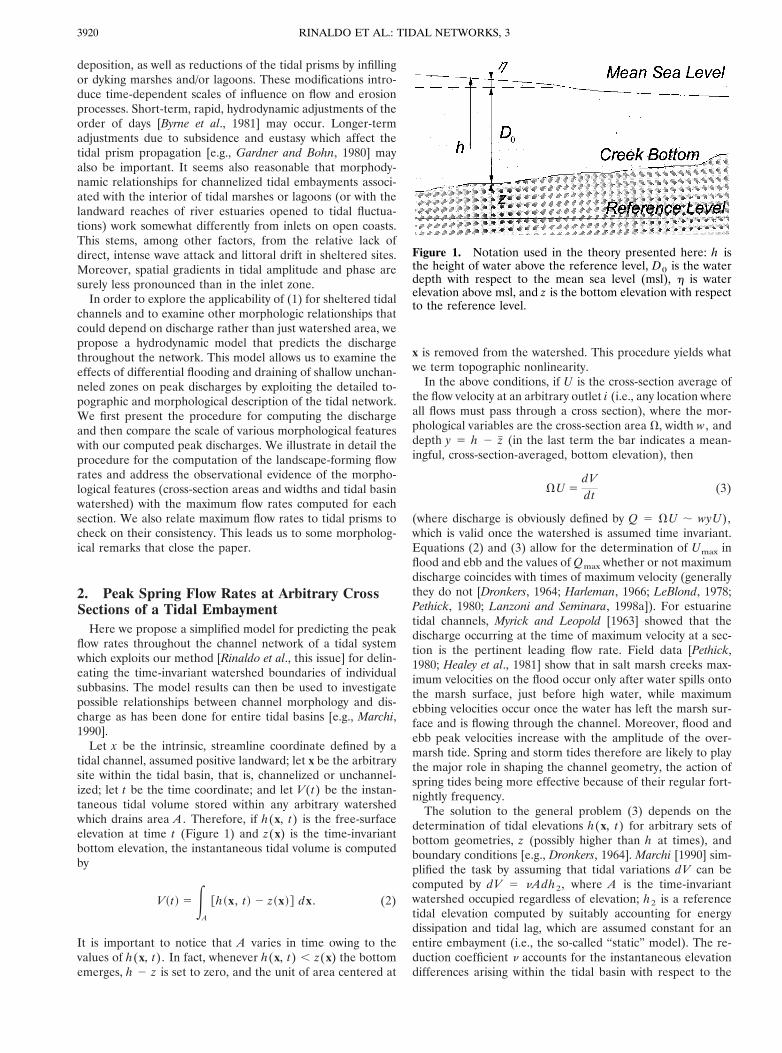
Let x be the intrinsic, streamline coordinate defined by atidal channel, assumed positive landward; let x be the arbitrarysite within the tidal basin, that is, channelized or unchannel-ized; let t be the time coordinate; and let V(t) be the instan-taneous tidal volume stored within any arbitrary watershedwhich drains area A . Therefore, if h(x, t) is the free-surfaceelevation at time t (Figure 1) and z(x) is the time-invariantbottom elevation, the instantaneous tidal volume is computedby

V#t$ $ !A

%h#x , t$ % z#x$& dx . (2)

It is important to notice that A varies in time owing to thevalues of h(x, t). In fact, whenever h(x, t) ' z(x) the bottomemerges, h ( z is set to zero, and the unit of area centered at

x is removed from the watershed. This procedure yields whatwe term topographic nonlinearity.

In the above conditions, if U is the cross-section average ofthe flow velocity at an arbitrary outlet i (i.e., any location whereall flows must pass through a cross section), where the mor-phological variables are the cross-section area ", width w , anddepth y ) h ( z! (in the last term the bar indicates a mean-ingful, cross-section-averaged, bottom elevation), then

"U $dVdt (3)

(where discharge is obviously defined by Q ) "U * wyU),which is valid once the watershed is assumed time invariant.Equations (2) and (3) allow for the determination of Umax inflood and ebb and the values of Qmax whether or not maximumdischarge coincides with times of maximum velocity (generallythey do not [Dronkers, 1964; Harleman, 1966; LeBlond, 1978;Pethick, 1980; Lanzoni and Seminara, 1998a]). For estuarinetidal channels, Myrick and Leopold [1963] showed that thedischarge occurring at the time of maximum velocity at a sec-tion is the pertinent leading flow rate. Field data [Pethick,1980; Healey et al., 1981] show that in salt marsh creeks max-imum velocities on the flood occur only after water spills ontothe marsh surface, just before high water, while maximumebbing velocities occur once the water has left the marsh sur-face and is flowing through the channel. Moreover, flood andebb peak velocities increase with the amplitude of the over-marsh tide. Spring and storm tides therefore are likely to playthe major role in shaping the channel geometry, the action ofspring tides being more effective because of their regular fort-nightly frequency.

The solution to the general problem (3) depends on thedetermination of tidal elevations h(x, t) for arbitrary sets ofbottom geometries, z (possibly higher than h at times), andboundary conditions [e.g., Dronkers, 1964]. Marchi [1990] sim-plified the task by assuming that tidal variations dV can becomputed by dV ) &Adh2, where A is the time-invariantwatershed occupied regardless of elevation; h2 is a referencetidal elevation computed by suitably accounting for energydissipation and tidal lag, which are assumed constant for anentire embayment (i.e., the so-called “static” model). The re-duction coefficient & accounts for the instantaneous elevationdifferences arising within the tidal basin with respect to the

Figure 1. Notation used in the theory presented here: h isthe height of water above the reference level, D0 is the waterdepth with respect to the mean sea level (msl), ' is waterelevation above msl, and z is the bottom elevation with respectto the reference level.

RINALDO ET AL.: TIDAL NETWORKS, 33920

reference value h2 and thus allows us to define the true tidalprism only in an approximate manner. The approach is sound,as long as the validity of the so-called static assumption (i.e.,where the fluctuations of tidal elevations are spatially uniformimplying very short travel time of the tidal wave with respect toits period) is valid and provided no change in contributing areaA occurs even when parts of the tidal basin become fullydrained.

Consistent with our assumption underlying the method forwatershed delineation [Rinaldo et al., this issue], we assumethat flow directions are fixed (first) by the channel directionsdetermined automatically in objective manner from digital ter-rain maps (DTMs) [Fagherazzi et al., this issue] within thechannelized portion of the tidal basin and (second) by thegradients of the Poissonian potential surface [Rinaldo et al.,this issue] for tidal expansion areas external to the channelizedportion. While the first assumption seems quite reasonable ingeneral, because the channel is in any case a fundamentalattractor for the hydrodynamic flow directions, the secondassumption, though critically simplifying the analytical treat-ment of the problem, is certainly less valid in general. Ourassumptions in the watershed model of (third) small instanta-neous spatial gradients of elevations (basically implying shortembayments), (fourth) flat unchannelized areas and, (fifth)time invariance in watershed boundaries might result in some-what poor estimation of flow direction in shallow areas. Inwell-developed network structures like those investigated inthis paper [see, e.g., Fagherazzi et al., this issue, Figures 1–4],however, the variation in pathways across unchannelized areasis probably small, and watershed divide location may remainrelatively fixed.

We also assume that landscape-forming events are due tospring peak discharges which are driven by astronomical con-ditions [Boon, 1975; Friedrichs, 1995]. These peak discharges,then, can be estimated by imposing as a boundary conditionthe appropriate astronomical tidal conditions. We can then usethe approach similar to that of Dronkers [1972] to estimatetidal waves from the simple superposition of sinusoidal waveseach characterized by a given amplitude and frequency.

The basic tidal constituents in the upper Adriatic Sea areeight (M2, S2, N2, K2, K1, O1, P1, and S1) [Comune diVenezia, 1998]. Thus the basic boundary condition at sea,hs(t), is given by

hs#t$ $ h0 ( "i)1

M

ai#) i$ cos ) it , (4)

where h0 indicates mean sea level (msl), ai() i) is the ampli-tude of the i component, and ) i ) 2*/Ti, where Ti is therelevant astronomical period. Therefore, on setting h0 ) 0 mabove msl, one gets hs(t) ) 's(t) ) ¥ i)1

M ai() i) cos ) it ,where M ) 8 and the various values of ) i and ai() i) arecomputed via published harmonic constants (for the VeniceLagoon, see Comune di Venezia [1998] and Table 1).

To solve (3), we first compute the tidal propagation up thechannel network, where the deeper flows and the constrainedflow directions (forced to follow the channel banks) permit asimple calculation. To do this, we neglect spatial gradients offluid density (due, e.g., to salinity) and overall density currentsassuming that they are negligible at times of landscape-formingflows.

Consistent with the approximate framework leading to wa-tershed delineation, we will manipulate the flow equations toobtain closed-form solutions. If h ) z + D0 + ' is watersurface elevation (here z(x) ) z( x) is the bottom elevation,D0(x) ) D0( x) is the depth with respect to a datum, that is,mean sea level, and '(x, t) ) '( x , t) is the height of the tidalwave with respect to the mean water level, see Figure 1), theinstantaneous discharge Q is defined as

Q $ "U $ #D0 ( '$wU , (5)

and, having set Coriolis’ coefficient to zero [Dronkers, 1964],momentum and mass balance equations (neglecting wind ef-fects which should not be meaningful in the average on astro-nomical flows) can be written as

+Q+t %

QD0 ( '

+h+t %

Qw

+w+t

(Q" # +Q

+ x %Q

D0 ( ' $ dD0

dx (+'

+ x% %Qw

+w+ x&

$ (g"$ dzdx (

dD0

dx (+'

+ x% %g

!2"2#D0 ( '$'Q 'Q (6)

+Q+ x ( B

+h+t $ 0 (7)

where ! is the Chezy coefficient, g is the acceleration ofgravity, w is the channel width, and B is the width of channelsplus adjacent storage regions, if any (all other symbols havebeen defined in the context of (3)).

The width B clearly depends on our watershed delineationprocedure and can be computed, for each site, as follows. Wecompute watershed area A to a site characterized by a channelwith width w; we move forward or backward by a small dis-tance ,x (where w remains substantially unchanged) and mea-sure the new watershed area A + ,A and the channelizedarea A- * w,x occupied between the two stations. We thencompute B ) ,Aw/A- (Figure 2). This procedure allows foran adjustment of B at times when part of the tidal embaymentsis not underwater.

The continuity equation (7) uses the entire storage width(B) and accounts for changes in discharge per unit length dueto over-bank flows by assuming that flow depth h is constantalong B and changes instantaneously across the width. Thisassumption contributes to predict the experimentally observedreduction in tidal celerity through the main channels induced

Table 1. Best Estimate of Tidal Harmonic Constants Used for the Prediction of Astronomical Tides in the Venice Lagoon

M2 S2 N2 K2 K1 O1 P1 S1

Amplitude A, m 0.254 0.143 0.042 0.032 0.155 0.04 0.057 0.015Phase ,, deg 120 324 343 117 82 256 97 262Angular speed, deg/hr 28.9841 30.0 28.4397 30.0821 15.0411 13.9430 14.9589 15.0

Source is Comune di Venezia [1998].

3921RINALDO ET AL.: TIDAL NETWORKS, 3

by the expansion in adjacent storages [Istituto di Idraulicadell’Universita di Padova, 1979].

In order to obtain a solution to the above equations, wemake several important assumptions: (first) Spatial and tem-poral gradients of channel width w are negligible in the mo-mentum equation; (second) flow velocities are smaller than amean celerity of propagation of the tidal wave, that is, U ''.g(D0 + ') ; and (third) in the main channels, tidal excur-sions are relatively small, that is, ' '' D0. These assumptionsare only valid for the larger tidal channels and for the lowertidal flats in mesotidal lagoons. In the smallest channels andalong salt marshes these assumptions are seldom acceptable,and (8) will only yield a gross estimate of the local tidal flows.

To understand the impact of the proposed assumptions, afew observational figures from the Venice Lagoon case studymay be significant. There the maximum value of ' at the mouthfor spring tides is ' * 0.30 m which, in the experimental sitewhere topography is accurately measured, is dissipated downto a few centimeters, typically 0.05–0.10 m. The depth D0 ofthe channels ranges from D0 * 5 m to less than 0.5 m, whereastidal flats have, on average, depths from 0.5 to 1 m. The ratio'/D0 thus ranges from less than 0.05 to 0.2 but may approachhigher values for shallow salt marshes, and our assumptionsare reasonable in most of the tidal embayment.

A further assumption we will employ is that energy lossescan be linearized in the manner proposed by Lorentz[Dronkers, 1964; Zimmermann, 1982; Jay, 1991; Friedrichs andAubrey, 1994] such that we can define a damping constant / as/ * gQm/!2"0D0, where Qm is the maximum value of Q , !is Chezy’s coefficient, and "0 is the cross-section area at datumelevation. Linearization of the frictional term is rigorously jus-

tified only in weakly dissipative tidal channels and is formallyinvalid in the case of strongly dissipative channels [Lanzoni andSeminara, 1998a]. Nevertheless, in strongly dissipative, weaklyconvergent, and relatively short channels as those typicallyobserved in lagoons, a linearized approximation of frictionalresistence still leads to acceptable results [Friedrichs and Mad-sen, 1992]. The relatively small distance the tidal wave travels,in fact, causes the distortion of the tidal wave enhanced bynonlinearities to be small.

Finally, following Dronkers [1964], we define for conveniencetwo dimensionless parameters, -i ) [(1/2 + 1/2(1 + /2/)i

2)1/2]1/2

and ! i ) [1/2 + 1/2(1 + /2/) i2)1/ 2]1/ 2, and assume the fol-

lowing boundary conditions: At x ) 0, at the forcing tidal inlet,h(0, t) ) hs(t); the other boundary condition, required by thesecond-order differential equation, varies depending on theproblem at hand, and it could lead to resonant conditions. Thegeneral solution of (6) and (7) with the above stipulations is[Dronkers, 1964]

'# x , t$ $ "i)1

M # '1i#) i$e)i-ix/c0 cos ) i$ t (! i

c0x%

( '2i#) i$e()i-ix/c0 cos )$ t %! i

c0x% & (8)

c0 $ (g"0

w (wB , (9)

where the propagation velocity is represented by c0/! i. Theboundary conditions determine '1i and '2i and must satisfythe requirement that M remains the same as that of the forcingmodes because of the implied linearization, and '1i() i) +'2i() i) ) ai() i). Clearly, many more harmonics are gener-ated by topographic nonlinearities. The other boundary con-dition (i.e., at x ) 0 or imposing a reflecting barrier at somefinite distance xL) poses serious theoretical and practical prob-lems [Dronkers, 1964]. In fact, a simple harmonic wave gener-ated at x ) 0 in a channel of infinite length would call for'1i() i) ) 0 thus considerably simplifying the analytical ma-nipulations, while a finite length, say at x ) L , requires thecondition Q(L , t) ) 0, which in some cases might induceresonance. Owing to the dissipative character of tidal networksand the fact that we are interested in a relatively accurateestimate of the decay and phase shift of tidal propagation, wewill employ the infinite length approximation. Thus our esti-mate of the harmonic wave propagator within deeper channelsis

'# x , t$ ) "i)1

M

ai#) i$e()i-ix/c0 cos ) i$ t %! i

c0x% . (10)

The tidal propagation within the shallow storage zones adja-cent to the channel requires a different model. Our time-invariant choice of watershed delineation defines average flowdirections (i.e., time-averaged gradients of free surface eleva-tions), and thus the flow equations can be reduced to intrinsiccoordinates defined by the gradients of the free surface givenby the Poissonian model described by Rinaldo et al. [this issue].Therefore having chosen an arbitrary site x within the unchan-nelized basin, we can partition the total distance from x to theoutlet x ) 0 into two paths. The first, of length L1(x), ismeasured along the unchanneled basin from the site x to the

Figure 2. Geometrical relationships between changing stor-age on the plain and tidal wave propagation. Value w is thechannel width, ,A is the change of area along the channeldistance ,x , A- is the area of the channel bed along ,x , andthe travel distance to the outlet is composed of overland flowacross the plain L1 and the travel distance along the channelL0. The effective cross-sectional width of the plain B is ,A/,x , which is equivalent to w,A/A- . The celerity c is thuscorrected accordingly to account for the extent of adjacentstorage zones. Notice that the watershed areas A , A- in twosections, and the width of the channel (all known from ourgeomorphic procedure) yield the collaborating width B .


channel site with x ) L0 obtained at the intersection of thechannel with the unique Poissonian streamline through x (thusdefining a time-invariant outlet/inlet from and to the shallowstorage zones). The second, of length L0, is measured alongstream from x ) L0 to the outlet ( x ) 0). Under ourassumptions the basic mathematical form of the simple har-monic propagator is unchanged provided one accounts for thereduced tidal celerity, say c1 * .gD0( x) , which results fromthe smaller average flow depth D0( x) attained outside thechannel network. The expression used to determine the de-layed and damped oscillations at every site within a tidal basinthen reads

'#x , t$ ) "i)1

M

ai#) i$ exp#() i$!L0

L0+L1#x$ -1i

c1dl ( !

0

L0 -0i

c0dl% &

! cos ) i$ t % !L0

L0+L1#x$ !1i

c1dl % !

0

L0 !0i

c0dl% . (11)

Notice that whenever h ' z , one sets D ) 0 and, accordingly,reduces the area used to compute the tidal storage volume in(2). This allows the computation of nonlinear topographic ef-fects related to uncovering of storage zones characterized byshallow depths. The linear character of (11) does not allowgeneration of overtides or compound tides but, nevertheless,yields the asymmetries observed for bank-full tides. Topo-graphic nonlinearities have been observed to critically affectstage-flow relationships in marsh creeks [e.g., Pethick, 1980;Healey et al., 1981]. We observe that asymmetries in ebb/flooddischarges arise only whenever storage zones adjacent to the

tidal network are placed at the critical elevation range affectedby the oscillation of the water surface such that changes in theactive watershed are pronounced.

3. Application of the Hydrodynamic Modelto the Venice Lagoon

Figure 3 shows the test area chosen within the lagoon ofVenice for application of the model. Here, for the sake ofsimplicity, we selected two cross sections draining tidal basinsthat differed in size, channel density, proximity to the tidalinlet, and vegetation. In the large basin (site A) we expectmostly linear response, whereas nonlinearities arising fromcomplete drainage of the marsh plain (i.e., topographic non-linearities) should be significant in the small basin (site B).Figure 4a illustrates the astronomical tide at the outer bound-ary of the lagoon of Venice, obtained by superposing the basicfrequencies of Table 1. Figures 4b and 4c show plots of theforcing tide in the time window chosen for sections A and B,respectively; that is, they compare 's(t) and '( x , t) via (11)for the two chosen sections A and B of Figure 3, windowed atthe spring peaks producing the largest flow rates.

Notice that the only parameter required by the simulation ofthe tidal elevations via (11) is Chezy’s coefficient, here as-sumed, for the sake of simplicity, to be spatially constant andequal to a standard value ! ) 40 m1/2/s both in channeled andunchanneled paths. Although it would be a simple task toassign a separate Chezy coefficient to the rougher shallowareas, we wanted to avoid any attempt here to fine tune thismodel, particularly since we are applying it to ungauged tidal

Figure 3. Location of the two tidal subbasins in the Venice Lagoon (Italy) where we apply our proposedprocedure for predicting the spring peak discharges (which are driven by astronomical conditions). Basin Ais larger, lies closer to the inlet, and has few channels, all favoring tidal conditions that prevent the emergenceof the tidal flats at low tides. Section B lies in an area where tidal propagation uncovers large fractions of thewatershed, enhancing nonlinear storage effects.


basins in which details about the relative velocities in the chan-nel and on the adjacent plain are not well documented.

In Figures 4d and 4e, volumes V(t) and discharges Q(t) areplotted against time for the two cross sections, A and B, re-spectively (Figure 3), by solving (2) and (3) owing to point-by-point knowledge of h(x, t) and z(x) and suitable numericalquadrature.

Topographic nonlinear effects are evident when comparingthe stage-discharge plots in Figures 4f and 4g. The smaller,more landward, and more channelized basin B experiencessignificant periods of complete marsh plain drainage, giving

rise to the complex stage-discharge relationship in Figure 4g.This predicted behavior results from the influence of thethreshold depth (i.e., when h ' z and h ( z ) 0). Qualita-tively, the asymmetries induced in the stage-discharge relation-ship shown in Figure 4g conform with observational evidence[e.g., Myrick and Leopold, 1963; Bayliss-Smith et al., 1978; Hea-ley et al., 1981; French and Stoddard, 1992]. In particular, forbasins with marshlands that fully drain during a tidal cycle, themodel predicts that the maximum flood discharge occurs justwhen the tide exceeds bank-full elevation and inundates themarsh surface. On the contrary, the maximum ebb discharge

Figure 4. (a) Astronomical tides measured at the mouth of the Venice Lagoon, as produced by eight basicfrequencies and the proper amplitudes. (b) A window of the astronomical tides within the lagoon. The solidline represents the tide at sea inlet, while the dotted line is the corresponding tide at section A of Figure 3,computed by equation (11) with a constant value of ! ) 40 m1/2/s. (c) The same as in Figure 4b for sectionB of Figure 3. (d) Volume (solid line) and flow rates (dotted line) computed at section A. (e) The same as inFigure 4d for section B. (f) Stage-discharge relationship for section A during the tidal cycle of Figure 4b. (g)The same as in Figure 4f for section B.


occurs below bank-full elevation (a result similar to that re-ported by Healey et al. [1981] in their field study).

In order to further test the model, we have compared pre-dicted and observed discharge at various sites in the VeniceLagoon. The Istituto di Idraulica dell’Universita di Padova[1979] reported field measurements of discharge at severalsites in the lagoon during a period of well-documented tidalforcing. The measured flow rates were forced by regular tides(thus not necessarily the ones producing the critical landscape-forming discharges). Only discharges within the channel weremeasured. To apply our model, we used the observed tidalcycle and assumed the Chezy coefficient ! ) 40 .m/sthroughout the system. Figure 5 shows the measured peak flowrates (both in flood and ebb) plotted against the predictedpeak discharge for each site and the 1:1 line for perfect agree-ment. There may be a tendency to overpredict the discharge atlow values and underpredict at the highest discharge. Despitethe simplicity of the model, which only has one parameter (theChezy coefficient), it predicts most of the values within 30%.This result justifies exploring how channel morphology varieswith calculated peak discharges in the Venice Lagoon.

4. Morphologic Relationships to Peak DischargeIn order to explore the possible morphologic dependency on

peak flows in the Venice Lagoon, we calculated the springpeak discharge using well established tidal data (Table 1).Figure 6 shows the relationship between " and the peak dis-charge Qmax for hundreds of sites along the tidal channelnetwork of the northern lagoon of Venice. For channels withcross-sectional areas greater than about 50 m2, a clear powerlaw relationship emerges with an exponent close to 1.0; henceour model calculation agrees with (1) and the field observa-tions reported by others elsewhere. The deviation at smallcross-sectional areas occurs where there are progressively

larger uncertainties in the analysis because of the small size ofthe channels. This is reflected in the progressive increase in thescatter of the data with smaller cross-sectional area (Figure 6).We interpret this apparent break in the power law relationshipas being an artifact, then, of the poor morphologic resolutionof small channels in our model. The corresponding, supposedlyimproved relationship including a measure of the hydraulicradius (here approximated by the mean depth of the crosssections R * D! 0, where the bar denotes cross-section aver-age), that is, "R1/6 versus Qmax [Friedrichs, 1995], has alsobeen studied. The deviation from the power law relationshipstill persists for small channels, and the overall pattern is verysimilar to that shown in Figure 6, and thus it has not beenshown.

The approximate 1:1 relationship between cross-sectionalarea and stream power implies that the peak velocity is spa-tially constant. Figure 7 shows that while the calculated veloc-ities for the larger channels are roughly constant, there isconsiderable variance for a given cross section. The boundaryshear stress responsible for erosion and deposition is roughlyproportional to the square of the velocity; hence this centraltendency toward a spatially constant peak velocity may reflectan important morphologic adjustment toward a similar erosionpotential. It may also then suggest that, as Rinaldo et al. [1995]have argued for fluvial systems, there is an important role of athreshold boundary shear stress in the network development.

Figure 8 shows that the relationship between peak dischargeand channel width is a well-defined power law, with an expo-nent of 1.38, nearly identical to the power law relationshipbetween drainage area and channel width reported by Rinaldoet al. [this issue]. Unlike fluvial systems the range in peakdischarge increases to nearly 4 orders of magnitude for thesmallest channel. Neglecting this variance and inverting therelationship of the means gives an exponent of w on dischargeof 0.72. This value differs considerably from that reported forthe small tidal basins documented by Myrick and Leopold

Figure 5. Measured discharge [Istituto di Idraulicadell’Universita di Padova, 1979] versus computed dischargefrom the theory presented here for various sites in the VeniceLagoon.

Figure 6. Cross-section area of tidal channels versus peakflow induced by astronomical tides. The dots represent thedata from individual channel cross sections; the circles portraythe ensemble mean (binned logarithmically [e.g., Rodriguez-Iturbe and Rinaldo, 1997, chapter 2]) of at least 50 cross sec-tions. The solid line is the 1:1 slope. No major difference isnoticeable if the cross-section area–peak flow relationship iscorrected by the suggested 1/6 dependence on hydraulic radius[Friedrichs, 1995].


[1963] (see also Leopold et al. [1984, 1993] in which the expo-nent is about 0.1. These empirical field studies relied on cor-relations with bank-full discharge, that is, the stage at whichwater begins to flow over the adjacent marshlands. Bank-fulldischarges and the maximum ebb or flood flow rates do notnecessarily coincide in our scheme (see Figures 4f and 4g) andprobably do not in nature.

The observation of the lack of a break in the relationship ofpeak flows and channel width (Figure 8) yields further inter-esting speculations. In fact, as shown in Figure 9, the corre-sponding relationship of cross-section area " with watershedarea A , computed according to the procedure outlined byRinaldo et al. [this issue], clearly shows a break analogous tothat of Figure 6. We thus find that the factor showing a diversebehavior is undoubtedly the scaling of the mean depths h(across the cross section) with peak flows.

Two commonly used approximations in tidal networks arethat the formative discharge varies with drainage area (al-

though this is generally unlikely to be correct because of non-linear effects) and that tidal prism surrogates peak discharge.Figure 10a shows that our model calculations for the northernVenice Lagoon predict that peak discharge is simply propor-tional to the upslope drainage area (shown in reverse for con-venience in Figure 10a). Considerable scatter exists in the data,but, nonetheless, this simple result emerges. We do not knowhow general this might be, and on the basis of theoreticalgrounds we think it is not likely to be so. Figures 10b and 10cshow the expected relationship between tidal prism (calculatedeither as the watershed area times the height of the tide at theoutlet of the basin (Figure 10b) or from integration of (11) intime and space) and peak discharge. This supports the use oftidal prism as a measure of peak discharge.

5. Morphological ImplicationsThe importance of asymmetric tidal cycles (i.e., the growth

of compound constituents and harmonics in the tidal wave as itpropagates through estuaries or lagoons) in the transport, ac-cumulation, and/or erosion of sediment in shallow estuariesand coastal lagoons is well established [Postma, 1967; Groen,1967; Dronkers, 1986; Dyer, 1973, 1986, 1995]. Moreover, thedirection and intensity of the various sediment transport pro-cesses are related to size, shape, density, composition, and, tosome degree, biological processing of sediment particles.

Coarser cohesionless fractions are usually transported asbed load in high-velocity channeled flow and often lead to theformation of estuarine dunes and bars [Dalrymple and Rhodes,1995]. As observed by Dronkers [1986], bed load transport ismainly affected by the highest velocity and moves in the direc-tion of the maximum current. In a tidal cycle with unequalduration and magnitude of ebb and flood the presence of athreshold for sediment movement and the strongly nonlinearcharacter of the relationship between sediment transport ratesand current velocity may cause significant asymmetry in sedi-ment mobilization. In particular, a net landward sedimenttransport is induced in flood-dominated systems; conversely, inebb-dominated systems a seaward directed transport is at-tained. The total load of suspended sediment, and its distribu-tion within the water column over time, is also influenced bydifferences in flow acceleration during the two slack water

Figure 9. A plot of cross-section area " (m2) versus water-shed area A for the entire range of the Venice Lagoon. Thesymbols for single realizations and ensemble averages are as inthe caption of Figure 6.

Figure 7. Maximum velocity generated by spring tides plot-ted versus the area of the cross section of the tidal channelwhere it is computed. Velocities are computed by dividingdischarge (computed via equation (3)) by the actual cross-section area thereby fully accounting for propagation effectsembedded in the evaluation of the instantaneous storage V .

Figure 8. Plot of peak flow versus channel width, showingboth individual points and ensemble averages (as described inthe caption for Figure 6).


intervals. If the asymmetry between peak tidal velocities influ-ences the amounts of eroded and resuspended sediments, theunequal duration of slack periods crucially affects sedimentdeposition. These effects, coupled with the phase lags betweensuspended sediment concentration and water velocity inducedby the settling and erosion properties of mud, govern thecontinual and sometimes very rapid exchange between thesuspension phase and the bed [Kjerfve and Magill, 1989; Nicholsand Boon, 1994; Dyer, 1995].

In many estuaries the interplay of erosion and depositionmay originate a broad zone of abnormally high suspendedsediment concentration known as turbidity maximum. Al-though usually attributed to trapping of particles by the resid-ual flow at the landward limit of salt penetration, the turbiditymaximum may also have a tidal origin. The longer slack beforeebb and the higher peak velocity during the flood typical of aflood-dominated system, in fact, favors the predominance offlood erosion and generates a net upstream transport. In theupper tidal reaches of the estuary, however, the tidal wave andcurrents progressively damp out, the flood dominance disap-pears, and net sediment transport is directed seaward by theflowing, river-like waters. A tidal sediment trapping zone (attimes termed a “tidal node”) is thus created at the upstreamlimit of tides, even in the absence of residual density circula-tion. Tidal nodes, however, are generally located farther up-stream than the head of salt wedge intrusion [Allen et al., 1980].Owing to the complex interplay of tidal transport and densitycirculation and to the periodical variations in mixing inducedby the fortnightly spring-neap cycle or by the seasonal changesin freshwater discharge, the location of the tidal turbidity max-imum is a transient feature, moving up and down an estuary or,presumably, a tidal network.

Within the lagoon interior the form of tidal asymmetry (andhence the net direction of sediment transport) depends onclassifiable aspects of the general intertidal morphology.Friedrichs and Aubrey [1988] found that in well-mixed estuaries,nonlinear tidal distortion depends on (1) the frictional distor-tion in tidal channels (defined by the ratio a0/D0 of the tidalamplitude and the mean channel depth) and (2) the intertidalstorage in tidal flats and salt marshes (defined by the ratioAs/Ac of intertidal storage area occupied by tidal flats andmarshes As and channel area covered by water at mean lowtide Ac). Nonlinear friction results in greater frictional damp-ing in shallow water, slowing the propagation around low tide.Thus the time delay between low water at the inlet and lowwater in the inner estuary is greater than the time delaysbetween high waters, and flood dominates (this can be formallydefined in terms of elevation and velocity phases [Le Blond,1978; Boon and Byrne, 1981; Speer and Aubrey, 1985; Friedrichsand Aubrey, 1988, 1994; Parker, 1991; Lanzoni and Seminara,1998a]). This behavior is enhanced by large values of the ratioa0/D0. Low velocities in intertidal marshes and flats also causehigh tides to propagate slower than low tides. At low tide, infact, marshes and flats are empty while channels are still rela-tively deep, allowing a faster exchange. Therefore the tidalwave is characterized by a relatively shorter ebb, longer flood,and highest velocity currents during the ebb (i.e., ebb domi-nance). Ebb dominance is thus favored by large As/Ac ratios.

The critical area of tidal flats needed to produce the transi-tion from flood to ebb dominance has been discussed byFriedrichs and Aubrey [1988] and Speer et al. [1991]. Flood-dominant estuaries are typically shallow (a0/D0 1 0.3) withsmall to moderate areas of tidal flats. Ebb-dominated estuaries

generally tend to be deeper (a0/D0 ' 0.2) with frequentlyextensive regions of flats and marshes. Boon and Byrne [1981]suggested that flood-dominant tidal asymmetry can change toebb-dominant asymmetry along with sedimentary infilling of atidal basin. They argued that in a flood-dominant system with-out tidal flats, the landward directed sediment transport in-duced by tidal asymmetries may infill an initially deep basin,increase the area of flats, and eventually produce the transitionto ebb dominance. Friedrichs and Aubrey [1988], however, no-ticed that an evolution from flood dominance to ebb domi-nance due to tidal asymmetry is possible only in weakly flood-dominated basins and would require sedimentary infillingwhich did not increase a0/D0, that is, formation of tidal flatsand marshes at the edge of the tidal basin while maintaining

Figure 10. (a) Variation in watershed area. (b) Approximatetidal prism (watershed area A multiplied by tidal amplitude hat the watershed mouth). (c) Modeled tidal prism against peakdischarge.


consistently deep channels. Whether or not this evolutionarypattern may actually occur is not clear.

In systems in which basin infilling is not advanced or wheresystematic dredging sustains D0, there appears a tendency forflood dominance to occur particularly in landward shallowerreaches of the creek network, while ebb-dominance may occurin the deepest parts of channel network [Wright et al., 1973].Near inlet entrances, channel configuration and a0/D0 maydiscriminate flood or ebb dominance [Dyer, 1995] with floodtendency being enhanced by transport of wind-induced waves[Boon and Byrne, 1981]. So far, however, the question whetheror not a transition between flood and ebb dominance mayactually occur within coastal lagoons is not clearly understoodnor documented.

Our data suggest that the possible signature of ebb/floodtransition, as possibly marked by the break in Figure 6, maycorrespond to enhanced shoaling of the bed profile induced bythe net landward transport of sediments produced by flooddominance. This fact would imply a break in the (cross-sectionaverage) longitudinal profiles of tidal channels of smaller, in-ner creeks. We notice that similar occurrences are observed inestuaries [e.g., Collins et al., 1986; Speer et al., 1991]. Moreover,a theoretical basis for the break in longitudinal profiles hasbeen found from the study of shoaling phenomena at thecritical point where the net sediment transport changes direc-tion, that is, sea bound downstream and land bound upstream[Lanzoni and Seminara, 1998b]. This point could also mark thetidal turbidity maximum, although our results can merely sug-gest the validity of the above explanation.

6. ConclusionsWe have proposed a procedure for determination of the

maximum flow rates occurring at any arbitrary cross section ina tidal channel network. This procedure employs some ad hocsimplifications of the governing flow equations, which allows itto exploit our model [Rinaldo et al., this issue] for delineatingmarsh plain flow directions and local watershed areas. It isdriven by a simple harmonic oscillator at the inlet which mod-els observed tidal forcing, and it accounts for the effect ofcomplete marsh surface drainage during the tidal cycle. Thislater effect creates what we have called topographic nonlinear-ity and produces a complex stage-discharge relationship whereit is important. There is only one free parameter in the model,and that is the Chezy coefficient, which we have chosen to treatas spatially constant (i.e., the roughness difference between themarsh plain and the channel are not explicitly considered).

Despite its simplicity the model successfully predicts peakebb and flood discharge for our northern Venice Lagoon studyarea. It gives well-defined power law relationships for largerchannels between cross-sectional area, drainage area, tidalprism, channel width, and peak discharge. Variance, however,about the relationships is considerable, much larger than thatreported for corresponding fluvial systems; nevertheless, thelinkage of tidal hydrodynamics with the morphology of thetidal networks that we observe in nature holds in a surprisinglyrobust manner.

Acknowledgments. Funds provided by MURST (40%) NationalProject Morfodinamica fluviale e costiera and by the Universita diPadova (1999/048/2/14/05/001) are gratefully acknowledged. The papergreatly benefited from a thorough review by Chris Paola and an anon-

ymous reviewer and from discussions with Riccardo Rigon and IgnacioRodriguez-Iturbe.

ReferencesAllen, G. P., J. C. Salomon, P. Bassoullet, Y. Du Penhoat, and C. De

Grandpre, Effects of tides on mixing and suspended sediment trans-port in macrotidal estuaries, Sediment. Geol., 26, 69–90, 1980.

Bayliss-Smith, T. P., R. Healey, R. Lailey, T. Spencer, and D. R.Stoddart, Tidal flows in salt-marsh creeks, Estuarine Coastal Mar.Sci., 9, 235–255, 1978.

Boon, J. D., Tidal discharge asymmetry in a salt marsh drainage sys-tem, Limnol. Oceanogr., 20, 71–80, 1975.

Boon, J. D., and R. J. Byrne, On basin hypsometry and the morpho-dynamic response of coastal inlet systems, Mar. Geol., 40, 27–48,1981.

Bruun, P., Stability of Tidal Inlets, Elsevier, New York, 1978.Byrne, R. J., R. A. Gammisch, and G. R. Thomas, Tidal prism-inlet

area relations for small tidal inlets, Proceedings of the 17th Interna-tional Conference on Coastal Engineering, pp. 2517–2533, Am. Soc. ofCiv. Eng., Reston, Va., 1981.

Collins, L. M., J. M. Collins, and L. B. Leopold, Geomorphic processesof an estuarine marsh: Preliminary results and hypothesis, in 1986:Proceedings of the First International Conference on Geomorphology,vol. 1, edited by V. Gardiner, pp. 1049–1071, John Wiley, New York,1987.

Comune di Venezia and Istituto per lo Studio per la Dinamica delleGrandi Masse, Previsione delle altezze di marea per il bacino di S.Marco e delle velocita di corrente per il Canal Porto di Lido–Lagunadi Venezia: Valori astronomici, technical report, 33 pp., Ist. Poligr.dello Stato, Venice, Italy, 1998.

Dalrymple, R. W., and R. M. Rhodes, Estuarine dunes and bars, inGeomorphology and Sedimentology of Estuaries, Dev. Sedimentol., 53pp., 1995.

Dronkers, J. J., Tidal Computations in Rivers and Coastal Waters,North-Holland, New York, 1964.

Dronkers, J. J., Des considerations sur la maree de la Lagune deVenise, Atti Ist. Veneto Sci., Lett. Arti, Commissione di studio deiprovvedimenti per la conservazione e difesa della laguna e della cittadi Venezia, 5, 81–106, 1972.

Dronkers, J., Tidal asymmetry and estuarine morphology, Neth. J. SeaRes., 20, 117–131, 1986.

Dyer, K. R., Estuaries: A Physical Introduction, John Wiley, New York,1973.

Dyer, K. R., Coastal and Estuarine Sediment Dynamics, John Wiley,New York, 1986.

Dyer, K. R., Sediment transport processes in Estuaries, in Geomor-phology and Sedimentology of Estuaries, edited by G. M. E. Perillo,pp. 423–449, Elsevier, New York, 1995.

Fagherazzi, S., A. Bortoluzzi, W. E. Dietrich, A. Adami, S. Lanzoni,M. Marani, and A. Rinaldo, Tidal networks, 1, Automatic channelextraction and preliminary scaling features from digital terrainmaps, Water Resour. Res., this issue.

French, J. R., and D. R. Stoddart, Hydrodynamics of salt marsh creeksystems: Implications for marsh morphologic development and ma-terial exchange, Earth Surf. Processes Landforms, 17, 235–252, 1992.

Friedrichs, C. T., Stability, shear stress and equilibrium cross-sectionalgeometry of sheltered tidal sections, J. Coastal Res., 11(4), 1062–1074, 1995.

Friedrichs, C. T., and D. G. Aubrey, Nonlinear tidal distortion inshallow well-mixed estuaries: A synthesis, Estuarine Coastal ShelfSci., 27, 521–545, 1988.

Friedrichs, C. T., and D. G. Aubrey, Tidal propagation in stronglyconvergent channels, J. Geophys. Res., 99, 3321–3336, 1994.

Friedrichs, C. T., and O. S. Madsen, Nonlinear diffusion of the tidalsignal in frictionally dominated embayments, J. Geophys. Res., 97,5637–5650, 1992.

Gardner, C. R., and M. Bohn, Geomorphic and hydraulic evolution oftidal creeks on a subsiding beach ridge plain, North Inlet, S. C., Mar.Geol., 3–4, 91–97, 1980.

Groen, P., On the residual transport of suspended matter by an alter-nating tidal current, Neth. J. Sea Res., 3, 564–574, 1967.

Harleman, D. R. F., Tidal dynamics in estuaries, II, Real estuaries, inEstuary and Coastal Hydrodynamics, edited by A. T. Ippen, pp.522–545, McGraw-Hill, New York, 1966.

Healey, R. G., K. Pye, D. R. Stoddart, and T. P. Bayliss-Smith, Velocity


variation in salt marsh creeks, Norfolk, England, Estuarine CoastalShelf Sci., 13, 535–545, 1981.

Istituto di Idraulica dell’Universita di Padova, Le correnti di mareanella Laguna di Venezia, technical report, Minist. dei Lavori Pubbl.,Comitato per lo studio dei provvedimenti a difesa della citta diVenezia ed a salvaguardia dei suoi caratteri ambientali, (Studi eRicherche), 95 pp., Padua, Italy, 1979.

Jarrett, J. T., Tidal prism-inlet areas relationships, GITI Rep. 3, 136pp., Coastal Eng. Res. Cent., U.S. Army Corps of Eng., Fort Belvoir,Va., 1976.

Jay, D. A., Green’s law revisited: Tidal long-wave propagation in chan-nels with strong topography, J. Geophys. Res., 96, 20,585–20,598, 1991.

Kjerfve, B., and K. E. Magill, Geographic and hydrodynamic charac-teristics of shallow coastal lagoon, Mar. Geol., 88, 187–199, 1989.

Langbein, W. B., The hydraulic geometry of a shallow estuary, Int.Assoc. Sci. Hydrol., 8, 84–94, 1963.

Lanzoni, S., and G. Seminara, On tide propagation in convergentestuaries, J. Geophys. Res., 103, 30,793–30,812, 1998a.

Lanzoni, S., and G. Seminara, Sull’equilibrio morfodinamico degliestuari, in Proceedings of XXV Congresso di Idraulica e CostruzioniIdrauliche, vol. 1, pp. 333–344, Coop. Univ. Editrice Catanese diMagistero, Catania, Italy, 1998b.

LeBlond, P. H., On tidal propagation in shallow rivers, J. Geophys.Res., 83, 4717–4721, 1978.

Leopold, L. B., L. Collins, and M. Inbar, Channel and flow relation-ships in tidal salt marsh wetlands, Tech. Rep. G830-06, 78 pp., Calif.Water Resour. Cent., U.S. Geol. Surv., Univ. of Calif., Davis, 1984.

Leopold, L. B., J. N. Collins, and L. M. Collins, Hydrology of sometidal channels in estuarine marshlands near San Francisco, Catena,20, 469–493, 1993.

Marchi, E., Sulla stabilita delle bocche lagunari a marea, Rend. Fis.Mat. Accad. Lincei, 9, 137–150, 1990.

Myrick, R. M., and L. B. Leopold, Hydraulics geometry of a small tidalestuary, U.S. Geol. Surv. Prof. Pap. 422-B, 18 pp., 1963.

Nichols, M. N., and J. D. Boon, Sediment transport processes in costallagoons, in Coastal Lagoon Processes, edited by B. Kjerfve, Oceanogr.Ser., vol. 60, pp. 157–211, Elsevier, New York, 1994.

Nichols, M. M., G. H. Johnson, and P. C. Peebles, Modern sedimentsand facies model for a microcoastal plain estuary, the James estuary,Virginia, J. Sediment. Petrol., 61, 883–899, 1991.

O’Brien, M. P., Equilibrium flow areas of inlets in sandy coasts, J.Waterw. Harbors Coastal Eng. Div. Am. Soc. Civ. Eng., 95, 2261–2280,1969.

Parker, B. B., The relative importance of the various nonlinear mech-anisms in a wide range of tidal interactions, in Tidal Hydrodynamics,edited by B. B. Parker, pp. 237–268, John Wiley, New York, 1991.

Pethick, J. S., Velocity surges and asymmetry in tidal channels, Estu-arine Coastal Mar. Sci., 11, 331–345, 1980.

Postma, H., Sediment transport and sedimentation in the estuarineenvironment, in Estuaries, edited by G. H. Lauff, pp. 158–179, Am.Assoc. for the Adv. of Sci., Washington, D. C., 1967.

Regione del Veneto, Carta tecnica regionale, map Venice, Italy, 1970.Rinaldo, A., W. E. Dietrich, S. Vogel, R. Rigon, and I. Rodriguez-

Iturbe, Geomorphic signatures of varying climate, Nature, 374, 632–636, 1995.

Rinaldo, A., S. Fagherazzi, W. E. Dietrich, S. Lanzoni, and M. Marani,Tidal basins, 2, Watershed delineation and comparative networkmorphology, Water Resour. Res., this issue.

Rodriguez-Iturbe, I., and A. Rinaldo, Fractal River Basins: Chance andSelf-Organization, Cambridge Univ. Press, New York, 1997.

Speer, P. E., and D. G. Aubrey, A study on non-linear tidal propaga-tion in shallow inlet/estuarine systems, II, Theory, Estuarine CoastalShelf Sci., 21, 206–240, 1985.

Speer, P. E., D. G. Aubrey, and C. T. Friedrichs, Nonlinear hydrody-namics of shallow tidal inlet/bay systems, in Tidal Hydrodynamics,edited by B. B. Parker, pp. 321–339, John Wiley, New York, 1991.

Wright, L. D., J. M. Coleman, and B. G. Thom, Processes of channeldevelopment in a high-tide-range environment: Cambridge Gulf-Ord river delta, J. Geol., 81, 15–41, 1973.

Zimmermann, J. T. F., On the Lorentz linearization of a quadraticallydamped forced oscillator, Phys. Lett. A, 89(3), 123–124, 1982.

W. E. Dietrich, Department of Geology and Geophysics, Universityof California, Berkeley, Berkeley, CA 94720. ([email protected])

S. Fagherazzi, Computational Science and Engineering Program,Florida State University, Tallahassee, FL 32306. ([email protected])

S. Lanzoni, M. Marani, and A. Rinaldo, Dipartimento di IngegneriaIdraulica, Marittima e Geotecnia, Universita di Padova, via Loredan20, I-35131 Padua, Italy. ([email protected]; [email protected];[email protected])

(Received August 5, 1998; revised July 16, 1999;accepted July 21, 1999.)


tidal networks 3. landscape-forming discharges and studies...

Documents