Ocean Modelling 61 (2013) 38–48

Contents lists available at SciVerse ScienceDirect

Ocean Modelling

journal homepage: www.elsevier .com/locate /ocemod

Tide-surge-wave modelling and forecasting in the Mediterranean Sea with focuson the Italian coast

Christian Ferrarin a,b,⇑, Aron Roland c, Marco Bajo a, Georg Umgiesser a,d, Andrea Cucco b, Silvio Davolio e,Andrea Buzzi e, Piero Malguzzi e, Oxana Drofa e

a CNR – National Research Council of Italy, ISMAR – Marine Sciences Institute in Venice, Castello 2737/f, 30122 Venice, Italyb CNR – National Research Council of Italy, IAMC – Institute for the Coastal Marine Environment in Oristano, 090782 Torregrande, Oristano, Italyc Darmstadt University of Technology, Institute for Hydraulic and Water Resources Engineering, Darmstadt, Germanyd Coastal Research and Planning Institute, CORPI, Klaipeda University, H. Manto 84, 92294 Klaipeda, Lithuaniae CNR - National Research Council of Italy, ISAC - Institute of Atmospheric Sciences and Climate in Bologna, Via Gobetti 101, 40129 Bologna, Italy

a r t i c l e i n f o

Article history:Received 30 December 2011Received in revised form 10 September2012Accepted 17 October 2012Available online 10 November 2012

Keywords:Tide-wave-surgeMediterranean SeaFinite element modelKassandra forecast system

1463-5003 � 2012 Elsevier Ltd.http://dx.doi.org/10.1016/j.ocemod.2012.10.003

⇑ Corresponding author at: CNR – National ResearMarine Sciences Institute in Venice, Castello 2737/f,041 2407932; fax: +39 041 2407930.

E-mail addresses: c.ferrarin@ismar.cnr.it (C. Fer(A. Roland), m.bajo@ismar.cnr.it (M. Bajo), g.umgiesseandrea.cucco@cnr.it (A. Cucco), s.davolio@isac.cnr.it (S(A. Buzzi), p.malguzzi@isac.cnr.it (P. Malguzzi), o.drof

Open access under CC BY

a b s t r a c t

A tide-surge-wave modelling system, called Kassandra, was developed for the Mediterranean Sea. It con-sists of a 3-D finite element hydrodynamic model (SHYFEM), including a tidal model and a third gener-ation finite element spectral wave model (WWMII) coupled to the hydrodynamic model. The numericalgrid of the hydrodynamic and wave models covers the whole Mediterranean with variable resolution. Thecomparison with coastal tide gauge stations along the Italian peninsula results in a root sum square errorfor the main tidal components equal to 1.44 cm. The operational implementation of the Kassandra stormsurge system through the use of a high resolution meteorological model chain (GFS, BOLAM, MOLOCH)allows accurate forecast of total water level and wave characteristics. The root mean square error forthe first day of forecast is 5 cm for the total water level and 22 cm for the significant wave height. Sim-ulation results indicate that the use of a 3-D approach with a depth-varying loading factor and the inclu-sion of the non-linear interaction between tides and surge improve significantly the model performancein the Italian coast.

� 2012 Elsevier Ltd. Open access under CC BY-NC-ND license.

1. Introduction

Several authors (Kim et al., 2008; Brown and Wolf, 2009;Roland et al., 2009; Wolf, 2009) have shown that the coupling ofwave, surge and tide is a key element to improve the accuracy oftotal water level coastal prediction. At the same time, accuratewave forecasting in coastal waters, where the wave field is remark-ably influenced by time varying depths and currents, is only possi-ble through a two-way coupling with a hydrodynamic model.

Simulation of storm surge and of the principal physical pro-cesses affecting coastal areas requires the use of both numericalmodels at high spatial and temporal resolution and downscalingtechniques capable of reproducing mass exchange between theopen sea and coastal waters (Xing et al., 2011). This goal can beachieved through implementation of either nested numerical mod-

ch Council of Italy, ISMAR –30122 Venice, Italy. Tel.: +39

rarin), aaronroland@gmx.der@ismar.cnr.it (G. Umgiesser),. Davolio), a.buzzi@isac.cnr.ita@isac.cnr.it (O. Drofa).

-NC-ND license.

els based on regular and curvilinear spatial grids (Oddo et al., 2006;Kim et al., 2008; Brown and Wolf, 2009; Debreu et al., 2012), and ornumerical models based on unstructured grids Walters, 2006;Jones and Davies, 2008b; Zhang and Baptista, 2008; Roland et al.,2009; Lane et al., 2009; Xing et al., 2011.

The north Adriatic Sea is the Mediterranean sub-basin wherestorm surges reach higher values (Marcos et al., 2009). For this rea-son and also because of the presence of the city of Venice, in thisarea storm surges have been investigated and modelled since the1970s (Sguazzero et al., 1972; de Vries et al., 1995). Presently, anensemble of different statistical and deterministic models is oper-ationally used for daily forecasts of the water level in VeniceLionello et al., 2006; Bajo et al., 2007; Bajo and Umgiesser, 2010.However, all these models do not include interactions with wavesand/or tides. Climatological studies suggest that in the 21stcentury the storm surge frequency and magnitude in theMediterranean Sea will progressively decrease (Marcos et al.,2011; Bellafiore et al., 2011). On the other hand the expected sealevel rise will flush in the opposite direction. Exact quantificationsin this aspect are not yet foreseeable. Both for this reason andbecause we are necessarily interested in the present times, westeadily aim at improving the accuracy of the total water levelforecast.

C. Ferrarin et al. / Ocean Modelling 61 (2013) 38–48 39

The tidal oscillation in the Mediterranean Sea is generally of theorder of few cm, except for the north Adriatic Sea, the north AegeanSea and the Gulf of Gabes (Tsimplis et al., 1995).

The aim of this study is to investigate and forecast tides, stormsurges and waves in the Mediterranean Sea through an unstruc-tured-grid modelling system. Tidal model performance was evalu-ated against a three year long observational database of waterlevels acquired in the Italian coast. The accuracy of the operationalmodel was evaluated comparing the modelled water level andwave characteristics against the corresponding measurements ta-ken along the Italian peninsula over a one-year period.

The model chain, called Kassandra, consists of a finite-element3-D hydrodynamic model (SHYFEM), that includes an astronomicaltidal model, coupled with a finite element spectral wind wavemodel (WWMII). The principal forcing for the wave and hydrody-namic models is the wind at the sea surface. It is well known Wak-elin and Proctor, 2002; Zampato et al., 2007; Ardhuin et al., 2007;Cavaleri et al., 2010 that, due to the complicated bordering orogra-phy, high-resolution atmospheric modelling is required to properlysimulate and forecast wind fields in the Adriatic Sea. To implementan accurate forecasting system, meteorological fields are suppliedby the BOLAM and MOLOCH limited-area, high-resolution models,developed and implemented at ISAC-CNR (Institute of AtmosphericSciences and Climate – National Research Council of Italy) with adaily operational chain, using GFS (NOAA/NCEP) initial analysesand forecast lateral boundary conditions.

The short term (four days) forecasts for the Mediterranean Seaof the storm surge system are available at http://www.ismar.cn-r.it/kassandra. The corresponding meteorological model productsused as input of the marine model component are available athttp://www.isac.cnr.it/dinamica/projects/forecasts.

2. The modelling system

The system discusses here is a coupled wave, current and astro-nomical-tide model using the same computational grid for all theprocesses. Forecast 10 m wind and atmospheric pressure fieldsare provided by the high resolution meteorological models BOLAMand MOLOCH described in more detail in Section 2.3.

The application of triangular unstructured grids in both thehydrodynamic and wave models has the advantage of describingmore accurately complicated bathymetry and irregular boundariesin shallow water areas. It can also solve the combined large-scaleoceanic and small-scale coastal dynamics in the same discrete do-main by subdivision of the basin in triangles varying in form andsize.

The considered interactions between waves, surge and tides are:(1) the contribution of waves to the total water levels by mean of thewave set-up and wave set-down; (2) the influence of tides and stormsurge on the wave propagation affecting the refraction, shoaling andbreaking processes; (3) the effect of water level variation and cur-rents on the propagation, generation and decay of the wind waves.

The spatial variation of the wave action spectra causes a netmomentum flux known as radiation stress (Longuet-Higgins andSteward, 1964). The onshore component of this momentum fluxis balanced by a pressure gradient in the opposite direction. Thephysical manifestation of this pressure gradient is the rise or fallof the mean sea level, known as wave set-up and wave set-downrespectively. Especially during storm conditions, the radiationstress can be an important terms in storm surge applications aswave set-up increases the water level close to the coast causingwidespread damages associated with flooding of the coastal areas(Brown et al., 2011).

The influence of the wave dependent ocean surface roughnesson the wind stress parameterization Øyvind et al., 2007; Moon

et al., 2009; Olabarrieta et al., 2012; Bertin et al., 2012; Bolañoset al., 2011 and the increase of the bottom friction due to the pres-ence of a wave boundary layer (e.g.Grant and Madsen, 1979) arenot considered in this study and will be investigated in a futureversion of the modelling system.

2.1. The hydrodynamic model

The 3-D hydrodynamic model SHYFEM here applied uses finiteelements for horizontal spatial integration and a semi-implicitalgorithm for integration in time (Umgiesser and Bergamasco,1995; Umgiesser et al., 2004).

The primitive equations, vertically integrated over each layer,are:

@Ul

@tþ ul

@Ul

@xþ v l

@Ul

@y� fVl

¼ �ghl@f@x� ghl

q0

@

@x

Z f

�Hl

q0dz� hl

q0

@pa

@xþ 1

q0stopðlÞ

x � sbottomðlÞx

� �

þ @

@xAH

@Ul

@x

� �þ @

@yAH

@Ul

@y

� �þ Fx

l

qhlþ ghl

@g@x� ghlb

@f@x

ð1aÞ

@Vl

@tþ ul

@Vl

@xþ v l

@Vl

@yþ fUl

¼ �ghl@f@y� ghl

q0

@

@y

Z f

�Hl

q0dz� hl

q0

@pa

@y

þ 1q0

stopðlÞy � sbottomðlÞ

y

� �þ @

@xAH

@Vl

@x

� �þ @

@yAH

@Vl

@y

� �

þ Fyl

qhlþ ghl

@g@y� ghlb

@f@y

ð1bÞ

@f@tþX

l

@Ul

@xþX

l

@Vl

@y¼ 0 ð1cÞ

with l indicating the vertical layer, (Ul;Vl) the horizontal transportat each layer (integrated velocities), f the Coriolis parameter, pa

the atmospheric pressure, g the gravitational acceleration, f thesea level, q0 the average density of sea water, q ¼ q0 þ q0 the waterdensity, s the internal stress term at the top and bottom of eachlayer, hl the layer thickness, Hl the depth at the bottom of layer l.Smagorinsky’s formulation (Smagorinsky, 1963; Blumberg andMellor, 1987) is used to parameterize the horizontal eddy viscosity(Ah). For the computation of the vertical viscosities a turbulenceclosure scheme was used. This scheme is an adaptation of the k-�module of GOTM (General Ocean Turbulence Model) described inBurchard and Petersen, 1999.

The coupling of wave and current models was achieved throughthe gradients of the radiation stress induced by waves (Fx

l and Fyl )

computed using the theory of Longuet-Higgins and Steward(1964). The vertical variation of the radiation stress was accountedfollowing the theory of Xia et al. (2004). The shear component ofthis momentum flux along with the pressure gradient creates sec-ond-order currents.

The model calculates equilibrium tidal potential (g) and loadtides and uses these to force the free surface (Kantha, 1995). Theterm g in Eqs. 1a and 1b, is calculated as a sum of the tidalpotential of each tidal constituents multiplied by the frequency-dependent elasticity factor (Kantha and Clayson, 2000). The factorb accounts for the effect of the load tides, assuming that loading tidesare in-phase with the oceanic tide (Kantha, 1995). Four semi-diurnal(M2, S2, N2, K2), four diurnal (K1, O1, P1, Q1) and four long-termconstituents (Mf, Mm, Ssa, MSm) are considered by the model.

Velocities are computed in the center of the grid element,whereas scalars are computed at the nodes. Vertically the modelapplies Z layers with varying thickness. Most variables arecomputed in the center of each layer, whereas stress terms andvertical velocities are solved at the interfaces between layers. The

40 C. Ferrarin et al. / Ocean Modelling 61 (2013) 38–48

horizontal diffusion and the advective terms in the momentumequation are treated explicitly. The Coriolis force, the barotropicpressure gradient terms in the momentum equation and the diver-gence term in the continuity equation are treated semi-implicitly.The vertical stress terms and the bottom friction term are treatedfully implicitly for stability reasons in the very shallow parts ofthe domain. The discretization results in unconditional stabilitywhich is essential for modelling the effects of fast gravity waves,bottom friction and the Coriolis acceleration (Umgiesser and Ber-gamasco, 1995).

The boundary conditions for stress terms are:

ssurfacex ¼ cDqawx

ffiffiffiffiffiffiffiffiffiffiffiffiffiffiffiffiffiffiu2

w þ v2w

qssurface

y ¼ cDqawy

ffiffiffiffiffiffiffiffiffiffiffiffiffiffiffiffiffiffiu2

w þ v2w

qð2aÞ

sbottomx ¼ cBq0uL

ffiffiffiffiffiffiffiffiffiffiffiffiffiffiffiffiu2

L þ v2L

qsbottom

y ¼ cBq0vL

ffiffiffiffiffiffiffiffiffiffiffiffiffiffiffiffiu2

L þ v2L

qð2bÞ

where cD is the wind drag coefficient, cB is the bottom friction coef-ficient, qa is the air density, uw and vw are the zonal and meridionalcomponents of the wind velocity respectively, uL and vL are thewater velocities in the bottom layer.

2.2. The wind wave model

WWMII is a third generation spectral wind wave model, whichuses triangular elements in geographical space to solve the WaveAction Equation (WAE) (Roland et al., 2009). In Cartesian coordi-nates, the WAE reads as follows:

@

@tN|ffl{zffl}

Change in time

þ rXðcXNÞ|fflfflfflfflfflffl{zfflfflfflfflfflffl}Advection in geographical space

þ @

@rcrNð Þ þ @

@hchNð Þ|fflfflfflfflfflfflfflfflfflfflfflfflfflfflfflfflffl{zfflfflfflfflfflfflfflfflfflfflfflfflfflfflfflfflffl}

Intra-spectral propagation

¼ Stot|{z}Total source term

ð3Þ

where N ¼ Nðt; x; y;r; hÞ is the wave action density spectrum, t isthe time, X ¼ ðx; yÞ is the coordinate vector in geographical space,cX is the wave propagation velocity vector, cr and ch are the wavepropagation velocities in r and h space, respectively; r is the rela-tive frequency and h is the wave direction.

The WAE describes the evolution of wind waves in slowly vary-ing media. In this work the wave model is coupled to the hydrody-namic model to account for wave refraction and shoaling inducedby variable depths and currents. The propagation velocities in thedifferent phase spaces are defined as:

cX ¼ cg þ U ð4aÞ

ch ¼1k@r@H

@H@mþ k

@U@s

ð4bÞ

cr ¼@r@H

@H@tþ UA � rXH

� �� cgk

@U@s

ð4cÞ

where U is the velocity vector of the fluid (we use surface currentvelocity in deep water and depth average current velocity in shallowwater), s and m are the directions along wave propagation and per-pendicular to it, k ¼ ðkx; kyÞ is the wave number vector and k is itsmagnitude, cg is the group velocity and H is the water depth.

The model solves the geographical advection by using the fam-ily of so called residual distributions schemes, while the spectralpart is solved using ultimate quickest schemes (Tolman, 1991).

The term Stot in the right-hand side of Eq. (3) is the sourcefunction which includes the energy input due to wind (Sin), thenon-linear interaction in deep and shallow water (Snl4 and Snl3),the energy dissipation due to whitecapping and depth inducedwave breaking (Sds and Sbr) and the energy dissipation due tobottom friction (Sbf ):

Stot ¼ Sin þ Snl4 þ Sds|fflfflfflfflfflfflfflfflfflfflffl{zfflfflfflfflfflfflfflfflfflfflffl}Deep water source terms

þ Snl3 þ Sbr þ Sbf|fflfflfflfflfflfflfflfflfflfflffl{zfflfflfflfflfflfflfflfflfflfflffl}Shallow water source terms

ð5Þ

The non-linear terms Snl4 and Snl3 are evaluated with the discreteinteraction approximation (DIA) (Hasselmann and Hasselmann,1981) and the lumped triad approximation (LTA) (Eldeberky,1996) respectively. The dissipation formulation for bottom frictionis based on the empirical JONSWAP model by Hasselmann et al.(1973) with a constant dissipation coefficient of �0.067. For thedepth-induced wave breaking, the formulation of Battjes andJanssen (1978) was implemented. The wind input function andwhitecapping dissipation function are based on the formulation ofMakin and Stam (2003). In conditions when the waves run oppositeto the wind direction the formulation by Young and Sobey (1985)was used. The corresponding dissipation function has been formu-lated according to Makin and Stam (2003).

2.3. The meteorological models

At the ISAC-CNR (Italy) a numerical weather prediction chain isimplemented. The model framework comprises the hydrostaticmodel BOLAM and the non-hydrostatic model MOLOCH, nestedin BOLAM. The initial and boundary conditions are derived fromthe analyses (00 UTC) and forecasts of the GFS (NOAA/NCEP,USA) global model http://www.emc.ncep.noaa.gov/GFS.

BOLAM is operated with a horizontal grid spacing of 0.10 deg inrotated coordinates (spatial resolution about 11 km), with 50 ver-tical levels. Moist deep convection is parameterized using theKain–Fritsch convective scheme, updated on the basis of the revi-sion proposed by Kain (2004) and completely recoded imposingconservation of liquid water static energy. Moreover, additionalmodifications with respect to the Kain, 2004 version were intro-duced in order to stabilize a little more efficiently the lower tropo-sphere. The BOLAM model provides forecasts up to 3 days inadvance over a domain which comprises Europe and the wholeMediterranean Sea.

The non-hydrostatic MOLOCH model has a horizontal grid spac-ing of 0.021 deg, corresponding to 2.3 km, with 54 vertical levels.Moist deep convection is computed explicitly using direct simula-tion of the microphysical processes (Drofa and Malguzzi, 2004).MOLOCH forecasts are provided up to 48 h over Italy. See Buzziet al., 1994; Malguzzi et al., 2006 and Richard et al., 2007 for fur-ther details about the BOLAM and MOLOCH models.

The BOLAM and MOLOCH data (namely 10 m wind and meansea level pressure) is made available at hourly frequency for theduration of the respective forecast intervals, starting at 00 UTC ofeach day (03 for MOLOCH), on the original model grids. Such mete-orological forcing are then interpolated on the finite element mar-ine models grid. For the first two days of forecast the interpolatedfields are obtained combining the MOLOCH data over the Italianpeninsula and the BOLAM data for the remaining Mediterraneanregion. The BOLAM model provides all data for the third day offorecast. The GFS data (available at 0.5 deg resolution) is used toforce the oceanographic model during the fourth day of forecast.

2.4. Model set-up

The hydrodynamic and wave numerical computation is per-formed on a spatial domain that represents the MediterraneanSea by means of an unstructured grid. The use of elements of var-iable sizes, typical of finite element methods, is fully exploited, inorder to suit the complicated geometry of the basin, the rapidlyvarying topographic features, and the complex bathymetry.

The numerical grid used by the hydrodynamic and the wavemodel covers the whole Mediterranean with approximately140,000 triangular elements and a resolution that varies from15 km in the open sea to 5 km in coastal waters and less than1 km on the coasts of Italy (Fig. 1). The 1-min resolution GEBCO

Fig. 1. Hydrodynamic and wave models domain and bathymetry. The bottom panel shows a detailed view of the numerical grid around the Italian peninsula. Circles mark thelocation of the tidal gauges and squares indicate the location of the wave buoys. The black rectangle in the upper panel represents the spatial coverage of the MOLOCHatmospheric model.

C. Ferrarin et al. / Ocean Modelling 61 (2013) 38–48 41

(the general bathymetric charts of the oceans) bathymetric data isinterpolated on the finite element mesh.

The hydrodynamic model is applied in its 3-D version. Thewater column is discretized into 16 vertical levels with progres-sively increasing thickness varying from 2 m for the first 10 m to500 m for the deepest layer, beyond the continental shelf. The dragcoefficient for the momentum transfer of wind in the hydrody-namic model (cD) is set following Smith and Banke, 1975.

The astronomical tide calculated by the global FES2004 model(Lyard et al., 2006) is imposed to the hydrodynamic model asboundary condition at the Strait of Gibraltar. Baroclinic terms, riverinput and heat fluxes are not considered and no data assimilationis performed in the modelling system.

The wave model, which at this stage is parallelized using Open-MP, represents the most computationally expensive part of theforecast system. For the wave model integration, nine computer

42 C. Ferrarin et al. / Ocean Modelling 61 (2013) 38–48

processors are used and therefore we have adopted 18 wave fre-quencies, ranging from 0.04 to 1.0 Hz, and 18 uniformly wave dis-tributed directions. We are aware of the poor scaling of suchsetting for the Snl4.

3. Results and discussion

This section is organized in two main parts: the first describesthe hindcast modelling results and the second presents the resultsof the short term forecast system for the total water level and thesignificant wave height.

The accuracy of the model is evaluated by comparing the pre-dicted water level and significant wave height with observationscollected along the Italian coast. The Italian observational systemis administrated by the Italian Institute for Environmental Protec-tion and Research (ISPRA) and consists of 25 coastal tidal gauges(circles in Fig. 1, http://www.mareografico.it) and 15 coastal wavebuoys (squares in Fig. 1, http://www.telemisura.it).

3.1. Hindcast modelling

A five year-long hindcast simulation (2005–2009) was per-formed to evaluate model performance. The spin-up period of thissimulation was 2 years.

3.1.1. Tidal model validationTime series of available data and model results were analysed

with the TAPPY tidal analysis package (Cera, 2011). The observeddatabase consists of three year-long (2007–2009) hourly recordsfrom the tidal gauges located around the Italian peninsula (circlesin Fig. 1).

The model performance was assessed by calculating the vecto-rial differences for each of the diurnal and semi-diurnalconstituents:

di;j ¼ffiffiffiffiffiffiffiffiffiffiffiffiffiffiffiffiffiffiffiffiffiffiffiffiffiffiffiffiffiffiffiffiffiffiffiffiffiffiffiffiffiffiffiffiffiffiffiffiffiffiffiffiffiffiffiffiffiffiffiffiffiffiffiffiffiffiffiffiffiffiffiffiffiffiffiffiffiffiffiffiffiffiffiffiffiffiffiffiffiffiffiffiffiffiffiffiffiffiffiðao

i;jcosgoi;j � am

i;jcosgmi;jÞ

2 þ ðaoi;jsingo

i;j � ami;jsingm

i;jÞ2

qð6Þ

where a = amplitude (cm), g = phase (degrees), subscript i refers tothe tidal gauge station, subscript j refers to the tidal constituent,superscript o is the observed data from the tide gauge and super-script m is the model result (Foreman et al., 1993; Tsimplis et al.,1995).

For each tidal constituent j the root mean square deviation ofamplitude (RMS) is defined as follows:

RM

S an

d R

SS [c

m]

2-D3-D

3-D + β=const3-D + β=αH

3-D + β=αH + Surge

0.0

0.5

1.0

1.5

2.0

M2 S2 N2 K2

Fig. 2. RMS of principal diurnal and semi-diurnal tidal constituents and RSS for the conlinearly varying b parameter, 3-D with linearly varying b parameter and tide-surge inte

RMSj ¼

ffiffiffiffiffiffiffiffiffiffiffiffiffiffiffiffiffiffiffiffi1

2N

XN

i¼1

d2i;j

vuut ð7Þ

where N is the number of tide gauges considered and di;j is the vec-torial difference defined in Eq. 6 for each location i.

Furthermore the root sum of squares (RSS) was computed,which accounts for the total effect of the n major tide constituentsfor each model against the tide-gauge observations (Arabelos et al.,2010). RSS is defined as:

RSS ¼

ffiffiffiffiffiffiffiffiffiffiffiffiffiffiffiffiffiffiffiXn

j¼1

RMS2j

vuut ð8Þ

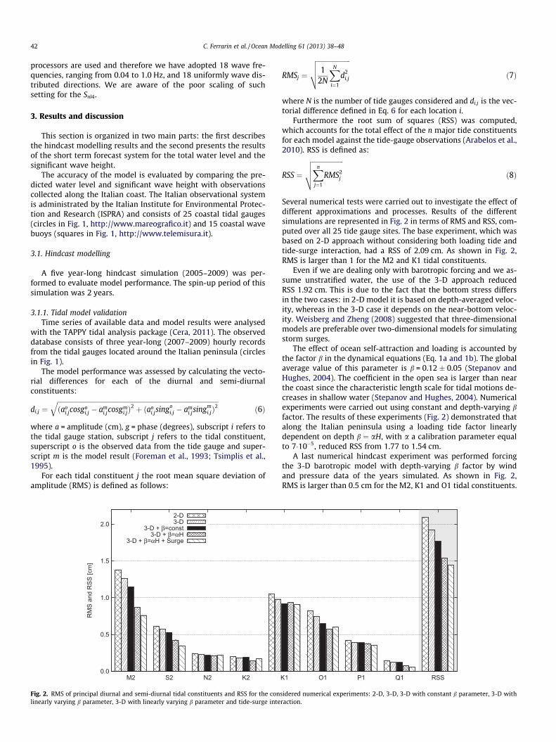
Several numerical tests were carried out to investigate the effect ofdifferent approximations and processes. Results of the differentsimulations are represented in Fig. 2 in terms of RMS and RSS, com-puted over all 25 tide gauge sites. The base experiment, which wasbased on 2-D approach without considering both loading tide andtide-surge interaction, had a RSS of 2.09 cm. As shown in Fig. 2,RMS is larger than 1 for the M2 and K1 tidal constituents.

Even if we are dealing only with barotropic forcing and we as-sume unstratified water, the use of the 3-D approach reducedRSS 1.92 cm. This is due to the fact that the bottom stress differsin the two cases: in 2-D model it is based on depth-averaged veloc-ity, whereas in the 3-D case it depends on the near-bottom veloc-ity. Weisberg and Zheng (2008) suggested that three-dimensionalmodels are preferable over two-dimensional models for simulatingstorm surges.

The effect of ocean self-attraction and loading is accounted bythe factor b in the dynamical equations (Eq. 1a and 1b). The globalaverage value of this parameter is b = 0.12 � 0.05 (Stepanov andHughes, 2004). The coefficient in the open sea is larger than nearthe coast since the characteristic length scale for tidal motions de-creases in shallow water (Stepanov and Hughes, 2004). Numericalexperiments were carried out using constant and depth-varying bfactor. The results of these experiments (Fig. 2) demonstrated thatalong the Italian peninsula using a loading tide factor linearlydependent on depth b ¼ aH, with a a calibration parameter equalto 7�10�5, reduced RSS from 1.77 to 1.54 cm.

A last numerical hindcast experiment was performed forcingthe 3-D barotropic model with depth-varying b factor by windand pressure data of the years simulated. As shown in Fig. 2,RMS is larger than 0.5 cm for the M2, K1 and O1 tidal constituents.

K1 O1 P1 Q1 RSS

sidered numerical experiments: 2-D, 3-D, 3-D with constant b parameter, 3-D withraction.

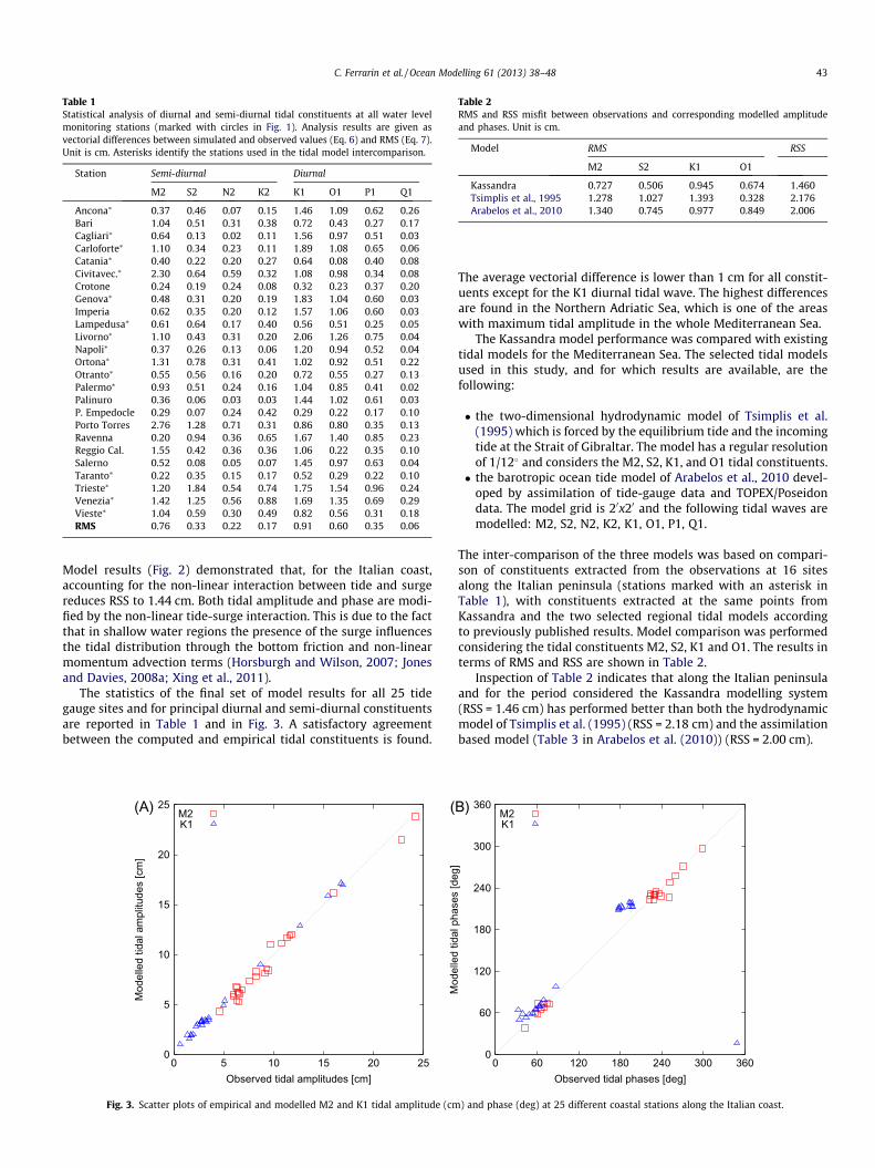
Table 1Statistical analysis of diurnal and semi-diurnal tidal constituents at all water levelmonitoring stations (marked with circles in Fig. 1). Analysis results are given asvectorial differences between simulated and observed values (Eq. 6) and RMS (Eq. 7).Unit is cm. Asterisks identify the stations used in the tidal model intercomparison.

Station Semi-diurnal Diurnal

M2 S2 N2 K2 K1 O1 P1 Q1

Ancona⁄ 0.37 0.46 0.07 0.15 1.46 1.09 0.62 0.26Bari 1.04 0.51 0.31 0.38 0.72 0.43 0.27 0.17Cagliari⁄ 0.64 0.13 0.02 0.11 1.56 0.97 0.51 0.03Carloforte⁄ 1.10 0.34 0.23 0.11 1.89 1.08 0.65 0.06Catania⁄ 0.40 0.22 0.20 0.27 0.64 0.08 0.40 0.08Civitavec.⁄ 2.30 0.64 0.59 0.32 1.08 0.98 0.34 0.08Crotone 0.24 0.19 0.24 0.08 0.32 0.23 0.37 0.20Genova⁄ 0.48 0.31 0.20 0.19 1.83 1.04 0.60 0.03Imperia 0.62 0.35 0.20 0.12 1.57 1.06 0.60 0.03Lampedusa⁄ 0.61 0.64 0.17 0.40 0.56 0.51 0.25 0.05Livorno⁄ 1.10 0.43 0.31 0.20 2.06 1.26 0.75 0.04Napoli⁄ 0.37 0.26 0.13 0.06 1.20 0.94 0.52 0.04Ortona⁄ 1.31 0.78 0.31 0.41 1.02 0.92 0.51 0.22Otranto⁄ 0.55 0.56 0.16 0.20 0.72 0.55 0.27 0.13Palermo⁄ 0.93 0.51 0.24 0.16 1.04 0.85 0.41 0.02Palinuro 0.36 0.06 0.03 0.03 1.44 1.02 0.61 0.03P. Empedocle 0.29 0.07 0.24 0.42 0.29 0.22 0.17 0.10Porto Torres 2.76 1.28 0.71 0.31 0.86 0.80 0.35 0.13Ravenna 0.20 0.94 0.36 0.65 1.67 1.40 0.85 0.23Reggio Cal. 1.55 0.42 0.36 0.36 1.06 0.22 0.35 0.10Salerno 0.52 0.08 0.05 0.07 1.45 0.97 0.63 0.04Taranto⁄ 0.22 0.35 0.15 0.17 0.52 0.29 0.22 0.10Trieste⁄ 1.20 1.84 0.54 0.74 1.75 1.54 0.96 0.24Venezia⁄ 1.42 1.25 0.56 0.88 1.69 1.35 0.69 0.29Vieste⁄ 1.04 0.59 0.30 0.49 0.82 0.56 0.31 0.18RMS 0.76 0.33 0.22 0.17 0.91 0.60 0.35 0.06

Table 2RMS and RSS misfit between observations and corresponding modelled amplitudeand phases. Unit is cm.

Model RMS RSS

M2 S2 K1 O1

Kassandra 0.727 0.506 0.945 0.674 1.460Tsimplis et al., 1995 1.278 1.027 1.393 0.328 2.176Arabelos et al., 2010 1.340 0.745 0.977 0.849 2.006

C. Ferrarin et al. / Ocean Modelling 61 (2013) 38–48 43

Model results (Fig. 2) demonstrated that, for the Italian coast,accounting for the non-linear interaction between tide and surgereduces RSS to 1.44 cm. Both tidal amplitude and phase are modi-fied by the non-linear tide-surge interaction. This is due to the factthat in shallow water regions the presence of the surge influencesthe tidal distribution through the bottom friction and non-linearmomentum advection terms (Horsburgh and Wilson, 2007; Jonesand Davies, 2008a; Xing et al., 2011).

The statistics of the final set of model results for all 25 tidegauge sites and for principal diurnal and semi-diurnal constituentsare reported in Table 1 and in Fig. 3. A satisfactory agreementbetween the computed and empirical tidal constituents is found.

0

5

10

15

20

25

0 5 10 15 20 25

Mod

elle

d tid

al a

mpl

itude

s [c

m]

Observed tidal amplitudes [cm]

(A) M2K1

(

Fig. 3. Scatter plots of empirical and modelled M2 and K1 tidal amplitude (cm

The average vectorial difference is lower than 1 cm for all constit-uents except for the K1 diurnal tidal wave. The highest differencesare found in the Northern Adriatic Sea, which is one of the areaswith maximum tidal amplitude in the whole Mediterranean Sea.

The Kassandra model performance was compared with existingtidal models for the Mediterranean Sea. The selected tidal modelsused in this study, and for which results are available, are thefollowing:

� the two-dimensional hydrodynamic model of Tsimplis et al.(1995) which is forced by the equilibrium tide and the incomingtide at the Strait of Gibraltar. The model has a regular resolutionof 1/12� and considers the M2, S2, K1, and O1 tidal constituents.� the barotropic ocean tide model of Arabelos et al., 2010 devel-

oped by assimilation of tide-gauge data and TOPEX/Poseidondata. The model grid is 20x20 and the following tidal waves aremodelled: M2, S2, N2, K2, K1, O1, P1, Q1.

The inter-comparison of the three models was based on compari-son of constituents extracted from the observations at 16 sitesalong the Italian peninsula (stations marked with an asterisk inTable 1), with constituents extracted at the same points fromKassandra and the two selected regional tidal models accordingto previously published results. Model comparison was performedconsidering the tidal constituents M2, S2, K1 and O1. The results interms of RMS and RSS are shown in Table 2.

Inspection of Table 2 indicates that along the Italian peninsulaand for the period considered the Kassandra modelling system(RSS = 1.46 cm) has performed better than both the hydrodynamicmodel of Tsimplis et al. (1995) (RSS = 2.18 cm) and the assimilationbased model (Table 3 in Arabelos et al. (2010)) (RSS = 2.00 cm).

0

60

120

180

240

300

360

0 60 120 180 240 300 360

Mod

elle

d tid

al p

hase

s [d

eg]

Observed tidal phases [deg]

B) M2K1

) and phase (deg) at 25 different coastal stations along the Italian coast.

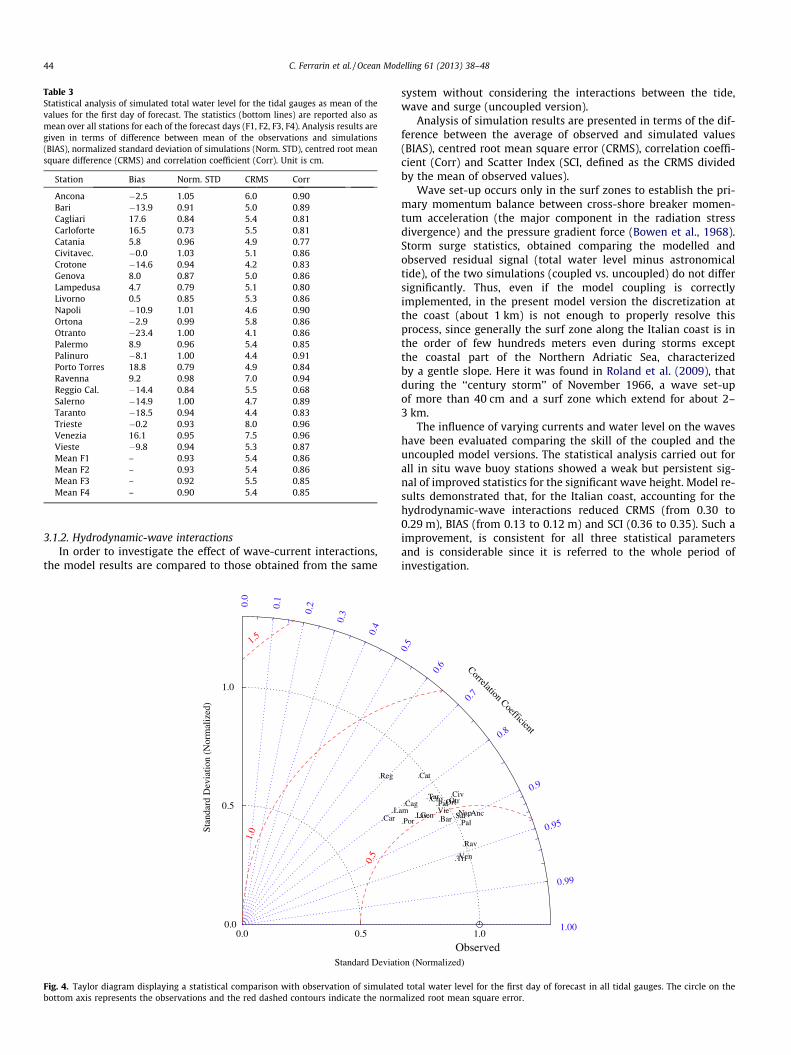
Table 3Statistical analysis of simulated total water level for the tidal gauges as mean of thevalues for the first day of forecast. The statistics (bottom lines) are reported also asmean over all stations for each of the forecast days (F1, F2, F3, F4). Analysis results aregiven in terms of difference between mean of the observations and simulations(BIAS), normalized standard deviation of simulations (Norm. STD), centred root meansquare difference (CRMS) and correlation coefficient (Corr). Unit is cm.

Station Bias Norm. STD CRMS Corr

Ancona �2.5 1.05 6.0 0.90Bari �13.9 0.91 5.0 0.89Cagliari 17.6 0.84 5.4 0.81Carloforte 16.5 0.73 5.5 0.81Catania 5.8 0.96 4.9 0.77Civitavec. �0.0 1.03 5.1 0.86Crotone �14.6 0.94 4.2 0.83Genova 8.0 0.87 5.0 0.86Lampedusa 4.7 0.79 5.1 0.80Livorno 0.5 0.85 5.3 0.86Napoli �10.9 1.01 4.6 0.90Ortona �2.9 0.99 5.8 0.86Otranto �23.4 1.00 4.1 0.86Palermo 8.9 0.96 5.4 0.85Palinuro �8.1 1.00 4.4 0.91Porto Torres 18.8 0.79 4.9 0.84Ravenna 9.2 0.98 7.0 0.94Reggio Cal. �14.4 0.84 5.5 0.68Salerno �14.9 1.00 4.7 0.89Taranto �18.5 0.94 4.4 0.83Trieste �0.2 0.93 8.0 0.96Venezia 16.1 0.95 7.5 0.96Vieste �9.8 0.94 5.3 0.87Mean F1 – 0.93 5.4 0.86Mean F2 – 0.93 5.4 0.86Mean F3 – 0.92 5.5 0.85Mean F4 – 0.90 5.4 0.85

44 C. Ferrarin et al. / Ocean Modelling 61 (2013) 38–48

3.1.2. Hydrodynamic-wave interactionsIn order to investigate the effect of wave-current interactions,

the model results are compared to those obtained from the same

0.00.0

0.5

0.5

1.0

0.1

0.2

0.3

0.4

0.0

0.5

1.0

1.5

Stan

dard

Dev

iatio

n (N

orm

aliz

ed)

Standard Deviati

.Car.L

.Reg

Fig. 4. Taylor diagram displaying a statistical comparison with observation of simulatebottom axis represents the observations and the red dashed contours indicate the norm

system without considering the interactions between the tide,wave and surge (uncoupled version).

Analysis of simulation results are presented in terms of the dif-ference between the average of observed and simulated values(BIAS), centred root mean square error (CRMS), correlation coeffi-cient (Corr) and Scatter Index (SCI, defined as the CRMS dividedby the mean of observed values).

Wave set-up occurs only in the surf zones to establish the pri-mary momentum balance between cross-shore breaker momen-tum acceleration (the major component in the radiation stressdivergence) and the pressure gradient force (Bowen et al., 1968).Storm surge statistics, obtained comparing the modelled andobserved residual signal (total water level minus astronomicaltide), of the two simulations (coupled vs. uncoupled) do not differsignificantly. Thus, even if the model coupling is correctlyimplemented, in the present model version the discretization atthe coast (about 1 km) is not enough to properly resolve thisprocess, since generally the surf zone along the Italian coast is inthe order of few hundreds meters even during storms exceptthe coastal part of the Northern Adriatic Sea, characterizedby a gentle slope. Here it was found in Roland et al. (2009), thatduring the ‘‘century storm’’ of November 1966, a wave set-upof more than 40 cm and a surf zone which extend for about 2–3 km.

The influence of varying currents and water level on the waveshave been evaluated comparing the skill of the coupled and theuncoupled model versions. The statistical analysis carried out forall in situ wave buoy stations showed a weak but persistent sig-nal of improved statistics for the significant wave height. Model re-sults demonstrated that, for the Italian coast, accounting for thehydrodynamic-wave interactions reduced CRMS (from 0.30 to0.29 m), BIAS (from 0.13 to 0.12 m) and SCI (0.36 to 0.35). Such aimprovement, is consistent for all three statistical parametersand is considerable since it is referred to the whole period ofinvestigation.

1.0

0.5

0.6

0.7

0.8

0.9

0.95

0.99

1.00

Correlation Coefficient

on (Normalized)

.Anc.Bar

.Cag

.Cat

.Civ.Cro

.Genam

.Liv .Nap.Ort.Otr.Pal

.Pal

.Rav

.Sal

.Tar

.Tri.Ven

.Vie.Por

Observed

d total water level for the first day of forecast in all tidal gauges. The circle on thealized root mean square error.

Table 4As Table 3 but for the significant wave height. Unit is m.

Station Bias Norm. STD CRMS Corr SCI

Alghero 0.06 0.92 0.29 0.96 0.28Ancona 0.08 0.95 0.19 0.90 0.34Cagliari 0.00 1.09 0.25 0.93 0.26Catania 0.07 0.93 0.20 0.92 0.31Cetraro 0.03 0.88 0.19 0.95 0.32Civitavec. 0.02 1.04 0.20 0.93 0.33Crotone 0.06 1.01 0.21 0.93 0.32La Spezia 0.10 0.98 0.26 0.93 0.35Mazara 0.03 0.98 0.20 0.95 0.25Monopoli 0.03 0.96 0.20 0.91 0.34Ortona 0.06 0.90 0.28 0.91 0.40Palermo 0.05 0.87 0.19 0.94 0.30Ponza 0.06 0.96 0.21 0.94 0.28Siniscola 0.01 0.95 0.16 0.91 0.29Venezia 0.00 1.00 0.24 0.83 0.55Mean F1 0.04 0.96 0.22 0.92 0.33Mean F2 0.05 0.96 0.25 0.90 0.37Mean F3 0.10 0.90 0.28 0.87 0.42Mean F4 0.15 0.81 0.33 0.82 0.48

C. Ferrarin et al. / Ocean Modelling 61 (2013) 38–48 45

3.2. Forecast modelling

The Kassandra forecasting system has been operational sinceFebruary 2011, hence almost one year of model results is availableat present for statistical analysis.

Model performance is graphically summarized through Taylordiagrams (Taylor, 2001). The position of each label on the graphrepresents a different model result and is determined by the valuesof the correlation coefficient and standard deviation. In the Taylordiagrams the statistics have been normalized by dividing both thecentred root mean square error and the standard deviation of themodel by the standard deviation of the observations. This proce-dure allows to plot together comparable statistical indexes for dif-ferent monitoring stations and for different fields. The perfect fit

0.00.0

0.5

0.5

1.0

0.1

0.2

0.3

0.4

0.0

0.5

1.0

1.5

Stan

dard

Dev

iatio

n (N

orm

aliz

ed)

Standard Deviati

Fig. 5. Taylor diagram as Fig. 4 but displaying a statistical comparison with observation

between model results and data is represented by a circle markon the x-axis at unit distance from the origin.

The statistics of the simulated water level are reported in Table3 and plotted in Fig. 4. On average, the total water level simulatedfor the first forecast day has a correlation of 0.86 and a CRMS of5.4 cm. The BIAS is highly varying along the Italian peninsula (from�24 to 18 cm) and could be partially attributed to the varyingAtlantic water level and to the sea level anomalies induced bythe thermohaline Mediterranean circulation which is not describedby the Kassandra barotropic model.

Model skill is high spatially varying over the considereddomain. Fig. 4 shows that in the Northern Adriatic Sea (stationsof Ravenna, Venezia, and Trieste) the model presents the bestagreement with the observations, with a correlation coefficientexceeding 0.94. These stations shows the highest correlationsand the lowest normalized CRMS (divided by the amplitude ofthe observations variation) because the Northern Adriatic Sea ischaracterized by water level oscillations higher than along theother Italian coasts. The contribution of the tidal signal relativeto the observed water level variance is more than 73% in the North-ern Adriatic Sea, while is about 30% in the Ionian Sea (the averageover the Italian peninsula is 44%).

The Kassandra modelling system is capable of producingaccurate forecasts of the wave field around the Italian peninsula.The results of the statistical analysis of the simulated significantwave height of the first day of forecast are reported in Table 4and graphically summarized by the Taylor diagram of Fig. 5.The model results compare reasonably well with the measure-ments, with a mean CRMS of 22 cm and a mean scatter indexof 0.33 (averaged over all stations). The correlation coefficientexceeds 0.90 in most of the stations (except Venezia) and theBIAS ranges from 0 to 10 cm. Wave model performance is com-parable with other existing wave forecasting systems operatingin the Mediterranean Sea (Bertotti and Cavaleri, 2009; Bertottiet al., 2011).

1.0

0.5

0.6

0.7

0.8

0.9

0.95

0.99

1.00

Correlation Coefficient

on (Normalized)

.Alg

.Anc .Cag

.Cat

.Cet

.Civ.Cro.La-

.Maz

.Mon.Ort

.Pal.Pon

.Sin

.Ven

Observed

of simulated significant wave height for the first day of forecast in all wave buoys.

0.00.0

0.5

0.5

1.0

1.0

0.1

0.2

0.3

0.4

0.5

0.6

0.7

0.8

0.9

0.95

0.99

1.00

0.0

0.5

1.0

1.5

Correlation Coefficient

Stan

dard

Dev

iatio

n (N

orm

aliz

ed)

Standard Deviation (Normalized)

..

..

W1

W2W3

W4. L1.

L2.L3.L4

Observed

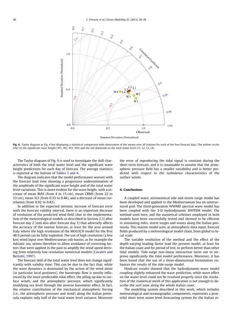
Fig. 6. Taylor diagram as Fig. 4 but displaying a statistical comparison with observation of the means over all stations for each of the four forecast days. The yellow circlesrefer to the significant wave height (W1, W2, W3, W4) and the red diamonds to the total water level (L1, L2, L3, L4).

46 C. Ferrarin et al. / Ocean Modelling 61 (2013) 38–48

The Taylor diagram of Fig. 6 is used to investigate the skill char-acteristics of both the total water level and the significant waveheight predictions for each day of forecast. The average statisticsis reported at the bottom of Tables 3 and 4.

The diagram indicates that the model performance worsen withthe forecast lead time showing a progressive underestimation ofthe amplitude of the significant wave height and of the total waterlevel variations. This is more evident for the wave height, with a in-crease of mean BIAS (from 4 to 15 cm), mean CRMS (from 22 to33 cm), mean SCI (from 0.33 to 0.48), and a decrease of mean cor-relation (from 0.92 to 0.82).

In addition to the expected intrinsic increase of forecast errorwith the forecast validity interval, there is an important decreaseof resolution of the predicted wind field (due to the implementa-tion of the meteorological models as described in Section 2.3) afterforecast day 2 (and also after forecast day 3) that adversely affectsthe accuracy of the marine forecast, at least for the area aroundItaly where the high resolution of the MOLOCH model for the first48 h period can be fully exploited. The use of high resolution (a fewkm) wind input over Mediterranean sub-basins, as for example theAdriatic sea, seems therefore to allow avoidance of correcting fac-tors that were applied in the past to amplify the wind speed deriv-ing from relatively low resolution numerical models (Cavaleri andBertotti, 1997).

The forecast skill of the total water level does not change signif-icantly with validity time. This can be due to the fact that, whilethe wave dynamics is dominated by the action of the wind alone(in particular local gustiness), the barotropic flow is mostly influ-enced by the more predictable tidal effect, the piling up due to sur-face winds, and the atmospheric pressure, which significantlymodifying sea level through the inverse barometer effect. In fact,the relative contribution of the mechanical atmospheric forcing(i.e., the atmospheric pressure and wind) along the Italian penin-sula explains only half of the total water level variance. Moreover

the error of reproducing the tidal signal is constant during theshort term forecast, and it is reasonable to assume that the atmo-spheric pressure field has a smaller variability and is better pre-dicted with respect to the turbulence characteristics of thesurface winds.

4. Conclusions

A coupled wave, astronomical tide and storm-surge model hasbeen developed and applied to the Mediterranean Sea on unstruc-tured grid. The third-generation WWMII spectral wave model hasbeen coupled with the 3-D hydrodynamic SHYFEM model. Themethod used here, and the numerical schemes employed in bothmodels have been successfully tested and showed to be efficientin simulating tides, storm surges and waves along the Italian pen-insula. This marine model uses, as atmospheric data input, forecastfields produced by a meteorological model chain, from global to lo-cal scale.

The variable resolution of the method and the effect of thedepth-varying loading factor lead the present model, at least forthe Italian coast and for period of test, to perform better than othertidal models. Tide-surge non-linear interaction turns out to im-prove significantly the tidal model performance. Moreover, it hasbeen found that the use of a three-dimensional formulation en-hances the results of the tide-surge model.

Hindcast results showed that the hydrodynamic-wave modelcoupling slightly enhanced the wave prediction, while wave effecton the water level could not be resolved properly since the resolu-tion of the numerical mesh of this application is not enough to de-scribe the surf zone along the whole Italian coast.

The modelling system described in this work, which includesmeteorological and oceanographic components, represents a pow-erful short term water level forecasting system for the Italian re-

C. Ferrarin et al. / Ocean Modelling 61 (2013) 38–48 47

gion. The high spatial resolution of the Kassandra system along theItalian peninsula, exploiting unprecedented high resolution mete-orological model input, allows the detailed description of the seawater level and the wave field. The developed model gives a signif-icant improvement in predicting the total water level along theItalian coastal area and represents a potentially useful tool inbathymetry and altimetry corrections. Even if the forecast skillfor the surge signal depends strongly on the range of the forecast,the total water level is less depended on it.

The short term storm surge forecasts of the Kassandra systemfor the whole Mediterranean are available at http://www.ismar.cn-r.it/kassandra. The operational model has been recently imple-mented also in the Black Sea. The implementation of thebaroclinic version of the model and the investigation of differentsurface wind stress parameterizations will be the subject of futurework.

Acknowledgements

The authors thank the Italian Institute for Environmental Pro-tection and Research (ISPRA) for providing water level and wavedata. Finally, the authors would like to thank Dr. Luigi Cavalerifor the critical review of the manuscript. This research was par-tially funded by RITMARE Flagship Project, funded by MIUR underthe NRP 2011-2013, approved by the CIPE Resolution 2/2011 of23.03.2011.

References

Arabelos, D.N., Papazachariou, D.Z., Contadakis, M.E., Spatalas, S.D., 2010. A new tidemodel for the Mediterranean Sea based on altimetry and tide gaugeassimilation. Ocean Sci. Discuss. 7, 1703–1737.

Ardhuin, F., Bertotti, L., Bidlot, J.-R., Cavaleri, L., Filipetto, V., Lefevre, J.-M.,Wittmann, P., 2007. Comparison of wind and wave measurements andmodels in the Western Mediterranean Sea. Ocean Eng. 34 (3–4), 526–541.

Bajo, M., Umgiesser, G., 2010. Storm surge forecast through a combination ofdynamic and neural network models. Ocean Modell. 33 (1–2), 1–9.

Bajo, M., Zampato, L., Umgiesser, G., Cucco, A., Canestrelli, P., 2007. A finite elementoperational model for storm surge prediction in Venice. Estuar Coast Shelf S. 75(1–2), 236–249.

Battjes, J.A., Janssen, J.P.F.M., 1978. Energy loss and set-up due to breaking ofrandom waves. In: Proceedings 16th International Conference Coastal Engineering,ASCE. pp. 569–587.

Bellafiore, D., Bucchignani, E., Gualdi, S., Carniel, S., Djurdjevi, V., Umgiesser, G.,2011. Evaluating meteorological climate model inputs to improve coastalhydrodynamic studies. Adv. Sci. Res. 6, 227–231.

Bertin, X., Bruneau, N., Breilh, J.-F., Fortunato, A.B., Karpytchev, M., 2012. Importanceof wave age and resonance in storm surges: The case Xynthia Bay of Biscay.Ocean Modell. 42, 16–30.

Bertotti, L., Cavaleri, L., 2009. Wind and wave predictions in the Adriatic Sea. J.Marine Syst. 78 (Supplement), S227–S234.

Bertotti, L., Bidlot, J.-R., Bunney, C., Cavaleri, L., Delli Passeri, L., Gomez, M., Lefèvre,J.-M., Paccagnella, T., Torrisi, L., Valentini, A., Vocino, A., 2011. Performance ofdifferent forecast systems in an exceptional storm in the WesternMediterranean Sea. Q. J. Roy. Meteor. Soc. 138, 34–55.

Blumberg, A., Mellor, G.L., 1987. A description of a three-dimensional coastal oceancirculation model. In: Heaps, N.S. (Ed.), Three-Dimensional Coastal OceanModels. American Geophysical Union, Washington, DC, pp. 1–16.

Bolaños, R., Osuna, P., Wolf, J., Monbaliu, J., Sanchez-Arcilla, A., 2011. Developmentof the POLCOMS-WAM current-wave model. Ocean Modell. 36 (1–2), 102–115.

Bowen, A.J., Inman, D.L., Simmons, V.P., 1968. Wave setdown and setup. J. Geophys.Res. 73, 2569–2577.

Brown, J.M., Wolf, J., 2009. Coupled wave and surge modelling for the eastern IrishSea and implications for model wind-stress. Continental Shelf Res. 29 (10),1329–1342.

Brown, J.M., Bolaños, R., Wolf, J., 2011. Impact assessment of advanced couplingfeatures in a tide-surge-wave model, POLCOMS-WAM, in a shallow waterapplication. J. Marine Syst. 87 (1), 13–24.

Burchard, H., Petersen, O., 1999. Models of turbulence in the marine environment –a comparative study of two equation turbulence models. J. Marine Syst. 21, 29–53.

Buzzi, A., Fantini, M., Malguzzi, P., Nerozzi, F., 1994. Validation of a limited areamodel in cases of Mediterranean cyclogenesis: surface fields and precipitationscores. Meteorol. Atmos. Phys. 53, 137–153.

Cavaleri, L., Bertotti, L., 1997. In search of the correct wind and wave fields in aminor basin. Mon. Weather Rev. 125 (8), 1964–1975.

Cavaleri, L., Bertotti, L., Buizza, R., Buzzi, A., Masato, V., Umgiesser, G., Zampieri, M.,2010. Predictability of extreme meteo-oceanographic events in the Adriatic Sea.Q. J. Roy. Meteor. Soc. 136, 400–413.

Cera, T.B., 2011. Tidal analysis program in python (TAPPY). Retrieved from <http://tappy.sourceforge.net>

Debreu, L., Marchesiello, P., Penven, P., Cambon, G., 2012. Two-way nesting in split-explicit ocean models: algorithms, implementation and validation. OceanModell. 49–50, 1–21.

de Vries, H., Breton, M., de Mulder, T., Krestenitis, Y., Ozer, J., Proctor, R., Ruddick, K.,Salomon, J.C., Voorrips, A., 1995. A comparison of 2d storm surge modelsapplied to three shallow european seas. Environ. Softw. 10 (1), 23–42.

Drofa, O.V., Malguzzi, P., 2004. Parameterization of microphysical processes in anon hydrostatic prediction model. In: Proceedings 14th InternationalConference on Clouds and Precipitation (ICCP). Bologna, 19–23 July 2004. pp.1297–3000.

Eldeberky, Y., 1996. Nonlinear Transformation of Wave Spectra in the NearshoreZone. Ph.D. thesis, TU-Deft, Delft, the Netherlands.

Foreman, M.G.G., Henry, R.F., Walters, R.A., Ballantyne, V.A., 1993. A finite elementmodel for tides and resonance along north coast of British Columbia. J. Geophys.Res. 98, 2509–2531.

Grant, W.D., Madsen, O.S., 1979. Combined wave and current interaction with arough bottom. J. Geophys. Res. 84, 1797–1808.

Hasselmann, S., Hasselmann, K., 1981. A symmetrical method of computing thenonlinear transfer in a gravity wave spectrum. Hamb. Geophys. EinzelSchr. A,52, 138.

Hasselmann, K., Barnett, T.P., Bouws, E., Cartwright, H.C.D., Enke, K., Ewing, J.A.,Gienapp, H., Hasselmann, D.E., Kruseman, P., Meerburg, A., Mqller, P., Olbers,D.J., Richter, K., Sell, W., Walden, H., 1973. Measurements of wind-wave growthand swell decay during the Joint North Sea Wave Project (JONSWAP). Tech. Rep.A8(12), Dtsch. Hydrogr Z., 1–95.

Horsburgh, K.J., Wilson, C., 2007. Tide-surge interaction and its role inthe distribution of surge residuals in the North Sea. J. Geophys. Res. 112,C08003.

Jones, J.E., Davies, A.M., 2008a. On the modification of tides in shallow waterregions by wind effects. Journal of Geophysical Research 113 (C05014),28pp.

Jones, J.E., Davies, A.M., 2008b. Storm surge computations for the west coast ofBritain using a finite element model (TELEMAC). Ocean Dyn. 58 (5–6),337–363.

Kain, J.S., 2004. The Kain–Fritsch convective parameterization: an update. J. Appl.Meteor. 43, 170–181.

Kantha, L.H., 1995. Barotropic tides in the global oceans from a nonlinear tidalmodel assimilating altimetric tides 1. Model description and results. J. Geophys.Res.100 (C12), 25, pp. 283–25, 309.

Kantha, L.H., Clayson, C.A., 2000. Numerical models of oceans and oceanic processes.Int. Geophys. 66.

Kim, S.Y., Yasuda, T., Mase, H., 2008. Numerical analysis of effects of tidal variationson storm surges and waves. Appl. Ocean Res. 30 (4), 311–322.

Lane, E., Walters, R., Gillibrand, P., Uddstrom, M., 2009. Operational forecasting ofsea level height using an unstructured grid ocean model. Ocean Modell. 28 (1–3), 88–96.

Lionello, P., Sanna, A., Elvini, E., Mufato, R., 2006. A data assimilation procedure foroperational prediction of storm surge in the northern adriatic sea. ContinentalShelf Res. 26 (4), 539–553.

Longuet-Higgins, M.S., Steward, R.W., 1964. Radiation stresses in water waves; aphysical discussion with applications. Deep-Sea Res. 11, 529–562.

Lyard, F., Lefevre, F., Letellier, T., Francis, O., 2006. Modelling the global ocean tides:modern insights from FES2004. Ocean Dyn. 56, 394–415.

Makin, V.K., Stam, M., 2003. New drag formulation in NEDWAM. Tech. Rep. TR-250,KNMI, pp. 16.

Malguzzi, P., Grossi, G., Buzzi, A., Ranzi, R., Buizza, R., 2006. The 1966 century floodin Italy: a meteorological and hydrological revisitation. J. Geophys. Res. 111,D24106.

Marcos, M., Tsimplis, M.N., Shaw, A.G.P., 2009. Sea level extremes in southernEurope. J. Geophys. Res. 144 (C01007), 16.

Marcos, M., Jordà, G., Gomis, D., Pérez, B., 2011. Changes in storm surges in southernEurope from a regional model under climate change scenarios. Global Planet.Change 77 (3–4), 116–128.

Moon, I.-J., Kwon, J.-I., Lee, J.-C., Shim, J.-S., Kang, S.K., Oh, I.S., Kwon, S.J., 2009. Effectof the surface wind stress parameterization on the storm surge modeling. OceanModell. 29 (2), 115–127.

Oddo, P., Pinardi, N., Zavatarelli, M., Colucelli, A., 2006. The adriatic basin forecastingsystem. Acta Adriatica 47 (Suppl), 169–184.

Olabarrieta, M., Warner, J.C., Armstrong, B., Zambon, J.B., He, R., 2012. Ocean-atmosphere dynamics during Hurricane Ida and Nor’Ida: an application of thecoupled ocean-atmosphere-wave-sediment transport (COAWST) modelingsystem. Ocean Modell. 43–44, 112–137.

Øyvind, S., Albretsen, J., Janssen, P.A.E.M., 2007. Sea-state-dependent momentumfluxes for ocean modeling. J. Phys. Oceanogr. 37, 2714–2725.

Richard, E., Buzzi, A., Zängl, G., 2007. Quantitative precipitation forecasting inmountainous regions: the advances achieved by the Mesoscale Alpineprogramme. Quart. J. Roy. Meteorol. Soc. 133, 831–846.

Roland, A., Cucco, A., Ferrarin, C., Hsu, T.-W., Liau, J.-M., Ou, S.-H., Umgiesser, G.,Zanke, U., 2009. On the development and verification of a 2d coupledwave-current model on unstructured meshes. J. Marine Syst. 78 (Supplement),S244–S254.

48 C. Ferrarin et al. / Ocean Modelling 61 (2013) 38–48

Sguazzero, P., Giommoni, A., Goldmann, A., 1972. An empirical model for theprediction of the sea level in Venice. Technical Report 25, IBM, Venice ScientificCenter.

Smagorinsky, J., 1963. General circulation experiments with the primitiveequations, I. The basic experiment. Monthly Weather Review 91, 99–152.

Smith, S., Banke, E., 1975. Variation of the sea surface drag coefficient with windspeed. Q. J. Roy. Meteorol. Soc. 101, 665–673.

Stepanov, V.N., Hughes, C.W., 2004. Parameterization of ocean self-attraction andloading in numerical models of the ocean circulation. J. Geophys. Res. 109,C03037.

Taylor, K.E., 2001. Summarizing multiple aspects of model performances in a singlediagram. J. Geophys. Res. 106, 7183–7192.

Tolman, H.L., 1991. A third generation model for wind waves on slowly varying,unsteady and inhomogeneous depths and currents. J. Phys. Oceanogr. 21, 782–797.

Tsimplis, M.N., Proctor, R., Flather, R.A., 1995. A two-dimensional tidal model for theMediterranean Sea. J. Geophys. Res. 100 (C8), 16, 223–16, 239.

Umgiesser, G., Bergamasco, A., 1995. Outline of a Primitive Equations Finite ElementModel. Rapporto e Studi, Istituto Veneto of Scienze, Lettere ed Arti XII, pp. 291–320.

Umgiesser, G., Melaku Canu, D., Cucco, A., Solidoro, C., 2004. A finite element modelfor the Venice Lagoon. Development, set up, calibration and validation. J. MarineSyst. 51, 123–145.

Wakelin, S.L., Proctor, R., 2002. The impact of meteorology on modelling stormsurges in the adriatic sea. Global Planet. Change 32, 97–119.

Walters, R.A., 2006. Design considerations for a finite element coastal ocean model.Ocean Modell. 15 (1–2), 90–100.

Weisberg, R.H., Zheng, L., 2008. Hurricane storm surge simulationscomparing three-dimensional with two-dimensional formulations based onan Ivan-like storm over the Tampa Bay, Florida region. J. Geophys. Res. 133(C12001).

Wolf, J., 2009. Coastal flooding: impacts of coupled wave-surge-tide models. Nat.Hazards 49 (2), 241–260.

Xia, H., Xia, Z., Zhu, L., 2004. Vertical variation in radiation stress and wave-inducedcurrent. Coastal Eng. 51, 309–321.

Xing, J., Jones, J.E., Davies, A.M., Hall, P., 2011. Modelling tide-surge interactioneffects using finite volume and finite element models of the Irish Sea. OceanDyn. 61 (8), 1137–1174.

Young, I.R., Sobey, R.J., 1985. Measurements of the wind-wave energy flux in anopposing wind. J. Fluid Mech. 151, 427–442.

Zampato, L., Umgiesser, G., Zecchetto, S., 2007. Sea level forecasting in Venicethrough high resolution meteorological fields. Estuar. Coast. Shelf Sci. 75 (1–2),223–235.

Zhang, Y., Baptista, A.M., 2008. SELFE: A semi-implicit Eulerian–Lagrangian finite-element model for cross-scale ocean circulation. Ocean Modell. 21 (3–4),71–96.