tiebreaker: certification and multiple credit ratings
TRANSCRIPT

Electronic copy available at: http://ssrn.com/abstract=1307782
Tiebreaker: Certification and Multiple Credit Ratings∗
DION BONGAERTS, K.J. MARTIJN CREMERS and WILLIAM N. GOETZMANN
ABSTRACT
This paper explores the economic role credit rating agencies play in the corporate bond market.
We consider three existing theories about multiple ratings: information production, rating shopping
and regulatory certification. Using differences in rating composition, default prediction and credit
spread changes, our evidence only supports regulatory certification. Marginal, additional credit
ratings are more likely to occur because of, and seem to matter primarily for regulatory purposes,
but do not seem to provide significant additional information related to credit quality.
Keywords: Credit Ratings, Credit Spreads
JEL: G12, G14, G24
∗Bongaerts is with Finance Group, RSM Erasmus University Rotterdam, and Cremers and Goetzmann are withInternational Center for Finance, Yale University. We would like to thank Patrick Behr, Michael Brennan, Mark Carlson,Erwin Charlier, Long Chen, Joost Driessen, Frank Fabozzi, Frank de Jong, Rik Frehen, Gary Gorton, Jean Helwege,Mark Huson, Ron Jongen, Pieter Klaassen, David Lesmond, Hamid Mehran, Catherine Nolan, Frank Packer, LudovicPhalippou, Paolo Porchia, Jorg Rocholl, Joao Santos, Joel Shapiro, Chester Spatt, Walter Stortelder, Dan Swanson,Anjan Thakor, Laura Veldkamp, Evert de Vries, Jacqueline Yen, Weina Zhang, and an anonymous referee as well asconference participants at the Financial Crisis conference at Pompeu Fabra University, the European Finance Associationannual meetings in Bergen (Norway, 2010), the Texas Finance Festival at UT Austin, the RMI conference at NationalUniversity of Singapore, the NBER meeting on Credit Ratings in Cambridge, the Conference on Credit Rating Agenciesat Humboldt University, the American Finance Association annual meetings in Denver (2011) and seminar participantsat University of Amsterdam, Rotterdam School of Management and the Dutch National Bank for helpful comments andinformation. We especially thank Campbell Harvey, an anonymous associate editor and an anonymous referee for manyhelpful comments and advice.

Electronic copy available at: http://ssrn.com/abstract=1307782
Credit Rating Agencies (CRAs) report information about the credit risk of fixed income securities.
The various ways the information is used by financial, legal and regulatory entities may potentially
influence the nature of the information production process. Bond ratings are not only used to assess
risk, they are also used for regulatory certification, e.g. to classify securities into investment grade (IG)
and high yield (HY, or junk) status. These classifications in turn influence institutional demand and
serve as bright-line triggers in corporate credit arrangements and regulatory oversight. Regulations may
mandate insurance companies and banks to keep much higher reserve capital for high yield issues than
for investment grade corporate bonds. Other institutions like pension funds and mutual funds are often
restricted by their charters in the amount of HY debt they can hold. Taken together, more than half of
all corporate bonds are held by institutions that are subject to rating-based restrictions on their holdings
of risky credit assets (Campbell and Taksler (2003)). Lower demand for high yield bond can significantly
increase the cost of borrowing for those issuers and is related to capital structure decisions (see Ellul,
Jotikasthira and Lundblad (2009), Kisgen and Strahan (2009), Kisgen (2006, 2009)). The institutional
and regulatory importance of credit ratings to issuers and investors has raised questions about whether
the current system provides the proper incentives for issuers to fully disclose value-relevant information,
and for investors to invest in research about credit risk.
Using a sample from 2000 - 2008, we document that almost all large, liquid US corporate bond
issues are rated by both S&P and Moody’s. Fitch typically plays the role of a ”third opinion” for large
bond issues1. During the time period the most prevalent institutional rule used for classifying rated
bonds was that, if an issue has two ratings, only the lower rating could be used to classify the issue (e.g.
into investment-grade or non-investment grade). However, for issues with three ratings, the middle
rating should be used (see, for example, the NAIC guidelines or the Basel II accord).2 Therefore, if
S&P and Moody’s ratings are on opposite sides of the investment grade boundary, the Fitch rating
(assuming it is the marginal, third rating) is the ’tie-breaker’ and will decide into which class the issue
falls. Moreover, this rule directly implies that adding a third rating cannot worsen the regulatory rating
classification, but could potentially lead to a higher one. Consistent with this option, we find that in
about 25% of Fitch rating additions, the addition leads to a regulatory rating improvement, i.e., the
resulting middle rating is higher than the lowest rating before the Fitch rating addition. Ex ante,
such an improvement would be particularly important when S&P and Moody’s ratings are on opposite
sides of the investment grade boundary. Absent the improving third rating, the split between S&P
and Moody’s would result in a classification of high yield. Thus, the value of the Fitch rating is that
1

Electronic copy available at: http://ssrn.com/abstract=1307782
it can only push the issue up into the investment grade category, not pull it down into the high yield
category.3
In this paper, we explore the nature of this tie-breaking role in the context of the broader question
of why corporate bonds generally have multiple credit ratings. We consider three hypotheses that could
lead to demand for multiple credit ratings, an ’information production’ hypothesis, a ’rating shopping’
hypothesis and a ’regulatory certification’ hypothesis. These are not mutually exclusive but they have
some different empirical implications that we exploit to shed light on their relative importance.
Under the information hypothesis, investors are averse to uncertainty, which is reduced by adding
extra ratings (see e.g. Guntay and Hackbarth (2010)). Under the rating shopping hypothesis, issuers
’shop’ for an additional rating in the hope of improving their rating (see e.g. Poon and Firth (2005),
Skreta and Veldkamp (2009), Sangiorgi, Sokobin and Spatt (2009)). Under the regulatory certification
hypothesis (see e.g. Brister, Kennedy and Liu (1994)), market and regulatory forces can naturally
arise from a need for credibly separating bond issues into two types: informationally sensitive and
non-informationally sensitive (Gorton and Pennacchi (1990) and Boot and Thakor (1993)). These
correspond to non-investment grade (also called high yield) and investment grade ratings, respectively.
If the regulatory certification role of CRA dominates, only the weaker issuers may need a third rating.
This leads us to investigate whether the option of a third rating leads to adverse selection effects. As
mentioned before, these hypotheses are not mutually exclusive. For example, rating shopping could be
more important and thus more prevalent around the HY-IG boundary.
We find the strongest evidence in favor of the regulatory certification hypothesis. First, we consider
what happens if a Fitch rating is added for bond issues at the IG/HY boundary, when Fitch could be
the tie-breaker and potentially move the bond issue into the IG class. The yield improves if Fitch rates
the issue IG, but there is no change following a HY rating, with a 40 basis point difference between an
IG and HY classification. This economically large difference suggests that the certification effect can
significantly lower the issuer’s cost of capital.
Second, Fitch rating additions or changes for issues that are not close to the HY-IG boundary do
not seem to be related to changes in yields. We find this not only for Fitch rating additions in a sample
of bond issues already rated by both Moody’s and S&P, but also for the full sample of all bonds and
using quarterly panel regressions of credit spread changes on rating updates made by Moody’s, S&P
and Fitch. In contrast, credit rating changes (especially downgrades) made by both Moody’s and S&P
2

are significantly associated with credit spread changes across the whole rating spectrum.
Third, Cox proportional hazard model regressions indicate that having and getting a Fitch rating
is positively associated with the potential to break the tie between Moody’s and S&P ratings, but again
only around the IG-HY boundary. Fourth and finally, comparing default predictions on a one year
horizon across credit rating agencies for corporate bonds rated by all three agencies over 2000 - 2008,
we find that Moody’s ratings perform best, immediately followed by S&P and then by Fitch. Ratings
by Moody’s and S&P add significant forecasting power to those of Fitch, whereas the reverse is not the
case. This is consistent with Fitch providing limited additional valuation information relative to that
contained in Moody’s and S&P ratings.
Thus, the credit spread change regressions provide no support for the information production
hypothesis; i.e. that the additional Fitch ratings provide significant information to investors. However,
further tests provide some suggestive evidence in support of the rating shopping hypothesis around the
HY-IG boundary for possible regulatory arbitrage, but not anywhere else. While the additional Fitch
rating tends to be more optimistic than pre-existing Moody’s and S&P ratings, investors do not seem
to incorporate such increased optimism by lowering credit spreads. This would undermine any rationale
to engage in rating shopping. However, we find that the additional Fitch rating is ”extra” optimistic
for issues rated just below IG or for those issues where Fitch is the tie-breaker around the IG-HY
boundary, i.e. more so than elsewhere on the rating spectrum. Those are exactly the issues where we
would expect rating shopping incentives to matter most. Specifically, if Moody’s and S&P ratings are
on opposite sides of the HY-IG boundary, the additional Fitch rating is more likely than otherwise to
lead to an improvement in the regulatory rating classification, which in this particular case means an
improvement from HY to IG classification (using ’the worst of 2 and median of 3 ratings applies’ rule).
This evidence is suggestive of rating shopping around the HY-IG boundary, or that the marginal rating
is used for regulatory arbitrage.4
Endogeneity is a significant concern in our study, as we rely on controlling for confounding variables
for identification. We seek to mitigate major selection issues by focusing on credit spread changes and
Fitch rating additions. We also directly estimate selection effects using the Cox proportional hazard
model to explain the time to add the third rating.
Taken together, our results suggest that a major function of Fitch ratings could be to avoid adverse
selection for intermediate quality corporate bonds (Gorton and Pennacchi (1990) and Boot and Thakor
3

(1993)). Relatively uninformed investors may be reluctant to trade bond issues where they may be
at a considerable information disadvantage, i.e. HY or junk issues. Investors specialized at producing
information might find it too costly to do so for medium quality issues, unless they can generate
profit from trading at an informational advantage with uninformed investors, This could lead to a no-
trade region for these intermediate quality bonds. An additional rating that give a clear signal about
whether research will yield relevant information (or whether relatively uninformed investors may be at
a disadvantage) could resolve such a no-trade region. The generally optimistic Fitch ratings may also
be requested as a precautionary measure. For example, issues rated by Fitch ratings are more likely to
have subsequent Moody’s and S&P rating transitions, suggesting that these issues have relatively less
stable ratings.
In the long run, a necessary condition for any credit rating agency to have credibility about the IG-
HY classification is that it produces and uses value-relevant information about the firm. A rubber-stamp
rating without research will not serve the certification purpose in the long run. If the regulatory emphasis
on credit ratings is reduced or regulation as to which rating should be used is tightened in the aftermath
of the recent credit crisis, the certification effect documented in this paper may become less pronounced.
In particular, our results suggest that fewer firms may opt for multiple ratings as a result, unless the
marginal CRA can convince the market that its ratings are useful not just for regulatory reasons but
also provide additional information about credit risk (and particularly about separating information-
sensitive from information-insensitive securities). Indeed, less regulatory emphasis on ratings may spur
increased competition among CRAs to improve their information production, especially around the
IG-HY boundary.
The remainder of the paper is organized as follows. Section I contains our motivation for the
empirical tests and the various hypotheses in light of the existing literature. In section II, we discuss
the sample construction and methodology. Section III presents the empirical results on the three
hypotheses. Section IV concludes.
4

I Motivation
A Credit Rating Agencies and Regulation
There are currently three major credit rating agencies (CRAs) in the U.S. market: S&P, Moody’s
and Fitch. In addition to these big three, there are seven smaller CRAs that issue credit ratings that
qualify for meeting regulatory standards. While the purpose of a credit rating is to reflect the credit-
worthiness of an issue or issuer, the rating agencies have some discretion in the philosophy underlying
their rating system and are not required to make their rating methodology public.5
CRAs are licensed as Nationally Recognized Statistical Rating Organizations (NRSRO) by the
Securities and Exchange Commission. This official designation has a number of effects. First, CRAs
are exempt from Regulation FD, allowing corporations to share value-relevant information with the
rating agency without disclosing it publicly. Second, the SEC designation allows credit ratings to be
used for meeting regulatory requirements that call for a minimum or an average rating value. For
example, the SEC requires that money market mutual funds hold instruments with a credit rating in
one of the two short-term higher credit rating categories.6 This effectively provides a ”safe harbor” for
money market mutual funds with respect to litigation over fund failures. Kisgen (2006) discusses the
strong link between short and long term debt ratings and access to the commercial paper market. He
concludes that in order to have access to the commercial paper market, typically a rating of BBB is
required.
US insurance companies explicitly rely on NRSRO ratings for determining risk-based capital. In
particular, bonds held by insurance companies are assigned capital charges based upon their credit
ratings. For example, a US life insurance company needs to hold over 3 times as much reserve capital
for a BB rated bond compared to a BBB rated bond. At the time of writing, European insurance
companies will soon be subject to comparable regulations with the implementation of ’Solvency II.’
Banking regulations enacted under the so-called ’Basel II accords’ impose very similar risk-based capital
requirements.7 Many pension funds and mutual funds are restricted from investing in non-investment
grade corporate bonds by their charter. Although there is much discussion about treating bank and
insurance assets in the context of their total portfolio that would take into account co-variance rather
than security-specific risk, as of mid-2010, a large portion of U.S. institutional portfolios are still subject
to rules and regulation tied to ratings by a relatively small number of NRSROs. The impact of such
5

rules and regulations on the functioning of the corporate bond market, in particular in determining
supply and demand, is almost certainly non-trivial since a vast majority of this market is dominated by
institutions that are subject to rating-related restrictions, either through explicit rules and regulations,
or through restrictions stated in their charters.8
In June, 2008, the SEC proposed eliminating language in many regulations pertaining to NRSROs,
and instead to allow an alternative decision-making function, perhaps recognizing that reliance on credit
ratings agencies had the potential to distort the information-gathering and investment decision-making
process. In addition, several other regulations were implemented to try to make rating agencies more
accountable and increase the transparency of the rating process. The motivation for these (proposed)
changes stemmed from the subprime mortgage crisis that began in 2007, and from concerns that the
top three CRAs may represent an oligopoly enabled by government regulation. Among other things,
the concern is that this oligopoly might not be the optimal mechanism for revealing information related
to the risk of fixed income securities, and instead might be used as an artificial safe-harbor to excuse
investment managers from exercising business judgment. As such, it could allow the CRAs to extract
rents from corporations by virtue of serving as ”gate-keepers” to the investment-grade (IG) rating,
especially as the CRAs are paid by the corporations whose bonds are rated. Moreover, competition
among CRAs could lead to a so called ”race to the bottom”, i.e. competition over deteriorating
standards to attract more customers. This is an often heard concern about the structured finance
market in the (subprime) mortgage crisis.
While all of the aforementioned issues are of a regulatory nature, the wider financial industry has
also grown increasingly dependent on CRAs. Financial institutions center self-regulation around credit
ratings, e.g. mutual funds stating in their charter to only invest in investment-grade (IG) quality fixed
income securities. Trading and internal risk management models often take credit ratings either as
primary or as calibration inputs. Many corporate credit arrangements, like collateral requirements and
haircuts are further driven by credit ratings. Moreover, ratings are an important factor in determining
whether a bond qualifies for inclusion in prominent corporate bond indices like the Barclays Capital
(formerly Lehman Brothers) US Corporate IG Index.9 Inclusion in such an index may greatly improve
the liquidity of an issue, since for example index tracking institutions will trade more in them. Several
papers show that a higher liquidity leads to lower credit spreads (see for example Chen, Lesmond and
Wei, 2007). Typically, these procedures tend to incorporate all (multiple) rating information available,
extending possible certification effects well beyond those resulting from financial regulation.
6

B Why Multiple Ratings Matter
In this subsection, we consider three different mechanisms that could lead firms to solicit and pay
for multiple ratings. We base these hypotheses also on empirical evidence provided by the previous liter-
ature, as summarized in the next subsection. The three hypotheses we consider are (i) the ”information
production” hypothesis, (ii) the ”rating shopping” hypothesis and (iii) the ”regulatory certification”
(or clientele, or regulation) hypothesis. Below, we will give a short description of each and discuss its
testable empirical predictions. As these hypotheses could co-exist and are generally not mutually exclu-
sive, we discuss both how they are related and how we can identify some differing empirical predictions
that allow us to distinguish which hypothesis may dominate empirically. These empirical predictions
are summarized in Table I.
First, the reason to apply for multiple ratings could be the need for increased information produc-
tion. More ratings can reduce uncertainty about the credit quality of the rated bonds. In a setting in
which each CRA relies on different kinds of information to rate bonds, multiple perspectives are advan-
tageous and reduce uncertainty about default probability. CRAs may specialize in evaluating particular
drivers of default and thus each may have some advantage that justifies its continued existence in the
marketplace. Thus, one would expect that issuers with greater ex-ante uncertainty are more likely to
apply for extra ratings, since the potential reduction of uncertainty is largest for them. Moreover, under
the information production hypothesis, an extra rating in agreement with the existing ratings would
reduce credit quality uncertainty and thereby lower credit spreads.
Second, the ”rating shopping” effect can arise in a setting in which CRAs do not perfectly agree or
there is considerably uncertainty about credit quality, while issuers may have better information about
their own credit quality. In this case, issuers can seek to maximize their average rating by soliciting
multiple bids or following a stopping rule that chooses the first rating agency whose rating equals or
exceeds the firm’s own assessment of quality. Applying for private ratings and making these public
only if favorable, or deciding which CRA to use based on advice from an investment bank that has
knowledge about (gaming) each CRA’s precise rating algorithms leads to similar patterns.
The rating shopping hypothesis thus predicts that issuers will only apply for any additional rating
if they think it will be an improvement. Therefore, additional ratings are on average better. Further, if
the issuer applies for an additional rating and this additional rating is an improvement, credit spreads
7

should go down. This can be either because the additional rating is actually closer to the firm’s true
credit quality or because it is not, but the market mistakenly takes the new rating at face value. In the
latter case, if the market is not fooled, there would be no incentive to engage in rating shopping.
The third explanation for multiple ratings is ”regulatory certification”. Financial regulation has
traditionally relied heavily on credit ratings to determine the suitability and riskiness of fixed income
investments. For instance, bond ratings are used to score the quality of bonds in the investment
portfolios of insurance companies and banks and regulatory capital reserve requirements are determined
by this score. Ratings are also important in the structured finance market, the commercial paper market,
and the overnight repo market. They are used to determine ”haircuts” at the discount window of the
central bank and for determining whether projects qualify for government assistance (see for example
the Basel Committee on Banking Supervision (2000)). They may be the basis for financial contracting
between private parties, as the world witnessed in the case of AIG’s rating downgrade that triggered
a need for increased collateral in its counterparty arrangements. This event underscores the enormous
potential impact of certification.
The most prominent distinction made in financial regulation as it pertains to credit ratings is
whether an issue, issuer or structured product is ”investment grade” (IG) or ”high yield” (HY). In
particular, the most prevalent institutional rule used for classifying rated bonds is that, if an issue
has two ratings, only the worse rating can be used to classify the issue into investment-grade or non-
investment grade. However, if an issue has three ratings, the middle rating is used (see for example the
NAIC guidelines or the Basel II accord).1011 Therefore, if S&P and Moody’s ratings are on opposite
sides of the investment grade boundary, the Fitch rating (assuming it is third rater) will decide into
which class the issue falls. This classification creates strong incentives for issuers trying to achieve
an investment grade rating. Thus, the IG-HY boundary is associated with a clear discontinuity in
institutional demand. Assuming a downward sloping demand curve, the lower demand for high yield
bond significantly increases the cost of borrowing for those issuers (see Ellul, Jotikasthira and Lundblad
(2010) and Kisgen and Strahan (2009)).12
Under the regulatory certification hypothesis, the principal value of a CRA which systematically
gives better ratings (i.e., in our data Fitch) than the other CRAs (i.e., Moody’s and S&P) is simply
that it helps satisfy the bright-line requirements of financial regulation. A rating from this CRA could
be requested by issuers for whom the extra rating might make them qualify for an IG classification.
8

In addition, issuers that consider themselves likely to experience a future downgrade from IG to HY
could opt for an extra rating for precautionary motives. This could lead to adverse selection effects, as
relatively weaker firms with higher credit spreads would then be more likely to apply for a Fitch rating.
Therefore, under the regulatory certification hypothesis, split ratings at the IG boundary by
Moody’s and S&P should give significant incentives to get an additional rating from Fitch. More-
over, an additional rating may provide a hedge against the regulatory and rule-based effects of possible
future rating downgrades, while also increasing the probability to reap regulatory benefits from up-
grades. This effect should be more pronounced for issuers expecting to have more volatile ratings over
time.
Gorton and Pennacchi (1990) and Boot and Thakor (1993) show that the information and regula-
tory certification hypotheses can be inherently related in a setting with two types of investors, in which
issues with a lower credit quality carry more uncertainty. Type I investors have a time-varying natural
demand for bonds and high research costs, and type II investors are without the natural demand but
have low research costs.13 Since type I investors are at an informational disadvantage relative to type
II investors, they will only invest in high credit quality securities for which the informational gain of
type II investors is small, i.e. in informationally insensitive assets, to avoid losses due to trading with
informed investors (see Gorton and Pennacchi (1990)). Typically, type II investors will provide liquid-
ity to this market to accommodate aggregate demand shocks. On the other end of the credit quality
spectrum, it is worthwhile for type II investors to generate the information needed.14 The region in the
middle could suffer from a market breakdown if Type II investors only make money if they could profit
from informed trading with type I investors (as in Boot and Thakor (1993)).15
The importance of regulatory certification could be in preventing a market breakdown for interme-
diate quality bonds. In this setting, credit ratings can restore trading by reducing the uncertainty about
the value of information. Ratings will not only yield information about credit quality, but also about the
profitability of research. If the conclusion is ”no substantial information benefit”, then type I investors
would invest and type II would not bother to research. If the conclusion is ”significant information
benefit”, then type I investors would not invest and type II investors would invest to hold the security.
The IG-HY boundary is the prime candidate for the location on the credit quality spectrum where the
unconditionally expected gains from informational trading offset the costs for acquiring information.
This setting thus explains how a certification effect could arise in equilibrium.
9

The regulatory certification and rating shopping hypotheses also have some possibly similar fea-
tures. In particular, while a rating shopping effect could be observed across the whole rating scale,
rating shopping incentives are likely strongest around the IG-HY boundary. Therefore, the distinction
between these two hypotheses merits discussion. The central prediction of rating shopping is that ad-
ditional ratings are, on average, optimistic relative to existing ratings. Thus, if rating shopping is most
important around the IG-HY boundary, the positive bias of the marginal rating should also be largest
there. In contrast, certification would give no reason to expect the additional CRA to be more positive
there as compared to other parts of the rating scale. Specifically, certification predicts that if Moody’s
and S&P ratings are on opposite sides of the IG-HY boundary, it is significantly more likely the issuer
pays for the (assumed marginal) Fitch rating. However, in contrast to the rating shopping hypothesis,
regulatory certification does not imply that this Fitch rating would be relatively (to Moody’s and S&P
ratings) more positive than Fitch ratings at other part of the rating scale.
Second, the expectation of future rating changes decreases incentives for rating shopping but in-
creases the importance for regulatory certification. Rating shopping is more worthwhile if investors
expect that ratings will remain relatively stable, as in that case credit rating improvements are less
likely to be undone or become redundant. Under the regulatory certification hypothesis, (future ex-
pected) rating volatility creates a strong precautionary motive, motivating issuers to get an additional
rating to hedge against any possible future downgrade below IG.16 For this reason, additional ratings
may be associated with adverse selection, as issuers expecting more negative credit news may be more
likely to apply for such precautionary, additional ratings.
Each of the three explanations of multiple ratings (information production, rating shopping and
regulatory certification) thus has distinct empirical predictions, though different explanations can co-
exist. There are potential differences in whether or not we would expect (i) credit spread effects of
agreeing ratings, (ii) credit spread effects of relatively optimistic ratings across the rating spectrum,
(iii) more uncertainty increasing the number of ratings and (iv) extra ratings when these could push
an issue into the IG category, (v) greater optimism of the additional rating around the boundary and
(vi) any positive or negative association between additional ratings and the likelihood of future rating
changes (see Table I for a summary).
[Table I about here]
Under information production, an additional rating that is in agreement with the prior ratings will
10

reduce uncertainty and thereby lower credit spreads, while more uncertainty would make an additional
rating more worthwhile and therefore lead to more ratings.
Under rating shopping, more uncertainty would again lead to more ratings since initial ratings will
err more often. Additional ratings are likely to be better and better ratings would lower the credit
spread.17 Time variation in ratings makes shopping less worthwhile since the preferred outcome will be
less stable.
Under regulatory certification, a better extra rating would only lead to a lower spread at the
boundary but unconditionally an additional rating could be a manifestation of adverse selection (only
weaker issuers take an extra rating) and consequently be associated with higher credit spreads. Higher
time variation in ratings will give rise to a rating-hedging incentive and thereby increase the probability
of having an extra rating even for issues that are not directly at the boundary.
C Related Research
As asset pricing relies fundamentally on the production and dissemination of information, and this
process is endogenously determined, the related literature is vast. CRAs are only one type of research
and information provider to the securities markets. Much of the academic literature about the role
of research and information providers has focused on equity analysts rather than CRAs rating corpo-
rate debt. Studies on the equity markets have addressed a broad range of questions about research
providers, ranging from whether analysts’ opinions convey value-relevant information, to whether con-
flicts of interest and personal, strategic considerations influence the nature of the information provided.
CRAs present a different institutional structure for analysis. While the same basic principles regarding
information production apply, CRAs have become integral to regulation pertaining to the credit market
(see also the discussion above).
Research about the role of CRAs is more limited. Theory has asked what role CRAs play in
the equilibrium pricing process. Boot, Milbourn and Schmeits (2006) highlight CRAs as a valuable
coordination device, in which CRAs provide little value-relevant information at the investment grade
boundary other than regulatory certification, but some useful valuation information about riskier issues.
Carlson and Hale (2005) point out that when each investor’s optimal strategy is dependent on the
strategy followed by other investors, the public rating provided by the rating agency can serve to
11

coordinate investor actions. Bannier and Tyrell (2006) introduce reputation and competition among
rating agencies. Under certain conditions, this will stimulate investors to search for private information
and will thus not only restore a unique equilibrium, but could even lead to a more efficient one.
Each of the three potential explanations for multiple ratings finds support in the existing academic
literature. On the issue of information production, a number of papers have looked at the effects of
rating changes on asset prices. For example, Kliger and Sarig (2000) use a refinement in the Moody’s
ratings system to show that rating changes channel information to the market that changes the value of
the debt. However, their results also suggest that this information leaves the aggregate company value
intact and thus only influences the value of the debt relative to the value of the equity. Guntay and
Hackbarth (2010) investigate the effect of analyst dispersion on credit spreads. They find that higher
analyst dispersion is associated with higher credit spreads and conclude that this is probably due to
cash flow uncertainty.
Jewell and Livingston (1999) investigate whether ratings differ systematically across rating agencies.
They find that the average Fitch rating is much better than Moody’s and S&P ratings, but that this
effect disappears once they restrict their sample to bonds only rated by all three CRAs. They also
investigate whether rating shopping takes place, but find no evidence. Covitz and Harrison (2003) look
at the trade-off that rating agencies face between income resulting from giving out favorable ratings and
expected future fees from customers resulting from reputation. They argue that reputation concerns
dominate and prevent CRAs from being ”bribed” by customers. Bannier, Behr and Guttler (2010),
like Poon (2003) and Poon and Firth (2005), investigate possible adverse selection and hold-up in the
context of CRA and issuer incentives when CRAs issue ratings on an unsolicited basis.18
Inspired by the financial crisis and the allegations addressed at CRAs, several recent theoretical
papers put forward models to motivate rating shopping. Skreta and Veldkamp (2009) develop a model
where incentives for rating shopping increase as the complexity of the products increases. Bolton,
Freixas and Shapiro (2009) show that naive investors in the market may give incentives to CRAs to
inflate their ratings and that in a duopoly, this gives extra incentives for rating shopping, which in turn
aggravates the problem. Sangiorgi, Sokobin and Spatt (2009) develop a theoretical model of rating
shopping and explore biases in ratings conditional upon heterogeneity across issuers in the extent to
which different raters agree.
In research most closely related to our own, Cantor and Packer (1997) also look for evidence of the
12

information effect, the shopping effect and the certification effect. They use issuer-level ratings data
for the year 1994 to understand the motivation for using a third rating agency, but do not use bond
price and yield data to evaluate the market effects and price implications of the third rating. Like our
paper, they find that the third CRA rating is systematically more optimistic. However, they fail to
find evidence that the use of a third CRA is motivated by information, rating shopping or certification
effects. Since the time of their study, bond price data has become more widely available for research.
This allows us to conduct more powerful tests of the market response to the additional rating, and to
understand in greater detail how market participants interpret and use ratings.
Another closely related paper is Becker and Milbourn (2009), which considers the impact of the
major growth in market share of Fitch since 1989. They find that more ”competition leads to lower
quality in the ratings market: the incumbent agencies produce more issuer-friendly and less informative
ratings when competition is stronger.” They explain this by applying the reputation model of Klein and
Leffler (1981), considering CRA incentives to invest in information production in order to improve their
reputation. First, such incentives would be weaker if future rents are diminished as a result of increased
competition. Second, if demand is more elastic with greater competition, this may force CRAs to spend
less on expensive information production or tempt them more responsive to issuer demands, potentially
inducing rating shopping.
Brister, Kennedy and Liu (1994) find evidence of a ”super-premium” in yields of junk bonds due
to regulation around the IG boundary. Based on only S&P rating data, they find that yields increase
disproportionally from a BBB to BB rating relative to the increase in default risk. Moreover, in a
recent paper, Kisgen and Strahan (2009) find that credit spreads change in the direction of a Dominion
bond rating after the accreditation of Dominion as an NRSRO. They also find that this effect is much
stronger around the IG boundary, indicating the importance of regulatory certification. Finally, Kisgen
(2006) and Kisgen (2009) investigate whether discrete rating boundaries influence capital structure
decisions before and after rating changes respectively. Kisgen (2006) finds indeed evidence of reduced
debt issuance when ratings are close to an up- or downgrade, suggesting that credit ratings directly affect
capital structure decisions in a way not incorporated by traditional capital structure theories. Moreover,
this effect is especially pronounced around the IG boundary. Kisgen (2009) finds that managers lower
leverage after a rating downgrade, suggesting that managers target credit ratings rather than debt levels
or leverage ratios. This effect is again more pronounced around the IG boundary.
13

With respect to the nature of the certification effect that we find, our research relates to earlier
work on security design. Gorton and Penacchi (1990) set up a model that incentivizes uninformed
investors to transform risky assets into information-sensitive and information-insensitive parts, where
for the latter category they can avoid losses due to trading with informed investors. Boot and Thakor
(1993), on the other hand, develop a model in which security issuers lower funding costs by making
informed trading more profitable. Our setup motivating the exploration of the regulatory certification
hypothesis uses key insights of both papers. In particular, the non-trading region in our setup is the
result of the absence of the uninformed investor, whereas the uninformed investor is needed to make
trading profitable for the informed investor.
II Sample Construction and Methodology
A Main Measures and Controls
We measure uncertainty or opaqueness by Analyst Dispersion of the firm’s earnings per share
or by the dispersion between Moody’s and S&P ratings (like the IG-HY barrier dummies, we also
require stability of the difference over at least 1 quarter).19 While rating dispersion is also a measure of
regulatory relevance, analyst dispersion is not, which will get us the required identification. We consider
two measures of rating dispersion: Notches of MSP Rating Dispersion, which is the absolute values of
the rating difference between Moody’s and S&P, and S&P and Moody’s Disagree, which is a dummy
equal to one if their ratings are not the same.
Our main measure for the importance of regulations pertaining to the IG-HY boundary is denoted
by Fitch could push IG, which is a dummy variable equal to one if Moody’s and S&P ratings are on
opposite sides of this boundary such that a Fitch rating would be decisive for the IG-HY classification.
In some regressions this measure is interacted with the outcome from Fitch.
To avoid spurious results due to omitted variables in our regressions, we correct for several issue and
issuer characteristics as well as for business cycle effects. On the issue level, we correct for callability
(using a dummy), size (offering size), and term structure effects (duration and convexity). On the
issuer level, we correct for credit risk (using the inputs of the Merton (1974) model, leverage and
volatility), profitability (ROA), systematic risk (equity beta) and tangibility of assets (PPE/total book
14

assets). Tangibility of assets is important since Moody’s is the only CRA that also incorporates expected
recovery in their ratings. We also include R&D intensity (R&D expenditure over book assets) as an
additional control. R&D intensity can be associated with several pricing mechanisms in the corporate
bond markets. For example, higher R&D industries may have higher growth opportunities and therefore
lower credit spreads. On the other hand, R&D projects tend to be riskier than normal projects,
which may increase credit risk. We will control for the aggregate effect. In the credit spread changes
regressions, we also include time fixed effects as controls for business cycle effects, since market wide
default probabilities, liquidity and risk premia are likely to vary with the business cycle.
B Data and Filters
For our main analysis, we use corporate bond pricing data from the TRACE database and merge
it with bond characteristic and rating data from FISD, equity data from CRSP, financial data from
Compustat Industrial Quarterly and analyst data from I/B/E/S. Our time series ranges from July 1st
2002 up to December 31st 2008.20 The TRACE data contain all trades in TRACE-eligible bonds by
NASD members that were disseminated to the public. The dissemination to the public happened in
phases, resulting in an expanding universe of bonds. A more comprehensive description of the TRACE
database as well as the dissemination process is given in Downing, Underwood and Xing (2005).
We apply several filters to our dataset to remove bonds with special features that we do not want
to consider, and to remove seemingly erroneous entries.21 Next, we use the FISD characteristics to
match the trades to bond characteristics using CUSIPs.22 We only use senior unsecured notes and
bonds. We discard all bonds that are exchangeable, putable, convertible or pay-in-kind, that have a
non-fixed coupon, that are subordinated, secured or guaranteed or are zero coupon bonds. Removing
callable bonds would reduce our sample substantially, so we leave those in, but correct for this feature
in our regressions using a dummy variable.
To diminish the impact of remaining data errors, we average the prices of all trades in each bond
by trading day. To reduce the effect of over-representation of very liquid bonds, we then make monthly
observations by only recording for each bond the last available daily average credit spread of every
month. We then construct quarterly observations by only looking at the last month every quarter. To
avoid issues with severe illiquidity and distressed debt as well as issues relating to non-linearity of credit
spreads with respect to rating scales, we remove all issues with an average (based on average Moody’s,
15

S&P) worse than B- (B3). For all bond trades in our sample, we calculate yields and credit spreads.
The benchmark rate that is used to construct credit spreads is based on an interpolation of the yields
of the two on-the-run government bonds bracketing the corporate bond with respect to duration.
Ratings data is obtained from FISD as provided by Mergent. The credit ratings data provider con-
firmed that due to changes in their data collecting procedures, the rating data before 2000 is incomplete.
This is illustrated by Figure 1, which shows the number of rated bond issues each quarter by Moody’s,
S&P and Fitch as well as the proportion of all bond issues in the sample rated by each of these CRAs
in a given quarter from 1994 - 2008. While the number of rated bond issues is steadily increasing over
time for all three CRAs, the sudden jump in the number of issues rated by S&P strongly suggests that
too many bond issues before 2000 have missing S&P ratings (i.e., issues had S&P ratings, but these are
missing from the database). Specifically, the percentage of all issues rated by S&P equals 58% at the
end of 1999 and jumps to 94% in 2000, and remains above 85% until the end of the sample. There is
likewise a significant, though smaller, jump in the percentage of bond issues rated by Fitch, from 29%
at the end of 1999 to 39% in 2000. As a result, for the analyses that do not require pricing data, we
use rating data from the second quarter of 2000 onwards. For our credit spread regressions the impact
of this will be minor, as TRACE only starts in the middle of 2002 and is dominated by data from 2004
onwards (when the number of bond issues contained in TRACE is greatly expanded).23
[Figure 1 about here]
We follow convention and use a numerical rating scale to convert ratings. Therefore, for Fitch
and S&P (with Moody’s rating between parentheses), the numerical scores corresponding to the rating
notches are, respectively, 1 for AAA (Aaa), 2 for AA+ (Aa1), 3 for AA (Aa2), 4 for AA- (Aa3), 5 for
A+ (A1), 6 for A (A2), 7 for A- (A3), 8 for BBB+ (Baa1), 9 for BBB (Baa2), 10 for BBB- (Baa3),
11 for BB+ (Ba1), 12 for BB (Ba2), 13 for BB- (Ba3), 14 for B+ (B1), 15 for B (B2) and 16 for B-
(B3). However, we will still refer to more optimistic ratings, i.e. implying lower bankruptcy likelihood,
as ’higher’ or ’better’ ratings.
Equity market data is obtained from CRSP. We calculate (rolling window) historical daily idiosyn-
cratic volatility and betas to the CRSP value-weighted index based on half a year of historical trading
data. An AR(1) filter is used to filter out bid-ask bounces in daily closing prices. For an observation
to be included, we need at least 111 return observations in the last half year.
16

Company data is obtained from Compustat Quarterly. We download data on firm size (total book
assets), debt (long and short term debt), profitability (earnings), tangibility of assets (PPE), R&D
spending (obtained from Compustat Annual, since usually reported in the annual only) and industry
(SIC code). From these data, we construct a leverage variable (total debt over total book assets), a
tangibility of assets variable (PPE/total book assets), an R&D spending variable (R&D expenses/total
book assets and a dummy for missing values) and a profitability variable (total earnings over total
assets). We also construct a ’SIC division’ variable that is defined as the division that the 2-digit SIC
belongs to. Observations with SIC codes 9100 to 9999 (Public Administration) are excluded because of
possible implicit government guarantees.
Analyst forecast data on the annual EPS are obtained from I/B/E/S. We download summary data
including number of analysts, standard deviation of forecasts, minimum and maximum forecast from
the unadjusted file. Following Guntay and Hackbarth (2010), we divide forecast dispersion measured
by analyst standard deviation by the share price to end up with dispersion per dollar invested.
We construct two samples with a quarterly frequency; a credit spread sample and a rating sample.
Because the rating sample does not require trade observations, this is a more inclusive panel, especially
for the less liquid bonds. Moreover, the period for which we have reliable data is also longer. Almost all
bonds in our final sample are rated by both Moody’s and S&P (see also Figure 1). Specifically, about
95% of all bonds in our database with at least 2 ratings are rated by both S&P and Moody’s. This
lack of cross-sectional variation in having an S&P or Moody’s rating means that we can only study the
implications for having Fitch as a third rating.
Accordingly, we remove from our sample all bond issues that do not have ratings from both S&P
and Moody’s. For this sample of bond issues rated by both Moody’s and S&P and using quarterly
observations for 2000-2008, about 68% of observations have a Fitch rating. As a result, the main
focus of our paper will be to consider the ’marginal’ role of Fitch ratings, while controlling for S&P
and Moody’s ratings. Table II presents summary statistics for the quarterly credit spread sample.
For completeness, Internet Appendix Table IA.I presents summary statistics for the quarterly ratings
sample. Figure 2 presents the average credit spreads over our sample by rating category. There is very
significant variation, especially starting the second half of 2007.
[Table II and Figure 2 about here]
17

III Empirical Results
A Rating Differences and Rating Information
Following Cantor and Packer (1997), we show that Fitch ratings are on average significantly more
optimistic than both Moody’s and S&P ratings for the same issue in the same quarter and present
the results in Table III and Figure 3. S&P is also, in general, more optimistic than Moody’s but the
difference is much smaller (both for the full sample and for the Fitch-rated sample alone).
[Table III and Figure 3 about here]
Next, we investigate the bond market reaction to the rating updates issued. We are most specifically
interested in the informational content of Fitch rating changes compared to the informational content of
Moody’s or S&P rating updates. To minimize issues relating to selection, we limit ourselves for this test
to the sample that is rated by all three CRAs. Table IV presents the results of regressing end-of-quarter
credit spread changes on dummy variables for these up- and downgrades for each CRA. All regressions
on credit spread changes in the paper use standard errors clustered by issuer (unless stated otherwise)
and include a large number of controls with time fixed effects.
[Table IV about here]
The credit spread change regressions in columns 1 - 3 of Table IV indicate that all CRAs appear
to be highly informative in single CRA specifications. However, in the joint specification in column
7, only S&P and Moody’s rating updates seem to contain relevant information associated with credit
spread changes. For example, Moody’s and S&P downgrades, respectively, are related to credit spread
increases of 8 and 17 basis points, respectively. However, Fitch rating updates are not statistically
significantly associated with changes in credit spreads. In joint significance tests, we can reject that
Fitch rating downgrade coefficients are equal to S&P or Moody’s rating downgrade coefficients, though
not for the equivalent rating upgrade coefficients. When we restrict ourselves to the upper end of the
rating spectrum (see column 5, using only issues with average rating of A- or better), Fitch seems to
contain no information even in the single CRA specification. We cannot reject that the reactions to
Fitch upgrades and downgrades are statistically different from each other in the presence of the up and
downgrades from the other CRAs, while we can for Moody’s and S&P (see Internet Appendix Table
IA.IX for these tests on Moody’s and S&P).
18

However, rating changes of Fitch at the IG boundary do matter, i.e. when Moody’s and S&P
ratings are on opposite sides of the IG-HY boundary and Fitch could be the tie-breaker and change the
classification of the bond issue into IG versus HY. Economically, the credit spread change associated
with Fitch changing the classification to IG rather than HY is about 49 basis points in the full sample
(column 4, p-value of 2.82%), about 41 basis points in a sample of bonds rated BBB+ or worse (column
6, p-value of 5.87%), and again about 41 basis points in the full sample controlling for Moody’s and S&P
rating updates (column 8, p-value of 6.07%). These results are consistent with a regulatory certification
effect and inconsistent with an information effect.
Table V presents regressions of price reactions to Fitch additions after the bond has been in our
sample for at least one quarter without a Fitch rating but with both Moody’s and S&P ratings. Here,
the sample consists of all issues rated by both Moody’s and S&P, and thus no longer conditions on
also having a Fitch rating as for the sample used for Table V. The subsequent table considers selection
directly in modeling the addition of a Fitch rating using Cox proportional hazard model regressions. If
selection effects were very strong, one could expect that the event of a Fitch addition by itself would be
associated with a change in credit spreads. For example, if adverse selection would lead only firms with
poorer prospects to request a (generally more optimistic) Fitch rating, we would expect to see a Fitch
rating addition to be associated with an increase in the credit spread. However, column 1 in Table V
indicates that a Fitch addition is not related to any change in credit spreads at all (coefficient of -2.28
basis points with a t-statistic of -0.65). This lack of any effect mitigates selection issues, although we
do find a mild adverse selection effect in a robustness test in Internet Appendix Table IA.6 where the
sample is restricted to the pre-crisis period.
[Table V about here]
Table V also fails to show any evidence in favor of an information production effect. When a Fitch
rating is added that confirms the average Moody’s and S&P rating, this does not lead to a significantly
lower credit spread (see columns 2 - 7). Neither does the interaction of the added Fitch rating with
measures of uncertainty show any significant effect (see column 6 with the Analyst Dispersion interaction
and column 7 with the ’Notches of MSP Rating Dispersion’ interaction). The negative (positive) sign
of a Fitch rating added that is better (worse) than the average Moody’s and S&P rating is consistent
with rating shopping and information production, but is not statistically significant. Likewise, the
coefficients on Fitch Added, Better and Fitch Added, Worse are not statistically different from each
19

other.
However, columns 3 - 5 provide strong evidence in favor of the regulatory certification hypothesis.
In the cases for which Moody’s and S&P ratings are on opposite sides of the IG-HY boundary, a Fitch
rating added that makes the issue qualify for IG is associated with a substantial drop in the credit
spread. The difference between Fitch classifying such bond issues as IG rather than HY is associated
with a difference in about 41 basis points (p-value of 3.23%) in the credit spread. This result is robust
to using either the whole sample or only issues with average Moody’s and S&P ratings between BBB+
and BB- (column 3 and 4, respectively) and to double clustering credit spread changes in both issuer
and time dimensions.24
B Adding a Fitch Rating
This section considers the selection of Fitch as the third rater (all bond issues in our sample
are restricted to be rated by both Moody’s and S&P). In Table VI, we use Cox proportional Hazard
regressions to model getting a Fitch rating, including variables that may be related to each of the three
hypotheses. In the Cox model, an ’exit’ is defined as the event of getting a Fitch rating. The Cox model
has the convenient property that one can focus on the relative rank of each subject in the cross-section
by ignoring the baseline hazard rate and optimizing the partial likelihood function only. The baseline
hazard rate can be separated out (as in any proportional hazard model), and therefore needs no specific
parametric form that can influence our results.
[Table VI about here]
In our analysis, we employ several proxies for information uncertainty: (i) the absolute difference
in number of notches difference between the Moody’s and S&P ratings and a dummy equal to one if the
S&P and Moody’s ratings are different, (ii) idiosyncratic volatility of daily stock returns, (iii) equity
analyst dispersion. We further include variables related to the relative importance of ratings, such as
leverage, firm size and issue offering size. A positive coefficient on the variables relating to information
uncertainty could be interpreted as evidence for information or rating shopping effects.
We investigate the certification effect by including the Fitch Could Break Tie dummy which equals
one if Moody’s and S&P ratings are on opposite sides of the IG-HY boundary. This approach exploits
the fact that regulations typically prescribe that if an issue has three ratings, the median rating should
20

be used to determine the issue’s rating, while the worst rating should be used if there are two ratings.
Therefore, if Moody’s and S&P ratings are on opposite sides of the IG-HY boundary, an additional Fitch
rating would be decisive about whether or not the issue becomes investment grade. As a robustness
check, we also include a dummy variable indicating whether Moody’s and S&P ratings are on opposite
sides of the A- boundary. The A- boundary obviously does not have the same regulatory importance
as the investment grade boundary, such that its coefficient would be expected to be insignificant.
Finally, we add several other controls that influence bond prices, such as rating group dummies
based on the average Moody’s and S&P ratings, whether the issue is redeemable, the maturity, liqui-
dation values (using proxies for fixed assets and R&D expenses), the maturity left and the square of
the maturity left, and always include industry dummies. Standard errors are again clustered by issuer.
The sample consists of all issues that are rated by both Moody’s and S&P over 2000 - 2008.
Empirically, we find that all the coefficients on variables related to uncertainty (i.e., analyst dis-
persion, idiosyncratic equity volatility and a dummy indicating Moody’s and S&P rating differences as
well as a variable measuring the size of the dispersion in notches) are either insignificant, or have the
wrong (i.e., negative) sign for an information or rating shopping effect. For example, we find that issues
with greater idiosyncratic volatility are less likely to get a Fitch rating, even though further information
production may be relatively useful for those issues. Thus, we find no support in the data for either
the information or the rating shopping effects.
On the other hand, column 1, 2 and 5 show that if an issue has Moody’s and S&P ratings on opposite
sides of the IG-HY boundary, the (conditional) likelihood that the issue gets a Fitch rating increases
considerably. The economic significance of the coefficient on Fitch could push IG is considerable. For
example, the coefficient of 0.717 in column 1 implies that issues where Fitch is the tie-breaker have
about twice (2.05 = exp(0.717)) the hazard rate, i.e. are about twice as likely to get a Fitch rating.
We interpret this as strong evidence in favor of a certification effect: it is precisely in those cases where
the marginal rating (i.e., Fitch) is decisive for the critical regulation classification of the bond issue into
investment and non-investment grade, that Fitch is much more likely to (be asked to) give a rating.
The downside of the Cox regression is that it basically discards any observations that already have
a Fitch rating, thereby ignoring some potentially useful information. Therefore, we try to corroborate
the results that regulatory certification is an important explanation for having a Fitch rating by directly
modeling having a Fitch rating using a logistic regression. Estimates of this regression can be found
21

in Internet Appendix Table IA.VII, which confirms that Fitch could push IG is strongly positively
associated with having a Fitch rating, while none of the three main measures of uncertainty provide
any evidence for the information production hypothesis. With a 12% higher probability to have a Fitch
rating if the other two CRAs split at the IG boundary, these results are also economically large. Internet
Appendix Table A.VIII shows that these results are robust with double clustering.
C CRA Performance
This subsection investigates the general performance of each CRA in default prediction. The main
purpose is to corroborate our previous finding that in general, Fitch rating changes or Fitch rating
additions are not associated with credit spread changes, unless Fitch is the tie-breaker around the IG-
HY boundary. If so, we would expect that Fitch rating differences to Moody’s and S&P ratings are
not significantly improving default prediction. We perform two tests. First, we run logistic regressions
of issue defaults on one-year lagged credit ratings. Second, we calculate accuracy ratios of the one-
year ahead default prediction (i.e., Gini coefficients) to measure rating performance of all three CRAs.
This method is also employed by the CRAs themselves for self-evaluation in their annual default study.
However, since sample periods and rated populations typically differ among CRAs, the self reported
results are not useful for comparative purposes.
The sample we use for this analysis is different from the sample we use for our other analysis.
Since defaults are relatively rare events, we maximize the size of our sample by incorporating as many
issues as possible. Therefore, we include bonds from issuers for which we have no Compustat, CRSP
or IBES data as well as bonds with ratings worse than B-/B3. We still restrict ourselves to only
senior unsecured US bonds in US dollars. As before, we exclude bonds that are putable, exchangeable,
convertible, perpetual, asset backed or floating rate. We collect ratings for all these bonds in FISD that
are rated by all three CRAs between 2000 and 2008 and can be matched with the Moody’s Default
Risk Services Corporate database containing issuer default events. To avoid over-weighting issuers with
many bonds outstanding that are likely to default at the same time, we weight each bond at each point
in time with the inverse of the number of bonds outstanding for its issuer. 25
Table VII shows the results of our default prediction study. Panel A shows that default prediction
is best for Moody’s and worst for Fitch. This ranking holds true in terms of the pseudo R2, as well as
to how much each CRA adds in default prediction relative to the others. First, we can compare the
22

pseudo R2 in flexible specifications with dummies for the various notched rating categories (i.e., AAA,
AA+, AA, AA-, and up to B-).26 The pseudo R2 for Moody’s is highest (37%, see column 1), followed
by S&P (33%, see column 3) and finally comes Fitch (32%, see column 5). In columns 2, 4 and 6, we
instead use a linear rating specification of the CRA ratings in notches, i.e., ’1’ corresponds to AAA, ’2’
to AAA-, etc. The resulting pseudo R2s are quite similar, with pseudo R2 of 37%, 33% and 31% for
Moody’s, S&P and Fitch, respectively, which suggests that the linear specification is quite reasonable.
[Table VII about here]
In subsequent columns, we compare different pairs of ratings: Moody’s and Fitch ratings in columns
7 - 8, S&P and Fitch ratings in columns 9 - 10 and Moody’s and S&P ratings in column 11 - 12. For
each comparison, we find pseudo R2 is not increased by adding the CRA with a lower pseudo R2 in
columns 1 - 6. For example, the pseudo R2 in columns 7 - 8 combining Moody’s and Fitch ratings equals
36.7%, basically identical to the pseudo R2 of Moody’s ratings by themselves of 36.6% in column 2 but
higher than the pseudo R2 of Fitch ratings by themselves of 30.8% in column 6. The difference between
Fitch and Moody’s ratings is further in insignificant in column 8, while it is significant in column 7.
Thus, a Moody’s rating adds predictive power to a Fitch rating while the reverse is not the case. We
show the same pattern in columns 9 and 10 for the comparison of Fitch with S&P. Taken together,
these results suggest that conditional on a Fitch rating, Moody’s or S&P ratings provide significant
additional information for default prediction one-year ahead, while the reverse is not the case.
Consistent with Panel A, the accuracy ratios (i.e., Gini coefficients) are highest for Moody’s and
lowest for Fitch. In Figure 4, we plot the cumulative fraction of default over the next year against the
cumulative fraction of ratings (from worst to best); this curve is also called a Cumulative Accuracy
Power curve (CAP-curve). Here, a smaller area in the upper left-hand corner of the graph implies
greater prediction accuracy. The accuracy ratios are the fractions of the areas underneath the plotted
lines minus the area under the 45 degree line multiplied by two, such that the accuracy ratio converges
to 1 as prediction accuracy improves and is equal to zero if ratings are assigned in a completely random
fashion. The graph shows that Fitch line is clearly below (and is thus worse than) the other two over
most of the rating spectrum.
[Figure 4 about here]
More formally, we find that accuracy ratio of Moody’s (77.9%) and S&P (76.5%) outperform Fitch
23

(71.8%), and that these differences are statistically significant. There is no statistical significant differ-
ence between Moody’s and S&P accuracy ratios (with standard errors calculated using a Jackknife with
re-sampling based on issuer). We conclude that these confirm the lack of support for the information
hypothesis in our data.27
D Further Explorations of Regulatory Certification and Rating Shopping
Arguably, rating shopping is more worthwhile around the IG boundary, thus leading to more
rating shopping at the boundary. On the other hand, under a certification effect, even for issuers at
the boundary that should not qualify for IG and thus expect a worse Fitch rating, the possibility of
achieving the IG status by sheer luck may be a motivation to apply for an additional Fitch rating.
Thus, at the boundary, one would expect more positive (optimistic) added Fitch ratings than elsewhere
in the rating spectrum if there is rating shopping.
As a proxy for the level of optimism in the additional, third Fitch rating, we consider whether or
not the additional Fitch rating leads to a regulatory gain, defined as the difference between ’worst of
two’ to ’medium of 3’ ratings.
Table VIII presents results of logistic regressions of regulatory gain on dummies indicating the
location of a bond in the rating spectrum. Observations are conditioned to have split ratings from
Moody’s and S&P as otherwise regulatory gain is impossible. The table provides some suggestive
evidence that the (additional) Fitch rating is more optimistic around the HY-IG boundary and thus
that some rating shopping might be going on around the IG-HY boundary.28
[Table VIII about here]
Moreover, the regulatory gain from the third, additional Fitch rating is largest if that Fitch rating
breaks the tie at the HY-IG boundary. If the Moody’s and S&P ratings are on opposite sides of the
HY-IG boundary, a regulatory gain is about 20% more likely (see columns 1 and 2). Fitch ratings being
generally more optimistic, the likelihood of a regulatory gain due to a Fitch rating addition in case
of Moody’s and S&P ratings disagreement is about 65% on average. As a result, this likelihood of a
regulatory gain climbs to about 85% if the Fitch rating could change the HY-IG regulatory classification
(controlling for everything else).
Next, one of the predictions in Table I was that of a precautionary extra rating. Given the
24

demand shock of being below the IG boundary, issuers may want to hedge the risk of becoming HY
by taking an extra rating due to a precautionary motive. Unfortunately, ratings are too persistent
to empirically estimate the frequency of rating changes reliably from the rating history. However,
due to data constraints and the forward looking nature of this effect, we can perform the analysis of
this precautionary effect the other way around, i.e. we estimate the association of the probability of
undergoing a future rating change with a dummy for having a Fitch rating and several controls for
opacity and volatility. The results can be found in Table IX. Indeed, we find that having future rating
changes is positively related to having a Fitch rating, over and beyond the usual measures of volatility
and opacity. Having a Fitch rating is associated with a quarterly transition probability that is 1.0% to
1.28% higher, which is economically sizable (Moody’s and S&P average transition frequencies are 5.2%
and 5.5% respectively).
[Table IX about here]
If the certification effect arises naturally in a setting with information sensitive and insensitive
investors, one would expect a very liquid IG market and an illiquid HY market. Moreover, issues
around the middle region should have a low liquidity that can be restored if Fitch makes an issue
qualify for information insensitive. However, if Fitch gives a HY rating, an issue at the boundary will
truly fall into the no-trade region and have an exceptionally low liquidity. Table X confirms these
predictions empirically. Bonds that qualify for HY based on their Moody’s and S&P rating have a
substantially lower turnover than those that qualify for IG. However, if Fitch pulls them into the IG
category, this effect is compensated. On the other hand, if Fitch could pull them into the IG category
but rather gives a HY rating, liquidity drops dramatically, even after correcting for issue and time fixed
effects as well as the on-the-run effect (corrected for by age).
[Table X about here]
IV Conclusion
Credit ratings play an important role in the capital markets. They are used by regulators and
market participants to establish capital requirements and, in a legal setting, to provide safe harbor for
fiduciaries. This widespread dependency upon credit ratings has the potential to influence how credit
rating agencies (CRAs) are used by issuers and how their ratings are evaluated by the market. A number
25

of theories have been proposed regarding how such dependency will affect the use of multiple CRAs,
the type of rating issued by CRAs depending upon their strategic position, and finally about how the
market interprets the informational output of rating agencies though the price formation process.
In this paper, we utilize bond issue credit ratings, characteristics and market prices to evaluate
some of these proposed theories. We test three hypotheses: (i) ”Information Production,” whether the
third rater adds value-relevant information, (ii) ”Rating Shopping” and (iii) ”Regulatory Certification,”
in particular whether a third agency plays the role of tie-breaker at the boundary of being classified
as investment-grade versus high-yield. The certification effect could arise naturally as an equilibrium
outcome in a setting with information-sensitive and insensitive investors and assets along the lines of
Gorton and Pennacchi (1990) and Boot and Thakor (1993). An extra rating indicating the potential
value to be gained from research could (partially) resolve a no-trade region around the IG-HY boundary.
Our empirical work contains several results. First, we find that significant differences exist across
multiple credit ratings of the same bond issue at the same point of time, with Fitch ratings on average
clearly more positive than Moody’s and S&P ratings. This is consistent with Fitch playing a strategic
role that reduces the threat that the other two CRAs could withhold investment-grade ratings and
extract compensation for regulatory certification, i.e., Fitch being available to push bonds into the
investment grade classification when the other two firms may disagree.
Bond price data reveal how the market regards a rating by the third agency. In general, credit
rating agencies provide useful information to the market about credit risk. However, we find no robust
evidence that Fitch ratings provide additional information incorporated in bond prices, relative to the
information already contained in the Moody’s and S&P ratings. Thus even though Fitch ratings are
on average clearly better (i.e. more optimistic) than Moody’s and S&P ratings, there seems little
information contained in these ratings that the bond market incorporates. This is inconsistent with
both the information and rating shopping hypotheses.
We find strong evidence that Fitch ratings have a regulatory certification effect. The likelihood of
getting a Fitch rating is strongly associated with Moody’s and S&P ratings being on opposite sides of
the investment grade boundary. This suggests that in equilibrium, Fitch ratings are sought as a kind
of ’tie-breaker’ in these cases. We find some suggestive evidence that Fitch ratings are relatively better
if the Fitch rating is decisive for the investment grade classification, as compared to all other Fitch
ratings. In particular, we find evidence that if Moody’s and S&P ratings are on opposite sides of the
26

HY-IG boundary, the additional Fitch rating is more likely than otherwise to lead to an improvement
in the regulatory rating classification, i.e., in this particular case to the IG classification. Overall, this
provides some evidence of rating shopping around the HY-IG boundary, or the marginal rating being
used for regulatory arbitrage.
In the cross-section of bond prices, we find that the certification effect is strongly associated with
credit spreads. Controlling for the average Moody’s and S&P rating, for issues where Moody’s and
S&P ratings are on opposite sides of the investment grade boundary, a Fitch rating pushing the issue
into the investment grade category has credit spreads that are about 41 basis points lower than if the
Fitch rating would push the issue into the high yield category. Moreover, bond issues experiencing
relatively many rating changes by Moody’s and S&P are more likely to have a Fitch rating, suggesting
a precautionary motive of getting a Fitch rating. These results combined with additional results on for
example the liquidity of the bonds are consistent with a third CRA arising as a tie-breaker in equilibrium
to resolve a no-trade region in a setting with information-sensitive and insensitive investors and assets.
References
Bannier, Christina E., Patrick Behr, and Andre Guttler, 2010, Rating opaque borrowers: why areunsolicited ratings lower?, Review of Finance, 14, 263-294.
Bannier, Christina E., and Marcel Tyrell, 2006, Modeling the Role of Credit Rating Agencies- Dothey Spark of Virtuous Circle?, Working Paper.
Basel Committee on Banking Supervision, 2000, Credit Ratings and Complementary Sources ofCredit Quality Information, Working Paper.
Becker, Bo and Todd T. Milbourn, 2008, Reputation and competition: evidence from the creditrating industry, Working Paper.
Bolton, Patrick, Xavier Freixas, and Joel Shapiro, 2009, The Credit Ratings Game, Working Paper
Boot, Arnoud W.A., Todd T. Milbourn, and Anjolein Schmeits, 2006, Credit Ratings as Coordi-nation Mechanisms, Review of Financial Studies, 19, 81-118.
Boot, Arnoud W.A. and Anjan V. Thakor, 1993, Security Design, Journal of Finance, 48, 1349-1378.
Brister, Bill M., Robert E. Kennedy, and Pu Liu, 1994, The Regulation Effect of Credit Ratingson Bond Interest Yield: The Case of Junk Bonds, Journal of Business Finance and Accounting, 21, 511- 531.
Campbell, John Y. and Glen Taksler, 2003, Volatility and Corporate Bond Yields, Journal ofFinance, 58, 2321-2349.
27

Cantor, Richard M., and Franck Packer, 1997, Differences in Opinion and Selection Bias in theCredit Rating Industry, Journal of Banking and Finance, 21, 1395-1417.
Carlson, Mark A. and Galina B. Hale, 2005, Courage to Capital? A Model of the Effects of RatingAgencies on Sovereign Debt Roll-over, Working Paper.
Chen, Long, David A. Lesmond, and Jason Z. Wei, 2007, Corporate Yield Spreads and BondLiquidity, Journal of Finance, 62, 119-149.
Covitz, Daniel M., and Paul Harrison, 2003, Testing Conflicts of Interest at Bond Rating Agencieswith Market Anticipation: Evidence that Reputation Incentives Dominate, Working Paper.
Downing, Christopher, Shane Underwood, and Yuhang Xing, 2005, Is liquidity risk priced in thecorporate bond market?, Working Paper.
Ellul, Andrew, Pab Jotikasthira, and Christian T. Lundblad, 2010, Regulatory Pressure and FireSales in the Corporate Bond Market, Working Paper.
Gorton, Gary B. and George G. Pennacchi, 1990, Financial Intermediaries and Liquidity Creation,Journal of Finance, 45, 49-72.
Guntay, Levent and Dirk Hackbarth, 2010, Corporate Bond Credit Spreads and Forecast Disper-sion, Journal of Banking and Finance, 34, 2328-2345.
Jewell, Jeff, and Miles Livingston, 1999, A Comparison of Bond Ratings from Moody’s, S&P andFitch, Financial Markets, Institutions and Instruments, 8 1-45.
Kisgen, Darren J., 2006, Credit Ratings and Capital Structure, Journal of Finance, 61, 1035-1072.
Kisgen, Darren J., 2009, Do Firms Target Credit Ratings or Leverage Levels, Journal of Financialand Quantitative Analysis, 44, 1323-1344.
Kisgen, Darren J. and Philip E. Strahan, 2009, Do Regulations Based on Credit Ratings Affect aFirm’s Cost of Capital?, Working Paper.
Klein, Benjamin and Keith B. Leffler, 1981, The Role of Market Forces in Assuring ContractualPerformance, Journal of Political Economy, 89, 615-641.
Kliger, Doron, and Oded Sarig, 2000, The Information Value of Bond Ratings, Journal of Finance,55, 2879-2902.
McFadden, Daniel, 1973, Conditional Logit Analysis of Qualitative Choice Behavior, in Zarembka,P., ed.: Frontiers in Econometrics (Academic Press), 105-142.
Partnoy, Frank, 2006, How and Why Credit Rating Agencies are Not Like Other Gatekeepers,Working Paper.
Poon, Winnie P. H., 2003, Are Unsolicited Ratings Downward Biased?, Journal of Banking andFinance, 27, 593-14.
Poon, Winnie P. H., and Firth, Michael, 2005, Are Unsolicited Credit Ratings lower? InternationalEvidence from Bank Ratings, Journal of Business Finance and Accounting, 32, 1741-771.
Sangiorgi, Francesco, Jonathan Sokobin and Chester Spatt, 2009, Credit-Rating Shopping, Selec-tion and the Equilibrium Structure of Ratings, Working Paper.
Skreta, Vasiliki and Laura Veldkamp, 2009, Ratings Shopping and Asset Complexity: A Theory ofRatings Inflation, Journal of Monetary Economics, 56, 678-695.
28

Notes
1For smaller corporate bond issues, Fitch is occasionally one of two raters. However, almost all bonds in our sample
are rated by both Moody’s and S&P (see also Figure 1). Specifically, about 95% of all bonds in our database with at
least 2 ratings are rated by both S&P and Moody’s. This lack of cross-sectional variation in having an S&P or Moody’s
rating means that we can only study the implications for having Fitch as a third rating. We remove from our sample all
bond issues that do not have ratings from both S&P and Moody’s. For this sample of bond issues rated by both Moody’s
and S&P and using quarterly observations for 2000-2008, about 60% of observations have a Fitch rating. As a result, the
main focus of our paper will be to consider the ’marginal’ role of Fitch ratings, while controlling for S&P and Moody’s
ratings. Throughout the paper, we only consider the three major Credit Rating Agencies (CRAs), ignoring all others, as
they are much smaller at this point.
2The National Association of Insurance Commissioners (NAIC) is the organization of state insurance regulators.
3For firms with split Moody’s and S&P ratings, 13% of Fitch additions are such boundary cases.
4There is some evidence that regulators are concerned about such ’ratings arbitrage.’ See e.g. proposals for the new
Basel II accord made in July 2008: ”If [an issue] has multiple ratings, the applicable rating would be the lowest rating. This
approach for determining the applicable rating differs from the New Accord. In the New Accord, if an exposure has two
ratings, a banking organization would apply the lower rating to the exposure to determine the risk weight. If an exposure
has three or more ratings, the banking organization would use the second lowest rating to risk weight the exposure. The
agencies believe that the proposed approach, which is designed to mitigate the potential for ratings arbitrage, more reliably
promotes safe and sound banking practices.” Source: http://www.occ.treas.gov/fr/fedregister/73fr43982.pdf.
5Indeed, some ratings have a point-in-time perspective, whereas others (including the three major CRAs) employ
a ’through-the-cycle’ vision. Similarly, while some rating agencies aim to reflect cross-sectional variation in default
probabilities (like S&P and Fitch), others aim to also incorporate loss given default and reflect dispersion in expected loss
(like Moody’s).
6This rule is likely to be revised in the future.
7See http://www.occ.treas.gov/law/basel.htm for an overview of legal and regulatory news pertaining to the Basel
accords from the Office of the Comptroller of the Currency (OCC).
8Campbell and Taksler (2003) report that about one third of all corporate bonds are held by insurance companies,
about 15% by pension and retirement funds, 5% to 10% by mutual funds and 5% by commercial banks; thus, approximately
60% of this market is held by institutions that qualify for ratings based constraints.
9The Barclays US corporate IG Index Factsheet is available at https://ecommerce.barcap.com/indices/index.dxml.
10Quoting the NAIC report: ”A security rated and monitored by two NRSROs is assigned the lowest of the two ratings.
A security rated by three or more NRSROs is ordered according to their NAIC equivalents and the rating falling second
lowest is selected, even if that rating is equal to that of the first lowest.” This report can be found at http://www.naic.org/
documents/committees_e_rating_agency_comdoc_naic_staff_report_use_of_ratings.doc. See also Basel Committee
29

on Banking Supervision (2000). If an issue has only one rating, that rating will be used. However, several regulations
prohibit institutional investors to invest in issues with only one rating.
11There have been some time series changes in NAIC regulations, but these changes not significantly affected the validity
of our ’tie-breaking’ assumption at any point in time, i.e., that the worst of two ratings or the medium of 3 ratings is
used for NAIC classifications. First, the NAIC issues its own ratings and 1994 to 2001 the Securities Valuation Office
(SVO) of the NAIC would assign an NAIC rating to each security. Anecdotal evidence suggests that the ratings from
CRAs were critical, but that the final decision was at the NAIC analyst’s discretion. In 2001 a Provisional Exemption
rule was introduced under which bonds with standard features would be assigned a NAIC 1 or NAIC2 rating (i.e,
allowing smaller capital charges than HY) automatically if at least one CRA would rate it A- or higher at least two
CRAs rate it BBB- or higher without the interference of an SVO analyst. Effectively, this came down to a middle
rating rule (see http://www.naic.org/documents/svo_research_SVO_jan01cc.pdf). Second, on January 1, 2004, the
NAIC implemented a Filing Exemption rule, stating that any issue rated by one or more CRAs would be assigned an
NAIC rating based on the CRA equivalent rating. In case of split ratings, the ’second best’ rating would be taken (see
http://www.naic.org/documents/svo_FE_FAQ.pdf). Third and finally, this ’second best’ rule was changed to a ’second
worst’ rule in 2007. However, both, the ’second best’ as well as the ’second worst’ rule effectively boil down to ’worst
of 2 if only 2 and medium of 3 ratings’ rule in view of the low market share of the other CRAs besides the big three.
Our contact within the NAIC SVO argued that these guidelines were in general well adhered to by the individual state
regulators.
12See further Chernenko and Sunderam (2009) on the effects of the market segmentation due to credit ratings on bond
issuance and investments.
13For simplicity, one could think about type I investors as commercial banks, insurance companies and pension funds,
where the natural demand for bonds stems from the random flow of deposits and claims, and type II investors as hedge
funds and proprietary trading desks.
14Type II investors do not suffer from the negative effect to utility due to uncertainty; if they need to trade due to
liquidity shocks, they trade amongst themselves on an equally informed basis.
15For type I investors, the losses due to informed trading prevent them from investing in this region; they realize that
they are at an information disadvantage and thus do not enter this market, while the limited gains for type II investors
do not make it worthwhile for them to produce costly information in this intermediate region.
16An alternative way to hedge is increasing the average maturity of their debt. However, this is costly since in this
region of the rating spectrum, the term structure of credit spreads is typically upward sloping.
17This is not necessarily true when a rating agency rates too optimistically, but if credit spreads do not decrease, there
seems to be no benefit and thus no reason for rating shopping.
18Adverse selection may explain why unsolicited ratings are on average worse than solicited ones. That is, firms that
receive a favorable unsolicited rating do not apply for a solicited rating anymore, whereas firms with an unfavorable unso-
licited rating pay for another (solicited) opinion. On the other, CRAs could create a holdup problem by underestimating
the creditworthiness of companies in their unsolicited ratings to prompt those companies to seek (improved) paid-for
30

solicited rating subsequently. The general conclusion of this literature is that for industrials unsolicited ratings are lower
than solicited ratings, and that this difference is largely due to adverse selection of debt issuers. There seems to be some
evidence for holdup by CRAs, but this is concentrated mainly on financials. Our dataset does not include information
on unsolicited ratings for US corporate bonds, so this paper does not address these findings directly. However, several
papers report a low incidence rate of unsolicited ratings, like for example Partnoy (2006), who estimates an incidence rate
of approximately 1%.
19To avoid capturing timing mismatches between (multiple) rating transitions, we require that any particular ratings
situation has existed for at least a quarter. This will also mitigate concerns about not correcting for credit watches and
credit outlooks (for these variables our data are too sparse to be useful). Time variation in ratings is hard to measure,
since ratings are rather persistent. Therefore, we do not explicitly include time variation in ratings as a variable in our
regressions but analyze the correlation between having a Fitch rating and the likelihood of experiencing rating changes.
20The TRACE database starts in July 2002.
21We remove all trades that include commission, have a settlement period of more than 5 days, and all trades that are
canceled. Trades that are corrected, we correct. Moreover, we remove all trades for which we have a negative reported
yield, since these will be mainly driven by implicit option premia in the yield. We also found trades with a settlement
date later than or equal to the maturity date and removed those bonds. Furthermore, we found several records that we
suspect to be duplicates, resulting from both parties involved in a trade reporting to the system. Thus, we filter out
duplicate trades that have identical prices, trading time and volume. Moreover, some of the yields changes are extremely
high or low. We remove trades with credit spreads of more than 1000 bps and credit spread changes of more than 500bps.
Finally, we deleted all issues with duration of less than 1 year.
22CUSIPs of non-exchange traded bonds do not change in case of mergers, acquisitions, etc (see http://www.cusip.com).
23FISD confirmed that from mid-2003 on, they have been using automated rating feeds from the CRAs, whereas before
that time these ratings were collected by hand, increasing the potential for data errors in the earlier period.
24As suggested by Cantor and Packer (1997), ratings by Fitch could be inflated. To address this issue, we repeat the
analysis of Table V where we correct all Fitch ratings by one notch (except for the tie breaking at the boundary). The
results can be found in Internet Appendix Table IA.II. These results are consistent with the results reported in Table V.
Furthermore, we show similar results in levels in Internet Appendix Table IA.IV, exploiting also observations that already
had a Fitch rating when they entered the sample. If anything, results are even stronger since an agreeing Fitch rating is
associated with a higher credit spread. The effect of certification is statistically and economically very similar. Finally,
one might be concerned that the large movements in credit spreads at the onset of the crisis might drive any of these
results. Internet Appendix Tables IA.V and A.VI (showing the results on the sample ending in June 2007) indicate that
this is not the case.
25That is, the weighting is done in a Weighted Least Squared sense.
26For all non-linear regressions in the paper we report McFadden (1973) Pseudo R2s.
27As a robustness check, we also investigate the predictive power of Fitch in case i) Moody’s and S&P disagree and ii)
31

when it breaks a tie at the IG/HY boundary. Results can be found in Internet Appendix Table A.III. For disagreements,
the additional predictive power of Fitch has the right sign, but is not significant at conventional levels. Also the tie-
breaking role around the IG/HY boundary does not yield any significant effect and has coefficients in the same direction
no matter whether Fitch pulls over or under the boundary.
28We thank our NBER discussant, Michael Brennan, for suggesting this test.
32

Table IEmpirical Predictions
The various empirical predictions of the three hypotheses are summarize in the table below, where ’−’indicates that the implication is not supported and ’+’ means it is supported.
Reason for multiple ratings Information
Production
Rating
Shopping
Regulatory
Certification
(i) Additional agreeing rating lowers credit spreads + − −
(ii) Additional relatively optimistic rating lowers
credit spreads (also away from IG-HY boundary)
+ + Only at IG
boundary
(iii) Uncertainty uniformly increases # of ratings + + possible
(iv) Additional rating especially if that could push
the issue to an investment grade classification
possible possible +
(v) Additional rating more optimistic (especially
around IG boundary)
− + Only for strate-
gic CRA
(vi) Additional rating associated with higher ex-
pected time variation in ratings
+ − +
33

Table IISummary Statistics for Credit Spreads Sample
The table presents summary statistics and a brief description for the sample of bonds issues that haveboth a Moody’s and an S&P rating in the quarterly credit spreads sample for 2002 - 2008.
Variable N Mean Std. Dev. Min Max ExplanationFitch Could Break Tie 44,366 0.032 0.18 0 1 Moodys and S&P on opposite
sides of the IG-HY boundaryFitch Rated 44,366 0.68 0.47 0 1 Rated by FitchFitch Rating 44,366 5.04 4.17 0 16 Fitch RatingMoodys Rating 44,366 7.33 3.6 1 18 Moody’s RatingS&P Rating 44,366 7.17 3.55 1 17 S&P RatingFitch makes IG 44,366 0.016 0.12 0 1 Fitch pulls IGFitch denies IG 44,366 0.0066 0.081 0 1 Fitch denies IGNotches of MSP RatingDispersion
44,366 0.43 0.69 0 12 Absolute value of MSP ratingdifference
Moodys Upgrade 44,366 0.027 0.16 0 1 Moody’s upgrade (common sam-ple)
Moodys Downgrade 44,366 0.034 0.18 0 1 Moody’s downgrade (commonsample)
S&P Upgrade 44,366 0.029 0.17 0 1 S&P upgrade (common sample)S&P Downgrade 44,366 0.038 0.19 0 1 S&P downgrade (common sam-
ple)Fitch Upgrade 44,366 0.017 0.13 0 1 Fitch upgrade (common sample)Fitch Downgrade 44,366 0.024 0.15 0 1 Fitch downgrade (common sam-
ple)Fitch Added, Better 44,366 0.0039 0.062 0 1 Fitch added and < MSPFitch Added, Equal 44,366 0.005 0.071 0 1 Fitch added and = MSPFitch Added, Worse 44,366 0.0003 0.017 0 1 Fitch added and > MSPCredit Spread 44,366 172.71 141.72 0.12 999.86 Credit spreadChange in Credit Spread 44,366 18.39 68.33 -478.36 498.42 Credit spread changeRedeemable 44,366 0.69 0.46 0 1 callableLog of Offering Amount 44,366 12.03 1.88 0 15.42 log offering amountDuration 44,366 6.32 3.72 1 18.91 durationIdios. Vol. 44,366 0.016 0.0084 0.0012 0.11 idiosyncratic stock volatilityLog of Total Assets 44,366 10.34 1.55 5.34 13.65 log of total assetsLeverage 44,366 0.34 0.17 0 5.77 leverageROA 44,366 0.014 0.02 -0.46 0.26 ROAPPE / Total Assets 44,196 0.36 0.24 0 0.95 PPE/total assetsR&D / Total Assets 44,366 0.012 0.023 0 0.23 R&D/total assetsR&D Missing 44,366 0.43 0.5 0 1 R&D missingAnalyst Dispersion 43,923 0.0033 0.013 0 1.1 analyst dispersionBeta 44,366 0.95 0.39 -0.25 4.21 equity betaConvexity 44,366 53.83 56.58 1 357.47 convexityTurnover 43,292 13.15 15.27 0.018 85.99 trading volume over offering,
times 1K
34

Table IIIAverage Rating Differences
Average rating differences for issues simultaneously rated by multiple CRAs, measured in rating notches,and split up by rating categories. Rating categories are defined by average Moody’s and S&P ratings.We follow convention and use the numerical rating scale to convert ratings. For Fitch and S&P (withMoody’s rating in parentheses), the numerical scores corresponding to the rating notches are, respec-tively, 1 for AAA (Aaa), 2 for AA+ (Aa1), 3 for AA (Aa2), 4 for AA- (Aa3), 5 for A+ (A1), 6 for A(A2), 7 for A- (A3), 8 for BBB+ (Baa1), 9 for BBB (Baa2), 10 for BBB- (Baa3), 11 for BB+ (Ba1),12 for BB (Ba2), 13 for BB- (Ba3), 14 for B+ (B1), 15 for B (B2) and 16 for B- (B3). Therefore, anegative number means that the first mentioned rating agency gives on average a better rating thanthe other CRA in that comparison. Quarterly data for 2000-2008 are used. t-statistics based on robuststandard errors clustered by issuer are in brackets. *, ** and *** indicate statistical significance at the10%, 5% and 1% level, respectively.
Fitch vs. Fitch vs. Moody’s vs. S&P Moody’s vs. S&PAll Bonds Moody’s S&P (Fitch rated sample) (full sample)
Difference -0.538*** -0.397*** 0.154*** 0.185***[-5.57] [-3.99] [2.79] [4.41]
N 70,624 70,747 70,738 104,435N. issuers 450 449 452 818
AAA to AA-Difference -0.111 -0.118 0.0217 0.0415
[-1.53] [-0.98] [0.14] [0.47]N 3,557 3,549 3,601 8,619N. issuers 37 37 37 57
A+ to A-Difference -0.751*** -0.599*** 0.165* 0.203***
[-5.85] [-4.63] [1.80] [2.68]N 36,461 36,539 36,532 48,905N. issuers 232 232 233 475
BBB+ to BBB-Difference -0.294*** -0.223*** 0.072 0.117**
[-5.03] [-3.82] [1.11] [2.42]N 24,177 24,193 24,186 36,841N. issuers 277 278 276 451
BB+ to BB-Difference -0.492*** -0.0574 0.478*** 0.471***
[-4.76] [-0.35] [3.30] [4.71]N 6,429 6,466 6,419 10,070N. issuers 165 163 165 295
B+ to B-Difference -0.800*** -0.457** 0.369* 0.430***
[-6.80] [-2.46] [1.82] [3.20]N 3,279 3,272 3,282 6,200N. issuers 98 98 99 268
35

Tab
leIV
Ch
ange
inC
red
itS
pre
ads
and
Rat
ing
Ch
ange
s
Usi
ngqu
arte
rly
pane
ldat
abe
twee
n20
02an
d20
08,w
ere
gres
sch
ange
sin
cred
itsp
read
sfo
rA
AA
toB
-rat
edbo
nds
that
are
rate
dby
all
thre
eC
RA
son
rati
ngup
-an
ddo
wng
rade
sfo
ral
lthr
eeC
RA
s,ch
ange
sin
bond
and
firm
char
acte
rist
ics,
dum
mie
sfo
rbo
unda
ryeff
ects
and
tim
efix
edeff
ects
.U
p-an
ddo
wng
rade
sar
eco
ded
asdu
mm
ies
indi
cati
ngw
heth
erea
chof
the
thre
eC
RA
sup
grad
edor
dow
ngra
ded
its
rati
ng.
The
follo
win
gfir
man
dbo
ndco
ntro
lsar
ein
clud
edbu
tno
tsh
own
(all
inch
ange
s):
Lev
erag
e,liq
uida
tion
/int
rins
icva
lue
(PP
E/t
otal
asse
ts),
R&
Dex
pens
es(d
ivid
edby
tota
las
sets
),R
OA
(ret
urn
onas
sets
),da
ilyid
iosy
ncra
tic
equi
tyvo
lati
lity,
His
tori
cal
Equ
ity
Bet
a(h
alf
year
daily
corr
ecte
dfo
rB
id-A
sk-b
ounc
es),
Log
Tot
alA
sset
s(fi
rmsi
ze,
book
valu
e)an
dL
ogO
fferi
ngSi
ze(i
ssue
size
),R
edee
mab
le(d
umm
yfo
rca
llabi
lity)
,D
urat
ion
and
Con
vexi
ty.
Fit
chU
pgra
de,
Bre
aks
Tie
isa
dum
my
indi
cati
ngth
ata
Fit
chup
grad
em
ade
the
issu
equ
alify
for
IG,
whi
leF
itch
Dow
ngra
de,
Bre
aks
Tie
isa
dum
my
indi
cati
ngth
ata
Fit
chdo
wng
rade
mad
eth
eis
sue
lose
its
IGqu
alifi
cati
on.
Fit
chC
ould
Bre
akT
ieis
adu
mm
yin
dica
ting
that
the
S&P
and
Moo
dy’s
rati
ngs
are
onop
posi
tesi
des
ofth
eIG
-HY
boun
dary
.C
olum
n(5
)is
rest
rict
edto
issu
esra
ted
A-
orbe
tter
byM
oody
’san
dS&
P,w
here
asco
lum
n(6
)is
rest
rict
edto
issu
esra
ted
BB
B+
orw
orse
byM
oody
’san
dS&
P.t-
stat
isti
csar
ein
brac
kets
(usi
ngro
bust
stan
dard
erro
rscl
uste
red
byis
suer
;N
.is
suer
give
sth
enu
mbe
rof
issu
ers)
.*,
**an
d**
*in
dica
tesi
gnifi
canc
eat
the
10%
,5%
and
1%le
vel,
resp
ecti
vely
.’F
-tes
tFu
p=F
dow
n(p
-val
ue)’
give
sth
ep-v
alue
for
the
coeffi
cien
tson
Fit
chU
pgra
dean
dF
itch
Dow
ngra
debe
ing
equa
l,w
hile
’F-t
est
Fup,
tie=
Fdo
wn,
tie
(p-v
alue
)’gi
ves
the
p-v
alue
for
the
F-t
est
ofth
eco
effici
ents
onF
itch
Upg
rade
d,B
reak
sT
iean
dF
itch
Dow
ngra
ded,
Bre
aks
Tie
bein
geq
ual.
(1)
(2)
(3)
(4)
(5)
(6)
(7)
(8)
Moo
dy’s
Upg
rade
-4.5
01**
-2.3
69-3
.125
[-1.
97]
[-1.
11]
[-1.
47]
Moo
dy’s
Dow
ngra
de14
.19*
**7.
385*
7.57
5**
[4.0
0][1
.96]
[2.1
0]S&
PU
pgra
de-5
.594
**-4
.312
-4.4
23[-
2.07
][-
1.62
][-
1.59
]S&
PD
owng
rade
22.3
4***
18.7
5***
17.3
2***
[5.2
5][4
.26]
[4.4
3]F
itch
Upg
rade
-6.4
63**
-5.6
12*
6.97
5-8
.209
***
-4.8
07-3
.892
[-2.
10]
[-1.
83]
[0.5
9][-
2.70
][-
1.59
][-
1.30
]F
itch
Dow
ngra
de12
.98*
*10
.52*
*-0
.595
22.3
0***
4.59
62.
875
[2.4
6][1
.99]
[-0.
26]
[4.0
0][0
.80]
[0.4
9]F
itch
Upg
rade
,Bre
aks
Tie
-17.
59-1
6.26
-14.
94[-
1.18
][-
1.11
][-
1.03
]F
itch
Dow
ngra
de,
Bre
aks
31.5
3*24
.67
26.6
5T
ie[1
.76]
[1.4
5][1
.49]
Con
tinu
edon
next
page
36

Tab
leIV
–co
nti
nu
edfr
omp
revio
us
pag
e
(1)
(2)
(3)
(4)
(5)
(6)
(7)
(8)
Fit
chC
ould
Bre
akT
ie13
.81*
*9.
475*
13.3
3**
[2.3
9][1
.75]
[2.4
8]La
gged
Cre
dit
Spre
ad-0
.253
***
-0.2
58**
*-0
.251
***
-0.2
53**
*-0
.400
***
-0.2
55**
*-0
.259
***
-0.2
61**
*C
hang
e[-
11.0
7][-
11.7
1][-
11.0
8][-
11.4
8][-
15.0
2][-
10.7
2][-
11.7
2][-
12.0
1]
Sam
ple
All
All
All
All
≤A
-≥
BB
B+
All
All
N24
,282
24,2
8224
,282
24,2
8211
,330
12,9
5224
,282
24,2
82A
dj.
R2
0.53
10.
533
0.53
10.
533
0.45
0.60
50.
534
0.53
6N
.is
suer
s38
038
038
038
011
731
338
038
0F
-tes
tFu
p=F
dow
n0.
15%
0.80
%56
.30%
0.00
%15
.00%
30.8
0%(p
-val
ue)
F-t
est
Fup,
tie=
Fdo
wn,
tie
(p-v
alue
)2.
82%
5.87
%6.
07%
37

Tab
leV
Cre
dit
Sp
read
Reg
ress
ion
son
Fit
chR
atin
gA
dd
itio
ns
Usi
ngqu
arte
rly
pane
ldat
abe
twee
n20
02an
d20
08,w
ere
gres
sch
ange
sin
cred
itsp
read
sfo
rA
AA
toB
-ra
ted
bond
sth
atar
era
ted
byM
oody
’san
dS&
Pon
rati
ngad
diti
ons
from
Fit
ch,
the
rela
tive
rank
ing
ofth
ose
addi
tion
san
dw
heth
erad
diti
ons
happ
ened
atth
eIG
boun
dary
,in
tera
ctio
nsw
ith
unce
rtai
nty
mea
sure
san
dch
ange
sin
bond
and
firm
char
acte
rist
ics
plus
tim
efix
edeff
ects
.F
itch
Add
ed,
Bet
ter,
Fit
chA
dded
,E
qual
and
Fit
chA
dded
,W
orse
are
dum
mie
sin
dica
ting
whe
ther
aF
itch
rati
ngha
sbe
enad
ded
that
isre
spec
tive
lybe
tter
than
,equ
alto
and
wor
seth
anth
eav
erag
era
ting
byM
oody
’san
dS&
P.F
itch
Add
ed,
Mak
esIG
and
Fit
chA
dded
,D
enie
sIG
are
dum
mie
sth
atin
dica
tew
heth
erth
ead
ded
Fit
chra
ting
mak
esth
eis
sue
qual
ifyfo
rIG
orno
t,co
ndit
iona
lon
Moo
dy’s
and
S&P
rati
ngs
bein
gon
oppo
site
side
sof
the
boun
dary
.Se
eT
able
IVfo
rde
scri
ptio
nsof
bond
and
firm
leve
lco
ntro
lva
riab
les.
t-st
atis
tics
are
inbr
acke
ts(u
sing
robu
stst
anda
rder
rors
clus
tere
dby
issu
erin
allc
olum
nsex
cept
colu
mn
5,w
hich
uses
doub
lecl
uste
ring
bybo
this
suer
and
tim
e).
*,**
and
***
indi
cate
sign
ifica
nce
atth
e10
%,5
%an
d1%
leve
l,re
spec
tive
ly.
’F-t
est
Fadd
ed,I
G=
Fadd
ed,H
Y(p
-val
ue)’
isth
ep-v
alue
ofth
eF
-tes
tof
Fit
chA
dded
,M
akes
IGan
dF
itch
Add
ed,
Mak
esH
Ybe
ing
equa
l.T
hesa
mpl
eis
all
issu
esra
ted
bybo
thM
oody
’san
dS&
Pw
ith
thei
rav
erag
era
ting
bett
eror
equa
lto
B-,
exce
ptin
colu
mn
4,w
here
thei
rav
erag
era
ting
isbe
twee
nB
BB
+an
dB
B-.
(1)
(2)
(3)
(4)
(5)
(6)
(7)
Fit
chA
dded
-2.2
8[-
0.65
]F
itch
Add
ed,
Bet
ter
-5.8
32-5
.254
-8.6
44-5
.254
-7.2
43-6
.197
[-0.
83]
[-0.
75]
[-1.
16]
[-0.
66]
[-1.
00]
[-0.
88]
Fit
chA
dded
,E
qual
-0.2
050.
0847
3.23
80.
0847
2.14
1.59
8[-
0.06
][0
.03]
[0.4
6][0
.02]
[0.5
9][0
.51]
Fit
chA
dded
,W
orse
4.42
25.
089
6.34
75.
089
3.06
35.
383
[0.8
4][0
.94]
[0.8
1][0
.98]
[0.4
0][0
.97]
Fit
chA
dded
,M
akes
IG-3
0.47
**-2
3.00
**-3
0.47
***
[-2.
54]
[-1.
98]
[-2.
76]
Fit
chA
dded
,M
akes
HY
10.8
22.9
310
.8[0
.65]
[1.0
4][0
.57]
At
IGbo
unda
ry15
.32*
**10
.93*
*15
.32*
*[3
.22]
[2.5
6][2
.23]
Fit
chA
dded
,E
qual
*-9
49.1
Ana
lyst
Dis
pers
ion
[-0.
90]
Ana
lyst
Dis
pers
ion
700.
4***
[6.2
4]C
onti
nued
onne
xtpa
ge
38

Tab
leV
–co
nti
nu
edfr
omp
revio
us
pag
e
(1)
(2)
(3)
(4)
(5)
(6)
(7)
Fit
chA
dded
,E
qual
*-4
.755
Rat
ing
Dis
pers
ion
[-0.
82]
S&P
and
Moo
dys
Dis
agre
e2.
417*
*[2
.02]
Lagg
edC
redi
tSp
read
-0.2
57**
*-0
.257
***
-0.2
58**
*-0
.277
***
-0.2
58**
*-0
.265
***
-0.2
58**
*C
hang
e[-
14.3
9][-
14.4
0][-
14.8
1][-
12.7
8][-
5.78
][-
14.9
6][-
14.6
7]
Sam
ple
All
All
All
BB
B+
toB
B-
All
All
All
Dou
ble
Clu
ster
ing
No
No
No
No
Yes
No
No
N34
,568
34,5
6834
,568
15,0
5834
,568
34,6
7134
,568
Adj
.R
20.
531
0.53
10.
532
0.62
60.
532
0.53
50.
531
N.
issu
ers
668
668
668
463
668
669
668
F-t
est
Fadd
ed,I
G=
Fadd
ed,H
Y(p
-val
ue)
3.23
%5.
58%
9.35
%
39

Table VICox Regressions for Time to Adding Fitch Rating
Cox Proportional Hazard model regressions of the time to adding a Fitch rating on rating categorydummies based on average Moody’s and S&P (MSP) ratings, measures for uncertainty as AnalystDispersion (standard deviation of analyst earning forecasts normalized per dollar share value) andMSP Rating Dispersion (absolute value of the notches difference between Moody’s and S&P), andwhether the Fitch rating ’could push’ the issue to IG or A-. F could push IG and F could push A-are dummies indicating whether the Moody’s and S&P ratings are on opposite sides of the IG or A-boundary respectively. Other controls that are included but not shown are the firm Beta, Leverage,PPE / Assets, R&D Expenses / Assets, ROA, Log of Offering Amount, Maturity Left and MaturityLeft Squared and Redeemable (see Table IV for descriptions). Quarterly data for 2000-2008 are used,and the sample consists of all issues with both Moody’s and S&P ratings that are on average ratedB- or better. Coefficients on the covariates in the partial hazard function are reported, and t-statisticsare in brackets (using robust standard errors clustered by issuer). *, ** and *** indicate statisticalsignificance at the 10%, 5% and 1% level, respectively. Pseudo R2 refers to McFadden (1973) pseudoR2.
(1) (2) (3) (4) (5)MSP A+ to A- Rating 1.553*** 1.548*** 1.568*** 1.524***
[3.04] [3.06] [3.08] [3.06]MSP BBB+ to BBB- Rating 1.146** 1.156** 1.119** 1.071**
[2.28] [2.32] [2.22] [2.19]MSP BB+ to BB- Rating 1.346** 1.481*** 1.408*** 1.292**
[2.53] [2.79] [2.60] [2.49]MSP B+ to B- Rating 1.131** 1.114** 1.159** 1.073**
[2.06] [2.06] [2.12] [2.00]Fitch could pull IG 0.717*** 0.693*** 0.702**
[2.83] [2.83] [2.44]Fitch could pull A 0.248 0.221 0.231
[1.23] [1.13] [1.00]Avg MSP BB+ 0.292
[1.27]Avg MSP BBB- 0.235
[1.41]Notches of MSP -0.128
Rating Dispersion [-0.72]S&P and Moodys Disagree -0.307 -0.267 -0.254 -0.251
[-1.16] [-0.90] [-1.03] [-1.02]Analyst Dispersion -4.988 -4.262 -6.275 -6.479 -5.979
[-0.58] [-0.53] [-0.69] [-0.70] [-0.64]Idiosyncratic Volatility -26.11*** -23.85*** -25.62*** -26.08*** -26.61***
[-3.95] [-3.86] [-3.86] [-3.93] [-3.88]Log of Total Assets 0.296*** 0.200** 0.290*** 0.299*** 0.289***
[5.53] [2.57] [5.39] [5.67] [5.26]
N 38,351 38,351 38,351 38,351 38,351Pseudo R2 0.029 0.019 0.029 0.029 0.028N. issuers 813 813 813 813 813
40

Tab
leV
IIC
RA
Def
ault
Pre
dic
tion
Usi
ngye
arly
pane
ldat
abe
twee
n20
00an
d20
08,w
eco
mpa
reC
RA
perf
orm
ance
wit
hre
spec
tto
defa
ult
pred
icti
onon
aon
eye
arho
rizo
n.P
anel
Ash
ows
resu
lts
from
alo
git
regr
essi
onof
issu
erde
faul
tev
ents
onra
ting
scal
es,
rati
ngsc
ale
dum
mie
san
dra
ting
diffe
renc
esfo
rth
eco
mpl
ete
univ
erse
ofbo
nds
that
are
rate
dby
all
thre
eC
RA
s.T
hera
ting
vari
able
sar
ein
notc
hes
whe
re’1
’co
rres
pond
sto
AA
A,
’2’
toA
AA
-,et
c.T
hedi
ffere
nce
vari
able
sm
easu
reth
edi
ffere
nce
betw
een
the
first
min
usth
ese
cond
CR
Ain
notc
hes.
Onl
ym
argi
nal
effec
tsar
ere
port
ed(m
ulti
plie
dby
10,0
00),
and
t-st
atis
tics
are
inbr
acke
ts(u
sing
robu
stst
anda
rder
rors
clus
tere
dby
issu
er).
Pan
elB
show
sA
ccur
acy
Rat
ios
and
thei
rdi
ffere
nces
for
all
thre
eC
RA
sfo
ra
one
and
two
year
fore
cast
ing
hori
zon.
Stan
dard
erro
rsar
eco
nstr
ucte
dus
ing
the
Jack
knife
met
hod
wit
hre
-sam
plin
gat
issu
erle
vel
(equ
ival
ent
tocl
uste
ring
byis
suer
).*,
**an
d**
*in
dica
tesi
gnifi
canc
eat
the
10%
,5%
and
1%le
vel,
resp
ecti
vely
.
Pan
elA
:D
efau
ltp
red
icti
onlo
git
regr
essi
ons
(1)
(2)
(3)
(4)
(5)
(6)
(7)
(8)
(9)
(10)
(11)
(12)
Moo
dy’s
Rat
ing
4.23
***
04.2
5***
4.22
***
[4.6
0][4
.59]
[4.5
5]S&
PR
atin
g5.
02**
*5.
08**
*4.
22**
*[4
.98]
[4.9
7][4
.55]
Fit
chR
atin
g5.
98**
*4.
25**
*05
.08*
**[5
.30]
[4.5
9][4
.97]
Diff
eren
ceM
oody
s3.
94**
*-0
.306
and
Fit
chR
atin
gs[4
.27]
[-0.
75]
Diff
eren
ceS&
Pan
d3.
84**
*-1
.24
Fit
chR
atin
gs[3
.72]
[-1.
49]
Diff
eren
ceM
oody
s3.
57**
*-0
.646
and
S&P
Rat
ings
[4.0
6][-
1.40
]
Moo
dys
Rat
.F
EY
esN
oN
oN
oN
oN
oN
oN
oN
oN
oN
oN
oF
itch
Rat
.F
EN
oN
oN
oN
oY
esN
oN
oN
oN
oN
oN
oN
oS&
PR
at.
FE
No
No
Yes
No
No
No
No
No
No
No
No
No
N10
4,96
611
2,32
997
,371
112,
329
103,
803
112,
329
112,
329
112,
329
112,
329
112,
329
112,
329
112,
329
pseu
doR
20.
371
0.36
60.
333
0.33
30.
323
0.30
80.
367
0.36
70.
337
0.33
70.
367
0.36
7N
.Is
suer
s1,
994
2,06
61,
949
2,06
61,
984
2,06
62,
066
2,06
62,
066
2,06
62,
066
2,06
6
41

Tab
leV
II–
conti
nu
edfr
omp
revio
us
pag
e
Pan
elB
:A
ccu
racy
rati
os
1ye
arho
rizo
n2
year
hori
zon
Val
uet-
stat
Val
uet-
stat
Moo
dy’s
Rat
ing
0.77
9***
25.3
80.
713*
**21
.05
Fit
chR
atin
g0.
718*
**18
.50.
657*
**15
.97
S&P
Rat
ing
0.76
5***
24.1
20.
704*
**20
.15
Moo
dys−
Fit
chR
atin
g0.
062*
*2.
460.
057*
*2.
25S&
P−
Fit
chR
atin
g0.
047*
1.83
0.04
7**
1.97
Moo
dys−
S&P
Rat
ing
0.01
51.
310.
009
0.8
42

Table VIIIRelative Rating Levels
The table shows logit regressions of achieving a regulatory gain on rating category dummies, AnalystDispersion (standard deviation of analyst earning forecasts normalized per dollar share value) as ameasure for uncertainty and whether the Fitch rating ’could push’ the issue to IG. F could push IG isa dummy indicating whether the Moody’s and S&P ratings are on opposite sides of the IG boundary.Other controls that are included but not shown are the firm Beta, Leverage, PPE / Assets, R&DExpenses / Assets, ROA, Log of Offering Amount, Maturity Left and Maturity Left Squared andRedeemable (see Table IV for descriptions). Quarterly data for 2000-2008 are used, and the sampleconsists of all issues rated by Moody’s, S&P and Fitch that are on average rated B- or better. Marginaleffects are reported for the regressions and all t-statistics are in brackets (using robust standard errorsclustered by issuer). *, ** and *** indicate statistical significance at the 10%, 5% and 1% level,respectively.
(1) (2) (3)A+ to A- 0.0691 0.0698
[0.43] [0.42]BBB+ to BBB- -0.155 -0.155
[-0.76] [-0.75]BB+ to BB- -0.0823 -0.016
[-0.34] [-0.08]B+ to B- -0.0516 -0.052
[-0.19] [-0.19]Fitch could push IG 0.187*** 0.196***
[3.73] [3.62]Analyst Dispersion 5.461 5.366 5.192
[1.44] [1.60] [1.41]Idiosyncratic Volatility -1.432 -2.132 -1.735
[-0.34] [-0.44] [-0.40]Log of Total Assets 0.0351 0.0476 0.0316
[0.90] [1.41] [0.80]
Other Controls Included Yes Yes YesOnly with MSP disagreement Yes Yes YesFitch added Yes Yes YesIndustry FE Yes Yes YesN 569 569 569pseudo R2 0.15 0.114 0.131N. issuers 170 170 170
43
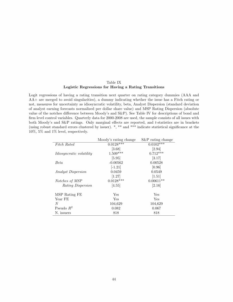
Table IXLogistic Regressions for Having a Rating Transitions
Logit regressions of having a rating transition next quarter on rating category dummies (AAA andAA+ are merged to avoid singularities), a dummy indicating whether the issue has a Fitch rating ornot, measures for uncertainty as idiosyncratic volatility, beta, Analyst Dispersion (standard deviationof analyst earning forecasts normalized per dollar share value) and MSP Rating Dispersion (absolutevalue of the notches difference between Moody’s and S&P). See Table IV for descriptions of bond andfirm level control variables. Quarterly data for 2000-2008 are used, the sample consists of all issues withboth Moody’s and S&P ratings. Only marginal effects are reported, and t-statistics are in brackets(using robust standard errors clustered by issuer). *, ** and *** indicate statistical significance at the10%, 5% and 1% level, respectively.
Moody’s rating change S&P rating changeFitch Rated 0.0128*** 0.0102***
[3.68] [2.94]Idiosyncratic volatility 1.509*** 0.712***
[5.95] [3.17]Beta -0.00562 0.00528
[-1.21] [0.96]Analyst Dispersion 0.0459 0.0549
[1.27] [1.51]Notches of MSP 0.0128*** 0.00611**
Rating Dispersion [4.55] [2.16]
MSP Rating FE Yes YesYear FE Yes YesN 104,629 104,629Pseudo R2 0.082 0.067N. issuers 818 818
44

Table XTurnover Regressions
OLS regressions of quarterly bond turnover, measured as aggregated trading volume over total valueof outstanding bonds on rating category dummies, a dummy indicating whether the issue has a Fitchrating or not and controls for off-the-run vs on-the-run effects (age). F makes (denies) IG is a dummyequal to 1 if Moody’s and S&P ratings are on opposite sides of the IG-HY boundary and the Fitchrating is IG (HY). All other control variables are dropped due to the use of both time and issue fixedeffects. Monthly data for July 2002-December 2008 are used; the sample consists of all issues with bothMoody’s and S&P ratings. t-statistics are in brackets (using robust standard errors clustered by issuer).*, ** and *** indicate statistical significance at the 10%, 5% and 1% level, respectively.
(1) (2) (3)MSP AAA to AA- Rating -2.889*** -2.887*** -2.891***
[-2.92] [-2.91] [-2.91]MSP BBB+ to BBB- Rating 0.722 0.749 0.745
[0.97] [1.00] [0.94]MSP BB+ to BB- Rating -2.434* -2.543* -2.554*
[-1.83] [-1.78] [-1.77]MSP B+ to B- Rating -5.368*** -5.270*** -5.280***
[-3.51] [-3.40] [-3.38]Age -4.035*** -4.033*** -4.022***
[-6.91] [-6.92] [-6.91]F makes IG 4.208*** 4.213***
[2.67] [2.67]F denies IG -5.801** -5.767**
[-2.18] [-2.16]Fitch Rated 0.952
[1.40]
Time FE Yes Yes YesIssue FE Yes Yes YesN 43,292 43,292 43,292adj. R2 0.278 0.279 0.279N. issuers 739 739 739
45

Figure 1FISD database coverage by CRA
The figure plots the percentage of bonds in FISD covered by S&P, Moody’s and Fitch. While FISD startsearlier, we use ratings starting in 2000, as S&P data seems incomplete before, as this figure suggests.
46

Figure 2Average Credit Spreads by Rating Category
47

Figure 3Rating Differences Across CRAs
The figure plots rating differences for different pairs of credit rating agencies (CRAs). We use a numericalscale for ratings, where a lower rating score means a better (more optimistic or lower bankruptcy likeli-hood) rating (see Table III for the full rating scale). In the figure, a negative number thus means that thefirst mentioned rating agency gives on average a better rating than the other CRA in that comparison.
48

Figure 4Default Prediction Accuracy
The figure plots the cumulative fraction of defaults on US corporate bonds over a oneyear horizon against the cumulative fraction of ratings (from worst to best), for Moody’s,S&P and Fitch based on data from 2000 to 2008. The accuracy ratios that rating agen-cies use for self-evaluation and that we report in Table VII Panel B are based on theareas under the graphs. A larger area under the graph corresponds to a better accu-racy. This type of graph is also known as a Cumulative Accuracy Power (CAP) curve.
49

Internet Appendix for ”Tiebreaker: Certification and Multiple
Credit Ratings”
Dion Bongaerts, K.J. Martijn Cremers, William N. Goetzmann∗
This Internet Appendix contains 9 supplementary tables to the main article.
∗Citation format: Bongaerts, Dion, K.J. Martijn Cremers and William N. Goetzmann, XXXX, Internet Appendixto ”Tiebreaker: Certification and Multiple Credit Ratings,” Journal of Finance XXX, pp XXXX, http://www.afajof.org/IA/XXXX.asp. Please note: Wiley-Blackwell is not responsible for the content or functionality of any supportinginformation supplied by the authors. Any queries (other than missing material) should be directed to the authors of thearticle.
1

Table IA.ISummary Statistics of Quarterly Ratings Sample
The table presents summary statistics and a brief description for the sample of bond issues that haveboth a Moody’s and an S&P rating in the quarterly rating sample for 2000 - 2008.
Variable Obs Mean Std. Dev. Min Max ExplanationFitch Rated 104,629 0.68 0.47 0 1 Dummy for Fitch ratingFitch Rating 70,863 7.27 2.84 1 19 Fitch ratingMoodys Rating 104,629 7.85 3.07 1 18 Moody’s RatingS&P Rating 104,629 7.66 2.99 1 20 S&P ratingFitch could push IG 104,629 0.04 0.19 0 1 Fitch could push IGFitch could push A- 104,629 0.05 0.22 0 1 Fitch could push A-S&P and Moodys Dis-agree
104,629 0.37 0.48 0 1 Dummy for MSP disagree-ment
Notches of MSP Rat-ing Dispersion
104,629 0.47 0.73 0 12 Notches of MSP ratingdispersion
Analyst Dispersion 104,629 0 0.02 0 1.66 Analyst dispersionStdev 104,629 0.02 0.01 0.0012 0.13 Daily idiosyncratic equity
volatility (past 180 days)Beta 104,629 0.94 0.44 -1.01 4.39 Equity beta (past 180
days)Log Total Assets 104,629 9.85 1.25 5.32 12.59 Log of total book value of
assetsPPE / Total Assets 104,629 0.38 0.23 0 0.96 PPE over total book as-
setsR&D / Total Assets 104,629 0.01 0.02 0 0.23 R&D expenditure over to-
tal book assetsR&D missing 104,629 0.45 0.5 0 1 R&D expenditure missingLeverage 104,629 0.35 0.15 0 6.04 Book leverage (debt/total
assets)ROA 104,629 0.01 0.02 -0.63 0.41 Return on book assets
(earnings/total assets)Log of OfferingAmount
104,629 11.42 2.2 0 15.07 Log of offering amount
Maturity Left 104,629 9.61 10.71 0 98.52 Maturity left (years)Redeemable 104,629 0.56 0.5 0 1 Dummy if the bond is re-
deemable
2

Table IA.IIFitch Inflated Credit Spread Regressions on Fitch Rating Additions
This table is equivalent to Table V of the main article except that for determining whether Fitch isbetter, equal or worse than the average of Moody’s and S&P rating, the Fitch rating is corrected withone notch. Thus, an original AAA rating by Fitch would in this table correspond to a AA+ rating.The column with only a dummy for a Fitch rating added in Table V is not replicated here since it isinvariant to this correction.
(1) (2) (3) (4) (5)Fitch added and better -0.726 0.132 -5.533 -2.973 -1.09
[-0.09] [0.02] [-0.73] [-0.35] [-0.15]Fitch added and equal -6.747 -6.22 -10.37 1.624 -1.683
[-0.84] [-0.77] [-0.95] [0.32] [-0.13]Fitch added and worse 2.645 2.953 9.538 2.909 3.203
[0.64] [0.71] [1.06] [0.70] [0.77]Fitch added and makes IG -30.71*** -22.98**
[-2.86] [-2.15]Fitch added and denies IG 11.16 22.99
[0.60] [0.89]At IG boundary 15.57*** 11.10***
[3.26] [2.60]Fitch added and equal* -2036.8
analyst dispersion [-1.10]analyst dispersion 588.2***
[4.13]Fitch added and equal* -8.636
rating dispersion [-1.11]rating dispersion 2.399**
[2.00]
Controls Yes Yes Yes Yes YesTime FE Yes Yes Yes Yes YesSegment All All BBB+ to BB- All AllN 34,621 34,621 15,100 34,724 34,621adj. R2 0.531 0.532 0.626 0.534 0.531N. issuers 671 671 465 672 671
3

Table IA.IIICRA Default Prediction with MSP Disagreement
Using yearly panel data between 2000 and 2008, we compare CRA performance with respect to defaultprediction on a one year horizon. The table shows results from a logit regression of issuer default eventson Moody’s and S&P rating scales, rating differences between Moody’s and Fitch, dummies for theeffect of Fitch as a tiebreaker when Moody’s and S&P are at different sides of the IG boundary andtime fixed effects for the complete universe of bonds that are rated by all three CRAs. The ratingvariables are in notches where 1 corresponds to AAA. The difference variables measure the differencebetween the First minus the second CRA in notches. Column 1 is restricted to cases where Moody’s andS&P disagree. Only marginal effects are reported (multiplied by 10,000 for readability), and t-statisticsare in brackets (using robust standard errors clustered by issuer). *, ** and *** indicate significance atthe 10%, 5% and 1% level, respectively.
(1) (2)Moody’s Rating 5.00*** 3.91***
[3.28] [4.00]S&P Rating 0.403 0.37
[0.54] [0.65]Difference Fitch vs Moody’s 5.00***
[3.28]Fitch makes IG -5.63
[-1.52]Fitch denies IG -4.08
[-0.96]
Year FE Yes YesMoody’s and S&P disagree only Yes NoN 56,376 112,329pseudo R2 0.372 0.369N. issuers 1693 2066
4

Table IA.IVCredit Spread Regressions, Full Sample
Using quarterly panel data between 2002 and 2008, we regress credit spread levels for AAA to B- ratedbonds on bond and firm characteristics, with rating and time fixed effects. Main variables of interestare whether a Fitch rating is better (FR < MSP ), equal to (FR = MSP ) or worse (FR > MSP ) thanthe average Moody’s and S&P rating, as well as variables relating to regulation (IG). See Table IA.Vfor descriptions of other control variable descriptions. However, levels instead of changes are used forthe controls. Time fixed effects are estimated for the IG and HY category separately to accommodatethe sharp widening of the IG/HY spread during the crisis. t-statistics are in brackets (using robuststandard errors clustered by issuer). *, ** and *** indicate significance at the 10%, 5% and 1% level,respectively.
(1) (2) (3) (4)Fitch<MSP 4.314 5.487 3.771 4.1
[1.14] [1.42] [1.00] [1.12]Fitch=MSP 7.151** 7.184** 6.594* 7.678**
[2.12] [2.15] [1.94] [2.27]Fitch>MSP 16.37** 13.16** 16.68** 15.71**
[2.28] [2.04] [2.30] [2.18]Fitch makes IG -26.35***
[-2.62]Fitch denies IG 18.22
[1.17]analyst dispersion* 207.4
Fitch=MSP [1.40]analyst dispersion 252.2
[0.95]Rating dispersion* -1.356
Fitch=MSP [-0.35]Rating dispersion 2.083
[0.64]
Controls Yes Yes Yes YesTime FE by IG/HY yes yes yes yesMSP Rating FE yes yes yes yesN 44,139 44,139 43,711 44,139adj. R2 0.814 0.815 0.815 0.814N. issuers 739 739 716 739
5

Tab
leIA
.VC
han
gein
Cre
dit
Sp
read
san
dR
atin
gC
han
ges,
Pre
-Cri
sis
Sam
ple
Usi
ngqu
arte
rly
pane
ldat
abe
twee
n20
02an
d20
07Q
2,w
ere
gres
sch
ange
sin
cred
itsp
read
sfo
rA
AA
toB
-ra
ted
bond
sth
atar
era
ted
byal
lthr
eeC
RA
son
rati
ngup
-an
ddo
wng
rade
sfo
ral
lthr
eeC
RA
s,ch
ange
sin
bond
and
firm
char
acte
rist
ics,
dum
mie
sfo
rbo
unda
ryeff
ects
and
tim
efix
edeff
ects
.U
p-an
ddo
wng
rade
sar
eco
ded
asdu
mm
ies
indi
cati
ngw
heth
erea
chof
the
thre
eC
RA
sup
grad
edor
dow
ngra
ded
its
rati
ng.
The
sefir
man
dbo
ndco
ntro
lsar
ein
clud
edbu
tno
tsh
own
(all
inch
ange
s):
Lev
erag
e,liq
uida
tion
/int
rins
icva
lue
(PP
E/t
otal
asse
ts),
R&
Dex
pens
es(d
ivid
edby
tota
las
sets
),R
OA
(ret
urn
onas
sets
),St
dev
(dai
lyid
iosy
ncra
tic
equi
tyvo
lati
lity)
,H
isto
rica
lEqu
ity
Bet
a(h
alf
year
daily
corr
ecte
dfo
rB
id-A
sk-b
ounc
es),
Log
Tot
alA
sset
s(fi
rmsi
ze,b
ook
valu
e)an
dL
ogO
fferi
ngSi
ze(i
ssue
size
),R
edee
mab
le(d
umm
yfo
rca
llabi
lity)
,D
urat
ion
and
Con
vexi
ty.
Fit
chU
pgra
de,
Bre
aks
Tie
isa
dum
my
indi
cati
ngth
ata
Fit
chup
grad
em
ade
the
issu
equ
alify
for
IG,w
hile
Fit
chD
owng
rade
,B
reak
sT
ieis
adu
mm
yin
dica
ting
that
aF
itch
dow
ngra
dem
ade
the
issu
elo
seit
sIG
qual
ifica
tion
.F
itch
Cou
ldB
reak
Tie
isa
dum
my
indi
cati
ngth
atth
eS&
Pan
dM
oody
’sra
ting
sar
eon
oppo
site
side
sof
the
IG-H
Ybo
unda
ry.
Col
umn
(5)
isre
stri
cted
tois
sues
rate
dA
-or
bett
erby
Moo
dy’s
and
S&P,
whe
reas
colu
mn
(6)
isre
stri
cted
tois
sues
rate
dB
BB
+or
wor
seby
Moo
dy’s
and
S&P.
t-st
atis
tics
are
inbr
acke
ts(u
sing
robu
stst
anda
rder
rors
clus
tere
dby
issu
er;
N.
issu
ergi
ves
the
num
ber
ofis
suer
s).
*,**
and
***
indi
cate
sign
ifica
nce
atth
e10
%,5
%an
d1%
leve
l,re
spec
tive
ly.
’F-t
est
Fup=
Fdo
wn
(p-v
alue
)’gi
ves
the
p-v
alue
for
the
coeffi
cien
tson
Fit
chU
pgra
dean
dF
itch
Dow
ngra
debe
ing
equa
l,w
hile
’F-t
est
Fup,
tie=
Fdo
wn,
tie
(p-v
alue
)’gi
ves
the
p-v
alue
for
the
coeffi
cien
tson
Fit
chU
pgra
ded,
Bre
aks
Tie
and
Fit
chD
owng
rade
d,B
reak
sT
iebe
ing
equa
l.
(1)
(2)
(3)
(4)
(5)
(6)
(7)
(8)
Moo
dy’s
Upg
rade
-5.5
46**
-2.7
94-2
.472
[-2.
44]
[-1.
41]
[-1.
28]
Moo
dy’s
Dow
ngra
de14
.59*
**9.
905*
*9.
704*
**[4
.42]
[2.5
6][2
.66]
S&P
Upg
rade
-9.2
68**
*-8
.036
***
-7.8
05**
*[-
3.20
][-
3.20
][-
3.13
]S&
PD
owng
rade
16.3
1***
11.6
6***
11.3
8***
[4.4
9][3
.47]
[3.5
3]F
itch
Upg
rade
-6.2
28*
-6.1
34*
-0.4
35-6
.175
-4.1
03-4
.227
[-1.
86]
[-1.
79]
[-0.
13]
[-1.
65]
[-1.
40]
[-1.
41]
Fit
chD
owng
rade
13.9
7***
10.3
1***
0.66
214
.95*
**6.
467
3.32
[3.0
4][2
.63]
[0.2
6][2
.89]
[1.4
4][0
.82]
Fit
chU
pgra
de,
Bre
aks
Tie
-3.2
22-5
.122
-0.1
85[-
0.38
][-
0.65
][-
0.02
]F
itch
Dow
ngra
de,
Bre
aks
44.2
0**
38.6
9*40
.55*
*T
ie[2
.16]
[1.9
2][1
.98]
Con
tinu
edon
next
page
6

Tab
leIA
.V–
conti
nu
edfr
omp
revio
us
pag
e
(1)
(2)
(3)
(4)
(5)
(6)
(7)
(8)
Fit
chC
ould
Bre
akT
ie-4
.869
*-3
.611
-5.0
81*
[-1.
85]
[-1.
42]
[-1.
94]
Lagg
edC
redi
tSp
read
-0.2
66**
*-0
.268
***
-0.2
64**
*-0
.263
***
-0.4
19**
*-0
.223
***
-0.2
71**
*-0
.270
***
Cha
nge
[-9.
24]
[-9.
14]
[-8.
95]
[-8.
91]
[-22
.09]
[-6.
67]
[-9.
38]
[-9.
32]
Sam
ple
All
All
All
All
≤A
-≥
BB
B+
All
All
N16
,889
16,8
8916
,889
16,8
898,
535
8,35
416
,889
16,8
89A
dj.
R2
0.20
40.
207
0.20
20.
206
0.26
90.
230.
212
0.21
4N
.is
suer
s34
334
334
334
310
727
634
334
3F
-tes
tFu
p=F
dow
n0.
05%
0.16
%79
.00%
0.09
%5.
19%
14.0
0%(p
-val
ue)
F-t
est
Fup,
tie=
Fdo
wn,
tie
3.25
%4.
44%
(p-v
alue
)
7

Tab
leIA
.VI
Cre
dit
Sp
read
Reg
ress
ion
son
Fit
chR
atin
gA
dd
itio
ns,
Pre
-Cri
sis
Sam
ple
Usi
ngqu
arte
rly
pane
ldat
abe
twee
n20
02an
d20
07Q
2,w
ere
gres
sch
ange
sin
cred
itsp
read
sfo
rA
AA
toB
-ra
ted
bond
sth
atar
era
ted
byM
oody
’san
dS&
Pon
rati
ngad
diti
ons
from
Fit
ch,
the
rela
tive
rank
ing
ofth
ose
addi
tion
san
dw
heth
erad
diti
ons
happ
ened
atth
eIG
boun
dary
,int
erac
tion
sw
ith
unce
rtai
nty
mea
sure
san
dch
ange
sin
bond
and
firm
char
acte
rist
ics
plus
tim
efix
edeff
ects
.F
itch
Add
ed,
Bet
ter,
Fit
chA
dded
,E
qual
and
Fit
chA
dded
,W
orse
are
dum
mie
sin
dica
ting
whe
ther
aF
itch
rati
ngha
sbe
enad
ded
that
isre
spec
tive
lybe
tter
than
,equ
alto
and
wor
seth
anth
eav
erag
era
ting
byM
oody
’san
dS&
P.F
itch
Add
ed,
Mak
esIG
and
Fit
chA
dded
,D
enie
sIG
are
dum
mie
sth
atin
dica
tew
heth
erth
ead
ded
Fit
chra
ting
mak
esth
eis
sue
qual
ifyfo
rIG
orno
t,co
ndit
iona
lon
Moo
dy’s
and
S&P
rati
ngs
bein
gon
oppo
site
side
sof
the
boun
dary
.Se
eT
able
IA.V
for
desc
ript
ions
ofbo
ndan
dfir
mle
vel
cont
rol
vari
able
s.t-
stat
isti
csar
ein
brac
kets
(usi
ngro
bust
stan
dard
erro
rscl
uste
red
byis
suer
inal
lcol
umns
exce
ptco
lum
n5,
whi
chus
esdo
uble
clus
teri
ngby
both
issu
eran
dti
me)
.*,
**an
d**
*in
dica
tesi
gnifi
canc
eat
the
10%
,5%
and
1%le
vel,
resp
ecti
vely
.’F
-tes
tFA
dded
,IG
=FA
dded
,HY
(p-v
alue
)’is
the
p-v
alue
ofth
eF
-tes
tof
Fit
chA
dded
,M
akes
IGan
dF
itch
Add
ed,
Mak
esH
Ybe
ing
equa
l.T
hesa
mpl
eis
all
issu
esra
ted
bybo
thM
oody
’san
dS&
Pw
ith
thei
rav
erag
era
ting
bett
eror
equa
lto
B-,
exce
ptin
colu
mn
4,w
here
thei
rav
erag
era
ting
isbe
twee
nB
BB
+an
dB
B-.
(1)
(2)
(3)
(4)
(5)
(6)
(7)
Fit
chA
dded
0.01
33[0
.00]
Fit
chA
dded
,B
ette
r-7
.003
-6.6
41-2
.535
-6.6
41-7
.365
-6.9
03[-
0.97
][-
0.91
][-
0.39
][-
0.83
][-
1.01
][-
0.95
]F
itch
Add
ed,
Equ
al5.
256*
5.02
1*11
.94*
*5.
021*
*2.
798
4.94
7*[1
.84]
[1.7
6][2
.11]
[2.0
3][0
.94]
[1.8
0]F
itch
Add
ed,
Wor
se-0
.001
41-0
.085
617
.21
-0.0
856
-0.4
66-0
.187
[-0.
00]
[-0.
01]
[0.8
6][-
0.01
][-
0.04
][-
0.02
]F
itch
Add
ed,
Mak
esIG
-20.
28*
-20.
13*
-20.
28*
[-1.
65]
[-1.
70]
[-1.
70]
Fit
chA
dded
,M
akes
HY
30.4
627
.03
30.4
6[1
.45]
[1.2
8][1
.35]
At
IGbo
unda
ry-1
.259
-1.1
49-1
.259
[-0.
46]
[-0.
45]
[-0.
46]
Fit
chA
dded
,E
qual
*12
80.3
Ana
lyst
Dis
pers
ion
[0.9
9]C
onti
nued
onne
xtpa
ge
8

Tab
leIA
.VI
–co
nti
nu
edfr
omp
revio
us
pag
e
(1)
(2)
(3)
(4)
(5)
(6)
(7)
Ana
lyst
Dis
pers
ion
184.
8[1
.51]
Fit
chA
dded
,E
qual
*0.
602
Rat
ing
Dis
pers
ion
[0.1
0]S&
Pan
dM
oody
sD
isag
ree
-0.6
86[-
1.24
]La
gged
Cre
dit
Spre
ad-0
.276
***
-0.2
77**
*-0
.277
***
-0.2
43**
*-0
.277
***
-0.2
79**
*-0
.277
***
Cha
nge
[-11
.99]
[-12
.02]
[-12
.01]
[-7.
62]
[-6.
84]
[-12
.18]
[-11
.99]
Sam
ple
All
All
All
BB
B+
toB
B-
All
All
All
Dou
ble
Clu
ster
ing
No
No
No
No
Yes
No
No
N24
,557
24,5
5724
,557
9,75
124
,557
24,6
5024
,557
Adj
.R
20.
205
0.20
60.
206
0.22
40.
206
0.20
70.
206
N.
issu
ers
605
605
605
404
608
605
F-t
est
FAdd
ed,I
G=
FAdd
ed,H
Y(p
-val
ue)
3.24
%4.
59%
8.93
%
9

Tab
leIA
.VII
Log
isti
cR
egre
ssio
ns
for
Hav
ing
aF
itch
Rat
ing
Log
itre
gres
sion
sof
havi
nga
Fit
chra
ting
onra
ting
cate
gory
dum
mie
sba
sed
onav
erag
eM
oody
’san
dS&
P(M
SP)
rati
ngs,
mea
sure
sfo
run
cert
aint
yas
Ana
lyst
Dis
pers
ion
(sta
ndar
dde
viat
ion
ofan
alys
tea
rnin
gfo
reca
sts
norm
aliz
edpe
rdo
llar
shar
eva
lue)
,Dum
my
S&P
and
Moo
dy’s
Dis
agre
eor
Not
ches
ofM
SPR
atin
gD
ispe
rsio
n(a
bsol
ute
valu
eof
the
notc
hes
diffe
renc
ebe
twee
nM
oody
’san
dS&
P),
and
FC
ould
Bre
akT
iean
dF
Cou
ldP
ush
A-
are
dum
mie
sin
dica
ting
whe
ther
the
Moo
dy’s
and
S&P
rati
ngs
are
onop
posi
tesi
des
ofth
eIG
-HY
and
A-
boun
dari
esre
spec
tive
ly.
All
spec
ifica
tion
sfu
rthe
rin
clud
ein
dust
ryfix
edeff
ects
.In
colu
mn
(6)
and
(7)
issu
esar
ere
mov
edaf
ter,
resp
ecti
vely
,the
irfir
stye
aran
dfir
stqu
arte
raf
ter
bein
gra
ted
byF
itch
.O
ther
cont
rols
that
are
incl
uded
but
not
show
nar
eth
efir
mB
eta,
Lev
erag
e,P
PE
/A
sset
s,R
&D
Exp
ense
s/
Ass
ets,
RO
A,L
ogof
Offe
ring
Am
ount
,Mat
urit
yL
eft
and
Mat
urit
yL
eft
Squa
red
and
Red
eem
able
(see
Tab
leIA
.Vfo
rde
scri
ptio
ns).
Qua
rter
lyda
tafo
r20
00-2
008
are
used
,an
dth
esa
mpl
eco
nsis
tsof
all
issu
esw
ith
both
Moo
dy’s
and
S&P
rati
ngs
that
are
onav
erag
era
ted
B-
orbe
tter
.M
argi
nal
effec
tsar
ere
port
ed,
and
t-st
atis
tics
are
inbr
acke
ts(u
sing
robu
stst
anda
rder
rors
clus
tere
dby
issu
er).
*,**
and
***
indi
cate
stat
isti
cal
sign
ifica
nce
atth
e10
%,
5%an
d1%
leve
l,re
spec
tive
ly.
Pse
udo
R2
refe
rsto
McF
adde
n(1
973)
pseu
doR
2.
(1)
(2)
(3)
(4)
(5)
(6)
(7)
MSP
Rat
ing
A+
toA
-0.
418*
**0.
417*
**0.
420*
**0.
414*
**0.
216*
*0.
0985
**[3
.97]
[3.9
3][3
.98]
[3.9
5][2
.36]
[2.0
2]M
SPR
atin
gB
BB
+to
BB
B-
0.40
1***
0.39
7***
0.38
6***
0.39
5***
0.19
1***
0.07
26**
[4.3
1][4
.21]
[4.0
8][4
.24]
[2.6
9][2
.26]
MSP
Rat
ing
BB
+to
BB
-0.
299*
**0.
291*
**0.
290*
**0.
289*
**0.
243*
0.12
3[6
.70]
[6.2
5][6
.12]
[6.2
3][1
.96]
[1.6
0]M
SPR
atin
gB
+to
B-
0.26
6***
0.26
6***
0.26
7***
0.26
3***
0.22
30.
111
[6.1
3][6
.09]
[6.1
9][5
.96]
[1.6
0][1
.30]
Fit
chC
ould
Bre
akT
ie0.
144*
**0.
117*
**0.
103*
*0.
092
0.03
69[3
.99]
[3.1
8][2
.51]
[1.6
0][1
.17]
Fit
chC
ould
Pul
lA
0.06
490.
0328
0.00
998
0.02
820.
0226
[1.3
1][0
.60]
[0.1
7][0
.63]
[0.9
6]A
vgM
SPB
B+
0.09
52**
[2.3
9]A
vgM
SPB
BB
-0.
0790
**[2
.24]
Not
ches
ofM
SPR
atin
g-0
.002
04D
ispe
rsio
n[-
0.07
]C
onti
nued
onne
xtpa
ge
10

Tab
leIA
.VII
–co
nti
nu
edfr
omp
revio
us
pag
e
(1)
(2)
(3)
(4)
(5)
(6)
(7)
S&P
and
Moo
dys
Dis
agre
e-0
.030
5-0
.030
9-0
.042
6-0
.033
3-0
.034
7-0
.022
[-0.
69]
[-0.
62]
[-0.
87]
[-0.
74]
[-1.
10]
[-1.
60]
Ana
lyst
Dis
pers
ion
0.83
50.
728
0.85
50.
816
0.90
30.
337
0.06
52[0
.96]
[0.8
4][0
.96]
[0.9
8][0
.97]
[1.2
1][1
.29]
Idio
sync
rati
cV
olat
ility
-5.4
32**
*-5
.334
***
-5.3
97**
*-5
.513
***
-5.3
88**
*-2
.103
**-0
.182
[-4.
67]
[-4.
80]
[-4.
70]
[-4.
75]
[-4.
68]
[-1.
98]
[-0.
56]
Log
ofT
otal
Ass
ets
0.17
7***
0.15
1***
0.17
7***
0.17
9***
0.17
8***
0.07
66**
*0.
0195
***
[8.8
6][5
.64]
[8.8
2][8
.90]
[8.8
7][5
.87]
[5.3
6]
Tim
eL
imit
afte
rF
itch
Add
itio
nN
oN
oN
oN
oN
o1
Yea
r1
Qua
rter
N10
4,43
510
4,43
510
4,43
510
4,43
510
4,43
527
,550
32,1
35P
seud
oR
20.
223
0.17
40.
224
0.22
50.
223
0.16
30.
098
N.
issu
ers
818
818
818
818
818
639
683
11

Table IA.VIIILogistic Regressions for Having a Fitch Rating with Double Clustering
Logit regressions of having a Fitch rating on rating category dummies based on average Moody’s andS&P (MSP) ratings, measures for uncertainty as Analyst Dispersion (standard deviation of analystearning forecasts normalized per dollar share value), Dummy S&P and Moody’s Disagree or Notchesof MSP Rating Dispersion (absolute value of the notches difference between Moody’s and S&P), and FCould Break Tie and F Could Push A- are dummies indicating whether the Moody’s and S&P ratingsare on opposite sides of the IG-HY and A- boundaries respectively. All specifications further includeindustry fixed effects. Other controls that are included but not shown are the firm Beta, Leverage, PPE/ Assets, R&D Expenses / Assets, ROA, Log of Offering Amount, Maturity Left and Maturity LeftSquared and Redeemable (see Table IA.V for descriptions). Quarterly data for 2000-2008 are used, andthe sample consists of all issues with both Moody’s and S&P ratings that are on average rated B- orbetter. Only coefficient estimates are reported, and t-statistics are in brackets using robust standarderrors clustered by issuer in Column (1) and standard errors clustered by issuer and time in Column(2). *, ** and *** indicate statistical significance at the 10%, 5% and 1% level, respectively. Doubleclustered standard errors are calculated using the Stata code available on Mitchel Petersen’s website.
(1) (2)MSP Rating A+ to A- 2.411*** 2.411***
[3.76] [3.69]MSP Rating BBB+ to BBB- 2.440*** 2.440***
[3.84] [3.74]MSP Rating BB+ to BB- 2.645*** 2.645***
[4.00] [3.92]MSP Rating B+ to B- 2.472*** 2.472***
[3.45] [3.39]Fitch Could Break Tie 0.705*** 0.705***
[2.61] [2.66]Fitch Could Pull A 0.172 0.172
[0.58] [0.59]Notches of MSP Rating Dispersion -0.213 -0.213
[-0.87] [-0.89]Analyst Dispersion 4.331 4.331
[0.96] [0.82]
Industry FE yes yesDouble clustering no yesN 104,435 104,435pseudo R2 0.224N. issuers 818
12

Tab
leIA
.IX
Ch
ange
inC
red
itS
pre
ads
and
Rat
ing
Ch
ange
s,ve
rifi
cati
onte
sts
Usi
ngqu
arte
rly
pane
lda
tabe
twee
n20
02an
d20
08,
we
regr
ess
chan
ges
incr
edit
spre
ads
for
AA
Ato
B-
rate
dbo
nds
that
are
rate
dby
allt
hree
CR
As
onra
ting
up-
and
dow
ngra
des
for
allt
hree
CR
As,
chan
ges
inbo
ndan
dfir
mch
arac
teri
stic
s,du
mm
ies
for
boun
dary
effec
tsan
dti
me
fixed
effec
ts.
Up-
and
dow
ngra
des
are
code
das
dum
mie
sin
dica
ting
whe
ther
each
ofth
eth
ree
CR
As
upgr
aded
ordo
wng
rade
dit
sra
ting
.T
hese
firm
and
bond
cont
rols
are
incl
uded
but
not
show
n(a
llin
chan
ges)
:L
ever
age,
liqui
dati
on/i
ntri
nsic
valu
e(P
PE
/tot
alas
sets
),R
&D
expe
nses
(div
ided
byto
tal
asse
ts),
RO
A(r
etur
non
asse
ts),
Stde
v(d
aily
idio
sync
rati
ceq
uity
vola
tilit
y),
His
tori
cal
Equ
ity
Bet
a(h
alf
year
daily
corr
ecte
dfo
rB
id-A
sk-b
ounc
es),
Log
Tot
alA
sset
s(fi
rmsi
ze,
book
valu
e)an
dL
ogO
fferi
ngSi
ze(i
ssue
size
),R
edee
mab
le(d
umm
yfo
rca
llabi
lity)
,D
urat
ion
and
Con
vexi
ty.
Fit
chU
pgra
de,
Bre
aks
Tie
,M
oody
’sU
pgra
de,
Bre
aks
Tie
and
S&P
Upg
rade
,B
reak
sT
iear
ea
dum
mie
sin
dica
ting
that
the
resp
ecti
veC
RA
upgr
ade
mad
eth
eis
sue
qual
ifyfo
rIG
,w
hile
Fit
chD
owng
rade
,br
eaks
noti
ean
ymor
e,M
oody
’sD
owng
rade
,br
eaks
noti
ean
ymor
ean
dS&
PD
owng
rade
,br
eaks
noti
ean
ymor
ear
edu
mm
ies
indi
cati
ngth
ata
dow
ngra
deby
the
resp
ecti
veC
RA
mad
eth
eis
sue
lose
its
IGqu
alifi
cati
on.
Fit
chC
ould
Bre
akT
ie,
Moo
dy’s
Cou
ldB
reak
Tie
and
S&P
Cou
ldB
reak
Tie
are
adu
mm
ies
indi
cati
ngth
atth
era
ting
sby
the
othe
rC
RA
sar
eon
oppo
site
side
sof
the
IG-H
Ybo
unda
ry.
Col
umns
(3)
and
(4)
are
rest
rict
edto
issu
esra
ted
A-
orbe
tter
byM
oody
’san
dS&
P,w
here
asco
lum
ns(5
)an
d(6
)ar
ere
stri
cted
tois
sues
rate
dB
BB
+or
wor
seby
Moo
dy’s
and
S&P.
t-st
atis
tics
are
inbr
acke
ts(u
sing
robu
stst
anda
rder
rors
clus
tere
dby
issu
er;
N.
issu
ergi
ves
the
num
ber
ofis
suer
s).
*,**
and
***
indi
cate
sign
ifica
nce
atth
e10
%,
5%an
d1%
leve
l,re
spec
tive
ly.
’F-t
est
Mup
=M
dow
n(p
-val
ue)’
and
’F-t
est
SPup
=SP
dow
n(p
-val
ue)’
give
the
p-v
alue
sfo
rth
ete
ston
the
coeffi
cien
tson
Moo
dy’s
Upg
rade
and
Moo
dy’s
Dow
ngra
debe
ing
equa
lan
dth
ete
ston
the
coeffi
cien
tson
S&P
Upg
rade
and
S&P
Dow
ngra
debe
ing
equa
lre
spec
tive
ly.
Sim
ilarl
y’F
-tes
tM
up,t
ie=
Mdo
wn,
tie
(p-v
alue
)’an
d’F
-tes
tSP
up,t
ie=
SPdo
wn,
tie
(p-v
alue
)’gi
veth
ep-v
alue
sfo
rth
ete
stof
the
coeffi
cien
tson
Moo
dy’s
Upg
rade
d,B
reak
sT
iean
dM
oody
’sD
owng
rade
d,B
reak
sT
iebe
ing
equa
lan
dth
ete
stof
the
coeffi
cien
tson
S&P
Upg
rade
d,B
reak
sT
iean
dS&
PD
owng
rade
d,B
reak
sT
iebe
ing
equa
lre
spec
tive
ly.
(1)
(2)
(3)
(4)
(5)
(6)
(7)
(8)
(9)
Moo
dy’s
upgr
ade
-4.4
63*
-5.4
14**
-8.7
04**
*-2
.493
-2.4
18-2
.587
[-1.
90]
[-2.
34]
[-3.
18]
[-1.
13]
[-1.
13]
[-1.
17]
Moo
dy’s
dow
ngra
de14
.06*
**9.
149*
*18
.55*
**7.
378*
*7.
032*
8.23
9**
[4.0
9][2
.22]
[3.9
7][2
.07]
[1.8
9][2
.41]
S&P
upgr
ade
-4.9
77*
-10.
41**
*-4
.846
-4.3
21-3
.701
-3.8
33[-
1.84
][-
2.64
][-
1.65
][-
1.62
][-
1.37
][-
1.40
]S&
Pdo
wng
rade
16.6
3***
4.09
420
.43*
**18
.70*
**13
.13*
**12
.95*
**[4
.39]
[1.0
6][4
.76]
[4.2
1][3
.52]
[3.5
0]F
itch
upgr
ade
-4.9
48-5
.207
*-4
.086
[-1.
64]
[-1.
72]
[-1.
36]
Fit
chdo
wng
rade
4.63
14.
779
4.2
[0.8
0][0
.84]
[0.7
1]C
onti
nued
onne
xtpa
ge
13

Tab
leIA
.IX
–co
nti
nu
edfr
omp
revio
us
pag
e
(1)
(2)
(3)
(4)
(5)
(6)
(7)
(8)
(9)
Fit
chup
grad
edan
dbr
eaks
-8.7
96ti
e[-
0.62
]F
itch
dow
ngra
ded
and
4.18
1br
eaks
noti
ean
ymor
e[0
.21]
Fit
chco
uld
brea
kti
e10
.27*
*[2
.08]
Moo
dy’s
upgr
aded
and
-2.4
793.
764
-0.7
281.
183
brea
ksti
e[-
0.37
][0
.58]
[-0.
12]
[0.2
1]M
oody
’sdo
wng
rade
dan
d1.
052
-2.0
68-1
.156
-18.
97br
eaks
noti
ean
ymor
e[0
.04]
[-0.
08]
[-0.
04]
[-0.
70]
Moo
dy’s
coul
dbr
eak
tie
2.81
8-0
.792
2.66
1-6
.331
[0.7
4][-
0.26
][0
.71]
[-1.
38]
S&P
upgr
aded
and
brea
ks-1
4.25
*-1
0.03
-13.
21*
-12.
1ti
e[-
1.82
][-
1.57
][-
1.73
][-
1.58
]S&
Pdo
wng
rade
dan
d40
.15*
**36
.08*
**39
.51*
**40
.53*
**br
eaks
noti
ean
ymor
e[2
.98]
[2.9
2][2
.84]
[2.6
1]S&
Pco
uld
brea
kti
e11
.87*
**8.
468*
*12
.14*
**7.
797*
[2.6
1][2
.13]
[2.6
4][1
.66]
Tim
eF
EY
esY
esY
esY
esY
esY
esY
esY
esY
esra
ted
byA
ll3
Yes
Yes
Yes
Yes
Yes
Yes
Yes
Yes
Yes
Ran
geA
llA
ll≤
A-
≤A
-≥
BB
B+
≥B
BB
+A
llA
llA
llN
2428
224
282
1133
011
330
1295
212
952
2428
224
282
2428
2ad
j.R
20.
531
0.53
70.
451
0.45
10.
602
0.60
80.
534
0.53
70.
538
N.
issu
er38
038
011
711
731
331
338
038
038
0F
-tes
tM
up=
Mdo
wn
(p-
val)
00.
008
00.
015
F-t
est
Mup
,tie
=M
dow
n,ti
e(p
-val
)
0.89
70.
833
0.98
7
F-t
est
SPup
=SP
dow
n(p
-va
l)0
0.00
80
0
Con
tinu
edon
next
page
14

Tab
leIA
.IX
–co
nti
nu
edfr
omp
revio
us
pag
e
(1)
(2)
(3)
(4)
(5)
(6)
(7)
(8)
(9)
F-t
est
SPup
,tie
=SP
dow
n,ti
e(p
-val
)
00.
001
0.00
1
15