Tilburg University

Explaining Environmental Kuznets Curves

Smulders, Sjak; Bretschger, L.

Publication date:2000

Link to publication

General rightsCopyright and moral rights for the publications made accessible in the public portal are retained by the authors and/or other copyright ownersand it is a condition of accessing publications that users recognise and abide by the legal requirements associated with these rights.

- Users may download and print one copy of any publication from the public portal for the purpose of private study or research - You may not further distribute the material or use it for any profit-making activity or commercial gain - You may freely distribute the URL identifying the publication in the public portal

Take down policyIf you believe that this document breaches copyright, please contact us providing details, and we will remove access to the work immediatelyand investigate your claim.

Download date: 01. Sep. 2018

Centerfor

Economic Research

No. 2000-95

EXPLAINING ENVIRONMENTAL KUZNETSCURVES: HOW POLLUTION INDUCES POLICY

AND NEW TECHNOLOGIES

By Sjak Smulders and Lucas Bretschger

October 2000

ISSN 0924-7815

Explaining Environmental Kuznets Curves:How Pollution Induces Policy and New Technologies

Sjak Smulders*andLucas Bretschger**

September 2000

AbstractProduction often causes pollution as a by-product. Once pollution problemsbecome too severe, regulation is introduced by political authorities which forcesthe economy to make a transition to cleaner production processes. We modelthis transition as a change in "general purpose technology" (GPT) andinvestigate how it interferes with economic growth driven by quality-improvements. The model gives an explanation for the inverted U-shapedrelationship found in empirical research for many pollutants, often referred to asthe Environmental Kuznets Curve (EKC). We provide an analytical foundationfor the claim that the rise and decline of pollution can be explained by policy-induced technology shifts.

Key words: Environmental Kuznets curve, general purpose technology, growth.

JEL Codes: O41, Q20.

* Corresponding author: Department of Economics, Tilburg University, P.O.Box90153, 5000 LE Tilburg, The Netherlands, j.a.smulders@kub.nl.** Ernst-Moritz-Arndt-Universität, Greifswald, Friedrich-Loeffler-Str. 70, 17487Greifswald, Germany, Lucas.Bretschger@uni-greifswald.de.

Smulders' research is supported by the Royal Dutch Academy of Arts andSciences. We thank Richard Nahuis and Participants of the workshop“Dynamique Economique et des Preoccupations Environmentales”, UniversityParis-X, June 2000.

2

1. Introduction

An old, classical, and recurring theme in economics is the relationship betweeneconomic growth and public concern for environmental problems. It rangesfrom the physiocrats’ focus on land, Jevon’s coal question, and the Club ofRome’s doomsday scenarios to the current greenhouse gas problem. In recentliterature, the relationship between economic development and pollution hasbeen widely discussed. For many pollutants, an inverted-U-shaped relationshipbetween per capita income and pollution, labeled the Environmental KuznetsCurve (EKC), is documented.1 Concentration of a certain pollutant typically firstincreases with production, which reflects a scale effect, but later on, emissionsare de-linked from income.

Hypotheses to explain this de-linking of pollution from growth are eitherthe assumption of a shift in the composition of production (from manufacturingto services), or a change in techniques used.2 Especially the latter change islikely to be policy-induced. If the environment is a “normal good” of whichdemand increases with income, higher income levels trigger more stringentenvironmental policies that induce firms to change technology. This kind of de-linking is thus achieved due to the combination of political correction of marketfailures and technological change. Before policy-induced technical change canarise, policy concerning environmental issues has to be shaped. Growingevidence of harmful effects and new findings by natural scientists have a largeimpact on public concern about the environment and may result eventually innew environmental policy measures. Examples of rather late policy reactions togrowing evidence of potential problems are the greenhouse and nuclear powerproblems. In sum, new information about ecological problems, theimplementation of policy measures, and new technological possibilities are atthe heart of the EKC.

Until now, there is a large empirical literature on EKCs, see Seldon andSong (1994), Shafik (1994), Cropper and Griffiths (1994), Grossman and Krueger(1995) and Hilton and Levinson (1998) in particular. But it is surprising that thetheoretical literature on environmental growth models does not say much aboutthe phenomenon.3 In general, the theory of growth tends to focus on balancedgrowth paths which seems difficult to combine with the non-linear nature of theEKC. Yet, the theory of endogenous growth exactly provides those buildingblocks that are needed to seriously study the interaction between growth,technology and environment. One of the exceptions is Stockey (1998) whopresents a model of growth and pollution in which relatively high marginalabatement costs for the first units of abatement makes poor countries to abstainfrom abatement activities. De Groot (1999) gives another growth-theoretical

1 See, for example, the special issues of Environment and Development Economics 1997 andEcological Economics 1998, and the survey article by De Bruyn 1999.2 See Copeland and Taylor (AER 1994) for the distinction between scale, composition andtechnique effects.3 See Smulders 1995 and 1999 for a survey on environmental growth models and Bretschger1999 for the integration of natural resource use into modern growth theory.

3

explanation for the EKC. In his model, endogenous sectoral changes, driven byincome effects and learning-by-doing, generate the EKC pattern. Thismechanism, however, seems less relevant for mature economies in whichintersectoral shifts are of minor importance relative to intrasectoral changes.Empirical decomposition studies confirm the overwhelming dominance ofintra-sectoral changes (Torvanger 1991, De Bruyn 1997, and 1999 p. 88). Finally,Andreoni and Levinson (2000) present a simple model of the EKC driven byincome effects. Their approach, however, does not explicitly model economicgrowth or technological change.

This paper aims to link the empirical evidence on the interaction betweeneconomic growth and environmental problems to theories of technologicalchange and economic growth. Specifically, it explains the EKC in anendogenous growth model with three key elements. First, technological changeallows for reductions in pollution. Second, intrasectoral shifts accompany theadoption of pollution-reducing technologies. Third, technical change andsectoral shifts are both driven by policy changes, which in turn occur at discretetimes and reflect awareness of environmental problems.

Pollution-saving inventions arise in clusters at discrete times; it is costlyto adopt them. They can be interpreted as general purpose technologies (GPT),defined by Bresnahan and Trajtenberg (1995) as technologies that have apotential to affect a large part of the economy. We can think of energy systems,for example the technologies to use horsepower, fossil fuels, or nuclear power assource of energy. Such technologies had and have a large impact on pollution,for example in the context of the regional pollution of air and water. GPTs havebeen studied in endogenous growth literature in the context of Romer’s varietyexpanding model (Helpman and Trajtenberg 1998) or models of growth basedon inhouse R&D (Nahuis 2000). We model GPTs in the context of the qualityladder model (Grossman and Helpman 1991, Chapter 4). Note that two types oftechnical change play a role. Emissions per unit of output change when a newGPT is adopted; quality of final goods changes if a new product generation isintroduced. Both adoption and quality improvements are costly andendogenous in the model.

Intrasectoral shifts and market structure dynamics affect pollution. Sinceit is costly to adopt new technologies, diffusion is slow and producers using oldtechnologies may coexist with producers using new ones. Producers areheterogeneous in terms of pollution output ratios, prices and output levels.Changes in pollution result not only from changes in the pollution tax, but alsofrom the process of creative destruction in which producers of one type aregradually replaced by producers of another type.

As our model has to include several technologies, different types ofproducers and different types of product qualities, the framework runs the riskof becoming very complex. To reduce complexity, we make a couple ofsimplifying assumptions. In particular, we set up the model such that only onetype of innovation is being undertaken at a certain moment in time, eitherquality improvements, or new GPT adoption. Also, at most two types of firmsare active at any point in time. In addition, we first describe the working of the

4

model in an informal manner. Moreover, we present possible extensionscomplicating the model in a special section at the end.

The remainder of the paper is organised as follows. Section 2 presents thegeneral mechanisms producing EKCs in our model. In section 3, the differenttime phases and acting firms are presented within a formal model. Section 4discusses possible extensions and section 5 concludes.

2. An Informal Overview of the Model

In this section, we preview how the model generates a time pattern ofpollution that first increases and then falls, that is, how it generates theenvironmental Kuznets curve. We distinguish four phases, which will bediscussed first. Figure 1 summarizes the main features of the phases.

In the first phase, the so-called “green phase”, production uses atraditional general purpose technology (GPT) which causes no pollution.

In the second phase, a new GPT exogenously becomes available and isgradually (and endogenously) adopted in the economy. This new GPT allowsproduction at lower labour cost than the traditional GPT. During adoption,pollution caused by firms using the new GPT is not yet known or,alternatively, not yet a public concern. Accordingly, we call this period the“confidence phase”. This phase can be divided into two subperiods. Initially,private research is used to invent the sector-specific complementaryinnovations that allow a specific sector to adopt the new labour-savingtechnology. Later, when all sectors in the economy have adopted the newGPT, research is redirected at improving existing product qualities.

The third phase starts after a considerable amount of information hasbeen revealed that the new technology is harmful and after public concern hasbecome widespread. It suddenly becomes evident that, during the confidencephase, pollution has steadily increased. From this point in time, the “alarmphase” begins. The government taxes emissions from producers that use thenew GPT.

As soon as a new clean GPT becomes available, a new phase ofadoption starts. We assume that this third GPT allows firms to reduce costssince it saves on pollution tax expenditures. With its invention, the “cleaning-up phase” starts. The clean GPT is gradually introduced in the differentsectors of the economy and pollution decreases in the course of time. Again,initially research is used to adopt the new GPT during a first subphase; oncethe clean GPT has been fully adopted, however, research again switches andthen exclusively aims at upgrading existing product varieties.

Neither technological breakthroughs nor environmental regulation areanticipated. New GPTs arise unexpectedly so that they do not affect agents’forward-looking behaviour. Once available, however, private firms evaluatewhether it is profitable to adopt a new GPT or not. Individual firms faceuncertainty of being replaced in the market, but because the number of firmsis large, this uncertainty washes out at the aggregate level. Households face

5

no aggregate uncertainty in the economy and anticipate future changes inmarket structure. In particular, they predict how market structure and the rateof return to innovation evolve over time.

Firms engage in R&D either to improve the quality of a good or to adopta new GPT. Both types of innovation result in creative destruction. Qualityimprovements drive producers with lower quality levels out of the market.Adoption drives producers exploiting the old technology out of the markets.Hence, innovation drives changes in market structure and it is crucial tounderstand what types of firms are active in which phases.

In the green phase, all incumbent firms use the traditional GPT so that,obviously, only quality improvement is possible. That is, research is exclusivelyaimed at upgrading of existing goods. Enterprises that produce these varietiesare called “traditional firms”. The next GPT is assumed to enable cutting costs inthe economy at a large scale, which is important to broaden industrialdevelopment in an early stage. Provided that the return on adopting the newGPT is larger than on improving product quality, research is fully directed atadoption activities in the first period of the confidence phase. Firms that haveadopted this GPT are called “labour-cost leaders” and gradually replacetraditional firms. When no traditional firms are left and the labour-savingtechnology is implemented in all sectors of the economy, researchers inventblueprints to upgrade goods qualities. Firms buying these blueprints replace theinitial cost leaders. As there is no environmental regulation, we call the firmsthat supply higher qualities “unregulated quality leaders”.

In the alarm phase, unregulated quality leaders suddenly become“regulated quality leaders” as they are now taxed for their emissions. No cleanGPT is yet available, but still, research is economically attractive. Thus in thealarm phase, research is again directed at upgrading of existing goods andimproved qualities become available in the economy.

This changes when a new clean GPT arrives and innovators have anincentive to adopt. In this “cleaning-up phase”, the pollution tax inducesadoption, since it causes the return on adoption to be larger than the return onquality upgrading. Firms that have adopted are called “first movers”. Thesefirms gradually replace enterprises using the older labour-saving technology.Once all goods are produced with the clean technology, it is again qualityuprading that is undertaken. As a consequence, new “ecological qualityleaders” gradually spread over the whole range of supplied varieties.

What happens with pollution over time? In the green phase, there are nopolluting activities. In the confidence phase, however, pollution increases andthus represents the upward sloping part of the EKC. Initially, pollution risesbecause of the increase in the number of cost leaders that implement the laboursaving but polluting GPT. Even when this polluting technology has diffusedover all sectors, pollution still increases but at a steadily decreasing pace. Thereason for the rising but flattening time pattern of pollution is that cost leaders,which charge a high price and produce relatively small output, are replaced byquality leaders, which charge a lower price and produce and pollute more. Sinceover time less and less cost leaders are in the market, this replacement effect

6

comes to an end and pollution stabilizes, which marks the end of the upwardsloping part of the EKC.

In the meantime, information about the adverse effects of the pollutantaccumulates and, at a certain moment, society imposes a tax on pollution, whichmarks the beginning of the alarm phase. Then, pollution already decreases in adiscrete jump because industrial products become more expensive and demandis smaller due to the tax. Firms can only avoid pollution by producing less. As aconsequence, more resources are used for research and less for currentproduction. This is the beginning of the downward sloping part of the EKC.When a new clean GPT arrives, which starts the cleaning-up phase, steadyreductions in pollution become feasible. In fact, the emissions that are caused byregulated quality leaders are gradually phased out in this period. When firstmovers serve all markets, pollution disappears from the economy. Growth isthen characterized by the steady appearance of new ecological quality leaders.

Figure 1 shows the development of pollution over time and exhibits thethree GPTs and the six types of acting firms in the four phases the economy isgoing through.

Insert Figure 1

3. The Model

3.1 Formal Overview

We first give a general overview of the model. We start from Grossman andHelpman (1991, Chapter 4) for the industrial structure of the economy, but weextend it to two types of innovation and we add pollution externalities.

There is a continuum of sectors, indexed i, each producing a good thatenters the households’ utility function as an imperfect substitute. Each good canbe produced in a number of varieties. Varieties differ in two dimensions. First,an unlimited number of different qualities of the same good can be produced.Second, the labour input requirements and pollution output ratios for a givenquality level may differ according to the general technology adopted. If a newgeneration of the product is of higher quality, it provides λ times as manyservices as the product of the generation before it. We refer to this type oftechnological development as quality improvements. It is the climbing of thequality ladder. The second type of technological progress is the switch to aproduction process belonging to a new general purpose technology. In sum,there are three dimensions of production: sector (i), quality (m) and (generalpurpose) technology (j). Innovation takes place in the latter two dimensions.

Both types of innovation are costly. Researchers target research in acertain sector to either develop a new quality or to develop the complementaryinnovations that allow implementation of a new GPT. Such a new GPT becomesavailable for adoption only at discrete times. Once a new technology becomesavailable, it can be potentially adopted in all sectors in the economy. Adoptionrequires a sunk cost (the development of the sector-specific blueprint) like

7

innovation, and hence the rate of adoption (or diffusion of the GPT) isendogenous. Because adoption is costly, only innovations that allow a switch tolower production costs are adopted in equilibrium. Once a sector has switchedto the new technology, quality improvements can be realized at the same cost asunder the old GPT.

Competition among producers in the same sector results in the situationthat only the producer with lowest production costs per unit of quality survives.This producer earns a profit that allows her to cover the cost of innovation oradoption.

Pollution hurts households’ utility. Whether a new technology causespollution or not is unknown at the time of its introduction. Only when exposureto the pollutant has been long enough, damages, if any, can be established andan emission tax is implemented. This increase in production costs makes itattractive to switch to new production processes with lower pollution outputratios.

Households4

The representative consumer maximizes intertemporal utility given by:

( )∫∞

−−=0

0 ][ln dteHCU ttt

ρ (1)

where ρ is the discount rate, C is the index of consumption, and H is harm fromemissions, which consumers take as given. Consumers have Cobb Douglaspreferences over a continuum of goods indexed i on the unit interval.Differentiated products of a given good i substitute perfectly for one another,once the appropriate adjustment is made for quality differences:

1

0

ln lnt im imtm

C q x di

= ∑∫ (2)

where qim is the quality of the mth generation of product in industry i and ximt isthe associated production at time t.

Maximization of utility subject to the usual budget constraints impliesthat only the good with lowest price per unit of quality is consumed in eachindustry i. We denote this good by im~ . Static utility maximization implies:

imttimt pYx /= for m= im~

(3)ximt = 0 otherwise

4 Households are modeled exactly as in Grossman and Helpman (1991), but for the inclusionof damages in the utility function.

8

where ∫ ∑≡1

0)( dixpY

m imtimtt denotes total consumption expenditure.

Utility maximization also implies that consumption expenditure Y growsat a rate equal to the difference between the (nominal) interest rate r and theutility discount rate:

ρ r = Y / Y −& . (4)

ProductionEach producer holds a unique blueprint (patent) for production such that themarket form is monopolistic competition. The blueprint allows the holder toproduce good i at quality m, using technology j.

Unit production costs vary with technology but not with sector orquality. Production of one unit of output x requires aLj units of labour and emitsaZj units of pollution if technology j is used. Unit costs c for technology j at time tare thus given by:

jt Lj t Zj tc a w a τ= + (5)

where w and J denote the wage and pollution tax respectively.Output in each sector is given by:

xi = Y/pi, (6)

that is spending per sector, Y (which equals aggregate spending because thetotal mass of sectors is normalized to one), divided by the price set by theincumbent in the sector, pi.

Within a sector, firms engage in Bertrand competition. The leadingfirm sets the limit price that equals the cost level of its closest rival correctedfor quality differences. It is useful to distinguish between two (broad) types offirms: cost leaders and quality leaders. Cost leaders are the first producers inthe sector that have introduced a new general purpose technology. They havea cost advantage over their closest rival (but produce the same quality level).Cost leaders using technology j set a price equal to their rival’s cost level cj−1.Quality leaders are the producers that supply the highest quality level in thesector. They have a cost advantage over their closest rival in terms of costscorrected for the quality lead (but use the same technology). A quality leaderusing technology j sets the limit price λ cj, where 1λ > represents the qualitydifference. Since new blueprints for higher quality levels become available as aresult of the innovation process (with the newest quality level being λ timesthe previous quality level developed), quality leaders are always λ ahead.This implies that we may write for the price set in sector i:

i jp cλ= if in i a quality leader is active that employs technology j,(7)

1i jp c −= if in i a cost leader is active that employs technology j.

9

Corresponding profit levels are given by

11i Yπλ

= −

if in i a quality leader is active that employs technology j,

(8)

1

1 ji

j

cY

cπ

−

= −

if in i a cost leader is active that employs technology j.

Let us now be more specific and distinguish between the three GPTs andsix types of producers already described above. The three GPTs appearing inthe model are indexed j=1,2,3 for the “traditional, “labour-saving” and“clean” technology respectively. GPT 1 and 3 require one unit of labour perunit of output and emissions are zero. GPT 2 requires 1η < units of labour, butemits 1 unit of the pollutant per unit of output. Hence we may write:

aL1=aL3=1, aL2=η , aZ1=aZ3=0, aZ2=1. (9)

In the green phase and in the confidence phase, there is no tax on pollution, thatis J=0, but from the alarm phase onward, emissions are taxed. The tax isassumed to be constant in terms of the wage, so we then have /wτ > 0.

Six types of producers must be distinguished, depending on thetechnology used, whether they are cost leaders or quality leaders, andwhether pollution is taxed or not. First, producers who supply the leadingedge quality level of a good and employ the traditional technology (GPT 1)are called “traditional firms”, which we denote by subscript T. Second,producers who are the first in their sector to use the labour-saving technology(GPT 2) are called “labour cost leaders”, denoted by subscript L. Third,quality leaders using the labour-saving GPT active in the confidence phaseare “unregulated quality leaders”, labelled by subscript U. Once pollution istaxed, the cost level of producers employing GPT 2 changes. Hence, qualityleaders that are subject to the emission tax are to be distinguished as a fourthtype of producers. They are labelled “regulated quality leaders” and denotedby subscript R. Fifth, firms that adopt the clean GPT 3 first are called “firstmovers” denoted by subscript F and, sixth, firms improving quality usingGPT 3 are the “ecological quality leaders” with subscript E.

It is now straightforward to determine prices and profits of each typeof producer from (7) and (8). Table 1 gives the results for producers of typek=T, L, U, R, F, E.

10

Table 1 Prices and profits for the six types of producersk : T L U R F E

kp : wλ w wλη ( )wλ η τ+ wη τ+ wλ

kπ : 11 Y

λ −

( )1 Yη− 11 Y

λ −

11 Y

λ −

11

/Y

wη τ

− + 1

1 Yλ

−

Total employment in manufacturing, to be denoted by Lx, equals aggregatemanufacturing output, which can be written as:

( ) ( )η η η

λ λη λ η τ η τ λ η τ= + + + + +

+ + +x T L U R F E

Y Y Y Y Y YL n n n n n n

w w w w w w(10)

where nT, nC, nU, nR, nF, and nE are the number of sectors with traditional firms,cost leaders, unregulated quality leaders, regulated quality leaders, first movers,and ecological quality leaders, respectively.

Total emissions are the sum of emissions of cost leaders, unregulatedquality leaders, and regulated quality leaders. Aggregate pollution can bestraightforwardly calculated as:

( )λη λ η τ= + +

+L U R

Y Y YZ n n n

w w w(11)

InnovationR&D aims at developing blueprints for improving the quality of a certainproduct or blueprints for incorporating the latest technology in a certain sector.The development of a blueprint requires a units of labour, so that the cost of ablueprint is aw. There are six types of blueprints corresponding to the six firmtypes. That is, there are blueprints for higher quality the traditional technology(denoted by T), blueprints for adopting the labour-saving GPT 2, denoted by L,and so on. We denote these blueprints as type k=T, L, U, R, F, E. The totalamount of blueprints developed per period, or the research intensity5, is:

1ι = ∑ gk

k

La

, (12)

where Lgk is the amount of labour engaged in developing blueprints of type k.The value of a blueprint equals the stock market value of a firm that

exploits the blueprint. Free entry in research guarantees that, whenever researchactivity is targeted at developing blueprints of type k=T, L, U, R, F, E, the valueof a firm of type k equals the cost of the blueprint:

5 Since the number of sectors is normalized to one, the number of blueprints developed equalsthe fraction of sectors in which innovation occurs.

11

awvk ≤ with equality whenever Lgk>0. (13)

The value of a firm is determined by the no arbitrage equation that statesthat the expected rate of return on stock must equal the return in an equal sizeinvestment in a riskless bond:

kkkk rvsv =−+ &π (k = T, L, U, R, F, E) (14)

where sk is the expected value of the capital loss that occurs because of shocks tothe sector. This capital loss crucially depends on what type of innovation isgoing on in the economy: whether it is quality innovation or adoption andwhich sectors innovation is aimed at. To solve the model, we only need to knowthe risk term for the type of firm for which new blueprints are developed. In thepresent model setup, only one type of blueprints is being developed at a certainpoint in time. Whenever quality improvements are being developed, qualityleaders face the risk of being replaced by a new quality leader. They lose totalvalue of the firm with a probability equal to the number of blueprints beingdeveloped: k ks vι= . However, when researchers develop blueprints to adopt thenewest technology, cost leaders − firms that already have adopted the newtechnology − face no risk such that sk = 0.

Labour marketTotal labour is supplied inelastically and equal to L. Labour demand consistsof employment in manufacturing and total employment in R&D.

x gkk

L L L= +∑ (15)

3.2 Innovation and pollution in the “green phase”

In the starting phase, all active enterprises are traditional firms, that is, qualityleaders using GPT 1. Innovation is aimed at improving product qualitieswithin GPT 1. The rate of innovation is exactly the one known fromGrossman/Helpman (chapter 4) and there is no pollution of the environment.

3.3 Innovation and pollution in the “confidence phase”

General equilibrium dynamicsThe confidence phase is divided into two periods. In the first one, the adoptionsubphase, technology GPT 2 is available for adoption, but has not beenimplemented in all sectors. Adoption is costly, since only after developing thesector-specific blueprint at cost aw, a sector can use the new technology.

12

Adoption takes place only if the returns to this research investment are largeenough.

Traditional quality leaders stay active as long as no rival in their sectorhas incurred the cost to adopt the new technology GPT 2. Innovators that dohave adopted become labour-cost leaders. They are able to supply the samequality at a lower price. If research were targeted not only at adoption but alsoat quality improvement in traditional sectors, we would require L Tπ π= for thisto be an equilibrium, which only happens by coincidence. If L Tπ π< , noadoption would take place (LgC=0), and the confidence phase would not start:the economy would remain in the starting phase without any effect of thearrival of a new GPT. We focus on the more interesting case in which L Tπ π> sothat adoption takes place without quality improvements in traditional sectors(LgT = 0, LgL > 0). Accordingly, we assume 1/η λ< . As long as there are stillsectors in which the new GPT 2 is not yet in use, all research is aimed atadoption and none at quality improvements because the former yields a higherreturn. Hence, once the new GPT becomes available, in the beginning alllabour in R&D develops blueprints for adoption so that Lgk =0 for all k … L,ιa =LgL, and LgL+Lx=L. The relevant state variable in this phase is the number

of labour-cost leaders nL, which starts at zero. It increases with the number ofpatents developed:

( )1L xn L L

aι= = −& (16)

As noted above, with adoption only, cost leaders face no risk of beingreplaced as long as no quality improvements take place (sL=0). Using (8), (13),and (14), we find the following no-arbitrage equation for adoption:

1

1−

− + =

&j

j

c Y wr

c aw w(17)

Substituting (4) into (17) to eliminate r, substituting 1/j jc c η− = , substituting(10) into (16) to eliminate Lx, and taking into account nT + nL = 1 and nU = nR =nF = nE = 0, we find:

( ) 11 η ρ = − −

&yy

y a(18)

1 1µ

λ = − −

&L L

Ln y n

a a(19)

where (1/ ) 0µ λ η= − > and y=Y/w. This system of differential equations in nL

and y characterizes the dynamics of the first period of the confidence phase.The resulting phase diagram is depicted in Figure 2 by the lower dy=0 locus

13

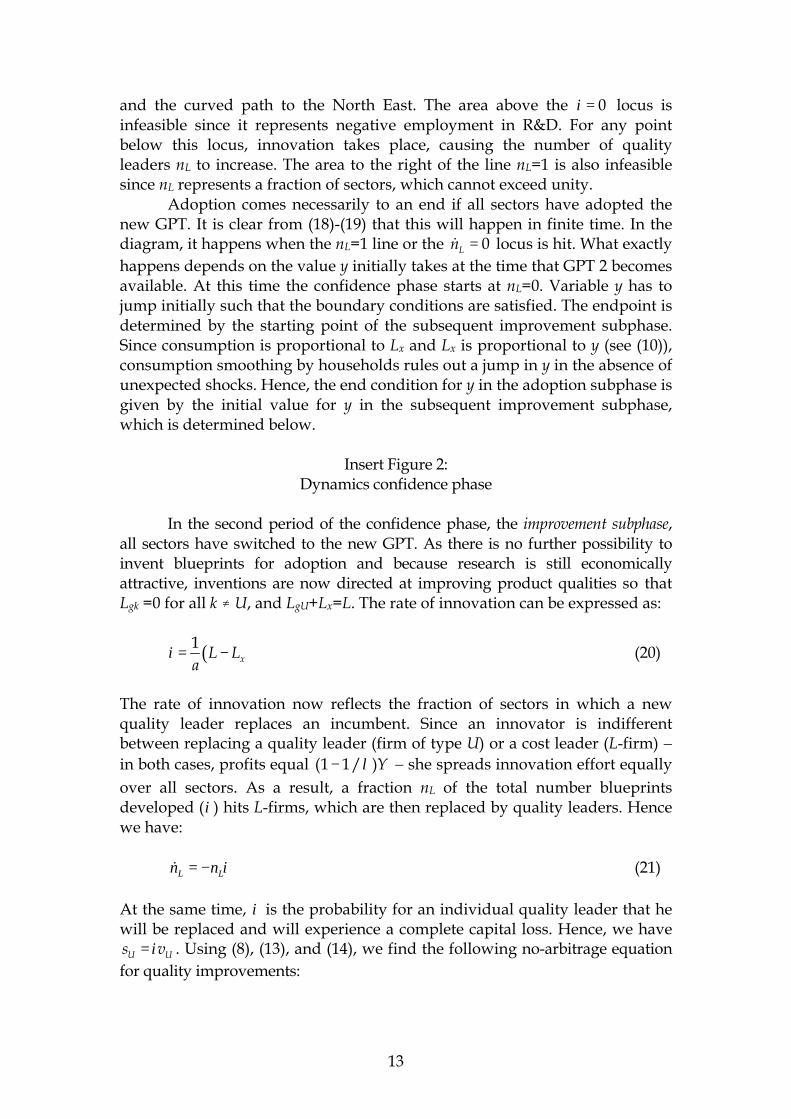
and the curved path to the North East. The area above the 0ι = locus isinfeasible since it represents negative employment in R&D. For any pointbelow this locus, innovation takes place, causing the number of qualityleaders nL to increase. The area to the right of the line nL=1 is also infeasiblesince nL represents a fraction of sectors, which cannot exceed unity.

Adoption comes necessarily to an end if all sectors have adopted thenew GPT. It is clear from (18)-(19) that this will happen in finite time. In thediagram, it happens when the nL=1 line or the 0Ln =& locus is hit. What exactlyhappens depends on the value y initially takes at the time that GPT 2 becomesavailable. At this time the confidence phase starts at nL=0. Variable y has tojump initially such that the boundary conditions are satisfied. The endpoint isdetermined by the starting point of the subsequent improvement subphase.Since consumption is proportional to Lx and Lx is proportional to y (see (10)),consumption smoothing by households rules out a jump in y in the absence ofunexpected shocks. Hence, the end condition for y in the adoption subphase isgiven by the initial value for y in the subsequent improvement subphase,which is determined below.

Insert Figure 2:Dynamics confidence phase

In the second period of the confidence phase, the improvement subphase,all sectors have switched to the new GPT. As there is no further possibility toinvent blueprints for adoption and because research is still economicallyattractive, inventions are now directed at improving product qualities so thatLgk =0 for all k … U, and LgU+Lx=L. The rate of innovation can be expressed as:

( )1xL L

aι = − (20)

The rate of innovation now reflects the fraction of sectors in which a newquality leader replaces an incumbent. Since an innovator is indifferentbetween replacing a quality leader (firm of type U) or a cost leader (L-firm) −in both cases, profits equal (1 1/ )Yλ− − she spreads innovation effort equallyover all sectors. As a result, a fraction nL of the total number blueprintsdeveloped (ι ) hits L-firms, which are then replaced by quality leaders. Hencewe have:

ι= −&L Ln n (21)

At the same time, ι is the probability for an individual quality leader that hewill be replaced and will experience a complete capital loss. Hence, we have

U Us vι= . Using (8), (13), and (14), we find the following no-arbitrage equationfor quality improvements:

14

11 ι

λ − + − =

&Y wr

aw w(22)

Substituting (4) into (22) to eliminate r, substituting (10) into (20) to eliminateLx, and taking into account nL + nU = 1, nT = nR = nF = nE = 0, we find:

( ) 11 µ ρ = − − +

&L

y Ln y

y a a(23)

1 1µ

λ = − −

&LL

L

n Ln y

n a a(24)

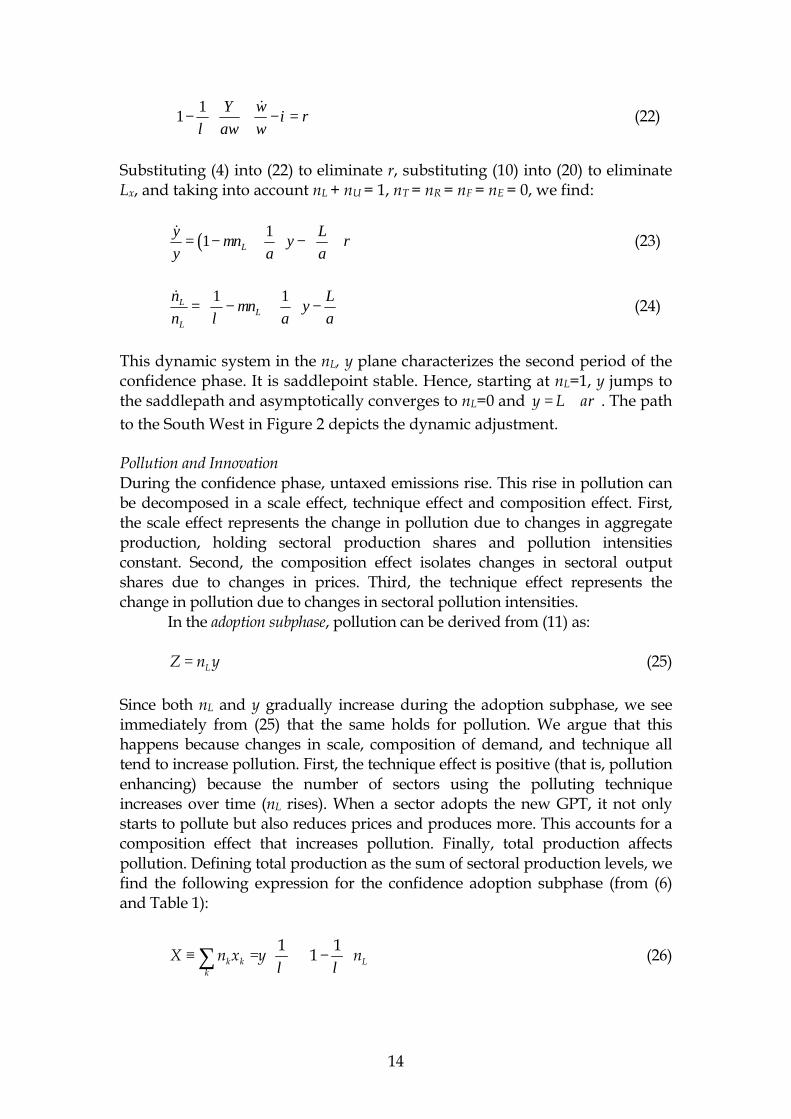
This dynamic system in the nL, y plane characterizes the second period of theconfidence phase. It is saddlepoint stable. Hence, starting at nL=1, y jumps tothe saddlepath and asymptotically converges to nL=0 and y L aρ= + . The pathto the South West in Figure 2 depicts the dynamic adjustment.

Pollution and InnovationDuring the confidence phase, untaxed emissions rise. This rise in pollution canbe decomposed in a scale effect, technique effect and composition effect. First,the scale effect represents the change in pollution due to changes in aggregateproduction, holding sectoral production shares and pollution intensitiesconstant. Second, the composition effect isolates changes in sectoral outputshares due to changes in prices. Third, the technique effect represents thechange in pollution due to changes in sectoral pollution intensities.

In the adoption subphase, pollution can be derived from (11) as:

LZ n y= (25)

Since both nL and y gradually increase during the adoption subphase, we seeimmediately from (25) that the same holds for pollution. We argue that thishappens because changes in scale, composition of demand, and technique alltend to increase pollution. First, the technique effect is positive (that is, pollutionenhancing) because the number of sectors using the polluting techniqueincreases over time (nL rises). When a sector adopts the new GPT, it not onlystarts to pollute but also reduces prices and produces more. This accounts for acomposition effect that increases pollution. Finally, total production affectspollution. Defining total production as the sum of sectoral production levels, wefind the following expression for the confidence adoption subphase (from (6)and Table 1):

1 11k k L

k

X n x y nλ λ

≡ = + − ∑ (26)

15

Because nL and y gradually increase during the adoption subphase, we seeimmediately from (26) that total production gradually rises, so that the scaleeffect also contributes to rising pollution levels.

To find out what happens to the rate of innovation, we need to knowhow Lx changes over time [see (16)]. The appendix shows that Lx increases(decreases) and innovation falls (rises) over time if η is large (small). Theintuition is as follows. On the one hand, the rate of innovation tends to fall overtime. This reflects the fact that the more sectors have switched, the feweropportunities are left for further adoption and the sooner innovation has to beredirected to quality improvements, which yields a lower rate of return.Forward-looking behaviour of investors ensures that the rate of return issmoothed and research efforts are gradually reduced. With lower researchefforts, labour becomes available to expand the scale of production. On the otherhand, however, if production with the new GPT saves a lot of labour (that is, ifη is small), the opposite happens and labour becomes available for research. Inthe latter case, the process of adoption is relatively fast and the scale ofproduction as measured by Lx declines. Nevertheless, pollution increases overtime since fast adoption allows the technique and composition effect todominate the scale effect.

In the improvement subphase, pollution increases as well over time,although at a decreasing pace. Since all sectors are using GPT 2 with a fixedemission output ratio, changes in pollution can be explained entirely by changesin total output (X) or labour in production (Lx). From (10) and (11) we find:

1xZ X L

η= = (27)

The Appendix shows that Lx rises over time. It implies a gradual increase inpollution and a gradual fall in innovation. The underlying cause is a fall in therate of return to innovation. As the proportion of low-price firms increases,more labour is allocated to incumbents and less is available per quality leaderthat replaces a cost-leader. As a result, profits for entrants fall and innovationbecomes less profitable.

The innovation intensity at the end of the confidence phase (when nL

approaches zero) proofs to be:

1 1GH

La

λι ρ ι

λ λ−

= − ≡ (28)

Not surprisingly, this equals the innovation rate in the Grossman andHelpman (1991) model (denoted by GHι ).

3.4 Innovation and pollution in the “alarm phase”

16

The economy enters the alarm phase once it starts taxing pollution. Society isaware or alarmed about the polluting effects of production using GPT 2. Tomitigate the adverse effects, firms are charged a pollution tax. Provided thatall sectors are at least hit once during the second period of the adoptionphase, all active firms in the alarm phase are regulated quality leaders (R-firms).

Because of the ongoing profit prospects, research is still active.Innovators develop new quality generations of the regulated products.Successful innovators become new quality leaders and set prices

( )Rp wλ η τ= + . No other types of innovation are undertaken, so that Lgk = 0 forkÖR and LgR+Lx=L. The value of a blueprint is determined by vR, and we haveaw=vR if LgR>0. For simplicity we assume that the alarm phase starts onlywhen the number of labour-cost leaders is negligibly small (nL=0).

The dynamics of the alarm phase can be determined analogous to thedynamics of the improvement subphase of the confidence phase. Substituting(4) into (22) to eliminate r, substituting (10) into (20) to eliminate Lx, andtaking into account nR = 1, nk = 0 for kÖR, we find:

( )1 1

/λ η

ρλ λ η τ

− = + − + +

&y Ly

y a w a(29)

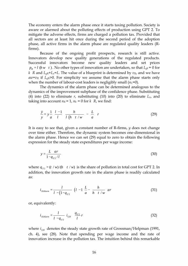
It is easy to see that, given a constant number of R-firms, y does not changeover time either. Therefore, the dynamic system becomes one-dimensional inthe alarm phase. Hence we can set (29) equal to zero to obtain the followingexpression for the steady state expenditures per wage income:

21 /ρ

θ λ+

=− Z

L ay (30)

where 2 ( / ) /( / )θ τ η τ= +Z w w is the share of pollution in total cost for GPT 2. Inaddition, the innovation growth rate in the alarm phase is readily calculatedas:

( ) ( )2

11 /λ η

ι λ ρλ θ η τ

= − − − − +

SSAlarmZ

La

a w(31)

or, equivalently:

2

2

λ θι ι ρ

λ θ λ = + −

ZSSAlarm GH

Z

(32)

where GHι denotes the steady state growth rate of Grossman/Helpman (1991,ch. 4), see (28). Note that spending per wage income and the rate ofinnovation increase in the pollution tax. The intuition behind this remarkable

17

result for growth is that a pollution tax increases the cost of productionrelative to that of R&D, which is a non-polluting activity. Thus in the alarmphase, the rate of innovation increases and total emissions fall compared tothe confidence phase.

3.5 Innovation and pollution in the “cleaning-up phase”

General equilibrium dynamicsFrom the point of view of GPTs, the cleaning-up phase is similar to theconfidence phase. A new unregulated technology is available for adoption,but its diffusion takes time. Adoption is costly, since only after developing thesector-specific blueprint at cost aw, a sector can use the new technology.Adoption takes place only if the returns to this kind of research investmentare large enough. To guarantee sufficient incentives to adopt we assume

/λ τ η< +w , so that π π<R F (see Table 1). Regulated quality leaders stayactive as long as no rival in their sector has incurred the cost to adopt GPT 3.Innovators that produce with the new GPT are first movers (F-Firms).

We can use expressions derived for the confidence phase to find outthe dynamics of the cleaning-up phase. For the adoption subphase, we needto replace nL by nF in (16). Substituting (4) into (17) to eliminate r, substituting

1/ 1/( / )j jc c wη τ− = + , substituting (10) into (16) to eliminate Lx, and takinginto account nR + nF = 1 and nT = nL = nU = nE = 0, we find:

1 11

/ρ

η τ = − − +

&yy

y w a(33)

2

1 1 1 1θ

η λ λ = − − +

&F L F

Ln y n

a a(34)

where 2 2/( / ) 1θ η η τ θ= + = −L Zw is the labour cost share for GPT 2.For the improvements subphase, we need to replace nL by nF in (21).

Substituting (4) into (22) to eliminate r, substituting (10) into (20) to eliminateLx, and taking into account nF + nE = 1, nT = nL = nU = nR = 0, we find:

( ) 11 µ ρ = − − +

&F F

y Ln y

y a a(35)

1 1ˆ µ

λ = − −

F F F

Ln n y

a a(36)

where (1/ ) 1/( / )µ λ η τ= − +F w .The two dynamic systems in (33)-(36) can be depicted in the nF, y plane

similar to Figure 2. The equilibrium dynamics can again be characterised by a

18

rise in nF from 0 to 1, while y increases. Then there is an endogenous switch tothe improvement subphase in which both nF and y fall over time.

Pollution and innovationPollution is obviously absent in the improvement subphase. Moreover,innovation falls similar to innovation in the improvement subphase of theconfidence regime. Hence, we focus on what happens to pollution andinnovation in the adoption subphase. Pollution is given by:

1( / )

FnZ y

wλ η τ −

= + (37)

It turns out that pollution continuously falls over time (see Appendix). Moreand more sectors switch to the clean technique (nF increases), which reducespollution. The upward pressures on pollution from increases in spending yare dominated by the technique effect.

Labour allocated to production can be written from (10) as:

( )( / )

Fx

nL y

wλ η ηλ η τ

− += +

(38)

Since y and nF increase over time, the amount of labour in production alsogradually increases. Since the rate of innovation is negatively related to Lx, asin (16), innovation falls over time.

4. Extensions

This section discusses extensions to our theory on EKCs. A first additionalfeature is the determination of the income level where pollution starts todecrease. In reality the critical level of income at which pollution is de-linkedfrom income differs greatly among different pollutants. Some pollutants arealready almost completely phased out in rich economies (for example, CFCs),while for other pollutants we see only the upward sloping part of the EKC (CO2for example).6

A related issue is the idea of overlapping EKCs. Booth (1998) has arguedquite strongly that one pollutant can only be phased out because it is replacedby another pollutant. Put more moderately, it could be that seemingly cleanGPTs turn out to be polluting in the end. If this is the case, additional GPTs haveto be developed until, finally, one really turns out to be clean.

If there are several shifts during economic development, a furtherquestion would be the possible ability of individuals to expect the arrival of newGPTs, at least with a certain probability. It is conceivable that, for certain 6 Of course, strictly speaking a monotonically increasing relationship between income andpollution is not an EKC by definition.

19

pollutants, technical solutions in the future can be anticipated to a certaindegree. In other cases, however, it seems reasonable to assume that the arrival ofa technological breakthrough is highly uncertain and arrives, if ever,unexpectedly.

In addition, the sequencing of the different phases can be more complexthan modelled in this approach. Arrival dates of profitable GPTs and/or theintroduction of taxes can be assumed to occur at different points in time so thatmore types of producers are active in the markets when a new phase begins.

Finally, one could elaborate more on optimal taxation. This requires theanalysis of instruments to correct pollution, to correct R&D, and to correctoutput levels in order to remove the distortionary pricing effects. All thesehighly challenging issues are left for future research.

5. Conclusions

The model used in this paper shows that the existence of EKCs canconceivably be explained by a combination of public tax policy and differenttechnology options. In particular, the gradual adoption of new generalpurpose technologies predicts a pattern of pollution over time that isconsistent with the the upward and downward sloping parts of the EKC.

It should be noted that our model does not necessarily predict an EKCfor all pollutants. In empirical research, the EKC is found only for specificpollutants. In the model, the downward sloping part of the EKC emerges onlyif the polluting GPT is replaced by a cleaner GPT. The adoption of the cleanerGPT requires sufficient incentives, a high pollution tax and low enoughlabour costs of the new GPT in particular. Otherwise, no technology shifttakes place and the pollution tax only has the conventional static (level) effect.In addition, the further use of the dirty GPT without and with pollution taxesyields a realistic background to demonstrate the reasons for the turning pointof the curve.

The framework has important policy implications. In the alarm phase, apollution tax both lowers emissions and raises growth, a classical win-winsituation. Moreover, the decline of pollution directly depends on the rate ofadoption of the new clean GPT. Subsidies to increase the invention of adoptionblueprints would be in favour of environmental quality. The optimum pollutiontax rate and the optimality of subsidies for adoption activities depend on theweight of a clean environment in the utility function.

20

Appendix

A. Pollution and innovation in the confidence phase.

To find out the development of aggregate pollution and the rate of innovation inthe confidence phase, we transform the phase diagram from Figure 2 andequations (18), (19), (23), (24) into a phase diagram in the Lx, nL plane.

Adoption subphaseWe show that Lx may either fall or rise during the adoption subphase,depending on whether η is small or large respectively.

From (10) we find the following expression for Lx in the confidenceadoption subphase:

1 (1 ) Lx

nL y

ληλ

− − =

(A.1)

We use (A.1) to replace y in (18) and (19) by Lx and find the following dynamicsystem for the adoption subphase:

{ }1[ (1 ) 1 ] (1 ) [1 (1 ) ]

[1 (1 ) ]x

x Lx L

LL L n a

L a nλ η λη λη λη ρ

λη= − + − − − − − −

− −

&

(A.2)1

( )L xn L La

= −& (A.3)

The 0xL =& locus is downward sloping as long as 1/λ η> which is the casedue to our assumption that 1/ 0µ λ η≡ − > . The initial jump in Lx isdetermined in the same way as that of y, see main text: the endvalue of Lx isdetermined by its initial value in the subsequent improvement subphase.However, we can also use the endvalue of y to determine the end value of Lx

by using the relation between these two variables given by (A.1). Hence, wecan infer some useful properties of the endvalue of Lx from the endvalue of y.From Figure 1 or (18) we see that when nL=1, y is bounded as follows:

1( )

1y L aρ

µ< +

−(A.4)

Thus, from (A.1) we see that when nL=1, Lx is bounded as follows:

( )1xL L a

ηρ

µ< +

−(A.5)

From (A.2) we see that when nL=1, we have

21

0xL ≤& if 1x

L aL

µ η ρµ η

+≤

+ −(A.6)

Now consider the following condition:

( )1 1

L aL a

η µ η ρρ

µ µ η+

+ ≤− + −

(A.7)

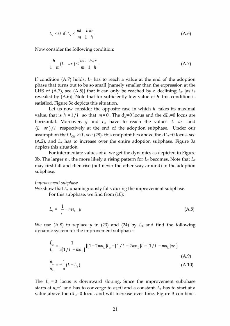
If condition (A.7) holds, Lx has to reach a value at the end of the adoptionphase that turns out to be so small [namely smaller than the expression at theLHS of (A.7), see (A.5)] that it can only be reached by a declining Lx [as isrevealed by (A.6)]. Note that for sufficiently low value of η this condition issatisfied. Figure 3c depicts this situation.

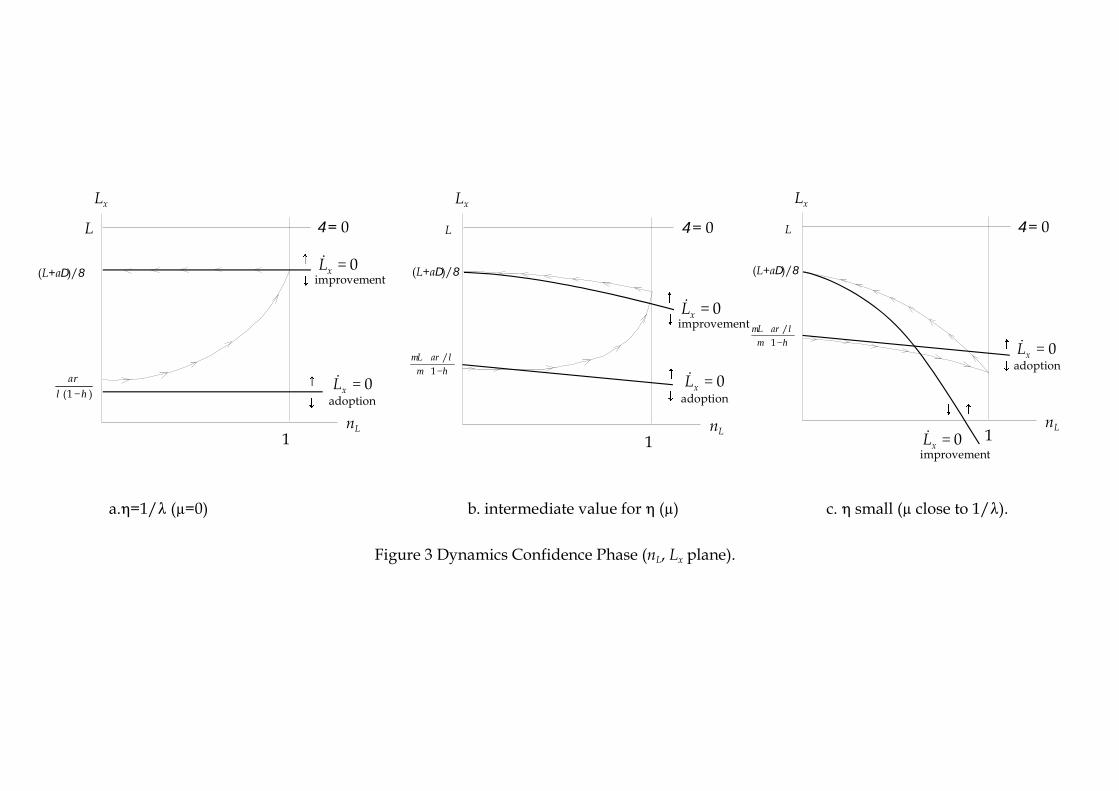
Let us now consider the opposite case in which η takes its maximalvalue, that is 1/η λ= so that 0µ = . The dy=0 locus and the dLx=0 locus arehorizontal. Moreover, y and Lx have to reach the values L aρ+ and( )/L aρ λ+ respectively at the end of the adoption subphase. Under ourassumption that 0GHι > , see (28), this endpoint lies above the dLx=0 locus, see(A.2), and Lx has to increase over the entire adoption subphase. Figure 3adepicts this situation.

For intermediate values of η we get the dynamics as depicted in Figure3b. The larger η , the more likely a rising pattern for Lx becomes. Note that Lx

may first fall and then rise (but never the other way around) in the adoptionsubphase.

Improvement subphaseWe show that Lx unambiguously falls during the improvement subphase.

For this subphase, we find from (10):

1x LL n yµ

λ = −

(A.8)

We use (A.8) to replace y in (23) and (24) by Lx and find the followingdynamic system for the improvement subphase:

{ }1[1 2 ] [1/ 2 ] [1/ ]

[1/ ]x

L x L Lx L

Ln L n L n a

L a nµ λ µ λ µ ρ

λ µ= − − − − −

−

&

(A.9)1

( )Lx

L

nL L

n a= − −

&(A.10)

The 0xL =& locus is downward sloping. Since the improvement subphasestarts at nL=1 and has to converge to nL=0 and a constant, Lx has to start at avalue above the dLx=0 locus and will increase over time. Figure 3 combines

22

the two subphases.

insert Figure 3

The development of pollution in the improvement subphase directly followsfrom (27) and the notion that Lx rises over time. The development of the rate ofinnovation is exactly the mirror of that of Lx, since ( )/xL L aι = − .

B. Pollution in the Cleaning-up phase.

We transform the dynamic system in (35)-(36) into a dynamic system in terms ofZ and nR. Substituting (37) in these equations to eliminate y, and replacing nF by1−nR, we find:

( / )R R

R

n Z L a nZZ an

ξ λ ρ− − −=

&(A.11)

[ / ( )]RR

R R

L n Znn an

λ λ η− − −= −

&(A.12)

where [ / (1 )]wξ η λ τ η λ= + − − − .It should be noted that [ / (1 )] 1 0wτ η λ− − > − > from our assumptions

made above to ensure adoption of the clean GPT. We now have twosituations, depending on whether ξ is positive or negative. First, if it ispositive, the dZ=0 locus slopes positive in the feasible region (for 0<nR<1) andthe saddlepath slopes downward so that pollution unambiguously falls withthe fall in nR. Second, if ξ is negative, the dZ=0 locus has a vertical asymptoteat / 1Rn λ ξ= − > and slopes downward in the feasible range (for 0<nR<1).However, the saddlepath slopes downward so that again pollutionunambiguously falls with the fall in nR.

23

References

Andreoni, J. and A. Levinson (2000), ‘The Simple Analytics of theEnvironmental Kuznets Curve’, Journal of Public Economics(forthcoming).

Booth, D.E. (1998), The Environmental Consequences of Growth, steady-stateeconomics as an alternative to ecological decline, London and NewYork:Routledge.

Bresnahan, T.F. and M. Trajtenberg (1995), ‘General Purpose Technologies„Engines of Growth“?‘, Journal of Econometrics, 95, 83-108.

Bretschger, L. (1999), Growth Theory and Sustainable Development, Aldershot,UK: Edward Elgar.

Copeland, B. and S. Taylor (1994), ‘North-South Trade and the Environment’,Quarterly Journal of Economics, 109 (3), 755-787.

Cropper, M. & Griffiths, C. (1994): The interaction of population growth andenvironmental quality, American Economic Review, 84, 250-254.

de Bruyn, S. M. (1997). Explaining the environmental Kuznets curve:structural change and international agreements in reducing sulphuremissions, Environment and Development Economics, 2, 485-504.

de Bruyn, S. M (1999), Economic Growth and the Environment, Ph.D. thesis, VrijeUniversiteit Amsterdam.

De Groot, H.L.F. (1999), ‘Structural Change, Economic Growth and theEnvironmental Kuznets Curve’, Ocfeb Research Memorandum 9911,Rotterdam University.

Grossman, G. M. and E. Helpman (1991), Innovation and Growth in the GlobalEconomy, Cambridge Mass.: MIT Press.

Grossman, G. M. & Krueger, A. B. (1995), ‘Economic growth and theenvironment’, Quarterly Journal of Economics, 112, 353-378.

Helpman, E. and M. Trajtenberg (1998), ‚A Time to Sow and a Time to Reap:growth based on general purpose technologies‘, in: E. Helpman (ed.)General purpose technologies and economic growth, Cambridge, Mass.: MITpress.

Nahuis, R. (2000), Knowlwdge and Economic Growth, Ph.D. thesis TilburgUniversity.

Selden, T. M., & Song, D. (1994): Environmental quality and development: Isthere a Kuznets curve for air pollution? Journal of EnvironmentalEconomics and Management 27, 147-162.

Shafik, N. (1994): Economic development and environmental quality: aneconometric analysis, Oxford Economic Papers, 46, 757-773.

Smulders, S. (1995) "Entropy, Environment and Endogenous EconomicGrowth", Journal of International Tax and Public Finance 2, 317-338.

Smulders, S. (1999) "Endogenous Growth Theory and the Environment", inJ.C.J.M. van den Bergh (ed.) Handbook of Environmental and ResourceEconomics, chapter 42, 610-621, Cheltenham UK: Edward Elgar.

Stockey, N. (1998), ‘Are there Limits to Economic Growth’, InternationalEconomic Review 39, 1-31.

24

Torvanger, A. (1991), ‘Manufacturing Sector Carbon Dioxide Emissions innine OECD countries, 1973-1987: a divisia index decomposition tochanges in fuel mix, emissions coefficients, industry structure, energyintensities and international structure’, Energy Economics 13, 168-186.

Greenphase

Allsectorshave

adopted

CleanGPT

arrives

Pollutiontax

imposed

Adoption

Confidence phase Alarmphase

Cleaning-up phase

Time

Adoptionsubphase

Improvementsubphase

Adoptionsubphase

Improvementsubphase

Allsectorshave

adopted

LaboursavingGPT

arrives

Quality Quality Quality Quality Adoption

TraditionalQualityLeaders

RegulatedQLs

Traditional QLs & Labour cost

leaders

Unregulated QLs&

Labour CLs

Regulated QLs&

First movers

Ecological QLs&

First movers

type ofinnovation:

activefirms:

pollution:

phase:

event:

Figure 1 Overview of the model

y

nL

(L+aD)/(1!µ)

aD/(1!0)

8L

L+aD

1

dy = 0

dy = 0

4 = 0

improvement

adoption

L/0

Figure 2 Dynamics Confidence Phase

(1 )aρ

λ η−

0xL =&

0xL =&

/1

L aµ ρ λµ η

++ −

0xL =&

0xL =&

/1

L aµ ρ λµ η

++ −

0xL =&

0xL =&

Lx

L

(L+aD)/8

1

4 = 0

improvement

adoption

nL

Lx

L

(L+aD)/8

1

4 = 0

improvement

adoption

nL

Lx

L

(L+aD)/8

1

4 = 0

improvement

adoption

nL

Figure 3 Dynamics Confidence Phase (nL, Lx plane).

a.0=1/8 (µ=0) b. intermediate value for 0 (µ) c. 0 small (µ close to 1/8).