time as a trade barrier david hummels purdue …...1 time as a trade barrier david hummels purdue...
TRANSCRIPT

1
Time as a trade barrier
David Hummels
Purdue University
July 2001
Abstract:
International trade occurs in physical space and moving goods requires time. This paper examines the importance of time as a trade barrier, estimates the magnitude of time costs, and relates these to patterns of trade and the international organization of production. Estimates indicate that each additional day spent in transport reduces the probability that the US will source from that country by 1 – 1.5 percent. Conditional on exporting country, estimates directly identify a willingness-to-pay for time savings using variation across exporters and commodities in the relative price / speed tradeoff for air and ocean shipping. Each day saved in shipping time is worth 0.8 percent ad-valorem for manufactured goods. Relative declines over time in air shipping prices make time-savings less expensive, providing a compelling explanation for aggregate trade growth, compositional effects in trade growth, as well as growth in time-intensive forms of integration such as vertical specialization. Specifically, the advent of fast transport (air shipping and faster ocean vessels) is equivalent to reducing tariffs on manufactured goods from 32% to 9% between 1950-1998.
Contact: David Hummels, Department of Economics, 1310 Krannert, Purdue University, West Lafayette
IN 47907-1310. ph: 765 494 4495 email: [email protected]

2
I. Introduction
International trade occurs in physical space and moving goods requires time.
Shipping containers from European ports to the US Midwest requires 2-3 weeks; Far
Eastern ports as long as 6 weeks. In contrast, air shipping requires only a day or less to
most destinations, but it is also much more expensive. For US trade in 1998, air freight
commands a typical premium equal to 25 percent of the transported good’s value.1
Despite the expense, a large and growing fraction is air shipped. Thirty percent of US
trade in 1998 was air-shipped, up from 7 percent in 1965 (and virtually no trade
employed air-shipment in 1950). Excluding Canada and Mexico, over half of US exports
are air-shipped. These facts suggest two inferences: lengthy shipping times impose costs
that impede trade, and importers exhibit significant willingness-to-pay to avoid those
costs.
This paper examines the importance of time as a trade barrier, and addresses three
questions. What specific costs does shipping time impose on trade? What is the
magnitude of these costs? And, what are the effects of time on patterns of trade and the
international organization of production?
Lengthy shipping times impose inventory-holding and depreciation costs on
shippers. Inventory-holding costs include both the capital cost of the goods while in
transit, as well as the need to hold larger buffer-stock inventories at final destinations to
accommodate variation in arrival time. Depreciation captures any reason that a newly
produced good might be preferable to an older good. Examples include literal spoilage
(fresh produce or cut flowers), items with immediate information content (newspapers),
1 See Table 1.

3
and goods with complex characteristics for which demand cannot be forecast well in
advance (holiday toys, high-fashion apparel). These costs will be magnified in the
presence of fragmentation. When countries specialize in stages of production and trade
intermediate goods the inventory-holding and depreciation costs for early-stage value-
added accrue throughout the duration of the production chain.
To estimate the magnitude of time costs, I examine a model of a firm’s choice of
export location and transport mode that trades off fast but expensive air transport against
slow but inexpensive ocean shipping. I employ a novel dataset that includes prices,
quantities, and speed for different transportation modes in US trade. Variation across
exporters and commodities in the relative price / speed tradeoff identify a willingness-to-
pay for time savings in shipment. This is translated into a direct measure of the ad-
valorem barrier equivalent of an additional day’s travel time. For manufactured goods I
find each day in travel is worth an average of 0.8 percent of the value of the good per
day, equivalent to a 16% tariff for the average length ocean shipment. An additional
benefit of the econometric model is the ability to explain partner selection in trade.
Estimates indicate that each additional day in ocean transit reduces the probability that a
country will export to the US by 1 percent (all goods) to 1.5 percent (manufactured
goods).
These estimates have pronounced implications for trade and the international
organization of production. In the post-war era, world trade relative to output has grown
at 2.9 percent per year (and manufacturing trade/output has grown at 3.7 percent
annually).2 Typical explanations attribute this growth to declining tariffs and improved
2 Data from WTO.

4
technology (information and transportation).3 Hummels (2000) documents very rapid
declines in air relative to ocean shipping rates, as well as extensive substitution toward
air-based shipping. To the extent that time is an important impediment to trade for all
goods, relative declines in air shipping prices may help explain aggregate trade growth.
And, time-sensitive goods (manufactures) should grow especially rapidly as a result of
shipping price declines, indicating an important compositional role of the relative price
declines.
The post-war era has seen rapid growth in other forms of integration, in particular,
foreign direct investment and vertical specialization/fragmentation. FDI increased at
6.8% per year and FDI/output increased 3% per year between 1960 and 1995. Hummels,
Ishii and Yi (2000) document that the share of vertical specialization in trade (defined as
the use of imported inputs in exported goods) has increased 30%, and been responsible
for roughly half of overall trade growth from 1970-1990. As argued above, vertical
specialization (aka multi-stage production or fragmentation) may be especially time
sensitive. If so, rapid declines in air transport costs, and the corresponding reduction in
the cost of time-saving, may be responsible for the growth of time and coordination-
intensive forms of integration.
The econometric technique employed here directly identifies the value of time
saving from transport modal choice, but the estimates are informative about many
policies and sources of technological change that speed goods to market. For example,
eliminating or streamlining elaborate customs procedures allow imported goods reach
their destinations more quickly. Investing in more efficient port infrastructure may
3 Baier and Bergstrand (1998) relate aggregate trade growth to changes in aggregate measures of transportation costs and tariffs, but do not emphasize compositional effects.

5
accomplish similar goals. The estimates that follow indicate that a four-day wait for
customs inspection is equivalent to the cost of explicit tariffs for most manufactures.
Another example is the economic value of increased cycle times in production. One
source of time costs is effective depreciation of a good caused by a mismatch between
what the firm produces and what the consumer desires to buy months later. The
estimates provided here can be used to calculate the value of changes in production
technique that narrow this time gap.
This work belongs to a literature on the analysis and measurement of trade
barriers that has received renewed attention of late. One can imagine a long list of
barriers that plausibly affect international integration, but careful measures of trade
impediments can be difficult to obtain. Contributions to the literature fall into two
categories. The first concerns simply obtaining data (of varying quality) on obvious
barriers such as tariffs and transportation costs and examining their impact on trade.4
The second seeks to identify more subtle barriers such as information (Rauch,
1999), product standards (Moenius, 1999), foreign exchange rate variability (Wei, 1998),
environmental standards (Edgerington and Minier 2000), non-tariff barriers of various
sorts and structural impediments. These barriers are less obvious and perhaps more
interesting, but also much more difficult to directly measure. As a consequence,
researchers rely primarily on indirect methods: positing a model of bilateral trade flows
and correlating flows with proxy variables meant to represent trade barriers.
Unfortunately, indirect calculations of trade barriers must necessarily be filtered
through a particular model to be meaningful. This raises a host of issues with model

6
selection, appropriate levels of aggregation, and interpretation of parameters.5 The
advantage of the current paper is that it offers the analysis of a novel impediment to trade,
provides a direct measure of its cost, and relates this measure specifically to the extent
and composition of trade and forms of integration other than trade.
Section II describes a simple location and modal choice problem for a firm in the
presence of time costs. Section III details the econometric specification and data
employed. Section IV provides and discusses results. Section V links time as a trade
barrier to changes in the extent, composition and organization of international integration.
Section VI concludes.
II. The Firm’s Problem
A firm wishing to export commodity k to the United States chooses an export
location i and a transportation mode m so as to minimize the total cost of the delivered
goods (expressed in per quantity units).
(1) k k k k kim i im im imTC C f Tτ ε= + + +
C is the production cost, f=F/Q is the total freight charge divided by quantity shipped, τ is
the time cost, T is the shipment time in days, and ε defines a location-mode-commodity
cost shifter.
4 Some examples include Yeats (early transport cost paper), Harrigan (1993), Haveman, Nair and Thursby (1998), Djankov, Evenett, and Yeung (1997), Baier and Bergstrand (1998), Hummels (1999), Trefler and Lai (1999), and Hummels (2000). 5 The canonical model employed for indirect measurment is the gravity equation, usually derived from a one-sector monopolistic competition model. Several authors have criticized the usefulness of this model as

7
The firm solves this cost minimization problem by asking: conditional on the
choice of exporter i, which transport mode should be chosen? Air shipping is chosen if
(2) k k k k k k k ki iA iA iA i io io ioC f T C f Tτ ε τ ε+ + + < + + +
Conditioning on an exporter drops production costs from this expression. Rearranging,
we have
(3) ( ) ( ) ( ) 0k k k k kio iA iA io iA ioT T f fτ ε ε− − − − − >
Air shipping is chosen if the greater time costs associated with ocean shipping exceed the
premium charged for air freight.
The solution to this problem determines an optimal mode m* for a given
production location and commodity. Given the location-specific cost minimizing mode,
the firm then chooses the optimal location from which to export. This depends not only
on the production costs, but also on the optimal mode’s level of freight rates and time
costs for that location relative to other locations. Returning to the cost function, the firm
exports from country i rather than j if
(4) * * * * * *( ) ( ) ( ) ( ) 0k k k k k k ki j im jm im jm im jmC C f f T Tτ ε ε− + − + − + − <
The per day time cost of the good, τ, is a function of two factors. The first is the
per day interest rate r on the good in transit, otherwise known as pipeline inventory. The
well as failures in typical implementation. Recent critiques include Anderson and VanWincoop (2000), Evans (2000), and Hillberry and Hummels (2001).

8
second factor is a “depreciation rate” δ for the good. The depreciation rate encompasses
any reason that a newly produced good might be preferable to an older good.
Obvious examples include spoilage that is literal and predictable such as fresh
produce or cut flowers. Depreciation may also be probabilistic -- in any given day of
transit there is a positive probability that the good may be damaged so that longer
shipment times increase the cumulative probability of damage. Depreciation may reflect
the immediate need for the good, and lost profitability/utility from the good if it is not
available. For example, the absence of key components can idle an entire assembly plant.
In this sense, an emergency shipment that arrives in a timely fashion may be worth many
times the nominal price of the component, while late arrivals are of considerably
depreciated value.
More generally, with long lags between production ordering and final sales, firms
may face a mismatch between what consumers want and what the firm has available to
sell.6 Suppose that consumers will pay a premium to purchase goods containing “ideal”
characteristics, but that they have unpredictable preferences over what constitutes the
ideal characteristic set. Further, let the firm learn about ideal types slowly over time so
that the characteristics of the goods made by the firm better match the consumers ideal
type. This leads to a few simple implications. First, there is a distance between ideal
type and what the firm has available to sell, with the price premium for the ideal type
growing in that distance. Second, the distance and therefore price premium grows larger
as the time increases between when a firm begins production and when the good is
consumed.
6 This feature of the story owes much to conversations with Alan Deardorff.

9
To fix ideas, write the consumer’s demand function as /D pα= . 1α ≤ is the
type produced by the firm, with 1α = being the ideal type. The firm can costlessly
choose characteristics of the good to match the ideal type, but its information about the
ideal type is imperfect. This can be represented as 1/ Tα λ= for 1Tλ ≥ . T is the time
(in days) between when the firm begins production and when the good is consumed. λ is
a learning parameter, describing the rate at which firms learn about the ideal type
(immediately customizable goods can always match the ideal type). The price of the
ideal type relative to the actual type (holding constant quantity) can then be written as
* /p p Tλ= . In this case, lambda is the “depreciation rate”.
Specific examples of goods with this property may be useful here. Toy
manufactures generally do not know in advance which toys will emerge from among
hundreds of competitors to capture the hearts and minds of children during the holiday
gift-giving season. The “ideal” types (Tickle me Elmos, and Cabbage Patch Kids come
to mind) command price premia over the non-ideal types. As firms near the holidays,
they receive market signals (product reviews, early sales) about the ideal type, and can
adjust accordingly. High fashion apparel is another example where ideal characteristics
are difficult to discern well in advance, and firms must produce (and ship) much closer to
sales dates.
Two products that exhibit extreme time sensitivity due to depreciation of this sort
are newspapers and personal computers. News must be manufactured (reported) very
close to its consumption date to have any value at all, and not coincidentally, newspapers
were among the very first goods to be imported via air shipment. The current practice for
many personal computer manufacturers is to allow no time between purchase and

10
manufacture, and therefore no depreciation rate. Standardized packages do not appeal to
many consumers who are willing to pay more for a customized good that is manufactured
to particular specifications (larger screen, more memory). So manufacturers simply do
not build the computer until they know the precise ideal characteristics, and thereafter the
customized build is over-nighted.
Combining the interest rate with the depreciation rate, we have a per day time cost
( )k k kr pτ δ= + . Using this in the modal choice decision (conditional on exporting
from importer i) we have
(5) ( ) ( ) ( ) ( ) 0k k k k k kiA io io iA iA iof f r p T Tδ ε ε− − + − + − <
Recall that the freight rates are described in terms of the quantity of the good to be sold.
Holding quantity units constant, time costs are weighted more heavily for higher priced
goods as both the interest and depreciation charges are expressed relative to the value of
the good. When comparing time costs across goods with varying units, it is convenient to
divide through by prices to express this equation in ad-valorem terms
(6) ( ) ( )( ) ( ) 0k k k k
kiA io iA ioio iAk k k k
f f r T Tp p p p
ε εδ− − + − + − <
Time costs are magnified in the presence of fragmented production -- multi-stage
production arrangements where dispersed plants link sequentially to complete a final
good. To understand this, realize that time costs for first stage value-added begin to

11
accumulate immediately and do not stop until the final good is sold. As a result, for n
stages of production, the first stage value added pays time costs n times, second stage
value added pays time costs (n-1) times…until last stage value added pays the cost only
for the last voyage. That is, value added (V) in stage c faces transport time after each
stage j c≥ , so that time costs over the whole system are
(7) 1
( )n nSc c jc j c
V r Tτ δ= =
= +∑ ∑
To simplify, if r and δ are the same for each stage this can be rewritten as price of
the good at each stage (equal to the sum of value added to that point) multiplied by the
time cost at that stage.
(8) 1
( ) nSc cc
r p Tτ δ=
= + ∑
This indicates that the importance of time savings in transport rises with each stage
because the time savings accrue to successively larger amounts of value-added. This
suggests that higher prices in equation (5) can be interpreted as greater cumulative value-
added rather than, say, higher quality. However, if the modal decision is described in ad-
valorem terms, as in equation (6), the time savings decision is based entirely on modal
optimality at the margin. In other words, the estimates to follow identify marginal time
costs, but the time costs over an entire fragmented system may be much larger. A back
of the envelope calculation based on this point is contained in section V.

12
As a final note in this section, the preceding interest rate and depreciation stories
emphasize time costs that arise from lengthy shipping times, not costs due to variability
in arrival times. This focus is guided by data constraints, not because variability is
unimportant. Indeed, arrival time variability is a potentially serious cost, especially in the
face of fragmented production. The absence of key components can idle an entire
assembly plant, which increases the optimal inventory on-hand necessary to
accommodate arrival time variation. The costs of defects in component quality are also
magnified, as sizable inventories (at the plant, in transit) may be built up before defects
are detected. The defect problem motivates “just-in-time” inventory techniques, which
aim to minimize both the inventory on-hand and in the pipeline. Studies of JIT indicate
some plants hold only a few hours of component inventory.7 Clearly, the ability to
implement a “just-in-time” strategy is limited when parts suppliers are a month of ocean
transit time removed from the assembly plant.
In the econometric work to follow, only data on shipment length are available.
However, if arrival variability is correlated with shipment length, the estimates should
pick up time costs associated with variability as well.
III. Econometric Specification
Section II suggests two principal ways in which time costs may affect trade.
Equation (4) indicates that firms with time sensitive goods (high τ) will, other things
equal, not produce for export in countries with high levels of time costs (i.e. where ocean
7 See Womack, et al (1990).
13
shipping is especially lengthy and air shipping is very expensive). Equation (6) indicates
that, conditional on the exporting country, firms will choose air shipping when the time
savings from air shipping exceed the price premium charged for it.
The overall effect of time as a trade barrier shows up both in the country selection
effect and in the modal choice decision. In order to capture both effects, I employ a
selection corrected probit model in modal choice.8 The first stage determines the
probability that country i will export a positive quantity of good k to the United States as
a function of underlying location characteristics. The second stage determines the
probability that air is chosen as the transport mode, conditional on country i exporting to
the US.
I implement equation (4) by estimating the probability that country i exports
commodity k to the US in 1998, as a function of production costs, and the freight and
time costs of the optimal mode. Production costs are captured by a vector of endowments
including labor, capital, and human capital. The optimal mode for each country x
commodity is not observed for countries that do not trade. Accordingly, freight costs are
captured by distance shipped, a significant determinant of both air and ocean freight
rates. Time costs are captured by ocean shipping times.
(9) 1 1( 0) ln ln ln / ln / lnkik i ip ip i i i i i iP T DAYS DIST L K Y H L TFPβ β> = + + + + +
8 In principal, one could alternatively employ a nested logit structure. The first level alternative is the choice of specific exporting country. The second level alternative, conditional on exporter, is modal choice. This structure is not employed for two reasons. First, it would be computationally intractable to include as specific first stage options each of the more than 200 countries that export to the US in 1998. Second, the reasons why Germany rather than Mozambique is chosen as an exporter are less interesting

14
The trade data contain exporter x US entry port x 10-digit Harmonized System
detail. Estimates are conducted separately for each 2-digit SITC commodity group, with
all exporter x US entry port x 10-digit HS commodity detail retained. This is equivalent
to treating each import record as an observation on a separate firm. Estimates are
conducted both with and without 5-digit SITC fixed effects.
Distances and travel days are calculated using exporter x US entry port
information. Zero trade value observations are created corresponding to cases where the
value of trade is zero for any exporter x 10-digit HS code. Distances and travel days for
the zero trade values are calculated relative to the nearest US port.
Conditional on trade being observed from an exporter, the probability that air
transport is chosen as
(10) ( | 0) ( )k k
k k iA ioik i i k k k io k ik
f fP m air T T Xp p
α α τ ε= > = − + ⋅ + +
The data on freight rates are discussed in detail in the next sub-section. Data on shipping
times are only available for ocean freight. On the assumption that air freight can reach
any worldwide destination within one day, the included variable is simply ocean shipping
less one day.
This model differs from equation (3) in the inclusion of a modal substitutability
parameter, α. This parameter describes the rate at which a higher air freight premia
lowers the probability that air shipping is selected. The coefficient on shipping times
than the characteristics of Germany relative to Mozambique. This is the flavor of the selection corrected probit.

15
includes both the per day time cost, τ, and the modal substitutability parameter.
Multiplying shipment times by the per day time cost yields the time cost of (longer)
ocean shipping in ad-valorem terms, equivalent to the included freight rates. Multiplying
by the modal substitution parameter converts this value into the probability that air
shipping is selected. This specification is very handy in that combining the estimated
coefficients on air freight premia and ocean time costs yields the per day time cost. The
usual problem with interpreting probits is that the marginal probabilities are non-constant
over the probability distribution. However, the relationship between time and freight
rates is constant. As an example, suppose that 5 extra days corresponds to a 2% freight
premium. While the effect of 5 additional days (or 2% higher rates) on the probability of
choosing the air transport mode varies over the distribution, the effect of 5 days relative
to a 2% freight premium is constant throughout.
Note that this estimation uses variation across all 3 dimensions (exporter x US
entry port x 10 digit HS cateogry within a 2-digit category) to identify the price/speed
trade-off. This modeling choice is employed because there are typically very few
exporters in any narrowly defined good, and this precludes identification. Moreover,
variation in characteristics (weight, bulk) across goods provides needed variability in
freight rates.
To assuage concerns about pooling over a too-large grouping of goods, estimates
are performed both with and without 5-digit SITC fixed effects. The argument for
employing the fixed effects is that goods within a 2-digit classification may exhibit
significant heterogeneity in the probability of employing air transport for reasons outside
the model. Of course, heterogeneity within 2-digit classifications also creates variation in

16
the air freight premium. For example, within office machinery, laptop computers are
always air shipped while large copying machines are generally ocean shipped. This
choice is driven by the relative air/ocean freight rates of the two goods and provides
precisely the sort of variation the model calls for to identify time costs. Including lower
level fixed effects in this case completely eliminates the useful variation in the data.
It is certainly the case that pooling over a larger set of goods will lead to a lower
modal substitution value, alpha. However, since alpha appears in both the air freight
premium and shipping time coefficients, examining the ratio of these coefficients
eliminates this problem. Accordingly, results are presented both ways to allow the reader
their preferred specification.
Data
Three essential pieces of information are necessary for this exercise -- modal
choice, prices, and shipping times. Data on ocean shipping times are derived from a
master schedule of shipping for 1999 taken from www.shipguide.com. This shipping
schedule describes all departures and arrivals of all commercial vessels operating
worldwide in this period. From this, I construct a matrix of shipping times between all
ports everywhere in the world and all US entry ports. Several modifications are
necessary. First, direct shipments are not available for every port-port combination
(Tunis does not ship directly to Houston). In these cases, I calculate all possible
combinations of indirect routings (Tunis to Rotterdam to Houston; Tunis to Rio to
Houston and so on) and take the minimum shipment time available through these
routings. Second, there are generally multiple ports within each origin country. In this

17
section, a within-country average of shipment time from these ports is employed.
Because US data include entry port detail, these are combined with destination-port
specific arrival times.
Some other complications are not currently pursued. Shipping times for
developing countries exhibit three interesting characteristics. First, these countries are,
on average, further away from destination markets and have longer distance related
shipping times. Second, shipping volumes for these countries are smaller and so a larger
number of stops is required to fill a vessel. These characteristics are accounted for in the
shipping schedule. Third, the frequency of visits is much lower. Ships arrive from Japan
daily while ships arrive from Africa every 15 days. Put another way, if a shipment is
ready to leave on March 1 but the next available vessel does not arrive for two weeks, the
effective shipping time is the time-on-vessel plus the arrival lag. Of course, production
timing for certain goods may then be adjusted endogenously to accommodate the
shipping lag. This problem becomes quite complicated and has been ignored in this draft.
Data on modal choice and prices are taken from US Census, “Imports of
Merchandise” CD-ROMs. These data include, for the 1974-1998 period, the value (V),
weight (W), freight and insurance charges (F) by transport mode (m=sea,air) for US
imports with detail by commodity groups (k), exporter (j) , and district of entry (i).
Commodities are defined according the 10-digit Harmonized System, or roughly 15,000
categories. 9 That is, I observe , ,m m mijk ijk ijkV W F for approximately one million records per
year. This is not quite shipment level data, meaning that I observe some aggregation over
several unique shipments within a (ijk) commodity x exporter x entry district record.
9 Prior to 1989 the commodity classification is TSUSA which maps reasonably well into HS.

18
While shipment-level data will always have a unique transport mode, these somewhat
more aggregated data may include both modes.
This creates a potential problem in that modal detail in the data is not purely
binary (0,1 – air,sea). An alternative approach to the probit model is to use a share
equation, in which the value share of goods moved via each mode is explained by relative
rates, time, and country and commodity characteristics. I have chosen not to employ the
share approach for several reasons. When employing maximum available detail, roughly
95% of all records are binary, either all sea or all air shipping. For the remaining 5% of
the observations, the weight/value ratio for the sea-shipped goods is many times higher
than that ratio for air-shipped goods. This suggests either data entry errors (perhaps mis-
coding the commodity) for the 5%, or meaningful but unobservable within-commodity
heterogeneity. As the cost of discarding these data consists of losing a small portion of a
very large dataset (one million plus observations in each year), I restrict my attention to
records with a single transportation mode.
Another problem posed by these data is that freight rates are only available for the
mode actually chosen by the exporter. This means that I must first use available data to
predict what the air or sea freight rate would have been had that transport mode been
chosen. Then I use the predicted rates to estimate the effect of air v. sea shipping costs
on the modal choice.
The base model for freight rates, estimated separately for air and ocean shipping
in each 2-digit SITC category, relates the total freight bill to importer and commodity
intercepts, the weight and value of the shipment, and the distance it travels.
(11) 1 2 3ln ln ln lnijk j k ijk ijk ij ijkF a a a WGT V DIST eβ β β= + + + + + +

19
Dividing the predicted total freight bill for the shipment by the shipment’s (observed)
value yields the ad-valorem freight rates firms would have faced had the chosen the
alternative mode.
Because the construction of these data are critical to the empirical exercise, I
applied several robustness checks to these estimates and experimented with different
functional forms. First, the transportation technology for a particular vessel is almost
certainly affine in distance. The vessel incurs some fixed costs of loading and unloading
and marginal costs (fuel, manning) that are very nearly linear in distance. However, this
shape is difficult to identify because the shipping fleet is very heterogeneous, with small
vessels (low fixed costs, high marginal costs) used for short hauls, and larger vessels
(larger fixed costs, lower marginal costs) used for longer hauls. The data do not
distinguish vessel type and so I observe a lower envelope of vessel costs. Attempts to
identify this shape with functional forms that allow non-zero fixed costs or splines result
in poor fit and nonsensical results.10
Second, data censoring may result in inconsistent estimates of parameters in
equation (3). Suppose that at any range of distance there is a set of available goods from
which an importer may select, and these goods exhibit some unobserved heterogeneity in
their ad-valorem freight rates. At short distances, freight rates are sufficiently low that
importers buy all available goods. However, at longer distances freight rates may rise so
as to prohibit trade entirely, and I will not observe these rates in the trade data. The
censoring may bias OLS estimates of the freight-distance relationship downward and so a
Heckman selection model is employed. The first step estimates a probit where the
10 Spline estimates, for example, yield line segments that are sharply decreasing in distance, or non-concave in distance.

20
dependent variable is an indicator for bilateral trade (0 if no trade takes places using
mode m, between importer i and exporter j in commodity k, and 1 otherwise).
Independent variables include importer and exporter intercepts, distance shipped, and as
an exogenous variable, the tariff rate that would be applied to that flow.
Third, a more pernicious sort of selection cannot be corrected through the
Heckman estimation. Suppose that the true freight rate for an ijkm observation is
idiosyncratically high in a way that is not predicted by the freight rate regressors.
However, the modal choice is unobserved precisely because it is idiosyncratically high
(and the other transport mode is chosen). This problem cannot be solved, but I can sign
the bias it imparts. If the unchosen mode has idiosyncratically high costs then, c.p., our
predicted rates will understate the true cost gap between the modes. The true value of
alpha will be biased downward, and by construction the value of tau will be biased
upward.
The only response to this problem is to fit the freight rates as precisely as
possible. Results of these regressions are collected in appendix Table A-1. The ocean
regressions typically explain 70-90 percent of the observed variation. Air freight rates
are noisier, especially for commodity categories where air is infrequently chosen. For
manufactures, air freight regressions typically explain 60-80 percent of the variation.
IV. Results
Table 1 reports summary statistics for the included variables for each 2-digit SITC
code. For SITC categories 0-4 (commodities) trade is observed for an average of 20

21
percent of observations; for SITC 5-8 (manufactures) trade is observed for nearly half.
Air shipping is more commonly chosen for manufactures, comprising half of observed
shipments, compared to one-quarter of commodity shipments. The median values of air
freight relative to ocean freight rates for each commodity group are also reported in Table
1.11 Air rates are typically 2.5 times higher than ocean rates, a premium equal to around
25 percent of the value of the good being shipped.
Table 2 reports estimation of equation (9), the probability that trade is observed
conditional on costs, distance shipped, and shipment days. Included cost variables are
strongly correlated with the probability of shipping. The probability of observing trade is
significantly decreasing in shipment days for all but 6 bulk materials categories (cork and
wood, pulp and waste, natural gas, coal, animal oils, and fertilizers). The reported
magnitudes indicate the effect of marginal changes of the included variables on the
probability of trade at the variable means. The effects are sizable. Increasing shipment
length by one day reduces the probability of trade by an average of one percent.
Restricting our attention to goods in SITC 7 and 8, shipment length decreases the
probability of observing trade by 1.5 percent.
These effects are conditional on shipment distance, which also enters significantly
in most of the regressions. However, the expected sign is reversed (greater distance
increases the probability of trade) for most commodities, and the magnitudes are very
small. Increasing distance by 1000 kilometers increases the probability of shipping
manufactures by 0.02 percent.
11 Medians are used rather than means because some predicted values (e.g. air freight rates for shipping iron ore) are enormous outliers.

22
There are two margins that shipping time may operate on. The first is a pure
partner selection effect. If a country experiences long shipping lags to the United States
it is much less likely to ship to the US. This may lead to general equilibrium effects in
which countries that are long shipping lags away from large markets simply do not
produce time sensitive goods. Disentangling these margins requires data for multiple
importers and is left for future research.
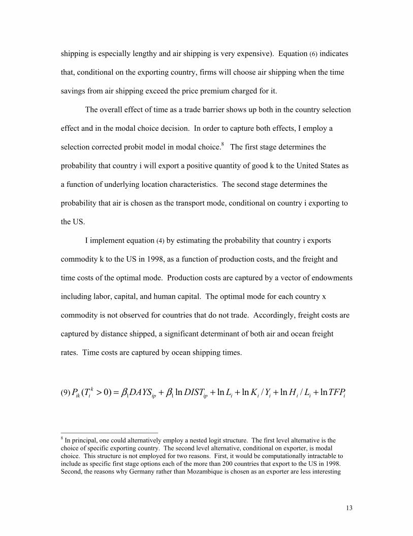
Tables 3 and 4 report estimates of equation . Table 3 reports probit estimates with
5-digit commodity specific effects. The left half of the table reports regressions that
ignore partner selection; the right half reports results that include a selection correction.
Coefficients on rates (air freight premium) and shipment days are included, as well as the
ratio of these two, which indicates estimates of the per day time cost. Recall that the
model predicts that air shipping is more likely to be chosen when air shipping is
relatively inexpensive and when ocean shipping is relatively lengthy. There are a great
many numbers in these tables, but several important patterns are evident.
First, this model poorly describes mode selection for commodity categories (SITC
0 – 4). Higher air freight rates lead to a lower probability that air is chosen for fewer than
a third of the regressions. In the regressions with no selection correction, increased ocean
shipment days decrease the probability of air shipment in most cases. This puzzling
result is reversed by the selection correction, but the positive magnitudes in these
regressions are not significant.
Second, considering categories SITC 5 and 6 (chemicals and simple manufactures
classified by materials) a higher air premium does lead to strong substitution away from
air shipping. However, shipment days are not strong predictors of air shipping. Focusing

23
on selection corrected estimates, ocean shipment days insignificantly affect air shipping
in half the cases, with the remaining half split evenly between positive and negative
significant effects.
Third, the model appears to work very well for SITC categories 7 (machinery)
and 8 (miscellaneous manufactures). Higher air premium strongly predict lower air
shipping in all categories, and longer ocean shipment days predict higher air shipping in
all but a few cases. Turning to the estimated time cost for those categories where rates
and days are significant and of the right sign, we find time costs around 0.4 percent per
day. That is, the average ocean travel time of 20 days corresponds to an 8 percent tariff.
Table 4 reports selection corrected probits omitting commodity fixed effects.
This has the effect of allowing commodity heterogeneity in freight rates within each 2-
digit classification to better explain the air/ocean choice. The Table 3 fixed effects
regressions entirely eliminate this variation from the data, whereas Table 4 exploits it.
Results for commodities 0-6 are qualitatively similar to Table 3, and so are not
reported here. In SITC 7 and 8, not controlling for within category heterogeneity affects
the estimates in two ways. First, the coefficients on the air freight premium are generally
lower than the Table 3 estimates, while the coefficients on ocean shipment days are
generally higher. The combined effect doubles the estimated time cost, to an average of
0.8 percent ad-valorem per day. That is, a 20 day ocean voyage imposes costs equal to a
16 percent tariff on these goods.
Precisely identifying the source of time costs is an exercise left to future work.
However, it is instructive to note that the largest measured effect comes in office
machinery, a category where the depreciation argument for time savings seems especially

24
strong. Each day in transit is worth 2.2 percent of the value of the good being shipped.
Suppose the only costs associated with shipping were the capital costs for the goods
during the time they are on the ocean vessel. The per-day cost should then be the
prevailing interest rate divided by 365. Using a 6.26 percent interest rate (the average US
T-bill rate in this year), we have a daily cost of .017 percent ad-valorem, roughly 130
times smaller than the measured cost.
V. Effects on Trade and Integration: back of the envelope
How does time affect trade and integration? The effects of time as a bilateral
trade barrier were demonstrated in section IV: shipping time strongly affects both the
selection of trading partners and raises the ad-valorem costs of trade conditional on
selection. Time may also play a role in explaining the extent and composition of trade
growth. Hummels (2000) shows that ocean shipping prices have been constant or
increasing in the post-war era while air shipping prices have dropped precipitously,
nearly 6 percent per annum in real terms.
What is the benefit of declining air transport rates, measured in terms of the ad-
valorem tariff equivalent reduction? It is clearly less than the 6 percent per annum
reduction in rates; there is imperfect substitutability between air and ocean transport and
declining air freight rates are not relevant to goods that are never air-shipped. The
estimates in the preceding section provide a simple way to calculate the benefit.
From 1950-1998 the share of US trade (excluding Canada and Mexico) that is air-
shipped rises from (approximately) 0 % to 50%. In addition, the introduction of

25
containerization in the late 1960s and 1970s results in a doubling of the average ocean
fleet speed. Finally, in 1998 the average shipment time for ocean shipped goods was 20
days. These facts allow a calculation of the decrease in the number of shipping days over
the past 50 years (holding constant the commodity and partner composition of trade).
1998: shipping days = ocean share * ocean days + air share * air days (1)
= .5 * 20 days + .5 * 1 day = 10.5 days
1950: shipping days = 40 days (100% ocean share and double shipping time)
This results in an average saving of 29.5 days. Evaluated at an average cost per day of
0.5% ad-valorem, the advent of relatively cheap fast shipping is equivalent to reducing
tariffs from 20% to 5.2%. However, these effects are far from uniform. Time savings
appear to be valued only for SITC categories 7 and 8, where the average effect is 0.8
percent ad-valorem per day. For these categories falling air shipping costs are equivalent
to reducing tariffs from 32% to 9%.
If air shipping prices play an important role in trade growth, we would expect it to
occur primarily through compositional effects. Table 5 shows the shares of SITC
categories for the US and the world, and the change in those category shares over the last
30 years. The share of SITC categories 0-4 and 6, which exhibit no value for time
savings, have shrunk considerably. SITC 7 and 8, with a large value for time savings,
have grown dramatically.
Finally, recall that equation (5) and the estimates based on it describe the optimal
modal choice for the good at the margin. However, the cumulative time costs over the

26
entire finished product are much larger for fragmented production. Consider a simple
example. Let production be divided into n stages, each of which adds 1/n of the final
good’s total value added, p. Assume the ocean travel time is 21 days, air shipping time is
one day, and time costs (r+d) are equal to 0.8 percent of each stage’s value added per day.
We can write the time costs for ocean transport relative to air travel over the entire
system as
1 1( ) ( ) 0.8(20)n nS S
o a o a n nc cr T T p pτ τ δ
= =− = + ⋅ − =∑ ∑
For n=1 this amounts to 16% of the price of the final good. For n=2, 24%; for n=3, 32%,
for n=4, 40%.
V. Conclusions and Future Directions
Each day of increased ocean transit time between two countries reduces the
probability of trade by 1 percent (all goods) to 1.5 percent (manufactures). Conditional
on the exporter, I find that modal selection reveals no time sensitivity for commodity type
goods. However, exporters in the largest manufacturing categories exhibit a willingness
to pay for time savings equal to 0.8% ad-valorem per day. This means that a average
length ocean voyage of 20 days is equivalent to a 16% tariff. This time sensitivity, plus
large reductions in the cost of air shipping over time, may play a significant role in the
extent and composition of trade growth. Back of the envelope calculations suggest that
air shipping cost declines are equivalent to reducing tariffs on manufactured goods from
32% to 9% ad-valorem. Moreover, these costs are significantly magnified in the
presence of fragmented production.

27
This work leaves open several interesting future avenues for research. The first is
to go beyond back of the envelope calculations and directly assess the role of time costs
and air shipping in trade growth. In addition to the growth of manufactured goods trade,
there are several additional margins that may matter. Extremely time sensitive goods
may not be traded at all in periods in which air transport is more expensive, and countries
may be entirely precluded from certain distant export markets. This suggests that the
availability of cheap air-freight may be responsible for the introduction of “new” goods
to international trade. This is noteworthy because the welfare gains from introduction of
“new” goods can be much greater than the welfare gains associated with marginal
increases in trade volumes for existing goods.12 Future research focused on why new
goods are introduced may point to even greater welfare gains from cheap air transport –
both in the time series, and in the cross-section.
12 See Romer (1994).

28
VI. References
Baier, Scott, and Bergstrand Jeffrey (1998) "The Growth of World Trade: Tariffs, Transportation Costs, and Intermediate Goods", mimeo, U. Notre Dame
Feenstra, Robert, 1996. "US Imports, 1972-1994: Data and Concordances" NBER Working Paper
#5515. Harrigan, James (1993) “OECD Imports and Trade Barriers in 1983” Journal of International Economics;
v35 n1-2, pp. 91-111. Haveman, Jon, Nair, Usha, and Jerry Thursby, 1998 "Trade Suppression, Compression and
Diversion: Empirical Regularities in Protective Measures". mimeo, Purdue University. Hummels, David, 2000 "Have International Transportation Costs Declined?" mimeo, Purdue
University. Hummels, David, Ishii, Jun, and Yi, Kei-Mu, 2000 “The Nature and Extent of Vertical
Specialization in International Trade”, forthcoming, Journal of International Economics. Krugman, Paul, (1995), "Growing World Trade: Causes and Consequences", Brookings Papers. Moenius, Johannes 2000 Rauch, James, 1999 "Networks versus Markets in International Trade", Journal of International
Economics. Romer, Paul. (1994) “New Goods, Old Theory, and the Welfare Costs of Trade Restrictions”, Journal of
Development Economics, Vol 43. Trefler, Dan, and Lai, 1999 Venables and Limao, 2000 Wei, Shang-Jin, 1996, "Intra-national versus International Trade: How Stubborn are Nations in
Global Integration?" NBER # 5531. Wei, Shang-Jin 1998, “Currency Hedging and Goods Trade” NBER 6742. Womack, James P, Jones, Daniel T. and Roos, Daniel, The Machine that Changed the World. 1990.
HarperPerennial Press.

Table 1 -- Summary Statistics
Code Name Total Trade > 0 Mode= Air Median Median No Trade(% of obs) (% of trade obs) Fa - Fo Fa / Fo Ocean Air
0 Live Animals 4677 8.32 99.74 -0.302 0.273 14.396 18.911 22.6541 Meat And Meat Products 14917 8.74 19.8 0.215 3.194 24.556 21.509 22.4922 Dairy Products 15692 6.67 18.62 0.278 3.765 21.180 16.361 22.5403 Fish 44365 18 26.21 0.288 4.165 20.474 16.335 22.5144 Cereals 12688 26 10.61 0.288 3.550 20.344 17.718 22.7105 Vegetables And Fruits 63193 19.56 11.34 0.388 5.616 19.985 16.460 22.7046 Sugars, Sugar Prep 7447 26.2 11.84 0.304 4.058 20.069 17.377 22.7867 Coffee, Tea 16218 31.47 18.48 0.253 3.530 20.194 18.017 22.8338 Feeding Stuff 5595 7.36 21.84 -0.005 0.980 19.877 17.506 22.6339 Misc food products 13146 24.74 16.21 0.342 4.417 19.013 17.840 22.776
11 Beverages 15276 49.41 6.76 0.188 2.526 18.956 17.466 22.99512 Tobacco 8496 15.65 45.49 0.177 2.505 18.198 13.382 22.63721 Hides, Skins 3692 11.4 73.87 0.082 1.445 22.038 19.348 22.74122 Oil Seeds 3485 11.16 16.45 0.190 2.403 20.284 18.402 22.56923 Crude Rubber 4090 36.21 20.39 0.272 3.394 20.614 17.526 22.62024 Cork And Wood 16285 17.98 7 0.014 1.071 21.946 18.214 22.66525 Pulp And Waste 2382 6.21 4.73 -0.275 0.223 19.422 26.587 22.64826 Textile Fibers 12164 16.93 32.35 0.246 2.947 21.396 16.938 22.62427 Crude Fertilize 11885 17.99 29.14 0.051 1.278 19.147 19.756 22.76928 Metalliferous Ores 10268 15.31 13.8 0.142 2.100 18.017 16.206 22.82529 Crude Animal n.e.s 21705 26.24 50.33 0.196 2.494 21.245 18.620 22.68732 Coal, Coke 1051 5.99 4.76 -1.233 0.000 17.925 18.875 22.55033 Petroleum, 7447 27.45 16.83 0.128 2.034 17.703 17.088 22.87034 Gas, Natural 1495 6.49 14.43 -0.360 0.131 21.643 15.311 22.47441 Animal Oils 1776 9.74 32.37 0.209 2.767 19.134 17.884 22.63942 Vegetable Fats 4694 20.37 11.72 0.291 4.080 22.059 17.932 22.64743 Animal Or Veget fats 1756 17.2 15.23 0.214 2.842 20.708 16.978 22.80651 Organic Chemical 99109 17.8 44.39 0.175 2.540 18.118 17.444 22.71952 Inorganic Chemicals 31217 20.49 31.64 0.189 2.570 17.997 16.914 22.817
SITC CategoriesTrade
Mean Days in TransitAir / Ocean Freight PremiumObservations

Table 1 -- Summary Statistics
Code Name Total Trade > 0 Mode= Air Median Median No Trade(% of obs) (% of trade obs) Fa - Fo Fa / Fo Ocean Air
SITC CategoriesTrade
Mean Days in TransitAir / Ocean Freight PremiumObservations
53 Dyeing, Tanning 20526 35.64 40.43 0.253 3.466 18.228 17.382 22.94154 Pharmaceuticals 17584 26.13 76.47 0.085 1.632 17.827 17.658 22.97855 Essential Oils 16067 50.61 51.02 0.164 2.174 18.580 17.902 23.28156 Fertilizers 2527 11.71 12.84 0.278 3.638 18.364 18.867 22.93257 Plastics In Primary 15487 51.63 45.94 0.282 3.466 16.933 16.717 23.36358 Plastics In Nonprimary 18575 62.15 55.05 0.254 3.057 17.829 16.904 23.37159 Chemical Materials nes 22733 32.37 42.72 0.216 2.881 17.738 17.439 23.03161 Leather manufactures 12077 45.58 75.06 0.183 2.369 20.565 19.971 22.98862 Rubber Manufactures 32620 71.33 52.23 0.237 2.841 18.955 17.660 23.29963 Cork And Wood Manufactures 27423 36.86 25.18 0.192 2.330 21.295 18.862 22.71864 Paper, Paperboard 28552 39.07 37.58 0.241 3.011 18.108 17.676 23.04865 Textile Yarn 222027 33.02 63.49 0.210 2.516 20.783 19.044 22.83966 Nonmetallic Manufactures 62190 55.36 34.06 0.199 2.483 19.796 18.580 23.17867 Iron And Steel 79414 25.16 18.1 0.301 4.315 19.234 16.625 22.93068 Nonferrous Metals 31954 27.29 40.28 0.236 3.285 18.281 16.696 22.94469 Manufactures Of metals nes 120989 63.38 42.11 0.236 3.062 19.181 17.963 23.22571 Power Generating Machinery 42480 54.57 67.61 0.175 2.465 17.227 17.274 23.21872 Machinery Specialized 83968 49.48 56.85 0.152 2.193 17.737 17.499 23.14473 Metalworking Machinery 37475 39.57 54.61 0.135 2.041 17.511 17.365 23.04774 General Industrial Machinery 129132 66.75 61.06 0.166 2.309 17.481 17.344 23.37975 Office Machines 35895 72.81 85 0.074 1.516 17.869 18.905 23.31976 Telecommunications 52604 52.63 70.53 0.109 1.829 18.644 17.895 22.87477 Electrical Machinery 135297 65.53 73.1 0.128 1.983 17.400 18.198 23.30078 Road Vehicles 42440 49.55 43.27 0.213 2.881 18.328 17.770 23.02579 Transport Equip 15353 35.7 75.81 0.041 1.266 18.555 16.975 22.87981 Prefabricated Buildings 12597 70.57 36.67 0.187 2.373 19.774 18.586 23.53382 Furniture 39344 81.72 20.48 0.188 2.334 20.523 17.631 23.54083 Travel Goods 21791 71.66 60.05 0.182 2.274 20.037 19.852 23.18984 Apparel 256493 51.35 63.86 0.169 2.262 20.669 20.143 22.84085 Footwear 47572 45.15 54.43 0.194 2.464 20.022 18.714 22.77487 Scientific Instruments 60739 65.13 80.83 0.078 1.525 17.464 17.469 23.35988 Photographic Equipment 73193 39.3 72.51 0.155 2.261 17.863 18.901 22.78889 Miscellaneous Manufactures 151475 66.01 55.79 0.168 2.179 19.146 18.808 23.105

Table 2 -- Location Selection(Probits on Trade, No Trade)
code Name obs adj R20 Live Animals -0.0001 -1.32E-06 b 0.008 a -0.030 a 0.066 a 0.01069 a 3387 0.421 Meat And Meat Products 0.0040 a -3.69E-06 a 0.012 a 0.038 a 0.203 a 0.051598 a 10683 0.322 Dairy Products 0.0020 a -2.96E-06 a 0.012 a 0.069 a 0.106 a 0.053356 a 11421 0.253 Fish -0.0136 a 1.80E-05 a 0.060 a -0.032 c 0.321 a -0.032838 a 33643 0.254 Cereals -0.0082 a 1.21E-05 a 0.128 a 0.156 a 0.167 a 0.15013 a 9640 0.425 Vegetables And Fruits -0.0122 a 1.01E-05 a 0.088 a 0.094 a -0.081 a 0.078513 a 48003 0.216 Sugars, Sugar Prep -0.0067 a 3.43E-06 0.109 a -0.106 b 0.304 a 0.132594 a 5638 0.347 Coffee, Tea -0.0104 a 7.01E-06 a 0.130 a 0.163 a -0.022 0.177081 a 12467 0.348 Feeding Stuff -0.0011 a 1.70E-06 a 0.020 a 0.002 0.092 a 0.030717 a 3645 0.379 Misc food products -0.0180 a 2.20E-05 a 0.099 a 0.093 a 0.182 a 0.097264 a 10067 0.36
11 Beverages 0.0077 a -2.89E-05 a 0.165 a 0.671 a 0.423 a 0.500794 a 12423 0.4112 Tobacco -0.0109 a 1.67E-06 0.059 a 0.074 b -0.177 a 0.03049 a 6422 0.2921 Hides, Skins 0.0034 a -6.76E-06 a 0.059 a 0.026 0.195 a 0.133979 a 2666 0.2522 Oil Seeds -0.0040 a 3.21E-06 0.052 a -0.120 a 0.196 a 0.062491 a 2399 0.3223 Crude Rubber -0.0200 a 5.11E-05 a 0.190 a 0.448 a -0.072 0.31709 a 3107 0.4624 Cork And Wood -0.0004 3.60E-06 a 0.064 a 0.119 a -0.062 a 0.098869 a 12307 0.2325 Pulp And Waste 0.0014 -1.87E-06 0.024 a 0.050 c 0.073 a 0.05933 a 1612 0.2226 Textile Fibers 0.0022 a -6.91E-07 0.079 a -0.063 a 0.413 a 0.134881 a 9182 0.3927 Crude Fertilize 0.0026 a -7.68E-06 a 0.097 a 0.068 a 0.224 a 0.113159 a 8855 0.4228 Metalliferous Ores -0.0067 a 1.17E-06 0.048 a 0.010 0.130 a 0.047623 a 7553 0.3729 Crude Animal n.e.s -0.0090 a 1.17E-05 a 0.129 a -0.110 a 0.483 a 0.133234 a 16666 0.2932 Coal, Coke 0.0002 -5.90E-06 b 0.030 a -0.046 0.156 a -0.000791 708 0.2833 Petroleum, 0.0034 b -2.45E-05 a 0.127 a 0.300 a 0.325 a 0.219934 a 5488 0.4234 Gas, Natural 0.0003 -9.05E-07 c 0.008 a 0.016 c 0.027 a 0.014679 a 1120 0.3241 Animal Oils -0.0001 2.80E-07 0.005 a 0.012 c 0.042 a 0.013547 a 1185 0.5442 Vegetable Fats 0.0036 a -3.41E-06 0.084 a 0.246 a -0.079 b 0.167014 a 3441 0.5043 Animal Or Veget fats -0.0035 c 8.86E-06 a 0.081 a 0.204 a 0.085 0.135481 a 1310 0.2851 Organic Chemical -0.0009 a -1.51E-07 0.071 a 0.111 a 0.189 a 0.08809 a 74121 0.4752 Inorganic Chemicals -0.0020 a -5.65E-07 0.084 a 0.074 a 0.251 a 0.0935 a 23002 0.5153 Dyeing, Tanning -0.0084 a 2.62E-06 0.258 a 0.157 a 0.826 a 0.306172 a 15528 0.5554 Pharmaceuticals -0.0015 b -5.09E-06 a 0.132 a 0.165 a 0.550 a 0.192947 a 13195 0.4855 Essential Oils -0.0145 a 7.40E-06 a 0.263 a 0.266 a 0.589 a 0.440115 a 12699 0.5356 Fertilizers 0.0007 -4.33E-06 a 0.032 a -0.001 0.164 a 0.038065 a 1793 0.4457 Plastics In Primary -0.0255 a 2.70E-05 a 0.364 a 0.701 a 1.153 a 0.77289 a 11866 0.6758 Plastics In Nonprimary -0.0202 a 2.49E-05 a 0.273 a 0.276 a 0.960 a 0.525632 a 14738 0.6159 Chemical Materials nes -0.0071 a 6.14E-06 a 0.177 a 0.305 a 0.616 a 0.315745 a 16971 0.53
lnhl lntfpdays dist lnl lnky

Table 2 -- Location Selection(Probits on Trade, No Trade)
code Name obs adj R2lnhl lntfpdays dist lnl lnky61 Leather manufactures 0.0037 a -1.29E-05 a 0.245 a 0.160 a 0.439 a 0.422971 a 9740 0.4362 Rubber Manufactures -0.0083 a 1.45E-05 a 0.146 a 0.248 a 0.466 a 0.257821 a 26483 0.6563 Cork And Wood Manufactures -0.0160 a 2.64E-05 a 0.176 a 0.249 a -0.078 a 0.239621 a 21506 0.4764 Paper, Paperboard -0.0215 a 2.35E-05 a 0.258 a 0.295 a 0.899 a 0.370188 a 22177 0.6165 Textile Yarn -0.0077 a 1.00E-05 a 0.229 a 0.188 a 0.280 a 0.393299 a 172930 0.4666 Nonmetallic Manufactures -0.0145 a 1.74E-05 a 0.280 a 0.450 a 0.474 a 0.366447 a 50332 0.5767 Iron And Steel 0.0009 a -1.30E-06 a 0.128 a 0.209 a 0.381 a 0.220049 a 59767 0.5168 Nonferrous Metals -0.0042 a 8.11E-07 0.138 a 0.182 a 0.519 a 0.217972 a 23674 0.4569 Manufactures Of metals nes -0.0159 a 2.29E-05 a 0.278 a 0.133 a 0.900 a 0.427129 a 99030 0.5971 Power Generating Machinery -0.0110 a 8.34E-06 a 0.326 a 0.841 a 1.213 a 0.657369 a 32968 0.6672 Machinery Specialized -0.0077 a 7.06E-06 a 0.311 a 0.674 a 1.208 a 0.717239 a 64290 0.6273 Metalworking Machinery -0.0080 a 9.43E-06 a 0.255 a 0.415 a 1.056 a 0.477115 a 28281 0.6374 General Industrial Machinery -0.0091 a 9.10E-06 a 0.232 a 0.514 a 0.893 a 0.434834 a 102093 0.6675 Office Machines -0.0098 a 2.09E-05 a 0.095 a 0.263 a 0.355 a 0.189461 a 30541 0.6376 Telecommunications -0.0335 a 7.11E-05 a 0.251 a 0.587 a 0.973 a 0.369752 a 43390 0.6077 Electrical Machinery -0.0225 a 3.72E-05 a 0.184 a 0.427 a 0.637 a 0.316592 a 110363 0.6278 Road Vehicles -0.0164 a 2.42E-05 a 0.363 a 0.289 a 1.201 a 0.670616 a 33297 0.6579 Transport Equip -0.0056 a 4.10E-06 c 0.231 a 0.294 a 0.997 a 0.455582 a 11415 0.6881 Prefabricated Buildings -0.0115 a 9.87E-06 a 0.138 a 0.043 c 0.397 a 0.166272 a 10747 0.5782 Furniture -0.0053 a 7.58E-06 a 0.051 a 0.027 a 0.139 a 0.060028 a 35043 0.5483 Travel Goods -0.0135 a 1.78E-05 a 0.124 a -0.097 a 0.172 a 0.118202 a 18985 0.4884 Apparel -0.0282 a 4.21E-05 a 0.187 a -0.200 a 0.024 a 0.211926 a 211249 0.3885 Footwear -0.0299 a 3.87E-05 a 0.302 a 0.514 a -0.110 a 0.292531 a 38747 0.5387 Scientific Instruments -0.0127 a 2.08E-05 a 0.228 a 0.458 a 1.005 a 0.42069 a 48122 0.6288 Photographic Equipment -0.0148 a 3.14E-05 a 0.230 a 0.951 a 0.755 a 0.283263 a 57924 0.5589 Miscellaneous Manufactures -0.0154 a 2.43E-05 a 0.173 a 0.049 a 0.517 a 0.213738 a 126959 0.55
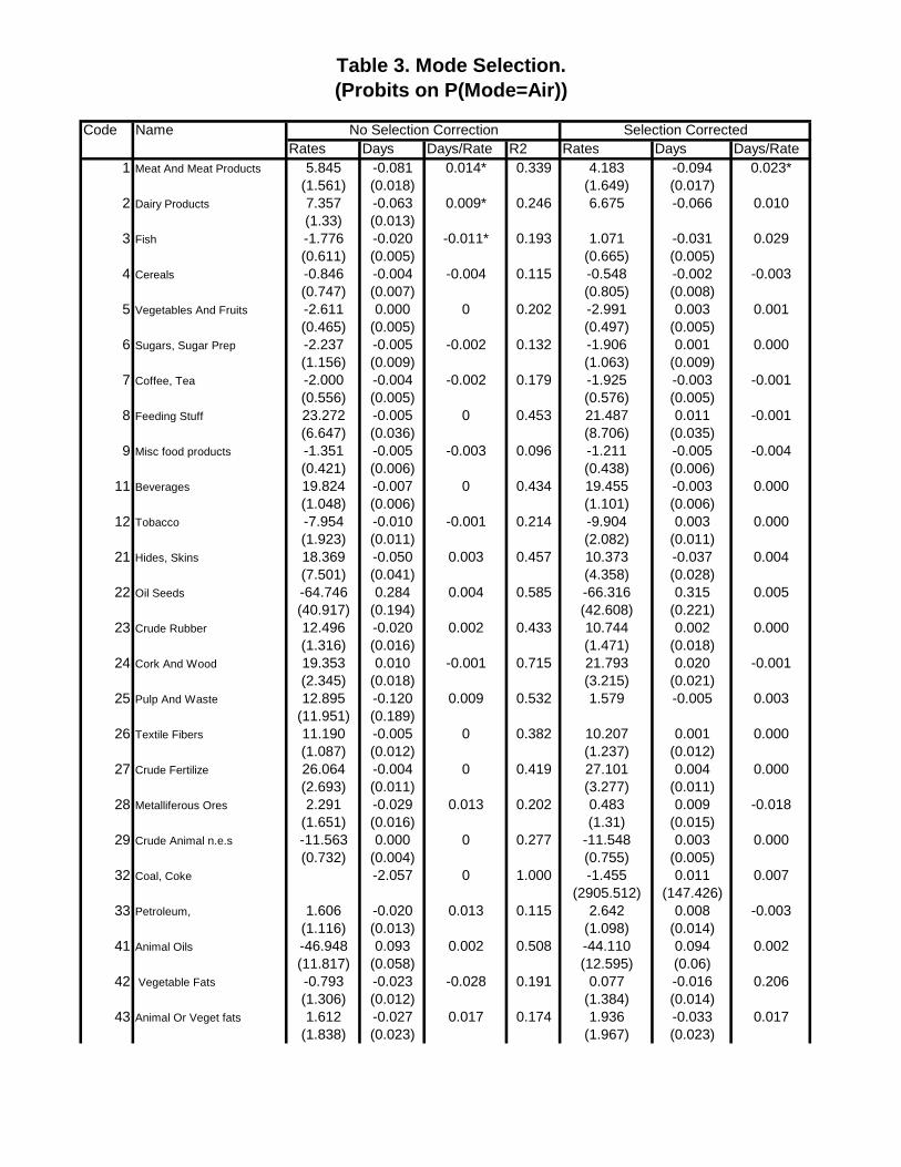
Table 3. Mode Selection.(Probits on P(Mode=Air))
Code NameRates Days Days/Rate R2 Rates Days Days/Rate
1 Meat And Meat Products 5.845 -0.081 0.014* 0.339 4.183 -0.094 0.023*(1.561) (0.018) (1.649) (0.017)
2 Dairy Products 7.357 -0.063 0.009* 0.246 6.675 -0.066 0.010(1.33) (0.013)
3 Fish -1.776 -0.020 -0.011* 0.193 1.071 -0.031 0.029(0.611) (0.005) (0.665) (0.005)
4 Cereals -0.846 -0.004 -0.004 0.115 -0.548 -0.002 -0.003(0.747) (0.007) (0.805) (0.008)
5 Vegetables And Fruits -2.611 0.000 0 0.202 -2.991 0.003 0.001(0.465) (0.005) (0.497) (0.005)
6 Sugars, Sugar Prep -2.237 -0.005 -0.002 0.132 -1.906 0.001 0.000(1.156) (0.009) (1.063) (0.009)
7 Coffee, Tea -2.000 -0.004 -0.002 0.179 -1.925 -0.003 -0.001(0.556) (0.005) (0.576) (0.005)
8 Feeding Stuff 23.272 -0.005 0 0.453 21.487 0.011 -0.001(6.647) (0.036) (8.706) (0.035)
9 Misc food products -1.351 -0.005 -0.003 0.096 -1.211 -0.005 -0.004(0.421) (0.006) (0.438) (0.006)
11 Beverages 19.824 -0.007 0 0.434 19.455 -0.003 0.000(1.048) (0.006) (1.101) (0.006)
12 Tobacco -7.954 -0.010 -0.001 0.214 -9.904 0.003 0.000(1.923) (0.011) (2.082) (0.011)
21 Hides, Skins 18.369 -0.050 0.003 0.457 10.373 -0.037 0.004(7.501) (0.041) (4.358) (0.028)
22 Oil Seeds -64.746 0.284 0.004 0.585 -66.316 0.315 0.005(40.917) (0.194) (42.608) (0.221)
23 Crude Rubber 12.496 -0.020 0.002 0.433 10.744 0.002 0.000(1.316) (0.016) (1.471) (0.018)
24 Cork And Wood 19.353 0.010 -0.001 0.715 21.793 0.020 -0.001(2.345) (0.018) (3.215) (0.021)
25 Pulp And Waste 12.895 -0.120 0.009 0.532 1.579 -0.005 0.003(11.951) (0.189)
26 Textile Fibers 11.190 -0.005 0 0.382 10.207 0.001 0.000(1.087) (0.012) (1.237) (0.012)
27 Crude Fertilize 26.064 -0.004 0 0.419 27.101 0.004 0.000(2.693) (0.011) (3.277) (0.011)
28 Metalliferous Ores 2.291 -0.029 0.013 0.202 0.483 0.009 -0.018(1.651) (0.016) (1.31) (0.015)
29 Crude Animal n.e.s -11.563 0.000 0 0.277 -11.548 0.003 0.000(0.732) (0.004) (0.755) (0.005)
32 Coal, Coke -2.057 0 1.000 -1.455 0.011 0.007(2905.512) (147.426)
33 Petroleum, 1.606 -0.020 0.013 0.115 2.642 0.008 -0.003(1.116) (0.013) (1.098) (0.014)
41 Animal Oils -46.948 0.093 0.002 0.508 -44.110 0.094 0.002(11.817) (0.058) (12.595) (0.06)
42 Vegetable Fats -0.793 -0.023 -0.028 0.191 0.077 -0.016 0.206(1.306) (0.012) (1.384) (0.014)
43 Animal Or Veget fats 1.612 -0.027 0.017 0.174 1.936 -0.033 0.017(1.838) (0.023) (1.967) (0.023)
No Selection Correction Selection Corrected

Table 3. Mode Selection.(Probits on P(Mode=Air))
Code NameRates Days Days/Rate R2 Rates Days Days/Rate
No Selection Correction Selection Corrected
51 Organic Chemical 0.817 -0.009 0.011* 0.083 0.435 -0.004 0.009(0.272) (0.003) (0.297) (0.003)
52 Inorganic Chemicals -1.797 -0.020 -0.011* 0.103 -1.581 -0.002 -0.001(0.545) (0.006) (0.618) (0.007)
53 Dyeing, Tanning -3.154 -0.003 -0.001 0.075 -1.825 0.008 0.004(0.4) (0.004) (0.451) (0.004)
54 Pharmaceuticals -3.636 0.000 0 0.089 -3.478 0.005 0.001(0.548) (0.007) (0.597) (0.008)
55 Essential Oils -8.720 0.007 0.001* 0.232 -8.593 0.010 0.001*(0.401) (0.003) (0.434) (0.004)
57 Fertilizers 2.032 -0.011 0.005* 0.097 2.186 0.010 -0.005*(0.314) (0.004) (0.332) (0.005)
58 Plastics In Primary -2.895 -0.006 -0.002 0.081 -2.776 0.001 0.000(0.206) (0.003) (0.225) (0.004)
59 Plastics In Nonprimary -3.331 -0.001 0 0.108 -2.855 0.014 0.005*(0.437) (0.005) (0.496) (0.006)
61 Leather manufactures -1.557 0.002 0.001 0.067 -1.643 0.004 0.002(0.466) (0.004) (0.491) (0.005)
62 Rubber Manufactures -2.536 -0.002 -0.001 0.114 -2.058 0.001 0.001(0.167) (0.002) (0.178) (0.003)
63 Cork And Wood Manufactures -2.547 -0.006 -0.002 0.091 -2.057 -0.009 -0.004*(0.536) (0.003) (0.566) (0.003)
64 Paper, Paperboard -4.357 0.004 0.001 0.112 -3.787 0.013 0.004*(0.31) (0.003) (0.328) (0.004)
65 Textile Yarn -0.536 -0.008 -0.015* 0.083 -0.386 -0.007 -0.018*(0.115) (0.001) (0.119) (0.001)
66 Nonmetallic Manufactures -1.181 -0.007 -0.006* 0.096 -0.805 -0.003 -0.004(0.217) (0.002) (0.228) (0.002)
67 Iron And Steel 0.018 -0.029 1.651 0.116 -0.256 -0.017 -0.068(0.288) (0.004) (0.334) (0.004)
68 Nonferrous Metals -2.199 -0.011 -0.005* 0.116 -2.023 -0.001 0.000(0.401) (0.005) (0.449) (0.005)
69 Manufactures Of metals nes -5.835 0.010 0.002* 0.143 -5.408 0.013 0.002*(0.119) (0.001) (0.126) (0.001)
Table 3. Mode Selection.(Probits on P(Mode=Air))
Code NameRates Days Days/Rate R2 Rates Days Days/Rate
No Selection Correction Selection Corrected
71 Power Generating Machinery -4.827 0.010 0.002* 0.119 -4.465 0.015 0.003*(0.202) (0.003) (0.223) (0.003)
72 Machinery Specialized -8.493 0.019 0.002* 0.204 -7.812 0.022 0.003*(0.228) (0.002) (0.25) (0.002)
73 Metalworking Machinery -9.248 0.002 0 0.210 -8.292 0.010 0.001(0.471) (0.004) (0.591) (0.014)
74 General Industrial Machinery -6.248 0.015 0.002* 0.131 -5.501 0.020 0.004*(0.125) (0.001) (0.136) (0.002)
75 Office Machines -7.067 0.022 0.003* 0.133 -6.677 0.028 0.004*(0.313) (0.003) (0.321) (0.004)
76 Telecommunications -4.776 0.010 0.002* 0.104 -4.347 0.015 0.004*(0.24) (0.003) (0.243) (0.003)
77 Electrical Machinery -6.870 0.013 0.002* 0.163 -6.412 0.016 0.002*(0.135) (0.002) (0.142) (0.002)
78 Road Vehicles -5.086 0.014 0.003* 0.090 -4.293 0.014 0.003*(0.241) (0.002) (0.258) (0.002)
79 Transport Equip -7.652 0.011 0.001 0.265 -6.892 0.017 0.002*(0.918) (0.007) (0.949) (0.007)
81 Prefabricated Buildings -4.870 0.013 0.003* 0.110 -4.644 0.016 0.004*(0.337) (0.003) (0.348) (0.003)
82 Furniture -2.780 -0.011 -0.004* 0.110 -2.559 -0.011 -0.004*(0.233) (0.002) (0.242) (0.002)
83 Travel Goods -2.147 0.014 0.006* 0.056 -1.899 0.016 0.008*(0.196) (0.002) (0.199) (0.002)
84 Apparel -1.325 0.002 0.001* 0.033 -1.241 0.000 0.000(0.113) (0.001) (0.114) (0.001)
85 Footwear 6.313 0.002 0 0.119 6.762 -0.001 0.000(0.264) (0.002) (0.272) (0.002)
87 Scientific Instruments -7.285 0.013 0.002* 0.148 -6.451 0.013 0.002*(0.232) (0.003) (0.246) (0.003)
88 Photographic Equipment -3.122 0.012 0.004* 0.096 -2.720 0.020 0.007*(0.276) (0.003) (0.285) (0.003)
89 Miscellaneous Manufactures -3.129 0.010 0.003* 0.098 -2.853 0.012 0.004*(0.107) (0.001) (0.112) (0.001)

Table 4 -- Modal SelectionSelection corrected probit P(mode=air); no commodity fixed effects
Code NameRates Days Days/Rate
51 Organic Chemical -2.642 -0.002 -0.001(0.087) (0.003)
52 Inorganic Chemicals -2.052 0.007 0.004(0.126) (0.006)
53 Dyeing, Tanning -2.650 0.003 0.001(0.13) (0.004)
54 Pharmaceuticals -1.465 -0.001 -0.001(0.171) (0.007)
55 Essential Oils -1.760 -0.001 0.000(0.087) (0.003)
57 Fertilizers -2.180 0.013 0.006*(0.103) (0.006)
58 Plastics In Primary -1.943 0.004 0.002(0.071) (0.004)
59 Plastics In Nonprimary -2.252 0.010 0.005*(0.118) (0.006)
61 Leather manufactures -0.954 0.001 0.001(0.105) (0.004)
62 Rubber Manufactures -1.552 0.001 0.000(0.048) (0.003)
63 Cork And Wood Manufactures -2.753 -0.005 -0.002(0.099) (0.003)
64 Paper, Paperboard -2.089 0.019 0.009*(0.078) (0.004)
65 Textile Yarn -1.557 -0.007 -0.005*(0.03) (0.001)
66 Nonmetallic Manufactures -2.475 -0.005 -0.002*(0.051) (0.002)
67 Iron And Steel -3.066 -0.004 -0.001(0.114) (0.005)
68 Nonferrous Metals -2.526 -0.006 -0.002(0.126) (0.006)
69 Manufactures Of metals nes -2.311 0.004 0.002*(0.033) (0.001)
Correlated

Table 4 -- Modal SelectionSelection corrected probit P(mode=air); no commodity fixed effects
Code NameRates Days Days/Rate
Correlated
71 Power Generating Machinery -1.566 0.013 0.008*(0.063) (0.003)
72 Machinery Specialized -2.140 0.003 0.001(0.05) (0.002)
73 Metalworking Machinery -1.905 0.003 0.001(0.084) (0.004)
74 General Industrial Machinery -1.683 0.012 0.007*(0.031) (0.002)
75 Office Machines -0.833 0.018 0.022*(0.054) (0.003)
76 Telecommunications -1.816 0.006 0.004*(0.058) (0.003)
77 Electrical Machinery -1.238 0.013 0.011*(0.031) (0.002)
78 Road Vehicles -1.778 0.016 0.009*(0.052) (0.002)
79 Transport Equip -0.963 0.009 0.009(0.116) (0.006)
81 Prefabricated Buildings -2.671 0.016 0.006*(0.096) (0.004)
82 Furniture -2.480 -0.008 -0.003*(0.054) (0.002)
83 Travel Goods -1.380 0.015 0.011*(0.053) (0.002)
84 Apparel -1.538 0.003 0.002*(0.023) (0.001)
85 Footwear -2.037 0.007 0.003*(0.06) (0.002)
87 Scientific Instruments -0.830 0.006 0.007*(0.054) (0.003)
88 Photographic Equipment -1.034 0.021 0.02*(0.057) (0.003)
89 Miscellaneous Manufactures -1.594 0.008 0.005*(0.024) (0.001)

Table 5 -- Composition of Trade Growth(Value Shares by Category)
% Change % ChangeSITC Commodity 1969 1998 1969-95 1970 1997 1970-1997
0 Food & Live Animals 12.3 3.7 -70.3 11.2 6.5 -42.41 Beverages & Tobacco 2.4 0.8 -65.3 1.3 1.1 -15.12 Crude Materials 9.8 2.3 -76.1 9.5 3.6 -62.23 Mineral Fuels 8.2 5.9 -28.3 8.7 7.5 -14.14 Animal & Vegetable Oils 0.4 0.2 -55.4 0.7 0.5 -34.75 Chemicals 3.0 6.1 99.7 6.8 8.9 31.16 Manufactures (by material) 23.0 11.6 -49.7 19.8 14.9 -24.77 Machinery & Transport Equip 26.8 46.1 71.6 26.0 38.7 48.88 Misc Manufactures 10.5 17.9 70.3 8.0 13.1 62.4
US Imports World Imports

Table A-1Regressions Used to Predict Air/Ocean Freight Rates
SITCCode Description weight value dist airshare obs Adj R2 weight value dist airshare obs Adj R200 Live Animals 0.62 0.31 0.30 -0.03 386 0.72 -0.78 2.58 -2.33 4 .01 Meat And Meat Products 0.42 0.55 0.93 0.05 258 0.77 0.39 0.56 0.09 -0.09 1129 0.8902 Dairy Products 0.44 0.47 0.60 -0.33 193 0.75 0.23 0.70 0.11 0.00 909 0.8503 Fish 0.50 0.47 0.45 0.02 2092 0.86 0.49 0.45 0.03 -0.08 6176 0.8804 Cereals 0.53 0.41 0.48 0.03 350 0.57 0.36 0.59 0.13 -0.06 3086 0.8405 Vegetables And Fruits 0.62 0.37 0.42 0.00 1401 0.87 0.49 0.48 0.07 -0.10 11258 0.8706 Sugars, Sugar Prep 0.39 0.53 0.25 -0.30 230 0.55 0.20 0.72 0.05 -0.16 1799 0.8807 Coffee, Tea 0.46 0.43 0.24 -0.04 941 0.59 0.25 0.66 0.18 -0.08 4454 0.8708 Feeding Stuff 0.10 0.66 0.40 -0.32 90 0.23 0.41 0.46 0.07 -0.31 330 0.8009 Misc food products 0.49 0.33 0.35 0.05 526 0.59 0.31 0.62 0.13 -0.07 2896 0.7811 Beverages 0.45 0.44 0.18 0.13 510 0.49 0.49 0.47 0.12 -0.05 7247 0.7812 Tobacco 0.57 0.31 0.32 -0.03 604 0.72 0.42 0.41 0.25 -0.07 785 0.8021 Hides, Skins 0.07 0.58 0.27 -0.12 309 0.54 0.17 0.64 0.15 -0.12 120 0.7422 Oil Seeds 0.29 0.67 0.68 -0.01 64 0.45 0.35 0.60 -0.07 0.03 328 0.8823 Crude Rubber 0.37 0.44 0.40 -0.12 302 0.60 0.36 0.50 0.28 -0.10 1237 0.6624 Cork And Wood -0.14 0.87 0.05 -0.80 205 0.30 0.33 0.62 0.22 -0.05 2768 0.7825 Pulp And Waste 1.30 -1.37 7 . 0.53 0.39 -0.21 -0.07 141 0.7926 Textile Fibers 0.37 0.39 0.08 -0.25 666 0.57 0.41 0.43 0.15 0.03 1479 0.8227 Crude Fertilize 0.26 0.53 0.27 -0.13 623 0.56 0.33 0.57 0.18 -0.02 1571 0.7328 Metalliferous Ores 0.47 0.32 0.32 0.36 207 0.71 0.44 0.40 0.00 -0.01 1387 0.7829 Crude Animal n.e.s 0.50 0.40 0.31 0.01 2859 0.80 0.39 0.51 0.15 -0.02 3293 0.7532 Coal, Coke -0.59 -1.05 3 . 0.49 0.38 1.01 -0.51 61 0.7033 Petroleum, 0.37 0.53 0.27 -0.17 344 0.49 0.26 0.68 0.25 -0.01 1752 0.9234 Gas, Natural 0.62 -0.40 0.24 0.78 14 0.28 0.22 0.75 0.92 0.09 83 0.7441 Animal Oils 0.28 0.85 -0.22 0.72 56 0.46 0.20 0.71 -0.44 0.18 133 0.4942 Vegetable Fats 0.45 0.42 0.20 -0.07 112 0.64 0.25 0.63 0.04 0.00 895 0.8343 Animal Or Veget fats 0.49 0.15 -0.32 -0.10 46 0.34 0.52 0.39 0.07 0.18 267 0.8751 Organic Chemical 0.42 0.33 0.41 -0.15 7831 0.69 0.39 0.48 0.19 0.04 10928 0.7952 Inorganic Chemicals 0.44 0.35 0.27 -0.21 2022 0.67 0.37 0.50 0.05 -0.10 4669 0.7753 Dyeing, Tanning 0.52 0.36 0.37 -0.19 2955 0.66 0.36 0.52 0.19 -0.03 4991 0.7354 Pharmaceuticals 0.46 0.32 0.34 -0.09 3431 0.76 0.26 0.57 0.25 -0.09 1365 0.7555 Essential Oils 0.49 0.45 0.24 -0.10 4139 0.72 0.26 0.65 0.07 -0.04 5019 0.7456 Fertilizers 0.72 0.52 -0.57 -0.38 38 0.61 0.27 0.61 -0.24 -0.06 259 0.8157 Plastics In Primary 0.48 0.35 0.24 -0.14 3668 0.63 0.34 0.48 0.12 -0.11 4969 0.7358 Plastics In Nonprimary 0.54 0.34 0.19 -0.08 6345 0.73 0.30 0.59 0.17 0.00 6297 0.7959 Chemical Materials nes 0.49 0.35 0.25 -0.18 3141 0.69 0.37 0.51 0.04 -0.14 4697 0.75
Air Freight Rate Regressions Ocean Freight Rate Regressions

Table A-1Regressions Used to Predict Air/Ocean Freight Rates
SITCCode Description weight value dist airshare obs Adj R2 weight value dist airshare obs Adj R2
Air Freight Rate Regressions Ocean Freight Rate Regressions
61 Leather manufactures 0.40 0.41 0.25 -0.06 4128 0.73 0.26 0.64 0.19 -0.03 1901 0.7162 Rubber Manufactures 0.47 0.45 0.20 -0.16 12146 0.73 0.28 0.68 0.25 -0.04 13016 0.8563 Cork And Wood Manufactures 0.46 0.46 0.50 -0.28 2544 0.56 0.40 0.53 0.30 -0.12 8191 0.8064 Paper, Paperboard 0.58 0.32 0.28 -0.14 4192 0.61 0.37 0.54 0.15 -0.02 7906 0.7965 Textile Yarn 0.48 0.36 0.22 -0.09 46539 0.75 0.28 0.60 0.15 0.07 33030 0.7866 Nonmetallic Manufactures 0.47 0.40 0.29 -0.21 11720 0.64 0.39 0.54 0.17 -0.11 25074 0.7867 Iron And Steel 0.49 0.37 0.33 -0.16 3617 0.63 0.38 0.55 0.13 0.03 16912 0.8868 Nonferrous Metals 0.49 0.35 0.20 -0.12 3422 0.66 0.26 0.61 0.05 -0.01 5685 0.7969 Manufactures Of metals nes 0.52 0.38 0.35 -0.18 32280 0.70 0.32 0.61 0.24 -0.08 49817 0.7871 Power Generating Machinery 0.54 0.32 0.29 -0.05 15663 0.70 0.24 0.68 0.24 -0.02 9105 0.7572 Machinery Specialized 0.56 0.31 0.29 -0.13 23611 0.70 0.34 0.52 0.11 -0.08 21035 0.7473 Metalworking Machinery 0.49 0.36 0.26 -0.20 8096 0.70 0.33 0.55 0.17 -0.14 7582 0.7574 General Industrial Machinery 0.50 0.38 0.31 -0.23 52627 0.68 0.29 0.63 0.17 -0.06 40543 0.7575 Office Machines 0.58 0.31 0.13 -0.14 22181 0.70 0.40 0.56 0.06 -0.12 5838 0.7976 Telecommunications 0.53 0.33 0.33 -0.23 19502 0.69 0.33 0.59 0.30 -0.13 10220 0.7677 Electrical Machinery 0.52 0.38 0.24 -0.19 64737 0.74 0.32 0.64 0.24 -0.15 30502 0.7878 Road Vehicles 0.51 0.39 0.40 -0.24 9083 0.64 0.33 0.60 0.25 -0.05 13884 0.8179 Transport Equip 0.43 0.41 0.26 -0.13 4153 0.70 0.26 0.58 0.12 -0.31 1595 0.6481 Prefabricated Buildings 0.59 0.30 0.38 -0.21 3258 0.64 0.39 0.54 0.29 -0.15 6443 0.8082 Furniture 0.52 0.37 0.38 -0.21 6581 0.54 0.39 0.56 0.23 -0.11 27326 0.8283 Travel Goods 0.59 0.33 0.34 -0.16 9369 0.78 0.34 0.60 0.26 -0.06 7863 0.8184 Apparel 0.50 0.41 0.29 -0.06 84064 0.84 0.35 0.58 0.23 0.00 62590 0.8185 Footwear 0.48 0.40 0.27 -0.11 11676 0.73 0.42 0.49 0.12 -0.06 12008 0.7687 Scientific Instruments 0.46 0.37 0.26 -0.20 31960 0.67 0.29 0.64 0.27 -0.13 9890 0.7488 Photographic Equipment 0.57 0.32 0.23 -0.08 15276 0.74 0.50 0.44 0.26 -0.02 7289 0.7789 Miscellaneous Manufactures 0.49 0.40 0.29 -0.17 55681 0.69 0.35 0.58 0.19 -0.07 53659 0.79