time-domain analysis of continuous-time...
TRANSCRIPT

Time-Domain Analysis ofContinuous-Time Systems*
*Systems are LTI from now on unless otherwise stated

Recall course objectives
Main Course Objective:Fundamentals of systems/signals interaction
(we’d like to understand how systems transform or affect signals)
Specific Course Topics:-Basic test signals and their properties-Systems and their properties-Signals and systems interaction
Time Domain: convolutionFrequency Domain: frequency response
-Signals & systems applications:audio effects, filtering, AM/FM radio
-Signal sampling and signal reconstruction

Signals & Systems interaction in the TD
GoalsI. Impulse Response (IR) and Convolution Formula -Definition of IR and its use for system identification
-Convolution formula and its graphical interpretation
II. Properties of systems from IR and convolution-Impulse response as a measure of system memory/stability-Alternative measures of memory/stability: step response
III. Applications of convolution-Audio effects: reverberation-Noise removal (i.e. signal filtering or smoothing)
The Impulse Response
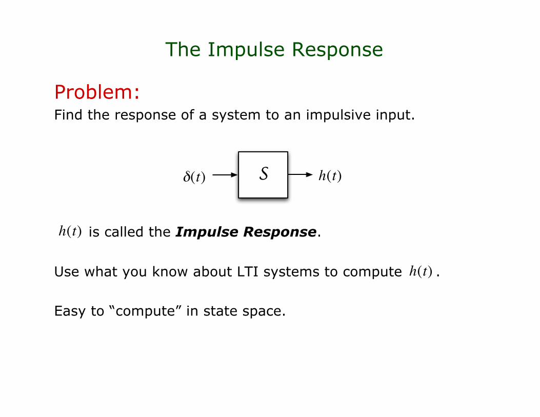
Problem:Find the response of a system to an impulsive input.
is called the Impulse Response.
Use what you know about LTI systems to compute .
Easy to “compute” in state space.
!
"(t) S
!
h(t)
!
h(t)
!
h(t)

Problem:Find the response of an LTI system in state space to an
impulsive input.
Solution:If the LTI system is causal it can be represented in state space.
We are looking for a solution to
Since the system is causal, and assuming zero initial conditions,we have that for all . In particular .Integrating from to
The Impulse Response

Solution (continued):
Fact #1: does not contain impulses! Therefore
From this point on the system has zero input and its response isthe homogenous solution:
Putting it all together:
where is the impulse response.
The Impulse Response
The Convolution Formula
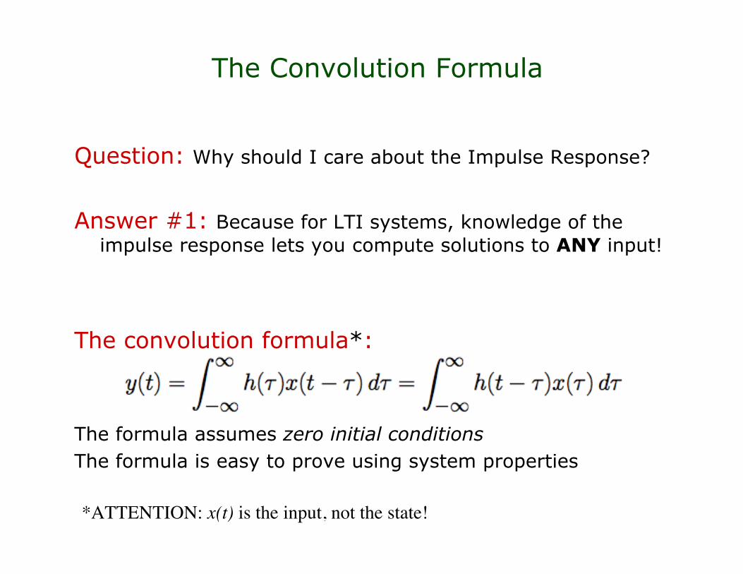
Question: Why should I care about the Impulse Response?
Answer #1: Because for LTI systems, knowledge of theimpulse response lets you compute solutions to ANY input!
The convolution formula*:
The formula assumes zero initial conditionsThe formula is easy to prove using system properties
*ATTENTION: x(t) is the input, not the state!
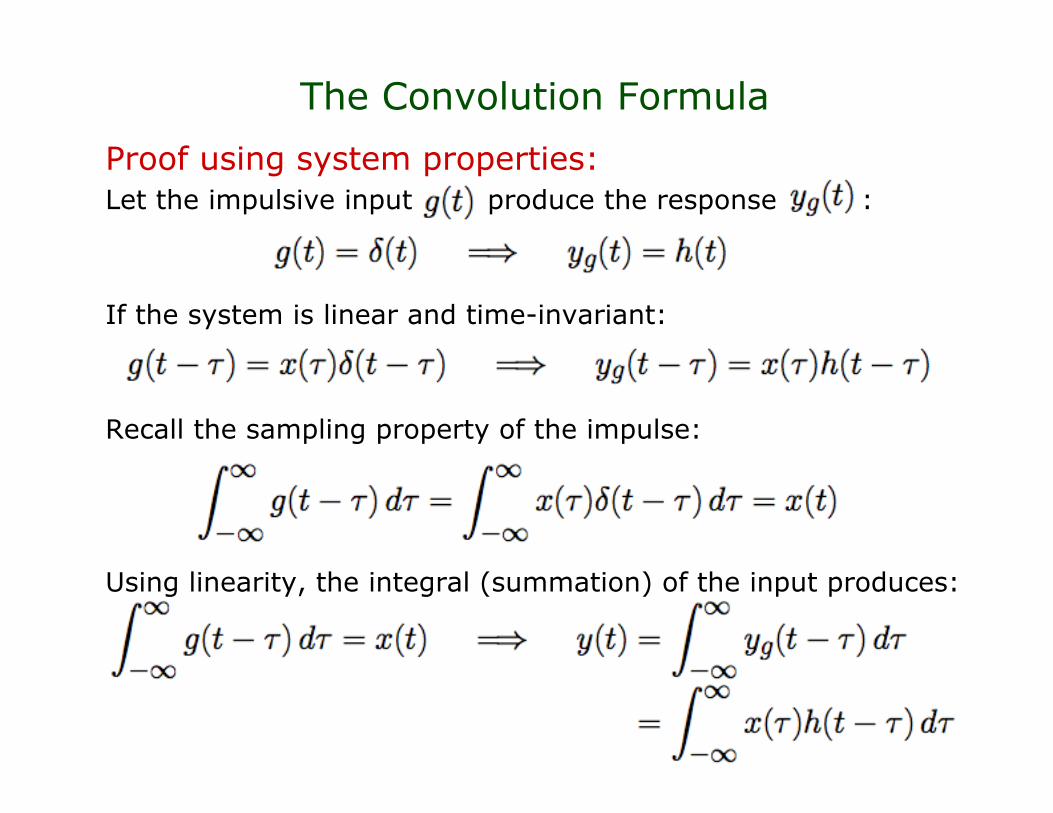
Proof using system properties:Let the impulsive input produce the response :
If the system is linear and time-invariant:
Recall the sampling property of the impulse:
Using linearity, the integral (summation) of the input produces:
The Convolution Formula

The Convolution Formula
Question: Why should I care about the Impulse Response?
Answer #1: Because for LTI systems, knowledge of theimpulse response lets you compute solutions to ANY input!
Answer #2: Because for LTI systems, knowledge of theimpulse response equals knowledge of the system!
System identification:When no mathematical model is available to describe a system,
then we can measure one signal (the impulse response) anduse this as a model!

System Identification
Perform the experiment and record the impulseresponse:
If the system is LTI, the Impulse Response is allwe need to know to obtain the response of thesystem to any input:
!
x(t)
!
h(t)
!
y(t)
!
"(t) S
!
h(t)
The Convolution Formula
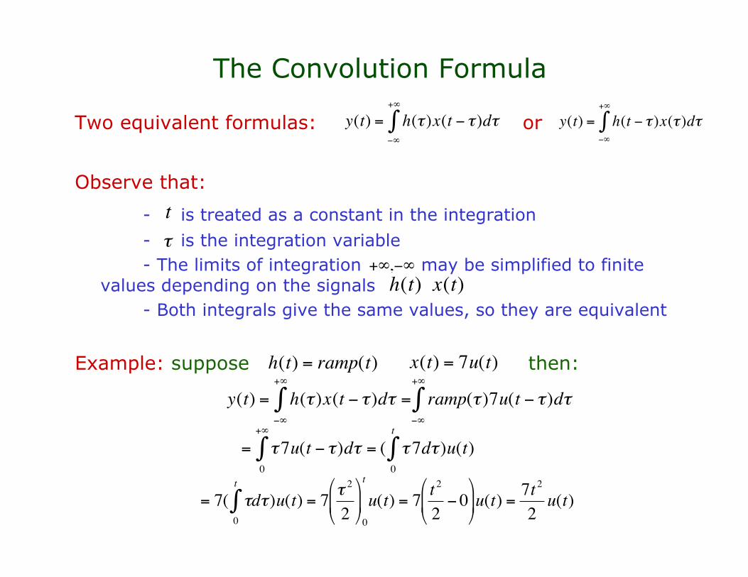
Two equivalent formulas: or
Observe that:
- is treated as a constant in the integration- is the integration variable- The limits of integration may be simplified to finite
values depending on the signals- Both integrals give the same values, so they are equivalent
Example: suppose then:
!
y(t) = h(" )x(t # " )d" =#$
+$
% ramp(" )7u(t # ")d"#$
+$
%
!
t
!
"
!
+",#"
!
x(t)
!
h(t)
!
y(t) = h(" )x(t # " )d"#$
+$
%
!
y(t) = h(t " # )x(# )d#"$
+$
%
!
h(t) = ramp(t)
!
x(t) = 7u(t)
!
= "7u(t # ")d"0
+$
% = ( "7d"0
t
% )u(t)
!
= 7( "d")u(t) = 7" 2
2
#
$ %
&
' (
0
t
)0
t
u(t) = 7t2
2* 0
#
$ %
&
' ( u(t) =
7t2
2u(t)

Graphical Interpretation of Convolution
Notation: From now on, we will use a * to denote theconvolution-formula operation. That is:
The Impulse Response tells us through the convolution formulahow different the output will be from the input.!
y(t) = x(t) * h(t) = h(" )x(t # " )d"#$
+$
%
Graphical Interpretation of Convolution
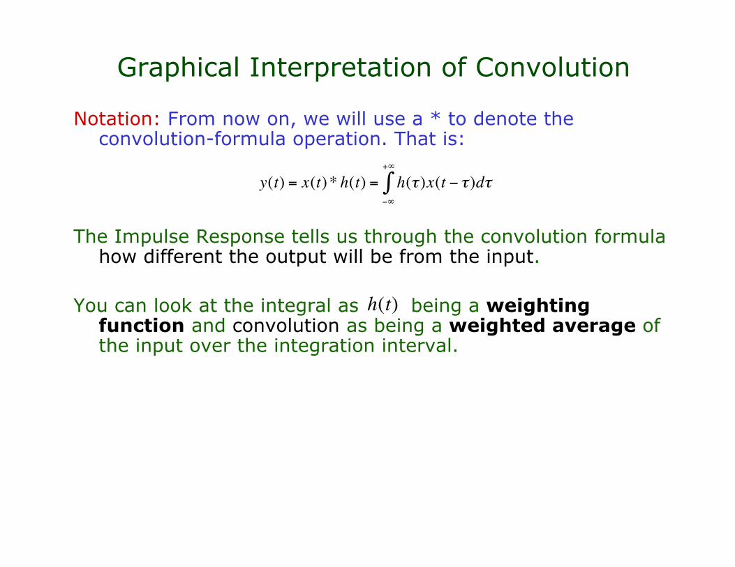
Notation: From now on, we will use a * to denote theconvolution-formula operation. That is:
The Impulse Response tells us through the convolution formulahow different the output will be from the input.
You can look at the integral as being a weightingfunction and convolution as being a weighted average ofthe input over the integration interval.
!
y(t) = x(t) * h(t) = h(" )x(t # " )d"#$
+$
%
!
h(t)

Graphical Interpretation of Convolution
Notation: From now on, we will use a * to denote theconvolution-formula operation. That is:
The Impulse Response tells us through the convolution formulahow different the output will be from the input.
You can look at the integral as being a weightingfunction and convolution as being a weighted average ofthe input over the integration interval.
The output value is then a compromise of the memoriesof the input from the past. In other words, thevalues tell how well the system remembers .
Therefore, the IR is a measure of the memory of the system.
!
y(t) = x(t) * h(t) = h(" )x(t # " )d"#$
+$
%
!
h(t)
!
x(t)
!
h(")
!
x(t " #)
!
y(t)
Graphical Interpretation of Convolution
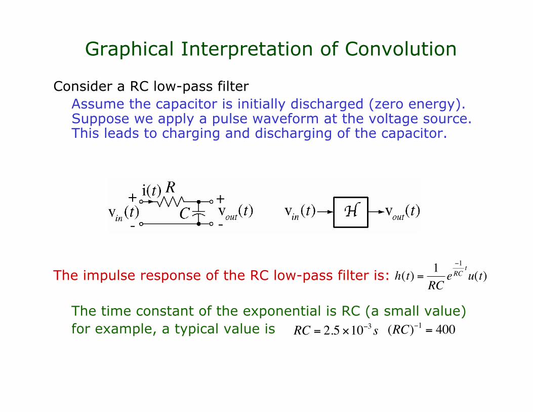
Consider a RC low-pass filterAssume the capacitor is initially discharged (zero energy).Suppose we apply a pulse waveform at the voltage source.This leads to charging and discharging of the capacitor.
The impulse response of the RC low-pass filter is:
The time constant of the exponential is RC (a small value)for example, a typical value is
!
h(t) =1
RCe
"1
RCt
u(t)
!
RC = 2.5 "10#3s
!
(RC)"1
= 400
Graphical Interpretation of Convolution
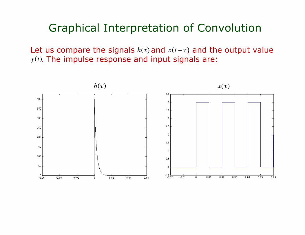
Let us compare the signals and , and the output value. The impulse response and input signals are:
!
h(")
!
x(t " #)
!
y(t)
!
h(")
!
x(")

Graphical Interpretation of Convolution
The output signal becomes:
!
y(t)
!
h(")
!
x(")
!
y(t)

Graphical Interpretation of Convolution
What is for different values of ?
!
x(t " #)
!
t
!
t = 0
!
x(")
!
x("# )

Graphical Interpretation of Convolution
What is for different values of ?
!
x(t " #)
!
t
!
t = 0.01
!
x(")
!
x(0.01" #)

Graphical Interpretation of Convolution
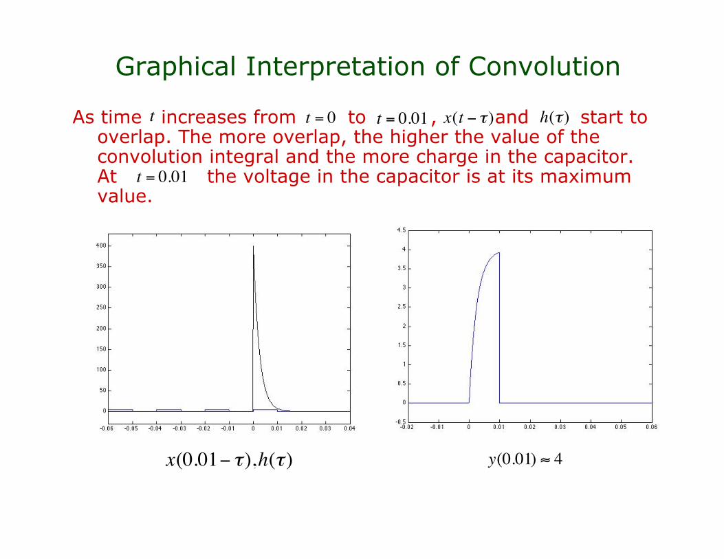
As time increases from to , and start tooverlap. The more overlap, the higher the value of theconvolution integral and the more charge in the capacitor.At the voltage in the capacitor is at its maximumvalue. !
x(t " #)
!
h(")
!
t
!
t = 0
!
t = 0.01
!
t = 0.01
!
x(0.005 " #),h(#)
!
y(0.005) " 3.5
Graphical Interpretation of Convolution
As time increases from to , and start tooverlap. The more overlap, the higher the value of theconvolution integral and the more charge in the capacitor.At the voltage in the capacitor is at its maximumvalue. !
x(t " #)
!
h(")
!
t
!
t = 0
!
t = 0.01
!
t = 0.01
!
x(0.01" #),h(#)
!
y(0.01) " 4
Graphical Interpretation of Convolution
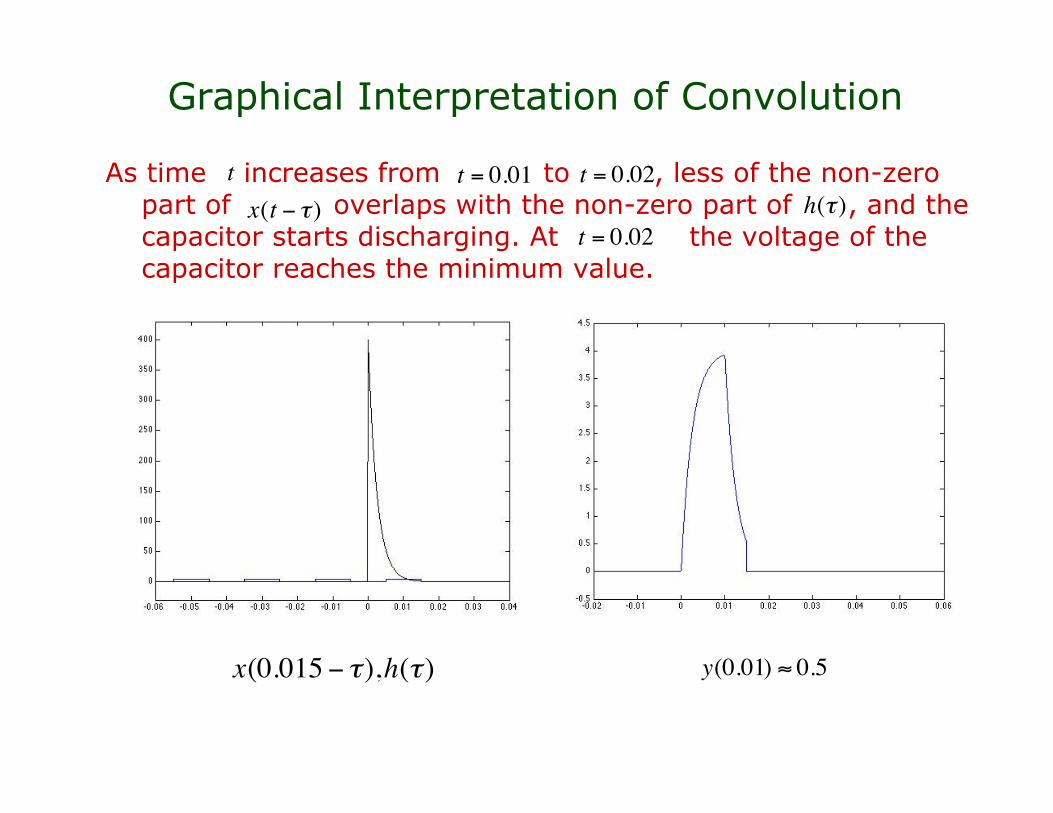
As time increases from to , less of the non-zeropart of overlaps with the non-zero part of , and thecapacitor starts discharging. At the voltage of thecapacitor reaches the minimum value.!
t
!
t = 0.01
!
t = 0.02
!
x(t " #)
!
h(")
!
t = 0.02
!
x(0.015 " #),h(#)
!
y(0.01) " 0.5

Graphical Interpretation of Convolution
As time increases from to , less of the non-zeropart of overlaps with the non-zero part of , and thecapacitor starts discharging. At the voltage of thecapacitor reaches the minimum value.!
t
!
t = 0.01
!
t = 0.02
!
x(t " #)
!
h(")
!
t = 0.02
!
y(0.02) " 0
!
x(0.02 " #),h(#)

Graphical Interpretation of Convolution
!
h(")
!
x(")
!
y(t)
tells us how different will be from In this case the output of the system is a “rounded” version of the input
!
h(")
!
y(t)
!
x(")

Signals & Systems Interaction in the TD
GoalsI. Impulse Response (IR) and Convolution Formula -Definition of IR and its use for system identification -Convolution formula and its graphical interpretation
II. Properties of systems from IR and convolution-Impulse response as a measure of system memory/stability-Alternative measures of memory/stability: step response
III. Applications of convolution-Audio effects: reverberation-Noise removal (i.e. signal filtering or smoothing)
Impulse Response and System Memory
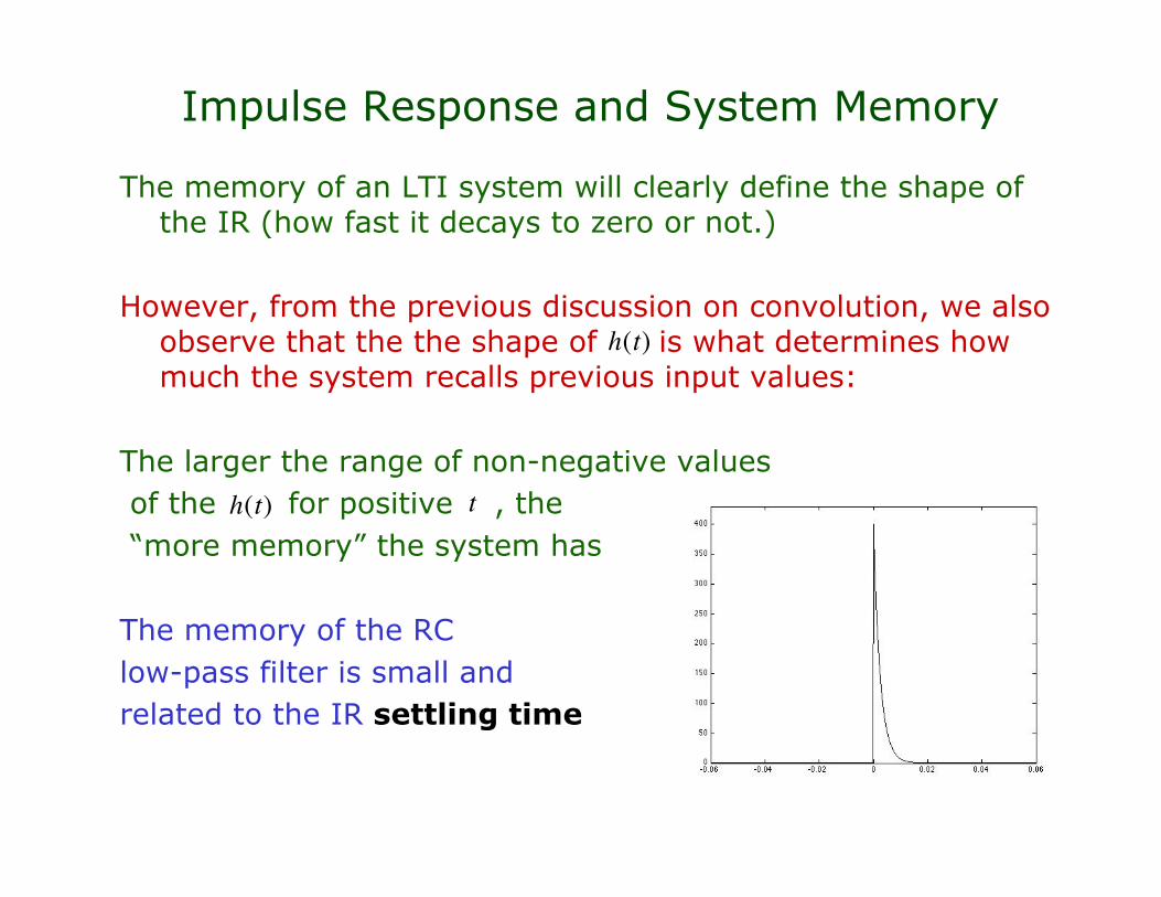
The memory of an LTI system will clearly define the shape ofthe IR (how fast it decays to zero or not.)
However, from the previous discussion on convolution, we alsoobserve that the the shape of is what determines howmuch the system recalls previous input values:
The larger the range of non-negative values of the for positive , the “more memory” the system has
The memory of the RClow-pass filter is small andrelated to the IR settling time
!
t
!
h(t)
!
h(t)

Impulse Response and System Memory
Definition:The settling time of a signalis the time it takes the signalto reach its steady-statevalue.
In this case we just compute to be the time whenreaches the value:
!
h(t)
!
h(ts) =
e"400t
s
400# 0.01
!
ts" 0.0265!
ts
!
0.01

Impulse Response and System Memory
If the IR of a system is a unit impulse signal, then the systemhas no memory of the past and leaves inputs unchanged!
From the convolutionformula, we obtain that
As an IR, the unit impulse just “samples” the input signal at the value . This is why we call this
property of the unit impulse function the “sampling property”(the associated system has no memory and leaves inputsunchanged.)
!
x(t)
!
h(t) = "(t)
!
t0
!
y(t0) = x(t)h(t " t
0)dt =
"#
+#
$ x(t)%(t " t0)dt = x(t
0)
"#
+#
$
Impulse Response and System Memory
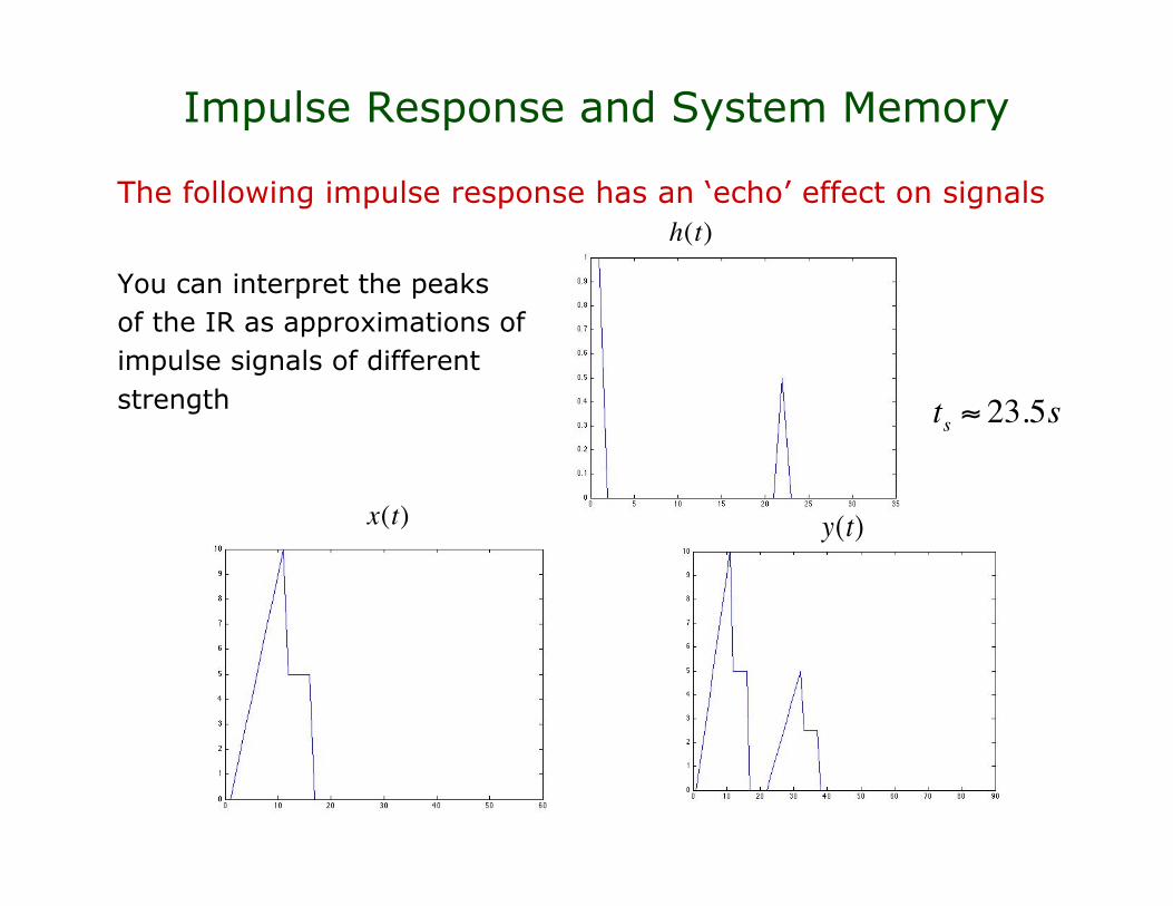
The following impulse response has an ‘echo’ effect on signals
You can interpret the peaksof the IR as approximations ofimpulse signals of differentstrength
!
h(t)
!
x(t)
!
y(t)!
ts" 23.5s
Impulse Response and System Stability
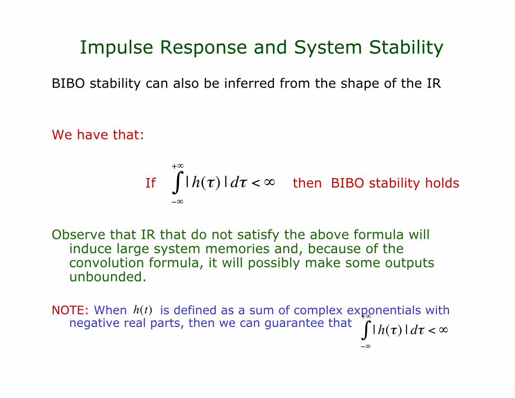
BIBO stability can also be inferred from the shape of the IR
We have that:
If then BIBO stability holds
Observe that IR that do not satisfy the above formula willinduce large system memories and, because of theconvolution formula, it will possibly make some outputsunbounded.
NOTE: When is defined as a sum of complex exponentials withnegative real parts, then we can guarantee that
!
| h(") | d"#$
+$
% <$
!
| h(") | d"#$
+$
% <$
!
h(t)
(Unit) step response
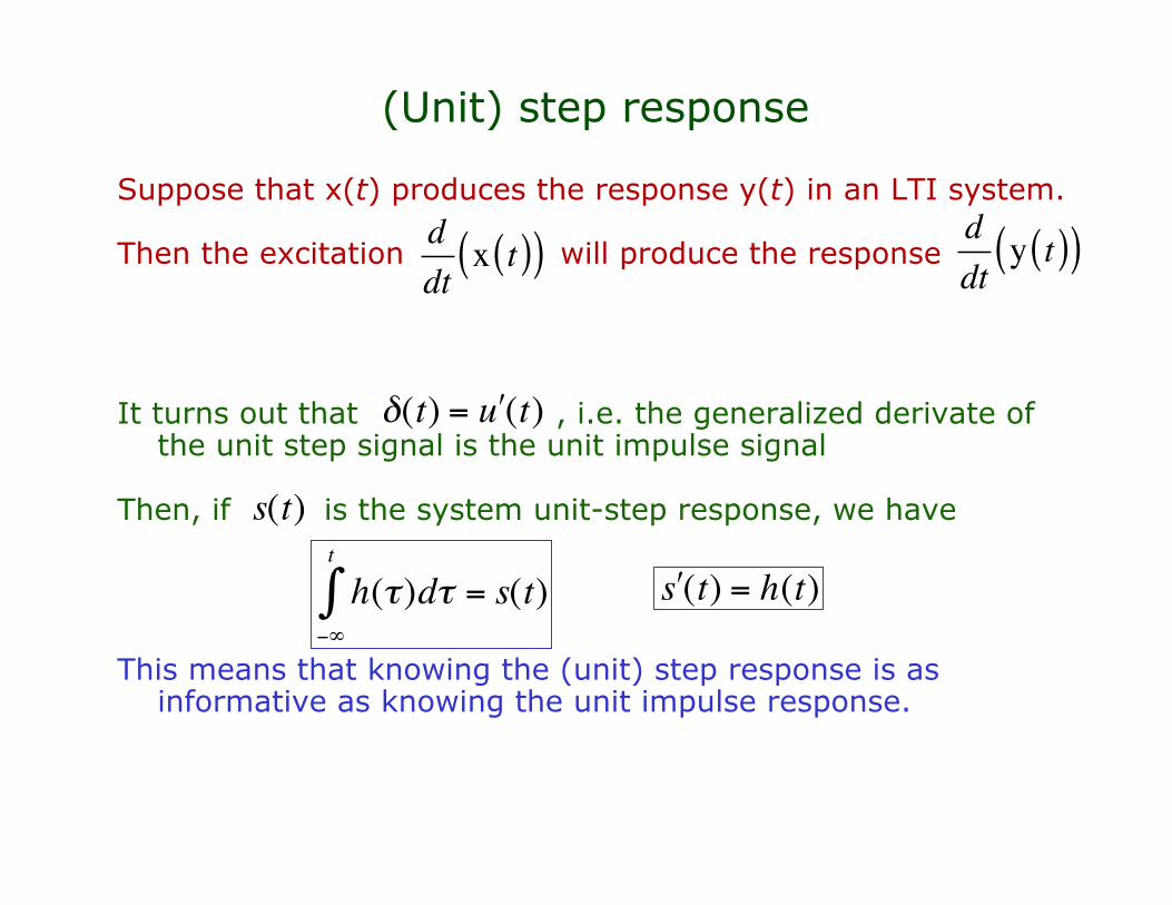
Suppose that x(t) produces the response y(t) in an LTI system.
Then the excitation will produce the response
It turns out that , i.e. the generalized derivate ofthe unit step signal is the unit impulse signal
Then, if is the system unit-step response, we have
This means that knowing the (unit) step response is asinformative as knowing the unit impulse response.
d
dtx t( )( )
d
dty t( )( )
!
"(t) = # u (t)
!
h(")d"#$
t
% = s(t)
!
s(t)
!
" s (t) = h(t)

(Unit) step response
The IR and a step response are used in practice to capture thetransient responses of the system (it tells you how thesystem reacts to disturbances and, qualitatively, about thesystem stability).
Constants of interest:Rise time: time it takes the signal to reach the vicinity of new set pointSettling timeOvershoot: maximum amount the system overshoots its final value divided by itPeak time: time to reach the overshoot value
!
tr" 7.7s
!
ts"15s
!
tp " 3.5s
!
Ov "11.5 /8.1
Example: system behavior from step response
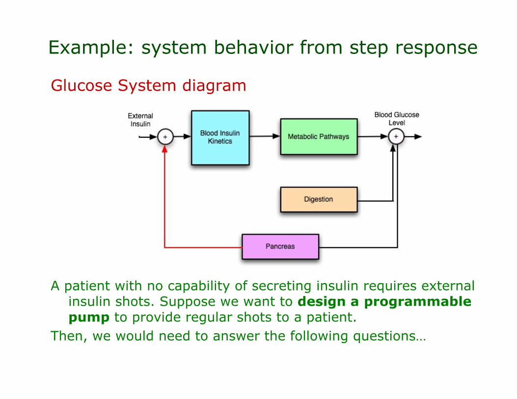
Glucose System diagram
A patient with no capability of secreting insulin requires externalinsulin shots. Suppose we want to design a programmablepump to provide regular shots to a patient.
Then, we would need to answer the following questions…
Example: system behavior from step response
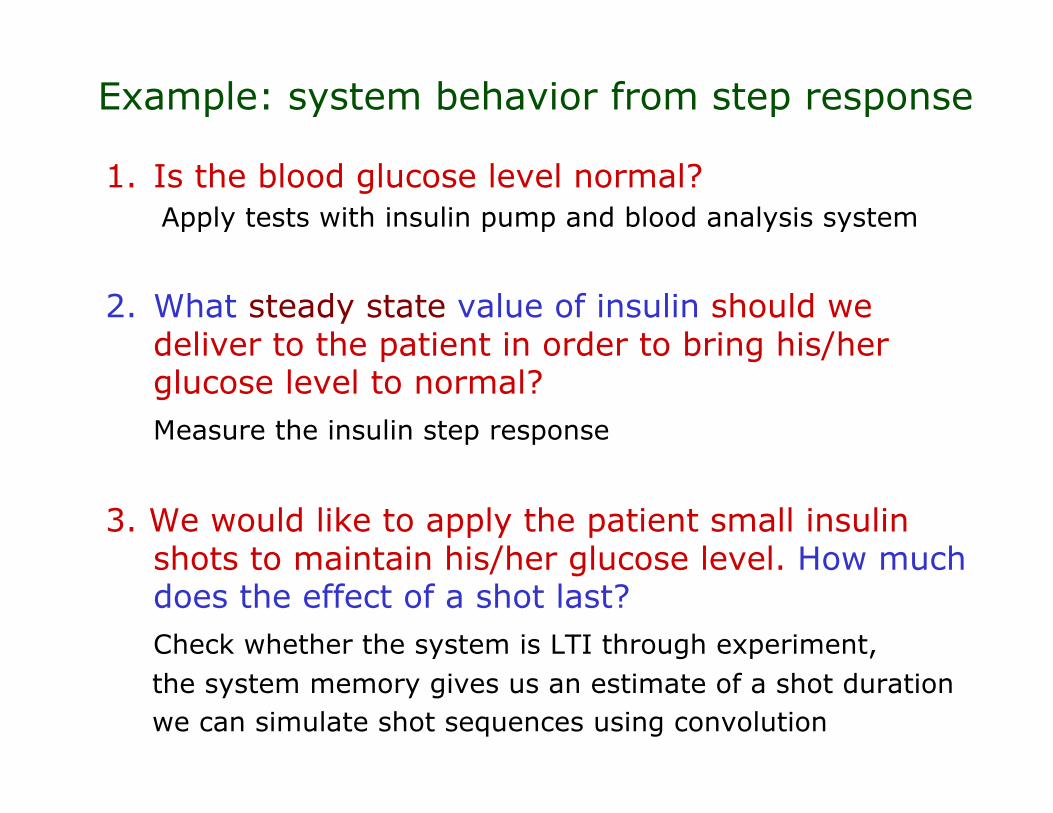
1. Is the blood glucose level normal? Apply tests with insulin pump and blood analysis system
2. What steady state value of insulin should wedeliver to the patient in order to bring his/herglucose level to normal?Measure the insulin step response
3. We would like to apply the patient small insulinshots to maintain his/her glucose level. How muchdoes the effect of a shot last?Check whether the system is LTI through experiment,
the system memory gives us an estimate of a shot duration we can simulate shot sequences using convolution

Example: system behavior from step response
4. Suppose the patient eats a meal. How should theinsulin dose change?
We would like to find the input that cancels out the effect ofthe meal, in other words…
If produces the output glucose level and is the input we need to produce
(under fasting conditions)
Then we need to find that produces . Then:
To solve for in we need to apply a“deconvolution” (easier in the Frequency Domain…)
!
ymeal (t)
!
x(t)
!
ynormal (t) + ymeal (t) "ymeal(t) =
!
h(t) * (xshot, fastn (t) + xmeal (t) + x(t)) =
!
ynormal (t)
!
xmeal(t)
!
x(t)
!
xshot, fastng (t)
!
ynormal (t)
!
h(t) * x(t) = "ymeal (t)
!
h(t) * x(t) = "ymeal (t)

Signals & Systems Interaction in the TD
GoalsI. Impulse Response (IR) and Convolution Formula -Definition of IR and its use for system identification -Convolution formula and its graphical interpretation
II. Properties of systems from IR and convolution-Impulse response as a measure of system memory/stability-Alternative measures of memory/stability: step response
III. Applications of convolution-Audio effects: reverberation-Noise removal (i.e. signal filtering or smoothing)

Reverberation effects
Reverberation (or reverb) effects are probably one of the mostheavily-used effects in music recording.
Reverberation is the result of many reflections of sound in aroom. Reflected waves reach to the listener later than wavesthat reach him/her directly. This produces an “echo” effect.
One way of implementing reverb effects is to convolve audiosignals with impulse responses like the following:

Reverberation effects
The process of obtaining a room Impulse Response is quitestraightforward. The following options are available:
1) Record a short impulse (hand clap, drum hit) in the room2) Room IR can be simulated in software also (e.g. MATLAB)3) There is also commercially available software (e.g. Altiverb)
that implements the reverb effects for different rooms
The IR records the room characteristics as follows:

Reverberation Effects
There are m files in MATLAB to approximate impulse responsesin rooms. For example the function rir.m freely available inthe Internet (“room impulse response”, you can take it fromWebCT.)
[h]=rir(fs, mic, n, r, rm, src);%RIR Room Impulse Response.% [h] = RIR(FS, MIC, N, R, RM, SRC) performs a room impulse% response calculation by means of the mirror image method.%% FS = sample rate.% MIC = row vector giving the x,y,z coordinates of% the microphone.% N = The program will account for (2*N+1)^3 virtual sources% R = reflection coefficient for the walls, in general -1<R<1.% RM = row vector giving the dimensions of the room.% SRC = row vector giving the x,y,z coordinates of% the sound source.
Reverberation Effects
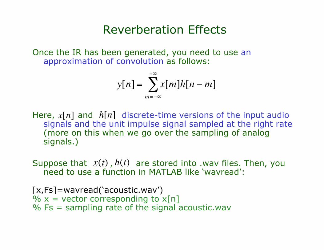
Once the IR has been generated, you need to use anapproximation of convolution as follows:
Here, and discrete-time versions of the input audiosignals and the unit impulse signal sampled at the right rate(more on this when we go over the sampling of analogsignals.)
Suppose that , are stored into .wav files. Then, youneed to use a function in MATLAB like ‘wavread’:
[x,Fs]=wavread(‘acoustic.wav’)% x = vector corresponding to x[n]% Fs = sampling rate of the signal acoustic.wav
!
y[n] = x[m]h[n "m]m="#
+#
$
!
x[n]
!
h[n]
!
x(t)
!
h(t)
Reverberation Effects
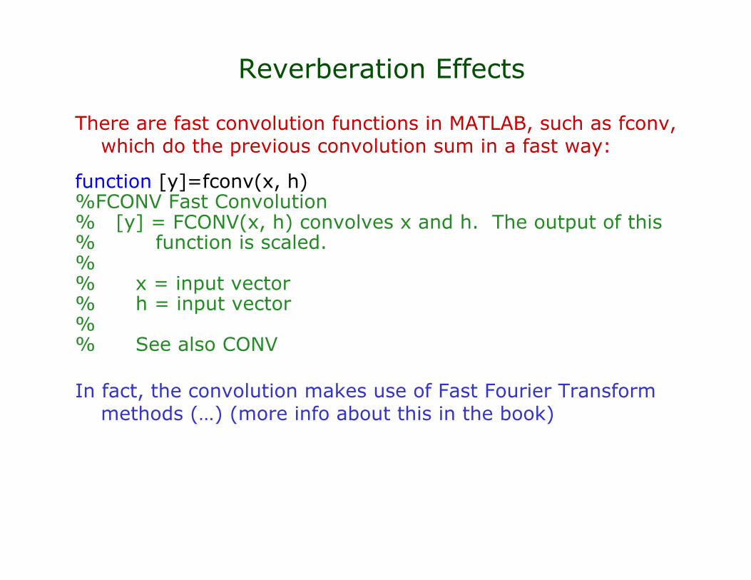
There are fast convolution functions in MATLAB, such as fconv,which do the previous convolution sum in a fast way:
function [y]=fconv(x, h)%FCONV Fast Convolution% [y] = FCONV(x, h) convolves x and h. The output of this% function is scaled.%% x = input vector% h = input vector%% See also CONV
In fact, the convolution makes use of Fast Fourier Transformmethods (…) (more info about this in the book)

Reverberation Effects
An example of how we call this function given an input signaland an Impulse Response is the following (in WebCT):
% reverb_convolution_eg.m% Script to call implement Convolution Reverbclose all;clear all;% read the sample waveformfilename='.acoustic.wav';[x,Fs,bits] = wavread(filename);
% read the impulse response waveform or take it from rir.mandsubstitute imp by the output of rir.m
filename='impulse_room.wav';
[imp,Fsimp,bitsimp] = wavread(filename);
% Do convolution with FFTy = fconv(x,imp);
% write outputwavwrite(y,Fs,bits,'out_IRreverb.wav');

Reverberation Effects
Finally, to play a wav file in MATLAB just use
[x,Fs]=wavread('acoustic.wav');sound(x,Fs)
In WebCT there are examples of room impulse responses andaudio files. Try them with your favorite wav files!
Just do the following:-Run ‘reverb_convolution_eg.m’ in MATLAB with theinput.wav file and IR.wav file you like-play out_IRreverb.wav using ‘wavread’ and ‘sound’ as above
More on sound processing and convolution
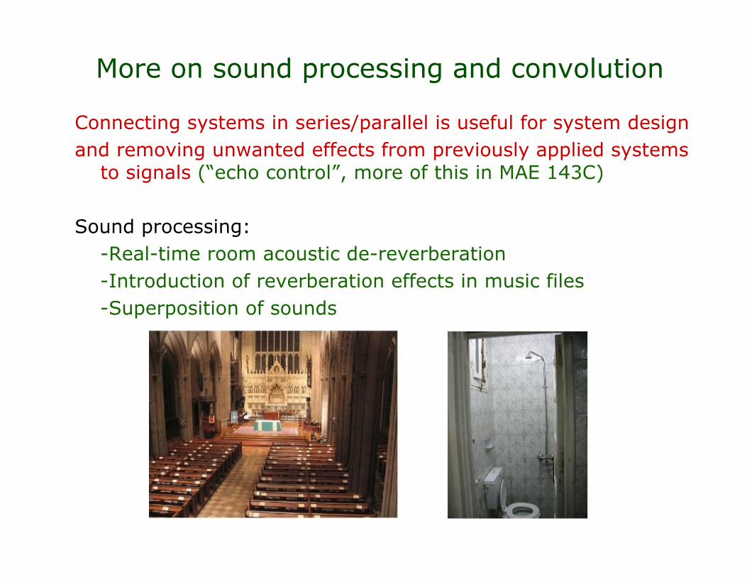
Connecting systems in series/parallel is useful for system designand removing unwanted effects from previously applied systems
to signals (“echo control”, more of this in MAE 143C)
Sound processing:-Real-time room acoustic de-reverberation-Introduction of reverberation effects in music files-Superposition of sounds

More on sound processing and convolution
Measure the room impulse responseFind another impulse response function such that (This
is possible for Invertible Systems. The new impulse response has tobe found by “deconvolution”. This is done in the Frequency Domain)
Consider your favorite impulse response to filter the speech
Similar ideas used in image processing; for example this is done incamera auto-focusing sub-routines
However, for image/sound processing, we need to deal with discretesignals and discrete systems counterparts (more on this later.)
!
h1(t)
!
h1(t) * h
2(t) = "(t)
!
h3(t)
!
h1(t)
!
h2(t)
!
h3(t)

Noise removal and signal smoothing
Convolution is commonly used to implement linear operationson audio signals and images such as filtering (noise removal)
Moving average filterTake a noisy signal
Herewhereand is a white noise
Gaussian white noise: for every , is Gaussian distributed(that is, the mean value of is zero and takes a realvalue close to zero with a standard deviation of )
!
f (t)
!
f (t)
!
f (t) = s(t) + w(t)
!
s(t) = e" t
2/ 2
!
w(t)
!
w(t)
!
t
!
w(t)
!
w(t)
!
"

Noise removal and signal smoothing
Take . The moving average filter is defined as theconvolution . The output is a new signalwith the same shape as (in general we can only say
)
Why does this work?Recall that
convolution = weighted averageThen have that
because the mean valueof is zero
!
h(t) = rect(t)
!
g(t) = h(t) * f (t)
!
g(t)
!
s(t)
!
g(t)
!
g(t) " h(# )(s(t $ #) + w% (t $ # ))
!
"1
m(s(t # $
i) + w(t # $
i))
i=1
m
%
!
"1
ms(t # $
i)% " s(t)
!
w(t)
!
s(t) " g(t)
Noise removal and signal smoothing
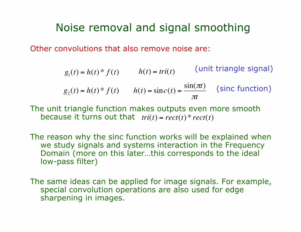
Other convolutions that also remove noise are:
(unit triangle signal)
(sinc function)
The unit triangle function makes outputs even more smoothbecause it turns out that
The reason why the sinc function works will be explained whenwe study signals and systems interaction in the FrequencyDomain (more on this later…this corresponds to the ideallow-pass filter)
The same ideas can be applied for image signals. For example,special convolution operations are also used for edgesharpening in images.
!
g1(t) = h(t) * f (t)
!
h(t) = tri(t)
!
h(t) = sinc(t) =sin("t)
"t
!
g2(t) = h(t) * f (t)
!
tri(t) = rect(t) * rect(t)

Summary
Important points to remember:1. The impulse response (IR) of a system is the particular output that the
system produces when excited with the unit impulse signal. In this way, theIR of a system can be obtained experimentally.
2. The IR of an LTI system can be used to obtain the response of thesystem to an arbitrary excitation via an operation called convolution.This turns out to be very useful if we don’t know an ODE model of the LTIsystem.
3. The IR of an LTI system can be seen as a measure of memory of thesystem. It can also tell us whether the system is BIBO stable or not.
4. Convolution can be understood as a weighted sum of input values.
5. The step response of a system is the (generalized) derivative of theImpulse Response. Thus, it is as informative as the IR.
6. Convolution has applications in the prediction of general (nonlinear)systems behavior (system identification), and in the treatment ofaudio/image signals (e.g. reverberation effects and noise removal.)