TIME DOMAIN PROBABILISTIC SEISMIC DEMAND ANALYSIS

OF SELF CENTERING BRIDGES UNDER NEAR

FAULT GROUND MOTIONS

By

MANISHA RAI

A thesis submitted in partial fulfilment of

the requirements for the degree of

MASTER OF SCIENCE in Civil Engineering

WASHINGTON STATE UNIVERSITY

Department of Civil & Environmental Engineering

AUGUST 2010

ii

To the Faculty of Washington State University:

The members of the Committee appointed to examine the thesis of MANISHA RAI

find it satisfactory and recommend that it be accepted.

___________________________________

Mohammad ElGawady, PhD., Chair

___________________________________

Adrian, Rodriguez-Marek, PhD.

___________________________________

William, Cofer, PhD.

iii

ACKNOWLEDGMENTS

I would first like to thank Dr. Mohammad ElGawady, the chair of my committee, for his

invaluable technical advice, guidance and support. I am very grateful for the time he spent on

reviewing my thesis; his comments really helped me in improving the overall quality of this

work.

I am grateful to Dr. Adrian Rodriguez-Marek, for his guidance, suggestions and for providing

me with the financial support. I would also like to thank Dr. Cofer for his participation and

assistance by serving on my committee. Special thanks go to Dr. Dolan for agreeing to my

request of substituting the committee, on a very short notice.

I would also like to thank my roommate Ruma Rani Paul and all my friends for the continued

support and friendship.

iv

TABLE OF CONTENTS

ACKNOWLEDGMENTS iii

TABLE OF CONTENTS iv

LIST OF FIGURES vi

Abstract 1

1 Introduction 2

2 Performance Based Seismic Design 4

3 PSDA methodologies 5

3.1 Traditional PSDA 5

3.2 Time Domain PSDA 6

3.3 Models needed to complete the PSDA analysis 7

3.3.1 Probability of pulse model 7

3.3.2 Predictive model for Ap and Tp 7

3.3.3 EDP-IM relationship 7

4 Bridge modelling 8

4.1 Bridge structure 8

4.2 Material models 10

4.2.1 Confined Concrete Model 10

4.2.2 Steel stress strain model 11

v

4.3 Plastic Hinge 11

4.3.1 Moment Curvature Analysis 12

4.3.2 P-M interaction diagram 13

4.4 Bridge model 15

4.5 Model calibration and Pushover analysis 18

5 Nonlinear Time History Analysis and Results 20

5.1 Ground Motions considered 20

5.2 EDP –IM relationship for FD and NFD ground motions 20

5.3 Genetic Programming 22

5.4 EDP vs Pulse parameter relationship for simplified Pulses. 23

6 Sites and Fault Geometry 27

7 PSDA results and discussion 29

8 Conclusions 42

References 44

APPENDIX A 48

vi

LIST OF FIGURES

Figure 1: Bridge structure a) Plan and b) Elevation (Zhu et. al 2006) 8

Figure 2: Cross sections configuration of RC column (Zhu et al 2006) 9

Figure 3: Illustrative figure showing PPT-CFFT column cross section. 10

Figure 4: Samaan’s stress-strain model for confined concrete 11

Figure 5: Comparisons of moment curvature plots of FRP-CFFT columns (at initial concrete

compression stresses of 45% f’c) with RC columns from Zhu et al. (2006) 12

Figure 6: Bilinearized Moment curvature diagram 14

Figure 7: P-M interaction diagram for the PPT-CFFT column 15

Figure 8: A bridge finite element model (a) entire bridge (b) pier frame (Zhu et al 2006) 17

Figure 9: Model of the bridge in SAP2000 (v.12.0.2) 18

Figure 10: Comparison of Pushover curves from SAP 2000 (v.12.0.2) and from Hewes and

Priestley (2002) model, after calibration for all the columns 19

Figure 11: Plots of response of bridge to Forward Directivity and Non-Forward directivity

ground motions 21

Figure 12: Tree representation of the function in genetic programming (for more

examples see Koza 1992) 23

Figure 13: A genetic crossover operation between two parents leading to two new children

(more examples in Koza 1992) 23

Figure 14: Screenshot of SAP 2000 (v.12.0.2) showing the deflected shape of the first

vii

mode 25

Figure 15: Plot showing / against

25

Figure 16: An EDP response surface of the bridge for simplified Gabor pulses 26

Figure 17: Bounded Guttenberg -Richter recurrence law for magnitudes within a range

of 5 to 8 28

Figure 18: Diagram showing fault and various bridge locations used for PSDA 28

Figure 19: Plots of rate of exceedence of drift versus maximum drifts for a site located at a

distance of a) 6 km b) 11 km c) 16 km and d) 21 km from the fault 32

Figure 20: An illustration of the relationship between maximum fault rupture length and

source to fault (rupture) distance 34

Figure 21: Distance magnitude deaggregation plots for a site located at distances of a) 6 km

b) 11 km c) 16 km and d) 21 km from the fault 36

Figure 22: Comparison of magnitude deaggregation plots from four methods at distances of

a) 6km b) 11 km c) 16 km and d) 21 km from the fault along its centreline 39

Figure 23: Period Amplitude deaggregation plots at distances of a) 6 km b) 11 km c) 16 km

and d) 21 km from the fault along its centreline 42

viii

Dedication

This thesis is dedicated to my parents who

have supported and guided me throughout my life

1

TIME DOMAIN PROBABILISTIC SEISMIC DEMAND ANALYSIS

OF SELF CENTERING BRIDGES UNDER NEAR

FAULT GROUND MOTIONS

Abstract

Ground motions at sites close to a fault are sometimes affected by forward directivity.

Forward directivity is a phenomenon by which most of the energy from an earthquake

rupture arrives at the site in a very short duration pulse. It is known that these pulses impose

a heavy demand on structures located in the vicinity of the fault. However these effects have

not been addressed clearly in the building codes and no specific guidelines exist on how to

account for them when determining the seismic hazard for a structure. In this research we

have done a Probabilistic Seismic Demand Analysis (PSDA) for a self centering bridge. Four

different methodologies namely Traditional, Broadband, Enhanced Broadband and Time

Domain methodology were used (Sehhati 2008). For the analysis, the maximum column drift

was chosen as the engineering demand parameter (EDP) and the spectral acceleration at the

bridge‟s fundamental period was chosen as the ground motion intensity measure (IM). A

bridge model was built and non-linear time history analysis was performed on the model

using SAP2000 (v.12.0.2), in the weak direction. The analysis was done using both pulse-

like and non pulse-like ground motion. Least squares regression was used to fit power-law

relationship between the EDP and the intensity measure for both pulse-like and non pulse-

like ground motions. For the time domain PSDA approach, which is done using simplified

pulses, the analysis discussed above was run on the structure using simplified Gabor pulses

for a range of pulse period and amplitude and the bridge‟s response was recorded for each. A

surface for bridge response was then fit using genetic algorithm software, Eureqa. Before the

PSDA analysis, the range of values of pulse period where simplified pulse represents the

actual forward directivity ground motions was determined. The surface was then used for

this range of period, to perform the PSDA, using the algorithm from Sehhati 2008. Results of

the PSDA showed that pulses impose heavy demands in near fault regions. It highlighted the

importance of considering small magnitude earthquakes in near fault hazard calculation. It

also showed that time domain approach is better than other traditional approaches for near

fault hazard calculations, as it is able to capture resonance in the structure in a better way.

2

1 INTRODUCTION

In this study, a detailed probabilistic seismic demand analysis (PSDA) of a self centering

bridge under near and far fault ground motions is performed. PSDA is an important step in

the performance based seismic design (PBSD) (SEAOC Vision 2000). PBSD methodology

aims to provide tools which can be used to design a structure to reach a specific performance

under a given ground motion. The performance can be evaluated in terms of decision

variables such as a specific sort of damage in the structural or non structural components of a

structure or more general terms such as downtime and dollar value of losses. PBSD is

required to find out the rate of exceedance of different levels of an Engineering Demand

Parameter (EDP) under given seismic loading. EDP is generally a response parameter like

base shear, floor acceleration, drift demand etc. PSDA builds upon the results of probabilistic

seismic hazard analysis (PSHA) (e.g., Kramer 1996). PSHA is used to find the annual rate of

exceedance of a certain Intensity Measure (IM) at a site. The IM is a measure of severity of

the ground motion and represents the hazard at a site. Many different ground motion

parameters like duration of the ground motion, peak ground acceleration (PGA), peak ground

velocity (PGV) etc. can be used as an IM.

PSDA builds upon the results of PSHA. For this, a relationship between EDP and IM is

required. The EDP values are related to IM levels through an empirical relationship, which

accounts for the uncertainty in the prediction of EDP. The final results from PSDA are the

rates of exceedance of various EDP levels. These results, along with relationships relating

damage to EDP, are used to develop damage fragility curves which give the rate of

exceedance of the different damage states. Damage states can range from no damage to fully

collapsed state. The damage fragility curves along with relationship linking damage states to

various decision variables also called DV ( most common DVs are dollar value of loss, death

3

due to collapse or downtime due to damage), are used to come up with the rate of exceedance

of different DV levels. This completes the PBSD process. The rate of exceedance of different

DV levels can then be compared to the design target and the design process is iterated until

the desired targets are met.

This study performs the PSDA of a self centering bridge located close by an active fault. A

self centering column comprises of a concrete core confined with a glass fiber reinforced

polymer tube. Unlike a regular RC column, no stirrups are provided in these columns. The

glass fiber tube acts as a lateral reinforcement, confining the concrete core. In order to

provide the restoring force, an unbonded post-tensioning rebar passing through duct located

at the center of the column is used. When subjected to a cyclic loading (e.g., earthquake

ground motion), such a column rocks back and forth on its foundation. However, once the

loading is removed, it re-centers itself due to the force by post tensioning rebar. ElGawady et

al. (2010) showed that residual displacement and damage in a Precast Post Tensioning

Concrete Filled Fiber Tube (PPT-CFFT) column is much lower than in a conventional

reinforced concrete column. As this system of self centring structures is gaining popularity in

recent days, this work will help in better understanding its performance under near fault

ground motion excitation.

Near fault sites sometimes experience directivity effect which makes the ground motion at

these sites very different from ground motions recorded far from the fault. Directivity effects

are observed at sites located near a given fault and the fault ruptures towards the site

(Somerville 1997). In this case, the energy from the rupture arrives at the site in the form of a

big pulse. This pulse applies large seismic demands on the structure (e.g., Bertero et al.,

1978; Anderson and Bertero, 1987; Hall et al., 1995; Iwan, 1997; Alavi and Krawinkler,

2001; Menun and Fu, 2002; Makris and Black, 2003; Mavroeidis et al., 2004; Akkar et al.,

2005; Luco and Cornell, 2007). These pulse like effects are generally not accounted for while

4

doing PSDA analysis. Near fault pulse like ground motions have both higher IM level than

non pulse like ground motions (Somerville et al. 1997; Spudich and Chiou 2008) and produce

higher response for same IM level compared to non pulse like ground motions (Hall 1998;

Zhang and Iwan 2002). Recent research has proposed methods to account for near fault

effects in PBSD calculation (e.g. Sehhati 2008), but no such analysis has been carried out on

self centering bridge structures. This study uses the PSDA framework proposed by Sehhati

(2008), to determine the seismic demand on a self-centering concrete bridge. Results from

this PSDA are compared to more traditional approaches used to do the PSDA for near fault

sites.

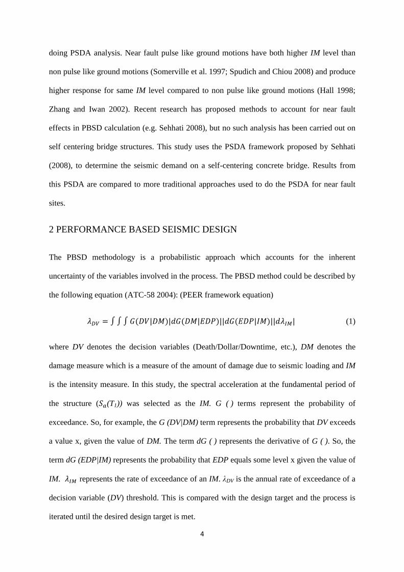
2 PERFORMANCE BASED SEISMIC DESIGN

The PBSD methodology is a probabilistic approach which accounts for the inherent

uncertainty of the variables involved in the process. The PBSD method could be described by

the following equation (ATC-58 2004): (PEER framework equation)

(1)

where DV denotes the decision variables (Death/Dollar/Downtime, etc.), DM denotes the

damage measure which is a measure of the amount of damage due to seismic loading and IM

is the intensity measure. In this study, the spectral acceleration at the fundamental period of

the structure ( (T1)) was selected as the IM. G ( ) terms represent the probability of

exceedance. So, for example, the G (DV|DM) term represents the probability that DV exceeds

a value x, given the value of DM. The term dG ( ) represents the derivative of G ( ). So, the

term dG (EDP|IM) represents the probability that EDP equals some level x given the value of

IM. represents the rate of exceedance of an IM. λDV is the annual rate of exceedance of a

decision variable (DV) threshold. This is compared with the design target and the process is

iterated until the desired design target is met.

5

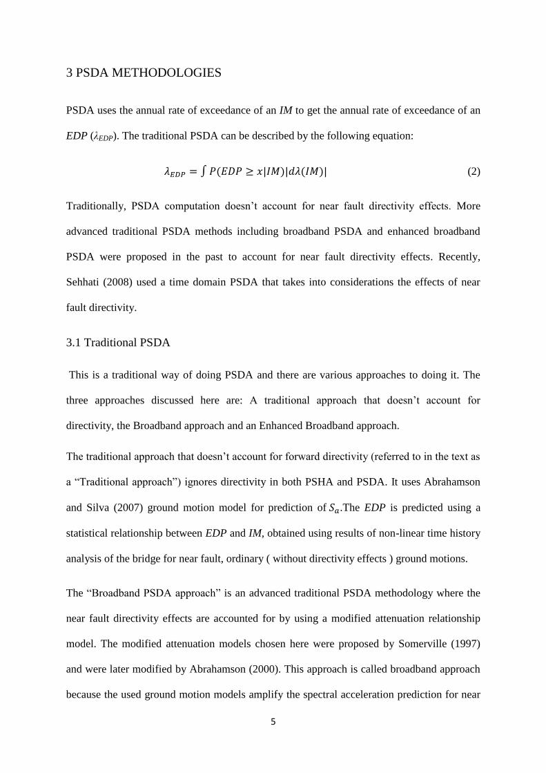
3 PSDA METHODOLOGIES

PSDA uses the annual rate of exceedance of an IM to get the annual rate of exceedance of an

EDP (λEDP). The traditional PSDA can be described by the following equation:

(2)

Traditionally, PSDA computation doesn‟t account for near fault directivity effects. More

advanced traditional PSDA methods including broadband PSDA and enhanced broadband

PSDA were proposed in the past to account for near fault directivity effects. Recently,

Sehhati (2008) used a time domain PSDA that takes into considerations the effects of near

fault directivity.

3.1 Traditional PSDA

This is a traditional way of doing PSDA and there are various approaches to doing it. The

three approaches discussed here are: A traditional approach that doesn‟t account for

directivity, the Broadband approach and an Enhanced Broadband approach.

The traditional approach that doesn‟t account for forward directivity (referred to in the text as

a “Traditional approach”) ignores directivity in both PSHA and PSDA. It uses Abrahamson

and Silva (2007) ground motion model for prediction of .The EDP is predicted using a

statistical relationship between EDP and IM, obtained using results of non-linear time history

analysis of the bridge for near fault, ordinary ( without directivity effects ) ground motions.

The “Broadband PSDA approach” is an advanced traditional PSDA methodology where the

near fault directivity effects are accounted for by using a modified attenuation relationship

model. The modified attenuation models chosen here were proposed by Somerville (1997)

and were later modified by Abrahamson (2000). This approach is called broadband approach

because the used ground motion models amplify the spectral acceleration prediction for near

6

fault sites in a wide range (broadband) of periods. The broadband approach accounts for the

effect of near fault pulses on the IM observed at the site but it ignores the effect of pulses on

EDP for a given IM level.

The “Enhanced broadband approach” is an advanced traditional PSDA. It builds upon the

broadband approach and uses the same modified ground motion model to account for the

effect of near fault directivity on IM. However, this approach also attempts to account for the

effect of near fault directivity on EDP (or structural response). The enhanced broadband

approach uses different predictive equation for EDP given the IM for cases when directivity

effects are observed and when they are not observed.

3. 2 Time Domain PSDA

The time domain approach proposed by Sehhati (2008) extends the enhanced broadband

approach by using vector IMs. In this approach the scenarios are divided into four cases: non-

near source, near source no pulse, near source pulse with pulse-out, near source pulse with

pulse-in. The „near source pulse with pulse-in‟ case refers to cases when the structural

response is driven by the pulse in the ground motion (i.e. the period of pulse lies within a

certain range of the period of the structure) and thus EDP can be predicted using a vector IM

which consists of the pulse parameters namely pulse amplitude (Ap) and pulse period (Tp).

An EDP predictive equation using Ap and Tp is used in this case.

The pulse-out case refers to the scenario when directivity effects are observed at the site but

the period of the pulse is very different from that of the structure. In this scenario, the EDP –

IM relationship for forward directivity ground motions is used for EDP prediction. The other

two cases (non- near source and near source no pulse) are sufficiently described by their

names.

7

3.3 Models needed to complete the PSDA analysis

The numerical algorithm for all the different PSDA methodology was proposed in Sehhati

(2008) and is presented in Appendix A here for completeness. In order to fully implement the

algorithm for PSDA one needs the following models.

3.3.1 Probability of pulse model

The broadband, enhanced broadband and time domain approach divide the hazard scenarios

into forward directivity and non forward directivity cases; hence, the probability of observing

forward directivity ground motion at a given site due to a given rupture scenario is required to

carry out the PSDA. The model proposed by Iervolino and Cornell (2008) is the latest model

for prediction of probability of observing forward directivity at a given site due to a given

fault scenario and was used in this study.

3.3.2 Predictive model for and

In order to carry out the time domain PSDA approach, it is required to determine the pulse

amplitude ( ) and pulse period ( ) at a specific site. The pulse amplitude ( ) is modelled

as 0.73 times PGV where the model of Bray and Rodriguez-Marek (2004) was used to

estimate the PGV at distances less than 20 km from fault. For PGV at distances greater than

60 km, another model developed by Abrahamson and Silva (2007) was used. For

intermediate distances, i.e. in between 20 to 60 km, a taper is used to transition between the

two models (see Sehhati 2008 for more details). The Baker (2007) model is used for the

prediction of

3.3.3 EDP – IM relationship

The EDP – relationship for both pulse like and non pulse like ground motion is needed for

the enhanced broadband approach and an EDP – ( ) relationship is needed for the time

domain approach. These relationships are developed in Section 5 of this study.

8

4 BRIDGE MODELLING

4.1 Bridge Structure

For this research, a bridge case study has been adopted. The bridge general geometric

characteristics are similar to those used in the NCHRP Project 12-49 (2002). The bridge was

also used by other researchers as (Zhu et al 2006). The plan and the elevation of the bridge

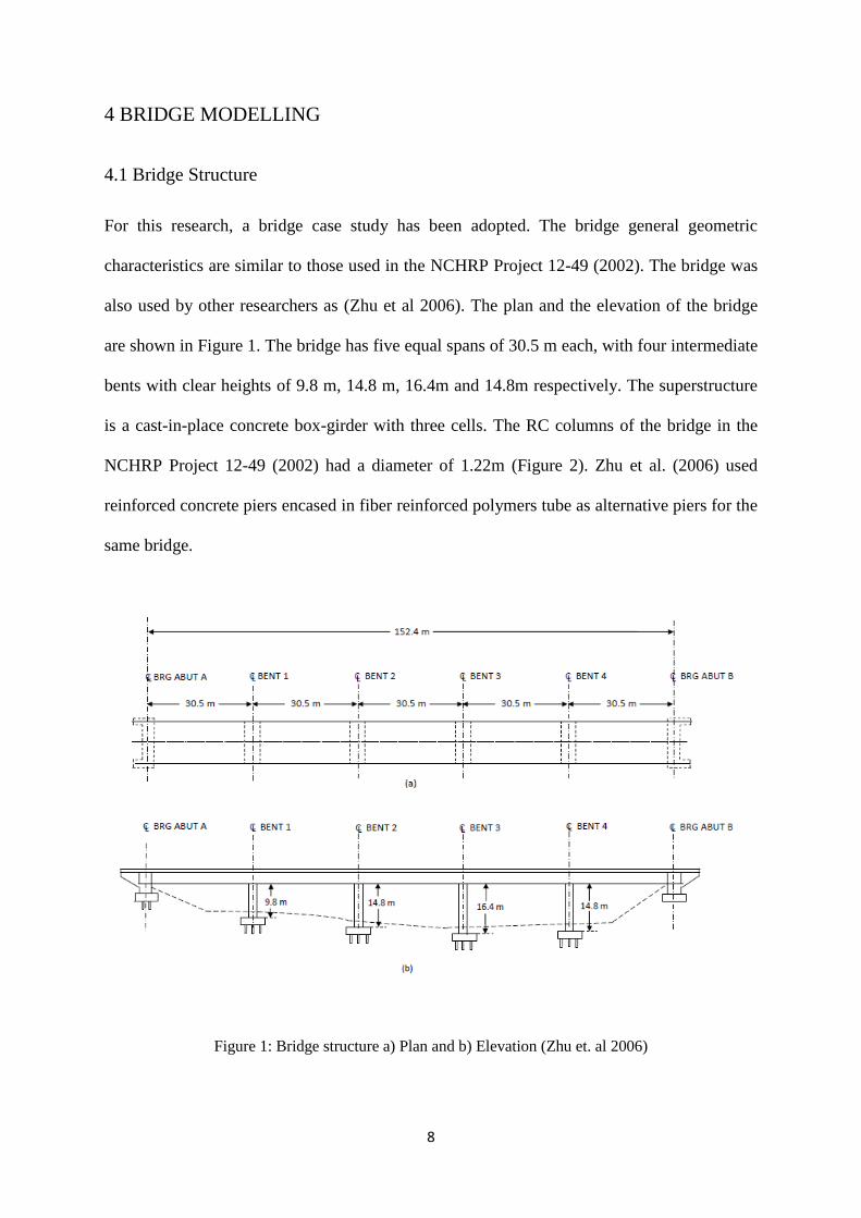
are shown in Figure 1. The bridge has five equal spans of 30.5 m each, with four intermediate

bents with clear heights of 9.8 m, 14.8 m, 16.4m and 14.8m respectively. The superstructure

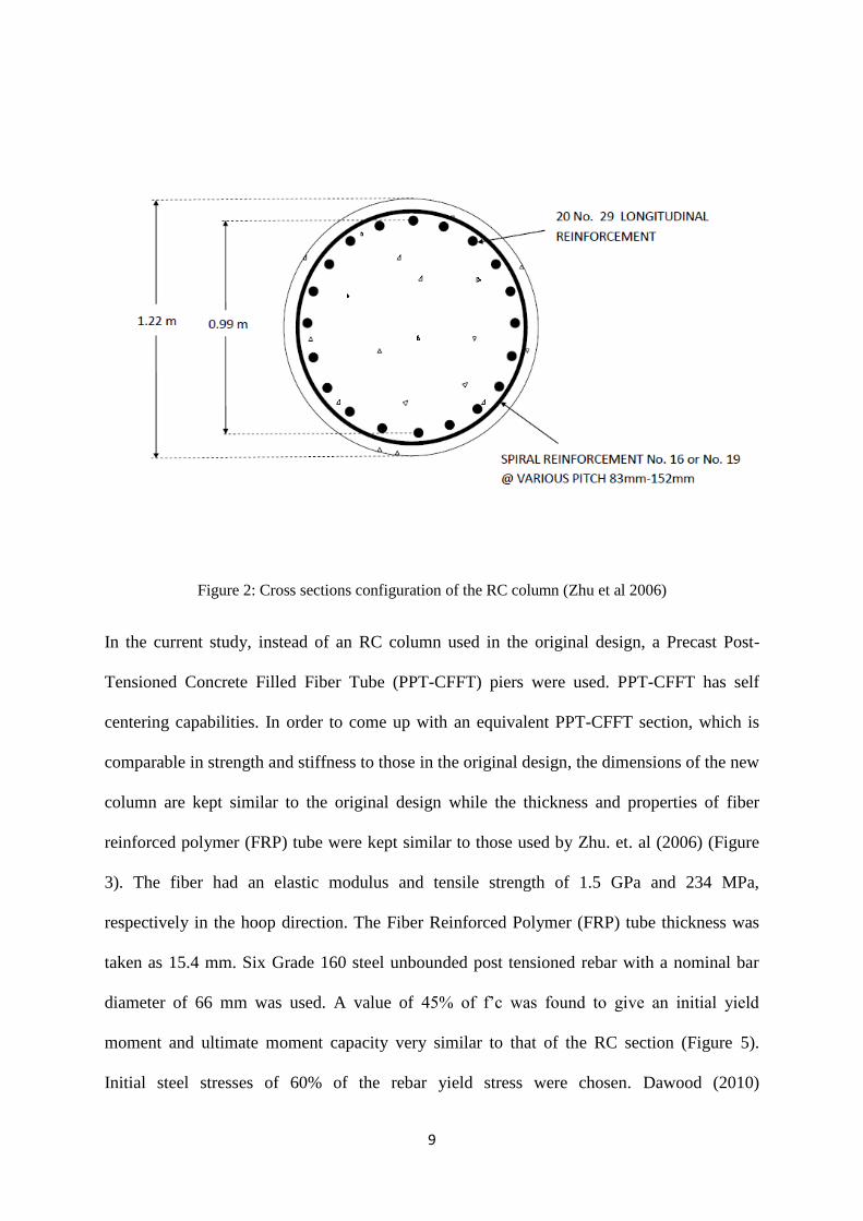
is a cast-in-place concrete box-girder with three cells. The RC columns of the bridge in the

NCHRP Project 12-49 (2002) had a diameter of 1.22m (Figure 2). Zhu et al. (2006) used

reinforced concrete piers encased in fiber reinforced polymers tube as alternative piers for the

same bridge.

Figure 1: Bridge structure a) Plan and b) Elevation (Zhu et. al 2006)

9

Figure 2: Cross sections configuration of the RC column (Zhu et al 2006)

In the current study, instead of an RC column used in the original design, a Precast Post-

Tensioned Concrete Filled Fiber Tube (PPT-CFFT) piers were used. PPT-CFFT has self

centering capabilities. In order to come up with an equivalent PPT-CFFT section, which is

comparable in strength and stiffness to those in the original design, the dimensions of the new

column are kept similar to the original design while the thickness and properties of fiber

reinforced polymer (FRP) tube were kept similar to those used by Zhu. et. al (2006) (Figure

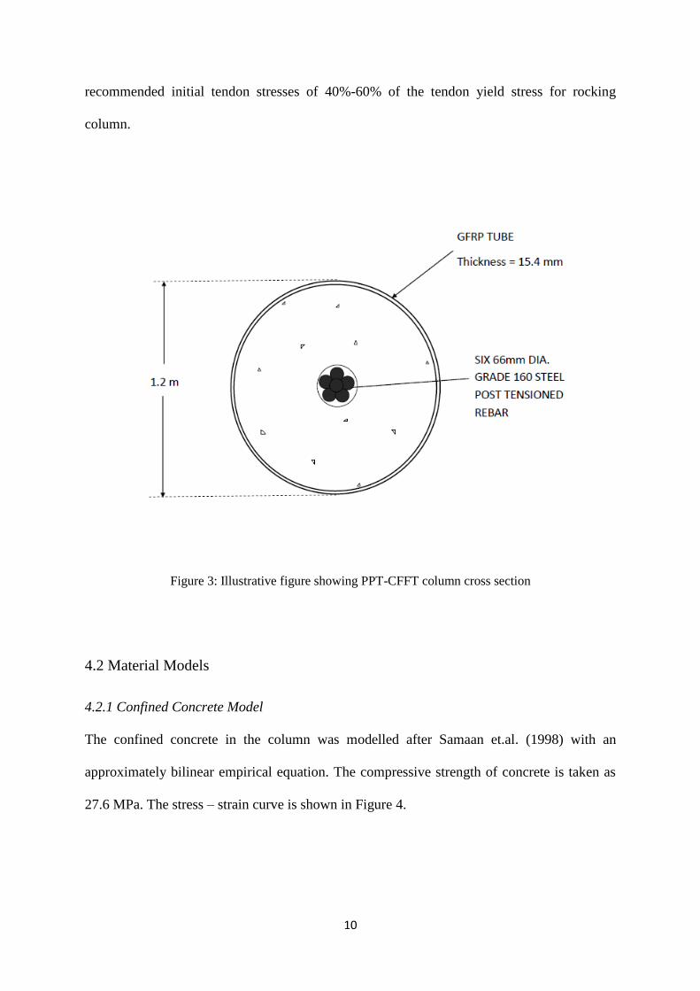
3). The fiber had an elastic modulus and tensile strength of 1.5 GPa and 234 MPa,

respectively in the hoop direction. The Fiber Reinforced Polymer (FRP) tube thickness was

taken as 15.4 mm. Six Grade 160 steel unbounded post tensioned rebar with a nominal bar

diameter of 66 mm was used. A value of 45% of f‟c was found to give an initial yield

moment and ultimate moment capacity very similar to that of the RC section (Figure 5).

Initial steel stresses of 60% of the rebar yield stress were chosen. Dawood (2010)

10

recommended initial tendon stresses of 40%-60% of the tendon yield stress for rocking

column.

Figure 3: Illustrative figure showing PPT-CFFT column cross section

4.2 Material Models

4.2.1 Confined Concrete Model

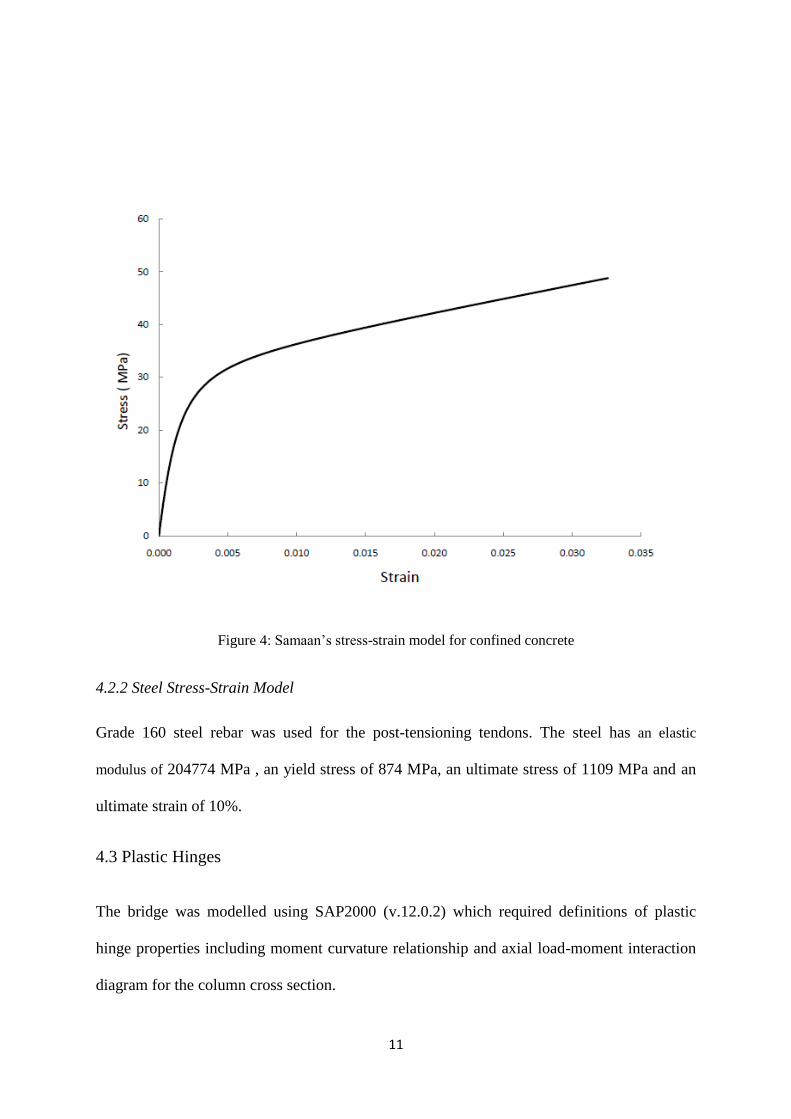
The confined concrete in the column was modelled after Samaan et.al. (1998) with an

approximately bilinear empirical equation. The compressive strength of concrete is taken as

27.6 MPa. The stress – strain curve is shown in Figure 4.

11

Figure 4: Samaan‟s stress-strain model for confined concrete

4.2.2 Steel Stress-Strain Model

Grade 160 steel rebar was used for the post-tensioning tendons. The steel has an elastic

modulus of 204774 MPa , an yield stress of 874 MPa, an ultimate stress of 1109 MPa and an

ultimate strain of 10%.

4.3 Plastic Hinges

The bridge was modelled using SAP2000 (v.12.0.2) which required definitions of plastic

hinge properties including moment curvature relationship and axial load-moment interaction

diagram for the column cross section.

12

4.3.1 Moment Curvature Analysis

Moment curvature analysis of a rocking column is different from regular RC column. This

difference is due to the inherent difference in the behaviour of the two columns under action

of a lateral load. A rocking or self centring column has the ability to rock back and forth on

its foundation, in an event of ground motion. In order to provide the restoring force, an

unbonded post tensioning rebar passing through duct located at the center of the column was

used.

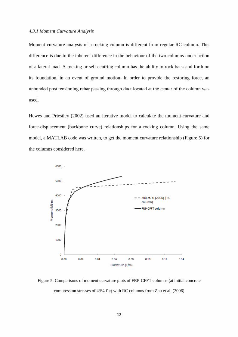
Hewes and Priestley (2002) used an iterative model to calculate the moment-curvature and

force-displacement (backbone curve) relationships for a rocking column. Using the same

model, a MATLAB code was written, to get the moment curvature relationship (Figure 5) for

the columns considered here.

Figure 5: Comparisons of moment curvature plots of FRP-CFFT columns (at initial concrete

compression stresses of 45% f‟c) with RC columns from Zhu et al. (2006)

13

4.3.2 P-M Interaction Diagram

In a conventional analysis, a moment axial load interaction diagram relationship is obtained

by taking various values for axial force and calculating the sections ultimate moment

capacity. It is assumed that the section‟s moment capacity doesn‟t change much after the

onset of yielding. However for a rocking section, as is evident from its moment curvature

diagram (Figure 5), there is no sharp yield point. In order to do the analysis, the following

method was adopted.

1. An axial force is assumed and the moment curvature analysis is performed, with

the total initial axial force as the sum of forces due to post tension and the applied

axial load.

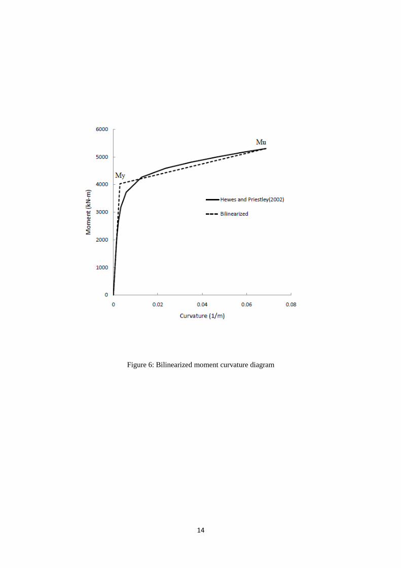
2. Method of equal area is adapted to come up with a bilinear moment curvature

relationship as shown in Figure 6. The point of intersection of two line segments,

marked as in the bilinear curve is recorded. This moment value serves as the

yield moment for the input. The ultimate moment is also recorded and the

ratio is noted.

3. Steps 1 and 2 were repeated for various values of the axial load (P) and the yield

moment ( ) was recorded for each of them.

4. Finally, all these values of the P were plotted against the calculated and this

gives the PM interaction diagram (Figure 7) that was used as an input in SAP2000

(v.12.0.2). Note that the positive values represent the column under compressive

axial load.

14

Figure 6: Bilinearized moment curvature diagram

15

Figure 7: P-M interaction diagram for the PPT-CFFT column

4.4 Bridge model

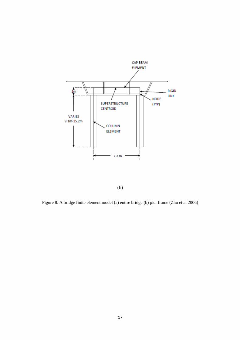
A three dimensional bridge model was assembled in SAP2000 (v.12.0.2) as shown in Figure

9. The bridge superstructure including the deck and box girder was combined together and

was modelled as one-line using elastic beam elements in the longitudinal direction. The beam

element representing each span passes through the centroid of the superstructure. Each span

was modelled using 4 beam elements. A cross girder at each bent was modelled using beam

elements located at the centroid of the box-girder , as shown in Figure 8b. A rigid beam

element was used to connect the top of the column to the cross girder. Geometric properties

of the bridge superstructure were similar to those used by Zhu et al (2002). The columns were

modelled using beam elements located at the geometric center of each column. Rigid moment

16

connections were used between the column and the foundation as well as between the column

and the link which in turn was connected to the superstructure. Plastic hinges were selected at

the top and bottom of ends of each column. The moment curvature relation along with the

PM interaction diagram, obtained above, is used to define the plastic hinges. The girder had a

dead load of 60KN/m. Additional dead load were due to five intermediate diaphragms of 68

kN each, two end diaphragms of 525 kN each and four intermediate pear beams of 454kN

each (Figure 8a).

(a)

17

(b)

Figure 8: A bridge finite element model (a) entire bridge (b) pier frame (Zhu et al 2006)

18

Figure 9: Model of the bridge in SAP2000 (v.12.0.2)

4.5 Model calibration and Pushover Analysis.

In order to calibrate the nonlinear behaviour of the FRP-CFFT sections, pushover analyses

were performed using SAP2000 (v.12.0.2) on columns identical to those used in the bridge

model and shown in Figure 3. The columns had heights of 9.1m, 13.7m and 15.2m. Each

column was subjected to an initial dead load value of 3118 kN. Also, the pushover curves

were calculated using Hewes and Priestley‟s model. SAP2000 (v.12.0.2) results had a higher

initial stiffness than the pushover curves obtained from Hewes and Priestley model. This

difference arose due to different models of concrete being used for the two analyses.

SAP2000 (v.12.0.2) uses the constant elastic modulus, whereas Hewes and Priestly (2002)

model used Samaan‟s model for confined concrete. The elastic moduli of concrete in both

these models are same initially however the modulus drops off very quickly in case of

19

Samaan‟s model. Thus for the same value of moment, using Samaan‟s model results in a

higher value of curvature than when using the unconfined concrete model.

In order to come up with the same stiffness, the rotational rigidity of the sections was altered.

A factor of 0.52 was used for the x and y moment of inertia for the column section. Figure 10

shows the results of pushover analyses of the bridge columns from SAP2000 (v.12.0.2)

(shown with a solid line) and from Hewes and Priestley‟s model (shown with a dotted line)

for all three columns after calibration. It can be seen that the results from both analyses are

close enough within the range of acceptable errors. This calibrated model was then used for

the non-linear time history analysis presented in the next section.

Figure 10: Comparison of Pushover curves from SAP2000 (v.12.0.2) and from Hewes and Priestley

(2002) model, after calibration for all the columns

20

5 NONLINEAR TIME HISTORY ANALYSIS AND RESULTS

The calibrated model was used for doing a non linear time history analysis of the bridge for a

set of forward directivity and non forward directivity ground motions. This bridge was also

analysed for simplified Gabor pulses. Details of the ground motions and analysis results will

be discussed in subsequent sections.

5.1 Ground motions considered

For the non-linear time history analyses of the bridge, the ground motions were extracted

from a database compiled by Sehhati (2008). The database consisted of 27 forward directivity

(FD) and 27 ordinary ground motions or non forward directivity (NFD), each having a

moment magnitude ( ) greater than 6.5 and with a source to site distance of less than 20

km. Only the fault-normal components of these records were used and applied to the

structures in the weak/ transverse direction. (It was assumed that the weak axis of the

structure is perpendicular to the fault). The maximum bridge drift at the top of each column

was selected as the engineering demand parameter as it more appropriately defines the

inelastic response of the bridge.

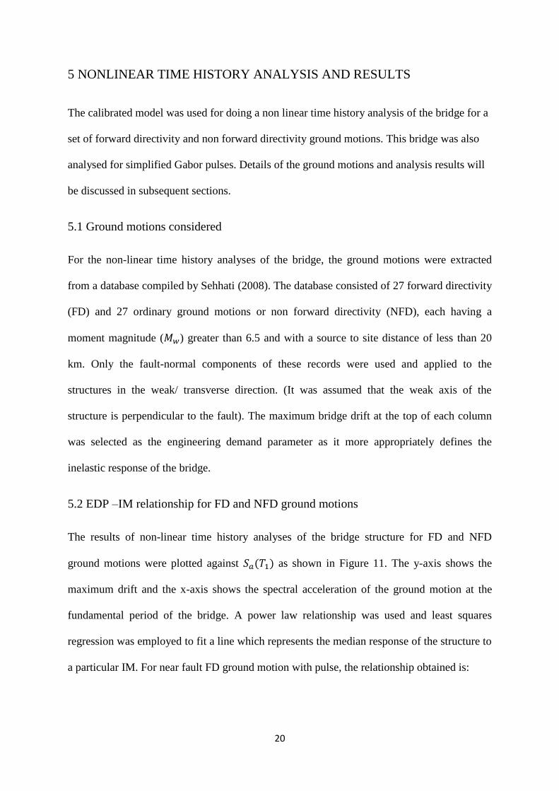
5.2 EDP –IM relationship for FD and NFD ground motions

The results of non-linear time history analyses of the bridge structure for FD and NFD

ground motions were plotted against as shown in Figure 11. The y-axis shows the

maximum drift and the x-axis shows the spectral acceleration of the ground motion at the

fundamental period of the bridge. A power law relationship was used and least squares

regression was employed to fit a line which represents the median response of the structure to

a particular IM. For near fault FD ground motion with pulse, the relationship obtained is:

21

(3)

Similarly, for the ordinary NFD ground motions the relationship is given by:

(4)

As shown in Figure 11, the median maximum drifts for forward directivity ground motions

are higher than those for ordinary ground motions for the same , since pulses induce higher

nonlinearities in the bridge resulting in a higher structural demand. Similar results for MIDD

were obtained for a MDOF structure by Sehhati (2008).

Figure 11: Plots of response of bridge to Forward Directivity and Non-Forward directivity ground

motions

22

5.3 Genetic Programming

Genetic programming (GP) (Koza 1992) is a modified form of genetic algorithm (GA)

(Goldberg 1989) where randomly generated computer programs are evolved to build a

program to solve a clearly defined problem. The method involves generation of a population

of randomly generated programs and evaluating the fitness of each member of this population

of programs. Then the “fit” programs are used to produce new programs which replace the

“unfit” programs from previous generation. This process of evolving a new generation of

fitter programs is repeated many times in hope of finding an optimal solution.

Genetic programming can be used to find functional forms which fit the data (the process is

also called symbolic regression) (Koza 1992). Here the functional form is generally

represented as a function tree and standard genetic operation like mutation and crossover is

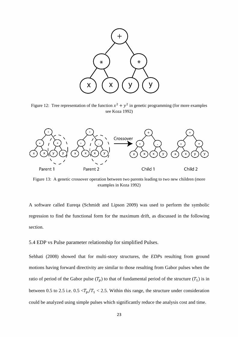
defined for the function trees. For example a function can be represented

by the tree shown in Figure 12. The internal nodes of the tree are called functions and the

leaves are called terminals. In order to define a GP problem, one needs to first define the set

of possible functions (generally +,-,*, / etc.) and sets of terminals (generally constants and

predictor variables). Crossover operation on trees is generally defined by selecting a random

node on each of the parent trees and then swapping the sub-tree rooted at that node to

generate two new off-springs , this process is illustrated by Figure 13. Mutation is defined by

selecting a node and replacing it by a randomly chosen function or terminal value.

23

Figure 12: Tree representation of the function in genetic programming (for more examples

see Koza 1992)

Figure 13: A genetic crossover operation between two parents leading to two new children (more

examples in Koza 1992)

A software called Eureqa (Schmidt and Lipson 2009) was used to perform the symbolic

regression to find the functional form for the maximum drift, as discussed in the following

section.

5.4 EDP vs Pulse parameter relationship for simplified Pulses.

Sehhati (2008) showed that for multi-story structures, the EDPs resulting from ground

motions having forward directivity are similar to those resulting from Gabor pulses when the

ratio of period of the Gabor pulse ( ) to that of fundamental period of the structure ( is in

between 0.5 to 2.5 i.e. 0.5 < < 2.5. Within this range, the structure under consideration

could be analyzed using simple pulses which significantly reduce the analysis cost and time.

24

The velocity time history of a Gabor pulse is given by the following equation (Gabor 1946;

Mavroeidis and Papageorgiou 2003):

(5)

Where, A is proportional to the amplitude of the wavelet, fp is the prevailing frequency of the

signal, is the phase angle (i.e., = 0 and = ±π/2 define symmetric and anti symmetric

signals, respectively), defines the oscillatory character of the signal, and to is the time of the

envelope‟s peak. In this study, only = 0 has been considered, for simplicity. Hence, the only

parameters required to define the Gabor wavelet pulse are A, fp, and . Sehhati (2008) used

Baker (2007) procedure to extract pulses from FD ground motions and based on the number

of peaks and troughs of the extracted pulses, the parameter was set as 3.

Before the pulse analysis can be conducted, structural response must be studied to determine

in which cases structural response to the simplified pulse motions (e.g., the Gabor pulses) is

similar to structural response to the full recorded ground motions. Figure 15 shows a

comparison of the EDP values in terms of drift angle values for the forward directivity

ground motions to those for equivalent pulses. As shown in the figure, the responses from the

forward directivity ground motions are equal to the responses from equivalent simplified

pulses (i.e. ratio = 1) when 0.5< <1.75, where (=0.8 sec) is the fundamental period of

the bridge (Figure 14) and is the period of the Gabor pulse. Note that this range is

different from the range 0.5< <2.5 obtained by Sehhati (2008) for MDOF structures.

This difference could be due to the inherent difference in behaviour of the two structures.

Thus, each structure has its unique range of values of pulse periods, where the simple pulse

analysis would be representative of the forward directivity ground motion.

25

Figure 14: Screenshot of SAP 2000 (v.12.0.2) showing the deflected shape of the first mode

Figure 15: Plot showing / against

26

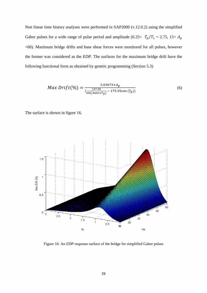
Non linear time history analyses were performed in SAP2000 (v.12.0.2) using the simplified

Gabor pulses for a wide range of pulse period and amplitude (0.25< < 2.75, 15<

<60). Maximum bridge drifts and base shear forces were monitored for all pulses, however

the former was considered as the EDP. The surfaces for the maximum bridge drift have the

following functional form as obtained by genetic programming (Section 5.3)

(6)

The surface is shown in figure 16.

Figure 16: An EDP response surface of the bridge for simplified Gabor pulses

27

6 SITES AND FAULT GEOMETRY

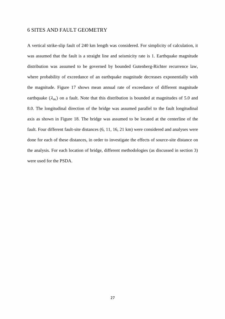
A vertical strike-slip fault of 240 km length was considered. For simplicity of calculation, it

was assumed that the fault is a straight line and seismicity rate is 1. Earthquake magnitude

distribution was assumed to be governed by bounded Gutenberg-Richter recurrence law,

where probability of exceedance of an earthquake magnitude decreases exponentially with

the magnitude. Figure 17 shows mean annual rate of exceedance of different magnitude

earthquake on a fault. Note that this distribution is bounded at magnitudes of 5.0 and

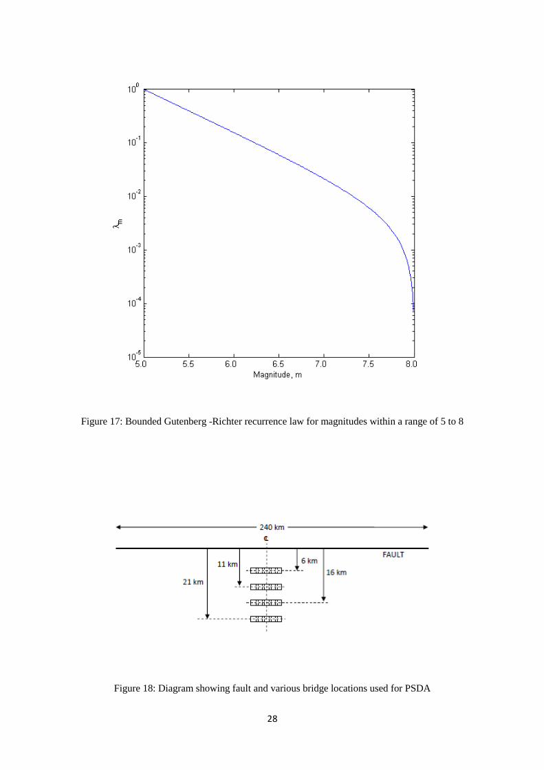
8.0. The longitudinal direction of the bridge was assumed parallel to the fault longitudinal

axis as shown in Figure 18. The bridge was assumed to be located at the centerline of the

fault. Four different fault-site distances (6, 11, 16, 21 km) were considered and analyses were

done for each of these distances, in order to investigate the effects of source-site distance on

the analysis. For each location of bridge, different methodologies (as discussed in section 3)

were used for the PSDA.

28

Figure 17: Bounded Gutenberg -Richter recurrence law for magnitudes within a range of 5 to 8

Figure 18: Diagram showing fault and various bridge locations used for PSDA

29

7 PSDA RESULTS AND DISCUSSION

The results of PSDA for 4 different bridge locations at 6, 11, 16 and 21 Km from the fault

have been shown in Figure19(a-d). In the left most of Figure 19(a), the probability of

exceedance due to two different components of the Enhanced Broadband PSDA, namely

pulse component and non-pulse component is presented. Also, shown in the figure is the total

probability of exceedance. As shown in the figure, the probability of exceedance (EDP) of the

non-pulse component is higher than those of the pulse component for small drift angles.

However, EDP for the non-pulse component decreases with increasing the drift angles. The

reason for this variation is as follows. Lower values of drift angle could be exceeded with

high probability of exceedance with lower magnitude ground motions which occur much

more frequently compared to larger magnitude ground motions. The probability that a lower

magnitude earthquake ground motion be in the form of a pulse is low. Hence, the overall

probability that a smaller value of drift angle is exceeded due to a pulse component also

decreases.

It is worth noting that the probability of having a pulse depends on the distance between the

point on the fault closest to the site and epicenter (R), length of rupture (S), and angle

between the strike of the fault and the line joining the epicenter to the site (. Lower

magnitude earthquakes have small median fault rupture length; hence, they have low

probability to be in the form of a pulse.

High values of drift angle would be exceeded only with larger magnitude earthquakes that

have higher probability of having a pulse. However, such high magnitude ground motions

have lower probability of occurrence, resulting in a lower overall probability that a large drift

angle is exceeded due to either a pulse or non-pulse component.

30

The middle of Figure 19a shows the contribution of four different components of the New

PSDA, namely Near Source Pulse-in (NS-P-in), Near Source Pulse-out (NS-P-out), Near

Source No Pulse (NS-NP) and Non-Near Source (Non-NS). For drift angle values smaller

than 0.25 %, the near source non pulse (NS-NP) component has the highest probability of

exceedance. Beyond that most of the contribution to the hazard is coming from the NS-P-in

scenario, pointing to the importance of such scenarios in the hazard calculations.

The right of Figure 19a shows a comparison of the probability of exceedance calculated using

all four PSDA methodologies. As shown in the figure, for drift angle smaller than 0.5%, all

the methods yield similar results. Beyond that, the time-domain PSDA yield higher values of

compared to the other three methodologies. This is because the time domain approach

captures resonance in a better way (by using and as intensity measures) as compared to

other methodologies and is thus able to better capture non-linearity at higher drift levels. In

addition, beyond a drift angle of about 0.5%, the enhanced broadband PSDA yielded higher

values of compared to the traditional and broadband PSDA methodologies. This

happens because at higher drift levels, major contribution comes from the pulse like

component and out of three methodologies (i.e. Enhanced BB, Broadband and No directivity)

only the Enhanced Broadband approach accounts for the effects of pulse like ground motion

to the EDP.

Moving farther away from the fault i.e. at distances of 11 km to 21 km, trends similar to

those discussed for site at 6 km were observed. However, the probability of exceeding a

particular drift angle became smaller compared to those of a site at 6 km. Also, with

increasing the distance between the fault and the site, the difference in the probability of

exceedance calculated using the New PSDA and Enhanced Broadband keeps decreasing,

indicating the reduction in contribution of pulse in components at this distance.

31

(a)

(b)

32

(c)

(d)

Figure 19: Plots of rate of exceedence of drift versus maximum drifts for a site located at a distance of

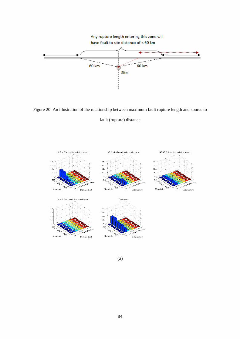
a) 6 km b) 11 km c) 16 km and d) 21 km from the fault

33

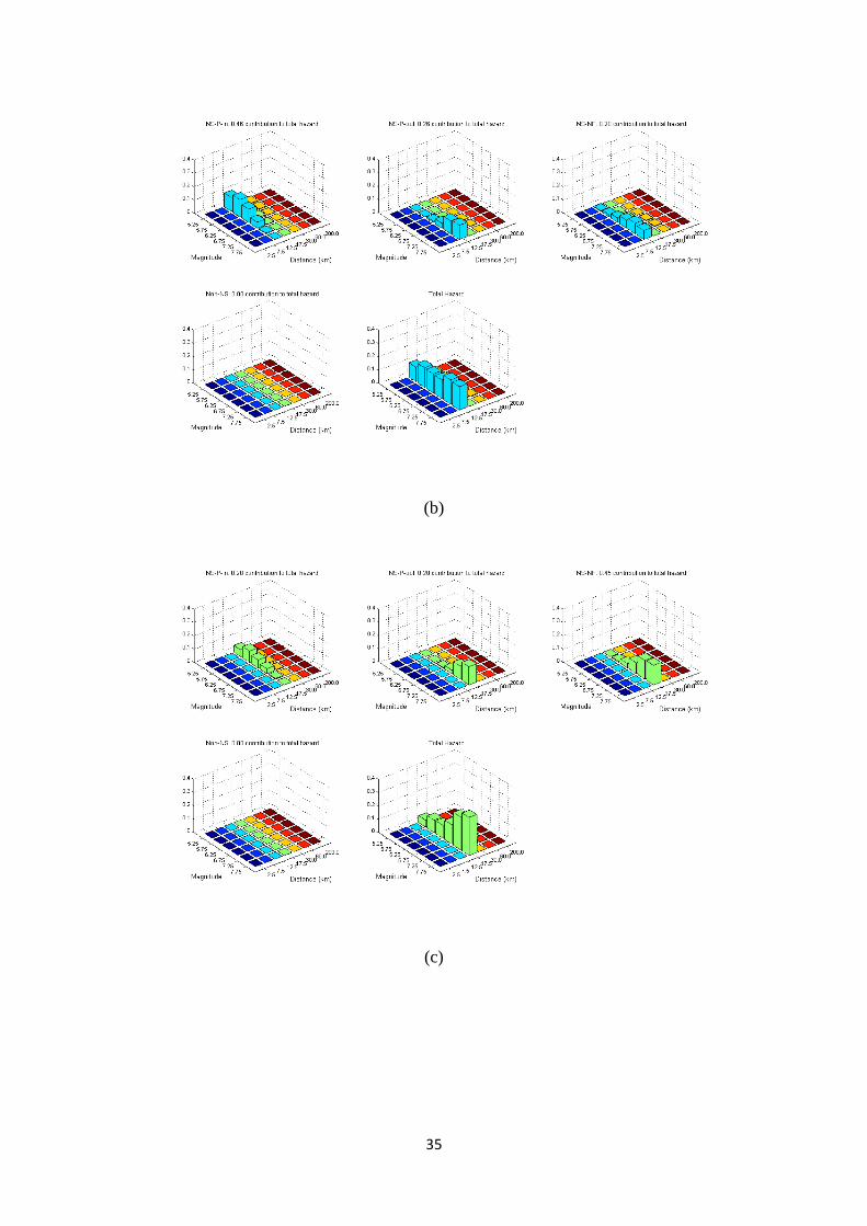
Figure 21 shows distance magnitude deaggregation plots for a drift angle of 1% (which is an

arbitrary selected value for illustrative purposes). Figure 21a shows the distance-magnitude

deaggregation plots for a site located at a distance of 6 km from the fault. Contributions from

different component of the New PSDA are shown. As expected, the main contribution to the

hazard is the near source scenario. The figure shows that the NS-P-in component represents

58% of total hazard which is the highest contribution to the hazard. The next higher

contributor to the total hazard is the NS-P-out component which represents 24% of the total

hazard. The NS-NP contributes 18% to the total hazard making it the third highest

contributor. The contribution from Non-NS was insignificant in this case and it represents 0.0

% of the total hazard since the Non near source scenarios are the ones with source to site

distance greater than 60 km. Any fault rupture at a distance greater than 60 km from the site

would be the one with smaller fault rupture length, hence from a smaller magnitude

earthquake. This is explained in Figure 20. It can be see that when the site to fault (rupture)

distance is greater than 60 km only a small portion of the fault is available for rupture (shown

by the solid arrow) as compared to when fault rupture to site distance is 30 km (shown by

dotted arrow). So, for larger fault rupture to site distances, the fault rupture length is smaller.

Since small magnitude earthquake at a large distance are not able to drive the drift of the

bridge more than 1%, no contribution is seen from this component.

34

Figure 20: An illustration of the relationship between maximum fault rupture length and source to

fault (rupture) distance

(a)

35

(b)

(c)

36

(d)

Figure 21: Distance magnitude deaggregation plots for a site located at distances of a) 6 km b) 11 km

c) 16 km and d) 21 km from the fault

Another important feature in the NS-P-in graph for 6 km is that the maximum contribution is

coming from low magnitude earthquakes at smaller distances, as opposed to what is observed

in the rest of the deaggregation graphs. The reason for this trend is that the lower magnitude

earthquakes occur with higher probabilities and when we consider pulse-in cases from such

earthquakes, it has high probability of exceeding drifts of 1%. Note that our structure has a

low period and it is highly probable that smaller magnitude earthquake will produce pulses

with period close to the period of our structure causing resonance. Therefore the probability

that this level of drift is exceeded by a NS-P-in component is higher for small magnitude

earthquakes. However, the probability that drift angle of 1% is exceeded by a NS-P-out and

NS-NP component by a small magnitude earthquake is lower than by a higher magnitude

earthquake. In the total hazard plot too, the maximum contributor is the lower magnitude

37

earthquake at a smaller distance, following the same reasoning. This highlights the

importance of lower magnitude earthquakes for structures located in the proximity of a fault

At a distance of 11 km (Figure 21b ), the NS-P-in contributions is 46% of the total, lower

than the value at 6 km, but still higher than all other components at this distance. As

explained earlier, the NS-P-in components of lower magnitude earthquakes contributed

significantly to the hazard. However, the higher magnitude earthquakes are contributing more

to the total hazard, as the contribution of NS-P-out and the NS-NP components has increased

compared to those calculated at distance of 6 km. As the distance between the fault and the

site increased (Figure 21c and d), the contribution of the NS-P-in components to the total

hazard decreased. In addition, the contribution of the NS-NP component and higher

magnitude earthquakes to the total hazard increased with increasing the distance between the

site and the fault.

Figures 22 shows the distance-magnitude deaggregation plots for a drift of 1% from four

different methods, mentioned earlier. At a site to fault distance of 6 km, the No directivity,

Broadband, and enhanced broadband models follow the same trend of higher magnitude

earthquakes contributing more to the total hazard; however, the New PSDA model showed

that smaller magnitude earthquakes contributed more to the total hazard. At a site to fault

distance of 11 km, all the four models showed that most of the hazard is due to higher

magnitude earthquakes. However, the New PSDA model showed that low magnitude

earthquakes significantly contributed to the total hazard which differs from the other models.

At site to fault distances of 16 and 21 km, all four models showed that the most contributions

to the hazard came from larger magnitude earthquakes since low magnitude earthquakes

occurred at large distances from the bridge resulted in small drift angles.

38

(a)

(b)

39

(c)

(d)

Figure 22: Comparison of magnitude deaggregation plots from four methods at distances of a) 6km b)

11 km c) 16 km and d) 21 km from the fault along its centerline

40

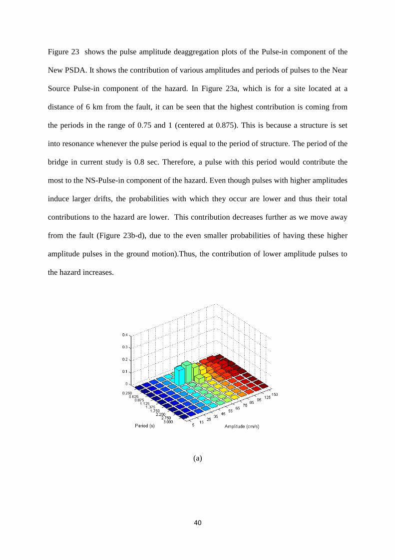
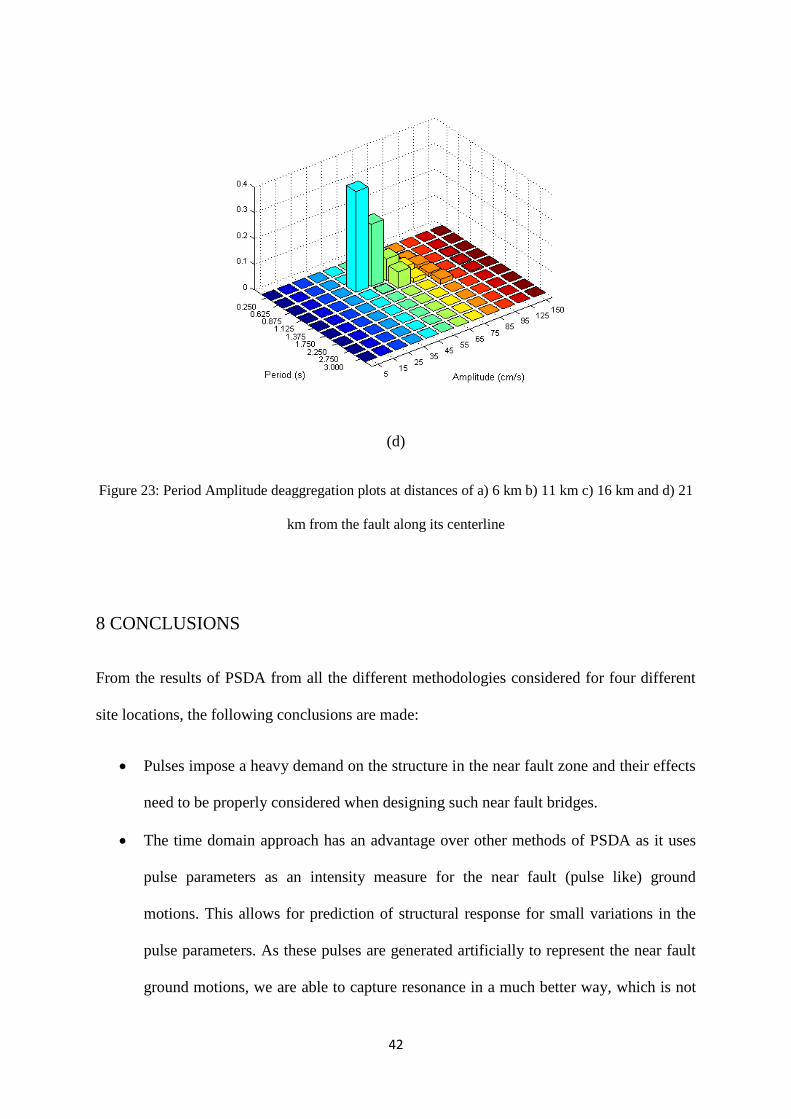
Figure 23 shows the pulse amplitude deaggregation plots of the Pulse-in component of the

New PSDA. It shows the contribution of various amplitudes and periods of pulses to the Near

Source Pulse-in component of the hazard. In Figure 23a, which is for a site located at a

distance of 6 km from the fault, it can be seen that the highest contribution is coming from

the periods in the range of 0.75 and 1 (centered at 0.875). This is because a structure is set

into resonance whenever the pulse period is equal to the period of structure. The period of the

bridge in current study is 0.8 sec. Therefore, a pulse with this period would contribute the

most to the NS-Pulse-in component of the hazard. Even though pulses with higher amplitudes

induce larger drifts, the probabilities with which they occur are lower and thus their total

contributions to the hazard are lower. This contribution decreases further as we move away

from the fault (Figure 23b-d), due to the even smaller probabilities of having these higher

amplitude pulses in the ground motion).Thus, the contribution of lower amplitude pulses to

the hazard increases.

(a)

41

(b)

(c)

42

(d)

Figure 23: Period Amplitude deaggregation plots at distances of a) 6 km b) 11 km c) 16 km and d) 21

km from the fault along its centerline

8 CONCLUSIONS

From the results of PSDA from all the different methodologies considered for four different

site locations, the following conclusions are made:

Pulses impose a heavy demand on the structure in the near fault zone and their effects

need to be properly considered when designing such near fault bridges.

The time domain approach has an advantage over other methods of PSDA as it uses

pulse parameters as an intensity measure for the near fault (pulse like) ground

motions. This allows for prediction of structural response for small variations in the

pulse parameters. As these pulses are generated artificially to represent the near fault

ground motions, we are able to capture resonance in a much better way, which is not

43

the case when we use spectral acceleration as an intensity measure. Also, structural

nonlinearities are automatically accounted for in time domain analysis, whereas in

using spectral accelerations, nonlinearities are only captured indirectly. The results of

the Time Domain analysis thus gives a better prediction of hazard for sites located in

a near fault region

The results of the PSDA showed that for a site located very close to the fault (6 km in

this study) even the smaller magnitude earthquakes can have significant contribution

in the hazard (Figure 21a). This observation seems counter intuitive at first since the

results from all methodologies other than time domain approach and the conventional

wisdom point to the fact that large magnitude events should contribute most to the

hazard. But if the period of the bridge is closer to the period of the pulses produced by

small magnitude events than those produced by large magnitude events, the response

of bridge from small magnitude events may be comparable to the response under

large magnitude events (Note that a similar effect is discussed in Somerville 2003).

Since the small magnitude events occur with greater frequency than large magnitude

events they can have high contribution in the hazard. The possibility of contribution

of small magnitude event to hazard should be considered while selecting ground

motions or while deciding the design scenarios.

If the Maximum Credible Earthquake (MCE) with a return period of 2475 years is

considered, the drift values that were obtained from the New PSDA is more than 30%

higher than those from Enhanced Broadband at distance of about 6 km (Figure 19a).

However this difference reduces to about 15% at a distance of 11 km (Figure 19b).

This difference keeps getting smaller with increasing fault to site distance and beyond

distances of 16 km (Figure 19c) the difference is less than 5% even with a high

seismicity rate considered here. So for more realistic seismicity rates, the difference

44

would be further reduced i.e. the effects of near fault ground motion are insignificant

for sites located more than 16 km from the fault. At such sites, simple methods such

as Broadband and Enhanced Broadband approach could be adopted for the hazard

calculation instead of the more computationally expensive New PSDA approach.

References

Abrahamson, N., and Silva, W. (2007). "NGA Ground Motion Relations for the Geometric

Mean Horizontal Component of Peak and Spectral Ground Motion Parameters." Pacific

Earthquake Engineering Research Center College of Engineering, University of California,

Berkeley.

Akkar, S., U. Yazgan, and P. Gulkan (2005). “Drift estimates in frame buildings subjected to

Near-Fault ground motions.” Journal of Structural Engineering 131 (7), 1014-1024.

Alavi, B., and Krawinkler, H. (2001). "Effects of near-fault ground motions on frame

structures." Dept. of Civil Eng., Stanford University, Stanford, CA.

Anderson, J. C., and Bertero, V. V. (1987). "Uncertainties in establishing design

earthquakes." ASCE Journal of Structural Engineering, 113(8), 1709-1724.

Baker, J. (2007a). "Quantitative classification of near-fault ground motions using wavelet

analysis." Bulletin of the Seismological Society of America, 97(5), 1486-1501.

Bertero, V. V., Mahin, S. A., and Herrera, R. A. (1978). "Aseismic design implications of

near-fault San Fernando earthquake records." Earthquake Engineering & Structural

Dynamics, 6, 31-42.

Bray, J. D., and Rodriguez-Marek, A. (2004). "Characterization of forward-directivity

ground motions in the near-fault region." Soil Dynamics and Earthquake Engineering, 24,

815-828.

45

Dawood, H. M., “Seismic Behavior of Segmental Precast Post-tensioned Concrete Piers”,

M.Sc. thesis, Washington State University, Washington, 2010

ElGawady, M. A., Sha‟lan A., and Dawood, H. M. (2010). “Seismic behavior of precast post-

tensioned segmented frames”, 9th U.S. National and 10th Canadian Conference on

Earthquake Engineering (July 25-29, 2010).

Gabor, D. (1946). "Theory of communication." IEEE, 93, 429-41.

Hall, J. F. (1998). "Seismic response of steel frame buildings to near-source ground motions."

Earthquake Engineering and Structural Dynamics, 27, 1445-1464.

Hall, J. F., Heaton, T. H., Halling, M. W., and Wald, D. J. (1995). "Near-source ground

motion and its effects on flexible buildings." Earthquake Spectra, 11(4), 569-605.

Hewes, J. T., and Priestley N. (2002). “Seismic design and performance of precast concrete

segmental bridge columns.” Report No. SSRP-2001/25, Univ. of California at San Diego

Iervolino, I. and C. A. Cornell (2008). Probability of occurence of velocity pulses in near-

source ground motions. Bulletin of the Seismological Society of America 98 (5), 2262-2277.

Iwan, W., Huang, C.-T., and Guyader, A. C. (1998). "Evaluation of the effects of near-source

ground motions." Report Developed for the PG&E/PEER Program, CalTech, Pasadena,

California.

Koza, J. R., 1992, Genetic Programming: On the Programming of Computers by Means of

Natural Selection, MIT Press, Cambridge, MA

Kramer, S. L. (1996). Geotechnical Earthquake Engineering, Prentice Hall, Upper Saddle

River, New Jersey.

Luco, N., and Cornell, C. A. (2007). "Structure-Specific Scalar Intensity Measures for Near-

Source and Ordinary Earthquake Ground Motions." Earthquake Spectra,Earthquake

Engineering Research Institute, 23(2), 357-392.

Makris, N. and C. J. Black (2004). “Dimensional analysis of bilinear oscillators under pulse-

type excitations.” Journal of Engineering Mechanics, 130 (9), 1019-1031.

46

Mavroeidis, G. P., and Papageorgiou, A. S. (2003). "A mathematical representation of

nearfault ground motions." Bulletin of the Seismological Society of America, 93(3), 1099-

1131.

Mavroeidis, G. P., G. Dong, and A. S. Papageorgiou (2004). “Near-Fault ground motions,

and the response of elastic and inelastic Single-Degree-of-Freedom (SDOF) systems.”

Earthquake Engineering & Structural Dynamics 33 (9), 1023-1049.

Menun, C. and Q. Fu (2002). “An analytical model for near-fault ground motions and the

response of SDOF systems”. In Proceedings, 7th U.S. National Conference on Earthquake

Engineering, Boston, MA, pp. 10.

PEER. (1999). "Pacific Earthquake Engineering Research Center, strong motion database.

http://peer.berkeley.edu/smcat/search.html."

Priestley, M. J. N., Calvi, G. M., and Kowalsky, M. J. (2007). Displacement-Based Seismic

Design of Structures, IUSS Press.

Samaan, M., Mirmiran, A., and Shahawy, M. (1998). „„Model of concrete confined by fiber

composite.‟‟ J. Struct. Eng., 124(9), 1025–1031.

SEAOC. (Vision 2000). "performance based seismic engineering for buildings." Structural

Engineers Association of California, Sacramento, CA, 1995.

Schmidt M., Lipson H. (2009) "Distilling Free-Form Natural Laws from Experimental Data,"

Science, Vol. 324, no. 5923, pp. 81 - 85.

Sehhati, R. (2008). “Probabilistic seismic demand analysis for the near-fault zone.” Ph.D.

Dissertation, Washington State University, Pullman, WA.

Somerville, P. G., Smith, N. F., Graves, R., and Abrahamson, N. A. (1997). "Modification of

Empirical Strong Ground Motion Attenuation Relations to Include the Amplitude and

Duration Effects of Rupture Directivity." Seismological Research Letters, 68(1), 199-222.

Somerville, P. G. (2003). "Magnitude scaling of the near fault rupture directivity pulse."

Physics of the Earth and Planetary Interiors, 137, 201-212.

47

Spudich, P., and Chiou, B. (2008). "Directivity in NGA earthquake ground motions: analysis

using isochrone theory." Earthquake Spectra, 24(1), 279-98.

Zhang, Y., and Iwan, W. (2002). "Active interaction control of tall buildings subjected to

near-field ground motions." Journal of Structural Engineering, 128, 69-79.

Zhu, Zenhu, Mirmiran, A. and Saiidii,M.S (2006). “ Seismic Perforance of Reinforced

Concrete Bridge Substrcuture Encased in Fiber Composites.” Transportation Research

Record, 197-206.

48

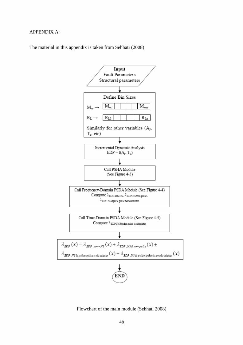
APPENDIX A:

The material in this appendix is taken from Sehhati (2008)

Flowchart of the main module (Sehhati 2008)

49

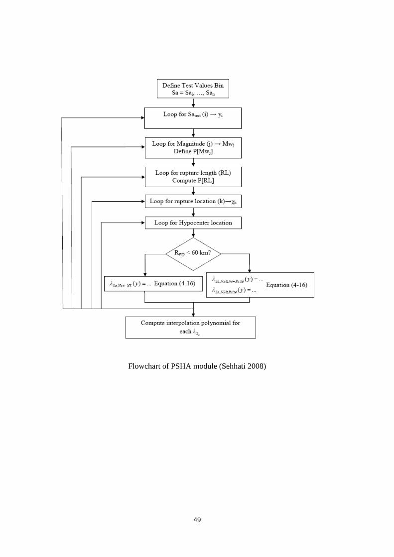
Flowchart of PSHA module (Sehhati 2008)

50

Flowchart of frequency domain PSDA module (Sehhati 2008)

51

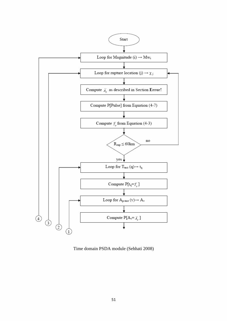
Time domain PSDA module (Sehhati 2008)

52

Time domain PSDA module (Sehhati 2008)