time harmonic electromagnetic fields - arraytool · 06/10/2012 · maxwell’s equationstime...

Maxwell’s Equations Time Harmonic Fields Helmholtz Wave Equation Propagation Constant Poynting Vector Reflection Summary Problems

Time Harmonic Electromagnetic Fields

S. R. [email protected]

School of Electronics EngineeringVellore Institute of Technology

October 19, 2012

Time Harmonic Electromagnetic Fields EE208, School of Electronics Engineering, VIT

mailto:[email protected]


Outline

1 Maxwell’s Equations

2 Time Harmonic Fields

3 Helmholtz Wave Equation

4 Propagation Constant

5 Poynting Vector

6 Reflection

7 Summary

8 Problems



Maxwell’s Equations Till Now ...

∇ · ~D = ρe(Gauss Law)

∇ ·~B = ρm(Gauss Law)

∇× ~H = ~Je(Ampere Law)

∇×~E = −~Jm −∂~B∂t

(Ampere Law + Faraday′s Law)

Now, what is wrong with the above set of equation ??? ...



Maxwell’s Equations Till Now ...



∇× ~H = ~Je(Ampere Law)

∇×~E = −~Jm −∂~B∂t


Compared to equation 4, equation 3 is missing something ... don’tyou think?



So, Maxwell’s Equations Should Look SomethingLike...



∇× ~H = ~Je +∂~D∂t


∇×~E = −~Jm −∂~B∂t


Now, equation 3 and 4 look similar ... and the term ∂~D∂t is called

displacement current

Then what is the name for~Je?



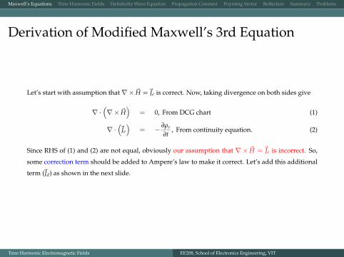
Derivation of Modified Maxwell’s 3rd Equation

Let’s start with assumption that ∇× ~H =~Je is correct. Now, taking divergence on both sides give

∇ ·(∇× ~H

)= 0, From DCG chart (1)

∇ ·(~Je

)= − ∂ρe

∂t, From continuity equation. (2)

Since RHS of (1) and (2) are not equal, obviously our assumption that ∇× ~H =~Je is incorrect. So,

some correction term should be added to Ampere’s law to make it correct. Let’s add this additional

term (~Jd) as shown in the next slide.



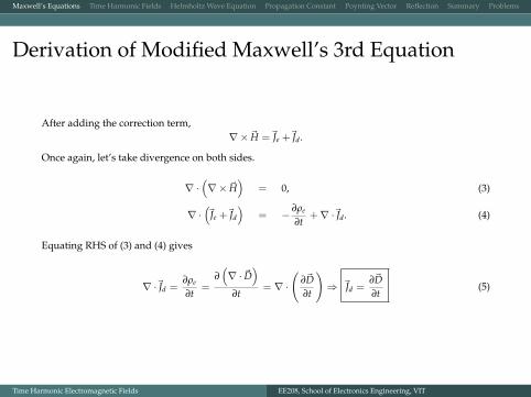
Derivation of Modified Maxwell’s 3rd Equation

After adding the correction term,∇× ~H =~Je +~Jd.

Once again, let’s take divergence on both sides.

∇ ·(∇× ~H

)= 0, (3)

∇ ·(~Je +~Jd

)= − ∂ρe

∂t+∇ ·~Jd. (4)

Equating RHS of (3) and (4) gives

∇ ·~Jd =∂ρe

∂t=

∂(∇ · ~D

)∂t

= ∇ ·(

∂~D∂t

)⇒ ~Jd =

∂~D∂t

(5)



That’s it Folks, Final Form of Maxwell’s Equations is ...

∇ · ~D = ρe(Gauss Law− E)

∇ ·~B = ρm(Gauss Law−M)

∇× ~H = ~Je +∂~D∂t

(Ampere Law−M + Faraday′s Law−M)

∇×~E = −~Jm −∂~B∂t

(Ampere Law− E + Faraday′s Law− E)



And Wait ... One More Thing ...

Equations given in the previous slide are called point form Maxwell’s equations. Their equivalentintegral forms can be derived using divergence and Stokes theorems and are given as

˚ (∇ · ~D

)dv =

˚ρedv =

‹~D · ~ds

˚ (∇ ·~B

)dv =

˚ρmdv =

‹~B · ~ds

¨ (∇× ~H

)· ~ds =

¨ (~Je +

∂~D∂t

)· ~ds =

˛~H · ~dl

¨ (∇×~E

)· ~ds = −

¨ (~Jm +

∂~B∂t

)· ~ds =

˛~E · ~dl



Outline





5 Poynting Vector

6 Reflection

7 Summary

8 Problems



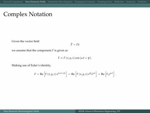
Complex Notation

Given the vector field~F = Fx

we assume that the component F is given as

F = F (x, y, z) cos (ωt + ψ) .

Making use of Euler’s identity,

F = Re[F (x, y, z) ej(ωt+ψ)

]= Re

[F (x, y, z) ejψejωt

]= Re

[Fsejωt

].



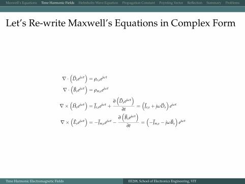
Let’s Re-write Maxwell’s Equations in Complex Form

∇ ·(~Dsejωt

)= ρe,sejωt

∇ ·(~Bsejωt

)= ρm,sejωt

∇×(~Hsejωt

)=~Je,sejωt +

∂(~Dsejωt

)∂t

=(~Je,s + jω~Ds

)ejωt

∇×(~Esejωt

)= −~Jm,sejωt −

∂(~Bsejωt

)∂t

=(−~Jm,s − jω~Bs

)ejωt



Outline





5 Poynting Vector

6 Reflection

7 Summary

8 Problems



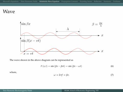
Wave

The wave shown in the above diagram can be represented as

F (x, t) = sin (βx− βvt) = sin (βx−ωt) (6)

where,ω = 2πf = βv. (7)



Wave Equation

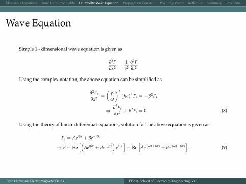
Simple 1 - dimensional wave equation is given as

∂2F∂x2 =

1v2

∂2F∂t2

Using the complex notation, the above equation can be simplified as

∂2Fs

∂x2 =

(β

ω

)2

(jω)2 Fs = −β2Fs

⇒ ∂2Fs

∂x2 + β2Fs = 0 (8)

Using the theory of linear differential equations, solution for the above equation is given as

Fs = Aejβx + Be−jβx

⇒ F = Re[(

Aejβx + Be−jβx)

ejωt]= Re

[Aej(ωt+βx) + Bej(ωt−βx)

]. (9)



Helmholtz Wave EquationIn a source-less dielectric medium,

∇ · ~Ds = 0

∇ ·~Bs = 0

∇× ~Hs = jω~Ds = jωε~Es (10)

∇×~Es = −jω~Bs = −jωµ~Hs (11)

Taking curl of (11) gives

∇×(∇×~Es

)= ∇×

(−jωµ~Hs

)⇒ ∇

(∇ ·~Es

)−∇2~Es = −jωµ

(∇× ~Hs

)⇒ ∇

(∇ ·~Es

)−∇2~Es = −jωµ

(jωε~Es

)⇒ ∇2~Es = ∇

(∇ ·~Es

)−ω2µε~Es

⇒ ∇2~Es =~0−ω2µε~Es (12)

Similarly, it can be proved that

∇2~Hs = −ω2µε~Hs. (13)



Finally, Let’s Analyze the Helmholtz Wave Equation

Let’s compare general wave equation (8) and Helmholtz wave equation (12).

∂2Fs∂x2 + β2Fs = 0 ∇2~Es + ω2µε~Es = 0

From the above comparison, we get,

β = ω√

µε. (14)

But, we already knew that

v =ω

β.

So, from the above equations, we get

v =1√

µε=

1√

µrεrc (15)

where c is the light velocity.



Solution of Helmholtz Equation (in Cartesian System)Vector Helmholtz equation can be decomposed as shown below:

∇2Exs + ω2µεExs = 0

∇2~Es + ω2µε~Es = 0 ∇2Eys + ω2µεEys = 0

∇2Eys + ω2µεEys = 0

Since all the differential equations are similar, let’s solve just one equation using variable-separablemethod. If Exs can be decomposed into

Exc = A (x)B (y)C (z)

then substituting the above equation into Helmholtz equation gives

∇2Exs + ω2µεExs = 0

⇒ ∂2Exs

∂x2 +∂2Exs

∂y2 +∂2Exs

∂z2 + ω2µεExs = 0

⇒ B (y)C (z)∂2A∂x2 + A (x)C (z)

∂2B∂y2 + A (x)B (y)

∂2C∂z2 + ω2µεA (x)B (y)C (z) = 0

⇒ 1A (x)

∂2A∂x2 +

1B (y)

∂2B∂y2 +

1C (z)

∂2C∂z2 −γ2 = 0



Solution of Helmholtz Equation ... Contd

⇒ 1A (x)

∂2A∂x2 +

1B (y)

∂2B∂y2 +

1C (z)

∂2C∂z2 −γ2 = 0

⇒ 1A (x)

∂2A∂x2 +

1B (y)

∂2B∂y2 +

1C (z)

∂2C∂z2 −γ2

x−γ2y−γ2

z = 0 (16)

The above equation can be decomposed into 3 separate equations:

1A (x)

∂2A∂x2 − γ2

x = 0

1B (y)

∂2B∂y2 − γ2

y = 0

1C (z)

∂2C∂z2 − γ2

z = 0

It is sufficient to solve only one of the above equations and it’s solution is given as

⇒ ∂2A∂x2 − γ2

xA (x) = 0

⇒ A (x) = L1eγxx + L2e−γxx = L−eγxx + L+e−γxx (17)



Solution of Helmholtz Equation ... Contd

So, finally Exc is given as

Exs =(L−eγxx + L+e−γxx) (M−eγyy + M+e−γyy) (N−eγzz + N+e−γzz) (18)

⇒ Ex = Re[(

L−eγxx + L+e−γxx) (M−eγyy + M+e−γyy) (N−eγzz + N+e−γzz) ejωt]

(19)

with the conditionγ2

x + γ2y + γ2

z = γ2. (20)



Outline





5 Poynting Vector

6 Reflection

7 Summary

8 Problems



Maxwell’s Equations in General

∇ · ~Ds = ρe,s

∇ ·~Bs = ρm,s

∇× ~Hs =~Je,s + jω~Ds = σ~Es + jωε~Es = jω[ε(

1− jσ

ωε

)]~Es

∇×~Es = −~Jm,s − jω~Bs



Propagation Constant

So, from the previous slide, for lossy dielectrics, εs is a complex number and is given as

εs = ε(

1− jσ

ωε

).

Then propagation constant γ is given from the equation

γ2 = −ω2µεs

= −ω2µε(

1− jσ

ωε

)= −ω2µε + jωµσ. (21)

From the above equation, γ can be written as γ = α + jβ. Now, we need to find out the values of αand β. We have

γ2 = (α + jβ)2 =(α2 − β2)+ j (2αβ) (22)

Comparing (21) and (22) we get,

α2 − β2 = −ω2µε

β =ωµσ

2α. (23)



Propagation Constant ... Contd

Solving the set of equations (23) gives

α2 −(ωµσ

2α

)2= −ω2µε

⇒ 4α4 −ω2µ2σ2 = −4α2ω2µε

⇒ 4α4 + 4α2ω2µε−ω2µ2σ2 = 0

⇒ 4ξ2 + 4ξω2µε−ω2µ2σ2 = 0

⇒ ξ =ω2µε

2

[±√

1 +( σ

ωε

)2− 1

]

⇒ α =√

ξ = ω

√√√√ µε

2

[√1 +

( σ

ωε

)2− 1

]. (24)

Similarly it can be proved that

β = ω

√√√√ µε

2

[√1 +

( σ

ωε

)2+ 1

](25)



Skin Depth

Skin Depth:The distance δ, through which the wave amplitude decreases by a factor 1

e is called skin depth orpenetration depth of the medium, that is

E0e−αδ =E0

e.

From the above equation,

δ =1α

(26)



Outline





5 Poynting Vector

6 Reflection

7 Summary

8 Problems



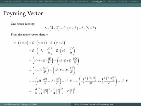
Poynting Vector

One Vector Identity:

∇ ·(~A×~B

)= ~B ·

(∇×~A

)−~A ·

(∇×~B

)From the above vector identity,

∇ ·(~E× ~H

)= ~H ·

(∇×~E

)−~E ·

(∇× ~H

)= ~H ·

(−~Jm −

∂~B∂t

)−~E ·

(σ~E +

∂~D∂t

)

=

(~H ·~0− ~H · ∂~B

∂t

)−(

σ~E ·~E +~E · ∂~D∂t

)

=

(−µ~H · ∂~H

∂t

)−(

σ~E ·~E + ε~E · ∂~E∂t

)

= −(

µ~H · ∂~H∂t

+ ε~E · ∂~E∂t

)− σ~E ·~E = −

µ12

∂(~H · ~H

)∂t

+ ε12

∂(~E ·~E

)∂t

− σ~E ·~E

= − ∂

∂t

(µ

2

∥∥∥~H∥∥∥2+

ε

2

∥∥∥~E∥∥∥2)− σ

∥∥∥~E∥∥∥2.



Poynting Vector ... Contd

⇒ ∇ ·(~E× ~H

)= − ∂

∂t

(µ

2

∥∥∥~H∥∥∥2+

ε

2

∥∥∥~E∥∥∥2)− σ

∥∥∥~E∥∥∥2

⇒˚∇ ·

(~E× ~H

)dv =

˚ (− ∂

∂t

(µ

2

∥∥∥~H∥∥∥2+

ε

2

∥∥∥~E∥∥∥2)− σ

∥∥∥~E∥∥∥2)

dv

⇒‹ (

~E× ~H)· ~dS︸︷︷︸

???

= − ∂

∂t

˚ (µ

2

∥∥∥~H∥∥∥2+

ε

2

∥∥∥~E∥∥∥2)

dv︸︷︷︸Rate of decrease of stored Energy

−˚

σ∥∥∥~E∥∥∥2

dv︸︷︷︸Ohmic power dissipated



Poynting Vector ... Physical Interpretation

~P = ~E× ~H =∥∥∥~E∥∥∥ ∥∥∥~H∥∥∥ sin θk (27)



Poynting Vector ... Physical Interpretation



Free Space / Uniform Dielectric Medium Impedance

In source-less medium,

∇×~Es = −jω~Bs

⇒ ∇×(E0e−γzzx

)= −jωµ~Hs

⇒ ~Hs =j

ωµ

[∇×

(E0e−γzzx

)]=

jωµ

[∇×

(E0e−γzzx

)]=

jωµ

[∂Exs

∂zy]=

jωµ

[∂ (E0e−γzz)

∂zy]

=

(−jγ0

ωµ

)Exsy =

(−jα + β

ωµ

)Exsy

So,Exs

Hys=

jωµ

α + jβ.

Wave

Pro

pag

ati

on

Dir

ect

ion

For loss-less case (i.e., α = 0),

Exs

Hys=

ωµ

β=

ωµ

ω√

µε=

√µ

ε.



Outline





5 Poynting Vector

6 Reflection

7 Summary

8 Problems



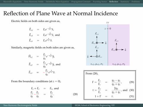
Reflection of Plane Wave at Normal IncidenceElectric fields on both sides are given as,

~Es,i = Eie−γ1z zx,

~Es,t = Ete−γ2z zx, and

~Es,r = Ereγ1z zx.

Similarly, magnetic fields on both sides are given as,

~Hs,i =Ei

η1e−γ1

z zy,

~Es,t =Et

η2e−γ2

z zy, and

~Es,r = − Er

η1eγ1

z zx.

From the boundary conditions (at z = 0),

Ei + Er = Et, andEi

η1− Er

η1=

Et

η2. (28)

x

From (28),

Γ =Er

Ei=

η2 − η1

η2 + η1, (29)

τ =Et

Ei=

2η2

η2 + η1, and (30)

1 + Γ = τ. (31)



Outline





5 Poynting Vector

6 Reflection

7 Summary

8 Problems



Summary

• v = ωβ

• γ2 = γ2x + γ2

y + γ2z = −ω2µε

• γ = α + jβ = ω

√µε2

[√1 +

(σ

ωε

)2 − 1]+ jω

√µε2

[√1 +

(σ

ωε

)2+ 1]

; δ = 1α

• ~P = ~E× ~H

• ExsHys

= jωµα+jβ ⇒ for the special case of lossless dielectric materials, Exs

Hys=√

µε

• Γ = ErEi

=η2−η1η2+η1

, τ =EtEi

=2η2

η2+η1, and 1 + Γ = τ



Outline





5 Poynting Vector

6 Reflection

7 Summary

8 Problems



Waves

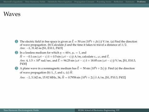
1 The electric field in free space is given as~E = 50 cos(108t + βx

)y V/m. (a) Find the direction

of wave propagation. (b) Calculate β and the time it takes to travel a distance of λ/2.Ans: −x, 31.42 ns [S1, E10.1, P415]

2 In a lossless medium for which η = 60π, µr = 1, and~H = −0.1 cos (ωt− z) x + 0.5 sin (ωt− z) y A/m, calculate εr, ω, and~E.Ans: 4, 1.5× 108 rad/sec, and~E = 94.25 sin (ωt− z) x + 18.85 cos (ωt− z) y V/m, [S1, E10.3,P430]

3 A plane wave in a nonmagnetic medium has~E = 50 sin(108t + 2z

)y. Find (a) the direction

of wave propagation (b) λ, f , and εr (c) ~H.

Ans: −z, 3.142 m, 15.92 MHz, 36, ~H = 0.7958 sin(108t + 2z

)x A/m, [S1, P10.3, P432]



Reflection


time harmonic electromagnetic fields - arraytool · 06/10/2012 · maxwell’s equationstime...

Documents