Time-Inconsistent Portfolio Investment Problems

Yidong Dong∗ Ronnie Sircar †

April 2014; revised October 6, 2014

Abstract

The explicit results for the classical Merton optimal investment/consumption problem rely on theuse of constant risk aversion parameters and exponential discounting. However, many studies havesuggested that individual investors can have different risk aversions over time, and they discount futurerewards less rapidly than exponentially. While state-dependent risk aversions and non-exponential type(e.g. hyperbolic) discounting align more with the real life behavior and household consumption data,they have tractability issues and make the problem time-inconsistent. We analyze the cases where theseproblems can be closely approximated by time-consistent ones. By asymptotic approximations, we areable to characterize the equilibrium strategies explicitly in terms of the corrections to solutions for thebase problems with constant risk aversion and exponential discounting. We also explore the effects ofhyperbolic discounting under proportional transaction costs.

1 Introduction and Background

1.1 The Merton Problem of Portfolio Optimization

The portfolio optimization problem in a continuous-time diffusion model was first introduced by Mertonin the 1960s, with the original papers reprinted later in [24], where he was able to derive explicit solutionsfor the value functions and optimal strategies in cases with geometric Brownian motions and special typesof utility functions. Ever since then, there has been plenty of development aimed at generalizing Merton’sresults in different ways. To deal with market incompleteness is a direction that a large proportion of theworks have been dedicated to. For example, Campbell and Viceira [4] and Wachter [31] studied the problemwith stochastic drift returns. For problems of partial hedging with a non-traded asset, as well as utilityindifference pricing, one could refer to the collection [5]. Meanwhile, stochastic volatility and transactioncost are two topics that have received much attention and popularity. We refer the reader to Chacko andViceira [6] and Kraft [22] for some explicit results in cases with stochastic volatility. For transaction costs,things are much more subtle as the problem becomes less tractable. Davis and Norman [10] were able tosolve the problem numerically as a free-boundary ODE system, and Shreve and Soner [28] treated it usingthe viscosity solution approach.

More recently, asymptotic methods have been used widely to solve the extensions of Merton’s problemaround their classical and well-established counterpart problems. For example, Fouque et al. [15] have∗Department of Operations Research and Financial Engineering, Princeton University, Princeton, NJ 08544, USA.

yidongd@princeton.edu.†Department of Operations Research and Financial Engineering, Princeton University, Princeton, NJ 08544, USA.

sircar@princeton.edu. Partially supported by NSF grant DMS-1211906.

1

used multiscale expansions to approximate the case with stochastic volatility around the constant volatilitycase. Bouchard et al. [3] used asymptotics for small transaction costs to derive tractable models for a partialhedging problem under expected loss constraints.

1.2 Time Inconsistency

The key to solving Merton’s problem is the use of the Dynamic Programming Principle (hereinafter DPP)in order to formulate the Hamilton-Jacobi-Bellman (hereinafter HJB) equation. In a typical dynamic pro-gramming problem setup, when an agent wants to optimize an objective function by choosing the best plan,he is only required to decide his current action. This is because DPP assumes that one’s future selves aregoing to solve the remaining part of today’s problem and act optimally when future comes. However, inmany problems, the DPP does not hold, and an agent does not have such “commitment power” on theirfuture selves, which is the ability to enforce a course of plans obtained by repeatedly optimizing the sameobjective function over time. In such problems, the future selves may have changed preferences or tastes, orwould want to make decisions based on different objective functions, effectively acting as opponents of thecurrent self.

The dilemma described above is called dynamic inconsistency, which has been noted and studied byeconomists for many years, mainly in the context of non-exponential type discount functions. In [29], Strotzdemonstrated that when a discount function was applied to consumption plans, one could favor a certainplan at the beginning, but later switch preference to another plan. This would hold true for most types ofdiscount functions, the only exception being the exponential. Nevertheless, exponential discounting is thedefault setting in most literatures, as none of the other types could produce explicit solutions. Results fromexperimental studies contradict this assumption (see, for example, Loewenstein and Prelec [23]), indicatingthat the discount rates for the near future are much lower than the discount rates for the time further away infuture, and therefore a hyperbolic type discount function would be more realistic.

Other types of time-inconsistency do exist as well. Bjork and Murgoci [1] listed out three possiblescenarios where time inconsistency would occur in typical Markovian stochastic control problems. Morespecifically, given an objective function of the following form:

J(t, x, π) = E[∫ T

tϕ(s− t)F (Xπ

s , x)ds+G(XπT , x)

]+H(x,E [Xπ

T ]),

where Xπ is some controlled diffusion process with Xπt = x and π being our control, the optimization for

J(t, x, π) is a time-inconsistent problem if:

1. the discount function ϕ(s− t) is not of exponential type, e.g. a hyperbolic discount function;2. x appears in the objective function, e.g. a utility function that depends on the initial wealth x;3. H() is a nonlinear function of E [Xπ

T ], e.g. continuous-time mean-variance optimization on XπT .

In all the three cases, the standard HJB equations cannot be derived since the usual formulation requiresan argument about the value function (process) being a supermartingale for arbitrary controls and being amartingale at optimum, which does not hold here. In light of the non-applicability of DPP on these problems,some have turned in a game-theoretic direction. By treating the problem as a game played with one’s futureselves, it is possible to derive a sub-game Nash equilibrium. In the next section, we will discuss recent workon deriving equilibrium strategies in some of the time-inconsistent problems.

2

1.3 Recent Literature on Time-inconsistent Portfolio Optimization

One of the earlier advances was made by Harris and Laibson who discussed the existence and uniqueness ofan equilibrium consumption path in the case of hyperbolic (in [16]) and quasi-hyperbolic (in [17]) discountfunctions in a discrete-time setup. They also derived the Euler relation for the equilibrium path using therecursive property of an equilibrium consumption plan. Ekeland and Lazrak [11] studied the problem incontinuous time with a more general non-exponential type discount function and derived an equation for theequilibrium value function process, which was comparable to Harris and Laibson’s results and resembles theclassical HJB equation plus a non-local term. Later, Ekeland et al. [13] looked at an investment/consumptionproblem from life insurance with time-inconsistent discount functions. They solved the non-local HJB-type equation numerically and were able to obtain a hump-shaped consumption path that agreed with thehousehold consumption data, as opposed to the monotone shape path produced by exponential discountfunctions.

Progress has been made on other types of time inconsistent problems as well. Bjork et al. [2] used thesame technique to study the continuous time mean-variance optimization problem with a state-dependentrisk aversion parameter. They obtained a system of HJB-type equations which they were able to reduce toan ODE system and solve numerically if risk aversion had a special form. Their equilibrium strategy wascomparable to the utility-maximizing strategy in a Merton model statically, but was able to capture somehorizon effect as opposed to the Merton optimal strategy which was constant in time. On the other hand,Hu et al. [18] derived an open-loop equilibrium strategy, characterized by a system of forward-backwardstochastic differential equations, to solve a time-inconsistent stochastic linear quadratic control problem,which is the generalized version of the mean-variance problem. Pirvu and Zhang [26] have studied theproblem of utility indifference pricing under a discrete time model with a state-dependent risk aversionmodeled by a two-state regime-switching Markov chain.

The remaining part of this article is organized as follows. In Section 2, we study the portfolio optimiza-tion problem with time-varying risk aversions that depend on the wealth or volatility factor. A discrete-timeexample will be given to illustrate the time inconsistency, followed by the derivation of the HJB-type equa-tion in continuous time. We will use asymptotic methods to derive the equilibrium strategies up to first order.In Section 3, we look at hyperbolic discounting problems and use similar methodologies to obtain tractablesolutions in this case. An extension with proportional transaction costs is also studied, and we provide somenumerical results for this problem. Section 4 concludes.

2 Utility Maximization with Time-varying Risk Aversion

In this section, we look at the classical Merton’s problem of portfolio optimization, but with the risk aversionparameter being state-dependent1. Our motivation is that, in the classical case, we need to, at time 0,fix a (constant) risk aversion parameter for expected utility at terminal time T . This value reflects ourpresent conjecture about our future attitude towards risk, and thus it would be unnatural for this conjectureto be independent of the current state of the world, for example the wealth level and economic conditions.There are many indicators in the market that can, at least partially, measure investors’ risk aversion. Asmentioned in Coudert and Gex [9], the movement of risk aversion is often correlated with market indices,for example the gold price and VIX. There are also aggregate indicators of risk aversion created by financialinstitutions such as JP Morgan’s Liquidity, Credit and Volatility Index. The consequence of incorporating

1These models can be seen as a particular example of the studies on state-dependent utility/preference by Karni [20]. In thiscase the dependency has an explicit functional form as γ(·).

3

such dependence is that the problem now becomes time-inconsistent, as the risk aversion will likely to bedifferent at a later time leading to a different objective function to optimize. An example is provided in thenext section as an illustration. We will follow closely the methodology described in [1]. As we will seelater, a system of equations of the HJB type can be obtained in this manner, which admits the equilibriumsolution via first order conditions. And when the risk aversion is constant, this system will degenerate to theclassical HJB equation.

2.1 Time-inconsistency and Wealth-dependent Risk Aversion

To keep the dimension small, we start by describing the time-inconsistency problem with the risk aversionbeing dependent on the current wealth level, Xt. Since the current wealth level is an indicator on howmuch loss (downside risk) one is able to bear, we believe this dependence is natural. We will illustrate thederivation of the HJB-type system of equations in this case, which can be easily extended to cases whererisk aversion depends on other state variables.

2.1.1 An Illustration

We can use a simple two-period binomial tree to illustrate the time inconsistency that results from the wealth-dependent risk aversion. Let k ∈ {0, 1, 2} denote the time periods. Suppose there are two assets Sk andBk, Bk being the risk free asset and Sk being the risky one with u > 1, d < 1 and p ∈ [0, 1] as the usualparameters in a binomial tree model. We also assume that both assets have value equal to 1 at time 0 and wehave zero interest rate so Bk = 1 ∀ k.

S0 : 1

u

d

u2

ud

d2

1− p

p

B0 : 1 1 1

Let Xk denote our wealth at time k and suppose X0 = 1 for simplicity. We use an exponential utilityfunction U(x) = −e−γx here, and we let the risk aversion γ be a function of the current wealth level(denoted as x here):

γ(x) =

a if x > 11 if x = 1b if x < 1,

for a, b > 0.Let 0 < π < 1 denote the amount of wealth invested in Sk at time 0. At time k = 0, with wealth

X0 = 1, the expected utility of terminal wealth Xπ2 := πS2 + (1− π)B2 can be written as:

E[U(Xπ2 )] = −e−1

{p2eπ(1−u2) + 2p(1− p)eπ(1−ud) + (1− p)2eπ(1−d2)

}=: −e−1f1(π),

4

where the risk aversion γ = 1. At time k = 1, depending on whether the stock price goes up or down, therisk aversion will becomes γ = a or b because we have either X1 > 1 or X1 < 1. The expected utility ofXπ

2 at time 1 is either

E[U(Xπ2 ) S1 = u] = −e−1

{peπ(1−u2)a + (1− p)eπ(1−ud)a

}=: −e−1f2(π),

or

E[U(Xπ2 ) S1 = d] = −e−1

{peπ(1−ud)b + (1− p)eπ(1−d2)b

}=: −e−1f3(π).

Remark 2.1. It is possible to choose p, u, d, π such that

∂

∂πf1(π) > 0,

∂

∂πf2(π) < 0 and

∂

∂πf3(π) < 0.

For instance, if a = 0.5 and b = 2, then by choosing u = 2, d = 0.5, p = 0.5 and π = 0.5 we can obtainthe desired inequalities.

Suppose we have Portfolio #1 that has π in the stock and 1 − π in the bank, and Portfolio #2 thathas π − ε in stock and 1 − π + ε in the bank for an infinitesimal positive amount ε. The signs of the firstderivatives in Remark 2.1 tell us that, at the second period, Portfolio #1 is always favored over Portfolio#2. However, at time 0, Portfolio #2 is the better one. We recall the definition of time consistent utilityfunction, such as in [21] and [7]:

Definition 2.2. A dynamic utility function (Ut)Tt=0 is time-consistent if for all X, Y ∈ L(FT ) and t ∈

0, . . . , T − 1,Ut+1(X) ≥ Ut+1(Y ) implies Ut(X) ≥ Ut(Y ).

We can see that in our case the preference between Portfolio #1 and #2 is “flipped” in the two periods,which clearly violates the definition of time consistency.

2.1.2 Formal Problem Setup in Continuous Time

We use the standard two-asset framework where we have a risky stock St and a risk-free bond that we caninvest our wealth in. By assuming zero interest rate or working under the discounted unit, we only need todefine the stock dynamics:

dSt = µSt dt+ σSt dWt, (1)

where Wt denotes a standard Brownian motion, so St is a geometric Brownian motion (henceforth GBM).For the time being, we assume constant drift µ and volatility σ. The case where the volatility is stochasticwill be discussed in Section 2.3 when we consider the volatility-dependent risk aversion as an extension ofthis problem.

Let Xt denote our wealth at time t, which consists of the cash amount πt invested in the risky stockas well as the remaining part invested in the riskless bond. The wealth process Xt follows the controlleddiffusion:

dXt = πtdStSt

= πt[µdt+ σ dWt]. (2)

5

The optimization problem is to maximize the expected utility of terminal wealth at time T among alladmissible strategies π, given the wealth level being Xt = x at time t. This problem can be representedusing the value function V (t, x)

V (t, x) := supπ∈Π

Et,x [U(XπT , γ(Xt))]

= supπ∈Π

J(t, x,π),(3)

where Π is the set of all admissible strategies that are adapted to the filtration (Fs) generated by the stockprice process and which satisfy E[

∫ Tt π2

sds < ∞], and γ(Xt) is the risk aversion that we fix for our fu-ture self at time T based on the current wealth level Xt. Here U(x1, γ(x2)) denotes the von Neumann-Morgenstern utility function which is a twice differentiable, concave function in x1 ∈ R+.

Remark 2.3. Note that in U(x1, γ(x2)), x1 is the wealth at future for which we want to compute theutility, with risk aversion computed using current wealth level x2. In order to retain the differentiability andconcavity at terminal time T when x1 and x2 coincide, we also require γ(x2) to be chosen such that

• U(x1, γ(x2)) is twice differentiable in x2;

• (Ux1x1 + Ux2x2 + 2Ux1x2) x2=x1 < 0 for all x1 > 0.

In the classical case, the risk aversion γ is constant so we can suppress its argument by denoting theutility function asU = Uγ(x). Then the optimal strategy can be computed from the HJB equation associatedwith the value function, and the DPP, from which the HJB equation is derived, guarantees that the optimalstrategy π∗ computed at the initial time will remain optimal at a later time. A rigorous proof of the derivationof HJB equation from DPP can be found in, for example, Pham [25]. In this case, the optimal strategy takesthe form:

π∗t =

λ

σ

1

γfor exponential utility functions

λ

σ

x

γfor log and power utility functions,

where Xt = x and λ is the Sharpe ratio defined by λ := µσ .

Now, as we have made the risk aversion wealth dependent, intuitively the optimal strategy might beobtained by replacing the constant γ with γ(x) in the above expressions. Is it really the case? It turns outthat this is not so trivial, since we cannot even formulate the HJB equation (in the classical DPP sense)once we allow the risk aversion to change with the current wealth level. As our objective function changesconstantly, our future selves will not solve the “remaining” part of the optimization problem that our currentself is facing now.

Using a game-theoretic approach, we can think of it as a game played by a number of ordered players(our selves at different times), each of whom has his own utility function and has temporary control over theresource (wealth). For a particular player, when the resource is in his possession (obtained from the previousplayer), he can choose the strategy to be applied to the resource at this particular moment. After that, theplayer has to pass on the resource to the next player and he will no longer be able to apply strategies to itor control what other players’ strategies will be. As the game is played by a continuum of players in thecontinuous time setting, each player would have to play against all his future selves.

To define the equilibrium in this game, we follow the explanation given in [11], in which it was assumedthat the current self has the ability to commit all future selves to his decision up to a small period ε > 0.

6

Thus the player can form a small coalition with players in the near future. Now suppose π ≡ (πs)s∈[t,T ] isan admissible policy (all strategies over time). Define another policy πε as:

πε =

{π, s ∈ [t, t+ ε]πs, s ∈ (t+ ε, T ],

(4)

where π can be any strategy that makes πε admissible. Then the following from [11] gives the definition ofthe equilibrium policy.

Definition 2.4. A policy π : (t, x)→ R is an equilibrium one if for any t, x > 0 and any arbitrary π,

limε ↓ 0

J(t, x, π)− J(t, x, πε)

ε≥ 0

where J is our objective function.

This definition means that, if we are using the equilibrium policy π, then we will not be better off bycommitting the immediate future selves to our action instead of letting them choose the best strategy intheir views. This also means that the equilibrium policy computed at one time should coincide, from thenext period onward, with the equilibrium policy computed at the next period. The equilibrium policy istherefore time-consistent as the future selves have no incentives to deviate from this path. We refer thereaders to the paragraphs following Definition 1 in Ekeland and Lazrak [12] for a detailed explanation aboutthe equilibrium strategy in discrete time setting. The definition leads to the following result as appeared in,e.g. [1]:

Proposition 1. Assuming sufficient regularity, the equilibrium value function and Markovian policy satisfythe following extended HJB-type system:

supπt∈R

(AπtV (t, x)−Aπtf(t, x, x) +Aπtfw(t, x)) = 0

Aπ∗t fw(t, x) = 0

V (T, x) = U(x, γ(x))

f(T, x, w) = U(x, γ(w)),

(5)

where Aπt contains the infinitesimal generator of the wealth process taking the form:

Aπtg(t, x) = gt + µπtgx +1

2σ2π2

t gxx

Aπth(t, x, x) = ht + µπthx + µπthw|w=x +1

2σ2π2

t hxx +1

2σ2π2

t hww|w=x + σ2π2t hxw|w=x,

and fw(t, x) means fixing the w variable of f(t, x, w) as constant.

Proof. We need to define the following “auxiliary value function”:

f(t, x, w) = Et,x[U(Xπ∗

T , γ(w))],

which is made from V (t, x) by making the initial wealth value in γ(·) vary independently from Xt, andwhere π∗ denotes the equilibrium strategy. For every fixed w, γ(w) can be treated as a constant, as w and

7

x are independent. Thus f(t, x, w) is the value function for a Merton problem with constant risk aversionparameter γ(w).

By construction of πε from the definition, we have the following equality:

Et,x [J(t+ ε,Xt+ε,πε)] = Et,x [f(t+ ε,Xt+ε, Xt+ε)]

= Et,x [f(t+ ε,Xt+ε, Xt+ε)] + J(t, x,π)− Et,x [U(XπT , γ(x))]

= Et,x [f(t+ ε,Xt+ε, Xt+ε)] + J(t, x,π)− Et,x [E [U(XπT , γ(x)) | Xt+ε, t]]

= Et,x [f(t+ ε,Xt+ε, Xt+ε)] + J(t, x,π)− Et,x [f(t+ ε,Xt+ε, x)] .

Since J(t+ ε,Xt+ε,πε) = V (t+ ε,Xt+ε), we can write the above equation as:

Et,x [V (t+ ε,Xt+ε)] = Et,x [f(t+ ε,Xt+ε, Xt+ε)] + J(t, x,π)− Et,x [f(t+ ε,Xt+ε, x)] .

Taking the supremum and rearranging the equation, we get

supπ∈Π

(Et,x [V (t+ ε,Xt+ε)]− V (t, x) + Et,x [f(t+ ε,Xt+ε, x)]− Et,x [f(t+ ε,Xt+ε, Xt+ε)]) = 0.

Now we take the limit ε→ 0,

supπt

(AπtV (t, x)−Aπtf(t, x, x) +Aπtfw|w=x(t, x)

)= 0. (6)

Meanwhile, for every fixed w, f(t,Xt, w) corresponds to a martingale process and thus it must satisfythe PDE

Aπ∗t fw(t, x) = 0, (7)

where π∗ is the equilibrium policy appeared in the definition of f(t, x, w). In addition, there are two terminalconditions for V and f : {

V (T, x) = U(x, γ(x))

f(T, x, w) = U(x, γ(w)).(8)

We get the extended HJB-type system by combining equations (6), (7) and (8).

The verification theorem provided by [1] holds here, we shall quote:

Theorem 1 (Bjork and Murgoci). Assume that (V (t, x), f(t, x, w)) is a solution of the system defined in(5), and that the strategy path π∗ realizes the supremum in the equation. Then π∗ is an equilibrium policy,and V (t, x) is the corresponding value function.

Proof. See [1].

When writing out the first two equations in (5) explicitly, we get the following two PDEs:Vt + sup

π

{µπ(Vx − fw) +

1

2σ2π2(Vxx − fww − 2fxw)

}= 0

ft + µπ∗fx +1

2σ2π∗2fxx = 0.

(9)

Note that all w partial derivatives are evaluated at the point w = x.

8

We can find the equilibrium strategy by the first order condition:

π∗ = −λσ

Vx − fwVxx − fww − 2fxw

w=x, (10)

where λ denotes the constant Sharpe ratio. Inserting (10) back into (9) and we obtain the following twoPDEs to solve for V (t, x) and f(t, x, w)

Vt −1

2λ2 V

2x − 2Vxfy + f2

w

Vxx − fww − 2fxw= 0

ft + λ2

[fx(fw − Vx)

Vxx − fww − 2fxw+

1

2

(V 2x − 2Vxfw + f2

w)fxx(Vxx − fww − 2fxw)2

]= 0.

(11)

2.1.3 A Remark: Why Two Equations Instead of One?

As we can see from above, we now face an HJB-type system of two equations instead of solving one singleHJB equation as in the time-consistent case. It turns out this is essential for characterizing the equilibriumstrategy and value function. In the definition of the equilibrium strategy, coalition is allowed for an infinites-imal period, during which we are actually solving a Merton problem with constant risk aversion. That iswhat the function f(t, x, w) represents when setting w = x and it is the time-consistent part of the problem.After this infinitesimal period, however, the evolution of the value function cannot be characterized by thisfunction f(t, x, w) any more, as the problem now is time-inconsistent. This is the reason we need V (t, x)as our value function.

In Harris and Laibson [17], the dynamic consumption choice problem with quasi-hyperbolic discount-ing was also solved by the equilibrium strategy and value function that were defined similarly using twofunctions. There is a continuation-value function characterizing the dynamics of the true time-inconsistentvalue function and there is another current-value function, which is used locally at the current point (t, x)to derive the equilibrium strategy. Our HJB-type system has a strong analogy to the two functions in theirwork.

Another way of describing this is that the true value function V (t, x) cannot be solved alone. For eachpoint (t, x), the value of V (t, x) is determined by another non-local function f(t, x, w) by setting w = xin its third argument, i.e. V (t, x) = f(t, x, x). The first equation in (5) can be considered as a PDE of thenon-local type. For the non-exponential discounting problem in [11], a non-local integro-PDE was obtained,where the dynamics of the value function depends on an integral of the value function at all future time. Ingeneral, non-local PDEs are very difficult to solve.

2.1.4 Asymptotic Expansions

If the time-inconsistent problem is close to a time-consistent one, we can approximate the first problem veryeffectively using the latter by asymptotic methods. Here we look at the special case where the risk aversiononly varies slowly with the wealth level, i.e. it is close to the case of constant risk aversion. Mathematically,this corresponds to

γ(x) = γ0 + εγ1(x) + · · ·

for positive ε� 1. We look for an expansion of the form

V (t, x) = V0(t, x) + εV1(t, x) + · · · ,

9

andf(t, x, w) = f0(t, x) + εf1(t, x, w) + · · · ,

for the equations in (11).We first introduce a few notations.

Definition 2.5. We define the risk tolerance to be

R := − V0,x

V0,xx;

and we use Dk to denote

Dk := Rk∂k

∂xk;

and finally define the linear operator Lt,x as

Lt,x := ∂t + λ2D1 +1

2λ2D2.

Collecting zeroth order terms in (11) we get{Lt,xV0 = 0

Lt,xf0 = 0,(12)

with terminal conditions V0(T, x) = U(x, γ0) and f0(T, x) = U(x, γ0). Since f0 and V0 have the sameterminal condition, we find V0(t, x) = f0(t, x) which is the classical Merton value function with constantrisk aversion parameter γ0.

At the first order, we have:Lt,xV1 = λ2Rf1,w +λ2

2R2 (f1,ww + 2f1,xw)

Lt,xf1 = 0,

(13)

with terminal conditions V1(T, x) = ∂U∂γ (x, γ0)γ1(x) and f1(T, x, w) = ∂U

∂γ (x, γ0)γ1(w). The followingproposition will be useful for solving the order ε PDEs.

Lemma 1. We have∂

∂γLt,xV0 = Lt,x

(∂V0

∂γ

). (14)

Proof. For any function v,

∂

∂γLt,xv =

∂

∂γ

(vt + λ2Rvx +

1

2λ2R2vxx

)= Lt,x

(∂v

∂γ

)+ λ2∂R

∂γvx + λ2

(R∂R

∂γ

)vxx.

The last two terms cancel out when v = V0 since R = − V0,xV0,xx

.

10

Lemma 1 will lead us to the solutions of f1 and V1.

Proposition 2. The solution to the second equation in (13) is

f1(t, x, w) = γ1(w)∂f0

∂γ.

Therefore the order ε value function is

V1(t, x) = γ1(x)∂V0

∂γ. (15)

Proof. By direct substitution and verification.

2.1.5 Effect on the Trading Strategy

Recall the equilibrium strategy from (10)

π∗ = −λσ

Vx − fwVxx − fww − 2fxw

.

We plug in V = V0 + εV1 and f = f0 + εf1,

π∗ = −λσ

V0,x + εhxγ1(x)

V0,xx + εhxxγ1(x)

=λ

σR(1 + ε

hxγ1(x)

V0,x+ o(ε2))(1− εhxxγ1(x)

V0,xx+ o(ε2))

=λ

σR

[1 + εγ1(x)

(hxV0,x

− hxxV0,xx

)]+ o(ε2), (16)

where we denote h := ∂V0∂γ . Thus the equilibrium strategy will deviate from the optimal strategy in the case

of constant risk aversion γ0 by a fraction given by εγ1(x)(hxV0,x− hxx

V0,xx

).

2.1.6 Power Utility Case

Recall that the power utility function with constant risk aversion parameter γ is:

U(x) =x1−γ

1− γ.

For the Merton problem with power utility and constant risk aversion, the value function V (t, x) satisfies

Vt −1

2λ2 V

2x

Vxx= 0,

with terminal condition V (T, x) = x1−γ

1−γ . The solution for the PDE above is given by

V (t, x) =x1−γ

1− γeλ2

2

(1−γγ

)(T−t)

.

11

This is our zeroth order value function V0(t, x) once we replace γ with γ0. We can find the first ordercorrection by taking the partial derivative w.r.t. γ and multiplying by γ1(x):

V1(t, x) = γ1(x)

[1

1− γ0− log(x)− λ2(T − t)

2γ20

]V0(t, x). (17)

The equilibrium trading strategy up to first order is given by:

π∗ =λ

σγ0

[1 + εγ1(x)

(hxV0,x

− hxxV0,xx

)]=

λ

σγ0

[1 + ε

γ1(x)

γ0

].

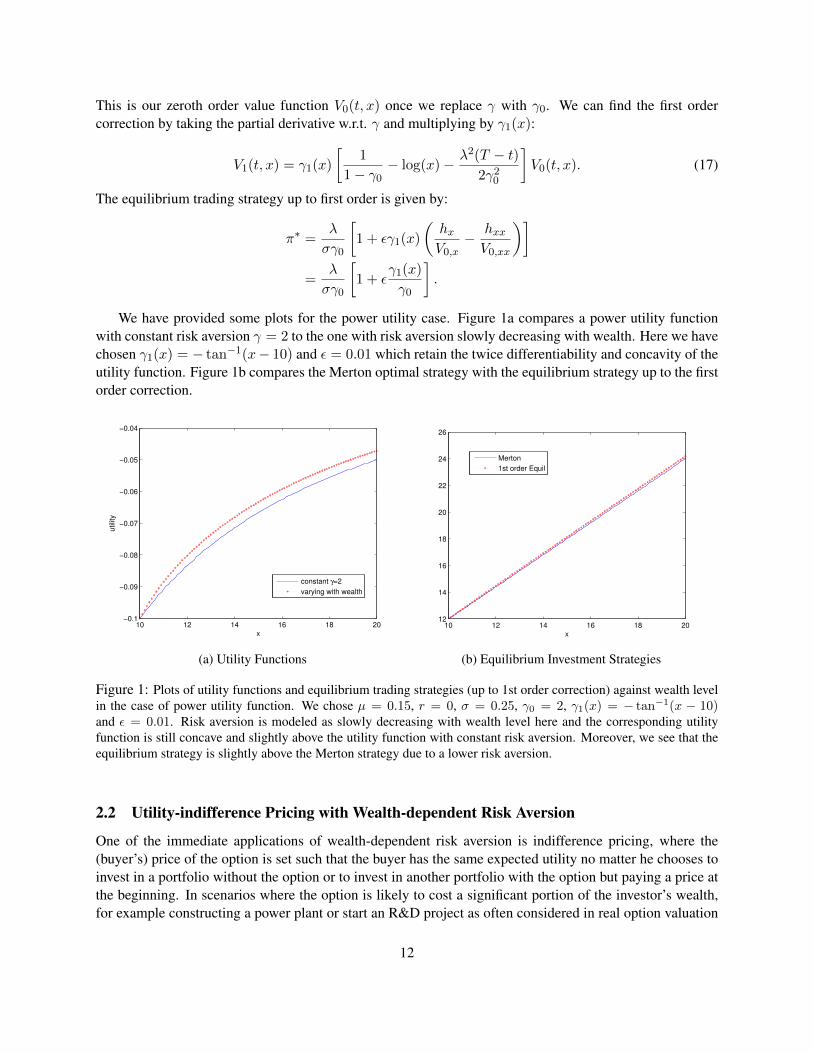
We have provided some plots for the power utility case. Figure 1a compares a power utility functionwith constant risk aversion γ = 2 to the one with risk aversion slowly decreasing with wealth. Here we havechosen γ1(x) = − tan−1(x− 10) and ε = 0.01 which retain the twice differentiability and concavity of theutility function. Figure 1b compares the Merton optimal strategy with the equilibrium strategy up to the firstorder correction.

10 12 14 16 18 20−0.1

−0.09

−0.08

−0.07

−0.06

−0.05

−0.04

x

utilit

y

constant γ=2

varying with wealth

(a) Utility Functions

10 12 14 16 18 2012

14

16

18

20

22

24

26

x

Merton

1st order Equil

(b) Equilibrium Investment Strategies

Figure 1: Plots of utility functions and equilibrium trading strategies (up to 1st order correction) against wealth levelin the case of power utility function. We chose µ = 0.15, r = 0, σ = 0.25, γ0 = 2, γ1(x) = − tan−1(x − 10)and ε = 0.01. Risk aversion is modeled as slowly decreasing with wealth level here and the corresponding utilityfunction is still concave and slightly above the utility function with constant risk aversion. Moreover, we see that theequilibrium strategy is slightly above the Merton strategy due to a lower risk aversion.

2.2 Utility-indifference Pricing with Wealth-dependent Risk Aversion

One of the immediate applications of wealth-dependent risk aversion is indifference pricing, where the(buyer’s) price of the option is set such that the buyer has the same expected utility no matter he chooses toinvest in a portfolio without the option or to invest in another portfolio with the option but paying a price atthe beginning. In scenarios where the option is likely to cost a significant portion of the investor’s wealth,for example constructing a power plant or start an R&D project as often considered in real option valuation

12

problems, it is possible for the investor to become more risk averse after he purchases the option. A wealth-dependent risk aversion can be used to capture this change. Here we look at the indifference pricing of anoption written on a non-traded asset. The controlled wealth process follows

dXπ,xt = πt dS

(1)t + r(Xπ,x

t − πtS(1)t )dt,

where the price S(1)t of the traded asset follows the geometric Brownian motion with drift µ

dS1t = µS

(1)t dt+ σS

(1)t dW

(1)t .

The option written on the non-traded asset S(2)t has payoff C(S

(2)T ) at terminal time T . And S(2)

t followsthe SDE

dS(2)t = p dt+ q dW

(2)t ,

where W (1)t and W (2)

t have correlation ρ. Now assuming r = 0, the value function for the Merton problemwithout the option is

V (x, 0) =− e−γ0x−λ2T/2 + εγ1(x)xe−γ0x−λ2T/2 + o(ε2)

=− e−γ0x−λ2T/2 (1− εγ1(x)x) + o(ε2). (18)

Note that we are using exponential utility here to simplify the calculations. Now the value function with along position in k units of the option is given by

V (x− pk, k) =− e−γ0(x−pk)−λ2T/2 (1− εγ1(x)x)(EQ0 [e−kγ0(1−ρ2)C(S

(2)T )(1− kεγ1(x)(1− ρ2)C(S

(2)T ))]

)1/(1−ρ2)

=− e−γ0(x−pk)−λ2T/2 (1− εγ1(x)x)(EQ0 [e−kγ0(1−ρ2)C(S

(2)T )])1/(1−ρ2)

+ εkγ1(x)e−γ0(x−pk)−λ2T/2(EQ0 [e−kγ0(1−ρ2)C(S

(2)T )])ρ2/(1−ρ2)

EQ0 [C(S(2)T )e−kγ0(1−ρ2)C(S

(2)T )],

(19)

where Q0 is the probability measure under which S(2)t has a new drift p− ρλq but the same diffusion q.

For the solution of pk, we seek the following expansion:

pk = p(0)k + εp

(ε)k + o(ε2).

Consequently,

V (x− p(0)k − εp

(ε)k , k) =

V 0(x, 0)eγ0p(0)k Θ

11−ρ2T

1 + ε

1− γ1(x− p(0)k )x−

kγ1(x− p(0)k )EQ0

[C(S

(2)T )ΛT

]ΘT

+ o(ε2)

(20)

where we have used the following notation

V 0(x, 0) := −e−γ0x−λ2T/2,

ΛT := e−kγ0(1−ρ2)C(S(2)T ),

ΘT := EQ0 [ΛT ],

13

and that γ1(x− p(0)k − εp

(ε)k ) ≈ γ1(x− p(0)

k ).Now we just need to equate (18) and (20). At the zeroth order,

−e−γ0x−λ2T/2 = −e−γ0(x−p(0)k )−λ2T/2Θ1/(1−ρ2)T ,

from which we can find the zeroth order indifference price:

p(0)k = − 1

(1− ρ2)γ0log ΘT .

At order ε, after substituting in p(0)k , we have

−γ1(x)x = p(ε)k − γ1(x− p(0)

k )x− kγ1(x− p(0)k )Θ−1

T EQ0

[C(S

(2)T )ΛT

],

from which we can get the order ε correction to the indifference price

p(ε)k =(γ1(x− p(0)

k )− γ1(x))x+kγ1(x− p(0)

k )EQ0 [C(S(2)T )ΛT ]

ΘT.

As we have assumed that the investor will become more risk averse when holding the option, i.e. γ1(x −p

(0)k ) ≥ γ1(x), the correction p(ε)

k above tells us that the true indifference price will be higher than theconstant risk aversion case for k > 0 and C(·) ≥ 0.

2.3 Stochastic Volatility Models with Volatility-dependent Risk Aversion

Since first introduced by Hull and White [19] for pricing options, stochastic volatility models have gainedwide popularity as they could reproduce features about the implied volatility surface that are missing in thestandard Black-Scholes models. Incorporating the stochastic volatility framework is also one of the manyextensions being studied recently for the classical Merton portfolio optimization problems.

One way to look at the problem is to use the timescale stochastic volatility asymptotics, which havebeen applied to many option pricing problems, see Fouque et al. [14] and the references therein. In thisframework, the volatility is assumed to have a fast mean-reverting factor following a speeded-up diffusionprocess and/or a slow factor following a slowed-down diffusion. The empirical evidence to support themultiscale stochastic volatility model can be found in Chernov [8]. When Fouque et al. [15] treated theMerton problem in this way, they obtained in explicit forms both the fast and slow scale corrections to thevalue function, which resemble the stochastic volatility corrections for pricing European-style options.

A natural question to ask is whether volatility, an indicator of investment risk, would affect the riskaversion parameter, a measure of investor’s attitude towards risk. This question is nontrivial when the as-sumption of constant volatility has been dropped. Intuitively the answer should be yes, as investors wouldusually focus on preserving capitals when the risky assets have high volatility, thus becoming more riskaverse. Empirical results also support this argument, which can be found in Scheicher [27] and Tarashevet al. [30]. Scheicher [27] discovered a positive relationship between the implied risk aversion in Germanequity market and the implied volatility of the US market, and Tarashev et al. [30] concluded from re-sults obtained in different equity and fixed income markets that a higher risk aversion is linked to highervolatilities and this is more noticeable in the equity markets.

In the next section, we will look at the case where risk aversion is a function of the slow scale volatilityfactor so it slowly varies. Our rationale is that the effect from the fast scale factor would likely be averaged

14

out over the investment horizon if it is long enough; and it is the general trend of the volatility that wouldreflect the change in investors’ risk aversion. We will derive the extended HJB system and carry out the slowscale asymptotic expansion in this case to approximate the value function and equilibrium strategy. Usingpower utility functions, we will show that it is possible to obtain results similar to Fouque et al. [15] butwith an additional correction term to account for change in risk aversion.

2.3.1 Slow Scale Stochastic Volatility Model

Suppose that the volatility slowly fluctuates as a general diffusion process and the stock price follows ageometric Brownian Motion as usual:{

dSt = µSt dt+ σ(Zt)St dWt

dZt = δc(Zt) dt+√δg(Zt) dW

′t ,

(21)

where Wt and W ′t are Brownian motions with correlation ρ′ ∈ (−1, 1). We have the wealth process:

dXt = πtµdt+ πtσ(Zt)dWt, (22)

and the associated infinitesimal generator:

Aπt(t, x, z) = ∂t + πtµ(z)∂x +1

2π2t σ(z)2∂2

x + δc(z)∂z +1

2δg(z)2∂2

z +√δπtρg(z)σ(z)∂2

xz.

The portfolio optimization problem we consider here is:

V (t, x, z) = supπ

Et,x,z [U(XπT , γ(Zt))] , (23)

where we make the risk aversion dependent on current level of the slow factor Zt. The extended HJB systemfor the value function can be derived in the same way as the wealth-dependent risk aversion case (with a twodimensional state process now), which is given by

supπt{Vt + πtµ(z)Vx +

1

2π2t σ(z)2Vxx +

√δρπtg(z)σ(z)(Vxz − fxw)

+δc(z)(Vz − fw) +1

2δg(z)2(Vzz − fww − 2fwz)} = 0

ft + π∗t µ(z)fx +1

2π∗2t σ(z)2fxx + δc(z)fz +

1

2δg(z)2fzz +

√δρπ∗t g(z)σ(z)fxz = 0,

(24)

with terminal conditions: {V (T, x, z) = U(x, γ(z))

f(T, x, z, w) = U(x, γ(w)).(25)

By the first order conditions, the equilibrium strategy takes the form:

π∗t = −µ(z)Vx +√δρg(z)σ(z)[Vxz − fxw]

σ(z)2Vxx

∣∣∣∣w=z

. (26)

15

Plugging this equilibrium strategy back to the extended HJB system, we get:

Vt −{µ(z)Vx +

√δρg(z)σ(z)[Vxz − fxw]}2

2σ(z)2Vxx+ δ{c(z)(Vz − fw) +

g(z)2

2[Vzz − fww − 2fzw]} = 0

ft −µ(z)Vx +

√δρg(z)σ(z)[Vxz − fxw]

σ(z)2Vxx[µ(z)fx +

√δρg(z)σ(z)fxz]

+{µ(z)Vx +

√δρg(z)σ(z)[Vxz − fxw]}2

2σ(z)2V 2xx

fxx + δ[c(z)fz +g(z)2

2fzz] = 0.

(27)Now we assume that the risk aversion γ(Zt) takes the form:

γ(Zt) = γ0 +√δγ1(Zt) + o(δ), (28)

thus slowly varies with the slow scale volatility factor. And we expand V and f as:

V (t, x, z) = V0(t, x, z) +√δV1(t, x, z) + δV2(t, x, z) + o(δ

32 )

f(t, x, z, w) = f0(t, x, z, w) +√δf1(t, x, z, w) + δf2(t, x, z, w) + o(δ

32 ).

(29)

Now introduce the risk tolerance function:

R := R(t, x, z) = − V0,x(t, x, z)

V0,xx(t, x, z),

and the differential operator:

Dk := Rk∂k

∂xk,

as well as the linear operator:

Lt,x,z = ∂t + λ(z)2D1 +1

2λ(z)2D2,

where λ(z) := µσ(z) denotes the Sharpe ratio.

We can find that V0(t, x, z) = f0(t, x, z, z) is the Merton value function with Sharpe ratio fixed at λ(z)and risk aversion parameter fixed at γ0. As a result, order

√δ equations become:{

Lt,x,zV1 + ρg(z)λ(z)D1(V0,z −���f0,w) = 0

Lt,x,zf1 + ρg(z)λ(z)D1f0,z = 0,(30)

with terminal condition given by: V1(T, x, z) = γ1(z)

∂U

∂γ(x, γ0)

f1(T, x, z, w) = γ1(w)∂U

∂γ(x, γ0).

Proposition 3. The solution to (30) is given by:

V1(t, x, z) = γ1(z)V0,γ +1

2(T − t)ρλ(z)g(z)D1V0,z. (31)

16

Proof. Using the result from Lemma 1, we can see that γ1(w)f0,γ is a solution to the PDE problem below:Lt,x,zf1 = 0,

f1(T, x, z, w) = γ1(w)∂U

∂γ(x, γ0),

which is the original order√δ PDE problem without the source term. Now if we can find the solution to the

full PDE problme with zero terminal condition, we can find the full solution satisfying the original terminalcondition by combining the two partial solutions. This can be done by making use of the “Vega-Gamma”relation in Lemma 3.1 of Fouque et al. [15], which states

f0,z = −(T − t)λ(z)λ′(z)D2f0.

The second problem can be rewritten as follows{Lt,x,zf1 = (T − t)ρg(z)λ(z)2λ′(z)D1D2f0

f1(T, x, z, w) = 0.

Using the commutativity property of Lt,x,z withD1 and the equalityD1f0 = −D2f0 from [15], we find that

f1(t, x, z, w) = −1

2(T − t)2ρg(z)λ(z)2λ′(z)D1D2f0

=1

2(T − t)ρλ(z)g(z)D1f0,z

is the solution. We get the solution for V (t, x, z) by combining the two partial solutions and replacing thew variable with z.

Once we get the solution of V1, the equilibrium trading strategy up to order o(√δ) can be computed:

π∗ =λ(z)

σ(z)R−√δ

{ρg(z)

σ(z)

V0,xz

V0,xx+λ(z)

σ(z)

[V1,x

V0,xx+R

V1,xx

V0,xx

]}. (32)

Power Utility Case For a power utility function:

U(x, γ(z)) =1

1− γ(z)x1−γ(z), (33)

we have the zeroth order value function given by:

V0(t, x, z) =x1−γ0

1− γ0eλ(z)2

21−γ0γ0

(T−t). (34)

Thus the explicit form of the first order value function is:

V1(t, x, z) =

{(T − t)2ρg(z)λ(z)2λ′(z)(1− γ0)2

2γ20

+ γ1(z)

[1

1− γ0− log(x)− λ(z)2(T − t)

2γ20

]}V0(t, x, z).

(35)

17

The strategy is given by:

π∗ =λ(z)x

σ(z)γ0+√δ

[ρg(z)λ′(z)λ(z)(1− γ0)(T − t)

σ(z)γ20︸ ︷︷ ︸

slow factor adjustment in [15]

− λ(z)

σ(z)

γ1(z)

γ0(1 +

1

γ0)

]︸ ︷︷ ︸

risk aversion adjustment

x. (36)

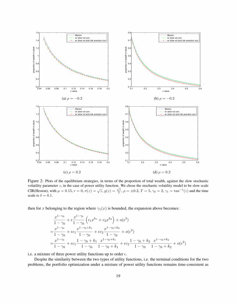
We now compare the Merton optimal strategy, the optimal strategy with first order correction for the slowvolatility factor appeared in [15] and our equilibrium strategy with first order correction. Note that thesecond strategy is equivalent to (36) with only the first fractional term inside the square bracket. We noticethat for different levels of the slow factor, the proportions that the two adjustment factors would contribute tothe first order correction are different. Figure 2 contains the plots of the three strategies for different rangesof the slow factor. Figures 2a and 2c show that for small z, the main contributor of the first order correctionis the first fractional term inside the square bracket of (71), whereas for larger values of z, as Figures 2band 2d suggest, an increasing risk aversion plays the major role instead. The direction to which the firstadjustment factor affects the strategy depends on the sign of the correlation factor ρ.

2.4 Comparison with Mixture of Power Utility Functions

A mixture of power utility functions takes the following form:

Umix(x) = c1x1−γ1

1− γ1+ c2

x1−γ2

1− γ2,

as introduced in Fouque et al. [15], where γ1 6= γ2 and c1, c2 are positive constants. Under this utilityfunction, the relative risk aversion is not constant any more but decreases in x. Now let us look at a powerutility function with wealth-dependent risk aversion:

U(x) =x1−γ(x)

1− γ(x). (37)

We can choose γ(x) to make Umix(x) = U(x), but in the case of power utility the solution will be acomplex-valued function due to the presence of γ(x) in the exponent of x. (In contrast, for a mixture ofexponential utility functions, γ(x) will be real-valued).

For the case of small wealth-dependence, we have the following expansion:

U(x) =x1−(γ0+εγ1+o(ε2))

1− (γ0 + εγ1 + o(ε2))

=x1−γ0 − εγ1log(x)x1−γ0 + o(ε2)

1− γ0(1 + ε

γ1

1− γ0+ o(ε2))

=x1−γ0

1− γ0+ ε

{− x

1−γ0

1− γ0γ1log(x) +

x1−γ0

1− γ0

γ1

1− γ0

}+ +o(ε2)

where γ1 ≡ γ1(x) can be chosen in such a way that the expansion is also a mixture of power utility functions.For example, we can set γ1(x) to be:

γ1(x) =c1x

k1 + c2xk2

−log(x) + 11−γ0

18

0.04 0.06 0.08 0.1 0.12 0.14 0.16 0.18 0.20.2

0.4

0.6

0.8

1

1.2

1.4

1.6

z value

pro

po

rtio

n o

f w

ea

lth

in

sto

ck

Merton

w/ slow vol corr.

w/ slow vol and risk aversion corr.

(a) ρ = −0.2

0.1 0.2 0.3 0.4 0.5 0.60.1

0.2

0.3

0.4

0.5

0.6

0.7

0.8

z value

pro

po

rtio

n o

f w

ea

lth

in

sto

ck

Merton

w/ slow vol corr.

w/ slow vol and risk aversion corr.

(b) ρ = −0.2

0.04 0.06 0.08 0.1 0.12 0.14 0.16 0.18 0.20.2

0.4

0.6

0.8

1

1.2

1.4

1.6

z value

pro

po

rtio

n o

f w

ea

lth

in

sto

ck

Merton

w/ slow vol corr.

w/ slow vol and risk aversion corr.

(c) ρ = 0.2

0.1 0.2 0.3 0.4 0.5 0.60.1

0.2

0.3

0.4

0.5

0.6

0.7

0.8

z value

pro

po

rtio

n o

f w

ea

lth

in

sto

ck

Merton

w/ slow vol corr.

w/ slow vol and risk aversion corr.

(d) ρ = 0.2

Figure 2: Plots of the equilibrium strategies, in terms of the proportion of total wealth, against the slow stochasticvolatility parameter z, in the case of power utility function. We chose the stochastic volatility model to be slow scaleCIR(Heston), with µ = 0.15, r = 0, σ(z) =

√z, g(z) =

√z2 , ρ = ±0.2, T = 5, γ0 = 2, γ1 = tan−1(z) and the time

scale is δ = 0.1.

then for x belonging to the region where γ1(x) is bounded, the expansion above becomes:

x1−γ0

1− γ0+ ε

x1−γ0

1− γ0

(c1x

k1 + c2xk2)

+ o(ε2)

=x1−γ0

1− γ0+ εc1

x1−γ0+k1

1− γ0+ εc2

x1−γ0+k2

1− γ0+ o(ε2)

=x1−γ0

1− γ0+ εc1

1− γ0 + k1

1− γ0

x1−γ0+k1

1− γ0 + k1+ εc2

1− γ0 + k2

1− γ0

x1−γ0+k2

1− γ0 + k2+ o(ε2)

i.e. a mixture of three power utility functions up to order ε.Despite the similarity between the two types of utility functions, i.e. the terminal conditions for the two

problems, the portfolio optimization under a mixture of power utility functions remains time-consistent as

19

the risk aversion always depends on the terminal wealth, which is a random variable revealed at time T . Inour problem here, we have made γ(·) dependent on the instantaneous level of wealth which becomes thesource of time inconsistency.

3 Investment/Consumption Problems with Non-exponential Discounting

In the previous section we have looked at the utility maximization for terminal wealth with time-varying riskaversions by using the method of asymptotic expansions. Here we want to study the investment/consumptionproblem under non-exponential discounting. We adopt the same two-asset diffusion model (1) for thisproblem thus we have our wealth process being

dXt = [πt(µ− r)Xt + (rXt − ct)] dt+ πtσXt dWt, (38)

where the additional term ct denotes our instantaneous consumption rate and πt is the proportion of wealthinvested in the risky asset. We define the objective function as:

J(t, x, π, c) = Et,x[∫ T

tϕ(s− t)U(cs)ds+ ϕ(T − t)U(Xπ,c

T )

], (39)

where U(·) is some appropriate utility function to be chosen and ϕ(·) is the discount function for the utilityderived from consumption. We do not require ϕ(·) to be exponential, which is the source of time inconsis-tency for this problem. As usual, the value function is defined as:

V (t, x) = supπ, c

J(t, x, π, c). (40)

Similar to the utility maximization for terminal wealth case, we have the following result as a consequenceof Definition 2.4:

Proposition 4. The value function V (t, x) satisfies the following HJB-type equation:

supπ,c∈R×R+

{∂V∂t

+ [πx(µ− r) + (rx− c)]∂V∂x

+π2

2σ2x2∂

2V

∂x2+ U(c)} =

−Et,x[

∫ T

tϕ′(s− t)U(c∗s)ds+ ϕ′(T − t)U(Xπ,c∗

T )] (41)

where we have terminal and boundary conditions given by

V (T, x) = 0

V (t, 0) = 0,

and c∗s denotes the equilibrium consumption in the future time s ≥ t.

Proof. For this proof we ignore the ϕ(T − t)U(Xπ,c∗

T ) term for simplicity. Using the definition of equilib-rium strategies in (4), let us define:

πεs =

{π for s ∈ [t, t+ ε]

π∗ for s ∈ (t+ ε, T ]and cεs =

{c for s ∈ [t, t+ ε]

c∗ for s ∈ (t+ ε, T ].

20

i.e. our policy u := (πεs, cεs)s∈[t, T ] is defined such that it is a uniform and arbitrary perturbation from u∗ for

the period [t, t+ ε] and the two strategy will coincide after t+ ε. Therefore we have

J(t+ ε,Xt+ε,u) = V (t+ ε,Xt+ε),

which we take the expectation conditional on (t, x) and plug into the following inequality:

V (t, x) ≥ J(t, x,u)

= J(t, x,u)− Et,x[J(t+ ε,Xt+ε,u)] + Et,x [V (t+ ε,Xt+ε)]

= Et,x[∫ T

tϕ(s− t)U(cεs)ds−

∫ T

t+εϕ(s− t− ε)U(c∗s)ds

]+ Et,x [V (t+ ε,Xt+ε)]

≈ εEt,x[U(cεt+ε)−

∫ T

t+εϕ′(s− t− ε)U(cεs)ds

]+ Et,x[V (t+ ε,Xt+ε)],

which in turn is a result of the following simple Taylor expansion for point t around (t+ ε):∫ T

tϕ(s−t)U(cεs)ds ≈

∫ T

t+εϕ(s−t−ε)U(cεs)ds+(−ε)

(−U(cεt+ε)−

∫ T

t+εϕ′(s− t− ε)U(cεs)ds)

)+o(ε2).

Dividing the inequality by ε and taking the limit ε→ 0, we obtain:

Gπ,cV (t, x) + U(ct) + Et,x[∫ T

tϕ′(s− t)U(c∗s)ds

]≤ 0,

where Gπ,c denotes the infinitesimal generator for V (t, x). If we take the supremum over π and c, theinequality above becomes equality and we recover the HJB-type equation for V (t, x) less the E[ϕ′(T −t)U(Xπ,c∗

T )] term, which can be obtained using the same argument as above. The boundary conditions arestraightforward.

Remark 3.1. A first look may suggest that the result (41) above contradicts the remark made in Section 2.1.3regarding the two-equation characteristics for time inconsistency, since this time we only have one HJB-typeequation. In fact, the two-equation feature is masked in the term Et,x[

∫ Tt ϕ′(s − t)U(c∗s)ds], which char-

acterizes the difference on how one’s current self and his immediate future self would value consumption.This is equivalent to saying that the derivative characterizes the difference between the current value func-tion and the continuation value function. If we take the discounting function to be of exponential type, thenthe term Et,x[

∫ Tt ϕ′(s− t)U(c∗s)ds] will simply reduce to−rV (t, x), where r is the exponential discounting

rate; and the HJB-type equation will reduce to the classical HJB equation for an investment/consumptionproblem. However, for all non-exponential-type discounting functions, Et,x[

∫ Tt ϕ′(s − t)U(c∗s)ds] makes

the equation non-local and thus hard to solve. See Ekeland et al. [13] for a numerical treatment of a similarproblem using backward integration.

3.1 Approximating a Hyperbolic Discount Function

On one hand, the exponential discounting produces explicit solutions but is less realistic. On the other hand,a hyperbolic discount function is in accordance with how people behave but becomes less tractable. Thereis a clear trade-off between tractability and realisticity. Consider the following discount function:

ϕα(τ) = e(α−1)δ0τ−α log(1+δ1τ) (42)

21

for α ∈ [0, 1]. When α = 0, this is an exponential discount function with discount rate δ0. When α = 1,this is a hyperbolic discount function with rate δ1. For α ∈ (0, 1), the discount function will have partialamount of the features that a hyperbolic discount function has.

Now we consider the case where α = ε > 0 is very small, then

ϕε(τ) ≈ e−δ0τ(1 + ε∆(τ) + o(ε2)

), (43)

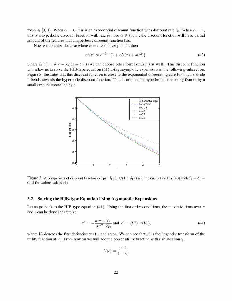
where ∆(τ) = δ0τ − log(1 + δ1τ) (we can choose other forms of ∆(τ) as well). This discount functionwill allow us to solve the HJB-type equation (41) using asymptotic expansions in the following subsection.Figure 3 illustrates that this discount function is close to the exponential discounting case for small ε whileit bends towards the hyperbolic discount function. Thus it mimics the hyperbolic discounting feature by asmall amount controlled by ε.

0 1 2 3 4 50.4

0.5

0.6

0.7

0.8

0.9

1

t

dis

co

un

t ra

te

exponential disc

hyperbolic

ε=0.05

ε=0.1

ε=0.2

ε=0.3

Figure 3: A comparison of discount functions exp(−δ0τ), 1/(1 + δ1τ) and the one defined by (43) with δ0 = δ1 =0.15 for various values of ε.

3.2 Solving the HJB-type Equation Using Asymptotic Expansions

Let us go back to the HJB type equation (41). Using the first order conditions, the maximizations over πand c can be done separately:

π∗ = −µ− rxσ2

VxVxx

and c∗ = (U ′)−1(Vx), (44)

where Vx denotes the first derivative w.r.t x and so on. We can see that c∗ is the Legendre transform of theutility function at Vx. From now on we will adopt a power utility function with risk aversion γ:

U(c) =c1−γ

1− γ,

22

thus we have c∗ = (Vx)−1/γ . We plug π∗ and c∗ into (41) to obtain the following nonlinear non-local PDE:

Vt −λ2

2

V 2x

Vxx+

γ

1− γ(Vx)

γ−1γ + rxVx = −Et,x

[∫ T

tϕ′(s− t)U(c∗s)ds+ ϕ′(T − t)U(Xπ,c∗

T )

], (45)

with boundary conditions V (T, x) = 0 and V (t, 0) = 0.As a consequence of the expansion (43) for the discount function, we seek a similar expansion for the

value function:V (t, x) = V0(t, x) + εV1(t, x) + o(ε2), (46)

which we plug into (45). After grouping terms of different orders, we have the following PDEs for the firsttwo orders:

V0,t −λ2

2

V 20,x

V0,xx+

γ

1− γ(V0,x)

γ−1γ + rxV0,x − δ0V0 = 0,

V1,t −(λ2 V0,x

V0,xx+ (V0,x)

− 1γ − rx

)V1,x +

λ2

2

V 20,x

V 20,xx

V1,xx − δ0V1 = (47)

−Et,x[∫ T

t∆′(s− t) e−δ0(s−t) [c∗0,s(X

(0)s )]1−γ

1− γds+ ∆′(T − t)

(X(0)T )1−γ

1− γ

],

where X(0)s denotes the wealth process under the zeroth order equilibrium investment and consumption

strategies π∗0 and c∗0. The detail of the decomposition of (45) into (47) can be found in the Appendix.

Note The first equation in (47) can be solved in a fairly standard way with the appropriate boundary con-ditions. Once this is solved, we obtain the zeroth order value function as well as the zeroth order strategiesthat will give explicit forms for the parameters of the second equation. As we will see later, the solution tothe second PDE can be found explicitly. We have therefore managed to bypass the “nonlocal” issue in theHJB-type PDE by using asymptotic expansions. This allows us to avoid the usual numerical procedures asseen for example, in [13].

3.2.1 Zeroth Order Solution

The solution to the zeroth order equation with zero terminal & boundary conditions is very well-known.Using separation of variables method, we seek solution V0(t, x) of the following form:

V0(t, x) =x1−γ

1− γ[f(t)]γ . (48)

The original PDE problem reduces to the following ODE problem

f ′(t) +1− γγ

(λ2

2γ+ r

)f(t) + e

δ0γt

= 0, (49)

with f(T ) = 1. Thus we have

f(t) =−eA2t +A3e

A2T+A1(T−t)

A1 +A2(50)

23

where A1 = 1−γγ

(λ2

2γ + r)

, A2 = δ0γ and A3 = A1+A2+eA2T

eA2T. We can also compute the zeroth order

equilibrium strategies:

π∗0 =λ

σγand c∗0 =

x

f(t). (51)

3.2.2 First Order Solution

Using the preceding result, we can simplify the first order PDE from (47) into:

V1,t +

(λ2

γ+ r − 1

)xV1,x +

λ2

2γ2x2V1,xx − δ0V1 = (52)

Et,x

[∫ T

t∆′(s− t)e−δ0(s−t) [c∗0,s(X

(0)s )]1−γ

1− γds+ ∆′(T − t)

(X(0)T )1−γ

1− γ

].

In order to deal with the expectation term on the right side, we need the dynamics of the zeroth order wealthprocess X(0)

t under zeroth order equilibrium strategies:

dX(0)t =

(π∗0(µ− r) + r − f(t)−1

)X

(0)t dt+ π∗0σX

(0)t dWt, (53)

which we notice is a lognormal process and we can write out the expectation term explicitly.It follows that

E0,x

[(X

(0)t )1−γ

1− γ

]=x1−γ

1− γe(1−γ)[π∗0(µ−r)+r−f(t)−1− γ

2π∗20 σ2]t. (54)

Therefore, (52) becomes

V1,t +

(λ2

γ+ r − 1

)xV1,x +

λ2

2γ2x2V1,xx = δ0V1 +

x1−γ

1− γF (t), (55)

where F (t) denotes the integral:

F (t) :=

∫ T

t∆′(s− t)e−δ0(s−t)e(1−γ)[π∗0(µ−r)+r−f(s)−1− γ

2π∗20 σ2]sds.

The ansatz V1(t, x) = x1−γ

1−γ g(t) reduces (55) to a first order ODE problem:

g′(t) +

[(λ2

2γ+ r − 1

)(1− γ)− δ0

]g(t) = F (t), (56)

with terminal condition g(T ) = 0, which has a solution given by:

g(t) =

∫ T

tF (s)eB1(s−t)ds, (57)

where B1 :=(λ2

2γ + r − 1)

(1− γ)− δ0.

24

3.2.3 First Order Corrections for Equilibrium Strategies

Proposition 5. We have the following respective first order corrections (to multiply by ε) to the equilibriumstrategies:

π∗1 = 0 and c∗1 = −1

γ

g(t)

f(t)c∗0. (58)

Proof. We haveV0(t, x) = U(x)f(t) and V1(t, x) = U(x)g(t)

where U(x) is the power utility function with risk aversion γ. For the equilibrium proportion of wealthinvested in the risky asset, we have

π∗ ≈ −µ− rxσ2

V0,x + εV1,x

V0,xx + εV1,xx= −µ− r

xσ2

U ′(x)

U ′′(x)

(f(t) + εg(t))

(f(t) + εg(t))=µ− rγσ2

≡ π∗0,

whereas for the equilibrium consumption rate, we have

c∗ ≈ (V0,x + εV1,x)− 1γ = (V0,x)

− 1γ

[1− ε

γ

V1,x

V0,x+ o(ε2)

]= c∗0

(1− ε

γ

g(t)

f(t)

).

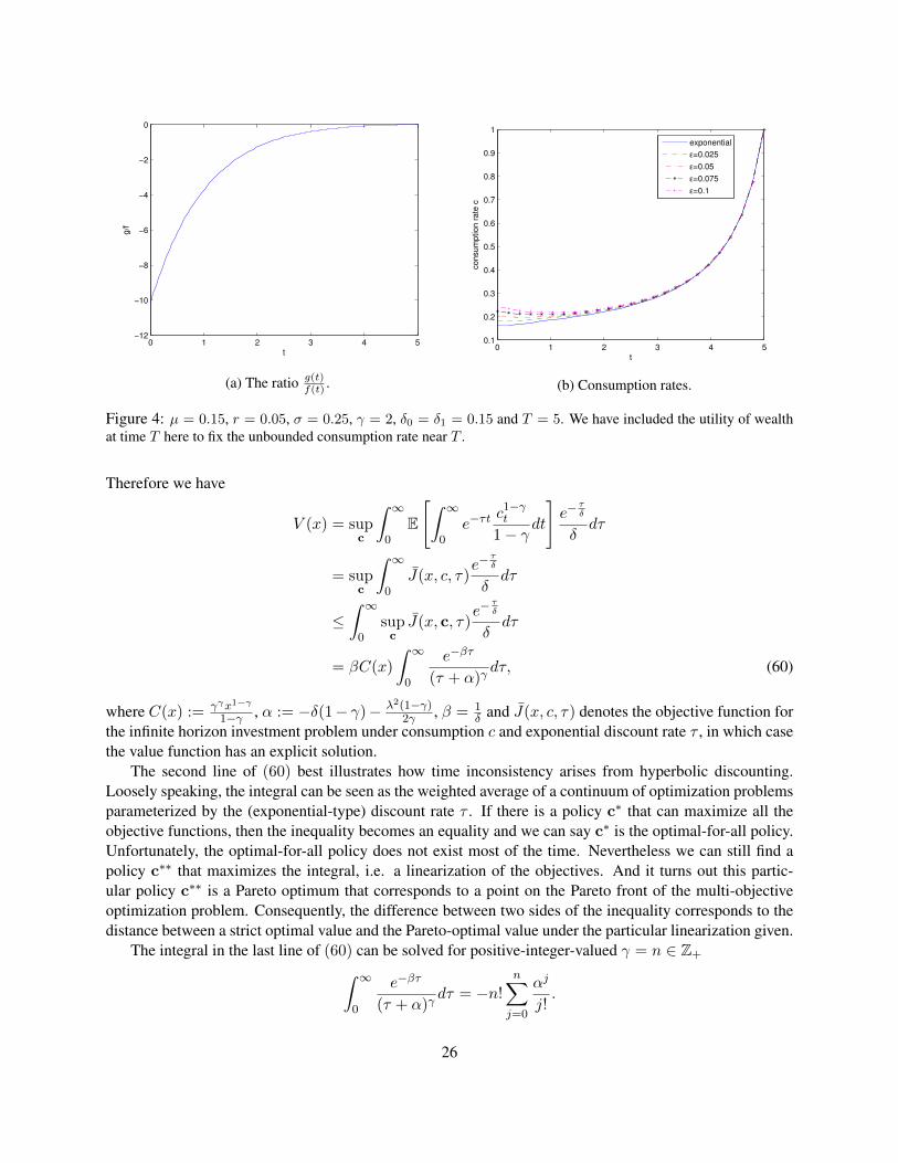
We have found that adding a small amount of hyperbolic-discounting feature to the discount functiondoes not change the proportion of wealth invested in the risky asset, while it will affect the consumption rateby a fraction depending on the ratio g(t)

f(t) . Figure 4 illustrates how the approximated equilibrium strategieschange over time compared to the optimal one in the exponential discounting case. In general, we find thathyperbolic discounting would encourage one to consume at a faster rate. The fact that g(t) is negative alsomeans that the value function is more negative compared to the exponential discounting case, indicating aloss of welfare. For relatively larger values of ε, the equilibrium strategy is clearly non-monotonic. Moreprecisely, the ideal consumption speed starts at some higher level compared to the exponential discountingcase and it has a decreasing trend at the beginning. But eventually the consumption speed will start toincrease monotonically once we are sufficiently far away from the commencing point t = 0. In fact, thisnon-monotonicity feature agrees with the consumption pattern observed in real-life household data, whichis one of the main reasons economists support the use of hyperbolic discounting. We also note that similarresults were obtained in [13] in which the authors made use of backward numerical integration techniquesto solve the full extended HJB equation analogous to (41).

3.3 A Bound for the Value Function: Infinite Horizon Case

In this section we want to illustrate some characteristics of the hyperbolic discounting problem using Laplacetransform. Suppose we have an infinite horizon investment/consumption problem instead:

V (x) = supc

E

[∫ ∞0

1

1 + δt

c1−γt

1− γdt

]. (59)

The following equation holds for the hyperbolic discount function by Laplace transform:

1

1 + δt=

∫ ∞0

e−τ(t+ 1δ

)

δdτ.

25

0 1 2 3 4 5−12

−10

−8

−6

−4

−2

0

t

g/f

(a) The ratio g(t)f(t) .

0 1 2 3 4 50.1

0.2

0.3

0.4

0.5

0.6

0.7

0.8

0.9

1

t

co

nsu

mp

tio

n r

ate

c

exponential

ε=0.025

ε=0.05

ε=0.075

ε=0.1

(b) Consumption rates.

Figure 4: µ = 0.15, r = 0.05, σ = 0.25, γ = 2, δ0 = δ1 = 0.15 and T = 5. We have included the utility of wealthat time T here to fix the unbounded consumption rate near T .

Therefore we have

V (x) = supc

∫ ∞0

E

[∫ ∞0

e−τtc1−γt

1− γdt

]e−

τδ

δdτ

= supc

∫ ∞0

J(x, c, τ)e−

τδ

δdτ

≤∫ ∞

0sup

cJ(x, c, τ)

e−τδ

δdτ

= βC(x)

∫ ∞0

e−βτ

(τ + α)γdτ, (60)

where C(x) := γγx1−γ

1−γ , α := −δ(1− γ)− λ2(1−γ)2γ , β = 1

δ and J(x, c, τ) denotes the objective function forthe infinite horizon investment problem under consumption c and exponential discount rate τ , in which casethe value function has an explicit solution.

The second line of (60) best illustrates how time inconsistency arises from hyperbolic discounting.Loosely speaking, the integral can be seen as the weighted average of a continuum of optimization problemsparameterized by the (exponential-type) discount rate τ . If there is a policy c∗ that can maximize all theobjective functions, then the inequality becomes an equality and we can say c∗ is the optimal-for-all policy.Unfortunately, the optimal-for-all policy does not exist most of the time. Nevertheless we can still find apolicy c∗∗ that maximizes the integral, i.e. a linearization of the objectives. And it turns out this partic-ular policy c∗∗ is a Pareto optimum that corresponds to a point on the Pareto front of the multi-objectiveoptimization problem. Consequently, the difference between two sides of the inequality corresponds to thedistance between a strict optimal value and the Pareto-optimal value under the particular linearization given.

The integral in the last line of (60) can be solved for positive-integer-valued γ = n ∈ Z+∫ ∞0

e−βτ

(τ + α)γdτ = −n!

n∑j=0

αj

j!.

26

Thus we have produced a bound for the value function in case γ is a positive integer

V (x) ≤ −βn!

n∑j=0

αj

j!C(x). (61)

3.4 Extension with Proportional Transaction Costs

We extend our study to the situation where proportional transaction cost exists. The dynamics of the portfoliocan be represented as below:

dX(b)t = (rX

(b)t − ct)dt− (1 + κ)dLt + (1− λ)dMt

dX(s)t = µX

(s)t dt+ σX

(s)t dWt + dLt − dMt, (62)

where X(b)t and X(s)

t represent the wealth in the risk-free bank account and in the risky asset (stock) respec-tively. Again ct is the rate of consumption and dLt := ltdt and dMt := mtdt denote the purchase and sellof the risky asset which will incur proportional transaction costs κ and λ respectively.

Our objective function has now been modified into maximizing consumption utility over an infinitehorizon because we want to make the analysis simpler. The objective function is given by

J(x(b), x(s), c, l, m) = E[∫ ∞

0ϕ(s)U(cs)ds X

(b)0 = x(b) , X

(s)0 = x(s)

], (63)

given the current level of wealth x(b) in the bank account and x(s) in the stock as well as the admissiblecontrols c, m, l, where the utility function U(.) is still chosen to be the power type. Now define the valuefunction:

V (x(b), x(s)) = supc,m,l

J(x(b), x(s), c, l, m). (64)

Almost identical to the result from Proposition 4, the value function satisfies the HJB-type equation:

supc,m,l

(rx(b) − c)Vx(b) + µx(s)Vx(1) +1

2σ2(x(s))2Vx(s)x(s) + [(1− λ)Vx(b) − Vx(s))]m

+ [Vx(1) − (1 + κ)Vx(b) ]l + U(c) = −Ex(b)x(s)[∫ ∞

0ϕ′(s)U(c∗s)ds

],

(65)

only this time there is no time derivative. When ϕ(·) is exponential type, this becomes the HJB equation thatwas probably first derived by Davis and Norman [10], who noticed that the desirable strategies for purchaseand sell were “bang-bang” type which only took place on the boundaries of the no-transaction region atmaximum possible rates.

The homothetic property holds for the value function since we have chosen a power utility function,meaning that

V (ρx(b), ρx(s)) = ρ1−γV (x(b), x(s)), (66)

for any positive constant ρ. Thus we can write the value function V (x(b), x(s)) into

V (x(b), x(s)) = (x(s))1−γV (x(b)/x(s), 1) := (x(s))1−γΦ(x(b)/x(s)). (67)

27

As a consequence, it is sufficient to study the transformed value function Φ(z) where we use z to denote theratio x(b)/x(s).

The problem reduces to a free boundary ODE problem:

(µ− 1

2σ2γ)(1− γ)Φ(z) + (r − µ+ σ2γ)zΦ′(z) +

1

2σ2z2Φ′′(z)

+γ

1− γ[Φ′(z)

]−(1−γ)/γ+ Ez

[∫ ∞0

ϕ′(s)[Φ′(Zs)]

−(1−γ)/γ

1− γds

]= 0, (68)

with free boundary conditions:

Φ′(l)(1− λ+ l)− (1− γ)Φ(l) = 0

Φ′(u)(1 + κ+ u)− (1− γ)Φ(u) = 0, (69)

where the upper and lower boundaries u and l are to be determined. The ODE (68) is difficult to solve

because it involves a free boundary as well as a non-local term Ez[∫∞

0 ϕ′(s) [Φ′(Zs)]−(1−γ)/γ

1−γ ds]

that is thesource of time inconsistency. Again let us deal with it using the asymptotic approximation method. Weassume the same expansion for the discount function ϕ(·) as in (43). And we seek an expansion for thesolution Φ(z) of the following form:

Φ(z) = Φ0(z) + εΦ1(z) + o(ε2). (70)

At zeroth order, we need to solve the free boundary ODE:β0Φ0 + β1zΦ

′0 + β2z

2Φ′′0 +γ

1− γ[Φ′0] γ−1

γ = 0

Φ′0(l0)(1− λ+ l0)− (1− γ)Φ0(l0) = 0

Φ′0(u0)(1 + κ+ u0)− (1− γ)Φ0(u0) = 0,

(71)

with l0, u0 to be determined, where β0, β1 and β2 are constant parameters defined as

β0 := (µ− 1

2σ2γ)(1− γ)− δ0, β1 := r − µ+ σ2γ, β2 :=

1

2σ2.

At first order, we need to solve a fixed boundary ODE problem, but with a nonlocal term:β0Φ1 +

[β1z +

γ

1− γ(Φ′0)

− 1γ

]Φ′1 + β2z

2Φ′′1 + Ez

[∫ ∞0

e−δ0s∆′(s)(Φ′0)

γ−1γ

1− γds

]= 0

Φ′1(l0)(1− λ+ l0)− (1− γ)Φ1(l0) = 0

Φ′1(u0)(1 + κ+ u0)− (1− γ)Φ1(u0) = 0,

(72)

from which we can compute the first order corrections to the NT boundary as

l1 = − (1− λ+ l0)Φ′′1(l0) + γΦ′1(l0)

(1− λ+ l0)Φ′′′0 (l0) + (1 + γ)Φ′′0(l0)

u1 = − (1 + κ+ u0)Φ′′1(u0) + γΦ′1(u0)

(1 + κ+ u0)Φ′′′0 (u0) + (1 + γ)Φ′′0(u0), (73)

which are derived from the original boundary equations.

28

3.4.1 Zeroth Order Solution

The zeroth order problem (71) is exactly the original problem in [10], which has been shown to have asolution that can be written as

Φ0(z) =1

1− γ

[1− γγ

h1(z)

]−γ(

z

h2(z))1−γ , (74)

where h2(z) and h1(z) solve the system below

h′2(z) =1

β2z[R(h2(z))− h1(z)]

h′1(z) =1− γγ

h1(z)

β2zh2(z)[h1(z)−Q(h2(z))] , (75)

with boundary conditions

h2(l0) =l0

l0 + 1− λ, h1(l0) = Q

(l0

l0 + 1− λ

), h2(u0) =

u0

u0 + 1 + κ, h1(u0) = Q

(u0

u0 + 1 + κ

),

where we define Q(x) := − β01−γ − β1x+ β2γx

2 and R(x) := Q(x) + β2(1− x)x. This ODE system (75)can be solved numerically using a shooting method as suggested by [10].

3.4.2 First Order Solution

Recall (72), in order to obtain Φ1(z), we need to solve a fixed boundary ODE, which is numerically straight-forward except for the source term

Ez

[∫ ∞0

e−δ0s∆′(s)(Φ′0(Zs))

γ−1γ

1− γds

],

which involves a path integral depending on the processZt ≡ XtYt

. Note that the major issue here is that we donot have an explicit form for Φ0 as it is computed numerically, whereas the nonlocality issue has disappearedsimilar to the case without transaction cost because of the expansion we have used. To approximate thesource term we reply on Monte Carlo method to generate a large number of sample paths for Zt up to sometime T and evaluate the truncated integral for each of these paths using Riemann-sum approximation, afterwhich the estimated expectation can be obtained by taking the average. We first use Ito’s Lemma to get thedynamics for the process Zs under the zeroth order equilibrium strategies c∗0, dL

∗0 and dM∗0 :

dZt = [(r − µ+σ2

2)Zt − c∗0,t]dt− σZtdWt − (1 + κ+ Zt)dL

∗0,t + (1− λ+ Zt)dM

∗0,t. (76)

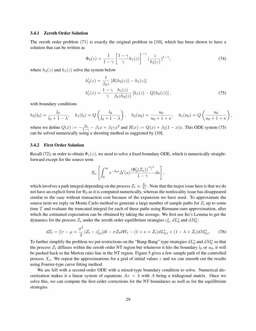
To further simplify the problem we put restrictions on the “Bang-Bang” type strategies dL∗0 and dM∗0 so thatthe process Zt diffuses within the zeroth order NT region but whenever it hits the boundary l0 or u0, it willbe pushed back to the Merton ratio line in the NT region. Figure 5 gives a few sample path of the controlledprocess Xs. We repeat the approximations for a grid of initial values z and we can smooth out the resultsusing Fourier-type curve fitting method.

We are left with a second-order ODE with a mixed-type boundary condition to solve. Numerical dis-cretization makes it a linear system of equations Ax = b with A being a tridiagonal matrix. Once wesolve this, we can compute the first-order corrections for the NT boundaries as well as for the equilibriumstrategies.

29

0 0.2 0.4 0.6 0.8 10.2

0.25

0.3

0.35

0.4

0.45

0.5

0.55

0.6

0.65

t

Zt

(a) Zs, σ = 0.25

0 0.2 0.4 0.6 0.8 11

1.5

2

2.5

t

Zt

(b) Zs, σ = 0.35

Figure 5: Some realizations of Zs with zeroth order optimal consumption rate c∗0 and boundaries l0 and u0.Note that each time the process hits the boundaries, it will be pushed back to the Merton line inside the NTregion.

3.4.3 Numerical Results

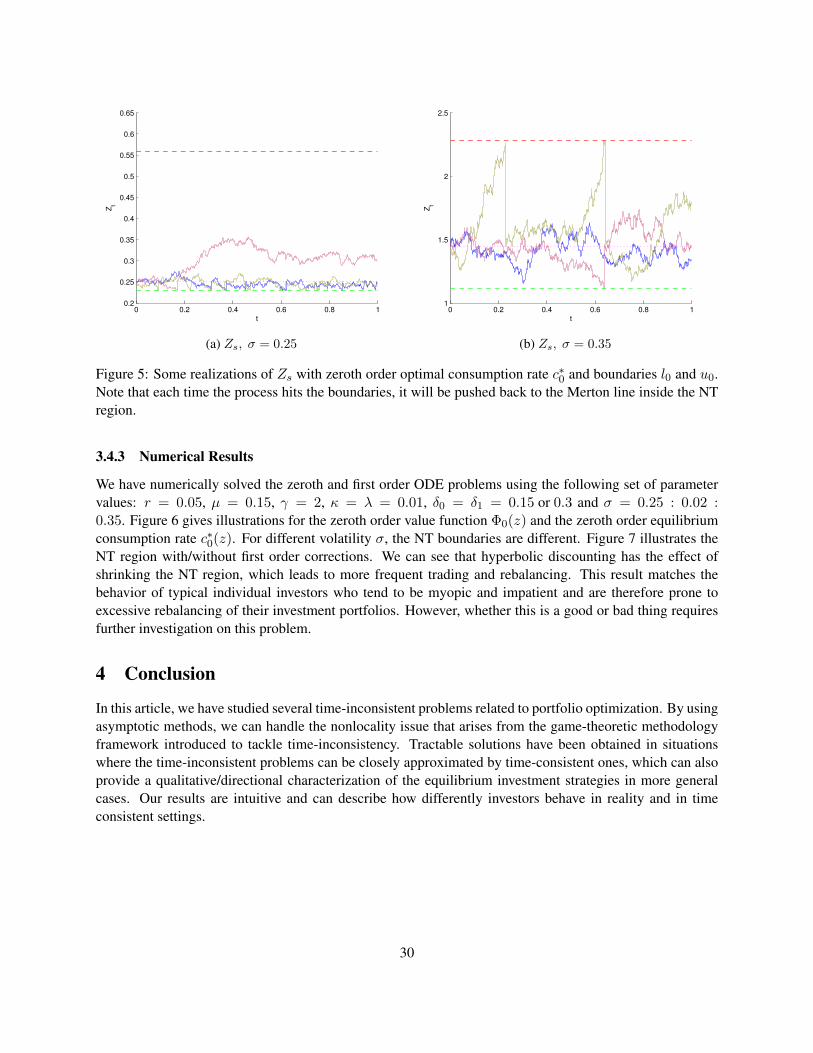
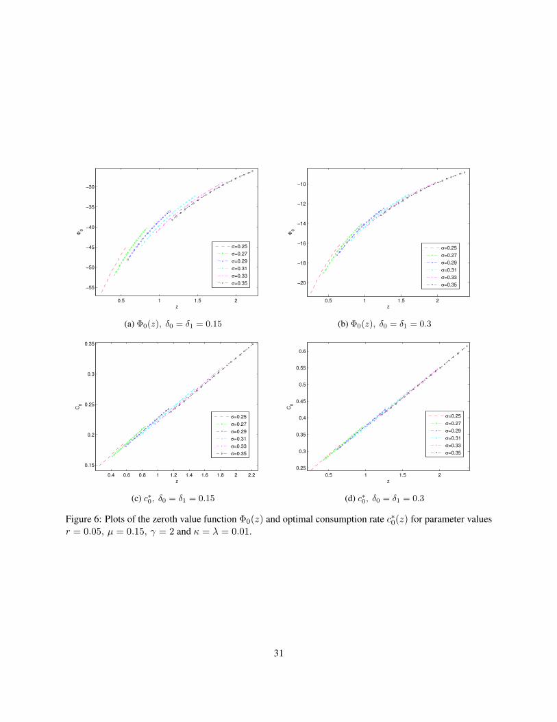
We have numerically solved the zeroth and first order ODE problems using the following set of parametervalues: r = 0.05, µ = 0.15, γ = 2, κ = λ = 0.01, δ0 = δ1 = 0.15 or 0.3 and σ = 0.25 : 0.02 :0.35. Figure 6 gives illustrations for the zeroth order value function Φ0(z) and the zeroth order equilibriumconsumption rate c∗0(z). For different volatility σ, the NT boundaries are different. Figure 7 illustrates theNT region with/without first order corrections. We can see that hyperbolic discounting has the effect ofshrinking the NT region, which leads to more frequent trading and rebalancing. This result matches thebehavior of typical individual investors who tend to be myopic and impatient and are therefore prone toexcessive rebalancing of their investment portfolios. However, whether this is a good or bad thing requiresfurther investigation on this problem.

4 Conclusion

In this article, we have studied several time-inconsistent problems related to portfolio optimization. By usingasymptotic methods, we can handle the nonlocality issue that arises from the game-theoretic methodologyframework introduced to tackle time-inconsistency. Tractable solutions have been obtained in situationswhere the time-inconsistent problems can be closely approximated by time-consistent ones, which can alsoprovide a qualitative/directional characterization of the equilibrium investment strategies in more generalcases. Our results are intuitive and can describe how differently investors behave in reality and in timeconsistent settings.

30

0.5 1 1.5 2

−55

−50

−45

−40

−35

−30

z

Φ0

σ=0.25

σ=0.27

σ=0.29

σ=0.31

σ=0.33

σ=0.35

(a) Φ0(z), δ0 = δ1 = 0.15

0.5 1 1.5 2

−20

−18

−16

−14

−12

−10

z

Φ0

σ=0.25

σ=0.27

σ=0.29

σ=0.31

σ=0.33

σ=0.35

(b) Φ0(z), δ0 = δ1 = 0.3

0.4 0.6 0.8 1 1.2 1.4 1.6 1.8 2 2.2

0.15

0.2

0.25

0.3

0.35

z

C0

σ=0.25

σ=0.27

σ=0.29

σ=0.31

σ=0.33

σ=0.35

(c) c∗0, δ0 = δ1 = 0.15

0.5 1 1.5 2

0.25

0.3

0.35

0.4

0.45

0.5

0.55

0.6

z

C0

σ=0.25

σ=0.27

σ=0.29

σ=0.31

σ=0.33

σ=0.35

(d) c∗0, δ0 = δ1 = 0.3

Figure 6: Plots of the zeroth value function Φ0(z) and optimal consumption rate c∗0(z) for parameter valuesr = 0.05, µ = 0.15, γ = 2 and κ = λ = 0.01.

31

0.25 0.3 0.350

0.5

1

1.5

2

2.5

σ

z

l0

u0

l0+0.005l

1

u0+0.005u

1

(a) δ0 = δ1 = 0.15

0.25 0.3 0.350

0.5

1

1.5

2

2.5

σ

z

l0

u0

l0+0.005l

1

u0+0.005u

1

(b) δ0 = δ1 = 0.3

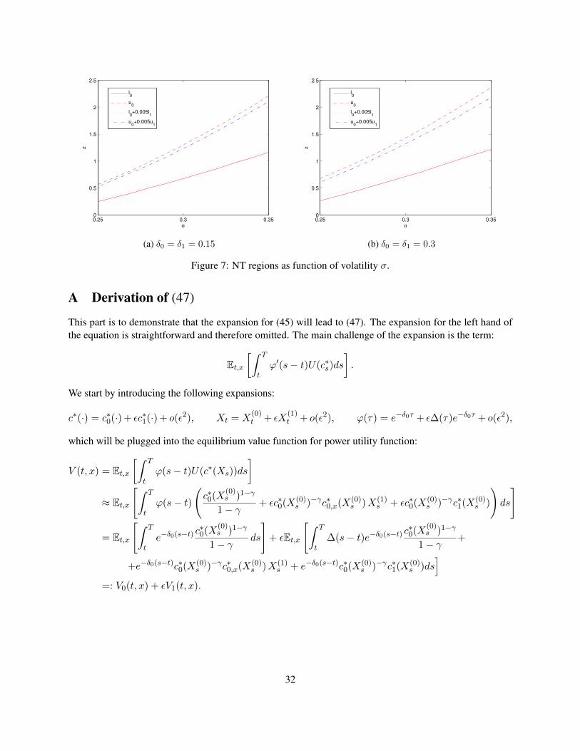
Figure 7: NT regions as function of volatility σ.

A Derivation of (47)

This part is to demonstrate that the expansion for (45) will lead to (47). The expansion for the left hand ofthe equation is straightforward and therefore omitted. The main challenge of the expansion is the term:

Et,x[∫ T

tϕ′(s− t)U(c∗s)ds

].

We start by introducing the following expansions:

c∗(·) = c∗0(·) + εc∗1(·) + o(ε2), Xt = X(0)t + εX

(1)t + o(ε2), ϕ(τ) = e−δ0τ + ε∆(τ)e−δ0τ + o(ε2),

which will be plugged into the equilibrium value function for power utility function:

V (t, x) = Et,x[∫ T

tϕ(s− t)U(c∗(Xs))ds

]≈ Et,x

[∫ T

tϕ(s− t)

(c∗0(X

(0)s )1−γ

1− γ+ εc∗0(X(0)

s )−γc∗0,x(X(0)s )X(1)

s + εc∗0(X(0)s )−γc∗1(X(0)

s )

)ds

]

= Et,x

[∫ T

te−δ0(s−t) c

∗0(X

(0)s )1−γ

1− γds

]+ εEt,x

[∫ T

t∆(s− t)e−δ0(s−t) c

∗0(X

(0)s )1−γ

1− γ+

+e−δ0(s−t)c∗0(X(0)s )−γc∗0,x(X(0)

s )X(1)s + e−δ0(s−t)c∗0(X(0)

s )−γc∗1(X(0)s )ds

]=: V0(t, x) + εV1(t, x).

32

This leads to the expansion:

Et,x[∫ T

tϕ′(s− t)U(c∗s)ds

]≈− δ0Et,x

[∫ T

te−δ0(s−t) c

∗0(X

(0)s )1−γ

1− γds

]− εδ0Et,x

[∫ T

t∆(s− t)e−δ0(s−t) c

∗0(X

(0)s )1−γ

1− γ+

+e−δ0(s−t)c∗0(X(0)s )−γc∗0,x(X(0)

s )X(1)s + e−δ0(s−t)c∗0(X(0)

s )−γc∗1(X(0)s )ds

]+

+ εEt,x

[∫ T

t∆′(s− t)e−δ0(s−t) [c∗0,s(X

(0)s )]1−γ

1− γds

]

=− δ0V0 − εδ0V1 + εEt,x

[∫ T

t∆′(s− t)e−δ0(s−t) [c∗0,s(X

(0)s )]1−γ

1− γds

],

of which the zeroth order term will go into the RHS of the first equation in (47) and the remaining two termswill go into the V1 equation.

References[1] T. Bjork and A. Murgoci. A general theory of markovian time inconsistent stochastic control problems. Preprint,

2010.

[2] T. Bjork, A. Murgoci, and X. Zhou. Mean–variance portfolio optimization with state-dependent risk aversion.Mathematical Finance, 2012.

[3] B. Bouchard, L. Moreau, and M. H. Soner. Hedging under an expected loss constraint with small transactioncosts. arXiv preprint arXiv:1309.4916, 2013.

[4] J. Y. Campbell and L. M. Viceira. Consumption and portfolio decisions when expected returns are time varying.The Quarterly Journal of Economics, 114(2):433–495, 1999.

[5] R. Carmona. Indifference Pricing: Theory and Applications. Princeton Series in Financial Engineering. Prince-ton University Press, 2008.

[6] G. Chacko and L. M. Viceira. Dynamic consumption and portfolio choice with stochastic volatility in incompletemarkets. Review of Financial Studies, 18(4):1369–1402, 2005.

[7] P. Cheridito and M. Kupper. Composition of time-consistent dynamic monetary risk measures in discrete time.International Journal of Theoretical and Applied Finance, 14(01):137–162, 2011.

[8] M. Chernov, A. Ronald Gallant, E. Ghysels, and G. Tauchen. Alternative models for stock price dynamics.Journal of Econometrics, 116(1):225–257, 2003.

[9] V. Coudert and M. Gex. Does risk aversion drive financial crises? testing the predictive power of empiricalindicators. Journal of Empirical Finance, 15(2):167–184, 2008.

[10] M. H. Davis and A. R. Norman. Portfolio selection with transaction costs. Mathematics of Operations Research,15(4):676–713, 1990.

[11] I. Ekeland and A. Lazrak. Being serious about non-commitment: subgame perfect equilibrium in continuoustime. arXiv preprint math/0604264, 2006.

[12] I. Ekeland and A. Lazrak. Equilibrium policies when preferences are time inconsistent. arXiv preprintarXiv:0808.3790, 2008.

33

[13] I. Ekeland, O. Mbodji, and T. A. Pirvu. Time-consistent portfolio management. SIAM Journal on FinancialMathematics, 3(1):1–32, 2012.

[14] J.-P. Fouque, G. Papanicolaou, R. Sircar, and K. Solna. Multiscale Stochastic Volatility for Equity, Interest Rate,and Credit Derivatives. Cambridge University Press, 2011.

[15] J.-P. Fouque, R. Sircar, and T. Zariphopoulou. Portfolio optimization & stochastic volatility asymptotics.Preprint, 2013.

[16] C. Harris and D. Laibson. Dynamic choices of hyperbolic consumers. Econometrica, 69(4):935–957, 2001.

[17] C. J. Harris and D. Laibson. Hyperbolic discounting and consumption. In M. Dewatripont, L. P. Hansen, andS. Turnovsky, editors, Advances in Economics and Econometrics: Theory and Applications, Volume 1, pages258–298. Eighth World Congress, 2002.

[18] Y. Hu, H. Jin, and X. Y. Zhou. Time-inconsistent stochastic linear–quadratic control. SIAM Journal on Controland Optimization, 50(3):1548–1572, 2012.

[19] J. Hull and A. White. The Pricing of Options on Assets with Stochastic Volatilities. Journal of Finance,42(2):281–300, June 1987.

[20] E. Karni. Risk aversion for state-dependent utility functions: Measurement and applications. InternationalEconomic Review, 24(3):pp. 637–647, 1983.

[21] T. C. Koopmans. Stationary ordinal utility and impatience. Econometrica: Journal of the Econometric Society,pages 287–309, 1960.

[22] H. Kraft. Optimal portfolios and Heston’s stochastic volatility model: an explicit solution for power utility.Quantitative Finance, 5(3):303–313, 2005.

[23] G. Loewenstein and D. Prelec. Anomalies in intertemporal choice: Evidence and an interpretation. The QuarterlyJournal of Economics, 107(2):573–597, 1992.

[24] R. Merton. Continuous-Time Finance. Wiley, 1992.

[25] H. Pham. Continuous-time Stochastic Control and Optimization with Financial Applications. Springer, 2009.

[26] T. A. Pirvu and H. Zhang. Utility indifference pricing: A time consistent approach. Applied MathematicalFinance, 20(4):304–326, 2013.

[27] M. Scheicher. What drives investor risk aversion? daily evidence from the german equity market. BIS QuarterlyReview, pages 67–74, 2003.

[28] S. Shreve and H. Soner. Optimal investment and consumption with transaction costs. Ann. Appl. Prob., 4:609–692, 1994.

[29] R. H. Strotz. Myopia and inconsistency in dynamic utility maximization. The Review of Economic Studies, pages165–180, 1955.

[30] N. Tarashev, K. Tsatsaronis, and D. Karampatos. Investors’ attitude towards risk: what can we learn fromoptions? BIS Quarterly Review, 6:57–65, 2003.

[31] J. A. Wachter. Portfolio and consumption decisions under mean-reverting returns: An exact solution for completemarkets. Journal of financial and quantitative analysis, 37(01):63–91, 2002.

34