Time simulation of squeal phenomena in realistic brakemodels

G. Vermot des Roches1,2, E. Balmes1,2, T. Pasquet3, R. Lemaire3

1 Ecole Centrale Paris, Laboratoire MSS-MAT, CNRS UMR 8579Grande Voie des Vignes, 92295, Chatenay-Malabry, France2 SDTools44, Rue Vergniaud, 75013, Paris, Francevermot@sdtools.com balmes@sdtools.com3 Bosch (Chassis Systems Brakes),126, Rue de Stalingrad, 93700, Drancy, FranceThierry.Pasquet@fr.bosch.com Remi.Lemaire@fr.bosch.com

AbstractThis paper presents a modeling strategy employed to obtain converged results on long time simulation ofcomplex finite element brake models. First a novel reduction method, adapted to models showing largeinterface DOF, is presented. The small finite element area in the vicinity of the contact is treated as fullynon-linear and while the remaining of the structure is represented by a superelement. The method is thussuited for large finite element models. A time integration scheme, based on a non-linear Newmark, is thenadapted to allow large models to be computed over long time periods. This is achieved mainly by the use of afixed iteration operator throughout the simulation. This technique is applied first to a simplified brake modelfor validation purposes, then to a state-of-the-art brake model designed by Bosch Chassis Brake Systems.The simulation results are put in perspective with recent publications on the subject.

Introduction

The work presented in this paper seeks to introduce time simulation of brake instabilities on industrial brakemodels. Brake squeal corresponds to instabilities that generate high frequency vibrations (from 1 to 16 kHz)leading to unpleasant noises up to 120 dB in the brake vicinity, at low speed, low pressure braking caseswhich mostly happen in urban areas. Although the brake efficiency is not challenged, brake squeal is an im-portant source of negative customer feedback and therefore needs to be avoided. In addition, new constraintson brake design involve strong weight restrictions and efficiency improvement so that squeal occurrences areeven more difficult to handle.

The current industrial practice in numerical simulation for brake squeal is the study of complex mode stability[1, 2, 3]. This considers a linearization of the system equations around a stationary static state and evaluatesstability in the sense of Lyapunov.

One of the drawbacks of these methods is that unstable complex modes only provide potential unstablemodes. In the best case, only some of these modes are actually found to generate squeal instabilities. Timesimulations have the potential to really describe the non-linear oscillations found after the instability inducesa divergence from the stationary static state. They can thus be expected to allow an effective discriminationbetween the modes that are effectively leading to instabilities and those that are not destabilized in practice.Such method was successfully applied to train brake models in [2] by tracking unstable complex modescontribution to the time response.

Previous work on the time simulation of squeal (see [4, 2] for example) has been focused on somewhatsimplified models, which do not account for the full geometrical complexity of actual brakes. Experimentson real brakes do however show a strong sensitivity on the actual brake configuration: details of the padgeometry, spring connectors, ... The first objective of this work is thus to introduce a practical methodologyto allow time simulations for brake models that have high levels of details. The associated model reductionmethodology is introduced in section 1.

The second issue is linked to the time integration over long intervals of problems with contact and friction.Treating non-linear systems usually challenges the convergence results obtained with linear systems, asshown in [5]. The use of a modified non-linear Newmark scheme adapted to contact formulations presentedin section 2 has two main advantages. It allows larger than usual models (50,000 DOF) to be treated over200,000 time steps. It also solves some of the convergence issues encountered with more classical schemes.In particular, the ’bouncing behavior’ of the basic Newmark scheme is addressed. These results are illustratedusing a simplified brake model as a demonstrator. Eventually, section 3 presents numerical results of squealsimulation on the industrial brake model provided by Bosch Chassis Brake Systems.

The proposed methodology is validated on both simplified and realistic brake models shown in figure 1.The simplified model consists of a cylindrical disc, with two cylindrical section shaped pads. The pads areguided in vertical translation at both edges, the disc is linked to the ground by springs fixed at the centralinner nodes. A uniform pressure is applied to the pad backplates. The model shown is meshed using 8 nodehexahedrons but other shapes and incompatible meshes have also been considered.

The realistic brake model conforms to a design from Bosch. It is composed of 8 components, the disc, outerand inner pads, anchor, caliper, piston, hub and knuckle modeled using the finite element method. Sincebrake squeal can reach high frequencies, the mesh is rather fine, which leads to approximately 600,000 DOF.The different components are in contact with each other and an exponential contact force is assumed. Theparts too small to model such as the hub bearing, the pad springs, piston seal and boots are replaced byequivalent stiffness.

Figure 1: Finite element models of a simplified and a realistic brake

1 Reduction method for a system with local non-linearities

This section presents a novel reduction method adapted for finite elements models showing large interfaces.Indeed, classical reduction methods usually keep the interface DOF explicitly, thus generating potentiallylarge full blocks in the resulting system matrices. This proves to be computationally inefficient and motivatesthe introduction of a method implicitly eliminating interface DOFs.

Component Mode Synthesis methods have traditionally been based on the assumptions [6] of componentindependence (reduction of a component is performed without knowing the others), static solution capability(static responses to applicable loads, in particular interface loads, are included explicitly), explicit boundarycoordinates (in order to ease direct stiffness assembly).

When these methods were developed in the 70’s, the objectives were linked to numerical performance andthe ability to couple test and analysis models. The context of the proposed application is quite different. Theobjective is to reproduce the dynamics and steady state static response of the full brake model as closelyas possible, while retaining the ability to account for the local non-linearities in the model. In applicationto brake squeal the disc/pad contact area is of great importance since it is the location where the instabilityoriginates. One thus chooses to keep all DOFs qc of elements connected to the contact area explicitly, asshown in figure 2.

To achieve the first objective, one proposes to use a Rayleigh-Ritz method that use full system modes φ1:NM

and the steady state response q0 as assumed shapes. To be compatible with the retention of all contact areaDOFs, the modes are only are only assumed on DOFs qb of the reduced part. In other words one considersthe reduced basis {

qbqc

}=

[[[φ1:NM ]b q0b] 0

0 [I]c

]{qrqc

}(1)

A Craig-Bampton reduction would proceed very differently. The DOFs to be retained explicitly would bedivided in two sets: ci for those part of elements connected to the reduced area and cc for those purelyinternal to the unreduced part of the model. The reduction would then consider

qbqciqcc

=

[φFixed] −K−1cc Kcci 0

0 I 00 0 I

qrqciqcc

(2)

(a) Superelement (b) Finite element area

Figure 2: Brake model split in SE and kept area

In the present case, 250 modes, corresponding to a 20 kHz cutoff, are kept for the superelement reduction.In figure 3 one clearly distinguishes DOFs associated to the unreduced part of the disk, the two pads andthe reduced component. The contact stiffness terms clearly couple the disk and the pads. With reductionbasis (1), the reduced component is coupled with the unreduced part on the b, c block, which is small (251 :the number of considered modes + one static shape). In the Craig-Bampton approach, figure 3b, the couplingoccurs for the ci, cc block which for linear tetra4 elements already represents 1765 elements (11,200 fortetra10). A clear advantage is obtained in terms of memory. The number of non null terms increases from 1million with the new method to 8 millions with the classical Craig Bampton.

(a) New (b) Craig-Bampton

Figure 3: Reduced matrix topologies for the tetra4 model. Left proposed reduction. Right : Craig-Bamptonreduction

Another advantage of the proposed reduction is that the real modes of the full model and the ones of thereduced model are theoretically identical. Here, a slight error is introduced in the realistic brake model dueto differences in the contact handling between the Abaqus static step and the SDT time integration.

2 Time integration of the non-linear contact/friction model

Many numerical applications of contact resolution methods are targeting relatively small models. The opti-mization needed to handle large models has specificities which need to be addressed. This section presentsthe models, the contact and friction laws, a non-linear modified Newmark scheme based on [7] put in thecontact perspective and eventually the damping strategy.

2.1 Contact laws

In a mechanical assembly, the components are in physical contact with each other. Penetration is defined asthe relative displacement along the normal N of master and slave surfaces with a possible offset g0

{g} = N.(uslave − umaster)− {g0} (3)

The Signorini contact law represents the normal contact behavior between two solids and is plotted in fig-ure 4a. The ideal Signorini contact shows no penetration and repulsive contact forces, written as a pressurep {N}, which are null when no contact occurs

g ≤ 0p ≤ 0

(g).(p) = 0(4)

An exact implementation of the Signorini equations can be obtained with a Lagrange formulation that keepsthe contact forces as unknowns and solves a coupled displacement/force problem. This method is not chosen

here due to the increased DOF number for a large contact area and the difficulty to implement it properlyin dynamics. An solution would however be the non-smooth contact dynamics method suggested in [8] andapplied successfully for brake squeal simulation in [2].

Penalization methods introduce a relationship between the gap and the contact pressures. An exponentiallaw is considered here,

p(g) = p0e−λg (5)

In brakes, rough surfaces are contacting. A Signorini contact would thus be an idealization valid for very stiffcontact stiffness between the asperities. The exponential contact law is another idealization and it is quitedifficult to rank their relative validity. Experiments have however led Bosch to consider that p0 = 10−2MPaand λ = 750mm−1 are realistic values for disk/pad contact. The perspective that this exponential law is aregularization of the Signorini contact law is classical, but not necessarily valid here.

(a) Signorini (b) Exponential normal contact law versuslinear contact law

Figure 4: Contact laws, Signorini and regularizations

This contact formulation is applied to a finite element model by pairing a master surface which containscontact integration points and a slave surface. The contact points of the master surface are paired withthe nodes of the slave surface to define the model displacement formulation. The contact forces are useddirectly in the formulation (section 2.3). They are computed at the integration points using Gauss weightingcoefficient and the element contact force density.

{q}T {fN} =∫{u}T NpdS '

∑j

{u}T {N} p(xj , q)ωjJ(xj) (6)

where fN is the global contact force, p the contact pressure, xj are the integration points, q a virtual dis-placement, q the displacement and J(xj) the jacobian of the shape transformation (surface associated withintegration point).

At a contact integration point, a contact stiffness can be defined as the derivative of the contact pressure

kc(g) =∂p

∂g= λp0e

−λg (7)

This leads to a contact stiffness matrix given by

{q} [Kc] {q} =∫{u(q)}T {N}λp0e

−λg {u(q)}T {N} dS'

∑j {u}

T {u(q)}T {N}λp0e−λg {u(q)}T {N}ωjJ(xj)

(8)

2.2 Friction laws

The Coulomb law describes the tangential contact behavior in the presence of friction. The sliding velocityws is defined as the relative speed between the two bodies in contact. the contact force is split into a normalcontact force FN and a tangential contact force FT that one links using the friction coefficient µ.

{‖FT ‖ ≤ µ‖FN‖ ws = 0‖FT ‖ = µ‖FN‖ ∃A ≥ 0, ws = −AFT

(9)

(a) Coulomb (b) Regularized Coulomb

Figure 5: The Coulomb contact laws

In application to brake squeal, a monodirectional contact force, along θ in cylindrical coordinates, is com-puted. The Coulomb law is regularized by assuming a permanent sliding state, and penalizing small slidingvelocities as shown in figure 5b and written as{

‖FT ‖ = kt‖ws‖ if ‖ws‖ < µkt

‖FT ‖ = µ‖FN‖ else(10)

Actual materials used in the car industry show a friction coefficient of µ = 0.6 which was used for this study.The choice of kt is still opened, it was taken as kt = 50s−1.

2.3 Time integration scheme

A modification of the non linear, displacement based, Newmark scheme presented in Ref. [7] is consideredhere. The scheme, shown in figure 6, is classically divided in an external time incrementation loop with aprediction phase and an internal non linear correction phase. The Newmark coefficients noted β = 1

4 andγ = 1

2 are kept as usual.

The correction phase is performed with a Newton scheme where the residual (14) is computed with thecontact forces FN and FT and the correction is given by (15). In a standard Newton scheme, the Jacobiancorresponds to sensitivity of the residual with respect to a change in the unknown, taken here to be theposition,

[J(q)] =∂r

∂δq= [Kel] + [Kc(q)] +

γ

βh[C] +

1βh2

[M ] (11)

Time Incrementation

tn+1 = tn + h (12)

?Prediction

q0n+1 = qn + hqn + h2(12 − β)qn

˙q0n+1 = qn + h(1− γ)qn¨q0n+1 = 0

(13)

?Correction

r(qkn+1) = − [Kel] qkn+1 − [C] qkn+1 − [M ] qkn+1

+fc + FN ((q, q)kn+1) + FT ((q, q)kn+1)(14)

[J ] {∆q} = rk (15)qk+1n+1 = qkn+1 + ∆qqk+1n+1 = qkn+1 + γ

βh∆qqk+1n+1 = qkn+1 + 1

βh2 ∆q(16)

?

Convergence ?

‖rk+1‖‖fc‖

≤ ε (17)

‖∆q‖‖q‖

≤ εq (18)

�����

PPPPP�����

PPPP

P

yes

�

no

-

Figure 6: Non-linear Newmark scheme

Considering a variable jacobian [J ] is impractical. The reduced brake model presented in section 1 hasaround 50,000 DOF, and 200,000 time steps are needed. Since the best jacobian factorization time for suchmatrix is of the order of 10 seconds, even a single factorization by time step would require over a thousandhours of computation. Besides, the very soft behavior of the exponential contact law shown in figure 4b maycause divergence for low overclosures.

The Newton scheme is thus modified to use a constant jacobian. In (11), one introduces a constant referencecontact stiffness by replacing [Kc(q)] by kc [Kc], where [Kc] is the contact coupling matrix for a unity contactstiffness. The scalar value of the contact stiffness kc is then optimized to ensure convergence speed.

The adjustment of kc is illustrated, in figure 7, for the simplified brake model and an exponential law (pre-sented in section 2.1). For a small kc, divergence (set at 200 iterations) occurs. As kc is increased oscillationsare found. This can be linked to examples given in the litterature (e.g. in [5]) of bouncing effects when theintegration scheme fails to converge without explicitely diverging. An optimum kc value clearly appears inthe second graph of figure 7, just after convergence is met.

Although the jacobian has to be optimized, its effect is mostly observed during the static computation. In-deed, the time steps used for a squeal simulation are very low, which combined to the displacement incrementconvergence criterium, yields a limited number of Newton iterations. Getting the right order for kc is usuallyenough. The value used for the realistic brake model is 185 MPa.

Figure 7: Static state convergence as function of kc on a simplified brake model

A posteriori, it was found that the optimum value is close to the average tangent stiffness value at the equilib-rium. Since the jacobian is constant, it corresponds to the direct path to the solution. The contact distributionis not evenly distributed so a few iterations are still needed to find the real contact distribution from anaveraged state.

The convergence criterion (17) is another key point since a poor choice may lead to numerous costly Newtoniteration when the displacement is close to the solution. An alternative is to combine it with a displacementconvergence test in equation (18), which considers that convergence is achieved if a negligible Newton dis-placement increment happens. In most cases, it decreases the number of Newton iteration needed by timestep, but it must be used carefully since it overrides the verification of the mechanical equilibrium (equa-tion (14)). In practice, a convergence criterion on the displacement increment was chosen with a toleranceof εq = 10−6.

2.4 Damping

Using a Rayleigh damping formulation, the notion of contact damping can be introduced. The contactstiffness can be segragated from the stiffness matrix and therefore be applied a specific coefficient.

[C] = a [M ] + b [Kel] + b [Kc] (19)

where [M ], [C], [Kel], [Kc] are respectively the mass, damping, elastic stiffness and contact stiffness matri-ces, a = 0, b = 2.12 10−7 and b = 0 are parameters set here for only high frequency damping.

The use of (19) yields the jacobian formulation used in this paper, written in equation (20). No numericaldamping is used.

[J ] =(

1 +γb

βh

)[Kel] + kc

(1 +

γb

βh

)[Kc] +

(1βh2

+γa

βh

)[M ] (20)

Contact damping is stated to be of importance in [2], none was used in the presented study since it did notcorrelate to any obvious physical meaning.

3 Time simulation results

This section presents squeal simulations obtained with a simplified brake for convergence validations and arealistic brake. The results are related to common phenomena observed in other works.

3.1 Validations on a simplified brake model

The simplified brake model illustrated in the introduction is meshed in 8 nodes hexahedrons elements. Thedisc and backplate are elastic isotropic, the lining is transverse anisotropic, using the materials of the realisticbrake. To trigger the instability, a pressure shock is applied at the beginning of the simulation (a 10%overpressure during the first 10−5s). A friction coeffcient of 0.25 is applied.

The time scheme convergenge is assumed when reducing the time step does not change the solution. Figure 8and 9a shows that for dt ≤ 10−7s, the time responses are perfectly overlaying. This time step will be keptfor the next simulations.

Figure 8: Time simulation on the simple model, as function of the time step

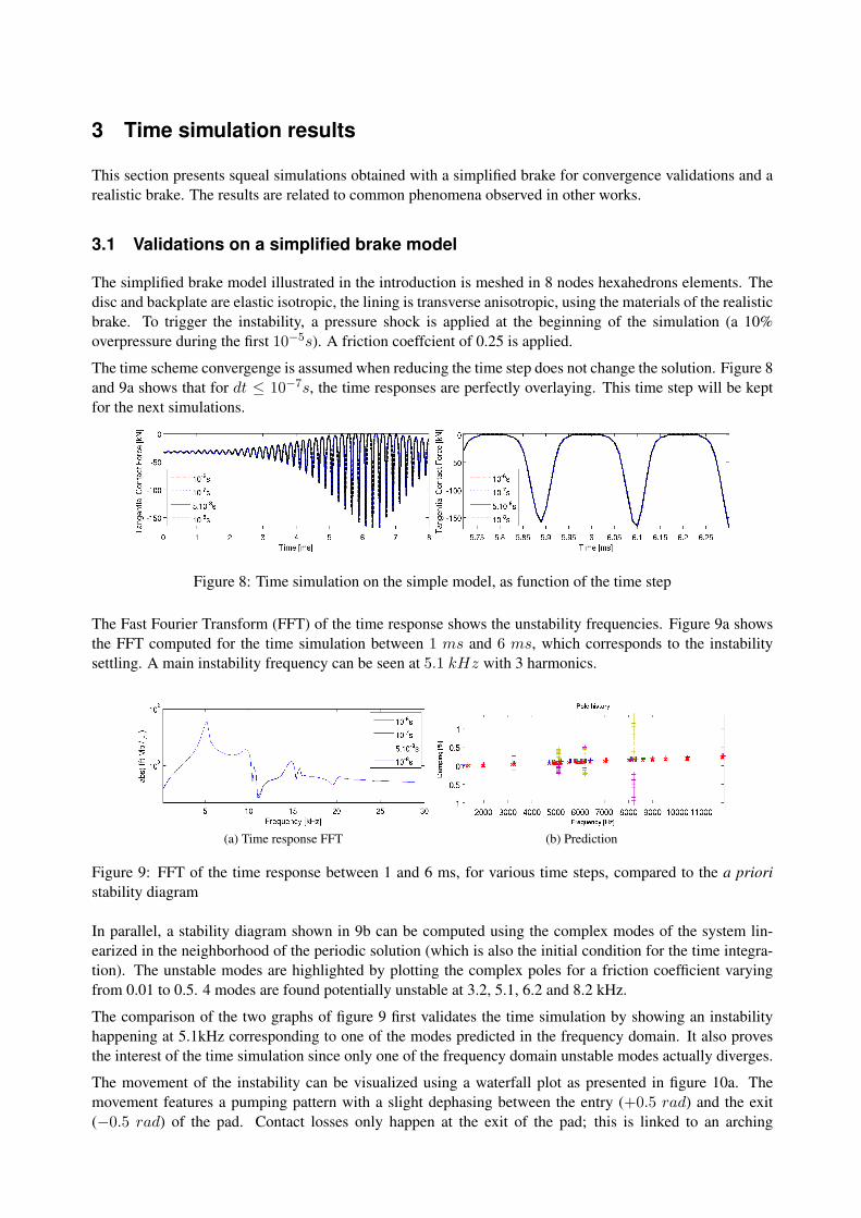
The Fast Fourier Transform (FFT) of the time response shows the unstability frequencies. Figure 9a showsthe FFT computed for the time simulation between 1 ms and 6 ms, which corresponds to the instabilitysettling. A main instability frequency can be seen at 5.1 kHz with 3 harmonics.

(a) Time response FFT (b) Prediction

Figure 9: FFT of the time response between 1 and 6 ms, for various time steps, compared to the a prioristability diagram

In parallel, a stability diagram shown in 9b can be computed using the complex modes of the system lin-earized in the neighborhood of the periodic solution (which is also the initial condition for the time integra-tion). The unstable modes are highlighted by plotting the complex poles for a friction coefficient varyingfrom 0.01 to 0.5. 4 modes are found potentially unstable at 3.2, 5.1, 6.2 and 8.2 kHz.

The comparison of the two graphs of figure 9 first validates the time simulation by showing an instabilityhappening at 5.1kHz corresponding to one of the modes predicted in the frequency domain. It also provesthe interest of the time simulation since only one of the frequency domain unstable modes actually diverges.

The movement of the instability can be visualized using a waterfall plot as presented in figure 10a. Themovement features a pumping pattern with a slight dephasing between the entry (+0.5 rad) and the exit(−0.5 rad) of the pad. Contact losses only happen at the exit of the pad; this is linked to an arching

phenomenon due to the disc rotation. Indeed the contact pressure is higher at the disc entry than at theexit, which

(a) Time instability, mean pressure over a radius as function ofthe angle

(b) Unstable mode at 5.1 kHz

Figure 10: Pattern of the unstable mode found in the time simulation

3.2 Realistic brake simulation results

The real brake presented in 1 is meshed using 10 nodes tetrahedron elements. The friction braking pressure isset at 5 bar, and the disc angular velocity at 5 rad s−1 the fiction coefficient is set at 0.6. The results presentedin this section took 12 hours of computation (equally divided between displacement incrementation andresidue computation). The use of the mkl library from intel has already cut the computation time by 30 %.The braking torque was taken as a reference signal to detect instability. Figure 11 shows the braking torqueand the global friction coefficient.

Figure 11: Result of the squeal simulation: braking torque and global friction coefficient

The braking torque shows the common limit cycle instability type. The stable periodic solution transitsthrough an exponential divergence phase before the amplitude range settles to a bounded value. The globalfriction coefficient was computed; it is not constant. It is the ratio of the normal contact force resultant andthe tangential force resultant over time. Although the local coefficient is set constant at 0.6, the measuredµ can decrease due to the loss of contact caused by the vibrations. This was also observed in [4]. Anotherillustration is given in figure 12 where the tangential contact force at an integration contact point is plotted.

Figure 12 highlights stick/slip transition by showing the sign switching of the contact force at a contactintegration point. The stick property is not really implemented in the system although low sliding velocities

are penalized, it does not account properly for the phenomenon and yields very quick slip velocity directionswitching.

Figure 12: Tangential contact force at an intergration contact point

The frequency of instability is happening at 30 Khz, which is higher than the cutoff frequency retained for thesuperelement. Besides, there is very low damping in the system, it comes only from the Rayleigh damping,set a 1% at 15kHz. More damping must in fact be taken into account regarding the viscoelasticity of thelining material, the contact damping, the stick states, or the numerical high frequency damping. Their effectneeds to be studied to obtain a better insight of the squeal instability.

Eventually, the precision of the static state input needs to be very accurate due to the use of an exponentialcontact law. At high contact pressures, coarse round-off errors should be avoided however, such accuracywas not achieved due to handling difficulties using Abaqus 6.6-1. Figure 13 shows the difference between thecontact distribution proposed by Abaqus and SDT. Both solutions are computed from the static displacementoutput by Abaqus. The Abaqus solution corresponds to the contact forces recovered using the elastic stiffnessmatrix (without interaction) also output by Abaqus. The SDT solution corresponds to the contact forcescomputed from the Abaqus static displacement by using the analytical exponential contact law prosposed insection 2.1 and the usual finite element shape function for 6 points triangles, using three contact integrationpoints placed at the Gauss points.

Figure 13: Differences between SDT and Abaqus. Contact points sorted by incresing value of the SDTsolution, contact forces in N

None of the solutions shown are regular but great differences exists. In particular an outlier is detected in theAbaqus normal contact force solution. A lot of noise is seen on the tangential force with oscillations at thelow contact area higher than the maximum contact force. This low level of accuracy obtained for the initialcondition is also believed to play a role in the convergence difficulties experimented with the realistic brakemodel.

Conclusion

This paper has proposed a time simulation of brake squeal applied to industrial brake models. First a novelreduction strategy was proposed to combine a non reduced finite element part around the pad/disc contactarea and the superelement containing the system’s remains. This method allows the interface DOF to beimplicitely eliminated, thus avoiding large full blocks patterns obtained with a classical Craig-Bamptonapproach. Besides, the full and reduced real modes are identical. An improvement which may prove to benecessary is the implementation of a residual mode for precision; an automatic method is being developpedto deal with some Abaqus implementation issues.

The time integration scheme proposed solves some common convergence issues acknowlegded for the non-linear Newmark scheme. However, the brake instability caught in the time simulation is much higher thanexpected, and it has been found that the combination of a basic regularization of the Coulomb law (per-manent sliding state, quick transitions) and the modified Newmark could yield numerical instabilities. Thedevelopement of a Lagrangian tangential contact formulation is under developement to improve the stickmodel. This would generate an hybrid contact law, using an exponential penalization formulation for thenormal contact law, and a Lagrangian formulation for the tangential one. From the time integration point ofview, alternative schemes will be tested in particular the modified θ-method originally proposed in [8] andadapted in [2].

Further development will imply the implementation of richer damping models. Although litterature concern-ing damping in time simulation is usually limited to numerical damping and Rayleigh damping, models fromthe frequency domain will be studied. First, time domain modal damping will be treated allowing to spreadthe damping to other interfaces in the superelement. It is based on the mass normalization of the modesconstituting the reduction basis to recover the full damping matrix.

Viscoelastic damping will also be addressed to enrich mode pad lining material model. Such behavior hasbeen acknowledged for this material only taken as elastic transverse anisotropic in this study. The formu-lation will be different from the one used in the frequency domain since the use of an imaginary matrix isimpossible; a formulation featuring relaxation times would be preferred. Eventually, friction damping willbe studied; its importance is highlighted in [2] for example, and a basic realization is suggested in this paper.Again, such damping will be prone to stabilize the stick/slip transitions by penalizing the sliding velocity.

References

[1] F. Moirot Study of stability of an equilibrium in presence of Coulomb’s friction. Application to disc brakesqueal ph.D Thesis (1998).

[2] X. Lorang, Instabilite vibratoire des structures en contact frottant: Application au crissement des freinsde TGV, ph.D Thesis (2007).

[3] G. Fritz, J-J. Sinou, J-M. Duffal, L. Jezequel, Investigation of the relationship between damping andmode-coupling patterns in case of brake squeal, Journal of Sound and Vibration, 6 November 2007,voluem 307, Issues 3-5, Pages 591-609.

[4] V. Linck, Modelisation numerique temporelle d’un contact frottant. Mise en evidence d’instabilites lo-cales de contact - Consequences tribologiques, ph.D Thesis (2005).

[5] B. Magnain, Z-Q. Feng, J-M. Cros, Schema d’integration adapte aux problemes d’impact, ComptesRendus Mecanique, Volume 333, Issue 5, May 2005, Pages 419-424.

[6] R. Jr. Craig A review of time-domain and frequency domain component mode synthesis methods Int. J.Anal. and Exp. Modal Analysis, 1987, Volume 1, Pages 59-72.

[7] M. Geradin, D. Rixen, Mechanical Vibrations : Theory and Applications to Structural Dynamics, WileyInterscience, Second edition, 1996.

[8] M. Jean, The non-smooth contact dynamics method, Computer Methods in Applied Mechanics and En-gineering, 20 July 1999, Volume 177, Issues 3-4, Pages 235-357.