time table generation system
TRANSCRIPT

THE UNIVERSITY OF ZAMBIA
SCHOOL OF NATURAL SCIENCES
DEPARTMENT OF COMPUTER STUDIES
TIME TABLE GENERATION
SYSTEM
BY
ANDREW BIEMBA
SUPERVISOR
MRS. LEENA KUMAR.
CSC 4004 FINAL YEAR PROJECT

i
TIME TABLE GENERATION SYSTEM
By
Andrew Biemba
A thesis submitted in partial fulfillment of the
requirements for the Degree of
Bachelor of Science in Computer Science.
The Department Of Computer Studies
The University Of Zambia
August 2014.

ii
DECLARATION
I, the undersigned here, declare that this dissertation is entirely my own original work and
that, to the best of my knowledge, it has not been presented or submitted for any degree
or examination in any other university, and that all the sources I have used or quoted have
been indicated and acknowledged by complete references.
Author: Andrew Biemba Computer Number: 10059563
Signature: ……………………………… Date: …………………………
PROJECT SUPERVISOR
Name: Mrs. Leena Kumar.
Signature: ………………………………… Date: …………………………

iii
ACKNOWLEDGEMENTS
First and foremost, I wish to thank the Supreme Being, God Almighty, for enabling me to
come this far and making everything possible for the project to be a success. In times of
despair, when I was almost giving up, Jehovah gave me renewed hope and insight, He
granted me the strength and courage to go on. For this, He deserves all the praise and
glory.
I would like to express my sincere gratitude to my project supervisor, Mrs. L. Kumar, for
the direction, guidance, help, support and invaluable advice. I would also like to extend
special gratitude to my father, Mr. C. Biemba Snr., for the financial assistance rendered
towards me during my stay at UNZA from day one and to my mother, Mrs. D. Biemba,
for the love, care, moral and spiritual support during my entire stay at campus. Mum and
dad, I am indebted to you. My siblings (Carol, Jack, Jane, Harriet, Henry, Lexinah and
Memory), your prayers and best wishes have seen me through this. Finally, I give some
special thanks to classmates I consulted from when I reached an impasse.

iv
DEDICATION
This work is dedicated to my late brother, Chrispin Biemba Jr. who really wanted to
pursue a career in Computer Science but time was insufficient for him on this earth. The
pain my family and I went through was too much to handle and compelled me to do
something that would make him look down on me and smile where he is now.
This is also for my mother, father, brothers and sisters who so unconditionally love me
and have always believed in my abilities from inception. I will always reserve a special
place for them in my heart. May God bless them all!

v
ABSTRACT
Timetabling is the allocation, subject to constraints, of given resources to objects in
space-time domain to satisfy a set of desirable objectives as nearly as possible.
Particularly, the university timetabling problem for classes or lectures can be viewed as
fixing in time and space a sequence of meetings between instructors and students, while
simultaneously satisfying a number of various essential conditions or constraints.
The timetabling problem concerns virtually every educational institution, be it high
school, college, or university and thus requires to be solved effectively. This is usually
done ‘by hand’, taking several days or weeks of iterative repair after feedback from
lecturers complaining that the timetable is unfair to them in some way.
The basic challenge is to schedule lectures over a limited time period so as to avoid
conflicts and to satisfy a number of side constraints. The problem, in its simplest form, is
one of assigning lectures to periods and rooms such that either no conflicts or a minimum
number of conflicts occur. By "conflicts", I mean when a lecture is scheduled to be
lectured in two or more places at the same time or when two or more lectures are
scheduled to be lectured in one place at the same time. Computer timetabling and
administration systems do exist to ease this burden but each timetabling problem is as
individual as the institution from which it originates.
In this project, a program that uses an optimal algorithm is to be developed that provides
a solution to the lecture timetabling problem. The system, to be developed in Java,
Microsoft Access and an XML Knowledge Base, is a replacement of the traditional
manual way used to create lecture timetables. The system will be tested using input from
various departments at the University of Zambia. Ideally, the system is expected to be
generic and thus accommodate various sets of requirements and be able to work in other
universities and colleges.
vi
This system aims to schedule different lectures given a set of classrooms, lecture theatres,
halls or labs in a specified time frame, say for instance, from 08:00 hours in the morning
to 17:00 hours in the afternoon from Monday to Friday. Lunch break or any other break
can be easily set, say from 13:00 to 14:00 hours according to a user’s preference. It will
take various inputs like details of students or student groups, courses, classrooms/halls
and lecturers available. Depending upon these inputs, it will generate a possible time
table which can be exported to html or pdf, making optimal utilization of all resources in
a way that will best suit any of the constraints or university rules. The system will have
room for extension/expansion and shall be able to accommodate as many requirements as
possible.
The system is expected to produce significantly better timetables than those that were
actually employed (produced by hand), and should always take a considerably short
period of time to generate them. The application will provide an easy, time-saving way to
generate lecture timetables within given constraints.

vii
LIST OF ACRONYMS
CLP Constraint Logic Programming.
DBMS Database Management System.
DSATUR Degree of Saturation.
GB Giga Byte.
GHz Giga Hertz.
GraphML Graph Markup Language.
GUI Graphical User Interface.
HCI Human Computer Interaction.
HTML HyperText Markup Language.
IDE Integrated Development Environment.
IP Integer Programming.
JDBC Java Database Connectivity.
JDK Java Development Kit.
JNA Java Native Access.
JNI Java Native Interface.
JVM Java Virtual Machine.
KB Knowledge Base.
LP Linear Programming.
MathML Mathematical Markup Language.
MB Mega Byte.
Ms Microsoft.
MusicXML Music Extensible Markup Language.
NP Non-deterministic Polynomial-time.
ODBC Open Database Connectivity.
PDF Portable Document Format.
PM Probability of Mutation.
PR Probability of Crossover.
PROLOG Program Logistics/Programming in Logic.
RAM Random Access Memory.
RAPS Review of Automated Personnel System.
RIA Rich Internet Application.
RSS Rich Site Summary.
RUP Rational Unified Process.
SGML Standard Generalized Markup Language.
TTGS Time Table Generation System.
UML Unified Modeling Language.
UP Unified Process.
USDP Unified Software Development Process.
VDU Visual Display Unit.
VGA Video Graphics Array.
W3C World Wide Web Consortium.
XHTML Extensible HyperText Markup language.
XML Extensible Markup Language.

viii
TABLE OF CONTENTS
TIME TABLE GENERATION SYSTEM ...................................................................................... i DECLARATION ......................................................................................................................ii ACKNOWLEDGEMENTS ....................................................................................................... iii DEDICATION ........................................................................................................................ iv
ABSTRACT ............................................................................................................................. v
LIST OF ACRONYMS ............................................................................................................ vii TABLE OF CONTENTS......................................................................................................... viii LIST OF FIGURES .................................................................................................................. xi LIST OF TABLES .................................................................................................................. xiii 1 CHAPTER ONE: INTRODUCTION .................................................................................. 1
1.1 INTRODUCTION ....................................................................................................... 1
1.2 MOTIVATION ........................................................................................................... 2
1.3 PROBLEM STATEMENT ............................................................................................ 3
1.4 AIM .......................................................................................................................... 3
1.5 OBJECTIVES ............................................................................................................. 3
1.6 SCOPE ...................................................................................................................... 3
1.7 EXPECTED BENEFITS ................................................................................................ 4
1.8 REQUIREMENTS ...................................................................................................... 4
1.8.1 HARDWARE REQUIREMENTS (SYSTEM CONFIGURATION) ............................. 4
1.8.2 SOFTWARE REQUIREMENTS (DEVELOPER TOOLS) ......................................... 5
1.8.3 USER TOOLS .................................................................................................... 5
1.8.4 TOOLS FOR DOCUMENTATION ....................................................................... 5
1.8.5 METHODOLOGY .............................................................................................. 5
1.8.6 ARCHITECTURE ................................................................................................ 5
1.9 CONSTRAINTS.......................................................................................................... 6
2 CHAPTER TWO: LITERATURE REVIEW ......................................................................... 8
2.1 TIMETABLE SOLUTION GENERATION ALGORITHMS ............................................. 10
2.1.1 GRAPH COLORING ALGORITHMS .................................................................. 10
2.1.2 TABU SEARCH ................................................................................................ 11
2.1.3 SIMULATED ANNEALING ............................................................................... 12
2.1.4 GENETIC ALGORITHMS ................................................................................. 13
2.1.5 TILING ALGORITHMS ..................................................................................... 14
2.1.6 AGENTS ......................................................................................................... 14
2.1.7 LINEAR/INTEGER PROGRAMMING ............................................................... 15
2.1.8 DIRECT HEURISTICS ....................................................................................... 16
2.1.9 NETWORK FLOW TECHNIQUES ..................................................................... 17
2.1.10 LOGIC PROGRAMMING APPROACH .............................................................. 18
2.1.11 CONSTRAINT-BASED APPROACH .................................................................. 19

ix
2.1.12 COMBINATION OF METHODS ....................................................................... 20
2.1.13 RULE-BASED APPROACH ............................................................................... 20
2.1.14 CONSTRAINT LOGIC PROGRAMMING APPROACH ........................................ 22
3 CHAPTER THREE: METHODOLOGY ............................................................................ 23
3.1 THE RATIONAL UNIFIED PROCESS (RUP)............................................................... 23
3.1.1 ITERATIONS ................................................................................................... 23
3.1.2 INCREMENTAL ............................................................................................... 25
3.1.3 WHY RUP? ..................................................................................................... 25
3.1.4 UP BEST PRACTICES ....................................................................................... 25
3.1.5 ADVANTAGES OF RUP ................................................................................... 26
4 CHAPTER FOUR: SYSTEM ANALYSIS .......................................................................... 27
4.1 JAVA ...................................................................................................................... 27
4.1.1 DETAILS ABOUT JAVA .................................................................................... 27
4.1.2 PLATFORM INDEPENDENCE .......................................................................... 27
4.2 XML ....................................................................................................................... 27
4.2.1 ADVANTAGES OF XML................................................................................... 28
4.3 DATA STRUCTURE & FLOW DIAGRAM .................................................................. 29
4.4 FLOW OF DATA WITHIN THE PROJECT .................................................................. 30
4.5 FUNCTIONAL REQUIREMENTS .............................................................................. 31
4.5.1 USE CASE DIAGRAM ...................................................................................... 31
4.6 NON-FUNCTIONAL REQUIREMENTS ..................................................................... 32
4.6.1 PRODUCT REQUIREMENTS ........................................................................... 32
4.6.2 ORGANIZATIONAL REQUIREMENTS .............................................................. 34
4.6.3 HARDWARE REQUIREMENTS ........................................................................ 34
4.6.4 EXTERNAL REQUIREMENTS ........................................................................... 35
5 CHAPTER FIVE: SYSTEM DESIGN ............................................................................... 36
5.1 PROPOSED SYSTEM ............................................................................................... 36
5.2 TTGS FEATURES ..................................................................................................... 37
5.3 CLASS DIAGRAM .................................................................................................... 40
5.4 LOGIN TABLE ......................................................................................................... 42
6 CHAPTER SIX: IMPLEMENTATION ............................................................................. 43
6.1 XML KNOWLEDGEBASE ......................................................................................... 43
6.2 USER INTERFACE CODE ......................................................................................... 44
6.3 OUTPUT GENERATOR CODE.................................................................................. 46
6.4 TIMETABLE GENERATOR CODE ............................................................................. 47
7 CHAPTER SEVEN: TESTING AND RESULTS ................................................................. 50
7.1 TESTING STRATEGIES ............................................................................................ 50
7.1.1 UNIT TESTING ................................................................................................ 50
7.1.2 INTEGRATION TESTING ................................................................................. 50
7.1.3 SYSTEM TESTING ........................................................................................... 51
7.2 EXTERNAL INTERFACES ......................................................................................... 51

x
7.2.1 USER INTERFACE DESCRIPTION AND CHARACTERISTICS .............................. 51
7.3 SCREEN SHOT OF TTGS ......................................................................................... 52
7.3.1 HOME SCREEN .............................................................................................. 52
7.3.2 TTGS SYSTEM SCREEN ................................................................................... 55
7.3.3 TIMETABLE VIEW SCREEN ............................................................................. 63
7.4 TEST CASES ............................................................................................................ 67
7.4.1 TEST CASE 1: LOGIN SCREEN ......................................................................... 67
7.4.2 TEST CASE 2: COMPUTER STUDIES DEPARTMENT. ....................................... 68
8 CHAPTER EIGHT: CONCLUSION ................................................................................. 69
8.1 CHALLENGES ......................................................................................................... 69
8.2 CONCLUSION ......................................................................................................... 69
8.3 FUTURE WORK ...................................................................................................... 70
8.4 RECOMMENDATIONS ........................................................................................... 70
9 REFERENCES .............................................................................................................. 72
10 APPENDIX .................................................................................................................. 75
10.1 APPENDIX A: MAIN ALGORITHM .......................................................................... 75
10.2 APPENDIX B: GANTT CHART .................................................................................. 77
10.3 APPENDIX C: HOW TO RUN THE PROGRAM ......................................................... 78
10.3.1 PROCEDURE: ................................................................................................. 78

xi
LIST OF FIGURES
Figure 1: The iterations and the phases............................................................................. 24
Figure 2: Iterations in RUP ............................................................................................... 24
Figure 3: Data Structure. ...................................................................................................29
Figure 4: Flow of Data within project............................................................................... 30
Figure 5: Use Case Diagram ............................................................................................. 31
Figure 6: Proposed System ............................................................................................... 37
Figure 7: Timetable Generation Process ........................................................................... 38
Figure 8: General View of TTGS. .................................................................................... 39
Figure 9: Class Diagram 1 ................................................................................................ 40
Figure 10: Class Diagram 2 .............................................................................................. 41
Figure 11: temp.ttgs.xml - XML Knowledgebase ............................................................ 43
Figure 12: TTGS Main Class ............................................................................................ 44
Figure 13: Matrix3D Class................................................................................................ 45
Figure 14: Output Generator - Export to HTML file. ....................................................... 46
Figure 15: TTGS Main Algorithm Code .......................................................................... 47
Figure 16: TTGS Activity Generation .............................................................................. 48
Figure 17: TTGS Placement of activity ............................................................................ 49
Figure 18: Home Screen ................................................................................................... 53
Figure 19: Login Screen.................................................................................................... 54
Figure 20: TTGS System Screen showing the main menu ............................................... 55
Figure 21: Lecturer Manager Screen ................................................................................ 56
Figure 22: Timeslot Manager Screen ................................................................................ 57
Figure 23: Subject-Student Assignment ........................................................................... 58
Figure 24: Course - Lecturer Assignment ......................................................................... 59
Figure 25: Activity Manager Screen ................................................................................. 60
Figure 26: Rules Manager Screen ..................................................................................... 61
Figure 27: Timetable Generation ...................................................................................... 62
Figure 28: Teacher Timetable View ................................................................................. 63
Figure 29: Student Timetable View .................................................................................. 64

xii
Figure 30: Room Timetable View .................................................................................... 65
Figure 31: Timetables Export to HTML ........................................................................... 66

xiii
LIST OF TABLES
Table 1: Datasheet View of the Login Table…………………………………………….42
Table 2: Design View of the Login Table……………………………………………….42
Table 3: Test Case for the Login Screen…….…………………….……………………..67
Table 4: Computer Studies Dept. work load……………………………..………………68

1
1 CHAPTER ONE: INTRODUCTION
1.1 INTRODUCTION
Time table scheduling has been in human requirements since they thought of managing time
effectively. It is widely used in schools, colleges and other fields of teaching and working like crash
courses, couching centers, training programs etc. In the early days, time table scheduling was done
manually with a single person or some group involved in the task of scheduling it with their hands,
which takes a lot of effort and time. Scheduling even the smallest constraints can take a lot of time
and the case is even worse when the number of constraints or the amount of data to deal with
increases. In such cases, a perfectly designed time table is reused for the whole generation without
any changes, proving to be dull in such situations. Other cases that can cause problems is when the
number of employers or workers is weak, resulting in rescheduling of the time table or they will
need to fill on empty seats urgently.
Academic Institutions (Schools, Colleges, Universities, etc.) are the regular users of such time tables.
They need to schedule their courses to meet the need of current duration and facilities that are
available to them. However, their schedule should meet the requirement of new course addition and
newly enrolled students to fresh batches. This may result in rescheduling the entire time table once
again for its entire batches and to be scheduled in the shortest possible time before the batch courses
start.
Timetable generation is an NP-hard problem .i.e. there is no specific algorithm which can be used
for creating timetables. As constraints for timetables vary from institute to institute, a separate
algorithm has to be defined for each one of them. To get the best performance out of our algorithms,
we allot slots to subjects in such a way that either they get their final positions or remain unalloted
which is allotted later after other subjects are allotted. Also the arrangement of teachers plays a
major role in the methodology to be used as most of the subject constraints as well as teachers are
validated while assigning teachers.
Basically, this problem depends on the lecture-room, lecturer-lecture relations. Solution of this
problem is to schedule all lectures in a timetable by considering the rooms/labs/lecture theatres that

2
will be used and the lectures that will be offered. This problem has some specific constraints. In
literature they are known as “hard‟ and “soft‟ constraints. Hard constraints are important and they
have to be satisfied in order to have a feasible solution. Soft constraints do not have to be satisfied
but they make the solution more applicable.
The timetable problem can be categorized into various types (e.g., rail timetable, examination
timetable, school timetable, course timetable etc.) by considering different specific constraints,
processes and resources. The particular instance chosen for implementation in this project is the
lecture timetable. The lecture timetable problem is to organize Subject, Teacher, Room, and Period
in order to satisfy the set of constraints. The problem formulation is as follows:
Set of subjects S = {s1, s2,…, sn}
Set of teachers T = {t1, t2, …, tm}
Set of rooms R = {r1, r2, …, ro}
Set of periods P = {p1, p2,… pk}
A combination (a, b, c, d) in which a є S, b є T, c є R, d є P, can be stated as “teacher b teaches
subject a in room c during period d”. The relation of subjects and teachers are fixed in all tuples. The
lecture timetable problem can be interpreted as the scheduled rooms and periods in tuples and the
solution of this problem is a set of tuples which satisfy all constraints.
Assigning lectures to time periods is equivalent to the graph colouring problem. This is one of the
approaches or algorithms that shall be investigated. Another approach, a heuristic algorithm, will
also be looked at in great detail.
1.2 MOTIVATION
The motivation to develop this Timetable Generation System came from the fact that Lecture
Timetable Scheduling is still mostly done manually due to its inherent difficulties. Universities,
colleges, high schools and other academic institutions are supposed to make time tables for each
semester or term. Manually creating timetables is a very boring, tedious and a pain staking job.
Hence the project’s idea to computerize this hectic process.
3
1.3 PROBLEM STATEMENT
The manual solution of the timetabling problem usually requires many person-days of work. In
addition, the solution obtained may be unsatisfactory in some respect.
How can lectures be scheduled or assigned to periods and rooms over a limited time period such that
either no conflicts or a minimum number of conflicts occur and to satisfy a number of side
constraints?
1.4 AIM
The aim of this project is to develop a simple, easily understandable and efficient program using an
effective and optimal algorithm, which automatically generates good quality time tables within
seconds, while considering all constraints and violating none of the hard constraints.
1.5 OBJECTIVES
• To use the timetabling problem of various departments at the University of Zambia
(UNZA) to investigate the process of solving a real world problem.
• To minimize or completely avoid conflicts or clashes, which occur when lectures involve
common students, common lecturers or require the same classrooms/labs/halls.
• To research on various types of timetabling problem algorithms and determine the most
efficient, effective, fastest and optimal algorithm.
1.6 SCOPE
The project is particularly focused on tackling the school lecture timetabling problem and will not
consider exam scheduling. It will be tested in various departments at the University of Zambia and

4
thus will consider varying requirements depending on the type of courses, lecturers, rooms and labs
associated with a concerned department.
Efforts were put in place to ensure that the system developed is generic enough to accommodate the
varying constraints that come along with each specific academic institution. With this system, there
is no need to modify or redesign the algorithm for any particular institution. Therefore, this system is
expected to work for most if not all departments at the University of Zambia and many other
universities and colleges.
1.7 EXPECTED BENEFITS
The system to be developed is expected to generate conflict free timetables (while satisfying all the
hard constraints concerned) in less time (just a matter of seconds), with less effort and with more
efficiency. It will allow users to work on and view time tables in different platforms and view
different information simultaneously. It will have a simple interface and hence will be so easy to use.
1.8 REQUIREMENTS
Included in this section are the minimum requirements a computer system should have in order to
make this software system work. This software works fine in any operating system in which the
developer tools or the user tools can be installed. So usually the requirement specification will be
same as that of the operating system. So a standard specification will be provided.
1.8.1 HARDWARE REQUIREMENTS (SYSTEM CONFIGURATION)
Processor: minimum 1 GHz x86/x64 processor, Pentium III or higher.
RAM: 512 MB or more.
5 GB of hard-drive space.
Monitor (Screen/VDU) to display output.
Keyboard/Mouse for data input.

5
1.8.2 SOFTWARE REQUIREMENTS (DEVELOPER TOOLS)
Operating System: Windows XP or Newer
Front end: Java
Back end : Microsoft Access, XML Knowledge Base, JDBC - To - ODBC Bridge.
IDE: Eclipse IDE with Sun's/Oracle Java Development Kit (JDK).
1.8.3 USER TOOLS
Sun's/Oracle Java Run Time Environment.
Ms Access, ODBC connector.
1.8.4 TOOLS FOR DOCUMENTATION
Microsoft Word 2013.
Visual Paradigms For UML (Community Edition).
Microsoft Project 2007.
XML Notepad 2007.
1.8.5 METHODOLOGY
Rational Unified Process (RUP)
1.8.6 ARCHITECTURE
Three-tier Client-Server Architecture.

6
1.9 CONSTRAINTS
The lecture timetabling problem consists of scheduling all lectures of a set of courses into a weekly
timetable, where each lecture of a course must be assigned a period and a room in accordance with a
given set of constraints. In this problem, constraints are considered in two types. One of them is
called hard constraints. Hard constraints are those constraints that must be met by the timetable in
order for the lecture timetable to be feasible. For example, there should not be any clashes, i.e.
lecturers should not be required to be in two different rooms at the same time. Every acceptable
timetable must satisfy these constraints. On the other hand, there are some conditions that are
considered helpful but not essential in a good timetable. The more these conditions are satisfied, the
better the timetable will be. They are called soft constraints and therefore they will have a weight in
the objective function. Soft constraints are constraints that we would like the timetable to satisfy, but
can be broken if necessary. For example, lectures must be well spaced over the timetable. It is highly
unlikely that all the soft constraints will be met by a timetable as those are usually contradictory. All
hard constraints must be strictly satisfied and the number of soft constraint violations should be
minimized. A feasible timetable is one in which all lectures have been scheduled at a period and a
room, so that the hard constraints are satisfied. The four hard constraints H1∼H4 and four soft
constraints S1∼S4 are defined as follows:
• H1. Lectures. All lectures of a course must be scheduled to a distinct period and a room.
• H2. Room Occupancy. Any two lectures cannot be assigned in the same period and the
same room.
• H3. Conflicts. Lectures of courses in the same curriculum or taught by the same teacher
cannot be scheduled in the same period, i.e., any period cannot have an overlapping of
students or teachers.
• H4. Availability. If the teacher of a course is not available at a given period, then no
lectures of the course can be assigned to that period.
• S1. Room Capacity. For each lecture, the number of students attending the course should
not be greater than the capacity of the room hosting the lecture.
• S2. Room Stability. All lectures of a course should be scheduled at the same room. If
this is impossible, the number of occupied rooms should be as few as possible.

7
• S3. Minimum Working Days. The lectures of a course should be spread into the given
minimum number of days.
• S4. Curriculum Compactness. For a given curriculum, a violation is counted if there is
one lecture not adjacent to any other lecture belonging to the same curriculum within the
same day, which means the agenda of students should be as compact as possible.

8
2 CHAPTER TWO: LITERATURE REVIEW
A large number of variants of the timetabling problem have been proposed in the literature, which
differ from each other based on the type of institution (university or school) involved and the type of
constraints. We classify the timetabling problems into three main classes:
School timetabling: The weekly scheduling for all the classes of a school, avoiding teachers
meeting two classes at the same time, and vice versa;
Course timetabling: The weekly scheduling for all the lectures of a set of university courses,
minimizing the overlaps of lectures of courses having common students;
Examination timetabling: The scheduling for the exams of a set of university courses,
avoiding overlap of exams of courses having common students, and spreading the exams for
the students as much as possible.
Based on this classification, we develop a separate discussion for each of the three problems and we
devote a section to each of them. However, such classification is not strict, in the sense that there are
some specific problems that can fall between two classes, and cannot be easily placed within the
above classification. For example, the timetabling of a specific school which gives large freedom to
the student regarding the set of courses can be similar to a course timetabling problem (A. Schaerf,
1999).
In some cases, the timetabling problem consists of finding any timetable that satisfies all the
constraints. In these cases, the problem is formulated as a search problem. In other cases, the
problem is formulated as an optimization problem. That is, what is required is a timetable that
satisfies all the hard constraints and minimizes (or maximizes) a given objective function which
embeds the soft constraints. As shown later, in some approaches, the optimization formulation is just
a means to apply optimization techniques to a search problem. In this case, what is minimized is the
so-called distance to feasibility. Even when the problem is a true optimization problem, the distance
to feasibility may be included in the objective function. This is generally done to facilitate the search
for the best solution. In both cases (search and optimization), we define the underlying problem,
which is the problem of deciding if there exists a solution, in the case of a search problem, and the
9
problem of deciding if there exists a solution with a given value of the objective function, in the case
of an optimization problem. When we mention the complexity of the problem, we refer to the
complexity of the underlying decision problem (A. Schaerf, 1999).
As we will see later, the underlying problem is NP complete in almost all variants. Therefore, an
exact solution is achievable only for small cases (e.g., less than 10 courses), whereas real instances
usually may involve a few hundreds of courses. It follows that only heuristic methods (Pearl, 1984)
are feasible, which have not guaranteed to reach the (optimal) solution.
Most of the early techniques (Schmidt and Strohlein, 1979) were based on a simulation of the human
way of solving the problem. All such techniques, that we call direct heuristics, were based on a
successive augmentation. That is, a partial timetable is extended, lecture by lecture, until all lectures
have been scheduled. The underlying idea of all approaches is “schedule the most constrained
lecture first", and they differ only on the meaning they give to the expression `most constrained'.
Later on, researchers started to apply general techniques to this problem. We therefore see
algorithms based on integer programming, network flow, and others. In addition, the problem has
also been tackled by reducing it to a well-studied problem: graph coloring.
More recently, some approaches based on search techniques used also in Artificial Intelligence
appeared in the literature; among others, we have simulated annealing, tabu search, genetic
algorithms, and constraint satisfaction.
In this research, the solution techniques are surveyed, putting the emphasis on the most recent
approaches in general, and on Artificial Intelligence techniques in particular.
Notice that included in the list of techniques also are some items, e.g., logic programming, which are
general tools for the development of the solution, rather than real solution techniques. In those cases,
specified also is the technique implemented using the given tool.
Many authors believe that the timetabling problem cannot be completely automated. The reason is
twofold: On the one hand, there are reasons that make one timetable better than another one that

10
cannot easily be expressed in an automatic system. On the other hand, since the search space is
usually huge, a human intervention may bias the search toward promising directions that the system
by itself might be not able to find. For the above reasons, most of the systems allow the user at least
to adjust manually the final output. Some systems however, require a much larger human
intervention, so that we call them interactive (or semi-automatic) timetabling systems (A. Schaerf,
1999).
2.1 TIMETABLE SOLUTION GENERATION ALGORITHMS
2.1.1 GRAPH COLORING ALGORITHMS
The graph coloring problem is one of the classical NP-complete problems on graphs (Garey and
Johnson, 1979, GT4, p. 191): Given an undirected graph G = (V, E), the problem consists of finding
a partition of V into a minimum number of color classes (or simply colors) c1,…, ck, where no two
vertices can be in the same color class if there is an edge between them. The simplest graph coloring
heuristics is the following one (called SEQ in Johnson et al., 1991): Vertices v1,…, vn, and colors
c1,…, ck are ordered. Initially, vertex v1 is assigned to color c1. Thereafter, vertex vi in turn is
assigned to the “smallest” color that contains no vertices adjacent to vi. Such method performs rather
poorly in worst-case (see Johnson et al., 1991). Welsh and Powell (1967) propose a variant of the
above method in which the vertices are ordered by degree (in decreasing order). That is, the vertices
with highest degree are colored first. The underlying idea of this method is that the vertices with
high degree are the most difficult to be colored. Other methods based on the same idea have also
been proposed. For example, Leighton (1979) adds to the algorithm of Welsh and Powell the idea of
recomputing the degree of the vertices at each step, eliminating the vertices already colored. A
number of methods based on ordering the vertices by degree is discussed in (Carter, 1986).
A slightly different idea is used in the algorithm DSATUR by Brélaz (1979): At each step, DSATUR
chooses the vertex to color next by picking the one that is adjacent to the largest number of distinctly
colored vertices.
Hertz and de Werra (1987) propose the use of tabu search, whereas Chams et al. (1987) and Johnson
et al. (1991) make use of simulated annealing. In particular, Johnson et al. (1991) propose three

11
different simulated annealing implementations, and they compare such implementation with many
other methods for a class of random graphs.
Coloring of weighted graphs may also be useful for timetabling applications. In fact, the weight of
an edge may represent the degree of confliction between two lectures. The problem of coloring of
weighted graphs and its application to timetabling are discussed in (Cangalovic and Schreuder, 1991;
Kiaer and Yellen, 1992).
2.1.2 TABU SEARCH
Tabu search is a local search technique designed to solve optimization problems (Glover, 1989;
Glover and Laguna, 1993). Local search techniques are based on the notion of neighbour: Given an
optimization problem P, let S be the search space of P, and let f be the objective function to
minimize (the case of maximization problems is analogous). A function N, which depends on the
structure of the specific problem, assigns to each feasible solution s є S its neighbourhood N(s) C S.
Each solution ś є N(s) is called a neighbour of s.
A local search technique, starting from an initial solution sinit, which can be obtained with some other
technique or generated at random, the algorithm enters in a loop that navigates the search space,
stepping from one solution to one of its neighbours. The connectivity of the search space, w.r.t. the
neighbour relation, is a necessary condition for the technique to work effectively.
In tabu search, the algorithm explores a subset V of the neighbourhood N(s) of the current solution s;
the member of V that gives the minimum value of the objective function becomes the new current
solution independently of the fact that its value is better or worse than the value in s.
In order to prevent cycling, there is a so-called tabu list, which is the list of solutions to which it is
forbidden to move back. It is the list of the last k current solutions, where k is a parameter of the
method, and it is run as a queue; that is, when a new solution is added, due to a move, the oldest one
is discarded.
There is also a mechanism that overrides the tabu status of a solution: If a solution gives a large
improvement of the objective function, then its tabu status is dropped and the solution is accepted as

12
new current one. More precisely, we define an aspiration function A that, for each value of the
objective function, returns another value for it, which represents the value that the algorithm aspires
to reach from the given value. Given a current solution s, the objective function f, and the best
neighbour solution ś, if f (ś) < A (f(s)) then ś becomes the new current solution, even if ś is a tabu
move.
The procedure stops either when the number of iterations reaches a given value or when the value of
the objective function in the current solution reaches a given lower bound.
The main control parameters of the procedure are the length of the tabu list k, the aspiration function
A and the cardinality of the set V of neighbour solutions tested at each iteration.
2.1.3 SIMULATED ANNEALING
Simulated annealing is a probabilistic local search technique for finding solutions to optimization
problems. It has been proposed by Kirkpatrick et al. (1983) and extensively studied by van
Laarhoven and Aarts, Aarts and Korst (1987, 1989). Its name comes from the fact that it simulates
the cooling of a collection of hot vibrating atoms. The process starts by creating a random initial
solution. The main procedure consists of a loop that generates at random at each iteration a
neighbour of the current solution. Like for tabu search, the definition of neighbour depends on the
specific structure of the problem.
Let's call Δ the difference in the objective function between the new solution and the current one and
suppose to deal with a minimization problem. If Δ < 0 the new solution is accepted and becomes the
current one. If Δ ≥ 0 the new solution is accepted with probability e-Δ/T, where T is a parameter,
called the temperature.
The temperature T is initially set to an appropriately high value T0. After a fixed number of
iterations, the temperature is decreased by the cooling rate a, such that Tn = a x Tn-1, where 0 ≤ a ≤ 1.
13
The procedure stops when the temperature reaches a value very closed to 0 and no solution that
increases the objective function is accepted anymore, i.e. the system is frozen. The solution obtained
when the system is frozen is obviously a local minimum.
The control knobs of the procedure are the cooling rate a, the number of iterations at each
temperature, and the starting temperature T0.
A special architecture (both hardware and software) for performing fast programs based on
simulated annealing is described in (Abramson, 1992).
2.1.4 GENETIC ALGORITHMS
Genetic algorithms are a solution technique for optimization problems (Davis, 1991; Michalewicz,
1994). Differently from tabu search and simulated annealing, they are not based on local search.
A genetic algorithm starts with a set of solutions randomly chosen {s01,…, s0
n}, which is called the
population at time 0.
The core procedure is a loop that creates the population {s1t+1,…, sn
t+1} at time t+1 starting from the
population at time t. To this aim, the value of the objective function is computed for each solution sit.
Based on a weighted randomization, n elements of the population at time t are selected. Obviously,
some solution may be selected more than once. The randomization is biased by the value of the
objective function so as to assign a higher probability to be selected to the solutions that result in a
better value of the objective function. In this way the best solutions get more copies, and the worse
ones probably die off.
At this point each solution is selected for recombination with a given probability (PR). The
recombination is done by the crossover operator. That is, two selected solutions are mixed by
swapping corresponding segments of their representations. One of the most common ways to do the
crossover is by selecting a fixed number of positions in which the swapping takes place (fixed-point
crossover).

14
For example, if two solutions are represented by the strings abcdef and uvwxyz and we choose two
crossover points after the second and the fifth character, then the new solutions would be abwxyf
and uvcdez.
In addition, mutation arbitrarily alters randomly some part of some solutions randomly selected,
based on a given probability value (PM).
The method terminates either when it generates a fixed number of populations, or when the best
solution reaches a certain value of the objective function, or when the algorithm does not make any
progress for a certain number of iterations.
The main control parameters of the method are the population size n, the probability of crossover PR,
and the probability of mutation PM.
2.1.5 TILING ALGORITHMS
A tiling algorithm collects the classes to be scheduled into clusters known as tiles. Each of these tiles
hold classes which can run simultaneously; these tiles are then assigned times using a separate
search algorithm of some kind. This approach was used with some degree of success (Kingston,
2005), but only in situations such as that in a high school where several classes of students sit the
same subject simultaneously. These groups of classes are clustered into the tiles for scheduling – this
does not tend to happen in a university timetable where cohort groups sit far more varied courses.
2.1.6 AGENTS
Multi Agent Systems, such as that described by Kaplansky (Kaplansky, 2004), employ several
software agents communicating with each other working towards different goals. Each agent can be
set up to view the timetable from a different perspective and amends it until a stable timetable
satisfying all agents is found.

15
2.1.7 LINEAR/INTEGER PROGRAMMING
The Linear and Integer Programming techniques, the first applied to timetabling, were developed
from the broader area of mathematical programming. Mathematical programming is applicable to
the class of problems characterised by a large number of variables that intersect within boundaries
imposed by a set of restraining conditions (Thompson, 1967). The word "programming" means
planning in this context and is related to the type of application (Feiring, 1986). This scheme of
programming was developed during World War II in connection with finding optimal strategies for
conducting the war effort and used afterwards in the fields of industry, commerce and government
services (Bunday, 1984).
Linear Programming (LP) is that subset of mathematical programming concerned with the efficient
allocation of limited resources to known activities with the objective of meeting a desired goal such
as maximising profits or minimising costs (Feiring, 1986). Integer Programming (IP) deals with the
solution of mathematical programming problems in which some or all of the variables can assume
non-negative integer values only. Although LP methods are very valuable in formulating and solving
problems related to the efficient use of limited resources they are not restricted to only these
problems (Bunday, 1984). Linear programming problems are generally acknowledged to be
efficiently solved by just three methods, namely the graphical method, the simplex method, and the
transportation method (Palmers and Innes, 1976; Makower and Williamson, 1985).
The construction of a linear programming model involves three successive problem-solving steps.
The first step identifies the unknown or independent decision variables. Step two requires the
identification of the constraints and the formulation of these constraints as linear equations. Finally,
in step three, the objective function is identified and written as a linear function of the decision
variables.

16
2.1.8 DIRECT HEURISTICS
Direct heuristics usually fill up the complete timetable with one lecture (or one group of lectures) at
a time as far as no-conflicts arise. At that point they start making some swapping so as to
accommodate other lectures.
A typical example of this method is the system SCHOLA described in (Junginger, 1986). The
system is based on the following three strategies:
A. Assign the most urgent lecture to the most favourable period for that lecture.
B. When a period can be used only for one lecture, assign the period to that lecture.
C. Move an already-scheduled lecture to a free period so as to leave the period for the lecture
that we are currently trying to schedule.
A lecture is “urgent” when it is tightly constrained; that is, when the teacher (and the class) has little
availability and many lectures to give. A period is “favourable” when few other lectures can be
scheduled at that period based on the availability of the other teachers and classes.
The system SCHOLA schedules the lectures alternating Strategies A and B as much as possible.
When no more lecture can be scheduled in this way, it starts using Strategy C.
Strategy A is the core of the system, and it is employed almost in all systems, with different way of
defining urgency and favourableness. The use of Strategy B might prevent Strategy A to enter in
dead-ends. Strategy C provides a limited form of backtracking to recover from the “mistakes” of
Strategy A.
The algorithm in (Papoulias, 1980) can also be considered a direct heuristics. It stresses on the
requirement that lectures must be spread across days. The favourableness of a period for a lecture is
therefore based also on the fact that another lecture of the same teacher to the same class has not
been already assigned to a consecutive day.

17
2.1.9 NETWORK FLOW TECHNIQUES
Ostermann and de Werra (1983) reduce the timetabling problem to a sequence of network flow
problems. The general network model can be formulated as follows:
where Anxm is the vertex edge incidence matrix, bnx1 is the vector of supplies, and u1xm; l1xm are
vectors of capacities and lower bounds.
Ostermann and de Werra create a network for each period so that the flow in the network identifies
the lectures given in that period. De Werra (1985) proposes a similar method creating a network for
each class. We now briefly describe the latter one.
For a given class ci, do the following steps: (i) introduce a vertex for each period k and each teacher
tj; (ii) connect k with tj if teacher tj is available at period k and he/she has not been assigned to
another class for period k in a previous network; (iii) introduce a source vertex s with edges (s, k) for
all periods k and a sink vertex t with edges (tj ; t) for all teachers tj; (iv) set both the capacities u(tj ; t)
and the lower bounds l(tj; t) to rij ; (v) for all other edges u = 1 and l = 0.
The solution of the network, which is always integer due to the total unimodularity property
(Papadimitriou and Steiglitz, 1982, pp. 316-318), gives a schedule for all the lectures for the given
class.
The construction of the network is repeated for all classes and eventually, if a solution is found for
all networks, it leads to a complete timetable. Obviously, since there is no backtracking on the
classes already scheduled, we have no guarantee that the solution is found whenever it exists.
A network flow approach has been recently used by Ikeda et al. (1995) for the implementation of the
SECTA system.
18
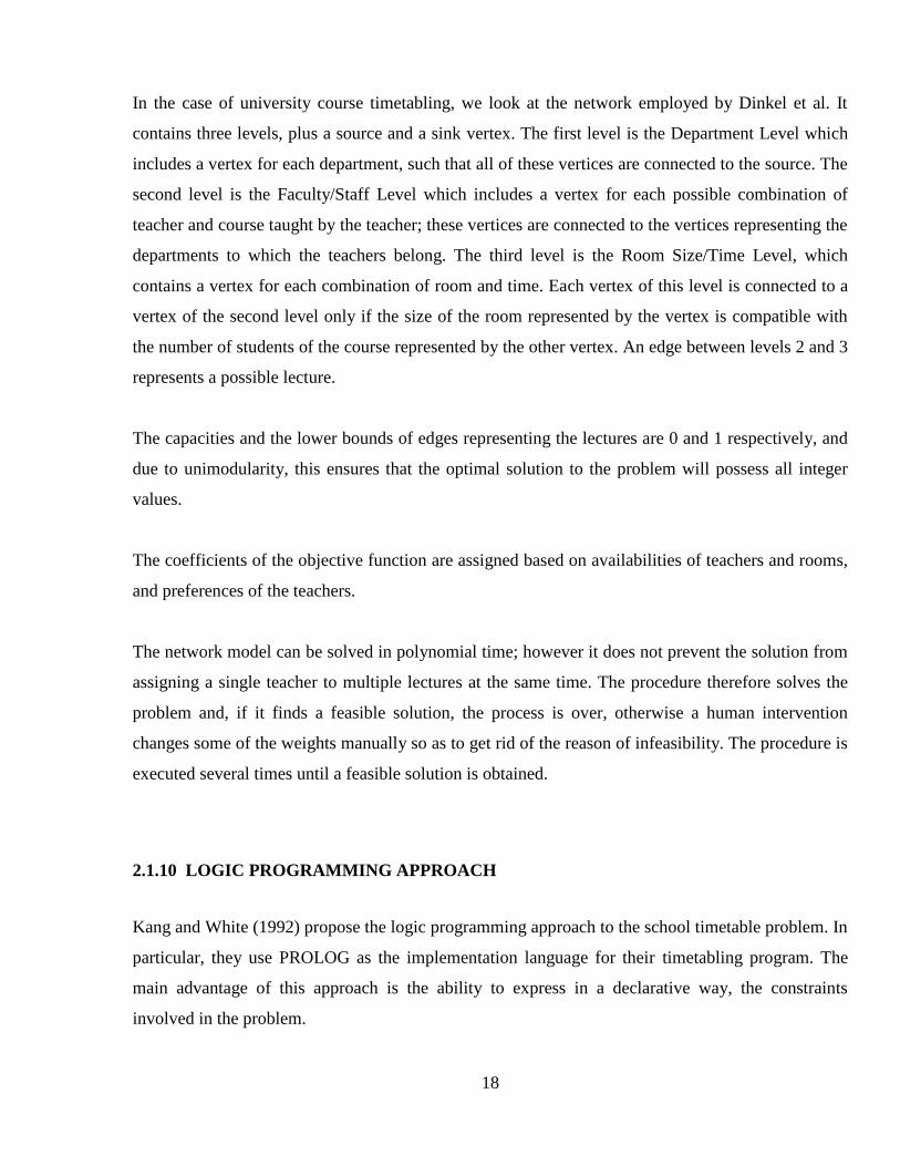
In the case of university course timetabling, we look at the network employed by Dinkel et al. It
contains three levels, plus a source and a sink vertex. The first level is the Department Level which
includes a vertex for each department, such that all of these vertices are connected to the source. The
second level is the Faculty/Staff Level which includes a vertex for each possible combination of
teacher and course taught by the teacher; these vertices are connected to the vertices representing the
departments to which the teachers belong. The third level is the Room Size/Time Level, which
contains a vertex for each combination of room and time. Each vertex of this level is connected to a
vertex of the second level only if the size of the room represented by the vertex is compatible with
the number of students of the course represented by the other vertex. An edge between levels 2 and 3
represents a possible lecture.
The capacities and the lower bounds of edges representing the lectures are 0 and 1 respectively, and
due to unimodularity, this ensures that the optimal solution to the problem will possess all integer
values.
The coefficients of the objective function are assigned based on availabilities of teachers and rooms,
and preferences of the teachers.
The network model can be solved in polynomial time; however it does not prevent the solution from
assigning a single teacher to multiple lectures at the same time. The procedure therefore solves the
problem and, if it finds a feasible solution, the process is over, otherwise a human intervention
changes some of the weights manually so as to get rid of the reason of infeasibility. The procedure is
executed several times until a feasible solution is obtained.
2.1.10 LOGIC PROGRAMMING APPROACH
Kang and White (1992) propose the logic programming approach to the school timetable problem. In
particular, they use PROLOG as the implementation language for their timetabling program. The
main advantage of this approach is the ability to express in a declarative way, the constraints
involved in the problem.

19
The full backtracking capability of the PROLOG machine is overridden by a heuristics that allows
only for a limited attempt to reschedule assignments that create conflicts. In particular, when a
lecture becomes unschedulable, the procedure finds an “equivalent” lecture already scheduled and
reassigns it to a different period. If no equivalent lecture can be moved to a different period, leaving
a feasible period for the currently-processed lecture, it is put into a list of lectures which will be
manually scheduled later.
2.1.11 CONSTRAINT-BASED APPROACH
The work in (Yoshikawa et al., 1996) proposes the use of a general-purpose Constraint Relaxation
Problem solver, called COASTOOL. In a constraint relaxation problem, a given penalty is assigned
to each constraint and the objective is to find an assignment of the problem variables that minimizes
the total penalty.
The constraint language allows the user to express several types of constraints. For example, it is
possible to express the unavailabilities of a given teacher. The following constraint states that the set
lectures of the teacher Smith, identified by the set SmithLessons, cannot take place during the set of
period representing the unavailabilities of Smith, identified by the set SmithAbsence.
(define-constraint PartTimerSmith
:object ((:set lesson SmithLessons))
:variables ((v lesson))
:condition (not (is-a v SmithAbsence))
:penalty 10)
The solution method combines a greedy algorithm for finding an initial solution and a hill-climbing
procedure for the optimization phase (Minton et al., 1992). The employment of a smart greedy
algorithm, called Really-Fully-Lookahead algorithm, for the initialization phase, and a strongly
biased optimization algorithm, for the optimization phase, allows the method to find a high-quality
solution in a reasonable amount of time.

20
2.1.12 COMBINATION OF METHODS
The algorithm in (Cooper and Kingston, 1993) combines several heuristics. As a core strategy, it
uses a form of bipartite graph matching, that they call meta-matching.
The algorithm identifies groups of lectures that must be scheduled all at different times, which are
called meeting-sets. Thereafter, it iteratively performs a matching between lectures belonging to a
meeting set, on one side, and the so-called prototimes on the other; the prototimes are variable time
slots that are later assigned to actual periods in a successive phase.
The algorithm is improved by choosing among the possible assignments those that assign as many
lectures as possible to the prototimes already used for previously scheduled meeting-sets. This
enhancement helps in finding a feasible timetable in presence of many large meeting-sets.
As already mentioned, the cited paper solves an extension of the basic problem which requires to
deal with different interchangeable resources, such as teachers and rooms. Actual resources are
assigned to lectures by a specific procedure. Such procedure, depending on the number of resources
involved may use a brute-force algorithm or a covering technique called beam search.
2.1.13 RULE-BASED APPROACH
A solution technique based on expert systems is given in (Meisels et al., 1991; Solotorevsky et al.,
1994).
Solotorevsky et al. define a rule-based language, called RAPS, for specifying general resource
allocation problems, and they use it, among the others, for a course timetabling problem. In
particular, they consider lectures as activities and periods as resources to be assigned to the
activities.
RAPS has five types of rules, namely assignment rules, constraint rules, local change rules, context
rules, and priority rules.

21
Assignment rules assign lectures to periods, one at a time, and therefore, they are the core of the
system. These rules, like all the others, are supplied by the user, and thus the heuristics used is not
predefined but is chosen by the user.
Constraint rules specify the constraints that the solution must satisfy. They are checked each time a
new lecture is assigned to a period (i.e. a new activity is assigned to a resource). Constraint rules are
split into positive and negative ones, that is, constraints that must be satisfied and constraints that
must fail. Constraint rules allow to identify conflicts as soon as they arise.
Local change rules specify the action to perform when there is a lecture that the assignment rules are
not able to tackle. The purpose of local change rule is to undo a previous assignment in order to
create the opportunity to assign the current one.
Context rules select the active context. In fact, the system allows for multiple contexts: In different
contexts the various lectures and periods may have different priority. The priority of the objects
determines which object, among those of a given type, is processed first.
Priority rules determine the priorities of the lectures and the periods, in each context. The priorities
are calculated each time a context is entered.
The system may work in two possible modes: greedy and non-greedy. In the greedy mode, when the
assignment rules fail to make an assignment, the system selects a different lecture. Conversely, in the
non-greedy mode, when a fail occurs, the control is passed to the local change rules.
Dhar and Ranganathan (1990) propose the use of an expert system, called PROTEUS, for the
allocation of teachers to courses, and compare it to integer programming techniques.

22
2.1.14 CONSTRAINT LOGIC PROGRAMMING APPROACH
A constraint logic programming (CLP) system (Jaffar and Lassez, 1987) is a tool for modeling a
specific search problem, which provides the ability to declare variables and their domains, and to
place constraints.
In order to search for a solution, a CLP system generates values for the variables, propagating values
through the constraints in order to prune parts of the solution space where inconsistencies are
discovered. The basic method is therefore, a backtrack search where the constraints allow the system
to look ahead to the consequences of decisions and spot failure earlier.
For dealing with optimization problems, the CLP systems provide a solution technique based on a
form of depth first branch-and-bound search.
Azevedo and Barahona (1994) deal with the timetabling problem using a CLP language called
DOMLOG. DOMLOG extends CHIP (Van Hentenryck, 1991), a popular CLP language, with
features such as user-defined heuristics and a flexible lookahead constraint solving.
In particular, DOMLOG allows for the possibility to specify a finite domain for the variables. In
addition, the user can specify the heuristics for the selection of the value of a domain to assign first
to a given variable.
Several other authors recently employed constraint logic programming for course timetabling with a
good success. Frangouli et al. (1995) and Gueret et al. (1995) solve their course timetabling problem
relying on the finite domain libraries of the logic programming language ECLiPSe (ECRC, 1995)
and CHIP, respectively. Henz and WÜrtz (1995) rely on the Oz system (Smolka, 1995), which is a
multi-paradigm concurrent constraint language.

23
3 CHAPTER THREE: METHODOLOGY
3.1 THE RATIONAL UNIFIED PROCESS (RUP)
The Rational Unified Process (RUP) methodology for software development was used in the
development of this system. The Unified Process has emerged as a popular and effective software
development process. In particular, the Rational Unified Process, as modified at Rational Software,
is widely practiced and adopted by industry. RUP is a complete software-development process
framework, developed by Rational Corporation. It’s an iterative development methodology based
upon six industry-proven best practices. Processes derived from RUP vary from being lightweight
i.e. addressing the needs of small projects, to more comprehensive processes addressing the needs of
large, possibly distributed project teams.
The critical idea in the Rational Unified Process is Iterative Development. Iterative Development is
successively enlarging and refining a system through multiple iterations, using feedback and
adaptation. Each iteration will include requirements, analysis, design, and implementation. Iterations
are timeboxed.
RUP adopts the Unified Software Development Process (USDP) Key ideas of being use-case driven;
architecture-centric; and Iterative and incremental.
Software Engineers now agree that an iterative model is required to facilitate changes to earlier
decision-making documents. This model allows each phase to be visited any number of times, so
that corrections and improvements can be made. USDP aims to deliver working, free-standing,
useful ‘chunks’ of software, one at a time, e.g., each use case may represent one increment of
delivered software.
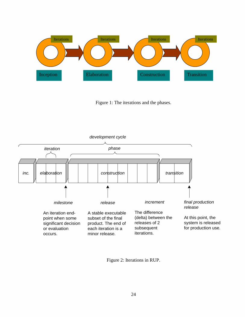
3.1.1 ITERATIONS
Each phase has iterations, each having the purpose of producing a demonstrable piece of software.
The duration of iteration may vary from two weeks or less up to six months.
24
Figure 1: The iterations and the phases.
Figure 2: Iterations in RUP.
Inception Elaboration Construction Transition
Iterations Iterations Iterations Iterations
inc. elaboration construction transition
iteration phase
development cycle
release
A stable executable
subset of the final
product. The end of
each iteration is a
minor release.
increment
The difference
(delta) between the
releases of 2
subsequent
iterations.
final production
release
At this point, the
system is released
for production use.
milestone
An iteration end-
point when some
significant decision
or evaluation
occurs.

25
3.1.2 INCREMENTAL
The idea behind an incremental model is that once something is produced by a process, it can be
used as a basis for the next process. For example, when a part of the software system has been
designed, the developers can begin the implementation for that software unit. This is true in spite of
the fact that the rest of the software system has not yet been designed.
3.1.3 WHY RUP?
The philosophy of process-oriented methods is that the requirements of a project are completely
frozen before the design and development process commences. As this approach is not always
feasible, there is also a need for flexible, adaptable and agile methods, which allow the developers to
make late changes in specifications.
The Unified Process reduces risk since it allows you to develop the most critical and risky aspects of
the project before addressing the less risky. If the risky aspects of the project fail, the project was
only a small failure since it failed so early. Often you will also develop a prototype or skeleton of the
user interface. User interface changes can be caught early, and modified quickly before it affects
very much of the rest of the system.
The UP was created to be an agile software development methodology. In other words, if
requirements, expectations, technologies, personnel, etc. change, the project should be able to adapt
with minimal waste of effort.
3.1.4 UP BEST PRACTICES
Get high risk and high value first.
Constant user feedback and engagement.
Early cohesive core architecture.
Test early, often, and realistically.

26
Apply use cases where needed.
Do some visual modeling with UML.
Manage requirements.
Manage change requests and configuration.
3.1.5 ADVANTAGES OF RUP
The RUP puts an emphasis on addressing very early high risks areas.
It does not assume a fixed set of firm requirements at the inception of the project, but allows
to refine the requirements as the project evolves.
It does not put either a strong focus on documents.
The main focus remains the software product itself, and its quality.

27
4 CHAPTER FOUR: SYSTEM ANALYSIS
4.1 JAVA
Java is widely adopted and there is a vast range of both commercial and open source libraries
available for the platform, making it possible to include support for virtually any system, including
native applications via JNI or JNA. When it comes to RIAs, Java’s main weakness is its multimedia
support. Java 6 Update N improves some features that have hindered the use of Java for RIAs
including startup time and download size, and Sun Inc. has even included new multimedia support in
this release.
4.1.1 DETAILS ABOUT JAVA
Java is a programming language originally developed by Sun Microsystems and released in 1995 as
a core component of Sun’s Java platform. The language derives much of its syntax from C and C++
but has a simpler object model and fewer low-level facilities. Java applications are typically
compiled to byte code which can run on any Java Virtual Machine (JVM) regardless of computer
architecture.
4.1.2 PLATFORM INDEPENDENCE
One characteristic, platform independence, means that programs written in the Java language must
run similarly on any supported hardware/operating system platform. One should be able to write a
program once, compile it once, and run it anywhere.
4.2 XML
The Extensible Markup Language (XML) is a general-purpose specification for creating custom
markup languages. It is classified as an extensible language because it allows its users to define their
own elements. Its primary purpose is to facilitate the sharing of structured data across different

28
information systems, particularly via the Internet, and it is used both to encode documents and to
serialize data.
It started as a simplified subset of the Standard Generalized Markup Language (SGML), and is
designed to be relatively human-legible. By adding semantic constraints, application languages can
be implemented in XML. These include XHTML, RSS, MathML, GraphML, and Scalable Vector
Graphics, MusicXML, and thousands of others. Moreover, XML is sometimes used as the
specification language for such application languages.
XML is recommended by the World Wide Web Consortium. It is a fee-free open standard. The W3C
recommendation specifies both the lexical grammar and the requirements for parsing.
4.2.1 ADVANTAGES OF XML
• It is text-based.
• It can represent common computer science data structures: records, lists and trees.
• The strict syntax and parsing requirements make the necessary parsing algorithms extremely
simple, efficient, and consistent.
• XML is heavily used as a format for document storage and processing, both online and offline.
• The hierarchical structure is suitable for most (but not all) types of documents.
• It is platform-independent, thus relatively immune to changes in technology.

29
4.3 DATA STRUCTURE & FLOW DIAGRAM
XML File contains the following sections as shown in the figure 3 below:
1. Teacher List
2. Subject List
3. Room List
4. Timeslot List
5. Students List
6. Days Options
7. Constraints, Rules
Figure 3: Data Structure.

30
4.4 FLOW OF DATA WITHIN THE PROJECT
Figure 4 below shows the flow of data from the user to the timetable generator algorithm and back to
the user.
Figure 4: Flow of Data within project.
31
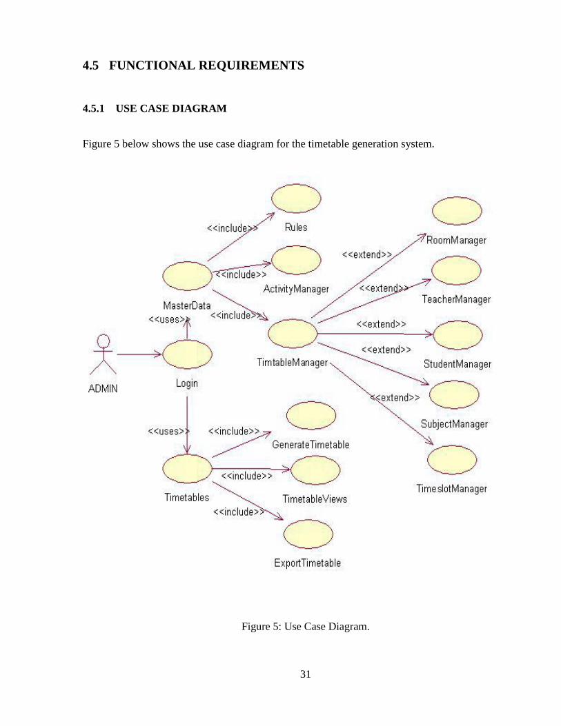
4.5 FUNCTIONAL REQUIREMENTS
4.5.1 USE CASE DIAGRAM
Figure 5 below shows the use case diagram for the timetable generation system.
Figure 5: Use Case Diagram.

32
A use case is made up of a set of scenarios (such as: Login, Data Management, Rules settings etc.).
Each scenario is a sequence of steps that encompass an interaction between a user and a system.
4.6 NON-FUNCTIONAL REQUIREMENTS
Non-functional requirements describe the constraints on the services and/or functions offered by the
system and constraints on the development process and standards. These requirements are grouped
into three main types: Product requirements which specify product behavior, Organizational
requirements which are derived from policies and procedures in the customer’s and developer’s
organization, and External requirements which are derived from factors external to the system and
its development process.
4.6.1 PRODUCT REQUIREMENTS
The TTGS System must have the following attributes:
4.6.1.1 USABILITY REQUIREMENTS
The system must have an easy to use and understandable user interface. This will ensure that the
user, for which this system is intended, will be able to achieve a level of proficiency with the system
with minimum effort in a very short period of time.
4.6.1.2 EFFICIENCY REQUIREMENTS
Response time, memory utilization, processing time and other performance factors should be optimal
in the system. In the event that only the most minimum of system resources are available, the system
should be able to function optimally and it should not make wasteful use of system resources.
4.6.1.3 RELIABILITY REQUIREMENTS
The system’s functions and services should be available to its users most of the times. The rate of
failure and/or the probability of it not being available should both be very low. Failures in the system
should not occur too often, at least a longer time space between them.

33
4.6.1.4 DEPENDABILITY REQUIREMENTS
In the event of the system failing due to any reason, it should not cause any physical or economic
damage to the customers, end users or the developers.
4.6.1.5 ROBUSTNESS REQUIREMENTS
The time taken for the system to restart after a system failure should be very short. The percentage of
user and system events that cause failures should be very minimal. The probability of data being
corrupted due to a failure should be very minimal as well.
4.6.1.6 MAINTAINABILITY REQUIREMENTS
Since software specifications change all the time as business needs change for organizations, the
TTGS system has been designed in such a way that it easily evolves meeting the customers’
changing demands. The system should be easy to maintain so as to cut on the maintenance costs.
4.6.1.7 FLEXIBILITY
The system should be modifiable depending on the changing needs of the user. Such modifications
should not entail extensive reconstructing or recreation of software. It should also be portable to
different computer systems.
4.6.1.8 SECURITY
This is a very important aspect of the design and should cover areas of hardware reliability, fall back
procedures, physical security of data and provision for detection of fraud and abuse. System design
involves logical design first and then physical construction of the system. The logical design
describes the structure and characteristics of features, like the outputs, inputs, files, database and
procedures. The physical construction, which follows the logical design, produces actual program
software, files and a working system.

34
4.6.1.9 PORTABILITY
The system should be installed or re-installed somewhere else with little or no modification. The
system shall be cross platform and be compatible with a number of common architectures and
should also be able to run on a variety of operating systems.
4.6.1.10 CONSISTENCY
The system shall maintain a constant look and appearance and exhibit high levels of consistency
among its various modules and components.
4.6.2 ORGANIZATIONAL REQUIREMENTS
4.6.2.1 IMPLEMENTATION REQUIREMENTS
The system has been developed following the RUP methodology thus increments of software or
code were added iteratively at each stage. An XML Knowledge Base has been used as the storage
structure for the system. The front end (GUI) has been written in the Java programming language
using eclipse as an Integrated Development Environment (IDE).
4.6.2.2 STANDARDS REQUIREMENTS
The initial system is done in English, that is, all text, labels and system documentation. However,
alternative local language support for dictionary lookup may be added later if need be.
4.6.2.3 DELIVERY REQUIREMENTS
The system will be delivered to its intended users only after thorough testing, verification and
validation of the individual system components. Also all necessary documentation needed by the
user will be delivered.
4.6.3 HARDWARE REQUIREMENTS
In summary form:
CPU : 1GHz Minimum.

35
Memory : 512MB Minimum.
Capacity : 5GB Hard Drive Space.
Others : Mouse, Keyboard, VGA Digital Monitor.
4.6.4 EXTERNAL REQUIREMENTS
4.6.4.1 INTEROPERABILITY
The system has been designed to easily integrate with other systems once deployed. It should be able
to function properly on any system without giving an idea to the user as to what could be happening
in the background.
4.6.4.2 ETHNICAL REQUIREMENTS
Only authorized users will be able to view certain details of the information supplied by the users
and all information supplied will be treated with the highest confidence. Information displayed will
only have necessary detail for the general public.
36
5 CHAPTER FIVE: SYSTEM DESIGN
5.1 PROPOSED SYSTEM
The Timetabling Algorithm is the main component of this project which produces the HTML based
timetable sheet as the output. The project takes various inputs from the user such as Teacher List,
Course List, Student Set List, Room List, Day List and Timeslot as well as various rules, facts and
constraints using web based forms, which are stored in XML based knowledge base. This knowledge
base serves as input to the Timetable Generator Algorithm residing on the server machine.
The system is organized into a three-tier architecture. The knowledgebase lies in the middle,
between the timetabling algorithm and the GUI front end. After the representation of the KB was
standardized, the timetabling algorithm was designed. The design of the timetabling algorithm took
most of the project total time.

37
The diagram below (Figure 6) shows the proposed System – The Timetable Generation System
Figure 6: Proposed System.
5.2 TTGS FEATURES
• Simple... Easy-to-understand & simple-to-operate with intuitive user interface, guides and
samples.
• Fast... Generates timetable in minutes, saving your time, efforts and money.
• Rules configuration and verification.
• Different views of timetable depending upon who is viewing timetable.

38
With Timetable Generation System, timetable generation process involves just a few simple steps:
Figure 7: Timetable Generation Process.
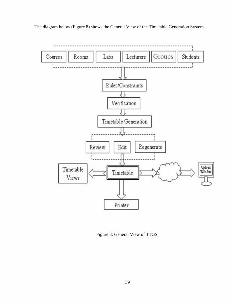
39
The diagram below (Figure 8) shows the General View of the Timetable Generation System.
Figure 8: General View of TTGS.

40
5.3 CLASS DIAGRAM
Packages: Packages allow us to break up a large number of objects into related groupings. In many
object oriented languages (such as Java), packages are used to provide scope and division to classes
and interfaces.
Classes: The core element of the class diagram is the class. In an object oriented system, classes are
used to represent entities within the system; entities that often relate to real world objects.
The following diagram (Figure 9) shows the package DataSourceKB which contains classes to
handle the Back End (Knowledge Base).
Figure 9: Class Diagram 1.

41
The following diagram (Figure 10) shows the package TTGS which contains sub packages and
classes to create the Front End.
Figure 10: Class Diagram 2

42
5.4 LOGIN TABLE
The LOGIN table was designed and created using Microsoft Access Database Management System
(DBMS) as shown in Table 1 and 2 below.
Table 1: Datasheet View of the Login Table.
Table 2: Design View of the Login Table.

43
6 CHAPTER SIX: IMPLEMENTATION
6.1 XML KNOWLEDGEBASE
As XML was preferred as the back-end, I had to design it first using XML Notepad 2007 and then
retrieve it using Java into the system application.
Figure 11: temp.ttgs.xml - XML Knowledgebase.
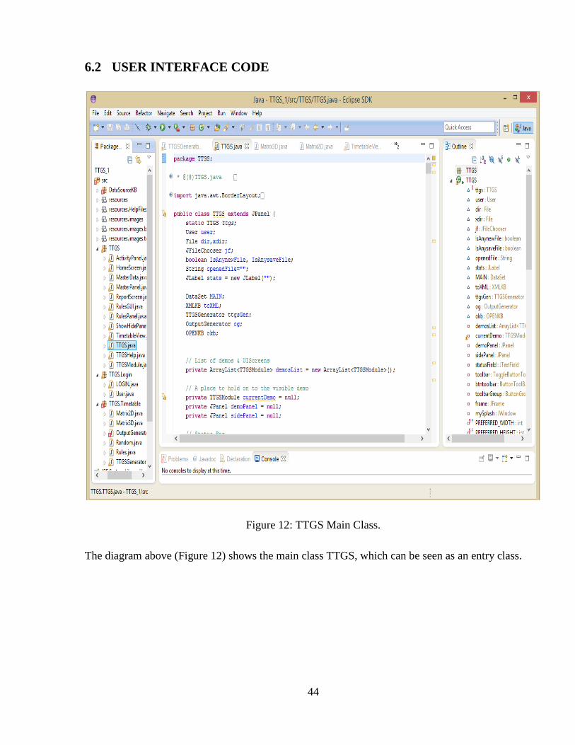
44
6.2 USER INTERFACE CODE
Figure 12: TTGS Main Class.
The diagram above (Figure 12) shows the main class TTGS, which can be seen as an entry class.

45
The following diagram (Figure 13) shows the Matrix3D class, which can be viewed as a Template
Class. A Template class can take many forms, i.e. we can instantiate this class by any data type (e.g.,
String, Integer, Boolean).
Figure 13: Matrix3D Class.

46
6.3 OUTPUT GENERATOR CODE
The following diagram (Figure 14) shows how the generated timetable can be represented in HTML.
Figure 14: Output Generator - Export to HTML file.

47
6.4 TIMETABLE GENERATOR CODE
The following diagram (Figure 15) shows the Main algorithm. This is the heart of the project. It
works in the following way:
Initiates storage matrices.
Performs allocation by checking TSR (Teacher, Student, Room) resources.
If any resource is absent (not available), it exits, else it places the activity at current timeslot
and day.
Figure 15: TTGS Main Algorithm Code.

48
The following diagram (Figure 16) shows how activities should be generated.
Figure 16: TTGS Activity Generation.

49
The following diagram (Figure 17) shows how the particular activity can be placed at (Day,
Timeslot). It is called in the Main Algorithm.
Figure 17: TTGS Placement of activity.

50
7 CHAPTER SEVEN: TESTING AND RESULTS
7.1 TESTING STRATEGIES
The TTGS System was subjected to different kinds of testing strategies in order to identify its
limitations and determine its full capabilities. To demonstrate that the system met the requirements, a
separate test was done for every requirement in the user and system requirements document. Thus
validation testing was performed. To discover faults or defects in the system where the behavior of
the system is incorrect, undesirable or does not conform to its specification, defect testing was also
performed. The different components of the system were each put on extensive unit testing to
ensure that the system was robust. Below is a list of the various test strategies that were performed
and a brief explanation for each.
7.1.1 UNIT TESTING
The system’s individual components were tested independently to ensure that they operate correctly.
The database, being one of the critical components of the system, was subjected to thorough testing.
Data integrity was maintained through enforcement of some constraints on the attributes. Test cases
were developed to ensure that all valid queries sent to the database returned the correct information.
Testing the Graphical User Interface
Test cases used for unit testing included:
Test for all valid user events
Test for invalid user events such as malformed text inputs like invalid words, or words
containing invalid characters.
Test for correctness of the results. Ensure that results displayed are for the requested
inputs
7.1.2 INTEGRATION TESTING
The system consists of many independent modules. These modules were tested independently every
time a change occurred in one of them. The modules were then integrated with the rest of the system

51
subsystems and tested as a whole to ensure that they worked together and met the specified
requirements.
7.1.3 SYSTEM TESTING
The individual subsystems were then merged to form a fully-fledged system. To ensure functionality
and completeness of the system, the entire system was then tested as a whole keeping particular
attention to how subsystems were coordinating and making changes to all irregularities and system
errors.
7.2 EXTERNAL INTERFACES
7.2.1 USER INTERFACE DESCRIPTION AND CHARACTERISTICS
The user interface is the main component of the three-tier architecture model and is the only way
through which users can use and interact with the system. Therefore, the design of the interface was
in such a way that users should not struggle to use the system. To ensure that the system is usable, a
user-centered design approach was followed. The following features added usability:
Windows: These enabled more information to be displayed and some data to be entered
through the user’s screen.
Icons: These are images (or shortcuts) that represent applications, objects and various
operations and commands to be performed on the system.
Menus: These offer users a structured way of choosing from the available set of optional
services the system provides.
Pointing Devices: Pointing devices like the mouse control the cursor as a point of entry to the
windows, menus, and icons on the screen.
Designed with the principles of Multimedia and Human Computer Interaction (HCI), the following
were some of the goals that had to be met by the interfaces:
Attractive to use and simple
Consistent with most operations (Consistency)
Easy to learn (Learnability)

52
Easy to use (Usability)
Have a good utility
Reduce on error rate
Familiar with users of the system
7.3 SCREEN SHOT OF TTGS
The Screen Shots of the system were taken as shown in the following diagrams (Figure 18 to Figure
31). As the Graphical User Interface (GUI) is main entry point to any software application, I tried by
all means necessary to make the Timetabling System as highly interactive as possible so as to make
it ideal and simple for both naive and sophisticated users. The TTGS front-end has been designed in
Java (Swingset), hence the reason why I was able to make the interfaces with so much ease.
7.3.1 HOME SCREEN
This is the first interface that a user sees and interacts with upon launching TTGS. It is a simple
interface that is so easy to navigate and understand at one instance. In order to access the various
services offered by the system, the user simply has to log in using a correct username and password.
The diagram on figure 18 shows the home screen which is the entry point to the TTGS Application.

53
Figure 18: Home Screen.

54
The following diagram (Figure 19) shows the Login Screen which allows authorized access to the
TTGS Application.
Figure 19: Login Screen.

55
7.3.2 TTGS SYSTEM SCREEN
This is the screen or interface that is presented to the user after the user successfully logs in. This
screen contains a menu bar that provides key functionalities or sections of the system. This is shown
in the diagram (figure 20) below.
Figure 20: TTGS System Screen showing the main menu.

56
The diagram below (Figure 21) shows the Lecturer Manager Screen which provides the facility to
enter all data entities. The other Manager Screens similar to this one are the Course, Student, Room
and Timeslot Manager Screens.
Figure 21: Lecturer Manager Screen.

57
The following diagram (Figure 22) shows the Timeslot Manager Screen which provides a way to set
the working days & timings.
Figure 22: Timeslot Manager Screen.

58
The diagram below (Figure 23) shows the Subject-Student (Course-Student) Assignment Screen
which facilitates the administrator to assign a set of subjects or courses to Students.
Figure 23: Subject-Student Assignment

59
The diagram below (Figure 24) shows the Subject-Teacher (Course-Lecturer) Assignment Screen
which allows the user to assign one or more subjects (courses) to a teacher or lecturer.
Figure 24: Course - Lecturer Assignment.

60
The following diagram (Figure 25) shows the Activity Manager Screen which allows the user to
generate activities based on Teacher-Student-Subject Assignment.
Figure 25: Activity Manager Screen.

61
The following diagram (Figure 26) shows the Rules Manager Screen which allows the user to set the
soft constraints such as Break Time, Teacher Availability, Student Availability, etc.
Figure 26: Rules Manager Screen.

62
The diagram below (Figure 27) shows the Timetable Generation Screen which allows the user to
generate the timetable. If the timetable is successfully generated, a message is displayed that
indicates that the timetable has been generated successfully. If the user desires a different output,
then they just have to regenerate it.
Figure 27: Timetable Generation.

63
7.3.3 TIMETABLE VIEW SCREEN
The diagram (Figure 28) below shows various Timetable Views after successful timetable
generation.
Figure 28: Teacher Timetable View.
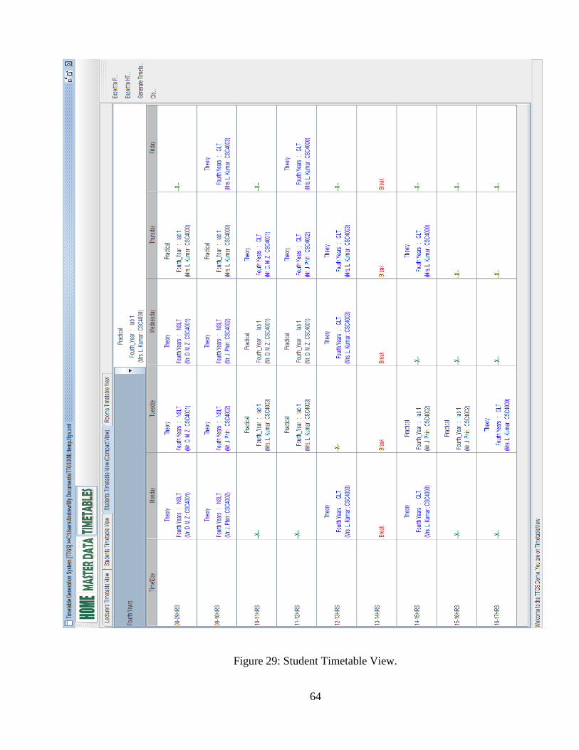
64
Figure 29: Student Timetable View.

65
Figure 30: Room Timetable View.
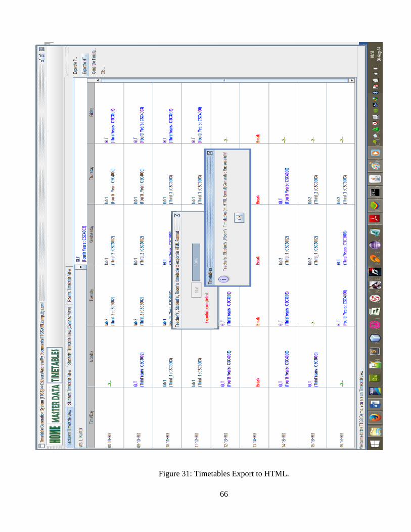
66
Figure 31: Timetables Export to HTML.

67
7.4 TEST CASES
7.4.1 TEST CASE 1: LOGIN SCREEN
Objective : - To check whether user name & password are valid or invalid.
Test Data : - User Name = ”admin” and Password =”admin”.
Sr No. Steps Data Excepted Data Actual
result
Status
1 Enter username,
password and click on
the Login button.
admin
admin
Should display a welcome
message and take the user to
the main screen.
Pass
2 Enter correct User
name and blank
password and click on
the Login button.
admin Should display an error
message ‘Must Enter
Password.’
Pass
3 Enter blank username
and correct password
and click on the
submit button.
admin Should display an error
message ‘Must Enter User
Name.’
Pass
4 Enter blank user name
and blank password
and click on the
submit button.
admin Should display an error
message ‘Must Enter User
Name & Password.’
Pass
5
Enter wrong user
name and password.
andrew
biemba
Should display an error
message ‘Sorry try again!’
Pass
Table 3: Test Case for the Login Screen.

68
7.4.2 TEST CASE 2: COMPUTER STUDIES DEPARTMENT.
The table below shows the work load of the Computer Studies Department.
Sr. No Name Of Staff Courses Year/ Group Theory
(Hrs)
Practical/Lab
(Hrs)
Total
(Hrs)
1 Dr. J. Phiri CSC 4722
CSC 4130
Fourth Years
Fourth Years
3
3
3*1
3*1
6
6
2 Dr. E. Lampi CSC 4130
CSC 3120
Fourth Years
Third Years
3
3
3*1
3*1
6
6
3 Mrs. L. Kumar CSC 3600
CSC 3612
Third Years
Third Years
3
3
3*1
3*1
6
6
4 Mr. D. M. Zulu CSC 4921
CSC 3402
Fourth Years
Third Years
3
3
3*1
3*1
6
6
5 Mr. M. Phiri CSC 4630
CSC 3712
Fourth Years
Third Years
3
3
3*1
3*1
6
6
6 Mr. A. Theu CSC 4745
CSC 4505
Fourth Years
Fourth Years
3
3
3*1
3*1
6
6
7 Mr. S. Chibuta CSC 2202
CSC 3712
Second Years
Third Years
3
3
3*1
3*1
6
6
8 Mr. S. Mwanza CSC 2000
CSC 2702
Second Years
Second Years
3
3
3*1
3*1
6
6
Table 4: Computer Studies Dept. work load.

69
8 CHAPTER EIGHT: CONCLUSION
8.1 CHALLENGES
It has not been an easy road and certainly a number of challenges here and there were encountered. I
came across many difficulties and problems while implementing this software but my tremendous
desire to complete the project made me overcome them.
The issue of time management posed a great challenge on the completion of the project. The project,
to start with, was started later into the academic year and not at the beginning. To ensure timely
completion of the project, it was a mammoth task to adequately define and identify sequences of all
activities to be carried out. Estimating activity resources and their duration was hectic. Schedule
development and controlling it throughout the project lifespan was difficult too. Despite all this, the
project was successfully implemented.
8.2 CONCLUSION
This project has evolved from just a mere idea into a life changing Time Table Generation System
that will definitely have an instant impact on academic institutions. Users (college or university
administrators) will generate timetables automatically instead of the laborious manual way of having
to brain storm on how to avoid course or room clashes by student groups. The system will generate
time tables in a quicker and more convenient way, thereby saving a lot of time and effort in the
process.
During the system analysis and design stages, objects were identified from the functional
requirements, contextual and block designs were constructed and with the aid of special software
development tools such as Visual Paradigms, use case diagrams, sequence diagrams, activity
diagrams and class diagrams were created which ultimately led to the implementation of the full-
fledged software system.

70
The project met the aims and objectives and thus the software system is capable of performing the
core operations it was primarily developed for. It includes all the fundamental functionalities stated
in the proposal. Therefore, it was a major success and my hope is that this software will be used in
colleges, universities and other academic institutions as an Open Source Project.
Finally, it is hoped that the knowledge acquired in this undertaking shall be put to good use and also
be applied in solving real life problems in the industry and hence ultimately make the world a better
place to live in.
It is expected that this system will receive overwhelming response from the general public due to its
user friendliness and hence will simplify the lives of the masses and make time table creation a joy
indeed.
8.3 FUTURE WORK
To extend the system so as to accommodate all lecture sessions across the university.
To generate timetables for all classes which use shared resources.
To also include exam scheduling in the system.
To provide additional features such as:
- Student Attendance.
- Assignment Distribution over the intranet.
- Direct Export to college site.
8.4 RECOMMENDATIONS
A lot of issues have been identified and learnt throughout the development of the TTGS project. To
this effect, I put forth the following recommendations:
The department should convince the corporate world, probably through the project’s
coordinator, to give and/or allow students to do some of their projects.
The department should ensure that projects are started on time, at the beginning of the
academic year, to facilitate early or timely and smooth completion of projects.

71
The department of computer studies should introduce courses that focus on Web Technology
to help students apply the techniques in their final year projects.

72
9 REFERENCES
1. Brelaz (1979), New methods to color vertices of a graph. Communications of the ACM,
22:251-256.
2. M. Chams, A. Hertz, and D. de Werra (1987), Some experiments with simulated annealing
for coloring graphs. European Journal of Operational Research, 32:260-266.
3. T. B. Cooper and J. H. Kingston (1993), The solution of real instances of the timetabling
problem. The Computer Journal, 36(7):645-653.
4. Costa. A (1994), tabu search algorithm for computing an operational timetable. European
Journal of Operational Research, 76:98-110.
5. A. Schaerf (1996), Tabu search techniques for large high-school timetabling problems. In
Proc. of the 13th Nat. Conf. on Artificial Intelligence (AAAI-96), pages 363-368, Press/MIT
Press, Portland, USA.
6. Schmidt and T. Strohlein (1979), Timetable construction - an annotated bibliography. The
Computer Journal, 23(4):307-316.
7. M. R. Garey and D. S. Johnson (1979), Computers and Intractability-A guide to NP-
completeness. W.H. Freeman and Company, San Francisco.
8. T. Leighton. (1979), A graph coloring algorithm for large scheduling problems. J. Res. Natl.
Bur. Standards, 84:489-506.
9. D. Klein (1983), The application of computerized solution techniques to the problem of
timetabling in high schools and universities. Master's thesis, Concordia University.
10. L. H. Klingen (1981), Stundenplan-erstellung mit dem computer. Log In, 1(4):31-33.
11. Laporte and S. Desroches (1986), The problem of assigning students to course sections in a
large engineering school. Computers and Operational Research, 13:387-394.
12. L. Kiaer and J. Yellen (1992), Weighted graphs and university course timetabling.
Computers and Operational Research, 19(1):59-67.
13. M. Chams, A. Hertz, and D. de Werra (1987), Some experiments with simulated annealing
for coloring graphs. European Journal of Operational Research, 32:260-266.
14. M. W. Carter, G. Laporte, and J. W. Chinneck (1994), A general examination scheduling
system. Interfaces, 24(3):109-120.

73
15. M. Cangalovic and J. A. M. Schreuder (1991), Exact coloring algorithm for weighted graph
applied to timetabling problems with lectures of different length. Journal of Operational
Research, 51(2):248-258.
16. E. Burke, D. Elliman, and R. Weare (1994), A genetic algorithm based university timetabling
system. In 2nd East-West International Conference on Computer Technologies in Education.,
Crimea, Ukraine.
17. E. H. L. Aarts and J. Korst (1989), Simulated Annealing and Boltzmann Machines. John
Wiley & Sons, New York, USA.
18. R. Alvarez-Valdes, G. Martin, and J.M. Tamarit (1996), Constructing good solutions for the
Spanish school timetabling problem. Journal of the Operational Research Society. To appear.
19. F. Azevedo and P. Barahona (1994), Timetabling in constraint logic programming. In
Proceedings of World Congress on Expert Systems '94.
20. Jaffar and J.-L. Lassez (1987), Constraint logic programming. In Proc. of the 14th ACM
POPL Symposium, Munich, Germany.
21. L. Kang and G. M. White (1992), A logic approach to the resolution of constraints in
timetabling. European Journal of Operational Research, 61:306-317.
22. S. Kirkpatrick, C. D. Gelatt, Jr, and M. P. Vecchi (1983), Optimization by simulated
annealing. Science, 220:671-680.
23. Meisels, E. Gudes, and T. Kuik (1991), Limited-resource time-tabling by a generalized
expert system. Knowledge-Based Systems, 4:215-224.
24. Z. Michalewicz (1994), Genetic algorithms + data structures = evolution programs, Second,
extended edition, Springer-Verlag.
25. S. Minton, M. D. Johnston, A. B. Philips, and P. Laird (1992), Minimizing conflicts: a
heuristic repair method for constraint satisfaction and scheduling problems. Artificial
Intelligence, 58:161-205.
26. C. H. Papadimitriou and K. Steiglitz (1982), Combinatorial Optimization: Algorithms and
Complexity. Prentice-Hall, Englewood Cliffs, New Jersey.
27. D. B. Papoulias (1980), The assignment-to-days problem in a school time-table, a heuristic
approach. European Journal of Operational Research, 4:31-41.
28. C. Petrie, R. Causey, D. Steiner, and V. Dhar (1989), A planning problem: revisable
academic course scheduling. Technical Report ACT-AI-020, Microelectronics and Computer
Technology Corporation.

74
29. G. Smolka. The Oz programming model (1995). In J. van Leeuwen, editor, Current Trend in
Computer Science, number 1000 in Lecture Notes in Computer Science, pages 324-343.
Springer-Verlag.
30. Pressman R. S. (2010), Software Engineering: A Practitioner’s Approach, Seventh Edition,
McGraw-Hill Companies, Inc., New York, USA.
31. Larman C. (2004), Applying UML and patterns: An introduction to Object-Oriented Analysis
and Design, Third Edition, Addison-Wesley, Boston, USA.
32. Sommerville I. (2011), Software Engineering, Ninth Edition, Addison-Wesley, Boston, USA.
33. Benneth C., et al (2008), GoF Design Patterns - with examples using Java and UML2, Sixth
Edition, Pearson Education Inc., Upper Saddle River, New Jersey, USA.
34. Freeman E. et al (2004), Head First Design Patterns, First Edition, O'Reilly Media, Inc.,
USA.

75
10 APPENDIX
10.1 APPENDIX A: MAIN ALGORITHM
public void MainAlgo(int itration) {
if (GENERATE_SUCCESS) {
System.out.println("FIN" + itration);
} else {
initMatrices();
Random ActR = new Random(ds.getActivityLength());
for (int Days = 0; Days < c; Days++) {
for (int TimeSlot = 0; TimeSlot < r; TimeSlot++) {
for (int activity = 0; activity < ds.getActivityLength(); activity++) {
int randAct = ActR.getRandValue(activity);
if (!isActPlace.get(randAct).booleanValue())
if (placeActivity(randAct, TimeSlot, Days))
isActPlace.set(randAct, true);
}
}
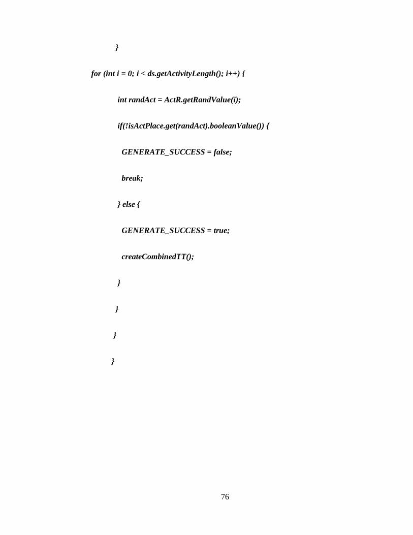
76
}
for (int i = 0; i < ds.getActivityLength(); i++) {
int randAct = ActR.getRandValue(i);
if(!isActPlace.get(randAct).booleanValue()) {
GENERATE_SUCCESS = false;
break;
} else {
GENERATE_SUCCESS = true;
createCombinedTT();
}
}
}
}

77
10.2 APPENDIX B: GANTT CHART

78
10.3 APPENDIX C: HOW TO RUN THE PROGRAM
10.3.1 PROCEDURE:
1. Ensure that you have JDK installed on your machine and that you have set the correct path to
the java compiler (javac) in the environmental variables of your system.
2. Copy the folder or directory named “TTGS” which contains the java files and other
supporting files and libraries onto your computer system.
3. Open the command prompt or terminal.
4. Change the directory to the “TTGS” directory.
5. Compile all the files in this directory (you can use the command “javac *.java” to compile all
the files in the directory at once).
6. Compile the Driver (Main) Class separately (use the command “javac TTGS.java”).
7. Run or execute the TTGS.java file (use the command “java TTGS”).
Alternatively, you will require to install Eclipse IDE onto your machine. With Eclipse IDE running
on your machine, you simply have to copy the contents of the TTGS folder to the IDE or just import
the folder as a new project. Then select the folder in the eclipse window and click on the execute
button or icon to run the program.